5,018 Matching Annotations
  1. Nov 2025
    1. Author response:

      The following is the authors’ response to the original reviews

      eLife Assessment

      This manuscript makes valuable contributions to our understanding of cell polarisation dynamics and its underlying mechanisms. Through the development of a computational pipeline, the authors provide solid evidence that compensatory actions, whether regulatory or spatial, are essential for the robustness of the polarisation pattern. However, a more comprehensive validation against experimental data and a proper estimation of model parameters are required for further characterization and predictions in natural systems, such as the C. elegans embryo.

      We sincerely thank the editor(s) for their pertinent assessment. We have carefully considered the constructive recommendations and made the necessary revisions in the manuscript, which are also detailed in this response letter. We have implemented most of the revisions requested by the reviewers. For the few requests we did not fully accept, we have provided justifications. The corresponding revisions in both the Manuscript and Supplementary Information are highlighted with a yellow background. To provide a more comprehensive validation against experimental data and model parameters used for characterizing and predicting natural systems, we reproduced the qualitative and semi-quantitative phenomenon in three more experimental groups previously published (Section 2.5; Fig. S8) [Gotta et al., Curr. Biol., 2001; Aceto et al., Dev. Biol., 2006]. Combined with the original experiments (Section 2.5; Fig. S7) [Hoege et al., Curr. Biol., 2010; Beatty et al., Development, 2010; Beatty et al., Development, 2013], now we have reproduced five experimental groups in total (two acting on LGL-1 and three on CDC-42), comprising eight perturbed conditions and using wild-type as the reference. These results effectively demonstrate how comprehensively the network structure and parameters capture the characteristics of the C. elegans embryo. We have also acknowledged the limitations of the current cell polarization model and provided, in 2. Results and 3. Discussion and conclusion, a detailed outline of potential model improvements.

      Joint Public Review:

      The polarisation phenomenon describes how proteins within a signalling network segregate into different spatial domains. This phenomenon holds fundamental importance in biology, contributing to various cellular processes such as cell migration, cell division, and symmetry breaking in embryonic morphogenesis. In this manuscript, the authors assess the robustness of stable asymmetric patterns using both a previously proposed minimal model of a 2-node network and a more realistic 5-node network based on the C. elegans cell polarisation network, which exhibits anterior-posterior asymmetry. They introduce a computational pipeline for numerically exploring the dynamics of a given reaction-diffusion network and evaluate the stability of a polarisation pattern. Typically, the establishment of polarisation requires the mutual inhibition of two groups of proteins, forming a 2-node antagonistic network. Through a reaction-diffusion formulation, the authors initially demonstrate that the widely-used 2-node antagonistic network for creating polarised patterns fails to maintain the polarised pattern in the face of simple modifications. However, the collapsed polarisation can be restored by combining two or more opposing regulations. The position of the interface can be adjusted with spatially varied kinetic parameters. Furthermore, the authors show that the 5-node network utilised by C. elegans is the most stable for maintaining polarisation against parameter changes, identifying key parameters that impact the position of the interface.

      We sincerely thank the editor(s) for the pertinent summary!

      While the results offer novel and insightful perspectives on the network's robustness for cell polarisation, the manuscript lacks comprehensive validation against experimental data, justified node-node network interactions, and proper estimation of model parameters (based on quantitative measurements or molecular intensity distributions). These limitations significantly restrict the utility of the model in making meaningful predictions or advancing our understanding of cell polarisation and pattern formation in natural systems, such as the C. elegans embryo.

      We sincerely thank the editor(s) for the comment!

      To provide a more comprehensive validation against experimental data and model parameters, we reproduced the qualitative and semi-quantitative phenomenon in three more experimental groups previously published (Section 2.5; Fig. S8) [Gotta et al., Curr. Biol., 2001; Aceto et al., Dev. Biol., 2006]. Combined with the original experiments (Section 2.5; Fig. S7) [Hoege et al., Curr. Biol., 2010; Beatty et al., Development, 2010; Beatty et al., Development, 2013], now we have reproduced five experimental groups in total (two acting on LGL-1 and three on CDC-42), comprising eight perturbed conditions and using wild-type as the reference. These meaningful predictions effectively demonstrate the utility of our model’s network structure and parameters in advancing our understanding of cell polarisation and pattern formation in natural systems, exemplified by the C. elegans embryo.

      We have also acknowledged the limitations of the current cell polarization model and provided, in 2. Results and 3. Discussion and conclusion, a detailed outline of potential model improvements. The limitations include, but are not limited to, issues involving “node-node network interactions” and the “proper estimation of model parameters (based on quantitative measurements or molecular intensity distributions)”, both of which rely on experimental measurements of biological information.   However, comprehensive experimental measurement data on every molecular species, their interactions, and each species’ intensity distribution in space and time were not fully available from prior research. Refinement is lacking for some of these interactions, potentially requiring years of additional experimentation. Moreover, for certain species at specific developmental stages, only relative (rather than absolute) intensity measurements are available. We agreed that such information is essential for establishing a more utilizable model and discussed it thoroughly in 3. Discussion and conclusion. From a theoretical perspective, we adopted assumptions from the previous literature and constructed a minimal model for a specific cell polarization phase to investigate the network's robustness, supported by five experimental groups and eight perturbed conditions in the C. elegans embryo.

      The study extends its significance by examining how cells maintain pattern stability amid spatial parameter variations, which are common in natural systems due to extracellular and intracellular fluctuations. The authors found that in the 2-node network, varying individual parameters spatially disrupt the pattern, but stability is restored with compensatory variations. Additionally, the polarisation interface stabilises around the step transition between parameter values, making its localisation tunable. This suggests a potential biological mechanism where localisation might be regulated through signalling perception.

      We sincerely thank the editor(s) for the pertinent review!

      Focusing on the C. elegans cell polarisation network, the authors propose a 5-node network based on an exhaustive literature review, summarised in a supplementary table. Using their computational pipeline, they identify several parameter sets capable of achieving stable polarisation and claim that their model replicates experimental behaviour, even when simulating mutants. They also found that among 34 possible network structures, the wild-type network with mutual inhibition is the only one that proves viable in the computational pipeline. Compared with previous studies, which typically considered only 2- or 3-node networks, this analysis provides a more complete and realistic picture of the signalling network behind polarisation in the C. elegans embryo. In particular, the model for C. elegans cell polarisation paves the way for further in silico experiments to investigate the role of the network structure over the polarisation dynamics. The authors suggest that the natural 5-node network of C. elegans is optimised for maintaining cell polarisation, demonstrating the elegance of evolution in finding the optimal network structure to achieve certain functions.

      We sincerely thank the editor(s) for the pertinent review!

      Noteworthy limitations are also found in this work. To simplify the model for numerical exploration, the authors assume several reactions have equivalent dynamics, reducing the parameter space to three independent dimensions. While the authors briefly acknowledge this limitation in the "Discussion and Conclusion" section, further analysis might be required to understand the implications. For instance, it is not clear how the results depend on the particular choice of parameters. The authors showed that adding additional regulation might disrupt the polarised pattern, with the conclusion apparently depending on the strength of the regulation. Even for the 5-node wild-type network, which is the most robust, adding a strong enough self-activation of [A], as done in the 2-node network, will probably cause the polarised pattern to collapse as well.

      We sincerely thank the editor(s) for the comment!

      Now we have thoroughly expanded our acknowledgment of the model’s limitations in in 2. Results and 3. Discussion and conclusion. To rule out the equivalent dynamics assumption undermines our conclusions, we have added simulations showing that the cell polarization pattern stability does not depend on the exact strength of each regulation, provided the regulations on both sides are initially balanced as a whole (Fig. S5). Specifically, we used a Monte Carlo method to sample a wide range of various parameter values ( i.e., γ, α, k<sub>1</sub>, k<sub>2</sub>, q<sub>1</sub>, q<sub>2</sub> and [X<sub>c</sub>) for all nodes and regulations in simple 2-node network and C. elegans 5-node network, to achieve pattern stability. Under these conditions (i.e., without any reduction in the parameter space), single-sided self-regulation, single-sided additional regulation, and unequal system parameters still cause the stable polarized pattern to collapse, consistent with our conclusions in the simplified conditions with the parameter space reduced to three independent dimensions.

      Additionally, the authors utilise parameter values that are unrealistic, fail to provide units for some of them, and assume unknown parameter values without justification. The model appears to have non-dimensionalised length but not time, resulting in a mix of dimensional and non-dimensional variables that can be confusing. Furthermore, they assume equal values for Hill coefficients and many parameters associated with activation and inhibition pathways, while setting inhibition intensity parameters to 1. These arbitrary choices raise concerns about the fidelity of the proposed model in representing the real system, as their selected values could potentially differ by many orders of magnitude from the actual parameters.

      We sincerely thank the editor(s) for the comment!

      We apologize for the confusion. The non-dimensionalised parameter values are adopted from previous theoretical research [Seirin-Lee et al., Cells, 2020], which originates from the experimental measurement in [Goehring et al., J. Cell Biol., 2011; Goehring et al., Science, 2011]. With the in silico time set as 2 sec per step, now we have added the Supplemental Text justifying how the units are removed during non-dimensionalization. This demonstrates that the derived non-dimensionalized parameter in this paper achieves realistic values on the same order of magnitude as those observed in reality, confirming the fidelity of the proposed model in representing the real system.

      The assumption of “equal values for Hill coefficients and many parameters associated with activation and inhibition pathways” is to reduce the parameter space for affordable computational cost. It is a widely-used strategy to fix Hill coefficients [Seirin-Lee et al., J. Theor. Biol., 2015; Seirin-Lee, Bull. Math. Biol., 2021] and unify parameter values for different pathways in network research about both cell polarization [Marée et al., Bull. Math. Biol., 2006; Goehring et al., Science, 2011; Trong et al., New J. Phys., 2014] and other biological topics (e.g., plasmid transferring in the microbial community [Wang et al., Nat. Commun., 2020]), to control computational cost. Nevertheless, to rule out that the equivalent dynamics assumption undermines our conclusions, we have added simulations showing that the cell polarization pattern stability does not depend on the exact parameter values associated with activation and inhibition pathways, provided the regulations on both sides are initially balanced as a whole (Fig. S5). Specifically, we used a Monte Carlo method to sample a wide range of various parameter values (i.e_., _γ, α, k<sub>1</sub>, k<sub>2</sub>, q<sub>1</sub>, q<sub>2</sub> and [X<sub>c</sub>) for all nodes and regulations in simple 2-node network and C. elegans 5-node network, to achieve pattern stability. Under these conditions ( i.e., without any reduction in the parameter space), single-sided self-regulation, single-sided additional regulation, and unequal system parameters still cause the stable polarized pattern to collapse, consistent with our conclusions in the simplified conditions with the parameter space reduced to three independent dimensions.

      To confirm the fidelity of the proposed model in representing the real system, we reproduced the qualitative and semi-quantitative phenomenon in three more experimental groups previously published (Section 2.5; Fig. S8) [Gotta et al., Curr. Biol., 2001; Aceto et al., Dev. Biol., 2006]. Combined with the original experiments (Section 2.5; Fig. 5; Fig. S7) [Hoege et al., Curr. Biol., 2010; Beatty et al., Development, 2010; Beatty et al., Development, 2013], now we have reproduced five experimental groups in total (two acting on LGL-1 and three on CDC-42), comprising eight perturbed conditions and using wild-type as the reference. These results effectively demonstrate how comprehensively the network structure and parameters capture the characteristics of the C. elegans embryo. We have also acknowledged the limitations of the current cell polarization model and provided, in 2. Results and 3. Discussion and conclusion, a detailed outline of potential model improvements.

      It is worth noting that, although a strict match between numerical and realistic parameter values with consistent units is always helpful, a lot of notable pure numerical studies successfully unveil principles that help interpret [Ma et al., Cell, 2009] and synthesize real biological systems [Chau et al., Cell, 2012]. These studies suggest that numerical analysis in biological systems remains powerful, even when comprehensive experimental data from prior research are not fully available.

      The definition of stability and its evaluation in the proposed pipeline might also be too narrow. Throughout the paper, the authors discuss the stability of the polarised pattern, checked by an exhaustive search of the parameter space where the system reaches a steady state with a polarised pattern instead of a homogeneous pattern. It is not clear if the stability is related to the linear stability analysis of the reaction terms, as conducted in Goehring et al. (Science, 2011), which could indicate if a homogeneous state exists and whether it is stable or unstable. The stability test is performed through a pipeline procedure where they always start from a polarised pattern described by their model and observe how it evolves over time. It is unclear if the conclusions depend on the chosen initial conditions. Particularly, it is unclear what would happen if the initial distribution of posterior molecules is not exactly symmetric with respect to the anterior molecules, or if the initial polarisation is not strong.

      We sincerely thank the editor(s) for the comment!

      The definition of stability and its evaluation in the proposed pipeline consider two criteria: 1. The pattern is polarized; 2. The pattern is stable. Following simulations, figures, and videos (Fig. 1-6; Fig. S1-S5; Fig. S7-S9; Movie S1-S5) have sufficiently demonstrated that the parameters and networks set up capture the cell polarization dynamis regarding both the stable and unstable states very well.

      Now we have added new simulation on alternative initial conditions. They demonstrating the necessity of a polarized initial pattern set up independently of the reaction-diffusion network during the establishment phase, probably through additional mechanisms such as the active actomyosin contractility and flow [Cuenca et al., Development, 2003; Gross et al., Nat. Phys., 2019]. Our conclusions ( i.e., single-sided self-regulation, single-sided additional regulation, and unequal system parameters cause the stable polarized pattern to collapse) have little dependence on the chosen initial conditions as long as the unsymmetric initial patterns can set up a stable polarized pattern. A part of the simulations institutively show our conclusions still hold if the initial distribution of posterior molecules is not exactly symmetric with respect to the anterior molecules, or if the initial polarisation is not strong (Fig. S4 and Fig. S9).

      Regarding the biological interpretation and relevance of the model, it overlooks some important aspects of the C. elegans polarisation system. The authors focus solely on a reaction-diffusion formulation to reproduce the polarisation pattern. However, the polarisation of the C. elegans zygote consists of two distinct phases: establishment and maintenance, with actomyosin dynamics playing a crucial role in both phases (see Munro et al., Dev Cell 2004; Shivas & Skop, MBoC 2012; Liu et al., Dev Biol 2010; Wang et al., Nat Cell Biol 2017). Both myosin and actin are crucial to maintaining the localisation of PAR proteins during cell polarisation, yet the authors neglect cortical flows during the establishment phase and any effects driven by myosin and actin in their model, failing to capture the system's complexity. How this affects the proposed model and conclusions about the establishment of the polarisation pattern needs careful discussion. Additionally, they assume that diffusion in the cytoplasm is infinitely fast and that cytoplasmic flows do not play any role in cell polarity. Finite cytoplasmic diffusion combined with cytoplasmic flows could compromise the stability of the anterior-posterior molecular distributions. The authors claim that cytoplasmic diffusion coefficients are two orders of magnitude higher than membrane diffusion coefficients, but they seem to differ by only one order of magnitude (Petrášek et al., Biophys. J. 2008). The strength of cytoplasmic flows has been quantified by a few studies, including Cheeks et al., and Curr Biol 2004.

      We sincerely thank the editor(s) for the comment!

      Indeed, previous research highlighted the importance of convective cortical flow in orchestrating the localisation of PAR proteins during the establishment phase of polarisation formation [Goehring et al., J. Cell Biol., 2011; Rose et al., WormBook, 2014; Beatty et al., Development, 2013]. However, during the maintenance phase, the non-muscle myosin II (NMY-2) is regulated downstream by the PAR protein network rather than serving as the primary upstream factor controlling PAR protein localization [Goehring et al., J. Cell Biol., 2011; Rose et al., WormBook, 2014; Beatty et al., Development, 2013]. While some theoretical studies integrated both reaction-diffusion dynamics and the effects of myosin and actin [Tostevin, 2008; Goehring, Science, 2011], others focused exclusively on reaction-diffusion dynamics [Dawes et al., Biophys. J., 2011; Seirin-Lee et al., Cells, 2020]. We have now clarified the distinction between the establishment and maintenance phases in 1. Introduction, emphasized our research focus on the reaction-diffusion dynamics during the maintenance phase in 2. Results, and provided a discussion of the omitted actomyosin dynamics to foster a more comprehensive understanding in the future in 3. Discussion and conclusion. The effect of the establishment phase is studied as the initial condition for the cell polarization simulation solely governed by reaction-diffusion dynamics, with new simulations demonstrating the necessity of a polarized initial pattern set up independently of the reaction-diffusion network during the establishment phase, probably through additional mechanisms such as the active actomyosin contractility and flow [Cuenca et al., Development, 2003; Gross et al., Nat. Phys., 2019].

      Cytoplasmic and membrane diffusion coefficients differ by two orders of magnitude according to previous experimental measurements on PAR-2 and PAR-6 [Goehring et al., J. Cell Biol., 2011; Lim et al., Cell Rep., 2021]. Many previous C. elegans cell polarization models have incorporated mass-conservation model combined with finite cytoplasmic diffusion, but this model description can lead to reverse spatial concentration distribution between the cell membrane and cytosol [Fig. 3 of Seirin-Lee et al., J. Theor. Biol., 2016; Fig. 2ab of Seirin-Lee et al., J. Math. Biol., 2020], disobeying experimental observation [Fig. 4A of Sailer et al., Dev. Cell, 2015; Fig. 1A of Lim et al., Cell Rep., 2021]. This implies that the infinite cytoplasmic diffusion, without precise experiment-based parameter assignment or accounting for other hidden biological processes ( e.g., protein production and degradation), may be inappropriate in modeling the real spatial concentration distributions distinguished between the cell membrane and cytosol. To address this issue, some theoretical research incorporated protein production and degradation into their model, to acquire the consistent spatial concentration distribution between the cell membrane and cytosol [Tostevin et al., Biophys. J., 2008]. More definitive experimental data on the spatiotemporal changes in protein diffusion, production, and degradation are essential for providing a more realistic representation of cellular dynamics and enhancing the model's predictive power.

      Now we have acknowledged the possibly overlooked aspects of the C. elegans polarisation system in 3. Discussion and conclusion, a detailed outline of potential model improvements. Those aspects include, but are not limited to, issues involving “neglect cortical flows” and the “diffusion in the cytoplasm is infinitely fast”. From a theoretical perspective, we adopted assumptions from the previous literature and constructed a minimal model for a specific cell polarization phase to investigate the network's robustness. The meaningful predictions of five experimental groups and eight perturbed conditions in the C. elegans embryo faithfully supports the biological interpretation and relevance of the model.

      Although the authors compare their model predictions to experimental observations, particularly in reproducing mutant behaviours, they do not explicitly show or discuss these comparisons in detail. Diffusion coefficients and off-rates for some PAR proteins have been measured (Goehring et al., JCB 2011), but the authors seem to use parameter values that differ by many orders of magnitude, perhaps due to applied scaling. To ensure meaningful predictions, whether their proposed model captures the extensive published data should be evaluated. Various cellular/genetic perturbations have been studied to understand their effects on anterior-posterior boundary positioning. Testing these perturbations' responses in the model would be important. For example, comparing the intensity distribution of PAR-6 and PAR-2 with measurements during the maintenance phase by Goehring et al., JCB 2011, or comparing the normalised intensity of PAR-3 and PKC-3 from the model with those measured by Wang et al., Nat Cell Biol 2017, during establishment and maintenance phases (in both wild-type and cdc-42 (RNAi) zygotes) could provide insightful validation. Additionally, in the presence of active CDC-42, it has been observed that PAR-6 extends further into the posterior side (Aceto et al., Dev Biol 2006). Conducting such validation tests is essential to convince readers that the model accurately represents the actual system and provides insights into pattern formation during cell polarisation.

      We sincerely thank the editor(s) for the comment!

      To provide more comprehensive validations and refinements to ensure the model accurately represents biological systems, we extensively reproduced the qualitative and semi-quantitative phenomenon in three more experimental groups previously published (Section 2.5; Fig. S8) [Gotta et al., Curr. Biol., 2001; Aceto et al., Dev. Biol., 2006]. Combined with the original experiments (Section 2.5; Fig. 5; Fig. S7) [Hoege et al., Curr. Biol., 2010; Beatty et al., Development, 2010; Beatty et al., Development, 2013], now we have reproduced five experimental groups in total from published data, comprising eight perturbed conditions and using wild-type as the reference. We have also explicitly show the comparison between model predictions and experimental observations (including the mutant behaviors reproduction as well) in detail, by describing how “cell polarization pattern characteristics in simulation” responds to various cellular/genetic perturbations (Section 2.5; Fig. 5; Fig. S7 and S8). The original and new validation tests conducted can convince readers that the model accurately represents the actual system and provides insights into pattern formation during cell polarisation.

      The diffusion coefficients for anterior and posterior molecular species were assigned according to previous experimental and theoretical research [Goehring et al., J. Cell Biol., 2011; Goehring et al., Science, 2011; Seirin-Lee et al., Cells, 2020]. The off-rates are assigned uniformly by searching viable parameter sets that can set up a network with cell polarization pattern stability. Now we have added simulations showing that the cell polarization pattern stability and response to network structure and parameter perturbation does not depend on the exact parameter values (incl., diffusion coefficients and off-rates), provided the parameter values on both sides are initially balanced as a whole (Fig. S5). Specifically, we used a Monte Carlo method to sample a wide range of various parameter values ( i.e., γ, α, k<sub>1</sub>, k<sub>2</sub>, q<sub>1</sub>, q<sub>2</sub> and [X<sub>c</sub>) for all nodes and regulations in simple 2-node network and C. elegans 5-node network, to achieve pattern stability. Under these conditions ( i.e., without any reduction in the parameter space), single-sided self-regulation, single-sided additional regulation, and unequal system parameters still cause the stable polarized pattern to collapse, consistent with our conclusions in the simplified conditions with the parameter space reduced to three independent dimensions.

      With the in silico time set as 2 sec per step, now we have added the Supplemental Text justifying how the units are removed during non-dimensionalization. This demonstrates that the derived non-dimensionalized parameter in this paper achieves realistic values on the same order of magnitude as those observed in reality, confirming the fidelity of the proposed model in representing the real system. We agreed that full experimental measurements of biological information are essential for establishing a more utilizable model and discussed it thoroughly in 3. Discussion and conclusion.

      A clear justification, with references, for each network interaction between nodes in the five-node model is needed. Some of the activatory/inhibitory signals proposed by the authors have not been demonstrated ( e.g. CDC-42 directly inhibiting CHIN-1). Table S2 provided by the authors is insufficient to justify each node-node interaction, requiring additional explanations. (See the review by Gubieda et al., Phil. Trans. R. Soc. B 2020, for a similar node network that differs from the authors' model.) Additionally, the intensity distributions of cortical PAR-3 and PKC-3 seem to vary significantly during both establishment and maintenance phases (Wang et al., Nat Cell Biol 2017), yet the authors consider the PAR-3/PAR-6/PKC-3 as a single complex. The choices in the model should be justified, as the presence or absence of clustering of these PAR proteins can be crucial during cell polarisation (Wang et al., Nat Cell Biol 2017; Dawes & Munro, Biophys J 2011).

      We sincerely thank the editor(s) for the comment!

      Now we have acknowledged the limitations of the current cell polarization model and provided, in 2. Results and 3. Discussion and conclusion, a detailed outline of potential model improvements. The limitations include, but are not limited to, issues involving “each network interaction between nodes” and the “consider the PAR-3/PAR-6/PKC-3 as a single complex”, in which the former one relies on experimental measurements of biological information. However, comprehensive experimental measurement data on every molecular species, their interactions, and each species’ intensity distribution in space and time were not fully available from prior research. Refinement is lacking for some of these interactions, potentially requiring years of additional experimentation. Moreover, for certain species at specific developmental stages, only relative (rather than absolute) intensity measurements are available. We agreed that such information is essential for establishing a more utilizable model and discussed it thoroughly in 3. Discussion and conclusion.

      In consistent with previous modeling efforts [Goehring et al., Science, 2011; Gross et al., Nat. Phys., 2019; Lim et al., Cell Rep., 2021], our model treats the PAR-3/PAR-6/PKC-3 complex as a single entity for simplification, thus neglecting the potentially distinct spatial distributions of each single molecular species. We agree that a more comprehensive model, capable of resolving the individual localization patterns of these anterior PAR proteins, would be a valuable future direction. From a theoretical perspective, we adopted assumptions from the previous literature and constructed a minimal model for a specific cell polarization phase to investigate the network's robustness, supported by five experimental groups and eight perturbed conditions in the C. elegans embryo.

      In summary, the authors successfully demonstrate the importance of compensatory actions in maintaining polarisation robustness. Their computational pipeline offers valuable insights into the dynamics of reaction-diffusion networks. However, the lack of detailed experimental validation and realistic parameter estimation limits the model's applicability to real biological systems. While the study provides a solid foundation, further work is needed to fully characterise and validate the model in natural contexts. This work has the potential to significantly impact the field by providing a new perspective on the robustness of cell polarisation networks.

      We sincerely thank the editor(s) for the pertinent summary!

      To provide a more comprehensive validation against experimental data and model parameters, three more groups of the qualitative and semi-quantitative phenomenon regarding CDC-42 are reproduced based on previously published experiments (Section 2.5; Fig. S8) [Gotta et al., Curr. Biol., 2001; Aceto et al., Dev. Biol., 2006]. Combined with the original experiments (Section 2.5; Fig. 5; Fig. S7) [Hoege et al., Curr. Biol., 2010; Beatty et al., Development, 2010; Beatty et al., Development, 2013], now we have reproduced five experimental groups in total, comprising eight perturbed conditions and using wild-type as the reference.

      With the in silico time set as 2 sec per step, now we have added the Supplemental Text justifying how the units are removed during non-dimensionalization. This demonstrates that the derived non-dimensionalized parameter in this paper achieves realistic values on the same order of magnitude as those observed in reality, confirming the fidelity of the proposed model in representing the real system. Together with the reproduction of five experimental groups (eight perturbed conditions with wild-type as the reference), the model’s applicability to real biological systems in natural contexts are are fully characterised and validated.

      The computational pipeline developed could be a valuable tool for further in silico experiments, allowing researchers to explore the dynamics of more complex networks. To maximise its utility, the model needs comprehensive validation and refinement to ensure it accurately represents biological systems. Addressing these limitations, particularly the need for more detailed experimental validation and realistic parameter choices, will enhance the model's predictive power and its applicability to understanding cell polarisation in natural systems.

      We sincerely thank the editor(s) for the comment!

      To provide more comprehensive validations and refinements to ensure the model accurately represents biological systems, we extensively reproduced the qualitative and semi-quantitative phenomenon in three more experimental groups previously published (Section 2.5; Fig. S8) [Gotta et al., Curr. Biol., 2001; Aceto et al., Dev. Biol., 2006]. Combined with the original experiments (Section 2.5; Fig. 5; Fig. S7) [Hoege et al., Curr. Biol., 2010; Beatty et al., Development, 2010; Beatty et al., Development, 2013], now we have reproduced five experimental groups in total from published data, comprising eight perturbed conditions and using wild-type as the reference. We have also explicitly show the comparison between model predictions and experimental observations (including the mutant behaviors reproduction as well) in detail, by describing how “cell polarization pattern characteristics in simulation” responds to various cellular/genetic perturbations (Section 2.5; Fig. 5; Fig. S7 and S8).

      With the in silico time set as 2 sec per step, now we have added the Supplemental Text justifying how the units are removed during non-dimensionalization. This demonstrates that the derived non-dimensionalized parameter in this paper achieves realistic values on the same order of magnitude as those observed in reality, confirming the fidelity of the proposed model in representing the real system. Together with the reproduction of five experimental groups (eight perturbed conditions with wild-type as the reference), the model's predictive power and its applicability to understanding cell polarisation in natural systems are enhanced.

      Now we have added simulations showing that the cell polarization pattern stability and response to network structure and parameter perturbation does not depend on the exact parameter values (incl., diffusion coefficients, basal off-rates and inhibition intensity), provided the parameter values on both sides are initially balanced as a whole (Fig. S5). Specifically, we used a Monte Carlo method to sample a wide range of various parameter values (i.e., γ, α, k<sub>1</sub>, k<sub>2</sub>, q<sub>1</sub>, q<sub>2</sub> and [X<sub>c</sub>) for all nodes and regulations in simple 2-node network and C. elegans 5-node network, to achieve pattern stability. Under these conditions ( i.e., without any reduction in the parameter space), single-sided self-regulation, single-sided additional regulation, and unequal system parameters still cause the stable polarized pattern to collapse, consistent with our conclusions in the simplified conditions with the parameter space reduced to three independent dimensions.

      Recommendations for the Authors:

      (1) Parameterisation and Model Validation: The authors utilise parameter values that lack realism and fail to provide units for some of them, which can lead to confusion. For instance, the length of the cell is set to 0.5 without clear justification, raising questions about the scale used. Additionally, there's a mix of dimensional and non-dimensional variables, potentially complicating interpretation. Furthermore, arbitrary choices such as equal Hill coefficients and setting inhibition intensity parameters to 1 raise concerns about model fidelity. To ensure meaningful predictions, the authors should validate their model against extensive published data, including cellular/genetic perturbations. For example, comparing intensity distributions of PAR proteins measured during maintenance phases by Goehring et al., JCB 2011, and those obtained from the model could provide valuable validation. Similarly, comparisons with data from Wang et al., Nat Cell Biol 2017, on wild-type and cdc-42 (RNAi) zygotes, as well as observations from Aceto et al., Dev Biol 2006, on PAR-6 extension in the presence of active CDC-42, would strengthen the model's validity. Such validation tests are essential for convincing readers that the model accurately represents the actual system and can provide insights into pattern formation during cell polarisation.

      We sincerely thank the editor(s) and referee(s) for the helpful suggestion!

      Now we have added a new section, Parameter Nondimensionalization and Order of Magtitude Consistency, into Supplemental Text. In this section, we introduced how we adopted the parameter nondimensionalization and value assignments from previous works [Goehring et al., J. Cell Biol., 2011; Goehring et al., Science, 2011; Seirin-Lee et al., Cells, 2020]. We listed four examples (i.e., evolution time, membrane diffusion coefficient, basal off-rate, and inhibition intensity) to show the consistency in order of magtitude between numerical and realistic values.

      The assumption of “equal Hill coefficients” is to reduce the parameter space for an affordable computational cost. It is a widely-used strategy to fix Hill coefficients [Seirin-Lee et al., J. Theor. Biol., 2015; Seirin-Lee, Bull. Math. Biol., 2021] in network research, to control computational cost. Besides, setting inhibition intensity parameters to 1 is for determining a numerical scale. Now we have added simulations showing that the cell polarization pattern stability does not depend on the exact parameter values associated with activation and inhibition pathways, provided the regulations on both sides are initially balanced as a whole (Fig. S5). Specifically, we used a Monte Carlo method to sample a wide range of various parameter values (i.e., γ, α, k<sub>1</sub>, k<sub>2</sub>, q<sub>1</sub>, q<sub>2</sub> and [X<sub>c</sub>) for all nodes and regulations in simple 2-node network and C. elegans 5-node network, to achieve pattern stability. Under these conditions (i.e., without any reduction in the parameter space), single-sided self-regulation, single-sided additional regulation, and unequal system parameters still cause the stable polarized pattern to collapse, consistent with our conclusions in the simplified conditions with the parameter space reduced to three independent dimensions.

      To confirm the fidelity of the proposed model in representing the real system, we reproduced the qualitative and semi-quantitative phenomenon in three more experimental groups previously published (Section 2.5; Fig. S8) [Gotta et al., Curr. Biol., 2001; Aceto et al., Dev. Biol., 2006]. Combined with the original experiments (Section 2.5; Fig. 5; Fig. S7) [Hoege et al., Curr. Biol., 2010; Beatty et al., Development, 2010; Beatty et al., Development, 2013], now we have reproduced five experimental groups in total (two acting on LGL-1 and three on CDC-42), comprising eight perturbed conditions and using wild-type as the reference. These results effectively demonstrate how comprehensively the network structure and parameters capture the characteristics of the C. elegans embryo. We have also acknowledged the limitations of the current cell polarization model and provided, in 2. Results and 3. Discussion and conclusion, a detailed outline of potential model improvements.

      It is worth noting that, although a strict match between numerical and realistic parameter values with consistent units is always helpful, a lot of notable pure numerical studies successfully unveil principles that help interpret [Ma et al., Cell, 2009] and synthesize real biological systems [Chau et al., Cell, 2012]. These studies suggest that numerical analysis in biological systems remains powerful, even when comprehensive experimental data from prior research are not fully available.

      (2) Parameter Changes: It is not clear how the parameters change as more complicated networks are explored, and how this affects the comparison between the simple and complete model. Clarification on this point would be beneficial.

      We sincerely thank the editor(s) and referee(s) for the helpful suggestion!

      The computational pipeline in Section 2.1 is generalized for all reaction-diffusion networks, including the simple and complete ones studied in this paper. The parameter changes included two parts: 1. The mutual activation in the anterior (none for the simple 2-node network and q<sub2</sub> for the complete 5-node network); 2. The viable parameter sets (122 sets for the simple 2-node network and 602 sets for the complete 5-node network). Now we have explicitly clarified those differences:

      Those differences don’t affect the comparison between the simple and complete models. Now we have added comprehensive comparisons between the simple and complete models about 1. How they respond to alternative initial conditions consistently (Fig. S2). 2. How they respond to alternative single modifications consistently (Fig. S4 and S9), even when the parameters (i.e., γ, α, k<sub>1</sub>, k<sub>2</sub>, q<sub>1</sub>, q<sub>2</sub> and [X<sub>c</sub>) are assigned with various values concerning all nodes and regulations (Fig. S5).

      (3) Exploration of Model Parameter Space: In the two-node dual antagonistic model, the authors observe that the cell polarisation pattern is unstable for different systems (Fig. 1). However, it remains uncertain whether this instability holds true for the entire model parameter space. Have the authors thoroughly screened the full model parameter space to support their statements? It would be beneficial for the authors to provide clarification on the extent of their exploration of the model parameter space to ensure the robustness of their conclusions.

      We sincerely thank the editor(s) and referee(s) for the helpful suggestion!

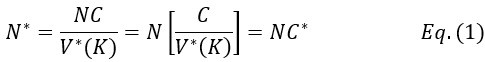
      The trade-off between considered parameter space and computational cost is a long-term challenge in network study as there are always numerous combinations of network nodes, edges, and parameters [Ma et al., Cell, 2009; Chau et al., Cell, 2012]. The computational pipeline in Section 2.1 generalized for all reaction-diffusion networks exerts two strategies to limit the computational cost and set up a basic network reference: 1. Dimension Reduction (Strategy 1) - Unifying the parameter values for different nodes and different edges within the same regulatory type to minimize the unidentical parameter numbers into 3; 2: Parameter Space Confinement (Strategy 2): Enumerating the dimensionless parameter set on a three-dimensional (3D) grid confined by γ∈ [0,0.05] in steps ∆γ = 0.001, k<sub>1</sub>∈[0,5] in steps ∆k<sub>1</sub> = 0.05,  and  in steps .

      In the early stage of our project, we tried to explore “the entire model parameter space” as indicated by the reviewer. We first tried to use the Monte Carlo method to find parameter solutions in an open parameter space and with all parameter values allowed to be different. However, such a process is full of randomness and is computationally expensive (taking months to search viable parameter sets but still unable to profile the continuous viable parameter space; the probability of finding a viable parameter set is no higher than 0.02%, making it very hard to profile a continuous viable parameter space). Now we clearly can see the viable parameter space is a thin curved surface where all parameters have to satisfy a critical balance (Fig. 3a, b, Fig. 5e, f). This is why we exert a typical strategy for dimension reduction in network research in both cell polarization [Marée et al., Bull. Math. Biol., 2006; Goehring et al., Science, 2011; Trong et al., New J. Phys., 2014] and other biological topics (e.g., plasmid transferring in the microbial community [Wang et al., Nat. Commun., 2020]), i.e., unifying the parameter values for different nodes and different edges within the same regulatory type.

      Additionally, the curved surface for viable parameter space can be extended to infinite as long as the parameter balance is achieved (Fig. 3a, b, Fig. 5e, f), it is impossible or unnecessary to explore “the entire model parameter space”. Setting up a confined parameter region near the original point for parameter enumeration can help profile the continuous viable parameter space, which is sufficient for presenting the central conclusion of this paper – that is - the network structure and parameter need to satisfy a balance for stable cell polarization.

      To support a comprehensive study considering all kinds of reference and perturbed networks, we have maximized the parameter domain size by exhausting all the computational research we can access, including 400-500 Intel(R) Core(TM) E5-2670v2 and Gold 6132 CPU on the server (High-Performance Computing Platform at Peking University) and 5 Intel(R) Core(TM) i9-14900HX CPU on personal computers.

      To make it certain that instability holds true when the model parameter space is extended, we add a comprehensive comparison between the simple and complete models about how their instability occurs consistently even when the parameters (i.e., γ, α, k<sub>1</sub>, k<sub>2</sub>, q<sub>1</sub>, q<sub>2</sub> and [X<sub>c</sub>) are assigned with various values concerning all nodes and regulations, searched by the Monte Carlo method (Fig. S5).

      (4) Sensitivity of Numerical Solutions to Initial Conditions: Are the numerical solutions in both models sensitive to the chosen initial condition? What results do the models provide if uniform initial distributions were utilised instead?

      We sincerely thank the editor(s) and referee(s) for the comments!

      To investigate both the simple network and the realistic network consisting of various node numbers and regulatory pathways [Goehring et al., Science, 2011; Lang et al., Development, 2017], we propose a computational pipeline for numerical exploration of the dynamics of a given reaction-diffusion network's dynamics, specifically targeting the maintenance phase of stable cell polarization after its initial establishment [Motegi et al., Nat. Cell Biol., 2011; Goehring et al., Science, 2011; Seirin-Lee et al., Cells, 2020].

      Now we have added new simulations and explanations for the sensitivity of numerical solutions to initial conditions. For both models, a uniform initial distribution leads to a homogeneous pattern while a Gaussian noise distribution leads to a multipolar pattern. In contrast, an initial polarized distribution (even with shifts in transition planes, weak polarization, or asymmetric curve shapes between the two molecular species) can maintain cell polarization reliably.

      (5) Initial Conditions and Stability Tests: In Figure 1, the authors discuss the stability of the basic two-node network (a) upon modifications in (b-d). The stability test is performed through a pipeline procedure in which they always start from a polarised pattern described by Equation (4) and observe how the pattern evolves over time. It would be beneficial to explore whether the stability test depends on this specific initial condition. For instance, what would happen if the posterior molecules have an initial distribution of 1/(1+e^(-10x)), which is not exactly symmetric with respect to the anterior molecules' distribution of 1-1/(1+e^(-20x))? Additionally, if the initial polarisation is not as strong, for example, with the anterior molecules having a distribution of 10-1/(1+e^(-20x)) and the posterior molecules having a distribution of 9+1/(1+e^(-20x)), how would this affect the results?

      We sincerely thank the editor(s) and referee(s) for the constructive advice!

      Now we have added comprehensive comparisons between the simple and complete models about how they respond to alternative initial conditions consistently (Fig. S4, Fig. S9). The successful cell polarization pattern requests an initial polarized pattern, but its following stability and response to perturbation depend very little on the specific form of the initial polarized pattern. All the conditions mentioned by the reviewer have been included.

      (6) Stability Analysis: Throughout the paper, the authors discuss the stability of the polarised pattern. The stability is checked by an exhaustive search of the parameter space, ensuring the system reaches a steady state with a polarised pattern instead of a homogeneous pattern. It would be beneficial to explore if this stability is related to a linear stability analysis of the model parameters, similar to what was conducted in Reference [18], which can determine if a homogeneous state exists and whether it is stable or unstable. Including such an analysis could provide deeper insights into the system's stability and validate its robustness.

      We sincerely thank the editor(s) and referee(s) for the comments!

      We agree that the linear stability analysis can potentially offer additional insights into polarized pattern behavior. However, this approach often requests the aid of numerical solutions and is therefore not entirely independent [Goehring et al., Science, 2011]. Over the past decade, numerical simulations have consistently proven to be a reliable and sufficient approach for studying network dynamics, spanning from C. elegans cell polarization [Tostevin et al., Biophys. J, 2008; Blanchoud et al., Biophys. J, 2015; Seirin-Lee, Dev. Growth Differ., 2020] to topics in metazoon [Chau et al., Cell, 2012; Qiao et al., eLife, 2022; Sokolowski et al., arXiv, 2023]. Numerous purely numerical studies have successfully unveiled principles that help interpret [Ma et al., Cell, 2009] and synthesized real biological systems [Chau et al., Cell, 2012], independent of additional mathematical analysis. Thus, we leverage our numerical framework to address the cell polarization problems cell polarization problems in this paper.

      To confirm the reliability of stability checked by an exhaustive search of the parameter space, now we reproduce the qualitative and semi-quantitative phenomenon in three more experimental groups previously published (Section 2.5; Fig. S8) [Gotta et al., Curr. Biol., 2001; Aceto et al., Dev. Biol., 2006]. Combined with the original experiments (Section 2.5; Fig. 5; Fig. S7) [Hoege et al., Curr. Biol., 2010; Beatty et al., Development, 2010; Beatty et al., Development, 2013], we reproduce five experimental groups in total (two acting on LGL-1 and three acting on CDC-42), comprising eight perturbed conditions and using wild-type as the reference.

      To confirm the robustness of our conclusions regarding the system's stability, now we add comprehensive comparisons between the simple and complete models about 1. How they respond to alternative initial conditions consistently (Fig. S4; Fig. S9). 2. How they respond to alternative single modifications consistently, even when the parameters (i.e., γ, α, k<sub>1</sub>, k<sub>2</sub>, q<sub>1</sub>, q<sub>2</sub> and [X<sub>c</sub> ) are assigned with various values concerning all nodes and regulations (Fig. S5).

      (7) Interface Position Determination: In Figure 4, the authors demonstrate that by using a spatially varied parameter, the position of the interface can be tuned. Particularly, the interface is almost located at the step where the parameter has a sharp jump. However, in the case of a homogeneous parameter (e.g., Figure 4(a)), the system also reaches a stable polarised pattern with the interface located in the middle (x = 0), similar to Figure 4(b), even though the homogeneous parameter does not contain any positional information of the interface. It would be helpful to clarify the difference between Figure 4(a) and Figure 4(b) in terms of the interface position determination.

      We sincerely thank the editor(s) and referee(s) for the comments!

      The case of a homogeneous parameter (e.g., Fig. 4a), in which the system also reaches a stable polarised pattern with the interface located in the middle (x = 0), is just a reference adopted from Fig. 1a to show that the inhomogeneous positional information in Fig. 4b can achieve a similar stable polarised pattern.

      Now we clarify the interface position determination to Section 2.4 to improve readability. Moreover, it is marked with grey dashed line in all the patterns in Fig. 4 and Fig. 6 to highlight the importance of inhomogeneous parameters on interface localization.

      (8) Presented Comparison with Experimental Observations: The comparison with experimental observations lacks clarity. It isn't clear that the model "faithfully recapitulates" the experimental observations (lines 369-370). We recommend discussing and showing these comparisons more carefully, highlighting the expectations and similarities.

      We sincerely thank the editor(s) and referee(s) for the constructive suggestion!

      Now we remove the word “faithfully” and highlight the expectations and similarities of each experimental group by describing “cell polarization pattern characteristics in simulation: …”.

      (9) Validation of Model with Experimental Data: Given the extensive number of model parameters and the uncertainty of their values, it is essential for the authors to validate their model by comparing their results with experimental data. While C. elegans polarisation has been extensively studied, the authors have yet to utilise existing data for parameter estimation and model validation. Doing so would considerably strengthen their study.

      We sincerely thank the editor(s) and referee(s) for the constructive suggestion!

      To utilise existing data for parameter estimation, now we add a new section, Parameter Nondimensionalization and Order of Magtitude Consistency, into Supplemental Text. In this section, we introduced how we adopted the parameter nondimensionalization and value assignments from previous works [Goehring et al., J. Cell Biol., 2011; Goehring et al., Science, 2011; Seirin-Lee et al., Cells, 2020]. We listed four examples (i.e., evolution time, membrane diffusion coefficient, basal off-rate, and inhibition intensity) to show the consistency in order of magtitude between numerical and realistic values.

      To utilise existing data for model validation, now we reproduce the qualitative and semi-quantitative phenomenon in three more experimental groups previously published (Section 2.5; Fig. S8) [Gotta et al., Curr. Biol., 2001; Aceto et al., Dev. Biol., 2006]. Combined with the original experiments (Section 2.5; Fig. 5; Fig. S7) [Hoege et al., Curr. Biol., 2010; Beatty et al., Development, 2010; Beatty et al., Development, 2013], we reproduce five experimental groups in total (two acting on LGL-1 and three acting on CDC-42), comprising eight perturbed conditions and using wild-type as the reference.

      Also, we acknowledge the limitations of the current cell polarization model and provided, in 3. Discussion and conclusion, a detailed outline of potential model improvements. The limitations include, but are not limited to, issues involving “extensive number of model parameters” and “uncertainty of their values”, both of which rely on experimental measurements of biological information. However, comprehensive experimental measurement data on every molecular species, their interactions, and each species’ intensity distribution in space and time were not fully available from prior research. Refinement is lacking for some of these interactions, potentially requiring years of additional experimentation. Moreover, for certain species at specific developmental stages, only relative (rather than absolute) intensity measurements are available. We agreed that such information is essential for establishing a more utilizable model and discussed it thoroughly in 3. Discussion and conclusion. From a theoretical perspective, we adopted assumptions from the previous literature and constructed a minimal model for a specific cell polarization phase to investigate the network's robustness, supported by five experimental groups and eight perturbed conditions with wild-type as a reference in the C. elegans embryo.

      (10) Enhancing Model Accuracy by Considering Cortical Flows: The authors are encouraged to include cortical flows in their cell polarisation model, as these flows are known to be pivotal in the process. Although the current model successfully predicts cell polarisation without accounting for cortical flows, research has demonstrated their significant role in polarisation formation. By incorporating cortical flows, the model would provide a more thorough and precise representation of the biological process. Furthermore, previous studies, such as those by Goehring et al. (References 17 and 18), highlight the importance of convective actin flow in initiating polarisation. It would be valuable for the authors to address the contribution of convection with actin flow to the establishment of the polarisation pattern. The polarisation of the C. elegans zygote progresses through two distinct phases: establishment and maintenance, both heavily influenced by actomyosin dynamics. Works by Munro et al. (Dev Cell 2004), Shivas & Skop (MBoC 2012), Liu et al. (Dev. Biol. 2010), and Wang et al. (Nat Cell Biol 2017) underscore the critical roles of myosin and actin in orchestrating the localisation of PAR proteins during cell polarisation. To enhance the fidelity of their model, we recommend that the authors either integrate cortical flows and consider the effects driven by myosin and actin, or provide a discussion on the repercussions of omitting these dynamics.

      We sincerely thank the editor(s) and referee(s) for the comment!

      Indeed, previous research highlighted the importance of convective cortical flow in orchestrating the localisation of PAR proteins during the establishment phase of polarisation formation [Goehring et al., J. Cell Biol., 2011; Rose et al., WormBook, 2014; Beatty et al., Development, 2013]. However, during the maintenance phase, the non-muscle myosin II (NMY-2) is regulated downstream by the PAR protein network rather than serving as the primary upstream factor controlling PAR protein localization. While some theoretical studies integrated both reaction-diffusion dynamics and the effects of myosin and actin [Tostevin et al., Biophys J, 2008; Goehring et al, Science, 2011], others focused exclusively on reaction-diffusion dynamics [Dawes et al., Biophys. J., 2011; Seirin-Lee et al., Cells, 2020]. Now we clarify the distinction between the establishment and maintenance phases, emphasize our research focus on the reaction-diffusion dynamics during the maintenance phase, and provide a discussion of these omitted dynamics to foster a more comprehensive understanding in the future, as suggested.

      (11) Further Justification of Network Interactions: The authors should provide additional explanations, supported by empirical evidence, for the network interactions assumed in their model. This includes both node-node interactions and the rationale behind protein complex formations. Some of the proposed interactions lack empirical validation, as noted in studies such as Gubieda et al., Phil. Trans. R. Soc. B 2020. Additionally, discrepancies in protein intensity distributions, as observed in Wang et al., Nat Cell Biol 2017, should be addressed, particularly concerning the consideration of the PAR-3/PAR-6/PKC-3 complex as a single entity. Justifying these choices is crucial for ensuring the model's credibility and alignment with experimental findings.

      We sincerely thank the editor(s) and referee(s) for the helpful advice!

      In consistency with previous modeling efforts [Goehring et al., Science, 2011; Gross et al., Nat. Phys., 2019; Lim et al., Cell Rep., 2021], our model treats the PAR-3/PAR-6/PKC-3 complex as a single entity for simplification, thus neglecting the potentially distinct spatial distributions of each single molecular species.

      Now we acknowledge the limitations of the current cell polarization model and provided, in 3. Discussion and conclusion, a detailed outline of potential model improvements. The limitations include, but are not limited to, issues involving “node-node interactions” and “discrepancies in protein intensity distributions”, both of which rely on experimental measurements of biological information. However, comprehensive experimental measurement data on every molecular species, their interactions, and each species’ intensity distribution in space and time were not fully available from prior research. Refinement is lacking for some of these interactions, potentially requiring years of additional experimentation. Moreover, for certain species at specific developmental stages, only relative (rather than absolute) intensity measurements are available. We agreed that such information is essential for establishing a more utilizable model and discussed it thoroughly in 3. Discussion and conclusion.

      To ensure the model's credibility and alignment with experimental findings, now we reproduce the qualitative and semi-quantitative phenomenon in three more experimental groups previously published (Section 2.5; Fig. S8) [Gotta et al., Curr. Biol., 2001; Aceto et al., Dev. Biol., 2006]. Combined with the original experiments (Section 2.5; Fig. 5; Fig. S7) [Hoege et al., Curr. Biol., 2010; Beatty et al., Development, 2010; Beatty et al., Development, 2013], now we have reproduced five experimental groups in total (two acting on LGL-1 and three on CDC-42), comprising eight perturbed conditions and using wild-type as the reference.

      (12) Further Justification of Node-Node Network Interactions: The authors should provide further justification for the node-node network interactions assumed in their study. To the best of our knowledge, some of the node-node interactions proposed have not yet been empirically demonstrated. Providing additional explanations for these interactions would enhance the credibility of the model and ensure its alignment with empirical evidence.

      We sincerely thank the editor(s) and referee(s) for the helpful advice!

      Now we acknowledge the limitations of the current cell polarization model and provided, in 3. Discussion and conclusion, a detailed outline of potential model improvements. The limitations include, but are not limited to, issues involving “node-node network interactions”, which rely on experimental measurements of biological information. However, comprehensive experimental measurement data on every molecular species, their interactions, and each species’ intensity distribution in space and time were not fully available from prior research. Refinement is lacking for some of these interactions, potentially requiring years of additional experimentation. Moreover, for certain species at specific developmental stages, only relative (rather than absolute) intensity measurements are available. We agreed that such information is essential for establishing a more utilizable model and discussed it thoroughly in 3. Discussion and conclusion.

      To enhance the credibility of the model and ensure its alignment with empirical evidence, we reproduced the qualitative and semi-quantitative phenomenon in three more experimental groups previously published (Section 2.5; Fig. S8) [Gotta et al., Curr. Biol., 2001; Aceto et al., Dev. Biol., 2006]. Combined with the original experiments (Section 2.5; Fig. 5; Fig. S7) [Hoege et al., Curr. Biol., 2010; Beatty et al., Development, 2010; Beatty et al., Development, 2013], now we have reproduced five experimental groups in total (two acting on LGL-1 and three on CDC-42), comprising eight perturbed conditions and using wild-type as the reference.

      (13) Justification for Network Interactions and Protein Complexes: The authors must provide clear justifications, supported by references, for each network interaction between nodes in the five-node model. Some of the activatory/inhibitory signals proposed lack empirical validation, such as CDC-42 directly inhibiting CHIN-1. The provided Table S2 is insufficient to justify these interactions, necessitating additional explanations. Reviewing relevant literature, such as the work by Gubieda et al., Phil. Trans. R. Soc. B 2020, may offer insights into similar node networks. Furthermore, the authors should address discrepancies in protein intensity distributions, as observed in studies like Wang et al., Nat Cell Biol 2017. Specifically, the authors consider the PAR-3/PAR-6/PKC-3 complex as a single entity despite potential differences in their distributions. Justification for this choice is essential, particularly considering the importance of clustering dynamics during cell polarisation, as demonstrated by Wang et al., Nat Cell Biol 2017, and Dawes & Munro, Biophys J 2011.

      We sincerely thank the editor(s) and referee(s) for the helpful advice!

      In consistent with previous modeling efforts [Goehring et al., Science, 2011; Gross et al., Nat. Phys., 2019; Lim et al., Cell Rep., 2021], our model treats the PAR-3/PAR-6/PKC-3 complex as a single entity for simplification, thus neglecting the potentially distinct spatial distributions of each single molecular species. Besides, the inhibition of CHIN-1 from CDC-42, which recruits cytoplasmic PAR-6/PKC-3 to form a complex, may act indirectly to restrict CHIN-1 localization through phosphorylation [Sailer et al., Dev. Cell, 2015; Lang et al., Development, 2017].

      Now we acknowledge the limitations of the current cell polarization model and provided, in 3. Discussion and conclusion, a detailed outline of potential model improvements. The limitations include, but are not limited to, issues involving “each network interaction between nodes in the five-node model” and “discrepancies in protein intensity distributions”, both of which rely on experimental measurements of biological information. However, comprehensive experimental measurement data on every molecular species, their interactions, and each species’ intensity distribution in space and time were not fully available from prior research. Refinement is lacking for some of these interactions, potentially requiring years of additional experimentation. Moreover, for certain species at specific developmental stages, only relative (rather than absolute) intensity measurements are available. We agreed that such information is essential for establishing a more utilizable model and discussed it thoroughly in 3. Discussion and conclusion. From a theoretical perspective, we adopted assumptions from the previous literature and constructed a minimal model for a specific cell polarization phase to investigate the network's robustness, supported by five experimental groups and eight perturbed conditions with wild-type as a reference in the C. elegans embryo.

      (14) Incorporating Cytoplasmic Dynamics into the Model: The authors assume infinite cytoplasmic diffusion and neglect the role of cytoplasmic flows in cell polarity, which may oversimplify the model. Finite cytoplasmic diffusion combined with flows could potentially compromise the stability of anterior-posterior molecular distributions, affecting the accuracy of the model's predictions. The authors claim a significant difference between cytoplasmic and membrane diffusion coefficients, but the actual disparity seems smaller based on data from Petrášek et al., Biophys. J. 2008. For example, cytosolic diffusion coefficients for NMY-2 and PAR-2 differ by less than one order of magnitude. Additionally, the strength of cytoplasmic flows, as quantified by studies such as Cheeks et al., and Curr Biol 2004, should be considered when assessing the impact of cytoplasmic dynamics on polarity stability. Incorporating finite cytoplasmic diffusion and cytoplasmic flows into the model could provide a more realistic representation of cellular dynamics and enhance the model's predictive power.

      We sincerely thank the editor(s) and referee(s) for the comment!

      Cytoplasmic and membrane diffusion coefficients differ by two orders of magnitude according to previous experimental measurements on PAR-2 and PAR-6 [Goehring et al., J. Cell Biol., 2011; Lim et al., Cell Rep., 2021]. Many previous C. elegans cell polarization models have incorporated mass-conservation model combined with finite cytoplasmic diffusion, but this model description can lead to reverse spatial concentration distribution between the cell membrane and cytosol [Fig. 3 of Seirin-Lee et al., J. Theor. Biol., 2016; Fig. 2ab of Seirin-Lee et al., J. Math. Biol., 2020], disobeying experimental observation [Fig. 4A of Sailer et al., Dev. Cell, 2015; Fig. 1A of Lim et al., Cell Rep., 2021]. This implies that the infinite cytoplasmic diffusion, without precise experiment-based parameter assignment or accounting for other hidden biological processes (e.g., protein production and degradation), may be inappropriate in modeling the real spatial concentration distributions distinguished between the cell membrane and cytosol. To address this issue, some theoretical research incorporated protein production and degradation into their model, to acquire the consistent spatial concentration distribution between the cell membrane and cytosol [Tostevin et al., Biophys. J., 2008]. More definitive experimental data on the spatiotemporal changes in protein diffusion, production, and degradation are essential for providing a more realistic representation of cellular dynamics and enhancing the model's predictive power.

      Cytoplasmic flows indeed play an unneglectable role in cell polarity during the establishment phase [Kravtsova et al., Bull. Math. Biol., 2014], which creates a spatial gradient of actomyosin contractility and directs PAR-3/PKC-3/PAR-6 to the anterior membrane by cortical flow [Rose et al., WormBook, 2014; Lang et al., Development, 2017]. However, during the maintenance phase, the non-muscle myosin II (NMY-2) is regulated downstream by the PAR protein network rather than serving as the primary upstream factor controlling PAR protein localization [Goehring et al., J. Cell Biol., 2011; Rose et al., WormBook, 2014; Geβele et al., Nat. Commun., 2020]. While some theoretical studies integrated both reaction-diffusion dynamics and the effects of myosin and actin [Tostevin, 2008; Goehring, Science, 2011], others focused exclusively on reaction-diffusion dynamics [Dawes et al., Biophys. J., 2011; Seirin-Lee et al., Cells, 2020]. We now emphasize our research focus on the reaction-diffusion dynamics during the maintenance phase, so the dynamics between NMY-2 and PAR-2 are not included. We have also provided a discussion of the simplified cytoplasmic diffusion and omitted cytoplasmic flows to foster a more comprehensive understanding in the future.

      (15) Explanation of Lethality References: On page 13, the authors mention lethality without adequately explaining why they are drawing connections with lethality experimental data.

      We sincerely thank the editor(s) and referee(s) for the comment!

      It is well-known that cell polarity loss in C. elegans zygote will lead to symmetric cell division, which brings out the more symmetric allocation of molecular-to-cellular contents in daughter cells; this will result in abnormal cell size, cell cycle length, and cell fate in daughter cells, followed by embryo lethality [Beatty et al., Development, 2010; Beatty et al., Development, 2013; Rodriguez et al., Dev. Cell, 2017; Jankele et al., eLife, 2021]. Now we explain why we are drawing connections with lethality experimental data in Section 2.5.

      (16) Improved Abstract: "...However, polarity can be restored through a combination of two modifications that have opposing effects..." This sentence could be revised for better clarity. For example, the authors could consider rephrasing it as follows: "...However, polarity restoration can be achieved by combining two modifications with opposing effects...".

      We sincerely thank the editor(s) and referee(s) for helpful advice!

      Now we revise the abstract as follows:

      “Abstract – However, polarity restoration can be achieved by combining two modifications with opposing effects.”

      (17) Conservation of Mass in Network Models: Is conservation of mass satisfied in their network models?

      We sincerely thank the editor (s) and referee(s) for the comment!

      While previous experiments provide evidence for near-constant protein mass during the establishment phase [Goehring et al., Science, 2011], whether this is consistent until the end of maintenance is unclear.

      Many previous C. elegans cell polarization models have assumed mass conservation on the cell membrane and in the cell cytosol, this model description can lead to reverse spatial concentration distribution between the cell membrane and cytosol [Fig. 3 of Seirin-Lee et al., J. Theor. Biol., 2016; Fig. 2ab of Seirin-Lee et al., J. Math. Biol., 2020], disobeying experimental observation [Fig. 4A of Sailer et al., Dev. Cell, 2015; Fig. 1A of Lim et al., Cell Rep., 2021]. This implies that mass conservation may be inappropriate in modeling the real spatial concentration distributions distinguished between the cell membrane and cytosol. To address this issue, some theoretical research incorporated protein production and degradation into their model, instead of assuming mass conservation [Tostevin et al., Biophys. J., 2008]. More definitive experimental data on the spatiotemporal changes in protein mass are essential for constructing a more accurate model.

      Given the absence of a universally accepted model in agreement with experimental observation, we adopted the assumption that the concentration of molecules in the cytosol (not the total mass on the cell membrane and in the cell cytosol) is spatially inhomogeneous and temporally constant, which was also used before [Kravtsova et al., Bull. Math. Biol., 2014]. In the context of this well-mixed constant cytoplasmic concentration, our model successfully reproduced the cell polarization phenotype in wild-type and eight perturbed conditions (Section 2.5; Fig. S7; Fig. S8), supporting the validity of this simplified, yet effective, model. Now we have provided a discussion of protein mass assumption to foster a more comprehensive understanding in the future.

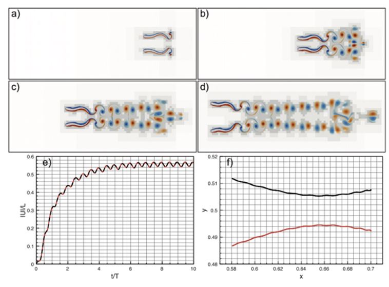
      (18) Comparison of Network Structures: In Figure 1c, the authors demonstrate that the symmetric two-node network is susceptible to single-sided additional regulation. They considered four subtypes of modifications, depending on whether [L] is in the anterior or posterior and whether [A] and [L] are mutually activating or inhibiting. What is the difference between the structure where [L] is in the anterior and in the posterior? Upon comparing the time evolution of the left panel ([L] is sided with

      ) and the right panel ([L] is sided with [A]), the difference is so tiny that they are almost indistinguishable. It might be beneficial for the authors to provide a clearer explanation of the differences between these network structures to aid in understanding their implications.

      We sincerely thank the editor(s) and referee(s) for the constructive suggestion!

      The difference between the structures where [L] is in the anterior and posterior is the initial spatial concentration distribution of [L], which is polarized to have a higher concentration in the anterior and posterior respectively. The time evolution of the left panel ([L] is sided with [P]) and the right panel [L] is sided with [P]) is almost indistinguishable because the perturbation from [L] is slight (less than over one order of magnitude) compared to the predominant [A]~[P] interaction ( for [A]~[P] mutual inhibition while for [A]~[L] mutual inhibition and for [A]~[L] mutual activation), highlighting the response of cell polarization pattern. To aid the readers in understanding their implications, we have added the [L] and plotted the spatial concentration distribution of all three molecular species at t=0,100, 200, 300, 400 and 500 in Fig. S3, where the difference between the [L] ones in the left and right panels are distinguishably shown.

      (19) Figure Reference: In line 308, Fig. 4a is referenced when explaining the loss of pattern stability by modifying an individual parameter, but this is not shown in that panel. Please update the panel or adjust the reference in the main text.

      We sincerely thank the editor(s) and referee(s) for pointing out this problem!

      Fig. 4 focuses on the regulatable shift of the zero-velocity interface by modifying a pair of individual parameters, not on the loss (or recovery) of pattern stability, which has been analyzed as a focus in Fig. 1, Fig. 2, and Fig. 3. Fig. 4a is actually from the same simulation as the one in Fig. 1a, which has spatially uniform parameters used as a reference in Fig. 4. The individual parameter modification in other subfigures of Fig. 4 shows how the zero-velocity interface is shifted in a regulatable manner always in the context of pattern stability. Now we update the panel, adjust the reference, add one more paragraph, and improve the wording to clarify how the analyses in Fig. 4 are carried out on top of the pattern stability already studied.

      (20) Viable Parameter Sets: In line 355, the number of viable parameter sets (602) is not very informative by itself. We suggest reporting the fraction or percentage of sets tested that resulted in viable results instead. This applies similarly to lines 411 and 468.

      We sincerely thank the editor(s) and referee(s) for the constructive comment!

      Now the fraction/percentage of parameter sets tested that resulted in viable results are added everywhere the number appears.

      (21) Perturbation Experiments: In lines 358-359, "the perturbation experiments" implies that those considered are the only possible ones. Please rephrase to clarify.

      We sincerely thank the editor(s) and referee(s) for the helpful advice!

      Now we rephrase three paragraphs to clarify why the perturbation experiments involved with [L] and [C] are considered instead of other possible ones.

      (22) Figure 2S: This figure is unclear. The caption states that panel (a) shows the "final concentration distribution," but only a line is shown. If "distribution" refers to spatial distribution, please clarify which parameters are shown.

      We sincerely thank the editor(s) and referee(s) for pointing out this problem!

      Now we clarify the “spatial concentration distribution” and which parameters are shown in the figure caption.

      (23) Figure 5 and 6 Captions: The captions for Figures 5 and 6 could benefit from clarification for better understanding.

      We sincerely thank the editor(s) and referee(s) for the constructive suggestion!

      Now we clarify the details in the captions of Fig. 5 and Fig. 6 for better understanding.

      (24) Figure 5 Legend: The legend on the bottom right corner of Figure 5 is unclear. Please specify to which panel it refers.

      We sincerely thank the editor(s) and referee(s) for the constructive suggestion!

      Now we clarify to which the legend on the bottom right corner of Fig. 5 refers.

      (25) L and A~C Interactions: In paragraphs 405-418, please explain why the L and A~C interactions are removed for the comparison instead of others.

      We sincerely thank the editor(s) and referee(s) for the constructive suggestion!

      Now we add a separate paragraph and a supplemental figure to explain why the L and A~C interactions are removed for the comparison instead of others.

      (26) Network Structures in Figure S3: From the "34 possible network structures" considered in Figure S3 (lines 440-441), why are the "null cases" (L disconnected from the network) relevant? Shouldn't only 32 networks be considered?

      We sincerely thank the editor(s) and referee(s) for pointing out this problem!

      Now the two “null cases” are removed:

      (27) Figure S3 Caption: The caption must state that the position of the nodes (left or right) implies the polarisation pattern. Additionally, with the current size of the figure, the dashed lines are extremely hard to differentiate from the continuous lines.

      We sincerely thank the editor(s) and referee(s) for the constructive suggestion!

      Now we state that the position of the nodes (left or right) implies the polarization pattern. Additionally, we have modified the figure size and dashed lines so that the dash lines are adequately distinguishable from the continuous lines.

      (28) Equation #7: It is confusing to use P as the number of independent simulations when P is also one of the variables/species in the network. Please consider using different notation.

      We sincerely thank the editor(s) and refer(s) for the hhelpful advice!

      Now we replace the P in current Equation #8 with Q and the P in current Equation #10 with W.

      (29) Use of "Detailed Balance": The authors used the term "detailed balance" to describe the intricate balance between the two groups of proteins when forming a polarised pattern. However, "detailed balance" is a term with a specific meaning in thermodynamics. Breaking detailed balance is a feature of nonequilibrium systems, and the polarisation phenomenon is evidently a nonequilibrium process. Using the term "detailed balance" may cause confusion, especially for readers with a physics background. It might be advisable to reconsider the terminology to avoid potential confusion and ensure clarity for readers.

      We sincerely thank the editor(s) and referee(s) for the constructive suggestion!

      To avoid potential confusion and ensure clarity for readers, now we replace “detailed balance” with “balance”, “required balance”, or “interplay” regarding different contexts.

      (30) Terminology: The word "molecule" is used where "molecular species" would be more appropriate, e.g., lines 456 and 551. Please revise these instances.

      We sincerely thank the editor(s) and referee(s) for the constructive suggestion!

      Now we replace all the “molecule” by “molecular species” as suggested.

      (31) Section 2.5: This section is confusing. It isn't clear where the "method outlined" (line 464) is nor what "span an iso-velocity surface at vanishing speed" means in line 470. The sentence in lines 486-488, "An expression similar to Eq. 8 enables quantitative prediction...", is too vague. Please clarify these points and specify what the "similar expression" is and where it can be found.

      We sincerely thank the editor(s) and referee(s) for the constructive suggestion!

      Now we clarify these points and specify the terms as suggested.

      (32) Software Mention: The software is only mentioned in the abstract and conclusions. It should also be mentioned where the computational pipeline is described, and the instructions available in the supplementary information need to be referenced in the main text.

      We sincerely thank the editor(s) and referee(s) for pointing out this problem!

      Now we mention the software where the computational pipeline is described and reference the instructions available in the Supplemental Text.

      (33) Supplementary Material References: Several parts of the supplementary material are never referenced in the main text, including Figure S1, Movies S3-S4, and the Instructions for PolarSim. Please reference these in the main text to clarify their relevance and how they fit with the manuscript's narrative.

      We sincerely thank the editor(s) and referee(s) for pointing out this problem!

      Now we add all the missing references for supplementary materials to the main text properly.

    1. Author response:

      The following is the authors’ response to the original reviews.

      Preliminary note from the Reviewing Editor:

      The evaluations of the two Reviewers are provided for your information. As you can see, their opinions are very different.

      Reviewer #1 is very harsh in his/her evaluation. Clearly, we don't expect you to be able to affect one type of actin network without affecting the other, but rather to change the balance between the two. However, he/she also raises some valid points, in particular that more rationale should be added for the perturbations (also mentioned by Reviewer #2). Both Reviewers have also excellent suggestions for improving the presentation of the data.

      We sincerely appreciate your and the reviewers’ suggestions. The comments are amended accordingly.

      On another point, I was surprised when reading your manuscript that a molecular description of chirality change in cells is presented as a completely new one. Alexander Bershadsky's group has identified several factors (including alpha-actinin) as important regulators of the direction of chirality. The articles are cited, but these important results are not specifically mentioned. Highlighting them would not call into question the importance of your work, but might even provide additional arguments for your model.

      We appreciate the editor’s comment. Alexander Bershadsky's group has done marvelous work in cell chirality. They introduced the stair-stepping and screw theory, which suggested how radial fiber polymerization generates ACW force and drives the actin cytoskeleton into the ACW pattern. Moreover, they have identified chiral regulators like alpha-actinin 1, mDia1, capZB, and profilin 1, which can reverse or neutralize the chiral expression.

      It is worth noting that Bershadsky's group primarily focuses on radial fibers. In our manuscript, instead, we primarily focused on the contractile unit in the transverse arcs and CW chirality in our investigation. Our manuscript incorporates our findings in the transverse arcs and the radial fibers theory by Bershadsky's group into the chirality balance hypothesis, providing a more comprehensive understanding of the chirality expression.

      We have included relevant articles from Alexander Bershadsky's group, we agree that highlighting these important results of chiral regulators would further strengthen our manuscript. The manuscript was revised as follows:

      “ACW chirality can be explained by the right-handed axial spinning of radial fibers during polymerization, i.e. ‘stair-stepping' mode proposed by Tee et al. (Tee et al. 2015) (Figure 8A; Video 4). As actin filament is formed in a right-handed double helix, it possesses an intrinsic chiral nature. During the polymerization of radial fiber, the barbed end capped by formin at focal adhesion was found to recruit new actin monomers to the filament. The tethering by formin during the recruitment of actin monomers contributes to the right-handed tilting of radial fibers, leading to ACW rotation. Supporting this model, Jalal et al. (Jalal et al. 2019) showed that the silencing of mDia1, capZB, and profilin 1 would abolish the ACW chiral expression or reverse the chirality into CW direction. Specifically, the silencing of mDia1, capZB or profilin-1 would attenuate the recruitment of actin monomer into the radial fiber, with mDia1 acting as the nucleator of actin filament (Tsuji et al. 2002), CapZB promoting actin polymerization as capping protein (Mukherjee et al. 2016), and profilin-1 facilitating ATP-bound G-actin to the barbed ends(Haarer and Brown 1990; Witke 2004). The silencing resulted in a decrease in the elongation velocity of radial fiber, driving the cell into neutral or CW chirality. These results support that our findings that reduction of radial fiber elongation can invert the balance of chirality expression, changing the ACW-expressing cell into a neutral or CW-expressing cell.”

      By incorporating their findings into our revision and discussion, we provide additional support for our radial fiber-transverse arc balance model for chirality expression. The revision is made on pages 8 to 9, 13, lines 253 to 256, 284, 312 to 313, 443, 449 to 459.

      Public Reviews:

      Reviewer #1 (Public Review):

      Summary:

      Kwong et al. present evidence that two actin-filament based cytoskeletal structures regulate the clockwise and anticlockwise rotation of the cytoplasm. These claims are based on experiments using cells plated on micropatterned substrates (circles). Previous reports have shown that the actomyosin network that forms on the dorsal surface of a cell plated on a circle drives a rotational or swirling pattern of movement in the cytoplasm. This actin network is composed of a combination of non-contractile radial stress fibers (AKA dorsal stress fibers) which are mechanically coupled to contractile transverse actin arcs (AKA actin arcs). The authors claim that directionality of the rotation of the cytoplasm (i.e., clockwise or anticlockwise) depends on either the actin arcs or radial fibers, respectively. While this would interesting, the authors are not able to remove either actin-based network without effecting the other. This is not surprising, as it is likely that the radial fibers require the arcs to elongate them, and the arcs require the radial fibers to stop them from collapsing. As such, it is difficult to make simple interpretations such as the clockwise bias is driven by the arcs and anticlockwise bias is driven by the radial fibers.

      Weaknesses:

      (1) There are also multiple problems with how the data is displayed and interpreted. First, it is difficult to compare the experimental data with the controls as the authors do not include control images in several of the figures. For example, Figure 6 has images showing myosin IIA distribution, but Figure 5 has the control image. Each figure needs to show controls. Otherwise, it will be difficult for the reader to understand the differences in localization of the proteins shown. This could be accomplished by either adding different control examples or by combining figures.

      We appreciate the reviewer’s comment. We agree with the reviewer that it is difficult to compare our results in the current arrangement. The controls are included in the new Figure 6.

      (2) It is important that the authors should label the range of gray values of the heat maps shown. It is difficult to know how these maps were created. I could not find a description in the methods, nor have previous papers laid out a standardized way of doing it. As such, the reader needs some indication as to whether the maps showing different cells were created the same and show the same range of gray levels. In general, heat maps showing the same protein should have identical gray levels. The authors already show color bars next to the heat maps indicating the range of colors used. It should be a simple fix to label the minimum (blue on the color bar) and the maximum (red on the color bar) gray levels on these color bars. The profiles of actin shown in Figure 3 and Figure 3- figure supplement 3 were useful for interpretating the distribution of actin filaments. Why did not the authors show the same for the myosin IIa distributions?

      We appreciate the reviewer’s comment. For generating the distribution heatmap, the images were taken under the same setting (e.g., fluorescent staining procedure, excitation intensity, or exposure time). The prerequisite of cells for image stacking was that they had to be fully spread on either 2500 µm2 or 750 µm2 circular patterns. Then, the location for image stacking was determined by identifying the center of each cell spread in a perfect circle. Finally, the images were aligned at the cell center to calculate the averaged intensity to show the distribution heatmap on the circular pattern. Revision is made on pages 19 to 20, lines 668 to 677.

      It is important to note that the individual heatmaps represent the normalized distribution generated using unique color intensity ranges. This approach was chosen to emphasize the proportional distribution of protein within cells and its variations among samples, especially for samples with generally lower expression levels. Additionally, a differential heatmap with its own range was employed to demonstrate the normalized differences compared to the control sample. Furthermore, to provide additional insight, we plotted the intensity profile of the same protein with the same size for comparative analysis. Revision is made on pages 20, lines 679 to 682.

      The labels of the heatmap are included to show the intensity in the revised Figure 3, Figure 5, Figure 6, and Figure 3 —figure supplement 4.

      To better illustrate the myosin IIa distribution, the myosin intensity profiles were plotted for Y27 treatment and gene silencing. The figures are included as Figure 5—figure supplement 2 and Figure 6—figure supplement 2. Revisions are made on pages 10, lines 332 to 334 and pages 11, lines 377 to 379.

      (3) Line 189 "This absence of radial fibers is unexpected". The authors should clarify what they mean by this statement. The claim that the cell in Figure 3B has reduced radial stress fiber is not supported by the data shown. Every actin structure in this cell is reduced compared to the cell on the larger micropattern in Figure 3A. It is unclear if the radial stress fibers are reduced more than the arcs. Are the authors referring to radial fiber elongation?

      We appreciate the reviewer’s comment. We calculated the structures' pixel number and the percentage in the image to better illustrate the reduction of radial fiber or transverse arc. As radial fibers emerge from the cell boundary and point towards the cell center and the transverse arcs are parallel to the cell edge, the actin filament can be identified by their angle with respect to the cell center. We found that the pixel number of radial fiber is greatly reduced by 91.98 % on 750 µm2 compared to the 2500 µm2 pattern, while the pixel number of transverse arc is reduced by 70.58 % (Figure 3- figure supplement 3A). Additionally, we compared the percentage of actin structures on different pattern sizes (Figure 3- figure supplement 3B). On 2500 µm2 pattern, the percentage of radial fiber in the actin structure is 61.76 ± 2.77 %, but it only accounts for 31.13 ± 2.76 % while on 750 µm2 pattern. These results provide evidence of the structural reduction on a smaller pattern.

      Regarding the radial fiber elongation, we only discussed the reduction of radial fiber on 750 µm2 compared to the 2500 µm2 pattern in this part. For more understanding of the radial fiber contribution to chirality, we compared the radial fiber elongation rate in the LatA treatment and control on 2500 µm2 pattern (Figure 4). This result suggests the potential role of radial fiber in cell chirality. Revisions are made on page 6, lines 186 to 194; pages 17 to 18, 601 to 606; and the new Figure 3- figure supplement 3.

      (4) The choice of the small molecule inhibitors used in this study is difficult to understand, and their results are also confusing. For example, sequestering G actin with Latrunculin A is a complicated experiment. The authors use a relatively low concentration (50 nM) and show that actin filament-based structures are reduced and there are more in the center of the cell than in controls (Figure 3E). What was the logic of choosing this concentration?

      We appreciate the reviewer’s comment. The concentration of drugs was selected based on literatures and their known effects on actin arrangement or chiral expression.

      For example, Latrunculin A was used at 50 nM concentration, which has been proven effective in reversing the chirality at or below 50 nM (Bao et al., 2020; Chin et al., 2018; Kwong et al., 2019; Wan et al., 2011). Similarly, the 2 µM A23187 treatment concentration was selected to initiate the actin remodeling (Shao et al., 2015). Furthermore, NSC23677 at 100 µM was found to efficiently inhibit the Rac1 activation and resulted in a distinct change in actin structure (Chen et al., 2011; Gao et al., 2004), enhancing ACW chiral expression. The revision is made on pages 6 to 7, lines 202 to 211.

      (5) Using a small molecule that binds the barbed end (e.g., cytochalasin) could conceivably be used to selectively remove longer actin filaments, which the radial fibers have compared to the lamellipodia and the transverse arcs. The authors should articulate how the actin cytoskeleton is being changed by latruculin treatment and the impact on chirality. Is it just that the radial stress fibers are not elongating? There seems to be more radial stress fibers than in controls, rather than an absence of radial stress fibers.

      We appreciate the reviewer’s comment. Our results showed Latrunculin A treatment reversed the cell chirality. To compare the amount of radial fiber and transverse arc, we calculated the structures' pixel percentage. We found that, the percentage of radial fibers pixel with LatA treatment was reduced compared to that of the control, while the percentage of transverse arcs pixel increased (Figure 3— figure supplement 5). This result suggests that radial fibers are inhibited under Latrunculin A treatment.

      Furthermore, the elongation rate of radial fibers is reduced by Latrunculin A treatment (Figure 4). This result, along with the reduction of radial fiber percentage under Latrunculin A treatment suggests the significant impact of radial fiber on the ACW chirality.  Revisions are made on pages 7 to 8, lines 244 to 250 and the new Figure 3— figure supplement 5 and Figure 3— figure supplement 6.

      (6) Similar problems arise from the other small molecules as well. LPA has more effects than simply activating RhoA. Additionally, many of the quantifiable effects of LPA treatment are apparent only after the cells are serum starved, which does not seem to be the case here.

      We appreciate the reviewer’s comment. The reviewer mentioned that the quantifiable effects of LPA treatments were seen after the cells were serum-starved. LPA is known to be a serum component and has an affinity to albumin in serum (Moolenaar, 1995). Serum starvation is often employed to better observe the effects of LPA by comparing conditions with and without LPA. We agree with the reviewer that the effect of LPA cannot be fully seen under the current setting. Based on the reviewer’s comment and after careful consideration, we have decided to remove the data related to LPA from our manuscript. Revisions are made on pages 6 to 7, 17 and Figure 3— figure supplement 4.

      (7) Furthermore, inhibiting ROCK with, Y-27632, effects myosin light chain phosphorylation and is not specific to myosin IIA. Are the two other myosin II paralogs expressed in these cells (myosin IIB and myosin IIC)? If so, the authors’ statements about this experiment should refer to myosin II not myosin IIa.

      We appreciate the reviewer’s comment. We agree that ensuring accuracy and clarity in our statements is important. The terminology is revised to myosin II regarding the Y27632 experiment for a more concise description. Revision is made on pages 9 to 10 and 29, lines 317 to 341, 845 and 848.  

      (8) None of the uses of the small molecules above have supporting data using a different experimental method. For example, backing up the LPA experiment by perturbing RhoA tho.

      We appreciate the reviewer’s comment. After careful consideration, we have decided to remove the data related to LPA from our manuscript. Revisions are made on pages 6 to 7, 17 and Figure 3— figure supplement 4.

      (9) The use of SMIFH2 as a "formin inhibitor" is also problematic. SMIFH2 also inhibits myosin II contractility, making interpreting its effects on cells difficult to impossible. The authors present data of mDia2 knockdown, which would be a good control for this SMIFH2.

      We appreciate the reviewer’s comment. We agree that there is potential interference of SMIFH2 with myosin II contractility, which could introduce confounding factors to the results. Based on your comment and further consideration, we have decided to remove the data related to SMIFH2 from our manuscript. Revisions are made on pages 6 to 7, 10, 17 and Figure 3— figure supplement 4.

      (10) However, the authors claim that mDia2 "typically nucleates tropomyosin-decorated actin filaments, which recruit myosin II and anneal endwise with α-actinin- crosslinked actin filaments."

      There is no reference to this statement and the authors own data shows that both arcs and radial fibers are reduced by mDia2 knockdown. Overall, the formin data does not support the conclusions the authors report.

      We appreciate the reviewer’s comment. We apologize for the lack of citation for this claim. To address this, we have added a reference to support this claim in the revised manuscript (Tojkander et al., 2011). Revision is made on page 10, line 345 to 347.

      Regarding the actin structure of mDia2 gene silencing, our results showed that myosin II was disassociated from the actin filament compared to the control. At the same time, there is no considerable differences in the actin structure of radial fibers and transverse arcs between the mDia2 gene silencing and the control.  

      (11) The data in Figure 7 does not support the conclusion that myosin IIa is exclusively on top of the cell. There are clear ventral stress fibers in A (actin) that have myosin IIa localization. The authors simply chose to not draw a line over them to create a height profile.

      We appreciate the reviewer’s comment. To better illustrate myosin IIa distribution in a cell, we have included a video showing the myosin IIa staining from the base to the top of the cell (Video 7). At the cell base, the intensity of myosin IIa is relatively low at the center. However, when the focal plane elevates, we can clearly see the myosin II localizes near the top of the cell (Figure 7B and Video 7). Revision is made on page 12, lines 421 to 424, and the new Video 7. 

      Reviewer #2 (Public Review):

      Summary:

      Chirality of cells, organs, and organisms can stem from the chiral asymmetry of proteins and polymers at a much smaller lengthscale. The intrinsic chirality of actin filaments (F-actin) is implicated in the chiral arrangement and movement of cellular structures including F-actin-based bundles and the nucleus. It is unknown how opposite chiralities can be observed when the chirality of F-actin is invariant. Kwong, Chen, and co-authors explored this problem by studying chiral cell-scale structures in adherent mammalian cultured cells. They controlled the size of adhesive patches, and examined chirality at different timepoints. They made various molecular perturbations and used several quantitative assays. They showed that forces exerted by antiparallel actomyosin bundles on parallel radial bundles are responsible for the chirality of the actomyosin network at the cell scale.

      Strengths:

      Whereas previously, most effort has been put into understanding radial bundles, this study makes an important distinction that transverse or circumferential bundles are made of antiparallel actomyosin arrays. A minor point that was nice for the paper to make is that between the co-existing chirality of nuclear rotation and radial bundle tilt, it is the F-actin driving nuclear rotation and not the other way around. The paper is clearly written.

      Weaknesses:

      The paper could benefit from grammatical editing. Once the following Major and Minor points are addressed, which may not require any further experimentation and does not entail additional conditions, this manuscript would be appropriate for publication in eLife.

      Recommendations for the authors:

      Reviewer #2 (Recommendations For The Authors):

      Major:

      (1) The binary classification of cells as exhibiting clockwise or anticlockwise F-actin structures does not capture the instances where there is very little chirality, such as in the mDia2-depleted cells on small patches (Figure 6B). Such reports of cell chirality throughout the cell population need to be reported as the average angle of F-actin structures on a per cell basis as a rose plot or scatter plot of angle. These changes to cell-scoring and data display will be important to discern between conditions where chirality is random (50% CW, 50% ACW) from conditions where chirality is low (radial bundles are radial and transverse arcs are circumferential).

      We appreciate the reviewer’s comment. We apologize if we did not convey our analysis method clearly enough. Throughout the manuscript, unless mentioned otherwise, the chirality analysis was based on the chiral nucleus rotation within a period of observation. The only exception is the F-actin structure chirality, in Figure 3—figure supplement 1, which we analyzed the angle of radial fiber of the control cell on 2500 µm2. It was described on pages 5 to 6, lines 169-172, and the method section “Analysis of fiber orientation and actin structure on circular pattern” on page 17.

      Based on the feedback, we attempted to use a scatter plot to present the mDia2 overexpression and silencing to show the randomness of the result. However, because scatter plots primarily focus on visualizing the distribution, they become cluttered and visually overwhelming, as shown below.

      Author response image 1.

      (A) Percentage of ACW nucleus rotational bias on 2500 µm2 with untreated control (reused data from Figure 3D, n = 57), mDia2 silencing (n = 48), and overexpression (n = 25). (B) Probability of ACW/CW rotation on 750 µm2 pattern with untreated control (reused data from Figure 3E, n = 34), mDia2 silencing (n = 53), and overexpressing (n = 22). Mean ± SEM. Two-sample equal variance two-tailed t-test.

      Therefore, in our manuscript, the presentation primarily used a column bar chart with statistical analysis, the Student T-test. The column bar chart makes it easier to understand and compare values. In brief, the Student T-test is commonly used to evaluate whether the means between the two groups are significantly different, assuming equal variance. As such, the Student T-test is able to discern the randomness of the chirality.

      (2) The authors need to discuss the likely nucleator of F-actin in the radial bundles, since it is apparently not mDia2 in these cells.

      We appreciate the reviewer’s comment. In our manuscript, we originally focused on mDia2 and Tpm4 as they are the transverse arc nucleator and the mediator of myosin II motion. However, we agree with the reviewer that discussing the radial fiber nucleator would provide more insight into radial fiber polymerization in ACW chirality and improve the completeness of the story.

      Radial fiber polymerizes at the focal adhesion. Serval proteins are involved in actin nucleation or stress fiber formation at the focal adhesion, such as Arp2/3 complex (Serrels et al., 2007), Ena/VASP (Applewhite et al., 2007; Gateva et al., 2014), and formins (Dettenhofer et al., 2008; Sahasrabudhe et al., 2016; Tsuji et al., 2002), etc. Within the formin family, mDia1 is the likely nucleator of F-actin in the radial bundle. The presence of mDia1 facilitates the elongation of actin bundles at focal adhesion (Hotulainen and Lappalainen, 2006). Studies by Jalal, et al (2019) (Jalal et al., 2019) and Tee, et al (2023) (Tee et al., 2023), have demonstrated the silencing of mDia1 abolished the ACW actin expression. Silencing of other nucleation proteins like Arp2/3 complex or Ena/VASP would only reduce the ACW actin expression without abolishing it.

      Based on these findings, the attenuation of radial fiber elongation would abolish the ACW chiral expression, providing more support for our model in explaining chirality expression.

      This part is incorporated into the Discussion. The revision is made on page 13, lines 443, 449 to 459.

      Minor:

      (1) In the introduction, additional observations of handedness reversal need to be referenced (line 79), including Schonegg, Hyman, and Wood 2014 and Zaatri, Perry, and Maddox 2021.

      We appreciate the reviewer’s comment. The observations of handedness reversal references are cited on page 3, line 78 to 79.

      (2) For clarity of logic, the authors should share the rationale for choosing, and results from administering, the collection of compounds as presented in Figure 3 one at a time instead of as a list.

      We appreciate the reviewer’s comment. The concentration of drugs was determined based on existing literature and their known outcomes on actin arrangement or chiral expression.

      To elucidate, the use of Latrunculin A was based on previous studies, which have demonstrated to reverse the chirality at or below 50 nM (Bao et al., 2020; Chin et al., 2018; Kwong et al., 2019; Wan et al., 2011).  Because inhibiting F-actin assembly can lead to the expression of CW chirality, we hypothesized that the opposite treatment might enhance ACW chirality. Therefore, we chose A23187 treatment with 2 µM concentration as it could initiate the actin remodeling and stress fiber formation (Shao et al., 2015).

      Furthermore, in the attempt to replicate the reversal of chirality by inhibiting F-actin assembly through other pathways, we explored NSC23677 at 100 µM, which was found to inhibit the Rac1 activation (Chen et al., 2011; Gao et al., 2004) and reduce cortical F-actin assembly (Head et al., 2003). However, it failed to reverse the chirality but enhanced the ACW chirality of the cell.

      We carefully selected the drugs and the applied concentration to investigate various pathways and mechanisms that influence actin arrangement and might affect the chiral expression. We believe that this clarification strengthens the rationale behind our choice of drug. The revision is made on pages 6 to 7, lines 202 to 211.

      (3) "Image stacking" isn't a common term to this referee. Its first appearance in the main text (line 183) should be accompanied with a call-out to the Methods section. The authors could consider referring to this approach more directly. Related issue: Image stacking fails to report the prominent enrichment of F-actin at the very cell periphery (see Figure 3 A and F) except for with images of cells on small islands (Figure 3H). Since this data display approach seems to be adding the intensity from all images together, and since cells on circular adhesive patches are relatively radially symmetric, it is unclear how to align cells, but perhaps cells could be aligned based on a slight asymmetry such as the peripheral location with highest F-actin intensity or the apparent location of the centrosome.

      We appreciate the reviewer’s comment. We fully acknowledge the uncommon use of “image stacking” and the insufficient description of image stacking under the Method section. First, we have added a call-out to the Methods section at its first appearance (Page 6, Lines 182 to 183). The method of image stacking is as follows. During generating the distribution heatmap, the images were taken under the same setting (e.g., staining procedure, fluorescent intensity, exposure time, etc.). The prerequisite of cells to be included in image stacking was that they had to be fully spread on either 2500 µm2 or 750 µm2 circular patterns. Then, the consistent position for image stacking could be found by identifying the center of each cell spreading in a perfect circle. Finally, the images were aligned at the center to calculate the averaged intensity to show the distribution heatmap on the circular pattern.

      We agree with the reviewer that our image alignment and stacking are based on cells that are radially symmetric. As such, the intensity distribution of stacked image is to compare the difference of F-actin along the radial direction. Revision is made on page 19, lines 668 to 682.

      (4) The authors need to be consistent with wording about chirality, avoiding "right" and left (e.g. lines 245-6) since if the cell periphery were oriented differently in the cropped view, the tilt would be a different direction side-to-side but the same chirality. This section is confusing since the peripheral radial bundles are quite radial, and the inner ones are pointing from upper left to lower right, pointing (to the right) more downward over time, rather than more right-ward, in the cropped images.

      We appreciate the reviewer’s comment. We apologize for the confusion caused by our description of the tilting direction. For consistency in our later description, we mention the “right” or “left” direction of the radial fibers referencing to the elongation of the radial fiber, which then brings the “rightward tilting” toward the ACW rotation of the chiral pattern. To maintain the word “rightward tilting”, we added the description to ensure accurate communication in our writing. We also rearrange the image in the new Figure 4A and Video 2 for better observation. Revision is made on page 8, lines 262 to 263.

      (5) Why are the cells Figure 4A dominated by radial (and more-central, tilting fibers, while control cells in 4D show robust circumferential transverse arcs? Have these cells been plated for different amounts of time or is a different optical section shown?

      We appreciate the reviewer’s comment. The cells in Figure 4A and Figure 4D are prepared with similar conditions, such as incubation time and optical setting. Actin organization is a dynamic process, and cells can exhibit varied actin arrangements, transitioning between different forms such as circular, radial, chordal, chiral, or linear patterns, as they spread on a circular island (Tee et al., 2015). In Figure 4A, the actin is arranged in a chiral pattern, whereas in Figure 4D, the actin exhibits a radial pattern. These variations reflect the natural dynamics of actin organization within cells during the imaging process.

      (6) All single-color images (such as Fig 5 F-actin) need to be black-on-white, since it is far more difficult to see F-actin morphology with red on black.

      We appreciate the reviewer’s comment. We have changed all F-actin images (single color) into black and white for better image clarity. Revisions are made in the new Figure 5, Figure 6 and Figure 7.

      (7) Figure 5A, especially the F-actin staining, is quite a bit blurrier than other micrographs. These images should be replaced with images of comparable quality to those shown throughout.

      We appreciate the reviewer’s comment. We agree that the F-actin staining in Figure 5 is difficult to observe. To improve image clarity, the F-actin staining images are replaced with more zoomed-in image. Revision is made in the new Figure 5.

      (8) F-actin does not look unchanged by Y27632 treatment, as the authors state in line 306. This may be partially due to image quality and the ambiguities of communicating with the blue-to-red colormap. Similarly, I don't agree that mDia2 depletion did not change F-actin distribution (line 330) as cells in that condition had a prominent peripheral ring of F-actin missing from cells in other conditions.

      We appreciate the reviewer’s comment. We agree with the reviewer’s observation that the F-actin distribution is indeed changed under Y27632 treatment compared to the control in Figure 5A-B. Here, we would like to emphasize that the actin ring persists despite the actin structure being altered under the Y27632 treatment. The actin ring refers to the darker red circle in the distribution heatmap. It presents the condensed actin structure, including radial fibers and transverse arcs. This important structure remains unaffected despite the disruption of myosin II, the key component in radial fiber.

      Furthermore, we agree with the reviewer that mDia2 depletion does change F-actin distribution. Similar to the Y27632 treatment, the actin ring persists despite the actin structure being altered under mDia2 gene silencing. Moreover, compared to other treatments, mDia2 depletion has less significant impact on actin distribution. To address these points more comprehensively, we have made revision in Y27632 treatment and mDia2 sections. The revisions of Y27632 and mDia2 are made on pages 10, lines 324-327 and 352-353, respectively.

      (9) The colormap shown for intensity coding should be reconsidered, as dark red is harder to see than the yellow that is sub-maximal. Verdis is a colormap ranging from cooler and darker blue, through green, to warmer and lighter yellow as the maximum. Other options likely exist as well.

      We appreciate the reviewer’s comment. We carefully considered the reviewer’s concern and explored other color scale choices in the colormap function in Matlab. After evaluating different options, including “Verdis” color scale, we found that “jet” provides a wide range of colors, allowing the effective visual presentation of intensity variation in our data. The use of ‘jet’ allows us to appropriately visualize the actin ring distribution, which represented in red or dark re. While we understand that dark red could be harder to see than the sub-maximal yellow, we believe that “jet” serves our purpose of presenting the intensity information.

      (10) For Figure 6, why doesn't average distribution of NMMIIa look like the example with high at periphery, low inside periphery, moderate throughout lamella, low perinuclear, and high central?

      We appreciate the reviewer’s comment. We understand that the reviewer’s concern about the average distribution of NMMIIa not appearing as the same as the example. The chosen image is the best representation of the NMMIIa disruption from the transverse arcs after the mDia2 silencing. Additionally, it is important to note that the average distribution result is a stacked image which includes other images. As such, the NMMIIA example and the distribution heatmap might not necessarily appear identical.

      (11) In 2015, Tee, Bershadsky and colleagues demonstrated that transverse bundles are dorsal to radial bundles, using correlative light and electron microscopy. While it is important for Kwong and colleagues to show that this is true in their cells, they should reference Tee et al. in the rationale section of text pertaining to Figure 7.

      We appreciate the reviewer’s comment. Tee, et al (Tee et al., 2015) demonstrated the transverse fiber is at the same height as the radial fiber based on the correlative light and electron microscopy. Here, using the position of myosin IIa, a transverse arc component, our results show the dorsal positioning of transverse arcs with connection to the extension of radial fibers (Figure 7C), which is consistent with their findings. It is included in our manuscript, page 12, lines 421 to 424, and page 14 lines 477 to 480.

      Reference

      Applewhite, D.A., Barzik, M., Kojima, S.-i., Svitkina, T.M., Gertler, F.B., and Borisy, G.G. (2007). Ena/Vasp Proteins Have an Anti-Capping Independent Function in Filopodia Formation. Mol. Biol. Cell. 18, 2579-2591. DOI: https://doi.org/10.1091/mbc.e06-11-0990

      Bao, Y., Wu, S., Chu, L.T., Kwong, H.K., Hartanto, H., Huang, Y., Lam, M.L., Lam, R.H., and Chen, T.H. (2020). Early Committed Clockwise Cell Chirality Upregulates Adipogenic Differentiation of Mesenchymal Stem Cells. Adv. Biosyst. 4, 2000161. DOI: https://doi.org/10.1002/adbi.202000161

      Chen, Q.-Y., Xu, L.-Q., Jiao, D.-M., Yao, Q.-H., Wang, Y.-Y., Hu, H.-Z., Wu, Y.-Q., Song, J., Yan, J., and Wu, L.-J. (2011). Silencing of Rac1 Modifies Lung Cancer Cell Migration, Invasion and Actin Cytoskeleton Rearrangements and Enhances Chemosensitivity to Antitumor Drugs. Int. J. Mol. Med. 28, 769-776. DOI: https://doi.org/10.3892/ijmm.2011.775

      Chin, A.S., Worley, K.E., Ray, P., Kaur, G., Fan, J., and Wan, L.Q. (2018). Epithelial Cell Chirality Revealed by Three-Dimensional Spontaneous Rotation. Proc. Natl. Acad. Sci. U.S.A. 115, 12188-12193. DOI: https://doi.org/10.1073/pnas.1805932115

      Dettenhofer, M., Zhou, F., and Leder, P. (2008). Formin 1-Isoform IV Deficient Cells Exhibit Defects in Cell Spreading and Focal Adhesion Formation. PLoS One 3, e2497. DOI:  https://doi.org/10.1371/journal.pone.0002497

      Gao, Y., Dickerson, J.B., Guo, F., Zheng, J., and Zheng, Y. (2004). Rational Design and Characterization of a Rac GTPase-Specific Small Molecule Inhibitor. Proc. Natl. Acad. Sci. U.S.A. 101, 7618-7623. DOI: https://doi.org/10.1073/pnas.0307512101

      Gateva, G., Tojkander, S., Koho, S., Carpen, O., and Lappalainen, P. (2014). Palladin Promotes Assembly of Non-Contractile Dorsal Stress Fibers through Vasp Recruitment. J. Cell Sci. 127, 1887-1898. DOI: https://doi.org/10.1242/jcs.135780

      Haarer, B., and Brown, S.S. (1990). Structure and Function of Profilin.

      Head, J.A., Jiang, D., Li, M., Zorn, L.J., Schaefer, E.M., Parsons, J.T., and Weed, S.A. (2003). Cortactin Tyrosine Phosphorylation Requires Rac1 Activity and Association with the Cortical Actin Cytoskeleton. Mol. Biol. Cell. 14, 3216-3229. DOI: https://doi.org/10.1091/mbc.e02-11-0753

      Hotulainen, P., and Lappalainen, P. (2006). Stress Fibers are Generated by Two Distinct Actin Assembly Mechanisms in Motile Cells. J. Cell Biol. 173, 383-394. DOI: https://doi.org/10.1083/jcb.200511093

      Jalal, S., Shi, S., Acharya, V., Huang, R.Y., Viasnoff, V., Bershadsky, A.D., and Tee, Y.H. (2019). Actin Cytoskeleton Self-Organization in Single Epithelial Cells and Fibroblasts under Isotropic Confinement. J. Cell Sci. 132. DOI: https://doi.org/10.1242/jcs.220780

      Kwong, H.K., Huang, Y., Bao, Y., Lam, M.L., and Chen, T.H. (2019). Remnant Effects of Culture Density on Cell Chirality after Reseeding. J. Cell Sci. 132. DOI: https://doi.org/10.1242/jcs.220780

      Moolenaar, W.H. (1995). Lysophosphatidic Acid, a Multifunctional Phospholipid Messenger. J. Cell Sci. 132. DOI: https://doi.org/10.1242/jcs.220780

      Mukherjee, K., Ishii, K., Pillalamarri, V., Kammin, T., Atkin, J.F., Hickey, S.E., Xi, Q.J., Zepeda, C.J., Gusella, J.F., and Talkowski, M.E. (2016). Actin Capping Protein Capzb Regulates Cell Morphology, Differentiation, and Neural Crest Migration in Craniofacial Morphogenesis. Hum. Mol. Genet. 25, 1255-1270. DOI: https://doi.org/10.1093/hmg/ddw006

      Sahasrabudhe, A., Ghate, K., Mutalik, S., Jacob, A., and Ghose, A. (2016). Formin 2 Regulates the Stabilization of Filopodial Tip Adhesions in Growth Cones and Affects Neuronal Outgrowth and Pathfinding In Vivo. Development 143, 449-460. DOI: https://doi.org/10.1242/dev.130104

      Serrels, B., Serrels, A., Brunton, V.G., Holt, M., McLean, G.W., Gray, C.H., Jones, G.E., and Frame, M.C. (2007). Focal Adhesion Kinase Controls Actin Assembly via a Ferm-Mediated Interaction with the Arp2/3 Complex. Nat. Cell Biol. 9, 1046-1056. DOI: https://doi.org/10.1038/ncb1626

      Shao, X., Li, Q., Mogilner, A., Bershadsky, A.D., and Shivashankar, G. (2015). Mechanical Stimulation Induces Formin-Dependent Assembly of a Perinuclear Actin Rim. Proc. Natl. Acad. Sci. U.S.A. 112, E2595-E2601. DOI: https://doi.org/10.1073/pnas.1504837112

      Tee, Y.H., Goh, W.J., Yong, X., Ong, H.T., Hu, J., Tay, I.Y.Y., Shi, S., Jalal, S., Barnett, S.F., and Kanchanawong, P. (2023). Actin Polymerisation and Crosslinking Drive Left-Right Asymmetry in Single Cell and Cell Collectives. Nat. Commun. 14, 776. DOI: https://doi.org/10.1038/s41467-023-35918-1

      Tee, Y.H., Shemesh, T., Thiagarajan, V., Hariadi, R.F., Anderson, K.L., Page, C., Volkmann, N., Hanein, D., Sivaramakrishnan, S., Kozlov, M.M., and Bershadsky, A.D. (2015). Cellular Chirality Arising from the Self-Organization of the Actin Cytoskeleton. Nat. Cell Biol. 17, 445-457. DOI: https://doi.org/10.1038/ncb3137

      Tojkander, S., Gateva, G., Schevzov, G., Hotulainen, P., Naumanen, P., Martin, C., Gunning, P.W., and Lappalainen, P. (2011). A Molecular Pathway for Myosin II Recruitment to Stress Fibers. Curr. Biol. 21, 539-550. DOI: https://doi.org/10.1016/j.cub.2011.03.007

      Tsuji, T., Ishizaki, T., Okamoto, M., Higashida, C., Kimura, K., Furuyashiki, T., Arakawa, Y., Birge, R.B., Nakamoto, T., Hirai, H., and Narumiya, S. (2002). Rock and mdia1 Antagonize in Rho-Dependent Rac Activation in Swiss 3T3 Fibroblasts. J. Cell Biol. 157, 819-830. DOI: https://doi.org/10.1083/jcb.200112107

      Wan, L.Q., Ronaldson, K., Park, M., Taylor, G., Zhang, Y., Gimble, J.M., and Vunjak-Novakovic, G. (2011). Micropatterned Mammalian Cells Exhibit Phenotype-Specific Left-Right Asymmetry. Proc. Natl. Acad. Sci. U.S.A. 108, 12295-12300. DOI: https://doi.org/10.1073/pnas.1103834108

      Witke, W. (2004). The Role of Profilin Complexes in Cell Motility and Other Cellular Processes. Trends Cell Biol. 14, 461-469. DOI: https://doi.org/10.1016/j.tcb.2004.07.003

    1. Author response:

      The following is the authors’ response to the original reviews.

      eLife assessment

      This important study combines fMRI and electrophysiology in sedated and awake rats to show that LFPs strongly explain spatial correlations in resting-state fMRI but only weakly explain temporal variability. They propose that other, electrophysiology-invisible mechanisms contribute to the fMRI signal. The evidence supporting the separation of spatial and temporal correlations is convincing, however, the support of electrophysiological-invisible mechanisms is incomplete, considering alternative potential factors that could account for the differences in spatial and temporal correlation that were observed. This work will be of interest to researchers who study the fundamental mechanisms behind resting-state fMRI.

      We appreciate the encouraging comments. We added a section in discussion that thoroughly discussed the potential alternative factors that could account for the differences in spatial and temporal correlation that we observed. 

      Public Reviews:

      Reviewer #1 (Public Review):

      Tu et al investigated how LFPs recorded simultaneously with rsfMRI explain the spatiotemporal patterns of functional connectivity in sedated and awake rats. They find that connectivity maps generated from gamma band LFPs (from either area) explain very well the spatial correlations observed in rsfMRI signals, but that the temporal variance in rsfMRI data is more poorly explained by the same LFP signals. The authors excluded the effects of sedation in this effect by investigating rats in the awake state (a remarkable feat in the MRI scanner), where the findings generally replicate. The authors also performed a series of tests to assess multiple factors (including noise, outliers, and nonlinearity of the data) in their analysis.

      This apparent paradox is then explained by a hypothetical model in which LFPs and neurovascular coupling are generated in some sense "in parallel" by different neuron types, some of which drive LFPs and are measured by ePhys, while others (nNOS, etc.) have an important role in neurovascular coupling but are less visible in Ephys data. Hence the discrepancy is explained by the spatial similarity of neural activity but the more "selective" LFPs picked up by Ephys account for the different temporal aspects observed.

      This is a deep, outstanding study that harnesses multidisciplinary approaches (fMRI and ephys) for observing brain activity. The results are strongly supported by the comprehensive analyses done by the authors, which ruled out many potential sources for the observed findings. The study's impact is expected to be very large.

      Comment: There are very few weaknesses in the work, but I'd point out that the 1second temporal resolution may have masked significant temporal correlations between

      LFPs and spontaneous activity, for instance, as shown by Cabral et al Nature Communications 2023, and even in earlier QPP work from the Keilholz Lab. The synchronization of the LFPs may correlate more with one of these modes than the total signal. Perhaps a kind of "dynamic connectivity" analysis on the authors' data could test whether LFPs correlate better with the activity at specific intervals. However, this could purely be discussed and left for future work, in my opinion.

      We appreciate this great point. Indeed, it is likely that LFP and rsfMRI signals are more strongly related during some modes/instances than others, and hence correlation across the entire time series may have masked this effect. In addition, we agree that 1-second temporal resolution may obscure some temporal correlations between LFPs and rsfMRI signal. The choice of 1-second temporal resolution was made to be consistent with the TR in our fMRI experiment, considering the slow hemodynamic response. Ultrafast fMRI imaging combined with dynamic connectivity analysis in a future study might enable more detailed examination of BOLD-LFP temporal correlations at higher temporal resolutions. We have added the following paragraph to the revised manuscript:

      “Our proposed theoretic model represents just one potential explanation for the apparent discrepancy in temporal and spatial relationships between resting-state electrophysiology and BOLD signals. It is important to acknowledge that there may be other scenarios where a stronger temporal relationship between LFP and BOLD signals could manifest. For instance, recent research suggests that the relationship between LFP and rsfMRI signals may vary across different modes or instances (Cabral et al., 2023), which can be masked by correlations across the entire time series. Moreover, the 1-second temporal resolution employed in our study may obscure certain temporal correlations between LFPs and rsfMRI signals. Future investigations employing ultrafast fMRI imaging coupled with dynamic connectivity analysis could offer a more nuanced exploration of BOLD-LFP temporal correlations at higher temporal resolutions (Bolt et al., 2022; Cabral et al., 2023; Ma and Zhang, 2018; Thompson et al., 2014).”

      Reviewer #2 (Public Review):

      The authors address a question that is interesting and important to the sub-field of rsfMRI that examines electrophysiological correlates of rsfMRI. That is, while electrophysiology-produced correlation maps often appear similar to correlation maps produced from BOLD alone (as has been shown in many papers) is this actually coming from the same source of variance, or independent but spatially-correlated sources of variance? To address this, the authors recorded LFP signals in 2 areas (M1 and ACC) and compared the maps produced by correlating BOLD with them to maps produced by BOLD-BOLD correlations. They then attempt to remove various sources of variance and see the results.

      The basic concept of the research is sound, though primarily of interest to the subset of rsfMRI researchers who use simultaneous electrophysiology. However, there are major problems in the writing, and also a major methodological problem.

      Major problems with writing:

      Comment 1: There is substantial literature on rats on site-specific LFP recording compared to rsfMRI, and much of it already examined removing part of the LFP and examining rsfMRI, or vice versa. The authors do not cover it and consider their work on signal removal more novel than it is.

      We have added more literature studies to the revised manuscript. It is important to note that while there exists a substantial body of literature on site-specific LFP recording coupled with rsfMRI, our paper makes a significant contribution by unveiling the disparity in temporal and spatial relationships between resting-state electrophysiological and fMRI signals. This goes beyond mere reporting of spatial/temporal correlations. Furthermore, our exploration of the impact of removing LFP on rsfMRI spatial patterns constitutes one among several analyses employed to demonstrate that the temporal fluctuations of LFP minimally affect BOLD-derived RSN spatial patterns. We wish to clarify that our intention is not to claim this aspect of our work is more novel than similar analyses conducted in previous studies (we apologize if our original manuscript conveyed that impression). Rather, the novelty lies in the objective of this analysis, which is to elucidate the displarity in temporal and spatial relationships between resting-state electrophysiological and fMRI signals—a crucial issue that has not been thoroughly addressed previously. 

      Comment 2: The conclusion of the existence of an "electrophysiology-invisible signal" is far too broad considering the limited scope of this study. There are many factors that can be extracted from LFP that are not used in this study (envelope, phase, infraslow frequencies under 0.1Hz, estimated MUA, etc.) and there are many ways of comparing it to the rsfMRI data that are not done in this study (rank correlation, transformation prior to comparison, clustering prior to comparison, etc.). The one non-linear method used, mutual information, is low sensitivity and does not cover every possible nonlinear interaction. Mutual information is also dependent upon the number of bins selected in the data. Previous studies (see 1) have seen similar results where fMRI and LFP were not fully commensurate but did not need to draw such broad conclusions.

      First we would like to clarify that the existence of "electrophysiologyinvisible signal" is not necessarily a conclusion of the present study, per se, as described by the reviewer. As we stated in our manuscript, it is a proposed theoretical model. We fully acknowledge that this model represents just one potential explanation for the apparent discrepancy in temporal and spatial relationships between resting-state electrophysiology and BOLD signals. It is important to acknowledge that there may be other scenarios where a stronger temporal relationship between LFP and BOLD signals could manifest. This issue has been further clarified in the revised manuscript (see the section of Potential pitfalls). 

      We agree with the reviewer that not all factors that can be extracted from LFP are examined. In our current study we focused solely on band-limited LFP power as the primary feature in our analysis, given its prevalence in prior studies of LFP-rsfMRI correlates. More importantly, we demonstrate that band-specific LFP powers can yield spatial patterns nearly identical to those derived from rsfMRI signals, prompting a closer examination of the temporal relationship between these same features. Furthermore, since correlational analysis was used in studying the LFP-BOLD spatial relationship, we used the same analysis method when comparing their temporal relationship. 

      Extracting all possible features from the electrophysiology signal and examining their relationship with the rsfMRI signal or exploring all other types of ways of comparing LFP and rsfMRI signals goes beyond the scope of the current study. However, to address the reviewer’s concern, we tried a couple of analysis methods suggested by the reviewer, and results remain persistent. Figure S14 shows the results from (A) the rank correlation and (B) z transformation prior to comparison. We added these new results to the revised manuscript.

      Comment 3: The writing refers to the spatial extent of correlation with the LFP signal as "spatial variance." However, LFP was recorded from a very limited point and the variance in the correlation map does not necessarily reflect underlying electrophysiological spatial distributions (e.g. Yu et al. Nat Commun. 2023 Mar 24;14(1):1651.)

      The reviewer accurately pointed out that in our paper, “spatial variance” refers to the spatial variance of BOLD correlates with the LFP signal. Our objective is to assess the extent to which this spatial variance, which is derived from the neural activity captured by LFP in the M1 or ACC, corresponds to the BOLD-derived spatial patterns from the same regions. We acknowledge that this spatial variance may differ from the spatial map obtained by multi-site electrophysiology recordings. Nevertheless, numerous studies have consistently reported a high spatial correspondence between BOLD- and electrophysiology-derived RSNs using various methodologies across different physiological states in both humans and animals. For instance, research employing electroencephalography (EEG) or electrocorticography (ECoG) in humans demonstrates that RSNs derived from the power of multiple-site electrophysiological signals exhibit similar spatial patterns to classic BOLD-derived RSNs such as the default-mode network (Hacker et al., 2017; Kucyi et al., 2018). These studies well agree with our findings. Notably, the reference paper cited by the reviewer studies brain-wide changes during transitions between awake and various sleep stages, which is quite different from the brain states examined in our study.

      Major method problem:

      Comment 4: Correlating LFP to fMRI is correlating two biological signals, with unknown but presumably not uniform distributions. However, correlating CC results from correlation maps is comparing uniform distributions. This is not a fair comparison, especially considering that the noise added is also uniform as it was created with the rand() function in MATLAB.

      This is a good point. We examined the distributions of both LFP powers and fMRI signals. They both seem to follow a normal distribution. Below shows distributions of the two signals from a random scan. In addition, z transformation prior to comparison generated the same results (Fig. S14).

      Author response image 1.

      Exemplar distributions of A) the fMRI signal of M1, and B) HRF-convolved LFP power in M1.

      Reviewer #1 (Recommendations For The Authors):

      Comment 1: In the Discussion, a few more calcium imaging papers could be fruitfully discussed (e.g. Ma et al Resting-state hemodynamics are spatiotemporally coupled to synchronized and symmetric neural activity in excitatory neurons, PNAS 2016, or more recently Vafaii et al, Multimodal measures of spontaneous brain activity reveal both common and divergent patterns of cortical functional organization, Nat Comms 2024).

      We appreciate this suggestion. We have added the following discussions to the revised manuscript: 

      “These findings indicate the temporal information provided by gamma power can only explain a minor portion (approximately 35%) of the temporal variance in the BOLD time series, even after accounting for the noise effect, which is in line with the reported correlation value between the cerebral blood volume and fluctuations in GCaMP signal in head-fixed mice during periods of immobility (R = 0.63) (Ma et al., 2016).” 

      “It is plausible that employing different features or comparison methods could yield a stronger BOLD-electrophysiology temporal relationship (Ma et al., 2016).”

      “Furthermore, in a more recent study by Vafaii and colleagues, overlapping cortical networks were identified using both fMRI and calcium imaging modalities, suggesting that networks observable in fMRI studies exhibit corresponding neural activity spatial patterns (Vafaii et al., 2024).” 

      “Furthermore, Vafaii et. al. revealed notable differences in functional connectivity strength measured by fMRI and calcium imaging, despite an overlapping spatial pattern of cortical networks identified by both modalities (Vafaii et al., 2024).”

      Comment 2: Similarly when discussing the "invisible" populations, perhaps Uhlirova et al eLife 2016 should be mentioned as some types of inhibitory processes may also be less clearly observed in LFPs but rather strongly contribute to NVC.

      We appreciate the suggestion. We added the following sentences to the revised manuscript. 

      “Additionally, Uhlirova et al. conducted a study where they utilized optogenetic stimulation and two-photon imaging to investigate how the activation of different neuron types affects blood vessels in mice. They discovered that only the activation of inhibitory neurons led to vessel constriction, albeit with a negligible impact on LFP (Uhlirova et al., 2016).”

      Reviewer #2 (Recommendations For The Authors):

      Major problems with writing:

      Comment 1: The authors need to review past work to better place their study in the context of the literature (some review articles: Lurie et al. Netw Neurosci. 2020 Feb 1;4(1):30-69. & Thompson et al. Neuroimage. 2018 Oct 15;180(Pt B):448-462.)

      Here are some LFP and BOLD "resting state" papers focused on dynamic changes.

      Many of these papers examine both spatial and temporal extents of correlations. Several of these papers use similar methods to the reviewed paper.

      Also, many of these papers dispute the claim that correlations seen are

      "electrophysiology invisible signal." Note that I am NOT saying that "electrophysiology invisible" correlations do not exist (it seems very likely some DO exist). However, the authors did not show that in the reviewed paper, and some of the correlations which they call an "electrophysiology invisible signal" probably would be visible if analyzed in a different manner.

      Quite a few literature studies that the reviewer suggested were already included in the original manuscript. We have also added more literature studies to the revised manuscript. Again, we would like to emphasize that the novelty of our study centers on the discovery of the disparity in temporal and spatial relationships between resting-state electrophysiological and fMRI signals. See below our responses to individual literature studies listed.

      In humans:

      https://pubmed.ncbi.nlm.nih.gov/38082179/ Predicts by using models the paper under review does not use here.

      The following discussion was added to the revised manuscript: 

      “Some other comparison methods such as rank correlation and transformation prior to comparison were also tested and results remain persistent (Fig. S14). These findings align with the notion that, compared to nonlinear models, linear models offer superior predictive value for the rsfMRI signal using LFP data, as comprehensively illustrated in (Nozari et al., 2024) (also see Fig. S7). Importantly, in this study, the predictive powers (represented by R2) of various comparison methods tested all remain below 0.5 (Nozari et al., 2024), suggesting that while certain models may enhance the temporal relationship between LFP and BOLD signals, the improvement is likely modest.”

      In nonhuman primates: https://pubmed.ncbi.nlm.nih.gov/34923136/ Most of the variance that could be creating resting state networks is in the <1 Hz band which the paper under review did not study

      ]We also examined infraslow LFP activity (< 1Hz) in our data. Consistent with the finding in the reference paper (Li et al., 2022), infraslow LFP power and the BOLD signal can derive consistent RSN spatial patterns (for M1, spatial correlation = 0.70), while the temporal correlation remains very low (temporal correlation = 0.08). These results and the reference paper were added to the revised manuscript.

      https://pubmed.ncbi.nlm.nih.gov/28461461/ Compares actual spread of LFP vs. spread of BOLD instead of just correlation between LFP and BOLD.

      The following sentence has been added to the revised manuscript.

      “This high spatial correspondence between rsfMRI and LFP signals can even be found at the columnar level (Shi et al., 2017).”   

      https://pubmed.ncbi.nlm.nih.gov/24048850/ Comparison of small (from LFP) to large (from BOLD) spatial correlations in the context of temporal correlations.

      In this study, researchers compared neurophysiological maps and fMRI maps of the inferior temporal cortex in macaques in response to visual images. They observed that the spatial correlation increased as the neurophysiological maps got greater levels of spatial smoothing. This suggests that fMRI can capture large-scale spatial information, but it may be limited in capturing fine details. Although interesting, this paper did not study the electrophysiology-fMRI relationship at the resting state and hence is not very relevant to our study.

      https://pubmed.ncbi.nlm.nih.gov/20439733/ Electrophysiology from a single site can correlate across nearly the entire cerebral cortex.

      We have included the discussion of this paper in the original manuscript.

      https://pubmed.ncbi.nlm.nih.gov/18465799/ The original dynamic BOLD and LFP work from 2008 by Shmuel and Leopold included spatiotemporal dynamics.

      We have included the discussion of this paper in the original manuscript.

      In rodents:

      https://pubmed.ncbi.nlm.nih.gov/34296178/ Better electrophysiological correspondence was found using alternate methods the paper under review does not use.

      This study investigates the electrophysiological correspondence in taskbased fMRI, while our study focused on resting state signals.

      https://pubmed.ncbi.nlm.nih.gov/31785420/ Electrophysiological basis of co-activation patterns, similar comparisons to the paper under review.

      We have included the discussion of this paper in the original manuscript.

      https://pubmed.ncbi.nlm.nih.gov/29161352/ Cross-frequency coupling of LFP modulating the BOLD, perhaps more so than raw amplitudes.

      This paper investigated the impact of AMPA microinjections in the VTA and found reduced ventral striatal functional connectivity, correlation between the delta band and BOLD signal, and phase–amplitude coupling of low-frequency LFP and highfrequency LFP, suggesting changes in low-frequency LFP might modulate the BOLD signal.

      Consistent with our study, we also found that low-frequency LFP is negatively coupled with the BOLD signal, but we did not investigate changes in neurovascular coupling with disturbed neural activity using pharmacological methods, and hence, we did not discuss this paper in our study.

      https://pubmed.ncbi.nlm.nih.gov/24071524/ This paper did the same kind of tests comparing LFP-BOLD correlations to BOLD-BOLD correlations as the paper under review.

      This study examined the neural mechanism underpinning dynamic restingstate fMRI, revealing a spatiotemporal coupling of infra-slow neural activity with a quasiperiodic pattern (QPP). While our current investigation centered on stationary restingstate functional connectivity, we acknowledge that dynamic analysis will provide additional value for investigating the relationship between LFP and rsfMRI signals. This warrants more investigation in a future study. This point has been added to the revised manuscript.

      https://pubmed.ncbi.nlm.nih.gov/24904325/ This paper found that different frequencies of electrophysiology (including ones not studied in the reviewed paper) contribute independently to the BOLD signal

      This paper identified phase-amplitude coupling in rats anesthetized with isoflurane but not with dexmedetomidine, indicating that this coupling arises from a special type of neural activity pattern, burst-suppression, which was probably induced by high-dose isoflurane. They conjectured that high and low-frequency neural activities may independently or differentially influence the BOLD signal. Our study also examined the influence of various LFP frequency bands on the BOLD signal and found inversed LFP-BOLD relationship between low- and high-frequency LFP powers. We also added more results on the analysis of infraslow LFP signals. Regardless, since the reference study did not examine the spatial relationship of LFP and BOLD activities, we cannot comment on how it may provide insight into our results. 

      https://pubmed.ncbi.nlm.nih.gov/26041826/ This paper found electrophysiological correlates within the BOLD signal when using BOLD analysis methods not used in the reviewed paper, and furthermore that some of these correlate with electrophysiological frequencies not studied in the reviewed paper (< 1 Hz).

      We have added more results on the analysis of infraslow LFP signals and acknowledged the value of dynamic rsfMRI analysis in studies of BOLDelectrophysiology relationship.

      I am not saying the authors need to use all these methods or even cite these papers. As I stated in their review, they merely need to (1) cite some of the most relevant for the proper context, the above list can maybe help (2) remove the claim of an "electrophysiology invisible signal" (3) use terms more commonly used in these papers for the extent of correlation with the electrode, other than "spatial variance."

      We thank the reviewer again for providing a detailed list of reference studies. We have added the related discussion to the revised manuscript as described above.

      Comment 2: The abstract entirely and much of the rest of the paper should be rewritten to be more reasonable. The authors would do well to review some of the past controversies in this area, e.g. Magri et al. J Neurosci. 2012 Jan 25;32(4):1395-407.

      We have made significant revision to improve the writing of the paper. The reference paper has been added to the revised manuscript.

      Comment 3: This should be re-written and the terminology used here should be chosen more carefully.

      The writing of the manuscript has been improved with more careful choice of terminology.    

      Major method problem:

      Comment 4: At a minimum, the authors should be transforming the uniform distribution of CC results to Z or T values and using randn() instead of rand() in MATLAB.

      Below is the figure illustrating the simulation results by transforming CC values to Z score. Results obtained remain consistent.

      Author response image 2.

      Minor problems:

      Comment 5: "MR-510 compatible electrodes (MRCM16LP, NeuroNexus Inc)"

      Details of this type of electrode are not readily available. But for studies like this one, further information on materials is critical as this determines the frequency coverage, which is not even across all LFP frequencies for all materials. Most commercially prepared electrodes cannot record <1Hz accurately, and this study includes at least 0.11Hz in some of its analysis.

      The type of electrode used in our current study is a silicon-based micromachined probe. These probes are fabricated using photolithographic techniques to pattern thin layers of conductive materials onto a silicon substrate. This probe is capable of recording the LFP activity within a broad frequency range, starting from 0.1Hz . We added this information to the revised manuscript. 

      Comment 6: Grounding to the cerebellum in theory would remove global conduction from the LFP but also global signal regression is done to the fMRI. Does the LFP-rsfMRI correlation change due to the regression or does only the rsfMRI-rsfMRI correlation change?

      The results obtained with global signal regression were consistent with those obtained without it (see Figs. S4-S5), and therefore, we do not believe our results are affected by this preprocessing step. 

      Comment 7. Avoid colloquial language like "on the other hand" etc.

      We used more appropriate language in the revised manuscript.

      References:

      Bolt, T., Nomi, J.S., Bzdok, D., Salas, J.A., Chang, C., Thomas Yeo, B.T., Uddin, L.Q., Keilholz, S.D., 2022. A parsimonious description of global functional brain organization in three spatiotemporal patterns. Nat Neurosci 25, 1093-1103.

      Cabral, J., Fernandes, F.F., Shemesh, N., 2023. Intrinsic macroscale oscillatory modes driving long range functional connectivity in female rat brains detected by ultrafast fMRI. Nat Commun 14, 375.

      Hacker, C.D., Snyder, A.Z., Pahwa, M., Corbetta, M., Leuthardt, E.C., 2017. Frequencyspecific electrophysiologic correlates of resting state fMRI networks. Neuroimage 149, 446-457.

      Kucyi, A., Schrouff, J., Bickel, S., Foster, B.L., Shine, J.M., Parvizi, J., 2018. Intracranial Electrophysiology Reveals Reproducible Intrinsic Functional Connectivity within Human Brain Networks. J Neurosci 38, 4230-4242.

      Li, J.M., Acland, B.T., Brenner, A.S., Bentley, W.J., Snyder, L.H., 2022. Relationships between correlated spikes, oxygen and LFP in the resting-state primate. Neuroimage 247, 118728.

      Ma, Y., Shaik, M.A., Kozberg, M.G., Kim, S.H., Portes, J.P., Timerman, D., Hillman, E.M., 2016. Resting-state hemodynamics are spatiotemporally coupled to synchronized and symmetric neural activity in excitatory neurons. Proc Natl Acad Sci U S A 113, E8463-E8471.

      Ma, Z., Zhang, N., 2018. Temporal transitions of spontaneous brain activity. Elife 7.

      Shi, Z., Wu, R., Yang, P.F., Wang, F., Wu, T.L., Mishra, A., Chen, L.M., Gore, J.C., 2017. High spatial correspondence at a columnar level between activation and resting state fMRI signals and local field potentials. Proc Natl Acad Sci U S A 114, 52535258.

      Thompson, G.J., Pan, W.J., Magnuson, M.E., Jaeger, D., Keilholz, S.D., 2014. Quasiperiodic patterns (QPP): large-scale dynamics in resting state fMRI that correlate with local infraslow electrical activity. Neuroimage 84, 1018-1031.

      Uhlirova, H., Kilic, K., Tian, P., Thunemann, M., Desjardins, M., Saisan, P.A., Sakadzic, S., Ness, T.V., Mateo, C., Cheng, Q., Weldy, K.L., Razoux, F., Vandenberghe, M.,

      Cremonesi, J.A., Ferri, C.G., Nizar, K., Sridhar, V.B., Steed, T.C., Abashin, M.,

      Fainman, Y., Masliah, E., Djurovic, S., Andreassen, O.A., Silva, G.A., Boas, D.A., Kleinfeld, D., Buxton, R.B., Einevoll, G.T., Dale, A.M., Devor, A., 2016. Cell type specificity of neurovascular coupling in cerebral cortex. Elife 5.

      Vafaii, H., Mandino, F., Desrosiers-Gregoire, G., O'Connor, D., Markicevic, M., Shen, X.,

      Ge, X., Herman, P., Hyder, F., Papademetris, X., Chakravarty, M., Crair, M.C., Constable, R.T., Lake, E.M.R., Pessoa, L., 2024. Multimodal measures of spontaneous brain activity reveal both common and divergent patterns of cortical functional organization. Nat Commun 15, 229.

    1. Author response:

      The following is the authors’ response to the original reviews.

      eLife assessment

      This important study provides solid evidence that both psychiatric dimensions (e.g. anhedonia, apathy, or depression) and chronotype (i.e., being a morning or evening person) influence effort-based decision-making. Notably, the current study does not elucidate whether there may be interactive effects of chronotype and psychiatric dimensions on decision-making. This work is of importance to researchers and clinicians alike, who may make inferences about behaviour and cognition without taking into account whether the individual may be tested or observed out-of-sync with their phenotype.

      We thank the three reviewers for their comments, and the Editors at eLife. We have taken the opportunity to revise our manuscript considerably from its original form, not least because we feel a number of the reviewers’ suggested analyses strengthen our manuscript considerably (in one instance even clarifying our conclusions, leading us to change our title)—for which we are very appreciative indeed. 

      Public Reviews:

      Reviewer #1 (Public Review):

      Summary:

      This study uses an online cognitive task to assess how reward and effort are integrated in a motivated decision-making task. In particular the authors were looking to explore how neuropsychiatric symptoms, in particular apathy and anhedonia, and circadian rhythms affect behavior in this task. Amongst many results, they found that choice bias (the degree to which integrated reward and effort affects decisions) is reduced in individuals with greater neuropsychiatric symptoms, and late chronotypes (being an 'evening person').

      Strengths:

      The authors recruited participants to perform the cognitive task both in and out of sync with their chronotypes, allowing for the important insight that individuals with late chronotypes show a more reduced choice bias when tested in the morning.<br /> Overall, this is a well-designed and controlled online experimental study. The modelling approach is robust, with care being taken to both perform and explain to the readers the various tests used to ensure the models allow the authors to sufficiently test their hypotheses.

      Weaknesses:

      This study was not designed to test the interactions of neuropsychiatric symptoms and chronotypes on decision making, and thus can only make preliminary suggestions regarding how symptoms, chronotypes and time-of-assessment interact.

      We appreciate the Reviewer’s positive view of our research and agree with their assessment of its weaknesses; the study was not designed to assess chronotype-mental health interactions. We hope that our new title and contextualisation makes this clearer. We respond in more detail point-by-point below.

      Reviewer #2 (Public Review):

      Summary:

      The study combines computational modeling of choice behavior with an economic, effort-based decision-making task to assess how willingness to exert physical effort for a reward varies as a function of individual differences in apathy and anhedonia, or depression, as well as chronotype. They find an overall reduction in effort selection that scales with apathy and anhedonia and depression. They also find that later chronotypes are less likely to choose effort than earlier chronotypes and, interestingly, an interaction whereby later chronotypes are especially unwilling to exert effort in the morning versus the evening.

      Strengths:

      This study uses state-of-the-art tools for model fitting and validation and regression methods which rule out multicollinearity among symptom measures and Bayesian methods which estimate effects and uncertainty about those estimates. The replication of results across two different kinds of samples is another strength. Finally, the study provides new information about the effects not only of chronotype but also chronotype by timepoint interactions which are previously unknown in the subfield of effort-based decision-making.

      Weaknesses:

      The study has few weaknesses. One potential concern is that the range of models which were tested was narrow, and other models might have been considered. For example, the Authors might have also tried to fit models with an overall inverse temperature parameter to capture decision noise. One reason for doing so is that some variance in the bias parameter might be attributed to noise, which was not modeled here. Another concern is that the manuscripts discuss effort-based choice as a transdiagnostic feature - and there is evidence in other studies that effort deficits are a transdiagnostic feature of multiple disorders. However, because the present study does not investigate multiple diagnostic categories, it doesn't provide evidence for transdiagnosticity, per se.

      We appreciate Reviewer 2’s assessment of our research and agree generally with its weaknesses. We have now addressed the Reviewer’s comments regarding transdiagnosticity in the discussion of our revised version and have addressed their detailed recommendations below (see point-by-point responses).

      In addition to the below specific changes, in our Discussion section, we now have also added the following (lines 538 – 540):

      “Finally, we would like to note that as our study is based on a general population sample, rather than a clinical one. Hence, we cannot speak to transdiagnosticity on the level of multiple diagnostic categories.”

      Reviewer #3 (Public Review):

      Summary:

      In this manuscript, Mehrhof and Nord study a large dataset of participants collected online (n=958 after exclusions) who performed a simple effort-based choice task. They report that the level of effort and reward influence choices in a way that is expected from prior work. They then relate choice preferences to neuropsychiatric syndromes and, in a smaller sample (n<200), to people's circadian preferences, i.e., whether they are a morning-preferring or evening-preferring chronotype. They find relationships between the choice bias (a model parameter capturing the likelihood to accept effort-reward challenges, like an intercept) and anhedonia and apathy, as well as chronotype. People with higher anhedonia and apathy and an evening chronotype are less likely to accept challenges (more negative choice bias). People with an evening chronotype are also more reward sensitive and more likely to accept challenges in the evening, compared to the morning.

      Strengths:

      This is an interesting and well-written manuscript which replicates some known results and introduces a new consideration related to potential chronotype relationships which have not been explored before. It uses a large sample size and includes analyses related to transdiagnostic as well as diagnostic criteria. I have some suggestions for improvements.

      Weaknesses:

      (1) The novel findings in this manuscript are those pertaining to transdiagnostic and circadian phenotypes. The authors report two separate but "overlapping" effects: individuals high on anhedonia/apathy are less willing to accept offers in the task, and similarly, individuals tested off their chronotype are less willing to accept offers in the task. The authors claim that the latter has implications for studying the former. In other words, because individuals high on anhedonia/apathy predominantly have a late chronotype (but might be tested early in the day), they might accept less offers, which could spuriously look like a link between anhedonia/apathy and choices but might in fact be an effect of the interaction between chronotype and time-of-testing. The authors therefore argue that chronotype needs to be accounted for when studying links between depression and effort tasks.

      The authors argue that, if X is associated with Y and Z is associated with Y, X and Z might confound each other. That is possible, but not necessarily true. It would need to be tested explicitly by having X (anhedonia/apathy) and Z (chronotype) in the same regression model. Does the effect of anhedonia/apathy on choices disappear when accounting for chronotype (and time-of-testing)? Similarly, when adding the interaction between anhedonia/apathy, chronotype, and time-of-testing, within the subsample of people tested off their chronotype, is there a residual effect of anhedonia/apathy on choices or not?

      If the effect of anhedonia/apathy disappeared (or got weaker) while accounting for chronotype, this result would suggest that chronotype mediates the effect of anhedonia/apathy on effort choices. However, I am not sure it renders the direct effect of anhedonia/apathy on choices entirely spurious. Late chronotype might be a feature (induced by other symptoms) of depression (such as fatigue and insomnia), and the association between anhedonia/apathy and effort choices might be a true and meaningful one. For example, if the effect of anhedonia/apathy on effort choices was mediated by altered connectivity of the dorsal ACC, we would not say that ACC connectivity renders the link between depression and effort choices "spurious", but we would speak of a mechanism that explains this effect. The authors should discuss in a more nuanced way what a significant mediation by the chronotype/time-of-testing congruency means for interpreting effects of depression in computational psychiatry.

      We thank the Reviewer for pointing out this crucial weakness in the original version of our manuscript. We have now thought deeply about this and agree with the Reviewer that our original results did not warrant our interpretation that reported effects of anhedonia and apathy on measures of effort-based decision-making could potentially be spurious. At the Reviewer’s suggestion, we decided to test this explicitly in our revised version—a decision that has now deepened our understanding of our results, and changed our interpretation thereof.  

      To investigate how the effects of neuropsychiatric symptoms and the effects of circadian measures relate to each other, we have followed the Reviewer’s advice and conducted an additional series of analyses (see below). Surprisingly (to us, but perhaps not the Reviewer) we discovered that all three symptom measures (two of anhedonia, one of apathy) have separable effects from circadian measures on the decision to expend effort (note we have also re-named our key parameter ‘motivational tendency’ to address this Reviewer’s next comment that the term ‘choice bias’ was unclear). In model comparisons (based on leave-one-out information criterion which penalises for model complexity) the models including both circadian and psychiatric measures always win against the models including either circadian or psychiatric measures. In essence, this strengthens our claims about the importance of measuring circadian rhythm in effort-based tasks generally, as circadian rhythm clearly plays an important role even when considering neuropsychiatric symptoms, but crucially does not support the idea of spurious effects: statistically, circadian measures contributes separably from neuropsychiatric symptoms to the variance in effort-based decision-making. We think this is very interesting indeed, and certainly clarifies (and corrects the inaccuracy in) our original interpretation—and can only express our thanks to the Reviewer for helping us understand our effect more fully.

      In response to these new insights, we have made numerous edits to our manuscript. First, we changed the title from “Overlapping effects of neuropsychiatric symptoms and circadian rhythm on effort-based decision-making” to “Both neuropsychiatric symptoms and circadian rhythm alter effort-based decision-making”. In the remaining manuscript we now refrain from using the word ‘overlapping’ (which could be interpreted as overlapping in explained variance), and instead opted to describe the effects as parallel. We hope our new analyses, title, and clarified/improved interpretations together address the Reviewer’s valid concern about our manuscript’s main weakness.

      We detail these new analyses in the Methods section as follows (lines 800 – 814):

      “4.5.2. Differentiating between the effects of neuropsychiatric symptoms and circadian measures on motivational tendency

      To investigate how the effects of neuropsychiatric symptoms on motivational tendency (2.3.1) relate to effects of chronotype and time-of-day on motivational tendency we conducted exploratory analyses. In the subsamples of participants with an early or late chronotype (including additionally collected data), we first ran Bayesian GLMs with neuropsychiatric questionnaire scores (SHAPS, DARS, AES respectively) predicting motivational tendency, controlling for age and gender. We next added an interaction term of chronotype and time-of-day into the GLMs, testing how this changes previously observed neuropsychiatric and circadian effects on motivational tendency. Finally, we conducted a model comparison using LOO, comparing between motivational tendency predicted by a neuropsychiatric questionnaire, motivational tendency predicted by chronotype and time-of-day, and motivational tendency predicted by a neuropsychiatric questionnaire and time-of-day (for each neuropsychiatric questionnaire, and controlling for age and gender).”

      Results of the outlined analyses are reported in the results section as follows (lines 356 – 383):

      “2.5.2.1 Neuropsychiatric symptoms and circadian measures have separable effects on motivational tendency

      Exploratory analyses testing for the effects of neuropsychiatric questionnaires on motivational tendency in the subsamples of early and late chronotypes confirmed the predictive value of the SHAPS (M=-0.24, 95% HDI=[-0.42,-0.06]), the DARS (M=-0.16, 95% HDI=[-0.31,-0.01]), and the AES (M=-0.18, 95% HDI=[-0.32,-0.02]) on motivational tendency.

      For the SHAPS, we find that when adding the measures of chronotype and time-of-day back into the GLMs, the main effect of the SHAPS (M=-0.26, 95% HDI=[-0.43,-0.07]), the main effect of chronotype (M=-0.11, 95% HDI=[-0.22,-0.01]), and the interaction effect of chronotype and time-of-day (M=0.20, 95% HDI=[0.07,0.34]) on motivational tendency remain. Model comparison by LOOIC reveals motivational tendency is best predicted by the model including the SHAPS, chronotype and time-of-day as predictors, followed by the model including only the SHAPS. Note that this approach to model comparison penalizes models for increasing complexity.

      Repeating these steps with the DARS, the main effect of the DARS is found numerically, but the 95% HDI just includes 0 (M=-0.15, 95% HDI=[-0.30,0.002]). The main effect of chronotype (M=-0.11, 95% HDI=[-0.21,-0.01]), and the interaction effect of chronotype and time-of-day (M=0.18, 95% HDI=[0.05,0.33]) on motivational tendency remain. Model comparison identifies the model including the DARS and circadian measures as the best model, followed by the model including only the DARS.

      For the AES, the main effect of the AES is found (M=-0.19, 95% HDI=[-0.35,-0.04]). For the main effect of chronotype, the 95% narrowly includes 0 (M=-0.10, 95% HDI=[-0.21,0.002]), while the interaction effect of chronotype and time-of-day (M=0.20, 95% HDI=[0.07,0.34]) on motivational tendency remains. Model comparison identifies the model including the AES and circadian measures as the best model, followed by the model including only the AES.”

      We have now edited parts of our Discussion to discuss and reflect these new insights, including the following.

      Lines 399 – 402:

      “Various neuropsychiatric disorders are marked by disruptions in circadian rhythm, such as a late chronotype. However, research has rarely investigated how transdiagnostic mechanisms underlying neuropsychiatric conditions may relate to inter-individual differences in circadian rhythm.”

      Lines 475 – 480:

      “It is striking that the effects of neuropsychiatric symptoms on effort-based decision-making largely are paralleled by circadian effects on the same neurocomputational parameter. Exploratory analyses predicting motivational tendency by neuropsychiatric symptoms and circadian measures simultaneously indicate the effects go beyond recapitulating each other, but rather explain separable parts of the variance in motivational tendency.”

      Lines 528 – 532:

      “Our reported analyses investigating neuropsychiatric and circadian effects on effort-based decision-making simultaneously are exploratory, as our study design was not ideally set out to examine this. Further work is needed to disentangle separable effects of neuropsychiatric and circadian measures on effort-based decision-making.”

      Lines 543 – 550:

      “We demonstrate that neuropsychiatric effects on effort-based decision-making are paralleled by effects of circadian rhythm and time-of-day. Exploratory analyses suggest these effects account for separable parts of the variance in effort-based decision-making. It unlikely that effects of neuropsychiatric effects on effort-based decision-making reported here and in previous literature are a spurious result due to multicollinearity with chronotype. Yet, not accounting for chronotype and time of testing, which is the predominant practice in the field, could affect results.”

      (2) It seems that all key results relate to the choice bias in the model (as opposed to reward or effort sensitivity). It would therefore be helpful to understand what fundamental process the choice bias is really capturing in this task. This is not discussed, and the direction of effects is not discussed either, but potentially quite important. It seems that the choice bias captures how many effortful reward challenges are accepted overall which maybe captures general motivation or task engagement. Maybe it is then quite expected that this could be linked with questionnaires measuring general motivation/pleasure/task engagement. Formally, the choice bias is the constant term or intercept in the model for p(accept), but the authors never comment on what its sign means. If I'm not mistaken, people with higher anhedonia but also higher apathy are less likely to accept challenges and thus engage in the task (more negative choice bias). I could not find any discussion or even mention of what these results mean. This similarly pertains to the results on chronotype. In general, "choice bias" may not be the most intuitive term and the authors may want to consider renaming it. Also, given the sign of what the choice bias means could be flipped with a simple sign flip in the model equation (i.e., equating to accepting more vs accepting less offers), it would be helpful to show some basic plots to illustrate the identified differences (e.g., plotting the % accepted for people in the upper and lower tertile for the SHAPS score etc).

      We apologise that this was not made clear previously: the meaning and directionality of “choice bias” is indeed central to our results. We also thank the Reviewer for pointing out the previousely-used term “choice bias” itself might not be intuitive. We have now changed this to ‘motivational tendency’ (see below) as well as added substantial details on this parameter to the manuscript, including additional explanations and visualisations of the model as suggested by the Reviewer (new Figure 3) and model-agnostic results to aid interpretation (new Figure S3). Note the latter is complex due to our staircasing procedure (see new figure panel D further detailing our staircasing procedure in Figure 2). This shows that participants with more pronounced anhedonia are less likely to accept offers than those with low anhedonia (Fig. S3A), a model-agnostic version of our central result.

      Our changes are detailed below:

      After careful evaluation we have decided to term the parameter “motivational tendency”, hoping that this will present a more intuitive description of the parameter.

      To aid with the understanding and interpretation of the model parameters, and motivational tendency in particular, we have added the following explanation to the main text:

      Lines 149 – 155:

      “The models posit efforts and rewards are joined into a subjective value (SV), weighed by individual effort (and reward sensitivity (parameters. The subjective value is then integrated with an individual motivational tendency (a) parameter to guide decision-making. Specifically, the motivational tendency parameter determines the range at which subjective values are translated to acceptance probabilities: the same subjective value will translate to a higher acceptance probability the higher the motivational tendency.”

      Further, we have included a new figure, visualizing the model. This demonstrates how the different model parameters contribute to the model (A), and how different values on each parameter affects the model (B-D).

      We agree that plotting model agnostic effects in our data may help the reader gain intuition of what our task results mean. We hope to address this with our added section on “Model agnostic task measures relating to questionnaires”. We first followed the reviewer’s suggestion of extracting subsamples with higher and low anhedonia (as measured with the SHAPS, highest and lowest quantile) and plotted the acceptance proportion across effort and reward levels (panel A in figure below). However, due to our implemented task design, this only shows part of the picture: the staircasing procedure individualises which effort-reward combination a participant is presented with. Therefore, group differences in choice behaviour will lead to differences in the development of the staircases implemented in our task. Thus, we plotted the count of offered effort-reward combinations for the subsamples of participants with high vs. low SHAPS scores by the end of the task, averaged across staircases and participants.

      As the aspect of task development due to the implemented staircasing may not have been explained sufficiently in the main text, we have included panel (D) in figure 2.

      Further, we have added the following figure reference to the main text (lines 189 – 193):

      “The development of offered effort and reward levels across trials is shown in figure 2D; this shows that as participants generally tend to accept challenges rather than reject them, the implemented staircasing procedure develops toward higher effort and lover reward challenges.”

      To statistically test effects of model-agnostic task measures on the neuropsychiatric questionnaires, we performed Bayesian GLMs with the proportion of accepted trials predicted by SHAPS and AES. This is reported in the text as follows.

      Supplement, lines 172 – 189:

      “To explore the relationship between model agnostic task measures to questionnaire measures of neuropsychiatric symptoms, we conducted Bayesian GLMs, with the proportion of accepted trials predicted by SHAPS scores, controlling for age and gender. The proportion of accepted trials averaged across effort and reward levels was predicted by the Snaith-Hamilton Pleasure Scale (SHAPS) sum scores (M=-0.07; 95%HDI=[-0.12,-0.03]) and the Apathy Evaluation Scale (AES) sum scores (M=-0.05; 95%HDI=[-0.10,-0.002]). Note that this was not driven only by higher effort levels; even confining data to the lowest two effort levels, SHAPS has a predictive value for the proportion of accepted trials: M=-0.05; 95%HDI=[-0.07,-0.02].<br /> A visualisation of model agnostic task measures relating to symptoms is given in Fig. S4, comparing subgroups of participants scoring in the highest and lowest quartile on the SHAPS. This shows that participants with a high SHAPS score (i.e., more pronounced anhedonia) are less likely to accept offers than those with a low SHAPS score (Fig. S4A). Due to the implemented staircasing procedure, group differences can also be seen in the effort-reward combinations offered per trial. While for both groups, the staircasing procedure seems to devolve towards high effort – low reward offers, this is more pronounced in the subgroup of participants with a lower SHAPS score (Fig S4B).”

      (3) None of the key effects relate to effort or reward sensitivity which is somewhat surprising given the previous literature and also means that it is hard to know if choice bias results would be equally found in tasks without any effort component. (The only analysis related to effort sensitivity is exploratory and in a subsample of N=56 per group looking at people meeting criteria for MDD vs matched controls.) Were stimuli constructed such that effort and reward sensitivity could be separated (i.e., are uncorrelated/orthogonal)? Maybe it would be worth looking at the % accepted in the largest or two largest effort value bins in an exploratory analysis. It seems the lowest and 2nd lowest effort level generally lead to accepting the challenge pretty much all the time, so including those effort levels might not be sensitive to individual difference analyses?

      We too were initially surprised by the lack of effect of neuropsychiatric symptoms on reward and effort sensitivity. To address the Reviewer’s first comment, the nature of the ‘choice bias’ parameter (now motivational tendency) is its critical importance in the context of effort-based decision-making: it is not modelled or measured explicitly in tasks without effort (such as typical reward tasks), so it would be impossible to test this in tasks without an effort component. 

      For the Reviewer’s second comment, the exploratory MDD analysis is not our only one related to effort sensitivity: the effort sensitivity parameter is included in all of our central analyses, and (like reward sensitivity), does not relate to our measured neuropsychiatric symptoms (e.g., see page 15). Note most previous effort tasks do not include a ‘choice bias’/motivational tendency parameter, potentially explaining this discrepancy. However, our model was quantitatively superior to models without this parameter, for example with only effort- and reward-sensitivity (page 11, Fig. 3).

      Our three model parameters (reward sensitivity, effort sensitivity, and choice bias/motivational tendency) were indeed uncorrelated/orthogonal to one another (see parameter orthogonality analyses below), making it unlikely that the variance and effect captured by our motivational tendency parameter (previously termed “choice bias”) should really be attributed to reward sensitivity. As per the Reviewer’s suggestion, we also examined whether the lowest two effort levels might not be sensitive to individual differences; in fact, we found out proportion of accepted trials on the lowest effort levels alone was nevertheless predicted by anhedonia (see ceiling effect analyses below).

      Specifically, in terms of parameter orthogonality:

      When developing our task design and computational modelling approach we were careful to ensure that meaningful neurocomputational parameters could be estimated and that no spurious correlations between parameters would be introduced by modelling. By conducting parameter recoveries for all models, we showed that our modelling approach could reliably estimate parameters, and that estimated parameters are orthogonal to the other underlying parameters (as can be seen in Figure S1 in the supplement). It is thus unlikely that the variance and effect captured by our motivational tendency parameter (previously termed “choice bias”) should really be attributed to reward sensitivity.

      And finally, regarding the possibility of a ceiling effect for low effort levels:

      We agree that visual inspection of the proportion of accepted results across effort and reward values can lead to the belief that a ceiling effect prevents the two lowest effort levels from capturing any inter-individual differences. To test whether this is the case, we ran a Bayesian GLM with the SHAPS sum score predicting the proportion of accepted trials (controlling for age and gender), in a subset of the data including only trials with an effort level of 1 or 2. We found the SHAPS has a predictive value for the proportion of accepted trials in the lowest two effort levels: M=-0.05; 95%HDI=[-0.07,-0.02]). This is noted in the text as follows.

      Supplement, lines 175 – 180:

      “The proportion of accepted trials averaged across effort and reward levels was predicted by the Snaith-Hamilton Pleasure Scale (SHAPS) sum scores (M=-0.07; 95%HDI=[-0.12,-0.03]) and the Apathy Evaluation Scale (AES) sum scores (M=-0.05; 95%HDI=[-0.10,-0.002]). Note that this was not driven only by higher effort levels; even confining data to the lowest two effort levels, SHAPS has a predictive value for the proportion of accepted trials: M=-0.05; 95%HDI=[-0.07,-0.02].”

      (4) The abstract and discussion seem overstated (implications for the school system and statements on circadian rhythms which were not measured here). They should be toned down to reflect conclusions supported by the data.

      We thank the Reviewer for pointing this out, and have now removed these claims from the abstract and Discussion; we hope they now better reflect conclusions supported by these data directly.

      Recommendations for the authors:

      Reviewer #1 (Recommendations For The Authors):

      (1) Suggestions for improved or additional experiments, data or analyses.

      - For a non-computational audience, it would be useful to unpack the influence of the choice bias on behavior, as it is less clear how this would affect decision-making than sensitivity to effort or reward. Perhaps a figure showing accept/reject decisions when sensitivities are held and choice bias is high would be beneficial.

      We thank the Reviewer for suggesting additional explanations of the choice bias parameter to aid interpretation for non-computational readers; as per the Reviewer’s suggestion, we have now included additional explanations and visualisations (Figure 3) to make this as clear as possible. Please note also that, in response to one of the other Reviewers and after careful considerations, we have decided to rename the “choice bias” parameter to “motivational tendency”, hoping this will prove more intuitive.

      To aid with the understanding and interpretation of this and the other model parameters, we have added the following explanation to the main text.

      Lines 149 – 155:

      “The models posit efforts and rewards are joined into a subjective value (SV), weighed by individual effort (and reward sensitivity (parameters. The subjective value is then integrated with an individual motivational tendency (a) parameter to guide decision-making. Specifically, the motivational tendency parameter determines the range at which subjective values are translated to acceptance probabilities: the same subjective value will translate to a higher acceptance probability the higher the motivational tendency.”

      Additionally, we add the following explanation to the Methods section.

      Lines 698 – 709:

      First, a cost function transforms costs and rewards associated with an action into a subjective value (SV):

      with and for reward and effort sensitivity, and ℛ and 𝐸 for reward and effort. Higher effort and reward sensitivity mean the SV is more strongly influenced by changes in effort and reward, respectively (Fig. 3B-C). Hence, low effort and reward sensitivity mean the SV, and with that decision-making, is less guided by effort and reward offers, as would be in random decision-making.

      This SV is then transformed to an acceptance probability by a softmax function:

      with for the predicted acceptance probability and 𝛼 for the intercept representing motivational tendency. A high motivational tendency means a subjects has a tendency, or bias, to accept rather than reject offers (Fig. 3D).

      Our new figure (panels A-D in figure 3) visualizes the model. This demonstrates how the different model parameters come at play in the model (A), and how different values on each parameter affects the model (B-D).

      - The early and late chronotype groups have significant differences in ages and gender. Additional supplementary analysis here may mitigate any concerns from readers.

      The Reviewer is right to notice that our subsamples of early and late chronotypes differ significantly in age and gender, but it important to note that all our analyses comparing these two groups take this into account, statistically controlling for age and gender. We regret that this was previously only mentioned in the Methods section, so this information was not accessible where most relevant. To remedy this, we have amended the Results section as follows.

      Lines 317 – 323:

      “Bayesian GLMs, controlling for age and gender, predicting task parameters by time-of-day and chronotype showed effects of chronotype on reward sensitivity (i.e. those with a late chronotype had a higher reward sensitivity; M= 0.325, 95% HDI=[0.19,0.46]) and motivational tendency (higher in early chronotypes; M=-0.248, 95% HDI=[-0.37,-0.11]), as well as an interaction between chronotype and time-of-day on motivational tendency (M=0.309, 95% HDI=[0.15,0.48]).”

      (2) Recommendations for improving the writing and presentation.

      - I found the term 'overlapping' a little jarring. I think the authors use it to mean both neuropsychiatric symptoms and chronotypes affect task parameters, but they are are not tested to be 'separable', nor is an interaction tested. Perhaps being upfront about how interactions are not being tested here (in the introduction, and not waiting until the discussion) would give an opportunity to operationalize this term.

      We agree with the Reviewer that our previously-used term “overlapping” was not ideal: it may have been misleading, and was not necessarily reflective of the nature of our findings. We now state explicitly that we are not testing an interaction between neuropsychiatric symptoms and chronotypes in our primary analyses. Additionally, following suggestions made by Reviewer 3, we ran new exploratory analyses to investigate how the effects of neuropsychiatric symptoms and circadian measures on motivational tendency relate to one another. These results in fact show that all three symptom measures have separable effects from circadian measures on motivational tendency. This supports the Reviewer’s view that ‘overlapping’ was entirely the wrong word—although it nevertheless shows the important contribution of circadian rhythm as well as neuropsychiatric symptoms in effort-based decision-making. We have changed the manuscript throughout to better describe this important, more accurate interpretation of our findings, including replacing the term “overlapping”. We changed the title from “Overlapping effects of neuropsychiatric symptoms and circadian rhythm on effort-based decision-making” to “Both neuropsychiatric symptoms and circadian rhythm alter effort-based decision-making”.

      To clarify the intention of our primary analyses, we have added the following to the last paragraph of the introduction.

      Lines 107 – 112:

      “Next, we pre-registered a follow-up experiment to directly investigate how circadian preference interacts with time-of-day on motivational decision-making, using the same task and computational modelling approach. While this allows us to test how circadian effects on motivational decision-making compare to neuropsychiatric effects, we do not test for possible interactions between neuropsychiatric symptoms and chronobiology.”

      We detail our new analyses in the Methods section as follows.

      Lines 800 – 814:

      “4.5.2 Differentiating between the effects of neuropsychiatric symptoms and circadian measures on motivational tendency

      To investigate how the effects of neuropsychiatric symptoms on motivational tendency (2.3.1) relate to effects of chronotype and time-of-day on motivational tendency we conducted exploratory analyses. In the subsamples of participants with an early or late chronotype (including additionally collected data), we first ran Bayesian GLMs with neuropsychiatric questionnaire scores (SHAPS, DARS, AES respectively) predicting motivational tendency, controlling for age and gender. We next added an interaction term of chronotype and time-of-day into the GLMs, testing how this changes previously observed neuropsychiatric and circadian effects on motivational tendency. Finally, we conducted a model comparison using LOO, comparing between motivational tendency predicted by a neuropsychiatric questionnaire, motivational tendency predicted by chronotype and time-of-day, and motivational tendency predicted by a neuropsychiatric questionnaire and time-of-day (for each neuropsychiatric questionnaire, and controlling for age and gender).”

      Results of the outlined analyses are reported in the Results section as follows.

      Lines 356 – 383:

      “2.5.2.1 Neuropsychiatric symptoms and circadian measures have separable effects on motivational tendency

      Exploratory analyses testing for the effects of neuropsychiatric questionnaires on motivational tendency in the subsamples of early and late chronotypes confirmed the predictive value of the SHAPS (M=-0.24, 95% HDI=[-0.42,-0.06]), the DARS (M=-0.16, 95% HDI=[-0.31,-0.01]), and the AES (M=-0.18, 95% HDI=[-0.32,-0.02]) on motivational tendency.

      For the SHAPS, we find that when adding the measures of chronotype and time-of-day back into the GLMs, the main effect of the SHAPS (M=-0.26, 95% HDI=[-0.43,-0.07]), the main effect of chronotype (M=-0.11, 95% HDI=[-0.22,-0.01]), and the interaction effect of chronotype and time-of-day (M=0.20, 95% HDI=[0.07,0.34]) on motivational tendency remain. Model comparison by LOOIC reveals motivational tendency is best predicted by the model including the SHAPS, chronotype and time-of-day as predictors, followed by the model including only the SHAPS. Note that this approach to model comparison penalizes models for increasing complexity.

      Repeating these steps with the DARS, the main effect of the DARS is found numerically, but the 95% HDI just includes 0 (M=-0.15, 95% HDI=[-0.30,0.002]). The main effect of chronotype (M=-0.11, 95% HDI=[-0.21,-0.01]), and the interaction effect of chronotype and time-of-day (M=0.18, 95% HDI=[0.05,0.33]) on motivational tendency remain. Model comparison identifies the model including the DARS and circadian measures as the best model, followed by the model including only the DARS.

      For the AES, the main effect of the AES is found (M=-0.19, 95% HDI=[-0.35,-0.04]). For the main effect of chronotype, the 95% narrowly includes 0 (M=-0.10, 95% HDI=[-0.21,0.002]), while the interaction effect of chronotype and time-of-day (M=0.20, 95% HDI=[0.07,0.34]) on motivational tendency remains. Model comparison identifies the model including the AES and circadian measures as the best model, followed by the model including only the AES.”

      In addition to the title change, we edited our Discussion to discuss and reflect these new insights, including the following.

      Lines 399 – 402:

      “Various neuropsychiatric disorders are marked by disruptions in circadian rhythm, such as a late chronotype. However, research has rarely investigated how transdiagnostic mechanisms underlying neuropsychiatric conditions may relate to inter-individual differences in circadian rhythm.”

      Lines 475 – 480:

      “It is striking that the effects of neuropsychiatric symptoms on effort-based decision-making largely are paralleled by circadian effects on the same neurocomputational parameter. Exploratory analyses predicting motivational tendency by neuropsychiatric symptoms and circadian measures simultaneously indicate the effects go beyond recapitulating each other, but rather explain separable parts of the variance in motivational tendency.”

      Lines 528 – 532:

      “Our reported analyses investigating neuropsychiatric and circadian effects on effort-based decision-making simultaneously are exploratory, as our study design was not ideally set out to examine this. Further work is needed to disentangle separable effects of neuropsychiatric and circadian measures on effort-based decision-making.”

      Lines 543 – 550:

      “We demonstrate that neuropsychiatric effects on effort-based decision-making are paralleled by effects of circadian rhythm and time-of-day. Exploratory analyses suggest these effects account for separable parts of the variance in effort-based decision-making. It unlikely that effects of neuropsychiatric effects on effort-based decision-making reported here and in previous literature are a spurious result due to multicollinearity with chronotype. Yet, not accounting for chronotype and time of testing, which is the predominant practice in the field, could affect results.”

      - A minor point, but it could be made clearer that many neurotransmitters have circadian rhythms (and not just dopamine).

      We agree this should have been made clearer, and have added the following to the Introduction.

      Lines 83 – 84:

      “Bi-directional links between chronobiology and several neurotransmitter systems have been reported, including dopamine47.

      (47) Kiehn, J.-T., Faltraco, F., Palm, D., Thome, J. & Oster, H. Circadian Clocks in the Regulation of Neurotransmitter Systems. Pharmacopsychiatry 56, 108–117 (2023).”

      - Making reference to other studies which have explored circadian rhythms in cognitive tasks would allow interested readers to explore the broader field. One such paper is: Bedder, R. L., Vaghi, M. M., Dolan, R. J., & Rutledge, R. B. (2023). Risk taking for potential losses but not gains increases with time of day. Scientific reports, 13(1), 5534, which also includes references to other similar studies in the discussion.

      We thank the Reviewer for pointing out that we failed to cite this relevant work. We have now included it in the Introduction as follows.

      Lines 97 – 98:

      “A circadian effect on decision-making under risk is reported, with the sensitivity to losses decreasing with time-of-day66.

      (66) Bedder, R. L., Vaghi, M. M., Dolan, R. J. & Rutledge, R. B. Risk taking for potential losses but not gains increases with time of day. Sci Rep 13, 5534 (2023).”

      (3) Minor corrections to the text and figures.

      None, clearly written and structured. Figures are high quality and significantly aid understanding.

      Reviewer #2 (Recommendations For The Authors):

      I did have a few more minor comments:

      - The manuscript doesn't clarify whether trials had time limits - so that participants might fail to earn points - or instead they did not and participants had to continue exerting effort until they were done. This is important to know since it impacts on decision-strategies and behavioral outcomes that might be analyzed. For example, if there is no time limit, it might be useful to examine the amount of time it took participants to complete their effort - and whether that had any relationship to choice patterns or symptomatology. Or, if they did, it might be interesting to test whether the relationship between choices and exerted effort depended on symptoms. For example, someone with depression might be less willing to choose effort, but just as, if not more likely to successfully complete a trial once it is selected.

      We thank the Reviewer for pointing out this important detail in the task design, which we should have made clearer. The trials did indeed have a time limit which was dependent on the effort level. To clarify this in the manuscript, we have made changes to Figure 2 and the Methods section. We agree it would be interesting to explore whether the exerted effort in the task related to symptoms. We explored this in our data by predicting the participant average proportion of accepted but failed trials by SHAPS score (controlling for age and gender). We found no relationship: M=0.01, 95% HDI=[-0.001,0.02]. However, it should be noted that the measure of proportion of failed trials may not be suitable here, as there are only few accepted but failed trials (M = 1.3% trials failed, SD = 3.50). This results from several task design characteristics aimed at preventing subjects from failing accepted trials, to avoid confounding of effort discounting with risk discounting. As an alternative measure, we explored the extent to which participants went “above and beyond” the target in accepted trials. Specifically, considering only accepted and succeeded trials, we computed the factor by which the required number of clicks was exceeded (i.e., if a subject clicked 15 times when 10 clicks were required the factor would be 1.3), averaging across effort and reward level. We then conducted a Bayesian GLM to test whether this subject wise click-exceedance measure can be predicted by apathy or anhedonia, controlling for age and gender. We found neither the SHAPS (M=-0.14, 95% HDI=[-0.43,0.17]) nor the AES (M=0.07, 95% HDI=[-0.26,0.41]) had a predictive value for the amount to which subjects exert “extra effort”. We have now added this to the manuscript.

      In Figure 2, which explains the task design in the results section, we have added the following to the figure description.

      Lines 161 – 165:

      “Each trial consists of an offer with a reward (2,3,4, or 5 points) and an effort level (1,2,3, or 4, scaled to the required clicking speed and time the clicking must be sustained for) that subjects accept or reject. If accepted, a challenge at the respective effort level must be fulfilled for the required time to win the points.”

      In the Methods section, we have added the following.

      Lines 617 – 622:

      “We used four effort-levels, corresponding to a clicking speed at 30% of a participant’s maximal capacity for 8 seconds (level 1), 50% for 11 seconds (level 2), 70% for 14 seconds (level 3), and 90% for 17 seconds (level 4). Therefore, in each trial, participants had to fulfil a certain number of mouse clicks (dependent on their capacity and the effort level) in a specific time (dependent on the effort level).”

      In the Supplement, we have added the additional analyses suggested by the Reviewer.

      Lines 195 – 213:

      “3.2 Proportion of accepted but failed trials

      For each participant, we computed the proportion of trial in which an offer was accepted, but the required effort then not fulfilled (i.e., failed trials). There was no relationship between average proportion of accepted but failed trials and SHAPS score (controlling for age and gender): M=0.01, 95% HDI=[-0.001,0.02]. However, there are intentionally few accepted but failed trials (M = 1.3% trials failed, SD = 3.50). This results from several task design characteristics aimed at preventing subjects from failing accepted trials, to avoid confounding of effort discounting with risk discounting.”

      “3.3 Exertion of “extra effort”

      We also explored the extent to which participants went “above and beyond” the target in accepted trials. Specifically, considering only accepted and succeeded trials, we computed the factor by which the required number of clicks was exceeded (i.e., if a subject clicked 15 times when 10 clicks were required the factor would be 1.3), averaging across effort and reward level. We then conducted a Bayesian GLM to test whether this subject wise click-exceedance measure can be predicted by apathy or anhedonia, controlling for age and gender. We found neither the SHAPS (M=-0.14, 95% HDI=[-0.43,0.17]) nor the AES (M=0.07, 95% HDI=[-0.26,0.41]) had a predictive value for the amount to which subjects exert “extra effort”.”

      - Perhaps relatedly, there is evidence that people with depression show less of an optimism bias in their predictions about future outcomes. As such, they show more "rational" choices in probabilistic decision tasks. I'm curious whether the Authors think that a weaker choice bias among those with stronger depression/anhedonia/apathy might be related. Also, are choices better matched with actual effort production among those with depression?

      We think this is a very interesting comment, but unfortunately feel our manuscript cannot properly speak to it: as in our response to the previous comment, our exploratory analysis linking the proportion of accepted but failed trials to anhedonia symptoms (i.e. less anhedonic people making more optimistic judgments of their likelihood of success) did not show a relationship between the two. However, this null finding may be the result of our task design which is not laid out to capture such an effect (in fact to minimize trials of this nature). We have added to the Discussion section.

      Lines 442 – 445:

      “It is possible that a higher motivational tendency reflects a more optimistic assessment of future task success, in line with work on the optimism bias95; however our task intentionally minimized unsuccessful trials by titrating effort and reward; future studies should explore this more directly.

      (95) Korn, C. W., Sharot, T., Walter, H., Heekeren, H. R. & Dolan, R. J. Depression is related to an absence of optimistically biased belief updating about future life events. Psychological Medicine 44, 579–592 (2014).”

      - The manuscript does not clarify: How did the Authors ensure that each subject received each effort-reward combination at least once if a given subject always accepted or always rejected offers?

      We have made the following edit to the Methods section to better explain this aspect of our task design.

      Lines 642 – 655:

      “For each subject, trial-by-trial presentation of effort-reward combinations were made semi-adaptively by 16 randomly interleaved staircases. Each of the 16 possible offers (4 effort-levels x 4 reward-levels) served as the starting point of one of the 16 staircase. Within each staircase, after a subject accepted a challenge, the next trial’s offer on that staircase was adjusted (by increasing effort or decreasing reward). After a subject rejected a challenge, the next offer on that staircase was adjusted by decreasing effort or increasing reward. This ensured subjects received each effort-reward combination at least once (as each participant completed all 16 staircases), while individualizing trial presentation to maximize the trials’ informative value. Therefore, in practice, even in the case of a subject rejecing all offers (and hence the staircasing procedures always adapting by decreasing effort or increasing reward), the full range of effort-reward combinations will be represented in the task across the startingpoints of all staircases (and therefore before adaption takeplace).”

      - The word "metabolic" is misspelled in Table 1

      - Figure 2 is missing panel label "C"

      - The word "effort" is repeated on line 448.

      We thank the Reviewer for their attentive reading of our manuscript and have corrected the mistakes mentioned.

      Reviewer #3 (Recommendations For The Authors):

      It is a bit difficult to get a sense of people's discounting from the plots provided. Could the authors show a few example individuals and their fits (i.e., how steep was effort discounting on average and how much variance was there across individuals; maybe they could show the mean discount function or some examples etc)

      We appreciate very much the Reviewer's suggestion to visualise our parameter estimates within and across individuals. We have implemented this in Figure .S2

      It would be helpful if correlations between the various markers used as dependent variables (SHAPS, DARS, AES, chronotype etc) could plotted as part of each related figure (e.g., next to the relevant effects shown).

      We agree with the Reviewer that a visual representation of the various correlations between dependent variables would be a better and more assessable communication than our current paragraph listing the correlations. We have implemented this by adding a new figure plotting all correlations in a heat map, with asterisks indicating significance.

      The authors use the term "meaningful relationship" - how is this defined? If undefined, maybe consider changing (do they mean significant?)

      We understand how our use of the term “(no) meaningful relationship” was confusing here. As we conducted most analyses in a Bayesian fashion, this is a formal definition of ‘meaningful’: the 95% highest density interval does not span across 0. However, we do not want this to be misunderstood as frequentist “significance” and agree clarity can be improved here, To avoid confusion, we have amended the manuscript where relevant (i.e., we now state “we found a (/no) relationship / effect” rather than “we found a meaningful relationship”.

      The authors do not include an inverse temperature parameter in their discounting models-can they motivate why? If a participant chose nearly randomly, which set of parameter values would they get assigned?

      Our decision to not include an inverse temperature parameter was made after an extensive simulation-based investigation of different models and task designs. A series of parameter recovery studies including models with an inverse temperature parameter revealed the inverse temperature parameter could not be distinguished from the reward sensitivity parameter. Specifically, inverse temperature seemed to capture the variance of the true underlying reward sensitivity parameter, leading to confounding between the two. Hence, including both reward sensitivity and inverse temperature would not have allowed us to reliably estimate either parameter. As our pre-registered hypotheses related to the reward sensitivity parameter, we opted to include models with the reward sensitivity parameter rather than the inverse temperature parameter in our model space. We have now added these simulations to our supplement.

      Nevertheless, we believe our models can capture random decision-making. The parameters of effort and reward sensitivity capture how sensitive one is to changes in effort/reward level. Hence, random decision-making can be interpreted as low effort and reward sensitivity, such that one’s decision-making is not guided by changes in effort and reward magnitude. With low effort/reward sensitivity, the motivational tendency parameter (previously “choice bias”) would capture to what extend this random decision-making is biased toward accepting or rejecting offers.

      The simulation results are now detailed in the Supplement.

      Lines 25 – 46:

      “1.2.1 Parameter recoveries including inverse temperature

      In the process of task and model space development, we also considered models incorportating an inverse temperature paramater. To this end, we conducted parameter recoveries for four models, defined in Table S3.

      Parameter recoveries indicated that, parameters can be recovered reliably in model 1, which includes only effort sensitivity ( ) and inverse temperature as free parameters (on-diagonal correlations: .98 > r > .89, off-diagonal correlations: .04 > |r| > .004). However, as a reward sensitivity parameter is added to the model (model 2), parameter recovery seems to be compromised, as parameters are estimated less accurately (on-diagonal correlations: .80 > r > .68), and spurious correlations between parameters emerge (off-diagonal correlations: .40 > |r| > .17). This issue remains when motivational tendency is added to the model (model 4; on-diagonal correlations: .90 > r > .65; off-diagonal correlations: .28 > |r| > .03), but not when inverse temperature is modelled with effort sensitivity and motivational tendency, but not reward sensitivity (model 3; on-diagonal correlations: .96 > r > .73; off-diagonal correlations: .05 > |r| > .003).

      As our pre-registered hypotheses related to the reward sensitivity parameter, we opted to include models with the reward sensitivity parameter rather than the inverse temperature parameter in our model space.”

      And we now discuss random decision-making specifically in the Methods section.

      Lines 698 – 709:

      “First, a cost function transforms costs and rewards associated with an action into a subjective value (SV):

      with and for reward and effort sensitivity, and  and  for reward and effort. Higher effort and reward sensitivity mean the SV is more strongly influenced by changes in effort and reward, respectively (Fig. 3B-C). Hence, low effort and reward sensitivity mean the SV, and with that decision-making, is less guided by effort and reward offers, as would be in random decision-making.

      This SV is then transformed to an acceptance probability by a softmax function:

      with for the predicted acceptance probability and  for the intercept representing motivational tendency. A high motivational tendency means a subjects has a tendency, or bias, to accept rather than reject offers (Fig. 3D).”

      The pre-registration mentions effects of BMI and risk of metabolic disease-those are briefly reported the in factor loadings, but not discussed afterwards-although the authors stated hypotheses regarding these measures in their preregistration. Were those hypotheses supported?

      We reported these results (albeit only briefly) in the factor loadings resulting from our PLS regression and results from follow-up GLMs (see below). We have now amended the Discussion to enable further elaboration on whether they confirmed our hypotheses (this evidence was unclear, but we have subsequently followed up in a sample with type-2 diabetes, who also show reduced motivational tendency).

      Lines 258 – 261:

      “For the MEQ (95%HDI=[-0.09,0.06]), MCTQ (95%HDI=[-0.17,0.05]), BMI (95%HDI=[-0.19,0.01]), and FINDRISC (95%HDI=[-0.09,0.03]) no relationship with motivational tendency was found, consistent with the smaller magnitude of reported component loadings from the PLS regression.”

      We have added the following paragraph to our discussion.

      Lines 491 – 502:

      “To our surprise, we did not find statistical evidence for a relationship between effort-based decision-making and measures of metabolic health (BMI and risk for type-2 diabetes). Our analyses linking BMI to motivational tendency reveal a numeric effect in line with our hypothesis: a higher BMI relating to a lower motivational tendency. However, the 95% HDI for this effect narrowly included zero (95%HDI=[-0.19,0.01]). Possibly, our sample did not have sufficient variance in metabolic health to detect dimensional metabolic effects in a current general population sample. A recent study by our group investigates the same neurocomputational parameters of effort-based decision-making in participants with type-2 diabetes and non-diabetic controls matched by age, gender, and physical activity105. We report a group effect on the motivational tendency parameter, with type-2 diabetic patients showing a lower tendency to exert effort for reward.”

      “(105) Mehrhof, S. Z., Fleming, H. A. & Nord, C. A cognitive signature of metabolic health in effort-based decision-making. Preprint at https://doi.org/10.31234/osf.io/4bkm9 (2024).”

      R-values are indicated as a range (e.g., from 0.07-0.72 for the last one in 2.1 which is a large range). As mentioned above, the full correlation matrix should be reported in figures as heatmaps.

      We agree with the Reviewer that a heatmap is a better way of conveying this information – see Figure 1 in response to their previous comment.  

      The answer on whether data was already collected is missing on the second preregistration link. Maybe this is worth commenting on somewhere in the manuscript.

      This question appears missing because, as detailed in the manuscript, we felt that technically some data *was* already collected by the time our second pre-registration was posted. This is because the second pre-registration detailed an additional data collection, with the goal of extending data from the original dataset to include extreme chronotypes and increase precision of analyses. To avoid any confusion regarding the lack of reply to this question in the pre-registration, we have added the following disclaimer to the description of the second pre-registration:

      “Please note the lack of response to the question regarding already collected data. This is because the data collection in the current pre-registration extends data from the original dataset to increase the precision of analyses. While this original data is already collected, none of the data collection described here has taken place.”

      Some referencing is not reflective of the current state of the field (e.g., for effort discounting: Sugiwaka et al., 2004 is cited). There are multiple labs that have published on this since then including Philippe Tobler's and Sven Bestmann's groups (e.g., Hartmann et al., 2013; Klein-Flügge et al., Plos CB, 2015).

      We agree absolutely, and have added additional, more recent references on effort discounting.

      Lines 67 – 68:

      “Higher costs devalue associated rewards, an effect referred to as effort-discounting33–37.”

      (33) Sugiwaka, H. & Okouchi, H. Reformative self-control and discounting of reward value by delay or effort1. Japanese Psychological Research 46, 1–9 (2004).

      (34) Hartmann, M. N., Hager, O. M., Tobler, P. N. & Kaiser, S. Parabolic discounting of monetary rewards by physical effort. Behavioural Processes 100, 192–196 (2013).

      (35) Klein-Flügge, M. C., Kennerley, S. W., Saraiva, A. C., Penny, W. D. & Bestmann, S. Behavioral Modeling of Human Choices Reveals Dissociable Effects of Physical Effort and Temporal Delay on Reward Devaluation. PLOS Computational Biology 11, e1004116 (2015).

      (36) Białaszek, W., Marcowski, P. & Ostaszewski, P. Physical and cognitive effort discounting across different reward magnitudes: Tests of discounting models. PLOS ONE 12, e0182353 (2017).

      (37) Ostaszewski, P., Bąbel, P. & Swebodziński, B. Physical and cognitive effort discounting of hypothetical monetary rewards. Japanese Psychological Research 55, 329–337 (2013).

      There are lots of typos throughout (e.g., Supplementary martial, Mornignness etc)

      We thank the Reviewer for their attentive reading of our manuscript and have corrected our mistakes.

      In Table 1, it is not clear what the numbers given in parentheses are. The figure note mentions SD, IQR, and those are explicitly specified for some rows, but not all.

      After reviewing Table 1 we understand the comment regarding the clarity of the number in parentheses. In our original manuscript, for some variables, numbers were given per category (e.g. for gender and ethnicity), rather than per row, in which case the parenthetical statistic was indicated in the header row only. However, we now see that the clarity of the table would have been improved by adding the reported statistic for each row—we have corrected this.

      In Figure 1C, it would be much more helpful if the different panels were combined into one single panel (using differently coloured dots/lines instead of bars).

      We agree visualizing the proportion of accepted trials across effort and reward levels in one single panel aids interpretability. We have implemented it in the following plot (now Figure 2C).

      In Sections 2.2.1 and 4.2.1, the authors mention "mixed-effects analysis of variance (ANOVA) of repeated measures" (same in the preregistration). It is not clear if this is a standard RM-ANOVA (aggregating data per participant per condition) or a mixed-effects model (analysing data on a trial-by-trial level). This model seems to only include within-subjects variable, so it isn't a "mixed ANOVA" mixing within and between subjects effects.

      We apologise that our use of the term "mixed-effects analysis of variance (ANOVA) of repeated measures" is indeed incorrectly applied here. We aggregate data per participant and effort-by-reward combination, meaning there are no between-subject effects tested. We have corrected this to “repeated measures ANOVA”.

      In Section 2.2.2, the authors write "R-hats>1.002" but probably mean "R-hats < 1.002". ESS is hard to evaluate unless the total number of samples is given.

      We thank the Reviewer for noticing this mistake and have corrected it in the manuscript.

      In Section 2.3, the inference criterion is unclear. The authors first report "factor loadings" and then perform a permutation test that is not further explained. Which of these factors are actually needed for predicting choice bias out of chance? The permutation test suggests that the null hypothesis is just "none of these measures contributes anything to predicting choice bias", which is already falsified if only one of them shows an association with choice bias. It would be relevant to know for which measures this is the case. Specifically, it would be relevant to know whether adding circadian measures into a model that already contains apathy/anhedonia improves predictive performance.

      We understand the Reviewer’s concerns regarding the detail of explanation we have provided for this part of our analysis, but we believe there may have been a misunderstanding regarding the partial least squares (PLS) regression. Rather than identifying a number of factors to predict the outcome variable, a PLS regression identifies a model with one or multiple components, with various factor loadings of differing magnitude. In our case, the PLS regression identified a model with one component to best predict our outcome variable (motivational tendency, which in our previous various we called choice bias). This one component had factor loadings of our questionnaire-based measures, with measures of apathy and anhedonia having highest weights, followed by lesser weighted factor loadings by measures of circadian rhythm and metabolic health. The permutation test tests whether this component (consisting of the combination of factor loadings) can predict the outcome variable out of sample.

      We hope we have improved clarity on this in the manuscript by making the following edits to the Results section.

      Lines 248 – 251:

      “Permutation testing indicated the predictive value of the resulting component (with factor loadings described above) was significant out-of-sample (root-mean-squared error [RMSE]=0.203, p=.001).”

      Further, we hope to provide a more in-depth explanation of these results in the Methods section.

      Lines 755 – 759:

      “Statistical significance of obtained effects (i.e., the predictive accuracy of the identified component and factor loadings) was assessed by permutation tests, probing the proportion of root-mean-squared errors (RMSEs) indicating stronger or equally strong predictive accuracy under the null hypothesis.”

      In Section 2.5, the authors simply report "that chronotype showed effects of chronotype on reward sensitivity", but the direction of the effect (higher reward sensitivity in early vs. late chronotype) remains unclear.

      We thank the Reviewer for pointing this out. While we did report the direction of effect, this was only presented in the subsequent parentheticals and could have been made much clearer. To assist with this, we have made the following addition to the text.

      Lines 317 – 320:

      “Bayesian GLMs, controlling for age and gender, predicting task parameters by time-of-day and chronotype showed effects of chronotype on reward sensitivity (i.e. those with a late chronotype had a higher reward sensitivity; M= 0.325, 95% HDI=[0.19,0.46])”

      In Section 4.2, the authors write that they "implemented a previously-described procedure using Prolific pre-screeners", but no reference to this previous description is given.

      We thank the Reviewer for bringing our attention to this missing reference, which has now been added to the manuscript.

      In Supplementary Table S2, only the "on-diagonal correlations" are given, but off-diagonal correlations (indicative of trade-offs between parameters) would also be informative.

      We agree with the Reviewer that off-diagonal correlations between underlying and recovered parameters are crucial to assess confounding between parameters during model estimation. We reported this in figure S1D, where we present the full correlation matric between underlying and recovered parameters in a heatmap. We have now noticed that this plot was missing axis labels, which have been added now.

      I found it somewhat difficult to follow the results section without having read the methods section beforehand. At the beginning of the Results section, could the authors briefly sketch the outline of their study? Also, given they have a pre-registration, could the authors introduce each section with a statement of what they expected to find, and close with whether the data confirmed their expectations? In the current version of the manuscript, many results are presented without much context of what they mean.

      We agree a brief outline of the study procedure before reporting the results would be beneficial to following the subsequently text and have added the following to the end of our Introduction.

      Lines 101 – 106:

      “Here, we tested the relationship between motivational decision-making and three key neuropsychiatric syndromes: anhedonia, apathy, and depression, taking both a transdiagnostic and categorical (diagnostic) approach. To do this, we validate a newly developed effort-expenditure task, designed for online testing, and gamified to increase engagement. Participants completed the effort-expenditure task online, followed by a series of self-report questionnaires.”

      We have added references to our pre-registered hypotheses at multiple points in our manuscript.

      Lines 185 – 187:

      “In line with our pre-registered hypotheses, we found significant main effects for effort (F(1,14367)=4961.07, p<.0001) and reward (F(1,14367)=3037.91, p<.001), and a significant interaction between the two (F(1,14367)=1703.24, p<.001).”

      Lines 215 – 221:

      “Model comparison by out-of-sample predictive accuracy identified the model implementing three parameters (motivational tendency a, reward sensitivity , and effort sensitivity ), with a parabolic cost function (subsequently referred to as the full parabolic model) as the winning model (leave-one-out information criterion [LOOIC; lower is better] = 29734.8; expected log posterior density [ELPD; higher is better] = -14867.4; Fig. 31ED). This was in line with our pre-registered hypotheses.”

      Lines 252 – 258:

      “Bayesian GLMs confirmed evidence for psychiatric questionnaire measures predicting motivational tendency (SHAPS: M=-0.109; 95% highest density interval (HDI)=[-0.17,-0.04]; AES: M=-0.096; 95%HDI=[-0.15,-0.03]; DARS: M=-0.061; 95%HDI=[-0.13,-0.01]; Fig. 4A). Post-hoc GLMs on DARS sub-scales showed an effect for the sensory subscale (M=-0.050; 95%HDI=[-0.10,-0.01]). This result of neuropsychiatric symptoms predicting a lower motivational tendency is in line with our pre-registered hypothesis.”

      Lines 258 – 263:

      “For the MEQ (95%HDI=[-0.09,0.06]), MCTQ (95%HDI=[-0.17,0.05]), BMI (95%HDI=[-0.19,0.01]), and FINDRISC (95%HDI=[-0.09,0.03]) no meaningful relationship with choice biasmotivational tendency was found, consistent with the smaller magnitude of reported component loadings from the PLS regression. This null finding for dimensional measures of circadian rhythm and metabolic health was not in line with our pre-registered hypotheses.”

      Lines 268 – 270:

      “For reward sensitivity, the intercept-only model outperformed models incorporating questionnaire predictors based on RMSE. This result was not in line with our pre-registered expectations.”

      Lines 295 – 298:

      “As in our transdiagnostic analyses of continuous neuropsychiatric measures (Results 2.3), we found evidence for a lower motivational tendency parameter in the MDD group compared to HCs (M=-0.111, 95% HDI=[ -0.20,-0.03]) (Fig. 4B). This result confirmed our pre-registered hypothesis.”

      Lines 344 – 355:

      “Late chronotypes showed a lower motivational tendency than early chronotypes (M=-0.11, 95% HDI=[-0.22,-0.02])—comparable to effects of transdiagnostic measures of apathy and anhedonia, as well as diagnostic criteria for depression. Crucially, we found motivational tendency was modulated by an interaction between chronotype and time-of-day (M=0.19, 95% HDI=[0.05,0.33]): post-hoc GLMs in each chronotype group showed this was driven by a time-of-day effect within late, rather than early, chronotype participants (M=0.12, 95% HDI=[0.02,0.22], such that late chronotype participants showed a lower motivational tendency in the morning testing sessions, and a higher motivational tendency in the evening testing sessions; early chronotype: 95% HDI=[-0.16,0.04]) (Fig. 5A). These results of a main effect and an interaction effect of chronotype on motivational tendency confirmed our pre-registered hypothesis.”

      Lines 390 – 393:

      “Participants with an early chronotype had a lower reward sensitivity parameter than those with a late chronotype (M=0.27, 95% HDI=[0.16,0.38]). We found no effect of time-of-day on reward sensitivity (95%HDI=[-0.09,0.11]) (Fig. 5B). These results were in line with our pre-registered hypotheses.”

    1. Author response:

      The following is the authors’ response to the current reviews.

      Reviewer #1 (Public Review):

      Comments on revisions:

      This revision addressed all my previous comments.

      Reviewer #3 (Public Review):

      Comments on revisions:

      The authors addressed my comments and it is ready for publication.

      We are grateful for the reviewers’ effort and are encouraged by their generally positive assessment of our manuscript.

      Reviewer #1 (Recommendations For The Authors):

      This revision addressed all my previous comments. The only new issue concerns the authors’ response to the following comment of reviewer 3:

      (2) Authors note ”monovalent positive salt ions such as Na+ can be attracted, somewhat counterintuitively, into biomolecular condensates scaffolded by positively-charged polyelectrolytic IDRs in the presence of divalent counterions”. This may be due to the fact that the divalent negative counterions present in the dense phase (as seen in the ternary phase diagrams) also recruit a small amount of Na+.

      Author reply: The reviewer’s comment is valid, as a physical explanation for this prediction is called for. Accordingly, the following sentence is added to p. 10, lines 27-29: ...

      Here are my comments on this issue. Most IDPs with a net positive charge still have negatively charged residues, which in theory can bind cations. In fact, Caprin1 has 3 negatively charged residues (same as A1-LCD). All-atom simulations of MacAinsh et al (ref 72) have shown that these negatively charged residues bind Na+; I assume this effect can be captured by the coarsegrained models in the present study. Moreover, all-atom simulations showed that Na+ has a strong tendency to be coordinated by backbone carbonyls, which of course are present on all residues. Suggestions:

      (a) The authors may want to analyze the binding partners of Na+. Are they predominantly the3 negatively charged residues, or divalent counterions, or both?

      (b) The authors may want to discuss the potential underestimation of Na+ inside Caprin1 condensates due to the lack of explicit backbone carbonyls that can coordinate Na+ in their models. A similar problem applies to backbone amides that can coordinate anions, but to a lesser extent (see Fig. 3A of ref 72).

      The reviewer’s comments are well taken. Regarding the statement in the revised manuscript “This phenomenon arises because the positively charge monovalent salt ions are attracted to the negatively charged divalent counterions in the protein-condensed phase.”, it should be first noted that the statement was inferred from the model observation that Na+ is depleted in condensed Caprin1 (Fig. 2a) when the counterion is monovalent (an observation that was stated almost immediately preceding the quoted statement). To make this logical connection clearer as well as to address the reviewer’s point about the presence of negatively charged residues in Caprin1, we have modified this statement in the Version of Record (VOR) as follows:

      “This phenomenon most likely arises from the attraction of the positively charge monovalent salt ions to the negatively charged divalent counterions in the proteincondensed phase because although the three negatively charged D residues in Caprin1 can attract Na+, it is notable that Na+ is depleted in condensed Caprin1 when the counterion is monovalent (Fig. 2a).”

      The reviewer’s suggestion (a) of collecting statistics of Na+ interactions in the Caprin1 condensate is valuable and should be attempted in future studies since it is beyond the scope of the present work. Thus far, our coarse-grained molecular dynamics has considered only monovalent Cl− counterions. We do not have simulation data for divalent counterions.

      Following the reviewer’s suggestion (b), we have now added the following sentence in Discussion under the subheading “Effects of salt on biomolecular LLPS”:

      “In this regard, it should be noted that positively and negatively charged salt ions can also coordinate with backbone carbonyls and amides, respectively, in addition to coordinating with charged amino acid sidechains (MacAinsh et al., eLife 2024). The impact of such effects, which are not considered in the present coarse-grained models, should be ascertained by further investigations using atomic simulations (MacAinsh et al., eLife 2024; Rauscher & Pom`es, eLife 2017; Zheng et al., J Phys Chem B 2020).”

      Here we have added a reference to Rauscher & Pom`es, eLife 2017 to more accurately reflect progress made in atomic simulations of biomolecular condensates.

      More generally, regarding the reviewer’s comments on the merits of coarse-grained versus atomic approaches, we re-emphasize, as stated in our paper, that these approaches are complementary. Atomic approaches undoubtedly afford structurally and energetically high-resolution information. However, as it stands, simulations of the assembly-disassembly process of biomolecular condensate are nonideal because of difficulties in achieving equilibration even for a small model system with < 10 protein chains (MacAinsh et al., eLife 2024) although well-equilibrated simulations are possible for a reasonably-sized system with ∼ 30 chains when the main focus is on the condensed phase (Rauscher & Pom`es, eLife 2017). In this context, coarse-grained models are valuable for assessing the energetic role of salt ions in the thermodynamic stability of biomolecular condensates of physically reasonable sizes under equilibrium conditions.

      In addition to the above minor additions, we have also added citations in the VOR to two highly relevant recent papers: Posey et al., J Am Chem Soc 2024 for salt-dependent biomolecular condensation (mentioned in Dicussion under subheadings “Tielines in protein-salt phase diagrams” and “Counterion valency” together with added references to Hribar et al., J Am Chem Soc 2002 and Nostro & Ninham, Chem Rev 2012 for the Hofmeister phenomena discussed by Posey et al.) and Zhu et al., J Mol Cell Biol 2024 for ATP-modulated reentrant behavior (mentioned in Introduction). We have also added back a reference to our previous work Lin et al., J Mol Liq 2017 to provide more background information for our formulation.

      Reviewer #2 (Recommendations For The Authors):

      The authors have done a great job addressing previous comments.

      We thank this reviewer for his/her effort and are encouraged by the positive assessment of our revised manuscript.

      ---

      The following is the authors’ response to the original reviews.

      Reviewer #1 (Public Review):

      Summary:

      The authors used multiple approaches to study salt effects in liquid-liquid phase separation (LLPS). Results on both wild-type Caprin1 and mutants and on different types of salts contribute to a comprehensive understanding.

      Strengths:

      The main strength of this work is the thoroughness of investigation. This aspect is highlighted by the multiple approaches used in the study, and reinforced by the multiple protein variants and different salts studied.

      We are encouraged by this positive overall assessment.

      Weaknesses: (1) The multiple computational approaches are a strength, but they’re cruder than explicit-solvent all-atom molecular dynamics (MD) simulations and may miss subtle effects of salts. In particular, all-atom MD simulations demonstrate that high salt strengthens pi-types of interactions (ref. 42 and MacAinsh et al, https://www.biorxiv.org/content/10.1101/2024.05.26.596000v3).

      The relative strengths and limitations of coarse-grained vs all-atom simulation are now more prominently discussed beginning at the bottom of p. 5 through the first 8 lines of p. 6 of the revised manuscript (page numbers throughout this letter refer to those in the submitted pdf file of the revised manuscript), with MacAinsh et al. included in this added discussion (cited as ref. 72 in the revised manuscript). The fact that coarse-grained simulation may not provide insights into more subtle structural and energetic effects afforded by all-atom simulations with regard to π-related interaction is now further emphasized on p. 11 (lines 23–30), with reference to MacAinsh et al. as well as original ref. 42 (Krainer et al., now ref. 50 in the revised manuscript).

      (2) The paper can be improved by distilling the various results into a simple set of conclusions. By example, based on salt effects revealed by all-atom MD simulations, MacAinsh et al. presented a sequence-based predictor for classes of salt dependence. Wild-type Caprin1 fits right into the “high net charg”e class, with a high net charge and a high aromatic content, showing no LLPS at 0 NaCl and an increasing tendency of LLPS with increasing NaCl. In contrast, pY-Caprin1 belongs to the “screening” class, with a high level of charged residues and showing a decreasing tendency of LLPS.

      This is a helpful suggestion. We have now added a subsection with heading “Overview of key observations from complementary approaches” at the beginning of the “Results” section on p. 6 (lines 18–37) and the first line of p. 7. In the same vein, a few concise sentences to summarize our key results are added to the first paragraph of “Discussion” (p. 18, lines 23– 26). In particular, the relationship of Caprin1 and pY-Caprin1 with the recent classification by MacAinsh et al. (ref. 72) in terms of “high net charge” and “screening” classes is now also stated, as suggested by this reviewer, on p. 18 under “Discussion” (lines 26–30).

      (3) Mechanistic interpretations can be further simplified or clarified. (i) Reentrant salt effects (e.g., Fig. 4a) are reported but no simple explanation seems to have been provided. Fig. 4a,b look very similar to what has been reported as strong-attraction promotor and weak-attraction suppressor, respectively (ref. 50; see also PMC5928213 Fig. 2d,b). According to the latter two studies, the “reentrant” behavior of a strong-attraction promotor, CL- in the present case, is due to Cl-mediated attraction at low to medium [NaCl] and repulsion between Cl- ions at high salt. Do the authors agree with this explanation? If not, could they provide another simple physical explanation? (ii) The authors attributed the promotional effect of Cl- to counterionbridged interchain contacts, based on a single instance. There is another simple explanation, i.e., neutralization of the net charge on Caprin1. The authors should analyze their simulation results to distinguish net charge neutralization and interchain bridging; see MacAinsh et al.

      The relationship of Cl− in bridging and neutralizing configurations, respectively, with the classification of “strong-attraction promoter” and “weak-attraction suppressor” by Zhou and coworkers is now stated on p. 13 (lines 29–31), with reference to original ref. 50 by Ghosh, Mazarakos & Zhou (now ref. 59 in the revised manuscript) as well as the earlier patchy particle model study PMC5928213 by Nguemaha & Zhou, now cited as ref. 58 in the revised manuscript. After receiving this referee report, we have conducted an extensive survey of our coarse-grained MD data to provide a quantitative description of the prevalence of counterion (Cl−) bridging interactions linking positively charged arginines (Arg+s) on different Caprin1 chains in the condensed phase (using the [Na+] = 0 case as an example). The newly compiled data is reported under a new subsection heading “Explicit-ion MD offers insights into counterion-mediated interchain bridging interactions among condensed Caprin1 molecules” on p. 12 (last five lines)–p. 14 (first 10 lines) [∼ 1_._5 additional page] as well as a new Fig. 6 to depict the statistics of various Arg+–Cl−–Arg+ configurations, with the conclusion that a vast majority (at least 87%) of Cl− counterions in the Caprin1-condensed phase engage in favorable condensation-driving interchain bridging interactions.

      (4) The authors presented ATP-Mg both as a single ion and as two separate ions; there is no explanation of which of the two versions reflects reality. When presenting ATP-Mg as a single ion, it’s as though it forms a salt with Na+. I assume NaCl, ATP, and MgCl2 were used in the experiment. Why is Cl- not considered? Related to this point, it looks like ATP is just another salt ion studied and much of the Results section is on NaCl, so the emphasis of ATP (“Diverse Roles of ATP” in the title is somewhat misleading.

      We model ATP and ATP-Mg both as single-bead ions (in rG-RPA) and also as structurally more realistic short multiple-bead polymers (in field-theoretic simulation, FTS). We have now added discussions to clarify our modeling rationale in using and comparing different models for ATP and ATP-Mg, as follows:

      p. 8 (lines 19–36):

      “The complementary nature of our multiple methodologies allows us to focus sharply on the electrostatic aspects of hydrolysis-independent role of ATP in biomolecular condensation by comparing ATP’s effects with those of simple salt. Here, Caprin1 and pY-Caprin1 are modeled minimally as heteropolymers of charged and neutral beads in rG-RPA and FTS. ATP and ATP-Mg are modeled as simple salts (singlebead ions) in rG-RPA whereas they are modeled with more structural complexity as short charged polymers (multiple-bead chains) in FTS, though the latter models are still highly coarse-grained. Despite this modeling difference, rG-RPA and FTS both rationalize experimentally observed ATP- and NaCl-modulated reentrant LLPS of Caprin1 and a lack of a similar reentrance for pY-Caprin1 as well as a prominent colocalization of ATP with the Caprin1 condensate. Consistently, the same contrasting trends in the effect of NaCl on Caprin1 and pY-Caprin1 are also seen in our coarse-grained MD simulations, though polymer field theories tend to overestimate LLPS propensity [99]. The robustness of the theoretical trends across different modeling platforms underscores electrostatics as a significant component in the diverse roles of ATP in the context of its well-documented ability to modulate biomolecular LLPS via hydrophobic and π-related effects [63, 65, 67].”

      Here, the last sentence quoted above addresses this reviewer’s question about our intended meaning in referring to “diverse roles of ATP” in the title of our paper. To make this point even clearer, we have also added the following sentence to the Abstract (p. 2, lines 12–13):

      “... The electrostatic nature of these features complements ATP’s involvement in π-related interactions and as an amphiphilic hydrotrope, ...”

      Moreover, to enhance readability, we have now added pointers in the rG-RPA part of our paper to anticipate the structurally more complex ATP and ATP-Mg models to be introduced subsequently in the FTS part, as follows:

      p. 9 (lines 13–15):

      “As mentioned above, in the present rG-RPA formulation, (ATP-Mg)<sup>2−</sup> and ATP<sup>4−</sup> are modeled minimally as a single-bead ion. They are represented by charged polymer models with more structural complexity in the FTS models below.”

      p. 11 (lines 8–11):

      These observations from analytical theory will be corroborated by FTS below with the introduction of structurally more realistic models of (ATP-Mg) <sup>2−</sup>, ATP<sup>4−</sup> together with the possibility of simultaneous inclusion of Na<sup>+</sup>, Cl−, and Mg<sup>2+</sup> in the FTS models of Caprin1/pY-Caprin1 LLPS systems.

      Reviewer #2 (Public Review):

      Summary:

      In this paper, Lin and colleagues aim to understand the role of different salts on the phase behavior of a model protein of significant biological interest, Caprin1, and its phosphorylated variant, pY-Caprin1. To achieve this, the authors employed a variety of methods to complement experimental studies and obtain a molecular-level understanding of ion partitioning inside biomolecular condensates. A simple theory based on rG-RPA is shown to capture the different salt dependencies of Caprin1 and pY-Caprin1 phase separation, demonstrating excellent agreement with experimental results. The application of this theory to multivalent ions reveals many interesting features with the help of multicomponent phase diagrams. Additionally, the use of CG model-based MD simulations and FTS provides further clarity on how counterions can stabilize condensed phases.

      Strengths:

      The greatest strength of this study lies in the integration of various methods to obtain complementary information on thermodynamic phase diagrams and the molecular details of the phase separation process. The authors have also extended their previously proposed theoretical approaches, which should be of significant interest to other researchers. Some of the findings reported in this paper, such as bridging interactions, are likely to inspire new studies using higher-resolution atomistic MD simulations.

      Weaknesses:

      The paper does not have any major issues.

      We are very encouraged by this reviewer’s positive assessment of our work.

      Reviewer #3 (Public Review):

      Authors first use rG-RPA to reproduce two observed trends. Caprin1 does not phase separate at very low salt but then undergoes LLPS with added salt while further addition of salt reduces its propensity to LLPS. On the other hand pY-Caprin1 exhibits a monotonic trend where the propensity to phase separate decreases with the addition of salt. This distinction is captured by a two component model and also when salt ions are explicitly modeled as a separate species with a ternary phase diagram. The predicted ternary diagrams (when co and counter ions are explicitly accounted for) also predict the tendency of ions to co-condense or exclude proteins in the dense phase. Predicted trends are generally in line with the measurement for Cparin1 [sic]. Next, the authors seek to explain the observed difference in phase separation when Arginines are replaced by Lysines creating different variants. In the current rG-RPA type models both Arginine (R) and Lysine (K) are treated equally since non-electrostatic effects are only modeled in a meanfield manner that can be fitted but not predicted. For this reason, coarse grain MD simulation is suitable. Moreover, MD simulation affords structural features of the condensates. They used a force field that is capable of discriminating R and K. The MD predicted degrees of LLPS of these variants again is consistent with the measurement. One additional insight emerges from MD simulations that a negative ion can form a bridge between two positively charged residues on the chain. These insights are not possible to derive from rG-RPA. Both rG-RPA and MD simulation become cumbersome when considering multiple types of ions such as Na, Cl, [ATP] and [ATP-Mg] all present at the same time. FTS is well suited to handle this complexity. FTS also provides insights into the co-localization of ions and proteins that is consistent with NMR. By using different combinations of ions they confirm the robustness of the prediction that Caprin1 shows salt-dependent reentrant behavior, adding further support that the differential behavior of Caprin1, and pY-Caprin1 is likely to be mediated by charge-charge interactions.

      We are encouraged by this reviewer’s positive assessment of our manuscript.

      Reviewer #1 (Recommendations For The Authors):

      Analysis:

      Analyze the simulation results to distinguish net charge neutralization and interchain bridging; see MacAinsh et al.

      Please see response above to points (3) and (4) under “Weaknesses” in this reviewer’s public review. We have now added a 1.5-page subsection starting from the bottom of p. 12 to the top of p. 14 to discuss a new extensive analysis of Arg<sup>+</sup>–Cl<sup>−</sup>–Arg<sup>+</sup> configurations to identify bridging interactions, with key results reported in a new Fig. 6 (p. 42). Recent results from MacAinsh, Dey & Zhou (cited now as ref. 72) are included in the added discussion. Relevant advances made in MacAinsh et al., including clarification and classification of salt-mediated interactions in the phase separation of A1-LCD are now mentioned multiple times in the revised manuscript (p. 5, lines 19–20; p. 6, lines 2–5; p. 11, line 30; p. 14, line 10; p. 18, lines 28–29; and p. 20, line 4).

      Writing and presentation

      (1) Cite subtle effects that may be missed by the coarser approaches in this study

      Please see response above to point (1) under “Weaknesses” in this reviewer’s public review.

      (2) Try to distill the findings into a simple set of conclusions

      Please see response above to point (2) under “Weaknesses” in this reviewer’s public review.

      (3) Clarify and simplify physical interpretations

      Please see response above to point (2) under “Weaknesses” in this reviewer’s public review.

      (4) Explain the treatment of ATP-Mg as either a single ion or two separate ions; reconsider modifying the reference to ATP in the title

      Please see response above to point (4) under “Weaknesses” in this reviewer’s public review.

      (5) Minor points:

      p. 4, citation of ref 56: this work shows ATP is a driver of LLPS, not merely a regulator (promotor or suppressor)

      This citation to original ref. 56 (now ref. 63) on p. 4 is now corrected (bottom line of p. 4).

      p. 7 and throughout: “using bulk [Caprin1]” – I assume this is the initial overall Caprin1 concentration. It would avoid confusion to state such concentrations as “initial” or “initial overall”

      We have now added “initial overall concentration” in parentheses on p. 8 (line 4) to clarify the meaning of “bulk concentration”.

      p. 7 and throughout: both mM (also uM) and mg/ml have been used as units of protein concentration and that can cause confusion. Indeed, the authors seem to have confused themselves on p. 9, where 400 (750) mM is probably 400 (750) mg/ml. The same with the use of mM and M for salt concentrations (400 mM Mg2+ but 0.1 and 1.0 M Na+)

      Concentrations are now given in both molarity and mass density in Fig. 1 (p. 37), Fig. 2 (p. 38), Fig. 4 (p. 40), and Fig. 7 (p. 43), as noted in the text on p. 8 (lines 4–5). Inconsistencies and errors in quoting concentrations are now corrected (p. 10, line 18, and p. 11, line 2).

      p. 7, “LCST-like”: isn’t this more like a case of a closed coexistence curve that contains both UCST and LCST?

      The discussion on p. 8 around this observation from Fig. 1d is now expanded, including alluding to the theoretical possibility of a closed co-existence curve mentioned by this reviewer, as follows:

      “Interestingly, the decrease in some of the condensed-phase [pY-Caprin1]s with decreasing T (orange and green symbols for ≲ 20◦C in Fig. 1d trending toward slightly lower [pY-Caprin1]) may suggest a hydrophobicity-driven lower critical solution temperature (LCST)-like reduction of LLPS propensity as temperature approaches ∼ 0◦C as in cold denaturation of globular proteins [7,23] though the hypothetical LCST is below 0◦C and therefore not experimentally accessible. If that is the case, the LLPS region would resemble those with both an UCST and a LCST [4]. As far as simple modeling is concerned, such a feature may be captured by a FH model wherein interchain contacts are favored by entropy at intermediate to low temperatures and by enthalpy at high temperatures, thus entailing a heat capacity contribution in χ(T), with [7,109,110] beyond the temperature-independent ϵ<sub>h</sub> and ϵ<sub>s</sub> used in Fig. 1c,d and Fig. 2. Alternatively, a reduction in overall condensed-phase concentration can also be caused by formation of heterogeneous locally organized structures with large voids at low temperatures even when interchain interactions are purely enthalpic (Fig. 4 of ref. [111]).”

      p. 8 “Caprin1 can undergo LLPS without the monovalent salt (Na+) ions (LLPS regions extend to [Na+] = 0 in Fig. 2e,f”: I don’t quite understand what’s going on here. Is the effect caused by a small amount of counterion (ATP-Mg) that’s calculated according to eq 1 (with z s set to 0)?

      The discussion of this result in Fig. 2e,f is now clarified as follows (p. 10, lines 8–14 in the revised manuscript):

      “The corresponding rG-RPA results (Fig. 2e–h) indicate that, in the present of divalent counterions (needed for overall electric neutrality of the Caprin1 solution), Caprin1 can undergo LLPS without the monvalent salt (Na+) ions (LLPS regions extend to [Na+] = 0 in Fig. 2e,f; i.e., ρs \= 0, ρc > 0 in Eq. (1)), because the configurational entropic cost of concentrating counterions in the Caprin1 condensed phase is lesser for divalent (zc \= 2) than for monovalent (zc \= 1) counterions as only half of the former are needed for approximate electric neutrality in the condensed phase.”

      p. 9 “Despite the tendency for polymer field theories to overestimate LLPS propensity and condensed-phase concentrations”: these limitations should be mentioned earlier, along with the very high concentrations (e.g., 1200 mg/ml) in Fig. 2

      This sentence (now on p. 11, lines 11–18) is now modified to clarify the intended meaning as suggested by this reviewer:

      “Despite the tendency for polymer field theories to overestimate LLPS propensity and condensed-phase concentrations quantitatively because they do not account for ion condensation [99]—which can be severe for small ions with more than ±1 charge valencies as in the case of condensed [Caprin1] ≳ 120 mM in Fig. 2i–l, our present rG-RPA-predicted semi-quantitative trends are consistent with experiments indicating “

      In addition, this limitation of polymer field theories is also mentioned earlier in the text on p. 6, lines 30–31.

      Reviewer #2 (Recommendations For The Authors):

      (1) he current version of the paper goes through many different methodologies, but how these methods complement or overlap in terms of their applicability to the problem at hand may not be so clear. This can be especially difficult for readers not well-versed in these methods. I suggest the authors summarize this somewhere in the paper.

      As mentioned above in response to Reviewer #1, we have now added a subsection with heading “Overview of key observations from complementary approaches” at the beginning of the “Results” section on p. 6 (lines 18–37) and the first line of p. 7 to make our paper more accessible to readers who might not be well-versed in the various theoretical and computational techniques. A few sentences to summarize our key results are added as well to the first paragraph of “Discussion” (p. 18, lines 23–26).

      (2) It wasn’t clear if the authors obtained LCST-type behavior in Figure 1d or if another phenomenon is responsible for the non-monotonic change in dense phase concentrations. At the very least, the authors should comment on the possibility of observing LCST behavior using the rG-RPA model and if modifications are needed to make the theory more appropriate for capturing LCST.

      As mentioned above in response to Reviewer #1, the discussion regarding possible LCSTtype behanvior in Fig. 1d is now expanded to include two possible physical origins: (i) hydrophobicity-like temperature-dependent effective interactions, and (ii) formation of heterogeneous, more open structures in the condensed phase at low temperatures. Three additional references [109, 110, 111] (from the Dill, Chan, and Panagiotopoulos group respectively) are now included to support the expanded discussion. Again, the modified discussion is as follows:

      “Interestingly, the decrease in some of the condensed-phase [pY-Caprin1]s with decreasing T (orange and green symbols for ≲ 20◦C in Fig. 1d trending toward slightly lower [pY-Caprin1]) may suggest a hydrophobicity-driven lower critical solution temperature (LCST)-like reduction of LLPS propensity as temperature approaches ∼ 0◦C as in cold denaturation of globular proteins [7,23] though the hypothetical LCST is below 0◦C and therefore not experimentally accessible. If that is the case, the LLPS region would resemble those with both an UCST and a LCST [4]. As far as simple modeling is concerned, such a feature may be captured by a FH model wherein interchain contacts are favored by entropy at intermediate to low temperatures and by enthalpy at high temperatures, thus entailing a heat capacity contribution in χ(T), with [7,109,110] beyond the temperature-independent ϵ<sub>h</sub> and ϵ<sub>s</sub> used in Fig. 1c,d and Fig. 2. Alternatively, a reduction in overall condensed-phase concentration can also be caused by formation of heterogeneous locally organized structures with large voids at low temperatures even when interchain interactions are purely enthalpic (Fig. 4 of ref. [111]).”

      (3) In Figures 4c and 4d, ionic density profiles could be shown as a separate zoomed-in version to make it easier to see the results.

      This is an excellent suggestion. Two such panels are now added to Fig. 4 (p. 40) as parts (g) and (h).

      Reviewer #3 (Recommendations For The Authors):

      I would suggest authors make some minor edits as noted here.

      (1) Please note down the chi values that were used when fitting experimental phase diagrams with rG-RPA theory in Figure 2a,b. At present there aren’t too many such values available in the literature and reporting these would help to get an estimate of effective chi values when electrostatics is appropriately modeled using rG-RPA.

      The χ(T) values and their enthalpic and entropic components ϵh and ϵs used to fit the experimental data in Fig. 1c,d are now stated in the caption for Fig. 1 (p. 37). Same fitted χ(T) values are used in Fig. 2 (p. 38) as it is now stated in the revised caption for Fig. 2. Please note that for clarity we have now changed the notation from ∆h and ∆s in our originally submitted manuscript to ϵh and ϵs in the revised text (p. 7, last line) as well as in the revised figure captions to conform to the notation in our previous works [18, 71].

      (2) Authors note “monovalent positive salt ions such as Na+ can be attracted, somewhat counterintuitively, into biomolecular condensates scaffolded by positively-charged polyelectrolytic IDRs in the presence of divalent counterions”. This may be due to the fact that the divalent negative counterions present in the dense phase (as seen in the ternary phase diagrams) also recruit a small amount of Na+.

      The reviewer’s comment is valid, as a physical explanation for this prediction is called for. Accordingly, the following sentence is added to p. 10, lines 27–29:

      “This phenomenon arises because the positively charge monovalent salt ions are attracted to the negatively charged divalent counterions in the protein-condensed phase.”

      (3) In the discussion where authors contrast the LLPS propensity of Caprin1 against FUS, TDP43, Brd4, etc, they correctly note majority of these other proteins have low net charge and possibly higher non-electrostatic interaction that can promote LLPS at room temperature even in the absence of salt. It is also worth noting if some of these proteins were forced to undergo LLPS with crowding which is sometimes typical. A quick literature search will make this clear.

      A careful reading of the work in question (Krainer et al., ref. 50) does not suggest that crowders were used to promote LLPS for the proteins the authors studied. Nonetheless, the reviewer’s point regarding the potential importance of crowder effects is well taken. Accordingly, crowder effects are now mentioned briefly in the Introduction (p. 4, line 13), with three additional references on the impact of crowding on LLPS added [30–32] (from the Spruijt, Mukherjee, and Rakshit groups respectively). In this connection, to provide a broader historical context to the introductory discussion of electrostatics effects in biomolecular processes in general, two additional influential reviews (from the Honig and Zhou groups respectively) are now cited as well [15, 16].

    1. Author response:

      The following is the authors’ response to the original reviews.

      Reviewer 1:

      (1) Peptides were synthesized with fluorescein isothiocyanate (FITC) and Tat tag, and then PEGylated with methoxy PEG Succinimidyl Succinate.

      I have two concerns about the peptide design. First, FTIC was intended "for monitoring" (line 129), but was never used in the manuscript. Second, PEGylation targets the two lysine sidechains on the Tat, which would alter its penetration property.

      We conducted an analysis of the cellular trafficking of FITC-tagged peptides following their permeabilization into cells.

      Author response image 1.

      However, we did not include it in the main text because it is a basic result.

      (2) As can be seen in the figure above, after pegylation and permeabilization, the cells were stained with FITC. It appears that this does not affect the ability to penetrate into the cells.

      (2) "Superdex 200 increase 10/300 GL column" (line 437) was used to isolate mono/di PEGylated PDZ and separate them from the residual PEG and PDZ peptide. "m-PEG-succinimidyl succinate with an average molecular weight of 5000 Da" (lines 133 and 134).

      To my knowledge, the Superdex 200 increase 10/300 GL column is not suitable and is unlikely to produce traces shown in Figure 1B.

      As Superdex 200 increase 10/300 GL featrues a fractionation range of 10,000 to 600,000 Da, we used it to fractionate PEGylated products including DiPEGylated PDZ (approx. 15 kDa) and MonoPEGylated PDZ (approx. 10 kDa) from residuals (PDZ and PEG), demonstrating successful isolation of PEGylated products (Figure 1C). Considering the molecular weights of PDZ and PEG are approximately 4.1 kDa and and 5.0 kDa, respectively, the late eluting peaks from SEC were likely to represent a mixed absorbance of PDZ and PEG at 215 nm.

      However, as the reviewer pointed out, it could be unreasonable to annotate peaks representing PDZ and PEG, respectively, from mixed absorbance detected in a region (11-12 min) beyond the fractionation range.

      In our revised manuscript, therefore, multiple peaks in the late eluting volume (11-12 min) were labeled as 'Residuals' all together. As a reference, the revised figure 1B includes a chromatogram of pure PDZ-WT under the same analytic condition.

      Therefore, we changed Fig.1B to new results as followed:

      (3) "the in vivo survival effect of LPS and PDZ co-administration was examined in mice. The pretreatment with WT PDZ peptide significantly increased survival and rescued compared to LPS only; these effects were not observed with the mut PDZ peptide (Figure 2a)." (lines 159-160).

      Fig 2a is the weight curve only. The data is missing in the manuscript.

      We added the survived curve into Fig. 2A as followed:

      (4) Table 1, peptide treatment on ALT and AST appears minor.

      In mice treated with LPS, levels of ALT and AGT in the blood are elevated, but these levels decrease upon treatment with WT PDZ. However, the use of mut PDZ does not result in significant changes. Figure 3A shows inflammatory cells within the central vein, yet no substantial hepatotoxicity is observed during the 5-day treatment with LPS. Normally, the ranges of ALT and AGT in C57BL6 mice are 16 ~ 200 U/L and 46 ~ 221 U/L, respectively, according to UCLA Diagnostic Labs. Therefore, the values in all experiments fall within these normal ranges. In summary, a 5-day treatment with LPS induces inflammation in the liver but is too short a duration to induce hepatotoxicity, resulting in lower values.

      (5) MitoTraker Green FM shouldn't produce red images in Figure 6.

      We changed new results (GREEN one) into Figs 6A and B as followed:

      (6) Figure 5. Comparison of mRNA expression in PDZ-treated BEAS-2B cells. Needs a clearer and more detailed description both in the main text and figure legend. The current version is very hard to read.

      We changed Fig. 5A to new one to understand much easier and added more detailed results and figure legend as followed:

      Results Section in Figure 5:

      “…we performed RNA sequencing analysis. The results of RNA-seq analysis showed the expression pattern of 24,424 genes according to each comparison combination, of which the results showed the similarity of 51 genes overlapping in 4 gene categories and the similarity between each comparison combination (Figure 5a). As a result, compared to the control group, it was confirmed that LPS alone, WT PDZ+LPS, and mut PDZ+LPS were all upregulated above the average value in each gene, and when LPS treatment alone was compared with WT PDZ+LPS, it was confirmed that they were averaged or downregulated. When comparing LPS treatment alone and mut PDZ+LPS, it was confirmed that about half of the genes were upregulated. Regarding the similarity between comparison combinations, the comparison combination with LPS…”

      Figure 5 Legend Section:

      “Figure 5. Comparison of mRNA expression in PDZ-treated BEAS-2B cells.

      BEAS-2B cells were treated with wild-type PDZ or mutant PDZ peptide for 24 h and then incubated with LPS for 2 h, after which RNA sequencing analysis was performed. (a) The heat map shows the general regulation pattern of about 51 inflammation-related genes that are differentially expressed when WT PDZ and mut PDZ are treated with LPS, an inflammatory substance. All samples are RED = upregulated and BLUE = downregulated relative to the gene average. Each row represents a gene, and the columns represent the values of the control group treated only with LPS and the WT PDZ and mut PDZ groups with LPS. This was used by converting each log value into a fold change value. All genes were adjusted to have the same mean and standard deviation, the unit of change is the standard deviation from the mean, and the color value range of each row is the same. (b) Significant genes were selected using Gene category chat (Fold change value of 2.00 and normalized data (log2) value of 4.00). The above pie chart shows the distribution of four gene categories when comparing LPS versus control, WT PDZ+LPS/LPS, and mut PDZ+LPS/LPS. The bar graph below shows RED=upregulated, GREEN=downregulated for each gene category, and shows the number of upregulated and downregulated genes in each gene category. (c) The protein-protein interaction network constructed by the STRING database differentially displays commonly occurring genes by comparing WT PDZ+LPS/LPS, mut PDZ+LPS/LPS, and LPS. These nodes represent proteins associated with inflammation, and these connecting lines denote interactions between two proteins. Different line thicknesses indicate types of evidence used in predicting the associations.”

      Reviewer 2:

      (1) In this paper, the authors demonstrated the anti-inflammatory effect of PDZ peptide by inhibition of NF-kB signaling. Are there any results on the PDZ peptide-binding proteins (directly or indirectly) that can regulate LPS-induced inflammatory signaling pathway? Elucidation of the PDZ peptide-its binding partner protein and regulatory mechanisms will strengthen the author's hypothesis about the anti-inflammatory effects of PDZ peptide

      As mentioned in the Discussion section, we believe it is crucial to identify proteins that directly interact with PDZ and regulate it. This direct interaction can modulate intracellular signaling pathways, so we plan to express GST-PDZ and induce binding with cellular lysates, then characterize it using the LC-Mass/Mass method. We intend to further research these findings and submit them for publication.

      (2) The authors presented interesting insights into the therapeutic role of the PDZ motif peptide of ZO-1. PDZ domains are protein-protein interaction modules found in a variety of species. It has been thought that many cellular and biological functions, especially those involving signal transduction complexes, are affected by PDZ-mediated interactions. What is the rationale for selecting the core sequence that regulates inflammation among the PDZ motifs of ZO-1 shown in Figure 1A?

      The rationale for selecting the core sequence that regulates inflammation among the PDZ motifs of ZO-1, as shown in Figure 1A, is grounded in the specific roles these motifs play in signal transduction pathways that are crucial for inflammatory processes. PDZ domains are recognized for their ability to function as scaffolding proteins that organize signal transduction complexes, crucial for modulating cellular and biological functions. The chosen core sequence is particularly important because it is conserved across ZO-1, ZO-2, and ZO-3, indicating a fundamental role in maintaining cellular integrity and signaling pathways. This conservation suggests that the sequence’s involvement in inflammatory regulation is not only significant in ZO-1 but also reflects a broader biological function across the ZO family.

      (3) In Figure 3, the authors showed the representative images of IHC, please add the quantification analysis of Iba1 expression and PAS-positive cells using Image J or other software. To help understand the figure, an indication is needed to distinguish specifically stained cells (for example, a dotted line or an arrow).

      We added the semi-quantitative results into Figs. 4d,e,f as followed:

      Result section: “The specific physiological mechanism by which WT PDZ peptide decreases LPS-induced systemic inflammation in mice and the signal molecules involved remain unclear. These were confirmed by a semi-quantitative analysis of Iba-1 immunoreactivity and PAS staining in liver, kidney, and lung,respectively (Figures 4d, e, and f). To examine whether WT PDZ peptide can alter LPS-induced tissue damage in the kidney, cell toxicity assay was performed (Figure 3g). LPS induced cell damage in the kidney, however, WT PDZ peptide could significantly alleviate the toxicity, but mut PDZ peptide could not. Because cytotoxicity caused by LPS is frequently due to ROS production in the kidney (Su et al., 2023; Qiongyue et al., 2022), ROS production in the mitochondria was investigated in renal mitochondria cells harvested from kidney tissue (Figure 3h)....”

      Figure legend section: “Indicated scale bars were 20 μm. (d,e,f) Semi-quantitative analysis of each are positive for Iba-1 in liver and kidney, and positive cells of PAS in lung, respectively. (g) After the kidneys were harvested, tissue lysates were used for MTT assay. (h) After...”

      (4) In Figure 6G, H, the authors confirmed the change in expression of the M2 markers by PDZ peptide using the mouse monocyte cell line Raw264.7. It would be good to add an experiment on changes in M1 and M2 markers caused by PDZ peptides in human monocyte cells (for example, THP-1).

      We thank you for your comments. To determine whether PDZ peptide regulates M1/M2 polarization in human monocytes, we examined changes in M1 and M2 gene expression in THP-1 cells. As a result, wild-type PDZ significantly suppressed the expression of M1 marker genes (hlL-1β, hIL-6, hIL-8, hTNF-ɑ), while increasing the expression of M2 marker genes (hlL-4, hIL-10, hMRC-1). However, mutant PDZ did not affect M1/M2 polarization. These results suggest that PDZ peptide can suppress inflammation by regulating M1/M2 polarization of human monocyte cells. These results are for the reviewer's reference only and will not be included in the main content.

      Author response image 2.

      Author response image 3.

      Minor point:

      The use of language is appropriate, with good writing skills. Nevertheless, a thorough proofread would eliminate small mistakes such as:

      - line 254, " mut PDZ+LPS/LPS (45.75%) " → " mut PDZ+LPS/LPS (47.75%) "

      - line 296, " Figure 6f " → " Figure 6h "

      We changed these points into the manuscript.

    1. Author response:

      eLife Assessment

      This valuable short paper is an ingenious use of clinical patient data to address an issue in imaging neuroscience. The authors clarify the role of face-selectivity in human fusiform gyrus by measuring both BOLD fMRI and depth electrode recordings in the same individuals; furthermore, by comparing responses in different brain regions in the two patients, they suggested that the suppression of blood oxygenation is associated with a decrease in local neural activity. While the methods are compelling and provide a rare dataset of potentially general importance, the presentation of the data in its current form is incomplete.

      We thank the Reviewing editor and Senior editor at eLife for their positive assessment of our paper. After reading the reviewers’ comments – to which we reply below - we agree that the presentation of the data could be completed. We provide additional presentation of data in the responses below and we will slightly modify Figure 2 of the paper. However, in keeping the short format of the paper, the revised version will have the same number of figures, which support the claims made in the paper.

      Reviewer #1 (Public review):

      Summary:

      Measurement of BOLD MR imaging has regularly found regions of the brain that show reliable suppression of BOLD responses during specific experimental testing conditions. These observations are to some degree unexplained, in comparison with more usual association between activation of the BOLD response and excitatory activation of the neurons (most tightly linked to synaptic activity) in the same brain location. This paper finds two patients whose brains were tested with both non-invasive functional MRI and with invasive insertion of electrodes, which allowed the direct recording of neuronal activity. The electrode insertions were made within the fusiform gyrus, which is known to process information about faces, in a clinical search for the sites of intractable epilepsy in each patient. The simple observation is that the electrode location in one patient showed activation of the BOLD response and activation of neuronal firing in response to face stimuli. This is the classical association. The other patient showed an informative and different pattern of responses. In this person, the electrode location showed a suppression of the BOLD response to face stimuli and, most interestingly, an associated suppression of neuronal activity at the electrode site.

      Strengths:

      Whilst these results are not by themselves definitive, they add an important piece of evidence to a long-standing discussion about the origins of the BOLD response. The observation of decreased neuronal activation associated with negative BOLD is interesting because, at various times, exactly the opposite association has been predicted. It has been previously argued that if synaptic mechanisms of neuronal inhibition are responsible for the suppression of neuronal firing, then it would be reasonable

      Weaknesses:

      The chief weakness of the paper is that the results may be unique in a slightly awkward way. The observation of positive BOLD and neuronal activation is made at one brain site in one patient, while the complementary observation of negative BOLD and neuronal suppression actually derives from the other patient. Showing both effects in both patients would make a much stronger paper.

      We thank reviewer #1 for their positive evaluation of our paper. Obviously, we agree with the reviewer that the paper would be much stronger if BOTH effects – spike increase and decrease – would be found in BOTH patients in their corresponding fMRI regions (lateral and medial fusiform gyrus) (also in the same hemisphere). Nevertheless, we clearly acknowledge this limitation in the (revised) version of the manuscript (p.8: Material and Methods section).

      In the current paper, one could think that P1 shows only increases to faces, and P2 would show only decreases (irrespective of the region). However, that is not the case since 11% of P1’s face-selective units are decreases (89% are increases) and 4% of P2’s face-selective units are increases. This has now been made clearer in the manuscript (p.5).

      As the reviewer is certainly aware, the number and position of the electrodes are based on strict clinical criteria, and we will probably never encounter a situation with two neighboring (macro-micro hybrid electrodes), one with microelectrodes ending up in the lateral MidFG, the other in the medial MidFG, in the same patient. If there is no clinical value for the patient, this cannot be done.

      The only thing we can do is to strengthen these results in the future by collecting data on additional patients with an electrode either in the lateral or the medial FG, together with fMRI. But these are the only two patients we have been able to record so far with electrodes falling unambiguously in such contrasted regions and with large (and comparable) measures.

      While we acknowledge that the results may be unique because of the use of 2 contrasted patients only (and this is why the paper is a short report), the data is compelling in these 2 cases, and we are confident that it will be replicated in larger cohorts in the future.

      Reviewer #2 (Public review):

      Summary:

      This is a short and straightforward paper describing BOLD fMRI and depth electrode measurements from two regions of the fusiform gyrus that show either higher or lower BOLD responses to faces vs. objects (which I will call face-positive and facenegative regions). In these regions, which were studied separately in two patients undergoing epilepsy surgery, spiking activity increased for faces relative to objects in the face-positive region and decreased for faces relative to objects in the face-negative region. Interestingly, about 30% of neurons in the face-negative region did not respond to objects and decreased their responses below baseline in response to faces (absolute suppression).

      Strengths:

      These patient data are valuable, with many recording sessions and neurons from human face-selective regions, and the methods used for comparing face and object responses in both fMRI and electrode recordings were robust and well-established. The finding of absolute suppression could clarify the nature of face selectivity in human fusiform gyrus since previous fMRI studies of the face-negative region could not distinguish whether face < object responses came from absolute suppression, or just relatively lower but still positive responses to faces vs. objects.

      Weaknesses:

      The authors claim that the results tell us about both 1) face-selectivity in the fusiform gyrus, and 2) the physiological basis of the BOLD signal. However, I would like to see more of the data that supports the first claim, and I am not sure the second claim is supported.

      (1) The authors report that ~30% of neurons showed absolute suppression, but those data are not shown separately from the neurons that only show relative reductions. It is difficult to evaluate the absolute suppression claim from the short assertion in the text alone (lines 105-106), although this is a critical claim in the paper.

      We thank reviewer #2 for their positive evaluation of our paper. We understand the reviewer’s point, and we partly agree. Where we respectfully disagree is that the finding of absolute suppression is critical for the claim of the paper: finding an identical contrast between the two regions in terms of RELATIVE increase/decrease of face-selective activity in fMRI and spiking activity is already novel and informative. Where we agree with the reviewer is that the absolute suppression could be more documented: it wasn’t, due to space constraints (brief report). We provide below an example of a neuron showing absolute suppression to faces. In the frequency domain, there is only a face-selective response (1.2 Hz and harmonics) but no significant response at 6 Hz (common general visual response). In the time-domain, relative to face onset, the response drops below baseline level. It means that this neuron has baseline (non-periodic) spontaneous spiking activity that is actively suppressed when a face appears.

      Author response image 1.

      (2) I am not sure how much light the results shed on the physiological basis of the BOLD signal. The authors write that the results reveal "that BOLD decreases can be due to relative, but also absolute, spike suppression in the human brain" (line 120). But I think to make this claim, you would need a region that exclusively had neurons showing absolute suppression, not a region with a mix of neurons, some showing absolute suppression and some showing relative suppression, as here. The responses of both groups of neurons contribute to the measured BOLD signal, so it seems impossible to tell from these data how absolute suppression per se drives the BOLD response.

      It is a fact that we find both kinds of responses in the same region.  We cannot tell with this technique if neurons showing relative vs. absolute suppression of responses are spatially segregated for instance (e.g., forming two separate sub-regions) or are intermingled. And we cannot tell from our data how absolute suppression per se drives the BOLD response. In our view, this does not diminish the interest and originality of the study, but the statement "that BOLD decreases can be due to relative, but also absolute, spike suppression in the human brain” will be rephrased in the revised manuscript, in the following way: "that BOLD decreases can be due to relative, or absolute (or a combination of both), spike suppression in the human brain”.

      Reviewer #3 (Public review):

      In this paper the authors conduct two experiments an fMRI experiment and intracranial recordings of neurons in two patients P1 and P2. In both experiments, they employ a SSVEP paradigm in which they show images at a fast rate (e.g. 6Hz) and then they show face images at a slower rate (e.g. 1.2Hz), where the rest of the images are a variety of object images. In the first patient, they record from neurons over a region in the mid fusiform gyrus that is face-selective and in the second patient, they record neurons from a region more medially that is not face selective (it responds more strongly to objects than faces). Results find similar selectivity between the electrophysiology data and the fMRI data in that the location which shows higher fMRI to faces also finds face-selective neurons and the location which finds preference to non faces also shows non face preferring neurons.

      Strengths:

      The data is important in that it shows that there is a relationship between category selectivity measured from electrophysiology data and category-selective from fMRI. The data is unique as it contains a lot of single and multiunit recordings (245 units) from the human fusiform gyrus - which the authors point out - is a humanoid specific gyrus.

      Weaknesses:

      My major concerns are two-fold:

      (i) There is a paucity of data; Thus, more information (results and methods) is warranted; and in particular there is no comparison between the fMRI data and the SEEG data.

      We thank reviewer #3 for their positive evaluation of our paper. If the reviewer means paucity of data presentation, we agree and we provide more presentation below, although the methods and results information appear as complete to us. The comparison between fMRI and SEEG is there, but can only be indirect (i.e., collected at different times and not related on a trial-by-trial basis for instance). In addition, our manuscript aims at providing a short empirical contribution to further our understanding of the relationship between neural responses and BOLD signal, not to provide a model of neurovascular coupling.

      (ii) One main claim of the paper is that there is evidence for suppressed responses to faces in the non-face selective region. That is, the reduction in activation to faces in the non-face selective region is interpreted as a suppression in the neural response and consequently the reduction in fMRI signal is interpreted as suppression. However, the SSVEP paradigm has no baseline (it alternates between faces and objects) and therefore it cannot distinguish between lower firing rate to faces vs suppression of response to faces.

      We understand the concern of the reviewer, but we respectfully disagree that our paradigm cannot distinguish between lower firing rate to faces vs. suppression of response to faces. Indeed, since the stimuli are presented periodically (6 Hz), we can objectively distinguish stimulus-related activity from spontaneous neuronal firing. The baseline corresponds to spikes that are non-periodic, i.e., unrelated to the (common face and object) stimulation. For a subset of neurons, even this non-periodic baseline activity is suppressed, above and beyond the suppression of the 6 Hz response illustrated on Figure 2. We mention it in the manuscript, but we agree that we do not present illustrations of such decrease in the time-domain for SU, which we did not consider as being necessary initially (please see below for such presentation).

      (1) Additional data: the paper has 2 figures: figure 1 which shows the experimental design and figure 2 which presents data, the latter shows one example neuron raster plot from each patient and group average neural data from each patient. In this reader's opinion this is insufficient data to support the conclusions of the paper. The paper will be more impactful if the researchers would report the data more comprehensively.

      We answer to more specific requests for additional evidence below, but the reviewer should be aware that this is a short report, which reaches the word limit. In our view, the group average neural data should be sufficient to support the conclusions, and the example neurons are there for illustration. And while we cannot provide the raster plots for a large number of neurons, the anonymized data will be made available upon publication of the final version of the paper.

      (a) There is no direct comparison between the fMRI data and the SEEG data, except for a comparison of the location of the electrodes relative to the statistical parametric map generated from a contrast (Fig 2a,d). It will be helpful to build a model linking between the neural responses to the voxel response in the same location - i.e., estimate from the electrophysiology data the fMRI data (e.g., Logothetis & Wandell, 2004).

      As mentioned above the comparison between fMRI and SEEG is indirect (i.e., collected at different times and not related on a trial-by-trial basis for instance) and would not allow to make such a model.

      (b) More comprehensive analyses of the SSVEP neural data: It will be helpful to show the results of the frequency analyses of the SSVEP data for all neurons to show that there are significant visual responses and significant face responses. It will be also useful to compare and quantify the magnitude of the face responses compared to the visual responses.

      The data has been analyzed comprehensively, but we would not be able to show all neurons with such significant visual responses and face-selective responses.

      (c) The neuron shown in E shows cyclical responses tied to the onset of the stimuli, is this the visual response?

      Correct, it’s the visual response at 6 Hz.

      If so, why is there an increase in the firing rate of the neuron before the face stimulus is shown in time 0?

      Because the stimulation is continuous. What is displayed at 0 is the onset of the face stimulus, with each face stimulus being preceded by 4 images of nonface objects.

      The neuron's data seems different than the average response across neurons; This raises a concern about interpreting the average response across neurons in panel F which seems different than the single neuron responses

      The reviewer is correct, and we apologize for the confusion. This is because the average data on panel F has been notch-filtered for the 6 Hz (and harmonic responses), as indicated in the methods (p.11):  ‘a FFT notch filter (filter width = 0.05 Hz) was then applied on the 70 s single or multi-units time-series to remove the general visual response at 6 Hz and two additional harmonics (i.e., 12 and 18 Hz)’.

      Here is the same data without the notch-filter (the 6Hz periodic response is clearly visible):

      Author response image 2.

      For sake of clarity, we prefer presenting the notch-filtered data in the paper, but the revised version will make it clear in the figure caption that the average data has been notch-filtered.

      (d) Related to (c) it would be useful to show raster plots of all neurons and quantify if the neural responses within a region are homogeneous or heterogeneous. This would add data relating the single neuron response to the population responses measured from fMRI. See also Nir 2009.

      We agree with the reviewer that this is interesting, but again we do not think that it is necessary for the point made in the present paper. Responses in these regions appear rather heterogenous, and we are currently working on a longer paper with additional SEEG data (other patients tested for shorter sessions) to define and quantify the face-selective neurons in the MidFusiform gyrus with this approach (without relating it to the fMRI contrast as reported here).

      (e) When reporting group average data (e.g., Fig 2C,F) it is necessary to show standard deviation of the response across neurons.

      We agree with the reviewer and have modified Figure 2 accordingly in the revised manuscript.

      (f) Is it possible to estimate the latency of the neural responses to face and object images from the phase data? If so, this will add important information on the timing of neural responses in the human fusiform gyrus to face and object images.

      The fast periodic paradigm to measure neural face-selectivity has been used in tens of studies since its original reports:

      - in EEG: Rossion et al., 2015: https://doi.org/10.1167/15.1.18

      - in SEEG: Jonas et al., 2016: https://doi.org/10.1073/pnas.1522033113

      In this paradigm, the face-selective response spreads to several harmonics (1.2 Hz, 2.4 Hz, 3.6 Hz, etc.) (which are summed for quantifying the total face-selective amplitude). This is illustrated below by the averaged single units’ SNR spectra across all recording sessions for both participants.

      Author response image 3.

      There is no unique phase-value, each harmonic being associated with a phase-value, so that the timing cannot be unambiguously extracted from phase values. Instead, the onset latency is computed directly from the time-domain responses, which is more straightforward and reliable than using the phase. Note that the present paper is not about the specific time-courses of the different types of neurons, which would require a more comprehensive report, but which is not necessary to support the point made in the present paper about the SEEG-fMRI sign relationship.

      g) Related to (e) In total the authors recorded data from 245 units (some single units and some multiunits) and they found that both in the face and nonface selective most of the recoded neurons exhibited face -selectivity, which this reader found confusing: They write “ Among all visually responsive neurons, we found a very high proportion of face-selective neurons (p < 0.05) in both activated and deactivated MidFG regions (P1: 98.1%; N = 51/52; P2: 86.6%; N = 110/127)’. Is the face selectivity in P1 an increase in response to faces and P2 a reduction in response to faces or in both it’s an increase in response to faces

      Face-selectivity is defined as a DIFFERENTIAL response to faces compared to objects, not necessarily a larger response to faces. So yes, face-selectivity in P1 is an increase in response to faces and P2 a reduction in response to faces.

      (1) Additional methods

      (a) it is unclear if the SSVEP analyses of neural responses were done on the spikes or the raw electrical signal. If the former, how is the SSVEP frequency analysis done on discrete data like action potentials?

      The FFT is applied directly on spike trains using Matlab’s discrete Fourier Transform function. This function is suitable to be applied to spike trains in the same way as to any sampled digital signal (here, the microwires signal was sampled at 30 kHz, see Methods).

      In complementary analyses, we also attempted to apply the FFT on spike trains that had been temporally smoothed by convolving them with a 20ms square window (Le Cam et al., 2023, cited in the paper ). This did not change the outcome of the frequency analyses in the frequency range we are interested in.

      (b) it is unclear why the onset time was shifted by 33ms; one can measure the phase of the response relative to the cycle onset and use that to estimate the delay between the onset of a stimulus and the onset of the response. Adding phase information will be useful.

      The onset time was shifted by 33ms because the stimuli are presented with a sinewave contrast modulation (i.e., at 0ms, the stimulus has 0% contrast). 100% contrast is reached at half a stimulation cycle, which is 83.33ms here, but a response is likely triggered before reaching 100% contrast. To estimate the delay between the start of the sinewave (0% contrast) and the triggering of a neural response, we tested 7 SEEG participants with the same images presented in FPVS sequences either as a sinewave contrast (black line) modulation or as a squarewave (i.e. abrupt) contrast modulation (red line).  The 33ms value is based on these LFP data obtained in response to such sinewave stimulation and squarewave stimulation of the same paradigm. This delay corresponds to 4 screen refresh frames (120 Hz refresh rate = 8.33ms by frame) and 35% of the full contrast, as illustrated below (please see also Retter, T. L., & Rossion, B. (2016). Uncovering the neural magnitude and spatio-temporal dynamics of natural image categorization in a fast visual stream. Neuropsychologia, 91, 9–28).

      Author response image 4.

      (2) Interpretation of suppression:

      The SSVEP paradigm alternates between 2 conditions: faces and objects and has no baseline; In other words, responses to faces are measured relative to the baseline response to objects so that any region that contains neurons that have a lower firing rate to faces than objects is bound to show a lower response in the SSVEP signal. Therefore, because the experiment does not have a true baseline (e.g. blank screen, with no visual stimulation) this experimental design cannot distinguish between lower firing rate to faces vs suppression of response to faces.

      The strongest evidence put forward for suppression is the response of non-visual neurons that was also reduced when patients looked at faces, but since these are non-visual neurons, it is unclear how to interpret the responses to faces.

      We understand this point, but how does the reviewer know that these are non-visual neurons? Because these neurons are located in the visual cortex, they are likely to be visual neurons that are not responsive to non-face objects. In any case, as the reviewer writes, we think it’s strong evidence for suppression.

      We thank all three reviewers for their positive evaluation of our paper and their constructive comments.

    1. Author Response

      Reviewer 1:

      Comment 1.1: The distinction of PIGS from nearby OPA, which has also been implied in navigation and ego-motion, is not as clear as it could be.

      Response1.1: The main functional distinction between TOS/OPA and PIGS is that TOS/OPA responds preferentially to moving vs. stationary stimuli (even concentric rings), likely due to its overlap with the retinotopic motion-selective visual area V3A, for which this is a defining functional property (e.g. Tootell et al., 1997, J Neurosci). In comparison, PIGS does not show such a motion-selectivity. Instead, PIGS responds preferentially to more complex forms of motion within scenes. In this revision, we tried to better highlight this point in the Discussion (see also the response to the first comment from Reviewer #2).

      Reviewer 2:

      Comment 2.1: First, the scene-selective region identified appears to overlap with regions that have previously been identified in terms of their retinotopic properties. In particular, it is unclear whether this region overlaps with V7/IPS0 and/or IPS1. This is particularly important since prior work has shown that OPA often overlaps with v7/IPS0 (Silson et al, 2016, Journal of Vision). The findings would be much stronger if the authors could show how the location of PIGS relates to retinotopic areas (other than V6, which they do currently consider). I wonder if the authors have retinotopic mapping data for any of the participants included in this study. If not, the authors could always show atlas-based definitions of these areas (e.g. Wang et al, 2015, Cerebral Cortex).

      Response 2.1: We thank the reviewers for reminding us to more clearly delineate this issue of possible overlap, including the information provided by Silson et al, 2016. The issue of possible overlap between area TOS/OPA and the retinotopic visual areas, both in humans and non-human primates, was also clarified by our team in 2011 (Nasr et al., 2011). As you can see in the enclosed figure, and consistent with those previous studies, TOS/OPA overlaps with visual areas V3A/B and V7. Whereas PIGS is located more dorsally close to IPS2-4. As shown here, there is no overlap between PIGS and TOS/OPA and there is no overlap between PIGS and areas V3A/B and V7. To more directly address the reviewer’s concern, in the next revision, we will show the relative position of PIGS and the retinotopic areas (at least) in one individual subject.

      Author response image 1.

      The relative location of PIGS, TOS/OPA and the retinotopic visual areas. The left panel showed the result of high-resolution (7T; voxel size = 1 mm; no spatial smoothing) polar angle mapping in one individual. The right panel shows the location of scene-selective areas PIGS and TOS/OPA in the same subject (7T; voxel size = 1 mm; no spatial smoothing). While area TOS/OPA shows some overlap with the retinotopic visual areas V3A/B and V7, PIGS shows partial overlap with area IPS2-4. In both panels, the activity maps are overlaid on the subjects’ own reconstructed brain surface.

      Comment 2.2: Second, recent studies have reported a region anterior to OPA that seems to be involved in scene memory (Steel et al, 2021, Nature Communications; Steel et al, 2023, The Journal of Neuroscience; Steel et al, 2023, biorXiv). Is this region distinct from PIGS? Based on the figures in those papers, the scene memory-related region is inferior to V7/IPS0, so characterizing the location of PIGS to V7/IPS0 as suggested above would be very helpful here as well. If PIGS overlaps with either of V7/IPS0 or the scene memory-related area described by Steel and colleagues, then arguably it is not a newly defined region (although the characterization provided here still provides new information).

      Response 2.2: The lateral-place memory area (LPMA) is located on the lateral brain surface, anterior relative to the IPS (see Figure 1 from Steel et al., 2021 and Figure 3 from Steel et al., 2023). In contrast, PIGS is located on the posterior brain surface, also posterior relative to the IPS. In other words, they are located on two different sides of a major brain sulcus. In this revision we have clarified this point, including the citations by Steel and colleagues.

      Comments 2.3: Another reason that it would be helpful to relate PIGS to this scene memory area is that this scene memory area has been shown to have activity related to the amount of visuospatial context (Steel et al, 2023, The Journal of Neuroscience). The conditions used to show the sensitivity of PIGS to ego-motion also differ in the visuospatial context that can be accessed from the stimuli. Even if PIGS appears distinct from the scene memory area, the degree of visuospatial context is an alternative account of what might be represented in PIGS.

      Response 2.3: The reviewer raises an interesting point. One minor confusion is that we may be inadvertently referring to two slightly different types of “visuospatial context”. Specifically, the stimuli used in the ego-motion experiment here (i.e. coherently vs. incoherently changing scenes) represent the same scenes, and the only difference between the two conditions is the sequence of images across the experimental blocks. In that sense, the two experimental conditions may be considered to have the same visuospatial context. However, it could be also argued that the coherently changing scenes provide more information about the environmental layout. In that case, considering the previous reports that PPA/TPA and RSC/MPA may also be involved in layout encoding (Epstein and Kanwisher 1998; Wolbers et al. 2011), we expected to see more activity within those regions in response to coherently compared incoherently changing scenes. These issues are now more explicitly discussed in the revised article.

      Reviewer 3:

      Comment 3.1: There are few weaknesses in this work. If pressed, I might say that the stimuli depicting ego-motion do not, strictly speaking, depict motion, but only apparent motion between 2s apart photographs. However, this choice was made to equate frame rates and motion contrast between the 'ego-motion' and a control condition, which is a useful and valid approach to the problem. Some choices for visualization of the results might be made differently; for example, outlines of the regions might be shown in more plots for easier comparison of activation locations, but this is a minor issue.

      Response 3.1: We thank the reviewer for these constructive suggestions, and we agree with their comment that the ego-motion stimuli are not smooth, even though they were refreshed every 100 ms. However, the stimuli were nevertheless coherent enough to activate areas V6 and MT, two major areas known to respond preferentially to coherent compared to incoherent motion.

      Epstein, R., and N. Kanwisher. 1998. 'A cortical representation of the local visual environment', Nature, 392: 598-601.

      Wolbers, T., R. L. Klatzky, J. M. Loomis, M. G. Wutte, and N. A. Giudice. 2011. 'Modality-independent coding of spatial layout in the human brain', Curr Biol, 21: 984-9.

    1. Loved by people /* widget: Testimonial Carousel */ /* general styles */ .uc_quote_slider{ min-height:1px; } #uc_responsive_testemonial_carousel_elementor_534a33f *{ box-sizing:border-box; } #uc_responsive_testemonial_carousel_elementor_534a33f .uc_quote_info .uc_author_avatar { width: 100%; } #uc_responsive_testemonial_carousel_elementor_534a33f .uc_quote_info .uc_author { display: inline-flex; align-items: center; text-align:center; } #uc_responsive_testemonial_carousel_elementor_534a33f .uc_stars{ display:flex; } #uc_responsive_testemonial_carousel_elementor_534a33f .uc_quote_info{ display:flex; } #uc_responsive_testemonial_carousel_elementor_534a33f *{ outline:none; } #uc_responsive_testemonial_carousel_elementor_534a33f .ue-image{ flex-grow:0; flex-shrink:0; } #uc_responsive_testemonial_carousel_elementor_534a33f .uc_quote_info .uc_author_info .uc_company { color: ; } #uc_responsive_testemonial_carousel_elementor_534a33f .ue-image-spacing{ flex-grow:0; flex-shrink:0; } #uc_responsive_testemonial_carousel_elementor_534a33f .ue-icon{ display:inline-flex; justify-content:center; align-items:center; } #uc_responsive_testemonial_carousel_elementor_534a33f .ue-icon svg{ width:1em; height:1em; } #uc_responsive_testemonial_carousel_elementor_534a33f .uc_quote_item, #uc_responsive_testemonial_carousel_elementor_534a33f .ue-flip-item-content{ transition: all .3s; } /* end general styles */ /* carousel type owl */ #uc_responsive_testemonial_carousel_elementor_534a33f .owl-dots { overflow:hidden; } #uc_responsive_testemonial_carousel_elementor_534a33f .owl-dot { display:inline-block; } #uc_responsive_testemonial_carousel_elementor_534a33f .owl-nav .owl-prev, #uc_responsive_testemonial_carousel_elementor_534a33f .owl-nav .owl-next{ position:absolute; display:inline-block; text-align:center; } /* end carousel type owl */ Trey W., Georgia Their cosmetic inspection found damage that the auction missed completely. It paid for the service 10x over. Rebecca L., California Finally, an inspection service that protects the buyer. ReconCash should be the new standard. Tony N., Illinois This isn’t just an inspection — it’s a dealership profit tool. My margins are stronger every month. Alex R., Arizona I’ve recovered thousands in missed damages since switching to ReconCash. Their team catches what auction PSI doesn’t. Mia T., Nevada The first car they inspected earned me a $1,050 concession. I was sold right there. John M., Utah I used to dread arbitration. Now I don’t lift a finger — ReconCash inspects, files, and gets it done. Trey W., Georgia Their cosmetic inspection found damage that the auction missed completely. It paid for the service 10x over. Rebecca L., California Finally, an inspection service that protects the buyer. ReconCash should be the new standard. Tony N., Illinois This isn’t just an inspection — it’s a dealership profit tool. My margins are stronger every month. Alex R., Arizona I’ve recovered thousands in missed damages since switching to ReconCash. Their team catches what auction PSI doesn’t. Mia T., Nevada The first car they inspected earned me a $1,050 concession. I was sold right there. John M., Utah I used to dread arbitration. Now I don’t lift a finger — ReconCash inspects, files, and gets it done. /* widget: Testimonial Carousel */ /* general styles */ .uc_quote_slider{ min-height:1px; } #uc_responsive_testemonial_carousel_elementor_e1039fe *{ box-sizing:border-box; } #uc_responsive_testemonial_carousel_elementor_e1039fe .uc_quote_info .uc_author_avatar { width: 100%; } #uc_responsive_testemonial_carousel_elementor_e1039fe .uc_quote_info .uc_author { display: inline-flex; align-items: center; text-align:center; } #uc_responsive_testemonial_carousel_elementor_e1039fe .uc_stars{ display:flex; } #uc_responsive_testemonial_carousel_elementor_e1039fe .uc_quote_info{ display:flex; } #uc_responsive_testemonial_carousel_elementor_e1039fe *{ outline:none; } #uc_responsive_testemonial_carousel_elementor_e1039fe .ue-image{ flex-grow:0; flex-shrink:0; } #uc_responsive_testemonial_carousel_elementor_e1039fe .uc_quote_info .uc_author_info .uc_company { color: ; } #uc_responsive_testemonial_carousel_elementor_e1039fe .ue-image-spacing{ flex-grow:0; flex-shrink:0; } #uc_responsive_testemonial_carousel_elementor_e1039fe .ue-icon{ display:inline-flex; justify-content:center; align-items:center; } #uc_responsive_testemonial_carousel_elementor_e1039fe .ue-icon svg{ width:1em; height:1em; } #uc_responsive_testemonial_carousel_elementor_e1039fe .uc_quote_item, #uc_responsive_testemonial_carousel_elementor_e1039fe .ue-flip-item-content{ transition: all .3s; } /* end general styles */ /* carousel type owl */ #uc_responsive_testemonial_carousel_elementor_e1039fe .owl-dots { overflow:hidden; } #uc_responsive_testemonial_carousel_elementor_e1039fe .owl-dot { display:inline-block; } #uc_responsive_testemonial_carousel_elementor_e1039fe .owl-nav .owl-prev, #uc_responsive_testemonial_carousel_elementor_e1039fe .owl-nav .owl-next{ position:absolute; display:inline-block; text-align:center; } /* end carousel type owl */ Marcus D., Florida I thought arbitration was a waste of time… until ReconCash won me $825 on a frame issue I didn’t catch Sarah G., North Carolina The revenue share model is genius. I only pay when they win — and they usually do Chad P., Michigan They helped me unwind two bad purchases and saved me over $5,000 in one month Vanessa K., Texas They’re fast, professional, and they actually work for me — not the auction. It's really great! Luis H., Colorado I’ve stopped using auction PSIs entirely. ReconCash is cheaper and more effective James B., Ohioy Their portal makes it so easy to track what’s happening. I don’t chase emails or make calls anymore Marcus D., Florida I thought arbitration was a waste of time… until ReconCash won me $825 on a frame issue I didn’t catch Sarah G., North Carolina The revenue share model is genius. I only pay when they win — and they usually do Chad P., Michigan They helped me unwind two bad purchases and saved me over $5,000 in one month Vanessa K., Texas They’re fast, professional, and they actually work for me — not the auction. It's really great! Luis H., Colorado I’ve stopped using auction PSIs entirely. ReconCash is cheaper and more effective James B., Ohioy Their portal makes it so easy to track what’s happening. I don’t chase emails or make calls anymore

      Loved by Customers

    1. Author response:

      The following is the authors’ response to the original reviews.

      Reviewer #1 (Public review): 

      The authors present a substantial improvement to their existing tool, MorphoNet, intended to facilitate assessment of 3D+t cell segmentation and tracking results, and curation of high-quality analysis for scientific discovery and data sharing. These tools are provided through a user-friendly GUI, making them accessible to biologists who are not experienced coders. Further, the authors have re-developed this tool to be a locally installed piece of software instead of a web interface, making the analysis and rendering of large 3D+t datasets more computationally efficient. The authors evidence the value of this tool with a series of use cases, in which they apply different features of the software to existing datasets and show the improvement to the segmentation and tracking achieved. 

      While the computational tools packaged in this software are familiar to readers (e.g., cellpose), the novel contribution of this work is the focus on error correction. The MorphoNet 2.0 software helps users identify where their candidate segmentation and/or tracking may be incorrect. The authors then provide existing tools in a single user-friendly package, lowering the threshold of skill required for users to get maximal value from these existing tools. To help users apply these tools effectively, the authors introduce a number of unsupervised quality metrics that can be applied to a segmentation candidate to identify masks and regions where the segmentation results are noticeably different from the majority of the image. 

      This work is valuable to researchers who are working with cell microscopy data that requires high-quality segmentation and tracking, particularly if their data are 3D time-lapse and thus challenging to segment and assess. The MorphoNet 2.0 tool that the authors present is intended to make the iterative process of segmentation, quality assessment, and re-processing easier and more streamlined, combining commonly used tools into a single user interface.   

      We sincerely thank the reviewer for their thorough and encouraging evaluation of our work. We are grateful that they highlighted both the technical improvements of MorphoNet 2.0 and its potential impact for the broader community working with complex 3D+t microscopy datasets. We particularly appreciate the recognition of our efforts to make advanced segmentation and tracking tools accessible to non-expert users through a user-friendly and locally installable interface, and for pointing out the importance of error detection and correction in the iterative analysis workflow. The reviewer’s appreciation of the value of integrating unsupervised quality metrics to support this process is especially meaningful to us, as this was a central motivation behind the development of MorphoNet 2.0. We hope the tool will indeed facilitate more rigorous and reproducible analyses, and we are encouraged by the reviewer’s positive assessment of its utility for the community.

      One of the key contributions of the work is the unsupervised metrics that MorphoNet 2.0 offers for segmentation quality assessment. These metrics are used in the use cases to identify low-quality instances of segmentation in the provided datasets, so that they can be improved with plugins directly in MorphoNet 2.0. However, not enough consideration is given to demonstrating that optimizing these metrics leads to an improvement in segmentation quality. For example, in Use Case 1, the authors report their metrics of interest (Intensity offset, Intensity border variation, and Nuclei volume) for the uncurated silver truth, the partially curated and fully curated datasets, but this does not evidence an improvement in the results. Additional plotting of the distribution of these metrics on the Gold Truth data could help confirm that the distribution of these metrics now better matches the expected distribution. 

      Similarly, in Use Case 2, visual inspection leads us to believe that the segmentation generated by the Cellpose + Deli pipeline (shown in Figure 4d) is an improvement, but a direct comparison of agreement between segmented masks and masks in the published data (where the segmentations overlap) would further evidence this. 

      We agree that demonstrating the correlation between metric optimization and real segmentation improvement is essential. We have added new analysis comparing the distributions of the unsupervised metrics with the gold truth data before and after curation. Additionally, we provided overlap scores where ground truth annotations are available, confirming the improvement. We also explicitly discussed the limitation of relying solely on unsupervised metrics without complementary validation.

      We would appreciate the authors addressing the risk of decreasing the quality of the segmentations by applying circular logic with their tool; MorphoNet 2.0 uses unsupervised metrics to identify masks that do not fit the typical distribution. A model such as StarDist can be trained on the "good" masks to generate more masks that match the most common type. This leads to a more homogeneous segmentation quality, without consideration for whether these metrics actually optimize the segmentation 

      We thank the reviewer for this important and insightful comment. It raises a crucial point regarding the risk of circular logic in our segmentation pipeline. Indeed, relying on unsupervised metrics to select “good” masks and using them to train a model like StarDist could lead to reinforcing a particular distribution of shapes or sizes, potentially filtering out biologically relevant variability. This homogenization may improve consistency with the chosen metrics, but not necessarily with the true underlying structures.

      We fully agree that this is a key limitation to be aware of. We have revised the manuscript to explicitly discuss this risk, emphasizing that while our approach may help improve segmentation quality according to specific criteria, it should be complemented with biological validation and, when possible, expert input to ensure that important but rare phenotypes are not excluded.

      In Use case 5, the authors include details that the errors were corrected by "264 MorphoNet plugin actions ... in 8 hours actions [sic]". The work would benefit from explaining whether this is 8 hours of human work, trying plugins and iteratively improving, or 8 hours of compute time to apply the selected plugins. 

      We clarified that the “8 hours” refer to human interaction time, including exploration, testing, and iterative correction using plugins. 

      Reviewer #2 (Public review):

      Summary: 

      This article presents Morphonet 2.0, a software designed to visualise and curate segmentations of 3D and 3D+t data. The authors demonstrate their capabilities on five published datasets, showcasing how even small segmentation errors can be automatically detected, easily assessed, and corrected by the user. This allows for more reliable ground truths, which will in turn be very much valuable for analysis and training deep learning models. Morphonet 2.0 offers intuitive 3D inspection and functionalities accessible to a non-coding audience, thereby broadening its impact. 

      Strengths: 

      The work proposed in this article is expected to be of great interest to the community by enabling easy visualisation and correction of complex 3D(+t) datasets. Moreover, the article is clear and well written, making MorphoNet more likely to be used. The goals are clearly defined, addressing an undeniable need in the bioimage analysis community. The authors use a diverse range of datasets, successfully demonstrating the versatility of the software. 

      We would also like to highlight the great effort that was made to clearly explain which type of computer configurations are necessary to run the different datasets and how to find the appropriate documentation according to your needs. The authors clearly carefully thought about these two important problems and came up with very satisfactory solutions. 

      We would like to sincerely thank the reviewer for their positive and thoughtful feedback. We are especially grateful that they acknowledged the clarity of the manuscript and the potential value of MorphoNet 2.0 for the community, particularly in facilitating the visualization and correction of complex 3D(+t) datasets. We also appreciate the reviewer’s recognition of our efforts to provide detailed guidance on hardware requirements and access to documentation—two aspects we consider crucial to ensuring the tool is both usable and widely adopted. Their comments are very encouraging and reinforce our commitment to making MorphoNet 2.0 as accessible and practical as possible for a broad range of users in the bioimage analysis community.

      Weaknesses: 

      There is still one concern: the quantification of the improvement of the segmentations in the use cases and, therefore, the quantification of the potential impact of the software. While it appears hard to quantify the quality of the correction, the proposed work would be significantly improved if such metrics could be provided. 

      The authors show some distributions of metrics before and after segmentations to highlight the changes. This is a great start, but there seem to be two shortcomings: first, the comparison and interpretation of the different distributions does not appear to be trivial. It is therefore difficult to judge the quality of the improvement from these. Maybe an explanation in the text of how to interpret the differences between the distributions could help. A second shortcoming is that the before/after metrics displayed are the metrics used to guide the correction, so, by design, the scores will improve, but does that accurately represent the improvement of the segmentation? It seems to be the case, but it would be nice to maybe have a better assessment of the improvement of the quality. 

      We thank the reviewer for this constructive and important comment. We fully agreed that assessing the true quality improvement of segmentation after correction is a central and challenging issue. While we initially focused on changes in the unsupervised quality metrics to illustrate the effect of the correction, we acknowledged that interpreting these distributions was not always straightforward, and that relying solely on the metrics used to guide the correction introduced an inherent bias in the evaluation.

      To address the first point, we revised the manuscript to provide clearer guidance on how to interpret the changes in metric distributions before and after correction, with additional examples to make this interpretation more intuitive.

      Regarding the second point, we agreed that using independent, external validation was necessary to confirm that the segmentation had genuinely improved. To this end, we included additional assessments using complementary evaluation strategies on selected datasets where ground truth was accessible, to compare pre- and post-correction segmentations with an independent reference. These results reinforced the idea that the corrections guided by unsupervised metrics generally led to more accurate segmentations, but we also emphasized their limitations and the need for biological validation in real-world cases.

      Reviewer #3 (Public review): 

      Summary: 

      A very thorough technical report of a new standalone, open-source software for microscopy image processing and analysis (MorphoNet 2.0), with a particular emphasis on automated segmentation and its curation to obtain accurate results even with very complex 3D stacks, including timelapse experiments. 

      Strengths: 

      The authors did a good job of explaining the advantages of MorphoNet 2.0, as compared to its previous web-based version and to other software with similar capabilities. What I particularly found more useful to actually envisage these claimed advantages is the five examples used to illustrate the power of the software (based on a combination of

      Python scripting and the 3D game engine Unity). These examples, from published research, are very varied in both types of information and image quality, and all have their complexities, making them inherently difficult to segment. I strongly recommend the readers to carefully watch the accompanying videos, which show (although not thoroughly) how the software is actually used in these examples. 

      We sincerely thanked the reviewer for their thoughtful and encouraging feedback. We were particularly pleased that the reviewer appreciated the comparative analysis of MorphoNet 2.0 with both its earlier version and existing tools, as well as the relevance of the five diverse and complex use cases we had selected. Demonstrating the software’s versatility and robustness across a variety of challenging datasets was a key goal of this work, and we were glad that this aspect came through clearly. We also appreciated the reviewer’s recommendation to watch the accompanying videos, which we had designed to provide a practical sense of how the tool was used in real-world scenarios. Their positive assessment was highly motivating and reinforced the value of combining scripting flexibility with an interactive 3D interface.

      Weaknesses: 

      Being a technical article, the only possible comments are on how methods are presented, which is generally adequate, as mentioned above. In this regard, and in spite of the presented examples (chosen by the authors, who clearly gave them a deep thought before showing them), the only way in which the presented software will prove valuable is through its use by as many researchers as possible. This is not a weakness per se, of course, but just what is usual in this sort of report. Hence, I encourage readers to download the software and give it time to test it on their own data (which I will also do myself).   

      We fully agreed that the true value of MorphoNet 2.0 would be demonstrated through its practical use by a wide range of researchers working with complex 3D and 3D+t datasets. In this regard, we improved the user documentation and provided a set of example datasets to help new users quickly familiarize themselves with the platform. We were also committed to maintaining and updating MorphoNet 2.0 based on user feedback to further support its usability and impact.

      In conclusion, I believe that this report is fundamental because it will be the major way of initially promoting the use of MorphoNet 2.0 by the objective public. The software itself holds the promise of being very impactful for the microscopists' community. 

      Reviewer #1 (Recommendations for the authors): 

      (1) In Use Case 1, when referring to Figure 3a, they describe features of 3b? 

      We corrected the mismatch between Figure 3a and 3b descriptions.

      (2) In Figure 3g-I, columns for Curated Nuclei and All Nuclei appear to be incorrectly labelled, and should be the other way around. 

      We corrected  the label swapped between “Curated Nuclei” and “All Nuclei.”

      (3) Some mention of how this will be supported in the future would be of interest. 

      We added a note on long-term support plans  

      (4) Could Morphonet be rolled into something like napari and integrated into its environment with access to its plugins and tools? 

      We thank the reviewer for this pertinent suggestion. We fully recognize the growing importance of interoperability within the bioimage analysis community, and we have been working on establishing a bridge between MorphoNet and napari to enable data exchange and complementary use of the two tools. As a platform, all new developments are first evaluated by our beta testers before being officially released to the user community and subsequently documented. The interoperability component is still under active development and will be announced shortly in a beta-testing phase. For this reason, we were not able to include it in the present manuscript, but we plan to document it in a future release.

      (5) Can meshes be extracted/saved in another format? 

      We agreed that the ability to extract and save meshes in standard formats was highly useful for interoperability with other tools. We implemented this feature in the new version of MorphoNet, allowing users to export meshes in commonly used formats such as OBJ or STL. Response: We thank the reviewer for this pertinent suggestion. We fully recognize the growing importance of interoperability within the bioimage analysis community, and we have been working on establishing a bridge between MorphoNet and napari to enable data exchange and complementary use of the two tools. As a platform, all new developments are first evaluated by our beta testers before being officially released to the user community and subsequently documented. The interoperability component is still under active development and will be announced shortly in a beta-testing phase. For this reason, we were not able to include it in the present manuscript, but we plan to document it in a future release.

      Reviewer #2 (Recommendations for the authors): 

      As a comment, since the authors mentioned the recent progress in 3D segmentation of various biological components, including organelles, it could be interesting to have examples of Morphonet applied to investigate subcellular structures. These present different challenges in visualization and quantification due to their smaller scale.

      We thank the reviewer for this insightful suggestion. We fully agree that applying MorphoNet 2.0 to the analysis of sub-cellular structures is a promising direction, particularly given the specific challenges these datasets present in terms of resolution, visualization, and quantification. While our current use cases focus on cellular and tissue-level segmentation, we are actively interested in extending the applicability of the tool to finer scales. We are currently exploring plugins for spot detection and curation in single-molecule FISH data. However, this requires more time to properly validate relevant use cases, and we plan to include this functionality in the next release.

      Another comment is that the authors briefly mention two other state-of-the-art softwares (namely FIJI and napari) but do not really position MorphoNet against them. The text would likely benefit from such a comparison so the users can better decide which one to use or not. 

      We agreed that providing a clearer comparison between MorphoNet 2.0 and other widely used tools such as FIJI and Napari would greatly benefit readers and potential users. In response, we included a new paragraph in the supplementary materials of the revised manuscript, highlighting the main features, strengths, and limitations of each tool in the context of 3D+t segmentation, visualization, and correction workflows. This addition helped users better understand the positioning of MorphoNet 2.0 and make informed choices based on their specific needs.

      Minor comments: 

      L 439: The Deli plugin is mentioned but not introduced in the main text; it could be helpful to have an idea of what it is without having to dive into the supplementary material. 

      We included a brief description in the main text and thoroughly revise the help pages to improve clarity

      Figure 4: It is not clear how the potential holes created by the removal of objects are handled. Are the empty areas filled by neighboring cells, for example, are they left empty? 

      We clarified in the figure legend of Figure 4.

      Please remove from the supplementary the use cases that are already in the main text. 

      We cleaned up redundant use case descriptions.

      Typos: 

      L 22: the end of the sentence is missing. 

      L 51: There are two "."   

      L 370: replace 'et' with 'and'.   

      L 407-408, Figure 3: panels g-i, the columns 'curated nuclei' and 'all nuclei' seem to be inverted. 

      L 549: "four 4". 

      Reviewer #3 (Recommendations for the authors): 

      Dear Authors, what follows are "minor comments" (the only sort of comment I have for this nice report): 

      Minor issues: 

      (1) Not being a user of MorphoNet, I found that reading the manuscript was a bit hard due to the several names of plugins or tools that are mentioned, many times without a clear explanation of what they do. One way of improving this could be to add a table, a sort of glossary, with those names, a brief explanation of what they are, and a link to their "help" page on the web. 

      We understood that the manuscript might be difficult to follow for readers unfamiliar with MorphoNet, especially due to the numerous plugin and tool names referenced. To address this, we carried out a complete overhaul of the help pages to make them clearer, more structured, and easier to navigate.

      (2) Figure 4d, orthogonal view: It is claimed that this segmentation is correct according to the original intensity image, but it is not clear why some cells in the border actually appear a lot bigger than other cells in the embryo. It does look like an incomplete segmentation due to the poor image quality at the border. Whether this is the case or if the authors consider the contrary, it should be somehow explained/discussed in the figure legend or the main text. 

      We revised the figure legend and main text to acknowledge the challenge of segmenting peripheral regions with low signal-to-noise ratios and discussed how this affects segmentation.

      Small writing issues I could spot:   

      Line 247: there is a double point after "Sup. Mat..". 

      Line 329: probably a diagrammation error of the pdf I use to review, there is a loose sentence apparently related to a figure: "Vegetal view ofwith smoothness". 

      Line 393 (and many other places): avoid using numbers when it is not a parameter you are talking about, and the number is smaller than 10. In this case, it should be: "The five steps...". 

      Line 459: Is "opposite" referring to "Vegetal", like in g? In addition, it starts with lower lowercase. 

      Lines 540-541: Check if redaction is correct in "...projected the values onto the meshed dual of the object..." (it sounds obscure to me). 

      Lines 548-549: Same thing for "...included two groups of four 4 nuclei and one group of 3 fused nuclei.". 

      Line 637: Should it be "Same view as b"? 

      Line 646: "The property highlights..."? 

      Line 651: In the text, I have seen a "propagation plugin" named as "Prope", "Propa", and now "Propi". Are they all different? Is it a mistake? Please, see my first "Minor issue", which might help readers navigate through this sort of confusing nomenclature. 

      Line 702: I personally find the use of the term "eco-system" inappropriate in this context. We scientists know what an ecosystem is, and the fact that it has now become a fashionable word for politicians does not make it correct in any context. 

      We thank the reviewer for their careful reading of the manuscript and for pointing out these writing and typographic issues. We corrected all the mentioned points in the revised version, including punctuation, sentence clarity, consistent naming of tools (e.g., the propagation plugin), and appropriate use of terms such as “ecosystem.” We also appreciated the suggestion to avoid numerals for numbers under ten when not referring to parameters, and we ensured consistency throughout the text. These corrections improved the clarity and readability of the manuscript, and we were grateful for the reviewer’s attention to detail.

  2. Oct 2025
    1. Author response:

      The following is the authors’ response to the original reviews.

      Reviewer #1 (Public Review):

      Lu & Golomb combined EEG, artificial neural networks, and multivariate pattern analyses to examine how different visual variables are processed in the brain. The conclusions of the paper are mostly well supported, but some aspects of methods and data analysis would benefit from clarification and potential extensions.

      The authors find that not only real-world size is represented in the brain (which was known), but both retinal size and real-world depth are represented, at different time points or latencies, which may reflect different stages of processing. Prior work has not been able to answer the question of real-world depth due to the stimuli used. The authors made this possible by assessing real-world depth and testing it with appropriate methodology, accounting for retinal and real-world size. The methodological approach combining behavior, RSA, and ANNs is creative and well thought out to appropriately assess the research questions, and the findings may be very compelling if backed up with some clarifications and further analyses.

      The work will be of interest to experimental and computational vision scientists, as well as the broader computational cognitive neuroscience community as the methodology is of interest and the code is or will be made available. The work is important as it is currently not clear what the correspondence between many deep neural network models and the brain is, and this work pushes our knowledge forward on this front. Furthermore, the availability of methods and data will be useful for the scientific community.

      Reviewer #2 (Public Review):

      Summary:

      This paper aims to test if neural representations of images of objects in the human brain contain a 'pure' dimension of real-world size that is independent of retinal size or perceived depth. To this end, they apply representational similarity analysis on EEG responses in 10 human subjects to a set of 200 images from a publicly available database (THINGS-EEG2), correlating pairwise distinctions in evoked activity between images with pairwise differences in human ratings of real-world size (from THINGS+). By partialling out correlations with metrics of retinal size and perceived depth from the resulting EEG correlation time courses, the paper claims to identify an independent representation of real-world size starting at 170 ms in the EEG signal. Further comparisons with artificial neural networks and language embeddings lead the authors to claim this correlation reflects a relatively 'high-level' and 'stable' neural representation.

      Strengths:

      The paper features insightful figures/illustrations and clear figures.

      The limitations of prior work motivating the current study are clearly explained and seem reasonable (although the rationale for why using 'ecological' stimuli with backgrounds matters when studying real-world size could be made clearer; one could also argue the opposite, that to get a 'pure' representation of the real-world size of an 'object concept', one should actually show objects in isolation).

      The partial correlation analysis convincingly demonstrates how correlations between feature spaces can affect their correlations with EEG responses (and how taking into account these correlations can disentangle them better).

      The RSA analysis and associated statistical methods appear solid.

      Weaknesses:

      The claim of methodological novelty is overblown. Comparing image metrics, behavioral measurements, and ANN activations against EEG using RSA is a commonly used approach to study neural object representations. The dataset size (200 test images from THINGS) is not particularly large, and neither is comparing pre-trained DNNs and language models, or using partial correlations.

      Thanks for your feedback. We agree that the methods used in our study – such as RSA, partial correlations, and the use of pretrained ANN and language models – are indeed well-established in the literature. We therefore revised the manuscript to more carefully frame our contribution: rather than emphasizing methodological novelty in isolation, we now highlight the combination of techniques, the application to human EEG data with naturalistic images, and the explicit dissociation of real-world size, retinal size, and depth representations as the primary strengths of our approach. Corresponding language in the Abstract, Introduction, and Discussion has been adjusted to reflect this more precise positioning:

      (Abstract, line 34 to 37) “our study combines human EEG and representational similarity analysis to disentangle neural representations of object real-world size from retinal size and perceived depth, leveraging recent datasets and modeling approaches to address challenges not fully resolved in previous work.”

      (Introduction, line 104 to 106) “we overcome these challenges by combining human EEG recordings, naturalistic stimulus images, artificial neural networks, and computational modeling approaches including representational similarity analysis (RSA) and partial correlation analysis …”

      (Introduction, line 108) “We applied our integrated computational approach to an open EEG dataset…”

      (Introduction, line 142 to 143) “The integrated computational approach by cross-modal representational comparisons we take with the current study…”

      (Discussion, line 550 to 552) “our study goes beyond the contributions of prior studies in several key ways, offering both theoretical and methodological advances: …”

      The claims also seem too broad given the fairly small set of RDMs that are used here (3 size metrics, 4 ANN layers, 1 Word2Vec RDM): there are many aspects of object processing not studied here, so it's not correct to say this study provides a 'detailed and clear characterization of the object processing process'.

      Thanks for pointing this out. We softened language in our manuscript to reflect that our findings provide a temporally resolved characterization of selected object features, rather than a comprehensive account of object processing:

      (line 34 to 37) “our study combines human EEG and representational similarity analysis to disentangle neural representations of object real-world size from retinal size and perceived depth, leveraging recent datasets and modeling approaches to address challenges not fully resolved in previous work.”

      (line 46 to 48) “Our research provides a temporally resolved characterization of how certain key object properties – such as object real-world size, depth, and retinal size – are represented in the brain, …”

      The paper lacks an analysis demonstrating the validity of the real-world depth measure, which is here computed from the other two metrics by simply dividing them. The rationale and logic of this metric is not clearly explained. Is it intended to reflect the hypothesized egocentric distance to the object in the image if the person had in fact been 'inside' the image? How do we know this is valid? It would be helpful if the authors provided a validation of this metric.

      We appreciate the comment regarding the real-world depth metric. Specifically, this metric was computed as the ratio of real-world size (obtained via behavioral ratings) to measured retinal size. The rationale behind this computation is grounded in the basic principles of perspective projection: for two objects subtending the same retinal size, the physically larger object is presumed to be farther away. This ratio thus serves as a proxy for perceived egocentric depth under the simplifying assumption of consistent viewing geometry across images.

      We acknowledge that this is a derived estimate and not a direct measurement of perceived depth. While it provides a useful approximation that allows us to analytically dissociate the contributions of real-world size and depth in our RSA framework, we agree that future work would benefit from independent perceptual depth ratings to validate or refine this metric. We added more discussions about this to our revised manuscript:

      (line 652 to 657) “Additionally, we acknowledge that our metric for real-world depth was derived indirectly as the ratio of perceived real-world size to retinal size. While this formulation is grounded in geometric principles of perspective projection and served the purpose of analytically dissociating depth from size in our RSA framework, it remains a proxy rather than a direct measure of perceived egocentric distance. Future work incorporating behavioral or psychophysical depth ratings would be valuable for validating and refining this metric.”

      Given that there is only 1 image/concept here, the factor of real-world size may be confounded with other things, such as semantic category (e.g. buildings vs. tools). While the comparison of the real-world size metric appears to be effectively disentangled from retinal size and (the author's metric of) depth here, there are still many other object properties that are likely correlated with real-world size and therefore will confound identifying a 'pure' representation of real-world size in EEG. This could be addressed by adding more hypothesis RDMs reflecting different aspects of the images that may correlate with real-world size.

      We thank the reviewer for this thoughtful and important point. We agree that semantic category and real-world size may be correlated, and that semantic structure is one of the plausible sources of variance contributing to real-world size representations. However, we would like to clarify that our original goal was to isolate real-world size from two key physical image features — retinal size and inferred real-world depth — which have been major confounds in prior work on this topic. We acknowledge that although our analysis disentangled real-world size from depth and retinal size, this does not imply a fully “pure” representation; therefore, we now refer to the real-world size representations as “partially disentangled” throughout the manuscript to reflect this nuance.

      Interestingly, after controlling for these physical features, we still found a robust and statistically isolated representation of real-world size in the EEG signal. This motivated the idea that realworld size may be more than a purely perceptual or image-based property — it may be at least partially semantic. Supporting this interpretation, both the late layers of ANN models and the non-visual semantic model (Word2Vec) also captured real-world size structure. Rather than treating semantic information as an unwanted confound, we propose that semantic structure may be an inherent component of how the brain encodes real-world size.

      To directly address the your concern, we conducted an additional variance partitioning analysis, in which we decomposed the variance in EEG RDMs explained by four RDMs: real-world depth, retinal size, real-world size, and semantic information (from Word2Vec). Specifically, for each EEG timepoint, we quantified (1) the unique variance of real-world size, after controlling for semantic similarity, depth, and retinal size; (2) the unique variance of semantic information, after controlling for real-world size, depth, and retinal size; (3) the shared variance jointly explained by real-world size and semantic similarity, controlling for depth and retinal size. This analysis revealed that real-world size explained unique variance in EEG even after accounting for semantic similarity. And there was also a substantial shared variance, indicating partial overlap between semantic structure and size. Semantic information also contributed unique explanatory power, as expected. These results suggest that real-world size is indeed partially semantic in nature, but also has independent neural representation not fully explained by general semantic similarity. This strengthens our conclusion that real-world size functions as a meaningful, higher-level dimension in object representation space.

      We now include this new analysis and a corresponding figure (Figure S8) in the revised manuscript:

      (line 532 to 539) “Second, we conducted a variance partitioning analysis, in which we decomposed the variance in EEG RDMs explained by three hypothesis-based RDMs and the semantic RDM (Word2Vec RDM), and we still found that real-world size explained unique variance in EEG even after accounting for semantic similarity (Figure S9). And we also observed a substantial shared variance jointly explained by real-world size and semantic similarity and a unique variance of semantic information. These results suggest that real-world size is indeed partially semantic in nature, but also has independent neural representation not fully explained by general semantic similarity.”

      The choice of ANNs lacks a clear motivation. Why these two particular networks? Why pick only 2 somewhat arbitrary layers? If the goal is to identify more semantic representations using CLIP, the comparison between CLIP and vision-only ResNet should be done with models trained on the same training datasets (to exclude the effect of training dataset size & quality; cf Wang et al., 2023). This is necessary to substantiate the claims on page 19 which attributed the differences between models in terms of their EEG correlations to one of them being a 'visual model' vs. 'visual-semantic model'.

      We argee that the choice and comparison of models should be better contextualized.

      First, our motivation for selecting ResNet-50 and CLIP ResNet-50 was not to make a definitive comparison between model classes, but rather to include two widely used representatives of their respective categories—one trained purely on visual information (ResNet-50 on ImageNet) and one trained with joint visual and linguistic supervision (CLIP ResNet-50 on image–text pairs). These models are both highly influential and commonly used in computational and cognitive neuroscience, allowing for relevant comparisons with existing work (line 181-187).

      Second, we recognize that limiting the EEG × ANN correlation analyses to only early and late layers may be viewed as insufficiently comprehensive. To address this point, we have computed the EEG correlations with multiple layers in both ResNet and CLIP models (ResNet: ResNet.maxpool, ResNet.layer1, ResNet.layer2, ResNet.layer3, ResNet.layer4, ResNet.avgpool; CLIP: CLIP.visual.avgpool, CLIP.visual.layer1, CLIP.visual.layer2, CLIP.visual.layer3, CLIP.visual.layer4, CLIP.visual.attnpool). The results, now included in Figure S4, show a consistent trend: early layers exhibit higher similarity to early EEG time points, and deeper layers show increased similarity to later EEG stages. We chose to highlight early and late layers in the main text to simplify interpretation.

      Third, we appreciate the reviewer’s point that differences in training datasets (ImageNet vs. CLIP's dataset) may confound any attribution of differences in brain alignment to the models' architectural or learning differences. We agree that the comparisons between models trained on matched datasets (e.g., vision-only vs. multimodal models trained on the same image–text corpus) would allow for more rigorous conclusions. Thus, we explicitly acknowledged this limitation in the text:

      (line 443 to 445) “However, it is also possible that these differences between ResNet and CLIP reflect differences in training data scale and domain.”

      The first part of the claim on page 22 based on Figure 4 'The above results reveal that realworld size emerges with later peak neural latencies and in the later layers of ANNs, regardless of image background information' is not valid since no EEG results for images without backgrounds are shown (only ANNs).

      We revised the sentence to clarify that this is a hypothesis based on the ANN results, not an empirical EEG finding:

      (line 491 to 495) “These results show that real-world size emerges in the later layers of ANNs regardless of image background information, and – based on our prior EEG results – although we could not test object-only images in the EEG data, we hypothesize that a similar temporal profile would be observed in the brain, even for object-only images.”

      While we only had the EEG data of human subjects viewing naturalistic images, the ANN results suggest that real-world size representations may still emerge at later processing stages even in the absence of background, consistent with what we observed in EEG under with-background conditions.

      The paper is likely to impact the field by showcasing how using partial correlations in RSA is useful, rather than providing conclusive evidence regarding neural representations of objects and their sizes.

      Additional context important to consider when interpreting this work:

      Page 20, the authors point out similarities of peak correlations between models ('Interestingly, the peaks of significant time windows for the EEG × HYP RSA also correspond with the peaks of the EEG × ANN RSA timecourse (Figure 3D,F)'. Although not explicitly stated, this seems to imply that they infer from this that the ANN-EEG correlation might be driven by their representation of the hypothesized feature spaces. However this does not follow: in EEG-image metric model comparisons it is very typical to see multiple peaks, for any type of model, this simply reflects specific time points in EEG at which visual inputs (images) yield distinctive EEG amplitudes (perhaps due to stereotypical waves of neural processing?), but one cannot infer the information being processed is the same. To investigate this, one could for example conduct variance partitioning or commonality analysis to see if there is variance at these specific timepoints that is shared by a specific combination of the hypothesis and ANN feature spaces.

      Thanks for your thoughtful observation! Upon reflection, we agree that the sentence – "Interestingly, the peaks of significant time windows for the EEG × HYP RSA also correspond with the peaks of the EEG × ANN RSA timecourse" – was speculative and risked implying a causal link that our data do not warrant. As you rightly points out, observing coincident peak latencies across different models does not necessarily imply shared representational content, given the stereotypical dynamics of evoked EEG responses. And we think even variance partitioning analysis would still not suffice to infer that ANN-EEG correlations are driven specifically by hypothesized feature spaces. Accordingly, we have removed this sentence from the manuscript to avoid overinterpretation. 

      Page 22 mentions 'The significant time-window (90-300ms) of similarity between Word2Vec RDM and EEG RDMs (Figure 5B) contained the significant time-window of EEG x real-world size representational similarity (Figure 3B)'. This is not particularly meaningful given that the Word2Vec correlation is significant for the entire EEG epoch (from the time-point of the signal 'arriving' in visual cortex around ~90 ms) and is thus much less temporally specific than the realworld size EEG correlation. Again a stronger test of whether Word2Vec indeed captures neural representations of real-world size could be to identify EEG time-points at which there are unique Word2Vec correlations that are not explained by either ResNet or CLIP, and see if those timepoints share variance with the real-world size hypothesized RDM.

      We appreciate your insightful comment. Upon reflection, we agree that the sentence – "'The significant time-window (90-300ms) of similarity between Word2Vec RDM and EEG RDMs (Figure 5B) contained the significant time-window of EEG x real-world size representational similarity (Figure 3B)" – was speculative. And we have removed this sentence from the manuscript to avoid overinterpretation. 

      Additionally, we conducted two analyses as you suggested in the supplement. First, we calculated the partial correlation between EEG RDMs and the Word2Vec RDM while controlling for four ANN RDMs (ResNet early/late and CLIP early/late) (Figure S8). Even after regressing out these ANN-derived features, we observed significant correlations between Word2Vec and EEG RDMs in the 100–190 ms and 250–300 ms time windows. This result suggests that

      Word2Vec captures semantic structure in the neural signal that is not accounted for by ResNet or CLIP. Second, we conducted an additional variance partitioning analysis, in which we decomposed the variance in EEG RDMs explained by four RDMs: real-world depth, retinal size, real-world size, and semantic information (from Word2Vec) (Figure S9). And we found significant shared variance between Word2Vec and real-world size at 130–150 ms and 180–250 ms. These results indicate a partially overlapping representational structure between semantic content and real-world size in the brain.

      We also added these in our revised manuscript:

      (line 525 to 539) “To further probe the relationship between real-world size and semantic information, and to examine whether Word2Vec captures variances in EEG signals beyond that explained by visual models, we conducted two additional analyses. First, we performed a partial correlation between EEG RDMs and the Word2Vec RDM, while regressing out four ANN RDMs (early and late layers of both ResNet and CLIP) (Figure S8). We found that semantic similarity remained significantly correlated with EEG signals across sustained time windows (100-190ms and 250-300ms), indicating that Word2Vec captures neural variance not fully explained by visual or visual-language models. Second, we conducted a variance partitioning analysis, in which we decomposed the variance in EEG RDMs explained by three hypothesis-based RDMs and the semantic RDM (Word2Vec RDM), and we still found that real-world size explained unique variance in EEG even after accounting for semantic similarity (Figure S9). And we also observed a substantial shared variance jointly explained by realworld size and semantic similarity and a unique variance of semantic information. These results suggest that real-world size is indeed partially semantic in nature, but also has independent neural representation not fully explained by general semantic similarity.”

      Reviewer #3 (Public Review):

      The authors used an open EEG dataset of observers viewing real-world objects. Each object had a real-world size value (from human rankings), a retinal size value (measured from each image), and a scene depth value (inferred from the above). The authors combined the EEG and object measurements with extant, pre-trained models (a deep convolutional neural network, a multimodal ANN, and Word2vec) to assess the time course of processing object size (retinal and real-world) and depth. They found that depth was processed first, followed by retinal size, and then real-world size. The depth time course roughly corresponded to the visual ANNs, while the real-world size time course roughly corresponded to the more semantic models.

      The time course result for the three object attributes is very clear and a novel contribution to the literature. However, the motivations for the ANNs could be better developed, the manuscript could better link to existing theories and literature, and the ANN analysis could be modernized. I have some suggestions for improving specific methods.

      (1) Manuscript motivations

      The authors motivate the paper in several places by asking " whether biological and artificial systems represent object real-world size". This seems odd for a couple of reasons. Firstly, the brain must represent real-world size somehow, given that we can reason about this question. Second, given the large behavioral and fMRI literature on the topic, combined with the growing ANN literature, this seems like a foregone conclusion and undermines the novelty of this contribution.

      Thanks for your helpful comment. We agree that asking whether the brain represents real-world size is not a novel question, given the existing behavioral and neuroimaging evidence supporting this. Our intended focus was not on the existence of real-world size representations per se, but the nature of these representations, particularly the relationship between the temporal dynamics and potential mechanisms of representations of real-world size versus other related perceptual properties (e.g., retinal size and real-world depth). We revised the relevant sentence to better reflect our focue, shifting from a binary framing (“whether or not size is represented”) to a more mechanistic and time-resolved inquiry (“how and when such representations emerge”):

      (line 144 to 149) “Unraveling the internal representations of object size and depth features in both human brains and ANNs enables us to investigate how distinct spatial properties—retinal size, realworld depth, and real-world size—are encoded across systems, and to uncover the representational mechanisms and temporal dynamics through which real-world size emerges as a potentially higherlevel, semantically grounded feature.”

      While the introduction further promises to "also investigate possible mechanisms of object realworld size representations.", I was left wishing for more in this department. The authors report correlations between neural activity and object attributes, as well as between neural activity and ANNs. It would be nice to link the results to theories of object processing (e.g., a feedforward sweep, such as DiCarlo and colleagues have suggested, versus a reverse hierarchy, such as suggested by Hochstein, among others). What is semantic about real-world size, and where might this information come from? (Although you may have to expand beyond the posterior electrodes to do this analysis).

      We thank the reviewer for this insightful comment. We agree that understanding the mechanisms underlying real-world size representations is a critical question. While our current study does not directly test specific theoretical frameworks such as the feedforward sweep model or the reverse hierarchy theory, our results do offer several relevant insights: The temporal dynamics revealed by EEG—where real-world size emerges later than retinal size and depth—suggest that such representations likely arise beyond early visual feedforward stages, potentially involving higherlevel semantic processing. This interpretation is further supported by the fact that real-world size is strongly captured by late layers of ANNs and by a purely semantic model (Word2Vec), suggesting its dependence on learned conceptual knowledge.

      While we acknowledge that our analyses were limited to posterior electrodes and thus cannot directly localize the cortical sources of these effects, we view this work as a first step toward bridging low-level perceptual features and higher-level semantic representations. We hope future work combining broader spatial sampling (e.g., anterior EEG sensors or source localization) and multimodal recordings (e.g., MEG, fMRI) can build on these findings to directly test competing models of object processing and representation hierarchy.

      We also added these to the Discussion section:

      (line 619 to 638) “Although our study does not directly test specific models of visual object processing, the observed temporal dynamics provide important constraints for theoretical interpretations. In particular, we find that real-world size representations emerge significantly later than low-level visual features such as retinal size and depth. This temporal profile is difficult to reconcile with a purely feedforward account of visual processing (e.g., DiCarlo et al., 2012), which posits that object properties are rapidly computed in a sequential hierarchy of increasingly complex visual features. Instead, our results are more consistent with frameworks that emphasize recurrent or top-down processing, such as the reverse hierarchy theory (Hochstein & Ahissar, 2002), which suggests that high-level conceptual information may emerge later and involve feedback to earlier visual areas. This interpretation is further supported by representational similarities with late-stage artificial neural network layers and with a semantic word embedding model (Word2Vec), both of which reflect learned, abstract knowledge rather than low-level visual features. Taken together, these findings suggest that real-world size is not merely a perceptual attribute, but one that draws on conceptual or semantic-level representations acquired through experience. While our EEG analyses focused on posterior electrodes and thus cannot definitively localize cortical sources, we see this study as a step toward linking low-level visual input with higher-level semantic knowledge. Future work incorporating broader spatial coverage (e.g., anterior sensors), source localization, or complementary modalities such as MEG and fMRI will be critical to adjudicate between alternative models of object representation and to more precisely trace the origin and flow of real-world size information in the brain.”

      Finally, several places in the manuscript tout the "novel computational approach". This seems odd because the computational framework and pipeline have been the most common approach in cognitive computational neuroscience in the past 5-10 years.

      We have revised relevant statements throughout the manuscript to avoid overstating novelty and to better reflect the contribution of our study.

      (2) Suggestion: modernize the approach

      I was surprised that the computational models used in this manuscript were all 8-10 years old. Specifically, because there are now deep nets that more explicitly model the human brain (e.g., Cornet) as well as more sophisticated models of semantics (e.g., LLMs), I was left hoping that the authors had used more state-of-the-art models in the work. Moreover, the use of a single dCNN, a single multi-modal model, and a single word embedding model makes it difficult to generalize about visual, multimodal, and semantic features in general.

      Thanks for your suggestion. Indeed, our choice of ResNet and CLIP was motivated by their widespread use in the cognitive and computational neuroscience area. These models have served as standard benchmarks in many studies exploring correspondence between ANNs and human brain activity. To address you concern, we have now added additional results from the more biologically inspired model, CORnet, in the supplementary (Figure S10). The results for CORnet show similar patterns to those observed for ResNet and CLIP, providing converging evidence across models.

      Regarding semantic modeling, we intentionally chose Word2Vec rather than large language models (LLMs), because our goal was to examine concept-level, context-free semantic representations. Word2Vec remains the most widely adopted approach for obtaining noncontextualized embeddings that reflect core conceptual similarity, as opposed to the contextdependent embeddings produced by LLMs, which are less directly suited for capturing stable concept-level structure across stimuli.

      (3) Methodological considerations

      (a) Validity of the real-world size measurement

      I was concerned about a few aspects of the real-world size rankings. First, I am trying to understand why the scale goes from 100-519. This seems very arbitrary; please clarify. Second, are we to assume that this scale is linear? Is this appropriate when real-world object size is best expressed on a log scale? Third, the authors provide "sand" as an example of the smallest realworld object. This is tricky because sand is more "stuff" than "thing", so I imagine it leaves observers wondering whether the experimenter intends a grain of sand or a sandy scene region. What is the variability in real-world size ratings? Might the variability also provide additional insights in this experiment?

      We now clarify the origin, scaling, and interpretation of the real-world size values obtained from the THINGS+ dataset.

      In their experiment, participants first rated the size of a single object concept (word shown on the screen) by clicking on a continuous slider of 520 units, which was anchored by nine familiar real-world reference objects (e.g., “grain of sand,” “microwave oven,” “aircraft carrier”) that spanned the full expected size range on a logarithmic scale. Importantly, participants were not shown any numerical values on the scale—they were guided purely by the semantic meaning and relative size of the anchor objects. After the initial response, the scale zoomed in around the selected region (covering 160 units of the 520-point scale) and presented finer anchor points between the previous reference objects. Participants then refined their rating by dragging from the lower to upper end of the typical size range for that object. If the object was standardized in size (e.g., “soccer ball”), a single click sufficed. These size judgments were collected across at least 50 participants per object, and final scores were derived from the central tendency of these responses. Although the final size values numerically range from 0 to 519 (after scaling), this range is not known to participants and is only applied post hoc to construct the size RDMs.

      Regarding the term “sand”: the THINGS+ dataset distinguished between object meanings when ambiguity was present. For “sand,” participants were instructed to treat it as “a grain of sand”— consistent with the intended meaning of a discrete, minimal-size reference object. 

      Finally, we acknowledge that real-world size ratings may carry some degree of variability across individuals. However, the dataset includes ratings from 2010 participants across 1854 object concepts, with each object receiving at least 50 independent ratings. Given this large and diverse sample, the mean size estimates are expected to be stable and robust across subjects. While we did not include variability metrics in our main analysis, we believe the aggregated ratings provide a reliable estimate of perceived real-world size.

      We added these details in the Materials and Method section:

      (line 219 to 230) “In the THINGS+ dataset, 2010 participants (different from the subjects in THINGS EEG2) did an online size rating task and completed a total of 13024 trials corresponding to 1854 object concepts using a two-step procedure. In their experiment, first, each object was rated on a 520unit continuous slider anchored by familiar reference objects (e.g., “grain of sand,” “microwave oven,” “aircraft carrier”) representing a logarithmic size range. Participants were not shown numerical values but used semantic anchors as guides. In the second step, the scale zoomed in around the selected region to allow for finer-grained refinement of the size judgment. Final size values were derived from aggregated behavioral data and rescaled to a range of 0–519 for consistency across objects, with the actual mean ratings across subjects ranging from 100.03 (‘grain of sand’) to 423.09 (‘subway’).”

      (b) This work has no noise ceiling to establish how strong the model fits are, relative to the intrinsic noise of the data. I strongly suggest that these are included.

      We have now computed noise ceiling estimates for the EEG RDMs across time. The noise ceiling was calculated by correlating each participant’s EEG RDM with the average EEG RDM across the remaining participants (leave-one-subject-out), at each time point. This provides an upper-bound estimate of the explainable variance, reflecting the maximum similarity that any model—no matter how complex—could potentially achieve, given the intrinsic variability in the EEG data.

      Importantly, the observed EEG–model similarity values are substantially below this upper bound. This outcome is fully expected: Each of our model RDMs (e.g., real-world size, ANN layers) captures only a specific aspect of the neural representational structure, rather than attempting to account for the totality of the EEG signal. Our goal is not to optimize model performance or maximize fit, but to probe which components of object information are reflected in the spatiotemporal dynamics of the brain’s responses.

      For clarity and accessibility of the main findings, we present the noise ceiling time courses separately in the supplementary materials (Figure S7). Including them directly in the EEG × HYP or EEG × ANN plots would conflate distinct interpretive goals: the model RDMs are hypothesis-driven probes of specific representational content, whereas the noise ceiling offers a normative upper bound for total explainable variance. Keeping these separate ensures each visualization remains focused and interpretable. 

      Reviewer #1 (Recommendations For The Authors)::

      Some analyses are incomplete, which would be improved if the authors showed analyses with other layers of the networks and various additional partial correlation analyses.

      Clarity

      (1) Partial correlations methods incomplete - it is not clear what is being partialled out in each analysis. It is possible to guess sometimes, but it is not entirely clear for each analysis. This is important as it is difficult to assess if the partial correlations are sensible/correct in each case. Also, the Figure 1 caption is short and unclear.

      For example, ANN-EEG partial correlations - "Finally, we directly compared the timepoint-bytimepoint EEG neural RDMs and the ANN RDMs (Figure 3F). The early layer representations of both ResNet and CLIP were significantly correlated with early representations in the human brain" What is being partialled out? Figure 3F says partial correlation

      We apologize for the confusion. We made several key clarifications and corrections in the revised version.

      First, we identified and corrected a labeling error in both Figure 1 and Figure 3F. Specifically, our EEG × ANN analysis used Spearman correlation, not partial correlation as mistakenly indicated in the original figure label and text. We conducted parital correlations for EEG × HYP and ANN × HYP. But for EEG × ANN, we directly calculated the correlation between EEG RDMs and ANN RDM corresponding to different layers respectively. We corrected these errors: (1) In Figure 1, we removed the erroneous “partial” label from the EEG × ANN path and updated the caption to clearly outline which comparisons used partial correlation. (2) In Figure 3F, we corrected the Y-axis label to “(correlation)”.

      Second, to improve clarity, we have now revised the Materials and Methods section to explicitly describe what is partialled out in each parital correlation analysis:

      (line 284 to 286) “In EEG × HYP partial correlation (Figure 3D), we correlated EEG RDMs with one hypothesis-based RDM (e.g., real-world size), while controlling for the other two (retinal size and real-world depth).”

      (line 303 to 305) “In ANN (or W2V) × HYP partial correlation (Figure 3E and Figure 5A), we correlated ANN (or W2V) RDMs with one hypothesis-based RDM (e.g., real-world size), while partialling out the other two.”

      Finally, the caption of Figure 1 has been expanded to clarify the full analysis pipeline and explicitly specify the partial correlation or correlation in each comparison.

      (line 327 to 332) “Figure 1 Overview of our analysis pipeline including constructing three types of RDMs and conducting comparisons between them. We computed RDMs from three sources: neural data (EEG), hypothesized object features (real-world size, retinal size, and real-world depth), and artificial models (ResNet, CLIP, and Word2Vec). Then we conducted cross-modal representational similarity analyses between: EEG × HYP (partial correlation, controlling for other two HYP features), ANN (or W2V) × HYP (partial correlation, controlling for other two HYP features), and EEG × ANN (correlation).”

      We believe these revisions now make all analytic comparisons and correlation types full clear and interpretable.

      Issues / open questions

      (2) Semantic representations vs hypothesized (hyp) RDMs (real-world size, etc) - are the representations explained by variables in hyp RDMs or are there semantic representations over and above these? E.g., For ANN correlation with the brain, you could partial out hyp RDMs - and assess whether there is still semantic information left over, or is the variance explained by the hyp RDMs?

      Thank for this suggestion. As you suggested, we conducted the partial correlation analysis between EEG RDMs and ANN RDMs, controlling for the three hypothesis-based RDMs. The results (Figure S6) revealed that the EEG×ANN representational similarity remained largely unchanged, indicating that ANN representations capture much more additional representational structure not accounted for by the current hypothesized features. This is also consistent with the observation that EEG×HYP partial correlations were themselves small, but EEG×ANN correlations were much greater.

      We also added this statement to the main text:

      (line 446 to 451) “To contextualize how much of the shared variance between EEG and ANN representations is driven by the specific visual object features we tested above, we conducted a partial correlation analysis between EEG RDMs and ANN RDMs controlling for the three hypothesis-based RDMs (Figure S6). The EEG×ANN similarity results remained largely unchanged, suggesting that ANN representations capture much more additional rich representational structure beyond these features. ”

      (3) Why only early and late layers? I can see how it's clearer to present the EEG results. However, the many layers in these networks are an opportunity - we can see how simple/complex linear/non-linear the transformation is over layers in these models. It would be very interesting and informative to see if the correlations do in fact linearly increase from early to later layers, or if the story is a bit more complex. If not in the main text, then at least in the supplement.

      Thank you for the thoughtful suggestion. To address this point, we have computed the EEG correlations with multiple layers in both ResNet and CLIP models (ResNet: ResNet.maxpool, ResNet.layer1, ResNet.layer2, ResNet.layer3, ResNet.layer4, ResNet.avgpool; CLIP:CLIP.visual.avgpool, CLIP.visual.layer1, CLIP.visual.layer2, CLIP.visual.layer3, CLIP.visual.layer4, CLIP.visual.attnpool). The results, now included in Figure S4 and S5, show a consistent trend: early layers exhibit higher similarity to early EEG time points, and deeper layers show increased similarity to later EEG stages. We chose to highlight early and late layers in the main text to simplify interpretation, but now provide the full layerwise profile for completeness.

      (4) Peak latency analysis - Estimating peaks per ppt is presumably noisy, so it seems important to show how reliable this is. One option is to find the bootstrapped mean latencies per subject.

      Thanks for your suggestion. To estimate the robustness of peak latency values, we implemented a bootstrap procedure by resampling the pairwise entries of the EEG RDM with replacement. For each bootstrap sample, we computed a new EEG RDM and recalculated the partial correlation time course with the hypothesis RDMs. We then extracted the peak latency within the predefined significant time window. Repeating this process 1000 times allowed us to get the bootstrapped mean latencies per subject as the more stable peak latency result. Notably, the bootstrapped results showed minimal deviation from the original latency estimates, confirming the robustness of our findings. Accordingly, we updated the Figure 3D and added these in the Materials and Methods section:

      (line 289 to 298) “To assess the stability of peak latency estimates for each subject, we performed a bootstrap procedure across stimulus pairs. At each time point, the EEG RDM was vectorized by extracting the lower triangle (excluding the diagonal), resulting in 19,900 unique pairwise values. For each bootstrap sample, we resampled these 19,900 pairwise entries with replacement to generate a new pseudo-RDM of the same size. We then computed the partial correlation between the EEG pseudo-RDM and a given hypothesis RDM (e.g., real-world size), controlling for other feature RDMs, and obtained a time course of partial correlations. Repeating this procedure 1000 times and extracting the peak latency within the significant time window yielded a distribution of bootstrapped latencies, from which we got the bootstrapped mean latencies per subject.”

      (5) "Due to our calculations being at the object level, if there were more than one of the same objects in an image, we cropped the most complete one to get a more accurate retinal size. " Did EEG experimenters make sure everyone sat the same distance from the screen? and remain the same distance? This would also affect real-world depth measures.

      Yes, the EEG dataset we used (THINGS EEG2; Gifford et al., 2022) was collected under carefully controlled experimental conditions. We have confirmed that all participants were seated at a fixed distance of 0.6 meters from the screen throughout the experiment. We also added this information in the method (line 156 to 157).

      Minor issues/questions - note that these are not raised in the Public Review

      (6) Title - less about rigor/quality of the work but I feel like the title could be improved/extended. The work tells us not only about real object size, but also retinal size and depth. In fact, isn't the most novel part of this the real-world depth aspect? Furthermore, it feels like the current title restricts its relevance and impact... Also doesn't touch on the temporal aspect, or processing stages, which is also very interesting. There may be something better, but simply adding something like"...disentangled features of real-world size, depth, and retinal size over time OR processing stages".

      Thanks for your suggestion! We changed our title – “Human EEG and artificial neural networks reveal disentangled representations and processing timelines of object real-world size and depth in natural images”.

      (7) "Each subject viewed 16740 images of objects on a natural background for 1854 object concepts from the THINGS dataset (Hebart et al., 2019). For the current study, we used the 'test' dataset portion, which includes 16000 trials per subject corresponding to 200 images." Why test images? Worth explaining.

      We chose to use the “test set” of the THINGS EEG2 dataset for the following two reasons:

      (1) Higher trial count per condition: In the test set, each of the 200 object images was presented 80 times per subject, whereas in the training set, each image was shown only 4 times. This much higher trial count per condition in the test set allows for substantially higher signal-tonoise ratio in the EEG data.

      (2) Improved decoding reliability: Our analysis relies on constructing EEG RDMs based on pairwise decoding accuracy using linear SVM classifiers. Reliable decoding estimates require a sufficient number of trials per condition. The test set design is thus better suited to support high-fidelity decoding and robust representational similarity analysis.

      We also added these explainations to our revised manuscript (line 161 to 164).

      (8) "For Real-World Size RDM, we obtained human behavioral real-world size ratings of each object concept from the THINGS+ dataset (Stoinski et al., 2022).... The range of possible size ratings was from 0 to 519 in their online size rating task..." How were the ratings made? What is this scale - do people know the numbers? Was it on a continuous slider?

      We should clarify how the real-world size values were obtained from the THINGS+ dataset.

      In their experiment, participants first rated the size of a single object concept (word shown on the screen) by clicking on a continuous slider of 520 units, which was anchored by nine familiar real-world reference objects (e.g., “grain of sand,” “microwave oven,” “aircraft carrier”) that spanned the full expected size range on a logarithmic scale. Importantly, participants were not shown any numerical values on the scale—they were guided purely by the semantic meaning and relative size of the anchor objects. After the initial response, the scale zoomed in around the selected region (covering 160 units of the 520-point scale) and presented finer anchor points between the previous reference objects. Participants then refined their rating by dragging from the lower to upper end of the typical size range for that object. If the object was standardized in size (e.g., “soccer ball”), a single click sufficed. These size judgments were collected across at least 50 participants per object, and final scores were derived from the central tendency of these responses. Although the final size values numerically range from 0 to 519 (after scaling), this range is not known to participants and is only applied post hoc to construct the size RDMs.

      We added these details in the Materials and Method section:

      (line 219 to 230) “In the THINGS+ dataset, 2010 participants (different from the subjects in THINGS EEG2) did an online size rating task and completed a total of 13024 trials corresponding to 1854 object concepts using a two-step procedure. In their experiment, first, each object was rated on a 520unit continuous slider anchored by familiar reference objects (e.g., “grain of sand,” “microwave oven,” “aircraft carrier”) representing a logarithmic size range. Participants were not shown numerical values but used semantic anchors as guides. In the second step, the scale zoomed in around the selected region to allow for finer-grained refinement of the size judgment. Final size values were derived from aggregated behavioral data and rescaled to a range of 0–519 for consistency across objects, with the actual mean ratings across subjects ranging from 100.03 (‘grain of sand’) to 423.09 (‘subway’).”

      (9) "For Retinal Size RDM, we applied Adobe Photoshop (Adobe Inc., 2019) to crop objects corresponding to object labels from images manually... " Was this by one person? Worth noting, and worth sharing these values per image if not already for other researchers as it could be a valuable resource (and increase citations).

      Yes, all object cropping were performed consistently by one of the authors to ensure uniformity across images. We agree that this dataset could be a useful resource to the community. We have now made the cropped object images publicly available https://github.com/ZitongLu1996/RWsize.

      We also updated the manuscript accordingly to note this (line 236 to 239).

      (10) "Neural RDMs. From the EEG signal, we constructed timepoint-by-timepoint neural RDMs for each subject with decoding accuracy as the dissimilarity index " Decoding accuracy is presumably a similarity index. Maybe 1-accuracy (proportion correct) for dissimilarity?

      Decoding accuracy is a dissimilarity index instead of a similarity index, as higher decoding accuracy between two conditions indicates that they are more distinguishable – i.e., less similar – in the neural response space. This approach aligns with prior work using classification-based representational dissimilarity measures (Grootswagers et al., 2017; Xie et al., 2020), where better decoding implies greater dissimilarity between conditions. Therefore, there is no need to invert the decoding accuracy values (e.g., using 1 - accuracy).

      Grootswagers, T., Wardle, S. G., & Carlson, T. A. (2017). Decoding dynamic brain patterns from evoked responses: A tutorial on multivariate pattern analysis applied to time series neuroimaging data. Journal of Cognitive Neuroscience, 29(4), 677-697.

      Xie, S., Kaiser, D., & Cichy, R. M. (2020). Visual imagery and perception share neural representations in the alpha frequency band. Current Biology, 30(13), 2621-2627.

      (11) Figure 1 caption is very short - Could do with a more complete caption. Unclear what the partial correlations are (what is being partialled out in each case), what are the comparisons "between them" - both in the figure and the caption. Details should at least be in the main text.

      Related to your comment (1). We revised the caption and the corresponding text.

      Reviewer #2 (Recommendations For The Authors):

      (1) Intro:

      Quek et al., (2023) is referred to as a behavioral study, but it has EEG analyses.

      We corrected this – “…, one recent study (Quek et al., 2023) …”

      The phrase 'high temporal resolution EEG' is a bit strange - isn't all EEG high temporal resolution? Especially when down-sampling to 100 Hz (40 time points/epoch) this does not qualify as particularly high-res.

      We removed this phrasing in our manuscript.

      (2) Methods:

      It would be good to provide more details on the EEG preprocessing. Were the data low-pass filtered, for example?

      We added more details to the manuscript:

      (line 167 to 174) “The EEG data were originally sampled at 1000Hz and online-filtered between 0.1 Hz and 100 Hz during acquisition, with recordings referenced to the Fz electrode. For preprocessing, no additional filtering was applied. Baseline correction was performed by subtracting the mean signal during the 100 ms pre-stimulus interval from each trial and channel separately. We used already preprocessed data from 17 channels with labels beginning with “O” or “P” (O1, Oz, O2, PO7, PO3, POz, PO4, PO8, P7, P5, P3, P1, Pz, P2) ensuring full coverage of posterior regions typically involved in visual object processing. The epoched data were then down-sampled to 100 Hz.”

      It is important to provide more motivation about the specific ANN layers chosen. Were these layers cherry-picked, or did they truly represent a gradual shift over the course of layers?

      We appreciate the reviewer’s concern and fully agree that it is important to ensure transparency in how ANN layers were selected. The early and late layers reported in the main text were not cherry-picked to maximize effects, but rather intended to serve as illustrative examples representing the lower and higher ends of the network hierarchy. To address this point directly, we have computed the EEG correlations with multiple layers in both ResNet and CLIP models (ResNet: ResNet.maxpool, ResNet.layer1, ResNet.layer2, ResNet.layer3, ResNet.layer4, ResNet.avgpool; CLIP: CLIP.visual.avgpool, CLIP.visual.layer1, CLIP.visual.layer2, CLIP.visual.layer3, CLIP.visual.layer4, CLIP.visual.attnpool). The results, now included in Figure S4, show a consistent trend: early layers exhibit higher similarity to early EEG time points, and deeper layers show increased similarity to later EEG stages.

      It is important to provide more specific information about the specific ANN layers chosen. 'Second convolutional layer': is this block 2, the ReLu layer, the maxpool layer? What is the 'last visual layer'?

      Apologize for the confusing! We added more details about the layer chosen:

      (line 255 to 257) “The early layer in ResNet refers to ResNet.maxpool layer, and the late layer in ResNet refers to ResNet.avgpool layer. The early layer in CLIP refers to CLIP.visual.avgpool layer, and the late layer in CLIP refers to CLIP.visual.attnpool layer.”

      Again the claim 'novel' is a bit overblown here since the real-world size ratings were also already collected as part of THINGS+, so all data used here is available.

      We removed this phrasing in our manuscript.

      Real-world size ratings ranged 'from 0 - 519'; it seems unlikely this was the actual scale presented to subjects, I assume it was some sort of slider?

      You are correct. We should clarify how the real-world size values were obtained from the THINGS+ dataset.

      In their experiment, participants first rated the size of a single object concept (word shown on the screen) by clicking on a continuous slider of 520 units, which was anchored by nine familiar real-world reference objects (e.g., “grain of sand,” “microwave oven,” “aircraft carrier”) that spanned the full expected size range on a logarithmic scale. Importantly, participants were not shown any numerical values on the scale—they were guided purely by the semantic meaning and relative size of the anchor objects. After the initial response, the scale zoomed in around the selected region (covering 160 units of the 520-point scale) and presented finer anchor points between the previous reference objects. Participants then refined their rating by dragging from the lower to upper end of the typical size range for that object. If the object was standardized in size (e.g., “soccer ball”), a single click sufficed. These size judgments were collected across at least 50 participants per object, and final scores were derived from the central tendency of these responses. Although the final size values numerically range from 0 to 519 (after scaling), this range is not known to participants and is only applied post hoc to construct the size RDMs.

      We added these details in the Materials and Method section:

      (line 219 to 230) “In the THINGS+ dataset, 2010 participants (different from the subjects in THINGS EEG2) did an online size rating task and completed a total of 13024 trials corresponding to 1854 object concepts using a two-step procedure. In their experiment, first, each object was rated on a 520unit continuous slider anchored by familiar reference objects (e.g., “grain of sand,” “microwave oven,” “aircraft carrier”) representing a logarithmic size range. Participants were not shown numerical values but used semantic anchors as guides. In the second step, the scale zoomed in around the selected region to allow for finer-grained refinement of the size judgment. Final size values were derived from aggregated behavioral data and rescaled to a range of 0–519 for consistency across objects, with the actual mean ratings across subjects ranging from 100.03 (‘grain of sand’) to 423.09 (‘subway’).”

      Why is conducting a one-tailed (p<0.05) test valid for EEG-ANN comparisons? Shouldn't this be two-tailed?

      Our use of one-tailed tests was based on the directional hypothesis that representational similarity between EEG and ANN RDMs would be positive, as supported by prior literature showing correspondence between hierarchical neural networks and human brain representations (e.g., Cichy et al., 2016; Kuzovkin et al., 2014). This is consistent with a large number of RSA studies which conduct one-tailed tests (i.e., testing the hypothesis that coefficients were greater than zero: e.g., Kuzovkin et al., 2018; Nili et al., 2014; Hebart et al., 2018; Kaiser et al., 2019; Kaiser et al., 2020; Kaiser et al., 2022). Thus, we specifically tested whether the similarity was significantly greater than zero.

      Cichy, R. M., Khosla, A., Pantazis, D., Torralba, A., & Oliva, A. (2016). Comparison of deep neural networks to spatio-temporal cortical dynamics of human visual object recognition reveals hierarchical correspondence. Scientific reports, 6(1), 27755.

      Kuzovkin, I., Vicente, R., Petton, M., Lachaux, J. P., Baciu, M., Kahane, P., ... & Aru, J. (2018). Activations of deep convolutional neural networks are aligned with gamma band activity of human visual cortex. Communications biology, 1(1), 107.

      Nili, H., Wingfield, C., Walther, A., Su, L., Marslen-Wilson, W., & Kriegeskorte, N. (2014). A toolbox for representational similarity analysis. PLoS computational biology, 10(4), e1003553.

      Hebart, M. N., Bankson, B. B., Harel, A., Baker, C. I., & Cichy, R. M. (2018). The representational dynamics of task and object processing in humans. Elife, 7, e32816.

      Kaiser, D., Turini, J., & Cichy, R. M. (2019). A neural mechanism for contextualizing fragmented inputs during naturalistic vision. elife, 8, e48182.

      Kaiser, D., Inciuraite, G., & Cichy, R. M. (2020). Rapid contextualization of fragmented scene information in the human visual system. Neuroimage, 219, 117045.

      Kaiser, D., Jacobs, A. M., & Cichy, R. M. (2022). Modelling brain representations of abstract concepts. PLoS Computational Biology, 18(2), e1009837.

      Importantly, we note that using a two-tailed test instead would not change the significance of our results. However, we believe the one-tailed test remains more appropriate given our theoretical prediction of positive similarity between ANN and brain representations.

      The sentence on the partial correlation description (page 11 'we calculated partial correlations with one-tailed test against the alternative hypothesis that the partial correlation was positive (greater than zero)') didn't make sense to me; are you referring to the null hypothesis here?

      We revised this sentence to clarify that we tested against the null hypothesis that the partial correlation was less than or equal to zero, using a one-tailed test to assess whether the correlation was significantly greater than zero.

      (line 281 to 284) “…, we calculated partial correlations and used a one-tailed test against the null hypothesis that the partial correlation was less than or equal to zero, testing whether the partial correlation was significantly greater than zero.”

      (3) Results:

      I would prevent the use of the word 'pure', your measurement is one specific operationalization of this concept of real-world size that is not guaranteed to result in unconfounded representations. This is in fact impossible whenever one is using a finite set of natural stimuli and calculating metrics on those - there can always be a factor or metric that was not considered that could explain some of the variance in your measurement. It is overconfident to claim to have achieved some form of Platonic ideal here and to have taken into account all confounds.

      Your point is well taken. Our original use of the term “pure” was intended to reflect statistical control for known confounding factors, but we recognize that this wording may imply a stronger claim than warranted. In response, we revised all relevant language in the manuscript to instead describe the statistically isolated or relatively unconfounded representation of real-world size, clarifying that our findings pertain to the unique contribution of real-world size after accounting for retinal size and real-world depth.

      Figure 2C: It's not clear why peak latencies are computed on the 'full' correlations rather than the partial ones.

      No. The peak latency results in Figure 2C were computed on the partial correlation results – we mentioned this in the figure caption – “Temporal latencies for peak similarity (partial Spearman correlations) between EEG and the 3 types of object information.”

      SEM = SEM across the 10 subjects?

      Yes. We added this in the figure caption.

      Figure 3F y-axis says it's partial correlations but not clear what is partialled out here.

      We identified and corrected a labeling error in both Figure 1 and Figure 3F. Specifically, our EEG × ANN analysis used Spearman correlation, not partial correlation as mistakenly indicated in the original figure label and text. We conducted parital correlations for EEG × HYP and ANN × HYP. But for EEG × ANN, we directly calculated the correlation between EEG RDMs and ANN RDM corresponding to different layers respectively. We corrected these errors: (1) In Figure 1, we removed the erroneous “partial” label from the EEG × ANN path and updated the caption to clearly outline which comparisons used partial correlation. (2) In Figure 3F, we corrected the Y-axis label to “(correlation)”.

      Reviewer #3 (Recommendations For The Authors):

      (1) Several methodologies should be clarified:

      (a) It's stated that EEG was sampled at 100 Hz. I assume this was downsampled? From what original frequency?

      Yes. We added more detailed about EEG data:

      (line 167 to 174) “The EEG data were originally sampled at 1000Hz and online-filtered between 0.1 Hz and 100 Hz during acquisition, with recordings referenced to the Fz electrode. For preprocessing, no additional filtering was applied. Baseline correction was performed by subtracting the mean signal during the 100 ms pre-stimulus interval from each trial and channel separately. We used already preprocessed data from 17 channels with labels beginning with “O” or “P” (O1, Oz, O2, PO7, PO3, POz, PO4, PO8, P7, P5, P3, P1, Pz, P2) ensuring full coverage of posterior regions typically involved in visual object processing. The epoched data were then down-sampled to 100 Hz.”

      (b) Why was decoding accuracy used as the human RDM method rather than the EEG data themselves?

      Thanks for your question! We would like to address why we used decoding accuracy for EEG RDMs rather than correlation. While fMRI RDMs are typically calculated using 1 minus correlation coefficient, decoding accuracy is more commonly used for EEG RDMs (Grootswager et al., 2017; Xie et al., 2020). The primary reason is that EEG signals are more susceptible to noise than fMRI data. Correlation-based methods are particularly sensitive to noise and may not reliably capture the functional differences between EEG patterns for different conditions. Decoding accuracy, by training classifiers to focus on task-relevant features, can effectively mitigate the impact of noisy signals and capture the representational difference between two conditions.

      Grootswagers, T., Wardle, S. G., & Carlson, T. A. (2017). Decoding dynamic brain patterns from evoked responses: A tutorial on multivariate pattern analysis applied to time series neuroimaging data. Journal of Cognitive Neuroscience, 29(4), 677-697.

      Xie, S., Kaiser, D., & Cichy, R. M. (2020). Visual imagery and perception share neural representations in the alpha frequency band. Current Biology, 30(13), 2621-2627.

      We added this explanation to the manuscript:

      (line 204 to 209) “Since EEG has a low SNR and includes rapid transient artifacts, Pearson correlations computed over very short time windows yield unstable dissimilarity estimates (Kappenman & Luck, 2010; Luck, 2014) and may thus fail to reliably detect differences between images. In contrast, decoding accuracy - by training classifiers to focus on task-relevant features - better mitigates noise and highlights representational differences.”

      (c) How were the specific posterior electrodes selected?

      The 17 posterior electrodes used in our analyses were pre-selected and provided in the THINGS EEG2 dataset, and corresponding to standard occipital and parietal sites based on the 10-10 EEG system. Specifically, we included all 17 electrodes with labels beginning with “O” or “P”, ensuring full coverage of posterior regions typically involved in visual object processing (Page 7).

      (d) The specific layers should be named rather than the vague ("last visual")

      Apologize for the confusing! We added more details about the layer information:

      (line 255 to 257) “The early layer in ResNet refers to ResNet.maxpool layer, and the late layer in ResNet refers to ResNet.avgpool layer. The early layer in CLIP refers to CLIP.visual.avgpool layer, and the late layer in CLIP refers to CLIP.visual.attnpool layer.”

      (line 420 to 434) “As shown in Figure 3F, the early layer representations of both ResNet and CLIP (ResNet.maxpool layer and CLIP.visual.avgpool) showed significant correlations with early EEG time windows (early layer of ResNet: 40-280ms, early layer of CLIP: 50-130ms and 160-260ms), while the late layers (ResNet.avgpool layer and CLIP.visual.attnpool layer) showed correlations extending into later time windows (late layer of ResNet: 80-300ms, late layer of CLIP: 70-300ms). Although there is substantial temporal overlap between early and late model layers, the overall pattern suggests a rough correspondence between model hierarchy and neural processing stages.

      We further extended this analysis across intermediate layers of both ResNet and CLIP models (from early to late, ResNet: ResNet.maxpool, ResNet.layer1, ResNet.layer2, ResNet.layer3, ResNet.layer4, ResNet.avgpool; from early to late, CLIP: CLIP.visual.avgpool, CLIP.visual.layer1, CLIP.visual.layer2, CLIP.visual.layer3, CLIP.visual.layer4, CLIP.visual.attnpool).”

      (e) p19: please change the reporting of t-statistics to standard APA format.

      Thanks for the suggestion. We changed the reporting format accordingly:

      (line 392 to 394) “The representation of real-word size had a significantly later peak latency than that of both retinal size, t(9)=4.30, p=.002, and real-world depth, t(9)=18.58, p<.001. And retinal size representation had a significantly later peak latency than real-world depth, t(9)=3.72, p=.005.”

      (2) "early layer of CLIP: 50-130ms and 160-260ms), while the late layer representations of twoANNs were significantly correlated with later representations in the human brain (late layer of ResNet: 80-300ms, late layer of CLIP: 70-300ms)."

      This seems a little strong, given the large amount of overlap between these models.

      We agree that our original wording may have overstated the distinction between early and late layers, given the substantial temporal overlap in their EEG correlations. We revised this sentence to soften the language to reflect the graded nature of the correspondence, and now describe the pattern as a general trend rather than a strict dissociation:

      (line 420 to 427) “As shown in Figure 3F, the early layer representations of both ResNet and CLIP (ResNet.maxpool layer and CLIP.visual.avgpool) showed significant correlations with early EEG time windows (early layer of ResNet: 40-280ms, early layer of CLIP: 50-130ms and 160-260ms), while the late layers (ResNet.avgpool layer and CLIP.visual.attnpool layer) showed correlations extending into later time windows (late layer of ResNet: 80-300ms, late layer of CLIP: 70-300ms). Although there is substantial temporal overlap between early and late model layers, the overall pattern suggests a rough correspondence between model hierarchy and neural processing stages.”

      (3) "Also, human brain representations showed a higher similarity to the early layer representation of the visual model (ResNet) than to the visual-semantic model (CLIP) at an early stage. "

      This has been previously reported by Greene & Hansen, 2020 J Neuro.

      Thanks! We added this reference.

      (4) "ANN (and Word2Vec) model RDMs"

      Why not just "model RDMs"? Might provide more clarity.

      We chose to use the phrasing “ANN (and Word2Vec) model RDMs” to maintain clarity and avoid ambiguity. In the literature, the term “model RDMs” is sometimes used more broadly to include hypothesis-based feature spaces or conceptual models, and we wanted to clearly distinguish our use of RDMs derived from artificial neural networks and language models. Additionally, explicitly referring to ANN or Word2Vec RDMs improves clarity by specifying the model source of each RDM. We hope this clarification justifies our choice to retain the original phrasing for clarity.

    1. Note: This response was posted by the corresponding author to Review Commons. The content has not been altered except for formatting.

      Learn more at Review Commons


      Reply to the reviewers

      General Statements

      We would like to thank the referees for their time and effort in giving feedback on our work, and their overall positive attitude towards the manuscript. Most of the referees' points were of clarifying and textual nature. We have identified three points which we think require more attention in the form of additional analyses, simulations or significant textual changes:

      Within the manuscript we state that conserved non coding sequences (CNSs) are a proxy for cis regulatory elements (CREs). We proceed to use these terms interchangeably without explaining the underlying assumption, which is inaccurate. To improve on this point we ensured in the new text that we are explicit about when we mean CNS or CRE. Secondly, we added a section to the discussion (‘Limitations of CNSs as CREs’) dedicated to this topic. During stabilising selection (maintaining the target phenotype) DSD can occur fully neutrally, or through the evolution of either mutational or developmental robustness. We describe the evolutionary trajectories of our simulations as neutral once fitness mostly plateaued; however, as reviewer 3 points out, small gains in median fitness still occur, indicating that either development becomes more robust to noisy gene expression and tissue variation, and/or the GRNs become more robust to mutations. To discern between fully neutral evolution where the fitness distribution of the population does not change, and the higher-order emergence of robustness, we performed additional analysis of the given results. Preliminary results showed that many (near-)neutral mutations affect the mutational robustness and developmental robustness, both positively and negatively. To investigate this further we will run an additional set of simulations without developmental stochasticity, which will take about a week. These simulations should allow us to more closely examine the role of stabilising selection (of developmental robustness) in DSD by removing the need to evolve developmental robustness. Additionally, we will set up simulations in which we changed the total number of genes, and the number of genes under selection to investigate how this modelling choice influences DSD. In the section on rewiring (‘Network redundancy creates space for rewiring’) we will analyse the mechanism allowing for rewiring in more depth, especially in the light of gene duplications and redundancy. We will extend this section with an additional analysis aimed to highlight how and when rewiring is facilitated. We will describe the planned and incorporated revisions in detail below; we believe these have led to a greatly improved manuscript.

      Kind regards,

      Pjotr van der Jagt, Steven Oud and Renske Vroomans

      Description of the planned revisions

      Referee cross commenting (Reviewer 4)

      Reviewer 3's concern about DSD resulting from stabilising selection for robustness is something I missed -- this is important and should be addressed.

      We understand this concern, and agree that we should be more thorough in our analysis of DSD by assessing the higher-order effects of stabilising selection on mutational robustness and/or environmental (developmental) robustness (McColgan & DiFrisco 2024).

      We will 1) extend our analysis of fitness under DSD by computing the mutational and developmental robustness (similar to Figure 2F) over time for a number of ancestral lineages. By comparing these two measures over evolutionary time we will gain a much more fine grained image of the evolutionary dynamics and should be able to find adaptive trends through gain of either type of robustness. Preliminary results suggest that during the plateaued fitness phase both mutational robustness and developmental robustness undergo weak gains and losses, likely due to the pleiotropic nature of our GPM. Collectively, these weak gains and losses result in the gain observed in Figure S3. So, rather than fully neutral we should discern (near-)neutral regimes in which clear adaptive steps are absent, but in which the sum of them is a net gain. These are interesting findings we initially missed, and give insights into how this high-dimensional fitness landscape is traversed, and will be included in a future revised version of the manuscript.

      2) We will run extra simulations without stochasticity to investigate DSD in the absence of adaptation through developmental robustness, and include the comparison between these and our original simulations in a future revised version.

      Finally 3) we will address stabilising selection more prominently in the introduction and discussion to accommodate these additional simulations.

      Reviewer 3 suggests that the model construction may favor DSD because there are many genes (14) of which only two determine fitness. I agree that some discussion on this point is warranted, though I am not sure enough is known about "the possible difference in constraints between the model and real development" for such a discussion to be on firm biological footing. A genetic architecture commonly found in quantitative genetic studies is that a small number of genes have large effects on the phenotype/fitness, whereas a very large number of genes have effects that are individually small but collectively large (see, e.g. literature surrounding the "omnigenic model" of complex traits). Implementing such an architecture is probably beyond the scope of the study here. More generally, would be natural to assume that the larger the number of genes, and the smaller the number of fitness-determining genes, the more likely DSD / re-wiring is to occur. That being said, I think the authors' choice of a 14-gene network is biologically defensible. It could be argued that the restriction of many modeling studies to small networks (often including just 3 genes) on the ground of convenience artificially ensures that DSD will not occur in these networks.

      The choice of 14 genes does indeed stem from a compromise between constraining the number of available genes, but at the same time allowing for sufficient degrees of freedom and redundancy. We have added a ‘modelling choices’ section in the discussion in which we address this point. Additionally, it is important to note that, while the fitness criterion only measures the pattern of 2 genes, throughout the evolutionary lineage additional genes become highly important for the fitness of an individual, because these genes evolved to help generate the target pattern (see for example Figure 4); the other genes indeed reflect reviewer 4’s point that most genes have a small effect. Crucially, we observe that even the genes and interactions that are important for fitness undergo DSD.

      Nevertheless, we think it is interesting to investigate this point of the influence of this particular modelling choice on the potential for DSD, and have set up an extra set of simulations with fewer gene types, and one with additional fitness genes.

      Furthermore, we discuss the choice of our network architecture more in depth in a discussion section on our modelling choices: ‘Modelling assumptions and choices’.

      Reviewer 1

      The observation of DSD in the computational models remains rather high-level in the sense that no motifs, mechanisms, subgraphs, mutations or specific dynamics are reported to be associated to it ---with the exception of gene expression domains overlapping. Perhaps the authors feel it is beyond this study, but a Results section with a more in-depth "mechanistic" analysis on what enables DSD would (a) make a better case for the extensive and expensive computational models and (b) would push this paper to a next level. As a starting point, it could be nice to check Ohno's intuition that gene duplications are a creative "force" in evolution. Are they drivers of DSD? Or are TFBS mutations responsible for the majority of cases?

      We agree that some mechanistic analysis would strengthen the manuscript, and will therefore extend the section ‘Network redundancy creates space for rewiring’ to address how this redundancy is facilitated. For instance, in the rewiring examples given in Figure 4 we can highlight how this new interaction emerges, if this is through a gene mutation followed by rewiring and loss of a redundant gene, or if the gain, redundancy and loss are all on the level of TFBS mutations. Effectively we will investigate which route of the three in the following schematic is most prominent:

      Additionally, we will do analysis on the different effects of the transcription dynamics for each of these routes. (note that this is not an exhaustive schematic, and combinations could be possible).

      l171. You discuss an example here, would it be possible to generalize this analysis and quantify the amount of DSD amongst all cloned populations? And related question: of the many conserved interactions in Fig 4A, how many do the two clonal lineages share? None? All?

      We agree that this is a good idea. In a new supplementary figure, we will show the number of times a conserved interaction gets lost, and a new interaction is gained as a metric for DSD in every cloned population.

      The populations in Fig 4A are cloned at generation 50.000, any interaction starting before then and still present at a point in time is shared. Any interactions starting after 50.000 are unique (or independently gained at least).

      - l269. What about phenotypic plasticity due to stochastic gene expression? Does it play a role in DSD in your model? I am thinking about https://pubmed.ncbi.nlm.nih.gov/24884746/ and https://pubmed.ncbi.nlm.nih.gov/21211007/

      We agree that this is an interesting point which should be included into the discussion. Following the comments of reviewer 3 we have set up extra simulations to investigate this in more detail, we will make sure to include these citations in the revised discussion when we have the results of those simulations.

      Reviewer 3

      Issue One: Interpretation of fitness gains under stabilising selection

      A central issue concerns how the manuscript defines and interprets developmental systems drift (DSD) in relation to evolution on the fitness landscape. The authors define DSD as the conservation of a trait despite changes in its underlying genetic basis, which is consistent with the literature. However, the manuscript would benefit from clarifying the relationship between DSD, genotype-to-phenotype maps, and fitness landscapes. Very simply, we can say that (i) DSD can operate along neutral paths in the fitness landscape, (ii) DSD can operate along adaptive paths in the fitness landscape. During DSD, these neutral or adaptive paths along the fitness landscape are traversed by mutations that change the gene regulatory network (GRN) and consequent gene expression patterns whilst preserving the developmental outcome, i.e., the phenotype. While this connection between DSD and fitness landscapes is referenced in the introduction, it is not fully elaborated upon. A complete elaboration is critical because, when I read the manuscript, I got the impression that the manuscript claims that DSD is prevalent along neutral paths in the fitness landscape, not just adaptive ones. If I am wrong and this is not what the authors claim, it should be explicitly stated in the results and discussed. Nevertheless, claiming DSD operates along neutral paths is a much more interesting statement than claiming it operates along adaptive paths. However, it requires sufficient evidence, which I have an issue with.

      The issue I have is about adaptations under stabilising selection. Stabilising selection occurs when there is selection to preserve the developmental outcome. Stabilising selection is essential to the results because evolutionary change in the GRN under stabilising selection should be due to DSD, not adaptations that change the developmental outcome. To ensure that the populations are under stabilising selection, the authors perform clonal experiments for 100,000 generations for 8 already evolved populations, 5 clones for each population. They remove 10 out of 40 clones because the fitness increase is too large, indicating that the developmental outcome changes over the 100,000 generations. However, the remaining 30 clonal experiments exhibit small but continual fitness increases over 100,000 generations. The authors claim that the remaining 30 are predominantly evolving due to drift, not adaptations (in the main text, line 137: "indicating predominantly neutral evolution", and section M: "too shallow for selection to outweigh drift"). The author's evidence for this claim is a mathematical analysis showing that the fitness gains are too small to be caused by beneficial adaptations, so evolution must be dominated by drift. I found this explanation strange, given that every clone unequivocally increases in fitness throughout the 100,000 generations, which suggests populations are adapting. Upon closer inspection of the mathematical analysis (section M), I believe it will miss many kinds of adaptations possible in their model, as I now describe.

      The mathematical analysis treats fitness as a constant, but it's a random variable in the computational model. Fitness is a random variable because gene transcription and protein translation are stochastic (Wiener terms in Eqs. (1)-(5)) and cell positions change for each individual (Methods C). So, for a genotype G, the realised fitness F is picked from a distribution with mean μ_G and higher order moments (e.g., variance) that determine the shape of the distribution. I think these assumptions lead to two problems.

      The first problem with the mathematical analysis is that F is replaced by an absolute number f_q, with beneficial mutations occurring in small increments denoted "a", representing an additive fitness advantage. The authors then take a time series of the median population fitness from their simulations and treat its slope as the individual's additive fitness advantage "a". The authors claim that drift dominates evolution because this slope is lower than a drift-selection barrier, which they derive from the mathematical analysis. This analysis ignores that the advantage "a" is a distribution, not a constant, which means that it does not pick up adaptations that change the shape of the distribution. Adaptations that change the shape of the distribution can be adaptations that increase robustness to stochasticity. Since there are multiple sources of noise in this model, I think it is highly likely that robustness to noise is selected for during these 100,000 generations.

      The second problem is that the mathematical analysis ignores traits that have higher-order effects on fitness. A trait has higher-order effects when it increases the fitness of the lineage (e.g., offspring) but not the parent. One possible trait that can evolve in this model with higher-order effects is mutational robustness, i.e., traits that lower the expected mutational load of descendants. Since many kinds of mutations occur in this model (Table 2), mutational robustness may be also evolving.

      Taken together, the analysis in Section M is set up to detect only immediate, deterministic additive gains in a single draw of fitness. It therefore cannot rule out weak but persistent adaptive evolution of robustness (to developmental noise and/or to mutations), and is thus insufficient evidence that DSD is occurring along neutral paths instead of adaptive paths. The small but monotonic fitness increases observed in all 40 clones are consistent with such adaptation (Fig. S3). The authors also acknowledge the evolution of robustness in lines 129-130 and 290-291, but the possibility of these adaptations driving DSD instead of neutral evolution is not discussed.

      To address the issue I have with adaptations during stabilising selection, the authors should, at a minimum, state clearly in their results that DSD is driven by both the evolution of robustness and drift. Moreover, a paragraph in the discussion should be dedicated to why this is the case, and why it is challenging to separate DSD through neutral evolution vs DSD through adaptations such as those that increase robustness.

      [OPTIONAL] A more thorough approach would be to make significant changes to the manuscript by giving sufficient evidence that the experimental clones are evolving by drift, or changing the model construction. One possible way to provide sufficient evidence is to improve the mathematical analysis. Another way is to show that the fitness distributions (both without and with mutations, like in Fig. 2F) do not significantly change throughout the 100,000 generations in experimental clones. It seems more likely that the model construction makes it difficult to separate the evolution of robustness from evolution by drift in the stabilising selection regime. Thus, I think the model should be constructed differently so that robustness against mutations and noise is much less likely to evolve after a "fitness plateau" is reached. This could be done by removing sources of noise from the model or reducing the kinds of possible mutations (related to issue two). In fact, I could not find justification in the manuscript for why these noise terms are included in the model, so I assume they are included for biological realism. If this is why noise is included, or if there is a separate reason why it is necessary, please write that in the model overview and/or the methods.

      We agree that we should be more precise about whether DSD operates along neutral vs adaptive paths in the fitness landscape, and have expanded our explanation of this distinction in the introduction. We also agree that it is worthwhile to distinguish between neutral evolution that does not change the fitness distribution of the population (either through changes in developmental or mutational robustness), higher-order evolutionary processes that increase developmental robustness, and drift along a neutral path in the fitness landscape towards regions of greater connectivity, resulting in mutational robustness (as described in Huynen et al., 1999). We have performed a preliminary analysis to identify changes in mutational robustness and developmental robustness over evolutionary time in the populations in which the maximum fitness has already plateaued. This analysis shows frequent weak gains and losses, in which clear adaptive steps are absent but a net gain can be seen in robustness, as consistent with higher-order fitness effects.

      To investigate the role of stabilising selection more in depth we will run simulations without developmental noise in the form of gene expression noise and tissue connectivity variation, thus removing the effect of the evolution of developmental robustness. We will compare the evolutionary dynamics of the GRNs with our original set of simulations, and include both these types of analyses in a supplementary figure of the revised manuscript.

      Furthermore, we now discuss the limitations of the mathematical analysis with regard to adaptation vs neutrality in our simulations, in the supplementary section.

      Issue two: The model construction may favour DSD

      In this manuscript, fitness is determined by the expression pattern of two types of genes (genes 12 and 13 in Table 1). There are 14 types of genes in total that can all undergo many kinds of mutations, including duplications (Table 2). Thus, gene regulatory networks (GRNs) encoded by genomes in this model tend to contain large numbers of interactions. The results show that most of these interactions have minimal effect on reaching the target pattern in high fitness individuals (e.g. Fig. 2F). A consequence of this is that only a minimal number of GRN interactions are conserved through evolution (e.g. Fig. 2D). From these model constructions and results from evolutionary simulations, we can deduce that there are very few constraints on the GRN. By having very few constraints on the GRN, I think it makes it easy for a new set of pattern-producing traits to evolve and subsequently for an old set of pattern-producing traits to be lost, i.e., DSD. Thus, I believe that the model construction may favour DSD.

      I do not have an issue with the model favouring DSD because it reflects real multicellular GRNs, where it is thought that a minority fraction of interactions are critical for fitness and the majority are not. However, it is unknown whether the constraints GRNs face in the model are more or less constrained than real GRNs. Thus, it is not known whether the prevalence of DSD in this model applies generally to real development, where GRN constraints depend on so many factors. At a minimum, the possible difference in constraints between the model and real development should be discussed as a limitation of the model. A more thorough change to the manuscript would be to test the effect of changing the constraints on the GRN. I am sure there are many ways to devise such a test, but I will give my recommendation here.

      [OPTIONAL] My recommendation is that the authors should run additional simulations with simplified mutational dynamics by constraining the model to N genes (no duplications and deletions), of which M out of these N genes contribute to fitness via the specific pattern (with M=2 in the current model). The authors should then test the effect of changing N and M independently, and how this affects the prevalence of DSD. If the prevalence of DSD is robust to changes in N and M, it supports the authors argument that DSD is highly prevalent in developmental evolution. If DSD prevalence is highly dependent on M and/or N, then the claims made in the manuscript about the prevalence of DSD must change accordingly. I acknowledge that these simulations may be computationally expensive, and I think it would be great if the authors knew (or devised) a more efficient way to test the effect of GRN constraints on DSD prevalence. Nevertheless, these additional simulations would make for a potentially very interesting manuscript.

      We agree that these modelling choices likely influence the potential for DSD. We think that our model setup, where most transcription factors are not under direct selection for a particular pattern, more accurately reflects biological development, where the outcome of the total developmental process (a functional organism) is what is under selection, rather than each individual gene pattern. As also mentioned by the referee, in real multicellular development the majority of interactions is not crucial for fitness, similar to our model. We also observe that, as fitness increases, additional genes experience emergent selection for particular expression patterns or interaction structures in the GRN, resulting in their conservation. Nevertheless, we do agree that the effect of model construction on DSD is an unexplored avenue and this work lends itself to addressing this. We will run additional sets of simulations: one in which we reduce the size of the network (‘N’), and a second set where we double the number of fitness contributing genes (‘M’), and show the effect on the extent of DSD in a future supplementary figure.

      Description of the revisions that have already been incorporated in the transferred manuscript

      Referee cross commenting (Reviewer 4)

      Overall I agree with the comments of Reviewer 1, 2 and 3. I note that reviewers 1, 3, and 4 each pointed out the difficulties with assuming that CNSs = CREs, so this needs to be addressed. Two reviewers (3 and 4) also point out problems with equating bulk RNAseq with a conserved phenotype.

      We agree that caution is warranted with the assumption of CNSs = CREs. We have added a section to the discussion in which we discuss this more thoroughly, see ‘Limitations of CNSs as CREs’ in the revised manuscript.

      Additionally, we made textual changes to the statement of significance, abstract and results to better reflect when we talk about CNSs or CREs.

      I agree with Reviewer 1's hesitancy about the rhetorical framing of the paper potentially generalising too far from a computational model of plant meristem patterning.

      We agree that the title should reflect the scope of the manuscript, and our short title reflects that better than ubiquitous, which implies we investigated beyond plant (meristem) development. We have changed the title in the revised version, to ‘System drift in the evolution of plant meristem development’.

      Reviewer 1

      It is system drift, not systems drift (see True and Haag 2001). No 's' after system.

      Thank you for catching this – we corrected this throughout.

      - I am afraid I have a problem with the manuscript title. I think "Ubiquitoes" is misplaced, because it strongly suggests you have a long list of case studies across plants and animals, and some quantification of DSD in these two kingdoms. That would have been an interesting result, but it is not what you report. I suggest something along the lines of "System drift in the evolution of plant meristem development", similar to the short title used in the footer.

      - Alternatively, the authors may aim to say that DSD happens all over the place in computational models of development? In that case the title should reflect that the claim refers to modeling. (But what then about the data analysis part?)

      As remarked in the summary (point 2), we agree with this assessment and have changed the title to ‘System drift in the evolution of plant meristem development’’

      Multiple times in the Abstract and Introduction the authors make statements on "cis-regulatory elements" that are actually "conserved non-coding sequences" (CNS). Even if it is not uncommon for CNSs to harbor enhancers etc., I would be very hesitant to use the two as synonyms. As the authors state themselves, sequences, even non-coding, can be conserved for many reasons other than CREs. I would ask the authors to support better their use of "CREs" or adjust language. As roughly stated in their Discussion (lines 310-319), one way forward could be to show for a few CNS that are important in the analysis (of Fig 5), that they have experimentally-verified enhancers. Is that do-able or a bridge too far?

      We changed the text such that we use CNS instead of CRE when discussing the bioinformatic analysis. Additionally we added a section in the discussion to clarify the relationship between CNS and CRE.

      line 7. evo-devo is jargon

      We changed this to ‘…evolution of development (evo-devo) research…

      l9. I would think "using a computational model and data analysis"

      Yes, corrected.

      l13. Strictly speaking you did not look at CREs, but at conserved non-coding sequences.

      Indeed, we changed this to CNS.

      l14. "widespread" is exaggerated here, since you show for a single organ in a handful of plant species. You may extrapolate and argue that you do not see why it should not be widespread, but you did not show it. Or tie in all the known cases that can be found in literature.

      We understand that ‘widespread’ seems to suggest that we have investigated a broader range of species and organs. To be more accurate we changed the wording to ‘prevalent’.

      l16. "simpler" than what?

      We added the example of RNA folding.

      l27. Again the tension between CREs and non-coding sequence.

      Changed to conserved non coding sequence.

      l28. I don't understand the use of "necessarily" here.

      This is indeed confusing and unnecessary, removed

      l34-35. A very general biology statement is backed up by two modeling studies. I would have expected also a few based on comparative analyses (e.g., fossils, transcriptomics, etc).

      We added extra citations and a discussion of more experimental work

      l36. I was missing the work on "phenogenetic drift" by Weiss; and Pavlicev & Wagner 2012 on compensatory mutations.

      Changed the text to:

      This phenomenon is called developmental system drift (DSD) (True and Haag, 2001; McColgan and DiFrisco, 2024), or phenogenetic drift (Weiss and Fullerton, 2000), and can occur when multiple genotypes which are separated by few mutational steps encode the same phenotype, forming a neutral (Wagner, 2008a; Crombach et al., 2016); or adaptive path (Johnson and Porter, 2007; Pavlicev and Wagner, 2012) .

      l38. Kimura and Wagner never had a developmental process in mind, which is much bigger than a single nucleotide or a single gene, respectively. First paper that I am aware of that explicitly connects DSD to evolution on genotype networks is my own work (Crombach 2016), since the editor of that article (True, of True and Haag 2001) highlighted that point in our communications.

      Added citation and moved Kimura to the theoretical examples of protein folding DSD.

      l40. While Hunynen and Hogeweg definitely studied the GP map in many of their works, the term goes back to Pere Alberch (1991).

      Added citation.

      l54-55. I'm missing some motivation here. If one wants to look at multicellular structures that display DSD, vulva development in C. elegans and related worms is an "old" and extremely well-studied example. Also, studies on early fly development by Yogi Jaeger and his co-workers are not multicellular, but at least multi-nuclear. Obviously these are animal-based results, so to me it would make sense to make a contrast animal-plant regarding DSD research and take it from there.

      Indeed, DSD has been found in these species and we now reference some of this work; the principle is better known in animals. Nevertheless, within the theoretical literature there is a continuing debate on the importance/extent of DSD.

      Changed text:

      ‘For other GPMs, such as those resulting from multicellular development, it has been suggested that complex phenotypes are sparsely distributed in genotype space, and have low potential for DSD because the number of neutral mutations anti-correlates with phenotypic complexity (Orr, 2000; Hagolani et al., 2021). On the other hand, theoretical and experimental studies in nematodes and fruit flies have shown that DSD is present in a phenotypically complex context (Verster et al., 2014; Crombach et al., 2016; Jaeger, 2018). It therefore remains debated how much DSD actually occurs in species undergoing multicellular development. DSD in plants has received little attention. One multicellular structure which …’

      l66-86. It is a bit of a style-choice, but this is a looong summary of what is to come. I would not have done that. Instead, in the Introduction I would have expected a bit more digging into the concept of DSD, mention some of the old animal cases, perhaps summarize where in plants it should be expected. More context, basically.

      We extended the paragraph on empirical examples of DSD by adding the animal cases and condensed our summary.

      l108. Could you quantify the conserved interactions shared between the populations? Or is each simulation so different that they are pretty much unique?

      Each simulation here is independent of the other simulations, so a per interaction comparison would be uninformative. After cloning they do share ancestry, but that is much later in the manuscript and here the quantification of the conserved interactions would be the inverse of the divergence as shown in, for instance Figure 3B.

      l169. "DSD driving functional divergence" needs some context, since DSD is supposed to not affect function (of the final phenotype). Or am I misunderstanding?

      This is indeed a confusing sentence. We mean to say that DSD allows for divergence to such an extent that the underlying functional pathway is changed. So instead of a mere substitution of the underlying network, in which the topology and relative functions stay conserved, a different network structure is found. We have modified the line to read “Taken together, we found that DSD can drive functional divergence in the underlying GRN resulting in novel spatial expression dynamics of the genes not directly under selection.

      l176. Say which interaction it is. Is it 0->8, as mentioned in the next paragraph?

      It is indeed 0->8, we have clarified this in the text.

      l197. Bulk RNAseq has the problem of averaging gene expression over the population of cells. How do you think that impacts your test for rewiring? If you would do a similar "bulk RNA" style test on your computational models, would you pick up DSD?

      The rewiring is based on the CNSs, whereas the RNAseq is used as phenotype, so it does not impact the test for rewiring.

      The averaging of bulk RNAseq does however, mean that we cannot show conservation/divergence of the phenotype within the tissues, only between the different tissues.

      The most important implication of doing this in our model would be the definition of the ‘phenotype’ which undergoes DSD. Currently the phenotype is a gene expression pattern on a cellular level, for bulk RNA this phenotype would change to tissue-level gene expression.

      This change in what we measure as phenotype implicates how we interpret our results, but would not hinder us in picking up DSD, it just has a different meaning than DSD on a cellular - and single tissue scale.

      We added clarification of the roles of the datasets at the start of the paragraph.

      ‘The Conservatory Project collects conserved non-coding sequences (CNSs) across plant genomes, which we used to investigate the extent of GRN rewiring in flowering plants. Schuster et al. measured gene expression in different homologous tissues of several species via bulk RNAseq, which we used to test for gene expression (phenotype) conservation, and how this relates to the GRN rewiring inferred from the CNSs.’

      l202. I do not understand the "within" of a non-coding sequence within an orthogroup. How are non-coding sequences inside an orthogroup of genes?

      We clarify this sentence by saying ‘A CNS is defined as a non-coding sequence conserved within the upstream/downstream region of genes within an orthogroup’, to more clearly separate the CNS from the orthogroup of genes. We also updated Figure 5A to reflect this better.

      l207-217. This paragraph is difficult to read and would benefit of a rephrasing. Plant-specific jargon, numbers do not add up (line 211), statements are rather implicit (9 deeply conserved CNS are the 3+6? Where do I see them in Fig 5B? And where do I see the lineage-specific losses?).

      We added extra annotations to the figure to make the plant jargon (angiosperm, eudicot, Brassicaceae) clear, and show the loss more clearly in the figure. We also clarified the text by splitting up 9 to 3 and 6.

      l223. Looking at the shared CNS between SEP1-2, can you find a TF binding site or another property that can be interpreted as regulatory importance?

      Reliably showing an active TF binding site would require experimental data, which we don’t have. We do mention in the discussion the need for datasets which could help address this gap.

      l225. My intuition says that the continuity of the phenotype may not be necessary if its loss can be compensated for somehow by another part of the organism. I.e., DSD within DSD. It is a poorly elaborated thought, I leave it here for your information. Perhaps a Discussion point?

      Although very interesting we think this discussion might be outside of the scope of this work, and would benefit from a standalone discussion – especially since the capacity for such compensation might differ between animals and plants (which are more “modular” organisms). This is our interpretation:

      First, let’s take a step back from ‘genotype’ and ‘phenotype’ and redefine DSD more generally: in a system with multiple organisational levels, where a hierarchical mapping between them exists, DSD is changes on one organisational level which do not alter the outcome of the ‘higher’ organisational level. In other words, DSD can exist any many-to-one mapping in which a set of many (which map to the same one) are within a certain distance in space, which we generally define as a single mutational step.

      Within this (slightly) more general definition we can extend the definition of DSD to the level of phenotype and function, in which phenotype describes the ‘many’ layer, and multiple phenotypes can fulfill the same function. When we are freed from the constraint of ‘genotype’ and ‘phenotype’, and DSD is defined at the level of this mapping, than it becomes an easy exercise to have multiple mappings (genotype→phenotype→function) and thus ‘DSD within DSD’.

      l233. "rarely"? I don't see any high Pearson distances.

      True in the given example there are no high Pearson distances, however some of the supplementary figures do so rarely felt like the most honest description. We changed the text to refer to these supplementary figures.

      Fig 4. Re-order of panels? I was expecting B at C and vice versa.

      Agreed, we swapped the order of the panels

      Fig 5B. Red boxes not explained. Mention that it is an UpSetplot?

      We added clarification to the figure caption.

      Fig 5D. It would be nice to quantify the minor and major diffs between orthologs and paralogs.

      We quantify the similarities (and thus differences) in Figure F, but we do indeed not show orthologs vs paralogs explicitly. We have extended Figure F to distinguish which comparisons are between orthologs vs paralogs with different tick marks, which shows their different distributions quite clearly.

      - l247. Over-generalization. In a specific organ of plants...

      Changed to vascular plant meristem.

      - l249. Where exactly is this link between diverse expression patterns and the Schuster dataset made? I suggest the authors to make it more explicit in the Results.

      We are slightly overambitious in this sentence. The Schuster dataset confirms the preservation of expression where the CNS dataset shows rewiring. That this facilitates diversification of expression patterns in traits not under selection is solely an outcome of the computational model. We have changed the text to reflect this more clearly.

      - l268. Final sentence of the paragraph left me puzzled. Why talk about opposite function?

      The goal here was to highlight regulatory rewiring which, in the most extreme case, would achieve an opposite function for a given TF within development. We agree that this was formulated vaguely so we rewrote this to be more to the point.

      These examples demonstrate that whilst the function of pathways is conserved, their regulatory wiring often is not.

      - l269. What about time scales generated by the system? Looking at Fig 2C and 2D, the elbow pattern is pretty obvious. That means interactions sort themselves into either short-lived or long-lived. Worth mentioning?

      Added a sentence to highlight this.

      - l291. Evolution in a *constant* fitness landscape increases robustness.

      Changed

      - l296. My thoughts, for your info: I suspect morphogenesis as single parameters instead of as mechanisms makes for a brittle landscape, resulting in isolated parts of the same phenotype.

      We agree, and now include citations to different models in which morphogenesis evolves which seem to display a more connected landscape.

      Reviewer 2

      Every computational model necessarily makes some simplifying assumptions. It would be nice if the authors could summarise in a paragraph in the Discussion the main assumptions made by their model, and which of those are most worth revisiting in future studies. In the current draft, some assumptions are described in different places in the manuscript, which makes it hard for a non-expert to evaluate the limitations of this model.

      We added a section to the discussion: ‘Modelling assumptions and choices’

      I did not find any mention of potential energetic constraints or limitations in this model. For example, I would expect high levels of gene expression to incur significant energy costs, resulting in evolutionary trade-offs. Could the authors comment on how taking energy limitations into account might influence their results?

      This would put additional constraints on the evolution/fitness landscape. Some paths/regions of the fitness landscape which are currently accessible will not be traversable anymore. On the other hand, an energy constraint might reduce certain high fitness areas to a more even plane and thus make it more traversable. During analysis of our data there were no signs of extremely high gene expression levels.

      Figure 3C lists Gene IDs 1, 2, 8, and 11, but the caption refers to genes 1, 2, 4, and 11.

      Thank you for catching this.

      Reviewer 3

      The authors present an analysis correlating conserved non-coding sequence (CNS) composition with gene expression to investigate developmental systems drift. One flaw of this analysis is that it uses deeply conserved sequences as a proxy for the entire cis-regulatory landscape. The authors acknowledge this flaw in the discussion.

      Another potential flaw is equating the bulk RNA-seq data with a conserved phenotype. In lines 226-227 of the manuscript, it is written that "In line with our computational model, we compared gene expression patterns to measure changes in phenotype." I am not sure if there is an equivalence between the two. In the computational model, the developmental outcome determining fitness is a spatial pattern, i.e., an emergent product of gene expression and cell interactions. In contrast, the RNA-seq data shows bulk measurements in gene expression for different organs. It is conceivable that, despite having very similar bulk measurements, the developmental outcome in response to gene expression (such as a spatial pattern or morphological shape) changes across species. I think this difference should be explicitly addressed in the discussion. The authors may have intended to discuss this in lines 320-326, although it is unclear to me.

      It is correct that the CNS data and RNA-seq data has certain limitations, and the brief discussion of some of these limitations in lines 320-326 is not sufficient. We have been more explicit on this point in the discussion.

      The gene expression data used in this study represents bulk expression at the organ level, such as the vegetative meristem (Schuster et al., 2024). This limits our analysis of the phenotypic effects of rewiring to comparisons between organs, which is different to our computational simulations where we look at within organ gene expression. Additionally, the bulk RNA-seq does not allow us to discern whether the developmental outcome of similar gene expression is the same in all these species. More fine-grained approaches, such as single-cell RNA sequencing or spatial transcriptomics, will provide a more detailed understanding of how gene expression is modulated spatially and temporally within complex tissues of different organisms, allowing for a closer alignment between computational predictions and experimental observations.

      Can the authors justify using these six species in the discussion or the results? Are there any limitations with choosing four closely related and two distantly related species for this analysis, in contrast to, say, six distantly related species? If so, please elaborate in the discussion.

      The use of these six species is mainly limited by the datasets we have available. Nevertheless, the combination of four closely related species, and two more distantly related species gives a better insight into the short vs long term divergence dynamics than six distantly related species would. We have noted this when introducing the datasets:

      This set of species contains both closely (A. thaliana, A. lyrata, C. rubella, E. salsugineum) and more distantly related species (M. truncatula, B. distachyon), which should give insight in short and long term divergence.

      In Figure S7, some profiles show no conservation across the six species. Can we be sure that a stabilising selection pressure conserves any CNSs? Is it possible that the deeply conserved CNSs mentioned in the main text are conserved by chance, given the large number of total CNSs? A brief comment on these points in the results or discussion would be helpful.

      In our simulations, we find that even CREs that were under selection for a long time can disappear; however, in our neutral simulations, CREs were not conserved, suggesting that deep conservation is the result of selection. When it comes to CNSs, the assumption is that they often contain CREs that are under selection.We have added a more elaborate section on CNSs in the discussion. See ‘Limitations of CNSs as CREs

      Line 7-8: I thought this was a bit difficult to read. The connection between (i) evolvability of complex phenotypes, (ii) neutral/beneficial change hindered by deleterious mutations, and (iii) DSD might not be so simple for many readers, so I think it should be rewritten. The abstract was well written, though.

      We made the connection to DSD and evolvability clearer and removed the specific mutational outcomes:

      *A key open question in evolution of development (evo-devo) is the evolvability of complex phenotypes. Developmental system drift (DSD) may contribute to evolvability by exploring different genotypes with similar phenotypic outcome, but with mutational neighbourhoods that have different, potentially adaptive, phenotypes. We investigated the potential for DSD in plant development using a computational model and data analysis. *

      Line 274 vs 276: Is there a difference between regulatory dynamics and regulatory mechanisms?

      No, we should use the same terminology. We have changed this to be clearer.

      Figure S4: Do you expect the green/blue lines to approach the orange line in the long term? In some clonal experiments, it seems like it will. In others, it seems like it has plateaued. Under continual DSD, I assume they should converge. It would be interesting to see simulations run sufficiently long to see if this occurs.

      In principle yes, however this might take a considerable amount of time given that some conserved interactions take >75000 generations to be rewired.

      Line 27: Evolutionarily instead of evolutionary?

      Changed

      Line 67-68: References in brackets?

      Changed

      Line 144: Capitalise "fig"

      Changed

      Fig. 3C caption: correct "1, 2, 4, 11" (should be 8)

      Changed

      Line 192: Reference repeated

      Changed

      Fig. 5 caption: Capitalise "Supplementary figure"

      Changed

      Line 277: Correct "A previous model Johnson.."

      Changed

      Line 290: Brackets around reference

      Changed

      Line 299: Correct "will be therefore be"

      Changed

      Line 394: Capitalise "table"

      Changed

      Line 449: Correct "was build using"

      Changed

      Fig. 5B: explain the red dashed boxes in the caption

      Added explanation to the caption

      Some of the Figure panels might benefit from further elaboration in their respective captions, such as 3C and 5F.

      Improved the figure captions.

      Reviewer 4

      Statement of significance. The logical connection between the first two sentences is not clear. What does developmental system drift have to do with neutral/beneficial mutations?

      This is indeed an unclear jump. Changed such that the connection between evolvability of complex phenotypes and DSD is more clear:

      *A key open question in evolution of development (evo-devo) is the evolvability of complex phenotypes. Developmental system drift (DSD) contributes to evolvability by exploring different genotypes with similar phenotypic outcome, but with mutational neighbourhoods that have different, potentially adaptive, phenotypes..We investigated the potential for DSD in plant development using a computational model and data analysis. *

      l 41 - "DSD is found to ... explain the developmental hourglass." Caution is warranted here. Wotton et al 2015 claim that "quantitative system drift" explains the hourglass pattern, but it would be more accurate to say that shifting expression domains and strengths allows compensatory regulatory change to occur with the same set of genes (gap genes). It is far from clear how DSD could explain the developmental hourglass pattern. What does DSD imply about the causes of differential conservation of different developmental stages? It's not clear there is any connection here.

      We should indeed be more cautious here. DSD is indeed not in itself an explanation of the hourglass model, but only a mechanism by which the developmental divergence observed in the hourglass model could have emerged. As per Pavlicev and Wagner, 2012, compensatory changes resulting from other shifts would fall under DSD, and can explain how the patterning outcome of the gap gene network is conserved. However, this does not explain why some stages are under stronger selection than others. We changed the text to reflect this.

      ‘...be a possible evolutionary mechanism involved in the developmental hourglass model (Wotton et al., 2015; Crombach et al., 2016)...’

      ll 51-53 - "Others have found that increased complexity introduces more degrees of freedom, allowing for a greater number of genotypes to produce the same phenotype and potentially allowing for more DSD (Schiffman and Ralph, 2022; Greenbury et al., 2022)." Does this refer to increased genomic complexity or increased phenotypic complexity? It is not clear that increased phenotypic complexity allows a greater number of genotypes to produce the same phenotype. Please explain further.

      The paragraph discusses complexity in the GPM as a whole, where the first few examples in the paragraph regard phenotypic complexity, and the ones in l51-53 refer to genomic complexity. This is currently not clear so we clarified the text.

      ‘For other GPMs, such as those resulting from multicellular development, it has been suggested that complex phenotypes are sparsely distributed in genotype space, and have low potential for DSD because the number of neutral mutations anti-correlates with phenotypic complexity (Orr, 2000; Hagolani et al., 2021). Others have found that increased genomic complexity introduces more degrees of freedom, allowing for a greater number of genotypes to produce the same phenotype and potentially allowing for more DSD (Schiffman and Ralph, 2022; Greenbury et al., 2022).’

      It was not clear why some gene products in the model have the ability to form dimers. What does this contribute to the simulation results? This feature is introduced early on, but is not revisited. Is it necessary?

      *Fitness. The way in which fitness is determined in the model was not completely clear to me. *

      Dimers are not necessary, but as they have been found to play a role in actual SAM development we added them to increase the realism of the developmental simulations. In some simulations the patterning mechanism involves the dimer, in others it does not, suggesting that dimerization is not essential for DSD.

      We have made changes to the methods to clarify fitness.

      Lines 103-104 say: "Each individual is assigned a fitness score based on the protein concentration of two target genes in specific regions of the SAM: one in the central zone (CZ), and one in the organizing center (OC)." How are these regions positionally defined in the simulation?

      We have defined bounding boxes to define cells as either CZ, OC or both. We have added these bounds in the figure description and more clearly in the revised methods.

      F, one reads (l. 385): "Fitness depends on the correct protein concentration of the two fitness genes in each cell, pcz and poc respectively." This sounds like fitness is determined by the state of all cells rather than the state of the two specific regions of the SAM. Please clarify.

      A fitness penalty is given for incorrect expression so it is true that the fitness is determined by the state of all cells. We agree that it is phrased unclearly and have clarified this in the text.

      The authors use conserved non-coding sequences as a proxy for cis-regulatory elements. More specification of how CNSs were assigned to an orthogroup seems necessary in this section. Is assignment based on proximity to the coding region? Of course the authors will appreciate that regulatory elements can be located far from the gene they regulate. This data showed extensive gains and losses of CNS. It might be interesting to consider how much of this is down to transposons, in which case rapid rearrangement is not unexpected. A potential problem with the claim that the data supports the simulation results follows from the fact that DSD is genetic divergence despite trait conservation, but conserved traits appear to have only been defined or identified in the case of the SEP genes. It can't be ruled out that divergence in CNSs and in gene expression captured by the datasets is driven by straightforward phenotypic adaptation, thus not by DSD. Further caution on this point is needed.

      CNSs are indeed assigned based on proximity up to 50kb, the full methods are described in detail in Hendelman et al., (2021). CREs can be located further than 50kb, but evidence suggests that this is rare for species with smaller genomes.

      In the cases where both gene expression and the CNSs diverged it can indeed not be ruled out that there has been phenotypic adaptation. We clarified in the text that the lower Pearson distances are informative for DSD as they highlight conserved phenotypes.

      l. 290-291 - "However, evolution has been shown to increase mutational robustness over time, resulting in the possibility for more neutral change." It is doubtful that there is any such unrestricted trend. If mutational robustness only tended to increase, new mutations would not affect the phenotype, and phenotypes would be unable to adapt to novel environments. Consider rethinking this statement.

      We have reformulated this statement, since it is indeed not expected that this trend is indefinite. Infinite robustness would indeed result in the absence of evolvability; however, it has been shown for other genotype-phenotype maps that mutational robustness, where a proportion of mutations is neutral, aids the evolution of novel traits. The evolution of mutational robustness also depends on population size and mutation rate. This trend will, most probably, also be stronger in modelling work where the fitness function is fixed, compared to a real life scenario where ‘fitness’ is much less defined and subject to continuous change. We added ‘constant’ to the fitness landscape to highlight this disparity.

      ll. 316-317 "experimental work investigating the developmental role of CREs has shown extensive epistasis - where the effect of a mutation depends on the genetic background - supporting DSD." How does extensive epistasis support DSD? One can just as easily imagine scenarios where high interdependence between genes would prevent DSD from occurring. Please explain further.

      We should be more clear. Experimental work has shown that the effect of mutating a particular CRE strongly depends on the genetic background, also known as epistasis. Counterintuitively, this indirectly supports the presence of DSD, since it means that different species or strains have slightly different developmental mechanisms, resulting in these different mutational effects. We have shown how epistatic effects shift over evolutionary time.

      Overall I found the explanation of the Methods, especially the formal aspects, to be unclear at times and would recommend that the authors go back over the text to improve its clarity.

      We rewrote parts of the methods and some of the equations to be more clear and cohesive throughout the text.

      C. Tissue Generation. Following on the comment on fitness above, it would be advisable to provide further details on how cell positions are defined. How much do the cells move over the course of the simulation? What is the advantage of modelling the cells as "springs" rather than as a simple grid?

      The tissue generation is purely a process to generate a database of tissue templates: the random positions, springs and voronoi method serve the purpose of having similar but different tissues to prevent unrealistic overfitting of our GRNs on a single topology. For each individual’s development however, only one, unchanging template is used. We clarified this in the methods.

      E. Development of genotype into phenotype. The diffusion term in the SDE equations is hard to understand as no variable for spatial position (x) is included in the equation. It seems this equation should rather be an SPDE with a position variable and a specified boundary condition (i.e. the parabola shape). In eq. 5 it should be noted that the Wi are independent. Also please justify the choice of how much noise/variance is being stipulated here.

      We have rewritten parts of this section for clarity and added citations.

      F. Fitness function. I must say I found formula 7 to be unclear. It looks like fi is the fitness of cell(s) but, from Section G, fitness is a property of the individual. It seems formula 7 should define fi as a sum over the cell types or should capture the fitness contribution of the cell types.

      Correct. We have rewritten this equation. We’ll define fi as the fitness contribution of a cell, F as the sum of fi, so the fitness of an individual, and use F in function 8.

      What is the basis for the middle terms (fractions) in the equation? After plugging in the values for pcz and poc, this yields a number, but how does that number assign a cell to one of the types? If a reviewer closely scrutinizing this section cannot make sense of it, neither will readers. Please explain further.

      The cell type is assigned based on the spatial location of the cell, and the correct fitness function for each of these cell types is described in this equation. We have clarified the text and functions.

      A minor note: it would be best practice not to re-use variables to refer to different things within the same paper. For example p refers to protein concentration but also probability of mutation.

      Corrected

    1. AbstractBackground Technological advances in sequencing and computation have allowed deep exploration of the molecular basis of diseases. Biological networks have proven to be a useful framework for interrogating omics data and modeling regulatory gene and protein interactions. Large collaborative projects, such as The Cancer Genome Atlas (TCGA), have provided a rich resource for building and validating new computational methods resulting in a plethora of open-source software for downloading, pre-processing, and analyzing those data. However, for an end-to-end analysis of regulatory networks a coherent and reusable workflow is essential to integrate all relevant packages into a robust pipeline.Findings We developed tcga-data-nf, a Nextflow workflow that allows users to reproducibly infer regulatory networks from the thousands of samples in TCGA using a single command. The workflow can be divided into three main steps: multi-omics data, such as RNA-seq and methylation, are downloaded, preprocessed, and lastly used to infer regulatory network models with the netZoo software tools. The workflow is powered by the NetworkDataCompanion R package, a standalone collection of functions for managing, mapping, and filtering TCGA data. Here we show how the pipeline can be used to study the differences between colon cancer subtypes that could be explained by epigenetic mechanisms. Lastly, we provide pre-generated networks for the 10 most common cancer types that can be readily accessed.Conclusions tcga-data-nf is a complete yet flexible and extensible framework that enables the reproducible inference and analysis of cancer regulatory networks, bridging a gap in the current universe of software tools.

      This work has been peer reviewed in GigaScience (see https://doi.org/10.1093/gigascience/giaf126), which carries out open, named peer-review. These reviews are published under a CC-BY 4.0 license and were as follows:

      Reviewer 2: Jérôme Salignon

      This manuscript presents tcga-data-nf, a Nextflow-based pipeline for downloading, preprocessing, and analyzing TCGA multi-omic data, with a focus on gene regulatory network (GRN) inference. The workflow integrates established bioinformatics tools (PANDA, DRAGON, and LIONESS) and adheres to best practices for reproducibility through containerization (Docker, Conda, and Nextflow profiles). The authors demonstrate the utility of their pipeline by applying it to colorectal cancer subtypes, identifying potential regulatory interactions in TGF-β signaling. The manuscript is well-written and well-structured and provides sufficient methodological details, as well as Jupyter notebooks, for reproducibility. However, there are some areas that require clarification and improvement for acceptance in GigaScience, particularly regarding the scope of the tool, the quality of the inferred regulatory networks, the case study figure, benchmarking, statistical validation, and parameters.

      Major comments:

      • While the pipeline is well designed and executed, the overall impact of the tool feels somewhat limited, especially for a journal like GigaScience, due to its pretty specific application to building GRNs in TCGAs, the relatively small number of parameters, the support of only 2 omics type, and the lack of novel algorithms. To increase the impact of this tool I would recommend adding functionalities, such as:

      o Supporting additional tools. A great strength of the pipeline is the integration with the Network Zoo (NetZoo) ecosystem. However, only three tools are included from NetZoo. Including additional tools would likely increase the scope of users interested in using the pipeline. In particular, an important weakness of the current pipeline is that it is not possible to conduct differential analysis between different networks, which prevents users from identifying the most significant differences between two networks of interest (e.g., CMS2 vs CMS4). The NetZoo contains different tools to conduct such analyses, such as Alpaca 1 or Crane 2, thus this may be implemented to make the pipeline more useful to a broader user base.

      o Adding parameters. A strength of the pipeline is the ability to customize it using various parameters. However, as such the pipeline does not offer many parameters. It would be beneficial to make the pipeline a bit more customizable. For example, novel parameters could be: adding options for excluding selected samples, using different batch correction methods, different methods to map CpGs to genes, additional normalization methods, and additional quality controls (e.g., PCA for methylation samples, md5sum checks). These are just examples and do not need to be all implemented but adding some extra parameters would help make the pipeline more appealing and customizable to various users.

      • The quality of the inferred regulatory networks is hard to judge. There are no direct comparisons with any other tools.

      o For instance, it is mentioned in the text that GRAND networks were derived using a fixed set of parameters, but it could be helpful to show a direct comparison between GRNs built from your tools with those from GRAND. This could reveal how the ability to customize GRNs using the pipeline's parameters helps in getting better biological insights.

      o Alternatively, or in addition, one could compare how networks built by your method fare in comparison to networks built from other methods, like RegEnrich 3 or NetSeekR 4, in terms of biological insights, accuracy, scalability, speed, functionalities and/or memory usage.

      o Another angle to judge the regulatory networks would be to check in a case study if the predicted gene interactions between disease and control networks are enriched in disease and gene-gene interactions databases, such as DisGeNet 5.

      • Figure 2 needs re-work:

      o Panel A and C: text is too small. "tf" should be written TF. "oi" should have another name. These panels might be moved to the supplements.

      o Panel D is confusing. Without significance it is hard to understand what the point of this panel is. I can see that certain TFs are cited in the main text but without information about significance, these may seem like cherry-picking. The legends states: Annotation of all TFs in cluster D (columns) to the Reactome parent term. "Immune system" and "Cellular respondes to stimuli" are more consistenly involved in cluster D, in comparison to cluster A.. However, this is a key result which should be shown in a main figure, not in Figure S6. I would also recommend using a -log scale when displaying the p-values to highlight the most significant entries.

      o Panel E is quite confusing; first, the color coding is unclear. For instance, what represents blue, purple and red colors? Second, what represents the edges' widths? I would recommend using different shapes for the methylation and expression nodes to reduce the number of colors, and adding a color legend. I would also consider merging the two graphs and representing in color the difference in the edge values so the reader can directly see the key differences.

      • Benchmarking analysis could be included to show the runtime and memory requirement for each pipeline step. It would also be beneficial to analyze a larger dataset than colon cancer to assess the scalability.

      • Statistical analysis: If computationally feasible, permutation testing could be implemented to quantify the robustness of inferred regulatory interactions. Also, in the method section, it should be clarified that FDR correction was applied for pathway enrichment analysis.

      Minor comments:

      • I am not sure why duplicate samples are discarded in the pipeline. Why not add counts for RNA-Seq and averaging beta values? I would expect that to yield more robust results.

      • It is a bit unclear in what context the NetworkDataCompanion tool could be used outside the workflow. It is also unclear how it helps with quality controls. Please clarify these aspects.

      • The manuscript is well-written, but words are sometimes missing or wrongly written, it needs careful re-read.

      • The expression '"same-same"' is unclear to me.

      • In this sentence: "Some of "same-same" genes (STAT5A, CREB3L1"…, I am not sure in which table or figure I can find this result?

      • Text is too small in the Directed Acyclic Graph, especially in Figure S4. Also, I would recommend adding the Directed Acyclic Graphs from Figure S1-S4 to the online documentation.

      • Regarding the code, I was puzzled to see a copyConfigFiles process. Also, there are files in bin/r/local_assets, these should be located in assets. And the container for the singularity and docker profile is likely the same, this should be clarified in the code.

      • It is recommended to remove the "defaults" channel from the list of channels declared in the containers/conda_envs/analysis.yml file. Please see information about that here https://www.anaconda.com/blog/is-conda-free and here https://www.theregister.com/2024/08/08/anaconda_puts_the_squeeze_on/.

      Additional comments (which do not need to be addressed):

      • Future work may consider enabling the use of the pipeline to build GRNs from other data sources than TCGA (i.e., nf-netzoo). Recount3 data is already being parsed for GTEx and TCGA samples, so it might be relatively easy to adapt the pipeline so that it can be used on any arbitrary recount3 dataset. Similarly, it could be useful if one could specify a dataset on the recountmethylation database 6 to build GRNs. While these unimodal datasets could not be used with the DRAGON method they would still benefit from all other features of the pipeline.

      • Using a nf-core template would enable better structure of the code and increase the visibility of the tool. Also using multiple containers is usually easier to maintain and update than a single large container, especially when a single tool needs to be updated or when modifying part of the pipeline. Another comment is that the code contains many comments which are not to explain the code but more like quick draft which makes the code harder to read by others.

      References 1. Padi, M., and Quackenbush, J. (2018). Detecting phenotype-driven transitions in regulatory network structure. npj Syst Biol Appl 4, 1-12. https://doi.org/10.1038/s41540-018-0052-5. 2. Lim, J.T., Chen, C., Grant, A.D., and Padi, M. (2021). Generating Ensembles of Gene Regulatory Networks to Assess Robustness of Disease Modules. Front. Genet. 11. https://doi.org/10.3389/fgene.2020.603264. 3. Tao, W., Radstake, T.R.D.J., and Pandit, A. (2022). RegEnrich gene regulator enrichment analysis reveals a key role of the ETS transcription factor family in interferon signaling. Commun Biol 5, 1-12. https://doi.org/10.1038/s42003-021-02991-5. 4. Srivastava, H., Ferrell, D., and Popescu, G.V. (2022). NetSeekR: a network analysis pipeline for RNA-Seq time series data. BMC Bioinformatics 23, 54. https://doi.org/10.1186/s12859-021-04554-1. 5. Hu, Y., Guo, X., Yun, Y., Lu, L., Huang, X., and Jia, S. (2025). DisGeNet: a disease-centric interaction database among diseases and various associated genes. Database 2025, baae122. https://doi.org/10.1093/database/baae122. 6. Maden, S.K., Walsh, B., Ellrott, K., Hansen, K.D., Thompson, R.F., and Nellore, A. (2023). recountmethylation enables flexible analysis of public blood DNA methylation array data. Bioinformatics Advances 3, vbad020. https://doi.org/10.1093/bioadv/vbad020.

    1. Author response:

      The following is the authors’ response to the original reviews

      Reviewer #1 (Public review):

      This study investigates the sex determination mechanism in the clonal ant Ooceraea biroi, focusing on a candidate complementary sex determination (CSD) locus-one of the key mechanisms supporting haplodiploid sex determination in hymenopteran insects. Using whole genome sequencing, the authors analyze diploid females and the rarely occurring diploid males of O. biroi, identifying a 46 kb candidate region that is consistently heterozygous in females and predominantly homozygous in diploid males. This region shows elevated genetic diversity, as expected under balancing selection. The study also reports the presence of an lncRNA near this heterozygous region, which, though only distantly related in sequence, resembles the ANTSR lncRNA involved in female development in the Argentine ant, Linepithema humile (Pan et al. 2024). Together, these findings suggest a potentially conserved sex determination mechanism across ant species. However, while the analyses are well conducted and the paper is clearly written, the insights are largely incremental. The central conclusion - that the sex determination locus is conserved in ants - was already proposed and experimentally supported by Pan et al. (2024), who included O. biroi among the studied species and validated the locus's functional role in the Argentine ant. The present study thus largely reiterates existing findings without providing novel conceptual or experimental advances.

      Although it is true that Pan et al., 2024 demonstrated (in Figure 4 of their paper) that the synteny of the region flanking ANTSR is conserved across aculeate Hymenoptera (including O. biroi), Reviewer 1’s claim that that paper provides experimental support for the hypothesis that the sex determination locus is conserved in ants is inaccurate. Pan et al., 2024 only performed experimental work in a single ant species (Linepithema humile) and merely compared reference genomes of multiple species to show synteny of the region, rather than functionally mapping or characterizing these regions.

      Other comments:

      The mapping is based on a very small sample size: 19 females and 16 diploid males, and these all derive from a single clonal line. This implies a rather high probability for false-positive inference. In combination with the fact that only 11 out of the 16 genotyped males are actually homozygous at the candidate locus, I think a more careful interpretation regarding the role of the mapped region in sex determination would be appropriate. The main argument supporting the role of the candidate region in sex determination is based on the putative homology with the lncRNA involved in sex determination in the Argentine ant, but this argument was made in a previous study (as mentioned above).

      Our main argument supporting the role of the candidate region in sex determination is not based on putative homology with the lncRNA in L. humile. Instead, our main argument comes from our genetic mapping (in Fig. 2), and the elevated nucleotide diversity within the identified region (Fig. 4). Additionally, we highlight that multiple genes within our mapped region are homologous to those in mapped sex determining regions in both L. humile and Vollenhovia emeryi, possibly including the lncRNA.

      In response to the Reviewer’s assertion that the mapping is based on a small sample size from a single clonal line, we want to highlight that we used all diploid males available to us. Although the primary shortcoming of a small sample size is to increase the probability of a false negative, small sample sizes can also produce false positives. We used two approaches to explore the statistical robustness of our conclusions. First, we generated a null distribution by randomly shuffling sex labels within colonies and calculating the probability of observing our CSD index values by chance (shown in Fig. 2). Second, we directly tested the association between homozygosity and sex using Fisher’s Exact Test (shown in Supplementary Fig. S2). In both cases, the association of the candidate locus with sex was statistically significant after multiple-testing correction using the Benjamini-Hochberg False Discovery Rate. These approaches are clearly described in the “CSD Index Mapping” section of the Methods.

      We also note that, because complementary sex determination loci are expected to evolve under balancing selection, our finding that the mapped region exhibits a peak of nucleotide diversity lends orthogonal support to the notion that the mapped locus is indeed a complementary sex determination locus.

      The fourth paragraph of the results and the sixth paragraph of the discussion are devoted to explaining the possible reasons why only 11/16 genotyped males are homozygous in the mapped region. The revised manuscript will include an additional sentence (in what will be lines 384-388) in this paragraph that includes the possible explanation that this locus is, in fact, a false positive, while also emphasizing that we find this possibility to be unlikely given our multiple lines of evidence.

      In response to Reviewer 1’s suggestion that we carefully interpret the role of the mapped region in sex determination, we highlight our careful wording choices, nearly always referring to the mapped locus as a “candidate sex determination locus” in the title and throughout the manuscript. For consistency, the revised manuscript version will change the second results subheading from “The O. biroi CSD locus is homologous to another ant sex determination locus but not to honeybee csd” to “O. biroi’s candidate CSD locus is homologous to another ant sex determination locus but not to honeybee csd,” and will add the word “candidate” in what will be line 320 at the beginning of the Discussion, and will change “putative” to “candidate” in what will be line 426 at the end of the Discussion.

      In the abstract, it is stated that CSD loci have been mapped in honeybees and two ant species, but we know little about their evolutionary history. But CSD candidate loci were also mapped in a wasp with multi-locus CSD (study cited in the introduction). This wasp is also parthenogenetic via central fusion automixis and produces diploid males. This is a very similar situation to the present study and should be referenced and discussed accordingly, particularly since the authors make the interesting suggestion that their ant also has multi-locus CSD and neither the wasp nor the ant has tra homologs in the CSD candidate regions. Also, is there any homology to the CSD candidate regions in the wasp species and the studied ant?

      In response to Reviewer 1’s suggestion that we reference the (Matthey-Doret et al. 2019) study in the context of diploid males being produced via losses of heterozygosity during asexual reproduction, the revised manuscript will include (in what will be lines 123-126) the highlighted portion of the following sentence: “Therefore, if O. biroi uses CSD, diploid males might result from losses of heterozygosity at sex determination loci (Fig. 1C), similar to what is thought to occur in other asexual Hymenoptera that produce diploid males (Rabeling and Kronauer 2012; Matthey-Doret et al. 2019).”

      We note, however, that in their 2019 study, Matthey-Doret et al. did not directly test the hypothesis that diploid males result from losses of heterozygosity at CSD loci during asexual reproduction, because the diploid males they used for their mapping study came from inbred crosses in a sexual population of that species.

      We address this further below, but we want to emphasize that we do not intend to argue that O. biroi has multiple CSD loci. Instead, we suggest that additional, undetected CSD loci is one possible explanation for the absence of diploid males from any clonal line other than clonal line A. In response to Reviewer 1’s suggestion that we reference the (Matthey-Doret et al. 2019) study in the context of multilocus CSD, the revised manuscript version will include the following additional sentence in the fifth paragraph of the discussion (in what will be lines 372-374): “Multi-locus CSD has been suggested to limit the extent of diploid male production in asexual species under some circumstances (Vorburger 2013; Matthey-Doret et al. 2019).”

      Regarding Reviewer 2’s question about homology between the putative CSD loci from the (Matthey-Doret et al. 2019) study and O. biroi, we note that there is no homology. The revised manuscript version will have an additional Supplementary Table (which will be the new Supplementary Table S3) that will report the results of this homology search. The revised manuscript will also include the following additional sentence in the Results, in what will be lines 172-174: “We found no homology between the genes within the O. biroi CSD index peak and any of the genes within the putative L. fabarum CSD loci (Supplementary Table S3).”

      The authors used different clonal lines of O. biroi to investigate whether heterozygosity at the mapped CSD locus is required for female development in all clonal lines of O. biroi (L187-196). However, given the described parthenogenesis mechanism in this species conserves heterozygosity, additional females that are heterozygous are not very informative here. Indeed, one would need diploid males in these other clonal lines as well (but such males have not yet been found) to make any inference regarding this locus in other lines.

      We agree that a full mapping study including diploid males from all clonal lines would be preferable, but as stated earlier in that same paragraph, we have only found diploid males from clonal line A. We stand behind our modest claim that “Females from all six clonal lines were heterozygous at the CSD index peak, consistent with its putative role as a CSD locus in all O. biroi.” In the revised manuscript version, this sentence (in what will be lines 199-201) will be changed slightly in response to a reviewer comment below: “All females from all six clonal lines (including 26 diploid females from clonal line B) were heterozygous at the CSD index peak, consistent with its putative role as a CSD locus in all O. biroi.”

      Reviewer #2 (Public review):

      The manuscript by Lacy et al. is well written, with a clear and compelling introduction that effectively conveys the significance of the study. The methods are appropriate and well-executed, and the results, both in the main text and supplementary materials, are presented in a clear and detailed manner. The authors interpret their findings with appropriate caution.

      This work makes a valuable contribution to our understanding of the evolution of complementary sex determination (CSD) in ants. In particular, it provides important evidence for the ancient origin of a non-coding locus implicated in sex determination, and shows that, remarkably, this sex locus is conserved even in an ant species with a non-canonical reproductive system that typically does not produce males. I found this to be an excellent and well-rounded study, carefully analyzed and well contextualized.

      That said, I do have a few minor comments, primarily concerning the discussion of the potential 'ghost' CSD locus. While the authors acknowledge (line 367) that they currently have no data to distinguish among the alternative hypotheses, I found the evidence for an additional CSD locus presented in the results (lines 261-302) somewhat limited and at times a bit difficult to follow. I wonder whether further clarification or supporting evidence could already be extracted from the existing data. Specifically:

      We agree with Reviewer 2 that the evidence for a second CSD locus is limited. In fact, we do not intend to advocate for there being a second locus, but we suggest that a second CSD locus is one possible explanation for the absence of diploid males outside of clonal line A. In our initial version, we intentionally conveyed this ambiguity by titling this section “O. biroi may have one or multiple sex determination loci.” However, we now see that this leads to undue emphasis on the possibility of a second locus. In the revised manuscript, we will split this into two separate sections: “Diploid male production differs across O. biroi clonal lines” and “O. biroi lacks a tra-containing CSD locus.”

      (1) Line 268: I doubt the relevance of comparing the proportion of diploid males among all males between lines A and B to infer the presence of additional CSD loci. Since the mechanisms producing these two types of males differ, it might be more appropriate to compare the proportion of diploid males among all diploid offspring. This ratio has been used in previous studies on CSD in Hymenoptera to estimate the number of sex loci (see, for example, Cook 1993, de Boer et al. 2008, 2012, Ma et al. 2013, and Chen et al., 2021). The exact method might not be applicable to clonal raider ants, but I think comparing the percentage of diploid males among the total number of (diploid) offspring produced between the two lineages might be a better argument for a difference in CSD loci number.

      We want to re-emphasize here that we do not wish to advocate for there being two CSD loci in O. biroi. Rather, we want to explain that this is one possible explanation for the apparent absence of diploid males outside of clonal line A. We hope that the modifications to the manuscript described in the previous response help to clarify this.

      Reviewer 2 is correct that comparing the number of diploid males to diploid females does not apply to clonal raider ants. This is because males are vanishingly rare among the vast numbers of females produced. We do not count how many females are produced in laboratory stock colonies, and males are sampled opportunistically. Therefore, we cannot report exact numbers. However, we will add the highlighted portion of the following sentence (in what will be lines 268-270) to the revised manuscript: “Despite the fact that we maintain more colonies of clonal line B than of clonal line A in the lab, all the diploid males we detected came from clonal line A.”

      (2) If line B indeed carries an additional CSD locus, one would expect that some females could be homozygous at the ANTSR locus but still viable, being heterozygous only at the other locus. Do the authors detect any females in line B that are homozygous at the ANTSR locus? If so, this would support the existence of an additional, functionally independent CSD locus.

      We thank the reviewer for this suggestion, and again we emphasize that we do not want to argue in favor of multiple CSD loci. We just want to introduce it as one possible explanation for the absence of diploid males outside of clonal line A.

      The 26 sequenced diploid females from clonal line B are all heterozygous at the mapped locus, and the revised manuscript will clarify this in what will be lines 199-201. Previously, only six of those diploid females were included in Supplementary Table S2, and that will be modified accordingly.

      (3) Line 281: The description of the two tra-containing CSD loci as "conserved" between Vollenhovia and the honey bee may be misleading. It suggests shared ancestry, whereas the honey bee csd gene is known to have arisen via a relatively recent gene duplication from fem/tra (10.1038/nature07052). It would be more accurate to refer to this similarity as a case of convergent evolution rather than conservation.

      In the sentence that Reviewer 2 refers to, we are representing the assertion made in the (Miyakawa and Mikheyev 2015) paper in which, regarding their mapping of a candidate CSD locus that contains two linked tra homologs, they write in the abstract: “these data support the prediction that the same CSD mechanism has indeed been conserved for over 100 million years.” In that same paper, Miyakawa and Mikheyev write in the discussion section: “As ants and bees diverged more than 100 million years ago, sex determination in honey bees and V. emeryi is probably homologous and has been conserved for at least this long.”

      As noted by Reviewer 2, this appears to conflict with a previously advanced hypothesis: that because fem and csd were found in Apis mellifera, Apis cerana, and Apis dorsata, but only fem was found in Mellipona compressipes, Bombus terrestris, and Nasonia vitripennis, that the csd gene evolved after the honeybee (Apis) lineage diverged from other bees (Hasselmann et al. 2008). However, it remains possible that the csd gene evolved after ants and bees diverged from N. vitripennis, but before the divergence of ants and bees, and then was subsequently lost in B. terrestris and M. compressipes. This view was previously put forward based on bioinformatic identification of putative orthologs of csd and fem in bumblebees and in ants [(Schmieder et al. 2012), see also (Privman et al. 2013)]. However, subsequent work disagreed and argued that the duplications of tra found in ants and in bumblebees represented convergent evolution rather than homology (Koch et al. 2014). Distinguishing between these possibilities will be aided by additional sex determination locus mapping studies and functional dissection of the underlying molecular mechanisms in diverse Aculeata.

      Distinguishing between these competing hypotheses is beyond the scope of our paper, but the revised manuscript will include additional text to incorporate some of this nuance. We will include these modified lines below (in what will be lines 287-295), with the additions highlighted:

      “A second QTL region identified in V. emeryi (V.emeryiCsdQTL1) contains two closely linked tra homologs, similar to the closely linked honeybee tra homologs, csd and fem (Miyakawa and Mikheyev 2015). This, along with the discovery of duplicated tra homologs that undergo concerted evolution in bumblebees and ants (Schmieder et al. 2012; Privman et al. 2013) has led to the hypothesis that the function of tra homologs as CSD loci is conserved with the csd-containing region of honeybees (Schmieder et al. 2012; Miyakawa and Mikheyev 2015). However, other work has suggested that tra duplications occurred independently in honeybees, bumblebees, and ants (Hasselmann et al. 2008; Koch et al. 2014), and it remains to be demonstrated that either of these tra homologs acts as a primary CSD signal in V. emeryi.”

      (4) Finally, since the authors successfully identified multiple alleles of the first CSD locus using previously sequenced haploid males, I wonder whether they also observed comparable allelic diversity at the candidate second CSD locus. This would provide useful supporting evidence for its functional relevance.

      As is already addressed in the final paragraph of the results and in Supplementary Fig. S4, there is no peak of nucleotide diversity in any of the regions homologous to V.emeryiQTL1, which is the tra-containing candidate sex determination locus (Miyakawa and Mikheyev 2015). In the revised manuscript, the relevant lines will be 307-310. We want to restate that we do not propose that there is a second candidate CSD locus in O. biroi, but we simply raise the possibility that multi-locus CSD *might* explain the absence of diploid males from clonal lines other than clonal line A (as one of several alternative possibilities).

      Overall, these are relatively minor points in the context of a strong manuscript, but I believe addressing them would improve the clarity and robustness of the authors' conclusions.

      Reviewer #3 (Public review):

      Summary:

      The sex determination mechanism governed by the complementary sex determination (CSD) locus is one of the mechanisms that support the haplodiploid sex determination system evolved in hymenopteran insects. While many ant species are believed to possess a CSD locus, it has only been specifically identified in two species. The authors analyzed diploid females and the rarely occurring diploid males of the clonal ant Ooceraea biroi and identified a 46 kb CSD candidate region that is consistently heterozygous in females and predominantly homozygous in males. This region was found to be homologous to the CSD locus reported in distantly related ants. In the Argentine ant, Linepithema humile, the CSD locus overlaps with an lncRNA (ANTSR) that is essential for female development and is associated with the heterozygous region (Pan et al. 2024). Similarly, an lncRNA is encoded near the heterozygous region within the CSD candidate region of O. biroi. Although this lncRNA shares low sequence similarity with ANTSR, its potential functional involvement in sex determination is suggested. Based on these findings, the authors propose that the heterozygous region and the adjacent lncRNA in O. biroi may trigger female development via a mechanism similar to that of L. humile. They further suggest that the molecular mechanisms of sex determination involving the CSD locus in ants have been highly conserved for approximately 112 million years. This study is one of the few to identify a CSD candidate region in ants and is particularly noteworthy as the first to do so in a parthenogenetic species.

      Strengths:

      (1) The CSD candidate region was found to be homologous to the CSD locus reported in distantly related ant species, enhancing the significance of the findings.

      (2) Identifying the CSD candidate region in a parthenogenetic species like O. biroi is a notable achievement and adds novelty to the research.

      Weaknesses

      (1) Functional validation of the lncRNA's role is lacking, and further investigation through knockout or knockdown experiments is necessary to confirm its involvement in sex determination.

      See response below.

      (2) The claim that the lncRNA is essential for female development appears to reiterate findings already proposed by Pan et al. (2024), which may reduce the novelty of the study.

      We do not claim that the lncRNA is essential for female development in O. biroi, but simply mention the possibility that, as in L. humile, it is somehow involved in sex determination. We do not have any functional evidence for this, so this is purely based on its genomic position immediately adjacent to our mapped candidate region. We agree with the reviewer that the study by Pan et al. (2024) decreases the novelty of our findings. Another way of looking at this is that our study supports and bolsters previous findings by partially replicating the results in a different species.

      Recommendations for the authors:

      Reviewer #1 (Recommendations for the authors):

      L307-308 should state homozygous for either allele in THE MAJORITY of diploid males.

      This will be fixed in the revised manuscript, in what will be line 321.

      Reviewer #3 (Recommendations for the authors):

      The association between heterozygosity in the CSD candidate region and female development in O. biroi, along with the high sequence homology of this region to CSD loci identified in two distantly related ant species, is not sufficient to fully address the evolution of the CSD locus and the mechanisms of sex determination.

      Given that functional genetic tools, such as genome editing, have already been established in O. biroi, I strongly recommend that the authors investigate the role of the lncRNA through knockout or knockdown experiments and assess its impact on the sex-specific splicing pattern of the downstream tra gene.

      Although knockout experiments of the lncRNA would be illuminating, the primary signal of complementary sex determination is heterozygosity. As is clearly stated in our manuscript and that of (Pan et al. 2024), it does not appear to be heterozygosity within the lncRNA that induces female development, but rather heterozygosity in non-transcribed regions linked to the lncRNA. Therefore, future mechanistic studies of sex determination in O. biroi, L. humile, and other ants should explore how homozygosity or heterozygosity of this region impacts the sex determination cascade, rather than focusing (exclusively) on the lncRNA.

      With this in mind, we developed three sets of guide RNAs that cut only one allele within the mapped CSD locus, with the goal of producing deletions within the highly variable region within the mapped locus. This would lead to functional hemizygosity or homozygosity within this region, depending on how the cuts were repaired. We also developed several sets of PCR primers to assess the heterozygosity of the resultant animals. After injecting 1,162 eggs over several weeks and genotyping the hundreds of resultant animals with PCR, we confirmed that we could induce hemizygosity or homozygosity within this region, at least in ~1/20 of the injected embryos. Although it is possible to assess the sex-specificity of the splice isoform of tra as a proxy for sex determination phenotypes (as done by (Pan et al. 2024)), the ideal experiment would assess male phenotypic development at the pupal stage. Therefore, over several more weeks, we injected hundreds more eggs with these reagents and reared the injected embryos to the pupal stage. However, substantial mortality was observed, with only 12 injected eggs developing to the pupal stage. All of these were female, and none of them had been successfully mutated.

      In conclusion, we agree with the reviewer that functional experiments would be useful, and we made extensive attempts to conduct such experiments. However, these experiments turned out to be extremely challenging with the currently available protocols. Ultimately, we therefore decided to abandon these attempts.  

      We opted not to include these experiments in the paper itself because we cannot meaningfully interpret their results. However, we are pleased that, in this response letter, we can include a brief description for readers interested in attempting similar experiments.

      Since O. biroi reproduces parthenogenetically and most offspring develop into females, observing a shift from female- to male-specific splicing of tra upon early embryonic knockout of the lncRNA would provide much stronger evidence that this lncRNA is essential for female development. Without such functional validation, the authors' claim (lines 36-38) seems to reiterate findings already proposed by Pan et al. (2024) and, as such, lacks sufficient novelty.

      We have responded to the issue of “lack of novelty” above. But again, the actual CSD locus in both O. biroi and L. humile appears to be distinct from (but genetically linked to) the lncRNA, and we have no experimental evidence that the putative lncRNA in O. biroi is involved in sex determination at all. Because of this, and given the experimental challenges described above, we do not currently intend to pursue functional studies of the lncRNA.

      References

      Hasselmann M, Gempe T, Schiøtt M, Nunes-Silva CG, Otte M, Beye M. 2008. Evidence for the evolutionary nascence of a novel sex determination pathway in honeybees. Nature 454:519–522.

      Koch V, Nissen I, Schmitt BD, Beye M. 2014. Independent Evolutionary Origin of fem Paralogous Genes and Complementary Sex Determination in Hymenopteran Insects. PLOS ONE 9:e91883.

      Matthey-Doret C, van der Kooi CJ, Jeffries DL, Bast J, Dennis AB, Vorburger C, Schwander T. 2019. Mapping of multiple complementary sex determination loci in a parasitoid wasp. Genome Biology and Evolution 11:2954–2962.

      Miyakawa MO, Mikheyev AS. 2015. QTL mapping of sex determination loci supports an ancient pathway in ants and honey bees. PLOS Genetics 11:e1005656.

      Pan Q, Darras H, Keller L. 2024. LncRNA gene ANTSR coordinates complementary sex determination in the Argentine ant. Science Advances 10:eadp1532.

      Privman E, Wurm Y, Keller L. 2013. Duplication and concerted evolution in a master sex determiner under balancing selection. Proceedings of the Royal Society B: Biological Sciences 280:20122968.

      Rabeling C, Kronauer DJC. 2012. Thelytokous parthenogenesis in eusocial Hymenoptera. Annual Review of Entomology 58:273–292.

      Schmieder S, Colinet D, Poirié M. 2012. Tracing back the nascence of a new sex-determination pathway to the ancestor of bees and ants. Nature Communications 3:1–7.

      Vorburger C. 2013. Thelytoky and Sex Determination in the Hymenoptera: Mutual Constraints. Sexual Development 8:50–58.

    1. Author response:

      The following is the authors’ response to the original reviews.

      Reviewer #1 (Public review):

      Summary:

      Dendrotweaks provides its users with a solid tool to implement, visualize, tune, validate, understand, and reduce single-neuron models that incorporate complex dendritic arbors with differential distribution of biophysical mechanisms. The visualization of dendritic segments and biophysical mechanisms therein provide users with an intuitive way to understand and appreciate dendritic physiology.

      Strengths:

      (1) The visualization tools are simplified, elegant, and intuitive.

      (2) The ability to build single-neuron models using simple and intuitive interfaces.

      (3) The ability to validate models with different measurements.

      (4) The ability to systematically and progressively reduce morphologically-realistic neuronal models.

      Weaknesses:

      (1) Inability to account for neuron-to-neuron variability in structural, biophysical, and physiological properties in the model-building and validation processes.

      We agree with the reviewer that it is important to account for neuron-to-neuron variability. The core approach of DendroTweaks, and its strongest aspect, is the interactive exploration of how morpho-electric parameters affect neuronal activity. In light of this, variability can be achieved through the interactive updating of the model parameters with widgets. In a sense, by adjusting a widget (e.g., channel distribution or kinetics), a user ends up with a new instance of a cell in the parameter space and receives almost real-time feedback on how this change affected neuronal activity. This approach is much simpler than implementing complex optimization protocols for different parameter sets, which would detract from the interactivity aspect of the GUI. In its revised version, DendroTweaks also accounts for neuron-to-neuron morphological variability, as channel distributions are now based on morphological domains (rather than the previous segment-specific approach). This makes it possible to apply the same biophysical configuration across various morphologies. Overall, both biophysical and morphological variability can be explored within DendroTweaks. 

      (2) Inability to account for the many-to-many mapping between ion channels and physiological outcomes. Reliance on hand-tuning provides a single biased model that does not respect pronounced neuron-to-neuron variability observed in electrophysiological measurements.

      We acknowledge the challenge of accounting for degeneracy in the relation between ion channels and physiological outcomes and the importance of capturing neuron-to-neuron variability. One possible way to address this, as we mention in the Discussion, is to integrate automated parameter optimization algorithms alongside the existing interactive hand-tuning with widgets. In its revised version, DendroTweaks can integrate with Jaxley (Deistler et al., 2024) in addition to NEURON. The models created in DendroTweaks can now be run with Jaxley (although not all types of models, see the limitations in the Discussion), and their parameters can be optimized via automated and fast gradient-based parameter optimization, including optimization of heterogeneous channel distributions. In particular, a key advantage of integrating Jaxley with DendroTweaks was its NMODL-to-Python converter, which significantly reduced the need to manually re-implement existing ion channel models for Jaxley (see here: https://dendrotweaks.readthedocs.io/en/latest/tutorials/convert_to_jaxley.html).

      (1) Michael Deistler, Kyra L. Kadhim, Matthijs Pals, Jonas Beck, Ziwei Huang, Manuel Gloeckler, Janne K. Lappalainen, Cornelius Schröder, Philipp Berens, Pedro J. Gonçalves, Jakob H. Macke Differentiable simulation enables large-scale training of detailed biophysical models of neural dynamics bioRxiv 2024.08.21.608979; doi:https://doi.org/10.1101/2024.08.21.608979

      Lack of a demonstration on how to connect reduced models into a network within the toolbox.

      Building a network of reduced models is an exciting direction, yet beyond the scope of this manuscript, whose primary goal is to introduce DendroTweaks and highlight its capabilities. DendroTweaks is designed for single-cell modeling, aiming to cover its various aspects in great detail. Of course, we expect refined single-cell models, both detailed and simplified, to be further integrated into networks. But this does not need to occur within DendroTweaks. We believe this network-building step is best handled by dedicated network simulation platforms. To facilitate the network-building process, we extended the exporting capabilities of DendroTweaks. To enable the export of reduced models in DendroTweaks’s modular format, as well as in plain simulator code, we implemented a method to fit the resulting parameter distributions to analytical functions (e.g., polynomials). This approach provided a compact representation, requiring a few coefficients to be stored in order to reproduce a distribution, independently of the original segmentation. The reduced morphologies can be exported as SWC files, standardized ion channel models as MOD files, and channel distributions as JSON files. Moreover, plain NEURON code (Python) to instantiate a cell class can be automatically generated for any model, including the reduced ones. Finally, to demonstrate how these exported models can be integrated into larger simulations, we implemented a "toy" network model in a Jupyter notebook included as an example in the GitHub repository. We believe that these changes greatly facilitate the integration of DendroTweaks-produced models into networks while also allowing users to run these networks on their favorite platforms.

      (4) Lack of a set of tutorials, which is common across many "Tools and Resources" papers, that would be helpful in users getting acquainted with the toolbox.

      This is an important point that we believe has been addressed fully in the revised version of the tool and manuscript. As previously mentioned, the lack of documentation was due to the software's early stage. We have now added comprehensive documentation, which is available at https://dendrotweaks.readthedocs.io. This extensive material includes API references, 12 tutorials, 4 interactive Jupyter notebooks, and a series of video tutorials, and it is regularly updated with new content. Moreover, the toolbox's GUI with example models is available through our online platform at https://dendrotweaks.dendrites.gr.  

      Reviewer #2 (Public review):

      The paper by Makarov et al. describes the software tool called DendroTweaks, intended for the examination of multi-compartmental biophysically detailed neuron models. It offers extensive capabilities for working with very complex distributed biophysical neuronal models and should be a useful addition to the growing ecosystem of tools for neuronal modeling.

      Strengths

      (1) This Python-based tool allows for visualization of a neuronal model's compartments.

      (2) The tool works with morphology reconstructions in the widely used .swc and .asc formats.

      (3) It can support many neuronal models using the NMODL language, which is widely used for neuronal modeling.

      (4) It permits one to plot the properties of linear and non-linear conductances in every compartment of a neuronal model, facilitating examination of the model's details.

      (5) DendroTweaks supports manipulation of the model parameters and morphological details, which is important for the exploration of the relations of the model composition and parameters with its electrophysiological activity.

      (6) The paper is very well written - everything is clear, and the capabilities of the tool are described and illustrated with great attention to detail.

      Weaknesses

      (1) Not a really big weakness, but it would be really helpful if the authors showed how the performance of their tool scales. This can be done for an increasing number of compartments - how long does it take to carry out typical procedures in DendroTweaks, on a given hardware, for a cell model with 100 compartments, 200, 300, and so on? This information will be quite useful to understand the applicability of the software.

      DendroTweaks functions as a layer on top of a simulator. As a result, its performance scales in the same way as for a given simulator. The GUI currently displays the time taken to run a simulation (e.g., in NEURON) at the bottom of the Simulation tab in the left menu. While Bokeh-related processing and rendering also consume time, this is not as straightforward to measure. It is worth noting, however, that this time is short and approximately equivalent to rendering the corresponding plots elsewhere (e.g., in a Jupyter notebook), and thus adds negligible overhead to the total simulation time. 

      (2) Let me also add here a few suggestions (not weaknesses, but something that can be useful, and if the authors can easily add some of these for publication, that would strongly increase the value of the paper).

      (3) It would be very helpful to add functionality to read major formats in the field, such as NeuroML and SONATA.

      We agree with the reviewer that support for major formats will substantially improve the toolbox, ensuring the reproducibility and reusability of the models. While integration with these formats has not been fully implemented, we have taken several steps to ensure elegant and reproducible model representation. Specifically, we have increased the modularity of model components and developed a custom compact data format tailored to single-cell modeling needs. We used a JSON representation inspired by the Allen Cell Types Database schema, modified to account for non-constant distributions of the model parameters. We have transitioned from a representation of parameter distributions dependent on specific segmentation graphs and sections to a more generalized domain-based distribution approach. In this revised methodology, segment groups are no longer explicitly defined by segment identifiers, but rather by specification of anatomical domains and conditional expressions (e.g., “select all segments in the apical domain with the maximum diameter < 0.8 µm”). Additionally, we have implemented the export of experimental protocols into CSV and JSON files, where the JSON files contain information about the stimuli (e.g., synaptic conductance, time constants), and the CSV files store locations of recording sites and stimuli. These features contribute toward a higher-level, structured representation of models, which we view as an important step toward eventual compatibility with standard formats such as NeuroML and SONATA. We have also initiated a two-way integration between DendroTweaks and SONATA. We developed a converter from DendroTweaks to SONATA that automatically generates SONATA files to reproduce models created in DendroTweaks. Additionally, support for the DendroTweaks JSON representation of biophysical properties will be added to the SONATA data format ecosystem, enabling models with complex dendritic distributions of channels. This integration is still in progress and will be included in the next version of DendroTweaks. While full integration with these formats is a goal for future releases, we believe the current enhancements to modularity and exportability represent a significant step forward, providing immediate value to the community.

      (4) Visualization is available as a static 2D projection of the cell's morphology. It would be nice to implement 3D interactive visualization.

      We offer an option to rotate a cell around the Y axis using a slider under the plot. This is a workaround, as implementing a true 3D visualization in Bokeh would require custom Bokeh elements, along with external JavaScript libraries. It's worth noting that there are already specialized tools available for 3D morphology visualization. In light of this, while a 3D approach is technically feasible, we advocate for a different method. The core idea of DendroTweaks’ morphology exploration is that each section is “clickable”, allowing its geometric properties to be examined in a 2D "Section" view. Furthermore, we believe the "Graph" view presents the overall cell topology and distribution of channels and synapses more clearly.

      (5) It is nice that DendroTweaks can modify the models, such as revising the radii of the morphological segments or ionic conductances. It would be really useful then to have the functionality for writing the resulting models into files for subsequent reuse.

      This functionality is fully available in local installations. Users can export JSON files with channel distributions and SWC files after morphology reduction through the GUI. Please note that for resource management purposes, file import/export is disabled on the public online demo. However, it can be enabled upon local installation by modifying the configuration file (app/default_config.json). In addition, it is now possible to generate plain NEURON (Python) code to reproduce a given model outside the toolbox (e.g., for network simulations). Moreover, it is now possible to export the simulation protocols as CSV files for locations of stimuli and recordings and JSON files for stimuli parameters.

      (6) If I didn't miss something, it seems that DendroTweaks supports the allocation of groups of synapses, where all synapses in a group receive the same type of Poisson spike train. It would be very useful to provide more flexibility. One option is to leverage the SONATA format, which has ample functionality for specifying such diverse inputs.

      Currently, each population of “virtual” neurons that form synapses on the detailed cell shares the same set of parameters for both biophysical properties of synapses (e.g., reversal potential, time constants) and presynaptic "population" activity (e.g., rate, onset). The parameter that controls an incoming Poisson spike train is the rate, which is indeed shared across all synapses in a population. Unfortunately, the current implementation lacks the capability to simulate complex synaptic inputs with heterogeneous parameters across individual synapses or those following non-uniform statistical distributions (the present implementation is limited to random uniform distributions). We have added this information in the Discussion (3. Discussion - 3.2 Limitations and future directions - ¶.5) to make users aware of the limitations. As it requires a substantial amount of additional work, we plan to address such limitations in future versions of the toolbox.

      (7) "Each session can be saved as a .json file and reuploaded when needed" - do these files contain the whole history of the session or the exact snapshot of what is visualized when the file is saved? If the latter, which variables are saved, and which are not? Please clarify.

      In the previous implementation, these files captured the exact snapshot of the model's latest state. In the new version, we adopted a modular approach where the biophysical configuration (e.g., channel distributions) and stimulation protocols are exported to separate files. This allows the user to easily load and switch the stimulation protocols for a given model. In addition, the distribution of parameters (e.g., channel conductances) is now based on the morphological domains and is agnostic of the exact morphology (i.e., sections and segments), which allows the same JSON files with biophysical configurations to be reused across multiple similar morphologies. This also allows for easy file exchange between the GUI and the standalone version.

      Joint recommendations to Authors:

      The reviewers agreed that the paper is well written and that DendroTweaks offers a useful collection of tools to explore models of single-cell biophysics. However, the tooling as provided with this submission has critical limitations in the capabilities, accessibility, and documentation that significantly limit the utility of DendroTweaks. While we recognize that it is under active development and features may have changed already, we can only evaluate the code and documentation available to us here.

      We thank the reviewers for their positive evaluation of the manuscript and express our sincere appreciation for their feedback. We acknowledge the limitations they have pointed out and have addressed most of these concerns in our revised version.

      In particular, we would emphasize:

      (1) While the features may be rich, the documentation for either a user of the graphical interface or the library is extremely sparse. A collection of specific tutorials walking a GUI user through simple and complex model examples would be vital for genuine uptake. As one category of the intended user is likely to be new to computational modeling, it would be particularly good if this documentation could also highlight known issues that can arise from the naive use of computational techniques. Similarly, the library aspect needs to be documented in a more standard manner, with docstrings, an API function list, and more didactic tutorials for standard use cases.

      DendroTweaks now features comprehensive documentation. The standalone Python library code is well-documented with thorough docstrings. The overall code modularity and readability have improved. The documentation is created using the widely adopted Sphinx generator, making it accessible for external contributors, and it is available via ReadTheDocs https://dendrotweaks.readthedocs.io/en/latest/index.html. The documentation provides a comprehensive set of tutorials (6 basic, 6 advanced) covering all key concepts and workflows offered by the toolbox. Interactive Jupyter notebooks are included in the documentation, along with the quick start guide. All example models also have corresponding notebooks that allow users to build the model from scratch.

      The toolbox has its own online platform, where a quick-start guide for the GUI is available https://dendrotweaks.dendrites.gr/guide.html. We have created video tutorials for the GUI covering the basic use cases. Additionally, we have added tips and instructions alongside widgets in the GUI, as well as a status panel that displays application status, warnings, and other information. Finally, we plan to familiarize the community with the toolbox by organizing online and in-person tutorials, as the one recently held at the CNS*2025 conference (https://cns2025florence.sched.com/event/25kVa/building-intuitive-and-efficient-biophysicalmodels-with-jaxley-and-dendrotweaks). Moreover, the toolbox was already successfully used for training young researchers during the Taiwan NeuroAI 2025 Summer School, founded by Ching-Lung Hsu. The feedback was very positive.

      (2) The paper describes both a GUI web app and a Python library. However, the code currently mixes these two in a way that largely makes sense for the web app but makes it very difficult to use the library aspect. Refactoring the code to separate apps and libraries would be important for anyone to use the library as well as allowing others to host their own DendroTweak servers. Please see the notes from the reviewing editor below for more details.

      The code in the previous `app/model` folder, responsible for the core functionality of the toolbox, has been extensively refactored and extended, and separated into a standalone library. The library is included in the Python package index (PyPI, https://pypi.org/project/dendrotweaks).

      Notes from the Reviewing Editor Comments (Recommendations for the authors):

      (1) While one could import morphologies and use a collection of ion channel models, details of synapse groups and stimulation approaches appeared to be only configurable manually in the GUI. The ability to save and load full neuron and simulation states would be extremely useful for reproducibility and sharing data with collaborators or as an interactive data product with a publication. There is a line in the text about saving states as json files (also mentioned by Reviewer #2), but I could see no such feature in the version currently online.

      We decided to reserve the online version for demonstration and educational purposes, with more example models being added over time. However, this functionality is available upon local installation of the app (and after specifying it in the ‘default_config.json’ in the root directory of the app). We’ve adopted a modular model representation to store separately morphology, channel models, biophysical parameters, and stimulation protocols.

      (2) Relatedly, GUI exploration of complex data is often a precursor to a more automated simulation run. An easy mechanism to go from a user configuration to scripting would be useful to allow the early strength of GUIs to feed into the power of large-scale scripting.

      Any model could be easily exported to a modular DendroTweaks representation and later imported either in the GUI or in the standalone version programmatically. This ensures a seamless transition between the two use cases.

      (3) While the paper discusses DendroTweaks as both a GUI and a python library, the zip file of code in the submission is not in good form as a library. Back-end library code is intermingled with front-end web app code, which limits the ability to install the library from a standard python interface like PyPI. API documentation is also lacking. Functions tend to not have docstrings, and the few that do, do not follow typical patterns describing parameters and types.

      As stated above, all these issues have been resolved in the new version of the toolbox. The library code is now housed in a separate repository https://github.com/Poirazi-Lab/DendroTweaks and included in PyPI https://pypi.org/project/dendrotweaks. The classes and public methods follow Numpy-style docstrings, and the API reference is available in the documentation: https://dendrotweaks.readthedocs.io/en/latest/genindex.html.

      (4) Library installation is very difficult. The requirements are currently a lockfile, fully specifying exact versions of all dependencies. This is exactly correct for web app deployment to maintain consistency, but is not feasible in the context of libraries where you want to have minimal impact on a user's environment. Refactoring the library from the web app is critical for making DendroTweaks usable in both forms described in the paper.

      The lockfile makes installation more or less impossible on computer setups other than that of the author. Needless to say, this is not acceptable for a tool, and I would encourage the authors to ask other people to attempt to install their code as they describe in the text. For example, attempting to create a conda environment from the environment.yml file on an M1 MacBook Pro failed because it could not find several requirements. I was able to get it to install within a Linux docker image with the x86 platform specified, but this is not generally viable. To make this be the tool it is described as in text, this must be resolved. A common pattern that would work well here is to have a requirements lockfile and Docker image for the web app that imports a separate, more minimally restrictive library package with that could be hosted on PyPI or, less conveniently, through conda-forge.

      The installation of the standalone library is now straightforward via pip install dendrotweaks.On the Windows platform, however, manual installation of NEURON is required as described          in the official NEURON documentation https://nrn.readthedocs.io/en/8.2.6/install/install_instructions.html#windows.

      (5) As an aside, to improve potential uptake, the authors might consider an MIT-style license rather than the GNU Public License unless they feel strongly about the GPL. Many organizations are hesitant to build on GPL software because of the wide-ranging demands it places on software derived from or using GPL code.

      We thank the editor for this suggestion. We are considering changing the licence to MPL 2.0. It will maintain copyleft restrictions only on the package files while allowing end-users to freely choose their own license for any derived work, including the models, generated data files, and code that simply imports and uses our package.

      Reviewer #1 (Recommendations for the authors):

      (1) Abstract: Neurons rely on the interplay between dendritic morphology and ion channels to transform synaptic inputs into a sequence of somatic spikes. Technically, this would have to be morphology, ion channels, pumps, transporters, exchangers, buffers, calcium stores, and other molecules. For instance, if the calcium buffer concentration is large, then there would be less free calcium for activating the calcium-activated potassium channels. If there are different chloride co-transporters - NKCC vs. KCC - expressed in the neuron or different parts of the neuron, that would alter the chloride reversal for all the voltage- or ligand-gated chloride channels in the neuron. So, while morphology and ion channels are two important parts of the transformation, it would be incorrect to ignore the other components that contribute to the transformation. The statement might be revised to make these two components as two critical components.

      The phrase “Two critical components” was added as it was suggested by the reviewer.

      (2) Section 2.1 - The overall GUI looks intuitive and simple.

      (3) Section 2.2

      (a) The Graph view of morphology, especially accounting for the specific d_lambda is useful.

      (b) "Note that while microgeometry might not significantly affect the simulation at a low spatial resolution (small number of segments) due to averaging, it can introduce unexpected cell behavior at a higher level of spatial discretization."

      It might be good to warn the users that the compartmentalization and error analyses are with reference to the electrical lambda. If users have to account for calcium microdomains, these analyses wouldn't hold given the 2 orders of magnitude differences between the electrical and the calcium lambdas (e.g., Zador and Koch, J Neuroscience, 1994). Please sensitize users that the impact of active dendrites in regulating calcium microdomains and signaling is critical when it comes to plasticity models in morphologically realistic structures.

      We thank the reviewer for this important point. We have clarified in the text that our spatial discretization specifically refers to the electrical length constant. We acknowledge that electrical and chemical processes operate on fundamentally different spatial and temporal scales, which requires special consideration when modeling phenomena like synaptic plasticity. We have sensitized users about this distinction. However, we do not address such examples in the manuscript, thus leaving the detailed discussion of non-electrical compartmentalization beyond the scope of this work.

      (c) I am not very sure if the "smooth" tool for diameters that is illustrated is useful. Users shouldn't consider real variability in morphology as artifacts of reconstruction. As mentioned above, while this might not be an issue with electrical compartmentalization, calcium compartmentalization will severely be affected by small changes in morphology. Any model that incorporates calcium-gated channels should appropriately compartmentalize calcium. Without this, the spread of activation of calcium-dependent conductances would be an overestimate. Even small changes in cellular shape and curvature can have large impacts when it comes to signaling in terms of protein aggregation and clustering.

      Although this functionality is still available in the toolbox, we have removed the emphasis from it in the manuscript. Nevertheless, for the purpose of addressing the reviewer’s comment, we provide an example when this “smoothening” might be needed:please see Figure S1 from Tasciotti et al. 2025.

      (2) Simone Tasciotti, Daniel Maxim Iascone, Spyridon Chavlis, Luke Hammond, Yardena Katz, Attila Losonczy, Franck Polleux, Panayiota Poirazi. From Morphology to Computation: How Synaptic Organization Shapes Place Fields in CA1 Pyramidal Neurons bioRxiv 2025.05.30.657022; doi: https://doi.org/10.1101/2025.05.30.657022

      (4) Section 2.3

      (a) The graphical representation of channel gating kinetics is very useful.

      (b) Please warn the users that experimental measurements of channel gating kinetics are extremely variable. Taking the average of the sigmoids or the activation/deactivation/inactivation kinetics provides an illusion that each channel subtype in a given cell type has fixed values of V_1/2, k, delta, and tau, but it is really a range obtained from several experiments. The heterogeneity is real and reflects cell-to-cell variability in channel gating kinetics, not experimental artifacts. Please sensitize the readers that there is not a single value for these channel parameters.

      This is a fair comment, and it refers to a general problem in neuronal modeling. In DendroTweaks, we follow the approach widely used in the community that indeed doesn't account for heterogeneity. We added a paragraph in the revised manuscript's Discussion (3. Discussion - 3.3 Limitations and future directions - ¶.3) to address this issue.

      (5) Section 2.4

      (a) Same as above: Please sensitize users that the gradients in channel conductances are measured as an average of measurements from several different cells. This gradient need not be present in each neuron, as there could be variability in location-dependent measurements across cells. The average following a sigmoid doesn't necessarily mean that each neuron will have the channel distributed with that specific sigmoid (or even a sigmoid!) with the specific parametric values that the average reported. This is extremely important because there is an illusion that the gradient is fixed across cells and follows a fixed functional form.

      We added this information to our Discussion in the same paragraph mentioned above.

      (b) Please provide an example where the half-maximal voltage of a channel varies as a function of distance (such as Poolos et al., Nature Neuroscience, 2002 or Migliore et al., 1999; Colbert and Johnston, 1997). This might require a step-like function in some scenarios. An illustration would be appropriate because people tend to assume that channel gating kinetics are similar throughout the dendrite. Again, please mention that these shifts are gleaned from the average and don't really imply that each neuron must have that specific gradient, given neuron-to-neuron variability in these measurements.

      We thank the reviewer for the provided literature, which we now cite when describing parameter distributions (2. Results - 2.4 Distributing ion channels - ¶.1). Please note that DendroTweaks' programming interface and data format natively support non-linear distribution of kinetic parameters alongside the channel conductances. As for the step-like function, users can either directly apply the built-in step-like distribution function or create it by combining two constant distributions.

      (6) Section 2.5

      (a) It might be useful to provide a mechanism for implementing the normalization of unitary conductances at the cell body, (as in Magee and Cook, 2000; Andrasfalvy et al., J Neuroscience, 2001). Specifically, users should be able to compute AMPAR conductance values at each segment which would provide a somatic EPSP value of 0.2 mV.

      This functionality is indeed useful and will be added in future releases. Currently, it has been mentioned in the list of known limitations when working with synaptic inputs (3. Discussion - 3.3 Limitations and future directions - ¶.5).

      (b) Users could be sensitized about differences in decay time constants of GABA_A receptors that are associated with parvalbamin vs. somatostatin neurons. As these have been linked to slow and fast gamma oscillations and different somatodendritic locations along different cell types, this might be useful (e.g., 10.1016/j.neuron.2017.11.033;10.1523/jneurosci.0261-20.2020; 10.7554/eLife.95562.1; 10.3389/fncel.2023.1146278).

      We thank the reviewer for highlighting this important biological detail. DendroTweaks enables users to define model parameters specific to their cell type of interest. For practical reasons, we leave the selection of biologically relevant parameters to the users. However, we will consider adding an explicit example in our tutorials to showcase the toolbox's flexibility in this regard.

      (7) Section 2.6

      While reducing the morphological complexity has its advantages, users of this tool should be sensitized in this section about how the reduction does not capture all the complexity of the dendritic computation. For instance, the segregation/amplification properties of Polsky et al., 2004, Larkum et al., 2009 would not be captured by a fully reduced model. An example across different levels of reductions, implementing simulations in Figure 7F (but for synapses on the same vs. different branches), would be ideal. Demonstrate segregation/amplification in the full model for the same set of synapses - coming on the same branch/different branch (linear integration of synapses on different branches and nonlinear integration of synapses on the same branch). Then, show that with different levels of reduction, this segregation/amplification vanishes in the reduced model. In addition, while impedance-based approaches account for account for electrical computation, calcium-based computation is not something that is accountable with reduced models, given the small lambda_calcium values. Given the importance of calcium-activated conductances in electrical behaviour, this becomes extremely important to account for and sensitize users to. The lack of such sensitization results in presumptuous reductions that assume that all dendritic computation is accounted for by reduced models!

      We agree with the reviewer that reduction leads to a loss in the complexity of dendritic computation. This has been stated in both the original algorithm paper (Amsalem et al., 2020) and in our manuscript (e.g., 3. Discussion - 3.2 Comparison to existing modeling software - ¶.6). In fact, to address this problem, we extended the functionality of neuron_reduce to allow for multiple levels of morphology reduction. Our motivation for integrating morphology reduction in the toolbox was to leverage the exploratory power of DendroTweaks to assess how different degrees of reduction alter cell integrative properties, determining which computations are preserved, which are lost, and at what specific reduction level these changes occur. Nevertheless, to address this comment, we've made it more explicit in the Discussion that reduction inevitably alters integrative properties and, at a certain level, leads to loss of dendritic computations.

      (8) Section 2.7

      (a) The validation process has two implicit assumptions:

      (i) There is only one value of physiological measurements that neurons and dendrites are endowed with. The heterogeneity in these measurements even within the same cell type is ignored. The users should be allowed to validate each measurement over a range rather than a single value. Users should be sensitized about the heterogeneity of physiological measurements.

      (ii) The validation process is largely akin to hand-tuning models where a one-to-one mapping of channels to measurements is assumed. For instance, input resistance can be altered by passive properties, by Ih, and by any channel that is active under resting conditions. Firing rate and patterns can be changed by pretty much every single ion channel that expresses along the somatodendritic axis.

      An updated validation process that respects physiological heterogeneities in measurements and accounts for global dependencies would be more appropriate. Please update these to account for heterogeneities and many-to-many mappings between channels and measurements. An ideal implementation would be to incorporate randomized search procedures (across channel parameters spanning neuron-to-neuron variability in channel conductances/gating properties) to find a population of models that satisfy all physiological constraints (including neuron-to-neuron variability in each physiological measurement), rather than reliance on procedures that are akin to hand-tuning models. Such population-based approaches are now common across morphologically-realistic models for different cell types (e.g., Rathour and Narayanan, PNAS, 2014; Basak and Narayanan, J Physiology, 2018; Migliore et al., PLoS Computational Biology, 2018; Basak and Narayanan, Brain Structure and Function, 2020; Roy and Narayanan, Neural Networks, 2021; Roy and Narayanan, J Physiology, 2023; Arnaudon et al., iScience, 2023; Reva et al., Patterns, 2023; Kumari and Narayanan, J Neurophysiology, 2024) and do away with the biases introduced by hand-tuning as well as the assumption of one-to-one mapping between channels and measurements.

      We appreciate the reviewer’s comment and the suggested alternatives to our validation process. We have extended the discussion on these alternative approaches (3. Discussion - 2. Comparison to existing modeling software - ¶.5). However, it is important to note that neither one-value nor one-to-one mapping assumption is imposed in our approach. It is true that validation is performed on a given model instance with fixed single-value parameters. However, users can discover heterogeneity and degeneracy in their models via interactive exploration. In the GUI, a given parameter can be changed, and the influence of this change on model output can be observed in real time. Validation can be run after each change to see whether the model output still falls within a biologically plausible regime or not. This is, of course, time-consuming and less efficient than any automated parameter optimization.

      However, and importantly, this is the niche of DendroTweaks. The approach we provide here can indeed be referred to as model hand-tuning. This is intentional: we aim to complement black-box optimization by exposing the relationship between parameters and model outputs. DendroTweaks is not aimed at automated parameter optimization and is not meant to provide the user with parameter ranges automatically. The built-in validation in DendroTweaks is intended as a lightweight, fast feedback tool to guide manual tuning of dendritic model parameters so as to enhance intuitive understanding and assess the plausibility of outputs, not as a substitute for comprehensive model validation or optimization. The latter can be done using existing frameworks, designed for this purpose, as mentioned by the reviewer. 

      (b) Users could be asked to wait for RMP to reach steady state. For instance, in some of the traces in Figure 7, the current injection is provided before RMP reaches steady-state. In the presence of slow channels (HCN or calcium-activated channels), the RMP can take a while to settle down. Users might be sensitized about this. This would also bring to attention the ability of several resting channels in modulating RMP, and the need to wait for steady-state before measurements are made.

      We agree with the observation and updated the validation process accordingly. We have added functionality for simulation stabilization, allowing users to pre-run a simulation before the main simulation time. For example, model.run(duration=1000, prerun_time=300) could be used to stabilize the model for a period of 300 ms before running the main simulation for 1 s.

      (c) Strictly speaking, it is incorrect to obtain membrane time constant by fitting a single exponential to the initial part of the sag response (Figure 7A). This may be confirmed in the model by setting HCN to zero (strictly all active channel conductances to zero), obtaining the voltage-response to a pulse current, fitting a double exponential (as Rall showed, for a finite cable or for a real neuron, a single exponential would yield incorrect values for the tau) to the voltage response, and mapping membrane time constant to the slower of the two time-constants (in the double exponential fit). This value will be very different from what is obtained in Figure 7A. Please correct this, with references to Rall's original papers and to electrophysiological papers that use this process to assess membrane properties of neurons and their dendrites (e.g., Stuart and Spruston, J Neurosci, 1998; Golding and Spruston, J Physiology, 2005).

      We updated the algorithm for calculating the membrane time constant based on the reviewer's suggestions and added the suggested references. The time constant is now obtained in a model with blocked HCN channels (setting maximal conductance to 0) via a double exponential fit, taking the slowest component.

      (9) Section 3

      (a) May be good to emphasize the many-to-many mapping between ion channels and neuronal functions here in detail, and on how to explore this within the Dendrotweaks framework.

      We have added a paragraph in the Discussion that addresses both the problems of heterogeneity and degeneracy in biological neurons and neuronal models (3. Discussion - 3.3 Limitations and future directions - ¶.3)

      (b) May be good to have a specific section either here or in results about how the different reduced models can actually be incorporated towards building a network.

      As mentioned earlier, building a network of reduced models is a promising new direction. However, it is beyond the scope of this manuscript, whose primary goal is to introduce DendroTweaks and highlight its capabilities. DendroTweaks is designed for single-cell modeling and provides export capabilities that allow integrating it into broader workflows, including network modeling. We have added a paragraph in the manuscript (3. Discussion - 3.1 Conceptual and implementational accessibility - ¶.2) that addresses how DendroTweaks could be used alongside other software, in particular for scaling up single-cell models to the network level.

      (10) Section 4

      (a) Section 4.3: In the second sentence (line 568), the "first Kirchhoff's law" within parentheses immediately after Q=CV gives an illusion that Q=CV is the first Kirchhoff's law! Please state that this is with reference to the algebraic sum of currents at a node.

      We have corrected the equations and apologize for this oversight. 

      (b) Table 1: In the presence of active ion channels, input resistance, membrane time constant, and voltage attenuation are not passive properties. Input resistance is affected by any active channel that is active at rest (HCN, Kir, A-type K+ through the window current, etc). The same holds for membrane time constant and voltage attenuation as well. This could be made clear by stating if these measurements are obtained in the presence or absence of active ion channels. In real neurons, all these measurements are affected by active ion channels; so, ideally, these are also active properties, not passive! Also, please mention that in the presence of resonating channels (e.g., HCN, M-type K+), a single exponential fit won't be appropriate to obtain tau, given the presence of sag.

      We thank the reviewer for pointing out this ambiguity. What the term “Passive” means in Table 1 (e.g., for the input resistance, R_in) is that the minimal set of parameters needed to validate R_in are the passive ones (i.e., Cm, Ra, and Leak). We have changed the table listing to reflect this.

      Reviewer #2 (Recommendations for the authors):

      (1) Figure 2B and the caption to Figure 2F show and describe the diameter of the sections, whereas the image in Figure 2F shows the radius. Which is the correct one?

      The reason for this is that Figure 2B shows the sections' geometry as it is represented in NEURON, i.e., with diameters, while Figure 2F shows the geometry as it is represented in an SWC file (as these changes are made based on the SWC file). Nevertheless, as mentioned earlier, we decided to remove panel F from the figure in the new version, to present a more important panel on tree graph representations.

      (2) "Each segment can be viewed as an equivalent RC circuit representing a part of the membrane". The example in Figure 2B is perhaps a relatively simple case. For more complex cases where multiple nonlinear conductances are present in each section, would it be possible to show each of these conductances explicitly? If yes, it would be nice to illustrate that.

      We would like to clarify that "can be viewed" here was intended to mean "can be considered," and we have updated the text accordingly. The schematic RC circuits were added to the corresponding figure for illustration purposes only and are not present in the GUI, as this would indeed be impractical for multiple conductances.

      (3) Some extra citations could be added. For example, it is a little strange that BRIAN2 is mentioned, but NEST is not. It might be worth mentioning and citing it. Also, the Allen Cell Types Database is mentioned, but no citation for it is given. It could be useful to add such citations (https://doi.org/10.1038/s41593-019-0417-0, https://doi.org/10.1038/s41467-017-02718-3).

      Brian 2 is extensively used in our lab on its own and as a foundation of the Dendrify library (Pagkalos et al., 2023). As stated in the discussion, we are considering bridging reduced Hodgkin-Huxley-type models to Dendrify leaky integrate-and-fire type models. For these reasons, Brian 2 is mentioned in the discussion. However, we acknowledge that our previous overview omitted references to some key software, which have now been added to the updated manuscript. We appreciate the reviewer providing references that we had overlooked.

      (3) Pagkalos, M., Chavlis, S. & Poirazi, P. Introducing the Dendrify framework for incorporating dendrites to spiking neural networks. Nat Commun 14, 131 (2023). https://doi.org/10.1038/s41467-022-35747-8

    1. Author response:

      The following is the authors’ response to the original reviews.

      Reviewer #1 (Public Review):

      In the current article, Octavia Soegyono and colleagues study "The influence of nucleus accumbens shell D1 and D2 neurons on outcome-specific Pavlovian instrumental transfer", building on extensive findings from the same lab. While there is a consensus about the specific involvement of the Shell part of the Nucleus Accumbens (NAc) in specific stimulus-based actions in choice settings (and not in General Pavlovian instrumental transfer - gPIT, as opposed to the Core part of the NAc), mechanisms at the cellular and circuitry levels remain to be explored. In the present work, using sophisticated methods (rat Cre-transgenic lines from both sexes, optogenetics, and the well-established behavioral paradigm outcome-specific PIT-sPIT), Octavia Soegyono and colleagues decipher the diNerential contribution of dopamine receptors D1 and D2 expressing spiny projection neurons (SPNs). 

      After validating the viral strategy and the specificity of the targeting (immunochemistry and electrophysiology), the authors demonstrate that while both NAc Shell D1- and D2SPNs participate in mediating sPIT, NAc Shell D1-SPNs projections to the Ventral Pallidum (VP, previously demonstrated as crucial for sPIT), but not D2-SPNs, mediates sPIT. They also show that these eNects were specific to stimulus-based actions, as valuebased choices were left intact in all manipulations. 

      This is a well-designed study, and the results are well supported by the experimental evidence. The paper is extremely pleasant to read and adds to the current literature.

      We thank the Reviewer for their positive assessment. 

      Reviewer 2 (Public Review):

      Summary: 

      This manuscript by Soegyono et al. describes a series of experiments designed to probe the involvement of dopamine D1 and D2 neurons within the nucleus accumbens shell in outcome-specific Pavlovian-instrumental transfer (osPIT), a well-controlled assay of cueguided action selection based on congruent outcome associations. They used an optogenetic approach to phasically silence NAc shell D1 (D1-Cre mice) or D2 (A2a-Cre mice) neurons during a subset of osPIT trials. Both manipulations disrupted cue-guided action selection but had no eNects on negative control measures/tasks (concomitant approach behavior, separate valued guided choice task), nor were any osPIT impairments found in reporter-only control groups. Separate experiments revealed that selective inhibition of NAc shell D1 but not D2 inputs to ventral pallidum was required for osPIT expression, thereby advancing understanding of the basal ganglia circuitry underpinning this important aspect of decision making.

      Strengths: 

      The combinatorial viral and optogenetic approaches used here were convincingly validated through anatomical tract-tracing and ex vivo electrophysiology. The behavioral assays are sophisticated and well-controlled to parse cue and value-guided action selection. The inclusion of reporter-only control groups is rigorous and rules out nonspecific eNects of the light manipulation. The findings are novel and address a critical question in the literature. Prior work using less decisive methods had implicated NAc shell D1 neurons in osPIT but suggested that D2 neurons may not be involved. The optogenetic manipulations used in the current study provide a more direct test of their involvement and convincingly demonstrate that both populations play an important role. Prior work had also implicated NAc shell connections to ventral pallidum in osPIT, but the current study reveals the selective involvement of D1 but not D2 neurons in this circuit. The authors do a good job of discussing their findings, including their nuanced interpretation that NAc shell D2 neurons may contribute to osPIT through their local regulation of NAc shell microcircuitry. 

      We thank the Reviewer for their positive assessment. 

      Weaknesses: 

      The current study exclusively used an optogenetic approach to probe the function of D1 and D2 NAc shell neurons. Providing a complementary assessment with chemogenetics or other appropriate methods would strengthen conclusions, particularly the novel demonstration of D2 NAc shell involvement. Likewise, the null result of optically inhibiting D2 inputs to the ventral pallidum leaves open the possibility that a more complete or sustained disruption of this pathway may have impaired osPIT.

      We acknowledge the reviewer's valuable suggestion that demonstrating NAc-S D1- and D2-SPNs engagement in outcome-specific PIT through another technique would strengthen our optogenetic findings. Several approaches could provide this validation. Chemogenetic manipulation, as the reviewer suggested, represents one compelling option. Alternatively, immunohistochemical assessment of phosphorylated histone H3 at serine 10 (P-H3) oMers another promising avenue, given its established utility in reporting striatal SPNs plasticity in the dorsal striatum (Matamales et al., 2020). We hope to complete such an assessment in future work since it would address the limitations of previous work that relied solely on ERK1/2 phosphorylation measures in NAc-S SPNs (Laurent et al., 2014). The manuscript was modified to report these future avenues of research (page 12). 

      Regarding the null result from optical silencing of D2 terminals in the ventral pallidum, we agree with the reviewer's assessment. While we acknowledge this limitation in the current manuscript (page 13), we aim to address this gap in future studies to provide a more complete mechanistic understanding of the circuit.

      Reviewer 3 (Public Review):

      Summary:

      The authors present data demonstrating that optogenetic inhibition of either D1- or D2MSNs in the NAc Shell attenuates expression of sensory-specific PIT while largely sparing value-based decision on an instrumental task. They also provide evidence that SS-PIT depends on D1-MSN projections from the NAc-Shell to the VP, whereas projections from D2-MSNs to the VP do not contribute to SS-PIT.

      Strengths:

      This is clearly written. The evidence largely supports the authors' interpretations, and these eNects are somewhat novel, so they help advance our understanding of PIT and NAc-Shell function.

      We thank the Reviewer for their positive assessment. 

      Weaknesses:

      I think the interpretation of some of the eNects (specifically the claim that D1-MSNs do not contribute to value-based decision making) is not fully supported by the data presented.

      We appreciate the reviewer's comment regarding the marginal attenuation of valuebased choice observed following NAc-S D1-SPN silencing. While this manipulation did produce a slight reduction in choice performance, the behavior remained largely intact. We are hesitant to interpret this marginal eMect as evidence for a direct role of NAc-S D1SPNs in value-based decision-making, particularly given the substantial literature demonstrating that NAc-S manipulations typically preserve such choice behavior (Corbit et al., 2001; Corbit & Balleine, 2011; Laurent et al., 2012). Furthermore, previous work has shown that NAc-S D1 receptor blockade impairs outcome-specific PIT while leaving value-based choice unaMected (Laurent et al., 2014). We favor an alternative explanation for our observed marginal reduction. As documented in Supplemental Figure 1, viral transduction extended slightly into the nucleus accumbens core (NAc-C), a region established as critical for value-based decision-making (Corbit et al., 2001; Corbit & Balleine, 2011; Laurent et al., 2012; Parkes et al., 2015). The marginal impairment may therefore reflect inadvertent silencing of a small number of  NAc-C D1-SPNs rather than a functional contribution from NAc-S D1-SPNs. Future studies specifically targeting larger NAc-C D1-SPN populations would help clarify this possibility and provide definitive resolution of this question.

      Reviewer 1 (Recommendations for the Author):

      My main concerns and comments are listed below.

      (1) Could the authors provide the "raw" data of the PIT tests, such as PreSame vs Same vs PreDiNerent vs DiNerent? Could the authors clarify how the Net responding was calculated? Was it Same minus PreSame & DiNerent minus PreDiNerent, or was the average of PreSame and PreDiNerent used in this calculation?

      The raw data for PIT testing across all experiments are now included in the Supplemental Figures (Supplemental Figures S1E, S2E, S3E, and S4E). Baseline responding was quantified as the average number of lever presses per minute for both actions during the two-minute period (i.e., average of PreSame and PreDiMerent) preceding each stimulus presentation. This methodology has been clarified in the revised manuscript (page 7).

      (2) While both sexes are utilized in the current study, no statistical analysis is provided. Can the authors please comment on this point and provide these analyses (for both training and tests)?

      As noted in the original manuscript, the final sample sizes for female and male rats were insuMicient to provide adequate statistical power for sex-based analyses (page 15). To address this limitation, we have now cited a previous study from our laboratory (Burton et al., 2014) that conducted such analyses with suMicient power in identical behavioural tasks. That study identified only marginal sex diMerences in performance, with female rats exhibiting slightly higher magazine entry rates during Pavlovian conditioning. Importantly, no diMerences were observed in outcome-specific PIT or value-based choice performance between sexes.

      (3) Regarding Figure 1 - Anterograde tracing in D1-Cre and A2a-Cre rats (from line 976), I have one major and one minor question:

      (3.1) I do not understand the rationale of showing anterograde tracing from the Dorsal Striatum (DS) as this region is not studied in the current work. Moreover, sagittal micrographs of D1-Cre and A2a-Cre would be relevant here. Could the authors please provide these micrographs and explain the rationale for doing tracing in DS?

      We included dorsal striatum (DS) tracing data as a reference because the projection patterns of D1 and D2 SPNs in this region are well-established and extensively characterized, in contrast to the more limited literature on these cell types in the NAc-S. Regarding the comment about sagittal micrographs, we are uncertain of the specific concern as these images are presented in Figure 1B.

      If the reviewer is requesting sagittal micrographs for NAc-S anterograde tracing, we did not employ this approach because: (1) the NAc-S and ventral pallidum are anatomically adjacent regions and (2) the medial-lateral coordinates of the ventral pallidum and lateral hypothalamus do not align optimally with those of the NAc-S, limiting the utility of sagittal analysis for these projections.

      (3.2) There is no description about how the quantifications were done: manually? Automatically? What script or plugin was used? If automated, what were the thresholding conditions? How many brain sections along the anteroposterior axis? What was the density of these subpopulations? Can the authors include a methodological section to address this point?

      We apologize for the omission of quantification methods used to assess viral transduction specificity. This methodological description has now been added to the revised manuscript (page 22). Briefly, we employed a manual procedure in two sections per rat, and cell counts were completed in a defined region of interest located around the viral infusion site.

      (4) Lex A & Hauber (2008) Dopamine D1 and D2 receptors in the nucleus accumbens core and shell mediate Pavlovian-instrumental transfer. Learning & memory 15:483- 491, should be cited and discussed. It also seems that the contribution of the main dopaminergic source of the brain, the ventral tegmental area, is not cited, while it has been investigated in PIT in at least 3 studies regarding sPIT only, notably the VP-VTA pathway (Leung & Balleine 2015, accurately cited already).

      We did not include the Lex & Hauber (2008) study because its experimental design (single lever and single outcome) prevents diMerentiation between the eMects of Pavlovian stimuli on action performance (general PIT) versus action selection (outcome-specific PIT, as examined in the present study). Drawing connections between their findings and our results would require speculative interpretations regarding whether their observed eMects reflect general or outcome-specific PIT mechanisms, which could distract from the core findings reported in the article.

      Several studies examining the role of the VTA in outcome-specific PIT were referenced in the manuscript's introduction. Following the reviewer's recommendation, these references have also been incorporated into the discussion section (page 13). 

      (5) While not directly the focus of this study, it would be interesting to highlight the accumbens dissociation between General vs Specific PIT, and how the dopaminergic system (diNerentially?) influences both forms of PIT.

      We agree with the reviewer that the double dissociation between nucleus accumbens core/shell function and general/specific PIT is an interesting topic. However, the present manuscript does not examine this dissociation, the nucleus accumbens core, or general PIT. Similarly, our study does not directly investigate the dopaminergic system per se. We believe that discussing these topics would distract from our core findings and substantially increase manuscript length without contributing novel data directly relevant to these areas. 

      (6) While authors indicate that conditioned response to auditory stimuli (magazine visits) are persevered in all groups, suggesting intact sensitivity to the general motivational properties of reward-predictive stimuli (lines 344, 360), authors can't conclude about the specificity of this behavior i.e. does the subject use a mental representation of O1 when experiencing S1, leading to a magazine visits to retrieve O1 (and same for S2-O2), or not? Two food ports would be needed to address this question; also, authors should comment on the fact that competition between instrumental & pavlovian responses does not explain the deficits observed.

      We agree with the Reviewer that magazine entry data cannot be used to draw conclusions about specificity, and we do not make such claims in our manuscript. We are therefore unclear about the specific concern being raised. Following the Reviewer’s recommendation, we have commented on the fact that response competition could not explain the results obtained (page 11, see also supplemental discussion). 

      The minor comments are listed below.

      (7) A high number of rats were excluded (> 32 total), and the number of rats excluded for NAc-S D1-SPNs-VP is not indicated.

      We apologize for omitting the number of rats excluded from the experiment examining NAc-S D1-SPN projections to the ventral pallidum. This information has been added to the revised manuscript (page 22).

      (7.1) Can authors please comment on the elevated number of exclusions?

      A total of 133 rats were used across the reported experiments, with 40 rats excluded based on post-mortem analyses. This represents an attrition rate of approximately 30%, which we consider reasonable given that most animals received two separate viral infusions and two separate fiber-optic cannula implantations, and that the inclusion of both female and male rats contributed to some variability in coordinates and so targeting. 

      (7.2) Can authors please present the performance of these animals during the tasks (OFF conditions, and for control ones, both ON & OFF conditions)?

      Rats were excluded after assessing the spread of viral infusions, placement of fibre-optic cannulas and potential damage due to the surgical procedures (page 21). The requested data are presented below and plotted in the same manner as in Figures 3-6. The pattern of performance in excluded animals was highly variable. 

      Author response image 1.


      (8) For tracing, only males were used, and for electrophysiology, only females were used.

      (8.1) Can authors please comment on not using both sexes in these experiments? 

      We agree that equal allocation of female and male rats in the experiments presented in Figures 1-2 would have been preferable. Animal availability was the sole factor determining these allocations. Importantly, both female and male D1-Cre and A2A-Cre rats were used for the NAc-S tracing studies, and no sex diMerences were observed in the projection patterns. The article describing the two transgenic lines of rats did not report any sex diMerence (Pettibone et al., 2019). 

      (8.2) Is there evidence in the literature that the electrophysiological properties of female versus male SPNs could diNer?

      The literature indicates that there is no sex diMerence in the electrophysiological properties of NAc-S SPNs (Cao et al., 2018; Willett et al., 2016).  

      (8.3) It seems like there is a discrepancy between the number of animals used as presented in the Figure 2 legend versus what is described in the main text. In the Figure legend, I understand that 5 animals were used for D1-Cre/DIO-eNpHR3.0 validation, and 7 animals for A2a-Cre/DIO-eNpHR3.0; however, the main text indicates the use of a total of 8 animals instead of the 12 presented in the Figure legend. Can authors please address this mismatch or clarify?

      The number of rats reported in the main text and Figure 2 legend was correct. However, recordings sometimes involved multiple cells from the same animal, and this aspect of the data was incorrectly reported and generated confusion. We have clarified the numbers in both the main text and Figure 2 legend to distinguish between animal counts and cell counts. 

      (9) Overall, in the study, have the authors checked for outliers?

      Performance across all training and testing stages was inspected to identify potential behavioral outliers in each experiment. Abnormal performance during a single session within a multi-session stage was not considered suMicient grounds for outlier designation. Based on these criteria, no subjects remaining after post-mortem analyses exhibited performance patterns warranting exclusion through statistical outlier analysis. However, we have conducted the specific analyses requested by the Reviewer, as described below. 

      (9.1) In Figure 3, it seems that one female in the eYFP group, in the OFF situation, for the diNerent condition, has a higher level of responding than the others. Can authors please confirm or refute this visual observation with the appropriate statistical analysis?

      Statistical analysis (z-score) confirmed the reviewer's observation regarding responding of the diMerent action in the OFF condition for this subject (|z| = 2.58). Similar extreme responding was observed in the ON condition (|z| = 2.03). Analyzing responding on the diMerent action in isolation is not informative in the context of outcome-specific PIT. Additional analyses revealed |z| < 2 when examining the magnitude of choice discrimination in outcome-specific PIT (i.e., net same versus net diMerent responding) in both ON and OFF conditions. Furthermore, this subject showed |z| < 2 across all other experimental stages. Based on these analyses, we conclude that the subject should be kept in all analyses. 

      (9.2) In Figure 5, it seems that one male, in the ON situation, in the diNerent condition, has a quite higher level of responding - is this subject an outlier? If so, how does it aNect the statistical analysis after being removed? And who is this subject in the OFF condition?

      The reviewer has identified two diMerent male rats infused with the eNpHR3.0 virus and has asked closer examination of their performance.

      The first rat showed outlier-level responding on the diMerent action in the ON condition (|z| = 2.89) but normal responding for all other measures across LED conditions (|z| < 2). Additional analyses revealed |z| = 2.55 when examining choice discrimination magnitude in outcome-specific PIT during the ON condition but not during the OFF condition (|z| = 0.62). This subject exhibited |z| < 2 across all other experimental stages.

      The second rat showed outlier-level responding on the same action in the OFF condition (|z| = 2.02) but normal responding for all other measures across LED conditions (|z| < 2). Additional analyses revealed |z| = 2.12 when examining choice discrimination magnitude in outcome-specific PIT during the OFF condition but not during the ON condition (|z| = 0.67). This subject also exhibited |z| < 2 across all other experimental stages.

      We excluded these two subjects and conducted the same analyses as described in the original manuscript. Baseline responding did not diMer between groups (p = 0.14), allowing to look at the net eMect of the stimuli. Overall lever presses were greater in the eYFP rats (Group: F(1,16) = 6.08, p < 0.05; η<sup>2</sup> = 0.28) and were reduced by LED activation (LED: F(1,16) = 9.52, p < 0.01; η<sup>2</sup> = 0.44) and this reduction depended on the group considered (Group x LED: F(1,16) = 12.125, p < 0.001; η<sup>2</sup> = 0.43). Lever press rates were higher on the action earning the same outcome as the stimuli compared to the action earning the diMerent outcome (Lever: F(1,16)= 49.32; η<sup>2</sup> = 0.76; p < 0.001), regardless of group (Group x Lever: p = 0.14). There was a Lever by LED light condition interaction (Lever x LED: F(1,16)= 5.25; η<sup>2</sup> = 0.24; p < 0.05) but no an interaction between group, LED light condition, and Lever during the presentation of the predictive stimuli (p = 0.10). Given the significant Group x LED and Lever x LED interactions, additional analyses were conducted to determine the source of these interactions. In eYFP rats, LED activation had no eMect (LED: p = 0.70) and lever presses were greater on the same action (Lever: (F(1,9) = 23.94, p < 0.001; η<sup>2</sup> = 0.79) regardless of LED condition (LED x Lever: p = 0.72). By contrast, in eNpHR3.0 rats, lever presses were reduced by LED activation (LED: F(1,9) = 23.97, p < 0.001; η<sup>2</sup> = 0.73), were greater on the same action (Lever: F(1,9) = 16.920, p < 0.001; η<sup>2</sup> = 0.65) and the two factors interacted (LED x Lever: F(1,9) = 9.12, p < 0.01; η<sup>2</sup> = 0.50). These rats demonstrated outcome-specific PIT in the OFF condition (F(1,9) = 27.26, p < 0.001; η<sup>2</sup> = 0.75) but not in the ON condition (p = 0.08).

      Overall, excluding these two rats altered the statistical analyses, but both the original and revised analyses yielded the same outcome: silencing the NAc-S D1-SPN to VP pathway disrupted PIT. More importantly, we do not believe there are suMicient grounds to exclude the two rats identified by the reviewer. These animals did not display outlier-level responding across training stages or during the choice test. Their potential classification as outliers would be based on responding during only one LED condition and not the other, with notably opposite patterns between the two rats despite belonging to the same experimental group. 

      (10) I think it would be appreciable if in the cartoons from Figure 5.A and 6.A, the SPNs neurons were color-coded as in the results (test plots) and the supplementary figures (histological color-coding), such as D1- in blue & D2-SPNs in red.

      Our current color-coding system uses blue for D1-SPNs transduced with eNpHR3.0 and red for D2-SPNs transduced with eNpHR3.0. The D1-SPNs and D2-SPNs shown in Figures 5A and 6A represent cells transduced with either eYFP (control) or eNpHR3.0 virus and therefore cannot be assigned the blue or red color, which is reserved for eNpHR3.0transduced cells specifically. The micrographs in the Supplemental Figures maintain consistency with the color-coding established in the main figures.

      (11) As there are (relatively small) variations in the control performance in term of Net responding (from ~3 to ~7 responses per min), I wonder what would be the result of pooling eYFP groups from the two first experiments (Figures 3 & 4) and from the two last ones (Figures 5 & 6) - would the same statically results stand or vary (as eYFP vs D1-Cre vs A2a-Cre rats)? In particular for Figures 3 & 4, with and without the potential outlier, if it's indeed an outlier.

      We considered the Reviewer’s recommendation but do not believe the requested analysis is appropriate. The Reviewer is requesting the pooling of data from subjects of distinct transgenic strains (D1-Cre and A2A-Cre rats) that underwent surgical and behavioral procedures at diMerent time points, sometimes months apart. Each experiment was designed with necessary controls to enable adequate statistical analyses for testing our specific hypotheses. 

      (12) Presence of cameras in operant cages is mentioned in methods, but no data is presented regarding recordings, though authors mention that they allow for real-time observations of behavior. I suggest removing "to record" or adding a statement about the fact that no videos were recorded or used in the present study.

      We have removed “to record” from the manuscript (page 18). 

      (13) In all supplementary Figures, "F" is wrongly indicated as "E".

      We thank the Reviewer for reporting these errors, which have been corrected. 

      (14) While the authors acknowledge that the eNicacy of optogenetic inhibition of terminals is questionable, I think that more details are required to address this point in the discussion (existing literature?). Maybe, the combination of an anterograde tracer from SPNs to VP, to label VP neurons (to facilitate patching these neurons), and the Credependent inhibitory opsin in the NAc Shell, with optogenetic illumination at the level of the VP, along with electrophysiological recordings of VP neurons, could help address this question but may, reasonably, seem challenging technically.

      Our manuscript does not state that optogenetic inhibition of terminals is questionable. It acknowledges that we do not provide any evidence about the eMicacy of the approach. Regardless, we have provided additional details and suggestions to address this lack of evidence (page 13). 

      (15) A nice addition could be an illustration of the proposed model (from line 374), but it may be unnecessary.

      We have carefully considered the reviewer's recommendation. The proposed model is detailed in three published articles, including one that is freely accessible, which we have cited when presenting the model in our manuscript (page 14). This reference should provide interested readers with easy access to a comprehensive illustration of the model.

      Reviewer 2 (Recommendations for the Author):

      As noted in my public comments, this is a truly excellent and compelling study. I have only a few minor comments.

      (1) I could not find the coordinates/parameters for the dorsal striatal AAV injections for that component of the tract tracing experiment.

      We apologize for this omission, which has now been corrected (page 16). 

      (2) Please add the final group sizes to the figure captions.

      We followed the Reviewer’s recommendation and added group sizes in the main figure captions. 

      (3) The discussion of group exclusions (p 21 line 637) seems to accidentally omit (n = X) the number of NAc-S D1-SPNs-VP mice excluded.

      We apologize for this omission, which has now been corrected (page 22). 

      (4) There were some labeling issues in the supplementary figures (perhaps elsewhere, too). Specifically, panel E was listed twice (once for F) in captions.

      We apologize for this error, which has now been corrected.  

      (5) Inspection of the magazine entry data from PIT tests suggests that the optogenetic manipulations may have had some eNects on this behavior and would encourage the authors to probe further. There was a significant group diNerence for D1-SPN inhibition and a marginal group eNect for D2-SPNs. The fact that these eNects were in opposite directions is intriguing, although not easily interpreted based on the canonical D1/D2 model. Of course, the eNects are not specific to the light-on trials, but this could be due to carryover into light-oN trials. An analysis of trial-order eNects seems crucial for interpreting these eNects. One might also consider normalizing for pre-test baseline performance. Response rates during Pavlovian conditioning seem to suggest that D2eNpHR mice showed slightly higher conditioned responding during training, which contrasts with their low entry rates at test. I don't see any of this as problematic -- but more should be done to interpret these findings.

      We thank the reviewer for raising this interesting point regarding magazine entry rates. Since these data are presented in the Supplemental Figures, we have added a section in the Supplemental Material file that elaborates on these findings. This section does not address trial order eMects, as trial order was fully counterbalanced in our experiments and the relevant statistical analyses would lack adequate power. Baseline normalization was not conducted because the reviewer's suggestion was based on their assumption that eNpHR3.0 rats in the D2-SPNs experiment showed slightly higher magazine entries during Pavlovian training. However, this was not the case. In fact, like the eNpHR3.0 rats in the D1-SPNs experiment, they tended to display lower magazine entries during training. The added section therefore focuses on the potential role of response competition during outcome-specific PIT tests. Although we concluded that response competition cannot explain our findings, we believe it may complicate interpretation of magazine entry behavior. Thus, we recommend that future studies examine the role of NAc-S SPNs using purely Pavlovian tasks. It is worth nothing that we have recently completed experiments (unpublished) examining NAc-S D1- and D2-SPN silencing during stimulus presentation in a Pavlovian task identical to the one used here. Silencing of either SPN population had no eMect on magazine entry behavior.

      Reviewer 3 (Recommendations for the Author):

      Broad comments:

      Throughout the manuscript, the authors draw parallels between the eNect established via pharmacological manipulations and those shown here with optogenetic manipulation. I understand using the pharmacological data to launch this investigation, but these two procedures address very diNerent physiological questions. In the case of a pharmacological manipulation, the targets are receptors, wherever they are expressed, and in the case of D2 receptors, this means altering function in both pre-synaptically expressed autoreceptors and post-synaptically expressed D2 MSN receptors. In the case of an optogenetic approach, the target is a specific cell population with a high degree of temporal control. So I would just caution against comparing results from these types of studies too closely.

      Related to this point is the consideration of the physiological relevance of the manipulation. Under normal conditions, dopamine acts at D1-like receptors to increase the probability of cell firing via Ga signaling. In contrast, dopamine binding of D2-like receptors decreases the cell's firing probability (signaling via Gi/o). Thus, shunting D1MSN activation provides a clear impression of the role of these cells and, putatively, the role of dopamine acting on these cells. However, inhibiting D2-MSNs more closely mimics these cells' response to dopamine (though optogenetic manipulations are likely far more impactful than Gi signaling). All this is to say that when we consider the results presented here in Experiment 2, it might suggest that during PIT testing, normal performance may require a halting of DA release onto D2-MSNs. This is highly speculative, of course, just a thought worth considering.

      We agree with the comments made by the Reviewer, and the original manuscript included statements acknowledging that pharmacological approaches are limited in the capacity to inform about the function of NAc-S SPNs (pages 4 and 9). As noted by the Reviewer, these limitations are especially salient when considering NAc-S D2-SPNs. Based on the Reviewer’s comment, we have modified our discussion to further underscore these limitations (page 12). Finally, we agree with the suggestion that PIT may require a halting of DA release onto D2-SPNs. This is consistent with the model presented, whereby D2-SPNs function is required to trigger enkephalin release (page 13).     

      Section-Specific Comments and Questions:

      Results:

      Anterograde tracing and ex vivo cell recordings in D1 Cre and A2a Cre rats: Why are there no statistics reported for the e-phys data in this section? Was this merely a qualitative demonstration? I realize that the A2a-Cre condition only shows 3 recordings, so I appreciate the limitations in analyzing the data presented.

      The reviewer is correct that we initially intended to provide a qualitative demonstration. However, we have now included statistical analyses for the ex vivo recordings. It is important to note that there were at least 5 recordings per condition, though overlapping data points may give the impression of fewer recordings in certain conditions. We have provided the exact number of recordings in both the main text (page 5) and figure legend. 

      What does trial by trial analysis look like, because in addition to the eNects of extinction, do you know if the responsiveness of the opsin to light stimulation is altered after repeated exposures, or whether the cells themselves become compromised in any way with repeated light-inhibition, particularly given the relatively long 2m duration of the trial.

      The Reviewer raises an interesting point, and we provide complete trial-by-trial data for each experiment below. As identified by the Reviewer, there is some evidence for extinction, although it remained modest. Importantly, the data suggest that light stimulation did not aMect the physiology of the targeted cells. In eNpHR3.0 rats, performance across OFF trials remained stable (both for Same and DiMerent) even though they were preceded by ON trials, indicating no carryover eMects from optical stimulation.

      Author response image 2.


      The statistics for the choice test are not reported for eNpHR-D1-Cre rats, but do show a weakening of the instrumental devaluation eNect "Group x Lever x LED: F1,18 = 10.04, p < 0.01, = 0.36". The post hoc comparisons showed that all groups showed devaluation, but it is evident that there is a weakening of this eNect when the LED was on (η<sup>2</sup> = 0.41) vs oN (η<sup>2</sup> = 0.78), so I think the authors should soften the claim that NAcS-D1s are not involved in value-based decision-making. (Also, there is a typo in the legend in Figure S1, where the caption for panel "F" is listed as "E".) I also think that this could be potentially interesting in light of the fact that with circuit manipulation, this same weakening of the instrumental devaluation eNect was not observed. To me, this suggests that D1-NAcS that project to a diNerent region (not VP) contribute to value-based decision making.

      This comment overlaps with one made in the Public Review, for which we have already provided a response. Given its importance, we have added a section addressing this point in the supplemental discussion of the Supplementary Material file, which aligns with the location of the relevant data. The caption labelling error has been corrected.

      Materials and Methods:

      Subjects:

      Were these heterozygous or homozygous rats? If hetero, what rats were used for crossbreeding (sex, strain, and vendor)? Was genotyping done by the lab or outsourced to commercial services? If genotyping was done within the lab, please provide a brief description of the protocol used. How was food restriction established and maintained (i.e., how many days to bring weights down, and was maintenance achieved by rationing or by limiting ad lib access to food for some period in the day)?

      The information requested by the Reviewer have been added to the subjects section (pages 15-16).  

      Were rats pair/group housed after implantation of optic fibers?

      We have clarified that rats were group houses throughout (see subjects section; pages 15-16). 

      Behavioral Procedures:

      How long did each 0.2ml sucrose infusion take? For pellets, for each US delivery, was it a single pellet or two in quick succession?

      We have modified the method section to indicate that the sucrose was delivered across 2 seconds and that a single pellet was provided (page 17). 

      The CS to ITI duration ratio is quite low. Is there a reason such a short ratio was used in training?

      These parameters are those used in all our previous experiments on outcome-specific PIT. There is no specific reason for using such a ratio, except that it shortens the length of the training session. 

      Relative to the end of training, when were the optical implantation surgeries conducted, and how much recovery time was given before initiating reminder training and testing?

      Fibre-optic implantation was conducted 3-4 days after training and another 3-4 days were given for recovery. This has been clarified in the Materials and methods section (pages 15-16).

      I think a diagram or schematic showing the timeline for surgeries, training, and testing would be helpful to the audience.

      We opted for a text-based experimental timeline rather than a diagram due to slight temporal variations across experiments (page 15).

      On trials, when the LED was on, was light delivered continuously or pulsed? Do these opto-receptors 'bleach' within such a long window?

      We apologize for the lack of clarity; the light was delivered continuously. We have modified the manuscript (pages 6 and 19) and figure legend accordingly. The postmortem analysis did not provide evidence for photobleaching (Supplemental Figures) and as noted above, the behavioural results do not indicate any negative physiological impact on cell function.  

      Immunofluorescence: The blocking solution used during IHC is described as "NHS"; is this normal horse serum?

      The Reviewer is correct; NHS stands for normal horse serum. This has been added (page 21). 

      Microscopy and imaging:

      For the description of rats excluded due to placement or viral spread problems, an n=X is listed for the NAc S D1 SPNs --> VP silencing group. Is this a typo, or was that meant to read as n=0? Also, was there a major sex diNerence in the attrition rate? If so, I think reporting the sex of the lost subjects might be beneficial to the scientific community, as it might reflect a need for better guidance on sex-specific coordinates for targeting small nuclei.

      We apologize for the error regarding the number of excluded animals. This error has been corrected (page 23). There were no major sex diMerences in the attrition rate. The manuscript has been updated to provide information about the sex of excluded animals (page 23). 

      References

      Cao, J., Willett, J. A., Dorris, D. M., & Meitzen, J. (2018). Sex DiMerences in Medium Spiny Neuron Excitability and Glutamatergic Synaptic Input: Heterogeneity Across Striatal Regions and Evidence for Estradiol-Dependent Sexual DiMerentiation. Front Endocrinol (Lausanne), 9, 173. https://doi.org/10.3389/fendo.2018.00173

      Corbit, L. H., Muir, J. L., Balleine, B. W., & Balleine, B. W. (2001). The role of the nucleus accumbens in instrumental conditioning: Evidence of a functional dissociation between accumbens core and shell. J Neurosci, 21(9), 3251-3260. http://eutils.ncbi.nlm.nih.gov/entrez/eutils/elink.fcgi?dbfrom=pubmed&id=11312 310&retmode=ref&cmd=prlinks

      Corbit, L. H., & Balleine, B. W. (2011). The general and outcome-specific forms of Pavlovian-instrumental transfer are diMerentially mediated by the nucleus accumbens core and shell. J Neurosci, 31(33), 11786-11794. https://doi.org/10.1523/JNEUROSCI.2711-11.2011

      Laurent, V., Bertran-Gonzalez, J., Chieng, B. C., & Balleine, B. W. (2014). δ-Opioid and Dopaminergic Processes in Accumbens Shell Modulate the Cholinergic Control of Predictive Learning and Choice. J Neurosci, 34(4), 1358-1369. https://doi.org/10.1523/JNEUROSCI.4592-13.2014

      Laurent, V., Leung, B., Maidment, N., & Balleine, B. W. (2012). μ- and δ-opioid-related processes in the accumbens core and shell diMerentially mediate the influence of reward-guided and stimulus-guided decisions on choice. J Neurosci, 32(5), 1875-1883. https://doi.org/10.1523/JNEUROSCI.4688-11.2012

      Matamales, M., McGovern, A. E., Mi, J. D., Mazzone, S. B., Balleine, B. W., & BertranGonzalez, J. (2020). Local D2- to D1-neuron transmodulation updates goal-directed learning in the striatum. Science, 367(6477), 549-555. https://doi.org/10.1126/science.aaz5751

      Parkes, S. L., Bradfield, L. A., & Balleine, B. W. (2015). Interaction of insular cortex and ventral striatum mediates the eMect of incentive memory on choice between goaldirected actions. J Neurosci, 35(16), 6464-6471. https://doi.org/10.1523/JNEUROSCI.4153-14.2015

      Pettibone, J. R., Yu, J. Y., Derman, R. C., Faust, T. W., Hughes, E. D., Filipiak, W. E., Saunders, T. L., Ferrario, C. R., & Berke, J. D. (2019). Knock-In Rat Lines with Cre Recombinase at the Dopamine D1 and Adenosine 2a Receptor Loci. eNeuro, 6(5). https://doi.org/10.1523/ENEURO.0163-19.2019

      Willett, J. A., Will, T., Hauser, C. A., Dorris, D. M., Cao, J., & Meitzen, J. (2016). No Evidence for Sex DiMerences in the Electrophysiological Properties and Excitatory Synaptic Input onto Nucleus Accumbens Shell Medium Spiny Neurons. eNeuro, 3(1), ENEURO.0147-15.2016. https://doi.org/10.1523/ENEURO.0147-15.2016

    1. Author response:

      The following is the authors’ response to the original reviews

      Public Reviews: 

      Reviewer #1 (Public review): 

      This study presents evidence that remote memory in the APP/PS1 mouse model of Alzheimer's disease (AD) is associated with PV interneuron hyperexcitability and increased inhibition of cortical engram cells. Its strength lies in the fact that it explores a neglected aspect of memory research - remote memory impairments related to AD (for which the primary research focus is usually on recent memory impairments) -which has received minimal attention to date. While the findings are intriguing, the weakness of the paper hovers around purely correlational types of evidence and superficial data analyses, which require substantial revisions as outlined below. 

      We thank the reviewer for their feedback, and we appreciate the recognition of the study’s novelty in addressing remote memory impairments in AD. We acknowledge the reviewer’s concerns and have implemented revisions to strengthen the manuscript.

      Major concerns: 

      (1) In light of previous work, including that by the authors themselves, the data in Figure 1 should be implemented by measurements of recent memory recall in order to assess whether remote memories are exclusively impaired or whether remote memory recall merely represents a continuation of recent memory impairments.

      We agree with the reviewer that is an important point. In line with their suggestion in minor comment 1, we now omitted the statement on recent memory in the results (previously on lines 109-111 and 117). Nonetheless, previous independent experiments from our group have repeatedly shown recent memory deficits in APP/PS1 mice at 12 weeks of age, including a recent article published in 2023. We refer the reviewer to figure 2c in Végh et al. (2014) and figure 2i in Kater et al. (2023). We have added a reference of the latter paper to our discussion section (line 458-459). Therefore, we are confident that the recent memory deficit at 12 weeks of age is a stable phenotype in our APP/PS1 mice.

      With these data in mind, we argue that the remote memory recall impairment is not a continuation of recent memory impairments. Recent memory deficits emerge already at 12 weeks of age, and when remote memory is assessed at 16 weeks (4 weeks after training at 12 weeks of age), APP/PS1 mice are still capable of forming and retrieving a remote memory. This suggests that remote memory retrieval can occur even when recent memory is compromised, arguing against the idea that the remote memory deficit observed at 20 weeks is a continuation of earlier recent memory impairments. We have clarified this point in the revised manuscript by adding the following sentence to the discussion section (line 462-465): 

      ‘This suggests that a remote memory can be formed even when recent memory expression is already compromised, indicating that the remote memory deficit in 20-week-old APP/PS1 mice is not a continuation of earlier recent memory impairments.’

      (2) Figure 2 shows electrophysiological properties of PV cells in the mPFC that correlate with the behavior shown in Figure 1. However, the mice used in Figure 2 are different than the mice used in Figure 1. Thus, the data are correlative at best, and the authors need to confirm that behavioral impairments in the APP/PS1 mice crossed to PV-Cre (and SST-Cre mice) used in Figure 2 are similar to those of the APP/PS1 mice used in Figure 1. Without that, no conclusions between behavioral impairments and electrophysiological as well as engram reactivation properties can be made, and the central claims of the paper cannot be upheld. 

      We thank the reviewer for raising this concern. Indeed, the remote memory impairment and PV hyperexcitability are correlative data, and therefore we do not make causal claims based on these data. However, please note that most of our key findings, including behavioural impairments, characterization of the engram ensemble and reactivation thereof, as well as inhibitory input measurements, were acquired using the same mouse line (APP/PS1), strengthening the coherence of our conclusions. Also, our electrophysiological findings in APP/PS1 (enhanced sIPSC frequency) and APP/PS1-PV-Cre-tdTomato (enhanced PV cell excitability) mice align well. Direct comparisons between the transgenic mouse lines APP/PS1 and APP/PS1 Parv-Cre were performed in our previous studies, confirming that these lines are similar in terms of behaviour and pathology. Specifically, we demonstrated that APP/PS1 mice display spatial memory impairments at 16 weeks of age, Fig 4a-d, consistent with the deficits observed in APP/PS1 Parv-Cre mice at 16 weeks of age, Fig 5a-c (Hijazi et al., 2020a). Additionally, Hijazi et al. (2020a) showed that soluble and insoluble Aβ levels do not differ between APP/PS1 Parv-Cre and APP/PS1 mice (sFig. 1), indicating comparable levels of pathology between these lines. While we do not have a similar characterization of the APP/PS1 SST-Cre line, we should mention that we also did not observe excitability differences in SST cells. We now acknowledge the limitation in the revised discussion section (line 480-487), and stress that our electrophysiology and behavioural findings are correlative in nature:

      ‘Although the excitability measurements were performed in APP/PS1-PV-Cre-tdTomato mice, and not in the APP/PS1 parental line, we previously found that these transgenic mouse lines exhibit comparable amyloid pathology (both soluble and insoluble amyloid beta levels) as well as similar spatial memory deficits (Hijazi et al., 2020a; Kater et al., 2023). Thus, our observations indicate that the APP/PS1 PV-Cre-tdTomato and APP/PS1 lines are similar in terms of pathology and behaviour. Nonetheless, further work is needed to identify a causal link between PV cell hyperexcitability and remote memory impairment.’ 

      (3) The reactivation data starting in Figure 3 should be analysed in much more depth: 

      a) The authors restrict their analysis to intra-animal comparisons, but additional ones should be performed, such as inter-animal (WT vs APP/PS1) as well as inter-age (12-16w vs 16-20w). In doing so, reactivation data should be normalized to chance levels per animal, to account for differences in labelling efficiency - this is standard in the field (see original Tonegawa papers and for a reference). This could highlight differences in total reactivation that are already apparent, such as for instance in WT vs APP/PS1 at 20w (Figure 3o) and highlight a decrease in reactivation in AD mice at this age, contrary to what is stated in lines 213-214. 

      We would like to thank the reviewer for the valuable input on the reactivation data in Figure 3. 

      We agree with the reviewer and now depict the data as normalized to chance levels (Figure 3). The original figures are now supplemental (sFig. 5). The reactivation data normalized to chance are similar to the original results, i.e. no difference was observed in the reactivation of the mPFC engram ensemble between genotypes. The reviewer may have overlooked that we did perform inter-animal (WT vs. APP/PS1) comparisons, however these were not significantly different. We have made this clearer in the main text, lines 277, 288-289, 294-295 and 303-304. Moreover, the reviewer recommended including inter-age group comparisons, which have now been added to the supplemental figures (sFig. 6). No genotype-dependent differences were observed. While a main effect of age group did emerge, indicating that there is a potential increased overlap between Fos+ and mCherry+ in animals aged 16-20 weeks, we caution against overinterpreting this finding. These experimental groups were processed in separate cohorts, with viral injection and 4TM-induced tagging performed at different moments in time, which may have contributed to the observed differences in overlap. We have addressed this point in the revised discussion (line 612-617):

      ‘Furthermore, we also observed an increase in the amount overlap between Fos+ and mCherry+ engram cells when comparing the 12-16w and 16-20w age groups. This finding should be interpreted with caution, as the experimental groups were processed in separate cohorts, with viral injections and 4TM-induced tagging performed at different moments in time. This may have contributed to the observed differences between ages.’

      b) Comparing the proportion of mcherry+ cells in PV- and PV+ is problematic, considering that the PV- population is not "pure" like the PV+, but rather likely to represent a mix of different pyramidal neurons (probably from several layers), other inhibitory neurons like SST and maybe even glial cells. Considering this, the statement on line 218 is misleading in saying that PVs are overrepresented. If anything, the same populations should be compared across ages or groups.  

      We thank the reviewer for their insightful comment and agree that the PV- population of cells is likely more heterogenous than the PV+ population. However, we would like to clarify that all quantified cells were selected based on Nissl immunoreactivity, and to exclude non-neuronal cells, stringent thresholding was applied in the script that was used to identify Nissl+ cells. The threshold information has now been added to the methods section (line 758-760). Thus, although heterogenous, the analysed PV- population reflects a neuronal subset. In response to the reviewer’s suggestion, we have now included overlap measurements relative to chance levels (Figure 3). These analyses did not reveal differences with the original analyses, i.e., there are no genotype specific differences. We have also incorporated the suggested inter-age group comparisons (sFig. 6) and found no differences between age groups. In light of the raised concerns, we have removed the statement that PV cells were overrepresented in the engram ensemble.

      c) A similar concern applies to the mcherry- population in Figure 4, which could represent different types of neurons that were never active, compared to the relatively homogeneous engram mcherry+ population. This could be elegantly fixed by restricting the comparison to mCherry+Fos+ vs mCherry+Fos- ensembles and could indicate engram reactivation-specific differences in perisomatic inhibition by PV cells. 

      The comparison the reviewer suggests, comparing mCherry+Fos+ to mCherry+Fos- is indeed conceptually interesting and could provide more insight into engram reactivation and PV input. However, there are practical limitations to performing this analysis, as neurons in close proximity need to be compared in a pairwise manner to account for local variability in staining intensity. As shown in Figure 3c+k and Figure 4a+b, d+e, PV immunostaining intensity varies to a certain extend within a given image. While pairwise comparisons of neighbouring neurons were feasible when analysing mCherry+ and mCherry- cells, they are unfortunately not feasible for the mCherry+Fos+ vs. mCherry+Fos- comparison. The occurrence of spatially adjacent mCherry+Fos+ and mCherry+Fos- neurons is too sparse for a pairwise comparison. This analysis would therefore result in substantial under-sampling and limit the reliability of the analysis. Nonetheless, we agree with the reviewer that the mCherry- population may be more heterogenous than the mCherry+ population, despite the fact that PV+ neurons and that non-neuronal cells were excluded from both populations in the analyses. We therefore added a statement to the discussion to acknowledge this limitation (line 536-539): 

      ‘Although PV+ cells were not included in this analysis and we excluded non-neuronal cells based on the area of the Nissl stain, the mCherry- population was potentially more heterogenous than the mCherry+ population, which may have contributed to the differences we observed.’

      (4) At several instances, there are some doubts about the statistical measures having been employed: 

      a) In Figure 4f, it is unclear why a repeated measurement ANOVA was used as opposed to a regular ANOVA. 

      b) In Supplementary Figure 2b, a Mann-Whitney test was used, supposedly because the data were not normally distributed. However, when looking at the individual data points, the data does seem to be normally distributed. Thus, the authors need to provide the test details as to how they measured the normalcy of distribution. 

      a) Based on the pairwise comparison of neighbouring neurons within animals, the data in Figure 4f was analysed with a repeated measure ANOVA. 

      b) We thank the author for their comment on Supplementary Figure 2b. The data is indeed normally distributed, and we have analysed it using a D’Agostino & Pearson test. We have corrected this in the supplemental figure. 

      Minor concerns: 

      (1) Line 117: The authors cite a recent memory impairment here, as shown by another paper. However, given the notorious difficulty in replicating behavioral findings, in particular in APP/PS1 mice (number of backcrossings, housing conditions, etc., might differ between laboratories), such a statement cannot be made. The authors should either show in their own hands that recent memory is indeed affected at 12 weeks of age, or they should omit this statement. 

      We thank the reviewer for this thoughtful comment. As noted in our response to major concern (1), we have addressed this concern by providing additional information and clarification in the discussion (line 462-465) regarding the possibility that remote memory impairments are a continuation of recent memory impairments. As mentioned in our response, we have added a reference to a more recent study from our lab (Kater et al. (2023). These findings are consistent with the earlier report from our lab (Végh et al. (2014), underscoring the reproducibility of this phenotype across independent cohorts and time. Notably, the experiments in the 2023 and present study were performed using the same housing and experimental conditions. Nevertheless, in light of the reviewer’s suggestion, and to avoid overstatement or speculation, we have now omitted the sentence referring to recent memory impairments at 12 weeks of age from the results section.

      (2) Pertaining to Figure 3, low-resolution images of the mPFC should be provided to assess the spread of injection and the overall degree of double-positive cells.  

      We agree with the reviewer and have added images of the mPFC as a supplemental figure (sFig. 3) that show the spread of the injection. Unfortunately, it is not possible to visualize the overall degree of double-positive cells at a lower magnification (or low-resolution). Representative examples of colocalization are presented in Figure 3.

      Reviewer #2 (Public review): 

      This study presents a comprehensive investigation of remote memory deficits in the APP/PS1 mouse model of Alzheimer's disease. The authors convincingly show that these deficits emerge progressively and are paralleled by selective hyperexcitability of PV interneurons in the mPFC. Using viral-TRAP labeling and patch-clamp electrophysiology, they demonstrate that inhibitory input onto labeled engram cells is selectively increased in APP/PS1 mice, despite unaltered engram size or reactivation. These findings support the idea that alterations in inhibitory microcircuits may contribute to cognitive decline in AD. 

      However, several aspects of the study merit further clarification. Most critically, the central paradox, i.e., increased inhibitory input without an apparent change in engram reactivation, remains unresolved. The authors propose possible mechanisms involving altered synchrony or impaired output of engram cells, but these hypotheses require further empirical support. Additionally, the study employs multiple crossed transgenic lines without reporting the progression of amyloid pathology in the mPFC, which is important for interpreting the relationship between circuit dysfunction and disease stage. Finally, the potential contribution of broader network dysfunction, such as spontaneous epileptiform activity reported in APP/PS1 mice, is also not addressed. 

      We thank the reviewer for their evaluation and appreciate the positive assessment of our study’s contributing to understanding remote memory deficits and the dysfunction of inhibitory microcircuits in AD. We also acknowledge the relevant points raised and have revised the manuscript to clarify our interpretations. 

      Recommendations for the authors:

      Reviewer #1 (Recommendations for the authors): 

      (1) Line 68: What are "APP23xPS45" mice? This is most likely a typo.

      This line is a previously reported double transgenic amyloid beta mouse model that was obtained by crossing APP23 (overexpressing human amyloid precursor protein with the Swedish double mutation at position 670/671) with PS45 (carrying a transgene for mutant Presenilin 1, G384A mutation) (Busche et al., 2008; Grienberger et al., 2012). 

      (2) Line 148: The authors should also briefly describe in the main text that APP/PS1 x SST-Cre mice were generated and used here.  

      We thank the reviewer for their comment and have added their suggestion to the main text (line 166-168):

      ‘To do this, APP/PS1 mice were crossed with SST-Cre mice to generate APP/PS1 SST-Cre mice. Following microinjection of AAV-hSyn::DIO-mCherry into the mPFC, recordings were obtained from SST neurons.’

      (3) The discussion should be condensed because of redundancies on several occasions. For example, memory allocation is discussed starting on line 371, then again on line 392. This should be combined. Likewise, how the correlative nature of the findings about PV interneurons could be further functionally addressed is discussed on lines 413 and 454, and should be condensed into one paragraph. 

      We thank the reviewer for this suggestion and have revised the discussion to remove the redundancies as proposed.  

      Reviewer #2 (Recommendations for the authors): 

      To strengthen the manuscript, the following points should be addressed: 

      (1) Quantify amyloid pathology: It is essential to assess amyloid-β levels (soluble and insoluble) in the mPFC of APP/PS1-PV-Cre-tdTomato mice at the studied ages. This would help determine whether the observed circuitlevel changes track with disease progression as seen in canonical APP/PS1 models. 

      We thank the reviewer for this valuable suggestion and agree that assessing Aβ levels in the mPFC is important to determine whether the observed circuit level alterations in APP/PS1 mice coincide with the progression of amyloid pathology. Therefore, we assessed the amyloid plaque load in the mPFC of APP/PS1 mice at 16 and 20 weeks of age (new supplemental figure sFig. 1) and observed no difference in plaque load between these two time points. This suggests that the increased excitability in the mPFC cannot be attributed to differences in plaque load (insoluble amyloid beta).

      In line with this, we previously studied both soluble and insoluble Aβ levels in the CA1 and reported that there are no differences between 12 and 16 weeks of age (Kater et al., 2023), while PV cell hyperexcitability is present at 16 weeks of age (Hijazi et al., 2020a). From 24 weeks onwards, the level of amyloid beta increases. Similarly, Végh et al. (2014) showed using immunoblotting that monomeric and low molecular weight oligomeric forms of soluble Aβ are already present as early as 6 weeks of age and become more prominent at 24 weeks of age. Although the soluble Aβ measurements were performed in the hippocampus, we think these findings can be extrapolated to cortical regions, as the APP and PS1 mutations in APP/PS1 mice are driven by a prion promotor, which should induce consistent expression across brain regions. Data from other research groups support this hypothesis (Kim et al., 2015; Zhang et al., 2011). Thus, large regional differences in soluble Aβ are not expected. The temporal progression suggests that increasing levels of soluble amyloid beta might contribute to the emergence of PV cell hyperexcitability. We have added this point to the manuscript (line 585-591):

      ‘Since amyloid beta plaque load in the mPFC remains comparable between 16- and 20-week-old APP/PS1 mice, the observed increased excitability is unlikely the result of changes in insoluble amyloid beta levels. Previous data from our lab show that soluble amyloid beta is already present as early as 6 weeks of age and becomes more prominent at 24 weeks of age (Kater et al., 2023; Végh et al., 2014). The progressive increase in soluble amyloid beta levels may contribute to the emergence of PV cell hyperexcitability.’

      Finally, we previously compared soluble and insoluble amyloid beta levels in APP/PS1 and APP/PS1 Parv Cre mice and show that these are similar (Hijazi et al., 2020a). While our current study shows the progression of amyloid beta accumulation in APP/PS1 mice, these mice also exhibit altered microcircuitry (enhanced sIPSC frequency on engram cells) at 20 weeks of age, the same age at which we observed PV cell hyperexcitability in APP/PS1 Parv Cre tdTomato mice. This further supports the generalizability of our findings across genotypes, between APP/PS1 and APP/PS1 Parv Cre tdTomato mice. 

      (2) Examine later disease stages: Since the current effects are modest, assessing memory performance, PV cell excitability, and engram inhibition at more advanced stages could clarify whether these alterations become more pronounced with disease progression. 

      We thank the reviewer for this thoughtful suggestion. Investigating advanced disease stages could indeed provide valuable insights into whether the observed alterations in memory performance, PV cell hyperexcitability and engram inhibition become more pronounced over time. Our previous work has shown that changes in pyramidal cell excitability emerge at a later stage than in PV cells, supporting the idea of progressive circuit dysfunction (Hijazi et al., 2020a). However, at these more advanced stages, additional pathological processes, such as an increased gliosis (Janota, Brites, Lemere, & Brito, 2015; Kater et al., 2023) and synaptic loss (Alonso-Nanclares, MerinoSerrais, Gonzalez, & DeFelipe, 2013; Bittner et al., 2012), will likely contribute to both electrophysiological and behavioural measurements. Furthermore, we would like to point out that the current changes observed in memory performance, PV hyperexcitability and increased inhibitory input on engram cells at 16-20 weeks of age are not modest, but already quite substantial. Our focus on these early time points in APP/PS1 mice were intentional, as it helps us understand the initial changes in Alzheimer’s disease at a circuit level and to identify therapeutic targets early intervention. What happens at later stages is certainly of interest, but beyond the scope of this study and should therefore be addressed in future studies. We have incorporated a discussion related to this point into the revised manuscript (line 602-606):

      ‘Moreover, it is relevant to investigate whether changes in PV and PYR cell excitability, as well as input onto engram cells in the mPFC, become more pronounced at later disease stages. Nonetheless, by focussing on early disease timepoints in the present study, we aimed to understand the initial circuit-level changes in AD and identify targets for early therapeutic intervention.’

      (3) Address network hyperexcitability: Spontaneous epileptiform activity has been reported in APP/PS1 mice from 4 months of age (Reyes-Marin & Nuñez, 2017). Including EEG data or discussing this point in relation to your findings would help contextualize the observed inhibitory remodeling within broader network dysfunction. 

      We thank the reviewer for this valuable input and for highlighting the study by Reyes-Marin and Nuñez (2017). In line with this, we recently reported longitudinal local field potential (LFP) recordings in freely behaving APP/PS1 Parv-Cre mice and wild type control animals between the ages of 3 to 12 months (van Heusden et al., 2023). Weekly recordings were performed in the home cage under awake mobile conditions. These data showed no indications of epileptiform activity during wakefulness, consistent with previous findings that epileptic discharges in APP/PS1 mice predominantly occur during sleep (Gureviciene et al., 2019). Recordings were obtained from the prefrontal cortex (PFC), parietal cortex and the hippocampus. In contrast, the study by Reyes-Marin and Nuñez (2017) recorded from the somatosensory cortex in anesthetized animals. Here, during spontaneous recordings, no differences were observed in delta, theta or alpha frequency bands between APP/PS1 and WT mice. Interestingly, we observed an early increase in absolute power, particularly in the hippocampus and parietal cortex from 12 to 24 weeks of age in APP/PS1 mice. In the PFC we found a shift in relative power from lower to higher frequencies and a reduction in theta power. Connectivity analyses revealed a progressive, age-dependent decline in theta/alpha coherence between the PFC and both the parietal cortex and hippocampus. Given the well-established role of PV interneurons network synchrony and coordinating theta and gamma oscillations critical for cognitive function (Sohal, Zhang, Yizhar, & Deisseroth, 2009; Xia et al., 2017), these findings support the idea of early circuit dysfunction in APP/PS1 mice. Our findings, i.e. hyperexcitability of PV cells, align with these LFP based networklevel observations. These data suggest an early shift in the E/I balance, contributing to altered oscillatory dynamics and impaired inter-regional connectivity, possibly leading to alterations in memory. However, whether the observed PV hyperexcitability in our study directly contributes to alterations in power and synchrony remains to be elucidated. Furthermore, it would be interesting to determine the individual contribution of PV cell hyperexcitability in the hippocampus versus the mPFC to network changes and concurrent memory deficits. We have added a statement on network hyperexcitability to the discussion (line 561-565). 

      ‘Interestingly, we recently found a progressive disruption of oscillatory network synchrony between the mPFC and hippocampus in APP/PS1 Parv-Cre mice (van Heusden et al., 2023). However, whether the observed PV cell hyperexcitability directly contributes to changes in inter-regional synchrony, and whether this leads to alterations at a network level, i.e. increased inhibitory input on engram cells, and consequently to memory deficits, remains to be elucidated in future studies.’ 

      (4) Mechanisms responsible for PV hyperexcitability: Related to the previous point, a discussion of the possible underlying mechanisms, e.g., direct effects of amyloid-β, inflammatory processes, or compensatory mechanisms, would strengthen the discussion. 

      We agree with the reviewer that this will strengthen the discussion. We have now added a comprehensive discussion in the revised manuscript to address potential mechanisms responsible for PV cell hyperexcitability (line 579-594).:

      ‘Prior studies have shown that neurons in the vicinity of amyloid beta plaques show increased excitability (Busche et al., 2008). We demonstrated that PV neurons in the CA1 are hyperexcitable and that treatment with a BACE1 inhibitors, i.e. reducing amyloid beta levels, rescues PV excitability (Hijazi et al., 2020a). In line with this, we also reported that addition of amyloid beta to hippocampal slices increases PV excitability, without altering pyramidal cell excitability (Hijazi et al., 2020a). Finally, applying amyloid beta to an induced mouse model of PV hyperexcitability further impairs PV function (Hijazi et al., 2020b). Since amyloid beta plaque load in the mPFC remains comparable between 16- and 20-week-old APP/PS1 mice, the observed increased excitability is unlikely the result of changes in insoluble amyloid beta levels. Previous data from our lab show that soluble amyloid beta is already present as early as 6 weeks of age and becomes more prominent at 24 weeks of age (Kater et al., 2023; Végh et al., 2014). The progressive increase in soluble amyloid beta levels may contribute to the emergence of PV cell hyperexcitability. We hypothesize that the hyperexcitability induced by amyloid beta may result from disrupted ion channel function, as PV neuron dysfunction can result from altered potassium (Olah et al., 2022) and sodium channel activity (Verret et al., 2012).’

      (5) Excitatory-inhibitory balance: While the main focus is on increased inhibition onto engram cells, the reported increase in sEPSC frequency (Figure 5g) across genotypes suggests the presence of excitatory remodelling as well. A brief discussion of how this may interact with increased inhibition would be valuable.  

      We thank the reviewer for this comment regarding the interaction between excitatory and inhibitory remodelling. We have now incorporated this discussion point into the revised manuscript (line 528-534):

      ‘Interestingly, both WT and APP/PS1 mice showed an increase in sEPSC frequency onto engram cells, suggesting that increased excitatory input is a consequence of memory retrieval and not affected by genotype. However, only in APP/PS1 mice, the augmented excitatory input coincided with an elevation of inhibitory input onto engram cells. The resulting imbalance between excitation and inhibition could therefore potentially disrupt the precise control of engram reactivation and contribute to the observed remote memory impairment.’

      References

      Alonso-Nanclares, L., Merino-Serrais, P., Gonzalez, S., & DeFelipe, J. (2013). Synaptic changes in the dentate gyrus of APP/PS1 transgenic mice revealed by electron microscopy. J Neuropathol Exp Neurol, 72(5), 386-395. doi:10.1097/NEN.0b013e31828d41ec

      Bittner, T., Burgold, S., Dorostkar, M. M., Fuhrmann, M., Wegenast-Braun, B. M., Schmidt, B., . . . Herms, J. (2012). Amyloid plaque formation precedes dendritic spine loss. Acta Neuropathologica, 124(6), 797807. doi:10.1007/s00401-012-1047-8

      Busche, M. A., Eichhoff, G., Adelsberger, H., Abramowski, D., Wiederhold, K. H., Haass, C., . . . Garaschuk, O. (2008). Clusters of hyperactive neurons near amyloid plaques in a mouse model of Alzheimer's disease. Science, 321(5896), 1686-1689. doi:10.1126/science.1162844

      Grienberger, C., Rochefort, N. L., Adelsberger, H., Henning, H. A., Hill, D. N., Reichwald, J., . . . Konnerth, A. (2012). Staged decline of neuronal function in vivo in an animal model of Alzheimer's disease. Nat Commun, 3, 774. doi:10.1038/ncomms1783

      Gureviciene, I., Ishchenko, I., Ziyatdinova, S., Jin, N., Lipponen, A., Gurevicius, K., & Tanila, H. (2019). Characterization of Epileptic Spiking Associated With Brain Amyloidosis in APP/PS1 Mice. Front Neurol, 10, 1151. doi:10.3389/fneur.2019.01151

      Hijazi, S., Heistek, T. S., Scheltens, P., Neumann, U., Shimshek, D. R., Mansvelder, H. D., . . . van Kesteren, R. E. (2020a). Early restoration of parvalbumin interneuron activity prevents memory loss and network hyperexcitability in a mouse model of Alzheimer's disease. Mol Psychiatry, 25(12), 3380-3398. doi:10.1038/s41380-019-0483-4

      Hijazi, S., Heistek, T. S., van der Loo, R., Mansvelder, H. D., Smit, A. B., & van Kesteren, R. E. (2020b). Hyperexcitable Parvalbumin Interneurons Render Hippocampal Circuitry Vulnerable to Amyloid Beta. iScience, 23(7), 101271. doi:10.1016/j.isci.2020.101271

      Janota, C. S., Brites, D., Lemere, C. A., & Brito, M. A. (2015). Glio-vascular changes during ageing in wild-type and Alzheimer's disease-like APP/PS1 mice. Brain Res, 1620, 153-168. doi:10.1016/j.brainres.2015.04.056

      Kater, M. S. J., Huffels, C. F. M., Oshima, T., Renckens, N. S., Middeldorp, J., Boddeke, E., . . . Verheijen, M. H. G. (2023). Prevention of microgliosis halts early memory loss in a mouse model of Alzheimer's disease. Brain Behav Immun, 107, 225-241. doi:10.1016/j.bbi.2022.10.009

      Kim, H. Y., Kim, H. V., Jo, S., Lee, C. J., Choi, S. Y., Kim, D. J., & Kim, Y. (2015). EPPS rescues hippocampus-dependent cognitive deficits in APP/PS1 mice by disaggregation of amyloid-β oligomers and plaques. ature Communications, 6(1), 8997. doi:10.1038/ncomms9997

      Olah, V. J., Goettemoeller, A. M., Rayaprolu, S., Dammer, E. B., Seyfried, N. T., Rangaraju, S., . . . Rowan, M. J. M. (2022). Biophysical Kv3 channel alterations dampen excitability of cortical PV interneurons and contribute to network hyperexcitability in early Alzheimer’s. Elife, 11, e75316. doi:10.7554/eLife.75316

      Reyes-Marin, K. E., & Nuñez, A. (2017). Seizure susceptibility in the APP/PS1 mouse model of Alzheimer's disease and relationship with amyloid β plaques. Brain Res, 1677, 93-100. doi:10.1016/j.brainres.2017.09.026

      Sohal, V. S., Zhang, F., Yizhar, O., & Deisseroth, K. (2009). Parvalbumin neurons and gamma rhythms enhance cortical circuit performance. Nature, 459(7247), 698-702. doi:10.1038/nature07991

      van Heusden, F. C., van Nifterick, A. M., Souza, B. C., França, A. S. C., Nauta, I. M., Stam, C. J., . . . van Kesteren, R. E. (2023). Neurophysiological alterations in mice and humans carrying mutations in APP and PSEN1 genes. Alzheimers Res Ther, 15(1), 142. doi:10.1186/s13195-023-01287-6

      Végh, M. J., Heldring, C. M., Kamphuis, W., Hijazi, S., Timmerman, A. J., Li, K. W., . . . van Kesteren, R. E. (2014). Reducing hippocampal extracellular matrix reverses early memory deficits in a mouse model of Alzheimer's disease. Acta Neuropathol Commun, 2, 76. doi:10.1186/s40478-014-0076-z

      Verret, L., Mann, E. O., Hang, G. B., Barth, A. M., Cobos, I., Ho, K., . . . Palop, J. J. (2012). Inhibitory interneuron deficit links altered network activity and cognitive dysfunction in Alzheimer model. Cell, 149(3), 708-721. doi:10.1016/j.cell.2012.02.046

      Xia, F., Richards, B. A., Tran, M. M., Josselyn, S. A., Takehara-Nishiuchi, K., & Frankland, P. W. (2017). Parvalbumin-positive interneurons mediate neocortical-hippocampal interactions that are necessary for memory consolidation. Elife, 6. doi:10.7554/eLife.27868

      Zhang, W., Hao, J., Liu, R., Zhang, Z., Lei, G., Su, C., . . . Li, Z. (2011). Soluble Aβ levels correlate with cognitive deficits in the 12-month-old APPswe/PS1dE9 mouse model of Alzheimer's disease. Behavioural Brain Research, 222(2), 342-350. doi:https://doi.org/10.1016/j.bbr.2011.03.072

    1. Author response:

      Reviewer #1 (Public review):

      Major Concerns:

      (1) Lack of Direct Evidence for RadD-NKp46 Interaction

      The central claim that RadD interacts with NKp46 is not formally demonstrated. A direct binding assay (e.g., Biacore, ELISA, or pull-down with purified proteins) is essential to support this assertion. The absence of this fundamental experiment weakens the mechanistic conclusions of the study.

      The reviewer is correct. Direct assays are currently quite impossible because RadD is huge protein and it will take years to purify it. Instead, we used immunoprecipitation assays using NKp46-Ig (Author response images 1 and 2). Fusobacteria were lysed using RIPA buffer, and the lysates were centrifuged twice to separate the supernatant from the pellet (which contains the bacterial membranes). The resulting lysates were incubated overnight with 2.5 µg of purified NKp46 and protein G-beads. After thorough washing, the bound proteins were placed in sample buffer and heated at 95 °C for 8 minutes. The eluates were run on a 10% acrylamide gel and visualized by Coomassie blue staining. As can be seen the NKp46-Ig was able to precipitate protein band around 350Kd in both F. polymorphum ATCC10953 (Author response image 1) and in F. nucleatum ATCC23726 (Author response image 2).

      Author response image 1. NKp46 immunoprecipitation with Fusobacterium polymorphum (ATCC 10953) lysates. The resulting lysates of supernatant and pellet of Fusobacterium were immunoprecipitated (IP) with 2.5 μg of control fusion protein (RBD-Ig) or with NKp46-Ig. A 2.5 μg of purified fusion proteins were also run on gel.

      Author response image 2. NKp46 immunoprecipitation with Fusobacterium nucleatum (ATCC 23726) lysates. The resulting lysates of supernatant and pellet of Fusobacterium were immunoprecipitated (IP) with 2.5 μg of Control fusion protein (RBD-Ig) or with NKp46-Ig. 2.5 μg of purified fusion proteins were also run on gel.

      (2) Figure 2: Binding Specificity and Bacterial Strains

      A CEACAM1-Ig control should be included in all binding experiments to distinguish between specific and non-specific Ig interactions. There is differential Ig binding between strains ATCC 23726 and 10953. The authors should quantify RadD expression in each strain to determine if the difference in binding is due to variation in RadD levels.

      No significant difference in mCEACAM-1-Ig binding was observed across multiple independent experiments. Author response image 3 shows a representative histogram showing mCEACAM-1-Ig binding to F. nucleatum ATCC 23726 and F. polymorphum ATCC 10953. Comparable binding levels were detected in both bacterial species (upper histogram). Similarly, NKp46-Ig and Ncr1-Ig fusion proteins exhibited comparable binding patterns (lower histogram). It is currently not possible to quantify RadD expression directly, as no anti-RadD antibody is available.

      Author response image 3. CEACAM-1 Ig binding to Fusobacterium ATCC 23726 and ATCC 10953. Upper histograms show staining with secondary antibody alone (gray) compared to CEACAM-1 Ig (black line). Lower histograms show binding of NKp46 and Ncr1 fusion proteins to the two Fusobacterium strains. Gray represent secondary antibody controls.

      (3) Figure 3: Flow Cytometry Inconsistencies and Missing Controls

      What do the FITC-negative, Ig-negative events represent? The authors should clarify whether these are background signals, bacterial aggregates, or debris.

      We now present the gating strategy used in these experiments (Author response image 4). Fusion negative Ig samples were the bacterial samples stained only with the secondary antibody APC (anti-human AF647). The TITC-negative represent unlabeled bacteria.

      Author response image 4. Gating strategy for FITC-labeled Fusobacterium stained with fusion proteins. Bacteria were first gated as shown in the left panel. The gated population was then further analyzed in the right plot: the lower-left quadrant represents bacterial debris, the upper-left quadrant corresponds to FITC-stained bacteria only, and the upper-right quadrant shows bacteria double-positive for FITC and APC, indicating binding of the fusion proteins.

      Panel B, CEACAM1-Ig binding appears markedly increased compared to WT bacteria. The reason for this enhancement should be discussed-does it reflect upregulation of the bacterial ligand or an artifact of overexpression? Fluorescence compensation should be carefully reviewed for the NKp46/NCR1-Ig binding assays to ensure that the signals are not due to spectral overlap or nonspecific binding. Importantly, binding experiments using the FadI/RadD double knockout strain are missing and should be included. This control is essential.

      We don’t know why expression of CEACAM1-Ig binding is increased. Indeed, it will be nice to have the FadI/RadD double knockout strain which we currently don’t have.

      In Panel E, the basis for calculating fold-change in MFI is unclear. Please indicate the reference condition to which the change is normalized.

      The mean fluorescence intensity (MFI) fold change was calculated by dividing the MFI obtained from staining with the fusion proteins by the MFI of the corresponding secondary antibody control (bacteria incubated without fusion proteins).

      (4) Figure 4: Binding Inhibition and Receptor Sensitivity

      Panel A lacks representative FACS plots and is currently difficult to interpret.

      Fusobacteria binding to CEACAM-1, NKp46, and NCR1 fusion proteins was tested in the presence of 5 and 10 mM L-arginine (Author response image 5). L-arginine inhibited the binding of NKp46-Ig and NCR1-Ig, whereas no effect was observed on CEACAM-1-Ig binding.

      Author response image 5. Fusobacterium binding inhibition by L-Arginine. The figure shows the binding of CEACAM1-Ig (left panel), NKp46-Ig (middle panel), and Ncr1-Ig (right panel) in the presence of 0 mM (black), 5 mM (red), and 10 mM (blue) L-arginine.

      Differences in the sensitivity of human vs. mouse NKp46 to arginine inhibition should be discussed, given species differences in receptor-ligand interactions.

      Ncr1, the murine orthologue of human NKp46, shares approximately 58% sequence identity with its human counterpart (1). The observed differences in arginine-mediated inhibition of bacterial binding between mouse and human NKp46 might stem from structural differences or distinct posttranslational modifications, such as glycosylation. Indeed, prediction algorithms combined with high-performance liquid chromatography analysis revealed that Ncr1 possesses two putative novel O-glycosylation sites, of which only one is conserved in humans (2).

      References

      (1) Biassoni R., Pessino A., Bottino C., Pende D., Moretta L., Moretta A. The murine homologue of the human NKp46, a triggering receptor involved in the induction of natural cytotoxicity. Eur J Immunol. 1999 Mar; 29(3).

      (2) Glasner A., Roth Z., Varvak A., Miletic A., Isaacson B., Bar-On Y., Jonjić S., Khalaila I., Mandelboim O. Identification of putative novel O-glycosylations in the NK killer receptor Ncr1 essential for its activity. Cell Discov. 2015 Dec 22; 1:15036.

      What are the inhibition results using F. nucleatum strains deficient in FadI?

      The inhibition pattern observed in the F. nucleatum ΔFadI mutant was comparable to that of the wild-type strain (Author response image 6). When cultured under identical conditions and exposed to increasing concentrations of arginine (0, 5, and 10 mM), the F. nucleatum ΔFadI strain also demonstrated a dose-dependent reduction in binding to NKp46 and Ncr1.

      Author response image 6. Arginine inhibition of NKp46-Ig and Ncr1-Ig binding in F. nucleatum ΔFadI. Histograms show NKp46-Ig (A, C) and Ncr1-Ig (B, D) binding to F. nucleatum ATCC10953 ΔFadI (A and B) and to F. nucleatum ATCC23726 ΔFadI (A and B) following exposure to 5 mM and 10 mM L-Arginine. Panels (E) and (F) display the mean fluorescence intensity (MFI) quantification corresponding to (A and B) and (C and D), respectively.

      In Panel B, CEACAM1-Ig and RadD-deficient bacteria must be included as negative controls for binding specificity upon anti-NKp46 blocking.

      We appreciate the request to include CEACAM1-Ig and RadD-deficient bacteria as negative controls for specificity under anti-NKp46 blocking. We don’t not think it is necessary since the 02 antibody is specific for NKp46, we used other anti0NKp46 antibodies that did not block the interaction and an irrelevant antibofy, we showed that arginine produced a dose-dependent reduction in NKp46/Ncr1 binding, consistent with an arginine-inhibitable RadD interaction already shown in our manuscript (Fig. 4A). The ΔRadD strains we used already demonstrate loss of NKp46/Ncr1 binding and loss of NK-boosting activity (Figs. 3, 5). Collectively, these data establish that NKp46/Ncr1 recognition of a high-molecular-weight ligand consistent with RadD is specific and functionally relevant.

      Figure 5: Functional NK Activation and Tumor Killing

      In Panels B and C, the key control condition (NK cells + anti-NKp46, without bacteria) is missing. This is needed to evaluate if NKp46 recognition is involved in tumor killing. The authors should explicitly test whether pre-incubation of NK cells with bacteria enhances their anti-tumor activity.

      No significant difference in NK cell cytotoxicity was observed between untreated NK cells and NK cells incubated with anti-NKp46 antibody in the absence of bacteria. Therefore, the NK + anti-NKp46 (O2) group was included as an additional control alongside the other experimental conditions shown in Figures 5b and 5c, and is presented in Author response image 7 below.

      Author response image 7. NK cytotoxicity against breast cancer cell lines. NK cell cytotoxicity against T47D (left) and MCF7 (right) breast cancer cell lines. This experiment follows the format of Figure 5b and 5c, with the addition of the NK cells + O2 antibody group. No significant differences were observed when values were normalized to NK cells alone.

      Could bacteria induce stress signals in tumor cells that sensitize them to NK killing? This distinction is critical.

      It remains unclear whether the bacteria induce stress-related signals in tumor cells that render them more susceptible to NK cell–mediated cytotoxicity.

      (6) Figure 5D: Mechanism of Peripheral Activation

      It is suggested that contact between bacteria and NK cells in the periphery leads to their activation. Can the authors confirm whether this pre-activation leads to enhanced killing of tumor targets, or if bacteria-tumor co-localization is required? The literature indicates that F. nucleatum localizes intracellularly within tumor cells. If so, how is RadD accessible to NKp46 on infiltrating NK cells?

      We do not expect that pre-activation of NK cells with bacteria would enhance their tumor-killing capacity. In fact, when NK cells were co-incubated with bacteria, we occasionally observed NK cell death. Although F. nucleatum can reside intracellularly, bacterial entry requires prior adhesion to tumor cells. At this stage—before internalization—the bacteria are accessible for recognition and binding by NK cells.

      (8) Figure 5E and In Vivo Relevance

      Surprisingly, F. nucleatum infection is associated with increased tumor burden. Does this reflect an immunosuppressive effect? Are NK cells inhibited or exhausted in infected mice (TGIT, SIGLEC7...)? If NK cell activation leads to reduced tumor control in the infected context, the role of RadD-induced activation needs further explanation. RadD-deficient bacteria, which do not activate NK cells, result in even poorer tumor control. This paradox needs to be addressed: how can NK activation impair tumor control while its absence also reduces tumor control?

      Siglec-7 lacks a direct orthologue in mice, and neither mouse TIGIT nor CEACAM1 bind F. nucleatum. The increased tumor burden observed in infected mice may therefore result from bacterial interference with immune cell infiltration and accumulation within the tumor microenvironment (Parhi, L., Alon-Maimon, T., Sol, A. et al. Breast cancer colonization by Fusobacterium nucleatum accelerates tumor growth and metastatic progression. Nat Commun 11, 3259 (2020)). Consequently, the NK cells that do reach the tumor site can recognize and kill F. nucleatum–bearing tumor cells through RadD–NKp46 interactions. In the absence of RadD, this recognition is impaired, leading to reduced NK-mediated cytotoxicity and increased tumor growth.

      (9) NKp46-Deficient Mice: Inconsistencies

      In Ncr1⁻/⁻ mice, infection with WT or RadD-deficient F. nucleatum has no impact on tumor burden. This suggests that NKp46 is dispensable in this context and casts doubt on the physiological relevance of the proposed mechanism. This contradiction should be discussed more thoroughly.

      Ncr1 is also directly involved in mediating NK cell–dependent killing of tumor cells, even in the absence of bacterial infection. Therefore, in Ncr1-deficient mice, F. nucleatum has no additional effect on tumor progression (Glasner, A., Ghadially, H., Gur, C., Stanietsky, N., Tsukerman, P., Enk, J., Mandelboim, O. Recognition and prevention of tumor metastasis by the NK receptor NKp46/NCR1. J Immunol. 2012).

      Reviewer #2 (Public review):

      Weaknesses:

      (1) A previous study by this group (PMID: 38952680) demonstrated that RadD of F. nucleatum binds to NK cells via Siglec-7, thereby diminishing their cytotoxic potential. They further proposed that the RadD-Siglec-7 interaction could act as an immune evasion mechanism exploited by tumor cells. In contrast, the present study reports that RadD of F. nucleatum can also bind to the activating receptor NKp46 on NK cells, thereby enhancing their cytotoxic function.

      Siglec-7 lacks a direct orthologue in mice, and neither mouse TIGIT nor CEACAM1 bind F. nucleatum. In contrast, NKp46 and its murine homologue, Ncr1, both recognize and bind the bacterium.

      While F. nucleatum-mediated tumor progression has been documented in breast and colon cancers, the current study proposes an NK-activating role for F. nucleatum in HNSC. However, it remains unclear whether tumor-infiltrating NK cells in HNSC exhibit differential expression of NKp46 compared to Siglec-7. Furthermore, heterogeneity within the NK cell compartment, particularly in the relative abundance of NKp46⁺ versus Siglec-7⁺ subsets, may differ substantially among breast, colon, and HNSC tumors. Such differences could have been readily investigated using publicly available single-cell datasets. A deeper understanding of this subset heterogeneity in NK cells would better explain why F. nucleatum is passively associated with a favorable prognosis in HNSC but correlates with poor outcomes in breast and colon cancers.

      Currently, there are no publicly available single-cell datasets suitable for characterizing NK cell heterogeneity in the context of F. nucleatum infection—particularly regarding the expression of Siglec-7, NKp46, or CEACAM1 and their potential association with poor clinical outcomes in breast, head and neck squamous cell carcinoma (HNSC), or colorectal cancer (CRC). Furthermore, no RNA-seq datasets are available for breast cancer cases specifically associated with F. nucleatum infection and poor prognosis. Therefore, we analyzed bulk RNA expression datasets for Siglec-7 and CEACAM1 and evaluated their associations with HNSC and CRC using the same patient databases utilized in our manuscript (Author response image 8). No significant differences in Siglec-7 expression were detected between HNSC and CRC samples (Author response image 8A). Although CEACAM1 mRNA levels did not differ between F. nucleatum–positive and –negative cases within either cancer type, its overall expression was higher in CRC compared to HNSC (Author response image 8B).

      Author response image 8. Siglec7 and Ceacam1 expression and the prognostic effect of F. nucleatum in a tumor-type-specific manner. Comparison of Siglec7 (A) and Ceacam1 (B) expression across HNSC and CRC tumors. Log₂ expression levels of NKp46 mRNA were compared across HNSC and CRC cohorts, stratified by F. nucleatum positive and negative. Results were analyzed by one-way ANOVA with Bonferroni post hoc correction.

      (2) The in vivo tumor data (Figure 5D-F) appear to contradict the authors' claims. Specifically, Figure 5E suggests that WT mice engrafted with AT3 breast tumors and inoculated with WT F. nucleatum exhibited an even greater tumor burden compared to mice not inoculated with F. nucleatum, indicating a tumor-promoting effect. This finding conflicts with the interpretation presented in both the results and discussion sections.

      Siglec-7 lacks a direct orthologue in mice, and neither mouse TIGIT nor CEACAM1 bind F. nucleatum. The increased tumor burden observed in infected mice may therefore result from bacterial interference with immune cell infiltration and accumulation within the tumor microenvironment (Parhi, L., Alon-Maimon, T., Sol, A. et al. Breast cancer colonization by Fusobacterium nucleatum accelerates tumor growth and metastatic progression. Nat Commun 11, 3259 (2020)). Consequently, the NK cells that do reach the tumor site can recognize and kill F. nucleatum–bearing tumor cells through RadD–NKp46 interactions. In the absence of RadD, this recognition is impaired, leading to reduced NK-mediated cytotoxicity and increased tumor growth.

      (3) Although the authors acknowledge that F. nucleatum may have tumor context-specific roles in regulating NK cell responses, it is unclear why they chose a breast cancer model in which F. nucleatum has been reported to promote tumor growth. A more appropriate choice would have been the well-established preclinical oral cancer model, such as the 4-nitroquinoline 1-oxide (4NQO)-induced oral cancer model in C57BL/6 mice, which would more directly relate to HNSC biology.

      The tumor model we employed is, to date, the only model in which F. nucleatum has been shown to exert a measurable effect, which is why we selected it for our study (Parhi, L., Alon-Maimon, T., Sol, A. et al. Breast cancer colonization by Fusobacterium nucleatum accelerates tumor growth and metastatic progression. Nat Commun. 2020; 11: 3259). We have not tested the 4-nitroquinoline-1-oxide (4NQO)–induced oral cancer model, and we are uncertain whether its use would be ethically justified.

      (4) Since RadD of F. nucleatum can bind to both Siglec-7 and NKp46 on NK cells, exerting opposing functional effects, the expression profiles of both receptors on intratumoral NK cells should be evaluated. This would clarify the balance between activating and inhibitory signals in the tumor microenvironment and provide a more mechanistic explanation for the observed tumor context-dependent outcomes.

      This question was answered in Author response image 8 above.

    1. Author response:

      The following is the authors’ response to the previous reviews

      Reviewer #1 (Public review):

      Summary:

      The manuscript characterizes a functional peptidergic system in the echinoderm Apostichopus japonicus that is related to the widely conserved family of calcitonin/diuretic hormone 31 (CT/DH31) peptides in bilaterian animals. In vitro analysis of receptor-ligand interactions, using multiple receptor activation assays, identifies three cognate receptors for two CT-like peptides in the sea cucumber, which stimulate cAMP, calcium, and ERK signaling. Only one of these receptors clusters within the family of calcitonin and calcitonin-like receptors (CTR/CLR) in bilaterian animals, whereas two other receptors cluster with invertebrate pigment dispersing factor receptors (PDFRs). In addition, this study sheds light on the expression and in vivo functions of CT-like peptides in A. japonicus, by quantitative real-time PCR, immunohistochemistry, pharmacological experiments on body wall muscle and intestine preparations, and peptide injection and RNAi knockdown experiments. This reveals a conserved function of CT-like peptides as muscle relaxants and growth regulators in A. japonicus.

      Strengths:

      This work combines both in vitro and in vivo functional assays to identify a CT-like peptidergic system in an economically relevant echinoderm species, the sea cucumber A. japonicus. A major strength of the study is that it identifies three G protein-coupled receptors for AjCT-like peptides, one related to the CTR/CLR family and two related to the PDFR family. A similar finding was previously reported for the CT-related peptide DH31 in Drosophila melanogaster that activates both CT-type and PDF-type receptors. Here, the authors expand this observation to a deuterostomian animal, which suggests that receptor promiscuity is a more general feature of the CT/DH31 peptide family and that CT/DH31-like peptides may activate both CT-type and PDF-type receptors in other animals as well.

      Besides the identification of receptor-ligand pairs, the downstream signaling pathways of AjCT receptors have been characterized, revealing broad and in some cases receptor-specific effects on cAMP, calcium, and ERK signaling.

      Functional characterization of the CT-related peptide system in heterologous cells is complemented with ex vivo and in vivo experiments. First, peptide injection and RNAi knockdown experiments establish transcriptional regulation of all three identified receptors in response to changing AjCT peptide levels. Second, ex vivo experiments reveal a conserved role for the two CT-like peptides as muscle relaxants, which have differential effects on body wall muscle and intestine preparations. Finally, peptide injection and knockdown experiments uncover a growth-promoting role for one CT-like peptide (AjCT2). Injection of AjCT2 at high concentration, or long-term knockdown of the AjCT precursor, affects diverse growth-related parameters including weight gain rate, specific growth rate, and transcript levels of growth-regulating transcription factors. The authors also reveal a growth-promoting function for the PDFR-like receptor AjPDFR2, suggesting that this receptor mediates the effects of AjCT2 on growth.

      Weaknesses:

      The authors present a more detailed phylogenetic analysis in the revised version, including a larger number of species. But some clusters in the analysis are not well supported because they have only low bootstrap values. This makes it difficult to interpret the clustering in some parts of the tree.

      Thank you for the reviewer’s comments. In response, we have produced a new phylogenetic analysis using the maximum likelihood method. This was done by Nayeli Escudero Castelán and Kite Jones in the Elphick group at QMUL and therefore they have been added as co-authors of this paper. The new phylogenetic tree (Figure 2, line 206) includes broad taxonomic sampling of CT-type receptors and PDF-type receptors. CRH-type receptors, which are also members of the secretin-type GPCR sub-family, have been included as an outgroup to root the tree. In the previous version the much more distantly related vasopressin/oxytocin-type receptors, which are rhodopsin-type GPCRs, were included as an outgroup. Furthermore, VIP-type receptors were also included in the previous tree but these have been omitted from the new tree because VIP receptor orthologs only occur in vertebrates and therefore they are not representative of a bilaterian GPCR family. The new tree shows high bootstrap support for key clades, notably achieving a bootstrap value of 100 for a clade comprising both deuterostomian and protostomian PDF receptors. This provides important evidence that the A. japonicus PDF-type receptors characterised in this study (AjPDFR1, AjPDFR2) are co-orthologs of the PDF-type receptor that has been characterised previously in Drosophila. Similarly, there is strong bootstrap support (100) for a clade comprising CT/DH31-type receptors and, importantly, the CT-type receptor characterised in this study (AjCTR) is positioned in a branch of this clade that comprises deuterostomian CT-type receptors (with bootstrap support of 100). Details of methods employed to produce the new receptor tree are included in lines 727-739. The new phylogenetic tree is shown below and has been incorporated into the revised manuscript (Figure 2, line 206). The description of new phylogenetic tree has also been modified accordingly in the revised manuscript (line 169-183).

      References:

      Bauknecht P, Jékely G. Large-Scale Combinatorial Deorphanization of Platynereis Neuropeptide GPCRs. Cell reports, 2015, 12(4), 684–693. doi:  10.1016/j.celrep.2015.06.052.

      Beets I, Zels S, Vandewyer E, Demeulemeester J, et al. System-wide mapping of peptide-GPCR interactions in C. elegans. Cell reports, 2023, 42(9), 113058. doi: 10.1016/j.celrep.2023.113058.

      Cardoso J C, Mc Shane J C, Li Z, et al. Revisiting the evolution of Family B1 GPCRs and ligands: Insights from mollusca. Molecular and cellular endocrinology, 2024, 586, 112192. doi: 10.1016/j.mce.2024.112192.

      Gorn A H, Lin H Y, Yamin M, et al. Cloning, characterization, and expression of a human calcitonin receptor from an ovarian carcinoma cell line. The Journal of clinical investigation, 1992, 90(5), 1726–1735. doi: 10.1172/JCI116046.

      Huang T, Su J, Wang X, et al. Functional Analysis and Tissue-Specific Expression of Calcitonin and CGRP with RAMP-Modulated Receptors CTR and CLR in Chickens. Animals: an open access journal from MDPI, 2024, 14(7), 1058. doi: 10.3390/ani14071058.

      Johnson E C, Shafer O T, Trigg J S, et al. A novel diuretic hormone receptor in Drosophila: evidence for conservation of CGRP signaling. Journal of Experimental Biology, 2005, 208(7): 1239-1246. doi: 10.1242/jeb.01529.

      McLatchie L M, Fraser N J, Main M J, et al. RAMPs regulate the transport and ligand specificity of the calcitonin-receptor-like receptor. Nature, 1998, 393(6683): 333-339. doi: 10.1038/30666.

      Schwartz J, Réalis-Doyelle E, Dubos M P, et al. Characterization of an evolutionarily conserved calcitonin signaling system in a lophotrochozoan, the Pacific oyster (Crassostrea gigas). Journal of Experimental Biology, 2019, 222(13): jeb201319. doi: 10.1242/jeb.201319.

      Sekiguchi T, Kuwasako K, Ogasawara M, et al. Evidence for conservation of the calcitonin superfamily and activity-regulating mechanisms in the basal chordate Branchiostoma floridae: insights into the molecular and functional evolution in chordates. Journal of Biological Chemistry, 2016, 291(5): 2345-2356. doi: 10.1074/jbc.M115.664003.

      Expression of CT-like peptides was investigated both at transcript and protein level, but insight into the expression of the three peptide receptors is limited. This makes it difficult to understand the mechanism underlying the (different) functions of the two CT-like peptides in vivo. The authors identify differences in signal transduction cascades activated by each peptide, which might underpin distinct functions, but these differences were established only in heterologous cells.

      We appreciate the reviewer's insightful comments. Regarding expression of CT-like peptide receptors, we have quantitatively analyzed the mRNA expression levels of the three receptors in key tissues using qRT-PCR (Figure 6, line 319) and receptor expression exhibits significant tissue-specific differences. Combined with the heterologous expression assays and In vivo functional validation, we believe our findings have provided clear mechanistic insights into the functional divergence of the two CT-like peptides. Investigation of the expression of the three receptor proteins in A. japonicus would require generation of specific antibodies, which was beyond the scope of this study. Furthermore, immunohistochemical visualization of neuropeptide receptor expression in other invertebrates has not been reported widely, which likely reflects technical difficulties in generation of antibodies that can be used to specifically detect receptor proteins that are typically expressed a low level in comparison to the neuropeptides that act as their ligands. 

      We acknowledge that investigating signal transduction cascades in heterologous cells (rather than native A. japonicus cells) is a limitation. However, as a non-model organism, A. japonicus currently lacks established cell lines for such research. Therefore, using heterologous cells was the most feasible approach to examine the differential signaling cascades activated by the peptides through the three receptors. Importantly, our in vivo experiments demonstrated that long-term knockdown of either the AjCT precursor or AjPDFR2 resulted in similar and significant growth defects. The phenotypic consistency strongly suggests that AjCT2 and AjPDFR2 function within the same signaling pathway, with AjPDFR2 serving as the key receptor functionally activated by AjCT2.

      The authors show overlapping phenotypes for a long-term knockdown of the AjCT precursor and the AjPDFR2 receptor, suggesting that the growth-regulating functions of AjCT2 are mediated by this receptor pathway. However, it remains unclear whether this mechanism underpins the growth-regulating function of AjCT2, until further in vivo evidence for this ligand-receptor interaction is presented. For example, the authors could investigate whether knockdown of AjPDFR2 attenuates the effects of AjCT2 peptide injection. In addition, a functional PDF system in this species remains uncharacterized, and a potential role of PDF-like peptides in growth regulation has not yet been investigated in A. japonicus. Therefore, it also remains unclear whether the ability of CT-like peptides to activate PDFRs is an evolutionary ancient property of this peptide family or whether this is an example of convergent evolution in some protostomian (Drosophila) and deuterostomian (sea cucumber) species.

      Thank you for the reviewer’s insightful comments and constructive questions. We acknowledge the request for more direct evidence to demonstrate how AjCT2 functions in vivo through AjPDFR2. However, long-term knockdown of the AjCT precursor and AjPDFR2 both resulted in identical and significant growth defect phenotypes. The high phenotypic consistency, combined with the activation effect of AjCT2 on AjPDFR2 in heterologous cells, strongly suggests that they function within the same signaling pathway, with AjPDFR2 serving as the key receptor functionally activated by AjCT2. While exogenous peptide injection combined with receptor knockdown is a classic method for verifying receptor activation, phenotypic overlap itself is widely accepted in genetic research as robust evidence for pathway association (Shafer and Taghert, 2009; Van Sinay et al., 2017). A. japonicus is a non-model organism with a 3-month aestivation period in summer followed shortly by winter hibernation. During these periods, we are unable to conduct in vivo experiments. Any single experimental suggestion from reviewers could potentially require one more year of research and we have already conducted an additional year of research, in response to reviewer feedback, since submitting the original manuscript. We hope therefore that these challenges associated with working with aquatic invertebrate non-model organisms is recognized by the reviewers.

      We fully agree that the functional PDF/PDFR system in A. japonicus and its potential role in growth regulation remain uncharacterized. Currently, the precursors of the PDF-type neuropeptide in echinoderms remain unidentified, which precludes clear pharmacological characterization of the two receptors. While further exploration of echinoderm PDF-type neuropeptides is still needed, our phylogenetic analysis-conducted using the maximum likelihood method with optimized parameters and rigorous sequence curation-demonstrates that the deuterostomian PDFRs (including AjPDFR1 and AjPDFR2) are positioned in a clade with the well-characterized protostomian PDFR clades with extremely high bootstrap support (value=100). Therefore, these two receptors in A. japonicus clearly belong to the PDF receptor family and our findings clearly indicate that the ability of CT-like peptides to activate PDFRs is either an evolutionarily ancient and conserved property or has arisen independently in different lineages. Details of methods employed to produce the new receptor tree are included in line 727-739. The new phylogenetic tree is shown below and has been incorporated into the revised manuscript (Figure 2, line 206). The description of new phylogenetic tree has also been modified accordingly in the revised manuscript (line 169-183).

      References:

      Bauknecht P, Jékely G. Large-Scale Combinatorial Deorphanization of Platynereis Neuropeptide GPCRs. Cell reports, 2015, 12(4), 684–693. doi:  10.1016/j.celrep.2015.06.052.

      Beets I, Zels S, Vandewyer E, Demeulemeester J, et al. System-wide mapping of peptide-GPCR interactions in C. elegans. Cell reports, 2023, 42(9), 113058. doi: 10.1016/j.celrep.2023.113058.

      Cardoso J C, Mc Shane J C, Li Z, et al. Revisiting the evolution of Family B1 GPCRs and ligands: Insights from mollusca. Molecular and cellular endocrinology, 2024, 586, 112192. doi: 10.1016/j.mce.2024.112192.

      Gorn A H, Lin H Y, Yamin M, et al. Cloning, characterization, and expression of a human calcitonin receptor from an ovarian carcinoma cell line. The Journal of clinical investigation, 1992, 90(5), 1726–1735. doi: 10.1172/JCI116046.

      Huang T, Su J, Wang X, et al. Functional Analysis and Tissue-Specific Expression of Calcitonin and CGRP with RAMP-Modulated Receptors CTR and CLR in Chickens. Animals: an open access journal from MDPI, 2024, 14(7), 1058. doi: 10.3390/ani14071058.

      Johnson E C, Shafer O T, Trigg J S, et al. A novel diuretic hormone receptor in Drosophila: evidence for conservation of CGRP signaling. Journal of Experimental Biology, 2005, 208(7): 1239-1246. doi: 10.1242/jeb.01529.

      McLatchie L M, Fraser N J, Main M J, et al. RAMPs regulate the transport and ligand specificity of the calcitonin-receptor-like receptor. Nature, 1998, 393(6683): 333-339. doi: 10.1038/30666.

      Schwartz J, Réalis-Doyelle E, Dubos M P, et al. Characterization of an evolutionarily conserved calcitonin signaling system in a lophotrochozoan, the Pacific oyster (Crassostrea gigas). Journal of Experimental Biology, 2019, 222(13): jeb201319. doi: 10.1242/jeb.201319.

      Sekiguchi T, Kuwasako K, Ogasawara M, et al. Evidence for conservation of the calcitonin superfamily and activity-regulating mechanisms in the basal chordate Branchiostoma floridae: insights into the molecular and functional evolution in chordates. Journal of Biological Chemistry, 2016, 291(5): 2345-2356. doi: 10.1074/jbc.M115.664003.

      Shafer, O. T., & Taghert, P. H. (2009). RNA-interference knockdown of Drosophila pigment dispersing factor in neuronal subsets: the anatomical basis of a neuropeptide's circadian functions. PloS one, 4(12), e8298. doi: 10.1371/journal.pone.0008298.

      Van Sinay, E., Mirabeau, O., Depuydt, G., Van Hiel, M. B., Peymen, K., Watteyne, J., Zels, S., Schoofs, L., & Beets, I. (2017). Evolutionarily conserved TRH neuropeptide pathway regulates growth in Caenorhabditis elegans. Proceedings of the National Academy of Sciences of the United States of America, 114(20), E4065–E4074. doi: 10.1073/pnas.1617392114.

      Reviewer #2 (Public review):

      Summary:

      The authors show that A. japonicus calcitonins (AjCT1 and AjCT2) activate not only the calcitonin/calcitonin-like receptor, but they also activate the two "PDF receptors", ex vivo. They also explore secondary messenger pathways that are recruited following receptor activation. They determine the source of CT1 and CT2 using qPCR and in situ hybridization and finally test the effects of these peptides on tissue contractions, feeding and growth. This study provides solid evidence that CT1 and CT2 act as ligands for calcitonin receptors; however, evidence supporting cross-talk between CT peptides and "PDF receptors" is weak.

      Strengths:

      This is the first study to report pharmacological characterization of CT receptors in an echinoderm. Multiple lines of evidence in cell culture (receptor internalization and secondary messenger pathways) support this conclusion.

      Weaknesses:

      The authors claim that A. japonicus CTs activate "PDF" receptors and suggest that this cross-talk is evolutionary ancient since similar phenomenon also exists in the fly Drosophila melanogaster. These conclusions are not fully supported. The authors perform phylogenetic analysis to show that the two "PDF" receptors form an independent clade. The bootstrap support is quite low in a lot of instances, especially for the deuterostomian and protostomian PDFR clades which is below 30. With such low support, it is unclear if the clade comprising deuterostomian "PDFR" is in fact PDFRs and not another receptor type whose endogenous ligand (besides CT) remains to be discovered.

      Thank you for the reviewer’s comments. In response, we have produced a new phylogenetic analysis using the maximum likelihood method. This was done by Nayeli Escudero Castelán and Kite Jones in the Elphick group at QMUL and therefore they have been added as co-authors of this paper. The new phylogenetic tree (Figure 2, line 206) includes broad taxonomic sampling of CT-type receptors and PDF-type receptors. CRH-type receptors, which are also members of the secretin-type GPCR sub-family, have been included as an outgroup to root the tree. In the previous version the much more distantly related vasopressin/oxytocin-type receptors, which are rhodopsin-type GPCRs, were included as an outgroup. Furthermore, VIP-type receptors were also included in the previous tree but these have been omitted from the new tree because VIP receptor orthologs only occur in vertebrates and therefore they are not representative of a bilaterian GPCR family. The new tree shows high bootstrap support for key clades, notably achieving a bootstrap value of 100 for a clade comprising both deuterostomian and protostomian PDF receptors. This provides important evidence that the A. japonicus PDF-type receptors characterized in this study (AjPDFR1, AjPDFR2) are co-orthologs of the PDF-type receptor that has been characterized previously in Drosophila. Similarly, there is strong bootstrap support (100) for a clade comprising CT/DH31-type receptors and, importantly, the CT-type receptor characterized in this study (AjCTR) is positioned in a branch of this clade that comprises deuterostomian CT-type receptors (with bootstrap support of 100). Details of methods employed to produce the new receptor tree are included in lines 727-739. The new phylogenetic tree is shown below and has been incorporated into the revised manuscript (Figure 2, line 206). The description of new phylogenetic tree has also been modified accordingly in the revised manuscript (line 169-183).

      References:

      Bauknecht P, Jékely G. Large-Scale Combinatorial Deorphanization of Platynereis Neuropeptide GPCRs. Cell reports, 2015, 12(4), 684–693. doi:  10.1016/j.celrep.2015.06.052.

      Beets I, Zels S, Vandewyer E, Demeulemeester J, et al. System-wide mapping of peptide-GPCR interactions in C. elegans. Cell reports, 2023, 42(9), 113058. doi: 10.1016/j.celrep.2023.113058.

      Cardoso J C, Mc Shane J C, Li Z, et al. Revisiting the evolution of Family B1 GPCRs and ligands: Insights from mollusca. Molecular and cellular endocrinology, 2024, 586, 112192. doi: 10.1016/j.mce.2024.112192.

      Gorn A H, Lin H Y, Yamin M, et al. Cloning, characterization, and expression of a human calcitonin receptor from an ovarian carcinoma cell line. The Journal of clinical investigation, 1992, 90(5), 1726–1735. doi: 10.1172/JCI116046.

      Huang T, Su J, Wang X, et al. Functional Analysis and Tissue-Specific Expression of Calcitonin and CGRP with RAMP-Modulated Receptors CTR and CLR in Chickens. Animals: an open access journal from MDPI, 2024, 14(7), 1058. doi: 10.3390/ani14071058.

      Johnson E C, Shafer O T, Trigg J S, et al. A novel diuretic hormone receptor in Drosophila: evidence for conservation of CGRP signaling. Journal of Experimental Biology, 2005, 208(7): 1239-1246. doi: 10.1242/jeb.01529.

      McLatchie L M, Fraser N J, Main M J, et al. RAMPs regulate the transport and ligand specificity of the calcitonin-receptor-like receptor. Nature, 1998, 393(6683): 333-339. doi: 10.1038/30666.

      Schwartz J, Réalis-Doyelle E, Dubos M P, et al. Characterization of an evolutionarily conserved calcitonin signaling system in a lophotrochozoan, the Pacific oyster (Crassostrea gigas). Journal of Experimental Biology, 2019, 222(13): jeb201319. doi: 10.1242/jeb.201319.

      Sekiguchi T, Kuwasako K, Ogasawara M, et al. Evidence for conservation of the calcitonin superfamily and activity-regulating mechanisms in the basal chordate Branchiostoma floridae: insights into the molecular and functional evolution in chordates. Journal of Biological Chemistry, 2016, 291(5): 2345-2356. doi: 10.1074/jbc.M115.664003.

      Reviewer #2 (Recommendations for the authors):

      Figure 1C: The bootstrap support is quite low in a lot of instances, especially for the deuterostomian and protostomian PDFR clades which is below 30. With such support, I would be hesitant to label the blue clade as deuterostomian PDFR for two reasons: 1) no members of this clade have been shown to be activated by a PDF-like substance and 2) the current study shows that these receptors are activated by CT-type peptides. Therefore, the phylogenetic analyses do not support the conclusions of this paper. What is the basis for calling these receptors PDFR and not CTR in light of weak phylogenetic support?

      Thank you for the reviewer’s comments. In response, we have produced a new phylogenetic analysis using the maximum likelihood method. This was done by Nayeli Escudero Castelán and Kite Jones in the Elphick group at QMUL and therefore they have been added as co-authors of this paper. The new phylogenetic tree (Figure 2, line 206) includes broad taxonomic sampling of CT-type receptors and PDF-type receptors. CRH-type receptors, which are also members of the secretin-type GPCR sub-family, have been included as an outgroup to root the tree. In the previous version the much more distantly related vasopressin/oxytocin-type receptors, which are rhodopsin-type GPCRs, were included as an outgroup. Furthermore, VIP-type receptors were also included in the previous tree but these have been omitted from the new tree because VIP receptor orthologs only occur in vertebrates and therefore they are not representative of a bilaterian GPCR family. The new tree shows high bootstrap support for key clades, notably achieving a bootstrap value of 100 for a clade comprising both deuterostomian and protostomian PDF receptors. This provides important evidence that the A. japonicus PDF-type receptors characterized in this study (AjPDFR1, AjPDFR2) are co-orthologs of the PDF-type receptor that has been characterized previously in Drosophila. Similarly, there is strong bootstrap support (100) for a clade comprising CT/DH31-type receptors and, importantly, the CT-type receptor characterized in this study (AjCTR) is positioned in a branch of this clade that comprises deuterostomian CT-type receptors (with bootstrap support of 100). Details of methods employed to produce the new receptor tree are included in lines 727-739 The new phylogenetic tree is shown below and has been incorporated into the revised manuscript (Figure 2, line 206). The description of new phylogenetic tree has also been modified accordingly in the revised manuscript (line 169-183).

      We agree with the reviewer that no members of the PDF-type receptor clade in deuterostomes have yet been shown to be activated by a PDF-like substance. That is because the precursors of the PDF-type neuropeptides in echinoderms remain unidentified so far, which precludes clear pharmacological characterization of these receptors within the deuterostomian PDFR clade. However, the new phylogenetic tree now provides strong support (bootstrap value = 100) for the clade comprising deuterostomian and protostomian PDFRs, confirming the classification of AjPDFR1 and AjPDFR2 as PDF-type receptors. 

      References:

      Bauknecht P, Jékely G. Large-Scale Combinatorial Deorphanization of Platynereis Neuropeptide GPCRs. Cell reports, 2015, 12(4), 684–693. doi:  10.1016/j.celrep.2015.06.052.

      Beets I, Zels S, Vandewyer E, Demeulemeester J, et al. System-wide mapping of peptide-GPCR interactions in C. elegans. Cell reports, 2023, 42(9), 113058. doi: 10.1016/j.celrep.2023.113058.

      Cardoso J C, Mc Shane J C, Li Z, et al. Revisiting the evolution of Family B1 GPCRs and ligands: Insights from mollusca. Molecular and cellular endocrinology, 2024, 586, 112192. doi: 10.1016/j.mce.2024.112192.

      Gorn A H, Lin H Y, Yamin M, et al. Cloning, characterization, and expression of a human calcitonin receptor from an ovarian carcinoma cell line. The Journal of clinical investigation, 1992, 90(5), 1726–1735. doi: 10.1172/JCI116046.

      Huang T, Su J, Wang X, et al. Functional Analysis and Tissue-Specific Expression of Calcitonin and CGRP with RAMP-Modulated Receptors CTR and CLR in Chickens. Animals: an open access journal from MDPI, 2024, 14(7), 1058. doi: 10.3390/ani14071058.

      Johnson E C, Shafer O T, Trigg J S, et al. A novel diuretic hormone receptor in Drosophila: evidence for conservation of CGRP signaling. Journal of Experimental Biology, 2005, 208(7): 1239-1246. doi: 10.1242/jeb.01529.

      McLatchie L M, Fraser N J, Main M J, et al. RAMPs regulate the transport and ligand specificity of the calcitonin-receptor-like receptor. Nature, 1998, 393(6683): 333-339. doi: 10.1038/30666.

      Schwartz J, Réalis-Doyelle E, Dubos M P, et al. Characterization of an evolutionarily conserved calcitonin signaling system in a lophotrochozoan, the Pacific oyster (Crassostrea gigas). Journal of Experimental Biology, 2019, 222(13): jeb201319. doi: 10.1242/jeb.201319.

      Sekiguchi T, Kuwasako K, Ogasawara M, et al. Evidence for conservation of the calcitonin superfamily and activity-regulating mechanisms in the basal chordate Branchiostoma floridae: insights into the molecular and functional evolution in chordates. Journal of Biological Chemistry, 2016, 291(5): 2345-2356. doi: 10.1074/jbc.M115.664003.

      The new results following AjCT and AjPDFR2 knockdown are a welcome addition. While this additional evidence supports the claim that AjCT could mediate its effects via AjPDFR2, this evidence does not show that AjCT acts as an endogenous ligand for PDFR in vivo. In combination with the weak phylogenetic analyses, I would recommend the authors to key down their claims that they have functionally characterized a PDFR (in the title and text).

      Thank you for your insightful comments and we do understand the reviewer’s concern. 

      Regarding “the weak phylogenetic analyses”, as highlighted above, we have produced a new phylogenetic tree (Fig 2, line 206) that provides strong bootstrap support for the clade comprising deuterostome and protostome PDF-type receptors. For this reason, it is our opinion that inclusion of “pigment-dispersing factor-type receptors” in the title of the paper is appropriate. The details of phylogenetic analysis method were added in line 727-739, and the updated phylogenetic tree has been incorporated into the revised manuscript (Figure 2, line 206). The description of new phylogenetic tree has also been modified accordingly in the revised manuscript (line 169-183). Besides, long-term knockdown of the AjCT precursor and AjPDFR2 both resulted in identical and significant growth defect phenotypes. And the observation of phenotypic overlap is widely accepted in genetic research as strong evidence for pathway association (Shafer and Taghert, 2009; Van Sinay et al., 2017). This high degree of phenotypic consistency, coupled with our in vitro finding that AjCT2 specifically activates AjPDFR2, strongly supports the conclusion that AjCT2 and AjPDFR2 function within the same signaling pathway in vivo, with AjPDFR2 serving as the key receptor functionally activated by AjCT2.

      References:

      Shafer, O. T., & Taghert, P. H. (2009). RNA-interference knockdown of Drosophila pigment dispersing factor in neuronal subsets: the anatomical basis of a neuropeptide's circadian functions. PloS one, 4(12), e8298. doi: 10.1371/journal.pone.0008298.

      Van Sinay, E., Mirabeau, O., Depuydt, G., Van Hiel, M. B., Peymen, K., Watteyne, J., Zels, S., Schoofs, L., & Beets, I. (2017). Evolutionarily conserved TRH neuropeptide pathway regulates growth in Caenorhabditis elegans. Proceedings of the National Academy of Sciences of the United States of America, 114(20), E4065–E4074. doi: 10.1073/pnas.1617392114.

      Since there is no formal logic defining the use of "type" vs "like" vs "related", I would encourage the authors to use one term (of their choice) to avoid unnecessary confusion. Or another possibility is that these relationships are defined at some point in the manuscript so that it becomes clear to the reader.

      Thank you for the reviewer’s comments. The “CT-related peptides” has defined in the Introduction (line 54-58). As per your suggestion, we have now defined both “CT-type peptides” and “CT-like peptides” in the Introduction (line 76-79). “CT-type peptides” are characterized by an N-terminal disulphide bridge, whereas “CT-like peptides” (diuretic hormone 31 (DH31)-type peptides) lack this feature. Additionally, in accordance with the definitions, we have corrected these three descriptions in the revised manuscript (line 80, 83, 88 for “CT-type peptides”) to ensure consistent and accurate usage of these terms.

      "To provide in vivo evidence supporting CT-mediated activation of "PDF" receptors, we conducted the following experiments: Firstly, we confirmed that AjPDFR1 and AjPDFR2were the functional receptors of AjCT1and AjCT2 (Figure 2, 3 and 4). Secondly, injection of AjCT2 and siAjCTP1/2-1 in vivo induced corresponding changes in AjPDFR1and AjPDFR2expression levels in the intestine (Figure 8C, 9A, 9B and 9C)."

      None of these experiments provide direct evidence that CT activates PDFR in vivo. The functional studies are indeed a welcome addition but they cannot discriminate between correlation and causation.

      Thank you for the reviewer’s insightful comments. We agree that the functional studies do not constitute direct proof that CT’s activation of PDFR in vivo. However, we observed identical and significant growth defect phenotypes following long-term knockdown of the AjCT precursor and the AjPDFR2. This high degree of phenotypic congruence, combined with the established in vitro activation of AjPDFR2 by AjCT2, provides strong support for the conclusion that AjCT2 acts as the key endogenous ligand activating the AjPDFR2 signaling pathway in vivo. Importantly, such phenotypic overlap has been widely accepted in genetic research as strong evidence for functional pathway association (Shafer and Taghert, 2009; Van Sinay et al., 2017).

      References:

      Shafer, O. T., & Taghert, P. H. (2009). RNA-interference knockdown of Drosophila pigment dispersing factor in neuronal subsets: the anatomical basis of a neuropeptide's circadian functions. PloS one, 4(12), e8298. doi: 10.1371/journal.pone.0008298.

      Van Sinay, E., Mirabeau, O., Depuydt, G., Van Hiel, M. B., Peymen, K., Watteyne, J., Zels, S., Schoofs, L., & Beets, I. (2017). Evolutionarily conserved TRH neuropeptide pathway regulates growth in Caenorhabditis elegans. Proceedings of the National Academy of Sciences of the United States of America, 114(20), E4065–E4074. doi: 10.1073/pnas.1617392114.

  3. bafybeibje2lf6mvlla6qirggc5kwjnk2cpcfki43qw2i2x3vbyidopdxbe.ipfs.inbrowser.link bafybeibje2lf6mvlla6qirggc5kwjnk2cpcfki43qw2i2x3vbyidopdxbe.ipfs.inbrowser.link
    1. Author response:

      The following is the authors’ response to the original reviews.

      Reviewer #1 (Public review):

      Summary:

      Measurement of BOLD MR imaging has regularly found regions of the brain that show reliable suppression of BOLD responses during specific experimental testing conditions. These observations are to some degree unexplained, in comparison with more usual association between activation of the BOLD response and excitatory activation of the neurons (most tightly linked to synaptic activity) in the same brain location. This paper finds two patients whose brains were tested with both non-invasive functional MRI and with invasive insertion of electrodes, which allowed the direct recording of neuronal activity. The electrode insertions were made within the fusiform gyrus, which is known to process information about faces, in a clinical search for the sites of intractable epilepsy in each patient. The simple observation is that the electrode location in one patient showed activation of the BOLD response and activation of neuronal firing in response to face stimuli. This is the classical association. The other patient showed an informative and different pattern of responses. In this person, the electrode location showed a suppression of the BOLD response to face stimuli and, most interestingly, an associated suppression of neuronal activity at the electrode site.

      Strengths:

      Whilst these results are not by themselves definitive, they add an important piece of evidence to a long-standing discussion about the origins of the BOLD response. The observation of decreased neuronal activation associated with negative BOLD is interesting because, at various times, exactly the opposite association has been predicted. It has been previously argued that if synaptic mechanisms of neuronal inhibition are responsible for the suppression of neuronal firing, then it would be reasonable

      Weaknesses:

      The chief weakness of the paper is that the results may be unique in a slightly awkward way. The observation of positive BOLD and neuronal activation is made at one brain site in one patient, while the complementary observation of negative BOLD and neuronal suppression actually derives from the other patient. Showing both effects in both patients would make a much stronger paper.

      We thank reviewer #1 for their positive evaluation of our paper. Obviously, we agree with the reviewer that the paper would be much stronger if BOTH effects – spike increase and decrease – would be found in BOTH patients in their corresponding fMRI regions (lateral and medial fusiform gyrus) (also in the same hemisphere). Nevertheless, we clearly acknowledge this limitation in the (revised) version of the manuscript (p.8: Material and Methods section).

      Note that with respect to the fMRI data, our results are not surprising, as we indicate in the manuscript: BOLD increases to faces (relative to nonface objects) are typically found in the LatFG and BOLD decreases in the medialFG (in the revised version, we have added the reference to an early neuroimaging paper that describes this dissociation clearly:

      Pelphrey, K. A., Mack, P. B., Song, A., Güzeldere, G., & McCarthy, G. Faces evoke spatially differentiated patterns of BOLD activation and deactivation. Neuroreport 14, 955–959 (2003).

      This pattern of increase/decrease in fMRI can be appreciated in both patients on Figure 2, although one has to consider both the transverse and coronal slices to appreciate it.

      Regarding electrophysiological data, in the current paper, one could think that P1 shows only increases to faces, and P2 would show only decreases (irrespective of the region). However, that is not the case since 11% of P1’s face-selective units are decreases (89% are increases) and 4% of P2’s face-selective units are increases. This has now been made clearer in the revised manuscript (p.5).

      As the reviewer is certainly aware, the number and positions of the electrodes are based on strict clinical criteria, and we will probably never encounter a situation with two neighboring (macro-micro hybrid electrodes), one with microelectrodes ending up in the lateral MidFG, the other in the medial MidFG, in the same patient. If there is no clinical value for the patient, this cannot be done.

      The only thing we can do is to strengthen these results in the future by collecting data on additional patients with an electrode either in the lateral or the medial FG, together with fMRI. But these are the only two patients we have been able to record so far with electrodes falling unambiguously in such contrasted regions and with large (and comparable) measures.

      While we acknowledge that the results may be unique because of the use of 2 contrasted patients only (and this is why the paper is a short report), the data is compelling in these 2 cases, and we are confident that it will be replicated in larger cohorts in the future.

      Finally, information regarding ethics approval has been provided in the paper.

      Reviewer #2 (Public review):

      Summary:

      This is a short and straightforward paper describing BOLD fMRI and depth electrode measurements from two regions of the fusiform gyrus that show either higher or lower BOLD responses to faces vs. objects (which I will call face-positive and facenegative regions). In these regions, which were studied separately in two patients undergoing epilepsy surgery, spiking activity increased for faces relative to objects in the face-positive region and decreased for faces relative to objects in the face-negative region. Interestingly, about 30% of neurons in the face-negative region did not respond to objects and decreased their responses below baseline in response to faces (absolute suppression).

      Strengths:

      These patient data are valuable, with many recording sessions and neurons from human face-selective regions, and the methods used for comparing face and object responses in both fMRI and electrode recordings were robust and well-established. The finding of absolute suppression could clarify the nature of face selectivity in human fusiform gyrus since previous fMRI studies of the face-negative region could not distinguish whether face < object responses came from absolute suppression, or just relatively lower but still positive responses to faces vs. objects.

      Weaknesses:

      The authors claim that the results tell us about both 1) face-selectivity in the fusiform gyrus, and 2) the physiological basis of the BOLD signal. However, I would like to see more of the data that supports the first claim, and I am not sure the second claim is supported.

      (1) The authors report that ~30% of neurons showed absolute suppression, but those data are not shown separately from the neurons that only show relative reductions. It is difficult to evaluate the absolute suppression claim from the short assertion in the text alone (lines 105-106), although this is a critical claim in the paper.

      We thank reviewer #2 for their positive evaluation of our paper. We understand the reviewer’s point, and we partly agree. Where we respectfully disagree is that the finding of absolute suppression is critical for the claim of the paper: finding an identical contrast between the two regions in terms of RELATIVE increase/decrease of face-selective activity in fMRI and spiking activity is already novel and informative. Where we agree with the reviewer is that the absolute suppression could be more documented: it wasn’t, due to space constraints (brief report). We provide below an example of a neuron showing absolute suppression to faces (P2), as also requested in the recommendations to authors. In the frequency domain, there is only a face-selective response (1.2 Hz and harmonics) but no significant response at 6 Hz (common general visual response). In the time-domain, relative to face onset, the response drops below baseline level. It means that this neuron has baseline (non-periodic) spontaneous spiking activity that is actively suppressed when a face appears.

      Author response image 1.

      (2) I am not sure how much light the results shed on the physiological basis of the BOLD signal. The authors write that the results reveal "that BOLD decreases can be due to relative, but also absolute, spike suppression in the human brain" (line 120). But I think to make this claim, you would need a region that exclusively had neurons showing absolute suppression, not a region with a mix of neurons, some showing absolute suppression and some showing relative suppression, as here. The responses of both groups of neurons contribute to the measured BOLD signal, so it seems impossible to tell from these data how absolute suppression per se drives the BOLD response.

      It is a fact that we find both kinds of responses in the same region. We cannot tell with this technique if neurons showing relative vs. absolute suppression of responses are spatially segregated for instance (e.g., forming two separate sub-regions) or are intermingled. And we cannot tell from our data how absolute suppression per se drives the BOLD response. In our view, this does not diminish the interest and originality of the study, but the statement "that BOLD decreases can be due to relative, but also absolute, spike suppression in the human brain” has been rephrased in the revised manuscript: "that BOLD decreases can be due to relative, or absolute (or a combination of both), spike suppression in the human brain”.

      Reviewer #3 (Public review):

      In this paper the authors conduct two experiments an fMRI experiment and intracranial recordings of neurons in two patients P1 and P2. In both experiments, they employ a SSVEP paradigm in which they show images at a fast rate (e.g. 6Hz) and then they show face images at a slower rate (e.g. 1.2Hz), where the rest of the images are a variety of object images. In the first patient, they record from neurons over a region in the mid fusiform gyrus that is face-selective and in the second patient, they record neurons from a region more medially that is not face selective (it responds more strongly to objects than faces). Results find similar selectivity between the electrophysiology data and the fMRI data in that the location which shows higher fMRI to faces also finds face-selective neurons and the location which finds preference to non faces also shows non face preferring neurons.

      Strengths:

      The data is important in that it shows that there is a relationship between category selectivity measured from electrophysiology data and category-selective from fMRI. The data is unique as it contains a lot of single and multiunit recordings (245 units) from the human fusiform gyrus - which the authors point out - is a humanoid specific gyrus.

      Weaknesses:

      My major concerns are two-fold:

      (i) There is a paucity of data; Thus, more information (results and methods) is warranted; and in particular there is no comparison between the fMRI data and the SEEG data.

      We thank reviewer #3 for their positive evaluation of our paper. If the reviewer means paucity of data presentation, we agree and we provide more presentation below, although the methods and results information appear as complete to us. The comparison between fMRI and SEEG is there, but can only be indirect (i.e., collected at different times and not related on a trial-by-trial basis for instance). In addition, our manuscript aims at providing a short empirical contribution to further our understanding of the relationship between neural responses and BOLD signal, not to provide a model of neurovascular coupling.

      (ii) One main claim of the paper is that there is evidence for suppressed responses to faces in the non-face selective region. That is, the reduction in activation to faces in the non-face selective region is interpreted as a suppression in the neural response and consequently the reduction in fMRI signal is interpreted as suppression. However, the SSVEP paradigm has no baseline (it alternates between faces and objects) and therefore it cannot distinguish between lower firing rate to faces vs suppression of response to faces.

      We understand the concern of the reviewer, but we respectfully disagree that our paradigm cannot distinguish between lower firing rate to faces vs. suppression of response to faces. Indeed, since the stimuli are presented periodically (6 Hz), we can objectively distinguish stimulus-related activity from spontaneous neuronal firing. The baseline corresponds to spikes that are non-periodic, i.e., unrelated to the (common face and object) stimulation. For a subset of neurons, even this non-periodic baseline activity is suppressed, above and beyond the suppression of the 6 Hz response illustrated on Figure 2. We mention it in the manuscript, but we agree that we do not present illustrations of such decrease in the time-domain for SU, which we did not consider as being necessary initially (please see below for such presentation).

      (1) Additional data: the paper has 2 figures: figure 1 which shows the experimental design and figure 2 which presents data, the latter shows one example neuron raster plot from each patient and group average neural data from each patient. In this reader's opinion this is insufficient data to support the conclusions of the paper. The paper will be more impactful if the researchers would report the data more comprehensively.

      We answer to more specific requests for additional evidence below, but the reviewer should be aware that this is a short report, which reaches the word limit. In our view, the group average neural data should be sufficient to support the conclusions, and the example neurons are there for illustration. And while we cannot provide the raster plots for a large number of neurons, the anonymized data is made available at:

      (a) There is no direct comparison between the fMRI data and the SEEG data, except for a comparison of the location of the electrodes relative to the statistical parametric map generated from a contrast (Fig 2a,d). It will be helpful to build a model linking between the neural responses to the voxel response in the same location - i.e., estimate from the electrophysiology data the fMRI data (e.g., Logothetis & Wandell, 2004).

      As mentioned above the comparison between fMRI and SEEG is indirect (i.e., collected at different times and not related on a trial-by-trial basis for instance) and would not allow to make such a model.

      (b) More comprehensive analyses of the SSVEP neural data: It will be helpful to show the results of the frequency analyses of the SSVEP data for all neurons to show that there are significant visual responses and significant face responses. It will be also useful to compare and quantify the magnitude of the face responses compared to the visual responses.

      The data has been analyzed comprehensively, but we would not be able to show all neurons with such significant visual responses and face-selective responses.

      (c) The neuron shown in E shows cyclical responses tied to the onset of the stimuli, is this the visual response?

      Correct, it’s the visual response at 6 Hz.

      If so, why is there an increase in the firing rate of the neuron before the face stimulus is shown in time 0?

      Because the stimulation is continuous. What is displayed at 0 is the onset of the face stimulus, with each face stimulus being preceded by 4 images of nonface objects.

      The neuron's data seems different than the average response across neurons; This raises a concern about interpreting the average response across neurons in panel F which seems different than the single neuron responses

      The reviewer is correct, and we apologize for the confusion. This is because the average data on panel F has been notch-filtered for the 6 Hz (and harmonic responses), as indicated in the methods (p.11): ‘a FFT notch filter (filter width = 0.05 Hz) was then applied on the 70 s single or multi-units time-series to remove the general visual response at 6 Hz and two additional harmonics (i.e., 12 and 18 Hz)’.

      Here is the same data without the notch-filter (the 6Hz periodic response is clearly visible):

      Author response image 2.

      For sake of clarity, we prefer presenting the notch-filtered data in the paper, but the revised version makes it clear in the figure caption that the average data has been notch-filtered.

      (d) Related to (c) it would be useful to show raster plots of all neurons and quantify if the neural responses within a region are homogeneous or heterogeneous. This would add data relating the single neuron response to the population responses measured from fMRI. See also Nir 2009.

      We agree with the reviewer that this is interesting, but again we do not think that it is necessary for the point made in the present paper. Responses in these regions appear rather heterogenous, and we are currently working on a longer paper with additional SEEG data (other patients tested for shorter sessions) to define and quantify the face-selective neurons in the MidFusiform gyrus with this approach (without relating it to the fMRI contrast as reported here).

      (e) When reporting group average data (e.g., Fig 2C,F) it is necessary to show standard deviation of the response across neurons.

      We agree with the reviewer and have modified Figure 2 accordingly in the revised manuscript.

      (f) Is it possible to estimate the latency of the neural responses to face and object images from the phase data? If so, this will add important information on the timing of neural responses in the human fusiform gyrus to face and object images.

      The fast periodic paradigm to measure neural face-selectivity has been used in tens of studies since its original reports:

      In this paradigm, the face-selective response spreads to several harmonics (1.2 Hz, 2.4 Hz, 3.6 Hz, etc.) (which are summed for quantifying the total face-selective amplitude). This is illustrated below by the averaged single units’ SNR spectra across all recording sessions for both participants.

      Author response image 3.

      There is no unique phase-value, each harmonic being associated with a phase-value, so that the timing cannot be unambiguously extracted from phase values. Instead, the onset latency is computed directly from the time-domain responses, which is more straightforward and reliable than using the phase. Note that the present paper is not about the specific time-courses of the different types of neurons, which would require a more comprehensive report, but which is not necessary to support the point made in the present paper about the SEEG-fMRI sign relationship.

      (g) Related to (e) In total the authors recorded data from 245 units (some single units and some multiunits) and they found that both in the face and nonface selective most of the recoded neurons exhibited face -selectivity, which this reader found confusing: They write “ Among all visually responsive neurons, we found a very high proportion of face-selective neurons (p < 0.05) in both activated and deactivated MidFG regions (P1: 98.1%; N = 51/52; P2: 86.6%; N = 110/127)’. Is the face selectivity in P1 an increase in response to faces and P2 a reduction in response to faces or in both it’s an increase in response to faces

      Face-selectivity is defined as a DIFFERENTIAL response to faces compared to objects, not necessarily a larger response to faces. So yes, face-selectivity in P1 is an increase in response to faces and P2 a reduction in response to faces.

      Additional methods

      (a) it is unclear if the SSVEP analyses of neural responses were done on the spikes or the raw electrical signal. If the former, how is the SSVEP frequency analysis done on discrete data like action potentials?

      The FFT is applied directly on spike trains using Matlab’s discrete Fourier Transform function. This function is suitable to be applied to spike trains in the same way as to any sampled digital signal (here, the microwires signal was sampled at 30 kHz, see Methods).

      In complementary analyses, we also attempted to apply the FFT on spike trains that had been temporally smoothed by convolving them with a 20ms square window (Le Cam et al., 2023, cited in the paper ). This did not change the outcome of the frequency analyses in the frequency range we are interested in. We have also added one sentence with information in the methods section about spike detection (p.10).

      (b) it is unclear why the onset time was shifted by 33ms; one can measure the phase of the response relative to the cycle onset and use that to estimate the delay between the onset of a stimulus and the onset of the response. Adding phase information will be useful.

      The onset time was shifted by 33ms because the stimuli are presented with a sinewave contrast modulation (i.e., at 0ms, the stimulus has 0% contrast). 100% contrast is reached at half a stimulation cycle, which is 83.33ms here, but a response is likely triggered before reaching 100% contrast. To estimate the delay between the start of the sinewave (0% contrast) and the triggering of a neural response, we tested 7 SEEG participants with the same images presented in FPVS sequences either as a sinewave contrast (black line) modulation or as a squarewave (i.e. abrupt) contrast modulation (red line). The 33ms value is based on these LFP data obtained in response to such sinewave stimulation and squarewave stimulation of the same paradigm. This delay corresponds to 4 screen refresh frames (120 Hz refresh rate = 8.33ms by frame) and 35% of the full contrast, as illustrated below (please see also Retter, T. L., & Rossion, B. (2016). Uncovering the neural magnitude and spatio-temporal dynamics of natural image categorization in a fast visual stream. Neuropsychologia, 91, 9–28).

      Author response image 4.

      (2) Interpretation of suppression:

      The SSVEP paradigm alternates between 2 conditions: faces and objects and has no baseline; In other words, responses to faces are measured relative to the baseline response to objects so that any region that contains neurons that have a lower firing rate to faces than objects is bound to show a lower response in the SSVEP signal. Therefore, because the experiment does not have a true baseline (e.g. blank screen, with no visual stimulation) this experimental design cannot distinguish between lower firing rate to faces vs suppression of response to faces.

      The strongest evidence put forward for suppression is the response of non-visual neurons that was also reduced when patients looked at faces, but since these are non-visual neurons, it is unclear how to interpret the responses to faces.

      We understand this point, but how does the reviewer know that these are non-visual neurons? Because these neurons are located in the visual cortex, they are likely to be visual neurons that are not responsive to non-face objects. In any case, as the reviewer writes, we think it’s strong evidence for suppression.

      We thank all three reviewers for their positive evaluation of our paper and their constructive comments.

    1. Author response:

      The following is the authors’ response to the previous reviews.

      To the Senior Editor and the Reviewing Editor:

      We sincerely appreciate the valuable comments provided by the reviewers, the reviewing editor, and the senior editor. Based on our last response and revision, we are confused by the two limitations noted in the eLife assessment. 

      (1) benchmarking against comparable methods is limited.

      In our last revision, we added the comparison experiments with TNDM, as the reviewers requested. Additionally, it is crucial to emphasize that our evaluation of decoding capabilities of behaviorally relevant signals has been benchmarked against the performance of the ANN on raw signals, which, as Reviewer #1 previously noted, nearly represents the upper limit of performance. Consequently, we believe that our benchmarking methods are sufficiently strong.

      (2) some observations may be a byproduct of their method, and may not constitute new scientific observations.

      We believe that our experimental results are sufficient to demonstrate that our conclusions are not byproducts of d-VAE based on three reasons:

      (1) The d-VAE, as a latent variable model, adheres to the population doctrine, which posits that latent variables are responsible for generating the activities of individual neurons. The goal of such models is to maximize the explanation of the raw signals. At the signal level, the only criterion we can rely on is neural reconstruction performance, in which we have achieved unparalleled results. Thus, it is inappropriate to focus on the mixing process during the model's inference stage while overlooking the crucial de-mixing process during the generation stage and dismissing the significance of our neural reconstruction results. For more details, please refer to the first point in our response to Q4 from Reviewer #4.

      (2) The criterion that irrelevant signals should contain minimal information can effectively demonstrate that our conclusions are not by-products of d-VAE. Unfortunately, the reviewers seem to have overlooked this criterion. For more details, please refer to the third point in our response to Q4 from Reviewer #4

      (3) Our synthetic experimental results also substantiate that our conclusions are not byproducts of d-VAE. However, it appears the reviewers did not give these results adequate consideration. For more details, please refer to the fourth point in our response to Q4 from Reviewer #4.

      Furthermore, our work presents not just "a useful method" but a comprehensive framework. Our study proposes, for the first time, a framework for defining, extracting, and validating behaviorally relevant signals. In our current revision, to clearly distinguish between d-VAE and other methods, we have formalized the extraction of behaviorally relevant signals into a mathematical optimization problem. To our knowledge, current methods have not explicitly proposed extracting behaviorally relevant signals, nor have they identified and addressed the key challenges of extracting relevant signals. Similarly, existing research has not yet defined and validated behaviorally relevant signals. For more details, please refer to our response to Q1 from Reviewer #4.

      Based on these considerations, we respectfully request that you reconsider the eLife assessment of our work. We greatly appreciate your time and attention to this matter.

      The main revisions made to the manuscript are as follows:

      (1) We have formalized the extraction of behaviorally relevant signals into a mathematical optimization problem, enabling a clearer distinction between d-VAE and other models.

      (2) We have moderated the assertion about linear readout to highlight its conjectural nature and have broadened the discussion regarding this conclusion. 

      (3) We have elaborated on the model details of d-VAE and have removed the identifiability claim.

      To Reviewer #1

      Q1: “As reviewer 3 also points out, I would, however, caution to interpret this as evidence for linear read-out of the motor system - your model performs a non-linear transformation, and while this is indeed linearly decodable, the motor system would need to do something similar first to achieve the same. In fact to me it seems to show the opposite, that behaviour-related information may not be generally accessible to linear decoders (including to down-stream brain areas).”

      Thank you for your comments. It's important to note that the conclusions we draw are speculative and not definitive. We use terms like "suggest" to reflect this uncertainty. To further emphasize the conjectural nature of our conclusions, we have deliberately moderated our tone.

      The question of whether behaviorally-relevant signals can be accessed by linear decoders or downstream brain regions hinges on the debate over whether the brain employs a strategy of filtering before decoding. If the brain employs such a strategy, the brain can probably access these signals. In our opinion, it is likely that the brain utilizes this strategy.

      Given the existence of behaviorally relevant signals, it is reasonable to assume that the brain has intrinsic mechanisms to differentiate between relevant and irrelevant signals. There is growing evidence suggesting that the brain utilizes various mechanisms, such as attention and specialized filtering, to suppress irrelevant signals and enhance relevant signals [1-3]. Therefore, it is plausible that the brain filters before decoding, thereby effectively accessing behaviorally relevant signals.

      Thank you for your valuable feedback.

      (1) Sreenivasan, Sameet, and Ila Fiete. "Grid cells generate an analog error-correcting code for singularly precise neural computation." Nature neuroscience 14.10 (2011): 1330-1337.

      (2) Schneider, David M., Janani Sundararajan, and Richard Mooney. "A cortical filter that learns to suppress the acoustic consequences of movement." Nature 561.7723 (2018): 391-395.

      (3) Nakajima, Miho, L. Ian Schmitt, and Michael M. Halassa. "Prefrontal cortex regulates sensory filtering through a basal ganglia-to-thalamus pathway." Neuron 103.3 (2019): 445-458.

      Q2: “As in my initial review, I would also caution against making strong claims about identifiability although this work and TNDM seem to show that in practise such methods work quite well. CEBRA, in contrast, offers some theoretical guarantees, but it is not a generative model, so would not allow the type of analysis done in this paper. In your model there is a para,eter \alpha to balance between neural and behaviour reconstruction. This seems very similar to TNDM and has to be optimised - if this is correct, then there is manual intervention required to identify a good model.”

      Thank you for your comments. 

      Considering your concerns about our identifiability claims and the fact that identifiability is not directly relevant to the core of our paper, we have removed content related to identifiability.

      Firstly, our model is based on the pi-VAE, which also has theoretical guarantees. However, it is important to note that all such theoretical guarantees (including pi-VAE and CEBRA) are based on certain assumptions that cannot be validated as the true distribution of latent variables remains unknown.

      Secondly, it is important to clarify that the identifiability of latent variables does not impact the conclusions of this paper, nor does this paper make specific conclusions about the model's latent variables. Identifiability means that distinct latent variables correspond to distinct observations. If multiple latent variables can generate the same observation, it becomes impossible to determine which one is correct given the observation, which leads to the issue of nonidentifiability. Notably, our analysis focuses on the generated signals, not the latent variables themselves, and thus the identifiability of these variables does not affect our findings. 

      Our approach, dedicated to extracting these signals, distinctly differs from methods such as TNDM, which focuses on extracting behaviorally relevant latent dynamics. To clearly set apart d-VAE from other models, we have framed the extraction of behaviorally relevant signals as the following mathematical optimization problem:

      where 𝑥# denotes generated behaviorally-relevant signals, 𝑥 denotes raw noisy signals, 𝐸(⋅,⋅) demotes reconstruction loss, and 𝑅(⋅) denotes regularization loss. It is important to note that while both d-VAE and TNDM employ reconstruction loss, relying solely on this term is insufficient for determining the optimal degree of similarity between the generated and raw noisy signals. The key to accurately extracting behaviorally relevant signals lies in leveraging prior knowledge about these signals to determine the optimal similarity degree, encapsulated by 𝑅(𝒙𝒓).  Other studies have not explicitly proposed extracting behaviorally-relevant signals, nor have they identified and addressed the key challenges involved in extracting relevant signals. Consequently, our approach is distinct from other methods.

      Thank you for your valuable feedback.

      Q3: “Somewhat related, I also found that the now comprehensive comparison with related models shows that the using decoding performance (R2) as a metric for model comparison may be problematic: the R2 values reported in Figure 2 (e.g. the MC_RTT dataset) should be compared to the values reported in the neural latent benchmark, which represent well-tuned models (e.g. AutoLFADS). The numbers (difficult to see, a table with numbers in the appendix would be useful, see: https://eval.ai/web/challenges/challenge-page/1256/leaderboard) seem lower than what can be obtained with models without latent space disentanglement. While this does not necessarily invalidate the conclusions drawn here, it shows that decoding performance can depend on a variety of model choices, and may not be ideal to discriminate between models. I'm also surprised by the low neural R2 for LFADS I assume this is condition-averaged) - LFADS tends to perform very well on this metric.”

      Thank you for your comments. The dataset we utilized is not from the same day as the neural latent benchmark dataset. Notably, there is considerable variation in the length of trials within the RTT paradigm, and the dataset lacks explicit trial information, rendering trial-averaging unsuitable. Furthermore, behaviorally relevant signals are not static averages devoid of variability; even behavioral data exhibits variability. We computed the neural R2 using individual trials rather than condition-averaged responses. 

      Thank you for your valuable feedback.

      Q4: “One statement I still cannot follow is how the prior of the variational distribution is modelled. You say you depart from the usual Gaussian prior, but equation 7 seems to suggest there is a normal prior. Are the parameters of this distribution learned? As I pointed out earlier, I however suspect this may not matter much as you give the prior a very low weight. I also still am not sure how you generate a sample from the variational distribution, do you just draw one for each pass?”

      Thank you for your questions.

      The conditional distribution of prior latent variables 𝑝%(𝒛|𝒚) is a Gaussian distribution, but the distribution of prior latent variables 𝑝(𝒛) is a mixture Gaussian distribution. The distribution of prior latent variables 𝑝(𝒛) is:

      where denotes the empirical distribution of behavioral variables

      𝒚, and 𝑁 denotes the number of samples, 𝒚(𝒊) denotes the 𝒊th sample, δ(⋅) denotes the Dirac delta function, and 𝑝%(𝒛|𝒚) denotes the conditional distribution of prior latent variables given the behavioral variables parameterized by network 𝑚. Based on the above equation, we can see that 𝑝(𝒛) is not a Gaussian distribution, it is a Gaussian mixture model with 𝑁 components, which is theoretically a universal approximator of continuous probability densities.

      Learning this prior is important, as illustrated by our latent variable visualizations, which are not a Gaussian distribution. Upon conducting hypothesis testing for both latent variables and behavioral variables, neither conforms to Gaussian distribution (Lilliefors test and Kolmogorov-Smirnov test). Consequently, imposing a constraint on the latent variables towards N(0,1) is expected to affect performance adversely.

      Regarding sampling, during training process, we draw only one sample from the approximate posterior distribution . It is worth noting that drawing multiple samples or one sample for each pass does not affect the experimental results. After training, we can generate a sample from the prior by providing input behavioral data 𝒚(𝒊) and then generating corresponding samples via and . To extract behaviorally-relevant signals from raw signals, we use and .

      Thank you for your valuable feedback.

      Q5: “(1) I found the figures good and useful, but the text is, in places, not easy to follow. I think the manuscript could be shortened somewhat, and in some places more concise focussed explanations would improve readability.

      (2) I would not call the encoding "complex non-linear" - non-linear is a clear term, but complex can mean many things (e.g. is a quadratic function complex?) ”

      Thank you for your recommendation. We have revised the manuscript for enhanced clarity.  We call the encoding “complex nonlinear” because neurons encode information with varying degrees of nonlinearity, as illustrated in Fig. 3b, f, and Fig. S3b.

      Thank you for your valuable feedback.

      To Reviewer #2

      Q1: “I still remain unconvinced that the core findings of the paper are "unexpected". In the response to my previous Specific Comment #1, they say "We use the term 'unexpected' due to the disparity between our findings and the prior understanding concerning neural encoding and decoding." However, they provide no citations or grounding for why they make those claims. What prior understanding makes it unexpected that encoding is more complex than decoding given the entropy, sparseness, and high dimensionality of neural signals (the "encoding") compared to the smoothness and low dimensionality of typical behavioural signals (the "decoding")?” 

      Thank you for your comments. We believe that both the complexity of neural encoding and the simplicity of neural decoding in motor cortex are unexpected.

      The Complexity of Neural Encoding: As noted in the Introduction, neurons with small R2 values were traditionally considered noise and consequently disregarded, as detailed in references [1-3]. However, after filtering out irrelevant signals, we discovered that these neurons actually contain substantial amounts of behavioral information, previously unrecognized. Similarly, in population-level analyses, neural signals composed of small principal components (PCs) are often dismissed as noise, with analyses typically utilizing only between 6 and 18 PCs [4-10]. Yet, the discarded PC signals nonlinearly encode significant amounts of information, with practically useful dimensions found to range between 30 and 40—far exceeding the usual number analyzed. These findings underscore the complexity of neural encoding and are unexpected.

      The Simplicity of Neural Decoding: In the motor cortex, nonlinear decoding of raw signals has been shown to significantly outperform linear decoding, as evidenced in references [11,12]. Interestingly, after separating behaviorally relevant and irrelevant signals, we observed that the linear decoding performance of behaviorally relevant signals is nearly equivalent to that of nonlinear decoding—a phenomenon previously undocumented in the motor cortex. This discovery is also unexpected.

      Thank you for your valuable feedback.

      (1) Georgopoulos, Apostolos P., Andrew B. Schwartz, and Ronald E. Kettner. "Neuronal population coding of movement direction." Science 233.4771 (1986): 1416-1419.

      (2) Hochberg, Leigh R., et al. "Reach and grasp by people with tetraplegia using a neurally controlled robotic arm." Nature 485.7398 (2012): 372-375. 

      (3) Inoue, Yoh, et al. "Decoding arm speed during reaching." Nature communications 9.1 (2018): 5243.

      (4) Churchland, Mark M., et al. "Neural population dynamics during reaching." Nature 487.7405 (2012): 51-56.

      (5) Kaufman, Matthew T., et al. "Cortical activity in the null space: permitting preparation without movement." Nature neuroscience 17.3 (2014): 440-448.

      (6) Elsayed, Gamaleldin F., et al. "Reorganization between preparatory and movement population responses in motor cortex." Nature communications 7.1 (2016): 13239.

      (7) Sadtler, Patrick T., et al. "Neural constraints on learning." Nature 512.7515 (2014): 423426.

      (8) Golub, Matthew D., et al. "Learning by neural reassociation." Nature neuroscience 21.4 (2018): 607-616.

      (9) Gallego, Juan A., et al. "Cortical population activity within a preserved neural manifold underlies multiple motor behaviors." Nature communications 9.1 (2018): 4233.

      (10) Gallego, Juan A., et al. "Long-term stability of cortical population dynamics underlying consistent behavior." Nature neuroscience 23.2 (2020): 260-270.

      (11) Glaser, Joshua I., et al. "Machine learning for neural decoding." Eneuro 7.4 (2020).

      (12) Willsey, Matthew S., et al. "Real-time brain-machine interface in non-human primates achieves high-velocity prosthetic finger movements using a shallow feedforward neural network decoder." Nature Communications 13.1 (2022): 6899.

      Q2: “I still take issue with the premise that signals in the brain are "irrelevant" simply because they do not correlate with a fixed temporal lag with a particular behavioural feature handchosen by the experimenter. In the response to my previous review, the authors say "we employ terms like 'behaviorally-relevant' and 'behaviorally-irrelevant' only regarding behavioral variables of interest measured within a given task, such as arm kinematics during a motor control task.". This is just a restatement of their definition, not a response to my concern, and does not address my concern that the method requires a fixed temporal lag and continual decoding/encoding. My example of reward signals remains. There is a huge body of literature dating back to the 70s on the linear relationships between neural and activity and arm kinematics; in a sense, the authors have chosen the "variable of interest" that proves their point. This all ties back to the previous comment: this is mostly expected, not unexpected, when relating apparently-stochastic, discrete action potential events to smoothly varying limb kinematics.”

      Thank you for your comments. 

      Regarding the experimenter's specification of behavioral variables of interest, we followed common practice in existing studies [1, 2]. Regarding the use of fixed temporal lags, we followed the same practice as papers related to the dataset we use, which assume fixed temporal lags [3-5]. Furthermore, many studies in the motor cortex similarly use fixed temporal lags [68].

      Concerning the issue of rewards, in the paper you mentioned [9], the impact of rewards occurs after the reaching phase. It's important to note that in our experiments, we analyze only the reaching phase, without any post-movement phase. 

      If the impact of rewards can be stably reflected in the signals in the reaching phase of the subsequent trial, and if the reward-induced signals do not interfere with decoding—since these signals are harmless for decoding and beneficial for reconstruction—our model is likely to capture these signals. If the signals induced by rewards during the reaching phase are randomly unstable, our model will likely be unable to capture them.

      If the goal is to extract post-movement neural activity from both rewarded and unrewarded trials, and if the neural patterns differ between these conditions, one could replace the d-VAE's regression loss, used for continuous kinematics decoding, with a classification loss tailored to distinguish between rewarded and unrewarded conditions.

      To clarify the definition, we have revised it in the manuscript. Specifically, before a specific definition, we briefly introduce the relevant signals and irrelevant signals. Behaviorally irrelevant signals refer to those not directly associated with the behavioral variables of interest and may include noise or signals from variables of no interest. In contrast, behaviorally relevant signals refer to those directly related to the behavioral variables of interest. For instance, rewards in the post-movement phase are not directly related to behavioral variables (kinematics) in the reaching movement phase.

      It is important to note that our definition of behaviorally relevant signals not only includes decoding capabilities but also specific requirement at the signal level, based on two key requirements:

      (1) they should closely resemble raw signals to preserve the underlying neuronal properties without becoming so similar that they include irrelevant signals. (encoding requirement), and  (2) they should contain behavioral information as much as possible (decoding requirement). Signals that meet both requirements are considered effective behaviorally relevant signals. In our study, we assume raw signals are additively composed of behaviorally-relevant and irrelevant signals. We define irrelevant signals as those remaining after subtracting relevant signals from raw signals. Therefore, we believe our definition is clearly articulated. 

      Thank you for your valuable feedback.

      (1) Sani, Omid G., et al. "Modeling behaviorally relevant neural dynamics enabled by preferential subspace identification." Nature Neuroscience 24.1 (2021): 140-149.

      (2) Buetfering, Christina, et al. "Behaviorally relevant decision coding in primary somatosensory cortex neurons." Nature neuroscience 25.9 (2022): 1225-1236.

      (3) Wang, Fang, et al. "Quantized attention-gated kernel reinforcement learning for brain– machine interface decoding." IEEE transactions on neural networks and learning systems 28.4 (2015): 873-886.

      (4) Dyer, Eva L., et al. "A cryptography-based approach for movement decoding." Nature biomedical engineering 1.12 (2017): 967-976.

      (5) Ahmadi, Nur, Timothy G. Constandinou, and Christos-Savvas Bouganis. "Robust and accurate decoding of hand kinematics from entire spiking activity using deep learning." Journal of Neural Engineering 18.2 (2021): 026011.

      (6) Churchland, Mark M., et al. "Neural population dynamics during reaching." Nature 487.7405 (2012): 51-56.

      (7) Kaufman, Matthew T., et al. "Cortical activity in the null space: permitting preparation without movement." Nature neuroscience 17.3 (2014): 440-448.

      (8) Elsayed, Gamaleldin F., et al. "Reorganization between preparatory and movement population responses in motor cortex." Nature communications 7.1 (2016): 13239.

      (9) Ramkumar, Pavan, et al. "Premotor and motor cortices encode reward." PloS one 11.8 (2016): e0160851.

      Q3: “The authors seem to have missed the spirit of my critique: to say "linear readout is performed in motor cortex" is an over-interpretation of what their model can show.”

      Thank you for your comments. It's important to note that the conclusions we draw are speculative and not definitive. We use terms like "suggest" to reflect this uncertainty. To further emphasize the conjectural nature of our conclusions, we have deliberately moderated our tone.

      The question of whether behaviorally-relevant signals can be accessed by downstream brain regions hinges on the debate over whether the brain employs a strategy of filtering before decoding. If the brain employs such a strategy, the brain can probably access these signals. In our view, it is likely that the brain utilizes this strategy.

      Given the existence of behaviorally relevant signals, it is reasonable to assume that the brain has intrinsic mechanisms to differentiate between relevant and irrelevant signals. There is growing evidence suggesting that the brain utilizes various mechanisms, such as attention and specialized filtering, to suppress irrelevant signals and enhance relevant signals [1-3]. Therefore, it is plausible that the brain filters before decoding, thereby effectively accessing behaviorally relevant signals.

      Regarding the question of whether the brain employs linear readout, given the limitations of current observational methods and our incomplete understanding of brain mechanisms, it is challenging to ascertain whether the brain employs a linear readout. In many cortical areas, linear decoders have proven to be sufficiently accurate. Consequently, numerous studies [4, 5, 6], including the one you referenced [4], directly employ linear decoders to extract information and formulate conclusions based on the decoding results. Contrary to these approaches, our research has compared the performance of linear and nonlinear decoders on behaviorally relevant signals and found their decoding performance is comparable. Considering both the decoding accuracy and model complexity, our results suggest that the motor cortex may utilize linear readout to decode information from relevant signals. Given the current technological limitations, we consider it reasonable to analyze collected data to speculate on the potential workings of the brain, an approach that many studies have also embraced [7-10]. For instance, a study [7] deduces strategies the brain might employ to overcome noise by analyzing the structure of recorded data and decoding outcomes for new stimuli.

      Thank you for your valuable feedback.

      (1) Sreenivasan, Sameet, and Ila Fiete. "Grid cells generate an analog error-correcting code for singularly precise neural computation." Nature neuroscience 14.10 (2011): 1330-1337.

      (2) Schneider, David M., Janani Sundararajan, and Richard Mooney. "A cortical filter that learns to suppress the acoustic consequences of movement." Nature 561.7723 (2018): 391-395.

      (3) Nakajima, Miho, L. Ian Schmitt, and Michael M. Halassa. "Prefrontal cortex regulates sensory filtering through a basal ganglia-to-thalamus pathway." Neuron 103.3 (2019): 445-458.

      (4) Jurewicz, Katarzyna, et al. "Irrational choices via a curvilinear representational geometry for value." bioRxiv (2022): 2022-03.

      (5) Hong, Ha, et al. "Explicit information for category-orthogonal object properties increases along the ventral stream." Nature neuroscience 19.4 (2016): 613-622.

      (6) Chang, Le, and Doris Y. Tsao. "The code for facial identity in the primate brain." Cell 169.6 (2017): 1013-1028.

      (7) Ganmor, Elad, Ronen Segev, and Elad Schneidman. "A thesaurus for a neural population code." Elife 4 (2015): e06134.

      (8) Churchland, Mark M., et al. "Neural population dynamics during reaching." Nature 487.7405 (2012): 51-56.

      (9) Gallego, Juan A., et al. "Cortical population activity within a preserved neural manifold underlies multiple motor behaviors." Nature communications 9.1 (2018): 4233.

      (10) Gallego, Juan A., et al. "Long-term stability of cortical population dynamics underlying consistent behavior." Nature neuroscience 23.2 (2020): 260-270.

      Q4: “Agreeing with my critique is not sufficient; please provide the data or simulations that provides the context for the reference in the fano factor. I believe my critique is still valid.”

      Thank you for your comments. As we previously replied, Churchland's research examines the variability of neural signals across different stages, including the preparation and execution phases, as well as before and after the target appears. Our study, however, focuses exclusively on the movement execution phase. Consequently, we are unable to produce comparative displays similar to those in his research. Intuitively, one might expect that the variability of behaviorally relevant signals would be lower; however, since no prior studies have accurately extracted such signals, the specific FF values of behaviorally relevant signals remain unknown. Therefore, presenting these values is meaningful, and can provide a reference for future research. While we cannot compare FF across different stages, we can numerically compare the values to the Poisson count process. An FF of 1 indicates a Poisson firing process, and our experimental data reveals that most neurons have an FF less than 1, indicating that the variance in firing counts is below the mean.  Thank you for your valuable feedback.

      To Reviewer #4

      Q1: “Overall, studying neural computations that are behaviorally relevant or not is an important problem, which several previous studies have explored (for example PSID in (Sani et al. 2021), TNDM in (Hurwitz et al. 2021), TAME-GP in (Balzani et al. 2023), pi-VAE in (Zhou and Wei 2020), and dPCA in (Kobak et al. 2016), etc). However, this manuscript does not properly put their work in the context of such prior works. For example, the abstract states "One solution is to accurately separate behaviorally-relevant and irrelevant signals, but this approach remains elusive", which is not the case given that these prior works have done that. The same is true for various claims in the main text, for example "Furthermore, we found that the dimensionality of primary subspace of raw signals (26, 64, and 45 for datasets A, B, and C) is significantly higher than that of behaviorally-relevant signals (7, 13, and 9), indicating that using raw signals to estimate the neural dimensionality of behaviors leads to an overestimation" (line 321). This finding was presented in (Sani et al. 2021) and (Hurwitz et al. 2021), which is not clarified here. This issue of putting the work in context has been brought up by other reviewers previously but seems to remain largely unaddressed. The introduction is inaccurate also in that it mixes up methods that were designed for separation of behaviorally relevant information with those that are unsupervised and do not aim to do so (e.g., LFADS). The introduction should be significantly revised to explicitly discuss prior models/works that specifically formulated this behavior separation and what these prior studies found, and how this study differs.”  

      Thank you for your comments. Our statement about “One solution is to accurately separate behaviorally-relevant and irrelevant signals, but this approach remains elusive” is accurate. To our best knowledge, there is no prior works to do this work--- separating accurate behaviorally relevant neural signals at both single-neuron and single-trial resolution. The works you mentioned have not explicitly proposed extracting behaviorally relevant signals, nor have they identified and addressed the key challenges of extracting relevant signals, namely determining the optimal degree of similarity between the generated relevant signals and raw signals. Those works focus on the latent neural dynamics, rather than signal level.

      To clearly set apart d-VAE from other models, we have framed the extraction of behaviorally relevant signals as the following mathematical optimization problem:

      where 𝒙𝒓 denotes generated behaviorally-relevant signals, 𝒙 denotes raw noisy signals, 𝐸(⋅,⋅) demotes reconstruction loss, and 𝑅(⋅) denotes regularization loss. It is important to note that while both d-VAE and TNDM employ reconstruction loss, relying solely on this term is insufficient for determining the optimal degree of similarity between the generated and raw noisy signals. The key to accurately extracting behaviorally relevant signals lies in leveraging prior knowledge about these signals to determine the optimal similarity degree, encapsulated by 𝑅(𝒙𝒓). All the works you mentioned did not have the key part 𝑅(𝒙𝒓).

      Regarding the dimensionality estimation, the dimensionality of neural manifolds quantifies the degrees of freedom required to describe population activity without significant information loss.

      There are two differences between our work and PSID and TNDM. 

      First, the dimensions they refer to are fundamentally different from ours. The dimensionality we describe pertains to a linear subspace, where a neural dimension or neural mode or principal component basis, , with N representing the number of neurons. However, the vector length of a neural mode of PSID and our approach differs; PSID requires concatenating multiple time steps T, essentially making , TNDM, on the other hand, involves nonlinear dimensionality reduction, which is different from linear dimensionality reduction.

      Second, we estimate neural dimensionality by explaining the variance of neural signals, whereas PSID and TNDM determine dimensionality through decoding performance saturation. It is important to note that the dimensionality at which decoding performance saturates may not accurately reflect the true dimensionality of neural manifolds, as some dimensions may contain redundant information that does not enhance decoding performance.

      We acknowledge that while LFADS can generate signals that contain some behavioral information, it was not specifically designed to do so. Following your suggestion, we have removed this reference from the Introduction.

      Thank you for your valuable feedback.

      Q2: “Claims about linearity of "motor cortex" readout are not supported by results yet stated even in the abstract. Instead, what the results support is that for decoding behavior from the output of the dVAE model -- that is trained specifically to have a linear behavior readout from its embedding -- a nonlinear readout does not help. This result can be biased by the very construction of the dVAE's loss that encourages a linear readout/decoding from embeddings, and thus does not imply a finding about motor cortex.”

      Thank you for your comments. We respectfully disagree with the notion that the ability of relevant signals to be linearly decoded is due to constraints that allow embedding to be linearly decoded. Embedding involves reorganizing or transforming the structure of original signals, and they can be linearly decoded does not mean the corresponding signals can be decoded linearly.

      Let's clarify this with three intuitive examples:

      Example 1: Image denoising is a well-established field. Whether employing supervised or blind denoising methods [1, 2], both can effectively recover the original image. This denoising process closely resembles the extraction of behaviorally relevant signals from raw signals. Consider if noisy images are not amenable to linear decoding (classification); would removing the noise enable linear decoding? The answer is no. Typically, the noise in images captured under normal conditions is minimal, yet even the clear images remain challenging to decode linearly.

      Example 2: Consider the task of face recognition, where face images are set against various backgrounds, in this context, the pixels representing the face corresponds to relevant signals, while the background pixels are considered irrelevant. Suppose a network is capable of extracting the face pixels and the resulting embedding can be linearly decoded. Can the face pixels themselves be linearly decoded? The answer is no. If linear decoding of face pixels were feasible, the challenging task of face recognition could be easily resolved by merely extracting the face from the background and training a linear classifier.

      Example 3: In the MNIST dataset, the background is uniformly black, and its impact is minimal. However, linear SVM classifiers used directly on the original pixels significantly underperform compared to non-linear SVMs.

      In summary, embedding involves reorganizing the structure of the original signals through a feature transformation function. However, the reconstruction process can recover the structure of the original signals from the embedding. The fact that the structure of the embedding can be linearly decoded does not imply that the structure of the original signals can be linearly decoded in the same way. It is inappropriate to focus on the compression process without equally considering the reconstruction process.

      Thank you for your valuable feedback.

      (1) Mao, Xiao-Jiao, Chunhua Shen, and Yu-Bin Yang. "Image restoration using convolutional auto-encoders with symmetric skip connections." arXiv preprint arXiv:1606.08921 (2016).

      (2) Lehtinen, Jaakko, et al. "Noise2Noise: Learning image restoration without clean data." International Conference on Machine Learning. International Machine Learning Society, 2018.

      Q3: “Related to the above, it is unclear what the manuscript means by readout from motor cortex. A clearer definition of "readout" (a mapping from what to what?) in general is needed. The mapping that the linearity/nonlinearity claims refer to is from the *inferred* behaviorally relevant neural signals, which themselves are inferred nonlinearly using the VAE. This should be explicitly clarified in all claims, i.e., that only the mapping from distilled signals to behavior is linear, not the whole mapping from neural data to behavior. Again, to say the readout from motor cortex is linear is not supported, including in the abstract.” 

      Thank you for your comments. We have revised the manuscript to make it more clearly. Thank you for your valuable feedback.

      Q4: “Claims about individual neurons are also confounded. The d-VAE distilling processing is a population level embedding so the individual distilled neurons are not obtainable on their own without using the population data. This population level approach also raises the possibility that information can leak from one neuron to another during distillation, which is indeed what the authors hope would recover true information about individual neurons that wasn't there in the recording (the pixel denoising example). The authors acknowledge the possibility that information could leak to a neuron that didn't truly have that information and try to rule it out to some extent with some simulations and by comparing the distilled behaviorally relevant signals to the original neural signals. But ultimately, the distilled signals are different enough from the original signals to substantially improve decoding of low information neurons, and one cannot be sure if all of the information in distilled signals from any individual neuron truly belongs to that neuron. It is still quite likely that some of the improved behavior prediction of the distilled version of low-information neurons is due to leakage of behaviorally relevant information from other neurons, not the former's inherent behavioral information. This should be explicitly acknowledged in the manuscript.”

      Thank you for your comments. We value your insights regarding the mixing process. However, we are confident in the robustness of our conclusions. We respectfully disagree with the notion that the small R2 values containing significant information are primarily due to leakage, and we base our disagreement on four key reasons.

      (1) Neural reconstruction performance is a reliable and valid criterion.

      The purpose of latent variable models is to explain neuronal activity as much as possible. Given the fact that the ground truth of behaviorally-relevant signals, the latent variables, and the generative model is unknow, it becomes evident that the only reliable reference at the signal level is the raw signals. A crucial criterion for evaluating the reliability of latent variable models (including latent variables and generated relevant signals) is their capability to effectively explain the raw signals [1]. Consequently, we firmly maintain the belief that if the generated signals closely resemble the raw signals to the greatest extent possible, in accordance with an equivalence principle, we can claim that these obtained signals faithfully retain the inherent properties of single neurons. 

      Reviewer #4 appears to focus on the compression (mixing) process without giving equal consideration to the reconstruction (de-mixing) process. Numerous studies have demonstrated that deep autoencoders can reconstruct the original signal very effectively. For example, in the field of image denoising, autoencoders are capable of accurately restoring the original image [2, 3]. If one persistently focuses on the fact of mixing and ignores the reconstruction (demix) process, even if the only criterion that we can rely on at the signal level is high, one still won't acknowledge it. If this were the case, many problems would become unsolvable. For instance, a fundamental criterion for latent variable models is their ability to explain the original data. If the ground truth of the latent variables remains unknown and the reconstruction criterion is disregarded, how can we validate the effectiveness of the model, the validity of the latent variables, or ensure that findings related to latent variables are not merely by-products of the model? Therefore, we disagree with the aforementioned notion. We believe that as long as the reconstruction performance is satisfactory, the extracted signals have successfully retained the characteristics of individual neurons.

      In our paper, we have shown in various ways that our generated signals sufficiently resemble the raw signals, including visualizing neuronal activity (Fig. 2m, Fig. 3i, and Fig. S5), achieving the highest performance among competitors (Fig. 2d, h, l), and conducting control analyses. Therefore, we believe our results are reliable. 

      (1) Cunningham, J.P. and Yu, B.M., 2014. Dimensionality reduction for large-scale neural recordings. Nature neuroscience, 17(11), pp.1500-1509.

      (2) Mao, Xiao-Jiao, Chunhua Shen, and Yu-Bin Yang. "Image restoration using convolutional auto-encoders with symmetric skip connections." arXiv preprint arXiv:1606.08921 (2016).

      (3) Lehtinen, Jaakko, et al. "Noise2Noise: Learning image restoration without clean data." International Conference on Machine Learning. International Machine Learning Society, 2018.

      (2) There is no reason for d-VAE to add signals that do not exist in the original signals.

      (1) Adding signals that does not exist in the small R2 neurons would decrease the reconstruction performance. This is because if the added signals contain significant information, they will not resemble the irrelevant signals which contain no information, and thus, the generated signals will not resemble the raw signals. The model optimizes towards reducing the reconstruction loss, and this scenario deviates from the model's optimization direction. It is worth mentioning that when the model only has reconstruction loss without the interference of decoding loss, we believe that information leakage does not happen. Because the model can only be optimized in a direction that is similar to the raw signals; adding non-existent signals to the generated signals would increase the reconstruction loss, which is contrary to the objective of optimization. 

      (2) Information carried by these additional signals is redundant for larger R2 neurons, thus they do not introduce new information that can enhance the decoding performance of the neural population, which does not benefit the decoding loss.

      Based on these two points, we believe the model would not perform such counterproductive and harmful operations.

      (3) The criterion that irrelevant signals should contain minimal information can effectively rule out the leakage scenario.

      The criterion that irrelevant signals should contain minimal information is very important, but it seems that reviewer #4 has continuously overlooked their significance. If the model's reconstruction is insufficient, or if additional information is added (which we do not believe will happen), the residuals would decode a large amount of information, and this criterion would exclude selecting such signals. To clarify, if we assume that x, y, and z denote the raw, relevant, and irrelevant signals of smaller R2 neurons, with x=y+z, and the extracted relevant signals become y+m, the irrelevant signals become z-m in this case. Consequently, the irrelevant signals contain a significant amount of information.

      We presented the decoding R2 for irrelevant signals in real datasets under three distillation scenarios: a bias towards reconstruction (alpha=0, an extreme case where the model only has reconstruction loss without decoding loss), a balanced trade-off, and a bias towards decoding (alpha=0.9), as detailed in Table 1. If significant information from small R2 neurons leaks from large R2 neurons, the irrelevant signals should contain a large amount of information. However, our results indicate that the irrelevant signals contain only minimal information, and their performance closely resembles that of the model training solely with reconstruction loss, showing no significant differences (P > 0.05, Wilcoxon rank-sum test). When the model leans towards decoding, some useful information will be left in the residuals, and irrelevant signals will contain a substantial amount of information, as observed in Table 1, alpha=0.9. Therefore, we will not choose these signals for analysis.

      In conclusion, the criterion that irrelevant signals should contain minimal information is a very effective measure to exclude undesirable signals.

      Author response table 1.

      Decoding R2 of irrelevant signals

      (4) Synthetic experiments can effectively rule out the leakage scenario.

      In the absence of ground truth data, synthetic experiments serve as an effective method for validating models and are commonly employed [1-3]. 

      Our experimental results demonstrate that d-VAE can effectively extract neural signals that more closely resemble actual behaviorally relevant signals (Fig. S2g).  If there were information leakage, it would decrease the similarity to the ground truth signals, hence we have ruled out this possibility. Moreover, in synthetic experiments with small R2 neurons (Fig. S10), results also demonstrate that our model could make these neurons more closely resemble ground truth relevant signals and recover their information. 

      In summary, synthetic experiments strongly demonstrate that our model can recover obscured neuronal information, rather than adding signals that do not exist.

      (1) Pnevmatikakis, Eftychios A., et al. "Simultaneous denoising, deconvolution, and demixing of calcium imaging data." Neuron 89.2 (2016): 285-299.

      (2) Schneider, Steffen, Jin Hwa Lee, and Mackenzie Weygandt Mathis. "Learnable latent embeddings for joint behavioural and neural analysis." Nature 617.7960 (2023): 360-368.

      (3) Zhou, Ding, and Xue-Xin Wei. "Learning identifiable and interpretable latent models of high-dimensional neural activity using pi-VAE." Advances in Neural Information Processing Systems 33 (2020): 7234-7247.

      Based on these four points, we are confident in the reliability of our results. If Reviewer #4 considers these points insufficient, we would highly appreciate it if specific concerns regarding any of these aspects could be detailed.

      Thank you for your valuable feedback.

      Q5: “Given the nuances involved in appropriate comparisons across methods and since two of the datasets are public, the authors should provide their complete code (not just the dVAE method code), including the code for data loading, data preprocessing, model fitting and model evaluation for all methods and public datasets. This will alleviate concerns and allow readers to confirm conclusions (e.g., figure 2) for themselves down the line.”

      Thanks for your suggestion.

      Our codes are now available on GitHub at https://github.com/eric0li/d-VAE. Thank you for your valuable feedback.

      Q6: “Related to 1) above, the authors should explore the results if the affine network h(.) (from embedding to behavior) was replaced with a nonlinear ANN. Perhaps linear decoders would no longer be as close to nonlinear decoders. Regardless, the claim of linearity should be revised as described in 1) and 2) above, and all caveats should be discussed.”

      Thank you for your suggestion. We appreciate your feasible proposal that can be empirically tested. Following your suggestion, we have replaced the decoding of the latent variable z to behavior y with a nonlinear neural network, specifically a neural network with a single hidden layer. The modified model is termed d-VAE2. We applied the d-VAE2 to the real data, and selected the optimal alpha through the validation set. As shown in Table 1, results demonstrate that the performance of KF and ANN remains comparable. Therefore, the capacity to linearly decode behaviorally relevant signals does not stem from the linear decoding of embeddings.

      Author response table 2.

      Decoding R2 of behaviorally relevant signals obtained by d-VAE2

      Additionally, it is worth noting that this approach is uncommon and is considered somewhat inappropriate according to the Information Bottleneck theory [1]. According to the Information Bottleneck theory, information is progressively compressed in multilayer neural networks, discarding what is irrelevant to the output and retaining what is relevant. This means that as the number of layers increases, the mutual information between each layer's embedding and the model input gradually decreases, while the mutual information between each layer's embedding and the model output gradually increases. For the decoding part, if the embeddings that is not closest to the output (behaviors) is used, then these embeddings might contain behaviorally irrelevant signals. Using these embeddings to generate behaviorally relevant signals could lead to the inclusion of irrelevant signals in the behaviorally relevant signals.

      To demonstrate the above statement, we conducted experiments on the synthetic data. As shown in Table 2, we present the performance (neural R2 between the generated signals and the ground truth signals) of both models at several alpha values around the optimal alpha of dVAE (alpha=0.9) selected by the validation set. The experimental results show that at the same alpha value, the performance of d-VAE2 is consistently inferior to that of d-VAE, and d-VAE2 requires a higher alpha value to achieve performance comparable to d-VAE, and the best performance of d-VAE2 is inferior to that of d-VAE.

      Author response table 3.

      Neural R2 between generated signals and real behaviorally relevant signals

      Thank you for your valuable feedback.

      (1) Shwartz-Ziv, Ravid, and Naftali Tishby. "Opening the black box of deep neural networks via information." arXiv preprint arXiv:1703.00810 (2017).

      Q7: “The beginning of the section on the "smaller R2 neurons" should clearly define what R2 is being discussed. Based on the response to previous reviewers, this R2 "signifies the proportion of neuronal activity variance explained by the linear encoding model, calculated using raw signals". This should be mentioned and made clear in the main text whenever this R2 is referred to.”

      Thank you for your suggestion. We have made the modifications in the main text. Thank you for your valuable feedback.

      Q8: “Various terms require clear definitions. The authors sometimes use vague terminology (e.g., "useless") without a clear definition. Similarly, discussions regarding dimensionality could benefit from more precise definitions. How is neural dimensionality defined? For example, how is "neural dimensionality of specific behaviors" (line 590) defined? Related to this, I agree with Reviewer 2 that a clear definition of irrelevant should be mentioned that clarifies that relevance is roughly taken as "correlated or predictive with a fixed time lag". The analyses do not explore relevance with arbitrary time lags between neural and behavior data.”

      Thanks for your suggestion. We have removed the “useless” statements and have revised the statement of “the neural dimensionality of specific behaviors” in our revised manuscripts.

      Regarding the use of fixed temporal lags, we followed the same practice as papers related to the dataset we use, which assume fixed temporal lags [1-3]. Furthermore, many studies in the motor cortex similarly use fixed temporal lags [4-6]. To clarify the definition, we have revised the definition in our manuscript. For details, please refer to the response to Q2 of reviewer #2 and our revised manuscript. We believe our definition is clearly articulated.

      Thank you for your valuable feedback.

      (1) Wang, Fang, et al. "Quantized attention-gated kernel reinforcement learning for brain– machine interface decoding." IEEE transactions on neural networks and learning systems 28.4 (2015): 873-886.

      (2) Dyer, Eva L., et al. "A cryptography-based approach for movement decoding." Nature biomedical engineering 1.12 (2017): 967-976.

      (3) Ahmadi, Nur, Timothy G. Constandinou, and Christos-Savvas Bouganis. "Robust and accurate decoding of hand kinematics from entire spiking activity using deep learning." Journal of Neural Engineering 18.2 (2021): 026011.

      (4) Churchland, Mark M., et al. "Neural population dynamics during reaching." Nature 487.7405 (2012): 51-56.

      (5) Kaufman, Matthew T., et al. "Cortical activity in the null space: permitting preparation without movement." Nature neuroscience 17.3 (2014): 440-448.

      (6) Elsayed, Gamaleldin F., et al. "Reorganization between preparatory and movement population responses in motor cortex." Nature communications 7.1 (2016): 13239. 

      Q9: “CEBRA itself doesn't provide a neural reconstruction from its embeddings, but one could obtain one via a regression from extracted CEBRA embeddings to neural data. In addition to decoding results of CEBRA (figure S3), the neural reconstruction of CEBRA should be computed and CEBRA should be added to Figure 2 to see how the behaviorally relevant and irrelevant signals from CEBRA compare to other methods.”

      Thank you for your question. Modifying CEBRA is beyond the scope of our work. As CEBRA is not a generative model, it cannot obtain behaviorally relevant and irrelevant signals, and therefore it lacks the results presented in Fig. 2. To avoid the same confusion encountered by reviewers #3 and #4 among our readers, we have opted to exclude the comparison with CEBRA. It is crucial to note, as previously stated, that our assessment of decoding capabilities has been benchmarked against the performance of the ANN on raw signals, which almost represents the upper limit of performance. Consequently, omitting CEBRA does not affect our conclusions.

      Thank you for your valuable feedback.

      Q10: “Line 923: "The optimal hyperparameter is selected based on the lowest averaged loss of five-fold training data." => why is this explained specifically under CEBRA? Isn't the same criteria used for hyperparameters of other methods? If so, clarify.”

      Thank you for your question. The hyperparameter selection for CEBRA follows the practice of the original CEBRA paper. The hyperparameter selection for generative models is detailed in the Section “The strategy for selecting effective behaviorally-relevant signals”.  Thank you for your valuable feedback.

    1. Author response:

      The following is the authors’ response to the previous reviews.

      Reviewer #1 (Public Review):

      In this paper, the authors evaluate the utility of brain age derived metrics for predicting cognitive decline by performing a 'commonality' analysis in a downstream regression that enables the different contribution of different predictors to be assessed. The main conclusion is that brain age derived metrics do not explain much additional variation in cognition over and above what is already explained by age. The authors propose to use a regression model trained to predict cognition ('brain cognition') as an alternative suited to applications of cognitive decline. While this is less accurate overall than brain age, it explains more unique variance in the downstream regression.  

      Importantly, in this revision, we clarified that we did not intend to use Brain Cognition as an alternative approach. This is because, by design, the variation in fluid cognition explained by Brain Cognition should be higher or equal to that explained by Brain Age. Here we made this point more explicit and further stated that the relationship between Brain Cognition and fluid cognition indicates the upper limit of Brain Age’s capability in capturing fluid cognition. By examining what was captured by Brain Cognition, over and above Brain Age and chronological age via the unique effects of Brain Cognition, we were able to quantify the amount of co-variation between brain MRI and fluid cognition that was missed by Brain Age. 

      REVISED VERSION: while the authors have partially addressed my concerns, I do not feel they have addressed them all. I do not feel they have addressed the weight instability and concerns about the stacked regression models satisfactorily.

      Please see our responses to Reviewer #1 Public Review #3 below

      I also must say that I agree with Reviewer 3 about the limitations of the brain age and brain cognition methods conceptually. In particular that the regression model used to predict fluid cognition will by construction explain more variance in cognition than a brain age model that is trained to predict age. This suffers from the same problem the authors raise with brain age and would indeed disappear if the authors had a separate measure of cognition against which to validate and were then to regress this out as they do for age correction. I am aware that these conceptual problems are more widespread than this paper alone (in fact throughout the brain age literature), so I do not believe the authors should be penalised for that. However, I do think they can make these concerns more explicit and further tone down the comments they make about the utility of brain cognition. I have indicated the main considerations about these points in the recommendations section below. 

      Thank you so much for raising this point. We now have the following statement in the introduction and discussion to address this concern (see below). 

      Briefly, we made it explicit that, by design, the variation in fluid cognition explained by Brain Cognition should be higher or equal to that explained by Brain Age. That is, the relationship between Brain Cognition and fluid cognition indicates the upper limit of Brain Age’s capability in capturing fluid cognition. More importantly, by examining what was captured by Brain Cognition, over and above Brain Age and chronological age via the unique effects of Brain Cognition, we were able to quantify the amount of co-variation between brain MRI and fluid cognition that was missed by Brain Age. And this is the third goal of this present study. 

      From Introduction:

      “Third and finally, certain variation in fluid cognition is related to brain MRI, but to what extent does Brain Age not capture this variation? To estimate the variation in fluid cognition that is related to the brain MRI, we could build prediction models that directly predict fluid cognition (i.e., as opposed to chronological age) from brain MRI data. Previous studies found reasonable predictive performances of these cognition-prediction models, built from certain MRI modalities (Dubois et al., 2018; Pat, Wang, Anney, et al., 2022; Rasero et al., 2021; Sripada et al., 2020; Tetereva et al., 2022; for review, see Vieira et al., 2022). Analogous to Brain Age, we called the predicted values from these cognition-prediction models, Brain Cognition. The strength of an out-of-sample relationship between Brain Cognition and fluid cognition reflects variation in fluid cognition that is related to the brain MRI and, therefore, indicates the upper limit of Brain Age’s capability in capturing fluid cognition. This is, by design, the variation in fluid cognition explained by Brain Cognition should be higher or equal to that explained by Brain Age. Consequently, if we included Brain Cognition, Brain Age and chronological age in the same model to explain fluid cognition, we would be able to examine the unique effects of Brain Cognition that explain fluid cognition beyond Brain Age and chronological age. These unique effects of Brain Cognition, in turn, would indicate the amount of co-variation between brain MRI and fluid cognition that is missed by Brain Age.”

      From Discussion:

      “Third, by introducing Brain Cognition,  we showed the extent to which Brain Age indices were not able to capture the variation in fluid cognition that is related to brain MRI. More specifically, using Brain Cognition allowed us to gauge the variation in fluid cognition that is related to the brain MRI, and thereby, to estimate the upper limit of what Brain Age can do. Moreover, by examining what was captured by Brain Cognition, over and above Brain Age and chronological age via the unique effects of Brain Cognition, we were able to quantify the amount of co-variation between brain MRI and fluid cognition that was missed by Brain Age.

      From our results, Brain Cognition, especially from certain cognition-prediction models such as the stacked models, has relatively good predictive performance, consistent with previous studies (Dubois et al., 2018; Pat, Wang, Anney, et al., 2022; Rasero et al., 2021; Sripada et al., 2020; Tetereva et al., 2022; for review, see Vieira et al., 2022). We then examined Brain Cognition using commonality analyses (Nimon et al., 2008) in multiple regression models having a Brain Age index, chronological age and Brain Cognition as regressors to explain fluid cognition. Similar to Brain Age indices, Brain Cognition exhibited large common effects with chronological age. But more importantly, unlike Brain Age indices, Brain Cognition showed large unique effects, up to around 11%. As explained above, the unique effects of Brain Cognition indicated the amount of co-variation between brain MRI and fluid cognition that was missed by a Brain Age index and chronological age. This missing amount was relatively high, considering that Brain Age and chronological age together explained around 32% of the total variation in fluid cognition. Accordingly, if a Brain Age index was used as a biomarker along with chronological age, we would have missed an opportunity to improve the performance of the model by around one-third of the variation explained.” 

      This is a reasonably good paper and the use of a commonality analysis is a nice contribution to understanding variance partitioning across different covariates. I have some comments that I believe the authors ought to address, which mostly relate to clarity and interpretation 

      Reviewer #1 Public Review #1

      First, from a conceptual point of view, the authors focus exclusively on cognition as a downstream outcome. I would suggest the authors nuance their discussion to provide broader considerations of the utility of their method and on the limits of interpretation of brain age models more generally. 

      Thank you for your comments on this issue. 

      We now discussed the broader consideration in detail:

      (1) the consistency between our findings on fluid cognition and other recent works on brain disorders, 

      (2) the difference between studies investigating the utility of Brain Age in explaining cognitive functioning, including ours and others (e.g., Butler et al., 2021; Cole, 2020, 2020; Jirsaraie, Kaufmann, et al., 2023) and those explaining neurological/psychological disorders (e.g., Bashyam et al., 2020; Rokicki et al., 2021)

      and 

      (3) suggested solutions we and others made to optimise the utility of Brain Age for both cognitive functioning and brain disorders.

      From Discussion:

      “This discrepancy between the predictive performance of age-prediction models and the utility of Brain Age indices as a biomarker is consistent with recent findings (for review, see Jirsaraie, Gorelik, et al., 2023), both in the context of cognitive functioning (Jirsaraie, Kaufmann, et al., 2023) and neurological/psychological disorders (Bashyam et al., 2020; Rokicki et al., 2021). For instance,  combining different MRI modalities into the prediction models, similar to our stacked models, ocen leads to the highest performance of age prediction models, but does not likely explain the highest variance across different phenotypes, including cognitive functioning and beyond (Jirsaraie, Gorelik, et al., 2023).”

      “There is a notable difference between studies investigating the utility of Brain Age in explaining cognitive functioning, including ours and others (e.g., Butler et al., 2021; Cole, 2020, 2020; Jirsaraie, Kaufmann, et al., 2023) and those explaining neurological/psychological disorders (e.g., Bashyam et al., 2020; Rokicki et al., 2021). We consider the former as a normative type of study and the lader as a case-control type of study (Insel et al., 2010; Marquand et al., 2016). Those case-control Brain Age studies focusing on neurological/psychological disorders often build age-prediction models from MRI data of largely healthy participants (e.g., controls in a case-control design or large samples in a population-based design), apply the built age-prediction models to participants without vs. with neurological/psychological disorders and compare Brain Age indices between the two groups. On the one hand, this means that case-control studies treat Brain Age as a method to detect anomalies in the neurological/psychological group (Hahn et al., 2021). On the other hand, this also means that case-control studies have to ignore underfided models when applied prediction models built from largely healthy participants to participants with neurological/psychological disorders (i.e., Brain Age may predict chronological age well for the controls, but not for those with a disorder). On the contrary, our study and other normative studies focusing on cognitive functioning often build age prediction models from MRI data of largely healthy participants and apply the built age prediction models to participants who are also largely healthy. Accordingly, the age prediction models for explaining cognitive functioning in normative studies, while not allowing us to detect group-level anomalies, do not suffer from being under-fided. This unfortunately might limit the generalisability of our study into just the normative type of study. Future work is still needed to test the utility of brain age in the case-control case.”

      “Next, researchers should not select age-prediction models based solely on age-prediction performance. Instead, researchers could select age-prediction models that explained phenotypes of interest the best. Here we selected age-prediction models based on a set of features (i.e., modalities) of brain MRI. This strategy was found effective not only for fluid cognition as we demonstrated here, but also for neurological and psychological disorders as shown elsewhere (Jirsaraie, Gorelik, et al., 2023; Rokicki et al., 2021). Rokicki and colleagues (2021), for instance, found that, while integrating across MRI modalities led to age prediction models with the highest age-prediction performance, using only T1 structural MRI gave age-prediction models that were better at classifying Alzheimer’s disease. Similarly, using only cerebral blood flow gave age-prediction models that were better at classifying mild/subjective cognitive impairment, schizophrenia and bipolar disorder. 

      As opposed to selecting age-prediction models based on a set of features, researchers could also select age-prediction models based on modelling methods. For instance, Jirsaraie and colleagues (2023) compared gradient tree boosting (GTB) and deep-learning brain network (DBN) algorithms in building age-prediction models. They found GTB to have higher age prediction performance but DBN to have better utility in explaining cognitive functioning. In this case, an algorithm with better utility (e.g., DBN) should be used for explaining a phenotype of interest. Similarly, Bashyam and colleagues (2020) built different DBN-based age-prediction models, varying in age-prediction performance. The DBN models with a higher number of epochs corresponded to higher age-prediction performance. However, DBN-based age-prediction models with a moderate (as opposed to higher or lower) number of epochs were better at classifying Alzheimer’s disease, mild cognitive impairment and schizophrenia. In this case, a model from the same algorithm with better utility (e.g., those DBN with a moderate epoch number) should be used for explaining a phenotype of interest.

      Accordingly, this calls for a change in research practice, as recently pointed out by Jirasarie and colleagues (2023, p7), “Despite mounting evidence, there is a persisting assumption across several studies that the most accurate brain age models will have the most potential for detecting differences in a given phenotype of interest”. Future neuroimaging research should aim to build age-prediction models that are not necessarily good at predicting age, but at capturing phenotypes of interest.”

      Reviewer #1 Public Review #2

      Second, from a methods perspective, there is not a sufficient explanation of the methodological procedures in the current manuscript to fully understand how the stacked regression models were constructed. I would request that the authors provide more information to enable the reader to beUer understand the stacked regression models used to ensure that these models are not overfit. 

      Thank you for allowing us an opportunity to clarify our stacked model. We made additional clarification to make this clearer (see below). We wanted to confirm that we did not use test sets to build a stacked model in both lower and higher levels of the Elastic Net models. Test sets were there just for testing the performance of the models.  

      From Methods:

      “We used nested cross-validation (CV) to build these prediction models (see Figure 7). We first split the data into five outer folds, leaving each outer fold with around 100 participants. This number of participants in each fold is to ensure the stability of the test performance across folds. In each outer-fold CV loop, one of the outer folds was treated as an outer-fold test set, and the rest was treated as an outer-fold training set. Ultimately, looping through the nested CV resulted in a) prediction models from each of the 18 sets of features as well as b) prediction models that drew information across different combinations of the 18 separate sets, known as “stacked models.” We specified eight stacked models: “All” (i.e., including all 18 sets of features),  “All excluding Task FC”, “All excluding Task Contrast”, “Non-Task” (i.e., including only Rest FC and sMRI), “Resting and Task FC”, “Task Contrast and FC”, “Task Contrast” and “Task FC”. Accordingly, there were 26 prediction models in total for both Brain Age and Brain Cognition.

      To create these 26 prediction models, we applied three steps for each outer-fold loop. The first step aimed at tuning prediction models for each of 18 sets of features. This step only involved the outer-fold training set and did not involve the outer-fold test set. Here, we divided the outer-fold training set into five inner folds and applied inner-fold CV to tune hyperparameters with grid search. Specifically, in each inner-fold CV, one of the inner folds was treated as an inner-fold validation set, and the rest was treated as an inner-fold training set. Within each inner-fold CV loop, we used the inner-fold training set to estimate parameters of the prediction model with a particular set of hyperparameters and applied the estimated model to the inner-fold validation set. Acer looping through the inner-fold CV, we, then, chose the prediction models that led to the highest performance, reflected by coefficient of determination (R2), on average across the inner-fold validation sets. This led to 18 tuned models, one for each of the 18 sets of features, for each outer fold.

      The second step aimed at tuning stacked models. Same as the first step, the second step only involved the outer-fold training set and did not involve the outer-fold test set. Here, using the same outer-fold training set as the first step, we applied tuned models, created from the first step, one from each of the 18 sets of features, resulting in 18 predicted values for each participant. We, then, re-divided this outer-fold training set into new five inner folds. In each inner fold, we treated different combinations of the 18 predicted values from separate sets of features as features to predict the targets in separate “stacked” models. Same as the first step, in each inner-fold CV loop, we treated one out of five inner folds as an inner-fold validation set, and the rest as an inner-fold training set. Also as in the first step, we used the inner-fold training set to estimate parameters of the prediction model with a particular set of hyperparameters from our grid. We tuned the hyperparameters of stacked models using grid search by selecting the models with the highest R2 on average across the inner-fold validation sets. This led to eight tuned stacked models.

      The third step aimed at testing the predictive performance of the 18 tuned prediction models from each of the set of features, built from the first step, and eight tuned stacked models, built from the second step. Unlike the first two steps, here we applied the already tuned models to the outer-fold test set. We started by applying the 18 tuned prediction models from each of the sets of features to each observation in the outer-fold test set, resulting in 18 predicted values. We then applied the tuned stacked models to these predicted values from separate sets of features, resulting in eight predicted values. 

      To demonstrate the predictive performance, we assessed the similarity between the observed values and the predicted values of each model across outer-fold test sets, using Pearson’s r, coefficient of determination (R2) and mean absolute error (MAE). Note that for R2, we used the sum of squares definition (i.e., R2 \= 1 – (sum of squares residuals/total sum of squares)) per a previous recommendation (Poldrack et al., 2020). We considered the predicted values from the outer-fold test sets of models predicting age or fluid cognition, as Brain Age and Brain Cognition, respectively.”

      Author response image 1.

      Diagram of the nested cross-validation used for creating predictions for models of each set of features as well as predictions for stacked models. 

      Note some previous research, including ours (Tetereva et al., 2022), splits the observations in the outer-fold training set into layer 1 and layer 2 and applies the first and second steps to layers 1 and 2, respectively. Here we decided against this approach and used the same outer-fold training set for both first and second steps in order to avoid potential bias toward the stacked models. This is because, when the data are split into two layers, predictive models built for each separate set of features only use the data from layer 1, while the stacked models use the data from both layers 1 and 2. In practice with large enough data, these two approaches might not differ much, as we demonstrated previously (Tetereva et al., 2022).

      Reviewer #1 Public Review #3

      Please also provide an indication of the different regression strengths that were estimated across the different models and cross-validation splits. Also, how stable were the weights across splits? 

      The focus of this article is on the predictions. Still, it is informative for readers to understand how stable the feature importance (i.e., Elastic Net coefficients) is. To demonstrate the stability of feature importance, we now examined the rank stability of feature importance using Spearman’s ρ (see Figure 4). Specifically, we correlated the feature importance between two prediction models of the same features, used in two different outer-fold test sets. Given that there were five outer-fold test sets, we computed 10 Spearman’s ρ for each prediction model of the same features.  We found Spearman’s ρ to be varied dramatically in both age-prediction (range\=.31-.94) and fluid cognition-prediction (range\=.16-.84) models. This means that some prediction models were much more stable in their feature importance than others. This is probably due to various factors such as a) the collinearity of features in the model, b) the number of features (e.g., 71,631 features in functional connectivity, which were further reduced to 75 PCAs, as compared to 19 features in subcortical volume based on the ASEG atlas), c) the penalisation of coefficients either with ‘Ridge’ or ‘Lasso’ methods, which resulted in reduction as a group of features or selection of a feature among correlated features, respectively, and d) the predictive performance of the models. Understanding the stability of feature importance is beyond the scope of the current article. As mentioned by Reviewer 1, “The predictions can be stable when the coefficients are not,” and we chose to focus on the prediction in the current article.   

      Author response image 2.

      Stability of feature importance (i.e., Elastic Net Coefficients) of prediction models. Each dot represents rank stability (reflected by Spearman’s ρ) in the feature importance between two prediction models of the same features, used in two different outer-fold test sets. Given that there were five outer-fold test sets, there were 10 Spearman’s ρs for each prediction model.  The numbers to the right of the plots indicate the mean of Spearman’s ρ for each prediction model.  

      Reviewer #1 Public Review #4

      Please provide more details about the task designs, MRI processing procedures that were employed on this sample in addition to the regression methods and bias correction methods used. For example, there are several different parameterisations of the elastic net, please provide equations to describe the method used here so that readers can easily determine how the regularisation parameters should be interpreted.  

      Thank you for the opportunity for us to provide more methodical details.

      First, for the task design, we included the following statements:

      From Methods:

      “HCP-A collected fMRI data from three tasks: Face Name (Sperling et al., 2001), Conditioned Approach Response Inhibition Task (CARIT) (Somerville et al., 2018) and VISual MOTOR (VISMOTOR) (Ances et al., 2009). 

      First, the Face Name task (Sperling et al., 2001) taps into episodic memory. The task had three blocks. In the encoding block [Encoding], participants were asked to memorise the names of faces shown. These faces were then shown again in the recall block [Recall] when the participants were asked if they could remember the names of the previously shown faces. There was also the distractor block [Distractor] occurring between the encoding and recall blocks. Here participants were distracted by a Go/NoGo task. We computed six contrasts for this Face Name task: [Encode], [Recall], [Distractor], [Encode vs. Distractor], [Recall vs. Distractor] and [Encode vs. Recall].

      Second, the CARIT task (Somerville et al., 2018) was adapted from the classic Go/NoGo task and taps into inhibitory control. Participants were asked to press a budon to all [Go] but not to two [NoGo] shapes. We computed three contrasts for the CARIT task: [NoGo], [Go] and [NoGo vs. Go]. 

      Third, the VISMOTOR task (Ances et al., 2009) was designed to test simple activation of the motor and visual cortices. Participants saw a checkerboard with a red square either on the lec or right. They needed to press a corresponding key to indicate the location of the red square. We computed just one contrast for the VISMOTOR task: [Vismotor], which indicates the presence of the checkerboard vs. baseline.” 

      Second, for MRI processing procedures, we included the following statements.

      From Methods:

      “HCP-A provides details of parameters for brain MRI elsewhere (Bookheimer et al., 2019; Harms et al., 2018). Here we used MRI data that were pre-processed by the HCP-A with recommended methods, including the MSMALL alignment (Glasser et al., 2016; Robinson et al., 2018) and ICA-FIX (Glasser et al., 2016) for functional MRI. We used multiple brain MRI modalities, covering task functional MRI (task fMRI), resting-state functional MRI (rsfMRI) and structural MRI (sMRI), and organised them into 19 sets of features.”

      “Sets of Features 1-10: Task fMRI contrast (Task Contrast)

      Task contrasts reflect fMRI activation relevant to events in each task. Bookheimer and colleagues (2019) provided detailed information about the fMRI in HCP-A. Here we focused on the pre-processed task fMRI Connectivity Informatics Technology Initiative (CIFTI) files with a suffix, “_PA_Atlas_MSMAll_hp0_clean.dtseries.nii.” These CIFTI files encompassed both the cortical mesh surface and subcortical volume (Glasser et al., 2013). Collected using the posterior-to-anterior (PA) phase, these files were aligned using MSMALL (Glasser et al., 2016; Robinson et al., 2018), linear detrended (see hdps://groups.google.com/a/humanconnectome.org/g/hcp-users/c/ZLJc092h980/m/GiihzQAUAwAJ) and cleaned from potential artifacts using ICA-FIX (Glasser et al., 2016). 

      To extract Task Contrasts, we regressed the fMRI time series on the convolved task events using a double-gamma canonical hemodynamic response function via FMRIB Software Library (FSL)’s FMRI Expert Analysis Tool (FEAT) (Woolrich et al., 2001). We kept FSL’s default high pass cutoff at 200s (i.e., .005 Hz). We then parcellated the contrast ‘cope’ files, using the Glasser atlas (Gordon et al., 2016) for cortical surface regions and the Freesurfer’s automatic segmentation (aseg) (Fischl et al., 2002) for subcortical regions. This resulted in 379 regions, whose number was, in turn, the number of features for each Task Contrast set of features. “ 

      “Sets of Features 11-13: Task fMRI functional connectivity (Task FC)

      Task FC reflects functional connectivity (FC ) among the brain regions during each task, which is considered an important source of individual differences (Elliod et al., 2019; Fair et al., 2007; Gradon et al., 2018). We used the same CIFTI file “_PA_Atlas_MSMAll_hp0_clean.dtseries.nii.” as the task contrasts. Unlike Task Contrasts, here we treated the double-gamma, convolved task events as regressors of no interest and focused on the residuals of the regression from each task (Fair et al., 2007). We computed these regressors on FSL, and regressed them in nilearn (Abraham et al., 2014). Following previous work on task FC (Elliod et al., 2019), we applied a highpass at .008 Hz. For parcellation, we used the same atlases as Task Contrast (Fischl et al., 2002; Glasser et al., 2016). We computed Pearson’s correlations of each pair of 379 regions, resulting in a table of 71,631 non-overlapping FC indices for each task. We then applied r-to-z transformation and principal component analysis (PCA) of 75 components (Rasero et al., 2021; Sripada et al., 2019, 2020). Note to avoid data leakage, we conducted the PCA on each training set and applied its definition to the corresponding test set. Accordingly, there were three sets of 75 features for Task FC, one for each task. 

      Set of Features 14: Resting-state functional MRI functional connectivity (Rest FC) Similar to Task FC, Rest FC reflects functional connectivity (FC ) among the brain regions, except that Rest FC occurred during the resting (as opposed to task-performing) period. HCPA collected Rest FC from four 6.42-min (488 frames) runs across two days, leading to 26-min long data (Harms et al., 2018). On each day, the study scanned two runs of Rest FC, starting with anterior-to-posterior (AP) and then with posterior-to-anterior (PA) phase encoding polarity. We used the “rfMRI_REST_Atlas_MSMAll_hp0_clean.dscalar.nii” file that was preprocessed and concatenated across the four runs.  We applied the same computations (i.e., highpass filter, parcellation, Pearson’s correlations, r-to-z transformation and PCA) with the Task FC. 

      Sets of Features 15-18: Structural MRI (sMRI)

      sMRI reflects individual differences in brain anatomy. The HCP-A used an established preprocessing pipeline for sMRI (Glasser et al., 2013). We focused on four sets of features: cortical thickness, cortical surface area, subcortical volume and total brain volume. For cortical thickness and cortical surface area, we used Destrieux’s atlas (Destrieux et al., 2010; Fischl, 2012) from FreeSurfer’s “aparc.stats” file, resulting in 148 regions for each set of features. For subcortical volume, we used the aseg atlas (Fischl et al., 2002) from FreeSurfer’s “aseg.stats” file, resulting in 19 regions. For total brain volume, we had five FreeSurfer-based features: “FS_IntraCranial_Vol” or estimated intra-cranial volume, “FS_TotCort_GM_Vol” or total cortical grey mader volume, “FS_Tot_WM_Vol” or total cortical white mader volume, “FS_SubCort_GM_Vol” or total subcortical grey mader volume and “FS_BrainSegVol_eTIV_Ratio” or ratio of brain segmentation volume to estimated total intracranial volume.”

      Third, for regression methods and bias correction methods used, we included the following statements:

      From Methods:

      “For the machine learning algorithm, we used Elastic Net (Zou & Hastie, 2005). Elastic Net is a general form of penalised regressions (including Lasso and Ridge regression), allowing us to simultaneously draw information across different brain indices to predict one target variable. Penalised regressions are commonly used for building age-prediction models (Jirsaraie, Gorelik, et al., 2023). Previously we showed that the performance of Elastic Net in predicting cognitive abilities is on par, if not better than, many non-linear and morecomplicated algorithms (Pat, Wang, Bartonicek, et al., 2022; Tetereva et al., 2022). Moreover, Elastic Net coefficients are readily explainable, allowing us the ability to explain how our age-prediction and cognition-prediction models made the prediction from each brain feature (Molnar, 2019; Pat, Wang, Bartonicek, et al., 2022) (see below). 

      Elastic Net simultaneously minimises the weighted sum of the features’ coefficients. The degree of penalty to the sum of the feature’s coefficients is determined by a shrinkage hyperparameter ‘a’: the greater the a, the more the coefficients shrink, and the more regularised the model becomes. Elastic Net also includes another hyperparameter, ‘ℓ! ratio’, which determines the degree to which the sum of either the squared (known as ‘Ridge’; ℓ! ratio=0) or absolute (known as ‘Lasso’; ℓ! ratio=1) coefficients is penalised (Zou & Hastie, 2005). The objective function of Elastic Net as implemented by sklearn (Pedregosa et al., 2011) is defined as:

      where X is the features, y is the target, and b is the coefficient. In our grid search, we tuned two Elastic Net hyperparameters: a using 70 numbers in log space, ranging from .1 and 100, and ℓ!-ratio using 25 numbers in linear space, ranging from 0 and 1.

      To understand how Elastic Net made a prediction based on different brain features, we examined the coefficients of the tuned model. Elastic Net coefficients can be considered as feature importance, such that more positive Elastic Net coefficients lead to more positive predicted values and, similarly, more negative Elastic Net coefficients lead to more negative predicted values (Molnar, 2019; Pat, Wang, Bartonicek, et al., 2022). While the magnitude of Elastic Net coefficients is regularised (thus making it difficult for us to interpret the magnitude itself directly), we could still indicate that a brain feature with a higher magnitude weights relatively stronger in making a prediction. Another benefit of Elastic Net as a penalised regression is that the coefficients are less susceptible to collinearity among features as they have already been regularised (Dormann et al., 2013; Pat, Wang, Bartonicek, et al., 2022).

      Given that we used five-fold nested cross validation, different outer folds may have different degrees of ‘a’ and ‘ℓ! ratio’, making the final coefficients from different folds to be different. For instance, for certain sets of features, penalisation may not play a big part (i.e., higher or lower ‘a’ leads to similar predictive performance), resulting in different ‘a’ for different folds. To remedy this in the visualisation of Elastic Net feature importance, we refitted the Elastic Net model to the full dataset without spli{ng them into five folds and visualised the coefficients on brain images using Brainspace (Vos De Wael et al., 2020) and Nilern (Abraham et al., 2014) packages. Note, unlike other sets of features, Task FC and Rest FC were modelled acer data reduction via PCA. Thus, for Task FC and Rest FC, we, first, multiplied the absolute PCA scores (extracted from the ‘components_’ attribute of ‘sklearn.decomposition.PCA’) with Elastic Net coefficients and, then, summed the multiplied values across the 75 components, leaving 71,631 ROI-pair indices.

      References

      Abraham, A., Pedregosa, F., Eickenberg, M., Gervais, P., Mueller, A., Kossaifi, J., Gramfort, A., Thirion, B., & Varoquaux, G. (2014). Machine learning for neuroimaging with scikitlearn. Frontiers in Neuroinformatics, 8, 14. hdps://doi.org/10.3389/fninf.2014.00014

      Ances, B. M., Liang, C. L., Leontiev, O., Perthen, J. E., Fleisher, A. S., Lansing, A. E., & Buxton, R. B. (2009). Effects of aging on cerebral blood flow, oxygen metabolism, and blood oxygenation level dependent responses to visual stimulation. Human Brain Mapping, 30(4), 1120–1132. hdps://doi.org/10.1002/hbm.20574

      Bashyam, V. M., Erus, G., Doshi, J., Habes, M., Nasrallah, I. M., Truelove-Hill, M., Srinivasan, D., Mamourian, L., Pomponio, R., Fan, Y., Launer, L. J., Masters, C. L., Maruff, P., Zhuo, C., Völzke, H., Johnson, S. C., Fripp, J., Koutsouleris, N., Saderthwaite, T. D., … on behalf of the ISTAGING Consortium,  the P. A. disease C., ADNI, and CARDIA studies. (2020). MRI signatures of brain age and disease over the lifespan based on a deep brain network and 14 468 individuals worldwide. Brain, 143(7), 2312–2324. hdps://doi.org/10.1093/brain/awaa160

      Bookheimer, S. Y., Salat, D. H., Terpstra, M., Ances, B. M., Barch, D. M., Buckner, R. L., Burgess, G. C., Curtiss, S. W., Diaz-Santos, M., Elam, J. S., Fischl, B., Greve, D. N., Hagy, H. A., Harms, M. P., Hatch, O. M., Hedden, T., Hodge, C., Japardi, K. C., Kuhn, T. P., … Yacoub, E. (2019). The Lifespan Human Connectome Project in Aging: An overview. NeuroImage, 185, 335–348. hdps://doi.org/10.1016/j.neuroimage.2018.10.009

      Butler, E. R., Chen, A., Ramadan, R., Le, T. T., Ruparel, K., Moore, T. M., Saderthwaite, T. D., Zhang, F., Shou, H., Gur, R. C., Nichols, T. E., & Shinohara, R. T. (2021). Pi alls in brain age analyses. Human Brain Mapping, 42(13), 4092–4101. hdps://doi.org/10.1002/hbm.25533

      Cole, J. H. (2020). Multimodality neuroimaging brain-age in UK biobank: Relationship to biomedical, lifestyle, and cognitive factors. Neurobiology of Aging, 92, 34–42. hdps://doi.org/10.1016/j.neurobiolaging.2020.03.014

      Destrieux, C., Fischl, B., Dale, A., & Halgren, E. (2010). Automatic parcellation of human cortical gyri and sulci using standard anatomical nomenclature. NeuroImage, 53(1), 1–15. hdps://doi.org/10.1016/j.neuroimage.2010.06.010

      Dormann, C. F., Elith, J., Bacher, S., Buchmann, C., Carl, G., Carré, G., Marquéz, J. R. G., Gruber, B., Lafourcade, B., Leitão, P. J., Münkemüller, T., McClean, C., Osborne, P. E., Reineking, B., Schröder, B., Skidmore, A. K., Zurell, D., & Lautenbach, S. (2013). Collinearity: A review of methods to deal with it and a simulation study evaluating their performance. Ecography, 36(1), 27–46. hdps://doi.org/10.1111/j.16000587.2012.07348.x

      Dubois, J., Galdi, P., Paul, L. K., & Adolphs, R. (2018). A distributed brain network predicts general intelligence from resting-state human neuroimaging data. Philosophical Transactions of the Royal Society B: Biological Sciences, 373(1756), 20170284. hdps://doi.org/10.1098/rstb.2017.0284

      Elliod, M. L., Knodt, A. R., Cooke, M., Kim, M. J., Melzer, T. R., Keenan, R., Ireland, D., Ramrakha, S., Poulton, R., Caspi, A., Moffid, T. E., & Hariri, A. R. (2019). General functional connectivity: Shared features of resting-state and task fMRI drive reliable and heritable individual differences in functional brain networks. NeuroImage, 189, 516–532. hdps://doi.org/10.1016/j.neuroimage.2019.01.068

      Fair, D. A., Schlaggar, B. L., Cohen, A. L., Miezin, F. M., Dosenbach, N. U. F., Wenger, K. K., Fox, M. D., Snyder, A. Z., Raichle, M. E., & Petersen, S. E. (2007). A method for using blocked and event-related fMRI data to study “resting state” functional connectivity. NeuroImage, 35(1), 396–405. hdps://doi.org/10.1016/j.neuroimage.2006.11.051

      Fischl, B. (2012). FreeSurfer. NeuroImage, 62(2), 774–781. hdps://doi.org/10.1016/j.neuroimage.2012.01.021

      Fischl, B., Salat, D. H., Busa, E., Albert, M., Dieterich, M., Haselgrove, C., van der Kouwe, A., Killiany, R., Kennedy, D., Klaveness, S., Montillo, A., Makris, N., Rosen, B., & Dale, A. M. (2002). Whole Brain Segmentation. Neuron, 33(3), 341–355. hdps://doi.org/10.1016/S0896-6273(02)00569-X

      Glasser, M. F., Smith, S. M., Marcus, D. S., Andersson, J. L. R., Auerbach, E. J., Behrens, T. E. J., Coalson, T. S., Harms, M. P., Jenkinson, M., Moeller, S., Robinson, E. C., Sotiropoulos, S. N., Xu, J., Yacoub, E., Ugurbil, K., & Van Essen, D. C. (2016). The Human Connectome Project’s neuroimaging approach. Nature Neuroscience, 19(9), 1175– 1187. hdps://doi.org/10.1038/nn.4361

      Glasser, M. F., Sotiropoulos, S. N., Wilson, J. A., Coalson, T. S., Fischl, B., Andersson, J. L., Xu, J., Jbabdi, S., Webster, M., Polimeni, J. R., Van Essen, D. C., & Jenkinson, M. (2013). The minimal preprocessing pipelines for the Human Connectome Project. NeuroImage, 80, 105–124. hdps://doi.org/10.1016/j.neuroimage.2013.04.127

      Gordon, E. M., Laumann, T. O., Adeyemo, B., Huckins, J. F., Kelley, W. M., & Petersen, S. E. (2016). Generation and Evaluation of a Cortical Area Parcellation from Resting-State Correlations. Cerebral Cortex, 26(1), 288–303. hdps://doi.org/10.1093/cercor/bhu239

      Gradon, C., Laumann, T. O., Nielsen, A. N., Greene, D. J., Gordon, E. M., Gilmore, A. W., Nelson, S. M., Coalson, R. S., Snyder, A. Z., Schlaggar, B. L., Dosenbach, N. U. F., & Petersen, S. E. (2018). Functional Brain Networks Are Dominated by Stable Group and Individual Factors, Not Cognitive or Daily Variation. Neuron, 98(2), 439-452.e5. hdps://doi.org/10.1016/j.neuron.2018.03.035

      Hahn, T., Fisch, L., Ernsting, J., Winter, N. R., Leenings, R., Sarink, K., Emden, D., Kircher, T., Berger, K., & Dannlowski, U. (2021). From ‘loose fi{ng’ to high-performance, uncertainty-aware brain-age modelling. Brain, 144(3), e31–e31. hdps://doi.org/10.1093/brain/awaa454

      Harms, M. P., Somerville, L. H., Ances, B. M., Andersson, J., Barch, D. M., Bastiani, M., Bookheimer, S. Y., Brown, T. B., Buckner, R. L., Burgess, G. C., Coalson, T. S., Chappell, M. A., Dapredo, M., Douaud, G., Fischl, B., Glasser, M. F., Greve, D. N., Hodge, C., Jamison, K. W., … Yacoub, E. (2018). Extending the Human Connectome Project across ages: Imaging protocols for the Lifespan Development and Aging projects. NeuroImage, 183, 972–984. hdps://doi.org/10.1016/j.neuroimage.2018.09.060

      Insel, T., Cuthbert, B., Garvey, M., Heinssen, R., Pine, D. S., Quinn, K., Sanislow, C., & Wang, P. (2010). Research Domain Criteria (RDoC): Toward a New Classification Framework for Research on Mental Disorders. American Journal of Psychiatry, 167(7), 748–751. hdps://doi.org/10.1176/appi.ajp.2010.09091379

      Jirsaraie, R. J., Gorelik, A. J., Gatavins, M. M., Engemann, D. A., Bogdan, R., Barch, D. M., & Sotiras, A. (2023). A systematic review of multimodal brain age studies: Uncovering a divergence between model accuracy and utility. PaUerns, 4(4), 100712. hdps://doi.org/10.1016/j.pader.2023.100712

      Jirsaraie, R. J., Kaufmann, T., Bashyam, V., Erus, G., Luby, J. L., Westlye, L. T., Davatzikos, C., Barch, D. M., & Sotiras, A. (2023). Benchmarking the generalizability of brain age models: Challenges posed by scanner variance and prediction bias. Human Brain Mapping, 44(3), 1118–1128. hdps://doi.org/10.1002/hbm.26144

      Marquand, A. F., Rezek, I., Buitelaar, J., & Beckmann, C. F. (2016). Understanding Heterogeneity in Clinical Cohorts Using Normative Models: Beyond Case-Control Studies. Biological Psychiatry, 80(7), 552–561. hdps://doi.org/10.1016/j.biopsych.2015.12.023

      Molnar, C. (2019). Interpretable Machine Learning. A Guide for Making Black Box Models Explainable. hdps://christophm.github.io/interpretable-ml-book/

      Nimon, K., Lewis, M., Kane, R., & Haynes, R. M. (2008). An R package to compute commonality coefficients in the multiple regression case: An introduction to the package and a practical example. Behavior Research Methods, 40(2), 457–466. hdps://doi.org/10.3758/BRM.40.2.457

      Pat, N., Wang, Y., Anney, R., Riglin, L., Thapar, A., & Stringaris, A. (2022). Longitudinally stable, brain-based predictive models mediate the relationships between childhood cognition and socio-demographic, psychological and genetic factors. Human Brain Mapping, hbm.26027. hdps://doi.org/10.1002/hbm.26027

      Pat, N., Wang, Y., Bartonicek, A., Candia, J., & Stringaris, A. (2022). Explainable machine learning approach to predict and explain the relationship between task-based fMRI and individual differences in cognition. Cerebral Cortex, bhac235. hdps://doi.org/10.1093/cercor/bhac235

      Pedregosa, F., Varoquaux, G., Gramfort, A., Michel, V., Thirion, B., Grisel, O., Blondel, M., Predenhofer, P., Weiss, R., Dubourg, V., Vanderplas, J., Passos, A., Cournapeau, D., Brucher, M., Perrot, M., & Duchesnay, É. (2011). Scikit-learn: Machine Learning in Python. Journal of Machine Learning Research, 12(85), 2825–2830.

      Poldrack, R. A., Huckins, G., & Varoquaux, G. (2020). Establishment of Best Practices for Evidence for Prediction: A Review. JAMA Psychiatry, 77(5), 534–540. hdps://doi.org/10.1001/jamapsychiatry.2019.3671

      Rasero, J., Sentis, A. I., Yeh, F.-C., & Verstynen, T. (2021). Integrating across neuroimaging modalities boosts prediction accuracy of cognitive ability. PLOS Computational Biology, 17(3), e1008347. hdps://doi.org/10.1371/journal.pcbi.1008347

      Robinson, E. C., Garcia, K., Glasser, M. F., Chen, Z., Coalson, T. S., Makropoulos, A., Bozek, J., Wright, R., Schuh, A., Webster, M., Huder, J., Price, A., Cordero Grande, L., Hughes, E., Tusor, N., Bayly, P. V., Van Essen, D. C., Smith, S. M., Edwards, A. D., … Rueckert, D. (2018). Multimodal surface matching with higher-order smoothness constraints. NeuroImage, 167, 453–465. hdps://doi.org/10.1016/j.neuroimage.2017.10.037

      Rokicki, J., Wolfers, T., Nordhøy, W., Tesli, N., Quintana, D. S., Alnæs, D., Richard, G., de Lange, A.-M. G., Lund, M. J., Norbom, L., Agartz, I., Melle, I., Nærland, T., Selbæk, G., Persson, K., Nordvik, J. E., Schwarz, E., Andreassen, O. A., Kaufmann, T., & Westlye, L. T. (2021). Multimodal imaging improves brain age prediction and reveals distinct abnormalities in patients with psychiatric and neurological disorders. Human Brain Mapping, 42(6), 1714–1726. hdps://doi.org/10.1002/hbm.25323

      Somerville, L. H., Bookheimer, S. Y., Buckner, R. L., Burgess, G. C., Curtiss, S. W., Dapredo, M., Elam, J. S., Gaffrey, M. S., Harms, M. P., Hodge, C., Kandala, S., Kastman, E. K., Nichols, T. E., Schlaggar, B. L., Smith, S. M., Thomas, K. M., Yacoub, E., Van Essen, D. C., & Barch, D. M. (2018). The Lifespan Human Connectome Project in Development: A large-scale study of brain connectivity development in 5–21 year olds. NeuroImage, 183, 456–468. hdps://doi.org/10.1016/j.neuroimage.2018.08.050

      Sperling, R. A., Bates, J. F., Cocchiarella, A. J., Schacter, D. L., Rosen, B. R., & Albert, M. S. (2001). Encoding novel face-name associations: A functional MRI study. Human Brain Mapping, 14(3), 129–139. hdps://doi.org/10.1002/hbm.1047

      Sripada, C., Angstadt, M., Rutherford, S., Kessler, D., Kim, Y., Yee, M., & Levina, E. (2019). Basic Units of Inter-Individual Variation in Resting State Connectomes. Scientific Reports, 9(1), Article 1. hdps://doi.org/10.1038/s41598-018-38406-5

      Sripada, C., Angstadt, M., Rutherford, S., Taxali, A., & Shedden, K. (2020). Toward a “treadmill test” for cognition: Improved prediction of general cognitive ability from the task activated brain. Human Brain Mapping, 41(12), 3186–3197. hdps://doi.org/10.1002/hbm.25007

      Tetereva, A., Li, J., Deng, J. D., Stringaris, A., & Pat, N. (2022). Capturing brain-cognition relationship: Integrating task-based fMRI across tasks markedly boosts prediction and test-retest reliability. NeuroImage, 263, 119588. hdps://doi.org/10.1016/j.neuroimage.2022.119588

      Vieira, B. H., Pamplona, G. S. P., Fachinello, K., Silva, A. K., Foss, M. P., & Salmon, C. E. G. (2022). On the prediction of human intelligence from neuroimaging: A systematic review of methods and reporting. Intelligence, 93, 101654. hdps://doi.org/10.1016/j.intell.2022.101654

      Vos De Wael, R., Benkarim, O., Paquola, C., Lariviere, S., Royer, J., Tavakol, S., Xu, T., Hong, S.J., Langs, G., Valk, S., Misic, B., Milham, M., Margulies, D., Smallwood, J., & Bernhardt, B. C. (2020). BrainSpace: A toolbox for the analysis of macroscale gradients in neuroimaging and connectomics datasets. Communications Biology, 3(1), 103. hdps://doi.org/10.1038/s42003-020-0794-7

      Woolrich, M. W., Ripley, B. D., Brady, M., & Smith, S. M. (2001). Temporal Autocorrelation in Univariate Linear Modeling of FMRI Data. NeuroImage, 14(6), 1370–1386. hdps://doi.org/10.1006/nimg.2001.0931

      Zou, H., & Hastie, T. (2005). Regularization and variable selection via the elastic net. Journal of the Royal Statistical Society: Series B (Statistical Methodology), 67(2), 301–320. hdps://doi.org/10.1111/j.1467-9868.2005.00503.x

    1. Author Response

      The following is the authors’ response to the previous reviews.

      Reviewer #2 (Public Review):

      Summary:

      In the revised manuscript, the authors aim to investigate brain-wide activation patterns following administration of the anesthetics ketamine and isoflurane, and conduct comparative analysis of these patterns to understand shared and distinct mechanisms of these two anesthetics. To this end, they perform Fos immunohistochemistry in perfused brain sections to label active nuclei, use a custom pipeline to register images to the ABA framework and quantify Fos+ nuclei, and perform multiple complementary analyses to compare activation patterns across groups.

      In the latest revision, the authors have made some changes in response to our previous comments on how to fix the analyses. However, the revised analyses were not changed correctly and remain flawed in several fundamental ways.

      Critical problems:

      (1) Before one can perform higher level analyses such as hiearchal cluster or network hub (or PC) analysis, it is fundamental to validate that you have significant differences of the raw Fos expression values in the first place. First of all, this means showing figures with the raw data (Fos expression levels) in some form in Figures 2 and 3 before showing the higher level analyses in Figures 4 and 5; this is currently switched around. Second and most importantly, when you have a large number of brain areas with large differences in mean values and variance, you need to account for this in a meaningful way. Changing to log values is a step in the right direction for mean values but does not account well for differences in variance. Indeed, considering the large variances in brain areas with high mean values and variance, it is a little difficult to believe that all brain regions, especially brain areas with low mean values, passed corrections for multiple comparisons test. We suggested Z-scores relative to control values for each brain region; this would have accounted for wide differences in mean values and variance, but this was not done. Overall, validation of anesthesia-induced differences in Fos expression levels is not yet shown.

      (a) Reordering the figures.

      Thank you for your suggestion. We have added Figure 2 (for 201 brain regions) and Figure 2—figure supplement 1 (for 53 brain regions) to demonstrate the statistical differences in raw Fos expression between KET and ISO compared to their respective control groups. These figures specifically present the raw c-Fos expression levels for both KET and ISO in the same brain areas, providing a fundamental basis for the subsequent analyses. Additionally, we have moved the original Figures 4 and 5 to Figures 3 and 4.

      (b) Z-score transformation and validation of anesthesia-induced differences in Fos expression.

      Thank you for your suggestion. Before multiple comparisons, we transformed the data into log c-Fos density and then performed Z-scores relative to control values for each brain region. Indeed, through Z-score transformation, we have identified a larger number of significantly activated brain regions in Figure 2. The number of brain regions showing significant activation increased by 100 for KET and by 39 for ISO. We have accordingly updated the results section to include these findings in Line 80-181. Besides, we have added the following content in the Statistical Analysis section in Line 489: "…In Figure 2 and Figure 2–figure supplement 1, c-Fos densities in both experimental and control groups were log-transformed. Z-scores were calculated for each brain region by normalizing these log-transformed values against the mean and standard deviation of its respective control group. This involved subtracting the control mean from the experimental value and dividing the result by the control standard deviation. For statistical analysis, Z-scores were compared to a null distribution with a zero mean, and adjustments were made for multiple comparisons using the Benjamini–Hochberg method with a 5% false discovery rate (Q)..…".

      Author response image 1.

      KET and ISO induced c-Fos expression relative to their respective control group across 201 distinct brain regions. Z-scores represent the normalized c-Fos expression in the KET and ISO groups, calculated against the mean and standard deviation from their respective control groups. Statistical analysis involved the comparison of Z-scores to a null distribution with a zero mean and adjustment for multiple comparisons using the Benjamini–Hochberg method at a 5% false discovery rate (p < 0.05, p < 0.01, **p < 0.001). n = 6, 6, 8, 6 for the home cage, ISO, saline, and KET, respectively. Missing values resulted from zero standard deviations in control groups. Brain regions are categorized into major anatomical subdivisions, as shown on the left side of the graph.

      Author response image 2.

      KET and ISO induced c-Fos expression relative to their respective control group across 53 distinct brain regions. Z-scores for c-Fos expression in the KET and ISO groups were normalized to the mean and standard deviation of their respective control groups. Statistical analysis involved the comparison of Z-scores to a null distribution with a zero mean and adjustment for multiple comparisons using the Benjamini–Hochberg method at a 5\% false discovery rate (p < 0.05, p < 0.01, **p < 0.001). Brain regions are organized into major anatomical subdivisions, as indicated on the left side of the graph.

      (2) Let's assume for a moment that the raw Fos expression analyses indicate significant differences. They used hierarchal cluster analyses as a rationale for examining 53 brain areas in all subsequent analyses of Fos expression following isoflurane versus home cage or ketamine versus saline. Instead, the authors changed to 201 brain areas with no validated rationale other than effectively saying 'we wanted to look at more brain areas'. And then later, when they examined raw Fos expression values in Figures 4 and 5, they assess 43 brain areas for ketamine and 20 brain areas for isoflurane, without any rationale for why choosing these numbers of brain areas. This is a particularly big problem when they are trying to compare effects of isoflurane versus ketamine on Fos expression in these brain areas - they did not compare the same brain areas.

      (a) Changing to 201 brain areas with validated rationale.

      Thank you for your question. We have revised the original text from “To enhance our analysis of c-Fos expression patterns induced by KET and ISO, we expanded our study to 201 subregions.” to Line 100: "…To enable a more detailed examination and facilitate clearer differentiation and comparison of the effects caused by KET and ISO, we subdivided the 53 brain regions into 201 distinct areas. This approach, guided by the standard mouse atlas available at http://atlas.brain-map.org/atlas, allowed for an in-depth analysis of the responses in various brain regions…". For hierarchal cluster analyses from 53 to 201 brain regions, Line 215: "…To achieve a more granular analysis and better discern the responses between KET and ISO, we expanded our study from the initial 53 brain regions to 201 distinct subregions…"

      (b) Compare the same brain areas for KET and ISO and the rationale for why choosing these numbers of brain areas in Figures 3 and 4.

      We apologize for the confusion and lack of clarity regarding the selection of brain regions for analysis. In Figure 2 and Figure 2—figure supplement 1, we display the c-Fos expression in the same brain regions affected by KET and ISO. In Figures 3 and 4, we applied a uniform standard to specifically report the brain areas most prominently activated by KET and ISO, respectively. As specified in Line 104: "…Compared to the saline group, KET activated 141 out of a total of 201 brain regions (Figure 2). To further identify the brain regions that are most significantly affected by KET, we calculated Cohen's d for each region to quantify the magnitude of activation and subsequently focused on those regions that had a corrected p-value below 0.05 and effect size in the top 40% (Figure 3, Figure 3—figure supplement 1)…" and Line 142: "…Using the same criteria applied to KET, which involved selecting regions with Cohen's d values in the top 40% of significantly activated areas from Figure 2, we identified 32 key brain regions impacted by ISO (Figure 4, Figure 4—figure supplement 1).…".

      Moreover, we illustrate the co-activated brain regions by KET and ISO in Figure 4C. As detailed in Lines 167-180:"…The co-activation of multiple brain regions by KET and ISO indicates that they have overlapping effects on brain functions. Examples of these effects include impacts on sensory processing, as evidenced by the activation of the PIR, ENT 1, and OT2, pointing to changes in sensory perception typical of anesthetics. Memory and cognitive functions are influenced, as indicated by the activation of the subiculum (SUB) 3, dentate gyrus (DG) 4, and RE 5. The reward and motivational systems are engaged, involving the ACB and ventral tegmental area (VTA), signaling the modulation of reward pathways 6. Autonomic and homeostatic control are also affected, as shown by areas like the lateral hypothalamic area (LHA) 7 and medial preoptic area (MPO) 8, emphasizing effects on functions such as feeding and thermoregulation. Stress and arousal responses are impacted through the activation of the paraventricular hypothalamic nucleus (PVH) 10,11 and LC 12. This broad activation pattern highlights the overlap in drug effects and the complexity of brain networks in anesthesia…". Below are the revised Figures 3 and 4.

      (1) Chapuis, J. et al. Lateral entorhinal modulation of piriform cortical activity and fine odor discrimination. J. Neurosci. 33, 13449-13459 (2013). https://doi.org:10.1523/jneurosci.1387-13.2013

      (2) Giessel, A. J. & Datta, S. R. Olfactory maps, circuits and computations. Curr. Opin. Neurobiol. 24, 120-132 (2014). https://doi.org:10.1016/j.conb.2013.09.010

      (3) Roy, D. S. et al. Distinct Neural Circuits for the Formation and Retrieval of Episodic Memories. Cell 170, 1000-1012.e1019 (2017). https://doi.org:10.1016/j.cell.2017.07.013

      (4) Sun, X. et al. Functionally Distinct Neuronal Ensembles within the Memory Engram. Cell 181, 410-423.e417 (2020). https://doi.org:10.1016/j.cell.2020.02.055

      (5) Huang, X. et al. A Visual Circuit Related to the Nucleus Reuniens for the Spatial-Memory-Promoting Effects of Light Treatment. Neuron (2021).

      (6) Al-Hasani, R. et al. Ventral tegmental area GABAergic inhibition of cholinergic interneurons in the ventral nucleus accumbens shell promotes reward reinforcement. Nat. Neurosci. 24, 1414-1428 (2021). https://doi.org:10.1038/s41593-021-00898-2

      (7) Mickelsen, L. E. et al. Single-cell transcriptomic analysis of the lateral hypothalamic area reveals molecularly distinct populations of inhibitory and excitatory neurons. Nat. Neurosci. 22, 642-656 (2019). https://doi.org:10.1038/s41593-019-0349-8

      (8) McGinty, D. & Szymusiak, R. Keeping cool: a hypothesis about the mechanisms and functions of slow-wave sleep. Trends Neurosci. 13, 480-487 (1990). https://doi.org:10.1016/0166-2236(90)90081-k

      (9) Mullican, S. E. et al. GFRAL is the receptor for GDF15 and the ligand promotes weight loss in mice and nonhuman primates. Nat. Med. 23, 1150-1157 (2017). https://doi.org:10.1038/nm.4392

      (10) Rasiah, N. P., Loewen, S. P. & Bains, J. S. Windows into stress: a glimpse at emerging roles for CRH(PVN) neurons. Physiol. Rev. 103, 1667-1691 (2023). https://doi.org:10.1152/physrev.00056.2021

      (11) Islam, M. T. et al. Vasopressin neurons in the paraventricular hypothalamus promote wakefulness via lateral hypothalamic orexin neurons. Curr. Biol. 32, 3871-3885.e3874 (2022). https://doi.org:10.1016/j.cub.2022.07.020

      (12) Ross, J. A. & Van Bockstaele, E. J. The Locus Coeruleus- Norepinephrine System in Stress and Arousal: Unraveling Historical, Current, and Future Perspectives. Front Psychiatry 11, 601519 (2020). https://doi.org:10.3389/fpsyt.2020.601519

      Author response image 3.

      Brain regions exhibiting significant activation by KET. (A) Fifty-five brain regions exhibited significant KET activation. These were chosen from the 201 regions analyzed in Figure 2, focusing on the top 40\% ranked by effect size among those with corrected p values less than 0.05. Data are presented as mean ± SEM, with p-values adjusted for multiple comparisons (p < 0.05, p < 0.01, **p < 0.001). (B) Representative immunohistochemical staining of brain regions identified in Figure 3A, with control group staining available in Figure 3—figure supplement 1. Scale bar: 200 µm.

      Author response image 4.

      Brain regions exhibiting significant activation by ISO. (A) Brain regions significantly activated by ISO were initially identified using a corrected p-value below 0.05. From these, the top 40% in effect size (Cohen’s d) were further selected, resulting in 32 key areas. p-values are adjusted for multiple comparisons (p < 0.01, *p < 0.001). (B) Representative immunohistochemical staining of brain regions identified in Figure 4A. Control group staining is available in Figure 4—figure supplement 1. Scale bar: 200 µm. Scale bar: 200 µm. (C) A Venn diagram displays 43 brain regions co-activated by KET and ISO, identified by the adjusted p-values (p < 0.05) for both KET and ISO. CTX: cerebral cortex; CNU: cerebral nuclei; TH: thalamus; HY: hypothalamus; MB: midbrain; HB: hindbrain.

      Less critical comments:

      (3) The explanation of hierarchical level's in lines 90-95 did not make sense.

      We have revised the section that initially stated in lines 90-95, "…Based on the standard mouse atlas available at http://atlas.brain-map.org/, the mouse brain was segmented into nine hierarchical levels, totaling 984 regions. The primary level consists of grey matter, the secondary of the cerebrum, brainstem, and cerebellum, and the tertiary includes regions like the cerebral cortex and cerebellar nuclei, among others, with some regions extending to the 8th and 9th levels. The fifth level comprises 53 subregions, with detailed expression levels and their respective abbreviations presented in Supplementary Figure 2…". Our revised description, now in line 91: "…Building upon the framework established in previous literature, our study categorizes the mouse brain into 53 distinct subregions1…"

      (1) Do JP, Xu M, Lee SH, Chang WC, Zhang S, Chung S, Yung TJ, Fan JL, Miyamichi K, Luo L et al: Cell type-specific long-range connections of basal forebrain circuit. Elife 2016, 5.

      (4) I am still perplexed by why the authors consider the prelimbic and infralimbic cortex 'neuroendocrine' brain areas in the abstract. In contrast, the prelimbic and infralimbic were described better in the introduction as "associated information processing" areas.

      Thank you for bringing this to our attention. We agree that classifying the prelimbic and infralimbic cortex as 'neuroendocrine' in the abstract was incorrect, which was an oversight on our part. In the revised version, as detailed in line 167, we observed an increased number of brain regions showing overlapping activation by both KET and ISO, which is depicted in Figure 4C. This extensive co-activation across various regions makes it challenging to narrowly define the functional classification of each area. Consequently, we have revised the abstract, updating this in line 21: "…KET and ISO both activate brain areas involved in sensory processing, memory and cognition, reward and motivation, as well as autonomic and homeostatic control, highlighting their shared effects on various neural pathways.…".

      (5) It looks like overall Fos levels in the control group Home (ISO) are a magnitude (~10-fold) lower than those in the control group Saline (KET) across all regions shown. This large difference seems unlikely to be due to a biologically driven effect and seems more likely to be due to a technical issue, such as differences in staining or imaging between experiments. The authors discuss this issue but did not answer whether the Homecage-ISO experiment or at least the Fos labeling and imaging performed at the same time as for the Saline-Ketamine experiment?

      Thank you for highlighting this important point. The c-Fos labeling and imaging for the Home (ISO) and Saline (KET) groups were carried out in separate sessions due to the extensive workload involved in these processes. This study processed a total of 26 brain samples. Sectioning the entire brain of each mouse required approximately 3 hours, yielding 5 slides, with each slide containing 12 to 16 brain sections. We were able to stain and image up to 20 slides simultaneously, typically comprising 2 experimental groups and 2 corresponding control groups. Imaging these 20 slides at 10x magnification took roughly 7 hours, while additional time was required for confocal imaging of specific areas of interest at 20x magnification. Given the complexity of these procedures, to ensure consistency across all experiments, they were conducted under uniform conditions. This included the use of consistent primary and secondary antibody concentrations, incubation times, and imaging parameters such as fixed light intensity and exposure time. Furthermore, in the saline and KET groups, intraperitoneal injections might have evoked pain and stress responses in mice despite four days of pre-experiment acclimation, which could have contributed to the increased c-Fos expression observed. This aspect, along with the fact that procedures were conducted in separate sessions, might have introduced some variations. Thus, we have included a note in our discussion section in Line 353: "…Despite four days of acclimation, including handling and injections, intraperitoneal injections in the saline and KET groups might still elicit pain and stress responses in mice. This point is corroborated by the subtle yet measurable variations in brain states between the home cage and saline groups, characterized by changes in normalized EEG delta/theta power (home cage: 0.05±0.09; saline: -0.03±0.11) and EMG power (home cage: -0.37±0.34; saline: 0.04±0.13), as shown in Figure 1–figure supplement 1. These changes suggest a relative increase in brain activity in the saline group compared to the home cage group, potentially contributing to the higher c-Fos expression. Additionally, despite the use of consistent parameters for c-Fos labeling and imaging across all experiments, the substantial differences observed between the saline and home cage groups might be partly attributed to the fact that the operations were conducted in separate sessions.…"

      Reviewer #3 (Public Review):

      The present study presents a comprehensive exploration of the distinct impacts of Isoflurane and Ketamine on c-Fos expression throughout the brain. To understand the varying responses across individual brain regions to each anesthetic, the researchers employ principal component analysis (PCA) and c-Fos-based functional network analysis. The methodology employed in this research is both methodical and expansive. Notably, the utilization of a custom software package to align and analyze brain images for c-Fos positive cells stands out as an impressive addition to their approach. This innovative technique enables effective quantification of neural activity and enhances our understanding of how anesthetic drugs influence brain networks as a whole.

      The primary novelty of this paper lies in the comparative analysis of two anesthetics, Ketamine and Isoflurane, and their respective impacts on brain-wide c-Fos expression. The study reveals the distinct pathways through which these anesthetics induce loss of consciousness. Ketamine primarily influences the cerebral cortex, while Isoflurane targets subcortical brain regions. This finding highlights the differing mechanisms of action employed by these two anesthetics-a top-down approach for Ketamine and a bottom-up mechanism for Isoflurane. Furthermore, this study uncovers commonly activated brain regions under both anesthetics, advancing our knowledge about the mechanisms underlying general anesthesia.

      We are thankful for your positive and insightful comments on our study. Your recognition of the study's methodology and its significance in advancing our understanding of anesthetic mechanisms is greatly valued. By comprehensively mapping c-Fos expression across a wide range of brain regions, our study reveals the distinct and overlapping impacts of these anesthetics on various brain functions, providing a valuable foundation for future research into the mechanisms of general anesthesia, potentially guiding the development of more targeted anesthetic agents and therapeutic strategies. Thus, we are confident that our work will captivate the interest of our readers.

    2. Author Response

      The following is the authors’ response to the original reviews.

      We sincerely thank the editor and reviewers for their constructive feedback on our manuscript. Based on their recommendations, we've conducted additional experiments, made revisions to the text and figures, and provide a point-by-point response below.

      Reviewer #1 (Recommendations for the authors):

      1) The lack of behavioral/physiological measures of the depth of anesthesia (ventilation, heart rate, blood pressure, temperature, O2, pain reflexes, etc...) combined with the lack of dose-response and the use of different routes of administration makes the data difficult to interpret. Sure, there is a clear difference in network activation between KET and ISO, but are those effects due to the depth of the anesthesia, the route of administration, and the dose used? The lack of behavioral/physiological measures prevents the identification of brain regions responsible for some of the physiological effects and different effects of anesthetics.

      We greatly appreciate the insightful feedback you have provided.

      In response to the concerns about anesthesia depth:

      a. We recorded EEG and EMG data both before and after drug administration. Supplementary Figure 1 showcases the changes in EEG and EMG power observed 30 minutes post-drug administration, normalized to a 5-minute baseline taken prior to the drug's administration. Notably, no significant differences were detected in the normalized EEG and EMG power between the ISO and KET groups. Given the marked statistical differences observed between the EEG power in the KET and saline groups, and the EMG power in the home cage and ISO groups, we infer that both anesthetics effectively induced a loss of consciousness.

      b. We used standard methods and doses for inducing c-Fos expression with anesthetics, as documented in prior studies (Hua, T, et al., Nat Neurosci, 2020; 23(7): 854-868; Jiang-Xie, L F, et al., Neuron, 2019; 102(5): 1053-1065.e4; Lu, J, et al., J Comp Neurol, 2008; 508(4): 648-62). In future research, it might be more optimal to adopt continuous intraperitoneal or intravenous administration of ketamine.

      c. Within the scope of our study, while disparities in anesthesia duration might potentially influence the direct statistical comparison of ISO and KET, such disparities wouldn't compromise the identification of brain regions activated by KET or ISO when assessed as distinct stimuli (ISO vs. home cage; KET vs. saline) or in relation to their individual functional network hub node results.

      We hope these additions and clarifications adequately address your concerns and enhance the comprehensibility of our data.

      2) Under anesthesia there should be an overall reduction of activity, is that the case? There is no mention of significantly downregulated regions. The authors use multiple transformations of the data to interpret the results (%, PC1 values, logarithm) without much explanation or showing the full raw data in Fig 1. It would be helpful to interpret the data to compare the average fos+ neurons in each region between treatment and control for each drug.

      Absence of Significantly Downregulated Regions Under Anesthesia: There are two primary reasons for this observation:

      a. Our study's sampling time for the home cage, ISO, saline, and KET groups was during Zeitgeber Time (ZT) 6-7.5. During this period, mice in both the home cage and saline groups typically showed reduced spontaneous activity or were in a sleep state. Our Supplementary Figure 1 EEG and EMG data corroborate this, revealing no significant statistical variations in EEG power between the home cage and ISO groups, nor in EMG power between the saline and KET groups.

      b. Our immunohistochemical data showed that the total number of c-Fos positive cells in the two control groups was notably lower than in the experimental groups (Saline group vs KET group: 11808±2386 versus 308705±106131, P = 0.006; Home cage vs ISO group: 3371±840 vs 12326±1879, P = 0.001). This is in line with previous studies, like the one by Cirelli C and team, which found minimal c-Fos expression throughout the mouse brain during physiological sleep (Cirelli, C, and G Tononi, Sleep, 2000; 23(4): 453-69). Thus, in our analysis, we did not detect regions with significant downregulation when comparing anesthetized mice with controls.

      Interpreting Raw Data from Figure 1: Regarding the average Fos+ neurons:

      In Figures 4 and 5, we utilized raw data (c-Fos cell count) to assess cell expression differences across 201 brain regions within each group. Only brain regions that had significant statistical differences after multiple comparison corrections are shown in the figures.

      3) I do not understand their interpretation of the PCA analyses. For instance, in Fig 2 they claim that KET is associated with PC1 while ISO is associated with PC2. Looking at the distribution of points it's clear that the KET animals are all grouped at around +2.5 on PC1 and -2.0 on PC2, this means that KET is associated with both PC1 and PC2 to a similar degree (2 to 2.5). Moreover, I'm confused about why they use PCA to represent the animals/group. PCA is a powerful technique to reduce dimensionality and identify groups of variables that may represent the same underlying construct; however, it is not the best way to identify clusters of individuals or groups.

      Clarification on PCA Analyses in Figure 2: Thank you for pointing out the ambiguities in our initial presentation of the PCA analyses. We are grateful for the opportunity to address these concerns.

      KET and ISO Associations with PC1 and PC2: You rightly observed that KET samples manifest both a positive value on PC1 (around +2.5) and a negative one on PC2 (around -2.0), suggesting that KET has a substantial influence on both principal components. In PCA, a positive score implies a positive association with that component, whereas a negative score suggests a negative association. Contrarily, ISO samples predominantly exhibit values around +2.5 on PC2, with nearly neutral values for PC1, underlining its stronger association with PC2 and lack of significant correlation with PC1. To ensure transparency and clarity, we've adjusted the corresponding descriptions in our manuscript, which can be found on Line 100.

      Rationale Behind Using PCA to Represent Animals/Groups: Our initial step was to conduct PCA clustering analysis on the 201 brain regions within both the ISO and KET groups. In the accompanying chart, varying colors denote different brain regions, while distinct shapes represent separate clusters. There wasn't a pronounced distribution pattern within the ISO and KET groups, which led us to adopt the current computational method presented in the paper. This approach was chosen to directly contrast the relative differential expressions between ISO and KET.

      We deeply value your feedback, which has steered us toward a clearer and more accurate presentation of our data. We genuinely appreciate your meticulous review.

      Author response image 1.

      4) The actual metric used for the first PCA is unclear, is it the FOS density in each of the regions (some of those regions are large and consist of many subregions, how does that affect the analysis) is it the %-fos, or normalized cells? The wording describing this is variable causing some confusion. How would looking at these different metrics influence the analysis?

      Thank you for raising concerns about the metrics used in our PCA analysis. We recognize the need for clearer exposition and appreciate the opportunity to clarify.

      PCA Metrics: The metric for our PCA is calculated by obtaining the ratio of the Fos density within a specific brain region to the global Fos density across the brain. Briefly, this entails dividing the number of Fos-positive cells in a given region by its volume, and then comparing this to the Fos density of the whole brain. The logarithm of this ratio provides our PCA metric. We've elaborated on this in the Materials and Methods section (Lines 401) and enhanced clarity in our revised manuscript, particularly at Line 96.

      In Figure 2A, we employed 53 larger, mutually exclusive brain regions based on the reference from the study by Do et al. (eLife, 2016;5:e13214). However, in Figure 3A, we used a more detailed segmentation, incorporating 201 distinct brain areas that are more granular than those in Figure 2A. Notably, the PCA results from both representations were consistent. The rationale behind selecting either the 53 or 201 brain regions can be found in our response to Question 10.

      Rationale for Metric Choice: The log ratio of regional c-Fos densities relative to the global brain density was chosen due to:

      a. Notable disparities in c-Fos cell expression across the groups.

      b. A significant non-normal distribution of density values across animals within the group. Employing the log ratio effectively mitigates the impact of extreme values and outliers, achieving a more standardized data distribution.

      We've added PCA plots based on c-Fos densities, depicted in Author response image 2. However, the data dispersion has resulted in a significantly spread-out horizontal scale for these visuals.

      Author response image 2.

      5) Based on Fig 3 the authors concludes that ISO activates the hypothalamic regions and inhibits the cortex, however, Fig 1 shows neither an activation of the hypothalamus in the ISO nor an inhibition of the cortex when compared to home cage control. If anything it suggests the opposite.

      Thank you for your insightful observations regarding the discrepancies between Figures 2 and 3. We believe that when you refer to Figure 1, you are actually referencing Figure 2C.

      ISO activation in Hypothalamus: In Figure 2C, we regret the oversight where we inadvertently interchanged the positions of ISO and Saline. When accurately represented, Figure 2C indeed shows that ISO notably activates the periventricular zone (PVZ) and the lateral zone (LZ) of the hypothalamus compared to the home cage group. Moreover, there's a discernible difference in the hypothalamic response between ISO and KET.

      ISO's Effect on the Cortex: The main aim of Figure 3 was to highlight the differing responses between ISO and KET in the cortex. Notably, KET demonstrates a positive correlation with PC1 (+7 on PC1), whereas ISO shows a negative association (-3 on PC1). Given that the coefficient of PC1 for the cortical region is positive, it suggests that the cortical areas activated by KET are inhibited by ISO (with KET's distribution around 0 on PC2). However, the divergence between ISO and the home cage is most apparent in PC2, with ISO clusters at +4 and the home cage approximately at -2, suggesting that ISO activates a different set of cortical nuclei. In alignment with this, Figure 2C also illustrates that ISO activates specific cortical areas, such as ILA and PIR, in contrast to the home cage.

      Thus, Figure 3 primarily employs PCA to delineate the contrasts between ISO and KET, whereas Figure 2C emphasizes the comparison of each against their respective controls.

      6) Control for isoflurane should be air in the induction chamber rather than home cage. It is possible that Fos activation reflects handling/stress pre-anesthesia in the animals, which would increase Fos expression in the stress-related regions such as the BST, striatum (CeA), hypothalamus (PVH) and potentially the LC.

      Thank you for emphasizing the importance of an appropriate control for Isoflurane.

      In our efforts to minimize the potential impact of stress-induced c-Fos expression, we implemented several precautionary measures. Prior to the experiment, both groups of mice were subjected to handling and acclimatization within the induction chamber over four days. By the day of the experiment, for the mice in the experimental group, we ensured they were comfortable and exhibited no signs of distress or fear—such as cowering or evading. With care, we slowly relocated them to the nearby anesthesia induction chamber. Using 5% ISO, anesthesia was induced promptly, following a meticulously devised protocol to reduce stress impacts on c-Fos expression.

      Moreover, existing studies have shown Isoflurane's activation of BST/CeA (Hua, T, et al., Nat Neurosci, 2020, 23: 854-868), PVH (Xu, Z, et al., British Journal of Anaesthesia, 2023, 130: 446-458), and LC (Lu, J, et al., J Comp Neurol, 2008, 508: 648-62), even when using oxygen controls. Such literature supports our findings, indicating that the activation we observed was indeed due to Isoflurane and not purely stress-related.

      7) In the Ket network there are a few anticorrelated regions, most of which are amongst the list of the most activated regions, does this mean that the strong correlation results from an overall decreased activation? And if so, is it possible that the ketamine anesthesia was stronger than the isoflurane, causing a more general reduction in activity?

      The pronounced correlations observed within the ketamine (KET) network do not signify a generalized decrease in activation. Instead, these correlations reflect significantly enhanced activity in specific regions under KET anesthesia. This amplified correlation is an indication of a more widespread increase in activity, rather than a decrease. These findings are consistent with previous research, which showed that anesthetic doses of ketamine produce patterns of Fos expression in the CNS similar to wakefulness (Lu, J, et al., J Comp Neurol, 2008; 508(4): 648-62).

      Regarding the comparative strength of KET versus ISO anesthesia, our electroencephalographic evidence confirms that both agents induce a loss of consciousness. No significant differences were observed in EEG and EMG readings within the first 30 minutes post-administration. In future research, a continuous intravenous or intraperitoneal administration of KET might be a preferable method.

      8) Since they have established networks it would be easy and useful to look at how the different regions identified (sleep, pain, neuroendocrine, motor-related, ...) work together to maintain analgesia, are they within the same module? Do they become functionally connected and is this core network of functional connections similar for KET and ISO?

      Thank you for your suggestion. In response to your inquiry, we undertook analysis of the core functional networks for KET and ISO, using a set threshold at r>0.82 and P<0.05. For evaluating the modularity of each network, we utilized Newman's spectral community detection algorithm.

      (A) The ISO’s core functional network (56 nodes, 372 edges) predominantly divides into two modules with a modularity quotient of 0.345. ISO-active regions include arousal-associated regions (PL, ILA, PVT), analgesia-related (CeA, LC, PB), neuroendocrine function nuclei (TU, PVi, ARH, PVH, SON) as detailed in Figure 5. Notably, ARH and SON weren't incorporated into the core network. Analgesia-associated regions, such as CeA, LC, and PB, reside within module 1, while neuroendocrine nuclei are spread between modules 1 and 2.

      (B) In contrast, KET's core functional network (61 nodes, 1820 edges) splits into three distinct modules, but its low modularity quotient (0.06) indicates a lack of clear functional modularization, suggesting denser interconnections among brain regions. Furthermore, functionally-related regions such as arousal (PL, ILA, PVT, DR), analgesia-related (ACA, APN, PAG, LC), and neuroendocrine regulation (PVH, SON),etc., as seen in Figure 4, are distributed across different modules. This distribution may implies that functions like analgesia and neuroendocrine regulation are not governed by simple, linear processes, but arise from complex, overlapping pathways spanning various modules and functional zones.

      In summary, the core functional networks of ISO and KET differ, with functionally-related regions spanning multiple modules, reflecting their diverse roles in varied physiological regulations.

      Author response image 3.

      9) The naming of the function of some of the regions is very much debatable. For instance, PL/ILA are named "sleep-wakefulness regulation" regions in the paper. I can think of many more important functions of the PL/IL including executive functions, behavioral flexibility, and emotional control. It is unclear how the functions of all the regions were attributed. I am not sure that this biased labeling of structure-function is useful to the reports, it may instead suggest wrong conclusions.

      Thank you for your thoughtful feedback regarding our classification of the functions of the PL/ILA regions in our manuscript.

      We recognize the challenge in accurately defining the functions of brain regions. While there is evidence highlighting the role of PL/ILA in arousal pathways, we also acknowledge their documented roles in executive functions, behavioral flexibility, and emotional control. In response to your comments, we have refined our description, changing "sleep-wakefulness regulation" to "wake-promoting pathways" (see Line: 159, 164).

      It's worth noting that many brain regions, including the PL/ILA, have multiple functions. We agree that a single label might not capture the entirety of their roles. To provide a broader perspective, we will add a section in our manuscript that sheds light on the varied functions of these regions (Line: 181).

      10) A point of concern and confusion is the number of brain regions analyzed. In the introduction, it is mentioned that 987 brain regions are considered, but this is reduced to 53 selected brain regions in Figure 2, then 201 brain regions in Figure 3, and reduced again to 63 for the network analysis. The rationale for selecting different brain regions is not clear.

      For the 987 brain regions: Using the standard mouse atlas available at http://atlas.brain-map.org/, the mouse brain is organized into nine levels. The broadest category is the grey matter, which then progresses to more specific subdivisions, totaling 987 unique regions.

      For the 53 brain regions: To effectively understand the activation patterns of ISO and KET, we started with a broad approach, looking at larger brain areas like the thalamus and hypothalamus. This broad view, presented in Figure 2, focuses on the 5th-level brain regions, encompassing 53 primary areas. This methodology is also employed in the study by Do et al. (Elife, 2016; 5: e13214). We have added the rationale for selecting these brain regions in the main text (Line: 92).

      Regarding the 201 brain regions in Figures 3, 4, and 5: We delved deeper, examining the 6th-level brain regions, a common granularity in neuroscience research. This detailed view allowed us to highlight specific areas, like the CeA and PVH (Line:129).

      Finally, for Figures 6 and 7, we selected 63 regions that were activated by both ISO and KET, as well as regions previously reported to be related to the mechanism of general anesthesia(Leung, L, et al., Progress in neurobiology, 2014; 122: 24-44) (Line: 220). Using these regions, we analyzed the correlation of c-Fos expression, aiming to construct a functional brain network with strong positive connections.

      We hope this clarifies our approach and the rationale behind our region selection at each stage of the study. Thank you for your attention to this detail.

      11) The statistical analysis does not seem appropriate considering the high number of comparisons. They use simple t-tests without correction for multiple comparisons.

      Thank you for pointing out the concern regarding our statistical analysis. In the revised manuscript, we addressed the issue of multiple comparisons correction in our t-tests. We adopted the statistical methods detailed in the papers by Renier, N, et al., Cell, 2016; and Benjamini, Y, and Y Hochberg, 1995. P-values were adjusted for multiple comparisons using the two-stage linear step-up procedure of Benjamini, Krieger, and Yekutieli, with a false discovery rate (FDR) threshold (Q) of 0.05. This approach is now explained in the Materials and Methods section (Line: 434). After this adjustment, the brain regions we initially identified remained statistically significant. Furthermore, we revisited the original immunohistochemical images to confirm the differences in c-Fos cell expression between the experimental and control groups, reinforcing our conclusions.

      12) There is no statistical analysis in Fig 2C。

      Thank you for bringing to our attention the lack of statistical analysis in Fig 2C. We have now added the relevant statistical data in Supplementary Table 1 and provided annotations in Fig 2C to reflect this.

      Reviewer #2

      1) The authors report 987 brain regions in the introduction, but I cannot find any analysis that incorporates these or even which regions they are. Very little rationale is provided for the regions included in any of the analyses and numbers range from 53 in Figure 1, to 201 in Figure 3, to 63 in Figure 6. It would help if the authors could first survey Fos+ counts across all regions to identify a subset that is of interest (significantly changed by either condition compared to control) for follow up analysis.

      Thank you for your insightful comments on the number of brain regions analyzed in our study.

      987 Brain Regions: The reference to 987 brain regions from the standard mouse atlas (http://atlas.brain-map.org/) represents the entire categorization of the mouse brain across nine levels. We recognize that a comprehensive analysis of all these regions would be valuable, but to ensure clarity and depth, we took a focused approach.

      Region Selection Rationale:

      Figure 2: Concentrated on 5th-level brain regions (53 areas), inspired by methods from Do et al. (eLife, 2016;5:e13214). This provided a broad overview of c-Fos expression differences. Figures 4 and 5: Delved into 6th-level brain regions (201 areas), a common practice in neuroscience for more detailed study. Figure 6: We focused on 63 regions, which encompass not only the regions activated by both ISO and KET but also those previously reported to be associated with the mechanisms of general anesthesia. Methodological Approach: Our region selection was rooted in identifying areas with significant changes under anesthetic conditions compared to controls. This staged approach allowed a targeted analysis of the most affected regions, ensuring robust conclusions.

      Enhancements: We've incorporated comparative analyses of activated brain regions at different hierarchical levels in Figures 4 and 5. For clearer comprehension, we’ve added clarifications in the manuscript at Lines: 92, 130, and 220.

      2) Different data transformations are used for each analysis. One that is especially confusing is the 'normalization' of brain regions by % of total brain activation for each animal prior to PCA analysis in Figures 2 and 3. This would obscure any global differences in activation and make it unlikely to observe decreases in activation (which I think is likely here) that could be identified using the Fos+ counts after normalizing for region size (ie. Fos+ count / mm3) which is standard practice in such Fos-based activity mapping studies. While PCA can be powerful approach to identify global patterns, the purpose of the analysis in its current form is unclear. It would be more meaningful to show that regional activation patterns (measured as counts/mm3) are on separate PCs by group.

      Thank you for your thoughtful comments. We regret any confusion caused by our initial presentation. For the PCA analysis in Figures 2A and 3A, we calculated the ratio of cell density in each brain region to the overall brain density, and then applied a logarithmic transformation to this ratio. Our approach in Figure 2C was to use the proportion of c-Fos cell counts in individual brain regions to the total cell counts throughout the brain. This methodology considers variations in overall c-Fos cell counts across animals, effectively mitigating potential biases due to differential global activation levels across subjects.

      Furthermore, our direct comparison of differences in c-Fos cell counts between ISO, KET, and their respective control groups in Figures 4 and 5 addresses your concerns about potential decreases in activation. Notably, we did not identify any brain regions with significant suppression in these figures, which is consistent with the trends observed post-normalization in Figure 2C.

      Given your feedback, we conducted another PCA using cell densities for each region (counts/mm3). However, we found significant variability and non-normal distribution of c-Fos density across the groups, leading to extensive data dispersion. Consequently, normalizing the cell counts across regions and then applying a logarithmic transformation before PCA might be more appropriate.

      Author response image 4.

      Additionally, our exploration of regional activation patterns using PCA analysis for ISO and KET separately, based on the logarithm ratio of the c-Fos density, revealed that there was no distinct clustering feature among the different brain regions (as illustrated in Author response image 5: colors represented distinct brain regions, while the shapes were indicative of different clusters). This observation further suggests that our original statistical approach might be more suitable.

      Author response image 5.

      3) Critical problem: The authors include a control group for each anesthetic (ketamine vs. saline, isofluorane vs. homecage) but most analyses do not make use of the control groups or directly compare Fos+ counts across the groups. Strictly speaking, they should have compared relative levels of induction by ketamine versus induction by isoflurane using ANOVAs. Instead, each type of induction was separate from the other. This does not account for increased variability in the ketamine versus isoflurane groups. There is no mention in the Statistics section or in Results section that any multiple comparison corrections were used. It appears that the authors only used Students t-test for each region and did not perform any corrections.

      We appreciate the reviewer's insights and have addressed your concerns:

      Given the pronounced difference in c-Fos cell count expression between the KET and ISO groups, a direct comparison of Fos+ counts may not effectively capture their inherent disparities. To better highlight these distinctions, we used the logarithm ratio of c-Fos density in our PCA analysis (Figure 3), mitigating potential disparities in overall cell counts between samples and emphasizing relative variations. However, in response to your feedback, we've included additional analyses. Author response image 6 depicts the c-Fos density (cells/mm^3) across different brain regions for the home cage, ISO, saline, and KET groups, with regions like the cerebral cortex, cerebral nuclei, thalamus, and others differentiated by shaded backgrounds. Data are represented as mean ± SEM. We performed a one-way ANOVA followed by Tukey’s post hoc test, marking significant differences between ISO and KET with asterisks: P < 0.001, P < 0.01, P < 0.05.

      Regarding multiple comparison corrections, we've conducted thorough analyses on the data in Figure 2C and Figures 4, 5, and 6, implementing multiple comparison corrections. The detailed methodology is provided in the “Statistical analysis” section.

      Author response image 6.

      4) Figures 4 and 5 show brain regions 'significantly activated' following KET or ISO respectively, but again a subset of regions are shown and the stats seem to be t-tests with no multiple comparisons correction. It would help to show these two figures side by side, include the same regions, and keep the y axis ranges similar so the reader can easily compare the 'activation patterns' across the two treatments. Indeed, it looks like KET/Saline induced activation is an order or magnitude or two higher than ISO/Homecage. I would also recommend that this be the first data figure before any other analyses and maybe further analysis could be restricted to regions that are significantly changed in following KET or ISO here.

      Thank you for your constructive feedback regarding Figures 4 and 5.

      Comparison and Presentation of Figures 4 and 5: We acknowledge your suggestion to present these figures side by side for easier comparison. In the supplementary figure provided in the previous question, we've placed Figures 4 and 5 adjacent to each other, with consistent y-axis ranges, ensuring that readers can make direct comparisons between the activation patterns elicited by KET and ISO.

      Statistical Concerns and Region Selection: As mentioned in our previous response, we have conducted multiple comparison corrections on the data presented in Figures 4 and 5. Detailed procedures are elaborated in the “Statistical analysis” section. We believe this approach addresses your concerns regarding the use of t-tests without corrections for multiple comparisons.

      Difference in Activation Levels: We observed that the c-Fos activation due to KET is significantly higher than that from ISO. When presented side-by-side using the same scale, ISO activations appear less prominent, potentially mask subtle differences in the activation patterns of ISO, particularly if both KET and ISO showed changes in the same direction in certain brain regions but differed in magnitude. To address this, we used the proportion of c-Fos cell counts in Figure 2C, the logarithm ratio of c-Fos density in Figure 2A and Figure 3. This method emphasizes the relative changes, rather than absolute values, giving a more balanced view of the effects of each treatment.

      5) Analyses in Figure 6 and 7 are interesting but again the choice of regions to include is unclear and makes interpreting the results impossible. For example, in Figure 7 it is unclear why the list of regions in bar graphs showing Degree and Betweenness Centrality are not the same even within a single row?

      Thank you for your pertinent observation. The choice of brain regions in Figures 6 and 7 was carefully determined based on two main criteria: regions that were significantly activated by ISO or KET within the scope of our study, and those previously reported to be associated with anesthesia mechanisms and sleep-wake regulation.

      Regarding your second concern on Figure 7, the discrepancies observed in the x-axes of the bar graphs arise from our methodological approach. We prioritized presenting the top 20% of regions based on their Degree or Betweenness Centrality values. By separately ranking these regions from highest to lowest, the regions presented for each metric inherently differ. This approach was taken to elucidate nodes that consistently emerge as significant across both metrics, thereby highlighting core nodes in the functional network. Were we to use a consistent x-axis without this ranking, it would not only necessitate a more extensive presentation but might also dilute the emphasis on key information. To clarify this methodology and its rationale for our readers, we have expanded upon this in the manuscript at Line 243.

      We hope these clarifications address your concerns and facilitate a clearer understanding of our findings.

      Reviewer #1 (Recommendations For The Authors):

      Minor points

      1) In Table 1: the separation of which substructures belong to which brain structure is not clear

      2) Line 132 on page 3 seems to repeat the sentence earlier in the paragraph "KET predominantly affects brain regions within the cerebral cortex (CTX), while significantly inhibiting the hypothalamus, midbrain, and hindbrain."

      3) Typos

      a) Line 99/100 and 130 Central nucleus (CNU) should be cerebral nucleus

      b) Comma on line 166

      c) Fig. 4D: KET instead of Keta

      d) Line 263 "ep"

      e) Line 332: 35" "ml (add space)

      4) Will data and code be made available?

      Thank you for your detailed feedback.

      1. We have revised Table 1 to clarify which substructures belong to which brain structures.

      2. We acknowledge the redundancy and have now edited line 139 on page 3 to remove the repeated sentence regarding the effects of KET on brain regions.

      3. We have addressed the typos you pointed out:

      a. The terms "Central nucleus (CNU)" have been corrected to "cerebral nucleus."

      b. The comma issue on line 166 has been rectified.

      c. In Fig. 4D, we have corrected "Keta" to "KET."

      d. We have corrected the typo "ep" on line 263.

      e. A space has been added between "35" and "ml" on line 332 as you indicated.

      1. Regarding the availability of data and code, we are currently conducting additional analyses related to this study. Once these analyses are completed, we will be more than happy to make the data and code available.

      Thank you for assisting us in improving our manuscript.

      Reviewer #2 (Recommendations For The Authors):

      Minor comments:

      6) The term 'whole-brain mapping' in the title suggests that the mapping was performed on 'intact brains' where in fact serial sections were used here. Maybe the authors could change to 'brain-wide mapping' to align better with the study.

      Thank you for your insightful comments.

      We have revised the title as suggested, changing "whole-brain mapping" to "brain-wide mapping".

      7) It is unclear if the mice were kept under anesthesia for the 90-min duration and how the authors monitored the level of sedation. Additionally, if the KET mice were already sedated why were they further sedated with ISO before perfusions and tissue extraction? The methods should be clarified and any potential confounds discussed.

      To maintain consistency in the experimental protocol and to reduce stress reactions in the mice, ISO was used before perfusion in all cases. However, this does not affect c-Fos expression as the expression of c-Fos protein starts 20-30 minutes after stimulation (Lara Aparicio, S Y, et al., NeuroSci, 2022; 3(4): 687-702).

      We appreciate your guidance in enhancing the clarity of our manuscript.

      Reviewer #3 (Recommendations For The Authors):

      Recommendation: Minor corrections.

      1) The authors should delve deeper into the molecular mechanisms underlying the observed effects, particularly the changes associated with NMDA and GABA receptors. Exploring these mechanisms would provide a more comprehensive understanding of how Ketamine and Isoflurane modulate neural activity and induce anesthesia.

      2) The clinical relevance of these findings has not been sufficiently addressed. It would be valuable to elaborate on how the current research outcomes could potentially lead to changes in current anesthesia practices. For instance, identifying the distinct pathways of action for Ketamine and Isoflurane could aid anesthesiologists in selecting the most appropriate anesthetic based on the specific needs of individual patients or surgical procedures.

      3) Both Ketamine and Isoflurane have been associated with neurotoxicity. It is important to discuss how the c-Fos activation induced by these anesthetics could contribute, at least partially, to anesthesia-related neurotoxicity. Examining the potential neurotoxic effects would provide a more comprehensive understanding of the risks associated with these anesthetics and aid in the development of safer anesthesia protocols.

      Thank you for your valuable suggestions.

      Regarding the three points (1, 2, and 3) you've raised, we fully recognize their significance. In the current study, our primary focus was on the differential impacts of Isoflurane and Ketamine on widespread c-Fos expression in the brain. However, we indeed acknowledge the importance of delving deeper into these mechanisms and their clinical relevance. Therefore, we intend to explore these critical issues in greater detail in our future research endeavors.

      We appreciate your feedback, which provides constructive guidance for our subsequent research directions.

    1. Author Response:

      The following is the authors’ response to the previous reviews.

      We carefully read through the second-round reviews and the additional reviews. To us, the review process is somewhat unusual and very much dominated by referee 2, who aggressively insists that we mixed up the trigeminal nucleus and inferior olive and that as a consequence our results are meaningless. We think the stance of referee 2 and the focus on one single issue (the alleged mix-up of trigeminal nucleus and inferior olive) is somewhat unfortunate, leaves out much of our findings and we debated at length on how to deal with further revisions. In the end, we decided to again give priority to addressing the criticism of referees 2, because it is hard to go on with a heavily attacked paper without resolving the matter at stake. The following is a summary of, what we did:

      Additional experimental work:

      (1) We checked if the peripherin-antibody indeed reliably identifies climbing fibers.

      To this end, we sectioned the elephant cerebellum and stained sections with the peripherin-antibody. We find: (i) the cerebellar white matter is strongly reactive for peripherin-antibodies, (ii) cerebellar peripherin-antibody staining of has an axonal appearance. (iii) Cerebellar Purkinje cell somata appear to be ensheated by peripherin-antibody staining. (iv) We observed that the peripherin-antibody reactivity gradually decreases from Purkinje cell somata to the pia in the cerebellar molecular layer. This work is shown in our revised Figure 2. All these four features align with the distribution of climbing fibers (which arrive through the white matter, are axons, ensheat Purkinje cell somata, and innervate Purkinje cell proximally not reaching the pia). In line with previous work, which showed similar cerebellar staining patterns in several species (Errante et al. 1998), we conclude that elephant climbing fibers are strongly reactive for peripherin-antibodies.

      (2) We delineated the elephant olivo-cerebellar tract.

      The strong peripherin-antibody reactivity of elephant climbing fibers enabled us to delineate the elephant olivo-cerebellar tract. We find the elephant olivo-cerebellar tract is a strongly peripherin-antibody reactive, well-delineated fiber tract several millimeters wide and about a centimeter in height. The unstained olivo-cerebellar tract has a greyish appearance. In the anterior regions of the olivo-cerebellar tract, we find that peripherin-antibody reactive fibers run in the dorsolateral brainstem and approach the cerebellar peduncle, where the tract gradually diminishes in size, presumably because climbing fibers discharge into the peduncle. Indeed, peripherin-antibody reactive fibers can be seen entering the cerebellar peduncle. Towards the posterior end of the peduncle, the olivo-cerebellar disappears (in the dorsal brainstem directly below the peduncle. We note that the olivo-cerebellar tract was referred to as the spinal trigeminal tract by Maseko et al. 2013. We think the tract in question cannot be the spinal trigeminal tract for two reasons: (i) This tract is the sole brainstem source of peripherin-positive climbing fibers entering the peduncle/ the cerebellum; this is the defining characteristic of the olivo-cerebellar tract. (ii) The tract in question is much smaller than the trigeminal nerve, disappears posterior to where the trigeminal nerve enters the brainstem (see below), and has no continuity with the trigeminal nerve; the continuity with the trigeminal nerve is the defining characteristic of the spinal trigeminal tract, however.

      The anterior regions of the elephant olivo-cerebellar tract are similar to the anterior regions of olivo-cerebellar tract of other mammals in its dorsolateral position and the relation to the cerebellar peduncle. In its more posterior parts, the elephant olivo-cerebellar tract continues for a long distance (~1.5 cm) in roughly the same dorsolateral position and enters the serrated nucleus that we previously identified as the elephant inferior olive. The more posterior parts of the elephant olivo-cerebellar tract therefore differ from the more posterior parts of the olivo-cerebellar tract of other mammals, which follows a ventromedial trajectory towards a ventromedially situated inferior olive. The implication of our delineation of the elephant olivo-cerebellar tract is that we correctly identified the elephant inferior olive.

      (3) An in-depth analysis of peripherin-antibody reactivity also indicates that the trigeminal nucleus receives no climbing fiber input.

      We also studied the peripherin-antibody reactivity in and around the trigeminal nucleus. We had also noted in the previous submission that the trigeminal nucleus is weakly positive for peripherin, but that the staining pattern is uniform and not the type of axon bundle pattern that is seen in the inferior olive of other mammals. To us, this observation already argued against the presence of climbing fibers in the trigeminal nucleus. We also noted that the myelin stripes of the trigeminal nucleus were peripherin-antibody-negative. In the context of our olivo-cerebellar tract tracing we now also scrutinized the surroundings of the trigeminal nucleus for peripherin-antibody reactivity. We find that the ventral brainstem surrounding the trigeminal nucleus is devoid of peripherin-antibody reactivity. Accordingly, no climbing fibers, (which we have shown to be strongly peripherin-antibody-positive, see our point 1) arrive at the trigeminal nucleus. The absence of climbing fiber input indicates that previous work that identified the (trigeminal) nucleus as the inferior olive (Maseko et al 2013) is unlikely to be correct.

      (4) We characterized the entry of the trigeminal nerve into the elephant brain.

      To better understand how trigeminal information enters the elephant’s brain, we characterized the entry of the trigeminal nerve. This analysis indicated to us that the trigeminal nerve is not continuous with the olivo-cerebellar tract (the spinal trigeminal tract of Maseko et al. 2013) as previously claimed by Maseko et al. 2013. We show some of this evidence in Referee-Figure 1 below. The reason we think the trigeminal nerve is discontinuous with the olivo-cerebellar tract is the size discrepancy between the two structures. We first show this for the tracing data of Maseko et al. 2013. In the Maseko et al. 2013 data the trigeminal nerve (Referee-Figure 1A, their plate Y) has 3-4 times the diameter of the olivocerebellar tract (the alleged spinal trigeminal tract, Referee-Figure 1B, their plate Z). Note that most if not all trigeminal fibers are thought to continue from the nerve into the trigeminal tract (see our rat data below). We plotted the diameter of the trigeminal nerve and diameter of the olivo-cerebellar (the spinal trigeminal tract according to Maseko et al. 2013) from the Maseko et al. 2013 data (Referee-Figure 1C) and we found that the olivocerebellar tract has a fairly consistent diameter (46 ± 9 mm2, mean ± SD). Statistical considerations and anatomical evidence suggest that the tracing of the trigeminal nerve into the olivo-cerebellar (the spinal trigeminal tract according to Maseko et al. 2013) is almost certainly wrong. The most anterior point of the alleged spinal trigeminal tract has a diameter of 51 mm2 which is more than 15 standard deviations different from the most posterior diameter (194 mm2) of the trigeminal tract. For this assignment to be correct three-quarters of trigeminal nerve fibers would have to spontaneously disappear, something that does not happen in the brain. We also made similar observations in the African elephant Bibi, where the trigeminal nerve (Referee-Figure 1D) is much larger in diameter than the olivocerebellar tract (Referee-Figure 1E). We could also show that the olivocerebellar tract disappears into the peduncle posterior to where the trigeminal nerve enters (Referee-Figure 1F). Our data are very similar to Maseko et al. indicating that their outlining of structures was done correctly. What appears to have been oversimplified, is the assignment of structures as continuous. We also quantified the diameter of the trigeminal nerve and the spinal trigeminal tract in rats (from the Paxinos & Watson atlas; Referee-Figure 1D); as expected we found the trigeminal nerve and spinal trigeminal tract diameters are essentially continuous.

      In our hands, the trigeminal nerve does not continue into a well-defined tract that could be traced after its entry. In this regard, it differs both from the olivo-cerebellar tract of the elephant or the spinal trigeminal tract of the rodent, both of which are well delineated. We think the absence of a well-delineated spinal trigeminal tract in elephants might have contributed to the putative tracing error highlighted in our Referee-Figure 1A-C.

      We conclude that a size mismatch indicates trigeminal fibers do not run in the olivo-cerebellar tract (the spinal trigeminal tract according to Maseko et al. 2013).

      Author response image 1.

      The trigeminal nerve is discontinuous with the olivo-cerebellar tract (the spinal trigeminal tract according to Maseko et al. 2013). A, Trigeminal nerve (orange) in the brain of African elephant LAX as delineated by Maseko et al. 2013 (coronal section; their plate Y). B, Most anterior appearance of the spinal trigeminal tract of Maseko et al. 2013 (blue; coronal section; their plate Z). Note the much smaller diameter of the spinal trigeminal tract compared to the trigeminal nerve shown in C, which argues against the continuity of the two structures. Indeed, our peripherin-antibody staining showed that the spinal trigeminal tract of Maseko corresponds to the olivo-cerebellar tract and is discontinuous with the trigeminal nerve. C, Plot of the trigeminal nerve and olivo-cerebellar tracts (the spinal trigeminal tract according to Maseko et al. 2013) diameter along the anterior-posterior axis. The trigeminal nerve is much larger in diameter than the olivocerebellar tract (the spinal trigeminal tract according to Maseko et al. 2013). C, D measurements, for which sections are shown in panels C and D respectively. The olivocerebellar tract (the spinal trigeminal tract according to Maseko et al. 2013) has a consistent diameter; data replotted from Maseko et al. 2013. At mm 25 the inferior olive appears. D, Trigeminal nerve entry in the brain of African elephant Bibi; our data, coronal section, the trigeminal nerve is outlined in orange, note the large diameter. E, Most anterior appearance of the olivo-cerebellar tract in the brain of African elephant Bibi; our data, coronal section, approximately 3 mm posterior to the section shown in A, the olivocerebellar tract is outlined in blue. Note the smaller diameter of the olivo-cerebellar tract compared to the trigeminal nerve, which argues against the continuity of the two structures. F, Plot of the trigeminal nerve and olivo-cerebellar tract diameter along the anterior-posterior axis. The nerve and olivo-cerebellar tract are discontinuous and the trigeminal nerve is much larger in diameter than the olivocerebellar tract (the spinal trigeminal tract according to Maseko et al. 2013); our data. D, E measurements, for which sections are shown in panels D and E respectively. At mm 27 the inferior olive appears. G, In the rat the trigeminal nerve is continuous in size with the spinal trigeminal tract. Data replotted from Paxinos and Watson.

      Reviewer 2 (Public Review):

      As indicated in my previous review of this manuscript (see above), it is my opinion that the authors have misidentified, and indeed switched, the inferior olivary nuclear complex (IO) and the trigeminal nuclear complex (Vsens). It is this specific point only that I will address in this second review, as this is the crucial aspect of this paper - if the identification of these nuclear complexes in the elephant brainstem by the authors is incorrect, the remainder of the paper does not have any scientific validity.

      Comment: We agree with the referee that it is most important to sort out, the inferior olivary nuclear complex (IO) and the trigeminal nuclear complex, respectively.Change: We did additional experimental work to resolve this matter as detailed at the beginning of our response. Specifically, we ascertained that elephant climbing fibers are strongly peripherin-positive. Based on elephant climbing fiber peripherin-reactivity we delineated the elephant olivo-cerebellar tract. We find that the olivo-cerebellar connects to the structure we refer to as inferior olive to the cerebellum (the referee refers to this structure as the trigeminal nuclear complex). We also found that the trigeminal nucleus (the structure the referee refers to as inferior olive) appears to receive no climbing fibers. We provide indications that the tracing of the trigeminal nerve into the olivo-cerebellar tract by Maseko et al. 2023 was erroneous (Author response image 1). These novel findings support our ideas but are very difficult to reconcile with the referee’s partitioning scheme.

      The authors, in their response to my initial review, claim that I "bend" the comparative evidence against them. They further claim that as all other mammalian species exhibit a "serrated" appearance of the inferior olive, and as the elephant does not exhibit this appearance, that what was previously identified as the inferior olive is actually the trigeminal nucleus and vice versa. 

      For convenience, I will refer to IOM and VsensM as the identification of these structures according to Maseko et al (2013) and other authors and will use IOR and VsensR to refer to the identification forwarded in the study under review. <br /> The IOM/VsensR certainly does not have a serrated appearance in elephants. Indeed, from the plates supplied by the authors in response (Referee Fig. 2), the cytochrome oxidase image supplied and the image from Maseko et al (2013) shows a very similar appearance. There is no doubt that the authors are identifying structures that closely correspond to those provided by Maseko et al (2013). It is solely a contrast in what these nuclear complexes are called and the functional sequelae of the identification of these complexes (are they related to the trunk sensation or movement controlled by the cerebellum?) that is under debate.

      Elephants are part of the Afrotheria, thus the most relevant comparative data to resolve this issue will be the identification of these nuclei in other Afrotherian species. Below I provide images of these nuclear complexes, labelled in the standard nomenclature, across several Afrotherian species. 

      (A) Lesser hedgehog tenrec (Echinops telfairi) 

      Tenrecs brains are the most intensively studied of the Afrotherian brains, these extensive neuroanatomical studies undertaken primarily by Heinz Künzle. Below I append images (coronal sections stained with cresol violet) of the IO and Vsens (labelled in the standard mammalian manner) in the lesser hedgehog tenrec. It should be clear that the inferior olive is located in the ventral midline of the rostral medulla oblongata (just like the rat) and that this nucleus is not distinctly serrated. The Vsens is located in the lateral aspect of the medulla skirted laterally by the spinal trigeminal tract (Sp5). These images and the labels indicating structures correlate precisely with that provide by Künzle (1997, 10.1016, see his Figure 1K,L. Thus, in the first case of a related species, there is no serrated appearance of the inferior olive, the location of the inferior olive is confirmed through connectivity with the superior colliculus (a standard connection in mammals) by Künzle (1997), and the location of Vsens is what is considered to be typical for mammals. This is in agreement with the authors, as they propose that ONLY the elephants show the variations they report. 

      (B) Giant otter shrew (Potomogale velox) 

      The otter shrews are close relatives of the Tenrecs. Below I append images of cresyl violet (left column) and myelin (right column) stained coronal sections through the brainstem with the IO, Vsens and Sp5 labelled as per standard mammalian anatomy. Here we see hints of the serration of the IO as defined by the authors, but we also see many myelin stripes across the IO. Vsens is located laterally and skirted by the Sp5. This is in agreement with the authors, as they propose that ONLY the elephants show the variations they report.

      (C) Four-toed sengi (Petrodromus tetradactylus) 

      The sengis are close relatives of the Tenrecs and otter shrews, these three groups being part of the Afroinsectiphilia, a distinct branch of the Afrotheria. Below I append images of cresyl violet (left column) and myelin (right column) stained coronal sections through the brainstem with the IO, Vsens and Sp5 labelled as per standard mammalian anatomy. Here we see vague hints of the serration of the IO (as defined by the authors), and we also see many myelin stripes across the IO. Vsens is located laterally and skirted by the Sp5. This is in agreement with the authors, as they propose that ONLY the elephants show the variations they report. 

      (D) Rock hyrax (Procavia capensis) 

      The hyraxes, along with the sirens and elephants form the Paenungulata branch of the Afrotheria. Below I append images of cresyl violet (left column) and myelin (right column) stained coronal sections through the brainstem with the IO, Vsens and Sp5 labelled as per the standard mammalian anatomy. Here we see hints of the serration of the IO (as defined by the authors), but we also see evidence of a more "bulbous" appearance of subnuclei of the IO (particularly the principal nucleus), and we also see many myelin stripes across the IO. Vsens is located laterally and skirted by the Sp5. This is in agreement with the authors, as they propose that ONLY the elephants show the variations they report. 

      (E) West Indian manatee (Trichechus manatus) 

      The sirens are the closest extant relatives of the elephants in the Afrotheria. Below I append images of cresyl violet (top) and myelin (bottom) stained coronal sections (taken from the University of Wisconsin-Madison Brain Collection, https://brainmuseum.org, and while quite low in magnification they do reveal the structures under debate) through the brainstem with the IO, Vsens and Sp5 labelled as per standard mammalian anatomy. Here we see the serration of the IO (as defined by the authors). Vsens is located laterally and skirted by the Sp5. This is in agreement with the authors, as they propose that ONLY the elephants show the variations they report.

      These comparisons and the structural identification, with which the authors agree as they only distinguish the elephants from the other Afrotheria, demonstrate that the appearance of the IO can be quite variable across mammalian species, including those with a close phylogenetic affinity to the elephants. Not all mammal species possess a "serrated" appearance of the IO. Thus, it is more than just theoretically possible that the IO of the elephant appears as described prior to this study. 

      So what about elephants? Below I append a series of images from coronal sections through the African elephant brainstem stained for Nissl, myelin, and immunostained for calretinin. These sections are labelled according to standard mammalian nomenclature. In these complete sections of the elephant brainstem, we do not see a serrated appearance of the IOM (as described previously and in the current study by the authors). Rather the principal nucleus of the IOM appears to be bulbous in nature. In the current study, no image of myelin staining in the IOM/VsensR is provided by the authors. However, in the images I provide, we do see the reported myelin stripes in all stains - agreement between the authors and reviewer on this point. The higher magnification image to the bottom left of the plate shows one of the IOM/VsensR myelin stripes immunostained for calretinin, and within the myelin stripes axons immunopositive for calretinin are seen (labelled with an arrow). The climbing fibres of the elephant cerebellar cortex are similarly calretinin immunopositive (10.1159/000345565). In contrast, although not shown at high magnification, the fibres forming the Sp5 in the elephant (in the Maseko description, unnamed in the description of the authors) show no immunoreactivity to calretinin. 

      Comment: We appreciate the referee’s additional comments. We concede the possibility that some relatives of elephants have a less serrated inferior olive than most other mammals. We maintain, however, that the elephant inferior olive (our Figure 1J) has the serrated appearance seen in the vast majority of mammals.

      Change: None.

      Peripherin Immunostaining 

      In their revised manuscript the authors present immunostaining of peripherin in the elephant brainstem. This is an important addition (although it does replace the only staining of myelin provided by the authors which is unusual as the word myelin is in the title of the paper) as peripherin is known to specifically label peripheral nerves. In addition, as pointed out by the authors, peripherin also immunostains climbing fibres (Errante et al., 1998). The understanding of this staining is important in determining the identification of the IO and Vsens in the elephant, although it is not ideal for this task as there is some ambiguity. Errante and colleagues (1998; Fig. 1) show that climbing fibres are peripherin-immunopositive in the rat. But what the authors do not evaluate is the extensive peripherin staining in the rat Sp5 in the same paper (Errante et al, 1998, Fig. 2). The image provided by the authors of their peripherin immunostaining (their new Figure 2) shows what I would call the Sp5 of the elephant to be strongly peripherin immunoreactive, just like the rat shown in Errant et al (1998), and more over in the precise position of the rat Sp5! This makes sense as this is where the axons subserving the "extraordinary" tactile sensitivity of the elephant trunk would be found (in the standard model of mammalian brainstem anatomy). Interestingly, the peripherin immunostaining in the elephant is clearly lamellated...this coincides precisely with the description of the trigeminal sensory nuclei in the elephant by Maskeo et al (2013) as pointed out by the authors in their rebuttal. Errante et al (1998) also point out peripherin immunostaining in the inferior olive, but according to the authors this is only "weakly present" in the elephant IOM/VsensR. This latter point is crucial. Surely if the elephant has an extraordinary sensory innervation from the trunk, with 400 000 axons entering the brain, the VsensR/IOM should be highly peripherin-immunopositive, including the myelinated axon bundles?! In this sense, the authors argue against their own interpretation - either the elephant trunk is not a highly sensitive tactile organ, or the VsensR is not the trigeminal nuclei it is supposed to be. 

      Comment: We made sure that elephant climbing fibers are strongly peripherin-positive (our revised Figure 2). As we noted in already our previous ms, we see weak diffuse peripherin-reactivity in the trigeminal nucleus (the inferior olive according to the referee), but no peripherin-reactive axon bundles (i.e. climbing fibers) that are seen in the inferior olive of other species. We also see no peripherin-reactive axon bundles (i.e. the olivo-cerebellar tract) arriving in the trigeminal nucleus as the tissue surrounding the trigeminal nucleus is devoid of peripherin-reactivity. Again, this finding is incompatible with the referee’s ideas. As far as we can tell, the trigeminal fibers are not reactive for peripherin in the elephant, i.e. we did not observe peripherin-reactivity very close to the nerve entry, but unfortunately, we did not stain for peripherin-reactivity into the nerve. As the referee alludes to the absence of peripherin-reactivity in the trigeminal tract is a difference between rodents and elephants.

      Change: Our novel Figure 2.

      Summary: 

      (1) Comparative data of species closely related to elephants (Afrotherians) demonstrates that not all mammals exhibit the "serrated" appearance of the principal nucleus of the inferior olive. 

      (2) The location of the IO and Vsens as reported in the current study (IOR and VsensR) would require a significant, and unprecedented, rearrangement of the brainstem in the elephants independently. I argue that the underlying molecular and genetic changes required to achieve this would be so extreme that it would lead to lethal phenotypes. Arguing that the "switcheroo" of the IO and Vsens does occur in the elephant (and no other mammals) and thus doesn't lead to lethal phenotypes is a circular argument that cannot be substantiated. 

      (3) Myelin stripes in the subnuclei of the inferior olivary nuclear complex are seen across all related mammals as shown above. Thus, the observation made in the elephant by the authors in what they call the VsensR, is similar to that seen in the IO of related mammals, especially when the IO takes on a more bulbous appearance. These myelin stripes are the origin of the olivocerebellar pathway, and are indeed calretinin immunopositive in the elephant as I show. 

      (4) What the authors see aligns perfectly with what has been described previously, the only difference being the names that nuclear complexes are being called. But identifying these nuclei is important, as any functional sequelae, as extensively discussed by the authors, is entirely dependent upon accurately identifying these nuclei. 

      (4) The peripherin immunostaining scores an own goal - if peripherin is marking peripheral nerves (as the authors and I believe it is), then why is the VsensR/IOM only "weakly positive" for this stain? This either means that the "extraordinary" tactile sensitivity of the elephant trunk is non-existent, or that the authors have misinterpreted this staining. That there is extensive staining in the fibre pathway dorsal and lateral to the IOR (which I call the spinal trigeminal tract), supports the idea that the authors have misinterpreted their peripherin immunostaining.

      (5) Evolutionary expediency. The authors argue that what they report is an expedient way in which to modify the organisation of the brainstem in the elephant to accommodate the "extraordinary" tactile sensitivity. I disagree. As pointed out in my first review, the elephant cerebellum is very large and comprised of huge numbers of morphologically complex neurons. The inferior olivary nuclei in all mammals studied in detail to date, give rise to the climbing fibres that terminate on the Purkinje cells of the cerebellar cortex. It is more parsimonious to argue that, in alignment with the expansion of the elephant cerebellum (for motor control of the trunk), the inferior olivary nuclei (specifically the principal nucleus) have had additional neurons added to accommodate this cerebellar expansion. Such an addition of neurons to the principal nucleus of the inferior olive could readily lead to the loss of the serrated appearance of the principal nucleus of the inferior olive, and would require far less modifications in the developmental genetic program that forms these nuclei. This type of quantitative change appears to be the primary way in which structures are altered in the mammalian brainstem. 

      Comment: We still disagree with the referee. We note that our conclusions rest on the analysis of 8 elephant brainstems, which we sectioned in three planes and stained with a variety of metabolic and antibody stains and in which assigned two structures (the inferior olive and the trigeminal nucleus). Most of the evidence cited by the referee stems from a single paper, in which 147 structures were identified based on the analysis of a single brainstem sectioned in one plane and stained with a limited set of antibodies. Our synopsis of the evidence is the following.

      (1) We agree with the referee that concerning brainstem position our scheme of a ventromedial trigeminal nucleus and a dorsolateral inferior olive deviates from the usual mammalian position of these nuclei (i.e. a dorsolateral trigeminal nucleus and a ventromedial inferior olive).

      (2) Cytoarchitectonics support our partitioning scheme. The compact cellular appearance of our ventromedial trigeminal nucleus is characteristic of trigeminal nuclei. The serrated appearance of our dorsolateral inferior olive is characteristic of the mammalian inferior olive; we acknowledge that the referee claims exceptions here. To our knowledge, nobody has described a mammalian trigeminal nucleus with a serrated appearance (which would apply to the elephant in case the trigeminal nucleus is situated dorsolaterally).

      (3) Metabolic staining (Cyto-chrome-oxidase reactivity) supports our partitioning scheme. Specifically, our ventromedial trigeminal nucleus shows intense Cyto-chrome-oxidase reactivity as it is seen in the trigeminal nuclei of trigeminal tactile experts.

      (4) Isomorphism. The myelin stripes on our ventromedial trigeminal nucleus are isomorphic to trunk wrinkles. Isomorphism is a characteristic of somatosensory brain structures (barrel, barrelettes, nose-stripes, etc) and we know of no case, where such isomorphism was misleading.

      (5) The large-scale organization of our ventromedial trigeminal nuclei in anterior-posterior repeats is characteristic of the mammalian trigeminal nuclei. To our knowledge, no such organization has ever been reported for the inferior olive.

      (6) Connectivity analysis supports our partitioning scheme. According to our delineation of the elephant olivo-cerebellar tract, our dorsolateral inferior olive is connected via peripherin-positive climbing fibers to the cerebellum. In contrast, our ventromedial trigeminal nucleus (the referee’s inferior olive) is not connected via climbing fibers to the cerebellum.

      Change: As discussed, we advanced further evidence in this revision. Our partitioning scheme (a ventromedial trigeminal nucleus and a dorsolateral inferior olive) is better supported by data and makes more sense than the referee’s suggestion (a dorsolateral trigeminal nucleus and a ventromedial inferior olive). It should be published.

      Reviewer #3 (Public Review):

      Summary: 

      The study claims to investigate trunk representations in elephant trigeminal nuclei located in the brainstem. The researchers identify large protrusions visible from the ventral surface of the brainstem, which they examined using a range of histological methods. However, this ventral location is usually where the inferior olivary complex is found, which challenges the author's assertions about the nucleus under analysis. They find that this brainstem nucleus of elephants contains repeating modules, with a focus on the anterior and largest unit which they define as the putative nucleus principalis trunk module of the trigeminal. The nucleus exhibits low neuron density, with glia outnumbering neurons significantly. The study also utilizes synchrotron X-ray phase contrast tomography to suggest that myelin-stripe-axons traverse this module. The analysis maps myelin-rich stripes in several specimens and concludes that based on their number and patterning that they likely correspond with trunk folds; however this conclusion is not well supported if the nucleus has been misidentified. 

      Comment: The referee provides a summary of our work. The referee also notes that the correct identification of the trigeminal nucleus is critical to the message of our paper.

      Change: In line with these assessments we focused our revision efforts on the issue of trigeminal nucleus identification, please see our introductory comments and our response to Referee 2.

      Strengths: 

      The strength of this research lies in its comprehensive use of various anatomical methods, including Nissl staining, myelin staining, Golgi staining, cytochrome oxidase labeling, and synchrotron X-ray phase contrast tomography. The inclusion of quantitative data on cell numbers and sizes, dendritic orientation and morphology, and blood vessel density across the nucleus adds a quantitative dimension. Furthermore, the research is commendable for its high-quality and abundant images and figures, effectively illustrating the anatomy under investigation.

      Comment: We appreciate this positive assessment.

      Change: None

      Weaknesses: 

      While the research provides potentially valuable insights if revised to focus on the structure that appears to be inferior olivary nucleus, there are certain additional weaknesses that warrant further consideration. First, the suggestion that myelin stripes solely serve to separate sensory or motor modules rather than functioning as an "axonal supply system" lacks substantial support due to the absence of information about the neuronal origins and the termination targets of the axons. Postmortem fixed brain tissue limits the ability to trace full axon projections. While the study acknowledges these limitations, it is important to exercise caution in drawing conclusions about the precise role of myelin stripes without a more comprehensive understanding of their neural connections. 

      Comment: We understand these criticisms and the need for cautious interpretation. As we noted previously, we think that the Elife-publishing scheme, where critical referee commentary is published along with our ms, will make this contribution particularly valuable.

      Change: Our additional efforts to secure the correct identification of the trigeminal nucleus.

      Second, the quantification presented in the study lacks comparison to other species or other relevant variables within the elephant specimens (i.e., whole brain or brainstem volume). The absence of comparative data to different species limits the ability to fully evaluate the significance of the findings. Comparative analyses could provide a broader context for understanding whether the observed features are unique to elephants or more common across species. This limitation in comparative data hinders a more comprehensive assessment of the implications of the research within the broader field of neuroanatomy. Furthermore, the quantitative comparisons between African and Asian elephant specimens should include some measure of overall brain size as a covariate in the analyses. Addressing these weaknesses would enable a richer interpretation of the study's findings. 

      Comment: We understand, why the referee asks for additional comparative data, which would make our study more meaningful. We note that we already published a quantitative comparison of African and Asian elephant facial nuclei (Kaufmann et al. 2022). The quantitative differences between African and Asian elephant facial nuclei are similar in magnitude to what we observed here for the trigeminal nucleus, i.e. African elephants have about 10-15% more facial nucleus neurons than Asian elephants. The referee also notes that data on overall elephant brain size might be important for interpreting our data. We agree with this sentiment and we are preparing a ms on African and Asian elephant brain size. We find – unexpectedly given the larger body size of African elephants – that African elephants have smaller brains than Asian elephants. The finding might imply that African elephants, which have more facial nucleus neurons and more trigeminal nucleus trunk module neurons, are neurally more specialized in trunk control than Asian elephants.

      Change: We are preparing a further ms on African and Asian elephant brain size, a first version of this work has been submitted.

      Reviewer #4 (Public Review): 

      Summary: 

      The authors report a novel isomorphism in which the folds of the elephant trunk are recognizably mapped onto the principal sensory trigeminal nucleus in the brainstem. Further, they identifiy the enlarged nucleus as being situated in this species in an unusual ventral midline position. 

      Comment: The referee summarizes our work.

      Change: None.

      Strengths: 

      The identity of the purported trigeminal nucleus and the isomorphic mapping with the trunk folds is supported by multiple lines of evidence: enhanced staining for cytochrome oxidase, an enzyme associated with high metabolic activity; dense vascularization, consistent with high metabolic activity; prominent myelinated bundles that partition the nucleus in a 1:1 mapping of the cutaneous folds in the trunk periphery; near absence of labeling for the anti-peripherin antibody, specific for climbing fibers, which can be seen as expected in the inferior olive; and a high density of glia.

      Comment: The referee again reviews some of our key findings.

      Change: None. 

      Weaknesses: 

      Despite the supporting evidence listed above, the identification of the gross anatomical bumps, conspicuous in the ventral midline, is problematic. This would be the standard location of the inferior olive, with the principal trigeminal nucleus occupying a more dorsal position. This presents an apparent contradiction which at a minimum needs further discussion. Major species-specific specializations and positional shifts are well-documented for cortical areas, but nuclear layouts in the brainstem have been considered as less malleable. 

      Comment: The referee notes that our discrepancy with referee 2, needs to be addressed with further evidence and discussion, given the unusual position of both inferior olive and trigeminal nucleus in the partitioning scheme and that the mammalian brainstem tends to be positionally conservative. We agree with the referee. We note that – based on the immense size of the elephant trigeminal ganglion (50 g), half the size of a monkey brain – it was expected that the elephant trigeminal nucleus ought to be exceptionally large.

      Change: We did additional experimental work to resolve this matter: (i) We ascertained that elephant climbing fibers are strongly peripherin-positive. (ii) Based on elephant climbing fiber peripherin-reactivity we delineated the elephant olivo-cerebellar tract. We find that the olivo-cerebellar connects to the structure we refer to as inferior olive to the cerebellum. (iii) We also found that the trigeminal nucleus (the structure the referee refers to as inferior olive) appears to receive no climbing fibers. (iv) We provide indications that the tracing of the trigeminal nerve into the olivo-cerebellar tract by Maseko et al. 2023 was erroneous (Referee-Figure 1). These novel findings support our ideas.

      Reviewer #5 (Public Review): 

      After reading the manuscript and the concerns raised by reviewer 2 I see both sides of the argument - the relative location of trigeminal nucleus versus the inferior olive is quite different in elephants (and different from previous studies in elephants), but when there is a large disproportionate magnification of a behaviorally relevant body part at most levels of the nervous system (certainly in the cortex and thalamus), you can get major shifting in location of different structures. In the case of the elephant, it looks like there may be a lot of shifting. Something that is compelling is that the number of modules separated but the myelin bands correspond to the number of trunk folds which is different in the different elephants. This sort of modular division based on body parts is a general principle of mammalian brain organization (demonstrated beautifully for the cuneate and gracile nucleus in primates, VP in most of species, S1 in a variety of mammals such as the star nosed mole and duck-billed platypus). I don't think these relative changes in the brainstem would require major genetic programming - although some surely exists. Rodents and elephants have been independently evolving for over 60 million years so there is a substantial amount of time for changes in each l lineage to occur.

      I agree that the authors have identified the trigeminal nucleus correctly, although comparisons with more out groups would be needed to confirm this (although I'm not suggesting that the authors do this). I also think the new figure (which shows previous divisions of the brainstem versus their own) allows the reader to consider these issues for themselves. When reviewing this paper, I actually took the time to go through atlases of other species and even look at some of my own data from highly derived species. Establishing homology across groups based only on relative location is tough especially when there appears to be large shifts in relative location of structures. My thoughts are that the authors did an extraordinary amount of work on obtaining, processing and analyzing this extremely valuable tissue. They document their work with images of the tissue and their arguments for their divisions are solid. I feel that they have earned the right to speculate - with qualifications - which they provide. 

      Comment: The referee summarizes our work and appears to be convinced by the line of our arguments. We are most grateful for this assessment. We add, again, that the skeptical assessment of referee 2 will be published as well and will give the interested reader the possibility to view another perspective on our work.

      Change: None. 

      Recommendations for the authors: 

      Reviewer #1 (Recommendations For The Authors):

      With this manuscript being virtually identical to the previous version, it is possible that some of the definitive conclusions about having identified the elephant trigeminal nucleus and trunk representation should be moderated in a more nuanced manner, especially given the careful and experienced perspective from reviewers with first hand knowledge elephant neuroanatomy.

      Comment: We agree that both our first and second revisions were very much centered on the debate of the correct identification of the trigeminal nucleus and that our ms did not evolve as much in other regards. This being said we agree with Referee 2 that we needed to have this debate. We also think we advanced important novel data in this context (the delineation of elephant olivo-cerebellar tract through the peripherin-antibody).

      Changes: Our revised Figure 2. 

      The peripherin staining adds another level of argument to the authors having identified the trigeminal brainstem instead of the inferior olive, if differential expression of peripherin is strong enough to distinguish one structure from the other.

      Comment: We think we showed too little peripherin-antibody staining in our previous revision. We have now addressed this problem.

      Changes: Our revised Figure 2, i.e. the delineation of elephant olivo-cerebellar tract through the peripherin-antibody).

      There are some minor corrections to be made with the addition of Fig. 2., including renumbering the figures in the manuscript (e.g., 406, 521). 

      I continue to appreciate this novel investigation of the elephant brainstem and find it an interesting and thorough study, with the use of classical and modern neuroanatomical methods.

      Comment: We are thankful for this positive assessment.

      Reviewer #2 (Recommendations For The Authors):

      I do realise the authors are very unhappy with me and the reviews I have submitted. I do apologise if feelings have been hurt, and I do understand the authors put in a lot of hard work and thought to develop what they have; however, it is unfortunate that the work and thoughts are not correct. Science is about the search for the truth and sometimes we get it wrong. This is part of the scientific process and why most journals adhere to strict review processes of scientific manuscripts. As I said previously, the authors can use their data to write a paper describing and quantifying Golgi staining of neurons in the principal olivary nucleus of the elephant that should be published in a specialised journal and contextualised in terms of the motor control of the trunk and the large cerebellum of the elephant. 

      Comment: We appreciate the referee’s kind words. Also, no hard feelings from our side, this is just a scientific debate. In our experience, neuroanatomical debates are resolved by evidence and we note that we provide evidence strengthening our identification of the trigeminal nucleus and inferior olive. As far as we can tell from this effort and the substantial evidence accumulated, the referee is wrong.

      Reviewer #4 (Recommendations For The Authors):

      As a new reviewer, I have benefited from reading the previous reviews and Author response, even while having several new comments to add. 

      (1) The identification of the inferior olive and trigeminal nuclei is obviously center stage. An enlargement of the trigeminal nuclei is not necessarily problematic, given the published reports on the dramatic enlargement of the trigeminal nerve (Purkart et al., 2022). At issue is the conspicuous relocation of the trigeminal nuclei that is being promoted by Reveyaz et al. Conspicuous rearrangements are not uncommon; for example, primary sensory cortical fields in different species (fig. 1 in H.H.A. Oelschlager for dolphins; S. De Vreese et al. (2023) for cetaceans, L. Krubitzer on various species, in the context of evolution). The difficult point here concerns what looks like a rather conspicuous gross anatomical rearrangement, in BRAINSTEM - the assumption being that the brainstem bauplan is going to be specifically conservative and refractory to gross anatomical rearrangement. 

      Comment: We agree with the referee that the brainstem rearrangements are unexpected. We also think that the correct identification of nuclei needs to be at the center of our revision efforts.

      Change: Our revision provided further evidence (delineation of the olivo-cerebellar tract, characterization of the trigeminal nerve entry) about the identity of the nuclei we studied.

      Why would a major nucleus shift to such a different location? and how? Can ex vivo DTI provide further support of the correct identification? Is there other "disruption" in the brainstem? What occupies the traditional position of the trigeminal nuclei? An atlas-equivalent coronal view of the entire brainstem would be informative. The Authors have assembled multiple criteria to support their argument that the ventral "bumps" are in fact a translocated trigeminal principal nucleus: enhanced CO staining, enhanced vascularization, enhanced myelination (via Golgi stains and tomography), very scant labeling for a climbing fiber specific antibody ( anti-peripherin), vs. dense staining of this in the alternative structure that they identify as IO; and a high density of glia. Admittedly, this should be sufficient, but the proposed translocation (in the BRAINSTEM) is sufficiently startling that this is arguably NOT sufficient. <br /> The terminology of "putative" is helpful, but a more cogent presentation of the results and more careful discussion might succeed in winning over at least some of a skeptical readership. 

      Comment: We do not know, what led to the elephant brainstem rearrangements we propose. If the trigeminal nuclei had expanded isometrically in elephants from the ancestral pattern, one would have expected a brain with big lateral bumps, not the elephant brain with its big ventromedial bumps. We note, however, that very likely the expansion of the elephant trigeminal nuclei did not occur isometrically. Instead, the neural representation of the elephant nose expanded dramatically and in rodents the nose is represented ventromedially in the brainstem face representation. Thus, we propose a ‘ventromedial outgrowth model’ according to which the elephant ventromedial trigeminal bumps result from a ventromedially direct outgrowth of the ancestral ventromedial nose representation.

      We advanced substantially more evidence to support our partitioning scheme, including the delineation of the olivo-cerebellar tract based on peripherin-reactivity. We also identified problems in previous partitioning schemes, such as the claim that the trigeminal nerve continues into the ~4x smaller olivocerebellar tract (Referee-Figure 1C, D); we think such a flow of fibers, (which is also at odds with peripherin-antibody-reactivity and the appearance of nerve and olivocerebellar tract), is highly unlikely if not physically impossible. With all that we do not think that we overstate our case in our cautiously presented ms.

      Change: We added evidence on the identification of elephant trigeminal nuclei and inferior olive.

      (2) Role of myelin. While the photos of myelin are convincing, it would be nice to have further documentation. Gallyas? Would antibodies to MBP work? What is the myelin distribution in the "standard" trigeminal nuclei (human? macaque or chimpanzee?). What are alternative sources of the bundles? Regardless, I think it would be beneficial to de-emphasize this point about the role of myelin in demarcating compartments. <br /> I would in fact suggest an alternative (more neutral) title that might highlight instead the isomorphic feature; for example, "An isomorphic representation of Trunk folds in the Elephant Trigeminal Nucleus." The present title stresses myelin, but figure 1 already focuses on CO. Additionally, the folds are actually mentioned almost in passing until later in the manuscript. I recommend a short section on these at the beginning of the Results to serve as a useful framework.

      Here I'm inclined to agree with the Reviewer, that the Authors' contention that the myelin stipes serve PRIMARILY to separate trunk-fold domains is not particularly compelling and arguably a distraction. The point can be made, but perhaps with less emphasis. After all, the fact that myelin has multiple roles is well-established, even if frequently overlooked. In addition, the Authors might make better use of an extensive relevant literature related to myelin as a compartmental marker; for example, results and discussion in D. Haenelt....N. Weiskopf (eLife, 2023), among others. Another example is the heavily myelinated stria of Gennari in primate visual cortex, consisting of intrinsic pyramidal cell axons, but where the role of the myelination has still not been elucidated. 

      Comment: (1) Documentation of myelin. We note that we show further identification of myelinated fibers by the fluorescent dye fluomyelin in Figure 4B. We also performed additional myelin stains as the gold-myelin stain after the protocol of Schmued (Referee-Figure 2). In the end, nothing worked quite as well to visualize myelin-stripes as the bright-field images shown in Figure 4A and it is only the images that allowed us to match myelin-stripes to trunk folds. Hence, we focus our presentation on these images.

      (2) Title: We get why the referee envisions an alternative title. This being said, we would like to stick with our current title, because we feel it highlights the major novelty we discovered.

      (3) We agree with many of the other comments of the referee on myelin phenomenology. We missed the Haenelt reference pointed out by the referee and think it is highly relevant to our paper

      Change: 1. Review image 2. Inclusion of the Haenelt-reference.

      Author response image 2.

      Myelin stripes of the elephant trunk module visualized by Gold-chloride staining according to Schmued. A, Low magnification micrograph of the trunk module of African elephant Indra stained with AuCl according to Schmued. The putative finger is to the left, proximal is to the right. Myelin stripes can easily be recognized. The white box indicates the area shown in B. B, high magnification micrograph of two myelin stripes. Individual gold-stained (black) axons organized in myelin stripes can be recognized.

      Schmued, L. C. (1990). A rapid, sensitive histochemical stain for myelin in frozen brain sections. Journal of Histochemistry & Cytochemistry,38(5), 717-720.

      Are the "bumps" in any way "analogous" to the "brain warts" seen in entorhinal areas of some human brains (G. W. van Hoesen and A. Solodkin (1993)? 

      Comment: We think this is a similar phenomenon.

      Change: We included the Hoesen and A. Solodkin (1993) reference in our discussion.

      At least slightly more background (ie, a separate section or, if necessary, supplement) would be helpful, going into more detail on the several subdivisions of the ION and if these undergo major alterations in the elephant.

      Comment: The strength of the paper is the detailed delineation of the trunk module, based on myelin stripes and isomorphism. We don’t think we have strong evidence on ION subdivisions, because it appears the trigeminal tract cannot be easily traced in elephants. Accordingly, we find it difficult to add information here.

      Change: None.

      Is there evidence from the literature of other conspicuous gross anatomical translocations, in any species, especially in subcortical regions? 

      Comment: The best example that comes to mind is the star-nosed mole brainstem. There is a beautiful paper comparing the star-nosed mole brainstem to the normal mole brainstem (Catania et al 2011). The principal trigeminal nucleus in the star-nosed mole is far more rostral and also more medial than in the mole; still, such rearrangements are minor compared to what we propose in elephants.

      Catania, Kenneth C., Duncan B. Leitch, and Danielle Gauthier. "A star in the brainstem reveals the first step of cortical magnification." PloS one 6.7 (2011): e22406.

      Change: None.

      (3) A major point concerns the isomorphism between the putative trigeminal nuclei and the trunk specialization. I think this can be much better presented, at least with more discussion and other examples. The Authors mention about the rodent "barrels," but it seemed strange to me that they do not refer to their own results in pig (C. Ritter et al., 2023) nor the work from Ken Catania, 2002 (star-nosed mole; "fingerprints in the brain") or other that might be appropriate. I concur with the Reviewer that there should be more comparative data. 

      Comment: We agree.

      Change: We added a discussion of other isomorphisms including the the star-nosed mole to our paper.

      (4) Textual organization could be improved. 

      The Abstract all-important Introduction is a longish, semi "run-on" paragraph. At a minimum this should be broken up. The last paragraph of the Introduction puts forth five issues, but these are only loosely followed in the Results section. I think clarity and good organization is of the upmost importance in this manuscript. I recommend that the Authors begin the Results with a section on the trunk folds (currently figure 5, and discussion), continue with the several points related to the identification of the trigeminal nuclei, and continue with a parallel description of ION with more parallel data on the putative trigeminal and IO structures (currently referee Table 1, but incorporate into the text and add higher magnification of nucleus-specific cell types in the IO and trigeminal nuclei). Relevant comparative data should be included in the Discussion.

      Comment: 1. We agree with the referee that our abstract needed to be revised. 2. We also think that our ms was heavily altered by the insertion of the new Figure 2, which complemented Figure 1 from our first submission and is concerned with the identification of the inferior olive. From a standpoint of textual flow such changes were not ideal, but the revisions massively added to the certainty with which we identify the trigeminal nuclei. Thus, although we are not as content as we were with the flow, we think the ms advanced in the revision process and we would like to keep the Figure sequence as is. 3. We already noted above that we included additional comparative evidence.

      Change: 1. We revised our abstract. 2. We added comparative evidence.

      Reviewer #5 (Recommendations For The Authors): 

      The data is invaluable and provides insights into some of the largest mammals on the planet. 

      Comment: We are incredibly thankful for this positive assessment.

    2. Reviewer #2 (Public Review):

      Here I submit my previous review and a great deal of additional information following on from the initial review and the response by the authors.

      * Initial Review *

      Assessment:

      This manuscript is based upon the unprecedented identification of an apparently highly unusual trigeminal nuclear organization within the elephant brainstem, related to a large trigeminal nerve in these animals. The apparently highly specialized elephant trigeminal nuclear complex identified in the current study has been classified as the inferior olivary nuclear complex in four previous studies of the elephant brainstem. The entire study is predicated upon the correct identification of the trigeminal sensory nuclear complex and the inferior olivary nuclear complex in the elephant, and if this is incorrect, then the remainder of the manuscript is merely unsupported speculation. There are many reasons indicating that the trigeminal nuclear complex is misidentified in the current study, rendering the entire study, and associated speculation, inadequate at best, and damaging in terms of understanding elephant brains and behaviour at worst.

      Original Public Review:

      The authors describe what they assert to be a very unusual trigeminal nuclear complex in the brainstem of elephants, and based on this, follow with many speculations about how the trigeminal nuclear complex, as identified by them, might be organized in terms of the sensory capacity of the elephant trunk.<br /> The identification of the trigeminal nuclear complex/inferior olivary nuclear complex in the elephant brainstem is the central pillar of this manuscript from which everything else follows, and if this is incorrect, then the entire manuscript fails, and all the associated speculations become completely unsupported.

      The authors note that what they identify as the trigeminal nuclear complex has been identified as the inferior olivary nuclear complex by other authors, citing Shoshani et al. (2006; 10.1016/j.brainresbull.2006.03.016) and Maseko et al (2013; 10.1159/000352004), but fail to cite either Verhaart and Kramer (1958; PMID 13841799) or Verhaart (1962; 10.1515/9783112519882-001). These four studies are in agreement, but the current study differs.

      Let's assume for the moment that the four previous studies are all incorrect and the current study is correct. This would mean that the entire architecture and organization of the elephant brainstem is significantly rearranged in comparison to ALL other mammals, including humans, previously studied (e.g. Kappers et al. 1965, The Comparative Anatomy of the Nervous System of Vertebrates, Including Man, Volume 1 pp. 668-695) and the closely related manatee (10.1002/ar.20573). This rearrangement necessitates that the trigeminal nuclei would have had to "migrate" and shorten rostrocaudally, specifically and only, from the lateral aspect of the brainstem where these nuclei extend from the pons through to the cervical spinal cord (e.g. the Paxinos and Watson rat brain atlases), the to the spatially restricted ventromedial region of specifically and only the rostral medulla oblongata. According to the current paper the inferior olivary complex of the elephant is very small and located lateral to their trigeminal nuclear complex, and the region from where the trigeminal nuclei are located by others appears to be just "lateral nuclei" with no suggestion of what might be there instead.

      Such an extraordinary rearrangement of brainstem nuclei would require a major transformation in the manner in which the mutations, patterning, and expression of genes and associated molecules during development occur. Such a major change is likely to lead to lethal phenotypes, making such a transformation extremely unlikely. Variations in mammalian brainstem anatomy are most commonly associated with quantitative changes rather than qualitative changes (10.1016/B978-0-12-804042-3.00045-2).

      The impetus for the identification of the unusual brainstem trigeminal nuclei in the current study rests upon a previous study from the same laboratory (10.1016/j.cub.2021.12.051) that estimated that the number of axons contained in the infraorbital branch of the trigeminal nerve that innervate the sensory surfaces of the trunk is approximately 400 000. Is this number unusual? In a much smaller mammal with a highly specialized trigeminal system, the platypus, the number of axons innervating the sensory surface of the platypus bill skin comes to 1 344 000 (10.1159/000113185). Yet, there is no complex rearrangement of the brainstem trigeminal nuclei in the brain of the developing or adult platypus (Ashwell, 2013, Neurobiology of Monotremes), despite the brainstem trigeminal nuclei being very large in the platypus (10.1159/000067195). Even in other large-brained mammals, such as large whales that do not have a trunk, the number of axons in the trigeminal nerve ranges between 400,000 and 500,000 (10.1007/978-3-319-47829-6_988-1). The lack of comparative support for the argument forwarded in the previous and current study from this laboratory, and that the comparative data indicates that the brainstem nuclei do not change in the manner suggested in the elephant, argues against the identification of the trigeminal nuclei as outlined in the current study. Moreover, the comparative studies undermine the prior claim of the authors, informing the current study, that "the elephant trigeminal ganglion ... point to a high degree of tactile specialization in elephants" (10.1016/j.cub.2021.12.051). While clearly the elephant has tactile sensitivity in the trunk, it is questionable as to whether what has been observed in elephants is indeed "truly extraordinary".

      But let's look more specifically at the justification outlined in the current study to support their identification of the unusually located trigeminal sensory nuclei of the brainstem.

      (1) Intense cytochrome oxidase reactivity<br /> (2) Large size of the putative trunk module<br /> (3) Elongation of the putative trunk module<br /> (4) Arrangement of these putative modules correspond to elephant head anatomy<br /> (5) Myelin stripes within the putative trunk module that apparently match trunk folds<br /> (6) Location apparently matches other mammals<br /> (7) Repetitive modular organization apparently similar to other mammals.<br /> (8) The inferior olive described by other authors lacks the lamellated appearance of this structure in other mammals

      Let's examine these justifications more closely.

      (1) Cytochrome oxidase histochemistry is typically used as an indicative marker of neuronal energy metabolism. The authors indicate, based on the "truly extraordinary" somatosensory capacities of the elephant trunk, that any nuclei processing this tactile information should be highly metabolically active, and thus should react intensely when stained for cytochrome oxidase. We are told in the methods section that the protocols used are described by Purkart et al (2022) and Kaufmann et al (2022). In neither of these cited papers is there any description, nor mention, of the cytochrome oxidase histochemistry methodology, thus we have no idea of how this histochemical staining was done. In order to obtain the best results for cytochrome oxidase histochemistry, the tissue is either processed very rapidly after buffer perfusion to remove blood or in recently perfusion-fixed tissue (e.g., 10.1016/0165-0270(93)90122-8). Given: (1) the presumably long post-mortem interval between death and fixation - "it often takes days to dissect elephants"; (2) subsequent fixation of the brains in 4% paraformaldehyde for "several weeks"; (3) The intense cytochrome oxidase reactivity in the inferior olivary complex of the laboratory rat (Gonzalez-Lima, 1998, Cytochrome oxidase in neuronal metabolism and Alzheimer's diseases); and (4) The lack of any comparative images from other stained portions of the elephant brainstem; it is difficult to support the justification as forwarded by the authors. It is likely that the histochemical staining observed is background reactivity from the use of diaminobenzidine in the staining protocol. Thus, this first justification is unsupported.<br /> Justifications (2), (3), and (4) are sequelae from justification (1). In this sense, they do not count as justifications, but rather unsupported extensions.

      (4) and (5) These are interesting justifications, as the paper has clear internal contradictions, and (5) is a sequelae of (4). The reader is led to the concept that the myelin tracts divide the nuclei into sub-modules that match the folding of the skin on the elephant trunk. One would then readily presume that these myelin tracts are in the incoming sensory axons from the trigeminal nerve. However, the authors note that this is not the case: "Our observations on trunk module myelin stripes are at odds with this view of myelin. Specifically, myelin stripes show no tapering (which we would expect if axons divert off into the tissue). More than that, there is no correlation between myelin stripe thickness (which presumably correlates with axon numbers) and trigeminal module neuron numbers. Thus, there are numerous myelinated axons, where we observe few or no trigeminal neurons. These observations are incompatible with the idea that myelin stripes form an axonal 'supply' system or that their prime function is to connect neurons. What do myelin stripe axons do, if they do not connect neurons? We suggest that myelin stripes serve to separate rather than connect neurons." So, we are left with the observation that the myelin stripes do not pass afferent trigeminal sensory information from the "truly extraordinary" trunk skin somatic sensory system, and rather function as units that separate neurons - but to what end? It appears that the myelin stripes are more likely to be efferent axonal bundles leaving the nuclei (to form the olivocerebellar tract). This justification is unsupported.

      (6) The authors indicate that the location of these nuclei matches that of the trigeminal nuclei in other mammals. This is not supported in any way. In ALL other mammals in which the trigeminal nuclei of the brainstem have been reported they are found in the lateral aspect of the brainstem, bordered laterally by the spinal trigeminal tract. This is most readily seen and accessible in the Paxinos and Watson rat brain atlases. The authors indicate that the trigeminal nuclei are medial to the facial nerve nucleus, but in every other species, the trigeminal sensory nuclei are found lateral to the facial nerve nucleus. This is most salient when examining a close relative, the manatee (10.1002/ar.20573), where the location of the inferior olive and the trigeminal nuclei matches that described by Maseko et al (2013) for the African elephant. This justification is not supported.

      (7) The dual to quadruple repetition of rostro-caudal modules within the putative trigeminal nucleus as identified by the authors relies on the fact that in the neurotypical mammal, there are several trigeminal sensory nuclei arranged in a column running from the pons to the cervical spinal cord, these include (nomenclature from Paxinos and Watson in roughly rostral to caudal order) the Pr5VL, Pr5DM, Sp5O, Sp5I, and Sp5C. But, these nuclei are all located far from the midline and lateral to the facial nerve nucleus, unlike what the authors describe in the elephants. These rostrocaudal modules are expanded upon in Figure 2, and it is apparent from what is shown that the authors are attributing other brainstem nuclei to the putative trigeminal nuclei to confirm their conclusion. For example, what they identify as the inferior olive in figure 2D is likely the lateral reticular nucleus as identified by Maseko et al (2013). This justification is not supported.

      (8) In primates and related species, there is a distinct banded appearance of the inferior olive, but what has been termed the inferior olive in the elephant by other authors does not have this appearance, rather, and specifically, the largest nuclear mass in the region (termed the principal nucleus of the inferior olive by Maseko et al, 2013, but Pr5, the principal trigeminal nucleus in the current paper) overshadows the partial banded appearance of the remaining nuclei in the region (but also drawn by the authors of the current paper). Thus, what is at debate here is whether the principal nucleus of the inferior olive can take on a nuclear shape rather than evince a banded appearance. The authors of this paper use this variance as justification that this cluster of nuclei could not possibly be the inferior olive. Such a "semi-nuclear/banded" arrangement of the inferior olive is seen in, for example, giraffe (10.1016/j.jchemneu.2007.05.003), domestic dog, polar bear, and most specifically the manatee (a close relative of the elephant) (brainmuseum.org; 10.1002/ar.20573). This justification is not supported.

      Thus, all the justifications forwarded by the authors are unsupported. Based on methodological concerns, prior comparative mammalian neuroanatomy, and prior studies in the elephant and closely related species, the authors fail to support their notion that what was previously termed the inferior olive in the elephant is actually the trigeminal sensory nuclei. Given this failure, the justifications provided above that are sequelae also fail. In this sense, the entire manuscript and all the sequelae are not supported.

      What the authors have not done is to trace the pathway of the large trigeminal nerve in the elephant brainstem, as was done by Maseko et al (2013), which clearly shows the internal pathways of this nerve, from the branch that leads to the fifth mesencephalic nucleus adjacent to the periventricular grey matter, through to the spinal trigeminal tract that extends from the pons to the spinal cord in a manner very similar to all other mammals. Nor have they shown how the supposed trigeminal information reaches the putative trigeminal nuclei in the ventromedial rostral medulla oblongata. These are but two examples of many specific lines of evidence that would be required to support their conclusions. Clearly tract tracing methods, such as cholera toxin tracing of peripheral nerves cannot be done in elephants, thus the neuroanatomy must be done properly and with attention to detail to support the major changes indicated by the authors.

      So what are these "bumps" in the elephant brainstem?

      Four previous authors indicate that these bumps are the inferior olivary nuclear complex. Can this be supported?

      The inferior olivary nuclear complex acts "as a relay station between the spinal cord (n.b. trigeminal input does reach the spinal cord via the spinal trigeminal tract) and the cerebellum, integrating motor and sensory information to provide feedback and training to cerebellar neurons" (https://www.ncbi.nlm.nih.gov/books/NBK542242/). The inferior olivary nuclear complex is located dorsal and medial to the pyramidal tracts (which were not labelled in the current study by the authors but are clearly present in Fig. 1C and 2A) in the ventromedial aspect of the rostral medulla oblongata. This is precisely where previous authors have identified the inferior olivary nuclear complex and what the current authors assign to their putative trigeminal nuclei. The neurons of the inferior olivary nuclei project, via the olivocerebellar tract to the cerebellum to terminate in the climbing fibres of the cerebellar cortex.

      Elephants have the largest (relative and absolute) cerebellum of all mammals (10.1002/ar.22425), this cerebellum contains 257 x109 neurons (10.3389/fnana.2014.00046; three times more than the entire human brain, 10.3389/neuro.09.031.2009). Each of these neurons appears to be more structurally complex than the homologous neurons in other mammals (10.1159/000345565; 10.1007/s00429-010-0288-3). In the African elephant, the neurons of the inferior olivary nuclear complex are described by Maseko et al (2013) as being both calbindin and calretinin immunoreactive. Climbing fibres in the cerebellar cortex of the African elephant are clearly calretinin immunopositive and also are likely to contain calbindin (10.1159/000345565). Given this, would it be surprising that the inferior olivary nuclear complex of the elephant is enlarged enough to create a very distinct bump in exactly the same place where these nuclei are identified in other mammals?

      What about the myelin stripes? These are most likely to be the origin of the olivocerebellar tract and probably only have a coincidental relationship to the trunk. Thus, given what we know, the inferior olivary nuclear complex as described in other studies, and the putative trigeminal nuclear complex as described in the current study, is the elephant inferior olivary nuclear complex. It is not what the authors believe it to be, and they do not provide any evidence that discounts the previous studies. The authors are quite simply put, wrong. All the speculations that flow from this major neuroanatomical error are therefore science fiction rather than useful additions to the scientific literature.

      What do the authors actually have?<br /> The authors have interesting data, based on their Golgi staining and analysis, of the inferior olivary nuclear complex in the elephant.

      * Review of Revised Manuscript *

      Assessment:

      There is a clear dichotomy between the authors and this reviewer regarding the identification of specific structures, namely the inferior olivary nuclear complex and the trigeminal nuclear complex, in the brainstem of the elephant. The authors maintain the position that in the elephant alone, irrespective of all the published data on other mammals and previously published data on the elephant brainstem, these two nuclear complexes are switched in location. The authors maintain that their interpretation is correct, but this reviewer maintains that this interpretation is erroneous. The authors expressed concern that the remainder of the paper was not addressed by the reviewer, but the reviewer maintains that these sequelae to the misidentification of nuclear complexes in the elephant brainstem render any of these speculations irrelevant as the critical structures are incorrectly identified. It is this reviewer's opinion that this paper is incorrect. I provide a lot of detail below in order to provide support to the opinion I express.

      Public Review of Current Submission:

      As indicated in my previous review of this manuscript (see above), it is my opinion that the authors have misidentified, and indeed switched, the inferior olivary nuclear complex (IO) and the trigeminal nuclear complex (Vsens). It is this specific point only that I will address in this second review, as this is the crucial aspect of this paper - if the identification of these nuclear complexes in the elephant brainstem by the authors is incorrect, the remainder of the paper does not have any scientific validity.

      The authors, in their response to my initial review, claim that I "bend" the comparative evidence against them. They further claim that as all other mammalian species exhibit a "serrated" appearance of the inferior olive, and as the elephant does not exhibit this appearance, what was previously identified as the inferior olive is actually the trigeminal nucleus and vice versa.

      For convenience, I will refer to IOM and VsensM as the identification of these structures according to Maseko et al (2013) and other authors and will use IOR and VsensR to refer to the identification forwarded in the study under review.<br /> The IOM/VsensR certainly does not have a serrated appearance in elephants. Indeed, from the plates supplied by the authors in response (Referee Fig. 2), the cytochrome oxidase image supplied and the image from Maseko et al (2013) shows a very similar appearance. There is no doubt that the authors are identifying structures that closely correspond to those provided by Maseko et al (2013). It is solely a contrast in what these nuclear complexes are called and the functional sequelae of the identification of these complexes (are they related to the trunk sensation or movement controlled by the cerebellum?) that is under debate.

      Elephants are part of the Afrotheria, thus the most relevant comparative data to resolve this issue will be the identification of these nuclei in other Afrotherian species. Below I provide images of these nuclear complexes, labelled in the standard nomenclature, across several Afrotherian species.

      (A) Lesser hedgehog tenrec (Echinops telfairi)

      Tenrecs brains are the most intensively studied of the Afrotherian brains, these extensive neuroanatomical studies were undertaken primarily by Heinz Künzle. Below I append images (coronal sections stained with cresol violet) of the IO and Vsens (labelled in the standard mammalian manner) in the lesser hedgehog tenrec. It should be clear that the inferior olive is located in the ventral midline of the rostral medulla oblongata (just like the rat) and that this nucleus is not distinctly serrated. The Vsens is located in the lateral aspect of the medulla skirted laterally by the spinal trigeminal tract (Sp5). These images and the labels indicating structures correlate precisely with that provided by Künzle (1997, 10.1016/S0168- 0102(97)00034-5), see his Figure 1K,L. Thus, in the first case of a related species, there is no serrated appearance of the inferior olive, the location of the inferior olive is confirmed through connectivity with the superior colliculus (a standard connection in mammals) by Künzle (1997), and the location of Vsens is what is considered to be typical for mammals. This is in agreement with the authors, as they propose that ONLY the elephants show the variations they report.

      Review image 1.

      (B) Giant otter shrew (Potomogale velox)

      The otter shrews are close relatives of the Tenrecs. Below I append images of cresyl violet (left column) and myelin (right column) stained coronal sections through the brainstem with the IO, Vsens and Sp5 labelled as per standard mammalian anatomy. Here we see hints of the serration of the IO as defined by the authors, but we also see many myelin stripes across the IO. Vsens is located laterally and skirted by the Sp5. This is in agreement with the authors, as they propose that ONLY the elephants show the variations they report.

      Review image 2.

      (C) Four-toed sengi (Petrodromus tetradactylus)

      The sengis are close relatives of the Tenrecs and otter shrews, these three groups being part of the Afroinsectiphilia, a distinct branch of the Afrotheria. Below I append images of cresyl violet (left column) and myelin (right column) stained coronal sections through the brainstem with the IO, Vsens and Sp5 labelled as per standard mammalian anatomy. Here we see vague hints of the serration of the IO (as defined by the authors), and we also see many myelin stripes across the IO. Vsens is located laterally and skirted by the Sp5. This is in agreement with the authors, as they propose that ONLY the elephants show the variations they report.

      Review image 3.

      (D) Rock hyrax (Procavia capensis)

      The hyraxes, along with the sirens and elephants form the Paenungulata branch of the Afrotheria. Below I append images of cresyl violet (left column) and myelin (right column) stained coronal sections through the brainstem with the IO, Vsens and Sp5 labelled as per the standard mammalian anatomy. Here we see hints of the serration of the IO (as defined by the authors), but we also see evidence of a more "bulbous" appearance of subnuclei of the IO (particularly the principal nucleus), and we also see many myelin stripes across the IO. Vsens is located laterally and skirted by the Sp5. This is in agreement with the authors, as they propose that ONLY the elephants show the variations they report.

      Review image 4.

      (E) West Indian manatee (Trichechus manatus)

      The sirens are the closest extant relatives of the elephants in the Afrotheria. Below I append images of cresyl violet (top) and myelin (bottom) stained coronal sections (taken from the University of Wisconsin-Madison Brain Collection, https://brainmuseum.org, and while quite low in magnification they do reveal the structures under debate) through the brainstem with the IO, Vsens and Sp5 labelled as per standard mammalian anatomy. Here we see the serration of the IO (as defined by the authors). Vsens is located laterally and skirted by the Sp5. This is in agreement with the authors, as they propose that ONLY the elephants show the variations they report.

      Review image 5.

      These comparisons and the structural identification, with which the authors agree as they only distinguish the elephants from the other Afrotheria, demonstrate that the appearance of the IO can be quite variable across mammalian species, including those with a close phylogenetic affinity to the elephants. Not all mammal species possess a "serrated" appearance of the IO. Thus, it is more than just theoretically possible that the IO of the elephant appears as described prior to this study.

      So what about elephants? Below I append a series of images from coronal sections through the African elephant brainstem stained for Nissl, myelin, and immunostained for calretinin. These sections are labelled according to standard mammalian nomenclature. In these complete sections of the elephant brainstem, we do not see a serrated appearance of the IOM (as described previously and in the current study by the authors). Rather the principal nucleus of the IOM appears to be bulbous in nature. In the current study, no image of myelin staining in the IOM/VsensR is provided by the authors. However, in the images I provide, we do see the reported myelin stripes in all stains - agreement between the authors and reviewer on this point. The higher magnification image to the bottom left of the plate shows one of the IOM/VsensR myelin stripes immunostained for calretinin, and within the myelin stripes axons immunopositive for calretinin are seen (labelled with an arrow). The climbing fibres of the elephant cerebellar cortex are similarly calretinin immunopositive (10.1159/000345565). In contrast, although not shown at high magnification, the fibres forming the Sp5 in the elephant (in the Maseko description, unnamed in the description of the authors) show no immunoreactivity to calretinin.

      Review image 6.

      Peripherin Immunostaining

      In their revised manuscript the authors present immunostaining of peripherin in the elephant brainstem. This is an important addition (although it does replace the only staining of myelin provided by the authors which is unusual as the word myelin is in the title of the paper) as peripherin is known to specifically label peripheral nerves. In addition, as pointed out by the authors, peripherin also immunostains climbing fibres (Errante et al., 1998). The understanding of this staining is important in determining the identification of the IO and Vsens in the elephant, although it is not ideal for this task as there is some ambiguity. Errante and colleagues (1998; Fig. 1) show that climbing fibres are peripherin-immunopositive in the rat. But what the authors do not evaluate is the extensive peripherin staining in the rat Sp5 in the same paper (Errante et al, 1998, Fig. 2). The image provided by the authors of their peripherin immunostaining (their new Figure 2) shows what I would call the Sp5 of the elephant to be strongly peripherin immunoreactive, just like the rat shown in Errant et al (1998), and moreover in the precise position of the rat Sp5! This makes sense as this is where the axons subserving the "extraordinary" tactile sensitivity of the elephant trunk would be found (in the standard model of mammalian brainstem anatomy). Interestingly, the peripherin immunostaining in the elephant is clearly lamellated...this coincides precisely with the description of the trigeminal sensory nuclei in the elephant by Maskeo et al (2013) as pointed out by the authors in their rebuttal. Errante et al (1998) also point out peripherin immunostaining in the inferior olive, but according to the authors this is only "weakly present" in the elephant IOM/VsensR. This latter point is crucial. Surely if the elephant has an extraordinary sensory innervation from the trunk, with 400,000 axons entering the brain, the VsensR/IOM should be highly peripherin-immunopositive, including the myelinated axon bundles?! In this sense, the authors argue against their own interpretation - either the elephant trunk is not a highly sensitive tactile organ, or the VsensR is not the trigeminal nuclei it is supposed to be.

      Summary:

      (1) Comparative data of species closely related to elephants (Afrotherians) demonstrates that not all mammals exhibit the "serrated" appearance of the principal nucleus of the inferior olive.

      (2) The location of the IO and Vsens as reported in the current study (IOR and VsensR) would require a significant, and unprecedented, rearrangement of the brainstem in the elephants independently. I argue that the underlying molecular and genetic changes required to achieve this would be so extreme that it would lead to lethal phenotypes. Arguing that the "switcheroo" of the IO and Vsens does occur in the elephant (and no other mammals) and thus doesn't lead to lethal phenotypes is a circular argument that cannot be substantiated.

      (3) Myelin stripes in the subnuclei of the inferior olivary nuclear complex are seen across all related mammals as shown above. Thus, the observation made in the elephant by the authors in what they call the VsensR, is similar to that seen in the IO of related mammals, especially when the IO takes on a more bulbous appearance. These myelin stripes are the origin of the olivocerebellar pathway and are indeed calretinin immunopositive in the elephant as I show.

      (4) What the authors see aligns perfectly with what has been described previously, the only difference being the names that nuclear complexes are being called. But identifying these nuclei is important, as any functional sequelae, as extensively discussed by the authors, is entirely dependent upon accurately identifying these nuclei.

      (4) The peripherin immunostaining scores an own goal - if peripherin is marking peripheral nerves (as the authors and I believe it is), then why is the VsensR/IOM only "weakly positive" for this stain? This either means that the "extraordinary" tactile sensitivity of the elephant trunk is non-existent, or that the authors have misinterpreted this staining. That there is extensive staining in the fibre pathway dorsal and lateral to the IOR (which I call the spinal trigeminal tract), supports the idea that the authors have misinterpreted their peripherin immunostaining.

      (5) Evolutionary expediency. The authors argue that what they report is an expedient way in which to modify the organisation of the brainstem in the elephant to accommodate the "extraordinary" tactile sensitivity. I disagree. As pointed out in my first review, the elephant cerebellum is very large and comprised of huge numbers of morphologically complex neurons. The inferior olivary nuclei in all mammals studied in detail to date, give rise to the climbing fibres that terminate on the Purkinje cells of the cerebellar cortex. It is more parsimonious to argue that, in alignment with the expansion of the elephant cerebellum (for motor control of the trunk), the inferior olivary nuclei (specifically the principal nucleus) have had additional neurons added to accommodate this cerebellar expansion. Such an addition of neurons to the principal nucleus of the inferior olive could readily lead to the loss of the serrated appearance of the principal nucleus of the inferior olive and would require far less modifications in the developmental genetic program that forms these nuclei. This type of quantitative change appears to be the primary way in which structures are altered in the mammalian brainstem.

    3. Reviewer #2 (Public Review):

      Here I submit my previous review and a great deal of additional information following on from the initial review and the response by the authors.

      * Initial Review *

      Assessment:

      This manuscript is based upon the unprecedented identification of an apparently highly unusual trigeminal nuclear organization within the elephant brainstem, related to a large trigeminal nerve in these animals. The apparently highly specialized elephant trigeminal nuclear complex identified in the current study has been classified as the inferior olivary nuclear complex in four previous studies of the elephant brainstem. The entire study is predicated upon the correct identification of the trigeminal sensory nuclear complex and the inferior olivary nuclear complex in the elephant, and if this is incorrect, then the remainder of the manuscript is merely unsupported speculation. There are many reasons indicating that the trigeminal nuclear complex is misidentified in the current study, rendering the entire study, and associated speculation, inadequate at best, and damaging in terms of understanding elephant brains and behaviour at worst.

      Original Public Review:

      The authors describe what they assert to be a very unusual trigeminal nuclear complex in the brainstem of elephants, and based on this, follow with many speculations about how the trigeminal nuclear complex, as identified by them, might be organized in terms of the sensory capacity of the elephant trunk.<br /> The identification of the trigeminal nuclear complex/inferior olivary nuclear complex in the elephant brainstem is the central pillar of this manuscript from which everything else follows, and if this is incorrect, then the entire manuscript fails, and all the associated speculations become completely unsupported.

      The authors note that what they identify as the trigeminal nuclear complex has been identified as the inferior olivary nuclear complex by other authors, citing Shoshani et al. (2006; 10.1016/j.brainresbull.2006.03.016) and Maseko et al (2013; 10.1159/000352004), but fail to cite either Verhaart and Kramer (1958; PMID 13841799) or Verhaart (1962; 10.1515/9783112519882-001). These four studies are in agreement, the current study differs.

      Let's assume for the moment that the four previous studies are all incorrect and the current study is correct. This would mean that the entire architecture and organization of the elephant brainstem is significantly rearranged in comparison to ALL other mammals, including humans, previously studied (e.g. Kappers et al. 1965, The Comparative Anatomy of the Nervous System of Vertebrates, Including Man, Volume 1 pp. 668-695) and the closely related manatee (10.1002/ar.20573). This rearrangement necessitates that the trigeminal nuclei would have had to "migrate" and shorten rostrocaudally, specifically and only, from the lateral aspect of the brainstem where these nuclei extend from the pons through to the cervical spinal cord (e.g. the Paxinos and Watson rat brain atlases), the to the spatially restricted ventromedial region of specifically and only the rostral medulla oblongata. According to the current paper the inferior olivary complex of the elephant is very small and located lateral to their trigeminal nuclear complex, and the region from where the trigeminal nuclei are located by others, appears to be just "lateral nuclei" with no suggestion of what might be there instead.

      Such an extraordinary rearrangement of brainstem nuclei would require a major transformation in the manner in which the mutations, patterning, and expression of genes and associated molecules during development occurs. Such a major change is likely to lead to lethal phenotypes, making such a transformation extremely unlikely. Variations in mammalian brainstem anatomy are most commonly associated with quantitative changes rather than qualitative changes (10.1016/B978-0-12-804042-3.00045-2).

      The impetus for the identification of the unusual brainstem trigeminal nuclei in the current study rests upon a previous study from the same laboratory (10.1016/j.cub.2021.12.051) that estimated that the number of axons contained in the infraorbital branch of the trigeminal nerve that innervate the sensory surfaces of the trunk is approximately 400 000. Is this number unusual? In a much smaller mammal with a highly specialized trigeminal system, the platypus, the number of axons innervating the sensory surface of the platypus bill skin comes to 1 344 000 (10.1159/000113185). Yet, there is no complex rearrangement of the brainstem trigeminal nuclei in the brain of the developing or adult platypus (Ashwell, 2013, Neurobiology of Monotremes), despite the brainstem trigeminal nuclei being very large in the platypus (10.1159/000067195). Even in other large-brained mammals, such as large whales that do not have a trunk, the number of axons in the trigeminal nerve ranges between 400 000 and 500 000 (10.1007/978-3-319-47829-6_988-1). The lack of comparative support for the argument forwarded in the previous and current study from this laboratory, and that the comparative data indicates that the brainstem nuclei do not change in the manner suggested in the elephant, argues against the identification of the trigeminal nuclei as outlined in the current study. Moreover, the comparative studies undermine the prior claim of the authors, informing the current study, that "the elephant trigeminal ganglion ... point to a high degree of tactile specialization in elephants" (10.1016/j.cub.2021.12.051). While clearly the elephant has tactile sensitivity in the trunk, it is questionable as to whether what has been observed in elephants is indeed "truly extraordinary".

      But let's look more specifically at the justification outlined in the current study to support their identification of the unusual located trigeminal sensory nuclei of the brainstem.

      (1) Intense cytochrome oxidase reactivity<br /> (2) Large size of the putative trunk module<br /> (3) Elongation of the putative trunk module<br /> (4) Arrangement of these putative modules correspond to elephant head anatomy<br /> (5) Myelin stripes within the putative trunk module that apparently match trunk folds<br /> (6) Location apparently matches other mammals<br /> (7) Repetitive modular organization apparently similar to other mammals.<br /> (8) The inferior olive described by other authors lacks the lamellated appearance of this structure in other mammals

      Let's examine these justifications more closely.

      (1) Cytochrome oxidase histochemistry is typically used as an indicative marker of neuronal energy metabolism. The authors indicate, based on the "truly extraordinary" somatosensory capacities of the elephant trunk, that any nuclei processing this tactile information should be highly metabolically active, and thus should react intensely when stained for cytochrome oxidase. We are told in the methods section that the protocols used are described by Purkart et al (2022) and Kaufmann et al (2022). In neither of these cited papers is there any description, nor mention, of the cytochrome oxidase histochemistry methodology, thus we have no idea of how this histochemical staining was done. In order to obtain the best results for cytochrome oxidase histochemistry, the tissue is either processed very rapidly after buffer perfusion to remove blood or in recently perfusion-fixed tissue (e.g., 10.1016/0165-0270(93)90122-8). Given: (1) the presumably long post-mortem interval between death and fixation - "it often takes days to dissect elephants"; (2) subsequent fixation of the brains in 4% paraformaldehyde for "several weeks"; (3) The intense cytochrome oxidase reactivity in the inferior olivary complex of the laboratory rat (Gonzalez-Lima, 1998, Cytochrome oxidase in neuronal metabolism and Alzheimer's diseases); and (4) The lack of any comparative images from other stained portions of the elephant brainstem; it is difficult to support the justification as forwarded by the authors. It is likely that the histochemical staining observed is background reactivity from the use of diaminobenzidine in the staining protocol. Thus, this first justification is unsupported.<br /> Justifications (2), (3), and (4) are sequelae from justification (1). In this sense, they do not count as justifications, but rather unsupported extensions.

      (4) and (5) These are interesting justifications, as the paper has clear internal contradictions, and (5) is a sequelae of (4). The reader is led to the concept that the myelin tracts divide the nuclei into sub-modules that match the folding of the skin on the elephant trunk. One would then readily presume that these myelin tracts are in the incoming sensory axons from the trigeminal nerve. However, the authors note that this is not the case: "Our observations on trunk module myelin stripes are at odds with this view of myelin. Specifically, myelin stripes show no tapering (which we would expect if axons divert off into the tissue). More than that, there is no correlation between myelin stripe thickness (which presumably correlates with axon numbers) and trigeminal module neuron numbers. Thus, there are numerous myelinated axons, where we observe few or no trigeminal neurons. These observations are incompatible with the idea that myelin stripes form an axonal 'supply' system or that their prime function is to connect neurons. What do myelin stripe axons do, if they do not connect neurons? We suggest that myelin stripes serve to separate rather than connect neurons." So, we are left with the observation that the myelin stripes do not pass afferent trigeminal sensory information from the "truly extraordinary" trunk skin somatic sensory system, and rather function as units that separate neurons - but to what end? It appears that the myelin stripes are more likely to be efferent axonal bundles leaving the nuclei (to form the olivocerebellar tract). This justification is unsupported.

      (6) The authors indicate that the location of these nuclei matches that of the trigeminal nuclei in other mammals. This is not supported in any way. In ALL other mammals in which the trigeminal nuclei of the brainstem have been reported they are found in the lateral aspect of the brainstem, bordered laterally by the spinal trigeminal tract. This is most readily seen and accessible in the Paxinos and Watson rat brain atlases. The authors indicate that the trigeminal nuclei are medial to the facial nerve nucleus, but in every other species the trigeminal sensory nuclei are found lateral to the facial nerve nucleus. This is most salient when examining a close relative, the manatee (10.1002/ar.20573), where the location of the inferior olive and the trigeminal nuclei matches that described by Maseko et al (2013) for the African elephant. This justification is not supported.

      (7) The dual to quadruple repetition of rostro-caudal modules within the putative trigeminal nucleus as identified by the authors relies on the fact that in the neurotypical mammal, there are several trigeminal sensory nuclei arranged in a column running from the pons to the cervical spinal cord, these include (nomenclature from Paxinos and Watson in roughly rostral to caudal order) the Pr5VL, Pr5DM, Sp5O, Sp5I, and Sp5C. But, these nuclei are all located far from the midline and lateral to the facial nerve nucleus, unlike what the authors describe in the elephants. These rostrocaudal modules are expanded upon in Figure 2, and it is apparent from what is shown is that the authors are attributing other brainstem nuclei to the putative trigeminal nuclei to confirm their conclusion. For example, what they identify as the inferior olive in figure 2D is likely the lateral reticular nucleus as identified by Maseko et al (2013). This justification is not supported.

      (8) In primates and related species, there is a distinct banded appearance of the inferior olive, but what has been termed the inferior olive in the elephant by other authors does not have this appearance, rather, and specifically, the largest nuclear mass in the region (termed the principal nucleus of the inferior olive by Maseko et al, 2013, but Pr5, the principal trigeminal nucleus in the current paper) overshadows the partial banded appearance of the remaining nuclei in the region (but also drawn by the authors of the current paper). Thus, what is at debate here is whether the principal nucleus of the inferior olive can take on a nuclear shape rather than evince a banded appearance. The authors of this paper use this variance as justification that this cluster of nuclei could not possibly be the inferior olive. Such a "semi-nuclear/banded" arrangement of the inferior olive is seen in, for example, giraffe (10.1016/j.jchemneu.2007.05.003), domestic dog, polar bear, and most specifically the manatee (a close relative of the elephant) (brainmuseum.org; 10.1002/ar.20573). This justification is not supported.

      Thus, all the justifications forwarded by the authors are unsupported. Based on methodological concerns, prior comparative mammalian neuroanatomy, and prior studies in the elephant and closely related species, the authors fail to support their notion that what was previously termed the inferior olive in the elephant is actually the trigeminal sensory nuclei. Given this failure, the justifications provided above that are sequelae also fail. In this sense, the entire manuscript and all the sequelae are not supported.

      What the authors have not done is to trace the pathway of the large trigeminal nerve in the elephant brainstem, as was done by Maseko et al (2013), which clearly shows the internal pathways of this nerve, from the branch that leads to the fifth mesencephalic nucleus adjacent to the periventricular grey matter, through to the spinal trigeminal tract that extends from the pons to the spinal cord in a manner very similar to all other mammals. Nor have they shown how the supposed trigeminal information reaches the putative trigeminal nuclei in the ventromedial rostral medulla oblongata. These are but two examples of many specific lines of evidence that would be required to support their conclusions. Clearly tract tracing methods, such as cholera toxin tracing of peripheral nerves cannot be done in elephants, thus the neuroanatomy must be done properly and with attention to details to support the major changes indicated by the authors.

      So what are these "bumps" in the elephant brainstem?

      Four previous authors indicate that these bumps are the inferior olivary nuclear complex. Can this be supported?

      The inferior olivary nuclear complex acts "as a relay station between the spinal cord (n.b. trigeminal input does reach the spinal cord via the spinal trigeminal tract) and the cerebellum, integrating motor and sensory information to provide feedback and training to cerebellar neurons" (https://www.ncbi.nlm.nih.gov/books/NBK542242/). The inferior olivary nuclear complex is located dorsal and medial to the pyramidal tracts (which were not labelled in the current study by the authors but are clearly present in Fig. 1C and 2A) in the ventromedial aspect of the rostral medulla oblongata. This is precisely where previous authors have identified the inferior olivary nuclear complex and what the current authors assign to their putative trigeminal nuclei. The neurons of the inferior olivary nuclei project, via the olivocerebellar tract to the cerebellum to terminate in the climbing fibres of the cerebellar cortex.

      Elephants have the largest (relative and absolute) cerebellum of all mammals (10.1002/ar.22425), this cerebellum contains 257 x109 neurons (10.3389/fnana.2014.00046; three times more than the entire human brain, 10.3389/neuro.09.031.2009). Each of these neurons appears to be more structurally complex than the homologous neurons in other mammals (10.1159/000345565; 10.1007/s00429-010-0288-3). In the African elephant, the neurons of the inferior olivary nuclear complex are described by Maseko et al (2013) as being both calbindin and calretinin immunoreactive. Climbing fibres in the cerebellar cortex of the African elephant are clearly calretinin immunopositive and also are likely to contain calbindin (10.1159/000345565). Given this, would it be surprising that the inferior olivary nuclear complex of the elephant is enlarged enough to create a very distinct bump in exactly the same place where these nuclei are identified in other mammals?

      What about the myelin stripes? These are most likely to be the origin of the olivocerebellar tract and probably only have a coincidental relationship to the trunk. Thus, given what we know, the inferior olivary nuclear complex as described in other studies, and the putative trigeminal nuclear complex as described in the current study, is the elephant inferior olivary nuclear complex. It is not what the authors believe it to be, and they do not provide any evidence that discounts the previous studies. The authors are quite simply put, wrong. All the speculations that flow from this major neuroanatomical error are therefore science fiction rather than useful additions to the scientific literature.

      What do the authors actually have?<br /> The authors have interesting data, based on their Golgi staining and analysis, of the inferior olivary nuclear complex in the elephant.

      * Review of Revised Manuscript *

      Assessment:

      There is a clear dichotomy between the authors and this reviewer regarding the identification of specific structures, namely the inferior olivary nuclear complex and the trigeminal nuclear complex, in the brainstem of the elephant. The authors maintain the position that in the elephant alone, irrespective of all the published data on other mammals and previously published data on the elephant brainstem, these two nuclear complexes are switched in location. The authors maintain that their interpretation is correct, this reviewer maintains that this interpretation is erroneous. The authors expressed concern that the remainder of the paper was not addressed by the reviewer, but the reviewer maintains that these sequelae to the misidentification of nuclear complexes in the elephant brainstem renders any of these speculations irrelevant as the critical structures are incorrectly identified. It is this reviewer's opinion that this paper is incorrect. I provide a lot of detail below in order to provide support to the opinion I express.

      Public Review of Current Submission:

      As indicated in my previous review of this manuscript (see above), it is my opinion that the authors have misidentified, and indeed switched, the inferior olivary nuclear complex (IO) and the trigeminal nuclear complex (Vsens). It is this specific point only that I will address in this second review, as this is the crucial aspect of this paper - if the identification of these nuclear complexes in the elephant brainstem by the authors is incorrect, the remainder of the paper does not have any scientific validity.

      The authors, in their response to my initial review, claim that I "bend" the comparative evidence against them. They further claim that as all other mammalian species exhibit a "serrated" appearance of the inferior olive, and as the elephant does not exhibit this appearance, that what was previously identified as the inferior olive is actually the trigeminal nucleus and vice versa.

      For convenience, I will refer to IOM and VsensM as the identification of these structures according to Maseko et al (2013) and other authors and will use IOR and VsensR to refer to the identification forwarded in the study under review.<br /> The IOM/VsensR certainly does not have a serrated appearance in elephants. Indeed, from the plates supplied by the authors in response (Referee Fig. 2), the cytochrome oxidase image supplied and the image from Maseko et al (2013) shows a very similar appearance. There is no doubt that the authors are identifying structures that closely correspond to those provided by Maseko et al (2013). It is solely a contrast in what these nuclear complexes are called and the functional sequelae of the identification of these complexes (are they related to the trunk sensation or movement controlled by the cerebellum?) that is under debate.

      Elephants are part of the Afrotheria, thus the most relevant comparative data to resolve this issue will be the identification of these nuclei in other Afrotherian species. Below I provide images of these nuclear complexes, labelled in the standard nomenclature, across several Afrotherian species.

      (A) Lesser hedgehog tenrec (Echinops telfairi)

      Tenrecs brains are the most intensively studied of the Afrotherian brains, these extensive neuroanatomical studies undertaken primarily by Heinz Künzle. Below I append images (coronal sections stained with cresol violet) of the IO and Vsens (labelled in the standard mammalian manner) in the lesser hedgehog tenrec. It should be clear that the inferior olive is located in the ventral midline of the rostral medulla oblongata (just like the rat) and that this nucleus is not distinctly serrated. The Vsens is located in the lateral aspect of the medulla skirted laterally by the spinal trigeminal tract (Sp5). These images and the labels indicating structures correlate precisely with that provide by Künzle (1997, 10.1016/S0168- 0102(97)00034-5), see his Figure 1K,L. Thus, in the first case of a related species, there is no serrated appearance of the inferior olive, the location of the inferior olive is confirmed through connectivity with the superior colliculus (a standard connection in mammals) by Künzle (1997), and the location of Vsens is what is considered to be typical for mammals. This is in agreement with the authors, as they propose that ONLY the elephants show the variations they report.

      Review image 1.

      (B) Giant otter shrew (Potomogale velox)

      The otter shrews are close relatives of the Tenrecs. Below I append images of cresyl violet (left column) and myelin (right column) stained coronal sections through the brainstem with the IO, Vsens and Sp5 labelled as per standard mammalian anatomy. Here we see hints of the serration of the IO as defined by the authors, but we also see many myelin stripes across the IO. Vsens is located laterally and skirted by the Sp5. This is in agreement with the authors, as they propose that ONLY the elephants show the variations they report.

      Review image 2.

      (C) Four-toed sengi (Petrodromus tetradactylus)

      The sengis are close relatives of the Tenrecs and otter shrews, these three groups being part of the Afroinsectiphilia, a distinct branch of the Afrotheria. Below I append images of cresyl violet (left column) and myelin (right column) stained coronal sections through the brainstem with the IO, Vsens and Sp5 labelled as per standard mammalian anatomy. Here we see vague hints of the serration of the IO (as defined by the authors), and we also see many myelin stripes across the IO. Vsens is located laterally and skirted by the Sp5. This is in agreement with the authors, as they propose that ONLY the elephants show the variations they report.

      Review image 3.

      (D) Rock hyrax (Procavia capensis)

      The hyraxes, along with the sirens and elephants form the Paenungulata branch of the Afrotheria. Below I append images of cresyl violet (left column) and myelin (right column) stained coronal sections through the brainstem with the IO, Vsens and Sp5 labelled as per the standard mammalian anatomy. Here we see hints of the serration of the IO (as defined by the authors), but we also see evidence of a more "bulbous" appearance of subnuclei of the IO (particularly the principal nucleus), and we also see many myelin stripes across the IO. Vsens is located laterally and skirted by the Sp5. This is in agreement with the authors, as they propose that ONLY the elephants show the variations they report.

      Review image 4.

      (E) West Indian manatee (Trichechus manatus)

      The sirens are the closest extant relatives of the elephants in the Afrotheria. Below I append images of cresyl violet (top) and myelin (bottom) stained coronal sections (taken from the University of Wisconsin-Madison Brain Collection, https://brainmuseum.org, and while quite low in magnification they do reveal the structures under debate) through the brainstem with the IO, Vsens and Sp5 labelled as per standard mammalian anatomy. Here we see the serration of the IO (as defined by the authors). Vsens is located laterally and skirted by the Sp5. This is in agreement with the authors, as they propose that ONLY the elephants show the variations they report.

      Review image 5.

      These comparisons and the structural identification, with which the authors agree as they only distinguish the elephants from the other Afrotheria, demonstrate that the appearance of the IO can be quite variable across mammalian species, including those with a close phylogenetic affinity to the elephants. Not all mammal species possess a "serrated" appearance of the IO. Thus, it is more than just theoretically possible that the IO of the elephant appears as described prior to this study.

      So what about elephants? Below I append a series of images from coronal sections through the African elephant brainstem stained for Nissl, myelin, and immunostained for calretinin. These sections are labelled according to standard mammalian nomenclature. In these complete sections of the elephant brainstem, we do not see a serrated appearance of the IOM (as described previously and in the current study by the authors). Rather the principal nucleus of the IOM appears to be bulbous in nature. In the current study, no image of myelin staining in the IOM/VsensR is provided by the authors. However, in the images I provide, we do see the reported myelin stripes in all stains - agreement between the authors and reviewer on this point. The higher magnification image to the bottom left of the plate shows one of the IOM/VsensR myelin stripes immunostained for calretinin, and within the myelin stripes axons immunopositive for calretinin are seen (labelled with an arrow). The climbing fibres of the elephant cerebellar cortex are similarly calretinin immunopositive (10.1159/000345565). In contrast, although not shown at high magnification, the fibres forming the Sp5 in the elephant (in the Maseko description, unnamed in the description of the authors) show no immunoreactivity to calretinin.

      Review image 6.

      Peripherin Immunostaining

      In their revised manuscript the authors present immunostaining of peripherin in the elephant brainstem. This is an important addition (although it does replace the only staining of myelin provided by the authors which is unusual as the word myelin is in the title of the paper) as peripherin is known to specifically label peripheral nerves. In addition, as pointed out by the authors, peripherin also immunostains climbing fibres (Errante et al., 1998). The understanding of this staining is important in determining the identification of the IO and Vsens in the elephant, although it is not ideal for this task as there is some ambiguity. Errante and colleagues (1998; Fig. 1) show that climbing fibres are peripherin-immunopositive in the rat. But what the authors do not evaluate is the extensive peripherin staining in the rat Sp5 in the same paper (Errante et al, 1998, Fig. 2). The image provided by the authors of their peripherin immunostaining (their new Figure 2) shows what I would call the Sp5 of the elephant to be strongly peripherin immunoreactive, just like the rat shown in Errant et al (1998), and more over in the precise position of the rat Sp5! This makes sense as this is where the axons subserving the "extraordinary" tactile sensitivity of the elephant trunk would be found (in the standard model of mammalian brainstem anatomy). Interestingly, the peripherin immunostaining in the elephant is clearly lamellated...this coincides precisely with the description of the trigeminal sensory nuclei in the elephant by Maskeo et al (2013) as pointed out by the authors in their rebuttal. Errante et al (1998) also point out peripherin immunostaining in the inferior olive, but according to the authors this is only "weakly present" in the elephant IOM/VsensR. This latter point is crucial. Surely if the elephant has an extraordinary sensory innervation from the trunk, with 400 000 axons entering the brain, the VsensR/IOM should be highly peripherin-immunopositive, including the myelinated axon bundles?! In this sense, the authors argue against their own interpretation - either the elephant trunk is not a highly sensitive tactile organ, or the VsensR is not the trigeminal nuclei it is supposed to be.

      Summary:

      (1) Comparative data of species closely related to elephants (Afrotherians) demonstrates that not all mammals exhibit the "serrated" appearance of the principal nucleus of the inferior olive.

      (2) The location of the IO and Vsens as reported in the current study (IOR and VsensR) would require a significant, and unprecedented, rearrangement of the brainstem in the elephants independently. I argue that the underlying molecular and genetic changes required to achieve this would be so extreme that it would lead to lethal phenotypes. Arguing that the "switcheroo" of the IO and Vsens does occur in the elephant (and no other mammals) and thus doesn't lead to lethal phenotypes is a circular argument that cannot be substantiated.

      (3) Myelin stripes in the subnuclei of the inferior olivary nuclear complex are seen across all related mammals as shown above. Thus, the observation made in the elephant by the authors in what they call the VsensR, is similar to that seen in the IO of related mammals, especially when the IO takes on a more bulbous appearance. These myelin stripes are the origin of the olivocerebellar pathway, and are indeed calretinin immunopositive in the elephant as I show.

      (4) What the authors see aligns perfectly with what has been described previously, the only difference being the names that nuclear complexes are being called. But identifying these nuclei is important, as any functional sequelae, as extensively discussed by the authors, is entirely dependent upon accurately identifying these nuclei.

      (4) The peripherin immunostaining scores an own goal - if peripherin is marking peripheral nerves (as the authors and I believe it is), then why is the VsensR/IOM only "weakly positive" for this stain? This either means that the "extraordinary" tactile sensitivity of the elephant trunk is non-existent, or that the authors have misinterpreted this staining. That there is extensive staining in the fibre pathway dorsal and lateral to the IOR (which I call the spinal trigeminal tract), supports the idea that the authors have misinterpreted their peripherin immunostaining.

      (5) Evolutionary expediency. The authors argue that what they report is an expedient way in which to modify the organisation of the brainstem in the elephant to accommodate the "extraordinary" tactile sensitivity. I disagree. As pointed out in my first review, the elephant cerebellum is very large and comprised of huge numbers of morphologically complex neurons. The inferior olivary nuclei in all mammals studied in detail to date, give rise to the climbing fibres that terminate on the Purkinje cells of the cerebellar cortex. It is more parsimonious to argue that, in alignment with the expansion of the elephant cerebellum (for motor control of the trunk), the inferior olivary nuclei (specifically the principal nucleus) have had additional neurons added to accommodate this cerebellar expansion. Such an addition of neurons to the principal nucleus of the inferior olive could readily lead to the loss of the serrated appearance of the principal nucleus of the inferior olive, and would require far less modifications in the developmental genetic program that forms these nuclei. This type of quantitative change appears to be the primary way in which structures are altered in the mammalian brainstem.

    1. Author response:

      The following is the authors’ response to the previous reviews.

      eLife Assessment

      This neuroimaging and electrophysiology study in a small cohort of congenital cataract patients with sight recovery aims to characterize the effects of early visual deprivation on excitatory and inhibitory balance in visual cortex. While contrasting sight-recovery with visually intact controls suggested the existence of persistent alterations in Glx/GABA ratio and aperiodic EEG signals, it provided only incomplete evidence supporting claims about the effects of early deprivation itself. The reported data were considered valuable, given the rare study population. However, the small sample sizes, lack of a specific control cohort and multiple methodological limitations will likely restrict usefulness to scientists working in this particular subfield.

      We thank the reviewing editors for their consideration and updated assessment of our manuscript after its first revision.

      In order to assess the effects of early deprivation, we included an age-matched, normally sighted control group recruited from the same community, measured in the same scanner and laboratory. This study design is analogous to numerous studies in permanently congenitally blind humans, which typically recruited sighted controls, but hardly ever individuals with a different, e.g. late blindness history. In order to improve the specificity of our conclusions, we used a frontal cortex voxel in addition to a visual cortex voxel (MRS). Analogously, we separately analyzed occipital and frontal electrodes (EEG).

      Moreover, we relate our findings in congenital cataract reversal individuals to findings in the literature on permanent congenital blindness. Note, there are, to the best of our knowledge, neither MRS nor resting-state EEG studies in individuals with permanent late blindness.

      Our participants necessarily have nystagmus and low visual acuity due to their congenital deprivation phase, and the existence of nystagmus is a recruitment criterion to diagnose congenital cataracts.

      It might be interesting for future studies to investigate individuals with transient late blindness. However, such a study would be ill-motivated had we not found differences between the most “extreme” of congenital visual deprivation conditions and normally sighted individuals (analogous to why earlier research on permanent blindness investigated permanent congenitally blind humans first, rather than permanently late blind humans, or both in the same study). Any result of these future work would need the reference to our study, and neither results in these additional groups would invalidate our findings.

      Since all our congenital cataract reversal individuals by definition had visual impairments, we included an eyes closed condition, both in the MRS and EEG assessment. Any group effect during the eyes closed condition cannot be due to visual acuity deficits changing the bottom-up driven visual activation.

      As we detail in response to review 3, our EEG analyses followed the standards in the field.

      Public Reviews:

      Reviewer #1 (Public review):

      Summary

      In this human neuroimaging and electrophysiology study, the authors aimed to characterise effects of a period of visual deprivation in the sensitive period on excitatory and inhibitory balance in the visual cortex. They attempted to do so by comparing neurochemistry conditions ('eyes open', 'eyes closed') and resting state, and visually evoked EEG activity between ten congenital cataract patients with recovered sight (CC), and ten age-matched control participants (SC) with normal sight.

      First, they used magnetic resonance spectroscopy to measure in vivo neurochemistry from two locations, the primary location of interest in the visual cortex, and a control location in the frontal cortex. Such voxels are used to provide a control for the spatial specificity of any effects, because the single-voxel MRS method provides a single sampling location. Using MR-visible proxies of excitatory and inhibitory neurotransmission, Glx and GABA+ respectively, the authors report no group effects in GABA+ or Glx, no difference in the functional conditions 'eyes closed' and 'eyes open'. They found an effect of group in the ratio of Glx/GABA+ and no similar effect in the control voxel location. They then perform multiple exploratory correlations between MRS measures and visual acuity, and report a weak positive correlation between the 'eyes open' condition and visual acuity in CC participants.

      The same participants then took part in an EEG experiment. The authors selected two electrodes placed in the visual cortex for analysis and report a group difference in an EEG index of neural activity, the aperiodic intercept, as well as the aperiodic slope, considered a proxy for cortical inhibition. Control electrodes in the frontal region did not present with the same pattern. They report an exploratory correlation between the aperiodic intercept and Glx in one out of three EEG conditions.

      The authors report the difference in E/I ratio, and interpret the lower E/I ratio as representing an adaptation to visual deprivation, which would have initially caused a higher E/I ratio. Although intriguing, the strength of evidence in support of this view is not strong. Amongst the limitations are the low sample size, a critical control cohort that could provide evidence for higher E/I ratio in CC patients without recovered sight for example, and lower data quality in the control voxel. Nevertheless, the study provides a rare and valuable insight into experience-dependent plasticity in the human brain.

      Strengths of study

      How sensitive period experience shapes the developing brain is an enduring and important question in neuroscience. This question has been particularly difficult to investigate in humans. The authors recruited a small number of sight-recovered participants with bilateral congenital cataracts to investigate the effect of sensitive period deprivation on the balance of excitation and inhibition in the visual brain using measures of brain chemistry and brain electrophysiology. The research is novel, and the paper was interesting and well written.

      Limitations

      Low sample size. Ten for CC and ten for SC, and further two SC participants were rejected due to lack of frontal control voxel data. The sample size limits the statistical power of the dataset and increases the likelihood of effect inflation.

      In the updated manuscript, the authors have provided justification for their sample size by pointing to prior studies and the inherent difficulties in recruiting individuals with bilateral congenital cataracts. Importantly, this highlights the value the study brings to the field while also acknowledging the need to replicate the effects in a larger cohort.

      Lack of specific control cohort. The control cohort has normal vision. The control cohort is not specific enough to distinguish between people with sight loss due to different causes and patients with congenital cataracts with co-morbidities. Further data from a more specific populations, such as patients whose cataracts have not been removed, with developmental cataracts, or congenitally blind participants, would greatly improve the interpretability of the main finding. The lack of a more specific control cohort is a major caveat that limits a conclusive interpretation of the results.

      In the updated version, the authors have indicated that future studies can pursue comparisons between congenital cataract participants and cohorts with later sight loss.

      MRS data quality differences. Data quality in the control voxel appears worse than in the visual cortex voxel. The frontal cortex MRS spectrum shows far broader linewidth than the visual cortex (Supplementary Figures). Compared to the visual voxel, the frontal cortex voxel has less defined Glx and GABA+ peaks; lower GABA+ and Glx concentrations, lower NAA SNR values; lower NAA concentrations. If the data quality is a lot worse in the FC, then small effects may not be detectable.

      In the updated version, the authors have added more information that informs the reader of the MRS quality differences between voxel locations. This increases the transparency of their reporting and enhances the assessment of the results.

      Because of the direction of the difference in E/I, the authors interpret their findings as representing signatures of sight improvement after surgery without further evidence, either within the study or from the literature. However, the literature suggests that plasticity and visual deprivation drives the E/I index up rather than down. Decreasing GABA+ is thought to facilitate experience dependent remodelling. What evidence is there that cortical inhibition increases in response to a visual cortex that is over-sensitised to due congenital cataracts? Without further experimental or literature support this interpretation remains very speculative.

      The updated manuscript contains key reference from non-human work to justify their interpretation.

      Heterogeneity in patient group. Congenital cataract (CC) patients experienced a variety of duration of visual impairment and were of different ages. They presented with co-morbidities (absorbed lens, strabismus, nystagmus). Strabismus has been associated with abnormalities in GABAergic inhibition in the visual cortex. The possible interactions with residual vision and confounds of co-morbidities are not experimentally controlled for in the correlations, and not discussed.

      The updated document has addressed this caveat.

      Multiple exploratory correlations were performed to relate MRS measures to visual acuity (shown in Supplementary Materials), and only specific ones shown in the main document. The authors describe the analysis as exploratory in the 'Methods' section. Furthermore, the correlation between visual acuity and E/I metric is weak, not corrected for multiple comparisons. The results should be presented as preliminary, as no strong conclusions can be made from them. They can provide a hypothesis to test in a future study.

      This has now been done throughout the document and increases the transparency of the reporting.

      P.16 Given the correlation of the aperiodic intercept with age ("Age negatively correlated with the aperiodic intercept across CC and SC individuals, that is, a flattening of the intercept was observed with age"), age needs to be controlled for in the correlation between neurochemistry and the aperiodic intercept. Glx has also been shown to negatively correlates with age.

      This caveat has been addressed in the revised manuscript.

      Multiple exploratory correlations were performed to relate MRS to EEG measures (shown in Supplementary Materials), and only specific ones shown in the main document. Given the multiple measures from the MRS, the correlations with the EEG measures were exploratory, as stated in the text, p.16, and in Fig.4. yet the introduction said that there was a prior hypothesis "We further hypothesized that neurotransmitter changes would relate to changes in the slope and intercept of the EEG aperiodic activity in the same subjects." It would be great if the text could be revised for consistency and the analysis described as exploratory.

      This has been done throughout the document and increases the transparency of the reporting.

      The analysis for the EEG needs to take more advantage of the available data. As far as I understand, only two electrodes were used, yet far more were available as seen in their previous study (Ossandon et al., 2023). The spatial specificity is not established. The authors could use the frontal cortex electrode (FP1, FP2) signals as a control for spatial specificity in the group effects, or even better, all available electrodes and correct for multiple comparisons. Furthermore, they could use the aperiodic intercept vs Glx in SC to evaluate the specificity of the correlation to CC.

      This caveat has been addressed. The authors have added frontal electrodes to their analysis, providing an essential regional control for the visual cortex location.

      Comments on the latest version:

      The authors have made reasonable adjustments to their manuscript that addressed most of my comments by adding further justification for their methodology, essential literature support, pointing out exploratory analyses, limitations and adding key control analyses. Their revised manuscript has overall improved, providing valuable information, though the evidence that supports their claims is still incomplete.

      We thank the reviewer for suggesting ways to improve our manuscript and carefully reassessing our revised manuscript.

      Reviewer #2 (Public review):

      Summary:

      The study examined 10 congenitally blind patients who recovered vision through the surgical removal of bilateral dense cataracts, measuring neural activity and neuro chemical profiles from the visual cortex. The declared aim is to test whether restoring visual function after years of complete blindness impacts excitation/inhibition balance in the visual cortex.

      Strengths:

      The findings are undoubtedly useful for the community, as they contribute towards characterising the many ways in which this special population differs from normally sighted individuals. The combination of MRS and EEG measures is a promising strategy to estimate a fundamental physiological parameter - the balance between excitation and inhibition in the visual cortex, which animal studies show to be heavily dependent upon early visual experience. Thus, the reported results pave the way for further studies, which may use a similar approach to evaluate more patients and control groups.

      Weaknesses:

      The main methodological limitation is the lack of an appropriate comparison group or condition to delineate the effect of sight recovery (as opposed to the effect of congenital blindness). Few previous studies suggested that Excitation/Inhibition ratio in the visual cortex is increased in congenitally blind patients; the present study reports that E/I ratio decreases instead. The authors claim that this implies a change of E/I ratio following sight recovery. However, supporting this claim would require showing a shift of E/I after vs. before the sight-recovery surgery, or at least it would require comparing patients who did and did not undergo the sight-recovery surgery (as common in the field).

      We thank the reviewer for suggesting ways to improve our manuscript and carefully reassessing our revised manuscript.

      Since we have not been able to acquire longitudinal data with the experimental design of the present study in congenital cataract reversal individuals, we compared the MRS and EEG results of congenital cataract reversal individuals  to published work in congenitally permanent blind individuals. We consider this as a resource saving approach. We think that the results of our cross-sectional study now justify the costs and enormous efforts (and time for the patients who often have to travel long distances) associated with longitudinal studies in this rare population.

      There are also more technical limitations related to the correlation analyses, which are partly acknowledged in the manuscript. A bland correlation between GLX/GABA and the visual impairment is reported, but this is specific to the patients group (N=10) and would not hold across groups (the correlation is positive, predicting the lowest GLX/GABA ratio values for the sighted controls - opposite of what is found). There is also a strong correlation between GLX concentrations and the EEG power at the lowest temporal frequencies. Although this relation is intriguing, it only holds for a very specific combination of parameters (of the many tested): only with eyes open, only in the patients group.

      Given the exploratory nature of the correlations, we do not base the majority of our conclusions on this analysis. There are no doubts that the reported correlations need replication; however, replication is only possible after a first report. Thus, we hope to motivate corresponding analyses in further studies.

      It has to be noted that in the present study significance testing for correlations were corrected for multiple comparisons, and that some findings replicate earlier reports (e.g. effects on EEG aperiodic slope, alpha power, and correlations with chronological age).

      Conclusions:

      The main claim of the study is that sight recovery impacts the excitation/inhibition balance in the visual cortex, estimated with MRS or through indirect EEG indices. However, due to the weaknesses outlined above, the study cannot distinguish the effects of sight recovery from those of visual deprivation. Moreover, many aspects of the results are interesting but their validation and interpretation require additional experimental work.

      We interpret the group differences between individuals tested years after congenital visual deprivation and normally sighted individuals as supportive of the E/I ratio being impacted by congenital visual deprivation. In the absence of a sensitive period for the development of an E/I ratio, individuals with a transient phase of congenital blindness might have developed a visual system indistinguishable  from normally sighted individuals. As we demonstrate, this is not so. Comparing the results of congenitally blind humans with those of congenitally permanently blind humans (from previous studies) allowed us to identify changes of E/I ratio, which add to those found for congenital blindness.  

      We thank the reviewer for the helpful comments and suggestions related to the first submission and first revision of our manuscript. We are keen to translate some of them into future studies.

      Reviewer #3 (Public review):

      This manuscript examines the impact of congenital visual deprivation on the excitatory/inhibitory (E/I) ratio in the visual cortex using Magnetic Resonance Spectroscopy (MRS) and electroencephalography (EEG) in individuals whose sight was restored. Ten individuals with reversed congenital cataracts were compared to age-matched, normally sighted controls, assessing the cortical E/I balance and its interrelationship and to visual acuity. The study reveals that the Glx/GABA ratio in the visual cortex and the intercept and aperiodic signal are significantly altered in those with a history of early visual deprivation, suggesting persistent neurophysiological changes despite visual restoration.

      First of all, I would like to disclose that I am not an expert in congenital visual deprivation, nor in MRS. My expertise is in EEG (particularly in the decomposition of periodic and aperiodic activity) and statistical methods.

      Although the authors addressed some of the concerns of the previous version, major concerns and flaws remain in terms of methodological and statistical approaches along with the (over)interpretation of the results. Specific concerns include:

      (1 3.1) Response to Variability in Visual Deprivation<br /> Rather than listing the advantages and disadvantages of visual deprivation, I recommend providing at least a descriptive analysis of how the duration of visual deprivation influenced the measures of interest. This would enhance the depth and relevance of the discussion.

      Although Review 2 and Review 3 (see below) pointed out problems in interpreting multiple correlational analyses in small samples, we addressed this request by reporting such correlations between visual deprivation history and measured EEG/MRS outcomes.

      Calculating the correlation between duration of visual deprivation and behavioral or brain measures is, in fact, a common suggestion. The existence of sensitive periods, which are typically assumed to not follow a linear gradual decline of neuroplasticity, does not necessary allow predicting a correlation with duration of blindness. Daphne Maurer has additionally worked on the concept of “sleeper effects” (Maurer et al., 2007), that is, effects on the brain and behavior by early deprivation which are observed only later in life when the function/neural circuits matures.

      In accordance with this reasoning, we did not observe a significant correlation between duration of visual deprivation and any of our dependent variables.

      (2 3.2) Small Sample Size<br /> The issue of small sample size remains problematic. The justification that previous studies employed similar sample sizes does not adequately address the limitation in the current study. I strongly suggest that the correlation analyses should not feature prominently in the main manuscript or the abstract, especially if the discussion does not substantially rely on these correlations. Please also revisit the recommendations made in the section on statistical concerns.

      In the revised manuscript, we explicitly mention that our sample size is not atypical for the special group investigated, but that a replication of our results in larger samples would foster their impact. We only explicitly mention correlations that survived stringent testing for multiple comparisons in the main manuscript.

      Given the exploratory nature of the correlations, we have not based the majority of our claims on this analysis.

      (3 3.3) Statistical Concerns<br /> While I appreciate the effort of conducting an independent statistical check, it merely validates whether the reported statistical parameters, degrees of freedom (df), and p-values are consistent. However, this does not address the appropriateness of the chosen statistical methods.

      We did not intend for the statcheck report to justify the methods used for statistics, which we have done in a separate section with normality and homogeneity testing (Supplementary Material S9), and references to it in the descriptions of the statistical analyses (Methods, Page 13, Lines 326-329 and Page 15, Lines 400-402).

      Several points require clarification or improvement:<br /> (4) Correlation Methods: The manuscript does not specify whether the reported correlation analyses are based on Pearson or Spearman correlation.

      The depicted correlations are Pearson correlations. We will add this information to the Methods.

      (5) Confidence Intervals: Include confidence intervals for correlations to represent the uncertainty associated with these estimates.

      We have added the confidence intervals for all measured correlations to the second revision of our manuscript.

      (6) Permutation Statistics: Given the small sample size, I recommend using permutation statistics, as these are exact tests and more appropriate for small datasets.

      Our study focuses on a rare population, with a sample size limited by the availability of participants. Our findings provide exploratory insights rather than make strong inferential claims. To this end, we have ensured that our analysis adheres to key statistical assumptions (Shapiro-Wilk as well as Levene’s tests, Supplementary Material S9), and reported our findings with effect sizes, appropriate caution and context.

      (7) Adjusted P-Values: Ensure that reported Bonferroni corrected p-values (e.g., p > 0.999) are clearly labeled as adjusted p-values where applicable.

      In the revised manuscript, we have changed Figure 4 to say ‘adjusted p,’  which we indeed reported.

      (8) Figure 2C

      Figure 2C still lacks crucial information that the correlation between Glx/GABA ratio and visual acuity was computed solely in the control group (as described in the rebuttal letter). Why was this analysis restricted to the control group? Please provide a rationale.

      Figure 2C depicts the correlation between Glx/GABA+ ratio and visual acuity in the congenital cataract reversal group, not the control group. This is mentioned in the Figure 2 legend, as well as in the main text where the figure is referred to (Page 18, Line 475).

      The correlation analyses between visual acuity and MRS/EEG measures were only performed in the congenital cataract reversal group since the sighed control group comprised of individuals with vision in the normal range; thus this analyses would not make sense. Table 1 with the individual visual acuities for all participants, including the normally sighted controls, shows the low variance in the latter group.  

      For variables in which no apiori group differences in variance were predicted, we performed the correlation analyses across groups (see Supplementary Material S12, S15).

      We have now highlighted these motivations more clearly in the Methods of the revised manuscript (Page 16, Lines 405-410).

      (9 3.4) Interpretation of Aperiodic Signal

      Relying on previous studies to interpret the aperiodic slope as a proxy for excitation/inhibition (E/I) does not make the interpretation more robust.

      How to interpret aperiodic EEG activity has been subject of extensive investigation. We cite studies which provide evidence from multiple species (monkeys, humans) and measurements (EEG, MEG, ECoG), including studies which pharmacologically manipulated E/I balance.

      Whether our findings are robust, in fact, requires a replication study. Importantly, we analyzed the intercept of the aperiodic activity fit as well, and discuss results related to the intercept.

      Quote:

      “(3.4) Interpretation of aperiodic signal:

      - Several recent papers demonstrated that the aperiodic signal measured in EEG or ECoG is related to various important aspects such as age, skull thickness, electrode impedance, as well as cognition. Thus, currently, very little is known about the underlying effects which influence the aperiodic intercept and slope. The entire interpretation of the aperiodic slope as a proxy for E/I is based on a computational model and simulation (as described in the Gao et al. paper).

      Apart from the modeling work from Gao et al., multiple papers which have also been cited which used ECoG, EEG and MEG and showed concomitant changes in aperiodic activity with pharmacological manipulation of the E/I ratio (Colombo et al., 2019; Molina et al., 2020; Muthukumaraswamy & Liley, 2018). Further, several prior studies have interpreted changes in the aperiodic slope as reflective of changes in the E/I ratio, including studies of developmental groups (Favaro et al., 2023; Hill et al., 2022; McSweeney et al., 2023; Schaworonkow & Voytek, 2021) as well as patient groups (Molina et al., 2020; Ostlund et al., 2021).

      - The authors further wrote: We used the slope of the aperiodic (1/f) component of the EEG spectrum as an estimate of E/I ratio (Gao et al., 2017; Medel et al., 2020; Muthukumaraswamy & Liley, 2018). This is a highly speculative interpretation with very little empirical evidence. These papers were conducted with ECoG data (mostly in animals) and mostly under anesthesia. Thus, these studies only allow an indirect interpretation by what the 1/f slope in EEG measurements is actually influenced.

      Note that Muthukumaraswamy et al. (2018) used different types of pharmacological manipulations and analyzed periodic and aperiodic MEG activity in humans, in addition to monkey ECoG (Muthukumaraswamy & Liley, 2018). Further, Medel et al. (now published as Medel et al., 2023) compared EEG activity in addition to ECoG data after propofol administration. The interpretation of our results are in line with a number of recent studies in developing (Hill et al., 2022; Schaworonkow & Voytek, 2021) and special populations using EEG. As mentioned above, several prior studies have used the slope of the 1/f component/aperiodic activity as an indirect measure of the E/I ratio (Favaro et al., 2023; Hill et al., 2022; McSweeney et al., 2023; Molina et al., 2020; Ostlund et al., 2021; Schaworonkow & Voytek, 2021), including studies using scalp-recorded EEG from humans.

      In the introduction of the revised manuscript, we have made more explicit that this metric is indirect (Page 3, Line 91), (additionally see Discussion, Page 24, Lines 644-645, Page 25, Lines 650-657).

      While a full understanding of aperiodic activity needs to be provided, some convergent ideas have emerged. We think that our results contribute to this enterprise, since our study is, to the best of our knowledge, the first which assessed MRS measured neurotransmitter levels and EEG aperiodic activity. “

      (10) Additionally, the authors state:

      "We cannot think of how any of the exploratory correlations between neurophysiological measures and MRS measures could be accounted for by a difference e.g. in skull thickness."

      (11) This could be addressed directly by including skull thickness as a covariate or visualizing it in scatterplots, for instance, by representing skull thickness as the size of the dots.

      We are not aware of any study that would justify such an analysis.

      Our analyses were based on previous findings in the literature.

      Since to the best of our knowledge, no evidence exists that congenital cataracts go together with changes in skull thickness, and that skull thickness might selectively modulate visual cortex Glx/GABA+ but not NAA measures, we decided against following this suggestion.

      Notably, the neurotransmitter concentration reported here is after tissue segmentation of the voxel region. The tissue fraction was shown to not differ between groups in the MRS voxels (Supplementary Material S4). The EEG electrode impedance was lowered to <10 kOhm in every participant (Methods, Page 13, Line 344), and preparation was identical across groups.

      (12 3.5) Problems with EEG Preprocessing and Analysis

      Downsampling: The decision to downsample the data to 60 Hz "to match the stimulation rate" is problematic. This choice conflates subsequent spectral analyses due to aliasing issues, as explained by the Nyquist theorem. While the authors cite prior studies (Schwenk et al., 2020; VanRullen & MacDonald, 2012) to justify this decision, these studies focused on alpha (8-12 Hz), where aliasing is less of a concern compared of analyzing aperiodic signal. Furthermore, in contrast, the current study analyzes the frequency range from 1-20 Hz, which is too narrow for interpreting the aperiodic signal as E/I. Typically, this analysis should include higher frequencies, spanning at least 1-30 Hz or even 1-45 Hz (not 20-40 Hz).

      As previously mentied in the Methods (Page 15 Line 376) and the previous response, the pop_resample function used by EEGLAB applies an anti-aliasing filter, at half the resampling frequency (as per the Nyquist theorem

      https://eeglab.org/tutorials/05_Preprocess/resampling.html). The upper cut off of the low pass filter set by EEGlab prior to down sampling (30 Hz) is still far above the frequency of interest in the current study  (1-20 Hz), thus allowing us to derive valid results.

      Quote:

      “- The authors downsampled the data to 60Hz to "to match the stimulation rate". What is the intention of this? Because the subsequent spectral analyses are conflated by this choice (see Nyquist theorem).

      This data were collected as part of a study designed to evoke alpha activity with visual white-noise, which ranged in luminance with equal power at all frequencies from 1-60 Hz, restricted by the refresh rate of the monitor on which stimuli were presented (Pant et al., 2023). This paradigm and method was developed by VanRullen and colleagues (Schwenk et al., 2020; Vanrullen & MacDonald, 2012), wherein the analysis requires the same sampling rate between the presented frequencies and the EEG data. The downsampling function used here automatically applies an anti-aliasing filter (EEGLAB 2019) .”

      Moreover, the resting-state data were not resampled to 60 Hz. We have made this clearer in the Methods of the second revision (Page 15, Line 367).

      Our consistent results of group differences across all three EEG conditions, thus, exclude any possibility that they were driven by aliasing artifacts.

      The expected effects of this anti-aliasing filter can be seen in the attached Author response image 1, showing an example participant’s spectrum in the 1-30 Hz range (as opposed to the 1-20 Hz plotted in the manuscript), clearly showing a 30-40 dB drop at 30 Hz. Any aliasing due to, for example, remaining line noise, would additionally be visible in this figure (as well as Figure 3) as a peak.

      Author response image 1.

      Power spectral density of one congenital cataract-reversal (CC) participant in the visual stimulation condition across all channels. The reduced power at 30 Hz shows the effects of the anti-aliasing filter applied by EEGLAB’s pop_resample function.

      As we stated in the manuscript, and in previous reviews, so far there has been no consensus on the exact range of measuring aperiodic activity. We made a principled decision based on the literature (showing a knee in aperiodic fits of this dataset at 20 Hz) (Medel et al., 2023; Ossandón et al., 2023), data quality (possible contamination by line noise at higher frequencies) and the purpose of the visual stimulation experiment (to look at the lower frequency range by stimulating up to 60 Hz, thereby limiting us to quantifying below 30 Hz), that 1-20 Hz would be the fit range in this dataset.

      Quote:

      “(3) What's the underlying idea of analyzing two separate aperiodic slopes (20-40Hz and 1-19Hz). This is very unusual to compute the slope between 20-40 Hz, where the SNR is rather low.

      "Ossandón et al. (2023), however, observed that in addition to the flatter slope of the aperiodic power spectrum in the high frequency range (20-40 Hz), the slope of the low frequency range (1-19 Hz) was steeper in both, congenital cataract-reversal individuals, as well as in permanently congenitally blind humans."

      The present manuscript computed the slope between 1-20 Hz. Ossandón et al. as well as Medel et al. (2023) found a “knee” of the 1/f distribution at 20 Hz and describe further the motivations for computing both slope ranges. For example, Ossandón et al. used a data driven approach and compared single vs. dual fits and found that the latter fitted the data better. Additionally, they found the best fit if a knee at 20 Hz was used. We would like to point out that no standard range exists for the fitting of the 1/f component across the literature and, in fact, very different ranges have been used (Gao et al., 2017; Medel et al., 2023; Muthukumaraswamy & Liley, 2018). “

      (13) Baseline Removal: Subtracting the mean activity across an epoch as a baseline removal step is inappropriate for resting-state EEG data. This preprocessing step undermines the validity of the analysis. The EEG dataset has fundamental flaws, many of which were pointed out in the previous review round but remain unaddressed. In its current form, the manuscript falls short of standards for robust EEG analysis. If I were reviewing for another journal, I would recommend rejection based on these flaws.

      The baseline removal step from each epoch serves to remove the DC component of the recording and detrend the data. This is a standard preprocessing step (included as an option in preprocessing pipelines recommended by the EEGLAB toolbox, FieldTrip toolbox and MNE toolbox), additionally necessary to improve the efficacy of ICA decomposition (Groppe et al., 2009).

      In the previous review round, a clarification of the baseline timing was requested, which we added. Beyond this request, there was no mention of the appropriateness of the baseline removal and/or a request to provide reasons for why it might not undermine the validity of the analysis.

      Quote:

      “- "Subsequently, baseline removal was conducted by subtracting the mean activity across the length of an epoch from every data point." The actual baseline time segment should be specified.

      The time segment was the length of the epoch, that is, 1 second for the resting state conditions and 6.25 seconds for the visual stimulation conditions. This has been explicitly stated in the revised manuscript (Page 13, Line 354).”

      Prior work in the time (not frequency) domain on event-related potential (ERP) analysis has suggested that the baselining step might cause spurious effects (Delorme, 2023) (although see (Tanner et al., 2016)). We did not perform ERP analysis at any stage. One recent study suggests spurious group differences in the 1/f signal might be driven by an inappropriate dB division baselining method (Gyurkovics et al., 2021), which we did not perform.

      Any effect of our baselining procedure on the FFT spectrum would be below the 1 Hz range, which we did not analyze.  

      Each of the preprocessing steps in the manuscript match pipelines described and published in extensive prior work. We document how multiple aspects of our EEG results replicate prior findings (Supplementary Material S15, S18, S19), reports of other experimenters, groups and locations, validating that our results are robust.

      We therefore reject the claim of methodological flaws in our EEG analyses in the strongest possible terms.

      Quote:

      “(3.5) Problems with EEG preprocessing and analysis:

      - It seems that the authors did not identify bad channels nor address the line noise issue (even a problem if a low pass filter of below-the-line noise was applied).

      As pointed out in the methods and Figure 1, we only analyzed data from two occipital channels, O1 and O2 neither of which were rejected for any participant. Channel rejection was performed for the larger dataset, published elsewhere (Ossandón et al., 2023; Pant et al., 2023). As control sites we added the frontal channels FP1 and Fp2 (see Supplementary Material S14)

      Neither Ossandón et al. (2023) nor Pant et al. (2023) considered frequency ranges above 40 Hz to avoid any possible contamination with line noise. Here, we focused on activity between 0 and 20 Hz, definitely excluding line noise contaminations (Methods, Page 14, Lines 365-367). The low pass filter (FIR, 1-45 Hz) guaranteed that any spill-over effects of line noise would be restricted to frequencies just below the upper cutoff frequency.

      Additionally, a prior version of the analysis used spectrum interpolation to remove line noise; the group differences remained stable (Ossandón et al., 2023). We have reported this analysis in the revised manuscript (Page 14, Lines 364-357).

      Further, both groups were measured in the same lab, making line noise (~ 50 Hz) as an account for the observed group effects in the 1-20 Hz frequency range highly unlikely. Finally, any of the exploratory MRS-EEG correlations would be hard to explain if the EEG parameters would be contaminated with line noise.

      - What was the percentage of segments that needed to be rejected due to the 120μV criteria? This should be reported specifically for EO & EC and controls and patients.

      The mean percentage of 1 second segments rejected for each resting state condition and the percentage of 6.25 long segments rejected in each group for the visual stimulation condition have been added to the revised manuscript (Supplementary Material S10), and referred to in the Methods on Page 14, Lines 372-373).

      - The authors downsampled the data to 60Hz to "to match the stimulation rate". What is the intention of this? Because the subsequent spectral analyses are conflated by this choice (see Nyquist theorem).

      This data were collected as part of a study designed to evoke alpha activity with visual white-noise, which changed in luminance with equal power at all frequencies from 1-60 Hz, restricted by the refresh rate of the monitor on which stimuli were presented (Pant et al., 2023). This paradigm and method was developed by VanRullen and colleagues (Schwenk et al., 2020; VanRullen & MacDonald, 2012), wherein the analysis requires the same sampling rate between the presented frequencies and the EEG data. The downsampling function used here automatically applies an anti-aliasing filter (EEGLAB 2019) .

      - "Subsequently, baseline removal was conducted by subtracting the mean activity across the length of an epoch from every data point." The actual baseline time segment should be specified.

      The time segment was the length of the epoch, that is, 1 second for the resting state conditions and 6.25 seconds for the visual stimulation conditions. This has now been explicitly stated in the revised manuscript (Page 14, Lines 379-380).

      - "We excluded the alpha range (8-14 Hz) for this fit to avoid biasing the results due to documented differences in alpha activity between CC and SC individuals (Bottari et al., 2016; Ossandón et al., 2023; Pant et al., 2023)." This does not really make sense, as the FOOOF algorithm first fits the 1/f slope, for which the alpha activity is not relevant.

      We did not use the FOOOF algorithm/toolbox in this manuscript. As stated in the Methods, we used a 1/f fit to the 1-20 Hz spectrum in the log-log space, and subtracted this fit from the original spectrum to obtain the corrected spectrum. Given the pronounced difference in alpha power between groups (Bottari et al., 2016; Ossandón et al., 2023; Pant et al., 2023), we were concerned it might drive differences in the exponent values. Our analysis pipeline had been adapted from previous publications of our group and other labs (Ossandón et al., 2023; Voytek et al., 2015; Waschke et al., 2017).

      We have conducted the analysis with and without the exclusion of the alpha range, as well as using the FOOOF toolbox both in the 1-20 Hz and 20-40 Hz ranges (Ossandón et al., 2023). The findings of a steeper slope in the 1-20 Hz range as well as lower alpha power in CC vs SC individuals remained stable. In Ossandón et al., the comparison between the piecewise fits and FOOOF fits led the authors to use the former, as it outperformed the FOOOF algorithm for their data.

      - The model fits of the 1/f fitting for EO, EC, and both participant groups should be reported.

      In Figure 3 of the manuscript, we depicted the mean spectra and 1/f fits for each group.

      In the revised manuscript, we added the fit quality metrics (average R<sup>2</sup> values > 0.91 for each group and condition) (Methods Page 15, Lines 395-396; Supplementary Material S11) and additionally show individual subjects’ fits (Supplementary Material S11). “

      (14) The authors mention:

      "The EEG data sets reported here were part of data published earlier (Ossandón et al., 2023; Pant et al., 2023)." Thus, the statement "The group differences for the EEG assessments corresponded to those of a larger sample of CC individuals (n=38) " is a circular argument and should be avoided."

      The authors addressed this comment and adjusted the statement. However, I do not understand, why not the full sample published earlier (Ossandón et al., 2023) was used in the current study?

      The recording of EEG resting state data stated in 2013, while MRS testing could only be set up by the second half of 2019. Moreover, not all subjects who qualify for EEG recording qualify for being scanned (e.g. due to MRI safety, claustrophobia)

      References

      Bottari, D., Troje, N. F., Ley, P., Hense, M., Kekunnaya, R., & Röder, B. (2016). Sight restoration after congenital blindness does not reinstate alpha oscillatory activity in humans. Scientific Reports. https://doi.org/10.1038/srep24683

      Colombo, M. A., Napolitani, M., Boly, M., Gosseries, O., Casarotto, S., Rosanova, M., Brichant, J. F., Boveroux, P., Rex, S., Laureys, S., Massimini, M., Chieregato, A., & Sarasso, S. (2019). The spectral exponent of the resting EEG indexes the presence of consciousness during unresponsiveness induced by propofol, xenon, and ketamine. NeuroImage, 189(September 2018), 631–644. https://doi.org/10.1016/j.neuroimage.2019.01.024

      Delorme, A. (2023). EEG is better left alone. Scientific Reports, 13(1), 2372. https://doi.org/10.1038/s41598-023-27528-0

      Favaro, J., Colombo, M. A., Mikulan, E., Sartori, S., Nosadini, M., Pelizza, M. F., Rosanova, M., Sarasso, S., Massimini, M., & Toldo, I. (2023). The maturation of aperiodic EEG activity across development reveals a progressive differentiation of wakefulness from sleep. NeuroImage, 277. https://doi.org/10.1016/J.NEUROIMAGE.2023.120264

      Gao, R., Peterson, E. J., & Voytek, B. (2017). Inferring synaptic excitation/inhibition balance from field potentials. NeuroImage, 158(March), 70–78. https://doi.org/10.1016/j.neuroimage.2017.06.078

      Groppe, D. M., Makeig, S., & Kutas, M. (2009). Identifying reliable independent components via split-half comparisons. NeuroImage, 45(4), 1199–1211. https://doi.org/10.1016/j.neuroimage.2008.12.038

      Gyurkovics, M., Clements, G. M., Low, K. A., Fabiani, M., & Gratton, G. (2021). The impact of 1/f activity and baseline correction on the results and interpretation of time-frequency analyses of EEG/MEG data: A cautionary tale. NeuroImage, 237. https://doi.org/10.1016/j.neuroimage.2021.118192

      Hill, A. T., Clark, G. M., Bigelow, F. J., Lum, J. A. G., & Enticott, P. G. (2022). Periodic and aperiodic neural activity displays age-dependent changes across early-to-middle childhood. Developmental Cognitive Neuroscience, 54, 101076. https://doi.org/10.1016/J.DCN.2022.101076

      Maurer, D., Mondloch, C. J., & Lewis, T. L. (2007). Sleeper effects. In Developmental Science. https://doi.org/10.1111/j.1467-7687.2007.00562.x

      McSweeney, M., Morales, S., Valadez, E. A., Buzzell, G. A., Yoder, L., Fifer, W. P., Pini, N., Shuffrey, L. C., Elliott, A. J., Isler, J. R., & Fox, N. A. (2023). Age-related trends in aperiodic EEG activity and alpha oscillations during early- to middle-childhood. NeuroImage, 269, 119925. https://doi.org/10.1016/j.neuroimage.2023.119925

      Medel, V., Irani, M., Crossley, N., Ossandón, T., & Boncompte, G. (2023). Complexity and 1/f slope jointly reflect brain states. Scientific Reports, 13(1), 21700. https://doi.org/10.1038/s41598-023-47316-0

      Molina, J. L., Voytek, B., Thomas, M. L., Joshi, Y. B., Bhakta, S. G., Talledo, J. A., Swerdlow, N. R., & Light, G. A. (2020). Memantine Effects on Electroencephalographic Measures of Putative Excitatory/Inhibitory Balance in Schizophrenia. Biological Psychiatry: Cognitive Neuroscience and Neuroimaging, 5(6), 562–568. https://doi.org/10.1016/j.bpsc.2020.02.004

      Muthukumaraswamy, S. D., & Liley, D. T. (2018). 1/F electrophysiological spectra in resting and drug-induced states can be explained by the dynamics of multiple oscillatory relaxation processes. NeuroImage, 179(November 2017), 582–595. https://doi.org/10.1016/j.neuroimage.2018.06.068

      Ossandón, J. P., Stange, L., Gudi-Mindermann, H., Rimmele, J. M., Sourav, S., Bottari, D., Kekunnaya, R., & Röder, B. (2023). The development of oscillatory and aperiodic resting state activity is linked to a sensitive period in humans. NeuroImage, 275, 120171. https://doi.org/10.1016/J.NEUROIMAGE.2023.120171

      Ostlund, B. D., Alperin, B. R., Drew, T., & Karalunas, S. L. (2021). Behavioral and cognitive correlates of the aperiodic (1/f-like) exponent of the EEG power spectrum in adolescents with and without ADHD. Developmental Cognitive Neuroscience, 48, 100931. https://doi.org/10.1016/j.dcn.2021.100931

      Pant, R., Ossandón, J., Stange, L., Shareef, I., Kekunnaya, R., & Röder, B. (2023). Stimulus-evoked and resting-state alpha oscillations show a linked dependence on patterned visual experience for development. NeuroImage: Clinical, 103375. https://doi.org/10.1016/J.NICL.2023.103375

      Schaworonkow, N., & Voytek, B. (2021). Longitudinal changes in aperiodic and periodic activity in electrophysiological recordings in the first seven months of life. Developmental Cognitive Neuroscience, 47. https://doi.org/10.1016/j.dcn.2020.100895

      Schwenk, J. C. B., VanRullen, R., & Bremmer, F. (2020). Dynamics of Visual Perceptual Echoes Following Short-Term Visual Deprivation. Cerebral Cortex Communications, 1(1). https://doi.org/10.1093/TEXCOM/TGAA012

      Tanner, D., Norton, J. J. S., Morgan-Short, K., & Luck, S. J. (2016). On high-pass filter artifacts (they’re real) and baseline correction (it’s a good idea) in ERP/ERMF analysis. Journal of Neuroscience Methods, 266, 166–170. https://doi.org/10.1016/j.jneumeth.2016.01.002

      Vanrullen, R., & MacDonald, J. S. P. (2012). Perceptual echoes at 10 Hz in the human brain. Current Biology. https://doi.org/10.1016/j.cub.2012.03.050

      Voytek, B., Kramer, M. A., Case, J., Lepage, K. Q., Tempesta, Z. R., Knight, R. T., & Gazzaley, A. (2015). Age-related changes in 1/f neural electrophysiological noise. Journal of Neuroscience, 35(38). https://doi.org/10.1523/JNEUROSCI.2332-14.2015

      Waschke, L., Wöstmann, M., & Obleser, J. (2017). States and traits of neural irregularity in the age-varying human brain. Scientific Reports 2017 7:1, 7(1), 1–12. https://doi.org/10.1038/s41598-017-17766-4

    1. Author response:

      The following is the authors’ response to the current reviews.

      eLife assessment

      This useful manuscript challenges the utility of current paradigms for estimating brain-age with magnetic resonance imaging measures, but presents inadequate evidence to support the suggestion that an alternative approach focused on predicting cognition is more useful. The paper would benefit from a clearer explication of the methods and a more critical evaluation of the conceptual basis of the different models. This work will be of interest to researchers working on brain-age and related models.

      Thank you so much for providing high-quality reviews on our manuscript. We revised the manuscript to address all of the reviewers’ comments and provided full responses to each of the comments below. Importantly, in this revision, we clarified that we did not intend to use Brain Cognition as an alternative approach as mentioned by the editor. This is because, by design, the variation in fluid cognition explained by Brain Cognition should be higher or equal to that explained by Brain Age. Here we made this point more explicit and further stated that the relationship between Brain Cognition and fluid cognition indicates the upper limit of Brain Age’s capability in capturing fluid cognition. By examining what was captured by Brain Cognition, over and above Brain Age and chronological age via the unique effects of Brain Cognition, we were able to quantify the amount of co-variation between brain MRI and fluid cognition that was missed by Brain Age. And such quantification is the third aim of this study.

      Reviewer #1 (Public Review):

      In this paper, the authors evaluate the utility of brain age derived metrics for predicting cognitive decline by performing a 'commonality' analysis in a downstream regression that enables the different contribution of different predictors to be assessed. The main conclusion is that brain age derived metrics do not explain much additional variation in cognition over and above what is already explained by age. The authors propose to use a regression model trained to predict cognition ('brain cognition') as an alternative suited to applications of cognitive decline. While this is less accurate overall than brain age, it explains more unique variance in the downstream regression.

      Importantly, in this revision, we clarified that we did not intend to use Brain Cognition as an alternative approach. This is because, by design, the variation in fluid cognition explained by Brain Cognition should be higher or equal to that explained by Brain Age. Here we made this point more explicit and further stated that the relationship between Brain Cognition and fluid cognition indicates the upper limit of Brain Age’s capability in capturing fluid cognition. By examining what was captured by Brain Cognition, over and above Brain Age and chronological age via the unique effects of Brain Cognition, we were able to quantify the amount of co-variation between brain MRI and fluid cognition that was missed by Brain Age.

      REVISED VERSION: while the authors have partially addressed my concerns, I do not feel they have addressed them all. I do not feel they have addressed the weight instability and concerns about the stacked regression models satisfactorily.

      Please see our responses to #3 below

      I also must say that I agree with Reviewer 3 about the limitations of the brain age and brain cognition methods conceptually. In particular that the regression model used to predict fluid cognition will by construction explain more variance in cognition than a brain age model that is trained to predict age. This suffers from the same problem the authors raise with brain age and would indeed disappear if the authors had a separate measure of cognition against which to validate and were then to regress this out as they do for age correction. I am aware that these conceptual problems are more widespread than this paper alone (in fact throughout the brain age literature), so I do not believe the authors should be penalised for that. However, I do think they can make these concerns more explicit and further tone down the comments they make about the utility of brain cognition. I have indicated the main considerations about these points in the recommendations section below.

      Thank you so much for raising this point. We now have the following statement in the introduction and discussion to address this concern (see below).

      Briefly, we made it explicit that, by design, the variation in fluid cognition explained by Brain Cognition should be higher or equal to that explained by Brain Age. That is, the relationship between Brain Cognition and fluid cognition indicates the upper limit of Brain Age’s capability in capturing fluid cognition. More importantly, by examining what was captured by Brain Cognition, over and above Brain Age and chronological age via the unique effects of Brain Cognition, we were able to quantify the amount of co-variation between brain MRI and fluid cognition that was missed by Brain Age. And this is the third goal of this present study.

      From Introduction:

      “Third and finally, certain variation in fluid cognition is related to brain MRI, but to what extent does Brain Age not capture this variation? To estimate the variation in fluid cognition that is related to the brain MRI, we could build prediction models that directly predict fluid cognition (i.e., as opposed to chronological age) from brain MRI data. Previous studies found reasonable predictive performances of these cognition-prediction models, built from certain MRI modalities (Dubois et al., 2018; Pat, Wang, Anney, et al., 2022; Rasero et al., 2021; Sripada et al., 2020; Tetereva et al., 2022; for review, see Vieira et al., 2022). Analogous to Brain Age, we called the predicted values from these cognition-prediction models, Brain Cognition. The strength of an out-of-sample relationship between Brain Cognition and fluid cognition reflects variation in fluid cognition that is related to the brain MRI and, therefore, indicates the upper limit of Brain Age’s capability in capturing fluid cognition. This is, by design, the variation in fluid cognition explained by Brain Cognition should be higher or equal to that explained by Brain Age. Consequently, if we included Brain Cognition, Brain Age and chronological age in the same model to explain fluid cognition, we would be able to examine the unique effects of Brain Cognition that explain fluid cognition beyond Brain Age and chronological age. These unique effects of Brain Cognition, in turn, would indicate the amount of co-variation between brain MRI and fluid cognition that is missed by Brain Age.”

      From Discussion:

      “Third, by introducing Brain Cognition, we showed the extent to which Brain Age indices were not able to capture the variation in fluid cognition that is related to brain MRI. More specifically, using Brain Cognition allowed us to gauge the variation in fluid cognition that is related to the brain MRI, and thereby, to estimate the upper limit of what Brain Age can do. Moreover, by examining what was captured by Brain Cognition, over and above Brain Age and chronological age via the unique effects of Brain Cognition, we were able to quantify the amount of co-variation between brain MRI and fluid cognition that was missed by Brain Age.

      From our results, Brain Cognition, especially from certain cognition-prediction models such as the stacked models, has relatively good predictive performance, consistent with previous studies (Dubois et al., 2018; Pat, Wang, Anney, et al., 2022; Rasero et al., 2021; Sripada et al., 2020; Tetereva et al., 2022; for review, see Vieira et al., 2022). We then examined Brain Cognition using commonality analyses (Nimon et al., 2008) in multiple regression models having a Brain Age index, chronological age and Brain Cognition as regressors to explain fluid cognition. Similar to Brain Age indices, Brain Cognition exhibited large common effects with chronological age. But more importantly, unlike Brain Age indices, Brain Cognition showed large unique effects, up to around 11%. As explained above, the unique effects of Brain Cognition indicated the amount of co-variation between brain MRI and fluid cognition that was missed by a Brain Age index and chronological age. This missing amount was relatively high, considering that Brain Age and chronological age together explained around 32% of the total variation in fluid cognition. Accordingly, if a Brain Age index was used as a biomarker along with chronological age, we would have missed an opportunity to improve the performance of the model by around one-third of the variation explained.”

      This is a reasonably good paper and the use of a commonality analysis is a nice contribution to understanding variance partitioning across different covariates. I have some comments that I believe the authors ought to address, which mostly relate to clarity and interpretation

      Reviewer #1 Public Review #1

      First, from a conceptual point of view, the authors focus exclusively on cognition as a downstream outcome. I would suggest the authors nuance their discussion to provide broader considerations of the utility of their method and on the limits of interpretation of brain age models more generally.

      Thank you for your comments on this issue.

      We now discussed the broader consideration in detail:

      (1) the consistency between our findings on fluid cognition and other recent works on brain disorders,

      (2) the difference between studies investigating the utility of Brain Age in explaining cognitive functioning, including ours and others (e.g., Butler et al., 2021; Cole, 2020, 2020; Jirsaraie, Kaufmann, et al., 2023) and those explaining neurological/psychological disorders (e.g., Bashyam et al., 2020; Rokicki et al., 2021)

      and

      (3) suggested solutions we and others made to optimise the utility of Brain Age for both cognitive functioning and brain disorders.

      From Discussion:

      “This discrepancy between the predictive performance of age-prediction models and the utility of Brain Age indices as a biomarker is consistent with recent findings (for review, see Jirsaraie, Gorelik, et al., 2023), both in the context of cognitive functioning (Jirsaraie, Kaufmann, et al., 2023) and neurological/psychological disorders (Bashyam et al., 2020; Rokicki et al., 2021). For instance, combining different MRI modalities into the prediction models, similar to our stacked models, often leads to the highest performance of age-prediction models, but does not likely explain the highest variance across different phenotypes, including cognitive functioning and beyond (Jirsaraie, Gorelik, et al., 2023).”

      “There is a notable difference between studies investigating the utility of Brain Age in explaining cognitive functioning, including ours and others (e.g., Butler et al., 2021; Cole, 2020, 2020; Jirsaraie, Kaufmann, et al., 2023) and those explaining neurological/psychological disorders (e.g., Bashyam et al., 2020; Rokicki et al., 2021). We consider the former as a normative type of study and the latter as a case-control type of study (Insel et al., 2010; Marquand et al., 2016). Those case-control Brain Age studies focusing on neurological/psychological disorders often build age-prediction models from MRI data of largely healthy participants (e.g., controls in a case-control design or large samples in a population-based design), apply the built age-prediction models to participants without vs. with neurological/psychological disorders and compare Brain Age indices between the two groups. On the one hand, this means that case-control studies treat Brain Age as a method to detect anomalies in the neurological/psychological group (Hahn et al., 2021). On the other hand, this also means that case-control studies have to ignore under-fitted models when applied prediction models built from largely healthy participants to participants with neurological/psychological disorders (i.e., Brain Age may predict chronological age well for the controls, but not for those with a disorder). On the contrary, our study and other normative studies focusing on cognitive functioning often build age-prediction models from MRI data of largely healthy participants and apply the built age-prediction models to participants who are also largely healthy. Accordingly, the age-prediction models for explaining cognitive functioning in normative studies, while not allowing us to detect group-level anomalies, do not suffer from being under-fitted. This unfortunately might limit the generalisability of our study into just the normative type of study. Future work is still needed to test the utility of brain age in the case-control case.”

      “Next, researchers should not select age-prediction models based solely on age-prediction performance. Instead, researchers could select age-prediction models that explained phenotypes of interest the best. Here we selected age-prediction models based on a set of features (i.e., modalities) of brain MRI. This strategy was found effective not only for fluid cognition as we demonstrated here, but also for neurological and psychological disorders as shown elsewhere (Jirsaraie, Gorelik, et al., 2023; Rokicki et al., 2021). Rokicki and colleagues (2021), for instance, found that, while integrating across MRI modalities led to age-prediction models with the highest age-prediction performance, using only T1 structural MRI gave age-prediction models that were better at classifying Alzheimer’s disease. Similarly, using only cerebral blood flow gave age-prediction models that were better at classifying mild/subjective cognitive impairment, schizophrenia and bipolar disorder.

      As opposed to selecting age-prediction models based on a set of features, researchers could also select age-prediction models based on modelling methods. For instance, Jirsaraie and colleagues (2023) compared gradient tree boosting (GTB) and deep-learning brain network (DBN) algorithms in building age-prediction models. They found GTB to have higher age-prediction performance but DBN to have better utility in explaining cognitive functioning. In this case, an algorithm with better utility (e.g., DBN) should be used for explaining a phenotype of interest. Similarly, Bashyam and colleagues (2020) built different DBN-based age-prediction models, varying in age-prediction performance. The DBN models with a higher number of epochs corresponded to higher age-prediction performance. However, DBN-based age-prediction models with a moderate (as opposed to higher or lower) number of epochs were better at classifying Alzheimer’s disease, mild cognitive impairment and schizophrenia. In this case, a model from the same algorithm with better utility (e.g., those DBN with a moderate epoch number) should be used for explaining a phenotype of interest. Accordingly, this calls for a change in research practice, as recently pointed out by Jirasarie and colleagues (2023, p7), “Despite mounting evidence, there is a persisting assumption across several studies that the most accurate brain age models will have the most potential for detecting differences in a given phenotype of interest”. Future neuroimaging research should aim to build age-prediction models that are not necessarily good at predicting age, but at capturing phenotypes of interest.”

      Reviewer #1 Public Review #2

      Second, from a methods perspective, there is not a sufficient explanation of the methodological procedures in the current manuscript to fully understand how the stacked regression models were constructed. I would request that the authors provide more information to enable the reader to better understand the stacked regression models used to ensure that these models are not overfit.

      Thank you for allowing us an opportunity to clarify our stacked model. We made additional clarification to make this clearer (see below). We wanted to confirm that we did not use test sets to build a stacked model in both lower and higher levels of the Elastic Net models. Test sets were there just for testing the performance of the models.

      From Methods: “We used nested cross-validation (CV) to build these prediction models (see Figure 7). We first split the data into five outer folds, leaving each outer fold with around 100 participants. This number of participants in each fold is to ensure the stability of the test performance across folds. In each outer-fold CV loop, one of the outer folds was treated as an outer-fold test set, and the rest was treated as an outer-fold training set. Ultimately, looping through the nested CV resulted in a) prediction models from each of the 18 sets of features as well as b) prediction models that drew information across different combinations of the 18 separate sets, known as “stacked models.” We specified eight stacked models: “All” (i.e., including all 18 sets of features), “All excluding Task FC”, “All excluding Task Contrast”, “Non-Task” (i.e., including only Rest FC and sMRI), “Resting and Task FC”, “Task Contrast and FC”, “Task Contrast” and “Task FC”. Accordingly, there were 26 prediction models in total for both Brain Age and Brain Cognition.

      To create these 26 prediction models, we applied three steps for each outer-fold loop. The first step aimed at tuning prediction models for each of 18 sets of features. This step only involved the outer-fold training set and did not involve the outer-fold test set. Here, we divided the outer-fold training set into five inner folds and applied inner-fold CV to tune hyperparameters with grid search. Specifically, in each inner-fold CV, one of the inner folds was treated as an inner-fold validation set, and the rest was treated as an inner-fold training set. Within each inner-fold CV loop, we used the inner-fold training set to estimate parameters of the prediction model with a particular set of hyperparameters and applied the estimated model to the inner-fold validation set. After looping through the inner-fold CV, we, then, chose the prediction models that led to the highest performance, reflected by coefficient of determination (R2), on average across the inner-fold validation sets. This led to 18 tuned models, one for each of the 18 sets of features, for each outer fold.

      The second step aimed at tuning stacked models. Same as the first step, the second step only involved the outer-fold training set and did not involve the outer-fold test set. Here, using the same outer-fold training set as the first step, we applied tuned models, created from the first step, one from each of the 18 sets of features, resulting in 18 predicted values for each participant. We, then, re-divided this outer-fold training set into new five inner folds. In each inner fold, we treated different combinations of the 18 predicted values from separate sets of features as features to predict the targets in separate “stacked” models. Same as the first step, in each inner-fold CV loop, we treated one out of five inner folds as an inner-fold validation set, and the rest as an inner-fold training set. Also as in the first step, we used the inner-fold training set to estimate parameters of the prediction model with a particular set of hyperparameters from our grid. We tuned the hyperparameters of stacked models using grid search by selecting the models with the highest R2 on average across the inner-fold validation sets. This led to eight tuned stacked models.

      The third step aimed at testing the predictive performance of the 18 tuned prediction models from each of the set of features, built from the first step, and eight tuned stacked models, built from the second step. Unlike the first two steps, here we applied the already tuned models to the outer-fold test set. We started by applying the 18 tuned prediction models from each of the sets of features to each observation in the outer-fold test set, resulting in 18 predicted values. We then applied the tuned stacked models to these predicted values from separate sets of features, resulting in eight predicted values.

      To demonstrate the predictive performance, we assessed the similarity between the observed values and the predicted values of each model across outer-fold test sets, using Pearson’s r, coefficient of determination (R2) and mean absolute error (MAE). Note that for R2, we used the sum of squares definition (i.e., R2 = 1 – (sum of squares residuals/total sum of squares)) per a previous recommendation (Poldrack et al., 2020). We considered the predicted values from the outer-fold test sets of models predicting age or fluid cognition, as Brain Age and Brain Cognition, respectively.”

      Note some previous research, including ours (Tetereva et al., 2022), splits the observations in the outer-fold training set into layer 1 and layer 2 and applies the first and second steps to layers 1 and 2, respectively. Here we decided against this approach and used the same outer-fold training set for both first and second steps in order to avoid potential bias toward the stacked models. This is because, when the data are split into two layers, predictive models built for each separate set of features only use the data from layer 1, while the stacked models use the data from both layers 1 and 2. In practice with large enough data, these two approaches might not differ much, as we demonstrated previously (Tetereva et al., 2022).

      Reviewer #1 Public Review #3

      Please also provide an indication of the different regression strengths that were estimated across the different models and cross-validation splits. Also, how stable were the weights across splits?

      The focus of this article is on the predictions. Still, it is informative for readers to understand how stable the feature importance (i.e., Elastic Net coefficients) is. To demonstrate the stability of feature importance, we now examined the rank stability of feature importance using Spearman’s ρ (see Figure 4). Specifically, we correlated the feature importance between two prediction models of the same features, used in two different outer-fold test sets. Given that there were five outer-fold test sets, we computed 10 Spearman’s ρ for each prediction model of the same features. We found Spearman’s ρ to be varied dramatically in both age-prediction (range=.31-.94) and fluid cognition-prediction (range=.16-.84) models. This means that some prediction models were much more stable in their feature importance than others. This is probably due to various factors such as a) the collinearity of features in the model, b) the number of features (e.g., 71,631 features in functional connectivity, which were further reduced to 75 PCAs, as compared to 19 features in subcortical volume based on the ASEG atlas), c) the penalisation of coefficients either with ‘Ridge’ or ‘Lasso’ methods, which resulted in reduction as a group of features or selection of a feature among correlated features, respectively, and d) the predictive performance of the models. Understanding the stability of feature importance is beyond the scope of the current article. As mentioned by Reviewer 1, “The predictions can be stable when the coefficients are not,” and we chose to focus on the prediction in the current article.

      Reviewer #1 Public Review #4

      Please provide more details about the task designs, MRI processing procedures that were employed on this sample in addition to the regression methods and bias correction methods used. For example, there are several different parameterisations of the elastic net, please provide equations to describe the method used here so that readers can easily determine how the regularisation parameters should be interpreted.

      Thank you for the opportunity for us to provide more methodical details.

      First, for the task design, we included the following statements:

      From Methods:

      “HCP-A collected fMRI data from three tasks: Face Name (Sperling et al., 2001), Conditioned Approach Response Inhibition Task (CARIT) (Somerville et al., 2018) and VISual MOTOR (VISMOTOR) (Ances et al., 2009).

      First, the Face Name task (Sperling et al., 2001) taps into episodic memory. The task had three blocks. In the encoding block [Encoding], participants were asked to memorise the names of faces shown. These faces were then shown again in the recall block [Recall] when the participants were asked if they could remember the names of the previously shown faces. There was also the distractor block [Distractor] occurring between the encoding and recall blocks. Here participants were distracted by a Go/NoGo task. We computed six contrasts for this Face Name task: [Encode], [Recall], [Distractor], [Encode vs. Distractor], [Recall vs. Distractor] and [Encode vs. Recall].

      Second, the CARIT task (Somerville et al., 2018) was adapted from the classic Go/NoGo task and taps into inhibitory control. Participants were asked to press a button to all [Go] but not to two [NoGo] shapes. We computed three contrasts for the CARIT task: [NoGo], [Go] and [NoGo vs. Go].

      Third, the VISMOTOR task (Ances et al., 2009) was designed to test simple activation of the motor and visual cortices. Participants saw a checkerboard with a red square either on the left or right. They needed to press a corresponding key to indicate the location of the red square. We computed just one contrast for the VISMOTOR task: [Vismotor], which indicates the presence of the checkerboard vs. baseline.”

      Second, for MRI processing procedures, we included the following statements.

      From Methods: “HCP-A provides details of parameters for brain MRI elsewhere (Bookheimer et al., 2019; Harms et al., 2018). Here we used MRI data that were pre-processed by the HCP-A with recommended methods, including the MSMALL alignment (Glasser et al., 2016; Robinson et al., 2018) and ICA-FIX (Glasser et al., 2016) for functional MRI. We used multiple brain MRI modalities, covering task functional MRI (task fMRI), resting-state functional MRI (rsfMRI) and structural MRI (sMRI), and organised them into 19 sets of features.”

      “ Sets of Features 1-10: Task fMRI contrast (Task Contrast) Task contrasts reflect fMRI activation relevant to events in each task. Bookheimer and colleagues (2019) provided detailed information about the fMRI in HCP-A. Here we focused on the pre-processed task fMRI Connectivity Informatics Technology Initiative (CIFTI) files with a suffix, “_PA_Atlas_MSMAll_hp0_clean.dtseries.nii.” These CIFTI files encompassed both the cortical mesh surface and subcortical volume (Glasser et al., 2013). Collected using the posterior-to-anterior (PA) phase, these files were aligned using MSMALL (Glasser et al., 2016; Robinson et al., 2018), linear detrended (see https://groups.google.com/a/humanconnectome.org/g/hcp-users/c/ZLJc092h980/m/GiihzQAUAwAJ) and cleaned from potential artifacts using ICA-FIX (Glasser et al., 2016).

      To extract Task Contrasts, we regressed the fMRI time series on the convolved task events using a double-gamma canonical hemodynamic response function via FMRIB Software Library (FSL)’s FMRI Expert Analysis Tool (FEAT) (Woolrich et al., 2001). We kept FSL’s default high pass cutoff at 200s (i.e., .005 Hz). We then parcellated the contrast ‘cope’ files, using the Glasser atlas (Gordon et al., 2016) for cortical surface regions and the Freesurfer’s automatic segmentation (aseg) (Fischl et al., 2002) for subcortical regions. This resulted in 379 regions, whose number was, in turn, the number of features for each Task Contrast set of features. “

      “ Sets of Features 11-13: Task fMRI functional connectivity (Task FC) Task FC reflects functional connectivity (FC ) among the brain regions during each task, which is considered an important source of individual differences (Elliott et al., 2019; Fair et al., 2007; Gratton et al., 2018). We used the same CIFTI file “_PA_Atlas_MSMAll_hp0_clean.dtseries.nii.” as the task contrasts. Unlike Task Contrasts, here we treated the double-gamma, convolved task events as regressors of no interest and focused on the residuals of the regression from each task (Fair et al., 2007). We computed these regressors on FSL, and regressed them in nilearn (Abraham et al., 2014). Following previous work on task FC (Elliott et al., 2019), we applied a highpass at .008 Hz. For parcellation, we used the same atlases as Task Contrast (Fischl et al., 2002; Glasser et al., 2016). We computed Pearson’s correlations of each pair of 379 regions, resulting in a table of 71,631 non-overlapping FC indices for each task. We then applied r-to-z transformation and principal component analysis (PCA) of 75 components (Rasero et al., 2021; Sripada et al., 2019, 2020). Note to avoid data leakage, we conducted the PCA on each training set and applied its definition to the corresponding test set. Accordingly, there were three sets of 75 features for Task FC, one for each task.

      Set of Features 14: Resting-state functional MRI functional connectivity (Rest FC) Similar to Task FC, Rest FC reflects functional connectivity (FC ) among the brain regions, except that Rest FC occurred during the resting (as opposed to task-performing) period. HCP-A collected Rest FC from four 6.42-min (488 frames) runs across two days, leading to 26-min long data (Harms et al., 2018). On each day, the study scanned two runs of Rest FC, starting with anterior-to-posterior (AP) and then with posterior-to-anterior (PA) phase encoding polarity. We used the “rfMRI_REST_Atlas_MSMAll_hp0_clean.dscalar.nii” file that was pre-processed and concatenated across the four runs. We applied the same computations (i.e., highpass filter, parcellation, Pearson’s correlations, r-to-z transformation and PCA) with the Task FC.

      Sets of Features 15-18: Structural MRI (sMRI)

      sMRI reflects individual differences in brain anatomy. The HCP-A used an established pre-processing pipeline for sMRI (Glasser et al., 2013). We focused on four sets of features: cortical thickness, cortical surface area, subcortical volume and total brain volume. For cortical thickness and cortical surface area, we used Destrieux’s atlas (Destrieux et al., 2010; Fischl, 2012) from FreeSurfer’s “aparc.stats” file, resulting in 148 regions for each set of features. For subcortical volume, we used the aseg atlas (Fischl et al., 2002) from FreeSurfer’s “aseg.stats” file, resulting in 19 regions. For total brain volume, we had five FreeSurfer-based features: “FS_IntraCranial_Vol” or estimated intra-cranial volume, “FS_TotCort_GM_Vol” or total cortical grey matter volume, “FS_Tot_WM_Vol” or total cortical white matter volume, “FS_SubCort_GM_Vol” or total subcortical grey matter volume and “FS_BrainSegVol_eTIV_Ratio” or ratio of brain segmentation volume to estimated total intracranial volume.”

      Third, for regression methods and bias correction methods used, we included the following statements:

      From Methods:

      “For the machine learning algorithm, we used Elastic Net (Zou & Hastie, 2005). Elastic Net is a general form of penalised regressions (including Lasso and Ridge regression), allowing us to simultaneously draw information across different brain indices to predict one target variable. Penalised regressions are commonly used for building age-prediction models (Jirsaraie, Gorelik, et al., 2023). Previously we showed that the performance of Elastic Net in predicting cognitive abilities is on par, if not better than, many non-linear and more-complicated algorithms (Pat, Wang, Bartonicek, et al., 2022; Tetereva et al., 2022). Moreover, Elastic Net coefficients are readily explainable, allowing us the ability to explain how our age-prediction and cognition-prediction models made the prediction from each brain feature (Molnar, 2019; Pat, Wang, Bartonicek, et al., 2022) (see below).

      Elastic Net simultaneously minimises the weighted sum of the features’ coefficients. The degree of penalty to the sum of the feature’s coefficients is determined by a shrinkage hyperparameter ‘α’: the greater the α, the more the coefficients shrink, and the more regularised the model becomes. Elastic Net also includes another hyperparameter, ‘l1 ratio’, which determines the degree to which the sum of either the squared (known as ‘Ridge’; l1 ratio=0) or absolute (known as ‘Lasso’; l1 ratio=1) coefficients is penalised (Zou & Hastie, 2005). The objective function of Elastic Net as implemented by sklearn (Pedregosa et al., 2011) is defined as:

      where X is the features, y is the target, and β is the coefficient. In our grid search, we tuned two Elastic Net hyperparameters: α using 70 numbers in log space, ranging from .1 and 100, and l_1-ratio using 25 numbers in linear space, ranging from 0 and 1.

      To understand how Elastic Net made a prediction based on different brain features, we examined the coefficients of the tuned model. Elastic Net coefficients can be considered as feature importance, such that more positive Elastic Net coefficients lead to more positive predicted values and, similarly, more negative Elastic Net coefficients lead to more negative predicted values (Molnar, 2019; Pat, Wang, Bartonicek, et al., 2022). While the magnitude of Elastic Net coefficients is regularised (thus making it difficult for us to interpret the magnitude itself directly), we could still indicate that a brain feature with a higher magnitude weights relatively stronger in making a prediction. Another benefit of Elastic Net as a penalised regression is that the coefficients are less susceptible to collinearity among features as they have already been regularised (Dormann et al., 2013; Pat, Wang, Bartonicek, et al., 2022).

      Given that we used five-fold nested cross validation, different outer folds may have different degrees of ‘α’ and ‘l1 ratio’, making the final coefficients from different folds to be different. For instance, for certain sets of features, penalisation may not play a big part (i.e., higher or lower ‘α’ leads to similar predictive performance), resulting in different ‘α’ for different folds. To remedy this in the visualisation of Elastic Net feature importance, we refitted the Elastic Net model to the full dataset without splitting them into five folds and visualised the coefficients on brain images using Brainspace (Vos De Wael et al., 2020) and Nilern (Abraham et al., 2014) packages. Note, unlike other sets of features, Task FC and Rest FC were modelled after data reduction via PCA. Thus, for Task FC and Rest FC, we, first, multiplied the absolute PCA scores (extracted from the ‘components_’ attribute of ‘sklearn.decomposition.PCA’) with Elastic Net coefficients and, then, summed the multiplied values across the 75 components, leaving 71,631 ROI-pair indices. “

      References

      Abraham, A., Pedregosa, F., Eickenberg, M., Gervais, P., Mueller, A., Kossaifi, J., Gramfort, A., Thirion, B., & Varoquaux, G. (2014). Machine learning for neuroimaging with scikit-learn. Frontiers in Neuroinformatics, 8, 14. https://doi.org/10.3389/fninf.2014.00014

      Ances, B. M., Liang, C. L., Leontiev, O., Perthen, J. E., Fleisher, A. S., Lansing, A. E., & Buxton, R. B. (2009). Effects of aging on cerebral blood flow, oxygen metabolism, and blood oxygenation level dependent responses to visual stimulation. Human Brain Mapping, 30(4), 1120–1132. https://doi.org/10.1002/hbm.20574

      Bashyam, V. M., Erus, G., Doshi, J., Habes, M., Nasrallah, I. M., Truelove-Hill, M., Srinivasan, D., Mamourian, L., Pomponio, R., Fan, Y., Launer, L. J., Masters, C. L., Maruff, P., Zhuo, C., Völzke, H., Johnson, S. C., Fripp, J., Koutsouleris, N., Satterthwaite, T. D., … on behalf of the ISTAGING Consortium, the P. A. disease C., ADNI, and CARDIA studies. (2020). MRI signatures of brain age and disease over the lifespan based on a deep brain network and 14 468 individuals worldwide. Brain, 143(7), 2312–2324. https://doi.org/10.1093/brain/awaa160

      Bookheimer, S. Y., Salat, D. H., Terpstra, M., Ances, B. M., Barch, D. M., Buckner, R. L., Burgess, G. C., Curtiss, S. W., Diaz-Santos, M., Elam, J. S., Fischl, B., Greve, D. N., Hagy, H. A., Harms, M. P., Hatch, O. M., Hedden, T., Hodge, C., Japardi, K. C., Kuhn, T. P., … Yacoub, E. (2019). The Lifespan Human Connectome Project in Aging: An overview. NeuroImage, 185, 335–348. https://doi.org/10.1016/j.neuroimage.2018.10.009

      Butler, E. R., Chen, A., Ramadan, R., Le, T. T., Ruparel, K., Moore, T. M., Satterthwaite, T. D., Zhang, F., Shou, H., Gur, R. C., Nichols, T. E., & Shinohara, R. T. (2021). Pitfalls in brain age analyses. Human Brain Mapping, 42(13), 4092–4101. https://doi.org/10.1002/hbm.25533

      Cole, J. H. (2020). Multimodality neuroimaging brain-age in UK biobank: Relationship to biomedical, lifestyle, and cognitive factors. Neurobiology of Aging, 92, 34–42. https://doi.org/10.1016/j.neurobiolaging.2020.03.014

      Destrieux, C., Fischl, B., Dale, A., & Halgren, E. (2010). Automatic parcellation of human cortical gyri and sulci using standard anatomical nomenclature. NeuroImage, 53(1), 1–15. https://doi.org/10.1016/j.neuroimage.2010.06.010

      Dormann, C. F., Elith, J., Bacher, S., Buchmann, C., Carl, G., Carré, G., Marquéz, J. R. G., Gruber, B., Lafourcade, B., Leitão, P. J., Münkemüller, T., McClean, C., Osborne, P. E., Reineking, B., Schröder, B., Skidmore, A. K., Zurell, D., & Lautenbach, S. (2013). Collinearity: A review of methods to deal with it and a simulation study evaluating their performance. Ecography, 36(1), 27–46. https://doi.org/10.1111/j.1600-0587.2012.07348.x

      Dubois, J., Galdi, P., Paul, L. K., & Adolphs, R. (2018). A distributed brain network predicts general intelligence from resting-state human neuroimaging data. Philosophical Transactions of the Royal Society B: Biological Sciences, 373(1756), 20170284. https://doi.org/10.1098/rstb.2017.0284

      Elliott, M. L., Knodt, A. R., Cooke, M., Kim, M. J., Melzer, T. R., Keenan, R., Ireland, D., Ramrakha, S., Poulton, R., Caspi, A., Moffitt, T. E., & Hariri, A. R. (2019). General functional connectivity: Shared features of resting-state and task fMRI drive reliable and heritable individual differences in functional brain networks. NeuroImage, 189, 516–532. https://doi.org/10.1016/j.neuroimage.2019.01.068

      Fair, D. A., Schlaggar, B. L., Cohen, A. L., Miezin, F. M., Dosenbach, N. U. F., Wenger, K. K., Fox, M. D., Snyder, A. Z., Raichle, M. E., & Petersen, S. E. (2007). A method for using blocked and event-related fMRI data to study “resting state” functional connectivity. NeuroImage, 35(1), 396–405. https://doi.org/10.1016/j.neuroimage.2006.11.051

      Fischl, B. (2012). FreeSurfer. NeuroImage, 62(2), 774–781. https://doi.org/10.1016/j.neuroimage.2012.01.021

      Fischl, B., Salat, D. H., Busa, E., Albert, M., Dieterich, M., Haselgrove, C., van der Kouwe, A., Killiany, R., Kennedy, D., Klaveness, S., Montillo, A., Makris, N., Rosen, B., & Dale, A. M. (2002). Whole Brain Segmentation. Neuron, 33(3), 341–355. https://doi.org/10.1016/S0896-6273(02)00569-X

      Glasser, M. F., Smith, S. M., Marcus, D. S., Andersson, J. L. R., Auerbach, E. J., Behrens, T. E. J., Coalson, T. S., Harms, M. P., Jenkinson, M., Moeller, S., Robinson, E. C., Sotiropoulos, S. N., Xu, J., Yacoub, E., Ugurbil, K., & Van Essen, D. C. (2016). The Human Connectome Project’s neuroimaging approach. Nature Neuroscience, 19(9), 1175–1187. https://doi.org/10.1038/nn.4361

      Glasser, M. F., Sotiropoulos, S. N., Wilson, J. A., Coalson, T. S., Fischl, B., Andersson, J. L., Xu, J., Jbabdi, S., Webster, M., Polimeni, J. R., Van Essen, D. C., & Jenkinson, M. (2013). The minimal preprocessing pipelines for the Human Connectome Project. NeuroImage, 80, 105–124. https://doi.org/10.1016/j.neuroimage.2013.04.127

      Gordon, E. M., Laumann, T. O., Adeyemo, B., Huckins, J. F., Kelley, W. M., & Petersen, S. E. (2016). Generation and Evaluation of a Cortical Area Parcellation from Resting-State Correlations. Cerebral Cortex, 26(1), 288–303. https://doi.org/10.1093/cercor/bhu239

      Gratton, C., Laumann, T. O., Nielsen, A. N., Greene, D. J., Gordon, E. M., Gilmore, A. W., Nelson, S. M., Coalson, R. S., Snyder, A. Z., Schlaggar, B. L., Dosenbach, N. U. F., & Petersen, S. E. (2018). Functional Brain Networks Are Dominated by Stable Group and Individual Factors, Not Cognitive or Daily Variation. Neuron, 98(2), 439-452.e5. https://doi.org/10.1016/j.neuron.2018.03.035

      Hahn, T., Fisch, L., Ernsting, J., Winter, N. R., Leenings, R., Sarink, K., Emden, D., Kircher, T., Berger, K., & Dannlowski, U. (2021). From ‘loose fitting’ to high-performance, uncertainty-aware brain-age modelling. Brain, 144(3), e31–e31. https://doi.org/10.1093/brain/awaa454

      Harms, M. P., Somerville, L. H., Ances, B. M., Andersson, J., Barch, D. M., Bastiani, M., Bookheimer, S. Y., Brown, T. B., Buckner, R. L., Burgess, G. C., Coalson, T. S., Chappell, M. A., Dapretto, M., Douaud, G., Fischl, B., Glasser, M. F., Greve, D. N., Hodge, C., Jamison, K. W., … Yacoub, E. (2018). Extending the Human Connectome Project across ages: Imaging protocols for the Lifespan Development and Aging projects. NeuroImage, 183, 972–984. https://doi.org/10.1016/j.neuroimage.2018.09.060

      Insel, T., Cuthbert, B., Garvey, M., Heinssen, R., Pine, D. S., Quinn, K., Sanislow, C., & Wang, P. (2010). Research Domain Criteria (RDoC): Toward a New Classification Framework for Research on Mental Disorders. American Journal of Psychiatry, 167(7), 748–751. https://doi.org/10.1176/appi.ajp.2010.09091379

      Jirsaraie, R. J., Gorelik, A. J., Gatavins, M. M., Engemann, D. A., Bogdan, R., Barch, D. M., & Sotiras, A. (2023). A systematic review of multimodal brain age studies: Uncovering a divergence between model accuracy and utility. Patterns, 4(4), 100712. https://doi.org/10.1016/j.patter.2023.100712

      Jirsaraie, R. J., Kaufmann, T., Bashyam, V., Erus, G., Luby, J. L., Westlye, L. T., Davatzikos, C., Barch, D. M., & Sotiras, A. (2023). Benchmarking the generalizability of brain age models: Challenges posed by scanner variance and prediction bias. Human Brain Mapping, 44(3), 1118–1128. https://doi.org/10.1002/hbm.26144

      Marquand, A. F., Rezek, I., Buitelaar, J., & Beckmann, C. F. (2016). Understanding Heterogeneity in Clinical Cohorts Using Normative Models: Beyond Case-Control Studies. Biological Psychiatry, 80(7), 552–561. https://doi.org/10.1016/j.biopsych.2015.12.023

      Molnar, C. (2019). Interpretable Machine Learning. A Guide for Making Black Box Models Explainable. https://christophm.github.io/interpretable-ml-book/

      Nimon, K., Lewis, M., Kane, R., & Haynes, R. M. (2008). An R package to compute commonality coefficients in the multiple regression case: An introduction to the package and a practical example. Behavior Research Methods, 40(2), 457–466. https://doi.org/10.3758/BRM.40.2.457

      Pat, N., Wang, Y., Anney, R., Riglin, L., Thapar, A., & Stringaris, A. (2022). Longitudinally stable, brain‐based predictive models mediate the relationships between childhood cognition and socio‐demographic, psychological and genetic factors. Human Brain Mapping, hbm.26027. https://doi.org/10.1002/hbm.26027

      Pat, N., Wang, Y., Bartonicek, A., Candia, J., & Stringaris, A. (2022). Explainable machine learning approach to predict and explain the relationship between task-based fMRI and individual differences in cognition. Cerebral Cortex, bhac235. https://doi.org/10.1093/cercor/bhac235

      Pedregosa, F., Varoquaux, G., Gramfort, A., Michel, V., Thirion, B., Grisel, O., Blondel, M., Prettenhofer, P., Weiss, R., Dubourg, V., Vanderplas, J., Passos, A., Cournapeau, D., Brucher, M., Perrot, M., & Duchesnay, É. (2011). Scikit-learn: Machine Learning in Python. Journal of Machine Learning Research, 12(85), 2825–2830.

      Poldrack, R. A., Huckins, G., & Varoquaux, G. (2020). Establishment of Best Practices for Evidence for Prediction: A Review. JAMA Psychiatry, 77(5), 534–540. https://doi.org/10.1001/jamapsychiatry.2019.3671

      Rasero, J., Sentis, A. I., Yeh, F.-C., & Verstynen, T. (2021). Integrating across neuroimaging modalities boosts prediction accuracy of cognitive ability. PLOS Computational Biology, 17(3), e1008347. https://doi.org/10.1371/journal.pcbi.1008347

      Robinson, E. C., Garcia, K., Glasser, M. F., Chen, Z., Coalson, T. S., Makropoulos, A., Bozek, J., Wright, R., Schuh, A., Webster, M., Hutter, J., Price, A., Cordero Grande, L., Hughes, E., Tusor, N., Bayly, P. V., Van Essen, D. C., Smith, S. M., Edwards, A. D., … Rueckert, D. (2018). Multimodal surface matching with higher-order smoothness constraints. NeuroImage, 167, 453–465. https://doi.org/10.1016/j.neuroimage.2017.10.037

      Rokicki, J., Wolfers, T., Nordhøy, W., Tesli, N., Quintana, D. S., Alnæs, D., Richard, G., de Lange, A.-M. G., Lund, M. J., Norbom, L., Agartz, I., Melle, I., Nærland, T., Selbæk, G., Persson, K., Nordvik, J. E., Schwarz, E., Andreassen, O. A., Kaufmann, T., & Westlye, L. T. (2021). Multimodal imaging improves brain age prediction and reveals distinct abnormalities in patients with psychiatric and neurological disorders. Human Brain Mapping, 42(6), 1714–1726. https://doi.org/10.1002/hbm.25323

      Somerville, L. H., Bookheimer, S. Y., Buckner, R. L., Burgess, G. C., Curtiss, S. W., Dapretto, M., Elam, J. S., Gaffrey, M. S., Harms, M. P., Hodge, C., Kandala, S., Kastman, E. K., Nichols, T. E., Schlaggar, B. L., Smith, S. M., Thomas, K. M., Yacoub, E., Van Essen, D. C., & Barch, D. M. (2018). The Lifespan Human Connectome Project in Development: A large-scale study of brain connectivity development in 5–21 year olds. NeuroImage, 183, 456–468. https://doi.org/10.1016/j.neuroimage.2018.08.050

      Sperling, R. A., Bates, J. F., Cocchiarella, A. J., Schacter, D. L., Rosen, B. R., & Albert, M. S. (2001). Encoding novel face-name associations: A functional MRI study. Human Brain Mapping, 14(3), 129–139. https://doi.org/10.1002/hbm.1047

      Sripada, C., Angstadt, M., Rutherford, S., Kessler, D., Kim, Y., Yee, M., & Levina, E. (2019). Basic Units of Inter-Individual Variation in Resting State Connectomes. Scientific Reports, 9(1), Article 1. https://doi.org/10.1038/s41598-018-38406-5

      Sripada, C., Angstadt, M., Rutherford, S., Taxali, A., & Shedden, K. (2020). Toward a “treadmill test” for cognition: Improved prediction of general cognitive ability from the task activated brain. Human Brain Mapping, 41(12), 3186–3197. https://doi.org/10.1002/hbm.25007

      Tetereva, A., Li, J., Deng, J. D., Stringaris, A., & Pat, N. (2022). Capturing brain‐cognition relationship: Integrating task‐based fMRI across tasks markedly boosts prediction and test‐retest reliability. NeuroImage, 263, 119588. https://doi.org/10.1016/j.neuroimage.2022.119588

      Vieira, B. H., Pamplona, G. S. P., Fachinello, K., Silva, A. K., Foss, M. P., & Salmon, C. E. G. (2022). On the prediction of human intelligence from neuroimaging: A systematic review of methods and reporting. Intelligence, 93, 101654. https://doi.org/10.1016/j.intell.2022.101654

      Vos De Wael, R., Benkarim, O., Paquola, C., Lariviere, S., Royer, J., Tavakol, S., Xu, T., Hong, S.-J., Langs, G., Valk, S., Misic, B., Milham, M., Margulies, D., Smallwood, J., & Bernhardt, B. C. (2020). BrainSpace: A toolbox for the analysis of macroscale gradients in neuroimaging and connectomics datasets. Communications Biology, 3(1), 103. https://doi.org/10.1038/s42003-020-0794-7

      Woolrich, M. W., Ripley, B. D., Brady, M., & Smith, S. M. (2001). Temporal Autocorrelation in Univariate Linear Modeling of FMRI Data. NeuroImage, 14(6), 1370–1386. https://doi.org/10.1006/nimg.2001.0931

      Zou, H., & Hastie, T. (2005). Regularization and variable selection via the elastic net. Journal of the Royal Statistical Society: Series B (Statistical Methodology), 67(2), 301–320. https://doi.org/10.1111/j.1467-9868.2005.00503.x


      The following is the authors’ response to the previous reviews.

      eLife assessment

      This useful manuscript challenges the utility of current paradigms for estimating brain-age with magnetic resonance imaging measures, but presents inadequate evidence to support the suggestion that an alternative approach focused on predicting cognition is more useful. The paper would benefit from a clearer explication of the methods and a more critical evaluation of the conceptual basis of the different models. This work will be of interest to researchers working on brain-age and related models.

      Thank you so much for providing high-quality reviews on our manuscript. We revised the manuscript to address all of the reviewers’ comments and provided full responses to each of the comments below. Importantly, in this revision, we clarified that we did not intend to use Brain Cognition as an alternative approach. This is because, by design, the variation in fluid cognition explained by Brain Cognition should be higher or equal to that explained by Brain Age. Here we made this point more explicit and further stated that the relationship between Brain Cognition and fluid cognition indicates the upper limit of Brain Age’s capability in capturing fluid cognition. By examining what was captured by Brain Cognition, over and above Brain Age and chronological age via the unique effects of Brain Cognition, we were able to quantify the amount of co-variation between brain MRI and fluid cognition that was missed by Brain Age. And such quantification is the third aim of this study.

      Public Reviews:

      Reviewer 1 (Public Review):

      In this paper, the authors evaluate the utility of brain-age-derived metrics for predicting cognitive decline by performing a 'commonality' analysis in a downstream regression that enables the different contribution of different predictors to be assessed. The main conclusion is that brain-age-derived metrics do not explain much additional variation in cognition over and above what is already explained by age. The authors propose to use a regression model trained to predict cognition ("brain-cognition") as an alternative suited to applications of cognitive decline. While this is less accurate overall than brain age, it explains more unique variance in the downstream regression.

      (1) I thank the authors for addressing many of my concerns with this revision. However, I do not feel they have addressed them all. In particular I think the authors could do more to address the concern I raised about the instability of the regression coefficients and about providing enough detail to determine that the stacked regression models do not overfit.

      Thank you Reviewer 1 for the comment. We addressed them in our response to Reviewer 1 Recommendations For The Authors #1 and #2 (see below).

      (2) In considering my responses to the authors revision, I also must say that I agree with Reviewer 3 about the limitations of the brain age and brain cognition methods conceptually. In particular that the regression model used to predict fluid cognition will by construction explain more variance in cognition than a brain age model that is trained to predict age. To be fair, these conceptual problems are more widespread than this paper alone, so I do not believe the authors should be penalised for that. However, I would recommend to make these concerns more explicit in the manuscript

      Thank you Reviewer 1 for the comment. We addressed them in our response to Reviewer 1 Recommendations For The Authors #3 (see below).

      Reviewer 2 (Public Review):

      In this study, the authors aimed to evaluate the contribution of brain-age indices in capturing variance in cognitive decline and proposed an alternative index, brain-cognition, for consideration.

      The study employs suitable methods and data to address the research questions, and the methods and results sections are generally clear and easy to follow.

      I appreciate the authors' efforts in significantly improving the paper, including some considerable changes, from the original submission. While not all reviewer points were tackled, the majority of them were adequately addressed. These include additional analyses, more clarity in the methods and a much richer and nuanced discussion. While recognising the merits of the revised paper, I have a few additional comments.

      (1) Perhaps it would help the reader to note that it might be expected for brain-cognition to account for a significantly larger variance (11%) in fluid cognition, in contrast to brain-age. This stems from the fact that the authors specifically trained brain-cognition to predict fluid cognition, the very variable under consideration. In line with this, the authors later recommend that researchers considering the use of brain-age should evaluate its utility using a regression approach. The latter involves including a brain index (e.g. brain-cognition) previously trained to predict the regression's target variable (e.g. fluid cognition) alongside a brain-age index (e.g., corrected brain-age gap). If the target-trained brain index outperforms the brain-age metric, it suggests that relying solely on brain-age might not be the optimal choice. Although not necessarily the case, is it surprising for the target-trained brain index to demonstrate better performance than brain-age? This harks back to the broader point raised in the initial review: while brain-age may prove useful (though sometimes with modest effect sizes) across diverse outcomes as a generally applicable metric, a brain index tailored for predicting a specific outcome, such as brain-cognition in this case, might capture a considerably larger share of variance in that specific context but could lack broader applicability. The latter aspect needs to be empirically assessed.

      Thank you so much for raising this point. Reviewer 1 (Public Review #2/Recommendations For The Authors #3) and Reviewer 3 (Recommendations for the Authors #1) made a similar observation. We now made changes to the introduction and discussion to address this concern (please see our responses to Reviewer 1 Recommendations For The Authors #3 below).

      Briefly, as in our 2nd revision, we did not intend to compare Brain Age with Brain Cognition since, by design, the variation in fluid cognition explained by Brain Cognition should be higher or equal to that explained by Brain Age. Here we made this point more explicit and further stated that the relationship between Brain Cognition and fluid cognition indicates the upper limit of Brain Age’s capability in capturing fluid cognition. By examining what was captured by Brain Cognition, over and above Brain Age and chronological age via the unique effects of Brain Cognition, we were able to quantify the amount of co-variation between brain MRI and fluid cognition that was missed by Brain Age. And such quantification is the third aim of this study.

      (2) Furthermore, the discussion pertaining to training brain-age models on healthy populations for subsequent testing on individuals with neurological or psychological disorders seems somewhat one-sided within the broader debate. This one-sidedness might potentially confuse readers. It is worth noting that the choice to employ healthy participants in the training model is likely deliberate, serving as a norm against which atypical populations are compared. To provide a more comprehensive understanding, referencing Tim Hans's counterargument to Bashyam's perspective could offer a more complete view (https://academic.oup.com/brain/article/144/3/e31/6214475?login=false).

      Thank you Reviewer 2 for bringing up this issue. We have now revised the paragraph in question and added nuances on the usage of Brain Age for normative vs. case-control studies. We also cited Tim Hahn’s article that explained the conceptual foundation of the use of Brain Age in case-control studies. Please see below. Additionally, we also made a statement about our study not being able to address issues about the case-control studies directly in the newly written conclusion (see Reviewer 3 Recommendations for the Authors #3).

      Discussion:

      “There is a notable difference between studies investigating the utility of Brain Age in explaining cognitive functioning, including ours and others (e.g., Butler et al., 2021; Cole, 2020, 2020; Jirsaraie et al., 2023) and those explaining neurological/psychological disorders (e.g., Bashyam et al., 2020; Rokicki et al., 2021). We consider the former as a normative type of study and the latter as a case-control type of study (Insel et al., 2010; Marquand et al., 2016). Those case-control Brain Age studies focusing on neurological/psychological disorders often build age-prediction models from MRI data of largely healthy participants (e.g., controls in a case-control design or large samples in a population-based design), apply the built age-prediction models to participants without vs. with neurological/psychological disorders and compare Brain Age indices between the two groups. On the one hand, this means that case-control studies treat Brain Age as a method to detect anomalies in the neurological/psychological group (Hahn et al., 2021). On the other hand, this also means that case-control studies have to ignore under-fitted models when applied prediction models built from largely healthy participants to participants with neurological/psychological disorders (i.e., Brain Age may predict chronological age well for the controls, but not for those with a disorder). On the contrary, our study and other normative studies focusing on cognitive functioning often build age-prediction models from MRI data of largely healthy participants and apply the built age-prediction models to participants who are also largely healthy. Accordingly, the age-prediction models for explaining cognitive functioning in normative studies, while not allowing us to detect group-level anomalies, do not suffer from being under-fitted. This unfortunately might limit the generalisability of our study into just the normative type of study. Future work is still needed to test the utility of brain age in the case-control case.”

      (3) Overall, this paper makes a significant contribution to the field of brain-age and related brain indices and their utility.

      Thank you for the encouragement.

      Reviewer 3 (Public Review):

      The main question of this article is as follows: "To what extent does having information on brain-age improve our ability to capture declines in fluid cognition beyond knowing a person's chronological age?" This question is worthwhile, considering that there is considerable confusion in the field about the nature of brain-age.

      (1) Thank you to the authors for addressing so many of my concerns with this revision. There are a few points that I feel still need addressing/clarifying related to 1) calculating brain cognition, 2) the inevitability of their results, and 3) their continued recommendation to use brain-age metrics.

      Thank you Reviewer 3 for the comment. We addressed them in our response to Reviewer 3 Recommendations For The Authors #1-3 (see below).

      Recommendations for the authors:

      Reviewer 1 (Recommendations For The Authors):

      (1) I do not feel the authors have fully addressed the concern I raised about the stacked regression models. Despite the new figure, it is still not entirely clear what the authors are using as the training set in the final step. To be clear, the problem occurs because of the parameters, not the hyperparameters (which the authors now state that they are optimising via nested grid search). in other words, given a regression model y = X*beta, if the X are taken to be predictions from a lower level regression model, then they contain information that is derived from both the training set at the test set for the model that this was trained on. If the split is the same (i.e. the predictions are derived on the same test set as is being used at the second level), then this can lead to overfitting. It is not clear to me whether the authors have done this or not. Please provide additional detail to clarify this point.

      Thank you for allowing us an opportunity to clarify our stacked model. We wanted to confirm that we did not use test sets to build a stacked model in both lower and higher levels of the Elastic Net models. Test sets were there just for testing the performance of the models. We made additional clarification to make this clearer (see below). Let us explain what we did and provide the rationales below.

      From Methods:

      “We used nested cross-validation (CV) to build these prediction models (see Figure 7). We first split the data into five outer folds, leaving each outer fold with around 100 participants. This number of participants in each fold is to ensure the stability of the test performance across folds. In each outer-fold CV loop, one of the outer folds was treated as an outer-fold test set, and the rest was treated as an outer-fold training set. Ultimately, looping through the nested CV resulted in a) prediction models from each of the 18 sets of features as well as b) prediction models that drew information across different combinations of the 18 separate sets, known as “stacked models.” We specified eight stacked models: “All” (i.e., including all 18 sets of features), “All excluding Task FC”, “All excluding Task Contrast”, “Non-Task” (i.e., including only Rest FC and sMRI), “Resting and Task FC”, “Task Contrast and FC”, “Task Contrast” and “Task FC”. Accordingly, there were 26 prediction models in total for both Brain Age and Brain Cognition.

      To create these 26 prediction models, we applied three steps for each outer-fold loop. The first step aimed at tuning prediction models for each of 18 sets of features. This step only involved the outer-fold training set and did not involve the outer-fold test set. Here, we divided the outer-fold training set into five inner folds and applied inner-fold CV to tune hyperparameters with grid search. Specifically, in each inner-fold CV, one of the inner folds was treated as an inner-fold validation set, and the rest was treated as an inner-fold training set. Within each inner-fold CV loop, we used the inner-fold training set to estimate parameters of the prediction model with a particular set of hyperparameters and applied the estimated model to the inner-fold validation set. After looping through the inner-fold CV, we, then, chose the prediction models that led to the highest performance, reflected by coefficient of determination (R2), on average across the inner-fold validation sets. This led to 18 tuned models, one for each of the 18 sets of features, for each outer fold.

      The second step aimed at tuning stacked models. Same as the first step, the second step only involved the outer-fold training set and did not involve the outer-fold test set. Here, using the same outer-fold training set as the first step, we applied tuned models, created from the first step, one from each of the 18 sets of features, resulting in 18 predicted values for each participant. We, then, re-divided this outer-fold training set into new five inner folds. In each inner fold, we treated different combinations of the 18 predicted values from separate sets of features as features to predict the targets in separate “stacked” models. Same as the first step, in each inner-fold CV loop, we treated one out of five inner folds as an inner-fold validation set, and the rest as an inner-fold training set. Also as in the first step, we used the inner-fold training set to estimate parameters of the prediction model with a particular set of hyperparameters from our grid. We tuned the hyperparameters of stacked models using grid search by selecting the models with the highest R2 on average across the inner-fold validation sets. This led to eight tuned stacked models.

      The third step aimed at testing the predictive performance of the 18 tuned prediction models from each of the set of features, built from the first step, and eight tuned stacked models, built from the second step. Unlike the first two steps, here we applied the already tuned models to the outer-fold test set. We started by applying the 18 tuned prediction models from each of the sets of features to each observation in the outer-fold test set, resulting in 18 predicted values. We then applied the tuned stacked models to these predicted values from separate sets of features, resulting in eight predicted values.

      To demonstrate the predictive performance, we assessed the similarity between the observed values and the predicted values of each model across outer-fold test sets, using Pearson’s r, coefficient of determination (R2) and mean absolute error (MAE). Note that for R2, we used the sum of squares definition (i.e., R2 = 1 – (sum of squares residuals/total sum of squares)) per a previous recommendation (Poldrack et al., 2020). We considered the predicted values from the outer-fold test sets of models predicting age or fluid cognition, as Brain Age and Brain Cognition, respectively.”

      Author response image 1.

      Diagram of the nested cross-validation used for creating predictions for models of each set of features as well as predictions for stacked models.

      Note some previous research, including ours (Tetereva et al., 2022), splits the observations in the outer-fold training set into layer 1 and layer 2 and applies the first and second steps to layers 1 and 2, respectively. Here we decided against this approach and used the same outer-fold training set for both first and second steps in order to avoid potential bias toward the stacked models. This is because, when the data are split into two layers, predictive models built for each separate set of features only use the data from layer 1, while the stacked models use the data from both layers 1 and 2. In practice with large enough data, these two approaches might not differ much, as we demonstrated previously (Tetereva et al., 2022).

      (2) I also do not feel the authors have fully addressed the concern I raised about stability of the regression coefficients over splits of the data. I wanted to see the regression coefficients, not the predictions. The predictions can be stable when the coefficients are not.

      The focus of this article is on the predictions. Still, as pointed out by reviewer 1, it is informative for readers to understand how stable the feature importance (i.e., Elastic Net coefficients) is. To demonstrate the stability of feature importance, we now examined the rank stability of feature importance using Spearman’s ρ (see Figure 4). Specifically, we correlated the feature importance between two prediction models of the same features, used in two different outer-fold test sets. Given that there were five outer-fold test sets, we computed 10 Spearman’s ρ for each prediction model of the same features. We found Spearman’s ρ to be varied dramatically in both age-prediction (range=.31-.94) and fluid cognition-prediction (range=.16-.84) models. This means that some prediction models were much more stable in their feature importance than others. This is probably due to various factors such as a) the collinearity of features in the model, b) the number of features (e.g., 71,631 features in functional connectivity, which were further reduced to 75 PCAs, as compared to 19 features in subcortical volume based on the ASEG atlas), c) the penalisation of coefficients either with ‘Ridge’ or ‘Lasso’ methods, which resulted in reduction as a group of features or selection of a feature among correlated features, respectively, and d) the predictive performance of the models. Understanding the stability of feature importance is beyond the scope of the current article. As mentioned by Reviewer 1, “The predictions can be stable when the coefficients are not,” and we chose to focus on the prediction in the current article.

      Author response image 2.

      Stability of feature importance (i.e., Elastic Net Coefficients) of prediction models. Each dot represents rank stability (reflected by Spearman’s ρ) in the feature importance between two prediction models of the same features, used in two different outer-fold test sets. Given that there were five outer-fold test sets, there were 10 Spearman’s ρs for each prediction model. The numbers to the right of the plots indicate the mean of Spearman’s ρ for each prediction model.

      (3) I also must say that I agree with Reviewer 3 about the limitations of the brain-age and brain-cognition methods conceptually. In particular that the regression model used to predict fluid cognition will by construction explain more variance in cognition than a brain-age model that is trained to predict age. This suffers from the same problem the authors raise with brain-age and I agree that this would probably disappear if the authors had a separate measure of cognition against which to validate and were then to regress this out as they do for age correction. I am aware that these conceptual problems are more widespread than this paper alone (in fact throughout the brain-age literature), so I do not believe the authors should be penalised for that. However, I do think they can make these concerns more explicit and further tone down the comments they make about the utility of brain-cognition.

      Thank you so much for raising this point. Reviewer 2 (Public Review #1) and Reviewer 3 (Recommendations for the Authors #1) made a similar observation. We now made changes to the introduction and discussion to address this concern (see below).

      Briefly, we made it explicit that, by design, the variation in fluid cognition explained by Brain Cognition should be higher or equal to that explained by Brain Age. That is, the relationship between Brain Cognition and fluid cognition indicates the upper limit of Brain Age’s capability in capturing fluid cognition. More importantly, by examining what was captured by Brain Cognition, over and above Brain Age and chronological age via the unique effects of Brain Cognition, we were able to quantify the amount of co-variation between brain MRI and fluid cognition that was missed by Brain Age. And this is the third goal of this present study.

      From Introduction:

      “Third and finally, certain variation in fluid cognition is related to brain MRI, but to what extent does Brain Age not capture this variation? To estimate the variation in fluid cognition that is related to the brain MRI, we could build prediction models that directly predict fluid cognition (i.e., as opposed to chronological age) from brain MRI data. Previous studies found reasonable predictive performances of these cognition-prediction models, built from certain MRI modalities (Dubois et al., 2018; Pat et al., 2022; Rasero et al., 2021; Sripada et al., 2020; Tetereva et al., 2022; for review, see Vieira et al., 2022). Analogous to Brain Age, we called the predicted values from these cognition-prediction models, Brain Cognition. The strength of an out-of-sample relationship between Brain Cognition and fluid cognition reflects variation in fluid cognition that is related to the brain MRI and, therefore, indicates the upper limit of Brain Age’s capability in capturing fluid cognition. This is, by design, the variation in fluid cognition explained by Brain Cognition should be higher or equal to that explained by Brain Age. Consequently, if we included Brain Cognition, Brain Age and chronological age in the same model to explain fluid cognition, we would be able to examine the unique effects of Brain Cognition that explain fluid cognition beyond Brain Age and chronological age. These unique effects of Brain Cognition, in turn, would indicate the amount of co-variation between brain MRI and fluid cognition that is missed by Brain Age.”

      From Discussion:

      “Third, by introducing Brain Cognition, we showed the extent to which Brain Age indices were not able to capture the variation in fluid cognition that is related to brain MRI. More specifically, using Brain Cognition allowed us to gauge the variation in fluid cognition that is related to the brain MRI, and thereby, to estimate the upper limit of what Brain Age can do. Moreover, by examining what was captured by Brain Cognition, over and above Brain Age and chronological age via the unique effects of Brain Cognition, we were able to quantify the amount of co-variation between brain MRI and fluid cognition that was missed by Brain Age.

      From our results, Brain Cognition, especially from certain cognition-prediction models such as the stacked models, has relatively good predictive performance, consistent with previous studies (Dubois et al., 2018; Pat et al., 2022; Rasero et al., 2021; Sripada et al., 2020; Tetereva et al., 2022; for review, see Vieira et al., 2022). We then examined Brain Cognition using commonality analyses (Nimon et al., 2008) in multiple regression models having a Brain Age index, chronological age and Brain Cognition as regressors to explain fluid cognition. Similar to Brain Age indices, Brain Cognition exhibited large common effects with chronological age. But more importantly, unlike Brain Age indices, Brain Cognition showed large unique effects, up to around 11%. As explained above, the unique effects of Brain Cognition indicated the amount of co-variation between brain MRI and fluid cognition that was missed by a Brain Age index and chronological age. This missing amount was relatively high, considering that Brain Age and chronological age together explained around 32% of the total variation in fluid cognition. Accordingly, if a Brain Age index was used as a biomarker along with chronological age, we would have missed an opportunity to improve the performance of the model by around one-third of the variation explained.”

      Reviewer #3 (Recommendations For The Authors):

      Thank you to the authors for addressing so many of my concerns with this revision. There are a few points that I feel still need addressing/clarifying related to: 1) calculating brain cognition, 2) the inevitability of their results, and 3) their continued recommendation to use brain age metrics.

      (1) I understand your point here. I think the distinction is that it is fine to build predictive models, but then there is no need to go through this intermediate step of "brain-cognition". Just say that brain features can predict cognition XX well, and brain-age (or some related metric) can predict cognition YY well. It creates a confusing framework for the reader that can lead them to believe that "brain-cognition" is not just a predicted value of fluid cognition from a model using brain features to predict cognition. While you clearly state that that is in fact what it is in the text, which is a huge improvement, I do not see what is added by going through brain-cognition instead of simply just obtaining a change in R2 where the first model uses brain features alone to predict cognition, and the second adds on brain-age (or related metrics), or visa versa, depending on the question. Please do this analysis, and either compare and contrast it with going through "brain-cognition" in your paper, or switch to this analysis, as it more directly addresses the question of the incremental predictive utility of brain-age above and beyond brain features.

      Thank you so much for raising this point. Reviewer 1 (Public Review #2/Recommendations For The Authors #3) and Reviewer 2 (Public Review #1) made a similar observation. We now made changes to the introduction and discussion to address this concern (see our responses to Reviewer 1 Recommendations For The Authors #3 above).

      Briefly, as in our 2nd revision, we made it explicitly clear that we did not intend to compare Brain Age with Brain Cognition since, by design, the variation in fluid cognition explained by Brain Cognition should be higher or equal to that explained by Brain Age. And, by examining what was captured by Brain Cognition, over and above Brain Age and chronological age via the unique effects of Brain Cognition, we were able to quantify the amount of co-variation between brain MRI and fluid cognition that was missed by Brain Age.

      We have thought about changing the name Brain Cognition into something along the lines of “predicted values of prediction models predicting fluid cognition based on brain MRI.” However, this made the manuscript hard to follow, especially with the commonality analyses. For instance, the sentence, “Here, we tested Brain Cognition’s unique effects in multiple regression models with a Brain Age index, chronological age and Brain Cognition as regressors to explain fluid cognition” would become “Here, we tested predicted values of prediction models predicting fluid cognition based on brain MRI unique effects in multiple regression models with a Brain Age index, chronological age and predicted values of prediction models predicting fluid cognition based on brain MRI as regressors to explain fluid cognition.” We believe, given our additional explanation (see our responses to Reviewer 1 Recommendations For The Authors #3 above), readers should understand what Brain Cognition is, and that we did not intend to compare Brain Age and Brain Cognition directly.

      As for the suggested analysis, “obtaining a change in R2 where the first model uses brain features alone to predict cognition, and the second adds on brain-age (or related metrics), or visa versa,” we have already done this in the form of commonality analysis (Nimon et al., 2008) (see Figure 7 below). That is, to obtain unique and common effects of the regressors, we need to look at all of the possible changes in R2 when all possible subsets of regressors were excluded or included, see equations 12 and 13 below.

      From Methods:

      “Similar to the above multiple regression model, we had chronological age, each Brain Age index and Brain Cognition as the regressors for fluid cognition:

      Fluid Cognitioni = β0 + β1 Chronological Agei + β2 Brain Age Indexi,j + β3 Brain Cognitioni + εi, (12)

      Applying the commonality analysis here allowed us, first, to investigate the addictive, unique effects of Brain Cognition, over and above chronological age and Brain Age indices. More importantly, the commonality analysis also enabled us to test the common, shared effects that Brain Cognition had with chronological age and Brain Age indices in explaining fluid cognition. We calculated the commonality analysis as follows (Nimon et al., 2017):

      Unique Effectchronological age = ΔR2chronological age = R2chronological age, Brain Age index, Brain Cognition – R2 Brain Age index, Brain Cognition

      Unique EffectBrain Age index = ΔR2Brain Age index = R2chronological age, Brain Age index, Brain Cognition – R2 chronological age, Brain Cognition

      Unique EffectBrain Cognition = ΔR2Brain Cognition = R2chronological age, Brain Age index, Brain Cognition – R2 chronological age, Brain Age Index

      Common Effectchronological age, Brain Age index = R2chronological age, Brain Cognition + R2 Brain Age index, Brain Cognition – R2 Brain Cognition – R2chronological age, Brain Age index, Brain Cognition

      Common Effectchronological age, Brain Cognition = R2chronological age, Brain Age Index + R2 Brain Age index, Brain Cognition – R2 Brain Age Index – R2chronological age, Brain Age index, Brain Cognition

      Common Effect Brain Age index, Brain Cognition = R2chronological age, Brain Age Index + R2 chronological age, Brain Cognition – R2 chronological age – R2chronological age, Brain Age index, Brain Cognition

      Common Effect chronological age, Brain Age index, Brain Cognition = R2 chronological age + R2 Brain Age Index + R2 Brain Cognition – R2chronological age, Brain Age Index – R2 chronological age, Brain Cognition – R2 Brain Age Index, Brain Cognition – R2chronological age, Brain Age index, Brain Cognition , (13)”

      (2) I agree that the solution is not to exclude age as a covariate, and that there is a big difference between inevitable and obvious. I simply think a further discussion of the inevitability of the results would be clarifying for the readers. There is a big opportunity in the brain-age literature to be as direct as possible about why you are finding what you are finding. People need to know not only what you found, but why you found what you found.

      Thank you. We agreed that we need to make this point more explicit and direct. In the revised manuscript, we had the statements in both Introduction and Discussion (see below) about the tight relationship between Brain Age and chronological age by design, making the small unique effects of Brain Age inevitable.

      Introduction:

      “Accordingly, by design, Brain Age is tightly close to chronological age. Because chronological age usually has a strong relationship with fluid cognition, to begin with, it is unclear how much Brain Age adds to what is already captured by chronological age.“

      Discussion:

      “First, Brain Age itself did not add much more information to help us capture fluid cognition than what we had already known from a person’s chronological age. This can clearly be seen from the small unique effects of Brain Age indices in the multiple regression models having Brain Age and chronological age as the regressors. While the unique effects of some Brain Age indices from certain age-prediction models were statistically significant, there were all relatively small. Without Brain Age indices, chronological age by itself already explained around 32% of the variation in fluid cognition. Including Brain Age indices only added around 1.6% at best. We believe the small unique effects of Brain Age were inevitable because, by design, Brain Age is tightly close to chronological age. Therefore, chronological age and Brain Age captured mostly a similar variation in fluid cognition.

      Investigating the simple regression models and the commonality analysis between each Brain Age index and chronological age provided additional insights….”

      (3) I believe it is very important to critically examine the use of brain-age and related metrics. As part of this process, I think we should be asking ourselves the following questions (among others): Why go through age prediction? Wouldn't the predictions of cognition (or another variable) using the same set of brain features always be as good or better? You still have not justified the use of brain-age. As I said before, if you are going to continue to recommend the use of brain-age, you need a very strong argument for why you are recommending this. What does it truly add? Otherwise, temper your statements to indicate possible better paths forward.

      Thank you Reviewer 3 for making an argument against the use of Brain Age. We largely agree with you. However, our work only focuses on one phenotype, fluid cognition, and on the normative situation (i.e., not having a case vs control group). As Reviewer 2 pointed out, Brain Age might still have utility in other cases, not studied here. Still, future studies that focus on other phenotypes may consider using our approach as a template to test the utility of Brain Age in other situations. We added the conclusion statement to reflect this.

      From Discussion:

      “Altogether, we examined the utility of Brain Age as a biomarker for fluid cognition. Here are the three conclusions. First, Brain Age failed to add substantially more information over and above chronological age. Second, a higher ability to predict chronological age did not correspond to a higher utility to capture fluid cognition. Third, Brain Age missed up to around one-third of the variation in fluid cognition that could have been explained by brain MRI. Yet, given our focus on fluid cognition, future empirical research is needed to test the utility of Brain Age on other phenotypes, especially when Brain Age is used for anomaly detection in case-control studies (e.g., Bashyam et al., 2020; Rokicki et al., 2021). We hope that future studies may consider applying our approach (i.e., using the commonality analysis that includes predicted values from a model that directly predicts the phenotype of interest) to test the utility of Brain Age as a biomarker for other phenotypes.”

      References

      Bashyam, V. M., Erus, G., Doshi, J., Habes, M., Nasrallah, I. M., Truelove-Hill, M., Srinivasan, D., Mamourian, L., Pomponio, R., Fan, Y., Launer, L. J., Masters, C. L., Maruff, P., Zhuo, C., Völzke, H., Johnson, S. C., Fripp, J., Koutsouleris, N., Satterthwaite, T. D., … on behalf of the ISTAGING Consortium, the P. A. disease C., ADNI, and CARDIA studies. (2020). MRI signatures of brain age and disease over the lifespan based on a deep brain network and 14 468 individuals worldwide. Brain, 143(7), 2312–2324. https://doi.org/10.1093/brain/awaa160

      Butler, E. R., Chen, A., Ramadan, R., Le, T. T., Ruparel, K., Moore, T. M., Satterthwaite, T. D., Zhang, F., Shou, H., Gur, R. C., Nichols, T. E., & Shinohara, R. T. (2021). Pitfalls in brain age analyses. Human Brain Mapping, 42(13), 4092–4101. https://doi.org/10.1002/hbm.25533

      Cole, J. H. (2020). Multimodality neuroimaging brain-age in UK biobank: Relationship to biomedical, lifestyle, and cognitive factors. Neurobiology of Aging, 92, 34–42. https://doi.org/10.1016/j.neurobiolaging.2020.03.014

      Dubois, J., Galdi, P., Paul, L. K., & Adolphs, R. (2018). A distributed brain network predicts general intelligence from resting-state human neuroimaging data. Philosophical Transactions of the Royal Society B: Biological Sciences, 373(1756), 20170284. https://doi.org/10.1098/rstb.2017.0284

      Hahn, T., Fisch, L., Ernsting, J., Winter, N. R., Leenings, R., Sarink, K., Emden, D., Kircher, T., Berger, K., & Dannlowski, U. (2021). From ‘loose fitting’ to high-performance, uncertainty-aware brain-age modelling. Brain, 144(3), e31–e31. https://doi.org/10.1093/brain/awaa454

      Insel, T., Cuthbert, B., Garvey, M., Heinssen, R., Pine, D. S., Quinn, K., Sanislow, C., & Wang, P. (2010). Research Domain Criteria (RDoC): Toward a New Classification Framework for Research on Mental Disorders. American Journal of Psychiatry, 167(7), 748–751. https://doi.org/10.1176/appi.ajp.2010.09091379

      Jirsaraie, R. J., Kaufmann, T., Bashyam, V., Erus, G., Luby, J. L., Westlye, L. T., Davatzikos, C., Barch, D. M., & Sotiras, A. (2023). Benchmarking the generalizability of brain age models: Challenges posed by scanner variance and prediction bias. Human Brain Mapping, 44(3), 1118–1128. https://doi.org/10.1002/hbm.26144

      Marquand, A. F., Rezek, I., Buitelaar, J., & Beckmann, C. F. (2016). Understanding Heterogeneity in Clinical Cohorts Using Normative Models: Beyond Case-Control Studies. Biological Psychiatry, 80(7), 552–561. https://doi.org/10.1016/j.biopsych.2015.12.023

      Nimon, K., Lewis, M., Kane, R., & Haynes, R. M. (2008). An R package to compute commonality coefficients in the multiple regression case: An introduction to the package and a practical example. Behavior Research Methods, 40(2), 457–466. https://doi.org/10.3758/BRM.40.2.457

      Pat, N., Wang, Y., Anney, R., Riglin, L., Thapar, A., & Stringaris, A. (2022). Longitudinally stable, brain‐based predictive models mediate the relationships between childhood cognition and socio‐demographic, psychological and genetic factors. Human Brain Mapping, hbm.26027. https://doi.org/10.1002/hbm.26027

      Poldrack, R. A., Huckins, G., & Varoquaux, G. (2020). Establishment of Best Practices for Evidence for Prediction: A Review. JAMA Psychiatry, 77(5), 534–540. https://doi.org/10.1001/jamapsychiatry.2019.3671

      Rasero, J., Sentis, A. I., Yeh, F.-C., & Verstynen, T. (2021). Integrating across neuroimaging modalities boosts prediction accuracy of cognitive ability. PLOS Computational Biology, 17(3), e1008347. https://doi.org/10.1371/journal.pcbi.1008347

      Rokicki, J., Wolfers, T., Nordhøy, W., Tesli, N., Quintana, D. S., Alnæs, D., Richard, G., de Lange, A.-M. G., Lund, M. J., Norbom, L., Agartz, I., Melle, I., Nærland, T., Selbæk, G., Persson, K., Nordvik, J. E., Schwarz, E., Andreassen, O. A., Kaufmann, T., & Westlye, L. T. (2021). Multimodal imaging improves brain age prediction and reveals distinct abnormalities in patients with psychiatric and neurological disorders. Human Brain Mapping, 42(6), 1714–1726. https://doi.org/10.1002/hbm.25323

      Sripada, C., Angstadt, M., Rutherford, S., Taxali, A., & Shedden, K. (2020). Toward a “treadmill test” for cognition: Improved prediction of general cognitive ability from the task activated brain. Human Brain Mapping, 41(12), 3186–3197. https://doi.org/10.1002/hbm.25007

      Tetereva, A., Li, J., Deng, J. D., Stringaris, A., & Pat, N. (2022). Capturing brain‐cognition relationship: Integrating task‐based fMRI across tasks markedly boosts prediction and test‐retest reliability. NeuroImage, 263, 119588. https://doi.org/10.1016/j.neuroimage.2022.119588

      Vieira, B. H., Pamplona, G. S. P., Fachinello, K., Silva, A. K., Foss, M. P., & Salmon, C. E. G. (2022). On the prediction of human intelligence from neuroimaging: A systematic review of methods and reporting. Intelligence, 93, 101654. https://doi.org/10.1016/j.intell.2022.101654

    1. Author Response

      The following is the authors’ response to the original reviews.

      Reviewer #1 (Recommendations for The Authors):

      To hopefully contribute to more strongly support the conclusions of the manuscript, I am including a series of concerns regarding the experiments, as well as some recommendations that could be followed to address these issues:

      (1) The Q-nMT bundle is largely unaffected by the nocodazole treatment in most phases during its formation. However, cells were only treated with nocodazole for a very short period of time (15 min). Have the authors analyzed Q-nMT stability after longer nocodazole exposures? Is a similar treatment enough to depolymerize the mitotic spindle? This result could be further substantiated by treatment with other MT-depolymerizing agents. Furthermore, the dynamicity of the Q-nMT bundle could be ideally also assessed by other techniques, such as FRAP.

      The experiments suggested by the reviewer have been published in our previous paper (Laporte et al, JCB 2013). In this previous study, we presented data demonstrating the resistance of the Q-nMT bundle to several MT poisons: TBZ, benomyl, MBC (Sup Fig 2D) and to an increasing amount of nocodazole after a 90 min treatment (Sup Fig2E). These published figures are provided below.

      Author response image 1.

      The nMT array contains highly stable MTS. (A) Variation Of nuclear MT length in function Of time (second) in proliferating cells. Cells express GFP•Tubl (green) and Nup2•RFP (red). Bars, 2 pm. N = l, n is indicated. (B) Variation of the nMT array length in function of time measured for BirnlGFP—expressing cells In = 161, for 6-d•old Dad2GFP—expressing cells In = 171, for Stu2GFP—expressing cells (n = 17), and 6•d-old Nuf2• GFP—expressing cells (n = 17). Examples Of corresponding time lapse are shown. Time is in minutes experiments). Bar, 2 pm. (CJ Nuf2•GFP dots detected along nMT array (arrow) are immobile. Several time lapse images of cells are shown. Time is in minutes. gar, 2 pm _ MT organizations in proliferating cells and 4-d•old quiescent cells before and after a 90-min treatment With indicated drugs. Bar, 2 pm. (E) MT organizations in Sci-old quiescent cells before and after a 90min treatment With increasing concentrations Of nocodazole.

      In the same article, we showed that Q-nMT bundles resist a 3h nocodazole treatment, while all MT structures assembled in proliferating cells, including mitotic spindle, vanished (see Fig 2E below). In addition, in our previous article, FRAP experiments were provided in Fig 2D.

      Author response image 2.

      The nuclear array is composed of stable MTS. Variation of the length in function of time of (A) aMTs in proliferating cells, (B) nMT array in quiescent cells (7 d), and the two MT structures in early quiescent cells (4 d). White arrows point ot dynamic aMTs. In A—C, N = 2, n is indicated ID) FRAP on 7-d-old quiescent cells. White arrows point to bleach areas. Error bars are SEM. In A—D. time is in seconds. (E) nMT array is not affected by nocodazole treatment. Before and various times after carbon exhaustion (red dashed line), cells were incubated for 3 h with 22.5 pg/pL nocodozole and then imaged. The corresponding control experiment is shown in Fig I A. In all panels, cells expressing GFP-TtJbl (green) and Nup2-RFP (red) are shown; bars, 2 pm.

      This previous study was mentioned in the introduction and is now re-cited at the beginning of the results section (line 107-108).

      As expected from our previous study, when proliferating cells were treated with Noc (30 µg/ml) in the same conditions as in Fig1, most of the short and the long mitotic spindles vanished after a 15 min treatment as shown in the graph below.

      Author response image 3.

      Proliferating cells expressing NOf2=GFP and mTQZ-TUb1 (00—2) were treated or not With NOC (30vgfmI) for 15 min.% Of cells With detectable MT and representative cells are shown. Khi-teet values are indicated. Bar: 2 pm,

      (2) The graph in Figure 1B is somewhat confusing. Is the X-axis really displaying the length of the MTs as stated in the legend? If so, one would expect to see a displacement of the average MT length of the population as cells progress from phase II to phase III, as previously demonstrated in Figure 1A. Likewise, no data points would be anticipated for those phases in which the MT length is 0 or close to 0. Moreover, when the length of half pre-anaphase mitotic spindle was measured as a control, how can one get MT lengths that are equal or close to 0 in these cells? The length of the pre-anaphase spindle is between 2-4 um, so MT length values should range from 1 to 2 um if half the spindle is measured.

      The graph in Fig1B represents the fluorescence intensity (a proxy for the Q-nMT bundle thickness) along the Q-nMT bundle length.

      Fluorescence intensity is measured along a “virtual line” that starts 0,5 µm before the extremity of the QnMT bundle that is in contact with the SPB. In other words, we aligned all intensity measurements at the fluorescence increasing onset on the SPB side. We arbitrarily set the ‘zero’ at 0,5um before the fluorescence increased onset. That is why the fluorescence intensity is zero between 0 and 0,5 µm – The X-axis represents this virtual line, the 0 being set 0,5 µm before the Q-nMT bundle extremity on the SPB side. This virtual line allows us to standardize our “thickness” measurements for all Q-nMT bundles.

      Using this standardization, it is clear that the length of the Q-nMT bundles increased from phase II to III (see the red arrow). Yet, as in phase II, Q-nMT bundles are not yet stable, their lengths are shorter in phase II than in phase II after a Noc treatment (compare the end of the orange line and the end of the blue line in phase II).

      Author response image 4.

      This is now explained in details in the Material and Methods section (line 539-545).

      This is the same for the inset of Fig 1B and in Sup Fig 1A, in which we measured fluorescence intensity along the halfmitotic spindle just as we did for MT bundle. The X-axis represent a virtual line along the mitotic spindle, starting 0,5 µm before the SBP spindle extremity.

      Author response image 5.

      (3) Microtubules seem to locate next to or to extend beyond the nucleus in the control cells (DMSO) in Figure 1H. Since both nuclear MTs and cytoplasmic MTs emanate from the SPBs, it would have been desirable to display the morphology of the nucleus when possible. Moreover, since the nucleus is a tridimensional structure, it would also be advisable to image different Z-sections.

      Analysis demonstrating that Q-nMT bundles are located inside the nucleus have been provided in our previous paper (Laporte et al, JCB 2013). In this article most of the images are maximal projections of Z-stacks in which the nuclear envelope is visualized via Nup2-RFP (see Fig1 of Laporte et al, JCB 2013 as an example below).

      Author response image 6.

      MTsare organized as a nuclear array in quiescent cells. (A) MT reorganization upon quiescence entry. Cells expressing GFP-Tub1 (green) and Nup2RFP (red) are shown. Glucose exhaustion is indicated as a red dashed line. Quiescent cells dl expressing Tub I-RFP and either Spc72GFP,

      In Laporte et al, JCB 2013, we also provided EM analysis both in cryo and immune-gold (Fig 1E below).

      Author response image 7.

      (top) or coexpr;sse8 with Tub I-RFP (bottom). Arrows point dot along the nMT array. Bars: (A—C)) 2 pm. (E) AMT arroy visualized in WT cells by EMI Yellow arrows, MTS; red arrowheads, nuclear membrane; pink arrow, SPB. Insets: nMT cut transversally. Bar, 100 nm.

      (4) Movies depicting the process of Q-nMT bundle formation in live cells would have been really informative to more precisely evaluate the MT dynamics. Likewise, together with still images (Fig 1D and Supp. Fig. 1D), movies depicting the changes in the localization of Nuf2-GFP would have further facilitated the analysis of this process.

      In a new Sup Fig 1E, we now provide images of Q-nMT bundle formation initiation in phase I, in which it can be observed that Nuf2-GFP accompanies the growth of MT (mTQZ-TUB1) at the onset of Q-nMT bundle formation. Unfortunately, it is technically very challenging to follow the entire process of Q-nMT bundle formation in individual cells, as it takes > 48h. Indeed, for movies longer than 24h, on both microscope pads or specific microfluidic devices (Jacquel, et al, eLife 2021), phototoxicity and oxygen availability become problematic and affect cells’ viability.

      (5) Western blot images displaying the relative protein levels for mTQZ-Tub1 and of the ADH2 promoter-driven mRuby-Tub1 at the different time points should be included to more strongly support the conclusion that new tubulin molecules are introduced in the Q-nMT bundle only after phase I. It is worth noting, in this sense, that the percentage of cells with 2 colors Q-nMT bundle is analyzed only 1 hour after expression of mRuby-Tub1 was induced for phase I cells, but after 24 hours for phase II cells.<br /> We have modified Fig 1F and now provide images of cells after 3, 6 and 24h after glucose exhaustion and the corresponding percentage of cells displaying Q-nMT bundle with the two colors. We also now provide a western blot in Sup Fig 1H using specific antibodies against mTQZ (anti-GFP) and mRuby (anti-RFP).

      (6) In order to demonstrate that Q-nMT formation is an active process induced by a transient signal and that the Q-nMT bundle is required for cell survival, the authors treated cells with nocodazole for 24 h (Fig 1H and Supp Fig 1K). Both events, however, could be associated with the toxic effects of the extremely prolonged nocodazole treatment leading to cell death.

      We have treated 5 days old cells for 24h with 30 µg/ml Noc. We then washed the drug and transferred the cells into a glucose free medium. We then followed both cell survival, using methylene blue, and the cell’s capacity to form a colony after refeeding. In these conditions, we did not observe any toxic effect of the nocodazole. This result is now provided in Sup Fig 1L and discussed line 172-176.

      (7) The "Tub1-only" mutant displays shorter but stable Q-nMT bundles in phase II, although they are thinner than in wild-type cells. What happens in the "Tub3-only" mutant, which also has beta-tubulin levels similar to wild-type cells (Supp. Fig. 2B)?

      In order to measure Q-nMT bundle length and thickness, we used Tub1 fused to GFP. This cannot be done in a Tub3-only mutant. Yet, we have measured Q-nMT bundle length in Tub3-only cells using Bim1-3GFP as a MT marker (as in Laporte et al, JCB 2013). As shown in the figure below, Q-nMT bundles were shorter in Tub3-only cells than in WT cells whatever the phase.

      Author response image 8.

      We do not know if this effect is directly linked to the absence of Tub1 or if it is very indirect and for example due to the fact that Tub1 and Tub3 interact differently with Bim1 or other proteins that are involved in Q-nMT bundle stabilization. As we cannot give a clear interpretation for that result, we decided not to present those data in our manuscript.

      (8) Why were wild-type and ndc80-1 cells imaged after a 20 min nocodazole treatment to evaluate the role of KT-MT attachments in Q-nMT bundle formation (Fig 3A)? Importantly, this experiment is also missing a control in which Q-nMT length is analyzed in both wild-type and ndc80-1 cells at 25ºC instead of 37ºC.

      In this experiment, we used nocodazole to test both the formation and the stability of the Q-nMT bundle. Fig 3A shows MT length distribution in WT (grey) and ndc80-1 (violet) cells expressing mTQZTub1 (green) and Nuf2-GFP (red), shifted to 37 °C at the onset of glucose exhaustion and kept at this non-permissive temperature for 12 or 96 h then treated with Noc. The control experiment was provided in Sup Fig 3B. Indeed, this figure shows MT length in WT (grey) and ndc80-1 (violet) expressing mTQZ-Tub1 (green) and Nuf2-GFP (red) grown for 4 d (96h) at 25 °C, and treated or not with Noc. This is now indicated in the text line 216 and in the figure legend line 976

      Author response image 9.

      (9) As a general comment linked to the previous concern, it is striking that in many instances, Q-nMT bundle length is measured after nocodazole treatment without any evident reason to do this and without displaying the results in untreated cells as a control. If nocodazole is used, the authors should explicitly indicate it and state the reason for it.

      We provide control experiments without nocodazole for all of the figures. For the sake of figure clarity, for Fig.3A the control without the drug is in Sup. Fig. 3B, for Fig. 3B it is shown in Sup. Fig. 3D, for Fig. 4B, it is shown in Sup. Fig 4A. This is now stated in the text and in the figure legend: for Fig. 3A: line 216 and in the figure legend line 976; for Fig. 3B: line 222 and figure legend line 984; for Fig. 4B: line 280 and in the figure legend line 1017.

      The only figures where the untreated cells are not shown is for Fig 1D since the goal of the experiment is to make dynamic MTs shorten.

      In Fig. 5C and Sup. Fig. 5D to F, we used nocodazole to get rid of dynamic cytoplasmic MTs that form upon quiescence exit in order to facilitate Q-nMT bundle measurement. This was explained in our previous study (Laporte et al, JCB 2013). We now mention it in the figure legends, see for example Fig. 5 legend line 1054.

      (10) Ipl1 inactivation using the ipl1-1 thermosensitive allele impedes Q-nMT bundle formation. The inhibitor-sensitive ipl1-as1 allele could have been further used to show whether this depends on its kinase activity, also avoiding the need to increase the temperature, which affects MT dynamics. As suggested, we have used the ipl1-5as allele. We have thus modified Fig 3B and now show that is it indeed the Ipl1 kinase activity that is required for Q-nMT bundle formation initiation (line 222). In any case, it is surprising that deletion of SLI15 does not affect Q-nMT formation (in fact, MT length is even larger), despite the fact that Sli15, which localizes and activates Ipl1, is present at the Q-nMT (Fig 3C). Likewise, deletion of BIR1 has barely any effect on MT length after 4 days in quiescence (Fig 3D). Do the previous observations mean that Ipl1 role is CPC-independent? Does the lack of Sli15 or Bir1 aggravate the defect in Q-nMT formation of ipl1-1 cells at non-permissive or semi-permissive temperature?

      Thanks to the Reviewer’s comments, we have re-checked our sli15Δ strain and found that it was accumulating suppressors very rapidly. To circumvent this problem, we utilized the previously described sli15-3 strain (Kim et al, JCB 1999). We found that sli15-3 was synthetic lethal with both ipl1-1, ipl1-2 (as described in Kim et al, JCB 1999) and with ipl1-as5, preventing us from addressing the CPC dependence of the Ipl1 effect asked by the Reviewer. However, using the sli15-3 strain, we now show that inactivation of Sli15 upon glucose exhaustion does prevent Q-nMT bundle formation (See new Sup Fig 3F and the text line 226-227).

      (11) Lack of both Bir1 and Bim1 act in a synergistic way with regard to the defect in Q-nMT bundle formation. Although the absence of both Sli15 and Bim1 is proposed to lead to a similar defect, this is not sustained by the data provided, particularly in the absence of nocodazole treatment (Supp. Fig 3E).

      Deletion of bir1 alone has only a subtle effect on Q-nMT bundle length in the absence of Noc, yet in bir1Δ cells, Q-nMT bundles are sensitive to Noc. Deletion of BIM1 (bim1Δ) aggravates this phenotype (Fig. 3D). As mentioned above, Q-nMT bundle formation is impaired in sli15-3 cells. In our hands, and as expected from (Zimnaik et al, Cur Biol 2012), this allele is synthetic lethal with bim1Δ.

      On the other hand, the simultaneous lack of Bir1 and Bim1 drastically reduces the viability of cells in quiescence and this is proposed to be evidence supporting that KT-MT attachments are critical for QnMT bundle assembly (Supp Fig 3G). However, similarly to what was indicated previously for the 24 h nocodazole treatment, here again, the lack of viability could be originated by other reasons that are associated with the lack of Bir1 and Bim1 and not necessarily with problems in Q-nMT formation. In fact, the viability defect of cells lacking Bir1 and Bim1 is similar to that of cells only lacking Bir1 (Supp Fig 3G).

      We have previously shown that many mutants impaired for Q-nMT bundle formation (dyn1Δ, nip100Δ etc) have a reduced viability in quiescence (Laporte et al, JCB 2013). In the current study, a very strong phenotype is observed for other mutants impaired for Q-nMT bundle formation such as bim1Δ bir1Δ cells, but also for slk19Δ bim1Δ.

      Importantly, as shown in the new Sup Fig 1L, in WT cells treated with Noc upon entry into quiescence, a treatment that prevents Q-nMT formation, showed a reduced viability, while a Noc treatment that does not affect Q-nMT bundle formation, i.e. a treatment in late quiescence, has no effect on cell survival. This solid set of data point to a clear correlation between the ability of cells to assemble a Q-nMT bundle and their ability to survive in quiescence. Yet, of course, we cannot formally exclude that in all these mutants, the reduction of cell viability in quiescence is due to another reason.

      (12) Both Mam1 and Spo13 are, to my knowledge, meiosis-specific proteins. It is therefore surprising that mutants in these proteins have an effect on MT bundle formation (Fig 3G-H, Supp. Fig. 3G). Are Mam1 and Spo13 also expressed during quiescence? Transcription of MAM1 or SPO13 does not seem to be induced by glucose depletion in previously published microarray experiments, but if Mam1 are Spo13 are expressed in quiescent cells, the authors should show this together with their results.<br /> Indeed, it is interesting to notice that Mam1 and Spo13 are involved in both meiosis and Q-nMT bundle formation. As suggested by the Reviewer we have performed western blots in order to address the expression of those proteins in proliferation and quiescence (4d). We tagged Spo13 with either GFP, HA or Myc but none of the fusion proteins were functional. Yet, as shown in the new Sup Fig 3I, Mam1-GFP, Csm1-GFP and Lsr4-GFP were expressed both in proliferation and quiescence.

      (13) In the laser ablation experiments that demonstrate that KT-MT attachments are not needed in order to maintain Q-nMT bundles once formed, anaphase spindles of proliferating cells were cut as a control (Supp. Fig 3I). However, late anaphase cells have already segregated the chromosomes, which lie next to the SPBs (this can be evidenced by looking at Dad2-GFP localization in Supp. Fig 3I), so that only interpolar MTs are severed in these experiments. The authors should have instead used metaphase cells as a control, since chromosomes are maintained at the spindle midzone and the length and width of the metaphase spindle is more similar to that of the Q-nMT bundle.

      We have tried to “cut” short metaphase spindles, but as they are < 1 µm, after the laser pulse, it is difficult to verify that spindles are indeed cut and not solely “bleached”. Furthermore, after the cut, the remaining MT structure that is detectable is very short, and we are not confident in our length measurements. Yet, this type of experiment has been done in S. pombe (Khodjakov et al, Cur Biol 2004 and Zareiesfandabadi et al, Biophys. J. 2022). In these articles the authors have demonstrated that after a cut, metaphase spindles are unstable and rapidly shrink through the action of Kinesin14 and dynein. This is now mentioned in the text line 265.

      (14) In the experiment that shows that cycloheximide prevents Q-nMT disassembly after quiescence exit, and therefore that this process requires de novo protein synthesis (Fig. 5A), cells are indicated to express only Spc42-RFP and Nuf2-GFP. However, Stu2-GFP images are also shown next to the graph and, according to the figure legend, it was indeed Stu2-GFP that was used to measure individual QnMT bundles in cells treated with cycloheximide. In the graph, additionally, time t=0 represents the onset of MT bundle depolymerization, but Q-nMT bundle disassembly does not take place after cycloheximide treatment. The authors should clarify these aspects of the experiment.

      Following the Reviewer’s suggestion, to clarify these aspects we have split Fig. 5A into 2 panels.

      Finally, some minor issues are:

      (1) The text should be checked for proper spelling and grammar.

      We have done our best.

      (2) In some instances, there is no indication of how many cells were imaged and analyzed.

      We now provide all these details either in the figure itself or in the figure legend.

      (3) Besides the Q-nMT bundle, it is sometimes noticeable an additional strong cytoplasmic fluorescent signal in cells that express mTQZ-Tub1 and/or mRuby-Tub1 (e.g., Figs 1F, 1H and, particularly, Supp Fig 1H). What is the nature of these cytoplasmic MT structures?

      We did mention this observation in the material and methods section (see line 526-528). This signal is a background fluorescence signal detected with our long pass GFP filter. It is not GFP as it is “yellowish” when we view it via the microscope oculars. This background signal can also be observed in quiescent WT cells that do not express any GFP. We do not know what molecule could be at the origin of that signal but it may be derivative of an adenylic metabolite that accumulates in quiescence and could be fluorescent in the 550nm –ish wavelength, but this is pure speculation.

      (4) It is remarkable that a 20-30% decrease in tubulin levels had such a strong impact on the assembly of the Q-nMT bundle (Supp. Fig. 2). Can this phenotype be recovered by increasing the amount of tubulin in the mutants impaired for tubulin folding?

      Yes, this is astonishing, but we believe our data are very solid since we observed that with both tub3Δ and in all the tubulin folding mutants we have tested (See Sup. Fig. 2). To answer Reviewer’s question, we would need to increase the amount of properly folded tubulin, in a tubulin folding mutant. One way to try to do that would be to find suppressors of GIM mutations, but this is a lengthy process that we feel would not add much strength to this conclusion.

      (5) The graphs displaying the length of the Q-nMT bundle in several mutants in microtubule motors throughout a time course are presented in a different manner than in previous experiments, with data points for individual cells being only shown for the most extreme values (Fig 4C, 4H). It would be advisable, for the sake of comparison, to unify the way to represent the data.

      We have now unified the way we present our figures.

      (6) How was the exit from quiescence established in the experiments evaluating Q-nMT disassembly? How synchronous is quiescence exit in the whole population of cells once they are transferred to a rich medium?

      We set the “zero” time upon cell refeeding with new medium. In fact, quiescence exit is NOT synchronous. We have reported this in previous publications, with the best description of this phenomena being in Laporte et al, MIC 2017 . <br /> The figures below are the same data but on the left graph, the kinetic is aligned upon SPB separation onset, while on the right graph (Fig 5A), it is aligned on MT shrinking onset.

      Author response image 10.

      We can add this piece of data in a Sup Figure if the Reviewer believes it is important.

      Reviewer #2 (Recommendations For The Authors):

      General:

      • In general, more precise language that accurately describes the experiments would improve the text. <br /> We have tried to do our best to improve the text.

      • The authors should clearly define what they mean by an active process and provide context to support this statement regarding the Q-nMT.

      We have strived to clarify this point in the text (see paragraph form line 146 to 178).

      • It is reasonable to assume that structures composed of microtubules are dynamic during the assembly process. The authors should clarify what they mean by "stable by default i.e., intrinsically stable." Do they mean that when Q-nMT assembly starts, it will proceed to completion regardless of a change in condition?

      We mean that in phase I the Q-nMT bundle is stabilized as it grows and that stabilization is concomitant with polymerization. By contrast, MTs polymerized during phase II are not stabilized upon elongation beyond the phase I polymer, and get stabilized later, in a separate phase (i.e. in phase III). We hope to have clarified this point in the text (see line 108-110).

      • In lines 33-34, the authors claim that the Q-nMT bundle functions as a "sort of checkpoint for cell cycle resumption." This wording is imprecise, and more significantly the authors do not provide evidence supporting a direct role for Q-nMT in a quiescence checkpoint that inhibits re-entry into the cell cycle.

      We have softened and clarified the text in the abstract (see line 29-30)., in the introduction (line 101104), in the result section (line 331-332) and in the discussion (line 426-430).

      • Many statements are qualitative and subjective. Quantitative statements supported by the results should be used where possible, and if not possible restated or removed.

      We provide statistical data analysis for all the figures.

      • The number of hours after glucose exhaustion used for each phase varies between assays. This is likely a logistical issue but should be explained.

      This is indeed a logistical issue and when pertinent, it is explained in the text.

      • It would be interesting to address how this process occurs in diploids. Do they form a Q-nMT? How does this relate to the decision to enter meiosis?

      Diploid cells enter meiosis when they are starved for nitrogen. Upon glucose exhaustion diploids do form a Q-nMT bundle. This is shown and measured in the new Sup Fig1C. In fact, in diploids, Q-nMT bundles are thicker than in haploid cells.

      • It would be interesting to address how the timescale of this process compares to the types of nutrient stress yeast would be exposed to in the environment.

      We have transferred proliferating yeast cells to water, to try to mimic what could happen when yeast cells face rain in the wild. As shown below, they do form a Q-nMT bundle that becomes nocodazole resistant after 30h. This data is now provided in the new Sup Fig 1D.

      • It is recommended that the authors use FRAP experiments to directly measure the stability of the QnMT bundles.

      This experiment was published in (Laporte et al, 2013). Please see response to Reviewer #1.

      • In many cases, the description of the experimental methods lacks sufficient detail to evaluate the approach or for independent verification of results.

      We have strived to provide a more detailed material and methods section, as well as more detailed figure legends and statistical informations.

      Specific comments on figures:

      • In Figure 1 c), what do the polygons represent? They do not contain all the points of the associated colour.

      The polygon represented the area of distribution of 90% of the data points. As they did not significantly add to the data presentation they have been removed.

      • In Figure 2 a), is the use of two different sets of markers to control for the effect of the markers on microtubule dynamics?

      Yes, we are always concerned about the influence of GFP on our results, so very often we replicate our experiments with different fluorescent proteins or even with different proteins tagged with GFP. This is now mentioned in the text (line 184-186).

      • Is it accurate to say (line 201, figure 3 a)) that no Q-nMT bundles were detected in ndc80-1 cells shifted to 37 degrees, or are they just shorter?

      As shown in Fig 3A, in ndc80-1 cells, most of the MT structures that we measured are below 0,5um. This has been re-phrased in the text (line 214-215).

      • Lines 265-269, figure 4 b), how can the phenotype observed in cin8∆ cells be explained given the low abundance of Cin8 that is detected in quiescent cells?

      Faint fluorescence signal is not synonymous of an absence of function. As shown in Sup Fig 4B, we do detect Cin8-GFP in quiescent cells.

      • Quantification is needed in Figure 4 panels c) and h).

      Fig 4C and 4H have been changed and quantification are provided in the figure legend.

      Reviewer #3 (Recommendations For The Authors):

      A few points should be addressed for clarity:

      (1) Sup. Fig. 1K: are only viable cells used for the colony-forming assay? How were these selected? If not, the assay would just measure survival (as in the viability assay).

      Yes, only viable cells were selected for the colony forming assay. We used methylene blue to stain dead cells. Then, we used a micromanipulation instrument (Singer Spore Play) that is commonly used for tetrad dissection to select “non blue cells” and position them on a plate (as we do with spores). Each micromanipulated cell is then allowed to grow on the plate and we count colonies (see picture in Sup Fig 1L right panel). This was described in Laporte et al, JCB 2011. We have added that piece of information in the legend (line 1129-1130) and in the M&M section (line 580-586).

      (2) Could Tub3 have a role in phase I? It is not clear why the authors conclude involvement only in phase II.

      As it can be seen in Fig 2D, MT bundle length and thickness are quite similar in WT and Tub1-only cells in phase I, indicating that the absence of Tub3 as no effect in phase I. In Tub1-only cells, MT bundles are thinner in both phase II and phase III, yet, they get fully stabilized in phase III. Thus, the effect of Tub3 is largely specific to the nucleation/elongation of phase II MTs. We hope to have clarified that point in the text (line 203-207).

      (3) Quantifications, statistics: for all quantifications, the authors should clearly state the number of experiments (replicates), and number of cells used in each, and what number was used for statistics. For all quantifications in cells, it seems that the values from the total number of cells across different experiments were plotted and used for statistics. This is not very useful and results in extremely small p values. I assume that the values for individual cells were obtained from multiple, independent experiments. Unless there are technical limitations that allow only a very small sample size (not the case here for most experiments), for experiments involving treatments the authors should determine values for each experiment and show statistics for comparison between experiments rather than individual cells pooled from multiple experiments.

      All the experiments have been done at least in replicate. In the new Fig. 1A, we now display each independent experiment with a specific color code. For Fig 2B and 2C we now provide the data obtained for each separate experiment in Sup Fig 2C. Additional details about quantifications and statistics are provided in the M&M section or in the specific figure legends.

    1. Author response:

      The following is the authors’ response to the original reviews.

      Public Reviews:

      Reviewer #1:

      Summary:

      The work by Combrisson and colleagues investigates the degree to which reward and punishment learning signals overlap in the human brain using intracranial EEG recordings. The authors used information theory approaches to show that local field potential signals in the anterior insula and the three sub regions of the prefrontal cortex encode both reward and punishment prediction errors, albeit to different degrees. Specifically, the authors found that all four regions have electrodes that can selectively encode either the reward or the punishment prediction errors. Additionally, the authors analyzed the neural dynamics across pairs of brain regions and found that the anterior insula to dorsolateral prefrontal cortex neural interactions were specific for punishment prediction errors whereas the ventromedial prefrontal cortex to lateral orbitofrontal cortex interactions were specific to reward prediction errors. This work contributes to the ongoing efforts in both systems neuroscience and learning theory by demonstrating how two differing behavioral signals can be differentiated to a greater extent by analyzing neural interactions between regions as opposed to studying neural signals within one region.

      Strengths:

      The experimental paradigm incorporates both a reward and punishment component that enables investigating both types of learning in the same group of subjects allowing direct comparisons.

      The use of intracranial EEG signals provides much needed insight into the timing of when reward and punishment prediction errors signals emerge in the studied brain regions.

      Information theory methods provide important insight into the interregional dynamics associated with reward and punishment learning and allows the authors to assess that reward versus punishment learning can be better dissociated based on interregional dynamics over local activity alone.

      We thank the reviewer for this accurate summary. Please find below our answers to the weaknesses raised by the reviewer.

      Weaknesses:

      The analysis presented in the manuscript focuses solely on gamma band activity. The presence and potential relevance of other frequency bands is not discussed. It is possible that slow oscillations, which are thought to be important for coordinating neural activity across brain regions could provide additional insight.

      We thank the reviewer for pointing us to this missing discussion in the first version of the manuscript. We now made this point clearer in the Methods sections entitled “iEEG data analysis” and “Estimate of single-trial gamma-band activity”:

      “Here, we focused solely on broadband gamma for three main reasons. First, it has been shown that the gamma band activity correlates with both spiking activity and the BOLD fMRI signals (Lachaux et al., 2007; Mukamel et al., 2004; Niessing et al., 2005; Nir et al., 2007), and it is commonly used in MEG and iEEG studies to map task-related brain regions (Brovelli et al., 2005; Crone et al., 2006; Vidal et al., 2006; Ball et al., 2008; Jerbi et al., 2009; Darvas et al., 2010; Lachaux et al., 2012; Cheyne and Ferrari, 2013; Ko et al., 2013). Therefore, focusing on the gamma band facilitates linking our results with the fMRI and spiking literatures on probabilistic learning. Second, single-trial and time-resolved high-gamma activity can be exploited for the analysis of cortico-cortical interactions in humans using MEG and iEEG techniques (Brovelli et al., 2015; 2017; Combrisson et al., 2022). Finally, while previous analyses of the current dataset (Gueguen et al., 2021) reported an encoding of PE signals at different frequency bands, the power in lower frequency bands were shown to carry redundant information compared to the gamma band power.”

      The data is averaged across all electrodes which could introduce biases if some subjects had many more electrodes than others. Controlling for this variation in electrode number across subjects would ensure that the results are not driven by a small subset of subjects with more electrodes.

      We thank the reviewer for raising this important issue. We would like to point out that the gamma activity was not averaged across bipolar recordings within an area, nor measures of connectivity. Instead, we used a statistical approach proposed in a previous paper that combines non-parametric permutations with measures of information (Combrisson et al., 2022). As we explain in the “Statistical analysis” section, mutual information (MI) is estimated between PE signals and single-trial modulations in gamma activity separately for each contact (or for each pair of contacts). Then, a one-sample t-test is computed across all of the recordings of all subjects to form the effect size at the group-level. We will address the point of the electrode number in our answer below.

      The potential variation in reward versus punishment learning across subjects is not included in the manuscript. While the time course of reward versus punishment prediction errors is symmetrical at the group level, it is possible that some subjects show faster learning for one versus the other type which can bias the group average. Subject level behavioral data along with subject level electrode numbers would provide more convincing evidence that the observed effects are not arising from these potential confounds.

      We thank the reviewer for the two points raised. We performed additional analyses at the single-participant level to address the issues raised by the reviewer. We should note, however, that these results are descriptive and cannot be generalized to account for population-level effects. As suggested by the reviewer, we prepared two new figures. The first supplementary figure summarizes the number of participants that had iEEG contacts per brain region and pair of brain regions (Fig. S1A in the Appendix). It can be seen that the number of participants sampled in different brain regions is relatively constant (left panel) and the number of participants with pairs of contacts across brain regions is relatively homogeneous, ranging from 7 to 11 (right panel). Fig. S1B shows the number of bipolar derivations per subject and per brain region.

      Author response image 1.

      Single subject anatomical repartition. (A) Number of unique subject per brain region and per pair of brain regions (B) Number of bipolar derivations per subject and per brain region

      The second supplementary figure describes the estimated prediction error for rewarding and punishing trials for each subject (Fig. S2). The single-subject error bars represent the 95th percentile confidence interval estimated using a bootstrap approach across the different pairs of stimuli presented during the three to six sessions. As the reviewer anticipated, there are indeed variations across subjects, but we observe that RPE and PPE are relatively symmetrical, even at the subject level, and tend toward zero around trial number 10. These results therefore corroborate the patterns observed at the group-level.

      Author response image 2.

      Single-subject estimation of predictions errors. Single-subject trial-wise reward PE (RPE - blue) and punishment PE (PPE - red), ± 95% confidence interval.

      Finally, to assess the variability of local encoding of prediction errors across participants, we quantified the proportion of subjects having at least one significant bipolar derivation encoding either the RPE or PPE (Fig. S4). As expected, we found various proportions of unique subjects with significant R/PPE encoding per region. The lowest proportion was achieved in the ventromedial prefrontal cortex (vmPFC) and lateral orbitofrontal cortex (lOFC) for encoding PPE and RPE, respectively, with approximately 30% of the subjects having the effect. Conversely, we found highly reproducible encodings in the anterior insula (aINS) and dorsolateral prefrontal cortex (dlPFC) with a maximum of 100% of the 9 subjects having at least one bipolar derivation encoding PPE in the dlPFC.

      Author response image 3.

      Taken together, we acknowledge a certain variability per region and per condition. Nevertheless, the results presented in the supplementary figures suggest that the main results do not arise from a minority of subjects.

      We would like to point out that in order to assess across-subject variability, a much larger number of participants would have been needed, given the low signal-to-noise ratios observed at the single-participant level. We thus prefer to add these results as supplementary material in the Appendix, rather than in the main text.

      It is unclear if the findings in Figures 3 and 4 truly reflect the differential interregional dynamics in reward versus punishment learning or if these results arise as a statistical byproduct of the reward vs punishment bias observed within each region. For instance, the authors show that information transfer from anterior insula to dorsolateral prefrontal cortex is specific to punishment prediction error. However, both anterior insula and dorsolateral prefrontal cortex have higher prevalence of punishment prediction error selective electrodes to begin with. Therefore the findings in Fig 3 may simply be reflecting the prevalence of punishment specificity in these two regions above and beyond a punishment specific neural interaction between the two regions. Either mathematical or analytical evidence that assesses if the interaction effect is simply reflecting the local dynamics would be important to make this result convincing.

      This is an important point that we partly addressed in the manuscript. More precisely, we investigated whether the synergistic effects observed between the dlPFC and vmPFC encoding global PEs (Fig. 5) could be explained by their respective local specificity. Indeed, since we reported larger proportions of recordings encoding the PPE in the dlPFC and the RPE in the vmPFC (Fig. 2B), we checked whether the synergy between dlPFC and vmPFC could be mainly due to complementary roles where the dlPFC brings information about the PPE only and the vmPFC brings information to the RPE only. To address this point, we selected PPE-specific bipolar derivations from the dlPFC and RPE-specific from the vmPFC and, as the reviewer predicted, we found synergistic II between the two regions probably mainly because of their respective specificity. In addition, we included the II estimated between non-selective bipolar derivations (i.e. recordings with significant encoding for both RPE and PPE) and we observed synergistic interactions (Fig. 5C and Fig. S9). Taken together, the local specificity certainly plays a role, but this is not the only factor in defining the type of interactions.

      Concerning the interaction information results (II, Fig. 3), several lines of evidence suggest that local specificity cannot account alone for the II effects. For example, the local specificity for PPE is observed across all four areas (Fig. 2A) and the percentage of bipolar derivations displaying an effect is large (equal or above 10%) for three brain regions (aINS, dlPLF and lOFC). If the local specificity were the main driving cause, we would have observed significant redundancy between all pairs of brain regions. On the other hand, the interaction between the aINS and lOFC displayed no significant redundant effect (Fig. 3B). Another example is the result observed in lOFC: approximately 30% of bipolar derivations display a selectivity for PPE (Fig. 2B, third panel from the left), but do not show clear signs of redundant encoding at the level of within-area interactions (Fig. 3A, bottom-left panel). Similarly, the local encoding for RPE is observed across all four brain regions (Fig. 2A) and the percentage of bipolar derivations displaying an effect is large (equal or above 10%) for three brain regions (aINS, dlPLF and vmPFC). Nevertheless, significant between-regions interactions have been observed only between the lOFC and vmPFC (Fig. 3B bottom right panel).

      To further support the reasoning, we performed a simulation to show that it is possible to observe synergistic interactions between two regions with the same specificity. As an example, we may consider one region locally encoding early trials of RPE and a second region encoding the late trials of the RPE. Combining the two with the II would lead to synergistic interactions, because each one of them carries information that is not carried by the other. To illustrate this point, we simulated the data of two regions (x and y). To simulate redundant interactions (first row), each region receives a copy of the prediction (one-to-all) and for the synergy (second row), x and y receive early and late PE trials, respectively (all-to-one). This toy example illustrates that the local specificity is not the only factor determining the type of their interactions. We added the following result to the Appendix.

      Author response image 4.

      Local specificity does not fully determine the type of interactions. Within-area local encoding of PE using the mutual information (MI, in bits) for regions X and Y and between-area interaction information (II, in bits) leading to (A) redundant interactions and (B) synergistic interactions about the PE

      Regarding the information transfer results (Fig. 4), similar arguments hold and suggest that the prevalence is not the main factor explaining the arising transfer entropy between the anterior insula (aINS) and dorsolateral prefrontal cortex (dlPFC). Indeed, the lOFC has a strong local specificity for PPE, but the transfer entropy between the lOFC and aINS (or dlPFC) is shown in Fig. S7 does not show significant differences in encoding between PPE and RPE.

      Indeed, such transfer can only be found when there is a delay between the gamma activity of the two regions. In this example, the transfer entropy quantifies the amount of information shared between the past activity of the aINS and the present activity of the dlPFC conditioned on the past activity of the dlPFC. The conditioning ensures that the present activity of the dlPFC is not only explained by its own past. Consequently, if both regions exhibit various prevalences toward reward and punishment but without delay (i.e. at the same timing), the transfer entropy would be null because of the conditioning. As a fact, between 10 to -20% of bipolar recordings show a selectivity to the reward PE (represented by a proportion of 40-60% of subjects, Fig.S4). However, the transfer entropy estimated from the aINS to the dlPFC across rewarding trials is flat and clearly non-significant. If the transfer entropy was a byproduct of the local specificity then we should observe an increase, which is not the case here.

      Reviewer #2:

      Summary:

      Reward and punishment learning have long been seen as emerging from separate networks of frontal and subcortical areas, often studied separately. Nevertheless, both systems are complimentary and distributed representations of rewards and punishments have been repeatedly observed within multiple areas. This raised the unsolved question of the possible mechanisms by which both systems might interact, which this manuscript went after. The authors skillfully leveraged intracranial recordings in epileptic patients performing a probabilistic learning task combined with model-based information theoretical analyses of gamma activities to reveal that information about reward and punishment was not only distributed across multiple prefrontal and insular regions, but that each system showed specific redundant interactions. The reward subsystem was characterized by redundant interactions between orbitofrontal and ventromedial prefrontal cortex, while the punishment subsystem relied on insular and dorsolateral redundant interactions. Finally, the authors revealed a way by which the two systems might interact, through synergistic interaction between ventromedial and dorsolateral prefrontal cortex.

      Strengths:

      Here, the authors performed an excellent reanalysis of a unique dataset using innovative approaches, pushing our understanding on the interaction at play between prefrontal and insular cortex regions during learning. Importantly, the description of the methods and results is truly made accessible, making it an excellent resource to the community.

      This manuscript goes beyond what is classically performed using intracranial EEG dataset, by not only reporting where a given information, like reward and punishment prediction errors, is represented but also by characterizing the functional interactions that might underlie such representations. The authors highlight the distributed nature of frontal cortex representations and propose new ways by which the information specifically flows between nodes. This work is well placed to unify our understanding of the complementarity and specificity of the reward and punishment learning systems.

      We thank the reviewer for the positive feedback. Please find below our answers to the weaknesses raised by the reviewer.

      Weaknesses:

      The conclusions of this paper are mostly supported by the data, but whether the findings are entirely generalizable would require further information/analyses.

      First, the authors found that prediction errors very quickly converge toward 0 (less than 10 trials) while subjects performed the task for sets of 96 trials. Considering all trials, and therefore having a non-uniform distribution of prediction errors, could potentially bias the various estimates the authors are extracting. Separating trials between learning (at the start of a set) and exploiting periods could prove that the observed functional interactions are specific to the learning stages, which would strengthen the results.

      We thank the reviewer for this question. We would like to note that the probabilistic nature of the learning task does not allow a strict distinction between the exploration and exploitation phases. Indeed, the probability of obtaining the less rewarding outcome was 25% (i.e., for 0€ gain in the reward learning condition and -1€ loss in the punishment learning condition). Thus, participants tended to explore even during the last set of trials in each session. This is evident from the average learning curves shown in Fig. 1B of (Gueguen et al., 2021). Learning curves show rates of correct choice (75% chance of 1€ gain) in the reward condition (blue curves) and incorrect choice (75% chance of 1€ loss) in the punishment condition (red curves).

      For what concerns the evolution of PEs, as reviewer #1 suggested, we added a new figure representing the single-subject estimates of the R/PPE (Fig S2). Here, the confidence interval is obtained across all pairs of stimuli presented during the different sessions. We retrieved the general trend of the R/PPE converging toward zero around 10 trials. Both average reward and punishment prediction errors converge toward zero in approximately 10 trials, single-participant curves display large variability, also at the end of each session. As a reminder, the 96 trials represent the total number of trials for one session for the four pairs and the number of trials for each stimulus was only 24.

      Author response image 5.

      Single-subject estimation of predictions errors. Single-subject trial-wise reward PE (RPE - blue) and punishment PE (PPE - red), ± 95% confidence interval

      However, the convergence of the R/PPE is due to the average across the pairs of stimuli. In the figure below, we superimposed the estimated R/PPE, per pair of stimuli, for each subject. It becomes very clear that high values of PE can be reached, even for late trials. Therefore, we believe that the split into early/late trials because of the convergence of PE is far from being trivial.

      Author response image 6.

      Single-subject estimation of predictions errors per pair of stimuli. Single-subject trial-wise reward PE (RPE - blue) and punishment PE (PPE - red)

      Consequently, nonzero PRE and PPE occur during the whole session and separating trials between learning (at the start of a set) and exploiting periods, as suggested by the reviewer, does not allow a strict dissociation between learning vs no-learning. Nevertheless, we tested the analysis proposed by the reviewer, at the local level. We splitted the 24 trials of each pair of stimuli into early, middle and late trials (8 trials each). We then reproduced Fig. 2 by computing the mutual information between the gamma activity and the R/PPE for subsets of trials: early (first row) and late trials (second row). We retrieved significant encoding of both R/PPE in the aINS, dlPFC and lOFC in both early and late trials. The vmPFC also showed significant encoding of both during early trials. The only difference emerges in the late trials of the vmPFC where we found a strong encoding of the RPE only. It should also be noted that here since we are sub-selecting the trials, the statistical analyses are only performed using a third of the trials.

      Taken together, the combination of high values of PE achieved even for late trials and the fact that most of the findings are reproduced even with a third of the trials does not justify the split into early and late trials here. Crucially, this latest analysis confirms that the neural correlates of learning that we observed reflect PE signals rather than early versus late trials in the session.

      Author response image 7.

      MI between gamma activity and R/PPE using early and late trials. Time courses of MI estimated between the gamma power and both RPE (blue) and PPE (red) using either early or late trials (first and second row, respectively). Horizontal thick lines represent significant clusters of information (p<0.05, cluster-based correction, non-parametric randomization across epochs).

      Importantly, it is unclear whether the results described are a common feature observed across subjects or the results of a minority of them. The authors should report and assess the reliability of each result across subjects. For example, the authors found RPE-specific interactions between vmPFC and lOFC, even though less than 10% of sites represent RPE or both RPE/PPE in lOFC. It is questionable whether such a low proportion of sites might come from different subjects, and therefore whether the interactions observed are truly observed in multiple subjects. The nature of the dataset obviously precludes from requiring all subjects to show all effects (given the known limits inherent to intracerebral recording in patients), but it should be proven that the effects were reproducibly seen across multiple subjects.

      We thank the reviewer for this remark that has also been raised by the first reviewer. This issue was raised by the first reviewer. Indeed, we added a supplementary figure describing the number of unique subjects per brain region and per pair of brain regions (Fig. S1A) such as the number of bipolar derivations per region and per subject (Fig. S1B).

      Author response image 8.

      Single subject anatomical repartition. (A) Number of unique subject per brain region and per pair of brain regions (B) Number of bipolar derivations per subject and per brain region

      Regarding the reproducibility of the results across subjects for the local analysis (Fig. 2), we also added the instantaneous proportion of subjects having at least one bipolar derivation showing a significant encoding of the RPE and PPE (Fig. S4). We found a minimum proportion of approximately 30% of unique subjects having the effect in the lOFC and vmPFC, respectively with the RPE and PPE. On the other hand, both the aINS and dlPFC showed between 50 to 100% of the subjects having the effect. Therefore, local encoding of RPE and PPE was never represented by a single subject.

      Author response image 9.

      Similarly, we performed statistical analysis on interaction information at the single-subject level and counted the proportion of unique subjects having at least one pair of recordings with significant redundant and synergistic interactions about the RPE and PPE (Fig. S5). Consistently with the results shown in Fig. 3, the proportions of significant redundant and synergistic interactions are negative and positive, respectively. For the within-regions interactions, approximately 60% of the subjects with redundant interactions are about R/PPE in the aINS and about the PPE in the dlPFC and 40% about the RPE in the vmPFC. For the across-regions interactions, 60% of the subjects have redundant interactions between the aINS-dlPFC and dlPFC-lOFC about the PPE, and 30% have redundant interactions between lOFC-vmPFC about the RPE. Globally, we reproduced the main results shown in Fig. 3.

      Author response image 10.

      Inter-subjects reproducibility of redundant interactions about PE signals. Time-courses of proportion of subjects having at least one pair of bipolar derivation with a significant interaction information (p<0.05, cluster-based correction, non-parametric randomization across epochs) about the RPE (blue) or PPE (red). Data are aligned to the outcome presentation (vertical line at 0 seconds). Proportion of subjects with redundant (solid) and synergistic (dashed) interactions are respectively going downward and upward.

      Finally, the timings of the observed interactions between areas preclude one of the authors' main conclusions. Specifically, the authors repeatedly concluded that the encoding of RPE/PPE signals are "emerging" from redundancy-dominated prefrontal-insular interactions. However, the between-region information and transfer entropy between vmPFC and lOFC for example is observed almost 500ms after the encoding of RPE/PPE in these regions, questioning how it could possibly lead to the encoding of RPE/PPE. It is also noteworthy that the two information measures, interaction information and transfer entropy, between these areas happened at non overlapping time windows, questioning the underlying mechanism of the communication at play (see Figures 3/4). As an aside, when assessing the direction of information flow, the authors also found delays between pairs of signals peaking at 176ms, far beyond what would be expected for direct communication between nodes. Discussing this aspect might also be of importance as it raises the possibility of third-party involvement.

      The local encoding of RPE in the vmPFC and lOFC is observed in a time interval ranging from approximately 0.2-0.4s to 1.2-1.4s after outcome presentation (blue bars in Fig. 2A). The encoding of RPE by interaction information covers a time interval from approximately 1.1s to 1.5s (blue bars in Fig. 3B, bottom right panel). Similarly, significant TE modulations between the vmPFC and lOFC specific for PPE occur mainly in the 0.7s-1.1s range. Thus, it seems that the local encoding of PPE precedes the effects observed at the level of the neural interactions (II and TE). On the other hand, the modulations in MI, II and TE related to PPE co-occur in a time window from 0.2s to 0.7s after outcome presentation. Thus, we agree with the reviewer that a generic conclusion about the potential mechanisms relating the three levels of analysis cannot be drawn. We thus replaced the term “emerge from” by “occur with” from the manuscript which may be misinterpreted as hinting at a potential mechanism. We nevertheless concluded that the three levels of analysis (and phenomena) co-occur in time, thus hinting at a potential across-scales interaction that needs further study. Indeed, our study suggests that further work, beyond the scope of the current study, is required to better understand the interaction between scales.

      Regarding the delay for the conditioning of the transfer entropy, the value of 176 ms reflects the delay at which we observed a maximum of transfer entropy. However, we did not use a single delay for conditioning, we used every possible delay between [116, 236] ms, as explained in the Method section. We would like to stress that transfer entropy is a directed metric of functional connectivity, and it can only be interpreted as quantifying statistical causality defined in terms of predictacìbility according to the Wiener-Granger principle, as detailed in the methods. Thus, it cannot be interpreted in Pearl’s causal terms and as indexing any type of direct communication between nodes. This is a known limitation of the method, which has been stressed in past literature and that we believe does not need to be addressed here.

      To account for this, we revised the discussion to make sure this issue is addressed in the following paragraph:

      “Here, we quantified directional relationships between regions using the transfer entropy (Schreiber, 2000), which is a functional connectivity measure based on the Granger-Wiener causality principle. Tract tracing studies in the macaque have revealed strong interconnections between the lOFC and vmPFC in the macaque (Carmichael and Price, 1996; Öngür and Price, 2000). In humans, cortico-cortical anatomical connections have mainly been investigated using diffusion magnetic resonance imaging (dMRI). Several studies found strong probabilities of structural connectivity between the anterior insula with the orbitofrontal cortex and dorsolateral part of the prefrontal cortex (Cloutman et al., 2012; Ghaziri et al., 2017), and between the lOFC and vmPFC (Heather Hsu et al., 2020). In addition, the statistical dependency (e.g. coherence) between the LFP of distant areas could be potentially explained by direct anatomical connections (Schneider et al., 2021; Vinck et al., 2023). Taken together, the existence of an information transfer might rely on both direct or indirect structural connectivity. However, here we also reported differences of TE between rewarding and punishing trials given the same backbone anatomical connectivity (Fig. 4). [...] “

      Reviewer #3:

      Summary:

      The authors investigated that learning processes relied on distinct reward or punishment outcomes in probabilistic instrumental learning tasks were involved in functional interactions of two different cortico-cortical gamma-band modulations, suggesting that learning signals like reward or punishment prediction errors can be processed by two dominated interactions, such as areas lOFC-vmPFC and areas aINS-dlPFC, and later on integrated together in support of switching conditions between reward and punishment learning. By performing the well-known analyses of mutual information, interaction information, and transfer entropy, the conclusion was accomplished by identifying directional task information flow between redundancy-dominated and synergy-dominated interactions. Also, this integral concept provided a unifying view to explain how functional distributed reward and/or punishment information were segregated and integrated across cortical areas.

      Strengths:

      The dataset used in this manuscript may come from previously published works (Gueguen et al., 2021) or from the same grant project due to the methods. Previous works have shown strong evidence about why gamma-band activities and those 4 areas are important. For further analyses, the current manuscript moved the ideas forward to examine how reward/punishment information transfer between recorded areas corresponding to the task conditions. The standard measurements such mutual information, interaction information, and transfer entropy showed time-series activities in the millisecond level and allowed us to learn the directional information flow during a certain window. In addition, the diagram in Figure 6 summarized the results and proposed an integral concept with functional heterogeneities in cortical areas. These findings in this manuscript will support the ideas from human fMRI studies and add a new insight to electrophysiological studies with the non-human primates.

      We thank the reviewer for the summary such as for highlighting the strengths. Please find below our answers regarding the weaknesses of the manuscript.

      Weaknesses:

      After reading through the manuscript, the term "non-selective" in the abstract confused me and I did not actually know what it meant and how it fits the conclusion. If I learned the methods correctly, the 4 areas were studied in this manuscript because of their selective responses to the RPE and PPE signals (Figure 2). The redundancy- and synergy-dominated subsystems indicated that two areas shared similar and complementary information, respectively, due to the negative and positive value of interaction information (Page 6). For me, it doesn't mean they are "non-selective", especially in redundancy-dominated subsystem. I may miss something about how you calculate the mutual information or interaction information. Could you elaborate this and explain what the "non-selective" means?

      In the study performed by Gueguen et al. in 2021, the authors used a general linear model (GLM) to link the gamma activity to both the reward and punishment prediction errors and they looked for differences between the two conditions. Here, we reproduced this analysis except that we used measures from the information theory (mutual information) that were able to capture linear and non-linear relationships (although monotonic) between the gamma activity and the prediction errors. The clusters we reported reflect significant encoding of either the RPE and/or the PPE. From Fig. 2, it can be seen that the four regions have a gamma activity that is modulated according to both reward and punishment PE. We used the term “non-selective”, because the regions did not encode either one or the other, but various proportions of bipolar derivations encoding either one or both of them.

      The directional information flows identified in this manuscript were evidenced by the recording contacts of iEEG with levels of concurrent neural activities to the task conditions. However, are the conclusions well supported by the anatomical connections? Is it possible that the information was transferred to the target via another area? These questions may remain to be elucidated by using other approaches or animal models. It would be great to point this out here for further investigation.

      We thank the reviewer for this interesting question. We added the following paragraph to the discussion to clarify the current limitations of the transfer entropy and the link with anatomical connections :

      “Here, we quantified directional relationships between regions using the transfer entropy (Schreiber, 2000), which is a functional connectivity measure based on the Granger-Wiener causality principle. Tract tracing studies in the macaque have revealed strong interconnections between the lOFC and vmPFC in the macaque (Carmichael and Price, 1996; Öngür and Price, 2000). In humans, cortico-cortical anatomical connections have mainly been investigated using diffusion magnetic resonance imaging (dMRI). Several studies found strong probabilities of structural connectivity between the anterior insula with the orbitofrontal cortex and dorsolateral part of the prefrontal cortex (Cloutman et al., 2012; Ghaziri et al., 2017), and between the lOFC and vmPFC (Heather Hsu et al., 2020). In addition, the statistical dependency (e.g. coherence) between the LFP of distant areas could be potentially explained by direct anatomical connections (Schneider et al., 2021). Taken together, the existence of an information transfer might rely on both direct or indirect structural connectivity. However, here we also reported differences of TE between rewarding and punishing trials given the same backbone anatomical connectivity (Fig. 4). Our results are further supported by a recent study involving drug-resistant epileptic patients with resected insula who showed poorer performance than healthy controls in case of risky loss compared to risky gains (Von Siebenthal et al., 2017).”

      References

      Carmichael ST, Price J. 1996. Connectional networks within the orbital and medial prefrontal cortex of macaque monkeys. J Comp Neurol 371:179–207.

      Cloutman LL, Binney RJ, Drakesmith M, Parker GJM, Lambon Ralph MA. 2012. The variation of function across the human insula mirrors its patterns of structural connectivity: Evidence from in vivo probabilistic tractography. NeuroImage 59:3514–3521. oi:10.1016/j.neuroimage.2011.11.016

      Combrisson E, Allegra M, Basanisi R, Ince RAA, Giordano BL, Bastin J, Brovelli A. 2022. Group-level inference of information-based measures for the analyses of cognitive brain networks from neurophysiological data. NeuroImage 258:119347. doi:10.1016/j.neuroimage.2022.119347

      Ghaziri J, Tucholka A, Girard G, Houde J-C, Boucher O, Gilbert G, Descoteaux M, Lippé S, Rainville P, Nguyen DK. 2017. The Corticocortical Structural Connectivity of the Human Insula. Cereb Cortex 27:1216–1228. doi:10.1093/cercor/bhv308

      Gueguen MCM, Lopez-Persem A, Billeke P, Lachaux J-P, Rheims S, Kahane P, Minotti L, David O, Pessiglione M, Bastin J. 2021. Anatomical dissociation of intracerebral signals for reward and punishment prediction errors in humans. Nat Commun 12:3344. doi:10.1038/s41467-021-23704-w

      Heather Hsu C-C, Rolls ET, Huang C-C, Chong ST, Zac Lo C-Y, Feng J, Lin C-P. 2020. Connections of the Human Orbitofrontal Cortex and Inferior Frontal Gyrus. Cereb Cortex 30:5830–5843. doi:10.1093/cercor/bhaa160

      Lachaux J-P, Fonlupt P, Kahane P, Minotti L, Hoffmann D, Bertrand O, Baciu M. 2007. Relationship between task-related gamma oscillations and BOLD signal: new insights from combined fMRI and intracranial EEG. Hum Brain Mapp 28:1368–1375. doi:10.1002/hbm.20352

      Mukamel R, Gelbard H, Arieli A, Hasson U, Fried I, Malach R. 2004. Coupling Between Neuronal Firing, Field Potentials, and fMRI in Human Auditory Cortex. Cereb Cortex 14:881.

      Niessing J, Ebisch B, Schmidt KE, Niessing M, Singer W, Galuske RA. 2005. Hemodynamic signals correlate tightly with synchronized gamma oscillations. science 309:948–951.

      Nir Y, Fisch L, Mukamel R, Gelbard-Sagiv H, Arieli A, Fried I, Malach R. 2007. Coupling between neuronal firing rate, gamma LFP, and BOLD fMRI is related to interneuronal correlations. Curr Biol 17:1275–1285.

      Öngür D, Price JL. 2000. The organization of networks within the orbital and medial prefrontal cortex of rats, monkeys and humans. Cereb Cortex 10:206–219.

      Schneider M, Broggini AC, Dann B, Tzanou A, Uran C, Sheshadri S, Scherberger H, Vinck M. 2021. A mechanism for inter-areal coherence through communication based on connectivity and oscillatory power. Neuron 109:4050-4067.e12. doi:10.1016/j.neuron.2021.09.037

      Schreiber T. 2000. Measuring information transfer. Phys Rev Lett 85:461.

      Von Siebenthal Z, Boucher O, Rouleau I, Lassonde M, Lepore F, Nguyen DK. 2017. Decision-making impairments following insular and medial temporal lobe resection for drug-resistant epilepsy. Soc Cogn Affect Neurosci 12:128–137. doi:10.1093/scan/nsw152

      Recommendations for the authors

      Reviewer #1

      (1) Overall, the writing of the manuscript is dense and makes it hard to follow the scientific logic and appreciate the key findings of the manuscript. I believe the manuscript would be accessible to a broader audience if the authors improved the writing and provided greater detail for their scientific questions, choice of analysis, and an explanation of their results in simpler terms.

      We extensively modified the introduction to better describe the rationale and research question.

      (2) In the introduction the authors state "we hypothesized that reward and punishment learning arise from complementary neural interactions between frontal cortex regions". This stated hypothesis arrives rather abruptly after a summary of the literature given that the literature summary does not directly inform their stated hypothesis. Put differently, the authors should explicitly state what the contradictions and/or gaps in the literature are, and what specific combinations of findings guide them to their hypothesis. When the authors state their hypothesis the reader is still left asking: why are the authors focusing on the frontal regions? What do the authors mean by complementary interactions? What specific evidence or contradiction in the literature led them to hypothesize that complementary interactions between frontal regions underlie reward and punishment learning?

      We extensively modified the introduction and provided a clearer description of the brain circuits involved and the rationale for searching redundant and synergistic interactions between areas.

      (3) Related to the above point: when the authors subsequently state "we tested whether redundancy- or synergy dominated interactions allow the emergence of collective brain networks differentially supporting reward and punishment learning", the Introduction (up to the point of this sentence) has not been written to explain the synergy vs. redundancy framework in the literature and how this framework comes into play to inform the authors' hypothesis on reward and punishment learning.

      We extensively modified the introduction and provided a clearer description of redundant and synergistic interactions between areas.

      (4) The explanation of redundancy vs synergy dominated brain networks itself is written densely and hard to follow. Furthermore, how this framework informs the question on the neural substrates of reward versus punishment learning is unclear. The authors should provide more precise statements on how and why redundancy vs. synergy comes into play in reward and punishment learning. Put differently, this redundancy vs. synergy framework is key for understanding the manuscript and the introduction is not written clearly enough to explain the framework and how it informs the authors' hypothesis and research questions on the neural substrates of reward vs. punishment learning.

      Same as above

      (5) While the choice of these four brain regions in context of reward and punishment learning does makes sense, the authors do not outline a clear scientific justification as to why these regions were selected in relation to their question.

      Same as above

      (6) Could the authors explain why they used gamma band power (as opposed to or in addition to the lower frequency bands) to investigate MI. Relatedly, when the authors introduce MI analysis, it would be helpful to briefly explain what this analysis measures and why it is relevant to address the question they are asking.

      Please see our answer to the first public comment. We added a paragraph to the discussion section to justify our choice of focusing on the gamma band only. We added the following sentence to the result section to justify our choice for using mutual-information:

      The MI allowed us to detect both linear and non-linear relationships between the gamma activity and the PE

      An extended explanation justifying our choice for the MI was already present in the method section.

      (7) The authors state that "all regions displayed a local "probabilistic" encoding of prediction errors with temporal dynamics peaking around 500 ms after outcome presentation". It would be helpful for the reader if the authors spelled out what they mean by probabilistic in this context as the term can be interpreted in many different ways.

      We agree with the reviewer that the term “probabilistic” can be interpreted in different ways. In the revised manuscript we changed “probabilistic” for “mixed”.

      (8) The authors should include a brief description of how they compute RPE and PPE in the beginning of the relevant results section.

      The explanation of how we estimated the PE is already present in the result section: “We estimated trial-wise prediction errors by fitting a Q-learning model to behavioral data. Fitting the model consisted in adjusting the constant parameters to maximize the likelihood of observed choices etc.”

      (9) It is unclear from the Methods whether the authors have taken any measures to address the likely difference in the number of electrodes across subjects. For example, it is likely that some subjects have 10 electrodes in vmPFC while others may have 20. In group analyses, if the data is simply averaged across all electrodes then each subject contributes a different number of data points to the analysis. Hence, a subject with more electrodes can bias the group average. A starting point would be to state the variation in number of electrodes across subjects per brain region. If this variation is rather small, then simple averaging across electrodes might be justified. If the variation is large then one idea would be to average data across electrodes within subjects prior to taking the group average or use a resampling approach where the minimum number of electrodes per brain area is subsampled.

      We addressed this point in our public answers. As a reminder, the new version of the manuscript contains a figure showing the number of unique patients per region, the PE at per participant level together with local-encoding at the single participant level.

      (10) One thing to consider is whether the reward and punishment in the task is symmetrical in valence. While 1$ increase and 1$ decrease is equivalent in magnitude, the psychological effect of the positive (vs. the negative) outcome may still be asymmetrical and the direction and magnitude of this asymmetry can vary across individuals. For instance, some subjects may be more sensitive to the reward (over punishment) while others are more sensitive to the punishment (over reward). In this scenario, it is possible that the differentiation observed in PPE versus RPE signals may arise from such psychological asymmetry rather than the intrinsic differences in how certain brain regions (and their interactions) may encode for reward vs punishment. Perhaps the authors can comment on this possibility, and/or conduct more in depth behavioral analysis to determine if certain subjects adjust their choice behavior faster in response to reward vs. punishment contexts.

      While it could be possible that individuals display different sensitivities vis-à-vis positive and negative prediction errors (and, indeed, a vast body of human reinforcement learning literature seems to point in this direction; Palminteri & Lebreton, 2022), it is unclear to us how such differences would explain into the recruitment of anatomically distinct areas reward and punishment prediction errors. It is important to note here that our design partially orthogonalized positive and reward vs. negative and punishment PEs, because the neutral outcome can generate both positive and negative prediction errors, as a function of the learning context (reward-seeking and punishment avoidance). Back to the main question, for instance, Lefebvre et al (2017) investigated with fMRI the neural correlates of reward prediction errors only and found that inter-individual differences in learning rates for positive and negative prediction errors correlated with differences in the degree of striatal activation and not with the recruitment of different areas. To sum up, while we acknowledge that individuals may display different sensitivity to prediction errors (and reward magnitudes), we believe that such differences should translated in difference in the degree of activation of a given system (the reward systems vs the punishment one) rather than difference in neural system recruitment

      (11) As summarized in Fig 6, the authors show that information transfer between aINS to dlPFC was PPE specific whereas the information transfer between vmPFC to lOFC was RPE specific. What is unclear is if these findings arise as an inevitable statistical byproduct of the fact that aINS has high PPE-specificity and that vmPFC has high RPE-specificity. In other words, it is possible that the analysis in Fig 3,4 are sensitive to fact that there is a larger proportion of electrodes with either PPE or RPE sensitivity in aINS and vmPFC respectively - and as such, the II analysis might reflect the dominant local encoding properties above and beyond reflecting the interactions between regions per se. Simply put, could the analysis in Fig 3B turn out in any other way given that there are more PPE specific electrodes in aINS and more RPE specific electrodes in vmPFC? Some options to address this question would be to limit the electrodes included in the analyses (in Fig 3B for example) so that each region has the same number of PPE and RPE specific electrodes included.

      Please see the simulation we added to the revised manuscript (Fig. S10) demonstrating that synergistic interactions can emerge between regions with the same specificity.

      Regarding the possibility that Fig. 3 and 4 are sensitive to the number of bipolar derivations being R/PPE specific, a counter-example is the vmPFC. The vmPFC has a few recordings specific to punishment (Fig. 2) in almost 30% of the subjects (Fig. S4). However, there is no II about the PPE between recordings of the vmPFC (Fig. 3). The same reasoning also holds for the lOFC. Therefore, the proportion of recordings being RPE or PPE-specific is not sufficient to determine the type of interactions.

      (12)  Related to the point above, what would the results presented in Fig 3A (and 3B) look like if the authors ran the analyses on RPE specific and PPE specific electrodes only. Is the vmPFC-vmPFC RPE effect in Fig 3A arising simply due to the high prevalence of RPE specific electrodes in vmPFC (as shown in Fig. 2)?

      Please see our answer above.

      Reviewer #2:

      Regarding Figure 2A, the authors argued that their findings "globally reproduced their previously published findings" (from Gueguen et al, 2021). It is worth noting though that in their original analysis, both aINS and lOFC show differential effects (aINS showing greater punishment compared to reward, and the opposite for lOFC) compared to the current analysis. Although I would be akin to believe that the nonlinear approach used here might explain part of the differences (as the authors discussed), I am very wary of the other argument advanced: "the removal of iEEG sites contaminated with pathological activity". This raised some red flags. Does that mean some of the conclusions observed in Gueguen et al (2021) are only the result of noise contamination, and therefore should be disregarded? The author might want to add a short supplementary figure using the same approach as in Gueguen (2021) but using the subset of contacts used here to comfort potential readers of the validity of their previous manuscript.

      We appreciate the reviewer's concerns and understand the request for additional information. However, we would like to point out that the figure suggested by the reviewer is already present in the supplementary files of Gueguen et al. 2021 (see Fig. S2). The results of this study should not be disregarded, as the supplementary figure reproduces the results of the main text after excluding sites with pathological activity. Including or excluding sites contaminated with epileptic activity does not have a significant impact on the results, as analyses are performed at each time-stamp and across trials, and epileptic spikes are never aligned in time across trials.

      That being said, there are some methodological differences between the two studies. To extract gamma power, Gueguen et al. filtered and averaged 10 Hz sub-bands, while we used multi-tapers. Additionally, they used a temporal smoothing of 250 ms, while we used less smoothing. However, as explained in the main text, we used information-theoretical approaches to capture the statistical dependencies between gamma power and PE. Despite divergent methodologies, we obtained almost identical results.

      The data and code supporting this manuscript should be made available. If raw data cannot be shared for ethical reasons, single-trial gamma activities should at least be provided. Regarding the code used to process the data, sharing it could increase the appeal (and use) of the methods applied.

      We thank the reviewer for this suggestion. We added a section entitled “Code and data availability” and gave links to the scripts, notebooks and preprocessed data.

    1. Author Response:

      The following is the authors’ response to the original reviews.

      eLife assessment

      This study presents potentially useful findings describing how activity in the corticotropin-releasing hormone neurons in the paraventricular nucleus of the hypothalamus modulates sevoflurane anesthesia, as well as a phenomenon the authors term a "general anesthetic stress response". The technical approaches are solid and the data presented are largely clear. However, the primary conclusion, that the PVHCRH neurons are a mechanism of sevoflurane anesthesia, is inadequately supported.

      We appreciate the editors and reviewers for their thorough assessment and constructive feedback. We have provided clarifications and updated the manuscripts to better interpret our results, please see below. As for the primary conclusion, we revised it as PVH CRH neurons potently modulate states of anaesthesia in sevoflurane general anesthesia, being a part of anaesthesia regulatory network of sevoflurane.

      Combined Public Review:

      This study describes a group of CRH-releasing neurons, located in the paraventricular nucleus of the hypothalamus, which, in mice, affects both the state of sevoflurane anesthesia and a grooming behavior observed after it. PVH-CRH neurons showed elevated calcium activity during the post-anesthesia period. Optogenetic activation of these PVH-CRH neurons during sevoflurane anesthesia shifts the EEG from burst-suppression to a seemingly activated state (an apparent arousal effect), although without a behavioral correlate. Chemogenetic activation of the PVH-CRH neurons delays sevoflurane-induced loss of righting reflex (another apparent arousal effect). On the other hand, chemogenetic inhibition of PVH-CRH neurons delays recovery of the righting reflex and decreases sevoflurane-induced stress (an apparent decrease in the arousal effect). The authors conclude that PVH-CRH neurons are a common substrate for sevoflurane-induced anesthesia and stress. The PVH-CRH neurons are related to behavioral stress responses, and the authors claim that these findings provide direct evidence for a relationship between sevoflurane anesthesia and sevoflurane-mediated stress that might exist even when there is no surgical trauma, such as an incision. In its current form, the article does not achieve its intended goal.

      Thank you for the detailed review. We have carefully considered your comments and have revised the manuscript to provide a clearer interpretation of our findings. Our findings indicate that PVH CRH neurons integrate the anesthetic effect and post-anesthesia stress response of sevoflurane (GA), providing new evidence for understanding the neuronal regulation of sevoflurane GA and identifying a potential brain target for further investigation into modulating the post-anesthesia stress response. However, we did not propose that there was a direct relationship between sevoflurane anesthesia and sevoflurane-mediated stress in the absence of incision. Our results mainly concluded that PVH CRH neurons integrate the anaesthetic effect and post-anaesthesia stress response of sevoflurane GA, which offers new evidence for the neuronal regulation of sevoflurane GA and provides an important but ignored potential cause of the post-anesthesia stress response.

      Strengths:

      The manuscript uses targeted manipulation of the PVH-CRH neurons, and is technically sound. Also, the number of experiments is substantial.

      Thank you.

      Weaknesses:

      The most significant weaknesses are a) the lack of consideration and measurement of GABAergic mechanisms of sevoflurane anesthesia, b) the failure to use another anesthetic as a control, c) a failure to document a compelling post-anesthesia stress response to sevoflurane in humans, d) limitations in the novelty of the findings. These weaknesses are related to the primary concerns described below:

      Concerns about the primary conclusion, that PVH-CRH neurons mediate "the anesthetic effects and post-anesthesia stress response of sevoflurane GA".

      Thanks for the advice. Our responses are as below:

      1) Just because the activity of a given neural cell type or neural circuit alters an anesthetic's response, this does not mean that those neurons play a role in how the anesthetic creates its anesthetic state. For example, sevoflurane is commonly used in children. Its primary mechanism of action is through enhancement of GABA-mediated inhibition. Children with ADHD on Ritalin (a dopamine reuptake inhibitor) who take it on the day of surgery can often require increased doses of sevoflurane to achieve the appropriate anesthetic state. The mesocortical pathway through which Ritalin acts is not part of the mechanism of action of sevoflurane. Through this pathway, Ritalin is simply increasing cortical excitability making it more challenging for the inhibitory effects of sevoflurane at GABAergic synapses to be effective. Similarly, here, altering the activity of the PVHCRH neurons and seeing a change in anesthetic response to sevoflurane does not mean that these neurons play a role in the fundamental mechanism of this anesthetic's action. With the current data set, the primary conclusions should be tempered.

      Thank you for your comments. Our results adequately uncover PVH CRH neurons that modulate the state of consciousness as well as the stress response in sevoflurane GA, but are insufficient to demonstrate that these neurons play a role in the underlying mechanism of sevoflurane anesthesia. We will revise our conclusions and make them concrete. The primary conclusion has been revised as PVH CRH neurons potently modulate states of anaesthesia in sevoflurane GA, being a part of the anaesthesia regulatory network of sevoflurane.

      2) It is important to compare the effects of sevoflurane with at least one other inhaled ether anesthetic. Isoflurane, desflurane, and enflurane are ether anesthetics that are very similar to each other, as well as being similar to sevoflurane. It is important to distinguish whether the effects of sevoflurane pertain to other anesthetics, or, alternatively, relate to unique idiosyncratic properties of this gas that may not be a part of its anesthetic properties.

      For example, one study cited by the authors (Marana et al.. 2013) concludes that there is weak evidence for differences in stress-related hormones between sevoflurane and desflurane, with lower levels of cortisol and ACTH observed during the desflurane intraoperative period. It is not clear that this difference in some stress-related hormones is modeled by post-sevoflurane excess grooming in the mice, but using desflurane as a control could help determine this.

      Thank you for your suggestions. We completely agree on the importance of determining whether the effects of sevoflurane apply to other anesthetics or arise from unique idiosyncratic attributes separate from its anesthetic properties. However, it is challenging to definitively conclude whether the effects of sevoflurane observed in our study extend to other inhaled anesthetics, even with desflurane as a control. While sevoflurane shares many common anesthetic properties with other inhalation agents, it also exhibits distinct characteristics and potential idiosyncrasies that set it apart from its counterparts. Regarding studies related to desflurane's impact on hormone levels or stress-like behaviors, one study involving 20 women scheduled for elective total abdominal hysterectomy demonstrated that there was no significant correlation between the intra-operative depth of anesthesia achieved with desflurane and the extent of the endocrine-metabolic stress response (as indicated by the concentrations of plasma cortisol, glucose, and lactate)1. Besides, a study conducted with mice suggested the abilities related to sensorimotor functions, anxiety and depression did not undergo significant changes after 7 days of anesthesia administered with 8.0% desflurane for 6 h2. Furthermore, a study involving 50 Caucasian women undergoing laparoscopic surgery for benign ovarian cysts demonstrated that in low stress surgery, desflurane, when compared to sevoflurane, exhibited superior control over the intraoperative cortisol and ACTH response 3. Based on these findings, we propose that the effect we observed in this study is likely attributed to the unique idiosyncratic properties of sevoflurane. We will conduct additional experiments to investigate this proposal with other commonly used anaesthetics in our future studies.

      Concerns about the clinical relevance of the experiments

      In anesthesiology practice, perioperative stress observed in patients is more commonly related to the trauma of the surgical intervention, with inadequate levels of antinociception or unconsciousness intraoperatively and/or poor post-operative pain control. The authors seem to be suggesting that the anesthetic itself is causing stress, but there is no evidence of this from human patients cited. We were not aware that this is a documented clinical phenomenon. It is important to know whether sevoflurane effectively produces behavioral stress in the recovery room in patients that could be related to the putative stress response (excess grooming) observed in mice. For example, in surgeries or procedures that required only a brief period of unconsciousness that could be achieved by administering sevoflurane alone (comparable to the 30 min administered to the mice), is there clinical evidence of post-operative stress?

      Thank you for your question. There is currently no direct evidence available. Studies on sevoflurane in humans primarily focus on its use during surgical interventions, making it difficult to find studies that solely administer sevoflurane, as was done in our study with mice. Generally, a short anesthesia time refers to procedures that last less than one hour, while a long anesthesia time could be considered for procedures lasting several hours or more4. A study published in eLife investigated the patterns of reemerging consciousness and cognitive function in 30 healthy adults who underwent GA for three hours 5. This finding suggests that the cognitive dysfunction observed immediately and persistently after GA in healthy animals may not necessarily apply anesthesia and postoperative neurocognitive disorders could be influenced by factors other than GA, such as surgery or patient comorbidity. Therefore, further studies are needed to verify the post-operative stress in sevoflurane-only short time anesthesia.

      Indeed, stress after surgeries can result from multiple factors aside from anesthesia, including pain, anxiety, inflammation, but what we want to illustrate in this study is that anesthesia could be one of these factors that we ignored in previous studies. In our current study, we did not propose that there was a direct relationship between sevoflurane anesthesia and sevoflurane-mediated stress without incision. We observed stress-related behavioural changes after exposure of sevoflurane GA in mouse model, indicating sevoflurane-mediated stress might exist without surgical trauma. Importantly, whether anesthetic administration alone will cause post-operative stress is worth studying in different species especially human.

      Patients who receive sevoflurane as the primary anesthetic do not wake up more stressed than if they had had one of the other GABAergic anesthetics. If there were signs of stress upon emergence (increased heart rate, blood pressure, thrashing movements) from general anesthesia, the anesthesiologist would treat this right away. The most likely cause of post-operative stress behaviors in humans is probably inadequate anti-nociception during the procedure, which translates into inadequate post-op analgesia and likely delirium. It is the case that children receiving sevoflurane do have a higher likelihood of post-operative delirium. Perhaps the authors' studies address a mechanism for delirium associated with sevoflurane, but this is not considered. Delirium seems likely to be the closest clinical phenomenon to what was studied.

      We agree with your idea. We aim to establish a connection between post-operative delirium in humans and stress-like behaviors observed in mice following sevoflurane anesthesia. Specifically, we have observed that the increased grooming behavior exhibited by mice after sevoflurane anesthesia resembles the fuzzy state of consciousness experienced during post-operative delirium6. In our discussion, we also emphasized the occurrence of sevoflurane-induced emergence agitation, a common phenomenon reported in clinical studies with an incidence of up to 80%. This state is characterized by hyperactivity, confusion, delirium, and emotional agitation 7,8. Meanwhile, in our experimental tests, namely the open field test (OFT) and elevated plus maze (EPM) test, we observed that mice exposed to sevoflurane inhalation displayed reduced movement distances during both the OFT and EPM tests (Figure 7G and I). These findings suggest a decline in behavioral activity similar to what is observed in cases of delirium.

      Concerns about the novelty of the findings

      CRH is associated with arousal in numerous studies. In fact, the authors' own work, published in eLife in 2021, showed that stimulating the hypothalamic CRH cells leads to arousal and their inhibition promotes hypersomnia. In both papers, the authors use fos expression in CRH cells during a specific event to implicate the cells, then manipulate them and measure EEG responses. In the previous work, the cells were active during wakefulness; here- they were active in the awake state that follows anesthesia (Figure 1). Thus, the findings in the current work are incremental.

      Thank you for acknowledging our previous work focusing on the changes in the sleep-wake state of mice when PVH CRH neurons are manipulated. In this study, our primary objective was to identify the neuronal mechanisms mediating the anesthetic effects and post-anesthetic stress response of sevoflurane GA. While our study claims that activation of PVH CRH neurons leads to arousal, it provides evidence that PVH CRH neurons may play a role in the regulation of conscious states in GA. Our current findings uncover that PVH CRH neurons modulate the state of consciousness as well as the stress response in sevoflurane GA, and that the modulation of PVH CRH neurons bidirectionally altered the induction and recovery of sevoflurane GA. This identifies a new brain region involved in sevoflurane GA that goes beyond the arousal-related regions.

      The activation of CRH cells in PVN has already been shown to result in grooming by Jaideep Bains (cited as reference 58). Thus, the involvement of these cells in this behavior is expected. The authors perform elaborate manipulations of CRH cells and numerous analyses of grooming and related behaviors. For example, they compare grooming and paw licking after anesthesia with those after other stressors such as forced swim, spraying mice with water, physical attack, and restraint. However, the relevance of these behaviors to humans and generalization to other types of anesthetics is not clear.

      The hyperactivity of PVH CRH neurons and behavior (e.g., excessive self-grooming) in mice may partially mirror the observed agitation and underlying mechanisms during emergence from sevoflurane GA in patients. As mentioned in the Discussion section (page 16, lines 371-374), sevoflurane-induced emergence agitation represents a prevalent manifestation of the post-anesthesia stress response. It is frequently observed, with an incidence of up to 80% in clinical reports, and is characterized by hyperactivity, confusion, delirium, and emotional agitation7,8. Our aim in this study is to distinguish the excessive stress responses of patients to sevoflurane GA from stress triggered by other factors. Other stimuli, such as forced swimming, can be considered sources of both physical and emotional stress, which are associated with depression and anxiety in humans.

      Regarding generalization to other types of anesthetics, we propose that the stress-related behavioral effects observed in this study might occur in cases of the administration of certain types of anesthetics. For example, one study showed that intravenous ketamine infusion (10 mg/kg, 2 hours) elevated plasma corticosterone and progesterone levels in rats, reducing locomotor activity (sedation) 9. The administration of intravenous anesthesia with propofol combined with sevoflurane caused greater postoperative stress than the single use of propofol10. However, desflurane, a common inhaled ether anesthetic, when compared to sevoflurane, was associated with better control of intraoperative cortisol and ACTH response in low-stress surgeries8. Thus, these behaviors observed after exposure to sevoflurane GA may be related to the post-anesthesia stress response in humans, which might also occur in cases of the administration of certain types of anesthetics.

      Recommendations for the authors:

      Reviewer 1

      1) The CRH-Cre mouse line should be validated. There are several lines of these mice, and their fidelity varies.

      The CRH-Cre mouse line we used in this study is from The Jackson Laboratory (https://www.jax.org/strain/012704) with the name B6(Cg)-Crhtm1(cre)Zjh/J (Strain #: 012704). These CRH-ires-CRE knock-in mice have Cre recombinase expression directed to CRH positive neurons by the endogenous promoter/enhancer elements of the corticotropin releasing hormone locus (Crh). We have done standard PCR to validate the mouse line following genotyping protocols provided by the Jackson Laboratory. The protocol primers were: 10574 (SEQUENCE 5' → 3': CTT ACA CAT TTC GTC CTA GCC); 10575 (SEQUENCE 5' → 3': CAC GAC CAG GCT GCG GCT AAC); 10576 (SEQUENCE 5' → 3': CAA TGT ATC TTA TCA TGT CTG GAT CC). The 468-bp CRH-specific PCR product was amplified in mutant (CRH-Cre+/+) mice; in heterozygote (CRH-Cre+/-) mice, both the 468-bp and the 676-bp PCR products were detected; in wild type (WT) mice, only the 676-bp WT allele-specific PCR product was amplified. An example of PCR results is presented below. The heterozygote and mutant mice were included in our study.

      Author response image 1.

      1. It would be very helpful to validate the CRH antibody. Using any antiserum at 1:800 suggests that it may not be potent or highly specific.

      As requested, we used the same CRH antibody at a concentration of 1:800, following the methods described in the Method section. The results are displayed below.

      Author response image 2.

      1. In Figure 1C, the control sections are out of focus, any cells are blurry, reducing confidence in the analyses (locus ceruleus cells appear confluent in the control?)

      Sorry for the confusing figure and we have revised the control section part of Figure 1C:

      Author response image 3.

      Reviewer 2

      1) In the Abstract, to say that "General anesthetics benefit patients undergoing surgeries without consciousness. ..." is a gross understatement of the essential role that general anesthesia plays today to make surgery not only tolerable but humane. This opening sentence should be rewritten. General anesthesia is a fundamental process required to undertake safely and humanely a high fraction of surgeries and invasive diagnostic procedures.

      As requested, we rewrote this opening sentence, please see the follows:

      GA is a fundamental process required to undertake surgeries and invasive diagnostic procedures safely and humanely. However, the undesired stress response associated with GA can lead to delayed recovery and even increased morbidity in clinical settings.

      2) In the Abstract, when discussing the response of the PVN-CRH neurons to chemogenetic inhibition, say exactly what the "opposite effect" is.

      Thanks for your insights. We have rewritten our abstract as follows:

      Chemogenetic activation of these neurons delayed the induction and accelerated emergence from sevoflurane GA, whereas chemogenetic inhibition of PVH CRH neurons promoted induction and prolonged emergence from sevoflurane GA.

      3) In all spectrograms the dynamic range is compressed between 0.5 and 1. Please make use of the full range, as some details might be missed because of this compression.

      We are sorry for the incorrect unit of the spectrograms. We have provided the correct one with full range, please see below:

      Author response image 4.

      Author response image 5.

      4) The spectrogram in Figure 2D has several frequency chirps that do not seem physiological.

      Thank you for your comments. The frequency chips of the spectrogram during the During and Post 1 phase were caused by recording noises. To avoid confusion, we have deleted the spectrogram in Figure 2D.

      5) The 3D plots in Figures 3G and H are not helpful. Thanks for the comment. We'd like to keep the 3D plots as they aid visual comparison of three different features of grooming, which complements other panels in Figure 3.

      6) The spectrograms in Figures 5A and B are too small, while the spectra in Figures 5C and D are too large. Please invert this relationship, as it is interesting and important to see the details in the spectrograms. The same happens in Figure 6.

      We adjusted the layout of the Figure 5 and Figure 6 as requested, please see below:

      Author response image 6.

      Author response image 7.

      7) In Figure 6H, the authors compute the burst-suppression ratio during a period that seemingly has no bursts or suppressions (Figure 6B).

      The burst-suppression ratio was computed from data with the minimum duration of burst and suppression periods set at 0.5 s. Sorry for the confusion. We added a new supplementary figure (Figure 6-figure supplement 8) displaying a 40-second EEG with a burst suppression period to better visualize the burst suppression.

      Author response image 8.

      8) The data analyses are done in terms of p-values. They should be reported as confidence intervals so that any effect the authors wish to establish is measured along with its uncertainty.

      Thank you for your valuable suggestions regarding our manuscript. We appreciate your thoughtful consideration of our work. We understand your concern but we would like to provide some justification for our choice of reporting p-values and explain why we believe they are appropriate for our study. First, the use of p-values for hypothesis testing and significance assessment is a common practice in our field. Many previous studies in our area of research also report results in terms of p-values. For example, Wei Xu11 published in 2020 suggested sevoflurane inhibits MPB neurons through postsynaptic GABAA-Rs and background potassium channels, Ao Y12 demonstrated that activation of the TH:LC-PVT projections is helpful in facilitating the transition from isoflurane anesthesia to an arousal state, using P-value as data analyses. By adhering to this convention, we ensure that our findings are consistent with the existing body of literature. This makes it easier for readers to compare and integrate our results with previous work. Secondly, while confidence intervals can provide a measure of effect size and uncertainty, p-values offer a concise way to communicate statistical significance. They help readers quickly assess whether an effect is statistically significant or not, which is often the primary concern when interpreting research findings. We hope that by providing these reasons for our choice of reporting p-values, we can address your concern while maintaining the integrity and consistency of our study. If you believe there are specific instances where reporting confidence intervals would be more informative, please feel free to highlight those, and we will consider your suggestion on a case-by-case basis. 

      References

      1. Baldini, G., Bagry, H. & Carli, F. Depth of anesthesia with desflurane does not influence the endocrine-metabolic response to pelvic surgery. Acta Anaesthesiol Scand 52, 99-105, doi:10.1111/j.1399-6576.2007.01470.x (2008).
      2. Niikura, R. et al. Exploratory analyses of postanesthetic effects of desflurane using behavioral test battery of mice. Behav Pharmacol 31, 597-609, doi:10.1097/fbp.0000000000000567 (2020).
      3. Marana, E. et al. Desflurane versus sevoflurane: a comparison on stress response. Minerva Anestesiol 79, 7-14 (2013).
      4. Vutskits, L. & Xie, Z. Lasting impact of general anaesthesia on the brain: mechanisms and relevance. Nat Rev Neurosci 17, 705-717, doi:10.1038/nrn.2016.128 (2016).
      5. Mashour, G. A. et al. Recovery of consciousness and cognition after general anesthesia in humans. Elife 10, doi:10.7554/eLife.59525 (2021).
      6. Mattison, M. L. P. Delirium. Ann Intern Med 173, Itc49-itc64, doi:10.7326/aitc202010060 (2020).
      7. Dahmani, S. et al. Pharmacological prevention of sevoflurane- and desflurane-related emergence agitation in children: a meta-analysis of published studies. Br J Anaesth 104, 216-223, doi:10.1093/bja/aep376 (2010).
      8. Lim, B. G. et al. Comparison of the incidence of emergence agitation and emergence times between desflurane and sevoflurane anesthesia in children: A systematic review and meta-analysis. Medicine (Baltimore) 95, e4927, doi:10.1097/MD.0000000000004927 (2016).
      9. Radford, K. D. et al. Association between intravenous ketamine-induced stress hormone levels and long-term fear memory renewal in Sprague-Dawley rats. Behav Brain Res 378, 112259, doi:10.1016/j.bbr.2019.112259 (2020).
      10. Yang, L., Chen, Z. & Xiang, D. Effects of intravenous anesthesia with sevoflurane combined with propofol on intraoperative hemodynamics, postoperative stress disorder and cognitive function in elderly patients undergoing laparoscopic surgery. Pak J Med Sci 38, 1938-1944, doi:10.12669/pjms.38.7.5763 (2022).
      11. Xu, W. et al. Sevoflurane depresses neurons in the medial parabrachial nucleus by potentiating postsynaptic GABA(A) receptors and background potassium channels. Neuropharmacology 181, 108249, doi:10.1016/j.neuropharm.2020.108249 (2020).
      12. Ao, Y. et al. Locus Coeruleus to Paraventricular Thalamus Projections Facilitate Emergence From Isoflurane Anesthesia in Mice. Front Pharmacol 12, 643172, doi:10.3389/fphar.2021.643172 (2021).
    1. Author response:

      The following is the authors’ response to the current reviews.

      eLife assessment:

      The manuscript establishes a sophisticated mouse model for acute retinal artery occlusion (RAO) by combining unilateral pterygopalatine ophthalmic artery occlusion (UPOAO) with a silicone wire embolus and carotid artery ligation, generating ischemia-reperfusion injury upon removal of the embolus. This clinically relevant model is useful for studying the cellular and molecular mechanisms of RAO. The data overall are solid, presenting a novel tool for screening pathogenic genes and promoting further therapeutic research in RAO.

      Thank you for your thorough evaluation. We are pleased that you find our mouse model for acute retinal artery occlusion to be sophisticated and clinically relevant. Your recognition of the model’s utility in studying the cellular and molecular mechanisms of RAO, as well as its potential for advancing therapeutic research, is highly encouraging and underscores the significance of our work. We are grateful for your supportive feedback.

      Public Reviews:

      Reviewer #1:

      Summary:

      Wang, Y. et al. used a silicone wire embolus to definitively and acutely clot the pterygopalatine ophthalmic artery in addition to carotid artery ligation to completely block blood supply to the mouse inner retina, which mimic clinical acute retinal artery occlusion. A detailed characterization of this mouse model determined the time course of inner retina degeneration and associated functional deficits, which closely mimic human patients. Whole retina transcriptome profiling and comparison revealed distinct features associated with ischemia, reperfusion, and different model mechanisms. Interestingly and importantly, this team found a sequential event including reperfusion-induced leukocyte infiltration from blood vessels, residual microglial activation, and neuroinflammation that may lead to neuronal cell death.

      Strengths:

      Clear demonstration of the surgery procedure with informative illustrations, images, and superb surgical videos.

      Two time points of ischemia and reperfusion were studied with convincing histological and in vivo data to demonstrate the time course of various changes in retinal neuronal cell survivals, ERG functions, and inner/outer retina thickness.

      The transcriptome comparison among different retinal artery occlusion models provides informative evidence to differentiate these models.

      The potential applications of the in vivo retinal ischemia-reperfusion model and relevant readouts demonstrated by this study will certainly inspire further investigation of the dynamic morphological and functional changes of retinal neurons and glial cell responses during disease progression and before and after treatments.

      We sincerely appreciate your detailed and positive feedback. These evaluations are invaluable in highlighting the significance and impact of our work. Thank you for your thoughtful and supportive review.

      Weaknesses:

      The revised manuscript has been significantly improved in clarity and readability. It has addressed all my questions convincingly.

      Thank you for your positive feedback. We are pleased to hear that the revisions have significantly improved the manuscript's clarity and readability, and that we have convincingly addressed all your questions. Your encouraging words are of great importance to us.

      Reviewer #2 (Public Review):

      Summary:

      The authors of this manuscript aim to develop a novel animal model to accurately simulate the retinal ischemic process in retinal artery occlusion (RAO). A unilateral pterygopalatine ophthalmic artery occlusion (UPOAO) mouse model was established using silicone wire embolization combined with carotid artery ligation. This manuscript provided data to show the changes of major classes of retinal neural cells and visual dysfunction following various durations of ischemia (30 minutes and 60 minutes) and reperfusion (3 days and 7 days) after UPOAO. Additionally, transcriptomics was utilized to investigate the transcriptional changes and elucidate changes in the pathophysiological process in the UPOAO model post-ischemia and reperfusion. Furthermore, the authors compared transcriptomic differences between the UPOAO model and other retinal ischemic-reperfusion models, including HIOP and UCCAO, and revealed unique pathological processes.

      Strengths:

      The UPOAO model represents a novel approach for studying retinal artery occlusion. The study is very comprehensive.

      Thank you for your positive feedback. We are delighted that you find the UPOAO model to be a novel and comprehensive approach to studying retinal artery occlusion. Your recognition of the depth and significance of our study is highly valuable and encourages us in our ongoing research.

      Weaknesses:

      Originally, some statements were incorrect and confusing. However, the authors have made clarifications in the revised manuscript to avoid confusion.

      We sincerely appreciate your meticulous review of the manuscript. We have thoroughly addressed the inaccuracies identified in the revised version. Additionally, we have polished the article to ensure improved readability. We apologize for any confusion caused by these inaccuracies and genuinely. We appreciate your careful attention to detail, and your patience and meticulous suggestions have significantly improved the clarity and readability of our manuscript.


      The following is the authors’ response to the original reviews.

      Recommendations for the authors:

      Reviewer #1:

      The revised manuscript has been significantly improved in clarity and readability. It has addressed all my questions convincingly.

      Thank you for your positive feedback. We are pleased to hear that the revisions have significantly improved the manuscript's clarity and readability, and that we have convincingly addressed all your questions. Your encouraging words are of great importance to us.

      Reviewer #2:

      The authors have revised the manuscript and/or provided answers to the majority of prior comments, which have helped to strengthen the work. However, addressing the following concerns is still necessary to further improve the manuscript.

      Thank you for acknowledging our revisions and the improvements made to the manuscript. We appreciate your continued feedback and will address the remaining concerns to further enhance the quality of our work.

      The quantification method of RGCs is described in detail in the response letter, but this detailed methodology was not included in the revised manuscript to clarify the quantification process.

      Thank you for your helpful recommendations. We have added detailed methodology in the revised manuscript to clarify the quantification process (line 180-188).

      The graphs in Fig. 3D b-wave and Fig. 3E-b wave are duplicated.

      We apologize for the error in our figures. We have corrected the mistake by replacing the duplicated image in Fig. 3E-b wave with the correct one (line 880). Your careful observation has been very helpful in improving our manuscript. Thank you for bringing this to our attention.

      The quantifications of the thickness of retinal layers in HE-stained sections in Figure 4 (IPL) and Response Figure 2 are incorrect. For mice retina, the thickness of the IPL is approximately 50 µm.

      Thank you for your meticulous review of the manuscript. We have rectified the inaccuracies in the quantification of retinal layer thickness in HE-stained sections in Figure 4, addressing the initial issue with the scale bar.

      We consulted with a microscope engineer and used a microscope microscale to calibrate the scale of the fluorescence microscope (BX63; Olympus, Tokyo, Japan) at the suggestion of the engineer.

      We recount the thickness of all layers of the HE-stained retinal section (line 902). The inner retina thickness in Figure 4 has been adjusted under a new scale bar, and the thickness of the outer retinal layers is now displayed in

      Author response image 1. However, the IPL thickness of the sham eye in the UPOAO model is still not aligned with the common thickness of 50 µm. Therefore we review the literature within our laboratory, focusing on C57BL/6 mice from the same source, revealed that the inner retina thickness (GCC+INL) in the HE-stained sections of the sham eye in the UPOAO model (around 80 µm) is consistent with previous findings (see Author response image 2) conducted by Kaibao Ji and published in Experimental Eye Research in 2021 [1].

      We captured and analyzed the average retinal thickness of each layer over a long range of 200-1100 μm from the optic nerve head (see Author response image 3, highlighted by the green line). The field region has been corrected in the revised manuscript (line 232). Considering the significant variation in retinal thickness from the optic nerve to the periphery, we consulted literature on multi-point measurements of HE-stained retinas. The average thickness of the GCC layer in the control group was approximately 57 µm at 600 µm from the optic nerve head and about 48 µm at 1200 µm from the optic nerve head in the literature [2] (see Author response image 4). The GCC layer thickness of the sham eye in the UPOAO model is around 50 µm, in alignment with existing literature. In future studies, we will pay more attention to the issue of thickness averaging.

      We appreciate your thorough review and valuable feedback, which has enabled us to correct errors and enhance the accuracy of our research.

      Author response image 1.

      Thickness of OPL, ONL, IS/OS+RPE in HE staining. n=3; ns: no significance (p>0.05).

      Author response image 2.

      Cited from Ji, K., et al., Resveratrol attenuates retinal ganglion cell loss in a mouse model of retinal ischemia reperfusion injury via multiple pathways. Experimental Eye Research, 2021. 209: p. 108683.

      Author response image 3.

      Schematic diagram illustrating the selection of regions. The figure was captured using a fluorescence microscope (BX63; Olympus, Tokyo, Japan) under a 4X objective. Scale bar=500 µm.

      Author response image 4.

      Cited from Feng, L., et al., Ripa-56 protects retinal ganglion cells in glutamate-induced retinal excitotoxic model of glaucoma. Sci Rep, 2024. 14(1): p. 3834.

      There are some typos in the summary table. For example: 'Amplitudes of a-wave (0.3, 2.0, and 10.0 cd.s/m²)' should be 'Amplitudes of a-wave (0.3, 3.0, and 10.0 cd.s/m²)'; and 'IINL thickness' in HE' should be 'INL thickness'.

      Thank you for pointing out the typos in the summary table (line 1073). We have corrected 'Amplitudes of a-wave (0.3, 2.0, and 10.0 cd.s/m²)' to 'Amplitudes of a-wave (0.3, 3.0, and 10.0 cd.s/m²)' and 'IINL thickness' to 'INL thickness'. Your attention to detail is greatly appreciated and has been very helpful in improving our manuscript.

      References

      (1) Ji, K., et al., Resveratrol attenuates retinal ganglion cell loss in a mouse model of retinal ischemia reperfusion injury via multiple pathways. Experimental Eye Research, 2021. 209: p. 108683.

      (2) Feng, L., et al., Ripa-56 protects retinal ganglion cells in glutamate-induced retinal excitotoxic model of glaucoma. Sci Rep, 2024. 14(1): p. 3834.

    1. Author response:

      The following is the authors’ response to the previous reviews

      Public Reviews:

      Reviewer #1 (Public review):

      (1) Authors' experimental designs have some caveats to definitely support their claims. Authors claimed that aged LT-HSCs have no myeloid-biased clone expansion using transplantation assays. In these experiments, authors used 10 HSCs and young mice as recipients. Given the huge expansion of old HSC by number and known heterogeneity in immunophenotypically defined HSC populations, it is questionable how 10 out of so many old HSCs (an average of 300,000 up to 500,000 cells per mouse; Mitchell et al., Nature Cell Biology, 2023) can faithfully represent old HSC population. The Hoxb5+ old HSC primary and secondary recipient mice data (Fig. 2C and D) support this concern. In addition, they only used young recipients. Considering the importance of inflammatory aged niche in the myeloid-biased lineage output, transplanting young vs old LT-HSCs into aged mice will complete the whole picture. 

      We sincerely appreciate your insightful comment regarding the existence of approximately 500,000 HSCs per mouse in older mice. To address this, we have conducted a statistical analysis to determine the appropriate sample size needed to estimate the characteristics of a population of 500,000 cells with a 95% confidence level and a ±5% margin of error. This calculation was performed using the finite population correction applied to Cochran’s formula.

      For our calculations, we used a proportion of 50% (p = 0.5), as it has been reported that approximately 50% of HSCs are myeloid-biased1,2. The formula used is as follows:

      N \= 500,000 (total population size)

      Z = 1.96 (Z-score for a 95% confidence level)

      p = 0.5 (expected proportion)

      e \= 0.05 (margin of error)

      Applying this formula, we determined that the required sample size is approximately 384 cells. This sample size ensures that the observed proportion in the sample will reflect the characteristics of the entire population. In our study, we have conducted functional experiments across Figures 2, 3, 5, 6, S3, and S6, with a total sample size of n = 126, which corresponds to over 1260 cells. While it would be ideal to analyze all 500,000 cells, this would necessitate the use of 50,000 recipient mice, which is not feasible. We believe that the number of cells analyzed is reasonable from a statistical standpoint. 

      References

      (1) Dykstra, Brad et al. “Clonal analysis reveals multiple functional defects of aged murine hematopoietic stem cells.” The Journal of experimental medicine vol. 208,13 (2011): 2691-703. doi:10.1084/jem.20111490

      (2) Beerman, Isabel et al. “Functionally distinct hematopoietic stem cells modulate hematopoietic lineage potential during aging by a mechanism of clonal expansion.” Proceedings of the National Academy of Sciences of the United States of America vol. 107,12 (2010): 5465-70. doi:10.1073/pnas.1000834107

      (2) Authors' molecular data analyses need more rigor with unbiased approaches. They claimed that neither aged LT-HSCs nor aged ST-HSCs exhibited myeloid or lymphoid gene set enrichment but aged bulk HSCs, which are just a sum of LTHSCs and ST-HSCs by their gating scheme (Fig. 4A), showed the "tendency" of enrichment of myeloid-related genes based on the selected gene set (Fig. 4D). Although the proportion of ST-HSCs is reduced in bulk HSCs upon aging, since STHSCs do not exhibit lymphoid gene set enrichment based on their data, it is hard to understand how aged bulk HSCs have more myeloid gene set enrichment compared to young bulk HSCs. This bulk HSC data rather suggest that there could be a trend toward certain lineage bias (although not significant) in aged LT-HSCs or ST-HSCs. Authors need to verify the molecular lineage priming of LT-HSCs and ST-HSCs using another comprehensive dataset. 

      Thank you for your thoughtful feedback regarding the lack of myeloid or lymphoid gene set enrichment in aged LT-HSCs and aged ST-HSCs, despite the observed tendency for myeloid-related gene enrichment in aged bulk HSCs.

      First, we acknowledge that the GSEA results vary among the different myeloid gene sets analyzed (Fig. 4, D–F; Fig. S4, C–D). Additionally, a comprehensive analysis of mouse HSC aging using multiple RNA-seq datasets reported that nearly 80% of differentially expressed genes show poor reproducibility across datasets[1]. These factors highlight the challenges of interpreting lineage bias in HSCs based solely on previously published transcriptomic data.

      Given these points, we believe that emphasizing functional experimental results is more critical than incorporating an additional dataset to support our claim. In this regard, we have confirmed that young and aged LT-HSCs have similar differentiation capacity (Figure 3), while myeloid-biased hematopoiesis is observed in aged bulk HSCs (Figure S3). These findings are further corroborated by independent functional experiments. We sincerely appreciate your insightful comments.

      Reference

      (1) Flohr Svendsen, Arthur et al. “A comprehensive transcriptome signature of murine hematopoietic stem cell aging.” Blood vol. 138,6 (2021): 439-451. doi:10.1182/blood.2020009729

      (3) Although authors could not find any molecular evidence for myeloid-biased hematopoiesis from old HSCs (either LT or ST), they argued that the ratio between LT-HSC and ST-HSC causes myeloid-biased hematopoiesis upon aging based on young HSC experiments (Fig. 6). However, old ST-HSC functional data showed that they barely contribute to blood production unlike young Hoxb5- HSCs (ST-HSC) in the transplantation setting (Fig. 2). Is there any evidence that in unperturbed native old hematopoiesis, old Hoxb5- HSCs (ST-HSC) still contribute to blood production?

      If so, what are their lineage potential/output? Without this information, it is hard to argue that the different ratio causes myeloid-biased hematopoiesis in aging context. 

      Thank you for the insightful and important question. The post-transplant chimerism of ST-HSCs was low in Fig. 2, indicating that transplantation induced a short-term loss of hematopoietic potential due to hematopoietic stress per cell. 

      To reduce this stress, we increased the number of HSCs in transplantation setting. In Fig. S6, old LT-HSCs and old ST-HSCs were transplanted in a 50:50 or 20:80 ratio, respectively. As shown in Fig. S6.D, the 20:80 group, which had a higher proportion of old ST-HSCs, exhibited a statistically significant increase in the lymphoid percentage in the peripheral blood post-transplantation. 

      These findings suggest that old ST-HSCs contribute to blood production following transplantation. 

      Reviewer #2 (Public review):

      While aspects of their work are fascinating and might have merit, several issues weaken the overall strength of the arguments and interpretation. Multiple experiments were done with a very low number of recipient mice, showed very large standard deviations, and had no statistically detectable difference between experimental groups. While the authors conclude that these experimental groups are not different, the displayed results seem too variable to conclude anything with certainty. The sensitivity of the performed experiments (e.g. Fig 3; Fig 6C, D) is too low to detect even reasonably strong differences between experimental groups and is thus inadequate to support the author's claims. This weakness of the study is not acknowledged in the text and is also not discussed. To support their conclusions the authors need to provide higher n-numbers and provide a detailed power analysis of the transplants in the methods section. 

      Response #2-1:

      Thank you for your important remarks. The power analysis for this experiment shows that power = 0.319, suggesting that more number may be needed. On the other hand, our method for determining the sample size in Figure 3 is as follows:

      (1) First, we checked whether myeloid biased change is detected in the bulk-HSC fraction (Figure S3). The results showed that the difference in myeloid output at 16 weeks after transplantation was statistically significant (young vs. aged = 7.2 ± 8.9 vs. 42.1 ± 35.5%, p = 0.01), even though n = 10.

      (2) Next, myeloid biased HSCs have been reported to be a fraction with high selfrenewal ability (2004, Blood). If myeloid biased HSCs increase with aging, the increase in myeloid biased HSCs in LT-HSC fraction would be detected with higher sensitivity than in the bulk-HSC fraction used in Figure S3.

      (3) However, there was no difference not only in p-values but also in the mean itself, young vs aged = 51.4±31.5% vs 47.4±39.0%, p = 0.82, even though n = 8 in Figure 3. Since there was no difference in the mean itself, it is highly likely that no difference will be detected even if n is further increased.

      Regarding Figure 6, we obtained a statistically significant difference and consider the sample size to be sufficient. In addition, we have performed various functional experiments (Figures 2, 5, 6 and S6), and have obtained consistent results that expansion of myeloid biased HSCs does not occur with aging in Hoxb5+HSCs fraction. Based on the above, we conclude that the LT-HSC fraction does not differ in myeloid differentiation potential with aging.

      As the authors attempt to challenge the current model of the age-associated expansion of myeloid-biased HSCs (which has been observed and reproduced by many different groups), ideally additional strong evidence in the form of single-cell transplants is provided. 

      Response #2-2:

      Thank you for the comments. As the reviewer pointed out, we hope we could reconfirm our results using single-cell level technology in the future.

      On the other hand, we have reported that the ratio of myeloid to lymphoid cells in the peripheral blood changes when the number of HSCs transplanted, or the number of supporting cells transplanted with HSCs, is varied[1-2]. Therefore, single-cell transplant data need to be interpreted very carefully to determine differentiation potential.

      From this viewpoint, future experiments will combine the Hoxb5 reporter system with a lineage tracing system that can track HSCs at the single-cell level over time. This approach will investigate changes in the self-renewal capacity of individual HSCs and their subsequent differentiation into progenitor cells and peripheral blood cells. We have reflected this comment by adding the following sentences in the manuscript.

      [P19, L451] “In contrast, our findings should be considered in light of some limitations. In this report, we primarily performed ten to twenty cell transplantation assays. Therefore, the current theory should be revalidated using single-cell technology with lineage tracing system[3-4]. This approach will investigate changes in the self-renewal capacity of individual HSCs and their subsequent differentiation into progenitor cells and peripheral blood cells.” 

      It is also unclear why the authors believe that the observed reduction of ST-HSCs relative to LT-HSCs explains the myeloid-biased phenotype observed in the peripheral blood. This point seems counterintuitive and requires further explanation. 

      Response #2-3:

      Thank you for your comment. We apologize for the insufficient explanation. Our data, as shown in Figures 3 and 4, demonstrate that the differentiation potential of LT-HSCs remains unchanged with age. Therefore, rather than suggesting that an increase in LT-HSCs with a consistent differentiation capacity leads to myeloidbiased hematopoiesis, it seems more accurate to highlight that the relative decrease in the proportion of ST-HSCs, which remain in peripheral blood as lymphocytes, leads to a relative increase in myeloid cells in peripheral blood and thus causes myeloid-biased hematopoiesis.

      However, if we focus on the increase in the ratio of LT-HSCs, it is also plausible to explain that “with aging, the proportion of LT-HSCs capable of long-term myeloid hematopoiesis increases. As a result, from 16 weeks after transplantation, the influence of LT-HSCs maintaining the long-term ability to produce myeloid cells becomes relatively more significant, leading to an increase in the ratio of myeloid cells in the peripheral blood and causing myeloid-biased hematopoiesis.”

      Based on my understanding of the presented data, the authors argue that myeloidbiased HSCs do not exist, as 

      a) they detect no difference between young/aged HSCs after transplant (mind low nnumbers and large std!!!); b) myeloid progenitors downstream of HSCs only show minor or no changes in frequency and c) aged LT-HSCs do not outperform young LT-HSC in myeloid output LT-HSCs in competitive transplants (mind low n-numbers and large std!!!). 

      However, given the low n-numbers and high variance of the results, the argument seems weak and the presented data does not support the claims sufficiently. That the number of downstream progenitors does not change could be explained by other mechanisms, for instance, the frequently reported differentiation short-cuts of HSCs and/or changes in the microenvironment. 

      Response #2-4:

      We appreciate the comments. As mentioned above, we will correct the manuscript regarding the sample size. Regarding the interpreting of the lack of increase in the percentage of myeloid progenitor cells in the bone marrow with age, it is instead possible that various confounding factors, such as differentiation shortcuts or changes in the microenvironment, are involved.

      However, even when aged LT-HSCs and young LT-HSCs are transplanted into the same recipient mice, the timing of the appearance of different cell fractions in peripheral blood is similar (Figure 3 of this paper). Therefore, we have not obtained data suggesting that clear shortcuts exist in the differentiation process of aged HSCs into neutrophils or monocytes. Additionally, it is currently consensually accepted that myeloid cells, including neutrophils and monocytes, differentiate from GMPs[1]. Since there is no changes in the proportion of GMPs in the bone marrow with age, we concluded that the differentiation potential into myeloid cells remains consistent with aging.

      "Then, we found that the myeloid lineage proportions from young and aged LT-HSCs were nearly comparable during the observation period after transplantation (Fig. 3, B and C)." 

      [Comment to the authors]: Given the large standard deviation and low n-numbers, the power of the analysis to detect differences between experimental groups is very low. Experimental groups with too large standard deviations (as displayed here) are difficult to interpret and might be inconclusive. The absence of clearly detectable differences between young and aged transplanted HSCs could thus simply be a false-negative result. The shown experimental results hence do not provide strong evidence for the author's interpretation of the data. The authors should add additional transplants and include a detailed power analysis to be able to detect differences between experimental groups with reasonable sensitivity. 

      Response #2-5:

      Thank you for providing these insights. Regarding the sample size, we have addressed this in Response #2-1.

      Line 293: "Based on these findings, we concluded that myeloid-biased hematopoiesis observed following transplantation of aged HSCs was caused by a relative decrease in ST-HSC in the bulk-HSC compartment in aged mice rather than the selective expansion of myeloid-biased HSC clones." 

      Couldn't that also be explained by an increase in myeloid-biased HSCs, as repeatedly reported and seen in the expansion of CD150+ HSCs? It is not intuitively clear why a reduction of ST-HSCs clones would lead to a myeloid bias. The author should try to explain more clearly where they believe the increased number of myeloid cells comes from. What is the source of myeloid cells if the authors believe they are not derived from the expanded population of myeloid-biased HSCs? t 

      Response #2-6:

      Thank you for pointing this out. We apologize for the insufficient explanation. We will explain using Figure 8 from the paper.

      First, our data show that LT-HSCs maintain their differentiation capacity with age, while ST-HSCs lose their self-renewal capacity earlier, so that only long-lived memory lymphocytes remain in the peripheral blood after the loss of selfrenewal capacity in ST-HSCs (Figure 8, upper panel). In mouse bone marrow, the proportion of LT-HSCs increases with age, while the proportion of ST-HSCs relatively decreases (Figure 8, lower panel and Figure S5). 

      Our data show that merely reproducing the ratio of LT-HSCs to ST-HSCs observed in aged mice using young LT-HSCs and ST-HSCs can replicate myeloidbiased hematopoiesis. This suggests that the increase in LT-HSC and the relative decrease in ST-HSC within the HSC compartment with aging are likely to contribute to myeloid-biased hematopoiesis.

      As mentioned earlier, since the differentiation capacity of LT-HSCs remain unchaged with age, it seems more accurate to describe that the relative decrease in the proportion of ST-HSCs, which retain long-lived memory lymphocytes in peripheral blood, leads to a relative increase in myeloid cells in peripheral blood and thus causes myeloid-biased hematopoiesis.

      However, focusing on the increase in the proportion of LT-HSCs, it is also possible to explain that “with aging, the proportion of LT-HSCs capable of long-term myeloid hematopoiesis increases. As a result, from 16 weeks after transplantation, the influence of LT-HSCs maintaining the long-term ability to produce myeloid cells becomes relatively more significant, leading to an increase in the ratio of myeloid cells in the peripheral blood and causing myeloid-biased hematopoiesis.”

      Recommendations for the authors: 

      Reviewer #2 (Recommendations for the authors):

      Summary: 

      Comment #2-1: While aspects of their work are fascinating and might have merit, several issues weaken the overall strength of the arguments and interpretation. Multiple experiments were done with a very low number of recipient mice, showed very large standard deviations, and had no statistically detectable difference between experimental groups. While the authors conclude that these experimental groups are not different, the displayed results seem too variable to conclude anything with certainty. The sensitivity of the performed experiments (e.g. Figure 3; Figure 6C, D) is too low to detect even reasonably strong differences between experimental groups and is thus inadequate to support the author's claims. This weakness of the study is not acknowledged in the text and is also not discussed. To support their conclusions the authors, need to provide higher n-numbers and provide a detailed power analysis of the transplants in the methods section. 

      Response #2-1

      Thank you for your important remarks. The power analysis for this experiment shows that power = 0.319, suggesting that more number may be needed. On the other hand, our method for determining the sample size in Figure 3 is as follows: 

      (1) First, we checked whether myeloid biased change is detected in the bulk-HSC fraction (Figure S3). The results showed that the difference in myeloid output at 16 weeks after transplantation was statistically significant (young vs. aged = 7.2 {plus minus} 8.9 vs. 42.1 {plus minus} 35.5%, p = 0.01), even though n = 10. 

      (2) Next, myeloid biased HSCs have been reported to be a fraction with high selfrenewal ability (2004, Blood). If myeloid biased HSCs increase with aging, the increase in myeloid biased HSCs in LT-HSC fraction would be detected with higher sensitivity than in the bulk-HSC fraction used in Figure S3. 

      (3) However, there was no difference not only in p-values but also in the mean itself, young vs aged = 51.4{plus minus}31.5% vs 47.4{plus minus}39.0%, p = 0.82, even though n = 8 in Figure 3. Since there was no difference in the mean itself, it is highly likely that no difference will be detected even if n is further increased. 

      Regarding Figure 6, we obtained a statistically significant difference and consider the sample size to be sufficient. In addition, we have performed various functional experiments (Figures 2, 5, 6 and S6), and have obtained consistent results that expansion of myeloid-biased HSCs does not occur with aging in Hoxb5+HSCs fraction. Based on the above, we conclude that the LT-HSC fraction does not differ in myeloid differentiation potential with aging. 

      [Comment for authors]  

      Paradigm-shifting extraordinary claims require extraordinary data. Unfortunately, the authors do not provide additional data to further support their claims. Instead, the authors argue the following: Because they were able to find significant differences between experimental groups in some experiments, the absence of significant differences in the results of other experiments must be correct, too. 

      This logic is in my view flawed. Any assay/experiment with highly variable data has a very low sensitivity to detect significant differences between groups. If, as in this case, the variance is as large as the entire dynamic range of the readout, it becomes impossible to be able to detect any difference. In these cases, it is not surprising and actually expected that the mean of the group is located close to the center of the dynamic range as is the case here (center of dynamic range: 50%). In other words, this means that the experiments are simply not reproducible. It is absolutely critical to remember that any experiment and its associated statistical analysis has 3 (!!!) instead of 2 possible outcomes: 

      (1) There is a statistically significant difference 

      (2) There is no statistically significant difference 

      (3) The results of the experiment are inconclusive because the replicates are too variable and the results are not reproducible.  

      While most of us are inclined to think about outcomes (1) or (2), outcome (3) cannot be neglected. While it might be painful to accept, the only way to address concerns about data reproducibility is to provide additional data, improve reproducibility, and lower the power of the analysis to an acceptable level (e.g. able to detect difference of 5-10% between groups). 

      Without going into the technical details, the example graph from the link below illustrates that with a power 0.319 as stated by the authors, approx. 25 transplants, instead of 8, would be required. 

      Typically, however, a power of 0.8 is a reasonable value for any power analysis (although it's not a very strong power either). Even if we are optimistic and assume that there might be a reasonably large difference between experimental groups (in the example above P2 = 0.6, which is actually not that large) we can estimate that we would need over 10 transplants per group to say with confidence that two experimental groups likely do not differ. With smaller differences, these numbers increase quickly to 20+ transplants per group as can be seen in the example graph using an Alpha of 0.1 above. 

      Further reading can be found here and in many textbooks or other online resources: https://power-analysis.com/effect_size.htm  https://tss.awf.poznan.pl/pdf-188978-110207? filename=Using%20power%20analysis%20to.pdf 

      Response:

      Thank you for your feedback. We fully agree with the reviewer that paradigmshifting claims must be supported by equally robust data. It has been welldocumented that the frequency of myeloid-biased HSCs increases with age, with reports indicating that over 50% of the HSC compartment in aged mice consists of myeloid-biased HSCs[1,2]. Based on this, we believe that if aged LT-HSCs were substantially myeloid-biased, the difference should be readily detectable.

      To further validate our findings, we showed the similar preliminary experiment. The resulting data are shown below (n = 8). 

      Author response image 1.

      (A) Experimental design for competitive co-transplantation assay. Ten CD45.2<sup>+</sup> young LT-HSCs and ten CD45.2<sup>+</sup> aged LT-HSCs were transplanted with 2 × 10<sup>5</sup> CD45.1<sup>+</sup>/CD45.2<sup>+</sup> supporting cells into lethally irradiated CD45.1<sup>+</sup> recipient mice (n \= 8). (B) Lineage output of young or aged LT-HSCs at 4, 8, 12, 16 weeks after transplantation. Each bar represents an individual mouse. *P < 0.05. **P < 0.01.

      While a slight increase in myeloid-biased hematopoiesis was observed in the aged LT-HSC fraction, the difference was not statistically significant. These new results are presented alongside the original Figure 3, which was generated using a larger sample size (n = 16).

      Author response image 2.

      (A) Experimental design for competitive co-transplantation assay. Ten CD45.2<sup>+</sup> young LT-HSCs and ten CD45.2<sup>+</sup> aged LT-HSCs were transplanted with 2 × 10<sup>5</sup> CD45.1<sup>+</sup>/CD45.2<sup>+</sup> supporting cells into lethally irradiated CD45.1<sup>+</sup> recipient mice (n \= 16). (B) Lineage output of young or aged LT-HSCs at 4, 8, 12, 16 weeks after transplantation. Each bar represents an individual mouse. 

      Consistent with the original data, aged LT-HSCs exhibited a lineage output that was nearly identical to that of young LT-HSCs. Nonetheless, as the reviewer rightly pointed out, we cannot completely exclude the possibility that subtle differences may exist but remain undetected. To address this, we have added the following sentence to the manuscript:  

      [P9, L200] “These findings unmistakably demonstrated that mixed/bulk-HSCs showed myeloid skewed hematopoiesis in PB with aging. In contrast, LT-HSCs maintained a consistent lineage output throughout life, although subtle differences between aged and young LT-HSCs may exist and cannot be entirely ruled out.”

      References

      (1) Dykstra, Brad et al. “Clonal analysis reveals multiple functional defects of aged murine hematopoietic stem cells.” The Journal of experimental medicine vol. 208,13 (2011): 2691-703. doi:10.1084/jem.20111490

      (2) Beerman, Isabel et al. “Functionally distinct hematopoietic stem cells modulate hematopoietic lineage potential during aging by a mechanism of clonal expansion.” Proceedings of the National Academy of Sciences of the United States of America vol. 107,12 (2010): 5465-70. doi:10.1073/pnas.1000834107

      Comment #2-3: It is also unclear why the authors believe that the observed reduction of STHSCs relative to LT-HSCs explains the myeloid-biased phenotype observed in the peripheral blood. This point seems counterintuitive and requires further explanation. 

      Response #2-3:  

      Thank you for your comment. We apologize for the insufficient explanation. Our data, as shown in Figures 3 and 4, demonstrate that the differentiation potential of LTHSCs remains unchanged with age. Therefore, rather than suggesting that an increase in LT-HSCs with a consistent differentiation capacity leads to myeloid biased hematopoiesis, it seems more accurate to highlight that the relative decrease in the proportion of ST-HSCs, which remain in peripheral blood as lymphocytes, leads to a relative increase in myeloid cells in peripheral blood and thus causes myeloid-biased hematopoiesis. However, if we focus on the increase in the ratio of LT-HSCs, it is also plausible to explain that "with aging, the proportion of LT-HSCs capable of long-term myeloid hematopoiesis increases. As a result, from 16 weeks after transplantation, the influence of LT-HSCs maintaining the long-term ability to produce myeloid cells becomes relatively more significant, leading to an increase in the ratio of myeloid cells in the peripheral blood and causing myeloid-biased hematopoiesis." 

      [Comment for authors] 

      While this interpretation of the data might make sense the shown data do not exclude alternative explanations. The authors do not exclude the possibility that LTHSCs expand with age and that this expansion in combination with an aging microenvironment drives myeloid bias. The authors should quantify the frequency [%] and absolute number of LT-HSCs and ST-HSCs in young vs. aged animals. Especially analyzing the abs. numbers of cells will be important to support their claims as % can be affected by changes in the frequency of other populations. 

      Thank you for your very important point. As this reviewer pointed out, we do not exclude the possibility that the combination of aged microenvironment drives myeloid bias. Additionally, we acknowledge that myeloid-biased hematopoiesis with age is a complex process likely influenced by multiple factors. We would like to discuss the mechanism mentioned as a future research direction. Thank you for the insightful feedback. Regarding the point about the absolute cell numbers mentioned in the latter half of the paragraph, we will address this in detail in our subsequent response (Response #2-4).

      Comment #2-4: Based on my understanding of the presented data, the authors argue that myeloid-biased HSCs do not exist, as a) they detect no difference between young/aged HSCs after transplant (mind low n-numbers and large std!); b) myeloid progenitors downstream of HSCs only show minor or no changes in frequency and c) aged LT-HSCs do not outperform young LT-HSCs in myeloid output LTHSCs in competitive transplants (mind low n-numbers and large std!). However, given the low n-numbers and high variance of the results, the argument seems weak and the presented data does not support the claims sufficiently. That the number of downstream progenitors does not change could be explained by other mechanisms, for instance, the frequently reported differentiation short-cuts of HSCs and/or changes in the microenvironment. 

      Response #2-4:  

      We appreciate the comments. As mentioned above, we will correct the manuscript regarding the sample size. Regarding the interpreting of the lack of increase in the percentage of myeloid progenitor cells in the bone marrow with age, it is instead possible that various confounding factors, such as differentiation shortcuts or changes in the microenviroment, are involved. However, even when aged LT-HSCs and young LT-HSCs are transplanted into the same recipient mice, the timing of the appearance of different cell fractions in peripheral blood is similar (Figure 3 of this paper). Therefore, we have not obtained data suggesting that clear shortcuts exist in the differentiation process of aged HSCs into neutrophils or monocytes. Additionally, it is currently consensually accepted that myeloid cells, including neutrophils and monocytes, differentiate from GMPs1. Since there are no changes in the proportion of GMPs in the bone marrow with age, we concluded that the differentiation potential into myeloid cells remains consistent with aging. 

      Reference 

      (1) Akashi K and others, 'A Clonogenic Common Myeloid Progenitor That Gives Rise to All Myeloid Lineages', Nature, 404.6774 (2000), 193-97. 

      [Comment for authors] 

      As the relative frequency of cell population can be misleading, the authors should compare the absolute numbers of progenitors in young vs. aged mice to strengthen their argument. It would also be helpful to quantify the absolute numbers and relative frequencies in WT mice to exclude the possibility the HoxB5-trimcherry mouse model suffers from unexpected aging phenotypes and the hematopoietic system differs from wild-type animals.

      Thank you for your valuable feedback. We understand the importance of comparing the absolute numbers of progenitors in young versus aged mice to provide a more accurate representation of the changes in cell populations.

      Therefore, we quantified the absolute cell count of hematopoietic cells in the bone marrow using flow cytometry data. 

      Author response image 3.

      As previously reported, we observed a 10-fold increase in the number of pHSCs in aged mice compared to young mice. Additionally, our analysis revealed a statistically significant decrease in the number of Flk2+ progenitors and CLPs in aged mice. On the other hand, there was no statistically significant change in the number of myeloid progenitors between the two age groups. We appreciate the suggestion and hope that this additional information strengthens our argument and addresses your concerns.

      Comment #2-5:  

      "Then, we found that the myeloid lineage proportions from young and aged LT-HSCs were nearly comparable during the observation period after transplantation (Figure 3, B and C)." Given the large standard deviation and low n-numbers, the power of the analysis to detect differences between experimental groups is very low. Experimental groups with too large standard deviations (as displayed here) are difficult to interpret and might be inconclusive. The absence of clearly detectable differences between young and aged transplanted HSCs could thus simply be a false-negative result. The shown experimental results hence do not provide strong evidence for the author's interpretation of the data. The authors should add additional transplants and include a detailed power analysis to be able to detect differences between experimental groups with reasonable sensitivity. 

      Response #2-5:  

      Thank you for providing these insights. Regarding the sample size, we have addressed this in Response #2-1. 

      [Comment for authors]  

      As explained in detail in the response to #2-1 the provided arguments are not convincing. As the authors pointed out, the power of these experiments is too low to make strong claims. If the author does not intend to provide new data, the language of the manuscript needs to be adjusted to reflect this weakness. A paragraph discussing the limitations of the study mentioning the limited power of the data should be included beyond the above-mentioned rather vague statement that the data should be validated (which is almost always necessary anyway). 

      Thank you for your valuable comment. We agree with the importance of discussing potential limitations in our experimental design. In response to the reviewer’s suggestion, we have revised the manuscript to include the following sentences:

      [P19, L434] "In the co-transplantation assay shown in Figure 3, the myeloid lineage output derived from young and aged LT-HSCs was comparable (Young LT-HSC: 51.4 ± 31.5% vs. Aged LT-HSC: 47.4 ± 39.0%, p = 0.82). Although no significant difference was detected, the small sample size (n = 8) may limit the sensitivity of the assay to detect subtle myeloid-biased phenotypes."

      This addition acknowledges the potential limitations of our analysis and highlights the need for further investigation with larger cohorts.

      Comment #2-6:

      Line 293: "Based on these findings, we concluded that myeloid biased hematopoiesis observed following transplantation of aged HSCs was caused by a relative decrease in ST-HSC in the bulk-HSC compartment in aged mice rather than the selective expansion of myeloid-biased HSC clones." Couldn't that also be explained by an increase in myeloid-biased HSCs, as repeatedly reported and seen in the expansion of CD150+ HSCs? It is not intuitively clear why a reduction of STHSCs clones would lead to a myeloid bias. The author should try to explain more clearly where they believe the increased number of myeloid cells comes from. What is the source of myeloid cells if the authors believe they are not derived from the expanded population of myeloid-biased HSCs?

      Response #2-6:

      Thank you for pointing this out. We apologize for the insufficient explanation. We will explain using attached Figure 8 from the paper. First, our data show that LT-HSCs maintain their differentiation capacity with age, while ST-HSCs lose their self-renewal capacity earlier, so that only long-lived memory lymphocytes remain in the peripheral blood after the loss of self-renewal capacity in ST-HSCs (Figure 8, upper panel). In mouse bone marrow, the proportion of LT-HSCs increases with age, while the proportion of STHSCs relatively decreases (Figure 8, lower panel and Figure S5).

      Our data show that merely reproducing the ratio of LT-HSCs to ST-HSCs observed in aged mice using young LT-HSCs and ST-HSCs can replicate myeloid-biased hematopoiesis. This suggests that the increase in LT-HSC and the relative decrease in ST-HSC within the HSC compartment with aging are likely to contribute to myeloid-biased hematopoiesis.

      As mentioned earlier, since the differentiation capacity of LT-HSCs remain unchanged with age, it seems more accurate to describe that the relative decrease in the proportion of STHSCs, which retain long-lived memory lymphocytes in peripheral blood, leading to a relative increase in myeloid cells in peripheral blood and thus causes myeloid-biased hematopoiesis. However, focusing on the increase in the proportion of LT-HSCs, it is also possible to explain that "with aging, the proportion of LT-HSCs capable of long-term myeloid hematopoiesis increases. As a result, from 16 weeks after transplantation, the influence of LT-HSCs maintaining the long-term ability to produce myeloid cells become relatively more significant, leading to an increase in the ratio of myeloid cells in the peripheral blood and causing myeloid biased hematopoiesis."

      [Comment for authors]

      While I can follow the logic of the argument, my concerns about the interpretation remain as I see discrepancies in other findings in the published literature. For instance, what the authors call ST-HSCs, differs from the classical functional definition of ST-HSCs. It is thus difficult to relate the described observations to previous reports. ST-HSCs typically can contribute significantly to multiple lineages for several weeks (see for example PMID: 29625072). It is somewhat surprising that the ST-HSC in this study don't show this potential and loose their potential much quicker.

      The authors should thus provide a more comprehensive depth of immunophenotypic and molecular characterization to compare their LT-HSCs to ST-HSCs. For instance, are LT-HSCs CD41- HSCs? How do ST-HSCs differ in their surface marker expression from previously used definitions of ST-HSCs? A list of differentially expressed genes between young and old LT-HSCs and ST-HSCs should be done and will likely provide important insights into the molecular programs/markers (beyond the provided GO analysis, which seems superficial).

      Thank you for your valuable feedback. As the reviewer noted, there are indeed multiple definitions of ST-HSCs. We appreciate the opportunity to clarify our definitions of ST-HSCs. We define ST-HSCs functionally, rather than by surface antigens, which we believe is the most classical and widely accepted definition [1]. In our study, we define long-term hematopoietic stem cells (LT-HSCs) as those HSCs that continue to contribute to hematopoiesis after a second transplantation and possess long-term self-renewal potential. Conversely, we define short-term hematopoietic stem cells (ST-HSCs) as those HSCs that do not contribute to hematopoiesis after a second transplantation and only exhibit self-renewal potential in the short term. 

      Next, in the paper referenced by the reviewer[2], the chimerism of each fraction of ST-HSCs also peaked at 4 weeks and then decreased to approximately 0.1% after 12 weeks post-transplantation. Author response image 5 illustrates our ST-HSC donor chimerism in Figure 2. We believe that data in the paper referenced by the reviewer2 is consistent with our own observations of the hematopoietic pattern following ST-HSC transplantation, indicating a characteristic loss of hematopoietic potential 4 weeks after the transplantation. Furthermore, as shown in Figures 2D and 2F, the fraction of ST-HSCs does not exhibit hematopoietic activity after the second transplantation. Therefore, we consider this fraction to be ST-HSCs.

      Author response image 4.

      Additionally, the RNAseq data presented in Figures 4 and S4 revealed that the GSEA results vary among the different myeloid gene sets analyzed (Fig. 4, D–F; Fig. S4, C–D). Moreover, a comprehensive analysis of mouse HSC aging using multiple RNA-seq datasets reported that nearly 80% of differentially expressed genes show poor reproducibility across datasets[3]. From the above, while RNAseq data is indeed helpful, we believe that emphasizing functional experimental results is more critical than incorporating an additional dataset to support our claim. Thank you once again for your insightful feedback.

      References

      (1) Kiel, Mark J et al. “SLAM family receptors distinguish hematopoietic stem and progenitor cells and reveal endothelial niches for stem cells.” Cell vol. 121,7 (2005): 1109-21. doi:10.1016/j.cell.2005.05.026

      (2) Yamamoto, Ryo et al. “Large-Scale Clonal Analysis Resolves Aging of the Mouse Hematopoietic Stem Cell Compartment.” Cell stem cell vol. 22,4 (2018): 600-607.e4. doi:10.1016/j.stem.2018.03.013

      (3) Flohr Svendsen, Arthur et al. “A comprehensive transcriptome signature of murine hematopoietic stem cell aging.” Blood vol. 138,6 (2021): 439-451. doi:10.1182/blood.2020009729

      Reviewer #3 (Public review): 

      Although the topic is appropriate and the new model provides a new way to think about lineage-biased output observed in multiple hematopoietic contexts, some of the experimental design choices, as well as some of the conclusions drawn from the results could be substantially improved. Also, they do not propose any potential mechanism to explain this process, which reduces the potential impact and novelty of the study. 

      The authors have satisfactorily replied to some of my comments. However, there are multiple key aspects that still remain unresolved.

      Reviewer #3 (Recommendations for the authors): 

      Comment #3-1,2:  

      Although the additional details are much appreciated the core of my original comments remains unanswered. There are still no details about the irradiation dose for each particular experiment. Is any transplant performed using a 9.1 Gy dose? If yes, please indicate it in text or figure legend. If not, please remove this number from the corresponding method section. 

      Again, 9.5 Gy (split in two doses) is commonly reported as sublethal. The fact that the authors used a methodology that deviates from the "standard" for the field makes difficult to put these results in context with previous studies. It is not possible to know if the direct and indirect effects of this conditioning method in the hematopoietic system have any consequences in the presented results. 

      Thank you for your clarification. We confirm that none of the transplantation experiments described were performed using a 9.1 Gy irradiation dose. We have therefore removed the mention of "9.1 Gy" from the relevant section of the Materials and Methods. We appreciate helpful suggestion to improve the clarity of the manuscript.

      [P22, L493] “12-24 hours prior to transplantation, C57BL/6-Ly5.1 mice, or aged C57BL/6J recipient mice were lethally irradiated with single doses of 8.7 Gy.”

      Regarding the reviewer’s concern about the radiation dose used in our experiments, we will address this point in more detail in our subsequent response (see Response #3-4).

      Comment #3-4(Original): When representing the contribution to PB from transplanted cells, the authors show the % of each lineage within the donor-derived cells (Figures 3B-C, 5B, 6B-D, 7C-E, and S3 B-C). To have a better picture of total donor contribution, total PB and BM chimerism should be included for each transplantation assay. Also, for Figures 2C-D and Figures S2A-B, do the graphs represent 100% of the PB cells? Are there any radioresistant cells?

      Response #3-4 (Original): Thank you for highlighting this point. Indeed, donor contribution to total peripheral blood (PB) is important information. We have included the donor contribution data for each figure above mentioned.

      In Figure 2C-D and Figure S2A-B, the percentage of donor chimerism in PB was defined as the percentage of CD45.1-CD45.2+ cells among total CD45.1-CD45.2+ and CD45.1+CD45.2+ cells as described in method section.

      Comment for our #3-4 response:  

      Thanks for sharing these data. These graphs should be included in their corresponding figures along with donor contribution to BM. 

      Regarding Figure2 C-D, as currently shown, the graphs only account for CD45.1CD45.2+ (donor-derived) and CD45.1+CD45.2+ (supporting-derived). What is the percentage of CD45.1+CD45.2- (recipient-derived)? Since the irradiation regiment is atypical, including this information would help to know more about the effects of this conditioning method. 

      Thank you for your insightful comment regarding Figure 2C-D. To address the concern that the reviewer pointed out, we provide the kinetics of the percentage of CD45.1+CD45.2- (recipient-derived) in Author response image 7.

      Author response image 5.

      As the reviewer pointed out, we observed the persistence of recipient-derived cells, particularly in the secondary transplant. As noted, this suggests that our conditioning regimen may have been suboptimal. In response, we will include the donor chimerism analysis in the total cells and add the following statement in the study limitations section to acknowledge this point:

      [P19, L439] “Additionally, in this study, we purified LT-HSCs using the Hoxb5 reporter system and employed a moderate conditioning regimen (8.7 Gy). To have a better picture of total donor contribution, total PB chimerism are presented in Figure S7 and we cannot exclude the possibility that these factors may have influenced the results. Therefore, it would be ideal to validate our findings using alternative LT-HSC markers and different conditioning regimens.”

      Comment #3-5: For BM progenitor frequencies, the authors present the data as the frequency of cKit+ cells. This normalization might be misleading as changes in the proportion of cKit+ between the different experimental conditions could mask differences in these BM subpopulations. Representing this data as the frequency of BM single cells or as absolute numbers (e.g., per femur) would be valuable.

      Response #3-5:

      We appreciate the reviewer's comment on this point. 

      Firstly, as shown in Supplemental Figures S1B and S1C, we analyze the upstream (HSC, MPP, Flk2+) and downstream (CLP, MEP, CMP, GMP) fractions in different panels. Therefore, normalization is required to assess the differentiation of HSCs from upstream to downstream.

      Additionally, the reason for normalizing by c-Kit+ is that the bone marrow analysis was performed after enrichment using the Anti-c-Kit antibody for both upstream and downstream fractions. Based on this, we calculated the progenitor populations as a frequency within the c-Kit positive cells. Next, the results of normalizing the whole bone marrow cells (live cells) are shown below. 

      Author response image 6.

      Similar to the results of normalizing c-Kit+ cells, myeloid progenitors remained unchanged, including a statistically significant decrease in CMP in aged mice. Additionally, there were no significant differences in CLP. In conclusion, similar results were obtained between the normalization with c-Kit and the normalization with whole bone marrow cells (live cells).

      However, as the reviewer pointed out, it is necessary to explain the reason for normalization with c-Kit. Therefore, we will add the following description.

      [P21, L502] For the combined analysis of the upstream (HSC, MPP, Flk2+) and downstream (CLP, MEP, CMP, GMP) fractions in Figures 1B, we normalized by cKit+ cells because we performed a c-Kit enrichment for the bone marrow analysis.

      Comment for our #3-5 response:

      I understand that normalization is necessary to compare across different BM populations. However, the best way would be to normalize to single cells. As I mentioned in my original comment, normalizing to cKit+ cells could be misleading, as the proportion of cKit+ cells could be different across the experimental conditions. Further, enriching for cKit+ cells when analyzing BM subpopulation frequencies could introduce similar potential errors. The enrichment would depend on the level of expression of cKit for each of these population, what would alter the final quantification. Indeed, CLP are typically defined as cKit-med/low. Thus, cKit enrichment would not be a great method to analyze the frequency of these cells. 

      The graph in the authors' response to my comment, show similar trend to what is represented Figure 1B for some populations. However, there are multiple statistically significant changes that disappear in this new version. This supports my original concern and, in consequence, I would encourage to represent this data as the frequency of BM single cells or as absolute numbers (e.g., per femur). 

      Thank you for your thoughtful follow-up comment. In response to the reviewer’s suggestion, we will represent the data as the frequency among total BM single cells. These revised graphs have been incorporated into the updated Figure 7F and corresponding figure legend have been revised accordingly to accurately reflect these representations. We appreciate your valuable input, which has helped us improve the clarity and rigor of our data presentation.

      Comment #3-6: Regarding Figure 1B, the authors argue that if myeloid-biased HSC clones increase with age, they should see increased frequency of all components of the myeloid differentiation pathway (CMP, GMP, MEP). This would imply that their results (no changes or reduction in these myeloid subpopulations) suggest the absence of myeloid-biased HSC clones expansion with age. This reviewer believes that differentiation dynamics within the hematopoietic hierarchy can be more complex than a cascade of sequential and compartmentalized events (e.g., accelerated differentiation at the CMP level could cause exhaustion of this compartment and explain its reduction with age and why GMP and MEP are unchanged) and these conclusions should be considered more carefully.

      Response #3-6:

      We wish to thank the reviewer for this comment. We agree with that the differentiation pathway may not be a cascade of sequential events but could be influenced by various factors such as extrinsic factors.

      In Figure 1B, we hypothesized that there may be other mechanisms causing myeloid-biased hematopoiesis besides the age-related increase in myeloid-biased HSCs, given that the percentage of myeloid progenitor cells in the bone marrow did not change with age. However, we do not discuss the presence or absence of myeloid-biased HSCs based on the data in Figure 1B. 

      Our newly proposed theories—that the differentiation capacity of LT-HSCs remains unchanged with age and that age-related myeloid-biased hematopoiesis is due to changes in the ratio of LT-HSCs to ST-HSCs—are based on functional experiment results. As the reviewer pointed out, to discuss the presence or absence of myeloid-biased HSCs based on the data in Figure 1B, it is necessary to apply a system that can track HSC differentiation at single-cell level. The technology would clarify changes in the self-renewal capacity of individual HSCs and their differentiation into progenitor cells and peripheral blood cells. The authors believe that those single-cell technologies will be beneficial in understanding the differentiation of HSCs. Based on the above, the following statement has been added to the text.

      [P19, L440] In contrast, our findings should be considered in light of some limitations. In this report, we primarily performed ten to twenty cell transplantation assays. Therefore, the current theory should be revalidated using single-cell technology with lineage tracing system1-2. This approach will investigate changes in the self-renewal capacity of individual HSCs and their subsequent differentiation into progenitor cells and peripheral blood cells. 

      Comment for our #3-6 response:

      Thanks for the response. My original comments referred to the statement "On the other hand, in contrast to what we anticipated, the frequency of GMP was stable, and the percentage of CMP actually decreased significantly with age, defying our prediction that the frequency of components of the myeloid differentiation pathway, such as CMP, GMP, and MEP would increase in aged mice if myeloid-biased HSC clones increase with age (Fig. 1 B)" (lines #129-133). Again, the absence of an increase in CMP, GMP and MEP with age does not mean the absence of and increase in myeloid-biased HSC clones. This statement should be considered more carefully. 

      Thank you for the insightful comment. We agree that the absence of an increase in CMP, GMP and MEP with age does not mean the absence of an increase in myeloid-biased HSC clones. In our revised manuscript, we have refined the statement to acknowledge this nuance more clearly. The updated text now reads as follows:

      P6, L129] On the other hand, in contrast to what we anticipated, the frequency of GMP was stable, and the percentage of CMP actually decreased significantly with age, defying our prediction that the frequency of components of the myeloid differentiation pathway, such as CMP, GMP, and MEP may increase in aged mice, if myeloid-biased HSC clones increase with age. 

      Comment #3-7: Within the few recipients showing good donor engraftment in Figure 2C, there is a big proportion of T cells that are "amplified" upon secondary transplantation (Figure 2D). Is this expected?

      Response #3-7:

      We wish to express our deep appreciation to the reviewer for insightful comment on this point. As the reviewers pointed out, in Figure 2D, a few recipients show a very high percentage of T cells. The authors had the same question and considered this phenomenon as follows:

      (1) One reason for the very high percentage of T cells is that we used 1 x 10⁷ whole bone marrow cells in the secondary transplantation. Consequently, the donor cells in the secondary transplantation contained more T-cell progenitor cells, leading to a greater increase in T cells compared to the primary transplantation.

      (2) We also consider that this phenomenon may be influenced by the reduced selfrenewal capacity of aged LT-HSCs, resulting in decreased sustained production of myeloid cells in the secondary recipient mice. As a result, long-lived memorytype lymphocytes may preferentially remain in the peripheral blood, increasing the percentage of T cells in the secondary recipient mice.

      We have discussed our hypothesis regarding this interesting phenomenon. To further clarify the characteristics of the increased T-cell count in the secondary recipient mice, we will analyze TCR clonality and diversity in the future.

      Comment for our #3-7 response:

      Thanks for the potential explanations to my question. This fact is not commonly reported in previous transplantation studies using aged HSCs. Could Hoxb5 label fraction of HSCs that is lymphoid/T-cell biased upon secondary transplantation? The number of recipients with high frequency of lymphoid cells in the peripheral blood (even from young mice) is remarkable. 

      Response:

      Thank you for your insightful suggestion. Based on this comment, we calculated the percentage of lymphoid cells in the donor fraction at 16 weeks following the secondary transplantation, which was 56.1 ± 25.8% (L/M = 1.27). According to the Müller-Sieburg criteria, lymphoid-biased hematopoiesis is defined as having an L/M ratio greater than 10. 

      Given our findings, we concluded that the Hoxb5-labeled fraction does not specifically indicate lymphoid-biased hematopoiesis. We sincerely appreciate the valuable input, which helped us to further clarify the interpretation of our results.

      Comment #3-8: Do the authors have any explanation for the high level of variabilitywithin the recipients of Hoxb5+ cells in Figure 2C?

      Response #3-8:

      We appreciate the reviewer's comment on this point. As noted in our previous report, transplantation of a sufficient number of HSCs results in stable donor chimerism, whereas a small number of HSCs leads to increased variability in donor chimerism1. Additionally, other studies have observed high variability when fewer than 10 HSCs are transplanted2-3. Based on this evidence, we consider that the transplantation of a small number of cells (10 cells) is the primary cause of the high level of variability observed.

      Comment for our #3-8 response:

      I agree that transplanting low number of HSC increases the mouse-to-mouse variability. For that reason, a larger cohort of recipients for this kind of experiment would be ideal. 

      Response:

      Thank you for the insightful comment. We agree that a larger cohort of recipients would be ideal for this type of experiment. In Figure 2, the difference between Hoxb5<suup>+</sup> and Hoxb5⁻ cells are robust, allowing for a clear statistical distinction despite the cohort size. However, we also recognize that a larger cohort would be necessary to detect more subtle differences, particularly in Figure 3. In response, we have added the following statement to the main text to acknowledge this limitation.

      P9, L200] These findings unmistakably demonstrated that mixed/bulk-HSCs showed myeloid skewed hematopoiesis in PB with aging. In contrast, LT-HSCs maintained a consistent lineage output throughout life, although subtle differences between aged and young LT-HSCs may exist and cannot be entirely ruled out.

      Comment #3-10: Is Figure 2G considering all primary recipients or only the ones that were used for secondary transplants? The second option would be a fairer comparison.

      Response #3-10:

      We appreciate the reviewer's comment on this point. We considered all primary recipients in Figure 2G to ensure a fair comparison, given the influence of various factors such as the radiosensitivity of individual recipient mice[1]. Comparing only the primary recipients used in the secondary transplantation would result in n = 3 (primary recipient) vs. n = 12 (secondary recipient). Including all primary recipients yields n = 11 vs. n = 12, providing a more balanced comparison. Therefore, we analyzed all primary recipient mice to ensure the reliability of our results.

      Comment for our #3-10 response:

      I respectfully disagree. Secondary recipients are derived from only 3 of the primary recipients. Therefore, the BM composition is determined by the composition of their donors. Including primary recipients that are not transplanted into secondary recipients for is not the fairest comparison for this analysis. 

      Thank you for your comment and for highlighting this important issue. We acknowledge the concern that including primary recipients that are not transplanted into secondary recipients is not the fairest comparison for this analysis. In response, we have reanalyzed the data using only the primary recipients whose bone marrow was actually transplanted into secondary recipients. 

      Author response image 7.

      Importantly, the reanalysis confirmed that the kinetics of myeloid cell proportions in peripheral blood were consistent between primary and secondary transplant recipients. We sincerely appreciate your thoughtful feedback, which has helped us improve the clarity.

      Comment #3-11: When discussing the transcriptional profile of young and aged HSCs, the authors claim that genes linked to myeloid differentiation remain unchanged in the LT-HSC fraction while there are significant changes in the STHSCs. However, 2 out of the 4 genes shown in Figure S4B show ratios higher than 1 in LT-HSCs.

      Response #3-11:

      Thank you for highlighting this important point. As the reviewer pointed out, when we analyze the expression of myeloid-related genes, some genes are elevated in aged LT-HSCs compared to young LT-HSCs. However, the GSEA analysis using myeloid-related gene sets, which include several hundred genes, shows no significant difference between young and aged LT-HSCs (see Figure S4C in this paper). Furthermore, functional experiments using the co-transplantation system show no difference in differentiation capacity between young and aged LT-HSCs (see Figure 3 in this paper). Based on these results, we conclude that LT-HSCs do not exhibit any change in differentiation capacity with aging.

      Comment for our #3-11 response:

      The authors used the data in Figure S4 to claim that "myeloid genes were tended to be enriched in aged bulk-HSCs but not in aged LT-HSCs compared to their respective controls" (this is the title of the figure; line # 1326). This is based on an increase in gene expression of CD150, vWF, Selp, Itgb3 in aged cells compared to young cells (Figure S4B). However, an increase in Selp and Itgb3 is also observed for LT-HSCs (lower magnitude, but still and increase). 

      Also, regarding the GSEA, the only term showing statistical significance in bulk HSCs is "Myeloid gene set", which does not reach significance in LT-HSCs, but present a trend for enrichment (q = 0.077). None of the terms in shown in this panel present statistical significance in ST-HSCs. 

      Thank you for your valuable point. As the reviewer noted, the current title may cause confusion. Therefore, we propose changing it to the following:

      [P52, L1331] “Figure S4. Compared to their respective young controls, aged bulk-HSCs exhibit greater enrichment of myeloid gene expression than aged LT-HSCs”

    1. Author Response

      The following is the authors’ response to the previous reviews.

      Recommendations for the authors:

      (1) Substantial revision of the claims and interpretation of the results is needed, especially in the setting of additional data showing enhanced erythrophagocytosis with decreased RBC lifespan.

      Thank you for your valuable feedback and suggestion for a substantial revision of the claims and interpretation of our results. We acknowledge the importance of considering additional data that shows enhanced erythrophagocytosis with decreased RBC lifespan. In response, we have revised our manuscript and incorporated additional experimental data to support and clarify our findings.

      (1) In our original manuscript, we reported a decrease in the number of splenic red pulp macrophages (RPMs) and phagocytic erythrocytes after hypobaric hypoxia (HH) exposure. This conclusion was primarily based on our observations of reduced phagocytosis in the spleen.

      (2) Additional experimental data on RBC labeling and erythrophagocytosis:

      • Experiment 1 (RBC labeling and HH exposure)

      We conducted an experiment where RBCs from mice were labeled with PKH67 and injected back into the mice. These mice were then exposed to normal normoxia (NN) or HH for 7 or 14 days. The subsequent assessment of RPMs in the spleen using flow cytometry and immunofluorescence detection revealed a significant decrease in both the population of splenic RPMs (F4/80hiCD11blo, new Figure 5A and C) and PKH67-positive macrophages after HH exposure (as depicted in new Figure 5A and C-E). This finding supports our original claim of reduced phagocytosis under HH conditions.

      Author response image 1.

      -Experiment 2 (erythrophagocytosis enhancement)

      To examine the effects of enhanced erythrophagocytosis, we injected Tuftsin after administering PKH67-labelled RBCs. Our observations showed a significant decrease in PKH67 fluorescence in the spleen, particularly after Tuftsin injection compared to the NN group. This result suggests a reduction in RBC lifespan when erythrophagocytosis is enhanced (illustrated in new Figure 7, A-B).

      Author response image 2.

      (3) Revised conclusions:

      • The additional data from these experiments support our original findings by providing a more comprehensive view of the impact of HH exposure on splenic erythrophagocytosis.

      • The decrease in phagocytic RPMs and phagocytic erythrocytes after HH exposure, along with the observed decrease in RBC lifespan following enhanced erythrophagocytosis, collectively suggest a more complex interplay between hypoxia, erythrophagocytosis, and RBC lifespan than initially interpreted.

      We think that these revisions and additional experimental data provide a more robust and detailed understanding of the effects of HH on splenic erythrophagocytosis and RBCs lifespan. We hope that these changes adequately address the concerns raised and strengthen the conclusions drawn in our manuscript.

      (2) F4/80 high; CD11b low are true RPMs which the cells which the authors are presenting, i.e. splenic monocytes / pre-RPMs. To discuss RPM function requires the presentation of these cells specifically rather than general cells in the proper area of the spleen.

      Thank you for your feedback requesting a substantial revision of our claims and interpretation, particularly considering additional data showing enhanced erythrophagocytosis with decreased RBC lifespan. In response, we have thoroughly revised our manuscript and included new experimental data that further elucidate the effects of HH on RPMs and erythrophagocytosis.

      (1) Re-evaluation of RPMs population after HH exposure:

      • Flow cytometry analysis (new Figure 3G, Figure 5A and B): We revisited the analysis of RPMs (F4/80hiCD11blo) in the spleen after 7 and 14 days of HH exposure. Our revised flow cytometry data consistently showed a significant decrease in the RPMs population post-HH exposure, reinforcing our initial findings.

      Author response image 3.

      Author response image 4.

      • In situ expression of RPMs (Figure S1, A-D):

      We further confirmed the decreased population of RPMs through in situ co-staining with F4/80 and CD11b, and F4/80 and CD68, in spleen tissues. These results clearly demonstrated a significant reduction in F4/80hiCD11blo (Figure S1, A and B) and F4/80hiCD68hi (Figure S1, C and D) cells following HH exposure.

      Author response image 5.

      (2) Single-cell sequencing analysis of splenic RPMs:

      • We conducted a single-cell sequencing analysis of spleen samples post 7 days of HH exposure (Figure S2, A-C). This analysis revealed a notable shift in the distribution of RPMs, predominantly associated with Cluster 0 under NN conditions, to a reduced presence in this cluster after HH exposure.

      • Pseudo-time series analysis indicated a transition pattern change in spleen RPMs, with a shift from Cluster 2 and Cluster 1 towards Cluster 0 under NN conditions, and a reverse transition following HH exposure (Figure S2, B and D). This finding implies a decrease in resident RPMs in the spleen under HH conditions.

      (3) Consolidated findings and revised interpretation:

      • The comprehensive analysis of flow cytometry, in situ staining, and single-cell sequencing data consistently indicates a significant reduction in the number of RPMs following HH exposure.

      • These findings, taken together, strongly support the revised conclusion that HH exposure leads to a decrease in RPMs in the spleen, which in turn may affect erythrophagocytosis and RBC lifespan.

      Author response image 6.

      In conclusion, our revised manuscript now includes additional experimental data and analyses, strengthening our claims and providing a more nuanced interpretation of the impact of HH on spleen RPMs and related erythrophagocytosis processes. We believe these revisions and additional data address your concerns and enhance the scientific validity of our study.

      (3) RBC retention in the spleen should be measured anyway quantitatively, eg, with proper flow cytometry, to determine whether it is increased or decreased.

      Thank you for your query regarding the quantitative measurement of RBC retention in the spleen, particularly in relation to HH exposure. We have utilized a combination of techniques, including flow cytometry and histological staining, to investigate this aspect comprehensively. Below is a summary of our findings and methodology.

      (1) Flow cytometry analysis of labeled RBCs:

      • Our study employed both NHS-biotin (new Figure 4, A-D) and PKH67 labeling (new Figure 4, E-H) to track RBCs in mice exposed to HH. Flow cytometry results from these experiments (new Figure 4, A-H) showed a decrease in the proportion of labeled RBCs over time, both in the blood and spleen. Notably, there was a significantly greater reduction in the amplitude of fluorescently labeled RBCs after NN exposure compared to the reduced amplitude of fluorescently labeled RBCs observed in blood and spleen under HH exposure. The observed decrease in labeled RBCs was initially counterintuitive, as we expected an increase in RBC retention due to reduced erythrophagocytosis. However, this decrease can be attributed to the significantly increased production of RBCs following HH exposure, diluting the proportion of labeled cells.

      • Specifically, for blood, the biotin-labeled RBCs decreased by 12.06% under NN exposure and by 7.82% under HH exposure, while the PKH67-labeled RBCs decreased by 9.70% under NN exposure and by 4.09% under HH exposure. For spleen, the biotin-labeled RBCs decreased by 3.13% under NN exposure and by 0.46% under HH exposure, while the PKH67-labeled RBCs decreased by 1.16% under NN exposure and by 0.92% under HH exposure. These findings suggest that HH exposure leads to a decrease in the clearance rate of RBCs.

      Author response image 7.

      (2) Detection of erythrophagocytosis in spleen:

      To assess erythrophagocytosis directly, we labeled RBCs with PKH67 and analyzed their uptake by splenic macrophages (F4/80hi) after HH exposure. Our findings (new Figure 5, D-E) indicated a decrease in PKH67-positive macrophages in the spleen, suggesting reduced erythrophagocytosis.

      Author response image 8.

      (3) Flow cytometry analysis of RBC retention:

      Our flow cytometry analysis revealed a decrease in PKH67-positive RBCs in both blood and spleen (Figure S4). We postulated that this was due to increased RBC production after HH exposure. However, this method might not accurately reflect RBC retention, as it measures the proportion of PKH67-labeled RBCs relative to the total number of RBCs, which increased after HH exposure.

      Author response image 9.

      (4) Histological and immunostaining analysis:

      Histological examination using HE staining and band3 immunostaining in situ (new Figure 6, A-D, and G-H) revealed a significant increase in RBC numbers in the spleen after HH exposure. This was further confirmed by detecting retained RBCs in splenic single cells using Wright-Giemsa composite stain (new Figure 6, E and F) and retained PKH67-labelled RBCs in spleen (new Figure 6, I and J).

      Author response image 10.

      (5) Interpreting the data:

      The comprehensive analysis suggests a complex interplay between increased RBC production and decreased erythrophagocytosis in the spleen following HH exposure. While flow cytometry indicated a decrease in the proportion of labeled RBCs, histological and immunostaining analyses demonstrated an actual increase in RBCs retention in the spleen. These findings collectively suggest that while the overall RBCs production is upregulated following HH exposure, the spleen's capacity for erythrophagocytosis is concurrently diminished, leading to increased RBCs retention.

      (6) Conclusion:

      Taken together, our results indicate a significant increase in RBCs retention in the spleen post-HH exposure, likely due to reduced residual RPMs and erythrophagocytosis. This conclusion is supported by a combination of flow cytometry, histological staining, and immunostaining techniques, providing a comprehensive view of RBC dynamics under HH conditions. We think these findings offer a clear quantitative measure of RBC retention in the spleen, addressing the concerns raised in your question.

      (4) Numerous other methodological problems as listed below.

      We appreciate your question, which highlights the importance of using multiple analytical approaches to understand complex physiological processes. Please find below our point-by-point response to the methodological comments.

      Reviewer #1 (Recommendations For The Authors):

      (1) Decreased BM and spleen monocytes d/t increased liver monocyte migration is unclear. there is no evidence that this happens or why it would be a reasonable hypothesis, even in splenectomized mice.

      Thank you for highlighting the need for further clarification and justification of our hypothesized decrease in BM and spleen monocytes due to increased monocyte migration to the liver, particularly in the context of splenectomized mice. Indeed, our study has not explicitly verified an augmentation in mononuclear cell migration to the liver in splenectomized mice.

      Nonetheless, our investigations have revealed a notable increase in monocyte migration to the liver after HH exposure. Noteworthy is our discovery of a significant upregulation in colony stimulating factor-1 (CSF-1) expression in the liver, observed after both 7 and 14 days of HH exposure (data not included). This observation was substantiated through flow cytometry analysis (as depicted in Figure S4), which affirmed an enhanced migration of monocytes to the liver. Specifically, we noted a considerable increase in the population of transient macrophages, monocytes, and Kupffer cells in the liver following HH exposure.

      Author response image 11.

      Considering these findings, we hypothesize that hypoxic conditions may activate a compensatory mechanism that directs monocytes towards the liver, potentially linked to the liver’s integral role in the systemic immune response. In accordance with these insights, we intend to revise our manuscript to reflect the speculative nature of this hypothesis more accurately, and to delineate the strategies we propose for its further empirical investigation. This amendment ensures that our hypothesis is presented with full consideration of its speculative basis, supported by a coherent framework for future validation.

      (2) While F4/80+CD11b+ population is decreased, this is mainly driven by CD11b and F4/80+ alone population is significantly increased. This is counter to the hypothesis.

      Thank you for addressing the apparent discrepancy in our findings concerning the F4/80+CD11b+ population and the increase in the F4/80+ alone population, which seems to contradict our initial hypothesis. Your observation is indeed crucial for the integrity of our study, and we appreciate the opportunity to clarify this matter.

      (1) Clarification of flow cytometry results:

      • In response to the concerns raised, we revisited our flow cytometry experiments with a focus on more clearly distinguishing the cell populations. Our initial graph had some ambiguities in cell grouping, which might have led to misinterpretations.

      • The revised flow cytometry analysis, specifically aimed at identifying red pulp macrophages (RPMs) characterized as F4/80hiCD11blo in the spleen, demonstrated a significant decrease in the F4/80 population. This finding is now in alignment with our immunofluorescence results.

      Author response image 12.

      Author response image 13.

      (2) Revised data and interpretation:

      • The results presented in new Figure 3G and Figure 5 (A and B) consistently indicate a notable reduction in the RPMs population following HH exposure. This supports our revised understanding that HH exposure leads to a decrease in the specific macrophage subset (F4/80hiCD11blo) in the spleen.

      We’ve updated our manuscript to reflect these new findings and interpretations. The revised manuscript details the revised flow cytometry analysis and discusses the potential mechanisms behind the observed changes in macrophage populations.

      (3) HO-1 expression cannot be used as a surrogate to quantify number of macrophages as the expression per cell can decrease and give the same results. In addition, the localization of effect to the red pulp is not equivalent to an assertion that the conclusion applies to macrophages given the heterogeneity of this part of the organ and the spleen in general.

      Thank you for your insightful comments regarding the use of HO-1 expression as a surrogate marker for quantifying macrophage numbers, and for pointing out the complexity of attributing changes in HO-1 expression specifically to macrophages in the splenic red pulp. Your observations are indeed valid and warrant a detailed response.

      (1) Role of HO-1 in macrophage activity:

      • In our study, HO-1 expression was not utilized as a direct marker for quantifying macrophages. Instead, it was considered an indicator of macrophage activity, particularly in relation to erythrophagocytosis. HO-1, being upregulated in response to erythrophagocytosis, serves as an indirect marker of this process within splenic macrophages.

      • The rationale behind this approach was that increased HO-1 expression, induced by erythrophagocytosis in the spleen’s red pulp, could suggest an augmentation in the activity of splenic macrophages involved in this process.

      (2) Limitations of using HO-1 as an indicator:

      • We acknowledge your point that HO-1 expression per cell might decrease, potentially leading to misleading interpretations if used as a direct quantifier of macrophage numbers. The variability in HO-1 expression per cell indeed presents a limitation in using it as a sole indicator of macrophage quantity.

      • Furthermore, your observation about the heterogeneity of the spleen, particularly the red pulp, is crucial. The red pulp is a complex environment with various cell types, and asserting that changes in HO-1 expression are exclusive to macrophages could oversimplify this complexity.

      (3) Addressing the concerns:

      • To address these concerns, we propose to supplement our HO-1 expression data with additional specific markers for macrophages. This would help in correlating HO-1 expression more accurately with macrophage numbers and activity.

      • We also plan to conduct further studies to delineate the specific cell types in the red pulp contributing to HO-1 expression. This could involve techniques such as immunofluorescence or immunohistochemistry, which would allow us to localize HO-1 expression to specific cell populations within the splenic red pulp.

      We’ve revised our manuscript to clarify the role of HO-1 expression as an indirect marker of erythrophagocytosis and to acknowledge its limitations as a surrogate for quantifying macrophage numbers.

      (4) line 63-65 is inaccurate as red cell homeostasis reaches a new steady state in chronic hypoxia.

      Thank you for pointing out the inaccuracy in lines 63-65 of our manuscript regarding red cell homeostasis in chronic hypoxia. Your feedback is invaluable in ensuring the accuracy and scientific integrity of our work. We’ve revised lines 63-65 to accurately reflect the understanding.

      (5) Eryptosis is not defined in the manuscript.

      Thank you for highlighting the omission of a definition for eryptosis in our manuscript. We acknowledge the significance of precisely defining such key terminologies, particularly when they play a crucial role in the context of our research findings. Eryptosis, a term referenced in our study, is a specialized form of programmed cell death unique to erythrocytes. Similar with apoptosis in other cell types, eryptosis is characterized by distinct physiological changes including cell shrinkage, membrane blebbing, and the externalization of phosphatidylserine on the erythrocyte surface. These features are indicative of the RBCs lifecycle and its regulated destruction process.

      However, it is pertinent to note that our current study does not extensively delve into the mechanisms or implications of eryptosis. Our primary focus has been to elucidate the effects of HH exposure on the processes of splenic erythrophagocytosis and the resultant impact on the lifespan of RBCs. Given this focus, and to maintain the coherence and relevance of our manuscript, we have decided to exclude specific discussions of eryptosis from our revised manuscript. This decision aligns with our aim to provide a clear and concentrated exploration of the influence of HH exposure on RBCs dynamics and splenic function.

      We appreciate your input, which has significantly contributed to enhancing the clarity and accuracy of our manuscript. The revision ensures that our research is presented with a focused scope, aligning closely with our experimental investigations and findings.

      (6) Physiologically, there is no evidence that there is any "free iron" in cells, making line 89 point inaccurate.

      Thank you for highlighting the concern regarding the reference to "free iron" in cells in line 89 of our manuscript. The term "free iron" in our manuscript was intended to refer to divalent iron (Fe2+), rather than unbound iron ions freely circulating within cells. We acknowledge that the term "free iron" might lead to misconceptions, as it implies the presence of unchelated iron, which is not physiologically common due to the potential for oxidative damage. To rectify this and provide clarity, we’ve revised line 89 of our manuscript to reflect our meaning more accurately. Instead of "free iron," we use "divalent iron (Fe2+)" to avoid any misunderstanding regarding the state of iron in cells. We also ensure that any implications drawn from the presence of Fe2+ in cells are consistent with current scientific literature and understanding.

      (7) Fig 1f no stats

      We appreciate your critical review and suggestions, which help in improving the accuracy and clarity of our research. We’ve revised statistic diagram of new Figure 1F.

      (8) Splenectomy experiments demonstrate that erythrophagocytosis is almost completely replaced by functional macrophages in other tissues (likely Kupffer cells in the liver). there is only a minor defect and no data on whether it is in fact the liver or other organs that provide this replacement function and makes the assertions in lines 345-349 significantly overstated.

      Thank you for your critical assessment of our interpretation of the splenectomy experiments, especially concerning the role of erythrophagocytosis by macrophages in other tissues, such as Kupffer cells in the liver. We appreciate your observation that our assertions may be overstated and acknowledge the need for more specific data to identify which organs compensate for the loss of splenic erythrophagocytosis.

      (1) Splenectomy experiment findings:

      • Our findings in Figure 2D do indicate that in the splenectomized group under NN conditions, erythrophagocytosis is substantially compensated for by functional macrophages in other tissues. This is an important observation that highlights the body's ability to adapt to the loss of splenic function.

      • However, under HH conditions, our data suggest that the spleen plays an important role in managing erythrocyte turnover, as indicated by the significant impact of splenectomy on erythrophagocytosis and subsequent erythrocyte dynamics.

      (2) Addressing the lack of specific organ identification:

      • We acknowledge that our study does not definitively identify which organs, such as the liver or others, take over the erythrophagocytosis function post-splenectomy. This is an important aspect that needs further investigation.

      • To address this, we also plan to perform additional experiments that could more accurately point out the specific tissues compensating for the loss of splenic erythrophagocytosis. This could involve tracking labeled erythrocytes or using specific markers to identify macrophages actively engaged in erythrophagocytosis in various organs.

      (3) Revising manuscript statements:

      Considering your feedback, we’ve revised the statements in lines 345-349 (lines 378-383 in revised manuscript) to enhance the scientific rigor and clarity of our research presentation.

      (9) M1 vs M2 macrophage experiments are irrelevant to the main thrust of the manuscript, there are no references to support the use of only CD16 and CD86 for these purposes, and no stats are provided. It is also unclear why bone marrow monocyte data is presented and how it is relevant to the rest of the manuscript.

      Thank you for your critical evaluation of the relevance and presentation of the M1 vs. M2 macrophage experiments in our manuscript. We appreciate your insights, especially regarding the use of specific markers and the lack of statistical analysis, as well as the relevance of bone marrow monocyte data to our study's main focus.

      (1) Removal of M1 and M2 macrophage data:

      Based on your feedback and our reassessment, we agree that the results pertaining to M1 and M2 macrophages did not align well with the main objectives of our manuscript. Consequently, we have decided to remove the related content on M1 and M2 macrophages from the revised manuscript. This decision was made to ensure that our manuscript remains focused and coherent, highlighting our primary findings without the distraction of unrelated or insufficiently supported data.

      The use of only CD16 and CD86 markers for M1 and M2 macrophage characterization, without appropriate statistical analysis, was indeed a methodological limitation. We recognize that a more comprehensive set of markers and rigorous statistical analysis would be necessary for a meaningful interpretation of M1/M2 macrophage polarization. Furthermore, the relevance of these experiments to the central theme of our manuscript was not adequately established. Our study primarily focuses on erythrophagocytosis and red pulp macrophage dynamics under hypobaric hypoxia, and the M1/M2 polarization aspect did not contribute significantly to this narrative.

      (2) Clarification on bone marrow monocyte data:

      Regarding the inclusion of bone marrow monocyte data, we acknowledge that its relevance to the main thrust of the manuscript was not clearly articulated. In the revised manuscript, we provide a clearer rationale for its inclusion and how it relates to our primary objectives.

      (3) Commitment to clarity and relevance:

      We are committed to ensuring that every component of our manuscript contributes meaningfully to our overall objectives and research questions. Your feedback has been instrumental in guiding us to streamline our focus and present our findings more effectively.

      We appreciate your valuable feedback, which has led to a more focused and relevant presentation of our research. These changes enhance the clarity and impact of our manuscript, ensuring that it accurately reflects our key research findings.

      (10) Biotinolated RBC clearance is enhanced, demonstrating that RBC erythrophagocytosis is in fact ENHANCED, not diminished, calling into question the founding hypothesis that the manuscript proposes.

      Thank you for your critical evaluation of our data on biotinylated RBC clearance, which suggests enhanced erythrophagocytosis under HH conditions. This observation indeed challenges our founding hypothesis that erythrophagocytosis is diminished in this setting. Below is a summary of our findings and methodology.

      (1) Interpretation of RBC labeling results:

      Both the previous results of NHS-biotin labeled RBCs (new Figure 4, A-D) and the current results of PKH67-labeled RBCs (new Figure 4, E-H) demonstrated a decrease in the number of labeled RBCs with an increase in injection time. The production of RBCs, including bone marrow and spleen production, was significantly increased following HH exposure, resulting in a consistent decrease in the proportion of labeled RBCs via flow cytometry detection both in the blood and spleen of mice compared to the NN group. However, compared to the reduced amplitude of fluorescently labeled RBCs observed in blood and spleen under NN exposure, there was a significantly weaker reduction in the amplitude of fluorescently labeled RBCs after HH exposure. Specifically, for blood, the biotin-labeled RBCs decreased by 12.06% under NN exposure and by 7.82% under HH exposure, while the PKH67-labeled RBCs decreased by 9.70% under NN exposure and by 4.09% under HH exposure. For spleen, the biotin-labeled RBCs decreased by 3.13% under NN exposure and by 0.46% under HH exposure, while the PKH67-labeled RBCs decreased by 1.16% under NN exposure and by 0.92% under HH exposure.

      Author response image 14.

      (2) Increased RBCs production under HH conditions:

      It's important to note that RBCs production, including from bone marrow and spleen, was significantly increased following HH exposure. This increase in RBCs production could contribute to the decreased proportion of labeled RBCs observed in flow cytometry analyses, as there are more unlabeled RBCs diluting the proportion of labeled cells in the blood and spleen.

      (3) Analysis of erythrophagocytosis in RPMs:

      Our analysis of PKH67-labeled RBCs content within RPMs following HH exposure showed a significant reduction in the number of PKH67-positive RPMs in the spleen (new Figure 5). This finding suggests a decrease in erythrophagocytosis by RPMs under HH conditions.

      Author response image 15.

      (4) Reconciling the findings:

      The apparent contradiction between enhanced RBC clearance (suggested by the reduced proportion of labeled RBCs) and reduced erythrophagocytosis in RPMs (indicated by fewer PKH67-positive RPMs) may be explained by the increased overall production of RBCs under HH. This increased production could mask the actual erythrophagocytosis activity in terms of the proportion of labeled cells. Therefore, while the proportion of labeled RBCs decreases more significantly under HH conditions, this does not necessarily indicate an enhanced erythrophagocytosis rate, but rather an increased dilution effect due to higher RBCs turnover.

      (5) Revised interpretation and manuscript changes:

      Given these factors, we update our manuscript to reflect this detailed interpretation and clarify the implications of the increased RBCs production under HH conditions on our observations of labeled RBCs clearance and erythrophagocytosis. We appreciate your insightful feedback, which has prompted a careful re-examination of our data and interpretations. We hope that these revisions provide a more accurate and comprehensive understanding of the effects of HH on erythrophagocytosis and RBCs dynamics.

      (11) Legend in Fig 4c-4d looks incorrect and Fig 4e-4f is very non-specific since Wright stain does not provide evidence of what type of cells these are and making for a significant overstatement in the contribution of this data to "confirming" increased erythrophagocytosis in the spleen under HH exposure (line 395-396).

      Thank you for your insightful observations regarding the data presentation and figure legends in our manuscript, particularly in relation to Figure 4 (renamed as Figure 6 in the revised manuscript) and the use of Wright-Giemsa composite staining. We appreciate your constructive feedback and acknowledge the importance of presenting our data with utmost clarity and precision.

      (1) Amendments to Figure legends:

      We recognize the necessity of rectifying inaccuracies in the legends of the previously labeled Figure 4C and D. Corrections have been meticulously implemented to ensure the legends accurately contain the data presented. Additionally, we acknowledge the error concerning the description of Wright staining. The method employed in our study is Wright-Giemsa composite staining, which, unlike Wright staining that solely stains cytoplasm (RBC), is capable of staining both nuclei and cytoplasm.

      (2) Addressing the specificity of Wright-Giemsa Composite staining:

      Our approach involved quantifying RBC retention using Wright-Giemsa composite staining on single splenic cells post-perfusion at 7 and 14 days post HH exposure. We understand and appreciate your concerns regarding the nonspecific nature of Wright staining. Although Wright stain is a general hematologic stain and not explicitly specific for certain cell types, its application in our study aimed to provide preliminary insights. The spleen cells, devoid of nuclei and thus likely to be RBCs, were stained and observed post-perfusion, indicating RBC retention within the spleen.

      (3) Incorporating additional methods for RBC identification:

      To enhance the specificity of our findings, we integrated supplementary methods for RBC identification in the revised manuscript. We employed band3 immunostaining (in the new Figure 6, C-D and G-H) and PKH67 labeling (Figure 6, I-J) for a more targeted identification of RBCs. Band3, serving as a reliable marker for RBCs, augments the specificity of our immunostaining approach. Likewise, PKH67 labeling affords a direct and definitive means to assess RBC retention in the spleen following HH exposure.

      Author response image 16. same as 10

      (4) Revised interpretation and manuscript modifications:

      Based on these enhanced methodologies, we have refined our interpretation of the data and accordingly updated the manuscript. The revised narrative underscores that our conclusions regarding reduced erythrophagocytosis and RBC retention under HH conditions are corroborated by not only Wright-Giemsa composite staining but also by band3 immunostaining and PKH67 labeling, each contributing distinctively to our comprehensive understanding.

      We are committed to ensuring that our manuscript precisely reflects the contribution of each method to our findings and conclusions. Your thorough review has been invaluable in identifying and rectifying areas for improvement in our research report and interpretation.

      (12) Ferroptosis data in Fig 5 is not specific to macrophages and Fer-1 data confirms the expected effect of Fer-1 but there is no data that supports that Fer-1 reverses the destruction of these cells or restores their function in hypoxia. Finally, these experiments were performed in peritoneal macrophages which are functionally distinct from splenic RPM.

      Thank you for your critique of our presentation and interpretation of the ferroptosis data in Figure 5 (renamed as Figure 9 in the revised manuscript), as well as your observations regarding the specificity of the experiments to macrophages and the effects of Fer-1. We value your input and acknowledge the need to clarify these aspects in our manuscript.

      (1) Clarification on cell type used in experiments:

      • We appreciate your attention to the details of our experimental setup. The experiments presented in Figure 9 were indeed conducted on splenic macrophages, not peritoneal macrophages, as incorrectly mentioned in the original figure legend. This was an error in our manuscript, and we have revised the figure legend accordingly to accurately reflect the cell type used.

      (2) Specificity of ferroptosis data:

      • We recognize that the data presented in Figure 9 need to be more explicitly linked to the specific macrophage population being studied. In the revised manuscript, we ensure that the discussion around ferroptosis data is clearly situated within the framework of splenic macrophages.

      • We also provide additional methodological details in the 'Methods' section to reinforce the specificity of our experiments to splenic macrophages.

      (3) Effects of Fer-1 on macrophage function and survival:

      • Regarding the effect of Fer-1, we agree that while our data confirms the expected effect of Fer-1 in inhibiting ferroptosis, we have not provided direct evidence that Fer-1 reverses the destruction of macrophages or restores their function in hypoxia.

      • To address this, we propose additional experiments to specifically investigate the impact of Fer-1 on the survival and functional restoration of splenic macrophages under hypoxic conditions. This would involve assessing not only the inhibition of ferroptosis but also the recovery of macrophage functionality post-treatment.

      (4) Revised interpretation and manuscript changes:

      • We’ve revised the relevant sections of our manuscript to reflect these clarifications and proposed additional studies. This includes modifying the discussion of the ferroptosis data to more accurately represent the cell types involved and the limitations of our current findings regarding the effects of Fer-1.

      • The revised manuscript presents a more detailed interpretation of the ferroptosis data, clearly describing what our current experiments demonstrate and what remains to be investigated.

      We are grateful for your insightful feedback, which has highlighted important areas for improvement in our research presentation. We think that these revisions will enhance the clarity and scientific accuracy of our manuscript, ensuring that our findings and conclusions are well-supported and precisely communicated.

      Reviewer #2 (Recommendations For The Authors):

      The following questions and remarks should be considered by the authors:

      (1) The methods should clearly state whether the HH was discontinued during the 7 or 14 day exposure for cleaning, fresh water etc. Moreover, how was CO2 controlled? The procedure for splenectomy needs to be described in the methods.

      Thank you for your inquiry regarding the specifics of our experimental methods, particularly the management of HH exposure and the procedure for splenectomy. We appreciate your attention to detail and the importance of these aspects for the reproducibility and clarity of our research.

      (1) HH exposure conditions:

      In our experiments, mice were continuously exposed to HH for the entire duration of 7 or 14 days, without interruption for activities such as cleaning or providing fresh water. This uninterrupted exposure was crucial for maintaining consistent hypobaric conditions throughout the experiment. The hypobaric chamber was configured to ensure a ventilation rate of 25 air exchanges per minute. This high ventilation rate was effective in regulating the concentration of CO2 inside the chamber, thereby maintaining a stable environment for the mice.

      (2) The splenectomy was performed as follows:

      After anesthesia, the mice were placed in a supine position, and their limbs were fixed. The abdominal operation area was skinned, disinfected, and covered with a sterile towel. A median incision was made in the upper abdomen, followed by laparotomy to locate the spleen. The spleen was then carefully pulled out through the incision. The arterial and venous directions in the splenic pedicle were examined, and two vascular forceps were used to clamp all the tissue in the main cadre of blood vessels below the splenic portal. The splenic pedicle was cut between the forceps to remove the spleen. The end of the proximal hepatic artery was clamped with a vascular clamp, and double or through ligation was performed to secure the site. The abdominal cavity was then cleaned to ensure there was no bleeding at the ligation site, and the incision was closed. Post-operatively, the animals were housed individually. Generally, they were able to feed themselves after recovering from anesthesia and did not require special care.

      We hope this detailed description addresses your queries and provides a clear understanding of the experimental conditions and procedures used in our study. These methodological details are crucial for ensuring the accuracy and reproducibility of our research findings.

      (2) The lack of changes in MCH needs explanation? During stress erythropoiesis some limit in iron availability should cause MCH decrease particularly if the authors claim that macrophages for rapid iron recycling are decreased. Fig 1A is dispensable. Fig 1G NN control 14 days does not make sense since it is higher than 7 days of HH.

      Thank you for your inquiry regarding the lack of changes in Mean Corpuscular Hemoglobin (MCH) in our study, particularly in the context of stress erythropoiesis and decreased macrophage-mediated iron recycling. We appreciate the opportunity to provide further clarification on this aspect.

      (1) Explanation for stable MCH levels:

      • Our research identified a decrease in erythrophagocytosis and iron recycling in the spleen following HH exposure. Despite this, the MCH levels remained stable. This observation can be explained by considering the compensatory roles of other organs, particularly the liver and duodenum, in maintaining iron homeostasis.

      • Specifically, our investigations revealed an enhanced capacity of the liver to engulf RBCs and process iron under HH conditions. This increased hepatic erythrophagocytosis likely compensates for the reduced splenic activity, thereby stabilizing MCH levels.

      (2) Role of hepcidin and DMT1 expression:

      Additionally, hypoxia is known to influence iron metabolism through the downregulation of Hepcidin and upregulation of Divalent Metal Transporter 1 (DMT1) expression. These alterations lead to enhanced intestinal iron absorption and increased blood iron levels, further contributing to the maintenance of MCH levels despite reduced splenic iron recycling.

      (3) Revised Figure 1 and data presentation

      To address the confusion regarding the data presented in Figure 1G, we have made revisions in our manuscript. The original Figure 1G, which did not align with the expected trends, has been removed. In its place, we have included a statistical chart of Figure 1F in the new version of Figure 1G. This revision will provide a clearer and more accurate representation of our findings.

      (4) Manuscript updates and future research:

      • We update our manuscript to incorporate these explanations, ensuring that the rationale behind the stable MCH levels is clearly articulated. This includes a discussion on the role of the liver and duodenum in iron metabolism under hypoxic conditions.

      • Future research could explore in greater detail the mechanisms by which different organs contribute to iron homeostasis under stress conditions like HH, particularly focusing on the dynamic interplay between hepatic and splenic functions.

      We thank you for your insightful question, which has prompted a thorough re-examination of our findings and interpretations. We believe that these clarifications will enhance the overall understanding of our study and its implications in the context of iron metabolism and erythropoiesis under hypoxic conditions.

      (3) Fig 2 the difference between sham and splenectomy is really marginal and not convincing. Is there also a difference at 7 days? Why does the spleen size decrease between 7 and 14 days?

      Thank you for your observations regarding the marginal differences observed between sham and splenectomy groups in Figure 2, as well as your inquiries about spleen size dynamics over time. We appreciate this opportunity to clarify these aspects of our study.

      (1) Splenectomy vs. Sham group differences:

      • In our experiments, the difference between the sham and splenectomy groups under HH conditions, though subtle, was consistent with our hypothesis regarding the spleen's role in erythrophagocytosis and stress erythropoiesis. Under NN conditions, no significant difference was observed between these groups, which aligns with the expectation that the spleen's contribution is more pronounced under hypoxic stress.

      (2) Spleen size dynamics and peak stress erythropoiesis:

      • The observed splenic enlargement prior to 7 days can be attributed to a combination of factors, including the retention of RBCs and extramedullary hematopoiesis, which is known to be a response to hypoxic stress.

      • Prior research has elucidated that splenic stress-induced erythropoiesis, triggered by hypoxic conditions, typically attains its zenith within a timeframe of 3 to 7 days. This observation aligns with our Toluidine Blue (TO) staining results, which indicated that the apex of this response occurs at the 7-day mark (as depicted in Figure 1, F-G). Here, the culmination of this peak is characteristically succeeded by a diminution in extramedullary hematopoiesis, a phenomenon that could elucidate the observed contraction in spleen size, particularly in the interval between 7 and 14 days.

      • This pattern of splenic response under prolonged hypoxic stress is corroborated by studies such as those conducted by Wang et al. (2021), Harada et al. (2015), and Cenariu et al. (2021). These references collectively underscore that the spleen undergoes significant dynamism in reaction to sustained hypoxia. This dynamism is initially manifested as an enlargement of the spleen, attributable to escalated erythropoiesis and erythrophagocytosis. Subsequently, as these processes approach normalization, a regression in spleen size ensues.

      We’ve revised our manuscript to include a more detailed explanation of these splenic dynamics under HH conditions, referencing the relevant literature to provide a comprehensive context for our findings. We will also consider performing additional analysis or providing further data on spleen size changes at 7 days to support our observations and ensure a thorough understanding of the splenic response to hypoxic stress over time.

      (4) Fig 3 B the clusters should be explained in detail. If the decrease in macrophages in Fig 3K/L is responsible for the effect, why does splenectomy not have a much stronger effect? How do the authors know which cells died in the calcein stained population in Fig 3D?

      Thank you for your insightful questions regarding the details of our data presentation in Figure 3, particularly about the identification of cell clusters and the implications of macrophage reduction. We appreciate the opportunity to address these aspects and clarify our findings.

      (1) Explanation of cell clusters in Figure 3B:

      • In the revised manuscript, we have included detailed notes for each cell population represented in Figure 3B (Figure 3D in revised manuscript). These notes provide a clearer understanding of the cell types present in each cluster, enhancing the interpretability of our single-cell sequencing data.

      • This detailed annotation will help readers to better understand the composition of the splenic cell populations under study and how they are affected by hypoxic conditions.

      (2) Impact of splenectomy vs. macrophage reduction:

      • The interplay between the reduction in macrophage populations, as evidenced by our single-cell sequencing data, and the ramifications of splenectomy presents a multifaceted scenario. Notably, the observed decline in macrophage numbers following HH exposure does not straightforwardly equate to a comparable alteration in overall splenic function, as might be anticipated with splenectomy.

      • In the context of splenectomy under HH conditions, a significant escalation in the RBCs count was observed, surpassing that in non-splenectomized mice exposed to HH. This finding underscores the spleen's critical role in modulating RBCs dynamics under HH. It also indirectly suggests that the diminished phagocytic capacity of the spleen following HH exposure contributes to an augmented RBCs count, albeit to a lesser extent than in the splenectomy group. This difference is attributed to the fact that, while the number of RPMs in the spleen post-HH is reduced, they are still present, unlike in the case of splenectomy, where they are entirely absent.

      • Splenectomy entails the complete removal of the spleen, thus eliminating a broad spectrum of functions beyond erythrophagocytosis and iron recycling mediated by macrophages. The nuanced changes observed in our study may be reflective of the spleen's diverse functionalities and the organism's adaptive compensatory mechanisms in response to the loss of this organ.

      (3) Calcein stained population in Figure 3D:

      • Regarding the identification of cell death in the calcein-stained population in Figure 3D (Figure 3A in revised manuscript), we acknowledge that the specific cell types undergoing death could not be distinctly determined from this analysis alone.

      • The calcein staining method allows for the visualization of live (calcein-positive) and dead (calcein-negative) cells, but it does not provide specific information about the cell types. The decrease in macrophage population was inferred from the single-cell sequencing data, which offered a more precise identification of cell types.

      (4) Revised manuscript and data presentation:

      • Considering your feedback, we have revised our manuscript to provide a more comprehensive explanation of the data presented in Figure 3, including the nature of the cell clusters and the interpretation of the calcein staining results.

      • We have also updated the manuscript to reflect the removal of Figure 3K/L results and to provide a more focused discussion on the relevant findings.

      We are grateful for your detailed review, which has helped us to refine our data presentation and interpretation. These clarifications and revisions will enhance the clarity and scientific rigor of our manuscript, ensuring that our conclusions are well-supported and accurately conveyed.

      (5) Is the reduced phagocytic capacity in Fig 4B significant? Erythrophagocytosis is compromised due to the considerable spontaneous loss of labelled erythrocytes; could other assays help? (potentially by a modified Chromium release assay?). Is it necessary to stimulated phagocytosis to see a significant effect?

      Thank you for your inquiry regarding the significance of the reduced phagocytic capacity observed in Figure 4B, and the potential for employing alternative assays to elucidate erythrophagocytosis dynamics under HH conditions.

      (1) Significance of reduced phagocytic capacity:

      The observed reduction in the amplitude of fluorescently labeled RBCs in both the blood and spleen under HH conditions suggests a decrease in erythrophagocytosis. This is indicative of a diminished phagocytic capacity, particularly when contrasted with NN conditions.

      (2) Investigation of erythrophagocytosis dynamics:

      To delve deeper into erythrophagocytosis under HH, we employed Tuftsin to enhance this process. Following the injection of PKH67-labeled RBCs and subsequent HH exposure, we noted a significant decrease in PKH67 fluorescence in the spleen, particularly marked after the administration of Tuftsin. This finding implies that stimulated erythrophagocytosis can influence RBCs lifespan.

      (3) Erythrophagocytosis under normal and hypoxic conditions:

      Under normal conditions, the reduction in phagocytic activity is less apparent without stimulation. However, under HH conditions, our findings demonstrate a clear weakening of the phagocytic effect. While we established that promoting phagocytosis under NN conditions affects RBC lifespan, the impact of enhanced phagocytosis under HH on RBCs numbers was not explicitly investigated.

      (4) Potential for alternative assays:

      Considering the considerable spontaneous loss of labeled erythrocytes, alternative assays such as a modified Chromium release assay could provide further insights. Such assays might offer a more nuanced understanding of erythrophagocytosis efficiency and the stability of labeled RBCs under different conditions.

      (5) Future research directions:

      The implications of these results suggest that future studies should focus on comparing the effects of stimulated phagocytosis under both NN and HH conditions. This would offer a clearer picture of the impact of hypoxia on the phagocytic capacity of macrophages and the subsequent effects on RBC turnover.

      In summary, our findings indicate a diminished erythrophagocytic capacity, with enhanced phagocytosis affecting RBCs lifespan. Further investigation, potentially using alternative assays, would be beneficial to comprehensively understand the dynamics of erythrophagocytosis in different physiological states.

      (6) Can the observed ferroptosis be influenced by bi- and not trivalent iron chelators?

      Thank you for your question regarding the potential influence of bi- and trivalent iron chelators on ferroptosis under hypoxic conditions. We appreciate the opportunity to discuss the implications of our findings in this context.

      (1) Analysis of iron chelators on ferroptosis:

      In our study, we did not specifically analyze the effects of bi- and trivalent iron chelators on ferroptosis under hypoxia. However, our observations with Deferoxamine (DFO), a well-known iron chelator, provide some insights into how iron chelation may influence ferroptosis in splenic macrophages under hypoxic conditions.

      (2) Effect of DFO on oxidative stress markers:

      Our findings showed that under 1% O2, there was an increase in Malondialdehyde (MDA) content, a marker of lipid peroxidation, and a decrease in Glutathione (GSH) content, indicative of oxidative stress. These changes are consistent with the induction of ferroptosis, which is characterized by increased lipid peroxidation and depletion of antioxidants. Treatment with Ferrostatin-1 (Fer-1) and DFO effectively reversed these alterations. This suggests that DFO, like Fer-1, can mitigate ferroptosis in splenic macrophages under hypoxia, primarily by impacting MDA and GSH levels.

      Author response image 17.

      (3) Potential role of iron chelators in ferroptosis:

      The effectiveness of DFO in reducing markers of ferroptosis indicates that iron availability plays a crucial role in the ferroptotic process under hypoxic conditions. It is plausible that both bi- and trivalent iron chelators could influence ferroptosis, given their ability to modulate iron availability within cells. Since ferroptosis is an iron-dependent form of cell death, chelating iron, irrespective of its valence state, could potentially disrupt the process by limiting the iron necessary for the generation of reactive oxygen species and lipid peroxidation.

      (4) Additional research and manuscript updates:

      Our study highlights the need for further research to explore the differential effects of various iron chelators on ferroptosis, particularly under hypoxic conditions. Such studies could provide a more comprehensive understanding of the role of iron in ferroptosis and the potential therapeutic applications of iron chelators. We update our manuscript to include these findings and discuss the potential implications of iron chelation in the context of ferroptosis under hypoxic conditions. This will provide a broader perspective on our research and its significance in understanding the mechanisms of ferroptosis.

    2. Author Response

      The following is the authors’ response to the original reviews.

      We gratefully thank the editors and all reviewers for their time spend making their constructive remarks and useful suggestions, which has significantly raised the quality of the manuscript and has enable us to improve the manuscript. Each suggested comment brought forward by the reviewers was accurately considered. The manuscript has been revised in consideration of all suggestions.

      Reviewer #1 (Public Review):

      Wang and all present an interesting body of work focused on the effects of high altitude and hypoxia on erythropoiesis, resulting in erythrocytosis. This work is specifically focused on the spleen, identifying splenic macrophages as central cells in this effect. This is logical since these cells are involved in erythrophagocytosis and iron recycling. The results suggest that hypoxia induces splenomegaly with decreased number of splenic macrophages. There is also evidence that ferroptosis is induced in these macrophages, leading to cell destruction. Finally, the data suggest that ferroptosis in splenic red pulp macrophages causes the decrease in RBC clearance, resulting in erythrocytosis aka lengthening the RBC lifespan. However, there are many issues with the presented results, with somewhat superficial data, meaning the conclusions are overstated and there is decreased confidence that the hypotheses and observed results are directly causally related to hypoxia.

      Major points:

      1) The spleen is a relatively poorly understood organ but what is known about its role in erythropoiesis especially in mice is that it functions both to clear as well as to generate RBCs. The later process is termed extramedullary hematopoiesis and can occur in other bones beyond the pelvis, liver, and spleen. In mice, the spleen is the main organ of extramedullary erythropoiesis. The finding of transiently decreased spleen size prior to splenomegaly under hypoxic conditions is interesting but not well developed in the manuscript. This is a shortcoming as this is an opportunity to evaluate the immediate effect of hypoxia separately from its more chronic effect. Based just on spleen size, no conclusions can be drawn about what happens in the spleen in response to hypoxia.

      Thank you for your insightful comments and questions. The spleen is instrumental in both immune response and the clearance of erythrocytes, as well as serving as a significant reservoir of blood in the body. This organ, characterized by its high perfusion rate and pliability, constricts under conditions of intense stress, such as during peak physical exertion, the diving reflex, or protracted periods of apnea. This contraction can trigger an immediate release of red blood cells (RBCs) into the bloodstream in instances of substantial blood loss or significant reduction of RBCs. Moreover, elevated oxygen consumption rates in certain animal species can be partially attributed to splenic contractions, which augment hematocrit levels and the overall volume of circulating blood, thereby enhancing venous return and oxygen delivery (Dane et al. J Appl Physiol, 2006, 101:289-97; Longhurst et al. Am J Physiol, 1986, 251: H502-9). In our investigation, we noted a significant contraction of the spleen following exposure to hypoxia for a period of one day. We hypothesized that the body, under such conditions, is incapable of generating sufficient RBCs promptly enough to facilitate enhanced oxygen delivery. Consequently, the spleen reacts by releasing its stored RBCs through splenic constriction, leading to a measurable reduction in spleen size.

      However, we agree with you that further investigation is required to fully understand the implications of these changes. Considering the comments, we extended our research by incorporating more detailed examinations of spleen morphology and function during hypoxia, including the potential impact on extramedullary hematopoiesis. We anticipate that such an expanded analysis would not only help elucidate the initial response to hypoxia but also provide insights into the more chronic effects of this condition on spleen function and erythropoiesis.

      2) Monocyte repopulation of tissue resident macrophages is a minor component of the process being described and it is surprising that monocytes in the bone marrow and spleen are also decreased. Can the authors conjecture why this is happening? Typically, the expectation would be that a decrease in tissue resident macrophages would be accompanied by an increase in monocyte migration into the organ in a compensatory manner.

      We appreciate your insightful query regarding the observed decrease in monocytes in the bone marrow and spleen, particularly considering the typical compensatory increase in monocyte migration into organs following a decrease in tissue resident macrophages.

      The observed decrease in monocytes within the bone marrow is likely attributable to the fact that monocytes and precursor cells for red blood cells (RBCs) both originate from the same hematopoietic stem cells within the bone marrow. It is well established that exposure to hypobaric hypoxia (HH) induces erythroid differentiation specifically within the bone marrow, originating from these hematopoietic stem cells (Exp Hematol, 2021 May;97:32-46). As such, the differentiation to monocyte is reduced under hypoxic conditions, which may subsequently cause a decrease in migration to spleen.

      Furthermore, we hypothesize that an increased migration of monocytes to other tissues under HH exposure may also contribute to the decreased migration to the spleen. The liver, which partially contributes to the clearance of RBCs, may play a role in this process. Our investigations to date have indeed identified an increased monocyte migration to the liver. We were pleased to discover an elevation in CSF1 expression in the liver following HH exposure for both 7 and 14 days. This finding was corroborated through flow cytometry, which confirmed an increase in monocyte migration to the liver.

      Consequently, we propose that under HH conditions, the liver requires an increased influx of monocytes, which in turn leads to a decrease in monocyte migration to the spleen. However, it is important to note that these findings will be discussed more comprehensively in our forthcoming publication, and as such, the data pertaining to these results have not been included in the current manuscript.

      Author response image 1.

      3) Figure 3 does not definitively provide evidence that cell death is specifically occurring in splenic macrophages and the fraction of Cd11b+ cells is not changed in NN vs HH. Furthermore, the IHC of F4/80 in Fig 3U is not definitive as cells can express F4/80 more or less brightly and no negative/positive controls are shown for this panel.

      We appreciate your insightful comments and critiques regarding Figure 3. We acknowledge that the figure, as presented, does not definitively demonstrate that cell death is specifically occurring in splenic macrophages. While it is challenging to definitively determine the occurrence of cell death in macrophages based solely on Figure 3D-F, our single-cell analysis provides strong evidence that such an event occurs. We initially observed cell death within the spleen under hypobaric hypoxia (HH) conditions, and to discern the precise cell type involved, we conducted single-cell analyses. Regrettably, we did not articulate this clearly in our preliminary manuscript.

      In the revised version, we have modified the sequence of Figure 3A-C and Figure 3D-F for better clarity. Besides, we observed a significant decrease in the fraction of F4/80hiCD11bhi macrophages under HH conditions compared to NN. To make the changes more evident in CD86 and CD206, we have transformed these scatter plots into histograms in our revised manuscript.

      Author response image 2.

      Considering the limitations of F4/80 as a conclusive macrophage identifier, we have concurrently presented the immunohistochemical (IHC) analyses of heme oxygenase-1 (HO-1). Functioning as a macrophage marker, particularly in cells involved in iron metabolism, HO-1 offers additional diagnostic accuracy. Observations from both F4/80 and HO-1 staining suggested a primary localization of positively stained cells within the splenic red pulp. Following exposure to hypoxia-hyperoxia (HH) conditions, a decrease was noted in the expression of both F4/80 and HO-1. This decrease implies that HH conditions contribute to a reduction in macrophage population and impede the iron metabolism process. In the revised version of our manuscript, we have enhanced the clarity of Figure 3U to illustrate the presence of positive staining, with an emphasis on HO-1 staining, which is predominantly observed in the red pulp.

      Author response image 3.

      4) The phagocytic function of splenic red pulp macrophages relative to infection cannot be used directly to understand erythrophagocytosis. The standard approach is to use opsonized RBCs in vitro. Furthermore, RBC survival is a standard method to assess erythrophagocytosis function. In this method, biotin is injected via tail vein directly and small blood samples are collected to measure the clearance of biotinilation by flow; kits are available to accomplish this. Because the method is standard, Fig 4D is not necessary and Fig 4E needs to be performed only in blood by sampling mice repeatedly and comparing the rate of biotin decline in HH with NN (not comparing 7 d with 14 d).

      We appreciate your insightful comments and suggestions. We concur that the phagocytic function of splenic red pulp macrophages in the context of infection may not be directly translatable to understanding erythrophagocytosis. Given our assessment that the use of cy5.5-labeled E.coli alone may not be sufficient to accurately evaluate the phagocytic function of macrophages, we extended our study to include the use of NHS-biotin-labeled RBCs to assess phagocytic capabilities. While the presence of biotin-labeled RBCs in the blood could provide an indication of RBC clearance, this measure does not exclusively reflect the spleen's role in the process, as it fails to account for the clearance activities of other organs.

      Consequently, we propose that the remaining biotin-labeled RBCs in the spleen may provide a more direct representation of the organ's function in RBC clearance and sequestration. Our observations of diminished erythrophagocytosis at both 7- and 14-days following exposure to HH guided our subsequent efforts to quantify biotin-labeled RBCs in both the circulatory system and spleen. These measurements were conducted during the 7 to 14-day span following the confirmation of impaired erythrophagocytosis. Comparative evaluation of RBC clearance rates under NN and HH conditions provided further evidence supporting our preliminary observations, with the data revealing a decrease in the RBC clearance rate in the context of HH conditions. In response to feedback from other reviewers, we have elected to exclude the phagocytic results and the diagram of the erythrocyte labeling assay. These amendments will be incorporated into the revised manuscript. The reviewers' constructive feedback has played a crucial role in refining the methodological precision and coherence of our investigation.

      5) It is unclear whether Tuftsin has a specific effect on phagocytosis of RBCs without other potential confounding effects. Furthermore, quantifying iron in red pulp splenic macrophages requires alternative readily available more quantitative methods (e.g. sorted red pulp macrophages non-heme iron concentration).

      We appreciate your comments and questions regarding the potential effect of Tuftsin on the phagocytosis of RBCs and the quantification of iron in red pulp splenic macrophages. Regarding the role of Tuftsin, we concur that the literature directly associating Tuftsin with erythrophagocytosis is scant. The work of Gino Roberto Corazza et al. does suggest a link between Tuftsin and general phagocytic capacity, but it does not specifically address erythrophagocytosis (Am J Gastroenterol, 1999;94:391-397). We agree that further investigations are required to elucidate the potential confounding effects and to ascertain whether Tuftsin has a specific impact on the phagocytosis of RBCs. Concerning the quantification of iron in red pulp splenic macrophages, we acknowledge your suggestion to employ readily available and more quantitative methods. We have incorporated additional Fe2+ staining in the spleen at two time points: 7 and 14 days subsequent to HH exposure (refer to the following Figure). The resultant data reveal an escalated deposition of Fe2+ within the red pulp, as evidenced in Figures 5 (panels L and M) and Figure S1 (panels L and M).

      Author response image 4.

      6) In Fig 5, PBMCs are not thought to represent splenic macrophages and although of some interest, does not contribute significantly to the conclusions regarding splenic macrophages at the heart of the current work. The data is also in the wrong direction, namely providing evidence that PBMCs are relatively iron poor which is not consistent with ferroptosis which would increase cellular iron.

      We appreciate your insightful critique regarding Figure 5 and the interpretation of our data on peripheral blood mononuclear cells (PBMCs) in relation to splenic macrophages. We understand that PBMCs do not directly represent splenic macrophages, and we agree that any conclusions drawn from PBMCs must be considered with caution when discussing the behavior of splenic macrophages.

      The primary rationale for incorporating PBMCs into our study was to investigate the potential correspondence between their gene expression changes and those observed in the spleen after HH exposure. This was posited as a working hypothesis for further exploration rather than a conclusive statement. The gene expression in PBMCs was congruous with changes in the spleen's gene expression, demonstrating an iron deficiency phenotype, ostensibly due to the mobilization of intracellular iron for hemoglobin synthesis. Thus, it is plausible that NCOA4 may facilitate iron mobilization through the degradation of ferritin to store iron.

      It remains ambiguous whether ferroptosis was initiated in the PBMCs during our study. Ferroptosis primarily occurs as a response to an increase in Fe2+ rather than an overall increase in intracellular iron. Our preliminary proposition was that relative changes in gene expression in PBMCs could potentially mirror corresponding changes in protein expression in the spleen, thereby potentially indicating alterations in iron processing capacity post-HH exposure. However, we fully acknowledge that this is a conjecture requiring further empirical substantiation or clinical validation.

      7) Tfr1 increase is typically correlated with cellular iron deficiency while ferroptosis consistent with iron loading. The direction of the changes in multiple elements relevant to iron trafficking is somewhat confusing and without additional evidence, there is little confidence that the authors have reached the correct conclusion. Furthermore, the results here are analyses of total spleen samples rather than specific cells in the spleen.

      We appreciate your astute comments and agree that the observed increase in transferrin receptor (TfR) expression, typically associated with cellular iron deficiency, appears contradictory to the expected iron-loading state associated with ferroptosis. We understand that this apparent contradiction might engender some uncertainty about our conclusions. In our investigation, we evaluated total spleen samples as opposed to distinct cell types within the spleen, a factor that could have contributed to the seemingly discordant findings. An integral element to bear in mind is the existence of immature RBCs in the spleen, particularly within the hematopoietic island where these immature RBCs cluster around nurse macrophages. These immature RBCs contain abundant TfR which was needed for iron uptake and hemoglobin synthesis. These cells, which prove challenging to eliminate via perfusion, might have played a role in the observed upregulation in TfR expression, especially in the aftermath of HH exposure. Our further research revealed that the expression of TfR in macrophages diminished following hypoxic conditions, thereby suggesting that the elevated TfR expression in tissue samples may predominantly originate from other cell types, especially immature RBCs (refer to Author response image 5).

      Author response image 5.

      Reviewer #2 (Public Review):

      The authors aimed at elucidating the development of high altitude polycythemia which affects mice and men staying in the hypoxic atmosphere at high altitude (hypobaric hypoxia; HH). HH causes increased erythropoietin production which stimulates the production of red blood cells. The authors hypothesize that increased production is only partially responsible for exaggerated red blood cell production, i.e. polycythemia, but that decreased erythrophagocytosis in the spleen contributes to high red blood cells counts.

      The main strength of the study is the use of a mouse model exposed to HH in a hypobaric chamber. However, not all of the reported results are convincing due to some smaller effects which one may doubt to result in the overall increase in red blood cells as claimed by the authors. Moreover, direct proof for reduced erythrophagocytosis is compromised due to a strong spontaneous loss of labelled red blood cells, although effects of labelled E. coli phagocytosis are shown. Their discussion addresses some of the unexpected results, such as the reduced expression of HO-1 under hypoxia but due to the above-mentioned limitations much of the discussion remains hypothetical.

      Thank you for your valuable feedback and insight. We appreciate the recognition of the strength of our study model, the exposure of mice to hypobaric hypoxia (HH) in a hypobaric animal chamber. We also understand your concerns about the smaller effects and their potential impact on the overall increase in red blood cells (RBCs), as well as the apparent reduced erythrophagocytosis due to the loss of labelled RBCs.

      Erythropoiesis has been predominantly attributed to the amplified production of RBCs under conditions of HH. The focus of our research was to underscore the potential acceleration of hypoxia-associated polycythemia (HAPC) as a result of compromised erythrophagocytosis. Considering the spontaneous loss of labelled RBCs in vivo, we assessed the clearance rate of RBCs at the stages of 7 and 14 days within the HH environment, and subsequently compared this rate within the period from 7 to 14 days following the clear manifestation of erythrophagocytosis impairment at the two aforementioned points identified in our study. This approach was designed to negate the effects of spontaneous loss of labelled RBCs in both NN and HH conditions. Correspondingly, the results derived from blood and spleen analyses corroborated a decline in the RBC clearance rate under HH when juxtaposed with NN conditions.

      Apart from the E. coli phagocytosis and the labeled RBCs experiment (this part of the results was removed in the revision), the injection of Tuftsin further substantiated the impairment of erythrophagocytosis in the HH spleen, as evidenced by the observed decrease in iron within the red pulp of the spleen post-perfusion. Furthermore, to validate our findings, we incorporated RBCs staining in splenic cells at 7 and 14 days of HH exposure, which provided concrete confirmation of impaired erythrophagocytosis (new Figure 4E).

      Author response image 6.

      As for the reduced expression of heme oxygenase-1 (HO-1) under hypoxia, we agree that this was an unexpected result, and we are in the process of further exploring the underlying mechanisms. It is possible that there are other regulatory pathways at play that are yet to be identified. However, we believe that by offering possible interpretations of our data and potential directions for future research, we contribute to the ongoing scientific discourse in this area.

      Reviewer #3 (Public Review):

      The manuscript by Yang et al. investigated in mice how hypobaric hypoxia can modify the RBC clearance function of the spleen, a concept that is of interest. Via interpretation of their data, the authors proposed a model that hypoxia causes an increase in cellular iron levels, possibly in RPMs, leading to ferroptosis, and downregulates their erythrophagocytic capacity. However, most of the data is generated on total splenocytes/total spleen, and the conclusions are not always supported by the presented data. The model of the authors could be questioned by the paper by Youssef et al. (which the authors cite, but in an unclear context) that the ferroptosis in RPMs could be mediated by augmented erythrophagocytosis. As such, the loss of RPMs in vivo which is indeed clear in the histological section shown (and is a strong and interesting finding) can be not directly caused by hypoxia, but by enhanced RBC clearance. Such a possibility should be taken into account.

      Thank you for your insightful comments and constructive feedback. In their research, Youssef et al. (2018) discerned that elevated erythrophagocytosis of stressed red blood cells (RBCs) instigates ferroptosis in red pulp macrophages (RPMs) within the spleen, as evidenced in a mouse model of transfusion. This augmentation of erythrophagocytosis was conspicuous five hours post-injection of RBCs. Conversely, our study elucidated the decrease in erythrophagocytosis in the spleen after both 7 and 14 days.

      Typically, macrophages exhibit an enhanced phagocytic capacity in the immediate aftermath of stress or stimulation. Nonetheless, the temporal points of observation in our study were considerably extended (7 and 14 days). It is currently unclear whether the phagocytic capacity is amplified during the acute phase of HH exposure, especially on the first day. Considering that the spleen contraction on the next day of HH leads to the release of stored RBCs into the bloodstream, and whether this initial reaction leads to ferroptosis, and the phagocytic capacity of RBCs is subsequently weakened after 7 or 14 days under sustained HH conditions.

      Major points:

      1) The authors present data from total splenocytes and then relate the obtained data to RPMs, which are quantitatively a minor population in the spleen. Eg, labile iron is increased in the splenocytes upon HH, but the manuscript does not show that this occurs in the red pulp or RPMs. They also measure gene/protein expression changes in the total spleen and connect them to changes in macrophages, as indicated in the model Figure (Fig. 7). HO-1 and levels of Ferritin (L and H) can be attributed to the drop in RPMs in the spleen. Are any of these changes preserved cell-intrinsically in cultured macrophages? This should be shown to support the model (relates also to lines 487-88, where the authors again speculate that hypoxia decreases HO-1 which was not demonstrated). In the current stage, for example, we do not know if the labile iron increase in cultured cells and in the spleen in vivo upon hypoxia is the same phenomenon, and why labile iron is increased. To improve the manuscript, the authors should study specifically RPMs.

      We express our gratitude for your perceptive remarks. In our initial manuscript, we did not evaluate labile iron within the red pulp and red pulp macrophages (RPMs). To address this oversight, we utilized the Lillie staining method, in accordance with the protocol outlined by Liu et al., (Chemosphere, 2021, 264(Pt 1):128413), to discern Fe2+ presence within these regions. The outcomes were consistent with our antecedent Western blot and flow cytometry findings in the spleen, corroborating an increment in labile iron specifically within the red pulp of the spleen.

      Author response image 7.

      However, we acknowledge the necessity for other supplementary experimental efforts to further validate these findings. Additionally, we scrutinized the expression of heme oxygenase-1 (HO-1) and iron-related proteins, including transferrin receptor (TfR), ferroportin (Fpn), ferritin (Ft), and nuclear receptor coactivator 4 (NCOA4) in primary macrophages subjected to 1% hypoxic conditions, both with and without hemoglobin treatment. Our results indicated that the expression of ferroptosis-related proteins was consistent with in vivo studies, however the expression of iron related proteins was not similar in vitro and in vivo. It suggesting that the increase in labile iron in cultured cells and the spleen in vivo upon hypoxia are not identical phenomena. However, the precise mechanism remains elusive.

      In our study, we observed a decrease in HO-1 protein expression following 7 and 14 days of HH exposure, as shown in Figure 3U, 5A, and S1A. This finding contradicts previous research that identified HO-1 as a hypoxia-inducible factor (HIF) target under hypoxic conditions (P J Lee et al., 1997). Our discussion, therefore, addressed the potential discrepancy in HO-1 expression under HH. According to our findings, HO-1 regulation under HH appears to be predominantly influenced by macrophage numbers and the RBCs to be processed in the spleen or macrophages, rather than by hypoxia alone.

      It is challenging to discern whether the increased labile iron observed in vitro accurately reflects the in vivo phenomenon, as replicating the iron requirements for RBCs production induced by HH in vitro is inherently difficult. However, by integrating our in vivo and in vitro studies, we determined that the elevated Fe2+ levels were not dependent on HO-1 protein expression, as HO-1 levels was increased in vitro while decreasing in vivo under hypoxic/HH exposure.

      Author response image 8.

      2) The paper uses flow cytometry, but how this method was applied is suboptimal: there are no gating strategies, no indication if single events were determined, and how cell viability was assessed, which are the parent populations when % of cells is shown on the graphs. How RBCs in the spleen could be analyzed without dedicated cell surface markers? A drop in splenic RPMs is presented as the key finding of the manuscript but Fig. 3M shows gating (suboptimal) for monocytes, not RPMs. RPMs are typically F4/80-high, CD11-low (again no gating strategy is shown for RPMs). Also, the authors used single-cell RNAseq to detect a drop in splenic macrophages upon HH, but they do not indicate in Fig. A-C which cluster of cells relates to macrophages. Cell clusters are not identified in these panels, hence the data is not interpretable).

      Thank you for your comments and constructive critique regarding our flow cytometry methodology and presentation. We understand the need for greater transparency and detailed explanation of our procedures, and we acknowledge that the lack of gating strategies and other pertinent information in our initial manuscript may have affected the clarity of our findings.

      In our initial report, we provided an overview of the decline in migrated macrophages (F4/80hiCD11bhi), including both M1 and M2 expression in migrated macrophages, as illustrated in Figure 3, but did not specifically address the changes in red pulp macrophages (RPMs). Based on previous results, it is difficult to identify CD11b- and CD11blo cells. We will repeat the results and attempt to identify F4/80hiCD11blo cells in the revised manuscript. The results of the reanalysis are now included (Figure 3M). However, single-cell in vivo analysis studies may more accurately identify specific cell types that decrease after exposure to HH.

      Author response image 9.

      Furthermore, we substantiated the reduction in red pulp, as evidenced by Figure 4J, given that iron processing primarily occurs within the red pulp. In Figure 3, our initial objective was merely to illustrate the reduction in total macrophages in the spleen following HH exposure.

      To further clarify the characterization of various cell types, we conducted a single-cell analysis. Our findings indicated that clusters 0,1,3,4,14,18, and 29 represented B cells, clusters 2, 10, 12, and 28 represented T cells, clusters 15 and 22 corresponded to NK cells, clusters 5, 11, 13, and 19 represented NKT cells, clusters 6, 9, and 24 represented cell cycle cells, clusters 26 and 17 represented plasma cells, clusters 21 and 23 represented neutrophils, cluster 30 represented erythrocytes, and clusters 7, 8, 16, 20, 24, and 27 represented dendritic cells (DCs) and macrophages, as depicted in Figure 3E.

      3) The authors draw conclusions that are not supported by the data, some examples: a) they cannot exclude eg the compensatory involvement of the liver in the RBCs clearance (the differences between HH sham and HH splenectomy is mild in Fig. 2 E, F and G).

      Thank you for your insightful comments and for pointing out the potential involvement of other organs, such as the liver, in the RBC clearance under HH conditions. We concur with your observation that the differences between the HH sham and HH splenectomy conditions in Fig. 2 E, F, and G are modest. This could indeed suggest a compensatory role of other organs in RBC clearance when splenectomy is performed. Our intent, however, was to underscore the primary role of the spleen in this process under HH exposure.

      In fact, after our initial investigations, we conducted a more extensive study examining the role of the liver in RBC clearance under HH conditions. Our findings, as illustrated in the figures submitted with this response, indeed support a compensatory role for the liver. Specifically, we observed an increase in macrophage numbers and phagocytic activity in the liver under HH conditions. Although the differences in RBC count between the HH sham and HH splenectomy conditions may seem minor, it is essential to consider the unit of this measurement, which is value*1012/ml. Even a small numerical difference can represent a significant biological variation at this scale.

      Author response image 10.

      b) splenomegaly is typically caused by increased extramedullary erythropoiesis, not RBC retention. Why do the authors support the second possibility? Related to this, why do the authors conclude that data in Fig. 4 G,H support the model of RBC retention? A significant drop in splenic RBCs (poorly gated) was observed at 7 days, between NN and HH groups, which could actually indicate increased RBC clearance capacity = less retention.

      Prior investigations have predominantly suggested that spleen enlargement under hypoxic conditions stems from the spleen's extramedullary hematopoiesis. Nevertheless, an intriguing study conducted in 1994 by the General Hospital of Xizang Military Region reported substantial exaggeration and congestion of splenic sinuses in high altitude polycythemia (HAPC) patients. This finding was based on the dissection of spleens from 12 patients with HAPC (Zou Xunda, et al., Southwest Defense Medicine, 1994;5:294-296). Moreover, a recent study indicated that extramedullary erythropoiesis reaches its zenith between 3 to 7 days (Wang H et al., 2021).

      Considering these findings, the present study postulates that hypoxia-induced inhibition of erythrophagocytosis may lead to RBC retention. However, we acknowledge that the manuscript in its current preprint form does not offer conclusive evidence to substantiate this hypothesis. To bridge this gap, we further conducted experiments where the spleen was perfused, and total cells were collected post HH exposure. These cells were then smeared onto slides and subjected to Wright staining. Our results unequivocally demonstrate an evident increase in deformation and retention of RBCs in the spleen following 7 and 14 days of HH exposure. This finding strengthens our initial hypothesis and contributes a novel perspective to the understanding of splenic responses under hypoxic conditions.

      Author response image 11.

      c) lines 452-54: there is no data for decreased phagocytosis in vivo, especially in the context of erythrophagocytosis. This should be done with stressed RBCs transfusion assays, very good examples, like from Youssef et al. or Threul et al. are available in the literature.

      Thanks. In their seminal work, Youssef and colleagues demonstrated that the transfusion of stressed RBCs triggers erythrophagocytosis and subsequently incites ferroptosis in red pulp macrophages (RPMs) within a span of five hours. Given these observations, the applicability of this model to evaluate macrophage phagocytosis in the spleen or RPMs under HH conditions may be limited, as HH has already induced erythropoiesis in vivo. In addition, it was unclear whether the membrane characteristics of stress induced RBCs were similar to those of HH induced RBCs, as this is an important signal for in vivo phagocytosis. The ambiguity arises from the fact that we currently lack sufficient knowledge to discern whether the changes in phagocytosis are instigated by the presence of stressed RBCs or by changes of macrophages induced by HH in vivo. Nonetheless, we appreciate the potential value of this approach and intend to explore its utility in our future investigations. The prospect of distinguishing the effects of stressed RBCs from those of HH on macrophage phagocytosis is an intriguing line of inquiry that could yield significant insights into the mechanisms governing these physiological processes. We will investigate this issue in our further study.

      d) Line 475 - ferritinophagy was not shown in response to hypoxia by the manuscript, especially that NCOA4 is decreased, at least in the total spleen.

      Drawing on the research published in eLife in 2015, it was unequivocally established that ferritinophagy, facilitated by Nuclear Receptor Coactivator 4 (NCOA4), is indispensable for erythropoiesis. This process is modulated by iron-dependent HECT and RLD domain containing E3 ubiquitin protein ligase 2 (HERC2)-mediated proteolysis (Joseph D Mancias et al., eLife. 2015; 4: e10308). As is widely recognized, NCOA4 plays a critical role in directing ferritin (Ft) to the lysosome, where both NCOA4 and Ft undergo coordinated degradation. In our study, we provide evidence that exposure to HH stimulates erythropoiesis (Figure 1). We propose that this, in turn, could promote ferritinophagy via NCOA4, resulting in a decrease in NCOA4 protein levels post-HH exposure. We will further increase experiments to verify this concern. This finding not only aligns with the established understanding of ferritinophagy and erythropoiesis but also adds a novel dimension to the understanding of cellular responses to hypoxic conditions.

      4) In a few cases, the authors show only representative dot plots or histograms, without quantification for n>1. In Fig. 4B the authors write about a significant decrease (although with n=1 no statistics could be applied here; of note, it is not clear what kind of samples were analyzed here). Another example is Fig. 6I. In this case, it is even more important as the data are conflicting the cited article and the new one: PMCID: PMC9908853 which shows that hypoxia stimulates efferocytosis. Sometimes the manuscript claim that some changes are observed, although they are not visible in representative figures (eg for M1 and M2 macrophages in Fig. 3M)

      We recognize that our initial portrayal of Figure 4B was lacking in precision, given that it did not include the corresponding statistical graph. While our results demonstrated a significant reduction in the ability to phagocytose E. coli, in line with the recommendations of other reviewers, we have opted to remove the results pertaining to E. coli phagocytosis in this revision, as they primarily reflected immune function.

      In relation to PMC9908853, which reported metabolic adaptation facilitating enhanced macrophage efferocytosis in limited-oxygen environments, it is worth noting that the macrophages investigated in this study were derived from ER-Hoxb8 macrophage progenitors following the removal of β-estradiol. Consequently, questions arise regarding the comparability between these cultured macrophages and primary macrophages obtained fresh from the spleen post HH exposure. The characteristics and functions of these two different macrophage sources may not align precisely, and this distinction necessitates further investigation.

      5) There are several unclear issues in methodology:

      • what is the purity of primary RPMs in the culture? RPMs are quantitatively poorly represented in splenocyte single-cell suspensions. This reviewer is quite skeptical that the processing of splenocytes from approx 1 mm3 of tissue was sufficient to establish primary RPM cultures. The authors should prove that the cultured cells were indeed RPMs, not monocyte-derived macrophages or other splenic macrophage subtypes.

      Thank you for your thoughtful comments and inquiries. Firstly, I apologize if we did not make it clear in the original manuscript. The purity of the primary RPMs in our culture was found to be approximately 40%, as identified by F4/80hiCD11blo markers using flow cytometry. We recognize that RPMs are typically underrepresented in splenocyte single-cell suspensions, and the concern you raise about the potential for contamination by other cell types is valid.

      We apologize for any ambiguities in the methodological description that may have led to misunderstandings during the review. Indeed, the entirety of the spleen is typically employed for splenic macrophage culture. The size of the spleen can vary dependent on the species and age of the animal, but in mice, it is commonly approximately 1 cm in length. The spleen is then dissected into minuscule fragments, each approximately 1 mm3 in volume, to aid in enzymatic digestion. This procedure does not merely utilize a single 1 mm3 tissue fragment for RPMs cultures. Although the isolation and culture of spleen macrophages can present considerable challenges, our method has been optimized to enhance the yield of this specific cell population.

      • (around line 183) In the description of flow cytometry, there are several missing issues. In 1) it is unclear which type of samples were analyzed. In 2) it is not clear how splenocyte cell suspension was prepared.

      1) Whole blood was extracted from the mice and collected into an anticoagulant tube, which was then set aside for subsequent thiazole orange (TO) staining.

      2) Splenic tissue was procured from the mice and subsequently processed into a single-cell suspension using a 40 μm filter. The erythrocytes within the entire sample were subsequently lysed and eliminated, and the remaining cell suspension was resuspended in phosphate-buffered saline (PBS) in preparation for ensuing analyses.

      We have meticulously revised these methodological details in the corresponding section of the manuscript to ensure clarity and precision.

      • In line 192: what does it mean: 'This step can be omitted from cell samples'?

      The methodology employed for the quantification of intracellular divalent iron content and lipid peroxidation level was executed as follows: Splenic tissue was first processed into a single cell suspension, subsequently followed by the lysis of RBCs. It should be noted that this particular stage is superfluous when dealing with isolated cell samples. Subsequently, a total of 1 × 10⁶ cells were incubated with 100 μL of BioTracker Far-red Labile Fe2+ Dye (1 mM, Sigma, SCT037, USA) for a duration of 1 hour, or alternatively, C11-Bodipy 581/591 (10 μM, Thermo Fisher, D3861, USA) for a span of 30 minutes. Post incubation, cells were thoroughly washed twice with PBS. Flow cytometric analysis was subsequently performed, utilizing the FL6 (638 nm/660 nm) channel for the determination of intracellular divalent iron content, and the FL1 (488 nm/525 nm) channel for the quantification of the lipid peroxidation level.

      • 'TO method' is not commonly used anymore and hence it was unclear to this Reviewer. Reticulocytes should be analyzed with proper gating, using cell surface markers.

      We are appreciative of your astute observation pertaining to the methodology we employed to analyze reticulocytes in our study. We value your recommendation to utilize cell surface markers for effective gating, which indeed represents a more modern and accurate approach. However, as reticulocyte identification is not the central focus of our investigation, we opted for the TO staining method—due to its simplicity and credibility of results. In our initial exploration, we adopted the TO staining method in accordance with the protocol outlined (Sci Rep, 2018, 8(1):12793), primarily owing to its established use and demonstrated efficacy in reticulocyte identification.

      • The description of 'phagocytosis of E. coli and RBCs' in the Methods section is unclear and incomplete. The Results section suggests that for the biotinylated RBCs, phagocytosis? or retention? Of RBCs was quantified in vivo, upon transfusion. However, the Methods section suggests either in vitro/ex vivo approach. It is vague what was indeed performed and how in detail. If RBC transfusion was done, this should be properly described. Of note, biotinylation of RBCs is typically done in vivo only, being a first step in RBC lifespan assay. The such assay is missing in the manuscript. Also, it is not clear if the detection of biotinylated RBCs was performed in permeablized cells (this would be required).

      Thanks for the comments. In our initial methodology, we employed Cy5.5-labeled Escherichia coli to probe phagocytic function, albeit with the understanding that this may not constitute the most ideal model for phagocytosis detection within this context (in light of recommendations from other reviewers, we have removed the E. coli phagocytosis results from this revision, as they predominantly mirror immune function). Our fundamental aim was to ascertain whether HH compromises the erythrophagocytic potential of splenic macrophages. In pursuit of this, we subsequently analyzed the clearance of biotinylated RBCs in both the bloodstream and spleen to assess phagocytic functionality in vivo.

      In the present study, instead of transfusing biotinylated RBCs into mice, we opted to inject N-Hydroxysuccinimide (NHS)-biotin into the bloodstream. NHS-biotin is capable of binding with cell membranes in vivo and can be recognized by streptavidin-fluorescein isothiocyanate (FITC) after cells are extracted from the blood or spleen in vitro. Consequently, biotin-labeled RBCs were detectable in both the blood and spleen following NHS-biotin injection for a duration of 21 days. Ultimately, we employed flow cytometry to analyze the NHS-biotin labeled RBCs in the blood or spleen. This method facilitates the detection of live cells and is not applicable to permeabilized cells. We believe this approach better aligns with our investigative goals and offers a more robust evaluation of erythrophagocytic function under hypoxic conditions.

      Recommendations for the authors: please note that you control which, if any, revisions, to undertake.

      Thank you for your comments and recommendations. We appreciate your understanding that the choice of implementing revisions ultimately rests with us. However, we also value your expertise and will seriously consider your suggestions as they can provide additional perspectives to our work and contribute to the overall quality and robustness of our study.

      We strive to produce research that meets the highest scientific standards and we believe that constructive criticism, such as yours, helps us to achieve this objective. We will carefully review your comments and consider the appropriate changes to make in order to address your concerns and improve our manuscript.

      Reviewer #1 (Recommendations For The Authors):

      Minor:

      1) HCV in text is a typo, should be HCT. Please edit.

      Thanks for the correction. We’ve revised it.

      1. Fig 2D is not useful beyond the more accurate measure of HCT in Fig 2G and should be removed.

      Thank you for your feedback and suggestion about Fig. 2D. We understand your point regarding the comparative accuracy of HCT in Fig. 2G. However, our intention in including Fig. 2D was to provide a more intuitive visual representation of the erythrocyte position levels, which we believe complements the more precise HCT data. We have observed that the erythrocyte positions significantly increased for 14 days after HH splenectomy, and this trend is visually depicted in Fig. 2D. While HCT provides a more accurate measure, Fig. 2D provides a snapshot that can be more immediately graspable, especially for readers who may prefer visual data. Nevertheless, we appreciate your perspective and will reassess whether the inclusion of Fig. 2D adds enough value to the overall understanding of our findings. If we find that it indeed does not contribute significantly, we will consider removing it in line with your suggestion.

      1. What is the purpose of performing splenectomy? It is well established that reticuloendothelial cells of the liver perform a redundant function to splenic macrophages and since these cells are not being evaluated, data following splenectomy is of limited value. Please remove or move to supplement. Alternatively, evaluate what happens in the liver in response to hypoxia. Is there an increase in erythroblasts? Is there a decrease in liver macrophages in the same way as in the spleen in non-splenectomized mice? The minimally increased HCT in hypoxic splenectomized mice (relative to non-splenectomized mice) suggests that the spleen does the primary work of clearance but not exclusively since there is still a major increase in response to hypoxia in splenectomized mice. The sentence (page 16, line 292) states that the spleen is essential which is not the case based on this data.

      Thank you for your comments and recommendations. In reality, we have been consistently studying the liver's response to hypobaric hypoxia (HH) exposure. Nevertheless, the changes observed in the liver are contrary to those in the spleen, including an increase in macrophage count and the capacity for erythrophagocytosis, as well as processing heme iron (refer to the above figure for details).

      It is widely accepted that HH exposure predominantly induces erythropoiesis by stimulating bone marrow production. The primary objective of this study was not to refute this central mechanism behind erythrocytosis. Instead, our intent was to supplement this understanding by proposing that impaired clearance of red blood cells (RBCs) could potentially exacerbate erythrocytosis. We believe this additional perspective could significantly enhance our understanding of the complex dynamics involved in RBC production and clearance under hypoxic conditions.

      Reviewer #2 (Recommendations For The Authors):

      The following questions and remarks should be considered by the authors:

      1). The methods should clearly state whether the HH was discontinued during the 7- or 14-day exposure for cleaning, fresh water etc. Moreover, how was CO2 controlled? The procedure for splenectomy needs to be described in the methods.

      Thank you for your insightful comments and questions. We apologize for any lack of clarity in our original description. To address your questions:

      During the 7- or 14-day HH exposure, the HH was not discontinued for cleaning or providing fresh water. We ensured that the cage was thoroughly cleaned, and food and water were sufficiently stocked before placing the mice into the HH chamber. The design of the cage and the HH chamber allowed the mice to have continuous access to food and water during the entire exposure period.

      Regarding the control of CO2, the HH chamber was equipped with a CO2 scrubbing system. The system utilized soda lime to absorb excess CO2 produced by the mice, and the air inside the chamber was exchanged with the air outside 25 times per hour to maintain a stable atmospheric concentration and ensure adequate oxygen supply.

      As for the procedure for splenectomy, we apologize for the omission in the original manuscript. The mice were anesthetized using isoflurane, and a small incision was made in the left flank to expose the spleen. The spleen was then gently exteriorized, ligated, and excised. The incision was sutured, and the mice were allowed to recover under close monitoring. We ensured that all procedures were performed in accordance with our institution's guidelines for animal care.

      2) The lack of changes in MCH needs explanation? During stress erythropoiesis some limit in iron availability should cause MCH decrease particularly if the authors claim that macrophages for rapid iron recycling are decreased. Fig 1A is dispensable. Fig 1G NN control 14 days does not make sense since it is higher than 7 days of HH.

      Thank you for your insightful comments and queries. Regarding the lack of changes in Mean Corpuscular Hemoglobin (MCH), our hypothesis is that the decrease in iron recycling in the spleen following HH is potentially compensated by the increased iron absorption or supply from the liver, thus maintaining the iron requirement for erythropoiesis. This may explain why MCH levels did not significantly change after HH exposure. We have indeed observed an increase in macrophage numbers and their erythrophagocytosis/heme iron processing ability after HH exposure for 7 or 14 days in liver (please refer to the above figure for details), suggesting a compensatory mechanism to ensure adequate iron for erythropoiesis.

      Regarding your comment on Fig 1A, we included this figure to provide a baseline of the experimental condition before any treatment. However, we understand your point and will consider removing it if it does not contribute significantly to the interpretation of our results. As for Fig 1G, we agree that the control at 14 days being higher than 7 days of HH may seem counterintuitive. We believe this could be due to individual variations among the mice or potential experimental errors. However, considering recommendations from other reviewers, we have removed this result from the revised manuscript.

      3) Fig 2, the difference between sham and splenectomy is really marginal and not convincing. Is there also a difference at 7 days? Why does the spleen size decrease between 7 and 14 days?

      We understand your concerns regarding the observed differences in Fig. 2 between sham and splenectomy groups. We acknowledge that while the absolute numerical differences may appear marginal, it is important to consider the unit of measurement. In the case of RBC count, the unit is 1012/L, hence even slight numerical differences can translate to significant variations in the actual count of RBCs.

      We did not examine alterations occurring 7 days post-splenectomy in our study. The discernible trend of spleen size diminution between the 7th and 14th days is indeed compelling. It is plausible that this might be attributable to the body's adaptive response to hypobaric hypoxia (HH) exposure, wherein spleen size initially enlarges (at day 7) in response to compensatory erythropoiesis, followed by a reduction (at day 14) as the body acclimatizes to the HH conditions. Nevertheless, we did not identify a statistically significant difference between the measurements at day 7 and day 14, suggesting that this observation warrants further scrutiny.

      4) Fig 3B, the clusters should be explained in detail. If the decrease in macrophages in Fig 3K/L is responsible for the effect, why does splenectomy not have a much stronger effect? How do the authors know which cells died in the calcein stained population in Fig 3D?

      Thank you for your insightful queries and comments. Regarding Fig. 3B, we apologize for not providing sufficient detail on the clusters in the original manuscript. We will ensure that we include a comprehensive explanation of the clusters, including the specific cell types and their respective markers, in our revision. (clusters 0,1,3,4,14,18, and 29 represented B cells, clusters 2, 10, 12, and 28 represented T cells, clusters 15 and 22 corresponded to NK cells, clusters 5, 11, 13, and 19 represented NKT cells, clusters 6, 9, and 24 represented cell cycle cells, clusters 26 and 17 represented plasma cells, clusters 21 and 23 represented neutrophils, cluster 30 represented erythrocytes, and clusters 7, 8, 16, 20, 24, and 27 represented dendritic cells (DCs) and macrophages).

      As for the decrease in macrophages observed in Fig. 3K/L, it's important to note that the spleen is a complex organ comprising numerous cell types, all of which can contribute to its overall function. While macrophages play a crucial role in iron recycling and erythropoiesis, other cell types and factors may also influence these processes. Therefore, while splenectomy results in the removal of all splenic cells, the overall impact on these processes may not be as pronounced as the specific reduction in macrophages due to compensatory mechanisms from other tissues and cells.

      Concerning Fig. 3D, we acknowledge the ambiguity in the initial interpretation. The calcein staining was utilized to determine cell viability, but it doesn't identify the specific cell types that have died. To address this, we performed a single-cell analysis, which can provide a more accurate identification of the specific cell types affected.

      5) Is the reduced phagocytic capacity in Fig4B significant? Erythrophagocytosis is compromised due to the considerable spontaneous loss of labelled erythrocytes; could other assays help? (potentially by a modified Chromium release assay?). Is it necessary to stimulated phagocytosis to see a significant effect?

      We express our gratitude for your insightful queries and recommendations. In response to your initial question, the observed reduction in phagocytic capacity illustrated in Fig. 4B was indeed statistically significant. However, in alignment with feedback from other reviewers, we have elected to exclude the phagocytic results from this revised manuscript, as they predominantly reflect immune function rather than erythrophagocytosis of macrophages.

      With respect to your proposal of potential alternatives to the erythrophagocytosis assay, we concur that the spontaneous loss of labeled erythrocytes could have influenced our results. Your suggestion of implementing a modified Chromium release assay is indeed an intriguing possibility that warrants further exploration.

      Regarding the requirement for stimulating phagocytosis, we employed stimulation as a mechanism to investigate the potential for augmenting erythrophagocytosis and iron processing within the red pulp. Our findings suggest that increased phagocytosis in the spleen contributes positively to these processes. As part of the Tuftsin injection experiment, we assessed the RBC count and hemoglobin content. Despite an observed reduction trend, there were no statistically significant alterations. We are uncertain if the observation period was insufficiently long. Nevertheless, we concur that it would be worthwhile to explore inherent changes without external stimulation, and we will take this into consideration in our future research.

      6) Can the observed ferroptosis be influenced by bi- and not trivalent iron chelators?

      Thank you for your insightful question. Indeed, the role of iron chelators in the observed ferroptosis is an important aspect to explore. Ferroptosis is a form of regulated cell death characterized by an iron-dependent accumulation of lipid peroxides, and the role of different iron chelators could potentially influence this process.

      In the case of bi- versus trivalent iron chelators, their influence on ferroptosis could be distinct due to their specificities for different forms of iron. However, we have not yet investigated this in our current study.

      Your suggestion has highlighted a valuable direction for our future research. We agree that examining the influence of bi- and trivalent iron chelators on the observed ferroptosis would provide a deeper understanding of the iron-dependent mechanisms involved in this process. We will consider this important aspect in our subsequent investigations.

      Reviewer #3 (Recommendations For The Authors):

      Methodology:

      1) Several syntax and grammatical errors, and unclear phrasing. Some factual errors as well: eg, line 380-81 the authors wrote that hypoxia increased viable cell numbers and phagocytosis ability, although their data suggest the opposite. Lines in Discussion 454-55 and in the Results 346-47 convey opposite messages.

      We appreciate your attention to detail and your feedback on the language and factual discrepancies within the manuscript.

      Upon revisiting lines 380-381, we would like to clarify that we had made a mistake. Our data indeed suggest that hypoxia led to a reduction in viable cell numbers and phagocytosis ability, not an increase as originally stated. We sincerely apologize for the confusion and will correct this statement in our revised manuscript.

      As for the opposing messages between lines 454-455 in the Discussion and 346-347 in the Results, we apologize for any confusion caused. We understand that it is crucial to maintain consistent interpretation of our data throughout the manuscript. We will carefully reevaluate these sections and adjust our phrasing to ensure that our interpretations accurately reflect our results.

      2) It is not clear why the authors investigated CD47 expression.

      Thank you for your question regarding our investigation of CD47 expression. CD47, also known as integrin-associated protein, is ubiquitously expressed on many cell types, including red blood cells (RBCs). In the context of our study, we used CD47 expression as an indicator of young RBCs, as CD47 is known to be highly expressed on newly produced RBCs. Our intention was to use CD47 positive cells as a proxy for new RBC production, which would give us insights into erythropoiesis under hypobaric hypoxia conditions. This marker thus provides valuable information about the rate and effectiveness of erythropoietic response to hypoxic stress. However, according to others reviewers’ suggestion, we removed this part of results in the revised manuscript.

      Minor:

      1) Y axis is often labeled without sufficient detail.

      2) The legends do not specify the exact statistical tests.

      3) Some in vivo exp contain n=3 which is relatively low for mouse-based studies.

      Some suggestions for the text:

      Line 60: is the main cause of erythrocytosis which in turn alleviates..

      62-66 - argumentation is not clear/grammatically correct and should be rephrased (eg, „RBC homeostasis is disturbed and never formed into a homeostasis status" - „homeostasis.. is never formed into a homeostasis status" sounds incorrect.

      Ref # 8 - does not fit, I assume this was a mistake and the authors aimed to cite a Review article by Slusarczyk and Mleczko-Sanecka in Genes. However, this reference seems appropriate to be discussed in the Discussion section as it is very directly connected to the content of the present manuscript

      76-78 - unclear/incomplete sentence (binding of iron to Tf and Tf-Fe delivery to the erythroid compartment is missing in this sentence, please, rephrase)

      80 - iron is not stored ON FtL

      90 - should be written: important role in iron recycling from RBCs

      94 - phrasing 'damage of erythrophagocytosis' is incorrect

      96-97 - should be written, for example: 'followed by eryptosis and iron recycling defects in the spleen'

      282 - the sentence is grammatically incorrect and unclear.

      292-94 - the statement is completely unclear, what can 'inhibit the excessive proliferation of RBCs'? What does it mean?

      Reference to tuftsin was not provided (Am J Gastroenterol, 1999;94:391-397; PLoS One. 2012;7(4):e34933)

      How quantification of microscopy images for F4/80 signal was performed?

      In Figure 5, more explanation is required for the readers regarding the measured genes/proteins - why the patter of gene expression changes suggest ferroptosis?

      Writing that ferroptosis INHIBITS phagocytosis is incorrect

      Line 460 is unclear

      468 - erythrocytophagy is not a commonly used term/

      We are grateful for your keen eye and the time you have taken to provide such thorough feedback. It will undoubtedly help us to significantly enhance the clarity and completeness of our research. We have modified the corresponding sections in our manuscript to include these details. The comments have helped us ensure that our methodology is transparent and our findings are presented clearly. We have taken all your comments into consideration in our revision. we also have revised our manuscript to discuss these alternative interpretations more clearly and to acknowledge the potential limitations of our data.

    1. Author response:

      The following is the authors’ response to the previous reviews.

      Public Reviews:

      Reviewer #1 (Public review):

      Summary:

      Shen et al. conducted three experiments to study the cortical tracking of the natural rhythms involved in biological motion (BM), and whether these involve audiovisual integration (AVI). They presented participants with visual (dot) motion and/or the sound of a walking person. They found that EEG activity tracks the step rhythm, as well as the gait (2-step cycle) rhythm. The gait rhythm specifically is tracked superadditively (power for A+V condition is higher than the sum of the A-only and V-only condition, Experiments 1a/b), which is independent of the specific step frequency (Experiment 1b). Furthermore, audiovisual integration during tracking of gait was specific to BM, as it was absent (that is, the audiovisual congruency effect) when the walking dot motion was vertically inverted (Experiment 2). Finally, the study shows that an individual's autistic traits are negatively correlated with the BM-AVI congruency effect.

      Strengths:

      The three experiments are well designed and the various conditions are well controlled. The rationale of the study is clear, and the manuscript is pleasant to read. The analysis choices are easy to follow, and mostly appropriate.

      Weaknesses:

      There is a concern of double-dipping in one of the tests (Experiment 2, Figure 3: interaction of Upright/Inverted X Congruent/Incongruent). I raised this concern on the original submission, and it has not been resolved properly. The follow-up statistical test (after channel selection using the interaction contrast permutation test) still is geared towards that same contrast, even though the latter is now being tested differently. (Perhaps not explicitly testing the interaction, but in essence still testing the same.) A very simple solution would be to remove the post-hoc statistical tests and simply acknowledge that you're comparing simple means, while the statistical assessment was already taken care of using the permutation test. (In other words: the data appear compelling because of the cluster test, but NOT because of the subsequent t-tests.)

      We are sorry that we did not explain this issue clearly before, which might have caused some misunderstanding. When performing the cluster-based permutation test, we only tested whether the audiovisual congruency effect (congruent vs. incongruent) between the upright and inverted conditions was significantly different [i.e., (UprCon – UprInc) vs. (InvCon – InvInc)], without conducting extra statistical analyses on whether the congruency effect was significant in each orientation condition. Such an analysis yielded a cluster with a significant interaction between audiovisual integration and BM orientation for the cortical tracking effect at 1Hz (but not at 2Hz). However, this does not provide valid information about whether the audiovisual congruency effect at this cluster is significant in each orientation condition, given that a significant interaction effect may result from various patterns of data across conditions: such as significant congruency effects in both orientation conditions (Author response image 1a), a significant congruency effect in the upright condition and a non-significant effect in the inverted condition (Author response image 1b), or even non-significant yet opposite effects in the two conditions (Author response image 1c). Here, our results conform to the second pattern, indicating that cortical tracking of the high-order gait cycles involves a domain-specific process exclusively engaged in the AVI of BM. In a similar vein, the non-significant interaction found at 2Hz does not necessarily indicate that the congruency effect is non-significant in each orientation condition (Author response image 1f&e). Indeed, the congruency effect was significant in both the upright and inverted conditions at 2Hz in our study despite the non-significant interaction, suggesting that neural tracking of the lower-order step cycles is associated with a domain-general AVI process mostly driven by temporal correspondence in physical stimuli.

      Therefore, we need to perform subsequent t-tests to examine the significance of the simple effects in the two orientation conditions, which do not duplicate the clusterbased permutation test (for interaction only) and cause no double-dipping. Results from interaction and simple effects, put together, provide solid evidence that the cortical tracking of higher-order and lower-order rhythms involves BM-specific and domaingeneral audiovisual processing, respectively.

      To avoid ambiguity, we have removed the sentence “We calculated the audiovisual congruency effect for the upright and the inverted conditions” (line 194, which referred to the calculation of the indices rather than any statistical tests) from the manuscript. We have also clarified the meanings of the findings based on the interaction and simple effects together at the two temporal scales, respectively (Lines 205-207; Lines 213-215).

      Author response image 1.

      Examples of different patterns of data yielding a significant or nonsignificant interaction effect.

      Reviewer #2 (Public review):

      Summary:

      The authors evaluate spectral changes in electroencephalography (EEG) data as a function of the congruency of audio and visual information associated with biological motion (BM) or non-biological motion. The results show supra-additive power gains in the neural response to gait dynamics, with trials in which audio and visual information was presented simultaneously producing higher average amplitude than the combined average power for auditory and visual conditions alone. Further analyses suggest that such supra-additivity is specific to BM and emerges from temporoparietal areas. The authors also find that the BM-specific supra-additivity is negatively correlated with autism traits.

      Strengths:

      The manuscript is well-written, with a concise and clear writing style. The visual presentation is largely clear. The study involves multiple experiments with different participant groups. Each experiment involves specific considered changes to the experimental paradigm that both replicate the previous experiment's finding yet extend it in a relevant manner.

      Weaknesses:

      In the revised version of the paper, the manuscript better relays the results and anticipates analyses, and this version adequately resolves some concerns I had about analysis details. Still, it is my view that the findings of the study are basic neural correlate results that do not provide insights into neural mechanisms or the causal relevance of neural effects towards behavior and cognition. The presence of an inversion effect suggests that the supra-additivity is related to cognition, but that leaves open whether any detected neural pattern is actually consequential for multi-sensory integration (i.e., correlation is not causation). In other words, the fact that frequency-specific neural responses to the [audio & visual] condition are stronger than those to [audio] and [visual] combined does not mean this has implications for behavioral performance. While the correlation to autism traits could suggest some relation to behavior and is interesting in its own right, this correlation is a highly indirect way of assessing behavioral relevance. It would be helpful to test the relevance of supra-additive cortical tracking on a behavioral task directly related to the processing of biological motion to justify the claim that inputs are being integrated in the service of behavior. Under either framework, cortical tracking or entrainment, the causal relevance of neural findings toward cognition is lacking.

      Overall, I believe this study finds neural correlates of biological motion, and it is possible that such neural correlates relate to behaviorally relevant neural mechanisms, but based on the current task and associated analyses this has not been shown.

      Thank you for providing these thoughtful comments regarding the theoretical implications of our neural findings. Previous behavioral evidence highlights the specificity of the audiovisual integration (AVI) of biological motion (BM) and reveals the impairment of such ability in individuals with autism spectrum disorder. However, the neural implementation underlying the AVI of BM, its specificity, and its association with autistic traits remain largely unknown. The current study aimed to address these issues.

      It is noteworthy that the operation of multisensory integration does not always depend on specific tasks, as our brains tend to integrate signals from different sensory modalities even when there is no explicit task. Hence, many studies have investigated multisensory integration at the neural level without examining its correlation with behavioral performance. For example, the widely known super-additivity mode for multisensory integration proposed by Perrault and colleagues was based on single-cell recording findings without behavioral tasks (Perrault et al., 2003, 2005). As we mentioned in the manuscript, the super-additive and sub-additive modes indicate non-linear interaction processing, either with potentiated neural activation to facilitate the perception or detection of near-threshold signals (super-additive) or a deactivation mechanism to minimize the processing of redundant information cross-modally (subadditive) (Laurienti et al., 2005; Metzger et al., 2020; Stanford et al., 2005; Wright et al., 2003). Meanwhile, the additive integration mode represents a linear combination between two modalities. Distinguishing among these integration modes helps elucidate the neural mechanism underlying AVI in specific contexts, even though sometimes, the neural-level AVI effects do not directly correspond to a significant behavioral-level AVI effect (Ahmed et al., 2023; Metzger et al., 2020). In the current study, we unveiled the dissociation of multisensory integration modes between neural responses at two temporal scales (Exps. 1a & 1b), which may involve the cooperation of a domain-specific and a domain-general AVI processes (Exp. 2). While these findings were not expected to be captured by a single behavioral index, they revealed the multifaceted mechanism whereby hierarchical cortical activity supports audiovisual BM integration. They also advance our understanding of the emerging view that multi-timescale neural dynamics coordinate multisensory integration (Senkowski & Engel, 2024), especially from the perspective of natural stimuli processing.

      Meanwhile, our finding that the cortical tracking of higher-order rhythmic structure in audiovisual BM specifically correlated with individual autistic traits extends previous behavioral evidence that ASD children exhibited reduced orienting to audiovisual synchrony in BM (Falck-Ytter et al., 2018), offering new evidence that individual differences in audiovisual BM processing are present at the neural level and associated with autistic traits. This finding opens the possibility of utilizing the cortical tracking of BM as a potential neural maker to assist the diagnosis of autism spectrum disorder (see more details in our Discussion Lines 334-346).

      However, despite the main objective of the current study focusing on the neural processing of BM, we agree with the reviewer that it would be helpful to test the relevance of supra-additive cortical tracking on a behavioral task directly related to BM perception, for further justifying that inputs are being integrated in the service of behavior. In the current study, we adopted a color-change detection task entirely unrelated to audiovisual correspondence but only for maintaining participants’ attention. The advantage of this design is that it allows us to investigate whether and how the human brain integrates audiovisual BM information under task-irrelevant settings, as people in daily life can integrate such information even without a relevant task. However, this advantage is accompanied by a limitation: the task does not facilitate the direct examination of the correlation between neural responses and behavioral performance, since the task performance was generally high (mean accuracy >98% in all experiments). Future research could investigate this issue by introducing behavioral tasks more relevant to BM perception (e.g., Shen et al., 2023). They could also apply advanced neuromodulation techniques to elucidate the causal relevance of the cortical tracking effect to behavior (e.g., Ko sem et al., 2018, 2020).

      We have discussed the abovementioned points as a separate paragraph in the revised manuscript (Lines 322-333). In addition, since the scope of the current study does not involve a causal correlation with behavioral performance, we have removed or modified the descriptions related to "functional relevance" in the manuscript (Abstract; Introduction, lines 101-103; Results, lines 239; Discussion, line 336; Supplementary Information, line 794、803). Moreover, we have strengthened the descriptions of the theoretical implications of the current findings in the abstract.

      We hope these changes adequately address your concern.

      References

      Ahmed, F., Nidiffer, A. R., O’Sullivan, A. E., Zuk, N. J., & Lalor, E. C. (2023). The integration of continuous audio and visual speech in a cocktail-party environment depends on attention. Neuroimage, 274, 120143. https://doi.org/10.1016/j.neuroimage.2023.120143

      Falck-Ytter, T., Nystro m, P., Gredeba ck, G., Gliga, T., Bo lte, S., & the EASE team. (2018). Reduced orienting to audiovisual synchrony in infancy predicts autism diagnosis at 3 years of age. Journal of Child Psychology and Psychiatry, 59(8), 872–880. https://doi.org/10.1111/jcpp.12863

      Ko sem, A., Bosker, H., Jensen, O., Hagoort, P., & Riecke, L. (2020). Biasing the Perception of Spoken Words with Transcranial Alternating Current Stimulation. Journal of Cognitive Neuroscience, 32, 1–10. https://doi.org/10.1162/jocn_a_01579

      Ko sem, A., Bosker, H. R., Takashima, A., Meyer, A., Jensen, O., & Hagoort, P. (2018). Neural Entrainment Determines the Words We Hear. Current Biology, 28(18), 2867-2875.e3. https://doi.org/10.1016/j.cub.2018.07.023

      Laurienti, P. J., Perrault, T. J., Stanford, T. R., Wallace, M. T., & Stein, B. E. (2005). On the use of superadditivity as a metric for characterizing multisensory integration in functional neuroimaging studies. Experimental Brain Research, 166(3), 289–297. https://doi.org/10.1007/s00221-005-2370-2

      Metzger, B. A., Magnotti, J. F., Wang, Z., Nesbitt, E., Karas, P. J., Yoshor, D., & Beauchamp, M. S. (2020). Responses to Visual Speech in Human Posterior Superior Temporal Gyrus Examined with iEEG Deconvolution. The Journal of Neuroscience: The Official Journal of the Society for Neuroscience, 40(36), 6938–6948. https://doi.org/10.1523/JNEUROSCI.0279-20.2020

      Perrault, T. J., Vaughan, J. W., Stein, B. E., & Wallace, M. T. (2003). Neuron-Specific Response Characteristics Predict the Magnitude of Multisensory Integration. Journal of Neurophysiology, 90(6), 4022–4026. https://doi.org/10.1152/jn.00494.2003

      Perrault, T. J., Vaughan, J. W., Stein, B. E., & Wallace, M. T. (2005). Superior Colliculus Neurons Use Distinct Operational Modes in the Integration of Multisensory Stimuli. Journal of Neurophysiology, 93(5), 2575–2586. https://doi.org/10.1152/jn.00926.2004

      Senkowski, D., & Engel, A. K. (2024). Multi-timescale neural dynamics for multisensory integration. Nature Reviews Neuroscience, 25(9), 625–642. https://doi.org/10.1038/s41583-024-00845-7

      Shen, L., Lu, X., Wang, Y., & Jiang, Y. (2023). Audiovisual correspondence facilitates the visual search for biological motion. Psychonomic Bulletin & Review, 30(6), 2272–2281. https://doi.org/10.3758/s13423-023-02308-z

      Stanford, T. R., Quessy, S., & Stein, B. E. (2005). Evaluating the Operations Underlying Multisensory Integration in the Cat Superior Colliculus. Journal of Neuroscience, 25(28), 6499–6508. https://doi.org/10.1523/JNEUROSCI.5095-04.2005

      Wright, T. M., Pelphrey, K. A., Allison, T., McKeown, M. J., & McCarthy, G. (2003). Polysensory Interactions along Lateral Temporal Regions Evoked by Audiovisual Speech. Cerebral Cortex, 13(10), 1034–1043. https://doi.org/10.1093/cercor/13.10.1034

    1. Author Response

      The following is the authors’ response to the original reviews.

      Reviewer #1 (Public Review):

      This is an interesting and somewhat unusual paper supporting the idea that creatine is a neurotransmitter in the central nervous system of vertebrates. The idea is not entirely new, and the authors carefully weigh the evidence, both past and newly acquired, to make their case. The strength of the paper lies in the importance of the potential discovery - as the authors point out, creatine ticks more boxes on criteria of neurotransmitters than some of the ones listed in textbooks - and the list of known transmitters (currently 16) certainly is textbook material. A further strength of the manuscript is the careful consideration of a list of criteria for transmitters and newly acquired evidence for four of these criteria: 1. evidence that creatine is stored in synaptic vesicles, 2. mutants for creatine synthesis and a vesicular transporter show reduced storage and release of creatine, 3. functional measurement that creatine release has an excitatory or inhibitory (here inhibitory) effect in vivo, and 4. ATP-dependence. The key weakness of the paper is that there is no single clear 'smoking gun', like a postsynaptic creatine receptor, that would really demonstrate the function as a transmitter. Instead, the evidence is of a cumulative nature, and not all bits of evidence are equally strong. On balance, I found the path to discovery and the evidence assembled in this manuscript to establish a clear possibility, positive evidence, and to provide a foundation for further work in this direction.

      it is notable that, historically, no neurotransmitter has ever been established in a single paper. While creatine will not be an exception, data presented in this paper are more than any previous paper in demonstrating the possibility of a new neurotransmitter. However, we added an entire paragraph in the Discussion part about differences between Cr and classic neurotransmitters such as Glu, beginning with the absence of a molecularly defined receptor at this point and the Ca2+ independent component of Cr release induced by extracellular K+.

      We appreciate the reviewer for noting that evidence obtained by us now support that creatine satisfies all 4 criteria of transmitters.

      We respectively disagree the point about a smoking gun: any of these four is a smoking gun, while the satisfication of all 4 is quite strong, more than a smoking gun.

      We find it disagreeable that a receptor “would really demonstrate the function of a transmitter”. Textbook criteria for a transmitter usually require postsynaptic responses, not a molecularly defined receptor. A molecularly defined receptor for many of the known transmitters required many years of work, while they were accepted as transmitters before their receptors were finally molecularly defined. As long as there is a postsynaptic response, there is of course a receptor, though its molecular properties should be further studied. For examples, responses to choline were discovered in 1900 (Hunt, Am J Physiol 3, xviii-xix, 1900), those to acetylcholine in 1906 (Hunt and Taveau, Br Med J 2:1788-1789, 1906), those to supradrenal glands before 1894 (Oliver and Schäfer, J Physiol 18:230-276 1895). Henry Dale was awarded a Nobel prize in 1936 partly for his work on acetylcholine. Receptors for acetylcholine and noradrenaline were not molecularly defined until the 1970s and 1980s. Before then, they were only known by mediating responses to natural transmitters and synthesized chemicals.

      There were two previous reports that creatine could be taken into brain slices (Almeida et al., 2006) or synaptosomes (Peral, Vázquez-Carretero and Ilundain, 2010). These were used by the reviewer to argue that the idea of creatine as a neurotransmitter “is not entirely new”. However, no one has followed up these studies for 10 years, thus they would not be considered as good smoking guns. While we have reproduced the synaptosome uptake result (together with our new finding that this uptake was dependent on SLC6A8), it should be noted that uptake of molecules into synaptosomes is not absolutely required for a neurotransmitter because degradation of a transmitter is equally valid. Furthermore, molecules required synaptically but not as a transmitter can also be transported into the synaptic terminal.

      Our detection of Cr in the synaptic vesicles provides much stronger evidence supporting its importance. If a smoking gun is important, the detection of creatine in the SVs is the best smoking gun, whose discovery in fact was the reason leading us to study its release, postsynaptic responses as well as repeating the uptake experiment with genetic mutants.

      Reviewer #2 (Public Review):

      Summary:

      Bian et al studied creatine (Cr) in the context of central nervous system (CNS) function. They detected Cr in synaptic vesicles purified from mouse brains with anti-Synaptophysin using capillary electrophoresis-mass spectrometry. Cr levels in the synaptic vesicle fraction were reduced in mice lacking the Cr synthetase AGAT, or the Cr transporter SLC6A8. They provide evidence for Cr release within several minutes after treating brain slices with KCl. This KCl-induced Cr release was partially calcium-dependent and was attenuated in slices obtained from AGAT and SLC6A8 mutant mice. Cr application also decreased the excitability of cortical pyramidal cells in one third of the cells tested. Finally, they provide evidence for SLC6A8-dependent Cr uptake into synaptosomes, and ATP-dependent Cr loading into synaptic vesicles. Based on these data, the authors propose that Cr may act as a neurotransmitter in the CNS.

      Strengths:

      1) A major strength of the paper is the broad spectrum of tools used to investigate Cr.

      2) The study provides strong evidence that Cr is present in/loaded into synaptic vesicles.

      Weaknesses:

      (in sequential order)

      1) Are Cr levels indeed reduced in Agat-/-? The decrease in Cr IgG in Agat-/- (and Agat+/-) is similar to the corresponding decrease in Syp (Fig. 3B). What is the explanation for this? Is the decrease in Cr in Agat-/- significant when considering the drop in IgG? The data should be normalized to the respective IgG control.

      We measured the Cr concentration in the whole brain lysates using Creatine Assay Kit (Sigma, MAK079). Cr levels in the brain were reduced in Agat-/- mice. The Cr concentration in AGAT-/- mice was reduced to about 1/10 of AGAT+/+ and AGAT+/- mice (Author response image 1).

      Author response image 1.

      Cr concentration in brain from AGAT+/+, AGAT+/- and AGAT-/- mice (n=5 male mice for each group). , p<0.05, **, p<0.001, one-way ANOVA with Tukey’s correction.

      As pointed by the reviewer, the decrease in Cr IgG in Agat-/- seems similar to the corresponding decrease in Syp (Fig. 3B in the paper). Cr pulled down by IgG was 0.46 ± 0.04, 0.37 ± 0.06 and 0.17 ±0.03 pmol/μg anti-syp antibody for Agat+/+, Agat+/-, and Agat-/- mice respectively. There was a trend of reduction Cr IgG in Agat-/-, however, there were no statistically significant differences between Agat-/- and Agat+/+, or between Agat-/- and Agat+/-, as determined by one-way ANOVA (Fig. 3B in the paper). Due to the fact that Agat-/- reduced Cr concentration in the brain, we speculate that the apparent drop in Cr pulled down by IgG may have partially resulted from the overall reduction of Cr content in the brain.

      The absolute content of Cr pulled down by Syp in Agat-/- mice was reduced to 21.6% of Agat+/+ mice and 23.6% of Agat+/- mice (Fig. 3B in the paper). As suggested by the reviewer, we normalized the Cr pulled down by Syp to the respective IgG control (Author response image 2). The normalized Cr content in AGAT-/- mice has a tendency to decrease, but not statistically significant, as compared to Agat+/+ and Agat+/- mice (n=10 for each group, one-way ANOVA).

      Author response image 2.

      Normalized Cr content in brain from AGAT+/+, AGAT+/- and AGAT-/- mice (n=10 for each group). Cr pulled down by anti-Syp antibody was normalized to that of IgG.

      2) The data supporting that depolarization-induced Cr release is SLC6A8 dependent is not convincing because the relative increase in KCl-induced Cr release is similar between SLC6A8-/Y and SLC6A8+/Y (Fig. 5D). The data should be also normalized to the respective controls.

      As suggested by the reviewer, we normalized the Cr release during KCl stimulation to the baseline (Author response image 3). The ratio of Cr release evoked by high KCl stimulation to the baseline was similar in WT and Slc6a8 knockouts. This suggests that Cr is not released through SLC6A8 transporter.

      Author response image 3.

      Normalized Cr release from slices from Slc6a8+/Y and Slc6a8-/Y mice (n=7 slices for each group). Cr released evoked by high KCl stimulation was normalized to baseline.

      However, without Slc6a8, KCl-induced release of Cr was significantly reduced (Figure 5D in the paper). This is because Slc6a8 is a transporter to Cr uptake into synaptic terminals (Figure 5D and 8C in the paper). Therefore, Cr content in SVs (Figure 2C in the paper) indirectly reduced Cr release.

      3) The majority (almost 3/4) of depolarization-induced Cr release is Ca2+ independent (Fig. 5G). Furthermore, KCl-induced, Ca2+-independent release persists in SLC6A8-/Y (Fig. 5G). What is the model for Ca2+-independent Cr release? Why is there Ca2+-independent Cr release from SLC6A8 KO neurons? How does this relate to the prominent decrease in Ca2+-dependent Cr release in SLC6A8-/Y (Fig. 5G)? They show a prominent decrease in Cr control levels in SLC6A8-/Y in Fig. 5D. Were the data shown in Fig. 5D obtained in the presence or absence of Ca2+? Could the decrease in Ca2+-dependent Cr release in SLC6A8-/Y (Fig. 5G) be due to decreased Cr baseline levels in the presence of Ca2+ (Fig. 5D)?

      These are interesting questions that, at this point, could only be answered by references to literature. For example, one possibility was that Ca2+-independent Cr release might occurs in glia, since as pointed by the reviewer in Point 6, high GAMT levels were reported for astrocytes and oligodendrites (Schmidt et al. 2004; Rosko et al. 2023). As reported, other neuromodulators such as taurine can be released from astrocytes (Philibert, Rogers, and Dutton 1989) or slices (Saransaari and Oja 2006) in Ca2+ independent manner. In addition, in the absence of potassium stimulation, Ca2+ depletion lead to increased release of taurine in cultured astrocytes (Takuma et al. 1996) or in striatum in vivo (Molchanova, Oja, and Saransaari 2005). Similarly, in SLC6A8 KO slices, Ca2+ depletion (Figure 5G) also increased creatine baseline levels as compared to that in normal ACSF (Figure 5D). Another possibility was that Ca2+-independent Cr release might occurs in neurons lacking SLC6a8 expression.

      As mentioned in the paper, data shown in Figure 5D was obtained in the presence Ca2+. Reduction of Ca2+-dependent Cr release evoked by potassium in SLC6A8-/Y (Figure 5G) may be due to decreased Cr baseline levels in the presence of Ca2+ and reduced Cr in synaptic vesicles (Figure 5D).

      4) Cr levels are strongly reduced in Agat-/- (Figure 6B). However, KCl-induced Cr release persists after loss of AGAT (Figure 6B). These data do not support that Cr release is Agat dependent.

      Although KCl-induced Cr release persisted in AGAT-/- mutants, it was dropped to 11.6% of WT mice (Figure 6B). AGAT is not directly involved in the release, but required for providing sufficient Cr.

      5) The authors show that Cr application decreases excitability in ~1/3 of the tested neurons (Figure 7). How were responders and non-responders defined? What justifies this classification? The data for all Cr-treated cells should be pooled. Are there indeed two distributions (responders/non-responders)? Running statistics on pre-selected groups (Figure 7H-J) is meaningless. Given that the effects could be seen 2-8 minutes after Cr application - at what time points were the data shown in Figure 7E-J collected? Is the Cr group shown in Figure 7F significantly different from the control group/wash?

      The responders were defined by three criteria: (1) When Cr was applied, the rheobase was increased as compared to both control and wash conditions. (2) The number of total evoked spikes was decreased during Cr application than both control and wash. (3) The number of total evoked spikes was decreased at least by 10% than control or wash.

      For all the individual responders, when Cr was applied, the rheobase was increased (Figure 7E and 7F). While in individual non-responders, the rheobase was either identical to both control and wash (n=19/35), identical to either control or wash (n=11/35), between control and wash (n=2/35) or smaller than both control and wash (n=3/35) following Cr application. Thus, the responders and non-responders were separatable. When the rheobase data were pulled together, many points were overlapped, so we did not pull the data here.

      As suggested, we pulled the data of the ratio of spike changes in response to 100 μM Cr application for all neurons together (Author response image 4). Evoked spikes of non-responders were typically (34/35) changed in the range of -10% to 10%.

      Author response image 4.

      Relative changes of total evoked spikes in response to 100 μM Cr. Responders are represented by red dots and non-responders by black dots. Dashed black line indicates 10%. Relative change = (Cr-(Control +wash)/2)/((Control +wash)/2)*100%.

      In Figure 7E-J, we collected data at time points when the maximal response was reached. The Cr group shown in Figure 7F was indeed significantly different from the control group/wash (p<0.05, paired t test, for data points collected under 75-500 pA current injection).

      6) Indirect effects: The phenotypes could be partially caused by indirect effects of perturbing the Cr/PCr/CK system, which is known to play essential roles in ATP regeneration, Ca2+ homeostasis, neurotransmission, intracellular signaling systems, axonal and dendritic transport... Similarly, high GAMT levels were reported for astrocytes (e.g., Schmidt et al. 2004; doi: 10.1093/hmg/ddh112), and changes in astrocytic Cr may underlie the phenotypes. Cr has been also reported to be an osmolyte: a hyperosmotic shock of astrocytes induced an increase in Cr uptake, suggesting that Cr can work as a compensatory osmolyte (Alfieri et al. 2006; doi: 10.1113/jphysiol.2006.115006). Potential indirect effects are also consistent with a trend towards decreased KCl-induced GABA (and Glutamate) release in SLC6A8-/Y (Figure 5C). These indirect effects may in part explain the phenotypes seen after perturbing Agat, SLC6A8, and should be thoroughly discussed.

      We discussed the possibility of creatine/phosphocreatine as non-transmitters in discussion part. We added the possibility of astrocytic Cr in discussion part. KCl-induced GABA (and Glutamate) release in SLC6A8-/Y (Figure 5C) was not significant.

      7) As stated by the authors, there is some evidence that Cr may act as a co-transmitter for GABAA receptors (although only at high concentrations). Would a GABAA blocker decrease the fraction of cells with decreased excitability after Cr exposure?

      We performed another experiment in CA1 pyramidal neurons in hippocampus showing that Cr at 100 μM did not change GABAergic neurotransmission (n=8, Author response image 5). Inhibitory postsynaptic currents (IPSCs) recorded in the presence of glutamate receptor blockers (10 μM APV and 10 μM CNQX) were not changed by 100 μM creatine in hippocampal CA1 pyramidal neurons (Bgroup data of IPSC frequency (B) and amplitude (C) averaged in 1 min duration). These did not support Cr activation of GABAA receptors.

      Author response image 5.

      IPSCs recorded in in hippocampal CA1 pyramidal neurons. (A) representative raw traces before (Control), during (Creatine) and after (Wash) the application of 100 μM creatine. (B&C) group data of IPSC frequency (B) and amplitude (C) averaged in 1 min duration.

      8) The statement "Our results have also satisfied the criteria of Purves et al. 67,68, because the presence of postsynaptic receptors can be inferred by postsynaptic responses." (l.568) is not supported by the data and should be removed.

      We have deleted this sentence, though what could mediate postsynaptic responses other than receptors?

      Reviewer #3 (Public Review):

      SUMMARY:

      The manuscript by Bian et al. promotes the idea that creatine is a new neurotransmitter. The authors conduct an impressive combination of mass spectrometry (Fig. 1), genetics (Figs. 2, 3, 6), biochemistry (Figs. 2, 3, 8), immunostaining (Fig. 4), electrophysiology (Figs. 5, 6, 7), and EM (Fig. 8) in order to offer support for the hypothesis that creatine is a CNS neurotransmitter.

      We thank the reviewer for the summary.

      STRENGTHS:

      There are many strengths to this study.

      • The combinatorial approach is a strength. There is no shortage of data in this study.

      • The careful consideration of specific criteria that creatine would need to meet in order to be considered a neurotransmitter is a strength.

      • The comparison studies that the authors have done in parallel with classical neurotransmitters are helpful.

      • Demonstration that creatine has inhibitory effects is another strength.

      • The new genetic mutations for Slc6a8 and AGAT are strengths and potentially incredibly helpful for downstream work.

      WEAKNESSES:

      • Some data are indirect. Even though Slc6a8 and AGAT are helpful sentinels for the presence of creatine, they are not creatine themselves. Therefore, the conclusions that are drawn should be circumspect.

      SLC6A8 and AGAT mutants are not essential for Cr’s role as a neurotransmitter.

      • Regarding Slc6a8, it seems to work only as a reuptake transporter - not as a transporter into SVs. Therefore, we do not know what the transporter is.

      Indeed, SLC6A8 is only a transporter on the cytoplasmic membrane, not a transporter on synaptic vesicles. We have shown biochemistry here, and we have unpublished data that showed other SLCs on SVs, which did not include SLC6A8.

      • Puzzlingly, Slc6a8 and AGAT are in different cells, setting up the complicated model that creatine is created in one cell type and then processed as a neurotransmitter in another.

      • No candidate receptor for creatine has been identified postsynaptically.

      • Because no candidate receptor has been identified, is it possible that creatine is exerting its effects indirectly through other inhibitory receptors (e.g., GABAergic Rs)?

      As shown in our response to Question 7 of Reviewer 2, Cr did not exert its effects through inhibitory GABAA receptors.

      • More broadly, what are the other possibilities for roles of creatine that would explain these observations other than it being a neurotransmitter? Could it simply be a modifier that exists in the SVs (lots of molecules exist in SVs)?

      We discussed the possibility of a non-transmitter role for creatine/phosphocreatine in discussion part.

      • The biochemical studies are helpful in terms of comparing relevant molecules (e.g., Figs. 8 and S1), but the images of the westerns are all so fuzzy that there are questions about processing and the accuracy of the quantification.

      Multiple members (>4) have carried out SV purifications repeatedly over the last decade in our group, we are highly confident of SV purifications presented in Figs. 8 and S1.

      There are several criteria that define a neurotransmitter. The authors nicely delineated many criteria in their discussion, but it is worth it for readers to do the same with their own understanding of the data.

      By this reviewer's understanding (and the Purves' textbook definition) a neurotransmitter: 1) must be present within the presynaptic neuron and stored in vesicles; 2) must be released by depolarization of the presynaptic terminal; 3) must require Ca2+ influx upon depolarization prior to release; 4) must bind specific receptors present on the postsynaptic cell; 5) exogenous transmitter can mimic presynaptic release; 6) there exists a mechanism of removal of the neurotransmitter from the synaptic cleft.

      6 criteria seem to be only required by the reviewer. As discussed in our Discussion part, Purves’ textbook did not list 6 criteria but only three criteria, “the substance must be present within the presynaptic neuron; the substance must be released in response to presynaptic depolarization, and the release must be Ca2+ dependent; specific receptors for the substance be present on the postsynaptic cell” (Purves et al., 2001, 2016).

      Kandel et al. (2013, 2021) listed 4 criteria for a neurotransmitter: “it is synthesized in the presynaptic neuron; it is present within vesicles and is released in amounts sufficient to exert a defined action on the postsynaptic neuron or effector organ; when administered exogenously in reasonable concentrations it mimics the action of the endogenous transmitter; a specific mechanism usually exists for removing the substance from the synaptic cleft”.

      While we agree that any neuroscientist can have his/her own criteria, it is more reasonable to accept the textbooks that have been widely read for decades.

      For a paper to claim that the work has identified a new neurotransmitter, several of these criteria would be met - and the paper would acknowledge in the discussion which ones have not been met. For this particular paper, this reviewer finds that condition 1 is clearly met.

      Conditions 2 and 3 seem to be met by electrophysiology, but there are caveats here. High KCl stimulation is a blunt instrument that will depolarize absolutely everything in the prep all at once and could result in any number of non-specific biological reactions as a result of K+ rushing into all neurons in the prep. Moreover, the results in 0 Ca2+ are puzzling. For creatine (and for the other neurotransmitters), why is there such a massive uptick in release, even when the extracellular saline is devoid of calcium?

      To avoid the disadvantage of high KCl stimulation, we performed optogenetic experiments recently, with encouraging preliminary data. We do not know the source of Ca2+-independent release of Cr and neurotransmitters, though astrocytes are a possibility.

      Condition 4 is not discussed in detail at all. In the discussion, the authors elide the criterion of receptors specified by Purves by inferring that the existence of postsynaptic responses implies the existence of receptors. True, but does it specifically imply the existence of creatinergic receptors? This reviewer does not think that is necessarily the case. The authors should be appropriately circumspect and consider other modes of inhibition that are induced by activation or potentiation of other receptors (e.g., GABAergic or glycinergic).

      Our results did not support Cr stimulation of inhibitory GABAA receptors (see our answer to Point 7 in of Reviewer 2).

      Condition 5 may be met, because the authors applied exogenous creatine and observed inhibition (Fig. 7). However, this is tough to know without understanding the effects of endogenous release of creatine. if they were to test if the absence of creatine caused excess excitation (at putative creatinergic synapses), then that would be supportive of the same.

      After the submission of our manuscript, we found a recent paper showing that slc6a8 knockout led to increased excitation in pyramidal neurons in the prefrontal cortex (PFC), with increased firing frequency (Ghirardini et al., 2023). Because we have shown that slc6a8 knockout would cause decrease of Cr in SVs (Figure 2 in our paper), this result provide the evidence described as Condition 5 of this reviewer: that decrease of Cr in SVs led to excess excitation.

      For condition 6, the authors made a great effort with Slc6a8. This is a very tough criterion to understand for many synapses and neurotransmitters.

      In terms of fundamental neuroscience, the story would be impactful if proven correct. There are certainly more neurotransmitters out there than currently identified.

      The impact as framed by the authors in the abstract and introduction for intellectual disability is uncertain (forming a "new basis for ID pathogenesis") and it seems quite speculative beyond the data in this paper.

      We deleted this sentence.

      Reviewer #1 (Recommendations For The Authors):

      To strengthen the manuscript, I suggest the following considerations:

      1) The key missing evidence to my mind is a receptor - but this is clearly outside the scope of this paper. Yet, I am surprised that in the list of criteria for neurotransmitters in general there is no mention of a receptor. Furthermore, many receptors have been identified through receptor agonists or antagonists, like neurotoxins or drugs. The authors do not talk about putative receptors except for a sentence in the discussion where they speculate on a GPCR. There are numerous GPCR agonists and antagonists, which may be a long-shot, or something even a bit more designed based on knowledge about creatine? I do not think the publication of this manuscript should have been made dependent on finding an agonist or antagonist of this specific unknown receptor (if it exists), but it would be good to have at least some leads on this from the authors what has been tried or what could be done? How about a manipulation of G-protein-coupled signal transduction to support the idea that there IS such a GPCR? There may be a real opportunity here to test existing compounds in wild type, the slc6a8 and agat mutants.

      We will keep trying, but accept the reality that Rome was not built in a single day and that no transmitter was proven by one single paper.

      A key new puzzle piece of evidence is the identification of creatine in synaptic vesicles. The experiment relies heavily on the purity of the SV fraction using the anti-synaptophysin antibody. I am quite sure that these preparations contain many other compartments - and of course a big mix of synaptic (and other) vesicles. Would it be possible to purify with an anti slc6a8 antibody?

      Sl6a8 is expressed in on the plasma membrane of neurons7-9, instead of synaptic vesicles. Consistent with this, we could not detect obvious Slc6a8-HA signal in our starting material (Lane S in Author response image 6) that was used for SV purification. We have tried to purify SVs by HA antibody in Slc6a8 mice and SV markers could not be detected.

      Author response image 6.

      Lack of Slc6a8-HA in our starting material. In Slc6a8-HA knock-in mice, the HA signal was present in whole brain homogenate (H), but not obvious in supernatants (S) following 35000 × centrifugation. In contrast, SV marker Syp was present in supernatants.

      The K stimulation protocol in slices is relatively crude, as all neurons in the slice get simultaneously overactivated - and some of the effects on Ca-dependent release are not very strong (e.g. the 35 neurons that were not responsive to creatine at all). A primary neuronal culture of neurons that respond to creatine would strengthen this section.

      To avoid the disadvantage of K stimulation, we also performed optogenetic experiments recently and obtained encouraging preliminary results.

      Reviewer #2 (Recommendations For The Authors):

      1) The different sections of the manuscript are not separated by headers.

      2) The beginning of the results section either does not reference the underlying literature or refers to unpublished data.

      We have kept a bit background in the beginning of the Results section.

      3) The text contains many opinions and historical information that are not required (e.g., "It has never been easy to discover a new neurotransmitter, especially one in the central nervous system (CNS). We have been searching for new neurotransmitters for 12 years."; l. 17).

      This is a field that has been dormant for decades and such background introductions are helpful for at least some readers.

      4) Almeida et al. (2008; doi: 10.1002/syn.20280) provided evidence for electrical activity-, and Ca2+-dependent Cr release from rat brain slices. This paper should be introduced in the introduction.

      Those were stand-alone papers which have not been reproduced or paid attention to. Our introduction part did not mention them because our research did not begin with those papers. We had no idea that those papers existed when we began. We started with SV purification and only read those papers afterwards. Thus, they were not necessary background to our paper but can be discussed after we discovered Cr in SVs.

      5) Fig. 7: A Y-scale for the stimulation protocol is missing.

      Revised.

      Reviewer #3 (Recommendations For The Authors):

      The main suggestion by this reviewer (beyond the details in the public review) is to consider the full spectrum of biology that is consistent with these results. By my reading, creatine could be a neurotransmitter, but other possibilities also exist, and the authors need to highlight those too.

      We have discussed non-transmitter role in the discussion.

      References

      Ghirardini, E., G. Sagona, A. Marquez-Galera, F. Calugi, C. M. Navarron, F. Cacciante, S. Chen, F. Di Vetta, L. Dada, R. Mazziotti, L. Lupori, E. Putignano, P. Baldi, J. P. Lopez-Atalaya, T. Pizzorusso, and L. Baroncelli. 2023. Cell-specific vulnerability to metabolic failure: the crucial role of parvalbumin expressing neurons in creatine transporter deficiency. Acta Neuropathol Commun, 11: 34. doi: 10.1186/s40478-023-01533-w.

      Lowe, M. T., Faull, R. L., Christie, D. L. & Waldvogel, H. J. Distribution of the creatine transporter throughout the human brain reveals a spectrum of creatine transporter immunoreactivity. J Comp Neurol 523, 699-725 (2015). https://doi.org:10.1002/cne.23667

      Mak, C. S. et al. Immunohistochemical localisation of the creatine transporter in the rat brain. Neuroscience 163, 571-585 (2009). https://doi.org:10.1016/j.neuroscience.2009.06.065.

      Molchanova, S. M., Oja, S. S. & Saransaari, P. Mechanisms of enhanced taurine release under Ca2+ depletion. Neurochem Int 47, 343-349 (2005). https://doi.org:10.1016/j.neuint.2005.04.027

      Philibert, R. A., Rogers, K. L. & Dutton, G. R. K+-evoked taurine efflux from cerebellar astrocytes: on the roles of Ca2+ and Na+. Neurochem Res 14, 43-48 (1989). https://doi.org:10.1007/BF00969756

      Rosko, L. M. et al. Cerebral Creatine Deficiency Affects the Timing of Oligodendrocyte Myelination. J Neurosci 43, 1143-1153 (2023). https://doi.org:10.1523/JNEUROSCI.2120-21.2022

      Saransaari, P. & Oja, S. S. Characteristics of taurine release in slices from adult and developing mouse brain stem. Amino Acids 31, 35-43 (2006). https://doi.org:10.1007/s00726-006-0290-5

      Schmidt, A. et al. Severely altered guanidino compound levels, disturbed body weight homeostasis and impaired fertility in a mouse model of guanidinoacetate N-methyltransferase (GAMT) deficiency. Hum Mol Genet 13, 905-921 (2004). https://doi.org:10.1093/hmg/ddh112

      Speer, O. et al. Creatine transporters: a reappraisal. Mol Cell Biochem 256-257, 407-424 (2004). https://doi.org:10.1023/b:mcbi.0000009886.98508.e7

      Takuma, K. et al. Ca2+ depletion facilitates taurine release in cultured rat astrocytes. Jpn J Pharmacol 72, 75-78 (1996). https://doi.org:10.1254/jjp.72.75

    1. Author response:

      The following is the authors’ response to the current reviews.

      Reviewer #2 (Public review):

      Dipasree Hajra et al demonstrated that Salmonella was able to modulate the expression of Sirtuins (Sirt1 and Sirt3) and regulate the metabolic switch in both host and Salmonella, promoting its pathogenesis. The authors found Salmonella infection induced high levels of Sirt1 and Sirt3 in macrophages, which were skewed toward the M2 phenotype allowing Salmonella to hyper-proliferate. Mechanistically, Sirt1 and Sirt3 regulated the acetylation of HIF-1alpha and PDHA1, therefore mediating Salmonella-induced host metabolic shift in the infected macrophages. Interestingly, Sirt1 and Sirt3-driven host metabolic switch also had an effect on the metabolic profile of Salmonella. Counterintuitively, inhibition of Sirt1/3 led to increased pathogen burdens in an in vivo mouse model. Overall, this is a well-designed study.<br /> The revised manuscript has addressed all of the previous comments. The re-analysis of flow cytometry and WB data by authors makes the results and conclusion more complete and convincing.

      We are immensely grateful to the reviewer for improving the strength of the manuscript by providing insightful comments and for appreciating the work.

      Reviewer #3 (Public review):

      Summary:

      In this paper Hajra et al have attempted to identify the role of Sirt1 and Sirt3 in regulating metabolic reprogramming and macrophage host defense. They have performed gene knock down experiments in RAW macrophage cell line to show that depletion of Sirt1 or Sirt3 enhances the ability of macrophages to eliminate Salmonella Typhimurium. However, in mice inhibition of Sirt1 resulted in dissemination of the bacteria but the bacterial burden was still reduced in macrophages. They suggest that the effect they have observed is due to increased inflammation and ROS production by macrophages. They also try to establish a weak link with metabolism. They present data to show that the switch in metabolism from glycolysis to fatty acid oxidation is regulated by acetylation of Hif1a, and PDHA1.

      Strengths:

      The strength of the manuscript is that the role of Sirtuins in host-pathogen interactions have not been previously explored in-depth making the study interesting. It is also interesting to see that depletion of either Sirt1 or Sirt3 result in a similar outcome.

      Weaknesses:

      The major weakness of the paper is the low quality of data, making it harder to substantiate the claims. Also, there are too many pathways and mechanisms being investigated. It would have been better if the authors had focussed on either Sirt1 or Sirt3 and elucidated how it reprograms metabolism to eventually modulate host response against Salmonella Typhimurium. Experimental evidences are also lacking to prove the proposed mechanisms. For instance they show correlative data that knockdown of Sirt1 mediated shift in metabolism is due to HIF1a acetylation but this needs to be proven with further experiments.

      As the public review of the reviewer remains unaltered as the previous version without further recommendations for authors, we are sticking to our former author’s response. We respect the reviewer’s opinion and thank the reviewer for the critical analysis of our work.

      ---------

      The following is the authors’ response to the previous reviews.

      Reviewer #2 (Public Review):

      Dipasree Hajra et al demonstrated that Salmonella was able to modulate the expression of Sirtuins (Sirt1 and Sirt3) and regulate the metabolic switch in both host and Salmonella, promoting its pathogenesis. The authors found Salmonella infection induced high levels of Sirt1 and Sirt3 in macrophages, which were skewed toward the M2 phenotype allowing Salmonella to hyper-proliferate. Mechanistically, Sirt1 and Sirt3 regulated the acetylation of HIF-1alpha and PDHA1, therefore mediating Salmonella-induced host metabolic shift in the infected macrophages. Interestingly, Sirt1 and Sirt3-driven host metabolic switch also had an effect on the metabolic profile of Salmonella. Counterintuitively, inhibition of Sirt1/3 led to increased pathogen burdens in an in vivo mouse model. Overall, this is a well-designed study.

      Comments on revised version:

      The authors have performed additional experiments to address the discrepancy between in vitro and in vivo data. While this offers some potential insights into the in vivo role of Sirt1/3 in different cell types and how this affects bacterial growth/dissemination, I still believe that Sirt1/3 inhibitors could have some effect on the gut microbiota contributing to increased pathogen counts. This possibility can be discussed briefly to give a better scenario of how Sirt1/3 inhibitors work in vivo. Additionally, the manuscript would improve significantly if some of the flow cytometry analysis and WB data could be better analyzed.

      We are highly grateful for your valuable and insightful comments. Thank you for appreciating the merit of our manuscript. As rightly pointed out by the eminent reviewer, we acknowledge the probable link of Sirtuin on gut microbiota and its effect on increased bacterial loads as indicated by previous literature studies (PMID: 22115311, PMID: 19228061). These reports suggested that a low dose of Sirt1 activator, resveratrol treatment in rats for 25 days treatment under 5% DSS induced colitis condition led to alterations in gut microbiota profile with increased lactobacilli and bifidobacteria alongside reduced abundance of enterobacteria. This study correlates with our study wherein we have detected enhanced Salmonella (belonging to Enterobacteriaceae family) loads under both Sirt1/3 in vivo knockdown condition or inhibitor-treated condition in C57BL/6 mice and reduced burden under Sirt-1 activator treatment SRT1720.

      As per your valid suggestion, we have discussed this possibility in our discussion section. (Line- 541-548).

      We have incorporated the suggestions for the improvement in the analysis of WB data and flow cytometry.

      Reviewer #3 (Public Review):

      Summary:

      In this paper Hajra et al have attempted to identify the role of Sirt1 and Sirt3 in regulating metabolic reprogramming and macrophage host defense. They have performed gene knock down experiments in RAW macrophage cell line to show that depletion of Sirt1 or Sirt3 enhances the ability of macrophages to eliminate Salmonella Typhimurium. However, in mice inhibition of Sirt1 resulted in dissemination of the bacteria but the bacterial burden was still reduced in macrophages. They suggest that the effect they have observed is due to increased inflammation and ROS production by macrophages. They also try to establish a weak link with metabolism. They present data to show that the switch in metabolism from glycolysis to fatty acid oxidation is regulated by acetylation of Hif1a, and PDHA1.

      Strengths:

      The strength of the manuscript is that the role of Sirtuins in host-pathogen interactions has not been previously explored in-depth making the study interesting. It is also interesting to see that depletion of either Sirt1 or Sirt3 results in a similar outcome.

      Weaknesses:

      The major weakness of the paper is the low quality of data, making it harder to substantiate the claims. Also, there are too many pathways and mechanisms being investigated. It would have been better if the authors had focussed on either Sirt1 or Sirt3 and elucidated how it reprograms metabolism to eventually modulate host response against Salmonella Typhimurium. Experimental evidence is also lacking to prove the proposed mechanisms. For instance they show correlative data that knock down of Sirt1 mediated shift in metabolism is due to HIF1a acetylation but this needs to be proven with further experiments.

      We appreciate the reviewer’s critical analysis of our work. In the revised manuscript, we aimed to eliminate the low-quality data sets and have tried to substantiate them with better and conclusive ones, as directed in the recommendations for the author section. We agree with the reviewer that the inclusion of both Sirtuins 1 and 3 has resulted in too many pathways and mechanisms and focusing on one SIRT and its mechanism of metabolic reprogramming and immune modulation would have been a less complicated alternative approach. However, as rightly pointed out, our work demonstrated the shared and few overlapping roles of the two sirtuins, SIRT1 and SIRT3, together mediating the immune-metabolic switch upon Salmonella infection. As per the reviewer’s suggestion, we have performed additional experiments with HIF-1α inhibitor treatment in our revised manuscript to substantiate our correlative findings on SIRT1-mediated regulation of host glycolysis (Fig.7G). We wanted to clarify our claim in this regard. Our results suggested that loss of SIRT1 function triggered increased host glycolysis alongside hyperacetylation of HIF-1α. HIF-1α is reported to be one of the important players in glycolysis regulation (Kierans SJ, Taylor CT. Regulation of glycolysis by the hypoxia-inducible factor (HIF): implications for cellular physiology. J Physiol. 2021;599(1):23-37. doi:10.1113/JP280572.) and additionally, SIRT1 has been shown to regulate HIF-1α acetylation status (Lim JH, Lee YM, Chun YS, Chen J, Kim JE, Park JW. Sirtuin 1 modulates cellular responses to hypoxia by deacetylating hypoxia-inducible factor 1 alpha. Mol Cell. 2010;38(6):864-878. doi:10.1016/j.molcel.2010.05.023.) Further, ectopic expression of SIRT1 has been demonstrated to reduce glycolysis by negatively regulating HIF-1α. (Wang Y, Bi Y, Chen X, et al. Histone Deacetylase SIRT1 Negatively Regulates the Differentiation of Interleukin-9-Producing CD4(+) T Cells. Immunity. 2016;44(6):1337-1349. doi:10.1016/j.immuni.2016.05.009). We have subsequently shown in Fig. 7G, that the increase in host glycolysis upon SIRT knockdown in the infected macrophages gets lowered upon HIF-1α inhibitor treatment, suggesting that one of the mechanisms of SIRT-mediated regulation of host glycolysis is via regulation of HIF-1α. However, this warrants further future mechanistic research.

      Recommendations for the authors:

      Reviewer #2 (Recommendations For The Authors):

      (1) Figures 8I-S: are only viable cells used for analysis? Please provide gating strategy used for these analyses.

      (2) Many changes seen in WB seem to be marginal. Since the authors used densitometric plot to quantify the band intensities, I expect these experiments were repeated at least three times. Please indicate the number of repeats. For instance, Figures 7C, 7I (UI SCR vs UI shSIRT3), 7J, show marginal changes or no changes. What do other WB images look like? Are they more convincing than the ones currently shown? Please provide them in the response letter.

      (3) Figure 7C: label is a bit misleading. Please relabel the figure title to Acetylated HIF vs total levels

      (4) Figure 7J: which band is AcPDHA1?

      (1) We are highly apologetic for not clarifying our gating strategy for the analysis.

      We initially gated the viable splenocyte population based on Forward scatter (FSC) and Side Scatter (SSC). This gated population was further subjected to gating based on cell FSC-H (height) versus FSC-A (area). Subsequently, the population was gated as per SSC-A and GFP (expressed by intracellular bacteria) based on the autofluorescence exhibited by the uninfected control (Fig. 8I-J).

      Author response image 1.

      UNINFECTED

      Author response image 2.

      VEHICLE CONTROL INFECTED

      Author response image 3.

      EX-527 INFECTED

      Author response image 4.

      3TYP INFECTED

      Author response image 5.

      SRT 1720 INFECTED

      For gating different cell types such as F4/80 (PE) positive population in Fig. 8K-L, the viable cell population was gated based on SSC-A versus PE-A to gate the macrophage population. These macrophage populations were gated further based on GFP (Salmonella) + population to obtain the percentage of macrophage population harboring GFP+ bacteria. Similar strategies were followed for other cell types as depicted in Fig. 8M-S, Fig. S8.

      (2) We agree with the reviewer’s concern with the marginal changes in the western blots (Figures 7C, 7I (UI SCR vs UI shSIRT3), 7J). As per the suggestions, we have provided the alternate blot images and have indicated the number of repeats in the manuscript. The alternate blot images are provided herewith:

      Author response image 6.

      Alternate blot images for Fig. 7B-C

      Author response image 7.

      Alternate blot images for Fig. 7I, J

      (1) We are highly thankful to the reviewer for recommending this suggestion. We have made the necessary modifications of relabelling Fig. C to Acetylated HIF-1α over total HIF-1α as per the suggestion.

      (2) 7J Acetylated PDHA1 has been duly pointed as per the suggestion. We are extremely apologetic for the inconvenience caused.

      Author response image 8.

      Reviewer #3 (Recommendations For The Authors):

      The authors have done some work to improve the manuscript. However, the data presented lacks clarity.

      Fig 4B: I still do not see a change in Ac p65 in the less saturated blot. It looks reduced as the band is distorted. I am not sure how this could be quantified.

      Fig S2 b-actin bands are hyper saturated, and it is not possible to decipher the knockdown efficiency. It is probably better to provide a ponceau staining similar to S2C. The band intensity values are out of place.

      Fig 5F HADHA blot: Lane 1 expression appears to be significantly higher than lane 3, but the values mentioned do not match the intensity of the bands.

      It is hard to interpret the authors' claim that the shift in metabolism is HIF1a-dependent.

      Fig 7B: I would expect HIF1a acetylation to be increased in UI ShSIRT1 compared to UI SCR. The blot shows reduced HIF1a acetylation.

      Fig 7D: SIRT1 immunoprecipitates with HIF1a equally under all conditions. Is this what the authors expect? Labelling of the blots are not clear. It looks like the bottom SIRT1 blot is from Beads IgG control.

      Fig 7H: How does PDHA1 interact with SIRT3 so strongly in shSIRT3 cells (lane 2)?

      Authors have mentioned in their response that a knockdown of 40% has been achieved in the uninfected but the blot does not reflect that. SIRT3 expression seems to be more in the knockdown.

      Blots are also not labelled properly especially Input. The lanes are not marked.

      We thank the reviewer for acknowledging the improvements in the revised version and for suggesting further clarifications and improvements.

      We have tried to incorporate the specified modifications to the best of our abilities in the revised manuscript.

      We are highly apologetic for the inconclusive blot image in the figure 4B. We have provided an alternative blot image with better clarity for Fig.4B used for quantification analysis.

      Author response image 9.


      As per the reviewer’s valuable suggestions, we have provided the ponceau image in the Fig. S2B.

      We thank the reviewers for rightly pointing out the discrepancy in the band intensity quantification in the Fig. 5F. We have re-evaluated the intensities on imageJ and have provided with the correct band intensities. We are highly apologetic for the inaccuracies.

      As per the reviewer’s previous suggestion, we have performed additional experiments with HIF-1α inhibitor treatment in our revised manuscript to substantiate our correlative findings on SIRT1-mediated regulation of host glycolysis (Fig.7G). We wanted to clarify our claim in this regard. Our results suggested that loss of SIRT1 function triggered increased host glycolysis alongside hyperacetylation of HIF-1α. HIF-1α is reported to be one of the important players of glycolysis regulation (Kierans SJ, Taylor CT. Regulation of glycolysis by the hypoxia-inducible factor (HIF): implications for cellular physiology. J Physiol. 2021;599(1):23-37. doi:10.1113/JP280572.) and additionally, SIRT1 has been shown to regulate HIF-1α acetylation status (Lim JH, Lee YM, Chun YS, Chen J, Kim JE, Park JW. Sirtuin 1 modulates cellular responses to hypoxia by deacetylating hypoxia-inducible factor 1alpha. Mol Cell. 2010;38(6):864-878. doi:10.1016/j.molcel.2010.05.023.) Further, ectopic expression of SIRT1 has been demonstrated to reduce glycolysis by negatively regulating HIF-1α. (Wang Y, Bi Y, Chen X, et al. Histone Deacetylase SIRT1 Negatively Regulates the Differentiation of Interleukin-9-Producing CD4(+) T Cells. Immunity. 2016;44(6):1337-1349. doi:10.1016/j.immuni.2016.05.009). We have subsequently shown in Fig. 7G, that the increase in host glycolysis upon SIRT knockdown in the infected macrophages gets lowered upon HIF-1α inhibitor treatment, suggesting that one of the mechanisms of SIRT-mediated regulation of host glycolysis is via regulation of HIF-1α. However, this warrants further future mechanistic research.

      We agree with the reviewer’s claim of increased HIF-1α acetylation in the UI sh1 versus UI SCR. The apparent reduced acetylation depicted in UI sh1 in Fig. 7B could be attributed to lower HIF-1α levels in the UI sh1 compared to UI SCR. Therefore, we have provided an alternate blot image that been used for quantification in Fig. 7C (Author response image 6).

      To answer the reviewer’s question in Fig. 7D, we have noticed more or less equal degree of immunoprecipitation of HIF-1α under pull down of HIF-1α in all the sample cohorts under conditions of SIRT1 inhibitor treatment. However, we have observed reduced interaction of HIF-1α with SIRT1 in the infected sample upon SIRT1 inhibitor treatment.

      We thank the reviewers for suggesting improvements in the blot labelling and for raising this concern. We have corrected the blot labelling to avoid the previous confusion.

      We appreciate the reviewer’s concern and therefore we have provided an alternate blot image for Fig. 7H which might address the previous stated concern wherein we have achieved an enhanced SIRT3 knockdown percentage.

      We are extremely apologetic for the improper labelling of the Input blot with unmarked lanes. We have addressed this issue by labelling the lanes in the input section of the blots.

    1. Author response:

      The following is the authors’ response to the previous reviews.

      Public Reviews:

      Reviewer #1 (Public review):

      Summary:

      In this work, the authors investigate the functional difference between the most commonly expressed form of PTH, and a novel point mutation in PTH identified in a patient with chronic hypocalcemia and hyperphosphatemia. The value of this mutant form of PTH as a potential anabolic agent for bone is investigated alongside PTH(1-84), which is a current anabolic therapy. The authors have achieved the aims of the study. Their conclusion that this suggests a "new path of therapeutic PTH analog development" seems unfounded; the benefit of this PTH variant is not clear, but the work is still interesting.

      The work does not identify why the patient with this mutation has hypocalcemia and hyperphosphatemia; this was not the goal of the study, but the data is useful for helping to understand it.

      Thank you for your valuable feedback. In this study, we confirmed that <sup>R25C</sup>PTH can form a dimer, and our in vivo experiments in the mouse model demonstrated that dimeric <sup>R25C</sup>PTH can stimulate bone formation similarly to normal PTH. Furthermore, patients with the <sup>R25C</sup>PTH mutation, who have been exposed to high levels of this variant over an extended period, were reported to have high bone mineral density. Based on these observations, we hypothesized that dimeric <sup>R25C</sup>PTH might have potential as a new therapeutic PTH analog, particularly as a bone anabolic agent. However, we acknowledge that it is premature to make definitive claims regarding its therapeutic utility. Thus, we are currently conducting follow-up research to further investigate the subsignaling pathway changes induced by dimeric <sup>R25C</sup>PTH and their impact on bone metabolism.

      Moreover, to fully understand the patient’s symptoms, it is crucial to determine the form in which <sup>R25C</sup>PTH exists in vivo. While our in vitro experiments demonstrated that <sup>R25C</sup>PTH is secreted primarily in its dimeric form, we do not yet know whether this dimeric structure is maintained in vivo. We are actively conducting experiments to analyze the circulating form of <sup>R25C</sup>PTH in patients through blood sample collection (Andersen et al., 2022; Lee et al., 2015). Should the mutation predominantly exist in its monomeric form in vivo, this would align with clinical findings reported by Lee et al. (2015), which could help explain the patient’s hypocalcemia and hyperphosphatemia. However, if <sup>R25C</sup>PTH primarily exists in its dimeric form, additional research will be necessary to uncover the underlying mechanisms. Based on our experimental results, the dimeric <sup>R25C</sup>PTH exhibits a reduced binding affinity to PTH1R compared to the monomeric form. Furthermore, our in vitro experiments revealed that dimeric <sup>R25C</sup>PTH induces lower levels of cAMP production upon PTH1R activation. Accordingly, we can assume that this reduction in receptor signaling is likely to account for the impaired regulation of calcium and phosphate in patients with the mutation. However, despite this diminished signaling in calcium and phosphate homeostasis, dimeric <sup>R25C</sup>PTH was still capable of promoting bone formation at levels comparable to wild-type PTH. This apparent paradox warrants further investigation, and we are actively pursuing studies to elucidate how the dimeric form exerts its effects on bone metabolism.

      References

      Andersen, S. L., Frederiksen, A. L., Rasmussen, A. B., Madsen, M., & Christensen, A. R. (2022). Homozygous missense variant of PTH (c.166C>T, p.(Arg56Cys)) as the cause of familial isolated hypoparathyroidism in a three-year-old child. J Pediatr Endocrinol Metab, 35(5), 691-694. https://doi.org/10.1515/jpem-2021-0752

      Lee, S., Mannstadt, M., Guo, J., Kim, S. M., Yi, H. S., Khatri, A., Dean, T., Okazaki, M., Gardella, T. J., & Juppner, H. (2015). A Homozygous [Cys25]PTH(1-84) Mutation That Impairs PTH/PTHrP Receptor Activation Defines a Novel Form of Hypoparathyroidism. J Bone Miner Res, 30(10), 1803-1813. https://doi.org/10.1002/jbmr.2532

      Strengths:

      The work is novel, as it describes the function of a novel, naturally occurring, variant of PTH in terms of its ability to dimerise, to lead to cAMP activation, to increase serum calcium, and its pharmacological action compared to normal PTH.

      Weaknesses:

      (1) The use of very young, 10 week old, mice as a model of postmenopausal osteoporosis remains a limitation of this study, but this is now quite clearly described as a limitation, including justifying the use of the primary spongiosa as a measurement site.

      We appreciate the reviewer’s comment.

      (2) Methods have been clarified. It is still necessary to properly define the micro-CT threshold in mm HA/cc^3. I think it might be acat about 200mg HA/cc^3 in this study.

      Thank you for your insightful comment. To address this, we utilized hydroxyapatite (HA) phantom with HA content ranging from 0 to 1200 mg/cm<sup>3</sup>, with calibration points at 0, 50, 200, 800, 1000, and 1200 mg CaHA/cm<sup>3</sup>, to measure grayscale values via µ-CT. Based on these measurements, the trabecular bone BMD in our study was determined to range from 100 to 200 mg/cm<sup>3</sup>.

      Author response image 1.

      (3) The apparent contradiction between the cortical thickness data (where there is no difference between the two PTH formulations) and the mechanical testing data (where there is a difference) remains unresolved. It is still not clear whether there is a material defect in the bone, which can be partially assessed by reporting the 3-point bending test, corrected for the diameters of the bone (i.e. as stress / strain curves).

      Thank you for your comment. First, we ensured that the bones sampled during the experiment showed no defects, and we carefully separated the femur bones from the mice to preserve their integrity. In the 3-point bending test, PTH treatment significantly increased the maximum load of the femur bone compared to the OVX-control group. Additionally, the maximum load in the PTH treatment group was significantly greater than that observed in the PTH dimer group. Furthermore, structural factors influencing bone strength, such as the perosteal perimeter and the endocortical bone perimeter, were also increased in the PTH treatment group compared to the PTH dimer group (data only for reviewer).

      Author response image 2.

      (4) It is also puzzling that both dimeric and monomeric PTH lead to a reduction in total bone area (cross sectional area?). This would suggest a reduction in bone growth. This should be discussed in the work.

      In our experiment, the data showed an increase in cortical bone area in the PTH treatment group, but not in the PTH dimer treatment group. However, both dimeric and monomeric PTH treatments resulted in a reduction in total tissue area. We added revised sentence in page 13 line 317 and page 14 line 333 as follows:

      “In addition, the data showed an increase in cortical bone area (Ct.Ar) in the PTH treatment group but not in the PTH dimer treatment group. However, both dimeric and monomeric PTH treatments reduced total tissue area (Tt.Ar), suggesting potential effects on bone growth in the width of mice or humans.”

      “This study has several limitations. First, it is urgently necessary to determine whether dimeric <sup>R25C</sup>PTH is present in human patient serum. Second, TRAP staining showed an inhibitory effect of PTH treatment on the primary spongiosa area. However, the secondary spongiosa, which more accurately reflects bone remodeling (55), was not examined due to the barely detectable bone in this area in OVX-induced osteoporosis mouse models. Third, it is unclear whether similar bone phenotypes exist between human <sup>R25C</sup>PTH patients and dimeric <sup>R25C</sup>PTH-treated mice, particularly regarding low bone strength. Although the dimeric <sup>R25C</sup>PTH-treated group showed higher cortical BMD compared to WT-Sham or PTH groups, there was no difference in bone strength compared to the osteoporotic mouse model. Fourth, our study demonstrated that PTH or <sup>R25C</sup>PTH treatment decreased circumferential length, which could affect bone growth in width. However, whether this phenotype is also observed in patients treated with PTH or <sup>R25C</sup>PTH remains uncertain.”

    1. Author Response

      The following is the authors’ response to the original reviews.

      We would like to thank the reviewers for their insightful comments and recommendations. We have extensively revised the manuscript in response to the valuable feedback. We believe the results is a more rigorous and thoughtful analysis of the data. Furthermore, our interpretation and discussion of the findings is more focused and highlights the importance of the circuit and its role in the response to stress. Thank you for helping to improve the presented science.

      Key changes made in response to the reviewers comments include:

      • Revision of statistical analyses for nearly all figures, with the addition of a new table of summary statistics to include F and/or t values alongside p-values.

      • Addition of statistical analyses for all fiber photometry data.

      • Examination of data for possible sex dependent effects.

      • Clarification of breeding strategies and genotype differences, with added details to methods to improve clarity.

      • Addressing concerns about the specificity of virus injections and the spread, with additional details added to methods.

      • Modification of terminology related to goal-directed behavior based on reviewer feedback, including removal of the term from the manuscript.

      • Clarification and additional data on the use of photostimulation and its effects, including efforts to inactivate neurons for further insight, despite technical challenges.

      • Correction of grammatical errors throughout the manuscript.

      Reviewer 1:

      Despite the manuscript being generally well-written and easy to follow, there are several grammatical errors throughout that need to be addressed.

      Thank you for highlighting this issue. Grammatical errors have been fixed in the revised version of the manuscript.

      Only p values are given in the text to support statistical differences. This is not sufficient. F and/or t values should be given as well.

      In response to this critique and similar comments from Reviewer 2, we re-evaluated our approach to statistical analyses and extensively revised analyses for nearly all figures. We also added a new table of summary statistics (Supplemental Table 1) containing the type of analysis, statistic, comparison, multiple comparisons, and p value(s). For Figures 4C-E, 5C, 6C-E, 7H-I, and 8H we analyzed these data using two-way repeated measures (RM) ANOVA that examined the main effect of time (either number of sessions or stimulation period) in the same animal and compared that to the main effect of genotype of the animal (Cre+ vs Cre-), and if there was an interaction. For Supplemental Figure 7A we also conducted a two-way RM ANOVA with time as a factor and activity state (number of port activations in active vs inactive nose port) as the other in Cre+ mice. For Figures 5D-E we conducted a two-way mixed model ANOVA that accounted and corrected for missing data. In figures that only compared two groups of data (Figures 5F-L, 6F, 8C-D, 8I, and Supp 6F-G) we used two-tailed t-test for the analysis. If our question and/or hypothesis required us to conduct multiple comparisons between or within treatments, we conducted Bonferroni’s multiple comparisons test for post hoc analysis (we note which groups we compared in Supplemental Table 1). For figures that did or did not show a change in calcium activity (Figure 3G, 3I-K, 7B, 7D-E, 8E-F), we compared waveform confidence intervals (Jean-Richard-Dit-Bressel, Clifford, McNally, 2020). The time windows we used as comparison are noted in Supplemental Table 1, and if the comparisons were significant at 95%, 99%, and 99.9% thresholds.

      None of prior comparisons in prior analyses that were significant were found to have fallen below thresh holds for significance. Of those found to be not significantly different, only one change was noted. In Figure 6E there was now a significant baseline difference between Cre+ and Cre- mice with Cre- mice taking longer to first engage the port compared to Cre+ mice (p=0.045). Although the more rigorous approach the statistical analyses did not change our interpretations we feel the enhanced the paper and thank the reviewer for pushing this improvement.

      Moreover, the fibre photometry data does not appear to have any statistical analyses reported - only confidence intervals represented in the figures without any mention of whether the null hypothesis that the elevations in activity observed are different from the baseline.

      This is particularly important where there is ambiguity, such as in Figure 3K, where the spontaneous activity of the animal appears to correlate with a spike in activity but the text mentions that there is no such difference. Without statistics, this is difficult to judge.

      Thank you for highlighting this critical point and providing an opportunity to strengthen our manuscript. We added statistical analyses of all fiber photometry data using a recently described approach based on waveform confidence intervals (Jean-Richard-Dit-Bressel, Clifford, McNally, 2020). In the statistical summary (Supplemental Table 1) we note the time window that we used for comparison in each analysis and if the comparisons were significant at 95%, 99%, and 99.9% thresholds. Thank you from highlighting this and helping make the manuscript stronger.

      With respect to Figure 3K, we are not certain we understood the spike in activity the reviewer referred to. Figure 3J and K include both velocity data (gold) and Ca2+ dependent signal (blue). We used episodes of velocity that were comparable to the avoidance respond during the ambush test and no significant differences in the Ca2+ signal when gating around changes in velocity in the absence of stressor (Supplemental Table1). This is in contrast to the significant change in Ca2+ signal following a mock predator ambush (Figure 3J). We interpret these data together to indicate that locomotion does not correlate with an increase in calcium activity in SuMVGLUT2+::POA neurons, but that coping to a stressor does. This conclusion is further examined in supplemental Figure 5, including examining cross-correlation to test for temporally offset relationship between velocity and Ca2+ signal in SUMVGLUT2+::POA neurons.

      The use of photostimulation only is unfortunate, it would have been really nice to see some inactivation of these neurons as well. This is because of the well-documented issues with being able to determine whether photostimulation is occurring in a physiological manner, and therefore makes certain data difficult to interpret. For instance, with regards to the 'active coping' behaviours - is this really the correct characterisation of what's going on? I wonder if the mice simply had developed immobile responding as a coping strategy but when they experience stimulation of these neurons that they find aversive, immobility is not sufficient to deal with the summative effects of the aversion from the swimming task as well as from the neuronal activation? An inactivation study would be more convincing.

      We agree with the point of the reviewer, experiments demonstrating necessity of SUMVGLUT2+::POA neurons would have added to the story here. We carried out multiple experiments aimed at addressing questions about necessity of SuMVGLUT2+::POA neurons in stress coping behaviors, specifically the forced swim assay. Efforts included employing chemogenetic, optogenetic, and tetanus toxin-based methods. We observed no effects on locomotor activity or stress coping. These experiments are both technically difficult and challenging to interpret. Interpretation of negative results, as we obtained, is particularly difficult because of potential technical confounds. Selective targeting of SuMVGLUT2+::POA neurons for inhibition requires a process requiring three viral injections and two recombination steps, increasing variability and reducing the number of neurons impacted. Alternatively, photoinhibition targeting SuMVGLUT2+::POA cells can be done using Retro-AAV injected into POA and a fiber implant over SuM. We tried both approaches. Data obtained were difficult to interpret because of questions about adequate coverage of SuMVGLUT2+::POA population by virally expressed constructs and/or light spread arose. The challenge of adequate coverage to effectively prevent output from the targeted population is further confounded by challenges inherent in neural inhibition, specifically determining if the inhibition created at the cellular level is adequate to block output in the context of excitatory inputs or if neurons must be first engaged in a particular manner for inhibition to be effective. Baseline neural activity, release probability, and post-synaptic effects could all be relevant, which photo-inhibition will potentially not resolve. So, while the trend is to always show “necessary and sufficient” effects, we’ve tried nearly everything, and we simply cannot conclude much from our mixed results. There are also wellestablished problems with existing photo-inhibition methods, which while people use them and tout them, are often ignored. We have a lot of expertise in photo-inhibition optogenetics, and indeed have used it with some success, developed new methods, yet in this particular case we are unable to draw conclusions related to inhibition. People have experienced similar challenges in locus coeruleus neurons, which have very low basal activity, and inhibition with chemogenetics is very hard, as well as with optogenetic pump-based approaches, because the neurons fire robust rebound APs. We have spent almost 2.5 years trying to get this to work in this circuit because reviews have been insistent on this result for the paper to be conclusive. Unfortunately, it simply isn’t possible in our view until we know more about the cell types involved. This is all in spite of experience using the approach in many other publications.

      We also employed less selective approaches, such as injecting AAV-DIO-tetanus toxin light chain (Tettox) constructs directly into SuM VGLUT2-Cre mice but found off target effects impacting animal wellbeing and impeding behavioral testing due viral spread to surrounding areas.

      While we are disappointed for being unable to directly address questions about necessity of SuMVGLUT2+::POA neurons in active coping with experimental data, we were unable to obtain results allowing for clear interpretation across numerous other domains the reviewers requested. We also feel strongly that until we have a clear picture of the molecular cell type architecture in the SuM, and Cre-drivers to target subsets of neurons, this question will be difficult to resolve for any group. We are working now on RNAseq and related spatial transcriptomics efforts in the SuM and examining additional behavioral paradigm to resolve these issues, so stay tuned for future publications.

      Accordingly, we avoid making statements relating to necessity in the manuscript. In spite of having several lines of physiological data with strong robust correlations behavior related to the SuMVGLUT2+::POA circuit.

      Nose poke is only nominally instrumental as it cannot be shown to have a unique relationship with the outcome that is independent of the stimuli-outcome relationships (in the same way that a lever press can, for example). Moreover, there is nothing here to show that the behaviours are goal-directed.

      Thank you for highlighting this point. Regarding goal-direct terminology, we removed this terminology from the manuscript. Since the mice perform highly selective (active vs inactive) port activation robustly across multiple days of training the behavior likely transitions to habitual behavior. We only tested the valuation of stimuli termination of the final day of training with time limited progressive ratio test. With respect to lever press versus active port activation, we are unclear how using a lever in this context would offer a different interpretation. Lever pressing may be more sensitive to changes in valuation when compared to nose poke port activation (Atalayer and Rowland 2008); however, in this study the focus of the operant behavior is separating innate behaviors for learned action–outcome instrumental learned behaviors for threat response (LeDoux and Daw 2018). The robust highly selective activation of the active port illustrated in Figure 6 fits as an action–outcome instrumental behavior wherein mice learn to engage the active but not inactive port to terminate photostimulation. The first activation of the port occurs through exploration of the arena but as demonstrated by the number of active port activations and the decline in time of the first active port engagement, mice expressing ChR2eYFP learn to engage the port to terminate the stimulation. To aid in illustrating this point we have added Supplemental Figure 7 showing active and inactive port activations for both Cre+ and Cre- mice. This adds clarity to high rate of selective port activation driven my stimulation of SUMVGLUT2+::POA neurons compared to controls. The elimination of goal directed and providing additional data narrows and supports one of the key points of the operant experiment.

      With regards to Figure 1: This is a nice figure, but I wonder if some quantification of the pathways and their density might be helpful, perhaps by measuring the intensity of fluorescence in image J (as these are processes, not cell bodies that can be counted)? Mind you, they all look pretty dense so perhaps this is not necessary! However, because the authors are looking at projections in so-called 'stress-engaged regions', the amygdala seems conspicuous by its absence. Did the authors look in the amygdala and find no projections? If so it seems that this would be worth noting.

      This is an interesting question but has proven to be a very technically challenging question. We consulted with several leaders who routinely use complimentary viral tracing methods in the field. We were unable to devise a method to provide a satisfactorily meaningful quantitative (as opposed to qualitative) approach to compare SUMVGLUT2+::POA to SuMVGLUT2+ projections. A few limitations are present that hinder a meaningful quantitative approach. One limitation was the need for different viral strategies to label the two populations. Labeling SuMVGLUT2+::POA neurons requires using VGLUT2-Flp mice with two injections into the POA and one into SuM. Two recombinase steps were required, reducing efficiency of overlap. This combination of viral injections, particularly the injections of RetroAAVs in the POA, can induce significant quantitative variability due to tropism, efficacy, and variability of retro-viral methods, and viral infection generally. These issues are often totally ignored in similar studies across the “neural circuit” landscape, but it doesn’t make them less relevant here.

      Although people do this in the field, and show quantification, we actually believe that it can be a quite misleading read-out of functionally relevant circuitry, given that neurotransmitter release ultimately is amplified by receptors post-synaptically, and many examples of robust behavioral effects have been observed with low fiber tracing complimentary methods (McCall, Siuda et al. 2017). In contrast, the broader SuMVGLUT2+ population was labeled using a single injection into the SuM. This means there like more efficient expression of the fluorophore. Additionally, in areas that contain terminals and passing fibers understanding and interpreting fluorescent signal is challenging. Together, these factors limit a meaningful quantitative comparison and make an interpretation difficult to make. In this context, we focused on a conservative qualitative presentation to demonstrate two central points. That 1) SuMVGLUT2+::POA neurons are subset of SuMVGLUT2+ neurons that project to specific areas and that exclude dentate gyrus, and they 2) arborize extensively to multiple areas which have be linked to threat responses. We agree that there is much to be learned about how different populations in SuM connect to targets in different regions of the brain and to continue to examine this question with different techniques. A meaningful quantitative study comparing projections is technically complex and, we feel, beyond our ability for this study.

      Also, for the reasons above we do not believe that quantification provides exceptional clarity with respect to the putative function of the circuit, glutamate released, or other cotransmitters given known amplification at the post-synaptic side of the circuit.

      With regard to the amygdala, other studies on SuM projections have found efferent projections to amygdala (Ottersen, 1980; Vertes, 1992). In our study we were unable to definitively determine projections from SuMVGLUT2+::POA neurons to amygdala, which if present are not particularly dense. For this reason we were conservative and do not comment on this particular structure.

      I would suggest removing the term goal-directed from the manuscript and just focusing on the active vs. passive distinction.

      We removed the use of goal-directed. Thank you for helping us clarify our terminology.

      The effect observed in Figure 7I is interesting, and I'm wondering if a rebound effect is the most likely explanation for this. Did the authors inhibit the VGAT neurons in this region at any other times and observe a similar rebound? If such a rebound was not observed it would suggest that it is something specific about this task that is producing the behaviour. I would like it if the authors could comment on this.

      We agree that results showing the change in coping strategy (passive to active) in forced swim after but not during stimulation of SuMVGAT+ neurons is quite interesting (Figure 7I). This experiment activated SuMVGAT+ neurons during a section of the forced swim assay and mice showed a robust shift to mobility after the stimulation of SuMVGAT+ neurons stopped. We did not carry out inhibition of SuMVGAT+ neurons in this manuscript. As the reviewer suggested, strong inhibition of local SuM neurons, including SUMVGLUT2+::POA neurons, could lead to rebound activity that may shift coping behaviors in confusing ways. We agree this is an interesting idea but do not have data to support the hypothesis further at this time.

      Reviewer 2

      (1) These are very difficult, small brain regions to hit, and it is commendable to take on the circuit under investigation here. However, there is no evidence throughout the manuscript that the authors are reliably hitting the targets and the spread is comparable across experiments, groups, etc., decreasing the significance of the current findings. There are no hit/virus spread maps presented for any data, and the representative images are cropped to avoid showing the brain regions lateral and dorsal to the target regions. In images where you can see the adjacent regions, there appears expression of cell bodies (such as Supp 6B), suggesting a lack of SuM specificity to the injections.

      We agree with the reviewer that the areas studied are small and technically challenging to hit. This was one of driving motivations for using multiple tools in tandem to restrict the area targeted for stimulation. Approaches included using a retrograde AAVs to express ChR2eFYP in SUMVGLUT2+::POA neurons; thereby, restricting expression to VGLUT2+ neurons that project to the POA. Targeting was further limited by placement of the optic fiber over cell bodies on SuM. Thus, only neurons that are VGLUT2+, project to the POA, and were close enough to the fiber were active by photostimulation. Regrettably, we were not able to compile images from mice where the fiber was misplaced leading to loss of behavioral effects. We would have liked to provide that here to address this comment. Unfortunately, generating heat maps for injections is not possible for anatomic studies that use unlabeled recombinase as part of an intersectional approach. Also determining the point of injection of a retroAAV can be difficult to accurately determine its location because neurons remote to injection site and their processes are labeled.

      Experiments described in Supplemental Figure 6B on VGAT neurons in SuM were designed and interpreted to support the point that SUMVGLUT2+::POA neurons are a distinct population that does not overlap with GABAergic neurons. For this point it is important that we targeted SuM, but highly confined targeting is not needed to support the central interpretation of the data. We do see labeling in SuM in VGAT-Cre mice but photo stimulation of SuMVGAT+ neurons does not generate the behavioral changes seen with activation of SUMVGLUT2+::POA neurons. As the reviewer points out, SuM is small target and viral injection is likely to spread beyond the anatomic boundaries to other VGAT+ neurons in the region, which are not the focus here. The activation would be restricted by the spread of light from the fiber over SuM (estimated to be about a 200um sphere in all directions). We did not further examine projections or localization of VGAT+ neurons in this study but focused on the differential behavioral effects of SUMVGLUT2+::POA neurons.

      (2) In addition, the whole brain tracing is very valuable, but there is very little quantification of the tracing. As the tracing is the first several figures and supp figure and the basis for the interpretation of the behavior results, it is important to understand things including how robust the POA projection is compared to the collateral regions, etc. Just a rep image for each of the first two figures is insufficient, especially given the above issue raised. The combination of validation of the restricted expression of viruses, rep images, and quantified tracing would add rigor that made the behavioral effects have more significance.

      For example, in Fig 2, how can one be sure that the nature of the difference between the nonspecific anterograde glutamate neuron tracing and the Sum-POA glutamate neuron tracing is real when there is no quantification or validation of the hits and expression, nor any quantification showing the effects replicate across mice? It could be due to many factors, such as the spread up the tract of the injection in the nonspecific experiment resulting in the labeling of additional regions, etc.

      Relatedly, in Supp 4, why isn’t C normalized to DAPI, which they show, or area? Similar for G what is the mcherry coverage/expression, and why isn’t Fos normalized to that?

      Thank you for highlighting the importance of anatomy and the value of anatomy. Two points based on the anatomic studies are central to our interpretation of the experimental data. First, SUMVGLUT2+::POA are a distinct population within the SuM. We show this by demonstrating they are not GABAergic and that they do not project to dentate gyrus. Projections from SuM to dentate gyrus have been described in multiple studies (Boulland et al., 2009; Haglund et al., 1987; Hashimotodani et al., 2018; Vertes, 1992) and we demonstrate them here for SuMVGLUT2+ cells. Using an intersectional approach in VGLUT2-Flp mice we show SUMVGLUT2+::POA neurons do not project to dentate gyrus. We show cell bodies of SUMVGLUT2+::POA neurons located in SuM across multiple figures including clear brain images. Thus, SUMVGLUT2+::POA neurons are SuM neurons that do not project to dentate gyrus, are not GABAergic, send projections to a distinct subset of targets, most notably excluding dentate gyrus. Second, SUMVGLUT2+::POA neurons arborize sending projections to multiple regions. We show this using a combinatorial genetic and viral approach to restrict expression of eYFP to only neurons that are in SuM (based on viral injection), project to the POA (based on retrograde AAV injection in POA), and VGLUT2+ (VGLUT2-Flp mice). Thus, any eYFP labeled projection comes from SUMVGLUT2+::POA neurons. We further confirmed projections using retroAAV injection into areas identified using anterograde approaches (Supplemental Figure 2). As discussed above in replies to Reviewer 1, we feel limitations are present that preclude meaningful quantitative analysis. We thus opted for a conservative interpretation as outlined.

      Prior studies have shown efferent projections from SuM to many areas, and projections to dentate gyrus have received substantial attention (Bouland et al., 2009; Haglund, Swanson, and Kohler, 1984; Hashimotodani et al., 2018; Soussi et al., 2010; Vertes, 1992; Pan and McNaugton, 2004). We saw many of the same projections from SuMVGLUT2+ neurons. We found no projections from SUMVGLUT2+::POA neurons to dentate gyrus (Figure 2). Our description of SuM projection to dentate gyrus is not new but finding a population of neurons in SuM that does not project to dentate gyrus but does project to other regions in hippocampus is new. This finding cannot be explained by spread of the virus in the tract or non-selective labeling.

      (3) The authors state that they use male and female mice, but they do not describe the n’s for each experiment or address sex as a biological variable in the design here. As there are baseline sex differences in locomotion, stress responses, etc., these could easily factor into behavioral effects observed here.

      Sex specific effects are possible; however, the studies presented here were not designed or powered to directly examine them. A point about experimental design that helps mitigate against strong sex dependent effect is that often the paradigm we used examined baseline (pre-stimulation) behavior, how behavior changed during stimulation, and how behavior returned (or not) to baseline after stimulation. Thus, we test changes in individual behaviors. Although we had limited statistical power, we conducted analyses to examine the effects of sex as variable in the experiments and found no differences among males and females.

      (4) In a similar vein as the above, the authors appear to use mice of different genotypes (however the exact genotypes and breeding strategy are not described) for their circuit manipulation studies without first validating that baseline behavioral expression, habituation, stress responses are not different. Therefore, it is unclear how to interpret the behavioral effects of circuit manipulation. For example in 7H, what would the VGLUT2-Cre mouse with control virus look like over time? Time is a confound for these behaviors, as mice often habituate to the task, and this varies from genotype to genotype. In Fig 8H, it looks like there may be some baseline differences between genotypes- what is normal food consumption like in these mice compared to each other? Do Cre+ mice just locomote and/or eat less? This issue exists across the figures and is related to issues of statistics, potential genotype differences, and other experimental design issues as described, as well as the question about the possibility of a general locomotor difference (vs only stress-induced). In addition, the authors use a control virus for the control groups in VGAT-Cre manipulation studies but do not explain the reasoning for the difference in approach.

      Thank you for highlighting the need for greater clarity about the breeding strategies used and for these related questions. We address the breeding strategy and then move to address the additional concerns raised. We have added details to the methods section to address this point. For VGLUT2-Cre mice we use litter mates controls from Cre/WT x WT/WT cross. The VGLUT2-Cre line (RRID:IMSR_JAX:028863) (Vong L , et al. 2011) used here been used in many other reports. We are not aware of any reports indicating a phenotype associated with the addition of the IRES-Cre to the Slc17a6 loci and there is no expected impact of expression of VGLUT2. Also, we see in many of the experiments here that the baseline (Figures 4, 5, and 7) behaviors are not different between the Cre+ and Cre- mice. For VGAT-Cre mice we used a different breeding strategy that allowed us to achieve greater control of the composition of litters and more efficient cohorts cohort. A Cre/Cre x WT/WT cross yielded all Cre/WT litters. The AAV injected, ChR2eYFP or eYFP, allowed us to balance the cohort.

      Regarding Figure 7H, which shows time immobile on the second day of a swim test, data from the Cre- mice demonstrate the natural course of progression during the second day of the test. The control mice in the VGAT-Cre cohort (Figure 7I) have similar trend. The change in behavior during the stimulation period in the Cre+ mice is caused by the activation of SUMVGLUT2+::POA neurons. The behavioral shift largely, but not completely, returns to baseline when the photostimulation stops. We have no reason to believe a VGLUT2-Cre+ mouse injected with control AAV to express eYFP would be different from WT littermate injected with AVV expressing ChR2eYFP in a Cre dependent manner.

      Turning to concerns related to 8H, which shows data from fasted mice quantify time spent interacting with food pellet immediately after presentation of a chow pellet, we found no significant difference between the control and Cre+ mice. We unaware of any evidence indicating that the two groups should have a different baseline since the Cre insertion is not expected to alter gene expression and we are unaware of reports of a phenotype relating to feeding and the presence of the transgene in this mouse line. Even if there were a small baseline shift this would not explain the large abrupt shift induced by the photostimulation. As noted above, we saw shifts in behavior abruptly induced by the initiation of photostimulation when compared to baseline in multiple experiments. This shift would not be explained by a hypothetical difference in the baseline behaviors of litter mates.

      (5) The statistics used throughout are inappropriate. The authors use serial Mann-Whitney U tests without a description of data distributions within and across groups. Further, they do not use any overall F tests even though most of the data are presented with more than two bars on the same graph. Stats should be employed according to how the data are presented together on a graph. For example, stats for pre-stim, stim, and post-stim behavior X between Cre+ and Cre- groups should employ something like a two-way repeated measures ANOVA, with post-hoc comparisons following up on those effects and interactions. There are many instances in which one group changes over time or there could be overall main effects of genotype. Not only is serially using Mann-Whitney tests within the same panel misleading and statistically inaccurate, but it cherry-picks the comparisons to be made to avoid more complex results. It is difficult to comprehend the effects of the manipulations presented without more careful consideration of the appropriate options for statistical analysis.

      We thank the reviewer for pointing this out and suggesting alterative analyses, we agree with the assessment on this topic. Therefore, we have extensively revised the statical approach to our data using the suggested approach. Reviewer 1 also made a similar comment, and we would like to point to our reply to reviewer 1’s second point in regard to what we changed and added to the new statistical analyses. Further, we have added a full table detailing the statical values for each figure to the paper.

      Conceptual:

      (6) What does the signal look like at the terminals in the POA? Any suggestion from the data that the projection to the POA is important?

      This is an interesting question that we will pursue in future investigations into the roles of the POA. We used the projection to the POA from SuM to identify a subpopulation in SuM and we were surprised to find the extensive arborization of these neurons to many areas associated with threat responses. We focused on the cell bodies as “hubs” with many “spokes”. Extensive studies are needed to understand the roles of individual projections and their targets. There is also the hypothetical technical challenge of manipulating one projection without activating retrograde propagation of action potentials to the soma. At the current time we have no specific insights into the roles of the isolated projection to POA. Interpretation of experiments activating only “spoke” of the hub would be challenging. Simple terminal stimulation experiments are challenged by the need to separate POA projections from activation of passing fibers targeting more anterior structures of the accumbens and septum.

      (7) Is this distinguishing active coping behavior without a locomotor phenotype? For example, Fig. 5I and other figure panels show a distance effect of stimulation (but see issues raised about the genotype of comparison groups). In addition, locomotor behavior is not included for many behaviors, so it is hard to completely buy the interpretation presented.

      We agree with the reviewer and thank them for highlighting this fundamental challenge in studies examining active coping behaviors in rodents, which requires movement. Additionally, actively responding to threatening stressors would include increased locomotor activity. Separation of movement alone from active coping can be challenging. Because of these concerns we undertook experiments using diverse behavioral paradigms to examine the elicited behaviors and the recruitment of SuMVGLUT2+::POA neurons to stressors. We conducted experiments to directly examine behaviors evoked by photoactivation of SuMVGLUT2+::POA. In these experiments we observed a diversity of behaviors including increased locomotion and jumping but also treading/digging (Figure 4). These are behaviors elicited in mice by threatening and noxious stimuli. An Increase of running or only jumping could signify a specific locomotor effect, but this is not what was observed. Based on these behaviors, we expected to find evidence of increase movement in open field (Figure 5G-I) and light dark choice (Figure 5J-L) assays. For many of the assays, reporting distance traveled is not practical. An important set of experiments that argues against a generic increase in locomotion is the operant behavior experiments, which require the animal to engage in a learned behavior while receiving photostimulation of SuMVGLUT2+::POA neurons (Figure 6). This is particularly true for testing using a progressive ratio when the time of ongoing photostimulation is longer, yet animals actively and selectively engage the active port (Figure 6G-H). Further, we saw a shift in behavioral strategy induce by photoactivation in forced swim test (Figure 7H). Thus, activation of SUMVGLUT2+::POA neurons elicited a range of behaviors that included swimming, jumping, treading, and learned response, not just increased movement. Together these data strongly argue that SuMVGLUT2+::POA neurons do not only promote increased locomotor behavior. We interpret these data together with the data from fiber photometry studies to show SuMVGLUT2+::POA neurons are recruited during acute stressors, contribute to aversive affective component of stress, and promote active behaviors without constraining the behavioral pattern.

      Regarding genotype, we address this in comments above as well but believe that clarifying the use of litter mates, the extensive use of the VGLUT2-Cre line by multiple groups, and experimental design allowing for comparison to baseline, stimulation evoked, and post stimulation behaviors within and across genotypes mitigate possible concerns relating to the genotype.

      (8) What is the role of GABA neurons in the SuM and how does this relate to their function and interaction with glutamate neurons? In Supp 8, GABA neuron activation also modulates locomotion and in Fig 7 there is an effect on immobility, so this seems pretty important for the overall interpretation and should probably be mentioned in the abstract.

      Thank you for noting these interesting findings. We added text to highlight these findings to the abstract. Possible roles of GABAergic neurons in SuM extend beyond the scope of the current study particularly since SuM neurons have been shown to release both GABA and glutamate (Li Y, Bao H, Luo Y, et al. 2020, Root DH, Zhang S, Barker DJ et al. 2018). GABAergic neurons regulate dentate gyrus (Ajibola MI, Wu JW, Abdulmajeed WI, Lien CC 2021), REM sleep (Billwiller F, Renouard L, Clement O, Fort P, Luppi PH 2017), and novelty processing Chen S, He L, Huang AJY, Boehringer R et al. 2020). The population of exclusively GABAergic vs dual neurotransmitter neurons in SuM requires further dissection to be understood. How they may relate to SUMVGLUT2+::POA neurons require further investigation.

      Questions about figure presentation:

      (9) In Fig 3, why are heat maps shown as a single animal for the first couple and a group average for the others?

      Thank you for highlighting this point for further clarification. We modified the labels in the figure to help make clear which figures are from one animal across multiple trials and those that are from multiple animals. In the ambush assay each animal one had one trial, to avoid habituation to the mock predator. Accordingly, we do not have multiple trials for each animal in this test. In contrast, the dunk assay (10 trial/animal) and the shock (5 trials/animal) had multiple trials for each animal. We present data from a representative animal when there are multiple trials per animal and the aggerate data.

      Why is the temporal resolution for J and K different even though the time scale shown is the same?

      Thank you for noticing this error carried forward from a prior draft of the figure so we could correct it. We replaced the image in 3J with a more correctly scaled heatmap.

      What is the evidence that these signal changes are not due to movement per se?

      Thank you for the question. There are two points of evidence. First, all the 465 nm excitation (Ca2+ dependent) data was collected in interleaved fashion with 415 nm (isosbestic) excitation data. The isosbestic signal is derived from GCaMP emission but is independent of Ca2+ binding (Martianova E, Aronson S, Proulx CD. 2019). This approach, time-division multiplexing, can correct calcium-dependent for changes in signal most often due to mechanical change. The second piece of evidence is experimental. Using multiple cohorts of mice, we examined if the change in Ca2+ signal was correlated with movement. We used the threshold of velocity of movement seen following the ambush. We found no correlation between high velocity movements and Ca2+ signal (Figure 3K) including cross correlational analysis (Supplemental figure 5). Based on these points together we conclude the change in the Ca2+ signal in SUMVGLUT2+::POA neurons is not due to movement induced mechanical changes and we find no correlation to movement unless a stressor is present, i.e. mock predator ambush or forced swim. Further, the stressors evoke very different locomotor responses fleeing, jumping, or swimming.

      (10) In Fig 4, the authors carefully code various behaviors in mice. While they pick a few and show them as bars, they do not show the distribution of behaviors in Cre- vs Cre+ mice before manipulation (to show they have similar behaviors) or how these behaviors shift categories in each group with stimulation. Which behaviors in each group are shifting to others across the stim and post-stim periods compared to pre-stim?

      This is an important point. We selected behaviors to highlight in Figure4 C-E because these behaviors are exhibited in response to stress (De Boer & Koolhaas, 2003; van Erp et al., 1994). For the highlighted behaviors, jumping, treading/digging, grooming, we show baseline (pre photostimulation), stimulation, and post stimulation for Cre+ and Cre- mice with the values for each animal plotted. We show all nine behaviors as a heat map in Figure 4B. The panels show changes that may occur as a function of time and show changes induced by photostimulation.

      The heatmaps demonstrate that photostimulation of SUMVGLUT2+::POA neurons causes a suppression of walking, grooming, and immobile behaviors with an increase in jumping, digging/treading, and rapid locomotion. After stimulation stops, there is an increase in grooming and time immobile. The control mice show a range of behaviors with no shifts noted with the onset or termination of photostimulation.

      Of note, issues of statistics, genotype, and SABV are important here. For example, the hint that treading/digging may have a slightly different pre-stim basal expression, it seems important to first evaluate strain and sex differences before interpreting these data.

      We examined the effects of sex as a biological variable in the experiments reported in the manuscript and found no differences among males and females in any of the experiments where we had enough animals in each sex (minimum of 5 mice) for meaningful comparisons. We did this by comparing means and SEM of males and females within each group (e.g. Cre+ males vs Cre+ female, Cre- males vs Cre- females) and then conducted a t-test to see if there was a difference. For figures that show time as a variable (e.g Figure 6C-E), we compared males and females with time x sex as main factors and compared them (including multiple comparisons if needed). We found no significant main effects or interactions between males and females. Because of this, and to maximize statistical power, we decided to move forward to keep males and females together in all the analyses presented in the manuscript. It is worth noting also that the core of the experimental design employed is a change in behavior caused by photostimulation. The mice are also the same strain with only difference being the modification to add an IRES and sequence for Cre behind the coding sequence of the Slc17A6 (VGLUT2) gene.

      (11) Why do the authors use 10 Hz stimulation primarily? is this a physiologically relevant stim frequency? They show that they get effects with 1 Hz, which can be quite different in terms of plasticity compared to 10 Hz.

      Thank you for the raising this important question. Because tests like open field and forced swim are subject to habituation and cannot be run multiple times per animal a test frequency was needed to use across multiple experiments for consistency. The frequency of 10Hz was selected because it falls within the rate of reported firing rates for SuM neurons (Farrel et al., 2021; Pedersen et al., 2017) and based on the robust but sub maximal effects seen in the real-time place preference assays. Identification of the native firing rates during stress response would be ideal but gathering this data for the identified population remains a dauting task.

      (12) In Fig 5A-F, it is unclear whether locomotion differences are playing a role. Entrances (which are low for both groups) are shown but distance traveled or velocity are not.

      In B, there is no color in the lower left panel. where are these mice spending their time? How is the entirety of the upper left panel brighter than the lower left? If the heat map is based on time distribution during the session, there should be more color in between blue and red in the lower left when you start to lose the red hot spots in the upper left, for example. That is, the mice have to be somewhere in apparatus. If the heat map is based on distance, it would seem the Cre- mice move less during the stim.

      We appreciate the opportunity to address this question, and the attention to detail the reviewer applied to our paper. In the real time place preference test (RTPP) stimulation would only be provided while the animal was on the stimulation side. Mice quickly leave the stimulation side of the arena, as seen in the supplemental video, particularly at the higher frequencies. Thus, the time stimulation is applied is quite low. The mice often retreat to a corner from entering the stimulation side during trials using higher frequency stimulation. Changing locomotor activity along could drive changes in the number entrances but we did not find this. In regard to the heat map, the color scale is dynamically set for each of the paired examples that are pulled from a single trial. To maximize the visibility between the paired examples the color scale does not transfer between the trials. As a result, in the example for 10 Hz the mouse spent a larger amount of time in the in the area corresponding to the lower right corner of the image and the maximum value of the color scale is assigned to that region. As seen in the supplemental video, mice often retreated to the corner of the non-stimulation side after entering the stimulation side. The control animal did not spend a concentrated amount of time in any one region, thus there is a lack of warmer colors. In contrast the baseline condition both Cre+ and Cre- mice spent time in areas disturbed on both sides of arena, as expected. As a result, the maximum value in the heat map is lower and more area are coded in warmer colors allowing for easier visual comparison between the pair. Using the scale for the 10 Hz pair across all leads to mostly dark images. We considered ways to optimized visualization across and within pairs and focused on the within pair comparison for visualization.

      (13) By starting with 1 hz, are the experimenters inducing LTD in the circuit? what would happen if you stop stimming after the first epoch? Would the behavioral effect continue? What does the heat map for the 1 hz stim look like?

      Relatedly, it is a lot of consistent stimulation over time and you likely would get glutamate depletion without a break in the stim for that long.

      Thank you for the opportunity to add clarity around this point regarding the trials in RTPP testing. Importantly, the trials were not carried out in order of increasing frequency of stimulation, as plotted. Rather, the order of trials was, to the extent possible with the number of mice, counterbalanced across the five conditions. Thus, possible contribution of effects of one trial on the next were minimized by altering the order of the trials.

      We have added a heat map for the 1 Hz condition to figure 5B.

      For experiments on RTPP the average stimulation time at 10Hz was less than 10 seconds per event. As a result, the data are unlikely to be affected by possible depletion of synaptic glutamate. For experiments using sustained stimulation (open field or light dark choice assays) we have no clear data to address if this might be a factor where 10Hz stimulation was applied for the entire trial.

      (14) In Fig 6, the authors show that the Cre- mice just don't do the task, so it is unclear what the utility of the rest of the figure is (such as the PR part). Relatedly, the pause is dependent on the activation, so isn't C just the same as D? In G and H, why ids a subset of Cre+ mice shown?

      Why not all mice, including Cre- mice?

      Thank you for the opportunity to improve the clarity of this section. A central aspect of the experiments in Figure 6 is the aversiveness of SUMVGLUT2+::POA neuron photostimulation, as shown in Figure 5B-F. The aversion to photostimulation drives task performance in the negative reinforcer paradigm. The mice perform a task (active port activation) to terminate the negative reinforcer (photostimulation of SuMVGLUT2+::POA neurons). Accordingly, control mice are not expected to perform the task because SuMVGLUT2+::POA neurons are not activated and, thus the mice are not motivated to perform the task.

      A central point we aim to covey in this figure is that while SuMVGLUT2+::POA neurons are being stimulated, mice perform the operant task. They selectively activated the active port (Supplemental Figure 7). As expected, control mice activate the active port at a low level in the process of exploring the arena. This diminishes on subsequent trials as mice habituate to the arena (Figure 6D). The data in Figures 6 C and D are related but can be divergent. Each pause in stimulation requires a port activation of a FR1 test but the number of port activations can exceed the pauses, which are 10 seconds long, if the animal continues to activate the port. Comparing data in Figures 6 C and D revels that mice generally activated the port two to three times for each pause earned with a trend towards greater efficiency on day 4 with more rewards and fewer activations.

      The purpose of the progressive ratio test is to examine if photostimulation of SuMVGLUT2+::POA continues to drive behavior as the effort required to terminate the negative stimuli increases. As seen in Figures 6 G and H, the stimulation of SuMVGLUT2+::POA neurons remains highly motivating. In the 20-minute trial we did not find a break point even as the number of port activations required to pause the stimulation exceed 50. We do not show the Cre- mice is Figure 6G and H because they did not perform the task, as seen in Figure 6F. For technical reasons in early trials, we have fully timely time stamped data for rewards and port activations from a subset of the Cre+ mice. Of note, this contains both the highest and lowest performing mice from the entire data set.

      Taken together, we interpret the results of the operant behavioral testing as demonstrating that SuMVGLUT2+::POA neuron activation is aversive, can drive performance of an operant tasks (as opposed to fixed escape behaviors), and is highly motivating.

      (15) In Fig 7, what does the GCaMP signal look like if aligned to the onset of immobility? It looks like since the hindpaw swimming is short and seems to precede immobility, and the increase in the signal is ramping up at the onset of hindpaw swimming, it may be that the calcium signal is aligned with the onset of immobility.

      What does it look like for swimming onset?

      In I, what is the temporal resolution for the decrease in immobility? Does it start prior to the termination of the stim, or does it require some elapsed time after the termination, etc?

      Thank for the opportunity to addresses these points and improve that clarity of our interpretation of the data. Regarding aligning the Ca2+ signal from fiber photometry recordings to swimming onset and offset, it is important to note that the swimming bouts are not the same length. As a result, in the time prior to alignment to offset of behaviors animals will have been swimming for different lengths of time. In Figure 7 C, we use the behavioral heat map to convey the behavioral average. Below we show the Ca2+ dependent signal aligned at the offset of hindpaw swim for an individual mouse (A) and for the total cohort (B). This alignment shows that the Ca2+ dependent signal declines corresponding to the termination of hindpaw swimming. Because these bouts last less than the total the widow shown, the data is largely included in Figure 7 C and D, which is aligned to onset. Due to the nuance of the difference is the alignment and the partial redundancy, we elected to include the requested alignment to swimming offset in the reply rather in primary figure.

      Author response image 1.

      Turning to the question regarding swimming onset, the animals started swimming immediately when placed in the water and maintained swimming and climbing behaviors until shifting behaviors as illustrated in Figure 7A and B. During this time the Ca2+-dependent signal was elevated but there is only one trial per animal. This question can perhaps be better addressed in the dunk assay presented in Figure 3C, F and G and Supplemental Figure 4 H and I. Here swimming started with each dunk and the Ca2+ signal increased.

      Regarding the question for about figure 7I. We scored for entire periods (2 mins) in aggerate. We noted in videos of the behavior test that there was an abrupt decrease in immobility tightly corresponding to the end of stimulation. In a few animals this shift occurred approximately 15-20s before the end of stimulation. This may relate to the depletion of neurotransmitter as suggested by the reviewer.

      Reviewer 3

      Major points

      (1) Results in Figure 1 suggested that SuM-Vglu2::POA projected not only POA but also to the diverse brain regions. We can think of two models which account for this. One is that homogeneous populations of neurons in SuM-Vglu2::POA have collaterals and innervated all the efferent targets shown in Figure 1. Another is to think of distinct subpopulations of neurons projecting subsets of efferent targets shown in Figure 1 as well as POA. It is suggested to address this by combining approaches taken in experiments for Figure 1 and Supplemental Figure 2.

      Thank you for raising this interesting point. We have attempted combining retroAAV injections into multiple areas that receive projections from SUMVGLUT2+::POA neurons. However, we have found the results unsatisfactory for separating the two models proposed. Using eYFP and tdTomato expressing we saw some overlapping expressing in SuM. We are not able to conclude if this indicates separate populations or partial labeling of a homogenous populations. A third option seems possible as well. There could be a mix of neurons projecting to different combinations of downstream targets. This seems particularly difficult to address using fluorophores. We are preparing to apply additional methodologies to this question, but it extends beyond the scope of this manuscript.

      (2) Since the authors drew a hypothetical model in which the diverse brain regions mediate the effect of SuM-Vglu2::POA activation in behavioral alterations at least in part, examination of the concurrent activation of those brain regions upon photoactivation of SuM-Vglu2::POA. This must help the readers to understand which neural circuits act upon the induction of active coping behavior under stress.

      Thank you for raising this important point. We agree that activating glutamatergic neurons should lead to activation of post synaptic neurons in the target regions. Delineating this in vivo is less straight forward. Doing so requires much greater knowledge of post synaptic partners of SUMVGLUT2+::POA neurons. There are a number of issues that would need to be accounted for. Undertaking two color photo stimulation plus fiber photometry is possible but not a technical triviality. Further, it is possible that we would measure Ca2+ signals in neurons that have no relevant input or that local circuits in a region may shape the signal. We would also lack temporal resolution to identify mono-postsynaptic vs polysynaptic connections. Thus, we would struggle to know if the change in signal was due to the excitatory input from SuM or from a second region. At present, we remain unclear on how to pursue this question experimentally in a manner that is likely to generate clearly interpretable results.

      (3) In Figure 4, "active coping behaviors" must be called "behaviors relevant to the active behaviors" or "active coping-like behaviors", since those behaviors were in the absence of stressors to cope with.

      Thank you for the suggestion on how to clarify our terminology. We have adopted the active coping-like term.

      (4) For the Dunk test, it is suggested to describe the results and methods more in detail, since the readers would be new to it. In particular, the mice could change their behavior between dunks under this test, although they still showed immobility across trials as in Supplemental Figure 4I. Since neural activity during the test was summarized across trials as in Figure 3, it is critical to examine whether the behavior changes according to time.

      Thank you for identifying this opportunity to improve our manuscript. We have expanded and added a detailed description of the dunk test in the methods section.

      As for Supplemental Figure 4I, we apologize for the confusion because the purpose of this figure is to show that mice remained mobile for the entire 30-second dunk trial. This did not appreciably change over the 10 trials. We have revised this figure to plot both immobile and mobile time to achieve greater clarity on this point.

      Minor points

      Typos

      In Figure 1, please add a serotype of AAVs to make it compatible with other figures and their legends.

      In the main text and Figure 2K, the authors used MHb/LHb and mHb/lHb in a mixed fashion. Please make them unified.

      In the figure legend of Figure 6, change "SuMVGLUT2+::POA neurons drive" to "SuMVGLUT2+::POA neurons " in the title.

      In line 86, please change "Retro-AAV2-Nuc-flox(mCherry)-eGFP" to "AAV5-Nuc-flox(mCherry)eGFP".

      In line 80, please change "Positive controls" to "As positive controls, ".

      Thank you for taking the time and making the effort to identify and call these out. We have corrected them.

    1. Author response:

      The following is the authors’ response to the previous reviews

      Overview of reviewer's concerns after peer review: 

      As for the initial submission, the reviewers' unanimous opinion is that the authors should perform additional controls to show that their key findings may not be affected by experimental or analysis artefacts, and clarify key aspects of their core methods, chiefly:  

      (1) The fact that their extremely high decoding accuracy is driven by frequency bands that would reflect the key press movements and that these are located bilaterally in frontal brain regions (with the task being unilateral) are seen as key concerns, 

      The above statement that decoding was driven by bilateral frontal brain regions is not entirely consistent with our results. The confusion was likely caused by the way we originally presented our data in Figure 2. We have revised that figure to make it more clear that decoding performance at both the parcel- (Figure 2B) and voxel-space (Figure 2C) level is predominantly driven by contralateral (as opposed to ipsilateral) sensorimotor regions. Figure 2D, which highlights bilateral sensorimotor and premotor regions, displays accuracy of individual regional voxel-space decoders assessed independently. This was the criteria used to determine which regional voxel-spaces were included in the hybridspace decoder. This result is not surprising given that motor and premotor regions are known to display adaptive interhemispheric interactions during motor sequence learning [1, 2], and particularly so when the skill is performed with the non-dominant hand [3-5]. We now discuss this important detail in the revised manuscript:

      Discussion (lines 348-353)

      “The whole-brain parcel-space decoder likely emphasized more stable activity patterns in contralateral frontoparietal regions that differed between individual finger movements [21,35], while the regional voxel-space decoder likely incorporated information related to adaptive interhemispheric interactions operating during motor sequence learning [32,36,37], particularly pertinent when the skill is performed with the non-dominant hand [38-40].”

      We now also include new control analyses that directly address the potential contribution of movement-related artefact to the results.  These changes are reported in the revised manuscript as follows:

      Results (lines 207-211):

      “An alternate decoder trained on ICA components labeled as movement or physiological artefacts (e.g. – head movement, ECG, eye movements and blinks; Figure 3 – figure supplement 3A, D) and removed from the original input feature set during the pre-processing stage approached chance-level performance (Figure 4 – figure supplement 3), indicating that the 4-class hybrid decoder results were not driven by task-related artefacts.”

      Results (lines 261-268):

      “As expected, the 5-class hybrid-space decoder performance approached chance levels when tested with randomly shuffled keypress labels (18.41%± SD 7.4% for Day 1 data; Figure 4 – figure supplement 3C). Task-related eye movements did not explain these results since an alternate 5-class hybrid decoder constructed from three eye movement features (gaze position at the KeyDown event, gaze position 200ms later, and peak eye movement velocity within this window; Figure 4 – figure supplement 3A) performed at chance levels (cross-validated test accuracy = 0.2181; Figure 4 – figure supplement 3B, C). “

      Discussion (Lines 362-368):

      “Task-related movements—which also express in lower frequency ranges—did not explain these results given the near chance-level performance of alternative decoders trained on (a) artefact-related ICA components removed during MEG preprocessing (Figure 3 – figure supplement 3A-C) and on (b) task-related eye movement features (Figure 4 – figure supplement 3B, C). This explanation is also inconsistent with the minimal average head motion of 1.159 mm (± 1.077 SD) across the MEG recording (Figure 3 – figure supplement 3D).“

      (2) Relatedly, the use of a wide time window (~200 ms) for a 250-330 ms typing speed makes it hard to pinpoint the changes underpinning learning, 

      The revised manuscript now includes analyses carried out with decoding time windows ranging from 50 to 250ms in duration. These additional results are now reported in:

      Results (lines 258-261):

      “The improved decoding accuracy is supported by greater differentiation in neural representations of the index finger keypresses performed at positions 1 and 5 of the sequence (Figure 4A), and by the trial-by-trial increase in 2-class decoding accuracy over early learning (Figure 4C) across different decoder window durations (Figure 4 – figure supplement 2).”

      Results (lines 310-312):

      “Offline contextualization strongly correlated with cumulative micro-offline gains (r = 0.903, R<sup>2</sup> = 0.816, p < 0.001; Figure 5 – figure supplement 1A, inset) across decoder window durations ranging from 50 to 250ms (Figure 5 – figure supplement 1B, C).“

      Discussion (lines 382-385):

      “This was further supported by the progressive differentiation of neural representations of the index finger keypress (Figure 4A) and by the robust trial-bytrial increase in 2-class decoding accuracy across time windows ranging between 50 and 250ms (Figure 4C; Figure 4 – figure supplement 2).”

      Discussion (lines 408-9):

      “Offline contextualization consistently correlated with early learning gains across a range of decoding windows (50–250ms; Figure 5 – figure supplement 1).”

      (3) These concerns make it hard to conclude from their data that learning is mediated by "contextualisation" ---a key claim in the manuscript; 

      We believe the revised manuscript now addresses all concerns raised in Editor points 1 and 2.

      (4) The hybrid voxel + parcel space decoder ---a key contribution of the paper--- is not clearly explained; 

      We now provide additional details regarding the hybrid-space decoder approach in the following sections of the revised manuscript:

      Results (lines 158-172):

      “Next, given that the brain simultaneously processes information more efficiently across multiple spatial and temporal scales [28, 32, 33], we asked if the combination of lower resolution whole-brain and higher resolution regional brain activity patterns further improve keypress prediction accuracy. We constructed hybrid-space decoders (N = 1295 ± 20 features; Figure 3A) combining whole-brain parcel-space activity (n = 148 features; Figure 2B) with regional voxel-space activity from a datadriven subset of brain areas (n = 1147 ± 20 features; Figure 2D). This subset covers brain regions showing the highest regional voxel-space decoding performances (top regions across all subjects shown in Figure 2D; Methods – Hybrid Spatial Approach). 

      […]

      Note that while features from contralateral brain regions were more important for whole-brain decoding (in both parcel- and voxel-spaces), regional voxel-space decoders performed best for bilateral sensorimotor areas on average across the group. Thus, a multi-scale hybrid-space representation best characterizes the keypress action manifolds.”

      Results (lines 275-282):

      “We used a Euclidian distance measure to evaluate the differentiation of the neural representation manifold of the same action (i.e. - an index-finger keypress) executed within different local sequence contexts (i.e. - ordinal position 1 vs. ordinal position 5; Figure 5). To make these distance measures comparable across participants, a new set of classifiers was then trained with group-optimal parameters (i.e. – broadband hybrid-space MEG data with subsequent manifold extraction (Figure 3 – figure supplements 2) and LDA classifiers (Figure 3 – figure supplements 7) trained on 200ms duration windows aligned to the KeyDown event (see Methods, Figure 3 – figure supplements 5). “

      Discussion (lines 341-360):

      “The initial phase of the study focused on optimizing the accuracy of decoding individual finger keypresses from MEG brain activity. Recent work showed that the brain simultaneously processes information more efficiently across multiple—rather than a single—spatial scale(s) [28, 32]. To this effect, we developed a novel hybridspace approach designed to integrate neural representation dynamics over two different spatial scales: (1) whole-brain parcel-space (i.e. – spatial activity patterns across all cortical brain regions) and (2) regional voxel-space (i.e. – spatial activity patterns within select brain regions) activity. We found consistent spatial differences between whole-brain parcel-space feature importance (predominantly contralateral frontoparietal, Figure 2B) and regional voxel-space decoder accuracy (bilateral sensorimotor regions, Figure 2D). The whole-brain parcel-space decoder likely emphasized more stable activity patterns in contralateral frontoparietal regions that differed between individual finger movements [21, 35], while the regional voxelspace decoder likely incorporated information related to adaptive interhemispheric interactions operating during motor sequence learning [32, 36, 37], particularly pertinent when the skill is performed with the non-dominant hand [38-40]. The observation of increased cross-validated test accuracy (as shown in Figure 3 – Figure Supplement 6) indicates that the spatially overlapping information in parcel- and voxel-space time-series in the hybrid decoder was complementary, rather than redundant [41].  The hybrid-space decoder which achieved an accuracy exceeding 90%—and robustly generalized to Day 2 across trained and untrained sequences— surpassed the performance of both parcel-space and voxel-space decoders and compared favorably to other neuroimaging-based finger movement decoding strategies [6, 24, 42-44].”

      Methods (lines 636-647):

      “Hybrid Spatial Approach.  First, we evaluated the decoding performance of each individual brain region in accurately labeling finger keypresses from regional voxelspace (i.e. - all voxels within a brain region as defined by the Desikan-Killiany Atlas) activity. Brain regions were then ranked from 1 to 148 based on their decoding accuracy at the group level. In a stepwise manner, we then constructed a “hybridspace” decoder by incrementally concatenating regional voxel-space activity of brain regions—starting with the top-ranked region—with whole-brain parcel-level features and assessed decoding accuracy. Subsequently, we added the regional voxel-space features of the second-ranked brain region and continued this process until decoding accuracy reached saturation. The optimal “hybrid-space” input feature set over the group included the 148 parcel-space features and regional voxelspace features from a total of 8 brain regions (bilateral superior frontal, middle frontal, pre-central and post-central; N = 1295 ± 20 features).”

      (5) More controls are needed to show that their decoder approach is capturing a neural representation dedicated to context rather than independent representations of consecutive keypresses; 

      These controls have been implemented and are now reported in the manuscript:

      Results (lines 318-328):

      “Within-subject correlations were consistent with these group-level findings. The average correlation between offline contextualization and micro-offline gains within individuals was significantly greater than zero (Figure 5 – figure supplement 4, left; t = 3.87, p = 0.00035, df = 25, Cohen's d = 0.76) and stronger than correlations between online contextualization and either micro-online (Figure 5 – figure supplement 4, middle; t = 3.28, p = 0.0015, df = 25, Cohen's d = 1.2) or micro-offline gains (Figure 5 – figure supplement 4, right; t = 3.7021, p = 5.3013e-04, df = 25, Cohen's d = 0.69). These findings were not explained by behavioral changes of typing rhythm (t = -0.03, p = 0.976; Figure 5 – figure supplement 5), adjacent keypress transition times (R2 = 0.00507, F[1,3202] = 16.3; Figure 5 – figure supplement 6), or overall typing speed (between-subject; R2 = 0.028, p \= 0.41; Figure 5 – figure supplement 7).”

      Results (lines 385-390):

      “Further, the 5-class classifier—which directly incorporated information about the sequence location context of each keypress into the decoding pipeline—improved decoding accuracy relative to the 4-class classifier (Figure 4C). Importantly, testing on Day 2 revealed specificity of this representational differentiation for the trained skill but not for the same keypresses performed during various unpracticed control sequences (Figure 5C).”

      Discussion (lines 408-423):

      “Offline contextualization consistently correlated with early learning gains across a range of decoding windows (50–250ms; Figure 5 – figure supplement 1). This result remained unchanged when measuring offline contextualization between the last and second sequence of consecutive trials, inconsistent with a possible confounding effect of pre-planning [30] (Figure 5 – figure supplement 2A). On the other hand, online contextualization did not predict learning (Figure 5 – figure supplement 3). Consistent with these results the average within-subject correlation between offline contextualization and micro-offline gains was significantly stronger than withinsubject correlations between online contextualization and either micro-online or micro-offline gains (Figure 5 – figure supplement 4). 

      Offline contextualization was not driven by trial-by-trial behavioral differences, including typing rhythm (Figure 5 – figure supplement 5) and adjacent keypress transition times (Figure 5 – figure supplement 6) nor by between-subject differences in overall typing speed (Figure 5 – figure supplement 7)—ruling out a reliance on differences in the temporal overlap of keypresses. Importantly, offline contextualization documented on Day 1 stabilized once a performance plateau was reached (trials 11-36), and was retained on Day 2, documenting overnight consolidation of the differentiated neural representations.”

      (6) The need to show more convincingly that their data is not affected by head movements, e.g., by regressing out signal components that are correlated with the fiducial signal;  

      We now include data in Figure 3 – figure supplement 3D showing that head movement was minimal in all participants (mean of 1.159 mm ± 1.077 SD).  Further, the requested additional control analyses have been carried out and are reported in the revised manuscript:

      Results (lines 204-211):

      “Testing the keypress state (4-class) hybrid decoder performance on Day 1 after randomly shupling keypress labels for held-out test data resulted in a performance drop approaching expected chance levels (22.12%± SD 9.1%; Figure 3 – figure supplement 3C). An alternate decoder trained on ICA components labeled as movement or physiological artefacts (e.g. – head movement, ECG, eye movements and blinks; Figure 3 – figure supplement 3A, D) and removed from the original input feature set during the pre-processing stage approached chance-level performance (Figure 4 – figure supplement 3), indicating that the 4-class hybrid decoder results were not driven by task-related artefacts.” Results (lines 261-268):

      “As expected, the 5-class hybrid-space decoder performance approached chance levels when tested with randomly shuffled keypress labels (18.41%± SD 7.4% for Day 1 data; Figure 4 – figure supplement 3C). Task-related eye movements did not explain these results since an alternate 5-class hybrid decoder constructed from three eye movement features (gaze position at the KeyDown event, gaze position 200ms later, and peak eye movement velocity within this window; Figure 4 – figure supplement 3A) performed at chance levels (cross-validated test accuracy = 0.2181; Figure 4 – figure supplement 3B, C). “

      Discussion (Lines 362-368):

      “Task-related movements—which also express in lower frequency ranges—did not explain these results given the near chance-level performance of alternative decoders trained on (a) artefact-related ICA components removed during MEG preprocessing (Figure 3 – figure supplement 3A-C) and on (b) task-related eye movement features (Figure 4 – figure supplement 3B, C). This explanation is also inconsistent with the minimal average head motion of 1.159 mm (± 1.077 SD) across the MEG recording (Figure 3 – figure supplement 3D). “

      (7) The offline neural representation analysis as executed is a bit odd, since it seems to be based on comparing the last key press to the first key press of the next sequence, rather than focus on the inter-sequence interval

      While we previously evaluated replay of skill sequences during rest intervals, identification of how offline reactivation patterns of a single keypress state representation evolve with learning presents non-trivial challenges. First, replay events tend to occur in clusters with irregular temporal spacing as previously shown by our group and others.  Second, replay of experienced sequences is intermixed with replay of sequences that have never been experienced but are possible. Finally, and perhaps the most significant issue, replay is temporally compressed up to 20x with respect to the behavior [6]. That means our decoders would need to accurately evaluate spatial pattern changes related to individual keypresses over much smaller time windows (i.e. - less than 10 ms) than evaluated here. This future work, which is undoubtably of great interest to our research group, will require more substantial tool development before we can apply them to this question. We now articulate this future direction in the Discussion:

      Discussion (lines 423-427):

      “A possible neural mechanism supporting contextualization could be the emergence and stabilization of conjunctive “what–where” representations of procedural memories [64] with the corresponding modulation of neuronal population dynamics [65, 66] during early learning. Exploring the link between contextualization and neural replay could provide additional insights into this issue [6, 12, 13, 15].”

      (8) And this analysis could be confounded by the fact that they are comparing the last element in a sequence vs the first movement in a new one. 

      We have now addressed this control analysis in the revised manuscript:

      Results (Lines 310-316)

      “Offline contextualization strongly correlated with cumulative micro-offline gains (r = 0.903, R<sup>2</sup> = 0.816, p < 0.001; Figure 5 – figure supplement 1A, inset) across decoder window durations ranging from 50 to 250ms (Figure 5 – figure supplement 1B, C). The offline contextualization between the final sequence of each trial and the second sequence of the subsequent trial (excluding the first sequence) yielded comparable results. This indicates that pre-planning at the start of each practice trial did not directly influence the offline contextualization measure [30] (Figure 5 – figure supplement 2A, 1st vs. 2nd Sequence approaches).”

      Discussion (lines 408-416):

      “Offline contextualization consistently correlated with early learning gains across a range of decoding windows (50–250ms; Figure 5 – figure supplement 1). This result remained unchanged when measuring offline contextualization between the last and second sequence of consecutive trials, inconsistent with a possible confounding effect of pre-planning [30] (Figure 5 – figure supplement 2A). On the other hand, online contextualization did not predict learning (Figure 5 – figure supplement 3). Consistent with these results the average within-subject correlation between offline contextualization and micro-offline gains was significantly stronger than within-subject correlations between online contextualization and either micro-online or micro-offline gains (Figure 5 – figure supplement 4).”

      It also seems to be the case that many analyses suggested by the reviewers in the first round of revisions that could have helped strengthen the manuscript have not been included (they are only in the rebuttal). Moreover, some of the control analyses mentioned in the rebuttal seem not to be described anywhere, neither in the manuscript, nor in the rebuttal itself; please double check that. 

      All suggested analyses carried out and mentioned are now in the revised manuscript.

      eLife Assessment 

      This valuable study investigates how the neural representation of individual finger movements changes during the early period of sequence learning. By combining a new method for extracting features from human magnetoencephalography data and decoding analyses, the authors provide incomplete evidence of an early, swift change in the brain regions correlated with sequence learning…

      We have now included all the requested control analyses supporting “an early, swift change in the brain regions correlated with sequence learning”:

      The addition of more control analyses to rule out that head movement artefacts influence the findings, 

      We now include data in Figure 3 – figure supplement 3D showing that head movement was minimal in all participants (mean of 1.159 mm ± 1.077 SD).  Further, we have implemented the requested additional control analyses addressing this issue:

      Results (lines 207-211):

      “An alternate decoder trained on ICA components labeled as movement or physiological artefacts (e.g. – head movement, ECG, eye movements and blinks; Figure 3 – figure supplement 3A, D) and removed from the original input feature set during the pre-processing stage approached chance-level performance (Figure 4 – figure supplement 3), indicating that the 4-class hybrid decoder results were not driven by task-related artefacts.”

      Results (lines 261-268):

      “As expected, the 5-class hybrid-space decoder performance approached chance levels when tested with randomly shuffled keypress labels (18.41%± SD 7.4% for Day 1 data; Figure 4 – figure supplement 3C). Task-related eye movements did not explain these results since an alternate 5-class hybrid decoder constructed from three eye movement features (gaze position at the KeyDown event, gaze position 200ms later, and peak eye movement velocity within this window; Figure 4 – figure supplement 3A) performed at chance levels (cross-validated test accuracy = 0.2181; Figure 4 – figure supplement 3B, C). “

      Discussion (Lines 362-368):

      “Task-related movements—which also express in lower frequency ranges—did not explain these results given the near chance-level performance of alternative decoders trained on (a) artefact-related ICA components removed during MEG preprocessing (Figure 3 – figure supplement 3A-C) and on (b) task-related eye movement features (Figure 4 – figure supplement 3B, C). This explanation is also inconsistent with the minimal average head motion of 1.159 mm (± 1.077 SD) across the MEG recording (Figure 3 – figure supplement 3D).“

      and to further explain the proposal of offline contextualization during short rest periods as the basis for improvement performance would strengthen the manuscript. 

      We have edited the manuscript to clarify that the degree of representational differentiation (contextualization) parallels skill learning.  We have no evidence at this point to indicate that “offline contextualization during short rest periods is the basis for improvement in performance”.  The following areas of the revised manuscript now clarify this point:  

      Summary (Lines 455-458):

      “In summary, individual sequence action representations contextualize during early learning of a new skill and the degree of differentiation parallels skill gains. Differentiation of the neural representations developed during rest intervals of early learning to a larger extent than during practice in parallel with rapid consolidation of skill.”

      Additional control analyses are also provided supporting a link between offline contextualization and early learning:

      Results (lines 302-318):

      “The Euclidian distance between neural representations of Index<sub>OP1</sub> (i.e. - index finger keypress at ordinal position 1 of the sequence) and Index<sub>OP5</sub> (i.e. - index finger keypress at ordinal position 5 of the sequence) increased progressively during early learning (Figure 5A)—predominantly during rest intervals (offline contextualization) rather than during practice (online) (t = 4.84, p < 0.001, df = 25, Cohen's d = 1.2; Figure 5B; Figure 5 – figure supplement 1A). An alternative online contextualization determination equaling the time interval between online and offline comparisons (Trial-based; 10 seconds between Index<sub>OP1</sub> and Index<sub>OP5</sub> observations in both cases) rendered a similar result (Figure 5 – figure supplement 2B).

      Offline contextualization strongly correlated with cumulative micro-offline gains (r = 0.903, R<sup>2</sup> = 0.816, p < 0.001; Figure 5 – figure supplement 1A, inset) across decoder window durations ranging from 50 to 250ms (Figure 5 – figure supplement 1B, C). The offline contextualization between the final sequence of each trial and the second sequence of the subsequent trial (excluding the first sequence) yielded comparable results. This indicates that pre-planning at the start of each practice trial did not directly influence the offline contextualization measure [30] (Figure 5 – figure supplement 2A, 1st vs. 2nd Sequence approaches). Conversely, online contextualization (using either measurement approach) did not explain early online learning gains (i.e. – Figure 5 – figure supplement 3).”  

      Public Reviews: 

      Reviewer #1 (Public review): 

      Summary: 

      This study addresses the issue of rapid skill learning and whether individual sequence elements (here: finger presses) are differentially represented in human MEG data. The authors use a decoding approach to classify individual finger elements and accomplish an accuracy of around 94%. A relevant finding is that the neural representations of individual finger elements dynamically change over the course of learning. This would be highly relevant for any attempts to develop better brain machine interfaces - one now can decode individual elements within a sequence with high precision, but these representations are not static but develop over the course of learning. 

      Strengths: 

      The work follows a large body of work from the same group on the behavioural and neural foundations of sequence learning. The behavioural task is well established a neatly designed to allow for tracking learning and how individual sequence elements contribute. The inclusion of short offline rest periods between learning epochs has been influential because it has revealed that a lot, if not most of the gains in behaviour (ie speed of finger movements) occur in these so-called micro-offline rest periods. 

      The authors use a range of new decoding techniques, and exhaustively interrogate their data in different ways, using different decoding approaches. Regardless of the approach, impressively high decoding accuracies are observed, but when using a hybrid approach that combines the MEG data in different ways, the authors observe decoding accuracies of individual sequence elements from the MEG data of up to 94%. 

      Weaknesses:  

      A formal analysis and quantification of how head movement may have contributed to the results should be included in the paper or supplemental material. The type of correlated head movements coming from vigorous key presses aren't necessarily visible to the naked eye, and even if arms etc are restricted, this will not preclude shoulder, neck or head movement necessarily; if ICA was conducted, for example, the authors are in the position to show the components that relate to such movement; but eye-balling the data would not seem sufficient. The related issue of eye movements is addressed via classifier analysis. A formal analysis which directly accounts for finger/eye movements in the same analysis as the main result (ie any variance related to these factors) should be presented.

      We now present additional data related to head (Figure 3 – figure supplement 3; note that average measured head movement across participants was 1.159 mm ± 1.077 SD) and eye movements (Figure 4 – figure supplement 3) and have implemented the requested control analyses addressing this issue. They are reported in the revised manuscript in the following locations: Results (lines 207-211), Results (lines 261-268), Discussion (Lines 362-368).

      This reviewer recommends inclusion of a formal analysis that the intra-vs inter parcels are indeed completely independent. For example, the authors state that the inter-parcel features reflect "lower spatially resolved whole-brain activity patterns or global brain dynamics". A formal quantitative demonstration that the signals indeed show "complete independence" (as claimed by the authors) and are orthogonal would be helpful.

      Please note that we never claim in the manuscript that the parcel-space and regional voxelspace features show “complete independence”.  More importantly, input feature orthogonality is not a requirement for the machine learning-based decoding methods utilized in the present study while non-redundancy is [7] (a requirement satisfied by our data, see below). Finally, our results show that the hybrid space decoder out-performed all other methods even after input features were fully orthogonalized with LDA (the procedure used in all contextualization analyses) or PCA dimensionality reduction procedures prior to the classification step (Figure 3 – figure supplement 2).

      Relevant to this issue, please note that if spatially overlapping parcel- and voxel-space timeseries only provided redundant information, inclusion of both as input features should increase model over-fitting to the training dataset and decrease overall cross-validated test accuracy [8]. In the present study however, we see the opposite effect on decoder performance. First, Figure 3 – figure supplement 1 & 2 clearly show that decoders constructed from hybrid-space features outperform the other input feature (sensor-, wholebrain parcel- and whole-brain voxel-) spaces in every case (e.g. – wideband, all narrowband frequency ranges, and even after the input space is fully orthogonalized through dimensionality reduction procedures prior to the decoding step). Furthermore, Figure 3 – figure supplement 6 shows that hybrid-space decoder performance supers when parceltime series that spatially overlap with the included regional voxel-spaces are removed from the input feature set. 

      We state in the Discussion (lines 353-356)

      “The observation of increased cross-validated test accuracy (as shown in Figure 3 – Figure Supplement 6) indicates that the spatially overlapping information in parcel- and voxel-space time-series in the hybrid decoder was complementary, rather than redundant [41].”

      To gain insight into the complimentary information contributed by the two spatial scales to the hybrid-space decoder, we first independently computed the matrix rank for whole-brain parcel- and voxel-space input features for each participant (shown in Author response image 1). The results indicate that whole-brain parcel-space input features are full rank (rank = 148) for all participants (i.e. - MEG activity is orthogonal between all parcels). The matrix rank of voxelspace input features (rank = 267± 17 SD), exceeded the parcel-space rank for all participants and approached the number of useable MEG sensor channels (n = 272). Thus, voxel-space features provide both additional and complimentary information to representations at the parcel-space scale.  

      Author response image 1.

      Matrix rank computed for whole-brain parcel- and voxel-space time-series in individual subjects across the training run. The results indicate that whole-brain parcel-space input features are full rank (rank = 148) for all participants (i.e. - MEG activity is orthogonal between all parcels). The matrix rank of voxel-space input features (rank = 267 ± 17 SD), on the other hand, approached the number of useable MEG sensor channels (n = 272). Although not full rank, the voxel-space rank exceeded the parcel-space rank for all participants. Thus, some voxel-space features provide additional orthogonal information to representations at the parcel-space scale.  An expression of this is shown in the correlation distribution between parcel and constituent voxel time-series in Figure 2—figure Supplement 2.

      Figure 2—figure Supplement 2 in the revised manuscript now shows that the degree of dependence between the two spatial scales varies over the regional voxel-space. That is, some voxels within a given parcel correlate strongly with the time-series of the parcel they belong to, while others do not. This finding is consistent with a documented increase in correlational structure of neural activity across spatial scales that does not reflect perfect dependency or orthogonality [9]. Notably, the regional voxel-spaces included in the hybridspace decoder are significantly less correlated with the averaged parcel-space time-series than excluded voxels. We now point readers to this new figure in the results.

      Taken together, these results indicate that the multi-scale information in the hybrid feature set is complimentary rather than orthogonal.  This is consistent with the idea that hybridspace features better represent multi-scale temporospatial dynamics reported to be a fundamental characteristic of how the brain stores and adapts memories, and generates behavior across species [9].  

      Reviewer #2 (Public review): 

      Summary: 

      The current paper consists of two parts. The first part is the rigorous feature optimization of the MEG signal to decode individual finger identity performed in a sequence (4-1-3-2-4; 1~4 corresponds to little~index fingers of the left hand). By optimizing various parameters for the MEG signal, in terms of (i) reconstructed source activity in voxel- and parcel-level resolution and their combination, (ii) frequency bands, and (iii) time window relative to press onset for each finger movement, as well as the choice of decoders, the resultant "hybrid decoder" achieved extremely high decoding accuracy (~95%). This part seems driven almost by pure engineering interest in gaining as high decoding accuracy as possible. 

      In the second part of the paper, armed with the successful 'hybrid decoder,' the authors asked more scientific questions about how neural representation of individual finger movement that is embedded in a sequence, changes during a very early period of skill learning and whether and how such representational change can predict skill learning. They assessed the difference in MEG feature patterns between the first and the last press 4 in sequence 41324 at each training trial and found that the pattern differentiation progressively increased over the course of early learning trials. Additionally, they found that this pattern differentiation specifically occurred during the rest period rather than during the practice trial. With a significant correlation between the trial-by-trial profile of this pattern differentiation and that for accumulation of offline learning, the authors argue that such "contextualization" of finger movement in a sequence (e.g., what-where association) underlies the early improvement of sequential skill. This is an important and timely topic for the field of motor learning and beyond. 

      Strengths: 

      Each part has its own strength. For the first part, the use of temporally rich neural information (MEG signal) has a significant advantage over previous studies testing sequential representations using fMRI. This allowed the authors to examine the earliest period (= the first few minutes of training) of skill learning with finer temporal resolution. Through the optimization of MEG feature extraction, the current study achieved extremely high decoding accuracy (approx. 94%) compared to previous works. For the second part, the finding of the early "contextualization" of the finger movement in a sequence and its correlation to early (offline) skill improvement is interesting and important. The comparison between "online" and "offline" pattern distance is a neat idea. 

      Weaknesses: 

      Despite the strengths raised, the specific goal for each part of the current paper, i.e., achieving high decoding accuracy and answering the scientific question of early skill learning, seems not to harmonize with each other very well. In short, the current approach, which is solely optimized for achieving high decoding accuracy, does not provide enough support and interpretability for the paper's interesting scientific claim. This reminds me of the accuracy-explainability tradeoff in machine learning studies (e.g., Linardatos et al., 2020). More details follow. 

      There are a number of different neural processes occurring before and after a key press, such as planning of upcoming movement and ahead around premotor/parietal cortices, motor command generation in primary motor cortex, sensory feedback related processes in sensory cortices, and performance monitoring/evaluation around the prefrontal area. Some of these may show learning-dependent change and others may not.  

      In this paper, the focus as stated in the Introduction was to evaluate “the millisecond-level differentiation of discrete action representations during learning”, a proposal that first required the development of more accurate computational tools.  Our first step, reported here, was to develop that tool. With that in hand, we then proceeded to test if neural representations differentiated during early skill learning. Our results showed they did.  Addressing the question the Reviewer asks is part of exciting future work, now possible based on the results presented in this paper.  We acknowledge this issue in the revised Discussion:  

      Discussion (Lines 428-434):

      “In this study, classifiers were trained on MEG activity recorded during or immediately after each keypress, emphasizing neural representations related to action execution, memory consolidation and recall over those related to planning. An important direction for future research is determining whether separate decoders can be developed to distinguish the representations or networks separately supporting these processes. Ongoing work in our lab is addressing this question. The present accuracy results across varied decoding window durations and alignment with each keypress action support the feasibility of this approach (Figure 3—figure supplement 5).”

      Given the use of whole-brain MEG features with a wide time window (up to ~200 ms after each key press) under the situation of 3~4 Hz (i.e., 250~330 ms press interval) typing speed, these different processes in different brain regions could have contributed to the expression of the "contextualization," making it difficult to interpret what really contributed to the "contextualization" and whether it is learning related. Critically, the majority of data used for decoder training has the chance of such potential overlap of signal, as the typing speed almost reached a plateau already at the end of the 11th trial and stayed until the 36th trial. Thus, the decoder could have relied on such overlapping features related to the future presses. If that is the case, a gradual increase in "contextualization" (pattern separation) during earlier trials makes sense, simply because the temporal overlap of the MEG feature was insufficient for the earlier trials due to slower typing speed.  Several direct ways to address the above concern, at the cost of decoding accuracy to some degree, would be either using the shorter temporal window for the MEG feature or training the model with the early learning period data only (trials 1 through 11) to see if the main results are unaffected would be some example. 

      We now include additional analyses carried out with decoding time windows ranging from 50 to 250ms in duration, which have been added to the revised manuscript as follows: 

      Results (lines 258-261):

      “The improved decoding accuracy is supported by greater differentiation in neural representations of the index finger keypresses performed at positions 1 and 5 of the sequence (Figure 4A), and by the trial-by-trial increase in 2-class decoding accuracy over early learning (Figure 4C) across different decoder window durations (Figure 4 – figure supplement 2).”

      Results (lines 310-312):

      “Offline contextualization strongly correlated with cumulative micro-offline gains (r = 0.903, R<sup>2</sup> = 0.816, p < 0.001; Figure 5 – figure supplement 1A, inset) across decoder window durations ranging from 50 to 250ms (Figure 5 – figure supplement 1B, C).“

      Discussion (lines 382-385):

      “This was further supported by the progressive differentiation of neural representations of the index finger keypress (Figure 4A) and by the robust trial-by trial increase in 2-class decoding accuracy across time windows ranging between 50 and 250ms (Figure 4C; Figure 4 – figure supplement 2).”

      Discussion (lines 408-9):

      “Offline contextualization consistently correlated with early learning gains across a range of decoding windows (50–250ms; Figure 5 – figure supplement 1).”

      Several new control analyses are also provided addressing the question of overlapping keypresses:

      Reviewer #3 (Public review):

      Summary: 

      One goal of this paper is to introduce a new approach for highly accurate decoding of finger movements from human magnetoencephalography data via dimension reduction of a "multi-scale, hybrid" feature space. Following this decoding approach, the authors aim to show that early skill learning involves "contextualization" of the neural coding of individual movements, relative to their position in a sequence of consecutive movements.

      Furthermore, they aim to show that this "contextualization" develops primarily during short rest periods interspersed with skill training and correlates with a performance metric which the authors interpret as an indicator of offline learning. 

      Strengths: 

      A strength of the paper is the innovative decoding approach, which achieves impressive decoding accuracies via dimension reduction of a "multi-scale, hybrid space". This hybridspace approach follows the neurobiologically plausible idea of concurrent distribution of neural coding across local circuits as well as large-scale networks. A further strength of the study is the large number of tested dimension reduction techniques and classifiers. 

      Weaknesses: 

      A clear weakness of the paper lies in the authors' conclusions regarding "contextualization". Several potential confounds, which partly arise from the experimental design (mainly the use of a single sequence) and which are described below, question the neurobiological implications proposed by the authors and provide a simpler explanation of the results. Furthermore, the paper follows the assumption that short breaks result in offline skill learning, while recent evidence, described below, casts doubt on this assumption.  

      Please, see below for detailed response to each of these points.

      Specifically: The authors interpret the ordinal position information captured by their decoding approach as a reflection of neural coding dedicated to the local context of a movement (Figure 4). One way to dissociate ordinal position information from information about the moving effectors is to train a classifier on one sequence and test the classifier on other sequences that require the same movements, but in different positions (Kornysheva et al., Neuron 2019). In the present study, however, participants trained to repeat a single sequence (4-1-3-2-4).

      A crucial difference between our present study and the elegant study from Kornysheva et al. (2019) in Neuron highlighted by the Reviewer is that while ours is a learning study, the Kornysheva et al. study is not. Kornysheva et al. included an initial separate behavioral training session (i.e. – performed outside of the MEG) during which participants learned associations between fractal image patterns and different keypress sequences. Then in a separate, later MEG session—after the stimulus-response associations had been already learned in the first session—participants were tasked with recalling the learned sequences in response to a presented visual cue (i.e. – the paired fractal pattern). 

      Our rationale for not including multiple sequences in the same Day 1 training session of our study design was that it would lead to prominent interference effects, as widely reported in the literature [10-12].  Thus, while we had to take the issue of interference into consideration for our design, the Kornysheva et al. study did not. While Kornysheva et al. aimed to “dissociate ordinal position information from information about the moving effectors”, we tested various untrained sequences on Day 2 allowing us to determine that the contextualization result was specific to the trained sequence. By using this approach, we avoided interference effects on the learning of the primary skill caused by simultaneous acquisition of a second skill.

      The revised manuscript states our findings related to the Day 2 Control data in the following locations:

      Results (lines 117-122):

      “On the following day, participants were retested on performance of the same sequence (4-1-3-2-4) over 9 trials (Day 2 Retest), as well as on the single-trial performance of 9 different untrained control sequences (Day 2 Controls: 2-1-3-4-2, 4-2-4-3-1, 3-4-2-3-1, 1-4-3-4-2, 3-2-4-3-1, 1-4-2-3-1, 3-2-4-2-1, 3-2-1-4-2, and 4-23-1-4). As expected, an upward shift in performance of the trained sequence (0.68 ± SD 0.56 keypresses/s; t = 7.21, p < 0.001) was observed during Day 2 Retest, indicative of an overnight skill consolidation effect (Figure 1 – figure supplement 1A).”

      Results (lines 212-219):

      “Utilizing the highest performing decoders that included LDA-based manifold extraction, we assessed the robustness of hybrid-space decoding over multiple sessions by applying it to data collected on the following day during the Day 2 Retest (9-trial retest of the trained sequence) and Day 2 Control (single-trial performance of 9 different untrained sequences) blocks. The decoding accuracy for Day 2 MEG data remained high (87.11% ± SD 8.54% for the trained sequence during Retest, and 79.44% ± SD 5.54% for the untrained Control sequences; Figure 3 – figure supplement 4). Thus, index finger classifiers constructed using the hybrid decoding approach robustly generalized from Day 1 to Day 2 across trained and untrained keypress sequences.”

      Results (lines 269-273):

      “On Day 2, incorporating contextual information into the hybrid-space decoder enhanced classification accuracy for the trained sequence only (improving from 87.11% for 4-class to 90.22% for 5-class), while performing at or below-chance levels for the Control sequences (≤ 30.22% ± SD 0.44%). Thus, the accuracy improvements resulting from inclusion of contextual information in the decoding framework was specific for the trained skill sequence.”

      As a result, ordinal position information is potentially confounded by the fixed finger transitions around each of the two critical positions (first and fifth press). Across consecutive correct sequences, the first keypress in a given sequence was always preceded by a movement of the index finger (=last movement of the preceding sequence), and followed by a little finger movement. The last keypress, on the other hand, was always preceded by a ring finger movement, and followed by an index finger movement (=first movement of the next sequence). Figure 4 - supplement 2 shows that finger identity can be decoded with high accuracy (>70%) across a large time window around the time of the keypress, up to at least +/-100 ms (and likely beyond, given that decoding accuracy is still high at the boundaries of the window depicted in that figure). This time window approaches the keypress transition times in this study. Given that distinct finger transitions characterized the first and fifth keypress, the classifier could thus rely on persistent (or "lingering") information from the preceding finger movement, and/or "preparatory" information about the subsequent finger movement, in order to dissociate the first and fifth keypress. 

      Currently, the manuscript provides little evidence that the context information captured by the decoding approach is more than a by-product of temporally extended, and therefore overlapping, but independent neural representations of consecutive keypresses that are executed in close temporal proximity - rather than a neural representation dedicated to context. 

      During the review process, the authors pointed out that a "mixing" of temporally overlapping information from consecutive keypresses, as described above, should result in systematic misclassifications and therefore be detectable in the confusion matrices in Figures 3C and 4B, which indeed do not provide any evidence that consecutive keypresses are systematically confused. However, such absence of evidence (of systematic misclassification) should be interpreted with caution, and, of course, provides no evidence of absence. The authors also pointed out that such "mixing" would hamper the discriminability of the two ordinal positions of the index finger, given that "ordinal position 5" is systematically followed by "ordinal position 1". This is a valid point which, however, cannot rule out that "contextualization" nevertheless reflects the described "mixing".

      The revised manuscript contains several control analyses which rule out this potential confound.

      Results (lines 318-328):

      “Within-subject correlations were consistent with these group-level findings. The average correlation between offline contextualization and micro-offline gains within individuals was significantly greater than zero (Figure 5 – figure supplement 4, left; t = 3.87, p = 0.00035, df = 25, Cohen's d = 0.76) and stronger than correlations between online contextualization and either micro-online (Figure 5 – figure supplement 4, middle; t = 3.28, p = 0.0015, df = 25, Cohen's d = 1.2) or micro-offline gains (Figure 5 – figure supplement 4, right; t = 3.7021, p = 5.3013e-04, df = 25, Cohen's d = 0.69). These findings were not explained by behavioral changes of typing rhythm (t = -0.03, p = 0.976; Figure 5 – figure supplement 5), adjacent keypress transition times (R<sup>2</sup> = 0.00507, F[1,3202] = 16.3; Figure 5 – figure supplement 6), or overall typing speed (between-subject; R<sup>2</sup> = 0.028, p \= 0.41; Figure 5 – figure supplement 7).”

      Results (lines 385-390):

      “Further, the 5-class classifier—which directly incorporated information about the sequence location context of each keypress into the decoding pipeline—improved decoding accuracy relative to the 4-class classifier (Figure 4C). Importantly, testing on Day 2 revealed specificity of this representational differentiation for the trained skill but not for the same keypresses performed during various unpracticed control sequences (Figure 5C).”

      Discussion (lines 408-423):

      “Offline contextualization consistently correlated with early learning gains across a range of decoding windows (50–250ms; Figure 5 – figure supplement 1). This result remained unchanged when measuring offline contextualization between the last and second sequence of consecutive trials, inconsistent with a possible confounding effect of pre-planning [30] (Figure 5 – figure supplement 2A). On the other hand, online contextualization did not predict learning (Figure 5 – figure supplement 3). Consistent with these results the average within-subject correlation between offline contextualization and micro-offline gains was significantly stronger than within subject correlations between online contextualization and either micro-online or micro-offline gains (Figure 5 – figure supplement 4). 

      Offline contextualization was not driven by trial-by-trial behavioral differences, including typing rhythm (Figure 5 – figure supplement 5) and adjacent keypress transition times (Figure 5 – figure supplement 6) nor by between-subject differences in overall typing speed (Figure 5 – figure supplement 7)—ruling out a reliance on differences in the temporal overlap of keypresses. Importantly, offline contextualization documented on Day 1 stabilized once a performance plateau was reached (trials 11-36), and was retained on Day 2, documenting overnight consolidation of the differentiated neural representations.”

      During the review process, the authors responded to my concern that training of a single sequence introduces the potential confound of "mixing" described above, which could have been avoided by training on several sequences, as in Kornysheva et al. (Neuron 2019), by arguing that Day 2 in their study did include control sequences. However, the authors' findings regarding these control sequences are fundamentally different from the findings in Kornysheva et al. (2019), and do not provide any indication of effector-independent ordinal information in the described contextualization - but, actually, the contrary. In Kornysheva et al. (Neuron 2019), ordinal, or positional, information refers purely to the rank of a movement in a sequence. In line with the idea of competitive queuing, Kornysheva et al. (2019) have shown that humans prepare for a motor sequence via a simultaneous representation of several of the upcoming movements, weighted by their rank in the sequence. Importantly, they could show that this gradient carries information that is largely devoid of information about the order of specific effectors involved in a sequence, or their timing, in line with competitive queuing. They showed this by training a classifier to discriminate between the five consecutive movements that constituted one specific sequence of finger movements (five classes: 1st, 2nd, 3rd, 4th, 5th movement in the sequence) and then testing whether that classifier could identify the rank (1st, 2nd, 3rd, etc) of movements in another sequence, in which the fingers moved in a different order, and with different timings. Importantly, this approach demonstrated that the graded representations observed during preparation were largely maintained after this cross decoding, indicating that the sequence was represented via ordinal position information that was largely devoid of information about the specific effectors or timings involved in sequence execution. This result differs completely from the findings in the current manuscript. Dash et al. report a drop in detected ordinal position information (degree of contextualization in figure 5C) when testing for contextualization in their novel, untrained sequences on Day 2, indicating that context and ordinal information as defined in Dash et al. is not at all devoid of information about the specific effectors involved in a sequence. In this regard, a main concern in my public review, as well as the second reviewer's public review, is that Dash et al. cannot tell apart, by design, whether there is truly contextualization in the neural representation of a sequence (which they claim), or whether their results regarding "contextualization" are explained by what they call "mixing" in their author response, i.e., an overlap of representations of consecutive movements, as suggested as an alternative explanation by Reviewer 2 and myself.

      Again, as stated in response to a related comment by the Reviewer above, it is not surprising that our results differ from the study by Kornysheva et al. (2019) . A crucial difference between the studies that the Reviewer fails to recognize is that while ours is a learning study, the Kornysheva et al. study is not. Our rationale for not including multiple sequences in the same Day 1 training session of our study design was that it would lead to prominent interference effects, as widely reported in the literature [10-12].  Thus, while we had to take the issue of interference into consideration for our design, the Kornysheva et al. study did not, since it was not concerned with learning dynamics. The strengths of the elegant Kornysheva study highlighted by the Reviewer—that the pre-planned sequence queuing gradient of sequence actions was independent of the effectors or timings used—is precisely due to the fact that participants were selecting between sequence options that had been previously—and equivalently—learned. The decoders in the Kornynsheva study were trained to classify effector- and timing-independent sequence position information— by design—so it is not surprising that this is the information they reflect.

      The questions asked in our study were different: 1) Do the neural representations of the same sequence action executed in different skill (ordinal sequence) locations differentiate (contextualize) during early learning?  and 2) Is the observed contextualization specific to the learned sequence? Thus, while Kornysheva et al. aimed to “dissociate ordinal position information from information about the moving effectors”, we tested various untrained sequences on Day 2 allowing us to determine that the contextualization result was specific to the trained sequence. By using this approach, we avoided interference effects on the learning of the primary skill caused by simultaneous acquisition of a second skill.

      Such temporal overlap of consecutive, independent finger representations may also account for the dynamics of "ordinal coding"/"contextualization", i.e., the increase in 2class decoding accuracy, across Day 1 (Figure 4C). As learning progresses, both tapping speed and the consistency of keypress transition times increase (Figure 1), i.e., consecutive keypresses are closer in time, and more consistently so. As a result, information related to a given keypress is increasingly overlapping in time with information related to the preceding and subsequent keypresses. The authors seem to argue that their regression analysis in Figure 5 - figure supplement 3 speaks against any influence of tapping speed on "ordinal coding" (even though that argument is not made explicitly in the manuscript). However, Figure 5 - figure supplement 3 shows inter-individual differences in a between-subject analysis (across trials, as in panel A, or separately for each trial, as in panel B), and, therefore, says little about the within-subject dynamics of "ordinal coding" across the experiment. A regression of trial-by-trial "ordinal coding" on trial-by-trial tapping speed (either within-subject, or at a group-level, after averaging across subjects) could address this issue. Given the highly similar dynamics of "ordinal coding" on the one hand (Figure 4C), and tapping speed on the other hand (Figure 1B), I would expect a strong relationship between the two in the suggested within-subject (or group-level) regression. 

      The aim of the between-subject regression analysis presented in the Results (see below) and in Figure 5—figure supplement 7 (previously Figure 5—figure supplement 3) of the revised manuscript, was to rule out a general effect of tapping speed on the magnitude of contextualization observed. If temporal overlap of neural representations was driving their differentiation, then participants typing at higher speeds should also show greater contextualization scores. We made the decision to use a between-subject analysis to address this issue since within-subject skill speed variance was rather small over most of the training session. 

      The Reviewer’s request that we additionally carry-out a “regression of trial-by-trial "ordinal coding" on trial-by-trial tapping speed (either within-subject, or at a group-level, after averaging across subjects)” is essentially the same request of Reviewer 2 above. That request was to perform a modified simple linear regression analysis where the predictor is the sum the 4-4 and 4-1 transition times, since these transitions are where any temporal overlaps of neural representations would occur.  A new Figure 5 – figure supplement 6 in the revised manuscript includes a scatter plot showing the sum of adjacent index finger keypress transition times (i.e. – the 4-4 transition at the conclusion of one sequence iteration and the 4-1 transition at the beginning of the next sequence iteration) versus online contextualization distances measured during practice trials. Both the keypress transition times and online contextualization scores were z-score normalized within individual subjects, and then concatenated into a single data superset. As is clear in the figure data, results of the regression analysis showed a very weak linear relationship between the two (R<sup>2</sup> = 0.00507, F[1,3202] = 16.3). Thus, contextualization score magnitudes do not reflect the amount of overlap between adjacent keypresses when assessed either within- or between-subject.

      The revised manuscript now states:

      Results (lines 318-328):

      “Within-subject correlations were consistent with these group-level findings. The average correlation between offline contextualization and micro-offline gains within individuals was significantly greater than zero (Figure 5 – figure supplement 4, left; t = 3.87, p = 0.00035, df = 25, Cohen's d = 0.76) and stronger than correlations between online contextualization and either micro-online (Figure 5 – figure supplement 4, middle; t = 3.28, p = 0.0015, df = 25, Cohen's d = 1.2) or micro-offline gains (Figure 5 – figure supplement 4, right; t = 3.7021, p = 5.3013e-04, df = 25, Cohen's d = 0.69). These findings were not explained by behavioral changes of typing rhythm (t = -0.03, p = 0.976; Figure 5 – figure supplement 5), adjacent keypress transition times (R<sup>2</sup> = 0.00507, F[1,3202] = 16.3; Figure 5 – figure supplement 6), or overall typing speed (between-subject; R<sup>2</sup> = 0.028, p \= 0.41; Figure 5 – figure supplement 7).”

      Furthermore, learning should increase the number of (consecutively) correct sequences, and, thus, the consistency of finger transitions. Therefore, the increase in 2-class decoding accuracy may simply reflect an increasing overlap in time of increasingly consistent information from consecutive keypresses, which allows the classifier to dissociate the first and fifth keypress more reliably as learning progresses, simply based on the characteristic finger transitions associated with each. In other words, given that the physical context of a given keypress changes as learning progresses - keypresses move closer together in time and are more consistently correct - it seems problematic to conclude that the mental representation of that context changes. To draw that conclusion, the physical context should remain stable (or any changes to the physical context should be controlled for). 

      The revised manuscript now addresses specifically the question of mixing of temporally overlapping information:

      Results (Lines 310-328)

      “Offline contextualization strongly correlated with cumulative micro-offline gains (r = 0.903, R<sup>2</sup> = 0.816, p < 0.001; Figure 5 – figure supplement 1A, inset) across decoder window durations ranging from 50 to 250ms (Figure 5 – figure supplement 1B, C). The offline contextualization between the final sequence of each trial and the second sequence of the subsequent trial (excluding the first sequence) yielded comparable results. This indicates that pre-planning at the start of each practice trial did not directly influence the offline contextualization measure [30] (Figure 5 – figure supplement 2A, 1st vs. 2nd Sequence approaches). Conversely, online contextualization (using either measurement approach) did not explain early online learning gains (i.e. – Figure 5 – figure supplement 3). Within-subject correlations were consistent with these group-level findings. The average correlation between offline contextualization and micro-offline gains within individuals was significantly greater than zero (Figure 5 – figure supplement 4, left; t = 3.87, p = 0.00035, df = 25, Cohen's d = 0.76) and stronger than correlations between online contextualization and either micro-online (Figure 5 – figure supplement 4, middle; t = 3.28, p = 0.0015, df = 25, Cohen's d = 1.2) or micro-offline gains (Figure 5 – figure supplement 4, right; t = 3.7021, p = 5.3013e-04, df = 25, Cohen's d = 0.69). These findings were not explained by behavioral changes of typing rhythm (t = -0.03, p = 0.976; Figure 5 – figure supplement 5), adjacent keypress transition times (R<sup>2</sup> = 0.00507, F[1,3202] = 16.3; Figure 5 – figure supplement 6), or overall typing speed (between-subject; R<sup>2</sup> = 0.028, p \= 0.41; Figure 5 – figure supplement 7). “

      Discussion (Lines 417-423)

      “Offline contextualization was not driven by trial-by-trial behavioral differences, including typing rhythm (Figure 5 – figure supplement 5) and adjacent keypress transition times (Figure 5 – figure supplement 6) nor by between-subject differences in overall typing speed (Figure 5 – figure supplement 7)—ruling out a reliance on differences in the temporal overlap of keypresses. Importantly, offline contextualization documented on Day 1 stabilized once a performance plateau was reached (trials 11-36), and was retained on Day 2, documenting overnight consolidation of the differentiated neural representations.”

      A similar difference in physical context may explain why neural representation distances ("differentiation") differ between rest and practice (Figure 5). The authors define "offline differentiation" by comparing the hybrid space features of the last index finger movement of a trial (ordinal position 5) and the first index finger movement of the next trial (ordinal position 1). However, the latter is not only the first movement in the sequence but also the very first movement in that trial (at least in trials that started with a correct sequence), i.e., not preceded by any recent movement. In contrast, the last index finger of the last correct sequence in the preceding trial includes the characteristic finger transition from the fourth to the fifth movement. Thus, there is more overlapping information arising from the consistent, neighbouring keypresses for the last index finger movement, compared to the first index finger movement of the next trial. A strong difference (larger neural representation distance) between these two movements is, therefore, not surprising, given the task design, and this difference is also expected to increase with learning, given the increase in tapping speed, and the consequent stronger overlap in representations for consecutive keypresses. Furthermore, initiating a new sequence involves pre-planning, while ongoing practice relies on online planning (Ariani et al., eNeuro 2021), i.e., two mental operations that are dissociable at the level of neural representation (Ariani et al., bioRxiv 2023).  

      The revised manuscript now addresses specifically the question of pre-planning:

      Results (lines 310-318):

      “Offline contextualization strongly correlated with cumulative micro-offline gains (r = 0.903, R<sup>2</sup> = 0.816, p < 0.001; Figure 5 – figure supplement 1A, inset) across decoder window durations ranging from 50 to 250ms (Figure 5 – figure supplement 1B, C). The offline contextualization between the final sequence of each trial and the second sequence of the subsequent trial (excluding the first sequence) yielded comparable results. This indicates that pre-planning at the start of each practice trial did not directly influence the offline contextualization measure [30] (Figure 5 – figure supplement 2A, 1st vs. 2nd Sequence approaches). Conversely, online contextualization (using either measurement approach) did not explain early online learning gains (i.e. – Figure 5 – figure supplement 3).”

      Discussion (lines 408-416):

      “Offline contextualization consistently correlated with early learning gains across a range of decoding windows (50–250ms; Figure 5 – figure supplement 1). This result remained unchanged when measuring offline contextualization between the last and second sequence of consecutive trials, inconsistent with a possible confounding effect of pre-planning [30] (Figure 5 – figure supplement 2A). On the other hand, online contextualization did not predict learning (Figure 5 – figure supplement 3). Consistent with these results the average within-subject correlation between offline contextualization and micro-offline gains was significantly stronger than within-subject correlations between online contextualization and either micro-online or micro-offline gains (Figure 5 – figure supplement 4).”

      A further complication in interpreting the results stems from the visual feedback that participants received during the task. Each keypress generated an asterisk shown above the string on the screen. It is not clear why the authors introduced this complicating visual feedback in their task, besides consistency with their previous studies. The resulting systematic link between the pattern of visual stimulation (the number of asterisks on the screen) and the ordinal position of a keypress makes the interpretation of "contextual information" that differentiates between ordinal positions difficult. During the review process, the authors reported a confusion matrix from a classification of asterisks position based on eye tracking data recorded during the task and concluded that the classifier performed at chance level and gaze was, thus, apparently not biased by the visual stimulation. However, the confusion matrix showed a huge bias that was difficult to interpret (a very strong tendency to predict one of the five asterisk positions, despite chance-level performance). Without including additional information for this analysis (or simply the gaze position as a function of the number of astersisk on the screen) in the manuscript, this important control analysis cannot be properly assessed, and is not available to the public.  

      We now include the gaze position data requested by the Reviewer alongside the confusion matrix results in Figure 4 – figure supplement 3.

      Results (lines 207-211):

      “An alternate decoder trained on ICA components labeled as movement or physiological artefacts (e.g. – head movement, ECG, eye movements and blinks; Figure 3 – figure supplement 3A, D) and removed from the original input feature set during the pre-processing stage approached chance-level performance (Figure 4 – figure supplement 3), indicating that the 4-class hybrid decoder results were not driven by task-related artefacts.” Results (lines 261-268):

      “As expected, the 5-class hybrid-space decoder performance approached chance levels when tested with randomly shuffled keypress labels (18.41%± SD 7.4% for Day 1 data; Figure 4 – figure supplement 3C). Task-related eye movements did not explain these results since an alternate 5-class hybrid decoder constructed from three eye movement features (gaze position at the KeyDown event, gaze position 200ms later, and peak eye movement velocity within this window; Figure 4 – figure supplement 3A) performed at chance levels (cross-validated test accuracy = 0.2181; Figure 4 – figure supplement 3B, C). “

      Discussion (Lines 362-368):

      “Task-related movements—which also express in lower frequency ranges—did not explain these results given the near chance-level performance of alternative decoders trained on (a) artefact-related ICA components removed during MEG preprocessing (Figure 3 – figure supplement 3A-C) and on (b) task-related eye movement features (Figure 4 – figure supplement 3B, C). This explanation is also inconsistent with the minimal average head motion of 1.159 mm (± 1.077 SD) across the MEG recording (Figure 3 – figure supplement 3D).”

      The rationale for the task design including the asterisks is presented below:

      Methods (Lines 500-514)

      “The five-item sequence was displayed on the computer screen for the duration of each practice round and participants were directed to fix their gaze on the sequence. Small asterisks were displayed above a sequence item after each successive keypress, signaling the participants' present position within the sequence. Inclusion of this feedback minimizes working memory loads during task performance [73]. Following the completion of a full sequence iteration, the asterisk returned to the first sequence item. The asterisk did not provide error feedback as it appeared for both correct and incorrect keypresses. At the end of each practice round, the displayed number sequence was replaced by a string of five "X" symbols displayed on the computer screen, which remained for the duration of the rest break. Participants were instructed to focus their gaze on the screen during this time. The behavior in this explicit, motor learning task consists of generative action sequences rather than sequences of stimulus-induced responses as in the serial reaction time task (SRTT). A similar real-world example would be manually inputting a long password into a secure online application in which one intrinsically generates the sequence from memory and receives similar feedback about the password sequence position (also provided as asterisks), which is typically ignored by the user.”

      The authors report a significant correlation between "offline differentiation" and cumulative micro-offline gains. However, this does not address the question whether there is a trial-by-trial relation between the degree of "contextualization" and the amount of micro-offline gains - i.e., the question whether performance changes (micro-offline gains) are less pronounced across rest periods for which the change in "contextualization" is relatively low. The single-subject correlation between contextualization changes "during" rest and micro-offline gains (Figure 5 - figure supplement 4) addresses this question, however, the critical statistical test (are correlation coefficients significantly different from zero) is not included. Given the displayed distribution, it seems unlikely that correlation coefficients are significantly above zero. 

      As recommend by the Reviewer, we now include one-way right-tailed t-test results which provide further support to the previously reported finding. The mean of within-subject correlations between offline contextualization and cumulative micro-offline gains was significantly greater than zero (t = 3.87, p = 0.00035, df = 25, Cohen's d = 0.76; see Figure 5 – figure supplement 4, left), while correlations for online contextualization versus cumulative micro-online (t = -1.14, p = 0.8669, df = 25, Cohen's d = -0.22) or micro-offline gains t = -0.097, p = 0.5384, df = 25, Cohen's d = -0.019) were not. We have incorporated the significant one-way t-test for offline contextualization and cumulative micro-offline gains in the Results section of the revised manuscript (lines 313-318) and the Figure 5 – figure supplement 4 legend.

      The authors follow the assumption that micro-offline gains reflect offline learning.

      However, there is no compelling evidence in the literature, and no evidence in the present manuscript, that micro-offline gains (during any training phase) reflect offline learning. Instead, emerging evidence in the literature indicates that they do not (Das et al., bioRxiv 2024), and instead reflect transient performance benefits when participants train with breaks, compared to participants who train without breaks, however, these benefits vanish within seconds after training if both groups of participants perform under comparable conditions (Das et al., bioRxiv 2024). During the review process, the authors argued that differences in the design between Das et al. (2024) on the one hand (Experiments 1 and 2), and the study by Bönstrup et al. (2019) on the other hand, may have prevented Das et al. (2024) from finding the assumed (lasting) learning benefit by micro-offline consolidation. However, the Supplementary Material of Das et al. (2024) includes an experiment (Experiment S1) whose design closely follows the early learning phase of Bönstrup et al. (2019), and which, nevertheless, demonstrates that there is no lasting benefit of taking breaks for the acquired skill level, despite the presence of micro-offline gains. 

      We thank the Reviewer for alerting us to this new data added to the revised supplementary materials of Das et al. (2024) posted to bioRxiv. However, despite the Reviewer’s claim to the contrary, a careful comparison between the Das et al and Bönstrup et al studies reveal more substantive differences than similarities and does not “closely follows a large proportion of the early learning phase of Bönstrup et al. (2019)” as stated. 

      In the Das et al. Experiment S1, sixty-two participants were randomly assigned to “with breaks” or “no breaks” skill training groups. The “with breaks” group alternated 10 seconds of skill sequence practice with 10 seconds of rest over seven trials (2 min and 2 sec total training duration). This amounts to 66.7% of the early learning period defined by Bönstrup et al. (2019) (i.e. - eleven 10-second-long practice periods interleaved with ten 10-second-long rest breaks; 3 min 30 sec total training duration).  

      Also, please note that while no performance feedback nor reward was given in the Bönstrup et al. (2019) study, participants in the Das et al. study received explicit performance-based monetary rewards, a potentially crucial driver of differentiated behavior between the two studies:

      “Participants were incentivized with bonus money based on the total number of correct sequences completed throughout the experiment.”

      The “no breaks” group in the Das et al. study practiced the skill sequence for 70 continuous seconds. Both groups (despite one being labeled “no breaks”) follow training with a long 3-minute break (also note that since the “with breaks” group ends with 10 seconds of rest their break is actually longer), before finishing with a skill “test” over a continuous 50-second-long block. During the 70 seconds of training, the “with breaks” group shows more learning than the “no breaks” group. Interestingly, following the long 3minute break the “with breaks” group display a performance drop (relative to their performance at the end of training) that is stable over the full 50-second test, while the “no breaks” group shows an immediate performance improvement following the long break that continues to increase over the 50-second test.  

      Separately, there are important issues regarding the Das et al. study that should be considered through the lens of recent findings not referred to in the preprint. A major element of their experimental design is that both groups—“with breaks” and “no breaks”— actually receive quite a long 3-minute break just before the skill test. This long break is more than 2.5x the cumulative interleaved rest experienced by the “with breaks” group. Thus, although the design is intended to contrast the presence or absence of rest “breaks”, that difference between groups is no longer maintained at the point of the skill test. 

      The Das et al. results are most consistent with an alternative interpretation of the data— that the “no breaks” group experiences offline learning during their long 3-minute break. This is supported by the recent work of Griffin et al. (2025) where micro-array recordings from primary and premotor cortex were obtained from macaque monkeys while they performed blocks of ten continuous reaching sequences up to 81.4 seconds in duration (see source data for Extended Data Figure 1h) with 90 seconds of interleaved rest. Griffin et al. observed offline improvement in skill immediately following the rest break that was causally related to neural reactivations (i.e. – neural replay) that occurred during the rest break. Importantly, the highest density of reactivations was present in the very first 90second break between Blocks 1 and 2 (see Fig. 2f in Griffin et al., 2025). This supports the interpretation that both the “with breaks” and “no breaks” group express offline learning gains, with these gains being delayed in the “no breaks” group due to the practice schedule.

      On the other hand, if offline learning can occur during this longer break, then why would the “with breaks” group show no benefit? Again, it could be that most of the offline gains for this group were front-loaded during the seven shorter 10-second rest breaks. Another possible, though not mutually exclusive, explanation is that the observed drop in performance in the “with breaks” group is driven by contextual interference. Specifically, similar to Experiments 1 and 2 in Das et al. (2024), the skill test is conducted under very different conditions than those which the “with breaks” group practiced the skill under (short bursts of practiced alternating with equally short breaks). On the other hand, the “no breaks” group is tested (50 seconds of continuous practice) under quite similar conditions to their training schedule (70 seconds of continuous practice). Thus, it is possible that this dissimilarity between training and test could lead to reduced performance in the “with breaks” group.

      We made the following manuscript revisions related to these important issues: 

      Introduction (Lines 26-56)

      “Practicing a new motor skill elicits rapid performance improvements (early learning) [1] that precede skill performance plateaus [5]. Skill gains during early learning accumulate over rest periods (micro-offline) interspersed with practice [1, 6-10], and are up to four times larger than offline performance improvements reported following overnight sleep [1]. During this initial interval of prominent learning, retroactive interference immediately following each practice interval reduces learning rates relative to interference after passage of time, consistent with stabilization of the motor memory [11]. Micro-offline gains observed during early learning are reproducible [7, 10-13] and are similar in magnitude even when practice periods are reduced by half to 5 seconds in length, thereby confirming that they are not merely a result of recovery from performance fatigue [11]. Additionally, they are unaffected by the random termination of practice periods, which eliminates the possibility of predictive motor slowing as a contributing factor [11]. Collectively, these behavioral findings point towards the interpretation that micro offline gains during early learning represent a form of memory consolidation [1]. 

      This interpretation has been further supported by brain imaging and electrophysiological studies linking known memory-related networks and consolidation mechanisms to rapid offline performance improvements. In humans, the rate of hippocampo-neocortical neural replay predicts micro-offline gains [6]. Consistent with these findings, Chen et al. [12] and Sjøgård et al. [13] furnished direct evidence from intracranial human EEG studies, demonstrating a connection between the density of hippocampal sharp-wave ripples (80-120 Hz)—recognized markers of neural replay—and micro-offline gains during early learning. Further, Griffin et al. reported that neural replay of task-related ensembles in the motor cortex of macaques during brief rest periods— akin to those observed in humans [1, 6-8, 14]—are not merely correlated with, but are causal drivers of micro-offline learning [15]. Specifically, the same reach directions that were replayed the most during rest breaks showed the greatest reduction in path length (i.e. – more efficient movement path between two locations in the reach sequence) during subsequent trials, while stimulation applied during rest intervals preceding performance plateau reduced reactivation rates and virtually abolished micro-offline gains [15]. Thus, converging evidence in humans and non-human primates across indirect non-invasive and direct invasive recording techniques link hippocampal activity, neural replay dynamics and offline skill gains in early motor learning that precede performance plateau.”

      Next, in the Methods, we articulate important constrains formulated by Pan and Rickard and Bonstrup et al for meaningful measurements:

      Methods (Lines 493-499)

      “The study design followed specific recommendations by Pan and Rickard (2015): 1) utilizing 10-second practice trials and 2) constraining analysis of micro-offline gains to early learning trials (where performance monotonically increases and 95% of overall performance gains occur) that precede the emergence of “scalloped” performance dynamics strongly linked to reactive inhibition effects ( [29, 72]). This is precisely the portion of the learning curve Pan and Rickard referred to when they stated “…rapid learning during that period masks any reactive inhibition effect” [29].”

      We finally discuss the implications of neglecting some or all of these recommendations:

      Discussion (Lines 444-452):

      “Finally, caution should be exercised when extrapolating findings during early skill learning, a period of steep performance improvements, to findings reported after insufficient practice [67], post-plateau performance periods [68], or non-learning situations (e.g. performance of non-repeating keypress sequences in  [67]) when reactive inhibition or contextual interference effects are prominent. Ultimately, it will be important to develop new paradigms allowing one to independently estimate the different coincident or antagonistic features (e.g. - memory consolidation, planning, working memory and reactive inhibition) contributing to micro-online and micro-offline gains during and after early skill learning within a unifying framework.”

      Along these lines, the authors' claim, based on Bönstrup et al. 2020, that "retroactive interference immediately following practice periods reduces micro-offline learning", is not supported by that very reference. Citing Bönstrup et al. (2020), "Regarding early learning dynamics (trials 1-5), we found no differences in microscale learning parameters (micro online/offline) or total early learning between both interference groups." That is, contrary to Dash et al.'s current claim, Bönstrup et al. (2020) did not find any retroactive interference effect on the specific behavioral readout (micro-offline gains) that the authors assume to reflect consolidation. 

      Please, note that the Bönstrup et al. 2020 paper abstract states: 

      “Third, retroactive interference immediately after each practice period reduced the learning rate relative to interference after passage of time (N = 373), indicating stabilization of the motor memory at a microscale of several seconds.”

      which is further supported by this statement in the Results: 

      “The model comprised three parameters representing the initial performance, maximum performance and learning rate (see Eq. 1, “Methods”, “Data Analysis” section). We then statistically compared the model parameters between the interference groups (Fig. 2d). The late interference group showed a higher learning rate compared with the early interference group (late: 0.26 ± 0.23, early: 2.15 ± 0.20, P=0.04). The effect size of the group difference was small to medium (Cohen’s d 0.15)[29]. Similar differences with a stronger rise in the learning curve of a late interference groups vs. an early interference group were found in a smaller sample collected in the lab environment (Supplementary Fig. 3).”

      We have modified the statement in the revised manuscript to specify that the difference observed was between learning rates: Introduction (Lines 30-32)

      “During this initial interval of prominent learning, retroactive interference immediately following each practice interval reduces learning rates relative to interference after passage of time, consistent with stabilization of the motor memory [11].”

      The authors conclude that performance improves, and representation manifolds differentiate, "during" rest periods (see, e.g., abstract). However, micro-offline gains (as well as offline contextualization) are computed from data obtained during practice, not rest, and may, thus, just as well reflect a change that occurs "online", e.g., at the very onset of practice (like pre-planning) or throughout practice (like fatigue, or reactive inhibition).  

      The Reviewer raises again the issue of a potential confound of “pre-planning” on our contextualization measures as in the comment above: 

      “Furthermore, initiating a new sequence involves pre-planning, while ongoing practice relies on online planning (Ariani et al., eNeuro 2021), i.e., two mental operations that are dissociable at the level of neural representation (Ariani et al., bioRxiv 2023).”

      The cited studies by Ariani et al. indicate that effects of pre-planning are likely to impact the first 3 keypresses of the initial sequence iteration in each trial. As stated in the response to this comment above, we conducted a control analysis of contextualization that ignores the first sequence iteration in each trial to partial out any potential preplanning effect. This control analyses yielded comparable results, indicating that preplanning is not a major driver of our reported contextualization effects. We now report this in the revised manuscript:

      We also state in the Figure 1 legend (Lines 99-103) in the revised manuscript that preplanning has no effect on the behavioral measures of micro-offline and micro-online gains in our dataset:

      The Reviewer also raises the issue of possible effects stemming from “fatigue” and “reactive inhibition” which inhibit performance and are indeed relevant to skill learning studies. We designed our task to specifically mitigate these effects. We now more clearly articulate this rationale in the description of the task design as well as the measurement constraints essential for minimizing their impact.

      We also discuss the implications of fatigue and reactive inhibition effects in experimental designs that neglect to follow these recommendations formulated by Pan and Rickard in the Discussion section and propose how this issue can be better addressed in future investigations.

      To summarize, the results of our study indicate that: (a) offline contextualization effects are not explained by pre-planning of the first action sequence iteration in each practice trial; and (b) the task design implemented in this study purposefully minimize any possible effects of reactive inhibition or fatigue.  Circling back to the Reviewer’s proposal that “contextualization…may just as well reflect a change that occurs "online"”, we show in this paper direct empirical evidence that contextualization develops to a greater extent across rest periods rather than across practice trials, contrary to the Reviewer’s proposal.  

      That is, the definition of micro-offline gains (as well as offline contextualization) conflates online and "offline" processes. This becomes strikingly clear in the recent Nature paper by Griffin et al. (2025), who computed micro-offline gains as the difference in average performance across the first five sequences in a practice period (a block, in their terminology) and the last five sequences in the previous practice period. Averaging across sequences in this way minimises the chance to detect online performance changes and inflates changes in performance "offline". The problem that "online" gains (or contextualization) is actually computed from data entirely generated online, and therefore subject to processes that occur online, is inherent in the very definition of micro-online gains, whether, or not, they computed from averaged performance.

      We would like to make it clear that the issue raised by the Reviewer with respect to averaging across sequences done in the Griffin et al. (2025) study does not impact our study in any way. The primary skill measure used in all analyses reported in our paper is not temporally averaged. We estimated instantaneous correct sequence speed over the entire trial. Once the first sequence iteration within a trial is completed, the speed estimate is then updated at the resolution of individual keypresses. All micro-online and -offline behavioral changes are measured as the difference in instantaneous speed at the beginning and end of individual practice trials.

      Methods (lines 528-530):

      “The instantaneous correct sequence speed was calculated as the inverse of the average KTT across a single correct sequence iteration and was updated for each correct keypress.”

      The instantaneous speed measure used in our analyses, in fact, maximizes the likelihood of detecting changes in online performance, as the Reviewer indicates.  Despite this optimally sensitive measurement of online changes, our findings remained robust, consistently converging on the same outcome across our original analyses and the multiple controls recommended by the reviewers. Notably, online contextualization changes are significantly weaker than offline contextualization in all comparisons with different measurement approaches.

      Results (lines 302-309)

      “The Euclidian distance between neural representations of Index<sub>OP1</sub> (i.e. - index finger keypress at ordinal position 1 of the sequence) and Index<sub>OP5</sub> (i.e. - index finger keypress at ordinal position 5 of the sequence) increased progressively during early learning (Figure 5A)—predominantly during rest intervals (offline contextualization) rather than during practice (online) (t = 4.84, p < 0.001, df = 25, Cohen's d = 1.2; Figure 5B; Figure 5 – figure supplement 1A). An alternative online contextualization determination equalling the time interval between online and offline comparisons (Trial-based; 10 seconds between Index<sub>OP1</sub> and Index<sub>OP5</sub> observations in both cases) rendered a similar result (Figure 5 – figure supplement 2B).

      Results (lines 316-318)

      “Conversely, online contextualization (using either measurement approach) did not explain early online learning gains (i.e. – Figure 5 – figure supplement 3).”

      Results (lines 318-328)

      “Within-subject correlations were consistent with these group-level findings. The average correlation between offline contextualization and micro-offline gains within individuals was significantly greater than zero (Figure 5 – figure supplement 4, left; t = 3.87, p = 0.00035, df = 25, Cohen's d = 0.76) and stronger than correlations between online contextualization and either micro-online (Figure 5 – figure supplement 4, middle; t = 3.28, p = 0.0015, df = 25, Cohen's d = 1.2) or microoffline gains (Figure 5 – figure supplement 4, right; t = 3.7021, p = 5.3013e-04, df = 25, Cohen's d = 0.69). These findings were not explained by behavioral changes of typing rhythm (t = -0.03, p = 0.976; Figure 5 – figure supplement 5), adjacent keypress transition times (R<sup>2</sup> = 0.00507, F[1,3202] = 16.3; Figure 5 – figure supplement 6), or overall typing speed (between-subject; R<sup>2</sup> = 0.028, p \= 0.41; Figure 5 – figure supplement 7).”

      We disagree with the Reviewer’s statement that “the definition of micro-offline gains (as well as offline contextualization) conflates online and "offline" processes”.  From a strictly behavioral point of view, it is obviously true that one can only measure skill (rather than the absence of it during rest) to determine how it changes over time.  While skill changes surrounding rest are used to infer offline learning processes, recovery of skill decay following intense practice is used to infer “unmeasurable” recovery from fatigue or reactive inhibition. In other words, the alternative processes proposed by the Reviewer also rely on the same inferential reasoning. 

      Importantly, inferences can be validated through the identification of mechanisms. Our experiment constrained the study to evaluation of changes in neural representations of the same action in different contexts, while minimized the impact of mechanisms related to fatigue/reactive inhibition [13, 14]. In this way, we observed that behavioral gains and neural contextualization occurs to a greater extent over rest breaks rather than during practice trials and that offline contextualization changes strongly correlate with the offline behavioral gains, while online contextualization does not. This result was supported by the results of all control analyses recommended by the Reviewers. Specifically:

      Methods (Lines 493-499)

      “The study design followed specific recommendations by Pan and Rickard (2015): 1) utilizing 10-second practice trials and 2) constraining analysis of micro-offline gains to early learning trials (where performance monotonically increases and 95% of overall performance gains occur) that precede the emergence of “scalloped” performance dynamics strongly linked to reactive inhibition effects ( [29, 72]). This is precisely the portion of the learning curve Pan and Rickard referred to when they stated “…rapid learning during that period masks any reactive inhibition effect” [29].”

      And Discussion (Lines 444-448):

      “Finally, caution should be exercised when extrapolating findings during early skill learning, a period of steep performance improvements, to findings reported after insufficient practice [67], post-plateau performance periods [68], or non-learning situations (e.g. performance of non-repeating keypress sequences in  [67]) when reactive inhibition or contextual interference effects are prominent.”

      Next, we show that offline contextualization is greater than online contextualization and predicts offline behavioral gains across all measurement approaches, including all controls suggested by the Reviewer’s comments and recommendations. 

      Results (lines 302-318):

      “The Euclidian distance between neural representations of Index<sub>OP1</sub> (i.e. - index finger keypress at ordinal position 1 of the sequence) and Index<sub>OP5</sub> (i.e. - index finger keypress at ordinal position 5 of the sequence) increased progressively during early learning (Figure 5A)—predominantly during rest intervals (offline contextualization) rather than during practice (online) (t = 4.84, p < 0.001, df = 25, Cohen's d = 1.2; Figure 5B; Figure 5 – figure supplement 1A). An alternative online contextualization determination equalling the time interval between online and offline comparisons (Trial-based; 10 seconds between Index<sub>OP1</sub> and Index<sub>OP5</sub> observations in both cases) rendered a similar result (Figure 5 – figure supplement 2B).

      Offline contextualization strongly correlated with cumulative micro-offline gains (r = 0.903, R<sup>2</sup> = 0.816, p < 0.001; Figure 5 – figure supplement 1A, inset) across decoder window durations ranging from 50 to 250ms (Figure 5 – figure supplement 1B, C). The offline contextualization between the final sequence of each trial and the second sequence of the subsequent trial (excluding the first sequence) yielded comparable results. This indicates that pre-planning at the start of each practice trial did not directly influence the offline contextualization measure [30] (Figure 5 – figure supplement 2A, 1st vs. 2nd Sequence approaches). Conversely, online contextualization (using either measurement approach) did not explain early online learning gains (i.e. – Figure 5 – figure supplement 3).”

      Results (lines 318-324)

      “Within-subject correlations were consistent with these group-level findings. The average correlation between offline contextualization and micro-offline gains within individuals was significantly greater than zero (Figure 5 – figure supplement 4, left; t = 3.87, p = 0.00035, df = 25, Cohen's d = 0.76) and stronger than correlations between online contextualization and either micro-online (Figure 5 – figure supplement 4, middle; t = 3.28, p = 0.0015, df = 25, Cohen's d = 1.2) or microoffline gains (Figure 5 – figure supplement 4, right; t = 3.7021, p = 5.3013e-04, df = 25, Cohen's d = 0.69).”

      Discussion (lines 408-416):

      “Offline contextualization consistently correlated with early learning gains across a range of decoding windows (50–250ms; Figure 5 – figure supplement 1). This result remained unchanged when measuring offline contextualization between the last and second sequence of consecutive trials, inconsistent with a possible confounding effect of pre-planning [30] (Figure 5 – figure supplement 2A). On the other hand, online contextualization did not predict learning (Figure 5 – figure supplement 3). Consistent with these results the average within-subject correlation between offline contextualization and micro-offline gains was significantly stronger than within subject correlations between online contextualization and either micro-online or micro-offline gains (Figure 5 – figure supplement 4).”

      We then show that offline contextualization is not explained by pre-planning of the first action sequence:

      Results (lines 310-316):

      “Offline contextualization strongly correlated with cumulative micro-offline gains (r = 0.903, R<sup>2</sup> = 0.816, p < 0.001; Figure 5 – figure supplement 1A, inset) across decoder window durations ranging from 50 to 250ms (Figure 5 – figure supplement 1B, C). The offline contextualization between the final sequence of each trial and the second sequence of the subsequent trial (excluding the first sequence) yielded comparable results. This indicates that pre-planning at the start of each practice trial did not directly influence the offline contextualization measure [30] (Figure 5 – figure supplement 2A, 1st vs. 2nd Sequence approaches).”

      Discussion (lines 409-412):

      “This result remained unchanged when measuring offline contextualization between the last and second sequence of consecutive trials, inconsistent with a possible confounding effect of pre-planning [30] (Figure 5 – figure supplement 2A).”

      In summary, none of the presented evidence in this paper—including results of the multiple control analyses carried out in response to the Reviewers’ recommendations— supports the Reviewer’s position. 

      Please note that the micro-offline learning "inference" has extensive mechanistic support across species and neural recording techniques (see Introduction, lines 26-56). In contrast, the reactive inhibition "inference," which is the Reviewer's alternative interpretation, has no such support yet [15].

      Introduction (Lines 26-56)

      “Practicing a new motor skill elicits rapid performance improvements (early learning) [1] that precede skill performance plateaus [5]. Skill gains during early learning accumulate over rest periods (micro-offline) interspersed with practice [1, 6-10], and are up to four times larger than offline performance improvements reported following overnight sleep [1]. During this initial interval of prominent learning, retroactive interference immediately following each practice interval reduces learning rates relative to interference after passage of time, consistent with stabilization of the motor memory [11]. Micro-offline gains observed during early learning are reproducible [7, 10-13] and are similar in magnitude even when practice periods are reduced by half to 5 seconds in length, thereby confirming that they are not merely a result of recovery from performance fatigue [11]. Additionally, they are unaffected by the random termination of practice periods, which eliminates the possibility of predictive motor slowing as a contributing factor [11]. Collectively, these behavioral findings point towards the interpretation that microoffline gains during early learning represent a form of memory consolidation [1]. 

      This interpretation has been further supported by brain imaging and electrophysiological studies linking known memory-related networks and consolidation mechanisms to rapid offline performance improvements. In humans, the rate of hippocampo-neocortical neural replay predicts micro-offline gains [6].

      Consistent with these findings, Chen et al. [12] and Sjøgård et al. [13] furnished direct evidence from intracranial human EEG studies, demonstrating a connection between the density of hippocampal sharp-wave ripples (80-120 Hz)—recognized markers of neural replay—and micro-offline gains during early learning. Further, Griffin et al. reported that neural replay of task-related ensembles in the motor cortex of macaques during brief rest periods— akin to those observed in humans [1, 6-8, 14]—are not merely correlated with, but are causal drivers of micro-offline learning [15]. Specifically, the same reach directions that were replayed the most during rest breaks showed the greatest reduction in path length (i.e. – more efficient movement path between two locations in the reach sequence) during subsequent trials, while stimulation applied during rest intervals preceding performance plateau reduced reactivation rates and virtually abolished micro-offline gains [15]. Thus, converging evidence in humans and non-human primates across indirect non-invasive and direct invasive recording techniques link hippocampal activity, neural replay dynamics and offline skill gains in early motor learning that precede performance plateau.”

      That said, absence of evidence, is not evidence of absence and for that reason we also state in the Discussion (lines 448-452):

      A simple control analysis based on shuffled class labels could lend further support to the authors' complex decoding approach. As a control analysis that completely rules out any source of overfitting, the authors could test the decoder after shuffling class labels. Following such shuffling, decoding accuracies should drop to chance-level for all decoding approaches, including the optimized decoder. This would also provide an estimate of actual chance-level performance (which is informative over and beyond the theoretical chance level). During the review process, the authors reported this analysis to the reviewers. Given that readers may consider following the presented decoding approach in their own work, it would have been important to include that control analysis in the manuscript to convince readers of its validity. 

      As requested, the label-shuffling analysis was carried out for both 4- and 5-class decoders and is now reported in the revised manuscript.

      Results (lines 204-207):

      “Testing the keypress state (4-class) hybrid decoder performance on Day 1 after randomly shuffling keypress labels for held-out test data resulted in a performance drop approaching expected chance levels (22.12%± SD 9.1%; Figure 3 – figure supplement 3C).”

      Results (lines 261-264):

      “As expected, the 5-class hybrid-space decoder performance approached chance levels when tested with randomly shuffled keypress labels (18.41%± SD 7.4% for Day 1 data; Figure 4 – figure supplement 3C).”

      Furthermore, the authors' approach to cortical parcellation raises questions regarding the information carried by varying dipole orientations within a parcel (which currently seems to be ignored?) and the implementation of the mean-flipping method (given that there are two dimensions - space and time - it is unclear what the authors refer to when they talk about the sign of the "average source", line 477). 

      The revised manuscript now provides a more detailed explanation of the parcellation, and sign-flipping procedures implemented:

      Methods (lines 604-611):

      “Source-space parcellation was carried out by averaging all voxel time-series located within distinct anatomical regions defined in the Desikan-Killiany Atlas [31]. Since source time-series estimated with beamforming approaches are inherently sign-ambiguous, a custom Matlab-based implementation of the mne.extract_label_time_course with “mean_flip” sign-flipping procedure in MNEPython [78] was applied prior to averaging to prevent within-parcel signal cancellation. All voxel time-series within each parcel were extracted and the timeseries sign was flipped at locations where the orientation difference was greater than 90° from the parcel mode. A mean time-series was then computed across all voxels within the parcel after sign-flipping.”

      Recommendations for the authors: 

      Reviewer #1 (Recommendations for the authors): 

      Comments on the revision: 

      The authors have made large efforts to address all concerns raised. A couple of suggestions remain: 

      - formally show if and how movement artefacts may contribute to the signal and analysis; it seems that the authors have data to allow for such an analysis  

      We have implemented the requested control analyses addressing this issue. They are reported in: Results (lines 207-211 and 261-268), Discussion (Lines 362-368):

      - formally show that the signals from the intra- and inter parcel spaces are orthogonal. 

      Please note that, despite the Reviewer’s statement above, we never claim in the manuscript that the parcel-space and regional voxel-space features show “complete independence”. 

      Furthermore, the machine learning-based decoding methods used in the present study do not require input feature orthogonality, but instead non-redundancy [7], which is a requirement satisfied by our data (see below and the new Figure 2 – figure supplement 2 in the revised manuscript). Finally, our results already show that the hybrid space decoder outperformed all other methods even after input features were fully orthogonalized with LDA or PCA dimensionality reduction procedures prior to the classification step (Figure 3 – figure supplement 2).

      We also highlight several additional results that are informative regarding this issue. For example, if spatially overlapping parcel- and voxel-space time-series only provided redundant information, inclusion of both as input features should increase model overfitting to the training dataset and decrease overall cross-validated test accuracy [8]. In the present study however, we see the opposite effect on decoder performance. First, Figure 3 – figure supplements 1 & 2 clearly show that decoders constructed from hybrid-space features outperform the other input feature (sensor-, whole-brain parcel- and whole-brain voxel-) spaces in every case (e.g. – wideband, all narrowband frequency ranges, and even after the input space is fully orthogonalized through dimensionality reduction procedures prior to the decoding step). Furthermore, Figure 3 – figure supplement 6 shows that hybridspace decoder performance supers when parcel-time series that spatially overlap with the included regional voxel-spaces are removed from the input feature set.  We state in the Discussion (lines 353-356)

      “The observation of increased cross-validated test accuracy (as shown in Figure 3 – Figure Supplement 6) indicates that the spatially overlapping information in parcel- and voxel-space time-series in the hybrid decoder was complementary, rather than redundant [41].”

      To gain insight into the complimentary information contributed by the two spatial scales to the hybrid-space decoder, we first independently computed the matrix rank for whole-brain parcel- and voxel-space input features for each participant (shown in Author response image 1). The results indicate that whole-brain parcel-space input features are full rank (rank = 148) for all participants (i.e. - MEG activity is orthogonal between all parcels). The matrix rank of voxelspace input features (rank = 267± 17 SD), exceeded the parcel-space rank for all participants and approached the number of useable MEG sensor channels (n = 272). Thus, voxel-space features provide both additional and complimentary information to representations at the parcel-space scale.  

      Figure 2—figure Supplement 2 in the revised manuscript now shows that the degree of dependence between the two spatial scales varies over the regional voxel-space. That is, some voxels within a given parcel correlate strongly with the time-series of the parcel they belong to, while others do not. This finding is consistent with a documented increase in correlational structure of neural activity across spatial scales that does not reflect perfect dependency or orthogonality [9]. Notably, the regional voxel-spaces included in the hybridspace decoder are significantly less correlated with the averaged parcel-space time-series than excluded voxels. We now point readers to this new figure in the results.

      Taken together, these results indicate that the multi-scale information in the hybrid feature set is complimentary rather than orthogonal.  This is consistent with the idea that hybridspace features better represent multi-scale temporospatial dynamics reported to be a fundamental characteristic of how the brain stores and adapts memories, and generates behavior across species [9].

      Reviewer #2 (Recommendations for the authors):  

      I appreciate the authors' efforts in addressing the concerns I raised. The responses generally made sense to me. However, I had some trouble finding several corrections/additions that the authors claim they made in the revised manuscript: 

      "We addressed this question by conducting a new multivariate regression analysis to directly assess whether the neural representation distance score could be predicted by the 4-1, 2-4, and 4-4 keypress transition times observed for each complete correct sequence (both predictor and response variables were z-score normalized within-subject). The results of this analysis also affirmed that the possible alternative explanation that contextualization effects are simple reflections of increased mixing is not supported by the data (Adjusted R<sup>2</sup> = 0.00431; F = 5.62).  We now include this new negative control analysis in the revised manuscript."  

      This approach is now reported in the manuscript in the Results (Lines 324-328 and Figure 5-Figure Supplement 6 legend.

      "We strongly agree with the Reviewer that the issue of generalizability is extremely important and have added a new paragraph to the Discussion in the revised manuscript highlighting the strengths and weaknesses of our study with respect to this issue." 

      Discussion (Lines 436-441)

      “One limitation of this study is that contextualization was investigated for only one finger movement (index finger or digit 4) embedded within a relatively short 5-item skill sequence. Determining if representational contextualization is exhibited across multiple finger movements embedded within for example longer sequences (e.g. – two index finger and two little finger keypresses performed within a short piece of piano music) will be an important extension to the present results.”

      "We strongly agree with the Reviewer that any intended clinical application must carefully consider the specific input feature constraints dictated by the clinical cohort, and in turn impose appropriate and complimentary constraints on classifier parameters that may differ from the ones used in the present study. We now highlight this issue in the Discussion of the revised manuscript and relate our present findings to published clinical BCI work within this context."  

      Discussion (Lines 441-444)

      “While a supervised manifold learning approach (LDA) was used here because it optimized hybrid-space decoder performance, unsupervised strategies (e.g. - PCA and MDS, which also substantially improved decoding accuracy in the present study; Figure 3 – figure supplement 2) are likely more suitable for real-time BCI applications.”

      and 

      "The Reviewer makes a good point. We have now implemented the suggested normalization procedure in the analysis provided in the revised manuscript." 

      Results (lines 275-282)

      “We used a Euclidian distance measure to evaluate the differentiation of the neural representation manifold of the same action (i.e. - an index-finger keypress) executed within different local sequence contexts (i.e. - ordinal position 1 vs. ordinal position 5; Figure 5). To make these distance measures comparable across participants, a new set of classifiers was then trained with group-optimal parameters (i.e. – broadband hybrid-space MEG data with subsequent manifold extraction (Figure 3 – figure supplements 2) and LDA classifiers (Figure 3 – figure supplements 7) trained on 200ms duration windows aligned to the KeyDown event (see Methods, Figure 3 – figure supplements 5). “

      Where are they in the manuscript? Did I read the wrong version? It would be more helpful to specify with page/line numbers. Please also add the detailed procedure of the control/additional analyses in the Method. 

      As requested, we now refer to all manuscript revisions with specific line numbers. We have also included all detailed procedures related to any additional analyses requested by reviewers.

      I also have a few other comments back to the authors' following responses: 

      "Thus, increased overlap between the "4" and "1" keypresses (at the start of the sequence) and "2" and "4" keypresses (at the end of the sequence) could artefactually increase contextualization distances even if the underlying neural representations for the individual keypresses remain unchanged. One must also keep in mind that since participants repeat the sequence multiple times within the same trial, a majority of the index finger keypresses are performed adjacent to one another (i.e. - the "4-4" transition marking the end of one sequence and the beginning of the next). Thus, increased overlap between consecutive index finger keypresses as typing speed increased should increase their similarity and mask contextualization- related changes to the underlying neural representations."  "We also re-examined our previously reported classification results with respect to this issue. 

      We reasoned that if mixing effects reflecting the ordinal sequence structure is an important driver of the contextualization finding, these effects should be observable in the distribution of decoder misclassifications. For example, "4" keypresses would be more likely to be misclassified as "1" or "2" keypresses (or vice versa) than as "3" keypresses. The confusion matrices presented in Figures 3C and 4B and Figure 3-figure supplement 3A display a distribution of misclassifications that is inconsistent with an alternative mixing effect explanation of contextualization." 

      "Based upon the increased overlap between adjacent index finger keypresses (i.e. - "4-4" transition), we also reasoned that the decoder tasked with separating individual index finger keypresses into two distinct classes based upon sequence position, should show decreased performance as typing speed increases. However, Figure 4C in our manuscript shows that this is not the case. The 2-class hybrid classifier actually displays improved classification performance over early practice trials despite greater temporal overlap. Again, this is inconsistent with the idea that the contextualization effect simply reflects increased mixing of individual keypress features."  

      As the time window for MEG feature is defined after the onset of each press, it is more likely that the feature overlap is the current and the future presses, rather than the current and the past presses (of course the three will overlap at very fast typing speed). Therefore, for sequence 41324, if we note the planning-related processes by a Roman numeral, the overlapping features would be '4i', '1iii', '3ii', '2iv', and '4iv'. Assuming execution-related process (e.g., 1) and planning-related process (e.g., i) are not necessarily similar, especially in finer temporal resolution, the patterns for '4i' and '4iv' are well separated in terms of process 'i' and 'iv,' and this advantage will be larger in faster typing speed. This also applies to the other presses. Thus, the author's arguments about the masking of contextualization and misclassification due to pattern overlap seem odd. The most direct and probably easiest way to resolve this would be to use a shorter time window for the MEG feature. Some decrease in decoding accuracy in this case is totally acceptable for the science purpose.  

      The revised manuscript now includes analyses carried out with decoding time windows ranging from 50 to 250ms in duration. These additional results are now reported in:

      Results (lines 258-268):

      “The improved decoding accuracy is supported by greater differentiation in neural representations of the index finger keypresses performed at positions 1 and 5 of the sequence (Figure 4A), and by the trial-by-trial increase in 2-class decoding accuracy over early learning (Figure 4C) across different decoder window durations (Figure 4 – figure supplement 2). As expected, the 5-class hybrid-space decoder performance approached chance levels when tested with randomly shuffled keypress labels (18.41%± SD 7.4% for Day 1 data; Figure 4 – figure supplement 3C). Task-related eye movements did not explain these results since an alternate 5-class hybrid decoder constructed from three eye movement features (gaze position at the KeyDown event, gaze position 200ms later, and peak eye movement velocity within this window; Figure 4 – figure supplement 3A) performed at chance levels (crossvalidated test accuracy = 0.2181; Figure 4 – figure supplement 3B, C).”

      Results (lines 310-316):

      “Offline contextualization strongly correlated with cumulative micro-offline gains (r = 0.903, R² = 0.816, p < 0.001; Figure 5 – figure supplement 1A, inset) across decoder window durations ranging from 50 to 250ms (Figure 5 – figure supplement 1B, C). The offline contextualization between the final sequence of each trial and the second sequence of the subsequent trial (excluding the first sequence) yielded comparable results. This indicates that pre-planning at the start of each practice trial did not directly influence the offline contextualization measure [30] (Figure 5 – figure supplement 2A, 1st vs. 2nd Sequence approaches). “

      Discussion (lines 380-385):

      “The first hint of representational differentiation was the highest false-negative and lowest false-positive misclassification rates for index finger keypresses performed at different locations in the sequence compared with all other digits (Figure 3C). This was further supported by the progressive differentiation of neural representations of the index finger keypress (Figure 4A) and by the robust trial-by-trial increase in 2class decoding accuracy across time windows ranging between 50 and 250ms (Figure 4C; Figure 4 – figure supplement 2).”

      Discussion (lines 408-9):

      “Offline contextualization consistently correlated with early learning gains across a range of decoding windows (50–250ms; Figure 5 – figure supplement 1).”

      "We addressed this question by conducting a new multivariate regression analysis to directly assess whether the neural representation distance score could be predicted by the 4-1, 2-4 and 4-4 keypress transition times observed for each complete correct sequence" 

      For regression analysis, I recommend to use total keypress time per a sequence (or sum of 4-1 and 4-4) instead of specific transition intervals, because there likely exist specific correlational structure across the transition intervals. Using correlated regressors may distort the result.  

      This approach is now reported in the manuscript:

      Results (Lines 324-328) and Figure  5-Figure Supplement 6 legend.

      "We do agree with the Reviewer that the naturalistic, generative, self-paced task employed in the present study results in overlapping brain processes related to planning, execution, evaluation and memory of the action sequence. We also agree that there are several tradeoffs to consider in the construction of the classifiers depending on the study aim. Given our aim of optimizing keypress decoder accuracy in the present study, the set of tradeoffs resulted in representations reflecting more the latter three processes, and less so the planning component. Whether separate decoders can be constructed to tease apart the representations or networks supporting these overlapping processes is an important future direction of research in this area. For example, work presently underway in our lab constrains the selection of windowing parameters in a manner that allows individual classifiers to be temporally linked to specific planning, execution, evaluation or memoryrelated processes to discern which brain networks are involved and how they adaptively reorganize with learning. Results from the present study (Figure 4-figure supplement 2) showing hybrid-space decoder prediction accuracies exceeding 74% for temporal windows spanning as little as 25ms and located up to 100ms prior to the KeyDown event strongly support the feasibility of such an approach." 

      I recommend that the authors add this paragraph or a paragraph like this to the Discussion. This perspective is very important and still missing in the revised manuscript. 

      We now included in the manuscript the following sections addressing this point:

      Discussion (lines 334-338)

      “The main findings of this study during which subjects engaged in a naturalistic, self-paced task were that individual sequence action representations differentiate during early skill learning in a manner reflecting the local sequence context in which they were performed, and that the degree of representational differentiation— particularly prominent over rest intervals—correlated with skill gains. “

      Discussion (lines 428-434)

      “In this study, classifiers were trained on MEG activity recorded during or immediately after each keypress, emphasizing neural representations related to action execution, memory consolidation and recall over those related to planning. An important direction for future research is determining whether separate decoders can be developed to distinguish the representations or networks separately supporting these processes. Ongoing work in our lab is addressing this question. The present accuracy results across varied decoding window durations and alignment with each keypress action support the feasibility of this approach (Figure 3—figure supplement 5).”

      "The rapid initial skill gains that characterize early learning are followed by micro-scale fluctuations around skill plateau levels (i.e. following trial 11 in Figure 1B)"  Is this a mention of Figure 1 Supplement 1 A?  

      The sentence was replaced with the following: Results (lines 108-110)

      “Participants reached 95% of maximal skill (i.e. - Early Learning) within the initial 11 practice trials (Figure 1B), with improvements developing over inter-practice rest periods (micro-offline gains) accounting for almost all total learning across participants (Figure 1B, inset) [1].”

      The citation below seems to have been selected by mistake; 

      "9. Chen, S. & Epps, J. Using task-induced pupil diameter and blink rate to infer cognitive load. Hum Comput Interact 29, 390-413 (2014)." 

      We thank the Reviewer for bringing this mistake to our attention. This citation has now been corrected.

      Reviewer #3 (Recommendations for the authors):  

      The authors write in their response that "We now provide additional details in the Methods of the revised manuscript pertaining to the parcellation procedure and how the sign ambiguity problem was addressed in our analysis." I could not find anything along these lines in the (redlined) version of the manuscript and therefore did not change the corresponding comment in the public review.  

      The revised manuscript now provides a more detailed explanation of the parcellation, and sign-flipping procedure implemented:

      Methods (lines 604-611):

      “Source-space parcellation was carried out by averaging all voxel time-series located within distinct anatomical regions defined in the Desikan-Killiany Atlas [31]. Since source time-series estimated with beamforming approaches are inherently sign-ambiguous, a custom Matlab-based implementation of the mne.extract_label_time_course with “mean_flip” sign-flipping procedure in MNEPython [78] was applied prior to averaging to prevent within-parcel signal cancellation. All voxel time-series within each parcel were extracted and the timeseries sign was flipped at locations where the orientation difference was greater than 90° from the parcel mode. A mean time-series was then computed across all voxels within the parcel after sign-flipping.”

      The control analysis based on a multivariate regression that assessed whether the neural representation distance score could be predicted by the 4-1, 2-4 and 4-4 keypress transition times, as briefly mentioned in the authors' responses to Reviewer 2 and myself, was not included in the manuscript and could not be sufficiently evaluated. 

      This approach is now reported in the manuscript: Results (Lines 324-328) and Figure  5-Figure Supplement 6 legend.

      The authors argue that differences in the design between Das et al. (2024) on the one hand (Experiments 1 and 2), and the study by Bönstrup et al. (2019) on the other hand, may have prevented Das et al. (2024) from finding the assumed learning benefit by micro-offline consolidation. However, the Supplementary Material of Das et al. (2024) includes an experiment (Experiment S1) whose design closely follows a large proportion of the early learning phase of Bönstrup et al. (2019), and which, nevertheless, demonstrates that there is no lasting benefit of taking breaks with respect to the acquired skill level, despite the presence of micro-offline gains.  

      We thank the Reviewer for alerting us to this new data added to the revised supplementary materials of Das et al. (2024) posted to bioRxiv. However, despite the Reviewer’s claim to the contrary, a careful comparison between the Das et al and Bönstrup et al studies reveal more substantive differences than similarities and does not “closely follows a large proportion of the early learning phase of Bönstrup et al. (2019)” as stated. 

      In the Das et al. Experiment S1, sixty-two participants were randomly assigned to “with breaks” or “no breaks” skill training groups. The “with breaks” group alternated 10 seconds of skill sequence practice with 10 seconds of rest over seven trials (2 min and 2 sec total training duration). This amounts to 66.7% of the early learning period defined by Bönstrup et al. (2019) (i.e. - eleven 10-second long practice periods interleaved with ten 10-second long rest breaks; 3 min 30 sec total training duration). Also, please note that while no performance feedback nor reward was given in the Bönstrup et al. (2019) study, participants in the Das et al. study received explicit performance-based monetary rewards, a potentially crucial driver of differentiated behavior between the two studies:

      “Participants were incentivized with bonus money based on the total number of correct sequences completed throughout the experiment.”

      The “no breaks” group in the Das et al. study practiced the skill sequence for 70 continuous seconds. Both groups (despite one being labeled “no breaks”) follow training with a long 3-minute break (also note that since the “with breaks” group ends with 10 seconds of rest their break is actually longer), before finishing with a skill “test” over a continuous 50-second-long block. During the 70 seconds of training, the “with breaks” group shows more learning than the “no breaks” group. Interestingly, following the long 3minute break the “with breaks” group display a performance drop (relative to their performance at the end of training) that is stable over the full 50-second test, while the “no breaks” group shows an immediate performance improvement following the long break that continues to increase over the 50-second test.  

      Separately, there are important issues regarding the Das et al study that should be considered through the lens of recent findings not referred to in the preprint. A major element of their experimental design is that both groups—“with breaks” and “no breaks”— actually receive quite a long 3-minute break just before the skill test. This long break is more than 2.5x the cumulative interleaved rest experienced by the “with breaks” group. Thus, although the design is intended to contrast the presence or absence of rest “breaks”, that difference between groups is no longer maintained at the point of the skill test. 

      The Das et al results are most consistent with an alternative interpretation of the data— that the “no breaks” group experiences offline learning during their long 3-minute break. This is supported by the recent work of Griffin et al. (2025) where micro-array recordings from primary and premotor cortex were obtained from macaque monkeys while they performed blocks of ten continuous reaching sequences up to 81.4 seconds in duration (see source data for Extended Data Figure 1h) with 90 seconds of interleaved rest. Griffin et al. observed offline improvement in skill immediately following the rest break that was causally related to neural reactivations (i.e. – neural replay) that occurred during the rest break. Importantly, the highest density of reactivations was present in the very first 90second break between Blocks 1 and 2 (see Fig. 2f in Griffin et al., 2025). This supports the interpretation that both the “with breaks” and “no breaks” group express offline learning gains, with these gains being delayed in the “no breaks” group due to the practice schedule.

      On the other hand, if offline learning can occur during this longer break, then why would the “with breaks” group show no benefit? Again, it could be that most of the offline gains for this group were front-loaded during the seven shorter 10-second rest breaks. Another possible, though not mutually exclusive, explanation is that the observed drop in performance in the “with breaks” group is driven by contextual interference. Specifically, similar to Experiments 1 and 2 in Das et al. (2024), the skill test is conducted under very different conditions than those which the “with breaks” group practiced the skill under (short bursts of practiced alternating with equally short breaks). On the other hand, the “no breaks” group is tested (50 seconds of continuous practice) under quite similar conditions to their training schedule (70 seconds of continuous practice). Thus, it is possible that this dissimilarity between training and test could lead to reduced performance in the “with breaks” group.

      We made the following manuscript revisions related to these important issues: 

      Introduction (Lines 26-56)

      “Practicing a new motor skill elicits rapid performance improvements (early learning) [1] that precede skill performance plateaus [5]. Skill gains during early learning accumulate over rest periods (micro-offline) interspersed with practice [1, 6-10], and are up to four times larger than offline performance improvements reported following overnight sleep [1]. During this initial interval of prominent learning, retroactive interference immediately following each practice interval reduces learning rates relative to interference after passage of time, consistent with stabilization of the motor memory [11]. Micro-offline gains observed during early learning are reproducible [7, 10-13] and are similar in magnitude even when practice periods are reduced by half to 5 seconds in length, thereby confirming that they are not merely a result of recovery from performance fatigue [11]. Additionally, they are unaffected by the random termination of practice periods, which eliminates the possibility of predictive motor slowing as a contributing factor [11]. Collectively, these behavioral findings point towards the interpretation that microoffline gains during early learning represent a form of memory consolidation [1]. 

      This interpretation has been further supported by brain imaging and electrophysiological studies linking known memory-related networks and consolidation mechanisms to rapid offline performance improvements. In humans, the rate of hippocampo-neocortical neural replay predicts micro-offline gains [6]. Consistent with these findings, Chen et al. [12] and Sjøgård et al. [13] furnished direct evidence from intracranial human EEG studies, demonstrating a connection between the density of hippocampal sharp-wave ripples (80-120 Hz)—recognized markers of neural replay—and micro-offline gains during early learning. Further, Griffin et al. reported that neural replay of task-related ensembles in the motor cortex of macaques during brief rest periods— akin to those observed in humans [1, 6-8, 14]—are not merely correlated with, but are causal drivers of micro-offline learning [15]. Specifically, the same reach directions that were replayed the most during rest breaks showed the greatest reduction in path length (i.e. – more efficient movement path between two locations in the reach sequence) during subsequent trials, while stimulation applied during rest intervals preceding performance plateau reduced reactivation rates and virtually abolished micro-offline gains [15]. Thus, converging evidence in humans and non-human primates across indirect non-invasive and direct invasive recording techniques link hippocampal activity, neural replay dynamics and offline skill gains in early motor learning that precede performance plateau.”

      Next, in the Methods, we articulate important constraints formulated by Pan and Rickard (2015) and Bönstrup et al. (2019) for meaningful measurements:

      Methods (Lines 493-499)

      “The study design followed specific recommendations by Pan and Rickard (2015): 1) utilizing 10-second practice trials and 2) constraining analysis of micro-offline gains to early learning trials (where performance monotonically increases and 95% of overall performance gains occur) that precede the emergence of “scalloped” performance dynamics strongly linked to reactive inhibition effects ([29, 72]). This is precisely the portion of the learning curve Pan and Rickard referred to when they stated “…rapid learning during that period masks any reactive inhibition effect” [29].”

      We finally discuss the implications of neglecting some or all of these recommendations:

      Discussion (Lines 444-452):

      “Finally, caution should be exercised when extrapolating findings during early skill learning, a period of steep performance improvements, to findings reported after insufficient practice [67], post-plateau performance periods [68], or non-learning situations (e.g. performance of non-repeating keypress sequences in  [67]) when reactive inhibition or contextual interference effects are prominent. Ultimately, it will be important to develop new paradigms allowing one to independently estimate the different coincident or antagonistic features (e.g. - memory consolidation, planning, working memory and reactive inhibition) contributing to micro-online and micro-offline gains during and after early skill learning within a unifying framework.”

      Personally, given that the idea of (micro-offline) consolidation seems to attract a lot of interest (and therefore cause a lot of future effort/cost public money) in the scientific community, I would find it extremely important to be cautious in interpreting results in this field. For me, this would include abstaining from the claim that processes occur "during" a rest period (see abstract, for example), given that micro-offline gains (as well as offline contextualization) are computed from data obtained during practice, not rest, and may, thus, just as well reflect a change that occurs "online", e.g., at the very onset of practice (like pre-planning) or throughout practice (like fatigue, or reactive inhibition). In addition, I would suggest to discuss in more depth the actual evidence not only in favour, but also against, the assumption of micro-offline gains as a phenomenon of learning.  

      We agree with the reviewer that caution is warranted. Based upon these suggestions, we have now expanded the manuscript to very clearly define the experimental constraints under which different groups have successfully studied micro-offline learning and its mechanisms, the impact of fatigue/reactive inhibition on micro-offline performance changes unrelated to learning, as well as the interpretation problems that emerge when those recommendations are not followed. 

      We clearly articulate the crucial constrains recommended by Pan and Rickard (2015) and Bönstrup et al. (2019) for meaningful measurements and interpretation of offline gains in the revised manuscript. 

      Methods (Lines 493-499)

      “The study design followed specific recommendations by Pan and Rickard (2015): 1) utilizing 10-second practice trials and 2) constraining analysis of micro-offline gains to early learning trials (where performance monotonically increases and 95% of overall performance gains occur) that precede the emergence of “scalloped” performance dynamics strongly linked to reactive inhibition effects ( [29, 72]). This is precisely the portion of the learning curve Pan and Rickard referred to when they stated “…rapid learning during that period masks any reactive inhibition effect” [29].”

      In the Introduction, we review the extensive evidence emerging from LFP and microelectrode recordings in humans and monkeys (including causality of neural replay with respect to micro-offline gains and early learning in the Griffin et al. Nature 2025 publication):

      Introduction (Lines 26-56)

      “Practicing a new motor skill elicits rapid performance improvements (early learning) [1] that precede skill performance plateaus [5]. Skill gains during early learning accumulate over rest periods (micro-offline) interspersed with practice [1, 6-10], and are up to four times larger than offline performance improvements reported following overnight sleep [1]. During this initial interval of prominent learning, retroactive interference immediately following each practice interval reduces learning rates relative to interference after passage of time, consistent with stabilization of the motor memory [11]. Micro-offline gains observed during early learning are reproducible [7, 10-13] and are similar in magnitude even when practice periods are reduced by half to 5 seconds in length, thereby confirming that they are not merely a result of recovery from performance fatigue [11]. Additionally, they are unaffected by the random termination of practice periods, which eliminates the possibility of predictive motor slowing as a contributing factor [11]. Collectively, these behavioral findings point towards the interpretation that microoffline gains during early learning represent a form of memory consolidation [1]. 

      This interpretation has been further supported by brain imaging and electrophysiological studies linking known memory-related networks and consolidation mechanisms to rapid offline performance improvements. In humans, the rate of hippocampo-neocortical neural replay predicts micro-offline gains [6]. Consistent with these findings, Chen et al. [12] and Sjøgård et al. [13] furnished direct evidence from intracranial human EEG studies, demonstrating a connection between the density of hippocampal sharp-wave ripples (80-120 Hz)—recognized markers of neural replay—and micro-offline gains during early learning. Further, Griffin et al. reported that neural replay of task-related ensembles in the motor cortex of macaques during brief rest periods— akin to those observed in humans [1, 6-8, 14]—are not merely correlated with, but are causal drivers of micro-offline learning [15]. Specifically, the same reach directions that were replayed the most during rest breaks showed the greatest reduction in path length (i.e. – more efficient movement path between two locations in the reach sequence) during subsequent trials, while stimulation applied during rest intervals preceding performance plateau reduced reactivation rates and virtually abolished micro-offline gains [15]. Thus, converging evidence in humans and non-human primates across indirect non-invasive and direct invasive recording techniques link hippocampal activity, neural replay dynamics and offline skill gains in early motor learning that precede performance plateau.”

      Following the reviewer’s advice, we have expanded our discussion in the revised manuscript of alternative hypotheses put forward in the literature and call for caution when extrapolating results across studies with fundamental differences in design (e.g. – different practice and rest durations, or presence/absence of extrinsic reward, etc). 

      Discussion (Lines 444-452):

      “Finally, caution should be exercised when extrapolating findings during early skill learning, a period of steep performance improvements, to findings reported after insufficient practice [67], post-plateau performance periods [68], or non-learning situations (e.g. performance of non-repeating keypress sequences in  [67]) when reactive inhibition or contextual interference effects are prominent. Ultimately, it will be important to develop new paradigms allowing one to independently estimate the different coincident or antagonistic features (e.g. - memory consolidation, planning, working memory and reactive inhibition) contributing to micro-online and micro-offline gains during and after early skill learning within a unifying framework.”

      References

      (1) Zimerman, M., et al., Disrupting the Ipsilateral Motor Cortex Interferes with Training of a Complex Motor Task in Older Adults. Cereb Cortex, 2012.

      (2) Waters, S., T. Wiestler, and J. Diedrichsen, Cooperation Not Competition: Bihemispheric tDCS and fMRI Show Role for Ipsilateral Hemisphere in Motor Learning. J Neurosci, 2017. 37(31): p. 7500-7512.

      (3) Sawamura, D., et al., Acquisition of chopstick-operation skills with the nondominant hand and concomitant changes in brain activity. Sci Rep, 2019. 9(1): p. 20397.

      (4) Lee, S.H., S.H. Jin, and J. An, The dieerence in cortical activation pattern for complex motor skills: A functional near- infrared spectroscopy study. Sci Rep, 2019. 9(1): p. 14066.

      (5) Grafton, S.T., E. Hazeltine, and R.B. Ivry, Motor sequence learning with the nondominant left hand. A PET functional imaging study. Exp Brain Res, 2002. 146(3): p. 369-78.

      (6) Buch, E.R., et al., Consolidation of human skill linked to waking hippocamponeocortical replay. Cell Rep, 2021. 35(10): p. 109193.

      (7) Wang, L. and S. Jiang, A feature selection method via analysis of relevance, redundancy, and interaction, in Expert Systems with Applications, Elsevier, Editor. 2021.

      (8) Yu, L. and H. Liu, Eeicient feature selection via analysis of relevance and redundancy. Journal of Machine Learning Research, 2004. 5: p. 1205-1224.

      (9) Munn, B.R., et al., Multiscale organization of neuronal activity unifies scaledependent theories of brain function. Cell, 2024.

      (10) Borragan, G., et al., Sleep and memory consolidation: motor performance and proactive interference eeects in sequence learning. Brain Cogn, 2015. 95: p. 54-61.

      (11) Landry, S., C. Anderson, and R. Conduit, The eeects of sleep, wake activity and timeon-task on oeline motor sequence learning. Neurobiol Learn Mem, 2016. 127: p. 5663.

      (12) Gabitov, E., et al., Susceptibility of consolidated procedural memory to interference is independent of its active task-based retrieval. PLoS One, 2019. 14(1): p. e0210876.

      (13) Pan, S.C. and T.C. Rickard, Sleep and motor learning: Is there room for consolidation? Psychol Bull, 2015. 141(4): p. 812-34.

      (14) , M., et al., A Rapid Form of Oeline Consolidation in Skill Learning. Curr Biol, 2019. 29(8): p. 1346-1351 e4.

      (15) Gupta, M.W. and T.C. Rickard, Comparison of online, oeline, and hybrid hypotheses of motor sequence learning using a quantitative model that incorporate reactive inhibition. Sci Rep, 2024. 14(1): p. 4661.

    1. Author response:

      The following is the authors’ response to the previous reviews.

      eLife assessment

      In this important study, the authors report a novel measurement of the Escherichia coli chemotactic response and demonstrate that these bacteria display an attractant response to potassium, which is connected to intracellular pH level. Whilst the experiments are mostly convincing, there are some confounders regards pH changes and fluorescent proteins that remain to be addressed.

      Public Reviews:

      Reviewer #1 (Public Review):

      Summary:

      This paper shows that E. coli exhibits a chemotactic response to potassium by measuring both the motor response (using a bead assay) and the intracellular signaling response (CheY phosporylation level via FRET) to step changes in potassium concentration. They find increase in potassium concentration induces a considerable attractant response, with amplitude comparable to aspartate, and cells can quickly adapt (and generally over-adapt). The authors propose that the mechanism for potassium response is through modifying intracellular pH; they find both that potassium modifies pH and other pH modifiers induce similar attractant responses. It is also shown, using Tar- and Tsr-only mutants, that these two chemoreceptors respond to potassium differently. Tsr has a standard attractant response, while Tar has a biphasic response (repellent-like then attractant-like). Finally, the authors use computer simulations to study the swimming response of cells to a periodic potassium signal secreted from a biofilm and find a phase delay that depends on the period of oscillation.

      Strengths:

      The finding that E. coli can sense and adapt to potassium signals and the connection to intracellular pH is quite interesting and this work should stimulate future experimental and theoretical studies regarding the microscopic mechanisms governing this response. The evidence (from both the bead assay and FRET) that potassium induces an attractant response is convincing, as is the proposed mechanism involving modification of intracellular pH. The updated manuscript controls for the impact of pH on the fluorescent protein brightness that can bias the measured FRET signal. After correction the response amplitude and sharpness (hill coefficient) are comparable to conventional chemoattractants (e.g. aspartate), indicating the general mechanisms underlying the response may be similar. The authors suggest that the biphasic response of Tar mutants may be due to pH influencing the activity of other enzymes (CheA, CheR or CheB), which will be an interesting direction for future study.

      Weaknesses:

      The measured response may be biased by adaptation, especially for weak potassium signals. For other attractant stimuli, the response typically shows a low plateau before it recovers (adapts). In the case of potassium, the FRET signal does not have an obvious plateau following the stimuli of small potassium concentrations, perhaps due to the faster adaptation compared to other chemoattractants. It is possible cells have already partially adapted when the response reaches its minimum, so the measured response may be a slight underestimate of the true response. Mutants without adaptation enzymes appear to be sensitive to potassium only at much larger concentrations, where the pH significantly disrupts the FRET signal; more accurate measurements would require development of new mutants and/or measurement techniques.

      We acknowledge and appreciate the reviewer's concerns regarding the potential impact of adaptation on the measured response magnitude. We have estimated the effect of adaptation on the measured response magnitude. The half-time of adaptation at 30 mM KCl was measured to be approximately 80 s, corresponding to a time constant of t = 80/ln(2) = 115.4 s, which is significantly longer than the time required for medium exchange in the flow chamber (less than 10 s). Consequently, the relative effect of adaptation on the measured response magnitude should be less than 1-exp(-10/t) = 8.3%. Even for the fastest adaptation (at the lowest KCl concentration) we measured, the effect should be less than 20%, which is within experimental uncertainties. Nevertheless, we agree that developing new techniques to measure the dose-response curve more precisely would be beneficial.

      Reviewer #2 (Public Review):

      Zhang et al investigated the biophysical mechanism of potassium-mediated chemotactic behavior in E coli. Previously, it was reported by Humphries et al that the potassium waves from oscillating B subtilis biofilm attract P aeruginosa through chemotactic behavior of motile P aeruginosa cells. It was proposed that K+ waves alter PMF of P aeruginosa. However, the mechanism was this behaviour was not elusive. In this study, Zhang et al demonstrated that motile E coli cells accumulate in regions of high potassium levels. They found that this behavior is likely resulting from the chemotaxis signalling pathway, mediated by an elevation of intracellular pH. Overall, a solid body of evidence is provided to support the claims. However, the impacts of pH on the fluorescence proteins need to be better evaluated. In its current form, the evidence is insufficient to say that the fluoresce intensity ratio results from FRET. It may well be an artefact of pH change.

      The authors now carefully evaluated the impact of pH on their FRET sensor by examining the YFP and CFP fluorescence with no-receptor mutant. The authors used this data to correct the impact of pH on their FRET sensor. This is an improvement, but the mathematical operation of this correction needs clarification. This is particularly important because, looking at the data, it is not fully convincing if the correction was done properly. For instance, 3mM KCl gives 0.98 FRET signal both in Fig3 and FigS4, but there is almost no difference between blue and red lines in Fig 3. FigS4 is very informative, but it does not address the concern raised by both reviewers that FRET reporter may not be a reliable tool here due to pH change.

      We apologize for not making the correction process clear. We corrected the impact of pH on the original signals for both CFP and YFP channels by

      where and represent the pH-corrected and original PMT signal (CFP or YFP channel) from the moment of addition of L mM KCl to the moment of its removal, respectively, and  is the correction factor, which is the ratio of PMT signal post- to pre-KCl addition for the no-receptor mutant at L mM KCl, for CFP or YFP channel as shown Fig. S5. The pH-corrected FRET response is then calculated as the ratio of the pH-corrected YFP to the pH-corrected CFP signals, normalized by the pre-stimulus ratio.

      As shown in Author response image1, which represents the same data as Fig. 3A and Fig. S5A, the original normalized FRET responses to 3 mM KCl are 0.967 for the wild-type strain (Fig. 3) and 0.981 for the no-receptor strain (Fig. S5). The standard deviation of the FRET values under steady-state conditions is 0.003. Thus, the difference in responses between the wild-type and no-receptor strains is significant and clearly exceeds the standard deviation. The pH correction factors CpH at 3 mM KCl are 1.004 for the YFP signal and 1.016 for the CFP signal. Consequently, the pH-corrected FRET responses are 0.967´1.016/1.004=0.979 for the wild-type and 0.981´1.016/1.004=0.993 for the no-receptor strain. The reason the pH-corrected FRET response for the no-receptor strain is 0.993 instead of the expected 1.000 is that this value represents the lowest observed response rather than the average value for the FRET response.

      The detailed mathematical operation for correcting the pH impact has now been included in the “FRET assay” section of Materials and Methods.

      Author response image 1.

      Chemotactic response of the wild-type strain (A, HCB1288-pVS88) and the no-receptor strain (B, HCB1414-pVS88) to stepwise addition and removal of KCl. The blue solid line denotes the original normalized signal. Downward and upward arrows indicate the time points of addition and removal of 3 mM KCl, respectively. The horizontal red dashed line denotes the original normalized FRET response value to 3 mM KCl.

      The authors show the FRET data with both KCl and K2SO4, concluding that the chemotactic response mainly resulted from potassium ions. However, this was only measured by FRET. It would be more convincing if the motility assay in Fig1 is also performed with K2SO4. The authors did not address this point. In light of complications associated with the use of the FRET sensor, this experiment is more important.

      We thank the reviewer for the suggestion. We agree that additional confirmation with a motility assay is important. To address this, we have now measured the response of the motor rotational signal to 15 mM K2SO4 using the bead assay and compared it with the response to 30 mM KCl. The results are shown in Fig. S2. The response of motor CW bias to 15 mM K2SO4 exhibited an attractant response, characterized by a decreased CW bias upon the addition of K2SO4, followed by an over-adaptation that is qualitatively similar to the response to 30 mM KCl. However, there were notable differences in the adaptation time and the presence of an overshoot. Specifically, the adaptation time to K2SO4 was shorter compared to that for KCl, and there was a notable overshoot in the CW bias during the adaptation phase. These differences may have resulted from the weaker response to K2SO4 (Fig. S1B) and additional modifications due to CysZ-mediated cellular uptake of sulfate (Zhang et al., Biochimica et Biophysica Acta 1838,1809–1816 (2014)). The faster adaptation and overshoot complicated the chemotactic drift in the microfluidic assay as in Fig. 1, such that we were unable to observe a noticeable drift in a K2SO4 gradient under the same experimental conditions used for the KCl gradient.

      The response of motor rotational signal to 15 mM K2SO4 has been added to Fig. S2.

      Recommendations for the authors:

      Reviewer #1 (Recommendations For The Authors):

      (1) The response curve and adaptation level/time in the main text (Fig. 4) should be replaced by the corrected counterparts (currently in Fig. S5). The current version is especially confusing because Fig. 6 shows the corrected response, but the difference from Fig. 4 is not mentioned.

      We thank the reviewer for the suggestion. We have now merged the results of the original Fig. S5 into Fig. 4.

      a. The discussion of the uncorrected response with small hill coefficient and potentially negative cooperativity was left in the text (lines 223-234), but the new measurements show this is not true for the actual response. This should be removed or significantly rephrased.

      We thank the reviewer for the suggestion. We have now removed the statement about potentially negative cooperativity and added the corrected results for the actual response.

      (2) It may be helpful to restate the definition of f_m in the methods (near Eq. 3-4).

      Thank you for the suggestion. We have now restated the definition of fm and fL below Eq. 3-4: “In the denominator on the right-hand side of Eq. 3, the two terms within the parentheses of exponential expression represent the methylation-dependent (fm) and ligand-dependent (fL) free energy, respectively.”

    1. Author Response

      The following is the authors’ response to the previous reviews.

      Public Reviews:

      Reviewer #2 (Public Review):

      I would like to express my appreciation for the authors' dedication to revising the manuscript. It is evident that they have thoughtfully addressed numerous concerns I previously raised, significantly contributing to the overall improvement of the manuscript.

      Response: We appreciate the reviewers’ recognition of our efforts in revising the manuscript.

      My primary concern regarding the authors' framing of their findings within the realm of habitual and goal-directed action control persists. I will try explain my point of view and perhaps clarify my concerns. While acknowledging the historical tendency to equate procedural learning with habits, I believe a consensus has gradually emerged among scientists, recognizing a meaningful distinction between habits and skills or procedural learning. I think this distinction is crucial for a comprehensive understanding of human action control. While these constructs share similarities, they should not be used interchangeably. Procedural learning and motor skills can manifest either through intentional and planned actions (i.e., goal-directed) or autonomously and involuntarily (habitual responses).

      Response: We would like to clarify that, contrary to the reviewer’s assertion of a scientific consensus on this matter, the discussion surrounding the similarities and differences between habits and skills remains an ongoing and unresolved topic of interest among scientists (Balleine and Dezfouli, 2019; Du and Haith, 2023; Graybiel and Grafton, 2015; Haith and Krakauer, 2018; Hardwick et al., 2019; Kruglanski and Szumowska, 2020; Robbins and Costa, 2017). We absolutely agree with the reviewer that “Procedural learning and motor skills can manifest either through intentional and planned actions (i.e., goal-directed) or autonomously and involuntarily (habitual responses)”. But so do habits. Some researchers also highlight the intentional/goal-directed nature of habits (e.g., Du and Haith, 2023, “Habits are not automatic” (preprint) or Kruglanski and Szumowska, 2020, “Habitual behavior is goal-driven”: “definitions of habits that include goal independence as a foundational attribute of habits are begging the question; they effectively define away, and hence dispose of, the issue of whether habits are goal-driven (p 1258).” Therefore, there is no clear consensus concerning the concept of habit.

      While we acknowledge the meaningful distinctions between habits and skills, we also recognize a substantial body of literature supporting the overlap between these concepts (cited in our manuscript), particularly at the neural level. The literature clearly indicates that both habits and skills are mediated by subcortical circuits, with a progressive disengagement of cognitive control hubs in frontal and cingulate cortices as repetition evolves. We do not use these concepts interchangeably. Instead, we simply present evidence supporting the assertion that our trained app sequences meet several criteria for their habitual nature.

      Our choice of Balleine and Dezfouli (2018)'s criteria stemmed from the comprehensive nature of their definitions, which effectively synthesized insights from various researchers (Mazar and Wood, 2018; Verplanken et al., 1998; Wood, 2017, etc). Importantly, their list highlights the positive features of habits that were previously overlooked. However, these authors still included a controversial criterion ("habits as insensitive to changes in their relationship to their individual consequences and the value of those consequences"), even though they acknowledged the problems of using outcome devaluation methods and of relying on a null-effect. According to Kruglanski and Szumowska (2020), this criterion is highly problematic as “If, by definition, habits are goalindependent, then any behavior found to be goal-dependent could not be a habit on sheer logical grounds” (p. 1257). In their definition, “habitual behavior is sensitive to the value of the reward (i.e., the goal) it is expected to mediate and is sensitive to the expectancy of goal attainment (i.e., obtainment of the reward via the behavior, p.1265). In fact, some recent analyses of habitual behavior are not using devaluation or revaluation as a criterion (Du and Haith, 2023). This article, for example, ascertains habits using different criteria and provides supporting evidence for trained action sequences being understood as skills, with both goal-directed and habitual components.

      In the discussion of our manuscript, we explicitly acknowledge that the app sequences can be considered habitual or goal-directed in nature and that this terminology does not alter the fact that our overtrained sequences exhibit clear habitual features.

      Watson et al. (2022) aptly detailed my concerns in the following statements: "Defining habits as fluid and quickly deployed movement sequences overlaps with definitions of skills and procedural learning, which are seen by associative learning theorists as different behaviors and fields of research, distinct from habits."

      "...the risk of calling any fluid behavioral repertoire 'habit' is that clarity on what exactly is under investigation and what associative structure underpins the behavior may be lost." I strongly encourage the authors, at the very least, to consider Watson et al.'s (2022) suggestion: "Clearer terminology as to the type of habit under investigation may be required by researchers to ensure that others can assess at a glance what exactly is under investigation (e.g., devaluationinsensitive habits vs. procedural habits)", and to refine their terminology accordingly (to make this distinction clear). I believe adopting clearer terminology in these respects would enhance the positioning of this work within the relevant knowledge landscape and facilitate future investigations in the field.

      Response: We would like to highlight that we have indeed followed Watson et al (2022)’s recommendations on focusing on other features/criteria of habits at the expense of the outcome devaluation/contingency degradation paradigm, which has been more controversial in the human literature. Our manuscript clearly aligns with Watson et al. (2022) ‘s recommendations: “there are many other features of habits that are not captured by the key metrics from outcome devaluation/contingency degradation paradigms such as the speed at which actions are performed and the refined and invariant characteristics of movement sequences (Balleine and Dezfouli, 2019). Attempts are being made to develop novel behavioral tasks that tap into these positive features of habits, and this should be encouraged as should be tasks that are not designed to assess whether that behavior is sensitive to outcome devaluation, but capture the definition of habits through other measures”.

      Regarding the authors' use of Balleine and Dezfouli's (2018) criteria to frame recorded behavior as habitual, as well as to acknowledgment the study's limitations, it's important to highlight that while the authors labelled the fourth criterion (which they were not fulfilling) as "resistance to devaluation," Balleine and Dezfouli (2018) define it as "insensitive to changes in their relationship to their individual consequences and the value of those consequences." In my understanding, this definition is potentially aligned with the authors' re-evaluation test, namely, it is conceptually adequate for evaluating the fourth criterion (which is the most accepted in the field and probably the one that differentiate habits from skills). Notably, during this test, participants exhibited goaldirected behavior.

      The authors characterized this test as possibly assessing arbitration between goal-directed and habitual behavior, stating that participants in both groups "demonstrated the ability to arbitrate between prior automatic actions and new goal-directed ones." In my perspective, there is no justification for calling it a test of arbitration. Notably, the authors inferred that participants were habitual before the test based on some criteria, but then transitioned to goal-directed behavior based on a different criterion. While I agree with the authors' comment that: "Whether the initiation of the trained motor sequences in experiment 3 (arbitration) is underpinned by an action-outcome association (or not) has no bearing on whether those sequences were under stimulus-response control after training (experiment 1)." they implicitly assert a shift from habit to goal-directed behavior without providing evidence that relies on the same probed mechanism. Therefore, I think it would be more cautious to refer to this test as solely an outcome revaluation test. Again, the results of this test, if anything, provide evidence that the fourth criterion was tested but not met, suggesting participants have not become habitual (or at least undermines this option).

      Response: In our previously revised manuscript, we duly acknowledged that the conventional (perhaps nowadays considered outdated) goal devaluation criterion was not met, primarily due to constraints in designing the second part of the study. We did cite evidence from another similar study that had used devaluation app-trained action sequences to demonstrate habitual qualities (but the reviewer ignored this).

      The reviewer points out that we did use a manipulation of goal revaluation in one of the follow-up tests conducted (although this was not a conventional goal revaluation test inasmuch that it was conducted in a novel context). In this test, please note that we used 2 manipulations: monetary and physical effort. Although we did show that subjects, including OCD patients, were apparently goaldirected in the monetary reward manipulation, this was not so clear when goal re-evaluation involved the physical effort expended. In this effort manipulation, participants were less goaloriented and OCD patients preferred to perform the longer, familiar, to the shorter, novel sequence, thus exhibiting significantly greater habitual tendencies, as compared to controls. Hence, we cannot decisively conclude that the action sequence is goal-directed as the reviewer is arguing. In fact, the evidence is equivocal and may reflect both habitual and goal-directed qualities in the performance of this sequence, consistent with recent interpretations of skilled/habitual sequences (Du and Haith, 2023). Relying solely on this partially met criterion to conclude that the app-trained sequences are goal-directed, and therefore not habitual, would be an inaccurate assessment for several reasons: 1) the action sequences did satisfy all other criteria for being habitual; 2) this approach would rest on a problematic foundation for defining habits, as emphasized by Kruglanski & Szumowska (2020); and 3) it would succumb to the pitfall of subscribing to a zero-sum game perspective, as cautioned by various researchers, including the review by Watson et al. (2022) cited by the referee, thus oversimplifying the nuanced nature of human behavior.

      While we have previously complied with the reviewer’s suggestion on relabelling our follow-up test as a “revaluation test” instead of an “arbitration test”, we have now explicitly removed all mentions of the term “arbitration” (which seems to raise concerns) throughout the manuscript. As the reviewer has suggested, we now use a more refined terminology by explicitly referring to the measured behavior as "procedural habits", as he/she suggested. We have also extensively revised the discussion section of our manuscript to incorporate the reviewer’s viewpoint. We hope that these adjustments enhance the clarity and accuracy of our manuscript, addressing the concerns raised during this review process.

      In essence, this is an ontological and semantic matter, that does not alter our findings in any way. Whether the sequences are consider habitual or goal directed, does not change our findings that 1) Both groups displayed equivalent procedural learning and automaticity attainment; 2) OCD patients exhibit greater subjective habitual tendencies via self-reported questionnaires; 3) Patients who had elevated compulsivity and habitual self-reported tendencies engaged significantly more with the motor habit-training app, practiced more and reported symptom relief at the end of the study; 4) these particular patients also show an augmented inclination to attribute higher intrinsic value to familiar actions, a possible mechanism underlying compulsions.

      Reviewer #2 (Recommendations For The Authors):

      A few more small comments (with reference to the point numbers indicated in the rebuttal):

      (14) I am not entirely sure why the suggested analysis is deemed impractical (i.e., why it cannot be performed by "pretending" participants received the points they should have received according to their performance). This can further support (or undermine) the idea of effect of reward on performance rather than just performance on performance.

      Response: We have now conducted this analysis, generating scores for each trial of practices after day 20, when participants no longer gained points for their performance. This analysis assesses whether participants trial-wise behavioral changes exhibit a similar pattern following simulated relative increases or decrease in scores, as if they had been receiving points at this stage. Note that this analysis has fewer trials available, around 50% less on average.

      Before presenting our results, we wish to emphasize the importance of distinguishing between the effects of performance on performance and the effects of reward on performance. In response to a reviewer's suggestion, we assessed the former in the first revision of our manuscript. We normalized the movement time variable and evaluated how normalized behavioral changes responded to score increments and decrements. The results from the original analyses were consistent with those from the normalized data.

      Regarding the phase where participants no longer received scores, we believe this phase primarily helps us understand the impact of 'predicted' or 'learned' rewards on performance. Once participants have learned the simple association between faster performance and larger scores, they can be expected to continue exhibiting the reward sensitivity effects described in our main analysis. We consider it is not feasible to assess the effects of performance on performance during the reward removal phase, which occurs after 20 days. Therefore, the following results pertain to how the learned associations between faster movement times and scores persist in influencing behavior, even when explicit scores are no longer displayed on the screen.

      Results: The main results of the effect of reward on behavioral changes persist, supporting that relative increases or decreases in scores (real or imagined/inferred) modulate behavioral adaptations trial-by-trial in a consistent manner across both cohorts. The direction of the effects of reward is the same as in the main analyses presented in the manuscript: larger mean behavioral changes (smaller std) following ∆R- . First, concerning changes in “normalized” movement time (MT) trial-by-trial, we conducted a 2 x 2 factorial analysis of the centroid of the Gaussian distributions with the same factors Reward, Group and Bin. This analysis demonstrated a significant main effect of Reward (P = 2e-16), but not of Group (P = 0.974) or Bin (P = 0.281). There were no significant interactions between factors. The main Reward effect can be observed in the top panel of the figure below. The same analysis applied to the spread (std) of the Gaussian distributions revealed a significant main effect of Reward (P = 0.000213), with no additional main effects or interactions.

      Author response image 1.

      Next, conducting the same 2 x 2 factorial analyses on the centroid and spread of the Gaussian distributions fitted to the Consistency data, we also obtained a robust significant main effect of Reward. For the centroid variable, we obtained a significant main effect of Reward (P = 0.0109) and Group (P = 0.0294), while Bin and the factor interactions were non-significant. See the top panel of the figure below.

      On the other hand, Reward also modulated significantly the spread of the Gaussian distributions fitted to the Consistency data, P = 0.00498. There were no additional significant main effects or interactions. See the bottom panel in the figure below.

      Note that here the factorial analysis was performed on the logarithmic transformation of the std.

      Author response image 2.

      (16) I find this result interesting and I think it might be worthwhile to include it in the paper.

      Response: We have now included this result in our revised manuscript (page 28)

      (18) I referred to this sentence: "The app preferred sequence was their preferred putative habitual sequence while the 'any 6' or 'any 3'-move sequences were the goal-seeking sequences." In my understanding, this implies one choice is habitual and another indicates goal-directedness.

      One last small comment:
In the Discussion it is stated: "Moreover, when faced with a choice between the familiar and a new, less effort-demanding sequence, the OCD group leaned toward the former, likely due to its inherent value. These insights align with the theory of goal-direction/habit imbalance in OCD (Gillan et al., 2016), underscoring the dominance of habits in particular settings where they might hold intrinsic value."

      This could equally be interpreted as goal-directed behavior, so I do not think there is conclusive support for this claim.

      Response: The choice of the familiar/trained sequence, as opposed to the 'any 6' or 'any 3'-move sequences cannot be explicitly considered goal-directed: firstly, because the app familiar sequences were associated with less monetary reward (in the any-6 condition), and secondly, because participants would clearly need more effort and time to perform them. Even though these were automatic, it would still be much easier and faster to simply tap one finger sequentially 6 times (any6) or 3 times (any-3). Therefore, the choice for the app-sequence would not be optimal/goaldirected. In this sense, that choice aligns with the current theory of goal-direction/habit imbalance of OCD. We found that OCD patients prefer to perform the trained app sequences in the physical effort manipulation (any-3 condition). While this, on one hand cannot be explicitly considered a goal-directed choice, we agree that there is another possible goal involved here, which links to the intrinsic value associated to the familiar sequence. In this sense the action could potentially be considered goal-directed. This highlights the difficulty of this concept of value and agrees with: 1) Hommel and Wiers (2017): “Human behavior is commonly not driven by one but by many overlapping motives . . . and actions are commonly embedded into larger-scale activities with multiple goals defined at different levels. As a consequence, even successful satiation of one goal or motive is unlikely to also eliminate all the others(p. 942) and 2) Kruglanski & Szumowska (2020)’s account that “habits that may be unwanted from the perspective of an outsider and hence “irrational” or purposeless, may be highly wanted from the perspective of the individual for whom a habit is functional in achieving some goal” (p. 1262) and therefore habits are goal-driven.

      References:

      Balleine BW, Dezfouli A. 2019. Hierarchical Action Control: Adaptive Collaboration Between Actions and Habits. Front Psychol 10:2735. doi:10.3389/fpsyg.2019.02735

      Du Y, Haith A. 2023. Habits are not automatic. doi:10.31234/osf.io/gncsf Graybiel AM, Grafton ST. 2015. The Striatum: Where Skills and Habits Meet. Cold Spring Harb Perspect Biol 7:a021691. doi:10.1101/cshperspect.a021691

      Haith AM, Krakauer JW. 2018. The multiple effects of practice: skill, habit and reduced cognitive load. Current Opinion in Behavioral Sciences 20:196–201. doi:10.1016/j.cobeha.2018.01.015

      Hardwick RM, Forrence AD, Krakauer JW, Haith AM. 2019. Time-dependent competition between goal-directed and habitual response preparation. Nat Hum Behav 1–11. doi:10.1038/s41562019-0725-0

      Hommel B, Wiers RW. 2017. Towards a Unitary Approach to Human Action Control. Trends Cogn Sci 21:940–949. doi:10.1016/j.tics.2017.09.009

      Kruglanski AW, Szumowska E. 2020. Habitual Behavior Is Goal-Driven. Perspect Psychol Sci 15:1256– 1271. doi:10.1177/1745691620917676

      Mazar A, Wood W. 2018. Defining Habit in Psychology In: Verplanken B, editor. The Psychology of Habit: Theory, Mechanisms, Change, and Contexts. Cham: Springer International Publishing. pp. 13–29. doi:10.1007/978-3-319-97529-0_2

      Robbins TW, Costa RM. 2017. Habits. Current Biology 27:R1200–R1206. doi:10.1016/j.cub.2017.09.060

      Verplanken B, Aarts H, van Knippenberg A, Moonen A. 1998. Habit versus planned behaviour: a field experiment. Br J Soc Psychol 37 ( Pt 1):111–128. doi:10.1111/j.2044-8309.1998.tb01160.x

      Watson P, O’Callaghan C, Perkes I, Bradfield L, Turner K. 2022. Making habits measurable beyond what they are not: A focus on associative dual-process models. Neurosci Biobehav Rev 142:104869. doi:10.1016/j.neubiorev.2022.104869

      Wood W. 2017. Habit in Personality and Social Psychology. Pers Soc Psychol Rev 21:389–403. doi:10.1177/1088868317720362

    1. Author Response

      The following is the authors’ response to the previous reviews.

      Thank you and the reviewers for further providing constructive comments and suggestions on our manuscript. On behalf of all the co-authors, I have enclosed a revised version of the above referenced paper. Below, I have merged similar public reviews and recommendations (if applicable) from each reviewer and provided point-by-point responses.

      Reviewer #1:

      People can perform a wide variety of different tasks, and a long-standing question in cognitive neuroscience is how the properties of different tasks are represented in the brain. The authors develop an interesting task that mixes two different sources of difficulty, and find that the brain appears to represent this mixture on a continuum, in the prefrontal areas involved in resolving task difficulty. While these results are interesting and in several ways compelling, they overlap with previous findings and rely on novel statistical analyses that may require further validation.

      Strengths

      1. The authors present an interesting and novel task for combining the contributions of stimulus-stimulus and stimulus-response conflict. While this mixture has been measured in the multi-source interference task (MSIT), this task provides a more graded mixture between these two sources of difficulty.

      2. The authors do a good job triangulating regions that encoding conflict similarity, looking for the conjunction across several different measures of conflict encoding. These conflict measures use several best-practice approaches towards estimating representational similarity.

      3. The authors quantify several salient alternative hypothesis and systematically distinguish their core results from these alternatives.

      4. The question that the authors tackle is important to cognitive control, and they make a solid contribution.

      The authors have addressed several of my concerns. I appreciate the authors implementing best practices in their neuroimaging stats.

      I think that the concerns that remain in my public review reflect the inherent limitations of the current work. The authors have done a good job working with the dataset they've collected.

      Response: We would like to thank the reviewer for the positive evaluation of our manuscript and the constructive comments and suggestions. In response to your suggestions and concerns, we have removed the Stroop/Simon-only and the Stroop+Simon models, revised our conclusion and modified the misleading phrases.

      We have provided detailed responses to your comments below.

      1. The evidence from this previous work for mixtures between different conflict sources makes the framing of 'infinite possible types of conflict' feel like a strawman. The authors cite classic work (e.g., Kornblum et al., 1990) that develops a typology for conflict which is far from infinite. I think few people would argue that every possible source and level of difficulty will have to be learned separately. This work provides confirmatory evidence that task difficulty is represented parametrically (e.g., consistent with the n-back, MOT, and random dot motion literature).

      notes for my public concerns.

      In their response, the authors say:

      'If each combination of the Stroop-Simon combination is regarded as a conflict condition, there would be infinite combinations, and it is our major goal to investigate how these infinite conflict conditions are represented effectively in a space with finite dimensions.'

      I do think that this is a strawman. The paper doesn't make a strong case that this position ('infinite combinations') is widely held in the field. There is previous work (e.g., n-back, multiple object tracking, MSIT, dot motion) that has already shown parametric encoding of task difficulty. This paper provides confirmatory evidence, using an interesting new task, that demand are parametric, but does not provide a major theoretical advance.

      Response: We agree that the previous expression may have seemed somewhat exaggerative. While it is not “infinite”, recent research indeed suggests that the cognitive control shows domain-specificity across various “domains”, including conflict types (Egner, 2008), sensory modalities (Yang et al., 2017), task-irrelevant stimuli (Spape et al., 2008), and task sets (Hazeltine et al., 2011), to name a few.

      These findings collectively support the notion that cognitive control is contextspecific (Bream et al., 2014). That is, cognitive control can be tuned and associated with different (and potentially large numbers of) contexts. Recently, Kikumoto and Mayr (2020) demonstrated that combinations of stimulus, rule and response in the same task formed separatable, conjunctive representations. They further showed that these conjunctive representations facilitate performance. This is in line with the idea that each stimulus-location combination in the present task may be represented separately in a domain-specific manner. Moreover, domain-general task representation can also become domain-specific with learning, which further increases the number of domain-specific conjunctive representations (Mill et al., 2023). In line with the domain-specific account of cognitive control, we referred to the “infinite combinations” in our previous response to emphasize the extreme case of domainspecificity. However, recognizing that the term “infinite” may lead to ambiguity, we have replaced it with phrases such as “a large number of”, “hugely varied”, in our revised manuscript.

      We appreciate the reviewer for highlighting the potential connection of our work to existing literature that showed the parametric encoding of task difficulty (e.g., Dagher et al., 1999; Ritz & Shenhav, 2023). For instance, in Ritz et al.’s (2023) study, they parametrically manipulated target difficulty based on consistent ratios of dot color, and found that the difficulty was encoded in the caudal part of dorsal anterior cingulate cortex. Analogically, in our study, the “difficulty” pertains to the behavioral congruency effect that we modulated within the spatial Stroop and Simon dimensions. Notably, we did identify univariate effects in the right dmPFC and IPS associated with the difficulty in the Simon dimension. This parametric effect may lend support to our cognitive space hypothesis, although we exercised caution in interpreting their significance due to the absence of a clear brain-behavioral relevance in these regions. We have added the connection of our work to prior literature in the discussion. The parametric encoding of conflict also mirrors prior research showing the parametric encoding of task demands (Dagher et al., 1999; Ritz & Shenhav, 2023).

      However, our analyses extend beyond solely testing the parametric encoding of difficulty. Instead, we focused on the multivariate representation of different conflict types, which we believe is independent from the univariate parametric encoding. Unlike the univariate encoding that relies on the strength within one dimension, the multivariate representation of conflict types incorporates both the spatial Stroop and Simon dimensions. Furthermore, we found that similar difficulty levels did not yield similar conflict representation, as indicated by the low similarity between the spatial Stroop and Simon conditions, despite both showing a similar level of congruency effect (Fig. S1). Additionally, we also observed an interaction between conflict similarity and difficulty (i.e., congruency, Fig. 4B/D), such that the conflict similarity effect was more pronounced when conflict was present. Therefore, we believe that our findings make contribution to the literature beyond the difficulty effect.

      Reference:

      Egner, T. (2008). Multiple conflict-driven control mechanisms in the human brain. Trends in Cognitive Sciences, 12(10), 374-380. https://doi.org/10.1016/j.tics.2008.07.001

      Yang, G., Nan, W., Zheng, Y., Wu, H., Li, Q., & Liu, X. (2017). Distinct cognitive control mechanisms as revealed by modality-specific conflict adaptation effects. Journal of Experimental Psychology: Human Perception and Performance, 43(4), 807-818. https://doi.org/10.1037/xhp0000351

      Spapé MM, Hommel B (2008). He said, she said: episodic retrieval induces conflict adaptation in an auditory Stroop task. Psychonomic Bulletin Review,15(6):1117-21. https://doi.org/10.3758/PBR.15.6.1117

      Hazeltine E, Lightman E, Schwarb H, Schumacher EH (2011). The boundaries of sequential modulations: evidence for set-level control. Journal of Experimental Psychology: Human Perception & Performance. 2011 Dec;37(6):1898-914. https://doi.org/10.1037/a0024662

      Braem, S., Abrahamse, E. L., Duthoo, W., & Notebaert, W. (2014). What determines the specificity of conflict adaptation? A review, critical analysis, and proposed synthesis. Frontiers in Psychology, 5, 1134. https://doi.org/10.3389/fpsyg.2014.01134

      Kikumoto A, Mayr U. (2020). Conjunctive representations that integrate stimuli, responses, and rules are critical for action selection. Proceedings of the National Academy of Sciences, 117(19):10603-10608. https://doi.org/10.1073/pnas.1922166117.

      Mill, R. D., & Cole, M. W. (2023). Neural representation dynamics reveal computational principles of cognitive task learning. bioRxiv. https://doi.org/10.1101/2023.06.27.546751

      Dagher, A., Owen, A. M., Boecker, H., & Brooks, D. J. (1999). Mapping the network for planning: a correlational PET activation study with the Tower of London task. Brain, 122 ( Pt 10), 1973-1987. https://doi.org/10.1093/brain/122.10.1973

      Ritz, H., & Shenhav, A. (2023). Orthogonal neural encoding of targets and distractors supports multivariate cognitive control. https://doi.org/10.1101/2022.12.01.518771

      1. (Public Reviews) The degree of Stroop vs Simon conflict is perfectly negatively correlated across conditions. This limits their interpretation of an integrated cognitive space, as they cannot separately measure Stroop and Simon effects. The author's control analyses have limited ability to overcome this task limitation. While these results are consistent with parametric encoding, they cannot adjudicate between combined vs separated representations.

      (Recommendations) I think that it is still an issue that the task's two features (stroop and simon conflict) are perfectly correlated. This fundamentally limits their ability to measure the similarity in these features. The authors provide several control analyses, but I think these are limited.

      Response: We need to acknowledge that the spatial Stroop and Simon components in the five conflict conditions were not “perfectly” correlated, with r = –0.89. This leaves some room for the preliminary model comparison to adjudicate between these models. However, it’s essential to note that conclusions based on these results must be tempered. In line with the reviewer’s observation, we agree that the high correlation between the two conflict sources posed a potential limitation on our ability to independently investigate the contribution of spatial Stroop and Simon conflicts. Therefore, in addition to the limitation we have previously acknowledged, we have now further revised our conclusion and adjusted our expressions accordingly.

      Specifically, we now regard the parametric encoding of cognitive control not as direct evidence of the cognitive space view but as preliminary evidence that led us to propose this hypothesis, which requires further testing. Notably, we have also modified the title from “Conflicts are represented in a cognitive space to reconcile domain-general and domain-specific cognitive control” to “Conflicts are parametrically encoded: initial evidence for a cognitive space view to reconcile the debate of domain-general and domain-specific cognitive control”. Also, we revised the conclusion as: In sum, we showed that the cognitive control can be parametrically encoded in the right dlPFC and guides cognitive control to adjust goal-directed behavior. This finding suggests that different cognitive control states may be encoded in an abstract cognitive space, which reconciles the long-standing debate between the domain-general and domain-specific views of cognitive control and provides a parsimonious and more broadly applicable framework for understanding how our brains efficiently and flexibly represents multiple task settings.

      From Recommendations The authors perform control analyses that test stroop-only and simon-only models. However, these analyses use a totally different similarity metric, that's based on set intersection rather than geometry. This metric had limited justification or explanation, and it's not clear whether these models fit worse because of the similarity metric. Even here, Simon-only model fit better than Stroop+Simon model. The dimensionality analyses may reflect the 1d manipulation by the authors (i.e. perfectly corrected stroop and simon effects).

      Response: The Jaccard measure is the most suitable method we can conceive of for assessing the similarity between two conflicts when establishing the Stroop-only and Simon-only models, achieved by projecting them onto the vertical or horizontal axes, respectively (Author response image 1A). This approach offers two advantages. First, the Jaccard similarity combines both similarity (as reflected by the numerator) and distance (reflected by the difference between denominator and numerator) without bias towards either. Second, the Jaccard similarity in our design is equivalent to the cosine similarity because the denominator in the cosine similarity is identical to the denominator in the Jaccard similarity (both are the radius of the circle, Author response image 1B).

      Author response image 1.

      Definition of Jaccard similarity. A) Two conflicts (1 and 2) are projected onto the spatial Stroop/Simon axis in the Stroop/Simon-only model, respectively. The Jaccard similarity for Stroop-only and Simon-only model are and respectively. Letters a-d are the projected vectors from the two conflicts to the two axes. Blue and red colors indicate the conflict conditions. Shorter vectors are the intersection and longer vectors are the union. B) According to the cosine similarity model, the similarity is defined as , where e is the projected vector from conflict 1 to conflict 2, and g is the vector of conflict 1. The Jaccard similarity for this case is defined by , where f is the projector vector from conflict 2 to itself. Because f = g in our design, the Jaccard similarity is equivalent to the cosine similarity.

      Therefore, we believe that the model comparisons between cosine similarity model and the Stroop/Simon-Only models were equitable. However, we acknowledge the reviewer’s and other reviewers’ concerns about the correlation between spatial Stroop and Simon conflicts, which reduces the space to one dimension (1d) and limits our ability to distinguish between the Stroop-only and Simon-only models, as well as between Stroop+Simon and cosine similarity models. While these distinctions are undoubtedly important for understanding the geometry of the cognitive space, we recognize that they go beyond the major objective of this study, that is, to differentiate the cosine similarity model from domain-general/specific models. Therefore, we have chosen to exclude the Stroop-only, Simon-only and Stroop+Simon models in our revised manuscript.

      Something that raised additional concerns are the RSMs in the key region of interest (Fig S5). The pure stroop task appears to be represented very differently from all of the conditions that include simon conflict.

      Together, I think these limitations reflect the structure of the task and research goals, not the statistical approach (which has been meaningfully improved).

      Response: We appreciate the reviewer for pointing this out. It is essential to clarify that our conclusions were based on the significant similarity modulation effect identified in our statistical analysis using the cosine similarity model, where we did not distinguish between the within-Stroop condition and the other four within-conflict conditions (Fig. 7A, now Fig. 8A). This means that the representation of conflict type was not biased by the seemingly disparities in the values shown here. Moreover, to specifically test the differences between the within-Stroop condition and the other within-conflict conditions, we conducted a mixed-effect model analysis only including trial pairs from the same conflict type. In this analysis, the primary predictor was the cross-condition difference (0 for within-Stroop condition and 1 for other within-conflict conditions). The results showed no significant cross-condition difference in either the incongruent (t = 1.22, p = .23) or the congruent (t = 1.06, p = .29) trials. Thus, we believe the evidence for different similarities is inconclusive in our data and decided not to interpret this numerical difference. We have added this note in the revised figure caption for Figure S5.

      Author response image 2.

      Fig. S5. The stronger conflict type similarity effect in incongruent versus congruent conditions. (A) Summary representational similarity matrices for the right 8C region in incongruent (left) and congruent (right) conditions, respectively. Each cell represents the averaged Pearson correlation of cells with the same conflict type and congruency in the 1400×1400 matrix. Note that the seemingly disparities in the values of Stroop and other within-conflict cells (i.e., the diagonal) did not reach significance for either incongruent (t = 1.22, p = .23) or congruent (t = 1.06, p = .29) trials. (2) Scatter plot showing the averaged neural similarity (Pearson correlation) as a function of conflict type similarity in both conditions. The values in both A and B are calculated from raw Pearson correlation values, in contrast to the z-scored values in Fig. 4D.

      Minor:

      • In the analysis of similarity_orientation, the df is very large (~14000). Here, and throughout, the df should be reflective of the population of subjects (ie be less than the sample size).

      Response: The large degrees of freedom (df) in our analysis stem from the fact that we utilized a mixed-effect linear model, incorporating all data points (a total of 400×35=14000). In mixed-effect models, the df is determined by subtracting the number of fixed effects (in our case, 7) from the total number of observations. Notably, we are in line with the literature that have reported the df in this manner (e.g., Iravani et al., 2021; Schmidt & Weissman, 2015; Natraj et al., 2022).

      Reference:

      Iravani B, Schaefer M, Wilson DA, Arshamian A, Lundström JN. The human olfactory bulb processes odor valence representation and cues motor avoidance behavior. Proc Natl Acad Sci U S A. 2021 Oct 19;118(42):e2101209118. https://doi.org/10.1073/pnas.2101209118.

      Schmidt, J.R., Weissman, D.H. Congruency sequence effects and previous response times: conflict adaptation or temporal learning?. Psychological Research 80, 590–607 (2016). https://doi.org/10.1007/s00426-015-0681-x.

      Natraj, N., Silversmith, D. B., Chang, E. F., & Ganguly, K. (2022). Compartmentalized dynamics within a common multi-area mesoscale manifold represent a repertoire of human hand movements. Neuron, 110(1), 154-174. https://doi.org/10.1016/j.neuron.2021.10.002.

      • it would improve the readability if there was more didactic justification for why analyses are done a certain way (eg justifying the jaccard metric). This will help less technically-savvy readers.

      Response: We appreciate the reviewer’s suggestion. However, considering the Stroop/Simon-only models in our design may not be a valid approach for distinguishing the contributions of the Stroop/Simon components, we have decided not to include the Jaccard metrics in our revised manuscript.

      Besides, to improve the readability, we have moved Figure S4 to the main text (labeled as Figure 7), and added the domain-general/domain-specific schematics in Figure 8.

      Author response image 3.

      Figure 8. Schematic of key RSMs. (A) and (B) show the orthogonality between conflict similarity and orientation RSMs. The within-subject RSMs (e.g., Group1-Group1) for conflict similarity and orientation are all the same, but the cross-group correlations (e.g., Group2-Group1) are different. Therefore, we can separate the contribution of these two effects when including them as different regressors in the same linear regression model. (C) and (D) show the two alternative models. Like the cosine model (A), within-group trial pairs resemble between-group trial pairs in these two models. The domain-specific model is an identity matrix. The domain-general model is estimated from the absolute difference of behavioral congruency effect, but scaled to 0(lowest similarity)-1(highest similarity) to aid comparison. The plotted matrices here include only one subject each from Group 1 and Group 2. Numbers 1-5 indicate the conflict type conditions, for spatial Stroop, StHSmL, StMSmM, StLSmH, and Simon, respectively. The thin lines separate four different sub-conditions, i.e., target arrow (up, down) × congruency (incongruent, congruent), within each conflict type.

      Reviewer #2:

      This study examines the construct of "cognitive spaces" as they relate to neural coding schemes present in response conflict tasks. The authors use a novel experimental design in which different types of response conflict (spatial Stroop, Simon) are parametrically manipulated. These conflict types are hypothesized to be encoded jointly, within an abstract "cognitive space", in which distances between task conditions depend only on the similarity of conflict types (i.e., where conditions with similar relative proportions of spatial-Stroop versus Simon conflicts are represented with similar activity patterns). Authors contrast such a representational scheme for conflict with several other conceptually distinct schemes, including a domain-general, domain-specific, and two task-specific schemes. The authors conduct a behavioral and fMRI study to test which of these coding schemes is used by prefrontal cortex. Replicating the authors' prior work, this study demonstrates that sequential behavioral adjustments (the congruency sequence effect) are modulated as a function of the similarity between conflict types. In fMRI data, univariate analyses identified activation in left prefrontal and dorsomedial frontal cortex that was modulated by the amount of Stroop or Simon conflict present, and representational similarity analyses (RSA) that identified coding of conflict similarity, as predicted under the cognitive space model, in right lateral prefrontal cortex.

      This study tackles an important question regarding how distinct types of conflict might be encoded in the brain within a computationally efficient representational format. The ideas postulated by the authors are interesting ones and the statistical methods are generally rigorous.

      Response: We would like to express our sincere appreciation for the reviewer’s positive evaluation of our manuscript and the constructive comments and suggestions. In response to your suggestions and concerns, we excluded the StroopOnly, SimonOnly and Stroop+Simon models, and added the schematic of domain-general/specific model RSMs. We have provided detailed responses to your comments below.

      The evidence supporting the authors claims, however, is limited by confounds in the experimental design and by lack of clarity in reporting the testing of alternative hypotheses within the method and results.

      1. Model comparison

      The authors commendably performed a model comparison within their study, in which they formalized alternative hypotheses to their cognitive space hypothesis. We greatly appreciate the motivation for this idea and think that it strengthened the manuscript. Nevertheless, some details of this model comparison were difficult for us to understand, which in turn has limited our understanding of the strength of the findings.

      The text indicates the domain-general model was computed by taking the difference in congruency effects per conflict condition. Does this refer to the "absolute difference" between congruency effects? In the rest of this review, we assume that the absolute difference was indeed used, as using a signed difference would not make sense in this setting. Nevertheless, it may help readers to add this information to the text.

      Response: We apologize for any confusion. The “difference” here indeed refers to the “absolute difference” between congruency effects. We have now clarified this by adding the word “absolute” accordingly.

      "Therefore, we defined the domain-general matrix as the absolute difference in their congruency effects indexed by the group-averaged RT in Experiment 2."

      Regarding the Stroop-Only and Simon-Only models, the motivation for using the Jaccard metric was unclear. From our reading, it seems that all of the other models --- the cognitive space model, the domain-general model, and the domain-specific model --- effectively use a Euclidean distance metric. (Although the cognitive space model is parameterized with cosine similarities, these similarity values are proportional to Euclidean distances because the points all lie on a circle. And, although the domain-general model is parameterized with absolute differences, the absolute difference is equivalent to Euclidean distance in 1D.) Given these considerations, the use of Jaccard seems to differ from the other models, in terms of parameterization, and thus potentially also in terms of underlying assumptions. Could authors help us understand why this distance metric was used instead of Euclidean distance? Additionally, if Jaccard must be used because this metric seems to be non-standard in the use of RSA, it would likely be helpful for many readers to give a little more explanation about how it was calculated.

      Response: We believe that the Jaccard similarity measure is consistent with the Cosine similarity measure. The Jaccard similarity is calculated as the intersection divided by the union. To define the similarity of two conflicts in the Stroop-only and Simon-only models, we first project them onto the vertical or horizontal axes, respectively (as shown in Author response image 1A). The Jaccard similarity in our design is equivalent to the cosine similarity because the denominator in the Jaccard similarity is identical to the denominator in the cosine similarity (both are the radius of the circle, Author response image 1B).

      However, it is important to note that a cosine similarity cannot be defined when conflicts are projected onto spatial Stroop or Simon axis simultaneously. Therefore, we used the Jaccard similarity in the previous version of our manuscript.

      Author response image 4.

      Definition of Jaccard similarity. A) Two conflicts (1 and 2) are projected onto the spatial Stroop/Simon axis in the Stroop/Simon-only model, respectively. The Jaccard similarity for Stroop-only and Simon-only model are and respectively. Letters a-d are the projected vectors from the two conflicts to the two axes. Blue and red colors indicate the conflict conditions. Shorter vectors are the intersection and longer vectors are the union. B) According to the cosine similarity model, the similarity is defined as , where e is the projected vector from conflict 1 to conflict 2, and g is the vector of conflict 1. The Jaccard similarity for this case is defined by , where f is the projector vector from conflict 2 to itself. Because f = g in our design, the Jaccard similarity is equivalent to the cosine similarity.

      However, we agree with the reviewer’s and other reviewers’ concern that the correlation between spatial Stroop and Simon conflicts makes it less likely to distinguish the Stroop+Simon from cosine similarity models. While distinguishing them is essential to understand the detailed geometry of the cognitive space, it is beyond our major purpose, that is, to distinguish the cosine similarity model with the domain-general/specific models. Therefore, we have chosen to exclude the Stroop-only, Simon-only and Stroop+Simon models from our revised manuscript.

      When considering parameterizing the Stroop-Only and Simon-Only models with Euclidean distances, one concern we had is that the joint inclusion of these models might render the cognitive space model unidentifiable due to collinearity (i.e., the sum of the Stroop-Only and Simon-Only models could be collinear with the cognitive space model). Could the authors determine whether this is the case? This issue seems to be important, as the presence of such collinearity would suggest to us that the design is incapable of discriminating those hypotheses as parameterized.

      Response: We acknowledge that our design does not allow for a complete differentiation between the parallel encoding (StroopOnly+SimonOnly) model and the cognitive space model, given their high correlation (r = 0.85). However, it is important to note that the StroopOnly+SimonOnly model introduces more free parameters, making the model fitting poorer than the cognitive space model.

      Additionally, the cognitive space model also shows high correlations with the StroopOnly and SimonOnly models (both rs = 0.66). It is crucial to emphasize that our study’s primary goal does not involve testing the parallel encoding hypothesis (through the StroopOnly+SimonOnly model). As a result, we have chosen to remove the model comparison results with the StroopOnly, SimonOnly and StroopOnly+SimonOnly models. Instead, the cognitive space model shows lower correlation with the purely domain-general (r = −0.16) and domain-specific (r = 0.46) models.

      1. Issue of uniquely identifying conflict coding

      We certainly appreciate the efforts that authors have taken to address potential confounders for encoding of conflict in their original submission. We broach this question not because we wish authors to conduct additional control analyses, but because this issue seems to be central to the thesis of the manuscript and we would value reading the authors' thoughts on this issue in the discussion.

      To summarize our concerns, conflict seems to be a difficult variable to isolate within aggregate neural activity, at least relative to other variables typically studied in cognitive control, such as task-set or rule coding. This is because it seems reasonable to expect that many more nuisance factors covary with conflict -- such as univariate activation, level of cortical recruitment, performance measures, arousal --- than in comparison with, for example, a well-designed rule manipulation. Controlling for some of these factors post-hoc through regression is commendable (as authors have done here), but such a method will likely be incomplete and can provide no guarantees on the false positive rate.

      Relatedly, the neural correlates of conflict coding in fMRI and other aggregate measures of neural activity are likely of heterogeneous provenance, potentially including rate coding (Fu et al., 2022), temporal coding (Smith et al., 2019), modulation of coding of other more concrete variables (Ebitz et al., 2020, 10.1101/2020.03.14.991745; see also discussion and reviews of Tang et al., 2016, 10.7554/eLife.12352), or neuromodulatory effects (e.g., Aston-Jones & Cohen, 2005). Some of these origins would seem to be consistent with "explicit" coding of conflict (conflict as a representation), but others would seem to be more consistent with epiphenomenal coding of conflict (i.e., conflict as an emergent process). Again, these concerns could apply to many variables as measured via fMRI, but at the same time, they seem to be more pernicious in the case of conflict. So, if authors consider these issues to be germane, perhaps they could explicitly state in the discussion whether adopting their cognitive space perspective implies a particular stance on these issues, how they interpret their results with respect to these issues, and if relevant, qualify their conclusions with uncertainty on these issues.

      Response: We appreciate the reviewer’s insightful comments regarding the representation and process of conflict.

      First, we agree that the conflict is not simply a pure feature like a stimulus but often arises from the interaction (e.g., dimension overlap) between two or more aspects. For example, in the manual Stroop, conflict emerges from the inconsistent semantic information between color naming and word reading. Similarly, other higher-order cognitive processes such as task-set also underlie the relationship between concrete aspects. For instance, in a face/house categorization task, the taskset is the association between face/house and the responses. When studying these higher-order processes, it is often impossible to completely isolate them from bottomup features. Therefore, methods like the representational similarity analysis and regression models are among the limited tools available to attempt to dissociate these concrete factors from conflict representation. While not perfect, this approach has been suggested and utilized in practice (Freund et al., 2021).

      Second, we agree that conflict can be both a representation and an emerging process. These two perspectives are not necessarily contradictory. According to David Marr’s influential three-level theory (Marr, 1982), representation is the algorithm of the process to achieve a goal based on the input. Therefore, a representation can refer to not only a static stimulus (e.g., the visual representation of an image), but also a dynamic process. Building on this perspective, we posit that the representation of cognitive control consists of an array of dynamic representations embedded within the overall process. A similar idea has been proposed that the abstract task profiles can be progressively constructed as a representation in our brain (Kikumoto & Mayr, 2020).

      We have incorporated this discussion into the manuscript:

      "Recently an interesting debate has arisen concerning whether cognitive control should be considered as a process or a representation (Freund, Etzel, et al., 2021). Traditionally, cognitive control has been predominantly viewed as a process. However, the study of its representation has gained more and more attention. While it may not be as straightforward as the visual representation (e.g., creating a mental image from a real image in the visual area), cognitive control can have its own form of representation. An influential theory, Marr’s (1982) three-level model proposed that representation serves as the algorithm of the process to achieve a goal based on the input. In other words, representation can encompass a dynamic process rather than being limited to static stimuli. Building on this perspective, we posit that the representation of cognitive control consists of an array of dynamic representations embedded within the overall process. A similar idea has been proposed that the representation of task profiles can be progressively constructed with time in the brain (Kikumoto & Mayr, 2020)."

      Reference:

      Freund, M. C., Etzel, J. A., & Braver, T. S. (2021). Neural Coding of Cognitive Control: The Representational Similarity Analysis Approach. Trends in Cognitive Sciences, 25(7), 622-638. https://doi.org/10.1016/j.tics.2021.03.011

      Marr, D. C. (1982). Vision: A computational investigation into human representation and information processing. New York: W.H. Freeman.

      Kikumoto A, Mayr U. (2020). Conjunctive representations that integrate stimuli, responses, and rules are critical for action selection. Proceedings of the National Academy of Sciences, 117(19):10603-10608. https://doi.org/10.1073/pnas.1922166117.

      1. Interpretation of measured geometry in 8C

      We appreciate the inclusion of the measured similarity matrices of area 8C, the key area the results focus on, to the supplemental, as this allows for a relatively model-agnostic look at a portion of the data. Interestingly, the measured similarity matrix seems to mismatch the cognitive space model in a potentially substantive way. Although the model predicts that the "pure" Stroop and Simon conditions will have maximal self-similarity (i.e., the Stroop-Stroop and Simon-Simon cells on the diagonal), these correlations actually seem to be the lowest, by what appears to be a substantial margin (particularly the Stroop-Stroop similarities). What should readers make of this apparent mismatch? Perhaps authors could offer their interpretation on how this mismatch could fit with their conclusions.

      Response: We appreciate the reviewer for bringing this to our attention. It is essential to clarify that our conclusions were based on the significant similarity modulation effect observed in our statistical analysis using the cosine similarity model, where we did not distinguish between the within-Stroop condition and the other four withinconflict conditions (Fig. 7A). This means that the representation of conflict type was not biased by the seemingly disparities in the values shown here. Moreover, to specifically address the potential differences between the within-Stroop condition and the other within-conflict conditions, we conducted a mixed-effect model. In this analysis, the primary predictor was the cross-condition difference (0 for within-Stroop condition and 1 for other within-conflict conditions). The results showed no significant cross-condition difference in either the incongruent trials (t = 1.22, p = .23) or the congruent (t = 1.06, p = .29) trials. Thus, we believe the evidence for different similarities is inconclusive in our data and decided not to interpret this numerical difference.

      We have added this note in the revised figure caption for Figure S5.

      Author response image 5.

      Fig. S5. The stronger conflict type similarity effect in incongruent versus congruent conditions. (A) Summary representational similarity matrices for the right 8C region in incongruent (left) and congruent (right) conditions, respectively. Each cell represents the averaged Pearson correlation of cells with the same conflict type and congruency in the 1400×1400 matrix. Note that the seemingly disparities in the values of Stroop and other within-conflict cells (i.e., the diagonal) did not reach significance for either incongruent (t = 1.22, p = .23) or congruent (t = 1.06, p = .29) trials. (2) Scatter plot showing the averaged neural similarity (Pearson correlation) as a function of conflict type similarity in both conditions. The values in both A and B are calculated from raw Pearson correlation values, in contrast to the z-scored values in Fig. 4D.

      1. It would likely improve clarity if all of the competing models were displayed as summarized RSA matrices in a single figure, similar to (or perhaps combined with) Figure 7.

      Response: We appreciate the reviewer’s suggestion. We now have incorporated the domain-general and domain-specific models into the Figure 7 (now Figure 8).

      Author response image 6.

      Figure 8. Schematic of key RSMs. (A) and (B) show the orthogonality between conflict similarity and orientation RSMs. The within-subject RSMs (e.g., Group1-Group1) for conflict similarity and orientation are all the same, but the cross-group correlations (e.g., Group2-Group1) are different. Therefore, we can separate the contribution of these two effects when including them as different regressors in the same linear regression model. (C) and (D) show the two alternative models. Like the cosine model (A), within-group trial pairs resemble between-group trial pairs in these two models. The domain-specific model is an identity matrix. The domain-general model is estimated from the absolute difference of behavioral congruency effect, but scaled to 0(lowest similarity)-1(highest similarity) to aid comparison. The plotted matrices here include only one subject each from Group 1 and Group 2. Numbers 1-5 indicate the conflict type conditions, for spatial Stroop, StHSmL, StMSmM, StLSmH, and Simon, respectively. The thin lines separate four different sub-conditions, i.e., target arrow (up, down) × congruency (incongruent, congruent), within each conflict type.

      1. Because this model comparison is key to the main inferences in the study, it might also be helpful for most readers to move all of these RSA model matrices to the main text, instead of in the supplemental.

      Response: We thank the reviewer for this suggestion. We have moved the Fig. S4 to the main text, labeled as the new Figure 7.

      1. It may be worthwhile to check how robust the observed brain-behavior association (Fig 4C) is to the exclusion of the two datapoints with the lowest neural representation strength measure, as these points look like they have high leverage.

      Response: We calculated the Pearson correlation after excluding the two points and found it does not affect the results too much, with the r = 0.50, p = .003 (compared to the original r = 0.52, p = .001).

      Additionally, we found the two axes were mistakenly shifted in Fig 4C. Therefore, we corrected this error in the revised manuscript. The correlation results would not be influenced.

      Author response image 7.

      Fig. 4. The conflict type effect. (A) Brain regions surviving the Bonferroni correction (p < 0.0001) across the regions (criterion 1). Labeled regions are those meeting the criterion 2. (B) Different encoding of conflict type in the incongruent with congruent conditions. * Bonferroni corrected p < .05. (C) The brain-behavior correlation of the right 8C (criterion 3). The x-axis shows the beta coefficient of the conflict type effect from the RSA, and the y-axis shows the beta coefficient obtained from the behavioral linear model using the conflict similarity to predict the CSE in Experiment 2. (D) Illustration of the different encoding strength of conflict type similarity in incongruent versus congruent conditions of right 8C. The y-axis is derived from the z-scored Pearson correlation coefficient, consistent with the RSA methodology. See Fig. S4B for a plot with the raw Pearson correlation measurement. l = left; r = right.

      Reviewer #3:

      Yang and colleagues investigated whether information on two task-irrelevant features that induce response conflict is represented in a common cognitive space. To test this, the authors used a task that combines the spatial Stroop conflict and the Simon effect. This task reliably produces a beautiful graded congruency sequence effect (CSE), where the cost of congruency is reduced after incongruent trials. The authors measured fMRI to identify brain regions that represent the graded similarity of conflict types, the congruency of responses, and the visual features that induce conflicts. They applied univariate, multivariate, and connectivity analyses to fMRI data to identify brain regions that represent the graded similarity of conflict types, the congruency of responses, and the visual features that induce conflicts. They further directly assessed the dimensionality of represented conflict space.

      The authors identified the right dlPFC (right 8C), which shows 1) stronger encoding of graded similarity of conflicts in incongruent trials and 2) a positive correlation between the strength of conflict similarity type and the CSE on behavior. The dlPFC has been shown to be important for cognitive control tasks. As the dlPFC did not show a univariate parametric modulation based on the higher or lower component of one type of conflict (e.g., having more spatial Stroop conflict or less Simon conflict), it implies that dissimilarity of conflicts is represented by a linear increase or decrease of neural responses. Therefore, the similarity of conflict is represented in multivariate neural responses that combine two sources of conflict.

      The strength of the current approach lies in the clear effect of parametric modulation of conflict similarity across different conflict types. The authors employed a clever cross-subject RSA that counterbalanced and isolated the targeted effect of conflict similarity, decorrelating orientation similarity of stimulus positions that would otherwise be correlated with conflict similarity. A pattern of neural response seems to exist that maps different types of conflict, where each type is defined by the parametric gradation of the yoked spatial Stroop conflict and the Simon conflict on a similarity scale. The similarity of patterns increases in incongruent trials and is correlated with CSE modulation of behavior.

      The main significance of the paper lies in the evidence supporting the use of an organized "cognitive space" to represent conflict information as a general control strategy. The authors thoroughly test this idea using multiple approaches and provide convincing support for their findings. However, the universality of this cognitive strategy remains an open question.

      (Public Reviews) Taken together, this study presents an exciting possibility that information requiring high levels of cognitive control could be flexibly mapped into cognitive map-like representations that both benefit and bias our behavior. Further characterization of the representational geometry and generalization of the current results look promising ways to understand representations for cognitive control.

      Response: We would like to thank the reviewer for the positive evaluation of our manuscript and for providing constructive comments. In response to your suggestions, we have acknowledged the potential limitation of the design and the cross-subject RSA approach, and incorporated the open questions to the discussions. Please find our detailed responses below.

      The task presented in the study involved two sources of conflict information through a single salient visual input, which might have encouraged the utilization of a common space.

      Response: We agree that the unified visual input in our design may have facilitated the utilization of a common space. However, we believe the stimuli are not necessarily unified in the construction of the common space. To further test the potential interaction between the concrete stimulus setting and the cognitive space representation, it is necessary to use varied stimuli in future research. We have left this as an open question in the discussion:

      Can we effectively map any sources of conflict with completely different stimuli into a single space?

      The similarity space was analyzed at the level of between-individuals (i.e., crosssubject RSA) to mitigate potential confounds in the design, such as congruency and the orientation of stimulus positions. This approach makes it challenging to establish a direct link between the quality of conflict space representation and the patterns of behavioral adaptations within individuals.

      Response: By setting the variables as random effects at the subject level, we have extracted the individual effects that incorporate both the group-level fixed effects and individual-level random effects. We believe this approach yields results that are as reliable, if not more, than effects calculated from individual data only. First, the mixed effect linear (LME) model has included all the individual data, forming the basis for establishing random effects. Therefore, the individual effects derived from this approach inherently reflect the individual-specific effects. To support this notion, we have included a simulation script (accessible in the online file “simulation_LME.mlx” at https://osf.io/rcq8w) to demonstrate the strong consistency between the two approaches (see Author response image 8). In this simulation, we generated random data (Y) for 35 subjects, each containing 20 repeated measurements across 5 conditions. To streamline the simulation, we only included one predictor (X), which was treated as both fixed and random effects at the subject level. We applied two methods to calculate the individual beta coefficient. The first involved extracting individual beta coefficients from the LME model by summing the fixed effect with the subject-specific random effect. The second method was entailed conducting a regression analysis using data from each subject to obtain the slope. We tested their consistency by calculating the Pearson correlation between the derived beta coefficients. This simulation was repeated 100 times.

      Author response image 8.

      The consistent individual beta coefficients between the mixed effect model and the individual regression analysis. A) The distribution of Pearson correlation between the two methods for 100 times. B) An example from the simulation showing the highly correlated results from the two methods. Each data point indicates a subject (n=35).

      Second, the potential difference between the two methods lies in that the LME model have also taken the group-level variance into account, such as the dissociable variances of the conflict similarity and orientation across subject groups. This enabled us to extract relatively cleaner conflict similarity effects for each subject, which we believe can be better linked to the individual behavioral adaptations. Moreover, we have extracted the behavioral adaptations scores (i.e., the similarity modulation effect on CSE) using a similar LME approach. Conducting behavioral analysis solely using individual data would have been less reliable, given the limited sample size of individual data (~32 points per subject). This also motivated us to maintain consistency by extracting individual neural effects using LME models.

      Furthermore, it remains unclear at which cognitive stages during response selection such a unified space is recruited. Can we effectively map any sources of conflict into a single scale? Is this unified space adaptively adjusted within the same brain region? Additionally, does the amount of conflict solely define the dimensions of this unified space across many conflict-inducing tasks? These questions remain open for future studies to address.

      Response: We appreciate the reviewer’s constructive open questions. We respond to each of them based on our current understanding.

      1) It remains unclear at which cognitive stages during response selection such a unified space is recruited.

      We anticipate that the cognitive space is recruited to guide the transference of behavioral CSE at two critical stages. The first stage involves the evaluation of control demands, where the representational distance/similarity between previous and current trials influences the adjustment of cognitive control. The second stage pertains to is control execution, where the switch from one control state to another follows a path within the cognitive space. It is worth noting that future studies aiming to address this question may benefit from methodologies with higher temporal resolutions, such as EEG and MEG, to provide more precise insights into the temporal dynamics of the process of cognitive space recruitment.

      2) Can we effectively map any sources of conflict into a single scale?

      It is possible that various sources of conflict can be mapped onto the same space based on their similarity, even if finding such an operational defined similarity may be challenging. However, our results may offer an approach to infer the similarity between two conflicts. One way is to examine their congruency sequence effect (CSE), with a stronger CSE suggesting greater similarity. The other way is to test their representational similarity within the dorsolateral prefrontal cortex.

      3) Is this unified space adaptively adjusted within the same brain region? We do not have an answer to this question. We showed that the cognitive space does not change with time (Note. S3). What have adjusted is the control demand to resolve the quickly changing conflict conditions from trial to trial. Though, it is an interesting question whether the cognitive space may be altered, for example, when the mental state changes significantly. And if yes, we can further test whether the change of cognitive space is also within the right dlPFC.

      4) Additionally, does the amount of conflict solely define the dimensions of this unified space across many conflict-inducing tasks?

      Our understanding of this comment is that the amount of conflict refers to the number of conflict sources. Based on our current finding, the dimensions of the space are indeed defined by how many different conflict sources are included. However, this would require the different conflict sources are orthogonal. If some sources share some aspects, the cognitive space may collapse to a lower dimension. We have incorporated the first question into the discussion:

      Moreover, we anticipate that the representation of cognitive space is most prominently involved at two critical stages to guide the transference of behavioral CSE. The first stage involves the evaluation of control demands, where the representational distance/similarity between previous and current trials influences the adjustment of cognitive control. The second stage pertains to control execution, where the switch from one control state to another follows a path within the cognitive space. However, we were unable to fully distinguish between these two stages due to the low temporal resolution of fMRI signals in our study. Future research seeking to delve deeper into this question may benefit from methodologies with higher temporal resolutions, such as EEG and MEG.

      We have included the other questions into the manuscript as open questions, calling for future research.

      Several interesting questions remains to be answered. For example, is the dimension of the unified space across conflict-inducing tasks solely determined by the number of conflict sources? Can we effectively map any sources of conflict with completely different stimuli into a single space? Is the cognitive space geometry modulated by the mental state? If yes, what brain regions mediate the change of cognitive space?

      Minor comments:

      • The original comment about out-of-sample predictions to examine the continuity of the space was a suggestion for testing neural representations, not behavior (I apologize for the lack of clarity). Given the low dimensionality of the conflict space shown by the participation ratio, we expect that linear separability exists only among specific combinations of conditions. For example, the pair of conflicts 1 and 5 together is not linearly separable from conflicts 2 and 3. But combined with other results, this is already implied.

      Response: We apologize for the misunderstanding. In fact, performing a prediction analysis using the extensive RSM in our study does presents certain challenges, primarily due to its substantial size (1400x1400) and the intricate nature of the mixed-effect linear model. In our efforts to simplify the prediction process by excluding random effects, we did observe a correlation between the predicted and original values, albeit a relatively small Pearson correlation coefficient of r = 0.024, p < .001. This small correlation can be attributed to two key factors. First, the exclusion of data points impacts not only the conflict similarity regressor but also other regressors within the model, thereby diminishing the predictive power. Secondly, the large amount of data points in the model heightens the risk of overfitting, subsequently reducing the model’s capacity for generalization and increasing the likelihood of unreliable predictions. Given these potential problems, we have opted not to include this prediction in the revised manuscript.

    1. Author Response

      The following is the authors’ response to the previous reviews.

      Point to point response for the editors

      We are deeply grateful for the time you have devoted to reviewing this manuscript, and we sincerely thank you. Your insightful feedback has been instrumental in enhancing the quality of our work.

      In the revised version of the manuscript, we have carefully addressed each of the concerns you raised. Below, you will find a detailed summary of how your feedback has been incorporated to improve the overall content and clarity of the document.

      1. P2RX7 effects: In Figure 2, the vehicle treated P2RX7 knockout (panel M) shows an Ashcroft score of about 1.5 after BLM. Comparing this to the Ashcroft score of 3 after BLM in the wildtype (panel C) suggests that P2RX7 deletion is an effective way to reduce fibrosis by half!.

      The argument that HEI3090 also reduces fibrosis by activating P2RX7 is of course very difficult to convey and it seems contradictory that P2RX7 deletion and P2RX7 activation can be both anti-fibrotic. This is an unusual claim and confuses the reviewers as well as the future readers.

      This has many important health implications because activating an inflammatory pathway via P2RX7 and IL-18 could be risky in terms of a fibrosis treatment as inflammatory activation can also worsen fibrosis. The authors' own P2RX7 KO data (untreated vehicle groups) indeed confirms that P2RX7 can be pro-fibrotic.

      We thank the editors for their comment highlighting the lack of clarity in our message. Indeed, we verified whether the antifibrotic action of HEI3090 depends on the expression of P2RX7 by inducing lung fibrosis in P2RX7 KO mice. In doing so, we initially observed that P2RX7 plays a role in the development of BLM-induced lung fibrosis. This is illustrated by a decrease of 50% in the Ashcroft score, as shown in Figure 2M and Supplemental Figure 2C of the revised manuscript.

      To increase the clarity of your message, we added in the text the following paragraph:

      "We further verified whether the antifibrotic action of HEI3090 depends on the expression of P2RX7 by inducing lung fibrosis in p2rx7 knockout (KO) mice. In doing so, we initially observed that P2RX7 plays a role in the development of BLM-induced lung fibrosis. This is illustrated by a decrease of 50% in the Ashcroft score, with a mean value of 1.7 in P2RX7 knockout mice compared to 3 in wild-type mice (Figure 2M and Supplemental Figure 2C). It is important to note that p2rx7 -/- mice still exhibit signs of lung fibrosis, such as thickening of the alveolar wall and a reduction in free air space, in comparison to naïve mice that received PBS instead of BLM (see Supplemental Figure 2A). This result confirms a previous report indicating that BLM-induced lung fibrosis partially depends on the activation of the P2RX7/pannexin-1 axis, leading to the production of IL-1β in the lung. Additionally, in contrast to the observations in WT mice, HEI3090 failed to attenuate the remaining lung fibrosis in p2rx7 -/- mice, as measured by the Ashcroft score (Figure 2M), the percentage of lung tissue with fibrotic lesions, or the intensity of collagen fibers (Supplemental Figure 2D). These results show that P2RX7 alone participates in fibrosis and that HEI3090 exerts a specific antifibrotic effect through this receptor (see Supplemental Figure 2C)."

      Since we used the HEI3090 compound in this study and to be closer to the results, we have replaced the title of 2 chapters in the results section as followed:

      “HEI3090 inhibits the onset of pulmonary fibrosis in the bleomycin mouse model” instead of P2RX7 activation inhibits the onset of pulmonary fibrosis in the bleomycin mouse model and “HEI3090 shapes immune cell infiltration in the lungs" instead of P2RX7 activation shapes immune cell infiltration in the lungs

      We concur that the observation of both anti-fibrotic effects following P2RX7 deletion and P2RX7 activation appears contradictory. This specific aspect has been thoroughly addressed and extensively discussed in the revised manuscript.

      “A major unmet need in the field of IPF is new treatment to fight this uncurable disease. In this preclinical study, we demonstrate the ability of immune cells to limit lung fibrosis progression. Based on the hypothesis that a local activation of a T cell immune response and upregulation of IFN-γ production has antifibrotic proprieties, we used the HEI3090 positive modulator of the purinergic receptor P2RX7, previously developed in our laboratory (Douguet et al., 2021), to demonstrate that activation of the P2RX7/IL-18 pathway attenuates lung fibrosis in the bleomycin mouse model. We have demonstrated that lung fibrosis progression is inhibited by HEI3090 in the fibrotic phase but also in the acute phase of the BLM fibrosis mouse model, i.e. during the period of inflammation. This lung fibrosis mouse model commonly employed in preclinical investigations, has recently been recognized as the optimal model for studying IPF (Jenkins et al., 2017). In this model, the intrapulmonary administration of BLM induces DNA damage in alveolar epithelial type 1 cells, triggering cellular demise and the release of ATP. The extracellular release of ATP from injured cells activates the P2RX7/pannexin 1 axis, initiating the maturation of IL1β and subsequent induction of inflammation and fibrosis. In line with this, mice lacking P2RX7 exhibited reduced neutrophil counts in their bronchoalveolar fluids and decreased levels of IL1β in their lungs compared to WT mice (Riteau et al., 2010). Based on these findings, Riteau and colleagues postulated that the inhibition of P2RX7 activity may offer a potential strategy for the therapeutic control of fibrosis in lung injury. In the present study we provided strong evidence showing that selective activation of P2RX7 on immune cells, through the use of HEI3090, can dampen inflammation and fibrosis by releasing IL-18. The efficacy of HEI3090 to inhibit lung fibrosis was evaluated histologically on the whole lung’s surface by evaluating the severity of fibrosis using three independent approaches applied to the whole lung, the Ashcroft score, quantification of fibroblasts/myofibroblasts (CD140a) and polarized-light microscopy of Sirius Red staining to quantify collagen fibers. All these methods of fibrosis assessment revealed that HEI3090 exerts an inhibitory effect on lung fibrosis, underscoring the necessity for a thorough pre-clinical assessment of HEI3090's mode of action. Notably, HEI3090 functions as an activator, rather than an inhibitor, of P2RX7, further emphasizing the importance of elucidating its intricate mechanisms.”

      We trust that the detailed explanation provided therein will adequately persuade both the reviewers and future readers.

      1. The statistical concerns are based on the phrasing of "the experiment was stopped when significantly statistical results were observed". This is different from the power analysis approach that the authors describe in their latest rebuttal. However, it raises the question why the power analysis was performed using "on a one-way ANOVA analysis comparing in each experiment the vehicle and the treated group". The analyses in the manuscript use the Mann-Whitney test for several comparisons which ahs the assumption that the samples do NOT have a normal distribution. An ANOVA and t-tests have the assumption that samples are normally distributed. If the power analysis and "statistical forecasting" assumed a normal distribution and used an ANOVA, then shouldn't all the analyses also use a statistical test appropriate for normally distributed samples such as ANOVA and t-tests?

      Several of the data points in the figures seem to be normally distributed and therefore t-test for two group comparisons would be more appropriate. The most rigorous approach would be to check for normal distribution before choosing the correct statistical test and using the t-test/ANOVA in normally distributed data as well as Mann-Whitney for non-normally distributed data.

      We described in the Material and Method section of the revised manuscript our approach to determine the size of experimental group.

      “The determination of experimental group sizes involved conducting a pilot experiment with four mice in each group. Subsequently, a power analysis, based on the pilot experiment's findings (which revealed a 40% difference with a standard error of 0.9, α risk of 0.05, and power of 0.8), was performed to ascertain the appropriate group size for studying the effects of HEI3090 on BLM-induced lung fibrosis. The results of the pilot experiment and power analysis indicated that a group size of four mice was sufficient to characterize the observed effects. For each full-scale experiment, we initiated the study with 6 to 8 mice per group, ensuring a minimum of 5 mice in each group for robust statistical analysis. Additionally, we systematically employed the ROULT method to identify and subsequently exclude any outliers present in each experiment before conducting statistical analyses”.

      We now described in the Material and Method section how we carried out the statistical analyses.

      “Quantitative data were described and presented graphically as medians and interquartiles or means and standard deviations. The distribution normality was tested with the Shapiro's test and homoscedasticity with a Bartlett's test. For two categories, statistical comparisons were performed using the Student's t-test or the Mann–Whitney's test. For three and more categories, analysis of variance (ANOVA) or non-parametric data with Kruskal–Wallis was performed to test variables expressed as categories versus continuous variables. If this test was significant, we used the Tukey's test to compare these categories and the Bonferroni’s test to adjust the significant threshold. For the Gene Set Enrichment Analyses (GSEA), bilateral Kolmogorov–Smirnov test, and false discovery rate (FDR) were used. All statistical analyses were performed by biostatistician using Prism8 program from GraphPad software. Tests of significance was two-tailed and considered significant with an alpha level of P < 0.05. (graphically: * for P < 0.05, ** for P < 0.01, *** for P < 0.001).”

      We also added in the legend of each figure, the statistical analysis used to determine each p-values.

      1. Adoptive transfer: The concerns of the reviewers include an unclear analysis of the effects of adoptive transfer itself and the approaches used to analyze the data independent of the HEI3090 effect. For example, in Figure 4, the adoptive transfer IL18-/- cells (vehicle group) leads to an Ashcroft score of about 1 and among the lowest of the BLM exposed mice. Does that mean that IL18 is pro-fibrotic and that its absence is beneficial? If yes, it would go against the core premise of the study that IL18 is beneficial. Statistical comparisons of the all the vehicle conditions in the adoptive transfer would help clarify whether adoptive transfer of NLRP3-/-, IL18-/- in wild-type and P2RX7-/- mice reduces or increases fibrosis. Such multiple comparisons are necessary to fully understand the adoptive transfer studies and would also require the appropriate statistical test with corrections for multiple comparisons such as Kruskal-Wallis for data without normal distribution and ANOVA with post hoc correction for normal distribution.

      We added a new paragraph in the revised version of the manuscript to explain the adoptive transfer approach.

      “We wanted to further investigate the mechanism of action of HEI3090 by identifying the cellular compartment and signaling pathway required for its activity. Since the expression of P2RX7 and the P2RX7-dependent release of IL-18 are mostly associated with immune cells (Ferrari et al., 2006), and since HEI3090 shapes the lung immune landscape (Figure 3), we investigated whether immune cells were required for the antifibrotic effect of HEI3090. To do so, we conducted adoptive transfer experiments wherein immune cells from a donor mouse were intravenously injected one day before BLM administration into an acceptor mouse. The intravenous injection route was chosen as it is a standard method for targeting the lungs, as previously documented (Wei and Zhao, 2014). This approach was previously used with success in our laboratory (Douguet et al., 2021). It is noteworthy that this adoptive transfer approach did not influence the response to HEI3090. This was observed consistently in both p2rx7 -/- mice and p2rx7 -/- mice that received splenocytes of the same genetic background. In both cases, HEI3090 failed to mitigate lung fibrosis, as depicted in Figure 2M and Supplemental Figures 2D and 6A and B.”

      We added the Supplemental Figure 7 showing that the genetic background does not impact lung fibrosis at steady step levels where p-values were analyzed by one-way ANOVA, with Kruskal-Wallis test for multiple comparisons.

      Author response image 1.

      Supplemental Figure 7 : The genetic background does not impact lung fibrosis at steady step levels. p2rx7-/- mice were given 3.106 WT, nlrp3-/ , i118-/ or illb -l- splenocytes i_v_ one day prior to BLM delivery (i_n_ 2.5 LJ/kg) p2rx7-/- mice or p2rx7-/- mice adoptively transferred with splenocytes from indicated genetic background were treated daily i.p with mg/kg HE13090 or vehicle for 14 days. Fibrosis score assessed by the Ashcroft method. P-values were analyzed on all treated and non treated groups by one-way ANOVA, with Kruskal-Wallis test for multiple comparisons. The violin plot illustrates the distribution of Ashcroft scores across indicated experimental groups. The width of the violin at each point represents the density of data, and the central line indicates the median expression level. Each point represents one biological replicate. ns, not significant

    1. Author Response

      The following is the authors’ response to the original reviews.

      Response to Reviewer 1 Comments (PublicReview)

      Point 1: First, the authors should provide more convincing data showing that tor and tapA genes are indeed duplicated genes in A. flavus. The authors appeared to use the A. flavus PTS strain as a parental strain for constructing the tor and tapA mutants. If so, the A. flavus CA14 strain (Hua et al., 2007) should be the parental wild-type strain for the A. flavus PTS strain. I did a BLAST search in NCBI for the torA (AFLA_044350) and tapA (AFLA_092770) genes using the most recent CA14 genome assembly sequence (GCA_014784225.2) and only found one allele for each gene: torA on chromosome 7 and tapA on chromosome 3. I could not find any other parts with similar sequences. Even in another popular A. flavus wild-type strain, NRRL3357, both torA and tapA exist as a single allele. Based on the published genome assembly data for A. flavus, there is no evidence to support the idea that tor and tapA exist as copies of each other. Therefore, the authors could perform a Southern blot analysis to further verify their claim. If torA and tapA indeed exist as duplicate copies in different chromosomal locations, Southern blot data could provide supporting results.

      Response 1: We thank the reviewer for their insightful observation. Based on the southern blot analysis results presented in Figure 1, we have determined that torA and tapA are single-copy genes. Additionally, we conducted protoplast transformation experiments repeated several times. which revealed that both torA and tapA transformants exhibited ectopic mutations. It is plausible that the deletion of torA and tapA genes may lead to the demise of A. flavus, this phenomenon is consistent with previous studies conducted on the fungus Fusarium graminearum[1].To ensure the rigor of the study, we have retracted the previously incorrect conclusion. We once again express our heartfelt appreciation to the experts for their valuable suggestions.

      Author response image 1.

      Fig.1 Southern blot hybridization analyses of WT, torA, and tapA transformants. (A) The structure diagram of the torA gene. (B) The structure diagram of the tapA gene. (C) Southern blot hybridization analyses of torA gene. (D) Southern blot hybridization analyses of tapA gene.

      Point 2: Second, the authors should consider the possibility of aneuploidy for their constructed mutants. When an essential gene is targeted for deletion, aneuploidy often occurs even in a fungal strain without the "ku" mutation, which results in seemingly dual copies of the gene. As the authors appear to use the A. flavus PTS strain having the "ku" mutation, the parental strain has increased genome instability, which may result in enhanced chromosomal rearrangements. So, it will be necessary to Illumina-sequence their tor and tapA mutants to make sure that they are not aneuploidy.

      Response 2: Thank you for your comment. Based on the sequencing results of the torA and tapA mutants, it was determined that the torA and tapA genes were still present in both mutants. In this case, it suggests that the torA and tapA genes may have undergone a genetic rearrangement or insertion at a different site in the mutant strains.

      Point 3: Furthermore, the genetic nomenclature +/- and -/- should be reserved for heterozygous and homozygous mutants in a diploid strain. As A. flavus is not a diploid strain, this type of description could cause confusion for the readers.

      Response 3: Thank you for your suggestion. We acknowledge your concerns about potential confusion caused by using this type of description, and we agree that it is best to avoid any misunderstandings for readers. Therefore, we have decided to remove this part of the content from the manuscript.

      Response to Reviewer 2 Comments (PublicReview)

      Point 1: However, findings have not been deeply explored and conclusions are mostly are based on parallel phenotypic observations. In addition, there are some concerns for the conclusions.

      Response 1: We are grateful for the suggestion. We conduct additional experiments and analyses to provide a more comprehensive understanding and address concerns raised.

      Response to Reviewer 3 Comments (PublicReview)

      Point 1: The paper by Li et al. describes the role of the TOR pathway in Aspergillus flavus. The authors tested the effect of rapamycin in WT and different deletion strains. This paper is based on a lot of experiments and work but remains rather descriptive and confirms the results obtained in other fungi. It shows that the TOR pathway is involved in conidiation, aflatoxin production, pathogenicity, and hyphal growth. This is inferred from rapamycin treatment and TOR1/2 deletions. Rapamycin treatment also causes lipid accumulation in hyphae. The phenotypes are not surprising as they have been shown already for several fungi. In addition, one caveat is in my opinion that the strains grow very slowly and this could cause many downstream effects. Several kinases and phosphatases are involved in the TOR pathway. They were known from S. cerevisiae or filamentous fungi. The authors characterized them as well with knock-out approaches.

      Response 1: Thank you for your comment. The role of the target of rapamycin (TOR) signaling pathway is of fundamental importance in the physiological processes of diverse eukaryotic organisms. Nevertheless, its precise involvement in regulating the developmental and virulent characteristics of opportunistic pathogenic fungi, such as A. flavus, has yet to be fully elucidated. Furthermore, the mechanistic underpinnings of TOR pathway activity specifically in A. flavus remain largely unresolved. Consequently, our study represents a significant contribution as the first comprehensive exploration of the conserved TOR signaling pathway encompassing a majority of its constituent genes in A. flavus.

      Response to Reviewer 1 Comments (Recommendations For The Authors)

      Point 1: In Table S3, the authors indicated that the Δku70 ΔniaD ΔpyrG::pyrG strain is A. flavus wild-type strain. However, this strain is not a wild-type strain because it seems like a control strain after introducing the pyrG gene into the A. flavus PTS strain (Δku70 ΔniaD ΔpyrG). So please indicate the real wild-type A. flavus strain name to help readers find out its original genome sequence data. Also, the reference for this Δku70 ΔniaD ΔpyrG::pyrG strain is "saved in our lab". This is not an eligible reference. If you use this control strain for the first time in this study, it should be described as "In this study". Otherwise, please indicate the proper reference for which the strain was first used.

      Response 1: Thank you for your valuable feedback on our manuscript. We appreciate your attention to detail and the opportunity to clarify the information regarding the strain in Table S3. The A. flavus CA14 strain which produces aflatoxins and large sclerotia was isolated from a pistachio bud in the Wolfskill Grant Experimental Farm (University of Davis, Winters, California, USA)[2]. The A. flavus CA14 strain is the parental wild-type strain for the A. flavus CA14 PTs (Δku70, ΔniaD, ΔpyrG) strain. The recipient strain CA14 PTs has been used satisfactorily in gene knockout and subsequent genetic complementation experiments[3]. In this study, the A. flavus CA14 PTs strain was used as the transformation recipient strain, and the control strain (Δku70, ΔniaD, ΔpyrG::pyrG) created by introducing the pyrG gene into the A. flavus CA14 PTs strain. Refer to previously published literature[4],this control strain (Δku70, ΔniaD, ΔpyrG::pyrG) was named wild-type strain. Therefore, this control strain was also named wild-type strain in this study. As this control strain is indeed used in this study, we will revise the reference to "In this study" Once again, we appreciate your keen attention to detail and thank you for bringing these issues to our attention.

      Response to Reviewer 2 Comments (Recommendations For The Authors)

      Point 1: As in response: However, the tor gene in A. flavus exhibited varying copy numbers, as was confirmed by absolute quantification PCR at the genome level (Table S1). However, it is hard to understand Table S1: Estimation of copy number of tor gene in A. flavus toro and sumoo stand for the initial copy number, and the data are figured as the mean {plus minus} 95% confidence limit. CN is copy number. As indicated in the section of Method, using sumo gene as reference, the tor and tapA gene copy number was calculated by standard curve. In Table S1 of WT, for tor gene, CN value is 1412537 compared to 1698243 in tor+/-, for the reference gene sumo,794328 compared to1584893, how these data could support copy gene numbers of tor?

      Response 1: Thank you for your suggestion. We understand the confusion with the data presented in Table S1 regarding the copy number estimation of the tor gene in A. flavus. We apologize for not providing a clear explanation for the data in the table. Quantitative real-time PCR (qPCR) is widely used to determine the copy number of a specific gene. It involves amplifying the gene of interest and a reference gene simultaneously using specific primers and probes. By comparing the amplification curves of the gene of interest and the reference gene, you can estimate the relative copy number of the gene.

      To address your concern and provide more accurate information, we have re-performed the copy number analysis using southern blot. Southern blot analysis allows for the direct estimation of gene copy number by hybridizing genomic DNA with a specific probe for the gene. This method provides more reliable and accurate results in determining gene copy numbers. The southern blot analysis results are presented in Figure 1.

      We appreciate your input and apologize for any confusion caused by the earlier presentation of the data.

      Point 2: In response: For the knockout of the FRB domain, we used the homologous recombination method, but because tor genes are double-copy genes, there are also double copies in the FRB domain. Despite our efforts, we encountered challenges in precisely determining the location of the other copy of the tor gene. I could not understand these consistent data, why not for using sequencing?

      Response 2: Thank you for your comment. We observed that the torA gene is a single copy. We removed this part of the results to avoid any ambiguity or potential misinterpretation.

      Point 3: Response in Due to the large number of genes involved, we did not perform a complementation experiment. If there were no complementation data, how to demonstrate data are solid?

      Response 3: Thank you for your important suggestion. We understand that complementation experiments are commonly used to validate gene deletions. Therefore, to ensure the reliability of our data, we have conducted supplementary experiments on specific gene deletions, such as ΔsitA-C and Δppg1-C. Thank you again for your positive comments and valuable suggestions to improve the quality of our manuscript.

      References:

      (1) Yu F, Gu Q, Yun Y, et al. The TOR signaling pathway regulates vegetative development and virulence in Fusarium graminearum. New Phytol. 2014; 203(1): 219-32.

      (2) Hua SS, Tarun AS, Pandey SN, Chang L, Chang PK. Characterization of AFLAV, a Tf1/Sushi retrotransposon from Aspergillus flavus. Mycopathologia. 2007 Feb;163(2):97-104.

      (3) Chang PK, Scharfenstein LL, Mack B, Hua SST. Genome sequence of an Aspergillus flavus CA14 strain that is widely used in gene function studies. Microbiol Resour Announc. 2019 Aug 15;8(33):e00837-19.

      (4) Zhu Z, Yang M, Yang G, Zhang B, Cao X, Yuan J, Ge F, Wang S. PP2C phosphatases Ptc1 and Ptc2 dephosphorylate PGK1 to regulate autophagy and aflatoxin synthesis in the pathogenic fungus Aspergillus flavus. mBio. 2023 Oct 31;14(5):e0097723.

    1. Author response:

      The following is the authors’ response to the previous reviews.

      Recommendations for the authors:

      Please make corrections as suggested by reviewer 1 to improve the manuscript. Specifically, reviewer 1 suggests making changes to p values in Figure 5, and the importance of citing original scholarly works related to effects of increase in excitability of sympathetic neurons by M1 receptors, and the terminology for M currents and KCNQ currents. These changes will improve the manuscript and are strongly recommended.

      The section dealing with Aging Reduces KCNQ currents seems to contain a lot of extraneous information especially in the last part of the long paragraph and this section should be rewritten for improved clarity and - the implications or lack thereof - of the correlation of KCNQ with AP firing rates. The apparent lack of correlation between KCNQ current and KCNQ2 protein needs to be better explained. This is a central part of the study and this result undercuts the premise of the paper. Additionally, the poor specificity of Linordipine for KCNQ should be pointed out in the limitations.

      Finally, the editor notes that the author response should not contain ambiguities in what was addressed in the revision. In the original summary of consolidated revisions that were requested, one clearly and separately stated point (point 4) was that experiments in slice cultures should be strongly considered to extend the significance of the work to an intact brain preparation. The author response letter seems to imply that this was done, but this is not the case. The author response seems to have combined this point with another separate point (point 3) about using KCNQ drugs, and imply that all concerns were addressed. Authors should be clear about what revisions were in fact addressed.

      Summary of recommendations from the three reviewers:

      Please make corrections as suggested by reviewer 1 to improve the manuscript.

      Specifically, reviewer 1 suggests making changes to p values in Figure 5,

      As a team, we have decided to keep p values. Here is our rationale:

      Our lab favors reporting p-values for all statistical comparisons to help readers identify what we consider statistically significant. We color-coded the p-values, with red for p-value < 0.05 and black for p-value > 0.05. As a reader, seeing a p-value=0.7 allows me to know that the authors performed an analysis comparing these conditions and found the mean not to be different. Not presenting the p-value makes me wonder whether the authors even analyzed those groups. We value the ability to analyze the data by seeing all p-values than not being distracted by non-significant p-values.

      and the importance of citing original scholarly works related to effects of increase in excitability of sympathetic neurons by M1 receptors, and the terminology for M currents and KCNQ currents. These changes will improve the manuscript and are strongly recommended.

      We cited original papers on that area and changed the terminology for M current. I kept KCNQ when referring to the channel protein or abundance.

      The section dealing with Aging Reduces KCNQ currents seems to contain a lot of extraneous information especially in the last part of the long paragraph and this section should be rewritten for improved clarity… and - the implications or lack thereof - of the correlation of KCNQ with AP firing rates.

      I separated the long paragraph in two. I also removed extraneous information in that section. It now reads:

      Previous work by our group and others demonstrated that cholinergic stimulation leads to a decrease in M current and increases the excitability of sympathetic motor neurons at young ages.67-71 The molecular determinants of the M current are channels formed by KCNQ2 and KCNQ3 in these neurons.70, 76, 77 Thus, Figure 6A shows a voltage response (measured in current-clamp mode) and a consecutive M current recording (measured in voltage-clamp mode) in the same neuron upon stimulation of cholinergic type 1 muscarinic receptors. It illustrates the temporal correlation between the decrease of M current with the increase in excitability and firing of APs. This strong dependence led us to hypothesize that aging decreases M current, leading to a depolarized RMP and hyperexcitability (Figure 6B). For these experiments, we measured the RMP and evoked activity using perforated patch, followed by the amplitude of M current using a whole-cell voltage clamp in the same cell. We also measured the membrane capacitance as a proxy for cell size. Interestingly, M current density was smaller by 29% in middle age (7.5 ± 0.7 pA/pF) and by 55% in old (4.8 ± 0.7 pA/pF) compared to young (10.6 ± 1.5 pA/pF) neurons (Figure 6C-D). The average capacitance was similar in young (30.8 ± 2.2 pF), middle-aged (27.4 ± 1.2 pF), and old (28.8 ± 2.3 pF) neurons (Figure 6E), suggesting that aging is not associated with changes in cell size of sympathetic motor neurons, and supporting the hypothesis that aging alters the levels of M current. Next, we tested the effect on the abundance of the channels mediating M current. Contrary to our expectation, we observed that KCNQ2 protein levels were 1.5 ± 0.1 -fold higher in old compared to young neurons (Figure 6F-G). Unfortunately, we did not find an antibody to detect consistently KCNQ3 channels. We concluded that the decrease in M current is not caused by a decrease in the abundance of KCNQ2 protein.

      B. and - the implications or lack thereof - of the correlation of KCNQ with AP firing rates.

      I am not sure to understand the request in the section on the correlation of KCNQ with AP firing rate. I divided the long paragraph.

      The apparent lack of correlation between KCNQ current and KCNQ2 protein needs to be better explained. This is a central part of the study and this result undercuts the premise of the paper.

      Indeed, total KCNQ2 protein abundance increases while M current decreases. We do not claim in our work that changes in excitability are caused by a reduction in the expression or density of KCNQ2 channels. On the contrary, our current working hypothesis is that the reduction in M current is caused by changes in traffic, degradation, posttranslational modifications, or cofactors for KCNQ2 or KCNQ3 channels. I have modified the description in the results section and discussion to clarify this concept. We also note that the discussion section contains a paragraph discussing this discrepancy.

      Additionally, the poor specificity of Linordipine for KCNQ should be pointed out in the limitations.

      Thank you for the suggestion. I have added the following sentences to the Limitations section. It reads: “We want to point out that linopirdine has been reported to affect other ionic currents besides M current (Neacsu and Babes, 2010; Lamas et al., 1997). Despite this limitation, the application of linopirdine to young sympathetic motor neurons led to depolarization and firing of action potentials.”

      Finally, the editor notes that the author response should not contain ambiguities in what was addressed in the revision. In the original summary of consolidated revisions that were requested, one clearly and separately stated point (point 4) was that experiments in slice cultures should be strongly considered to extend the significance of the work to an intact brain preparation. The author response letter seems to imply that this was done, but this is not the case. The author response seems to have combined this point with another separate point (point 3) about using KCNQ drugs, and imply that all concerns were addressed. Authors should be clear about what revisions were in fact addressed.

      We apologize for this omission. After reviewing this comment, I realized I did not respond to the Major points in the section of the Recommendations for the authors from Reviewer 3. We missed that entire section. Our previous responses addressed the Public review of Reviewer 3. When doing so, we did not separate the sentences, omitting the request to perform the experiment in slices.

      The proposed experiments will require an upward microscope coupled to an electrophysiology rig; unfortunately, we do not have the equipment to do these experiments. We agree that our findings need to be tested in intact preparations to understand how the hyperactivity of sympathetic motor neurons affects systemic responses and the function of controlling organ function. This is a crucial step to move the field forward. Our laboratory is trying to find the appropriate experimental design to address this problem. We believe we must go beyond redoing these experiments in slices.

      Reviewer #1 (Recommendations For The Authors):

      (1) The significance values greater than p < 0.05 do not add anything and distract focus from the results that are meaningful. Fig. 5 is a good example. What does p = 0.7 mean? Or p = 0.6? Does this help the reader with useful information?

      We thank Reviewer 1 for raising this question. We have attempted different versions of how we report p values, as we want to make sure to address rigor and transparency in reporting data.

      Our lab favors reporting p-values for all statistical comparisons to help readers identify what we consider statistically significant. We color-coded the p-values, with red for p-value < 0.05 and black for p-value > 0.05. As a reader, seeing a p-value=0.7 allows me to know that the authors performed an analysis comparing these conditions and found the mean not to be different. Not presenting the p-value makes me wonder whether the authors even analyzed those groups. We value the ability to analyze the data by seeing all p-values than not being distracted by non-significant p-values.

      (2) Fig. 1 is not informative and should be removed.

      Although we agree with the reviewer that this figure is not informative, it was created to guide the reader in identifying the problem addressed in our manuscript in the physiological context. Our colleagues who read the first drafts of the manuscript recommended this, so we prefer to keep the figure.

      (3) The emphasis on a particular muscarinic agonist favored by many ion channel physiologists, oxotremorine, is not meaningful (lines 192, 198). The important point is stimulation of muscarinic AChRs, which physiologically are stimulated by acetylcholine. The particular muscarinic agonist used is unimportant. Unless mandated by eLife, "cholinergic type 1 muscarinic receptors" are usually referred to as M1 mAChRs, or even better is "Gq-coupled M1 mAChRs." I don't think that Kruse and Whitten, 2021 were the first to demonstrate the increase in excitability of sympathetic neurons from stimulation of M1 mAChRs. Please try and cite in a more scholarly fashion.

      A) We have modified lines 192 and 198, removing the mention of oxotremorine.

      B) We have modified the nomenclature used to refer to cholinergic type 1 muscarinic receptors.

      C) We cited references on the role of M current on sympathetic motor neuron excitability.

      (4) The authors may want to use the term "M current" (after defining it) as the current produced by KCNQ2&3-containing channels in sympathetic neurons, and reserve "KCNQ" or "Kv7" currents as those made by cloned KCNQ/Kv7 channels in heterologous systems. A reason for this is to exclude currents KCNQ1-containing channels, which most definitely do not contribute to the "KCNQ" current in these cells. I am not mandating this, but rather suggesting it to conform with the literature.

      Thank you for the suggestion. I have modified the text to use the term M current. I maintained the use of KCNQ only when referring to KCNQ channel, such as in the section describing the abundance of KCNQ2.

      (5) The section in the text on "Aging reduces KCNQ current" is confusing. Can the authors describe their results and their interpretation more directly?

      (6) Please explain the meaning of the increase in KCNQ2 abundance with age in Fig. 6G. How is this increase in KCNQ2 expression consistent with an increase in excitability? The explanation of "The decrease in KCNQ current and the increase in the abundance of KCNQ2 protein suggest a potential compensatory mechanism that occurs during aging, which we are actively investigating in an independent study." is rather odd, considering that the entire thesis of this paper is that changes in excitability and firing properties are underlied by changes in KCNQ2/3 channel expression/density. Suddenly, is this not the case?? What about KCNQ3? It would be very enlightening if the authors would just quantify the ratio of KCNQ2:KCNQ3 subunits in M-type channels in young and old mice using simple TEA dose/response curves (see Shapiro et al., JNS, 2000; Selyanko et al., J. Physiol., Hadley et al., Br. J. Pharm., 2001 and a great many more). It is also surprising that the authors did not assess or probe for differences in mAChR-induced suppression of M current between SCG neurons of young and old mice. This would seem to be a fundamental experiment in this line of inquiry.

      We have divided this paragraph in sections.

      A. Please explain the meaning of the increase in KCNQ2 abundance with age in Fig. 6G. How is this increase in KCNQ2 expression consistent with an increase in excitability? The explanation of "The decrease in KCNQ current and the increase in the abundance of KCNQ2 protein suggest a potential compensatory mechanism that occurs during aging, which we are actively investigating in an independent study." is rather odd, considering that the entire thesis of this paper is that changes in excitability and firing properties are underlied by changes in KCNQ2/3 channel expression/density. Suddenly, is this not the case??

      Our interpretation is that the decrease in M current is not caused by a decrease in the abundance of KCNQ (2) channels. We do not claim that changes in excitability are caused by a reduction in the expression or density of KCNQ2 channels. On the contrary, our working hypothesis is that the reduction in M current is caused by changes in traffic, degradation, posttranslational modifications, or cofactors for KCNQ2 or KCNQ3 channels. We have modified the description in the results section to clarify this concept. “We concluded that the decrease in M current is not caused by a decrease in the abundance of KCNQ2 protein.”

      B. What about KCNQ3?

      Unfortunately, we did not find an antibody to detect KCNQ3 channels. I have added a sentence to state this.

      C. KCNQ2: KCNQ3 subunits in M-type channels in young and old mice using simple TEA dose/response curves.

      Our laboratory is working to deeply understand the mechanism behind the changes in M current and its regulation by mAChRs in young and old ages. However, it is part of different research to attend to the complexity of the question. We think pharmacology experiments are insufficient to understand the question's complexity as we described in the next answer.

      D. It is also surprising that the authors did not assess or probe for differences in mAChR-induced suppression of M current between SCG neurons of young and old mice. This would seem to be a fundamental experiment in this line of inquiry.

      As mentioned, our laboratory is working to understand the mechanism behind M current and its regulation in young and old ages deeply. Our preliminary data show that M currents recorded in old neurons show two behaviors with the activation of mAChR: 1) they do not respond (blue line), or 2) they show a smaller and slower current inhibition than young neurons (red line). This data shows the complexity of the mechanism behind the M current in old neurons where changes in basal levels of PIP2, phospholipids metabolism, KCNQ2/3 changes in traffic/degradation, and M current pharmacology need to be addressed together for a proper interpretation. Showing only one part of this set of experiments in this article may lead to misinterpretation of results.

      Author response image 1.

      (7) Why do the authors use linopirdine instead of XE-991? Both are dirty drugs hardly specific to KCNQ channels at 25 uM concentrations, but linopirdine less so. The Methods section lists the source of XE991 used in the study, not linopirdine. Is there an error?

      A. Why do the authors use linopirdine instead of XE-991?

      We use linopiridine with the experimental goal of observing the recovery phase during the washout. The main difference between the effects of XE991 and linopiridine on Kv7.2/3 is associated with the recovery phase. Currents under XE991 treatment recover 30% after 10 min compared to 93.4% with linopiridine in expression systems at -30 mV (Greene DL et al., 2017, J Pharmacol Exp Ther). After validation of KCNQ2/3 inhibition by linopirdine (IC50 value of 2.4 µM), we found linopirdine the most appropriate drug for our experiments.

      Unfortunately, we were not able to observe a recovery in our experiments. The limited recovery after washout may be associated with the membrane potential of our conditions (-60 to -50 mV).

      B. Both are dirty drugs hardly specific to KCNQ channels at 25 uM concentrations, but linopirdine less so.

      We understand the concern of the reviewer. The specificity of XE-991 and linopiridine is not absolute. Linopiridine has been reported to activate TRPV1 channels (EC50 =115 µM, Neacsu and Babes, 2010, J Pharmacol Sci) or nicotinic acetylcholine receptors and GABA-induced Cl- currents (EC50 =7.6 µM and 8.1 µM respectively; Lamas et al, 1997, Eur J Neurosci).

      To clarify this limitation in the article, we have added the following sentence in the section Limitations and Conclusions. “We want to point out that linopirdine has been reported to affect other ionic currents besides M current (Neacsu and Babes, 2010; Lamas et al., 1997). Despite this limitation, the application of linopirdine to young sympathetic motor neurons led to depolarization and firing of action potentials.”

      C. The Methods section lists the source of XE991 used in the study, not linopirdine. Is there an error?

      Thank you for pointing out this. We have added information for both retigabine and linopirdine in the Methods section; both were missing.

      (8) Can the authors use a more scientific explanation of RTG action than "activating KCNQ channels?" For instance, RTG induces both a negative-shift in the voltage-dependance of activation and a voltage-independent increase in the open probability, both of which differing in detail between KCNQ2 and KCNQ3 subunits. The authors are free to use these exact words. Thus, the degree of "activation" is very dependent upon voltage at any voltages negative to the saturating voltages for channel activation.

      We have modified the text to reflect your suggestion. Thank you.

      (9) Methods: did the authors really use "poly-l-lysine-coated coverslips?" Almost all investigators use poly-D-lysine as a coating for mammalian tissue-culture cells and more substantial coatings such as poly-D-lysine + laminin or rat-tail collagen for peripheral neurons, to allow firm attachment to the coverslip.

      That is correct. We used poly-L-lysine-coated coverslips. Sympathetic motor neurons do not adhere to poly-D-Lysine.

      (10) As a suggestion, sampling M-type/KCNQ/Kv7 current at 2 kHz is not advised, as this is far faster than the gating kinetics of the channels. Were the signals filtered?

      Signals were not filtered. Currents were sampled at 2KHz. Our conditions are not far from what is reported by others. Some sample at 10KHz and even 50 KHz. Others do not report the sample frequency.

      Reviewer #2:

      Weaknesses:

      None, the revised version of the manuscript has addressed all my concerns.

      We are very appreciative and glad that our responses satisfied your previous concerns.

      Reviewer #3:

      The main weakness is that this study is a descriptive tabulation of changes in the electrophysiology of neurons in culture, and the effects shown are correlative rather than establishing causality.

      In the previous revision, Reviewer 3 wrote: “It is difficult to know from the data presented whether the changes in KCNQ channels are in fact directly responsible for the observed changes in membrane excitability.” And suggested the “use of blockers and activators to provide greater relevance.”

      Attending this recommendation, we performed experiments in Fig. 8. Young neurons exposed to linopirdine depolarize membrane potential and promote action potential firing. In contrast, the old neurons treated with retigabine repolarize membrane potential and stop firing action potentials. This new set of experiments suggests age-related electrophysiological changes in old neurons are associated with changes in M current. The main finding of our article.

      If Reviewer 3 refers to establishing causality between aging and a reduction in M current, I would like to emphasize that our laboratory is working toward a better understanding of the molecular mechanism of how M current is affected by aging; however, it will be part of a different article.  One of our attempts was to reverse aging with rapamycin, but the previous recommendation was to remove those experiments.

      … but the specifics of the effects and relevance to intact preparations are unclear.

      Additional experiments in slice cultures would provide greater significance on the potential relevance of the findings for intact preparations.

      I apologize for missing this point in the previous revision. The proposed experiments will require an upward microscope coupled to an electrophysiology rig. Unfortunately, I do not

      have the equipment to do these experiments.

    1. Author response:

      The following is the authors’ response to the previous reviews.

      Response to reviewer’s comments

      Reviewer #2 (Public Review):

      Summary: 

      The manuscript focuses on comparison of two PLP-dependent enzyme classes that perform amino acyl decarboxylations. The goal of the work is to understand the substrate specificity and factors that influence catalytic rate in an enzyme linked to theanine production in tea plants.

      Strengths: 

      The work includes x-ray crystal structures of modest resolution of the enzymes of interest. These structures provide the basis for design of mutagenesis experiments to test hypotheses about substrate specificity and the factors that control catalytic rate. These ideas are tested via mutagenesis and activity assays, in some cases both in vitro and in plants. 

      Weaknesses:

      Although improved in a revision, the manuscript could be more clear in explaining the contents of the x-ray structures and how the complexes studied relate to the reactant and product complexes. The manuscript could also be more concise, with a discussion section that is largely redundant with the results and lacking in providing scholarly context from the literature to help the reader understand how the current findings fit in with work to characterize other PLP-dependent enzymes or protein engineering efforts. Some of the figures lack sufficient clarity and description. Some of the claims about the health benefits of tea are not well supported by literature citations.

      Thank you for your insightful comments on our manuscript and your recognition of the strengths of our study. We understand your concerns about the weaknesses mentioned, and we have addressed them appropriately in the revised manuscript. We acknowledge that the discussion section needs to be improved for conciseness and context. We have revised this part by removing the redundant content. We also acknowledge your comments concerning the clarity and description of some figures. We have revisited these figures and revised them, ensuring they are clear and adequately described. Lastly, concerning the claims about the health benefits of tea, we understand your concern about the lack of supporting citations. We ensure to back such claims with valid literature or, if necessary, omit these statements.

      Reviewer #2 (Recommendations For The Authors):

      (1) Line 21: Alanine Decarboxylase should not be capitalized.

      Thank you very much for your careful reading of the manuscript. We have corrected it in the revised manuscript.

      (2) Line 31: Grammatical error. Also not clear what "evolution analysis" means here. Revise to "Structural comparisons led us to..."

      Thank you very much for your careful reading of the manuscript. We have corrected it in the revised manuscript.

      (3) Line 34: Revise to "Combining a double mutant of CsAlaDC"

      Thank you very much for your careful reading of the manuscript. We have corrected it in the revised manuscript.

      (4) Line 35: Change word order to "increased theanine production 672%"

      Thank you very much for your careful reading of the manuscript. We have corrected it in the revised manuscript.

      (5) Line 37: meaning unclear. Revise to "provides a route to more efficient biosynthesis of theanine."

      Thank you very much for your careful reading of the manuscript. We have corrected it in the revised manuscript.

      (6) Line 44: I'm not sure that the "health effects" of tea have been proven in placebo controlled studies. And the references provided (2-4 and 5) do not describe original research articles supporting these claims. I would suggest removing these statements from the introduction and at later points in the manuscript.

      Thank you for your thoughtful feedback and suggestions. Based on your suggestion, we have removed these statements: "The popularity of tea is determined by its favorable flavor and numerous health benefits (2-4). The flavor and health-beneficial effects of tea are conferred by the abundant secondary metabolites, including catechins, caffeine, theanine, volatiles, etc (5). " As for the subsequent statement: " It has also many health-promoting functions, including neuroprotective effects, enhancement of immune functions, and potential anti-obesity capabilities, among others. " the referenced literature cited can substantiate this conclusion.

      (7) Line 58: insert "the" between provided and basis

      Thank you very much for your careful reading of the manuscript. We have corrected it in the revised manuscript.

      (8) Line 100: Not clear what this phrase means, "As expected, CsSerDC was closer to AtSerDC" Please clarify - closer to what?

      We apologize for any confusion caused by the unclear phrasing. When referring to "CsSerDC was closer to AtSerDC," we intended to convey that CsSerDC exhibits a higher degree of sequence homology with AtSerDC than it does with the other enzymes evaluated in our investigation. However, a 1.29% difference between 86.21% and 84.92% in amino acid similarity is not statistically significant (Figure 1B and Supplementary table 1 in the original manuscript), we have deleted the relevant descriptions in the revised manuscript.

      (9) Line 112: "were constructed into" makes no sense. It would be better to say the genes for the proteins of interest were inserted into the overexpression plasmid.

      Thank you very much for your careful reading of the manuscript. We have corrected it in the revised manuscript.

      (10) Line 115: missing the word "the" between generated and recombinant

      Thank you very much for your careful reading of the manuscript. We have corrected it in the revised manuscript.

      (11) Line 121: catalyze not catalyzed

      Thank you very much for your careful reading of the manuscript. We have corrected it in the revised manuscript.

      (12) Lines 129 and 130: The reported Km values are really large - in the mM range. Do these values make sense in terms of the available concentrations of the substrates inside the cell?

      The content of alanine in tea plant roots ranges from 0.28 to 4.18 mg/g DW (Yu et al., 2021; Cheng et al., 2017). Correspondingly, the physiological concentration of alanine is 3.14 mM to 46.92 mM, in tea plant roots. The content of serine in plants ranges from 0.014 to 17.6 mg/g DW (Kumar et al., 2017). Correspondingly, the physiological concentration of serine is 0.13 mM to 167.48 mM in plants. Therefore, in this study, the Km values are within the range of available substrate concentrations inside the cell.

      Yu, Y. et al. (2021) Glutamine synthetases play a vital role in high accumulation of theanine in tender shoots of albino tea germplasm "Huabai 1". J. Agric. Food Chem. 69 (46),13904-13915.

      Cheng, S. et al. (2017) Studies on the biochemical formation pathway of the amino acid L-theanine in tea (Camellia sinensis) and other plants. J. Agric. Food Chem. 65 (33), 7210-7216.

      Kumar, V. et al. (2017) Differential distribution of amino acids in plants. Amino Acids. 49(5), 821-869.

      (13) Line 211: it is unclear what the phrase "as opposed to wild-type" means. Please clarify.

      Thank you very much for your careful reading of the manuscript and valuable suggestions. We intend to communicate that the wild-type CsAlaDC and AtSerDC demonstrate decarboxylase activity, while the mutated proteins have experienced a loss of decarboxylation activity. We have already modified this concern in the revised version of the manuscript.

      (14) Line 222: residues not residue

      Thank you very much for your careful reading of the manuscript. We have corrected it in the revised manuscript.

      (15) Line 227 and Figure 4B: It is not clear what the different sequence logos mean in this part of the figure. The caption is too brief and not helpful. And the sentences describing this figure panel are also not sufficiently clear.

      Thank you very much for your careful reading of the manuscript and valuable suggestions. We have provided a more detailed explanation of this section in the revised manuscript and added additional annotations in the figure caption to provide further clarity.

      (16) Lines 233 and 234: "in the substrate specificity" is awkwardly worded. I would revise to "in selective binding of the appropriate substrate."

      Thank you very much for your careful reading of the manuscript and valuable suggestions. We have meticulously revised the description of this section.

      (17) Line 243: a word is missing in this sentence - but I can't figure out the intended meaning or what the missing word is. Rephrase to improve clarity.

      Thank you very much for your careful reading of the manuscript and valuable suggestions. We have revised this sentence to: " These findings indicate the essential role of Phe106 in the selective binding of alanine for CsAlaDC. "

      (18) Line 255: The "expression system...was carried out" is not correct. I would say the expression system was used - but you probably also want to rearrange the sentences to more directly say what it was used for. Later, the word "the" is also missing.

      Thank you very much for your careful reading of the manuscript and valuable suggestions. We have revised this sentence to: "To further verify that Phe106 of CsAlaDC and Tyr111 of AtSerDC were key amino acid residues determining its substrate recognition in planta, we employed the Nicotiana benthamiana transient expression system. "

      (19) Line 273: use "understand" instead of "elucidate" and instead of "we proposed a prediction test:" say "we designed a test of the prediction that..."

      Thank you very much for your careful reading of the manuscript. We have revised this sentence to: “In light of this observation, we postulated a hypothesis:”

      (20) Line 301: I don't think "effectuate" is a word. Replace with something else.

      Thank you very much for your careful reading of the manuscript. We have revised the sentence as: " The biosynthetic pathway of theanine in tea plants comprises two consecutive enzymatic steps: alanine decarboxylase facilitates the decarboxylation of alanine to generate EA, while theanine synthetase catalyzes the condensation reaction between EA and Glu to synthesize theanine. "

      (21) Line 307: replace "activity" with "ability"

      Thank you very much for your careful reading of the manuscript. We have corrected it in the revised manuscript.

      (22) Line 322: I didn't find the discussion very useful. Much of it is simply a recap of the results - which is not necessary. The structural comparisons are overly descriptive without providing appropriate rationale or topic sentence structure so that the reader understands why certain details are emphasized. I think the manuscript would be much stronger if this section were not included or integreted more concisely into the results section where appropriate.

      Thank you for your constructive comments. We understand your concerns about the discussion section of our manuscript. We acknowledge that the discussion section has redundancies with the result. In response to this, we have revised this section to eliminate unnecessary repetition of the results.

      (23) Line 369: "an amino acid devoid of the hydroxyl moiety present in Lys" - what does this mean? Lys does not have a hydroxyl functional group. Please correct so that the sentence makes sense.

      Thank you very much for your careful reading of the manuscript. This sentence states that the amino acid occupying the corresponding position in CsAlaDC is Phe, which lacks one hydroxyl functional group as compared to Lys. We have made modifications to the sentence as follows: "In contrast, the equivalent position in CsAlaDC is occupied by Phe, an amino acid lacking the hydroxyl group. This substitution enhances the hydrophobic nature of the substrate-binding pocket. "

      (24) Line 370: "This structural nuance portends a predisposition for CsAlaDC to select the comparatively hydrophobic amino acid alanine as its suitable substrate." This sentence also makes no sense - please revise to use simpler language so the meaning is more clear.

      Thank you very much for your careful reading of the manuscript and valuable suggestions. We have revised the sentence as follows: " Consequently, CsAlaDC demonstrates a unique predilection, selectively binding Ala (an amino acid with comparatively hydrophobic properties) as its preferred substrate."

      (25) Lines 376-384: This section makes several references to "catalytic rings." I have no idea what this term means? If the authors mean a loop structure in the enzyme - please use the term "loop"

      Thank you very much for your careful reading of the manuscript and valuable suggestions. We have corrected it in the revised manuscript.

      (26) Line 396-397: The authors reference data that is not shown in the manuscript. Either show the data in the results section or do not mention.

      Thank you for your insightful comment regarding the unshown data referenced in the manuscript. We have included Supplementary figure 9 in the revised manuscript to display this data.

      (27) Line 445-446: what is "mutation technology" - if the authors mean site-directed mutagenesis - please use the simpler and more recognizable terminology.

      Thank you very much for your careful reading of the manuscript and valuable suggestions. We have revised the sentence as follows: "Based on the findings of this study, site-directed mutagenesis can be employed to modify enzymes involved in theanine synthesis. This modification enhances the capacity of bacteria, yeast, model plants, and other organisms to synthesize theanine, thereby facilitating its application in industrial theanine production."

      Reviewer #3 (Public Review):

      In the manuscript titled "Structure and Evolution of Alanine/Serine Decarboxylases and the Engineering of Theanine Production," Wang et al. solved and compared the crystal structures of Alanine Decarboxylase (AlaDC) from Camellia sinensis and Serine Decarboxylase (SerDC) from Arabidopsis thaliana. Based on this structural information, the authors conducted both in vitro and in vivo functional studies to compare enzyme activities using site-directed mutagenesis and subsequent evolutionary analyses. This research has the potential to enhance our understanding of amino acid decarboxylase evolution and the biosynthetic pathway of the plant specialized metabolite theanine, as well as to further its potential applications in the tea industry.

      Thank you very much for taking the time to review this manuscript. We appreciate all your insightful comments.

      Reviewer #3 (Recommendations For The Authors):

      The additional material added by the authors addresses some of the previously raised questions and enhances the manuscript's quality. However, certain critical issues we pointed out earlier remain unaddressed. Some of the new data also raises new questions. To provide readers with more comprehensive data, the authors should include additional quantitative data and convert the data presented in the reviewer's comments into supplemental figure format.

      Thank you for acknowledging the improvements in the revised manuscript and providing further valuable feedback. We understand your concern about the critical issues that have not been fully addressed and the new questions raised by some of the newly added data. We have strived to address these issues with additional analysis and clarification in our subsequent revision. Regarding your suggestion for more quantitative data and converting the data mentioned in the reviewer's comments into a supplemental figure format, we agree that this would provide a more comprehensive view of the results. We have reformatted the relevant data into supplemental figures to enhance the clarity and accessibility of information. We are grateful for the time and effort you have dedicated to improving our manuscript.

      * Page 5 & Figure 1B

      "As expected, CsSerDC was most closed to AtSerDC, which implies that they shared similar functions. However, CsAlaDC is relatively distant from CsSerDC."

      : In Figure 1B, CsSerDC and AtSerDC are in different clades, and this figure does not show that the two enzymes are closest. To provide another quantitative comparison, please provide a matrix table showing amino acid sequence similarities as a supplemental table. 

      Comment: I don't believe that a 1.29% difference between 86.21% and 84.92% in amino acid similarity is statistically significant. Although the authors have rephrased the original sentence, it's improbable that this small 1.29% difference can explain the observed distinction.

      Many thanks. We have carefully considered your comments. Indeed, the 1.29% difference in amino acid similarity cannot reflect the functional difference between the AlaDC and SerDC proteins. We have deleted the relevant descriptions in the revised manuscript.

      * Page 6, Figure 2, Page 23 (Methods)

      "The supernatants were purified with a Ni-Agarose resin column followed by size-exclusion chromatography."

      : What kind of SEC column did the authors use? Can the authors provide the SEC elution profile comparison results and size standard curve?

      Comment: The authors should include the SEC elution profiles as a supplemental figure or incorporate them as a panel in Figure 2. Furthermore, they should provide a description of the oligomeric state of each protein in this experiment. Additionally, there is a significant difference between CsSerDC (65.38 mL) and CsAlaDC (74.37 mL) elution volumes. Can this difference be explained structurally? In comparison to the standard curve of molecular weight provided by the authors, it appears that these proteins are at least homo-tetramers, which contradicts the description in the text. This should be re-evaluated and clarified.  

      Thank you very much for your careful reading of the manuscript and valuable suggestions. We have included the SEC elution profile in Supplemental figure 1A and added descriptions of the oligomeric states of proteins in the revised manuscript. CsSerDC was eluted at 65.38 mL, corresponding to a molecular weight of 292 kDa, which is five times the monomeric protein (54.7 kDa). However, due to the absence of CsSerDC crystal structure, it remains uncertain whether the protein forms a pentamer. AtSerDC was eluted at 72.25 mL, with a corresponding molecular weight of 155 kDa, which is 3.3 times the monomer (47.3 kDa). CsAlaDC was eluted at 74.37 mL, with a corresponding molecular weight of 127 kDa, which is 2.7 times the monomer (47.3 kDa). The elution profiles suggest that AtSerDC and CsAlaDC potentially exist in homotrimeric form. This observation stands in contradiction to our subsequent findings where the protein manifests in a dimeric structure. A plausible explanation could be the non-ideal spherical shape of the protein. Under such circumstances, the hydrodynamic radius of the protein could supersede its actual size, potentially leading to an overestimation of the molecular weight on the size-exclusion chromatography [ref].

      References:

      Burgess, R. R. (2018) A brief practical review of size exclusion chromatography: Rules of thumb, limitations, and troubleshooting. Protein Expression and Purification. 150, 81-85.

      Erdner J. M., et al. (2006) Size-Exclusion Chromatography Using Deuterated Mobile Phases. Journal of Chromatography A. 1129(1):41–46.

      * Page 6 & Page 24 (Methods)

      "The 100 μL reaction mixture, containing 20 mM substrate (Ala or Ser), 100 mM potassium phosphate, 0.1 mM PLP, and 0.025 mM purified enzyme, was prepared and incubated at standard conditions (45 {degree sign}C and pH 8.0 for CsAlaDC, 40 {degree sign}C and pH 8.0 for AtSerDC for 30 min)."

      (1) The enzymatic activities of CsAldDC and AtSerDC were measured at two different temperatures (45 and 40 {degree sign}C), but their activities were directly compared. Is there a reason for experimenting at different temperatures?

      (2) Enzyme activities were measured at temperatures above 40{degree sign}C, which is not a physiologically relevant temperature and may affect the stability or activity of the proteins. At the very least, the authors should provide temperature-dependent protein stability data (e.g., CD spectra analysis) or, if possible, temperature-dependent enzyme activities, to show that their experimental conditions are suitable for studying the activities of these enzymes.

      Comment: I appreciate the authors for including temperature-dependent enzyme activity data in their study. However, it remains puzzling that plant enzymes were tested at a physiologically irrelevant temperature of 40 and 45 degrees Celsius. Additionally, it may not be appropriate to directly compare enzyme activity measurements at different temperatures. Furthermore, the data at 45 degrees in panel A appears to be an outlier, which contrasts with the overall trend observed in the graph.

      We appreciate your point regarding the testing temperatures for plant enzymes. We fully appreciate the importance of conducting experiments under physiologically relevant conditions. But the intent behind operating at these elevated temperatures was to assess the thermal stability of the enzymes, which can be a valuable characteristic in certain applications, such as industrial production processes, and does not necessarily reflect their physiological conditions. Our findings indicate that CsAlaDC exhibits its peak activity at 45 °C. This result aligns with previously reported data in the literature [Bai, P. et al. (2021) figure 4e], thus bolstering our confidence in the reliability of our experimental outcomes.

      Author response image 1.

      Relative activity of CsAlaDC at different temperatures.

      * Pages 6-7 & Table 1

      (1) Use the correct notation for Km and Vmax. Also, the authors show kinetic parameters and use multiple units (e.g., mmol/L or mM for Km).

      (2) When comparing the catalytic efficiency of enzymes, kcat/Km (or Vmax/Km) is generally used. The authors present a comparison of catalytic activity from results to conclusion. A clarification of what results are being compared is needed.

      Comment: The authors are still comparing catalytic efficiency solely based on the Vmax values. As previously suggested, it would be advisable to calculate kcat/Km and employ it for comparing catalytic efficiencies. Furthermore, based on the data provided by the authors, I conducted a rough calculation of these catalytic efficiencies and did not observe a significant difference, which contrasts with the authors' statement, "These findings indicated that the catalytic efficiency of CsAlaDC is considerably lower than that of both CsSerDC and AtSerDC." This discrepancy requires clarification.  

      We want to express our sincere appreciation for your meticulous review and constructive suggestions. We understand the importance of accurately comparing catalytic efficiencies using Kcat/Km values, rather than solely relying on Vmax values. Following your suggestion, we recalculated Kcat/Km to reanalyze our results. The computed Kcat/Km for CsSerDC and AtSerDC are 152.7 s-1 M-1 and 184.6 s-1 M-1, respectively. For CsAlaDC, the calculated Kcat/Km is 55.7 s-1 M-1. Therefore, the catalytic efficiency of CsSerDC and AtSerDC is approximately three times that of CsAlaDC.  What we intended to convey was that the Vmax of CsAlaDC is lower than that of CsSerDC and AtSerDC.  Our description in the manuscript was not accurate, and we have addressed this in the revised version.

      * Pages 9 & 10

      "This result suggested this Tyr is required for the catalytic activity of CsAlaDC and AtSerDC."

      : The author's results are interesting, but it is recommended to perform the experiments in a specific order. First, experiments should determine whether mutagenesis affects the protein's stability (e.g., CD, as discussed earlier), and second, whether mutagenesis affects ligand binding (e.g., ITC, SPR, etc.), before describing how site-directed mutagenesis alters enzyme activity. In particular, the authors' hypothesis would be much more convincing if they could show that the ligand binding affinity is similar between WT and mutants.

      Comments: While it is appreciated that you have included CD and UV-vis absorption spectra data, it would be more beneficial to provide quantitative data to address the previously proposed binding affinity. I also recommend presenting the data mentioned in the reviewer's comments as a supplementary figure for better clarity and reference.  

      Thank you for your valuable feedback and suggestions. I agree that providing quantitative data would lend more support to our findings and better address the proposed binding affinity.

      It is generally acknowledged that proteins complexed with PLP exhibit a yellow hue, and the ligand PLP forms a Schiff base structure with the ε-amino group of a lysine residue in the protein, with maximum absorbance around 420 nm. However, during our protein purification process, we observed that the purified protein retained its yellow coloration, even when PLP wasn't introduced into the purification buffer. Subsequent absorbance measurements revealed that the protein exhibited absorbance within the aforementioned wavelength (420 nm) (the experimental results are shown in the following figures), implying an inherent presence of the PLP ligand within the protein. This could have resulted from binding with PLP during the protein's expression in E. coli. Consequently, due to this inseparability between the protein and the ligand, obtaining quantitative data through experimental means becomes unfeasible.

      Author response image 2.

      (A) Absorption Spectra of CsAlaDC (WT) and CsAlaDC (Y336F). (B) Absorption Spectra of AtSerDC (WT) and AtSerDC (Y341F).

      Regarding your suggestion about presenting the data mentioned in the reviewer's comments as a supplementary figure, we agree that it is an excellent idea. We have prepared supplementary figure 7 and supplementary figure 8 accordingly, ensuring that they present the required data.

      * Page 10

      "The results showed that 5 mM L-DTT reduced the relative activity of CsAlaDC and AtSerDC to 22.0% and 35.2%, respectively"

      : The authors primarily use relative activity to compare WT and mutants. Can the authors specify the exact experiments, units, and experimental conditions? Is it Vmax or catalytic efficiency? If so, under what specific experimental conditions?

      Response: "However, due to the unknown mechanism of DTT inhibition on protein activity, we have removed this part of the content in the revised manuscript."

      Comment: I believe this requires a more comprehensive explanation rather than simply removing it from the text.  

      Although we have observed that DTT is capable of inhibiting enzyme activity, at present, we are unable to offer a comprehensive explanation for the inhibitory effect of DTT on enzyme activity in terms of its structural and catalytic mechanisms. Further research is required to elucidate the mechanism of action of DTT. It is worth noting, however, that our study does not emphasize investigating the specific inhibitory mechanisms of DTT on enzyme activity. Furthermore, the existing findings do not provide an adequate explanation for the observed phenomenon, leading us to exclude this particular aspect from the content.

      * Pages 10-12

      : The identification of 'Phe106 in CsAlaDC' and 'Tyr111 in AtSerDC,' along with the subsequent mutagenesis and enzymatic activity assays, is intriguing. However, the current manuscript lacks an explanation and discussion of the underlying reasons for these results. As previously mentioned, it would be helpful to gain insights and analysis from WT-ligand and mutant-ligand binding studies (e.g., ITC, SPR, etc.). Furthermore, the authors' analysis would be more convincing with accompanying structural analysis, such as steric hindrance analysis.

      Comment: While it is appreciated that you have included UV-vis absorption spectra data, it would be more beneficial to provide quantitative data to address the previously proposed binding affinity. I also recommend presenting the data mentioned in the reviewer's comments as a supplementary figure for better clarity and reference.  

      Response: Thank you for your valuable feedback and suggestions. Given that the protein forms a complex with PLP during its expression in E. coli and cannot be dissociated from it, obtaining quantitative data via experimental protocols is rendered impracticable.

      Author response image 3.

      (A) Absorption Spectra of CsAlaDC (WT) and CsAlaDC (F106Y). (B) Absorption Spectra of AtSerDC (WT) and AtSerDC (Y111F).

      Mutant proteins and wild-type proteins exhibited absorption bands at 420 nm, suggesting the formation of a Schiff base between PLP and the active-site lysine residue.

      Regarding your suggestion about presenting the data mentioned in the reviewer's comments as a supplementary figure, we have prepared supplementary figure 7 and supplementary figure 8 accordingly, ensuring that they present the required data.

    1. Author Response

      The following is the authors’ response to the previous reviews.

      We thank the reviewers for their reading of the manuscript, and their suggestions. We have extensively addressed all these concerns in the text, and also included several new data and figures in the revised version of the manuscript. We hope that our response and the new experimental data fully address the concerns raised by the reviewers. We include a detailed, pointby-point response to each of the reviewer concerns, pointing to new data and specific changes made in the main manuscript.

      Note: Do note that these new data have resulted in a new figure-figure 6, a new supplementary figure -figure 2-figure supplement 2, and an increase in the number of panels in each figure, as well as supplementary figures.

      General response comments, highlighting a few aspects missed by the reviewers

      This manuscript has an enormous amount of data in it. This is understandable, since in part we are proposing an entirely new hypothesis, and way to think about mitochondrial repression, built around substantial circumstantial evidences from diverse literature sources. But to keep the narrative readable and the main idea understandable, a lot of information had to be only very briefly mentioned in the text, and is therefore included as supplemental information. Due to that, it may not always be apparent that this study has set several technical benchmarks. These experiments are extremely challenging to perform, took many iterations to standardize, and in themselves are a first in the field. Yeast cells have the highest known rate of glycolytic flux for any organism. Measuring this glycolytic rate using the formation of intermediates is hard, and all current estimates have been in vitro, and using a stop-flow type set up. In this study, we optimized and directly measured the glycolytic flux using isotope labelled glucose (13C-glucose), which has never been reported before in highly glycolytic cells such as yeast. This is due to the very rapid label saturation (within seconds) after 13C glucose pulse (as is now shown in the figure 2-figure supplement 1). For brevity, this is summarized in this study with sufficient information to reproduce the method, but we will put out a more detailed, associated methodology paper describing several challenges, infrastructure requirements, and resources to be able to carry out these types of experiments using yeast. An added highlight of these experiments with WT and Ubp3 deletion strains is the most direct till date experimental demonstration that glycolytic flux in yeast in high glucose follows zero-order kinetics, and depends entirely on the amounts of the glycolytic enzymes (presumably operating at maximal activity). This nicely complements the recent study by Grigatis 2022 (cited in the discussion), that suggests this possibility.

      Separately, this study required the estimation of total inorganic phosphates, as well as mitochondrial pools of phosphates. Till date, there are no studies that have estimated mitochondrial pools of phosphate (for a variety of reasons). In this study, we also experimentally determined the changes in mitochondrial phosphate pools. For this, we had to establish and standardize a rapid mitochondrial isolation method in yeast. Thus, this study provides the first quantitative estimates of mitochondrial Pi amounts (in the context of measured mitochondrial outputs), as shown now in Figure 4. This component on mitochondrial isolation in yeast to assess metabolites may also be explored in future as a methods paper.

      Specific responses to the Reviews:

      Reviewer #1 (Public Review):

      The study by Vengayil et al. presented a role for Ubp3 for mediating inorganic phosphate (Pi) compartmentalization in cytosol and mitochondria, which regulates metabolic flux between cytosolic glycolysis and mitochondrial processes. Although the exact function of increased Pi in mitochondria is not investigated, findings have valuable implications for understanding the metabolic interplay between glycolysis and respiration under glucose-rich conditions. They showed that UBP3 KO cells regulated decreased glycolytic flux by reducing the key Pidependent-glycolytic enzyme abundances, consequently increasing Pi compartmentalization to mitochondria. Increased mitochondria Pi increases oxygen consumption and mitochondrial membrane potential, indicative of increased oxidative phosphorylation. In conclusion, the authors reported that the Pi utilization by cytosolic glycolytic enzymes is a key process for mitochondrial repression under glucose conditions.

      (1) However, the main claims are only partially supported by the low number of repeats and utilizing only one strain background, which decreased the overall rigor of the study. The fullpower yeast model could be utilized with testing findings in different backgrounds with increased biological repeats in many assays described in this study. In the yeast model, it has been well established that many phenotypes are genotype/strain dependent (Liti 2019, Gallone 2016, Boekout 2021, etc...). with some strains utilizing mitochondrial respiration even under high glucose conditions (Kaya 2021). It would be conclusive to test whether wild strains with increased respiration under high glucose conditions would also be characterized by increased mitochondrial Pi.

      “However, the main claims are only partially supported by the low number of repeats and utilizing only one strain background, which decreased the overall rigor of the study. The full-power yeast model could be utilized with testing findings in different backgrounds with increased biological repeats in many assays described in this study.”

      Thank you for the suggestion. We agree that a larger, universal statement cannot be made with data from a single strain, since yeasts do have substantial diversity. In this study, we had originally used a robust, prototrophic industrial strain (CEN.PK background). We have now utilized multiple, diverse strains of S. cerevisiae to test our findings. This includes strains from the common laboratory backgrounds – W303 and BY4742 – which have different auxotrophies, as well as another robust, highly flocculent strain from a prototrophic Σ1278 background. Using all these strains, we now comprehensively find that the role of altered Pi budgeting as a constraint for mitochondrial respiration, and the role of Ubp3 as a regulator of mitochondrial repression is very well conserved. In all tested strains of S. cerevisiae the loss of Ubp3 increases mitochondrial activity (as shown by increased mitochondrial membrane potential and increased Cox2 levels in Figure 6A, B). These data now expand the generality of our findings, and strengthen the manuscript. These results are included in the revised manuscript as a new figure- Figure 6 and the associated text.

      Some of the included data in the revised manuscript are shown below:

      Author response image 1.

      Mitochondrial activity and Cox2 levels in ubp3Δ in different genetic backgrounds

      We also used the W303 strain to assess Pi levels, and its role in increasing mitochondrial respiration. We find that the loss of Ubp3 in this genetic background also increases Pi levels and that the increased Pi is necessary for increasing mitochondrial respiration (Figure 6C, D).

      Author response image 2.

      Basal OCR in WT vs ubp3Δ (W303 strain background) in normal vs low Pi

      These experiments collectively have strengthened our findings on the critical role of intracellular Pi budgeting as a general constraint for mitochondrial respiration in high glucose.

      “It would be conclusive to test whether wild strains with increased respiration under high glucose conditions would also be characterized by increased mitochondrial Pi.”

      Addressed partially above. Right now the relative basal respiration in glucose across different strains is not well known. We measured mitotracker activity in high glucose in multiple WT strains of S. cerevisiae (W303, Σ1278, S288C and BY4742, compared to the CEN.PK strain). These strains all largely had similar mitotracker potential, except for a slight increase in mitochondrial membrane potential in Σ1278 strain, but not in other strains. We further characterized this using Cox2 protein levels as well as basal OCR, and found that these do not increase. These data is shown below, and is not included in the main text since it does not add any new component to the study.

      Author response image 3.

      Mitochondrial respiration in different WT strains

      We did find this suggestion very interesting though, and are exploring directions for future research based on this suggestion. Since we have now identified a role for intracellular Pi allocation in regulating the Crabtree effect, an interesting direction can be to understand the glucose dependent mitochondrial Pi transport in Crabtree negative yeast strains. We will have to bring in a range of new tools and strains for this, so these experiments are beyond the focus of this current study.

      We hope that these new experiments in different genetic backgrounds increases the breadth and generality of our findings, and stimulates new lines of thinking to address how important the role of Pi budgeting as a constraint for mitochondrial repression in high glucose might be.

      (2) It is not described whether the drop in glycolytic flux also affects TCA cycle flux. Are there any changes in the pyruvate level? If the TCA cycle is also impaired, what drives increased mitochondrial respiration?

      Thank you for pointing this out, and we agree this should be included. We have addressed these concerns in the revised version of the manuscript

      Since glucose derived pyruvate must enter the mitochondrial TCA cycle, one possibility is that a decrease in glycolytic rate could decrease the TCA flux. An alternate possibility is that the cells coincidently increase the pyruvate transport to mitochondria, to thereby maintain the TCA cycle flux comparable to that of WT cells. To test both these possibilities, we first measured the steady state levels of pyruvate and TCA cycle intermediates in WT vs ubp3Δ cells. We do not observe any significant change in the levels of pyruvate, or TCA cycle intermediates (except malate, which showed a significant decrease in ubp3Δ cells). This data is now included in the revised manuscript as Figure 2 – figure supplement 1D and figure supplement 2 A, along with associated text.

      Author response image 4.

      Pyruvate levels in WT vs ubp3Δ

      Author response image 5.

      Steady state TCA cycle intermediate levels

      Next, in order to address if the TCA cycle flux is impaired in ubp3Δ cells, we also measured the TCA cycle flux in WT vs ubp3Δ cells by pulsing the cells with 13C glucose and tracking 13C label incorporation from glucose into TCA cycle intermediates. This experiment first required substantial standardization, for the time of cell collection and quenching post 13C glucose addition, by measuring the kinetics of 13C incorporation into TCA cycle intermediates at different time points after 13C glucose addition. The standardization of this method is now included in the revised manuscript as Figure 2 – figure supplement 2 C, along with associated text, and is shown below for reference.

      Author response image 6.

      Kinetics of 13C labelling in TCA cycle intermediates

      Actual TCA cycle flux results: For measuring the TCA cycle flux, cells were treated with 1% 13C glucose, quenched and samples were collected at 7 mins post glucose addition which is in the linear range of 13C label incorporation (Figure 2- Figure 2 – figure supplement 2 C).

      Result: We did not observe any significant changes in the relative 13C label incorporation in TCA cycle intermediates. This data is included in the revised manuscript as Figure 2 – figure supplement 2 D, along with associated text, and is below for your reference.

      Author response image 7.

      TCA cycle flux

      What these data show is that the TCA cycle flux itself is not altered in ubp3Δ. A likely interpretation of this data is that this is due to the increase in the pyruvate transport to mitochondria in ubp3Δ cells, as indicated by the ~10-fold increase in Mpc3 (mitochondrial pyruvate transporter) protein levels (shown in Figure 5-figure supplement 5H), allowing the net same amount of pyruvate into the mitochondria. This increased mitochondrial pyruvate transport could support maintaining the TCA flux in ubp3Δ cells, and supporting the increased respiration. Putting a hierarchy together, the increased respiration in ubp3Δ cells could therefore be primarily due to increased Pi transport, followed by a consequent increase in ETC proteins. We leave it to the readers of this study to make this conclusion.

      We hope that we have addressed all concerns that the reviewer has with respect to TCA cycle flux in ubp3Δ cells.

      (3) In addition, some of the important literature was also missed in citation and discussion. For example, in a recent study (Ouyang et al., 2022), it was reported that phosphate starvation increases mitochondrial membrane potential independent of respiration in yeast and mammalian cells, and some of the conflicting results were presented in this study.

      We are very aware of the recent study by Ouyang et al, which reports that Pi starvation increases mitochondrial membrane potential independent of respiration. However, this study is distinct from the context of our case due to the reasons listed below.

      (a) The reviewer may have misinterpreted our low Pi condition as Pi starvation. There is no Pi ‘starvation’ in this study. Here, we cultured ubp3Δ and tdh2Δtdh3Δ cells in a low Pi medium with 1 mM Pi concentration in order to bring down the intracellular free Pi to that of WT levels. These cells are therefore not Pi-starved, but have been manipulated to have the same intracellular Pi levels as that of WT cells, as shown in Figure 4-figure supplement 1D. The Pi concentration in the medium is still in the millimolar range, and the cells are grown in this medium for a short time (~4 hrs) till they reach OD600 ~ 0.8. This is entirely different from the conditions used in Ouyang et al., 2022, where the cells were grown in a Pi-starvation condition with 1-100 micromolar Pi in the medium for a time duration of 6-8 hrs. Since cells respond differentially to changes in Pi concentrations over time (Vardi et al., 2014), the response to low Pi vs Pi starvation will be completely different.

      (b) In our study, mitochondrial membrane potential is used as only one of the readouts for mitochondrial activity. Our estimations of mitochondrial respiration are established by including other measurements such as Cox2 protein levels (as an indicator of the ETC) and basal OCR measurements (measuring respiration), all of which provide distinct information. The mitochondrial membrane potential can be regulated independent of mitochondrial respiration state (Liu et al., 2021), using membrane potential alone as a readout to estimate mitochondrial respiration can therefore be limiting in the information it provides. As indicated earlier, mitochondrial membrane potential can change, independent of mitochondrial respiration (Ouyang et al., 2022) and ATP synthesis (Liu et al., 2021). Since the focus of our study is mitochondrial respiration, and not just the change in membrane potential, making conclusions based on potential alone are ambiguous. Most studies in the field have in fact not used the comprehensive array of distinct estimates that we use in this study, and we believe the standards set in this study should become a norm for the field.

      (c) The only mutant that is similar to the Ouyang et al study is the Mir1 deletion mutant, which results in acute Pi starvation in mitochondria. In this strain, we find an increase in mitochondrial membrane potential. The data is not included in the manuscript but is shown below.

      Author response image 8.

      Mitochondrial potential in WT vs mir1Δ

      As clear from this data, mitochondrial membrane potential is significantly high in mir1Δ cells. However, the basal OCR and Cox2 protein levels clearly show decreased mitochondrial respiration which is expected in this mutant (Figure 5 A,B). This in fact highlights the limitations of solely relying on mitochondrial membrane potential measurements to draw conclusions, as doing so will lead to a misinterpretation of the actual mitochondrial activity in these cells. We do not wish to highlight limitations in other studies, but hope we make our point clear.

      (4) An additional experiment with strains lacking mitochondrial DNA under phosphate-rich and restricted conditions would further strengthen the result.

      Strains lacking mitochondrial DNA (Rho0 cells) cannot express the mitochondrially encoded ETC subunit proteins. These strains are therefore incapable of performing mitochondrial respiration. Since Rho0 cells are known to utilize alternate mechanisms to maintain their mitochondrial membrane potential (Liu et al., 2021), using mitotracker fluorescence as a readout of mitochondrial respiration in these strains under different Pi conditions is inconclusive and misleading due to the reasons mentioned in point number 3(b and c). However, since this was a concern raised by the reviewer, we now measured basal OCR in WT and Rho0 strains with Ubp3 deletion under normal vs low Pi medium. As expected, Rho0 cells show extremely low basal OCR values, an entire order of magnitude lower than WT cells. At these very low (barely detectable) levels the deletion of Ubp3 or change in Pi concentration in the medium does not change basal OCR, since these strains are not capable of respiration. We have included this data as Figure 4-figure supplement 1G.

      Author response image 9.

      Basal OCR in Rho0 cells

      (5) Western blot control panels should include entire membrane exposure, and non-cut western blots should be submitted as supplementary.

      The non-cut western blot images and the loading controls are now included in the revised manuscript as a supplementary file 2.

      (6) In Figure 4, it is shown that Pi addition decreases basal OCR to the WT level. However, the Cox2 level remains significantly higher. This data is confusing as to whether mitochondrial Pi directly regulates respiration or not.

      As described in the previous point, the Cox2 levels and the OCR provide distinct pieces of information. In figure 4, we show that culturing ubp3Δ in low Pi significantly decreases both Cox2 protein levels and basal OCR. Since Cox2 protein levels and basal OCR are different readouts for mitochondrial activity, there could be differences in the extent by which Pi availability controls each of these factors. Basal OCR is a direct readout for mitochondrial respiration, and is regulated by multiple factors including ETC protein levels, rate of ATP synthesis, rate of Pi transport etc. In figure 4, we find that culturing ubp3Δ in low Pi decreases basal OCR to WT level. This strongly suggests that high Pi levels are necessary to increase basal OCR in ubp3Δ.

      (7) Representative images of Ubx3 KO and wild-type strains stained with CMXRos are missing.

      Thank you for noticing this. This data is now included in the revised manuscript as Figure 1figure supplement 1C.

      Author response image 10.

      (8) Overall, mitochondrial copy number and mtDNA copy number should be analyzed in WT and Ubo3 KO cells as well as Pi-treated and non-treated cells, and basal OCR data should be normalized accordingly. The reported normalization against OD is not appropriate.

      This is a valid concern raised by the reviewer, and something we had extensively considered during the study. To normalize the total mitochondrial amounts in each strain, we always measure the protein levels of the mitochondrial outer membrane protein Tom70. While we had described this in the methods, it may not have been obvious in the text. But this information is included in Figure 1-figure supplement 1G. We did not observe any significant change in Tom70 levels, suggesting that the total mitochondrial amount does not change in ubp3Δ, and we have noted this in the manuscript (results section relevant to Figure 1). As an additional control, to directly measure the mitochondrial amount in these conditions, we have now measured the mitochondrial volume in ubp3Δ cells and WT cells treated with Pi. For this, we used a strain which encodes mitochondria targeted with mNeon green protein (described in Dua et al., JCB, 2023), and which can therefore independently assess total mitochondrial amount. We do not observe any changes in mitochondrial volume or amounts in ubp3Δ cells or WT+Pi, compared to that of WT cells. Therefore, the change in mitochondrial respiration in Ubp3 deletion and Pi addition are not due to changes in total amounts of mitochondria in these conditions. Given all these, the normalization of basal OCR using total cell number is therefore the most appropriate way for normalization. This is also conventionally used for basal OCR normalization in multiple studies.

      We have now included these additional data on mitochondrial volumes and amounts in the revised manuscript as Figure1-figure supplement 1F and Figure5-figure supplement 1D, and associated text, and is shown below.

      Author response image 11.

      Mitochondrial volume in WT vs ubp3Δ cells

      Author response image 12.

      Mitochondrial volume in WT and WT+Pi

      These data collectively address the reviewer’s concerns regarding changes in mitochondrial amounts in all the conditions and strains used in this study.

      Reviewer #2 (Public Review):

      Summary:

      Cells cultured in high glucose tend to repress mitochondrial biogenesis and activity, a prevailing phenotype type called Crabree effect that is observed in different cell types and cancer. Many signaling pathways have been put forward to explain this effect. Vengayil et al proposed a new mechanism involved in Ubp3/Ubp10 and phosphate that controls the glucose repression of mitochondria. The central hypothesis is that ∆ubp3 shifts the glycolysis to trehalose synthesis, therefore leading to the increase of Pi availability in the cytosol, then mitochondria receive more Pi, and therefore the glucose repression is reduced.

      Strengths:

      The strength is that the authors used an array of different assays to test their hypothesis. Most assays were well-designed and controlled.

      Weaknesses:

      I think the main conclusions are not strongly supported by the current dataset.

      (1) Although the authors discovered ∆ubp3 cells have higher Pi and mitochondrial activity than WT in high glucose, it is not known if WT cultured in different glucose concentration also change Pi that correlate with the mitochondrial activity. The focus of the research on ∆ubp3 is somewhat artificial because ∆ubp3 not only affects glycolysis and mitochondria, but many other cellular pathways are also changed. There is no idea whether culturing cells in low glucose, which derepress the mitochondrial activity, involves Ubp3 or not. Similarly, the shift of glycolysis to trehalose synthesis is also not relevant to the WT cells cultured in a low-glucose situation. “The focus of the research on ∆ubp3 is somewhat artificial because ∆ubp3 not only affects glycolysis and mitochondria, but many other cellular pathways are also changed. There is no idea whether culturing cells in low glucose, which de-repress the mitochondrial activity, involves Ubp3 or not.”

      We would like to clarify that the focus of this research is not on Ubp3, or to address mechanistic aspects of how Ubp3 regulates mitochondrial activity, or to identify the targets of Ubp3. That would be an entirely distinct study, with a very different approach.

      In this study, while carrying out a screen, we serendipitously found that ubp3Δ cells showed an increase in mitochondrial activity in high glucose. Subsequently, we used this observation, bolstered by diverse orthogonal approaches, to identify a general, systems-level principle that governs mitochondrial repression in high glucose. Through this, we identify a role of phosphate budgeting as a controller of mitochondrial repression in high glucose. In this study, our entire focus has been to use orthogonal approaches, as well as parsimonious interpretations, to establish this new hypothesis as a possibility. We hope this idea, supported by these data, will now enable researchers to pursue other experiments to establish the generality of this phenomenon.

      We have not focused our effort in identifying the role of Ubp3, or its regulation upon changes in glucose concentration in this context. That is a very specific, and separate effort, and misses the general point we address here. It is entirely possible that Ubp3 might also regulate mitochondrial activity by additional mechanisms other than mitochondrial Pi availability (such as via the reduction of key glycolytic enzymes at nodes of glycolysis, resulting in reduced glycolytic flux and rerouted glucose metabolism). Had the goal been to identify Ubp3 substrates, it is very likely that we would not have found the role of Pi homeostasis in controlling mitochondrial respiration. This is particularly because the loss of Ubp3 does not result in an acute disruption of glycolysis, unlike say a glycolytic enzyme mutant, which would have resulted in severe effects on growth and overall metabolic state. This would have made it difficult to dissect out finer details of metabolic principles that regulate mitochondrial respiration.

      In order to further corroborate our findings, we used the glycolysis defective mutant tdh2Δtdh3Δ cells, where we find a similar change in Pi balance. This complements the key observations made using ubp3Δ cells. Distinctly, we utilized the glycolytic inhibitor 2DG to independently assess the role of mitochondrial Pi transport in regulating respiration. Together, in this study we do not just relying on genetic mutants, but combine the Ubp3 deletion strain with a reduced GAPDH activity strain, and pharmacologic inhibition of glycolysis. Distinctly, we find that mitochondrial Pi transporter levels are repressed under high glucose (Figure 5C, Figure 5-figure supplement 1B). Further, we find that mitochondrial Pi transport is important in increasing mitochondrial respiration upon shift to low glucose and glycolytic inhibition by 2-DG. Therefore, we collectively unravel a more systems level principle that regulates glucose mediated mitochondrial repression, as opposed to a mechanistic study of Ubp3 targets.

      Of course, given the conservation of Ubp3, we are very excited to pursue a mechanistic study of Ubp3 targets in future. This is a general challenge for deubiquitinase enzymes, and till date there are very few bona fide substrates known for any deubiquitinase enzyme, from any cellular system (due to challenges in the field that we discuss separately, and have included in the discussion section of this text).

      “Similarly, the shift of glycolysis to trehalose synthesis is also not relevant to the WT cells cultured in a low-glucose situation”

      The reviewer is correct in pointing out that in low-glucose, the shift to trehalose synthesis might not be as relevant. We observe that the glycolysis defective mutant tdh2Δtdh3Δ cells does not show an increase in trehalose synthesis (Figure 3-figure supplement 1E). However, in this context, the decrease in the rate of GAPDH catalysed reaction alone appears to be sufficient to increase the Pi levels (Figure 3F) even without an increase in trehalose. Therefore, there might be differences in the relative contributions of these two arms towards Pi balance, based on whether it is low glucose in the environment, or a mutant such as ubp3 that modulates glycolytic flux. In ubp3Δ cells, the combination of low rate of GAPDH catalyzed reaction and high trehalose will happen (based on how glycolytic flux is modulated), vs only the low rate of GAPDH catalyzed reaction in tdh2Δtdh3Δ cells. As an end point the increase in Pi happens in both cases, but with slightly differing outcomes. It is also to be noted that in terms of free Pi sources a low-glucose condition (with low glycolytic rate) is very different from a no-glucose, respiratory condition (where cells perform very high gluconeogenesis). In high respiration conditions such as ethanol, cells switch to high gluconeogenesis, where there is a huge increase trehalose synthesis as a default (eg see Varahan et al 2019). In this condition, trehalose synthesis could be a major source for Pi (eg see Gupta 2021), and could support the increased mitochondrial respiration. In an ethanol medium, the directionality of GAPDH reaction is reversed. Therefore, this reaction will also now become an added source of Pi, instead of a consumer of Pi (see illustration in Figure 3G). Therefore, a reasonable interpretation is that a combination of increased trehalose and increased 1,3 BPG to G3P conversion can be a major Pi source to increasing mitochondrial respiration in a non-glucose, respiratory medium.

      “it is not known if WT cultured in different glucose concentration also change Pi that correlate with the mitochondrial activity”

      This is valid point raised by the reviewer. We have already found that the protein levels of mitochondrial Pi transporter is increased in a non-glucose respiratory (ethanol) medium and a low (0.1%) glucose medium (see Figure 5C, Figure5-figure supplement 1B). In addition, we have tried measuring mitochondrial Pi levels in cells grown in a high glucose medium vs a respiratory, ethanol medium. The results are shown below for the reviewer’s reference. Reviewer response image 3 – Mitochondrial Pi levels in ethanol vs glucose

      Author response image 13.

      We observe a clear trend where mitochondrial Pi levels are high in cells grown in ethanol medium compared to that of cells grown in high glucose. However, the estimation of Pi, and normalising the Pi levels in isolated mitochondria is extremely difficult in this condition (note that this has never been done before). This is likely due to a rapid rate of conversion of ADP and Pi to ATP (in ethanol) which increases the variation in the estimation of steady state Pi levels, and the high amounts of mitochondria in ethanol grown cells. Since the date shows high variation, we have not included this data in the manuscript, but we are happy to include it here in the response.

      Indeed, this study opens up the exciting question of addressing how intracellular Pi allocation is regulated in different conditions of glucose. This can be further extended to Crabtree negative strains such as K. lactis which do not show mitochondrial repression in high glucose. All of these are rich future research programs.

      (2) The central hypothesis that Pi is the key constraint behind the glucose repression of mitochondrial biogenesis/activity is supported by the data that limiting Pi will suppress mitochondrial activity increase in these conditions (e.g., ∆ubp3). However, increasing the Pi supply failed to increase mitochondrial activity. The explanation put forward by the authors is that increased Pi supply will increase glycolysis activity, and somehow even reduce the mitochondrial Pi. I cannot understand why only the increased Pi supply in ∆ubp3, but not the increased Pi by medium supplement, can increase mitochondrial activity. The authors said "...that ubp3Δ do not increase mitochondrial Pi by merely increasing the Pi transporters, but rather by increasing available Pi pools". They showed that ∆ubp3 mitochondria had higher Pi but WT cells with medium Pi supplement showed lower Pi, it is hard to understand why the same Pi increase in the cytosol had a different outcome in mitochondrial Pi. Later on, they showed that the isolated mito exposed to higher Pi showed increased activity, so why can't increased Pi in intact cells increase mito activity? Moreover, they first showed that ∆ubp3 had a Mir1 increase in Fig3A, then showed no changes in FigS4G. It is very confusing.

      “I cannot understand why only the increased Pi supply in ∆ubp3, but not the increased Pi by medium supplement, can increase mitochondrial activity.”

      This is an interesting point, that requires a nuanced explanation, which we try to provide below.

      For mitochondrial respiration to increase in the presence of high Pi, the cytosolic Pi has to be transported to the mitochondria sufficiently. In ubp3Δ the increased free Pi (as a consequence of rewired glycolysis) is transported to the mitochondria (Figure 4). This increased mitochondrial Pi can therefore increase mitochondrial respiration in ubp3Δ.

      In case of WT+Pi, the externally supplemented Pi cannot further enter mitochondria (as shown in Figure 5-Figure supplement 1C) and is most likely restricted to the cytosol. Because of this inability of the Pi to access mitochondria, the mitochondrial respiration does not increase in WT+Pi (Figure 5-Figure supplement 1E).

      The likely reason for this difference in mitochondrial Pi transport in ubp3Δ vs WT+Pi is the relative difference in their glycolytic rate. The glycolytic rate is inherently decreased in ubp3Δ, but not in WT+Pi. To dissect this possibility of glycolytic rate itself contributing to the Pi availability in the mitochondria, we inhibited glycolysis in WT cells (using 2DG), and then supplemented Pi. Compared to cells in the same glucose condition (with 2DG, but without supplementing excess Pi), now the WT+Pi (+2DG) has higher mitochondrial respiration (Figure 5-Figure supplement 1F). This suggests that a combination of low glycolysis and high Pi is required for increasing mitochondrial respiration (as elaborated in the discussion section of the manuscript).

      An obvious question that arises out of this observation is how does the change in glycolytic rate regulate mitochondrial Pi transport. One consequence of altering the glycolytic rate is a change in cytosolic pH. This itself will bear on the extent of Pi transport into mitochondria, as discussed in detail below.

      In mitochondria, Pi is co-transported along with protons. Therefore, changes in cytosolic pH (which changes the proton gradient) can control the mitochondrial Pi transport (Hamel et al., 2004). Glycolytic rate is a major factor that controls cytosolic pH. The cytosolic pH in highly glycolytic cells is ~7, and decreasing glycolysis results in cytosolic acidification (Orij et al., 2011). Therefore, under conditions of decreased glycolysis (such as loss of Ubp3), cytosolic pH becomes acidic. Since mitochondrial Pi transport is dependent on the proton gradient, a low cytosolic pH would favour mitochondrial Pi transport. Therefore, under conditions of decreased glycolysis (2DG treatment, or loss of Ubp3), where cytosolic pH would be acidic, increasing cytosolic Pi might indirectly increase mitochondria Pi transport, thereby leading to increased respiration.

      To explain this and integrate all these points, we have extended a discussion section in this manuscript. We include this section below:

      “Supplementing Pi under conditions of low glycolysis (where mitochondrial Pi transport is enhanced), as well as directly supplementing Pi to isolated mitochondria, increases respiration (Figure 5, Figure 5-figure supplement 1). Therefore, in order to derepress mitochondria, a combination of increased Pi along with decreased glycolysis is required. An additional systems-level phenomenon that might regulate Pi transport to the mitochondria is the decrease in cytosolic pH upon decreased glycolysis (60, 61). The cytosolic pH in highly glycolytic cells is ~7, and decreasing glycolysis results in cytosolic acidification (60, 61). Therefore, under conditions of decreased glycolysis (2DG treatment, deletion of Ubp3, and decreased GAPDH activity), cytosolic pH becomes acidic. Since mitochondrial Pi transport itself is dependent on the proton gradient, a low cytosolic pH would favour mitochondrial Pi transport (62). Therefore, under conditions of decreased glycolysis (2DG treatment, or loss of Ubp3, or decreased GAPDH activity), where cytosolic pH would be acidic, increasing cytosolic Pi might indirectly increase mitochondria Pi transport, thereby leading to increased respiration. Alternately, increasing mitochondrial Pi transporter amounts can achieve the same result, as seen by overexpressing Mir1 (Figure 5).”

      This possibility of changes in cytosolic pH regulating mitochondrial Pi transport and thereby respiration is a really interesting future research question, and an idea that has not yet been explored till date. This can stimulate new lines of thinking towards finding conserved biochemical principles that control mitochondrial repression in high glucose.

      “Moreover, they first showed that ∆ubp3 had a Mir1 increase in Fig3A, then showed no changes in FigS4G. It is very confusing”

      increase in Mir1 in ubp3Δ shown in figure 3A comes from the analysis of the proteomics dataset from a previous study (Isasa et al., 2015). Subsequently, we more systematically experimentally assessed Mir1 levels directly, and did not observe an increase in Mir1 (Figure 4figure supplement 1H in revised manuscript). It is entirely possible that in a large-scale study (as in Isasa 2015), some specific proteomic targets might not fully reproduce when tested very specifically (as is described in Handler et al., 2018 and Mehta et al., 2022). We do clearly indicate this in the text, but given the density of information in this study, it is understandable that this point was missed by the reviewer.

      (3) Given that there is no degradation difference for these glycolytic enzymes in ∆ubp3, and the authors found transcriptional level changes, suggests an alternative possibility where ∆ubp3 may signal through unknown mechanisms to parallelly regulate both mitochondrial biogenesis and glycolytic enzyme expression. The increase of trehalose synthesis usually happens in cells under proteostasis stress, so it is important to rule out whether ∆ubp3 signals these metabolic changes via proteostasis dysregulation. This echoes my first point that it is unknown whether wild-type cells use a similar mechanism as ∆ubp3 cells to regulate the glucose repression of mitochondria.

      We appreciate this point raised by the reviewer, but this again requires some clarification (as made earlier). The goal of this study was to identify systems-level principles that explain mitochondrial repression in high glucose. Although we started by performing a screen to identify proteostatic regulators of mitochondrial activity in high glucose, and identified Ubp3 as a mediator of mitochondrial activity, our approach was to use ubp3Δ cells as a model to understand the metabolic principles that regulate mitochondrial repression. This has been reiterated repeatedly in the manuscript – for example lines 123-124 “We therefore decided to use ubp3Δ cells to start delineating requirements for glucose-mediated mitochondrial repression.” and again in the discussion section – lines 442-460, where we discuss some unique advantages of using ubp3Δ cells to understand a general basis of mitochondrial regulation. To test this hypothesis, we also used orthogonal approaches, as well as other mutants and conditions with defective glycolysis, such as tdh2Δtdh3Δ cells and 2DG treatments. Only with these multiple converging evidences do we infer that there might be a role of the change in Pi balance (due to changes in glycolytic rate) in regulating mitochondrial activity.

      We certainly agree that there is great value in identifying the mechanistic details of how Ubp3 regulates mitochondria. But this requires very distinct approaches not pursued in this study. This is not the question that we are addressing in this story. Separately, identifying targets of DUBs is one of the exceptional challenges in biology, since there are currently no straightforward chemicalbiology approaches to do so for this class of proteins. Unlike kinase/phosphatase systems, or even ubiquitin ligases, substrate trapping mutants etc have proven to be abject failures in identifying direct targets of DUBs. A quantitative proteomics study might suggest some proteins/cellular processes regulated by Ubp3. This has been attempted for several DUBs, but rarely have any direct substrates of DUBs every been identified, in any system. A high quality quantitative, descriptive proteome dataset of ubp3Δ cells is already available from a previous study (Isasa et al., 2015), which we cite extensively in this manuscript, and indeed was invaluable for this study. We cannot improve the outstanding quality dataset already available. Interestingly, the findings of this study actually help substantiate our idea of an increased mitochondrial activity and change in Pi homeostasis in ubp3Δ cells. The Isasa et al dataset finds proteins involved in mitochondrial respiration that are high in ubp3Δ cells, and the glycolytic enzymes and PHO regulon proteins are reduced. In our study, using these data references, we were able to conceptually piece together how changes in glycolytic flux can alter Pi balance.

      Apart from identifying changes in protein levels, a separate challenge in making sense of this quantitative proteomics data is the difficulty in pinpointing any target of Ubp3 that specifically regulates these processes. A single DUB can have multiple substrates, and this could regulate the cellular metabolic state in a combinatorial manner. This is the essence of all signaling regulators in how they function, and it is therefore important to understand what their systems-level regulation of cell states are (separate from their specific individual substrates). Therefore, identifying the specific target of Ubp3 responsible for this metabolic rewiring can be very challenging. These experiments are well beyond the scope or interest of the current manuscript.

      If we had pursued that road in this study, we would not have made any general findings related to Pi balance, nor would this more general hypothesis have emerged.

      (4) Other major concerns:

      (a) The authors selectively showed a few proteins in their manuscript to support their conclusion. For example, only Cox2 and Tom70 were used to illustrate mitochondrial biogenesis difference in line 97. Later on, they re-analyzed the previous MS dataset from Isasa et al 2015 and showed a few proteins in Fig3A to support their conclusion that ∆ubp3 increases mitochondrial OXPHOS proteins. However, I checked that MS dataset myself and saw that many key OXPHOS proteins do not change, for example, both ATP1 and ATP2 do not change, which encode the alpha and beta subunits of F1 ATPase. They selectively reported the proteins' change in the direction along with their hypothesis.

      To clarify, we observe an increase in Cox2 protein levels but not in Tom70 levels which suggests that there is no increase in mitochondrial biogenesis. The increase is specific to some respiration related mitochondrial proteins such as Cox2 (Figure 1E, Figure 3A). We have clearly pointed out this in the manuscript. We used Cox2 protein levels as an additional readout for ETC activity, to validate our observations coming from the potentiometric mitotracker readouts, and basal oxygen consumption rate (OCR) measurements. This was for 3 reasons: Cox2 is a mitochondrial genome encoded subunit of the complex IV (cytochrome c oxidase) in the ETC, and has a redox centre critical for the cytochrome c oxidase activity. The biogenesis and assembly of complex IV subunits have been studied with respect to multiple conditions such as glucose availability and hypoxia and the expression and stability of the mitochondrial encoded complex IV subunits are exceptionally well correlated to changes in mitochondrial respiration (Fontanesi et al., 2006). Cox2 is very well characterised in S. cerevisiae, and the commercially available Cox2 antibodies are outstanding, which makes estimating Cox2 levels by western blotting unambiguous and reproducible.

      We re-analyzed the proteomic dataset from Isasa et al to find out additional information regarding the key nodes that are differentially regulated in ubp3Δ. We have not claimed at any point in the manuscript that all OXPHOS related proteins are upregulated in ubp3Δ, nor is there any need for that to be so. We identified Ubp3 from our screen, observed an increase in mitochondrial potential, basal OCR, and Cox2 levels. We later found out that the proteomic data set for ubp3Δ also supports our observations that mitochondrial respiration is upregulated in ubp3Δ. The reviewer points out that we “showed a few proteins in Fig3A to support their conclusion that ∆ubp3 increases mitochondrial OXPHOS proteins”. Our conclusion is that the deletion of Ubp3 increases mitochondrial respiration. The combined readouts which we used to reach this conclusion (OCR, mitochondrial potential, mitochondrial ATP production, Cox2 levels) are far more direct, comprehensive and conclusive than showing an increase in a few proteins related to OXPHOS, as also explained earlier toward a distinct reviewer query. Since different mitochondrial proteins are regulated by different mechanisms, we need not see an increase in all the OXPHOS proteins in a mutant like ubp3Δ where mitochondrial respiration is high. An increase in some key proteins would be sufficient to increase the respiration as seen in our case.

      To summarise, the proteomic dataset supports our observation, but our conclusions are not dependent on the increase in OXPHOS proteins observed in the dataset.

      (b) The authors said they deleted ETC component Cox2 in line 111. I checked their method and table S1, I cannot figure out how they selectively deleted COX2 from mtDNA. This must be a mistake.

      Yes, we understand that for mitochondrially encoded proteins, a simple knock-out strategy has limitations. However, we first tried to generate the Cox2 deletion mutant by a standard PCR mediated gene deletion strategy (Longtine 1998), with the optimistic assumption that even if all Cox2 is not lost, a substantial fraction of the Cox2 genes would be lost via recombination. We selected the transformants after strong antibiotic selection, and then we measured the Cox2 protein levels. Gratifyingly, we found that the mutant strain had substantially decreased Cox2 protein levels (but not a complete loss), and this was retained across generations. The data is shown below.

      Author response image 14.

      Cox2 levels in WT vs Cox2 mutants

      Since the mutants have decreased Cox2 levels, we went ahead and performed growth assays using this strain, in a WT or Ubp3 deletion background. Deletion of Ubp3 in the Cox2 mutant resulted in a more severe growth defect.

      However, we fully agree that this strain is not a complete Cox2 knockout, and it is possible that the decrease in Cox2 is due to modifications in some other unelated gene. In the text, we should also not have named this cox2Δ. Since we are not sure of the exact genetic modification in this mutant, we have removed this data from the revised manuscript.

      Instead, we have now repeated all experiments, utilizing a fully characterised Cox2 mutant -cox262, described in (5) which has defective respiration. In this revised version, we find that deletion of Ubp3 in this strain retains the originally observed severe growth defect in glucose. This is consistent with our conclusion that a functional mitochondria is required for proper growth in ubp3Δ mutant. To separately validate this conclusion, we also utilized a Rho0 strain which does not have mitochondrial DNA and thereby cannot perform mitochondrial respiration. We show that deletion of Ubp3 results in a more severe growth defect in a Rho0 strain. These results are included in the revised manuscript as figure 1-figure supplement 1 I.

      Author response image 15.

      Also, we further confirmed that the Rho0 strain and Rho0 ubp3 strain is incapable of respiration, using seahorse assay. This data is included in the revised manuscript as Figure 4-figure supplement 1G.

      Author response image 16.

      Basal OCR in Rho0 cells

      We hope that these new data address the reviewer’s concerns about the Cox2 mutant.

      (c) They used sodium azide in a lot of assays to inhibit complex IV. However, this chemical is nonspecific and broadly affects many ATPases as well. Not sure why they do not use more specific inhibitors that are commonly used to assay OCR in seahorse.

      We have now performed growth assays for WT and ubp3Δ cells in the presence of specific mitochondrial OXPHOS inhibitors - oligomycin and FCCP. We observe a more severe growth defect in ubp3Δ cells compared to WT cells in the presence of oligomycin and FCCP, similar to the results observed with sodium azide. All these data are now included in the revised manuscript as Figure 1I, Figure1-figure supplement 1H, along with associated text.

      Author response image 17.

      Growth rate in the presence of FCCP

      Author response image 18.

      Figure1-figure supplement 1H- Growth rate in the presence of oligomycin

      We hope that these new data addresses the reviewer’s concerns.

      (d) The authors measured cellular Pi level by grinding the entire cells to release Pi. However, this will lead to a mix of cytosolic and vacuolar Pi. Related to this caveat, the cytosol has ~50mM Pi, while only 1-2mM of these glycolysis metabolites, I am not sure why the reduction of several glycolysis enzymes will cause significant changes in cytosolic Pi levels and make Pi the limiting factor for mitochondrial respiration. One possibility is that the observed cytosolic Pi level changes were caused by the measurement issue mentioned above.

      The Pi estimation shown in figure 3 C, E, F and G is a measure of total Pi in the cells. The vacuole is a major storehouse of phosphate in cells. However, unlike plant cells where free phosphate is stored in vacuoles, yeast vacuoles store phosphate only in the form of polyphosphates (Yang et al., 2017, Hürlimann et al., 2007). The free Pi formed from the hydrolysis of polyphosphate is subsequently transported to cytosol via the exporter Pho91 (Hürlimann et al., 2007). This therefore makes cytosol and mitochondria the major storage of usable free Pi in yeast. Since the malachite green assay that we use for phosphate estimation is specific to free Pi, and not polyphosphate, the Pi estimates that we show in figure 3 come from a combination of cytosolic and mitochondrial Pi. As explained earlier, in order to specifically measure mitochondrial Pi, we have established methods to rapidly isolate mitochondria, and then followed this by estimating Pi in these isolated mitochondria (Figure 4B). Here we clearly see a large increase in mitochondrial Pi in the Ubp3 deletion cells. This allows us to estimate the changes in Pi levels that specific to mitochondria, without relying only on total Pi changes.

      “the cytosol has ~50mM Pi, while only 1-2mM of these glycolysis metabolites, I am not sure why the reduction of several glycolysis enzymes will cause significant changes in cytosolic Pi levels and make Pi the limiting factor for mitochondrial respiration”

      The reviewer has completely missed the fact that the glycolytic rate in yeast is the highest known for any cell. While the steady state levels of glycolytic metabolites might be ~2 mM, the process of glycolysis is not static but is rapid and continuous. Glucose is continuously broken down and converted to pyruvate, along with the consumption of Pi and generation of ATP. This is the reason for the rapid 13C label saturation (within seconds of 13C glucose addition) in yeast cells (Figure 2-figure supplement 1F). This instantaneous label saturation makes accurate flux measurements arduous because of which we had to optimize a method for measuring glycolytic flux in yeast cells (Figure 2-D, Figure 2-figure supplement 1F). Indeed, for that reason, our measurements of glycolytic flux in yeast are the first time this is being reported in the field. This in itself is an enormously challenging experiment, and establishes a new benchmark.

      In highly glycolytic cells, most of the ATP is synthesized via glycolysis and the rate of glycolysis and ATP synthesis is very high. In the reaction catalysed by GAPDH, Pi and ADP is converted to ATP. This ATP formed acts as a Pi donor to most of the Pi consuming reactions in the cells. Some of these processes such a protein translation utilizes ATP, but releases Pi and ADP and this Pi enters the cellular Pi pool. Several other reactions such as nucleotide biosynthesis, polyphosphate biosynthesis and protein phosphorylation use ATP as a Pi donor and the Pi is fixed in biomolecules. Increasing the rates of these ‘Pi sinks’ therefore can result in a decrease in Pi pools. This is a concept we have earlier tried to clarify more elaborately in (Gupta and Laxman, 2021). In fact, increasing nucleotide biosynthesis and polyphosphate synthesis has earlier been suggested to decrease available free Pi (Austin and Mayer 2020, Desfougères et al., 2016). When glycolytic flux is high, this is coupled/tuned to the consumption of Pi which will be correspondingly high due to increased ATP, nucleotide and polyphosphate synthesis. Pi levels rapidly decrease upon glucose addition, due to the continuous Pi consumption during glycolysis (Hohmann et al., 1996, Van Heerden et al., 2014 , Koobs et al., 1972). Therefore, changes in glycolytic rate due to change in glycolytic enzyme levels can result in significant changes in Pi levels due to changes in Pi consumption rate.

      Our results also show that the apart from Pi levels, the glycolytic state can regulate mitochondrial Pi transport as well. This is the reason for mitochondrial Pi levels and basal OCR not increasing merely by adding Pi to cells. We show that basal OCR can be increased by adding Pi in the presence of 2DG. This regulation of mitochondrial Pi transport is a major limiting factor for mitochondrial respiration and could be mediated partly by the regulating of Mir1 levels and also by the changes in the cytosolic pH which regulates the rate of mitochondrial Pi transport. We have discussed these points in the discussion section in our manuscript.

      We hope that this clarifies the reviewer’s concerns regarding how changes in glycolytic rate can regulate changes in cytosolic Pi levels.

      (e) The authors used ∆mir1 and MIR1 OE to show that Pi viability in the mitochondrial matrix is important for mitochondrial activity and biogenesis. This is not surprising as Pi is a key substrate required for OXPHOS activity. I doubt the approach of adding a control to determine whether Pi has a specific regulatory function, while other OXPHOS substrates, like ADP, O2 etc do not have the same effect.

      To clarify, we only used the mir1Δ cells to understand the requirement for Pi transport from cytosol to mitochondria in controlling respiration. The reviewer is correct in stating that deletion of Mir1 would reduce Pi import to mitochondria and thereby inhibit respiration. This is exactly the conclusion we suggest from this experiment as stated in the manuscript – “These data suggest that mitochondrial Pi transport (via Mir1) is critical for maintaining basal mitochondrial activity even in high glucose”. We have only used these experiments to support the idea that even though glycolysis and mitochondria are in different compartments, a change in Pi balance in one compartment (cytosol) can affect Pi levels in the other (mitochondria) since there is Pi transport between these two compartments. Since mitochondria has its own polyphosphate reserves, in the absence of these experiments with mir1Δ cells it can be imagined that mitochondria PolyP can be an additional source of Pi to support respiration, and therefore changes in cytosolic Pi may have only a minor effect on mitochondrial respiration. Our experiments with mir1Δ and Mir1-OEcells indubitably suggest that Pi transport to mitochondria from cytosol is important for respiration, and therefore changes in cytosolic Pi levels (or maintaining cytosolic Pi at a lower level due to the rate of glycolysis) will have rippling effects in mitochondrial Pi availability. Further, these data suggest that for example under glycolytic inhibition (low glucose, or 2DG), while all factors (signalling, substrate availability etc) favour respiration (and mitochondrial derepression), cells cannot unable to achieve this in the absence of ample Pi transport from cytosol. This therefore places Pi at the centre stage in controlling mitochondrial respiration.

      We conclude that Pi is a major, but not the only constraint for mitochondrial respiration. There certainly could be a role for ADP, oxygen availability etc in regulating respiration. However, these are beyond the scope of our study. We have discussed about the potential role of ADP in regulating mitochondrial repression in the discussion section. “An additional consideration is the possible contribution of changes in ADP in regulating mitochondrial activity, where the use of ADP in glycolysis might limit mitochondrial ADP. Therefore, when Pi changes as a consequence of glycolysis, it could be imagined that a change in ADP balance can coincidentally occur. However, prior studies show that even though cytosolic ADP decreases in the presence of glucose, this does not limit mitochondrial ADP uptake, or decrease respiration, due to the very high affinity of the mitochondrial ADP transporter.”

      We hope that this clarifies the reviewer’s concerns regarding the use of Mir1 OE and mir1Δ strains.

      Recommendations for the authors:

      Reviewer #1 (Recommendations For The Authors):

      Some of the experiments should be repeated in other strain backgrounds for reproducibility and rigor.

      As discussed in the response to point number 1, we have now utilized multiple strains of S. cerevisiae to test our findings. We now find that our discoveries regarding the role of altered Pi budgeting as a constraint for mitochondrial respiration, and the role of Ubp3 as a regulator of mitochondrial repression are conserved across multiple genetic backgrounds of S. cerevisiae. These results are included in the revised manuscript as a new figure- Figure 6 and associated text. We used the W303, Σ1278 and BY4742 strains of S. cerevisiae to show that deletion of Ubp3 increases mitochondrial activity (as shown by increased mitochondrial membrane potential and increased Cox2 levels). Using the W303 strain we show that the deletion of Ubp3 increases Pi levels and that the increased Pi is necessary for increasing mitochondrial respiration (Figure 6C, D). These added experiments have substantially broadened the generality of our findings.

      The number of biological repeats needs to be increased in all experiments.

      We have increased the number of biological repeats in key experiments that shows that the increased Pi levels are necessary for the increased mitochondrial respiration in ubp3Δ and tdh2Δtdh3Δ cells (revised Figure 4F). Apart from a few basal OCR measurements and mitotracker data in supplementary figure, all our experiments are performed for 3 biological repeats. In case of basal OCR measurements, yeast cells have to be aliquoted to poly-L-lysine coated seahorse plates and centrifuged to ensure that the cells are properly settled. This is due to the non-adherent nature of yeast cells. During the centrifugation step, the wells in the two end rows cannot be utilized due to uneven settling of cells which affects the basal OCR readings in these wells. In case of several experiments that involve multiple samples, we were therefore limited to restrict the number of biological replicates to 2 (repeated independently), so that all samples could be accommodated in the plate.

      Full western blot images should be supplemented along with the other data.

      The complete western blot images are now included in the revised manuscript as supplementary file 2.

      TCA cycle flux should be analyzed and presented in the study to conclude some of the findings.

      As discussed in detail in the response to point number 2, we have performed steady state and flux measurements for TCA cycle intermediates. This data is now included as a new supplement figure- Figure 2-figure supplement 2.

      Reviewer #2 (Recommendations For The Authors):

      (1) In Fig. 2A, they should also include the gluconeogenesis enzymes (fructose 1,6 bisphosphatase, PEP carboxykinase, and pyruvate carboxylase) to exclude the possibility that glycolytic intermediates are not rerouted to gluconeogenesis.

      We measured the protein levels of Fbp1 (fructose 1,6 bisphosphatase) and Pck1 (PEP carboxykinase). We observed an increase in the protein levels in both enzymes in ubp3Δ. The data is shown below.

      Author response image 19.

      Fbp1 and Pck1 protein levels

      While we agree that this is an interesting observation which might help us in understanding the metabolic rewiring in ubp3Δ, we have not included this data in the current revised version of the manuscript due to two main reasons.

      (1) Since ubp3Δ cells have a defective glycolysis and therefore a defective glucose repression, the mRNA and protein levels of gluconeogenic enzymes which are usually glucose-repressed might increase. This might be a response at the level of transcription and translation of these enzymes and might or might not change the rate of gluconeogenesis in these cells. This is because of multiple other factors that regulate gluconeogenic flux such as allostery, mass action etc. Therefore, to avoid confounding our main points and since we cannot make a conclusive assumption on the gluconeogenic metabolism in these mutants, we don’t include this data. The primary focus of our story is the mitochondrial repression component. Understanding the feedback controls that alter gluconeogenesis in these mutants is beyond the scope of this study and could be addressed in a separate future study.

      (2) As we highlight extensively in the response letter and in the manuscript, our aim is not to understand the specific mechanistic role of Ubp3. In this manuscript, we identify the conserved constraints that control mitochondrial repression without focusing just on the role of Ubp3 in regulating this. Whether Ubp3 regulates gluconeogenesis is a question that could be addressed in a future study that focuses on identifying the altered signalling mechanisms in ubp3Δ and the targets of Ubp3.

      (2) In line 292, page 10, there is a typo "dermine".

      We apologize for this mistake. Corrected.

      (3) In Figure 5A, is there a reason why they chose 0.1% glucose condition as a low glucose condition? Also, is there a dose-dependent change in OCR or other mitochondrial functions according to the concentration of glucose?

      The glucose concentration of 0.1% was selected to decrease (but not completely remove) the available glucose. 0.1% glucose is considered as a standard low glucose condition in S. cerevisiae (Yin et al., 2003) and the effect of this glucose concentration on cellular processes has been extensively studied (Yin et al., 2003, Takeda et al., 2015 etc). <0.2% glucose is the critical threshold for activating respiratory metabolism (Takeda et al., 2015) and shifting cells to 0.1% glucose in our experiments will activate respiration, as we show in our data. However, this is very different from completely removing glucose or using an alternate carbon source such as ethanol, because this would result in full activation of gluconeogenesis. We further find that when cells are grown in ethanol, the gluconeogenic activation will also change the Pi homeostasis. This will in part be a result of the fully reversed direction of the GAPDH catalysed reaction (Figure 3G). If such a condition is used, it could lead to misinterpretations, and confound the conclusions that we make from these set of experiments where Pi homeostasis play a major role. In 0.1% glucose it has been shown that gluconeogenesis is still partly repressed (Yin et al., 2003). The pathways utilizing alternate carbon sources still remain repressed (even though to a lower extend compared to 2% glucose) in 0.1% glucose (Yin et al., 2003). We hope that this clarifies the concerns regarding the rationale behind using 0.1% glucose in our experiments.

      The extent of glucose repression is dependent on the concentration of glucose. Glucose concentration >1% has been shown to activate degradation of mRNAs involved in alternate carbon utilization. Different signaling pathways involved in growth under glucose and glucose repression is regulated by glucose concentration. This is discussed in detail in Yin et al., 2002. We (Figure 5figure supplement 1A) also observe a dose dependent increase in mitochondrial membrane potential in the presence of 2DG. This also suggests that the rate of glycolysis (which could be also mediated by changes in glucose concentration) can regulate the extent of mitochondrial derepression.

    1. Author response:

      The following is the authors’ response to the current reviews.

      Public Reviews:

      Reviewer #1 (Public review):

      I applaud the authors' for providing a thorough response to my comments from the first round of review. The authors' have addressed the points I raised on the interpretation of the behavioral results as well as the validation of the model (fit to the data) by conducting new analyses, acknowledging the limitations where required and providing important counterpoints. As a result of this process, the manuscript has considerably improved. I have no further comments and recommend this manuscript for publication.

      We are pleased that our revisions have addressed all the concerns raised by Reviewer #1.

      Reviewer #2 (Public review):

      Summary:

      This manuscript proposes that the use of a latent cause model for assessment of memory-based tasks may provide improved early detection in Alzheimer's Disease as well as more differentiated mapping of behavior to underlying causes. To test the validity of this model, the authors use a previously described knock-in mouse model of AD and subject the mice to several behaviors to determine whether the latent cause model may provide informative predictions regarding changes in the observed behaviors. They include a well-established fear learning paradigm in which distinct memories are believed to compete for control of behavior. More specifically, it's been observed that animals undergoing fear learning and subsequent fear extinction develop two separate memories for the acquisition phase and the extinction phase, such that the extinction does not simply 'erase' the previously acquired memory. Many models of learning require the addition of a separate context or state to be added during the extinction phase and are typically modeled by assuming the existence of a new state at the time of extinction. The Niv research group, Gershman et al. 2017, have shown that the use of a latent cause model applied to this behavior can elegantly predict the formation of latent states based on a Bayesian approach, and that these latent states can facilitate the persistence of the acquisition and extinction memory independently. The authors of this manuscript leverage this approach to test whether deficits in production of the internal states, or the inference and learning of those states, may be disrupted in knock-in mice that show both a build-up of amyloid-beta plaques and a deterioration in memory as the mice age.

      Strengths:

      I think the authors' proposal to leverage the latent cause model and test whether it can lead to improved assessments in an animal model of AD is a promising approach for bridging the gap between clinical and basic research. The authors use a promising mouse model and apply this to a paradigm in which the behavior and neurobiology are relatively well understood - an ideal situation for assessing how a disease state may impact both the neurobiology and behavior. The latent cause model has the potential to better connect observed behavior to underlying causes and may pave a road for improved mapping of changes in behavior to neurobiological mechanisms in diseases such as AD.

      The authors also compare the latent cause model to the Rescorla-Wagner model and a latent state model allowing for better assessment of the latent cause model as a strong model for assessing reinstatement.

      Weaknesses:

      I have several substantial concerns which I've detailed below. These include important details on how the behavior was analyzed, how the model was used to assess the behavior, and the interpretations that have been made based on the model.

      (1) There is substantial data to suggest that during fear learning in mice separate memories develop for the acquisition and extinction phases, with the acquisition memory becoming more strongly retrieved during spontaneous recovery and reinstatement. The Gershman paper, cited by the authors, shows how the latent causal model can predict this shift in latent causes by allowing for the priors to decay over time, thereby increasing the posterior of the acquisition memory at the time of spontaneous recovery. In this manuscript, the authors suggest a similar mechanism of action for reinstatement, yet the model does not appear to return to the acquisition memory after reinstatement, at least based on the simulation and examples shown in figures 1 and 3. More specifically, in figure 1, the authors indicate that the posterior probability of the latent cause,z<sub>A</sub> (the putative acquisition memory), increases, partially leading to reinstatement. This does not appear to be the case as test 3 (day 36) appears to have similar posterior probabilities for z<sub>A</sub> as well as similar weights for the CS as compared to the last days of extinction. Rather, the model appears to mainly modify the weights in the most recent latent cause, z<sub>B</sub> - the putative the 'extinction state', during reinstatement. The authors suggest that previous experimental data have indicated that spontaneous recovery or reinstatement effects are due to an interaction of the acquisition and extinction memory. These studies have shown that conditioned responding at a later time point after extinction is likely due to a balance between the acquisition memory and the extinction memory, and that this balance can shift towards the acquisition memory naturally during spontaneous recovery, or through artificial activation of the acquisition memory or inhibition of the extinction memory (see Lacagnina et al. for example). Here the authors show that the same latent cause learned during extinction, z<sub>B</sub>, appears to dominate during the learning phase of reinstatement, with rapid learning to the context - the weight for the context goes up substantially on day 35 - in z<sub>B</sub>. This latent cause, z<sub>B</sub>, dominates at the reinstatement test, and due to the increased associative strength between the context and shock, there is a strong CR. For the simulation shown in figure 1, it's not clear why a latent cause model is necessary for this behavior. This leads to the next point.

      We would like to first clarify that our behavioral paradigm did not last for 36 days, as noted by the reviewer. Our reinstatement paradigm contained 7 phases and 36 trials in total: acquisition (3 trials), test 1 (1 trial), extinction 1 (19 trials), extinction 2 (10 trials), test 2 (1 trial), unsignaled shock (1 trial), test 3 (1 trial). The day is labeled under each phase in Figure 2A. 

      We have provided explanations on how the reinstatement is explained by the latent cause model in the first round of the review. Briefly, both acquisition and extinction latent causes contribute to the reinstatement (test 3). The former retains the acquisition fear memory, and the latter has the updated w<sub>context</sub> from unsignaled shock. Although the reviewer is correct that the z<sub>B</sub> in Figure 1D makes a great contribution during the reinstatement, we would like to argue that the elevated CR from test 2 (trial 34) to test 3 (trial 36) is the result of the interaction between z<sub>A</sub> and z<sub>B</sub>.

      We provided Author response image 1 using the same data in Figure 1D and 1E to further clarify this point. The posterior probability of z<sub>A</sub> increased after an unsignaled shock (trial 35), which may be attributed to the return of acquisition fear memory. The posterior probability of z<sub>A</sub> then decreased again after test 3 (trial 36) because there was no shock in this trial. Along with the weight change, the expected shock change substantially in these three trials, resulting in reinstatement. Note that the mapping of expected shock to CR in the latent cause model is controlled by parameter θ and λ. Once the expected shock exceeds the threshold θ, the CR will increase rapidly if λ is smaller.

      Lastly, accepting the idea that separate memories are responsible for acquisition and extinction in the memory modification paradigm, the latent cause model (LCM) is a rational candidate modeling this idea. Please see the following reply on why a simple model like the Rescorla-Wagner (RW) model is not sufficient to fully explain the behaviors observed in this study.

      Author response image 1.

      The sum posterior probability (A), the sum of associative weight of CS (B), and the sum of associative weight of context (C) of acquisition and extinction latent causes in Figure 1D and 1E.

      (2) The authors compared the latent cause model to the Rescorla-Wagner model. This is very commendable, particularly since the latent cause model builds upon the RW model, so it can serve as an ideal test for whether a more simplified model can adequately predict the behavior. The authors show that the RW model cannot successfully predict the increased CR during reinstatement (Appendix figure 1). Yet there are some issues with the way the authors have implemented this comparison:

      (2A) The RW model is a simplified version of the latent cause model and so should be treated as a nested model when testing, or at a minimum, the number of parameters should be taken into account when comparing the models using a method such as the Bayesian Information Criterion, BIC.

      We acknowledge that the number of parameters was not taken into consideration when we compared the models. We thank the reviewer for the suggestion to use the Bayesian Information Criterion (BIC). However, we did not use BIC in this study for the following reasons. We wanted a model that can explain fear conditioning, extinction and reinstatement, so our first priority is to fit the test phases. Models that simulate CRs well in non-test phases can yield lower BIC values even if they fail to capture reinstatement. When we calculate the BIC by using the half normal distribution (μ = 0, σ \= 0.3) as the likelihood for prediction error in each trial, the BIC of the 12-month-old control is -37.21 for the RW model (Appendix 1–figure 1C) and -11.60 for the LCM (Figure 3C). Based on this result, the RW model would be preferred, yet the LCM was penalized by the number of parameters, even though it fit better in trial 36. Because we did not think this aligned with our purpose to model reinstatement, we chose to rely on the practical criteria to determine whether the estimated parameter set is accepted or not for our purpose (see Materials and Methods). The number of accepted samples can thus roughly be seen as the model's ability to explain the data in this study. These exclusion criteria then created imbalances in accepted samples across models (Appendix 1–figure 2). In the RW model, only one or two samples met the criteria, preventing meaningful statistical comparisons of BIC within each group. Overall, though we agreed that BIC is one of the reasonable metrics in model comparison, we did not think it aligns with our purpose in this study.

      (2B) The RW model provides the associative strength between stimuli and does not necessarily require a linear relationship between V and the CR. This is the case in the original RW model as well as in the LCM. To allow for better comparison between the models, the authors should be modeling the CR in the same manner (using the same probit function) in both models. In fact, there are many instances in which a sigmoid has been applied to RW associative strengths to predict CRs. I would recommend modeling CRs in the RW as if there is just one latent cause. Or perhaps run the analysis for the LCM with just one latent cause - this would effectively reduce the LCM to RW and keep any other assumptions identical across the models.

      Regarding the suggestion to run the analysis using the LCM with one latent cause, we agree that this method is almost identical to the RW model, which is also mentioned in the original paper (Gershman et al., 2017). Importantly, it would also eliminate the RW model’s advantage of assigning distinct learning rates to different stimuli, highlighted in the next comment (2C).

      We thank the reviewer for suggesting applying the transformation of associative strength (V) to CR as in the LCM. We examined this possibility by heuristically selecting parameter values to test how such a transformation would influence the RW model (Author response image 2A). Specifically, we set α<sub>CS</sub> = 0.5, α<sub>context</sub> \= 1, β = 1, and introduced the additional parameters θ and λ, as in the LCM. This parameter set is determined heuristically to address the reviewer’s concern about a higher learning rate of context. The dark blue line is the plain associative strength. The remaining lines are CR curves under different combinations of θ and λ.

      Consistent with the reviewer’s comment, under certain parameter settings (θ \= 0.01, λ = 0.01), the extended RW model can reproduce higher CRs at test 3, thereby approximating the discrimination index observed in the 12-month-old control group. However, this modification changes the characteristics of CRs in other phases from those in the plain RW model. In the acquisition phase, the CRs rise more sharply. In the extinction phase, the CRs remain high when θ is small. Though changing λ can modulate the steepness, the CR curve is flat on the second day of the extinction phase, which does not reproduce the pattern in observed data (Figure 2B). These trade-offs suggest that the RW model with the sigmoid transformation does not improve fit quality and, in fact, sacrifices features that were well captured by simpler RW simulations (Appendix 1–figure 1A to 1D). To further evaluate this extended RW model (RW*), we applied the same parameter estimation method used in the LCM for individual data (see Materials and Methods). For each animal, α<sub>CS</sub>, α<sub>context</sub>, β, θ, and λ were estimated with their lower and upper bounds set as previously described (see Appendix 1, Materials and Methods). The results showed that the number of accepted samples slightly increased compared to the RW model without sigmoidal transformation of CR (RW* vs. RW in Author response image 2B, 2C). However, this improvement did not surpass the LCM (RW* vs. LCM in Author response image 2B, Author response image 1C). Overall, these results suggest that while using the same method to map the expected shock to CR, the RW model does not outperform the LCM. Practically, further extension, such as adding novel terms, might improve the fitting level. We would like to note that such extensions should be carefully validated if they are reasonable and necessary for an internal model, which is beyond the scope of this study. We hope this addresses the reviewer's concerns about the implementation of the RW model. 

      Author response image 2.

      Simulation (A) and parameter estimation (B and C) in the extended Rescorla-Wagner model.

      (2C) In the paper, the model fits for the alphas in the RW model are the same across the groups. Were the alphas for the two models kept as free variables? This is an important question as it gets back to the first point raised. Because the modeling of the reinstatement behavior with the LCM appears to be mainly driven by latent cause z<sub>B</sub>, the extinction memory, it may be possible to replicate the pattern of results without requiring a latent cause model. For example, the 12-month-old App NL-G-F mice behavior may have a deficit in learning about the context. Within the RW model, if the alpha for context is set to zero for those mice, but kept higher for the other groups, say alpha_context = 0.8, the authors could potentially observe the same pattern of discrimination indices in figure 2G and 2H at test. Because the authors don't explicitly state which parameters might be driving the change in the DI, the authors should show in some way that their results cannot simply be due to poor contextual learning in the 12 month old App NL-G-F mice, as this can presumably be predicted by the RW model. The authors' model fits using RW don't show this, but this is because they don't consider this possibility that the alpha for context might be disrupted in the 12-month-old App NL-G-F mice. Of course, using the RW model with these alphas won't lead to as nice of fits of the behavior across acquisition, extinction, and reinstatement as the authors' LCM, the number of parameters are substantially reduced in the RW model. Yet the important pattern of the DI would be replicated with the RW model (if I'm not mistaken), which is the important test for assessment of reinstatement.

      We would like to clarify that we estimated three parameters in the RW model for individuals:  α<sub>CS</sub>,  α<sub>context</sub>, and β. Even if we did so, many samples did not satisfy our criteria (Appendix 1–figure 2). Please refer to the “Evaluation of model fit” in Appendix 1 and the legend of Appendix 1–figure 1A to 1D, where we have written the estimated parameter values.

      We did not agree that paralyzing the contextual learning by setting  α<sub>context</sub>  as 0 in the RW model can explain the CR curve of 12-month-old AD mice well. Specifically, the RW model cannot capture the between-day extinction dynamics (i.e., the increase in CR at the beginning of day 2 extinction)  and the higher CR at test 3 relative to test 2 (i.e., DI between test 3 and test 2 is greater than 0.5). In addition, because the context input (= 0.2) was relatively lower than the CS input (= 1), and there is only a single unsignaled shock trial, even setting  α<sub>context</sub> = 1 results in only a limited increase in CR (Appendix 1–figure 1A to 1D; see also Author response image 2 9). Thus, the RW model cannot replicate the reinstatement effect or the critical pattern of discrimination index, even under conditions of stronger contextual learning.  

      (3) As stated by the authors in the introduction, the advantage of the fear learning approach is that the memory is modified across the acquisition-extinction-reinstatement phases. Although perhaps not explicitly stated by the authors, the post-reinstatement test (test 3) is the crucial test for whether there is reactivation of a previously stored memory, with the general argument being that the reinvigorated response to the CS can't simply be explained by relearning the CS-US pairing, because re-exposure the US alone leads to increase response to the CS at test. Of course there are several explanations for why this may occur, particularly when also considering the context as a stimulus. This is what I understood to be the justification for the use of a model, such as the latent cause model, that may better capture and compare these possibilities within a single framework. As such, it is critical to look at the level of responding to both the context alone and to the CS. It appears that the authors only look at the percent freezing during the CS, and it is not clear whether this is due to the contextual-US learning during the US re-exposure or to increased responding to the CS - presumably caused by reactivation of the acquisition memory. The authors do perform a comparison between the preCS and CS period, but it is not clear whether this is taken into account in the LCM. For example, the instance of the model shown in figure 1 indicates that the 'extinction cause', or cause z6, develops a strong weight for the context during the reinstatement phase of presenting the shock alone. This state then leads to increased freezing during the final CS probe test as shown in the figure. If they haven't already, I think the authors must somehow incorporate these different phases (CS vs ITI) into their model, particularly since this type of memory retrieval that depends on assessing latent states is specifically why the authors justified using the latent causal model. In more precise terms, it's not clear whether the authors incorporate a preCS/ITI period each day the cue is presented as a vector of just the context in addition to the CS period in which the vector contains both the context and the CS. Based on the description, it seemed to me that they only model the CRs during the CS period on days when the CS is presented, and thereby the context is only ever modeled on its own (as just the context by itself in the vector) on extinction days when the CS is not presented. If they are modeling both timepoints each day that the CS I presented, then I would recommend explicitly stating this in the methods section.

      In this study, we did not model the preCS freezing rate, and we thank the reviewer for the suggestion to model preCS periods as separate context-only trials. In our view, however, this approach is not consistent with the assumptions of the LCM. Our rationale is that the available periods of context and the CS are different. We assume that observation of the context lasts from preCS to CS. If we simulate both preCS (context) and CS (context and tone), the weight of context would be updated twice. Instead, we follow the same method as described in the original code from Gershman et al. (2017) to consider the context effect. We agree that explicitly modeling preCS could provide additional insights, but we believe it would require modifying or extending the LCM. We consider this an important direction for future research, but it is outside the scope of this study.

      (4) The authors fit the model using all data points across acquisition and learning. As one of the other reviewers has highlighted, it appears that there is a high chance for overfitting the data with the LCM. Of course, this would result in much better fits than models with substantially fewer free parameters, such as the RW model. As mentioned above, the authors should use a method that takes into account the number of parameters, such as the BIC.

      Please refer to the reply to public review (2A) for the reason we did not take the suggestion to use BIC. In addition, we feel that we have adequately addressed the concern of overfitting in the first round of the review. 

      (5) The authors have stated that they do not think the Barnes maze task can be modeled with the LCM. Whether or not this is the case, if the authors do not model this data with the LCM, the Barnes maze data doesn't appear valuable to the main hypothesis. The authors suggest that more sophisticated models such as the LCM may be beneficial for early detection of diseases such as Alzheimer's, so the Barnes maze data is not valuable for providing evidence of this hypothesis. Rather, the authors make an argument that the memory deficits in the Barnes maze mimic the reinstatement effects providing support that memory is disrupted similarly in these mice. Although, the authors state that the deficits in memory retrieval are similar across the two tasks, the authors are not explicit as to the precise deficits in memory retrieval in the reinstatement task - it's a combination of overgeneralizing latent causes during acquisition, poor learning rate, over differentiation of the stimuli.

      We would like to clarify that we valued the latent cause model not solely because it is more sophisticated and fits more data points, but it is an internal model that implicates the cognitive process. Please also see the reply to the recommendations to authors (3) about the reason why we did not take the suggestion to remove this data.

      Reviewer #3 (Public review):

      Summary:

      This paper seeks to identify underlying mechanisms contributing to memory deficits observed in Alzheimer's disease (AD) mouse models. By understanding these mechanisms, they hope to uncover insights into subtle cognitive changes early in AD to inform interventions for early-stage decline.

      Strengths:

      The paper provides a comprehensive exploration of memory deficits in an AD mouse model, covering early and late stages of the disease. The experimental design was robust, confirming age-dependent increases in Aβ plaque accumulation in the AD model mice and using multiple behavior tasks that collectively highlighted difficulties in maintaining multiple competing memory cues, with deficits most pronounced in older mice.

      In the fear acquisition, extinction, and reinstatement task, AD model mice exhibited a significantly higher fear response after acquisition compared to controls, as well as a greater drop in fear response during reinstatement. These findings suggest that AD mice struggle to retain the fear memory associated with the conditioned stimulus, with the group differences being more pronounced in the older mice.

      In the reversal Barnes maze task, the AD model mice displayed a tendency to explore the maze perimeter rather than the two potential target holes, indicating a failure to integrate multiple memory cues into their strategy. This contrasted with the control mice, which used the more confirmatory strategy of focusing on the two target holes. Despite this, the AD mice were quicker to reach the target hole, suggesting that their impairments were specific to memory retrieval rather than basic task performance.

      The authors strengthened their findings by analyzing their data with a leading computational model, which describes how animals balance competing memories. They found that AD mice showed somewhat of a contradiction: a tendency to both treat trials as more alike than they are (lower α) and similar stimuli as more distinct than they are (lower σx) compared to controls.

      Weaknesses:

      While conceptually solid, the model struggles to fit the data and to support the key hypothesis about AD mice's inability to retain competing memories. These issues are evident in Figure 3:

      (1) The model misses trends in the data, including the gradual learning of fear in all groups during acquisition, the absence of a fear response at the start of the experiment, and the faster return of fear during reinstatement compared to the gradual learning of fear during acquisition. It also underestimates the increase in fear at the start of day 2 of extinction, particularly in controls.

      (2) The model explains the higher fear response in controls during reinstatement largely through a stronger association to the context formed during the unsignaled shock phase, rather than to any memory of the conditioned stimulus from acquisition (as seen in Figure 3C). In the experiment, however, this memory does seem to be important for explaining the higher fear response in controls during reinstatement (as seen in Author Response Figure 3). The model does show a necessary condition for memory retrieval, which is that controls rely more on the latent causes from acquisition. But this alone is not sufficient, since the associations within that cause may have been overwritten during extinction. The Rescorla-Wagner model illustrates this point: it too uses the latent cause from acquisition (as it only ever uses a single cause across phases) but does not retain the original stimulus-shock memory, updating and overwriting it continuously. Similarly, the latent cause model may reuse a cause from acquisition without preserving its original stimulus-shock association.

      These issues lead to potential overinterpretation of the model parameters. The differences in α and σx are being used to make claims about cognitive processes (e.g., overgeneralization vs. over differentiation), but the model itself does not appear to capture these processes accurately.

      The authors could benefit from a model that better matches the data and captures the retention and retrieval of fear memories across phases. While they explored alternatives, including the Rescorla-Wagner model and a latent state model, these showed no meaningful improvement in fit. This highlights a broader issue: these models are well-motivated but may not fully capture observed behavior.

      Conclusion:

      Overall, the data support the authors' hypothesis that AD model mice struggle to retain competing memories, with the effect becoming more pronounced with age. While I believe the right computational model could highlight these differences, the current models fall short in doing so.

      We thank the reviewer for the insightful comments. For the comments (1) and (2), please refer to our previous author response to comments #26 and #27. We recognize that the models tested in this study have limitations and, as noted, do not fully capture all aspects of the observed behavioral data. We see this as an important direction for future research and value the reviewer’s suggestions.

      Recommendations for the authors:

      Reviewer #2 (Recommendations for the authors):

      I have maintained some of the main concerns included in the first round of reviews as I think they remain concerns with the new draft, even though the authors have included substantially more analysis of their data, which is appreciated. I particularly found the inclusion of the comparative modeling valuable, although I think the analysis comparing the models should be improved.

      (1) This relates to point 1 in the public assessment or #16 in the response to reviewers from the authors. The authors raise the point that even a low posterior can drive behavioral expression (lines 361-365 in the response to authors), and so the acquisition latent cause may partially drive reinstatement. Yet in the stimulation shown in figure 1D, this does not seem to be the case. As I mentioned in the public response, in figure 1, the posteriors for z<sub>A</sub> are similar on day 34 and day 36, yet only on day 36 is there a strong CR. At least in this example, it does not appear that z<sub>A</sub> contributes to the increased responding from day 34 (test 2) to day 36 (test 3). There may be a slight increase in z1 in figure 3C, but the dominant change from day 34 to day 36 appears to be the increase in the posterior of z3 and the substantial increase in w3. The authors then cite several papers which have shown the shift in balance between what it is the putative acquisition memory and extinction memory (i.e. Lacagnina et al.). Yet I do not see how this modeling fits with most of the previous findings. For example, in the Lacagnina et al. paper, activation of the acquisition ensemble or inhibition of the extinction ensemble drives freezing, whereas the opposite pattern reduces freezing. What appears to be the pattern in the modeling in this paper is primarily learning of context in the extinction latent cause to predict the shock. As I mention in point 2C of the public review, it's not clear why this pattern of results would require a latent cause model. Would a high alpha for context and not the CS not give a similar pattern of results in the RW model? At least for giving similar results of the DIs in figure 2?

      First, we would like to clarify that the x-axis in Figure 1D is labeled “Trial,” not “Day.” Please refer to the reply to public review (1), where we clarified the posterior probability of the latent cause from trials 34 to 36. Second, although we did not have direct neural circuit evidence in this study, we discussed the similarities between previous findings and the modeling in the first review. Briefly, our main point focuses on the interaction between acquisition and extinction memory. In other words, responses at different times arise from distinct internal states made up of competing memories. We assume that the reviewer expects a modeling result showing nearly full recovery of acquisition memory, which aligns with previous findings where optogenetic activation of the acquisition engram can partially mimic reinstatement (Zaki et al., 2022; see also the response to comment #12 in the first round of review). We acknowledge that such a modeling result cannot be achieved with the latent cause model and see it as a potential future direction for model improvement.

      Please also refer to the reply to public review (2) about how a high alpha for context in the RW model cannot explain the pattern we observed in the reinstatement paradigm.

      (2) This is related to point 3 in the public comments and #13 in the response to reviewers. I raised the question of comparing the preCS/ITI period with the CS period, but my main point was why not include these periods in the LCM itself as mentioned in more detail in point 3 in the current public review. The inclusion of the comparisons the authors performed helped, but my main point was that the authors could have a better measure of wcontext if they included the preCS period as a stimulus each day (when only the context is included in the stimulus). This would provide better estimates of wcontext. As stated in the public review, perhaps the authors did this, but my understanding of the methods this was not the case, rather, it seems the authors only included the CS period for CRs within the model (at least on days when the CS was present).

      Please refer to the reply to public review (3) about the reason why we did not model the preCS freezing rate.

      (3) This relates to point 4 in the public review and #15 and #24 in the response to authors. The authors have several points for why the two experiments are similar and how results may be extrapolated - lines 725-733. The first point is that associative learning is fundamental in spatial learning. I'm not sure that this broad connection between the two studies is particularly insightful for why one supports the other as associative learning is putatively involved in most behavioral tasks. In the second point about reversals, why not then use a reversal paradigm that would be easier to model with LCM? This data is certainly valuable and interesting, yet I don't think it's helpful for this paper to state qualitatively the similarities in the potential ways a latent cause framework might predict behavior on the Barnes maze. I would recommend that the authors either model the behavior with LCM, remove the experiment from the paper, or change the framing of the paper that LCM might be an ideal approach for early detection of dementia or Alzheimer's disease.

      We would like to clarify that our aim was not to present the LCM as an ideal tool for early detection of AD symptoms. Rather, our focus is on the broader idea of utilizing internal models and estimating individual internal states in early-stage AD. Regarding using a reversal paradigm that would be easier to model with LCM, the most straightforward approach is to use another type of paradigm for fear conditioning, then to examine the extent to which similar behavioral characteristics are observed between paradigms within subjects. However, re-exposing the same mice to such paradigms is constrained by strong carry-over effects, limiting the feasibility of this experiment. Other behavioral tasks relevant to AD that avoid shock generally involve action selection for subsequent observation (Webster et al., 2014), which falls outside the structure of LCM. Our rationale for including the Barnes maze task is that spatial memory deficit is implicated in the early stage of AD, making it relevant for translational research. While we acknowledge that exact modeling of Barnes maze behavior would require a more sophisticated model (as discussed in the first round of review), our intention to use the reversal Barnes maze paradigm is to suggest a presumable memory modification learning in a non-fear conditioning paradigm. We also discussed whether similar deficits in memory modification could be observed across two behavioral tasks.

      (4) Reviewer # mentioned that the change in pattern of behavior only shows up in the older mice questioning the clinical relevance of early detection. I do think this is a valid point and maybe should be addressed. There does seem to be a bit of a bump in the controls on day 23 that doesn't appear in the 6-month group. Perhaps this was initially a spontaneous recovery test indicated by the dotted vertical line? This vertical line does not appear to be defined in the figure 1 legend, nor in figures 2 and 3.

      We would like to emphasize that the App<sup>NL-G-F</sup> knock-in mouse is widely considered a model of early-stage AD, characterized by Aβ accumulation with little to no neurofibrillary tangle pathology or neuronal loss (see Introduction). By examining different ages, we can assess the contribution of both the amount and duration of Aβ accumulation as well as age-related factors. Modeling the deficit in the memory modification process in the older App<sup>NL-G-F</sup> knock-in mice, we suggested a diverged internal state in early-stage AD in older age, and this does not diminish the relevance of the model for studying early cognitive changes in AD.

      We would also like to clarify again that the x-axis in the figure is “Trial,” not “Day.” The vertical dashed lines in these figures indicate phase boundaries, and they were defined in the figure legend: in Figure 1C, “The vertical dashed lines separate the phases.”; in Figure 2B, “The dashed vertical line separates the extinction 1 and extinction 2 phases.”; in Figure 3, “The vertical dashed lines indicate the boundaries of phases.”

      (5) Are the examples in figure 3 good examples? The example for the 12-month-old control shows a substantial increase in weights for the context during test 3, but not for the CS. Yet in the bar plots in Figure 4 G and H, this pattern seems to be different. The weights for the context appear to substantially drop in the "after extinction" period as compared to the "extinction" period. It's hard to tell the change from "extinction" to "after extinction" for the CS weights (the authors change the y-axis for the CS weights but not for the context weights from panels G to H).

      We would like to clarify that in Figure 3C, the increase in weights for context is not presented during test 3 (trial 36), noted by the reviewer; rather, it is the unsignaled shock phase (trial 35).

      We assumed that the reviewer might misunderstand that the labels on the left in Figure 4, “Acquisition”, “Extinction”, and “After extinction”, indicate the time point. However, the data shown in Figure 4C to 4H are all from the same time point: test 3 (trial 36). The grouping reflects the classification of latent causes based on the trial in which they were inferred. In addition, for Figures 4G and 4H, the y‐axis limits were not set identically because the data range for “Sum of w<sub>CS</sub>” varied. This was done to ensure the visibility of all data points. In Figure 4, each dot represents one animal. Take Figure 3D as an example. The point in Figure 4G is the sum of w3 and w4 in trial 36, and the point in Figure 4H is w5 in trial 36, note that the subscript numerals indicate latent cause index. We hope this addresses the reviewer’s question about the difference between the two figures.


      The following is the authors’ response to the original reviews

      Reviewer #1 (Public review):

      Summary:

      The authors show certain memory deficits in a mouse knock-in model of Alzheimer's Disease (AD). They show that the observed memory deficits can be explained by a computational model, the latent cause model of associative memory. The memory tasks used include the fear memory task (CFC) and the 'reverse' Barnes maze. Research on AD is important given its known huge societal burden. Likewise, better characterization of the behavioral phenotypes of genetic mouse models of AD is also imperative to advance our understanding of the disease using these models. In this light, I applaud the authors' efforts.

      Strengths:

      (1) Combining computational modelling with animal behavior in genetic knock-in mouse lines is a promising approach, which will be beneficial to the field and potentially explain any discrepancies in results across studies as well as provide new predictions for future work.

      (2) The authors' usage of multiple tasks and multiple ages is also important to ensure generalization across memory tasks and 'modelling' of the progression of the disease.

      Weaknesses:

      [#1] (1) I have some concerns regarding the interpretation of the behavioral results. Since the computational model then rests on the authors' interpretation of the behavioral results, it, in turn, makes judging the model's explanatory power difficult as well. For the CFC data, why do knock-in mice have stronger memory in test 1 (Figure 2C)? Does this mean the knock-in mice have better memory at this time point? Is this explained by the latent cause model? Are there some compensatory changes in these mice leading to better memory? The authors use a discrimination index across tests to infer a deficit in re-instatement, but this indicates a relative deficit in re-instatement from memory strength in test 1. The interpretation of these differential DIs is not straightforward. This is evident when test 1 is compared with test 2, i.e., the time point after extinction, which also shows a significant difference across groups, Figure 2F, in the same direction as the re-instatement. A clarification of all these points will help strengthen the authors' case.

      We appreciate the reviewer for the critical comments. According to the latent cause framework, the strength of the memory is influenced by at least 2 parameters: associative weight between CS and US given a latent cause and posterior probability of the latent cause. The modeling results showed that a higher posterior probability of acquisition latent cause, but not higher associative weight, drove the higher test 1 CR in App<sup>NL-G-F</sup> mice (Results and Discussion; Figure 4 – figure supplement 3B, 3C). In terms of posterior, we agree that App<sup>NL-G-F</sup> mice have strong fear memory. On the other hand, this suggests that App<sup>NL-G-F</sup> mice exhibited a tendency toward overgeneralization, favoring modification of old memories, which adversely affected the ability to retain competing memories. The strong memory in test 1 would be a compensatory effect of overgeneralization.    

      To estimate the magnitude of reinstatement, at least, one would have to compare CRs between test 2 (extinction) and test 3 (reinstatement), as well as those between test 1 (acquisition) and test 3. These comparisons represent the extent to which the memory at the reinstatement is far from that in the extinction, and close to that in the acquisition. Since discrimination index (DI) has been widely used as a normalized measure to evaluate the extent to which the system can distinguish between two conditions, we applied DI consistently to behavioral and simulated data in the reinstatement experiment, and the behavioral data in the reversal Barnes maze experiment, allowing us to evaluate the discriminability of an agent in these experiments. In addition, we used DI to examine its correlation with estimated parameters, enabling us to explore how individual discriminability may relate to the internal state. We have already discussed the differences in DI between test 3 and test 1, as well as CR in test 1 between control and App<sup>NL-G-F</sup> in the manuscript and further elaborated on this point in Line 232, 745-748.   

      [#2] (2) I have some concerns regarding the interpretation of the Barnes maze data as well, where there already seems to be a deficit in the memory at probe test 1 (Figure 6C). Given that there is already a deficit in memory, would not a more parsimonious explanation of the data be that general memory function in this task is impacted in these mice, rather than the authors' preferred interpretation? How does this memory weakening fit with the CFC data showing stronger memories at test 1? While I applaud the authors for using multiple memory tasks, I am left wondering if the authors tried fitting the latent cause model to the Barnes maze data as well.

      While we agree that the deficits shown in probe test 1 may imply impaired memory function in App<sup>NL-G-F</sup> mice in this task, it would be difficult to explain this solely in terms of impairments in general memory function. The learning curve and the daily strategy changes suggested that App<sup>NL-G-F</sup> mice would have virtually intact learning ability in the initial training phase (Figure 6B, 6F, Figure 6 – figure supplement 1 and 3). For the correspondence relationship between the reinstatement and the reversal Barnes maze learning from the aspect of memory modification process, please also see our reply to comment #24. We have explained why we did not fit the latent cause model to the Barnes maze data in the provisional response.

      [#3] (3) Since the authors use the behavioral data for each animal to fit the model, it is important to validate that the fits for the control vs. experimental groups are similar to the model (i.e., no significant differences in residuals). If that is the case, one can compare the differences in model results across groups (Figures 4 and 5). Some further estimates of the performance of the model across groups would help.

      We have added the residual (i.e., observed CR minus simulated CR) in Figure 3 – figure supplement 1D and 1E. The fit was similar between control and App<sup>NL-G-F</sup> mice groups in the test trials, except test 3 in the 12-month-old group. The residual was significantly higher in the 12-month-old control mice than App<sup>NL-G-F</sup> mice, suggesting the model underestimated the reinstatement in the control, yet the DI calculated from the simulated CR replicates the behavioral data (Figure 3 – figure supplement 1A to 1C). These results suggest that the latent cause model fits our data with little systematic bias such as an overestimation of CR for the control group in the reinstatement, supporting the validity of the comparisons in estimated parameters between groups. These results and discussion have been added in the manuscript Line 269-276.

      One may notice that the latent cause model overestimated the CR in acquisition trials in all groups in Figure 3 – figure supplement 1D and 1E. We have discussed this point in the reply to comment #26, 34 questioned by reviewer 3.

      [#4] (4) Is there an alternative model the authors considered, which was outweighed in terms of prediction by this model? 

      Yes, we have further evaluated two alternative models: the Rescorla-Wagner (RW; Rescorla & Wagner, 1972) model and the latent state model (LSM; Cochran & Cisler, 2019). The RW model serves as a baseline, given its known limitations in explaining fear return after extinction. The LSM is another contemporary model that shares several concepts with the latent cause model (LCM) such as building upon the RW model, assuming a latent variable inferred by Bayes’ rule, and involving a ruminative update for memory modification. We evaluated the three models in terms of the prediction accuracy and reproducibility of key behavioral features. Please refer to the Appendix 1 for detailed methods and results for these two models.

      As expected, the RW model fit well to the data till the end of extinction but failed to reproduce reinstatement (Appendix 1 – figure 1A to 1D). Due to a large prediction error in test 3, few samples met the acceptance criteria we set (Appendix 1 – figure 2 and 3A). Conversely, the LSM reproduced reinstatement, as well as gradual learning in acquisition and extinction phases, particularly in the 12month-old control (Appendix 1 – figure 1G). The number of accepted samples in the LSM was higher than in the RW model but generally lower than in the LCM (Appendix 1 – figure 2). The sum of prediction errors over all trials in the LSM was comparable to that in the LCM in the 6-month-old group (Appendix 1 – figure 4A), it was significantly lower in the 12-month-old group (Appendix 1 – figure 4B). Especially the LSM generated smaller prediction errors during the acquisition trials than in the LCM, suggesting that the LSM might be better at explaining the behaviors of acquisition (Appendix 1 – figure 4A and 4B; but see the reply for comment #34). While the LSM generated smaller prediction errors than the LCM in test 2 of the control group, it failed to replicate the observed DIs, a critical behavioral phenotype difference between control and App<sup>NL-G-F</sup> mice (Appendix 1 – figure 6A to 6C; cf. Figure 2F to 2H, Figure 3 – figure supplement 1A to 1C).

      Thus, although each model could capture different aspects of reinstatement, standing on the LCM to explain the reinstatement better aligns with our purpose. It should also be noted that we did not explore all parameter spaces of the LSM, hence we cannot rule out the possibility that alternative parameter sets could provide a better fit and explain the memory modification process well. A more comprehensive parameter search in the LSM may be a valuable direction for future research. 

      [#5] One concern here is also parameter overfitting. Did the authors try leaving out some data (trials/mice) and predicting their responses based on the fit derived from the training data?

      Following the reviewer’s suggestion, we confirmed if overfitting occurred using all trials to estimate parameters. Estimating parameters while actually leaving out trials would disorder the time lapse across trials, and thereby the prior of latent causes in each trial. Instead, we removed the constraint of prediction error by setting the error threshold to 1 for certain trials to virtually leave these trials out. We treated these trials as a virtual “training” dataset, while the rest of the trials were a “test” dataset. For the median CR data of each group (Figure 3), we estimated parameters under 6 conditions with unique training and test trials, then evaluated the prediction error for the training and test trials. Note that training and test trials were arbitrarily decided. Also, the error threshold for the acquisition trial was set to 1 as described in Materials and Methods, which we have further discussed the reason in the reply to comment #34 and treated acquisition trials separately from the test trials. We expect that the contribution of the data from the acquisition and test trials for parameter estimation could be discounted compared to those from the training trials with the constraint, and if overfitting occurred, the prediction error in the test data would be worse than that in the training trials.

      Author response image 1A to 1F showed the simulated and observed CR under each condition, where acquisition trials were in light-shaded areas, test trials were in dark-shaded areas, and the rest of the trials were training trials. Author response image 1G showed mean squared prediction error across the acquisition, training and test trials under each condition. The dashed gray line showed the mean squared prediction error of training trials in Figure 3 as a baseline.

      In conditions i and ii, where two or four trials in the extinction were used for training (Author response image 1A and 1B), the prediction error was generally higher in test trials than in training trials. In conditions iii and iv where ten trials in the extinction were used for training (Author response image 1C and 1D), the difference in prediction error between testing and training trials became smaller. These results suggest that providing more extinction trial data would reduce overfitting. In condition v (Author response image 1E), the results showed that using trials until extinction can predict reinstatement in control mice but not App<sup>NL-G-F</sup> mice. Similarly, in condition vi (Author response image 1F), where test phase trials were left out, the prediction error differences were greater in App<sup>NL-G-F</sup> mice. These results suggest that the test trials should be used for the parameter estimation to minimize prediction error for all groups. Overall, this analysis suggests that using all trials would reduce prediction error with few overfitting. 

      Author response image 1.

      Leaving trials out in parameter estimation in the latent cause model. (A – F) The observed CR (colored line) is the median freezing rate during the CS presentation over the mice within each group, which is the same as that in Figure 3. The colors indicate different groups: orange represents 6-month-old control, light blue represents 6-month-old App<sup>NL-G-F</sup> mice, pink represents 12-month-old control, and dark blue represents 12-month-old App<sup>NL-G-F</sup> mice. Under six different leave-out conditions (i – vi), parameters were estimated and used for generating simulated CR (gray line). In each condition, trials were categorized as acquisition (light-shaded area), training data (white area), and test data (dark-shaded area) based on the error threshold during parameter estimation. Only the error threshold of the test data trial was different from the original method (see Material and Method) and set to 1. In conditions i to vi, the number of test data trials is 27, 25, 19, and 19 in extinction phases. In condition v, the number of test data trials is 2 (trials 35 and 36). In condition vi, test data trials were the 3 test phases (trials 4, 34, and 36). (G) Each subplot shows the mean squared prediction error for the test data trial (gray circles), training data trial (white squares), and acquisition trial (gray triangles) in each group. The left y-axis corresponds to data from test and training trials, and the right y-axis corresponds to data from acquisition trials. The dashed line indicates the results calculated from Figure 3 as a baseline.  

      Reviewer #1 (Recommendations for the authors):

      Minor:

      [#6] (1) I would like the authors to further clarify why 'explaining' the reinstatement deficit in the AD mouse model is important in working towards the understanding of AD i.e., which aspect of AD this could explain etc.

      In this study, we utilized the reinstatement paradigm with the latent cause model as an internal model to illustrate how estimating internal states can improve understanding of cognitive alteration associated with extensive Aβ accumulation in the brain. Our findings suggest that misclassification in the memory modification process, manifesting as overgeneralization and overdifferentiation, underlies the memory deficit in the App<sup>NL-G-F</sup> knock-in model mice. 

      The parameters in the internal model associated with AD pathology (e.g., α and σ<sub>x</sub><sup>2</sup> in this study) can be viewed as computational phenotypes, filling the explanatory gap between neurobiological abnormalities and cognitive dysfunction in AD. This would advance the understanding of cognitive symptoms in the early stages of AD beyond conventional behavioral endpoints alone.

      We further propose that altered internal states in App<sup>NL-G-F</sup> knock-in mice may underlie a wide range of memory-related symptoms in AD as we observed that App<sup>NL-G-F</sup> knock-in mice failed to retain competing memories in the reversal Barnes maze task. We speculate on how overgeneralization and overdifferentiation may explain some AD symptoms in the manuscript:

      - Line 565-569: overgeneralization may explain deficits in discriminating highly similar visual stimuli reported in early-stage AD patients as they misclassify the lure as previously learned object

      - Line 576-579: overdifferentiation may explain impaired ability to transfer previously learned association rules in early-stage AD patients as they misclassify them as separated knowledge. 

      - Line 579-582: overdifferentiation may explain delusions in AD patients as an extended latent cause model could simulate the emergence of delusional thinking

      We provide one more example here that overgeneralization may explain that early-stage AD patients are more susceptible to proactive interference than cognitively normal elders in semantic memory tests (Curiel Cid et al., 2024; Loewenstein et al., 2015, 2016; Valles-Salgado et al., 2024), as they are more likely to infer previously learned material. Lastly, we expect that explaining memory-related symptoms within a unified framework may facilitate future hypothesis generation and contribute to the development of strategies for detecting the earliest cognitive alteration in AD.  

      [#7] (2) The authors state in the abstract/introduction that such computational modelling could be most beneficial for the early detection of memory disorders. The deficits observed here are pronounced in the older animals. It will help to further clarify if these older animals model the early stages of the disease. Do the authors expect severe deficits in this mouse model at even later time points?

      The early stage of the disease is marked by abnormal biomarkers associated with Aβ accumulation and neuroinflammation, while cognitive symptoms are mild or absent. This stage can persist for several years during which the level of Aβ may reach a plateau. As the disease progresses, tau pathology and neurodegeneration emerge and drive the transition into the late stage and the onset of dementia. The App<sup>NL-G-F</sup> knock-in mice recapitulate the features present in the early stage (Saito et al., 2014), where extensive Aꞵ accumulation and neuroinflammation worsen along with ages (Figure 2 – figure supplement 1). Since App<sup>NL-G-F</sup> knock-in mice are central to Aβ pathology without tauopathy and neurodegeneration, it should be noted that it does not represent the full spectrum of the disease even at advanced ages. Therefore, older animals still model the early stages of the diseases and are suitable to study the long-term effect of Aβ accumulation and neuroinflammation. 

      The age tested in previous reports using App<sup>NL-G-F</sup> mice spanned a wide range from 2 months old to 24 months old. Different behavioral tasks have varied sensitivity but overall suggest the dysfunction worsens with aging (Bellio et al., 2024; Mehla et al., 2019; Sakakibara et al., 2018). We have tested the reinstatement experiment with 17-month-old App<sup>NL-G-F</sup> mice before (Author response image 2). They showed more advanced deficits with the same trends observed in 12-month-old App<sup>NL-G-F</sup> mice, but their freezing rates were overall at a lower level. There is a concern that possible hearing loss may affect the results and interpretation, therefore we decided to focus on 12-month-old data.

      Author response image 2.

      Freezing rate across reinstatement paradigm in the 17-month-old App<sup>NL-G-F</sup> mice. Dashed and solid lines indicate the median freezing rate over 34 mice before (preCS) and during (CS) tone presentation, respectively. Red, blue, and yellow backgrounds represent acquisition, extinction, and unsignaled shock in Figure 2A. The dashed vertical line separates the extinction 1 and extinction 2 phases.

      [#8] (3) There are quite a few 'marginal' p-values in the paper at p>0.05 but near it. Should we accept them all as statistically significant? The authors need to clarify if all the experimental groups are sufficiently powered.

      For our study, we decided a priori that p < 0.05 would be considered statistically significant, as described in the Materials and Methods. Therefore, in our Results, we did not consider these marginal values as statistically significant but reported the trend, as they may indicate substantive significance.

      We described our power analysis method in the manuscript Line 897-898 and have provided the results in Tables S21 and S22.

      [#9] (4) The authors emphasize here that such computational modelling enables us to study the underlying 'reasoning' of the patient (in the abstract and introduction), I do not see how this is the case. The model states that there is a latent i.e. another underlying variable that was not previously considered.

      Our use of the term “reasoning” was to distinguish the internal model, which describes how an agent makes sense of the world, from other generative models implemented for biomarker and disease progression prediction. However, we agree that using “reasoning” may be misleading and imprecise, so to reduce ambiguity we have removed this word in our manuscript Line 27: Nonetheless, internal models of the patient remain underexplored in AD; Line 85: However, previous approaches did not suppose an internal model of the world to predict future from current observation given prior knowledge.   

      [#10] (5) The authors combine knock-in mice with controls to compute correlations of parameters of the model with behavior of animals (e.g. Figure 4B and Figure 5B). They run the risk of spurious correlations due to differences across groups, which they have indeed shown to exist (Figure 4A and 5A). It would help to show within-group correlations between DI and parameter fit, at least for the control group (which has a large spread of data).

      We agree that genotype (control, App<sup>NL-G-F</sup>) could be a confounder between the estimated parameters and DI, thereby generating spurious correlations. To address this concern, we have provided withingroup correlation in Figure 4 – figure supplement 2 for the 12-month-old group and Figure 5 – figure supplement 2 for the 6-month-old group.

      In the 12-month-old group, the significant positive correlation between σx2 and DI remained in both control and App<sup>NL-G-F</sup> mice even if we adjusted the genotype effect, suggesting that it is very unlikely that the correlations in Figure 4B are due to the genotype-related confounding. On the other hand, the positive correlation between α and DI was found to be significant in the control mice but not in the App<sup>NL-G-F</sup> mice. Most of α were distributed around the lower bound in App<sup>NL-G-F</sup> mice, which possibly reduced the variance and correlation coefficient. These results support our original conclusion that α and σ<sub>x</sub><sup>2</sup> are parameters associated with a lower magnitude of reinstatement in aged App<sup>NL-G-F</sup> mice.

      In the 6-month-old group, the correlations shown in Figure 5B were not preserved within subgroups, suggesting genotype would be a confounder for α, σ<sub>x</sub><sup>2</sup>, and DI. We recognized that significant correlations in Figure 5B may arise from group differences, increased sample size, or greater variance after combining control and App<sup>NL-G-F</sup> mice. 

      Therefore, we concluded that α and σ<sub>x</sub><sup>2</sup> are associated with the magnitude of reinstatement but modulated by the genotype effect depending on the age. 

      We have added interpretations of within-group correlation in the manuscript Line 307-308, 375-378.

      [#11] (6) It is unclear to me why overgeneralization of internal states will lead to the animals having trouble recalling a memory. Would this not lead to overgeneralization of memory recall instead?

      We assume that the reviewer is referring to “overgeneralization of internal states,” a case in which the animal’s internal state remained the same regardless of the observation, thereby leading to “overgeneralization of memory recall.” We agree that this could be one possible situation and appears less problematic than the case in which this memory is no longer retrievable. 

      However, in our manuscript, we did not deal with the case of “overgeneralization of internal states”. Rather, our findings illustrated how the memory modification process falls into overgeneralization or overdifferentiation and how it adversely affects the retention of competing memories, thereby causing App<sup>NL-G-F</sup> mice to have trouble recalling the same memory as the control mice. 

      According to the latent cause model, retrieval failure is explained by a mismatch of internal states, namely when an agent perceives that the current cue does not match a previously experienced one, the old latent cause is less likely to be inferred due to its low likelihood (Gershman et al., 2017). For example, if a mouse exhibited higher CR in test 2, it would be interpreted as a successful fear memory retrieval due to overgeneralization of the fear memory. However, it reflects a failure of extinction memory retrieval due to the mismatch between the internal states at extinction and test 2. This is an example that overgeneralization of memory induces the failure of memory retrieval. 

      On the other hand, App<sup>NL-G-F</sup> mice exhibited higher CR in test 1, which is conventionally interpreted as a successful fear memory retrieval. When estimating their internal states, they would infer that their observation in test 1 well matches those under the acquisition latent causes, that is the overgeneralization of fear memory as shown by a higher posterior probability in acquisition latent causes in test 1 (Figure 4 – figure supplement 3). This is an example that over-generalization of memory does not always induce retrieval failure as we explained in the reply to comment #1. 

      Reviewer #2 (Public review):

      Summary:

      This manuscript proposes that the use of a latent cause model for the assessment of memory-based tasks may provide improved early detection of Alzheimer's Disease as well as more differentiated mapping of behavior to underlying causes. To test the validity of this model, the authors use a previously described knock-in mouse model of AD and subject the mice to several behaviors to determine whether the latent cause model may provide informative predictions regarding changes in the observed behaviors. They include a well-established fear learning paradigm in which distinct memories are believed to compete for control of behavior. More specifically, it's been observed that animals undergoing fear learning and subsequent fear extinction develop two separate memories for the acquisition phase and the extinction phase, such that the extinction does not simply 'erase' the previously acquired memory. Many models of learning require the addition of a separate context or state to be added during the extinction phase and are typically modeled by assuming the existence of a new state at the time of extinction. The Niv research group, Gershman et al. 2017, have shown that the use of a latent cause model applied to this behavior can elegantly predict the formation of latent states based on a Bayesian approach, and that these latent states can facilitate the persistence of the acquisition and extinction memory independently. The authors of this manuscript leverage this approach to test whether deficits in the production of the internal states, or the inference and learning of those states, may be disrupted in knock-in mice that show both a build-up of amyloid-beta plaques and a deterioration in memory as the mice age.

      Strengths:

      I think the authors' proposal to leverage the latent cause model and test whether it can lead to improved assessments in an animal model of AD is a promising approach for bridging the gap between clinical and basic research. The authors use a promising mouse model and apply this to a paradigm in which the behavior and neurobiology are relatively well understood - an ideal situation for assessing how a disease state may impact both the neurobiology and behavior. The latent cause model has the potential to better connect observed behavior to underlying causes and may pave a road for improved mapping of changes in behavior to neurobiological mechanisms in diseases such as AD.

      Weaknesses:

      I have several substantial concerns which I've detailed below. These include important details on how the behavior was analyzed, how the model was used to assess the behavior, and the interpretations that have been made based on the model.

      [#12] (1) There is substantial data to suggest that during fear learning in mice separate memories develop for the acquisition and extinction phases, with the acquisition memory becoming more strongly retrieved during spontaneous recovery and reinstatement. The Gershman paper, cited by the authors, shows how the latent causal model can predict this shift in latent states by allowing for the priors to decay over time, thereby increasing the posterior of the acquisition memory at the time of spontaneous recovery. In this manuscript, the authors suggest a similar mechanism of action for reinstatement, yet the model does not appear to return to the acquisition memory state after reinstatement, at least based on the examples shown in Figures 1 and 3. Rather, the model appears to mainly modify the weights in the most recent state, putatively the 'extinction state', during reinstatement. Of course, the authors must rely on how the model fits the data, but this seems problematic based on prior research indicating that reinstatement is most likely due to the reactivation of the acquisition memory. This may call into question whether the model is successfully modeling the underlying processes or states that lead to behavior and whether this is a valid approach for AD.

      We thank the reviewer for insightful comments. 

      We agree that, as demonstrated in Gershman et al. (2017), the latent cause model accounts for spontaneous recovery via the inference of new latent causes during extinction and the temporal compression property provided by the prior. Moreover, it was also demonstrated that even a relatively low posterior can drive behavioral expression if the weight in the acquisition latent cause is preserved. For example, when the interval between retrieval and extinction was long enough that acquisition latent cause was not dominant during extinction, spontaneous recovery was observed despite the posterior probability of acquisition latent cause (C1) remaining below 0.1 in Figure 11D of Gershman et al. (2017). 

      In our study, a high response in test 3 (reinstatement) is explained by both acquisition and extinction latent cause. The former preserves the associative weight of the initial fear memory, while the latter has w<sub>context</sub> learned in the unsignaled shock phase. These positive w were weighted by their posterior probability and together contributed to increased expected shock in test 3. Though the posterior probability of acquisition latent cause was lower than extinction latent cause in test 3 due to time passage, this would be a parallel instance mentioned above. To clarify their contributions to reinstatement, we have conducted additional simulations and the discussion in reply to the reviewer’s next comment (see the reply to comment #13).

      We recognize that our results might appear to deviate from the notion that reinstatement results from the strong reactivation of acquisition memory, where one would expect a high posterior probability of the acquisition latent cause. However, we would like to emphasize that the return of fear emerges from the interplay of competing memories. Previous studies have shown that contextual or cued fear reinstatement involves a neural activity switch back to fear state in the medial prefrontal cortex (mPFC), including the prelimbic cortex and infralimbic cortex, and the amygdala, including ventral intercalated amygdala neurons (ITCv), medial subdivision of central nucleus of the amygdala (CeM), and the basolateral amygdala (BLA) (Giustino et al., 2019; Hitora-Imamura et al., 2015; Zaki et al., 2022). We speculate that such transition is parallel to the internal states change in the latent cause model in terms of posterior probability and associative weight change.

      Optogenetic manipulation experiments have further revealed how fear and extinction engrams contribute to extinction retrieval and reinstatement. For instance, Gu et al. (2022) used a cued fear conditioning paradigm and found that inhibition of extinction engrams in the BLA, ventral hippocampus (vHPC), and mPFC after extinction learning artificially increased freezing to the tone cue. Similar results were observed in contextual fear conditioning, where silencing extinction engrams in the hippocampus dentate gyrus (DG) impaired extinction retrieval (Lacagnina et al., 2019). These results suggest that the weakening extinction memory can induce a return of fear response even without a reminder shock. On the other hand, Zaki et al. (2022) showed that inhibition of fear engrams in the BLA, DG, or hippocampus CA1 attenuated contextual fear reinstatement. However, they also reported that stimulation of these fear engrams was not sufficient to induce reinstatement, suggesting these fear engram only partially account for reinstatement. 

      In summary, reinstatement likely results from bidirectional changes in the fear and extinction circuits, supporting our interpretation that both acquisition and extinction latent causes contribute to the reinstatement. Although it remains unclear whether these memory engrams represent latent causes, one possible interpretation is that w<sub>context</sub> update in extinction latent causes during unsignaled shock indicates weakening of the extinction memory, while preservation of w in acquisition latent causes and their posterior probability suggests reactivation of previous fear memory. 

      [#13] (2) As stated by the authors in the introduction, the advantage of the fear learning approach is that the memory is modified across the acquisition-extinction-reinstatement phases. Although perhaps not explicitly stated by the authors, the post-reinstatement test (test 3) is the crucial test for whether there is reactivation of a previously stored memory, with the general argument being that the reinvigorated response to the CS can't simply be explained by relearning the CS-US pairing, because re-exposure the US alone leads to increase response to the CS at test. Of course there are several explanations for why this may occur, particularly when also considering the context as a stimulus. This is what I understood to be the justification for the use of a model, such as the latent cause model, that may better capture and compare these possibilities within a single framework. As such, it is critical to look at the level of responding to both the context alone and to the CS. It appears that the authors only look at the percent freezing during the CS, and it is not clear whether this is due to the contextual US learning during the US re-exposure or to increased response to the CS - presumably caused by reactivation of the acquisition memory. For example, the instance of the model shown in Figure 1 indicates that the 'extinction state', or state z6, develops a strong weight for the context during the reinstatement phase of presenting the shock alone. This state then leads to increased freezing during the final CS probe test as shown in the figure. By not comparing the difference in the evoked freezing CR at the test (ITI vs CS period), the purpose of the reinstatement test is lost in the sense of whether a previous memory was reactivated - was the response to the CS restored above and beyond the freezing to the context? I think the authors must somehow incorporate these different phases (CS vs ITI) into their model, particularly since this type of memory retrieval that depends on assessing latent states is specifically why the authors justified using the latent causal model.

      To clarify the contribution of context, we have provided preCS freezing rate across trials in Figure 2 – figure supplement 2. As the reviewer pointed out, the preCS freezing rate did not remain at the same level across trials, especially within the 12-month-old control and App<sup>NL-G-F</sup> group (Figure 2 – figure supplement 2A and 2B), suggesting the effect context. A paired samples t-test comparing preCS freezing (Figure 2 – figure supplement 2E) and CS freezing (Figure 2E) in test 3 revealed significant differences in all groups: 6-month-old control, t(23) = -6.344, p < 0.001, d = -1.295; 6-month-old App<sup>NL-G-F</sup>, t(24) = -4.679, p < 0.001, d = -0.936; 12-month-old control, t(23) = -4.512, p < 0.001, d = 0.921; 12-month-old App<sup>NL-G-F</sup>, t(24) = -2.408, p = 0.024, d = -0.482. These results indicate that the response to CS was above and beyond the response to context only. We also compared the change in freezing rate (CS freezing rate minus preCS freezing rate) in test 2 and test 3 to examine the net response to the tone. The significant difference was found in the control group, but not in the App<sup>NL-GF</sup> group (Author response image 3). The increased net response to the tone in the control group suggested that the reinstatement was partially driven by reactivation of acquisition memory, not solely by the contextual US learning during the unsignaled shock phase. We have added these results and discussion in the manuscript Line 220-231.

      Author response image 3.

      Net freezing rate in test 2 and test 3. Net freezing rate is defined as the CS freezing rate (i.e., freezing rate during 1 min CS presentation) minus the preCS freezing rate (i.e., 1 min before CS presentation). The dashed horizontal line indicates no freezing rate change from the preCS period to the CS presentation. *p < 0.05 by paired-sample Student’s t-test, and the alternative hypothesis specifies that test 2 freezing rate change is less than test 3. Colors indicate different groups: orange represents 6-month-old control (n = 24), light blue represents 6-month-old App<sup>NL-G-F</sup> mice (n = 25), pink represents 12-month-old control (n = 24), and dark blue represents 12-month-old App<sup>NL-G-F</sup> mice (n = 25). Each black dot represents one animal. Statistical results were as follows: t(23) = -1.927, p = 0.033, Cohen’s d = -0.393 in 6-month-old control; t(24) = -1.534, p = 0.069, Cohen’s d = -0.307 in 6-month-old App<sup>NL-G-F</sup>; t(23) = -1.775, p = 0.045, Cohen’s d = -0.362 in 12-month-old control; t(24) = 0.86, p = 0.801, Cohen’s d = 0.172 in 12-monthold App<sup>NL-G-F</sup>

      According to the latent cause model, if the reinstatement is merely induced by an association between the context and the US in the unsignaled shock phase, the CR given context only and that given context and CS in test 3 should be equal. However, the simulation conducted for each mouse using their estimated parameters confirmed that this was not the case in this study. The results showed that simulated CR was significantly higher in the context+CS condition than in the context only condition (Author response image 4). This trend is consistent with the behavioral results we mentioned above.

      Author response image 4.

      Simulation of context effect in test 3. Estimated parameter sets of each sample were used to run the simulation that only context or context with CS was present in test 3 (trial 36). The data are shown as median with interquartile range, where white bars with colored lines represent CR for context only and colored bars represent CR for context with CS. Colors indicate different groups: orange represents 6-month-old control (n = 15), light blue represents 6-month-old App<sup>NL-G-F</sup> mice (n = 12), pink represents 12-month-old control (n = 20), and dark blue represents 12-month-old App<sup>NL-G-F</sup> mice (n = 18). Each black dot represents one animal. **p < 0.01, and ***p < 0.001 by Wilcoxon signed-rank test comparing context only and context + CS in each group, and the alternative hypothesis specifies that CR in context is not equal to CR in context with CS. Statistical results were as follows: W = 15, p = 0.008, effect size r = -0.66 in 6-month-old control; W = 0, p < 0.001, effect size r = -0.88 in 6-month-old App<sup>NL-G-F</sup>; W = 25, p = 0.002, effect size r = -0.67 in 12-month-old control; W = 9, p = 0.002 , effect size r = -0.75 in 12-month-old App<sup>NL-G-F</sup>

      [#14] (3) This is related to the second point above. If the question is about the memory processes underlying memory retrieval at the test following reinstatement, then I would argue that the model parameters that are not involved in testing this hypothesis be fixed prior to the test. Unlike the Gershman paper that the authors cited, the authors fit all parameters for each animal. Perhaps the authors should fit certain parameters on the acquisition and extinction phase, and then leave those parameters fixed for the reinstatement phase. To give a more concrete example, if the hypothesis is that AD mice have deficits in differentiating or retrieving latent states during reinstatement which results in the low response to the CS following reinstatement, then perhaps parameters such as the learning rate should be fixed at this point. The authors state that the 12-month-old AD mice have substantially lower learning rate measures (almost a 20-fold reduction!), which can be clearly seen in the very low weights attributed to the AD mouse in Figure 3D. Based on the example in Figure 3D, it seems that the reduced learning rate in these mice is most likely caused by the failure to respond at test. This is based on comparing the behavior in Figures 3C to 3D. The acquisition and extinction curves appear extremely similar across the two groups. It seems that this lower learning rate may indirectly be causing most of the other effects that the authors highlight, such as the low σx, and the changes to the parameters for the CR. It may even explain the extremely high K. Because the weights are so low, this would presumably lead to extremely low likelihoods in the posterior estimation, which I guess would lead to more latent states being considered as the posterior would be more influenced by the prior.

      We thank the reviewer for the suggestion about fitting and fixing certain parameters in different phases.

      However, this strategy may not be optimal for our study for the following scientific reasons.

      Our primary purpose is to explore internal states in the memory modification process that are associated with the deficit found in App<sup>NL-G-F</sup> mice in the reinstatement paradigm. We did not restrict the question to memory retrieval, nor did we have a particular hypothesis such that only a few parameters of interest account for the impaired associative learning or structure learning in App<sup>NL-G-F</sup> mice while all other parameters are comparable between groups. We are concerned that restricting questions to memory retrieval at the test is too parsimonious and might lead to misinterpretation of the results. As we explain in reply to comment #5, removing trials in extinction during parameter estimation reduces the model fit performance and runs the risk of overfitting within the individual. Therefore, we estimated all parameters for each animal, with the assumption that the estimated parameter set represents individual internal state (i.e., learning and memory characteristics) and should be fixed within the animal across all trials.  

      Figure 3 is the parameter estimation and simulation results using the median data of each group as an individual. The estimated parameter value is one of the possible cases in that group to demonstrate how a typical learning curve fits the latent cause model. The reviewer mentioned “20-fold reduction in learning rate” is the comparison of two data points, not the actual comparison between groups. The comparison between control and App<sup>NL-G-F</sup> mice in the 12-month-old group for all parameters was provided in Table S7. The Mann-Whitney U test did not reveal a significant difference in learning rate (η): 12-month-old control (Mdn = 0.09, IQR=0.23) vs. 12-month-old App<sup>NL-G-F</sup> (Mdn = 0.12, IQR=0.23), U = 199, p = 0.587.  

      We agree that lower learning rate could bias the learning toward inferring a new latent cause. However, this tendency may depend on the value of other parameters and varied in different phases in the reinstatement paradigm. Here, we used ⍺ as an example and demonstrate their interaction in Appendix 2 – table 2 with relatively extreme values: ⍺ \= {1, 3} and η \= {0.01, 0.5} while the rest of the parameters fixed at the initial guess value. 

      When ⍺ = 1, the number of latent causes across phases (K<sub>acq</sub>, K<sub>ext</sub>, K<sub>rem</sub>) remain unchanged and their posterior probability in test 3 were comparable even if η increased from 0.01 to 0.5. This is an example that lower η does not lead to inferring new latent causes because of low ⍺. The effect of low learning rate manifests in test 3 CR due to low w<sub>context, acq</sub> and w<sub>context, ext</sub>

      When ⍺ = 3, the number of acquisition latent causes (K<sub>acq</sub>) was higher in the case of η = 0.01 than that of η = 0.5, showing the effect mentioned by the reviewer. However, test 1 CR is much lower when η = 0.01, indicating unsuccessful learning even after inferring a new latent cause. This is none of the cases observed in this study. During extinction phases, the effect of η is surpassed by the effect of high ⍺, where the number of extinction latent causes (K<sub>ext</sub>) is high and not affected by η. After the extinction phases, the effect of K kicks in as the total number of latent causes reaches its value (K = 33 in this example), especially in the case of η = 0.01. A new latent cause is inferred after extinction in the condition of η = 0.5, but the CR 3 is still high as the w<sub>context, acq</sub> and w<sub>context, ext</sub> are high. This is an example that a new latent cause is inferred in spite of higher η

      Overall, the learning rate would not have a prominent effect alone throughout the reinstatement paradigm, and it has a joint effect with other parameters. Note that the example here did not cover our estimated results, as the estimated learning rate was not significantly different between control and App<sup>NL-G-F</sup> mice (see above). Please refer to the reply to comment #31 for more discussion about the interaction among parameters when the learning rate is fixed. We hope this clarifies the reviewer’s concern.

      [#15] (4) Why didn't the authors use the latent causal model on the Barnes maze task? The authors mention in the discussion that different cognitive processes may be at play across the two tasks, yet reversal tasks have been suggested to be solved using latent states to be able to flip between the two different task states. In this way, it seems very fitting to use the latent cause model. Indeed, it may even be a better way to assess changes in σx as there are presumably 12 observable stimuli/locations.

      Please refer to our provisional response about the application of the latent cause model to the reversal Barnes maze task. Briefly, it would be difficult to directly apply the latent cause model to the Barnes maze data because this task involves operant learning, and thereby almost all conditions in the latent cause model are not satisfied. Please also see our reply to comment #24 for the discussion of the link between the latent cause model and Barnes maze task. 

      Reviewer #2 (Recommendations for the authors):

      [#16] (1) I had a bit of difficulty finding all the details of the model. First, I had to mainly rely on the Gershman 2017 paper to understand the model. Even then, there were certain aspects of the model that were not clear. For instance, it's not quite clear to me when the new internal states are created and how the maximum number of states is determined. After reading the authors' methods and the Gershman paper, it seems that a new internal state is generated at each time point, aka zt, and that the prior for that state decays onwards from alpha. Yet because most 'new' internal states don't ever take on much of a portion of the posterior, most of these states can be ignored. Is that a correct understanding? To state this another way, I interpret the equation on line 129 to indicate that the prior is determined by the power law for all existing internal states and that each new state starts with a value of alpha, yet I don't see the rule for creating a new state, or for iterating k other than that k iterates at each timestep. Yet this seems to not be consistent with the fact that the max number of states K is also a parameter fit. Please clarify this, or point me to where this is better defined.

      I find this to be an important question for the current paper as it is unclear to me when the states were created. Most notably, in Figure 3, it's important to understand why there's an increase in the posterior of z<sub>5</sub> in the AD 12-month mice at test. Is state z<sub>5</sub> generated at trial 5? If so, the prior would be extremely small by trial 36, making it even more perplexing why z<sub>5</sub> has such a high posterior. If its weights are similar to z<sub>3</sub> and z<sub>4</sub>, and they have been much more active recently, why would z<sub>5</sub> come into play?

      We assume that the “new internal state" the reviewer is referring to is the “new latent cause." We would like to clarify that “internal state" in our study refers to all the latent causes at a given time point and observation. As this manuscript is submitted as a Research Advance article in eLife, we did not rephrase all the model details. Here, we explain when a new latent cause is created (i.e., the prior probability of a new latent cause is greater than 0) with the example of the 12-month-old group (Figure 3C and 3D). 

      Suppose that before the start of each trial, an agent inferred the most likely latent cause with maximum posterior, and it inferred k latent causes so far. A new latent cause can be inferred at the computation of the prior of latent causes at the beginning of each trial.  

      In the latent cause model, it follows a distance-dependent Chinese Restaurant Process (CRP; Blei and Frazier, 2011). The prior of each old latent cause is its posterior probability, which is the final count of the EM update before the current. In addition, the prior of old latent causes is sensitive to the time passage so that it exponentially decreases as a forgetting function modulated by g (see Figure 2 in Gershman et al., 2017). Simultaneously, the prior of a new cause is assigned ⍺. The new latent cause is inferred at this moment. Hence, the prior of latent causes is jointly determined by ⍺, g and its posterior probability. The maximum number of latent causes K is set a priori and does not affect the prior while k < K (see also reply to comment #30 for the discussion of boundary set for K and comment #31 for the discussion of the interaction between ⍺ and K). Note that only one new latent cause can be inferred in each trial, and (k+1)<sup>th</sup> latent cause, which has never been inferred so far, is chosen as the new latent cause.

      In our manuscript, the subscript number in zₖ denotes the order in which they were inferred, not the trial number. In Figures 3C and 3D, z<sub>3</sub> and z<sub>4</sub> were inferred in trials 5 and 6 during extinction; z<sub>5</sub> is a new latent cause inferred in trial 36. Therefore, the prior of z<sub>5</sub> is not extremely small compared to z<sub>4</sub> and z<sub>3</sub>.

      In both control and App<sup>NL-G-F</sup> mice in the 12-month-old (Figures 3C and 3D), z<sub>3</sub> is dominant until trial 35. The unsignaled shock at trial 35 generates a large prediction error as only context is presented and followed by the US. This prediction error reduces posterior of z<sub>3</sub>, while increasing the posterior of z<sub>4</sub> and w<sub>context</sub> in z<sub>3</sub> and z<sub>4</sub>. This decrease of posterior of z<sub>3</sub> is more obvious in the App<sup>NL-G-F</sup> than in the control group, prompting them to infer a new latent cause z<sub>5</sub> (Figure 3C and 3D). Although Figure 3C and 3D are illustrative examples as we explained in the reply to comment #14, this interpretation would be plausible as the App<sup>NL-G-F</sup> group inferred a significantly larger number of latent causes after the extinction with slightly higher posteriors of them than those in the control group (Figure 4E).

      [#17] (2) Related to the above, Are the states z<sub>A</sub> and z<sub>B</sub> defined by the authors to help the reader group the states into acquisition and extinction states, or are they somehow grouped by the model? If the latter is true, I don't understand how this would occur based on the model. If the former, could the authors state that these states were grouped together by the author?

      We used z<sub>A</sub> and z<sub>B</sub> annotations to assist with the explanation, so this is not grouped by the model. We have stated this in the manuscript Line 181-182.

      [#18] (3) This expands on the third point above. In Figure 3D, internal states z<sub>3</sub>, z<sub>4</sub>, and z<sub>5</sub> appear to be pretty much identical in weights in the App group. It's not clear to me why then the posterior of z<sub>5</sub> would all of a sudden jump up. If I understand correctly, the posterior is the likelihood of the observations given the internal state (presumably this should be similar across z<sub>3</sub>, z<sub>4</sub>, and z<sub>5</sub>), multiplied by the prior of the state. Z3 and Z4 are the dominant inferred states up to state 36. Why would z<sub>5</sub> become more likely if there doesn't appear to be any error? I'm inferring no error because there are little or no changes in weights on trial 36, most prominently no changes inz<sub>3</sub> which is the dominant internal state in step 36. If there's little change in weights, or no errors, shouldn't the prior dominate the calculation of the posterior which would lead to z<sub>3</sub> and z<sub>4</sub> being most prominent at trial 36?

      We have explained how z<sub>5</sub> of the 12-month-old App<sup>NL-G-F</sup> was inferred in the reply to comment #16. Here, we explain the process underlying the rapid changes of the posterior of z<sub>3</sub>, z<sub>4</sub>, and z<sub>5</sub> from trial 35 to 36.

      During the extinction, the mice inferred z<sub>3</sub> given the CS and the context in the absence of US. In trial 35, they observed the context and the unsignaled shock in the absence of the CS. This reduced the likelihood for the CS under z<sub>3</sub> and thereby the posterior of z<sub>3</sub>, while relatively increasing the posterior of z<sub>4</sub>. The associative weight between the context and the US , w<sub>context</sub>, indeed increased in both z<sub>3</sub> and z<sub>4</sub>, but w<sub>context</sub> of z<sub>4</sub> was updated more than that of z<sub>3</sub> due to its higher posterior probability. At the beginning of trial 36, a new latent cause z<sub>5</sub> was inferred with a certain prior (see also the reply for comment #16), and w<sub>5</sub> = w<sub>0</sub>, where w<sub>0</sub> is the initial value of weight. After normalizing the prior over latent causes, the emergence of z<sub>5</sub> reduced the prior probability of other latent causes compared to the case where the prior of z<sub>5</sub> is 0. Since the CS was presented while the US was absent in trial 36, the likelihood of the CS and that of the US under z<sub>3</sub>, and especially z<sub>4</sub>, given the cues and w became lower than the case in which z<sub>5</sub> has not been inferred yet. Consequently, the posterior of z<sub>5</sub> became salient (Figure 3D).

      To maintain consistency across panels, we used a uniform y-axis range. However, we acknowledge that this may make it harder to notice the changes of associative weights in Figure 3D. We have provided the subpanel in Figure 3D with a smaller y-axis limit to reveal the weight changes at trial 35 in Author response image 5.

      Author response image 5.

      Magnified view of w<sub>context</sub> and wCS in the last 3 trials in Figure 3D. The graph format is the same as in Figure 3D. The weight for CS (w<sub>CS</sub>) and that for context (w<sub>context</sub>) in each latent cause across trial 34 (test 2), 35 (unsignaled shock), and 36 (test 3) in 12-month-old App<sup>NL-G-F</sup> in Figure 3D was magnified in the upper and lower magenta box, respectively.

      [#19] (8) In Figure 4B - The figure legend didn't appear to indicate at which time points the DIs are plotted.

      We have amended the figure legend to indicate that DI between test 3 and test 1 is plotted.

      [#20] (9) Lines 301-303 state that the posterior probabilities of the acquisition internal states in the 12month AD mice were much higher at test 1 and that this resulted in different levels of CR across the control and 12-month App group. This is shown in the Figure 4A supplement, but this is not apparent in Figure 3 panels C and D. Is the example shown in panel D not representative of the group? The CRs across the two examples in Figure 3 C and D look extremely similar at test 1. Furthermore, the posteriors of the internal states look pretty similar across the two groups for the first 4 trials. Both the App and control have substantial posterior probabilities for the acquisition period, I don't see any additional states at test 1. The pattern of states during acquisition looks strikingly similar across the two groups, whereas the weights of the stimuli are considerably different. I think it would help the authors to use an example that better represents what the authors are referring to, or provide data to illustrate the difference. Figure 4C partly shows this, but it's not very clear how strong the posteriors are for the 3rd state in the controls.

      Figure 3 serves as an example to explain the internal states in each group (see also the third paragraph in the reply to comment #14). Figure 4C to H showed the results from each sample for between-group comparison in selected features. Therefore, the results of direct comparisons of the parameter values and internal states between genotypes in Figure 3 are not necessarily the same as those in Figure 4. Both examples in Figure 3C and 3D inferred 2 latent causes during the acquisition. In terms of posterior till test 1 (trial 4), the two could be the same. However, such examples were not rare, as the proportion of the mice that inferred 2 latent causes during the acquisition was slightly lower than 50% in the control, and around 90% in the App<sup>NL-G-F</sup> mice (Figure 4C). The posterior probability of acquisition latent cause in test 1 showed a similar pattern (Figure 4 – figure supplement 3), with values near 1 in around 50% of the control mice and around 90% of the App<sup>NL-G-F</sup> mice.  

      [#21] (10) Line 320: This is a confusing sentence. I think the authors are saying that because the App group inferred a new state during test 3, this would protect the weights of the 'extinction' state as compared to the controls since the strength of the weight updates depends on the probability of the posterior.

      In order to address this, we have revised this sentence to “Such internal states in App<sup>NL-G-F</sup> mice would diverge the associative weight update from those in the control mice after extinction.” in the manuscript Line 349-351.

      [#22] (11) In lines 517-519 the authors address the difference in generalizing the occurrence of stimuli across the App and control groups. It states that App mice with lower alpha generalized observations to an old cause rather than attributing it as a new state. Going back to statement 3 above, I think it's important to show that the model fit of a reduction in alpha does not go hand-in-hand with a reduction in the learning rates and hence the weights. Again, if the likelihoods are diminished due to the low weights, then the fit of alpha might be reduced as well. To reiterate my point above, if the observations in changes in generalization and differentiation occur because of a reduction in the learning rate, the modeling may not be providing a particularly insightful understanding of AD, other than that poor learning leads to ineffectual generalization and differentiation. Do these findings hold up if the learning rates are more comparable across the control and App group?

      These findings were explained on the basis of comparable learning rates between control and App<sup>NL-GF</sup> mice in the 12-month-old group (see the reply to comment #14). In addition, we have conducted simulation for different ⍺ and σ<sub>x</sub><sup>2</sup> values under the condition of the fixed learning rate, where overgeneralization and overdifferentaiton still occurred (see the reply to comment #26).  

      [#23] (12) Lines 391 - 393. This is a confusing sentence. "These results suggest that App NL-G-F mice could successfully form a spatial memory of the target hole, while the memory was less likely to be retrieved by a novel observation such as the absence of the escape box under the target hole at the probe test 1." The App mice show improved behavior across days of approaching the correct hole. Is this statement suggesting that once they've approached the target hole, the lack of the escape box leads to a reduction in the retention of that memory?

      We speculated that when the mice observed the absence of the escape box, a certain prediction error would be generated, which may have driven the memory modification. In App<sup>NL-G-F</sup> mice, such modification, either overgeneralization or overdifferentiation, could render the memory of the target hole vulnerable; if overgeneralization occurred, the memory would be quickly overwritten as the goal no longer exists in this position in this maze, while if overdifferentiation occurred, a novel memory such that the goal does not exist in the maze different from previous one would be formed. In either case of misclassification, the probability of retrieving the goal position would be reduced. To reduce ambiguity in this sentence, we have revised the description in the manuscript Line 432-434 as follows: “These results suggest that App<sup>NL-G-F</sup> mice could successfully form a spatial memory of the target hole, while they did not retrieve the spatial memory of the target hole as strongly as control mice when they observed the absence of the escape box during the probe test.”

      [#24] (13) The connection between the results of Barnes maze and the fear learning paradigm is weak. How can changes in overgeneralization due to a reduction in the creation of inferred states and differentiation due to a reduced σx lead to the observations in the Barnes maze experiment?

      We extrapolated our interpretation in the reinstatement modeling to behaviors in a different behavioral task, to explore the explanatory power of the latent cause framework formalizing mechanisms of associative learning and memory modification. Here, we explain the results of the reversal Barnes maze paradigm in terms of the latent cause model, while conferring the reinstatement paradigm.

      Whilst we acknowledge that fear conditioning and spatial learning are not fully comparable, the reversal Barnes maze paradigm used in our study shares several key learning components with the reinstatement paradigm. 

      First, associative learning is fundamental in spatial learning (Leising & Blaisdell, 2009; Pearce, 2009). Although we did not make any specific assumptions of what kind of associations were learned in the Barnes maze, performance improvements in learning phases likely reflect trial-and-error updates of these associations involving sensory preconditioning or secondary conditioning. Second, the reversal training phases could resemble the extinction phase in the reinstatement paradigm, challenge previously established memory. In terms of the latent cause model, both the reversal learning phase in the reversal Barnes maze paradigm and the extinction phase in the reinstatement paradigm induce a mismatch of the internal state. This process likely introduces large prediction errors, triggering memory modification to reconcile competing memories.  

      Under the latent cause framework, we posit that the mice would either infer new memories or modify existing memories for the unexpected observations in the Barnes maze (e.g., changed location or absence of escape box) as in the reinstatement paradigm, but learn a larger number of association rules between stimuli in the maze compared to those in the reinstatement. In the reversal Barnes maze paradigm, the animals would infer that a latent cause generates the stimuli in the maze at certain associative weights in each trial, and would adjust behavior by retaining competing memories.

      Both overgeneralization and overdifferentiation could explain the lower exploration time of the target hole in the App<sup>NL-G-F</sup> mice in probe test 1. In the case of overgeneralization, the mice would overwrite the existing spatial memory of the target hole with a memory that the escape box is absent. In the case of overdifferentiation, the mice would infer a new memory such that the goal does not exist in the novel field, in addition to the old memory where the goal exists in the previous field. In both cases, the App<sup>NL-G-F</sup> mice would not infer that the location of the goal is fixed at a particular point and failed to retain competing spatial memories of the goal, leading to relying on a less precise, non-spatial strategy to solve the task.  

      Since there is no established way to formalize the Barnes maze learning in the latent cause model, we did not directly apply the latent cause model to the Barnes maze data. Instead, we used the view above to explore common processes in memory modification between the reinstatement and the Barnes maze paradigm. 

      The above description was added to the manuscript on page 13 (Line 410-414) and page 19-20 (Line 600-602, 626-639).

      [#25] (14) In the fear conditioning task, it may be valuable to separate responding to the context and the cue at the time of the final test. The mice can learn about the context during the reinstatement, but there must be an inference to the cue as it's not present during the reinstatement phase. This would provide an opportunity for the model to perhaps access a prior state that was formed during acquisition. This would be more in line with the original proposal by Gershman et al. 2017 with spontaneous recovery.

      Please refer to the reply to comment #13 regarding separating the response to context in test 3.  

      Reviewer #3 (Public review):

      Summary:

      This paper seeks to identify underlying mechanisms contributing to memory deficits observed in Alzheimer's disease (AD) mouse models. By understanding these mechanisms, they hope to uncover insights into subtle cognitive changes early in AD to inform interventions for early-stage decline.

      Strengths:

      The paper provides a comprehensive exploration of memory deficits in an AD mouse model, covering the early and late stages of the disease. The experimental design was robust, confirming age-dependent increases in Aβ plaque accumulation in the AD model mice and using multiple behavior tasks that collectively highlighted difficulties in maintaining multiple competing memory cues, with deficits most pronounced in older mice.

      In the fear acquisition, extinction, and reinstatement task, AD model mice exhibited a significantly higher fear response after acquisition compared to controls, as well as a greater drop in fear response during reinstatement. These findings suggest that AD mice struggle to retain the fear memory associated with the conditioned stimulus, with the group differences being more pronounced in the older mice.

      In the reversal Barnes maze task, the AD model mice displayed a tendency to explore the maze perimeter rather than the two potential target holes, indicating a failure to integrate multiple memory cues into their strategy. This contrasted with the control mice, which used the more confirmatory strategy of focusing on the two target holes. Despite this, the AD mice were quicker to reach the target hole, suggesting that their impairments were specific to memory retrieval rather than basic task performance.

      The authors strengthened their findings by analyzing their data with a leading computational model, which describes how animals balance competing memories. They found that AD mice showed somewhat of a contradiction: a tendency to both treat trials as more alike than they are (lower α) and similar stimuli as more distinct than they are (lower σx) compared to controls.

      Weaknesses:

      While conceptually solid, the model struggles to fit the data and to support the key hypothesis about AD mice's ability to retain competing memories. These issues are evident in Figure 3:

      [#26] (1) The model misses key trends in the data, including the gradual learning of fear in all groups during acquisition, the absence of a fear response at the start of the experiment, the increase in fear at the start of day 2 of extinction (especially in controls), and the more rapid reinstatement of fear observed in older controls compared to acquisition.

      We acknowledge these limitations and explained why they arise in the latent cause model as follows.

      a. Absence of a fear response at the start of the experiment and the gradual learning of fear during acquisition 

      In the latent cause model, the CR is derived from a sigmoidal transformation from the predicted outcome with the assumption that its mapping to behavioral response may be nonlinear (see Equation 10 and section “Conditioned responding” in Gershman et al., 2017). 

      The magnitude of the unconditioned response (trial 1) is determined by w<sub>0</sub>, θ, and λ. An example was given in Appendix 2 – table 3. In general, a higher w<sub>0</sub> and a lower θ produce a higher trial 1 CR when other parameters are fixed. During the acquisition phase, once the expected shock exceeds θ, CR rapidly approaches 1, and further increases in expected shock produce few changes in CR. This rapid increase was also evident in the spontaneous recovery simulation (Figure 11) in Gershman et al. (2017). The steepness of this rapid increase is modulated by λ such that a higher value produces a shallower slope. This is a characteristic of the latent cause model, assuming CR follows a sigmoid function of expected shock, while the ordinal relationship over CRs is maintained with or without the sigmoid function, as Gershman et al. (2017) mentioned. If one assumes that the CR should be proportional to the expected shock, the model can reproduce the gradual response as a linear combination of w and posteriors of latent causes while omitting the sigmoid transformation (Figure 3). 

      b. Increase in fear at the start of day 2 extinction

      This point is partially reproduced by the latent cause model. As shown in Figure 3, trial 24 (the first trial of day 2 extinction) showed an increase in both posterior probability of latent cause retaining fear memory and the simulated CRs in all groups except the 6-month-old control group, though the increase in CR was small due to the sigmoid transformation (see above). This can be explained by the latent cause model as 24 h time lapse between extinction 1 and 2 decreases the prior of the previously inferred latent cause, leading to an increase of those of other latent causes. 

      Unlike other groups, the 6-month-old control did not exhibit increased observed CR at trial 24

      but at trial 25 (Figure 3A). The latent cause model failed to reproduce it, as there was no increase in posterior probability in trial 24 (Figure 3A). This could be partially explained by the low value of g, which counteracts the effect of the time interval between days: lower g keeps prior of the latent causes at the same level as those in the previous trial. Despite some failures in capturing this effect, our fitting policy was set to optimize prediction among the test trials given our primary purpose of explaining reinstatement.

      c. more rapid reinstatement of fear observed in older controls compared to acquisition

      We would like to point out that this was replicated by the latent cause model as shown in Figure 3 – figure supplement 1C. The DI between test 3 and test 1 calculated from the simulated CR was significantly higher in 12-month-old control than in App<sup>NL-G-F</sup> mice (cf. Figure 2C to E).  

      [#27] (2) The model attributes the higher fear response in controls during reinstatement to a stronger association with the context from the unsignaled shock phase, rather than to any memory of the conditioned stimulus from acquisition. These issues lead to potential overinterpretation of the model parameters. The differences in α and σx are being used to make claims about cognitive processes (e.g., overgeneralization vs. overdifferentiation), but the model itself does not appear to capture these processes accurately. The authors could benefit from a model that better matches the data and that can capture the retention and recollection of a fear memory across phases.

      First, we would like to clarify that the latent cause model explains the reinstatement not only by the extinction latent cause with increased w<sub>context</sub> but also the acquisition latent cause with preserved wCS and w<sub>context</sub> (see also reply to comment #13). Second, the latent cause model primarily attributes the higher fear reinstatement in control to a lower number of latent causes inferred after extinction (Figure 4E) and higher w<sub>context</sub> in extinction latent cause (Figure 4G). We noted that there was a trend toward significance in the posterior probability of latent causes inferred after extinction (Figure 4E), which in turn influences those of acquisition latent causes. Although the posterior probability of acquisition latent cause appeared trivial and no significance was detected between control and App<sup>NL-G-F</sup> mice (Figure 4C), it was suppressed by new latent causes in App<sup>NL-G-F</sup> mice (Author response image 6).

      This indicates that App<sup>NL-G-F</sup> mice retrieved acquisition memory less strongly than control mice. Therefore, we argue that the latent cause model attributed a higher fear response in control during reinstatement not solely to the stronger association with the context but also to CS fear memory from acquisition. Although we tested whether additional models fit the reinstatement data in individual mice, these models did not satisfy our fitting criteria for many mice compared to the latent cause model (see also reply to comment #4 and #28).

      Author response image 6.

      Posterior probability of acquisition, extinction, and after extinction latent causes in test 3. The values within each bar indicate the mean posterior probability of acquisition latent cause (darkest shade), extinction latent cause (medium shade), and latent causes inferred after extinction (lightest shade) in test 3 over mice within genotype. Source data are the same as those used in Figure 4C–E (posterior of z).

      Conclusion:

      Overall, the data support the authors' hypothesis that AD model mice struggle to retain competing memories, with the effect becoming more pronounced with age. While I believe the right computational model could highlight these differences, the current model falls short in doing so.

      Reviewer #3 (Recommendations for the authors):

      [#28] Other computational models may better capture the data. Ideally, I'd look for a model that can capture the gradual learning during acquisition, and, in some mice, the inferring of a new latent cause during extinction, allowing the fear memory to be retained and referenced at the start of day 2 extinction and during later tests.

      We have further evaluated another computational model, the latent state model, and compared it with the latent cause model. The simulation of reinstatement and parameter estimation method of the latent state model were described in the Appendix.

      The latent state model proposed by Cochran and Cisler (2019) shares several concepts with the latent cause model, and well replicates empirical data under certain conditions. We expect that it can also explain the reinstatement. 

      Following the same analysis flow for the latent cause model, we estimated the parameters and simulated reinstatement in the latent state model from individual CRs and median of them. In the median freezing rate data of the 12-month-old control mice, the simulated CR replicated the observed CR well and exhibited the ideal features that the reviewer looked for: gradual learning during acquisition and an increased fear at the start of the second-day extinction (Appendix 1 – figure 1G). However, a lot of samples did not fit well to the latent state model. The number of anomalies was generally higher than that in the latent cause model (Appendix 1 – figure 2). Within the accepted samples, the sum of squared prediction error in all trials was significantly lower in the latent state model, which resulted from lower prediction error in the acquisition trials (Appendix 1 – figure 4A and 4B). In the three test trials, the squared prediction error was comparable between the latent state model and the latent cause model except for the test 2 trials in the control group (Appendix 1 – figure 4A and 4B, rightmost panel). On the other hand, almost all accepted samples continued to infer the acquisition latent states during extinction without inferring new states (Appendix 1 – figure 5B and 5E, left panel), which differed from the ideal internal states the reviewer expected. While the latent state model fit performance seems to be better than the latent cause model, the accepted samples cannot reproduce the lower DI between test 3 and test 1 in aged App<sup>NL-G-F</sup> mice (Appendix 1 – figure 6C). These results make the latent state model less suitable for our purpose and therefore we decided to stay with the latent cause model. It should also be noted that we did not explore all parameter spaces of the latent state model hence we cannot rule out the possibility that alternative parameter sets could provide a better fit and explain the memory modification process well. A more comprehensive parameter search in the LSM may be a valuable direction for future research.

      If you decide not to go with a new model, my preference would be to drop the current modeling. However, if you wish to stay with the current model, I'd like to see justification or acknowledgment of the following:

      [#29] (1) Lower bound on alpha of 1: This forces the model to infer new latent causes, but it seems that some mice, especially younger AD mice, might rely more on classical associative learning (e.g., Rescorla-Wagner) rather than inferring new causes.

      We acknowledge that the default value set in Gershman et al. (2017) is 0.1, and the constraint we set is a much higher value. However, ⍺ = 1 does not always force the model to infer new latent causes.

      In the standard form Chinese restaurant process (CRP), the prior that n<sup>th</sup> observation is assigned to a new cluster is given by ⍺ / (n - 1 + ⍺) (Blei & Gershman, 2012). When ⍺ = 1, the prior of the new cluster for the 2nd observation will be 0.5; when ⍺ = 3, this prior increases to 0.75. Thus, when ⍺ > 1, the prior of the new cluster is above chance early in the sequence, which may relate to the reviewer’s concern. However, this effect diminishes as the number of observations increases. For instance, the prior of the new cluster drops to 0.1 and 0.25 for the 10th observation when ⍺ = 1 and 3, respectively. Furthermore, the prior in the latent cause model is governed by not only α but also g, a scaling parameter for the temporal difference between successive observations (see Results in the manuscript) following “distance-dependent” CRP, then normalized over all latent causes including a new latent cause. Thus, it does not necessarily imply that ⍺ greater than 1 forces agents to infer a new latent cause_. As shown in Appendix 2 – table 4, the number of latent causes does not inflate in each trial when _α = 1. On the other hand, the high number of latent causes due to α = 2 can be suppressed when g = 0.01. More importantly, the driving force is the prediction error generated in each trial (see also comment #31 about the interaction between ⍺ and σ<sub>x</sub><sup>2</sup>). Raising the value of ⍺ per se can be viewed as increasing the probability to infer a new latent cause, not forcing the model to do so by higher α alone. 

      During parameter exploration using the median behavioral data under a wider range of ⍺ with a lower boundary at 0.1, the estimated value eventually exceeded 1. Therefore, we set the lower bound of ⍺ to be 1 is to reduce inefficient sampling. 

      [#30] (2) Number of latent causes: Some mice infer nearly as many latent causes as trials, which seems unrealistic.

      We set the upper boundary for the maximum number of latent causes (K) to be 36 to align with the infinite features of CRP. This allowed some mice to infer more than 20 latent causes in total. When we checked the learning curves in these mice, we found that they largely fluctuated or did not show clear decreases during the extinction (Author response image 7, colored lines). The simulated learning curves were almost flat in these trials (Author response image 7, gray lines). It might be difficult to estimate the internal states of such atypical mice if the sampling process tried to fit them by increasing the number of latent causes. Nevertheless, most of the samples have a reasonable total number of latent causes: 12-month-old control mice, Mdn = 5, IQR = 4; 12-month-old App<sup>NL-G-F</sup> mice, Mdn = 5, IQR = 1.75; 6-month-old control mice, Mdn = 7, IQR = 12.5; 6-month-old App<sup>NL-G-F</sup> mice, Mdn = 5, IQR = 5.25. These data were provided in Tables S9 and S12.  

      Author response image 7.

      Samples with a high number of latent causes. Observed CR (colored line) and simulated CR (gray line) for individual samples with a total number of inferred latent causes exceeding 20. 

      [#31] (3) Parameter estimation: With 10 parameters fitting one-dimensional curves, many parameters (e.g., α and σx) are likely highly correlated and poorly identified. Consider presenting scatter plots of the parameters (e.g., α vs σx) in the Supplement.

      We have provided the scatter plots with a correlation matrix in Figure 4 – figure supplement 1 for the 12-month-old group and Figure 5 – figure supplement 1 for the 6-month-old group. As pointed out by the reviewer, there are significant rank correlations between parameters including ⍺ and σ<sub>x</sub><sup>2</sup> in both the 6 and 12-month-old groups. However, we also noted that there are no obvious linear relationships between the parameters.

      The correlation above raises a potential problem of non-identifiability among parameters. First, we computed the variance inflation index (VIF) for all parameters to examine the risk of multicollinearity, though we did not consider a linear regression between parameters and DI in this study. All VIF values were below the conventional threshold 10 (Appendix 2 – table 5), suggesting that severe multicollinearity is unlikely to bias our conclusions. Second, we have conducted the simulation with different combinations of ⍺, σ<sub>x</sub><sup>2</sup>, and K to clarify their contribution to overgeneralization and overdifferentiation observed in the 12-month-old group. 

      In Appendix 2 – table 6, the values of ⍺ and σ<sub>x</sub><sup>2</sup> were either their upper or lower boundary set in parameter estimation, while the value K was selected heuristically to demonstrate its effect. Given the observed positive correlation between alpha and σ<sub>x</sub><sup>2</sup>, and their negative correlation with K (Figure 4 - figure supplement 1), we consider the product of K \= {4, 35}, ⍺ \= {1, 3} and σ<sub>x</sub><sup>2</sup> \= {0.01, 3}. Among these combinations, the representative condition for the control group is α = 3, σ<sub>x</sub><sup>2</sup> = 3, and that for the App<sup>NL-G-F</sup> group is α = 1, σ<sub>x</sub><sup>2</sup> = 0.01. In the latter condition, overgeneralization and overdifferentiation, which showed higher test 1 CR, lower number of acquisition latent causes (K<sub>acq</sub>), lower test 3 CR, lower DI between test 3 and test 1, and higher number of latent causes after extinction (K<sub>rem</sub>), was extremely induced. 

      We found conditions that fall outside of empirical correlation, such as ⍺ = 3, σ<sub>x</sub><sup>2</sup> = 0.01, also reproduced overgeneralization and overdifferentiation. Similarly, the combination, ⍺ = 1, σ<sub>x</sub><sup>2</sup> = 3, exhibited control-like behavior when K = 4 but shifted toward App<sup>NL-G-F</sup>-like behavior when K = 36. The effect of K was also evident when ⍺ = 3 and σ<sub>x</sub><sup>2</sup> = 3, where K = 36 led to over-differentiation. We note that these conditions were artificially set and likely not representative of biologically plausible. These results underscore the non-identifiability concern raised by the reviewer. Therefore, we acknowledge that merely attributing overgeneralization to lower ⍺ or overdifferentiation to lower σ<sub>x</sub><sup>2</sup> may be overly reductive. Instead, these patterns likely arise from the joint effect of ⍺, σ<sub>x</sub><sup>2</sup>, and K. We have revised the manuscript accordingly in Results and Discussion (page 11-13, 18-19).

      [#32] (4) Data normalization: Normalizing the data between 0 and 1 removes the interpretability of % freezing, making mice with large changes in freezing indistinguishable seem similar to mice with small changes.

      As we describe in our reply to comment #26, the conditioned response in the latent cause model was scaled between 0 and 1, and we assume 0 and 1 mean the minimal and maximal CR within each mouse, respectively. Furthermore, although we initially tried to fit simulated CRs to raw CRs, we found that the fitting level was low due to the individual difference in the degree of behavioral expression: some mice exhibited a larger range of CR, while others showed a narrower one. Thus, we decided to normalize the data. We agree that this processing will make the mice with high changes in freezing% indistinguishable from those with low changes. However, the freezing% changes within the mouse were preserved and did not affect the discrimination index.

      [#33] (5) Overlooking parameter differences: Differences in parameters, like w<sub>0</sub>, that didn't fit the hypothesis may have been ignored.

      Our initial hypothesis is that internal states were altered in App<sup>NL-G-F</sup> mice, and we did not have a specific hypothesis on which parameter would contribute to such a state. We mainly focus on the parameters (1) that are significantly different between control and App</sup>NL-G</sup>- mice and (2) that are significantly correlated to the empirical behavioral data, DI between test 3 and test 1. 

      In the 12-month-old group, besides ⍺ and σ<sub>x</sub><sup>2</sup>, w<sub>0</sub> and K showed marginal p-value in Mann-Whitney U test (Table S7) and moderate correlation with the DI (Table S8). While differences in K were already discussed in the manuscript, we did miss the point that w<sub>0</sub> could contribute to the differences in w between control and App<sup>NL-G-F</sup> (Figure 4G) in the previous manuscript. We explain the contribution of w<sub>0</sub> on the reinstatement results here. When other parameters are fixed, higher w<sub>0</sub> would lead to higher CR in test 3, because higher w<sub>0</sub> would allow increasing w<sub>context</sub> by the unsignaled shock, leading to reinstatement (Appendix 2 – table 7). It is likely that higher w<sub>0</sub> would be sampled through the parameter estimation in the 12-month-old control but not App<sup>NL-G-F</sup>. On the other hand, the number of latent causes is not sensitive to w<sub>0</sub> when other parameters were fixed at the initial guess value (Appendix 2 – table 1), suggesting w<sub>0</sub> has a small contribution to memory modification process. 

      Thus, we speculate that although the difference in w<sub>0</sub> between control and App<sup>NL-G-F</sup> mice may arise from the sampling process, resulting in a positive correlation with DI between test 3 and test 1, its contribution to diverged internal states would be smaller relative to α or σ<sub>x</sub><sup>2</sup> as a wide range of w<sub>0</sub> has no effect on the number of latent causes (Appendix 2 – table 7). We have added the discussion of differences in w<sub>0</sub> in the 12-month-old group in manuscript Line 357-359.

      In the 6-month-old group, besides ⍺ and σ<sub>x</sub><sup>2</sup>, 𝜃 is significantly higher in the AD mice group (Table S10) but not correlated with the DI (Table S11). We have already discussed this point in the manuscript.  

      [#34] (6) Initial response: Higher initial responses in the model at the start of the experiment may reflect poor model fit.

      Please refer to our reply to comment #26 for our explanation of what contributes to high initial responses in the latent cause model.

      In addition, achieving a good fit for the acquisition CRs was not our primary purpose, as the response measured in the acquisition phase includes not only a conditioned response to the CS and context but also an unconditioned response to the novel stimuli (CS and US). This mixed response presumably increased the variance of the measured freezing rate over individuals, therefore we did not cover the results in the discussion.

      Rather, we favor models at least replicating the establishment of conditioning, extinction and reinstatement of fear memory in order to explain the memory modification process. As we mentioned in the reply for comment #4, alternative models, the latent state model and the Rescorla-Wagner model, failed to replicate the observation (cf. Figure 3 – figure supplement 1A-1C). Thus, we chose to stand on the latent cause model as it aligns better with the purpose of this study. 

      [#35] In addition, please be transparent if data is excluded, either during the fitting procedure or when performing one-way ANCOVA. Avoid discarding data when possible, but if necessary, provide clarity on the nature of excluded data (e.g., how many, why were they excluded, which group, etc?).

      We clarify the information of excluded data as follows. We had 25 mice for the 6-month-old control group, 26 mice for the 6-month-old App<sup>NL-G-F</sup> group, 29 mice for the 12-month-old control group, and 26 mice for the 12-month-old App<sup>NL-G-F</sup> group (Table S1). 

      Our first exclusion procedure was applied to the freezing rate data in the test phase. If the mouse had a freezing rate outside of the 1.5 IQR in any of the test phases, it is regarded as an outlier and removed from the analysis (see Statistical analysis in Materials and Methods). One mouse in the 6-month-old control group, one mouse in the 6-month-old App<sup>NL-G-F</sup> group, five mice in the 12-month-old control group, and two mice in the 12-month-old App<sup>NL-G-F</sup> group were excluded.

      Our second exclusion procedure was applied during the fitting and parameter estimation (see parameter estimation in Materials and Methods). We have provided the number of anomaly samples during parameter estimation in Appendix 1 – figure 2.   

      Lastly, we would like to state that all the sample sizes written in the figure legends do not include outliers detected through the exclusion procedure mentioned above.

      [#36] Finally, since several statistical tests were used and the differences are small, I suggest noting that multiple comparisons were not controlled for, so p-values should be interpreted cautiously.

      We have provided power analyses in Tables S21 and S22 with methods described in the manuscript (Line 897-898) and added a note that not all of the multiple comparisons were corrected for in the manuscript (Line 898-899).

      References cited in the response letter only 

      Bellio, T. A., Laguna-Torres, J. Y., Campion, M. S., Chou, J., Yee, S., Blusztajn, J. K., & Mellott, T. J. (2024). Perinatal choline supplementation prevents learning and memory deficits and reduces brain amyloid Aβ42 deposition in App<sup>NL-G-F</sup> Alzheimer’s disease model mice. PLOS ONE, 19(2), e0297289. https://doi.org/10.1371/journal.pone.0297289

      Blei, D. M., & Frazier, P. I. (2011). Distance Dependent Chinese Restaurant Processes. Journal of Machine Learning Research, 12(74), 2461–2488.

      Cochran, A. L., & Cisler, J. M. (2019). A flexible and generalizable model of online latent-state learning. PLOS Computational Biology, 15(9), e1007331. https://doi.org/10.1371/journal.pcbi.1007331

      Curiel Cid, R. E., Crocco, E. A., Duara, R., Vaillancourt, D., Asken, B., Armstrong, M. J., Adjouadi, M., Georgiou, M., Marsiske, M., Wang, W., Rosselli, M., Barker, W. W., Ortega, A., Hincapie, D., Gallardo, L., Alkharboush, F., DeKosky, S., Smith, G., & Loewenstein, D. A. (2024). Different aspects of failing to recover from proactive semantic interference predicts rate of progression from amnestic mild cognitive impairment to dementia. Frontiers in Aging Neuroscience, 16. https://doi.org/10.3389/fnagi.2024.1336008

      Giustino, T. F., Fitzgerald, P. J., Ressler, R. L., & Maren, S. (2019). Locus coeruleus toggles reciprocal prefrontal firing to reinstate fear. Proceedings of the National Academy of Sciences, 116(17), 8570–8575. https://doi.org/10.1073/pnas.1814278116

      Gu, X., Wu, Y.-J., Zhang, Z., Zhu, J.-J., Wu, X.-R., Wang, Q., Yi, X., Lin, Z.-J., Jiao, Z.-H., Xu, M., Jiang, Q., Li, Y., Xu, N.-J., Zhu, M. X., Wang, L.-Y., Jiang, F., Xu, T.-L., & Li, W.-G. (2022). Dynamic tripartite construct of interregional engram circuits underlies forgetting of extinction memory. Molecular Psychiatry, 27(10), 4077–4091. https://doi.org/10.1038/s41380-022-01684-7

      Lacagnina, A. F., Brockway, E. T., Crovetti, C. R., Shue, F., McCarty, M. J., Sattler, K. P., Lim, S. C., Santos, S. L., Denny, C. A., & Drew, M. R. (2019). Distinct hippocampal engrams control extinction and relapse of fear memory. Nature Neuroscience, 22(5), 753–761. https://doi.org/10.1038/s41593-019-0361-z

      Loewenstein, D. A., Curiel, R. E., Greig, M. T., Bauer, R. M., Rosado, M., Bowers, D., Wicklund, M., Crocco, E., Pontecorvo, M., Joshi, A. D., Rodriguez, R., Barker, W. W., Hidalgo, J., & Duara, R. (2016). A Novel Cognitive Stress Test for the Detection of Preclinical Alzheimer’s Disease: Discriminative Properties and Relation to Amyloid Load. The American Journal of Geriatric Psychiatry : Official Journal of the American Association for Geriatric Psychiatry, 24(10), 804–813. https://doi.org/10.1016/j.jagp.2016.02.056

      Loewenstein, D. A., Greig, M. T., Curiel, R., Rodriguez, R., Wicklund, M., Barker, W. W., Hidalgo, J., Rosado, M., & Duara, R. (2015). Proactive Semantic Interference Is Associated With Total and Regional Abnormal Amyloid Load in Non-Demented Community-Dwelling Elders: A Preliminary Study. The American Journal of Geriatric Psychiatry : Official Journal of the American Association for Geriatric Psychiatry, 23(12), 1276–1279. https://doi.org/10.1016/j.jagp.2015.07.009

      Valles-Salgado, M., Gil-Moreno, M. J., Curiel Cid, R. E., Delgado-Á lvarez, A., Ortega-Madueño, I., Delgado-Alonso, C., Palacios-Sarmiento, M., López-Carbonero, J. I., Cárdenas, M. C., MatíasGuiu, J., Díez-Cirarda, M., Loewenstein, D. A., & Matias-Guiu, J. A. (2024). Detection of cerebrospinal fluid biomarkers changes of Alzheimer’s disease using a cognitive stress test in persons with subjective cognitive decline and mild cognitive impairment. Frontiers in Psychology, 15. https://doi.org/10.3389/fpsyg.2024.1373541

      Zaki, Y., Mau, W., Cincotta, C., Monasterio, A., Odom, E., Doucette, E., Grella, S. L., Merfeld, E., Shpokayte, M., & Ramirez, S. (2022). Hippocampus and amygdala fear memory engrams reemerge after contextual fear relapse. Neuropsychopharmacology, 47(11), 1992–2001. https://doi.org/10.1038/s41386-022-01407-0

    1. Author response:

      The following is the authors’ response to the original reviews

      Reviewer #1:

      The chosen classification scheme for aGPCRs may require reassessment and amendment by the authors in order to prevent confusion with previously issued classification attempts of this family. (…) Can the authors suggest another scheme (mind to avoid the subfamily IIX or the alternative ADGRA-G,L,V subfamily schemes of metazoan aGPCRs), and adapt their numbering throughout the text and all figures/supplementary figures/supplementary files?

      We appreciate the reviewer's comment and agree that a different nomenclature should be used for choanoflagellate aGPCRs to avoid possible confusion. We have now re-labeled the choanoflagellate aGPCR subfamilies, previously numbered from I to XIX, using alphabetical enumeration (from A to S). Changes have been made throughout the main text, in Figure 5, and in Supplementary Figures S6 and S7.

      line 10: The abbreviation 'GPCR-TKL/Ks' is not explained.

      Thank you for pointing this out. We have now revised the text to explain the abbreviation:

      “Adhesion GPCRs and a class of GPCRs fused to kinases (the GPCR-TKL/Ks) are the most abundant GPCRs in choanoflagellates.”

      line 30: "7TM domain is diagnostic for GPCRs": strange wording. Use an alternative expression.

      We changed the wording to: 

      “A conserved seven transmembrane (7TM) domain is a hallmark of GPCRs, while the wide spectrum of extracellular and intracellular domains in some GPCRs reflects the diversification of the gene family and its functions (Schiöth and Lagerström 2008).”

      line 33: In the case of rhodopsins, not the GPCR (i.e., the apoprotein) responds directly to photons, but the retinal, which isomerises upon illumination.

      We thank the reviewer for bringing this to our attention, and we have now removed mention of photons from the list of cues detected by GPCRs.

      “For example, the extracellular N-terminus and the three extracellular loops of the 7TM domain respond to a wide range of cues, including odorant molecules, peptides, amines, lipids, nucleotides, and other molecules (Yang et al. 2021).”

      line 111: What are "genome-enabled choanoflagellates"? Explain the term. As it stands, it doesn't make sense to me.

      We meant only to highlight that these two species have sequenced genomes. We have deleted the phrase “genome enabled.”

      “To assess the predictive power of our protein-detection pipeline, we then compared the new GPCR and cytosolic signaling component datasets from two choanoflagellates – Salpingoeca rosetta and Monosiga brevicollis – with previously published GPCR and downstream GPCR signaling component counts for these two species (Nordström et al. 2009a; Krishnan et al. 2012; De Mendoza et al. 2014; Krishnan et al. 2015; Lokits et al. 2018).”

      line 145: Please give a reasoning for the naming of each of the new families (e.g., RemiSens, Hidden Gold, GPCR-TLK/K, etc.) or at least the explanations of the acronyms/names early in the manuscript, even if they are discussed later in more detail.

      Thank you for identifying this as an area of confusion. While we feel that going into the rationale behind each of the names here would interrupt the flow of the manuscript, we have added a phrase encouraging readers to “hold that thought” with the hope that they can wait for the sections that specifically focus on each of these new GPCR families.

      “This left twelve new GPCR families that had not, to our knowledge, been previously detected in choanoflagellates: Rhodopsin, TMEM145, GPR180, TMEM87, GPR155, GPR157, and six additional GPCR families that appear to fall outside all previously characterized GPCR families in eukaryotes. For reasons that will be discussed further below, we have named these six new GPCR families “Rémi-Sans-Famille” (RSF), “Hidden Gold” (Hi-GOLD), GPCR-TKL/K, GPRch1, GPRch2, and GPRch3. (Fig. 1B; Table 1).”

      lines 297/298 and 2049: Rename tethered agonist "peptide" to "element". Synthetic peptides resembling the TA were used in experiments to test for the sufficiency of the TA for receptor activation, but because the naturally occurring TAs are part of the receptor protein, they are not peptides.

      Thank you for pointing this out. We have revised the text as suggested.

      line 2026: I think the letters in the acronym "CMR" are mixed up and were intended to read "CRM".

      Good catch! We have corrected the text.

      line 2048: "diagnostic" again. Change to "tell-tale", "hallmark", or another similar descriptor.

      We have corrected the text accordingly.

      2058: Strike "motif" in order to avoid confusion with the now obsolete term "GPS motif", which entailed the five most C-terminal β-strands of GAIN subdomain B (not thus neither the full GAIN domain nor the GPS).

      Thank you for pointing this out. We have corrected the text.

      Figure 5: Did the authors also find homologs placed in the aGPCR family based on their 7TM domain sequence but lacking a GAIN domain similar to vertebrate ADGRA/GPR123, the only aGPCR known to lack a GAIN domain (10.1016/j.tips.2013.06.002)? Irrespective of the authors' findings or non-finding on that matter, please insert a note on this in the results text.

      We thank the reviewer for bringing this interesting point to our attention. We have now added a new supplementary figure A in Fig. S9 to answer the reviewer's comment. We also modified the legend of Fig. S9  to take into account this change and uploaded a new supplementary data file 20 to support Fig. S9A. Finally, we revised the main text under the section “Adhesion GPCRs” as requested: 

      Lines 328-331: “ While the GAIN and aGPCR 7TM domains evolved before the origin of opisthokonts (Araç et al.2012; Krishnan et al. 2012; De Mendoza et al. 2014), we detected the fusion of these two domains into a single module (GAIN/7TM) in most, but not all, holozoan aGPCRs (Fig. 5D, Fig.S7B and S9A; Supplementary file 20; Prömel et al, 2013; Krishnan et al. 2014).

      Reviewer #2:

      While the study contributes several interesting observations, it does not radically revise the evolutionary history of the GPCR family. However, in an era increasingly concerned with the reproducibility of scientific findings, this is arguably a strength rather than a weakness. It is encouraging to see that previously established patterns largely hold, and that with expanded sampling and improved methods, new insights can be gained, especially at the level of specific GPCR subfamilies. Then, no functional follow-ups are provided in the model system Salpingoeca rosetta, but I am sure functional work on GPCRs in choanoflagellates is set to reveal very interesting molecular adaptations in the future.

      We agree with the reviewer and anticipate that this work will provide a useful resource to motivate the future functional characterization of GPCRs in choanoflagellates, other CRMs, as well as in metazoans.

      The GPCR-TKL fusion is a particularly interesting finding, especially given the presence of such sequences in sponges. This could potentially represent a synapomorphy shared between sponges and choanoflagellates, later lost in other animals. The authors mention that BLASTP searches using the kinase domain recover the sponge GPCR-TKLs, suggesting the fusion may be ancestral. It would be useful to include phylogenetic trees of both the GPCR and TKL domains to assess this possibility. The authors might also consider examining sponge genomes released by the DTOL project to increase representation from this group.

      We agree and thank the reviewer for this suggestion. We have now added the requested phylogenetic analyses to the new Figure S17, revised the supplementary files and Methods accordingly, and commented on these results in the main text under the section “GPCR-TKL/K and GPCR-TKs“.  

      Lines 579 – 589: “While no metazoan homologs were found when using the 7TM domain of choanoflagellate GPCR-TKs as queries, using the conserved tyrosine kinase domains as queries recovered GPCR-TKs in sponges but not in other metazoan lineages or other holozoans (Fig. S17E). To test whether GPCR-TKs in sponges and choanoflagellates are homologous, we performed phylogenetic analyses of their TK and 7TM domains (Fig. S17F and G). While the TK domains of GPCR-TKs from sponges and choanoflagellates formed a well-supported clade, their 7TM domains did not. These results point to a heterogeneous evolutionary history that may include domain swapping (i.e. ancestral GPCR-TKs in which the 7TM domain was replaced in either the sponge or choanoflagellate lineages) or convergent evolution, in which homologous 7TM domains fused with unrelated 7TM domains in the sponge and choanoflagellate lineages.”

      Added to the Method section “Sequence alignment and phylogenetic analyses”:

      Lines 913 – 933: “Phylogenetic analyses of holozoan aGPCRs, Glutamate Receptors, and Gα subunits, and the 7TM and Kinase domains from GPCR TK/TKL/Ks were performed in this study. (…) To construct the phylogenies of the Kinase domain and 7TM domain from the GPCR TK/TKL/Ks, we first built a dataset including all the GPCR TK/TKL/Ks sequences identified in choanoflagellates and in sponges, as well as the GPCR TKL/Ks previously published in oomycetes and amoebozoans (Van Den Hoogen et al. 2018). We extracted the 7TM domain and Kinase domain from each sequence by combining the transmembrane domain prediction tool TMHMM-2.0 and the protein domain prediction tool InterProScan with the alignment tool MAFFT (E-INS-I algorithm) on Geneious Prime v2024.07 (Supplementary Files 30 and 32). We then aligned the aGPCR, Glutamate and Glutamate GPCR TK/TKL/K Receptor 7TMs, the GPCR TK/TKL/Ks Kinase domain, or the full-length Gα sequences using MAFFT with the E-INS-I algorithm. The resulting alignments were then used for Maximum-likelihood and/or Bayesian inference of phylogenies (Fig. 3B, Fig. 5A, Fig. S3D, and Fig. S6A, and Fig. S17F and G; Supplementary Files 5, 9, 16,18, 31, and 33).”

      Rhodopsin-like receptors are proposed in the discussion to be potential cases of lateral gene transfer (LGT) between eukaryotes. To support or refute this hypothesis, it would be valuable to place the choanoflagellate and ichthyosporean Rhodopsins within a broader phylogeny of this family, including (a few) representatives from animals and other eukaryotes. Even if deep branching relationships remain unresolved, signs such as unusually short branches could point toward recent LGT events.

      Thank you for your suggestion. While we originally considered testing these alternative hypotheses in this manuscript by building a phylogeny, the rapid sequence evolution of the Rhodopsin family has stymied similar efforts in the past and instead motivated others to use clustering approaches like those used in our study (Hu et al. 2017; Thiel et al. 2023). Unfortunately, these types of analyses cannot be used to readily identify instances of LGT.

      Therefore, following the suggestion of the reviewer, we bit the bullet and performed phylogenetic analyses on the sequences in question. Unfortunately, these analyses were completely inconclusive, and we feel they do not warrant inclusion in the manuscript. The topologies of the sequence trees recovered were poorly supported and sensitive to most of the variables we tested – the set of rhodopsin sequences included, the multiple alignment algorithms used, and the probabilistic methods employed to infer the phylogenies. 

      Instead, we have revised the manuscript to highlight the challenge of differentiating between the different hypotheses that are consistent with the phylogenetic distribution of Rhodopsins:

      Lines 670 – 678: “Thus, while it is formally possible that Rhodopsins existed in stem choanoflagellates and were lost in most modern choanoflagellate lineages, either horizontal gene transfer or convergent evolution in the shared ancestor of S. macrocollata and S. punica are similarly plausible explanations for their presence in these species. Differentiating between these alternative evolutionary scenarios is challenging because of rapid rate of sequence evolution within the family and the resultant loss of phylogenetic signal. Our own preliminary investigations of Rhodopsin evolution in non-metazoans were inconclusive. Therefore, ambiguities about the provenance and function of CRM Rhodopsins currently obscure the ancestry of metazoan Rhodopsins and opsins.”

      While the study surveys most available holozoan genomes, it appears that the genomes of Amoebidium spp.-which are cited in the manuscript- were not included. It may not be necessary to repeat all analyses with these two species (A. appalachense and A. parasiticum), but a preliminary search indicates the presence of four candidate 7tm_1 (Rhodopsin-like) proteins in their proteomes. These may warrant closer inspection (e.g., via BLASTP against animal databases) to confirm whether they are genuine GPCRs or false positives.

      Author response image 1.

      We thank the reviewer for bringing these sequences to our attention. To be clear, we did not analyze the Amoebidium spp. genome and we can find no reference to it in our manuscript. If the reviewer had the impression that the genome was analyzed, we would be grateful to know the source of the confusion so that it can be corrected. (We did not intentionally exclude the genome; it simply was not available on the Multicell Genome database from which we retrieved the ichthyosporean genomes and transcriptomes used in this study.)

      Nevertheless, out of curiosity, we have now analyzed the sequences provided by the reviewer and summarize our findings here for the interest of the reviewer. Although the sequences were annotated as 7tm_1 (Rhodopsin-like) proteins in the original genome study, none of these sequences group with metazoan or choanoflagellate Rhodopsins in our clustering analysis; instead, we found that these putative GPCRs form a distinct cluster that only weakly resembles cAMP receptors, both on the basis of their sequence and predicted structures. 

      It is not surprising to find new GPCR clusters as new taxa are folded into the study, and these Amoebidium sequences do not add to our understanding of Rhodopsin evolution. Therefore, we have not added their analysis to the manuscript, but we hope the reviewer finds our quick analysis of interest.

      Author response image 2.

      In Figure 2, perhaps expanding the other holozoan clades would have been nice, as there are not too many species, but I understand if that's beyond the point of the manuscript, focused on choanoflagellates.

      Thank you for this comment. However, given the focus of this study, we feel that an expansion of the other holozoan clades would reduce the clarity of the figure.

      line 87 - "To this end, the 671 validated choanoflagellate GPCRs were sorted by sequence similarity, resulting in 18 clusters. "Some details in the results section would be nice, or at least clear references to where this is explained in more detail. How were the extra choanoflagellate GPCRs added if they failed to be identified with quite sensitive HMM profiles?

      We apologize for the possible confusion and thank the reviewer for the suggestion; we have now added specific references to the related sections from the material and methods for interested readers.

      We believe that the "extra choanoflagellate GPCRs" mentioned by the reviewer refer to the choanoflagellate GPCRs that failed to be detected when the choanoflagellate genomes and transcriptomes were searched with the predominantly metazoan-derived GPCRHMM and HMMs from the GPCR_A Pfam clan (CL0192). We were able to recover these extra choanoflagellate GPCRs by using custom choanoflagellate-specific GPCR HMMs and by blasting the choanoflagellate GPCRs previously identified as queries against the 23 choanoflagellate proteomes. We hope that the referencing of the Methods section "Recovering additional choanoflagellate GPCRs using choanoflagellate GPCR BLAST queries and custom choanoflagellate GPCR HMMs", in lines 91 and 93, will help clarify this point.

      line 108 - Well, from the figure it seems that most eukaryotes have an 'animal-like' G protein signalling, so that's perhaps more of an eukaryotic signature than something that puts choanoflagellates and animals together.

      Excellent point! We have revised the text.

      line 132 - It is unclear what the criteria are to include these taxa as helpers for choanoflagellate classification, and not adding the other unicellular holozoans. Just some text justification could help.

      Thank you for pointing this out. We have added an explanation of the rationale to the methods — section “Clustering of the 918 validated choanoflagellate GPCRs” — and referred to it in the main text.

      New text added to methods:

      “The non-choanoflagellate sequences added to the dataset were either top blast hits recovered after searching the entire Eukprot v3 dataset (993 species) with choanoflagellate GPCRs as queries, or previously published and well-documented GPCR sequences from metazoans.”

      line 145 - These families are listed, but perhaps it would be nice to explicitly mention that they will be covered in more detail later on in the manuscript. I found myself wondering about those exotic names, until I reached the sections in the manuscript where they are explained.

      Thank you for this suggestion. We have now modified our sentence to refer to the related sections.

      “For reasons that will be discussed further below, we have named these six new GPCR families “Rémi-Sans-Famille” (RSF), “Hidden Gold” (Hi-GOLD), GPCR-TKL/K, GPRch1, GPRch2, and GPRch3. (Fig. 1B; Table 1).”

      line 199 - perhaps would be nice to explain domain architecture of validated Dictyostelium GABA-like receptors (ANF domain?).

      Thank you for your suggestion. We have now modified the sentence to mention the protein domain composition of the validated GABA-like receptor, GrlE, in Dictyostelium.

      “The Glutamate Receptors from the amoebozan Dictyostelium discoideum, of which at least one, GrlE, binds both GABA and Glutamate presumably through its conserved ANF domain (Anjard and Loomis 2006; Taniura et al. 2006; Wu and Janetopoulos 2013), grouped separately from metazoan and CRM GPCRs in our analysis.”

      Figure S4 - Perhaps a stacked bar chart would be easier to browse than a bunch of pie charts, notoriously difficult to quantify.

      Thank you for this comment. Opinions differ on how best on whether pie charts or bar charts are more effective in this context (including between the authors of this manuscript). However, we think the point of Figure S4 a minor point, only to be appreciated by a tiny number of readers, and therefore have left the data presentation as it was in the original submission.

    1. Author response:

      The following is the authors’ response to the original reviews.

      Public Reviews:

      Reviewer #1 (Public Review):

      Summary: The authors of this study sought to define a role for IgM in responses to house dust mites in the lung.

      Strengths:

      Unexpected observation about IgM biology

      Combination of experiments to elucidate function

      Weaknesses:

      Would love more connection to human disease

      We thank the reviewer for these comments. At the time of this publication, we have not made a concrete link with human disease. While there is some anecdotal evidence of diseases such as Autoimmune glomerulonephritis, Hashimoto’s thyroiditis, Bronchial polyp, SLE, Celiac disease and other diseases in people with low IgM. Allergic disorders are also common in people with IgM deficiency, other studies have reported as high as 33-47%. The mechanisms for the high incidence of allergic diseases are unclear as generally, these patients have normal IgG and IgE levels. IgM deficiency may represent a heterogeneous spectrum of genetic defects, which might explain the heterogeneous nature of disease presentations. 

      Reviewer #2 (Public Review):

      Summary:

      The manuscript by Hadebe and colleagues describes a striking reduction in airway hyperresponsiveness in Igm-deficient mice in response to HDM, OVA and papain across the B6 and BALB-c backgrounds. The authors suggest that the deficit is not due to improper type 2 immune responses, nor an aberrant B cell response, despite a lack of class switching in these mice. Through RNA-Seq approaches, the authors identify few differences between the lungs of WT and Igm-deficient mice, but see that two genes involved in actin regulation are greatly reduced in IgM-deficient mice. The authors target these genes by CRISPR-Cas9 in in vitro assays of smooth muscle cells to show that these may regulate cell contraction. While the study is conceptually interesting, there are a number of limitations, which stop us from drawing meaningful conclusions.

      Strengths:

      Fig. 1. The authors clearly show that IgMKO mice have striking reduced AHR in the HDM model, despite the presence of a good cellular B cell response.

      Weaknesses:

      Fig. 2. The authors characterize the cd4 t cell response to HDM in IGMKO mice.<br /> They have restimulated medLN cells with antiCD3 for 5 days to look for IL-4 and IL-13, and find no discernible difference between WT and KO mice. The absence of PBS-treated WT and KO mice in this analysis means it is unclear if HDM-challenged mice are showing IL-4 or IL-13 levels above that seen at baseline in this assay.

      We thank the Reviewer for this comment. We would like to mention that a very minimal level of IL-4 and IL-13 in PBS mice was detected. We have indicated with a dotted line on the Figure to show levels in unstimulated or naïve cytokines. Please see Author response image 1 below from anti-CD3 stimulated cytokine ELISA data. The levels of these cytokines are very low and are not changed between WT and IgM<sup>-/-</sup> mice, this is also true for PMA/ionomycin-stimulated cells.

      Author response image 1.

      The choice of 5 days is strange, given that the response the authors want to see is in already primed cells. A 1-2 day assay would have been better.

      We agree with the reviewer that a shorter stimulation period would work. Over the years we have settled for 5-day re-stimulation for both anti-CD3 and HDM. We have tried other time points, but we consistently get better secretion of cytokines after 5 days.

      It is concerning that the authors state that HDM restimulation did not induce cytokine production from medLN cells, since countless studies have shown that restimulation of medLN would induce IL-13, IL-5 and IL-10 production from medLN. This indicates that the sensitization and challenge model used by the authors is not working as it should.

      We thank the reviewer for this observation. In our recent paper showing how antigen load affects B cell function, we used very low levels of HDM to sensitise and challenge mice (1 ug and 3 ug respectively). See below article, Hadebe et al., 2021 JACI. This is because Labs that have used these low HDM levels also suggested that antigen load impacts B cell function, especially in their role in germinal centres. We believe the reason we see low or undetectable levels of cytokines is because of this low antigen load sensitisation and challenge. In other manuscripts we have published or about to publish, we have shown that normal HDM sensitisation load (1 ug or 100 ug) and challenge (10 ug) do induce cytokine release upon restimulation with HDM. See the below article by Khumalo et al, 2020 JCI Insight (Figure 4A).

      Sabelo Hadebe, Jermaine Khumalo, Sandisiwe Mangali, Nontobeko Mthembu, Hlumani Ndlovu, Amkele Ngomti, Martyna Scibiorek, Frank Kirstein, Frank Brombacher. Deletion of IL-4Ra signalling on B cells limits hyperresponsiveness depending on antigen load. doi.org/10.1016/j.jaci.2020.12.635).

      Jermaine Khumalo, Frank Kirstein, Sabelo Hadebe, Frank Brombacher. IL-4Rα signalling in regulatory T cells is required for dampening allergic airway inflammation through inhibition of IL-33 by type 2 innate lymphoid cells. JCI Insight. 2020 Oct 15;5(20):e136206. doi: 10.1172/jci.insight.136206

      The IL-13 staining shown in panel c is also not definitive. One should be able to optimize their assays to achieve a better level of staining, to my mind.

      We agree with the reviewer that much higher IL-13-producing CD4 T cells should be observed. We don’t think this is a technical glitch or non-optimal set-up as we see much higher levels of IL-13-producing CD4 T cells when using higher doses of HDM to sensitise and challenge, say between 7 -20% in WT mice (see Author response image 2, lung stimulated with PMA/ionomycin+Monensin, please note this is for illustration purposes only and it not linked to the current manuscript, its merely to demonstrate a point from other experiments we have conducted in the lab).

      Author response image 2.

      In d-f, the authors perform a serum transfer, but they only do this once. The half life of IgM is quite short. The authors should perform multiple naïve serum transfers to see if this is enough to induce FULL AHR.

      We thank the reviewer for this comment. We apologise if this was not clear enough on the Figure legend and method, we did transfer serum 3x, a day before sensitisation, on the day of sensitisation and a day before the challenge to circumvent the short life of IgM. In our subsequent experiments, we have now used busulfan to deplete all bone marrow in IgM-deficient mice and replace it with WT bone marrow and this method restores AHR (Figure 3).

      This now appears in line 165 to 169 and reads

      “Adoptive transfer of naïve serum

      Naïve wild-type mice were euthanised and blood was collected via cardiac puncture before being spun down (5500rpm, 10min, RT) to collect serum. Serum (200mL) was injected intraperitoneally into IgM-deficient mice. Serum was injected intraperitoneally at day -1, 0, and a day before the challenge with HDM (day 10).”

      The presence of negative values of total IgE in panel F would indicate some errors in calculation of serum IgE concentrations.

      We thank the reviewer for this observation. For better clarity, we have now indicated these values as undetected in Figure , as they were below our detection limit.

      Overall, it is hard to be convinced that IgM-deficiency does not lead to a reduction in Th2 inflammation, since the assays appear suboptimal.

      We disagree with the reviewer in this instance, because we have shown in 3 different models and in 2 different strains and 2 doses of HDM (high and low) that no matter what you do, Th2 remains intact. Our reason for choosing low dose HDM was based on our previous work and that of others, which showed that depending on antigen load, B cells can either be redundant or have functional roles. Since our interest was to tease out the role of B cells and specifically IgM, it was important that we look at a scenario where B cells are known to have a function (low antigen load). We did find similar findings at high dose of HDM load, but effects on AHR were not as strong, but Th2 was not changed, in fact in some instances Th2 was higher in IgM-deficient mice.

      Fig. 3. Gene expression differences between WT and KO mice in PBS and HDM challenged settings are shown. PCA analysis does not show clear differences between all four groups, but genes are certainly up and downregulated, in particular when comparing PBS to HDM challenged mice. In both PBS and HDM challenged settings, three genes stand out as being upregulated in WT v KO mice. these are Baiap2l1, erdr1 and Chil1.

      Noted

      Fig. 4. The authors attempt to quantify BAIAP2L1 in mouse lungs. It is difficult to know if the antibody used really detects the correct protein. A BAIAP2L1-KO is not used as a control for staining, and I am not sure if competitive assays for BAIAP2L1 can be set up. The flow data is not convincing. The immunohistochemistry shows BAIAP2L1 (in red) in many, many cells, essentially throughout the section. There is also no discernible difference between WT and KO mice, which one might have expected based on the RNA-Seq data. So, from my perspective, it is hard to say if/where this protein is located, and whether there truly exists a difference in expression between wt and ko mice.

      We thank the reviewer for this comment. We are certain that the antibody does detect BAIAP2L1, we have used it in 3 assays, which we admit may show varying specificities since it’s a Polyclonal antibody. However, in our western blot, the antibody detects 1 band at 56.7kDa and no other bands, apart from what we think are isoforms. We agree that BAIAP2L1 is expressed by many cell types, including CD45+ cells and alpha smooth muscle negative cells and we show this in our supplementary Figure 9. Where we think there is a difference in expression between WT and IgM-deficient mice is in alpha-smooth muscle-positive cells. We have tested antibodies from different companies, and we find similar findings. We do not have access to BAIAP2L1 KO mice and to test specificity, we have also used single stain controls with or without secondary antibody and isotype control which show no binding in western blot and Immunofluorescence assays and Fluorescence minus one antibody in Flow cytometry, so that way we are convinced that the signal we are seeing is specific to BAIAP2L1.

      Fig. 5 and 6. The authors use a single cell contractility assay to measure whether BAIAP2L1 and ERDR1 impact on bronchial smooth muscle cell contractility. I am not familiar with the assay, but it looks like an interesting way of analysing contractility at the single cell level.

      The authors state that targeting these two genes with Cas9gRNA reduces smooth muscle cell contractility, and the data presented for contractility supports this observation. However, the efficiency of Cas9-mediated deletion is very unclear. The authors present a PCR in supp fig 9c as evidence of gene deletion, but it is entirely unclear with what efficiency the gene has been deleted. One should use sequencing to confirm deletion. Moreover, if the antibody was truly working, one should be able to use the antibody used in Fig 4 to detect BAIAP2L1 levels in these cells. The authors do not appear to have tried this.

      We thank the reviewer for these observations. We are in a process to optimise this using new polyclonal BAIAP2L1 antibodies from other companies, since the one we have tried doesn’t seem to work well on human cells via western blot. So hopefully in our new version, we will be able to demonstrate this by immunofluorescence or western blot.

      Other impressions:

      The paper is lacking a link between the deficiency of IgM and the effects on smooth muscle cell contraction.

      The levels of IL-13 and TNF in lavage of WT and IGMKO mice could be analysed.

      We have measured Th2 cytokine IL-13 in BAL fluid and found no differences between IgM-deficient mice and WT mice challenged with HDM (Author response image 1). We could not detected TNF-alpha in the BAL fluid, it was below detection limit.

      Author response image 3.

      IL-13 levels are not changed in IgM-deficient mice in the lung. Bronchoalveolar lavage fluid in WT or IgM-deficient mice sensitised and challenged with HDM. TNF-a levels were below the detection limit.

      Moreover, what is the impact of IgM itself on smooth muscle cells? In the Fig. 7 schematic, are the authors proposing a direct role for IgM on smooth muscle cells? Does IgM in cell culture media induce contraction of SMC? This could be tested and would be interesting, to my mind.

      We thank the Reviewer for these comments. We are still trying to test this, unfortunately, we have experienced delays in getting reagents such as human IgM to South Africa. We hope that we will be able to add this in our subsequent versions of the article. We agree it is an interesting experiment to do even if not for this manuscript but for our general understanding of this interaction at least in an in vitro system.

      Reviewer #3 (Public Review):

      Summary:

      This paper by Sabelo et al. describes a new pathway by which lack of IgM in the mouse lowers bronchial hyperresponsiveness (BHR) in response to metacholine in several mouse models of allergic airway inflammation in Balb/c mice and C57/Bl6 mice. Strikingly, loss of IgM does not lead to less eosinophilic airway inflammation, Th2 cytokine production or mucus metaplasia, but to a selective loss of BHR. This occurs irrespective of the dose of allergen used. This was important to address since several prior models of HDM allergy have shown that the contribution of B cells to airway inflammation and BHR is dose dependent.

      After a description of the phenotype, the authors try to elucidate the mechanisms. There is no loss of B cells in these mice. However, there is a lack of class switching to IgE and IgG1, with a concomitant increase in IgD. Restoring immunoglobulins with transfer of naïve serum in IgM deficient mice leads to restoration of allergen-specific IgE and IgG1 responses, which is not really explained in the paper how this might work. There is also no restoration of IgM responses, and concomitantly, the phenotype of reduced BHR still holds when serum is given, leading authors to conclude that the mechanism is IgE and IgG1 independent. Wild type B cell transfer also does not restore IgM responses, due to lack of engraftment of the B cells. Next authors do whole lung RNA sequencing and pinpoint reduced BAIAP2L1 mRNA as the culprit of the phenotype of IgM<sup>-/-</sup> mice. However, this cannot be validated fully on protein levels and immunohistology since differences between WT and IgM KO are not statistically significant, and B cell and IgM restoration are impossible. The histology and flow cytometry seems to suggest that expression is mainly found in alpha smooth muscle positive cells, which could still be smooth muscle cells or myofibroblasts. Next therefore, the authors move to CRISPR knock down of BAIAP2L1 in a human smooth muscle cell line, and show that loss leads to less contraction of these cells in vitro in a microscopic FLECS assay, in which smooth muscle cells bind to elastomeric contractible surfaces.

      Strengths:

      (1) There is a strong reduction in BHR in IgM-deficient mice, without alterations in B cell number, disconnected from effects on eosinophilia or Th2 cytokine production

      (2) BAIAP2L1 has never been linked to asthma in mice or humans

      Weaknesses:

      (1) While the observations of reduced BHR in IgM deficient mice are strong, there is insufficient mechanistic underpinning on how loss of IgM could lead to reduced expression of BAIAP2L1. Since it is impossible to restore IgM levels by either serum or B cell transfer and since protein levels of BAIAP2L1 are not significantly reduced, there is a lack of a causal relationship that this is the explanation for the lack of BHR in IgM-deficient mice. The reader is unclear if there is a fundamental (maybe developmental) difference in non-hematopoietic cells in these IgM-deficient mice (which might have accumulated another genetic mutation over the years). In this regard, it would be important to know if littermates were newly generated, or historically bred along with the KO line.

      We thank the reviewer for asking this question and getting us to think of this in a different way. This prompted us to use a different method to try and restore IgM function and since our animal facility no longer allows irradiation, we opted for busulfan. We present this data as new data in Figure 3. We had to go back and breed this strain and then generated bone marrow chimeras. What we have shown now with chimeras is that if we can deplete bone marrow from IgM-deficient mice and replace it with congenic WT bone marrow when we allow these mice to rest for 2 months before challenge with HDM (new Supplementary Figure 6 a-c) We also show that AHR (resistance and elastance) is partially restored in this way (Figure 3 a and b) as mice that receive congenic WT bone marrow after chemical irradiation can mount AHR and those that receive IgM-deficient bone marrow, can’t mount AHR upon challenge with HDM. If the mice had accumulated an unknown genetic mutation in non-hematopoietic cells, the transfer of WT bone marrow would not make a difference. So, we don’t believe the colony could have gained a mutation that we are unaware of. We have also shipped these mice to other groups and in their hands, this strains still only behaves as an IgM only knockout mice. See their publication below.

      Mark Noviski, James L Mueller, Anne Satterthwaite, Lee Ann Garrett-Sinha, Frank Brombacher, Julie Zikherman 2018. IgM and IgD B cell receptors differentially respond to endogenous antigens and control B cell fate. eLife 2018;7:e35074. DOI: https://doi.org/10.7554/eLife.35074 we have also added methods for bone marrow chimaeras and added results sections and new Figures related to this methods.

      Methods (line 171-182).

      “Busulfan Bone marrow chimeras

      WT (CD45.2) and IgM<sup>-/-</sup> (CD45.2) congenic mice were treated with 25 mg/kg busulfan (Sigma-Aldrich, Aston Manor, South Africa) per day for 3 consecutive days (75 mg/kg in total) dissolved in 10% DMSO and Phosphate buffered saline (0.2mL, intraperitoneally) to ablate bone marrow cells. Twenty-four hours after last administration of busulfan, mice were injected intravenously with fresh bone marrow (10x10<sup>6</sup> cells, 100mL) isolated from hind leg femurs of either WT (CD45.1) or IgM<sup>-/-</sup> mice(33). Animals were then allowed to complement their haematopoietic cells for 8 weeks. In some experiments the level of bone marrow ablation was assessed 4 days post-busulfan treatment in mice that did not receive donor cells. At the end of experiment level of complemented cells were also assessed in WT and IgM<sup>-/-</sup> mice that received WT (CD45.1) bone marrow.”

      Results (line 491-521)

      “Replacement of IgM-deficient mice with functional hematopoietic cells in busulfan mice chimeric mice restores airway hyperresponsiveness.

      We then generated bone marrow chimeras by chemical radiation using busulfan(33). We treated mice three times with busulfan for 3 consecutive days and after 24 hrs transferred naïve bone marrow from congenic CD45.1 WT mice or CD45.2 IgM<sup>-/-</sup> mice (Fig. 3a and Supplementary Fig. 5a). We showed that recipient mice that did not receive donor bone marrow after 4 days post-treatment have significantly reduced lineage markers (CD45+Sca-1+) or lineage negative (Lin-) cells in the bone marrow when compared to untreated or vehicle (10% DMSO) treated mice (Supplementary Figure 5b-c). We allowed mice to reconstitute bone marrow for 8 weeks before sensitisation and challenge with low dose HDM (Figure 3a). We showed that WT (CD45.2) recipient mice that received WT (CD45.1) donor bone marrow had higher airway resistance and elastance and this was comparable to IgM<sup>-/-</sup> (CD45.2) recipient mice that received donor WT (CD45.1) bone marrow (Figure 3b). As expected, IgM<sup>-/-</sup> (CD45.2) recipient mice that received donor IgM<sup>-/-</sup> (CD45.2) bone marrow had significantly lower AHR compared to WT (CD45.2) or IgM<sup>-/-</sup> (CD45.2) recipient mice that received WT (CD45.1) bone marrow (Figure 3b). We confirmed that the differences observed were not due to differences in bone marrow reconstitution as we saw similar frequencies of CD45.1 cells within the lymphocyte populations in the lungs and other tissues (Supplementary Fig. 5d). We observed no significant changes in the lung neutrophils, eosinophils, inflammatory macrophages, CD4 T cells or B cells in WT or IgM<sup>-/-</sup> (CD45.2) recipient mice that received donor WT (CD45.1/CD45.2) or IgM<sup>-/-</sup> (CD45.2) bone marrow when sensitised and challenged with low dose HDM (Fig. 3c)

      Restoring IgM function through adoptive reconstitution with congenic CD45.1 bone marrow in non-chemically irradiated recipient mice or sorted B cells into IgM<sup>-/-</sup> mice (Supplementary Fig.  6a) did not replenish IgM B cells to levels observed in WT mice and as a result did not restore AHR, total IgE and IgM in these mice (Supplementary Fig.  6b-c).”

      The 2 new figures are

      Figure 3 which moved the rest of the Figures down and Supplementary Figure 5, which also moved the rest of the supplementary figures down.

      Discussion appears in line 757-766 of the untracked version of the article.

      To resolve other endogenous factors that could have potentially influenced reduced AHR in IgM-deficient mice, we resorted to busulfan chemical irradiation to deplete bone marrow cells in IgM-deficient mice and replace bone marrow with WT bone marrow. While it is well accepted that busulfan chemical irradiation partially depletes bone marrow cells, in our case it was not possible to pursue other irradiation methods due to changes in ethical regulations and that fact that mice are slow to recover after gamma rays irradiation. Busulfan chemical irradiation allowed us to show that we could mostly restore AHR in IgM-deficient recipient mice that received donor WT bone marrow when challenged with low dose HDM.

      (2) There is no mention of the potential role of complement in activation of AHR, which might be altered in IgM-deficient mice 

      We thank the reviewer for this comment. We have not directly looked at complement in this instance, however, from our previous work on C3-/- mice, there have been comparable AHR to WT mice under the HDM challenge.

      (3) What is the contribution of elevated IgD in the phenotype of the IgM-deficient mice. It has been described by this group that IgD levels are clearly elevated

      We thank the reviewer for this question. We believe that IgD is essentially what drives partial class switching to IgG, we certainly have shown that in the case of VSV virus and Trypanosoma congolense and Trypanosoma brucei brucei that elevated IgD drive delayed but effective IgG in the absence of IgM (Lutz et al, 2001, Nature). This is also confirmed by Noviski studies where they show that both IgM and IgD do share some endogenous antigens, so its likely that external antigens can activate IgD in a similar manner to prompt class switching.

      (4) How can transfer of naïve serum in class switching deficient IgM KO mice lead to restoration of allergen specific IgE and IgG1?

      We thank the Reviewer for these comments, we believe that naïve sera transferred to IgM deficient mice is able to bind to the surface of B cells via IgM receptors (FcμR / Fcα/μR), which are still present on B cells and this is sufficient to facilitate class switching. Our IgM<sup>-/-</sup> mouse lacks both membrane-bound and secreted IgM, and transferred serum contains at least secreted IgM which can bind to surfaces via its Fc portion. We measured HDM-specific IgE and we found very low levels, but these were not different between WT and IgM<sup>-/-</sup> adoptively transferred with WT serum. We also detected HDM-specific IgG1 in IgM<sup>-/-</sup> transferred with WT sera to the same level as WT, confirming a possible class switching, of course, we can’t rule out that transferred sera also contains some IgG1. We also can’t rule out that elevated IgD levels can partially be responsible for class switched IgG1 as discussed above.

      In the discussion line 804-812, we also added the following

      “We speculate that IgM can directly activate smooth muscle cells by binding a number of its surface receptors including FcμR, Fcα/μR and pIgR(52-54). IgM binds to FcμR strictly, but shares Fcα/μR and pIgR with IgA(5,52,54). Both Fcα/μR and pIgR can be expressed by non-structural cells at mucosal sites(54,55). We would not rule out that the mechanisms of muscle contraction might be through one of these IgM receptors, especially the ones expressed on smooth muscle cells(54,55). Certainly, our future studies will be directed towards characterizing the mechanism by which IgM potentially activates the smooth muscle.”

      We have discussed this section under Discussion section, line 731 to 757. In addition, since we have now performed bone marrow chimaeras we have further added the following in our discussion in line 757-766.

      To resolve other endogenous factors that could have potentially influenced reduced AHR in IgM-deficient mice, we resorted to busulfan chemical irradiation to deplete bone marrow cells in IgM-deficient mice and replace bone marrow with WT bone marrow. While it is well accepted that busulfan chemical irradiation partially depletes bone marrow cells, in our case it was not possible to pursue other irradiation methods due to changes in ethical regulations and that fact that mice are slow to recover after gamma rays irradiation. Busulfan chemical irradiation allowed us to show that we could mostly restore AHR in IgM-deficient recipient mice that received donor WT bone marrow when challenged with low dose HDM.

      We removed the following lines, after performing bone marrow chimaeras since this changed some aspects.

      Our efforts to adoptively transfer wild-type bone marrow or sorted B cells into IgM-deficient mice were also largely unsuccessful partly due to poor engraftment of wild-type B cells into secondary lymphoid tissues. Natural secreted IgM is mainly produced by B1 cells in the peritoneal cavity, and it is likely that any transfer of B cells via bone marrow transfer would not be sufficient to restore soluble levels of IgM(3,10).

      (5) Alpha smooth muscle antigen is also expressed by myofibroblasts. This is insufficiently worked out. The histology mentions "expression in cells in close contact with smooth muscle". This needs more detail since it is a very vague term. Is it in smooth muscle or in myofibroblasts.

      Response: We appreciate that alpha-smooth muscle actin-positive cells are a small fraction in the lung and even within CD45 negative cells, but their contribution to airway hyperresponsiveness is major. We also concede that by immunofluorescence BAIAP2L1 seems to be expressed by cells adjacent to alpha-smooth muscle actin (Fig. 5b), however, we know that cells close to smooth muscle (such as extracellular matrix and myofibroblasts) contribute to its hypertrophy in allergic asthma.

      James AL, Elliot JG, Jones RL, Carroll ML, Mauad T, Bai TR, et al. Airway Smooth Muscle Hypertrophy and Hyperplasia in Asthma. Am J Respir Crit Care Med [Internet]. 2012;185:1058–64. Available from: https://doi.org/10.1164/rccm.201110-1849OC

      (6) Have polymorphisms in BAIAP2L1 ever been linked to human asthma?

      No, we have looked in asthma GWAS studies, at least summary statics and we have not seen any SNPs can could be associated with human asthma.

      (7) IgM deficient patients are at increased risk for asthma. This paper suggests the opposite. So the translational potential is unclear

      We thank the reviewer for these comments. At the time of this publication, we have not made a concrete link with human disease. While there is some anecdotal evidence of diseases such as Autoimmune glomerulonephritis, Hashimoto’s thyroiditis, Bronchial polyp, SLE, Celiac disease and other diseases in people with low IgM. Allergic disorders are also common in people with IgM deficiency as the reviewer correctly points out, other studies have reported as high as 33-47%. The mechanisms for the high incidence of allergic diseases are unclear as generally, these patients have normal or higher IgG and IgE levels. IgM deficiency may represent a heterogeneous spectrum of genetic defects, which might explain the heterogeneous nature of disease presentations.

    1. Author response:

      The following is the authors’ response to the original reviews.

      We are thankful to the reviewers and the editor for their detailed feedback, insightful suggestions, and thoughtful assessment of our work. The revised manuscript has taken into account all the comments of the three reviewers. We have also undertaken additional analyses and added materials in response to reviewer suggestions. In brief:

      (1) We have conducted a more in-depth analysis of frequency domain HRV metrics to better depict the change of autonomic tone.

      (2) We have revised the manuscript to provide justifications for the chosen taVNS protocol and to clearly articulate the objectives of the current study.

      (3) In response to comments from reviewer #2, we have included two new tables that present the absolute changes in cardiovascular metrics, clinical characteristics for the two trial arms, and effects of taVNS adjusted for age.

      Other significant amendments include:

      (1) An expanded discussion linking our findings to the existing literature on the effects of taVNS on cardiovascular function, biomarkers for taVNS response, the safety of taVNS, and the dose-response relationship of taVNS.

      (2) Revision to the Method section to provide details of QT interval calculation.

      Reviewer #1 (Public Review):

      The authors report the results of a randomized clinical trial of taVNS as a neuromodulation technique in SAH patients. They found that taVNS appears to be safe without inducing bradycardia or QT prolongation. taVNS also increased parasympathetic activity, as assessed by heart rate variability measures. Acute elevation in heart rate might be a biomarker to identify SAH patients who are likely to respond favorably to taVNS treatment. The latter is very important in light of the need for acute biomarkers of response to neuromodulation treatments.

      Comments:

      (1) Frequency domain heart rate variability measures should be analyzed and reported. Given the short duration of the ECG recording, the frequency domain may more accurately reflect autonomic tone.

      We sincerely appreciate this encouraging summary of our paper. We have analyzed and reported frequency-domain heart rate variability measures, including the relative power of the high-frequency band (0.15–0.4 Hz) and the relative power of the low-frequency band (0.04 – 0.15). We showed the distribution of the two frequency-domain HRV measures in supplementary Figure 2C-D. For 24-hour ECG recording, we found that the change in the relative high-frequency power from Day 1 was not significantly different between the treatment groups. As both high-frequency band and low-frequency band power are relative to the total power, the comparison of the relative power of the low-frequency band between groups would be the opposite of the relative power of the high-frequency band. As both time-domain and frequency-domain HRV measures can reflect the autonomic tone, we performed factor analysis to identify the parasympathetic activity component (Figure 2D). Comparing the change in parasympathetic activity component and relative high-frequency power, we observed similarities and discrepancies. Specifically, both the change in parasympathetic activity component and the change in relative high-frequency power were higher in the taVNS group at the early phase (Day 2 - 4).

      We also observed higher high-frequency power in the Sham group at the later phase. If the factor analysis successfully isolates the parasympathetic activity, there should be other factors than the parasympathetic activity affecting the relative power of the high-frequency band. One such factor is the respiration rate. The high-frequency range is between 0.15 to 0.4 Hz, corresponding to respiration's frequency range of approximately 9 to 24 breaths per minute. If the respiration rate increases and exceeds 24 breaths per minute, the respiratory-driven HRV might occur at a frequency higher than the typical high-frequency band. Given that the respiration rate was higher in the taVNS treatment group, a compensatory mechanism to ensure oxygen delivery (Figure 4E), we hypothesized that observed lower high-frequency power in the taVNS treatment group compared to sham at later phases is a result of increased respiration rate in the taVNS treatment group. Indeed, we found the normalized high-frequency power is higher when RR is less than 25 bpm compared to when RR > 25 bpm (Cohen’s d = 0.85, Supplementary Figure 3A). Moreover, an increase in RR in the taVNS treatment group is associated with a decrease in high-frequency power (Supplementary Figure 3B). These control analyses underscored the necessity of performing factor analysis to robustly measure parasympathetic activities and confirm that taVNS treatment mitigated the sympathetic overactivation during the early phase.

      We have now discussed the results of frequency-domain HRV measures in the Discussion section: taVNS and autonomic system (p23): “A key metric that reflects this restored sympathovagal balance is the increase in heart rate variability (Figure 3F). Specifically, the factor analysis showed that the parasympathetic activity was significantly higher in the taVNS treatment group. This difference was most pronounced during the early phase, particularly between Days 2 and 4 following SAH. In addition to analyzing the correlation between the parasympathetic activity factor and established HRV measures that reflect parasympathetic activity such as RMSSD and pNNI_50 (Figure 3C), we also examined changes in a frequency-domain HRV measure—the relative power of the high-frequency band (0.15–0.4 Hz)—to validate the accuracy of the factor analysis. the relative power of the high-frequency band is widely used to indicate respiratory sinus arrhythmia, a process primarily driven by the parasympathetic nervous system (Supplementary Figure 2). We found that both the change in parasympathetic activity factor and relative high-frequency power were higher in the taVNS group at the early phase (Day 2 - 4). Conversely, we observed higher high-frequency power in the Sham group during the later phase. If the factor analysis successfully isolates the parasympathetic activity, there should be other factors than the parasympathetic activity affecting the relative power of the high-frequency band. One such factor is the respiration rate. The high-frequency range is between 0.15 to 0.4 Hz, corresponding to respiration's frequency range of approximately 9 to 24 breaths per minute. If the respiration rate increases and exceeds 24 breaths per minute, the respiratory-driven HRV might occur at a frequency higher than the typical high-frequency band. Given that the respiration rate was higher in the taVNS treatment group, a compensatory mechanism to ensure oxygen delivery (Figure 4E), we hypothesized that observed lower high-frequency power in the taVNS treatment group compared to sham at later phases is a result of increased respiration rate in the taVNS treatment group. Indeed, we found the normalized high-frequency power is higher when RR is less than 25 bpm compared to when RR > 25 bpm (Cohen’s d = 0.85, Supplementary Figure 3A). Moreover, an increase in RR in the taVNS treatment group is associated with a decrease in high-frequency power (Supplementary Figure 3B). These control analyses underscored the necessity of performing factor analysis to robustly measure parasympathetic activities and confirm that taVNS treatment mitigated the sympathetic overactivation during the early phase.”

      We have also reported the changes in the relative power of the high-frequency band between the two treatment groups in Supplementary Figure 6. We did not find a significant change in relative high-frequency band power between the treatment groups (Treatment – pre-treatment difference: p = 0.74, Cohen’s d = -0.08, N(Sham) = 199, N(taVNS) = 188, Mann-Whitney U test). We reported these results in the Results section: Acute effects of taVNS on cardiovascular function (p18): “There were no significant differences in changes in corrected QT interval or heart rate variability, as measured by RMSSD, SDNN, and relative power of high-frequency band between treatment groups (Figure 5D and E and Supplementary Figure 6).”

      How was the "dose" chosen (20 minutes twice daily)?

      The choice of a 20-minute taVNS session twice daily was informed by findings from Addorisio et al. (2019), where the authors administered 5-minute taVNS twice daily to patients with rheumatoid arthritis for two days. They found that the circulating c-reactive protein (CRP) levels significantly reduced after two days of treatment but returned to baseline at the second clinical assessment by day 7. Given the high inflammatory state associated with subarachnoid hemorrhage (SAH) and our intention to maintain a steady reduction in inflammation, we extended the duration of taVNS to 20 minutes per session. We have clarified this stimulation schedule's rationale in the Results section (p5-6): “This treatment schedule was informed by findings from Addorisio et al., where a 5-minute taVNS protocol was administered twice daily to patients with rheumatoid arthritis for two days.29 Their study found that circulating c-reactive protein (CRP) levels significantly reduced after 2 days of treatment but returned to baseline at the second clinical assessment by day 7. Given the high inflammatory state associated with SAH and our intention to maintain a steady reduction in inflammation, we decided to extend the treatment duration to 20 minutes per session.”

      Addorisio, Meghan E., et al. "Investigational treatment of rheumatoid arthritis with a vibrotactile device applied to the external ear." Bioelectronic Medicine 5 (2019): 1-11.

      The use of an acute biomarker of response is very important. A bimodal response to taVNS has been previously shown in patients with atrial fibrillation (Kulkarni et al. JAHA 2021).

      Thank you for this valuable insight and for bringing the study by Kulkarni et al. to our attention. Their study showed that the response to Low-Level Tragus Stimulation (LLTS) varied among patients with atrial fibrillation, which can be predicted by acute P-wave alternans (PWA) to some degree. We have discussed the implication of the bimodal response to taVNS in the Discussion section (p26-27): “Kulkarni et al. showed that the response to low-level tragus stimulation (LLTS) varied among patients with atrial fibrillation.49 Similarly, in our study, not all patients in the taVNS treatment group showed a reduction in mRS scores (improved degree of disability or dependence). This differential response may be inherent to taVNS and potentially influenced by factors such as anatomical variations in the distribution of the vagus nerve at the outer ear. These findings underscore the importance of using acute biomarkers to guide patient selection and optimize stimulation parameters. Furthermore, we found that increased heart rate was a potential acute biomarker for identifying SAH patients who are most likely to respond favorably to taVNS treatment. Translating this finding into clinical practice will require further research to elucidate the mechanisms by which an acute increase in heart rate may predict the outcomes of patients receiving taVNS, including its relationship with neurological evaluations, vasospasm, echocardiography, and inflammatory markers.”

      Reviewer #2 (Public Review):

      Summary:

      This study investigated the effects of transcutaneous auricular vagus nerve stimulation (taVNS) on cardiovascular dynamics in subarachnoid hemorrhage (SAH) patients. The researchers conducted a randomized clinical trial with 24 SAH patients, comparing taVNS treatment to a Sham treatment group (20 minutes per day twice a day during the ICU stay). They monitored electrocardiogram (ECG) readings and vital signs to assess acute as well as middle-term changes in heart rate, heart rate variability, QT interval, and blood pressure between the two groups. The results showed that repetitive taVNS did not significantly alter heart rate, corrected QT interval, blood pressure, or intracranial pressure. However, it increased overall heart rate variability and parasympathetic activity after 5-10 days of treatment compared to the sham treatment. Acute taVNS led to an increase in heart rate, blood pressure, and peripheral perfusion index without affecting corrected QT interval, intracranial pressure, or heart rate variability. The acute post-treatment elevation in heart rate was more pronounced in patients who showed clinical improvement. In conclusion, the study found that taVNS treatment did not cause adverse cardiovascular effects, suggesting it is a safe immunomodulatory treatment for SAH patients. The mild acute increase in heart rate post-treatment could potentially serve as a biomarker for identifying SAH patients who may benefit more from taVNS therapy.

      Strengths:

      The paper is overall well written, and the topic is of great interest. The methods are solid and the presented data are convincing.

      Weaknesses:

      (1) It should be clearly pointed out that the current paper is part of the NAVSaH trial (NCT04557618) and presents one of the secondary outcomes of that study while the declared first outcomes (change in the inflammatory cytokine TNF-α in plasma and cerebrospinal fluid between day 1 and day 13, rate of radiographic vasospasm, and rate of requirement for long-term CSF diversion via a ventricular shunt) are available as a pre-print and currently under review (doi: 10.1101/2024.04.29.24306598.). The authors should better stress this point as well as the potential association of the primary with the secondary outcomes.

      Thank you for this valuable suggestion. The current study indeed focuses on the trial’s secondary outcomes. The main objective is to evaluate the cardiovascular safety of the taVNS protocol and to provide insights that will inform the application of taVNS in SAH patients. Following your comments, we have clarified this in the Introduction section (p6): “The current study is part of the NAVSaH trial (NCT04557618) and focuses on the trial’s secondary outcomes, including heart rate, QT interval, HRV, and blood pressure.32 This interim analysis aims to evaluate the cardiovascular safety of the taVNS protocol and to provide insights that will inform the application of taVNS in SAH patients. The primary outcomes of this trial, including change in the inflammatory cytokine TNF-α and rate of radiographic vasospasm, are available as a pre-print and currently under review.26”

      The negative association between HRV and inflammatory cytokines has been reported in numerous studies such as (Williams et al., Brain, Behavior, and Immunity, 2019; Haensel et al., Psychoneuroendocrinology. 2008). There are some studies suggesting that increased sympathetic tone following SAH is associated with vasospasm (Bjerkne Wenneberg, S. et al., Acta Anaesthesiologica Scandinavica. 2020; Megjhani et al., Neurocrit Care. 2020). Based on the literature, we compared the effects of taVNS on primary and secondary outcomes. The findings from the two parallel analyses are consistent: taVNS treatment reduced pro-inflammatory cytokines and increased HRV. Furthermore, the analyses of the primary outcomes revealed a reduction in the presence of any radiographic vasospasm in the taVNS treatment group compared to the sham. We have now integrated these findings and discussed them in the Discussion section (p25-26): “Given the negative association between pro-inflammatory markers and HRV, our finding that HRV was higher in the taVNS treatment group aligns with the findings of primary outcomes of this clinical trial, which showed that taVNS treatment reduced pro-inflammatory cytokines, including tumor necrosis factor-alpha (TNF-α) and interleukin-6.26,52 The consistency between these findings strengthens the evidence supporting the anti-inflammatory effects of taVNS. In addition, the sympathetic predominance following SAH is implicated in an increased risk of delayed cerebral vasospasm, which is most commonly detected 5-7 days after SAH.12 Given that taVNS treatment mitigated the sympathetic overactivation before the typical onset of cerebral vasospasm, it could potentially reduce the severity of this complication.”

      (2) The references should be implemented particularly concerning other relevant papers (including reviews and meta-analysis) of taVNS safety, particularly from a cardiovascular standpoint, such as doi: 10.1038/s41598-022-25864-1 and doi: 10.3389/fnins.2023.1227858).

      Thank you for providing the relevant papers. We have provided these references in the Introduction section to provide a more comprehensive background of our study (p6): “While some animal studies have reported a potential risk of bradycardia and decreased blood pressure associated with vagus nerve stimulation, two reviews of human studies have considered the cardiovascular effects of taVNS generally safe, with adverse effects reported only in patients with pre-existing heart diseases. 21,22,23

      (3) The dose-response issue that affects both VNS and taVNS applications in different settings should be mentioned (doi: 10.1093/eurheartjsupp/suac036.) as well as the need for more dose-finding preclinical as well as clinical studies in different settings (the best stimulation protocol is likely to be disease-specific).

      Overall, the present work has the important potential to further promote the usage of taVNS even on critically ill patients and might set the basis for future randomized studies in this setting

      Thank you for this valuable insight. Scientific understanding of the dose-response relationship and determining optimal parameters tailored to specific disease contexts has been recognized as an important part of taVNS research and, more generally, in the electrical neuromodulation field. Studies in this direction are often complex and time-intensive due to the multitude of possible parameter combinations. As such, most taVNS studies opted to use parameters that have been established in previous studies. For example, 20 Hz taVNS is extensively used as a therapeutic intervention in stroke (Matyas Jelinek ,2024, https://www.sciencedirect.com/science/article/pii/S0014488623003138). As we pioneer the application of taVNS as an immunomodulation technique in SAH patients, we also adopt parameters reported in similar studies, aiming to provide a basis for future preclinical and clinical studies of taVNS in this patient population. As you noted, the effects of taVNS are dose-dependent, necessitating systematic exploration of the parameter space, including frequency, intensity, and duration. Our findings of the acute biomarker (heart rate) hold the promise of close-loop taVNS. We have now emphasized the importance of investigating how parameters/dose affect taVNS’s effects on immune function and cardiovascular function in SAH patients (p28): “As we pioneer the application of taVNS as an immunomodulation technique in SAH patients, we adopt parameters (20 Hz, 0.4 mA) reported in similar studies.55 The current study provides a basis for future preclinical and clinical studies of taVNS in this patient population. To build on our findings, a systematic evaluation of the relationship between parameters such as frequency, intensity, and duration and taVNS’s effects on the immune system and cardiovascular function is necessary to establish taVNS as an effective therapeutic option for SAH patients.56”

      Reviewer #2 (Recommendations For The Authors):

      The paper is overall well written, and the topic is of great interest. The reviewer has some major comments:

      (1) It should be clearly pointed out that the current paper is part of the NAVSaH trial and presents one of the secondary outcomes of that study while the declared first outcomes (change in the inflammatory cytokine TNF-α in plasma and cerebrospinal fluid between day 1 and day 13, rate of radiographic vasospasm, and rate of the requirement for long-term CSF diversion via a ventricular shunt) are available as a pre-print and currently under review (doi: 10.1101/2024.04.29.24306598.).

      We have revised the manuscript following your comment. Please see comment Reviewer 2 Public Review and our response.

      The authors should assess the relationship between the impact of taVNS on inflammatory markers in plasma and in cerebrospinal fluid and the autonomic responses. The association between inflammatory markers and noninvasive autonomic markers as well as sympathovagal balance should also be assessed. Specifically, the authors should try to assess whether the acute post-treatment elevation in heart rate was more pronounced in patients who experienced a more pronounced reduction in inflammatory biomarkers. Indeed, since all patients in the current study received the same dose of taVNS (20 Hz frequency, 250 μs pulse width, and 0.4 mA intensity), while in several cardiovascular studies (doi: 10.1016/j.jacep.2019.11.008, doi: 10.1007/s10286-023-00997-z) the intensity (amplitude) of taVNS was differentially set based on the subjective pain/sensory threshold, that might be a marker of acute afferent neuronal engagement.

      We agree that analyzing the change in cardiovascular metrics and changes in inflammatory markers is an important next step. In particular, testing whether the acute elevation in heart rate correlates with changes in inflammatory markers could further establish heart rate as a biomarker to guide patient selection and optimize stimulation parameters. (Please refer to comment 1.3 and our responses). However, in this paper, the primary objective is the cardiovascular safety of the current taVNS protocol in SAH patients. This association between inflammatory markers and autonomic responses extends beyond the scope of the current manuscript and would be more appropriately addressed in a separate publication.

      Previous literature has shown a negative association between HRV and inflammatory markers in SAH patients (for example, Adam, J., 2023). It is reasonable to postulate that taVNS modulates the immune system and the autonomic system synergistically. We found that parasympathetic tone was higher in the taVNS treatment group, with the most notable differences observed between Days 2 and 4 following SAH (Figure 3F). In a separate study of the primary outcomes of this trial (Huguenard et al., 2024), serum levels of IL-6 (pro-inflammation cytokine) were also significantly lower in the taVNS treatment group on Day 4 (Figure 3A, in our preprint, https://doi.org/10.1101/2024.04.29.24306598).

      We appreciate your input regarding the potential mechanism behind acute heart rate changes. In this trial, all patients who were able to engage in verbal communication were asked if they felt any prickling or pain during all sessions. We confirmed that the current stimulation setting was sub-perception in all trialed patients, making it unlikely that the observed heart rate increase was due to pain or sensory perception. Our current hypothesis is that successful activation of the afferent vagal pathway by taVNS increased arousal, resulting in increased heart rate. We have revised the Discussion section based on your insight (p29): “All patients who were capable of verbal communication were asked if they felt any prickling or pain during all sessions. We confirmed that the current taVNS protocol is below the perception threshold for all trialed patients. Altogether, successful activation of the afferent vagal pathway by taVNS increased arousal, resulting in increased heart rate.50,51”

      Huguenard, A. L. et al. Auricular Vagus Nerve Stimulation Mitigates Inflammation and Vasospasm in Subarachnoid Hemorrhage: A Randomized Trial. (2024) doi:10.1101/2024.04.29.24306598.

      Adam, J., Rupprecht, S., Künstler, E. C. S. & Hoyer, D. Heart rate variability as a marker and predictor of inflammation, nosocomial infection, and sepsis – A systematic review. Autonomic Neuroscience vol. 249 103116 (2023).

      A new table should be provided with the mean (or median) values of the two arms of the population (taVNS and sham) including baseline clinical characteristics, comorbidities (mean age, % of female, % with known hypertension, diabetes, etc), ongoing medications (% on beta-betablockers, etc), and pre, during and post-treatment absolute values (expressed as mean or median depending on the distribution) of the studied parameters (QT and QTc absolute values, heart rate, SDNN, etc) in order for the reader to have a better understanding of how SAH affects these parameters. Absolute changes in the abovementioned parameters should also be presented in the table. For instance, the reported absolute increase in heart rate, based on Figure 5, panel C, seems very modest, below 2 bpm. This is very important to underlying for several reasons, including the fact that the evaluation of the impact of treatment on heart rate variability as assessed in the time domain might be influenced by concomitant changes in heart rate due to the nonlinearity of neural modulation of sinus node cycle length. Indeed, time-domain indexes of HRV intrinsically increase when heart rate decreases in a nonlinear way, while frequency domain indexes (e.g. the low frequency/high frequency (LF/HF) ratio), appear to be devoid of intrinsic rate-dependency (doi: 10.1016/s0008-6363(01)00240-1).

      Thank you for your suggestion. We have added the new table to the manuscript. In this table, we include clinical characteristics, the median of absolute values of cardiovascular metrics from 24-hour ECG recording, and the median absolute changes in these metrics for both arms. We believe that absolute values of cardiovascular metrics from 24-hour ECG recording are more informative about how SAH affects these parameters than metrics for the pre-, during-, and post-treatment periods.

      In Result (p7), we have added: “Supplementary Table 3 shows the clinical characteristics of the two treatment groups.” In Result, Acute effect of taVNS on cardiovascular function (p20), we have added: “Supplementary Table 3 summarizes the absolute changes in cardiovascular metrics for the treatment groups.”

      Thank you for raising the concern about HRV and providing the reference. We have now reported frequency domain indexes in our results: relative power of high-frequency power, which is negatively correlated with the LF/HF ratio. The high-frequency power is used to capture sinus arrhythmia, reflecting the parasympathetic modulation of the heart. Although the frequency domain metrics might be less susceptible to the rate-dependency (doi: 10.1016/s0008-6363(01)00240-1), there are circumstances when the frequency domain metrics might not accurately reflect the autonomic tone (Please see Reviewer 1 Publice Review and our responses).

      An attempt to correct the effect of taVNS on the evaluated autonomic parameters according to age should be provided, considering that there were no age limits and parasympathetic indexes, particularly at the sinus node level, are known to decrease with age, particularly for those older than 65 years.

      Thank you for the suggestion. We were aware of the influence of age on cardiac heart rate and heart rate variability. In our initial analysis, we compared the change in autonomic parameters from day 1 within each subject across the two treatment groups. This approach controls for individual differences, including those due to age. In addition to your comment, age is a risk factor for subarachnoid hemorrhage. Older individuals often face an increased risk of poor outcomes. To further verify if age influences autonomic changes following SAH, we performed ANCOVA on autonomic function parameters with age included as a covariate. This analysis showed that age was negatively correlated with changes in heart rate, SDNN, and RMSSD from Day 1, but not with changes in QT intervals. After adjusting for age, we found that RMSSD changes and SDNN changes were significantly higher in the taVNS treatment group, while QTc changes were significantly lower in this group. These results align with the main findings (Figures 2 and 3). In addition, autonomic changes following SAH may be influenced by age. Specifically, lower RMSSD and SDNN in older individuals suggest a greater shift toward sympathetic predominance following SAH. We have now reported these results in Supplementary Table 4 and discussed their implication in the Discussion section (p28): “To control for individual differences, including those due to age, our study compared the change in cardiovascular parameters from Day 1 within each subject across treatment groups. To further verify if age influences autonomic changes following SAH, we performed ANCOVA on autonomic function parameters with age included as a covariate. This analysis showed that age was negatively correlated with changes in heart rate, SDNN, and RMSSD from Day 1 but not with changes in QT intervals. After adjusting for age, we found that RMSSD changes and SDNN changes were significantly higher, while QTc changes were significantly lower in the taVNS treatment group (Supplementary Table 4). These results align with the conclusion that repetitive taVNS treatment increased HRV and was unlikely to cause bradycardia or QT prolongation. In addition, autonomic changes following SAH may be influenced by age. Specifically, lower RMSSD and SDNN in older individuals suggest a greater shift toward sympathetic predominance following SAH (Supplementary Table 4).”

      The results of the current study should be discussed considering what was previously demonstrated concerning the cardiovascular effects of taVNS (doi: 10.3389/fnins.2023.1227858).

      We appreciate the suggestion to consider previous findings on the cardiovascular effects of taVNS. However, it is important to note that most studies investigating the cardiovascular effects of taVNS involve healthy individuals, whereas our study focuses on SAH patients who are critically ill. Given the influence of SAH on cardiovascular parameters, we should be cautious when generalizing our findings to the broader population. Previous studies involving stroke populations have reported cardiovascular parameters descriptively as part of their safety assessments (doi: 10.1155/2020/8841752). Our study is currently the only one systematically investigating the cardiovascular safety of taVNS in SAH patients. Furthermore, the review paper (doi: 10.3389/fnins.2023.1227858) includes a highly heterogeneous mix of studies, such as auricular acupressure, auricular acupuncture, and electrical stimulation applied to different parts of the ear. For the subset of studies involving electrical stimulation, there is considerable variation in the parameters used, with frequencies ranging from 0.5 Hz to 100 Hz, currents from 0.1 mA to 45 mA, and durations spanning from 20 minutes to 168 days. These variations make direct comparisons with our findings challenging.

      It looks like QT measurements were performed automatically. It should be specified which method was used for the measurements (threshold, tangent, or superimposed method?).

      In our study, QT intervals were measured based on thresholding after wavelet transforming the ECG signals (Martínez, J. P., IEEE Transactions on Biomedical Engineering, 2004, doi: 10.1109/TBME.2003.821031). The local maxima of the wavelet transform correspond to significant changes in the ECG signal, such as the rapid upward or downward deflections associated with the QRS complex. The algorithm searches modulus maxima, that is, peaks of wavelet transform coefficients that exceed specific thresholds, to identify the QRS complex. R peaks are found as the zeros crossing between the positive-negative modulus maxima pair. After localizing the R peak, the Q onset is detected as the beginning of the first modulus maximum before the modulus maximum pair created by the R wave. To identify the T wave, the algorithm searches for local maxima in the absolute wavelet transform in a search window defined relative to the QRS complex. Thresholding is used to identify the offset of the T wave. Please refer to comments 3.4 and 3.5 and our responses for details. We have clarified the method for measuring QT in the Method section (p35): “This algorithm identifies the QRS complex by searching for modulus maxima, which are peaks in the wavelet transform coefficients that exceed specific thresholds. The onset of the QRS complex is determined as the beginning of the first modulus maximum before the modulus maximum pair created by the R wave. To identify the T wave, the algorithm searches for local maxima in the absolute wavelet transform in a search window defined relative to the QRS complex. Thresholding is used to identify the offset of the T wave.”

      QTc dispersion was not evaluated, and this should be listed as a limitation of the current study.

      We have added this limitation in the Discussion section: Limitations and outlook (p31): “The current study did not explore the effects of taVNS on less commonly used cardiovascular metrics, such as QTc dispersion.”

      It has been recently suggested (doi: 10.1016/j.brs.2018.12.510) that QTc, as a potential indirect marker of HRV, might be used as a biomarker for VNS response in the treatment of resistant depression. The author should try to assess whether in the current study baseline QTc before taVNS is associated with outcome and with taVNS response.

      Thank you for the suggestion. The conference abstract in the provided doi stated that QTc as an indirect marker of HRV before implantation was correlated with changes in the depression rating scale. The mechanism seems to be that QTc has information about the pathophysiology of the depression (10.1097/YCT.0000000000000684). The current study focused on the comparison between taVNS treatment and sham treatment. Our future study will further test if SAH patients’ response to taVNS can be predicted by baseline QTc.

      The dose-response issue that affects both VNS and taVNS in different settings should be mentioned (doi: 10.1093/eurheartjsupp/suac036.) as well as the need for more dose-finding preclinical as well as clinical studies in different settings (the best stimulation protocol is likely to be disease-specific).

      Please refer to our responses to comment 3.

      Minor Comments

      Some typos or commas instead of affirmative points and vice versa.

      Thank you for pointing this out. We have carefully proofread the manuscript and made the necessary corrections to ensure proper punctuation and grammar throughout.

      Table 1: why age is expressed as a range for each person?

      MedRxiv asks authors to remove all identifying information. Precise ages are direct identifiers, as opposed to age ranges. We have now revised the age column to ‘decade of life’ in the updated table. We believe this modification reduces confusion while adhering to MedRxiv’s guidelines.

      Although already reported in the study protocol (doi: 10.1101/2024.03.18.24304239), the heart rate limits for inclusion should be reported (sustained bradycardia on arrival with a heart rate < 50 beats per minute for > 5 minutes, implanted pacemaker or another electrical device).

      We have now added the specific inclusion and exclusion criteria in the Method details section (p33): “Inclusion criteria were: (1) Patients with SAH confirmed by CT scan; (2) Age > 18; (3) Patients or their legally authorized representative are able to give consent. Exclusion criteria were: (1) Age < 18; (2) Use of immunosuppressive medications; (3) Receiving ongoing cancer therapy; (4) Implanted electrical device; (5) Sustained bradycardia on admission with a heart rate < 50 beats per minute for > 5 minutes; (6) Considered moribund/at risk of imminent death.”

      Why did the authors choose a taVNS schedule of two times per day of 30 minutes each as compared for instance to one hour per day? Please comment on that also referring to other taVNS studies in the acute setting such as the one by Dasari T et al (doi: 10.1007/s10286-023-00997-z.) where taVNS was applied for 4 hours twice daily. For instance, Yum Kim et al (doi: 10.1038/s41598-022-25864-1) recently reported in a systematic review and meta-analysis of taVNS, safety, that repeated sessions and sessions lasting 60 min or more were shown to be more likely to lead to adverse events.

      The International Consensus-Based Review and Recommendations for Minimum Reporting Standards in Research on Transcutaneous Vagus Nerve Stimulation should be referred to and contextualized (doi: 10.3389/fnhum.2020.568051).

      Thank you for raising this question and providing relevant references. We have reviewed the proposed checklist for minimum reporting items in taVNS research (10.3389/fnhum.2020.568051) and have ensured that our manuscript complies with the recommended reporting items.

      The current taVNS schedule was based on findings from Addorisio et al. (2019). We have revised the manuscript to clarify the rationale behind the current taVNS protocol. Please refer to our response to comment 1.2. The two studies mentioned in the comments were published after our trial was designed and initiated (https://clinicaltrials.gov/study/NCT04557618). Based on the meta-analysis by Yum Kim et al., the short duration of treatment sessions might explain the cardiovascular safety of the current taVNS protocol. We are also currently assessing the effects of our taVNS protocol on inflammatory markers.

      Reviewer #3 (Public Review):

      Summary:

      The authors aimed to characterize the cardiovascular effects of acute and repetitive taVNS as an index of safety. The authors concluded that taVNS treatment did not induce adverse cardiovascular effects, such as bradycardia or QT prolongation.

      Strengths:

      This study has the potential to contribute important information about the clinical utility of taVNS as a safe immunomodulatory treatment approach for SAH patients.

      Weaknesses:

      A number of limitations were identified:

      (1) A primary hypothesis should be clearly stated. Even though the authors state the design is a randomized clinical trial, several aspects of the study appear to be exploratory. The method of randomization was not stated. I am assuming it is a forced randomization given the small sample size and approximately equal numbers in each arm.

      Thank you for the suggestion. The current study is part of the NAVSaH trial (NCT04557618), aiming to define the effects of taVNS on inflammatory markers, vasospasm, hydrocephalus, and continuous physiology data. This study focuses on the effects of repetitive and acute taVNS on continuous physiology data to evaluate the cardiovascular safety of the current taVNS protocol. The primary hypothesis tested in our study is that repetitive taVNS increased HRV but did not cause bradycardia and QT prolongation. Following your comments, we have clarified this in the Introduction section (p6): “This interim analysis aims to evaluate the cardiovascular safety of the taVNS protocol and to provide insights that will inform the application of taVNS in SAH patients. The primary outcomes of this trial, including change in the inflammatory cytokine TNF-α and rate of radiographic vasospasm, are available as a pre-print and currently under review.26 Based on a meta-analysis, repeated sessions lasting 60 min or more are likely to lead to aversive effects; therefore, we hypothesized that repetitive taVNS increased HRV but did not cause bradycardia and QT prolongation.23”

      (2) The authors "first investigated whether taVNS treatment induced bradycardia or QT prolongation, both potential adverse effects of vagus nerve stimulation. This analysis showed no significant differences in heart rate calculated from 24-hour ECG recording between groups." A justification should be provided for why a difference is expected from 20 minutes of taVNS over a period of 24 hours. Acute ECG changes are a concern for increasing arrhythmic risk, for example, due to cardiac electrical restitution properties.

      A human study (Clancy, L. A. et al., Brain Stimulation, 2017, https://doi.org/10.1016/j.brs.2014.07.031) has found that 15-min taVNS led to reduced sympathetic activity measured by low-frequency/high-frequency (LF/HF) ratio. The sympathetic activity remained lower than baseline levels during the recovery period, suggesting potential long-term effects of taVNS on cardiovascular function. In addition, the repetitive taVNS treatment in this clinical trial was intended to maintain a steady low-inflammatory state. Given the potential life-threatening implications of bradycardia and QT prolongation in these critically ill patients, we deemed it crucial to evaluate heart rate and QT interval both acutely and from 24-hour ECG monitoring. We have now provided the justification in the Result section (p11): “A study has shown that 15 minutes of taVNS reduced sympathetic activity in healthy individuals, with effects that persist during the recovery period.33 This finding suggests that taVNS may exert long-term effects on cardiovascular function. Therefore, we investigated whether repetitive taVNS treatment affects heart rate and QT interval, key indicators of bradycardia or QT prolongation, using 24-hour ECG recording.”

      An additional value of analyzing 24-hour ECG recording is that we can detect bradycardia or QT prolongation that happen outside the period of the stimulation, which could caused by repetitive taVNS. To this end, we reanalyzed the data and calculated the percentage of prolonged QT intervals using 500ms criterion (Giudicessi, J. R., Noseworthy, P. A. & Ackerman, M. J. The QT Interval. Circulation, 2019). When comparing the percentage of prolonged QT intervals between the treatment groups, we found that changes in prolonged QT intervals percentage from Day 1 were higher in the Sham group (Figure 3F, Mann–Whitney U test, N(taVNS) = 94, N(Sham)=95, p-value < 0.001, Cohen’s d = -0.72). We have now reported the results in the Result section (p11): “To ensure that repetitive taVNS did not lead to QT prolongation happening outside the period of stimulation, we calculated the percentage of prolonged QT intervals. Prolonged QT intervals were defined as corrected QT interval >= 500 ms. We found that changes in prolonged QT intervals percentage from Day 1 were higher in the Sham group (Figure 3F, Mann–Whitney U test, N(taVNS) = 94, N(Sham)=95, p-value < 0.001, Cohen’s d = -0.72).

      The concern regarding acute ECG changes related to increased arrhythmic risk is valid. We have improved the reasoning behind analyzing acute ECG change, which now reads (p20): “Assessing the acute effect of taVNS on cardiovascular is crucial for its safe translation into clinical practice. We compared the acute change of heart rate, corrected QT interval, and heart rate variability between treatment groups, as abrupt changes in the pacing cycle may increase the risk of arrhythmias.”

      (3) More rigorous evaluation is necessary to support the conclusion that taVNS did not change heart rate, HRV, QTc, etc. For example, shifts in peak frequencies of the high-frequency vs. low-frequency power may be effective at distinguishing the effects of taVNS. Further, compensatory sympathetic responses due to taVNS should be explored by quantifying the changes in the trajectory of these metrics during and following taVNS.

      We appreciate your concerns regarding the potential effects on the autonomic system associated with taVNS treatment. We would like to clarify that the primary objective of our study was to evaluate the cardiovascular safety of the taVNS protocol in SAH, with a specific focus on detecting any acute changes in heart rate and QT interval. As you highlighted, such acute ECG changes are a concern for increasing arrhythmic risk. By directly studying the trend of heart rate, HRV, and QT over the acute treatment periods, we found no significant change in these metrics between treatment groups. In addition, these metrics remained within 0.5 standard deviations of their daily fluctuations during and following taVNS treatment (Figure 5 and Supplementary Figure 6). These findings support the conclusion that the current protocol is unlikely to cause cardiac complications.

      In response to your suggestion to conduct a more rigorous analysis, particularly concerning peak frequencies within the high-frequency (HF) and low-frequency (LF) bands, we pursued this analysis to explore more nuanced effects of taVNS on the autonomic system. We compared the shifts in peak frequencies within these bands between the treatment groups and found no significant changes that would suggest a sympathetic or parasympathetic shift following acute taVNS.

      In detail, we have made the following revisions following your comments:

      (1) We have clarified the motivation behind studying the acute change of cardiac metrics following taVNS treatment – monitoring the cardiovascular safety of current taVNS protocol in SAH patients (p18): please refer to response to comment 3.2.

      (2) We compared the peak frequencies of the high-frequency and low-frequency bands following taVNS. added the results in the supplementary materials:

      We note that neurophysiology underlying peak frequencies has not been thoroughly studied in the literature compared to the LF-band power or HF-band power. Therefore, we report this result as an exploratory analysis.

      (3) We have added the changes of QTc during and following taVNS in Figure 5 and showed that they were within 0.5 standard deviations of their daily fluctuations during and following taVNS treatment. We have now shown the changes of HRV during and following taVNS in Supplementary Figure 6 A-D. We added the change of high-frequency power following Reviewer #1’s comment 1.1. Overall, our results suggest that repetitive taVNS increased parasympathetic activities, while there is no evidence that acute taVNS significantly affected heart rate or QT.

      (4) The authors do not state how the QT was corrected and at what range of heart rates. Because all forms of corrections are approximations, the actual QT data should be reported along with the corrected QT.

      The corrected QT interval (QTc) estimates the QT interval at a standard heart rate of 60 bpm. In practice, we removed RR intervals outside of the 300 – 2000 ms range. Further, we removed ectopic beats, defined as RR intervals differing by more than 20% from the one proceeding. We used the Bazett formula to correct the QT intervals: . We have now clarified how QT was corrected in the Method section – Data processing (p35-36): “R-peaks were detected as local maxima in the QRS complexes. P-waves, T-waves, and QRS waves were delineated based on the wavelet transform (Figure 2A-C).34  RR intervals were preprocessed to exclude outliers, defined as RR intervals greater than 2 s or less than 300 ms. RR intervals with > 20% relative difference to the previous interval were considered ectopic beats and excluded from analyses. After preprocessing, RR intervals were used to calculate heart rate, heart rate variability, and corrected QT (QTc) based on Bazett's formula: .44 The corrected QT interval (QTc) estimates the QT interval at a standard heart rate of 60 bpm.”

      We have reported the actual QT data in the Result section (p10 and p 19):” Moreover, changes in corrected QT interval from Day 1 were significantly higher in the Sham group compared to the taVNS group (Figure 3B, Mann–Whitney U test, N(taVNS) = 94, N(Sham)=95, p-value < 0.001, Cohen’s d = -0.57). Similarly, uncorrected QT intervals from Day 1 were higher in the Sham group (Supplementary Figure 10A, Cohen’s d = -0.42).”

      “Supplementary Figure 10B-C shows the acute changes in uncorrected QT interval.”

      (5) The QT extraction method needs to be more robust. For example, in Figure 2C, the baseline voltage of the ECG is shifting while the threshold appears to be fixed. If indeed the threshold is not dynamic and does not account for baseline fluctuations (e.g., due to impedance changes from respiration), then the measures of the QT intervals were likely inaccurate.

      A robust method to estimate the QT interval is essential in our study. To this end, we used the state-of-the-art method to calculate QT intervals. We first applied a 0.5 Hz fifth-order high-pass Butterworth filter and a 60 Hz powerline filter on the ECG recording. The high-pass filtering is used to correct potential baseline fluctuations. Subsequently, a wavelet-based algorithm was used to delineate the QRS complex and T wave (Martínez, J. P., IEEE Transactions on Biomedical Engineering, 2004). In short, this algorithm identifies QRS based on modulus maxima of the wavelet transform of ECG signals. After localizing the R peak, the Q onset is detected as the beginning of the first modulus maximum before the modulus maximum pair created by the R wave. The detection is performed on wavelet transform at a small scale rather than on the original signal, minimizing the effect of baseline shift (see III Detection methods, (5), Cuiwei Li et al., IEEE TBME, 1995, Detection of ECG Characteristic Points Using Wavelet Transforms). T wave is detected similarly based on wavelet transform. Please refer to our response to comment 2.9.

      Martínez, J. P., Almeida, R., Olmos, S., Rocha, A. P., & Laguna, P. (2004). A wavelet-based ECG delineator: evaluation on standard databases. IEEE Transactions on Biomedical Engineering, 51(4), 570-581.

      In Figure 2C, the purple and green lines take the value of 1 at the QRS onset or the T wave offset; otherwise, 0, which might appear to be a threshold. We have now used verticle lines to denote the detected QRS onsets and T wave offsets. Please see below for a comparison of the annotation:

      We have clarified the details of extracting QT intervals from ECG recordings in the Method section (p31): “To calculate cardiac metrics, we first applied a 0.5 Hz fifth-order high-pass Butterworth filter and a 60 Hz powerline filter on ECG data to reduce artifacts. 35 We detected QRS complexes based on the steepness of the absolute gradient of the ECG signal using the Neurokit2 software package.35 R-peaks were detected as local maxima in the QRS complexes. P waves, T waves, and QRS complexes were delineated based on the wavelet transform of the ECG signals proposed by Martinez J. P. et al. (Figure 2A-C).36 This algorithm identifies the QRS complex by searching for modulus maxima, which are peaks in the wavelet transform coefficients that exceed specific thresholds. The onset of the QRS complex is determined as the beginning of the first modulus maximum before the modulus maximum pair created by the R wave. To identify the T wave, the algorithm searches for local maxima in the absolute wavelet transform in a search window defined relative to the QRS complex. Thresholding is used to identify the offset of the T wave.”

      We have modified Figure 2C for better clarity:

      More statistical rigor is needed. For example, in Figure 2D, the change in heart rate for days 5-7, 8-10, and 11-13 is clearly a bimodal distribution and as such, should not be analyzed as a single distribution. Similarly, Figure 2E also shows a bimodal distribution. Without the QT data, it is unclear whether this is due to the application of the heart rate correction method.

      Thank you for raising this concern. Several factors could contribute to the observed distribution of changes in heart rate for days 5-7, 8-10, and 11-13, as shown in Figure 2D. One such factor is the smaller sample size in the later days. The mean duration of hospitalization for the 24 subjects included in this study was 11.29 days, with a standard deviation of 6.43, respectively. Other factors include variations in medical history, SAH pathology, and clinical outcomes during hospitalization. Further analysis revealed that heart rate was lower in patients with improved mRS scores (Supplementary Figure 4B), suggesting that clinical outcomes might impact changes in heart rate. Understanding the association between cardiovascular metrics and clinical assessments, such as vasospasm and inflammation, could help decide whether future taVNS trials should control for these factors when evaluating the effects of taVNS on cardiovascular function. We are currently continuing to recruit SAH patients in this clinical trial, and we plan to perform such analyses in future studies.

      In the manuscript, we reported the effect size between the treatment groups for days 5-7, 8-10, and 11-13. This should be interpreted in conjunction with the characteristics of the distribution. To provide a rigorous interpretation of our results, we have now discussed these considerations in the discussion section (p28): “We noticed a high variance of change in heart rate for days 5 – 7, 8 – 10, and 11 – 13 for both treatment groups (Figure 2D). This may be due to the small sample size in the later days, given that the mean duration of hospitalization for the 24 subjects included in this study was 11.3 days with a standard deviation of 6.4. Differences in medical history and clinical outcomes during hospitalization may also explain the variance of change in heart rate for the later days. For example. heart rate was lower in patients with improved mRS scores (Supplementary Figure 4B). Understanding the association between cardiovascular metrics and clinical assessments, such as vasospasm and inflammation, could help decide whether future taVNS trials should control for these factors when evaluating the effects of taVNS on cardiovascular function.”

      To test our hypothesis that repetitive taVNS does not induce significant heart rate change, we performed a two-tailed equivalence test of heart rate change between the two treatment groups, including data from days 2-13 (Figure 2D, left panel). To verify the validity of this approach, we calculated the Bimodality Coefficient (BC) and performed the Dip Test for unimodality for the distribution of heart rate change for the two treatment groups. The Bimodality Coefficient (BC) is a measure that combines skewness and kurtosis to assess whether a distribution is bimodal or unimodal. A BC value greater than 0.555 typically indicates a bimodal distribution, whereas a BC value less than or equal to 0.555 suggests an unimodal distribution. The Dip Test is a statistical test that assesses the unimodality of a distribution. A non-significant p-value (p-value ≥ 0.05) indicates that the distribution is likely unimodal. This analysis suggests that the distributions of heart rate changes in both treatment groups (days 2 - 13) are unimodal (BC = 0.457 and p = 0.374 for the taVNS treatment group; BC = 0.421 and p = 0.656 for the sham treatment group). This finding provides justification for our statistical approaches.

      Figure 3A shows a number of outliers. A SDNN range of 200 msec should raise concern for a non-sinus rhythm such as arrhythmia or artifact, instead of sinus arrhythmia. Moreover, Figure 3B shows that the Sham RMSSD data distribution is substantially skewed by the presence of at least 3 outliers, resulting in lower RMSSD values compared to taVNS. What types of artifact or arrhythmia discrimination did the authors employ to ensure the reported analysis is on sinus rhythm? The overall results seem to be driven by outliers.

      Mild cardiac abnormalities are common in SAH patients. Therefore, change in cardiovascular metrics was expected to differ from healthy individuals, which makes studying the cardiovascular effect on taVNS extremely important in this context. Following your comment, we investigated whether the large SDNN change was due to arrhythmia or artifacts. Except for a single instance where one subject exhibited an SDNN change of 200 ms on a particular day, all other SDNN changes were less than 150 msec. We identified the subject and day associated with the largest SDNN change, which is Day 7. As shown in Author response image 1A and B, SDNN of this subject increased on day 7 while the heart rate (HR) of this subject decreased. Changes in HRV were inversely related to HR changes, suggesting shifts in sympathetic and parasympathetic tone. We checked the ECG recording and the extracted NN intervals (processed RR intervals) on that day. The NN intervals are more variate on day 7 compared to day 1 (Author response image 1C and D). To determine whether the significant variance observed between 5:01 am and 5:02 am was due to arrhythmia or artifacts, we closely examined the corresponding ECG signals (Author response image 1E and F). Based on our analysis, the elevated SDNN is unlikely to be attributed to artifacts.

      Author response image 1.

      Similarly, we identified the subjects and days corresponding to the most prominent RMSSD decrease in the sham treatment group. We verified the ECG quality for this subject and the accuracy of RR interval identification, and that there was no significant cardiovascular event during the subject’s stay in the ICU. Based on the inclusion and exclusion criteria defined in our protocol (Huguenard A et al.m PLOS ONE, 2024), we did not exclude these data from our analysis.

      Huguenard A, Tan G, Johnson G, Adamek M, Coxon A, et al. (2024) Non-invasive Auricular Vagus nerve stimulation for Subarachnoid Hemorrhage (NAVSaH): Protocol for a prospective, triple-blinded, randomized controlled trial. PLOS ONE 19(8): e0301154. https://doi.org/10.1371/journal.pone.0301154

      To ensure accurate inferences about sympathetic and parasympathetic tone from these cardiovascular metrics, we have rigorously refined our methodologies, including correcting RR intervals outliers, correcting ectopic peaks, using state-of-art algorithms to identify QRS complex, P wave, and T wave (please refer to response to comment 3.5), and performing factor analysis. In addition, no significant cardiac complications have been reported by the attending physicians for the subjects included in this study. Nonetheless, it is important to note that ECG patterns in patients with SAH differ from those in healthy individuals, potentially impacting the accuracy of R peak identification. For example, one identified R peak (out of 73) was Q peak (F in the above figure). The pathology associated with SAH complicates the precise calculation of cardiovascular metrics and the interpretation of the results. We are committed to continually improving our methodologies for assessing autonomic function in SAH patients. We have now discussed these limitations in the Discussion section (p31-32): “Mild cardiac abnormalities are common in SAH patients5, complicating the precise calculation of cardiovascular metrics from ECG signals and the interpretation of the results. Systematic verification of methods for calculating cardiovascular metrics to ensure their applicability in SAH patients is crucial.”

      The above concern will also affect the power analysis, which was reported by authors to have been performed based on the t-test assuming the medium effect size, but the details of sample size calculations were not reported, e.g., X% power, t-test assumed Bonferroni correction in the power analysis, etc.

      Thank you for raising this concern. The current study is part of the NAVSaH trial (NCT04557618), focusing on the trial’s secondary outcomes (Please refer to comment 2.1 and our responses). The main objective of this interim analysis is to evaluate the cardiovascular safety of the current taVNS protocol. Goal enrollment for the pilot NAVSaH trial is 50 patients, based on power calculations to detect significant differences in inflammatory cytokines, radiographic vasospasm, and chronic hydrocephalus. The detailed power analysis is described in the protocol (Huguenard A et al.m PLOS ONE, 2024):

      “Under a 2-by-2 repeated measures design consisting of two groups of patients, each measured at two time points, our goal is to compare the change across time in the taVNS group to the change across time in the Sham group. Based upon previous work from Koopman et al. [67], we assume our study will observe 1.1 standardized inflammatory cytokines mean change difference between the two groups. Using a two-sided, two-sample t-test, assuming both time points have equal variance and there is a weak correlation (i.e., 0.15) between measurement pairs, a sample size of 25 in each group achieves at least 80% power to detect a standardized difference of 1.1 in mean changes, with a significance level (alpha) of 0.05 [68].

      Based on our preliminary data, we assume this study will observe 25% and 55% severe vasospasm in the taVNS and Sham groups, respectively. Under a design with 2 repeated measurements (i.e., 2 raters), assuming a compound symmetry covariance structure with a Rho of 0.2, at a significance level (alpha) of 0.05, a sample size of 25 in each group achieves at least 80% power when the null proportion is 0.55, and the alternative proportion is 0.25 [69–71].

      As previously described, LV et al. [8] studied the relationship between cytokine levels and clinical endpoints in SAH, including hydrocephalus. From their outcomes, we predict a needed enrollment of approximately 50 to detect these endpoints. From our own preliminary data, with an incidence of chronic hydrocephalus 0% in treated patients and 28.6% in control (despite grade of hemorrhage), alpha = 0.05 and power = 0.80, the projected sample size to capture that change is approximately 44 patients.”

      In this study, we used power analysis to report the achieved power of insignificant findings. For example, a Mann-Whitney U test on heart rate change between the treatment groups revealed no significant differences. We then used power analysis to calculate the achieved power. We have added the details of power analysis in the Method section (p34): “We calculated the achieved power of tests on heart rate change between the treatment groups assuming a medium effect size (Cohen’s d of 0.5) and a Type I error probability (a) of 0.05. Given that the Mann-Whitney U test is a non-parametric counterpart to the t-test and that the asymptotic relative efficiency of the U test relative to the t-test is 0.95 with normal distributions, we estimated the achieved power based on the power of a two-sample t-test, which is 0.93. We have clarified this in the introduction section and in the method section (p6 and p38):

      “The current study is part of the NAVSaH trial (NCT04557618) and focuses on the trial’s secondary outcomes, including heart rate, QT interval, HRV, and blood pressure.30 This interim analysis aims to evaluate the cardiovascular safety of the taVNS protocol and to provide insights that will inform the application of taVNS in SAH patients. The primary outcomes of this trial, including change in the inflammatory cytokine TNF-α and rate of radiographic vasospasm, are available as a pre-print and currently under review.24”

      “In this study, we reported the statistical power achieved for tests that yielded non-significant results. The achieved power is calculated based on a two-sample t-test assuming a medium effect size (Cohen’s d of 0.5) and a Type I error probability (a) of 0.05.”

      If the study was designed to show a cardiovascular effect, I am surprised that N=10 per group was considered to be sufficiently powered given the extensive reports in the literature on how HRV measures (except when pathologically low) vary within individuals. Moreover, HRV measures are especially susceptible to noise, artifacts, and outliers.

      If the study was designed to show a lack of cardiovascular effect (as the conclusions and introduction seem to suggest), then a several-fold larger sample size is warranted.

      The primary goal of this study is to assess the cardiovascular safety of the current taVNS protocol in SAH patients (please refer to comments 2.1 and 3.8 and our responses). More specifically, we want to assess whether the current taVNS protocol is associated with bradycardia or QT prolongation. The data in this study included ECG signals and vital signals from 24 subjects recruited between 2021 and 2024. The total number of days in the ICU is 271 days, which corresponds to 542 taVNS/sham treatment sessions. These data allow us to detect significant cardiovascular effects of acute taVNS with high power. For example, the comparison of heart rate from pre- to post-treatment sessions between treatment groups had power > 99% (N1 = 188, N2 = 199, assuming 0.05 type I error probability, medium effect size two sample t-test).

      To safely conclude that there is no significant cardiovascular effect of repetitive taVNS on any given day following SAH, we would need to perform statistical tests between treatment groups on Day 1, Day 2, and Day N. In this context, 64 subjects per treatment group are required to achieve 80% power assuming medium effect size and 0.05 type I error probability (two-sample t-test). We have acknowledged this limitation in the Discussion section. Thank you for raising this concern!

      The results reported in this study treat each day as an independent sample for several reasons. First, heart rate and HRV metrics exhibited great daily variations (Figure in comment 3.7, for example). Their value on one day was not predictive of the metrics on another day, which could be due to medications, interventions, or individualized SAH recovery process during the patient’s stay in the ICU. Second, SAH patients in the ICU often experience rapid/daily changes in clinical status, including fluctuations in intracranial pressure, blood pressure, neurological status, and other vital signs. Also, the recovery process from SAH is highly individualized, with different patients exhibiting distinct trajectories of recovery or complications. Day-to-day cardiovascular function changes varied as the patient recovered or encountered setbacks. Moreover, we verified ECG signal quality, corrected outliers and artifacts in ECG processing, and employed a state-of-the-art QRS delineation method (Please refer to comment 3.5). All these ensure the accuracy of our reported results.

      The revised Discussion section now reads (31): ” Our study considers each day as an independent sample for the following considerations: 1. heart rate and HRV metrics exhibited great daily variations. Their value on one day was not predictive of the metrics on another day, which could be due to medications, interventions, or individualized SAH recovery process during the patient’s stay in the ICU. 2. SAH patients in the ICU often experience daily changes in clinical status, including fluctuations in intracranial pressure, blood pressure, neurological status, and other vital signs. 3. Day-to-day cardiovascular function changes varied as the patient recovered or encountered setbacks. To conclusively establish that there is no significant cardiovascular effect of repetitive taVNS on any given day following SAH, we would need to perform statistical tests between treatment groups for each day. In this context, 64 subjects per treatment group are required to achieve 80% power assuming medium effect size and 0.05 type I error probability (two-sample t-test).”

    1. Author response:

      The following is the authors’ response to the original reviews.

      eLife assessment

      This manuscript presents useful findings on several phage from deep sea isolates of Lentisphaerae strains WC36 and zth2 that further our understanding of deep sea microbial life. The manuscript's primary claim is that phage isolates augment polysaccharide use in Pseudomonas bacteria via auxiliary metabolic genes (AMGs). However, the strength of the evidence is incomplete and does not support the primary claims. Namely, there are not data presented to rule out phage contamination in the polysaccharide stock solution, AMGs are potentially misidentified, and there is missing evidence of successful infection.

      Thanks for the Editor’s and Reviewers’ positive and constructive comments, which help us improve the quality of our manuscript entitled “Deep-sea bacteriophages facilitate host utilization of polysaccharides” (paper#eLife-RP-RA-2023-92345). The comments are valuable, and we have studied the comments carefully and have made corresponding revisions according to the suggestions. We removed some uncertain results and strengthened other parts of the manuscript, which evidently improved the accuracy and impact of the revised version. Revised portions are marked in blue in the modified manuscript. Please find the detailed responses as following.

      Public Reviews:

      Reviewer #1 (Public Review):

      Summary: This manuscript describes the identification and isolation of several phage from deep sea isolates of Lentisphaerae strains WC36 and zth2. The authors observe induction of several putative chronic phages with the introduction of additional polysaccharides to the media. The authors suggest that two of the recovered phage genomes encode AMGs associated with polysaccharide use. The authors also suggest that adding the purified phage to cultures of Pseudomonas stutzeri 273 increased the growth of this bacterium due to augmented polysaccharide use genes from the phage. While the findings were of interest and relevance to the field, it is my opinion that several of the analysis fall short of supporting the key assertions presented.

      Thanks for your comments. We removed some uncertain results and strengthened other parts of the manuscript, which evidently improved the accuracy and impact of the revised version. Please find the detailed responses as following.

      Strengths: Interesting isolate of deep sea Lentisphaerae strains which will undoubtedly further our understanding of deep sea microbial life.

      Thanks for your positive comments.  

      Weaknesses:

      (1) Many of the findings are consistent with a phage contamination in the polysaccharide stock solution. 

      Thanks for your comments. We are very sure that the phages are specifically derived from the Lentisphaerae strain WC36 but not the polysaccharide stock solution. The reasons are as following: (1) the polysaccharide stock solution was strictly sterilized to remove any phage contamination; (2) we have performed multiple TEM checks of the rich medium supplemented with 10 g/L laminarin alone (Supplementary Fig. 1A) or in 10 g/L starch alone (Supplementary Fig. 1B), and there were not any phage-like structures, which confirmed that the polysaccharides (laminarin/starch) we used were not contaminated with any phage-like structures; in addition, we also observed the polysaccharides (laminarin/starch) directly by TEM and did not find any phage-like structures (Supplementary Fig. 2); (3) the polysaccharide (starch) alone could not promote the growth of Pseudomonas stutzeri 273, however, the supplement of starch together with the extracted Phages-WC36 could effectively facilitate the growth of Pseudomonas stutzeri 273 (Author response image 1). The above results clearly indicated the phages were derived from the Lentisphaerae strain WC36 but not the polysaccharide stock solution. 

      Author response image 1.

      Growth curve and status of Pseudomonas stutzeri 273 cultivated in basal medium, basal medium supplemented with 20 μl/mL Phages-WC36, basal medium supplemented with 5 g/L starch, basal medium supplemented with 5 g/L starch and 20 μl/mL Phages-WC36. 


      (2) The genes presented as AMGs are largely well known and studied phage genes which play a role in infection cycles.

      Thanks for your comments. Indeed, these AMGs may be only common in virulent phages, while have never been reported in chronic phages. In virulent phages, these genes typically act as lysozymes, facilitating the release of virions from the host cell upon lysis, or injection of viral DNA upon infection. However, the chronic phages do not lyse the host. Therefore, the persistence of these genes in chronic phages may be due to their ability to assist the host in metabolizing polysaccharides. Finally, according to your suggestions, we have weakened the role of AMGs and added “potential” in front of it. The detailed information is shown below.

      (3) The evidence that the isolated phage can infect Pseudomonas stutzeri 273 is lacking, putting into question the dependent results.

      Thanks for your comments. Actually, we selected many marine strains (Pseudomonadota, Planctomycetes, Verrucomicrobia, Fusobacteria, and Tenericutes isolates) to investigate whether Phages-WC36 could assist them in degradation and utilization of polysaccharides, and found that Phages-WC36 could only promote the growth of strain 273. It is reported that filamentous phages could recognize and bind to the host pili, which causes the pili to shrink and brings the filamentous phages closer to and possibly through the outer membrane of host cells. The possible mechanism of other chronic phages release without breaking the host might be that it was enclosed in lipid membrane and released from the host cells by a nonlytic manner. Thus, these chronic phages may have a wider host range. However, we were unable to further reveal the infection mechanism due to some techniques absence. Therefore, according to your suggestions, we have deleted this section in the revised manuscript.

      Reviewer #1 (Recommendations For The Authors):

      I have previously reviewed this manuscript as a submission to another journal in 2022. My recommendations here mirror those of my prior suggestions, now with further added details.

      Thanks for your great efforts for reviewing our manuscript and valuable suggestions for last and this versions.

      Specific comments:

      Comment 1: Line 32. Rephrase to "polysaccharides cause the induction of multiple temperate phages infecting two strains of Lentisphaerae (WC36 and zth2) from the deep sea."

      Thanks for your positive suggestion. We have modified this description as “Here, we found for the first time that polysaccharides induced the production of multiple temperate phages infecting two deep-sea Lentisphaerae strains (WC36 and zth2).” in the revised manuscript (Lines 31-33). 

      Comment 2: Line 66. "Chronic" infections are not "lysogenic" as described here, suggesting the former is a subcategory of the latter. If you are going to introduce lifecycles you need a brief sentence distinguishing "chronic" from "lysogenic"

      Thanks for your positive suggestion. We added this sentence as “Currently, more and more attention has been paid to chronic life cycles where bacterial growth continues despite phage reproduction (Hoffmann Berling and Maze, 1964), which was different from the lysogenic life cycle that could possibly lyse the host under some specific conditions.” in the revised manuscript (Lines 66-69).

      Comment 3: Line 72. Please avoid generalized statements like "a hand-full" (or "plenty" line 85). Try to be at least somewhat quantitative regarding how many chronic phages are known. This is a fairly common strategy among archaeal viruses. 

      Thanks for your suggestion. Given that some filamentous phages also have a chronic life cycle that is not explicitly reported, we cannot accurately estimate their numbers. According to your suggestions, we have modified these descriptions as “however, to our best knowledge, only few phages have been described for prokaryotes in the pure isolates up to date (Roux et al., 2019; Alarcón-Schumacher et al., 2022; Liu et al., 2022).” in the revised manuscript (Lines 73-75). In addition, the number of chronic phages in the biosphere cannot be accurately estimated, according to the latest report (Chevallereau et al., 2022), which showed that “a large fraction of phages in the biosphere are produced through chronic life cycles”. Therefore, we have modified this description as “Therefore, a large percentage of phages in nature are proposed to replicate through chronic life cycles” in the revised manuscript (Lines 87-88). 

      Comment 4: Line 93. While Breitbart 2012 is a good paper to cite here, there have been several, much more advanced analysis of the oceans virome. https://doi.org/10.1016/j.cell.2019.03.040 is one example, but there are several others. A deeper literature review is required in this section.  

      Thanks for your valuable suggestions. We have added some literatures and modified this description as “A majority of these viruses are bacteriophages, which exist widely in oceans and affect the life activities of microbes (Breitbart, 2012; Roux et al., 2016; Gregory et al., 2019; Dominguez-Huerta et al., 2022).” in the revised manuscript (Lines 94-97). 

      References related to this response:

      Roux, S., Brum, J.R., Dutilh, B.E., Sunagawa, S., Duhaime, M.B., Loy, A., Poulos, B.T., Solonenko, N., Lara, E., Poulain, J., et al. (2016) Ecogenomics and potential biogeochemical impacts of globally abundant ocean viruses. Nature 537:689-693. 

      Gregory, A.C., Zayed, A.A., Conceição-Neto, N., Temperton, B., Bolduc, B., Alberti, A., Ardyna, M., Arkhipova, K., Carmichael, M., Cruaud, C., et al. (2019) Marine DNA Viral Macro- and Microdiversity from Pole to Pole. Cell 177:1109-1123.e1114. 

      Dominguez-Huerta, G., Zayed, A.A., Wainaina, J.M., Guo, J., Tian, F., Pratama, A.A., Bolduc, B., Mohssen, M., Zablocki, O., Pelletier, E., et al. (2022) Diversity and ecological footprint of Global Ocean RNA viruses. Science 376:1202-1208.

      Comment 5: Line 137. I see the phage upregulation in Figure 1, however in the text and figure it would be good to also elaborate on what the background expression generally looks like. Perhaps a transcriptomic read normalization and recruitment to the genome with a display of the coverage map, highlighting the prophage would be helpful. Are the polysacharides directly influencing phage induction or is there some potential for another cascading effect?  

      Thanks for your comments. We have elaborated all expressions of phage-associated genes under different conditions in the Supplementary Table 1, which showed that the background expressions were very low. The numbers in Fig. 1C were the gene expressions (by taking log2 values) of strain WC36 cultured in rich medium supplemented with 10 g/L laminarin compared with the rich medium alone.

      In addition, our RT-qPCR results (Fig. 1D) also confirmed that these genes encoding phage-associated proteins were significantly upregulated when 10 g/L laminarin was added in the rich medium. According to your suggestions, we have modified this description as “In addition to the up-regulation of genes related to glycan transport and degradation, when 10 g/L laminarin was added in the rich medium, the most upregulated genes were phage-associated (e. g. phage integrase, phage portal protein) (Fig. 1C and Supplementary Table 1), which were expressed at the background level in the rich medium alone.” in the revised manuscript (Lines 136-140). Based on the present results, we speculate that polysaccharides might directly induce phage production, which needs to be verified by a large number of experiments in the future.

      Comment 6: Line 179. We need some assurance that phage was not introduced by your laminarin or starch supplement. Perhaps a check on the TEM/sequencing check of supplement itself would be helpful? This may be what is meant on Line 188 "without culturing bacterial cells" however this is not clearly worded if that is the case. Additional note, further reading reinforces this as a key concern. Many of the subsequent results are consistent with a contaminated starch stock. 

      Thanks for your comments. We are very sure that the phages are specifically derived from the Lentisphaerae strain WC36 but not the polysaccharide stock solution. The reasons are as following: (1) we have performed multiple TEM checks of the rich medium supplemented with 10 g/L laminarin alone (Supplementary Fig. 1A) or in 10 g/L starch alone (Supplementary Fig. 1B), and there were not any phage-like structures, which confirmed that the polysaccharides (laminarin/starch) we used are not contaminated with any phage-like structures. In addition, we also observed the polysaccharides (laminarin/starch) directly by TEM and did not find any phage-like structures (Supplementary Fig. 2). According to your suggestions, we have modified this description as “We also tested and confirmed that there were not any phage-like structures in rich medium supplemented with 10 g/L laminarin alone (Supplementary Fig. 1A) or in 10 g/L starch alone (Supplementary Fig. 1B), ruling out the possibility of phage contamination from the polysaccharides (laminarin/ starch).” in the revised manuscript (Lines 158-162) and “Meanwhile, we also checked the polysaccharides (laminarin/ starch) in rich medium directly by TEM and did not find any phage-like structures (Supplementary Fig. 2).” in the revised manuscript (Lines 178-180). (2) the polysaccharide stock solution was strictly sterilized to remove any phage contamination. (3) the polysaccharide (starch) alone could not promote the growth of Pseudomonas stutzeri 273, however, the supplement of starch together with the extracted Phages-WC36 could effectively facilitate the growth of Pseudomonas stutzeri 273 (Response Figure 1). The above results clearly indicated the phage was derived from the Lentisphaerae strain WC36 but not the polysaccharide stock solution. 

      In addition, given that polysaccharide was a kind of critical energy source for most microorganisms, we sought to ask whether polysaccharide also induces the production of bacteriophages in other deep-sea bacteria. To this end, we cultured deep-sea representatives from other four other phyla (including Chloroflexi, Tenericutes, Proteobacteria, and Actinobacteria) in the medium supplemented with laminarin/starch, and checked the supernatant of cells suspension through TEM as described above. We could not find any phage-like structures in these cells suspension (Author reaponse image 2), which also confirmed that there was no phage contamination in the polysaccharides.

      Author response image 2.

      Growth curve and status of Pseudomonas stutzeri 273 cultivated in basal medium, basal medium supplemented with 20 μl/mL Phages-WC36, basal medium supplemented with 5 g/L starch, basal medium supplemented with 5 g/L starch and 20 μl/mL Phages-WC36.   

      Author response image 3.

      TEM observation of the supernatant of cells suspension of a Chloroflexi strain, a Tenericutes strain, a Proteobacteria strain and an Actinobacteria strain that cultivated in the rich medium supplemented with 10 g/L laminarin and 10 g/L starch. No phage-like particles could be observed.  

      Comment 7: Line 223. Correct generalized wording "long time". 

      Thanks for your comments. We have changed “after for a long time” to “after 30 days” in the revised manuscript (Line 197).

      Comment 8: Line 229. Please more explicitly describe what these numbers are (counts of virion like structures - filamentous and hexagonal respectively?), the units (per µL?), and how these were derived. The word "around" should be replaced with mean and standard deviation values for each count from replicates, without which these are not meaningful.

      Thanks for your comments. The average numbers per microliter (µL) of filamentous and hexagonal phages in each condition were respectively calculated by randomly choosing ten TEM images. According to your suggestions, we have modified this description as “Specifically, the average number per microliter of filamentous phages (9.7, 29 or 65.3) extracted from the supernatant of strain WC36 cultured in rich medium supplemented with 10 g/L laminarin for 5, 10 or 30 days was higher than that cultured in rich medium supplemented with 5 g/L laminarin (4.3, 13.7 or 35.3) (Fig. 3B). The average number per microliter of hexagonal phages (9, 30, 46.7) extracted from the supernatant of strain WC36 cultured in rich medium supplemented with 10 g/L laminarin for 5, 10 or 30 days was higher than that cultured in rich medium supplemented with 5 g/L laminarin (4, 11.3 or 17.7) (Fig. 3C).” in the revised manuscript (Lines 203-210).

      Comment 9: Line 242. This section should be included in the discussion of Figure 2 - around line 194.

      Thanks. According to your suggestion, we have moved this section to the discussion corresponding to Figure 2 (Lines 183-191).

      Comment 10: Figure 3. Stay consistent in the types of figures generated per strain. Figure 3A should be a growth curve.

      Thanks for your comments. Actually, figure 3A was a growth curve, the corresponding description “(A) Growth curve of strain WC36 cultivated in either rich medium alone or rich medium supplemented with 5 g/L or 10 g/L laminarin for 30 days.” was shown in the Figure 3A legend in this manuscript.

      Comment 11: Line 312. Move the discussion of AMGs to after the discussion of the phage genome identification.

      Thanks for your valuable comments. According to your suggestions, we have moved the discussion of AMGs to after the discussion of the phage genome identification.

      Comment 12: Line 312. It would be informative to sequence in-bulk each of your treatments as opposed to just sequencing the viral isolates (starch and no host included) to see what viruses can be identified in each. ABySS is also not a common assembler for viral analysis. Is there literature to support it as a sufficient tool in assembling viral genomes? What sequencing depths were obtained in your samples?

      Thanks for your comments. In previous studies, we did sequence the starch or laminarin alone (no host included) and did not detect any phage-related sequences. The introduction of ABySS software was shown in these literatures (Jackman SD, Vandervalk BP, Mohamadi H, Chu J, Yeo S, Hammond SA, Jahesh G, Khan H, Coombe L, Warren RL, Birol I. ABySS 2.0: resource-efficient assembly of large genomes using a Bloom filter. Genome Res. 2017 May;27(5):768-777; Simpson JT, Wong K, Jackman SD, Schein JE, Jones SJ, Birol I. ABySS: a parallel assembler for short read sequence data. Genome Res. 2009 Jun;19(6):1117-23.), which were also used to assemble viral genomes in these literatures (Guo Y, Jiang T. First Report of Sugarcane Mosaic Virus Infecting Goose Grass in Shandong Province, China. Plant Dis. 2024 Mar 21. doi: 10.1094/PDIS-11-23-2514-PDN; Tang M, Chen Z, Grover CE, Wang Y, Li S, Liu G, Ma Z, Wendel JF, Hua J. Rapid evolutionary divergence of Gossypium barbadense and G. hirsutum mitochondrial genomes. BMC Genomics. 2015 Oct 12;16:770.). The sequencing depth of the phages of strain WC36 and zth2 were 350x and 365x, respectively.

      Comment 13: Line 323. Replace "eventually" with more detail about what was done to derive the genomes. Were these the only four sequences identified as viral?

      Thanks for your comments. We have used the ABySS software (http://www.bcgsc.ca/platform/bioinfo/software/abyss) to perform genome assembly with multiple-Kmer parameters. VIBRANT v1.2.1 (Kieft et al., 2020), DRAM-v (Shaffer et al., 2020), VirSorter v1.0.5 (with categories 1 (“pretty sure”) and 2 (“quite sure”)) (Roux et al., 2015) and VirFinder v1.1 (with statistically significant viral prediction: score > 0.9 and P-value < 0.05) (Ren et al., 2017) with default parameters were used to identify viral genomes from these assembly sequences by searching against the both cultured and non-cultured viral NCBI-RefSeq database (http://blast.ncbi.nlm.nih.gov/) and IMG/VR database (Camargo et al., 2023). The GapCloser software (https://sourceforge.net/projects/soapdenovo2/files/GapCloser/) was subsequently applied to fill up the remaining local inner gaps and correct the single base polymorphism for the final assembly results. All the detailed processes were described in the supplementary information. The virus sequences with higher scores are only these four, but they are not complete genomes. Some virus sequences with shorter sequences and lower scores were excluded.

      Comment 14: Line 328. We need some details about the host genomes here. How were these derived? What is their completeness/contamination? What is their size? If the bins are poor, these would not serve as a reliable comparison to identify integrated phage.

      Thanks for your comments. For genomic sequencing, strains WC36 and zth2 were grown in the liquid rich medium supplemented with 5 g/L laminarin and starch and harvested after one week of incubation at 28 °C. Genomic DNA was isolated by using the PowerSoil DNA isolation kit (Mo Bio Laboratories Inc., Carlsbad, CA). Thereafter, the genome sequencing was carried out with both the Illumina NovaSeq PE150 (San Diego, USA) and Nanopore PromethION platform (Oxford, UK) at the Beijing Novogene Bioinformatics Technology Co., Ltd. A complete description of the library construction, sequencing, and assembly was performed as previously described (Zheng et al., 2021). We used seven databases to predict gene functions, including Pfam (Protein Families Database, http://pfam.xfam.org/), GO (Gene Ontology, http://geneontology.org/) (Ashburner et al., 2000), KEGG (Kyoto Encyclopedia of Genes and Genomes, http://www.genome.jp/kegg/) (Kanehisa et al., 2004), COG (Clusters of Orthologous Groups, http://www.ncbi.nlm.nih.gov/COG/) (Galperin et al., 2015), NR (Non-Redundant Protein Database databases), TCDB (Transporter Classification Database), and Swiss-Prot (http://www.ebi.ac.uk/uniprot/) (Bairoch and Apweiler, 2000). A whole genome Blast search (E-value less than 1e-5, minimal alignment length percentage larger than 40%) was performed against above seven databases.

      The completeness of the genomes of strains WC36 and zth2 were 100%, which were checked by the CheckM v1.2.2. The size of the genome of strains WC36 and zth2 were 3,660,783 bp and 3,198,720bp, respectively. The complete genome sequences of strains WC36 and zth2 presented in this study have been deposited in the GenBank database with accession numbers CP085689 and CP071032, respectively. 

      Moreover, to verify whether the absence of microbial contamination in phage sequencing results, we used the new alignment algorithm BWA-MEM (version 0.7.15) to perform reads mapping of host WGS to these phages. We found that all the raw reads of host strains (WC36 and zth2) were not mapping to these phages sequences (Author response image 3, shown as below). In addition, we also performed the evaluation of the assembly graph underlying the host consensus assemblies. Clean reads were mapped to the bacterial complete genome sequences by the Bowtie 2 (version 2.5.0), BWA (version 0.7.8) and SAMTOOLS (version 0.1.18). The results showed that the total mismatch rate of strains WC36 and zth2 were almost 0% and 0.03%, respectively (Author response table 1, shown as below). In addition, we also collected the cells of strains WC36 and zth2, and then sent them to another company for whole genome sequencing (named WC36G and ZTH, GenBank accession numbers CP151801 and CP119760, respectively). The completeness of the genomes of strains WC36G and ZTH were also 100%. The size of the genome of strains WC36G and ZTH were 3,660,783bp and 3,198,714bp, respectively. The raw reads of strains WC36G and zth2 were also not mapping to the phages sequences. Therefore, we can confirm that these bacteriophage genomes were completely outside of the host chromosomes. 

      Author response image 4.

      The read mapping from WGS to phage sequences.

      Author response table 1.

      Sequencing depth and coverage statistics.

      References related to this response:

      Zheng, R., Liu, R., Shan, Y., Cai, R., Liu, G., and Sun, C. (2021b) Characterization of the first cultured free-living representative of Candidatus Izemoplasma uncovers its unique biology ISME J 15:2676-2691. 

      Ashburner, M., Ball, C.A., Blake, J.A., Botstein, D., Butler, H., Cherry, J.M., Davis, A.P., Dolinski, K., Dwight, S.S., Eppig, J.T., et al. (2000) Gene ontology: tool for the unification of biology. The Gene Ontology Consortium Nat Genet 25:25-29. 

      Kanehisa, M., Goto, S., Kawashima, S., Okuno, Y., and Hattori, M. (2004) The KEGG resource for deciphering the genome Nucleic Acids Res 32:D277-280. 

      Galperin, M.Y., Makarova, K.S., Wolf, Y.I., and Koonin, E.V. (2015) Expanded microbial genome coverage and improved protein family annotation in the COG database Nucleic Acids Res 43:D261-269. 

      Bairoch, A., and Apweiler, R. (2000) The SWISS-PROT protein sequence database and its supplement TrEMBL in 2000 Nucleic Acids Res 28:45-48.

      Comment 15: Line 333. This also needs some details. What evidence do you have that these are not chromosomal? If not chromosomal where can they be found? Sequencing efforts should also be able to yield extrachromosomal elements such as plasmids etc... If you were to sequence your purified isolate cultures from the rich media alone and include all assemblies (not just those binned for example) as a reference, would you be able to recruit viral reads? The way this reads suggests that Chevallereau et al., worked specifically with these phage, which is not the case - please rephrase.

      Thanks for your comments. We carefully compared the bacteriophage genomes with those of the corresponding hosts (strains WC36 and zth2) using Galaxy Version 2.6.0 (https://galaxy.pasteur.fr/) (Afgan et al., 2018) with the NCBI BLASTN method and used BWA-mem software for read mapping from host whole genome sequencing (WGS) to these bacteriophages. These analyses both showed that the bacteriophage genomes are completely outside of the host chromosomes. Therefore, we hypothesized that the phage genomes might exist in the host in the form similar to that of plasmid.

      Comment 16: Line 335. More to the point here that we need confirmation that these phages were not introduced in the polysaccharide treatment

      Thanks for your comments. Please find our answers for this concern in the responses for comment 1 of “weakness” part and comment 6 of “Recommendations For The Authors” part.

      Comment 17: Line 342. Lacking significant detail here. Phylogeny based on what gene(s), how were the alignments computed/refined, what model used etc..?

      Thanks for your comments. According to your suggestions, all the related information was shown in this section “Materials and methods” of this manuscript. The maximum likelihood phylogenetic tree of Phage-WC36-2 and Phage-zth2-2 was constructed based on the terminase large subunit protein (terL). These proteins used to construct the phylogenetic trees were all obtained from the NCBI databases. All the sequences were aligned by MAFFT version 7 (Katoh et al., 2019) and manually corrected. The phylogenetic trees were constructed using the W-IQ-TREE web server (http://iqtree.cibiv.univie.ac.at) with the “GTR+F+I+G4” model (Trifinopoulos et al., 2016). Finally, we used the online tool Interactive Tree of Life (iTOL v5) (Letunic and Bork, 2021) to edit the tree. 

      Comment 18: Line 346. How are you specifically defining AMGs in this study? Most of these are well-known and studied phage genes with specific life cycle functions and could not be considered as polysaccharide processing AMGs even though in host cells many do play a role in polysaccharide processing systems. A substantially deeper literature review is needed in this section, which would ultimately eliminate most of these from the potential AMG pools. Further, the simple HMM/BLASTp evalues are not sufficient to support the functional annotation of these genes. At a minimum, catalytic/conserved regions should be identified, secondary structures compared, and phylogenetic analysis (where possible) developed etc... My recommendation is to eliminate this section entirely from the manuscript. 

      Categorically:

      - Glycoside hydrolase (various families), glucosaminidases, and transglycosylase are all very common to phage and operate generally as a lysins, facilitating the release of virions from the host cell upon lysis, or injection of viral DNA upon infection https://doi.org/10.3389/fmicb.2016.00745 (and citations therein) https://doi.org/10.1016/j.cmi.2023.10.018 etc... In order to confirm these as distinct AMGs we would need a very detailed analysis indicating that these are not phage infection cycle/host recognition related, however I strongly suspect that under such interrogation, these would prove to be as such.

      -TonB related systems including ExbB are well studied among phages as part of the trans-location step in infection. These could not be considered as AMGs. https://doi.org/10.1128/JB.00428-19. Other TonB dependent receptors play a role in host recognition.

      -Several phage acetyltransferases play a role in suppressing host RNA polymerase in order to reserve host cell resources for virion production, including polysaccharide production. https://doi.org/10.3390/v12090976. Further it has been shown that the E. coli gene neuO (O-acetyltransferase) is a homologue of lambdoid phage tail fiber genes https://doi.org/10.1073/pnas.0407428102. I suspect the latter is also the case here and this is a tail fiber gene.

      Thanks for your valuable comments. According to your suggestions, we have reanalyzed these AMGs and made some modifications (the new version Fig. 5A, shown as below). These genes encoding proteins associated with polysaccharide transport and degradation may be only common in virulent phages, and have never been reported in chronic phages. Unlike virulent phages, these genes typically act as lysozymes, facilitating the release of virions from the host cell upon lysis, or injection of viral DNA upon infection, chronic phages do not lyse the host. It is reported that, filamentous phages could recognize and bind to the host pili, which causes the pili to shrink and brings the filamentous phages closer to and possibly through the outer membrane of host cells (Riechmann et al., 1997; Sun et al., 1987). The possible mechanism of other chronic phage release without breaking the host might be that it was enclosed in lipid membrane and released from the host cells by a nonlytic manner. It has recently been reported that the tailless Caudoviricetes phage particles are enclosed in lipid membrane and are released from the host cells by a nonlytic manner (Liu et al., 2022), and the prophage induction contributes to the production of membrane vesicles by Lacticaseibacillus casei BL23 during cell growth (da Silva Barreira et al., 2022). Therefore, the persistence of these genes in chronic phages may be due to their ability to assist the host in metabolizing polysaccharides. 

      Finally, according to your suggestions, we have weakened the role of AMGs and added “potential” in front of it.

      References related to this response:

      Riechmann L, Holliger P. (1997) The C-terminal domain of TolA is the coreceptor for filamentous phage infection of E. coli Cell 90:351-60.

      Sun TP, Webster RE. (1987) Nucleotide sequence of a gene cluster involved in entry of E colicins and single-stranded DNA of infecting filamentous bacteriophages into Escherichia coli J Bacteriol 169:2667-74. 

      Liu Y, Alexeeva S, Bachmann H, Guerra Martníez J.A, Yeremenko N, Abee T et al. (2022) Chronic release of tailless phage particles from Lactococcus lactis Appl Environ Microbiol 88: e0148321. da Silva Barreira, D., Lapaquette, P., Novion Ducassou, J., Couté, Y., Guzzo, J., and Rieu, A. Spontaneous prophage induction contributes to the production of membrane vesicles by the gram-positive bacterium Lacticaseibacillus casei BL23. mBio_._ 2022;13:e0237522.

      Comment 19: Line 354. To make this statement that these genes are missing from the host, we would need to know that these genomes are complete.

      Thanks for your comments. The completeness of the genomes of strains WC36 and zth2 were 100%, which were checked by the CheckM v1.2.2. The size of the genome of strains WC36 and zth2 were 3,660,783 bp and 3,198,720bp, respectively. The complete genome sequences of strains WC36 and zth2 presented in this study have been deposited in the GenBank database with accession numbers CP085689 and CP071032, respectively. In addition, we also collected the cells of strains WC36 and zth2, and then sent it to another company for whole genome sequencing (named WC36G and ZTH, GenBank accession numbers CP151801 and CP119760, respectively). The completeness of the genomes of strains WC36G and ZTH were also 100%. The size of the genome of strains WC36G and ZTH were 3,660,783bp and 3,198,714bp, respectively. Therefore, these genomes of strains WC36 and zth2 were complete and circular.    

      Comment 20: Figure 5. Please see https://peerj.com/articles/11447/ and https://doi.org/10.1093/nar/gkaa621 for a detailed discussion on vetting AMGs. Several of these should be eliminated according to the standards set in the field. More specifically, and by anecdotal comparison with other inoviridae genomes, for Phage-WC36-1 and Phage-zth2-1, I am not convinced that the transactional regulator and glycoside hydrolase are a part of the phage genome. The phage genome probably ends at the strand switch.

      Thanks for your comments. According to your suggestions, we have analyzed these two articles carefully and modified the genome of Phage-WC36-1 and Phage-zth2-1 by anecdotal comparison with other inoviridae genomes. As you said, the transactional regulator and glycoside hydrolase are not a part of the phage genome.

      The new version Fig. 5A was shown.

      References related to this response:

      Shaffer, M., Borton, M.A., McGivern, B.B., Zayed, A.A., La Rosa, S.L., Solden, L.M., Liu, P., Narrowe, A.B., Rodrgíuez-Ramos, J., Bolduc, B., et al. (2020) DRAM for distilling microbial metabolism to automate the curation of microbiome function Nucleic Acids Res 48:8883-8900 

      Pratama, A.A., Bolduc, B., Zayed, A.A., Zhong, Z.P., Guo, J., Vik, D.R., Gazitúa, M.C., Wainaina, J.M., Roux, S., and Sullivan, M.B. (2021) Expanding standards in viromics: in silico evaluation of dsDNA viral genome identification, classification, and auxiliary metabolic gene curation PeerJ 9:e11447

      Comment 21: Line 380. This section needs to start with detailed evidence that this phage can even infect this particular strain. Added note, upon further reading the serial dilution cultures are not sufficient to prove these phage infect this Pseudomonas. We need at a minimum a one-step growth curve and wet mount microscopy. It is much more likely that some carry over contaminant is invading the culture and influencing OD600. With the given evidence, I am not at all convinced that these phages have anything to do with Pseudomonas polysaccharide use and I recommend either drastically revising this section or eliminating it entirely.

      Line 386-389. Could this be because you are observing your added phage in the starch enriched media while no phage were introduced with the "other types of media" so none would be observed? This could have nothing to do with infection dynamics. Further, this would also be consistent with your starch solution being contaminated by phage.

      Line 399. Again consistent with the starch media being contaminated.

      Line 401-408. This is more likely to do with the augmentation of the media with an additional carbon source and not involving the phage. 

      Line 410. I am not convinced that these viruses infect the Pseudomonas strain. Extensive further evidence of infection is needed to make these assertions.  Figure 6A. We need confirmation that the isolate culture remains pure and there are no other contaminants introduced with the phage.

      Thanks for your comments. We have proved that the polysaccharides (laminarin/ starch) didn't contaminate any phages above. Actually, we selected many marine strains (Pseudomonadota, Planctomycetes, Verrucomicrobia, Fusobacteria, and Tenericutes isolates) to investigate whether Phages-WC36 could assist them in degradation and utilization of polysaccharides, and found that Phages-WC36 could only promote the growth of strain 273. The presence of filamentous phages and hexagonal phages was detected in the supernatant of strain 273 cultured in basal medium supplemented with 5 g/L starch and 20 μl/mL Phages-WC36. After 3 passages of serial cultivation in basal medium supplemented with 5 g/L starch, we found that filamentous phages and hexagonal phages were also present in basal medium supplemented with starch, but not in the basal medium, which may mean that Phages-WC36 could infect strain 273 and starch is an important inducer. In addition, the Phages-WC36 used in the growth assay of strain 273 were multiple purified and eventually suspended in SM buffer (0.01% gelatin, 50 mM Tris-HCl, 100 mM NaCl and 10 mM MgSO4). Thus, these phages are provided do not contain some extracellular enzymes and/or nutrients. In addition, we set up three control groups in the growth assay of strain 273: basal medium, basal medium supplemented with Phages-WC36 and basal medium supplemented with starch. If the Phages-WC36 contains some extracellular enzymes and/or nutrients, strain 273 could also grow well in the basal medium supplemented only with Phages-WC36. However, the poor growth results of strain 273 cultivated in the basal medium supplemented with Phages-WC36 further confirmed that there were not some extracellular enzymes and/or nutrients in these phages.

      Finally, the possible mechanism of the chronic phage release without breaking the host might be that it was enclosed in lipid membrane and released from the host cells by a nonlytic manner. Thus, these chronic phages may have a wider host range. However, we were unable to further disclose the infection mechanism in this paper. Therefore, according to your suggestions, we have deleted this section entirely.

      Comment 27: Line 460. Details about how these genomes were reconstructed is needed here.  

      Thanks for your comments. According to your suggestions, we have added the detailed information about the genome sequencing, annotation, and analysis as “Genome sequencing, annotation, and analysis of strains WC36 and zth2 For genomic sequencing, strains WC36 and zth2 were grown in the liquid rich medium supplemented with 5 g/L laminarin and starch and harvested after one week of incubation at 28 °C. Genomic DNA was isolated by using the PowerSoil DNA isolation kit (Mo Bio Laboratories Inc., Carlsbad, CA). Thereafter, the genome sequencing was carried out with both the Illumina NovaSeq PE150 (San Diego, USA) and Nanopore PromethION platform (Oxford, UK) at the Beijing Novogene Bioinformatics Technology Co., Ltd. A complete description of the library construction, sequencing, and assembly was performed as previously described (Zheng et al., 2021b). We used seven databases to predict gene functions, including Pfam (Protein Families Database, http://pfam.xfam.org/), GO (Gene Ontology, http://geneontology.org/) (Ashburner et al., 2000), KEGG (Kyoto Encyclopedia of Genes and Genomes, http://www.genome.jp/kegg/) (Kanehisa et al., 2004), COG (Clusters of Orthologous Groups, http://www.ncbi.nlm.nih.gov/COG/) (Galperin et al., 2015), NR (Non-Redundant Protein Database databases), TCDB (Transporter Classification Database), and Swiss-Prot (http://www.ebi.ac.uk/uniprot/) (Bairoch and Apweiler, 2000). A whole genome Blast search (E-value less than 1e-5, minimal alignment length percentage larger than 40%) was performed against above seven databases.” in the revised manuscript (Lines 333-351).

      Comment 28: Line 462. Accession list of other taxa in the supplement would help here.  

      Thanks for your comments. The accession numbers of these strains were displayed behind these strains in Figure 1A. According to your suggestions, we have added an accession list of these taxa (Supplementary Table 6) in the revised manuscript.

      Comment 29: Line 463. Is there any literature to support that these are phylogenetically informative genes for Inoviridae?  

      Thanks for your comments. There are some literatures (Zeng et al, 2021; Evseev et al, 2023) to support that these are phylogenetically informative genes for Inoviridae. We have added these literatures in the revised manuscript. 

      References related to this response:

      Zeng, J., Wang, Y., Zhang, J., Yang, S., and Zhang, W. (2021) Multiple novel filamentous phages detected in the cloacal swab samples of birds using viral metagenomics approach Virol J 18:240

      Evseev, P., Bocharova, J., Shagin, D., and Chebotar, I. (2023) Analysis of Pseudomonas aeruginosa isolates from patients with cystic fibrosis revealed novel groups of filamentous bacteriophages. Viruses 15: 2215

      Reviewer #2 (Public Review):

      Summary: This paper investigates virus-host interactions in deep-sea bacteriophage systems which employ a seemingly mutualistic approach to viral replication in which the virus aids host cell polysaccharide import and utilization via metabolic reprogramming. The hypothesis being tested is supported with solid and convincing evidence and the findings are potentially generalizable with implications for our understanding of polysaccharide-mediated virus-host interactions and carbon cycles in marine ecosystems more broadly.

      Thanks for your positive comments.

      Strengths: This paper synthesizes sequencing and phylogenic analyses of two Lentisphaerae bacteria and three phage genomes; electron microscopy imaging of bacterial/phage particles; differential gene expression analyses; differential growth curve analyses, and differential phage proliferation assays to extract insights into whether laminarin and starch can induce both host growth and phage proliferation. The data presented convincingly demonstrate that both host culture density and phage proliferation increase as a result having host, phage, and polysaccharide carbon source together in culture.

      Thanks for your positive comments.  

      Weaknesses (suggestions for improvement): 

      (1) The article would be strengthened by the following additional experiment: providing the phage proteins hypothesized to be aiding host cell growth (red genes from Figure 5...TonB system energizer ExbB, glycosidases, etc) individually or in combination on plasmids rather than within the context of the actual phage itself to see if such additional genes are necessary and sufficient to realize the boosts in host cell growth/saturation levels observed in the presence of the phages tested.

      Thanks for your valuable comments. It is a really good idea to express individually or in combination on plasmids to see the effects of those polysaccharide-degradation proteins in the host cell. However, at present, we failed to construct the genetic and expression system for the strictly anaerobic strain WC36, which hindering our further detailed investigation of the functions of those polysaccharide-degradation proteins. In our lab, we are trying our best to build the genetic and expression system for strain WC36. We will definitely test your idea in the future. 

      (2) The paper would also benefit from additional experiments focused on determining how the polysaccharide processing, transport, and metabolism genes are being used by the phages to either directly increase viral infection/replication or else to indirectly do so by supporting the growth of the host in a more mutualistic manner (i.e. by improving their ability to import, degrade, and metabolize polysaccharides).  

      Thanks for your valuable comments. Indeed, due to the chronic phage genome is not within the chromosome of the host, it is very hard to disclose the exact auxiliary process and mechanism of chronic phages. At present, we are trying to construct a genetic manipulation system for the strictly anaerobic host WC36, and we will gradually reveal this auxiliary mechanism in the future. In addition, combined with the reviewer 1’s suggestions, the focus of revised manuscript is to emphasize that polysaccharides induce deep-sea bacteria to release chronic phages, and most of the content of phage assisting host metabolism of polysaccharides has been deleted.

      (3) The introduction would benefit from a discussion of what is known regarding phage and/or viral entry pathways that utilize carbohydrate anchors during host entry. The discussion could also be improved by linking the work presented to the concept of "selfishness" in bacterial systems (see for instance Giljan, G., Brown, S., Lloyd, C.C. et al. Selfish bacteria are active throughout the water column of the ocean. ISME COMMUN. 3, 11 (2023) https://doi.org/10.1038/s43705-023-00219-7). The bacteria under study are gram negative and it was recently demonstrated (https://www.nature.com/articles/ismej201726) that "selfish" bacteria sequester metabolizable polysaccharides in their periplasm to advantage. It is plausible that the phages may be hijacking this "selfishness" mechanism to improve infectivity and ENTRY rather than helping their hosts to grow and profilerate so they can reap the benefits of simply having more hosts to infect. The current work does not clearly distinguish between these two distinct mechanistic possibilities. The paper would be strengthened by at least a more detailed discussion of this possibility as well as the author's rationale for interpreting their data as they do to favor the "mutualistic" interpretation. In the same light, the paper would benefit from a more careful choice of words which can also help to make such a distinction more clear/evident/intentional. As currently written the authors seem to be actively avoiding giving insights wrt this question.  

      Thanks for your valuable comments. According to your suggestions, we have added the related discussion as “Moreover, it was recently demonstrated that selfish bacteria, which were common throughout the water column of the ocean, could bind, partially hydrolyze, and transport polysaccharides into the periplasmic space without loss of hydrolysis products (Reintjes et al., 2017; Giljan et al., 2023). Based on our results, we hypothesized that these chronic phages might also enter the host through this “selfishness” mechanism while assisting the host in metabolizing polysaccharides, thus not lysing the host. On the other hand, these chronic phages might hijack this “selfishness” mechanism to improve their infectivity and entry, rather than helping their hosts to grow and proliferate, so they could reap the benefits of simply having more hosts to infect. In the future, we need to construct a genetic operating system of the strictly anaerobic host strain WC36 to detailedly reveal the relationship between chronic phage and host.” in the revised manuscript (Lines 305-316). 

      References related to this response:

      Reintjes, G., Arnosti, C., Fuchs, B.M., and Amann, R. (2017) An alternative polysaccharide uptake mechanism of marine bacteria ISME J 11:1640-1650

      Giljan, G., Brown, S., Lloyd, C.C., Ghobrial, S., Amann, R., and Arnosti, C. (2023) Selfish bacteria are active throughout the water column of the ocean ISME Commun 3:11

      (4) Finally, I would be interested to know if the author’s sequencing datasets might be used to inform the question raised above by using bacterial immunity systems such as CRISPR/Cas9. For example, if the phage systems studied are truly beneficial/mutualistic for the bacteria then it’s less likely that there would be evidence of targeted immunity against that particular phage that has the beneficial genes that support polysaccharide metabolism.

      Thanks for your comments. According to your suggestions, we have carefully analyzed the genome of strain WC36, and found that there were no CRISPR/Cas9-related genes. Considering our results that the number of chronic phages was increased with the prolongation of culture time, we speculated that host might have no targeted immunity against these chronic phages.

      Reviewer #2 (Recommendations For The Authors):

      There are some minor grammatical errors and unclear statements (lines 99-100, 107-109, 163, 222, 223, 249-250, 254) which should also be fixed before final publication. 

      Thanks for your valuable comments. We have fixed these minor grammatical errors and unclear statements in the revised manuscript.

      Lines 99-100: we have modified this description as “For instance, AMGs of marine bacteriophages have been predicted to be involved in photosynthesis (Mann et al., 2003), nitrogen cycling (Ahlgren et al., 2019; Gazitúa et al., 2021), sulfur cycling (Anantharaman et al., 2014; Roux et al., 2016), phosphorus cycling (Zeng and Chisholm, 2012), nucleotide metabolism (Sullivan et al., 2005; Dwivedi et al., 2013; Enav et al., 2014), and almost all central carbon metabolisms in host cells (Hurwitz et al., 2013).” in the revised manuscript (Lines 100-105).

      Lines 107-109: we have modified this description as “However, due to the vast majority of deep-sea microbes cannot be cultivated in the laboratory, most bacteriophages could not be isolated.” in the revised manuscript (Lines 110-111).

      Line 163: we have modified this description as “Based on the growth curve of strain WC36, we found that the growth rate of strictly anaerobic strain WC36 was relatively slow.” in the revised manuscript (Lines 149-151).

      Lines 222-223: we have modified this description as “Regardless of whether the laminarin was present, the bacterial cells kept their cell shape intact, indicating they were still healthy after 30 days” in the revised manuscript (Lines 195-197).

      Lines 249-250: we have modified this description as “However, the entry and exit of the hexagonal phages into the WC36 cells were not observed.” in the revised manuscript (Lines 190-191).

      Line 254: we have modified this description as “To explore whether the production of bacteriophages induced by polysaccharide is an individual case, we further checked the effect of polysaccharides on another cultured deep-sea Lentisphaerae strain zth2.” in the revised manuscript (Lines 213-215).

    1. Author response:

      The following is the authors’ response to the original reviews.

      Reviewer #1 (Public Review):

      This manuscript introduced a new behavioral apparatus to regulate the animal's behavioral state naturally. It is a thermal maze where different sectors of the maze can be set to different temperatures; once the rest area of the animal is cooled down, it will start searching for a warmer alternative region to settle down again. They recorded with silicon probes from the hippocampus in the maze and found that the incidence of SWRs was higher at the rest areas and place cells representing a rest area were preferentially active during rest-SWRs as well but not during non-REM sleep.

      We thank the reviewer for carefully reading our manuscript and providing useful and constructive comments.

      Strengths:

      The maze can have many future applications, e.g., see how the duration of waking immobility can influence learning, future memory recall, or sleep reactivation. It represents an out-of-the-box thinking to study and control less-studies aspects of the animals' behavior.

      Weaknesses:

      The impact is only within behavioral research and hippocampal electrophysiology.

      We agree with this assessment but would like to add that the intersection of electrophysiological recordings in behaving animals is a very large field. Behavioral thermoregulation is a hotly researched area also by investigators using molecular tools as well. The ThermoMaze can be used for juxtacellular/intracellular recordings in behaving animals. Restricting the animal’s movement during these recordings can improve the length of recording time and recorded single unit yield in these experiments. 

      Moreover, the fact that animals can sleep within the task can open up new possibilities to compare the role of sleep in learning without having to move the animal from a maze back into its home cage. The cooling procedure can be easily adapted to head-fixed virtual reality experiments as well.

      I have only a few questions and suggestions for future analysis if data is available.

      Comment-1: Could you observe a relationship between the duration of immobility and the preferred SWR activation of place cells coding for the current (SWR) location of the animal? In the cited O'Neill et al. paper, they found that the 'spatial selectivity' of SWR activity gradually diminished within a 2-5min period, and after about 5min, SWR activity was no longer influenced by the current location of the animal. Of course, I can imagine that overall, animals are more alert here, so even over more extended immobility periods, SWRs may recruit place cells coding for the current location of the animal.

      We thank the reviewer for raising this question, which is a fundamental issue that we attempted to address using the ThermoMaze. First, we indeed observed persistent place-specific firing of CA1 neurons for up to around 5 minutes, which was the maximal duration of each warm spot epoch, as shown by the decoding analysis (based on firing rate map templates constructed during SPW-Rs) in Figure 5C and D. However, we did not observe above-chance-level decoding of the current position of the animal during sharp-wave ripples using templates constructed during theta, which aligns with previous observation that CA1 neurons during “iSWRs” (15–30 s time windows surrounding theta oscillations) did not show significant differences in their peak firing rate inside versus outside the place field (O’Neil et al., 2006). We reasoned that this could be potentially explained by a different (although correlated, see Figure 5E) neuronal representation of space during theta and during awake SPW-R.

      Comment-2: Following the logic above, if possible, it would be interesting to compare immobility periods on the thermal maze and the home cage beyond SWRs, as it could give further insights into differences in rest states associated with different alertness levels. E.g., power spectra may show a stronger theta band or reduced delta band compared to the home cage.

      If we are correct the Reviewer would like to know whether the brain state of the animal was similar in the ThermoMaze (warm spot location) and in the home cage during immobility. A comparison of the time-evolved power spectra shows similar changes from walking to immobility in both situations without notable differences. This analysis was performed on a subset of animals (n = 17 sessions in 7 mice) that were equipped with an accelerometer (home cage behavior was not monitored by video). We detected rest epochs that lasted at least 2 seconds during wakefulness in both the home cage and ThermoMaze. Using these time points we calculated the event-triggered power spectra for the delta and theta band (±2 s around the transition time) and found no difference between the home cage and ThermoMaze (Suppl. Fig. 4D).

      Prompted by the Reviewer’s question, we further quantified the changes in LFP in the two environments. We did not find any significant change in the frequencies between 1-40 Hz during Awake periods, but we did find higher delta power (1-4 Hz) in some animals in the ThermoMaze (Suppl. Fig. 4A, B). 

      We have also quantified the delta and theta power spectra in the few cases, when the warm spot was maintained, and the animal fell asleep. The time-resolved spectra classified the brain state as NREM, similar to sleeping in the home cage. Both delta and theta power were higher in the ThermoMaze following Awake-NREM transitions (±30 seconds around the transition, Suppl. Fig. 4C). It might well be that immobility/sleep outside the mouse’s nest might reflect some minor (but important) differences but our experiments with only a single camera recording do not have the needed resolution to reveal minor differences in posture.

      We added these results to the revised Supplementary material (Suppl. Fig. 4).

      Comment-3: Was there any behavioral tracking performed on naïve animals that were placed the first time in the thermal maze? I would expect some degree of learning to take place as the animal realizes that it can find another warm zone and that it is worth settling down in that area for a while. Perhaps such a learning effect could be quantified.

      Unfortunately, we did not record videos during the first few sessions in the ThermoMaze. Typically, we transferred a naïve animal into the ThermoMaze for an hour on the first day to acclimatize them to the environment. This was performed without video analysis. In addition, because the current version of the maze is relatively small (20 x 20 cm), the animal usually walked around the edges of the maze before settling down at a heated warm spot. It appeared to us that there was only a very weak drive to learn the sequence and location of the warm spot, and therefore we did not quantified learning in the current experiment. We agree with the reviewer that in future studies, it will be interesting to explore whether the ThermoMaze could be adapted to a land-version of the Morris water maze by increasing the size of the maze and performing more controlled behavioral training and testing.

      Comment-4: There may be a mislabeling in Figure 6g because the figure does not agree with the result text - the figure compares the population vector similarly of waking SWR vs sleep SWRs to exploration vs waking SWR and exploration vs sleep SWRs.

      We thank the reviewer for raising the point, we have updated the labels accordingly.

      Reviewer #2 (Public Review):

      In this manuscript, Vöröslakos and colleagues describe a new behavioural testing apparatus called ThermoMaze, which should facilitate controlling when a mouse is exploring the environment vs. remaining immobile. The floor of the apparatus is tiled with 25 plates, which can be individually heated, whereas the rest of the environment is cooled. The mouse avoids cooled areas and stays immobile on a heated tile. The authors systematically changed the location of the heated tile to trigger the mouse's exploratory behaviours. The authors showed that if the same plate stays heated longer, the mouse falls into an NREM sleep state. The authors conclude their apparatus allows easy control of triggering behaviours such as running/exploration, immobility and NREM sleep. The authors also carried out single-unit recordings of CA1 hippocampal cells using various silicone probes. They show that the location of a mouse can be decoded with above-chance accuracy from cell activity during sharp wave ripples, which tend to occur when the mouse is immobile or asleep. The authors suggest that consistent with some previous results, SPW-Rs encode the mouse's current location and any other information they may encode (such as past and future locations, usually associated with them).

      We thank the reviewer for carefully reading our manuscript and providing useful and constructive comments.

      Strengths:

      Overall, the apparatus may open fruitful avenues for future research to uncover the physiology of transitions from different behavioural states such as locomotion, immobility, and sleep. The setup is compatible with neural recordings. No training is required.

      Weaknesses:

      I have a few concerns related to the authors' methodology and some limitations of the apparatus's current form. Although the authors suggest that switching between the plates forces animal behaviour into an exploratory mode, leading to a better sampling of the enclosure, their example position heat maps and trajectories suggest that the behaviour is still very stereotypical, restricted mostly to the trajectories along the walls or the diagonal ones (between two opposite corners). This may not be ideal for studying spatial responses known to be affected by the stereotypicity of the animal's trajectories. Moreover, given such stereotypicity of the trajectories mice take before and after reaching a specific plate, it may be that the stable activity of SWR-P ripples used for decoding different quadrants may be representing future and/or past trajectories rather than the current locations suggested by the authors. If this is the case, it may be confusing/misleading to call such activity ' place-selective firing', since they don't necessarily encode a given place per se (line 281).

      We agree with the reviewer that the current version of the ThermoMaze does not necessarily motivate the mice to sample the entire maze during warm spot transitions. However, we did show correlational evidence that neuronal firing during awake sharp-wave ripples is place-selective. Both firing rate ratios and population vectors of CA1 neurons showed a reliable correlation between those during movement and awake sharp-wave ripples (Figure 5 E and F), indicating that spatial coding during movement persists into awake SWR-P state. This finding rejects the hypothesis that neuronal firing during ripples throughout the Cooling sub-session encodes past/future trajectories, which could be explained by a lack of goal-directed behavior in order to perform the task. We hope to test whether such place-specific firing during ripples can be causally involved in maintaining an egocentric representation of space in a future study.

      Besides, we have attempted to motivate the animal to visit the center of the maze during the Cooling sub-session. Moving the location of warm spots from the corners can shape the animals’ behavior and promote more exploration of the environment as we show in Suppl. Fig. 5. We agree with the Reviewer that the current size of the ThermoMaze poses these limitations. However, an example future application could be to warm the floor of a radial-arm maze by heating Peltier elements at the ends of maze arms and center in an otherwise cold room, allowing the experimenter to induce ambulation in the 1-dimensional arms, followed by extended immobility and sleep at designated areas.

      Another main study limitation is the reported instability of the location cells in the Thermomaze. This may be related to the heating procedure, differences in stereotypical sampling of the enclosure, or the enclosure size (too small to properly reveal the place code). It would be helpful if the authors separate pyramidal cells into place and non-place cells to better understand how stable place cell activity is. This information may also help to disambiguate the SPW-R-related limitations outlined above and may help to solve the poor decoding problem reported by the authors (lines 218-221).

      The ThermoMaze is a relatively small enclosure (20 x 20 cm) compared to typical 2D arenas (60 x 60 cm) used in hippocampal spatial studies. Due to the small environment, one possibility is that CA1 neurons encode less spatial information and only a small number of place cells could be found. Therefore, we identified place cells in each sub-session. We found 40.90%, 45.32%, and 41.26% of pyramidal cells to be place cells in the Pre-cooling, Cooling, and Post-cooling sub-sessions, respectively. Furthermore, we found on average 17.36% of pyramidal neurons pass the place cell criteria in all three sub-sessions in a daily session. Therefore, the strong decorrelation of spatial firing maps across sub-sessions cannot be explained by poor recording quality or weak neuronal encoding of spatial information but is potentially due to changes in environmental conditions.

      Some additional points/queries:

      Comment-1: Since the authors managed to induce sleeping on the warm pads during the prolonged stays, can they check their hypothesis that the difference in the mean ripple peak frequency (Fig. 4D) between the home cage and Thermomaze was due to the sleep vs. non-sleep states?

      In response to the reviewer’s comment, we compared the ripple peak frequency that occurred during wakefulness and NREM epochs in the home cage and ThermoMaze (n = 7 sessions in 4 mice). We found that the peak frequency of the awake ripples was higher compared to both home cage and ThermoMaze NREM sleep (one-way ANOVA with Tukey’s posthoc test, ripple frequencies were: 171.63 ± 11.69, 172.21 ± 11.86, 168.19 ± 11.10 and 168.26 ± 11.08 Hz mean±SD for home cage awake, ThermoMaze awake, home cage NREM and ThermoMaze NREM conditions, p < 0.001 between awake and NREM states). We added this quantification to the revised manuscript.

      Author response image 1.

      NREM sleep either in home cage or in ThermoMaze affects ripple mean peak frequency similarly.

      Comment-2: How many cells per mouse were recorded? How many of them were place cells? How many place cells at the same time on average? What are the place field size, peak, and mean firing rate distributions in these various conditions? It would be helpful if they could report this.

      For each animal on a given day, the average number of cells recorded was 57.5, which depended on the electrodes and duration after implantation. We first applied peak firing rate and spatial information thresholds to identify place cells in each sub-session (see more details in the revised Methods section for place cell definition). We found 40.90%, 45.32%, and 41.26% of pyramidal cells to be place cells in the Pre-cooling, Cooling, and Post-cooling sub-sessions respectively. Furthermore, we found on average 17.36% of pyramidal neurons pass the place cell criteria in all three sub-sessions in a daily session.

      For place cells identified in each sub-session, their place fields size is on average 61.03, 79.86, and 57.51 cm2 (standard deviation = 60.13, 69.98, and 49.64 cm2; Pre-cooling, Cooling, and Post-cooling correspondingly). A place field was defined to be a contiguous region of at least 20 cm2 (20 spatial bins) in which the firing rate was above 60% of the peak firing rate of the cell in the maze (Roux and Buzsaki et al., 2017). A place field also needs to contain at least one bin above 80% of the peak firing rate in the maze. With such definition, the average place field peak firing rate is 5.84, 5.22, and 6.48 Hz (standard deviation = 5.11, 4.65, and 5.83 Hz) and the average mean firing rate within the place fields is 4.54, 4.05, and 5.07 Hz (standard deviation = 4.00, 3.60, and 4.60).

      We would like to point out that these values depend strongly on the definition of place fields, which vary widely across studies. We reason that the ThermoMaze paradigm induced place field remapping which has been reported to occur upon changes in the environment such as visual cues (Leutgeb et al., 2009). We hypothesize that temperature gradient is an important aspect among the environmental cues, thus remapping is expected. Overall, we did not aim for biological discoveries in the first presentation of the ThermoMaze. Instead, our limited goal was the detailed description of the method and its validation for behavioral and physiological experiments.

      References

      (1) Mizuseki K, Royer S, Diba K, Buzsáki G. Activity dynamics and behavioral correlates of CA3 and CA1 hippocampal pyramidal neurons. Hippocampus. 2012 Aug;22(8):1659-80. doi: 10.1002/hipo.22002. Epub 2012 Feb 27. PMID: 22367959; PMCID: PMC3718552.

      (2) Skaggs WE,McNaughton BL,Gothard KM,Markus EJ. 1993. An information-theoretic approach to deciphering the hippocampal code. In: SJ Hanson, JD Cowan, CL Giles, editors. Advances in Neural Information Processing Systems, Vol. 5. San Francisco, CA: Morgan Kaufmann. pp 1030–1037.

      (3) Roux L, Hu B, Eichler R, Stark E, Buzsáki G. Sharp wave ripples during learning stabilize the hippocampal spatial map. Nat Neurosci. 2017 Jun;20(6):845-853. doi: 10.1038/nn.4543. Epub 2017 Apr 10. PMID: 28394323; PMCID: PMC5446786.

      (4) Markus, E.J., Barnes, C.A., McNaughton, B.L., Gladden, V.L. & Skaggs, W.E. Spatial information content and reliability of hippocampal CA1 neurons: effects of visual input. Hippocampus 4, 410–421 (1994).

    1. Author response:

      The following is the authors’ response to the original reviews.

      Public Reviews:

      We thank the reviewers for the detailed assessment of our work as well as their praise and constructive feedback which helped us to significantly improve our manuscript.

      Reviewer #1 (Public Review):

      The inferior colliculus (IC) is the central auditory system's major hub. It integrates ascending brainstem signals to provide acoustic information to the auditory thalamus. The superficial layers of the IC ("shell" IC regions as defined in the current manuscript) also receive a massive descending projection from the auditory cortex. This auditory cortico-collicular pathway has long fascinated the hearing field, as it may provide a route to funnel "high-level" cortical signals and impart behavioral salience upon an otherwise behaviorally agnostic midbrain circuit.

      Accordingly, IC neurons can respond differently to the same sound depending on whether animals engage in a behavioral task (Ryan and Miller 1977; Ryan et al., 1984; Slee & David, 2015; Saderi et al., 2021; De Franceschi & Barkat, 2021). Many studies also report a rich variety of non-auditory responses in the IC, far beyond the simple acoustic responses one expects to find in a "low-level" region (Sakurai, 1990; Metzger et al., 2006; Porter et al., 2007). A tacit assumption is that the behaviorally relevant activity of IC neurons is inherited from the auditory cortico-collicular pathway. However, this assumption has never been tested, owing to two main limitations of past studies:

      (1) Prior studies could not confirm if data were obtained from IC neurons that receive monosynaptic input from the auditory cortex.

      (2) Many studies have tested how auditory cortical inactivation impacts IC neuron activity; the consequence of cortical silencing is sometimes quite modest. However, all prior inactivation studies were conducted in anesthetized or passively listening animals. These conditions may not fully engage the auditory cortico-collicular pathway. Moreover, the extent of cortical inactivation in prior studies was sometimes ambiguous, which complicates interpreting modest or negative results.

      Here, the authors' goal is to directly test if auditory cortex is necessary for behaviorally relevant activity in IC neurons. They conclude that surprisingly, task relevant activity in cortico-recipient IC neuron persists in absence of auditory cortico-collicular transmission. To this end, a major strength of the paper is that the authors combine a sound-detection behavior with clever approaches that unambiguously overcome the limitations of past studies.

      First, the authors inject a transsynaptic virus into the auditory cortex, thereby expressing a genetically encoded calcium indicator in the auditory cortex's postsynaptic targets in the IC. This powerful approach enables 2-photon Ca2+ imaging from IC neurons that unambiguously receive monosynaptic input from auditory cortex. Thus, any effect of cortical silencing should be maximally observable in this neuronal population. Second, they abrogate auditory cortico-collicular transmission using lesions of auditory cortex. This "sledgehammer" approach is arguably the most direct test of whether cortico-recipient IC neurons will continue to encode task-relevant information in absence of descending feedback. Indeed, their method circumvents the known limitations of more modern optogenetic or chemogenetic silencing, e.g. variable efficacy.

      I also see three weaknesses which limit what we can learn from the authors' hard work, at least in the current form. I want to emphasize that these issues do not reflect any fatal flaw of the approach. Rather, I believe that their datasets likely contain the treasure-trove of knowledge required to completely support their claims.

      (1) The conclusion of this paper requires the following assumption to be true: That the difference in neural activity between Hit and Miss trials reflects "information beyond the physical attributes of sound." The data presentation complicates asserting this assumption. Specifically, they average fluorescence transients of all Hit and all Miss trials in their detection task. Yet, Figure 3B shows that mice's d' depends on sound level, and since this is a detection task the smaller d' at low SPLs presumably reflects lower Hit rates (and thus higher Miss rates). As currently written, it is not clear if fluorescence traces for Hits arise from trials where the sound cue was played at a higher sound level than on Miss trials. Thus, the difference in neural activity on Hit and Miss trials could indeed reflect mice's behavior (licking or not licking). But in principle could also be explained by higher sound-evoked spike rates on Hit compared to Miss trials, simply due to louder click sounds. Indeed, the amplitude and decay tau of their indicator GCaMP6f is non-linearly dependent on the number and rate of spikes (Chen et al., 2013), so this isn't an unreasonable concern.

      (2) The authors' central claim effectively rests upon two analyses in Figures 5 and 6. The spectral clustering algorithm of Figure 5 identifies 10 separate activity patterns in IC neurons of control and lesioned mice; most of these clusters show distinct activity on averaged Hit and Miss trials. They conclude that although the proportions of neurons from control and lesioned mice in certain clusters deviates from an expected 50/50 split, neurons from lesioned mice are still represented in all clusters. A significant issue here is that in addition to averaging all Hits and Miss trials together, the data from control and lesioned mice are lumped for the clustering. There is no direct comparison of neural activity between the two groups, so the reader must rely on interpreting a row of pie charts to assess the conclusion. It's unclear how similar task relevant activity is between control and lesioned mice; we don't even have a ballpark estimate of how auditory cortex does or does not contribute to task relevant activity. Although ideally the authors would have approached this by repeatedly imaging the same IC neurons before and after lesioning auditory cortex, this within-subjects design may be unfeasible if lesions interfere with task retention. Nevertheless, they have recordings from hundreds to thousands of neurons across two groups, so even a small effect should be observable in a between-groups comparison.

      (3) In Figure 6, the authors show that logistic regression models predict whether the trial is a Hit or Miss from their fluorescence data. Classification accuracy peaks rapidly following sound presentation, implying substantial information regarding mice's actions. The authors further show that classification accuracy is reduced, but still above chance in mice with auditory cortical lesions. The authors conclude from this analysis task relevant activity persists in absence of auditory cortex. In principle I do not disagree with their conclusion.

      The weakness here is in the details. First, the reduction in classification accuracy of lesioned mice suggests that auditory cortex does nevertheless transmit some task relevant information, however minor it may be. I feel that as written, their narrative does not adequately highlight this finding. Rather one could argue that their results suggest redundant sources of task-relevant activity converging in the IC. Secondly, the authors conclude that decoding accuracy is impaired more in partially compared to fully lesioned mice. They admit that this conclusion is at face value counterintuitive, and provide compelling mechanistic arguments in the Discussion. However, aside from shaded 95% CIs, we have no estimate of variance in decoding accuracy across sessions or subjects for either control or lesioned mice. Thus we don't know if the small sample sizes of partial (n = 3) and full lesion (n = 4) groups adequately sample from the underlying population. Their result of Figure 6B may reflect spurious sampling from tail ends of the distributions, rather than a true non-monotonic effect of lesion size on task relevant activity in IC.

      Our responses to the ‘recommendations for the authors’ below lay out in detail how we addressed each comment and concern. Besides filling in key information about how our original analysis aimed at minimizing any potential impact of differences in sound level distributions - namely that trials used for decoding were limited to a subset of sound levels - and which was accidentally omitted in the original manuscript, we have now carried out several additional analyses.

      We would like to highlight one of these because it supplements both the clustering and decoding analysis that we conducted to compare hit and miss trial activity, and directly addresses what the reviewer identified as our work’s main weakness (a possible confound between animal behavior and sound level distributions) and the request for an analysis that operates at the level of single units rather than the population level. Specifically, we assessed, separately for each recorded neuron, whether there was a statistically significant difference in the magnitude of neural activity between hit and miss trials. This approach allowed us to fully balance the numbers of hit and miss trials at each sound level that were entered into the analysis. The results revealed that a large proportion (close to 50%) of units were task modulated, i.e. had significantly different response magnitudes between hit and miss trials, and that this proportion was not significantly different between lesioned and non-lesioned mice. We hope that this, together with the rest of our responses, convincingly demonstrates that the shell of the IC encodes mouse sound detection behavior even when top-down input from the auditory cortex is absent.

      Reviewer #2 (Public Review):

      Summary:

      This study takes a new approach to studying the role of corticofugal projections from auditory cortex to inferior colliculus. The authors performed two-photon imaging of cortico-recipient IC neurons during a click detection task in mice with and without lesions of auditory cortex. In both groups of animals, they observed similar task performance and relatively small differences in the encoding of task-response variables in the IC population. They conclude that non-cortical inputs to the IC provide can substantial task-related modulation, at least when AC is absent. Strengths:

      This study provides valuable new insight into big and challenging questions around top-down modulation of activity in the IC. The approach here is novel and appears to have been executed thoughtfully. Thus, it should be of interest to the community.

      Weaknesses: There are, however, substantial concerns about the interpretation of the findings and limitations to the current analysis. In particular, Analysis of single unit activity is absent, making interpretation of population clusters and decoding less interpretable. These concerns should be addressed to make sure that the results can be interpreted clearly in an active field that already contains a number of confusing and possibly contradictory findings.

      Our responses to the ‘recommendations for the authors’ below lay out in detail how we addressed each comment and concern. Several additional analyses have now been carried out including ones that operate at the level of single units rather than the population level, as requested by the reviewer. We would like to briefly highlight one here because it supplements both the clustering and decoding analysis that we conducted to compare hit and miss trial activity and directly addresses what the other reviewers identified as our work’s main weakness (a possible confound between animal behavior and sound level distributions). Specifically, we assessed, separately for each recorded neuron, whether there was a statistically significant difference in the magnitude of neural activity between hit and miss trials. This approach allowed us to fully balance the numbers of hit and miss trials at each sound level that were entered into the analysis. The results revealed that a large proportion (close to 50%) of units were task modulated, i.e. had significantly different response magnitudes between hit and miss trials, and that this proportion was not significantly different between lesioned and non-lesioned mice. We hope that this, together with the rest of our responses, convincingly demonstrates that the shell of the IC encodes mouse sound detection behavior even when top-down input from the auditory cortex is absent.

      Reviewer #3 (Public Review):

      Summary:

      This study aims to demonstrate that cortical feedback is not necessary to signal behavioral outcome to shell neurons of the inferior colliculus during a sound detection task. The demonstration is achieved by the observation of the activity of cortico-recipient neurons in animals which have received lesions of the auditory cortex. The experiment shows that neither behavior performance nor neuronal responses are significantly impacted by cortical lesions except for the case of partial lesions which seem to have a disruptive effect on behavioral outcome signaling. Strengths:

      The experimental procedure is based on state of the art methods. There is an in depth discussion of the different effects of auditory cortical lesions on sound detection behavior. Weaknesses:

      The analysis is not documented enough to be correctly evaluated. Have the authors pooled together trials with different sound levels for the key hit vs miss decoding/clustering analysis? If so, the conclusions are not well supported, as there are more misses for low sound levels, which would completely bias the outcome of the analysis. It would possible that the classification of hit versus misses actually only reflects a decoding of sound level based on sensory responses in the colliculus, and it would not be surprising then that in the presence or absence of cortical feedback, some neurons responds more to higher sound levels (hits) and less to lower sound levels (misses). It is important that the authors clarify and in any case perform an analysis in which the classification of hits vs misses is done only for the same sound levels. The description of feedback signals could be more detailed although it is difficult to achieve good temporal resolution with the calcium imaging technique necessary for targeting cortico-recipient neurons.

      Our responses to the ‘recommendations for the authors’ below lay out in detail how we addressed each comment and concern. Besides filling in key information about how our original analysis aimed at minimizing any potential impact of differences in sound level distributions - namely that trials used for decoding were limited to a subset of sound levels - and which was accidentally omitted in the original manuscript, we have now carried out several additional analyses to directly address what the reviewer identified as our work’s main weakness (a possible confound between animal behavior and sound level distributions). This includes an analysis in which we were able to demonstrate for one imaging session with a sufficiently large number of trials that limiting the trials entered into the decoding analysis to those from a single sound level did not meaningfully impact decoding accuracy. We would like to highlight another new analysis here because it supplements both the clustering and decoding analyses that we conducted to compare hit and miss trial activity and addresses the other reviewers’ request for an analysis that operates at the level of single units rather than the population level. Specifically, we assessed, separately for each recorded neuron, whether there was a statistically significant difference in the magnitude of neural activity between hit and miss trials. This approach allowed us to fully balance the numbers of hit and miss trials at each sound level that were entered into the analysis. The results revealed that a large proportion (close to 50%) of units were task modulated, i.e. had significantly different response magnitudes between hit and miss trials, and that this proportion was not significantly different between lesioned and non-lesioned mice. We hope that this, together with the rest of our responses, convincingly demonstrates that the shell of the IC encodes mouse sound detection behavior even when top-down input from the auditory cortex is absent.

      Reviewer #1 (Recommendations For The Authors):

      Thank you for the opportunity to read your paper. I think the conclusion is exciting. Indeed, you indicate that perhaps contrary to many of our (untested) assumptions, task-relevant activity in the IC may persist in absence of auditory cortex.

      As mentioned in my public review: Despite my interest in the work, I also think that there are several opportunities to significantly strengthen your conclusions. I feel this point is important because your work will likely guide the efforts of future students and post-docs working on this topic. The data can serve as a beacon to move the field away from the (somewhat naïve) idea that the evolved forebrain imparts behavioral relevance upon an otherwise uncivilized midbrain. This knowledge will inspire a search for alternative explanations. Indeed, although you don't highlight it in your narrative, your results dovetail nicely with several studies showing task-relevant activity in more ventral midbrain areas that project to the IC (e.g., pedunculopontine nuclei; see work from Hikosaka in monkeys, and more recently in mice from Karel Svoboda's lab).

      Thanks for the kind words.

      These studies, in particular the work by Inagaki et al. (2022) outlining how the transformation of an auditory go signal into movement could be mediated via a circuit involving the PPN/MRN (which might rely on the NLL for auditory input) and the motor thalamus, are indeed highly relevant.

      We made the following changes to the manuscript text.

      Line 472:”...or that the auditory midbrain, thalamus and cortex are bypassed entirely if simple acousticomotor transformations, such as licking a spout in response to a sound, are handled by circuits linking the auditory brainstem and motor thalamus via pedunculopontine and midbrain reticular nuclei (Inagaki et al., 2022).”

      The beauty of the eLife experiment is that you are free to incorporate or ignore these suggestions. After all, it's your paper, not mine. Nevertheless, I hope you find my comments useful.<br /> First, a few suggestions to address my three comments in the public review.

      Suggestion for public comment #1: An easy way to address this issue is to average the neural activity separately for each trial outcome at each sound level. That way you can measure if fluorescence amplitude (or integral) varies as a function of mice's action rather than sound level. This approach to data organization would also open the door to the additional analyses for addressing comment #2, such as directly comparing auditory and putatively non-auditory activity in neurons recorded from control and lesioned mice.

      We have carried out additional analyses for distinguishing between the two alternative explanations of the data put forward by the reviewer: That the difference in neural activity between hit and miss trials reflects a) behavior or b) sound level (more precisely: differences in response magnitude arising from a higher proportion of high-sound-level trials in the hit trial group than in the miss trial group). If the data favored b), we would expect no difference in activity between hit and miss trials when plotted separately for each sound level. The new Figure 4 - figure supplement 1 indicates that this is not the case. Hit and miss trial activity are clearly distinct even when plotted separately for different sound levels, confirming that this difference in activity reflects the animals’ behavior rather than sensory information.

      Changes to manuscript.

      Line 214: “While averaging across all neurons cannot capture the diversity of responses, the averaged response profiles suggest that it is mostly trial outcome rather than the acoustic stimulus and neuronal sensitivity to sound level that shapes those responses (Figure 4 – figure supplement 1).”

      Additionally, we assessed for each neuron separately whether there was a significant difference between hit and miss trial activity and therefore whether the activity of the neuron could be considered “task-modulated”. To achieve this, we used equal numbers of hit and miss trials at each sound level to ensure balanced sound level distributions and thus rule out any potential confound between sound level distributions and trial outcome. This analysis revealed that the proportion of task-modulated neurons was very high (close to 50%) and not significantly different between lesioned and non-lesioned mice (Figure 6 - figure supplement 3).

      Changes to the manuscript.

      Line 217: “Indeed, close to half (1272 / 2649) of all neurons showed a statistically significant difference in response magnitude between hit and miss trials…”

      Line 307: “Although the proportion of individual neurons with distinct response magnitudes in hit and miss trials in lesioned mice did not differ from that in non-lesioned mice, it was significantly lower when separating out mice with partial lesions (Figure 6 – figure supplement 3).”

      Differences in the distributions of sound levels in the different trial types could also potentially confound the decoding into hit and miss trials. Our original analysis was actually designed to take this into account but, unfortunately, we failed to include sufficient details in the methods section.

      Changes to the manuscript.

      Line 710: “Rather than including all the trials in a given session, only trials of intermediate difficulty were used for the decoding analysis. More specifically, we only included trials across five sound levels, comprising the lowest sound level that exceeded a d’ of 1.5 plus the two sound levels below and above that level. That ensured that differences in sound level distributions would be small, while still giving us a sufficient number of trials to perform the decoding analysis.“

      In this context, it is worth bearing in mind that a) the decoding analysis was done on a frame-byframe basis, meaning that the decoding score achieved early in the trial has no impact on the decoding score at later time points in the trial, b) sound-driven activity predominantly occurs immediately after stimulus onset and is largely over about 1 s into the trial (see cluster 3, for instance, or average miss trial activity in Figure 4 – figure supplement 1), c) decoding performance of the behavioral outcome starts to plateau 500-1000 ms into the trial and remains high until it very gradually begins to decline after about 2 s into the trial. In other words, decoding performance remains high far longer than the stimulus would be expected to have an impact on the neurons’ activity. Therefore, we would expect any residual bias due to differences in the sound level distribution that our approach did not control for to be restricted to the very beginning of the trial and not to meaningfully impact the conclusions derived from the decoding analysis.

      Finally, we carried out an additional decoding analysis for one imaging session in which we had a sufficient number of trials to perform the analysis not only over the five (59, 62, 65, 68, 71 dB SPL) original sound levels, but also over a reduced range of three (62, 65, 68 dB SPL) sound levels, as well as a single (65 dB SPL) sound level (Figure 6 - figure supplement 1). The mean sound level differences between the hit trial distributions and miss trial distributions for these three conditions were 3.08, 1.01 and 0 dB, respectively. This analysis suggests that decoding performance is not meaningfully impacted by changing the range of sound levels (and sound level distributions), other than that including fewer sound levels means fewer trials and thus noisier decoding.

      Changes to manuscript.

      Line 287: ”...and was not meaningfully affected by differences in sound level distributions between hit and miss trials (Figure 6 – figure supplement 1).”

      Suggestion for public comment #2: Perhaps a solution would be to display example neuron activity in each cluster, recorded in control and lesioned mice. The reader could then visually compare example data from the two groups, and immediately grasp the conclusion that task relevant activity remains in absence of auditory cortex. Additionally, one possibility might be to calculate the difference in neural activity between Hit and Miss trials for each task-modulated neuron. Then, you could compare these values for neurons recorded in control and lesion mice. I feel like this information would greatly add to our understanding of cortico-collicular processing.

      I would also argue that it's perhaps more informative to show one (or a few) example recordings rather than averaging across all cells in a cluster. Example cells would give the reader a better handle on the quality of the imaging, and this approach is more standard in the field. Finally, it would be useful to show the y axis calibration for each example trace (e.g. Figure 5 supp 1). That is also pretty standard so we can immediately grasp the magnitude of the recorded signal.

      We agree that while the information we provided shows that neurons from lesioned and nonlesioned groups are roughly equally represented across the clusters, it does not allow the reader to appreciate how similar the activity profiles of neurons are from each of the two groups. However, picking examples can be highly subjective and thus potentially open to bias. We therefore opted instead to display, separately for lesioned and non-lesioned mice, the peristimulus time histograms of all neurons in each cluster, as well as the cluster averages of the response profiles (Figure 5 - figure supplement 3). This, we believe, convincingly illustrates the close correspondence between neural activity in lesioned and non-lesioned mice across different clusters. All our existing and new figures indicate the response magnitude either on the figures’ y-axis or via scale/color bars.

      Changes to manuscript.

      Line 254: “Furthermore, there was a close correspondence between the cluster averages of lesioned and non-lesioned mice (Figure 5 – figure supplement 3).”

      Furthermore, we’ve now included a video of the imaging data which, we believe, gives the reader a much better handle on the data quality than further example response profiles would.

      Changes to manuscript.

      Line 197: ”...using two-photon microscopy (Figure 4B, Video 1).”

      Suggestion for public comment #3: In absence of laborious and costly follow-up experiments to boost the sample size of partial and complete lesion groups, it may be more prudent to simply tone down the claims that lesion size differentially impacts decoding accuracy. The results of this analysis are not necessary for your main claims.

      Our new results on the proportions of ‘task-modulated’ neurons (Figure 6 - figure supplement 3) across different experimental groups show that there is no difference between non-lesioned and lesioned mice as a whole, but mice with partial lesions have a smaller proportion of taskmodulated neurons than the other two groups. While this corroborates the results of the decoding analysis, we certainly agree that the small sample size is a caveat that needs to be acknowledged.

      Changes to manuscript.

      Line 477: ”Some differences were observed for mice with only partial lesions of the auditory cortex.

      Those mice had a lower proportion of neurons with distinct response magnitudes in hit and miss trials than mice with (near-)complete lesions. Furthermore, trial outcomes could be read out with lower accuracy from these mice. While this finding is somewhat counterintuitive and is based on only three mice with partial lesions, it has been observed before that smaller lesions…”

      A few more suggestions unrelated to public review:

      Figure 1: This is somewhat of an oddball in this manuscript, and its inclusion is not necessary for the main point. Indeed, the major conclusion of Fig 1 is that acute silencing of auditory cortex impairs task performance, and thus optogenetic methods are not suitable to test your hypothesis. However, this conclusion is also easily supported from decades of prior work, and thus citations might suffice.

      We do not agree that these data can easily be substituted with citations of prior published work. While previous studies (Talwar et al., 2001, Li et al., 2017) have demonstrated the impact of acute pharmacological silencing on sound detection in rodents, pharmacological and optogenetic silencing are not equivalent. Furthermore, we are aware of only one published study (Kato et al., 2015) that investigated the impact of optogenetically perturbing auditory cortex on sound detection (others have investigated its impact on discrimination tasks). Kato et al. (2015) examined the effect of acute optogenetic silencing of auditory cortex on the ability of mice to detect the offsets of very long (5-9 seconds) sounds, which is not easily comparable to the click detection task employed by us. Furthermore, when presenting our work at a recent meeting and leaving out the optogenetics results due to time constraints, audience members immediately enquired whether we had tried an optogenetic manipulation instead of lesions. Therefore, we believe that these data represent a valuable piece of information that will be appreciated by many readers and have decided not to remove them from the manuscript.

      A worst case scenario is that Figure 1 will detract from the reader's assessment of experimental rigor. The data of 1C are pooled from multiple sessions in three mice. It is not clear if the signed-rank test compares performance across n = 3 mice or n = 13 sessions. If the latter, a stats nitpicker could argue that the significance might not hold up with a nested analysis considering that some datapoints are not independent of one another. Finally, the experiment does not include a control group, gad2-cre mice injected with a EYFP virus. So as presented, the data are equally compatible with the pessimistic conclusion that shining light into the brain impairs mice's licking. My suggestion is to simply remove Figure 1 from the paper. Starting off with Figure 3 would be stronger, as the rest of the study hinges upon the knowledge that control and lesion mice's behavior is similar.

      Instead of reporting the results session-wise and doing stats on the d’ values, we now report results per mouse and perform stats on the proportions of hits and false alarms separately for each mouse. The results are statistically significant for each mouse and suggest that the differences in d’ are primarily caused by higher false alarm rates during the optogenetic perturbation than in the control condition.

      Changes to manuscript.

      New Figure 1.

      We agree that including control mice not expressing ChR2 would be important for fully characterizing the optogenetic manipulation and that the lack of this control group should be acknowledged. However, in the context of this study, the outcome of performing this additional experiment would be inconsequential. We originally considered using an optogenetic approach to explore the contribution of cortical activity to IC responses, but found that this altered the animals’ sound detection behavior. Whether that change in behavior is due to activation of the opsin or simply due to light being shone on the brain has no bearing on the conclusion that this type of manipulation is unsuitable for determining whether auditory cortex is required for the choice-related activity that we recorded in the IC.

      Changes to manuscript.

      Line 106: ”Although a control group in which the auditory cortex was injected with an EYFP virus lacking ChR2 would be required to confirm that the altered behavior results from an opsindependent perturbation of cortical activity, this result shows that this manipulation is also unsuitable… ”

      Figure 2, comment #1: The micrograph of panel B shows the densest fluorescence in the central IC. You interpret this as evidence of retrograde labeling of central IC neurons that project to the shell IC. This is a nice finding, but perhaps a more relevant micrograph would be to show the actual injection site in the shell layers. The rest of Figure 2 documents the non-auditory cortical sources of forebrain feedback. Since non-auditory cortical neurons may or may not target distinct shell IC sub-circuits, it's important to know where the retrograde virus was injected. Stylistic comment: The flow of the panels is somewhat unorthodox. Panel A and B follow horizontally, then C and D follow vertically, followed by E-H in a separate column. Consider sequencing either horizontally or vertically to maximize the reader's experience.

      Figure 2, comment # 2: It would also be useful to show more rostral sections from these mice, perhaps as a figure supplement, if you have the data. I think there is a lot of value here given a recent paper (Olthof et al., 2019 Jneuro) arguing that the IC receives corticofugal input from areas more rostral to the auditory cortex. So it would be beneficial for the field to know if these other cortical sources do or do not represent likely candidates for behavioral modulation in absence of auditory cortex.

      Figure 2, comment #3: You have a striking cluster of retrogradely labeled PPC neurons, and I'm not sure PPC has been consistently reported as targeting the IC. It would be good to confirm that this is a "true" IC projection as opposed to viral leakage into the SC. Indeed, Figure 2, supplement 2 also shows some visual cortex neurons that are retrogradely labeled. This has bearing on the interpretations, because choice-related activity is rampant in PPC, and thus could be a potential source of the task relevant activity that persists in your recordings. This could be addressed as the point above, by showing the SC sections from these same mice.

      All IC injections were made under visual guidance with the surface of the IC and adjacent brain areas fully exposed after removal of the imaging window. Targeting the IC and steering clear of surrounding structures, including the SC, was therefore relatively straightforward.

      We typically observed strong retrograde labeling in the central nucleus after viral injections into the dorsal IC and, given the moderate injection volume (~50 nL at each of up to three sites), it was also typical to see spatially fairly confined labeling at the injection sites. For the mouse shown in Figure 2, we do not have further images of the IC. This was one of the earliest mice to be included in the study and we did not have access to an automatic slide scanner at the time. We had to acquire confocal images in a ‘manual’ and very time-consuming manner and therefore did not take further IC images for this mouse. We have now included, however, a set of images spanning the whole IC and the adjacent SC sections for the mouse for which we already show sections in Figure 2 - figure supplement 2. These were added as Figure 2 - figure supplement 3A to the manuscript. These images show that the injections were located in the caudal half of the IC and that there was no spillover into the SC - close inspection of those sections did not reveal any labeled cell bodies in the SC. Furthermore, we include as Figure 2 - figure supplement 3B a dozen additional rostral cortical sections of the same mouse illustrating corticocollicular neurons in regions spanning visual, parietal, somatosensory and motor cortex. Given the inclusion of the IC micrographs in the new supplementary figure, we removed panel B from Figure 2. This should also make it easier for the reader to follow the sequencing of the remaining panels.

      Changes to manuscript.

      New Figure 2 - figure supplement 3.

      Line 159: “After the experiments, we injected a retrogradely-transported viral tracer (rAAV2-retrotdTomato) into the right IC to determine whether any corticocollicular neurons remained after the auditory cortex lesions (Figure 2, Figure 2 – figure supplement 2, Figure 2 – figure supplement 3). The presence of retrogradely-labeled corticocollicular neurons in non-temporal cortical areas (Figure 2) was not the result of viral leakage from the dorsal IC injection sites into the superior colliculus (Figure 2 – figure supplement 3).”

      Line 495: “...projections to the IC, such as those originating from somatosensory cortical areas (Lohse et al., 2021; Lesicko et al., 2016) and parietal cortex may have contributed to the response profiles that we observed.

      Figure 5 (see also public review point #2): I am not convinced that this unsupervised method yields particularly meaningful clusters; a grain of salt should be provided to the reader. For example, Clusters 2, 5, 6, and 7 contain neurons that pretty clearly respond with either short latency excitation or inhibition following the click sound on Hits. I would argue that neurons with such diametrically opposite responses should not be "classified" together. You can see the same issue in some of Namboodiri/Stuber's clustering (their Figure 1). It might be useful to make it clear to the reader that these clusters can reflect idiosyncrasies of the algorithm, the behavior task structure, or both.

      We agree.

      Changes to manuscript.

      Line 666: “While clustering is a useful approach for organizing and visualizing the activity of large and heterogeneous populations of neurons, we need to be mindful that, given continuous distributions of response properties, the locations of cluster boundaries can be somewhat arbitrary and/or reflect idiosyncrasies of the chosen method and thus vary from one algorithm to another. We employed an approach very similar to that described in Namboodiri et al. (2019) because it is thought to produce stable results in high-dimensional neural data (Hirokawa et al. 2019).”

      Methods:

      How was a "false alarm" defined? Is it any lick happening during the entire catch trial, or only during the time period corresponding to the response window on stimulus trials?

      The response window was identical for catch and stimulus trials and a false alarm was defined as licking during the response window of a catch trial.

      Changes to manuscript.

      Line 598: “During catch trials, neither licking (‘false alarm’) during the 1.5-second response window …”

      L597 and so forth: What's the denominator in the conversion from the raw fluorescence traces into DF/F? Did you take the median or mode fluorescence across a chunk of time? Baseline subtract average fluorescence prior to click onset? Similarly, please provide some more clarification as to how neuropil subtraction was achieved. This information will help us understand how the classifier can decode trial outcome from data prior to sound onset.

      Signal processing did not involve the subtraction of a pre-stimulus period.

      Changes to manuscript.

      Line 629: ”Neuropil extraction was performed using default suite2p parameters (https://suite2p.readthedocs.io/en/latest/settings.html), neuropil correction was done using a coefficient of 0.7, and calcium ΔF/F signals were obtained by using the median over the entire fluorescence trace as F0. To remove slow fluctuations in the signal, a baseline of each neuron’s entire trace was calculated by Gaussian filtering in addition to minimum and maximum filtering using default suite2p parameters. This baseline was then subtracted from the signal.”

      Was the experimenter blinded to the treatment group during the behavior experiments? If not, were there issues that precluded blinding (limited staffing owing to lab capacity restrictions during the pandemic)? This is important to clarify for the sake of rigor and reproducibility.

      Changes to manuscript.

      Line 574: “The experimenters were not blinded to the treatment group, i.e. lesioned or non-lesioned, but they were blind to the lesion size both during the behavior experiments and most of the data processing.”

      Minor:

      L127-128: "In order to test...lesioned the auditory cortex bilaterally in 7 out of 16 animals". I would clarify this by changing the word animals to "mice" and 7 out of 16 by stating n = 9 and n = 7 are control and lesion groups, respectively.

      Agreed.

      Changes to manuscript.

      Line 129: “...compared the performance of mice with bilateral lesions of the auditory cortex (n = 7) with non-lesioned controls (n = 9)”

      L225-226: You rule out self-generated sounds as a likely source of behavioral modulation by citing Nate Sawtell's paper in the DCN. However, Stephen David's lab suggested that in marmosets, post sound activity in central IC may in fact reflect self-generated sounds during licking. I suggest addressing this with a nod to SVD's work (Singla et al., 2017; but see Shaheen et al., 2021).

      Agreed.

      Changes to manuscript.

      Line 243: “(Singla et al., 2017; but see Shaheen et al., 2021)”

      Line 238 - 239: You state that proportions only deviate greater than 10% for one of the four statistically significant clusters. Something must be unclear here because I don't understand: The delta between the groups in the significant clusters of Fig 5C is (from left to right) 20%, 20%, 38%, and 12%. Please clarify.

      Our wording was meant to convey that a deviation “from a 50/50 split” of 10% means that each side deviates from 50 by 10% resulting in a 40/60 (or 60/40) split. We agree that that has the potential to confuse readers and is not as clear as it could be and have therefore dropped the ambiguous wording.

      Changes to manuscript.

      Line 253: ”,..the difference between the groups was greater than 20% for only one of them.”

      L445: I looked at the cited Allen experiment; I'd be cautious with the interpretation here. A monosynaptic IC->striatum projection is news to me. I think Allen Institute used an AAV1-EGFP virus for these experiments, no? As you know, AAV1 is quite transsynaptic. The labeled fibers in striatum of that experiment may reflect disynaptic labeling of MGB neurons (which do project to striatum).

      Agreed. We deleted the reference to this Allen experiment.

      L650: Please define "network activity". Is this the fluorescence value for each ROI on each frame of each trial? Averaged fluorescence of each ROI per frame? Total frame fluorescence including neuropil? Depending on who you ask, each of these measures provides some meaningful readout of network activity, so clarification would be useful.

      Changes to manuscript.

      Line 707: “Logistic regression models were trained on the network activity of each session, i.e., the ΔF/F values of all ROIs in each session, to classify hit vs miss trials. This was done on a frame-by-frame basis, meaning that each time point (frame) of each session was trained separately.

      Figure 3 narrative or legend: Listing the F values for the anova would be useful. There is pretty clearly a main effect of training session for hits, but what about for the false alarms? That information is important to solidify the result, and would help more specialized readers interpret the d-prime plot in this figure.

      Agreed. There were significant main effects of training day for both hit rates and false alarm rates (as well as d’).

      Changes to manuscript.

      Line 165: “The ability of the mice to learn and perform the click detection task was evident in increasing hit rates and decreasing false alarm rates across training days (Figure 3A, p < 0.01, mixed-design ANOVAs).”

      In summary, thank you for undertaking this work. Your conclusions are provocative, and thus will likely influence the field's direction for years to come.

      Thank you for those kind words and valuable and constructive feedback, which has certainly improved the manuscript.

      Reviewer #2 (Recommendations For The Authors):

      MAJOR CONCERNS

      (1) (Fig. 5) What fraction of individual neurons actually encode task-related information in each animal group? How many neurons respond to sound? The clustering and decoding analyses are interesting, but they obscure these simple questions, which get more directly at the main questions of the study. Suggested approach: For a direct comparison of AC-lesioned and -non-lesioned animals, why not simply compare the mean difference between PSTH response for each neuron individually? To test for trial outcome effects, compare Hit and Miss trials (same stimulus, different behavior) and for sound response effects, compare Hit and False alarm trials (same behavior, different response). How do you align for time in the latter case when there's no stimulus? Align to the first lick event. The authors should include this analysis or explain why their approach of jumping right to analysis of clusters is justified.

      We have now calculated the fraction of neurons that encode trial outcome by comparing hit and miss trial activity. That fraction does not differ between non-lesioned animals and lesioned animals as a whole, but is significantly smaller in mice with partial lesions. The author’s suggestion of comparing hit and false alarm trial activity to assess sound responsiveness is problematic because hit trials involve reward delivery and consumption. Consequently, they are behaviorally very different from false alarm trials (not least because hit trials tend to contain much more licking). Therefore, we calculated the fraction of neurons that respond to the acoustic stimulus by comparing activity before and after stimulus onset in miss trials. We found no significant difference between the non-lesioned and lesioned mice or between subgroups.

      We have addressed these points with the following changes to the manuscript:

      Line 217: “Indeed, close to half (1272 / 2649) of all neurons showed a statistically significant difference in response magnitude between hit and miss trials, while only a small fraction (97 / 2649) exhibited a significant response to the sound.”

      Line 307: “Although the proportion of individual neurons with distinct response magnitudes in hit and miss trials in lesioned mice did not differ from that in non-lesioned mice, it was significantly lower when separating out mice with partial lesions (Figure 6 – figure supplement 3).”

      Line 648: “Analysis of task-modulated and sound-driven neurons. To identify individual neurons that produced significantly different response magnitudes in hit and miss trials, we calculated the mean activity for each stimulus trial by taking the mean activity over the 5 seconds following stimulus presentation and subtracting the mean activity over the 2 seconds preceding the stimulus during that same trial. A Mann-Whitney U test was then performed to assess whether a neuron showed a statistically significant difference (Benjamini-Hochberg adjusted p-value of 0.05) in response magnitude between hit and miss trials. The analysis was performed using equal numbers of hit and miss trials at each sound level to ensure balanced sound level distributions. If, for a given sound level, there were more hit than miss trials, we randomly selected a sample of hit trials (without substitution) to match the sample size for the miss trials and vice versa. Sounddriven neurons were identified by comparing the mean miss trial activity before and after stimulus presentation. Specifically, we performed a Mann-Whitney U test to assess whether there was a statistically significant difference (Benjamini-Hochberg adjusted p-value of 0.05) between the mean activity over the 2 seconds preceding the stimulus and the mean activity over the 1 second period following stimulus presentation.”

      Some more specific concerns about focusing only on cluster-level and population decoding analysis are included below.

      (2) (L 234) "larger field of view". Do task-related or lesion-dependent effects depend on the subregion of IC imaged? Some anatomists would argue that the IC shell is not a uniform structure, and concomitantly, task-related effects may differ between fields. Did coverage of IC subregions differ between experimental groups? Is there any difference in task related effects between subregions of IC? Or maybe all this work was carried out only in the dorsal area? The differences between lesioned and non-lesioned animals are relatively small, so this may not have a huge impact, but a more nuanced discussion that accounts for observed or potential (if not tested) differences between regions of the IC.

      The specific subregion coverage could also impact the decoding analysis (Fig 6), and if possible it might be worth considering an interaction between field of view and lesion size on decoding.

      Each day we chose a new imaging location to avoid recording the same neurons more than once and aimed to sample widely across the optically accessible surface of the IC. We typically stopped the experiment only when there were no more new areas to record from. In terms of the depth of the imaged neurons, we were limited by the fact that corticorecipient neurons become sparser with depth and that the signal available from the GCaMP6f labeling of the Ai95 mice becomes rapidly weaker with increasing distance from the surface. This meant that we recorded no deeper than 150 µm from the surface of the IC. Consequently, while there may have been some variability in the average rostrocaudal and mediolateral positioning of imaging locations from animal to animal due to differences between mice in how much of the IC surface was visible, cranial window positioning, and in neuronal labeling etc, our dataset is anatomically uniform in that all recorded neurons receive input from the auditory cortex and are located within 150 µm of the surface of the IC. Therefore, we think it highly unlikely that small sampling differences across animals could have a meaningful impact on the results.

      Given that there is no consensus as to where the border between the dorsal and external/lateral cortices of the IC is located and that it is typically difficult to find reliable anatomical reference points (the location of the borders between the IC and surrounding structures is not always obvious during imaging, i.e. a transition from a labeled area to a dark area near the edge of the cranial window could indicate a border with another structure, but also the IC surface sloping away from the window or simply an unlabeled area within the IC), we made no attempt to assign our recordings from corticorecipient neurons to specific subdivisions of the IC.

      Changes to manuscript.

      Line 195: “We then proceeded to record the activity of corticorecipient neurons within about 150 µm of the dorsal surface of the IC using two-photon microscopy (Figure 4B, Video 1).”

      Line 375: “We imaged across the optically accessible dorsal surface of the IC down to a depth of about 150 µm below the surface. Consequently, the neurons we recorded were located predominantly in the dorsal cortex. However, identifying the borders between different subdivisions of the IC is not straightforward and we cannot rule out the possibility that some were located in the lateral cortex.”

      (3) (L 482-483) "auditory cortex is not required for the task-related activity recording in IC neurons of mice performing a sound detection task". Most places in the text are clearer, but this statement is confusing. Yes, animals with lesions can have a "normal"-looking IC, but does that mean that AC does not strongly modulate IC during this behavior in normal animals? The authors have shown convincingly that subcortical areas can both shape behavior and modulate IC normally, but AC may still be required for IC modulation in non-lesioned animals. Given the complexity of this system, the authors should make sure they summarize their results consistently and clearly throughout the manuscript.

      The reviewer raises an important point. What we have shown is that corticorecipient dorsal IC neurons in mice without auditory cortex show neural activity during a sound detection task that is largely indistinguishable from the activity of mice with an intact auditory cortex. In lesioned mice, the auditory cortex is thus not required. Whether the IC activity of the non-lesioned group can be shaped by input from the auditory cortex in a meaningful way in other contexts, such as during learning, is a question that our data cannot answer.

      Changes to manuscript.

      Line 508: "While modulation of IC activity by this descending projection has been implicated in various functions, most notably in the plasticity of auditory processing, we have shown in mice performing a sound detection task that IC neurons show task-related activity in the absence of auditory cortical input."

      LESSER CONCERNS

      (L. 106-107) "Optogenetic suppression of cortical activity is thus also unsuitable..." It appears that behavior is not completely abolished by the suppression. One could also imagine using a lower dose of muscimol for partial inactivation of AC feedback. When some behavior persists, it does seem possible to measure task-related changes in the IC. This may not be necessary for the current study, but the authors should consider how these transient methods could be applied usefully in the Discussion. What about inactivation of cortical terminals in the IC? Is that feasible?

      Our argument is not that acute manipulations are unsuitable because they completely abolish the behavior, but because they significantly alter the behavior. Although it would not be trivial to precisely measure the extent of pharmacological cortical silencing in behaving mice that have been fitted with a midbrain window, it should be possible to titrate the size of a muscimol injection to achieve partial silencing of the auditory cortex that does not fully abolish the ability to detect sounds. However, such an outcome would likely render the data uninterpretable. If no effect on IC activity was observed, it would not be possible to conclude whether this was due to the fact that the auditory cortex was only partially silenced or that projections from the auditory cortex have no influence on the recorded IC activity. Similarly, if IC activity was altered, it would not be possible to say whether this was due to altered descending modulation resulting from the (partially) silenced auditory cortex or to the change in behavior, which would likely be reflected in the choice-related activity measured in the IC.

      Silencing of corticocollicular axons in the IC is potentially a more promising approach and we did devote a considerable amount of time and effort to establishing a method that would allow us to simultaneously image IC neurons while silencing corticocollicular axons, trying both eNpHR3.0 and Jaws with different viral labeling approaches and mouse lines. However, we ultimately abandoned those attempts because we were not convinced that we had achieved sufficient silencing or that we would be able to convincingly verify this. Furthermore, axonal silencing comes with its own pitfalls and the interpretation of its consequences is not straightforward. Given that our discussion already contains a section (line 421) on axonal silencing, we do not feel there would be any benefit in adding to that.

      (Figure 1). Can the authors break down the performance for FA and HR, as they do in Fig. 3? It would be helpful to know what aspect of behavior is impaired by the transient inactivation.

      Good point. Figure 1 has been updated to show the results separately for hit rates, false alarms and d’. The new figure indicates that the change in d’ is primarily a consequence of altered false alarm rates. Please also see our response to a related comment by reviewer #1.

      Changes to manuscript.

      New figure 1.

      (Figure 4 legend). Minor: Please clarify, what is time 0 in panel C? Time of click presentation?

      Yes, that is correct.

      Changes to manuscript.

      Line 209: ”Vertical line at time 0 s indicates time of click presentation.”

      (L. 228-229). There has been a report of lick and other motor related activity in the IC - e.g., see Shaheen, Slee et al. (J Neurosci 2021), the timing of which suggests that some of it may be acoustically driven.

      Thanks for pointing this out. Shaheen et al., 2021 should certainly have been cited by us in this context as well as in other parts of the manuscript.

      Changes to manuscript.

      Line 243: “(Singla et al., 2017; but see Shaheen et al., 2021)”

      Also, have the authors considered measuring a peri-lick response? The difference between hit and miss trials could be perceptual or it could reflect differences in motor activity. This may be hard to tease apart, but, for example, one can test whether activity is stronger on trials with many licks vs. few licks?

      (L. 261) "Behavior can be decoded..." similar or alternative to the previous question of evoked activity, can you decode lick events from the population activity?

      The difference between hit and miss trial activity almost certainly partially reflects motor activity associated with licking. This was stated in the Discussion, but to make that point more explicitly, we now include a plot of average false alarm trial activity, i.e. trials without sound (catch trials) in which animals licked (but did not receive a reward).

      Given a sufficient number of catch trials, it should be possible to decode false alarm and correct rejection trials. However, our experiment was not designed with that in mind and contains a much smaller number of catch trials than stimulus trials (approximately one tenth the number of stimulus trials), so we have not attempted this.

      Changes to manuscript.

      New Figure 4 - figure supplement 1.

      (L. 315) "Pre-stimulus activity..." Given reports of changes in activity related to pupil-indexed arousal in the auditory system, do the authors by any chance have information about pupil size in these datasets?

      Given that all recordings were performed in the dark, fluctuations in pupil diameter were relatively small. Therefore, we have not made any attempt to relate pupil diameter to any of the variables assessed in this manuscript.

      (L. 412) "abolishes sound detection". While not exactly the same task, the authors might comment on Gimenez et al (J Neurophys 2015) which argued that temporary or permanent lesioning of AC did not impair tone discrimination. More generally, there seems to be some disagreement about what effects AC lesions have on auditory behavior.

      Thank you for this suggestion. Gimenez et al. (2015) investigated the ability of freely moving rats to discriminate sounds (and, in addition, how they adapt to changes in the discrimination boundary). Broadly consistent with later reports by Ceballo et al. (2019) (mild impairment) and O’Sullivan et al. (2019) (no impairment), Gimenez et al. (2015) reported that discrimination performance is mildly impaired after lesioning auditory cortex. Where the results of Gimenez et al. (2015) stand out is in the comparatively mild impairments that were seen in their task when they used muscimol injections, which contrast with the (much) larger impairments reported by others (e.g. Talwar et al., 2001; Li et al., 2017; Jaramillo and Zador, 2014).

      Changes to manuscript.

      Line 433: ”However, transient pharmacological silencing of the auditory cortex in freely moving rats (Talwar et al., 2001), as well as head-fixed mice (Li et al., 2017), completely abolishes sound detection (but see Gimenez et al., 2015).”

      (L. 649) "... were generally separable" Is the claim here that the clusters are really distinct from each other? This is unexpected, and it might be helpful if the authors could show this result in a figure.

      The half-sentence that this comment refers to has been removed from the methods section. Please also see a related comment by reviewer #1 which prompted us to add the following to the methods section.

      Changes to manuscript.

      Line 666: “While clustering is a useful approach for organizing and visualizing the activity of large and heterogeneous populations of neurons we need to be mindful that, given continuous distributions of response properties, the locations of cluster boundaries can be somewhat arbitrary and/or reflect idiosyncrasies of the chosen method and thus vary from one algorithm to another. We employed an approach very similar to that described in Namboodiri et al. (2019) because it is thought to produce stable results in high-dimensional neural data (Hirokawa et al. 2019).”

      Reviewer #3 (Recommendations For The Authors):

      (1) The authors must absolutely clarify if the hit versus misses decoding and clustering analysis is done for a single sound level or for multiple sound levels (what is the fraction of trials for each sound leve?). If the authors did it for multiple sound levels they should redo all analyses sound-level by sound-level, or for a single sound level if there is one that dominates. No doubt that there is information about the trial outcome in IC, but it should not be over-estimated by a confound with stimulus information.

      This is an important point. The original clustering analysis was carried out across different sound levels. We have now carried out additional analysis for distinguishing between two alternative explanations of the data, which were also raised by reviewer #1. – that the difference in neural activity between hit and miss trials could reflect a) the animals’ behavior or b) relatively more hit trials at higher sound levels, which would be expected to produce stronger responses. If the data favored b), we would expect no difference in activity between hit and miss trials when plotted separately for different sound levels. The new figure 4 - figure supplement 1 indicates that that is not the case. Hit and miss trial activity are clearly distinct even when plotted separately for different sound levels, confirming that this difference in activity reflects the animals’ behavior rather than sensory information.

      We made the following changes to manuscript.

      Line 214: “While averaging across all neurons cannot capture the diversity of responses, the averaged response profiles suggest that it is mostly trial outcome rather than the acoustic stimulus and neuronal sensitivity to sound level that shapes those responses (Figure 4 – figure supplement 1).”

      Differences in the distributions of sound levels in the different trial types could also potentially confound the decoding into hit and miss trials. Our analysis actually aimed to take this into account but, unfortunately, we failed to include sufficient details in the methods section.

      Changes to manuscript.

      Line 710: “Rather than including all the trials in a given session, only trials of intermediate difficulty were used for the decoding analysis. More specifically, we only included trials across five sound levels, comprising the lowest sound level that exceeded a d’ of 1.5 plus the two sound levels below and above that level. That ensured that differences in sound level distributions would be small, while still giving us a sufficient number of trials to perform the decoding analysis.“

      In this context, it is worth bearing in mind that a) the decoding analysis was done on a frame-byframe basis, meaning that the decoding score achieved early in the trial has no impact on the decoding score at later time points in the trial, b) sound-driven activity predominantly occurs immediately after stimulus onset and is largely over about 1 s into the trial (see cluster 3, for instance, or average miss trial activity in figure 4 - figure supplement 1), c) decoding performance of the behavioral outcome starts to plateau 500-1000 ms into the trial and remains high until it very gradually begins to decline after about 2 s into the trial. In other words, decoding performance remains high far longer than the stimulus would be expected to have an impact on the neurons’ activity. Therefore, we would expect any residual bias due to differences in the sound level distribution that our approach did not control for to be restricted to the very beginning of the trial and not to meaningfully impact the conclusions derived from the decoding analysis.

      Furthermore, we carried out an additional decoding analysis for one imaging session in which we had a sufficient number of trials to perform the analysis not only over the five (59, 62, 65, 68, 71 dB SPL) original sound levels, but also over a reduced range of three (62, 65, 68 dB SPL) sound levels, as well as a single (65 dB SPL) sound level (Figure 6 - figure supplement 1). The mean sound level difference between the hit trial distributions and miss trial distributions for these three conditions were 3.08, 1.01 and 0 dB, respectively. This analysis suggests that decoding performance is not meaningfully impacted by changing the range of sound levels (and sound level distributions) other than that including fewer sound levels means fewer trials and thus noisier decoding.

      Changes to manuscript.

      Line 287: ”...and was not meaningfully affected by differences in sound level distributions between hit and miss trials (Figure 6 – figure supplement 1).”

      Finally, in order to supplement the decoding analysis, we determined for each individual neuron whether there was a significant difference between the average hit and average miss trial activity. Note that this was done using equal numbers of hit and miss trials at each sound level to ensure balanced sound level distributions and to rule out any potential confound of sound level. This revealed that the proportion of neurons containing “information about trial outcome” was generally very high, close to 50% on average, and not significantly different between lesioned and non-lesioned mice.

      Changes to manuscript.

      Line 307: “Although the proportion of individual neurons with distinct response magnitudes in hit and miss trials in lesioned mice did not differ from that in non-lesioned mice, it was significantly lower when separating out mice with partial lesions (Figure 6 – figure supplement 3).”

      Line 648: “Analysis of task-modulated and sound-driven neurons. To identify individual neurons that produced significantly different response magnitudes in hit and miss trials, we calculated the mean activity for each stimulus trial by taking the mean activity over the 5 seconds following stimulus presentation and subtracting the mean activity over the 2 seconds preceding the stimulus during that same trial. A Mann-Whitney U test was then performed to assess whether a neuron showed a statistically significant difference (Benjamini-Hochberg adjusted p-value of 0.05) in response magnitude between hit and miss trials. The analysis was performed using equal numbers of hit and miss trials at each sound level to ensure balanced sound level distributions. If, for a given sound level, there were more hit than miss trials we randomly selected a sample of hit trials (without substitution) to match the sample size for the miss trials and vice versa. ”

      (2) I have the feeling that the authors do not exploit fully the functional data recorded with two-imaging. They identify several cluster but do not describe their functional differences. For example, cluster 3 is obviously mainly sensory driven as it is not modulated by outcome. This could be mentioned. This could also be used to rule out that trial outcome is the results of insufficient sensory inputs. Could this cluster be used to predict trial outcome at the onset response? Could it be used to predict the presence of the sound, and with which accuracy. The authors discuss a bit the different cluster type, but in a very elusive manner. I recognize that one should be careful with the use of signal analysis methods in calcium imaging but a simple linear deconvolution of the calcium dynamic who help to illustrate the conclusions that the authors propose based on peak responses. It would also be very interesting to align the clusters responses (deconvolved) to the timing of licking and rewards event to check if some clusters do not fire when mice perform licks before the sound comes. It would help clarify if the behavioral signals described here require both the presence of the sound and the behavioral action or are just the reflection of the motor command. As noted by the authors, some clusters have late peak responses (2 and 5). However, 2 and 5 are not equivalent and a deconvolution would evidence that much better. 2 has late onset firing. 5 has early onset but prolonged firing.

      We agree with the reviewer’s statement that “cluster 3 is obviously mainly sensory driven”. In the Discussion we refer to cluster 3 as having a “largely behaviorally invariant response profile to the auditory stimulus” (line X), which is consistent with the statement of the reviewer. With regard to the reviewer’s suggestion to describe the “functional differences” between the clusters, we would like to refer to the subsequent three sentences of the same paragraph in which we speculate on the cognitive and behavioral variables that may underlie the response profiles of different clusters. Given the limitations imposed by the task structure, we do not think it is justified to expand on this.

      We have added an additional analysis in order to explicitly address the question of which neurons are sound responsive (please also see response to point 3 below and to point 1 of reviewer #2). That trial outcome could be predicted on the basis of only the sound-responsive neurons’ activity during the initial period of the trial (“predict trial outcome at the onset response”) is unlikely given their small number (only 97 of 2649 neurons show a statistically significant sound-evoked response) and given that only a minority (42/98) of those sound-driven neurons are also modulated by trial outcome within that initial trial period (i.e. 0-1s after stimulus onset; data not shown).

      Changes to manuscript.

      Line 219: “..., while only a small fraction (97 / 2649) exhibited a significant response to the sound.”

      Line 658: “Sound-driven neurons were identified by comparing the mean miss trial activity before and after stimulus presentation. Specifically, we performed a Mann-Whitney U test to assess whether there was a statistically significant difference (Benjamini-Hochberg adjusted p-value of 0.05) between the mean activity over the 2 seconds preceding the stimulus and the mean activity over the 1 second period following stimulus presentation. This analysis was performed using miss trials with click intensities from 53 dB SPL to 65 dB SPL (many sessions contained very few or no miss trials at higher sound levels).”

      While calcium traces represent an indirect measure of neural activity, deconvolution does not necessarily provide an accurate picture of the spiking underlying those traces and has the potential to introduce additional problems. For instance, deconvolution algorithms tend to perform poorly at inferring the spiking of inhibited neurons (Vanwalleghem et al., 2021). Given that suppression is such a prominent feature of IC activity and is evident both in our calcium data as well as in the electrophysiology data of others (Franceschi and Barkat, 2021), we decided against using deconvolved spikes in our analyses. See also the side-by-side comparison below of the hit and miss trial activity of one example neuron based on either the calcium trace (left) or deconvolved spikes (right) (extracted using the OASIS algorithm (Friedrich et al., 2017) incorporated into suite2p (Pachitariu et al., 2016).

      Author response image 1.

      (3) Along the same line, the very small proportion of really sensory driven neurons (cluster 3) is not discussed. Is it what on would expect in typical shell or core IC neurons?

      As requested by reviewer #2 and mentioned in response to the previous point, we have now quantified the number of neurons in the dataset that produced significant responses to sound (97 / 2649). For a given imaging area, the fraction of neurons that show a statistically significant change in neural activity following presentation of a click of between 53 dB SPL and 65 dB SPL rarely exceeded ten percent. While that number is low, it is not necessarily surprising given the moderate intensity and very short duration of the stimuli. For comparison: Using the same transgenics, labeling approach and imaging setup and presenting 200-ms long pure tones at 60 dB SPL with frequencies between 2 kHz and 64 kHz, we typically find that between a quarter and a third of neurons in a given imaging area exhibit a statistically significant response (data not shown).

      Changes to manuscript.

      Line 219: “..., while only a small fraction (97 / 2649) exhibited a significant response to the sound.”

      Line 658: “Sound-driven neurons were identified by comparing the mean miss trial activity before and after stimulus presentation. Specifically, we performed a Mann-Whitney U test to assess whether there was a statistically significant difference (Benjamini-Hochberg adjusted p-value of 0.05) between the mean activity over the 2 seconds preceding the stimulus and the mean activity over the 1 second period following stimulus presentation. This analysis was performed using miss trials with click intensities from 53 dB SPL to 65 dB SPL (many sessions contained very few or no miss trials at higher sound levels).”

      Line 220: “While the number of sound-responsive neurons is low, it is not necessarily surprising given the moderate intensity and very short duration of the stimuli. For comparison: Using the same transgenics, labeling approach and imaging setup and presenting 200-ms long pure tones at 60 dB SPL with frequencies between 2 kHz and 64 kHz, we typically find that between a quarter and a third of neurons in a given imaging area exhibit a statistically significant response (data not shown).”

      (4) In the discussion, the interpretation of different transient and permanent cortical inactivation experiment is very interesting and well balanced given the complexity of the issue. There is nevertheless a comment that is difficult to follow. The authors state:

      If cortical lesioning results in a greater weight being placed on the activity in spared subcortical circuits for perceptual judgements, we would expect the accuracy with which trial-by-trial outcomes could be read out from IC neurons to be greater in mice without auditory cortex. However, that was not the case.

      However, there is no indication that the activity they observe in shell IC is causal to the behavioral decision and likely it is not. There is also no indication that the behavioral signals seen by the authors reflect the weight put on the subcortical pathway for behavior. I find this argument handwavy and would remove it.

      While we are happy to amend this section, we would not wish to remove it because a) we believe that the point we are trying to make here is an important and reasonable one and b) because it is consistent with the reviewer’s comment. Hopefully, the following will make this clearer: In order for the mouse to make a perceptual judgment and act upon it - in the context of our task, hearing a sound and then licking a spout - auditory information needs to be read out and converted into a motor command. If the auditory cortex normally plays a key role in such perceptual judgments, cortical lesions would require the animal to base its decisions on the information available from the remaining auditory structures, potentially including the auditory midbrain. This might result in a greater correspondence between the mouse’s behavior and the neural activity in those structures. That we did not observe this outcome for the IC could mean that the auditory cortex did not contribute to the relevant perceptual judgments (sound detection) in the first place. Therefore, no reweighting of signals from the other structures is necessary. Alternatively, greater weight might be placed exclusively on structures other than the auditory midbrain, e.g. the thalamus. The latter would imply that the contribution of the IC remains the same. This includes the possibility that the IC shell does not play a causal role in the behavioral decision – in either control mice or mice with cortical lesions – as suggested by the reviewer.

      Changes to manuscript.

      Line 471: “This could imply that, following cortical lesions, greater weight is placed on structures other than the IC, with the thalamus being the most likely candidate, ..”

      (5) In Fig. 5 the two colors used in B and C are the same although they describe different categories.

      The dark green and ‘deep orange’ we used to distinguish between non-lesioned and lesioned in Figure 5C are slightly lighter than the colors used to distinguish between these two categories in other figures and therefore might be more easily confused with the blue and red in Figure 5B. This has been changed.

    1. Author response:

      The following is the authors’ response to the current reviews.

      We thank the Reviewers and Editors for the constructive comments, which we believe have significantly improved the quality of our manuscript.


      The following is the authors’ response to the original reviews.

      Reviewer #1 (Public Review):

      (1) With respect to the predictions, the authors propose that the subjects, depending on their linguistic background and the length of the tone in a trial, can put forward one or two predictions. The first is a short-term prediction based on the statistics of the previous stimuli and identical for both groups (i.e. short tones are expected after long tones and vice versa). The second is a long-term prediction based on their linguistic background. According to the authors, after a short tone, Basque speakers will predict the beginning of a new phrasal chunk, and Spanish speakers will predict it after a long tone.

      In this way, when a short tone is omitted, Basque speakers would experience the violation of only one prediction (i.e. the short-term prediction), but Spanish speakers will experience the violation of two predictions (i.e. the short-term and long-term predictions), resulting in a higher amplitude MMN. The opposite would occur when a long tone is omitted. So, to recap, the authors propose that subjects will predict the alternation of tone durations (short-term predictions) and the beginning of new phrasal chunks (long-term predictions).

      The problem with this is that subjects are also likely to predict the completion of the current phrasal chunk. In speech, phrases are seldom left incomplete. In Spanish is very unlikely to hear a function-word that is not followed by a content-word (and the opposite happens in Basque). On the contrary, after the completion of a phrasal chunk, a speaker might stop talking and a silence might follow, instead of the beginning of a new phrasal chunk.

      Considering that the completion of a phrasal chunk is more likely than the beginning of a new one, the prior endowed to the participants by their linguistic background should make us expect a pattern of results actually opposite to the one reported here.

      We thank the Reviewer #1 for this pertinent comment and the opportunity to address this issue. A very similar concern was also raised by Reviewer #2. Below we try to clarify the motivations that led us to predict that the hypothesized long-term predictions should manifest at the onset (and not within or the end) of a perceptual chunk. 

      Reviewers #1 and #2 contest a critical assumption of our study i.e., the fact that longterm predictions should occur at the beginning of a rhythmic chunk as opposed to its completion. They also contest the prediction deriving from this view i.e., omitting the first sound in a perceptual chunk (short for Spanish, long for Basque) would lead to larger error responses than omitting a later element. They suggest an alternative view: the omission of tones at the end of a perceptual rhythmic chunk would evoke larger error responses than omissions at its onset, as subjects are more likely to predict the completion of the chunk than its beginning. This view predicts an interaction effect in the opposite direction of our findings. 

      While we acknowledge this as a plausible hypothesis, we believe that the current literature provides strong support for our view. Indeed, many studies in the rhythm and music perception literature have investigated the ERP responses to deviant sounds and omissions placed at different positions within rhythmic patterns (e.g., Ladinig et al., 2009; Bouwer et al., 2016; Brochard et al., 2003; Potter et al., 2009; Yabe et al., 2001). For instance, Lading et al., 2009 presented participants with metrical rhythmical sound sequences composed of eight tones. In some deviant sequences, the first or a later tone was omitted. They found that earlier omissions elicited earlier and higher-amplitude MMN responses than later omissions (irrespective of attention). Overall, this and other studies showed that the amplitude of ERP responses are larger when deviants occur at positions that are expected to be the “start” of a perceptual group - “on the beat” in musical terms - and decline toward the end of the chunk. According to some of these studies, the first element of a chunk is particularly important to track the boundaries of temporal sequences, which is why more predictive resources are invested at that position. We believe that this body of evidence provides robust bases for our hypotheses and the directionality of our predictions.

      An additional point that should be considered concerns the amplitude of the prediction error response elicited by the omission. From a predictive coding perspective, the omission of the onset of a chunk should elicit larger error responses because the system is expecting the whole chunk (i.e., two tones/more acoustic information). On the other hand, the omission of the second tone - in the transition between two tones within the chunk - should elicit a smaller error response because the system is expecting only the missing tone (i.e. less acoustic information). 

      Given the importance of these points, we have now included them in the updated version of the paper, in which we try to better clarify the rationale behind our hypothesis (see Introduction section, around the 10th paragraph).

      (2) The authors report an interaction effect that modulates the amplitude of the omission response, but caveats make the interpretation of this effect somewhat uncertain. The authors report a widespread omission response, which resembles the classical mismatch response (in MEG) with strong activations in sensors over temporal regions. Instead, the interaction found is circumscribed to four sensors that do not overlap with the peaks of activation of the omission response.

      We thank the Reviewer for this comment. As mentioned in the provisional response, the approach employed to identify the presence of an interaction effect was conservative: We utilized a non-parametric test on combined gradiometers data, without making a priori assumptions about the location of the effect, and employed small cluster thresholds (cfg.clusteralpha = 0.05) to increase the chances of detecting highly localized clusters with large effect sizes. The fact that the interaction effect arises in a relatively small cluster of sensors does not alter its statistical robustness. It should be also considered that in the present analyses we focused on planar gradiometer data that, compared to magnetometers and axial gradiometers, present more fine-grained spatial resolution and are more suited for picking up relatively small effects. 

      The partial overlap of the cluster with the activation peaks may simply reflect the fact that different sources contribute to the generation of the omission-MMN, which has been reported in several studies (e.g., Zhang et al., 2018; Ross & Hamm, 2020).  We value the Reviewer’s input and are grateful for the opportunity to address these considerations.

      Furthermore, the boxplot in Figure 2E suggests that part of the interaction effect might be due to the presence of two outliers (if removed, the effect is no longer significant). Overall, it is possible that the reported interaction is driven by a main effect of omission type which the authors report, and find consistently only in the Basque group (showing a higher amplitude omission response for long tones than for short tones). Because of these points, it is difficult to interpret this interaction as a modulation of the omission response.

      We thank the Reviewer for the comment and appreciate the opportunity to address these concerns. We have re-evaluated the boxplot in Figure 2E and want to clarify that the two participants mentioned by Reviewer #1, despite being somewhat distant from the rest of the group, are not outliers according to the standard Tukey’s rule. As shown in the figure below, no participant fell outside the upper (Q3+1.5xIQR) and lower whiskers (Q1-1.5xIQR) of the boxplot. 

      Moreover, we believe that the presence of a main effect of omission type does not impact the interpretation of the interaction, especially considering that these effects emerge over distinct clusters of channels (see Fig. 1 C; Supplementary Fig. 2 A). 

      Based on these considerations - and along with the evidence collected in the control study and the source reconstruction data reported in the new version of the manuscript - we find it unlikely that the interaction effect is driven by outliers or by a main effect of omission type. We appreciate the opportunity provided by the Reviewer to address these concerns, as we believe they strengthen the claim that the observed effect is driven by the hypothesized long-term linguistic priors rather than uncontrolled group differences.

      Author response image 1.

      It should also be noted that in the source analysis, the interaction only showed a trend in the left auditory cortex, but in its current version the manuscript does not report the statistics of such a trend.

      We  appreciate  the  Reviewer’s  suggestion  to  incorporate  more comprehensive source analyses. In the new version of the paper, we perform new analyses on the source data using a new Atlas with more fine-grained parcellations of the regions of interests (ROIs) (Brainnetome atlas; Fan et al., 2016) and focusing on peak activity to increase response’s sensitivity in space and time. We therefore invite the Reviewer to read the updated part on source reconstruction included in the Results and Methods sections of the paper.  

      Reviewer #1 (Recommendations For The Authors):

      While I have described my biggest concerns with respect to this work in the public review, here I list more specific points that I hope will help to improve the manuscript. Some of these are very minor, but I hope you will still find them constructive. 

      (1) I understand the difficulties implied in recruiting subjects from two different linguistic groups, but with 20 subjects per group and a between-groups design, the current study is somewhat underpowered. A post-hoc power analysis shows an achieved power of 46% for medium effect sizes (d = 0.5, and alpha = 0.05, one-sided test). A sensitivity analysis shows that the experiment only has 80% power for effect sizes of d = 0.8 and above. It would be important to acknowledge this limitation in the manuscript. 

      We thank the Reviewer for reporting these analyses. It must be noted that our effect of interest was based on Molnar et al.’s (2016) behavioral experiment, in which a sample size of 16 subjects per group was sufficient to detect the perceptual grouping effect. In Yoshida et al., (2010), the perceptual grouping effect emerged with two groups of 20 7–8-month-old Japanese and English-learning infants. Based on these previous findings, we believe that a sample size of 20 participants per group can be considered appropriate for the current MEG study. We clarified these aspects in the Participants section of the manuscript, in which we specified that previous behavioral studies detected the perceptual grouping with similar sample sizes. Moreover, to acknowledge the limitation highlighted by the Reviewer, we also include the power and sensitivity analysis in a note in the same section (see note 2 in the Participants section).

      (2) All the line plots in the manuscript could be made much more informative by adding 95% CI bars. For example, in Figure 4A, the omission response for the long tone departs from the one for the short tone very early. Adding CIs would help to assess the magnitude of that early difference. Error bars are present in Figure 3, but it is not specified what these bars represent. 

      Thanks for the comments. We added the explanation of the error bars in the new version of Figure 3. For the remaining figures, we prefer maintaining the current version of the ERF, as the box-plots accompanying them provide information about the distribution of the effect across participants.

      (3) In the source analysis, there is only mention of an interaction trend in the left auditory cortex, but no statistics are presented. If the authors prefer to mention such a trend, I think it would be important to provide its stats to allow the reader to assess its relevance. 

      We performed new analysis on the source data, all reported in the updated version of the manuscript.

      (4) In the discussion section, the authors refer to the source analysis and state that "the interaction is evident in the left". But if only a statistical trend was observed, this statement would be misleading. 

      We agree with this comment. We invite the Reviewer to check the new part on source reconstruction, in which contrasts going in the same direction of the sensor level data are performed.

      (5) In the discussion the authors argue that "This result highlights the presence of two distinct systems for the generation of auditory" that operate at different temporal scales, but the current work doesn't offer evidence for the existence of two different systems. The effects of long-term priors and short-term priors presented here are not dissociated and instead sum up. It remains possible that a single system is in place, collecting statistics of stimuli over a lifetime, including the statistics experienced during the experiment. 

      Thanks for pointing that out. We changed the sentence above as follows: “This result highlights the presence of an active predictive system that relies on natural sound statistics learned over a lifetime to process incoming auditory input”.

      (6) In the discussion, the authors acknowledge that the omission response has been interpreted both as pure prediction and as pure prediction error. Then they declare that "Overall, these findings are consistent with the idea that omission responses reflect, at least in part, prediction error signals.". However an argument for this statement is not provided. 

      Thanks for pointing out this lack of argument. In the new version of the manuscript, we explained our rationale as follows: “Since sensory predictive signals primarily arise in the same regions as the actual input, the activation of a broader network of regions in omission responses compared to tones suggests that omission responses reflect, at least in part, prediction error signals”.

      (7) In the discussion the authors present an alternative explanation in which both groups might devote more resources to the processing of long events, because these are relevant content words. Following this, they argue that "Independently on the interpretation, the lack of a main effect of omission type in the control condition suggests that the long omission effect is driven by experience with the native language." However as there was no manipulation of duration in the control experiment, a lack of the main effect of omission type there does not rule out the alternative explanation that the authors put forward. 

      This is correct; thanks for noticing it. We removed the sentence above to avoid ambiguities.

      Minor points: 

      (8) The scale of the y-axis in Figure 2C might be wrong, as it goes from 9 to 11 and then to 12. If the scale is linear, the top value should be 13, or the bottom value should be 10. 

      Figure 2C has been modified accordingly, thanks for noticing the error.

      (9) There is a very long paragraph starting on page 7 and ending on page 8. Toward the end of the paragraph, the analysis of the control condition is presented. That could start a new paragraph.

      Thanks for the suggestion. We modified the manuscript as suggested.

      Reviewer #2 (Public Review):

      (1) Despite the evidence provided on neural responses, the main conclusion of the study reflects a known behavioral effect on rhythmic sequence perceptual organization driven by linguistic background (Molnar et al. 2016, particularly). Also, the authors themselves provide a good review of the literature that evidences the influence of longterm priors in neural responses related to predictive activity. Thus, in my opinion, the strength of the statements the authors make on the novelty of the findings may be a bit far-fetched in some instances.

      Thanks for the suggestion. A similar point was also advanced by Reviewer 1. In general, we believe our work speaks about the predictive nature of such experiencedependent  effects, and show that these linguistic priors shape sensory processes at very early stages. This is discussed in the sixth and seventh paragraphs of the Discussion section. In the new version of the article, we modified some statements and tried to make them more coherent with the scope of the present work. For instance, we changed "This result highlights the presence of two distinct systems for the generation of auditory predictive models, one relying on the transition probabilities governing the recent past, and another relying on natural sound statistics learned over a lifetime“ with “This result highlights the presence of an active predictive system that relies on natural sound statistics learned over a lifetime to process incoming auditory input”.

      (2) Albeit the paradigm is well designed, I fail to see the grounding of the hypotheses laid by the authors as framed under the predictive coding perspective. The study assumes that responses to an omission at the beginning of a perceptual rhythmic pattern will be stronger than at the end. I feel this is unjustified. If anything, omission responses should be larger when the gap occurs at the end of the pattern, as that would be where stronger expectations are placed: if in my language a short sound occurs after a long one, and I perceptually group tone sequences of alternating tone duration accordingly, when I hear a short sound I will expect a long one following; but after a long one, I don't necessarily need to expect a short one, as something else might occur.

      A similar point was advanced by Reviewer #1. We tried to clarify the rationale behind our hypothesis. Please refer to the response provided to the first comment of Reviewer #1 above.

      (3) In this regard, it is my opinion that what is reflected in the data may be better accounted for (or at least, additionally) by a different neural response to an omission depending on the phase of an underlying attentional rhythm (in terms of Large and Jones rhythmic attention theory, for instance) and putative underlying entrained oscillatory neural activity (in terms of Lakatos' studies, for instance). Certainly, the fact that the aligned phase may differ depending on linguistic background is very interesting and would reflect the known behavioral effect.

      We thank the Reviewer for this comment. We explored in more detail the possibility that the aligned phase may differ depending on linguistic background, which is indeed a very interesting hypothesis. In the phase analyses reported below we focused on the instantaneous phase angle time locked to the onset of short and long tones presented in the experiment.

      In short, we extracted time intervals of two seconds centered on the onset of the tones for each participant (~200 trials per condition) and using a wavelet transform (implemented in Fieldtrip ft_freqanalysis) we targeted the 0.92 Hz frequency that corresponds to the rhythm of presentation of our pairs of tones. We extracted the phase angle for each time point and using the circular statistics toolbox implemented in Matlab we computed the Raleigh z scores across all the sensor space for each tone (long and short tone) and group (Spanish (Spa) dominants and Basque (Eus) dominants). This method evaluates the instantaneous phase clustering at a specific time point, thus evaluating the presence of a specific oscillatory pattern at the onset of the specific tone. 

      Author response image 2.

      Here we observe that the phase clustering was stronger in the right sensors for both groups. The critical point is to evaluate the phase angle (estimated in phase radians) for the two groups and the two tones and see if there are statistical differences. We focused first on the sensor with higher clustering (right temporal MEG1323) and observed very similar phase angles for the two groups both for long and short tones (see image below). We then focused on the four left fronto-temporal sensor pairs who showed the significant interaction: here we observed one sensor (MEG0412) with different effects for the two groups (interaction group by tone was significant, p=0.02): for short tones the “Watson (1961) approximation U2 test” showed a p-value of 0.11, while for long tones the p-value was 0.03 (after correction for multiple comparisons). 

      Overall, the present findings suggest the tendency to phase aligning differently in the two groups to long and short tones in the left fronto-temporal hemisphere. However, the effect could be detected only in one gradiometer sensor and it was not statistically robust. The effect in the right hemisphere was statistically more robust, but it was not sensitive to group language dominance. 

      Due to the inconclusive nature of these analyses regarding the role of language experience in shaping the phase alignment to rhythmic sound sequences, we prefer to keep these results in the public review rather than incorporating them in the article.  Nonetheless, we believe that this decision does not undermine the main finding that the group differences in the MMN amplitude are driven by long-term predictions – especially in light of the many studies indicating the MMN as a putative index of prediction error (e.g., Bendixen et al., 2012; Heilbron and Chait, 2018). Moreover, as suggested in the preliminary reply, despite evoked responses and oscillations are often considered distinct electrophysiological phenomena, current evidence suggests that these phenomena are interconnected (e.g., Studenova et al., 2023). In our view, the hypotheses that the MMN reflects differences in phase alignment and long-term prediction errors are not mutually exclusive.

      Author response image 3.

      (4) Source localization is performed on sensor-level significant data. The lack of  sourcelevel statistics weakens the conclusions that can be extracted. Furthermore, only the source reflecting the interaction pattern is taken into account in detail as supporting their hypotheses, overlooking other sources. Also, the right IFG source activity is not depicted, but looking at whole brain maps seems even stronger than the left. To sum up, source localization data, as informative as it could be, does not strongly support the author's claims in its current state. 

      A similar comment was also advanced by Reviewer #1 (comment 2). We appreciate the suggestion to incorporate more comprehensive source analyses. In the new version of the paper, we perform new analyses on the source data using a new Atlas with more fine-grained parcellations of the ROIs, and focusing on peak activity to increase response’s sensitivity in space and time. We therefore invite the Reviewer to read the updated part on source reconstruction included in the Results and Methods sections of the paper. 

      In the article, we report only the source reconstruction data from ROIs in the left hemisphere, because it is there that the interaction effect arises at the sensor level. However, we also explored the homologous regions in the right hemisphere, as requested by the Reviewer. A cluster-based permutation test focusing on the interaction between language group and omission type was performed on both the right STG and IFG data. No significant interaction emerged in any of these regions. Below a plot of the source activity time series over ROIs in the right STG and IFG. 

      Author response image 4.

      Reviewer #2 (Recommendations For The Authors):

      In this set of private recommendations for the authors, I will outline a couple of minor comments and try to encourage additional data analyses that, in my opinion, would strengthen the evidence provided by the study. 

      (1) As I noted in the public review, I believe an oscillatory analysis of the data would, on one hand, provide stronger support for the behavioral effect of rhythmic perceptual organization given the lack of behavioral direct evidence; and, on the other hand, provide evidence (to be discussed if so) for a role of entrained oscillation phase in explaining the different pattern of omission responses. One analysis the authors could try is to measure the phase angle of an oscillation, the frequency of which relates to the length of the binary pattern, at the onset of short and long tones, separately, and compare it across groups. Also, single trials of omission responses could be sorted according to that phase. 

      Thanks for the suggestion. Please see phase analyses reported above.

      (2) I wonder why source activity for the right IFG was not shown. I urge the authors to provide and discuss a more complete picture of the source activity found. Given the lack of source statistics (which could be performed), I find it a must to give an overall view. I find it so because I believe the distinction between perceptual grouping effects due to inherent acoustic differences across languages or semantic differences is so interesting. 

      Thanks again for the invitation to provide a more complete picture of the source activity data. As mentioned in the response above, we invite the Reviewer to read the new related part included in the Results and Methods sections of the paper. In our updated source reconstruction analysis, we find that some regions around the left STG show a pattern that resembles the one found at the sensor-level, providing further support for the “acoustic” (rather than syntactic/semantic) nature of the effect. 

      We did not report ROI analysis on the right hemisphere because the interaction effect at sensor level emerged on the left hemisphere. Yet, we included a summary of this analysis in the public response above. 

      (3) Related to this, I have to acknowledge I had to read the whole Molnar et al. (2016) study to find the only evidence so far that, acoustically, in terms of sound duration, Basque and Spanish differ. This was hypothesized before but only at Molnar, an acoustic analysis is performed. I think this is key, and the authors should give it a deeper account in their manuscript. I spend my review of this study thinking, well, but when we speak we actually bind together different words and the syllabic structure does not need to reflect the written one, so maybe the effect is due to a high-level statistical prior related to the content of the words... but Molnar showed me that actually, acoustically, there's a difference in accent and duration: "Taken together, Experiments 1a and 1b show that Basque and Spanish exhibit the predicted differences in terms of the position of prosodic prominence in their phonological phrases (Basque: trochaic, Spanish: iambic), even though the acoustic realization of this prominence involves not only intensity in Basque but duration, as well. Spanish, as predicted, only uses duration as a cue to mark phrasal prosody." 

      Thanks for the suggestion, the distinction in terms of sound duration in Spanish and Basque reported by Molnar is indeed very relevant for the current study. 

      We add a few sentences to highlight the acoustic analysis by Molnar and the consequent acoustic nature of the reported effect.

      In the introduction: “Specifically, the effect has been proposed to depend on the quasiperiodic alternation of short and long auditory events in the speech signal – reported in previous acoustic analyses (Molnar et al., 2016) – which reflect the linearization of function words (e.g., articles, prepositions) and content words (e.g., nouns, adjectives, verbs).”

      In the discussion, paragraph 3, we changed “We hypothesized that this effect is linked to a long-term “duration prior” originating from the syntactic function-content word order of language, and specifically, from its acoustic consequences on the prosodic structure” with “We hypothesized that this effect is linked to a long-term “duration prior” originating from the acoustic properties of the two languages, specifically from the alternation of short and long auditory events in their prosody”.

      In the discussion, end of paragraph eight: “The reconstruction of cortical sources associated with the omission of short and long tones in the two groups showed that an interaction effect mirroring the one at the sensor level was present in the left STG, but not in the left IFG (fig. 3, B, C, D). Pairwise comparisons within different ROIs of the left STG indicated that the interaction effect was stronger over primary (BA 41/42) rather than associative (BAs 22) portions of the auditory cortex. Overall, these results suggest that the “duration prior” is linked to the acoustic properties of a given language rather than its syntactic configurations”.

      Now, some minor comments: 

      (1) Where did the experiments take place? Were they in accordance with the Declaration of Helsinki? Did participants give informed consent? 

      All the requested information has been added to the updated version of the manuscript. Thanks for pointing out this.

      (2) The fixed interval should be called inter-stimulus interval. 

      Thanks for pointing this out. We changed the wording as suggested.

      (3) The authors state that "Omission responses allow to examine the presence of putative error signals decoupled from bottom-up sensory input, offering a critical test for predictive coding (Walsh et al 2020, Heilbron and Chait, 2018).". However the way omission responses are computed in their study is by subtracting the activity from the previous tone. This necessarily means that in the omission activity analyzed, there's bottom-up sensory input activity. As performing another experiment with a control condition in which a sequence of randomly presented tones with different durations to compare directly the omission activity in both sequences (experimental and control) is possibly too demanding, I at least urge the authors to incorporate the fact that their omission responses do reflect also tone activity. And consider, for future experiments, the inclusion of further control conditions. 

      Thanks for the opportunity to clarify this aspect. Actually, the way we computed the omission MMN is not by subtracting the activity of the previous tone from the omission, but by subtracting the activity of randomly selected tones across the whole experiment. That is, we randomly selected around 120 long and short tones (i.e., about the same number as the omissions); we computed the ERF for the long and short tones; we subtracted these ERF from the ERF of the corresponding short and long omissions. We clarified these aspects in both the Materials and Methods (ERF analysis paragraph) and Results section.

      Moreover, the subtraction strategy - which is the standard approach to calculate the MMN - allows to handle possible neural carryover effects arising from the perception of the tone preceding the omission.

      The sentence "Omission responses allow to examine the presence of putative error signals decoupled from bottom-up sensory input, offering a critical test for predictive coding (Walsh et al 2020, Heilbron and Chait, 2018)." simply refer to the fact that the error responses resulting from an omission are purely endogenous, as omissions are just absence of an expected input (i.e., silence). On the other hand, when a predicted sequence of tones is disrupted by an auditory deviants (e.g., a tone with a different pitch or duration than the expected one), the resulting error response is not purely endogenous, but it partially includes the response to the acoustic properties of the deviant.

      (4) When multiple clusters emerged from a comparison, only the most significant cluster was reported. Why? 

      We found more than one significant cluster only in the comparison between pure omissions vs tones (figure 2 A, B). The additional significant cluster from this comparison is associated with a P-value of 0.04, emerges slightly earlier in time, and goes in the same direction as the cluster reported in the paper i.e., larger ERF responses for omission vs tones. We added a note specifying the presence of this second cluster, along with a figure on the supplementary material (Supplementary Fig. 1 A, B).

      (5) Fig 2, if ERFs are baseline corrected -50 to 0ms, why do the plots show pre-stimulus amplitudes not centered at 0? 

      This is because we combined the latitudinal and longitudinal gradiometers on the ERF obtained after baseline correction, by computing the root mean square of the signals at each sensor position (see also  https://www.fieldtriptoolbox.org/example/combineplanar_pipelineorder/). This information is reported in the methods part of the article.

      (6) Fig 2, add units to color bars. 

      Sure.

      (7) Fig 2 F and G, put colorbar scale the same for all topographies. 

      Sure, thanks for pointing this out.

      (8) The interaction effect language (Spanish; Basque) X omission type (short; long) appears only in a small cluster of 4 sensors not located at the locations with larger amplitudes to omissions. Authors report it as left frontotemporal, but it seems to me frontocentral with a slight left lateralization.

      (1) the fact that the cluster reflecting the interaction effect does not overlap with the peaks of activity is not surprising in our view. Many sources contribute to the generation of the MMN. The goal of our work was to establish whether there is also evidence for a long-term system (among the many) contributing to this. That is why we perform a first analysis on the whole omission response network (likely including many sources and predictive/attentional systems), and then we zoom in and focus on our hypothesized interaction. We never claim that the main source underlying the omissionMMM is the long-term predictive system. 

      (2) The exact location of those sensors is at the periphery of the left-hemisphere omission response, which mainly reflects activity from the left temporal regions. The sensor location of this cluster could be influenced by multiple factors, including (i) the direction of the source dipoles determining an effect; (ii) the combination of multiple sources contributing to the activity measured at a specific sensor location, whose unmixing could be solved only with a beamforming source approach. Based on the whole evidence we collected also in the source analyzes we concluded that the major contributors to the sensor-level interaction are emerging from both frontal and temporal regions.

      Reviewer #3 (Public Review):

      (1) The main weaknesses are the strength of the effects and generalisability. The sample size is also relatively small by today's standards, with N=20 in each group. Furthermore, the crucial effects are all mostly in the .01>P<.05 range, such as the crucial interaction P=.03. It would be nice to see it replicated in the future, with more participants and other languages. It would also have been nice to see behavioural data that could be correlated with neural data to better understand the real-world consequences of the effect.

      We appreciate the positive feedback from Reviewer #3. We agree that it would be nice to see this study replicated in the future with larger sample sizes and a behavioral counterpart. Below are a few comments concerning the weakness highlighted: 

      (i) Concerning the sample size: a similar point was raised by Reviewer #1. We report our reply as presented above: “Despite a sample size of 20 participants per group can be considered relatively small for detecting an effect in a between-group design, it must be noted that our effect of interest was based on Molnar et al.’s (2016) experiment, where a sample size of 16 subjects per group was sufficient to detect the perceptual grouping effect. In Yoshida et al., 2010, the perceptual grouping effect arose with two groups of 20 7–8-month-old Japanese and English-learning infants. Based on these findings, we believe that a sample size of 20 participants per group can be considered appropriate for the current study”. We clarified these aspects in the new version of the manuscript.

      (ii) We believe that the lack of behavioral data does not undermine the main findings of this study, given the careful selection of the participants and the well-known robustness of the perceptual grouping effect (e.g., Iversen 2008; Yoshida et al., 2010; Molnar et al. 2014; Molnar et al. 2016). As highlighted by Reviewer #2, having Spanish and Basque dominant “speakers as a sample equates that in Molnar et al. (2016), and thus overcomes the lack of direct behavioral evidence for a difference in rhythmic grouping across linguistic groups. Molnar et al. (2016)'s evidence on the behavioral effect is compelling, and the evidence on neural signatures provided by the present study aligns with it”. (iii) Regarding the fact that the “crucial effects are all mostly in the .01>P<.05 range”: we want to stress that the approach we used to detect the interaction effect was conservative, using a cluster-based permutation approach with no a priori assumptions about the location of the effect. The robustness of our approach has also been highlighted by Reviewer 2: “Data analyses. Sound, state-of-the-art methodology in the event-related field analyses at the sensor level.” In sum, despite some crucial effects being in the .01>P<.05 range, we believe that the statistical soundness of our analysis, combined with the lack of effect in the control condition, provides compelling evidence for our H1.

      Reviewer #3 (Recommendations For The Authors):

      Figures - Recommend converting all diagrams and plots to vector images to ensure they remain clear when zoomed in the PDF format. 

      Sure, thanks. 

      Figure 1: To improve clarity, the representation of sound durations in panels C and D should be revisited. The use of quavers/eighth notes can be confusing for those familiar with musical notation, as they imply isochrony. If printed in black and white, colour distinctions may be lost, making it difficult to discern the different durations. A more universal representation, such as spectrograms, might be more effective. 

      Thanks for the suggestion. It’s true that the quavers/eighth notes might be confusing in that respect. However, we find this notation as a relatively standard approach to define paradigms in auditory neuroscience, see for instance the two papers below. In the new version of the manuscript, we specified in the captions under the figure that the notes refer to individual tones, in order to avoid ambiguities.

      - Wacongne, C., Labyt, E., Van Wassenhove, V., Bekinschtein, T., Naccache, L., & Dehaene, S. (2011). Evidence for a hierarchy of predictions and prediction errors in human cortex. Proceedings of the National Academy of Sciences, 108(51), 20754-20759.

      - Dehaene, S., Meyniel, F., Wacongne, C., Wang, L., & Pallier, C. (2015). The neural representation of sequences: from transition probabilities to algebraic patterns and linguistic trees. Neuron, 88(1), 2-19.

      Figure 2 : In panel C of Figure 2, please include the exact p-value for the interaction observed. Refrain from using asterisks or "n.s." and opt for exact p-values throughout for the sake of clarity. 

      Thank you for your suggestion. We have included the exact p-value for the interaction in panel C of Figure 2. However, for the remaining figures, we have chosen to maintain the use of asterisks and "n.s.". We would like our pictures to convey the key findings concisely, while the numerical details can be found in the article text. The caption below the image also provides guidance on the interpretation of the p-values: (statistical significance: **p < 0.01, *p < 0.05, and ns p > 0.05).  

      Figure 3 Note typo "Omission reponse"

      Fixed. Thanks for noticing the typo. 

      A note: we moved the figure reflecting the main effect of long tone omission and the lack of main effect of language background (Figure 4 in the previous manuscript) in the supplementary material (Supplementary Figure 2).

      References

      Bendixen, A., SanMiguel, I., & Schröger, E. (2012). Early electrophysiological indicators for predictive processing in audition: a review. International Journal of Psychophysiology, 83(2), 120-131.

      Heilbron, M., & Chait, M. (2018). Great expectations: is there evidence for predictive coding in auditory cortex?. Neuroscience, 389, 54-73.

      Iversen, J. R., Patel, A. D., & Ohgushi, K. (2008). Perception of rhythmic grouping depends on auditory experience. The Journal of the Acoustical Society of America, 124(4), 22632271.

      Molnar, M., Lallier, M., & Carreiras, M. (2014). The amount of language exposure determines nonlinguistic tone grouping biases in infants from a bilingual environment. Language Learning, 64(s2), 45-64.

      Molnar, M., Carreiras, M., & Gervain, J. (2016). Language dominance shapes non-linguistic rhythmic grouping in bilinguals. Cognition, 152, 150-159.

      Ross, J. M., & Hamm, J. P. (2020). Cortical microcircuit mechanisms of mismatch negativity and its underlying subcomponents. Frontiers in Neural Circuits, 14, 13.

      Simon, J., Balla, V., & Winkler, I. (2019). Temporal boundary of auditory event formation: An electrophysiological marker. International Journal of Psychophysiology, 140, 53-61.

      Studenova, A. A., Forster, C., Engemann, D. A., Hensch, T., Sander, C., Mauche, N., ... & Nikulin, V. V. (2023). Event-related modulation of alpha rhythm explains the auditory P300 evoked response in EEG. bioRxiv, 2023-02.

      Yoshida, K. A., Iversen, J. R., Patel, A. D., Mazuka, R., Nito, H., Gervain, J., & Werker, J. F. (2010). The development of perceptual grouping biases in infancy: A Japanese-English cross-linguistic study. Cognition, 115(2), 356-361.

      Zhang, Y., Yan, F., Wang, L., Wang, Y., Wang, C., Wang, Q., & Huang, L. (2018). Cortical areas associated with mismatch negativity: A connectivity study using propofol anesthesia. Frontiers in Human Neuroscience, 12, 392.

      Ladinig, O., Honing, H., Háden, G., & Winkler, I. (2009). Probing attentive and preattentive emergent meter in adult listeners without extensive music training. Music Perception, 26(4), 377-386. 

      Brochard, R., Abecasis, D., Potter, D., Ragot, R., & Drake, C. (2003). The “ticktock” of our internal clock: Direct brain evidence of subjective accents in isochronous sequences. Psychological Science, 14(4), 362-366.

      Potter, D. D., Fenwick, M., Abecasis, D., & Brochard, R. (2009). Perceiving rhythm where none exists: Event-related potential (ERP) correlates of subjective accenting. Cortex, 45(1), 103-109.

      Bouwer, F. L., Werner, C. M., Knetemann, M., & Honing, H. (2016). Disentangling beat perception from sequential learning and examining the influence of attention and musical abilities on ERP responses to rhythm. Neuropsychologia, 85, 80-90.

    1. Author response:

      The following is the authors’ response to the original reviews.

      eLife assessment

      This study provides important evidence supporting the ability of a new type of neuroimaging, OPM-MEG system, to measure beta-band oscillation in sensorimotor tasks on 2-14 years old children and to demonstrate the corresponding development changes, since neuroimaging methods with high spatiotemporal resolution that could be used on small children are quite limited. The evidence supporting the conclusion is solid but lacks clarifications about the much-discussed advantages of OPM-MEG system (e.g., motion tolerance), control analyses (e.g., trial number), and rationale for using sensorimotor tasks. This work will be of interest to the neuroimaging and developmental science communities.

      We thank the editors and reviewers for their time and comments on our manuscript. We have responded in detail to the comments, on a point-by-point basis, below. Included in our responses (and our revised manuscript) are additional analyses to control for trial count, clarification of the advantages of OPM-MEG, and justification of our use of sensory (as distinct from motor) stimulation. In what follows, our responses are in bold typeface; additions to our manuscript are in bold italic typeface. 

      Reviewer #1 (Public Review):

      Summary:

      Compared with conventional SQUID-MEG, OPM-MEG offers theoretical advantages of sensor configurability (that is, sizing to suit the head size) and motion tolerance (the sensors are intrinsically in the head reference frame). This study purports to be the first to experimentally demonstrate these advantages in a developmental study from age 2 to age 34. In short, while the theoretical advantages of OPM-MEG are attractive - both in terms of young child sensitivity and in terms of motion tolerance - neither was in fact demonstrated in this manuscript. We are left with a replication of SQUID-MEG observations, which certainly establishes OPM-MEG as "substantially equivalent" to conventional technology but misses the opportunity to empirically demonstrate the much-discussed theoretical advantages/opportunities.

      Thank you for reviewing our manuscript. We agree that our results demonstrate substantial equivalence with conventional MEG. However, as mentioned by Reviewer 3, most past studies have “focused on older children and adolescents (e.g., 9-15 years old)” whereas our youngest group is 25 years. We believe that by obtaining data of sufficient quality in these age groups, without the need for any restriction of head movement, we have demonstrated the advantage of OPM-MEG. We now have made this clear in our discussion:

      “…our primary aim was to test the feasibility of OPM-MEG for neurodevelopmental studies. Our results demonstrate we were able to scan children down to age 2 years, measuring high-fidelity electrophysiological signals and characterising the neurodevelopmental trajectory of beta oscillations. The fact that we were able to complete this study demonstrates the advantages of OPM-MEG over conventional-MEG, the latter being challenging to deploy across such a large age range…”

      Strengths:

      A replication of SQUID-MEG observations, which certainly establishes OPM-MEG as "substantially equivalent" to conventional technology but misses the opportunity to empirically demonstrate the much-discussed theoretical advantages/opportunities.

      As noted above the demonstration of equivalence was one of our primary aims. We have elaborated further on the advantages below.

      Weaknesses:

      The authors describe 64 tri-axial detectors, which they refer to as 192 channels. This is in keeping with some of the SQUID-MEG description, but possibly somewhat disingenuous. For the scientific literature, perhaps "64 tri-axial detectors" is a more parsimonious description.

      The number of channels in a MEG system refers to the number of independent measurements of magnetic field. This, in turn, tells us the number of degrees of freedom in the data that can be exploited by algorithms like signal space separation or beamforming. E.g. the MEGIN (cryogenic) MEG system has 306 channels, 102 magnetometers and 204 planar gradiometers. Sensors are constructed as “triple sensor elements” with one magnetometer and 2 gradiometers (in orthogonal orientations) centred on a single location. In our system, each sensor has three orthogonal metrics of magnetic field which are (by definition) independent. We have 64 such sensors, and therefore 192 independent channels – indeed when implementing algorithms like SSS we have shown we can exploit this number of degrees of freedom.1 192 channels is therefore an accurate description of the system.

      A small fraction (<20%) of trials were eliminated for analysis because of "excess interference" - this warrants further elaboration.

      We agree that this is an important point. We now state in our methods section:

      “…Automatic trial rejection was implemented with trials containing abnormally high variance (exceeding 3 standard deviations from the mean) removed. All experimental trials were also inspected visually by an experienced MEG scientist, to exclude trials with large spikes/drifts that were missed by the automatic approach. In the adult group, there was a significant overlap between automatically and manually detected bad trials (0.7+-1.6 trials were only detected manually). In the children 10.0 +-9.4 trials were only detected manually)…”

      We also note that the other reviewers and editor questioned whether the higher rejection rate in children had any bearing on results. This is an extremely important question. In revising the manuscript this has also been taken into account with all data reanalysed with equal trial counts in children and adults. Results are presented in Supplementary Information Section 5.

      Figure 3 shows a reduced beta ERD in the youngest children. Although the authors claim that OPMMEG would be similarly sensitive for all ages and that SQUID-MEG would be relatively insensitive to young children, one trivial counterargument that needs to be addressed is that OPM has NOT in fact increased the sensitivity to young child ERD. This can possibly be addressed by analogous experiments using a SQUID-based system. An alternative would be to demonstrate similar sensitivity across ages using OPM to a brain measure such as evoked response amplitude. In short, how does Figure 3 demonstrate the (theoretical) sensitivity advantage of OPM MEG in small heads ?

      We completely understand the referees’ point – indeed the question of whether a neuromagnetic effect really changes with age, or apparently changes due to a drop in sensitivity (caused by reduced head size or - in conventional MEG and fMRI - increased subject movement) is a question that can be raised in all neurodevelopmental studies.

      Our authors have many years’ experience conducting studies using conventional MEG (including in neurodevelopment) and agreed that the idea of scanning subjects down to age two in conventional MEG would not be practical; their heads are too small and they typically fail to tolerate an environment where they are forced to remain still for long periods. Even if we tried a comparative study using conventional MEG, the likely data exclusion rate would be so high that the study would be confounded. This is why most conventional MEG studies only scan older children and adolescents. For this reason, we cannot undertake the comparative study the reviewer suggests. There are however two reasons why we believe sensitivity is not driving the neurodevelopmental effects that we observe:

      Proximity of sensors to the head: 

      For an ideal wearable MEG system, the distance between the sensors and the scalp surface (sensor proximity) would be the same regardless of age (and size), ensuring maximum sensitivity in all subjects. To test how our system performed in this regard, we undertook analyses to compute scalp-to-sensor distances. This was done in two ways:

      (1) Real distances in our adaptable system: We took the co-registered OPM sensor locations and computed the Euclidean distance from the centre of the sensitive volume (i.e. the centre of the vapour cell) to the closest point on the scalp surface. This was measured independently for all sensors, and an average across sensors calculated. We repeated this for all participants (recall participants wore helmets of varying size and this adaptability should help minimise any relationship between sensor proximity and age).

      (2) Simulated distances for a non-adaptable system: Here, the aim was to see how proximity might have changed with age, had only a single helmet size been used. We first identified the single example subject with the largest head (scanned wearing the largest helmet) and extracted the scalpto-sensor distances as above. For all other subjects, we used a rigid body transform to co-register their brain to that of the example subject (placing their head (virtually) inside the largest helmet). Proximity was then calculated as above and an average across sensors calculated. This was repeated for all participants.

      In both analyses, sensor proximity was plotted against age and significant relationships probed using Pearson correlation. 

      In addition, we also wanted to probe the relation between sensor proximity and head circumference. Head circumference was estimated by binarising the whole head MRI (to delineate volume of the head), and the axial slice with the largest circumference around was selected. We then plotted sensor proximity versus head circumference, for both the real (adaptive) and simulated (nonadaptive) case (expecting a negative relationship – i.e. larger heads mean closer sensor proximity). The slope of the relationship was measured and we used a permutation test to determine whether the use of adaptable helmets significantly lowered the identified slope (i.e. do adaptable helmets significantly improve sensor proximity in those with smaller head circumference).

      Results are shown in Figure R1. We found no measurable relationship between sensor proximity and age (r = -0.195; p = 0.171) in the case of the real helmets (panel A). When simulating a non-adaptable helmet, we did see a significant effect of age on scalp-to-sensor distance (r = -0.46; p = 0.001; panel B). This demonstrates the advantage of the adaptability of OPM-MEG; without the ability to flexibly locate sensors, we would have a significant confound of sensor proximity. 

      Plotting sensor proximity against head circumference we found a significant negative relationship in both cases (r = -0.37; p = 0.007 and  r = -0.78; p = 0.000001); however, the difference between slopes was significant according to a permutation test (p < 0.025) suggesting that adaptable has indeed improved sensor proximity in those with smaller head circumference. This again shows the benefits of adaptability to head size.

      Author response image 1.

      Scalp-to-sensor distance as a function of age (A/B) and head circumference (C/D). A and C show the case for the real helmets; B and D show the simulated non-adaptable case.

      In sum, the ideal wearable system would see sensors located on the scalp surface, to get as close as possible to the brain in all subjects. Our system of multiple helmet sizes is not perfect in this regard (there is still a significant relationship between proximity and head circumference). However, our solution has offered a significant improvement over a (simulated) non-adaptable system. Future systems should aim to improve even further on this, either by using additively manufactured bespoke helmets for every subject (this is a gold standard, but also costly for large studies), or potentially adaptable flexible helmets.

      Burst amplitudes:

      The reviewer suggested to “demonstrate similar sensitivity across ages using OPM to a brain measure”. We decided not to use the evoked response amplitude (as suggested), since this would be expected to change with age. Instead, we used the amplitude of the bursts.

      Our manuscript shows a significant correlation between beta modulation and burst probability – implying that the stimulus-related drop in beta amplitude occurs because bursts are less likely to occur. Further, we showed significant age-related changes in both beta amplitude and burst probability leading to a conclusion that the age dependence of beta modulation was caused by changes in the likelihood of bursts (i.e. bursts are less likely to ’switch off’ during sensory stimulation in children). We have now extended these analyses to test whether burst amplitude also changes significantly with age – we reasoned that if burst amplitude remained the same in children and adults, this would not only suggest that beta modulation is driven by burst probability (distinct from burst amplitude), but also show directly that the beta effects we see are not attributable to a lack of sensitivity in younger people. 

      We took the (unnormalized) beamformer projected electrophysiological time series from sensorimotor cortex and filtered it 5-48 Hz (the motivation for the large band was because bursts are known to be pan-spectral and have lower frequency content in children; this band captures most of the range of burst frequencies highlighted in our spectra). We then extracted the timings of the bursts, and for each burst took the maximum projected signal amplitude. These values were averaged across all bursts in an individual subject, and plotted for all subjects against age.

      Author response image 2.

      Beta burst amplitude as a function of age; A) shows index finger simulation trials; B shows little finger stimulation trials. In both case there was no significant modulation of burst amplitude with age.

      Results (see Figure R2) showed that the amplitude of the beta burst showed no significant age-related modulation (R2 = 0.01, p = 0.48 for index finger and R2 = 0.01, p = 0.57 for the little finger). This is distinct from both burst probability and task induced beta modulation. This adds weight to the argument that the diminished beta modulation in children is not caused by a lack of sensitivity to the MEG signal and supports our conclusion that burst probability is the primary driver of the agerelated changes in beta oscillations.

      Both of the above analyses have been added to our supplementary information and mentioned in the main manuscript. The first shows no confound of sensor proximity to the scalp with age in our study. The second shows that the bursts underlying the beta signal are not significantly lower amplitude in children – which we reasoned they would be if sensitivity was diminished at younger ages. We believe that the two together suggest that we have mitigated a sensitivity confound in our study.

      The data do not make a compelling case for the motion tolerance of OPM-MEG. Although an apparent advantage of a wearable system, an empirical demonstration is still lacking. How was motion tracked in these participants?

      We agree that this was a limitation of our experiment. 

      We have the equipment to track motion of the head during an experiment, using IR retroreflective markers placed on the helmet and a set of IR cameras located inside the MSR. However, the process takes a long time to set up, it lacks robustness, and would have required an additional computer (the one we typically use was already running the somatosensory stimulus and video). When the study was designed, we were concerned that the increased set up time for motion tracking would cause children to get bored, and result in increased participant drop out. For this reason we decided not to capture motion of the head during this study.

      With hindsight this was a limitation which – as the reviewer states – makes us unable to prove that motion robustness was a significant advantage for this study. That said, during scanning there was both a parent and an experimenter in the room for all of the children scanned, and anecdotally we can say that children tended to move their head during scans – usually to talk to the parent. Whilst this cannot be quantified (and is therefore unsatisfactory) we thought it worth mentioning in our discussion, which reads:

      “…One limitation of the current study is that practical limitations prevented us from quantitatively tracking the extent to which children (and adults) moved their head during a scan. Anecdotally however, experimenters present in the room during scans reported several instances where children moved, for example to speak to their parents who were also in the room. Such levels of movement could not be tolerated in conventional MEG or MRI and so this again demonstrates the advantages afforded by OPM-MEG…”

      As a note, empirical demonstrations of the motion tolerance of OPM-MEG have been published previously: Early demonstrations included Boto et al. 2 who captured beta oscillations in adults playing a ball game and Holmes et al. who measured visual responses as participants moved their head to change viewing angle3. In more recent demonstrations, Seymour et al. measured the auditory evoked field in standing mobile participants4; Rea et al. measured beta modulation as subjects carried out a naturalistic handwriting task5 and Holmes et al measured beta modulation as a subject walked around a room.6

      Furthermore, while the introduction discusses at some length the phenomenon of PMBR, there is no demonstration of the recording of PMBR (or post-sensory beta rebound). This is a shame because there is literature suggesting an age-sensitivity to this, that the optimal sensitivity of OPM-MEG might confirm/refute. There is little evidence in Figure 3 for adult beta rebound. Is there an explanation for the lack of sensitivity to this phenomenon in children/adolescents? Could a more robust paradigm (button-press) have shed light on this?

      We understand the question. There are two limitations to the current study in respect to measuring the PMBR:

      Firstly, sensory tasks generally do not induce as strong a PMBR as motor tasks and with this in mind a stronger rebound response could have been elicited using a button press. However, it was our intention to scan children down to age 2 and we were sceptical that the youngest children would carry out a button press as instructed. For this reason we opted for entirely passive stimulation, requiring no active engagement from our participants. The advantages of this was a stimulus that all subjects could engage with. However, this was at the cost of a diminished rebound.

      The second limitation relates to trial length. Multiple studies have shown that the PMBR can last over ~10 s 7,8. Indeed, Pfurtscheller et al. argued in 1999 that it was necessary to leave 10 s between movements to allow the PMBR to return to a true baseline9, though this has rarely been adhered to in the literature. Here, we wanted to keep recordings short for the comfort of the younger participants, so we adopted a short trial duration. However, a consequence of this short trial length is that it becomes impossible to access the PMBR directly; one can only measure beta modulation with the task. This limitation has now been addressed explicitly in our discussion:

      “…this was the first study of its kind using OPM-MEG, and consequently aspects of the study design could have been improved. Firstly, the task was designed for children; it was kept short while maximising the number of trials (to maximise signal to noise ratio). However, the classical view of beta modulation includes a PMBR which takes ~10 s to reach baseline following task cessation7–9. Our short trial duration therefore doesn’t allow the rebound to return to baseline between trials, and so conflates PMBR with rest. Consequently, we cannot differentiate the neural generators of the task induced beta power decrease and the PMBR; whilst this helped ensure a short, child friendly task, future studies should aim to use longer rest windows to independently assess which of the two processes is driving age related changes…”

      Data on functional connectivity are valuable but do not rely on OPM recording. They further do not add strength to the argument that OPM MEG is more sensitive to brain activity in smaller heads - in fact, the OPM recordings seem plagued by the same insensitivity observed using conventional systems.

      Given the demonstration above that bursts are not significantly diminished in amplitude in children relative to adults; and further given the demonstrations in the literature (e.g. Seedat et al.10) that functional connectivity is driven by bursts, we would argue that the effects of connectivity changing with age are not related to sensitivity but rather genuinely reflect a lack of coordination of brain activity.

      The discussion of burst vs oscillations, while highly relevant in the field, is somewhat independent of the OPM recording approach and does not add weight to the OPM claims.

      We agree that the burst vs. oscillations discussion does not add weight to the OPM claims per se. However, we had two aims of our paper, the second being to “investigate how task-induced beta modulation in the sensorimotor cortices is related to the occurrence of pan-spectral bursts, and how the characteristics of those bursts change with age.” As the reviewer states, this is highly relevant to the field, and therefore we believe adds impact, not only to the paper, but also by extension to the technology.

      In short, while the theoretical advantages of OPM-MEG are attractive - both in terms of young child sensitivity and in terms of motion tolerance, neither was in fact demonstrated in this manuscript. We are left with a replication of SQUID-MEG observations, which certainly establishes OPM-MEG as "substantially equivalent" to conventional technology but misses the opportunity to empirically demonstrate the much-discussed theoretical advantages/opportunities.

      We thank the referee for the time and important contributions to this paper. We believe the fact that we were able to record good data in children as young as two years old was, in itself, an experimental realisation of the ‘theoretical advantages’ of OPM-MEG. Our additional analyses, inspired by the reviewers comments, help to clarify the advantages of OPM-MEG over conventional technology. The reviewers’ insights have without doubt improved the paper.

      Reviewer #2 (Public Review):

      Summary:

      The authors introduce a new 192-channel OPM system that can be configured using different helmets to fit individuals from 2 to 34 years old. To demonstrate the veracity of the system, they conduct a sensorimotor task aimed at mapping developmental changes in beta oscillations across this age range. Many past studies have mapped the trajectory of beta (and gamma) oscillations in the sensorimotor cortices, but these studies have focused on older children and adolescents (e.g., 9-15 years old) and used motor tasks. Thus, given the study goals, the choice of a somatosensory task was surprising and not justified. The authors recorded a final sample of 27 children (2-13 years old) and 24 adults (21-34 years) and performed a time-frequency analysis to identify oscillatory activity. This revealed strong beta oscillations (decreases from baseline) following the somatosensory stimulation, which the authors imaged to discern generators in the sensorimotor cortices. They then computed the power difference between 0.3-0.8 period and 1.0-1.5 s post-stimulation period and showed that the beta response became stronger with age (more negative relative to the stimulation period). Using these same time windows, they computed the beta burst probability and showed that this probability increased as a function of age. They also showed that the spectral composition of the bursts varied with age. Finally, they conducted a whole-brain connectivity analysis. The goals of the connectivity analysis were not as clear as prior studies of sensorimotor development have not conducted such analyses and typically such whole-brain connectivity analyses are performed on resting-state data, whereas here the authors performed the analysis on task-based data. In sum, the authors demonstrate that they can image beta oscillations in young children using OPM and discern developmental effects.

      Thank you for this summary and for taking the time to review our manuscript.

      Strengths:

      Major strengths of the study include the novel OPM system and the unique participant population going down to 2-year-olds. The analyses are also innovative in many respects.

      Thank you – we also agree that the major strength is in the unique cohort.

      Weaknesses:

      Several weaknesses currently limit the impact of the study. 

      First, the choice of a somatosensory stimulation task over a motor task was not justified. The authors discuss the developmental motor literature throughout the introduction, but then present data from a somatosensory task, which is confusing. Of note, there is considerable literature on the development of somatosensory responses so the study could be framed with that.

      We completely understand the referee’s point, and we agree that the motivation for the somatosensory task was not made clear in our original manuscript.

      Our choice of task was motivated completely by our targeted cohort; whilst a motor task would have been our preference, it was generally felt that making two-year-olds comply with instructions to press a button would have been a significant challenge. In addition, there would likely have been differences in reaction times. By opting for a passive sensory stimulation we ensured compliance, and the same stimulus for all subjects. We have added text on this to our introduction as follows:

      “…Here, we combine OPM-MEG with a burst analysis based on a Hidden Markov Model (HMM) 10–12 to investigate beta dynamics. We scanned a cohort of children and adults across a wide age range (upwards from 2 years old). Because of this, we implemented a passive somatosensory task which can be completed by anyone, regardless of age…”

      We also state in our discussion:

      “…here we chose to use passive (sensory) stimulation. This helped ensure compliance with the task in subjects of all ages and prevented confounds of e.g. reaction time, force, speed and duration of movement which would be more likely in a motor task.7,8 However, there are many other systems to choose and whether the findings here regarding beta bursts and the changes with age also extend to other brain networks remains an open question.…”

      Regarding the neurodevelopmental literature – we are aware of the literature on somatosensory evoked responses – particularly median nerve stimulation – but we can find little on the neurodevelopmental trajectory of somatosensory induced beta oscillations (the topic of our paper). We have edited our introduction as follows:

      “…All these studies probed beta responses to movement execution; in the case of tactile stimulation (i.e. sensory stimulation without movement) both task induced beta power loss, and the post stimulus rebound have been consistently observed in adults9,13–18. Further, beta amplitude in sensory cortex has been related to attentional processes19 and is broadly thought to carry top down top down influence on primary areas20. However, there is less literature on how beta modulation changes with age during purely sensory tasks.…”

      We would be keen for the reviewer to point to any specific papers in the literature that we may have missed.

      Second, the primary somatosensory response actually occurs well before the time window of interest in all of the key analyses. There is an established literature showing mechanical stimulation activates the somatosensory cortex within the first 100 ms following stimulation, with the M50 being the most robust response. The authors focus on a beta decrease (desynchronization) from 0.3-0.8 s which is obviously much later, despite the primary somatosensory response being clear in some of their spectrograms (e.g., Figure 3 in older children and adults). This response appears to exhibit a robust developmental effect in these spectrograms so it is unclear why the authors did not examine it. This raises a second point; to my knowledge, the beta decrease following stimulation has not been widely studied and its function is unknown. The maps in Figure 3 suggest that the response is anterior to the somatosensory cortex and perhaps even anterior to the motor cortex. Since the goal of the study is to demonstrate the developmental trajectory of well-known neural responses using an OPM system, should the authors not focus on the best-understood responses (i.e., the primary somatosensory response that occurs from 0.0-0.3 s)?

      We understand the reviewer’s point. The original aim of our manuscript was to investigate the neurodevelopmental trajectory of beta oscillations, not the evoked response. In fact, the evoked response in this paradigm is complicated by the fact that there are three stimuli in a very short (<500 ms) time window. For this reason, we prefer the focus of our paper to remain on oscillations.

      Nevertheless, we agree that not including the evoked responses was a missed opportunity.  We have now added evoked responses to our analysis pipeline and manuscript. As surmised by the reviewer, the M50 shows neurodevelopmental changes (an increase with age). Our methods section has been updated accordingly and Figure 3 has been modified. The figure and caption are copied below for the convenience of the reviewer.

      Author response image 3.

      Beta band modulation with age: (A) Brain plots show slices through the left motor cortex, with a pseudo-T-statistical map of beta modulation (blue/green) overlaid on the standard brain. Peak MNI coordinates are indicated for each subgroup. Time frequency spectrograms show modulation of the amplitude of neural oscillations (fractional change in spectral amplitude relative to the baseline measured in the 2.5-3 s window). Vertical lines indicate the time of the first braille stimulus. In all cases results were extracted from the location of peak beta desynchronisation (in the left sensorimotor cortex). Note the clear beta amplitude reduction during stimulation. The inset line plots show the 4-40 Hz trial averaged phase-locked evoked response, with the expected prominent deflections around 20 and 50 ms. (B) Maximum difference in beta-band amplitude (0.3-0.8 s window vs 1-1.5 s window) plotted as a function of age (i.e., each data point shows a different participant; triangles represent children, circles represent adults). Note significant correlation (𝑅2 \= 0.29, 𝑝 = 0.00004 *). (C) Amplitude of the P50 component of the evoked response plotted against age. There was no significant correlation (𝑅2 \= 0.04, 𝑝 = 0.14 ). All data here relate to the index finger stimulation; similar results are available for the little finger stimulation in Supplementary Information Section 1.

      Regarding the developmental effects, the authors appear to compute a modulation index that contrasts the peak beta window (.3 to .8) to a later 1.0-1.5 s window where a rebound is present in older adults. This is problematic for several reasons. First, it prevents the origin of the developmental effect from being discerned, as a difference in the beta decrease following stimulation is confounded with the beta rebound that occurs later. A developmental effect in either of these responses could be driving the effect. From Figure 3, it visually appears that the much later rebound response is driving the developmental effect and not the beta decrease that is the primary focus of the study. Second, these time windows are a concern because a different time window was used to derive the peak voxel used in these analyses. From the methods, it appears the image was derived using the .3-.8 window versus a baseline of 2.5-3.0 s. How do the authors know that the peak would be the same in this other time window (0.3-0.8 vs. 1.0-1.5)? Given the confound mentioned above, I would recommend that the authors contrast each of their windows (0.3-0.8 and 1.0-1.5) with the 2.5-3.0 window to compute independent modulation indices. This would enable them to identify which of the two windows (beta decrease from 0.3-0.8 s or the increase from 1.0-1.5 s) exhibited a developmental effect. Also, for clarity, the authors should write out the equation that they used to compute the modulation index. The direction of the difference (positive vs. negative) is not always clear.

      We completely understand the referee’s point; referee 1 made a similar point. In fact, there are two limitations of our paradigm regarding the measurement of PMBR versus the task-induced beta decrease:

      Firstly, sensory tasks generally do not induce as strong a PMBR as motor tasks and with this in mind a stronger rebound response could have been elicited using a button press. However, as described above it was our intention to scan children down to age 2 and we were sceptical that the youngest children would carry out a button press as instructed.

      The second limitation relates to trial length. Multiple studies have shown that the PMBR can last over ~10 s7,8. Indeed, Pfurtscheller et al. argued in 1999 that it was necessary to leave 10 s between movements to allow the PMBR to return to a true baseline9 Here, we wanted to keep recordings relatively short for the younger participants, and so we adopted a short trial duration. However, a consequence of this short trial length is that it becomes impossible to access the PMBR directly because the PMBR of the nth trial is still ongoing when the (n+1)th trial begins. Because of this, there is no genuine rest period, and so the stimulus induced beta decrease and subsequent rebound cannot be disentangled. This limitation has now been made clear in our discussion as follows:

      “…this was the first study of its kind using OPM-MEG, and consequently aspects of the study design could have been improved. Firstly, the task was designed for children; it was kept short while maximising the number of trials (to maximise signal to noise ratio). However, the classical view of beta modulation includes a PMBR which takes ~10 s to reach baseline following task cessation7–9. Our short trial duration therefore doesn’t allow the rebound to return to baseline between trials, and so conflates PMBR with rest. Consequently, we cannot differentiate the neural generators of the task induced beta power decrease and the PMBR; whilst this helped ensure a short, child friendly task, future studies should aim to use longer rest windows to independently assess which of the two processes is driving age related changes…”

      To clarify our method of calculating the modulation index, we have added the following statement to the methods:

      “The beta modulation index was calculated using the equation , where , and are the average Hilbert-envelope-derived amplitudes in the stimulus (0.3-0.8s), post-stimulus (1-1.5s) and baseline (2.5-3s) windows, respectively.”

      Another complication of using a somatosensory task is that the literature on bursting is much more limited and it is unclear what the expectations would be. Overall, the burst probability appears to be relatively flat across the trial, except that there is a sharp decrease during the beta decrease (.3-.8 s). This matches the conventional trial-averaging analysis, which is good to see. However, how the bursting observed here relates to the motor literature and the PMBR versus beta ERD is unclear.

      Again, we agree completely; a motor task would have better framed the study in the context of existing burst literature – but as mentioned above, making 2-year-olds comply with the instructions for a motor task would have been difficult. Interestingly in a recent paper, Rayson et al. used EEG to investigate burst activity in infants (9 and 12 months) and adults during observed movement execution, with results showing stimulus induced decrease in beta burst rate at all ages, with the largest effects in adults21. This paper was not yet published when we submitted our article but does help us to frame our burst results since there is strong agreement between their study and ours. We now mention this study in both our introduction and discussion. 

      Another weakness is that all participants completed 42 trials, but 19% of the trials were excluded in children and 9% were excluded in adults. The number of trials is proportional to the signal-to-noise ratio. Thus, the developmental differences observed in response amplitude could reflect differences in the number of trials that went into the final analyses.

      This is an important observation and we thank the reviewer for raising the issue. We have now re-analysed all of our data, removing trials in the adults such that the overall number of trials was the same as for the children. All effects with age remained significant. We chose to keep the Figures in the main manuscript with all good trials (as previously) and present the additional analyses (with matched trial numbers) in supplementary information. However, if the reviewer feels strongly, we could do it the other way around (there is very little difference between the results).

      Reviewer #3 (Public Review):

      This study demonstrated the application of OPM-MEG in neurodevelopment studies of somatosensory beta oscillations and connections with children as young as 2 years old. It provides a new functional neuroimaging method that has a high spatial-temporal resolution as well wearable which makes it a new useful tool for studies in young children. They have constructed a 192-channel wearable OPM-MEG system that includes field compensation coils which allow free head movement scanning with a relatively high ratio of usable trials. Beta band oscillations during somatosensory tasks are well localized and the modulation with age is found in the amplitude, connectivity, and panspectral burst probability. It is demonstrated that the wearable OPM-MEG could be used in children as a quite practical and easy-to-deploy neuroimaging method with performance as good as conventional MEG. With both good spatial (several millimeters) and temporal (milliseconds) resolution, it provides a novel and powerful technology for neurodevelopment research and clinical applications not limited to somatosensory areas.

      We thank the reviewer for their summary, and their time in reviewing our manuscript.

      The conclusions of this paper are mostly well supported by data acquired under the proper method. However, some aspects of data analysis need to be improved and extended.

      (1) The colour bars selected for the pseudo-T-static pictures of beta modulation in Figures 2 and 3, which are blue/black and red/black, are not easily distinguished from the anatomical images which are grey-scale. A colour bar without black/white would make these figures better. The peak point locations are also suggested to be marked in Figure 2 and averaged locations in Figure 3 with an error bar.

      Thank you for this comment which we certainly agree with. The colour scheme used has now been changed to avoid black. We have also added peak locations. 

      (2) The data points in plots are not constant across figures. In Figures 3 and 5, they are classified into triangles and circles for children and adults, but all are circles in Figures 4 and 6.

      Thank you! We apologise for the confusion. Data points are now consistent across plots.

      (3) Although MEG is much less susceptible to conductivity inhomogeneity of the head than EEG, the forward modulating may still be impacted by the small head profile. Add more information about source localization accuracy and stability across ages or head size.

      This is an excellent point. We have added to our discussion relating to the accuracy of the forward model. 

      “…We failed to see a significant difference in the spatial location of the cortical representations of the index and little finger; there are three potential reasons for this. First, the system was not designed to look for such a difference – sensors were sparsely distributed to achieve whole head coverage (rather than packed over sensory cortex to achieve the best spatial resolution in one area22). Second, our “pseudo-MRI” approach to head modelling (see Methods) is less accurate than acquisition of participantspecific MRIs, and so may mask subtle spatial differences. Third, we used a relatively straightforward technique for modelling magnetic fields generated by the brain (a single shell forward model). Although MEG is much less susceptible to conductivity inhomogeneity of the head than EEG, the forward model may still be impacted by the small head profile. This may diminish spatial resolution and future studies might look to implement more complex models based on e.g. finite element modelling23. Finally, previous work 24 suggested that, for a motor paradigm in adults, only the beta rebound, and not the power reduction during stimulation, mapped motortopically. This may also be the case for purely sensory stimulation. Nevertheless, it remains the case that by placing sensors closer to the scalp, OPM-MEG should offer improved spatial resolution in children and adults; this should be the topic of future work…”

      Recommendations for the authors:

      Reviewer #2 (Recommendations For The Authors):

      Major items to further test include the differing number of trials, the windowing issue, and the focus on motor findings in the intro and discussion. First, I would recommend the authors adjust the number of trials in adults to equate them between groups; this will make their developmental effects easier to interpret.  

      Thank you for raising this important point. This has now been done and appears in our supplementary information as discussed above.

      Second, to discern which responses are exhibiting developmental effects, the authors need to contrast the 0.3-0.8 window with the later window (2.5-3.0), not the window that appears to have the PMBR-like response. This artificially accentuates the response. I also think they should image the 1.0-1.5 vs 2.5-3.0s window to determine whether the response in this time window is in the same location as the decrease and then contrast this for beta differences. 

      We completely understand this point, which relates to separating the reduction in beta amplitude during stimulation and the rebound post stimulation. However, as explained above, doing so unambiguously would require the use of much longer trials. Here we were only able to measure stimulus induced beta modulation (distinct from the separate contributions of the task induced beta power reduction and rebound). It may be that future studies, with >10 s trial length, could probe the role of the PMBR, but such studies require long paradigms which are challenging to implement with children.

      Third, changing the framing of the study to highlight the somatosensory developmental literature would also be an improvement.

      We have added to our introduction a stated in the responses above.

      Finally, the connectivity analysis on data from a somatosensory task did not make sense given the focus of the study and should be removed in my opinion. It is very difficult to interpret given past studies used resting state data and one would expect the networks to dynamically change during different parts of the current task (i.e., stimulation versus baseline).

      We appreciate the point regarding connectivity. However, it was our intention to examine the developmental trajectory of beta oscillations, and a major role of beta oscillations is in mediating connectivity. It is true that most studies are conducted in the resting state (or more recently – particularly in children – during movie watching). The fact that we had a sensory task running is a confound; nevertheless, the connectivity we derived in adults bears a marked similarity to that from previous papers (e.g. 25) and we do see significant changes with age. We therefore believe this to be an important addition to the paper and we would prefer to keep it.

      References

      (1) Holmes, N., Bowtell, R., Brookes, M. J. & Taulu, S. An Iterative Implementation of the Signal Space Separation Method for Magnetoencephalography Systems with Low Channel Counts.

      Sensors 23, 6537 (2023).

      (2) Boto, E. et al. Moving magnetoencephalography towards real-world applications with a wearable system. Nature (2018) doi:10.1038/nature26147.

      (3) Holmes, M. et al. A bi-planar coil system for nulling background magnetic fields in scalp mounted magnetoencephalography. NeuroImage 181, 760–774 (2018).

      (4) Seymour, R. A. et al. Using OPMs to measure neural activity in standing, mobile participants. NeuroImage 244, 118604 (2021).

      (5) Rea, M. et al. A 90-channel triaxial magnetoencephalography system using optically pumped magnetometers. annals of the new york academy of sciences 1517, https://doi.org/10.1111/nyas.14890 (2022).

      (6) Holmes, N. et al. Enabling ambulatory movement in wearable magnetoencephalography with matrix coil active magnetic shielding. NeuroImage 274, 120157 (2023).

      (7) Pakenham, D. O. et al. Post-stimulus beta responses are modulated by task duration. NeuroImage 206, 116288 (2020).

      (8) Fry, A. et al. Modulation of post-movement beta rebound by contraction force and rate of force development. Human Brain Mapping 37, 2493–2511 (2016).

      (9) Pfurtscheller, G. & Lopes da Silva, F. H. Event-related EEG/MEG synchronization and desynchronization: Basic principles. Clin Neurophysio 110, 1842–1857 (1999).

      (10) Seedat, Z. A. et al. The role of transient spectral ‘bursts’ in functional connectivity: A magnetoencephalography study. NeuroImage 209, 116537 (2020).

      (11) Baker, A. P. et al. Fast transient networks in spontaneous human brain activity. eLife 2014, 1867 (2014).

      (12) Vidaurre, D. et al. Spectrally resolved fast transient brain states in electrophysiological data. NeuroImage 126, 81–95 (2016).

      (13) Gaetz, W. & Cheyne, D. Localization of sensorimotor cortical rhythms induced by tactile stimulation using spatially filtered MEG. NeuroImage 30, 899–908 (2006).

      (14) Cheyne, D. et al. Neuromagnetic imaging of cortical oscillations accompanying tactile stimulation. Cognitive Brain Research 17, 599–611 (2003).

      (15) van Ede, F., Jensen, O. & Maris, E. Tactile expectation modulates pre-stimulus β-band oscillations in human sensorimotor cortex. NeuroImage 51, 867–876 (2010).

      (16) Salenius, S., Schnitzler, A., Salmelin, R., Jousmäki, V. & Hari, R. Modulation of Human Cortical Rolandic Rhythms during Natural Sensorimotor Tasks. NeuroImage 5, 221–228 (1997).

      (17) Cheyne, D. O. MEG studies of sensorimotor rhythms: A review. Experimental Neurology 245, 27–39 (2013).

      (18) Kilavik, B. E., Zaepffel, M., Brovelli, A., MacKay, W. A. & Riehle, A. The ups and downs of beta oscillations in sensorimotor cortex. Experimental Neurology 245, 15–26 (2013).

      (19) Bauer, M., Oostenveld, R., Peeters, M. & Fries, P. Tactile Spatial Attention Enhances Gamma-Band Activity in Somatosensory Cortex and Reduces Low-Frequency Activity in Parieto-Occipital Areas. J. Neurosci. 26, 490–501 (2006).

      (20) Barone, J. & Rossiter, H. E. Understanding the Role of Sensorimotor Beta Oscillations. Frontiers in Systems Neuroscience 15, (2021).

      (21) Rayson, H. et al. Bursting with Potential: How Sensorimotor Beta Bursts Develop from Infancy to Adulthood. J Neurosci 43, 8487–8503 (2023).

      (22) Hill, R. M. et al. Optimising the Sensitivity of Optically-Pumped Magnetometer Magnetoencephalography to Gamma Band Electrophysiological Activity. Imaging Neuroscience (2024) doi:10.1162/imag_a_00112.

      (23) Stenroos, M., Hunold, A. & Haueisen, J. Comparison of three-shell and simplified volume conductor models in magnetoencephalography. NeuroImage 94, 337–348 (2014).

      (24) Barratt, E. L., Francis, S. T., Morris, P. G. & Brookes, M. J. Mapping the topological organisation of beta oscillations in motor cortex using MEG. NeuroImage 181, 831–844 (2018).

      (25) Rier, L. et al. Test-Retest Reliability of the Human Connectome: An OPM-MEG study. Imaging Neuroscience (2023) doi:10.1162/imag_a_00020.

    1. Author response:

      The following is the authors’ response to the original reviews

      Joint Public Review:

      In this work, the authors develop a new computational tool, DeepTX, for studying transcriptional bursting through the analysis of single-cell RNA sequencing (scRNA-seq) data using deep learning techniques. This tool aims to describe and predict the transcriptional bursting mechanism, including key model parameters and the steady-state distribution associated with the predicted parameters. By leveraging scRNA-seq data, DeepTX provides high-resolution transcriptional information at the single-cell level, despite the presence of noise that can cause gene expression variation. The authors apply DeepTX to DNA damage experiments, revealing distinct cellular responses based on transcriptional burst kinetics. Specifically, IdU treatment in mouse stem cells increases burst size, promoting differentiation, while 5FU affects burst frequency in human cancer cells, leading to apoptosis or, depending on the dose, to survival and potential drug resistance. These findings underscore the fundamental role of transcriptional burst regulation in cellular responses to DNA damage, including cell differentiation, apoptosis, and survival. Although the insights provided by this tool are mostly well supported by the authors' methods, certain aspects would benefit from further clarification.

      The strengths of this paper lie in its methodological advancements and potential broad applicability. By employing the DeepTXSolver neural network, the authors efficiently approximate stationary distributions of mRNA counts through a mixture of negative binomial distributions, establishing a simple yet accurate mapping between the kinetic parameters of the mechanistic model and the resulting steady-state distributions. This innovative use of neural networks allows for efficient inference of kinetic parameters with DeepTXInferrer, reducing computational costs significantly for complex, multi-gene models. The approach advances parameter estimation for high-dimensional datasets, leveraging the power of deep learning to overcome the computational expense typically associated with stochastic mechanistic models. Beyond its current application to DNA damage responses, the tool can be adapted to explore transcriptional changes due to various biological factors, making it valuable to the systems biology, bioinformatics, and mechanistic modelling communities. Additionally, this work contributes to the integration of mechanistic modelling and -omics data, a vital area in achieving deeper insights into biological systems at the cellular and molecular levels.  

      We thank the reviewers for their positive opinion on our manuscript. As reflected in our detailed responses to the reviewers’ comments, we will make significant changes to address their concerns comprehensively.

      This work also presents some weaknesses, particularly concerning specific technical aspects. The tool was validated using synthetic data, and while it can predict parameters and steady-state distributions that explain gene expression behaviour across many genes, it requires substantial data for training. The authors account for measurement noise in the parameter inference process, which is commendable, yet they do not specify the exact number of samples required to achieve reliable predictions. Moreover, the tool has limitations arising from assumptions made in its design, such as assuming that gene expression counts for the same cell type follow a consistent distribution. This assumption may not hold in cases where RNA measurement timing introduces variability in expression profiles.

      Thank reviewers for detailed and constructive feedback on our work. We will address the key concerns raised from the following points:

      (1) Clarification on the required sample size: We tested the robustness of our inference method on simulated datasets by varying the number of single-cell samples. Our results indicated that the predictions of burst kinetics parameters become accurate when the number of cells reaches 500 (Supplementary Figure S3d, e). This sample size is smaller than the data typically obtained with current single-cell RNA sequencing (scRNA-seq) technologies, such as 10x Genomics and Smart-seq3 (Zheng GX et al., 2017; Hagemann-Jensen M et al., 2020). Therefore, we believed that our algorithm is well-suited for inferring burst kinetics from existing scRNA-seq datasets, where the sample size is sufficient for reliable predictions. We will clarify this point in the main text to make it easier for readers to use the tool.

      (2) Assumption-related limitations: One of the fundamental assumptions in our study is that the expression counts of each gene are independently and identically distributed (i.i.d.) among cells, which is a commonly adopted assumption in many related works (Larsson AJM et al., 2019; Ochiai H et al., 2020; Luo S et al., 2023). However, we acknowledged the limitations of this assumption. The expression counts of the same gene in each cell may follow distinct distributions even from the same cell type, and dependencies between genes could exist in realistic biological processes. We recognized this and will deeply discuss these limitations from assumptions and prospect as an important direction for future research.  

      The authors present a deep learning pipeline to predict the steady-state distribution, model parameters, and statistical measures solely from scRNA-seq data. Results across three datasets appear robust, indicating that the tool successfully identifies genes associated with expression variability and generates consistent distributions based on its parameters. However, it remains unclear whether these results are sufficient to fully characterise the transcriptional bursting parameter space. The parameters identified by the tool pertain only to the steady-state distribution of the observed data, without ensuring that this distribution specifically originates from transcriptional bursting dynamics.

      We appreciate reviewers’ comments and the opportunity to clarify our study’s contributions and limitations. Although we agree that assessing whether the results from these three realistic datasets can represent the characterize transcriptional burst parameter space is challenging, as it depends on data property and conditions in biology, we firmly believe that DeepTX has the capacity to characterize the full parameter space. This believes stems from the extensive parameters and samples we input during model training and inference across a sufficiently large parameter range (Method 1.3). Furthermore, the training of the model is both flexible and scalable, allowing for the expansion of the transcriptional burst parameter space as needed. We will clarify this in the text to enable readers to use DeepTX more flexibly.

      On the other hand, we agree that parameter identification is based on the steady-state distribution of the observed data (static data), which loses information about the fine dynamic process of the burst kinetics. In principle, tracking the gene expression of living cells can provide the most complete information about real-time transcriptional dynamics across various timescales (Rodriguez J et al., 2019).

      However, it is typically limited to only a small number of genes and cells, which could not investigate general principles of transcriptional burst kinetics on a genome-wide scale. Therefore, leveraging the both steady-state distribution of scRNA-seq data and mathematical dynamic modelling to infer genome-wide transcriptional bursting dynamics represents a critical and emerging frontier in this field. For example, the statistical inference framework based on the Markovian telegraph model, as demonstrated in (Larsson AJM et al., 2019), offers a valuable paradigm for understanding underlying transcriptional bursting mechanisms. Building on this, our study considered a more generalized non-Mordovian model that better captures transcriptional kinetics by employing deep learning method under conditions such as DNA damage. This provided a powerful framework for comparative analyses of how DNA damage induces alterations in transcriptional bursting kinetics across the genome. We will highlight the limitations of current inference using steady-state distributions in the text and look ahead to future research directions for inference using time series data across the genome.

      A primary concern with the TXmodel is its reliance on four independent parameters to describe gene state-switching dynamics. Although this general model can capture specific cases, such as the refractory and telegraph models, accurately estimating the parameters of the refractory model using only steadystate distributions and typical cell counts proves challenging in the absence of time-dependent data.

      We thank reviewers for highlighting this critical concern regarding the TXmodel's reliance on four independent parameters to describe gene state-switching dynamics. We acknowledge that estimating the parameters of the TXmodel using only steady-state distributions and typical single-cell RNA sequencing (scRNA-seq) data poses significant challenges, particularly in the absence of timeresolved measurements.

      As described in the response of last point, while time-resolved data can provide richer information than static scRNA-seq data, it is currently limited to a small number of genes and cells, whereas static scRNA-seq data typically capture genome-wide expression. Our framework leverages deep learning methods to link mechanistic models with static scRNA-seq data, enabling the inference of genome-wide dynamic behaviors of genes. This provides a potential pathway for comparative analyses of transcriptional bursting kinetics across the entire genome.

      Nonetheless, the refractory model and telegraphic model are important models for studying transcription bursts. We will discuss and compare them in terms of the accuracy of inferred parameters.

      Certainly, we agree that inferring the molecular mechanisms underlying transcriptional burst kinetics using time-resolved data remains a critical future direction. We will include a brief discussion on the role and importance of time-resolved data in addressing these challenges in the discussion section of the revised manuscript.

      The claim that the GO analysis pertains specifically to DNA damage response signal transduction and cell cycle G2/M phase transition is not fully accurate. In reality, the GO analysis yielded stronger p-values for pathways related to the mitotic cell cycle checkpoint signalling. As presented, the GO analysis serves more as a preliminary starting point for further bioinformatics investigation that could substantiate these conclusions. Additionally, while GSEA analysis was performed following the GO analysis, the involvement of the cardiac muscle cell differentiation pathway remains unclear, as it was not among the GO terms identified in the initial GO analysis.

      We thank the reviewer for this valuable feedback and for pointing out the need for clarification regarding the GO and GSEA analyses. We agree that the connection between the cardiac muscle cell differentiation pathway identified in the GSEA analysis and the GO terms from the initial analysis requires further clarification. This discrepancy arises because GSEA examines broader sets of pathways and may capture biological processes not highlighted by GO analysis due to differences in the statistical methods and pathway definitions used. We will revise the manuscript to address this point, explicitly discussing the distinct yet complementary nature of GO and GSEA analyses and providing a clearer interpretation of the results.

      As the advancement is primarily methodological, it lacks a comprehensive comparison with traditional methods that serve similar functions. Consequently, the overall evaluation of the method, including aspects such as inference accuracy, computational efficiency, and memory cost, remains unclear. The paper would benefit from being contextualised alongside other computational tools aimed at integrating mechanistic modelling with single-cell RNA sequencing data. Additional context regarding the advantages of deep learning methods, the challenges of analysing large, high-dimensional datasets, and the complexities of parameter estimation for intricate models would strengthen the work.

      We greatly appreciate your insightful feedback, which highlights important considerations for evaluating and contextualizing our methodological advancements. Below, we emphasize our advantages from both the modeling perspective and the inference perspective compared with previous model. As our work is rooted in a model-based approach to describe the transcriptional bursting process underlying gene expression, the classic telegraph model (Markovian) and non-Markovian models which are commonly employed are suitable for this purpose:

      Classic telegraph model: The classic telegraph model allows for the derivation of approximate analytical solutions through numerical integration, enabling efficient parameter point estimation via maximum likelihood methods, e.g., as explored in (Larsson AJM et al., 2019). Although exact analytical solutions for the telegraph model are not available, certain moments of its distribution can be explicitly derived. This allows for an alternative approach to parameter inference using moment-based estimation methods, e.g., as explored in (Ochiai H et al., 2020). However, it is important to note that higher-order sample moments can be unstable, potentially leading to significant estimation bias. 

      Non-Markovian Models: For non-Markovian models, analytical or approximate analytical solutions remain elusive. Previous work has employed pseudo-likelihood approaches, leveraging statistical properties of the model’s solutions to estimate parameters ,e.g., as explored in (Luo S et al., 2023).

      However, the method may suffer from low inference efficiency. 

      In our current work, we leverage deep learning to estimate parameters of TXmodel, which is nonMarkovian model. First, we represent the model's solution as a mixture of negative binomial distributions, which is obtained by the deep learning method. Second, through integration with the deep learning architecture, the model parameters can be optimized using automatic differentiation, significantly improving inference efficiency. Furthermore, by employing a Bayesian framework, our method provides posterior distributions for the estimated dynamic parameters, offering a comprehensive characterization of uncertainty. Compared to traditional methods such as moment-based estimation or pseudo-likelihood approaches, we believe our approach not only achieves higher inference efficiency but also delivers posterior distributions for kinetics parameters, enhancing the interpretability and robustness of the results. We will present and emphasize the computational efficiency and memory cost of our methods the revised version.

      Recommendations for the authors:

      There are various noise sources in biological progress. How transcriptional bursting fits within those as well as the reasons to focus only on this source needs to be clearly discussed in the introduction of the manuscript. Related to this last point, transcriptional bursting might not be the only mechanism to take advantage of the stochastic nature of biomolecular processes to make decisions. Once again, what are the implications of assuming this as the underlying mechanism?

      Thank the reviewer for this valuable comment. We fully agree that biological systems are subject to multiple stochastic sources, which arise from both intrinsic and extrinsic noise (Eling N et al., 2019). Intrinsic noise is primarily driven by the stochastic biochemical effects that directly influence mRNA and protein expression in a gene-specific manner, such as DNA, epigenetic, transcription, and translation levels. Extrinsic noise arises from fluctuations in cell-specific manners, such as changes in cell size, cell cycle, or cell signaling. Given that DNA damage most directly perturbs transcription and translation processes, focusing on intrinsic noise sources is appropriate for mechanistically modeling gene-specific expression variability, particularly since this variability can be captured at the genome-wide scale by scRNA-seq data.

      Among various intrinsic noise sources, transcriptional bursting offers a mechanistically wellcharacterized and quantifiable representation of gene expression variability (Tunnacliffe E & Chubb JR, 2020). It reflects the dynamic switching between active and inactive gene states and has been observed consistently across prokaryotic and eukaryotic cells (Eling N et al., 2019). Moreover, transcriptional bursting kinetics, defined by burst size and frequency, can be inferred from scRNA-seq data at the singlegene level using steady-state assumptions, making it an analytically tractable and biologically meaningful feature for large-scale inference (Rodriguez J & Larson DR, 2020).

      We acknowledge that transcriptional bursting is not the only mechanism through which cells can utilize stochasticity for fate decisions. Other processes, such as translational noise and chromatin accessibility, may also contribute. However, given the data modality (static scRNA-seq) and the established theoretical framework for bursting, we assume transcriptional bursting as a representative and interpretable proxy of stochastic regulation. This assumption enables us to extract meaningful insights while remaining open to future model extensions, incorporating additional regulatory layers as more data types become available.

      In this version of the manuscript, we have revised the introduction section to better clarify the rationale of this assumption and to more explicitly emphasize the important role of transcriptional bursting within stochastic noise.

      More careful discussion of how the proposed method differentiates from previous work that employs scRNA-seq to elucidate the diverse sources of noise (pp.3).

      Thank the reviewer for this suggestion. Our proposed method differs significantly from previous work that utilizes scRNA-seq data to study diverse noise sources from several aspects (Ochiai H et al., 2020; Eling N et al., 2019; Morgan MD & Marioni JC, 2018). Specifically, DeepTX infers genomewide burst kinetics by directly matching the full steady-state distribution of a mechanistic stochastic model to the observed scRNA-seq data, rather than relying solely on low-order statistics such as mean and variance. Moreover, by adopting a non-Markovian process that allows multi-step promoter switching, DeepTX extends beyond the classic telegraph model to better capture the complex molecular events underlying transcriptional activation and repression. Crucially, we used a deep-learning–based solver to obtain these intractable steady-state distributions rapidly and accurately. This combination of richer data usage, more realistic mechanistic assumptions, and scalable neural-network–accelerated computation lays the groundwork for incorporating additional noise sources into a unified inference framework in future work. 

      In this version of the manuscript, we have revised the discussion section to highlight the difference with previous works.

      The paper could benefit from being contextualised alongside other computational tools that aim to integrate mechanistic modelling with single-cell RNA sequencing data. This is an active area of research, and works such as Sukys and Grima (bioRxiv, 2024), Garrido-Rodriguez et al. (PLOS Computational Biology, 2021), Maizels (2024), and others could provide valuable context.

      Thank the reviewer for suggesting these relevant works. Garrido-Rodriguez et al. (PLOS Comput. Biol., 2021) integrated single-cell and bulk transcriptomic data into mechanistic pathway models to infer signaling dynamics, an approach complementary to our mapping of burst kinetic parameters onto pathway enrichment for linking transcriptional bursting to functional outcomes. Sukys and Grima et al. (bioRxiv, 2024; Now in Nucleic Acids Res., 2025) demonstrated that cell-cycle stage and cellular age significantly modulate burst frequency and size, highlighting the potential to enhance DeepTX by incorporating cell-cycle–dependent variability into genome-wide burst inference. Maizels et al. (Philos. Trans. R. Soc. Lond. B. Biol. Sci., 2024) reviewed methods for capturing single-cell temporal dynamics across multi-omic modalities, underscoring how higher time-resolved data could refine and validate steady-state burst inference frameworks to better resolve causal gene-expression mechanisms.

      We have cited these studies on the contextual relevance to DeepTX in the discussion sections.

      As the advancement is primarily methodological, it lacks a comprehensive comparison with traditional methods that serve similar functions. Consequently, the overall evaluation of the method, including aspects such as inference accuracy, computational efficiency, and memory cost, remains unclear. We suggest incorporating these experiments to provide readers with a more complete understanding of the proposed method's performance.

      Thank the reviewer for constructive suggestion regarding a comprehensive comparison with other previous methods. To address this problem, in this version, we compared DeepTX with our previous work, txABC, that utilized approximate Bayesian computation to infer parameters from the generalized telegraph model (Luo S et al., 2023). As a result, DeepTX achieved improvements in inference accuracy and computational efficiency (Supplementary Figure S4.). For memory cost during single-gene inference, DeepTX requires an average memory usage of approximately 70 MB, whose memory consumption accounts for only a small fraction of the total available memory on standard computing devices (typically exceeding 10 GB), while exhibiting superior inference efficiency compared to txABC. We have mentioned in the third result section.

      Discuss the validity of the assumption of the static snapshot provided by the scRNA-seq data as in steadystate (i.e., stationary distribution), and the implications of this assumption being untrue (for the proposed method).

      We thank the reviewer for the comment regarding the stationary assumption. We assume that each scRNA-seq snapshot approximates the steady-state (stationary) distribution of transcript counts because (i) typical single-cell experiments sample large, asynchronously dividing populations that collectively traverse many transcriptional burst cycles, and (ii) in the absence of a synchronized perturbation, mRNA production and degradation reach a dynamic balance on timescales much shorter than overall cell-type changes. Under these conditions, the empirical count distribution closely mirrors the model’s stationary solution, justifying steady-state inference of burst size and frequency from a single time point. This assumption is commonly adopted in probabilistic models of transcriptional bursting (Larsson AJM et al., 2019; Raj A & van Oudenaarden A, 2008).

      However, this steady-state assumption has some limitations. First, in some scenarios, the cell system may exhibit highly transient transcriptional programs that do not satisfy stationarity, leading to biased or misleading parameter estimates. For example, immediately following a synchronized developmental stimulus—such as serum shock–induced activation of immediate-early genes. Second, because DeepTX infers the mean burst frequency and size across the population, it cannot recover the underlying time-resolved dynamics or distinguish heterogeneous kinetic subpopulations. 

      We have added a statement in the discussion to acknowledge these limitations and suggest future extensions—such as incorporating time-series measurements or latent pseudo time covariates—to address non-stationarity and recover temporal burst dynamics.

      On page 3, "traditional telegraph model" is mentioned without any context. This model, and particularly the implications for the current work, might not be obvious to the reader. Take one or two sentences to give the reader context.

      Thank the reviewer for this helpful comment. We acknowledge that the mention of the "traditional telegraph model" on page 3 may not be immediately clear to all readers. The traditional telegraph model is a mathematical framework commonly used to describe gene expression burst dynamics, in which genes stochastically switch between active (ON) and inactive (OFF) states, with exponentially distributed waiting times for state transitions. To provide the necessary context, we added a brief introduction to the traditional telegraph model and its relevance to our work in the revised manuscript.

      A primary concern with the model used in Figure 2a (TXmodel) is its reliance on four independent parameters to describe gene state switching dynamics. While this general model can encompass specific cases such as the refractory model (Science 332, 472 (2011)) and the telegraph model, accurately estimating the parameters of the refractory model using only steady-state distributions and typical cell numbers (10³-10⁴) is challenging without time-dependent data. To address this, we suggest that the authors provide parameter inference results for each individual parameter, rather than only for burst size and burst frequency, based on synthetic data. This would help clarify the model's effectiveness and improve understanding of its estimation precision.

      Thank the reviewer for highlighting this important concern. We agree that the lack of timeresolved measurements may affect the accuracy of inferences about dynamic parameters, especially the unidentifiability of parameters inferred from steady-state distributions, i.e., multiple parameters leading to the same steady-state distribution. The unidentifiability of individual parameters is a common and critical problem in systems biology studies. To address this issue, for example, Trzaskoma et al. developed StochasticGene, a computationally efficient software suite that uses Bayesian inference to analyze arbitrary gene regulatory models and quantify parameter uncertainty across diverse data types (Trzaskoma P et al., 2024). Alexander et al. adopt a Bayesian approach to parameter estimation by incorporating prior knowledge through a prior distribution and classify a parameter as practically nonidentifiable if it cannot be uniquely determined beyond the confidence already provided by the prior (Browning AP et al., 2020). Hence, in DeepTX, we employed a Bayesian approach based on loss potential to infer the posterior distributions of the parameters (Figure 3E). 

      Although DeepTX also encounters the issue of unidentifiability for individual parameters (Supplementary Figure S11), the multimodal nature of the posterior distribution suggests that multiple distinct parameter sets can produce similarly good fits to the observed data, highlighting the inherent non-identifiability of the model. Nevertheless, in the multimodal posterior distribution, at least one of the posterior peaks aligns closely with the ground truth, thereby demonstrating the validity of the inferred result. Moreover, inference results on synthetic data confirm that the BS and BF can be accurately estimated (Supplementary Figure S3b and S3c). We also performed robustness analyses on synthetic datasets. As shown in Supplementary Figure S3d and S3e, our model reliably recovers the ground-truth burst kinetics of models when the number of cells reaches ~1000, which is within the range of typical single-cell RNA-seq experiments. 

      We have explicitly pointed out the potential issue of unidentifiability due to the lack of temporal resolution information in the discussion section. 

      Noteworthy, transcriptional is always a multi-step process (depending on the granularity with which the process is described). What do the authors mean by saying that "DNA damage turns transcription into a multi-step process rather than a single-step process"?

      Thank the reviewer for pointing out the lack of precision in our original statement. We agree that the phrasing could be misleading. Transcription is inherently a multi-step process, but most mechanistic studies simplify it to a single-step “telegraph” model for tractability. In the context of DNA damage, however, damage-induced pausing and repair-mediated delays introduce additional intermediary states in the transcription cycle that cannot be approximated by a single step. To capture these damage-specific interruptions, DeepTX explicitly consider a multi-step promoter switching framework rather than combining all transitions into one. What we originally wanted to express was the necessity of multi-step process modeling. We have replaced the original sentence in introduction with: “However, the presence of DNA damage necessitates modeling the transcriptional process as a multistep process, rather than a single-step process, to capture the additional complexity introduced by the damage”.

      It is unclear why the authors have chosen a different definition in Equation (2) rather than the commonly used burst frequency, 1/(k_deg * tau_off), as reported in the literature. Unlike the traditional definition, which is unit-free, the definition in Eq. (2) includes units, raising questions about its interpretability and consistency with established conventions. Clarifying this choice would improve the understanding and consistency of the methodology.

      Thank the reviewer for raising this important point. We acknowledge that there are multiple definitions of burst frequency (BF) in the literature. Here, we provide a detailed explanation, clarifying the differences between these definitions, including the one used and the traditional definition .

      First, the definition of burst frequency we adopt has been widely used in recent literatures, such as Benjamin Zoller et al. (Zoller B et al., 2018), Caroline Hoppe et al. (Hoppe C et al., 2020) and Daniel Ramsköld (Ramsköld D et al., 2024). And its quantity represents the average time it takes for the promoter to complete one full stochastic cycle between its active and inactive states . Secondly, the traditional definition can be regarded as a simplified version of our definition, under the assumptions that τ<sub>on</sub> is negligible and k<sub>deg</sub> =1 (i.e., rate parameters are normalized to be unit-free). Although it is reasonable to neglecting activate time τ<sub>on</sub>, as it is typically much shorter than inactive time under some conditions, we chose a more complete way to define the burst frequency so that it is applicable to more general situations. In addition, by defining the burst frequency as , the mean transcription level can be analytically represented as the product of burst size and burst frequency.

      This explanation has been clarified in the methods 1.2 section.

      The authors mention the need to model "more realistic gene expression processes". How is this exactly being incorporated into the model?

      Thank the reviewer for raising this important question. To incorporate "more realistic gene expression processes" into our model, we considered two critical aspects into DeepTX that are often oversimplified in traditional approaches:

      (1) Integration of gene expression and sequencing processes: Observations from scRNA-seq data are influenced by both the intrinsic gene expression processes and the subsequent sequencing procedure. Traditional models often focus solely on gene expression, neglecting the stochastic effects introduced by the sequencing process. Our model explicitly incorporates both the gene expression and sequencing processes, providing a more comprehensive and realistic representation of the observed data.

      (2) Modeling gene expression as a multi-step process: Gene expression is inherently a multi-step process. However, traditional telegraph models typically simplify gene state switching as a single-step process for tractable analysis, often assuming Markovian dynamics where transition waiting times follow exponential distributions. In contrast, our model accounts for the multi-step nature of gene state transitions by allowing the waiting times to follow non-exponential (non-Markovian) distributions. This model is more suitable for gene expression dynamics that cannot be simplified to a single-step process, such as DNA damage, which may introduce an intermediate state to represent pausing and repair in the transcription process.

      By addressing these factors, our model better reflects the complexity and stochastic nature of gene expression processes, aligning more closely with the data generated from biological systems. We have added detailed explanations after this sentence for clarification in the first result section.

      Better explanation of the previously developed TXmodel, and the assumption of a non-Markovian system. In particular, it isn't clear how using arbitrary distributions for the waiting times implies a non-Markovian process (as the previous state(s) of the system is not used to inform the transition probability, at least as explained in pp. 4). Without a clear discussion of the so-called arbitrary waiting time distribution, it isn't clear how these represent a mechanistic model. In general, a more careful discussion of the "mechanistic" model is needed.

      Thank the reviewer for this thoughtful comment. In this revised version, we provided a more detailed explanation of the relationship between the TXmodel and the non-Markovian system in the revised manuscript. Specifically, we will clarify the following points:

      (1) Why non-Markovian system: In a Markovian system, the waiting times for events are exponentially distributed, meaning that the state transitions depend solely on the current state and are memoryless (Van Kampen NG, 1992). However, when the waiting times follow non-exponential distributions, such as Gamma or Weibull distributions, the state transitions are no longer independent of the system's previous states. This introduces memory into the system, making it non-Markovian.

      (2) Why mechanistic model: First, it is important to clarify that regardless of whether the waiting time is arbitrary or exponential (corresponding to non-Markovian and Markovian systems), our TXmodel is a mechanistic model because it models the dynamic process of transcription bursts with interpretable kinetic parameters. Second, although we introduced arbitrarily distributed waiting times, reasonable selection of waiting time distributions can still make the distribution parameters mechanistically interpretable. For example, in the context of modeling ON and OFF state switching times using a Gamma distribution, the two parameters have clear interpretations: the shape parameter represents the number of sequential exponential (memoryless) steps required for the transition to occur, capturing the complexity or multi-step nature of the switching process, while the scale parameter denotes the average duration of each of these steps. We have added the explanation in methods 1.2 section.

      Include a brief discussion about the metric used to compare distributions (and introduce KL abbreviation).

      Thank the reviewer for this suggestion. In the second result and methods 1.3 section of revised manuscript, we have included a brief discussion to introduce and clarify the metric used to compare distributions. Specifically, we have given more explanation for the Kullback-Leibler (KL) divergence, which is a widely used metric for quantifying the difference between two probability distributions. We also ensured that the abbreviation "KL" is properly introduced when it first appears in the text, along with a concise description of its mathematical definition and interpretation within the context of our analysis. 

      What does the "CTM" model stand for (in supplementary information)? And "TX" model?

      Thank the reviewer for highlighting this point. We revised the supplementary information to explicitly define the "CTM" and "TX" models and clarify their distinctions.

      CTM model: The "CTM" model refers to the classic telegraph model, a widely used model for capturing Markovian gene expression burst kinetics. The CTM describes stochastic gene expression as a sequence of four biochemical reactions involving two gene states (ON and OFF), mRNA transcription and degradation:

      k<sub>off</sub> as the rate at which the gene switches from OFF to ON, k<sub>on</sub>  as the rate at which the gene switches from ON to OFF, k<sub>syn</sub>  as the rate of mRNA synthesis and k<sub>deg</sub>  as the rate of mRNA degradation. In this model, gene switching between active and inactive states is governed by a memoryless Markovian process, where the waiting times for transitions follow exponential distributions (Van Kampen NG, 1992).

      TX model: In contrast, the "TX" model is a more generalized telegraph model for transcriptional processes.

      Different from the CTM, the waiting times for state transitions between ON and OFF in the TX model follow arbitrary waiting time distributions. This implies that the future state of the system depends not only on the current state but may also be influenced by its historical trajectories. Consequently, the TX model exhibits non-Markovian behavior. We have added more detailed description on these two models in section 1.1 of supplementary text.

      Leaky transcription (in the OFF promoter state) is not considered. What would be the implications of its presence in the data?

      Thank the reviewer for pointing out the potential role of leaky transcription in our analysis. We acknowledge that leaky transcription, occurring in the promoter OFF state, was not explicitly considered in our current model. Our decision to exclude it assumed that the leaky transcription rate is relatively small and its impact on the observed data is negligible. This assumption is consistent with previous studies that similarly disregard leaky transcription in gene expression modeling due to its minimal contribution to the overall dynamics (Larsson AJM et al., 2019).

      However, we recognize that the leaky transcription should be considered, particularly in systems where the leaky rate is significant relative to the active transcription rate. In such cases, it may introduce additional variability to the observed expression levels or obscure the distinction between ON and OFF states. We have added relevant statements in the discussion section.

      In the main text, the waiting time for state transitions is described by two parameters, while in the methods/supplementary information only one parameter is considered per distribution (without a clear discussion of the so-called "dwell time distributions").

      Thank the reviewer for this comment. We recognize the need to clarify the discrepancy between the descriptions of waiting times in the main text and supplementary materials.

      Dwell time distribution refers to the probability distribution of the time in which a gene remains in a particular transcriptional state (ON or OFF) before transitioning to the other state. While in Markovian models the dwell time follows an exponential distribution, more complex or non-Markovian regulatory mechanisms may give rise to Gamma, Weibull, or other non-exponential dwell time distributions.

      In our model, we denote the dwell time distributions in the OFF and ON states by and , respectively, where w represents a vector of parameters characterizing the distribution, the dimensionality of which depends on the specific form of the distribution. For example, when an exponential distribution is assumed, w consists of a single rate parameter; in contrast, for distributions such as the Gamma or Weibull, w includes two parameters. In the main text, both and are modeled using Gamma distributions, whereas in the Supplementary Materials, we assume exponential distributions for both, resulting in a single-parameter representation. We have added relevant statements in the methods 1.2 section.

      Related, but more general, across the manuscript there are problems with the consistency in terminology. This is especially problematic with the figures. It makes it incredibly hard to follow the work. Better integration of the information, and consistency with the terminology, would improve the understanding for the reader.

      Thank the reviewer for the valuable feedback. To enhance clarity and readability, we have carefully revised the manuscript to ensure consistent terminology throughout the text and figures e.g., unifying terms such as "untreatment" and "control" under the consistent label "control"—across both the text and figures.

      One of the four main assumptions behind the model is that "the solution of the model can be explained by a mixed negative binomial distribution". The logic and implications of this assumption need to be discussed in the paper. (Methods, pp.13.) All four assumptions need to be carefully argued in the paper. 

      We appreciate the reviewer’s comment regarding the assumptions underlying our model. Here, we would like to clarify the rationale and implications of each assumption. 

      Assumption 1 (The gene expression of cells was in a stationary distribution during sequencing.) has been extensively used in previous studies for the inference and modeling of scRNA-seq data, demonstrating effectiveness in capturing mRNA expression distributions and inferring underlying dynamic parameters (Larsson AJM et al., 2019; Luo S et al., 2023; Ramsköld D et al., 2024; Gupta A et al., 2022).

      For Assumption 2 (Gene expression counts of the same cell type follow the same distribution.) is as follows: cell types are typically defined based on gene expression profiles or functional characteristics. Cells with similar functions often exhibit consistent transcriptional programs, leading to approximately identical gene expression distributions. This assumption has been widely adopted in previous research (Larsson AJM et al., 2019; Gupta A et al., 2022).

      Regarding Assumption 3 (The solution of the model can be approximated by a mixed negative binomial distribution.), in the most general formulation, a chemical master equation (CME) model of biological systems converges to a stationary distribution P(n;θ) over n∈ℕ. And P(n;θ) afford a real Poisson representation (Gardiner CW & Chaturvedi S, 1977): where F is a mixing cumulative distribution function (CDF). If such a Poisson representation exists, we can always write down a finite approximation over K Poisson kernels: , where w<sub>k</sub> are weights on a K-dimensional simplex. Further, as k →∞,QP . More problematically, convergence in the number of kernels in K is typically slow. Negative binomial kernels P<sub>Poisson</sub> (n m<sub> k</sub>,l<sub>k</sub>), which are continuous Poisson mixtures with a gamma mixing density can accelerate convergence in K (Gorin G et al., 2024). Hence, the solution of the TX model can be approximated by a mixed negative binomial distribution. 

      For Assumption 4 (The state space sampled from a sufficiently long single simulation is statistically equivalent to that obtained from multiple simulations at steady state in gene expression models.), when a sample trajectory of the model is simulated for a sufficiently long period, it is assumed to have traversed the entire stationary state space (Kuntz J et al., 2021). Therefore, by performing truncated statistical analysis on the trajectory, the corresponding stationary distribution of the model can be obtained. We have added the explanation in methods 1.1 section.

      The authors propose that the waiting times between promoter states follow a non-exponential distribution, but the choice of gamma distribution and the implications for the method and the biological conclusions need to be discussed.

      We thank the reviewer for this comment. To account for the impact of DNA damage on the transcription process, our model assumes that both the "ON" and "OFF" states of the promoter consist of multiple underlying sub-states. When a promoter switches from the "ON" state to the "OFF" state, the transition is governed by multiple distinct waiting time distributions that follow exponential distributions. Similarly, when a promoter switches from the "OFF" state to the "ON" state, there may be multiple transitions from different "OFF" sub-states. Consequently, the waiting times for the transitions from the "OFF" state to the "ON" state, and vice versa, must account for multiple exponential waiting time distributions associated with each "ON" state transition. We can map a multiple exponential-waiting-times reaction process to a single-step reaction process with a non-exponential waiting time distribution. Therefore, we use a Gamma distribution for dwell time of promoter switching, which can be expressed as the convolution of multiple exponential distributions (corresponding to a sum of multiple exponential variables). Additionally, other non-exponential distributions, such as those discussed in our previous studies (Zhang J & Zhou T, 2019), may also be considered, and we recognize that alternative choices could be made depending on the specific characteristics of the system. We have added the explanation in methods 1.2 section.

      BF - burst frequency; BS - burst size. These terms represent the main data output, but they are only mathematically defined in the methods, and never the intuition of the specific expression explained (e.g., why not using tON/(tON+tOFF) as BF instead of 1/(tON+tOFF), and why not kSYN*tON as BS instead of kSYN*tON).

      We appreciate the reviewer’s comment and agree that clarifying the biological intuition behind the mathematical definitions of burst frequency (BF) and burst size (BS) is important. Below, we provide a more detailed explanation of these definitions.

      BF: The definition of burst frequency we adopt has been widely used in previous literature, such as Benjamin Zoller et al (Zoller B et al., 2018), Caroline Hoppe et al (Hoppe C et al., 2020) and Daniel Ramsköld (Ramsköld D et al., 2024). And its quantity represents the average time it takes for the promoter to complete one full stochastic cycle between its active and inactive states.

      BS: The definition of burst size BS = we adopt is consistent with the definition proposed by the reviewer. Burst size refers to the average number of mRNA transcripts produced during a single transcriptional activation event of a gene. It reflects the quantity of gene product synthesized per activation and is influenced by the rate of transcription and the duration of the active state of the gene. Our definition aligns with this biological interpretation and is mathematically formulated as BS = , where k<sub>syn</sub> is the transcription rate and is the average duration of the active state.

      In addition, the mean transcription level can be analytically represented as the product of burst size and burst frequency. This analytical result has been included in the methods 1.2 section of revised manuscript.

      One can assume from the methods that omegaON and omegaOFF are the vector of (2) parameters describing the distribution, but the reader would benefit from some clarity here. The authors claim that they proved that the distribution moments can be obtained through an iterative process. How much does this rely on the assumption of an underlying binomial distribution?

      Thank the reviewer for this helpful suggestion. To clarify, the vectors omegaON and omegaOFF represent the parameters characterizing the waiting time distributions of the promoter's active and inactive states, respectively. The exact form and interpretation of these vectors depend on the specific distributional choice for the waiting times. For instance, when the waiting time distribution follows a Gamma distribution with shape parameter α>0  and scale parameter β>0 , denoted as , then w<sub>on</sub> = (α,β) . Conversely, when the waiting time distribution follows a Weibull distribution, denoted as , with shape parameter k >0 and scale parameter l>0, then w<sub>on</sub> = (l,k) . We have clarified it in the Methods 1.2 section of the revised manuscript.

      For the question about the binomial distribution, in our work, we use the binomial moment method to compute distributional statistics of chemical master equation (Zhang J et al., 2016). Binomial moments of the mRNA stationary distribution P(m) are defined as , where the symbol represents the combinatorial number. This technique refers to a mathematical tool for moment calculation and is not based on the assumption that the underlying distribution is binomial distribution (Luo S et al., 2023). Hence, our approach is general and does not require the distribution itself to follow a binomial form.

      More details about the parameter sampling are required. For instance, why are the specific ranges chosen and their implications? And is the space explored in logarithmic scale?  

      Thank the reviewer for the insightful comment regarding parameter sampling. In our study, we considered five parameters: . The parameters k<sub>off</sub>  and k<sub>on</sub> represent the number of intermediate reaction steps involved in transcriptional state transitions. These values were sampled uniformly from the range 1 to 15, which aligns with biological evidence indicating that most genes undergo either direct (single-step) transitions or a small number of intermediate steps, typically fewer than ten (Tunnacliffe E & Chubb JR, 2020). This range is sufficient to capture both widely used singlestep models and more detailed multi-step mechanisms without introducing biologically implausible complexity. 

      Among these parameters, r<sub>off</sub> and r<sub>on</sub> denote the rate constants governing stochastic transitions between the OFF and ON transcriptional states, respectively. The mean duration of the OFF state, which corresponds to the time between transcriptional bursts, is given by = k<sub>off</sub> / r<sub>off</sub> , and falls within the range ∈(0.1,150).Experimental measurements report a median value of approximately 3.7 (Gupta A et al., 2022), which is well contained within this range. Similarly, the mean duration of the ON state, referred to as the burst duration, is defined by = k<sub>on</sub> / r<sub>on</sub> , and spans the interval ∈(0.1,1500). The experimentally observed median value of 0.12 (Gupta A et al., 2022) confirms that the parameter range adequately captures biologically realistic dynamics.

      The parameter k<sub>syn</sub>  represents the normalized synthesis rate after accounting for molecular degradation. Its range was chosen based on empirical observations of transcriptional burst sizes, which typically vary from single molecules to several dozen (Gupta A et al., 2022). Considering the relationship BS = k<sub>syn</sub> * , the selected range of k<sub>syn</sub> ensures that the experimentally observed burst sizes are well represented within the defined parameter space. We have added the explanation in methods 1.2 section and supplementary text 4.

      We fully recognize the advantages of logarithmic sampling, particularly when parameters span several orders of magnitude. Logarithmic scaling ensures balanced exploration across wide ranges and prevents sampling bias towards larger values. However, in our work, we applied Sobol sampling directly within the original (linear) parameter space. Although we did not explicitly transform parameters into logarithmic scale, Sobol sequences provide low-discrepancy, quasi-random coverage, which promotes uniform sampling across bounded domains (Sobol IM, 1967). Further, if necessary, we can increase the parameter range adaptively, and perform simulation algorithm to obtain sample and train a new model to solve a larger parameter range. 

      On page 15, the rationale for selecting the parameter space is unclear. This is crucial, as fully connected neural networks typically exhibit poor extrapolation beyond their training parameter space. If the parameter space of an experimental dataset significantly differs from the training range, the inference results may become unreliable. We suggest further clarification on how the alignment between the parameter spaces of the experimental data and the training dataset can be ensured to maintain inference accuracy.

      We appreciate the reviewer’s insightful comment regarding the extrapolation limitations of fully connected neural networks. To address this concern, we have implemented a truncation strategy during inference, which constrains the inferred parameters to remain within the bounds of the training parameter space. This ensures that the neural network operates within a regime where its predictive accuracy has been validated, thereby enhancing the robustness of our results. Additionally, we have carefully selected the training parameter space to be reasonable, based on the characteristics of the experimental data. These ranges have been validated through domain knowledge and data analysis, ensuring that even when the experimental data approaches the boundaries of the training range, the inference results remain reliable and accurate.

      On page 16, it is unclear why the authors chose to incorporate the Fano factor instead of using the coefficient of variation or variance. Clarifying the reasoning behind the selection of the Fano factor over these other statistical measures would provide better insight into its relevance for their analysis.  

      We thank the reviewer for raising this point. Although the loss term is described using the Fano factor, its formulation actually involves both the variance and the mean. Specifically, the loss we use is: . We chose to use the Fano factor because it is particularly well-suited for quantifying transcriptional noise in systems where the mean expression level varies across conditions or parameters. Unlike variance, the Fano factor normalizes variability by the mean, making it more robust for comparing noise levels across genes or regulatory regimes with different expression levels. Compared to the coefficient of variation (CV), which normalizes by the square of the mean, the Fano factor tends to be less sensitive to low expression regimes and is commonly used in stochastic gene expression studies, especially when the distribution is skewed or over dispersed (i.e., variance exceeds the mean). This makes it a more appropriate metric in our context, where transcriptional bursting often leads to over dispersed expression distributions. We have added an explanation in the methods 1.3 of revised manuscript to explain this choice.

      On page 17, the definition of "sample" is unclear. Does it refer to the number of parameters sets or to the simulated trajectories generated by stochastic simulation algorithms?

      Thank reviewers for your valuable feedback. The term "sample" in this context refers to the data points used in the neural network training set. To eliminate any ambiguity, we included a precise mathematical definition of "sample" (θ<sub>i</sub>,P<sub>simulation,i</sub> ) in the methods 1.3 section of revised manuscript.

      Additionally, it is unclear how the authors determined the number of simulated trajectories per parameter set to ensure training accuracy. Furthermore, it would be relevant to address whether including moments during neural network training is beneficial.

      We appreciate the reviewer’s insightful questions regarding the simulation and training process. To clarify, for each parameter set, we did not simulate multiple trajectories to obtain the corresponding distribution. Instead, we simulated the system for a sufficiently long period to ensure that the system reached a steady-state distribution. From this steady-state data, we then used interpolation methods to derive the corresponding distribution for each parameter set.

      On the other hand, the moments were calculated theoretically without any approximations, providing higher accuracy. By incorporating the moments into the training process, we can effectively mitigate potential biases arising from insufficient sampling of the simulated data. Moreover, our experiments on the synthetic dataset demonstrate that introducing the moments as a loss function significantly enhances the model's performance on the test set (Figure 2E).

      What is the intuition behind the choice of alpha_cg? On page 18, the rationale for setting the sampling probability to 0.5 is unclear. Could this parameter be inferred rather than being preset?  

      We thank the reviewer for the insightful comment regarding the choice of α<sub>cg</sub>. We acknowledge that the typical values of this parameter in related literature often fall within a narrower range (e.g., 0.06–0.32) (Zheng GX et al., 2017; Macosko EZ et al., 2015). However, our decision to set α<sub>cg</sub> was based on a trade-off between sampling efficiency and computational tractability in our specific application context. While it is indeed possible to infer α<sub>cg</sub> as a learnable parameter, we opted for a fixed value in this work to reduce model complexity and avoid unidentifiability issues. In addition, we conducted inference under different capture efficiencies (0.5, 0.3, and 0.2), and found that the inferred burst size (BS) and burst frequency (BF) remained strongly correlated across these conditions (Supplementary Figure S12). This indicates that variations in capture efficiency do not significantly impact the outcomes of downstream enrichment analyses. Nevertheless, we agree that adaptively learning α<sub>cg</sub> could be a promising direction, and we plan to explore this in future work. We have added the explanation in methods 1.4 section.

      On page 19, the authors employed gradient descent for parameter inference. However, as this method is sensitive to initial values, it is unclear how the starting points were selected.

      We sincerely thank the reviewer for highlighting the sensitivity of gradient-based optimization methods to initial values. To address this concern, we adopted a black-box optimization strategy in the form of the adaptive differential evolution (DE) algorithm (Das S & Suganthan PN, 2010) to derive robust initial parameters for the parameter inference. The adaptive DE algorithm enables global exploration across a broad parameter space, thereby reducing the risk of convergence to suboptimal local minima. This yielded reasonably good initial estimates, which were subsequently refined using gradient-based optimization to identify high-quality solutions characterized by a vanishing gradient norm. This hybrid strategy, which combines global and local search, is widely adopted in optimization literature to alleviate the risk of entrapment in local optima (Ahandani MA et al., 2014). We have clarified this detail in the third result of the revised manuscript.

      Furthermore, clarification on how the gradients were computed - whether through finite difference approximation or other methods - would offer additional insight into the robustness and accuracy of their approach.

      Thank reviewers for valuable feedback. Regarding the computation of gradients, we use the chain rule in neural networks, and the gradients are computed through backpropagation. Specifically, we rely on automatic differentiation to efficiently calculate the gradients. Unlike finite difference approximation, automatic differentiation directly computes the derivative of the loss function with respect to each parameter, ensuring accurate gradient calculations (Baydin AG et al., 2018). We have clarified this detail in the discussion section of the revised manuscript.

      The paper presents several comparisons between continuous and discrete distributions in Figure 2B and Supplementary Figures S4, S6, and S8, described as a "comparison between mRNA distribution and inferred distribution by DeepTX for scRNA-seq data" or a "comparison between SSA results and DeepTX prediction results." This may lead to confusion for the reader, as the paper focuses on transcriptional bursting, a process where we would typically expect the distributions to be discrete. Clarifying this point would help align the figures with the main topic and enhance the reader's understanding.

      We sincerely thank the reviewer for this insightful comment. We understand the concern that the distributions shown in Figure 2B and Supplementary Figures S4, S6, and S8 may appear to be continuous, which could be confusing given that transcriptional bursting naturally results in discrete mRNA count distributions.

      We have clarified that in all these figures, both the empirical mRNA distributions derived from scRNAseq data and the model-predicted distributions from DeepTX are inherently discrete. To visualize the empirical distributions, we used histograms where the x-axis corresponds to discrete mRNA copy numbers and the y-axis represents the normalized frequency (density). To illustrate the DeepTX-inferred probability mass function, we plotted the predicted probabilities at each integer count as points and connected them with lines for clarity. While the connecting lines give the appearance of continuity, this is a standard graphical convention used to better show trends and model fit in discrete distributions.

      We suggest that Figure 3E could present the error as a percentage of the parameter value, as this would provide a more equitable comparison and better illustrate the relative accuracy of the parameter estimation.

      Thank reviewers for suggestion regarding Figure 3E. We agree that presenting the error as a percentage of the parameter value would offer a more equitable basis for comparison and better highlight the relative accuracy of our parameter estimation. Accordingly, we have revised Figure 3E to include the relative percentage error for each parameter.

      Figure 4A could be improved for better legibility. The contour plots are somewhat confusing, and the light blue points are difficult to distinguish. Additionally, the x-axis label "Untreatment" appears throughout the manuscript-could this term be referring to the control experiment?

      Thank reviewers for constructive feedback. We have revised Figure 4A to improve its clarity and legibility. Specifically, we adjusted the display style of the contour plots and enhanced the visibility of the light green points to make them more distinguishable.

      Additionally, we recognize the potential confusion caused by the term "Untreatment" and have replaced it with "Control" throughout the revised manuscript to ensure consistency and accuracy in terminology.

      Figure 4B was unclear, and further explanation would be helpful for understanding its purpose.

      Thank reviewers for feedback. The purpose of Figure 4B is to illustrate the relationship between bursting kinetics and the mean and variance of the model. In the revised manuscript, we will provide a more detailed explanation of how the figure captures these relationships, highlighting the key insights it offers into the underlying dynamics.

      Figure 4B illustrates the quantitative relationships among BS, BF, and gene expression noise within the framework of the transcriptional model. In this log-log-log 3D space, the mean expression level is constrained on a blue plane defined by the equation log(BS)+log(BF) = log(Mean), highlighting that the product of burst size and burst frequency determines the mean expression level. The orange plane represents a scaling relationship between expression noise and burst kinetics, expressed as log(BS)+log(BF) = klog(Noise), where k is a constant indicating how the burst kinetics co-vary with noise. Notably, the trajectory of the green sphere demonstrates that, under a fixed mean expression level (i.e., remaining on the blue plane), an increase in gene expression noise arises primarily from an increase in burst size. We have revised the caption of Figure 4B.

      In Figure 4D, two of the GO analysis terms are highlighted in red, but the meaning behind this emphasis is not clear. The same question applies to Figure 5E, where the green dots are missing from the plot.

      Clarification on these points would enhance the overall clarity.  

      We appreciate the reviewer’s thoughtful comments. We have added further clarification regarding the enrichment analysis results presented in Figure 4D. Specifically, we highlighted the "cell cycle G2/M phase transition" pathway because a delay in the G2/M phase transition has been shown to increase the probability of cell differentiation, which is a key aspect of our study. In addition, since IdU treatment is known to induce DNA damage, we emphasized the DNA damage-related pathway to support the biological relevance and consistency of our enrichment results. Similarly, in Figure 5E, we highlighted the apoptosis-related pathway. Apoptosis in this context is closely associated with cellular responses to toxic substances and mitochondrial dynamics. The enrichment of pathways related to these processes enables us to hypothesize the underlying mechanisms driving apoptosis in our system. Further, the absence of green dots in Figure 5E was due to an error in the figure caption. We have revised the figure caption accordingly to accurately describe all elements presented in the figure.

      Clarify axis labels in figures, particularly the y-axis in Figure 5A and the x-axis in Figure 6G. In the first case, it isn't clear what this "value" represents. In the second case, the x-label is very confusing. As I understand the figure description, in these plots you are always comparing the G0 arrested genes between control and treated cells. But the x-label says "G0 (0 D)", "Cycle (50 D)".

      Thank reviewers for pointing out the issues with the axis labels. We have made the necessary revisions to eliminate any confusion. In Figure 5A, the label for the y-axis has been changed from "value" to "log2 (value)" for clarity. The “value” in y-axis represents the value of statistical measure indicated at top of each panel. In Figure 6G, the x-axis label "Cycle (50 D)" has been updated to "G0 (50 D)" to accurately reflect the comparison between the G0-arrested genes in control and treated cells. We have revised the text of Figure 5A and Figure 6G.

      Figure 6 uses a QS metric (quality score), but the definition of this metric is not provided. Including a brief explanation of its meaning would be helpful for clarity.  

      Thank reviewers for feedback. In this version, we provided explanation of the QS (Quality Score) metric in the supplementary text 3 for better clarity. The QS is calculated based on the difference in z-scores derived from GSVA (Gene set variation analysis) of gene sets upregulated and downregulated during the quiescent phase, and is defined as QS = z(up genes)− z(down genes) , as described in the literature (Wiecek AJ et al., 2023). z(up genes) represents the standardized enrichment score of the gene set upregulated during quiescence in each sample. A higher value indicates that the quiescenceassociated upregulated genes are actively expressed, suggesting that the sample is more likely to be in a quiescent (G0) state. z(down genes)  corresponds to the standardized enrichment score of genes downregulated during quiescence. A lower value implies effective suppression of these genes, which is also consistent with quiescence. The difference score QS serves as an integrated indicator of the quiescent state: A higher value reflects simultaneous activation of quiescence-associated upregulated genes and repression of downregulated genes, indicating a gene expression profile that strongly aligns with the G0/quiescent state. A lower or negative value suggests a deviation from the quiescent signature, potentially reflecting a proliferative state or failure to enter quiescence. 

      In Figure 6G, light grey lines are shown, but their significance is unclear. It would be useful to specify what these lines represent.

      Thank reviewers for observation. In Figure 6G, each point represents a single gene, and the light grey lines indicate the trend of changes in the corresponding bursting kinetics values, mean and variance for genes. We have added the explanation in the caption of Figure 6G.

      Additionally, the manuscript should include references to the specific pathways used in the GO analysis to provide more context for the reader.

      Thank reviewers for the suggestion. We have included references to the specific pathways used in the GO analysis in the revised manuscript to provide additional context for the readers.

      In the discussion, sentences like "IdU drug treatment-induced BS enhancement delays the cell mitosis phase transition, impacting cell reprogramming and differentiation" are problematic as they imply causality, which I believe cannot be determined through the present analysis. The strength of the conclusions needs to be better argued (or toned down).

      We acknowledge that the original sentence lacked precision and may have conveyed a misleading implication of causality not fully supported by our current analysis. In the discussion section of revised manuscript, we have rephrased the statement to present a more nuanced interpretation: IdU drug treatment-induced BS enhancement of genes may be associated with a delayed transition in the cell mitosis phase, which could potentially influence cell reprogramming and differentiation.  

      Other (minor) comments:

      On pp. 10, "the BS down-regulates differential genes were mainly enriched..." appears to have a grammatical error/typo, "down-regulated"?

      We have made correction. We have revised “down-regulates” to “down-regulated” for grammatical consistency.

      Equation 2 doesn't match Figure 1A.

      We have made correction. The definition of BF = in Equation 2 is correct. We have revised the definition of BF in Figure 1A to ensure consistency with Equation 2.

      Reference

      Zheng, G.X., Terry, J.M., Belgrader, P., Ryvkin, P., Bent, Z.W., Wilson, R., Ziraldo, S.B., Wheeler, T.D., McDermott, G.P., Zhu, J., Gregory, M.T., Shuga, J., Montesclaros, L., Underwood, J.G., Masquelier, D.A., Nishimura, S.Y., Schnall-Levin, M., Wyatt, P.W., Hindson, C.M., Bharadwaj, R., Wong, A., Ness, K.D., Beppu, L.W., Deeg, H.J., McFarland, C., Loeb, K.R., Valente, W.J., Ericson, N.G., Stevens, E.A., Radich, J.P., Mikkelsen, T.S., Hindson, B.J., Bielas, J.H. 2017. Massively parallel digital transcriptional profiling of single cells. Nature Communications 8: 14049. DOI: https://dx.doi.org/10.1038/ncomms14049, PMID: 28091601

      Hagemann-Jensen, M., Ziegenhain, C., Chen, P., Ramsköld, D., Hendriks, G.J., Larsson, A.J.M., Faridani, O.R., Sandberg, R. 2020. Single-cell RNA counting at allele and isoform resolution using Smart-seq3. Nature Biotechnology 38: 708714. DOI: https://dx.doi.org/10.1038/s41587-020-0497-0, PMID: 32518404

      Larsson, A.J.M., Johnsson, P., Hagemann-Jensen, M., Hartmanis, L., Faridani, O.R., Reinius, B., Segerstolpe, A., Rivera, C.M., Ren, B., Sandberg, R. 2019. Genomic encoding of transcriptional burst kinetics. Nature 565: 251-254. DOI: https://dx.doi.org/10.1038/s41586-018-0836-1, PMID: 30602787

      Ochiai, H., Hayashi, T., Umeda, M., Yoshimura, M., Harada, A., Shimizu, Y., Nakano, K., Saitoh, N., Liu, Z., Yamamoto, T., Okamura, T., Ohkawa, Y., Kimura, H., Nikaido, I. 2020. Genome-wide kinetic properties of transcriptional bursting in mouse embryonic stem cells. Science Advances 6: eaaz6699. DOI: https://dx.doi.org/10.1126/sciadv.aaz6699, PMID: 32596448

      Luo, S., Wang, Z., Zhang, Z., Zhou, T., Zhang, J. 2023. Genome-wide inference reveals that feedback regulations constrain promoter-dependent transcriptional burst kinetics. Nucleic Acids Research 51: 68-83. DOI: https://dx.doi.org/10.1093/nar/gkac1204, PMID: 36583343

      Rodriguez, J., Ren, G., Day, C.R., Zhao, K., Chow, C.C., Larson, D.R. 2019. Intrinsic dynamics of a human gene reveal the basis of expression heterogeneity. Cell 176: 213-226.e218. DOI: https://dx.doi.org/10.1016/j.cell.2018.11.026, PMID: 30554876

      Luo, S., Zhang, Z., Wang, Z., Yang, X., Chen, X., Zhou, T., Zhang, J. 2023. Inferring transcriptional bursting kinetics from single-cell snapshot data using a generalized telegraph model. Royal Society Open Science 10: 221057. DOI: https://dx.doi.org/10.1098/rsos.221057, PMID: 37035293

      Eling, N., Morgan, M.D., Marioni, J.C. 2019. Challenges in measuring and understanding biological noise. Nature Reviews Genetics 20: 536-548. DOI: https://dx.doi.org/10.1038/s41576-019-0130-6, PMID: 31114032

      Tunnacliffe, E., Chubb, J.R. 2020. What is a transcriptional burst? Trends in Genetics 36: 288-297. DOI: https://dx.doi.org/10.1016/j.tig.2020.01.003, PMID: 32035656

      Rodriguez, J., Larson, D.R. 2020. Transcription in living Cells: molecular mechanisms of bursting. Annual Review of Biochemistry 89: 189-212. DOI: https://dx.doi.org/10.1146/annurev-biochem-011520-105250, PMID: 32208766

      Morgan, M.D., Marioni, J.C. 2018. CpG island composition differences are a source of gene expression noise indicative of promoter responsiveness. Genome Biology 19: 81. DOI: https://dx.doi.org/10.1186/s13059-018-1461-x, PMID: 29945659

      Raj, A., van Oudenaarden, A. 2008. Nature, nurture, or chance: stochastic gene expression and its consequences. Cell 135: 216-226. DOI: https://dx.doi.org/10.1016/j.cell.2008.09.050, PMID: 18957198

      Trzaskoma, P., Jung, S., Pękowska, A., Bohrer, C.H., Wang, X., Naz, F., Dell’Orso, S., Dubois, W.D., Olivera, A., Vartak, S.V. 2024. 3D chromatin architecture, BRD4, and Mediator have distinct roles in regulating genome-wide transcriptional bursting and gene network. Science Advances 10: eadl4893. DOI: https://dx.doi.org/https://www.science.org/doi/10.1126/sciadv.adl4893, PMID: 

      Browning, A.P., Warne, D.J., Burrage, K., Baker, R.E., Simpson, M.J. 2020. Identifiability analysis for stochastic differential equation models in systems biology. Journal of the Royal Society Interface 17: 20200652. DOI: https://dx.doi.org/10.1098/rsif.2020.0652, PMID: 33323054

      Zoller, B., Little, S.C., Gregor, T. 2018. Diverse spatial expression patterns emerge from unified kinetics of transcriptional bursting. Cell 175: 835-847.e825. DOI: https://dx.doi.org/10.1016/j.cell.2018.09.056, PMID: 30340044

      Hoppe, C., Bowles, J.R., Minchington, T.G., Sutcliffe, C., Upadhyai, P., Rattray, M., Ashe, H.L. 2020. Modulation of the promoter activation rate dictates the transcriptional response to graded BMP signaling levels in the drosophila embryo. Dev Cell 54: 727-741.e727. DOI: https://dx.doi.org/10.1016/j.devcel.2020.07.007, PMID: 32758422

      Ramsköld, D., Hendriks, G.J., Larsson, A.J.M., Mayr, J.V., Ziegenhain, C., Hagemann-Jensen, M., Hartmanis, L., Sandberg, R. 2024. Single-cell new RNA sequencing reveals principles of transcription at the resolution of individual bursts. Nature Cell Biology 26: 1725-1733. DOI: https://dx.doi.org/10.1038/s41556-024-01486-9, PMID: 39198695 Van Kampen, N.G. 1992. Stochastic Processes in Physics and Chemistry. Elsevier.

      Gupta, A., Martin-Rufino, J.D., Jones, T.R., Subramanian, V., Qiu, X., Grody, E.I., Bloemendal, A., Weng, C., Niu, S.Y., Min, K.H., Mehta, A., Zhang, K., Siraj, L., Al' Khafaji, A., Sankaran, V.G., Raychaudhuri, S., Cleary, B., Grossman, S., Lander, E.S. 2022. Inferring gene regulation from stochastic transcriptional variation across single cells at steady state. Proceedings of the National Academy of Sciences 119: e2207392119. DOI: https://dx.doi.org/10.1073/pnas.2207392119, PMID: 35969771

      Gardiner, C.W., Chaturvedi, S. 1977. The Poisson representation. I. A new technique for chemical master equations. Journal of Statistical Physics 17: 429-468. DOI: https://dx.doi.org/https://doi.org/10.1007/BF01014349, PMID: 

      Gorin, G., Carilli, M., Chari, T., Pachter, L. 2024. Spectral neural approximations for models of transcriptional dynamics. Biophysical Journal 123: 2892-2901. DOI: https://dx.doi.org/10.1016/j.bpj.2024.04.034, PMID: 38715358

      Kuntz, J., Thomas, P., Stan, G.-B., Barahona, M. 2021. Stationary distributions of continuous-time Markov chains: a review of theory and truncation-based approximations. SIAM Review 63: 3-64. DOI: 

      Zhang, J., Zhou, T. 2019. Computation of stationary distributions in stochastic models of cellular processes with molecular memory. bioRxiv: 521575. DOI: https://dx.doi.org/https://doi.org/10.1101/521575, PMID: 

      Zhang, J., Nie, Q., Zhou, T. 2016. A moment-convergence method for stochastic analysis of biochemical reaction networks. The Journal of chemical physics 144. DOI: 

      Sobol, I.M. 1967. On the distribution of points in a cube and the approximate evaluation of integrals. USSR Comput. Math. Math. Phys. 7: 784-802. DOI: https://dx.doi.org/10.1016/0041-5553(67)90144-9, PMID: 

      Macosko, E.Z., Basu, A., Satija, R., Nemesh, J., Shekhar, K., Goldman, M., Tirosh, I., Bialas, A.R., Kamitaki, N., Martersteck, E.M., Trombetta, J.J., Weitz, D.A., Sanes, J.R., Shalek, A.K., Regev, A., McCarroll, S.A. 2015. Highly parallel genome-wide expression profiling of individual cells using nanoliter dsroplets. Cell 161: 1202-1214. DOI: https://dx.doi.org/10.1016/j.cell.2015.05.002, PMID: 26000488

      Das, S., Suganthan, P.N. 2010. Differential evolution: A survey of the state-of-the-art. IEEE transactions on evolutionary computation 15: 4-31. DOI: https://dx.doi.org/10.1109/TEVC.2010.2059031, PMID: 

      Ahandani, M.A., Vakil-Baghmisheh, M.-T., Talebi, M. 2014. Hybridizing local search algorithms for global optimization. Computational Optimization and Applications 59: 725-748. DOI: https://dx.doi.org/https://doi.org/10.1007/s10589014-9652-1, PMID: 

      Baydin, A.G., Pearlmutter, B.A., Radul, A.A., Siskind, J.M. 2018. Automatic differentiation in machine learning: a survey. Journal of machine learning research 18: 1-43. DOI: https://dx.doi.org/https://dl.acm.org/doi/abs/10.5555/3122009.3242010, PMID: 

      Wiecek, A.J., Cutty, S.J., Kornai, D., Parreno-Centeno, M., Gourmet, L.E., Tagliazucchi, G.M., Jacobson, D.H., Zhang, P., Xiong, L., Bond, G.L., Barr, A.R., Secrier, M. 2023. Genomic hallmarks and therapeutic implications of G0 cell cycle arrest in cancer. Genome Biology 24: 128. DOI: https://dx.doi.org/10.1186/s13059-023-02963-4, PMID: 37221612

    1. Author response:

      The following is the authors’ response to the original reviews.

      Point-by-point reply in response to the Reviewer’s comments

      Reviewer #1

      Public review:

      [1] (a) Given that only a fraction of the FAPs express BDNF after injury, the authors need to demonstrate the specificity of the Prrx1-Cre for FAPs. This is particularly important because muscle stem cell also express GDNF receptors (Fig. 3C & D) and myogenic progenitors/satellite cells produce BDNF after nerve injury (Griesbeck et al., 1995 (PMID 8531223); Omura et al., 2005 (PMID 16221288)). (b) Moreover, as the authors point out, there are multipotent mesenchymal precursor cells in the nerve that migrate into the surrounding tissue following nerve injury and contribute to regeneration (Carr et al, PMID 30503141). Therefore, there are multiple possible sources of BDNF, highlighting the need to clearly demonstrate that FAP-derived BDNF is essential.

      - (a) As the Reviewer noted, both GDNF receptor expression and increased BDNF expression in response to nerve injury are detectable in both FAPs and muscle stem cells (MuSCs). Therefore, we agree with the Reviewer that demonstrating the specificity of Prrx1-Cre in FAPs is crucial to support our claim. In our previous publication (Kim et al., 2022), using Prrx1-Cre; Rosa-eYFP mice, we showed that while most of the CD31-CD45-Vcam1-Sca1+ FAPs are eYFP+, CD31-CD45-Vcam1+Sca1- MuSCs do not express eYFP (Liu et al., 2015; Kim et al., 2022) (Attached Figure 1). Additionally, genomic DNA PCR using mononuclear cells sorted from our Prrx1Cre; Bdnffl/fl mice showed that DNA recombination in the floxed Bdnf gene could only be detected in FAPs and CD31-CD45-Vcam1-Sca1- cells, but not in MuSCs (Author response image 2). This is consistent with a previous report that showed Prrx1-Cre activity in FAPs, pericytes, vascular smooth muscle cells (vSMCs) and tenocytes (Leinroth et al.,

      2022), where pericytes, vSMCs and tenocytes are included the CD31-CD45-Vcam1Sca1- population (Giordani et al., 2019). Together, these results demonstrate that while Prrx1-Cre is active in FAPs, it is absent in MuSCs.

      Author response image 1.

      Expression of eYFP in muscle-resident, lineage-negative, live mononuclear cells isolated from Prrx1Cre;RosaeYFP mice. Supplemental Figure 3A from Kim et al., 2022. Lin-: lineage-negative (CD31-CD45-); Neg.: Vcam1-Sca1-.

      Author response image 2.

      Recombination of the floxed Bdnf gene in the mononuclear cells sorted from muscles of Prrx1Cre; Bdnffl/fl or Bdnffl/fl mice. Genotypes and cell types sampled for each lane is specified. P4, P5, and P6 indicate primers used for each PCR. Lin+: lineage(CD31/CD45)-positive; DN: CD31-CD45-Vcam1-Sca1-.

      - (b) We appreciate and agree with the Reviewer’s comment that additional experiments are needed to confirm that FAP-derived BDNF is indeed essential for nerve regeneration, considering other potential cellular sources of BDNF, such as nerve-resident mesenchymal precursor cells. One possible experiment that could demonstrate the requirement of FAP-derived BDNF in nerve regeneration would be the transplantation of wild-type FAPs into our Prrx1Cre; Bdnf fl/fl mice and to see if the delay in nerve regeneration and remyelination is recovered, making the process similar to that in control mice. Unfortunately, since the genetic background of our Prrx1Cre; Bdnffl/fl mice is a mixture of B6, 129S4, and BALB/c, immune rejection of the transplanted cells may occur, which makes the experiment technically difficult. Another experimental approach could involve the use of FAP-specific Cre mouse line, as we have mentioned in the Discussion of our original manuscript. However, such a line does not yet exist due to the lack of a marker gene that is expressed specifically in FAPs, but not in nerve-resident mesenchymal precursor cells. Overcoming such technical challenges and demonstrating the requirement of FAP-derived BDNF in nerve regeneration would significantly strengthen our report, though we regret that these methods are currently unavailable.

      [2] Similarly, the authors should provide some evidence that BDNF protein is produced by FAPs. All of their data for BDNF expression is based on mRNA expression and that appears to only be increased in a small subset of FAPs. Perhaps an immunostaining could be done to demonstrate up-regulation of BDNF in FAPs after injury.

      - We appreciate the Reviewer’s constructive comment. To demonstrate that BDNF protein is produced by FAPs upon nerve injury, we performed western blot analysis. FAPs were isolated from either sciatic nerve crush injury-affected muscles at 7 days post injury (dpi) or from the contralateral, uninjured muscles, and protein samples were prepared for SDS-PAGE and western blot using anti-BDNF, anti-PDGFRα and antiGAPDH antibodies. As a result, while both nerve injury-affected and uninjured musclederived FAPs expressed PDGFRα, the mature from of BDNF protein was only detected in nerve injury-affected FAPs, showing that BDNF is indeed expressed in FAPs at the protein level after injury. We have added this new result as Figure 4F in the New Figure 4 with the experimental scheme as New Figure 4—figure supplement 1, and revised the Results section (lines 364-374) and the Materials and Methods section (lines 687-705) in our manuscript to include the new results in detail.

      [3] The suggestion that Schwann cell-derived GDNF is responsible for upregulation of BDNF in the FAPs is indirect, based largely on the data showing that injection of GDNF into the muscle is sufficient to up-regulate BDNF (Fig. 4F & G). However, to more directly connect the 2 observations in a causal way, the authors should inject a Ret/GDNF antagonist, such as a Ret-Fc construct, then measure the BDNF levels.

      - We appreciate the Reviewer’s constructive comment, and we agree that testing the necessity of GDNF/RET signaling in BDNF upregulation is crucial to link the expression of the two neurotrophic factors in a causal way. As a means to antagonize GDNF/RET signaling, we injected anti-GDNF antibodies into the tibialis anterior and gastrocnemius muscles following sciatic nerve crush injury to block the activity of intramuscular GDNF protein. As a result, although the differences were not statistically significant, we observed a tendancy towards decreased Bdnf mRNA expression upon anti-GDNF injection compared to IgG controls. We have added this new result as New Figure 4—figure supplement 2, and revised our manuscript to include the details in both the Results section (lines 381-390) and the Materials and Methods section (lines 611-616). We have also changed the title of New Figure 4 (line 332) to encompass the new results. We are aware that further experiments that may involve increasing the number of animals tested, increasing the antibody injection dosage or frequency, or implementation of genetic models such as Plp1CreER; Gdnffl/fl should be carried out to validate our hypothesis with statistical significance. Unfortunately, due to limited time, resources, and research funds, we were unable to perform such additional experiments. We hope that the Reviewer understands these limitations.

      [4] (a) In assessing the regeneration after nerve crush, the authors focus on remyelination, for example, assessing CMAP and g-ratios. However, they should also quantify axon regeneration, which can be done distal to the crush injury at earlier time points, before the 6 weeks scored in their study. Evaluating axon regeneration, which occurs prior to remyelination, would be especially useful because BDNF can act on both Schwann cells, to promote myelination, and axons, enhancing survival and growth. (b) They could also evaluate the stability of the neuromuscular junctions, particularly if a denervation was done with the conditional knock outs, although that may be a bit beyond the scope of this study.

      - (a) As the Reviewer mentioned, BDNF is known to act on both Schwann cells and axons, where it promotes myelination and axonal growth, respectively (Oudega and

      Hagg, 1998; Zhang et al., 2000; Chan et al., 2001; Xiao et al., 2009; English et al.,

      2013). We fully agree with the Reviewer’s comment that quantification of axon regeneration, which could be achieved through immunostaining of the distal part of the sciatic nerve at earlier time points after injury, would shed light on whether FAPderived BDNF can also contribute to axon regeneration in addition to remyelination. Unfortunately, we could not perform such additional experiments within the limited time frame, since preparing enough numbers of control and conditional knockout mice that match the age groups used in this study (3-4 months old), followed by waiting for additional 2-4 weeks after nerve crush injury for sample collection, and subsequent immunostaining for quantification could take almost 6 months in total. We hope that the Reviewer understands this limitation.

      - (b) We appreciate the Reviewer’s constructive comment. Although the number of animals used for neuromuscular junction (NMJ) analyses was not sufficient, we had briefly examined the structure of NMJs at 4 weeks post nerve crush injury in control (Ctrl) and conditional knockout (cKO) mice as a preliminary experiment. As a result, no significant differences were observed between Ctrl and cKO mice in terms of NMJ morphology and innervation (Author response image 3). 

      Author response image 3.

      Structures of neuromuscular junctions from Ctrl vs cKO mice at 4 weeks post nerve crush injury. Whole-mount immunostaining was done using the exterior digitorum longus muscles that were affected by sciatic nerve crush injury. Samples were stained with α-bungarotoxin (green), neurofilament (red), and synaptophysin (blue). Scale bar: 50 μm. 

      Going back to part (a) of this Reviewer’s comment, considering the data presented in Author response image 3, where innervation of axons into acetylcholine receptor clusters was not significantly different between Ctrl versus cKO mice, FAP-derived BDNF may not be critical for the axonal growth upon nerve injury. Although we acknowledge that additional experiments are required to draw a meaningful conclusion on this point, we could not perform such additional experiments due to insufficient time and resources.

      We hope that the Reviewer understands our limitation.

      Recommendations for the authors:

      [1] In citing the ability of BDNF to promote Schwann cell myelination the authors should include Chan et al., 2001 (PMID 11717413) in addition to the Zhang et al, 2000 and Xiao et al, 2009 references.

      - We apologize for missing out the reference mentioned by the Reviewer. We have added the suggested reference in our revised manuscript (lines 395, 425, and 517).

      Reviewer #2

      Public review:

      [1] Although, I find the data the authors generated enough for their claims. I do see them as relatively poor, and (a) a complementary analysis of protein expression would strengthen the paper through immunostaining of the different genes mentioned for FAPs and Schwann cells. The model is entirely supported by measuring mRNA levels and negative regulation of gene expression in specific cells. Additionally, (b) what happens to the structure of the neuromuscular junction after regeneration when GDNF or BDNF expression is reduced? (c) The determination of decreasing levels of FAPs BDNF mRNA during aging is interesting; is the gain of BDNF expression in FAPs reverting the phenotype?

      - (a) We appreciate and agree with the Reviewer’s comment that validation of BDNF protein expression in FAPs and GDNF protein expression in Schwann cells upon nerve injury would strengthen this paper. Regarding GDNF protein expression in Schwann cells upon nerve injury, it has already been demonstrated by previous studies (Höke et al., 2002; Xu et al., 2013). For BDNF protein expression in FAPs upon nerve injury, we performed western blot analysis for validation, as mentioned in the response to Reviewer #1 Public review [2]. The results showed that while the mature form of BDNF protein could not be readily detected in FAPs isolated from uninjured muscles, it could be detected in FAPs isolated from sciatic nerve crush injury-affected muscles at 7 days post injury. We have added the new result as Figure 4F in the New Figure 4 with the experimental scheme as New Figure 4—figure supplement 1, and revised the Results section (lines 364-374) and the Materials and Methods section (lines 687-705) in our manuscript to include the new results in detail.

      - (b) Though the data is preliminary, we examined the structures of neuromuscular junctions (NMJs) from control and Prrx1Cre; Bdnf fl/fl mice at 4 weeks post injury in the exterior digitorum longus muscles, as mentioned in the response to Reviewer #1 Publilc review [4](b). As a result, we could not identify significant differences between control versus Prrx1Cre; Bdnf fl/fl mice, where BDNF expression is reduced specifically in Prrx1-expressing cells, including FAPs (Attached Figure 3). Since other cellular sources of BDNF, such as Schwann cells, exist, regeneration of the NMJs may not have been as significantly affected as remyelination in our Prrx1Cre; Bdnf fl/fl mice. However, further experiments with a sufficient number of mice and more observation time points are required to statistically validate this hypothesis in detail. Unfortunately, preparing samples for such additional analyses would take more than four months, as we need to produce sufficient numbers of control and Prrx1Cre; Bdnf fl/fl mice that match the age groups used in this study. We hope that the Reviewer understands our limitation.

      Regarding analyzing NMJ structures after regeneration affected by reduced GDNF levels, using genetic models such as Plp1CreER; Gdnffl/fl mice would be appropriate, as we have used the Prrx1Cre; Bdnffl/fl mice in this study to reduce BDNF levels produced by FAPs. Unfortunately, we do not have the Gdnffl mice, and obtaining these mice to produce Plp1CreER; Gdnffl/fl mice and performing the additional experiment would take too much time for this current revision. In a further study, we will try to perform the additional experiment by obtaining the required mouse line. We hope that the Reviewer understands our limitation.

      - (c) We appreciate the Reviewer for highlighting this point. In this paper, we have shown that BDNF expression upon nerve injury is decreased in aged FAPs compared to young adult FAPs, and suggested that this may be one of the causes of the delayed nerve regeneration phenotype in aged mice. Previously, it has been reported that while intramuscular injection of BDNF accelerates nerve regeneration, intramuscular injection of anti-BDNF antibodies delays the regeneration process (Zheng et al., 2016). This implies that intramuscular levels of active BDNF can significantly influence the speed of nerve regeneration. Therefore, the gain of BDNF expression in aged FAPs may contribute to reversing the delayed nerve regeneration phenotype in aged mice, since it would result in additional supply of active, intramuscular BDNF, which has previously been shown to accelerate nerve regeneration. Though experimental validation is required to support such claim, we could not obtain sufficient numbers of aged mice within the limited time frame. We hope that the Reviewer understands our limitation.

      Recommendations for the authors:

      [1] The authors should include the experimental design and several drawings in the leading figures indicating, for example, how remyelination after injury was quantified and how the response of regenerated sciatic nerve to a depolarizing stimulus was studied.

      - We apologize for any confusion caused by insufficient information provided in the leading figures. Unfortunately, due to limited space, we could not add experimental designs or drawings in the leading figures. Instead, to do our best to comply with the

      Reviewer’s comment, we have revised the figure legends in the leading figures so that the experimental designs or diagrams can be referred to in the figure supplements.

      We hope that the Reviewer understands this limitation.

      Reviewer #3

      Public review:

      [1] In Fig. 1 and 2 authors provide data on scRNA seq and this is important information reporting the finding of RET and GFRa1 transcripts in the subpopulation of FAP cells. However, authors provide no data on the expression of RET and GFRa1 proteins in FAP cells.

      - Reply for this comment by the Reviewer is in the Recommendations for the authors section below ([2]), as the same comment is repeated.

      [2] Another problem is the lack of information showing that GDNF secreted by Schwann cells can activate RET and its down-stream signaling in FAP cells. There is no direct experimental proof that GDNF activating GFRa1-RET signaling triggers BDNF upregulation In FAP cells. The data that GDNF signaling is inducing the synthesis and secretion of BDNF is also not conclusive.

      - Reply for this comment by the Reviewer is in the Recommendations for the authors section below ([3]), as the same comment is repeated.

      Recommendations for the authors:

      [1] Although this is a novel study and contains very well-performed parts, the GDNF section is preliminary and requires additional experimentation. In the introduction authors describe well FAPs but even do not mention how GDNF is signaling. Moreover, the reader may get an impression that Ras-MAPK pathway is the only or at least the main GDNF signaling pathway. In fact, for neurons Akt and Src signaling pathways play also crucial role.

      - We apologize for the missing content in the Introduction section of our manuscript and for any confusion caused by our misleading description of the GDNF signaling pathway. We have revised our manuscript to include the GDNF signaling pathway in the Introduction section, along with a description of other downstream signaling pathways of GDNF that are known to play crucial roles, as mentioned by the Reviewer (lines 115-130). Additionally, we changed the expression in the Results section to avoid making any misleading impressions (lines 318-319).

      [2] In Fig. 1 and 2 authors provide data on scRNA seq and this is important information reporting the finding of RET and GFRa1 transcripts in the subpopulation of FAP cells. However, authors provide no data on the expression of RET and GFRa1 proteins in FAP cells.

      - We appreciate the Reviewer for the constructive comment. Though we fully agree with the Reviewer that validating the expression of RET and GFRα1 proteins in FAPs is needed, we were unable to obtain the antibodies required for such experiments within the limited time frame for this revision. We hope that the Reviewer understands our limitation. Although we could not directly show the expression of those GDNF receptor genes at the protein level in FAPs, based on the result where intramuscular GDNF injection could sufficiently induce Bdnf expression in FAPs compared to PBS control in the absence of nerve damage, it is likely that GDNF receptors are indeed expressed at the protein level in FAPs, since if otherwise, FAPs would not have been able to respond to the injected GDNF protein. Nevertheless, in a future study, we will try to validate the protein-level expression of GDNF receptors in FAPs to comply with the Reviewer’s suggestion and to further support this study.

      [3] Another problem is the lack of information showing that GDNF secreted by Schwann cells can activate RET and its down-stream signaling in FAP cells. Authors can monitor activation of MAPK pathway by detecting phospho-Erk and PI3 kinase-Akt pathway measuring phospho-S6 using immunohistochemistry. We can recommend to use the following antibodies: pErk1/2 (1:300, Cell Signaling, Cat# 4370L RRID:AB_2297462), pS6 (1:300, Cell Signaling, Cat# 4858L RRID:AB_1031194). These experiments are crucial because RET and GFRa1 proteins maybe not expressed at the sufficient level on the cell surface.

      - We sincerely appreciate the Reviewer’s constructive comment. In this study, we suggested that the GDNF-BDNF axis within FAPs would signal through the MAPK pathway based on the bioinformatic analysis of our single cell RNA-seq data and matching the results with the previously known pathways. We fully agree that monitoring the activation of the MAPK pathway and the PI3K-Akt pathway by immunohistochemistry would experimentally demostrate whether GDNF can activate those pathways within FAPs through GFRα1/RET activation. Unfortunately, we could not obtain the antibodies suggested by the Reviewer for this revision due to insufficient research funds and limited time frame. We hope that the Reviewer understands our limitation. In future studies, we will try to validate the detailed molecular pathway that mediates the GDNF-BDNF axis in FAPs by incorporating the methodology suggested by the Reviewer, along with implementation of genetic models such as Plp1CreER; Gdnffl/fl, Prrx1Cre; Retfl/fl or Prrx1Cre; Gfra1fl/fl to validate whether Schwann cell-derived

      GDNF can actually signal through its canonical receptor RET/GFRα1 expressed in FAPs to induce expression of BDNF upon nerve injury.

      [4] (a) There is no direct experimental proof that GDNF activating GFRa1-RET signaling triggers BDNF upregulation in FAP cells. Authors can use GDNF blocking antibodies, siRNA or use RET or GFRa1 cKO mice to delete them from FAP cells. (b) The data that GDNF signaling is inducing the synthesis and secretion of BDNF is also not conclusive. Authors should show that GDNF injection is increasing BDNF protein levels in FAPs. To get sufficient material for ELISA detection of BDNF is perhaps problematic. However, authors can use BDNF antibodies from Icosagen company and use IHC.

      - (a) We appreciate the Reviewer for the critical comment. As mentioned in the reply for Reviewer #1 Public review [3], we used GDNF blocking antibodies to reduce GDNF signaling within the tibialis anterior and gastrocnemius muscles by intramuscular injection after sciatic nerve crush injury, and included the result as a new figure supplement in our revised manuscript (New Figure 4—figure supplement 2) with its details in both the Results section (lines 381-390) and the Materials and Methods section (lines 611-616). Though the results were not statistically significant, intramuscular injection of anti-GDNF antibodies showed a tendency toward reduced Bdnf expression in FAPs, compared to IgG controls. As mentioned in the reply for Reviewer #1 Public review [3], and as suggested by the Reviewer, using cKO mice such as Plp1CreER; Gdnffl/fl, Prrx1Cre; Retfl/fl, or Prrx1Cre; Gfra1fl/fl mice would further validate the GDNF-BDNF axis suggested in this study, likely with statistical significance. Unfortunately, obtaining these genetic models within the limited time frame of this current revision is not feasible. We will try to adopt such models in our future study to validate the role of Schwann cell-derived GDNF in inducing BDNF expression in FAPs via activation of RET/GFRα1.  

      - (b) We appreciate the Reviewer for the constructive comment. Though we fully agree that the experiment suggested by the Reviewer would validate the synthesis and secretion of BDNF protein by GDNF signaling in FAPs, we were not able to perform it due to lack of research funds to obtain enough amount of the GDNF protein. We hope that the Reviewer understands our limitation. Still, combining the results from New Figure 4H in this study with the New Figure 4F, where GDNF injection induced Bdnf mRNA expression in FAPs, and BDNF protein expression in FAPs in response to nerve injury was demonstrated via western blot, we anticipate that GDNF injection would increase BDNF protein levels in FAPs, though direct validation of this statement would require conducting the additional experiments mentioned by the Reviewer.

      References

      Chan JR, Cosgaya JM, Wu YJ, and Shooter EM (2001). Neurotrophins are key mediators of the myelination program in the peripheral nervous system. Proceedings of the National Academy of Sciences 98:14661-14668.

      English AW, Liu K, Nicolini JM, Mulligan AM, and Ye K (2013). Small-molecule trkB agonists promote axon regeneration in cut peripheral nerves. Proc Natl Acad Sci U S A 110:16217-22.10.1073/pnas.1303646110

      Giordani L, He GJ, Negroni E, Sakai H, Law JY, Siu MM, Wan R, Corneau A, Tajbakhsh S, and Cheung TH (2019). High-dimensional single-cell cartography reveals novel skeletal muscle-resident cell populations. Molecular Cell 74:609-621. e6.

      Höke A, Gordon T, Zochodne D, and Sulaiman O (2002). A decline in glial cell-linederived neurotrophic factor expression is associated with impaired regeneration after long-term Schwann cell denervation. Experimental neurology 173:77-85.

      Kim J-H, Kang J-S, Yoo K, Jeong J, Park I, Park JH, Rhee J, Jeon S, Jo Y-W, and Hann S-H (2022). Bap1/SMN axis in Dpp4+ skeletal muscle mesenchymal cells regulates the neuromuscular system. JCI Insight 7:

      Leinroth AP, Mirando AJ, Rouse D, Kobayahsi Y, Tata PR, Rueckert HE, Liao Y, Long JT, Chakkalakal JV, and Hilton MJ (2022). Identification of distinct non-myogenic skeletal-muscle-resident mesenchymal cell populations. Cell Reports 39:

      Liu L, Cheung TH, Charville GW, and Rando TA (2015). Isolation of skeletal muscle stem cells by fluorescence-activated cell sorting. Nature protocols 10:1612-1624.

      Oudega M, and Hagg T (1998). Neurotrophins promote regeneration of sensory axons in the adult rat spinal cord. Brain Research 818:431-438.10.1016/S0006-8993(98)01314-6

      Xiao J, Wong AW, Willingham MM, Kaasinen SK, Hendry IA, Howitt J, Putz U, Barrett GL, Kilpatrick TJ, and Murray SS (2009). BDNF exerts contrasting effects on peripheral myelination of NGF-dependent and BDNF-dependent DRG neurons. J Neurosci 29:4016-22.10.1523/JNEUROSCI.3811-08.2009

      Xu P, Rosen KM, Hedstrom K, Rey O, Guha S, Hart C, and Corfas G (2013). Nerve injury induces glial cell linederived neurotrophic factor (gdnf) expression in schwann cells through purinergic signaling and the pkcpkd pathway. Glia 61:1029-1040.

      Zhang JY, Luo XG, Xian CJ, Liu ZH, and Zhou XF (2000). Endogenous BDNF is required for myelination and regeneration of injured sciatic nerve in rodents. European Journal of Neuroscience 12:4171-4180.10.1111/j.1460-9568.2000.01312.x

      Zheng J, Sun J, Lu X, Zhao P, Li K, and Li L (2016). BDNF promotes the axonal regrowth after sciatic nerve crush through intrinsic neuronal capability upregulation and distal portion protection. Neuroscience letters 621:1-8.

    1. Author response:

      The following is the authors’ response to the original reviews.

      eLife Assessment

      This manuscript reports valuable findings on the role of the Srs2 protein in turning off the DNA damage signaling response initiated by Mec1 (human ATR) kinase. The data provide solid evidence that Srs2 interaction with PCNA and ensuing SUMO modification is required for checkpoint downregulation. However, experimental evidence with regard to the model that Srs2 acts at gaps after camptothecin-induced DNA damage is currently lacking. The work will be of interest to cell biologists studying genome integrity but would be strengthened by considering the possible role of Rad51 and its removal. 

      We thank editors and reviewers for their constructive comments and address their main criticisms below. 

      (1)  Srs2 action sites. Our data provide support to the model that Srs2 removal of RPA is favored at ssDNA regions with proximal PCNA, but not at ssDNA regions lacking proximal PCNA. A prominent example of the former type of ssDNA regions is an ssDNA gap with a 3’ DNA end permissive for PCNA loading. Examples of the latter type of ssDNA sites include those within R-loops and negatively supercoiled regions, both lacking 3’ DNA end required for PCNA loading. The former type of ssDNA regions can recruit other DNA damage checkpoint proteins, such as 9-1-1, which requires a 5’ DNA end for loading; thus, these ssDNA regions are ideal for Srs2’s action in checkpoint dampening. In contrast, ssDNA within supercoiled and Rloop regions, both of which can be induced by CPT treatment (Pommier et al, 2022), lacks the DNA ends required for checkpoint activation. RPA loaded at these sites plays important roles, such as recruiting Rloop removal factors (Feng and Manley, 2021; Li et al, 2024; Nguyen et al, 2017), and they are not ideal sites for Srs2’s checkpoint dampening functions. Based on the above rationale and our data, we suggest that Srs2 removal of RPA is favored only at a subset of ssDNA regions prone to checkpoint activation and can be avoided at other ssDNA regions where RPA mainly helps DNA protection and repair. We have modified the text and model drawing to better articulate the implications of our work, that is, Srs2 can distinguish between two types of ssDNA regions by using PCNA proximity as a guide for RPA removal_._ We noted that the precise sites of Srs2 actions in the genome remain to be determined. 

      (2)  Rad51 in the Srs2-RPA antagonism. In our previous report (Dhingra et al, 2021), we provided several lines of evidence to support the conclusion that Rad51 is not relevant to the Srs2-RPA antagonism, despite it being the best-studied protein that is regulated by Srs2. For example, while rad51∆ rescues the hyperrecombination phenotype of srs2∆ cells as shown by others, we found that rad51∆ did not affect the hypercheckpoint phenotype of srs2∆. In contrast, rfa1-zm1/zm2 have the opposite effects. The differential effects of rad51∆ and rfa1-zm1/zm2 were also seen for the srs2-ATPase dead allele (srs2-K41A). For example, rfa1-zm2 rescued the hyper-checkpoint defect and the CPT sensitivity of srs2-K41A, while rad51∆ had neither effect. These and other data described by Dhingra et al (2021) suggest that Srs2’s effects on checkpoint vs. recombination can be separated and that Rad51 removal by Srs2 is distinct from the Srs2RPA antagonism in checkpoint regulation. Given the functional separation summarized above, in our current work investigating which Srs2 features affect the Srs2-RPA antagonism, we did not focus on the role of Rad51. However, we did examine all known features of Srs2, including its Rad51 binding domain. Consistent with our conclusion summarized above, deleting the Rad51 binding domain in Srs2 (srs2∆Rad51BD) has no effect on rfa1-zm2 phenotype in CPT (Figure 2D). This data provides yet another evidence that Srs2 regulation of Rad51 is separable from the Srs2-RPA antagonism. Our work provides a foundation for future examination of how Srs2 regulates RPA and Rad51 in different manners and if there is a crosstalk between them in specific contexts. We have added this point to the revised text.

      Public Reviews: 

      Reviewer #1.

      Overall, the data presented in this manuscript is of good quality. Understanding how cells control RPA loading on ssDNA is crucial to understanding DNA damage responses and genome maintenance mechanisms. The authors used genetic approaches to show that disrupting PCNA binding and SUMOylation of Srs2 can rescue the CPT sensitivity of rfa1 mutants with reduced affinity for ssDNA. In addition, the authors find that SUMOylation of Srs2 depends on binding to PCNA and the presence of Mec1. Noted weaknesses include the lack of evidence supporting that Srs2 binding to PCNA and its SUMOylation occur at ssDNA gaps, as proposed by the authors. Also, the mutants of Srs2 with impaired binding to PCNA or impaired SUMOylation showed no clear defects in checkpoint dampening, and in some contexts, even resulted in decreased Rad53 activation. Therefore, key parts of the paper would benefit from further experimentation and/or clarification. 

      We thank the reviewer for the positive comments, and we address her/his remark regarding ssDNA gaps below. In addition, we provide evidence that redundant pathways can mask checkpoint dampening phenotype of the srs2-∆PIM and -3KR alleles.

      Major Comments 

      (1) The central model proposed by the authors relies on the loading of PCNA at the 3' junction of an ssDNA gap, which then mediates Srs2 recruitment and RPA removal. While several aspects of the model are consistent with the data, the evidence that it is occurring at ssDNA gaps is not strong. The experiments mainly used CPT, which generates mostly DSBs. The few experiments using MMS, which mostly generates ssDNA gaps, show that Srs2 mutants lead to weaker rescue in this context (Figure S1). How do the authors explain this discrepancy? In the context of DSBs, are the authors proposing that Srs2 is engaging at later steps of HRdriven DSB repair where PCNA gets loaded to promote fill-in synthesis? If so, is RPA removal at that step important for checkpoint dampening? These issues need to be addressed and the final model adjusted. 

      Our data provide supports to the model that Srs2 removal of RPA is favored at ssDNA regions with proximal PCNA, but not at ssDNA regions lacking proximal PCNA (Figure 7). A prominent example of the former type is ssDNA gap with 3’ DNA end permissive for PCNA loading. Examples of the latter type of ssDNA sites are present within R-loops and negatively supercoiled regions, and these ssDNA sites lack 3’ DNA ends required for PCNA loading. In principle, the former can recruit other DNA damage checkpoint proteins, such as 9-1-1, which requires 5’ DNA end for loading, thus it is ideal for Srs2’s action in checkpoint dampening. In contrast, ssDNA within supercoiled and R-loop regions, which can be induced by CPT treatment (Pommier et al., 2022), lacks DNA ends required for checkpoint activation. RPA loaded at these sites plays important roles such as recruiting R-loop removal factors (Feng and Manley, 2021; Li et al., 2024; Nguyen et al., 2017), and these are not ideal sites for Srs2 removal of RPA to achieve checkpoint dampening. Our work suggests that Srs2 removal of RPA is favored only at a subset of ssDNA regions prone to checkpoint activation and can be avoided at other ssDNA regions where RPA mainly helps DNA protection and repair. We have modified the text and the model to clarify our conclusions and emphasized that Srs2 can distinguish between two types of ssDNA regions using PCNA proximity as a guide for RPA removal. 

      We note that in addition to DSBs, CPT also induces both types of ssDNA mentioned above. For example, CPT can lead to ssDNA gap formation upon excision repair or DNA-protein crosslink repair of trapped Top1 (Sun et al, 2020). The resultant ssDNA regions contain 3’ DNA end for PCNA loading, thus favoring Srs2 removal of RPA. CPT treatment also depletes the functional pool of Top1, thus causing topological stress and increased levels of DNA supercoiling and R-loops (Petermann et al, 2022; Pommier et al., 2022). As mentioned above, R-loops and supercoiled regions do not favor Srs2 removal of RPA due to a lack of PCNA loading. We have now adjusted the text to clarify that CPT can lead to the generation of two types of ssDNA regions as stated above. We have also adjusted the model drawing to indicate that while ssDNA gaps can be logical Srs2 action sites, other types of ssDNA regions with proximal PCNA (e.g., resected ssDNA tails) could also be targeted by Srs2. Our work paves the way to determine the precise ssDNA regions for Srs2’s action. 

      Multiple possibilities should be considered in explaining the less potent suppression of rfa1 mutants by srs2 alleles in MMS compared to CPT conditions. For example, MMS and CPT affect checkpoints differently. While CPT only activates the DNA damage checkpoint, MMS additionally induces DNA replication checkpoint (Menin et al, 2018; Redon et al, 2003; Tercero et al, 2003). It is possible that the Srs2-RPA antagonism is more relevant to the DNA damage checkpoint compared with the DNA replication checkpoint. Further investigation of this possibility among other scenarios will shed light on differential suppression seen here. We have included this discussion in the revised text.

      (2) The data in Figure 3 showing that Srs2 mutants reduce Rad53 activation in the rfa1-zm2 mutant are confusing, especially given the claim of an anti-checkpoint function for Srs2 (in which case Srs2 mutants should result in increased Rad53 activation). The authors propose that Rad53 is hyperactivated in rfa1-zm2 mutant because of compromised ssDNA protection and consequential DNA lesions, however, the effects sharply contrast with the central model. Are the authors proposing that in the rfa1-zm2 mutant, the compromised protection of ssDNA supersedes the checkpoint-dampening effect?  Perhaps a schematic should be included in Figure 3 to depict these complexities and help the reader. The schematic could also include the compensatory dampening mechanisms like Slx4 (on that note, why not move Figure S2 to a main figure?... and even expand experiments to better characterize the compensatory mechanisms, which seem important to help understand the lack of checkpoint dampening effect in the Srs2 mutants) 

      Partially defective alleles often do not manifest null phenotype. In this case, while srs2∆ increases Rad53 activation (Dhingra et al., 2021), srs2-∆PIM and -3KR did not (Figure 3A-3B). However, srs2-∆PIM did increase Rad53 activation when combined with another checkpoint dampening mutant slx4<sup>RIM</sup> (now Figure 4B-4C). This result suggests that defects of partially defective srs2 alleles can be masked by Slx4. Further, srs2-∆PIM and 3KR rescued rfa1-zm2’s checkpoint abnormality (now Figure 3B-3C), suggesting that Srs2 binding to PCNA and its sumoylation contribute to the Srs2-RPA antagonism in the DNA damage checkpoint response.

      Partially defective alleles that impair specific features of a protein without producing null phenotype have been used widely to reveal biological mechanisms. For example, a partially defective allele of the checkpoint protein Rad9 perturbing binding to gamma-H2A (rad9-K1088M) does not cause DNA damage sensitivity on its own, due to the compensation from other checkpoint factors (Hammet et al, 2007). However_, rad9-K1088M_ rescues the DNA damage sensitivity and persistent G2/M checkpoint of slx4 mutants, providing strong evidence for the notion that Slx4 dampens checkpoint via regulating Rad9 (Ohouo et al, 2013).

      We have now indicated that our model highlights the checkpoint recovery process and does not depict another consequence of the Srs2-RPA antagonism, that is, rfa1 DNA binding mutants can lead to increased levels of DNA lesions and consequently stronger checkpoint activation, which are rescued by lessening Srs2’s ability to strip RPA from DNA (Dhingra et al., 2021). We have stated these points more clearly in the text and added a schematic (Figure 3A) to outline the genetic relationship and interpretations. We also moved Figure S2 to the main figures (Figure 4), as suggested by the reviewer. Better characterizing the compensatory mechanisms among the multiple checkpoint dampening pathways requires substantial amounts of work that will be pursued in the future.

      (3) The authors should demarcate the region used for quantifying the G1 population in Figure 3B and explain the following discrepancy: By inspection of the cell cycle graph, all mutants have lower G1 peak height compared to WT (CPT 2h). However, in the quantification bar graph at the bottom, ΔPIM has higher G1 population than the WT. 

      We now describe how the G1 region of the FACS histogram was selected to derive the percentage of G1 cells in Figure 3B (now Figure 3C). Briefly, the G1 region from the “G1 sample” was used to demarcate the G1 region of the “CPT 2h” sample. We noticed that a mutant panel was mistakenly put in the place of wild-type, and this error is now corrected. The conclusion remains that srs2-∆PIM and srs2-3KR improved rfa1-zm2 cells’ ability to exit G2/M, while they themselves do not show difference from the wild-type control for the percentage of G1 cells after 2hr CPT treatment. We have added statistics in Figure 3C that support this conclusion.

      Reviewer #2:

      This is an interesting paper that delves into the post-translational modifications of the yeast Srs2 helicase and proteins with which it interacts in coping with DNA damage. The authors use mutants in some interaction domains with RPA and Srs2 to argue for a model in which there is a balance between RPA binding to ssDNA and Srs2's removal of RPA. The idea that a checkpoint is being regulated is based on observing Rad53 and Rad9 phosphorylation (so there are the attributes of a checkpoint), but evidence of cell cycle arrest is lacking. The only apparent delay in the cell cycle is the re-entry into the second S phase (but it could be an exit from G2/M); but in any case, the wild-type cells enter the next cell cycle most rapidly. No direct measurement of RPA residence is presented. 

      We thank the reviewer for the helpful comments. Previous studies have shown that CPT does not induce the DNA replication checkpoint, and thus does not slow down or arrest S phase progression; however, CPT does induce the DNA damage checkpoint, which causes a delay (not arrest) in G2/M phase and re-entering into the second G1 (Menin et al., 2018; Redon et al., 2003). Our result is consistent with these findings, showing that CPT induces G2/M delay but not arrest. We have now made this point clearer in the text.

      We have previously reported chromatin-bound RPA levels in rfa1-zm2, srs2, and their double mutants, as well as in vitro ssDNA binding by wild-type and mutant RPA complexes (Dhingra et al., 2021). These data showed that Srs2 loss or its ATPase dead mutant led to 4-6-fold increase of RPA levels on chromatin, which was rescued by rfa1-zm2 (Dhingra et al., 2021). On its own, rfa1-zm2 did not cause defective chromatin association, despite modestly reducing ssDNA binding in vitro (Dhingra et al., 2021). This discrepancy could be due to a lack of sensitivity of the chromatin fractionation assay in revealing moderate changes of RPA residence on DNA in vivo. Our functional assays (Figure 2-3) were more effective in identifying the Srs2 features pertaining to RPA regulation. 

      Strengths:

      Data concern viability assays in the presence of camptothecin and in the post-translational modifications of Srs2 and other proteins.  

      Weaknesses:

      There are a couple of overriding questions about the results, which appear technically excellent. Clearly, there is an Srs2-dependent repair process here, in the presence of camptothecin, but is it a consequence of replication fork stalling or chromosome breakage? Is repair Rad51-dependent, and if so, is Srs2 displacing RPA or removing Rad51 or both? If RPA is removed quickly what takes its place, and will the removal of RPA result in lower DDC1-MEC1 signaling? 

      Srs2 can affect both the checkpoint response and DNA repair processes in CPT conditions. However, rfa1zm2 mainly affects the former role of Srs2; this allows us to gain a deeper understanding of this role, which is critical for cell survival in CPT (Dhingra et al., 2021). Building on this understanding, our current study identified two Srs2 features that could afford spatial and temporal regulation of RPA removal from DNA, providing a rationale for how cells can properly utilize an activity that can be beneficial yet also dangerous if it were to lack regulation. Study of Srs2-mediated DNA repair in CPT conditions, either in Rad51-dependent or -independent manner, to deal with replication fork stalling or DNA breaks will require studies in the future.

      Moreover, it is worth noting that in single-strand annealing, which is ostensibly Rad51 independent, a defect in completing repair and assuring viability is Srs2-dependent, but this defect is suppressed by deleting Rad51. Does deleting Rad51 have an effect here? 

      We have previously shown that rad51∆ did not rescue the hyper-checkpoint phenotype of srs2∆ cells in CPT conditions, while rfa1-zm1 and -zm2 did (Dhingra et al., 2021). This differential effect was also seen for the srs2 ATPase-dead allele (Dhingra et al., 2021). These and other data described by Dhingra et al (2021) suggest that Srs2’s effects on checkpoint vs. recombination are separable at least in CPT condition, and that the Srs2-RPA antagonism in checkpoint regulation is not affected by Rad51 removal (unlike in SSA).

      Neither this paper nor the preceding one makes clear what really is the consequence of having a weakerbinding Rfa1 mutant. Is DSB repair altered? Neither CPT nor MMS are necessarily good substitutes for some true DSB assay. 

      We have previously showed that rfa1-zm1/zm2 did not affect the frequencies of rDNA recombination, gene conversation, or direct repeat repair (Dhingra et al., 2021). Further, rfa1-zm1/zm2 did not suppress the hyperrecombination phenotype of srs2∆, while rad51∆ did (Dhingra et al., 2021). In a DSB system, wherein the DNA repeats flanking the break were placed 30 kb away from each other, srs2∆ led to hyper-checkpoint and lethality, both of which were rescued by rfa1-zm mutants (Dhingra et al., 2021). In this assay, rfa1-zm1/zm2 did not show sensitivity, suggesting largely proficient DNA repair. Collectively, these data suggest that moderately weakening DNA binding of Rfa1 does not lead to detectable effect on the recombinational repair examined thus far, rather it affects Srs2-mediated checkpoint downregulation. In-depth studies of rfa1-zm mutations in the context of various DSB repair steps will be interesting to pursue in the future.

      With camptothecin, in the absence of site-specific damage, it is difficult to test these questions directly. (Perhaps there is a way to assess the total amount of RPA bound, but ongoing replication may obscure such a measurement). It should be possible to assess how CPT treatment in various genetic backgrounds affects the duration of Mec1/Rad53-dependent checkpoint arrest, but more than a FACS profile would be required. 

      Quantitative measurement of RPA residence time on DNA in cellular context and the duration of the

      Mec1/Rad53-mediated cell cycle delay/arrest will be informative but requires further technology development. Our current work provides a foundation for such quantitative assessment.

      It is also notable that MMS treatment does not seem to yield similar results (Fig. S1). 

      Figure S1 showed that srs2-∆PIM and srs2-3KR had weaker suppression of rfa1-zm2 growth on MMS plates than on CPT plates. Multiple possibilities should be considered in explaining the less potent suppression of rfa1 mutants by srs2 in MMS compared with CPT conditions. For example, MMS and CPT affect checkpoints differently. While CPT only activates the DNA damage checkpoint, MMS additionally induces DNA replication checkpoint (Menin et al., 2018; Redon et al., 2003; Tercero et al., 2003). It is therefore possible that the Srs2RPA antagonism is more relevant for the DNA damage checkpoint control compared with the DNA replication checkpoint. Further investigation of this possibility will shed light on differential suppression seen here. We have included this discussion in the revised text.

      Reviewer #3:

      The superfamily I 3'-5' DNA helicase Srs2 is well known for its role as an anti-recombinase, stripping Rad51 from ssDNA, as well as an anti-crossover factor, dissociating extended D-loops and favoring non-crossover outcome during recombination. In addition, Srs2 plays a key role in ribonucleotide excision repair. Besides DNA repair defects, srs2 mutants also show a reduced recovery after DNA damage that is related to its role in downregulating the DNA damage signaling or checkpoint response. Recent work from the Zhao laboratory (PMID: 33602817) identified a role of Srs2 in downregulating the DNA damage signaling response by removing RPA from ssDNA. This manuscript reports further mechanistic insights into the signaling downregulation function of Srs2. 

      Using the genetic interaction with mutations in RPA1, mainly rfa1-zm2, the authors test a panel of mutations in Srs2 that affect CDK sites (srs2-7AV), potential Mec1 sites (srs2-2SA), known sumoylation sites (srs2-3KR), Rad51 binding (delta 875-902), PCNA interaction (delta 1159-1163), and SUMO interaction (srs2SIMmut). All mutants were generated by genomic replacement and the expression level of the mutant proteins was found to be unchanged. This alleviates some concern about the use of deletion mutants compared to point mutations. The double mutant analysis identified that PCNA interaction and SUMO sites were required for the Srs2 checkpoint dampening function, at least in the context of the rfa1-zm2 mutant. There was no effect of these mutants in a RFA1 wild-type background. This latter result is likely explained by the activity of the parallel pathway of checkpoint dampening mediated by Slx4, and genetic data with an Slx4 point mutation affecting Rtt107 interaction and checkpoint downregulation support this notion. Further analysis of Srs2 sumoylation showed that Srs2 sumoylation depended on PCNA interaction, suggesting sequential events of Srs2 recruitment by PCNA and subsequent sumoylation. Kinetic analysis showed that sumoylation peaks after maximal Mec1 induction by DNA damage (using the Top1 poison camptothecin (CPT)) and depended on Mec1. These data are consistent with a model that Mec1 hyperactivation is ultimately leading to signaling downregulation by Srs2 through Srs2 sumoylation. Mec1-S1964 phosphorylation, a marker for Mec1 hyperactivation and a site found to be needed for checkpoint downregulation after DSB induction did not appear to be involved in checkpoint downregulation after CPT damage. The data are in support of the model that Mec1 hyperactivation when targeted to RPA-covered ssDNA by its Ddc2 (human ATRIP) targeting factor, favors Srs2 sumoylation after Srs2 recruitment to PCNA to disrupt the RPA-Ddc2-Mec1 signaling complex. Presumably, this allows gap filling and disappearance of long-lived ssDNA as the initiator of checkpoint signaling, although the study does not extend to this step. 

      Strengths 

      (1) The manuscript focuses on the novel function of Srs2 to downregulate the DNA damage signaling response and provide new mechanistic insights. 

      (2) The conclusions that PCNA interaction and ensuing Srs2-sumoylation are involved in checkpoint downregulation are well supported by the data. 

      We thank the reviewer for carefully reading our work and for his/her positive comments. 

      Weaknesses 

      (1) Additional mutants of interest could have been tested, such as the recently reported Pin mutant, srs2Y775A (PMID: 38065943), and the Rad51 interaction point mutant, srs2-F891A (PMID: 31142613). 

      Residue Y775 of Srs2 was shown to serve as a separation pin in unwinding D-loops and dsDNA with 3’ overhang in vitro; however, srs2-Y775A lacks cellular phenotype in assays for gene conversion, crossover, and genetic interactions. As such, the biological role of this residue has not been clear. In addressing reviewer’s comment, we obtained srs2-Y775A, and the control strains as described in the recent publication (Meir et al, 2023). While srs2-Y775A on its own did not affect CPT sensitivity, it improved rfa1-zm_2 mutant growth on media containing CPT. This result suggests that Y775 can influence RPA regulation during in checkpoint dampening. Given that truncated Srs2 (∆Cter 276 a.a.) containing Y775A showed normal RPA stripping activity _in vitro, it is possible that cellular assay using rfa1-zm2 is more sensitive for revealing defect of this activity or full-length protein is required for manifest Y775A effect. Future experiments distinguishing these possibilities can provide more clarity. Nevertheless, our result reveals the first phenotype of Srs2 separation pin mutant. We have added this new result (Figure S4) and our interpretation.

      We have already included data showing that a srs2 mutant lacking the Rad51 binding domain (srs2∆Rad51BD, ∆875-902) did not affect rfa1-zm2 growth in CPT nor caused defects in CPT on its own (Figure 2D). This data suggest that Rad51 binding is not relevant to the Srs2-RPA antagonism in CPT, a conclusion fully supported by data in our previous study (Dhingra et al., 2021). Collectively, these findings do not provide a strong rationale to test a point mutation within the Rad51BD region. 

      (2) The use of deletion mutants for PCNA and RAD51 interaction is inferior to using specific point mutants, as done for the SUMO interaction and the sites for post-translational modifications. 

      We generally agree with this view. However, it is less of a concern in the context of the Rad51 binding site mutant (srs2-∆Rad51BD) since it behaved as the wild-type allele in our assays. The srs2-∆PIM mutant (lacking 4 amino acids) has been examined for PCNA binding in vitro and in vivo (Kolesar et al, 2016; Kolesar et al, 2012); to our knowledge no detectable defect was reported. Thus, we believe that this allele is suitable for testing whether Srs2’s ability to bind PCNA is relevant to RPA regulation.

      (3) Figure 4D and Figure 5A report data with standard deviations, which is unusual for n=2. Maybe the individual data points could be plotted with a color for each independent experiment to allow the reader to evaluate the reproducibility of the results. 

      We have included individual data points as suggested and corrected figure legend to indicate that three independent biological samples per genotype were examined in both panels.

      References:

      Dhingra N, Kuppa S, Wei L, Pokhrel N, Baburyan S, Meng X, Antony E, Zhao X (2021) The Srs2 helicase dampens DNA damage checkpoint by recycling RPA from chromatin. Proc Natl Acad Sci U S A 118: e2020185118.

      Feng S, Manley JL (2021) Replication Protein A associates with nucleolar R loops and regulates rRNA transcription and nucleolar morphology. Genes Dev 35: 1579-1594.

      Fiorani S, Mimun G, Caleca L, Piccini D, Pellicioli A (2008) Characterization of the activation domain of the Rad53 checkpoint kinase. Cell Cycle 7: 493-499.

      Hammet A, Magill C, Heierhorst J, Jackson SP (2007) Rad9 BRCT domain interaction with phosphorylated H2AX regulates the G1 checkpoint in budding yeast. EMBO Rep 8: 851-857.

      Kolesar P, Altmannova V, Silva S, Lisby M, Krejci L (2016) Pro-recombination role of Srs2 protein requires SUMO (Small Ubiquitin-like Modifier) but is independent of PCNA (Proliferating Cell Nuclear Antigen) interaction. J Biol Chem 291: 7594-7607.

      Kolesar P, Sarangi P, Altmannova V, Zhao X, Krejci L (2012) Dual roles of the SUMO-interacting motif in the regulation of Srs2 sumoylation. Nucleic Acids Res 40: 7831-7843.

      Li Y, Liu C, Jia X, Bi L, Ren Z, Zhao Y, Zhang X, Guo L, Bao Y, Liu C et al (2024) RPA transforms RNase H1 to a bidirectional exoribonuclease for processive RNA-DNA hybrid cleavage. Nat Commun 15: 7464.

      Meir A, Raina VB, Rivera CE, Marie L, Symington LS, Greene EC (2023) The separation pin distinguishes the pro- and anti-recombinogenic functions of Saccharomyces cerevisiae Srs2. Nat Commun 14: 8144.

      Memisoglu G, Lanz MC, Eapen VV, Jordan JM, Lee K, Smolka MB, Haber JE (2019) Mec1(ATR) autophosphorylation and Ddc2(ATRIP) phosphorylation regulates dna damage checkpoint signaling. Cell Rep 28: 1090-1102 e1093.

      Menin L, Ursich S, Trovesi C, Zellweger R, Lopes M, Longhese MP, Clerici M (2018) Tel1/ATM prevents degradation of replication forks that reverse after Topoisomerase poisoning. EMBO Rep 19: e45535.

      Nguyen HD, Yadav T, Giri S, Saez B, Graubert TA, Zou L (2017) Functions of Replication Protein A as a sensor of R loops and a regulator of RNaseH1. Mol Cell 65: 832-847 e834.

      Ohouo PY, Bastos de Oliveira FM, Liu Y, Ma CJ, Smolka MB (2013) DNA-repair scaffolds dampen checkpoint signalling by counteracting the adaptor Rad9. Nature 493: 120-124.

      Papouli E, Chen S, Davies AA, Huttner D, Krejci L, Sung P, Ulrich HD (2005) Crosstalk between SUMO and ubiquitin on PCNA is mediated by recruitment of the helicase Srs2p. Mol Cell 19: 123-133.

      Petermann E, Lan L, Zou L (2022) Sources, resolution and physiological relevance of R-loops and RNA-DNA hybrids. Nat Rev Mol Cell Biol 23: 521-540.

      Pommier Y, Nussenzweig A, Takeda S, Austin C (2022) Human topoisomerases and their roles in genome stability and organization. Nat Rev Mol Cell Biol 23: 407-427.

      Redon C, Pilch DR, Rogakou EP, Orr AH, Lowndes NF, Bonner WM (2003) Yeast histone 2A serine 129 is essential for the efficient repair of checkpoint-blind DNA damage. EMBO Rep 4: 678-684.

      Sun Y, Saha S, Wang W, Saha LK, Huang SN, Pommier Y (2020) Excision repair of topoisomerase DNAprotein crosslinks (TOP-DPC). DNA Repair (Amst) 89: 102837.

      Tercero JA, Longhese MP, Diffley JFX (2003) A central role for DNA replication forks in checkpoint activation and response. Mol Cell 11: 1323-1336.

      Reviewer #1 (Recommendations For The Authors): 

      (1) "the srs2-ΔPIM (Δ1159-1163 amino acids)". "11" should not be italic.

      Corrected.

      (2) "the srs2-SIMmut (1170 IIVID 1173 to 1170 AAAAD 1173)". "1173" should be 1174.

      Corrected.

      (3) Can Slx4-RIM mutant rescue rfa1-zm2 CPT sensitivity?  

      We found that unlike srs2∆, slx4∆ failed to rescue rfa1-zm2 CPT sensitivity (picture on the right). On the other hand, slx4∆ counteracts Rad9-dependent Rad53 activation as shown by Ohouo et al (2013). 

      Author response image 1.

      (4) One genotype (rfa1-zm2 srs2-3KR) is missing in Figure 5B.

      Corrected.

      (5) In Fig. S2C, FACS plots do not match the bar graph (see major concern 3). 

      Corrected and is described in more detail in Major Concern #3.

      Reviewer #2 (Recommendations For The Authors): 

      Figure 1. The colors in A are not well-conserved in B.

      Colors for srs2-7AV and -2SA in panel B are now matched with those in panel A.

      Figure 2. Is srs2-SIMmut the same as srs2-sim? 

      This mutant allele is now referred to as srs2-SIM<sup>mut</sup> throughout the text and figures.

      The suppression of rfa1-zm2 and (less strongly) rfa-t33 by the Srs2 mutants is interesting. Based on previous data, the suppression is apparently mutual, though it isn't shown here, unless we misunderstand. 

      We have previously shown that rfa1-zm2 and srs2∆ showed mutual suppression (Dhingra et al 2021 PNAS) and have included an example in Figure S1A. Unlike srs2∆, srs2-∆PIM and -3KR showed little damage sensitivity and DDC defects, likely due to the compensation by the Slx4-mediated checkpoint dampening (detailed in the Public Review section). Suppression is not applicable toward mutants lacking a phenotype, though the mutants could confer suppression when there is a functional relationship with another mutant, as we see here toward rfa1-zm2.

      Is Srs2 interaction with PCNA dependent on its ubiquitylation or SUMO? Does PCNA mutant K164R mimic this mutation? (this may well be known; our ignorance). 

      It was known that Srs2 can bind unmodified PCNA, though SUMO enhances this interaction; however, a very small percentage of PCNA is sumoylated in cells and PCNA sumoylation affects both Srs2-dependent and independent processes (e.g., (Papouli et al, 2005). As such, the genetic interaction of K164R with rfa1-zm2 can be difficult to interpret.

      Why srs2-7AV or srs2-sim make rfa1-zm2 even more sensitive is also not obvious. The authors take refuge in the statement that Srs2 "has multiple roles in cellular survival of genotoxic stress" but don't attempt to be more precise. 

      Our understanding of srs2-7AV and -sim is limited; thus, more specific speculation cannot be made at this time.

      Figure 3. It is striking (Figure 3A) that all the cells have reached G2 an hour after releasing from alpha-factor arrest, even though presumably CPT treatment must impair replication. It is even more striking that there is apparently no G2/M arrest in the presumably damaged cells as the WT (Figure 3B) has the most rapid progression through the cell cycle. How does this compare with cells in the absence of CPT? The idea that CPT is triggering Rad53-mediated response is hard to understand if there is in fact no delay in the cell cycle. Instead, the several mutants appear to delay re-entry into S... Or maybe it is actually an exit from G2/M? 

      This phenomenon needs a better explanation. 

      CPT does not induce the DNA replication checkpoint nor S phase delay, explaining apparent G2 content by the one hour time point; however, CPT does induce the DNA damage checkpoint, and a delay (not arrest) in G2/M (Menin et al., 2018; Redon et al., 2003; Tercero et al., 2003). We confirmed these findings. In our hand, wildtype G1 cells released into the cell cycle in the absence of CPT complete the first cell cycle within 80 minutes, such that most cells are in the second G1 phase by 90 min. In contrast, when wild-type cells were treated with CPT, G2/M exit was only partial at 120min (e.g., Figure 3B). These features differentiate CPT treatment from MMS treatment, which induces both types of checkpoints and lengthening the time that cells reach G2. We have highlighted this unique feature of CPT in checkpoint induction.

      What is "active Rad53"? If the authors mean they are using a phospho-specific Ab versus Rad53, they should explain this. It's impossible to know if total Rad53 is altered from Figure 3A. A blot with an antibody that detects both phosphorylated and nonphosphorylated Rad53 would help. 

      The F9 antibody used here detects phosphorylated Rad53 forms induced by Mec1 activation and does not detect unphosphorylated Rad53 (Fiorani et al, 2008). We changed “active Rad53” to “phosphorylated Rad53”. We used Pgk1 as a loading control to ensure equal loading, which help to quantify the relative amount of “active Rad53” in cells. This method has been used widely in the field.

      Also is there a doublet of Rad53 in the right two lanes and in WT? Rad53 often shows more than one slowmigrating species, so this isn't necessarily a surprise. Were both forms used in quantitation? 

      Both forms are used for quantification. 

      Figure 4A. Is there a di-SUMO form above the band marked Srs2-Su? Is this known? Is it counted? 

      Mono-sumoylated form of Srs2 is the most abundant form of sumoylated Srs2, though we detected a sumoylated Srs2 band that can represent its di-sumo form. We did quantify both forms in the plot.

      B. The dip at 1.5 h in Rad9-P is curious. It would be useful to know what % of Rad9 is phosphorylated in a repair-defective (rad52?) background with CPT treatment. And would such rad52 cells show a long arrest? 

      This dip is reproducible and may reflect that a population of cells escape G2/M delay at this timepoint.  

      Figure 5. It seems clear that the autophosphorylation site of Mec1, which was implicated in turning off a longdelayed G2/M arrest has no effect here, but presumably, a kinase-dead Mec1 (or deletion) does? The idea that a checkpoint is being regulated seems to come more from an assumption than from any direct data; as noted above, the only apparent delay in the cell cycle is the re-entry into S. There clearly is Rad53 and Rad9 phosphorylation so there are the attributes of a checkpoint.  If PI3KK phosphorylation is important, can this be accomplished by Tel1 as well as Mec1? 

      A mec1 helicase dead or null would not activate the checkpoint at the first place, therefore will not be useful to address whether Mec1 autophosphorylation is implicated in turning off checkpoint. A recent study from the Haber lab provided evidence that Mec1 autophosphorylation at S1964 helps to turn off the checkpoint in a DSB situation (Memisoglu et al, 2019). The role of Tel1 in checkpoint dampening will be interesting to examine in the future.  

      Figure 6. Two Rfa1 phospho-sites don't appear to be important, but do the known multiple phosphorylations of Rfa2 play a role?  

      Figure 6D examined three Rfa2 phosphorylation sites and found no genetic interaction with srs2∆.   

      Summary:  There are a lot of interesting data here, but they don't strongly support the author's model in the absence of a more direct way to monitor RPA binding and removal. This could be done using some sitespecific damage, but hard to do with CPT or MMS (which themselves don't appear to have the same effect).  The abstract suggests Srs2 is "temporally and spatially regulated to both allow timely checkpoint termination and to prevent superfluous RPA removal." But where is the checkpoint termination if there's no evident checkpoint? And "superfluous" is probably not the right word (= unnecessary); probably the authors intend "excessive"? As noted above, it also isn't clear if the displacement is of RPA or of Rad51, which normally replaces RPA and which is well-known to be itself displaced by Srs2. Again, if CPT is causing enough damage to kill orders of magnitudes of cells (are the plate and liquid concentrations comparable, we suddenly wonder) then why isn't there some stronger evidence for a cell cycle response to the DDC? 

      As described in the Public Review section, we have previously shown that a lack of Srs2-mediated checkpoint downregulation leads to a 4-6 fold increase of RPA on chromatin, which was rescued by rfa1-zm2 (Dhingra et al., 2021). On its own, rfa1-zm2 did not cause defective chromatin association in our assays, despite modestly reducing ssDNA binding in vitro (Dhingra et al., 2021). This discrepancy could be due to a lack of sensitivity of chromatin fractionation assay in revealing moderate changes of RPA residence on DNA. Considering this, we decided to employ functional assays (Figure 2-3) that are more effective in identifying the specific Srs2 features pertaining to RPA regulation. 

      We respectfully disagree with the reviewer’s point that there is “no evident checkpoint” in CPT.  Previous studies have shown that CPT induces the DNA damage checkpoint as evidenced by Mec1 activation and phosphorylation of Rad53 and Rad9, and delaying exit from G2/M (Dhingra et al., 2021; Menin et al., 2018; Redon et al., 2003). Our data are fully consistent with these reports. It is important to note that DNA damage checkpoint can manifest at a range of strengths depending on the genotoxic conditions and treatment, but the fundamental principles are the same. For example, we found that the Srs2-RPA antagonism not only affects the checkpoint downregulation in CPT, but also does so in MMS treatment and in a DSB system. We focused on CPT condition in this work, since CPT only induces the DNA damage checkpoint but not DNA replication checkpoint while MMS induces both. Further investigating the Srs2-RPA antagonism in a DSB system can be interesting to pursue in the future.  

      We believe that “superfluous removal” is appropriately used when discussing RPA regulation at genomic sites wherein it supports ssDNA protection and DNA repair, rather than DDC. Examples of these sites include R-loops and negatively supercoiled regions. These sites lack 3’ and 5’ DNA ends at the ss-dsDNA junctions for loading PCNA and the 9-1-1 checkpoint factors, and thus are not designated for checkpoint regulation.

      We addressed the reviewer’s point regarding Rad51 in the Public Review section. We disagree with reviewer’s view that “Rad51 normally replaces RPA”. RPA is involved in many more processes than Rad51 wherein it is not replaced by Rad51.  

      Regarding toxicity of CPT, our view is that it stems from a combination of checkpoint regulation and other processes that also involve the Srs2-RPA antagonism. While this work focused on the checkpoint aspect of this antagonism, future studies will be conducted to address the latter.

      One reference is entered as Lee Zhou and Stephen J. Elledge as opposed to "Zhou and Elledge."

      Corrected.  

      Reviewer #3 (Recommendations For The Authors): 

      (1) It would be nice to see the additional point mutants (srs2-Y775A, srs2-F891A) be tested, as they showed little to no phenotypes in the previously reported analyses, which did not specifically test the function surveyed here. 

      This point is addressed in the Public Reviews section.

      (2) Maybe the caveat of using deletion versus point mutations could be discussed. 

      This point is addressed in the Public Reviews section.

      (3) Please plot individual data points of the two independent experiments in Figures 4D and 5A so that the reader can evaluate reproducibility. N=2 does not really allow deriving SD.

      This point is addressed in the Public Reviews section and three individual data points are now included in both panels.

      (4) It will help the reader to have the exact strains used in each experiment listed in each figure legend.  Minor point.

      The strain table is now updated to address this point.

      (5) Page 7 middle paragraph: The reference to Figure 4A in line 11 should probably be Figure S3A. 

      Corrected.

    1. Author response:

      The following is the authors’ response to the original reviews.

      Weaknesses to be addressed: 

      (1) More detail is required to understand the effects of genetic and drug manipulations on heart rate as these are important experiments. At the very least, a discussion on the limitations of these manipulations is needed. 

      - For example, how does one separate the pulsatile versus nutritive effects of blood flow/heartrate reduction? 

      - The conclusion that arterial SMC differentiation is driven by pulsatile blood flow needs to be toned down. Indeed, this conclusion is mainly supported by in vitro cell co-cultures exposed to laminar versus pulsatile flow. In vivo, reducing Tnnt2a expression affects cardiac contractility and blood flow does not selectively affect pulsatility. To make this conclusion, the authors would need an experimental means to selectively dampen the pulsatility of blood flow.

      We understand this concern and we toned down the statements related to the pulsatile flow of our conclusion by using 'flow' instead of 'pulsatile flow' in all text except for the in vitro co-cultures part. We also added a paragraph to discuss the limited capability of qualitatively reduce blood flow in vivo, and acknowledge that the effects of nutrients and flow reduction could not be uncoupled in live zebrafish embryos. We proposed that in the future, in vitro 3D vascular culture models may be combined with microfluidics to precisely calibrate nutrient composition in culture media, flow velocity and pulse; these methods would help address these questions more thoroughly. See page 11-12 line 312-322.

      (2) Since mural cells are sensitive to transmural pressure, could the authors elaborate on the potential role of raised intravascular pressure in SMC differentiation? This would better parallel rodents and humans. 

      We thank you for this suggestion. We added a paragraph to discuss the potential role of raised intravascular pressure in VSMC differentiation in the discussion section (see page 11 line 296-311).

      (3) The authors use nifedipine to reduce blood flow. Nifedipine is a specific and potent inhibitor of voltage-dependent calcium channels (VDCC) which are expressed in SMCs. Prior studies (PMID: 35588738) showed that VDCC blockers increased rather than inhibited SMC differentiation. Nifedipine is also likely to act upon VSMC calcium handling in the circle of Willis, which may in turn affect cell maturation. Could the authors comment on this seeming discrepancy?

      It is possible that off-target or indirect effects of Nifedipine decrease smooth muscle cell proliferation, or that altered cardiac contractility fundamentally alters aspects of vascular development other than blood flow. 

      - Additionally, it would be helpful to report the quantitative heart rate reduction achieved with Nifedipine. This would clear up concerns that the heart rate reduction is too large for normal vascular development to occur, and thus decrease proliferation rate independent of changes in blood flow pulsatility. 

      We concur with these comments, which is why our experimentation with Nifedipine is reinforced by employing an alternative, non-pharmacological strategy to inhibit blood flow: the use of morpholino against tnnt2a gene. The results with either Nifedipine or tnnt2a support the lack of VSMCs maturation. In addition, we provided the quantitative heart rate reduction achieved with Nifedipine shown in new Figure S2A-S2C, suggesting that the drug is not completely halting the heart rate but decreasing it. Nevertheless, we report that Zebrafish embryos can survive and develop a normal blood vascular system without any heartbeat. Hence, we exclude that the effect on VSMCs maturation is linked non-specifical effects caused by the loss of heartbeat. Nevertheless, we now acknowledged in our discussion the limitation of nifedipine, as it may affect VSMC through VDCCs (page 12, line 323-334).

      We also added a paragraph in the discussion section to compare nifedipine, an L-type VDCC blocker, and ML218, a T-type VDCC selective inhibitor from the previous study (Ando et al., 2022). We noted that in this previous study, the increase in VSMC differentiation only occur on anterior metencephalic central arteries (AMCtAs) that are more than 40 mm away from the BCA; these AMCtAs are much smaller than CoW arteries and have different geometry hence possible different kinetics of VSMC maturation (Ando et al., 2022) as our manuscript discovery would suggest.

      (4) The authors should provide more information on how blood flow velocity and wall shear stress are calculated from the Circle of Willis vascular structure. It is presumed that these values are dependent upon the 3-D morphology of the vessel network, as labeled by intravenous dextran dye, but this is not clear. (a second reviewer similarly comments: I was unclear how flow velocity values were obtained in Fig. 3E. Are they based on computational simulation, or are they experimentally calculated following the dextran injection?) Small local differences in vessel diameter and shape will influence blood flow velocity, but these morphological changes are not clearly articulated. Further, it is unclear how flow input levels to the CaDI and basilar arteries are decided across time points. For instance, is it possible to measure the blood flow speed empirically with line-scanning or high-speed tracking of labeled blood cells or particles? This would provide validation of the modeling results. 

      The computational fluid dynamic simulation was performed according to previous study from our lab (Barak et al., 2021). Blood flow velocity and wall shear stress are dependent upon the 3D morphology of the vessel network labeled by intravascular dextran. Details on how the computational fluid dynamic simulation was performed are added in method section page 17 line 433-449.

      Moreover, to address this reviewer concern we have now provided new experimental measurement of blood flow using the red blood cell (RBC) velocity via axial line scanning microscopy in Tg(kdrl:gfp;gata1:DsRed)zn1/sd2 zebrafish embryos at 54 hpf, 3 dpf, and 4 dpf. By using the experimental RBC velocity, we re-simulated the computational fluid dynamic. The new findings align with our conclusion and are further elaborated upon in response to this reviewer comment listed as point 6. Details on how RBC velocity calculated is added in method section page 16 line 414-431.

      (5) Does the cardiac injection of dextran itself affect the diameter of the arteries, given the invasiveness of the procedure? This could be examined in fish with a transgenic endothelial label with and without dextran. 

      Here, we performed an experiment on wildtype zebrafish at 5 days post-fertilization (dpf) with and without Dextran injection, examining the effects of Dextran injection on vessel diameters. As shown in the representative image below, the XZ panel clearly illustrates a Dextran-filled PCS vessel with no alteration in vessel size. Dextran microangiography, a technique employed to obtain vessel geometry with fluorescent microsphere, has been well established in zebrafish (Kamei et al., 2010). Our findings, demonstrating that Dextran does not affect vessel size, are consistent with previous studies utilizing Dextran microangiography.

      Author response image 1.

      (6) The data from the microangiography experiment in Figure 3 does not fully support the stated results. The authors report that the CaDI had the highest blood flow speed starting from 54 hpf, but it does not appear to be higher than the other arteries at this time point. Additionally, there is not sufficient evidence that wall shear stress coincides with smooth muscle cell differentiation in the CaDI. Wall shear stress appears to be similar between 54 hpf and 3 dpf in the CaDI, only increasing between 3 dpf and 4 dpf, while differentiation is shown to begin at 3 dpf. The authors need to address this and/or soften conclusions. 

      First, In response to this specific reviewer concern, we measured red blood cell (RBC) velocity by used axial line scanning microscopy to analyze Tg(kdrl:gfp;gata1:DsRed)zn1/sd2 zebrafish embryos (the detailed method was added in Method section in the manuscript). We replaced the computational simulated blood flow velocity by RBC velocity in new Figure 3E-3G, and re-run the computational simulated wall shear stress (WSS) using the RBC velocity in new Figure 3I-3K. We compared RBC velocity and WSS among different vessels at each time point. We confirmed that CaDI has the highest RBC velocity starting from 54 hpf to 4 dpf (new Figure 3A-3C, and 3E-3G) and found an overall increase in average WSS from 54 hpf to 4 dpf (new Figure 3A-3C, and 3H). Further, WSS in CaDI was significantly higher than BCA and PCS at 54 hpf, 3 dpf, and 4 dpf (new Figure 3A-3C, 3I-3K). Altogether, the CFD simulation suggests that CoW arteries experience different hemodynamic WSS that is associated with spatiotemporal pattern of VSMC differentiation on CoW arteries.”.  (Page 6, line 153-162)

      Second, to identify the correlation of WSS and VSMC differentiation in CaDI, we performed Pearson correlation analysis. In the image provided here, we plotted a linear regression with normalized # of acta2+ cells in CaDI and WSS with developmental stages (54 hpf, 3 and 4 dpf), and performed Pearson correlation coefficient analysis by using GraphPad Prism 10.0.3. The correlation coefficient r = 0.595, suggesting that the two variables (acta2+ cells and WSS) tend to increase together with developmental stages (54 hpf, 3 and 4 dpf).

      Author response image 2.

      Third, we softened our conclusion as the RBC velocity across CoW arteries was differentially distributed while VSMC differentiation occurred in these vessels.

      (7) It is unclear if acta2 expression is conferring vascular tone, as would be expected if the cells are behaving as mature VSMCs. Does arterial diameter decrease with an increase in acta2 expression? Are acta2-positive mural cells associated with more dynamic changes in arteriole diameter under basal or stimulated conditions? 

      Thanks for this interesting question. VSMC maturation and its vasoactivity could be further investigated in the future. Our study focused on early stage of VSMC differentiation, in which pdgfrb+ progenitors started to express VSMC marker acta2. We discussed the onset of transgelin expression and loss of abcc9 expression as markers of VSMC maturation. In addition, a previous study found that VSMC covered vessels in zebrafish brain dilate as early as 4 dpf and constrict at 6 dpf (Bahrami & Childs, 2020). Future study may focus on the association between expression of different VSMC markers and VSMC functional maturation. (page 10, line 272-279)

      (8) The authors argue that CoW vessels transition from venous to arterial identity (Fig. 1). However, kdrl is not an ideal arterial marker for this experiment as it is expressed in both arteries and veins. While it is true that many arterial beds have stronger kdrl expression than the veins, its expression in both arteries and veins changes with developmental stage, and its expression level may vary depending on the type of vessel. Therefore, showing that kdrl increases from 32 hpf - 4 dpf in CoW vessels is not convincing because its expression may increase in both venous or arterial vasculature as the vessels mature. In addition, flt4 expression is not exclusively venous; for example, it has noticeable expression in the dorsal aorta at 24-32 hpf stages. It would be helpful to confirm this transition by analyzing additional arterial and venous markers. 

      We acknowledge this and we added a paragraph to discuss the limitation. We combined loss of flt4 and increase in kdrl to establish the temporal sequence of circle of Willis morphogenesis, arterial specification, and VSMC differentiation. We acknowledge that additional arterial and venous markers need to be analyzed for a more thorough characterization of arterial specification in vertebrate brain vascular development. See page 12 line 335-341.

      (9) The authors show that acta2+ VSMCs are absent in tnnt2a MO embryos, concluding that blood flow is required for their differentiation from pericytes. However, there is no data showing that pericytes are still present in tnnt2a MO embryos. Although this has been previously shown by Ando et al 2016, it would be beneficial to confirm in the current study as this is a critical piece of evidence needed for this conclusion. 

      To determine if blood flow is dispensable for pdgfrb+ progenitor recruitment, we performed tnnt2a MO (0.35 ng/embryo) injection in Tg(pdgrb:egfp, kdrl:ras-mcherry) ncv22/s896. Loss of blood flow did not affect pdgfrb+ progenitor emergence around the CoW (new Figure S2G-S2H) at 3 days post fertilization (dpf). This is consistent with previous observation in Ando et al 2016 Figure S2C (Ando et al., 2016).

      (10) The authors show that klf2a MO injected embryos have a reduced number of VSMCs at 3 dpf but a normal number at 4 dpf (Fig. 6), concluding that klf2a is only important to initiate CaDI muscularization. If this is true, it would raise important questions about how VSMCs differentiate at a later stage in the absence of klf2a. For instance, is blood flow not required to differentiate at a later stage, or is there another factor that compensates in the absence of klf2a? The alternative explanation/ caveat is that klf2a MO loses efficacy with development, leading to the recovery of VSMCs at this stage. Therefore, it would be important to confirm this result using a genetic klf2a mutant. 

      Thank you for pointing this out.  We note that based on the klf2a reporter line, klf2a activity in CoW arterial endothelial cells is highly correlated with the number of acta2+ VSMCs in CaDI, BCA and PCS at 3 dpf (r = 0.974, new Figure S5J). Interestingly however, klf2a activity remained stable from 3 dpf to 4 dpf, well beyond initiation of VSMC differentiation. Thus, we speculate sustained klf2a expression may support further maturation of VSMCs, as acta2+ VSMCs showed distinct morphology at 4 dpf compared with 3 dpf. (Page 10, line 268-272). As for the observation that klf2a morphants have normal number of VSMCs at 4 dpf, we think that in addition to the temporary effect of morpholino, a proximal explanation is compensation by paralogous klf2b in zebrafish. We acknowledge that further characterization of CoW VSMC development in klf2a and klf2b double genetic mutants (Rasouli et al., 2018; Steed et al., 2016) may help determine whether klf2b compensates klf2a in CoW VSMC differentiation beyond 4 dpf. See page 10-11 line 292-295.

      (11) A large part of the discussion focuses on Notch and Wnt signaling, as downstream Klf2 effectors. While these are reasonable hypotheses to propose, there is no data on the involvement of these pathways in the current study. It seems excessive to speculate on detailed mechanisms of how Klf2 activates Notch and Wnt signaling in the absence of data showing that these pathways are affected in CoW vessels. Therefore, the discussion could be shortened here unless additional data can be obtained to demonstrate the involvement of these pathways in VSMCs in CoW.

      We concur and have condensed the discussion on Notch and Wnt signaling as downstream klf2 effectors.

      Minor comments: 

      (1) Line 138 "CaDI is the only vessels in the CoW receiving pulsatile arterial blood low ... ". Adding a reference to support this statement would be useful. 

      We agree and revised this sentence into ‘CaDI receive proximal arterial feed through lateral dorsal aorta from cardiac outflow tract (Isogai et al., 2001)’. It was also based on our general observation of zebrafish vascular anatomy and blood flow under a confocal microscope.

      (2) The image insets in Figs. 1A, 2A, 4E-L, 5A, 6A are quite small. Please make them larger to help the reader interpret the findings. 

      We agree. We maximized the image size to help the reader interpret the finding, and to visualize confocal images and schematics side-by-side.

      (3) The schematics in Figs. 1-2, and 4-6 are helpful, but the different cell types are difficult to see because they are small and their colors/shapes are not very distinct. 

      We agree. We increased the size and color contrast to provide better visualization of the schematics in new schematic Figures. 1-2 and 4-6.

      (4) It is stated that there are no diameter differences between different arteries, but statistics are not reported. 

      The statistics in Figure 3D were performed by ordinary two-way ANOVA followed by Tukey’s multiple comparisons test, with a single pooled variance. Here we added pairwise comparisons among vessels in the CoW. Hence when non indicated the difference are non-significant.

      (5) Figure 3F would be better visualized on a log scale, as it is difficult to see the differences between each post-fertilization timepoint. 

      We agree. In the new Figure 3H, the average wall shear stress (WSS) in CoW arteries is presented on log scale in y axis to see the differences between each post-fertilization timepoint.

      (6) Please provide more background and validation on the pericyte cell line, and their use for the questions in this study. 

      Thank you for the question, TgBAC(pdgfrb:egfp)ncv22 was generated and described by Ando et al 2016 to clarify mural cell coverage of vascular endothelium in zebrafish (Ando et al., 2016). We added a describe in the method section to provide background and validation on this pericyte line (see page 13 line 368-372).

      (7) Flow velocity and WSS changes are shown in each vessel in Figs. 3E,G. However, the comparison should be made between different types of vessels to see if there is a statistical difference and PCS, for example, which would explain differences in VSMC coverage. 

      We agreed. We compared the difference among arteries in the CoW at each developmental timepoint and performed ordinary one-way ANOVA with Tukey’s multiple comparisons test. Figure. 3E is replaced by new Figure. 3E-G and Figure. 3G is replaced by new Figure. 3I-K.

      (8) Similarly, between CaDI, the number of klf2a cells in Fig. 5B should be compared between different vessels, not between different stages of the same vessel. 

      We agree. In new Figure 5B-E, the number of klf2a+ cells per 100 μm vessel length are compared among different vessels at each developmental stage and analyzed by ordinary one-way ANOVA with Tukey’s multiple comparisons test.

      (9) When quantifying klf2+ cells in Fig. 5, it would be helpful to quantify klf2 expression level between cells in different vessels. This could be done by quantifying GFP expression in existing images. The difference in expression level may explain the variation between CaDI and PCS more accurately than just the difference in cell number. 

      The GFP expression reflect the stability of GFP protein expression and labels discrete nuclei with active klf2a expression. Hence the quantification of GFP level might not give an accurate readout of klf2a expression per se but rather of its activity. For this reason we don’t think that this experiment will add accurate measurement of klf2a expression.

      (10) Do data points in Figure 4D correspond to different cells in the same chamber experiment? If so, they cannot be treated as independent replicates. Each data point should correspond to an independent replicate experiment. 

      We agree. Now in the figure legend, we report the number of cells analyzed.

      (11) Graph placement is confusing in Figs. 4I, M. An adjacent Fig. 4G shows Nifedipine treated embryos, while the graph next to (Fig. 4I) shows acta+ cell number from tnnt2a 4 dpf experiment. Similarly, the bottom Fig. 4K tnn2a 4 dpf MO experiment has an adjacent graph Fig. 4M, which shows nifedipine treatment quantification, which makes it very confusing. 

      We agreed. We rearranged Figure 4E (representative images of control embryos at 3 dpf and 4 dpf), Figure 4F (tnnt2a MO embryos at 3 dpf and 4 dpf), Figure 4G (nifedipine treated embryos at 3 dpf and 4 dpf).

      Reference:

      Ando, K., Fukuhara, S., Izumi, N., Nakajima, H., Fukui, H., Kelsh, R. N., & Mochizuki, N. (2016). Clarification of mural cell coverage of vascular endothelial cells by live imaging of zebrafish. Development, 143(8), 1328-1339. https://doi.org/10.1242/dev.132654

      Ando, K., Tong, L., Peng, D., Vazquez-Liebanas, E., Chiyoda, H., He, L., Liu, J., Kawakami, K., Mochizuki, N., Fukuhara, S., Grutzendler, J., & Betsholtz, C. (2022). KCNJ8/ABCC9-containing K-ATP channel modulates brain vascular smooth muscle development and neurovascular coupling. Dev Cell, 57(11), 1383-1399 e1387. https://doi.org/10.1016/j.devcel.2022.04.019

      Bahrami, N., & Childs, S. J. (2020). Development of vascular regulation in the zebrafish embryo. Development, 147(10). https://doi.org/10.1242/dev.183061

      Barak, T., Ristori, E., Ercan-Sencicek, A. G., Miyagishima, D. F., Nelson-Williams, C., Dong, W., Jin, S. C., Prendergast, A., Armero, W., Henegariu, O., Erson-Omay, E. Z., Harmanci, A. S., Guy, M., Gultekin, B., Kilic, D., Rai, D. K., Goc, N., Aguilera, S. M., Gulez, B., . . . Gunel, M. (2021). PPIL4 is essential for brain angiogenesis and implicated in intracranial aneurysms in humans. Nat Med, 27(12), 2165-2175. https://doi.org/10.1038/s41591-021-01572-7

      Isogai, S., Horiguchi, M., & Weinstein, B. M. (2001). The vascular anatomy of the developing zebrafish: an atlas of embryonic and early larval development. Dev Biol, 230(2), 278-301. https://doi.org/10.1006/dbio.2000.9995

      Kamei, M., Isogai, S., Pan, W., & Weinstein, B. M. (2010). Imaging blood vessels in the zebrafish. In Methods in cell biology (Vol. 100, pp. 27-54). Elsevier.

      Rasouli, S. J., El-Brolosy, M., Tsedeke, A. T., Bensimon-Brito, A., Ghanbari, P., Maischein, H. M., Kuenne, C., & Stainier, D. Y. (2018). The flow responsive transcription factor Klf2 is required for myocardial wall integrity by modulating Fgf signaling. Elife, 7. https://doi.org/10.7554/eLife.38889

      Steed, E., Faggianelli, N., Roth, S., Ramspacher, C., Concordet, J. P., & Vermot, J. (2016). klf2a couples mechanotransduction and zebrafish valve morphogenesis through fibronectin synthesis. Nat Commun, 7, 11646. https://doi.org/10.1038/ncomms11646

    1. Author Response

      The following is the authors’ response to the original reviews.

      We thank the reviewers and the editors for their careful reading of our manuscript and for the detailed and constructive feedback on our work. Please find attached the revised version of the manuscript. We performed an extensive revision of the manuscript to address the issues raised by the referees. We provide new analyses (regarding the response consistency and the neural complexity), added supplementary figures and edits to figures and texts. Based on the reviewers’ comments, we introduced several major changes to the manuscript.

      Most notably, we

      • added a limitation statement to emphasize the speculative nature of our interpretation of the timing of word processing/associative binding

      • emphasized the limitations of the control condition

      • added analyses on the interaction between memory retrieval after 12h versus 36h

      • clarified our definition of episodic memory

      • added detailed analyses of the “Feeling of having heard” responses and the confidence ratings

      We hope that the revised manuscript addresses the reviewers' comments to their satisfaction. We believe that the revised manuscript has been significantly improved owing to the feedback provided. Below you can find a point-by-point response to each reviewer comment in blue. We are looking forward that the revision will be published in the Journal eLife.

      Reviewer #1 (Public Review):

      The authors show that concurrently presenting foreign words and their translations during sleep leads to the ability to semantically categorize the foreign words above chance. Specifically, this procedure was successful when stimuli were delivered during slow oscillation troughs as opposed to peaks, which has been the focus of many recent investigations into the learning & memory functions of sleep. Finally, further analyses showed that larger and more prototypical slow oscillation troughs led to better categorization performance, which offers hints to others on how to improve or predict the efficacy of this intervention. The strength here is the novel behavioral finding and supporting physiological analyses, whereas the biggest weakness is the interpretation of the peak vs. trough effect.

      R1.1. Major importance:

      I believe the authors could attempt to address this question: What do the authors believe is the largest implication of this studies? How far can this technique be pushed, and how can it practically augment real-world learning?

      We revised the discussion to put more emphasis on possible practical applications of this study (lines 645-656).

      In our opinion, the strength of this paper is its contribution to the basic understanding of information processing during deep sleep, rather than its insights on how to augment realworld learning. Given the currently limited data on learning during sleep, we believe it would be premature to make strong claims about potential practical applications of sleep-learning. In addition, as pointed out in the discussion section, we do not know what adverse effects sleep-learning has on other sleep-related mechanisms such as memory consolidation.

      R1.2. Lines 155-7: How do the authors argue that the words fit well within the half-waves when the sounds lasted 540 ms and didn't necessarily start right at the beginning of each half-wave? This is a major point that should be discussed, as part of the down-state sound continues into the up-state. Looking at Figure 3A, it is clear that stimulus presented in the slow oscillation trough ends at a time that is solidly into the upstate, and would not neurolinguists argue that a lot of sound processing occurs after the end of the sound? It's not a problem for their findings, which is about when is the best time to start such a stimulus, but it's a problem for the interpretation. Additionally, the authors could include some discussion on whether possibly presenting shorter sounds would help to resolve the ambiguities here.

      The word pairs’ presentations lasted on average ~540 ms. Importantly, the word pairs’ onset was timed to occur 100 ms before the maximal amplitude of the targeted peaks/troughs.

      Therefore, most of a word’s sound pattern appeared during the negative going half-wave (about 350ms of 540ms). Importantly, Brodbeck and colleagues (2022) have shown that phonemes are continuously analyzed and interpreted with delays of about 50-200 ms, peaking at 100ms delay. These results suggest that word processing started just following the negative maximum of a trough and finished during the next peak. Our interpretation (e.g. line 520+) suggests that low-level auditory processing reaches the auditory cortex before the positive going half-wave. During the positive going half-wave the higher-level semantic networks appear the extract the presented word's meaning and associate the two simultaneously presented words. We clarified the time course regarding slow-wave phases and sound presentation in the manuscript (lines 158-164). Moreover, we added the limitation that we cannot know for sure when and in which slow-wave phase words were processed (lines 645-656). Future studies might want to look at shorter lasting stimuli to narrow down the timing of the word processing steps in relation to the sleep slow waves.

      R1.3. Medium importance:

      Throughout the paper, another concern relates to the term 'closed-loop'. It appears this term has been largely misused in the literature, and I believe the more appropriate term here is 'real-time' (Bergmann, 2018, Frontiers in Psychology; Antony et al., 2022, Journal of Sleep Research). For instance, if there were some sort of algorithm that assessed whether each individual word was successfully processed by the brain during sleep and then the delivery of words was subsequently changed, that could be more accurately labelled as 'closed-loop'.

      We acknowledge that the meaning of “closed-loop” in its narrowest sense is not fulfilled here. We believe that “slow oscillation phase-targeted, brain-state-dependent stimulation” is the most appropriate term to describe the applied procedure (BSDBS, Bergmann, 2018). We changed the wording in the manuscript to brain-state-dependent stimulation algorithm. Nevertheless, we would like to point out that the algorithm we developed and used (TOPOSO) is very similar to the algorithms often termed closed-loop algorithm in memory and sleep (e.g. Esfahani et al., 2023; Garcia-Molina et al., 2018; Ngo et al., 2013, for a comparison of TOPOSO to these techniques see Wunderlin et al., 2022 and for more information about TOPOSO see Ruch et al., 2022).

      R1.4. Figure 5 and corresponding analyses: Note that the two conditions end up with different sounds with likely different auditory complexities. That is, one word vs. two words simultaneously likely differ on some low-level acoustic characteristics, which could explain the physiological differences. Either the authors should address this via auditory analyses or it should be added as a limitation.

      This is correct, the two conditions differ on auditory complexities. Accordingly, we added this issue as another limitation of the study (line 651-653). We had decided for a single word control condition to ensure that no associative learning (between pseudowords) could take place in the control condition because this was the critical learning process in the experimental condition. We would like to point out that we observed significant differences in brain responses to the presentation of word-pairs (experimental condition) vs single pseudowords (control condition) in the Trough condition, but not the Peak condition. If indeed low-level acoustic characteristics explained the EEG differences occurring between the two conditions then one would expect these differences occurring in both the trough and the peak condition because earlier studies showed that low-level acoustic processing proceeds in both phases of slow waves (Andrillon et al., 2016; Batterink et al., 2016; Daltrozzo et al., 2012).

      R1.5. Line 562-7 (and elsewhere in the paper): "episodic" learning is referenced here and many times throughout the paper. But episodic learning is not what was enhanced here. Please be mindful of this wording, as it can be confusing otherwise.

      The reported unconscious learning of novel verbal associations during sleep may not match textbook definitions of episodic memory. However, the traditional definitions of episodic memory have long been criticised (e.g., Dew & Cabeza, 2011; Hannula et al., 2023; Henke, 2010; Reder et al., 2009; Shohamy & Turk-Browne, 2013).

      We stand by our claim that sleep-learning was of episodic nature. Here we use a computational definition of episodic memory (Cohen & Eichenbaum, 1993; Henke, 2010; O’Reilly et al., 2014; O’Reilly & Rudy, 2000) and not the traditional definition of episodic memory that ties episodic memory to wakefulness and conscious awareness (Gabrieli, 1998; Moscovitch, 2008; Schacter, 1998; Squire & Dede, 2015; Tulving, 2002). We revised the manuscript to clarify that and how our definition differs from traditional definitions. Please see reviewer comment R3.1 for a more extensive answer.

      Reviewer #2 (Public Review):

      In this project, Schmidig, Ruch and Henke examined whether word pairs that were presented during slow-wave sleep would leave a detectable memory trace 12 and 36 hours later. Such an effect was found, as participants showed a bias to categorize pseudowords according to a familiar word that they were paired with during slow-wave sleep. This behavior was not accompanied by any sign of conscious understanding of why the judgment was made, and so demonstrates that long-term memory can be formed even without conscious access to the presented content. Unconscious learning occurred when pairs were presented during troughs but not during peaks of slow-wave oscillations. Differences in brain responses to the two types of presentation schemes, and between word pairs that were later correctly- vs. incorrectly-judged, suggest a potential mechanism for how such deep-sleep learning can occur.

      The results are very interesting, and they are based on solid methods and analyses. Results largely support the authors' conclusions, but I felt that there were a few points in which conclusions were not entirely convincing:

      R2.1. As a control for the critical stimuli in this study, authors used a single pseudoword simultaneously played to both ears. This control condition (CC) differs from the experimental condition (EC) in a few dimensions, among them: amount of information provided, binaural coherence and word familiarity. These differences make it hard to conclude that the higher theta and spindle power observed for EC over CC trials indicate associative binding, as claimed in the paper. Alternative explanations can be made, for instance, that they reflect word recognition, as only EC contains familiar words.

      We agree. In the revised version of the manuscript, we emphasise this as a limitation of our study (line 653-656). Moreover, we understand that the differences between stimuli of the control and the experimental condition must not rely only on the associative binding of two words. We cautioned our interpretation of the findings.

      Interestingly, EC vs CC exhibits differences following trough- but not peak targeting (see R1.4). If indeed all the EC vs CC differences were unrelated to associative binding, we would expect the same EC vs CC differences when peaks were targeted. Hence, the selective EC vs CC differences in the trough condition suggest that the brain is more responsive to sound, information, word familiarity and word semantics during troughs, where we found successful learning, compared to peaks, where no learning occurred. Troughtargeted word pairs (EC) versus foreign words (CC) enhanced the theta power 336 at 500 ms following word onset and this theta enhancement correlated significantly with interindividual retrieval performance indicating that theta probably promoted associative learning during sleep. This correlation was insignificant for spindle power.

      R2.2. The entire set of EC pairs were tested both following 12 hours and following 36 hours. Exposure to the pairs during test #1 can be expected to have an effect over memory one day later, during test #2, and so differences between the tests could be at least partially driven by the additional activation and rehearsal of the material during test #1. Therefore, it is hard to draw conclusions regarding automatic memory reorganization between 12 and 36 hours after unconscious learning. Specifically, a claim is made regarding a third wave of plasticity, but we cannot be certain that the improvement found in the 36 hour test would have happened without test #1.

      We understand that the retrieval test at 12h may have had an impact on performance on the retrieval test at 36h. Practicing retrieval of newly formed memories is known to facilitate future retrieval of the same memories (e.g. Karpicke & Roediger, 2008). Hence, practicing the retrieval of sleep-formed memories during the retrieval test at 12h may have boosted performance at 36h.

      However, recent literature suggests that retrieval practice is only beneficial when corrective feedback is provided (Belardi et al., 2021; Metcalfe, 2017). In our study, we only presented the sleep-played pseudowords at test and participants received no feedback regarding the accuracy of their responses. Thus, a proper conscious re-encoding could not take place. Nevertheless, the retrieval at 12h may have altered performance at 36h in other ways. For example, it could have tagged the reactivated sleep-formed memories for enhanced consolidation during the next night (Rabinovich Orlandi et al., 2020; Wilhelm et al., 2011).

      We included a paragraph on the potential carry-over effects from retrieval at 12h on retrieval at 36h in the discussion section (line 489-496; line 657-659). Furthermore, we removed the arguments about the “third wave of plasticity”.

      R2.3. Authors claim that perceptual and conceptual processing during sleep led to increased neural complexity in troughs. However, neural complexity was not found to differ between EC and CC, nor between remembered and forgotten pairs. It is therefore not clear to me why the increased complexity that was found in troughs should be attributed to perceptual and conceptual word processing, as CC contains meaningless vowels. Moreover, from the evidence presented in this work at least, I am not sure there is room to infer causation - that the increase in HFD is driven by the stimuli - as there is no control analysis looking at HFD during troughs that did not contain stimulation.

      With the analysis of the HFD we would like to provide an additional perspective to the oscillation-based analysis. We checked whether the boundary condition of Peak and Trough targeting changes the overall complexity or information content in the EEG. Our goal was to assess the change in neural complexity (relative to a pre-stimulus baseline) following the successful vs unsuccessful encoding of word pairs during sleep.

      We acknowledge that a causal interpretation about HFD is not warranted, and we revised the manuscript accordingly. It was unexpected that we could not find the same results in the contrast of EC vs CC or correct vs incorrect word pairs. We suggest that our signal-to noise ratio might have been too weak.

      One could argue that the phase targeting alone (without stimulation) induces peak/trough differences in complexity. We cannot completely rule out this concern. But we tried to use the EEG that was not influenced by the ongoing slow-wave: the EEG 2000-500ms before the stimulus onset and 500-2000ms after the stimulus onset. Therefore, we excluded the 1s of the targeted slow-wave, hoping that most of the phase inherent complexity should have faded out (see Figure 2). We could not further extend the time window of analysis due to the minimal stimulus onset interval of 2s. Of course we cannot exclude that the targeted Trough impacted the following HFD. We clarified this in the manuscript (line 384-425).

      Furthermore, we did find a difference of neural complexity between the pre-stimulus baseline and the post-stimulus complexity in the Peak condition but not in the Trough condition (we now added this contrast to the manuscript, line 416-419). Hence, the change in neural complexity is a reaction to the interaction of the specific slow-wave phase with the processing of the word pairs. Even though these results cannot provide unambiguous, causal links, we think they can figure as an important start for other studies to decipher neural complexity during slow wave sleep.

      Reviewer #3 (Public Review):

      The study aims at creating novel episodic memories during slow wave sleep, that can be transferred in the awake state. To do so, participants were simultaneously presented during sleep both foreign words and their arbitrary translations in their language (one word in each ear), or as a control condition only the foreign word alone, binaurally. Stimuli were presented either at the trough or the peak of the slow oscillation using a closed-loop stimulation algorithm. To test for the creation of a flexible association during sleep, participant were then presented at wake with the foreign words alone and had (1) to decide whether they had the feeling of having heard that word before, (2) to attribute this word to one out of three possible conceptual categories (to which translations word actually belong), and (3) to rate their confidence about their decision.

      R3.1. The paper is well written, the protocol ingenious and the methods are robust. However, the results do not really add conceptually to a prior publication of this group showing the possibility to associate in slow wave sleep pairs of words denoting large or small object and non words, and then asking during ensuing wakefulness participant to categorise these non words to a "large" or "small" category. In both cases, the main finding is that this type of association can be formed during slow wave sleep if presented at the trough (versus the peak) of the slow oscillation. Crucially, whether these associations truly represent episodic memory formation during sleep, as claimed by the authors, is highly disputable as there is no control condition allowing to exclude the alternative, simpler hypothesis that mere perceptual associations between two elements (foreign word and translation) have been created and stored during sleep (which is already in itself an interesting finding). In this latter case, it would be only during the awake state when the foreign word is presented that its presentation would implicitly recall the associated translation, which in turn would "ignite" the associative/semantic association process eventually leading to the observed categorisation bias (i.e., foreign words tending to be put in the same conceptual category than their associated translation). In the absence of a dis-confirmation of this alternative and more economical hypothesis, and if we follow Ocam's razor assumption, the claim that there is episodic memory formation during sleep is speculative and unsupported, which is a serious limitation irrespective of the merits of the study. The title and interpretations should be toned down in this respect

      Our study conceptually adds to and extends the findings by Züst et al. (a) by highlighting the precise time-window or brain state during which sleep-learning is possible (e.g. slow-wave trough targeting), (b) by demonstrating the feasibility of associative learning during night sleep, and (c) by uncovering the longevity of sleep-formed memories.

      We acknowledge that the reported unconscious learning of novel verbal associations during sleep may not match textbook definitions of episodic memory. However, the traditional definitions of episodic memory have long been criticised (e.g, (Dew & Cabeza, 2011; Hannula et al., 2023; Henke, 2010; Reder et al., 2009; Shohamy & Turk-Browne, 2013). We stand by our claim that sleep-learning was of episodic nature. We use a computational definition of episodic memory (Cohen & Eichenbaum, 1993; Henke, 2010; O’Reilly et al., 2014; O’Reilly & Rudy, 2000), and not the traditional definition of episodic memory that ties episodic memory to wakefulness and conscious awareness (Gabrieli, 1998; Moscovitch, 2008; Schacter, 1998; Squire & Dede, 2015; Tulving, 2002). The core computational features of episodic memory are 1) rapid learning, 2) association formation, and 3) a compositional and flexible representation of the associations in long-term memory.

      Therefore, we revised the manuscript to emphasize how our definition differs from traditional definitions (line 64).

      For the current study, we designed a retrieval task that calls on the core computational features of episodic memory by assessing flexible retrieval of sleep-formed compositional word-word associations. Reviewer 3 suggests an alternative interpretation for the learning observed here: mere perceptual associations between foreign words and translations words are stored during sleep, and semantic associations are only inferred at retrieval testing during ensuing wakefulness. First, these processing steps would require the rapid soundsound associative encoding, long-term storage, and the flexible sound retrieval, which would still require hippocampal processing and computations in the episodic memory system. Second, this mechanism seems highly laborious and inefficient. The sound pattern of a word at 12 hours after learning triggers the reactivation of an associated sound pattern of another word. This sound pattern then elicits the activation of the translation words’ semantics leading to the selection of the correct superordinate semantic category at test.

      Overall, we believe that our pairwise-associative learning paradigm triggered a rapid conceptual-associative encoding process mediated by the hippocampus that provided for flexible representations of foreign and translation words in episodic memory. This study adds to the existing literature by examining specific boundary conditions of sleep-learning and demonstrates the longevity (at least 36 hours) of sleep-learned associations.

      Other remarks:

      R3.2. Lines 43-45 : the assumption that the sleeping brain decides whether external events can be disregarded, requires awakening or should be stored for further consideration in the waking state is dubious, and the supporting references date from a time (the 60') during which hypnopedia was investigated in badly controlled sleep conditions (leaving open the doubt about the possibility that it occurred during micro awakenings)

      We revised the manuscript to add timelier and better controlled studies that bolster the 60ties-born claim (line 40-51). Recently, it has been shown that the sleeping brain preferentially processes relevant information. For example the information conveyed by unfamiliar voices (Ameen et al., 2022), emotional content (Holeckova et al., 2006; Moyne et al., 2022), our own compared to others’ names (Blume et al., 2018).

      R3.3. 1st paragraph, lines 48-53 , the authors should be more specific about what kind of new associations and at which level they can be stored during sleep according to recent reports, as a wide variety of associations (mostly elementary levels) are shown in the cited references. Limitations in information processing during sleep should also be acknowledged.

      In the lines to which R3 refers, we cite an article (Ruch & Henke, 2020) in which two of the three authors of the current manuscript elaborate in detail what kind of associations can be stored during sleep. We revised these lines to more clearly present the current understanding of the potential and the limitations of sleep-learning (line 40-51). Although information processing during sleep is generally reduced (Andrillon et al., 2016), a variety of different kinds of associations can be stored, ranging from tone-odour to word-word association (Arzi et al., 2012, 2014; Koroma et al., 2022; Züst et al., 2019).

      R3.4. The authors ran their main behavioural analyses on delayed retrieval at 36h rather than 12h with the argument that retrieval performance was numerically larger at 36 than 12h but the difference was non-significant (line 181-183), and that effects were essentially similar. Looking at Figure 2, is the trough effect really significant at 12h ? In any case, the fact that it is (numerically) higher at 36 than 12h might suggest that the association created at the first 12h retrieval (considering the alternative hypothesis proposed above) has been reinforced by subsequent sleep.

      The Trough effect at 12h is not significant, as stated on line 185 (“Planned contrasts against chance level revealed that retrieval performance significantly exceeded chance at 36 hours only (P36hours = 0.036, P12hours = 0.094).”). It seems that our wording was not clear. Therefore, we refined the description of the behavioural analysis in the manuscript (lines 188-193).

      In brief, we report an omnibus ANOVA with a significant main effect of targeting type (Trough vs Peak, main effect Peak versus Trough: F(1,28) = 5.237, p = 0.030, d = 0.865). Because Trough-targeting led to significantly better memory retention than Peak-targeting, we computed a second ANOVA, solely including participants with through-targeted word-pair encoding. The memory retention in the Trough condition is above chance (MTrough = 39.11%, SD = 10.76; FIntercept (1,14) = 5.660, p = 0.032) and does not significantly differ between the 12h and 36h retrieval (FEncoding-Test Delay (1,14) = 1.308, p = 0.272). However, the retrieval performance at 36h numerically exceeds the performance at 12h and the direct comparison against chance reveals that the 36h but not the 12h retrieval was significant (P36hours = 0.036, P12hours = 0.094). Hence, we found no evidence for above chance performance at the 12h retrieval and focused on the retrieval after 36h in the EEG analysis.

      We agree with the reviewer that the subsequent sleep seems to have improved consolidation and subsequent retrieval. We assume that the reviewer suggests that participants merely formed perceptual associations during sleep and encoded episodic-like associations during testing at 12h (as pointed out in R 3.1). However, we believe that it is unlikely that the awake encoding of semantic associations during the 12h retrieval led to improved performance after 36h. We changed the discussion regarding the interaction between retrieval at 12h and 36h (line 505-512, also see R 2.2)

      R3.5> In the discussion section lines 419-427, the argument is somehow circular in claiming episodic memory mechanisms based on functional neuroanatomical elements that are not tested here, and the supporting studies conducted during sleep were in a different setting (e.g. TMR)

      Indeed, the TMR and animal studies are a different setting compared to the present study. We re-wrote this part and only focused on the findings of Züst and colleagues (2019), who examined hippocampal activity during the awake retrieval of sleep-formed memories (lines 472-482). Additionally, we would like to emphasise that our main reasoning is that the task requirements called upon the episodic memory system.

      R3.6. Supplementary Material: in the EEG data the differentiation between correct and incorrect ulterior classifications when presented at the peak of the slow oscillation is only significant in association with 36h delayed retrieval but not at 12h, how do the authors explain this lack of effect at 12 hour ?

      We assume that the reviewer refers to the TROUGH condition (word-pairs targeted at a slow-wave trough) and not as written to the peak condition. We argue that the retention performance at 12h is not significantly above chance (M12hours = 37.4%, P12hours = 0.094).

      Hence, the distinction between “correctly” and “incorrectly” categorised word pairs was not informative for the EEG analysis during sleep. For whatever reason the 12h retrieval was not significantly above chance, the less successful memory recall and thus a less balanced trial count makes recall accuracy a worse delineator for separating EEG trials then the recall performance after 36 hours.

      Recommendations for the authors:

      Reviewer #1 (Recommendations For The Authors):

      Minor importance:

      Abstract: The opening framing is confusing here and in the introduction. Why frame the paper in the broadest terms about awakenings and threats from the environment when this is a paper about intersections between learning & memory and sleep? I do understand that there is an interesting point to be made about the counterintuitive behavioral findings with respect to sleep generally being perceived as a time when stimuli are blocked out, but this does not seem to me to be the broadest points or the way to start the paper. The authors should consider this but of course push back if they disagree.

      We understand the reviewer’s criticism but believe that this has more to do with personal preferences than with the scientific value or validity of our work. We believe that it is our duty as researchers to present our study in a broader context because this may help readers from various fields to understand why the work is relevant. To some readers, evidence for learning during sleep may seem trivial, to others, it may seem impossible or a weird but useless conundrum. By pointing out potential evolutionary benefits of the ability to acquire new information during sleep, we help the broad readership of eLife understand the relevance of this work.

      Lines 31-32: "Neural complexity" -> "neural measures of complexity" because it isn't clear what "neural complexity" means at this point in the abstract. Though, note my other point that I believe this analysis should be removed.

      To our understanding, “neural complexity” is a frequently used term in the field and yields more than 4000 entries on google scholar. Whereas ‘neural measures of complexity’ only finds 3 hits on google scholar [September 2023]. In order to link our study with other studies on neural complexity, we would like to keep this terminology. As an example, two recent publications using “neural complexity” are Lee et al. (2020) and Frohlich et al. (2022).

      Lines 42-43: The line of work on 'sentinel' modes would be good to cite here (e.g., Blume et al., 2017, Brain & Language).

      We added the suggested citation to the manuscript (lines 52).

      Lines 84-90: While I appreciate the authors desire to dig deep and try to piece this all together, this is far too speculative in my opinion. Please see my other points on the same topic.

      In this paragraph, we point out why both peaks and troughs are worth exploring for their contributions to sensory processing and learning during sleep. Peaks and troughs are contributing mutually to sleep-learning. Our speculations should inspire further work aimed at pinning down the benefits of peaks and troughs for sleep-learning. We clarified the purpose and speculative nature of our arguments in the revised version of the manuscript.

      Line 109: "outlasting" -> "lasting over" or "lasting >"

      We changed the wording accordingly.

      Line 111: I believe 'nonsense' is not the correct term here, and 'foreign' (again) would be preferred. Some may be offended to hear their foreign word regarded as 'nonsense'. However, please let me know if I have misunderstood.

      We would like to use the linguistic term “pseudoword” (aligned with reviewer 2’s comment) and we revised the manuscript accordingly.

      Figure 1A: "Enconding" -> "Encoding"

      Thank you for pointing this out.

      Lines 201-2: Were there interactions between confidence and correctness on the semantic categorization task? Were correct responses given with more confidence than incorrect ones? This would not necessarily be a problem for the authors' account, as there can of course be implicit influences on confidence (i.e., fluency).

      As is stated in the results section, confidence ratings did not differ significantly between correct and incorrect assignments (Trough condition: F(1,14) = 2.36, p = 0.15); Peak condition: F(1,14) = 0.48, p = 0.50).

      Line 236: "Nicknazar" -> "Niknazar"

      Thank you for pointing this out.

      Line 266: "profited" -> "benefited"

      We changed the wording accordingly.

      Lines 280-4: There seems some relevance here with Malerba et al. (2018) and her other papers to categorize slow oscillations.

      Diving into the details on how to best categorise slow oscillations is beyond the scope of this manuscript. Here, we build on work from the field of microstate analyses and use two measures to describe and quantify the targeted brain states: the topography of the electric field (i.e., the correlation of the electric field with an established template or “microstate”), and the field strength (global field power, GFP). While the topography of a quasi-stable electric field reflects activity in a specific neural network, the strength (GFP) of a field most likely mirrors the degree of activation (or inactivity) in the specific network. Here, we find that consistent targeting of a specific network state yielding a strong frontal negativity benefitted learning during sleep. For a more detailed explanation of the slow-wave phase targeting see (Ruch et al., 2022).

      Lines 343-6: Was it intentional to have 0.5 s (0.2-0.7 s) surrounding the analysis around 500 ms but only 0.4 s (0.8-1.2 s) surrounding the analysis around 1 s? Could the authors use the same size interval or justify having them be different?

      We apologise for the misleading phrasing and we clarified this in the revised manuscript. We applied the same procedure for the comparison of later correctly vs incorrectly classified pseudowords as we did for the comparison between EC and CC. Hence, we analysed the entire window from 0s to 2.5s with a cluster-based permutation approach. Contrary to the EC vs CC contrast, no cluster remained significant for the comparison of the subsequent memory effect. By mistake we reported the wrong time window. In the revised manuscript, the paragraph is corrected (lines 364-369).

      Line 356-entire HFD section: it is unclear what's gained by this analysis, as it could simply be another reflection of the state of the brain at the time of word presentation. In my opinion, the authors should remove this analysis and section, as it does not add clarity to other aspects of the paper.

      (If the authors keep the section) Line 361-2 - "Moreover, high HFD values have been associated with cognitive processing (Lau et al., 2021; Parbat & Chakraborty, 2021)." This statement is vague. Could the authors elaborate?

      Please see our answer to Reviewer 2 (2.3) for a more detailed explanation. In brief, we would like to keep the analysis with the broad time window of -2 to -0.5 and from 0.5 to 2 s.

      Lines 403-4: How was it determined that these neural networks mediated both conscious/unconscious processes? Perhaps the authors meant to make a different point, but the way it reads to me is that there is evidence that some neural networks are conscious and others are not and both forms engage in similar functions.

      We revised the manuscript to be more precise and clear: “The conscious and unconscious rapid encoding and flexible retrieval of novel relational memories was found to recruit the same or similar networks including the hippocampus(Henke et al., 2003; Schneider et al., 2021). This suggests that conscious and unconscious relational memories are processed by the same memory system.” (p. 22, top).

      Lines 433-41: Performance didn't actually significantly increase from 12 to 36 hours, so this is all too speculative in my opinion.

      We removed the speculative claim that performance may have increased from the retrieval at 12 hours to the retrieval at 36 hours.

      Line 534: "assisted by enhanced" -> "coincident with". It's unclear whether theta reflects successful processing as having occurred or whether it directly affects or assists with it.

      We have adjusted the wording to be more cautious, as suggested (line 588).

      Line 572-4: Rothschild et al. (2016) is relevant here.

      Unfortunately, we do not see the relevance of this article within the context of our work.

      Line 577 paragraph: The authors may consider adding a note on the importance of ethical considerations surrounding this form of 'inception'.

      We extended this part by adding ethical considerations to the discussion section (Stickgold et al., 2021, line 657).

      Line 1366: It would be better if the authors could eventually make their data publicly available. This is obviously not required, but I encourage the authors to consider it if they have not considered it already.

      In my opinion, the discussion is too long. I really appreciate the authors trying to figure out the set of precise times in which each level of neural processing might occur and how this intersects with their slow oscillation phase results. However, I found a lot of this too speculative, especially given that the sounds may bleed into parts of other phases of the slow oscillation. I do not believe this is a problem unique to these authors, as many investigators attempting to target certain phases in the target memory reactivation literature have faced the same problem, but I do believe the authors get ahead of the data here. In particular, there seems to be one paragraph in the discussion that is multiple pages long (p. 22-24). This paragraph I believe has too much detail and should be broken up regardless, as it is difficult for the reader to follow.

      Considering the recent literature, we believe this interpretation best explains the data. As argued earlier, we believe that a speculative interpretation of the reported phenomena can provide substantial added value because it inspires future experimental work. We have improved the manuscript by clearly distinguishing between data and interpretation. We do declare the speculative nature of some offered interpretations. We hope that these speculations, which are testable hypotheses (!), will eventually be confirmed or refuted experimentally.

      Reviewer #2 (Recommendations For The Authors):

      I very much enjoyed the paper and think it describes important findings. I have a few suggestions for improvement, and minor comments that caught my eye during reading:

      (1) I was missing an analysis of CC ERP, and its comparison to EC ERP.

      We added this analysis to the manuscript (line 299-301). The comparison of CC ERP with EC ERP did not yield any significant cluster for either the peak (cluster-level Monte Carlo p=0.54) or the trough (cluster-level Monte Carlo p>0.37). We assume that the noise level was too high for the identification of differences between CC and EC ERP.

      (2) Regarding my public review comment #2, some light can be shed on between-test effects, I believe, using an item-based analysis - looking at correlations between items' classifications in test #1 and test #2. The assumption seems to be that items that were correct in test #1 remained correct in test #2 while other new correct classifications were added, owing to the additional consolidation happening between the two tests. But that is an empirical question that can be easily tested. If no consistency in item classification is found, on the other hand, or if only consistency in correct classification is found, that would be interesting in itself. This item-based analysis can help tease away real memory from random correct classification. For instance, the subset of items that are consistently classified correctly could be regarded as non-fluke at higher confidence and used as the focus of subsequent-memory analysis instead of the ones that were correct only in test #2.

      Thanks, we re-analysed the data accordingly. Participants were consistent at choosing a specific object category for an item at 12 hours and 36 hours (consistency rate = 47% same category, chance level is 1/3). Moreover, the consistency rate did not differ between the Trough and the Peak condition (MTrough = 47.2%, MPeak = 47.0%, P = 0.98). The better retrieval performance in the Trough compared to the Peak condition after 36 hours is due to: A) if participants were correct at 12h, they chose again the correct answer at 36h (Trough: 20% & Peak: 14%). B) Following an incorrect answer at 12h, participants switched to another object category at 36h (Trough: 72%, Peak: 67%). C) If participants switched the object category following an incorrect answer at 12h, they switched more often to the correct category at 36h in the trough versus the peak condition (Trough: in 56% & Peak: 53%). Hence, the data support the reviewer’s assumption: items that were correct after 12 hours remained correct after 36 hours, while other new correct classifications were generated at 36h owing to the additional consolidation happening between the two tests. We added this finding to the manuscript (line 191-200, Figure S6):

      Author response image 1.

      As suggested, we re-analysed the ERP with respect to the subsequent memory effect. This time we computed four conditions according to the reviewer’s argument about consistently correctly classified pseudowords, presented in the figure below: ERP of trials that were correctly classified at 36h (blue), ERP of trials that were incorrectly classified at 36h (light blue), ERP of trials that were correctly classified twice (brown) and ERP of trials that were not correctly classified twice (orange, all trials that are not in brown). Please note that the two blue lines are reported in the manuscript and include all trials. The brown and the orange line take the consistency into account and together include as well all trials.

      Author response image 2.

      By excluding even more trials from the group of correct retrieval responses, the noise level gets high. Therefore, the difference between the twice-correct and the not-twice-correct trials is not significant (cluster-level Monte Carlo p > 0.27). Because the ERP of twice-correct trials seems very similar to the ERP of the trials correctly classified at 36h at frontal electrodes, we assume that our ERP effect is not driven by a few extreme subjects. Similarly, not-twicecorrect trials (orange) have a stronger frontal trough than the trials incorrectly classified at 36h (light blue).

      (3) In a similar vein, a subject-based analysis would be highly interesting. First and foremost, readers would benefit from seeing the lines that connect individual dots across the two tests in figures 2B and 2C. It is reasonable to expect that only a subset of participants were successful learners in this experiment. Finding them and analyzing their results separately could be revealing.

      We added a Figure S1 to the supplementary material, providing the pairing between performance of the 12h and the 36h retrieval.

      It is an interesting idea to look at successful learners alone. We computed the ERP of the subsequent memory effect for those participants, who had an above change retrieval accuracy at 36h. The result shows a similar effect as reported for all participants (frontal cluster ~0-0.3s). The p-value is only 0.08 because only 9 of 15 participants exhibited an above chance retrieval performance at 36 hours.

      Author response image 3.

      ERP effect of correct (blue) vs incorrect (light blue) pseudoword category assignment of participants with a retrieval performance above chance at 36h (SD as shades):

      We prefer to not include this data in the manuscript, but are happy to provide it here.

      (4) I wondered why the authors informed subjects of the task in advance (that they will be presented associations when they slept)? I imagine this may boost learning as compared to completely naïve subjects. Whether this is the reason or not, I think an explanation of why this was done is warranted, and a statement whether authors believe the manipulation would work otherwise. Also, the reader is left wondering why subjects were informed only about test #1 and not about test #2 (and when were they told about test #2).

      Subjects were informed of all the tests upfront. We apologize for the inconsistency in the manuscript and revised the method part. The explanation of why participants were informed is twofold: a) Participants had to sleep with in-ear headphones. We wanted to explain to participants why these are necessary and why they should not remove them. b) We hoped that participants would be expecting unconsciously sounds played during sleep, would process these sounds efficiently and would remain deeply asleep (no arousals).

      (5) FoHH is a binary yes/no question, and so may not have been sensitive enough to demonstrate small differences in familiarity. For comparison, the Perceptual Awareness Scale (Ramsøy & Overgaard, 2004) that is typically used in studies of unconscious processing is of a 4-point scale, and this allows to capture more nuanced effects such as partial consciousness and larger response biases. Regardless, it would be informative to have the FoHH numbers obtained in this study, and not just their comparison between conditions. Also, was familiarity of EC and CC pseudowords compared? One may wonder whether hearing the pseudowords clearly vs. in one ear alongside a familiar word would make the word slightly more familiar.

      We apologize for having simplified this part too much in the manuscript. Indeed, the FoHH is comparable to the PAS. We used a 4-point scale, where participants rated their feeling of whether they have heard the pseudoword during previous sleep. In the revised manuscript, we report the complete results (line 203-223). The FoHH did not differ between any of the suggested contrasts. Thus, for both the peak and the trough condition, the FoHH did not differ between sleep-played vs new; correct EC trials vs new; correct vs incorrect EC trials; EC vs CC trials. To illustrate the results, a figure of the FoHH has been added to the supplement (Figure S4).

      (6) Similarly, it would be good to report the numbers of the confidence ratings in the paper as well.

      In the revised manuscript, we extended the description of the confidence rating results. We added the descriptive statistics (line 224-236) and included a corresponding figure in the supplement (Figure S5).

      Minor/aesthetic comments:

      We implemented all the following suggestions.

      (1) I suggest using "pseudoword" or "nonsense word" instead of "foreign word", because "foreign word" typically means a real word from a different language. It is quite confusing when starting to read the paper.

      After reconsidering, we think that pseudoword is the appropriate linguistic term and have revised the manuscript accordingly.

      (2) Lines 1000-1001: "The required sample size of N = 30 was determined based on a previous sleep-learning study". I was missing a description of what study you are referring to.

      (3) I am not sure I understood the claim nor the rationale made in lines 414-417. Is the claim that pairs did not form one integrated engram? How do we know that? And why would having one engram not enable extracting the meaning from a visual-auditory presentation of the cue? The sentence needs some rewording and/or unpacking.

      (4) Were categories counterbalanced (i.e., did each subjects' EC contain 9 animal words, 9 tool words and 9 place words)?

      (5) Asterisks indicating significant effects are missing from Figure 4 and S2.

      (6) Fig1 legend: "Participants were played with pairs" is ungrammatical.

      (7) Line 1093: no need for a comma.

      (8) Line 1336: missing opening parenthesis

      (9) Line 430: "observe" instead of "observed".

      (10) Line 466: two dots instead of one..

      Reviewer #3 (Recommendations For The Authors):

      Methods: 2 separate ANOVAs are performed (lines 160-185), but would not it make more sense to combine both in one ? If kept separated then a correction for multiple comparisons might be needed (p/2 = 0.025)

      We computed an omnibus ANOVA. In a next step, we examined the effect in the significant targeting condition by computing another ANOVA. For further explanations, see reviewer comment 3.4.

      References

      Ameen, M. S., Heib, D. P. J., Blume, C., & Schabus, M. (2022). The Brain Selectively Tunes to Unfamiliar Voices during Sleep. Journal of Neuroscience, 42(9), 1791–1803. https://doi.org/10.1523/JNEUROSCI.2524-20.2021

      Andrillon, T., Poulsen, A. T., Hansen, L. K., Léger, D., & Kouider, S. (2016). Neural Markers of Responsiveness to the Environment in Human Sleep. The Journal of Neuroscience, 36(24), Article 24. https://doi.org/10.1523/JNEUROSCI.0902-16.2016

      Arzi, A., Holtzman, Y., Samnon, P., Eshel, N., Harel, E., & Sobel, N. (2014). Olfactory Aversive Conditioning during Sleep Reduces Cigarette-Smoking Behavior. Journal of Neuroscience, 34(46), Article 46. https://doi.org/10.1523/JNEUROSCI.2291-14.2014

      Arzi, A., Shedlesky, L., Ben-Shaul, M., Nasser, K., Oksenberg, A., Hairston, I. S., & Sobel, N. (2012). Humans can learn new information during sleep. Nature Neuroscience, 15(10), Article 10. https://doi.org/10.1038/nn.3193

      Batterink, L. J., Creery, J. D., & Paller, K. A. (2016). Phase of Spontaneous Slow Oscillations during Sleep Influences Memory-Related Processing of Auditory Cues. Journal of Neuroscience, 36(4), 1401–1409. https://doi.org/10.1523/JNEUROSCI.3175-15.2016

      Belardi, A., Pedrett, S., Rothen, N., & Reber, T. P. (2021). Spacing, Feedback, and Testing Boost Vocabulary Learning in a Web Application. Frontiers in Psychology, 12. https://www.frontiersin.org/articles/10.3389/fpsyg.2021.757262

      Bergmann, T. O. (2018). Brain State-Dependent Brain Stimulation. Frontiers in Psychology, 9, 2108. https://doi.org/10.3389/fpsyg.2018.02108

      Blume, C., del Giudice, R., Wislowska, M., Heib, D. P. J., & Schabus, M. (2018). Standing sentinel during human sleep: Continued evaluation of environmental stimuli in the absence of consciousness. NeuroImage, 178, 638–648. https://doi.org/10.1016/j.neuroimage.2018.05.056

      Brodbeck, C., & Simon, J. Z. (2022). Cortical tracking of voice pitch in the presence of multiple speakers depends on selective attention. Frontiers in Neuroscience, 16. https://www.frontiersin.org/articles/10.3389/fnins.2022.828546

      Cohen, N. J., & Eichenbaum, H. (1993). Memory, Amnesia, and the Hippocampal System. A Bradford Book.

      Daltrozzo, J., Claude, L., Tillmann, B., Bastuji, H., & Perrin, F. (2012). Working memory is partially preserved during sleep. PloS One, 7(12), Article 12.

      Dew, I. T. Z., & Cabeza, R. (2011). The porous boundaries between explicit and implicit memory: Behavioral and neural evidence. Annals of the New York Academy of Sciences, 1224(1), 174–190. https://doi.org/10.1111/j.1749-6632.2010.05946.x

      Esfahani, M. J., Farboud, S., Ngo, H.-V. V., Schneider, J., Weber, F. D., Talamini, L. M., & Dresler, M. (2023). Closed-loop auditory stimulation of sleep slow oscillations: Basic principles and best practices. Neuroscience & Biobehavioral Reviews, 153, 105379. https://doi.org/10.1016/j.neubiorev.2023.105379

      Frohlich, J., Chiang, J. N., Mediano, P. A. M., Nespeca, M., Saravanapandian, V., Toker, D., Dell’Italia, J., Hipp, J. F., Jeste, S. S., Chu, C. J., Bird, L. M., & Monti, M. M. (2022). Neural complexity is a common denominator of human consciousness across diverse regimes of cortical dynamics. Communications Biology, 5(1), Article 1. https://doi.org/10.1038/s42003-022-04331-7

      Gabrieli, J. D. E. (1998). Cognitive neuroscience of human memory. Annual Review of Psychology, 87–115.

      Garcia-Molina, G., Tsoneva, T., Jasko, J., Steele, B., Aquino, A., Baher, K., Pastoor, S., Pfundtner, S., Ostrowski, L., Miller, B., Papas, N., Riedner, B., Tononi, G., & White, D. P. (2018). Closed-loop system to enhance slow-wave activity. Journal of Neural Engineering, 15(6), 066018. https://doi.org/10.1088/1741-2552/aae18f

      Hannula, D. E., Minor, G. N., & Slabbekoorn, D. (2023). Conscious awareness and memory systems in the brain. WIREs Cognitive Science, 14(5), e1648. https://doi.org/10.1002/wcs.1648

      Henke, K. (2010). A model for memory systems based on processing modes rather than consciousness. Nature Reviews Neuroscience, 11(7), Article 7. https://doi.org/10.1038/nrn2850

      Henke, K., Mondadori, C. R. A., Treyer, V., Nitsch, R. M., Buck, A., & Hock, C. (2003). Nonconscious formation and reactivation of semantic associations by way of the medial temporal lobe. Neuropsychologia, 41(8), Article 8. https://doi.org/10.1016/S0028-3932(03)00035-6

      Holeckova, I., Fischer, C., Giard, M.-H., Delpuech, C., & Morlet, D. (2006). Brain responses to a subject’s own name uttered by a familiar voice. Brain Research, 1082(1), 142–152. https://doi.org/10.1016/j.brainres.2006.01.089

      Karpicke, J. D., & Roediger, H. L. (2008). The Critical Importance of Retrieval for Learning. Science, 319(5865), 966–968. https://doi.org/10.1126/science.1152408

      Koroma, M., Elbaz, M., Léger, D., & Kouider, S. (2022). Learning New Vocabulary Implicitly During Sleep Transfers With Cross-Modal Generalization Into Wakefulness. Frontiers in Neuroscience, 16, 801666. https://doi.org/10.3389/fnins.2022.801666

      Lee, Y., Lee, J., Hwang, S. J., Yang, E., & Choi, S. (2020). Neural Complexity Measures. Advances in Neural Information Processing Systems, 33, 9713–9724. https://proceedings.neurips.cc/paper/2020/hash/6e17a5fd135fcaf4b49f2860c2474c7 c-Abstract.html

      Metcalfe, J. (2017). Learning from Errors. Annual Review of Psychology, 68(1), 465–489. https://doi.org/10.1146/annurev-psych-010416-044022

      Moscovitch, M. (2008). The hippocampus as a “stupid,” domain-specific module: Implications for theories of recent and remote memory, and of imagination. Canadian Journal of Experimental Psychology/Revue Canadienne de Psychologie Expérimentale, 62, 62–79. https://doi.org/10.1037/1196-1961.62.1.62

      Moyne, M., Legendre, G., Arnal, L., Kumar, S., Sterpenich, V., Seeck, M., Grandjean, D., Schwartz, S., Vuilleumier, P., & Domínguez-Borràs, J. (2022). Brain reactivity to emotion persists in NREM sleep and is associated with individual dream recall. Cerebral Cortex Communications, 3(1), tgac003. https://doi.org/10.1093/texcom/tgac003

      Ngo, H.-V. V., Martinetz, T., Born, J., & Mölle, M. (2013). Auditory Closed-Loop Stimulation of the Sleep Slow Oscillation Enhances Memory. Neuron, 78(3), Article 3. https://doi.org/10.1016/j.neuron.2013.03.006

      O’Reilly, R. C., Bhattacharyya, R., Howard, M. D., & Ketz, N. (2014). Complementary Learning Systems. Cognitive Science, 38(6), 1229–1248. https://doi.org/10.1111/j.1551-6709.2011.01214.x

      O’Reilly, R. C., & Rudy, J. W. (2000). Computational principles of learning in the neocortex and hippocampus. Hippocampus, 10(4), 389–397. https://doi.org/10.1002/1098-1063(2000)10:4<389::AID-HIPO5>3.0.CO;2-P

      Rabinovich Orlandi, I., Fullio, C. L., Schroeder, M. N., Giurfa, M., Ballarini, F., & Moncada, D. (2020). Behavioral tagging underlies memory reconsolidation. Proceedings of the National Academy of Sciences, 117(30), 18029–18036. https://doi.org/10.1073/pnas.2009517117

      Reder, L. M., Park, H., & Kieffaber, P. D. (2009). Memory systems do not divide on consciousness: Reinterpreting memory in terms of activation and binding. Psychological Bulletin, 135(1), Article 1. https://doi.org/10.1037/a0013974

      Ruch, S., & Henke, K. (2020). Learning During Sleep: A Dream Comes True? Trends in Cognitive Sciences, 24(3), 170–172. https://doi.org/10.1016/j.tics.2019.12.007

      Ruch, S., Schmidig, F. J., Knüsel, L., & Henke, K. (2022). Closed-loop modulation of local slow oscillations in human NREM sleep. NeuroImage, 264, 119682. https://doi.org/10.1016/j.neuroimage.2022.119682

      Schacter, D. L. (1998). Memory and Awareness. Science, 280(5360), 59–60. https://doi.org/10.1126/science.280.5360.59

      Schneider, E., Züst, M. A., Wuethrich, S., Schmidig, F., Klöppel, S., Wiest, R., Ruch, S., & Henke, K. (2021). Larger capacity for unconscious versus conscious episodic memory. Current Biology, 31(16), 3551-3563.e9. https://doi.org/10.1016/j.cub.2021.06.012

      Shohamy, D., & Turk-Browne, N. B. (2013). Mechanisms for widespread hippocampal involvement in cognition. Journal of Experimental Psychology: General, 142(4), 1159–1170. https://doi.org/10.1037/a0034461

      Squire, L. R., & Dede, A. J. O. (2015). Conscious and Unconscious Memory Systems. Cold Spring Harbor Perspectives in Biology, 7(3), a021667. https://doi.org/10.1101/cshperspect.a021667

      Stickgold, R., Zadra, A., & Haar, A. J. H. (2021). Advertising in Dreams is Coming: Now What? Dream Engineering. https://dxe.pubpub.org/pub/dreamadvertising/release/1

      Tulving, E. (2002). Episodic Memory: From Mind to Brain. Annual Review of Psychology, 53(1), 1–25. https://doi.org/10.1146/annurev.psych.53.100901.135114

      Wilhelm, I., Diekelmann, S., Molzow, I., Ayoub, A., Mölle, M., & Born, J. (2011). Sleep Selectively Enhances Memory Expected to Be of Future Relevance. Journal of Neuroscience, 31(5), 1563–1569. https://doi.org/10.1523/JNEUROSCI.3575-10.2011

      Wunderlin, M., Koenig, T., Zeller, C., Nissen, C., & Züst, M. A. (2022). Automatized online prediction of slow-wave peaks during non-rapid eye movement sleep in young and old individuals: Why we should not always rely on amplitude thresholds. Journal of Sleep Research, 31(6), e13584. https://doi.org/10.1111/jsr.13584

      Züst, M. A., Ruch, S., Wiest, R., & Henke, K. (2019). Implicit Vocabulary Learning during Sleep Is Bound to Slow-Wave Peaks. Current Biology, 29(4), 541-553.e7. https://doi.org/10.1016/j.cub.2018.12.038

    1. Author response:

      The following is the authors’ response to the original reviews.

      Reviewer #1 (Public review): 

      Summary: 

      The authors aimed to confirm the association between the human leukocyte antigen (HLA)-II region and tuberculosis (TB) susceptibility within admixed African populations. Building upon previous findings from the International Tuberculosis Host Genetics Consortium (ITHGC), this study sought to address the limitations of small sample size and the inclusion of admixed samples by employing the Local Ancestry Allelic Adjusted (LAAA) model, as well as identify TB susceptibility loci in an admixed South African cohort. 

      Strengths: 

      The major strengths of this study include the use of six TB case-control datasets collected over 30 years from diverse South African populations and ADMIXTURE for global ancestry inference. The former represents comprehensive dataset used in this study and the later ensures accurate determination of ancestral contributions. In addition, the identified association in the HLA-DPB1 gene shows near-genomewide significance, enhancing the credibility of the findings. 

      Weaknesses: 

      The major weakness of this study includes insufficient significant discoveries and reliance on crossvalidation. This study only identified one variant significantly associated with TB status, located in an intergenic region with an unclear link to TB susceptibility. Despite identifying multiple lead SNPs, no other variants reached the genome-wide significance threshold, limiting the overall impact of the findings. The absence of an independent validation cohort, with the study relying solely on crossvalidation, is also a major limitation. This approach restricts the ability to independently confirm the findings and evaluate their robustness across different population samples. 

      Appraisal: 

      The authors successfully achieved their aims of confirming the association between the HLA-II region and TB susceptibility in admixed African populations. However, the limited number of significant discoveries, reliance on cross-validation, and insufficient discussion of model performance and SNP significance weaken the overall strength of the findings. Despite these limitations, the results support the conclusion that considering local ancestry is crucial in genetic studies of admixed populations. 

      Impact:  

      The innovative use of the LAAA model and the comprehensive dataset in this study make substantial contributions to the field of genetic epidemiology. 

      Reviewer #2 (Public review): 

      Summary: 

      This manuscript is about using different analytical approaches to allow ancestry adjustments to GWAS analyses amongst admixed populations. This work is a follow-on from the recently published ITHGC multi-population GWAS (https://doi.org/10.7554/eLife.84394), with a focus on the admixed South African populations. Ancestry adjustment models detected a peak of SNPs in the class II HLA DPB1, distinct from the class II HLA DQA1 loci significant in the ITHGC analysis. 

      Strengths: 

      Excellent demonstration of GWAS analytical pipelines in highly admixed populations. Further confirmation of the importance of the HLA class II locus in genetic susceptibility to TB. 

      Weaknesses: 

      Limited novelty compared to the group's previous existing publications and the body of work linking HLA class II alleles with TB susceptibility in South Africa or other African populations. This work includes only ~100 new cases and controls from what has already been published. High-resolution HLA typing has detected significant signals in both the DQA1 and DPB1 regions identified by the larger ITHGC and in this GWAS analysis respectively (Chihab L et al. HLA. 2023 Feb; 101(2): 124-137). Despite the availability of strong methods for imputing HLA from GWAS data (Karnes J et Plos One 2017), the authors did not confirm with HLA typing the importance of their SNP peak in the class II region. This would have supported the importance of this ancestry adjustment versus prior ITHGC analysis. 

      The populations consider active TB and healthy controls (from high-burden presumed exposed communities) and do not provide QFT or other data to identify latent TB infection. 

      Important methodological points for clarification and for readers to be aware of when reading this paper: 

      (1) One of the reasons cited for the lack of African ancestry-specific associations or suggestive peaks in the ITHGC study was the small African sample size. The current association test includes a larger African cohort and yields a near-genome-wide significant threshold in the HLA-DPB1 gene originating from the KhoeSan ancestry. The investigation is needed as to whether the increase in power is due to increased African samples and not necessarily the use of the LAAA model as stated on lines 295 and 296? 

      Thank you for your comment. The Manhattan plot in Figure 3 includes the results for all four models: the traditional GWAS model (GAO), the admixture mapping model (LAO), the ancestry plus allelic (APA) model and the LAAA model. In this figure, it is evident that only the LAAA model identified the association peak on chromosome 6, which lends support the argument that the increase in power is due to the use of the LAAA model and not solely due to the increase in sample size. 

      (2) In line 256, the number of SNPs included in the LAAA analysis was 784,557 autosomal markers; the number of SNPs after quality control of the imputed dataset was 7,510,051 SNPs (line 142). It is not clear how or why ~90% of the SNPs were removed. This needs clarification. 

      Thank you for your recommendation. In our manuscript (line 194), we mention that “…variants with minor allele frequency (MAF) < 1% were removed to improve the stability of the association tests.” A large proportion of imputed variants fell below this MAF threshold, and were subsequently excluded from this analysis. Below, we show the number of imputed variants across MAF bins for one of our datasets [RSA(A)] to substantiate this claim:  

      Author response image 1.

      (3) The authors have used the significance threshold estimated by the STEAM p-value < 2.5x10<sup>-6</sup> in the LAAA analysis. Grinde et al. (2019 implemented their significance threshold estimation approach tailored to admixture mapping (local ancestry (LA) model), where there is a reduction in testing burden. The authors should justify why this threshold would apply to the LAAA model (a joint genotype and ancestry approach). 

      Thank you for your recommendation. We describe in the methods (line 189 onwards) that the LAAA model is an extension of the APA model. Since the APA model itself simultaneously performs the null global ancestry only model and the local ancestry model (utilised in admixture mapping), we thus considered the use of a threshold tailored to admixture mapping appropriate for the LAAA model.  

      (4) Batch effect screening and correction (line 174) is a quality control check. This section is discussed after global and local ancestry inferences in the methods. Was this QC step conducted after the inferencing? If so, the authors should justify how the removed SNPs due to the batch effect did not affect the global and local ancestry inferences or should order the methods section correctly to avoid confusion. 

      Thank you for your comments. The batch effect correction method utilised a pseudo-case-control comparison which included global ancestry proportions. Thus, batch effect correction was conducted after ancestry inference. We excluded 36 627 SNPs that were believed to have been affected by the batch effect. We have amended line 186 to include the exact number of SNPs excluded due to batch effect. 

      The ancestry inference by RFMix utilised the entire merged dataset of 7 510 051 SNPs. Thus, the SNPs removed due to the batch effect make up a very small proportion of the SNPs used to conduct global and local ancestry inferences (less than 0.5%). As a result, we do not believe that the removed SNPs would have significantly affected the global and local ancestry inferences. However, we did conduct global ancestry inference with RFMix on each separate dataset as a sanity check. In the tables below, we show the average global ancestry proportions inferred for each separate dataset, the average global ancestry proportions across all datasets and the average global ancestry proportions inferred using the merged dataset. The SAC and Xhosa cohorts are shown in two separate tables due to the different number of contributing ancestral populations to each cohort. The differences between the combined average global ancestry proportions across the separate cohorts does not differ significantly to the global ancestry proportions inferred using the merged dataset. 

      Author response table 1.

      Comparison of global ancestry proportions across the separate SAC datasets and the merged cohort.

      Author response table 2.

      Comparison of global ancestry proportions in the Xhosa dataset and the merged cohort. 

      Reviewer #1 (Recommendations for the authors): 

      Suggestions for Improved or Additional Experiments, Data, or Analyses:   

      (1) It might be beneficial to consider splitting the data into separate discovery and validation cohorts rather than relying solely on cross-validation. This approach could provide a stronger basis for independently confirming the findings. 

      Thank you for your suggestion. However, we are hesitant to divide our already modest dataset (n=1544) into separate discovery and validation cohorts, as this would reduce the statistical power to detect significant associations.

      (2) Clearly stating the process of cross-validation in the methods section and reporting relevant validation statistics, such as accuracy, sensitivity, specificity, and area under the curve (AUC), would provide a more comprehensive assessment of the model's performance.  

      Thank you for your recommendation. We would like to highlight this article, “GWAS in the southern African context” (1), which evaluated the performance of the LAAA model compared to other models in three- and five-way admixed populations. Given the thorough evaluation of the model’s performance in that study, we did not find it necessary to reassess its performance in this manuscript.   

      (3) Analysing racial cohorts separately to see if you can replicate previous results and find significant markers in combined non-African populations that are not evident in African-only samples might be useful. 

      Thank you for your suggestion. We would like to respectfully note that race is a social construct, and its use as a proxy for genetic ancestry can be problematic (2). In our study, we rather rely on genetic ancestry inferred using ancestry inference software to provide a more accurate representation of our cohort's genetic diversity. Additionally, our cohort consists mostly of a highly admixed population group, with some individuals exhibiting ancestral contributions from up to five different global populations. Therefore, it is not possible to categorize our samples into distinct “Africanonly” or “non-African” groups.

      (4) It might be worthwhile to consider using polygenic risk scores (PRS) to combine multiple genetic influences. This approach could help in identifying cumulative genetic effects that are not apparent when examining individual SNPs.  

      Thank you for your recommendation. While constructing a polygenic risk score (PRS) is beyond the scope of the current study, but an ongoing interest in our group, we recognize its potential value and will consider incorporating this approach in future research endeavours or a separate publication. A recent publication by Majara et al showed that that PRS accuracy is low for all traits and varies across ancestrally and ethnically diverse South African groups (3).

      Recommendations for Improving the Writing and Presentation: 

      Including a more thorough discussion of the methodological limitations, such as the challenges of studying admixed populations and the potential limitations of the LAAA model, would provide a more balanced perspective. 

      Thank you for your suggestion. To provide a more balanced perspective, we included the limitations of our study in the discussion, from line 429 to like 451.

      Minor Corrections to the Text and Figures: 

      Including all relevant statistics would improve clarity. For example, providing confidence intervals for the odds ratios and discussing any observed trends or outliers would be beneficial. 

      Thank you for your recommendation. We have added 95% confidence intervals to all odds ratios reported in Table 3. However, beyond the association peak identified in the HL-II region associated with the phenotype, we do not observe any other trends or outliers in or LAAA analysis.  

      Reviewer #2 (Recommendations for the authors): 

      Points for improvement: 

      (1) Related to the different datasets and inclusions in previous publications, it would also be good to better understand the different numbers of cases and controls included across the previous and current analyses, or discussion thereof. For instance, the RSA(M) dataset includes 555/440 cases/controls for this analysis and only 410/405 cases/controls in the ITHGC analysis. Other discrepancies are noted across the other published datasets compared to those included in this analysis, and these always need to be detailed in a supplement or similar to better understand if this could have introduced bias or was in fact correct based on the additional ancestry-related restriction applied.  

      Thank you for your comments. Table 1 of our manuscript lists number of individuals in the RSA(M) dataset, including related individuals. As described in line 131, related individuals were subsequently excluded during quality control: “Individual datasets were screened for relatedness using KING software (Manichaikul et al., 2010) and individuals up to second degree relatedness were removed.” The ITHGC only reported the number of unrelated individuals included their analyses, which would account for the discrepancies in the reported number of cases and controls.  

      (2) The imbalance between cases and controls in this analysis is quite striking, and it is unusual to have the imbalance favour cases over controls. This contrasts with the ITHGC, where there are substantially more controls. There is no comment on how this could potentially impact this analysis. 

      Thank you for your comment. We have included a note on our case-control imbalance in the discussion:

      “While many studies discuss methods for addressing case-control imbalances with more controls than cases (which can inflate type 1 error rates (Zhou et al. 2018; Dai et al. 2021; Öztornaci et al. 2023), few address the implications of a large case-to-control ratio like ours (952 cases to 592 controls). To assess the impact of this imbalance, we used the Michigan genetic association study (GAS) power calculator (Skol et al. 2006). Under an additive disease model with an estimated prevalence of 0.15, a disease allele frequency of 0.3, a genotype relative risk of 1.5, and a default significance level of 7 × 10<sup>-6</sup>, we achieved an expected power of approximately 75%. With a balanced sample size of 950 cases and 950 controls, power would exceed 90%, but it would drop significantly with a smaller balanced cohort of 590 cases and 590 controls. Given these results, we proceeded with our analysis to maximize statistical power despite the case-control imbalance.” 

      Author response image 2.

      Minor comments 

      (1) Referencing around key points of TB epidemiology and disease states seems out of date, given recent epidemiology reviews and seminal nature or lancet review articles. Please update.  

      Thank you for your suggestion. We have included the following recent publications in the introductory paragraph: 

      Zaidi, S. M. A., Coussens, A. K., Seddon, J. A., Kredo, T., Warner, D., Houben, R. M. G. J., & Esmail, H. (2023). Beyond latent and active tuberculosis: a scoping review of conceptual frameworks. EClinicalMedicine, 66, 102332. https://doi.org/10.1016/j.eclinm.2023.102332

      Menzies, N. A., Swartwood, N., Testa, C., Malyuta, Y., Hill, A. N., Marks, S. M., Cohen, T., & Salomon, J. A. (2021). Time Since Infection and Risks of Future Disease for Individuals with Mycobacterium tuberculosis Infection in the United States. Epidemiology, 32(1), 70–78. https://doi.org/10.1097/EDE.0000000000001271  

      Cudahy, P. G. T., Wilson, D., & Cohen, T. (2020). Risk factors for recurrent tuberculosis after successful treatment in a high burden setting: a cohort study. BMC Infectious Diseases, 20(1), 789. https://doi.org/10.1186/s12879-020-05515-4  

      Escombe, A. R., Ticona, E., Chávez-Pérez, V., Espinoza, M., & Moore, D. A. J. (2019). Improving natural ventilation in hospital waiting and consulting rooms to reduce nosocomial tuberculosis transmission risk in a low resource setting. BMC Infectious Diseases, 19(1), 88. https://doi.org/10.1186/s12879-019-3717-9  

      Laghari, M., Sulaiman, S. A. S., Khan, A. H., Talpur, B. A., Bhatti, Z., & Memon, N. (2019). Contact screening and risk factors for TB among the household contact of children with active TB: a way to find source case and new TB cases. BMC Public Health, 19(1), 1274. https://doi.org/10.1186/s12889-0197597-0  

      Matose, M., Poluta, M., & Douglas, T. S. (2019). Natural ventilation as a means of airborne tuberculosis infection control in minibus taxis. South African Journal of Science, 115(9/10). https://doi.org/10.17159/sajs.2019/5737

      Smith, M. H., Myrick, J. W., Oyageshio, O., Uren, C., Saayman, J., Boolay, S., van der Westhuizen, L., Werely, C., Möller, M., Henn, B. M., & Reynolds, A. W. (2023). Epidemiological correlates of overweight and obesity in the Northern Cape Province, South Africa. PeerJ, 11, e14723. https://doi.org/10.7717/peerj.14723  

      (2) Lines 46 to 48 appear to have two contradictory statements next to each other. The first says there are numerous GWAS investigating TB susceptibility; the second says there are sparse. Please clarify.

      Thank you for bringing this to our attention. We have amended the lines as follows: 

      “Numerous genome-wide association studies (GWASs) investigating TB susceptibility have been conducted across different population groups. However, findings from these studies often do not replicate across population groups (Möller & Kinnear, 2020; Möller et al., 2018; Uren et al., 2017).”

      (3) Add ref in line 69 for two SAC populations.

      Thank you for your recommendation. We have included the citation for the ITHGC meta-analysis paper here: 

      “The authors described possible reasons for the lack of associations, including the smaller sample size compared to the other ancestry-specific meta-analyses, increased genetic diversity within African individuals and population stratification produced by two admixed cohorts from the South African Coloured (SAC) population (Schurz et al. 2024).”

      (4) Write out abbreviations the first time they appear (Line 121).

      Thank you for your recommendation. We have corrected the sentence as follows: 

      “Monomorphic sites were removed. Individuals were screened for deviations in Hardy-Weinberg Equilibrium (HWE) for each SNP and sites deviating from the HWE threshold of 10-5 were removed.”

      (5) It would be good in the supplement to see if there is a SNP peak in chromosome 20 with a hit that reached significance in the Bantu-speaking African ancestry.

      Thank you for your recommendation. We have included a regional plot for the lead variant identified on chromosome 20 originating from Bantu-speaking African ancestry in the supplementary material (Supplementary Figure 3).

      (6) It would be good to mention the p-values of rs28383206 from the ITHGC paper in this cohort for KhoeSan and Bantu-speaking African ancestries. 

      Thank you for your suggestion. We have included the following paragraph from line 352:

      “The lead variant identified in the ITHGC meta-analysis, rs28383206, was not present in our genotype or imputed datasets. The ITHGC imputed genotypes using the 1000 Genomes (1000G) reference panel (4). Variant rs28383206 has an alternate allele frequency of 11.26% in the African population subgroup within the 1000G dataset (https://www.ncbi.nlm.nih.gov/snp/rs28383206). However, rs28383206 is absent from our in-house whole-genome sequencing (WGS) datasets, which include Bantu-speaking African and KhoeSan individuals. This absence suggests that rs28383206 might not have been imputed in our datasets using the AGR reference panel, potentially due to its low alternate allele frequency in southern African populations. Our merged dataset contained two variants located within 800 base pairs of r_s28383206: rs482205_ (6:32576009) and rs482162 (6:32576019). However, these variants were not significantly associated with TB status in our cohort (Supplementary Table 1).” Supplementary Table 1 can be found in the supplementary material:

      (7) It would improve the readability of the ancestry proportions listed on lines 236 and 237 if these population groups were linked with the corresponding specific population used in Figure 1, as has been done in Table 2.

      Thank you for your suggestion. We have amended Figure 1 to include the corresponding population labels mentioned in Table 2.  

      (8) In line 209, it is not clear why the number of alleles of a specific ancestry at a locus is referred to as a covariate in admixture mapping when the corresponding marginal effect is the parameter of interest. 

      Thank you for bringing this to our attention. We have amended the description as follows: 

      “(2) Local ancestry (LA) model:

      This model is used in admixture mapping to identify ancestry-specific variants associated with a specific phenotype. The LA model evaluates the number of alleles of a specific ancestry at a locus and includes the corresponding marginal effect as a covariate in association analyses.”

      (9) Table 3 would benefit from a column on whether the SNP was genotyped or imputed. 

      Thank you for your suggestion. We have included a column indicating whether the SNP was genotyped or imputed, as well as an additional column with the INFO score for imputed genotypes. 

      (10) The authors should remove the print and download icons in Figure 1 on lines 240 and 241.

      Thank you for your suggestion. We have amended the figure as requested.  

      (11) In the quality control, the authors use a more relaxed threshold for missingness in individuals (90%) and genotypes (5%) and have strayed away from the conventional 97%-98%. An explanation of the choice of these thresholds will be helpful to the reader.

      Thank you for your suggestion. We aimed to use similar genotype and individual missingness thresholds outline by the ITHGC meta-analysis (which utilised a threshold of 10% for both genotype and individual missingness) and the previous LAAA analysis paper performed by Swart et al. in 2021. We have amended line 116 for more clarity: 

      “Individuals with genotype call rates less than 90% and SNPs with more than 5% missingness were removed as described previously (5).”

      References  

      (1) Swart Y, van Eeden G, Uren C, van der Spuy G, Tromp G, Moller M. GWAS in the southern African context. Cold Spring Harbor Laboratory. 2022;

      (2) Byeon YJJ, Islamaj R, Yeganova L, Wilbur WJ, Lu Z, Brody LC, et al. Evolving use of ancestry, ethnicity, and race in genetics research-A survey spanning seven decades. Am J Hum Genet. 2021 Dec 2;108(12):2215–23.

      (3) Majara L, Kalungi A, Koen N, Tsuo K, Wang Y, Gupta R, et al. Low and differential polygenic score generalizability among African populations due largely to genetic diversity. HGG Adv. 2023 Apr 13;4(2):100184.

      (4) Schurz H, Naranbhai V, Yates TA, Gilchrist JJ, Parks T, Dodd PJ, et al. Multi-ancestry metaanalysis of host genetic susceptibility to tuberculosis identifies shared genetic architecture. eLife. 2024 Jan 15;13.

      (5) Swart Y, Uren C, van Helden PD, Hoal EG, Möller M. Local ancestry adjusted allelic association analysis robustly captures tuberculosis susceptibility loci. Front Genet. 2021 Oct 15;12:716558.

    1. Author response:

      The following is the authors’ response to the original reviews.

      We thank the reviewers for their time and the thoughtful reviews on our manuscript. The reviewers brought good points regarding the sample size, and the low exposure in the South Asian cohort owing to their unique cultural and social practices. We recognize these as limitations of the paper and discussed these in the revised version. In the revised manuscript, we have taken the key suggestions by reviewers to 1) better illustrate the analytical flow and statistical methods, in particular, to show which datasets had been used in discovery, validation, and testing of the score – as a main figure in the manuscript and in the graphical abstract; 2) demonstrate there is no possibility of overfitting in our approach using statistical metrics of performance; 3) emphasize the goal was not for discovery (e.g. our own EWAS was not used for deriving the score), but to compare with existing EWASs and contrast the results from the white European and SA populations; 4) and supplement the analysis with previously derived maternal smoking, smoking and air pollution methylation score and to explore additional health outcomes in relation to lung health in newborns. Finally, we would also like to take this opportunity to re-iterate that it was not our objective to derive the most powerful methylation score of smoking nor to demonstrate the causal role of maternal smoking on birth weight via DNAm. We have restructure the manuscript as well as the discussion to clarify this. Please find below a point-by-point response to the comments below.

      Reviewer #1:

      The manuscript could benefit from a more detailed description of methods, especially those used to derive MRS for maternal smoking, which appears to involve overfitting. In particular, the addition of a flow chart would be very helpful to guide the reader through the data and analyses. The FDR correction in the EWAS corresponds to a fairly liberal p-value threshold. 

      We thank the reviewer for these good suggestions. In the revised manuscript, we have provided a flow chart as the new Figure 1, more detailed description of the method (added a subsection “Statistical analysis” under Materials and Methods) as well as metrics including measures of fit indices such as AUC and adjusted R2 for each validation and testing dataset to illustrate there is no danger of overfitting (in new Supplementary Table 5).

      The choice of use FDR was indeed arbitrary as there has been no consensus on what significance threshold, if any, should be used in the context of EWAS. Here we simply followed the convention in previous studies to contrast the top associated signals for their effects between different populations and with reported effect sizes. Throughout the manuscript, we have removed the notion of significant associations and used the phrase “top associated signals” or “top associations” when discussion EWAS results for individual CpGs.

      Reviewer #2:

      (1) The number of mothers who self-reported any smoking was very low, much lower than in the general population and practically non-existent in the South Asian population. As a result, all analyses appeared to have been underpowered. It is possibly for this reason that the authors chose to generate their DNA methylation model using previously published summary statistics. The resulting score is not of great value in itself due to the low-powered dataset used to estimate covariance between CpG sites. In fact, a score was generated for a much larger, better-powered dataset several years ago (Reese, EHP, 2017, PMID 27323799). 

      We thank the reviewer for pointing out the low exposure in the South Asian population, which we believe is complementary to the literature on maternal smoking that almost exclusively focused on white Europeans. However, the score was validating in the white European cohort (CHILD; current smoking 3.1%), which was reasonably similar to the trend that maternal cigarettes smoking is on the decline from 2016 to 2021, from 7.2% to 4.6% (Martin, Osterman, & Driscoll, 2023). This is also consistent with the fact that CHILD participants were recruited from major metropolitans of Canada with relatively high SES and education as compared to FAMILY.

      We do agree with the reviewers that a higher prevalence of maternal smoking in the validating sample could potential improve the power of the score. Our original analytical pipeline focused on CHILD as the validation dataset; FAMILY (see the new Figure 1) was used as the testing data. We alternatively provided an analytical scheme using FAMILY as the validation dataset, as it had a higher proportion of current smokers, however, this is limited by the number of CpGs available (128 in FAMILY vs. 2,619 in CHILD out of the 2,620 CpGs from (Joubert et al., 2016)). The results of all possible combinations of validation vs. testing and restriction of targeted array vs. HM450 are summarized in the new new Supplementary Table 5 and Supplementary Figure 5.

      To clarify, our choice to construct DNAm score using published summary statistics was not an ad-hoc decision due to the observed low power from CHILD EWAS. We agree with the reviewer that our study was indeed underpowered and was not originally intended for EWAS discovery. Thus, we specifically proposed to adopt a multivariate strategy from the literature of polygenic risk scores. This approach enabled us to leverage well-powered association signals without individual-level access to data with a sample size of n > 5,000 (Joubert et al., 2016). In comparison, the Reese maternal smoking score (Reese et al., 2017) had a discovery sample size of only n = 1,057. Our score was not out-performed, in fact, the AUC in both FAMILY (external validating dataset; n=411) and CHILD (external testing dataset; n=352) and was larger than that based on the Reese score as tabulated below (part of the new Supplementary Table 5).

      Author response table 1.

      Further, regarding the comment on the covariance matrix. Indeed, lassosum via elastic-net and summary data requires a reference covariance matrix that is consistent between the discovery data and external validation data. In fact, for moderately sized correlation/covariance values (r2 > 0.1), a sample size of >100 is sufficiently powered to detect it being different from 0 and thus used for estimation. Similar to the linkage disequilibrium of genotype data, the CpGs also exhibit a block-wise correlation structure and thus the theoretical framework of lassosum extends naturally to MRS.

      In the revised manuscript, we included the Reese score, as well as a few additional scores to compare their predictiveness of smoking phenotypes in white European cohorts. We note that the applicability was limited in the FAMILY cohort that was profiled using a targeted array and only 7 out of 28 of the CpGs in the Reese score were available. As a result, though the Reese score had similar performance than our derived score in CHILD (0.94 vs. 0.95), its performance in FAMILY was compromised (0.72 vs. 0.89).

      (2) The conclusion that "even minimal smoking exposure in South Asian mothers who were not active smokers showed a DNAm signature of small body size and low birthweight in newborns" is not warranted because no analyses were performed to show that the association between DNA methylation and birth size/weight was driven by maternal smoking. 

      We thank the reviewer for this subtle point – it was not our intention to suggest there was a causal relationship between DNA methylation and birth size that was mediated by maternal smoking. We meant to suggest that the maternal smoking methylation score was consistently associated with negative outcomes in newborns of both white European and South Asian mothers despite no maternal smoking was present in South Asian mothers. It is possible that maternal smoking MRS was capturing a lot more than just smoking and second-hand smoking, such as other environmental exposures that also lead to oxidative stress. These together are associated with reduced birth size/weight.

      In the revised manuscript, we have modified the conclusion above to:

      “Notably, these results indicate a consistent association between the DNAm signature of maternal smoking and a small body size and low birthweight in newborns, in both white European mothers who exhibited some amount of smoking and in South Asian mothers who themselves were not active smokers.”

      (3) Although it was likely that some mothers were exposed to second-hand smoke and/or pollution, data on this was either non-existent or not included in this study. Including this would have allowed a more novel investigation of the effects of smoke exposure on the pregnancies of non-smoking mothers.

      We agree with this comment – second-hand smoking was captured by self-reported weekly smoking exposure by the mothers. We reported the association with smoking exposure and found that it was not consistently associated with our methylation scores across the cohorts (cohort specific association p-values of 5.4×10⁻⁵, 3.4×10⁻⁵, and 0.58, for CHILD, FAMILY, and START; original Table 3), possibly due to the low exposure in South Asian population (max weekly exposure was 42 hrs in contrast to 168 hrs in FAMILY and 98 hrs in CHILD). Meanwhile, air pollution data are currently not available. Here we additionally performed the association between maternal smoking and air pollution methylation score, using key CpGs from the largest air pollution EWAS to-date (Gondalia et al., 2021). However, there was no association between the air pollution score and any maternal smoking phenotypes (ps > 0.4).

      (4) One of the European cohorts and half of the South Asian cohort had DNA methylation measured on only 2500 CpG sites. This set of sites included only 125 sites previously linked to prenatal smoking. The resulting model of prenatal smoking was small (only 11 CpG sites). It is possible that a large model may have been more powerful.

      That is correct – also see our response to R2 comment #1. In our previous analysis, we validated two scores (one based on CpGs on the < 3,000 CpGs array and the other one for the full HM450K). The score with more CpGs indeed had slightly better performance. We included this as one of the limitations of the paper. Nevertheless, it does not impact the conclusion that the scores (based on a larger or smaller model) are transferrable to diverse populations and can be used to comparatively study the DNAm influence of maternal smoking in newborns.

      The following was added in the discussion:

      “First, the customized array with a limited number of CpGs (<3,000) was designed in 2016 and many large EWASs on smoking and maternal smoking conducted more recently had not been included.”

      (5) The health outcomes investigated are potentially interesting but there are other possibly more important outcomes of interest such as birth complications, asthma, and intellectual impairment which are known to be associated with prenatal smoking.

      We thank the reviewer for bring up this point. One of the key health outcomes in the CHILD study was asthma, and data at later time points are available. However, we do not have similar outcomes collected in the other two studies (FAMILY and START), which focused on cardiometabolic health in young children. Thus, we did not initially include outcomes that were not available across all cohorts as the intention was to contrast the effects between populations.

      We recognize that this is an important question and decided to provide the association results for asthma and allergy at available time points in CHILD, FAMILY, and START. We also included mode of delivery via emergency C-section as an additional proxy outcome of birth complications. However, none of these were marginally (p < 0.05) associated with the DNAm smoking score. These are now included in the updated Supplementary Table 8.

      Reviewer #1 (Recommendations For The Authors):

      (1) The number of samples in the South Asian birth cohort given in the abstract (n = 887) does not match the sample size of the START cohort from the results section (results, page 7, line 139, n = 880). It is also different from the final analytical dataset size from the methods section (page 17, line 386, n = 890). Please clarify. 

      We thank the reviewer for pointing this out. In the abstract, it was the final sample sized used for EWAS (no missingness in smoking history). The 880 in result was a typo for 890, which contains three individuals with missing smoking data. These have been updated with the correct sample size for START cohort that had full epigenome-wide methylation data (n = 504, and 503 with non-missing smoking history).

      (2) Page 3, line 54: "consistent signal from the GFI1 gene (ps < 5×10⁻⁵)". Is ps a typo? If not then it might be clearer to state how many sites this included. 

      No, these summarized the six CpG sites in the GFI1 gene as outlined in Table 2. We have clarified in the abstract to show the number of CpG sites included.

      (3) Please report effect sizes together with information about the statistical significance (p values). 

      We have updated the manuscript with (standardized) effect sizes whenever possible along with p-values.

      (4) Page 4, line 80. This paragraph could be improved by adding a sentence explaining DNA methylation. 

      We thank the reviewer for this suggestion. A sentence was included to introduce DNAm at the beginning of the second paragraph:

      “DNA methylation is one of the most commonly studied epigenetic mechanisms by which cells regulate gene expression, and is increasingly recognized for its potential as a biomarker (13).”

      (5) Page 4, line 84. Sentence difficult to understand, please rephrase: "Our recent systematic review of 17 cord blood epigenome-wide association studies (EWAS) demonstrated that out of the 290 CpG sites reported, 19 sites were identified in more than one study; all of them associated with maternal smoking". 

      We have revised to clarify the review was on cord blood EWAS with five outcomes: maternal diabetes, pre-pregnancy body mass index, diet during pregnancy, smoking, and gestational age.

      “Our recent systematic review of 17 cord blood epigenome-wide association studies (EWAS) found that out of the 290 CpG sites reported to be associated with at least one of the following: maternal diabetes, pre-pregnancy body mass index (BMI), diet during pregnancy, smoking, and gestational age, 19 sites were identified in more than one study and all of them associated with maternal smoking.”

      (6) Page 5, line 93. The second part of the sentence is not necessary: "The majority of cohort studies have focused on participants of European ancestry, but few were designed to assess the influence of maternal exposures on DNA methylation changes in non-Europeans". 

      We have revised accordingly to:

      “Only a handful of cohort studies were designed to assess the influence of maternal exposures on DNA methylation changes in non-Europeans.”

      (7) Page 5, line 95. "It has been suggested that ancestral background could influence both systematic patterns of methylation (27), such as cell composition and smoking behaviours (28)". The sentence is slightly unclear. Could it be rephrased to say that cell composition differences may be present by ancestry, which can lead to differential DNAm patterns? 

      We have revised accordingly to:

      “It has been suggested that systematic patterns of methylation (Elliott et al., 2022), such as cell composition, could differ between individuals of different ancestral backgrounds, which could in turn confound the association between differential DNAm and smoking behaviours (Choquet et al., 2021).”

      (8) Page 5, line 108. How does reducing the number of predictors lead to more interpretable effect sizes? 

      This was meant as a general comment in the context of variable selection, whereby the fewer predictors there are, the effect size of each predictor becomes more interpretable. However, we recognize this comment might be irrelevant to the specific approaches we adopted. We have revised it to motivate methylation score as a powerful instrument for analysis:

      “Reducing the number of predictors and measurement noise in the data can lead to better statistical power and a more parsimonious instrument for subsequent analyses.”

      (9) Page 5, line 112. Health consequences seem a bit strong, given that the analysis describes correlations/associations. 

      We have revised it to “association with”:

      “In this paper, we investigated the epigenetic signature of maternal smoking on cord blood DNA methylation in newborns, as well as its influence on newborn and later life outcomes in one South Asian which refers to people who originate from the Indian subcontinent, and two predominantly European-origin birth cohorts.”

      Results

      (10) It would be very helpful to have a flow diagram to detail all of your analyses.

      We thank the reviewer for this suggestion. In the revised manuscript, we have provided a flow chart as the new Figure 1, updated the summary of analysis in . Table 3, and added a new Supplementary Table 5 for the DNAm score derivation, as well as more detailed description of the statistical analysis in the Materials and Methods under the subsection “Statistical analysis”.

      (11) Page 7, line 138. Please add a reference to the CHILD study. 

      We have added a reference of the CHILD study.

      (12) Tables in results and in supplemental data a) contain a mixture of fields describing the newborn and its mother (this is not true for Supplementary Table 2), b) lack column descriptions, c) lack descriptions of abbreviations and formatting used in tables, d) use different font types, e) lack descriptions of statistical tests that were used to obtain p-values, f) use inconsistent rounding. Please correct and add the missing information.

      We have consolidated the notation and nomenclature in all Tables and text. All numerical results are now rounded to 2 decimal places. The tests used were included in the Table headers as well as described in the Materials and Methods:

      “For continuous phenotypes, an analysis of variance (ANOVA) using the F-statistics or a two-sample t-test was used to compare the mean difference across the three cohorts or two groups, respectively. For categorical phenotypes, a chi-square test of independence was used to compare the difference in frequencies of observed categories. Note that three of the categories under smoking history in the START cohort had expected cell counts less than 5, and was thus excluded from the comparison, the reported p-value was for CHILD and FAMILY.”

      (13) Table 1. Sample sizes given in column descriptions do not add up to 1,650 (legend text).

      We thank the reviewer for pointing this out. The updated sample size is 1,267, based on the 352 CHILD samples, 411 FAMILY samples, and 352 START samples. Notice that we did not remove those without full smoking history data as Table 1 was intended for the epigenetic subsamples.

      (14) Page 7, line 156. Supplementary Tables are incorrectly numbered. In the text, Supplementary Table 4 comes after Supplementary Table 2.

      We thank the reviewer for catching this and have corrected the ordering of the Supplementary Tables and Figures. 

      (15) Page 7, line 158. "cell compositions" - do you mean estimated white cell proportions? 

      We have revised it to “estimated cord blood cell proportions” in the text throughout.

      (16) Smoking EWAS - do you see any overlap/directional consistency with the top findings from adult EWASs of smoking such as AHRR? 

      We annotated the top EWAS signals from the literature in the meta-analysis (new Figure 2; Supplementary Figures 1 and 3), but was only able to confirm associations in the GFI1 gene. The AHRR signals were also annotated, but below the FDR correction threshold as seen in new Figure 2 at the start of chromosome 5. We further added a new Supplementary Figure 3 to show the directional consistency with top findings (2,620 CpGs reported and 128 CpGs overlapped with our meta-analysis) from Joubert et al., 2016. The Pearson’s correlation coefficient with meta-analyzed effect for maternal smoking was 0.72 and for smoking exposure was 0.60.

      We added the following to Results:

      “Further, we observed consistency in the direction of association for the 128 CpGs that overlapped between our meta-analysis and the 2,620 CpGs with evidence of association for maternal smoking (19) (Supplementary Figure 3). Specifically, the Pearson’s correlation coefficient for maternal smoking and weekly smoking exposure was 0.72 and 0.60, respectively.”

      (17) Page 8, line 169. "also coincided with the GFI1 gene" this is a bit imprecise. Please report the correlation with the CpG from the maternal smoking analysis. 

      The CpG was inside the GFI1 gene, we have included the Pearson’s correlation with the top hit in the text below:

      “There were no CpGs associated with the ever-smoker status at an FDR of 0.05, though the top signal (cg09935388) was also mapped to the GFI1 gene (Pearson’s r2 correlation with cg12876356 = 0.75 and 0.68 in CHILD and FAMILY, respectively; Supplementary Figure 1).”

      (18) Page 8, line 171. Typo "ccg": "ccg01798813". 

      It has been corrected to “cpg01798813”.

      (19) Page 8, line 176. Please be clear about the phenotype used in these analyses. 

      The EWAS of weekly smoking exposure in START was removed in this version of the manuscript, in reflection of the results and the reviewer’s comments, as a result of this phenotyping being skewed and possibly leading to only spurious results (also see response to comment #20).

      We have clarified the phenotypes for these results under “Epigenetic Association of Maternal Smoking in White Europeans” below:

      “The maternal smoking and smoking exposure EWASs in CHILD did not yield any CpGs after FDR correction (Supplementary Figure 3).”

      (20) What was the genomic inflation for the EWASs? 474 loci in the South Asian EWAS seems like a lot of findings. Perhaps a more robust method (e.g., OSCA MOMENT) might help to control the false positive rate. 

      The genomic inflation factor was moderately across the cohorts for smoking exposure: 1.02 in CHILD, 0.94 in FAMILY, and 1.00 in START. However, there was more inflation in the tail of the distribution in START than the European cohorts. The empirical type I error rates at 0.01, 0.001, 0.00001, were high in START (x1.7, x5.7, and x165 times at each respective threshold), in contrast to CHILD (x1.06, x1.05, and x0.6) or FAMILY (x1.6, x1.9, and 0). The smoking exposure EWAS based on START was thus removed as these are likely false positives and there was very low smoking exposure to start with (11 reported weekly exposure between 2–42 hrs/week out of 462 with non-missing data). We have added the QQ-plots as well as the genomic inflation factor for the reported meta-analysis in the new Supplementary Figure 2. The following was added to the Results:

      “There was no noticeable inflation of empirical type I error in the association p-values from the meta-analysis, with the median of the observed association test statistic roughly equal to the expected median (Supplementary Figure 2).”

      (21) What is the targeted array? I don't think it has been introduced prior to this point. 

      We introduced it in the Materials and Methods under subsection “Methylation data processing and quality controls”. Considering this comment and previous comments on the ordering of Tables and Figures, we have decided to place Materials and Methods after Introduction and before Results.

      (22) The MRS section is described poorly in the results section. It is not clear where the 11 or 114 CpGs come from.

      We now include an analytical summary of all scores (derived or external from literature) in the new Supplementary Table 5. Further, we updated the description of scores in Materials and Methods under the subsection “Using DNA Methylation to Construct Predictive Models for Maternal Smoking” to clarify the source and types of MRSs derived:

      “To evaluate whether the targeted GMEL-EPIC array design has comparable performance as the epigenome-wide array to evaluate the epigenetic signature of maternal smoking, a total of three MRSs were constructed, two using the 128 CpGs available in all cohorts – across the HM450K and targeted GMEL-EPIC arrays – and with either CHILD (n = 347 with non-missing smoking history) or FAMILY (n = 397) as the validation cohort, and another using 2,107 CpGs that were only available in CHILD and START samples with CHILD as the validation cohort. Henceforth, we referred to these derived maternal smoking scores as the FAMILY targeted MRS, CHILD targeted MRS, and the HM450K MRS, respectively.”

      (23) Page 9, line 187. "There was no statistically significant difference between the two scores in all samples (p = 1.00) or among non-smokers (p = 0.24).". How was the significance assessed? Please describe the models (outcome, covariates, model type) used for comparing the two models. It would also be good to report the correlation between the scores.

      We have added a subsection “Statistical analysis” under Materials and Methods that described the tests. The correlation between scores is now summarized as a heatmap across all cohorts in the new Supplementary Figure 6.

      “For each cohort, we contrasted the three versions of the derived scores using an analysis of variance analysis (ANOVA) along with pairwise comparisons using a two-sample t-test to examine how much information might be lost due to the exclusion of more than 10-fold CpGs at the validation stage. We also examined the correlation structure between all derived and external MRSs using a heatmap summarizing their pairwise Pearson’s correlation coefficient.”

      (24) Please include the number of samples in the training/validation and in the test set in the methods and in the results.

      We thank the reviewer for this suggestion. In the revised manuscript, we have provided a flow chart as the new Figure 1 and more detailed description of the method in the Materials and Methods. Please also see response to comment #22. The training sample size is based on Joubert et al., (2016), which is 5,647. For our main analyses, the validation sample with non-missing phenotypes remained the CHILD cohort (n=347), while the FAMILY (n=397) and START (n=503) samples were the independent testing data. We alternatively provided another scenario, in which the FAMILY sample was the validation cohort, while CHILD and START were the testing cohorts. The exact sample size and performance metrics for each scenario and score are clearly summarized in the new Supplementary Table 5.

      (25) Table 3. Please clarify the type of information contained in the four last columns (p-value?).

      Yes – these are the individual cohort p-values. We have taken the suggestion from comment #12 to fully describe all columns and fields.

      (26) Page 10, line 215: "The meta-analysis revealed no heterogeneity in the direction nor the effect size of associations between populations". Please quote/refer to the results. 

      In the revision, the heterogeneity p-values were quoted and the relevant tables (Supplementary Table 8) were added to this sentence.

      (27) Figure 2 has issues with x labels. Due to the low number of ever smokers in START, the boxplot may not be the best visualisation method. It would also benefit from listing n's per group.

      We appreciate this comment to improve the figure presentation. We increased the font size for the X-labels. The sample size for each group in START was also labeled in the new Figure 3 (previously Figure 2).

      Discussion

      (28) Studying the association between maternal smoking and cord blood DNAm is interesting from a biological perspective as it allows for assessing the immediate and long-term effects of maternal smoking on newborn health. However, in terms of calculating the MRS, what are the benefits of using cord blood over the mother's blood? We know that blood-based DNAm smoking score is a powerful predictor of long-term smoking status. 

      The reviewer raises an interesting point – abundant literature supports that DNAm changes are tissue-specific. While mother’s blood DNAm smoking score reflect the long-term exposure to smoking in mothers, the cord blood DNAm captures the consequence of such long-term exposure for newborn health. One of the key results of our study is showing that established DNAm signatures of maternal smoking, which is known to mediate birth size and weight in white Europeans (these references were cited in the original manuscript), carries the same effect of reducing birth weight and size in the South Asian population. This is a critical finding from a DoHaD and public health perspective, as DNAm signatures of maternal smoking, irrespective of the smoking status of the mother, can influence the health trajectory of the newborns.

      We have expanded our discussion based on this suggestion to highlight the unique features of studying maternal smoking via different tissues and their implications. The following was added to the discussion:

      “There are several advantages of using a cord blood based biomarker from the DoHaD perspective. Firstly, cord blood provides a direct reflection of the in utero environment and fetal exposure to maternal smoking. Additionally, since cord blood is collected at birth, it eliminates potential confounding factors such as postnatal exposures that may affect maternal blood samples. Furthermore, studying cord blood DNAm allows for the assessment of epigenetic changes specifically relevant to the newborn, offering valuable information on the potential long-term health implications.”

      (29) Page 13, line 285: "Fourth" without "third".

      It has been revised accordingly.

      Methods 

      (30) The methods section does not contain all the details required to replicate the analysis. Whenever statistical analysis is conducted, this section should clearly describe the type of the analysis (linear regression, t-test, etc.) and name the dependent and independent variables. Sample sizes should also be given. 

      We added further details of test used and sample size for each analysis. We have also included a new “Statistical analysis” subsection under Materials and Methods.

      (31) Please describe MRS testing in the methods.

      We tested MRS with respect to binary and continuous smoking phenotypes using a logistic and linear regression, respectively. The predictive value was assessed using area under the roc curve for the binary outcome and an adjusted R2 for the continuous outcome. These were added to the new “Statistical analysis” subsection under Materials and Methods. See response to comments #22-24, and #30.

      (32) Please describe the methods used to compare the two versions of MRS for maternal

      smoking.

      It was a two-sample t-test, which was described in the Figure legends. We have now added this to the new “Statistical analysis” subsection under Materials and Methods.

      (33) Please describe testing the associations between MRS and Offspring Anthropometrics in more detail.

      We added further details on the regression model and the test for association in the methods. We have now added this to the new “Statistical analysis” subsection under Materials and Methods.

      (34) Meta analysing the 450k and GMEL arrays is going to substantially reduce the number of CpGs under investigation.

      We agree with the reviewer that this is not optimal for signal discovery. However, this is the only way we could synthesize evidence across the cohorts as FAMILY samples were only processed using the customized array. We added the following as a limitation of the study in the discussion.

      “First, the customized array with a limited number of CpGs (<3,000) was designed in 2016 and many large EWASs on smoking and maternal smoking conducted more recently had not been included.”

      (35) Page 16, line 364: GDM abbreviation was used in the results section (line 145), yet it is introduced in line 364. 

      Thank you for catching this, we have removed the duplicate.

      (36) Page 17, line 381: Given the stated importance of ancestry, why not restrict the sample to genetically confirmed groups?

      The reviewer has a valid point that ancestry, either perceived or genetic, can introduce additional heterogeneity due to potential differences in genetics, cultural and social practices, and lifestyles. Genetic data are indeed available for a subset of the individuals. In the original version of the manuscript, we used a stringent ancestry calling method by mapping all individuals with the 1000 Genomes samples from continental populations. The final definition was based on a combination of self-reported and genetically confirmed ancestry. However, if we restricted only to genetically confirmed groups, the sample size would be reduced to 312 (vs. 411), 268 (vs. 352), and 488 (vs. 504) in FAMILY, CHILD, and START, respectively.

      We compared the mean difference in the beta-values of the top associated CpGs and the derived MRS between those genetically confirmed vs. self-reported ancestral groups, and observed no material difference. These results are now included in the Supplementary Materials as part of the sensitivity analysis. Thus, given these considerations, we decided to use this complementary approach to retain the maximum number of samples while ensuring some aspect of ancestral homogeneity.

      “To maximize sample size in FAMILY and CHILD, we retained either self-identified or genetically confirmed Europeans based on available genetic data (Supplementary Table 1).”

      (37) Page 18, line 397: sensitivity analysis not sensitive analysis.

      Thank you for catching this, we have revised accordingly.

      (38) Page 18, line 409: smoking was rank transformed however, it would be good to see regression diagnostics for the lead loci in the EWAS to check that assumptions were met. 

      We thank the reviewer for this suggestion. Smoking exposure is indeed skewed and in fact very much zero-inflated across the cohorts. The raw phenotype violated several model assumptions in terms of variance heteroskedasticity, outlying values (influential points), and linearity. The diagnostics suggested improved deviation from model assumption, yet some aspects of the violation remained at a lesser degree. We included a comparison of results before and after transformation and model diagnostics for the lead CpG using CHILD and FAMILY data in the Supplementary Materials. The following was added to the results:

      “As a sensitivity analysis, we repeated the analysis for the continuous smoking exposure under rank transformation vs. raw phenotype for the associated CpG in GFI1 and examined the regression diagnostics (Supplementary Material), and found that the model under rank-transformation deviated less from assumptions.”

      (39) Page 19, line 418: FDR seems quite a lenient threshold, especially when genome-wide significance thresholds exist. I would be inclined to view the EWAS findings as null.

      The choice of use FDR to was indeed arbitrary as there has been no consensus on what significance threshold, if any, should be used in the context of EWAS. The significance threshold for GWAS (Pe’er et al., 2008) probably does not apply directly to EWAS as the number of effective tests will likely differ between genome-wide genetic variants and CpGs. The Bonferroni corrected p-value threshold in this context would be 0.05/200,050=2.5´10-7, which is still less stringent than the GWAS significance threshold. We originally decided to follow the convention of previous studies and use FDR to filter out a subset of plausible associations to contrast the top association signals for their effects between different populations and with reported effect sizes.

      We have revised the manuscript throughout by removing the notion of significant associations, and instead used the phrase “top associated signals” or “top associations” when discussion EWAS results for individual CpGs. The following was added to Materials and Methods to clarify the choice of our threshold:

      “For each EWAS or meta-analysis, the false discovery rate (FDR) adjustment was used to control multiple testing and we considered CpGs that passed an FDR-adjusted p-value < 0.05 to be relevant for maternal smoking.”

      (40) I do not understand Supplementary Figure 6 - how have the data been standardised? Why not plot the CpGs on the beta-value scale?

      The standardized values were plotted as the reported p-values for the mean and variance equality tests (i.e. ANOVA F-test, Levene’s test, Anderson-Darling test) were based on these transformed values to reduce inflation due to non-normality. We have since removed this comparison and kept only the comparison of the overall score as the number of CpGs in the HM450k score (143 CpGs) for comparison is too high to be visually interpretable.

      (41) It is my understanding, that the MRS for maternal smoking was constructed using external weights projected and regularised using elastic net (effectively trained) in CHILD cohort. The results section discusses associations between maternal smoking history and outcomes in CHILD, FAMILY, and START. Training and testing the score in the same sample (cohort) may result in overfitting and therefore should not be implemented.

      The original MRS was constructed using external weights from an independent discovery sample (Joubert et al., 2016; n > 5,000) and the LASSO validation was done in CHILD (n = 352), external testing was in FAMILY and START. This was the lassosum framework whereby we leverage larger sample size from external studies to select more plausible CpGs as candidates to include in the model. Thus, training, validation, and testing were not done in the same samples. We have included a Figure 1 to illustrate the updated analytical flow and a graphical abstract to summarize the methods.

      (42) Is it a concern that the findings don't seem to replicate Joubert's results, which came from a much larger study?

      Replication is usually done in samples much larger than the discovery samples, thus it is not a concern that we were unable to confirm all signals from Joubert et al., (2016). However, 6/7 of the top associations (FDR adjusted p-value < 0.05) in the meta-analysis were declared as significant in Joubert et al. (2016). In addition, the fact that using Joubert’s summary statistics, we were able to derive MRSs that were strongly associated with both smoking history and weekly exposure suggests shared signals. Also see response to  R1 comment #16 for a comparison of effect consistency.

      (43) Please check that all analysis scripts have been uploaded to Github and that the EWAS results are publicly available.

      We thank the reviewer for this suggestion. All updated scripts and EWAS results are available on Github. We are working to have the results also submitted to EWAS catalog.

      Reviewer #2 (Recommendations For The Authors):

      The impact of this study is reduced due to previous findings:

      (1) Previous studies have already shown that DNA methylation may mediate the effect of maternal smoking on birth size/weight (see e.g.https://doi.org/10.1098/rstb.2018.0120https://doi.org/10.1093/ije/dyv048).

      We thank the reviewer for this point and would like to take the opportunity to clarify that it was not our objective to examine whether there was a causal relationship, between DNA methylation and birth size that was mediated by maternal smoking. One of the key messages of our study is to evaluate whether epigenetic associations – at individual CpGs and aggregated as a score – are consistent between white European and South Asian populations. One way to examine this is through using established DNAm signatures of maternal smoking, which is known to mediate birth size and weight in white Europeans (these references were cited in the original manuscript), and confirm whether they also carry the same effect on birth outcomes in the South Asian population.

      Indeed, our results support that maternal smoking methylation score was consistently associated with negative outcomes in newborns of both white European and South Asian mothers despite no maternal smoking was present in South Asian mothers. These collective point to the possibility that the maternal smoking MRS was capturing a lot more than just smoking and second-hand smoking, but potentially other environmental exposures that also lead to oxidative stress. These together are associated with health consequences, including reduced birth size/weight. One of the candidates for such exposure is air pollution as some of the maternal smoking CpGs were previously linked to air pollution. However, we were unable to assess this hypothesis directly without the air pollution data, and the air pollution methylation score was not associated with smoking history (Supplementary Figure 5) nor smoking exposure (p > 0.4 in CHILD, FAMILY and START).

      The following was added to Materials and Methods under the subsection Using DNA Methylation to Construct Predictive Models for Maternal Smoking:

      “To benchmark and compare with existing maternal smoking MRSs, we calculated the Reese score using 28 CpGs (48,49),  Richmond score using 568 CpGs (49), Rauschert score using 204 CpGs (50), Joubert score using all 2,620 CpGs with evidence of association for maternal smoking (19), and finally a three-CpG score for air pollution (51). The details of these scores and score weight can be found in Supplementary Table 4.”

      The following was added to Results

      “Both produced methylation scores that were significantly associated with maternal smoking history (ANOVA F-test p-values =1.0×10⁻⁶ and 2.4×10⁻¹⁴ in CHILD and  6.9×10⁻¹⁶ and <2.2×10⁻¹⁶ in FAMILY), and the best among alternative scores for CHILD and FAMILY (Supplementary Table 5). With the exception of the air pollution MRS, all remaining scores were marginally associated with smoking history in both CHILD and FAMILY (Supplementary Figure 5).”

      (2) Due to the small study size and low levels of prenatal smoke exposure, the model derived here is of little value and is, in fact, superseded by a previously published model (PMID: 27323799). At the very least, the model should be evaluated here. A novel aspect of this study is the inclusion of a South Asian cohort. Unfortunately, smoke exposure is practically non-existent, so it is unclear how it can be used. The more interesting finding in this study is the possibility that environmental factors such as second-hand smoke or pollution may have similar effects on pregnancies as maternal smoking. Are these available? If so, they could be evaluated for associations with DNA methylation. This would be novel. 

      In the revised manuscript, we included the Reese score (Reese et al., 2017) and a few other maternal smoking scores for comparison. In the CHILD cohort, the performance was comparable to our derived score (AUC of 0.95 vs. 0.94 for Reese score), but its applicability was limited since the FAMILY dataset was profiled using a targeted array and only 7 out of 28 of the CpGs in the Reese score were available (AUC of 0.89 vs. 0.72 for Reese). As compared to the remaining scores from literature (see the new Supplementary Table 5 for complete results), Reese’s score has generally favorable performance.

      We did examine second-hand smoking in the original manuscript, showing a significant association with weekly maternal smoking exposure (original Table 3 and Supplementary Table 8). However, air pollution data is not available for assessment.

      (3) The other novel aspect is the evaluation of associations with outcomes later in life. Height and weight are interesting but impact could be gained by including other relevant outcomes such as birth complications, asthma, and intellectual impairment which are known to be associated with prenatal smoking. 

      We thank the reviewer for bring up this point. One of the key health outcomes in the CHILD study was asthma, and data at later time points are available. However, we do not have similar outcomes collected in the other two studies (FAMILY and START), which focused on cardiometabolic health in young children. Thus, we did not initially include outcomes that were not available across all cohorts as the intention was to contrast the effects between populations.

      We recognize that this is an important question and decided to provide the association results for mother reported asthma and allergy, but based on different definitions as these outcomes cannot be harmonized across the cohorts. We also included mode of delivery via emergency C-section as an additional proxy outcome of birth complication.

      The following was added to Materials and Methods:

      “Mode of delivery (emergency c-section vs. other) was collected at the time of delivery.”

      “Additional phenotypes included smoking exposures (hours per week) at home, potential allergy based on mother reporting any of: eczema, hay fever, wheeze, asthma, food allergy (egg, cow milk, soy, other) for her child in FAMILY and START, and asthma based on mother’s opinion in CHILD (“In your opinion, does the child have any of the following? Asthma”).”

      The following was added to Results:

      “The maternal smoking MRS was consistently associated with increasing weekly smoking exposure in children reported by mothers at the 1-year (0.51±0.15, FDR adjusted p= 0.0052) , 3-year (0.53±0.16, FDR adjusted p= 0.0052), and 5-year (0.40±0.15, FDR adjusted p= 0.021) visits with similar effects.”

      “We did not find any association with self-reported allergy or asthma in children at later visits (Supplementary Table 8). Further, there was no evidence of association between the MRS and any maternal outcomes (Supplementary Table 8).”

      REFERENCES:

      Gondalia, R., Baldassari, A., Holliday, K. M., Justice, A. E., Stewart, J. D., Liao, D., . . . Whitsel, E. A. (2021). Epigenetically mediated electrocardiographic manifestations of sub-chronic exposures to ambient particulate matter air pollution in the Women's Health Initiative and Atherosclerosis Risk in Communities Study. Environ Res, 198, 111211. doi:10.1016/j.envres.2021.111211

      Joubert, B. R., Felix, J. F., Yousefi, P., Bakulski, K. M., Just, A. C., Breton, C., . . . London, S. J. (2016). DNA Methylation in Newborns and Maternal Smoking in Pregnancy: Genome-wide Consortium Meta-analysis. Am J Hum Genet, 98(4), 680-696. doi:10.1016/j.ajhg.2016.02.019

      Martin, J. A., Osterman, M. J. K., & Driscoll, A. K. (2023). Declines in Cigarette Smoking During Pregnancy in the United States, 2016-2021. NCHS Data Brief(458), 1-8. Retrieved from https://www.ncbi.nlm.nih.gov/pubmed/36723453

      Reese, S. E., Zhao, S., Wu, M. C., Joubert, B. R., Parr, C. L., Haberg, S. E., . . . London, S. J. (2017). DNA Methylation Score as a Biomarker in Newborns for Sustained Maternal Smoking during Pregnancy. Environ Health Perspect, 125(4), 760-766. doi:10.1289/EHP333

    1. Authorr Response

      The following is the authors’ response to the original reviews.

      Reviewer #1 (Public Review):

      The objective of this investigation was to determine whether experimental pain could induce alterations in cortical inhibitory/facilitatory activity observed in TMS-evoked potentials (TEPs). Previous TMS investigations of pain perception had focused on motor evoked potentials (MEPs), which reflect a combination of cortical, spinal, and peripheral activity, as well as restricting the focus to M1. The main strength of this investigation is the combined use of TMS and EEG in the context of experimental pain. More specifically, Experiment 1 investigated whether acute pain altered cortical excitability, reflected in the modulation of TEPs. The main outcome of this study is that relative to non-painful warm stimuli, painful thermal stimuli led to an increase on the amplitude of the TEP N45, with a larger increase associated with higher pain ratings. Because it has been argued that a significant portion of TEPs could reflect auditory potentials elicited by the sound (click) of the TMS, Experiment 2 constituted a control study that aimed to disentangle the cortical response related to TMS and auditory activity. Finally, Experiment 3 aimed to disentangle the cortical response to TMS and reafferent feedback from muscular activity elicited by suprathreshold TMS applied over M1. The fact that the authors accompanied their main experiment with two control experiments strengthens the conclusion that the N45 TEP peak could be implicated in the perception of painful stimuli.

      Perhaps, the addition of a highly salient but non-painful stimulus (i.e. from another modality) would have further ruled out that the effects on the N45 are not predominantly related to intensity/saliency of the stimulus rather than to pain per se.

      We thank the reviewer for their comment on the possibility of whether stimulus intensity influences the N45 as opposed to pain per se. We agree that the ideal experiment would have included multiple levels of stimulation. We would argue, however, that that in Experiment 1, despite the same level of stimulus intensity for all participants (46 degrees), individual differences in pain ratings were associated with the change in the N45 amplitude, suggesting that the results cannot be explained by stimulus intensity, but rather by pain intensity.

      Reviewer #2 (Public Review):

      The authors have used transcranial magnetic stimulation (TMS) and motor evoked potentials (MEPs) and TMS-electroencephalography (EEG) evoked potentials (TEPs) to determine how experimental heat pain could induce alterations in these metrics.
In Experiment 1 (n = 29), multiple sustained thermal stimuli were administered over the forearm, with the first, second, and third block of stimuli consisting of warm but non-painful (pre-pain block), painful heat (pain block) and warm but non-painful (post-pain block) temperatures respectively. Painful stimuli led to an increase in the amplitude of the fronto-central N45, with a larger increase associated with higher pain ratings. Experiments 2 and 3 studied the correlation between the increase in the N45 in pain and the effects of a sham stimulation protocol/higher stimulation intensity. They found that the centro-frontal N45 TEP was decreased in acute pain. The study comes from a very strong group in the pain fields with long experience in psychophysics, experimental pain, neuromodulation, and EEG in pain. They are among the first to report on changes in cortical excitability as measured by TMS-EEG over M1. While their results are in line with reductions seen in motor-evoked responses during pain and effort was made to address possible confounding factors (study 2 and 3), there are some points that need attention. In my view the most important are:

      1) The method used to calculate the rest motor threshold, which is likely to have overestimated its true value : calculating highly abnormal RMT may lead to suprathreshold stimulations in all instances (Experiment 3) and may lead to somatosensory "contamination" due to re-afferent loops in both "supra" and "infra" (aka. less supra) conditions.

      The method used to assess motor threshold was the TMS motor threshold Assessment Tool (MTAT) which estimates motor threshold using maximum likelihood parametric estimation by sequential testing (Awiszus et al., 2003; Awiszus and Borckardt, 2011). This was developed as a quicker alternative for calculating motor threshold compared to the traditional Rossini-Rothwell method which involves determining the lowest intensity that evokes at least 5/10 MEPs of at least 50 microvolts. The method has been shown to achieve the same accuracy of determining motor threshold as the traditional Rossini-Rothwell method, but with fewer pulses (Qi et al., 2011; Silbert et al., 2013).

      We have now made this clearer in the manuscript:

      “The RMT was determined using the TMS motor thresholding assessment tool, which estimates the TMS intensity required to induce an MEP of 50 microvolts with a 50% probability using maximum likelihood parametric estimation by sequential testing (Awiszus, 2003; Awiszus & Borckardt, 2011). This method has been shown to achieve the accuracy of methods such as the Rossini-Rothwell method (Rossini et al., 1994; Rothwell et al., 1999) but with fewer pulses (Qi, Wu, & Schweighofer, 2011; Silbert, Patterson, Pevcic, Windnagel, & Thickbroom, 2013). The test stimulus intensity was set at 110% RMT to concurrently measure MEPs and TEPs during pre-pain, pain and post-pain blocks.”

      Therefore, the high RMTs in our study cannot be explained by the threshold assessment method. Instead, they are likely explained by aspects of the experimental setup that increased the distance between the TMS coil and the scalp, including the layer of foam placed over the coil, the EEG cap and the fact that the electrodes we used had a relatively thick profile. This has been explained in the paper:

      “We note that the relatively high RMTs are likely due to aspects of the experimental setup that increased the distance between the TMS coil and the scalp, including the layer of foam placed over the coil, the EEG cap and relatively thick electrodes (6mm)”

      Awiszus, F. (2003). TMS and threshold hunting. In Supplements to Clinical neurophysiology (Vol. 56, pp. 13-23). Elsevier.

      Qi, F., Wu, A. D., & Schweighofer, N. (2011). Fast estimation of transcranial magnetic stimulation motor threshold. Brain stimulation, 4(1), 50-57.

      Silbert, B. I., Patterson, H. I., Pevcic, D. D., Windnagel, K. A., & Thickbroom, G. W. (2013). A comparison of relative-frequency and threshold-hunting methods to determine stimulus intensity in transcranial magnetic stimulation. Clinical Neurophysiology, 124(4), 708-712.

      2) The low number of pulses used for TEPs (close to ⅓ of the usual and recommended)

      We agree that increasing the number of pulses can increase the signal to noise ratio. During piloting, participants were unable to tolerate the painful stimulus for long periods of time and we were required to minimize the number of pulses per condition.

      We note that there is no set advised number of trials in TMS-EEG research. According to the recommendations paper, the number of trials should be based on the outcome measure e.g., TEP peaks vs. frequency domain measures vs. other measures and based on previous studies investigating test-retest reliability (Hernandez-Pavon et al., 2023). The choice of 66 pulses per condition was based on the study by Kerwin et al., (2018) showing that optimal concordance between TEP peaks can be found with 60-100 TMS pulses delivered in the same run (as in the present study). The concordance was particularly higher for the N40 peak at prefrontal electrodes, which was the key peak and electrode cluster in our study. We have made this clearer:

      “Current recommendations (Hernandez-Pavon et al., 2023) suggest basing the number of TMS trials per condition on the key outcome measure (e.g., TEP peaks vs. frequency measures) and based on previous test-retest reliability studies. In our study the number of trials was based on a test-retest reliability study by (Kerwin, Keller, Wu, Narayan, & Etkin, 2018) which showed that 60 TMS pulses (delivered in the same run) was sufficient to obtain reliable TEP peaks (i.e., sufficient within-individual concordance between the resultant TEP peaks of each trial).”

      Further supporting the reliability of the TEP data in our experiment, we note that the scalp topographies of the TEPs for active TMS at various timepoints (Figures 5, 7 and 9) were similar across all three experiments, especially at 45 ms post-TMS (frontal negative activity, parietal-occipital positive activity).

      In addition to this, the interclass correlation coefficient (Two-way fixed, single measure) for the N45 to active suprathreshold TMS across timepoints for each experiment was 0.90 for Experiment 1 (across pre-pain, pain, post-pain time points), 0.74 for Experiment 2 (across pre-pain and pain conditions), and 0.95 for Experiment 3 (across pre-pain conditions). This suggests that even with the fluctuations in the N45 induced by pain, the N45 for each participant was stable across time, further supporting the reliability of our data. These ICCs are now reported in the supplementary material (subheading: Test-retest reliability of N45 Peaks).

      Hernandez-Pavon, J. C., Veniero, D., Bergmann, T. O., Belardinelli, P., Bortoletto, M., Casarotto, S., ... & Ilmoniemi, R. J. (2023). TMS combined with EEG: Recommendations and open issues for data collection and analysis. Brain Stimulatio, 16(3), 567-593

      Kerwin, L. J., Keller, C. J., Wu, W., Narayan, M., & Etkin, A. (2018). Test-retest reliability of transcranial magnetic stimulation EEG evoked potentials. Brain stimulation, 11(3), 536-544.

      Lack of measures to mask auditory noise.

      In TMS-EEG research, various masking methods have been proposed to suppress the somatosensory and auditory artefacts resulting from TMS pulses, such as white noise played through headphones to mask the click sound (Ilmoniemi and Kičić, 2010), and a thin layer of foam placed between the TMS coil and EEG cap to minimize the scalp sensation (Massimini et al., 2005). However, recent studies have shown that even when these methods are used, sensory contamination of TEPs is still present, as shown by studies that show commonalities in the signal between active and sensory sham conditions that mimic the auditory/somatosensory aspects of real TMS (Biabani et al., 2019; Conde et al., 2019; Rocchi et al., 2021). This has led many authors (Biabani et al., 2019; Conde et al., 2019) to recommend the use of sham conditions to control for sensory contamination. To separate the direct cortical response to TMS from sensory evoked activity, Experiment 2 included a sham TMS condition that mimicked the auditory/somatosensory aspects of active TMS to determine whether any alterations in the TEP peaks in response to pain were due to changes in sensory evoked activity associated with TMS, as opposed to changes in cortical excitability. Therefore, the lack of auditory masking does not impact the main conclusions of the paper.

      We have made this clearer:

      “… masking methods have been used to suppress these sensory inputs, (Ilmoniemi and Kičić, 2010; Massimini et al., 2005). However recent studies have shown that even when these methods are used, sensory contamination of TEPs is still present, as shown by commonalities in the signal between active and sensory sham conditions that mimic the auditory/somatosensory aspects of real TMS (Biabani et al., 2019; Conde et al., 2019; Rocchi et al., 2021). This has led many leading authors (Biabani et al., 2019; Conde et al., 2019) to recommend the use of sham conditions to control for sensory contamination.”

      Ilmoniemi, R. J., & Kičić, D. (2010). Methodology for combined TMS and EEG. Brain topography, 22, 233-248.

      Massimini, M., Ferrarelli, F., Huber, R., Esser, S. K., Singh, H., & Tononi, G. (2005). Breakdown of cortical effective connectivity during sleep. Science, 309(5744), 2228-2232.

      Biabani, M., Fornito, A., Mutanen, T. P., Morrow, J., & Rogasch, N. C. (2019). Characterizing and minimizing the contribution of sensory inputs to TMS-evoked potentials. Brain stimulation, 12(6), 1537-1552.

      Conde, V., Tomasevic, L., Akopian, I., Stanek, K., Saturnino, G. B., Thielscher, A., ... & Siebner, H. R. (2019). The non-transcranial TMS-evoked potential is an inherent source of ambiguity in TMS-EEG studies. Neuroimage, 185, 300-312.

      Rocchi, L., Di Santo, A., Brown, K., Ibáñez, J., Casula, E., Rawji, V., ... & Rothwell, J. (2021). Disentangling EEG responses to TMS due to cortical and peripheral activations. Brain stimulation, 14(1), 4-18.

      3) A supra-stimulus heat stimulus not based on individual HPT, that oscillates during the experiment and that lead to large variations in pain intensity across participants is unfortunate.

      The choice of whether to calibrate or fix stimulus intensity is a contentious question in experimental pain research. A recent discussion by Adamczyk et al., (2022) explores the pros and cons of each approach and recommends situations where one method may be preferred over the other. That paper suggests that the choice of the methodology is related to the research question – when the main outcome of the research is objective (neurophysiological measures) and researchers are interested in the variability in pain ratings, the fixed approach is preferrable. Given we explored the relationship between MEP/N45 modulation by pain and pain intensity, this question is better explored by using the same stimulus intensity for all participants, as opposed to calibrating the intensity to achieve a similar level of pain across participants.

      We have made this clearer:

      “Given we were interested in the individual relationship between pain and excitability changes, the fixed temperature of 46ºC ensured larger variability in pain ratings as opposed to calibrating the temperature of the thermode for each participant (Adamczyk et al., 2022).”.

      Adamczyk, W. M., Szikszay, T. M., Nahman-Averbuch, H., Skalski, J., Nastaj, J., Gouverneur, P., & Luedtke, K. (2022). To calibrate or not to calibrate? A methodological dilemma in experimental pain research. The Journal of Pain, 23(11), 1823-1832.

      So is the lack of report on measures taken to correct for a fortuitous significance (multiple comparison correction) in such a huge number of serial paired tests.

      Note that we used a Bayesian approach for all analyses as opposed to the traditional frequentist approach. In contrast to the frequentist approach, the Bayesian approach does not require corrections for multiple comparisons (Gelman et al., 2000) given that they provide a ratio representing the strength of evidence for the null vs. alternative hypotheses as opposed to accepting or rejecting the null hypothesis based on p-values. As such, throughout the paper, we frame our interpretations and conclusions based on the strength of evidence (e.g. anecdotal/weak, moderate, strong, very strong) as opposed to referring to the significance of the effects.

      Gelman A, Tuerlinckx F. (2000). Type S error rates for classical and Bayesian single and multiple comparison procedures. Computational statistics, 15(3):373-90.

      Reviewer #3 (Public Review):

      The present study aims to investigate whether pain influences cortical excitability. To this end, heat pain stimuli are applied to healthy human participants. Simultaneously, TMS pulses are applied to M1 and TMS-evoked potentials (TEPs) and pain ratings are assessed after each TMS pulse. TEPs are used as measures of cortical excitability. The results show that TEP amplitudes at 45 msec (N45) after TMS pulses are higher during painful stimulation than during non-painful warm stimulation. Control experiments indicate that auditory, somatosensory, or proprioceptive effects cannot explain this effect. Considering that the N45 might reflect GABAergic activity, the results suggest that pain changes GABAergic activity. The authors conclude that TEP indices of GABAergic transmission might be useful as biomarkers of pain sensitivity.

      Pain-induced cortical excitability changes is an interesting, timely, and potentially clinically relevant topic. The paradigm and the analysis are sound, the results are mostly convincing, and the interpretation is adequate. The following clarifications and revisions might help to improve the manuscript further.

      1) Non-painful control condition. In this condition, stimuli are applied at warmth detection threshold. At this intensity, by definition, some stimuli are not perceived as different from the baseline. Thus, this condition might not be perfectly suited to control for the effects of painful vs. non-painful stimulation. This potential confound should be critically discussed.

      In Experiment 3, we also collected warmth ratings to confirm whether the pre-pain stimuli were perceived as different from baseline. This detail has been added to them methods:

      “In addition to the pain rating in between TMS pulses, we collected a second rating for warmth of the thermal stimulus (0 = neutral, 10 = very warm) to confirm that the participants felt some difference in sensation relative to baseline during the pre-pain block. This data is presented in the supplementary material”.

      We did not include these data in the initial submission but have now included it in the supplemental material. These data showed warmth ratings were close to 2/10 on average. This confirms that the non-painful control condition produced some level of non-painful sensation.

      2) MEP differences between conditions. The results do not show differences in MEP amplitudes between conditions (BF 1.015). The analysis nevertheless relates MEP differences between conditions to pain ratings. It would be more appropriate to state that in this study, pain did not affect MEP and to remove the correlation analysis and its interpretation from the manuscript.

      The interindividual relationship between changes in MEP amplitude and individual pain rating is statistically independent from the overall group level effect of pain on MEP amplitude. Therefore, conclusions for the individual and group level effects can be made independently.

      It is also important to note that in the pain literature, there is now increasing emphasis placed on investigating the individual level relationship between changes in cortical excitability and pain as opposed to the group level effect (Seminowicz et al., 2019; Summers et al., 2019). As such, it is important to make these results readily available for the scientific community.

      We have made this clearer:

      ‘As there is now increasing emphasis placed on investigating the individual level relationship between changes in cortical excitability and pain and not only the group level effect, (Chowdhury et al., 2022; Seminowicz et al., 2018; Seminowicz, Thapa, & Schabrun, 2019; Summers et al., 2019) we also investigated the correlations between pain ratings and changes in MEP (and TEP) amplitude”

      Chowdhury, N. S., Chang, W. J., Millard, S. K., Skippen, P., Bilska, K., Seminowicz, D. A., & Schabrun, S. M. (2022). The Effect of Acute and Sustained Pain on Corticomotor Excitability: A Systematic Review and Meta-Analysis of Group and Individual Level Data. The Journal of Pain, 23(10), 1680-1696.

      Summers, S. J., Chipchase, L. S., Hirata, R., Graven-Nielsen, T., Cavaleri, R., & Schabrun, S. M. (2019). Motor adaptation varies between individuals in the transition to sustained pain. Pain, 160(9), 2115-2125.

      Seminowicz, D. A., Thapa, T., & Schabrun, S. M. (2019). Corticomotor depression is associated with higher pain severity in the transition to sustained pain: a longitudinal exploratory study of individual differences. The Journal of Pain, 20(12), 1498-1506.

      3) Confounds by pain ratings. The ISI between TMS pulses is 4 sec and includes verbal pain ratings. Considering this relatively short ISI, would it be possible that verbal pain ratings confound the TEP? Moreover, could the pain ratings confound TEP differences between conditions, e.g., by providing earlier ratings when the stimulus is painful? This should be carefully considered, and the authors might perform control analyses.

      It is unlikely that the verbal ratings contaminated the TEP response as the subsequent TMS pulse was not delivered until the verbal rating was complete and given that each participant was cued by the experimenter to provide the pain rating after each pulse (rather than the participant giving the rating at any time). As such, it would not be possible for participants to provide earlier ratings to more painful stimuli.

      We have made this clearer:

      "To avoid contamination of TEPs by verbal ratings, the subsequent TMS pulse was not delivered until the verbal rating was complete, and the participant was cued by the experimenter to provide the pain rating after each pulse.”

      4) Confounds by time effects. Non-painful and painful conditions were performed in a fixed order. Potential confounds by time effects should be carefully considered.

      Previous research suggests that pain alters neural excitability even after pain has subsided. In a recent meta-analysis (Chowdhury et al., 2022) we found effect sizes of 0.55-0.9 for MEP reductions 0-30 minutes after pain had resolved. As such, we avoided intermixing pain and warm blocks given subsequent warm blocks would not serve as a valid baseline, as each subsequent warm block would have residual effects from the previous pain blocks.

      Chowdhury, N. S., Chang, W. J., Millard, S. K., Skippen, P., Bilska, K., Seminowicz, D. A., & Schabrun, S. M. (2022). The Effect of Acute and Sustained Pain on Corticomotor Excitability: A Systematic Review and Meta-Analysis of Group and Individual Level Data. The Journal of Pain, 23(10), 1680-1696.

      At the same time, given there was no conclusive evidence for a difference in N45 amplitude between pre-pain and post-pain conditions of Experiment 1 (Supplementary Figure 1), it is unlikely that the effect of pain was an artefact of time i.e., the explanation that successive thermal stimuli applied to the skin results an increase in the N45, regardless of whether the stimuli are painful or not. We will make this point in our next revision.

      We have discussed this issue:

      “Lastly, future research should consider replicating our experiment using intermixed pain and no pain blocks, as opposed to fixed pre-pain and pain blocks, to control for order effects i.e., the explanation that successive thermal stimuli applied to the skin results an increase in the N45 peak, regardless of whether the stimuli are painful or not. However, we note that there was no conclusive evidence for a difference in N45 peak amplitude between pre-pain and post-pain conditions of Experiment 1 (Supplementary Figure 1), suggesting it is unlikely that the observed effects were an artefact of time.”

      5) Data availability. The authors should state how they make the data openly available.

      We have uploaded the MEP, TEP and pain data on the Open science framework https://osf.io/k3psu/

      Reviewer #1 (Recommendations For The Authors):

      I think the study is quite solid and I only have very minor recommendations for the authors:

      • Introduction, p. 3: "Functional magnetic resonance imaging has helped us understand where in the brain pain is processed". This is an overstatement. fMRI provides us with potential biomarkers (e.g. "the pain signature"), but the specificity of these responses for pain is debated and we still do not know where in the brain pain is processed.

      We have amended to:

      “functional magnetic resonance imaging has assisted in the localization of brain structures implicated in pain processing”

      • Introduction, p. 5: "neural baseline" should be "neutral baseline"?

      We thank the reviewer for identifying this – this has now been amended.

      Reviewer #2 (Recommendations For The Authors):

      INTRODUCTION

      The introduction mentions how important extra-motor areas can be explored by TMS-EEG, then the effects of DLPFC rTMS on TEPs ... but you do not explore the DLPFC... Perhaps the introduction should be reframed.

      The current work explores cortical excitability throughout the brain (as shown in our cluster-based permutation and source localization analyses), so our investigations are in line with the introductions statement about the importance of studying non-motor areas.

      The reference to DLPFC rTMS was to highlight current existing research that has applied TMS-EEG to understand pain. It was not used as a methodological rationale to investigate the DLPFC in the present study. To make the research gap clearer, we state:

      “While these studies assist us in understanding whether TEPs might mediate rTMS-induced pain reductions, no study has investigated whether TEPs are altered in direct response to pain”

      Lignes 63-65 the term "TMS" is used to refer to motor corticospinal excitability measures, in contrast to TMS-EEG measures of TEPs. Then the authors come back to TMS-EEG and then again back to MEPs. This is rather confusing: TMS means TMS... the concept of MEP/ motor corticospinal excitability measures is not intuitive when using the term "TMS". I suggest using motor corticospinal excitability measures when referring to MEP/MEP-based measures of cortical excitability...) and M1TMS-EEG-evoked potentials (usually abbreviated to TEPs) to refer to TMS-EEG responses as measured here.

      Throughout the manuscript, we now use the term TEPs when referring to TMS-EEG measures, and MEPs when referring to TMS-EMG measure. The use of TEPs vs. MEPs will make it easier for readers to follow which measures we are referring to.

      Line 83: "As such, the precise origin of the pain mechanism cannot be localized." Please rephrase, the sentence conveys the idea that it is indeed possible to localize the origin of a pain mechanism with a different approach, and we know this is not currently possible, irrespective of the methodological setup.

      We have replaced this with:

      “This makes it unclear as to whether pain processes occur at the cortical, spinal or peripheral level.”

      How can one predetermine the temperature that will be perceived as painful by someone else, and not base it on individual HPT? This is against principles of psychophysics. Please comment. Attesting all participants had HPT below 46 is important, but then being stimulated at 46C when our HPT is 45C is different from when our HPT is 39C. Please explain why the pain intensity was not standardised based on individual HPT.

      Please refer to our response to the public review related to the issue

      Line 38: "if we had used an alternative design with blocks of warm stimuli intermixed with blocks of painful stimuli, the warm stimuli blocks would not serve as a valid non-painful baseline". I do not understand why it is not possible to have a pain-free baseline, followed by a pain/warm sequence.

      In our study, we had the choice of either intermixing blocks or to use a fixed sequence. Previous research suggests that pain alters neural excitability even after pain has subsided. In a recent meta-analysis (Chowdhury et al., 2022) we found effect sizes of 0.55-0.9 for MEP reductions 0-30 minutes after pain had resolved. As such, we avoided intermixing pain and warm blocks given subsequent warm blocks would not serve as a valid baseline, as each subsequent warm block would have residual effects from the previous pain blocks.

      We have updated the manuscript to be clearer about why we used a fixed sequence:

      “The pre-pain/pain/post-pain design has been commonly used in the TMS-MEP pain literature, as many studies have demonstrated strong changes in corticomotor excitability that persist beyond the painful period. Indeed, in a systematic review, we showed effect sizes of 0.55-0.9 for MEP reductions 0-30 minutes after pain had resolved (Chowdhury et al., 2022). As such, if we had used an alternative design with blocks of warm stimuli intermixed with blocks of painful stimuli, the warm stimuli blocks would not serve as a valid non-painful baseline”

      Chowdhury, N. S., Chang, W. J., Millard, S. K., Skippen, P., Bilska, K., Seminowicz, D. A., & Schabrun, S. M. (2022). The Effect of Acute and Sustained Pain on Corticomotor Excitability: A Systematic Review and Meta-Analysis of Group and Individual Level Data. The Journal of Pain, 23(10), 1680-1696.

      Please explain, and provide evidence that stimulation of people with predetermined temperatures is able to create warm/pain/warm sensations, without entraining pain in the last warm stimulation.

      A previous study by Dube et al. (2011) used sequences of warm (36°C), painful and neutral (32° C) and found that participants did not experience pain at any time when the temperature was at a warm temperature of 36°C. We have now cited this study:

      “Based on a previous study (Dubé & Mercier, 2011) which also used sequences of painful (50ºC) and warm (36°C) thermal stimuli, we did not anticipate that the stimulus in the pain block would entrain pain in the post-pain block”

      Dubé, J. A., & Mercier, C. (2011). Effect of pain and pain expectation on primary motor cortex excitability. Clinical neurophysiology, 122(11), 2318-2323.

      METHODS

      It is not clear if participants with chronic pain, present in 20% of the general population, were excluded. If they were, please provide "how" in methods.

      We excluded participants with a history or presence of acute/chronic pain. This has now been clarified:

      “Participants were excluded if they had a history of chronic pain condition or any current acute pain”

      Line 489: the definition of warm detection threshold is unusual, please provide a reference.

      We used an identical method to Furman et al., (2020). We have made the reference to this clearer: “Warmth, cold and pain thresholds were assessed in line with a previous study (Furman et al., 2020)”

      Furman, A. J., Prokhorenko, M., Keaser, M. L., Zhang, J., Chen, S., Mazaheri, A., & Seminowicz, D. A. (2020). Sensorimotor peak alpha frequency is a reliable biomarker of prolonged pain sensitivity. Cerebral Cortex, 30(12), 6069-6082.

      In Experiment 2, please explain how the lack of randomisation between "pre-pain" and "pain" may have influenced results.

      Given we tried to replicate Experiment 1’s methodology as close as possible (to isolate the source of the effect from Experiment 1) we chose to repeat the same sequence of blocks as Experiment 1: pre-pain followed by pain.

      Given there was no conclusive evidence for a difference in N45 amplitude between pre-pain and post-pain conditions of Experiment 1 (Supplementary Figure 1), it is unlikely that the effect of pain was an order effect i.e., the explanation that successive thermal stimuli applied to the skin results an increase in the N45, regardless of whether the stimuli are painful or not.

      We now discuss the issue of randomization:

      “Lastly, future research should consider replicating our experiment using intermixed pain and no pain blocks, as opposed to fixed pre-pain and pain blocks, to control for order effects i.e. the explanation that successive thermal stimuli applied to the skin results an increase in the N45 peak, regardless of whether the stimuli are painful or not. However, we note that there was no conclusive evidence for a difference in N45 peak amplitude between pre-pain and post-pain conditions of Experiment 1 (Supplementary Figure 1), suggesting it is unlikely that the observed effects were an artefact of time”

      Also, in Methods in general, disclose how pain intensity was assessed, and how.

      Pain intensity was assessed using a verbal rating scale (0 = no pain, and 10 = most pain imaginable). We have provided more detail:

      “During each 40 second thermal stimulus, TMS pulses were manually delivered, with a verbal pain rating score (0 = no pain, and 10 = worst pain imaginable) obtained between pulses. To avoid contamination of TEPs by verbal ratings, the subsequent TMS pulse was not delivered until the verbal rating was complete, and the participant was cued by the experimenter to provide the pain rating after each pulse”

      Please explain how auditory masking was made during data collection.

      Auditory masking noise was not played through the headphones, given that Experiment 2 controlled for auditory evoked potentials. We have made this clearer:

      “Auditory masking was not used. Instead, auditory evoked potentials resulting from the TMS click sound were controlled for in Experiment 2”

      Please explain if online TEP monitoring was used during data collection

      Online TEP monitoring was not available with our EEG software. We have made this clearer in the manuscript:

      “Online TEP monitoring was not available with the EEG software”

      Line 499: what is subthreshold TMS here? You are measuring TEPs, and not MEPs initially, so you may have a threshold for MEPs and TEPs, which are not the same.

      The intensity was calibrated relative to the MEP response (rather than TEP response) - this has now been clarified:

      “… and the inclusion of a subthreshold TMS (90% of resting motor threshold) condition intermixed within both the pre-pain and pain blocks.”

      Please provide a reference and a figure to illustrate the electric stimulation used in the sham procedure in Study 2

      The apparatus for the electrical stimulation is shown in Figure 7A, and was based on previous papers using electrical stimulation over motor cortex to simulate the somatosensory aspect of real TMS (Chowdhury et al., 2022; Gordon et al., 2022; Rocchi et al., 2021). We have made this clearer:

      “Electrical stimulation was based on previous studies attempting to simulate the somatosensory component of active TMS (Chowdhury et al., 2022; Gordon et al., 2022; Rocchi et al., 2021)”

      Gordon, P. C., Jovellar, D. B., Song, Y., Zrenner, C., Belardinelli, P., Siebner, H. R., & Ziemann, U. (2021). Recording brain responses to TMS of primary motor cortex by EEG–utility of an optimized sham procedure. Neuroimage, 245, 118708.

      Chowdhury, N. S., Rogasch, N. C., Chiang, A. K., Millard, S. K., Skippen, P., Chang, W. J., ... & Schabrun, S. M. (2022). The influence of sensory potentials on transcranial magnetic stimulation–Electroencephalography recordings. Clinical Neurophysiology, 140, 98-109.

      Rocchi, L., Di Santo, A., Brown, K., Ibánez, J., Casula, E., Rawji, V., ... & Rothwell, J. (2021). Disentangling EEG responses to TMS due to cortical and peripheral activations. Brain stimulation, 14(1), 4-18.

      It is not so common to use active electrodes for TMS-EEG. Please confirm the electrodes used and if they are c-ring TMS compatible and provide reference if otherwise (or actual papers recommending active ones)

      To be more specific about the electrode type we have indicated:

      “Signals were recorded from 63 TMS-compatible active electrodes (6mm height, 13mm width), embedded in an elastic cap (ActiCap, Brain Products, Germany), in line with the international 10-10 system”

      A paper directly comparing TEPs between active and passive electrodes found no difference between the two and concluded TEPs can be reliably obtained using active electrodes (Mancuso et al., 2021). There is also evidence that active electrodes have better signal quality than passive electrodes at higher impedance levels (Laszlo et al., 2014).

      This information has now been added to the paper:

      “Active electrodes result in similar TEPs (both magnitude and peaks) to more commonly used passive electrodes (Mancuso et al., 2021). There is also evidence that active electrodes have higher signal quality than passive electrodes at higher impedance levels (Laszlo, Ruiz-Blondet, Khalifian, Chu, & Jin, 2014).”

      There is a growing literature showing that monophonic pulses are not reliable for TEPs when compared to biphasic ones, please provide references. https://doi.org/10.1016/j.brs.2023.02.009

      The reference provided by the reviewer states that biphasic and monophasic pulses both have advantages and disadvantages, rather than stating “monophonic pulses are not reliable for TEPs”. While there is some evidence that the artefacts resulting from monophasic pulses are larger than biphasic pulses, the EEG signal still returns to baseline levels within 5ms of the TMS pulse (Rogasch et al., 2013). Moreover, one paper (Casula et al. 2018) found that the resultant TEPs evoked by monophasic pulses are larger than those resulting from biphasic pulses. The authors postulated that monophasic pulses are more effective at activating widespread cortical areas than biphasic pulses. Ultimately the reference provided by the reviewer concludes that “effect of pulse shape on TEPs has not been systematically investigated and more studies are needed”.

      Rogasch, N. C., Thomson, R. H., Daskalakis, Z. J., & Fitzgerald, P. B. (2013). Short-latency artifacts associated with concurrent TMS–EEG. Brain stimulation, 6(6), 868-876.

      Casula, E. P., Rocchi, L., Hannah, R., & Rothwell, J. C. (2018). Effects of pulse width, waveform and current direction in the cortex: A combined cTMS-EEG study. Brain stimulation, 11(5), 1063-1070.

      In most heads, a pulse in the PA direction is not obtained by a coil oriented 45o to the midline. The later induced later-medial pulses, good to obtain MEPs

      We followed previous studies measuring MEPs from the ECRB elbow muscle (Schabrun et al., 2016; de Martino et al., 2019) whereby the TMS coil handle was angled at 45 degrees relative to the midline in order to induce a posterior-anterior current. We are not aware of literature that shows that the 45 degrees orientation does not induce a posterior anterior current in most heads.

      Schabrun, S. M., Christensen, S. W., Mrachacz-Kersting, N., & Graven-Nielsen, T. (2016). Motor cortex reorganization and impaired function in the transition to sustained muscle pain. Cerebral Cortex, 26(5), 1878-1890.

      De Martino, E., Seminowicz, D. A., Schabrun, S. M., Petrini, L., & Graven-Nielsen, T. (2019). High frequency repetitive transcranial magnetic stimulation to the left dorsolateral prefrontal cortex modulates sensorimotor cortex function in the transition to sustained muscle pain. Neuroimage, 186, 93-102.

      The definition of RMT is (very) unusual. RMT provides small 50microV MEPs in 50% of times. If you obtain MEPs at 50microV you are supra threshold!

      The TMS motor threshold assessment tool calculates threshold in the same manner as other threshold tools – it calculates the intensity that elicits an MEP of 50 microvolts, 50% of the time. We have made this clearer:

      “The RMT was determined using the TMS motor thresholding assessment tool, which estimates the TMS intensity required to induce an MEP of 50 microvolts with a 50% probability using maximum likelihood parametric estimation by sequential testing (Awiszus and Borckardt, 2011). This method has been shown to achieve the accuracy of methods such as the Rossini-Rothwell method (Rossini et al., 1994; Rothwell et al., 1999) but with fewer pulses (Qi et al., 2011; Silbert et al., 2013).”

      Please inform the inter TMS pulse interval used of TEPs and whether they were randomly generated.

      The pulses were delivered manually – the interval was not randomly generated – as stated:

      “As TMS was delivered manually, there was no set interpulse interval. However, the 40 second stimulus duration allowed for 11 pulses for each heat stimulus …. (~ 4 seconds in between …)”

      Why have you stimulated suprathreshold on M1 when assessing TEP´s? The whole idea is that large TEPs can be obtained at lower intensities below real RMT and that prevents re-entering loops of somatosensory and joint movement inputs that insert "noise" to the TEPs.

      The suprathreshold intensity was used to concurrently measure MEPs during pre-pain, pain and post-pain blocks.

      We have made this clearer:

      “The test stimulus intensity was set at 110% RMT to concurrently measure MEPs and TEPs during pre-pain, pain and post-pain blocks.”

      The influence of re-afferent muscle activity was controlled for in Experiment 3.

      Did you assess pain intensity after each of the TEP pulses? Please discuss how such a cognitive task may have influenced results

      Pain intensity was assessed after each TMS pulse, as stated:

      “TMS pulses were manually delivered, with a verbal pain rating score (0 = no pain, and 10 = most pain imaginable) obtained between pulses”

      Reviewer 3 also brought up a concern of whether the verbal rating task might have influenced the TEPs. However, it is unlikely that the task contaminated the TEP response as the subsequent TMS pulse was not delivered until the verbal rating was complete and given that each participant was cued by the experimenter to provide the pain rating after each pulse (rather than the participant giving the rating at any time). We have made this clearer where we state:

      “To avoid contamination of TEPs by verbal ratings, the subsequent TMS pulse was not delivered until the verbal rating was complete, and the participant was cued by the experimenter to provide the pain rating after each pulse”

      The QST approach is unusual. Please confirm the sequence of CDT, WDT and HPT were not randomised and that no interval beyond 6sec were used. Proper references are welcome.

      In line with a previous study (Furman et al., 2020), the sequence of the CPT, WDT and HPT were not randomized, and the interval was not more than 6 seconds.

      We have made this clearer:

      “A total of three trials was conducted for each test to obtain an average, with an interstimulus interval of six seconds. The sequence of cold, warmth and pain threshold was the same for all participants (Furman et al. 2020)”

      Performing 60 pulses for TEPs is unusual, and against the minimum number in recommendations

      Please explain and comment.https://doi.org/10.1016/j.brs.2023.02.009

      Please refer to our previous response to this concern in the public reviews.

      Line 578: when you refer to "heat" the reader may confound warm/heat with heat meaning suprathreshold. Please revise the wording.

      We have now replaced the word heat stimulus with thermal stimulus.

      Why were Bayesian statistics used instead as frequentist ones?

      We have made this clearer:

      “Given we were interested in determining the evidence for pain altering TEP peaks in certain conditions (e.g., active TMS) and pain not altering TEP peaks in other conditions (sham TMS), we used a Bayesian approach as opposed to a frequentist approach, which considers the strength of the evidence for the alternative vs. null hypothesis”

      RESULTS

      There is a huge response with high power after 100ms- Please discuss if you believe auditory potentials may have influenced it.

      It is indeed possible that auditory potentials were present at 100ms. We now state:

      “Indeed, the signal at ~100ms post-TMS from Experiment 1 may reflect an auditory N100 response”

      The presence of auditory contamination does not impact the main conclusions of the paper given this was controlled for in Experiment 2.

      Please discuss how pain ranging from 3-10 may have influenced results in the "PAIN" situation,

      It is anticipated that the fixed thermal stimulus intensity approach would lead to large variations in pain ratings (Adamczyk et al., 2022). This is a recommended approach when the aim of the research is to determine relationships between neurophysiological measures and individual differences in pain sensitivity (Adamczyk et al., 2022). Indeed, we were interested in whether alterations in neurophysiological measures were associated with pain intensity, and we found that higher pain ratings were associated with smaller reductions in MEP amplitude and larger increases in N45 amplitude.

      Adamczyk, W. M., Szikszay, T. M., Nahman-Averbuch, H., Skalski, J., Nastaj, J., Gouverneur, P., & Luedtke, K. (2022). To calibrate or not to calibrate? A methodological dilemma in experimental pain research. The Journal of Pain, 23(11), 1823-1832.

      Please indicate if any participants offered pain after warm stimulation ( possible given secondary hyperalgesia after so many plateaux of heat stimulation).

      As stated in the results “All participants reported 0/10 pain during the pre-pain and post-pain blocks”.

      Please discuss the potential effects of having around 10% of "bad channels) In average per experiment per participants, its impacts in source localisation and in TEP measurement. Same for >5 epochs excluded by participant.

      The number of bad channels has been incorrectly stated by the reviewer as being 10% on average per experiment per participant, whereas the correct number of reported bad channels was 3%, 4.7% and 9.8% for Experiment 1, 2 and 3 respectively (see supplementary material). These numbers are below the accepted number of bad channels to interpolate (10%) in EEG pipelines (e.g., Debnath et al., 2020; Kayhan et al., 2022), so it is unlikely that our channel exclusions significantly influenced the quality of our source localization an TEP data.

      Debnath, R., Buzzell, G. A., Morales, S., Bowers, M. E., Leach, S. C., & Fox, N. A. (2020). The Maryland analysis of developmental EEG (MADE) pipeline. Psychophysiology, 57(6), e13580.

      Kayhan, E., Matthes, D., Haresign, I. M., Bánki, A., Michel, C., Langeloh, M., ... & Hoehl, S. (2022). DEEP: A dual EEG pipeline for developmental hyperscanning studies. Developmental cognitive neuroscience, 54, 101104.

      The number of excluded epochs is unlikely to have influenced the results given there was evidence for no difference in the number of rejected epochs between conditions (E1 BF10 = 0.145, E2 BF10 = 0.27, E3 BF10 = 0.169 – these BFs have now been reported in the supplementary material), and given the reliability of the N45 was high (see response to previous comment on the number of trials per condition).

      HPT of 42.9 {plus minus} 2.5{degree sign}C means many participants had HPT close to 46oC. Please discuss

      While some participants did indeed have pain thresholds close to 46 degrees, they nonetheless reported pain during the test blocks. While such participants may have reported less pain compared to others, we aimed for larger variations in pain ratings, given one of the research questions was to determine why pain intensity differs between individuals (given the same noxious stimulus). Indeed, we showed that this variation was meaningful (pain intensity was related to alterations in N45 and MEP amplitude).

      Please explain the sentence : line 139 "As such, if we had used an alternative design with blocks of warm stimuli intermixed with blocks of painful stimuli, the warm stimuli blocks would not serve as a valid non-painful baseline." I cannot see why.

      Please refer to our previous point on why the fixed sequence was included.

      And on the top of that heat was not individualised according to HPT.

      Please refer to our previous point on why we used a fixed stimulus approach.

      Sequences of warm/heat were not randomised. Please refer to our previous point on the why the sequence of blocks was not randomized.

      Line 197: "However, as this is the first study investigating the effects of experimental pain on TEPsamplitude, there were no a priori regions or timepoints of interest to compare betweenconditions". This is not clear. It means you have not measured the activity (size of the N45) under the electrode closest to the TMS coil? The TEP is supposed to by higher under the stimulated target/respective corresponding electrode…

      We are not aware of any current recommendations that state that the region of interest should be based on the site of stimulation. The advantage of TMS-EEG is that it allows characterisation of cortical excitability changes throughout the brain, not just the site of stimulation. We based our region of interest on a cluster-based permutation analysis, as recommended by Frömer, Maier, & Abdel Rahman, (2018)

      Frömer, R., Maier, M., & Abdel Rahman, R. (2018). Group-level EEG-processing pipeline for flexible single trial-based analyses including linear mixed models. Frontiers in neuroscience, 12, 48.

      Please explain where N45 values came from.

      The N45 was calculated using the TESA peak function (Rogasch et al., 2017) which identifies a data point which is larger/smaller than +/- 5 data points within a specified time window (e,g, 40-70ms post-TMS as in the present study). Where multiple peaks are found, the amplitude of the largest peak is returned. Where no peak is found, the amplitude at the specified latency is returned.

      Rogasch, N. C., Sullivan, C., Thomson, R. H., Rose, N. S., Bailey, N. W., Fitzgerald, P. B., ... & Hernandez-Pavon, J. C. (2017). Analysing concurrent transcranial magnetic stimulation and electroencephalographic data: A review and introduction to the open-source TESA software. Neuroimage, 147, 934-951.

      If only the cluster assessment was made please provide the comparison between P45 from the target TMS channel location in pre pain vs pain.

      We assume the reviewer is referring to the N45 rather than P45, and that by “target” TMS channel they are referring to the stimulated region.

      We first clarify that there is no “target” channel given the motor hotspot differs between individuals and so the channel that is closest to the site of stimulation will always differ.

      Secondly, as stated above, we are not aware of any current recommendations in TMS-EEG research that states that the region of interest for TEP analysis should be based on the site of stimulation. The advantage of TMS-EEG is that it allows characterisation of cortical excitability throughout the brain, not just the site of stimulation. If we based our ROI on the target channel only, we would lose valuable information about excitability changes occurring in other brain regions.

      Lastly, the N45 was localized at frontocentral electrodes, which is also where the cluster differences emerged. As such, we do not believe it would be informative to compare N45 peak amplitude at the region of stimulation.

      Also explain how correction for multiple comparisons was made

      Please refer to our response to the public review related to this issue.

      And report data from pain vs post-pain.

      The pain vs. post-pain comparisons are now reported in the Supplementary material.

      There is a strong possibility the response at N85 is an auditory /muscle signal. Please provide the location of this response.

      We have opted not to include the topography at 85ms in the main paper as it would introduce too much clutter into the figures (which are already very dense), and because the topography was very similar to the topography at 100ms. As an example, for the reviewer, in Author response image 1 we have shown the topography for the pre-pain condition of Experiment 1.

      Author response image 1.

      Experiment 2: I have a strong impression both active TEPs and sham TEPs were contaminated by auditory (and muscle) noise. Please explain.

      While it possible that auditory noise may have influenced TEPs in the active and sham groups, it does not impact the main conclusions of the paper, given that the purpose of the sham condition was to control for auditory and somatosensory stimulation resulting from TMS.

      While muscle activity may also affect have influenced the TEPs in active and sham conditions, we used fastICA in all conditions to suppress muscle activity. The fastICA algorithm (Rogasch et al., 2017) runs an independent component analysis on the data, and classifies components as neural, TMS-evoked muscle, eye movements and electrode noise, based on a set of heuristic thresholding rules (e.g., amplitude, frequency and topography of the components). Components classified as TMS-evoked muscle/other muscle artefacts are then removed. In the supplementary material, we further report that the number of components removed did not differ between conditions, suggesting the impact of muscle artefacts are not larger in some conditions vs. others.

      Rogasch, N. C., Sullivan, C., Thomson, R. H., Rose, N. S., Bailey, N. W., Fitzgerald, P. B., ... & Hernandez-Pavon, J. C. (2017). Analysing concurrent transcranial magnetic stimulation and electroencephalographic data: A review and introduction to the open-source TESA software. Neuroimage, 147, 934-951.

      Experiment 3: One interpretation can be that both supra and sub-threshold TMS were leading to somatosensory re-afferent responses, based on the way RMT was calculated, which hyper estimate the RMT and delivers in reality 2 types of supra-threshold stimulations. Please discuss

      Please refer to our response to the public review related to this issue.

      Please provide correlation between N45 size and MEPs amplitudes.

      This has now been included:

      “There was no conclusive evidence of any relationship between alterations in MEP amplitude during pain, and alterations in N100, N45 and P60 amplitude during pain (see supplementary material).”<br /> The supporting statistics for these analyses have been included in the supplementary material.

      DISCUSSION

      Line 303: " The present study determined whether acute experimental pain induces alterations in cortical inhibitory and/or facilitatory activity observed in TMS-evoked potentials".

      Well, no. The study assessed the N45, and was based on it. It did not really explore other metrics in a systematic fashion. P60 and N100 changes were not replicated in experiments 2 and 3..

      We assume the reviewer is stating that we did not assess other TEP peaks (such as the N15, P30 and P180). However, we did indeed assess these peaks in a systematic fashion. First, we identified the ROI by using a cluster-based analysis. This is a recommended approach when the ROI is unclear (Frömer, Maier, & Abdel Rahman, 2018). We then analysed the TEP representing the mean voltage across the electrodes within the cluster, and then identified any differences in all peaks between conditions (not just the N45). This has been made clearer in the manuscript.

      This has now been included:

      “For all experiments, the mean TEP waveform of any identified clusters from Experiment 1 were plotted, and peaks (e.g., N15, P30, N45, P60, N100) were identified using the TESA peak function (Rogasch et al., 2017)”

      Frömer, R., Maier, M., & Abdel Rahman, R. (2018). Group-level EEG-processing pipeline for flexible single trial-based analyses including linear mixed models. Frontiers in neuroscience, 12, 48.

      And the N45 is not related to facilitatory or inhibitory activity, it is a measure of an evoked response indicating excitability

      Evidence suggests the N45 is mediated by GABAAergic neurotransmission (inhibitory activity), as drugs which increase GABAA receptor activity increase the amplitude of the N45 (Premoli et al., 2014) and drugs which decrease GABAA receptor activity decrease the amplitude of the N45 (Darmani et al., 2016). As such, we and various other empirical papers (e.g., Bellardinelli et al., 2021; Noda et al., 2021; Opie at 2019 ) and review papers (Farzan & Bortoletto, 2022; Tremblay et al., 2019) have interpreted changes in the N45 peak as reflecting changes in cortical inhibitory/GABAA mediated activity.

      Premoli, I., Castellanos, N., Rivolta, D., Belardinelli, P., Bajo, R., Zipser, C., ... & Ziemann, U. (2014). TMS-EEG signatures of GABAergic neurotransmission in the human cortex. Journal of Neuroscience, 34(16), 5603-5612.

      Belardinelli, P., König, F., Liang, C., Premoli, I., Desideri, D., Müller-Dahlhaus, F., ... & Ziemann, U. (2021). TMS-EEG signatures of glutamatergic neurotransmission in human cortex. Scientific reports, 11(1), 8159.

      Darmani, G., Zipser, C. M., Böhmer, G. M., Deschet, K., Müller-Dahlhaus, F., Belardinelli, P., ... & Ziemann, U. (2016). Effects of the selective α5-GABAAR antagonist S44819 on excitability in the human brain: a TMS–EMG and TMS–EEG phase I study. Journal of Neuroscience, 36(49), 12312-12320.

      Noda, Y., Barr, M. S., Zomorrodi, R., Cash, R. F., Lioumis, P., Chen, R., ... & Blumberger, D. M. (2021). Single-pulse transcranial magnetic stimulation-evoked potential amplitudes and latencies in the motor and dorsolateral prefrontal cortex among young, older healthy participants, and schizophrenia patients. Journal of Personalized Medicine, 11(1), 54.

      Farzan, F., & Bortoletto, M. (2022). Identification and verification of a'true'TMS evoked potential in TMS-EEG. Journal of neuroscience methods, 378, 109651.

      Opie, G. M., Foo, N., Killington, M., Ridding, M. C., & Semmler, J. G. (2019). Transcranial magnetic stimulation-electroencephalography measures of cortical neuroplasticity are altered after mild traumatic brain injury. Journal of Neurotrauma, 36(19), 2774-2784.

      Tremblay, S., Rogasch, N. C., Premoli, I., Blumberger, D. M., Casarotto, S., Chen, R., ... & Daskalakis, Z. J. (2019). Clinical utility and prospective of TMS–EEG. Clinical Neurophysiology, 130(5), 802-844.

      Line 321: why have you not measured SEPs in experiment 3?

      It is not possible to directly measure the somatosensory evoked potentials resulting from a TMS pulse, given that the TMS pulse produces a range of signals including cortical activity, muscle/eye blink responses, auditory responses, somatosensory responses and other artefacts. While some researchers attempt to isolate the SEP from TMS using pre-processing methods such as ICA, others use control conditions such as sensory sham conditions (to control for the “tapping” artefact) or subthreshold intensity conditions (to control for reafferent muscle activity), as we have done in Experiment 2 and 3 of our study.

      We have now stated this in the manuscript:

      “As it is extremely challenging to isolate and filter these auditory and somatosensory evoked potentials using pre-processing pipelines, masking methods have been used to suppress these sensory inputs, (Ilmoniemi and Kičić, 2010; Massimini et al., 2005). However recent studies have shown that even when these methods are used, sensory contamination of TEPs is still present, as shown by commonalities in the signal between active and sensory sham conditions that mimic the auditory/somatosensory aspects of real TMS (Biabani et al., 2019; Conde et al., 2019; Rocchi et al., 2021). This has led many leading authors (Biabani et al., 2019; Conde et al., 2019) to recommend the use of sham conditions to control for sensory contamination”

      Line 365: SICI is dependent on GABAa activity. But the way the text is written if conveys the idea that TMS pulses "activate" GABA receptors, which is weird...Please rephrase.

      This has now been reworded.

      “SICI refers to the reduction in MEP amplitude to a TMS pulse that is preceded 1-5ms by a subthreshold pulse, with this reduction believed to be mediated by GABAA neurotransmission (Chowdhury et al., 2022)”

      Reviewer #3 (Recommendations For The Authors):

      -Key references Ye et al., 2022 and Che et al., 2019 need to be included in the reference list.

      These references have now been included in the reference list.

      -Heat pain stimuli and TMS stimuli are applied simultaneously. Sometimes the term "stimulus" is used without specifying whether it refers to TMS pulses or heat pain stimuli. Clarifying this whenever the word "stimulus" is used would enhance clarity for the reader.

      We have now clarified the use of the word “stimulus” throughout the paper.

      -Panels A-D in Figure 6 should be correctly labeled in the text and the figure legend.

      Figure 6 Panel labels have now been amended.

    1. Author Response

      The following is the authors’ response to the original reviews.

      Reviewer #1:

      Watanuki et al used metabolomic tracing strategies of U-13C6-labeled glucose and 13C-MFA to quantitatively identify the metabolic programs of HSCs during steady-state, cell-cycling, and OXPHOS inhibition. They found that 5-FU administration in mice increased anaerobic glycolytic flux and decreased ATP concentration in HSCs, suggesting that HSC differentiation and cell cycle progression are closely related to intracellular metabolism and can be monitored by measuring ATP concentration. Using the GO-ATeam2 system to analyze ATP levels in single hematopoietic cells, they found that PFKFB3 can accelerate glycolytic ATP production during HSC cell cycling by activating the rate-limiting enzyme PFK of glycolysis. Additionally, by using Pfkfb3 knockout or overexpressing strategies and conducting experiments with cytokine stimulation or transplantation stress, they found that PFKFB3 governs cell cycle progression and promotes the production of differentiated cells from HSCs in proliferative environments by activating glycolysis. Overall, in their study, Watanuki et al combined metabolomic tracing to quantitatively identify metabolic programs of HSCs and found that PFKFB3 confers glycolytic dependence onto HSCs to help coordinate their response to stress. Even so, several important questions need to be addressed as below:

      We sincerely appreciate the constructive feedback from the reviewer. Additional experiments and textual improvements have been made to the manuscript based on your valuable suggestions. In particular, the major revisions are as follows: First, we investigated the extent to which other metabolites, not limited to the glycolytic system, affect metabolism in HSCs after 5-FU treatment. Second, the extent to which PFKFB3 contributes to the expansion of the HSPC pool in the bone marrow was adjusted to make the description more accurate based on the data. Finally, we overexpressed PFKFB3 in HSCs derived from GO-ATeam2 mice and confirmed that PRMT1 inhibition did not reduce the ATP concentration. We believe that the reviewer's valuable comments have further deepened our knowledge of the significance of glycolytic activation by PFKFB3 that we have demonstrated. Our response to the "Recommendations for Authors" is listed first, followed by our responses to all "Public Review" comments as follows:

      (Recommendations For The Authors):

      1. The methods used in key experiments should be described in more detail. For example, in the section on ‘Conversion of GO-ATeam2 fluorescence to ATP concentration’, the knock-in strategy for GO-ATeam2 should be described, as well as U-13C6 -glucose tracer assays.

      As per your recommendation, we have described the key experimental method in more detail in the revised manuscript: the GO-ATeam2 knock-in method was reported by Yamamoto et al. 1. Briefly, they used a CAG promoter-based knock-in strategy targeting the Rosa26 locus to generate GO-ATeam2 knock-in mice. A description of the method has been added to Methods and the reference has been added to the citation.

      For the U-13C6-glucose tracer analysis, the following points were added to describe the details of the analysis: First, a note was added that the number of cells used for the in vitro tracer analysis was the number of cells used for each sample. Second, we added the solution from which the cells were collected by sorting. We added that the incubation was performed under 1% O2 and 5% CO2.

      1. Confusing image label of Supplemental Figure 1H should be corrected in line 253.

      We have corrected the incorrect figure caption on line 217 in the revised manuscript to "Supplemental Figure 1N" as you suggested.

      1. The percentage of the indicated cell population should also be shown in Figure S1B.

      As you indicated, we have included the percentages for each population in Supplemental Figure 1B.

      Author response image 1.

      1. Please pay attention to the small size of the marks in the graph, such as in Figure S1F and so on.

      As you indicated, we have corrected the very small text contained in Figure S1F. Similar corrections have been made to Figures S1B and S5A.

      1. Please pay attention to the label of line in Figure S6A-D.

      Thank you very much for the advice. We have added line labels to the graph in the original Figures S6A–D.

      (Specific comments)

      1. Based on previous reports, the authors expanded the LSK gate to include as many HSCs as possible (Supplemental Figure 1B). However, while they showed the gating strategy on Day 6 after 5-FU treatment, results from other time-points should also be displayed to ensure the strict selection of time-points.

      Thank you for pointing this out. First, we did not enlarge the Sca-1 gating in this study. We apologize for any confusion caused by the incomplete description. The gating of c-Kit is based on that shown by Umemoto et al (Figure EV1A) 2, who used 250 mg/kg 5-FU, so their c-Kit reduction is more pronounced than ours.

      We followed this study and compared c-Kit expression in Lin-Sca-1+CD150+CD48-EPCR+ gates to BMMNCs on day 6 after 5-FU administration (150 mg/kg). The results are shown below.

      Author response image 2.

      Since the MFI of c-Kit was downregulated, we used gating that extended the c-Kit gate to lower-expression regions on day 6 after 5-FU administration (revised Figure S1C). At other time points, LSK gating was the same as in the PBS-treated group, as noted in the Methods.

      1. In Figure 1, the authors examined the metabolite changes on Day 6 after 5-FU treatment. However, it is important to consider whether there are any dynamic adjustments to metabolism during the early and late stages of 5-FU treatment in HSCs compared to PBS treatment, in order to coordinate cell homeostasis despite no significant changes in cell cycle progression at other time-points.

      Thank you for pointing this out. Below are the results of the GO-ATeam2 analysis during the very early phase (day 3) and late phase (day 15) after 5-FU administration (revised Figures S7A–H).

      Author response image 3.

      In the very early phase, such as day 3 after 5-FU administration, cell cycle progression had not started (Figure S1C) and was not preceded by metabolic changes. Meanwhile, in the late phase, such as day 15 after 5-FU administration, the cell cycle and metabolism returned to a steady state. In summary, the timing of the metabolic changes coincided with that of cell cycle progression. This point is essential for discussing the cell cycle-dependent metabolic system of HSCs and has been newly included in the Results (page 11, lines 321-323).

      1. As is well known, ATP can be produced through various pathways, including glycolysis, the TCA cycle, the PPP, NAS, lipid metabolism, amino acid metabolism and so on. Therefore, it is important to investigate whether treatment with 5-FU or oligomycin affects these other metabolic pathways in HSCs.

      As the reviewer pointed out, ATP production by systems other than the glycolytic system of HSCs is also essential. In this revised manuscript, we examined the effects of the FAO inhibitor (Etomoxir, 100 µM) and the glutaminolysis inhibitor 6-diazo-5-oxo-L-norleucine (DON, 2mM) alone or in combination on the ATP concentration of HSCs after PBS or 5-FU treatment. As shown below, there was no apparent decrease in ATP concentration (revised Figures S7J–M).

      Author response image 4.

      Fatty acid β-oxidation activity was also measured in 5-FU-treated HSCs using the fluorescent probe FAOBlue and was unchanged compared to PBS-treated HSCs (revised Figure S7N).

      Author response image 5.

      Notably, the addition of 100 µM etomoxir plus glucose and Pfkfb3 inhibitors resulted in a rapid decrease in ATP concentration in HSCs (revised Figures S7O–P). This indicates that etomoxir partially mimics the effect of oligomycin, suggesting that at a steady state, OXPHOS is driven by FAO, but can be compensated by the acceleration of the glycolytic system by Pfkfb3. Meanwhile, the exposure of HSCs to Pfkfb3 inhibitors in addition to 2 mM DON, which is an extremely high dose considering that the Ki value of DON for glutaminase is 6 µM, did not reduce ATP (revised Figures S7O–P). This suggests that ATP production from glutaminolysis is limited in HSCs at a steady state.

      Author response image 6.

      These points suggest that OXPHOS is driven by fatty acids at a steady state, but unlike the glycolytic system, FAO is not further activated by HSCs after 5-FU treatment. The results of these analyses and related descriptions are included in the revised manuscript (page 11, lines 332-344).

      1. In part 2, they showed that oligomycin treatment of HSCs exhibited activation of the glycolytic system, but what about the changes in ATP concentration under oligomycin treatment? Are other metabolic systems affected by oligomycin treatment?

      Thank you for your thoughtful comments. The relevant results we have obtained so far with the GO-ATeam2 system are as follows: First, OXPHOS inhibition in the absence of glucose significantly decreases the ATP concentration of HSCs (Figure 4C). Meanwhile, OXPHOS inhibition in the presence of glucose maintains the ATP concentration of HSCs (Figure 5B). Since it is difficult to imagine a completely glucose-free environment in vivo, it is thought that ATP concentration is maintained by the acceleration of the glycolytic system even under hypoxic or other conditions that inhibit OXPHOS.

      Meanwhile, glucose tracer analysis shows that OXPHOS inhibition suppresses nucleic acid synthesis (NAS) except for the activation of the glycolytic system (Figures 2C–F). This is because phosphate groups derived from ATP are transferred to nucleotide mono-/di-phosphate in NAS, but OXPHOS, the main source of ATP production, is impaired, along with the enzyme conjugated with OXPHOS in the process of NAS (dihydroorotate dehydrogenase, DHODH). We have added a new paragraph in the Discussion section (page 17, lines 511-515) to provide more insight to the reader by summarizing and discussing these points.

      1. In Figure 5M, it would be helpful to include a control group that was not treated with 2-DG. Additionally, if Figure 5L is used as the control, it is unclear why the level of ATP does not show significant downregulation after 2-DG treatment. Similarly, in Figure 5O, a control group with no glucose addition should be included.

      Thank you for your advice. The experiments corresponding to the control groups in Figures 5M and O were in Figures 5L and N, respectively, but we have combined them into one graph (revised Figures 5L–M). The results more clearly show that PFKFB3 overexpression enhances sensitivity to 2-DG, but also enhances glycolytic activation upon oligomycin administration.

      Author response image 7.

      1. In this study, their findings suggest that PFKFB3 is required for glycolysis of HSCs under stress, including transplantation. In Figure 7B, the results showed that donor-derived chimerism in PB cells decreased relative to that in the WT control group during the early phase (1 month post-transplant) but recovered thereafter. Although the transplantation cell number is equal in two groups of donor cells, it is unclear why the donor-derived cell count decreased in the 2-week post-transplantation period and recovered thereafter in the Pfkgb3 KO group. Therefore, they should provide an explanation for this. Additionally, they only detected the percentage of donor-derived cells in PB but not from BM, which makes it difficult to support the argument for Increasing the HSPC pool.

      As pointed out by the reviewer, it is interesting to note that the decrease in peripheral blood chimerism in the PFKFB3 knockout is limited to immediately after transplantation and then catches up with the control group (Figure 7B). We attribute this to the fact that HSPC proliferation is delayed immediately after transplantation in PFKFB3 deficiency, but after a certain time, PB cells produced by the delayed proliferating HSPCs are supplied. In support of this, the PFKFB3 knockout HSPCs did not exhibit increased cell death after transplantation (Figure 7K), while a delayed cell cycle was observed (Figures 7G–J). A description of this point has been added to the Discussion (page 19, lines 573-579).

      In addition, the knockout efficiency in bone marrow cells could not be verified because the number of cells required for KO efficiency analysis was not available. Therefore, we have added a statement on this point and have toned down our overall claim regarding the extent to which PFKFB3 is involved in the expansion of the HSPC pool (page 15, lines 474-476).

      1. In Figure 7E, they collected the BM reconstructed with Pfkfb3- or Rosa-KO HSPCs two months after transplantation, and then tested their resistance to 5-FU. However, the short duration of the reconstruction period makes it difficult to draw conclusions about the effects on steady-state blood cell production.

      We agree that we cannot conclude from this experiment alone that PFKFB3 is completely unnecessary in steady state because, as you pointed out, the observation period of the experiment in Figure 7E is not long. We have toned down the claim by stating that PFKFB3 is only less necessary in steady-state HSCs compared to proliferative HSCs (page 15, lines 460-461).

      1. PFK is allosterically activated by PFKFB, and other members of the PFKFB family could also participate in the glycolytic program. Therefore, they should investigate their function in contributing to glycolytic plasticity in HSCs during proliferation. Additionally, they should also analyze the protein expression and modification levels of other members. Although PFKFB3 is the most favorable for PFK activation, the role of other members should also be explored in HSC cell cycling to provide sufficient reasoning for choosing PFKFB3.

      To further justify why we chose PFKFB3 among the PFKFB family members, we reviewed our data and the publicly available Gene Expression Commons (GEXC) 3. PFKFB3 is the most highly expressed member of the PFKFB family in HSCs (revised Figure 4F), and its expression increases with proliferation (Author response image 9). In addition to this, we have also cited the literature 4 indicating that AZ PFKFB3 26 is a Pfkfb3-specific inhibitor that we used in this paper, and added a note to this point (that it is specific) (page 11, lines 327-329). Through these revisions, we sought to strengthen the rationale for Pfkfb3 as the primary target of the analysis.

      Author response image 8.

      Author response image 9.

      1. In this study, the authors identified PRMT1 as the upstream regulator of PFKFB3 that is involved in the glycolysis activation of HSCs. However, PRMT1 is also known to participate in various transcriptional activations. Thus, it is important to determine whether PRMT1 affects glycolysis through transcriptional regulation or through its direct regulation of PFKFB3? Additionally, the authors should investigate whether PRMT1i inhibits ATP production in normal HSCs. Moreover, could we combine Figure 6I and 6J for analysis. Finally, the authors could conduct additional rescue experiments to demonstrate that the effect of PRMT1 inhibitors on ATP production can be rescued by overexpression of PFKFB3.

      Although PRMT1 inhibition reduced m-PFKFB3 levels in HSCs, 5-FU treatment also reduced or did not alter Pfkfb3 transcript levels (Figures 6B, G) and the expression of genes such as Hoxa7/9/10, Itga2b, and Nqo1, which are representative transcriptional targets of PRMT1, in proliferating HSCs after 5-FU treatment (revised Figure S9).

      Author response image 10.

      These results suggest that PRMT1 promotes PFKFB3 methylation, which increases independently of transcription in HSCs after 5-FU treatment.

      A summary analysis of the original Figures 6I and 6J is shown below (revised Figure 6I).

      Author response image 11.

      Finally, we tested whether the inhibition of the glycolytic system and the decrease in ATP concentration due to PRMT1 inhibition could be rescued by the retroviral overexpression of PFKFB3. We found that PFKFB3 overexpression did not decrease the ATP concentration in HSCs due to PRMT1 inhibition (revised Figure 6J). Therefore, PFKFB3 overexpression mitigated the decrease in ATP concentration caused by PRMT1 inhibition. These data and related statements have been added to the revised manuscript (page 14, lines 427-428).

      Author response image 12.

      Reviewer #2:

      In the manuscript Watanuki et al. want to define the metabolic profile of HSCs in stress/proliferative (myelosuppression with 5-FU), and mitochondrial inhibition and homeostatic conditions. Their conclusions are that during proliferation HSCs rely more on glycolysis (as other cell types) while HSCs in homeostatic conditions are mostly dependent on mitochondrial metabolism. Mitochondrial inhibition is used to demonstrate that blocking mitochondrial metabolism results in similar features of proliferative conditions.

      The authors used state-of-the-art technologies that allow metabolic readout in a limited number of cells like rare HSCs. These applications could be of help in the field since one of the major issues in studying HSCs metabolism is the limited sensitivity of the“"standard”" assays, which make them not suitable for HSC studies.

      However, the observations do not fully support the claims. There are no direct evidence/experiments tackling cell cycle state and metabolism in HSCs. Often the observations for their claims are indirect, while key points on cell cycle state-metabolism, OCR analysis should be addressed directly.

      We sincerely appreciate the reviewer's constructive comments. Thank you for highlighting the importance of the highly sensitive metabolic assay developed in this study and the findings based on it. Meanwhile, the reviewer's comments have made us aware of areas where we can further improve this manuscript. In particular, in the revised manuscript, we have performed further studies to demonstrate the link between the cell cycle and metabolic state. Specifically, we further subdivided HSCs by the uptake of in vivo-administered 2-NBDG and performed cell cycle analysis. Next, HSCs after PBS or 5-FU treatment were analyzed by a Mito Stress test using the Seahorse flux analyzer, including ECAR and OCR, and a more direct relationship between the cell cycle state and the metabolic system was found. We believe that the reviewer's valuable suggestions have helped us clarify more directly the importance of the metabolic state of HSCs in response to cell cycle and stress that we wanted to show and emphasize the usefulness of the GO-ATeam2 system. Our response to "Recommendations For The Authors" is listed first, followed by our responses to all comments in "Public Review" as follows:

      (Recommendations For The Authors):

      In general, I believe it would be important:

      1. to directly associate cell cycle state with metabolic state. For example, by sorting HSC (+/- 5FU) based on their cell cycle state (exploiting the mouse model presented in the manuscript or by defining G0/G1/G2-S-M via Pyronin/Hoechst staining which allow to sort live cells) and follow the fate of radiolabeled glucose.

      Thank you for raising these crucial points. Unfortunately, it was difficult to perform the glucose tracer analysis by preparing HSCs with different cell cycle states as you suggested due to the amount of work involved. In particular, in the 5-FU group, more than 60 mice per group were originally required for an experiment, and further cell cycle-based purification would require many times that number of mice, which we felt was unrealistic under current technical standards. As an alternative, we administered 2-NBDG to mice and fractionated HSCs at the 2-NBDG fluorescence level for cell cycle analysis. The results are shown below (revised Figure S1M). Notably, even in the PBS-treated group, HSCs with high 2-NBDG uptake were more proliferative than those with low 2-NBDG uptake and are comparable to HSCs after 5-FU treatment, although the overall population of HSCs exiting the G0 phase and entering the G1 phase increased after 5-FU treatment. In both PBS/5-FU-treated groups, these large differences in cell cycle glucose utilization suggest a direct link between HSC proliferation and glycolysis activation. If a more sensitive type of glucose tracer analysis becomes available in the future, it may be possible to directly address the reviewer's comments. We see this as a topic for the future. The descriptions of the above findings and perspectives have been added to the Results and Discussion section (page 7, lines 208-214, page 20, lines 607-610).

      Author response image 13.

      1. Use other radio labeled substrates (fatty acid, glutamate)

      Thank you very much for your suggestion. While this is an essential point for future studies, we believe it is not the primary focus of the paper. We are planning another research project on tracer analysis using labeled fatty acids and glutamates, which we will report on in the near future. We have clearly stated in the Abstract and Introduction of the revised manuscript, that the focus of this study is on changes in glucose metabolism when HSCs are stressed (page 3, line 75 and 87, page 5, lines 135).

      Instead, we added the following analyses of metabolic changes in fatty acids and glutamate using the GO-ATeam2 system. HSCs derived from GO-ATeam2 mice treated with PBS or 5-FU were used to measure changes in ATP concentrations after exposure to the fatty acid beta-oxidation (FAO) inhibitor etomoxir and the glutaminolysis inhibitor 6-diazo-5-oxo-L-norleucine (DON). Etomoxir was used at 100 µM, a concentration that inhibits FAO without inhibiting mitochondrial electron transfer complex I, as previously reported 5. DON was used at 2 mM, a concentration that sufficiently inhibits the enzyme as the Ki for glutaminase is 6 µM. In this experiment, etomoxir alone, DON alone, or etomoxir and DON in combination did not decrease the ATP concentration of HSCs in the PBS and 5-FU groups (revised Figures S7J–M), suggesting that FAO and glutaminolysis were not essential for ATP production in HSCs in the short term. Thus, according to the analysis using the GO-Ateam2 system, HSCs exposed to acute stresses change the efficiency of glucose utilization (accelerated glycolytic ATP production) rather than other energy sources. Since there are reports that FAO and glutaminolysis are required for HSC maintenance in the long term 5,6, compensatory pathways may be able to maintain ATP levels in the short term. A description of these points has been added to the Discussion (page 11, lines 332-344).

      Author response image 14.

      1. Include OCR analyses.

      In addition to the ECAR data of the Mito Stress test (original Figures 2G–H), OCR data were added to the revised manuscript (revised Figures 2H, S3D). Compared to c-Kit+ myeloid progenitors (LKS- cells), HSC showed a similar increase in ECAR, while the decrease in OCR was relatively limited. A possible explanation for this is that glycolytic and mitochondrial metabolism are coupled in c-Kit+ myeloid progenitors, whereas they are decoupled in HSCs. This is also suggested by the glucose plus oligomycin experiment in Figures 5B, C, and S6A–D (orange lines). In summary, in HSCs, glycolytic and mitochondrial ATP production are decoupled and can maintain ATP levels by glycolytic ATP production alone, whereas in progenitors including GMPs, the two ATP production systems are constantly coupled, and glycolysis alone cannot maintain ATP concentration. We have added descriptions of these points in the Results and Discussion section (page 8, lines 240-243, page 18, lines 558-561).

      Author response image 15.

      Next, a Mito Stress test was performed using HSCs derived from PBS- or 5-FU-treated mice in the presence or absence of oligomycin (revised Figures 1G–H, S3A–B). Without oligomycin treatment, ECAR in 5-FU-treated HSCs was higher than in PBS-treated HSCs, and OCR was unchanged. Oligomycin treatment increased ECAR in both PBS- and 5-FU-treated HSCs, whereas OCR was unchanged in PBS-treated HSCs, but significantly decreased in 5-FU-treated HSCs. Changes in ECAR in response to oligomycin differed between HSC proliferation or differentiation: ECAR increased in 5-FU-treated HSCs but not in LKS- progenitors (original Figures 2G–H). This suggests a metabolic feature of HSCs in which the coupling of OXPHOS with glycolysis seen in LKS- cells is not essential in HSCs even after cell cycle entry. The results and discussion of this experiment have been added to page 7, lines 194-201 and page 18, lines 558-561).

      Author response image 16.

      1. Correlate proliferation-mitochondrial inhibition-metabolic state

      We agree that it is important to clarify this point. First, OXPHOS inhibition and proliferation similarly accelerate glycolytic ATP production with PFKFB3 (Figures 4G, I, and 5F–I). Meanwhile, oligomycin treatment rapidly decreases ATP in HSCs with or without 5-FU administration (Figure 4C). These results suggest that OXPHOS is a major source of ATP production both at a steady state and during proliferation, even though the analysis medium is pre-saturated with hypoxia similar to that in vivo. This has been added to the Discussion section (page 17, lines 520-523).

      1. Tune down the claim on HSCs in homeostatic conditions since from the data it seems that HSCs rely more on anaerobic glycolysis.

      Thanks for the advice. The original Figures S2C, D, F, and G show that HSC is dependent on the anaerobic glycolytic system even at a steady state, so we have toned down our claims (page 7, lines 192-194).

      1. For proliferative HSCs mitochondrial are key. When you block mitochondria with oligomycin there's the biggest drop in ATP.

      In the revised manuscript, we have tried to highlight the key findings that you have pointed out. First, we mentioned in the Discussion (page 17, lines 523-525) that previous studies suggested the importance of mitochondria in proliferating HSCs. Meanwhile, the GO-ATeam2 and glucose tracer analyses in this study newly revealed that the glycolytic system activated by PFKFB3 is activated during the proliferative phase, as shown in Figure 4C. We also confirmed that mitochondrial ATP production is vital in proliferating HSCs, and we hope to clarify the balance between ATP-producing pathways and nutrient sources in future studies.

      1. To better clarify this point authors, authors should do experiments in hypoxic conditions and compare it to oligomycin treatment and showing that mito-inhibition acts differently on HSCs (considering that all these drugs are toxic for mitochondria and induce rapidly stress responses ex: mitophagy).

      We apologize for any confusion caused by not clearly describing the experimental conditions. As pointed out by the reviewer, we also recognize the importance of experiments in a hypoxic environment. All GO-ATeam2 analyses were performed in a medium saturated sufficiently under hypoxic conditions and analyzed within minutes, so we believe that the medium did not become oxygenated (page S5-S6, lines 160-163 in the Methods). Despite being conducted under such hypoxic conditions, the substantial decrease in ATP after oligomycin treatment is intriguing (original Figures 4C, 5B, 5C). The p50 value of mitochondria (the partial pressure of oxygen at which respiration is half maximal) is 0.1 kPa, which is less than 0.1% of the oxygen concentration at atmospheric pressure 7. Thus, biochemically, it is consistent that OXPHOS can maintain sufficient activity even in a hypoxic environment like the bone marrow. We are currently embarking on a study to determine ATP concentration in physiological hypoxic conditions using in vivo imaging within the bone marrow, which we hope to report in a separate project. We have discussed these points, technical limitations, and perspectives in the Discussion section (page 20, lines 610-612).

      • In Figure 1 C, D, E and F, the comparison should be done as unpaired t test and the control group should not be 1 as the cells comes from different individuals.

      Thank you very much for pointing this out. We have reanalyzed and revised the figures (revised Figures 1C–F)

      Author response image 17.

      • In Figure S2A, the post-sorting bar of 6PG, R5P and S7P are missing.

      Metabolites below the detection threshold (post-sorting samples of 6PG, R5P, and S7P) are now indicated as N.D. (not detected) (revised Figure S2A).

      Author response image 18.

      • In the 2NBDG experiments, authors should add the appropriate controls, since it has been shown that 2NBDG cellular uptake do not correctly reflect glucose uptake (Sinclair LV, Immunometabolism 2020) (a cell type dependent variations) thus inhibitors of glucose transporters should be added as controls (cytochalasin B; 4,6-O-ethylidene-a-D-glucose) it would be quite challenging to test it in vivo but it would be sufficient to show that in vitro in the different HSPCs analyzed.

      We appreciate the essential technical point raised by the reviewer. In the revised manuscript, we performed a 2-NBDG assay with cytochalasin B and phloretin as negative controls. After PBS treatment, 2-NBDG uptake was higher in 5-FU-treated HSCs compared to untreated HSCs. This increase was inhibited by both cytochalasin B and phloretin. In PBS-treated HSCs, cytochalasin B did not downregulate 2-NBDG uptake, whereas phloretin did. Although cytochalasin B inhibits glucose transporters (GLUTs), it is also an inhibitor of actin polymerization. Therefore, its inhibitory effect on GLUTs may be weaker than that of phloretin. We have revised the figure (revised Figure S1L) and added the corresponding description (page 7, lines 207-208).

      Author response image 19.

      • S5C: authors should show the cell number for each population. If there's a decreased in % in Lin- that will be reflected in all HSPCs. Comparing the proportion of the cells doesn't show the real impact on HSPCs.

      Thank you for your insightful point. In the revision, we compared the numbers, not percentages, of HSPCs and found no difference in the number of cells in the major HSPC fractions in Lin-. The figure has been revised (revised Figure S6C) and the corresponding description has been added (page 10, lines 296-299).

      Author response image 20.

      Minor:

      1. In S1 F-G is not indicated in which day post 5FU injection is done the analysis. I assume on day 6 but it should be indicated in the figure legend and/or text.

      Thank you for pointing this out. As you assumed, the analysis was performed on day 6. The description has been added to the legend of the revised Figure S1G.

      1. S1K is not described in the text. What are proliferative and quiescence-maintaining conditions? The analyses are done by flow using LKS SLAM markers after culture? How long was the culture?

      Thank you for your comments. First, the figure citation on line 250 was incorrect and has been corrected to Figure S1N. Regarding the proliferative and quiescence-maintaining conditions, we have previously reported on these 8. In brief, these are culture conditions that maintain HSC activity at a high level while allowing for the proliferation or maintenance of HSCs in quiescence, achieved by culturing under fatty acid-rich, hypoxic conditions with either high or low cytokine concentrations. Analysis was performed after one week of culture, with the HSC number determined by flow cytometry based on the LSK-SLAM marker. While these are mentioned in the Methods section, we have added a description in the main text to highlight these points for the reader (page 7, lines 214-217).

      1. In Figure 5G, why does the blue line (PFKFB3 inhibitor) go up in the end of the real-time monitoring? Does it mean that other compensatory pathway is turned on?

      As you have pointed out, we cannot rule out the possibility that other unknown compensatory ATP production pathways were activated. We have added a note in the Discussion section to address this (page 18, lines 555-556).

      1. In Figure S6H&J, the reduction is marginal. Does it mean that PKM2 is not important for ATP production in HSCs?

      The activity of the inhibitor is essential in the GO-ATeam2 analysis. The commercially available PKM2 inhibitors have a higher IC50 value (IC50 = 2.95 μM in this case). Nevertheless, the effect of reducing the ATP concentration was observed in progenitor cells, but not in HSCs. The report by Wang et al. 9 on the analysis using a PKM2-deficient model suggests a stronger effect on progenitor cells than on HSCs. Our results are similar to those of the previous report.

      (Specific comments)

      Specifically, there are several major points that rise concerns about the claims:

      1. The gating strategy to select HSCs with enlarged Sca1 gating is not convincing. I understand the rationale to have a sufficient number of cells to analyze, however this gating strategy should be applied also in the control group. From the FACS plot seems that there are more HSCs upon 5FU treatment (Figure S1b). How that is possible? Is it because of the 20% more of cycling cells at day 6? To prove that this gating strategy still represents a pure HSC population, authors should compare the blood reconstitution capability of this population with a "standard" gated population. If the starting population is highly heterogeneous then the metabolic readout could simply reflect cell heterogeneity.

      Thank you for pointing this out. First, we did not enlarge the Sca-1 gating in this study. We apologize for any confusion caused by the incomplete description. The gating of c-Kit is based on that shown by Umemoto et al (Figure EV1A) 2, who used 250 mg/kg 5-FU, so their c-Kit reduction is more pronounced than ours.

      We followed this study and compared c-Kit expression in the Lin-Sca-1+CD150+CD48-EPCR+ gates to BMMNCs on day 6 after 5-FU administration (150 mg/kg). The results are shown below.

      Author response image 21.

      Since the MFI of c-Kit was downregulated, we used gating that extended the c-Kit gate to lower expression regions on day 6 after 5-FU administration (revised Figure S1C).

      At other time points, LSK gating was the same as in the PBS-treated group, as noted in the Methods.

      The reason why the number of HSCs appears to be higher in the 5-FU group is because most of the differentiated blood cells were lost due to 5-FU administration and the same number of cells as in the PBS group were analyzed by FACS, resulting in a relatively higher number of HSCs. The legend of Figure S1 shows that the number of HSCs in both the PBS and 5-FU groups appeared to increase because the same number of BMMNCs was obtained at the time of analysis (page S22, lines 596-598).

      Regarding cellular heterogeneity, from a metabolic point of view, the heterogeneity in HSCs is rather reduced by 5-FU administration. As shown in Figure S3A–C, this is simulated under stress conditions, such as after 5-FU administration or during OXPHOS inhibition, where the flux variability in each enzymatic reaction is significantly reduced. GO-ATeam2 analysis after 5-FU treatment showed no increase in cell population variability. After 2-DG treatment, ATP concentrations in HSCs were widely distributed from 0 mM to 0.8 mM in the PBS group, while more than 80% of those in the 5-FU group were less than 0.4 mM (Figures 4B, D). HSCs may have a certain metabolic diversity at a steady state, but under stress conditions, they may switch to a more specialized metabolism with less cellular heterogeneity in order to adapt.

      1. S2 does not show major differences before and after sorting. However, a key metabolite like Lactate is decreased, which is also one of the most present. Wouldn't that mean that HSCs once they move out from the hypoxic niche, they decrease lactate production? Do they decrease anaerobic glycolysis? How can quiescent HSC mostly rely on OXPHOS being located in hypoxic niche?

      2. Since HSCs in the niche are located in hypoxic regions of the bone marrow, would that not mimic OxPhos inhibition (oligomycin)? Would that not mean that HSCs in the niche are more glycolytic (anaerobic glycolysis)?

      3. In Figure 5B, the orange line (Glucose+OXPHOS inhibition) remains stable, which means HSCs prefer to use glycolysis when OXPHOS is inhibited. Which metabolic pathway would HSCs use under hypoxic conditions? As HSCs resides in hypoxic niche, does it mean that these steady-state HSCs prefer to use glycolysis for ATP production? As mentioned before, mitochondrial inhibition can be comparable at the in vivo condition of the niche, where low pO2 will "inhibit" mitochondria metabolism.

      Thank you for the first half of comment 2 on the technical features of our approach. First, as you have pointed out, there is minimal variation and stable detection of many metabolites before and after sorting (Figure S2A), suggesting that isolation from the hypoxic niche and sorting stress do not significantly alter metabolite detection performance. This is consistent with a previous report by Jun et al. 10. Meanwhile, lactate levels decreased by sorting. Therefore, if the activity of anaerobic glycolysis was suppressed in stressed HSCs, it may be difficult to detect these metabolic changes with our tracer analysis. However, in this study, several glycolytic metabolites, including an increase in lactate, were detected in HSCs from 5-FU-treated mice compared with HSCs from PBS-treated mice that were similarly sorted and prepared, suggesting an increase in glycolytic activity. In other words, we may have been fortunate to detect the stress-induced activation of the glycolytic system beyond the characteristic of our analysis system that lactate levels tend to appear lower than they are. Given that damage to the bone marrow hematopoiesis tends to alleviate the low-oxygen status of the niche 11, we postulate that this upregulated aerobic glycolysis arises intrinsically in HSCs rather than from external conditions.

      The second half of comment 2, and comments 7 and 10, are essential and overlapping comments and will be answered together. Although genetic analyses have shown that HSCs produce ATP by anaerobic glycolysis in low-oxygen environments 9,12, our GO-ATeam2 analysis in this study confirmed that HSCs also generate ATP via mitochondria. This is also supported by Ansó's prior findings where the knockout of the Rieske iron–sulfur protein (RISP), a constituent of the mitochondrial electron transport chain, impairs adult HSC quiescence and bone marrow repopulation 13. Bone marrow is a physiologically hypoxic environment (9.9–32.0 mmHg 11). However, the p50 value of mitochondria (the partial pressure of oxygen at which respiration is half maximal) is below 0.1% oxygen concentration at atmospheric pressure (less than 1 mmHg) 7. This suggests that OXPHOS can retain sufficient activity even under physiologically hypoxic conditions. We are currently initiating efforts to discern ATP concentrations in vivo within the bone marrow under physiological hypoxia. This will be reported in a separate project in the future. Admittedly, when we began this research, we did not anticipate the significant mitochondrial reliance of HSCs. As we previously reported, the metabolic uncoupling of glycolysis and mitochondria 12 may enable HSCs to activate only glycolysis, and not mitochondria, under stress conditions such as post-5-FU administration, suggesting a unique metabolic trait of HSCs. We have included these technical limitations and perspectives in the Discussion section (page 17, lines 520-523).

      1. The authors performed challenging experiments to track radiolabeled glucose, which are quite remarkable. However, the data do not fully support the conclusions. Mitochondrial metabolism in HSCs can be supported by fatty acid and glutamate, thus authors should track the fate of other energy sources to fully discriminate the glycolysis vs mito-metabolism dependency. From the data on S2 and Fig1 1C-F, the authors can conclude that upon 5FU treatment HSCs increase glycolytic rate.

      2. FIG.2B-C: Increase of Glycolysis upon oligomycin treatment is common in many different cell types. As explained before, other radiolabeled substrates should be used to understand the real effect on mitochondria metabolism.

      Thank you for your suggestion. While this is essential for future studies, we believe it is not the primary focus of the paper. We are planning another research project on tracer analysis using labeled fatty acids and glutamates, which we will report on in the near future. We have clearly stated in the Abstract and Introduction of the revised manuscript that the focus of this study is on changes in glucose metabolism when HSCs are stressed (page 3, line 75 and 87, page 5, lines 135).

      Instead, we have added the following analyses of metabolic changes in fatty acids and glutamate using the GO-ATeam2 system: HSCs derived from GO-ATeam2 mice treated with PBS or 5-FU were used to measure changes in ATP concentrations after exposure to the fatty acid beta-oxidation (FAO) inhibitor etomoxir and the glutaminolysis inhibitor 6-diazo-5-oxo-L-norleucine (DON). Etomoxir was used at 100 µM, a concentration that inhibits FAO without inhibiting mitochondrial electron transfer complex I, as previously reported 5. DON was used at 2 mM, a concentration that sufficiently inhibits the enzyme as the Ki for glutaminase is 6 µM. In this experiment, etomoxir alone, DON alone, or etomoxir and DON in combination did not decrease the ATP concentration of HSCs in the PBS and 5-FU groups (revised Figures S7J–M), suggesting that FAO and glutaminolysis were not essential for ATP production in HSCs in the short term. Thus, according to the analysis using the GO-Ateam2 system, HSCs exposed to acute stresses change the efficiency of glucose utilization (accelerated glycolytic ATP production) rather than other energy sources. Since there are reports that FAO and glutaminolysis are required for HSC maintenance in the long term 5,6, compensatory pathways may be able to maintain ATP levels in the short term. A description of these points has been added to the Discussion (page 17, lines 525-527).

      Author response image 22.

      Fatty acid β-oxidation activity was also measured in 5-FU-treated HSCs using the fluorescent probe FAOBlue and was unchanged compared to PBS-treated HSCs (revised Figure S7N).

      Author response image 23.

      Notably, the addition of 100 µM etomoxir plus glucose and Pfkfb3 inhibitors resulted in a rapid decrease in ATP concentration in HSCs (revised Figures S7O–P). This indicates that etomoxir partially mimics the effect of oligomycin, suggesting that at a steady state, OXPHOS is driven by FAO, but can be compensated by the acceleration of the glycolytic system by Pfkfb3. Meanwhile, the exposure of HSCs to Pfkfb3 inhibitors in addition to 2 mM DON did not reduce ATP (revised Figures S7O–P). This suggests that ATP production from glutaminolysis is limited in HSCs at a steady state.

      Author response image 24.

      These points suggest that OXPHOS is driven by fatty acids at a steady state, but unlike the glycolytic system, FAO is not further activated by HSCs after 5-FU treatment. The results of these analyses and related descriptions are included in the revised manuscript (page 11, lines 332-344).

      1. In Figure S1, 5-FU leads to the induction of cycling HSCs and in figure 1, 5-FU results in higher activation of glycolysis. Would it be possible to correlate these two phenotypes together? For example, by sorting NBDG+ cells and checking the cell cycle status of these cells?

      We appreciate the reviewer’s insightful comments. We administered 2-NBDG to mice and fractionated HSCs at the 2-NBDG fluorescence level for cell cycle analysis. The results are shown below (revised Figure S1M). Notably, even in the PBS-treated group, HSCs with high 2-NBDG uptake were more proliferative than HSCs with low 2-NBDG uptake and were comparable to HSCs after 5-FU treatment, although the overall population of HSCs that exited the G0 phase and entered the G1 phase increased after 5-FU treatment. In both PBS/5-FU-treated groups, these profound differences in cell cycle glucose utilization suggest a direct link between HSC proliferation and glycolysis activation. Descriptions of the above findings and perspectives have been added to the Results and Discussion section (page 7, lines 208-214, page 20, lines 607-610).

      Author response image 25.

      1. Why are only ECAR measurements (and not OCR measurements) shown? In Fig.2G, why are HSCs compared with cKit+ myeloid progenitors, and not with MPP1? The ECAR increased observed in HSC upon oligomycin treatment is shared with many other types of cells. However, cKit+ cells have a weird behavior. Upon oligo treatment cKit+ cells decrease ECAR, which is quite unusual. The data of both HSCs and cKit+ cells could be clarified by adding OCR curves. Moreover, it is recommended to run glycolysis stress test profile to assess the dependency to glycolysis (Glucose, Oligomycin, 2DG).

      In addition to the ECAR data of the Mito Stress test (original Figures 2G–H), OCR data were added in the revised manuscript (revised Figures 2H, S3D). Compared to c-Kit+ myeloid progenitors (LKS- cells), HSC exhibited a similar increase in ECAR, while the decrease in OCR was relatively limited. This may be because glycolytic and mitochondrial metabolism are coupled in c-Kit+ myeloid progenitors, whereas they are decoupled in HSCs. This is also suggested by the glucose plus oligomycin experiment in Figures 5B, C, and S6A–D (orange lines). In summary, in HSCs, glycolytic and mitochondrial ATP production are decoupled and can maintain ATP levels by glycolytic ATP production alone, whereas in progenitors including GMPs, the two ATP production systems are constantly coupled, and glycolysis alone cannot maintain the ATP concentration. While we could not conduct a glycolysis stress test, we believe that Pfkfb3-dependent glycolytic activation, which is evident in the oligomycin+glucose+Pfkfb3i experiment, is only apparent in HSCs when subjected to glucose+oligomycin treatment (original Figures 5F–I). We have added descriptions of these points in the Results and Discussion section (page 8, lines 240-243, page 18, lines 558-561).

      Author response image 26.

      FIG.3 A-C. As mentioned previously, the flux analyses should be integrated with data using other energy sources. If cycling HSCs are less dependent to OXPHOS, what happen if you inhibit OXHPHOS in 5-FU condition? Since the authors are linking OXPHOS inhibition and upregulation of Glycolysis to increase proliferation, do HSCs proliferate more when treated with oligomycin?

      First, please see our response to comments 3 and 5 regarding the first part of this comment about the flux analysis of other energy sources. According to the analysis using the GO-Ateam2 system, stressed HSCs change the efficiency of glucose utilization (accelerated glycolytic ATP production) rather than other energy sources. The change in ATP concentration after OXPHOS inhibition for 5-FU-treated HSCs is shown in Figures 4C and E, suggesting that the activity of OXPHOS itself does not increase. HSCs after oligomycin treatment and HSCs after 5-FU treatment are similar in that they activate glycolytic ATP production. However, inhibition of OXPHOS did not induce the proliferation of HSCs (original Figure S1K). This suggests that proliferation activates glycolysis and not that activation of the glycolytic system induces proliferation. This similarity and dissimilarity of glycolytic activation upon proliferation and OXPHOS inhibition is discussed in the Discussion section (page 16-17, lines 505-515).

      1. FIG.4 shows that in vivo administration of radiolabeled glucose especially marks metabolites of TCA cycle and Glycolysis. The authors interpret enhanced anaerobic glycolysis, but I am not sure this is correct; if more glycolysis products go in the TCA cycle, it might mean that HSC start engaging mitochondrial metabolism. What do the authors think about that?

      Thank you for pointing this out. We believe that the data are due to two differences in the experimental features between in vivo (Figure S5) and in vitro (Figures 1 and S2) tracer analysis. The first difference is that in in vivo tracer analysis, unlike in vitro, all cells can metabolize U-13C6-glucose. Another difference is that after glucose labeling in vivo, it takes approximately 120–180 minutes to purify HSCs to extract metabolites, and processing on ice may result in a gradual progression of metabolic reactions within HSCs. As a result, in vivo tracer analysis may detect an increased influx of labeled carbon derived from U-13C6-glucose into the TCA cycle over an extended period. However, it is difficult to interpret whether this influx of labeled carbon is derived from the direct influx of glycolysis or the re-uptake by HSCs of metabolites that have been metabolized to other metabolites in other cells. Meanwhile, as shown in Figure 4C using the GO-ATeam2 system, ATP production from mitochondria is not upregulated by 5-FU treatment. This suggests that even if the direct influx from glycolysis into the TCA cycle is increased, the rate of ATP production does not exceed that of glycolysis. Despite these technical caveats in interpretation, the results of in vivo and in vitro tracer analyses are considered essential. In particular, we consider the increased labeling of metabolites involved in glycolysis and nucleotide synthesis to be crucial. We have added a discussion of these points, including experimental limitations (page 17-18, lines 530-545).

      1. FIG.4: the experimental design is not clear. Are BMNNCs stained and then put in culture? Is it 6-day culture or BMNNCs are purified at day 6 post 5FU? FIG-4B-C The difference between PBS vs 5FU conditions are the most significant; however, the effect of oligomycin in both conditions is the most dramatic one. From this readout, it seems that HSCs are more dependent on mitochondria for energy production both upon 5FU treatment and in PBS conditions.

      We apologize for the incomplete description of the experimental details. The experiment involved dispensing freshly stained BMMNC with surface antigens into the medium and immediately subjecting them to flow cytometry analysis. For post-5-FU treatment HSCs, mice were administered with 5-FU (day 1), and freshly obtained BMMNCs were analyzed on day 6. The analysis of HSCs and progenitors was performed by gating each fraction within the BMMNC (original Figure S5A). We have added these details to ensure that readers can grasp these aspects more clearly (page S5, lines 155-158).

      As pointed out by the reviewer, we understand that HSCs produce more ATP through OXPHOS. However, ATP production by glycolysis, although limited, is observed under steady-state conditions (post-PBS treatment HSC), and its reliance increases during the proliferation phase (post-5-FU treatment HSC) (original Figures 4B, D). Until now, discussions on energy production in HSCs have focused on either glycolysis or mitochondrial functions. However, with the GO-ATeam2 system, it has become possible for the first time to compare their contributions to ATP production and evaluate compensatory pathways. As a result, it became evident that while OXPHOS is the main source of ATP production, the reliance on glycolysis plastically increases in response to stress. This has led to a better understanding of HSC metabolism. These points are included in the Discussion as well (page 16, lines 479-488).

      1. FIG.6H should be extended with cell cycle analyses. There are no differences between 5FU and ctrl groups. If 5FU induces HSCs cycling and increases glycolysis I would expect higher 2-NBDG uptake in the 5FU group. How do the authors explain this?

      Thank you for your comments. In the original Figure 6H, we found that 2-NBDG uptake correlated with mPFKFB3 levels in both the 5-FU and PBS groups. mPfkfb3 levels remained low in the few HSCs with low 2-NBDG uptake in the 5-FU group.

      In the revised manuscript, to directly relate glucose utilization to the cell cycle, we administered 2-NBDG to mice and fractionated HSCs at the 2-NBDG fluorescence level for cell cycle analysis. The results are shown below (revised Figure S1M). Notably, even in the PBS-treated group, HSCs with high 2-NBDG uptake were more proliferative than those with low 2-NBDG uptake and are comparable to HSCs after 5-FU treatment, although the overall population of HSCs that exited the G0 phase and entered the G1 phase increased after 5-FU treatment. The large differences in glucose utilization per cell cycle observed in both PBS/5-FU-treated groups suggest a direct link between HSC proliferation and glycolysis activation. Descriptions of the above findings have been added to the Results and Discussion ((page 7, lines 208-214, page 20, lines 607-610).

      Author response image 27.

      1. In S7 the experimental design is not clear. What are quiescent vs proliferative conditions? What does it mean "cell number of HSC-derived colony"? Is it a CFU assay? Then you should show colony numbers. When HSCs proliferate, they need more energy thus inhibition of metabolism will impact proliferation. What happens if you inhibit mitochondrial metabolism with oligomycin?

      Regarding the proliferative and quiescence-maintaining conditions, we have previously reported on these 8. In brief, these are culture conditions that maintain HSC activity at a high level while allowing for the proliferation or maintenance of HSCs in quiescence, achieved by culturing under fatty acid-rich, hypoxic conditions with either high or low cytokine concentrations. Analysis was performed after one week of culture, with the HSC number determined by flow cytometry based on the LSK-SLAM marker. While these are mentioned in the Methods section, we have added a description in the main text to highlight these points for the reader (page 7, lines 214-217).

      In vitro experiments with the oligomycin treatment of HSCs showed that OXPHOS inhibition activates the glycolytic system, but does not induce HSC proliferation (original Figure S1K). This suggests that proliferation activates glycolysis and not that activation of the glycolytic system induces proliferation. This similarity and dissimilarity of glycolytic activation upon proliferation and OXPHOS inhibition is discussed in the Discussion (page 16-17, lines 505-515).

      1. In FIG 7 since homing of HSCs is influenced by the cell cycle state, should be important to show if in the genetic model for PFKFB3 in HSCs there's a difference in homing efficiency.

      In response to the reviewer's comments, we knocked out PFKFB3 in HSPCs derived from Ubc-GFP mice, transplanted 200,000 HSPCs into recipients (C57BL/6 mice) post-8.5Gy irradiation, and harvested the bone marrow of recipients after 16 h to compare homing efficiency (revised Figure S10H). Even with the knockout of PFKFB3, no significant difference in homing efficiency was detected compared to the control group (Rosa knockout group). These results suggest that the short-term reduction in chimerism due to PFKFB3 knockout is not due to decreased homing efficiency or cell death by apoptosis (Figure 7K) but a transient delay in cell cycle progression. We have added descriptions regarding these findings in the Results and Discussion sections (page 15, lines 470-471, page 19, lines 576-578).

      Author response image 28.

      1. Yamamoto M, Kim M, Imai H, Itakura Y, Ohtsuki G. Microglia-Triggered Plasticity of Intrinsic Excitability Modulates Psychomotor Behaviors in Acute Cerebellar Inflammation. Cell Rep. 2019;28(11):2923-2938 e2928.

      2. Umemoto T, Johansson A, Ahmad SAI, et al. ATP citrate lyase controls hematopoietic stem cell fate and supports bone marrow regeneration. EMBO J. 2022:e109463.

      3. Seita J, Sahoo D, Rossi DJ, et al. Gene Expression Commons: an open platform for absolute gene expression profiling. PLoS One. 2012;7(7):e40321.

      4. Boyd S, Brookfield JL, Critchlow SE, et al. Structure-Based Design of Potent and Selective Inhibitors of the Metabolic Kinase PFKFB3. J Med Chem. 2015;58(8):3611-3625.

      5. Ito K, Carracedo A, Weiss D, et al. A PML–PPAR-δ pathway for fatty acid oxidation regulates hematopoietic stem cell maintenance. Nat Med. 2012;18(9):1350-1358.

      6. Oburoglu L, Tardito S, Fritz V, et al. Glucose and glutamine metabolism regulate human hematopoietic stem cell lineage specification. Cell Stem Cell. 2014;15(2):169-184.

      7. Gnaiger E, Mendez G, Hand SC. High phosphorylation efficiency and depression of uncoupled respiration in mitochondria under hypoxia. Proc Natl Acad Sci U S A. 2000;97(20):11080-11085.

      8. Kobayashi H, Morikawa T, Okinaga A, et al. Environmental Optimization Enables Maintenance of Quiescent Hematopoietic Stem Cells Ex Vivo. Cell Rep. 2019;28(1):145-158 e149.

      9. Wang YH, Israelsen WJ, Lee D, et al. Cell-state-specific metabolic dependency in hematopoiesis and leukemogenesis. Cell. 2014;158(6):1309-1323.

      10. Jun S, Mahesula S, Mathews TP, et al. The requirement for pyruvate dehydrogenase in leukemogenesis depends on cell lineage. Cell Metab. 2021;33(9):1777-1792 e1778.

      11. Spencer JA, Ferraro F, Roussakis E, et al. Direct measurement of local oxygen concentration in the bone marrow of live animals. Nature. 2014;508(7495):269-273.

      12. Takubo K, Nagamatsu G, Kobayashi CI, et al. Regulation of glycolysis by Pdk functions as a metabolic checkpoint for cell cycle quiescence in hematopoietic stem cells. Cell Stem Cell. 2013;12(1):49-61.

      13. Anso E, Weinberg SE, Diebold LP, et al. The mitochondrial respiratory chain is essential for haematopoietic stem cell function. Nat Cell Biol. 2017;19(6):614-625.

    1. Author response:

      The following is the authors’ response to the original reviews.

      Recommendations For The Authors:

      Reviewer #1:

      ●      It might help the reader if you make it explicit that mDES allows you to create an approximate amalgam of different kinds of experiences by assuming that, across individuals, there is a general consensus of experiences at particular points in the movie. Whether this assumption is an accurate reflection of the way in which each individual's brain is an important, testable prediction that could be discussed/examined in different projects. For instance, in other projects there are clear idiosyncratic responses to the same naturalistic stimuli: https://www.ncbi.nlm.nih.gov/pmc/articles/PMC8064646/.

      Thank you, this is an excellent point. We have included this article in our revision and expanded on the introduction to emphasize how this study relates to our work. Additionally, we have included an additional figure that helps illustrate how mDES can be used to evaluate the idiosyncrasy for each respective thought component to visually display the variance across moments in the film:

      Page 6-7 [137-148] In our study, we used multi-dimensional experience sampling (mDES) to describe ongoing thought patterns during the movie-watching experience [8]. mDES is an experience sampling method that identifies different features of thought by probing participants about multiple dimensions of their experiences. mDES can provide a description of a person’s thoughts, generating reliable thought patterns across laboratory cognitive tasks [22, 32, 33] and in daily life [34, 35], and is sensitive to accompanying changes in brain activity [24, 36]. Studies that use mDES to describe experience ask participants to provide experiential reports by answering a set of questions about different features of their thought on a continuous scale from 1 (Not at all) to 10 (Completely) [24, 32-41]. Each question describes a different feature of experience such as if their thoughts are oriented in the future or the past, about oneself or other people, deliberate or intrusive in nature, and more (See methods for a full list of questions used in the current study).

      ●      A cartoon describing the mDES technique could be helpful for uninitiated readers.

      Thank you for your suggestion, we have added an additional figure (Figure 3) that illustrates the process of mDES in the laboratory during this experiment, clarifying that participants answer mDES items using a slider to indicate their score (rather than expressing it verbally).

      ●      Did the authors check for any measures of reliability across mDES estimates other than split-half reliability? For instance, the authors could demonstrate construct validity by showing that engagement with certain features of the thought-sampling space aligned with specific points in the movies. If so, the start of the Results section would be a great place to demonstrate the reliability of the approach. For instance, did any two participants sample the same 15-second window of time in a particular stimulus? If so, you could compare their experience samples to determine whether the method was extensible across subjects.

      This is a great point, thank you very much for highlighting this. We have eight individuals at each time point in our analysis, which is probably not enough to calculate meaningful reliability measures. However, we have added a time series analysis of experience in each clip to our revision (Figure 3). In these time plots, it is possible to see clear moments in the film in which scores do not straddle 0 (using 95% CI), and often, these persist across successive moments (Figure 3; see time-series plot four for the clearest example).  When the confidence intervals of a sampling epoch do not overlap with zero, this suggests a high degree of agreement in thought content across participants. At the same time, our analysis shows that individual differences do exist since the relative presence of each component for each participant was linked to objective measures of movie watching (in this case, comprehension). In this revision we have specifically addressed this question by conducting ANOVAs to determine how scores on each component across the clip (See also supplementary table 11). This additional analysis shows that mDES effectively captures shared aspects of movie-watching and is also sensitive to individual variation (since it can describe individual differences).

      Page 15 [304-323]: Next, we examined how each pattern of thought changes across each movie clip. For this analysis, we conducted separate ANOVA for each film clip for the four components (see Table 1 and Figure 3). Clear dynamic changes were observed in several components for different films. We analyzed these data using an Analysis of Variance (ANOVA) in which the time in each clip were explanatory variables of interest. This identified significant change in “Episodic Social Cognition” scores across Little Miss Sunshine, F(1, 712) = 10.80, p = .001, , η2 = .03, and Citizenfour, F(1, 712) = 5.23, p = .023, , η2 = .02. There were also significant change in “Verbal Detail” scores across Little Miss Sunshine, F(1, 712) = 31.79, p <.001, η2 = .09. Lastly, there were significant changes in “Sensory Engagement” scores for both Citizenfour, F(1, 712) = 6.22, p = .013, η2 = .02, and 500 Days of Summer, F(1, 706) = 80.41, p <.001, η2 = .18. These time series are plotted in Figure 3 and highlight how mDES can capture the dynamics of different types of experience across the three movie clips. Moreover, in several of these time series plots, it is clear that thought patterns reported extend beyond adjacent time periods (e.g. scores above zero between time periods 150 to 400 for Sensory Engagement in 500 days of Summer and for time periods between 175 and 225 for Verbal Detail in Little Miss Sunshine). It is important to note that no participant completed experience sampling reports during adjacent sampling points (see Supplementary Figure 7), so the length of these intervals indicates agreement in how specific scenes within a film were experienced and conserved across different individuals. Notably, the component with the least evidence for temporal dynamics was “Intrusive Distraction.”

      ●      P10: "Generation of the thought-space" - how stable are these word clouds to individual subjects? If there are subject-specific differences, are there ways to account for this with some form of normalization?

      Thank you for bringing up this point. Our current goal was to show how the average experience of one group of participants relates to the brain activity of a second group. In this regard it is important to seek the patterns of similarity across individuals in how they experience the film. However, as is normal in our studies using mDES, we can also use the variation from the mean to predict other cognitive measures and, in this way, account for the variability that individuals have in their movie-watching experience. In other words, the word clouds reflect the mean of a particular dimension, so when an individual score is close to 0, their thought content does not align with this dimension -- however, deviating scores, positive or negative, indicating that this dimension provides meaningful information about the individual's experience. Evidence of the meaningful nature of this variation can be seen in the links between the reported thoughts and the individuals’ comprehension (e.g. individuals whose thoughts do not contain strong evidence of “Intrusive Distraction”, or in other words, a negative score, tended to do better on comprehension tests of information in the movies they watched).

      ●      P11: "Variation in thought patterns" - can the authors use a null model here to demonstrate that the associations they've observed would occur above chance levels (e.g., for a comparison of time series with similar temporal autocorrelation but non-preserved semantic structure)? Further, were there any pre-defined hypotheses over whether any of the three different movies would engage any of the 4 observed dimensions?

      This is a great point. We chose to sample from three distinctly different films to help us understand if mDES was sensitive to different semantic and affective features of films. Our analysis, therefore, shows that at a broad level, mDES is able to discriminate between films, highlighting its broad sensitivity to variation in semantic or affective content. Armed with this knowledge, researchers in the future could derive mechanistic insights into how the semantic features may influence the mDES data. For example, future studies could ask participants to watch movies in a scrambled order to understand how varying the structure of semantics or information breaks the mapping between brains and ongoing experience. In this revision we have amended the text to reflect this possibility:

      Page 34 [674-679]. Our analysis shows that mDES is able to discriminate between films, highlighting its broad sensitivity to variation in semantic or affective content. Armed with this knowledge, we propose that in the future, researchers could derive mechanistic insights into how the semantic features may influence the mDES data. For example, it may be possible to ask participants to watch movies in a scrambled order to understand how the structure of semantic or information influences the mapping between brains and ongoing experience as measured by mDES.

      ●      P14: "Brain - Thought Mappings: Voxel-space Analysis" - this is a cool analysis, and a nice validation of the authors' approach. I would personally love to see some form of reliability analysis on these approaches - e.g., do the same locations in the cerebral cortex align with the four features in all three movies? Across subjects?

      This is another great point, and we thank you for your enthusiasm. The data we have has only sampled mDES during a relatively short period of brain activity which we suspect would make an individual-by-individual analysis underpowered. In the future, however, it may be possible to adopt a precision mapping approach in which we sample mDES during longer periods of movie watching and identify how group-level mappings of experience relate to brain activity within a single subject. To reflect this possibility, we have amended the text in this revision in the following way:

      Page 34-35 [672-687]: In addition, our study is correlational in nature, and in the future, it could be useful to generate a more mechanistic understanding of how brain activity maps onto the participants' experience. Our analysis shows that mDES is able to discriminate between films, highlighting its broad sensitivity to variation in semantic or affective content. Armed with this knowledge, we propose that in the future, researchers could derive mechanistic insights into how the semantic features may influence the mDES data. For example, it may be possible to ask participants to watch movies in a scrambled order to understand how the structure of semantic or information influences the mapping between brains and ongoing experience as measured by mDES. Finally, our study focused on mapping group-level patterns of experience onto group-level descriptions of brain activity. In the future, it may be possible to adopt a “precision-mapping” approach by measuring longer periods of experience using mDES and determining how the neural correlates of experience vary across individuals who watched the same movies while brain activity was collected [1]. In the future, we anticipate that the ease with which our method can be applied to different groups of individuals and different types of media will make it possible to build a more comprehensive and culturally inclusive understanding of the links between brain activity and movie-watching experience

      Reviewer #2:

      (1) The three-dimensional scatter plot in Figure 2 does not represent "Intrusive Distraction." Would it make sense to color-code dots by this important dimension?

      Thank you for this suggestion. Although it could be possible to indicate the location of each film in all four dimensions, we were worried that this would make the already complex 3-D space confusing to a naive reader. In this case, we prefer to provide this information in the form of bar graphs, as we did in the previous submission.

      (2) The coloring of neural activation patterns in Figure 3 is not distinct enough between the different dimensions of thought. Please reconsider color intensities or coding. The same applies to the left panel in Figure 4.

      Thanks for this comment; we found it quite difficult to find a colour mapping that allows us to show the distinction between four states in a simple manner, yet we believe it is valuable to show all of the results on a similar brain. Nonetheless, to provide a more fine-grained viewing of our results in this revision we have provided a supplementary figure (Supplementary Figure 6) that shows each of the observed patterns of activity in isolation.

      (3) The new method (mDES) is mentioned too often without explanation, making it hard to follow without referring to the methods section. It would be helpful to state prominently that participants rated their thoughts on different dimensions instead of verbalizing them.

      Thank you for this point, we have adjusted the Introduction to clarify and expand on the mDES method. We have also included an example of the mDES method in an additional figure that we have now included to visually express how participants respond to mDES probes (Figure 3).

      Page 6-7 [136-148]: In our study, we used multi-dimensional experience sampling (mDES) to describe ongoing thought patterns during the movie-watching experience [2]. mDES is an experience sampling method that identifies different features of thought by probing participants about multiple dimensions of their experiences. mDES can provide a description of a person’s thoughts, generating reliable thought patterns across laboratory cognitive tasks [3-5] and in daily life [6, 7], and is sensitive to accompanying changes in brain activity when reports are gained during scanning [8, 9]. Studies that use mDES to describe experience ask participants to provide experiential reports by answering a set of questions about different features of their thought on a continuous scale from 1 (Not at all) to 10 (Completely) [3, 5-14]. Each question describes a different feature of experience, such as if their thoughts are oriented in the future or the past, about oneself or other people, deliberate or intrusive in nature, and more (See Methods for a full list of questions used in the current study).

      Author response image 1.

      (4) Reporting of single-movie thought patterns seems quite extensive. Could this be condensed in the main text?

      Thank you for this point, upon re-visiting the manuscript, we have adjusted the text to be more concise.

      Reviewer #3:

      ●      This is a very elegant experiment and seems like a very promising approach. The text is currently hard to read.

      Thank you for this point, we have since revisited the text and adjusted the manuscript to be more concise and add more clarity.

      ●      The introduction (+ analysis goals) fails to explain the basic aspects of the analysis and dataset. It is not clear how many participants and datapoints were used to establish the group-level thought patterns, nor is it entirely clear that the fMRI data is a separate existing dataset. Some terms are introduced and highlighted and never revisited (e.g decoupled states and the role of the DMN).

      Thank you for this critique, we have since adjusted the introduction to clearly explain the difference between Sample 1 and Sample 2 and further clarify that the fMRI data is an entirely separate, independent sample compared to the laboratory mDES sample:

      Page 7-8 [158-174]: Thus, to overcome this obstacle, we developed a novel methodological approach using two independent sample participants. In the current study, one set of 120 participants was probed with mDES five times across the three ten-minute movie clips (11 minutes total, no sampling in the first minute). We used a jittered sampling technique where probes were delivered at different intervals across the film for different people depending on the condition they were assigned. Probe orders were also counterbalanced to minimize the systematic impact of prior and later probes at any given sampling moment. We used these data to construct a precise description of the dynamics of experience for every 15 seconds of three ten-minute movie clips. These data were then combined with fMRI data from a different sample of 44 participants who had already watched these clips without experience sampling [15]. By combining data from two different groups of participants, our method allows us to describe the time series of different experiential states (as defined by mDES) and relate these to the time series of brain activity in another set of participants who watched the same films with no interruptions. In this way, our study set out to explicitly understand how the patterns of thoughts that dominate different moments in a film in one group of participants relate to the brain activity at these time points in a second set of participants and, therefore, better understand the contribution of different neural systems to the movie-watching experience.

      Page 8-9 [177-188] The goal of our study, therefore, was to understand the association between patterns of brain activity over time during movie clips in one group of participants and the patterns of thought that participants reported at the corresponding moment in a different set of participants (see Figure 1). This can be conceptualized as identifying the mapping between two multi-dimensional spaces, one reflecting the time series of brain activity and the other describing the time series of ongoing experience (see Figure 1 right-hand panel). In our study, we selected three 11-minute clips from movies (Citizenfour, Little Miss Sunshine and 500 Days of Summer) for which recordings of brain data in fMRI already existed (n = 44) [15] (Figure 1, Sample 1). A second set of participants (n = 120) viewed the same movie clips, providing intermittent reports on their thought patterns using mDES (Figure 1, Sample 2). Our goal was to understand the mapping between the patterns of brain activity at each moment of the film and the reports of ongoing thought recorded at the same point in the movies.

      ●      It is unclear what the utility of the method is - is it meant to be done in fMRI studies on the same participants? Or is the idea to use one sample to model another?

      Great point, thank you for highlighting this important question. This paper aimed to interrogate the relationship between experience and neural states while preserving the novelty of movie-watching. Although it could be done in the same sample, it may be difficult to collect frequent reports of experience without interrupting the dynamics of the brain. However, in the future it could be possible to collect mDES and brain activity in the same individuals while they watched movies. For example, our prior studies (e.g. [9]) where we combined mDES with openly-available brain data activity during tasks. In the future, this online method could also be applied during movie watching to identify direct mapping between brain activity and films. However, this online approach would make it very expensive to produce the time series of experience across each clip given that it would require a large number of participants (e.g. 200 as we used in our current study). The following has been included in our manuscript:

      Page 7 [149-159] One challenge that arises when attempting to map the dynamics of thought onto brain activity during movie watching is accounting for the inherently disruptive nature of experience sampling: to measure experience with sufficient frequency to map the dynamics of thoughts during movies would disrupt the natural dynamics of the brain and would also alter the viewer’s experience (for example, by pausing the film at a moment of suspense). Therefore, if we periodically interrupt viewers to acquire a description of their thoughts while recording brain activity, this could impact capturing important dynamic features of the brain. On the other hand, if we measured fMRI activity continuously over movie-watching (as is usually the case), we would lack the capacity to directly relate brain signals to the corresponding experiential states. Thus, to overcome this obstacle, we developed a novel methodological approach using two independent sample participants

      ●      The conclusions currently read as somewhat trivial (e.g "Our study, therefore, establishes both sensory and association cortex as core features of the movie-watching experience", "Our study supports the hypothesis that perceptual coupling between the brain and external input is a core feature of how we make sense of events in movies").

      Thank you for this comment. In this revision we have attempted to extend the theoretical significance of our work in the discussion (for example, in contrasting the links between Intrusive distraction and the other components). To this end we have amended the text in this revision by including the following sections:

      Page 33-35 [654-687]: Importantly, our study provides a novel method for answering these questions and others regarding the brain basis of experiences during films that can be applied simply and cost-effectively. As we have shown mDES can be combined with existing brain activity allowing information about both brain activity and experience to be determined at a relatively low cost.  For example, the cost-effective nature of our paradigm makes it an ideal way to explore the relationship between cognition and neural activity during movie-watching during different genres of film. In neuroimaging, conclusions are often made using one film in naturalistic paradigm studies [16]. Although the current study only used three movie clips, restraining our ability to form strong conclusions regarding how different patterns of thought relate to specific genres of film, in the future, it will be possible to map cognition across a more extensive set of movies and discern whether there are specific types of experience that different genres of films engage. One of the major strengths of our approach, therefore, is the ability to map thoughts across groups of participants across a wide range of movies at a relatively low cost.

      Nonetheless, this paradigm is not without limitations. This is the first study, as far as we know, that attempts to compare experiential reports in one sample of participants with brain activity in a second set of participants, and while the utility of this method enables us to understand the relationship between thought and brain activity during movies, it will be important to extend our analysis to mDES data during movie watching while brain activity is recorded. In addition, our study is correlational in nature, and in the future, it could be useful to generate a more mechanistic understanding of how brain activity maps onto the participants experience. Our analysis shows that mDES is able to discriminate between films, highlighting its broad sensitivity to variation in semantic or affective content. Armed with this knowledge, we propose that in the future, researchers could derive mechanistic insights into how the semantic features may influence the mDES data. For example, it may be possible to ask participants to watch movies in a scrambled order to understand how the structure of semantic or information influences the mapping between brains and ongoing experience as measured by mDES. Finally, our study focused on mapping group-level patterns of experience onto group-level descriptions of brain activity. In the future it may be possible to adopt a “precision-mapping” approach by measuring longer periods of experience using mDES and determining how the neural correlates of experience vary across individuals who watched the same movies while brain activity was collected [1]. In the future, we anticipate that the ease with which our method can be applied to different groups of individuals and different types of media will make it possible to build a more comprehensive and culturally inclusive understanding of the links between brain activity and movie-watching experience

      ●      The beginning of the discussion is very clear and explains the study very well. Some of it could be brought up in the intro/analysis goal sections.

      Thank you for this comment, this is an excellent idea. We have revisited the introduction and analysis goals section to mirror this clarity across the manuscript.

      ●      The different components are very interesting, and not entirely clear. Some examples in the text could help. Especially regarding your thought that verbal components would refer to a "decoupled" mental verbal analysis participants might be performing in their thoughts.

      Thank you for this point. We would prefer not to elaborate on this point since, at present, it would simply be conjecture based on our correlational design. However, we have included a section in the discussion which explains how, in principle, we would draw more mechanistic conclusions (for example, by shuffling the order of scenes in a movie as suggested by another reviewer). In the current revision, we have amended the text in the following way:

      Page 34 [674-679]: Our analysis shows that mDES is able to discriminate between films, highlighting its broad sensitivity to variation in semantic or affective content. Armed with this knowledge, we propose that in the future, researchers could derive mechanistic insights into how the semantic features may influence the mDES data. For example, it may be possible to ask participants to watch movies in a scrambled order to understand how the structure of semantic or information influences the mapping between brains and ongoing experience as measured by mDES

      ●      The reference to using neurosynth as performing a meta-analysis seems a little stretched.

      We have adjusted the manuscript to remove ‘meta-analysis’ when referring to the analysis computed with neurosynth. Thank you for bringing this to our attention.

      ●      State-space is defined as brain-space in the methods.

      Thank you, we have since updated this.

      ●      It could be useful to remind the reader what thought and brain spaces are at the top of the state-space results section.

      This is an excellent point, and it has since been updated to remind the reader of thought- and brain-space. Thank you for this comment.

      Page 24 [458-467]: Our next analysis used a “state-space” approach to determine how brain activity at each moment in the film predicted the patterns of thoughts reported at these moments (for prior examples in the domain of tasks, see [12, 17], See Methods). In this analysis, we used the coordinates of the group average of each TR in the “brain-space” and the coordinates of each experience sampling moment in the “thought-space.”. To clarify, the location of a moment in a film in “brain-space” is calculated by projecting the grand mean of brain activity for each volume of each film against the first five dimensions of brain activity from a decomposition of the Human Connectome Project (HCP) resting state data, referred to as Gradients 1-5. “Thought-space” is the decomposition of mDES items to create thought pattern components, referred to as “Episodic Knowledge”, “Intrusive Distraction”, “Verbal Detail” and “Sensory Engagement.”

      ●      DF missing from the t-test for episodic knowledge/grad 4.

      Thank you for catching this, the degrees of freedom has since been included in this revision.

      Page 24 [474-476]: First, we found a significant main effect of Gradient 4 (DAN to Visual), which predicted the similarity of answers to the “Episodic Knowledge” component, t(2046) = 2.17, p = .013, η2 = .01.

      Public Reviews:

      Reviewer #1:

      ●      The lack of direct interrogation of individual differences/reliability of the mDES scores warrants some pause.

      Our study's goal was to understand how group-level patterns of thought in one group of participants relate to brain activity in a different group of participants. To this end, we decomposed trial-level mDES data to show dimensions that are common across individuals, which demonstrated excellent split-half reliability. Then we used these data in two complementary ways. First, we established that these ratings reliably distinguished between the different films (showing that our approach is sensitive to manipulations of semantic and affective features in a film) and that these group-level patterns were also able to predict patterns of brain activity in a different group of participants (suggesting that mDES dimensions are also sensitive to broad differences in how brain activity emerges during movie watching). Second, we established that variation across individuals in their mDES scores predicted their comprehension of information from the films. This establishes that when applied to movie-watching, mDES is sensitive to individual differences in the movie-watching experience (as determined by an individual's comprehension). Given the success of this study and the relative ease with which mDES can be performed, it will be possible in the future to conduct mDES studies that hone in on the common and distinct features of the movie-watching experience.

      Reviewer #2:

      (1) The dimensions of thought seem to distinguish between sensory and executive processing states. However, it is unclear if this effect primarily pertains to thinking. I could imagine highly intrusive distractions in movie segments to correlate with stagnating plot development, little change in scenery, or incomprehensible events. Put differently, it may primarily be the properties of the movies that evoke different processing modes, but these properties are not accounted for. For example, I'm wondering whether a simple measure of engagement with stimulus materials could explain the effects just as much. How can the effects of thinking be distinguished from the perceptual and semantic properties of the movie, as well as attentional effects? Is the measure used here capturing thought processes beyond what other factors could explain?

      Our study used mDES to identify four distinct components of experience, each of which had distinct behavioural and neural correlates and relationships to comprehension. Together this makes it unlikely that a single measure of engagement would be able to capture the range of effects we observed in our study. For example, “Intrusive Distraction” was associated with regions of association cortex, while the other three components highlighted regions of sensory cortex. Behaviorally, we found that some components had a common effect on comprehension (e.g. “Intrusive distraction” was related to worse comprehension across all films), while others were linked to clear benefits to comprehension in specific films (e.g. “Episodic Knowledge” was associated with better comprehension in only one of the films). Given the complex nature of these effects, it would be difficult for a single metric of engagement to explain this pattern of results, and even if it did, this could be misleading because our analysis implies that they are better explained by a model of movie-watching experience in which there are several relatively orthogonal dimensions upon which our experience can vary.

      At the same time, we also found that films vary in the general types of experience they can engender. For example, Citizenfour was high on “Intrusive Distraction” and participants performed relatively low on comprehension. This shows that manipulations of the semantic and affective content of films also have implications for the movie-watching experience. This pattern is consistent with laboratory studies that applied mDES during tasks and found that different tasks evoke different types of experience (for example, patterns of ‘intrusive’ thoughts were common in movie clips that were suspenseful, [18]). At the same time, in the same study, patterns of intrusive thought across the tasks were also associated with trait levels of dysphoria reported by participants. Other studies using mDES in daily life have shown that the data can be described by multiple dimensions and that each of these types of thought is more prevalent in certain activities than others ([19]). For example, in daily life, patterns of ‘intrusive distraction’ thoughts were more prevalent when individuals were engaged in activities that were relatively unengaging (such as resting). Collectively, therefore, studies using mDES suggest that is likely that human thought is multidimensional in nature and that these dimensions vary in a complex way in terms of (a) the contexts that promote them, and (b) how they are impacted by features of the individual (whether they be traits like anxiety or depression or memory for information in a film).

      (2) I'm skeptical about taking human thought ratings at face value. Intrusive distraction might imply disengagement from stimulus materials, but it could also be an intended effect of the movie to trigger higher-level, abstract thinking. Can a label like intrusive distraction be misleading without considering the actual thought and movie content?

      Our method uses a data-driven approach to identify the dimensions that best describe the range of answers that our participants provided to describe their experience. We use these dimensions to understand how these patterns of thought emerge in different contexts and how they vary across individuals (in this case, in different movies, but in other studies, laboratory tasks [3, 8, 9, 12, 20-22] or activities in daily life[6, 7]). These context relationships help constrain interpretations of what the components mean. For example, “Intrusive Distraction” scores were highest in the film with the most real-world significance for the participants (Citizenfour) and were associated with worse comprehension. In daily life, however, patterns of “Intrusive Distraction” thoughts tend to occur when activities engage in non-demanding activities, like resting. Psychological perspectives on thoughts that arise spontaneously occur in this manner since there is evidence that they occur in non-demanding tasks with no semantic content (when there is almost no external stimulus to explain the occurrence of the experience, see [23]), however, other studies have shown that specific cues in the environment can also cue the experience (see [23]). Consistent with this perspective, and our current data, patterns of ‘Intrusive Distraction’ thought are likely to arise for multiple reasons, some of which are more intrinsic in nature (the general association with poor comprehension across all films) and others which are extrinsic in nature (the elevation of intrusive distraction in Citizenfour).

      It is also important to note that our data-driven approach also found patterns of experience that provide more information about the content of their experience, for example, the dimension of “Episodic Knowledge” is characterized by thoughts based on prior knowledge, involving the past, and concerning oneself, and was most prevalent in the romance film (500 Days of Summer). Likewise, “Sensory Engagement” was associated with experiences related to sensory input and positive emotionality and occurred more during the romance movie (500 Days of Summer) than in the documentary (Citizenfour) and was linked to increased brain activity across the sensory systems. This shows that mDES can also provide information about the content of that experience, and discriminate between different sources of experience. In the future, it will be possible to improve the level of detail regarding the content of experiences by changing the questions used to interrogate experience.     

      (3) A jittered sampling approach is used to acquire thought ratings every 15 seconds. Are ratings for the same time point averaged across participants? If so, how consistent are ratings among participants? High consistency would suggest thoughts are mainly stimulus-evoked. Low consistency would question the validity of applying ratings from one (group of) participant(s) to brain-related analyses of another participant.

      In this experiment, we sampled experience every 15 seconds in each clip, and in each sampling epoch, we gained mDES responses from eight participants. Furthermore, no participant was sampled at an adjacent time point, as our approach jittered probes approximately 2 minutes apart (See Supplementary Figure 7). To illustrate the consistency of mDES data, we have included an additional figure (Figure 3) highlighting how experience varies over time in each clip. It is evident from these plots that there are distinct moments in which group-averaged reported thoughts across participants are stable and that these can extend across adjacent sampling points (i.e. when the confidence intervals of the score at a timepoint do not overlap with zero). Therefore, in some cases, adjacent sampling points, consisting of different sets of eight participants, describe their experiences as having similar positions on the same mDES dimension. This suggests that there is agreement among individuals regarding how they experienced a specific moment in a film, and in some cases, this agreement was apparent in successive sets of eight participants. Together, our findings indicate a conservation of agreement across participants that spans multiple moments in a film. A clear example of agreement on experience across multiple sets of 10 participants can be seen between 150-400 seconds in the clip from 500 Days of Summer for the dimension of “Sensory Engagement” (time series plot 4 in Figure 3).

      (4) Using three different movies to conclude that different genres evoke different thought patterns (e.g., line 277) seems like an overinterpretation with only one instance per genre.

      We found that mDES was able to distinguish between each film on at least one dimension of experience. In other words, information encoded in the mDES dimensions was sensitive to variation in semantic and affective experiences in the different movie clips. This provides evidence that is necessary but not sufficient to conclude that we can distinguish different genres of films (i.e. if we could not distinguish between films, then we would not be able to distinguish genres). However, it is correct that to begin answering the broader question about experiences in different genres then it would be necessary to map cognition across a larger set of movies, ideally with multiple examples of each genre.

      (5) I see no indication that results were cross-validated, and no effect sizes are reported, leaving the robustness and strength of effects unknown.

      Thank you for drawing this to our attention. We have re-run the LMMs and ANOVA models to include partial eta-squared values to clarify the strength of the effects in each of our reported outcomes.

      Reviewer #3:

      ●      What are the considerations for treating high-order thought patterns that occur during film viewing as stable enough to be used across participants? What would be the limitations of this method? (Do all people reading this paper think comparable thoughts reading through the sections?)

      It is likely, based on our study, that films can evoke both stereotyped thought patterns (i.e. thoughts that many people will share) and others that are individualistic. It is clear that, in principle, mDES is capable of capturing empirical information on both stereotypical thoughts and idiosyncratic thoughts. For example, clear differences in experiences across films and, in particular, during specific periods within a film, show that movie-watching can evoke broadly similar thought patterns in different groups of participants (see Figure 3 right-hand panel). On the other hand, the association between comprehension and the different mDES components indicate that certain individuals respond to the same film clip in different ways and that these differences are rooted in objective information (i.e. their memory of an event in a film clip). A clear example of these more idiosyncratic features of movie watching experience can be seen in the association between “Episodic Knowledge” and comprehension. We found that “Episodic Knowledge” was generally high in the romance clip from 500 Days of Summer but was especially high for individuals who performed the best, indicating they remembered the most information. Thus good comprehends responded to the 500 Days of Summer clip with responses that had more evidence of “Episodic Knowledge” In the future, since the mDES approach can account for both stereotyped and idiosyncratic features of experience, it will be an important tool in understanding the common and distinct features that movie watching experiences can have, especially given the cost effective manner with which these studies can be run.   

      ●      How does this approach differ from collaborative filtering, (for example as presented in Chang et al., 2021)?

      Our study is very similar to the notion of collaborative filtering since we can use an approach that is similar to crowd-sourcing as a tool for understanding brain activity. One of its strengths is its generalizability since it is also a method that can be used to understand cognition because it is not limited to movie-watching. We can use the same mDES method to sample cognition in multiple situations in daily life ([6, 19]), while performing tasks in the behavioural lab [18, 24], and while brain activity is being acquired [8, 25, 26]. In principle, therefore, we can use mDES to understand cognition in different contexts in a common analytic space (see [27] for an example of how this could work)

      Page 5 [106-110]: In our study, we acquired experiential data in one group of participants while watching a movie clip and used these data to understand brain activity recorded in a second set of participants who watched the same clip and for whom no experiential data was recorded. This approach is similar to what is known as “collaborative filtering” [28].

      ●      In conclusion, this study tackles a highly interesting subject and does it creatively and expertly. It fails to discuss and establish the utility and appropriateness of its proposed method.

      Thank you very much for your feedback and critique. In our revision and our responses to these questions, we provided more information about the method's robustness utility and application to understanding cognition.

      References

      (1) Gordon, E.M., et al., Precision Functional Mapping of Individual Human Brains. Neuron, 2017. 95(4): p. 791-807.e7.

      (2) Smallwood, J., et al., The neural correlates of ongoing conscious thought. Iscience, 2021. 24(3).

      (3) Konu, D., et al., Exploring patterns of ongoing thought under naturalistic and conventional task-based conditions. Consciousness and Cognition, 2021. 93.

      (4) Smallwood, J., et al., The default mode network in cognition: a topographical perspective. Nature Reviews Neuroscience, 2021. 22(8): p. 503-513.

      (5) Turnbull, A., et al., Age-related changes in ongoing thought relate to external context and individual cognition. Consciousness and Cognition, 2021. 96: p. 103226.

      (6) McKeown, B., et al., The impact of social isolation and changes in work patterns on ongoing thought during the first COVID-19 lockdown in the United Kingdom. Proceedings of the National Academy of Sciences, 2021. 118(40): p. e2102565118.

      (7) Mulholland, B., et al., Patterns of ongoing thought in the real world. Consciousness and Cognition, 2023. 114: p. 103530.

      (8) Konu, D., et al., A role for the ventromedial prefrontal cortex in self-generated episodic social cognition. NeuroImage, 2020. 218: p. 116977.

      (9) Turnbull, A., et al., Left dorsolateral prefrontal cortex supports context-dependent prioritisation of off-task thought. Nature Communications, 2019. 10.

      (10) Ho, N.S.P., et al., Facing up to the wandering mind: Patterns of off-task laboratory thought are associated with stronger neural recruitment of right fusiform cortex while processing facial stimuli. NeuroImage, 2020. 214: p. 116765.

      (11) Karapanagiotidis, T., et al., Tracking thoughts: Exploring the neural architecture of mental time travel during mind-wandering. NeuroImage, 2017. 147: p. 272-281.

      (12) McKeown, B., et al., Experience sampling reveals the role that covert goal states play in task-relevant behavior. Scientific Reports, 2023. 13(1): p. 21710.

      (13) Vatansever, D., et al., Distinct patterns of thought mediate the link between brain functional connectomes and well-being. Network Neuroscience, 2020. 4(3): p. 637-657.

      (14) Wang, H.-T., et al., Dimensions of Experience: Exploring the Heterogeneity of the Wandering Mind. Psychological Science, 2017. 29(1): p. 56-71.

      (15) Aliko, S., et al., A naturalistic neuroimaging database for understanding the brain using ecological stimuli. Scientific Data, 2020. 7(1).

      (16) Yang, E., et al., The default network dominates neural responses to evolving movie stories. Nature Communications, 2023. 14(1): p. 4197.

      (17) Turnbull, A., et al., Reductions in task positive neural systems occur with the passage of time and are associated with changes in ongoing thought. Scientific Reports, 2020. 10(1): p. 9912.

      (18) Konu, D., et al., Exploring patterns of ongoing thought under naturalistic and conventional task-based conditions. Consciousness and cognition, 2021. 93: p. 103139.

      (19) Mulholland, B., et al., Patterns of ongoing thought in the real world. Consciousness and cognition, 2023. 114: p. 103530.

      (20) Christoff, K., et al., Experience sampling during fMRI reveals default network and executive system contributions to mind wandering. Proc Natl Acad Sci U S A, 2009. 106(21): p. 8719-24.

      (21) Zhang, M., et al., Perceptual coupling and decoupling of the default mode network during mind-wandering and reading. eLife, 2022. 11: p. e74011.

      (22) Zhang, M.C., et al., Distinct individual differences in default mode network connectivity relate to off-task thought and text memory during reading. Scientific Reports, 2019. 9.

      (23) Smallwood, J. and J.W. Schooler, The science of mind wandering: Empirically navigating the stream of consciousness. Annual review of psychology, 2015. 66(1): p. 487-518.

      (24) Turnbull, A., et al., The ebb and flow of attention: Between-subject variation in intrinsic connectivity and cognition associated with the dynamics of ongoing experience. Neuroimage, 2019. 185: p. 286-299.

      (25) Turnbull, A., et al., Left dorsolateral prefrontal cortex supports context-dependent prioritisation of off-task thought. Nature communications, 2019. 10(1): p. 3816.

      (26) Mckeown, B., et al., Experience sampling reveals the role that covert goal states play in task-relevant behavior. Scientific reports, 2023. 13(1): p. 21710.

      (27) Chitiz, L., et al., Mapping cognition across lab and daily life using experience-sampling. 2023.

      (28) Chang, L.J., et al., Endogenous variation in ventromedial prefrontal cortex state dynamics during naturalistic viewing reflects affective experience. Science Advances, 2021. 7(17): p. eabf7129.

    1. Author response:

      The following is the authors’ response to the original reviews.

      Public Reviews:

      Reviewer #1 (Public Review):

      Summary:

      The authors seek to establish what aspects of nervous system structure and function may explain behavioral differences across individual fruit flies. The behavior in question is a preference for one odor or another in a choice assay. The variables related to neural function are odor responses in olfactory receptor neurons or in the second-order projection neurons, measured via calcium imaging. A different variable related to neural structure is the density of a presynaptic protein BRP. The authors measure these variables in the same fly along with the behavioral bias in the odor assays. Then they look for correlations across flies between the structure-function data and the behavior.

      Strengths:

      Where behavioral biases originate is a question of fundamental interest in the field. In an earlier paper (Honegger 2019) this group showed that flies do vary with regard to odor preference, and that there exists neural variation in olfactory circuits, but did not connect the two in the same animal. Here they do, which is a categorical advance, and opens the door to establishing a correlation. The authors inspect many such possible correlations. The underlying experiments reflect a great deal of work, and appear to be done carefully. The reporting is clear and transparent: All the data underlying the conclusions are shown, and associated code is available online.

      We are glad to hear the reviewer is supportive of the general question and approach.

      Weaknesses:

      The results are overstated. The correlations reported here are uniformly small, and don't inspire confidence that there is any causal connection. The main problems are

      Our revision overhauls the interpretation of the results to prioritize the results we have high confidence in (specifically, PC 2 of our Ca++ data as a predictor of OCT-MCH preference) versus results that are suggestive but not definitive (such as PC 1 of Ca++ data as a predictor of Air-OCT preference).

      It’s true that the correlations are small, with R2 values typically in the 0.1-0.2 range. That said, we would call it a victory if we could explain 10 to 20% of the variance of a behavior measure, captured in a 3 minute experiment, with a circuit correlate. This is particularly true because, as the reviewer notes, the behavioral measurement is noisy.

      (1) The target effect to be explained is itself very weak. Odor preference of a given fly varies considerably across time. The systematic bias distinguishing one fly from another is small compared to the variability. Because the neural measurements are by necessity separated in time from the behavior, this noise places serious limits on any correlation between the two.

      This is broadly correct, though to quibble, it’s our measurement of odor preference which varies considerably over time. We are reasonably confident that more variance in our measurements can be attributed to sampling error than changes to true preference over time. As evidence, the correlation in sequential measures of individual odor preference, with delays of 3 hours or 24 hours, are not obviously different. We are separately working on methodological improvements to get more precise estimates of persistent individual odor preference, using averages of multiple, spaced measurements. This is promising, but beyond the scope of this study.

      (2) The correlations reported here are uniformly weak and not robust. In several of the key figures, the elimination of one or two outlier flies completely abolishes the relationship. The confidence bounds on the claimed correlations are very broad. These uncertainties propagate to undermine the eventual claims for a correspondence between neural and behavioral measures.

      We are broadly receptive to this criticism. The lack of robustness of some results comes from the fundamental challenge of this work: measuring behavior is noisy at the individual level. Measuring Ca++ is also somewhat noisy. Correlating the two will be underpowered unless the sample size is huge (which is impractical, as each data point requires a dissection and live imaging session) or the effect size is large (which is generally not the case in biology). In the current version we tried in some sense to avoid discussing these challenges head-on, instead trying to focus on what we thought were the conclusions justified by our experiments with sample sizes ranging from 20 to 60. Our revision is more candid about these challenges.

      That said, we believe the result we view as the most exciting — that PC2 of Ca++ responses predicts OCT-MCH preference — is robust. 1) It is based on a training set with 47 individuals and a test set composed of 22 individuals. The p-value is sufficiently low in each of these sets (0.0063 and 0.0069, respectively) to pass an overly stringent Bonferroni correction for the 5 tests (each PC) in this analysis. 2) The BRP immunohistochemistry provides independent evidence that is consistent with this result — PC2 that predicts behavior (p = 0.03 from only one test) and has loadings that contrast DC2 and DM2. Taken together, these results are well above the field-standard bar of statistical robustness.

      In our revision, we are explicit that this is the (one) result we have high confidence in. We believe this result convincingly links Ca++ and behavior, and warrants spotlighting. We have less confidence in other results, and say so, and we hope this addresses concerns about overstating our results.

      (3) Some aspects of the statistical treatment are unusual. Typically a model is proposed for the relationship between neuronal signals and behavior, and the model predictions are correlated with the actual behavioral data. The normal practice is to train the model on part of the data and test it on another part. But here the training set at times includes the testing set, which tends to give high correlations from overfitting. Other times the testing set gives much higher correlations than the training set, and then the results from the testing set are reported. Where the authors explored many possible relationships, it is unclear whether the significance tests account for the many tested hypotheses. The main text quotes the key results without confidence limits.

      Our primary analyses are exactly what the reviewer describes, scatter plots and correlations of actual behavioral measures against predicted measures. We produced test data in separate experiments, conducted weeks to months after models were fit on training data. This is more rigorous than splitting into training and test sets data collected in a single session, as batch/environmental effects reduce the independence of data collected within a single session.

      We only collected a test set when our training set produced a promising correlation between predicted and actual behavioral measures. We never used data from test sets to train models. In our main figures, we showed scatter plots that combined test and training data, as the training and test partitions had similar correlations.

      We are unsure what the reviewer means by instances where we explored many possible relationships. The greatest number of comparisons that could lead to the rejection of a null hypothesis was 5 (corresponding to the top 5 PCs of Ca++ response variation or Brp signal). We were explicit that the p-values reported were nominal. As mentioned above, applying a Bonferroni correction for n=5 comparisons to either the training or test correlations from the Ca++ to OCT-MCH preference model remains significant at alpha=0.05.

      Our revision includes confidence intervals around ⍴signal for the PN PC2 OCT-MCH model, and for the ORN Brp-Short PC2 OCT-MCH model (lines 170-172, 238)

      Reviewer #2 (Public Review):

      Summary:

      The authors aimed to identify the neural sources of behavioral variation in a decision between odor and air, or between two odors.

      Strengths:

      -The question is of fundamental importance.

      -The behavioral studies are automated, and high-throughput.

      -The data analyses are sophisticated and appropriate.

      -The paper is clear and well-written aside from some strong wording.

      -The figures beautifully illustrate their results.

      -The modeling efforts mechanistically ground observed data correlations.

      We are glad to read that the reviewer sees these strengths in the study. We hope the current revision addresses the strong wording.

      Weaknesses:

      -The correlations between behavioral variations and neural activity/synapse morphology are (i) relatively weak, (ii) framed using the inappropriate words "predict", "link", and "explain", and (iii) sometimes non-intuitive (e.g., PC 1 of neural activity).

      Taking each of these points in turn:

      i) It would indeed be nicer if our empirical correlations are higher. One quibble: we primarily report relatively weak correlations between measurements of behavior and Ca++/Brp. This could be the case even when the correlation between true behavior and Ca++/Brp is higher. Our analysis of the potential correlation between latent behavioral and Ca++ signals was an attempt to tease these relationships apart. The analysis suggests that there could, in fact, be a high underlying correlation between behavior and these circuit features (though the error bars on these inferences are wide).

      ii) We worked to ensure such words are used appropriately. “Predict” can often be appropriate in this context, as a model predicts true data values. Explain can also be appropriate, as X “explaining” a portion of the variance of Y is synonymous with X and Y being correlated. We cannot think of formal uses of “link,” and have revised the manuscript to resolve any inappropriate word choice.

      iii) If the underlying biology is rooted in non-intuitive relationships, there’s unfortunately not much we can do about it. We chose to use PCs of our Ca++/Brp data as predictors to deal with the challenge of having many potential predictors (odor-glomerular responses) and relatively few output variables (behavioral bias). Thus, using PCs is a conservative approach to deal with multiple comparisons. Because PCs are just linear transformations of the original data, interpreting them is relatively easy, and in interpreting PC1 and PC2, we were able to identify simple interpretations (total activity and the difference between DC2 and DM2 activation, respectively). All in all, we remain satisfied with this approach as a means to both 1) limit multiple comparisons and 2) interpret simple meanings from predictive PCs.

      No attempts were made to perturb the relevant circuits to establish a causal relationship between behavioral variations and functional/morphological variations.

      We did conduct such experiments, but we did not report them because they had negative results that we could not definitively interpret. We used constitutive and inducible effectors to alter the physiology of ORNs projecting to DC2 and DM2. We also used UAS-LRP4 and UAS-LRP4-RNAi to attempt to increase and decrease the extent of Brp puncta in ORNs projecting to DC2 and DM2. None of these manipulations had a significant effect on mean odor preference in the OCT-MCH choice, which was the behavioral focus of these experiments. We were unable to determine if the effectors had the intended effects in the targeted Gal4 lines, particularly in the LRP experiments, so we could not rule out that our negative finding reflected a technical failure.

      Author response image 1.

      We believe that even if these negative results are not technical failures, they are not necessarily inconsistent with the analyses correlating features of DC2 and DM2 to behavior. Specifically, we suspect that there are correlated fluctuations in glomerular Ca++ responses and Brp across individuals, due to fluctuations in the developmental spatial patterning of the antennal lobe. Thus, the DC2-DM2 predictor may represent a slice/subset of predictors distributed across the antennal lobe. This would also explain how we “got lucky” to find two glomeruli as predictors of behavior, when we were only able to image a small portion of the glomeruli.

      Reviewer #3 (Public Review):

      Churgin et. al. seeks to understand the neural substrates of individual odor preference in the Drosophila antennal lobe, using paired behavioral testing and calcium imaging from ORNs and PNs in the same flies, and testing whether ORN and PN odor responses can predict behavioral preference. The manuscript's main claims are that ORN activity in response to a panel of odors is predictive of the individual's preference for 3-octanol (3-OCT) relative to clean air, and that activity in the projection neurons is predictive of both 3-OCT vs. air preference and 3-OCT vs. 4-methylcyclohexanol (MCH). They find that the difference in density of fluorescently-tagged brp (a presynaptic marker) in two glomeruli (DC2 and DM2) trends towards predicting behavioral preference between 3-oct vs. MCH. Implementing a model of the antennal lobe based on the available connectome data, they find that glomerulus-level variation in response reminiscent of the variation that they observe can be generated by resampling variables associated with the glomeruli, such as ORN identity and glomerular synapse density.

      Strengths:

      The authors investigate a highly significant and impactful problem of interest to all experimental biologists, nearly all of whom must often conduct their measurements in many different individuals and so have a vested interest in understanding this problem. The manuscript represents a lot of work, with challenging paired behavioral and neural measurements.

      Weaknesses:

      The overall impression is that the authors are attempting to explain complex, highly variable behavioral output with a comparatively limited set of neural measurements.

      We would say that we are attempting to explain a simple, highly variable behavioral measure with a comparatively limited set of neural measurements, i.e. we make no claims to explain the complex behavioral components of odor choice, like locomotion, reversals at the odor boundary, etc.

      Given the degree of behavioral variability they observe within an individual (Figure 1- supp 1) which implies temporal/state/measurement variation in behavior, it's unclear that their degree of sampling can resolve true individual variability (what they call "idiosyncrasy") in neural responses, given the additional temporal/state/measurement variation in neural responses.

      We are confident that different Ca++ recordings are statistically different. This is borne out in the analysis of repeated Ca++ recordings in this study, which finds that the significant PCs of Ca++ variation contain 77% of the variation in that data. That this variation is persistent over time and across hemispheres was assessed in Honegger & Smith, et al., 2019. We are thus confident that there is true individuality in neural responses (Note, we prefer not to call it “individual variability” as this could refer to variability within individuals, not variability across individuals.) It is a separate question of whether individual differences in neural responses bear some relation to individual differences in behavioral biases. That was the focus of this study, and our finding of a robust correlation between PC 2 of Ca++ responses and OCT-MCH preference indicates a relation. Because behavior and Ca++ were collected with an hours-to-day long gap, this implies that there are latent versions of both behavioral bias and Ca++ response that are stable on timescales at least that long.

      The statistical analyses in the manuscript are underdeveloped, and it's unclear the degree to which the correlations reported have explanatory (causative) power in accounting for organismal behavior.

      With respect, we do not think our statistical analyses are underdeveloped, though we acknowledge that the detailed reviewer suggestions included the helpful suggestion to include uncertainty in the estimation of confidence intervals around the point estimate of the strength of correlation between latent behavioral and Ca++ response states – we have added these for the PN PC2 linear model (lines 170-172).

      It is indeed a separate question whether the correlations we observed represent causal links from Ca++ to behavior (though our yoked experiment suggests there is not a behavior-to-Ca++ causal relationship — at least one where odor experience through behavior is an upstream cause). We attempted to be precise in indicating that our observations are correlations. That is why we used that word in the title, as an example. In the revision, we worked to ensure this is appropriately reflected in all word choice across the paper.

      Recommendations for the Authors:

      Reviewer #1 (Recommendations for the Authors):

      Detailed comments: Many of the problems can be identified starting from Figure 4, which summarizes the main claims. I will focus on that figure and its tributaries.

      Acknowledging that the strength of several of our inferences are weak compared to what we consider the main result (the relationship between PC2 of Ca++ and OCT-MCH preference),we have removed Figure 4. This makes the focus of the paper much clearer and appropriately puts focus on the results that have strong statistical support.

      (1) The process of "inferring" correlation among the unobserved latent states for neural sensitivity and behavioral bias is unconventional and risky. The larger the assumed noise linking the latent to the observed variables (i.e. the smaller r_b and r_c) the bigger the inferred correlation rho from a given observed correlation R^2_cb. In this situation, the value of the inferred rho becomes highly dependent on what model one assumes that links latent to observed states. But the specific model drawn in Fig 4 suppl 1 is just one of many possible guesses. For example, models with nonlinear interactions could produce different inference.

      We agree with the reviewer’s notes of caution. To be clear, we do not intend for this analysis to be the main takeaway of the paper and have revised it to make this clear. The signal we are most confident in is the simple correlation between measured Ca++ PC2 and measured behavior. We have added more careful language saying that the attempt to infer the correlation between latent signals is one attempt at describing the data generation process (lines 166-172), and one possible estimate of an “underlying” correlation.

      (2) If one still wanted to go through with this inference process and set confidence bounds on rho, one needs to include all the uncertainties. Here the authors only include uncertainty in the value of R^2_c,b and they peg that at +/-20% (Line 1367). In addition there is plenty of uncertainty associated also with R^2_c,c and R^2_b,b. This will propagate into a wider confidence interval on rho.

      We have replaced the arbitrary +/- 20% window with bootstrapping the pairs of (predicted preference by PN PC2, measured preference) points and getting a bootstrap distribution of R2c,b, which is, not surprisingly, considerably wider. Still, we think there is some value in this analysis as the 90% CI of 𝜌signal under this model is 0.24-0.95. That is, including uncertainty about the R2b,b and R2c,c in the model still implies a significant relationship between latent calcium and behavior signals.

      (2.1) The uncertainty in R^2_cb is much greater than +/-20%. Take for example the highest correlation quoted in Fig 4: R^2=0.23 in the top row of panel A. This relationship refers to Fig 1L. Based on bootstrapping from this data set, I find a 90% confidence interval of CI=[0.002, 0.527]. That's an uncertainty of -100/+140%, not +/-20%. Moreover, this correlation is due entirely to the lone outlier on the bottom left. Removing that single fly abolishes any correlation in the data (R^2=0.04, p>0.3). With that the correlation of rho=0.64, the second-largest effect in Fig 4, disappears.

      We acknowledge that removal of the outlier in Fig 1L abolishes the correlation between predicted and measured OCT-AIR preference. We have thus moved that subfigure to the supplement (now Figure 1 – figure supplement 10B), note that we do not have robust statistical support of ORN PC1 predicting OCT-AIR preference in the results (lines 177-178), and place our emphasis on PN PC2’s capacity to predict OCT-MCH preference throughout the text.

      (2.2) Similarly with the bottom line of Fig 4A, which relies on Fig 1M. With the data as plotted, the confidence interval on R^2 is CI=[0.007, 0.201], again an uncertainty of -100/+140%. There are two clear outlier points, and if one removes those, the correlation disappears entirely (R^2=0.06, p=0.09).

      We acknowledge that removal of the two outliers in Fig 1M between predicted and measured OCT-AIR preference abolishes the correlation. We have also moved that subfigure to the supplement (now Figure 1 – figure supplement 10F) and do not claim to have robust statistical support of PN PC1 predicting OCT-AIR preference.

      (2.3) Similarly, the correlation R^2_bb of behavior with itself is weak and comes with great uncertainty (Fig 1 Suppl 1, panels B-E). For example, panel D figures prominently in computing the large inferred correlation of 0.75 between PN responses and OCT-MCH choice (Line 171ff). That correlation is weak and has a very wide confidence interval CI=[0.018, 0.329]. This uncertainty about R^2_bb should be taken into account when computing the likelihood of rho.

      We now include bootstrapping of the 3 hour OCT-MCH persistence data in our inference of 𝜌signal.

      (2.4) The correlation R^2_cc for the empirical repeatability of Ca signals seems to be obtained by a different method. Fig 4 suppl 1 focuses on the repeatability of calcium recording at two different time points. But Line 625ff suggests the correlation R^2_cc=0.77 all derives from one time point. It is unclear how these are related.

      Because our calcium model predictors utilize principal components of the glomerulus-odor responses (the mean Δf/f in the odor presentation window), we compute R2c,c through adding variance explained along the PCs, up to the point in which the component-wise variance explained does not exceed that of shuffled data (lines 609-620 in Materials and Methods). In this revision we now bootstrap the calcium data on the level of individual flies to get a bootstrap distribution of R2c,c, and propagate the uncertainty forward in the inference of 𝜌signal.

      (2.5) To summarize, two of the key relationships in Fig 1 are due entirely to one or two outlier points. These should not even be used for further analysis, yet they underlie two of the claims in Fig 4. The other correlations are weak, and come with great uncertainty, as confirmed by resampling. Those uncertainties should be propagated through the inference procedure described in Fig 4. It seems possible that the result will be entirely uninformative, leaving rho with a confidence interval that spans the entire available range [0,1]. Until that analysis is done, the claims of neuron-to-behavior correlation in this manuscript are not convincing.

      It is important to note that we never thought our analysis of the relationship between latent behavior and calcium signals should be interpreted as the main finding. Instead, the observed correlation between measured behavior and calcium is the take-away result. Importantly, it is also conservative compared to the inferred latent relationship, which in our minds was always a “bonus” analysis. Our revisions are now focused on highlighting the correlations between measured signals that have strong statistical support.

      As a response to these specific concerns, we have propagated uncertainty in all R2’s (calcium-calcium, behavior-behavior, calcium-behavior) in our new inference for 𝜌signal, yielding a new median estimate for PN PC 2 underlying OCT-MCH preference of 0.68, with a 90% CI of 0.24-0.95. (Lines 171-172 in results, Inference of correlation between latent calcium and behavior states section in Materials and Methods).

      (3) Other statistical methods:

      (3.1) The caption of Fig 4 refers to "model applied to train+test data". Does that mean the training data were included in the correlation measurement? Depending on the number of degrees of freedom in the model, this could have led to overfitting.

      We have removed Figure 4 and emphasize the key results in Figure 1 and 2 that we see statistically robust signal of PN PC 2 explaining OCT-MCH preference variation in both a training set and a testing set of flies (Fig 2 – figure supplement 1C-D).

      (3.2) Line 180 describes a model that performed twice as well on test data (31% EV) as it did on training data (15%). What would explain such an outcome? And how does that affect one's confidence in the 31% number?

      The test set recordings were conducted several weeks after the training set recordings, which were used to establish PN PC 2 as a correlate of OCT-MCH preference. The fact that the test data had a higher R2 likely reflects sampling error (these two correlation coefficients are not significantly different). Ultimately this gives us more confidence in our model, as the predictive capacity is maintained in a totally separate set of flies.

      (3.340 Multiple models get compared in performance before settling on one. For example, sometimes the first PC is used, sometimes the second. Different weighting schemes appear in Fig 2. Do the quoted p-values for the correlation plots reflect a correction for multiple hypothesis testing?

      For all calcium-behavior models, we restricted our analysis to 5 PCs, as the proportion of calcium variance explained by each of these PCs was higher than that explained by the respective PC of shuffled data — i.e., there were at most five significant PCs in that data. We thus performed at most 5 hypothesis tests for a given model. PN PC 2 explained 15% of OCT-MCH preference variation, with a p-value of 0.0063 – this p-value is robust to a conservative Bonferroni correction to the 5 hypotheses considered at alpha=0.05.

      The weight schemes in Figure 2 and Figure 1 – figure supplement 10 reflect our interpretations of the salient features of the PCs and are follow-up analysis of the single principal component hypothesis tests. Thus they do not constitute additional tests that should be corrected. We now state in the methods explicitly that all reported p-values are nominal (line 563).

      (3.4) Line 165 ff: Quoting rho without giving the confidence interval is misleading. For example, the rho for the presynaptic density model is quoted as 0.51, which would be a sizeable correlation. But in fact, the posterior on rho is almost flat, see caption of Fig 4 suppl 1, which lists the CI as [0.11, 0.85]. That means the experiments place virtually no constraint on rho. If the authors had taken no data at all, the posterior on rho would be uniform, and give a median of 0.5.

      We now provide a confidence interval around 𝜌signal for the PN PC 2 model (lines 170-172). But per above, and consistent with the new focus of this revision, we view the 𝜌signal inference as secondary to the simple, significant correlation between PN PC 2 and OCT-MCH preference.

      (4) As it stands now, this paper illustrates how difficult it is to come to a strong conclusion in this domain. This may be worth some discussion. This group is probably in a better position than any to identify what are the limiting factors for this kind of research.

      We thank the reviewer for this suggestion and have added discussion of the difficulties in detecting signals for this kind of problem. That said, we are confident in stating that there is a meaningful correlation between PC 2 of PN Ca++ responses and OCT-MCH behavior given our model’s performance in predicting preference in a test set of flies, and in the consistent signal in ORN Bruchpilot.

      Reviewer #3 (Recommendations for the Authors):

      Two major concerns, one experimental/technical and one conceptual:

      (1) I appreciate the difficulty of the experimental design and problem. However, the correlations reported throughout are based on neural measurements in only 5 glomeruli (~10% of the olfactory system) at early stages of olfactory processing.

      We acknowledge that only imaging 5 glomeruli is regrettable. We worked hard to develop image analysis pipelines that could reliably segment as many glomeruli as possible from almost all individual flies. In the end, we concluded that it was better to focus our analysis on a (small) core set of glomeruli for which we had high confidence in the segmentation. Increasing the number of analyzed glomeruli is high on the list of improvements for subsequent studies. Happily, we are confident that we are capturing a significant, biologically meaningful correlation between PC 2 of PN calcium (dominated by the responses in DC2 and DM2) and OCT-MCH preference.

      3-OCT and MCH activate many glomeruli in addition to the five studied, especially at the concentrations used. There is also limited odor-specificity in their response matrix: notably responses are more correlated in all glomeruli within an individual, compared to responses across individuals (they note this in lines 194-198, though I don't quite understand the specific point they make here). This is a sign of high experimental variability (typically the dynamic range of odor response within an individual is similar to the range across individuals) and makes it even more difficult to resolve underlying individual variation.

      We respectfully disagree with the reviewer’s interpretation here. There is substantial odor-specificity in our response matrix. This is evident in both the ORN and PN response matrices (and especially the PN matrix) as variation in the brightness across rows. Columns, which correspond to individuals, are more similar than rows, which correspond to odor-glomerulus pairs. The dynamic range within an individual (within a column, across rows) is indeed greater than the variation among individuals (within a row, across columns).

      As an (important) aside, the odor stimuli are very unusual in this study. Odors are delivered at extremely high concentrations (variably 10-25% sv, line 464, not exactly sure what "variably' means- is the stimulus intensity not constant?) as compared to even the highest concentrations used in >95% of other studies (usually <~0.1% sv delivered).

      We used these concentrations for a variety of reasons. First, following the protocol of Honegger and Smith (2020), we found that dilutions in this range produce a linear input-output relationship, i.e. doubling or halving one odorant yields proportionate changes in odor-choice behavior metrics. Second, such fold dilutions are standard for tunnel assays of the kind we used. Claridge-Chang et al. (2009) used 14% and 11% for MCH and OCT respectively, for instance. Finally, the specific dilution factor (i.e., within the range of 10-25%) was adjusted on a week-by-week basis to ensure that in an OCT-MCH choice, the mean preference was approximately 50%. This yields the greatest signal of individual odor preference. We have added this last point to the methods section where the range of dilutions is described (lines 442-445).

      A parsimonious interpretation of their results is that the strongest correlation they see (ORN PC1 predicts OCT v. air preference) arises because intensity/strength of ORN responses across all odors (e.g. overall excitability of ORNs) partially predicts behavioral avoidance of 3-OCT. However, the degree to which variation in odor-specific glomerular activation patterns can explain behavioral preference (3-OCT v. MCH) seems much less clear, and correspondingly the correlations are weaker and p-values larger for the 3-OCT v. MCH result.

      With respect, we disagree with this analysis. The correlation between ORN PC 1 and OCT v. air preference (R2 \= 0.23) is quite similar to that of PN PC 2 and OCT vs MCH preference (R2 \= 0.20). However, the former is dependent on a single outlying point, whereas the latter is not. The latter relationship is also backed up by the BRP imaging and modeling. Therefore in the revision we have de-emphasized the OCT v. air preference model and emphasized the OCT v. MCH preference models.

      (2) There is a broader conceptual concern about the degree of logical consistency in the authors' interpretation of how neural variability maps to behavioral variability. For instance, the two odors they focus on, 3-OCT and MCH, barely activate ORNs in 4 of the 5 glomeruli they study. Most of the correlation of ORN PC1 vs. behavioral choice for 3-OCT vs. air, then, must be driven by overall glomerular activation by other odors (but remains predictive since responses across odors appear correlated within an individual). This gives pause to the interpretation that 3-OCT-evoked ORN activity in these five glomeruli is the neural substrate for variability in the behavioral response to 3-OCT.

      Our interpretation of the ORN PC1 linear model is not that 3-OCT-evoked ORN activity is the neural substrate for variability – instead, it is the general responsiveness of an individual’s AL across multiple odors (this is our interpretation of the the uniformly positive loadings in ORN PC1). It is true that OCT and MCH do not activate ORNs as strongly as other odorants – our analysis rests on the loadings of the PCs that capture all odor/glomerulus combinations available in our data. All that said, since a single outlier in Figure 1L dominates the relationship, therefore we have de-emphasized these particular results in our revision.

      This leads to the most significant concern, which is that the paper does not provide strong evidence that odor-specific patterns of glomerular activation in ORNs and PNs underlie individual behavioral preference between different odors (that each drive significant levels of activity, e.g. 3-OCT v. MCH), or that the ORN-PN synapse is a major driver of individual behavioral variability. Lines 26-31 of the abstract are not well supported, and the language should be softened.

      We have modified the abstract to emphasize our confidence in PN calcium correlating with odor-vs-odor preference (removing the ORN & odor-vs-air language).

      Their conclusions come primarily from having correlated many parameters reduced from the ORN and PN response matrices against the behavioral data. Several claims are made that a given PC is predictive of an odor preference while others are not, however it does not appear that the statistical tests to support this are shown in the figures or text.

      For each linear model of calcium dynamics predicting preference, we restricted our analysis to the first 5 principal components. Thus, we do not feel that we correlated many parameters against the behavioral data. As mentioned below, the correlations identified by this approach comfortably survive a conservative Bonferroni correction. In this revision, a linear model with a single predictor – the projection onto PC 2 of PN calcium – is the result we emphasize in the text, and we report R2 between measured and predicted preference for both a training set of flies and for a test set of flies (Figure 1M and Figure 2 – figure supplement 1).

      That is, it appears that the correlation of models based on each component is calculated, then the component with the highest correlation is selected, and a correlation and p-value computed based on that component alone, without a statistical comparison between the predictive values of each component, or to account for effectively performing multiple comparisons. (Figure 1, k l m n o p, Figure 3, d f, and associated analyses).

      To reiterate, this was our process: 1) Collect a training data set of paired Ca++ recordings and behavioral preference scores. 2) Compute the first five PCs of the Ca++ data, and measure the correlation of each to behavior. 3) Identify the PC with the best correlation. 4) Collect a test data set with new experimental recordings. 5) Apply the model identified in step 3. For some downstream analyses, we combined test and training data, but only after confirming the separate significance of the training and test correlations.

      The p-values associated with the PN PC 2 model predicting OCT-MCH preference are sufficiently low in each of the training and testing sets (0.0063 and 0.0069, respectively) to pass a conservative Bonferroni multiple hypothesis correction (one hypothesis for each of the 5 PCs) at an alpha of 0.05.

      Additionally, the statistical model presented in Figure 4 needs significantly more explanation or should be removed- it's unclear how they "infer" the correlation, and the conclusions appears inconsistent with Figure 3 - Figure Supplement 2.

      We have removed Figure 4 and have improved upon our approach of inferring the strength of the correlation between latent calcium and behavior in the Methods, incorporating bootstrapping of all sources of data used for the inference (lines 622-628). At the same time, we now emphasize that this analysis is a bonus of sorts, and that the simple correlation between Ca++ and behavior is the main result.

      Suggestions:

      (1) If the authors want to make the claim that individual variation in ORN or PN odor representations (e.g. glomerular activation patterns) underlie differences in odor preference (MCH v. OCT), they should generalize the weak correlation between ORN/PN activity and behavior to additional glomeruli and pair of odors, where both odors drive significant activity. Otherwise, the claims in the abstract should be tempered.

      We have modified the abstract to focus on the effect we have the highest confidence in: contrasting PN calcium activation of DM2 and DC2 predicting OCT-MCH preference.

      (2) One of the most valuable contributions a study like this could provide is to carefully quantify the amount of measurement variation (across trials, across hemispheres) in neural responses relative to the amount of individual variation (across individuals). Beyond the degree of variation in the amplitude of odor responses, the rank ordering of odor response strength between repeated measurements (to try to establish conditions that account for adaptation, etc.), between hemispheres, and between individuals is important. Establishing this information is foundational to this entire field of study. The authors take a good first step towards this in Figure 1J and Figure 1, supplement 5C, but the plots do not directly show variance, and the comparison is flawed because more comparisons go into the individual-individual crunch (as evidenced by the consistently smaller range of quartiles). The proper way to do this is by resampling.

      We do not know what the reviewer means by “individual-individual crunch,” unfortunately. Thus, it is difficult to determine why they think the analysis is flawed. We are also uncertain about the role of resampling in this analysis. The medians, interquartile ranges and whiskers in the panels referenced by the reviewer are not confidence intervals as might be determined by bootstrap resampling. Rather, these are direct statistics on the coding distances as measured – the raw values associated with these plots are visualized in Figure 1H.

      In our revision we updated the heatmaps in Figure 1 – figure supplement 3 to include recordings across the lobes and trials of each individual fly, and we have added a new supplementary figure, Figure 1 – figure supplement 4, to show the correspondence between recordings across lobes or trials, with associated rank-order correlation coefficients. Since the focus of this study was whether measured individual differences predict individual behavioral preference, a full characterization of the statistics of variation in calcium responses was not the focus, though it was the focus of a previous study (Honegger & Smith et al., 2019).

      To help the reader understand the data, we would encourage displaying data prior to dimensionality reduction - why not show direct plots of the mean and variance of the neural responses in each glomerulus across repeats, hemispheres, individuals?

      We added a new supplementary figure, Figure 1 – figure supplement 4, to show the correspondence between recordings across lobes or trials.

      A careful analysis of this point would allow the authors to support their currently unfounded assertion that odor responses become more "idiosyncratic" farther from the periphery (line 135-36); presumably they mean beyond just noise introduced by synaptic transmission, e.g. "idiosyncrasy" is reproducible within an individual. This is a strong statement that is not well-supported at present - it requires showing the degree of similarity in the representation between hemispheres is more similar within a fly than between flies in PNs compared to ORNs (see Hige... Turner, 2015).

      Here are the lines in question: “PN responses were more variable within flies, as measured across the left and right hemisphere ALs, compared to ORN responses (Figure 1 – figure supplement 5C), consistent with the hypothesis that odor representations become more idiosyncratic farther from the sensory periphery.”

      That responses are more idiosyncratic farther from the periphery is therefore not an “unfounded assertion.” It is clearly laid out as a hypothesis for which we can assess consistency in the data. We stand by our original interpretation: that several observations are consistent with this finding, including greater distance in coding space in PNs compared to ORNs, particularly across lobes and across flies. In addition, higher accuracy in decoding individual identity from PN responses compared to ORN responses (now appearing as Figure 1 – figure supplement 6A) is also consistent with this hypothesis.

      Still, to make confusion at this sentence less likely, we have reworded it as “suggesting that odor representations become more divergent farther from the sensory periphery.” (lines 139-140)

      (3) Figure 3 is difficult to interpret. Again, the variability of the measurement itself within and across individuals is not established up front. Expression of exogenous tagged brp in ORNs is also not guaranteed to reflect endogenous brp levels, so there is an additional assumption at that level.

      Figure 3 – figure supplement 1 Panels A-C display the variability of measurements (Brp volume, total fluorescence and fluorescence density) both within (left/right lobes) and across individuals (the different data points). We agree that exogenous tagged Brp levels will not be identical to endogenous levels. The relationship appears significant despite this caveat.

      Again there are statistical concerns with the correlations. For instance, the claim that "Higher Brp in DM2 predicted stronger MCH preference... " on line 389 is not statistically supported with p<0.05 in the ms (see Figure 3 G as the closest test, but even that is a test of the difference of DM2 and DC2, not DM2 alone).

      We have changed the language to focus on the pattern of the loadings in PC 2 of Brp-Short density and replaced “predict.” (lines 366-369).

      Can the authors also discuss what additional information is gained from the expansion microscopy in the figure supplement, and how it compares to brp density in DC2 using conventional methods?

      The expansion microscopy analysis was an attempt to determine what specific aspect of Brp expression was predictive of behavior, on the level of individual Brp puncta, as a finer look compared to the glomerulus-wide fluorescence signal in the conventional microscopy approach. Since this method did not yield a large sample size, at best we can say it provided evidence consistent with the observation from confocal imaging that Brp fluorescent density was the best measure in terms of predicting behavior.

      I would prefer to see the calcium and behavioral datasets strengthened to better establish the relationship between ORN/PN responses and behavior, and to set aside the anatomical dataset for a future work that investigates mechanisms.

      We are satisfied that our revisions put appropriate emphasis on a robust result relating calcium and behavior measurements: the relationship between OCT-MCH preference and idiosyncratic PN calcium responses. Finding that idiosyncratic Brp density has similar PC 2 loadings that also significantly predict behavior is an important finding that increases confidence in the calcium-behavior finding. We agree with the reviewer that these anatomical findings are secondary to the calcium-behavior analyses, but think they warrant a place in the main findings of the study. As the reviewer suggests, we are conducting follow-on studies that focus on the relationship between neuroanatomical measures and odor preference.

      (4) The mean imputation of missing data may have an effect on the conclusions that it is possible to draw from this dataset. In particular, as shown in Figure 1, supplemental figure 3, there is a relatively large amount of missing data, which is unevenly distributed across glomeruli and between the cell types recorded from. Strikingly, DC2 is missing in a large fraction of ORN recordings, while it is present in nearly all the PN recordings. Because DC2 is one of the glomeruli implicated in predicting MCH-OCT preference, this lack of data may be particularly likely to effect the evaluation of whether this preference can be predicted from the ORN data. Overall, mean imputation of glomerulus activity prior to PCA will artificially reduce the amount of variance contributed by the glomerulus. It would be useful to see an evaluation of which results of this paper are robust to different treatments of this missing data.

      We confirmed that the linear model of predicted OCT-MCH using PN PC2 calcium was minimally altered when we performed imputation via alternating least squares using the pca function with option ‘als’ to infill missing values on the calcium matrix 1000 times and taking the mean infilled matrix (see MATLAB documentation and Figure 1 – figure supplement 5 of Werkhoven et al., 2021). Fitted slope value for model using mean-infilled data presented in article: -0.0806 (SE = 0.028, model R2 \= 0.15), fitted slope value using ALS-imputed model: -0.0806 (SE 0.026, model R2 \= 0.17).

      Additional comments:

      (1) On line 255 there is an unnecessary condition: "non-negative positive".

      Thank you – non-negative has been removed.

      (2) In Figure 4 and the associated analysis, selection of +/- 20% interval around the observed $R^2$ appears arbitrary. This could be based on the actual confidence interval, or established by bootstrapping.

      We have replaced the +/- 20% rule by bootstrapping the calculation of behavior-behavior R2, calcium-calcium R2, and calcium-behavior R2 and propagating the uncertainties forward (Inference of correlation between latent calcium and behavior states section in Materials and Methods).

      (3) On line 409 the claim is made "These sources of variation specifically implicate the ORN-PN synapse..." While the model recapitulates the glomerulus specific variation of activity under PN synapse density variation, it also occurs under ORN identity variation, which calls into question whether the synapse distribution itself is specifically implicated, or if any variation that is expected to be glomerulus specific would be equally implicated.

      We agree with this observation. We found that varying either the ORNs or the PNs that project to each glomeruli can produce patterns of PN response variation similar to what is measured experimentally. This is consistent with the idea that the ORN-PN synapse is a key site of behaviorally-relevant variation.

      (4) Line 214 "... we conclude that the relative responses of DM2 vs DC2 in PNs largely explains an individual's preference." is too strong of a claim, based on the fact that using the PC2 explains much more of the variance, while using the stated hypothesis noticeable decreases the predictive power ($R^2$ = 0.2 vs $R^2$ = 0.12 )

      We have changed the wording here to “we conclude that the relative responses of DM2 vs DC2 in PNs compactly predict an individual’s preference.” (lines 192-193)

    1. Author response:

      The following is the authors’ response to the original reviews.

      eLife Assessment

      This study attempts to resolve an apparent paradox of rapid evolutionary rates of multi-copy gene systems by using a theoretical model that integrates two classic population models. While the conceptual framework is intuitive and thus useful, the specific model is perplexing and difficult to penetrate for non-specialists. The data analysis of rRNA genes provides inadequate support for the conclusions due to a lack of consideration of technical challenges, mutation rate variation, and the relationship between molecular processes and model parameters.

      Overall Responses:

      Since the eLife assessment succinctly captures the key points of the reviews, the reply here can be seen as the overall responses to the summed criticisms. We believe that the overview should be sufficient to address the main concerns, but further details can be found in the point-by-point responses below. The overview covers the same grounds as the provisional responses (see the end of this rebuttal) but is organized more systematically in response to the reviews. The criticisms together fall into four broad areas. 

      First, the lack of engagement with the literature, particularly concerning Cannings models and non-diffusive limits. This is the main rebuttal of the companion paper (eLife-RP-RA-2024-99990). The literature in question is all in the WF framework and with modifications, in particular, with the introduction of V(K). Nevertheless, all WF models are based on population sampling. The Haldane model is an entirely different model of genetic drift, based on gene transmission. Most importantly, the WF models and the Haldane model differ in the ability to handle the four paradoxes presented in the two papers. These paradoxes are all incompatible with the WF models.

      Second, the poor presentation of the model that makes the analyses and results difficult to interpret. In retrospect, we fully agree and thank all the reviewers for pointing them out. Indeed, we have unnecessarily complicated the model. Even the key concept that defines the paradox, which is the effective copy number of rRNA genes, is difficult to comprehend. We have streamlined the presentation now. Briefly, the complexity arose from the general formulation permitting V(K) ≠ E(K) even for single copy genes. (It would serve the same purpose if we simply let V(K) = E(K) for single copy genes.) The sentences below, copied from the new abstract, should clarify the issue. The full text in the Results section has all the details.

      “On average, rDNAs have C ~ 150 - 300 copies per haploid in humans. While a neutral mutation of a single-copy gene would take 4N generations (N being the population size of an ideal population) to become fixed, the time should be 4NC* generations for rRNA genes (C* being the effective copy number). Note that C* >> 1, but C* < (or >) C would depend on the drift strength. Surprisingly, the observed fixation time in mouse and human is < 4N, implying the paradox of C* < 1.”

      Third, the confusion about which rRNA gene is being compared with which homology, as there are hundreds of them. We should note that the effective copy number C* indicates that the rRNA gene arrays do not correspond with the “gene locus” concept. This is at the heart of the confusion we failed to remove clearly. We now use the term “pseudo-population” to clarify the nature of rDNA variation and evolution. The relevant passage is reproduced from the main text shown below.

      “The pseudo-population of ribosomal DNA copies within each individual

      While a human haploid with 200 rRNA genes may appear to have 200 loci, the concept of "gene loci" cannot be applied to the rRNA gene clusters. This is because DNA sequences can spread from one copy to others on the same chromosome via replication slippage. They can also spread among copies on different chromosomes via gene conversion and unequal crossovers (Nagylaki 1983; Ohta and Dover 1983; Stults, et al. 2008; Smirnov, et al. 2021). Replication slippage and unequal crossovers would also alter the copy number of rRNA genes. These mechanisms will be referred to collectively as the homogenization process. Copies of the cluster on the same chromosome are known to be nearly identical in sequences (Hori, et al. 2021; Nurk, et al. 2022). Previous research has also provided extensive evidence for genetic exchanges between chromosomes (Krystal, et al. 1981; Arnheim, et al. 1982; van Sluis, et al. 2019).

      In short, rRNA gene copies in an individual can be treated as a pseudo-population of gene copies. Such a pseudo-population is not Mendelian but its genetic drift can be analyzed using the branching process (see below). The pseudo-population corresponds to the "chromosome community" proposed recently (Guarracino, et al. 2023). As seen in Fig. 1C, the five short arms harbor a shared pool of rRNA genes that can be exchanged among them. Fig. 1D presents the possible molecular mechanisms of genetic drift within individuals whereby mutations may spread, segregate or disappear among copies. Hence, rRNA gene diversity or polymorphism refers to the variation across all rRNA copies, as these genes exist as paralogs rather than orthologs. This diversity can be assessed at both individual and population levels according to the multi-copy nature of rRNA genes.”

      Fourth, the lack of consideration of many technical challenges. We have responded to the criticisms point-by-point below. One of the main criticisms is about mutation rate differences between single-copy and rRNA genes. We did in fact alluded to the parity in mutation rate between them in the original text but should have presented this property more prominently as is done now. Below is copied from the revised text:

      “We now consider the evolution of rRNA genes between species by analyzing the rate of fixation (or near fixation) of mutations. Polymorphic variants are filtered out in the calculation. Note that Eq. (3) shows that the mutation rate, m, determines the long-term evolutionary rate, l. Since we will compare the l values between rRNA and single-copy genes, we have to compare their mutation rates first by analyzing their long-term evolution. As shown in Table S1, l falls in the range of 50-60 (differences per Kb) for single copy genes and 40 – 70 for the non-functional parts of rRNA genes. The data thus suggest that rRNA and single-copy genes are comparable in mutation rate. Differences between their l values will have to be explained by other means.”

      While the overview should address the key issues, we now present the point-by-point response below. 

      Public Reviews:

      Reviewer #1 (Public Review):

      The manuscript by Wang et al is, like its companion paper, very unusual in the opinion of this reviewer. It builds off of the companion theory paper's exploration of the "Wright-Fisher Haldane" model but applies it to the specific problem of diversity in ribosomal RNA arrays.

      The authors argue that polymorphism and divergence among rRNA arrays are inconsistent with neutral evolution, primarily stating that the amount of polymorphism suggests a high effective size and thus a slow fixation rate, while we, in fact, observe relatively fast fixation between species, even in putatively non-functional regions.

      They frame this as a paradox in need of solving, and invoke the WFH model.

      The same critiques apply to this paper as to the presentation of the WFH model and the lack of engagement with the literature, particularly concerning Cannings models and non-diffusive limits. However, I have additional concerns about this manuscript, which I found particularly difficult to follow.

      Response 1: We would like to emphasize that, despite the many modified WF models, there has not been a model for quantifying genetic drift in multi-copy gene systems, due to the complexity of two levels of genetic drift – within individuals as well as between individuals of the population. We will address this question in the revised manuscript (Ruan, et al. 2024) and have included a mention of it in the text as follows:

      “In the WF model, gene frequency is governed by 1/N (or 1/2_N_ in diploids) because K would follow the Poisson distribution whereby V(K) = E(K). As E(K) is generally ~1, V(K) would also be ~ 1. In this backdrop, many "modified WF" models have been developed(Der, et al. 2011), most of them permitting V(K) ≠ E(K) (Karlin and McGregor 1964; Chia and Watterson 1969; Cannings 1974). Nevertheless, paradoxes encountered by the standard WF model apply to these modified WF models as well because all WF models share the key feature of gene sampling (see below and (Ruan, et al. 2024)). ”

      My first, and most major, concern is that I can never tell when the authors are referring to diversity in a single copy of an rRNA gene compared to when they are discussing diversity across the entire array of rRNA genes. I admit that I am not at all an expert in studies of rRNA diversity, so perhaps this is a standard understanding in the field, but in order for this manuscript to be read and understood by a larger number of people, these issues must be clarified.

      Response 2: We appreciate the reviewer’s feedback and acknowledge that the distinction between the diversity of individual rRNA gene copies and the diversity across the entire array of rRNA genes may not have been clearly defined in the original manuscript. The diversity in our manuscript is referring to the genetic diversity of the population of rRNA genes in the cell. To address this concern, we have revised the relevant paragraph in the text:

      “Hence, rRNA gene diversity or polymorphism refer to the variation across all rRNA copies, as these genes exist as paralogs rather than orthologs. This diversity can be assessed at both individual and population levels according to the multi-copy nature of rRNA genes.”

      Additionally, we have updated the Methods section to include a detailed description of how diversity is measured as follows:

      “All mapping and analysis are performed among individual copies of rRNA genes.

      Each individual was considered as a psedo-population of rRNA genes and the diversity of rRNA genes was calculated using this psedo-population of rRNA genes.”

      The authors frame the number of rRNA genes as roughly equivalent to expanding the population size, but this seems to be wrong: the way that a mutation can spread among rRNA gene copies is fundamentally different than how mutations spread within a single copy gene. In particular, a mutation in a single copy gene can spread through vertical transmission, but a mutation spreading from one copy to another is fundamentally horizontal: it has to occur because some molecular mechanism, such as slippage, gene conversion, or recombination resulted in its spread to another copy. Moreover, by collapsing diversity across genes in an rRNA array, the authors are massively increasing the mutational target size.   

      For example, it's difficult for me to tell if the discussion of heterozygosity at rRNA genes in mice starting on line 277 is collapsed or not. The authors point out that Hs per kb is ~5x larger in rRNA than the rest of the genome, but I can't tell based on the authors' description if this is diversity per single copy locus or after collapsing loci together. If it's the first one, I have concerns about diversity estimation in highly repetitive regions that would need to be addressed, and if it's the second one, an elevated rate of polymorphism is not surprising, because the mutational target size is in fact significantly larger.

      Response 3: As addressed in previous Response2, the measurement of diversity or heterozygosity of rRNA genes is consistently done by combining copies, as there is no concept of single gene locus for rDNAs. We agree that by combining the diversity across multiple rRNA gene copies into one measurement, the mutational target size is effectively increased, leading to higher observed levels of diversity than one gene. This is in line with our text:

      “If we use the polymorphism data, it is as if rDNA array has a population size 5.2 times larger than single-copy genes. Although the actual copy number on each haploid is ~ 110, these copies do not segregate like single-copy genes and we should not expect N* to be 100 times larger than N. The HS results confirm the prediction that rRNA genes should be more polymorphic than single-copy genes.”

      Under this consensus, the reviewer points out that the having a large number of rRNA genes is not equivalent to having a larger population size, because the spreading of mutations among rDNA copies within a species involves two stages: within individual (horizontal transmission) and between individuals (vertical transmission). Let’s examine how the mutation spreading mechanisms influence the population size of rRNA genes.

      First, an increase in the copy number of rRNA genes dose increase the actual population size (CN) of rRNA genes. If reviewer is referring to the effective population size of rRNA genes in the context of diversity (N* = CN/V*(K)), then an increase in C would also increase N*. In addition, the linkage among copies would reduce the drift effect, leading to increase diversity. Conversely, homogenization mechanism, like gene conversion and unequal crossing-over would reduce genetic variations between copies and increase V*(K), leading to lower diversity. Therefore, the C* =C/V*(K) in mice is about 5 times larger for rRNA genes than the rest of the genome (which mainly single-copy genes), even though the actual copy number is about 110, indicating a high homogenization rate.

      Even if these issues were sorted out, I'm not sure that the authors framing, in terms of variance in reproductive success is a useful way to understand what is going on in rRNA arrays. The authors explicitly highlight homogenizing forces such as gene conversion and replication slippage but then seem to just want to incorporate those as accounting for variance in reproductive success. However, don't we usually want to dissect these things in terms of their underlying mechanism? Why build a model based on variance in reproductive success when you could instead explicitly model these homogenizing processes? That seems more informative about the mechanism, and it would also serve significantly better as a null model, since the parameters would be able to be related to in vitro or in vivo measurements of the rates of slippage, gene conversion, etc.

      In the end, I find the paper in its current state somewhat difficult to review in more detail, because I have a hard time understanding some of the more technical aspects of the manuscript while so confused about high-level features of the manuscript. I think that a revision would need to be substantially clarified in the ways I highlighted above.

      Response 4: We appreciate your perspective on modeling the homogenizing processes of rRNA gene arrays.

      We employ the WFH model to track the drift effect of the multi-copy gene system. In the context of the Haldane model, the term K is often referred to as reproductive success, but it might be more accurate to interpret it as “transmission rate” in this study. As stated in the caption of Figure 1D, two new mutations can have very large differences in individual output (K) when transmitted to the next generation through homogenization process.

      Regarding why we did not explicitly model different mechanisms of homogenization, previous elegant models of multigene families have involved mechanisms like unequal crossing over(Smith 1974a; Ohta 1976; Smith 1976) or gene conversion (Nagylaki 1983; Ohta 1985) for concerted evolution, or using conversion to approximate the joint effect of conversion and crossing over (Ohta and Dover 1984). However, even when simplifying the gene conversion mechanism, modeling remains challenging due to controversial assumptions, such as uniform homogenization rate across all gene members (Dover 1982; Ohta and Dover 1984). No models can fully capture the extreme complexity of factors, while these unbiased mechanisms are all genetic drift forces that contribute to changes in mutant transmission. Therefore, we opted for a more simplified and collective approach using V*(K) to see the overall strength of genetic drift.

      We have discussed the reason for using V*(K) to collectively represent the homogenization effect in Discussion. As stated in our manuscript:

      “There have been many rigorous analyses that confront the homogenizing mechanisms directly. These studies (Smith 1974b; Ohta 1976; Dover 1982; Nagylaki 1983; Ohta and Dover 1983) modeled gene conversion and unequal cross-over head on. Unfortunately, on top of the complexities of such models, the key parameter values are rarely obtainable. In the branching process, all these complexities are wrapped into V*(K) for formulating the evolutionary rate. In such a formulation, the collective strength of these various forces may indeed be measurable, as shown in this study.”

      Reviewer #2 (Public Review):

      Summary:

      Multi-copy gene systems are expected to evolve slower than single-copy gene systems because it takes longer for genetic variants to fix in the large number of gene copies in the entire population. Paradoxically, their evolution is often observed to be surprisingly fast. To explain this paradox, the authors hypothesize that the rapid evolution of multi-copy gene systems arises from stronger genetic drift driven by homogenizing forces within individuals, such as gene conversion, unequal crossover, and replication slippage. They formulate this idea by combining the advantages of two classic population genetic models -- adding the V(k) term (which is the variance in reproductive success) in the Haldane model to the Wright-Fisher model. Using this model, the authors derived the strength of genetic drift (i.e., reciprocal of the effective population size, Ne) for the multi-copy gene system and compared it to that of the single-copy system. The theory was then applied to empirical genetic polymorphism and divergence data in rodents and great apes, relying on comparison between rRNA genes and genome-wide patterns (which mostly are single-copy genes). Based on this analysis, the authors concluded that neutral genetic drift could explain the rRNA diversity and evolution patterns in mice but not in humans and chimpanzees, pointing to a positive selection of rRNA variants in great apes.

      Strengths:

      Overall, the new WFH model is an interesting idea. It is intuitive, efficient, and versatile in various scenarios, including the multi-copy gene system and other cases discussed in the companion paper by Ruan et al.

      Weaknesses:

      Despite being intuitive at a high level, the model is a little unclear, as several terms in the main text were not clearly defined and connections between model parameters and biological mechanisms are missing. Most importantly, the data analysis of rRNA genes is extremely over-simplified and does not adequately consider biological and technical factors that are not discussed in the model. Even if these factors are ignored, the authors' interpretation of several observations is unconvincing, as alternative scenarios can lead to similar patterns. Consequently, the conclusions regarding rRNA genes are poorly supported. Overall, I think this paper shines more in the model than the data analysis, and the modeling part would be better presented as a section of the companion theory paper rather than a stand-alone paper. My specific concerns are outlined below.

      Response 5: We appreciate the reviewer’s feedback and recognize the need for clearer definitions of key terms. We have made revisions to ensure that each term is properly defined upon its first use.

      Regarding the model’s simplicity, as in the Response4, our intention was to create a framework that captures the essence of how mutant copies spread by chance within a population, relying on the variance in transmission rates for each copy (V(K)). By doing so, we aimed to incorporate the various homogenization mechanisms that do not affect single-copy genes, highlighting the substantially stronger genetic drift observed in multi-copy systems compared to single-copy genes. We believe that simplifying the model was necessary to make it more accessible and practical for real-world data analysis and provides a useful approximation that can be applied broadly. It is clearly an underestimate the actual rate as some forces with canceling effects might not have been accounted for.

      (1) Unclear definition of terms

      Many of the terms in the model or the main text were not clearly defined the first time they occurred, which hindered understanding of the model and observations reported. To name a few:

      (i) In Eq(1), although C* is defined as the "effective copy number", it is unclear what it means in an empirical sense. For example, Ne could be interpreted as "an ideal WF population with this size would have the same level of genetic diversity as the population of interest" or "the reciprocal of strength of allele frequency change in a unit of time". A few factors were provided that could affect C*, but specifically, how do these factors impact C*? For example, does increased replication slippage increase or decrease C*? How about gene conversion or unequal cross-over? If we don't even have a qualitative understanding of how these processes influence C*, it is very hard to make interpretations based on inferred C*. How to interpret the claim on lines 240-241 (If the homogenization is powerful enough, rRNA genes would have C*<1)? Please also clarify what C* would be, in a single-copy gene system in diploid species.

      Response 6: We apology for the confusion caused by the lack of clear definitions in the initial manuscript. We recognize that this has led to misunderstandings regarding the concept we presented. Our aim was to demonstrate the concerted evolution in multi-copy gene systems, involving two levels of “effective copy number” relative to single-copy genes: first, homogenization within populations then divergence between species. We used C* and Ne* to try to designated the two levels driven by the same homogenization force, which complicated the evolutionary pattern.

      To address these issues, we have simplified the model and revised the abstract to prevent any misunderstandings:

      “On average, rDNAs have C ~ 150 - 300 copies per haploid in humans. While a neutral mutation of a single-copy gene would take 4_N_ (N being the population size) generations to become fixed, the time should be 4_NC* generations for rRNA genes where 1<< C* (C* being the effective copy number; C* < C or C* > C would depend on the drift strength). However, the observed fixation time in mouse and human is < 4_N, implying the paradox of C* < 1. Genetic drift that encompasses all random neutral evolutionary forces appears as much as 100 times stronger for rRNA genes as for single-copy genes, thus reducing C* to < 1.”

      Thus, it should be clear that the fixation time as well as the level of polymorphism represent the empirical measures of C*.We have also revised the relevant paragraph in the text to define C* and V*(K) and removed Eq. 2 for clarity:

      “Below, we compare the strength of genetic drift in rRNA genes vs. that of single-copy genes using the Haldane model (Ruan, et al. 2024). We shall use * to designate the equivalent symbols for rRNA genes; for example, E(K) vs. E*(K). Both are set to 1, such that the total number of copies in the long run remains constant.

      For simplicity, we let V(K) = 1 for single-copy genes. (If we permit V(K) ≠ 1, the analyses will involve the ratio of V*(K) and V(K) to reach the same conclusion but with unnecessary complexities.) For rRNA genes,  V*(K) ≥ 1 may generally be true because K for rDNA mutations are affected by a host of homogenization factors including replication slippage, unequal cross-over, gene conversion and other related mechanisms not operating on single copy genes. Hence,

      where C is the average number of rRNA genes in an individual and V*(K) reflects the homogenization process on rRNA genes (Fig. 1D). Thus,

      C* = C/V*(K)

      represents the effective copy number of rRNA genes in the population, determining the level of genetic diversity relative to single-copy genes. Since C is in the hundreds and V*(K) is expected to be > 1, the relationship of 1 << C* ≤ C is hypothesized. Fig. 1D is a simple illustration that the homogenizing process may enhance V*(K) substantially over the WF model.

      In short, genetic drift of rRNA genes would be equivalent to single copy genes in a population of size NC* (or N*). Since C* >> 1 is hypothesized, genetic drift for rRNA genes is expected to be slower than for single copy genes.”

      (ii) In Eq(1), what exactly is V*(K)? Variance in reproductive success across all gene copies in the population? What factors affect V*(K)? For the same population, what is the possible range of V*(K)/V(K)? Is it somewhat bounded because of biological constraints? Are V*(K) and C*(K) independent parameters, or does one affect the other, or are both affected by an overlapping set of factors?

      Response 7: - In Eq(1), what exactly is V*(K)?  In Eq(1), V*(K) refers to the variance in the number of progeny to whom the gene copy of interest is transmitted (K) over a specific time interval. When considering evolutionary divergence between species, V*(K) may correspond to the divergence time.

      - What factors affect V*(K)? For the same population, what is the possible range of V*(K)/V(K)? Is it somewhat bounded because of biological constraints?  “V*(K) for rRNA genes is likely to be much larger than V(K) for single-copy genes, because K for rRNA mutations may be affected by a host of homogenization factors including replication slippage, unequal cross-over, gene conversion and other related mechanisms not operating on single-copy genes. For simplicity, we let V(K) = 1 (as in a WF population) and V*(K) ≥ 1.” Thus, the V*(K)/V(K) = V*(K) can potentially reach values in the hundreds, and may even exceed C, resulting in C*(= C/V*(K)) values less than 1. Biological constraints that could limit this variance include the minimum copy number within individuals, sequence constraints in functional regions, and the susceptibility of chromosomes with large arrays to intrachromosomal crossover (which may lead to a reduction in copy number)(Eickbush and Eickbush 2007), potentially reducing the variability of K.

      - Are V*(K) and C*(K) independent parameters, or does one affect the other, or are both affected by an overlapping set of factors?  There is no C*(K), the C* is defined as follows in the text:

      “C* = C/V*(K) represents the effective copy number of rRNA genes, reflecting the level of genetic diversity relative to single-copy genes. Since C is in the hundreds and V*(K) is expected to be > 1, the relationship of 1 << C* ≤ C is hypothesized.” The factors influencing V*(K) directly affect C* due to this relationship.

      (iii) In the multi-copy gene system, how is fixation defined? A variant found at the same position in all copies of the rRNA genes in the entire population?

      Response 8: We appreciate the reviewer's suggestion and have now provided a clear definition of fixation in the context of multi-copy genes within the manuscript.

      “For rDNA mutations, fixation must occur in two stages – fixation within individuals and among individuals in the population. (Note that a new mutation can be fixed via homogenization, thus making rRNA gene copies in an individual a pseudo-population.)”

      The evolutionary dynamics of multi-copy genes differ from those of single-copy (Mendelian) genes, which mutate, segregate and evolve independently in the population. Fixation in multi-copy genes, such as rRNA genes, is influenced by their ability to transfer genetic information among their copies through nonreciprocal exchange mechanisms, like gene conversion and unequal crossover (Ohta and Dover 1984). These processes can cause fluctuations in the number of mutant copies within an individual's lifetime and facilitate the spread of a mutant allele across all copies even in non-homologous chromosomes. Over time, this can result in the mutant allele replacing all preexisting alleles throughout the population, leading to fixation (Ohta 1976) meaning that the same variant will eventually be present at the corresponding position in all copies of the rRNA genes across the entire population. Without such homogenization processes, fixation would be unlikely to be obtained in multi-copy genes.

      (iv) Lines 199-201, HI, Hs, and HT are not defined in the context of a multi-copy gene system. What are the empirical estimators?

      Response 9: We appreciate the reviewer's comment and would like to clarify the definitions and empirical estimators for within the context of a multi-copy gene system in the text:

      “A standard measure of genetic drift is the level of heterozygosity (H). At the mutation-selection equilibrium

      where μ is the mutation rate of the entire gene and Ne is the effective population size. In this study, Ne = N for single-copy gene and Ne = C*N for rRNA genes. The empirical measure of nucleotide diversity H is given by

      where L is the gene length (for each copy of rRNA gene, L ~ 43kb) and pi is the variant frequency at the i-th site.

      We calculate H of rRNA genes at three levels – within-individual, within-species and then, within total samples (HI, HS and HT, respectively). HS and HT are standard population genetic measures (Hartl, et al. 1997; Crow and Kimura 2009). In calculating HS, all sequences in the species are used, regardless of the source individuals. A similar procedure is applied to HT. The HI statistic is adopted for multi-copy gene systems for measuring within-individual polymorphism. Note that copies within each individual are treated as a pseudo-population (see Fig. 1 and text above). With multiple individuals, HI is averaged over them.”

      (v) Line 392-393, f and g are not clearly defined. What does "the proportion of AT-to-GC conversion" mean? What are the numerator and denominator of the fraction, respectively?

      Response 10: We appreciate the reviewer's comment and have revised the relevant text for clarity as well as improved the specific calculation methods for f and g in the Methods section.

      “We first designate the proportion of AT-to-GC conversion as f and the reciprocal, GC-to-AT, as g. Specifically, f represents the proportion of fixed mutations where an A or T nucleotide has been converted to a G or C nucleotide (see Methods). Given f ≠ g, this bias is true at the site level.”

      Methods:

      “Specifically, f represents the proportion of fixed mutations where an A or T nucleotide has been converted to a G or C nucleotide. The numerator for f is the number of fixed mutations from A-to-G, T-to-C, T-to-G, or A-to-C. The denominator is the total number of A or T sites in the rDNA sequence of the specie lineage.

      Similarly, g is defined as the proportion of fixed mutations where a G or C nucleotide has been converted to an A or T nucleotide. The numerator for g is the number of fixed mutations from G-to-A, C-to-T, C-to-A, or G-to-T. The denominator is the total number of G or C sites in the rDNA sequence of the specie lineage.

      The consensus rDNA sequences for the species lineage were generated by Samtools consensus (Danecek, et al. 2021) from the bam file after alignment. The following command was used:

      ‘samtools consensus -@ 20 -a -d 10 --show-ins no --show-del yes input_sorted.bam output.fa’.”

      (2) Technical concerns with rRNA gene data quality

      Given the highly repetitive nature and rapid evolution of rRNA genes, myriads of things could go wrong with read alignment and variant calling, raising great concerns regarding the data quality. The data source and methods used for calling variants were insufficiently described at places, further exacerbating the concern.

      (i) What are the accession numbers or sample IDs of the high-coverage WGS data of humans, chimpanzees, and gorillas from NCBI? How many individuals are in each species? These details are necessary to ensure reproducibility and correct interpretation of the results.

      Response 11: We apologize for not including the specific details of the sample information in the main text. All accession numbers and sample IDs for the WGS data used in this study, including mice, humans, chimpanzee, and gorilla, are already listed in Supplementary Tables S4-S5. We have revised the table captions and referenced them at the appropriate points in the Methods to ensure clarity.

      “The genome sequences of human (n = 8), chimpanzee (n = 1) and gorilla (n = 1) were sourced from National Center for Biotechnology Information (NCBI) (Supplementary Table 4). … Genomic sequences of mice (n = 13) were sourced from the Wellcome Sanger Institute’s Mouse Genome Project (MGP) (Keane, et al. 2011).

      The concern regarding the number of individuals needed to support the results will be addressed in Response 13.

      (ii) Sequencing reads from great apes and mice were mapped against the human and mouse rDNA reference sequences, respectively (lines 485-486). Given the rapid evolution of rRNA genes, even individuals within the same species differ in copy number and sequences of these genes. Alignment to a single reference genome would likely lead to incorrect and even failed alignment for some reads, resulting in genotyping errors. Differences in rDNA sequence, copy number, and structure are even greater between species, potentially leading to higher error rates in the called variants. Yet the authors provided no justification for the practice of aligning reads from multiple species to a single reference genome nor evidence that misalignment and incorrect variant calling are not major concerns for the downstream analysis.

      Response 12: While the copy number of rDNA varies in each individuals, the sequence identity among copies is typically very high (median identity of 98.7% (Nurk, et al. 2022)). Therefore, all rRNA genes were aligned against to the species-specific reference sequences, where the consensus nucleotide nearly accounts for >90% of the gene copies in the population. In minimize genotyping errors, our analysis focused exclusively on single nucleotide variants (SNVs) with only two alleles, discarding other mutation types.

      Regarding sequence divergence between species, which may have greater sequence variations, we excluded unmapped regions with high-quality reads coverage below 10. In calculation of substitution rate, we accounted for the mapping length (L), as shown in the column 3 in Table 3-5.

      We appreciate the reviewer’s comments and have provide details in the Methods.

      (vi) It is unclear how variant frequency within an individual was defined conceptually or computed from data (lines 499-501). The population-level variant frequency was calculated by averaging across individuals, but why was the averaging not weighted by the copy number of rRNA genes each individual carries? How many individuals are sampled for each species? Are the sample sizes sufficient to provide an accurate estimate of population frequencies?

      Response 13: Each individual was considered as a psedo-population of rRNA genes, varaint frequency within an individual was the proportions of mutant allele in this psedo-population. The calculation of varaint frequency is based on the number of supported reads of each individual.

      The reason for calculating population-level variant frequency by averaging across individuals is relevant in the calculation of FIS and FST. In calculating FST, the standard practice is to weigh each population equally. So, when we show FST in humans, we do not consider whether there are more Africans, Caucasians or Asians. There is a reason for not weighing them even though the population sizes could be orders of magnitude different, say, in the comparison between an ethnic minority and the main population. In the case of FIS, the issue is moot. Although copy number may range from 150 to 400 per haploid, most people have 300 – 500 copies with two haploids.

      As for the concern regarding the number the individuals needed to support of the results:

      Considering the nature of multi-copy genes, where gene members undergo continuous exchanges at a much slower rate compared to the rapid rate of random distribution of chromosomes at each generation of sexual reproduction, even a few variant copies that arise during an individual's lifetime would disperse into the gene pool in the next generation (Ohta and Dover 1984). Thus, there is minimal difference between individuals. Our analysis is also aligns with this theory, particularly in human population (FIS = 0.059), where each individual carries the majority of the population's genetic diversity. Therefore, even a single chimpanzee or gorilla individual caries sufficient diversity with its hundreds of gene copies to calculate divergence with humans.

      (vii) Fixed variants are operationally defined as those with a frequency>0.8 in one species. What is the justification for this choice of threshold? Without knowing the exact sample size of the various species, it's difficult to assess whether this threshold is appropriate.

      Response 14: First, the mutation frequency distribution is strongly bimodal (see Figure below) with a peak at zero and the other at 1. This high frequency peak starts to rise slowly at 0.8, similar to FST distribution in Figure 4C. That is why we use it as the cutoff although we would get similar results at the cutoff of 0.90 (see Table below). Second, the sample size for the calculation of mutant frequency is based on the number of reads which is usually in the tens of thousands. Third, it does not matter if the mutation frequency calculation is based on one individuals or multiple individuals because 95% of the genetic diversity of the population is captured by the gene pool within each individual.

      Author response image 1.

      Author response table 1.

      The A/T to G/C and G/C to A/T changes in apes and mouse.

      New mutants with a frequency >0.9 within an individual are considered as (nearly) fixed, except for humans, where the frequency was averaged over 8 individuals in the Table 2.

      The X-squared values for each species are as follows: 58.303 for human, 7.9292 for chimpanzee, and 0.85385 for M. m. domesticus.

      (viii) It is not explained exactly how FIS, FST, and divergence levels of rRNA genes were calculated from variant frequency at individual and species levels. Formulae need to be provided to explain the computation.

      Response 15: After we clearly defined the HI, HS, and HT in Response9, understanding FIS and F_ST_ becomes straightforward.

      “Given the three levels of heterozygosity, there are two levels of differentiation. First, FIS is the differentiation among individuals within the species, defined by

      FIS = [HS - HI]/HS  

      FIS is hence the proportion of genetic diversity in the species that is found only between individuals. We will later show FIS ~ 0.05 in human rDNA (Table 2), meaning 95% of rDNA diversity is found within individuals.

      Second, FST is the differentiation between species within the total species complex, defined as

      FST = [HT – HS]/HT 

      FST is the proportion of genetic diversity in the total data that is found only between species.”

      (3) Complete ignorance of the difference in mutation rate difference between rRNA genes and genome-wide average

      Nearly all data analysis in this paper relied on comparison between rRNA genes with the rest (presumably single-copy part) of the genome. However, mutation rate, a key parameter determining the diversity and divergence levels, was completely ignored in the comparison. It is well known that mutation rate differs tremendously along the genome, with both fine and large-scale variation. If the mutation rate of rRNA genes differs substantially from the genome average, it would invalidate almost all of the analysis results. Yet no discussion or justification was provided.

      Response 16: We appreciate the reviewer's observation regarding the potential impact of varying mutation rates across the genome. To address this concern, we compared the long-term substitution rates on rDNA and single-copy genes between human and rhesus macaque, which diverged approximately 25 million years ago. Our analysis (see Table S1 below) indicates that the substitution rate in rDNA is actually slower than the genome-wide average. This finding suggests that rRNA genes do not experience a higher mutation rate compared to single-copy genes, as stated in the text:

      “Note that Eq. (3) shows that the mutation rate, m, determines the long-term evolutionary rate, l. Since we will compare the l values between rRNA and single-copy genes, we have to compare their mutation rates first by analyzing their long-term evolution. As shown in Table S1, l falls in the range of 50-60 (differences per Kb) for single copy genes and 40 – 70 for the non-functional parts of rRNA genes. The data thus suggest that rRNA and single-copy genes are comparable in mutation rate. Differences between their l values will have to be explained by other means.”

      However, given the divergence time (Td) being equal to or smaller than Tf, even if the mutation rate per nucleotide is substantially higher in rRNA genes, these variants would not become fixed after the divergence of humans and chimpanzees without the help of strong homogenization forces. Thus, the presence of divergence sites (Table 5) still supports the conclusion that rRNA genes undergo much stronger genetic drift compared to single-copy genes.

      Related to mutation rate: given the hypermutability of CpG sites, it is surprising that the evolution/fixation rate of rRNA estimated with or without CpG sites is so close (2.24% vs 2.27%). Given the 10 - 20-fold higher mutation rate at CpG sites in the human genome, and 2% CpG density (which is probably an under-estimate for rDNA), we expect the former to be at least 20% higher than the latter.

      Response 17: While it is true that CpG sites exhibit a 10-20-fold higher mutation rate, the close evolution/fixation rates of rDNA with and without CpG sites (2.24% vs 2.27%) may be attributed to the fact that fixation rates during short-term evolutionary processes are less influenced by mutation rates alone. As observed in the Human-Macaque comparison in the table above, the substitution rate of rDNA in non-functional regions with CpG sites is 4.18%, while it is 3.35% without CpG sites, aligning with your expectation of 25% higher rates where CpG sites are involved.

      This discrepancy between the expected and observed fixation rates may be due to strong homogenization forces, which can rapidly fix or eliminate variants, thereby reducing the overall impact of higher mutation rates at CpG sites on the observed fixation rate. This suggests that the homogenization mechanisms play a more dominant role in the fixation process over short evolutionary timescales, mitigating the expected increase in fixation rates due to CpG hypermutability.

      Among the weaknesses above, concern (1) can be addressed with clarification, but concerns (2) and (3) invalidate almost all findings from the data analysis and cannot be easily alleviated with a complete revamp work.

      Recommendations for the authors:

      Reviewing Editor Comments:

      Both reviewers found the manuscript confusing and raised serious concerns. They pointed out a lack of engagement with previous literature on modeling and the presence of ill-defined terms within the model, which obscure understanding. They also noted a significant disconnection between the modeling approach and the biological processes involved. Additionally, the data analysis was deemed problematic due to the failure to consider essential biological and technical factors. One reviewer suggested that the modeling component would be more suitable as a section of the companion theory paper rather than a standalone paper. Please see their individual reviews for their overall assessment.

      Reviewer #2 (Recommendations For The Authors):

      Beyond my major concerns, I have numerous questions about the interpretation of various findings:

      Lines 62-63: Please explain under what circumstance Ne=N/V(K) is biologically nonsensical and why.

      Response 18: “Biologically non-sensical” is the term used in (Chen, et al. 2017). We now used the term “biologically untenable” but the message is the same. How does one get V(K) ≠ E(K) in the WF sampling? It is untenable under the WF structure. Kimura may be the first one to introduce V(K) ≠ E(K) into the WF model and subsequent papers use the same sort of modifications that are mathematically valid but biologically dubious. As explained extensively in the companion paper, the modifications add complexities but do not give the WF models powers to explain the paradoxes.

      Lines 231-234: The claim about a lower molecular evolution rate (lambda) is inaccurate - under neutrality, the molecular evolution rate is always the same as the mutation rate. It is true that when the species divergence Td is not much greater than fixation time Tf, the observed number of fixed differences would be substantially smaller than 2*mu*Td, but the lower divergence level does not mean that the molecular evolution is slower. In other words, in calculating the divergence level, it is the time term that needs to be adjusted rather than the molecular evolution rate.

      Response 19: Thanks, we agree that the original wording was not accurate. It is indeed the substitution rate rather than the molecular evolution rate that is affected when species divergence time Td is not much greater than the fixation time Tf. We have revised the relevant text in the manuscript to correct this and ensure clarity.

      Lines 277-279: Hs for rRNA is 5.2x fold than the genome average. This could be roughly translated as Ne*/Ne=5.2. According to Eq 2: (1/Ne*)/(1/Ne)= Vh/C*, it can be drived that mean Ne*/Ne=C*/Vh. Then why do the authors conclude "C*=N*/N~5.2" in line 278? Wouldn't it mean that C*/Vh is roughly 5.2?

      Response 20: We apologize for the confusion. To prevent misunderstandings, we have revised Equation 1 and deleted Equation 2 from the manuscript. Please refer to the Response6 for further details.

      Lines 291-292: What does "a major role of stage I evolution" mean? How does it lead to lower FIS?

      Response 21: We apologize for the lack of clarity in our original description, and we have revised the relevant content to make them more directly.

      “In this study, we focus on multi-copy gene systems, where the evolution takes place in two stages: both within (stage I) and between individuals (stage II).”

      FIS for rDNA among 8 human individuals is 0.059 (Table 2), much smaller than 0.142 in M. m. domesticus mice, indicating minimal genetic differences across human individuals and high level of genetic identity in rDNAs between homologous chromosomes among human population. … Correlation of polymorphic sites in IGS region is shown in Supplementary Fig. 1. The results suggest that the genetic drift due to the sampling of chromosomes during sexual reproduction (e.g., segregation and assortment) is augmented substantially by the effects of homogenization process within individual. Like those in mice, the pattern indicates that intra-species polymorphism is mainly preserved within individuals.”

      Line 297-300: why does the concentration at very allele frequency indicate rapid homogenization across copies? Suppose there is no inter-copy homogenization, and each copy evolves independently, wouldn't we still expect the SFS to be strongly skewed towards rare variants? It is completely unclear how homogenization processes are expected to affect the SFS.

      Response 22: We appreciate the reviewer’s insightful comments and apologize for any confusion in our original explanation. To clarify:

      If there is no inter-copy homogenization and each copy evolves independently, it would effectively result in an equivalent population size that is C times larger than that of single-copy genes. However, given the copies are distributed on five chromosomes, if the copies within a chromosome were fully linked, there would be no fixation at any sites. Considering the data presented in Table 4, where the substitution rate in rDNA is higher than in single-copy genes, this suggests that additional forces must be acting to homogenize the copies, even across non-homologous chromosomes.

      Regarding the specific data presented in the Figure 3, the allele frequency spectrum is based on human polymorphism sites and is a folded spectrum, as the ancestral state of the alleles was not determined. High levels of homogenization would typically push variant mutations toward the extremes of the SFS, leading to fewer intermediate-frequency alleles and reduced heterozygosity. The statement that "allele frequency spectrum is highly concentrated at very low frequency within individuals" was intended to emphasize the localized distribution of variants and the high identity at each site. However, we recognize that it does not accurately reflect the role of homogenization and this conclusion cannot be directly inferred from the figure as presented. Therefore, we have removed the sentence in the text.

      The evidence of gBGC in rRNA genes in great apes does not help explain the observed accelerated evolution of rDNA relative to the rest of the genome. Evidence of gBGC has been clearly demonstrated in a variety of species, including mice. It affects not only rRNA genes but also most parts of the genome, particularly regions with high recombination rates. In addition, gBGC increases the fixation probability of W>S mutations but suppresses the fixation of S>W mutations, so it is not obvious how gBGC will increase or decrease the molecular evolution rate overall.

      Response 23: We have thoroughly rewritten the last section of Results. The earlier writing has misplaced the emphasis, raising many questions (as stated above). To answer them, we would have to present a new set of equations thus adding unnecessary complexities to the paper. Here is the streamlined and more logical flow of the new section.

      First, Tables 4 and 5 have shown the accelerated evolution of the rRNA genes. We have now shown that rRNA genes do not have higher mutation rates. Below is copied from the revised text:

      “We now consider the evolution of rRNA genes between species by analyzing the rate of fixation (or near fixation) of mutations. Polymorphic variants are filtered out in the calculation. Note that Eq. (3) shows that the mutation rate, m, determines the long-term evolutionary rate, l. Since we will compare the l values between rRNA and single-copy genes, we have to compare their mutation rates first by analyzing their long-term evolution. As shown in Table S1 l falls in the range of 50-60 (differences per Kb) for single copy genes and 40 – 70 for the non-functional parts of rRNA genes. The data thus suggest that rRNA and single-copy genes are comparable in mutation rate. Differences between their l values will have to be explained by other means.”

      Second, we have shown that the accelerated evolution in mice is likely due to genetic drift, resulting in faster fixation of neutral variants. We also show that this is unlikely to be true in humans and chimpanzees; hence selection is the only possible explanation. The section below is copied from the revised text. It shows the different patterns of gene conversions between mice and apes, in agreement with the results of Tables 4 and 5. In essence, it shows that the GC ratio in apes is shifting to a new equilibrium, which is equivalent to a new adaptive peak. Selection is driving the rDNA genes to move to the new adaptive peak.

      Revision - “Thus, the much accelerated evolution of rRNA genes between humans and chimpanzees cannot be entirely attributed to genetic drift. In the next and last section, we will test if selection is operating on rRNA genes by examining the pattern of gene conversion. 

      3) Positive selection for rRNA mutations in apes, but not in mice – Evidence from gene conversion patterns

      For gene conversion, we examine the patterns of AT-to-GC vs. GC-to-AT changes. While it has been reported that gene conversion would favor AT-to-GC over GC-to-AT conversion (Jeffreys and Neumann 2002; Meunier and Duret 2004) at the site level, we are interested at the gene level by summing up all conversions across sites. We designate the proportion of AT-to-GC conversion as f and the reciprocal, GC-to-AT, as g. Both f and g represent the proportion of fixed mutations between species (see Methods). So defined, f and g are influenced by the molecular mechanisms as well as natural selection. The latter may favor a higher or lower GC ratio at the genic level between species. As the selective pressure is distributed over the length of the gene, each site may experience rather weak pressure.

      Let p be the proportion of AT sites and q be the proportion of GC sites in the gene. The flux of AT-to-GC would be pf and the flux in reverse, GC-to-AT, would be qg. At equilibrium, pf = qg. Given f and g, the ratio of p and q would eventually reach p/q \= g/f. We now determine if the fluxes are in equilibrium (pf =qg). If they are not, the genic GC ratio is likely under selection and is moving to a different equilibrium.

      In these genic analyses, we first analyze the human lineage (Brown and Jiricny 1989; Galtier and Duret 2007). Using chimpanzees and gorillas as the outgroups, we identified the derived variants that became nearly fixed in humans with frequency > 0.8 (Table 6). The chi-square test shows that the GC variants had a significantly higher fixation probability compared to AT. In addition, this pattern is also found in chimpanzees (p < 0.001). In M. m. domesticus (Table 6), the chi-square test reveals no difference in the fixation probability between GC and AT (p = 0.957). Further details can be found in Supplementary Figure 2. Overall, a higher fixation probability of the GC variants is found in human and chimpanzee, whereas this bias is not observed in mice.

      Tables 6-7 here

      Based on Table 6, we could calculate the value of p, q, f and g (see Table 7). Shown in the last row of Table 7, the (pf)/(qg) ratio is much larger than 1 in both the human and chimpanzee lineages. Notably, the ratio in mouse is not significantly different from 1. Combining Tables 4 and 7, we conclude that the slight acceleration of fixation in mice can be accounted for by genetic drift, due to gene conversion among rRNA gene copies. In contrast, the different fluxes corroborate the interpretations of Table 5 that selection is operating in both humans and chimpanzees.”

      References

      Arnheim N, Treco D, Taylor B, Eicher EM. 1982. Distribution of ribosomal gene length variants among mouse chromosomes. Proc Natl Acad Sci U S A 79:4677-4680.

      Brown T, Jiricny J. 1989. Repair of base-base mismatches in simian and human cells. Genome / National Research Council Canada = Génome / Conseil national de recherches Canada 31:578-583.

      Cannings C. 1974. The latent roots of certain Markov chains arising in genetics: A new approach, I. Haploid models. Advances in Applied Probability 6:260-290.

      Chen Y, Tong D, Wu CI. 2017. A New Formulation of Random Genetic Drift and Its Application to the Evolution of Cell Populations. Mol Biol Evol 34:2057-2064.

      Chia AB, Watterson GA. 1969. Demographic effects on the rate of genetic evolution I. constant size populations with two genotypes. Journal of Applied Probability 6:231-248.

      Crow JF, Kimura M. 2009. An Introduction to Population Genetics Theory: Blackburn Press.

      Danecek P, Bonfield JK, Liddle J, Marshall J, Ohan V, Pollard MO, Whitwham A, Keane T, McCarthy SA, Davies RM, et al. 2021. Twelve years of SAMtools and BCFtools. Gigascience 10.

      Datson NA, Morsink MC, Atanasova S, Armstrong VW, Zischler H, Schlumbohm C, Dutilh BE, Huynen MA, Waegele B, Ruepp A, et al. 2007. Development of the first marmoset-specific DNA microarray (EUMAMA): a new genetic tool for large-scale expression profiling in a non-human primate. Bmc Genomics 8:190.

      Der R, Epstein CL, Plotkin JB. 2011. Generalized population models and the nature of genetic drift. Theoretical Population Biology 80:80-99.

      Dover G. 1982. Molecular drive: a cohesive mode of species evolution. Nature 299:111-117.

      Eickbush TH, Eickbush DG. 2007. Finely orchestrated movements: evolution of the ribosomal RNA genes. Genetics 175:477-485.

      Galtier N, Duret L. 2007. Adaptation or biased gene conversion? Extending the null hypothesis of molecular evolution. Trends in Genetics 23:273-277.

      Gibbs RA, Rogers J, Katze MG, Bumgarner R, Weinstock GM, Mardis ER, Remington KA, Strausberg RL, Venter JC, Wilson RK, et al. 2007. Evolutionary and Biomedical Insights from the Rhesus Macaque Genome. Science 316:222-234.

      Guarracino A, Buonaiuto S, de Lima LG, Potapova T, Rhie A, Koren S, Rubinstein B, Fischer C, Abel HJ, Antonacci-Fulton LL, et al. 2023. Recombination between heterologous human acrocentric chromosomes. Nature 617:335-343.

      Hartl DL, Clark AG, Clark AG. 1997. Principles of population genetics: Sinauer associates Sunderland.

      Hori Y, Shimamoto A, Kobayashi T. 2021. The human ribosomal DNA array is composed of highly homogenized tandem clusters. Genome Res 31:1971-1982.

      Jeffreys AJ, Neumann R. 2002. Reciprocal crossover asymmetry and meiotic drive in a human recombination hot spot. Nat Genet 31:267-271.

      Karlin S, McGregor J. 1964. Direct Product Branching Processes and Related Markov Chains. Proceedings of the National Academy of Sciences 51:598-602.

      Keane TM, Goodstadt L, Danecek P, White MA, Wong K, Yalcin B, Heger A, Agam A, Slater G, Goodson M, et al. 2011. Mouse genomic variation and its effect on phenotypes and gene regulation. Nature 477:289-294.

      Krystal M, D'Eustachio P, Ruddle FH, Arnheim N. 1981. Human nucleolus organizers on nonhomologous chromosomes can share the same ribosomal gene variants. Proceedings of the National Academy of Sciences of the United States of America 78:5744-5748.

      Meunier J, Duret L. 2004. Recombination drives the evolution of GC-content in the human genome. Molecular Biology and Evolution 21:984-990.

      Nagylaki T. 1983. Evolution of a large population under gene conversion. Proc Natl Acad Sci U S A 80:5941-5945.

      Nurk S, Koren S, Rhie A, Rautiainen M, Bzikadze AV, Mikheenko A, Vollger MR, Altemose N, Uralsky L, Gershman A, et al. 2022. The complete sequence of a human genome. Science 376:44-53.

      Ohta T. 1985. A model of duplicative transposition and gene conversion for repetitive DNA families. Genetics 110:513-524.

      Ohta T. 1976. Simple model for treating evolution of multigene families. Nature 263:74-76.

      Ohta T, Dover GA. 1984. The Cohesive Population Genetics of Molecular Drive. Genetics 108:501-521.

      Ohta T, Dover GA. 1983. Population genetics of multigene families that are dispersed into two or more chromosomes. Proc Natl Acad Sci U S A 80:4079-4083.

      Ruan Y, Wang X, Hou M, Diao W, Xu S, Wen H, Wu C-I. 2024. Resolving Paradoxes in Molecular Evolution: The Integrated WF-Haldane (WFH) Model of Genetic Drift. bioRxiv:2024.2002.2019.581083.

      Smirnov E, Chmúrčiaková N, Liška F, Bažantová P, Cmarko D. 2021. Variability of Human rDNA. Cells 10.

      Smith GP. 1976. Evolution of Repeated DNA Sequences by Unequal Crossover. Science 191:528-535.

      Smith GP. 1974a. Unequal crossover and the evolution of multigene families. Cold Spring Harbor symposia on quantitative biology 38:507-513.

      Smith GP. 1974b. Unequal Crossover and the Evolution of Multigene Families.  38:507-513.

      Stults DM, Killen MW, Pierce HH, Pierce AJ. 2008. Genomic architecture and inheritance of human ribosomal RNA gene clusters. Genome Res 18:13-18.

      van Sluis M, Gailín M, McCarter JGW, Mangan H, Grob A, McStay B. 2019. Human NORs, comprising rDNA arrays and functionally conserved distal elements, are located within dynamic chromosomal regions. Genes Dev 33:1688-1701.

      Wall JD, Frisse LA, Hudson RR, Di Rienzo A. 2003. Comparative linkage-disequilibrium analysis of the beta-globin hotspot in primates. Am J Hum Genet 73:1330-1340.

    1. Author Response

      The following is the authors’ response to the current reviews.

      Responses to the reviewers

      We thank the editor and reviewers for their insightful feedback and valuable suggestions on our revised manuscript. In this reply, we provided further clarifications and made changes accordingly. Reviewers’ comments are in bold, and our responses are immediately below. Changes in the main text are presented in italics, accompanied by the specific line numbers in the revised manuscript where these changes can be found. Below, we respond to each reviewer’s comments in turn.

      Reviewer #1 (Public Review):

      Ps observed 24 objects and were asked which afforded particular actions (14 action types). Affordances for each object were represented by a 14-item vector, values reflecting the percentage of Ps who agreed on a particular action being afforded by the object. An affordance similarity matrix was generated which reflected similarity in affordances between pairs of objects. Two clusters emerged, reflecting correlations between affordance ratings in objects smaller than body size and larger than body size. These clusters did not correlate themselves. There was a trough in similarity ratings between objects ~105 cm and ~130 cm, arguably reflecting the body size boundary. The authors subsequently provide some evidence that this clear demarcation is not simply an incidental reflection of body size, but likely causally related. This evidence comes in the flavour of requiring Ps to imagine themselves as small as a cat or as large as an elephant and showing a predicted shift in the affordance boundary. The manuscript further demonstrates that ChatGPT (theoretically interesting because it's trained on language alone without sensorimotor information; trained now on words rather than images) showed a similar boundary.

      The authors also conducted a small MRI study task where Ps decide whether a probe action was affordable (graspable?) and created a congruency factor according to the answer (yes/no). There was an effect of congruency in posterior fusiform and superior parietal lobule for objects within body size range, but not outside. No effects in LOC or M1.

      The major strength of this manuscript in my opinion is the methodological novelty. I felt the correlation matrices were a clever method for demonstrating these demarcations, the imagination manipulation was also exciting, and the ChatGPT analysis provided excellent food for thought. These findings are important for our understanding of the interactions between action and perception, and hence for researchers from a range of domains of cognitive neuroscience.

      The major element that limits conclusions is that an MRI study with 12 P in this context can really only provide pilot data. Certainly the effects are not strong enough for 12 P to generate much confidence. The others of my concerns have been addressed in the revision.

      Reviewer #1 (Recommendations For The Authors):

      I think that the authors need to mention in the abstract that the MRI study constitutes a small pilot.

      Response: We appreciate the reviewer’s positive evaluation and constructive suggestions. In response to the concern about the limited number of participants in the fMRI study, we fully acknowledge the implications this has on the generalizability and robustness of our findings related to the congruency effect. To clarity, we have explicitly stated its preliminary nature of the MRI study in the abstract [line 22]: “A subsequent fMRI experiment offered preliminary evidence of affordance processing exclusively for objects within the body size range, but not for those beyond.”

      Reviewer #2 (Public Review):

      Summary

      In this work, the authors seek to test a version of an old idea, which is that our perception of the world and our understanding of the objects in it are deeply influenced by the nature of our bodies and the kinds of behaviours and actions that those objects afford. The studies presented here muster three kinds of evidence for a discontinuity in the encoding of objects, with a mental "border" between objects roughly of human body scale or smaller, which tend to relate to similar kinds of actions that are yet distinct from the kinds of actions implied by human-or-larger scale objects. This is demonstrated through observers' judgments of the kinds of actions different objects afford; through similar questioning of AI large-language models (LLMs); and through a neuroimaging study examining how brain regions implicated in object understanding make distinctions between kinds of objects at human and larger-than-human scales.

      Strengths 

      The authors address questions of longstanding interest in the cognitive neurosciences -- namely how we encode and interact with the many diverse kinds of objects we see and use in daily life. A key strength of the work lies in the application of multiple approaches. Examining the correlations among kinds of objects, with respect to their suitability for different action kinds, is novel, as are the complementary tests of judgments made by LLMs. The authors include a clever manipulation in which participants are asked to judge action-object pairs, having first adopted the imagined size of either a cat or an elephant, showing that the discontinuity in similarity judgments effectively moved to a new boundary closer to the imagined scale than the veridical human scale. The dynamic nature of the discontinuity hints that action affordances may be computed dynamically, "on the fly", during actual action behaviours with objects in the real world.

      Weaknesses 

      A limitation of the tests of LLMs may be that it is not always known what kinds of training material was used to build these models, leading to a possible "black box" problem. Further, presuming that those models are largely trained on previous human-written material, it may not necessarily be theoretically telling that the "judgments" of these models about action-object pairs shows human-like discontinuities. Indeed, verbal descriptions of actions are very likely to mainly refer to typical human behaviour, and so the finding that these models demonstrate an affordance discontinuity may simply reflect those statistics, rather than providing independent evidence for affordance boundaries.

      The relatively small sample size of the brain imaging experiment, and some design features (such as the task participants performed, and the relatively narrow range of objects tested) provide some limits on the extent to which it can be taken as support for the authors' claims.

      Response: We thank the reviewer for the positive evaluation and the constructive comments. We agree that how LLMs work is a “black box”, and thus it is speculative to assume them to possess any human-like ability, because, as the reviewer pointed out, “these models demonstrate an affordance discontinuity may simply reflect those statistics.” Indeed, our manuscript has expressed a similar idea [line 338]: “We speculated that ChatGPT models may have formed the affordance boundary through a human prism ingrained within its linguistic training corpus.” That is, our intention was not to suggest that such information could replace sensorimotor-based interaction or achieve human-level capability, but rather to highlight that embodied interaction is necessary. Additionally, the scope of the present study does not extend to elucidating the mechanisms behind LLMs’ resemblance of affordance boundary, whether through statistical learning or actual comprehension. To clarify this point, in the revised manuscript, we have clarified that the mechanisms underlying the observed affordance boundary in LLMs may be different from human cognitive processes, and advocated future studies to explore this possibility [line 415]: “Nevertheless, caution should be taken when interpreting the capability of LLMs like ChatGPT, which are often considered “black boxes.” That is, our observation indicates that certain sensorimotor information is embedded within human language materials presumably through linguistic statistics, but it is not sufficient to assert that LLMs have developed a human-like ability to represent affordances. Furthermore, such information alone may be insufficient for LLMs to mimic the characteristics of the affordance perception in biological intelligence. Future studies are needed to elucidate such limitation.”

      Regarding the concern about the models’ results not “providing independent evidence for affordance boundaries”, our objective in employing LLMs was to explore if an affordance boundary could emerge from conceptual knowledge without direct sensorimotor experience, rather than to validate the existence of the affordance boundary per se.

      As for the concern about the limitations imposed by the small sample size and certain design features of our brain imaging experiment, please see our reply to Reviewer #1.

      Reviewer #3 (Public Review):

      Summary:

      Feng et al. test the hypothesis that human body size constrains the perception of object affordances, whereby only objects that are smaller than the body size will be perceived as useful and manipulable parts of the environment, whereas larger objects will be perceived as "less interesting components."

      To test this idea, the study employs a multi-method approach consisting of three parts:

      In the first part, human observers classify a set of 24 objects that vary systematically in size (e.g., ball, piano, airplane) based on 14 different affordances (e.g., sit, throw, grasp). Based on the average agreement of ratings across participants, the authors compute the similarity of affordance profiles between all object pairs. They report evidence for two homogenous object clusters that are separated based on their size with the boundary between clusters roughly coinciding with the average human body size. In follow-up experiments, the authors show that this boundary is larger/smaller in separate groups of participants who are instructed to imagine themselves as an elephant/cat.

      In the second part, the authors ask different large language models (LLMs) to provide ratings for the same set of objects and affordances and conduct equivalent analyses on the obtained data. Some, but not all, of the models produce patterns of ratings that appear to show similar boundary effects, though less pronounced and at a different boundary size than in humans.

      In the third part, the authors conduct an fMRI experiment. Human observers are presented with four different objects of different sizes and asked if these objects afford a small set of specific actions. Affordances are either congruent or incongruent with objects. Contrasting brain activity on incongruent trials against brain activity on congruent trials yields significant effects in regions within the ventral and dorsal visual stream, but only for small objects and not for large objects.

      The authors interpret their findings as support for their hypothesis that human body size constrains object perception. They further conclude that this effect is cognitively penetrable, and only partly relies on sensorimotor interaction with the environment (and partly on linguistic abilities).

      Strengths:

      The authors examine an interesting and relevant question and articulate a plausible (though somewhat underspecified) hypothesis that certainly seems worth testing. Providing more detailed insights into how object affordances shape perception would be highly desirable. Their method of analyzing similarity ratings between sets of objects seems useful and the multi-method approach is original and interesting.

      Weaknesses:

      The study presents several shortcomings that clearly weaken the link between the obtained evidence and the drawn conclusions. Below I outline my concerns in no particular order:

      (1) It is not entirely clear to me what the authors are proposing and to what extent the conducted work actually speaks to this. For example, in the introduction, the authors write that they seek to test if body size serves not merely as a reference for object manipulation but also "plays a pivotal role in shaping the representation of objects." This motivation seems rather vague motivation and it is not clear to me how it could be falsified.

      Overall, the lack of theoretical precision makes it difficult to judge the appropriateness of the approaches and the persuasiveness of the obtained results. I would strongly suggest clarifying the theoretical rationale and explaining in more detail how the chosen experiments allow them to test falsifiable predictions.

      (2) The authors used only a very small set of objects and affordances in their study and they do not describe in sufficient detail how these stimuli were selected. This renders the results rather exploratory and clearly limits their potential to discover general principles of human perception. Much larger sets of objects and affordances and explicit data-driven approaches for their selection would provide a more convincing approach and allow the authors to rule out that their results are just a consequence of the selected set of objects and actions.

      (3) Relatedly, the authors could be more thorough in ruling out potential alternative explanations. Object size likely correlates with other variables that could shape human similarity judgments and the estimated boundary is quite broad (depending on the method, either between 80 and 150 cm or between 105 to 130 cm). More precise estimates of the boundary and more rigorous tests of alternative explanations would add a lot to strengthen the authors' interpretation.

      (4) While I appreciate the manipulation of imagined body size, as a clever way to solidify the link between body size and affordance perception, I find it unfortunate that it is implemented in a between-subjects design, as this clearly leaves open the possibility of pre-existing differences between groups. I certainly disagree with the authors' statement that their findings suggest "a causal link between body size and affordance perception."

      (5) The use of LLMs in the current study is not clearly motivated and I find it hard to understand what exactly the authors are trying to test through their inclusion. As it currently stands, I find it hard to discern how the presence of perceptual boundaries in LLMs could constitute evidence for affordance-based perception.

      (6) Along the same lines, the fMRI study also provides little evidence to support the authors' claims. The use of congruency effects as a way of probing affordance perception is not well motivated. Importantly (and related to comment 2 above), the very small set of objects and affordances in this experiment heavily complicates any conclusions about object size being the crucial variable determining the occurrence of congruency effects.

      Overall, I consider the main conclusions of the paper to be far beyond the reported data. Articulating a clearer theoretical framework with more specific hypotheses as well as conducting more principled analyses on more comprehensive data sets could help the authors obtain stronger tests of their ideas.

      Response: We appreciate the insightful inquiries regarding our manuscript. Below, we explained the theoretical motivation and rationale of each part of our experiments.

      In response to the reviewer’s insights, we have modified the expression “plays a pivotal role in shaping the representation of objects” in the revised manuscript and have restated the general question of our study in the introduction. Our motivation is on the long-lasting debate over the representation versus direct perception of affordance, specifically examining the “representationalization” of affordance. That is, we tested whether object affordance simply covaried directly with continuous constraints such as object size, a perspective aligned with the representation-free (direct perception) view, or whether affordance became representationalized, adhering to the representation-based view, constrained by body size. Such representationalization would generate a categorization between objects that are affordable and the environment that exceeds affordance.

      To test these hypotheses, we first delineated the affordance of various objects. We agree with the reviewer that in this step a broader selection of objects and actions could mitigate the risk of our results being influenced by the specific selection of objects and actions. However, our results are unlikely to be biased, because our selection was guided by two key criteria, rather than being arbitrary. First, the objects were selected from the dataset in Konkle and Oliva's study (2011), which systematically investigated object size’ impact on object recognition, thus providing a well-calibrated range of sizes (i.e., from 14 cm to 7,618 cm) reflective of real-world objects. Second, the selected actions covered a wide range of daily humans-objects/environments interactions, from single-point movements (e.g., hand, foot) to whole-body movements (e.g., lying, standing) based on the kinetics human action video dataset (Kay et al., 2017). Thus, this set of objects and actions is a representative sampling of typical human experiences.

      Upon demonstrating a trough in perceived affordance similarity, we recognized the location of the affordance boundary coincidentally fell within the range of human body size. We agree with the reviewer that this observation of the coincidence between body size and the location of boundary alone is not sufficient for a mechanistic explanation, because variables co-varying with object sizes might also generate this coincidence. The identification of a more precise location for the boundary unlikely rules out alternative explanations of this kind. To establish a causal link between body size and the affordance boundary, we opted for a direct manipulation of body sizes through imagination, while keeping all other variables constant across conditions. This approach allowed us to examine whether and how the affordance boundary shifts in response to body size changes.

      Regarding the between-subjects design of the imagination experiment, we wish to clarify that this design aimed to prevent carryover effects. Although a within-subjects design indeed is more sensitive in detecting manipulation effects by accounting for subject variability, it risks contamination across conditions. Specifically, transitioning immediately between different imagined body sizes poses a challenge, and sequential participation could induce undesirable response strategies, such as deliberately altering responses to the same objects in different conditions. The between-subjects design, which susceptible to participant variability (e.g., “pre-existing differences between groups” suggested by the reviewer), avoids such contamination. In addition, we employed random assignment of participants to different conditions (cat-size versus elephant-size).

      The body imagination experiment provided causal evidence of an embodied discontinuity, suggesting the boundary is tied to the agent’s motor capacity, rather than amodal sources. The LLMs experiment then sought to test a prediction from the embodied theories of cognition: the supramodality of object perception. Especially, we asked whether the embodied discontinuity is supramodally accessible, using LLMs to assess whether affordance perception discretization is supramodally accessible beyond the sensorimotor domain through linguistic understanding. From this perspective, our LLM experiment was employed not to affirm affordance-based perception but to examine and support a prediction by the embodied theories of cognition.

      Finally, our preliminary fMRI study aimed to conceptually replicate the perceptual discontinuity and explore it neural correlates using a subset of objects and actions from the behaviour experiments. This approach was chosen to achieve stable neural responses and enhance study power, employing the congruent effect (congruent - incongruent) as a metric for affordance processing (e.g., Kourtis et al., 2018), which reflects facilitated responses when congruent with objects’ affordances (e.g., Ellis & Tucker, 2000). Nevertheless, we recognize the limitation of a relatively small sample sizes, for details please see our reply to the reviewer #1.

      In summary, our findings contribute to the discourse on computationalism’s representation concept and influence of these representations, post-discretization, on processes beyond the sensorimotor domain. We hope that these additional explanations and revisions effectively address the concerns raised and demonstrate our commitment to enhancing the quality of our work in light of your valuable feedback. By acknowledging these limitations and directions for future research, we hope to further the discourse on affordance perception and embodied cognition.

      References

      Ellis, R., & Tucker, M. (2000). Micro‐affordance: The potentiation of components of action by seen objects. British Journal of Psychology, 91(4), 451-471.

      Kay, W., Carreira, J., Simonyan, K., Zhang, B., Hillier, C., Vijayanarasimhan, S., ... & Zisserman, A. (2017). The kinetics human action video dataset. arXiv preprint arXiv:1705.06950.

      Konkle, T., & Oliva, A. (2011). Canonical visual size for real-world objects. Journal of Experimental Psychology: human perception and performance, 37(1), 23.

      Kourtis, D., Vandemaele, P., & Vingerhoets, G. (2018). Concurrent cortical representations of function-and size-related object affordances: an fMRI study. Cognitive, Affective, & Behavioral Neuroscience, 18, 1221-1232.


      The following is the authors’ response to the original reviews.

      Responses to the reviewers

      We deeply appreciate the reviewers’ comments. In response to the concerns raised, we have revised the manuscript accordingly. Below we address each of the reviewers’ comments in turn. Reviewers’ comments are in bold, and our responses are immediately below. Changes in the main text are presented in italics, followed by corresponding page and line numbers in the revised manuscript. We also highlighted tracks of change in the revised manuscript.

      Reviewer #1 (Public Review):

      (1) The main behavioural work appears well-powered (>500 Ps). This sample reduces to 100 for the imagination study, after removing Ps whose imagined heights fell within the human range (100-200 cm). Why 100-200 cm? 100 cm is pretty short for an adult. Removing 80% of data feels like conclusions from the imagination study should be made with caution.

      R1: Sorry for the confusion. We did not remove 80% of the participants; instead, a separate sample of participants was recruited in the imagination experiment. The size of this sample (100 participants) was indeed smaller than the first experiment (528 participants), because the first experiment was set for exploratory purposes and was designed to be over-powered. Besides, inspection of the data of the first sample showed that the affordance pattern became stable after the first 50 participants. We explained this consideration in the revised manuscript:

      (p 21, ln 490) “…, another one hundred and thirty-nine participants from the same population were recruited from the same platform. We chose a smaller sample size for the imagination experiment compared to that for the object-action relation judgement task, because inspection of the data of the first sample showed that the affordance pattern became stable after the first 50 participants.”

      The average adult human height ranges from 140-170 cm for women and 150180 cm for men (NCD-RisC, 2016). Accordingly, the criterion of 100-200 cm covered this range and was set to ensure that participants unambiguously imagined a body schema different from that of human, as the tallest domestic cat below 100 cm according to the Guinness World Records and an elephant above 200 cm according to Crawley et al. (2017). We clarified these considerations in the revised manuscript:

      (p 21, ln 494) “To maximize the validity of the manipulation, data from participants whose imagined height fell within the average human size range (100cm - 200cm) were excluded from further analysis. Consequently, 100 participants (49 males, aged from 17 to 39 years, mean age = 23.2 years) remained in the analysis. This exclusion criterion was broader than the standard adult human height range of 140cm to 180cm (NCD-RisC, 2016). This approach ensured that our analysis focused on participants who unambiguously imagined a body schema different from humans, yet within the known height range of cats and elephants.”

      In addition, we also reanalysed the data with a more conservative criterion of 140cm to 180cm, and the results remained.

      (2) There are only 12 Ps in the MRI study, which I think should mean the null effects are not interpreted. I would not interpret these data as demonstrating a difference between SPL and LOC/M1, but rather that some analyses happened to fall over the significance threshold and others did not.

      R2: We would like to clarify that the null hypothesis of this fMRI study is the lack of two-way interaction between object size and object-action congruency, which was rejected by the observed significant interaction. That is, the interpretation of the present study did not rely on accepting any null effect.

      Having said this, we admit that the fMRI experiment is exploratory and the sample size is small (12 participants), which might lead to low power in estimating the affordance effect. In the revision, we acknowledge this issue explicitly:

      (p 16, ln 354) “…, supporting the idea that affordance is typically represented only for objects within the body size range. While it is acknowledged that the sample size of the fMRI study was small (12 participants), necessitating cautious interpretation of its results, the observed neural-level affordance discontinuity is notable. That is, qualitative differences in neural activity between objects within the affordance boundary and those beyond replicated our behavioral findings. This convergent evidence reinforced our claim that objects were discretized into two broad categories along the continuous size axis, with affordance only being manifested for objects within the boundary.”

      (3) I found the MRI ROI selection and definition a little arbitrary and not really justified, which rendered me even more cautious of the results. Why these particular sensory and motor regions? Why M1 and not PMC or SMA? Why SPL and not other parietal regions? Relatedly, ROIs were defined by thresholding pF and LOC at "around 70%" and SPL and M1 "around 80%", and it is unclear how and why these (different) thresholds were determined.

      R3: Our selection of these specific sensory and motor regions was based on prior literature reporting their distinct contribution to affordance perception (e.g., Borghi, 2005; Sakreida et al., 2016). The pFs was chosen as a representative region of the ventral visual stream, involved in object identification and classification, and the SPL was chosen as a representative region of the dorsal visual stream, involved in object perception and manipulation. The primary motor cortex (M1) has also been reported involved in affordance processing (e.g., McDannald et al., 2018), and we chose this region to probe the affordance congruency effect in the motor execution stage of the sense-think-act pathway. We did not choose the premotor cortex (PMC) and the supplementary motor area (SMA) because they were proposedly also involved in processes beyond motor execution (e.g., Hertrich et al., 2016; Kantak et al., 2012), and if any effect was observed, one cannot exclusively attribute the effect to motor execution. As for the parietal regions, our choice of the SPL not IPL/IPS is based on the meta-analysis of affordance processing areas where only the SPL shows consistent activation for both stable and variable affordances (Sakreida et al., 2016). We chose the SPL to capture effects on either type of affordances. In revision, we explained these considerations in the revised manuscript:

      (p 14, ln 280) “In addition to the pFs and SPL, we also examined the congruency effect in the lateral occipital cortex (LO), which is involved in object representation (e.g., Grill-Spector et al., 2000; Konkle & Caramazza, 2013) and provides inputs to both the pFs and SPL (Hebart et al., 2018). Meanwhile, the primary motor cortex (M1), which receives inputs from the dorsal stream (Vainio & Ellis, 2020), is involved in affordance processing (e.g., McDannald et al., 2018) and action executions (Binkofski et al., 2002).”

      (p 29, ln 684) “We chose the pFs, LO, SPL, and M1 as ROIs based on existing literature highlighting their distinct contributions to affordance perception (Borghi, 2005; Sakreida et al., 2016).”

      Regarding ROI thresholding, we apologize for the lack of clarity in reporting the thresholds in the original manuscript. The thresholds were different between ventral regions (from Zhen et al., 2015) and dorsal regions (from Fan et al., 2016) because they are from two different atlases. The former was constructed by probability maps of task-state fMRI activity during localizer contrast with stationary images and the latter by a parcellation of the brain's functional connectivity; therefore, the numerical values in these two atlases are not comparable. To extract ROIs with comparable sizes, we selected a threshold of 55% for the pFs, 90% for the LO, 78% for the SPL, and 94% for the M1 in the original manuscript.

      To rule out the possibility that the results were distorted by the specific choice of thresholds, we re-ran the analysis with a threshold 80% for all ROIs (resulting in 456 voxels in the lpFs, 427 voxels in the rpFs, 1667 voxels in the lLO, 999 voxels in the rLO, 661 voxels in the lSPL, 310 voxels in the rSPL, 231 voxels in the lM1, and 327 voxels in the rM1) with the 2-by-2 repeated-measures ANOVA. Our results remained the same qualitatively. A significant interaction between object type and congruency was observed in the pFs (F(1,11) = 24.87, p <.001, 𝜂2=.69) and SPL (F(1,11) = 14.62, p =.003, 𝜂2=.57). The simple effect analysis revealed the congruency effect solely for objects within body size range (pFs: p =.003; SPL: p <.001), not for objects beyond (ps >.30). For the M1 and LO, neither significant main effects (ps >.11) nor interactions were found (ps >.20).

      We clarified our choice of thresholds in the methods section in the revised manuscript:

      (p 29, ln 686) “Eight ROIs depicted in Fig. 3b were constructed based on the overlap between the whole-brain map activated by both objects within and beyond and corresponding functional atlases (the pFs and LO from Zhen et al., 2015; the SPL and M1 from Fan et al., 2016). To achieve ROIs of similar sizes, we applied varying thresholds to each cortical area: for the pFs and LO, the atlases were thresholded at 55% and 90%, resulting in 266 voxels in the lpFs, 427 in the rpFs, 254 in the lLO and 347 in the rLO; for the SPL and M1, the atlases were thresholded at 78% and 94%, resulting in 661 voxels in the lSPL, 455 in the rSPL, 378 in the lM1, and 449 in the rM1. In the subsequent analysis, homologous areas spanning both cortical hemispheres were merged.”

      (4) Discussion and theoretical implications. The authors discuss that the MRI results are consistent with the idea we only represent affordances within body size range. But the interpretation of the behavioural correlation matrices was that there was this similarity also for objects larger than body size, but forming a distinct cluster. I therefore found the interpretation of the MRI data inconsistent with the behavioural findings.

      R4: We speculated that the similarity in action perception among objects beyond the body size range may be due to these objects being similarly conceptualized as ‘environment’, in contrast to the objects within the body size range, which are categorized differently, namely as the ‘objects for the animal.’ Accordingly, in cortical regions involved in object processing, objects conceptualized as ‘environment’ unlikely showed the congruency effect, distinct from objects within the body size range. We have explained this point in the revised manuscript:

      (p 17, ln 370) “…which resonates the embodied influence on the formation of abstract concepts (e.g., Barsalou, 1999; Lakoff & Johnson, 1980) of objects and environment. Consistently, our fMRI data did not show the congruency effect for objects beyond the body size range, distinct from objects within this range, suggesting a categorization influenced by objects’ relative size to the human body.”

      (5) In the discussion, the authors outline how this work is consistent with the idea that conceptual and linguistic knowledge is grounded in sensorimotor systems. But then reference Barsalou. My understanding of Barsalou is the proposition of a connectionist architecture for conceptual representation. I did not think sensorimotor representation was privileged, but rather that all information communicates with all other to constitute a concept.

      R5: We are sorry for the confusion. We do not intend to argue that the sensorimotor representation is privileged. Instead, we would like to simply emphasize their engagement in concept. According to our understanding, Barsalou’s Perceptual Symbol Theory proposes that grounded concepts include sensorimotor information, and conceptual knowledge is grounded in the same neural system that supports action (Barsalou, 1999). This is consistent with our proposal that the affordance boundary locked to an animal’s sensorimotor capacity might give rise to a conceptual-ish representation of object-ness specific to the very animal. We have clarified this point in the introduction and discussion on the conceptual knowledge and sensorimotor information:

      In the introduction (p 2, ln 59) “…, and the body may serve as a metric that facilitates meaningful engagement with the environment by differentiating objects that are accessible for interactions from those not. Further, grounded cognition theory (see Barsalou, 2008 for a review) suggests that the outputs of such differentiation might transcend sensorimotor processes and integrate into supramodal concepts and language. From this perspective, we proposed two hypotheses...”

      In the discussion (p 18, ln 392) “Indeed, it has been proposed that conceptual knowledge is grounded in the same neural system that supports action (Barsalou, 1999; Glenberg et al., 2013; Wilson & Golonka, 2013), thereby suggesting that sensorimotor information, along with other modal inputs, may be embedded in language (e.g., Casasanto, 2011; Glenberg & Gallese, 2012; Stanfield & Zwaan, 2001), as the grounded theory proposed (see Barsalou, 2008 for a review).”

      (6) More generally, I believe that the impact and implications of this study would be clearer for the reader if the authors could properly entertain an alternative concerning how objects may be represented. Of course, the authors were going to demonstrate that objects more similar in size afforded more similar actions. It was impossible that Ps would ever have responded that aeroplanes afford grasping and balls afford sitting, for instance. What do the authors now believe about object representation that they did not believe before they conducted the study? Which accounts of object representation are now less likely?

      R6: We thank the reviewer for this suggestion. The theoretical motivation of the present study is to explore whether, for continuous action-related physical features (such as object size relative to the agents), affordance perception introduces discontinuity and qualitative dissociation, i.e., to allow the sensorimotor input to be assigned into discrete states/kinds, as representations envisioned by the computationalists; alternatively, whether the activity may directly mirror the input, free from discretization/categorization/abstraction, as proposed by the Replacement proposal of some embodied theories on cognition.

      By addressing this debate, we hoped to shed light on the nature of representation in, and resulted from, the vision-for-action processing. Our finding of affordance discontinuity suggests that sensorimotor input undergoes discretization implied in the computationalism idea of representation. Further, not contradictory to the claims of the embodied theories, these representations do shape processes out of the sensorimotor domain, but after discretization.

      We have now explained our hypotheses and alternatives explicitly in the revised introduction and discussion:

      In the introduction (p 2, ln 45) “However, the question of how object perception is influenced by the relative size of objects in relation to the human body remains open. Specifically, it is unclear whether this relative size simply acts as a continuous variable for locomotion reference, or if it affects differentiating and organizing object representation based on their ensued affordances.”

      In the discussion (p 14, ln 295) “One long-lasting debate on affordance centers on the distinction between representational and direct perception of affordance. An outstanding theme shared by many embodied theories of cognition is the replacement hypothesis (e.g., Van Gelder, 1998), which challenges the necessity of representation as posited by computationalism’s cognitive theories (e.g., Fodor, 1975). This hypothesis suggests that input is discretized/categorized and subjected to abstraction or symbolization, creating discrete stand-ins for the input (e.g., representations/states). Such representationalization would lead to a categorization between the affordable (the objects) and those beyond affordance (the environment), in contrast to the perspective offered by embodied theories. The present study probed this ‘representationalization’ of affordance by examining whether affordance perception introduces discontinuity and qualitative dissociation in response to continuous action-related physical features (such as object size relative to the agents), which allows sensorimotor input to be assigned into discrete states/kinds, in line with the representation-based view under the constraints of body size. Alternatively, it assessed whether activity directly mirrors the input, free from discretization/categorization/abstraction, in line with the representation-free view.

      First, our study found evidence demonstrating discretization in affordance perception. Then, through the body imagination experiment, we provided causal evidence suggesting that this discretization originates from sensorimotor interactions with objects rather than amodal sources, such as abstract object concepts independent of agent motor capability. Finally, we demonstrated the supramodality of this embodied discontinuity by leveraging the recent advances in AI. We showed that the discretization in affordance perception is supramodally accessible to disembodied agents such as large language models (LLMs), which lack sensorimotor input but can access linguistic materials built upon discretized representations. These results collectively suggest that sensorimotor input undergoes discretization, as implied in the computationalism’s idea of representation. Note that, these results are not contradictory to the claim of the embodied theories, as these representations do shape processes beyond the sensorimotor domain but after discretization.

      This observed boundary in affordance perception extends the understanding of the discontinuity in perception in response to the continuity of physical inputs (Harnad, 1987; Young et al., 1997).”

      Reviewer #1 (Recommendations For The Authors):

      a) I would recommend providing further justification for why 100-200 cm were used as the cut-offs reflecting acceptable imagined body size. Were these decisions preregistered anywhere? If so, please state.

      Ra: Please see R1.

      b) I would encourage the authors to call the MRI a small pilot study throughout, including in the abstract.

      Rb: We completely agree and have indicated the preliminary nature of this study in the revised version:

      (p 11, ln 236) “To test this speculation, we ran an fMRI experiment with a small number of participants to preliminarily investigate the neural basis of the affordance boundary in the brain by measuring neural activity in the dorsal and ventral visual streams when participants were instructed to evaluate whether an action was affordable by an object (Fig. 3a).”

      c) Please provide much further justification of ROI selection, why these thresholds were chosen, and therefore why they are different across regions.

      Rc: Please see R3.

      d) Further elucidation in the discussion would help the reader interpret the MRI data, which should always be interpreted also in light of the behavioural findings.

      Rd: Please see R4.

      e) The authors may wish to outline precisely what they claim concerning the nature of conceptual/linguistic representation. Is sensorimotor information privileged or just part of the distributed representation of concepts?

      Re: This is a great point. For details of corresponding revision, please see R5.

      f) There are some nods to alternative manners in which we plausibly represent objects (e.g. about what the imagination study tells us) but I think this theoretical progression should be more prominent.

      Rf: We thank the reviewer for this suggestion. For details of corresponding revision, please see R6.

      Reviewer #2 (Public Review):

      (1) A limitation of the tests of LLMs may be that it is not always known what kinds of training material was used to build these models, leading to a possible "black box" problem. Further, presuming that those models are largely trained on previous human-written material, it may not necessarily be theoretically telling that the "judgments" of these models about action-object pairs show human-like discontinuities. Indeed, verbal descriptions of actions are very likely to mainly refer to typical human behaviour, and so the finding that these models demonstrate an affordance discontinuity may simply reflect those statistics, rather than evidence that affordance boundaries can arise independently even without "organism-environment interactions" as the authors claim here.

      R1: We agree that how LLMs work is a “black box”, and thus it is speculative to assume them to possess any human-like ability, because, as the reviewer pointed out, “these models demonstrate an affordance discontinuity may simply reflect those statistics.” Indeed, our manuscript has expressed a similar idea: “We speculated that ChatGPT models may have formed the affordance boundary through a human prism ingrained within its linguistic training corpus. (p 16 ln 338)”. That is, we did not intend to claim that such information is sufficient to replace sensorimotor-based interaction, or to restore human-level capability, for which we indeed speculated that embodied interaction is necessary. In the revised manuscript, we have clarified our stand that the mechanism generating the observed affordance boundary in LLMs might be different from that in human cognition, and urged future studies to explore this possibility:

      (p 18, ln 413) “…, as well as alignment methods used in fine-tuning the model (Ouyang et al., 2022). Nevertheless, caution should be taken when interpreting the capabilities of LLMs like ChatGPT, which are often considered “black boxes.” That is, our observation indicates that some degree of sensorimotor information is embedded within human language materials presumably through linguistic statistics, but it is not sufficient to assert that LLMs have developed a human-like ability to represent affordances. Furthermore, such information alone may be insufficient for LLMs to mimic the characteristics of the affordance perception in biological intelligence. Future studies are needed to elucidate such limitation.”

      Indeed, because of this potential dissociation, our LLM study might bear novel implications for the development of AI agents. We elaborated on them in the revised discussion on LLMs:

      (p 19, ln 427) “…, represents a crucial human cognitive achievement that remains elusive for AI systems. Traditional AI (i.e., task-specific AI) has been confined with narrowly defined tasks, with substantial limitations in adaptability and autonomy. Accordingly, these systems have served primarily as tools for humans to achieve specific outcomes, rather than as autonomous agents capable of independently formulating goals and translating them into actionable plans. In recent years, significant efforts have been directed towards evolving traditional AI into more agent-like entities, especially in domains like navigation, object manipulation, and other interactions with the physical world. Despite these advancements, the capabilities of AI still fall behind human-level intelligence. On the other hand, embodied cognition theories suggest that sensorimotor interactions with the environment are foundational for various cognitive domains. From this point of view, endowing AI with human-level abilities in physical agent-environment interactions might provide an unreplaceable missing piece for achieving Artificial General Intelligence (AGI). This development would significantly facilitate AI’s role in robotics, particularly in actions essential for survival and goal accomplishment, a promising direction for the next breakthrough in AI (Gupta et al., 2021; Smith & Gasser, 2005).

      However, equipping a disembodied AI with the ability for embodied interaction planning within a specific environment remains a complex challenge. By testing the potential representationalization of action possibilities (affordances) in both humans and LLMs, the present study suggests a new approach to enhancing AI’s interaction ability with the environment. For instance, our finding of supramodal affordance representation may indicate a possible pathway for disembodied LLMs to engage in embodied physical interactions with their surroundings. From an optimistic view, these results suggest that LLM-based agents, if appropriately designed, may leverage affordance representations embedded in language to interact with the physical world. Indeed, by clarifying and aligning such representations with the physical constitutes of LLM-based agents, and even by explicitly constructing an agent-specific object space, we may foster the sensorimotor interaction abilities of LLM-based agents. This progression could lead to achieving animal-level interaction abilities with the world, potentially sparking new developments in the field of embodied cognition theories.”

      (2) The authors include a clever manipulation in which participants are asked to judge action-object pairs, having first adopted the imagined size of either a cat or an elephant, showing that the discontinuity in similarity judgments effectively moved to a new boundary closer to the imagined scale than the veridical human scale. The dynamic nature of the discontinuity suggests a different interpretation of the authors' main findings. It may be that action affordance is not a dimension that stably characterises the long-term representation of object kinds, as suggested by the authors' interpretation of their brain findings, for example. Rather these may be computed more dynamically, "on the fly" in response to direct questions (as here) or perhaps during actual action behaviours with objects in the real world.

      R2: We thank the reviewer for pointing out the dynamic nature of affordance perception in our study. This feature indeed reinforced our attribution of the boundary into an affordance-based process instead of a conceptual or semantic process, the latter of which would predict the action possibilities being a fixed belief about the objects, instead of being dynamically determined according to the feature of the agent-object dyads. In addition, this dynamic does not contradict with our interpretation of the observed boundary in affordance perception. With this observation, we speculated that continuous input was abstracted or representationalized into discontinued categories, and the boundary between these categories was drawn according to the motor capacity of the agent. The finding of the boundary adapting to manipulation on body schema suggests that the abstraction/representationalization dynamically updates according to the current belief of motor capacity and body schema of the animal. In addition, we agree that future studies are needed to examine the dynamics of the abstraction/representationalization of affordance, probably by investigating the evolvement of affordance representation during ongoing actual interactions with novel objects or manipulated motor capability. These points are now addressed in the revision:

      (p 17, ln 380) “Therefore, this finding suggests that the affordance boundary is cognitively penetrable, arguing against the directness of affordance perception (e.g., Gibson, 1979; Greeno, 1994; Prindle et al., 1980) or the exclusive sensorimotor origin of affordances (e.g., Gallagher, 2017; Thompson, 2010; Hutto & Myin, 2012; Chemero, 2013). Further, this finding that the boundary adapted to manipulation on body schema suggests that the abstraction/representationalization may be dynamically updated in response to the current motor capacity and body schema of the agent, suggesting that the affordance-based process is probably determined dynamically by the nature of the agent-object dyads, rather than being a fixed belief about objects. Future studies could explore the dynamics of affordance representationalization, probably by investigating how affordance representations evolve during active interactions with novel objects or under conditions of altered motor capabilities. Finally, our findings also suggest that disembodied conceptual knowledge pertinent to action likely modulates affordance perception.”

      Reviewer #2 (Recommendations For The Authors):

      a) As described, I think the authors could improve their discussion of the LLM work and consider more deeply possible different interpretations of their findings with those models. Are they really providing an independent data point about how objects may be represented, or instead is this a different, indirect way of asking humans the same questions (given the way in which these models are trained)?

      Ra: Please see R1.

      b) Some of the decisions behind the design of the fMRI experiment, and some of the logic of its interpretation, could be made clearer. Why those four objects per se? What kinds of confounds, such as familiarity, or the range of possible relevant actions per object, might need to be considered? Is there the possibility that relative performance on the in-scanner behavioural task may be in part responsible for the findings? Why were those specific regions of interest chosen and not others? The authors find that the dorsal and ventral regions make a univariate distinction between congruent and incongruent trials, but only for human-scale objects, but it was not clear from the framework that the authors adopted why that distinction should go in that direction (e.g. congruent > incongruent) nor why there shouldn't also be a distinction for the "beyond" objects? Finally, might some of these brain questions better be approached with an RSA or similar approach, as that would seem to better map onto the behavioural studies?

      Rb: We thank the reviewer for the detailed suggestions.

      Regarding the fMRI study, we have provided further justification on its rationale in the revised manuscript:

      (p 11, ln 231) “The distinct categories of reported affordances demarcated by the boundary imply that the objects on either side of the boundary may be represented differently in the brain. We thus speculated that the observed behavioral discontinuity is likely underpinned by distinct neural activities, which give rise to these discrete ‘representations’ separated by the boundary.”

      The objects used in the fMRI study were selected by taking into account the objective of the fMRI study, which was to provide the neural basis for the affordance discontinuity found in behaviour experiments. In other words, the fMRI study is not an exploratory experiment, but a validation experiment. To this end, we deliberately selected a small range of common objects to ensure that participants were sufficiently familiar with them, as confirmed through their oral reports. Furthermore, to ensure a fair comparison between the two categories of objects in terms of action possibility range, we predetermined an equal number of congruent and incongruent actions for each category. This arrangement was intended to eliminate any bias that might arise from different amount of action choices associated with each category. Therefore, the present object and action sets in the fMRI study, which were based on the behavior experiments, are sufficient for its purpose.

      Regarding the possibility that the performance of the in-scanner behavioural task may be in part responsible for the findings, we analysed participants’ performance. Not surprisingly, participants demonstrated high consistency and accuracy in their responses:

      𝑀𝑒𝑎𝑛𝐶𝑜𝑛𝑔𝑟𝑢𝑒𝑛𝑡_𝑂𝑏𝑗𝑒𝑐𝑡𝑊𝑖𝑡ℎ𝑖𝑛 = 0.991, SD = 0.018;

      𝑀𝑒𝑎𝑛𝐼𝑛𝑐𝑜𝑛𝑔𝑟𝑢𝑒𝑛𝑡_𝑂𝑏𝑗𝑒𝑐𝑡𝑊𝑖𝑡ℎ𝑖𝑛 = 0.996, SD = 0.007;

      𝑀𝑒𝑎𝑛𝐶𝑜𝑛𝑔𝑟𝑢𝑒𝑛𝑡_𝑂𝑏𝑗𝑒𝑐𝑡𝐵𝑒𝑦𝑜𝑛𝑑 = 0.996, SD = 0.004;

      𝑀𝑒𝑎𝑛𝐼𝑛𝑐𝑜𝑛𝑔𝑟𝑢𝑒𝑛𝑡𝑂𝑏𝑗𝑒𝑐𝑡𝐵𝑒𝑦𝑜𝑛𝑑 = 0.998, SD = 0.002

      in all conditions, suggesting constant active engagement with the task. Thus, the inscanner behaviour unlikely resulted in the lack of congruency effect for the ‘beyond’ objects observed in the brain.

      Regarding the selection of ROIs, our decision to focus on these specific sensory and motor regions was based on existing literature highlighting their distinct contribution to affordance perception (Borghi, 2005; Sakreida et al., 2016). The pFs was chosen for its role in object identification and classification, while the SPL was chosen for its involvement in object manipulation. Additionally, the primary motor cortex (M1) is known to be engaged in affordance processing (e.g., McDannald et al., 2018), which was included to investigate the affordance congruency effect during the motor execution stage of the sense-think-act pathway. These considerations are detailed in the revised manuscript:

      (p 14, ln 280) “In addition to the pFs and SPL, we also examined the congruency effect in the lateral occipital cortex (LO), which is involved in object representation (e.g., Grill-Spector et al., 2000; Konkle & Caramazza, 2013) and provides inputs to both the pFs and SPL (Hebart et al., 2018). Meanwhile, the primary motor cortex (M1), which receives inputs from the dorsal stream (Vainio & Ellis, 2020), is involved in affordance processing (e.g., McDannald et al., 2018) and action executions (Binkofski et al., 2002).”

      (p 29, ln 684) “We chose the pFs, LO, SPL, and M1 as ROIs based on existing literature highlighting their distinct contributions to affordance perception (Borghi, 2005; Sakreida et al., 2016).”

      Regarding the congruency effect, in our study, we followed the established fMRI research paradigm of employing the congruent effect as a measure of affordance processing (e.g., Kourtis et al., 2018), and the rationale behind the directionality of the distinction in our framework (congruent > incongruent) is grounded in the concept of affordance, in which the mere perception of a graspable object facilitates motor responses that are congruent with certain qualities of the object (e.g., Ellis & Tucker, 2000). From the interaction of congruency by object type, we observed only congruency effect for objects within rather than objects beyond. We speculate that the objects beyond the affordance boundary is generally beyond the motor capacities of the very animal, being too large for the animal to manipulate, thus no congruency effect was found. We have added these clarifications in the revised manuscript:

      (p 11, ln 244) “The congruency effect, derived from the contrast of Congruent versus Incongruent conditions, is a well-established measure of affordance processing (e.g., Kourtis et al., 2018).”

      (p 16, ln 340) “In contrast, objects larger than that range typically surpass the animal’s motor capabilities, rendering them too cumbersome for effective manipulation. Consequently, these larger objects are less likely to be considered as typical targets for manipulation by the animal, as opposed to the smaller objects. That is, they are perceived not as the “objects” in the animal’s eye, but as part of the background environment, due to their impracticality for direct interactions.”

      Regarding the RSA analysis, we agree with the reviewer that RSA may offer a more direct comparison with similarities among objects. However, our primary objective in this fMRI study was to explore the neural basis of the affordance boundary observed in the behavioural study, rather than explaining the similarities in neural responses between different objects. For this reason, we did not conduct RSA analysis.

      c) Page 4 Re statistical evaluation of the discontinuity in judgments, the authors might consider a Bayesian approach, which would be stronger than using "all ps > 0.05" to argue that within-boundary similarities are consistent and high.

      Rc: We thank the reviewer for the suggestion on the Bayesian approach for significance tests, which has been now added in the revised manuscript:

      In the results (p 4, ln 105) “This trough suggested an affordance boundary between size rank 4 and 5, while affordance similarities between neighboring ranks remained high (rs > 0.45) and did not significantly differ from each other (ps > 0.05, all 𝐵𝐹10 < 10) on either side of the boundary (Fig. 1d, left panel, green lines).”

      In the methods (p 25, ln 597) “Pearson and Filon’s (1898) Z, implemented in R package “cocor” (Diedenhofen & Musch, 2015) was used to evaluate the significance of these similarities (alpha level = .05, one-tail test). For significance tests, Bayesian statistical analyses were conducted using the web version of the “bayesplay” R package (Colling, 2021). Specifically, the data (likelihood) model was specified as a normal distribution, where the correlation coefficients were transformed to Fisher’s z. The null hypothesis was specified as a standard normal distribution centred at zero. Conversely, the alternative hypothesis was specified as a normal distribution centred at 2. Bayes factors (BF10) were calculated and interpreted using the classification scheme suggested by Wagenmakers et al. (2011), wherein a Bayes factor greater than 10 is considered strong evidence for accepting H1 over H0.”

      d) Page 4 One question I had about the big objects is whether their internal similarity and dissimilarity to smaller objects, might largely arise if most of the answers about actions for those larger objects are just "no"? This depends on the set of possible actions that were considered: the authors chose 14 from a previous study but did not describe these further or consider possible strengths/limitations of this selection. This is a very important point that needs addressing - to what extent are these findings "fragile" in that they relate only to that specific selection of 14 action kinds?

      Rd: The action judgements for objects beyond body size were not mostly “no”; in fact, there was no significant difference between average action possibilities related to objects beyond (25%) and within (26%). Rather, the dissimilarity between objects within and those beyond likely arose from the difference in most-plausible action set they related. For example, the top three actions related to objects within are “grasp”, “hold” and “throw”, while those related to objects beyond are “sit”, “lift” and “stand”, as stated in our original manuscript: “A further analysis on the affordances separated by the boundary revealed that objects within human body size range were primarily subjected to hand-related actions such as grasping, holding and throwing. These affordances typically involve object manipulation with humans’ effectors. In contrast, objects beyond the size range of human body predominantly afforded actions such as sitting and standing, which typically require locomotion or posture change of the whole body around or within the objects (p 11 ln 229)”.

      Regarding the validity of action selection, the selection of the objects and affordances in this study was guided by two key criteria. First, the objects were selected from the dataset published in Konkle and Oliva's study (2011), which systematically investigates the effect of object size on object recognition. Therefore, the range of object sizes, from 14 cm to 7,618 cm, is well-calibrated and represents a typical array of object sizes found in the real world. Second, the actions were selected to cover a wide range of daily humans-objects/environments interactions, from singlepoint movements (e.g., hand, foot) to whole-body movements (e.g., lying, standing), based on the kinetics human action video dataset (Kay et al., 2017). Thus, this set of objects and actions is a sufficiently representative of typic human experiences. In revision, we have clarified these two criteria in the methods section:

      (p 22, ln 517) “The full list of objects, their diagonal size, and size rankings were provided in Supplementary Table S6. The objects were selected from the dataset in Konkle and Oliva’s study (2011) to cover typic object sizes in the world (ranging from 14 cm to 7,618 cm), and actions related to these objects were selected to span a spectrum of daily humans-objects/environments interactions, from single-point movements (e.g., hand, foot) to whole-body movements (e.g., lying, standing), based on the Kinetics Human Action Video Dataset (Kay et al., 2017).”

      Having said this, we agree with reviewer that a larger set of objects and actions will facilitate finer localization of the representational discontinuity, which can be addressed in future studies

      (p 16, ln 344): “…, due to their impracticality for direct interactions. Future studies should incorporate a broader range of objects and a more comprehensive set of affordances for finer delineation of the representational discontinuity between objects and the environment.”

      e) Page 12 "no region showed the congruency effect for objects beyond the body size" in a whole brain analysis. What about a similar analysis for the humanscale objects? We must also keep in mind that with N=12 there may be relatively little power to detect such effects at the random-effects level, so this null finding may not be very informative.

      Re: We thank the reviewer for this advice. The whole brain analysis on the congruency effect for human-scale objects (objects within) has now been included in the supplementary materials (please see Author response figure 1d (New Supplementary Fig. S4d) and Author response table 1 (New Supplementary Table S5) below).

      Author response image 1.

      Significant brain activations of different contrasts in the whole-brain level analysis. a, the effect of object type, positive values (warm color) indicated higher activation for objects within than objects beyond and negative values (cold color) indicated the opposite. b, the effect of congruency, positive values indicated higher activation in congruent than incongruent condition. c, the effect of interaction between object type and congruency, positive values indicated the larger congruency effect for objects within than beyond. d, the congruency effect for objects within. All contrasts were corrected with cluster-level correction at p < .05. The detailed cluster-level results for each contrast map can be found in Supplementary Table S2 to S5.

      Author response table 1.

      Cortical regions showing significant congruency effect (congruent versus incongruent) for objects within, whole-brain analysis (R = right hemisphere, L = left hemisphere; Z > 2.3, p = 0.05, cluster corrected)

      Regarding the power of the fMRI study, we would like to clarify that, the critical test of this fMRI study is the two-way interaction of congruency effect by object size instead of the (null) congruency effect for the object beyond. Having said this, we agree that the sample size is small which might lead to lack of power in the fMRI study. In the revision we have now acknowledged this issue explicitly:

      (p 16, ln 354) “…supporting the idea that affordance is typically represented only for objects within the body size range. While it is acknowledged that the sample size of the fMRI study was small (12 participants), necessitating cautious interpretation of its results, the observed neural-level affordance discontinuity is notable. That is, qualitative differences in neural activity between objects within the affordance boundary and those beyond replicated our behavior findings. This convergent evidence reinforced our claim that objects were discretized into two broad categories along the continuous size axis, with affordance only being manifested for objects within the boundary.”

      f) Page 14 [the fMRI findings] "suggest that affordance perception likely requires perceptual processing and is not necessarily reflected in motor execution". This seems a large leap to make from a relatively basic experiment that tests only a small set of (arbitrarily chosen) objects and actions. It's important to keep in mind too that none of the studies here actually asked participants to interact with objects; that objects were shown as 2D images; and that the differences between real-world sizes of objects were greatly condensed by the way they are scaled for presentation on a computer screen (and such scaling is probably greater for the larger-than-human objects).

      Rf: The action-congruency judgement task is widely used in the studies of affordance processing (e.g., Kourtis et al., 2018; Peelen & Caramazza, 2012), so does the practice of not including actual interaction with the objects and using 2D instead of 3D objects (e.g., Peelen & Caramazza, 2012; Matić et al., 2020). However, we are aware that alternative practice exists in the field and we agree that it would be interesting for future studies to test whether actual interactions and 3D objects presentation may bring any change on the affordance boundary observed in our study.

      Our inference “affordance perception likely requires perceptual processing and is not necessarily reflected in motor execution” was based on the fMRI finding that the congruency effect only in cortical regions proposedly engaged in perceptual processing, but not in the M1 which is associated with motor execution. This significant two-way interaction pointed to a possibility that affordance processing may not necessarily manifest in motor execution.

      We acknowledge the scaling issue inherent in all laboratory experiments, but we doubt that it significantly influenced our results. In fact, it is a common practice in studies on object size to present objects of different physical sizes as constantly sized images on a screen (e.g., Konkle & Oliva, 2012; Huang et al., 2022). Moreover, scaling does not change the smoothness of object sizes, whereas the affordance boundary represents a singularity point that disrupts this smoothness. Finally, regarding the limited variety of objects and actions, please see Rd.

      g) Page 15 Why are larger objects "less interesting"? They have important implications for navigation, for example?

      Rg: We are sorry for the confusion. Our intention was to express that objects beyond the affordance boundary are generally beyond motor capacities of the animal in question. As such, compared to smaller objects within the environment, these larger objects may not typically be considered as potential targets for manipulation. We have now corrected the wording in the revised text:

      (p 16, ln 340) “In contrast, objects larger than that range typically surpass the animal’s motor capabilities, rendering them too cumbersome for effective manipulation. Consequently, these larger objects are less likely to be considered as typical targets for manipulation by the animal, as opposed to smaller objects in the environment. That is, they are perceived not as the “objects” in the animal’s eye, but as part of the background environment, due to their impracticality for direct interactions.”

      h) Page 15 At several places I wondered whether the authors were arguing against a straw man. E.g. "existing psychological studies...define objects in a disembodied manner..." but no citations are given on this point, nor do the authors describe previous theoretical positions that would make a strong counter-claim to the one advocated here.

      Rh: We are sorry for not presenting our argument clearly. Previous studies often define the object space based on object features alone, such as absolute size or function, without reference to the knowledge and the abilities of the agent (e.g., de Beeck et al., 2008; Konkle & Oliva, 2011). This perspective overlooks the importance of the features of the animal-object pairs. Gibson (1979) highlighted that an object’s affordance, which includes all action possibilities it offers to an animal, is determined by the object’s size relative to the animal’s size, rather than its real-world size. Under this embodied view, we argue that the object space is better defined by the features of the agent-object system, and this is the primary assumption and motivation of the present study. We have now clarified this point and added the references in the revision:

      (p 2, ln 35) “A contemporary interpretation of this statement is the embodied theory of cognition (e.g., Chemero, 2013; Gallagher, 2017; Gibbs, 2005; Wilson, 2002; Varela et al., 2017), which, diverging from the belief that size and shape are inherent object features (e.g., de Beeck et al., 2008; Konkle & Oliva, 2011), posits that human body scale (e.g., size) constrains the perception of objects and the generation of motor responses.”

      (p 17, ln 365) “Existing psychological studies, especially in the field of vision, define objects in a disembodied manner, primarily relying on their physical properties such as shape (e.g., de Beeck et al., 2008) and absolute size (e.g., Konkle & Oliva, 2011).”

      Reviewer #3 (Public Review):

      (1) Even after several readings, it is not entirely clear to me what the authors are proposing and to what extent the conducted work actually speaks to this. In the introduction, the authors write that they seek to test if body size serves not merely as a reference for object manipulation but also "plays a pivotal role in shaping the representation of objects." This motivation seems rather vague motivation and it is not clear to me how it could be falsified.

      Similarly, in the discussion, the authors write that large objects do not receive "proper affordance representation," and are "not the range of objects with which the animal is intrinsically inclined to interact, but probably considered a less interesting component of the environment." This statement seems similarly vague and completely beyond the collected data, which did not assess object discriminability or motivational values.

      Overall, the lack of theoretical precision makes it difficult to judge the appropriateness of the approaches and the persuasiveness of the obtained results. This is partly due to the fact that the authors do not spell out all of their theoretical assumptions in the introduction but insert new "speculations" to motivate the corresponding parts of the results section. I would strongly suggest clarifying the theoretical rationale and explaining in more detail how the chosen experiments allow them to test falsifiable predictions.

      R1: We are sorry for the confusion about the theoretical motivation and rationale. Our motivation is on the long-lasting debate regarding the representation versus direct perception of affordance. That is, we tested whether object affordance would simply covary with its continuous constraints such as object size, in line with the representation-free view, or, whether affordance would be ‘representationalized’, in line with the representation-based view, under the constrain of body size. In revision, we have clarified the motivation and its relation to our approach:

      In the introduction (p 2, ln 45): “However, the question of how object perception is influenced by the relative size of objects in relation to the human body remains open. Specifically, it is unclear whether this relative size simply acts as a continuous variable for locomotion reference, or if it affects differentiating and organizing object representations based on their ensued affordances.”

      In the discussion (p 14, ln 295): “One long-lasting debate on affordance centers on the distinction between representational and direct perception of affordance. An outstanding theme shared by many embodied theories of cognition is the replacement hypothesis (e.g., Van Gelder, 1998), which challenges the necessity of representation as posited by computationalism’s cognitive theories (e.g., Fodor, 1975). This hypothesis suggests that input is discretized/categorized and subjected to abstraction or symbolization, creating discrete stand-ins for the input (e.g., representations/states). Such representationalization would lead to a categorization between the affordable (the objects) and those beyond affordance (the environment). Accordingly, computational theories propose the emergence of affordance perception, in contrast to the perspective offered by embodied theories. The present study probed this ‘representationalization’ of affordance by examining whether affordance perception introduces discontinuity and qualitative dissociation in response to continuous action-related physical features (such as object size relative to the agents), which allows sensorimotor input to be assigned into discrete states/kinds, in line with the representation-based view under the constraints of body size. Alternatively, it assessed whether activity directly mirrors the input, free from discretization/categorization/abstraction, in line with the representation-free view.

      First, our study found evidence demonstrating discretization in affordance perception. Then, through the body imagination experiment, we provided causal evidence suggesting that this discretization originates from sensorimotor interactions with objects rather than amodal sources, such as abstract object concepts independent of agent motor capability. Finally, we demonstrated the supramodality of this embodied discontinuity by leveraging the recent advances in AI. We showed that the discretization in affordance perception is supramodally accessible to disembodied agents such as large language models (LLMs), which lack sensorimotor input but can access linguistic materials built upon discretized representations. These results collectively suggest that sensorimotor input undergoes discretization, as implied in the computationalism’s idea of representation. Note that, these results are not contradictory to the claim of the embodied theories, as these representations do shape processes beyond the sensorimotor domain but after discretization.

      The observed boundary in affordance perception extends the understanding of the discontinuity in perception in response to the continuity of physical inputs (Harnad, 1987; Young et al., 1997).”

      We are also sorry for the confusion about the expression “proper affordance representation”. We intended to express that the neural responses to objects beyond the boundary in the whole brain failed to reflect affordance congruency, and therefore did not show evidence of affordance processing. We have clarified this expression in the revised manuscript:

      (p 12, ln 265) “Taken together, the affordance boundary not only separated the objects into two categories based on their relative size to human body, but also delineated the range of objects that evoked neural representations associated with affordance processing.”

      Finally, we agree with the reviewer that the expressions, such as “not…inclined to interact” and “probably considered a less interesting component of the environment”, may be misleading. Rather, we intended to express that the objects beyond the affordance boundary is generally beyond the motor capacities of the very animal, being too large for the very animal to manipulated, as comparing to the smaller objects in the environment, may not be a typical target object for manipulation for the animal. We have revised these expressions in the manuscript and clarified their speculative nature:

      (p 16, ln 340) “In contrast, objects larger than that range typically surpass the animal’s motor capabilities, rendering them too cumbersome for effective manipulation. Consequently, these larger objects are less likely to be considered as typical targets for manipulation by the animal, as opposed to the smaller objects. That is, they are perceived not as the “objects” in the animal’s eye, but as part of the background environment, due to their impracticality for direct interactions.”

      (2) The authors used only a very small set of objects and affordances in their study and they do not describe in sufficient detail how these stimuli were selected. This renders the results rather exploratory and clearly limits their potential to discover general principles of human perception. Much larger sets of objects and affordances and explicit data-driven approaches for their selection would provide a far more convincing approach and allow the authors to rule out that their results are just a consequence of the selected set of objects and actions.

      R2: The selection of the objects and affordances in this study was guided by two key criteria. First, the objects were selected from the dataset published in Konkle and Oliva's study (2011), which systematically investigates the effect of object size on object recognition. Therefore, the range of object sizes, from 14 cm to 7,618 cm, is well-calibrated and represents a typical array of object sizes found in the real world. Second, the actions were selected to cover a wide range of daily humans objects/environments interactions, from single-point movements (e.g., hand, foot) to whole-body movements (e.g., lying, standing), based on the kinetics human action video dataset (Kay et al., 2017). Thus, this set of objects and actions is a sufficiently representative of typic human experiences. In revision, we have clarified these two criteria in the methods section:

      (p 22, ln 517) “The full list of objects, their diagonal sizes, and size rankings were provided in Supplementary Table S6. The objects were selected from the dataset in Konkle and Oliva’s study (2011) to cover typic object sizes in the world (ranging from 14 cm to 7,618 cm), and actions related to these objects were selected to span a spectrum of daily humans-objects/environments interactions, from single-point movements (e.g., hand, foot) to whole-body movements (e.g., lying, standing), based on the Kinetics Human Action Video Dataset (Kay et al., 2017).”

      Having said this, we agree with reviewer that a larger set of objects and actions will facilitate finer localization of the representational discontinuity, which can be addressed in future studies

      (p 16, ln 344): “…, due to their impracticality for direct interactions. Future studies should incorporate a broader range of objects and a more comprehensive set of affordances for finer delineation of the representational discontinuity between objects and the environment.”

      (3) Relatedly, the authors could be more thorough in ruling out potential alternative explanations. Object size likely correlates with other variables that could shape human similarity judgments and the estimated boundary is quite broad (depending on the method, either between 80 and 150 cm or between 105 to 130 cm). More precise estimates of the boundary and more rigorous tests of alternative explanations would add a lot to strengthen the authors' interpretation.

      R3: We agree with the reviewer that correlation analyses alone cannot rule out alternative explanations, as any variable co-varying with object sizes might also affect affordance perception. Therefore, our study experimentally manipulated the imagined body sizes, while keeping other variable constant across conditions. This approach provided evidence of a causal connection between body size and affordance perception, effectively ruling out alternative explanations. In revision, the rationale of experimentally manipulation of imagined body sizes has been clarified

      (p 7, ln 152): “One may argue that the location of the affordance boundary coincidentally fell within the range of human body size, rather than being directly influenced by it. To rule out this possibility, we directly manipulated participants’ body schema, referring to an experiential and dynamic functioning of the living body within its environment (Merleau-Ponty & Smith, 1962). This allowed us to examine whether the affordance boundary would shift in response to changes in the imagined body size. This experimental approach was able to establish a causal link between body size and affordance boundary, as other potential factors remained constant. Specifically, we instructed a new group of participants to imagine themselves as small as a cat (typical diagonal size: 77cm, size rank 4, referred to as the “cat condition”), and another new group to envision themselves as large as an elephant (typical diagonal size: 577 cm, size rank 7, referred to as the “elephant condition”) throughout the task (Fig. 2a).”

      Meanwhile, with correlational analysis, precise location of the boundary cannot help ruling out alternative explanation. However, we agree that future studies are needed to incorporate a broader range of objects and a more comprehensive set of affordances. For details, please see R2.

      (4) Even though the division of the set of objects into two homogenous clusters appears defensible, based on visual inspection of the results, the authors should consider using more formal analysis to justify their interpretation of the data. A variety of metrics exist for cluster analysis (e.g., variation of information, silhouette values) and solutions are typically justified by convergent evidence across different metrics. I would recommend the authors consider using a more formal approach to their cluster definition using some of those metrics.

      R4: We thank the reviewer for the suggestion. We performed three analyses on this point, all of which consistently indicated the division of objects into two distinct groups along the object size axis.

      First, a hierarchical clustering analysis of the heatmaps revealed a two-maincluster structure, which is now detailed in the revised methods section (p 25, ln 589) “A hierarchical clustering analysis was performed, employing the seaborn clustermap method with Euclidean distance and Complete linkage (Waskom, 2021).”

      Second, the similarity in affordances between neighbouring size ranks revealed the same two-main-cluster structure. In this analysis, each object was assigned a realworld size rank, and then Pearson’s correlation was calculated as the affordance similarity index for each pair of neighbouring size ranks to assess how similar the perceived affordances were between these ranks. Our results showed a clear trough in affordance similarity, with the lowest point approaching zero, while affordance similarities between neighbouring ranks on either side of the boundary remained high, confirming the observation that objects formed two groups based on affordance similarity.

      Finally, we analysed silhouette values for this clustering analysis, where 𝑎𝑖 represents the mean intra-cluster distance, and 𝑏𝑖 represents the mean nearest-cluster distance for each data point i. The silhouette coefficient is calculated as (Rousseeuw, 1987):

      The silhouette analysis revealed that the maximum silhouette value coefficient corresponded to a cluster number of two, further confirming the two-cluster structure (please see Author response table 2 below).

      Author response table 2.

      The silhouette values of a k-means clustering when k (number of clusters) = 2 to 10

      (5) While I appreciate the manipulation of imagined body size, as a way to solidify the link between body size and affordance perception, I find it unfortunate that this is implemented in a between-subjects design, as this clearly leaves open the possibility of pre-existing differences between groups. I certainly disagree with the authors' statement that their findings suggest "a causal link between body size and affordance perception."

      R5: The between-subjects design in the imagination experiment was employed to prevent contamination between conditions. Specifically, after imagining oneself as a particular size, it can be challenging to immediately transition to envisioning a different body size. In addition, participating sequentially participate in two conditions that only differ in imagined body sizes may lead to undesirable response strategies, such as deliberately altering responses to the same objects in the different conditions. The reason of employing the between-subjects design is now clarified in the revised text (p 7, ln 161): “A between-subject design was adopted to minimize contamination between conditions. This manipulation was effective, as evidenced by the participants’ reported imagined heights in the cat condition being 42 cm (SD = 25.6) and 450 cm (SD = 426.8) in the elephant condition on average, respectively, when debriefed at the end of the task.”

      Further, to address the concern that “pre-existing differences between groups” would generate this very result, we adhered to standard protocols such as random assignment of participants to different conditions (cat-size versus elephant-size). Moreover, experimentally manipulating one variable (i.e., body schema) to observe its effect on another variable (i.e., affordance boundary) is the standard method for establishing causal relationships between variables. We could not think of other better ways for this objective.

      (6) The use of LLMs in the current study is not clearly motivated and I find it hard to understand what exactly the authors are trying to test through their inclusion. As noted above, I think that the authors should discuss the putative roles of conceptual knowledge, language, and sensorimotor experience already in the introduction to avoid ambiguity about the derived predictions and the chosen methodology. As it currently stands, I find it hard to discern how the presence of perceptual boundaries in LLMs could constitute evidence for affordance-based perception.

      R6: The motivation of LLMs is to test the supramodality of this embodied discontinuity found in behavioral experiments: whether this discontinuity is accessible beyond the sensorimotor domain. To do this, we leveraged the recent advance in AI and tested whether the discretization observed in affordance perception is supramodally accessible to disembodied agents which lack access to sensorimotor input but only have access to the linguistic materials built upon discretized representations, such as large language models (LLM). The theoretical motivation and rationale regarding the LLM study are now included in the introduction and discussion:

      In the introduction (p 2, ln 59) “…, and the body may serve as a metric that facilitates meaningful engagement with the environment by differentiating objects that are accessible for interactions from those not. Further, grounded cognition theory (see Barsalou, 2008 for a review) suggests that the outputs of such differentiation might transcend sensorimotor processes and integrate into supramodal concepts and language. From this perspective, we proposed two hypotheses...”

      In the introduction (p 3, ln 70) “Notably, the affordance boundary varied in response to the imagined body sizes and showed supramodality. It could also be attained solely through language, as evidenced by the large language model (LLM), ChatGPT (OpenAI, 2022).”

      For details in the discussion, please see R1.

      (7) Along the same lines, the fMRI study also provides very limited evidence to support the authors' claims. The use of congruency effects as a way of probing affordance perception is not well motivated. What exactly can we infer from the fact a region may be more active when an object is paired with an activity that the object doesn't afford? The claim that "only the affordances of objects within the range of body size were represented in the brain" certainly seems far beyond the data.

      R7: In our study, we followed the established fMRI research paradigm of employing the congruent effect as a measure of affordance processing (e.g., Kourtis et al., 2018). The choice of this paradigm has now been clarified in the revised manuscript (p 11, ln 244): “The congruency effect, derived from the contrast of Congruent versus Incongruent conditions, is a well-established measure of affordance processing (e.g., Kourtis et al., 2018).”

      The statement that “only the affordances of objects within the range of body size were represented in the brain” is based on the observed interaction of congruency by object size. In the revised text, we have weakened this statement to better align with the direct implications of the interaction effect (p 1 ln 22): “A subsequent fMRI experiment revealed evidence of affordance processing exclusively for objects within the body size range, but not for those beyond. This suggests that only objects capable of being manipulated are the objects capable of offering affordance in the eyes of an organism.”

      (8) Importantly (related to my comments under 2) above), the very small set of objects and affordances in this experiment heavily complicates any conclusions about object size being the crucial variable determining the occurrence of congruency effects.

      R8: The objective of the fMRI study was to provide the neural basis for the affordance discontinuity found in behaviour experiments. In other words, the fMRI study is not an exploratory experiment, and therefore, the present object and action sets, which are based on the behaviour experiments, are sufficient.

      (9) I would also suggest providing a more comprehensive illustration of the results (including the effects of CONGRUENCY, OBJECT SIZE, and their interaction at the whole-brain level).

      R9: We agree and in revision, we have now included these analyses in the supplementary material (p 30, ln 711): “For the whole-brain analyses on the congruency effect, the object size effect, and their interaction, see Supplementary Fig. S4 and Table S2 to S5.” Please see Author response image 2 (New Supplementary Fig. S4) and Author responses tables 3 to 5 (New Supplementary Table S2 to S4) below.

      Author response image 2.

      Significant brain activations of different contrasts in the whole-brain level analysis. a, the effect of object type, positive values (warm color) indicated higher activation for objects within than objects beyond and negative values (cold color) indicated the opposite. b, the effect of congruency, positive values indicated higher activation in congruent than incongruent condition. c, the effect of interaction between object type and congruency, positive values indicated the larger congruency effect for objects within than beyond. d, the congruency effect for objects within. All contrasts were corrected with cluster-level correction at p < .05. The detailed cluster-level results for each contrast map can be found in Supplementary Table S2 to S5.

      Author response table 3.

      Cortical regions reaching significance in the contrasts of (A) objects within versus object beyond and (B) objects beyond versus objects within, whole-brain analysis (R = right hemisphere, L = left hemisphere; Z > 2.3, p = 0.05, cluster corrected).

      Author response table 4.

      Cortical regions reaching significance in contrasts of (A) congruent versus incongruent and (B) incongruent versus congruent, whole-brain analysis (R = right hemisphere, L = left hemisphere; Z > 2.3, p = 0.05, cluster corrected).

      Author response table 5.

      Review Table 5 (New Supplementary Table S4). Cortical regions showing significant interaction between object type and congruency, whole-brain analysis (OW = Objects within, OB = Objects beyond; R = right hemisphere, L = left hemisphere; Z > 2.3, p = 0.05, cluster corrected)

      Reviewer #3 (Recommendations For The Authors):

      a. >a) Clarify all theoretical assumptions already within the introduction and specify how the predictions are tested (and how they could be falsified).

      Ra: Please see R1.

      b. >b) Explain how the chosen experimental approach relates to the theoretical questions under investigation (e.g., it is not clear to me how affordance similarity ratings can inform inference about which part of the environment is perceived as more or less manipulable).

      Rb: We thank the reviewer for the suggestion, and the theoretical motivation and rationale are now clarified. For details, please see R1.

      c. >c) Include a much larger set of objects and affordances in the behavioural experiments (that is more generalizable and also permits a more precise estimation of the boundary), and use a more rigorous methodology to justify a particular cluster solution.

      Rc: Please see R2 for the limited variance of objects and actions, and R4 for more analyses on the boundary.

      d. >d) Clearly motivate what the use of LLMs can contribute to the study of affordance perception.

      Rd: Please see R6.

      e) Clearly motivate why congruency effects are thought to index "affordance representation in the brain" Re: Please see R7.

      e) Include a much larger set of objects and affordances in the fMRI study.

      Re: Please see R7.

      f) Consider toning down the main conclusions based on the limitations outlined above.

      Rf: We have toned down the main conclusions accordingly.

      We are profoundly grateful for the insightful comments and suggestions provided by the three reviewers, which have greatly improved the quality of this manuscript.   References

      Barsalou, L. W. (1999). Perceptual symbol systems. Behavioral and Brain Sciences, 22(4), 637-660.

      de Beeck, H. P. O., Torfs, K., & Wagemans, J. (2008). Perceived shape similarity among unfamiliar objects and the organization of the human object vision pathway. Journal of Neuroscience, 28(40), 10111-10123.

      Borghi, A. M. (2005). Object concepts and action. Grounding cognition: The role of perception and action in memory, language, and thinking, 8-34.

      Colling, L.J. (2021). ljcolling/go-bayesfactor: (Version v0.9.0).Zenodo. doi: 10.5281/zenodo.4642331

      Crawley, J. A. H., Mumby, H. S., Chapman, S. N., Lahdenperä, M., Mar, K. U., Htut, W., ... & Lummaa, V. (2017). Is bigger better? The relationship between size and reproduction in female Asian elephants. Journal of Evolutionary Biology, 30(10), 1836-1845.

      Ellis, R., & Tucker, M. (2000). Micro‐affordance: The potentiation of components of action by seen objects. British Journal of Psychology, 91(4), 451-471.

      Fan, L., Li, H., Zhuo, J., Zhang, Y., Wang, J., Chen, L., ... & Jiang, T. (2016). The human brainnetome atlas: a new brain atlas based on connectional architecture. Cerebral Cortex, 26(8), 3508-3526.

      Fodor, J. A. (1975). The Language of Thought (Vol. 5). Harvard University Press.

      Gibson, J. J. (1979). The ecological approach to visual perception: Classic edition.

      Hertrich, I., Dietrich, S., & Ackermann, H. (2016). The role of the supplementary motor area for speech and language processing. Neuroscience & Biobehavioral Reviews, 68, 602-610.

      Huang, T., Song, Y., & Liu, J. (2022). Real-world size of objects serves as an axis of object space. Communications Biology, 5(1), 1-12.

      Kantak, S. S., Stinear, J. W., Buch, E. R., & Cohen, L. G. (2012). Rewiring the brain: potential role of the premotor cortex in motor control, learning, and recovery of function following brain injury. Neurorehabilitation and Neural Repair, 26(3), 282-292.

      Kay, W., Carreira, J., Simonyan, K., Zhang, B., Hillier, C., Vijayanarasimhan, S., ... & Zisserman, A. (2017). The kinetics human action video dataset. arXiv preprint arXiv:1705.06950.

      Konkle, T., & Oliva, A. (2011). Canonical visual size for real-world objects. Journal of Experimental Psychology: human perception and performance, 37(1), 23.

      Kourtis, D., Vandemaele, P., & Vingerhoets, G. (2018). Concurrent cortical representations of function-and size-related object affordances: an fMRI study. Cognitive, Affective, & Behavioral Neuroscience, 18, 1221-1232.

      Matić, K., de Beeck, H. O., & Bracci, S. (2020). It's not all about looks: The role of object shape in parietal representations of manual tools. Cortex, 133, 358-370.

      McDannald, D. W., Mansour, M., Rydalch, G., & Bolton, D. A. (2018). Motor affordance for grasping a safety handle. Neuroscience Letters, 683, 131-137.

      NCD Risk Factor Collaboration (NCD-RisC). (2016). A century of trends in adult human height. Elife, 5, e13410.

      Peelen, M. V., & Caramazza, A. (2012). Conceptual object representations in human anterior temporal cortex. Journal of Neuroscience, 32(45), 15728-15736.

      Rousseeuw, P. J. (1987). Silhouettes: a graphical aid to the interpretation and validation of cluster analysis. Journal of Computational and Applied Mathematics, 20, 53-65.

      Sakreida, K., Effnert, I., Thill, S., Menz, M. M., Jirak, D., Eickhoff, C. R., ... & Binkofski, F. (2016). Affordance processing in segregated parieto-frontal dorsal stream sub-pathways. Neuroscience & Biobehavioral Reviews, 69, 89-112.

      Van Gelder, T. (1998). The dynamical hypothesis in cognitive science. Behavioral and Brain Sciences, 21(5), 615-628.

      Wagenmakers, E.-J., Wetzels, R., Borsboom, D. & van der Maas, H. L. J. Why psychologists must change the way they analyze their data: the case of psi: Comment on Bem (2011). Journal of Personality and Social Psychology, 100(3), 426–432.

      Zhen, Z., Yang, Z., Huang, L., Kong, X. Z., Wang, X., Dang, X., ... & Liu, J. (2015). Quantifying interindividual variability and asymmetry of face-selective regions: a probabilistic functional atlas. NeuroImage, 113, 13-25.

    1. Author Response

      The following is the authors’ response to the original reviews.

      We sincerely thank the reviewers for their in-depth consideration of our manuscript and their helpful reviews. Their efforts have made the paper much better. We have responded to each point. The previously provided public responses have been updated they are included after the private response for convenience.

      Reviewer #1 (Recommendations For The Authors):

      1. In general, the manuscript will benefit from copy editing and proof reading. Some obvious edits;

      2. Page 6 line 140. Do the authors mean Cholera toxin B?

      Response: We corrected this error and went through the entire paper carefully correcting for grammar and increased clarity.

      • Page 8 line 173. Methylbetacyclodextrin is misspelled.

      Response: Yes, corrected.

      • Figure 4c is missing representative traces for electrophysiology data.

      • Figure 4. Please check labeling ordering in figure legend as it does not match the panels in the figure.

      Thank you for the correction and we apologize for the confusion in figure 4. We uploaded an incomplete figure legend, and the old panel ‘e’ was not from an experiment that was still in the figure. It was removed and the figure legends are now corrected.

      • Please mention the statistical analysis used in all figure legends.

      Response: Thank you for pointing out this omission, statistics have been added.

      • Although the schematics in each figure helps guide readers, they are very inconsistent and sometimes confusing. For example, in Figure 5 the gating model is far-reaching without conclusive evidence, whereas in Figure 6 it is over simplified and unclear what the image is truly representing (granted that the downstream signaling mechanism and channel is not known).

      Response: Figure 5d is the summary figure for the entire paper. We have made this clearer in the figure legend and we deleted the title above the figure that gave the appearance that the panel relates to swell only. It is the proposed model based on what we show in the paper and what is known about the activation mechanism of TREK-1.

      Figure 6 is supposed to be simple. It is to help the reader understand that when PA is low mechanical sensitivity is high. Without the graphic, previous reviewers got confused about threshold going down and mechanosensitivity going up and how the levels of PA relate. Low PA= high sensitivity. We’ve added a downstream effector to the right side of the panel to avoid any biased to a putative downstream channel effector. The purpose of the experiment is to show PLD has a mechanosensitive phenotype in vivo.

      Reviewer #2 (Recommendations For The Authors):

      This manuscript outlines some really interesting findings demonstrating a mechanism by which mechanically driven alterations in molecular distributions can influence a) the activity of the PLD2 molecule and subsequently b) the activation of TREK-1 when mechanical inputs are applied to a cell or cell membrane.

      The results presented here suggest that this redistribution of molecules represents a modulatory mechanism that alters either the amplitude or the sensitivity of TREK-1 mediated currents evoked by membrane stretch. While the authors do present values for the pressure required to activate 50% of channels (P50), the data presented provides incomplete evidence to conclude a shift in threshold of the currents, given that many of the current traces provided in the supplemental material do not saturate within the stimulus range, thus limiting the application of a Boltzmann fit to determine the P50. I suggest adding additional context to enable readers to better assess the limitations of this use of the Boltzmann fit to generate a P50, or alternately repeating the experiments to apply stimuli up to lytic pressures to saturate the mechanically evoked currents, enabling use of the Boltzmann function to fit the data.

      Response: We thank the reviewer for pointing this out. We agree the currents did not reach saturation. Hence the term P50 could be misleading, so we have removed it from the paper. We now say “half maximal” current measured from non-saturating pressures of 0-60 mmHg. We also deleted the xPLD data in supplemental figure 3C since there is insufficient current to realistically estimate a half maximal response.

      In my opinion, the conclusions presented in this manuscript would be strengthened by an assessment of the amount of TREK-1 in the plasma membrane pre and post application of shear. While the authors do present imaging data in the supplementary materials, these data are insufficiently precise to comment on expression levels in the membrane. To strengthen this conclusion the authors could conduct cell surface biotinylation assays, as a more sensitive and quantitative measure of membrane localisation of the proteins of interest.

      1. Response: as mentioned previously, we do not have an antibody to the extracellular domain. Nonetheless to better address this concern we directly compared the levels of TREK-1, PIP2, and GM1; in xPLD2, mPLD2, enPLD2 with and without shear. The results are in supplemental figure 2. PLD2 is known to increase endocytosis1 and xPLD2 is known to block both agonist induced and constitutive endocytosis of µ-opioid receptor2. The receptor is trapped on the surface. This is true of many proteins including Rho3, ARF4, and ACE21 among others. In agreement with this mechanism, in Figure S2C,G we show that TREK increases with xPLD and the localization can clearly be seen at the plasma membrane just like in all of the other publications with xPLD overexpression. xPLD2 would be expected to inhibit the basal current but we presume the increased expression likely has compensated and there is sufficient PA and PG from other sources to allow for the basal current. It is in this state that we then conduct our ephys and monitor with a millisecond time resolution and see no activation. We are deriving conclusion from a very clear response—Figure 1b shows almost no current, even at 1-10 ms after applying pressure. There is little pressure current when we know the channel is present and capable of conducting ion (Figure 1d red bar). After shear there is a strong decrease in TREK-1 currents on the membrane in the presence of xPLD2. But it is not less than TREK-1 expression with mPLD2. And since mouse PLD2 has the highest basal current and pressure activation current. The amount of TREK-1 present is sufficient to conduct large current. To have almost no detective current would require at least a 10 fold reduction compared to mPLD2 levels before we would lack the sensitivity to see a channel open. Lasty endocytosis typically in on the order of seconds to minutes, no milliseconds.

      2. We have shown an addition 2 independent ways that TREK-1 is on the membrane during our stretch experiments. Figure 1d shows the current immediately prior to applying pressure for wt TREK-1. When catalytically dead PLD is present (xPLD2) there is almost normal basal current. The channel is clearly present. And then in figure 1a we show within a millisecond there is no pressure current. As a control we added a functionally dead TREK-1 truncation (xTREK). Compared to xPLD2 there is clearly normal basal current. If this is not strong evidence the channel was available on the surface for mechanical activation please help us understand why. And if you think within 2.1 ms 100% of the channel is gone by endocytosis please provide some evidence that this is possible so we can reconsider.

      3. We have TIRF super resolution imaging with ~20 nm x-y resolution and ~ 100nm z resolution and Figure 2b clearly shows the channel on the membrane. When we apply pressure in 1b, the channel is present.

      4. Lastly, In our previous studies we showed activation of PLD2 by anesthetics was responsible for all of TREK-1’s anesthetic sensitivity and this was through PLD2 binding to the C-terminus of TREK-15. We showed this was the case by transferring anesthetic sensitivity to an anesthetic insensitive homolog TRAAK. This established conclusively the basic premise of our mechanism. Here we show the same C-terminal region and PLD2 are responsible for the mechanical current observed by TREK-1. TRAAK is already mechanosensitive so the same chimera will not work for our purposes here. But anesthetic activation and mechanical activation are dramatically different stimuli, and the fact that the role of PLD is robustly observed in both should be considered.

      The authors discuss that the endogenous levels of TREK-1 and PLD2 are "well correlated: in C2C12 cells, that TREK-1 displayed little pair correlation with GM1 and that a "small amount of TREK-1 trafficked to PIP2". As such, these data suggest that the data outlined for HEK293T cells may be hampered by artefacts arising from overexpression. Can TREK-1 currents be activated by membrane stretch in these cells C2C12 cells and are they negatively impacted by the presence of xPLD2? Answering this question would provide more insight into the proposed mechanism of action of PLD2 outlined by the authors in this manuscript. If no differences are noted, the model would be called into question. It could be that there are additional cell-specific factors that further regulate this process.

      Response: The low pair correlation of TREK-1 and GM1 in C2C12 cells was due to insufficient levels of cholesterol in the cell membrane to allow for robust domain formation. In Figure 4b we loaded C2C12 cells with cholesterol using the endogenous cholesterol transport protein apoE and serum (an endogenous source of cholesterol). As can be seen in Fig. 4b, the pair correlation dramatically increased (purple line). This was also true in neuronal cells (N2a) (Fig 4d, purple bar). And shear (3 dynes/cm2) caused the TREK-1 that was in the GM1 domains to leave (red bar) reversing the effect of high cholesterol. This demonstrates our proposed mechanism is working as we expect with endogenously expressed proteins.

      There are many channels in C2C12 cells, it would be difficult to isolate TREK-1 currents, which is why we replicated the entire system (ephys and dSTORM) in HEK cells. Note, in figure 4c we also show that adding cholesterol inhibits TREK-1 whole cell currents in HEK293cells.

      As mentioned in the public review, the behavioural experiments in D. melanogaster can not solely be attributed to a change in threshold. While there may be a change in the threshold to drive a different behaviour, the writing is insufficiently precise to make clear that conclusions cannot be drawn from these experiments regarding the functional underpinnings of this outcome. Are there changes in resting membrane potential in the mutant flys? Alterations in Nav activity? Without controlling for these alternate explanations it is difficult to see what this last piece of data adds to the manuscript, particularly given the lack of TREK-1 in this organism. At the very least, some editing of the text to more clearly indicate that these data can only be used to draw conclusions on the change in threshold for driving the behaviour not the change in threshold of the actual mechanotransduction event (i.e. conversion of the mechanical stimulus into an electrochemical signal).

      Response: We agree; features other than PLDs direct mechanosensitivity are likely contributing. This was shown in figure 6g left side. We have an arrow going to ion channel and to other downstream effectors. We’ve added the putative alteration to downstream effectors to the right side of the panel. This should make it clear that we no more speculate the involvement of a channel than any of the other many potential downstream effectors. As mentioned above, the figure helps the reader coordinate low PA with increased mechanosensitivity. Without the graphic reviewers got confused that PA increased the threshold which corresponds to a decreased sensitivity to pain. Nonetheless we removed our conclusion about fly thresholds from the abstract and made clearer in the main text the lack of mechanism downstream of PLD in flies including endocytosis. Supplemental Figure S2H also helps emphasize this. .

      Nav channels are interesting, and since PLD contribute to endocytosis and Nav channels are also regulated by endocytosis there is likely a PLD specific effect using Nav channels. There are many ways PA likely regulates mechanosensitive thresholds, but we feel Nav is beyond the scope of our paper. Someone else will need to do those studies. We have amended a paragraph in the conclusion which clearly states we do not know the specific mechanism at work here with the suggestions for future research to discover the role of lipid and lipid-modifying enzymes in mechanosensitive neurons.

      There may be fundamental flaws in how the statistics have been conducted. The methods section indicates that all statistical testing was performed with a Student's t-test. A visual scan of many of the data sets in the figures suggests that they are not normally distributed, thus a parametric test such as a Student's t-test is not valid. The authors should assess if each data set is normally distributed, and if not, a non-parametric statistical test should be applied. I recommend assessing the robustness of the statistical analyses and adjusting as necessary.

      Response: We thank the reviewer for pointing this out, indeed there is some asymmetry in Figure 6C-d. The p values with Mann Whitney were slightly improved p=0.016 and p=0.0022 for 6c and 6d respectively. For reference, the students t-test had slightly worse statistics p=0.040 and p=0.0023. The score remained the same 1 and 2 stars respectively.

      The references provided for the statement regarding cascade activation of the TRPs are incredibly out of date. While it is clear that TRPV4 can be activated by a second messenger cascade downstream of osmotic swelling of cells, TRPV4 has also been shown to be activated by mechanical inputs at the cell-substrate interface, even when the second messenger cascade is inhibited. Recommend updating the references to reflect more current understanding of channel activation.

      Response: We thank the reviewer for pointing this out. We have updated the references and changed the comment to “can be” instead of “are”. The reference is more general to multiple ion channel types including KCNQ4. This should avoid any perceived conflict with the cellsubstrate interface mechanism which we very much agree is a correct mechanism for TRP channels.

      Minor comments re text editing etc:

      The central messages of the manuscript would benefit from extensive work to increase the precision of the writing of the manuscript and the presentation of data in the figures, such textual changes alone would help address a number of the concerns outlined in this review, by clarifying some ambiguities. There are numerous errors throughout, ranging from grammatical issues, ambiguities with definitions, lack of scale bars in images, lack of labels on graph axes, lack of clarity due to the mode of presentation of sample numbers (it would be far more precise to indicate specific numbers for each sample rather than a range, which is ambiguous and confusing), unnecessary and repeat information in the methods section. Below are some examples but this list is not exhaustive.

      Response: Thank you, reviewer # 1 also had many of these concerns. We have gone through the entire paper and improved the precision of the writing of the manuscript. We have also added the missing error bar to Figure 6. And axis labels have been added to the inset images. The redundancy in cell culture methods has been removed. Where a range is small and there are lots of values, the exact number of ‘n’ are graphically displayed in the dot plot for each condition.

      Text:

      I recommend considering how to discuss the various aspects of channel activation. A convention in the field is to use mechanical activation or mechanical gating to describe that process where the mechanical stimulus is directly coupled to the channel gating mechanism. This would be the case for the activation of TREK-1 by membrane stretch alone. The increase in activation by PLD2 activity then reflects a modulation of the mechanical activation of the channel, because the relevant gating stimulus is PA, rather than force/stretch. The sum of these events could be described as shear-evoked or mechanically-evoked, TREK-1 mediated currents (thus making it clear that the mechanical stimulus initiates the relevant cascade, but the gating stimulus may be other than direct mechanical input.) Given the interesting and compelling data offered in this manuscript regarding the sensitisation of TREK-1 dependent mechanicallyevoked currents by PLD2, an increase in the precision of the language would help convey the central message of this work.

      Response; We agree there needs to be convention. We have taken the suggestion of mechanically evoked and we suggest the following definitions:

      1. Mechanical activation of PLD2: direct force on the lipids releasing PLD2 from nonactivating lipids.

      2. Mechanical activation/gating of TREK1: direct force from lipids from either tension or hydrophobic mismatch that opens the channel.

      3. Mechanically evoked: a mechanical event that leads to a downstream effect. The effect is mechanically “evoked”.

      4. Spatial patterning/biochemistry: nanoscopic changes in the association of a protein with a nanoscopic lipid cluster or compartment.

      An example of where discussion of mechanical activation is ambiguous in the text is found at line 109: "channel could be mechanically activated by a movement from GM1 to PIP2 lipids." In this case, the sentence could be suggesting that the movement between lipids provides the mechanical input that activates the channel, which is not what the data suggest.

      Response: Were possible we have replaced “movement” with “spatial patterning” and “association” and “dissociation” from specific lipid compartment. This better reflects the data we have in this paper. However, we do think that a movement mechanically activates the channel, GM1 lipids are thick and PIP2 lipids are thin, so movement between the lipids could activate the channel through direct lipid interaction. We will address this aspect in a future paper.

      Inconsistencies with usage:

      • TREK1 versus TREK-1

      Response: corrected to TREK-1

      • mPLD2 versus PLD2

      Response: where PLD2 represents mouse this has been corrected.

      • K758R versus xPLD2

      Response: we replaced K758R in the methods with xPLD2.

      • HEK293T versus HEK293t Response: we have changed all instances to read HEK293T.

      • Drosophila melanogaster and D. melanogaster used inconsistently and in many places incorrectly

      Response: we have read all to read the common name Drosophila.

      Line 173: misspelled methylbetacyclodextrin

      Response corrected

      Line 174: degree symbol missing

      Response corrected

      Line 287: "the decrease in cholesterol likely evolved to further decrease the palmate order in the palmitate binding site"... no evidence, no support for this statement, falsely attributes intention to evolutionary processes .

      Response: we have removed the reference to evolution at the request of the reviewer, it is not necessary. But we do wish to note that to our knowledge, all biological function is scientifically attributed to evolution. The fact that cholesterol decreases in response to shear is evidence alone that the cell evolved to do it.

      Line 307: grammatical error

      Response: the redundant Lipid removed.

      Line 319: overinterpreted - how is the mechanosensitivy of GPCRs explained by this translocation?

      Response: all G-alpha subunits of the GPCR complex are palmitoylated. We showed PLD (which has the same lipidation) is mechanically activated. If the palmitate site is disrupted for PLD2, then it is likely disrupted for every G-alpha subunit as well.

      Line 582: what is the wild type referred to here?

      Response: human full length with a GFP tag.

      Methods:

      • Sincere apologies if I missed something but I do not recall seeing any experiments using purified TREK-1 or flux assays. These details should be removed from the methods section

      Response: Removed.

      • There is significant duplication of detail across the methods (three separate instances of electrophysiology details) these could definitely be consolidated.

      Response: Duplicates removed.

      Figures:

      • Figure 2- b box doesn't correspond to inset. Bottom panel should provide overview image for the cell that was assessed with shear. In bottom panel, circle outlines an empty space.

      Response: We have widened the box slightly to correspond so the non shear box corresponds to the middle panel. We have also added the picture for the whole cell to Fig S2g and outlined the zoom shown in the bottom panel of Fig 2b as requested. The figure is of the top of a cell. We also added the whole cell image of a second sheared cell.

      Author response image 1.

      • Figure 3 b+c: inset graph lacking axis labels

      Response; the inset y axis is the same as the main axis. We added “pair corr. (5nM)” and a description in the figure legend to make this clearer. The purpose of the inset is to show statistical significance at a single point. The contrast has been maximized but without zooming in points can be difficult to see.

      • Figure 5: replicate numbers missing and individual data points lacking in panels b + c, no labels of curve in b + c, insets, unclear what (5 nm) refers to in insets.

      Response: Thank you for pointing out these errors. The N values have been added. Similar to figure 3, the inset is a bar graph of the pair correlation data at 5 nm. A better explanation of the data has been added to the figure legend.

      • Figure 6: no scale bar, no clear membrane localization evident from images presented, panel g offers virtually nothing in terms of insight

      Response: We have added scale bars to figure 6b. Figure 6g is intentionally simplistic, we found that correlating decreased threshold with increased pain was confusing. A previous reviewer claimed our data was inconsistent. The graphic avoids this confusion. We also added negative effects of low PA on downstream effects to the right panel. This helps graphically show we don’t know the downstream effects.

      Reviewer #3 (Recommendations For The Authors):

      Minor suggestions:

      1. line 162, change 'heat' to 'temperature'.

      Response: changed.

      1. in figure 1, it would be helpful to keep the unit for current density consistent among different panels. 1e is a bit confusing: isn't the point of Figure 1 that most of TREK1 activation is not caused by direct force-sensing?

      Response: Yes, the point of figure 1 is to show that in a biological membrane over expressed TREK-1 is a downstream effector of PLD2 mechanosensation which is indirect. We agree the figure legend in the previous version of the paper is very confusing.

      There is almost no PLD2 independent current in our over expressed system, which is represented by no ions in the conduction pathway of the channel despite there being tension on the membrane.

      Purified TREK-1 is only mechanosensitive in a few select lipids, primarily crude Soy PC. It was always assumed that HEK293 and Cos cells had the correct lipids since over expressed TREK-1 responded to mechanical force in these lipids. But that does not appear to be correct, or at least only a small amount of TREK-1 is in the mechanosensitive lipids. Figure 1e graphically shows this. The arrows indicate tension, but the channel isn’t open with xPLD2 present. We added a few sentences to the discussion to further clarify.

      Panels c has different units because the area of the tip was measured whereas in d the resistance of the tip was measured. They are different ways for normalizing for small differences in tip size.

      1. line 178, ~45 of what?

      Response: Cells were fixed for ~30 sec.

      1. line 219 should be Figure 4f?

      Response: thank you, yes Figure 4f.

      Previous public reviews with minor updates.

      Reviewer #1 (Public Review):

      Force sensing and gating mechanisms of the mechanically activated ion channels is an area of broad interest in the field of mechanotransduction. These channels perform important biological functions by converting mechanical force into electrical signals. To understand their underlying physiological processes, it is important to determine gating mechanisms, especially those mediated by lipids. The authors in this manuscript describe a mechanism for mechanically induced activation of TREK-1 (TWIK-related K+ channel. They propose that force induced disruption of ganglioside (GM1) and cholesterol causes relocation of TREK-1 associated with phospholipase D2 (PLD2) to 4,5-bisphosphate (PIP2) clusters, where PLD2 catalytic activity produces phosphatidic acid that can activate the channel. To test their hypothesis, they use dSTORM to measure TREK-1 and PLD2 colocalization with either GM1 or PIP2. They find that shear stress decreases TREK-1/PLD2 colocalization with GM1 and relocates to cluster with PIP2. These movements are affected by TREK-1 C-terminal or PLD2 mutations suggesting that the interaction is important for channel re-location. The authors then draw a correlation to cholesterol suggesting that TREK-1 movement is cholesterol dependent. It is important to note that this is not the only method of channel activation and that one not involving PLD2 also exists. Overall, the authors conclude that force is sensed by ordered lipids and PLD2 associates with TREK-1 to selectively gate the channel. Although the proposed mechanism is solid, some concerns remain.

      1) Most conclusions in the paper heavily depend on the dSTORM data. But the images provided lack resolution. This makes it difficult for the readers to assess the representative images.

      Response: The images were provided are at 300 dpi. Perhaps the reviewer is referring to contrast in Figure 2? We are happy to increase the contrast or resolution.

      As a side note, we feel the main conclusion of the paper, mechanical activation of TREK-1 through PLD2, depended primarily on the electrophysiology in Figure 1b-c, not the dSTORM. But both complement each other.

      2) The experiments in Figure 6 are a bit puzzling. The entire premise of the paper is to establish gating mechanism of TREK-1 mediated by PLD2; however, the motivation behind using flies, which do not express TREK-1 is puzzling.

      Response: The fly experiment shows that PLD mechanosensitivity is more evolutionarily conserved than TREK-1 mechanosensitivity. We have added this observation to the paper.

      -Figure 6B, the image is too blown out and looks over saturated. Unclear whether the resolution in subcellular localization is obvious or not.

      Response: Figure 6B is a confocal image, it is not dSTORM. There is no dSTORM in Figure 6. We have added the error bars to make this more obvious. For reference, only a few cells would fit in the field of view with dSTORM.

      -Figure 6C-D, the differences in activity threshold is 1 or less than 1g. Is this physiologically relevant? How does this compare to other conditions in flies that can affect mechanosensitivity, for example?

      Response: Yes, 1g is physiologically relevant. It is almost the force needed to wake a fly from sleep (1.2-3.2g). See ref 33. Murphy Nature Pro. 2017.

      3) 70mOsm is a high degree of osmotic stress. How confident are the authors that a cell health is maintained under this condition and b. this does indeed induce membrane stretch? For example, does this stimulation activate TREK-1?

      Response: Yes, osmotic swell activates TREK1. This was shown in ref 19 (Patel et al 1998). We agree the 70 mOsm is a high degree of stress. This needs to be stated better in the paper.

      Reviewer #2 (Public Review):

      This manuscript by Petersen and colleagues investigates the mechanistic underpinnings of activation of the ion channel TREK-1 by mechanical inputs (fluid shear or membrane stretch) applied to cells. Using a combination of super-resolution microticopy, pair correlation analysis and electrophysiology, the authors show that the application of shear to a cell can lead to changes in the distribution of TREK-1 and the enzyme PhospholipaseD2 (PLD2), relative to lipid domains defined by either GM1 or PIP2. The activation of TREK-1 by mechanical stimuli was shown to be sensi>zed by the presence of PLD2, but not a catalytically dead xPLD2 mutant. In addition, the activity of PLD2 is increased when the molecule is more associated with PIP2, rather than GM1 defined lipid domains. The presented data do not exclude direct mechanical activation of TREK-1, rather suggest a modulation of TREK-1 activity, increasing sensitivity to mechanical inputs, through an inherent mechanosensitivity of PLD2 activity. The authors additionally claim that PLD2 can regulate transduction thresholds in vivo using Drosophila melanogaster behavioural assays. However, this section of the manuscript overstates the experimental findings, given that it is unclear how the disruption of PLD2 is leading to behavioural changes, given the lack of a TREK-1 homologue in this organism and the lack of supporting data on molecular function in the relevant cells.

      Response: We agree, the downstream effectors of PLD2 mechanosensitivity are not known in the fly. Other anionic lipids have been shown to mediate pain see ref 46 and 47. We do not wish to make any claim beyond PLD2 being an in vivo contributor to a fly’s response to mechanical force. We have removed the speculative conclusions about fly thresholds from the abstract.

      That said we do believe we have established a molecular function at the cellular level. We showed PLD is robustly mechanically activated in a cultured fly cell line (BG2-c2) Figure 6a of the manuscript. And our previous publication established mechanosensation of PLD (Petersen et. al. Nature Com 2016) through mechanical disruption of the lipids. At a minimum, the experiments show PLDs mechanosensitivity is evolutionarily better conserved across species than TREK1.

      This work will be of interest to the growing community of scientists investigating the myriad mechanisms that can tune mechanical sensitivity of cells, providing valuable insight into the role of functional PLD2 in sensi>zing TREK-1 activation in response to mechanical inputs, in some cellular systems.

      The authors convincingly demonstrate that, post application of shear, an alteration in the distribution of TREK-1 and mPLD2 (in HEK293T cells) from being correlated with GM1 defined domains (no shear) to increased correlation with PIP2 defined membrane domains (post shear). These data were generated using super-resolution microticopy to visualise, at sub diffraction resolution, the localisation of labelled protein, compared to labelled lipids. The use of super-resolution imaging enabled the authors to visualise changes in cluster association that would not have been achievable with diffraction limited microticopy. However, the conclusion that this change in association reflects TREK-1 leaving one cluster and moving to another overinterprets these data, as the data were generated from sta>c measurements of fixed cells, rather than dynamic measurements capturing molecular movements.

      When assessing molecular distribution of endogenous TREK-1 and PLD2, these molecules are described as "well correlated: in C2C12 cells" however it is challenging to assess what "well correlated" means, precisely in this context. This limitation is compounded by the conclusion that TREK-1 displayed little pair correlation with GM1 and the authors describe a "small amount of TREK-1 trafficked to PIP2". As such, these data may suggest that the findings outlined for HEK293T cells may be influenced by artefacts arising from overexpression.

      The changes in TREK-1 sensitivity to mechanical activation could also reflect changes in the amount of TREK-1 in the plasma membrane. The authors suggest that the presence of a leak currently accounts for the presence of TREK-1 in the plasma membrane, however they do not account for whether there are significant changes in the membrane localisation of the channel in the presence of mPLD2 versus xPLD2. The supplementary data provide some images of fluorescently labelled TREK-1 in cells, and the authors state that truncating the c-terminus has no effect on expression at the plasma membrane, however these data provide inadequate support for this conclusion. In addition, the data reporting the P50 should be noted with caution, given the lack of saturation of the current in response to the stimulus range.

      Response: We thank the reviewer for his/her concern about expression levels. We did test TREK-1 expression. mPLD decreases TREK-1 expression ~two-fold (see Author response image 2 below). We did not include the mPLD data since TREK-1 was mechanically activated with mPLD. For expression to account for the loss of TREK-1 stretch current (Figure 1b), xPLD would need to block surface expression of TREK-1 prior to stretch. The opposite was true, xPLD2 increased TREK-1 expression (see Figure S2c). Furthermore, we tested the leak current of TREK-1 at 0 mV and 0 mmHg of stretch. Basal leak current was no different with xPLD2 compared to endogenous PLD (Figure 1d; red vs grey bars respectively) suggesting TREK-1 is in the membrane and active when xPLD2 is present. If anything, the magnitude of the effect with xPLD would be larger if the expression levels were equal.

      Author response image 2.

      TREK expression at the plasma membrane. TREK-1 Fluorescence was measured by GFP at points along the plasma membrane. Over expression of mouse PLD2 (mPLD) decrease the amount of full-length TREK-1 (FL TREK) on the surface more than 2-fold compared to endogenously expressed PLD (enPLD) or truncated TREK (TREKtrunc) which is missing the PLD binding site in the C-terminus. Over expression of mPLD had no effect on TREKtrunc.

      Finally, by manipulating PLD2 in D. melanogaster, the authors show changes in behaviour when larvae are exposed to either mechanical or electrical inputs. The depletion of PLD2 is concluded to lead to a reduction in activation thresholds and to suggest an in vivo role for PA lipid signaling in setting thresholds for both mechanosensitivity and pain. However, while the data provided demonstrate convincing changes in behaviour and these changes could be explained by changes in transduction thresholds, these data only provide weak support for this specific conclusion. As the authors note, there is no TREK-1 in D. melanogaster, as such the reported findings could be accounted for by other explanations, not least including potential alterations in the activation threshold of Nav channels required for action potential generation. To conclude that the outcomes were in fact mediated by changes in mechanotransduction, the authors would need to demonstrate changes in receptor potential generation, rather than deriving conclusions from changes in behaviour that could arise from alterations in resting membrane potential, receptor potential generation or the activity of the voltage gated channels required for action potential generation.

      Response: We are willing to restrict the conclusion about the fly behavior as the reviewers see fit. We have shown PLD is mechanosensitivity in a fly cell line, and when we knock out PLD from a fly, the animal exhibits a mechanosensation phenotype. We tried to make it clear in the figure and in the text that we have no evidence of a particular mechanism downstream of PLD mechanosensation.

      This work provides further evidence of the astounding flexibility of mechanical sensing in cells. By outlining how mechanical activation of TREK-1 can be sensitised by mechanical regulation of PLD2 activity, the authors highlight a mechanism by which TREK-1 sensitivity could be regulated under distinct physiological conditions.

      Reviewer #3 (Public Review):

      The manuscript "Mechanical activation of TWIK-related potassium channel by nanoscopic movement and second messenger signaling" presents a new mechanism for the activation of TREK-1 channel. The mechanism suggests that TREK1 is activated by phosphatidic acids that are produced via a mechanosensitive motion of PLD2 to PIP2-enriched domains. Overall, I found the topic interesting, but several typos and unclarities reduced the readability of the manuscript. Additionally, I have several major concerns on the interpretation of the results. Therefore, the proposed mechanism is not fully supported by the presented data. Lastly, the mechanism is based on several previous studies from the Hansen lab, however, the novelty of the current manuscript is not clearly stated. For example, in the 2nd result section, the authors stated, "fluid shear causes PLD2 to move from cholesterol dependent GM1 clusters to PIP2 clusters and this activated the enzyme". However, this is also presented as a new finding in section 3 "Mechanism of PLD2 activation by shear."

      For PLD2 dependent TREK-1 activation. Overall, I found the results compelling. However, two key results are missing.

      1. Does HEK cells have endogenous PLD2? If so, it's hard to claim that the authors can measure PLD2-independent TREK1 activation.

      Response: yes, there is endogenous PLD (enPLD). We calculated the relative expression of xPLD2 vs enPLD. xPLD2 is >10x more abundant (Fig. S3d of Pavel et al PNAS 2020, ref 14 of the current manuscript). Hence, as with anesthetic sensitivity, we expect the xPLD to out compete the endogenous PLD, which is what we see. We added the following sentence and reference : “The xPLD2 expression is >10x the endogenous PLD2 (enPLD2) and out computes the TREK-1 binding site for PLD25.”

      1. Does the plasma membrane trafficking of TREK1 remain the same under different conditions (PLD2 overexpression, truncation)? From Figure S2, the truncated TREK1 seem to have very poor trafficking. The change of trafficking could significantly contribute to the interpretation of the data in Figure 1.

      Response: If the PLD2 binding site is removed (TREK-1trunc), yes, the trafficking to the plasma membrane is unaffected by the expression of xPLD and mPLD (Author response image 2 above). For full length TREK1 (FL-TREK-1), co-expression of mPLD decreases TREK expression (Author response image 2) and coexpression with xPLD increases TREK expression (Figure S2f). This is exactly opposite of what one would expect if surface expression accounted for the change in pressure currents. Hence, we conclude surface expression does not account for loss of TREK-1 mechanosensitivity with xPLD2. A few sentences was added to the discussion. We also performed dSTORM on the TREKtruncated using EGFP. TREK-truncated goes to PIP2 (see figure 2 of 6)

      Author response image 3.

      To better compare the levels of TREK-1 before and after shear, we added a supplemental figure S2f where the protein was compared simultaneously in all conditions. 15 min of shear significantly decreased TREK-1 except with mPLD2 where the levels before shear were already lowest of all the expression levels tested.

      For shear-induced movement of TREK1 between nanodomains. The section is convincing, however I'm not an expert on super-resolution imaging. Also, it would be helpful to clarify whether the shear stress was maintained during fixation. If not, what is the >me gap between reduced shear and the fixed state. lastly, it's unclear why shear flow changes the level of TREK1 and PIP2.

      Response: Shear was maintained during the fixing. xPLD2 blocks endocytosis, presumably endocytosis and or release of other lipid modifying enzymes affect the system. The change in TREK-1 levels appears to be directly through an interaction with PLD as TREK trunc is not affected by over expression of xPLD or mPLD.

      For the mechanism of PLD2 activation by shear. I found this section not convincing. Therefore, the question of how does PLD2 sense mechanical force on the membrane is not fully addressed. Par>cularly, it's hard to imagine an acute 25% decrease cholesterol level by shear - where did the cholesterol go? Details on the measurements of free cholesterol level is unclear and additional/alternative experiments are needed to prove the reduction in cholesterol by shear.

      Response: The question “how does PLD2 sense mechanical force on the membrane” we addressed and published in Nature Comm. In 2016. The title of that paper is “Kinetic disruption of lipid rafts is a mechanosensor for phospholipase D” see ref 13 Petersen et. al. PLD is a soluble protein associated to the membrane through palmitoylation. There is no transmembrane domain, which narrows the possible mechanism of its mechanosensation to disruption.

      The Nature Comm. reviewer identified as “an expert in PLD signaling” wrote the following of our data and the proposed mechanism:

      “This is a provocative report that identi0ies several unique properties of phospholipase D2 (PLD2). It explains in a novel way some long established observations including that the enzyme is largely regulated by substrate presentation which 0its nicely with the authors model of segregation of the two lipid raft domains (cholesterol ordered vs PIP2 containing). Although PLD has previously been reported to be involved in mechanosensory transduction processes (as cited by the authors) this is the 0irst such report associating the enzyme with this type of signaling... It presents a novel model that is internally consistent with previous literature as well as the data shown in this manuscript. It suggests a new role for PLD2 as a force transduction tied to the physical structure of lipid rafts and uses parallel methods of disrup0on to test the predic0ons of their model.”

      Regarding cholesterol. We use a fluorescent cholesterol oxidase assay which we described in the methods. This is an appropriate assay for determining cholesterol levels in a cell which we use routinely. We have published in multiple journals using this method, see references 28, 30, 31. Working out the metabolic fate of cholesterol after sheer is indeed interesting but well beyond the scope of this paper. Furthermore, we indirectly confirmed our finding using dSTORM cluster analysis (Figure 3d-e). The cluster analysis shows a decrease in GM1 cluster size consistent with our previous experiments where we chemically depleted cholesterol and saw a similar decrease in cluster size (see ref 13). All the data are internally consistent, and the cholesterol assay is properly done. We see no reason to reject the data.

      Importantly, there is no direct evidence for "shear thinning" of the membrane and the authors should avoid claiming shear thinning in the abstract and summary of the manuscript.

      Response: We previously established a kinetic model for PLD2 activation see ref 13 (Petersen et al Nature Comm 2016). In that publication we discussed both entropy and heat as mechanisms of disruption. Here we controlled for heat which narrowed that model to entropy (i.e., shear thinning) (see Figure 3c). We provide an overall justification below. But this is a small refinement of our previous paper, and we prefer not to complicate the current paper. We believe the proper rheological term is shear thinning. The following justification, which is largely adapted from ref 13, could be added to the supplement if the reviewer wishes.

      Justification: To establish shear thinning in a biological membrane, we initially used a soluble enzyme that has no transmembrane domain, phospholipase D2 (PLD2). PLD2 is a soluble enzyme and associated with the membrane by palmitate, a saturated 16 carbon lipid attached to the enzyme. In the absence of a transmembrane domain, mechanisms of mechanosensation involving hydrophobic mismatch, tension, midplane bending, and curvature can largely be excluded. Rather the mechanism appears to be a change in fluidity (i.e., kinetic in nature). GM1 domains are ordered, and the palmate forms van der Waals bonds with the GM1 lipids. The bonds must be broken for PLD to no longer associate with GM1 lipids. We established this in our 2016 paper, ref 13. In that paper we called it a kinetic effect, however we did not experimentally distinguish enthalpy (heat) vs. entropy (order). Heat is Newtonian and entropy (i.e., shear thinning) is non-Newtonian. In the current study we paid closer attention to the heat and ruled it out (see Figure 3c and methods). We could propose a mechanism based on kinetic disruption, but we know the disruption is not due to melting of the lipids (enthalpy), which leaves shear thinning (entropy) as the plausible mechanism.

      The authors should also be aware that hypotonic shock is a very dirty assay for stretching the cell membrane. Ouen, there is only a transient increase in membrane tension, accompanied by many biochemical changes in the cells (including acidification, changes of concentration etc). Therefore, I would not consider this as definitive proof that PLD2 can be activated by stretching membrane.

      Response: Comment noted. We trust the reviewer is correct. In 1998 osmotic shock was used to activate the channel. We only intended to show that the system is consistent with previous electrophysiologic experiments.

      References cited:

      1 Du G, Huang P, Liang BT, Frohman MA. Phospholipase D2 localizes to the plasma membrane and regulates angiotensin II receptor endocytosis. Mol Biol Cell 2004;15:1024–30. htps://doi.org/10.1091/mbc.E03-09-0673.

      2 Koch T, Wu DF, Yang LQ, Brandenburg LO, Höllt V. Role of phospholipase D2 in the agonist-induced and constistutive endocytosis of G-protein coupled receptors. J Neurochem 2006;97:365–72. htps://doi.org/10.1111/j.1471-4159.2006.03736.x.

      3 Wheeler DS, Underhill SM, Stolz DB, Murdoch GH, Thiels E, Romero G, et al. Amphetamine activates Rho GTPase signaling to mediate dopamine transporter internalization and acute behavioral effects of amphetamine. Proc Natl Acad Sci U S A 2015;112:E7138–47. htps://doi.org/10.1073/pnas.1511670112.

      4 Rankovic M, Jacob L, Rankovic V, Brandenburg L-OO, Schröder H, Höllt V, et al. ADP-ribosylation factor 6 regulates mu-opioid receptor trafficking and signaling via activation of phospholipase D2. Cell Signal 2009;21:1784–93. htps://doi.org/10.1016/j.cellsig.2009.07.014.

      5 Pavel MA, Petersen EN, Wang H, Lerner RA, Hansen SB. Studies on the mechanism of general anesthesia. Proc Natl Acad Sci U S A 2020;117:13757–66. htps://doi.org/10.1073/pnas.2004259117.

      6 Call IM, Bois JL, Hansen SB. Super-resolution imaging of potassium channels with genetically encoded EGFP. BioRxiv 2023. htps://doi.org/10.1101/2023.10.13.561998.

    1. Author response:

      The following is the authors’ response to the original reviews.

      Public Reviews:

      Reviewer #1 (Public review):

      These experiments are some of the first to assess the role of dopamine release and the activity of D1 and D2 MSNs in pair bond formation in Mandarin voles. This is a novel and comprehensive study that presents exciting data about how the dopamine system is involved in pair bonding. The authors provide very detailed methods and clearly presented results. Here they show dopamine release in the NAc shell is enhanced when male voles encounter their pair bonded partner 7 days after cohabitation. In addition, D2 MSN activity decreases whereas D1 MSN activity increases when sniffing the pair-bonded partner.

      The authors do not provide justification for why they only use males in the current study, without discussing sex as a biological variable these data can only inform readers about one sex (which in pair-bonded animals by definition have 2 sexes). In addition, the authors do not use an isosbestic control wavelength in photometry experiments, although they do use EGFP control mice which show no effects of these interventions, a within-subject control such as an isosbestic excitation wavelength could give more confidence in these data and rule out motion artefacts within subjects.

      We agree with your suggestion that mechanism underlying pair bonding in females should also be investigated. In general, natal philopatry among mammals is female biased in the wild(Greenwood, 1983; Brody and Armitage, 1985; Ims, 1990; Solomon and Jacquot, 2002); social mammals are rarely characterized by exclusively male natal philopatry (Solomon and Jacquot, 2002). Males often disperse from natal area to a new place. Thus, males rodents may play a dominant role in the formation and maintenance of mating relationships. This is a reason we investigate pair bonding in male firstly. Certainly, female mate selection, and sexual receptivity or refusal through olfactory cues from males, thereby affect the formation and maintenance of pair bonding (Hoglen and Manoli, 2022). This is also the reason why we should focus on the mechanisms underlying pair bonding formation in females in the future research. This has been added in the limitation in the discussion.

      In photometry experiments, rAAV-D1/D2-GCaMP6m, a D1/D2 genetically encoded fluorescent calcium sensor, was injected into the NAc shell. The changes in fluorescence signals during these social interactions were collected and digitalized. To assess the specific response to social stimulus in fluorescence signals, changes in fluorescence signals during non-social behavioral bouts (such as freezing, exploration of the environment, grooming, rearing, etc…) were also recorded and analyzed. The result showed that dopamine release or D1/D2 MSNs activity displayed no significant changes after cohabitation of 3 or 7 days upon occurring of no-social behavior such as freezing, exploring, grooming and rearing. In addition, GCaMP6m is a genetically encoded calcium indicator. Changes in its fluorescence signal reflect changes in intracellular calcium ion concentration. Using EGFP virus as a control, it can be determined whether the fluorescence signal observed in the experiment is generated by the specific response of GCaMP6m to calcium or if there are other non-specific factors leading to fluorescence changes. If there is no similar fluorescence change in the EGFP control group, it can more strongly prove that the signal detected by GCaMP6m is a calcium-related specific signal. In some research article, they also use EGFP control group in photometry experiments (Yamaguchi et al., 2020; Qu et al., 2024; Zhan et al., 2024). Therefore, changes in fluorescence signals observed in the present study reflect neuron activities upon specific social behaviors, but were not affected by motion artefacts.

      There is an existing literature (cited in this manuscript) from Aragona et al., (particularly Aragona et al., 2006) which has highlighted key differences in the roles of rostral versus caudal NAc shell dopamine in pair bond formation and maintenance. Specifically, they report that dopamine transmission promoting pair bonding only occurs in the rostral shell and not the caudal shell or core regions. Given that the authors have targeted more caudally a discussion of how these results fit with previous work and why there may be differences in these areas is warranted.

      Thanks for your professional consideration. The brain coordinates of Bilateral 26-gauge guide cannulae were NAc (1.6 mm rostral, ± 1 mm bilateral, 4.5 mm ventral (for shell), 3.5 mm ventral (for core) from bregma) in report from Aragona et al (2006). In the present study, the brain coordinates of virus injection were (AP: +1.5, ML: ±0.99, DV: −4.2 (for NAc shell)). Thus, the virus injection sites were close to rostral shell in our study. However, as the diffusive expression of the virus, part of neurons in the rostrocaudal border and caudal shell also be infected by the virus, so we did not distinguish different subregions of NAc shell. In the future, we will use AAV13, a viral strategy could target / manipulate precise local neural populations, to address this issue. NAc is a complex brain structure with distinct regions that have different functions. Previous study suggested that GABAergic substrates of positive and negative types of motivated behavior in the nucleus accumbens shell are segregated along a rostrocaudal gradient (Reynolds and Berridge, 2001). However, a study found that food intake is significantly enhanced by administering μ-selective opioid agonists into the NAc, especially its shell region (Znamensky et al., 2001). Also, μ-opioid stimulation increases the motivation to eat (“wanting”) both in the NAc shell and throughout the entire NAc, as well as in several limbic or striatal structures beyond. For DAMGO stimulation of eating, the “wanting” substrates anatomically extend additionally beyond the rostrodorsal shell and throughout the entire shell (the caudal shell). Furthermore, DAMGO stimulates eating at NAc shell and core, as well as the neostriatum, amygdala…(Gosnell et al., 1986; Gosnell and Majchrzak, 1989; Peciña and Berridge, 2000; Zhang and Kelley, 2000; Echo et al., 2002; Peciña and Berridge, 2005, 2013; Castro and Berridge, 2014). In pair bond formation and maintenance, the rostral shell is the specific subregion of the NAc important for DA regulation of partner preference (Aragona et al., 2006). In conclusion, it appears that the changes in real time dopamine release and activities and electrophysiological properties of D1R, D2R MSNs in the NAc shell after pair bond formation may have primarily targeted to the rostral shell in our study, which is consistent with the report from Aragona et al.

      The authors could discuss the differences between pair bond formation and pair bond maintenance more deeply.

      Thanks for your suggestion. I have discussed the differences between pair bond formation and pair bond maintenance more deeply.

      The dopamine and different types of dopamine receptors in the NAc may play different roles in regulation of pair bond formation and maintenance. The chemogenetic manipulation revealed that VP-projecting D2 MSNs are necessary and more important in pair bond formation compared to VPprojecting D1 MSNs. It is consistent with previous pharmacological experiments that blocking of D2R with its specific antagonist, while D1R was not blocked, can prevent the formation of a pair bond in prairie voles (Gingrich et al., 2000). This indicates that D2R is crucial for the initial formation of the pair bond. D2R is involved in the reward aspects related to mating. In female prairie voles, D2R in the NAc is important for partner preference formation. The activation of D2R may help to condition the brain to assign a positive valence to the partner's cues during mating, facilitating the development of a preference for a particular mate. In addition, the cohabitation caused the DA release, the high affinity Gi-coupled D2R was activated first, which inhibited D2 MSNs activity and promoted the pair bond formation. And then, after 7 days of cohabitation, the pair bonding was already established, the significantly increased release of dopamine significantly activated Gs-coupled D1R with the low affinity to dopamine, which increased D1 MSNs activity and maintained the formation of partner preference. While D1R is also present and involved in the overall process, its role in the initial formation of the pair bond is not as dominant as D2R (Aragona et al., 2006). However, it still participates in the neurobiological processes related to pair bond formation. For example, in male mandarin voles, after 7 days of cohabitation with females, D1R activity in the NAc shell was affected during pair bond formation. The extracellular DA concentration was higher when sniffing their partner compared to a stranger, and this increase in DA release led to an increase in D1R activity in the NAc shell. In prairie voles, dopamine D1 receptors seem to be essential for pair bond maintenance. Neonatal treatment with D1 agonists can impair partner preference formation later in life, suggesting an organizational role for D1 in maintaining the bond (Aragona et al., 2006). In pair-bonded male prairie voles, D1R is involved in inducing aggressive behavior toward strangers, which helps to maintain the pair bond by protecting it from potential rivals. In the NAc shell, D1 agonist decreases the latency to attack same-sex conspecifics, while D1 antagonism increases it (Aragona et al., 2006). In summary, D2R is more crucial for pair bond formation, being involved in reward association and necessary for the initial development of the pair bond. D1R, on the other hand, is more important for pair bond maintenance, being involved in aggression and mate guarding behaviors and having an organizational role in maintaining the pair bond over time. We therefore suggest that D2 MSNs are more predominantly involved in the formation of a pair bond compared with D1 MSNs.

      The authors have successfully characterised the involvement of dopamine release, changes in D1 and D2 MSNs, and projections to the VP in pair bonding voles. Their conclusions are supported by their data and they make a number of very reasonable discussion points acknowledging various limitations

      Reviewer #2 (Public review):

      Summary:

      Using in vivo fiber-photometry the authors first establish that DA release when contacting their partner mouse increases with days of cohabitation while this increase is not observed when contacting a stranger mouse. Similar effects are found in D1-MSNs and D2-MSNs with the D1MSN responses increasing and D2-MSN responses decreasing with days of cohabitation. They then use slice physiology to identify underlying plasticity/adaptation mechanisms that could contribute to the changes in D1/D2-MSN responses. Last, to address causality the authors use chemogenetic tools to selectively inhibit or activate NAc shell D1 or D2 neurons that project to the ventral pallidum. They found that D2 inhibition facilitates bond formation while D2 excitation inhibits bond formation. In contrast, both D1-MSN activation and inhibition inhibit bond formation.

      Strengths:

      The strength of the manuscript lies in combining in vivo physiology to demonstrate circuit engagement and chemogenetic manipulation studies to address circuit involvement in pair bond formation in a monogamous vole.

      Weaknesses:

      Comment: Weaknesses include that a large set of experiments within the manuscript are dependent on using short promoters for D1 and D2 receptors in viral vectors. As the authors acknowledge this approach can lead to ectopic expression and the presented immunohistochemistry supports this notion. It seems to me that the presented quantification underestimates the degree of ectopic expression that is observed by eye when looking at the presented immunohistochemistry. However, given that Cre transgenic animals are not available for Microtus mandarinus and given the distinct physiological and behavioral outcomes when imaging and manipulating both viral-targeted populations this concern is minor.

      Thanks for your professional comment. The virus used in the present study were purchased from brainVTA company. D1/D2 receptor promoter genes were predicted and amplified for validation by the company. The promoter gene was constructed and packaged by aav virus vector (taking rAAV-D2-mCherry-WPRE-bGH_polyA virus as an example, Author response image 1A). The D1/D2 promoter sequence is shown in the Author response image 1B-C. In addition, the D1 receptor gene promoter and D2 receptor gene promoter viruses used in this paper have been used in several published papers with high specificity (Zhao et al., 2019; Ying et al., 2022). In our paper, a high proportion of virus and mRNA co-localization was found through FISH verification and also showed high specificity of virus (Figure S15, S16).

      Author response image 1.

      (A)   Gene carrier of rAAV-D2-mCherry-WPRE-bGH_polyA. (B-C) Gene sequence of D1 promoter and D2 promoter.

      The slice physiology experiments provide some interesting outcomes but it is unclear how they can be linked to the in vivo physiological outcomes and some of the outcomes don't match intuitively (e.g. cohabitation enhances excitatory/inhibitory balance in D2-MSNs but the degree of contact-induced inhibition is enhanced in D2-MSN).

      Thanks for your comment. The present study found that the frequencies of sEPSC and sIPSC were significantly enhanced after the formation of a pair bond in NAc shell D2 MSNs. The excitatory/inhibitory balance of D2 MSNs was enhanced after cohabitation.These results are not consistent with the findings from fiber photometry of calcium signals. One study showed that NAc D2 MSNs was linked to both ‘liking’ (food consumption) and ‘wanting’ (food approach) but with opposing actions; high D2 MSNs activity signaled ‘wanting’, and low D2 MSNs activity enhanced ‘liking’. D2 MSNs are faced with a tradeoff between increasing ‘wanting’ by being more active or allowing ‘liking’ by remaining silent (Guillaumin et al., 2023). Therefore, the increase in frequencies of sEPSC and sIPSC in D2 MSNs may reflect two processes, liking and wanting, respectively. We thought that hedonia and motivation might influence D2 MSNs activity differently during cohabitation and contribute to the processing of pair bond formation in a more dynamic and complex way than previously expected.

      Moreover, the frequencies of sEPSC and sIPSC were significantly reduced in the NAc shell D1 MSNs after pair bonding, whereas the intrinsic excitability increased after cohabitation with females.

      The bidirectional modifications (reduced synaptic inputs vs. increased excitability) observed in D1 MSNs might result from homeostatic regulation. The overall synaptic transmission may produce no net changes, given that reductions in both excitatory and inhibitory synaptic transmission of D1 MSNs were observed. Also, increases in the intrinsic excitability of D1 MSNs would result in an overall excitation gain on D1 MSNs.

      One interesting finding is that the relationship between D2-MSN and pair bond formation is quite clear (inhibition facilitates while excitation inhibits pair bond formation). In contrast, the role of D1-MSNs is more complicated since both excitation and inhibition disrupt pair bond formation. This is not convincingly discussed.

      Considering the reviewer’s suggestion, the discussion has been added in the revised manuscript.

      In the present study, DREADDs approaches were used to inhibit or excite NAc MSNs to VP projection and it was found that D1 and D2 NAc MSNs projecting to VP play different roles in the formation of a pair bond. Chemogenetic inhibition of VP-projecting D2 MSNs promoted partner preference formation, while activation of VP-projecting D2 MSNs inhibited it (Figure 6). Chemogenetic activation of D2 MSNs produced the opposite effect of DA on the D2 MSNs on partner preference, while inhibition of these neurons produced the same effects of DA on D2 MSNs. DA binding with D2R is coupled with Gi and produces an inhibitory effect (Lobo and Nestler, 2011). It is generally assumed that activation of D2R produces aversive and negative reinforcement. These results were consistent with the reduced D2 MSNs activity upon sniffing their partner in the fiber photometry test and the increased frequency and amplitude of sIPSC in the present study. Our results also agree with other previous studies that chemogenetic inhibition of NAc D2 MSNs is sufficient to enhance reward-oriented motivation in a motivational task (Carvalho Poyraz et al., 2016; Gallo et al., 2018). Inhibition of D2 MSNs during self-administration enhanced response and motivation to obtain cocaine (Bock et al., 2013). This also suggests that the mechanism underlying attachment to a partner and drug addiction is similar.

      Besides, in the present study, the formation of partner preference was inhibited after activation or inhibition of VP-projecting D1 MSNs, which is not consistent with conventional understanding of prairie vole behavior. Alternatively, DA binding with D1R is coupled with Gs and produces an excitatory effect (Lobo and Nestler, 2011), while activation of D1R produces reward and positive reinforcement (Hikida et al., 2010; Tai et al., 2012; Kwak and Jung, 2019). For example, activation of D1 MSNs enhances the cocaine-induced conditioned place preference (Lobo et al., 2010). In addition, D1R activation by DA promotes D1 MSNs activation, which promotes reinforcement. However, a recent study found that NAc-ventral mesencephalon D1 MSNs promote reward and positive reinforcement learning; in contrast, NAc-VP D1 MSNs led to aversion and negative reinforcement learning (Liu et al., 2022). It is consistent with our results that activation of NAc-VP D1 MSNs pathway reduced time spent side-by-side and impaired partner preference after 7 days of cohabitation. In contrast to inhibition of D2 MSNs, we found that inhibition of the D1 MSNs did not elicit corresponding increases in partner preference. One possible explanation is that almost all D1 MSNs projecting to the VTA/ substantia nigra (SN) send collaterals to the VP (Pardo-Garcia et al., 2019). For example, optogenetically stimulating VP axons may inadvertently cause effects in the VTA/SN through the antidromic activation of axon collaterals (Yizhar et al., 2011). Therefore, chemogenetic inhibition of D1 MSNs may also inhibit DA neurons in VTA, subsequently inhibiting the formation of a pair bond.

      The dopamine and different types of dopamine receptors in the NAc may play different roles in regulation of pair bond formation and maintenance. The chemogenetic manipulation revealed that VP-projecting D2 MSNs are necessary and more important in pair bond formation compared to VPprojecting D1 MSNs. It is consistent with previous pharmacological experiments that blocking of D2R with its specific antagonist, while D1R was not blocked, can prevent the formation of a pair bond in prairie voles (Gingrich et al., 2000). This indicates that D2R is crucial for the initial formation of the pair bond. D2R is involved in the reward aspects related to mating. In female prairie voles, D2R in the NAc is important for partner preference formation. The activation of D2R may help to condition the brain to assign a positive valence to the partner's cues during mating, facilitating the development of a preference for a particular mate. In addition, the cohabitation caused the DA release, the high affinity Gi-coupled D2R was activated first, which inhibited D2 MSNs activity and promoted the pair bond formation. And then, after 7 days of cohabitation, the pair bonding was already established, the significantly increased release of dopamine significantly activated Gs-coupled D1R with the low affinity to dopamine, which increased D1 MSNs activity and maintained the formation of partner preference. While D1R is also present and involved in the overall process, its role in the initial formation of the pair bond is not as dominant as D2R (Aragona et al., 2006). However, it still participates in the neurobiological processes related to pair bond formation. For example, in male mandarin voles, after 7 days of cohabitation with females, D1R activity in the NAc shell was affected during pair bond formation. The extracellular DA concentration was higher when sniffing their partner compared to a stranger, and this increase in DA release led to an increase in D1R activity in the NAc shell. In prairie voles, dopamine D1 receptors seem to be essential for pair bond maintenance. Neonatal treatment with D1 agonists can impair partner preference formation later in life, suggesting an organizational role for D1 in maintaining the bond (Aragona et al., 2006). In pair-bonded male prairie voles, D1R is involved in inducing aggressive behavior toward strangers, which helps to maintain the pair bond by protecting it from potential rivals. In the NAc shell, D1 agonist decreases the latency to attack same-sex conspecifics, while D1 antagonism increases it (Aragona et al., 2006). In summary, D2R is more crucial for pair bond formation, being involved in reward association and necessary for the initial development of the bond. D1R, on the other hand, is more important for pair bond maintenance, being involved in aggression and mate guarding behaviors and having an organizational role in maintaining the bond over time. We therefore suggest that D2 MSNs are more predominantly involved in the formation of a pair bond compared with D1 MSNs.

      It seemed a missed opportunity that physiological readout is limited to males. I understand though that adding females may be beyond the scope of this manuscript.

      We gratefully appreciate for your valuable comment. The reviewer 1 also concerned this issue. We made a following response.

      In general, natal philopatry among mammals is female biased in the wild(Greenwood, 1983; Brody and Armitage, 1985; Ims, 1990; Solomon and Jacquot, 2002); social mammals are rarely characterized by exclusively male natal philopatry (Solomon and Jacquot, 2002). Males often disperse from natal area to a new place. Thus, male rodents may play a dominant role in the formation and maintenance of mating relationships. This is a reason we investigate pair bonding in male firstly. Certainly, female mate selection, and sexual receptivity or refusal through olfactory cues from males, thereby affect the formation and maintenance of pair bonding (Hoglen and Manoli, 2022). This is also the reason why we should focus on the mechanisms underlying pair bonding formation in females in the future research. This has been added in the limitation in the discussion.

      Reviewer #3 (Public review):

      Summary:

      The manuscript is evaluating changes in dopamine signaling in the nucleus accumbens following pair bonding and exposure to various stimuli in mandarin voles. In addition, the authors present chemogenetic data that demonstrate excitation and inhibition of D1 and D2 MSN affect pair bond formation.

      Strengths:

      The experimental designs are strong. The approaches are innovative and use cutting-edge methods.

      The manuscript is well written.

      Weaknesses:

      The statistical results are not presented, and not all statistical analyses are appropriate.

      Additionally, some details of methods are absent.

      As you suggested, we added the detailed information in the revised manuscript.

      Recommendations for the authors:

      Reviewer #1 (Recommendations for the authors):

      (1) Remove references to 'extreme significance' - p is set as a threshold and the test is either significant or not.

      Thanks for your suggestion. We have removed 'extreme significance' in the revised manuscript.

      (2) The second half of the abstract is a little confusing the use of activation/inhibition makes it difficult to read and follow, this could be re-worded for clarity.

      Sorry for the confusing. We reorganized the sentence as following.

      In addition, chemogenetic inhibition of ventral pallidum-projecting D2 MSNs in the NAc shell enhanced pair bond formation, while chemogenetic activation of VP-projecting D2 MSNs in the NAc shell inhibited pair bond formation.

      Reviewer #2 (Recommendations for the authors):

      (1) In many instances repeated measures are presented from the same mice (e.g. Figures 1F, I; S1BC). Repeated measures for each mouse should be connected with a line in the figures. This will allow the reader to visually compare the repeated measures for each animal.

      Thanks for your careful consideration. As reviewer suggested, the figures have been changed.

      (2) It is unclear to me how the time point 0 for sniffing was determined. How is the time point 0 for side-by-side contact determined?

      Sniffing is a behavior for olfactory investigation and defined as animals uses nose to inspect any portion of the stimulus mouse’s body, including the tail. The time point 0 for sniffing was the beginning of sniffing behavior occurs. The side-by-side behavior is defined as significant physical contact with a social object and huddle in a quiescent state. The time point 0 for side-byside behavior was the beginning of side-by-side behavior occurs.

      (3) Figure 1-3: For the fiber photometry data 7 events (sniffs) are shown in the heat maps. Are these the first 7 sniffs? What went into the quantification? It seems that DA and D1/D2 responses are habituating. This could be analyzed and would need to be discussed.

      In the heat maps (Figure 1-3), we showed the mean fluorescence signal changes of every subject (n = 7 voles) upon sniffing partner, stranger or an object in the experiment, but not the fluorescence signal changes of sniffing events in one vole. The quantification of changes in mean fluorescence signal of all subjects was showed in Figure 1F, 1I, Figure 2F, 2I, Figure 3F and 3I.

      (4) Generally, it is very difficult to obtain cell type selectivity using short promoters in viruses (the authors acknowledge this). Which D1 and D2 promoter sequences were used for obtaining specificity? The degree of ectopic expression looks much higher than the quantification (e.g. in Fig. 3b, 6C, 7C, S14A, C). Is this due to thresholding?

      The virus used in the present study were purchased from brainVTA company. D1/D2 receptor promoter genes were predicted and amplified for validation. The promoter gene was constructed and packaged by aav virus vector (taking rAAV-D2-mCherry-WPRE-bGH_polyA virus as an example, Author response image 1A). The D1/D2 promoter sequence is shown in the Author response image 1B-C. In addition, the D1 receptor gene promoter and D2 receptor gene promoter viruses used in this paper have been used in several published papers with high specificity (Zhao et al., 2019; Ying et al., 2022). In the Figure 6C, the first image is the merged fluorescence images that were taken under different fluorescence channels with the 20X objective. The second and the third images were taken under 40X objective from field of white box in the first image. The second and the third images were merged into fourth one. Due to the different exposure time and intensity, the fluorescence photo taken at 40X are clearer compared to image taken at the 20X. For example, in the Figure 6C, the labeled-cells were presented as following (Author response image 2). In our paper,virus infection and mRNA through FISH verification were co-localized in a high proportion displaying high specificity of virus (Figure S15, S16).Certainly, the number of positive neurons may be dependent on visuality (thresholding). Only visible cells were counted. The cell counting results at Author response image 2B and 2C are similar to the quantification in the Figure 6C.

      Author response image 2.

      (A) Immunohistological image showing co-localization of hM3Dq- mCherry-anti expression (green), D2R-mRNA (red), and DAPI (blue) in the NAc shell. Scale bar: 100 μm. (B) The cell counts and the determination of colocalization of the 20× immunohistochemistry images. The marked neurons were counted with white dots. (C) The cell counts and the determination of colocalization of the 40× immunohistochemistry images. The marked neurons were counted with white dots.

      (5) Figure 6D/7D: the time scale seems to be off for both traces (40 seconds). For the hM3D Gq experiment, only one trace is shown. It would be more convincing to provide an input-output curve from several mice and to statistically compare the curves.

      Response: Thanks for your careful consideration. As reviewer suggested, the figure of resting membrane potentials before and after drug CNO exposure from several voles was added in the revised manuscript.

      (6) The presence of GIRK channels in MSNs has been a long debate and hM4D Gi activation may mostly act at the level of terminals by inhibiting neurotransmitter release. For demonstrating hyperpolarization of the soma showing the resting membrane potential before and after drug CNO exposure would be more convincing.

      Thanks for your careful consideration. As reviewer suggested, the figure of resting membrane potential before and after drug CNO exposure was added in the revised manuscript.

      (7) It is unclear to me how far the slice physiology informs the in vivo physiology (e.g. cohabitation enhances excitatory/inhibitory balance in D2-MSNs but the degree of contact-induced inhibition is enhanced in D2-MSN; D2-MSNs become less responsive to DA in the slice yet but at the time of enhanced DA release D2-MSN activity is also strongly reduced).

      The present study found that the frequencies of sEPSC and sIPSC were significantly enhanced after the formation of a pair bond in NAc shell D2 MSNs. The excitatory/inhibitory balance of D2 MSNs was enhanced after cohabitation. These results are not consistent with the findings from fiber photometry of calcium signals. One study showed that NAc D2 MSNs was linked to both ‘liking’ (food consumption) and ‘wanting’ (food approach) but with opposing actions; high D2 MSNs activity signaled ‘wanting’, and low D2 MSNs activity enhanced ‘liking’. D2 MSNs are faced with a tradeoff between increasing ‘wanting’ by being more active or allowing ‘liking’ by remaining silent (Guillaumin et al., 2023). Therefore, the increase in frequencies of sEPSC and sIPSC in D2 MSNs may reflect two processes, liking and wanting, respectively. We thought that hedonia and motivation might different influence D2 MSNs activity during cohabitation and contribute to the processing of pair bond formation in a more dynamic and complex way than previously expected.

      Moreover, the frequencies of sEPSC and sIPSC were significantly reduced in the NAc shell D1

      MSNs after pair bonding, whereas the intrinsic excitability increased after cohabitation with females.

      The bidirectional modifications (reduced synaptic inputs vs. increased excitability) observed in D1 MSNs might result from homeostatic regulation. The overall synaptic transmission may produce no net changes, given that reductions in both excitatory and inhibitory synaptic transmission of D1 MSNs were observed. Also, increases in the intrinsic excitability of D1 MSNs would result in an overall excitation gain on D1 MSNs.

      (8) One interesting finding is that the relationship between D2-MSN and pair bond formation is quite clear (inhibition facilitates while excitation inhibits pair bond formation). In contrast, the role of D1-MSNs is more complicated since both excitation and inhibition disrupt pair bond formation.

      The discussion of this would benefit from another attempt.

      As reviewer suggested, the discussion was added in the revised manuscript.

      In the present study, DREADDs approaches were used to inhibit or excite NAc MSNs to VP projection and it was found that D1 and D2 NAc MSNs projecting to VP play different roles in the formation of a pair bond. Chemogenetic inhibition of VP-projecting D2 MSNs promoted partner preference formation, while activation of VP-projecting D2 MSNs inhibited it (Figure 6). Chemogenetic activation of D2 MSNs produced the opposite effect of DA on the D2 MSNs on partner preference, while inhibition of these neurons produced the same effects of DA on D2 MSNs. DA binding with D2R is coupled with Gi and produces an inhibitory effect (Lobo and Nestler, 2011). It is generally assumed that activation of D2R produces aversive and negative reinforcement. These results were consistent with the reduced D2 MSNs activity upon sniffing their partner in the fiber photometry test and the increased frequency and amplitude of sIPSC in the present study. Our results also agree with other previous studies, which showed that chemogenetic inhibition of NAc D2 MSNs is sufficient to enhance reward-oriented motivation in a motivational task (Carvalho Poyraz et al., 2016; Gallo et al., 2018). Inhibition of D2 MSNs during self-administration enhanced response and motivation to obtain cocaine (Bock et al., 2013). This also suggests that the mechanism underlying attachment to a partner and drug addiction is similar.

      Besides, in the present study, the formation of partner preference was inhibited after activation or inhibition of VP-projecting D1 MSNs, which is not consistent with conventional understanding of prairie vole behavior. Alternatively, DA binding with D1R is coupled with Gs and produces an excitatory effect (Lobo and Nestler, 2011), while activation of D1R produces reward and positive reinforcement (Hikida et al., 2010; Tai et al., 2012; Kwak and Jung, 2019). For example, activation of D1 MSNs enhances the cocaine-induced conditioned place preference (Lobo et al., 2010). In addition, D1R activation by DA promotes D1 MSNs activation, which promotes reinforcement. However, a recent study found that NAc-ventral mesencephalon D1 MSNs promote reward and positive reinforcement learning; in contrast, NAc-VP D1 MSNs led to aversion and negative reinforcement learning (Liu et al., 2022). It is consistent with our results that activation of NAc-VP D1 MSNs pathway reduced time spent side-by-side and impaired partner preference after 7 days of cohabitation. In contrast to inhibition of D2 MSNs, we found that inhibition of the D1 MSNs did not elicit corresponding increases in partner preference. One possible explanation is that almost all D1 MSNs projecting to the VTA/ substantia nigra (SN) send collaterals to the VP (Pardo-Garcia et al., 2019). For example, optogenetically stimulating VP axons may inadvertently cause effects in the VTA/SN through the antidromic activation of axon collaterals (Yizhar et al., 2011). Therefore, chemogenetic inhibition of D1 MSNs may also inhibit DA neurons in VTA, subsequently inhibiting the formation of a pair bond.

      The dopamine and different types of dopamine receptors in the NAc may play different roles in regulation of pair bond formation and maintenance. The chemogenetic manipulation revealed that VP-projecting D2 MSNs are necessary and more important in pair bond formation compared to VPprojecting D1 MSNs. It is consistent with previous pharmacological experiments that blocking of D2R with its specific antagonist, while D1R was not blocked, can prevent the formation of a pair bond in prairie voles (Gingrich et al., 2000). This indicates that D2R is crucial for the initial formation of the pair bond. D2R is involved in the reward aspects related to mating. In female prairie voles, D2R in the NAc is important for partner preference formation. The activation of D2R may help to condition the brain to assign a positive valence to the partner's cues during mating, facilitating the development of a preference for a particular mate. In addition, the cohabitation caused the DA release, the high affinity Gi-coupled D2R was activated first, which inhibited D2 MSNs activity and promoted the pair bond formation. And then, after 7 days of cohabitation, the pair bonding was already established, the significantly increased release of dopamine significantly activated Gs-coupled D1R with the low affinity to dopamine, which increased D1 MSNs activity and maintained the formation of partner preference. While D1R is also present and involved in the overall process, its role in the initial formation of the pair bond is not as dominant as D2R (Aragona et al., 2006). However, it still participates in the neurobiological processes related to pair bond formation. For example, in male mandarin voles, after 7 days of cohabitation with females, D1R activity in the NAc shell was affected during pair bond formation. The extracellular DA concentration was higher when sniffing their partner compared to a stranger, and this increase in DA release led to an increase in D1R activity in the NAc shell. In prairie voles, dopamine D1 receptors seem to be essential for pair bond maintenance. Neonatal treatment with D1 agonists can impair partner preference formation later in life, suggesting an organizational role for D1 in maintaining the bond (Aragona et al., 2006). In pair-bonded male prairie voles, D1R is involved in inducing aggressive behavior toward strangers, which helps to maintain the pair bond by protecting it from potential rivals. In the NAc shell, D1 agonist decreases the latency to attack same-sex conspecifics, while D1 antagonism increases it (Aragona et al., 2006). In summary, D2R is more crucial for pair bond formation, being involved in reward association and necessary for the initial development of the bond. D1R, on the other hand, is more important for pair bond maintenance, being involved in aggression and mate guarding behaviors and having an organizational role in maintaining the bond over time. We therefore suggest that D2 MSNs are more predominantly involved in the formation of a pair bond compared with D1 MSNs.

      (9) For the chemogenetic inhibition/excitation experiment please specify the temporal relationship between CNO injection and the behavioral testing. Are the DREADDs activated during the preference testing or are we only looking at the consequences of DREADD activation during cohabitation? This would impact the interpretation of the results.

      Considering the reviewer’s suggestion, we have clarified the time of CNO injection and the behavioral testing. In chemogenetic experiments, male voles were injected with CNO (1 mg/kg, i.p. injection) or saline once per day during 7-days cohabitation period. On day 3 and day 7 of cohabitation, the partner preference tests (3 h) were conducted after 3h of injection. Anton Pekcec (Jendryka et al., 2019) found that, in mice, after 60 min of CNO injection (i.p.), free CNO levels had dropped surprisingly sharply in CSF and cortex tissue, CNO could not be detected after 60 min. However, associated biological effects are reported to endure 6 - 24 h after CNO treatment (Farzi et al., 2018; Desloovere et al., 2019; Paretkar and Dimitrov, 2019). For example, René He et al. (Anacker et al., 2018) showed that chemogenetic inhibition of adult-born neurons in the vDG promotes susceptibility to social defeat stress by using of DREADDs for 10 days, whereas increasing neurogenesis confers resilience to chronic stress. Moreover, Ming-Ming Zhang et al. (Zhang et al., 2022) revealed that the selective activation or inhibition of the IC-BLA projection pathway strengthens or weakens the intensity of observational pain while the CNO (1 mg/kg) was i.p. injected into the infected mice on days 1, 3, 5, and 7 after virus expression. Furthermore, in study of James P Herman et al. (Nawreen et al., 2020) chronic inhibition of IL PV INs reduces passive and increases active coping behavior in FST. Therefore, we believe that 7-day CNO injections can produce chronic effects on MSNs and alters the formation of partner preferences.

      (10) Discussion: "The observed increase in DA release resulted in suppression of D2 neurons in the NAc shell". "In contrast, the rise in DA release increases D1 activity selectively in response to their partner after extended cohabitation." These statements would need to be weakened as causality is not shown here.

      Thanks for your rigorous consideration. We have reorganized the discussion in the revised manuscript.

      “The observed increase in DA release resulted in alterations in activities of D2 and D1 neurons in the NAc shell selectively in response to their partner after extended cohabitation.”

      (11) It would help if the order of supplementary figures would match their order of figures appearance in the result section.

      Thanks for your suggestion. We reorganized the order of appearance in the revised manuscript.

      (12) This may be beyond the focus of the study but it would be very interesting to know whether the physiological responses to partner contact are similarly observed in females.

      Thanks for your concern. It is regretful that we did not observe physiological responses of female to partner contact. We predict the females may show the similar response patterns to their partner. In the future, we will supplement the research on the mechanism of partner preferences in female voles.

      Reviewer #3 (Recommendations for the authors):

      The manuscript is evaluating changes in dopamine signaling in the nucleus accumbens following pair bonding and exposure to various stimuli in mandarin voles. The manuscript is generally wellwritten. The experiment designs seem strong, although there are missing details to fully evaluate them. The statistics are not completed correctly, and the statistical values are not reported making them even harder to evaluate. There are a lot of potential strengths in this research. However, my review is limited because I am limited in how to evaluate data interpretation when statistical analyses are not clear. I provide details below.

      Major

      (1) Statistics should be provided in the Results section. It is not clear how to evaluate the authors' interpretations without presenting the statistical data. What stats are being reported about viral expression in cells on lines 192-194? What posthocs? There is only one condition, so I assume the statistic was a one-sample t-test. The authors should report the t-value, df, and p-value. No post-hoc is needed. There are many issues like this, which makes reviewing this manuscript very difficult. If the statistics were not conducted properly and reported clearly, I do not have confidence that I can evaluate the author's interpretation of the results.

      Thanks for your suggestion. We report the t-value, df, and p-value in the Results section.

      (2) Statistical tests should be labeled correctly. ANOVAs (found in figure caption) for Figure 1 data are not repeated measures. Rather, they are one-way ANOVA (with stimulus as a within-subject variable).

      We used one-way ANOVA to analyze the changes in fluorescence signals in figure1-3. In the experiment, the changes in fluorescence signals of every subject were collected upon sniffing the partner, an unknown female, and an object. So, we used One-Way Repeated Measures ANOVA to analyze the data.

      (3) The protocol for behavioral assessment and stimulus presentation during fiber photometry recording is not clear. For example, the authors mention on line 662 that voles ate carrots during some of the recording sessions, but nothing else is described about the recording session. What was the order of stimulus presentation? What was the object provided? Why is eating carrots analyzed separately from object, partner, and stranger exposure?

      Response: Sorry for the confusing. The detailed description has been added. After 3 and 7 days of cohabitation, males were exposed to their partner or an unfamiliar female (each exposure lasted for 30 min) in random order in a clean social interaction cage. The changes in fluorescence signals during these social interactions with their partner, an unfamiliar vole of the opposite sex, or an object (Rubik's Cube) were collected and digitalized by CamFiberPhotometry software (ThinkerTech). To rule out that the difference in fluorescence signals was caused by the difference in virus expression at different time points, we used the same experimental strategy in new male mandarin voles and measured the fluorescence signal changes upon eating carrot after 3 and 7 days of cohabitation (The male mandarin voles were fasted for four hours before the test.). Since sniffing (object, partner, and stranger) and eating carrot were not tested in the same males, we analyzed sniffing and eating carrot separately.

      (4) Supplement figures would be better as figures instead of tables. Many effects are hard to interpret.

      As you suggested, we added the information of Supplement table1 in results.

      (5) Citations should be included to note when pair bonding occurs in mandarin voles.

      As you suggested, we added the citation in the revised manuscript.

      Minor

      (1) Add a citation for the statement that married people live longer than unmarried people (Lines 51-52).

      As you suggested, we added the citation in the revised manuscript.

      (2) There is a table labeling viral vectors, but the table is not titled properly or referenced in the methods section.

      Thanks for our careful checking. We reorganized the table title and the table was also cited in the revised manuscript.

      (3) Sentences on lines 608-610 and 610-612 seem redundant.

      This sentence was corrected.

      (4) This is a rather subjective statement "Carrots are voles' favorite food."

      We reorganized the sentence in the revised manuscript.

      "Carrots are voles' daily food."

      Anacker C, Luna VM, Stevens GS, Millette A, Shores R, Jimenez JC, Chen B, Hen R (2018) Hippocampal neurogenesis confers stress resilience by inhibiting the ventral dentate gyrus. Nature 559:98-102.

      Aragona BJ, Liu Y, Yu YJ, Curtis JT, Detwiler JM, Insel TR, Wang Z (2006) Nucleus accumbens dopamine differentially mediates the formation and maintenance of monogamous pair bonds. Nature neuroscience 9:133-139.

      Bock R, Shin JH, Kaplan AR, Dobi A, Markey E, Kramer PF, Gremel CM, Christensen CH, Adrover MF, Alvarez VA (2013) Strengthening the accumbal indirect pathway promotes resilience to compulsive cocaine use. Nature neuroscience 16:632-638.

      Brody AK, Armitage KB (1985) The effects of adult removal on dispersal of yearling yellow-bellied marmots. Canadian Journal of Zoology 63:2560-2564.

      Carvalho Poyraz F, Holzner E, Bailey MR, Meszaros J, Kenney L, Kheirbek MA, Balsam PD, Kellendonk C (2016) Decreasing Striatopallidal Pathway Function Enhances Motivation by Energizing the Initiation of Goal-Directed Action. The Journal of neuroscience : the official journal of the Society for Neuroscience 36:5988-6001.

      Castro DC, Berridge KC (2014) Opioid hedonic hotspot in nucleus accumbens shell: mu, delta, and kappa maps for enhancement of sweetness "liking" and "wanting". The Journal of neuroscience : the official journal of the Society for Neuroscience 34:4239-4250.

      Desloovere J, Boon P, Larsen LE, Merckx C, Goossens MG, Van den Haute C, Baekelandt V, De Bundel D, Carrette E, Delbeke J, Meurs A, Vonck K, Wadman W, Raedt R (2019) Longterm chemogenetic suppression of spontaneous seizures in a mouse model for temporal lobe epilepsy. Epilepsia 60:2314-2324.

      Echo JA, Lamonte N, Ackerman TF, Bodnar RJ (2002) Alterations in food intake elicited by GABA and opioid agonists and antagonists administered into the ventral tegmental area region of rats. Physiology & behavior 76:107-116.

      Farzi A, Lau J, Ip CK, Qi Y, Shi YC, Zhang L, Tasan R, Sperk G, Herzog H (2018) Arcuate nucleus and lateral hypothalamic CART neurons in the mouse brain exert opposing effects on energy expenditure. eLife 7.

      Gallo EF, Meszaros J, Sherman JD, Chohan MO, Teboul E, Choi CS, Moore H, Javitch JA, Kellendonk C (2018) Accumbens dopamine D2 receptors increase motivation by decreasing inhibitory transmission to the ventral pallidum. Nature communications 9:1086.

      Gingrich B, Liu Y, Cascio C, Wang Z, Insel TR (2000) Dopamine D2 receptors in the nucleus accumbens are important for social attachment in female prairie voles (Microtus ochrogaster). Behavioral neuroscience 114:173-183.

      Gosnell BA, Majchrzak MJ (1989) Centrally administered opioid peptides stimulate saccharin intake in nondeprived rats. Pharmacology, biochemistry, and behavior 33:805-810.

      Gosnell BA, Levine AS, Morley JE (1986) The stimulation of food intake by selective agonists of mu, kappa and delta opioid receptors. Life sciences 38:1081-1088.

      Greenwood PJ (1983) Mating systems and the evolutionary consequences of dispersal. The ecology of animal movement:116-131.

      Guillaumin MCC, Viskaitis P, Bracey E, Burdakov D, Peleg-Raibstein D (2023) Disentangling the role of NAc D1 and D2 cells in hedonic eating. Molecular psychiatry 28:3531-3547.

      Hikida T, Kimura K, Wada N, Funabiki K, Nakanishi S (2010) Distinct roles of synaptic transmission in direct and indirect striatal pathways to reward and aversive behavior. Neuron 66:896907.

      Hoglen NEG, Manoli DS (2022) Cupid's quiver: Integrating sensory cues in rodent mating systems. Frontiers in neural circuits 16:944895.

      Ims RA (1990) Determinants of natal dispersal and space use in grey-sided voles, Clethrionomys rufocanus : a combined field and laboratory experiment. Oikos 57:106-113.

      Jendryka M, Palchaudhuri M, Ursu D, van der Veen B, Liss B, Kätzel D, Nissen W, Pekcec A (2019) Pharmacokinetic and pharmacodynamic actions of clozapine-N-oxide, clozapine, and compound 21 in DREADD-based chemogenetics in mice. Scientific reports 9:4522.

      Kwak S, Jung MW (2019) Distinct roles of striatal direct and indirect pathways in value-based decision making. eLife 8.

      Liu Z, Le Q, Lv Y, Chen X, Cui J, Zhou Y, Cheng D, Ma C, Su X, Xiao L, Yang R, Zhang J, Ma L, Liu X (2022) A distinct D1-MSN subpopulation down-regulates dopamine to promote negative emotional state. Cell Res 32:139-156.

      Lobo MK, Nestler EJ (2011) The striatal balancing act in drug addiction: distinct roles of direct and indirect pathway medium spiny neurons. Front Neuroanat 5:41.

      Lobo MK, Covington HE, 3rd, Chaudhury D, Friedman AK, Sun H, Damez-Werno D, Dietz DM, Zaman S, Koo JW, Kennedy PJ, Mouzon E, Mogri M, Neve RL, Deisseroth K, Han MH, Nestler EJ (2010) Cell type-specific loss of BDNF signaling mimics optogenetic control of cocaine reward. Science (New York, NY) 330:385-390.

      Nawreen N, Cotella EM, Morano R, Mahbod P, Dalal KS, Fitzgerald M, Martelle S, Packard BA, Franco-Villanueva A, Moloney RD, Herman JP (2020) Chemogenetic Inhibition of Infralimbic Prefrontal Cortex GABAergic Parvalbumin Interneurons Attenuates the Impact of Chronic Stress in Male Mice. eNeuro 7.

      Pardo-Garcia TR, Garcia-Keller C, Penaloza T, Richie CT, Pickel J, Hope BT, Harvey BK, Kalivas PW, Heinsbroek JA (2019) Ventral Pallidum Is the Primary Target for Accumbens D1 Projections Driving Cocaine Seeking. The Journal of neuroscience : the official journal of the Society for Neuroscience 39:2041-2051.

      Paretkar T, Dimitrov E (2019) Activation of enkephalinergic (Enk) interneurons in the central amygdala (CeA) buffers the behavioral effects of persistent pain. Neurobiology of disease 124:364-372.

      Peciña S, Berridge KC (2000) Opioid site in nucleus accumbens shell mediates eating and hedonic 'liking' for food: map based on microinjection Fos plumes. Brain research 863:71-86.

      Peciña S, Berridge KC (2005) Hedonic hot spot in nucleus accumbens shell: where do mu-opioids cause increased hedonic impact of sweetness? The Journal of neuroscience : the official journal of the Society for Neuroscience 25:11777-11786.

      Peciña S, Berridge KC (2013) Dopamine or opioid stimulation of nucleus accumbens similarly amplify cue-triggered 'wanting' for reward: entire core and medial shell mapped as substrates for PIT enhancement. The European journal of neuroscience 37:1529-1540.

      Qu Y, Zhang L, Hou W, Liu L, Liu J, Li L, Guo X, Li Y, Huang C, He Z, Tai F (2024) Distinct medial amygdala oxytocin receptor neurons projections respectively control consolation or aggression in male mandarin voles. Nature communications 15:8139.

      Reynolds SM, Berridge KC (2001) Fear and feeding in the nucleus accumbens shell: rostrocaudal segregation of GABA-elicited defensive behavior versus eating behavior. The Journal of neuroscience : the official journal of the Society for Neuroscience 21:3261-3270.

      Solomon NG, Jacquot JJ (2002) Characteristics of resident and wandering prairie voles, Microtus ochrogaster. Canadian Journal of Zoology 80:951-955.

      Tai LH, Lee AM, Benavidez N, Bonci A, Wilbrecht L (2012) Transient stimulation of distinct subpopulations of striatal neurons mimics changes in action value. Nature neuroscience 15:1281-1289.

      Yamaguchi T, Wei D, Song SC, Lim B, Tritsch NX, Lin D (2020) Posterior amygdala regulates sexual and aggressive behaviors in male mice. Nature neuroscience 23:1111-1124.

      Ying L, Zhao J, Ye Y, Liu Y, Xiao B, Xue T, Zhu H, Wu Y, He J, Qin S, Jiang Y, Guo F, Zhang L, Liu N, Zhang L (2022) Regulation of Cdc42 signaling by the dopamine D2 receptor in a mouse model of Parkinson's disease. Aging cell 21:e13588.

      Yizhar O, Fenno LE, Davidson TJ, Mogri M, Deisseroth K (2011) Optogenetics in neural systems. Neuron 71:9-34.

      Zhan S, Qi Z, Cai F, Gao Z, Xie J, Hu J (2024) Oxytocin neurons mediate stress-induced social memory impairment. Current biology : CB 34:36-45.e34.

      Zhang M, Kelley AE (2000) Enhanced intake of high-fat food following striatal mu-opioid stimulation: microinjection mapping and fos expression. Neuroscience 99:267-277.

      Zhang MM et al. (2022) Glutamatergic synapses from the insular cortex to the basolateral amygdala encode observational pain. Neuron 110:1993-2008.e1996.

      Zhao J, Ying L, Liu Y, Liu N, Tu G, Zhu M, Wu Y, Xiao B, Ye L, Li J, Guo F, Zhang L, Wang H, Zhang L (2019) Different roles of Rac1 in the acquisition and extinction of methamphetamineassociated contextual memory in the nucleus accumbens. Theranostics 9:7051-7071.

      Znamensky V, Echo JA, Lamonte N, Christian G, Ragnauth A, Bodnar RJ (2001) gammaAminobutyric acid receptor subtype antagonists differentially alter opioid-induced feeding in the shell region of the nucleus accumbens in rats. Brain research 906:84-91.

    1. Author response:

      The following is the authors’ response to the original reviews.

      Public Reviews: 

      Reviewer #1 (Public review): 

      Summary: 

      The investigators in this study analyzed the dataset assembly from 540 Salmonella isolates, and those from 45 recent isolates from Zhejiang University of China. The analysis and comparison of the resistome and mobilome of these isolates identified a significantly higher rate of cross-region dissemination compared to localized propagation. This study highlights the key role of the resistome in driving the transition and evolutionary 

      Thank you for summarizing our work. According to your comments, we carefully considered and responded to them and made corresponding revisions to the text. Additionally, to fully contextualize the background knowledge and clarify the major points in this study, we add some references.

      Upon further review of our initial manuscript, we realized that the original submission did not strictly follow the lineage order proposed by Zhou et al. (Natl Sci Rev. 2023 Sep 2;10(10):nwad228). To avoid confusion and keep the uniform knowledge in the typing system, we have adjusted the lineage nomenclature along the revised manuscript to reflect the corrected order as follows:

      Author response table 1.

      To ensure consistency with previous studies, we have revised the nomenclature for the different lineages of bvSP.

      Strengths: 

      The isolates included in this study were from 16 countries in the past century (1920 to 2023). While the study uses S. Gallinarun as the prototype, the conclusion from this work will likely apply to other Salmonella serotypes and other pathogens. 

      Thanks for the constructive comments and the positive reception of the manuscript.

      Weaknesses: 

      While the isolates came from 16 countries, most strains in this study were originally from China. 

      We appreciate the reviewer's observation regarding the sampling distribution of isolates in this study. We acknowledge that while the isolates were collected from 15 different countries, with a significant proportion originated from China (Author response image 1). This focus is due to several reasons:

      Author response image 1.

      Geographic distribution of 580 S. Gallinarum. Different colors indicate the countries of origin for the 580 S. Gallinarum strains in the dataset. Darker shades represent higher numbers of strains.

      (1) As once a globally prevalent pathogen across the 20th century, S. Gallinarum was listed by the World Organization for Animal Health (WOAH) due to its economic importance. After 30 years of implementation of the National Poultry Improvement Plan in the US, it was almost eradicated in high-income countries, and interestingly, it became an endemic pathogen with sporadic outbreaks in most low- or middle-income countries like China and Brazil. Given the vast expanse of China's land area and the country's economic factors, implementing the same measures remains challenging.  

      (2) S. Gallinarum is an avian-specific pathogen, particularly affecting chickens, and its distribution is closely linked to chicken meat production in different countries. There are more frequent reports of fowl typhoid in some high chicken-producing developing countries. Data from the United States Department of Agriculture (USDA) on annual chicken meat production for 2023/2024 show that the global distribution of S. Gallinarum aligns closely with the overall chicken meat production of these countries (https://fas.usda.gov/data/production/commodity/0115000).

      Author response image 2.

      The United States Department of Agriculture (USDA) data on annual chicken meat production for 2023/2024 across different countries globally.

      (3) Our primary objective was to investigate the localized resistome adaptation of S. Gallinarum in regions. Being a region with significant disease burden, China has reported numerous outbreaks (Sci Data. 2022 Aug 13;9(1):495; Sci Data. 2024 Feb 27;11(1):244) and a high AMR prevalence of this serovar (Natl Sci Rev. 2023 Sep 2;10(10):nwad228; mSystems. 2023 Dec 21;8(6):e0088323), making it an excellent example for understanding localized resistance mechanisms.

      (4) As China is the primary country of origin for the strains in this study, it is necessary to ensure that the strains from China are consistent with the local geographic characteristics of the country. Therefore, we conducted a correlation analysis between the number of strains from different provinces in China and the total GDP/population size of those provinces (Author response image 3). The results show that most points fall within the 95% confidence interval of the regression line. Although some points exhibit relative unbalance in the number of S. Gallinarum strains, most data points for these regions have a small sample size (n < 15). Overall, we found that the prevalence of S. Gallinarum in different regions of China is consistent with the overall nationwide trend.

      Author response image 3.

      Correlation analysis between the number of S. Gallinarum collected from different provinces in China and the total GDP/population size. The figure depicts a series of points representing individual provinces. The x-axis indicates the number of S. Gallinarum included in the dataset, while the y-axis displays the values for total GDP and total population size, respectively.

      Nevertheless, a search of nearly a decade of literature on PubMed and a summary of the S. Gallinarum genome available on public databases indicate that the dataset used is the most complete. Furthermore, focusing on a specific region within China allowed us to conduct a detailed and thorough analysis. However, we highly agree that expanding the study to include more isolates from other countries would enhance the generalizability of our findings, and we are actively collecting additional S. Gallinarum genome data. In the revised manuscript, we have further emphasized the limitations as follow:

      Lines 427-429: “However, the current study has some limitations. Firstly, despite assembling the most comprehensive WGS database for S. Gallinarum from public and laboratory sources, there are still biases in the examined collection. The majority (438/580) of S. Gallinarum samples were collected from China, possibly since the WGS is a technology that only became widely available in the 21st century. This makes it impractical to sequence it on a large scale in the 20th century, when S. Gallinarum caused a global pandemic. So, we suspect that human intervention in the development of this epidemic is the main driving force behind the fact that most of the strains in the data set originated in China. In our future work, we aim to actively gather more data to minimize potential biases within our dataset, thereby improving the robustness and generalizability of our findings.”

      Reviewer #2 (Public review): 

      Summary: 

      The authors sequence 45 new samples of S. Gallinarum, a commensal Salmonella found in chickens, which can sometimes cause disease. They combine these sequences with around 500 from public databases, determine the population structure of the pathogen, and coarse relationships of lineages with geography. The authors further investigate known anti-microbial genes found in these genomes, how they associate with each other, whether they have been horizontally transferred, and date the emergence of clades. 

      Thank you for your constructive suggestions, which are valuable and highly beneficial for improving our paper. According to your comments, we carefully considered and responded to them and made corresponding revisions to the text. Furthermore, to fully contextualize the background knowledge and clarify the major points in this study, we add some references to support our findings and policy implications.

      Upon further review of our initial manuscript, we realized that the original submission did not strictly follow the lineage order proposed by Zhou et al. (Natl Sci Rev. 2023 Sep 2;10(10):nwad228). To avoid confusion in the typing system, we have adjusted the lineage nomenclature in the revised manuscript to reflect the corrected order (see Author response table 1).

      Strengths: 

      (1) It doesn't seem that much is known about this serovar, so publicly available new sequences from a high-burden region are a valuable addition to the literature. 

      (2) Combining these sequences with publicly available sequences is a good way to better contextualise any findings. 

      Thank you so much for your thorough review and constructive comments on the manuscript.

      Weaknesses: 

      There are many issues with the genomic analysis that undermine the conclusions, the major ones I identified being: 

      (1) Recombination removal using gubbins was not presented fully anywhere. In this diversity of species, it is usually impossible to remove recombination in this way. A phylogeny with genetic scale and the gubbins results is needed. Critically, results on timing the emergence (fig2) depend on this, and cannot be trusted given the data presented. 

      We sincerely thank you for pointing out this issue. In the original manuscript, we aimed to present different lineages of S. Gallinarum within a single phylogenetic tree constructed using BEAST. However, in the revised manuscript, we have addressed this issue by applying the approach recommended by Gubbins to remove recombination events for each lineage defined by FastBAPs. Additionally, to better illustrate the removal of recombination regions in the genome, we have included a figure generated by Gubbins (New Supplementary Figure 12). 

      Our results indicate that recombination events are relatively infrequent in Lineage 1, followed by Lineage 3, but occur more frequently in Lineage 2. In the revised manuscript, we have included additional descriptions in the Methods section to clarify this analysis. We hope these modifications adequately address the reviewer’s concerns and enhance the trustworthiness of our findings.

      (2) The use of BEAST was also only briefly presented, but is the basis of a major conclusion of the paper. Plot S3 (root-to-tip regression) is unconvincing as a basis of this data fitting a molecular clock model. We would need more information on this analysis, including convergence and credible intervals. 

      Thank you very much for raising this issue. We decided to reconduct separate BEAST analyses for each lineage, accurately presenting the evolutionary scale based on the abovementioned improvements. The implementation of individual lineage for BEAST analysis was conducted based on the following steps:

      (1) Using R51 as the reference, a reference-mapped multiple core-genome SNP sequence alignment was created, and recombination regions were detected and removed as described above.

      (2) TreeTime was used to assess the temporal structure by performing a regression analysis of the root-to-tip branch distances within the maximum likelihood tree, considering the sampling date as a variable (New Supplementary Figures 6). However, the root-to-tip regression analysis presented in New Supplementary Figures 6 was not intended as a basis for selecting the best molecular clock model; its purpose was to clean the dataset with appropriate measurements.

      (3) To determine the optimal model for running BEAST, we tested a total of six combinations in the initial phase of our study. These combinations included the strict clock, relaxed lognormal clock, and three population models (Bayesian SkyGrid, Bayesian Skyline, and Constant Size). Before conducting the complete BEAST analysis, we evaluated each combination using a Markov Chain Monte Carlo (MCMC) analysis with a total chain length of 100 million and sampling every 10,000 iterations. We then summarized the results using NSLogAnalyser and determined the optimal model based on the marginal likelihood value for each combination. The results indicated that the model incorporating the Bayesian Skyline and the relaxed lognormal clock yielded the highest marginal likelihood value in our sample. Then, we proceeded to perform a timecalibrated Bayesian phylogenetic inference analysis for each lineage. The following settings were configured: the "GTR" substitution model, “4 gamma categories”, the "Relaxed Clock Log Normal" model, the "Coalescent Bayesian Skyline" tree prior, and an MCMC chain length of 100 million, with sampling every 10,000 iterations.

      (4) Convergence was assessed using Tracer, with all parameter effective sampling sizes (ESS) exceeding 200. Maximum clade credibility trees were generated using TreeAnnotator. Finally, key divergence time points (with 95% credible intervals) were estimated, and the tree was visualized using FigTree. 

      For the key lineages, L2b and L3b (carrying the resistome, posing antimicrobial resistance (AMR) risks, and exhibiting intercontinental transmission events), we have redrawn Figure 2 based on the updated BEAST analysis results (New Figure 2). For L1, L2a, and L3c, we have added supplementary figures to provide a more detailed visualization of their respective BEAST analysis outcomes (New Supplementary Figures 3-5). The revised BEAST analysis indicates that the origin of L3b in China can be traced back to as early as 1683 (95% CI: 1608 to 1839). In contrast, the earliest possible origin of L2b in China dates back to 1880 (95% CI: 1838 to 1902). This indicates that the previous manuscript's assumption that L2b is an older lineage compared to L3b may be inaccurate. 

      Furthermore, In the revised manuscript, we specifically estimated the time points for the first intercontinental transmission events for the two major lineages, L2b and L3b. Our results indicate that L2b, likely underwent two major intercontinental transmission events. The first occurred around 1893 (95% CI: 1870 to 1918), with transmission from China to South America. The second major transmission event occurred in 1923 (95% CI: 1907 to 1940), involving the spread from South America to Europe. In contrast, the transmission pattern of L3b appears relatively more straightforward. Our findings show that L3b, an S. Gallinarum lineage originating in China, only underwent one intercontinental transmission event from China to Europe, likely occurring around 1790 (95% CI: 1661 to 1890) (New Supplementary Figure 7). Based on the more critical BEAST analysis for each lineage, we have revised the corresponding conclusions in the manuscript. We believe that the updated BEAST analysis, performed using a more accurate recombination removal approach, significantly enhances the rigor and credibility of our findings.

      (3) Using a distance of 100 SNPs for a transmission is completely arbitrary. This would at least need to be justified in terms of the evolutionary rate and serial interval. 

      Using single nucleotide polymorphism (SNP) distance to trace pathogen transmission is a common approach (J Infect Dis. 2015 Apr 1;211(7):1154-63) and in our previous studies (hLife 2024; 2(5):246-256. mLife 2024; 3(1):156-160.). When the SNP distance within a cluster falls below a set threshold, the strains in that cluster are considered to have a potential direct transmission link. It is generally accepted that the lower the threshold, the more stringent the screening process becomes. However, there is little agreement in the literature regarding what such a threshold should be, and the appropriate SNP cut-off for inferring transmission likely depends critically on the context (Mol Biol Evol. 2019 Mar 1;36(3):587-603).

      In this study, we compared various thresholds (SNPs = 5, 10, 20, 25, 30, 35, 40, 50, 100) to ensure clustering in an appropriate manner. First, we summarized the tracing results under each threshold (Author response image 4), which demonstrated that, regardless of the threshold used, all strains associated with transmission events originated from the same location (New Figure 3a).

      Author response image 4.

      Clustering results of 45 newly isolated S. Gallinarum strains using different SNP thresholds of 5, 10, 15, 20, 25, 28, 30, 50, and 100 SNPs. The nine subplots represent the clustering results under each threshold. Each point corresponds to an individual strain, and lines connect strains with potential transmission relationships.

      In response to your comments regarding the evolutionary rate, we estimated the overall evolutionary rate of the S. Gallinarum using BEAST. We applied the methodology described by Arthur W. Pightling et al. (Front Microbiol. 2022 Jun 16; 13:797997). The numbers of SNPs per year were determined by multiplying the evolutionary rates estimated with BEAST by the number of core SNP sites identified in the alignments. We hypothesize that a slower evolutionary rate in bacteria typically requires a lower SNP threshold when tracing transmission events using SNP distance analysis. Pightling et al.'s previous research found an average evolutionary rate of 1.97 SNPs per year (95% HPD, 0.48 to 4.61) across 22 different Salmonella serotypes. Our updated BEAST estimation for the evolutionary rate of S. Gallinarum suggests it is approximately 0.74 SNPs per year (95% HPD, 0.42 to 1.06). Based on these findings, and our previous experience with similar studies (mBio. 2023 Oct 31;14(5):e0133323.), we set a threshold of 5 SNPs in the revised manuscript.

      Then, we adopted the newly established SNP distance threshold (n=5) to update Figure 3a and New Supplementary Figure 8. The heatmap on the far right of New Figure 3a illustrates the SNP distances among 45 newly isolated S. Gallinarum strains from two locations in Zhejiang Province (Taishun and Yueqing). New Supplementary Figure 8 simulates potential transmission events between the bvSP strains isolated from Zhejiang Province (n=95) and those from China with available provincial information (n=435). These analyses collectively demonstrate the localized transmission pattern of bvSP within China. Our analysis using the newly established SNP threshold indicates that the 45 strains isolated from Taishun and Yueqing exhibit a highly localized transmission pattern, with pairs of strains exhibiting potential transmission events below the set threshold occurring exclusively within a single location. Subsequently, we conducted the SNP distance-based tracing analysis for the 95 strains from Zhejiang Province and those from China with available provincial information (n=435) (New Supplementary Figure 8, New Supplementary Table S8). Under the SNP distance threshold (n=5), we identified a total of 91 potential transmission events, all of which occurred exclusively within Zhejiang Province. No inter-provincial transmission events were detected. Based on these findings, we revised the methods and conclusions in the manuscript accordingly. We believe that the updated version well addresses your concerns.

      Nevertheless, the final revised and updated results do not change the conclusions presented in our original manuscript. Instead, applying a more stringent SNP distance threshold allows us to provide solid evidence supporting the localized transmission pattern of S. Gallinarum in China. 

      (4) The HGT definition is non-standard, and phylogeny (vertical inheritance) is not controlled for.  

      The cited method: 

      'In this study, potentially recently transferred ARGs were defined as those with perfect identity (more than 99% nucleotide identity and 100% coverage) in distinct plasmids in distinct host bacteria using BLASTn (E-value {less than or equal to}10−5)' 

      This clearly does not apply here, as the application of distinct hosts and plasmids cannot be used. Subsequent analysis using this method is likely invalid, and some of it (e.g. Figure 6c) is statistically very poor. 

      Thank you for raising this important question. In our study, Horizontal Gene Transfer (HGT) is defined as the transfer of genetic information between different organisms, a process that facilitates the spread of antibiotic resistance genes (ARGs) among bacteria. This definition of HGT is consistent with that used in previous studies (Evol Med Public Health. 2015; 2015(1):193–194; ISME J. 2024 Jan 8;18(1):wrad032). In Salmonella, the transfer of antimicrobial resistance genes via HGT is not solely dependent on plasmids; other mobile genetic elements (MGEs), such as transposons, integrons, and prophages, also play significant roles. This has also  been documented in our previous work (mSystems. 2023 Dec 21;8(6):e0088323). Given the involvement of various MGEs in the horizontal transfer of ARGs, we propose that the criteria for evaluating horizontal transfer via plasmids can also be applied to ARGs mediated by other MGEs.

      In this study, we adopted stricter criteria than those used by Xiaolong Wang et al. Specifically, we defined two ARGs as identical only if they exhibited 100% nucleotide identity and 100% coverage. To address concerns regarding the potential influence of vertical inheritance in our analysis, we have made the following improvements. In the revised manuscript, we provide a more detailed table that includes the co-localization analysis of each ARG with mobile genetic elements (New Supplementary Table 9). For prophages and plasmids, we required that ARGs be located directly within these elements. In contrast, for transposons and integrons, we considered ARGs to be associated if they were located within a 5 kb region upstream or downstream of these elements (Nucleic Acids Res. 2022 Jul 5;50(W1):W768-W773). 

      In the revised manuscript, we first categorized a total of 621 ARGs carried by 436 bvSP isolates collected in China according to the aforementioned criteria and found that 415 ARGs were located on MGEs. After excluding the ARGs not associated with MGEs, we recalculated the overall HGT frequency of 10 types of ARGs in China, the horizontal ARGs transfer frequency in three key regions, and the horizontal ARGs transfer frequency within a single region (New Supplementary Table 7). Based on the results, we updated relevant sections of the manuscript and remade Figure 6. The updated manuscript describes the results of this section as follows:

      “Horizontal transfer of resistome occurs widely in localized bvSP

      Horizontal transfer of the resistome facilitates the acquisition of AMR among bacteria, which may record the distinct acquisition event in the bacterial genome. To compare these events in a geographic manner, we further investigated the HGT frequency of each ARG carried by bvSP isolated from China and explored the HGT frequency of resistome between three defined regions. Potentially horizontally transferred ARGs were defined as those with perfect identity (100% identity and 100% coverage) and were located on MGEs across different strains (Fig. 6a). We first categorized a total of 621 ARGs carried by 436 bvSP isolates collected in China and found that 415 ARGs were located on MGEs. After excluding the ARGs not associated with MGEs, our findings reveal that horizontal gene transfer of ARGs is widespread among Chinese bvSP isolates, with an overall transfer rate of 92%. Specifically, 50% of the ARGs exhibited an HGT frequency of 100%, indicating that these ARGs might underwent extensive frequent horizontal transfer events (Fig. 6b). It is noteworthy that certain resistance genes, such as tet(A), aph(3'')-Ib, and aph(6)-Id, appear to be less susceptible to horizontal transfer.

      However, different regions generally exhibited a considerable difference in resistome HGT frequency. Overall, bvSP from the southern areas in China showed the highest HGT frequency (HGT frequency=95%). The HGT frequencies for bvSP within the eastern and northern regions of China are lower, at 92% and 91%, respectively (Fig. 6c). For specifical ARG type, we found tet(A) is more prone to horizontal transfer in the southern region, and this proportion was considerably lower in the eastern region. Interestingly, certain ARGs such as aph(6)-Id, undergo horizontal transfer only within the eastern and northern regions of China (Fig. 6d). Notably, as a localized transmission pathogen, resistome carried by bvSP exhibited a dynamic potential among inter-regional and local demographic transmission, especially from northern region to southern region (HGT frequency=93%) (Fig. 6e, Supplementary Table 7).”

      We also modified the current version of the pipeline used to calculat the HGT frequency of resistance genes. In the revised pipeline, users are required to provide a file specifying the locations of mobilome on the genome before formally calculating the HGT frequency of the target ARGs. The specific code and data used in the calculation have been uploaded to https://github.com/tjiaa/Cal_HGT_Frequency.

      However, we also acknowledge that the current in silico method has some limitations. This approach heavily relies heavily on prior information in existing resistome/mobilome databases. Additionally, the characteristics of second-generation sequencing data make it challenging to locate gene positions precisely. Using complete genome assemblies might be a crucial approach to address this issue effectively. In the revised manuscript, we have also provided a more detailed explanation of the implications of the current pipeline.

      Regarding your second concern, "some of it (e.g., Figure 6c) is statistically very poor," the horizontal ARG transfer frequency calculation for each region was based on the proportion of horizontal transfer events of ARGs in that region to the total possible transfer events. As a result, we are unable to calculate the statistical significance between the two regions. Our aim with this approach is to provide a rough estimate of the extent of horizontal ARG transfer within the S. Gallinarum population in each region. In future studies, we will refine our conclusions by developing a broader range of evaluation methods to ensure more comprehensive assessment and validation.

      (5) Associations between lineages, resistome, mobilome, etc do not control for the effect of genetic background/phylogeny. So e.g. the claim 'the resistome also demonstrated a lineage-preferential distribution' is not well-supported. 

      Thank you for your comments. We acknowledge that the associations between lineages and the mobilome/resistome may be influenced by the genetic background or phylogeny of the strains. For instance, our conclusion regarding the lineage-preferential distribution of the resistome was primarily based on New Figure 4a, where L3 is clearly shown to carry the most ARGs. Furthermore, we observed that L3b tends to harbor bla<sub>_TEM-1B</sub>, _sul2, and tet(A) more frequently than other lineages. However, we recognize that this evidence is insufficient to support a definitive conclusion of “demonstrated a lineage-preferential distribution”. Therefore, we have re-examined the current manuscript and described these findings as a potential association between the mobilome/resistome and lineages.

      (6) The invasiveness index is not well described, and the difference in means is not biologically convincing as although it appears significant, it is very small. 

      Thank you for pointing this out. For the invasiveness index mentioned in the manuscript, we used the method described in previous studies. (PLoS Genet. 2018 May 8;14(5), Nat Microbiol. 2021 Mar;6(3):327-338). Specifically, Salmonella’s ability to cause intestinal or extraintestinal infections in hosts is related to the degree of genome degradation. We evaluated the potential for extraintestinal infection by 45 newly isolated S. Gallinarum strains (L2b and L3b) using a model that quantitatively assesses genome degradation. We analyzed samples using the 196 top predictor genes, employing a machine-learning approach that utilizes a random forest classifier and delta-bitscore functional variant-calling. This method evaluated the invasiveness of S. Gallinarum towards the host, and the distribution of invasiveness index values for each region was statistically tested using unpaired t-test. The code used for calculating the invasiveness index is available at https://github.com/Gardner-BinfLab/invasive_salmonella. In the revised manuscript, we added a more detailed description of the invasiveness index calculation in the Methods section as follows:

      Lines 592-603: “Specifically, Salmonella’s ability to cause intestinal or extraintestinal infections in hosts is related to the degree of genome degradation. We evaluated the potential for extraintestinal infection by 45 newly isolated S. Gallinarum strains (L2b and L3b) using a model that quantitatively assesses genome degradation. We analyzed each sample using the 196 top predictor genes for measuring the invasiveness of S. Gallinarum, employing a machine-learning approach that utilizes a random forest classifier and deltabitscore functional variant-calling. This method evaluated the invasiveness of S. Gallinarum towards the host, and the distribution of invasiveness index values for each region was statistically tested using unpaired t-test. The code used for calculating the invasiveness index is available at: https://github.com/Gardner-BinfLab/invasive_salmonella.”

      Regarding the second question, 'the difference in means is not biologically convincing as although it appears significant, it is very small,' we believe that this difference is biologically meaningful. In our previous work, we infected chicken embryos with different lineages of S. Gallinarum (Natl Sci Rev. 2023 Sep 2;10(10):nwad228). The virulence of thirteen strains of Salmonella Gallinarum, comprising five from lineage L2b and eight from lineage L3b, was evaluated in 16-day-old SPF chicken embryos through inoculation into the allantoic cavity. Controls included embryos that inoculated with phosphate-buffered saline (PBS). The embryos were incubated in a thermostatic incubator maintained at 37.5°C with a relative humidity ranging from 50% to 60%. Prior to inoculation, the viability of the embryos was assessed by examining the integrity of their venous system and their movements; any dead embryos were excluded from the study. Overnight cultures resuspended in PBS at a concentration of 1000 CFU per 100 μL were administered to the embryos. Mortality was recorded daily for a period of five days, concluding upon the hatching of the chicks. 

      It is generally accepted that strains with higher invasive capabilities are more likely to cause chicken embryo mortality. Our experimental results showed that the L2b, which exhibits higher invasiveness, with a slightly higher to cause chicken embryo death (Author response image 5). 

      Author response image 5.

      The survival curves of chicken embryos infected with bvSP isolates from S. Gallinarum L2b and S. Gallinarum L3b. Inoculation with Phosphate Buffer Saline (PBS) were considered controls. 

      (7) 'In more detail, both the resistome and mobilome exhibited a steady decline until the 1980s, followed by a consistent increase from the 1980s to the 2010s. However, after the 2010s, a subsequent decrease was identified.' 

      Where is the data/plot to support this? Is it a significant change? Is this due to sampling or phylogenetics? 

      Thank you for highlighting these critical points. The description in this statement is based on New Supplementary Figure 11. On the right side of New Supplementary Figure 11, we presented the average number of Antimicrobial Resistance Genes (ARGs) and Mobile Genetic Elements (MGEs) carried by S. Gallinarum isolates from different years, and we described the overall trend across these years. However, we realized that this statement might overinterpret the data. Given that this sentence does not impact our emphasis on the overall increasing trends observed in the resistome and mobilome, as well as their potential association, we decided to remove it in the revised manuscript.

      The revised paragraph would read as follows:

      Lines 261-268: “Variations in regional antimicrobial use may result in uneven pressure for selecting AMR. The mobilome is considered the primary reservoir for spreading resistome, and a consistent trend between the resistome and the mobilome has been observed across different lineages, from L1-L3c. We observed an overall gradual rise in the resistome quantity carried by bvSP across various lineages, correlating with the total mobilome content (S11 Fig). Furthermore, we investigated the interplay between particular mobile elements and resistome types in bvSP.”

      (8) It is not clear what the burden of disease this pathogen causes in the population, or how significant it is to agricultural policy. The article claims to 'provide valuable insights for targeted policy interventions.', but no such interventions are described. 

      Thank you for your constructive suggestions. Salmonella Gallinarum is an avian-specific pathogen that induces fowl typhoid, a severe systemic disease characterized by high mortality rates in chickens, thereby posing a significant threat to the poultry industry, particularly in developing countries (Rev Sci Tech. 2000 Aug;19(2):40524). In our previous research, we conducted a comprehensive meta-analysis of 201 publications encompassing over 900 million samples to investigate the global impact of S. Gallinarum (Sci Data. 2022 Aug 13;9(1):495). Our findings estimated that the global prevalence of S. Gallinarum is 8.54% (with a 95% confidence interval of 8.43% to 8.65%), with notable regional variations in incidence rates.

      Our previously analysis focused on the prevalence of S. Gallinarum (including biovars SP and SG) across six continents. The results revealed that all continents, except Oceania, exhibited positive prevalences of S. Gallinarum. Asia had the highest prevalence at 17.31%, closely followed by Europe at 16.03%. In Asia, the prevalence of biovar SP was higher than that of biovar SG, whereas in Europe, biovar SG was observed to be approximately two hundred times more prevalent than biovar SP. In South America, the prevalence of S. Gallinarum was higher than that of biovar SP, at 10.06% and 13.20% respectively. Conversely, the prevalence of S. Gallinarum was relatively lower in North America (4.45%) compared to Africa (1.10%) (Author response image 6).

      Given the significant economic losses caused by S. Gallinarum to the poultry industry and the potential risk of escalating antimicrobial resistance, more targeted policy interventions are urgently needed. Further elaboration on this implication is provided in the revised “Discussion” section as follows:

      Lines 401-416: “In summary, the findings of this study highlight that S. Gallinarum remains a significant concern in developing countries, particularly in China. Compared to other regions, S. Gallinarum in China poses a notably higher risk of AMR, necessitating the development of additional therapies, i.e. vaccine, probiotics, bacteriophage therapy in response to the government's policy aimed at reducing antimicrobial use ( J Infect Dev Ctries. 2014 Feb 13;8(2):129-36). Furthermore, given the dynamic nature of S. Gallinarum risks across different regions, it is crucial to prioritize continuous monitoring in key areas, particularly in China's southern regions where the extensive poultry farming is located. Lastly, from a One-Health perspective, controlling AMR in S. Gallinarum should not solely focus on local farming environments, with improved overall welfare on poultry and farming style. The breeding pyramid of industrialized poultry production should be targeted on the top, with enhanced and accurate detection techniques (mSphere. 2024 Jul 30;9(7):e0036224). More importantly, comprehensive efforts should be made to reduce antimicrobial usage overall and mitigate potential AMR transmission from environmental sources or other hosts (Vaccines (Basel). 2024 Sep 18;12(9):1067; Vaccines (Basel). 2023 Apr 18;11(4):865; Front Immunol. 2022 Aug 11:13:973224).”

      Author response image 6.

      A comparison of the global prevalence of S. gallinarum across continents.

      (9) The abstract mentions stepwise evolution as a main aim, but no results refer to this. 

      Thank you for raising this issue. In the revised manuscript, we have changed “stepwise evolution” to simply “evolution” to ensure a more accurate and precise description.

      (10) The authors attribute changes in population dynamics to normalisation in China-EU relations and hen fever. However, even if the date is correct, this is not a strongly supported causal claim, as many other reasons are also possible (for example other industrial processes which may have changed during this period). 

      Thank you for raising this critical issue. In the revised manuscript, we conducted a more stringent BEAST analysis for each lineage, as described earlier. This led to some changes in the inferred evolutionary timelines. Consequently, we have removed the corresponding statement from the “Results” section. Instead, we now only provide a discussion of historical events, supported by literature, that could have facilitated the intercontinental spread of L2b and L3b in the “Discussion” section. We believe these revisions have made the manuscript more rigorous and precise.

      Lines 332-342: “_The biovar types of _S. Gallinarum have been well-defined as bvSP, bvSG, and bvSD historically ( J Vet Med B Infect Dis Vet Public Health. 2005 Jun;52(5):2148). Among these, bvSP can be further subdivided into five lineages (L1, L2a, L2b, L3b, and L3c) using hierarchical Bayesian analysis. Different sublineages exhibited preferential geographic distribution, with L2b and L3b of bvSP being predominant global lineage types with a high risk of AMR. The historical geographical transmission was verified using a spatiotemporal Bayesian framework. The result shows that L3b was initially spread from China to Europe in the 18<sup>th</sup>-19<sup>th</sup> century, which may be associated with the European hen fever event in the mid-19th century (Burnham GP. 1855. The history of the hen fever: a humorous record). L2b, on the other hand, appears to have spread to Europe via South America, potentially contributing to the prevalence of bvSP in the United States.”  

      (11) No acknowledgment of potential undersampling outside of China is made, for example, 'Notably, all bvSP isolates from Asia were exclusively found in China, which can be manually divided into three distinct regions (southern, eastern, and northern).'.

      Perhaps we just haven't looked in other places?

      We appreciate the reviewer's observation regarding the sampling distribution of isolates in this study. We acknowledge that while the isolates were collected from 15 different countries with, a significant proportion originated from China (Author response image 1). This focus is due to several reasons:

      (1) As once a globally prevalent pathogen across the 20th century, S. Gallinarum was listed by the World Organization for Animal Health (WOAH) due to its economic importance. After 30 years of implementation the National Poultry Improvement Plan in the US, it was almost eradicated in high-income countries, and interestingly, it became an endemic pathogen with sporadic outbreaks in most low- or middle-income countries like China and Brazil. Given the vast expanse of China's land area and the country's economic factors, implementing the same measures remains a challenging endeavour. 

      (2) S. Gallinarum is an avian-specific pathogen, particularly affecting chickens, and its distribution is closely linked to chicken meat production in different countries. In some high chicken-producing developing countries, such as China and Brazil, there are more frequent reports of fowl typhoid. Data from the United States Department of Agriculture (USDA) on annual chicken meat production for 2023/2024 show that the global distribution of S. Gallinarum aligns closely with the overall chicken meat production of these countries (https://fas.usda.gov/data/production/commodity/0115000).  

      (3) Our primary objective was to investigate the localized resistome adaptation of S. Gallinarum in regions. Being a region with significant disease burden, China has reported numerous outbreaks (Sci Data. 2022 Aug 13;9(1):495; Sci Data. 2024 Feb 27;11(1):244) and a high AMR prevalence of this serovar (Natl Sci Rev. 2023 Sep 2;10(10):nwad228; mSystems. 2023 Dec 21;8(6):e0088323), making it an excellent example for understanding localized resistance mechanisms. 

      Nevertheless, a search of nearly a decade of literature on PubMed and a summary of the S. Gallinarum genome available on public databases indicate that the dataset used is the most complete. Furthermore, focusing on a specific region within China allowed us to conduct a detailed and thorough analysis. However, we highly agree that expanding the study to include more isolates from other countries would enhance the generalizability of our findings, and we are actively collecting additional S. Gallinarum genome data. In the revised manuscript, we modified this sentence to indicate that this phenomenon is only observed in the current dataset, thereby avoiding an overly absolute statement:

      Lines 131-135: “For the bvSP strains from Asia included in our dataset, we found that all originated from China. To further investigate the distribution of bvSP across different regions in China, we categorized them into three distinct regions: southern, eastern, and northern (Supplementary Table 3)”.

      (12) Many of the conclusions are highly speculative and not supported by the data. 

      Thank you for your comment. We have carefully revised the manuscript to address your concerns. We hope that the changes made in the revised version meet your expectations and provide a clearer and more accurate interpretation of our findings.

      (13) The figures are not always the best presentation of the data: 

      a. Stacked bar plots in Figure 1 are hard to interpret, the total numbers need to be shown.

      Panel C conveys little information. 

      b. Figure 4B: stacked bars are hard to read and do not show totals. 

      c. Figure 5 has no obvious interpretation or significance. 

      Thank you for your comments. We have revised the figures to improve the clarity and presentation of the data.

      In summary, the quality of analysis is poor and likely flawed (although there is not always enough information on methods present to confidently assess this or provide recommendations for how it might be improved). So, the stated conclusions are not supported. 

      Thank you for your valuable feedback. We have carefully revised the manuscript to address your concerns. We hope that the updated figures and tables, and new data in the revised version meet your expectations and provide more appropriate interpretation of our findings.

      Recommendations for the authors:  

      Reviewer #1 (Recommendations for the authors): 

      This reviewer enjoyed reading this well-written manuscript. The authors are encouraged to address the following comments and revise the manuscript accordingly. 

      (1) Title: The authors use avian-restrict Salmonella to refer to Salmonella Gallinarum. Please consider using Salmonella Gallinarum in the title. Also, your analysis relates to resistome and mobilome. Would it make sense to add mobilome in the manuscript? 

      Thank you for your guidance. In the revised manuscript, we have changed the title to “Avian-specific Salmonella enterica Serovar Gallinarum transition to endemicity is accompanied by localized resistome and mobilome interaction”. We believe that this revised title more accurately reflects the content of our study.

      (2) Abstract: This study uses 45 isolates from your labs. However, you failed to include these 45 isolates in the Abstract. Also, please clarify the sources of these isolates (from dead chickens, or dead chicken embryos? You wrote in two different ways in this manuscript). Also, I am not entirely convinced how the results from these 45 isolates will support the overall conclusion of this work. 

      Thank you for your thorough review and constructive comments on the manuscript. In the revised version, we have added a description of 45 newly isolated S. Gallinarum strains in the Abstract to provide readers with a clearer understanding of the dataset used in this study.

      Lines 36-41: “Using the most comprehensive whole-genome sequencing dataset of Salmonella enterica serovar Gallinarum (S. Gallinarum) collected from 16 countries, including 45 newly recovered samples from two related local regions, we established the relationship among avian-specific pathogen genetic profiles and localization patterns.”

      Furthermore, the newly isolated S. Gallinarum strains were obtained from dead chicken embryos. We think your second concern may arise from the following description in the manuscript: “All 734 samples of dead chicken embryos were collected from Taishun and Yueqing in Zhejiang Province, China. After the thorough autopsy, the liver, intestines, and spleen were extracted and added separately into 2 mL centrifuge tubes containing 1 mL PBS. The organs were then homogenized by grinding.” In fact, all the collected dead chicken embryos were aged 19 to 20 days. At this developmental stage, collecting the liver, intestines, and spleen for isolation and cultivation of S. Gallinarum is possible. To avoid any confusion, we have included a more detailed description of the dead chicken embryos in the revised manuscript as follows:

      Lines 447-451: “All 734 samples of dead chicken embryos aged 19 to 20 days were collected from Taishun and Yueqing in Zhejiang Province, China. After a thorough autopsy, the liver, intestines, and spleen were extracted and added separately into 2 mL centrifuge tubes containing 1 mL PBS. The organs were then homogenized by grinding.”

      Regarding your concern about the statement, “I am not entirely convinced how the results from these 45 isolates will support the overall conclusion of this work,” we would like to clarify the significance of these new isolates. Our research first identified distinct characteristics in the 45 newly isolated S. Gallinarum strains from Taishun and Yueqing, Zhejiang Province. Specifically, we found that most of the strains from Yueqing belonged to sequence type ST92, whereas the majority from Taishun were ST3717. Additionally, there were significant differences between these geographically close strains in terms of SNP distance and predicted invasion capabilities. These findings suggest that S. Gallinarum may exhibit localized transmission patterns, which forms the basis of the scientific question and hypothesis we originally aimed to address. Furthermore, in our previous work, we collected 325 S. Gallinarum strains. By incorporating the newly isolated 45 strains, we aim to provide a more comprehensive view of the population diversity, transmission pattern and potential risk of S. Gallinarum. We will continue to endeavour to understand the global genomic and population diversity in this field.

      Finally, we revised the sentences that could potentially raise concerns for readers: 

      Lines 175-177: “To investigate the dissemination pattern of bvSP in China, we obtained forty-five newly isolated bvSP from 734 samples (6.1% overall isolation rate) collected from diseased chickens at two farms in Yueqing and Taishun, Zhejiang Province.”  >  “To investigate the dissemination pattern of bvSP, we obtained forty-five newly isolated bvSP from 734 samples (6.1% overall isolation rate) collected from diseased chickens at two farms in Yueqing and Taishun, Zhejiang Province.”

      (3) The manuscript uses nomenclature and classification into different sublineages. Did the authors establish the approaches for defining these sublineages in this group or did you follow the accepted standards? 

      Thank you very much for raising this important issue. The biovar types of Salmonella Gallinarum have historically been well-defined as S. Gallinarum biovar

      Pullorum (bvSP), S. Gallinarum biovar Gallinarum (bvSG), and S. Gallinarum biovar Duisburg (bvSD) (J Vet Med B Infect Dis Vet Public Health. 2005 Jun;52(5):214-8). However, there seems to be no widespread consensus on the population nomenclature for the key biovar bvSP. In a previous study, Zhou et al. classified bvSP into six lineages:

      L1, L2a, L2b, L3a, L3b, and L3c (Natl Sci Rev. 2023 Sep 2;10(10):nwad228). However, our more comprehensive analysis of S. Gallinarum using a larger dataset and hierarchical Bayesian clustering revealed that L3a, previously considered a distinct lineage, is actually a sublineage of L3c. Upon further review of our initial manuscript, we realized that the original submission did not strictly follow the lineage order proposed by Zhou et al. To avoid confusion in the typing system, we have adjusted the lineage nomenclature in the revised manuscript to reflect the corrected order (see Author response table 1).

      (4) This reviewer is convinced with the analysis approaches and conclusion of this work.

      In the meantime, the authors are encouraged to discuss the application of the conclusion of this study: a) can the data be somehow used in the prediction model? b) would the conclusion from S. Gallinarum have generalized application values for other pathogens. 

      Thank you for your constructive comments on the manuscript. 

      a) can the data be somehow used in the prediction model?

      We believe that genomic data can be effectively used for constructing prediction models; however, the success of such models largely depends on the specific traits being predicted. In this study, we utilized a random forest prediction model based on 196 top genes (PLoS Genet. 2018 May 8;14(5)) to predict the invasiveness of 45 newly isolated strains. In relation to the antimicrobial resistance (AMR) issue discussed in this paper, we also conducted relevant analyses. For instance, we explored the use of image-based models to predict whether a genome is resistant to specific antibiotics (Comput Struct Biotechnol J. 2023 Dec 29:23:559-565). We are confident that the incorporation of newly generated data will facilitate the development of future predictive models, and we plan to pursue further research in this area.

      b) would the conclusion from S. Gallinarum have generalized application values for other pathogens.

      This might be explained from two perspectives. First, the key role of the mobilome in facilitating the spread of the resistome, as emphasized in this study, has also been confirmed in research on other pathogens (mBio. 2024 Oct 16;15(10):e0242824). Thus, we believe that the pipeline we developed to assess the horizontal transfer frequency of different resistance genes across regions applies to various pathogens. On the other hand, due to distinct evolutionary histories, different pathogens exhibit varying levels of adaptation to their environments. In this study, we found that S. Gallinarum tends to spread highly localized; however, this conclusion may not necessarily hold for other pathogens.

      Reviewer #2 (Recommendations for the authors): 

      The authors would need to: 

      (1) Address my concerns about genomic analyses listed in the public review. 

      Thank you for your valuable feedback. We have carefully reviewed your concerns and made the necessary revisions to address the points raised about genomic analyses in the public review. We sincerely hope that these modifications meet your expectations and provide more robust analysis. We appreciate your thoughtful input and remain open to further suggestions to improve the manuscript.

      (2) Add more detail on the genomic methods and their outputs, as suggested above. 

      We have added further details to clarify the methodologies and outputs as mentioned above. Specifically, we expanded the description of the data processing, and the bioinformatic tools used for analysis. To ensure clarity, we also included an expanded discussion of the key outputs, highlighting their implications. We hope these revisions meet your expectations.

      (3) Critically rewrite their introduction to make it clear what problem they are trying to address. 

      Thank you for your guidance. In the revised manuscript, we have made the necessary modifications to the Introduction section to more clearly articulate the problem we aim to address.

      (4) Critically rewrite their conclusions so they are supported by the data they present, and make it clear when claims are more speculative. 

      Thank you for your guidance. In the revised manuscript, we have made the recommended modifications to the relevant sections of the conclusion as outlined above.

      More minor issues I identified: 

      (1) Typo in the title 'avian-restrict'. 

      Done.

      Line 1: “Avian-specific Salmonella enterica Serovar Gallinarum transition to endemicity is accompanied by localized resistome and mobilome interaction.”

      (2) 'By utilizing the pipeline we developed' -- a pipeline has not been introduced at this point. 

      In the revised manuscript, we have removed this section from the 'Abstract'.

      Lines 46-48: “Notably, the mobilome-resistome combination among distinct lineages exhibits a geographical-specific manner, further supporting a localized endemic mobilome-driven process.”

      (3) 'has more than 90% serovars' -- doesn't make sense. 

      Revised.

      Lines 82-83: “Salmonella, a pathogen with distinct geographical characteristics, has more than 90% of its serovars frequently categorized as geo-serotypes.”

      (4) 'horrific mortality rates that remain a disproportionate burden'. 

      Revised.

      Lines 83-87: “Among the thousands of geo-serotypes, Salmonella enterica Serovar Gallinarum (S. Gallinarum) is an avian-specific pathogen that causes severe mortality, with particularly detrimental effects on the poultry industry in low- and middle-income countries.”

      (5) What is the rate, what is a comparison, how is it disproportionate? 

      Thank you for your valuable feedback. It is challenging to accurately estimate the specific prevalence of S. Gallinarum, particularly due to the lack of comprehensive data in many countries. Numerous cases likely go unreported. However, S. Gallinarum is more commonly detected in low- and middle-income countries. Here, we provide three evidence supporting this observation. First, in our previous research, we conducted a comprehensive meta-analysis of 201 studies, involving over 900 million samples, to evaluate the global impact of S. Gallinarum (Sci Data. 2022 Aug 13;9(1):495). The estimated prevalence in 17 countries showed that Bangladesh had the highest rate (25.75%) of S. Gallinarum infections. However, for biovar Pullorum (bvSP), Argentina (20.69%) and China (18.18%) reported the highest prevalence rates. Second, previous studies have also reported that S. Gallinarum predominantly occurs in low- and middleincome countries (Vet Microbiol. 2019 Jan:228:165-172; BMC Microbiol. 2024 Oct 18;24(1):414). Finally, S. Gallinarum was once a globally prevalent pathogen in the 20th century. Following the implementation of eradication programs in most high-income countries, it was listed by the World Organization for Animal Health and subsequently became an endemic pathogen with sporadic outbreaks. However, similar eradication efforts are challenging to implement in low- and middle-income countries, leading to a disproportionately higher incidence of S. Gallinarum in these regions.

      In the revised manuscript, we have rephrased this sentence to enhance its accuracy:

      Lines 83-87: “Among the thousands of geo-serotypes, Salmonella enterica serovar Gallinarum (S. Gallinarum) is an avian-specific pathogen that causes severe mortality, with particularly detrimental effects on the poultry industry in low- and middle-income countries.”

      (6) 'we collected the most comprehensive set of 580 S. Gallinarum isolates', -> 'we collected the most comprehensive set S. Gallinarum isolates, consisting of 580 genomes'. 

      Revised.

      Lines 97-100: “To fill the gaps in understanding the evolution of S. Gallinarum under regional-associated AMR pressures and its adaptation to endemicity, we collected the most comprehensive set S. Gallinarum isolates, consisting of 580 genomes, spanning the period from 1920 to 2023.” 

      (7) Sequence reads are not available, and use a non-standard database. The eLife policy states: 'Sequence reads and assembly must be included for reference genomes, while novel short sequences, including epitopes, functional domains, genetic markers and haplotypes should be deposited, together with surrounding sequences, into Genbank, DNA Data Bank of Japan (DDBJ), or EMBL Nucleotide Sequence Database (ENA). DNA and RNA sequencing data should be deposited in NCBI Trace Archive or NCBI Sequence Read Archive (SRA).' So the sequences assemblies and reads should ideally be mirrored appropriately. 

      Thank you for your valuable suggestion regarding submitting the genome data for the newly isolated 45 S. Gallinarum strains. The genome data have been deposited in the NCBI Sequence Read Archive (SRA) under two BioProjects. The “SRA Accession number” for each strain have been added to New Supplementary Table 1. We believe this will ensure that the data are more readily accessible to a broader audience of researchers for download and analysis. We have revised the corresponding paragraph in the manuscript as follows:

      Lines 606-608: “For the newly isolated 45 strains of Salmonella Gallinarum, genome data have been deposited in NCBI Sequence Read Archive (SRA) database. The “SRA Accession” for each strain are listed in Supplementary Table 1.”

      (8) You should state at the start of the results which data is public, and how much is newly sequenced. 

      Revised.

      Lines 109-112: “To understand the global geographic distribution and genetic relationships of S. Gallinarum, we assembled the most comprehensive S. Gallinarum WGS dataset (n=580), comprising 535 publicly available genomes and 45 newly sequenced genomes.”

    1. Author response:

      The following is the authors’ response to the original reviews.

      Reviewer #1 (Public Review):

      Summary:  

      This paper investigates the relationship between ocular drift - eye movements long thought to be random - and visual acuity. This is a fundamental issue for how vision works. The work uses adaptive optics retinal imaging to monitor eye movements and where a target object is in the cone photoreceptor array. The surprising result is that ocular drift is systematic - causing the object to move to the center of the cone mosaic over the course of each perceptual trial. The tools used to reach this conclusion are state-of-the-art and the evidence presented is convincing.

      Strengths  

      P1.1. The central question of the paper is interesting, as far as I know, it has not been answered in past work, and the approaches employed in this work are appropriate and provide clear answers.

      P1.2. The central finding - that ocular drift is not a completely random process - is important and has a broad impact on how we think about the relationship between eye movements and visual perception.

      P1.3. The presentation is quite nice: the figures clearly illustrate key points and have a nice mix of primary and analyzed data, and the writing (with one important exception) is generally clear.

      Thank you for your positive feedback.

      Weaknesses

      P1.4. The handling of the Nyquist limit is confusing throughout the paper and could be improved. It is not clear (at least to me) how the Nyquist limit applies to the specific task considered. I think of the Nyquist limit as saying that spatial frequencies above a certain cutoff set by the cone spacing are being aliased and cannot be disambiguated from the structure at a lower spatial frequency. In other words, there is a limit to the spatial frequency content that can be uniquely represented by discrete cone sampling locations. Acuity beyond that limit is certainly possible with a stationary image - e.g. a line will set up a distribution of responses in the cones that it covers, and without noise, an arbitrarily small displacement of the line would change the distribution of cone responses in a way that could be resolved. This is an important point because it relates to whether some kind of active sampling or movement of the detectors is needed to explain the spatial resolution results in the paper. This issue comes up in the introduction, results, and discussion. It arises in particular in the two Discussion paragraphs starting on line 343.

      We thank you for pointing out a possible confusion for readers. Overall, we contrast our results to the static Nyquist limit because it is generally regarded as the upper limit of resolution acuity. We updated our text in a few places, especially the Discussion, and added a reference to make our use of the Nyquist limit clearer.

      We agree with the reviewer of how the Nyquist limit is interpreted within the context of visual structure. If visual structure is under-sampled, it is not lost, but creates new, interfered visual structure at lower spatial frequency. For regular patterns like gratings, interference patterns may emerge akin to Moire patterns, which have been shown to occur in the human eye, and which form is based on the arrangement and regularity of the photoreceptor mosaic (Williams, 1985). We note however that the successful resolution of the lower frequency pattern does not necessarily carry the same structural information, specifically, orientation, and the aliased structure might indeed mask the original stimulus. Please compare Figure 1f where we show individual static snapshots of such aliased patterns, especially visible when the optotypes are small (towards the lower right of the figure). We note that theoretical work predicts that with prior knowledge about the stimulus, even such static images might be possible to de-alias (Ruderman & Bialek, 1992). We added this to our manuscript.   

      We think the reviewer’s following point about the resolution of a line position, is only partially connected to the first, however. In our manuscript we note in the Introduction that resolution of the relative position of visual objects is a so called hyperacuity phenomenon. The fact that it occurs in humans and other animals demonstrates that visual brains have come up with neuronal mechanisms to determine relative stimulus position with sub-Nyquist resolution. The exact mechanism is however not fully clear. One solution is that relative cone signal intensities could be harnessed, similar as is employed technically, e.g. in a quadrant-cell detector. Its positional precision is much higher than the individual cell’s size (or Nyquist limit), predominantly determined by the detector’s sensitivity and to a lesser degree its size. On the other hand, such detector, being hyperacute with object location, would not have the same resolution as, for instance, letter-E orientation discrimination. 

      Note that in all the above occasions, a static image-sensor-relationship is assumed. In our paper, we were aiming to convey, like others did before, that a moving stimulus may give rise to sub-Nyquist structural resolution, beyond what is already known for positional acuity and hence, classical hyperacuity. 

      Based on the data shown in this manuscript and other experimental data currently collected in the lab, it seems to us that eye movements are indeed the crucial point in achieving sub-Nyquist resolution. For example, ultra-short presentation durations, allowing virtually no retinal slip, push thresholds close to the Nyquist limit and above. Furthermore, with AOSLO stimulation, it is possible to stabilize a stimulus on the retina, which would be a useful tool studying this hypothesis. Our current level of stabilization is however not accurate enough to completely mitigate retinal image motion in the foveola, where cells are smallest, and transients could occur. From what we observe and other studies that looked at resolution thresholds at more peripheral retinal locations, we would predict that foveolar resolution of a perfectly stabilized stimulus would be indeed limited by the Nyquist limit of the receptor mosaic.

      P1.5. One question that came up as I read the paper was whether the eye movement parameters depend on the size of the E. In other words, to what extent is ocular drift tuned to specific behavioral tasks?

      This is an interesting question. Yet, the experimental data collected for the current manuscript does not contain enough dispersion in target size to give a definitive answer, unfortunately. A larger range of stimulus sizes and especially a similar number of trials per size would be required. Nonetheless, when individual trials were re-grouped to percentiles of all stimulus sizes (scaled for each eye individually), we found that drift length and directionality was not significantly different between any percentile group of stimulus sizes (Wilcoxon sign rank test, p > 0.12, see also Figure R1). Our experimental trials started with a stimulus demanding visual acuity of 20/16 (logMAR = -0.1), therefore all presented stimulus sizes were rather close to threshold. The high visual demand in this AO resolution task might bring the oculomotor system to a limit, where ocular drift length can’t be decreased further. However, with the limitation due to the small range of stimulus sizes, further investigations would be needed. Given this and that this topic is also ongoing research in our lab where also more complex dynamics of FEM patterns are considered, we refrain from showing this analysis in the current manuscript.  

      Author response image 1.

      Drift length does not depend on stimulus sizes close to threshold. All experimental trials were sorted by stimulus size and then grouped into percentiles for each participant (left). Additionally, 10 % of trials with stimulus sizes just above or below threshold are shown for comparison (right). For each group, median drift lengths (z-scored) are shown as box and whiskers plot. Drift length was not significantly different across groups.  

      Reviewer #2 (Public Review):

      Summary:

      In this work, Witten et al. assess visual acuity, cone density, and fixational behavior in the central foveal region in a large number of subjects.

      This work elegantly presents a number of important findings, and I can see this becoming a landmark work in the field. First, it shows that acuity is determined by the cone mosaic, hence, subjects characterized by higher cone densities show higher acuity in diffraction-limited settings. Second, it shows that humans can achieve higher visual resolution than what is dictated by cone sampling, suggesting that this is likely the result of fixational drift, which constantly moves the stimuli over the cone mosaic. Third, the study reports a correlation between the amplitude of fixational motion and acuity, namely, subjects with smaller drifts have higher acuities and higher cone density. Fourth, it is shown that humans tend to move the fixated object toward the region of higher cone density in the retina, lending further support to the idea that drift is not a random process, but is likely controlled. This is a beautiful and unique work that furthers our understanding of the visuomotor system and the interplay of anatomy, oculomotor behavior, and visual acuity.

      Strengths:

      P2.1. The work is rigorously conducted, it uses state-of-the-art technology to record fixational eye movements while imaging the central fovea at high resolution and examines exactly where the viewed stimulus falls on individuals' foveal cone mosaic with respect to different anatomical landmarks in this region. The figures are clear and nicely packaged. It is important to emphasize that this study is a real tour-de-force in which the authors collected a massive amount of data on 20 subjects. This is particularly remarkable considering how challenging it is to run psychophysics experiments using this sophisticated technology. Most of the studies using psychophysics with AO are, indeed, limited to a few subjects. Therefore, this work shows a unique set of data, filling a gap in the literature.

      Thank you, we are very grateful for your positive feedback.

      Weaknesses:

      P2.2. No major weakness was noted, but data analysis could be further improved by examining drift instantaneous direction rather than start-point-end-point direction, and by adding a statistical quantification of the difference in direction tuning between the three anatomical landmarks considered.

      Thank you for these two suggestions. We now show the development of directionality with time (after the first frame, 33 ms as well as 165 ms, 330 ms and 462 ms), and performed a Rayleigh test for non-uniformity of circular data. Please also see our response to comment R2.4.

      Briefly, directional tuning was already visible at 33 ms after stimulus onset and continuously increases with longer analysis duration. Directionality is thus not pronounced at shorter analysis windows. These results have been added to the text and figures (Figure 4 - figure supplement 1).

      The statistical tests showed that circular sample directionality was not uniformly distributed for all three retinal locations. The circular average was between -10 and 10 ° in all cases and the variance was decreasing with increasing time (from 48.5 ° to 34.3 ° for CDC, 49.6 ° to 38.6 ° for PRL and 53.9 ° to 43.4 for PCD location, between frame 2 and 15). As we have discussed in the paper, we would expect all three locations to come out as significant, given their vicinity to the CDC (which is systematic in the case of PRL, and random in the case of PCD, see also comment R2.2).        

      Reviewer #3 (Public Review):

      Summary:

      The manuscript by Witten et al., titled "Sub-cone visual resolution by active, adaptive sampling in the human foveola," aims to investigate the link between acuity thresholds (and hyperacuity) and retinal sampling. Specifically, using in vivo foveal cone-resolved imaging and simultaneous microscopic photostimulation, the researchers examined visual acuity thresholds in 16 volunteers and correlated them with each individual's retinal sampling capacity and the characteristics of ocular drift.

      First, the authors found that although visual acuity was highly correlated with the individual spatial arrangement of cones, for all participants, visual resolution exceeded the Nyquist sampling limit - a well-known phenomenon in the literature called hyperacuity.

      Thus, the researchers hypothesized that this increase in acuity, which could not be explained in terms of spatial encoding mechanisms, might result from exploiting the spatiotemporal characteristics of visual input, which is continuously modulated over time by eye movements even during so-called fixations (e.g., ocular drift).

      Authors reported a correlation between subjects, between acuity threshold and drift amplitude, suggesting that the visual system benefits from transforming spatial input into a spatiotemporal flow. Finally, they showed that drift, contrary to the traditional view of it as random involuntary movement, appears to exhibit directionality: drift tends to move stimuli to higher cone density areas, therefore enhancing visual resolution.

      Strengths:

      P3.1. The work is of broad interest, the methods are clear, and the results are solid.

      Thank you.

      Weaknesses:

      P3.2. Literature (1/2): The authors do not appear to be aware of an important paper published in 2023 by Lin et al. (https://doi.org/10.1016/j.cub.2023.03.026), which nicely demonstrates that (i) ocular drifts are under cognitive influence, and (ii) specific task knowledge influences the dominant orientation of these ocular drifts even in the absence of visual information. The results of this article are particularly relevant and should be discussed in light of the findings of the current experiment.

      Thank you for pointing to this important work which we were aware of. It simply slipped through during writing. It is now discussed in lines 390-393. 

      P3.3. Literature (2/2): The hypothesis that hyperacuity is attributable to ocular movements has been proposed by other authors and should be cited and discussed (e.g., https://doi.org/10.3389/fncom.2012.00089, https://doi.org/10.10

      Thank you for pointing us towards these works which we have now added to the Discussion section. We would like to stress however, that we see a distinction between classical hyperacuity phenomena (Vernier, stereo, centering, etc.) as a form of positional acuity, and orientation discrimination.  

      P3.4. Drift Dynamic Characterization: The drift is primarily characterized as the "concatenated vector sum of all frame-wise motion vectors within the 500 ms stimulus duration.". To better compare with other studies investigating the link between drift dynamics and visual acuity (e.g., Clark et al., 2022), it would be interesting to analyze the drift-diffusion constant, which might be the parameter most capable of describing the dynamic characteristics of drift.

      During our analysis, we have computed the diffusion coefficient (D) and it showed qualitatively similar results to the drift length (see figures below). We decided to not show these results, because we are convinced that D is indeed not the most capable parameter to describe the typical drift characteristic seen here. The diffusion coefficient is computed as the slope of the mean square displacement (MSD). In our view, there are two main issues with applying this metric to our data, one conceptual, one factual:

      (1) Computation of a diffusion coefficient is based upon the assumption that the underlying movement is similar to a random walk process. From a historical perspective, where drift has been regarded as more random, this makes sense. We also agree that D can serve as a valuable metric, depending on the individual research question. In our data, however, we clearly show that drift is not random, and a metric quantifying randomness is thus ill-defined. 

      (2) We often observed out- and in-type motion traces, i.e. where the eye somewhat backtracks from where it started. Traces in this case are equally long (and fast) as other motion will be with a singular direction, but D would in this case be much smaller, as the MSD first increases and then decreases. In reality, the same number of cones would have been traversed as with the larger D of straight outward movement, albeit not unique cones. For our current analyses, the drift length captures this relationship better.

      Author response image 2.

      Diffusion coefficient (D) and the relation to visual acuity (see Figure 3 e-g for comparison to drift length). a, D was strongly correlated between fellow eyes. b, Cone density and D were not significantly correlated. c, The median D had a moderate correlation with visual acuity thresholds in dominant as well as non-dominant eyes. Dominant eyes are indicated by filled, nondominant eyes by open markers.

      We would like to put forward that, in general, better metrics are needed, especially in respect to the visual signals arising from the moving eye. We are actively looking into this in follow-up work, and we hope that the current manuscript might spark also others to come up with new ways of characterizing the fine movements of the eye during fixation.

      P3.5. Possible inconsistencies: Binocular differences are not expected based on the hypothesis; the authors may speculate a bit more about this. Additionally, the fact that hyperacuity does not occur with longer infrared wavelengths but the drift dynamics do not vary between the two conditions is interesting and should be discussed more thoroughly.

      Binocularity: the differences in performance between fellow eyes is rather subtle, and we do not have a firm grip on differences other than the cone mosaic and fixational motor behavior between the two eyes. We would rather not speculate beyond what we already do, namely that some factor related to the development of ocular dominance is at play. What we do show with our data is that cone density and drift patterns seem to have no part in it.  

      Effect of wavelength: even with the longer 840 nm wavelength, most eyes resolve below the Nyquist limit, with a general increase in thresholds (getting worse) compared to 788 nm. As we wrote in the manuscript, we assume that the increased image blur and reduced cone contrast introduced by the longer wavelength are key to why there is an overall reduction in acuity. No changes were made to the manuscript. As a more general remark, we would not consider the sub-Nyquist performances seen in our data to be a hyperacuity, although technically it is. The reason is that hyperacuity is usually associated with stimuli that require resolving positional shifts, and not orientation. There is a log unit of difference between thresholds in these tasks.  

      P3.6. As a Suggestion: can the authors predict the accuracy of individual participants in single trials just by looking at the drift dynamics?

      That’s a very interesting point that we indeed currently look at in another project. As a comment, we can add that by purely looking at the drift dynamics in the current data, we could not predict the accuracy (percent correct) of the participant. When comparing drift length or diffusion coefficients between trials with correct or false response, we do not observe a significant difference. Also, when adding an anatomical correlate and compare between trials where sampling density increases or decreases, there is no significant trend. We think that it is a more complex interplay between all the influencing factors that can perhaps be met by a model considering all drift dynamics, photoreceptor geometry and stimulus characteristics.   

      No changes were made to the manuscript.

      Recommendations for the authors:

      Reviewing Editor (Recommendations For The Authors):

      As you will see, the reviewers were quite enthusiastic about your work, but have a few issues for your consideration. We hope that this is helpful. We'll consider any revisions in composing a final eLife assessment.

      Reviewer #1 (Recommendations For The Authors):

      R1.1:  Discussion of myopia. Myopia takes a fair bit of space in the Discussion, but the paper does not include any subjects that are sufficiently myopic to test the predictions. I would suggest reducing the amount of space devoted to this issue, and instead making the prediction that myopia may help with resolution quickly. The introduction (lines 54-56) left me expecting a test of this hypothesis, and I think similarly that issue could be left out of the introduction.

      We have removed this part from the Introduction and shortened the Discussion.  

      R1.2: Line 118: define CDC here.

      Thank you for pointing this out, it is now defined at this location.  

      R1.3: Line 159-162: suggest breaking this sentence into two. This sentence also serves as a transition to the next section, but the wording suggests it is a result that is shown in the prior section. Suggest rewording to make the transition part clear. Maybe something like "Hence the spatial arrangement of cones only partially ... . Next we show that ocular motion and the associated ... are another important factor."

      Text was changed as suggested.  

      R1.4.: Figure 3: The retina images are a bit hard to see - suggest making them larger to take an entire row. As a reader, I also was wondering about the temporal progression of the drift trajectories and the relation to the CDC. Since you get to that in Figure 4, you could clarify in the text that you are starting by analyzing distance traveled and will return to the issue of directed trajectories.

      Visibility was probably an issue during the initial submission and review process where images were produced at lower resolution. The original figures are of sufficient resolution to fully appreciate the underlying cone mosaic and will later be able to zoom in the online publication.  

      We added a mention of the order of analysis in the Results section (LL 163-165)

      R1.5: Line 176: define "sum of piecewise drift amplitude" (e.g. refer to Figure where it is defined).

      We refer to this metric now as the drift length (as pointed out rightfully so by reviewer #2), and added its definition at this location.   

      R1.6: Lines 205-208: suggest clarifying this sentence is a transition to the next section. As for the earlier sentence mentioned above, this sounds like a result rather than a transition to an issue you will consider next.

      This sentence was changed to make the transition clearer. 

      R1.7: Line 225: suggest starting a new paragraph here.

      Done as suggested

      Reviewer #2 (Recommendations For The Authors):

      I don't have any major concerns, mostly suggestions and minor comments.

      R2.1: (1) The authors use piecewise amplitude as a measure of the amount of retinal motion introduced by ocular drift. However, to me, this sounds like what is normally referred to as the path length of a trace rather than its amplitude. I would suggest using the term length rather than amplitude, as amplitude is normally considered the distance between the starting and the ending point of a trace.

      This was changed as suggested throughout the manuscript. 

      R2.2: (2) It would be useful to elaborate more on the difference between CDC and PCD, I know the authors do this in other publications, but to the naïve reader, it comes a bit as a surprise that drift directionality is toward the CDC but less so toward the PCD. Is the difference between these metrics simply related to the fact that defining the PCD location is more susceptible to errors, especially if image quality is not optimal? If indeed the PCD is the point of peak cone density, assuming no errors or variability in the estimation of this point, shouldn't we expect drift moving stimuli toward this point, as the CDC will be characterized by a slightly lower density? I.e., is the absence of a PCD directionality trend as strong as the trend seen for the CDC simply the result of variability and error in the estimate of the PCD or it is primarily due to the distribution of cone density not being symmetrical around the PCD?

      Thank you for this comment. We already refer in the Methods section to the respective papers where this difference is analyzed in more detail, and shortly discuss it here.

      To briefly answer the reviewer’s final question: PCD location is too variable, and ought to be avoided as a retinal landmark. While we believe there is value in reporting the PCD as a metric of maximum density, it has been shown recently (Reiniger et al., 2021; Warr et al., 2024; Wynne et al., 2022) and is visible in our own (partly unpublished) data, that its location will change with changing one or more of these factors: cone density metric, window size or cone quantity selected, cone annotation quality, image quality (e.g. across days), individual grader, annotation software, and likely more. Each of these factors alone can change the PCD location quite drastically, all while of course, the retina does not change. The CDC on the other hand, given its low-pass filtering nature, is immune to the aforementioned changes within a much wider range and will thus reflect the anatomical and, shown here, functional center of vision, better. However, there will always be individual eyes where PCD location and the CDC are close, and thus researchers might be inclined to also use the PCD as a landmark. We strongly advise against this. In a way, the PCD is a non-sense location while its dimension, density, can be a valuable metric, as density does not vary that much (see e.g. data on CDC density and PCD density reported in this manuscript).  

      Below we append a direct comparison of PCD vs CDC location stability when only one of the mentioned factors are changed. Sixteen retinas imaged on two different days were annotated and analyzed by the same grader with the same approach, and the difference in both locations are shown.  

      Author response image 3.

      Reproducibility of CDC and PCD location in comparison. Two retinal mosaics which were recorded at two different timepoints, maximum 1 year apart from each other, were compared for 16 eyes. The retinal mosaics were carefully aligned. The retinal locations for CDC and PCD that were computed for the first timepoint were used as the spatial anchor (coordinate center), the locations plotted here as red circles (CDC) and gray diamonds (PCD) represent the deviations that were measured at the second timepoint for both metrics.  

      R2.3.: I don't see a statistical comparison between the drift angle tuning for CDC, PRL, and PCD. The distributions in Figure 4F look very similar and all with a relatively wide std. It would be useful to mark the mean of the distributions and report statistical tests. What are the data shown in this figure, single subjects, all subjects pooled together, average across subjects? Please specify in the caption.

      We added a Rayleigh test to test each distribution for nun-uniformity and Kolmogorov-Smirnov tests to compare the distributions towards the different landmarks.  We added the missing specifications to the figure caption of Figure 4 – figure supplement 1. 

      R2.4: I would suggest also calculating drift direction based on the average instantaneous drift velocity, similarly to what is done with amplitude. From Figure 3B it is clear that some drifts are more curved than others. For curved drifts with small amplitudes the start-point- end-point (SE) direction is not very meaningful and it is not a good representation of the overall directionality of the segment. Some drifts also seem to be monotonic and then change direction (eg. the last three examples from participant 10). In this case, the SE direction is likely quite different from the average instantaneous direction. I suspect that if direction is calculated this way it may show the trend of drifting toward the CDC more clearly.

      In response to this and a comment of reviewer #1, we add a calculation of initial  drift direction (and for increasing duration) and show it in Figure 4 – figure supplement 1. By doing so, we hope to capture initial directionality, irrespective of whether later parts in the path change direction. We find that directionality increases with increasing presentation duration. 

      R2.5: I find the discussion point on myopia a bit confusing. Considering that this is a rather tangential point and there are only two myopic participants, I would suggest either removing it from the discussion or explaining it more clearly.

      We changed this section, also in response to comment R1.1.

      R2.6: I would suggest adding to the discussion more elaboration on how these results may relate to acuity in normal conditions (in the presence of optical aberrations). For example, will this relationship between sampling cone density and visual acuity also hold natural viewing conditions?

      We added only a half sentence to the first paragraph of the discussion. We are hesitant to extend this because there is very likely a non-straightforward relationship between acuity in normal and fully corrected conditions. We would predict that, if each eye were given the same type and magnitude of aberrations (similar to what we achieved by removing them), cone density will be the most prominent factor of acuity differences. Given that individual aberrations can vary substantially between eyes, this effect will be diluted, up to the point where aberrations will be the most important factor to acuity. As an example, under natural viewing conditions, pupil size will dominantly modulate the magnitude of aberrations.

      R2.7: Line 398 - the point on the superdiffusive nature of drift comes out of the blue and it is unclear. What is it meant by "superdiffusive"?

      We simply wanted to express that some drift properties seem to be adaptable while others aren’t. The text was changed at this location to remove this seemingly unmotivated term. 

      R2.8: Although it is true that drift has been assumed to be a random motion, there has been mounting evidence, especially in recent years, showing a degree of control and knowledge about ocular drift (eg. Poletti et al, 2015, JN; Lin et al, 2023, Current Biology).

      We agree, of course. We mention this fact several times in the paper and adjusted some sentences to prevent misunderstandings. The mentioned papers are now cited in the Discussion. 

      R2.9: Reference 23 is out of context and should be removed as it deals with the control of fine spatial attention in the foveola rather than microsaccades or drift.

      We removed this reference. 

      R2.10: Minor point: Figures appear to be low resolution in the pdf.

      This seemed to have been an issue with the submission process. All figures will be available in high resolution in the final online version. 

      R2.11: Figure S3, it would be useful to mark the CDC at the center with a different color maybe shaded so it can be visible also on the plot on the left.

      We changed the color and added a small amount of transparency to the PRL markers to make the CDC marker more visible. 

      R2.12: Figure S2, it would be useful to show the same graphs with respect to the PCD and PRL and maybe highlight the subjects who showed the largest (or smallest) distance between PRL and CDC).

      Please find new Figure 4 supplement 1, which contains this information in the group histograms. Also, Figure 4 supplement 2 is now ordered by the distance PRL-CDC (while the participant naming is kept as maximum acuity exhibited. In this way, it should be possible to infer the information of whether PRL-CDC distance plays a role. For us it does not seem to be crucial. Rather, stimulus onset and drift length were related, which is captured in Figure 4g. 

      R2.13: There is a typo in Line 410.

      We could not find a typo in this line, nor in the ones above and below. “Interindividual” was written on purpose, maybe “intraindividual” was expected? No changes were made to the text. 

      References

      Reiniger, J. L., Domdei, N., Holz, F. G., & Harmening, W. M. (2021). Human gaze is systematically offset from the center of cone topography. Current Biology, 31(18), 4188–4193. https://doi.org/10.1016/j.cub.2021.07.005

      Ruderman, D. L., & Bialek, W. (1992). Seeing Beyond the Nyquist Limit. Neural Computation, 4(5), 682–690. https://doi.org/10.1162/neco.1992.4.5.682

      Warr, E., Grieshop, J., Cooper, R. F., & Carroll, J. (2024). The effect of sampling window size on topographical maps of foveal cone density. Frontiers in Ophthalmology, 4, 1348950. https://doi.org/10.3389/fopht.2024.1348950

      Williams, D. R. (1985). Aliasing in human foveal vision. Vision Research, 25(2), 195–205. https://doi.org/10.1016/0042-6989(85)90113-0

      Wynne, N., Cava, J. A., Gaffney, M., Heitkotter, H., Scheidt, A., Reiniger, J. L., Grieshop, J., Yang, K., Harmening, W. M., Cooper, R. F., & Carroll, J. (2022). Intergrader agreement of foveal cone topography measured using adaptive optics scanning light ophthalmoscopy. Biomedical Optics Express, 13(8), 4445–4454. https://doi.org/10.1364/boe.460821

    1. Author response:

      The following is the authors’ response to the original reviews.

      Public Reviews: 

      Reviewer #1 (Public Review): 

      Summary: 

      The manuscript by Mäkelä et al. presents compelling experimental evidence that the amount of chromosomal DNA can become limiting for the total rate of mRNA transcription and consequently protein production in the model bacterium Escherichia coli. Specifically, the authors demonstrate that upon inhibition of DNA replication the single-cell growth rate continuously decreases, in direct proportion to the concentration of active ribosomes, as measured indirectly by single-particle tracking. The decrease of ribosomal activity with filamentation, in turn, is likely caused by a decrease of the concentration of mRNAs, as suggested by an observed plateau of the total number of active RNA polymerases. These observations are compatible with the hypothesis that DNA limits the total rate of transcription and thus translation. The authors also demonstrate that the decrease of RNAp activity is independent of two candidate stress response pathways, the SOS stress response and the stringent response, as well as an anti-sigma factor previously implicated in variations of RNAp activity upon variations of nutrient sources.

      Remarkably, the reduction of growth rate is observed soon after the inhibition of DNA replication, suggesting that the amount of DNA in wild-type cells is tuned to provide just as much substrate for RNA polymerase as needed to saturate most ribosomes with mRNAs. While previous studies of bacterial growth have most often focused on ribosomes and metabolic proteins, this study provides important evidence that chromosomal DNA has a previously underestimated important and potentially rate-limiting role for growth. 

      Thank you for the excellent summary of our work.

      Strengths: 

      This article links the growth of single cells to the amount of DNA, the number of active ribosomes and to the number of RNA polymerases, combining quantitative experiments with theory. The correlations observed during depletion of DNA, notably in M9gluCAA medium, are compelling and point towards a limiting role of DNA for transcription and subsequently for protein production soon after reduction of the amount of DNA in the cell. The article also contains a theoretical model of transcription-translation that contains a Michaelis-Menten type dependency of transcription on DNA availability and is fit to the data. While the model fits well with the continuous reduction of relative growth rate in rich medium (M9gluCAA), the behavior in minimal media without casamino acids is a bit less clear (see comments below). 

      At a technical level, single-cell growth experiments and single-particle tracking experiments are well described, suggesting that different diffusive states of molecules represent different states of RNAp/ribosome activities, which reflect the reduction of growth. However, I still have a few points about the interpretation of the data and the measured fractions of active ribosomes (see below). 

      Apart from correlations in DNA-deplete cells, the article also investigates the role of candidate stress response pathways for reduced transcription, demonstrating that neither the SOS nor the stringent response are responsible for the reduced rate of growth. Equally, the anti-sigma factor Rsd recently described for its role in controlling RNA polymerase activity in nutrient-poor growth media, seems also not involved according to mass-spec data. While other (unknown) pathways might still be involved in reducing the number of active RNA polymerases, the proposed hypothesis of the DNA substrate itself being limiting for the total rate of transcription is appealing. 

      Finally, the authors confirm the reduction of growth in the distant Caulobacter crescentus, which lacks overlapping rounds of replication and could thus have shown a different dependency on DNA concentration. 

      Weaknesses: 

      There are a range of points that should be clarified or addressed, either by additional experiments/analyses or by explanations or clear disclaimers. 

      First, the continuous reduction of growth rate upon arrest of DNA replication initiation observed in rich growth medium (M9gluCAA) is not equally observed in poor media. Instead, the relative growth rate is immediately/quickly reduced by about 10-20% and then maintained for long times, as if the arrest of replication initiation had an immediate effect but would then not lead to saturation of the DNA substrate. In particular, the long plateau of a constant relative growth rate in M9ala is difficult to reconcile with the model fit in Fig 4S2. Is it possible that DNA is not limiting in poor media (at least not for the cell sizes studied here) while replication arrest still elicits a reduction of growth rate in a different way? Might this have something to do with the naturally much higher oscillations of DNA concentration in minimal medium?

      The reviewer is correct that there are interesting differences between nutrient-rich and -poor conditions. They were originally noted in the discussion, but we understand how our original presentation made it confusing. We reorganized the text and figures to better explain our results and interpretations. In the revised manuscript, the data related to the poor media are now presented separately (new Figure 6) from the data related to the rich medium (Figures 1-3).  The total RNAP activity (abundance x active fraction) is significantly reduced in poor media (Figure 6A-B) similarly to rich medium (Figure 3H). Thus, DNA is limiting for transcription across conditions. However, the total ribosome activity in poor media (Figure 6C-D) and thus the growth rate (Figure 6EF) was less affected in comparison to rich media (Figure 2H and 1C). Our interpretation of these results is that while DNA is limiting for transcription in all tested nutrient conditions (as shown by the total active RNAP data), post-transcriptional buffering activities compensate for the reduction in transcription in poor media, thereby maintaining a better scaling of growth rates under DNA limitation. 

      The authors argue that DNA becomes limiting in the range of physiological cell sizes, in particular for M9glCAA (Fig. 1BC). It would be helpful to know by how much (fold-change) the DNA concentration is reduced below wild-type (or multi-N) levels at t=0 in Fig 1B and how DNA concentration decays with time or cell area, to get a sense by how many-fold DNA is essentially 'overexpressed/overprovided' in wild-type cells. 

      We now provide crude estimates in the Discussion section. The revised text reads: “Crude estimations suggest that ≤ 40% DNA dilution is sufficient to negatively affect transcription (total RNAP activity) in M9glyCAAT, whereas the same effect was observed after less than 10% dilution in nutrient-poor media (M9gly or M9ala) (see Materials and Methods).” We obtained these numbers based on calculations and estimates described in the Materials and Methods section and Appendix 1 (Appendix 1 – Table 1).

      Fig. 2: The distribution of diffusion coefficients of RpsB is fit to Gaussians on the log scale. Is this based on a model or on previous work or simply an empirical fit to the data? An exact analytical model for the distribution of diffusion constants can be found in the tool anaDDA by Vink, ..., Hohlbein Biophys J 2020. Alternatively, distributions of displacements are expressed analytically in other tools (e.g., in SpotOn). 

      We use an empirical fit of Gaussian mixture model (GMM) of three states to the data and extract the fractions of molecules in each state. This avoids making too many assumptions on the underlying processes, e.g. a Markovian system with Brownian diffusion. The model in anaDDA (Vink et al.) is currently limited to two-transitioning states with a maximal step number of 8 steps per track for a computationally efficient solution (longer tracks are truncated). Using a short subset of the trajectories is less accurate than using the entire trajectory and because of this, we consider full tracks with at least 9 displacements. Meanwhile, Spot-On supports a three-state model but it is still based on a semi-analytical model with a pre-calculated library of parameters created by fitting of simulated data. Neither of these models considers the effect of cell confinement, which plays a major role in single-molecule diffusion in small-sized cells such as bacteria. For these reasons, we opted to use an empirical fit to the data. We note that the fractions of active ribosomes in WT cells, which we extracted from these diffusion measurements, are consistent with the range of estimates obtained by others using similar or different approaches (Forchhammer and Lindhal 1971; Mohapatra and Weisshaar, 2018; Sanamrad et al., 2014). 

      The estimated fraction of active ribosomes in wild-type cells shows a very strong reduction with decreasing growth rate (down from 75% to 30%), twice as strong as measured in bulk experiments (Dai et al Nat Microbiology 2016; decrease from 90% to 60% for the same growth rate range) and probably incompatible with measurements of growth rate, ribosome concentrations, and almost constant translation elongation rate in this regime of growth rates. Might the different diffusive fractions of RpsB not represent active/inactive ribosomes? See also the problem of quantification above. The authors should explain and compare their results to previous work. 

      We agree that our measured range is somewhat larger than the estimated range from Dai et al, 2016. However, they use different media, strains, and growth conditions. We also note that Dai et al did not make actual measurements of the active ribosome fraction. Instead, they calculate the “active ribosome equivalent” based on a model that includes growth rate, protein synthesis rate, RNA/protein abundance, and the total number of amino acids in all proteins in the cell. Importantly, our measurements show the same overall trend (a ~30% decrease) as Dai et al, 2016. Furthermore, our results are within the range of previous experimental estimates from ribosome profiling (Forchhammer and Lindhal 1971) or single-ribosome tracking (Mohapatra and Weisshaar, 2018; Sanamrad et al., 2014). We clarified this point in the revised manuscript. 

      To measure the reduction of mRNA transcripts in the cell, the authors rely on the fluorescent dye SYTO RNAselect. They argue that 70% of the dye signal represents mRNA. The argument is based on the previously observed reduction of the total signal by 70% upon treatment with rifampicin, an RNA polymerase inhibitor (Bakshi et al 2014). The idea here is presumably that mRNA should undergo rapid degradation upon rif treatment while rRNA or tRNA are stable. However, work from Hamouche et al. RNA (2021) 27:946 demonstrates that rifampicin treatment also leads to a rapid degradation of rRNA. Furthermore, the timescale of fluorescent-signal decay in the paper by Bakshi et al. (half life about 10min) is not compatible with the previously reported rapid decay of mRNA (24min) but rather compatible with the slower, still somewhat rapid, decay of rRNA reported by Hamouche et al.. A bulk method to measure total mRNA as in the cited Balakrishnan et al. (Science 2022) would thus be a preferred method to quantify mRNA. Alternatively, the authors could also test whether the mass contribution of total RNA remains constant, which would suggest that rRNA decay does not contribute to signal loss. However, since rRNA dominates total RNA, this measurement requires high accuracy. The authors might thus tone down their conclusions on mRNA concentration changes while still highlighting the compelling data on RNAp diffusion. 

      Thank you for bringing the Hamouche et al 2021 paper to our attention. To address this potential issue, we have performed fluorescence in situ hybridization (FISH) microscopy using a 16S rRNA probe (EUB338) to quantify rRNA concentration in 1N cells. We found that the rRNA signal only slightly decreases with cell size (i.e., genome dilution) compared to the RNASelect signal (e.g., a ~5% decrease for rRNA signal vs. 50% for RNASelect for a cell size range of 4 to 10 µm2). We have revised the text and added a figure to include the new rRNA FISH data (Figure 4). In addition, as a control, we validated our rRNA FISH method by comparing the intracellular concentration of 16S rRNA in poor vs. rich media (new Figure 4 – Figure supplement 3).

      The proteomics experiments are a great addition to the single-cell studies, and the correlations between distance from ori and protein abundance is compelling. However, I was missing a different test, the authors might have already done but not put in the manuscript: If DNA is indeed limiting the initiation of transcription, genes that are already highly transcribed in non-perturbed conditions might saturate fastest upon replication inhibition, while genes rarely transcribed should have no problem to accommodate additional RNA polymerases. One might thus want to test, whether the (unperturbed) transcription initiation rate is a predictor of changes in protein composition. This is just a suggestion the authors may also ignore, but since it is an easy analysis, I chose to mention it here. 

      We did not find any correlation when we examined the potential relation between RNA slopes and mRNA abundance (from our first CRISPRi oriC time point) or the transcription initiation rate (from Balakrishnan et al., 2022, PMID: 36480614) across genes. These new plots are presented in Figure 7 – Figure supplement 2B. In contrast, we found a small but significant correlation between RNA slopes and mRNA decay rates (from Balakrishnan et al., 2022, PMID: 36480614), specifically for genes with short mRNA lifetimes (new Figure 7F). This effect is consistent with our model prediction (Figure 5 – Figure supplement 2). 

      Related to the proteomics, in l. 380 the authors write that the reduced expression close to the ori might reflect a gene-dosage compensatory mechanism. I don't understand this argument. Can the authors add a sentence to explain their hypothesis? 

      We apologize for the confusion. While performing additional analyses for the revisions, we realized that while the proteins encoded by genes close to oriC tend to display subscaling behavior, this is not true at the mRNA level (new Figure 7 – Figure supplement 3B). In light of this result, we no longer have a hypothesis for the observed negative correlation at the protein level (originally Figure 5D, now Figure 7 – Figure supplement 3A). The text was revised accordingly.  

      In Fig. 1E the authors show evidence that growth rate increases with cell length/area. While this is not a main point of the paper it might be cited by others in the future. There are two possible artifacts that could influence this experiment: a) segmentation: an overestimation of the physical length of the cell based on phase-contrast images (e.g., 200 nm would cause a 10% error in the relative rate of 2 um cells, but not of longer cells). b) timedependent changes of growth rate, e.g., due to change from liquid to solid or other perturbations. To test for the latter, one could measure growth rate as a function of time, restricting the analysis to short or long cells, or measuring growth rate for short/long cells at selected time points. For the former, I recommend comparison of phase-contrast segmentation with FM4-64-stained cell boundaries.

      As the reviewer notes, the small increase in relative growth was just a minor observation that does not affect our story whether it is biologically meaningful or the result of a technical artefact. But we agree with the reviewer that others might cite it in future works and thus should be interpreted with caution.

      An artefact associated with time-dependent changes (e.g. changing from liquid cultures to more solid agarose pads) is unlikely for two reasons. 1. We show that varying the time that cells spend on agarose pads relative to liquid cultures does not affect the cell size-dependent growth rate results (Figure 1 – supplement 5A). 2. We show that the growth rate is stable from the beginning of the time-lapse with no transient effects upon cell placement on agarose pads for imaging (Figure 1 – supplement 1). These results were described in the Methods section where they could easily be missed. We revised the text to discuss these controls more prominently in the Results section.

      As for cell segmentation, we have run simulations and agree with the reviewer that a small overestimation of cell area (which is possible with any cell segmentation methods including ours) could lead to a small increase in relative growth with increasing cell areas (new Figure 1 – Figure supplement 3). Since the finding is not important to our story, we simply revised the text and added the simulation results to alert the readers to the possibility that the observation may be due to a small cell segmentation bias.

      Reviewer #2 (Public Review): 

      In this work, the authors uncovered the effects of DNA dilution on E. coli, including a decrease in growth rate and a significant change in proteome composition. The authors demonstrated that the decline in growth rate is due to the reduction of active ribosomes and active RNA polymerases because of the limited DNA copy numbers. They further showed that the change in the DNA-to-volume ratio leads to concentration changes in almost 60% of proteins, and these changes mainly stem from the change in the mRNA levels. 

      Thank you for the support and accurate summary!

      Reviewer #3 (Public Review): 

      Summary: 

      Mäkelä et al. here investigate genome concentration as a limiting factor on growth.

      Previous work has identified key roles for transcription (RNA polymerase) and translation (ribosomes) as limiting factors on growth, which enable an exponential increase in cell mass. While a potential limiting role of genome concentration under certain conditions has been explored theoretically, Mäkelä et al. here present direct evidence that when replication is inhibited, genome concentration emerges as a limiting factor. 

      Strengths: 

      A major strength of this paper is the diligent and compelling combination of experiment and modeling used to address this core question. The use of origin- and ftsZ-targeted CRISPRi is a very nice approach that enables dissection of the specific effects of limiting genome dosage in the context of a growing cytoplasm. While it might be expected that genome concentration eventually becomes a limiting factor, what is surprising and novel here is that this happens very rapidly, with growth transitioning even for cells within the normal length distribution for E. coli. Fundamentally, it demonstrates the fine balance of bacterial physiology, where the concentration of the genome itself (at least under rapid growth conditions) is no higher than it needs to be. 

      Thank you!

      Weaknesses: 

      One limitation of the study is that genome concentration is largely treated as a single commodity. While this facilitates their modeling approach, one would expect that the growth phenotypes observed arise due to copy number limitation in a relatively small number of rate-limiting genes. The authors do report shifts in the composition of both the proteome and the transcriptome in response to replication inhibition, but while they report a positional effect of distance from the replication origin (reflecting loss of high-copy, origin-proximal genes), other factors shaping compositional shifts and their functional effects on growth are not extensively explored. This is particularly true for ribosomal RNA itself, which the authors assume to grow proportionately with protein. More generally, understanding which genes exert the greatest copy number-dependent influence on growth may aid both efforts to enhance (biotechnology) and inhibit (infection) bacterial growth. 

      We agree but feel that identifying the specific limiting genes is beyond the scope of the study. This said, we carried out additional experiments and analyses to address the reviewer’s comment and identify potential contributing factors and limiting gene candidates. First, we examined the intracellular concentration of 16S ribosomal RNA (rRNA) by rRNA FISH microscopy and found that it decays much slower than the bulk of mRNAs as measured using RNASelect staining (new Figure 4 and Figure 4 – Figure supplements 1 and 3). We found that the rRNA signal is far more stable in 1N cells than the RNASelect signal, the former decreasing by only ~5% versus ~50% for the later in response to the same range of genome dilution (Figure 4C).  Second,  we carried out new correlation analyses between our proteomic/transcriptomic datasets and published genome-wide datasets that report various variables under unperturbed conditions (e.g., mRNA abundance, mRNA degradation rates, fitness cost, transcription initiation rates, essentiality for viability); see new Figure 7E-G and Figure 7 – Figure supplement 2. In the process, we found that genes essential for viability tend, on average, to display superscaling behavior (Figure 7G). This suggests that cells have evolved mechanisms that prioritize expression of essential genes over nonessential ones during DNA-limited growth. Furthermore, this analysis identified a small number of essential genes that display strong negative RNA slopes (Figure 7C, Datasets 1 and 2), indicating that the concentration of their mRNA decreases rapidly relative to the rest of the transcriptome upon genome dilution. These essential genes with strong subscaling behavior are candidates for being growth-limiting. 

      The text and figures were revised to include these new results.

      Overall, this study provides a fundamental contribution to bacterial physiology by illuminating the relationship between DNA, mRNA, and protein in determining growth rate. While coarse-grained, the work invites exciting questions about how the composition of major cellular components is fine-tuned to a cell's needs and which specific gene products mediate this connection. This work has implications not only for biotechnology, as the authors discuss, but potentially also for our understanding of how DNA-targeted antibiotics limit bacterial growth. 

      Thank you!

      Recommendations for the authors:

      Reviewer #2 (Recommendations For The Authors): 

      Below are my comments. 

      (1) I noticed that a paper by Li et al. on biorxiv has found similar results as this work ("Scaling between DNA and cell size governs bacterial growth homeostasis and resource allocation," https://doi.org/10.1101/2021.11.12.468234), including the linear growth of E. coli when the DNA concentration is low. This relevant reference was not cited or discussed in the current manuscript. 

      We agree that authors should cite and discuss relevant peer-reviewed literature. But broadly speaking, we feel that extending this responsibility to all preprints (and by extension any online material) that have not been reviewed is a bit dangerous. It would effectively legitimize unreviewed claims and risk their propagation in future publications. We think that while imperfect, the peer-reviewing process still plays an important role. 

      Regarding the specific 2021 preprint that the reviewer pointed out, we think that the presented growth rate data are quite noisy and that the experiments lack a critical control (multi-N cells), making interpretation difficult. Their report that plasmid-borne expression is enhanced when DNA is severely diluted is certainly interesting and makes sense in light of our measurements that the activities, but not the concentrations, of RNA polymerases and ribosomes are reduced in 1N cells. However, we do not know why this preprint has not yet been published since 2021. There could be many possible reasons for this. Therefore, we feel that it is safer to limit our discussion to peer-reviewed literature.

      (2) I think the kinetic Model B in the Appendix has been studied in previous works, such as Klump & Hwa, PNAS 2008, https://doi.org/10.1073/pnas.0804953105

      Indeed, Klumpp & Hwa 2008 modeled the kinetics of RNA polymerase and promoter association prior to our study. But there is a difference between their model and ours. Their model is based on Michaelis Menten-type (MM) functions in which the RNAP is analogous to the “substrate” and the promoter to the “enzyme” in the MM equation. In contrast, our model uses functions based on the law of mass action (instead of MMtype of function). We have revised the text, included the Klumpp & Hwa 2008 reference, and revised the Materials & Methods section to clarify these points. 

      (3) On lines 284-285, if I understand correctly, the fractions of active RNAPs and active ribosomes are relative to the total protein number. It would be helpful if the authors could mention this explicitly to avoid confusion. 

      The fractions of active RNAPs and active ribosomes are expressed as the percentage of the total RNAPs and ribosomes. We have revised the text to be more explicit. Thank you.

      (4) On line 835, I am not sure what the bulk transcription/translation rate means. I guess it is the maximum transcription/translation rate if all RNAPs/ribosomes are working according to Eq. (1,2). It would be helpful if the authors could explain the meaning of r_1 and r_2 more explicitly. 

      Our apology for the lack of clarity. We have added the following equations:

      (5) Regarding the changes in protein concentrations due to genome dilution, a recent theoretical paper showed that it may come from the heterogeneity in promoter strengths (Wang & Lin, Nature Communications 2021). 

      In the Wang and Lin model, the heterogeneity in promoter strength predicts that the “mRNA production rate equivalent”, which is the mRNA abundance multiplied by the mRNA decay rate, will correlate the RNA slopes. However, we found these two variables to be uncorrelated (see below, The Spearman correlation coefficient ρ was 0.02 with a p-value of 0.24, indicating non-significance (NS).

      Author response image 1.

      The mRNA production rate equivalent (mRNA abundance at the first time point after CRISPRi oriC induction multiplied by the mRNA degradation rate measured by Balakrishnan et al., 2022, PMID: 36480614, expressed in transcript counts per minute) does not correlate (Spearman correlation’s p-value = 0.24) with the RNA slope in 1N-rich cells.  Data from 2570 genes are shown (grey markers, Gaussian kernel density estimation - KDE), and their binned statistics (mean +/- SEM, ~280 genes per bin, orange markers). 

      In addition, we found no significant correlation between RNA slopes and mRNA abundance or transcription initiation rate. These plots are now included in Figure 7E and Figure 7 –Figure supplement 2B. Thus, the promoter strength does not appear to be a predictor of the RNA (and protein) scaling behavior under DNA limitation. 

      Reviewer #3 (Recommendations For The Authors): 

      One general area that could be developed further is analysis of changes in the proteome/transcriptome composition, given that there may be specific clues here as to the phenotypic effects of genome concentration limitation. Specifically: 

      • In Figure 5D, the authors demonstrate an effect of origin distance on sensitivity to replication inhibition, presumably as a copy number effect. However, the authors note that the effect was only slight and postulated a compensatory mechanism. Due to the stability of proteins, one should expect relatively small effects - even if synthesis of a protein stopped completely, its concentration would only decrease twofold with a doubling of cell area (slope = -1, if I'm interpreting things correctly). It would be helpful to display the same information shown in Figure 5D at the mRNA level, since I would anticipate that higher mRNA turnover rates mean that effects on transcription rate should be felt more rapidly. 

      We thank the reviewer for this suggestion. To our surprise, we found that there is no correlation between gene location relative to the origin and RNA slope across genes. This suggests that the observed correlation between gene location and protein slopes does not occur at the mRNA level. Given that we do not have an explanation for the underlying mechanism, we decided to present these data (the original data in Figure 5D and the new data for the RNA slope) in a supplementary figure (Figure 7 – Figure supplement 3).

      • Related to this, did the authors see any other general trends? For example, do highly expressed genes hit saturation faster, making them more sensitive to limited genome concentration? 

      We found that the RNA slopes do not correlate with mRNA abundance or transcription initiation rates. However, they do correlate with mRNA decay. That is, short-lived mRNAs tend to have negative RNA slopes. The new analyses have been added as Figure 7E-F and Figure 7 – Figure supplement 2B. The text has been revised to incorporate this information. 

      • Presumably loss of growth is primarily driven by a subset of genes whose copy number becomes limiting. Previously, it has been reported that there is a wide variety among "essential" genes in their expression-fitness relationship - i.e. how much of a reduction in expression you need before growth is reduced (e.g. PMID 33080209). It would be interesting to explore the shifts in proteome/transcriptome composition to see whether any genes particularly affected by restricted genome concentration are also especially sensitive to reduced expression - overlap in these datasets may reveal which genes drive the loss of growth. 

      This is a very interesting idea – thank you! We did not find a correlation between the protein/RNA slope and the relative gene fitness as previously calculated (PMID 33080209), as shown below.

      Author response image 2.

      The relative fitness of each gene (data by Hawkins et al., 2020, PMID: 33080209, median fitness from the highest sgRNA activity bin) plotted versus the gene-specific RNA and protein slopes that we measured in 1Nrich cells after CRISPRi oriC induction. More than 260 essential genes are shown (262 RNA slopes and 270 protein slopes, grey markers), and their binned statistics (mean +/- SEM, 43-45 essential genes per bin, orange markers). The spearman correlations (ρ) with p-values above 10-3 are considered not significant (NS). In our analyses, we only considered correlations significant if they have a Spearman correlation p-value below 10-10.

      However, while doing this suggested analysis, we noticed that the essential genes that were included in the forementioned study have RNA slopes above zero on average. This led us to compare the RNA slope distributions of essential genes relative to all genes (now included in Figure 7G). We found that they tend to display superscaling behavior (positive RNA slopes), suggesting the existence of regulatory mechanisms that prioritize the expression of essential genes over less important ones when genome concentration becomes limiting for growth.  The text has been revised to include this new information.

      Other suggestions: 

      • In Figure 3 the authors report that total RNAP concentration increases with increasing cytoplasmic volume. This is in itself an interesting finding as it may imply a compensatory mechanism - can the authors offer an explanation for this? 

      We do not have a straightforward explanation. But we agree that it is very interesting and should be investigated in future studies given that this superscaling behavior is common among essential genes. 

      • The explanation of the modeling within the main text could be improved. Specifically, equations 1 and 2, as well as a discussion of models A and B (lines 290-301), do not explicitly relate DNA concentration to downstream effects. The authors provide the key information in Appendix 1, but for a general reader, it would be helpful to provide some intuition within the main text about how genome concentration influences transcription rate (i.e. via 𝛼RNAP).  

      We apologize for the lack of clarity. We have added information that hopefully improves clarity.

    1. Author Response

      The following is the authors’ response to the original reviews.

      eLife assessment

      This article presents important results describing how the gathering, integration, and broadcasting of information in the brain changes when consciousness is lost either through anesthesia or injury. They provide convincing evidence to support their conclusions, although the paper relies on a single analysis tool (partial information decomposition) and could benefit from a clearer explication of its conceptual basis, methodology, and results. The work will be of interest to both neuroscientists and clinicians interested in fundamental and clinical aspects of consciousness.

      Public Reviews:

      Reviewer #1 (Public Review):

      Summary:

      In this paper, Luppi et al., apply the recently developed integrated information decomposition to the question how the architecture of information processing changes when consciousness is lost. They explore fMRI data from two different populations: healthy volunteers undergoing reversible anesthesia, as well as from patients who have long-term disorders of consciousness. They show that, in both populations, synergistic integration of information is disrupted in common ways. These results are interpreted in the context of the SAPHIRE model (recently proposed by this same group), that describes information processing in the brain as being composed of several distinct steps: 1) gatekeeping (where gateway regions introduce sensory information to the global synergistic workspace where 2) it is integrated or "processed" before 3) by broadcast back to to the brain.

      I think that this paper is an excellent addition to the literature on information theory in neuroscience, and consciousness science specifically. The writing is clear, the figures are informative, and the authors do a good job of engaging with existing literature. While I do have some questions about the interpretations of the various information-theoretic measures, all in all, I think this is a significant piece of science that I am glad to see added to the literature.

      One specific question I have is that I am still a little unsure about what "synergy" really is in this context. From the methods, it is defined as that part of the joint mutual information that is greater than the maximum marginal mutual information. While this is a perfectly fine mathematical measure, it is not clear to me what that means for a squishy organ like the brain. What should these results mean to a neuro-biologist or clinician?

      Right now the discussion is very high level, equating synergy to "information processing" or "integrated information", but it might be helpful for readers not steeped in multivariate information theory to have some kind of toy model that gets worked out in detail. On page 15, the logical XOR is presented in the context of the single-target PID, but 1) the XOR is discrete, while the data analyzed here are continuous BOLD signals w/ Gaussian assumptions and 2) the XOR gate is a single-target system, while the power of the Phi-ID approach is the multi-target generality. Is there a Gaussian analog of the single-target XOR gate that could be presented? Or some multi-target, Gaussian toy model with enough synergy to be interesting? I think this would go a long way to making this work more accessible to the kind of interdisciplinary readership that this kind of article with inevitably attract.

      We appreciate this observation. We now clarify that:

      “redundancy between two units occurs when their future spontaneous evolution is predicted equally well by the past of either unit. Synergy instead occurs when considering the two units together increases the mutual information between the units’ past and their future – suggesting that the future of each is shaped by its interactions with the other. At the microscale (e.g., for spiking neurons) this phenomenon has been suggested as reflecting “information modification” 36,40,47. Synergy can also be viewed as reflecting the joint contribution of parts of the system to the whole, that is not driven by common input48.”

      In the Methods, we have also added the following example to provide additional intuition about synergy in the case of continuous rather than discrete variables:

      “As another example for the case of Gaussian variables (as employed here), consider a 2-node coupled autoregressive process with two parameters: a noise correlation c and a coupling parameter a. As c increases, the system is flooded by “common noise”, making the system increasingly redundant because the common noise “swamps” the signal of each node. As a increases, each node has a stronger influence both on the other and on the system as a whole, and we expect synergy to increase. Therefore, synergy reflects the joint contribution of parts of the system to the whole that is not driven by common noise. This has been demonstrated through computational modelling (Mediano et al 2019 Entropy).”

      See below for the relevant parts of Figures 1 and 2 from Mediano et al (2019 Entropy), where Psi refers to the total synergy in the system.

      Author response image 1.

      Strengths

      The authors have a very strong collection of datasets with which to explore their topic of interest. By comparing fMRI scans from patients with disorders of consciousness, healthy resting state, and various stages of propofol anesthesia, the authors have a very robust sample of the various ways consciousness can be perturbed, or lost. Consequently, it is difficult to imagine that the observed effects are merely a quirk of some biophysical effect of propofol specifically, or a particular consequence of long-term brain injury, but do in fact reflect some global property related to consciousness. The data and analyses themselves are well-described, have been previously validated, and are generally strong. I have no reason to doubt the technical validity of the presented results.

      The discussion and interpretation of these results is also very nice, bringing together ideas from the two leading neurocognitive theories of consciousness (Global Workspace and Integrated Information Theory) in a way that feels natural. The SAPHIRE model seems plausible and amenable to future research. The authors discuss this in the paper, but I think that future work on less radical interventions (e.g. movie watching, cognitive tasks, etc) could be very helpful in refining the SAPHIRE approach.

      Finally, the analogy between the PID terms and the information provided by each eye redundantly, uniquely, and synergistically is superb. I will definitely be referencing this intuition pump in future discussions of multivariate information sharing.

      We are very grateful for these positive comments, and for the feedback on our eye metaphor.

      Weaknesses

      I have some concerns about the way "information processing" is used in this study. The data analyzed, fMRI BOLD data is extremely coarse, both in spatial and temporal terms. I am not sure I am convinced that this is the natural scale at which to talk about information "processing" or "integration" in the brain. In contrast to measures like sample entropy or Lempel-Ziv complexity (which just describe the statistics of BOLD activity), synergy and Phi are presented here as quasi-causal measures: as if they "cause" or "represent" phenomenological consciousness. While the theoretical arguments linking integration to consciousness are compelling, is this is right data set to explore them in? For example, the work by Newman, Beggs, and Sherril (nee Faber), synergy is associated with "computation" performed in individual neurons: the information about the future state of a target neuron that is only accessible when knowing both inputs (analogous to the synergy in computing the sum of two dice). Whether one thinks that this is a good approach neural computation or not, it fits within the commonly accepted causal model of neural spiking activity: neurons receive inputs from multiple upstream neurons, integrate those inputs and change their firing behavior accordingly.

      In contrast, here, we are looking at BOLD data, which is a proxy measure for gross-scale regional neural activity, which itself is a coarse-graining of millions of individual neurons to a uni-dimensional spectrum that runs from "inactive to active." It feels as though a lot of inferences are being made from very coarse data.

      We appreciate the opportunity to clarify this point. It is not our intention to claim that Phi-R and synergy, as measured at the level of regional BOLD signals, represent a direct cause of consciousness, or are identical to it. Rather, our work is intended to use these measures similarly to the use of sample entropy and LZC for BOLD signals: as theoretically grounded macroscale indicators, whose empirical relationship to consciousness may reveal the relevant underlying phenomena. In other words, while our results do show that BOLD-derived Phi-R tracks the loss and recovery of consciousness, we do not claim that they are the cause of it: only that an empirical relationship exists, which is in line with what we might expect on theoretical grounds. We have now clarified this in the Limitations section of our revised manuscript, as well as revising our language accordingly in the rest of the manuscript.

      We also clarify that the meaning of “information processing” that we adopt pertains to “intrinsic” information that is present in the system’s spontaneous dynamics, rather than extrinsic information about a task:

      “Information decomposition can be applied to neural data from different scales, from electrophysiology to functional MRI, with or without reference to behaviour 34. When behavioural data are taken into account, information decomposition can shed light on the processing of “extrinsic” information, understood as the translation of sensory signals into behavioural choices across neurons or regions 41,43,45,47. However, information decomposition can also be applied to investigate the “intrinsic” information that is present in the brain’s spontaneous dynamics in the absence of any tasks, in the same vein as resting-state “functional connectivity” and methods from statistical causal inference such as Granger causality 49. In this context, information processing should be understood in terms of the dynamics of information: where and how information is stored, transferred, and modified 34.”

      References:

      (1) Newman, E. L., Varley, T. F., Parakkattu, V. K., Sherrill, S. P. & Beggs, J. M. Revealing the Dynamics of Neural Information Processing with Multivariate Information Decomposition. Entropy 24, 930 (2022).

      Reviewer #2 (Public Review):

      The authors analysed functional MRI recordings of brain activity at rest, using state-of-the-art methods that reveal the diverse ways in which the information can be integrated in the brain. In this way, they found brain areas that act as (synergistic) gateways for the 'global workspace', where conscious access to information or cognition would occur, and brain areas that serve as (redundant) broadcasters from the global workspace to the rest of the brain. The results are compelling and consisting with the already assumed role of several networks and areas within the Global Neuronal Workspace framework. Thus, in a way, this work comes to stress the role of synergy and redundancy as complementary information processing modes, which fulfill different roles in the big context of information integration.

      In addition, to prove that the identified high-order interactions are relevant to the phenomenon of consciousness, the same analysis was performed in subjects under anesthesia or with disorders of consciousness (DOC), showing that indeed the loss of consciousness is associated with a deficient integration of information within the gateway regions.

      However, there is something confusing in the redundancy and synergy matrices shown in Figure 2. These are pair-wise matrices, where the PID was applied to identify high-order interactions between pairs of brain regions. I understand that synergy and redundancy are assessed in the way the brain areas integrate information in time, but it is still a little contradictory to speak about high-order in pairs of areas. When talking about a "synergistic core", one expects that all or most of the areas belonging to that core are simultaneously involved in some (synergistic) information processing, and I do not see this being assessed with the currently presented methodology. Similarly, if redundancy is assessed only in pairs of areas, it may be due to simple correlations between them, so it is not a high-order interaction. Perhaps it is a matter of language, or about the expectations that the word 'synergy' evokes, so a clarification about this issue is needed. Moreover, as the rest of the work is based on these 'pair-wise' redundancy and synergy matrices, it becomes a significative issue.

      We are grateful for the opportunity to clarify this point. We should highlight that PhiID is in fact assessing four variables: the past of region X, the past of region B, the future of region X, and the future of region Y. Since X and Y each feature both in the past and in the future, we can re-conceptualise the PhiID outputs as reflecting the temporal evolution of how X and Y jointly convey information: the persistent redundancy that we consider corresponds to information that is always present in both X and Y; whereas the persistent synergy is information that X and Y always convey synergistically. In contrast, information transfer would correspond to the phenomenon whereby information was conveyed by one variable in the past, and by the other in the future (see Luppi et al., 2024 TICS; and Mediano et al., 2021 arXiv for more thorough discussions on this point). We have now added this clarification in our Introduction and Results, as well as adding the new Figure 2 to clarify the meaning of PhiID terms.

      We would also like to clarify that all the edges that we identify as significantly changing are indeed simultaneously involved in the difference between consciousness and unconsciousness. This is because the Network-Based Statistic differs from other ways of identifying edges that are significantly different between two groups or conditions, because it does not consider edges in isolation, but only as part of a single connected component.

      Reviewer #3 (Public Review):

      The work proposes a model of neural information processing based on a 'synergistic global workspace,' which processes information in three principal steps: a gatekeeping step (information gathering), an information integration step, and finally, a broadcasting step. The authors determined the synergistic global workspace based on previous work and extended the role of its elements using 100 fMRI recordings of the resting state of healthy participants of the HCP. The authors then applied network analysis and two different measures of information integration to examine changes in reduced states of consciousness (such as anesthesia and after-coma disorders of consciousness). They provided an interpretation of the results in terms of the proposed model of brain information processing, which could be helpful to be implemented in other states of consciousness and related to perturbative approaches. Overall, I found the manuscript to be well-organized, and the results are interesting and could be informative for a broad range of literature, suggesting interesting new ideas for the field to explore. However, there are some points that the authors could clarify to strengthen the paper. Key points include:

      (1) The work strongly relies on the identification of the regions belonging to the synergistic global workspace, which was primarily proposed and computed in a previous paper by the authors. It would be great if this computation could be included in a more explicit way in this manuscript to make it self-contained. Maybe include some table or figure being explicit in the Gradient of redundancy-to-synergy relative importance results and procedure.

      We have now added the new Supplementary Figure 1 to clarify how the synergistic workspace is identified, as per Luppi et al (2022 Nature Neuroscience).

      (2) It would be beneficial if the authors could provide further explanation regarding the differences in the procedure for selecting the workspace and its role within the proposed architecture. For instance, why does one case uses the strength of the nodes while the other case uses the participation coefficient? It would be interesting to explore what would happen if the workspace was defined directly using the participation coefficient instead of the strength. Additionally, what impact would it have on the procedure if a different selection of modules was used? For example, instead of using the RSN, other criteria, such as modularity algorithms, PCA, Hidden Markov Models, Variational Autoencoders, etc., could be considered. The main point of my question is that, probably, the RSN are quite redundant networks and other methods, as PCA generates independent networks. It would be helpful if the authors could offer some comments on their intuition regarding these points without necessarily requiring additional computations.

      We appreciate the opportunity to clarify this point. Our rationale for the procedure used to identify the workspace is to find regions where synergy is especially prominent. This is due to the close mathematical relationship between synergistic information and integration of information (see also Luppi et al., 2024 TICS), which we view as the core function of the global workspace. This identification is based on the strength ranking, as per Luppi et al (2022 Nature Neuroscience), which demonstrated that regions where synergy predominates (i.e., our proposed workspace) are also involved with high-level cognitive functions and anatomically coincide with transmodal association cortices at the confluence of multiple information streams. This is what we should expect of a global workspace, which is why we use the strength of synergistic interactions to identify it, rather than the participation coefficient. Subsequently, to discern broadcasters from gateways within the synergistic workspace, we seek to encapsulate the meaning of a “broadcaster” in information terms. We argue that this corresponds with making the same information available to multiple modules. Sameness of information corresponds to redundancy, and multiplicity of modules can be reflected in the network-theoretic notion of participation coefficient. Thus, a broadcaster is a region in the synergistic workspace (i.e., a region with strong synergistic interactions) that in addition has a high participation coefficient for its redundant interactions.

      Pertaining specifically to the use of resting-state networks as modules, indeed our own (Luppi et al., 2022 Nature Neuroscience) and others’ research has shown that each RSN entertains primarily redundant interactions among its constituent regions. This is not surprising, since RSNs are functionally defined: their constituent elements need to process the same information (e.g., pertaining to a visual task in case of the visual network). We used the RSNs as our definition of modules, because they are widely understood to reflect the intrinsic organisation of brain activity into functional units; for example, Smith et al., (2009 PNAS) and Cole et al (2014 Neuron) both showed that RSNs reflect task-related co-activation of regions, whether directly quantified from fMRI in individuals performing multiple tasks, or inferred from meta-analysis of the neuroimaging literature. This is the aspect of a “module” that matters from the global workspace perspective: modules are units with distinct function, and RSNs capture this well. This is therefore why we use the RSNs as modules when defining the participation coefficient: they provide an a-priori division into units with functionally distinct roles.

      Nonetheless, we also note that RSN organisation is robustly recovered using many different methods, including seed-based correlation from specific regions-of-interest, or Independent Components Analysis, or community detection on the network of inter-regional correlations - demonstrating that they are not merely a function of the specific method used to identify them. In fact, we show significant correlation between participation coefficient defined in terms of RSNs, and in terms of modules identified in a purely data-driven manner from Louvain consensus clustering (Figure S4).

      (3) The authors acknowledged the potential relevance of perturbative approaches in terms of PCI and quantification of consciousness. It would be valuable if the authors could also discuss perturbative approaches in relation to inducing transitions between brain states. In other words, since the authors investigate disorders of consciousness where interventions could provide insights into treatment, as suggested by computational and experimental works, it would be interesting to explore the relationship between the synergistic workspace and its modifications from this perspective as well.

      We thank the Reviewer for bringing this up: we now cite several studies that in recent years have applied perturbative approaches to induce transitions between states of consciousness.

      “The PCI is used as a means of assessing the brain’s current state, but stimulation protocols can also be adopted to directly induce transitions between states of consciousness. In rodents, carbachol administration to frontal cortex awakens rats from sevoflurane anaesthesia120, and optogenetic stimulation was used to identify a role of central thalamus neurons in controlling transitions between states of responsiveness121,122. Additionally, several studies in non-human primates have now shown that electrical stimulation of the central thalamus can reliably induce awakening from anaesthesia, accompanied by the reversal of electrophysiological and fMRI markers of anaesthesia 123–128. Finally, in human patients suffering from disorders of consciousness, stimulation of intra-laminar central thalamic nuclei was reported to induce behavioural improvement 129, and ultrasonic stimulation 130,131 and deep-brain stimulation are among potential therapies being considered for DOC patients 132,133. It will be of considerable interest to determine whether our corrected measure of integrated information and topography of the synergistic workspace also restored by these causal interventions.”

      Recommendations for the authors:

      Reviewer #1 (Recommendations For The Authors):

      I would appreciate it if the authors could revisit the figures and make sure that:

      (1) All fonts are large enough to be readable for people with visual impairments (for ex. the ranges on the colorbars in Fig. 2 are unreadably small).

      Thank you: we have increased font sizes.

      (2) The colormaps are scaled to show meaningful differences (Fig. 2A)

      We have changed the color scale in Figure 2A and 2B.

      Also, the authors may want to revisit the references section: some of the papers that were pre-prints at one point have now been published and should be updated.

      Thank you: we have updated our references.

      Minor comments:

      • In Eqs. 2 and 3, the unique information term uses the bar notation ( | ) that is typically indicative of "conditioned on." Perhaps the authors could use a slash notation (e.g. Unq(X ; Z / Y)) to avoid this ambiguity? My understanding of the Unique information is that it is not necessarily "conditioned on", so much as it is "in the context of".

      Indeed, the “|” sign of “conditioning” could be misleading; however, the “/” sign could also be misleading, if interpreted as division. Therefore, we have opted for the “\” sign of “set difference”, in Eq 2 and 3, which is conceptually more appropriate in this context.

      • The font on the figures is a little bit small - for readers with poor eyes, it might be helpful to increase the wording size.

      We have increased font sizes in the figures where relevant.

      • I don't quite understand what is happening in Fig. 2A - perhaps it is a colormap issue, but it seems as though it's just a bit white square? It looks like redundancy is broadly correlated with FC (just based on the look of the adjacency matrices), but I have no real sense of what the synergistic matrix looks like, other than "flat."

      We have now changed the color scale in Figure 2.

      Reviewer #2 (Recommendations For The Authors):

      Besides the issues mentioned in the Public review, I have the following suggestions to improve the manuscript:

      • At the end of the introduction, a few lines could be added explaining why the study of DOC patients and subjects under anesthesia will be informative in the context of this work.

      By comparing functional brain scans from transient anaesthetic-induced unconsciousness and from the persistent unconsciousness of DOC patients, which arises from brain injury, we can search for common brain changes associated with loss of consciousness – thereby disambiguating what is specific to loss of consciousness.

      • On page and in general the first part of Results, it is not evident that you are working with functional connectivity. Many times the word 'connection' is used and sometimes I was wondering whether they were structural or functional. Please clarify. Also, the meaning of 'synergistic connection' or 'redundant connection' could be explained in lay terms.

      Thank you for bringing this up. We have now replaced the word “connection” with “interaction” to disambiguate this issue, further adding “functional” where appropriate. We have also provided, in the Introduction, an intuitive explanation of what synergy and redundancy mean int he context of spontaneous fMRI signals.

      • Figure 2 needs a lot of improvement. The matrix of synergistic interactions looks completely yellow-ish with some vague areas of white. So everything is above 2. What does it mean?? Pretty uninformative. The matrix of redundant connections looks a lot of black, with some red here and there. So everything is below 0.6. Also, what are the meaning and units of the colorbars?.

      We agree: we have increased font sizes, added labels, and changed the color scale in Figure 2. We hope that the new version of Figure 2 will be clearer.

      • Caption of Figure 2 mentions "... brain regions identified as belonging to the synergistic global workspace". I didn't get it clear how do you define these areas. Are they just the sum of gateways and broadcasters, or is there another criterion?

      Regions belonging to the synergistic workspace are indeed the set comprising gateways and broadcasters; they are the regions that are synergy-dominated, as defined in Luppi et al., 2022 Nature Neuroscience. We have now clarified this in the figure caption.

      • In the first lines of page 7, it is said that data from DOC and anesthesia was parcellated in 400 + 54 regions. However, it was said in a manner that made me think it was a different parcellation than the other data. Please make it clear that the parcellation is the same (if it is).

      We have now clarified that the 400 cortical regions are from the Schaefer atlas, and 54 subcortical regions from the Tian atlas, as for the other analysis. The only other parcellation that we use is the Schaefer-232, for the robustness analysis. This is also reported in the Methods.

      • Figure 3: the labels in the colorbars cannot be read, please make them bigger. Also, the colorbars and colorscales should be centered in white, to make it clear that red is positive and blue is negative. O at least maintain consistency across the panels (I can't tell because of the small numbers).

      Thank you: we have increased font sizes, added labels, indicated that white refers to zero (so that red is always an increase, and blue is always a decrease), and changed the color scale in Figure 2.

      • The legend of Figure 4 is written in a different style, interpreting the figure rather than describing it. Please describe the figure in the caption, in order to let the read know what they are looking at.

      We have endeavoured to rewrite the legend of Figure 4 in a style that is more consistent with the other figures.

      • In several parts the 'whole-minus-sum' phi measure is mentioned and it is said that it did not decrease during loss of consciousness. However, I did not see any figure about that nor any conspicuous reference to that in Results text. Where is it?

      We apologise for the confusion: this is Figure S3A, in the Supplementary. We have now clarified this in the text.

      Reviewer #3 (Recommendations For The Authors):

      (1) In the same direction, regarding Fig. 2, in my opinion, it does not effectively aid in understanding the selection of regions as more synergistic or redundant. In panels A) and B), the color scales could be improved to better distinguish regions in the matrices (panel A) is saturated at the upper limit, while panel B) is saturated at the lower limit). Additionally, I suggest indicating in the panels what is being measured with the color scales.

      Thank you: we have increased font sizes, added labels, and changed the color scale in Figure 2.

      (2) When investigating the synergistic core of human consciousness and interpreting the results of changes in information integration measures in terms of the proposed framework, did the authors consider the synergistic workspace computed in HCP data? If the answer is positive, it would be helpful for the authors to be more explicit about it and elaborate on any differences that may be found, as well as the potential impact on interpretation.

      This is correct: the synergistic workspace, including gateways and broadcasters, are identified from the Human Connectome Project dataset. We now clarify this in the manuscript.

      Minors:

      (1) I would suggest improving the readability of figures 2 and 3, considering font size (letters and numbers) and color bars (numbers and indicate what is measured with this scale). In Figure 1, the caption defines steps instead stages that are indicated in the figure.

      Thank you: we have increased font sizes, added labels, and replaced steps with “stages” in Figure 1.

    1. Author response:

      The following is the authors’ response to the original reviews.

      We summarized the main changes:

      (1) In the Introduction part, we give a general definition of habitat fragmentation to avoid confusion, as reviewers #1 and #2 suggested.

      (2) We clarify the two aspects of the observed “extinction”——“true dieback” and “emigration”, as reviewers #2 and #3 suggested.

      (3) In the Methods part, we 1) clarify the reason for testing the temporal trend in colonization/extinction dynamics and describe how to select islands as reviewer #1 suggested; 2) describe how to exclude birds from the analysis as reviewer #2 suggested.

      (4) In the Results part, we modified and rearranged Figure 4-6 as reviewers #1, #2 and #3 suggested.

      (5) In the Discussion part, we 1) discuss the multiple aspects of the metric of isolation for future research as reviewer #3 suggested; 2) provide concrete evidence about the relationship between habitat diversity or heterogeneity and island area and 3) provide a wider perspective about how our results can inform conservation practices in fragmented habitats as reviewer #2 suggested.

      eLife Assessment

      This important study enhances our understanding of how habitat fragmentation and climate change jointly influence bird community thermophilization in a fragmented island system. The evidence supporting some conclusions is incomplete, as while the overall trends are convincing, some methodological aspects, particularly the isolation metrics and interpretation of colonization/extinction rates, require further clarification. This work will be of broad interest to ecologists and conservation biologists, providing crucial insights into how ecosystems and communities react to climate change.

      We sincerely extend our gratitude to you and the esteemed reviewers for acknowledging the importance of our study and for raising these concerns. We have clarified the rationale behind our analysis of temporal trends in colonization and extinction dynamics, as well as the choice of distance to the mainland as the isolation metric. Additionally, we further discuss the multiple aspects of the metric of isolation for future research and provide concrete supporting evidence about the relationship between habitat diversity or heterogeneity and island area.

      Incorporating these valuable suggestions, we have thoroughly revised our manuscript, ensuring that it now presents a more comprehensive and nuanced account of our research. We are confident that these improvements will further enhance the impact and relevance of our work for ecologists and conservation biologists alike, offering vital insights into the resilience and adaptation strategies of communities facing the challenges of climate change.

      Reviewer #1 (Public Review):

      Summary:

      This study reports on the thermophilization of bird communities in a network of islands with varying areas and isolation in China. Using data from 10 years of transect surveys, the authors show that warm-adapted species tend to gradually replace cold-adapted species, both in terms of abundance and occurrence. The observed trends in colonisations and extinctions are related to the respective area and isolation of islands, showing an effect of fragmentation on the process of thermophilization.

      Strengths:

      Although thermophilization of bird communities has been already reported in different contexts, it is rare that this process can be related to habitat fragmentation, despite the fact that it has been hypothesized for a long time that it could play an important role. This is made possible thanks to a really nice study system in which the construction of a dam has created this incredible Thousand Islands lake. Here, authors do not simply take observed presence-absence as granted and instead develop an ambitious hierarchical dynamic multi-species occupancy model. Moreover, they carefully interpret their results in light of their knowledge of the ecology of the species involved.

      Response: We greatly appreciate your recognition of our study system and the comprehensive approach and careful interpretation of results. 

      Weaknesses:

      Despite the clarity of this paper on many aspects, I see a strong weakness in the authors' hypotheses, which obscures the interpretation of their results. Looking at Figure 1, and in many sentences of the text, a strong baseline hypothesis is that thermophilization occurs because of an increasing colonisation rate of warm-adapted species and extinction rate of cold-adapted species. However, there does not need to be a temporal trend! Any warm-adapted species that colonizes a site has a positive net effect on CTI; similarly, any cold-adapted species that goes extinct contributes to thermophilization.

      Thank you very much for these thoughtful comments. The understanding depends on the time frame of the study and specifically, whether the system is at equilibrium. We think your claim is based on this background: if the system is not at equilibrium, then CTI can shift simply by having differential colonization (or extinction) rates for warm-adapted versus cold-adapted species. We agree with you in this case.

      On the other hand, if a community is at equilibrium, then there will be no net change in CTI over time. Imagine we have an archipelago where the average colonization of warm-adapted species is larger than the average colonization of cold-adapted species, then over time the archipelago will reach an equilibrium with stable colonization/extinction dynamics where the average CTI is stable over time. Once it is stable, then if there is a temporal trend in colonization rates, the CTI will change until a new equilibrium is reached (if it is reached).

      For our system, the question then is whether we can assume that the system is or has ever been at equilibrium. If it is not at equilibrium, then CTI can shift simply by having differential colonization (or extinction) rates for warm-adapted versus cold-adapted species. If the system is at equilibrium (at the beginning of the study), then CTI will only shift if there is a temporal change or trend in colonization or extinction rates.

      Habitat fragmentation can affect biomes for decades after dam formation. The “Relaxation effect” (Gonzalez, 2000) refers to the fact that the continent acts as a potential species pool for island communities. Under relaxation, some species will be filtered out over time, mainly through the selective extinction of species that are highly sensitive to fragmentation. Meanwhile, for a 100-hectare patch, it takes about ten years to lose 50% of bird species; The smaller the patch area, the shorter the time required (Ferraz et al., 2003; Haddad et al., 2015). This study was conducted 50 to 60 years after the formation of the TIL, making the system with a high probability of reaching “equilibrium” through “Relaxation effect”(Si et al., 2014). We have no way of knowing exactly whether “equilibrium” is true in our system. Thus, changing rates of colonization-extinction over time is actually a much stronger test of thermophilization, which makes our inference more robust.

      We add a note to the legend of Figure 1 on Lines 781-786:

      “CTI can also change simply due to differential colonization-extinction rates by thermal affinity if the system is not at equilibrium prior to the study. In our study system, we have no way of knowing whether our island system was at equilibrium at onset of the study, thus, focusing on changing rates of colonization-extinction over time presents a much stronger tests of thermophilization.”

      We hope this statement can make it clear. Thank you again for this meaningful question.

      Another potential weakness is that fragmentation is not clearly defined. Generally, fragmentation sensu lato involves both loss of habitat area and changes in the spatial structure of habitats (i.e. fragmentation per se). Here, both area and isolation are considered, which may be slightly confusing for the readers if not properly defined.

      Thank you for reminding us of that. Habitat fragmentation in this study involves both habitat loss and fragmentation per se. We have clarified the general definition in the Introduction on Lines 61-63:

      “Habitat fragmentation, usually defined as the shifts of continuous habitat into spatially isolated and small patches (Fahrig, 2003), in particular, has been hypothesized to have interactive effects with climate change on community dynamics.”

      Reviewer #2 (Public Review):

      Summary:

      This study addresses whether bird community reassembly in time is related to climate change by modelling a widely used metric, the community temperature index (CTI). The authors first computed the temperature index of 60 breeding bird species thanks to distribution atlases and climatic maps, thus obtaining a measure of the species realized thermal niche.

      These indices were aggregated at the community level, using 53 survey transects of 36 islands (repeated for 10 years) of the Thousand Islands Lake, eastern China. Any increment of this CTI (i.e. thermophilization) can thus be interpreted as a community reassembly caused by a change in climate conditions (given no confounding correlations).

      The authors show thanks to a mix of Bayesian and frequentist mixed effect models to study an increment of CTI at the island level, driven by both extinction (or emigration) of cold-adapted species and colonization of newly adapted warm-adapted species. Less isolated islands displayed higher colonization and extinction rates, confirming that dispersal constraints (created by habitat fragmentation per se) on colonization and emigration are the main determinants of thermophilization. The authors also had the opportunity to test for habitat amount (here island size). They show that the lack of microclimatic buffering resulting from less forest amount (a claim backed by understory temperature data) exacerbated the rates of cold-adapted species extinction while fostering the establishment of warm-adapted species.

      Overall these findings are important to range studies as they reveal the local change in affinity to the climate of species comprising communities while showing that the habitat fragmentation VS amount distinction is relevant when studying thermophilization. As is, the manuscript lacks a wider perspective about how these results can be fed into conservation biology, but would greatly benefit from it. Indeed, this study shows that in a fragmented reserve context, habitat amount is very important in explaining trends of loss of cold-adapted species, hinting that it may be strategic to prioritize large habitats to conserve such species. Areas of diverse size may act as stepping stones for species shifting range due to climate change, with small islands fostering the establishment of newly adapted warm-adapted species while large islands act as refugia for cold-adapted species. This study also shows that the removal of dispersal constraints with low isolation may help species relocate to the best suitable microclimate in a heterogenous reserve context.

      Thank you very much for your valuable feedback. We greatly appreciate your recognition of the scientific question to the extensive dataset and diverse approach. In particular, you provided constructive suggestions and examples on how to extend the results to conservation guidance. This is something we can’t ignore in the manuscript. We have added a paragraph to the end of the Discussion, stating how our results can inform conservation, on Lines 339-347:

      ‘Overall, our findings have important implications for conservation practices. Firstly, we confirmed the role of isolation in limiting range shifting. Better connected landscapes should be developed to remove dispersal constraints and facilitate species’ relocation to the best suitable microclimate. Second, small patches can foster the establishment of newly adapted warm-adapted species while large patches can act as refugia for cold-adapted species. Therefore, preserving patches of diverse sizes can act as stepping stones or shelters in a warming climate depending on the thermal affinity of species. These insights are important supplement to the previous emphasis on the role of habitat diversity in fostering (Richard et al., 2021) or reducing (Gaüzère et al., 2017) community-level climate debt.’

      Strength:

      The strength of the study lies in its impressive dataset of bird resurveys, that cover 10 years of continued warming (as evidenced by weather data), 60 species in 36 islands of varying size and isolation, perfect for disentangling habitat fragmentation and habitat amount effects on communities. This distinction allows us to test very different processes mediating thermophilization; island area, linked to microclimatic buffering, explained rates for a variety of species. Dispersal constraints due to fragmentation were harder to detect but confirms that fragmentation does slow down thermophilization processes.

      This study is a very good example of how the expected range shift at the biome scale of the species materializes in small fragmented regions. Specifically, the regional dynamics the authors show are analogous to what processes are expected at the trailing and colonizing edge of a shifting range: warmer and more connected places display the fastest turnover rates of community reassembly. The authors also successfully estimated extinction and colonization rates, allowing a more mechanistic understanding of CTI increment, being the product of two processes.

      The authors showed that regional diversity and CTI computed only by occurrences do not respond in 10 years of warming, but that finer metrics (abundance-based, or individual islands considered) do respond. This highlights the need to consider a variety of case-specific metrics to address local or regional trends. Figure Appendix 2 is a much-appreciated visualization of the effect of different data sources on Species thermal Index (STI) calculation.

      The methods are long and diverse, but they are documented enough so that an experienced user with the use of the provided R script can follow and reproduce them.

      Thank you very much for your profound Public Review. We greatly appreciate your recognition of the scientific question, the extensive dataset and the diverse approach. 

      Weaknesses:

      While the overall message of the paper is supported by data, the claims are not uniformly backed by the analysis. The trends of island-specific thermophilization are very credible (Figure 3), however, the variable nature of bird observations (partly compensated by an impressive number of resurveys) propagate a lot of errors in the estimation of species-specific trends in occupancy, abundance change, and the extinction and colonization rates. This materializes into a weak relationship between STI and their respective occupancy and abundance change trends (Figure 4a, Figure 5, respectively), showing that species do not uniformly contribute to the trend observed in Figure 3. This is further shown by the results presented in Figure 6, which present in my opinion the topical finding of the study. While a lot of species rates response to island areas are significant, the isolation effect on colonization and extinction rates can only be interpreted as a trend as only a few species have a significant effect. The actual effect on the occupancy change rates of species is hard to grasp, and this trend has a potentially low magnitude (see below).

      Thank you very much for pointing out this shortcoming. The R2 between STI and their respective occupancy trends is relatively small (R2\=0.035). But the R2 between STI and their respective abundance change trends are relatively bigger, in the context of Ecology research (R2\=0.123). The R2 between STI and their respective colonization rate (R2\=0.083) and extinction rate trends (R2\=0.053) are also relatively small. Low R2 indicates that we can’t make predictions using the current model, we must notice that except STI, other factors may influence the species-specific occupancy trend. Nonetheless, it is important to notice that the standardized coefficient estimates are not minor and the trend is also significant, indicating the species-specific response is as least related to STI.

      The number of species that have significant interaction terms for isolation (Figure 6) is indeed low. Although there is uncertainty in the estimation of relationships, there are also consistent trends in response to habitat fragmentation of colonization of warm-adapted species and extinction of cold-adapted species. This is especially true for the effect of isolation, where on islands nearer to the mainland, warm-adapted species (15 out of 15 investigated species) increased their colonization probability at a higher rate over time, while most cold-adapted species (21 out of 23 species) increased their extinction probability at a higher rate. We now better highlight these results in the Results and Discussion.

      While being well documented, the myriad of statistical methods used by the authors ampere the interpretation of the figure as the posterior mean presented in Figure 4b and Figure 6 needs to be transformed again by a logit-1 and fed into the equation of the respective model to make sense of. I suggest a rewording of the caption to limit its dependence on the method section for interpretation.

      Thank you for this suggestion. The value on the Y axis indicates the posterior mean of each variable (year, area, isolation and their interaction effects) extracted from the MSOM model, where the logit(extinction rate) or logit(colonization rate) was the response variable. All variables were standardized before analysis to make them comparable so interpretation is actually quite straight forward: positive values indicate positive influence while negative values indicate negative influence. Because the goal of Figure 6 is to display the negative/positive effect, we didn’t back-transform them. Following your advice, we thus modified the caption of Figure 6 (now renumbered as Figure 5, following a comment from Reviewer #3, to move Figure 5 to Figure 4c). The modified title and legends of Figure 5 are on Lines 817-820:

      “Figure 5. Posterior estimates of logit-scale parameters related to cold-adapted species’ extinction rates and warm-adapted species’ colonization rates. Points are species-specific posterior means on the logit-scale, where parameters >0 indicate positive effects (on extinction [a] or colonization [b]) and parameters <0 indicate negative effects...”

      By using a broad estimate of the realized thermal niche, a common weakness of thermophilization studies is the inability to capture local adaptation in species' physiological or behavioral response to a rise in temperature. The authors however acknowledge this limitation and provide specific examples of how species ought to evade high temperatures in this study region.

      We appreciate your recognition. This is a common problem in STI studies. We hope in future studies, researchers can take more details about microclimate of species’ true habitat across regions into consideration when calculating STI. Although challenging, focusing on a smaller portion of its distribution range may facilitate achievement.

      Reviewer #3 (Public Review):

      Summary:

      Juan Liu et al. investigated the interplay between habitat fragmentation and climate-driven thermophilization in birds in an island system in China. They used extensive bird monitoring data (9 surveys per year per island) across 36 islands of varying size and isolation from the mainland covering 10 years. The authors use extensive modeling frameworks to test a general increase in the occurrence and abundance of warm-dwelling species and vice versa for cold-dwelling species using the widely used Community Temperature Index (CTI), as well as the relationship between island fragmentation in terms of island area and isolation from the mainland on extinction and colonization rates of cold- and warm-adapted species. They found that indeed there was thermophilization happening during the last 10 years, which was more pronounced for the CTI based on abundances and less clearly for the occurrence-based metric. Generally, the authors show that this is driven by an increased colonization rate of warm-dwelling and an increased extinction rate of cold-dwelling species. Interestingly, they unravel some of the mechanisms behind this dynamic by showing that warm-adapted species increased while cold-dwelling decreased more strongly on smaller islands, which is - according to the authors - due to lowered thermal buffering on smaller islands (which was supported by air temperature monitoring done during the study period on small and large islands). They argue, that the increased extinction rate of cold-adapted species could also be due to lowered habitat heterogeneity on smaller islands. With regards to island isolation, they show that also both thermophilization processes (increase of warm and decrease of cold-adapted species) were stronger on islands closer to the mainland, due to closer sources to species populations of either group on the mainland as compared to limited dispersal (i.e. range shift potential) in more isolated islands.

      The conclusions drawn in this study are sound, and mostly well supported by the results. Only a few aspects leave open questions and could quite likely be further supported by the authors themselves thanks to their apparent extensive understanding of the study system.

      Strengths:

      The study questions and hypotheses are very well aligned with the methods used, ranging from field surveys to extensive modeling frameworks, as well as with the conclusions drawn from the results. The study addresses a complex question on the interplay between habitat fragmentation and climate-driven thermophilization which can naturally be affected by a multitude of additional factors than the ones included here. Nevertheless, the authors use a well-balanced method of simplifying this to the most important factors in question (CTI change, extinction, and colonization, together with habitat fragmentation metrics of isolation and island area). The interpretation of the results presents interesting mechanisms without being too bold on their findings and by providing important links to the existing literature as well as to additional data and analyses presented in the appendix.

      We appreciate very much for your positive and constructive comments and suggestions. Thank you for your recognition of the scientific question, the modeling approach and the conclusions. 

      Weaknesses:

      The metric of island isolation based on the distance to the mainland seems a bit too oversimplified as in real life the study system rather represents an island network where the islands of different sizes are in varying distances to each other, such that smaller islands can potentially draw from the species pools from near-by larger islands too - rather than just from the mainland. Thus a more holistic network metric of isolation could have been applied or at least discussed for future research. The fact, that the authors did find a signal of island isolation does support their method, but the variation in responses to this metric could hint at a more complex pattern going on in real-life than was assumed for this study.

      Thank you for this meaningful question. Isolation can be measured in different ways in the study region. We chose the distance to the mainland as a measure of isolation based on the results of a previous study. One study in our system provided evidence that the colonization rate and extinction rate of breeding bird species were best fitted using distance to the nearest mainland over other distance-based measures (distance to the nearest landmass, distance to the nearest bigger landmass)(Si et al., 2014). Besides, their results produced almost identical patterns of the relationship between isolation and colonization/extinction rate (Si et al., 2014). That’s why we only selected “Distance to the mainland” in our current analysis and we do find some consistent patterns as expected. The plants on all islands were cleared out about 60 years ago due to dam construction, with all bird species coming from the mainland as the original species pool through a process called “relaxation”. This could be the reason why distance to the nearest mainland is the best predictor.

      We agree with you that it’s still necessary to consider more aspects of “isolation” at least in discussion for future research. In our Discussion, we address these on Lines 292-299:

      “As a caveat, we only consider the distance to the nearest mainland as a measure of fragmentation, consistent with previous work in this system (Si et al., 2014), but we acknowledge that other distance-based metrics of isolation that incorporate inter-island connections could reveal additional insights on fragmentation effects. The spatial arrangement of islands, like the arrangement of habitat, can influence niche tracking of species (Fourcade et al., 2021). Future studies should take these metrics into account to thoroughly understand the influence of isolation and spatial arrangement of patches in mediating the effect of climate warming on species.”

      Further, the link between larger areas and higher habitat diversity or heterogeneity could be presented by providing evidence for this relationship. The authors do make a reference to a paper done in the same study system, but a more thorough presentation of it would strengthen this assumption further.

      Thank you very much for this question. We now add more details about the relationship between habitat diversity and heterogeneity based on a related study in the same system. The observed number of species significantly increased with increasing island area (slope = 4.42, R2 = 0.70, p < .001), as did the rarefied species richness per island (slope = 1.03, R2 = 0.43, p < .001), species density (slope = 0.80, R2 = 0.33, p = .001) and the rarefied species richness per unit area (slope = 0.321, R2 = 0.32, p = .001). We added this supporting evidence on Lines 317-321:

      “We thus suppose that habitat heterogeneity could also mitigate the loss of these relatively cold-adapted species as expected. Habitat diversity, including the observed number of species, the rarefied species richness per island, species density and the rarefied species richness per unit area, all increased significantly with island area instead of isolation in our system (Liu et al., 2020)”

      Despite the general clear patterns found in the paper, there were some idiosyncratic responses. Those could be due to a multitude of factors which could be discussed a bit better to inform future research using a similar study design.

      Thank you for these suggestions. We added a summary statement about the reasons for idiosyncratic responses on Lines 334-338:

      “Overall, these idiosyncratic responses reveal several possible mechanisms in regulating species' climate responses, including resource demands and biological interactions like competition and predation. Future studies are needed to take these factors into account to understand the complex mechanisms by which habitat loss meditates species range shifts.”

      Reviewer #1 (Recommendations For The Authors):

      (1) Figure 1: I disagree that there should be a temporal trend in colonisation/extinction dynamics.

      Thank you again for these thoughtful comments. We have explained in detail in the response to the Public Review.

      (2) L 485-487: As explained before I disagree. I don't see why there needs to be a temporal trend in colonization and extinction.

      Thank you again for these thoughtful comments. Because we can’t guarantee that the study system has reached equilibrium, changing rates of colonization-extinction over time is actually a much stronger test of thermophilization. More detailed statement can be seen in the response to the Public Review.

      (3) L 141: which species' ecological traits?

      Sorry for the confusion. The traits included continuous variables (dispersal ability, body size, body mass and clutch size) and categorical variables (diet, active layer, residence type). Specifically, we tested the correlation between STI and dispersal ability, body size, body mass and clutch size using Pearson correlation test. We also tested the difference in STI between different trait groups using the Wilcoxon signed-rank test for three Category variables: diet (carnivorous/ omnivorous/ herbivory), active layer (canopy/mid/low), and residence type (resident species/summer visitor). There is no significant difference between any two groups for each of the three category variables (p > 0.2). We added these on Lines 141-145:

      “No significant correlation was found between STI and species’ ecological traits; specifically, the continuous variables of dispersal ability, body size, body mass and clutch size (Pearson correlations for each, |r| < 0.22), and the categorial variables of diet (carnivorous/omnivorous/herbivory), active layer (canopy/mid/low), and residence type (resident species/summer visitor)”

      (4) L 143: CTIoccur and CTIabun were not defined before.

      Because CTIoccur and CTIabun were first defined in Methods part (section 4.4), we change the sentence to a more general statement here on Lines 147-150:

      “At the landscape scale, considering species detected across the study area, occurrence-based CTI (CTIoccur; see section 4.4) showed no trend (posterior mean temporal trend = 0.414; 95% CrI: -12.751, 13.554) but abundance-based CTI (CTIabun; see section 4.4) showed a significant increasing trend.”

      (5) Figure 4: what is the dashed vertical line? I assume the mean STI across species?

      Sorry for the unclear description. The vertical dashed line indicates the median value of STI for 60 species, as a separation of warm-adapted species and cold-adapted species. We have added these details on Lines 807-809:

      “The dotted vertical line indicates the median of STI values. Cold-adapted species are plotted in blue and warm-adapted species are plotted in orange.”

      (6) Figure 6: in the legend, replace 'points in blue' with 'points in blue/orange' or 'solid dots' or something similar.

      Thank you for this suggestion. We changed it to “points in blue/orange” on Lines 823.

      (7) L 176-176: unclear why the interaction parameters are particularly important for explaining the thermophilization mechanism: if e.g. colonization rate of warm-adapted species is constantly higher in less isolated islands, (and always higher than the extinction rate of the same species), it means that thermophilization is increased in less isolated islands, right?

      Thank you for this question. This is also related to the question about “Why use temporal trends in colonization/extinction rate to test for thermophilization mechanisms”. Colonization-extinction over time is actually a much stronger test of thermophilization (more details refer to response to Public Review and Recommendations 1&2).

      Based on this, the two main driving processes of thermophilization mechanism include the increasing colonization rate of warm-adapted species and the increasing extinction rate of cold-adapted species with year. The interaction effect between island area (or isolation) and year on colonization rate (or extinction rate) can tell us how habitat fragmentation mediates the year effect. For example, if the interaction term between year and isolation is negative for a warm-adapted species that increased in colonization rate with year, it indicates that the colonization rate increased faster on less isolated islands. This is a signal of a faster thermophilization rate on less-isolated islands.

      (8) L201-203: this is only little supported by the results that actually show that there is NO significant interaction for most species.

      Thank you for this comment. Although most species showed non-significant interaction effect, the overall trend is relatively consistent, this is especially true for the effect of isolation. To emphasize the “trend” instead of “significant effect”, we slightly modified this sentence in more rigorous wording on Lines 205-208: 

      “We further found that habitat fragmentation influences two processes of thermophilization: colonization rates of most warm-adapted species tended to increase faster on smaller and less isolated islands, while the loss rates of most cold-adapted species tended to be exacerbated on less isolated islands.”

      (9) Section 2.3: can't you have a population-level estimate? I struggled a bit to understand all the parameters of the MSOM (because of my lack of statistical/mathematical proficiency) so I cannot provide more advice here.

      Thank you for raising this advice. We think what you are mentioning is the overall estimate across all species for each variable. From MSOM, we can get a standardized estimate of every variable (year, area, isolation, interaction) for each species, separately. Because the divergent or consistent responses among species are what we are interested in, we didn’t calculate further to get a population-level estimate.

      (10) L 291: a dot is missing.

      Done. Thank you for your correction.

      (11) L 305, 315: a space is missing

      Done

      (12) L 332: how were these islands selected?

      Thank you for this question. The 36 islands were selected according to a gradient of island area and isolation, spreading across the whole lake region. The selected islands guaranteed there is no significant correlation between island area and isolation (the Pearson correlation coefficient r = -0.21, p = 0.21). The biggest 7 islands among the 36 islands are also the only several islands larger than 30 ha in the whole lake region. We have modified this in the Method part on Lines 360-363.

      “We selected 36 islands according to a gradient of island area and isolation with a guarantee of no significant correlation between island area and isolation (Pearson r = -0.21, p = 0.21). For each island, we calculated island area and isolation (measured in the nearest Euclidean distance to the mainland) to represent the degree of habitat fragmentation.”

      (13) L 334: "Distance to the mainland" was used as a metric of isolation, but elsewhere in the text you argue that the observed thermophilization is due to interisland movements. It sounds contradictory. Why not include the average or shortest distance to the other islands?

      Thank you very much for raising this comment. Yes, “Distance to the mainland” was the only metric we used for isolation. We carefully checked through the manuscript where the “interisland movement” comes from and induces the misunderstanding. It must come from Discussion 3.1 (n Lines 217-221): “Notably, when tested on the landscape scale (versus on individual island communities), only the abundance-based thermophilization trend was significant, indicating thermophilization of bird communities was mostly due to inter-island occurrence dynamics, rather than exogenous community turnover.”

      Sorry, the word “inter-island” is not exactly what we want to express here, we wanted to express that “the thermophilization was mostly due to occurrence dynamics within the region, rather than exogenous community turnover outside the region”. We have changed the sentence in Discussion part on Lines 217-221:

      “Notably, when tested on the landscape scale (versus on individual island communities), only the abundance-based thermophilization trend was significant, indicating thermophilization of bird communities was mostly due to occurrence dynamics within the region, rather than exogenous community turnover outside the region.”

      Besides, I would like to explain why we use distance to the mainland. We chose the distance to the mainland as a measure of isolation based on the results of a previous study. One study in our system provided evidence that the colonization rate and extinction rate of breeding bird species were best fitted using distance to the nearest mainland over other distance-based measures (distance to the nearest landmass, distance to the nearest bigger landmass)(Si et al., 2014). Besides, their results produced almost identical patterns of the relationship between isolation and colonization/extinction rate(Si et al., 2014). That’s why we only selected “Distance to the mainland” in our current analysis and we do find some consistent patterns as expected. The plants on all islands were cleared out about 60 years ago due to dam construction, with all bird species coming from the mainland as the original species pool through a process called “relaxation”. This may be the reason why distance to the nearest mainland is the best predictor.

      In Discussion part, we added the following discussion and talked about the other measures on Lines 292-299:

      “As a caveat, we only consider the distance to the nearest mainland as a measure of fragmentation, consistent with previous work in this system (Si et al., 2014), but we acknowledge that other distance-based metrics of isolation that incorporate inter-island connections could reveal additional insights on fragmentation effects. The spatial arrangement of islands, like the arrangement of habitat, can influence niche tracking of species (Fourcade et al., 2021). Future studies should take these metrics into account to thoroughly understand the influence of isolation and spatial arrangement of patches in mediating the effect of climate warming on species.”

      (14) L 347: you write 'relative' abundance but this measure is not relative to anything. Better write something like "we based our abundance estimate on the maximum number of individuals recorded across the nine annual surveys".

      Thank you for this suggestion, we have changed the sentence on Lines 377-379:

      “We based our abundance estimate on the maximum number of individuals recorded across the nine annual surveys.”

      (15) L 378: shouldn't the formula for CTIoccur be (equation in latex format):

      CTI{occur, j, t} =\frac{\sum_{i=1}^{N_{j,t}}STI_{i}}{N_{j,t}}

      Where Nj,t is the total number of species surveyed in the community j in year t

      Thank you very much for this careful check, we have revised it on Lines 415, 417:

      “where Nj,t is the total number of species surveyed in the community j in year t.”

      Reviewer #2 (Recommendations For The Authors):

      (1) Line 76: "weakly"

      Done. Thank you for your correction.

      (2) Line 98: I suggest a change to this sentence: "For example, habitat fragmentation renders habitats to be too isolated to be colonized, causing sedentary butterflies to lag more behind climate warming in Britain than mobile ones"

      Thank you for this modification, we have changed it on Lines 99-101.

      (3) Line 101: remove either "higher" or "increasing"

      Done, we have removed “higher”. Thank you for this advice.

      (4) Line 102: "benefiting from near source of"

      Done.

      (5) Line 104: "emigrate"

      Done.

      (6) Introduction: I suggest making it more explicit what process you describe under the word "extinction". At first read, I thought you were only referring to the dieback of individuals, but you also included emigration as an extinction process. It also needs to be reworded in Fig 1 caption.

      Thank you for this suggestion. Yes, we can’t distinguish in our system between local extinction and emigration. The observed “extinction” of cold-adapted species over 10 years may involve two processes that usually occur in order: first “emigration” and then if can’t emigrate or withstand, “real local dieback”. It should also be included in the legend of Figure 1, as you said. We have modified the legend in Lines 780-781:

      “Note that extinction here may include both the emigration of species and then the local extinction of species.”

      There is also one part in the Discussion that mentions this on Lines 287-291: “While we cannot truly distinguish in our system between local extinction and emigration, we suspect that given two islands equal except in isolation, and if both lose suitability due to climate change, individuals can easily emigrate from the island nearer to the mainland, while individuals on the more isolated island would be more likely to be trapped in place until the species went locally extinct due to a lack of rescue”.

      (7) I also suggest differentiating habitat fragmentation (distances between islands) and habitat amount (area) as explained in Fahrig 2013 (Rethinking patch size and isolation effects: the habitat amount hypothesis) and her latter paper. This will help the reader what lies behind the general trend of fragmentation: fragmentation per se and habitat amount reduction.

      Thank you for this suggestion! Habitat fragmentation in this study involves both habitat loss and fragmentation per se. We now give a general definition of habitat fragmentation on Lines 61-63:

      “Habitat fragmentation, usually defined as the shifts of continuous habitat into spatially isolated and small patches (Fahrig, 2003), in particular, has been hypothesized to have interactive effects with climate change on community dynamics.”

      (8) Line 136: is the "+-" refers to the standard deviation or confidence interval, I suggest being explicit about it once at the start of the results.

      Thank you for reminding this. The "+-" refers to the standard deviation (SD). The modified sentence is now on Lines 135-139:

      “The number of species detected in surveys on each island across the study period averaged 13.37 ± 6.26 (mean ± SD) species, ranging from 2 to 40 species, with an observed gamma diversity of 60 species. The STI of all 60 birds averaged 19.94 ± 3.58 ℃ (mean ± SD) and ranged from 9.30 ℃ (Cuculus canorus) to 27.20 ℃ (Prinia inornate), with a median of STI is 20.63 ℃ (Appendix 1—figure 2; Appendix 1—figure 3).”

      (9) Line 143: please specify the unit of thermophilization.

      The unit of thermophilization rate is the change in degree per unit year. Because in all analyses, predictor variables were z-transformed to make their effect comparable. We have added on Line 151:

      “When measuring CTI trends for individual islands (expressed as °/ unit year)”

      (10) Line 289: check if no word is missing from the sentence.

      The sentence is: “In our study, a large proportion (11 out of 15) of warm-adapted species increasing in colonization rate and half (12 out of 23) of cold-adapted species increasing in extinction rate were changing more rapidly on smaller islands.”

      Given that we have defined the species that were included in testing the third prediction in both Methods part and Result part: 15 warm-adapted species that increased in colonization rate and 23 cold-adapted species that increased in extinction rate. We now remove this redundant information and rewrote the sentence as below on Lines 300-302:

      “In our study, the colonization rate of a large proportion of warm-adapted species (11 out of 15) and the extinction rate of half of old-adapted species (12 out of 23) were increasing more rapidly on smaller islands.”

      (11) Line 319: I really miss a concluding statement of your discussion, your results are truly interesting and deserve to be summarized in two or three sentences, and maybe a perspective about how it can inform conservation practices in fragmented settings.

      Thank you for this profound suggestion both in Public Review and here. We have added a paragraph to the end of the Discussion, stating how our results can inform conservation, on Lines 339-347:

      “Overall, our findings have important implications for conservation practices. Firstly, we confirmed the role of isolation in limiting range shifting. Better connected landscapes should be developed to remove dispersal constraints and facilitate species’ relocation to the best suitable microclimate. Second, small patches can foster the establishment of newly adapted warm-adapted species while large patches can act as refugia for cold-adapted species. Therefore, preserving patches of diverse sizes can act as stepping stones or shelters in a warming climate depending on the thermal affinity of species. These insights are important supplement to the previous emphasis on the role of habitat diversity in fostering (Richard et al., 2021) or reducing (Gaüzère et al., 2017) community-level climate debt.”

      (12) Line 335: I suggest " ... the islands has been protected by forbidding logging, ..."

      Thanks for this wonderful suggestion. Done. The new sentence is now on Lines 365-366:

      “Since lake formation, the islands have been protected by forbidding logging, allowing natural succession pathways to occur.”

      (13) Line 345: this speed is unusually high for walking, check the speed.

      Sorry for the carelessness, it should be 2.0 km/h. It has been corrected on Lines 375-376:

      “In each survey, observers walked along each transect at a constant speed (2.0 km/h) and recorded all the birds seen or heard on the survey islands.”

      (14) Line 351: you could add a sentence explaining why that choice of species exclusion was made. Was made from the start of the monitoring program or did you exclude species afterward?

      We excluded them afterward. We excluded non-breeding species, nocturnal and crepuscular species, high-flying species passing over the islands (e.g., raptors, swallows) and strongly water-associated birds (e.g., cormorants). These records were recorded during monitoring, including some of them being on the shore of the island or high-flying above the island, and some nocturnal species were just spotted by accident.

      We described more details about how to exclude species on Lines 379-387:

      “We excluded non-breeding species, nocturnal and crepuscular species, high-flying species passing over the islands (e.g., raptors, swallows) and strongly water-associated birds (e.g., cormorants) from our record. First, our surveys were conducted during the day, so some nocturnal and crepuscular species, such as the owls and nightjars were excluded for inadequate survey design. Second, wagtail, kingfisher, and water birds such as ducks and herons were excluded because we were only interested in forest birds. Third, birds like swallows, and eagles who were usually flying or soaring in the air rather than staying on islands, were also excluded as it was difficult to determine their definite belonging islands. Following these operations, 60 species were finally retained.”

      (15) Line 370: I suggest adding the range and median of STI.

      Thanks for this good suggestion. The range, mean±SD of STI were already in the Results part, we added the median of STI there as well. The new sentence is now in Results part on Lines 137-139:

      “The STI of all 60 birds averaged 19.94 ± 3.58 ℃ (mean ± SD) and ranged from 9.30 ℃ (Cuculus canorus) to 27.20 ℃ (Prinia inornate), with a median of 20.63 ℃ (Appendix 1—figure 2; Appendix 1—figure 3).”

      (16) Figure 4.b: Is it possible to be more explicit about what that trend is? the coefficient of the regression Logit(ext/col) ~ year + ...... ?

      Thank you for this advice. Your understanding is right: we can interpret it as the coefficient of the ‘year’ effect in the model. More specifically, the ‘year’ effect or temporal trend here is the ‘posterior mean’ of the posterior distribution of ‘year’ in the MSOM (Multi-species Occupancy Model), in the context of the Bayesian framework. We modified this sentence on Lines 811-813:

      “ Each point in (b) represents the posterior mean estimate of year in colonization, extinction or occupancy rate for each species.”

      (17) Figure 6: is it possible to provide an easily understandable meaning of the prior presented in the Y axis? E.g. "2 corresponds to a 90% probability for a species to go extinct at T+1", if not, please specify that it is the logit of a probability.

      Thank you for this question both in Public Review and here. The value on the Y axis indicates the posterior mean of each variable (year, area, isolation and their interaction effects) extracted from the MSOM model, where the logit(extinction rate) or logit(colonization rate) was the response variable. All variables were standardized before analysis to make them comparable. So, positive values indicate positive influence while negative values indicate negative influence. Because the goal of Figure 6 is to display the negative/positive effect, we didn’t back-transform them. Following your advice, we thus modified the caption of Figure 6 (now renumbered as Figure 5, following a comment from Reviewer #3, to move Figure 5 to Figure 4c). The modified title and legends of Figure 5 are on Lines 817-820:

      “Figure 5. Posterior estimates of logit-scale parameters related to cold-adapted species’ extinction rates and warm-adapted species’ colonization rates. Points are species-specific posterior means on the logit-scale, where parameters >0 indicate positive effects (on extinction [a] or colonization [b]) and parameters <0 indicate negative effects.”

      (18) Line 773: points in blue only are significant? I suggest "points in color".

      Thank you for your reminder. Points in blue and orange are all significant. We have revised the sentence on Line 823:

      “Points in blue/orange indicate significant effects.”

      These are all small suggestions that may help you improve the readability of the final manuscript. I warmly thank you for the opportunity to review this impressive study.

      We appreciate your careful review and profound suggestions. We believe these modifications will improve the final manuscript.

      Reviewer #3 (Recommendations For The Authors):

      I have a few minor suggestions for paper revision for your otherwise excellent manuscript. I wish to emphasize that it was a pleasure to read the manuscript and that I especially enjoyed a very nice flow throughout the ms from a nicely rounded introduction that led well into the research questions and hypotheses all the way to a good and solid discussion.

      Thank you very much for your review and recognition. We have carefully checked all recommendations and addressed them in the manuscript.

      (1) L 63: space before the bracket missing and I suggest moving the reference to the end of the sentence (directly after habitat fragmentation does not seem to make sense).

      Thank you very much for this suggestion. The missed space was added, and the reference has been moved to the end of the sentence. We also add a general definition of habitat fragmentation. The new sentence is on Lines 61-64:

      “Habitat fragmentation, usually defined as the shifts of continuous habitat into spatially isolated and small patches (Fahrig, 2003), in particular, has been hypothesized to have interactive effects with climate change on community dynamics.”

      (2) L 102: I suggest to write "benefitting ..." instead.

      Done.

      (3) L 103: higher extinction rates (add "s").

      Done.

      (4) L 104: this should probably say "emigrate" and "climate warming".

      Done.

      (5) L 130-133: this is true for emigration (more isolated islands show slower emigration). But what about increased local extinction, especially for small and isolated islands? Especially since you mentioned later in the manuscript that often emigration and extinction are difficult to identify or differentiate. Might be worth a thought here or somewhere in the discussion?

      Thank you for this good question. I would like to answer it in two aspects:

      Yes, we can’t distinguish between true local extinction and emigration. The observed local “extinction” of cold-adapted species over 10 years may involve two processes that usually occur in order: first “emigration” and then, if can’t emigrate or withstand, “real local dieback”. Over 10 years, the cold-adapted species would have to tolerate before real extinction on remote islands because of disperse limitation, while on less isolated islands it would be easy to emigrate and find a more suitable habitat for the same species. Consequently, it’s harder for us to observe “extinction” of species on more isolated islands, while it’s easier to observe “fake extinct” of species on less isolated islands due to emigration. As a result, the observed extinction rate is expected to increase more sharply for species on less remote islands, while the observed extinction rate is expected to increase relatively moderately for the same species on remote islands.

      We have modified the legend of Figure 1 on Lines 780-781:

      “Note that extinction here may include both the emigration of species and then the local extinction of species.”

      There is also one part in the Discussion that mentions this on Lines 287-291: “While we cannot truly distinguish in our system between local extinction and emigration, we suspect that given two islands equal except in isolation, if both lose suitability due to climate change, individuals can easily emigrate from the island nearer to the mainland, while individuals on the more isolated island would be more likely to be trapped in place until the species went locally extinct due to a lack of rescue”.

      Besides, you said “But what about increased local extinction, especially for small and isolated islands?”, I think you are mentioning the “high extinction rate per se on remote islands”. We want to test the “trend” of extinction rate on a temporal scale, rather than the extinction rate per se on a spatial scale. Even though species have a high extinction rate on remote islands, it can also show a slower changing rate in time.

      I hope these answers solve the problem.

      (6) L 245: I think this is the first time the acronym appears in the ms (as the methods come after the discussion), so please write the full name here too.

      Thank you for pointing out this. I realized “Thousand Island Lake” appears for the first time in the last paragraph of the Introduction part. So we add “TIL” there on Lines 108-109:

      “Here, we use 10 years of bird community data in a subtropical land-bridge island system (Thousand Island Lake, TIL, China, Figure 2) during a period of consistent climatic warming.”

      (7) L 319: this section could end with a summary statement on idiosyncratic responses (i.e. some variation in the responses you found among the species) and the potential reasons for this, such as e.g. the role of other species traits or interactions, as well as other ways to measure habitat fragmentation (see main comments in public review).

      Thank you for this suggestion both in Public Review and here. We added a summary statement about the reasons for idiosyncratic responses on Lines 334-338:

      “Overall, these idiosyncratic responses reveal several possible mechanisms in regulating species' climate responses, including resource demands and biological interactions like competition and predation. Future studies are needed to take these factors into account to understand the complex mechanisms by which habitat loss meditates species range shifts.”

      We only strengthen “habitat loss” here, because idiosyncratic responses mainly come from the mediating effect of habitat loss. For the mediating effect of isolation, the response is relatively consistent (see Page 8, Lines 183-188): “In particular, the effect of isolation on temporal dynamics of thermophilization was relatively consistent across cold- and warm-adapted species (Figure 5a, b); specifically, on islands nearer to the mainland, warm-adapted species (15 out of 15 investigated species) increased their colonization probability at a higher rate over time, while most cold-adapted species (21 out of 23 species) increased their extinction probability at a higher rate”.

      (8) L 333: what about the distance to other islands? it's more of a network than a island-mainland directional system (Figure 2). You could address this aspect in the discussion.

      Thank you for this good question again. Isolation can be measured in different ways in the study region. We chose distance to the mainland because it was the best predictor of colonization and extinction rate of breeding birds in the study region, and produced similar results like the other distance-based measures, including distance to the nearest landmass, distance to the nearest larger landmass (Si et al., 2014). We still agree with you that it’s necessary to consider more aspects of “isolation” at least in discussion for future research. In Discussion part, we addressed these on Lines 292-299. For more details refer to the response to Public Review.

      (9) Figure 2: Is B1 one of the sampled islands? It is clearly much larger than most other islands and I think it could thus serve as an important population source for many of the adjacent smaller islands? Thus, the nearest neighbor distance to B1 could be as important in addition to the distance to the mainland?

      Yes, B1 is one of the sampled islands and is also the biggest island. In previous research in our study system, we tried distance to the nearest landmass, to the nearest larger landmass and the nearest mainland, they produced similar results (For more details refer to the response to Public Review). We agree with you that the nearest neighbor distance to B1 could be a potentially important measure, but need further research. In our Discussion, we address these on Lines 292-299:

      “As a caveat, we only consider the distance to the nearest mainland as a measure of fragmentation, consistent with previous work in this system (Si et al., 2014), but we acknowledge that other distance-based metrics of isolation that incorporate inter-island connections could reveal additional insights on fragmentation effects. The spatial arrangement of islands, like the arrangement of habitat, can influence niche tracking of species (Fourcade et al., 2021). Future studies should take these metrics into account to thoroughly understand the influence of isolation and spatial arrangement of patches in mediating the effect of climate warming on species.”

      (10) L 345: 20km/h walking seems impressively fast? I assume this is a typo.

      Sorry for the carelessness, it should be 2.0 km/h. it has been corrected on Lines 375-376:

      “In each survey, observers walked along each transect at a constant speed (2.0 km/h) and recorded all the birds seen or heard on the survey islands.”

      (11) L 485: I had difficulties fully understanding the models that were fitted here and could not find them in the codes you provided (which were otherwise very well documented!). Could you explain this modeling step in a bit more detail?

      Thank you for your recognition! According to Line 485 in the online PDF version (Methods part 4.6.3), it says: “An increasing colonization trend of warm-adapted species and increasing extinction trend of cold-adapted species are two main expected processes that cause thermophilization (Fourcade et al., 2021). To test our third prediction about the mediating effect of habitat fragmentation, we selected warm-adapted species that had an increasing trend in colonization rate (positive year effect in colonization rate) and cold-adapted species that had an increasing extinction rate (positive year effect in extinction rate)…..”

      We carefully checked the code in Figshare link and found that the MOSM JAGS code was not uploaded before. Very sorry for that. Now it can be found in the document [MOSM.R] at https://figshare.com/s/7a16974114262d280ef7. Hope the code, together with the modeling process in section 4.5 in the Methods can help to understand the whole modeling process. Besides, we would like to explain how to decide the temporal trend in colonization or extinction of each species related to Line 485. Let’s take the model of species-specific extinction rate for example:

      In this model, “Island” was a random effect, “Year” is added as a random slope, thus allowing “year effect” (that is: the temporal trend) of extinction rate of species to vary with “island”. Further, the interaction effect between island variables (isolation, area) was added to test if the “year effect” was related to island area or isolation.

      Because we are only interested in warm-adapted species that have a positive temporal trend in colonization and cold-adapted species that have a positive temporal trend in extinction, which are two main processes underlying thermophilizaiton, we choose warm-adapted species that have a positive year-effect in colonization, and cold-adapted species that has a positive year-effect in extinction. Hope this explanation and the JAGS code can help if you are confused about this part.

      Hope these explanations can make it clearer.

      (12) Figure 1: to me, it would be more intuitive to put the landscape configuration in the titles of the panels b, c, and d instead of "only" the mechanisms. E.g. they could be: a) fragmented islands with low climate buffering; b) small islands with low habitat heterogeneity; c) isolated islands with dispersal limitations?

      It is also slightly confusing that the bird communities are above "island" in the middle of the three fragmented habitats - which all look a bit different in terms of tree species and structure which makes the reader first think that it has something to do with the "new" species community. so maybe worth rethinking how to illustrate the three fragmented islands?

      We would like to thank you for your nice proposition. Firstly, it’s a good idea to put the landscape configuration in the title of the panels b, c, d. The new title (a) is “Fragmented islands with low climate buffering”, title (b) is “Small islands with low habitat heterogeneity”, and title (c) is “Isolated patches with dispersal limitations”.

      Second, we realized that putting the “bird community” above “island” in the middle of the three patches is a bit confusing. Actually, we wanted to show bird communities only on that one island in the middle. The other two patches are only there to represent a fragmented background. To avoid misunderstanding, we added a sentence in the legend of Figure 1 on Lines 778-780:

      “The three distinct patches signify a fragmented background and the community in the middle of the three patches was selected to exhibit colonization-extinction dynamics in fragmented habitats.”

      (13) Figure 4: please add the description of the color code for panel a.

      Sorry for the unclear description. The vertical dashed line indicates the median value of STI for 60 species, as a separation of warm-adapted species and cold-adapted species. We have added these details on Lines 807-809:

      “The dotted vertical line indicates the median of STI values. Cold-adapted species are plotted in blue and warm-adapted species are plotted in orange.”

      (14) Figure 5: You could consider adding this as panel c to Figure 4 as it depicts the same thing as in 4a but for CTI-abundance.

      Thank you for this advice. We have moved the original Figure 5 to Figure 4c. Previous Figure 6 thus turned into Figure 5. All corresponding citations in the main text were checked to adapt to the new index. The new figure is now on Lines 801-815:

      References

      Ferraz, G., Russell, G. J., Stouffer, P. C., Bierregaard Jr, R. O., Pimm, S. L., & Lovejoy, T. E. (2003). Rates of species loss from Amazonian forest fragments. Proceedings of the National Academy of Sciences, 100(24), 14069-14073. doi:10.1073/pnas.2336195100

      Fourcade, Y., WallisDeVries, M. F., Kuussaari, M., van Swaay, C. A., Heliölä, J., & Öckinger, E. (2021). Habitat amount and distribution modify community dynamics under climate change. Ecology Letters, 24(5), 950-957. doi:10.1111/ele.13691

      Gaüzère, P., Princé, K., & Devictor, V. (2017). Where do they go? The effects of topography and habitat diversity on reducing climatic debt in birds. Global Change Biology, 23(6), 2218-2229. doi:10.1111/gcb.13500

      Gonzalez, A. (2000). Community relaxation in fragmented landscapes: the relation between species richness, area and age. Ecology Letters, 3(5), 441-448. doi:10.1046/j.1461-0248.2000.00171.x

      Haddad, N. M., Brudvig, L. A., Clobert, J., Davies, K. F., Gonzalez, A., Holt, R. D., . . . Collins, C. D. (2015). Habitat fragmentation and its lasting impact on Earth’s ecosystems. Science advances, 1(2), e1500052. doi:10.1126/sciadv.1500052

      Richard, B., Dupouey, J. l., Corcket, E., Alard, D., Archaux, F., Aubert, M., . . . Macé, S. (2021). The climatic debt is growing in the understorey of temperate forests: Stand characteristics matter. Global Ecology and Biogeography, 30(7), 1474-1487. doi:10.1111/geb.13312

      Si, X., Pimm, S. L., Russell, G. J., & Ding, P. (2014). Turnover of breeding bird communities on islands in an inundated lake. Journal of Biogeography, 41(12), 2283-2292. doi:10.1111/jbi.12379

    1. Author response:

      The following is the authors’ response to the original reviews.

      Public Reviews:

      Reviewer #1 (Public Review):

      Summary and Strengths:

      The ability of Wolbachia to be transmitted horizontally during parasitoid wasp infections is supported by phylogenetic data here and elsewhere. Experimental analyses have shown evidence of wasp-to-wasp transmission during coinfection (eg Huigins et al), host to wasp transmission (eg Heath et al), and mechanical ('dirty needle') transmission from host to host (Ahmed et al). To my knowledge this manuscript provides the first experimental evidence of wasp to host transmission. Given the strong phylogenetic pattern of host-parasitoid Wolbachia sharing, this may be of general importance in explaining the distribution of Wolbachia across arthropods. This is of interest as Wolbachia is extremely common in the natural world and influences many aspects of host biology.

      Weaknesses:

      The first observation of the manuscript is that the Wolbachia strains in hosts are more closely related to those in their parasitoids. This has been reported on multiple occasions before, dating back to the late 1990s. The introduction cites five such papers (the observation is made in other studies too that could be cited) but then dismisses them by stating "However, without quantitative tests, this observation could simply reflect a bias in research focus." As these studies include carefully collected datasets that were analysed appropriately, I felt this claim of novelty was rather strong. It is unclear why downloading every sequence in GenBank avoids any perceived biases, when presumably the authors are reanalysing the data in these papers.

      Thank you for bringing this to our attention. In this study, we downloaded all wsp sequences from GenBank and conducted a systematic analysis. We acknowledge that there could still be a bias in research focus, but a systematic analysis, compared to a limited dataset, may reduce this bias. We agree with the reviewer's point, and we have revised this statement to make it more accurate. Now the new sentence reads: "However, there is still a lack of systematic statistical analyses to support this hypothesis." (Lines 69–70 in the revised manuscript)

      I do not doubt the observation that host-parasitoid pairs tend to share related Wolbachia, as it is corroborated by other studies, the effect size is large, and the case study of whitefly is clearcut. It is also novel to do this analysis on such a large dataset. However, the statistical analysis used is incorrect as the observations are pseudo-replicated due to phylogenetic non-independence. When analysing comparative data like this it is essential to correct for the confounding effects of related species tending to be similar due to common ancestry. In this case, it is well-known that this is an issue as it is a repeated observation that related hosts are infected by related Wolbachia. However, the authors treat every pairwise combination of species (nearly a million pairs) as an independent observation. Addressing this issue is made more complex because there are both the host and symbiont trees to consider. The additional analysis in lines 123-124 (including shuffling species pairs) does not explicitly address this issue.

      We agree with your point about the non-independence of data due to phylogenetic relationships. In the analysis of species traits, a conventional phylogenetic correction assumes that traits follow a Brownian motion model (Felsenstein, 1985). The variance of the trait values for a species i is given by:

      Var[Yi]=σ2Ti,

      Where Ti represents the time from the root to the tip for species i. Consequently, the covariance between traits of species i and j is:

      Cov[Yij,Yj]=σ<sup>2</sup>Tii,

      where Tij is the time from the root to the most recent common ancestor (MRCA) of species i and j. Linear model analysis incorporates the covariance matrix to correct for the effects of non-independence. Mathematically, this method is equivalent to the independent contrasts approach (Felsenstein, 1985).

      In our analysis, we treat the minimum interspecific wsp distance between two species as a trait for the species pair (i, j). Similarly, for any two pairs of species (i, j) and (k, l), we postulate that the covariance between their traits is given by:

      Cov[Y<sub>ij</sub>,Y<sub>kl</sub>]=σ2⋅(T<sub>ik</sub>+T<sub>jl</sub>),

      where Tik denotes the time from the root to the MRCA of species i and k, and Tjl represents the time from the root to the MRCA of species j and l. This covariance matrix is then incorporated into our linear model analysis to account for the effects of phylogenetic non-independence.

      However, when extending trait analysis to pairs of species, the computational demands increase substantially. For instance, with a dataset of 1,377 species, forming all possible pairs yields 947,376 unique species combinations. Consequently, constructing a covariance matrix for these pairs would necessitate storing 897,521,285,376 entries, a requirement that far exceeds the memory capabilities of standard computing systems.

      To address this, we randomly sampled 1,000 pairs from the total of 947,376 species pairs within the 'Others' category, thereby reducing the computational load without compromising the representativeness of our analysis. Ultimately, even after accounting for phylogenetic correction using covariance, the effect of parasitism remains highly significant (p < 0.0001).

      We have added a “Phylogenetic correction” section to Materials and Methods (Lines 392–405 in the revised manuscript). The corresponding results are described on lines 120–121 and in supplementary Note 1. The data and scripts for this analysis are available at https://doi.org/10.6084/m9.figshare.24718119.

      REFERENCE

      Felsenstein J, 1985. Phylogenies and the comparative method. The American Naturalist, 125(1), 1-15.

      The sharing of Wolbachia between whitefly and their parasitoids is very striking, although this has been reported before (eg the authors recently published a paper entitled "Diversity and Phylogenetic Analyses Reveal Horizontal Transmission of Endosymbionts Between Whiteflies and Their Parasitoids"). In Lines 154-164 it is suggested that from the tree the direction of transfer between host and parasitoid can be inferred from the data. This is not obvious to me given the poor resolution of the tree due to low sequence divergence. There are established statistical approaches to test the direction of trait changes on a tree that could have been used (a common approach is to use the software BEAST).

      We thank the reviewer for this constructive feedback on our interpretation of Wolbachia transfer between whiteflies and their parasitoids. Inspired by the reviewer's comments, we have now incorporated a trait-based approach, using the taxonomic order of the source species of the wsp gene as a discrete trait for ancestral state reconstruction on the wsp tree. The estimated ancestral trait state for one clade, which clusters wsp sequences from whiteflies and parasitoids, is Hymenoptera, suggesting that within this clade, the direction of Wolbachia transfer may have been from parasitoids to hosts. Conversely, in another clade characterized by the ancestral trait state of Hemiptera, the inferred direction of transfer appears to be from hosts to parasitoids. We have added a “Ancestral state reconstruction” section to Materials and Methods (Lines 406–412 in the revised manuscript). The corresponding results are described on lines 159–163 and 167–168. The data and script for this analysis is available at https://doi.org/10.6084/m9.figshare.24718119.

      Reviewer #2 (Public Review):

      The paper by Yan et al. aims to provide evidence for horizontal transmission of the intracellular bacterial symbiont Wolbachia from parasitoid wasps to their whitefly hosts. In my opinion, the paper in its current form consists of major flaws.

      Weaknesses:

      The dogma in the field is that although horizontal transmission events of Wolbachia occur, in most systems they are so rare that the chances of observing them in the lab are very slim.

      For the idea of bacteria moving from a parasitoid to its host, the authors have rightfully cited the paper by Hughes, et al. (2001), which presents the main arguments against the possibility of documenting such transmissions. Thus, if the authors want to provide data that contradict the large volume of evidence showing the opposite, they should present a very strong case.

      In my opinion, the paper fails to provide such concrete evidence. Moreover, it seems the work presented does not meet the basic scientific standards.

      We are grateful for your critical perspective on our work. Nonetheless, we are confident in the credibility of our findings regarding the horizontal transmission of Wolbachia from En. formosa to B. tabaci. Our study has documented this phenomenon through phylogenetic tree analyses, and we have further substantiated our observations with rigorous experiments in both cages and petri dishes. The horizontal transfer of Wolbachia was confirmed via PCR, with the wsp sequences in B. tabaci showing complete concordance with those in En. formosa. Additionally, we utilized FISH, vertical transmission experiments, and phenotypic assays to demonstrate that the transferred Wolbachia could be vertically transmitted and induce significant fitness cost in B. tabaci. All experiments were conducted with strict negative controls and a sufficient number of replicates to ensure reliability, thereby meeting basic scientific standards. The collective evidence we present points to a definitive case of Wolbachia transmission from the parasitoid En. formosa to the whitefly B. tabaci.

      My main reservations are:

      - I think the distribution pattern of bacteria stained by the probes in the FISH pictures presented in Figure 4 looks very much like Portiera, the primary symbiont found in the bacterium of all whitefly species. In order to make a strong case, the authors need to include Portiera probes along with the Wolbachia ones.

      We thank you for your critical evaluation regarding the specificity of FISH in our study. We assure the reliability of our FISH results based on several reasons.

      (1) We implemented rigorous negative controls which exhibited no detectable signal, thereby affirming the specificity of our hybridization. (2) The central region of the whitefly nymphs is a typical oviposition site for En. formosa. Post-parasitism, we observed FISH signals around the introduced parasitoid eggs, distinct from bacteriocyte cells which are rich in endosymbionts including Portiera (Fig 3e-f). This observation supports the high specificity of our FISH method. (3) In the G3 whiteflies, we detected the presence of Wolbachia in bacteriocytes in nymphs and at the posterior end of eggs in adult females (Fig. 4). This distribution pattern aligns with previously reported localizations of Wolbachia in B. tabaci (Shi et al., 2016; Skaljac et al., 2013). Furthermore, the distribution of Wolbachia in the whiteflies does indeed exhibit some overlap with that of Portiera (Skaljac et al., 2013; Bing et al., 2014). 4) The primers used in our FISH assays have been widely cited (Heddi et al., 1999) and validated in studies on B. tabaci and other systems (Guo et al., 2018; Hegde et al., 2024; Krafsur et al., 2020; Rasgon et al., 2006; Uribe-Alvarez et al., 2019; Zhao et al., 2013).

      Taking all these points into consideration, we stand by the reliability of our FISH results.

      REFERENCES

      Bing XL, Xia WQ, Gui JD, et al., 2014. Diversity and evolution of the Wolbachia endosymbionts of Bemisia (Hemiptera: Aleyrodidae) whiteflies. Ecol Evol, 4(13):2714-37.

      Guo Y, Hoffmann AA, Xu XQ, et al., 2018. Wolbachia-induced apoptosis associated with increased fecundity in Laodelphax striatellus (Hemiptera: Delphacidae). Insect Mol Biol, 27:796-807.

      Heddi A, Grenier AM, Khatchadourian C, Charles H, Nardon P, 1999. Four intracellular genomes direct weevil biology: nuclear, mitochondrial, principal endosymbiont, and Wolbachia. Proc Natl Acad Sci USA, 96:6814-6819.

      Hegde S, Marriott AE, Pionnier N, et al., 2024. Combinations of the azaquinazoline anti-Wolbachia agent, AWZ1066S, with benzimidazole anthelmintics synergise to mediate sub-seven-day sterilising and curative efficacies in experimental models of filariasis. Front Microbiol, 15:1346068.

      Krafsur AM, Ghosh A, Brelsfoard CL, 2020. Phenotypic response of Wolbachia pipientis in a cell-free medium. Microorganisms, 8.

      Rasgon JL, Gamston CE, Ren X, 2006. Survival of Wolbachia pipientis in cell-free medium. Appl Environ Microbiol, 72:6934-6937.

      Shi P, He Z, Li S, et al., 2016. Wolbachia has two different localization patterns in whitefly Bemisia tabaci AsiaII7 species. PLoS One, 11: e0162558.

      Skaljac M, Zanić K, Hrnčić S, et al., 2013. Diversity and localization of bacterial symbionts in three whitefly species (Hemiptera: Aleyrodidae) from the east coast of the Adriatic Sea. Bull Entomol Res, 103(1):48-59.

      Uribe-Alvarez C, Chiquete-Félix N, Morales-García L, et al., 2019. Wolbachia pipientis grows in Saccharomyces cerevisiae evoking early death of the host and deregulation of mitochondrial metabolism. MicrobiologyOpen, 8: e00675.

      Zhao DX, Zhang XF, Chen DS, Zhang YK, Hong XY, 2013. Wolbachia-host interactions: Host mating patterns affect Wolbachia density dynamics. PLoS One, 8: e66373.

      - If I understand the methods correctly, the phylogeny presented in Figure 2a is supposed to be based on a wide search for Wolbachia wsp gene done on the NCBI dataset (p. 348). However, when I checked the origin of some of the sequences used in the tree to show the similarity of Wolbachia between Bemisia tabaci and its parasitoids, I found that most of them were deposited by the authors themselves in the course of the current study (I could not find this mentioned in the text), or originated in a couple of papers that in my opinion should not have been published to begin with.

      We appreciate your meticulous examination of the sources for our sequence data. All the sequences included in our phylogenetic analysis were indeed downloaded from the NCBI database as of July 2023. The sequences used to illustrate the similarity of Wolbachia between B. tabaci and its parasitoids include those from our previously published study (Qi et al., 2019), which were sequenced from field samples. Additionally, some sequences were also obtained from other laboratories (Ahmed et al., 2009; Baldo et al., 2006; Van Meer et al., 1999). We acknowledge that in our prior research (Qi et al., 2019), the sequences were directly submitted to NCBI and, regrettably, we did not update the corresponding publication information after the article were published. It is not uncommon for sequences on NCBI, with some never being followed by a published paper (e.g., FJ710487- FJ710511 and JF426137-JF426149), or not having their associated publication details updated post-publication (for instance, sequences MH918776-MH918794 from Qi et al., 2019, and KF017873-KF017878 from Fattah-Hosseini et al., 2018). We recognize that this practice can lead to confusion and apologize for the oversight in our work.

      REFERENCES

      Ahmed MZ, Shatters RG, Ren SX, Jin GH, Mandour NS, Qiu BL, 2009. Genetic distinctions among the Mediterranean and Chinese populations of Bemisia tabaci Q biotype and their endosymbiont Wolbachia populations. J Appl Entomol, 133:733-741.

      Baldo L, Dunning Hotopp JC, Jolley KA, et al., 2006. Multilocus sequence typing system for the endosymbiont Wolbachia pipientis. Appl Environ Microbiol. 72(11):7098-110.

      Fattah-Hosseini S, Karimi J, Allahyari H, 2014. Molecular characterization of Iranian Encarsia formosa Gahan populations with natural incidence of Wolbachia infection. J Entomol Res Soc, 20(1):85–100.

      Qi LD, Sun JT, Hong XY, Li YX, 2019. Diversity and phylogenetic analyses reveal horizontal transmission of endosymbionts between whiteflies and their parasitoids. J Econ Entomol, 112(2):894-905.

      Van Meer MM, Witteveldt J, Stouthamer R, 1999. Phylogeny of the arthropod endosymbiont Wolbachia based on the wsp gene. Insect Mol Biol, 8(3):399-408.

      - The authors fail to discuss or even acknowledge a number of published studies that specifically show no horizontal transmission, such as the one claimed to be detected in the study presented.

      Thank you for bringing this to our attention. We have made corresponding modifications to the discussion section (Lines 256271 in the revised manuscript) and have discussed the published studies that report no evidence of horizontal transmission (Lines 260263 in the revised manuscript). The added sentences read: “Experimental confirmations of Wolbachia horizontal transfer remain relatively rare, with only a limited number of documented cases (24, 27, 37, 38). Additionally, some experiments have found no evidence of horizontal transmission of Wolbachia (39-42).” (Lines 260263 in the revised manuscript)

      Reviewer #3 (Public Review):

      This is a very ordinary research paper. The horizontal of endosymbionts, including Wolbachia, Rickettsia etc. has been reported in detail in the last 10 years, and parasitoid vectored as well as plant vectored horizontal transmission is the mainstream of research. For example, Ahmed et al. 2013 PLoS One, 2015 PLoS Pathogens, Chiel et al. 2014 Enviromental Entomology, Ahmed et al. 2016 BMC Evolution Biology, Qi et al. 2019 JEE, Liu et al. 2023 Frontiers in Cellular and Infection Microbiology, all of these reported the parasitoid vectored horizontal transmission of endosymbiont. While Caspi-Fluger et al. 2012 Proc Roy Soc B, Chrostek et al. 2017 Frontiers in Microbiology, Li et al. 2017 ISME Journal, Li et al. 2017 FEMS, Shi et al. 2024 mBio, all of these reported the plant vectored horizontal transmission of endosymbiont. For the effects of endosymbiont on the biology of the host, Ahmed et al. 2015 PLoS Pathogens explained the effects in detail.

      Thank you for the insightful comments and for highlighting the relevant literature in the field of horizontal transmission of endosymbionts, including Wolbachia and Rickettsia. After careful consideration of the studies mentioned in the commences, we believe that our work presents significant novel contributions to the field. 1) Regarding the parasitoid-mediated horizontal transmission of Wolbachia, most of the cited articles, such as Ahmed et al. 2013 in PLoS One and Ahmed et al. 2016 in BMC Evolutionary Biology, propose hypotheses but do not provide definitive evidence. The transmission of Wolbachia within the whitefly cryptic species complex (Ahmed et al. 2013) or between moths and butterflies (Ahmed et al. 2016) could be mediated by parasitoids, plants, or other unknown pathways. 2) Chiel et al. 2014 in Environmental Entomology reported “no evidence for horizontal transmission of Wolbachia between and within trophic levels” in their study system. 3) The literature you mentioned about Rickettsia, rather than Wolbachia, indirectly reflects the relative scarcity of evidence for Wolbachia horizontal transmission. For example, the evidence for plant-mediated transmission of Wolbachia remains isolated, with Li et al. 2017 in the ISME Journal being one of the few reports supporting this mode of transmission. 4) While the effects of endosymbionts on their hosts are not the central focus of our study, the effects of transgenerational Wolbachia on whiteflies are primarily demonstrated to confirm the infection of Wolbachia into whiteflies. Furthermore, the effects we report of Wolbachia on whiteflies are notably different from those reported by Ahmed et al. 2015 in PLoS Pathogens, likely due to different whitefly species and Wolbachia strains. 6) More importantly, our study reveals a mechanism of parasitoid-mediated horizontal transmission of Wolbachia that is distinct from the mechanical transmission suggested by Ahmed et al. 2015 in PLoS Pathogens. Their study implies transmission primarily through dirty needle, without Wolbachia infection of the parasitoid, suggesting host-to-host transmission at the same trophic level, where parasitoids serve as phoretic vectors. In contrast, our findings demonstrate transmission from parasitoids to hosts through unsuccessful parasitism, which represents cross-trophic level transmission. To our knowledge, this is the first experimental evidence that Wolbachia can be transmitted from parasitoids to hosts. We believe these clarifications and the novel insights provided by our research contribute valuable knowledge to the field.

      REFERENCES

      Ahmed MZ, De Barro PJ, Ren SX, Greeff JM, Qiu BL, 2013. Evidence for horizontal transmission of secondary endosymbionts in the Bemisia tabaci cryptic species complex. PLoS One, 8(1):e53084.

      Ahmed MZ, Li SJ, Xue X, Yin XJ, Ren SX, Jiggins FM, Greeff JM, Qiu BL, 2015. The intracellular bacterium Wolbachia uses parasitoid wasps as phoretic vectors for efficient horizontal transmission. PLoS Pathog, 10(2):e1004672.

      Ahmed MZ, Breinholt JW, Kawahara AY, 2016. Evidence for common horizontal transmission of Wolbachia among butterflies and moths. BMC Evol Biol, 16(1):118.

      Caspi-Fluger A, Inbar M, Mozes-Daube N, Katzir N, Portnoy V, Belausov E, Hunter MS, Zchori-Fein E, 2012. Horizontal transmission of the insect symbiont Rickettsia is plant-mediated. Proc Biol Sci, 279(1734):1791-6.

      Chiel E, Kelly SE, Harris AM, Gebiola M, Li X, Zchori-Fein E, Hunter MS, 2014. Characteristics, phenotype, and transmission of Wolbachia in the sweet potato whitefly, Bemisia tabaci (Hemiptera: Aleyrodidae), and its parasitoid Eretmocerus sp. nr. emiratus (Hymenoptera: Aphelinidae). Environ Entomol, 43(2):353-62.

      Chrostek E, Pelz-Stelinski K, Hurst GDD, Hughes GL, 2017. Horizontal transmission of intracellular insect symbionts via plants. Front Microbiol, 8:2237.

      Li SJ, Ahmed MZ, Lv N, Shi PQ, Wang XM, Huang JL, Qiu BL, 2017. Plant-mediated horizontal transmission of Wolbachia between whiteflies. ISME J, 11(4):1019-1028.

      Li YH, Ahmed MZ, Li SJ, Lv N, Shi PQ, Chen XS, Qiu BL, 2017. Plant-mediated horizontal transmission of Rickettsia endosymbiont between different whitefly species. FEMS Microbiol Ecol, 93(12).

      Liu Y, He ZQ, Wen Q, Peng J, Zhou YT, Mandour N, McKenzie CL, Ahmed MZ, Qiu BL, 2023. Parasitoid-mediated horizontal transmission of Rickettsia between whiteflies. Front Cell Infect Microbiol, 12:1077494.

      Qi LD, Sun JT, Hong XY, Li YX, 2019. Diversity and phylogenetic analyses reveal horizontal transmission of endosymbionts between whiteflies and their parasitoids. J Econ Entomol, 112(2):894-905.

      Shi PQ, Wang L, Chen XY, Wang K, Wu QJ, Turlings TCJ, Zhang PJ, Qiu BL, 2024. Rickettsia transmission from whitefly to plants benefits herbivore insects but is detrimental to fungal and viral pathogens. mBio, 15(3):e0244823.

      Weaknesses:

      In the current study, the authors downloaded the MLST or wsp genes from a public database and analyzed the data using other methods, and I think the authors may not be familiar with the research progress in the field of insect symbiont transmission, and the current stage of this manuscript lacking sufficient novelty.

      We appreciate your critical perspective on our study. However, we respectfully disagree with the viewpoint that our manuscript lacks sufficient novelty.

      Recommendations for the authors:

      Reviewer #1 (Recommendations For The Authors):

      The data and scripts from the experimental section of the paper are not made publicly available. This would be good practice. It may well be a requirement for this journal too, but I have not read the journal policy on this matter.

      Thank you for the kind reminder, we have uploaded the data and scripts to the public database at https://doi.org/10.6084/m9.figshare.24718119.

      • Line 16 should read 'intertrophic' not 'intertropical'.

      Corrected.

      • Line 50 should not say 'the most infectious' as this is an incorrect use of the word 'infectious'. Maybe 'common'? Should also add something like 'likely' here.

      Corrected. The new sentence reads “Together, these characteristics make Wolbachia likely the most common microbe on Earth in terms of the number of species it infects (7, 8).” (Lines 47–49 in the revised manuscript).

      • Line 54 These references are all about mosquito disease vectors, not pests. More generally, in this paragraph, the research interest in Wolbachia relates overwhelmingly to blocking arbovirus transmission and not controlling pest populations.

      To enhance consistency with our statements, we have revised the supporting references as follows:

      X. Zheng et al., "Combined incompatible and sterile insect techniques eliminate mosquitoes," Nature 572, 56-61 (2019).

      A. A. Hoffmann et al., "Wolbachia establishment in Aedes populations to suppress dengue transmission," Nature 476, 454-457 (2011).

      J. T. Gong, T. P. Li, M. K. Wang, X. Y. Hong, "Prospects of Wolbachia in agricultural Pest Control," Current Opinion in Insect Science 57, 101039 (2023).J. T. Gong et al., "Stable integration of plant-virus-inhibiting Wolbachia into planthoppers for rice protection," Current Biology 30, 4837-4845.e4835 (2020).

      Regarding the content of the articles:

      Zheng et al. (2019) detail the successful suppression of wild mosquito populations through the release of male mosquitoes artificially infected with Wolbachia.

      Gong et al. (2020) present the potential of releasing Wolbachia-infected brown planthoppers to inhibit plant viruses and control pest populations.

      Gong et al. (2023) provide a comprehensive review on the application and future of Wolbachia in managing agricultural pests.

      • Line 60-61. This sentence seems poorly supported by theory or data. I suggest it is deleted. Why should CI cause extinction, and why would it have a major effect on genetic diversity beyond mtDNA?

      We have deleted the statements about extinction or genetic diversity. Now the sentence reads “It may also spread to nontarget organisms, potentially disrupting their population dynamics.” (Lines 57–58 in the revised manuscript)

      • Line 66. Reword to make clear these routes are not an exhaustive list.

      We have reworded these sentences. The new sentences now read “Similar to other symbionts, Wolbachia host shifts may occur through three main routes: parasitism, predation, and shared plant or other food sources (17). However, it is important to note that these are not the only routes through which transmission may occur, and the specific contributions of each to the overall process of host shift are not yet fully understood.” (Lines 62–66 in the revised manuscript).

      • Line 77-79. This could do with mentioning studies of parasitoid-to-host transmission like Ahmedd et al given that it is common knowledge that insects commonly survive parasitoid attacks.

      We have added sentences acknowledging the common occurrence of insects surviving parasitoid attacks and referenced and described the Ahmed et al. 2015 study. The added sentences read:

      “However, it is common in nature for hosts to survive parasitoid attacks (27-29). For example, whiteflies can survive after attacks of Eretmocerus parasitoids (27). These parasitoids can act as phoretic vectors, facilitating the spread of Wolbachia within whitefly populations through the contamination of their mouthparts and ovipositors with Wolbachia during the probing process (27).” (Lines 77–82 in the revised manuscript).

      • Line 173. Mention that there are three replicates of each cage. In Figures 2C and D, it is better to show each replicate as a separate line to see how consistent they are.

      In accordance with the reviewer's suggestion, we have included a statement highlighting the replication of our experiments: “Notably, each cage setup was replicated three times to ensure experimental rigor.” (Lines 179–180 in the revised manuscript).

      Regarding Figures 2C and D, we have revised the figures to display each replicate as a separate line, as suggested. However, we have encountered a visual clutter that may detract from the clarity of the figures. Additionally, in Figure C, the three black lines, all representing zero values, do not allow for the distinction of individual trends. Therefore, we recommend retaining the original figure format. In accordance with eLife's data policy, we have also provided the source data for all figures, ensuring that readers can access to the detailed data, thus balancing the need for visual simplicity with the provision of comprehensive data.

      Author response image 1.

      • The GloBI database is central to the phylogenetic analysis and it would be helpful to have a few words in the results stating where this information comes from.

      The revised sentence now reads: “To investigate potential horizontal transmission of Wolbachia, we retrieved 4685 wsp sequences from the NCBI database, and species interaction relationships were extracted from the GloBI database (for details, see Methods and Materials).” (Lines 94–96 in the revised manuscript).

      Reviewer #3 (Recommendations For The Authors):

      To improve the quality of this manuscript, I have some questions and suggestions.

      Introduction:

      Line 41-42, I don't agree with this statement, as mentioned above, the ways of insect symbiont transmission have been studied in the last 10 years.

      According to the reviewer’s suggestion, we have deleted this statement.

      Line 75-76, Again, the statement is not correct, many studies have clearly revealed and confirmed that Wolbachia CAN be transferred from parasitoid to their insect hosts including whitefly Bemisia tabaci.

      Thank you for your insightful comments. After careful consideration of the studies you have mentioned above, none of these articles provided definitive evidence supporting the transfer of Wolbachia from parasitoids to their insect hosts. A closely related study is Ahmed et al. (2015) in PLoS Pathogens. This article demonstrates that parasitoid wasps can act as phoretic vectors mediating the transmission of Wolbachia between whiteflies. However, Wolbachia did not infect the parasitoid wasps themselves. Therefore, this study does not provide evidence for intertrophic transmission of Wolbachia from parasitoids to their hosts. To avoid confusion, we have cited the Ahmed et al. (2015) reference following this statement and described its findings accordingly. (Lines 88-92 in revised manuscript).

      Results:

      Line 133-134, Ahmed et al. 2016 BMC Evolution Biology, clearly revealed and confirmed the "common horizontal transmission of Wolbachia between butterflies and moths".

      We thank you for guiding us to the relevant study. Ahmed et al. 2016 BMC Evolution Biology suggested common horizontal transmission of Wolbachia between butterflies and moths and proposed that this horizontal transmission might be caused by parasitoid wasps. Here, we present the potential Wolbachia transfer between Trichogramma and their lepidopteran hosts (Lines 135–136 in revised manuscript). Integrating the results from Ahmed et al. 2016, our result also suggests that Trichogramma wasps may be the vectors for horizontal transmission of Wolbachia among lepidopteran hosts. We have discussed this point in the discussion section and cited Ahmed et al. 2016 BMC Evolution Biology (Lines 239–246 in revised manuscript).

      Line 176-177, as we know Wolbachia in Encarsia formosa is a strain of parthenogenesis, why did it reduce the female ratio of whitefly progeny after it was transmitted to whitefly B. tabaci, it needs a convincing explanation.

      Wolbachia induces parthenogenesis in En. formosa. However, we observed that Wolbachia from En. formosa failed to induce parthenogenesis in B. tabaci, possibly due to the requirement for host gene compatibility. Additionally, we noted a reduced female ratio in B. tabaci infected with En. formosa Wolbachia. We speculate that this might result from the burden imposed by En. formosa Wolbachia on the new host, potentially reducing fertilization success rates and indirectly leading to a decrease in the female ratio. Similarly, we observed a decline in female fecundity, egg hatching rate, and immature survival rate in B. tabaci infected with En. formosa Wolbachia. The mechanisms underlying these fitness costs remain unclear and warrant further in-depth research.

      Line 189-190, do the authors have convincing evidence that the 60Gy irradiation only has effects on the reproduction of En. formosa, but does not have any negative effects on the activity of Wolbachia? I think there may be.

      We observed that after irradiation, the titer of Wolbachia within En. formosa significantly decreased (Fig S3). We agree that the irradiation may cause other negative effects on Wolbachia which is worth of close investigation. However, even with a significant reduction in Wolbachia titer, irradiation increased the infection rate of Wolbachia in surviving B. tabaci after wasp attacks (Fig 3C). We speculate that this may be due to irradiation of En. formosa increasing the rate of parasitic failure. While the full extent of the effects of irradiation on Wolbachia is not yet clear in our experiments, it does not alter our conclusion that Wolbachia can be transmitted from En. formosa to whitefly hosts through failed parasitism.

      Discussion:

      Line 289-290, I don't understand, why the authors think from parasitoid Eretmocerus to whitefly, and from Trichogramma to moth, are the same trophic level, they are indeed two different trophic levels.

      Thank you for your feedback. We have conducted a thorough search but were unable to locate the specific statement you are referring to. If there has been any ambiguity in our manuscript that has led to confusion, we sincerely apologize for any misunderstanding it may have caused. We agree with your perspective and have always considered the parasitoid Eretmocerus and whitefly, as well as Trichogramma and moth, to be at different trophic levels. However, in the context of specific references, such as Ahmed et al. 2015 in PLoS Pathogens, we believe that Wolbachia is transmitted within the same trophic level without infecting the parasitoid Eretmocerus, merely serving as a phoretic vector to facilitate the spread of Wolbachia among whitefly hosts. Similarly, in the case of Huigens et al. 2000 in Nature, Wolbachia uses lepidopteran hosts as vectors to promote its transmission among Trichogramma without the need to infect the lepidopteran hosts themselves.

      Materials and Methods

      Line 348, what is tblastn?

      We have corrected tblastn to TBLASTN. We are grateful to the reviewer for pointing this out. Here, we utilized TBLASTN instead of BLASTN, to avoid missing the rapidly evolving wsp sequences. Because alignment at the protein level is generally more sensitive than at the nucleotide level. TBLASTN is a bioinformatics tool within the BLAST (Basic Local Alignment Search Tool) suite used for comparing a protein query sequence against a nucleotide database. Specifically, TBLASTN aligns a given protein sequence with nucleotide sequences in a database by translating the nucleotide sequences into all possible protein sequences (considering different reading frames) and comparing them to the query protein sequence.

      Line 383, how was the Wolbachia-free line of B. tabaci established, by antibiotics? If so, how do we ensure the antibiotic does not have any negative to other symbionts in whitefly B. tabaci?

      The Wolbachia-free line of B. tabaci was collected from field, without the treatment of antibiotics. We have made revisions in the Materials and Methods section to clarify this, stating, "An iso-female line of B. tabaci, which is naturally Wolbachia-free and has not been treated with antibiotics, was established." (Lines 417–418 in the revised manuscript)

      Line 419-421 as I mentioned before, the irradiation may have negative effects on Wolbachia too, so change the biology of both Encarsia and whitefly host.

      We observed that after irradiation, the titer of Wolbachia within En. formosa significantly decreased (Fig S3). However, even with a significant reduction in Wolbachia titer, irradiation increased the infection rate of Wolbachia in surviving B. tabaci after wasp attacks (Fig 3C). We speculate that this may be due to irradiation of En. formosa increasing the rate of parasitic failure. While the full extent of the effects of irradiation on Wolbachia is not yet clear in our experiments, it does not alter our conclusion that Wolbachia can be transmitted from En. formosa to whitefly hosts through failed parasitism.

      Line 452-453, From egg to eclosion, it needs about 21 days to understand suitable temperature and other conditions, during this period, the egg and nymphs can not move, so how to keep the cut-leaf fresh enough in a Petri dish for 21 days?

      We apologize for not clearly describing the materials and methods. By using wet cotton to wrap the end of petiole of the leaf, we can keep the leaves fresh for up to a month. We have included this detail in the materials and methods to enhance the reproducibility of the experiment. “A single irradiated wasp was subsequently introduced into a Petri dish, which contained a tomato leaf infested with Wolbachia-free third or fourth instar whitefly nymphs, and wet cotton was used to wrap the end of the leaf petiole to keep the leaf fresh.” (Lines 455–458 in the revised manuscript)

    1. Author response:

      The following is the authors’ response to the original reviews.

      Reviewer 1:

      Comment 0: In this paper, the authors develop a comprehensive program to investigate the organization of chromosome structures at 100 kb resolution. It is extremely well executed. The authors have thought through all aspects of the problem. The resulting software will be most useful to the community. Interestingly they capture many experimental observations accurately.

      I have very few complaints.

      We appreciate the reviewer’s strong assessment of the paper’s significance, novelty, and broad interest, and we thank them for the detailed suggestions and comments.

      Comment 1: The number of parameters in the energy function is very large. Is there any justification for this? Could they simplify the functions?

      We extend our gratitude to the reviewer for their insightful remarks. The parameters within our model can be categorized into two groups: those governing chromosome-chromosome interactions and those governing chromosome-nuclear landmark interactions.

      In terms of chromosome-chromosome interactions, the parameter count is relatively modest compared to the vast amount of Hi-C data available. For instance, while the whole-genome Hi-C matrix at the 100KB resolution encompasses approximately 303212 contacts, our model comprises merely six parameters for interactions among different compartments, along with 1000 parameters for the ideal potential. As outlined in the supporting information, the ideal potential is contingent upon sequence separation, with 1000 chosen to encompass bead separations of up to 100MB. While it is theoretically plausible to reduce the number of parameters by assuming interactions cease beyond a certain sequence separation, determining this scale a priori presents a challenge.

      During the parameterization process, we observed that interchromosomal contacts predicted solely based on compartmental interactions inadequately mirrored Hi-C data. Consequently, we introduced 231 additional parameters to more accurately capture interactions between distinct pairs of autosomes. These interactions may stem from factors such as non-coding RNA or proteins not explicable by simple, non-specific compartmental interactions.

      Regarding parameters concerning chromosome-nuclear landmark interactions, we have 30321 parameters for speckles and 30321 for the nuclear lamina. To streamline the model, we opted to assign a unique parameter to each chromatin bead. However, it is conceivable that many chromatin beads share a similar mechanism for interacting with nuclear lamina or speckles, potentially allowing for a common parameter assignment. Nonetheless, implementing such simplification necessitates a deeper mechanistic understanding of chromosome-nuclear landmark interactions, an aspect currently lacking.

      As our comprehension of nuclear organization progresses, the interpretability of parameter counts may improve, facilitating their reduction.

      Comment 2: What would the modification be if the resolution is increased?

      To increase the resolution of chromatin, we can in principle keep the same energy function as defined in Eq. S6. In this case, we only need to carry out further parameter optimization.

      However, transitioning to higher resolutions may unveil additional features not readily apparent at 100kb. Notably, chromatin loops with an average size of 200kb or smaller have been identified in high-resolution Hi-C data [1]. To effectively capture these loops, new terms in the energy function must be incorporated. For instance, Qi and Zhang [2] employed additional contact potentials between CTCF sites to account for loop formation. Alternatively, an explicit loop-extrusion process could be introduced to model loop formation more accurately.

      Comment 3: They should state that the extracted physical values are scale-dependent. For example, viscosity.

      We thank the reviewer for the comment and would like to clarify that our model does not predict the viscosity. The nucleoplasmic viscosity was set as 1Pa · s to produce a diffusion coefficient that reproduces experimental value. The exact value for the nucleoplasmic viscosity is still rather controversial, and our selected value falls in the range of reported experimental values from 10−1Pa·s to 102Pa · s.

      We have modified the main text to clarify the calculation of the diffusion coefficient.

      “The exponent and the diffusion coefficient Dα = (27±11)×10−4μm2 · s−α both match well with the experimental values [cite], upon setting the nucleoplasmic viscosity as 1Pa · s (see Supporting Information Section: Mapping the reduced time unit to real time for more details).”

      Reviewer 2:

      Comment 0: In this work, Lao et al. develop an open-source software (OpenNucleome) for GPU-accelerated molecular dynamics simulation of the human nucleus accounting for chromatin, nucleoli, nuclear speckles, etc. Using this, the authors investigate the steady-state organization and dynamics of many of the nuclear components.

      We thank the reviewer for summary of our work.

      Comment 1: The authors could introduce a table having every parameter and the optimal parameter value used. This would greatly help the reader.

      We would like to point out that model parameters are indeed provided in Table S1, S2, S3, S4, and Fig. S7. In these tables, we further provided details on how the parameters were determined.

      Given the large number of parameters for the ideal potential (1000), we opted to plot it rather than listing out all the numbers. We added three new figures to plot the interaction parameters between chromosomes, between chromosomes and speckles, and between chromosomes and the nuclear lamina. Numerical values can be found online in the GitHub repository (parameters).

      Comment 2: How many total beads are simulated? Do all beads have the same size?

      The total number of the coarse-grained beads is 70542, including 60642 chromatin beads, 300 nucleolus beads, 1600 speckle beads, and 8000 nuclear lamina beads. The radius of the chromatin, nucleolus, and speckle beads is 0.25, while that of the lamina bead is 0.5. More information of the size and number of the beads are discussed in the Section: Components of the whole nucleus model.

      Comment 3: In Equation S17, what is the 3rd and 4th powers mean? What necessitates it?

      The potential defined in Equation S17 follows the definition of class2 bond in the LAMMPS package (LAMMPS docs). Compared to a typical harmonic potential, the presence of higher order terms produces sharper increase in the energy at large distances (Author response image 1). This essentially reduces the flucatuation of bond length in simulations.

      Author response image 1.

      Comparison between the Class2 potential (defined in Eq. S17) and the Harmonic potential (K(r − r0)2, with K = 20 and r0 = 0.5).

      Comment 4: What do the X-axis and Y-axis numbers in Figure 5A and 5B mean? What are their units?

      We apologize for the lack of clarify in our original figure. In Fig. 5A, the X and Y axis depicts the simulated and experimental radius of gyration (Rg) for individual chromosomes, as indicated in the title of the figure. Similarly, in Fig. 5B, the X and Y axis depicts the simulated and experimental radial position of individual chromosomes.

      We have converted the chromosome Rg values into reduced units and labeled the corresponding axes in the updated figure (Fig. 5). The normalized radial position is unitless and its detailed definition is included in the supporting information Section: Computing simulated normalized chromosome radial positions. We updated the figure caption to provide an explicit reference to the SI text.

      Reviewer 3:

      Comment 0: In this work, the authors present the development of OpenNucleome, a software for simulating the structure and dynamics of the human nucleus. It provides a detailed model of nuclear components such as chromosomes and nuclear bodies, and uses GPU acceleration for better performance based on the OpenMM package. The work also shows the model’s accuracy in comparisons with experimental data and highlights the utility in the understanding of nuclear organization. While I consider this work a good tool for the genome architecture scientific community, I have some comments and questions that could further clarify the usage of this tool and help potential users. I also have a few questions that would help to clarify the technique and results and some suggestions for references.

      We appreciate the reviewer’s strong assessment of the paper’s significance, novelty, and broad interest, and we thank them for the detailed suggestions and comments.

      Comment 1: Could the authors elaborate on what they consider to be ’well-established and easily adoptable modeling tools’?

      By well established, we meant that models that have been extensively validated and verified, and are highly regarded by the community.

      By easily adoptable, we meant that tools that are well documented and can be relatively easily learned by new groups without help from the developers.

      We have revised the text to clarify our meaning.

      “Despite the progress made in computational modeling, the absence of well-documented software with easy-to-follow tutorials pose a challenge.”

      Comment 2: Recognizing the value of a diverse range of tools in the community, the Open-MiChroM tool is also an open-source platform built on top of OpenMM. The documentation shows various modeling approaches and many tutorials that contain different approaches besides the MiChroM energy function. How does OpenNucleome compare in terms of facilitating crossvalidation and user accessibility? The two tools seem to be complementary, which is a gain to the field. I recommend adding one or two sentences in the matter. Also, while navigating the OpenNucleome GitHub, I have not found the tutorials mentioned in the text. I also consider a barrier in the process of generating necessary input files. I would suggest expanding the tutorials and documentation to help potential users.

      We thank the reviewer for the excellent comments. We agree that while many of the tutorials were included in the original package, they were not as clearly documented. We have revised them extensively to to now present:

      • A tutorial for optimizing chromosome chromosome interactions.

      • A tutorial for optimizing chromosome nuclear landmark interactions.

      • A tutorial for building initial configurations.

      • A tutorial for relaxing the initial configurations.

      • A tutorial for selecting the initial configurations.

      • A tutorial for setting up performing Langevin dynamics simulations.

      • A tutorial for setting up performing Brownian dynamics simulations.

      • A tutorial for setting up performing simulations with deformed nucleus.

      • A tutorial for analyzing simulation trajectories.

      • A tutorial for introducing new features to the model.

      These tutorials and our well-documented and open source code (https://zhanggroup-mitchemistry.github.io/OpenNucleome) should significantly promote user accessibility. Our inclusion of python scripts for analyzing simulation trajectorials shall allow users to compute various quantities for evaluating and comparing model quality.

      We added a new paragraph in the Section: Conclusions and Dicussion of the main text to compare OpenNucleosome with existing software for genome modeling.

      “Our software enhances the capabilities of existing genome simulation tools [cite]. Specifically, OpenNucleome aligns with the design principles of Open-MiChroM [cite], prioritizing open-source accessibility while expanding simulation capabilities to the entire nucleus. Similar to software from the Alber lab [cite], OpenNucleome offers highresolution genome organization that faithfully reproduces a diverse range of experimental data. Furthermore, beyond static structures, OpenNucleome facilitates dynamic simulations with explicit representations of various nuclear condensates, akin to the model developed by [citet].”

      Comment 3: Lastly, I would appreciate it if the authors could expand their definition of ’standardized practices’.

      We apologize for any confusion caused. By ”standardized practices,” we refer to the fact that different groups often employ unique procedures for structural modeling. These procedures differ in the representation of chromosomes, the nucleus environment, and the algorithms for parameter optimization. This absence of a consensus on the optimal practices for genome modeling can be daunting for newcomers to the field.

      We have revised the text to the following to avoid confusion:

      “Many research groups develop their own independent software, which complicates crossvalidation and hinders the establishment of best practices for genome modeling [3–5].”

      Comment 4: On page 7, the authors refer to the SI Section: Components of the whole nucleus model for further details. Could the authors provide more information on the simulated density of nuclear bodies? Is there experimental data available that details the ratio of chromatin to other nuclear components, which was used as a reference in the simulation?

      We thank the reviewer for the comment. Imaging studies have provided quantitative measures about the size and number of various nuclear bodies. For example, there are 2 ∼ 5 nucleoli per nucleus, with the typical size RNo ≈ 0.5μm [6–10]. In the review by Spector and Lamond [11], the authors showed that there are 20 ∼ 50 speckles, with the typical size RSp ≈ 0.3μm. We used these numbers to guide our simulation of nuclear bodies. These information was mentioned in the Section: Chromosomes as beads on the string polymers of the supporting information.

      The chromatin density is fixed by the average size of chromatin bead and the nucleus size. We chose the size of chromatin based on imaging studies as detailed in the Subsection: Mapping chromatin bead size to real unit of the supporting information. Upon fixing the bead size, the chromatin volume is determined.

      Comment 5: In the statement, ’the ideal potential is only applied for beads from the same chromosome to approximate the effect of loop extrusion by Cohesin molecules for chromosome compaction and territory formation,’ it would be helpful if the authors could clarify the scope of this potential. Specifically, the code indicates that the variable ’dend ideal’ is set at 1000, suggesting an interaction along a 100Mb polymer chain at a resolution of 100Kb per bead. Could the authors elaborate on their motivation for the Cohesin complex’s activity having a significant effect over such long distances within the polymer chain?

      We thank the reviewer for the insight comment. They are correct that the ideal potential was introduced to capture chromosome folding beyond the interactions between compartments, including loop extrusion. Practically, we parameterized the ideal potential such that the simulated average contact probabilities as a function of sequence separation match the experimental values. The reviewer is correct that beyond a specific value of sequence separation, one would expect the impact of loop extrusion on chromosome folding should be negligible, due to Cohesin dissociation. Correspondingly, the interaction potential should be zero at large sequence separations.

      However, it is important to note that the precise separation scale cannot be known a priori. We chose 100Mb as a conservative estimation. However, as we can see from Fig. S7, our parameterization scheme indeed produced interaction parameters are mainly zero at large sequence separations. Interesting, the scale at which the potential approaches 0 (∼ 500KB), indeed agree with the estimated length traveled by Cohesin molecules before dissociation [12].

      Comment 6: On pages 8 and 9, the authors discuss the optimization process. However, in reviewing the code and documentation available on the GitHub page, I could not find specific sections related to the optimization procedure described in the paper. In this context, I have a few questions: Could the authors provide more details or direct me to the parts of the documentation and the text/SI that address the optimization procedure used in their study? Additional clarification on the cost/objective function employed during the optimization process would be highly beneficial, as this was not readily apparent in the text.

      We thank the reviewer for the comment. We revised the SI to include the definition of the cost function for the Adam optimizer.

      “During the optimization process, our aim was to minimize the disparity between experimental findings and simulated data. To achieve this, we defined the cost function as follows:

      where the index i iterates over all the constraints defined in Eq. S28.”

      The detailed optimization procedure was included in the SI as quoted below

      “The details of the algorithm for parameter optimization are as follows

      (1) Starting with a set of values for and we performed 50 independent 3-million-step long MD simulations to obtain an ensemble of nuclear configurations. The 500K steps of each trajectory are discarded

      as equilibration. We collected the configurations at every 2000 simulation steps from the rest of the simulation trajectories to compute the ensemble averages defined on the left-hand side of Eq. S13.

      (2) Check the convergence of the optimization by calculating the percentage of error

      defined as . The summation over i includes all the average contact probabilities defined in Eq. S28.

      (3) If the error is less than a tolerance value etol, the optimization has converged, and we stop the simulations. Otherwise, we update the parameters, α, using the Adam optimizer [13]. With the new parameter values, we return to step one and restart the iteration.”

      Previously, the optimization code was included as part of the analysis folder. To avoid confusion and improve readability, a separate folder named optimization has been created. This folder provides the Adam optimization of chromosome-chromosome interactions (chr-chr optimization) and chromosome-nuclear landmarks interactions (chr-NL optimization).

      Comment 7: What was the motivation for choosing the Adam algorithm for optimization? Adam is designed for training on stochastic objective functions. Could the authors elucidate on the ’stochastic’ aspect of their function to be optimized? Why the Adam algorithm was considered the most appropriate choice for this application?

      We thank the reviewer for the comment. As defined in Eq. R1, the cost function measures the difference between the simulated constraints with corresponding experimental values. The estimation of simulation values, by averaging over an ensemble of chromosome configurations, is inherently noisy and stochastic. Exact ensemble averages can only be achieved with unlimited samples obtained from infinite long simulations.

      In the past, we have used the Newton’s method for parameterization, and the detailed algorithm can be found in the SI of Ref. 14. However, we found that Adam is more efficient as it is a first-order approximation method. The Newton’s method, on the other hand, is second-order approximation method and requires estimation of the Hessian matrix. When the number of constraints is large, as is in our case, the computational cost for estimating the Hessian matrix can be significant. Another advantage of the Adam algorithm lies in its adjustment of the learning rate along the optimization to further speedup convergence.

      Comment 8: The authors mention that examples of setting up simulations, parameter optimization, and introducing new features are provided in the GitHub repository. However, I was unable to locate these examples. Could the authors guide me to these specific resources or consider adding them if they are not currently available?

      We thank the reviewer for the comment. We have improved the GitHub repository and all the tutorials can be found using the links provided in Response to Comment 2.

      Comment 9: Furthermore, the paper states that ’a configuration file that provides the position of individual particles in the PDB file format is needed to initialize the simulations.’ It would be beneficial for new users if the authors could elaborate on how this file is generated. And all other input files in general. Detailing the procedures for a new user to run their system using OpenNucleome would be helpful.

      We thank the reviewer for the comment. The procedure for generating initial configurations was explained in the SI Section: Initial configurations for simulations and quoted below.

      “We first created a total of 1000 configurations for the genome by sequentially generating the conformation of each one of the 46 chromosomes as follows. For a given chromosome, we start by placing the first bead at the center (origin) of the nucleus. The positions of the following beads, i, were determined from the (i − 1)-th bead as . v is a normalized random vector, and 0.5 was selected as the bond length between neighboring beads. To produce globular chromosome conformations, we rejected vectors, v, that led to bead positions with distance from the center larger than 4σ. Upon creating the conformation of a chromosome i, we shift its center of mass to a value ri com determined as follows. We first compute a mean radial distance, with the following equation

      where Di is the average value of Lamin B DamID profile for chromosome i. Dhi and Dlo represent the highest and lowest average DamID values of all chromosomes, and 6σ and 2σ represent the upper and lower bound in radial positions for chromosomes. As shown in Fig. S6, the average Lamin B DamID profiles are highly correlated with normalized chromosome radial positions as reported by DNA MERFISH [cite], supporting their use as a proxy for estimating normalized chromosome radial positions. We then select as a uniformly distributed random variable within the range . Without loss of generality, we randomly chose the directions for shifting all 46 chromosomes.

      We further relaxed the 1000 configurations to build more realistic genome structures. Following an energy minimization process, one-million-step molecular dynamics (MD) simulations were performed starting from each configuration. Simulations were performed with the following energy function

      where UGenome is defined as in Eq. S7. UG-La is the excluded volume potential between chromosomes and lamina, i.e, only the second term in Eq. S24. Parameters in UGenome were from a preliminary optimization. The end configurations of the MD simulations were collected to build the final configuration ensemble (FCE).”

      The tutorial for preparing initial configurations can be found at this link.

      Comment 10: In the section discussing the correlation between simulated and experimental contact maps, as referenced in Figure 4A and Figure S2, the authors mention a high degree of correlation. Could the authors specify the exact value of this correlation and explain the method used for its computation? Considering that comparing two Hi-C matrices involves a large number of data points, it would be helpful to know if all data points were included in this analysis.

      We have updated Fig 4A and S2 to include Pearson correlation coefficients next to the contact maps. The reviewer is correct in that all the non-redundant data points of the contact maps are included in computing the correlation coefficients.

      For improved clarity, we added a new section in the supporting information to detail the calculations. The section is titled Computing Pearson correlation coefficients between experimental and simulated contact maps, and the relevant text is quoted below.

      “We computed the Pearson correlation coefficients (PCC) between experimental and simulated contact maps in Fig. 4A and Fig. S2 as

      xi and yi represent the experimental and simulated contact probabilities, and n is the total number of data points. Only non-redundant data points, i.e., half of the pairwise contacts, are used in the PCC calculation.”

      Comment 11: In addition, the author said: ”Moreover, the simulated and experimental average contact probabilities between pairs of chromosomes agree well, and the Pearson correlation coefficient between the two datasets reaches 0.89.” How does this correlation behave when not accounting for polymer compaction or scaling? An analysis presenting the correlation as a function of genomic distance would be interesting.

      Author response image 2.

      Pearson correlation coefficient between experimental and simulated contact probabilities as a function of the sequence separation within specific chromosomes. For each chromosome, we first gathered a set of experimental contacts alongside a matching set of simulated ones for genomic pairs within a particular separation range. The Pearson correlation coefficient at the corresponding sequence separation was then determined using Equation R4. We limited the calculations to half of the chromosome length to ensure the availability of sufficient data.

      We thank the reviewer for the comment. The analysis presenting the correlation as a function of genomic distance (sequence separation) for each chromosome is shown in Figure S12 and also included in the SI. While the correlation coefficients decreases at larger separation, the values around 0.5 is quite reasonable and comparable to results obtained using Open-Michrom.

      We also computed the correlation of whole genome contact maps after excluding intra-chromosomal contacts. The PCC decreased from 0.89 to 0.4. Again, the correlation coefficient is quite reasonable considering that these contacts are purely predicted by the compartmental interactions and were not directly optimized.

      Comment 12: I recommend using the web-server that is familiar to the authors to benchmark the OpenNucleome tool/model: ”3DGenBench: A Web-Server to Benchmark Computational Models for 3D Genomics.” Nucleic Acids Research, vol. 50, no. W1, July 2022, pp. W4-12.

      We appreciate the reviewer’s suggestion. Unfortunately, the website is no longer active during the time of the revision. However, as detailed in Response to comment 11, we used the one of the popular metrics to exclude polymer compact effect and evaluate the agreement between simulation and experiments.

      Comment 13: Regarding the comparison of simulation results with microscopy data from reference 34. Given their different resolutions and data point/space groupings, how do the authors align these datasets? Could the authors describe how they performed this comparison? How were the radial positions calculated in both the simulations and experiments? Since the data from reference 34 indicates a non-globular shape of the nucleus; how did this factor into the calculation of radial distributions?

      We thank the reviewer for the comment and apologize for the confusion. First, the average properties we examined, including radial positions and interchromosomal contacts, were averaged over all genomic loci. Therefore, they are independent of data resolution.

      Secondly, instead of calculating the absolute radial positions, which are subject to variations in nucleus shape and size, we defined the normalized radial positions. They measure the ratio between the distance from the nucleus center to the chromosome center and the distance from the nucleus center to the lamina. This definition was frequently used in prior imaging studies to measure chromosome radial positions.

      The calculation of the simulated normalized radial positions and the experimental normalized radial positions are discussed in the Section: Computing simulated normalized chromosome radial positions

      “For a given chromosome i, we first determined its center of mass position denoted as Ci. Starting from the center of the nucleus, O, we extend the the vector vOC to identify the intersection point with the nuclear lamina as Pi. The normalized chromosome radial position i is then defined as , where ||·|| represents the L2 norm.

      and Section: Computing experimental normalized chromosome radial positions.

      “We followed the same procedure outlined in Section: Computing simulated normalized chromosome radial positions to compute the experimental values. To determine the center of the nucleus using DNA MERFISH data, we used the algorithm, minimum volume enclosing ellipsoid (MVEE)[15], to fit an ellipsoid for each genome structure. The optimal ellipsoid defined as is obtained by optimizing subjecting to the constraint that . xi correspond to the list of chromatin positions determined experimentally.”

      Comment 14: In the sentence: ”It is evident that telomeres exhibit anomalous subdiffusive motion.” I recommend mentioning the work ”Di Pierro, Michele, et al., ”Anomalous Diffusion, Spatial Coherence, and Viscoelasticity from the Energy Landscape of Human Chromosomes.” Proceedings of the National Academy of Sciences, vol. 115, no. 30, July 2018, pp. 7753-58.”.

      We have revised the sentence to include the citation as follows.

      “In line with previous research [cite], telomeres display anomalous subdiffusive motion. When fitted with the equation , these trajectories yield a spectrum of α values, with a peak around 0.59.”

      Comment 15: Regarding the observation that ’chromosomes appear arrested and no significant changes in their radial positions are observed over timescales comparable to the cell cycle,’ could the authors provide more details on the calculations or analyses that led to this conclusion? Specifically, information on the equilibration/relaxation time of chromosome territories relative to rearrangements within a cell cycle would be interesting.

      Our conclusion here was mostly based on the time trace of normalized radial positions shown in Figure 6A of the main text. Over the timescale of an entire cell cycle (24 hours), the relatively little to no changes in the radial positions supports glassy dynamics of chromosomes. We further determined the mean squared displacement (MSD) for chromosome center of masses. As shown in the left panel of Fig. S12, the MSDs are much smaller than the average size of chromosomes (see Rg values in Fig. 5A), supporting arrested dynamics.

      We further computed the auto-correlation function of the normalized chromosome radial position as

      where t indexes over the trajectory frames and ¯r is the mean position. As shown in Fig. S12, the positions are not completely decorrelated over 10 hours, again supporting slow dynamics. It would be interesting to examine the relaxation timescale more closely in future studies.

      Comment 16: The authors also comment on the SI ”Section: Initial configurations for simulations provides more details on preparing the 1000 initial configurations.” and related to reference 34 mentioning that ”the average Lamin B DamID profiles are highly correlated with chromosome radial positions as reported by DNA MERFISH”. How do the authors account for situations where homologous chromosomes are neighbors or have an interacting interface? Ref. 34 indicates that distinguishing between these scenarios can be challenging, potentially leading to ’invalid distributions’ that are filtered out. Clarification on how such cases were handled in the simulations would be helpful.

      We would like to first clarify that when comparing with experimental data, we averaged over the homologous chromosomes to obtain haploid data. We added the following text in the manuscript to emphasize this point

      “Given that the majority of experimental data were analyzed for the haploid genome, we adopted a similar approach by averaging over paternal and maternal chromosomes to facilitate direct comparison. More details on data analysis can be found in the Supporting Information Section: Details of simulation data analysis.”

      Furthermore, we used the processed DNA MERFISH data from the Zhuang lab, which unambiguously assigns a chromosome ID to each data point. Therefore, the issue mentioned by the reviewer is not present in the procssed data. In our simulations, since we keep track of the explicit connection between genomic segments, the trace of individual chromosomes can be determined for any configuration. Therefore, there is no ambiguity in terms of simulation data.

      Comment 17: When discussing the interaction with nuclear lamina and nuclear envelop deformation, I suggest mentioning the following studies: The already cited ref 52 and ”Contessoto, Vin´ıcius G., et al. ”Interphase Chromosomes of the Aedes Aegypti Mosquito Are Liquid Crystalline and Can Sense Mechanical Cues.” Nature Communications, vol. 14, no. 1, Jan. 2023, p. 326.”

      We updated the text to include the suggested reference.

      “Numerous studies have highlighted the remarkable influence of nuclear shape on the positioning of chromosomes and the regulation of gene expression [16, 17].”

      Comment 18: The authors state that ’Tutorials in the format of Python Scripts with extensive documentation are provided to facilitate the adoption of the model by the community.’ However, as I mentioned, the documentation appears to be limited, and the available tutorials could benefit from further expansion. I suggest that the authors consider enhancing these resources to better assist users in adopting and understanding the model.

      As detailed in the Response to Comment 2, we have updated the GitHub repository to better document the included Jupyter notebooks and tutorials.

      Comment 19: In the Methods section, the authors discuss using Langevin dynamics for certain simulations and Brownian dynamics for others. Could the authors provide more detailed reasoning behind the choice of these different dynamics for different aspects of the simulation? Furthermore, it would be insightful to know how the results might vary if only one of these dynamics was utilized throughout the study. Such clarification would help in understanding the implications of these methodological choices on the outcomes of the simulations.

      We thank the reviewer for the comment. As detailed in the supporting information Section: Mapping the Reduced Time Unit to Real Time, the Brownian dynamics simulations provide a rigorous mapping to the biological timescale. By choosing a specific value for the nucleoplasmic viscosity, we determined the time unit in simulations as τ = 0.65s. With this time conversion, the simulated diffusion coefficients of telomeres match well with experimental values. Therefore, Brownian dynamics simulations are recommended for computing time dependent quantities and the large damping coefficients mimics the complex nuclear environment well.

      On the other hand, the large damping coefficient slows down the configuration relaxation of the system significantly. For computing equilibrium statistical properties, it is useful to use a small coefficient and the Langevin integrator with large time steps to facilitate conformational relaxation.

      References

      [1] Rao, S. S.; Huntley, M. H.; Durand, N. C.; Stamenova, E. K.; Bochkov, I. D.; Robinson, J. T.; Sanborn, A. L.; Machol, I.; Omer, A. D.; Lander, E. S.; others A 3D map of the human genome at kilobase resolution reveals principles of chromatin looping. Cell 2014, 159, 1665–1680.

      [2] Qi, Y.; Zhang, B. Predicting three-dimensional genome organization with chromatin states. PLoS computational biology 2019, 15, e1007024.

      [3] Yildirim, A.; Hua, N.; Boninsegna, L.; Zhan, Y.; Polles, G.; Gong, K.; Hao, S.; Li, W.; Zhou, X. J.; Alber, F. Evaluating the role of the nuclear microenvironment in gene function by population-based modeling. Nature Structural & Molecular Biology 2023, 1–14.

      [4] Junior, A. B. O.; Contessoto, V. G.; Mello, M. F.; Onuchic, J. N. A scalable computational approach for simulating complexes of multiple chromosomes. Journal of molecular biology 2021, 433, 166700.

      [5] Fujishiro, S.; Sasai, M. Generation of dynamic three-dimensional genome structure through phase separation of chromatin. Proceedings of the National Academy of Sciences 2022, 119, e2109838119.

      [6] Caragine, C. M.; Haley, S. C.; Zidovska, A. Nucleolar dynamics and interactions with nucleoplasm in living cells. Elife 2019, 8, e47533.

      [7] Brangwynne, C. P.; Mitchison, T. J.; Hyman, A. A. Active liquid-like behavior of nucleoli determines their size and shape in Xenopus laevis oocytes. Proceedings of the National Academy of Sciences 2011, 108, 4334–4339.

      [8] Farley, K. I.; Surovtseva, Y.; Merkel, J.; Baserga, S. J. Determinants of mammalian nucleolar architecture. Chromosoma 2015, 124, 323–331.

      [9] Qi, Y.; Zhang, B. Chromatin network retards nucleoli coalescence. Nature Communications 2021, 12, 6824.

      [10] Caragine, C. M.; Haley, S. C.; Zidovska, A. Surface fluctuations and coalescence of nucleolar droplets in the human cell nucleus. Physical review letters 2018, 121, 148101.

      [11] Spector, D. L.; Lamond, A. I. Nuclear speckles. Cold Spring Harbor perspectives in biology 2011, 3, a000646.

      [12] Banigan, E. J.; Mirny, L. A. Loop extrusion: theory meets single-molecule experiments. Current opinion in cell biology 2020, 64, 124–138.

      [13] Kingma, D. P.; Ba, J. Adam: A method for stochastic optimization. arXiv preprint arXiv:1412.6980 2014,

      [14] Zhang, B.; Wolynes, P. G. Topology, structures, and energy landscapes of human chromosomes. Proceedings of the National Academy of Sciences 2015, 112, 6062–6067.

      [15] Moshtagh, N.; others Minimum volume enclosing ellipsoid. Convex optimization 2005, 111, 1–9.

      [16] Brahmachari, S.; Contessoto, V. G.; Di Pierro, M.; Onuchic, J. N. Shaping the genome via lengthwise compaction, phase separation, and lamina adhesion. Nucleic Acids Res. 2022, 50, 1–14.

      [17] Contessoto, V. G.; Dudchenko, O.; Aiden, E. L.; Wolynes, P. G.; Onuchic, J. N.; Di Pierro, M. Interphase chromosomes of the Aedes aegypti mosquito are liquid crystalline and can sense mechanical cues. Nature Communications 2023, 14, 326.

    1. Author Response

      The following is the authors’ response to the original reviews.

      eLife assessment

      This study provides valuable insights into how the brain parses the syntactic structure of a spoken sentence. A unique contribution of the work is to use a large language model to quantify how the mental representation of syntactic structure updates as a sentence unfolds in time. Solid evidence is provided that distributive cortical networks are engaged for incremental parsing of a sentence, although the contribution could be further strengthened if the authors would further highlight the main results and clarify the benefit of using a large language model.

      We thank the editors for the overall positive assessment. We have revised our manuscript to further emphasize our main findings and highlight the advantages of using a large language model (LLM) over traditional behavioural and corpus-based data.

      This study aims to investigate the neural dynamics underlying the incremental construction of structured interpretation during speech comprehension. While syntactic cues play an important role, they alone do not define the essence of this parsing process. Instead, this incremental process is jointly determined by the interplay of syntax, semantics, and non-linguistic world knowledge, evoked by the specific words heard sequentially by listeners. To better capture these multifaceted constraints, we derived structural measures from BERT, which dynamically represent the evolving structured interpretation as a sentence unfolds word-by-word.

      Typically, the syntactic structure of a sentence can be represented by a context-free parse tree, such as a dependency parse tree or a constituency-based parse tree, which abstracts away from specific content, assigning a discrete parse depth to each word regardless of its semantics. However, this context-free parse tree merely represents the result rather than the process of sentence parsing and does not elucidate how a coherent structured interpretation is concurrently determined by multifaceted constraints. In contrast, BERT parse depth, trained to approach the context-free discrete dependency parse depth, is a continuous variable. Crucially, its deviation from the corresponding discrete parse depth indicates the preference for the syntactic structure represented by this context-free parse. As BERT processes a sentence delivered word-by-word, the dynamic change of BERT parse depth reflects the incremental nature of online speech comprehension.

      Our results reveal a behavioural alignment between BERT parse depth and human interpretative preference for the same set of sentences. In other words, BERT parse depth could represent a probabilistic interpretation of a sentence’s structure based on its specific contents, making it possible to quantify the preference for each grammatically correct syntactic structure during incremental speech comprehension. Furthermore, both BERT and human interpretations show correlations with linguistic knowledge, such as verb transitivity, and non-linguistic knowledge, like subject noun thematic role preference. Both types of knowledge are essential for achieving a coherent interpretation, in accordance with the “constraint-based hypothesis” of sentence processing.

      Motivated by the observed behavioural alignment between BERT and human listeners, we further investigated BERT structural measures in source-localized EEG/MEG using representational similarity analyses (RSA). This approach revealed the neural dynamics underlying incremental speech comprehension on millisecond scales. Our main findings include: (1) a shift from bi-hemispheric lateral frontal-temporal regions to left-lateralized regions in representing the current structured interpretation as a sentence unfolds, (2) a pattern of sequential activations in the left lateral temporal regions, updating the structured interpretation as syntactic ambiguity is resolved, and (3) the influence of lexical interpretative coherence activated in the right hemisphere over the resolved sentence structure represented in the left hemisphere.

      From our perspective, the advantages of using a LLM (or deep language model) like BERT are twofold. Conceptually, BERT structural measures offer a deep contextualized structural representation for any given sentence by integrating the multifaceted constraints unique to the specific contents described by the words within that sentence. Modelling this process on a word-by-word basis is challenging to achieve with behavioural or corpus-based metrics. Empirically, as demonstrated in our responses to the reviewers below, BERT measures show better performance compared to behavioural and corpus-based metrics in aligning with listeners’ neural activity. Moreover, when it comes to integrating multiple sources of constraints for achieving a coherent interpretation, BERT measures also show a better fit with the behavioural data of human listeners than corpus-based metrics.

      Taken together, we propose that LLMs, akin to other artificial neural networks (ANNs), can be considered as computational models for formulating and testing specific neuroscientific hypotheses, such as the “constraint-based hypothesis” of sentence processing in this study. However, we by no means overlook the importance of corpus-based and behavioural metrics. These metrics play a crucial role in interpreting and assessing whether and how ANNs stimulate human cognitive processes, a fundamental step in employing ANNs to gain new insights into the neural mechanisms of human cognition.

      Public Reviews:

      Reviewer #1 (Public Review):

      In this study, the authors investigate where and when brain activity is modulated by incoming linguistic cues during sentence comprehension. Sentence stimuli were designed such that incoming words had varying degrees of constraint on the sentence's structural interpretation as participants listened to them unfolding, i.e. due to varying degrees of verb transitivity and the noun's likelihood of assuming a specific thematic role. Word-by-word "online" structural interpretations for each sentence were extracted from a deep neural network model trained to reproduce language statistics. The authors relate the various metrics of word-by-word predicted sentence structure to brain data through a standard RSA approach at three distinct points of time throughout sentence presentation. The data provide convincing evidence that brain activity reflects preceding linguistic constraints as well as integration difficulty immediately after word onset of disambiguating material.

      We thank Reviewer #1 (hereinafter referred to as R1) for their recognition of the objectives of our study and the analytical approaches we have employed in this study.

      The authors confirm that their sentence stimuli vary in degree of constraint on sentence structure through independent behavioral data from a sentence continuation task. They also show a compelling correlation of these behavioral data with the online structure metric extracted from the deep neural network, which seems to pick up on the variation in constraints. In the introduction, the authors argue for the potential benefits of using deep neural networkderived metrics given that it has "historically been challenging to model the dynamic interplay between various types of linguistic and nonlinguistic information". Similarly, they later conclude that "future DLMs (...) may provide new insights into the neural implementation of the various incremental processing operations(...)".

      We appreciate R1’s positive comments on the design, quantitative modelling and behavioural validation of the sentence stimuli used in this experiment.

      By incorporating structural probing of a deep neural network, a technique developed in the field of natural language processing, into the analysis pipeline for investigating brain data, the authors indeed take an important step towards establishing advanced machine learning techniques for researching the neurobiology of language. However, given the popularity of deep neural networks, an argument for their utility should be carefully evidenced.

      We fully concur with R1 regarding the need for cautious evaluation and interpretation of deep neural networks’ utility. In fact, this perspective underpinned our decision to conduct extensive correlation analyses using both behavioural and corpus-based metrics to make sense of BERT metrics. These analyses were essential to interpret and validate BERT metrics before employing them to investigate listeners’ neural activity during speech comprehension. We do not in any way undermine the importance of behavioural or corpus-based data in studying language processing in the brain. On the contrary, as evidenced by our findings, these traditional metrics are instrumental in interpreting and guiding the use of metrics derived from LLMs.

      However, the data presented here don't directly test how large the benefit provided by this tool really is. In fact, the authors show compelling correlations of the neural network-derived metrics with both the behavioral cloze-test data as well as several (corpus-)derived metrics. While this is a convincing illustration of how deep language models can be made more interpretable, it is in itself not novel. The correlation with behavioral data and corpus statistics also raises the question of what is the additional benefit of the computational model? Is it simply saving us the step of not having to collect the behavioral data, not having to compute the corpus statistics or does the model potentially uncover a more nuanced representation of the online comprehension process? This remains unclear because we are lacking a direct comparison of how much variance in the neural data is explained by the neural network-derived metrics beyond those other metrics (for example the main verb probability or the corpusderived "active index" following the prepositional phrase).

      From our perspective, a primary advantage of using the neural network-derived metrics (or LLMs as computational models of language processing), compared to traditional behavioural and corpus-based metrics, lies in their ability to offer more nuanced, contextualized representations of natural language inputs. There seems no effective way of computationally capturing the distributed and multifaceted constraints within specific contexts until the current generation of LLMs came along. While it is feasible to quantify lexical properties or contextual effects based on the usage of specific words via corpora or behavioural tests, this method appears less effective in modelling the composition of meanings across more words on the sentence level. More critically, it struggles with capturing how various lexical constraints collectively yield a coherent structured interpretation.

      Accumulating evidence suggests that models designed for context prediction or next-word prediction, such as word2vec and LLMs, outperform classic count-based distributional semantic models (Baroni et al. 2014) in aligning with neural activity during language comprehension (Schrimpf et al. 2021; Caucheteux and King 2022). Relevant to this, we have conducted additional analyses to directly assess the additional variance of neural data explained by BERT metrics, over and above what traditional metrics account for. Specifically, using RSA, we re-tested model RDMs based on BERT metrics while controlling for the contribution from traditional metrics (via partial correlation).

      During the first verb (V1) epoch, we tested model RDMs of V1 transitivity based on data from either the behavioural pre-test (i.e., continuations following V1) or massive corpora. Contrasting sharply with the significant model fits observed for BERT V1 parse depth in bilateral frontal and temporal regions, the two metrics of V1 transitivity did not exhibit any significant effects (see Author response image 1).

      Author response image 1

      RSA model fits of BERT structural metrics and behavioural/corpus-based metrics in the V1 epoch. (upper) Model fits of BERT V1 parse depth (relevant to Appendix 1-figure 10A); (middle) Model fits of the V1 transitivity based on the continuation pre-rest conducted at the end of V1 (e.g., completing “The dog found …”); (bottom) Model fits of the V1 transitivity based on the corpus data (as described in Methods). Note that verb transitivity is quantified as the proportion of its transitive uses (i.e., followed by a direct object) relative to its intransitive uses.

      In the PP1 epoch, which was aligned to the onset of the preposition in the prepositional phrase (PP), we tested the probability of a PP continuation following V1 (e.g., the probability of a PP after “The dog found…”). While no significant results were found for PP probability, we have plotted the uncorrected results for PP probability (Author response image 2). These model fits have very limited overlap with those of BERT parse depth vector (up to PP1) in the left inferior frontal gyrus (approximately at 360 ms) and the left temporal regions (around 600 ms). It is noteworthy that the model fits of the BERT parse depth vector (up to PP1) remained largely unchanged even when PP probability was controlled for, indicating that the variance explained by BERT metrics cannot be effectively accounted for by the PP probability obtained from the human continuation pre-test.

      Author response image 2

      Comparison between the RSA model fits of BERT structural metrics and behavioural / corpusbased metrics in the PP1 epoch. (upper) Model fits of BERT parse depth vector up to PP1 (relevant to Figure 6B in the main text); (middle) Model fits of the probability of a PP continuation in the prerest conducted at the end of the first verb; (bottom) Model fits of BERT parse depth vector up to PP1 after partialling out the variance explained by PP probability.

      Finally, in the main verb (MV) epoch, we tested the model RDM based on the probability of a MV continuation following the PP (e.g., the probability after “The dog found in the park…”). When compared with the BERT parse depth vector (up to MV), we observed a similar effect in the left dorsal frontal regions (see Author response image 3). However, this effect did not survive after the whole-brain multiple comparison correction. Subsequent partial correlation analyses revealed that the MV probability accounted for only a small portion of the variance in neural data explained by the BERT metric, primarily the effect observed in the left dorsal frontal regions around 380 ms post MV onset. Meanwhile, the majority of the model fits of the BERT parse depth vector remained largely unchanged after controlling for the MV probability.

      Note that the probability of a PP/MV continuation reflect participants’ predictions based on speech input preceding the preposition (e.g., “The dog found…”) or the main verb (e.g., “The dog found in the park…”), respectively. In contrast, BERT parse depth vector is designed to represent the structure of the (partial) sentence in the speech already delivered to listeners, rather than to predict a continuation after it. Therefore, in the PP1 and MV epochs, we separately tested BERT parse depth vectors that included the preposition (e.g., “The dog found in…”) and the main verb (e.g., “The dog found in the park was…”) to accurately capture the sentence structure at these specific points in a sentence. Despite the differences in the nature of information captured by these two types of metrics, the behavioural metrics themselves did not exhibit significant model fits when tested against listeners’ neural activity.

      Author response image 3

      Comparison between the RSA model fits of BERT structural metrics and behavioural / corpusbased metrics in the MV epoch. (upper) Model fits of BERT parse depth vector up to MV (relevant to Figure 6C in the main text); (middle) Model fits of the probability of a MV continuation in the pre-rest conducted at the end of the prepositional phrase (e.g., “The dog found in the park …”); (bottom) Model fits of BERT parse depth vector up to MV after partialling out the variance explained by MV probability.

      Regarding the corpus-derived interpretative preference, we observed that neither the Active index nor the Passive index showed significant effects in the PP1 epoch. In the MV epoch, while significant model fits of the passive index were observed, which temporally overlapped with the BERT parse depth vector (up to MV) after the recognition point of the MV, the effects of these two model RDMs emerged in different hemispheres, as illustrated in Figures 6C and 8D in the main text. Consequently, we opted not to pursue further partial correlation analysis with the corpus-derived interpretative preference. Besides, as shown in Figure 8A, 8B and 8C, subject noun thematic role preference and non-directional index exhibit significant model fits in the PP1 or the MV epoch. Interesting, these effects lead corresponding effects of BERT metrics in the same epoch (see Figure 6B and 6C), suggesting that the overall structured interpretation emerges after the evaluation and integration of multifaceted lexical constraints.

      In summary, our findings indicate that, in comparison to corpus-derived or behavioural metrics, BERT structural metrics are more effective in explaining neural data, in terms of modelling both the unfolding sentence input (i.e., incremental BERT parse vector) and individual words (i.e., V1) within specific sentential contexts. This advantage of BERT metrics might be due to the hypothesized capacity of LLMs to capture more contextually rich representations. Such representations effectively integrate the diverse constraints present in a given sentence, thereby outperforming corpus-based metrics or behavioural metrics in this respect. Concurrently, it is important to recognize the significant role of corpus-based / behavioral metrics as explanatory variables. They are instrumental not only in interpreting BERT metrics but also in understanding their fit to listeners’ neural activity (by examining the temporal sequence and spatial distribution of model fits of these two types of metrics). Such an integrative approach allows for a more comprehensive understanding of the complex neural processes underpinning speech comprehension.

      With regards to the neural data, the authors show convincing evidence for early modulations of brain activity by linguistic constraints on sentence structure and importantly early modulation by the coherence between multiple constraints to be integrated. Those modulations can be observed across bilateral frontal and temporal areas as well as parts of the default mode network. The methods used are clear and rigorous and allow for a detailed exploration of how multiple linguistic cues are neurally encoded and dynamically shape the final representation of a sentence in the brain. However, at times the consequences of the RSA results remain somewhat vague with regard to the motivation behind different metrics and how they differ from each other. Therefore, some results seem surprising and warrant further discussion, for example: Why does the neural network-derived parse depth metric fit neural data before the V1 uniqueness point if the sentence pairs begin with the same noun phrase? This suggests that the lexical information preceding V1, is driving the results. However, given the additional results, we can already exclude an influence of subject likelihood for a specific thematic role as this did not model the neural data in the V1 epoch to a significant degree.

      As pointed out by R1, model fits of BERT parse depth vector (up to V1) and its mismatch for the active interpretation were observed before the V1 uniqueness point (Figures 6A and 6D). These early effects could be attributed to the inclusion of different subject nouns in the BERT parse depth vectors. In our MEG data analyses, RSA was performed using all LoTrans and HiTrans sentences. Each of the 60 sentence sets contained one LoTrans sentence and one HiTrans sentence, which resulted in a 120 x 120 neural data RDM for each searchlight ROI across the brain within each sliding time window. Although LoTrans and HiTrans sentences within the same sentence set shared the same subject noun, subject nouns varied across sentence sets. This variation was expected to be reflected in both the model RDM of BERT metrics and the data RDM, a point further clarified in the revised manuscript.

      In contrast, when employing a model RDM constructed solely from the BERT V1 parse depth, we observed model fits peaking precisely at the uniqueness point of V1 (see Appendix 1figure 10). It is important to note that BERT V1 parse depth is a contextualized metric influenced by the preceding subject noun, which could account for the effects of BERT V1 parse depth observed before the uniqueness point of V1.

      Relatedly, In Fig 2C it seems there are systematic differences between HiTrans and LoTrans sentences regarding the parse depth of determiner and subject noun according to the neural network model, while this is not expected according to the context-free parse.

      We thank R1 for pointing out this issue. Relevant to Figure 3D (Figure 2C in the original manuscript), we presented the distributions of BERT parse depth for individual words as the sentence unfolds in Appendix 1-figure 2. Our analysis revealed that the parse depth of the subject noun in high transitivity (HiTrans) and low transitivity (LoTrans) sentences did not significantly differ, except for the point at which the sentence reached V1 (two-tailed twosample t-test, P = 0.05).

      However, we observed a significant difference in the parse depth of the determiner between HiTrans and LoTrans sentences (two-tailed two-sample t-test, P < 0.05 for all results in Appendix 1-figure 2). Additionally, the parse depth of the determiner was found to covary with that of V1 as the input unfolded to different sentence positions (Pearson correlation, P < 0.05 for all plots in Appendix 1-figure 2). This difference, unexpected in terms of the contextfree (dependency) parse used for training the BERT structural probing model, might be indicative of a “leakage” of contextual information during the training of the structural probing model, given the co-variation between the determiner and V1 which was designed to be different in their transitivity in the two types of sentences.

      Despite such unexpected differences observed in the BERT parse depths of the determiner, we considered the two sentence types as one group with distributed features (e.g., V1 transitivity) in the RSA, and used the BERT parse depth vector including all words in the sentence input to construct the model RDMs. Moreover, as indicated in Appendix 1-figure 3, compared to the content words, the determiner contributed minimally to the incremental BERT parse depth vector. Consequently, the noted discrepancies in BERT parse depth of the determiner between HiTrans and LoTrans sentences are unlikely to significantly bias our RSA results.

      "The degree of this mismatch is proportional to the evidence for or against the two interpretations (...). Besides these two measures based on the entire incremental input, we also focused on Verb1 since the potential structural ambiguity lies in whether Verb1 is interpreted as a passive verb or the main verb." The neural data fits in V1 epoch differ in their temporal profile for the mismatch metrics and the Verb 1 depth respectively. I understand the "degree of mismatch" to be a measure of how strongly the neural network's hidden representations align with the parse depth of an active or passive sentence structure. If this is correct, then it is not clear from the text how far this measure differs from the Verb 1 depth alone, which is also indicating either an active or passive structure.

      Within the V1 epoch, we tested three distinct types of model RDMs based on BERT metrics: (1) The BERT parse depth vector, representing the neural network’s hidden representation of the incremental sentence structure including all words up to V1. (2) The mismatch metric for either the Active or Passive interpretation, calculated as the distance between the BERT parse depth vector and the context-free parse depth vector for each interpretation. (3) The BERT parse depth of V1, crucial in representing the preferred structural interpretation of the unfolding sentence given its syntactic role as either a passive verb or the main verb.

      While the BERT parse depth vector per se does not directly indicate a preferred interpretation, its mismatch with the context-free parse depth vectors of the two possible interpretations reveals the favoured interpretation, as significant neural fit is only anticipated for the mismatch with the interpretation being considered. The contextualized BERT depth of V1 is also indicative of the preferred structure given the context-free V1 parse depth corresponding to different syntactic roles, however, compared to the interpretative mismatch, it does not fully capture contributions from other words in the input. Consequently, we expected the interpretative mismatch and the BERT V1 depth to yield different results. Indeed, our analysis revealed that, although both metrics extracted from the same BERT layer (i.e., layer 13) demonstrated early RSA fits in the left fronto-temporal regions, the V1 depth showed relatively more prolonged effects with a notable peak occurring precisely at the uniqueness point of V1 (compare Figure 6C and Appendix 1-figure 10). These complementary results underscore the capability of BERT metrics to align with neural responses, in terms of both an incrementally unfolding sentence and a specific word within it.

      In previous studies, differences in neural activity related to distinct amounts of open nodes in the parse tree have been interpreted in terms of distinct working memory demands (Nelson et al. pnas 2017, Udden et al tics 2020). It seems that some of the metrics, for example the neural network-derived parse depth or the V1 depth may be similarly interpreted in the light of working memory demands. After all, during V1 epoch, the sentences do not only differ with respect to predicted sentence structure, but also in the amount of open nodes that need to be maintained. In the discussion, however, the authors interpret these results as "neural representations of an unfolding sentence's structure".

      We agree with the reviewer that the Active and Passive interpretations differ in terms of the number of open nodes before the actual main verb is heard. Given the syntactic ambiguity in our sentence stimuli (i.e., LoTrans and Hi Trans sentences), it is infeasible to determine the exact number of open nodes in each sentence as it unfolds. Nevertheless, the RSA fits observed in the dorsal lateral frontal regions could be indicative of the varying working memory demands involved in building the structured interpretations across sentences. We have added this perspective in the revised manuscript.

      Reviewer #2 (Public Review):

      This article is focused on investigating incremental speech processing, as it pertains to building higher-order syntactic structure. This is an important question because speech processing in general is lesser studied as compared to reading, and syntactic processes are lesser studied than lower-level sensory processes. The authors claim to shed light on the neural processes that build structured linguistic interpretations. The authors apply modern analysis techniques, and use state-of-the-art large language models in order to facilitate this investigation. They apply this to a cleverly designed experimental paradigm of EMEG data, and compare neural responses of human participants to the activation profiles in different layers of the BERT language model.

      We thank Reviewer #2 (hereinafter referred to as R2) for the overall positive remarks on our study.

      Strengths:

      (1) The study aims to investigate an under-explored aspect of language processing, namely syntactic operations during speech processing

      (2) The study is taking advantage of technological advancements in large language models, while also taking linguistic theory into account in building the hypothesis space

      (3) The data combine EEG and MEG, which provides a valuable spatio-temporally resolved dataset

      (4) The use of behavioural validation of high/low transitive was an elegant demonstration of the validity of their stimuli

      We thank R2 for recognizing and appreciating the motivation and the methodology employed in this study.

      Weaknesses:

      (1) The manuscript is quite hard to understand, even for someone well-versed in both linguistic theory and LLMs. The questions, design, analysis approach, and conclusions are all quite dense and not easy to follow.

      To address this issue, we have made dedicated efforts to clarify the key points in our study. We also added figures to visualize our experimental design and methods (see Figure 1, Figure 3C and Figure 5 in the revised main text). We hope that these revisions have made the manuscript more comprehensible and straightforward for the readers.

      (2) The analyses end up seeming overly complicated when the underlying difference between sentence types is a simple categorical distinction between high and low transitivity. I am not sure why tree depth and BERT are being used to evaluate the degree to which a sentence is being processed as active or passive. If this is necessary, it would be helpful for the authors to motivate this more clearly.

      Indeed, as pointed by R2, the only difference between LoTrans and HiTrans sentences is the first verb (V1), whose transitivity is crucial for establishing an initial preference for either an Active or a Passive interpretation as the sentence unfolds. Nonetheless, in line with the constraint-based approach to sentence processing and supported by previous research findings, a coherent structured interpretation of a sentence is determined by the combined constraints imposed by all words within that sentence. In our study, the transitivity of V1 alone is insufficient to fully explain the interpretative preference for the sentence structure. The overall sentence-level interpretation also depends on the thematic role preference of the subject noun – its likelihood of being an agent performing an action or a patient receiving the action.

      This was evident in our findings, as shown in Author response image 1 above, where the V1 transitivity based on corpus or behavioural data did not fit to the neural data during the V1 epoch. In contrast, BERT structural measures [e.g., BERT parse depth vector (up to V1) and BERT V1 parse depth] offered contextualized representations that are presumed to integrate various lexical constraints present in each sentence. These BERT metrics exhibited significant model fits for the same neural data in the V1 epoch. Besides, a notable feature of BERT is its bi-directional attention mechanism, which allows for the dynamic updating of an earlier word’s representation as more of the sentence is heard, which is also changeling to achieve with corpus or behavioural metrics. For instance, the parse depth of the word “found” in the BERT parse depth vector for “The dog found…” differs from its parse depth in the vector for “The dog found in…”. This feature of BERT is particularly advantageous for investigating the dynamic nature of structured interpretation during speech comprehension, as it stimulates the continual updating of interpretation that occurs as a sentence unfolds (as shown by Figure 7 in the main text). We have elaborated on the rationale for employing BERT parse depth in this regard in the revised manuscript.

      (3) The main data result figures comparing BERT and the EMEG brain data are hard to evaluate because only t-values are provided, and those, only for significant clusters. It would be helpful to see the full 600 ms time course of rho values, with error bars across subjects, to really be able to evaluate it visually. This is a summary statistic that is very far away from the input data

      We appreciate this suggestion from R2. In the Appendix 1 of the revised manuscript, we have provided individual participants’ Spearman’s rho time courses for every model RDM tested in all the three epochs (see Appendix 1-figures 8-10 & 14-15). Note that RSA was conducted in the source-localized E/MEG, it is infeasible to plot the rho time course for each searchlight at one of the 8196 vertices on the cortical surface mesh. Instead, we plotted the rho time course of each ROI reported in the original manuscript. These plots complement the time-resolved heatmap of peak t-value in Figures 6-8 in the main text.

      (4) Some details are omitted or not explained clearly. For example, how was BERT masked to give word-by-word predictions? In its default form, I believe that BERT takes in a set of words before and after the keyword that it is predicting. But I assume that here the model is not allowed to see linguistic information in the future.

      In our analyses, we utilized the pre-trained version of BERT (Devlin et al. 2019) as released by Hugging Face (https://github.com/huggingface). It is noteworthy that BERT, as described in the original paper, was initially trained using the Cloze task, involving the prediction of masked words within an input. In our study, however, we neither retrained nor fine-tuned the pre-trained BERT model, nor did we employ it for word-by-word prediction tasks. We used BERT to derive the incremental representation of a sentence’s structure as it unfolded word-by-word.

      Specifically, we sequentially input the text of each sentence into the BERT, akin to how a listener would receive the spoken words in a sentence (see Figure 3C in the main text). For each incremental input (such as “The dog found”), we extracted the hidden representations of each word from BERT. These representations were then transformed into their respective BERT parse depths using a structural probing model (which was trained using sentences with annotated dependency parse tress from the Penn Treebank Dataset). The resulting BERT parse depths were subsequently used to create model RDMs, which were then tested against neural data via RSA.

      Crucially, in our approach, BERT was not exposed to any future linguistic information in the sentence. We never tested BERT parse depth of a word in an epoch where this word had not been heard by the listener. For example, the three-dimensional BERT parse depth vector for “The dog found” was tested in the V1 epoch corresponding to “found”, while the fourdimensional BERT parse depth vector for “The dog found in” was tested in the PP1 epoch of “in”.

      How were the auditory stimuli recorded? Was it continuous speech or silences between each word? How was prosody controlled? Was it a natural speaker or a speech synthesiser?

      Consistent with our previous studies (Kocagoncu et al. 2017; Klimovich-Gray et al. 2019; Lyu et al. 2019; Choi et al. 2021), all auditory stimuli in this study were recorded by a female native British English speaker, ensuring a neutral intonation throughout. We have incorporated this detail into the revised version of our manuscript for clarity.

      It is difficult for me to fully assess the extent to which the authors achieved their aims, because I am missing important information about the setup of the experiment and the distribution of test statistics across subjects.

      We are sorry for the previously omitted details regarding the experimental setup and the results of individual participants. As detailed in our responses above, we have now included the necessary information in the revised manuscript.

      Reviewer #3 (Public Review):

      Syntactic parsing is a highly dynamic process: When an incoming word is inconsistent with the presumed syntactic structure, the brain has to reanalyze the sentence and construct an alternative syntactic structure. Since syntactic parsing is a hidden process, it is challenging to describe the syntactic structure a listener internally constructs at each time moment. Here, the authors overcome this problem by (1) asking listeners to complete a sentence at some break point to probe the syntactic structure mentally constructed at the break point, and (2) using a DNN model to extract the most likely structure a listener may extract at a time moment. After obtaining incremental syntactic features using the DNN model, the authors analyze how these syntactic features are represented in the brain using MEG.

      We extend our thanks to Reviewer #3 (referred to as R3 below) for recognizing the methods we used in this study.

      Although the analyses are detailed, the current conclusion needs to be further specified. For example, in the abstract, it is concluded that "Our results reveal a detailed picture of the neurobiological processes involved in building structured interpretations through the integration across multifaceted constraints". The readers may remain puzzled after reading this conclusion.

      Following R3’s suggestion, we have revised the abstract and refined our conclusions in the main text to explicitly highlight our principal findings. These include: (1) a shift from bihemispheric lateral frontal-temporal regions to left-lateralized regions in representing the current structured interpretation as a sentence unfolds, (2) a pattern of sequential activations in the left lateral temporal regions, updating the structured interpretation as syntactic ambiguity is resolved, and (3) the influence of lexical interpretative coherence activated in the right hemisphere over the resolved sentence structure represented in the left hemisphere.

      Similarly, for the second part of the conclusion, i.e., "including an extensive set of bilateral brain regions beyond the classical fronto-temporal language system, which sheds light on the distributed nature of language processing in the brain." The more extensive cortical activation may be attributed to the spatial resolution of MEG, and it is quite well acknowledged that language processing is quite distributive in the brain.

      We fully agree with R3 on the relatively low spatial resolution of MEG. Our emphasis was on the observed peak activations in specific regions outside the classical brain areas related to language processing, such as the precuneus in the default mode network, which are unlikely to be artifacts due to the spatial resolution of MEG. We have revised the relevant contents in the Abstract.

      The authors should also discuss:

      (1) individual differences (whether the BERT representation is a good enough approximation of the mental representation of individual listeners).

      To address the issue of individual differences which was also suggested by R2, we added individual participants’ model fits in ROIs with significant effects of BERT representations in Appendix 1 of the revised manuscript (see Appendix 1-figures 8-10 & 14-15).

      (2) parallel parsing (I think the framework here should allow the brain to maintain parallel representations of different syntactic structures but the analysis does not consider parallel representations).

      In the original manuscript, we did not discuss parallel parsing because the methods we used does not support a direct test for this hypothesis. In our analyses, we assessed the preference for one of two plausible syntactic structures (i.e., Active and Passive interpretations) based on the BERT parse vector of an incremental sentence input. This assessment was accomplished by calculating the mismatch between the BERT parse depth vector and the context-free dependency parse depth vector representing each of the two structures. However, we only observed one preferred interpretation in each epoch (see Figures 6D-6F) and did not find evidence supporting the maintenance of parallel representations of different syntactic structures in the brain. Nevertheless, in the revised manuscript, we have mentioned this possibility, which could be properly explored in future studies.

      Recommendations for the authors:

      Reviewer #1 (Recommendations For The Authors):

      Consider fitting the behavioral data from the continuation pre-test to the brain data in order to illustrate the claimed advantage of using a computational model beyond more traditional methods.

      Following R1’s suggestion, we conducted additional RSA using more behavioural and corpusbased metrics. We then directly compared the fits of these traditional metrics to brain data with those of BERT metrics in the same epoch to provide empirical evidence for the advantage of using a computational model like BERT to explain listeners’ neural data (see Appendix 1figures 11-13).

      Clarify the use of "neural representations: For a clearer assessment of the results, please discuss your results (especially the fits with BERT parse depth) in terms of the potential effects of distinct sentence structure expectations on working memory demands and make clear where these can be disentangled from neural representations of an unfolding sentence's structure.

      In the revised manuscript, we have noted the working memory demands associated with the online construction of a structured interpretation during incremental speech comprehension. As mentioned in our response to the relevant comment by R1 above, our experimental paradigm is not suitable for quantitatively assessing working memory demands since it is difficult to determine the exact number of open nodes for our stimuli with syntactic ambiguity before the disambiguating point (i.e., the main verb) is reached. Therefore, while we can speculate the potential contribution of varying working memory demands (which might correlate with BERT V1 parse depth) to RSA model fits, we think it is not possible to disentangle their effects from the neural representation of an unfolding sentence’s structure modelled by BERT parse depths in our current study.

      Please add in methods a description of how the uniqueness point was determined.

      In this study, we defined the uniqueness point of a word as the earliest point in time when this word can be fully recognized after removing all of its phonological competitors. To determine the uniqueness point for each word of interest, we first identified the phoneme by which this word can be uniquely recognized according to CELEX (Baayen et al. 1993). Then, we manually labelled the offset of this phoneme in the auditory file of the spoken sentence in which this word occurred. We have added relevant description of how the uniqueness point was determined in the Methods section of the revised manuscript.

      I found the name "interpretative mismatch" very opaque. Maybe instead consider "preference".

      We chose to use the term “interpretative mismatch” rather than “preference” based on the operational definition of this metric, which is the distance between a BERT parse depth vector and one of the two context-free parse depth vectors representing the two possible syntactic structures, so that a smaller distance value (or mismatch) signifies a stronger preference for the corresponding interpretation.

      In the abstract, the authors describe the cognitive process under investigation as one of incremental combination subject to "multi-dimensional probabilistic constraint, including both linguistic and non-linguistic knowledge". The non-linguistic knowledge is later also referred to as "broad world knowledge". These terms lack specificity and across studies have been operationalized in distinct ways. In the current study, this "world knowledge" is operationalized as the likelihood of a subject noun being an agent or patient and the probability for a verb to be transitive, so here a more specific term may have been the "knowledge about statistical regularities in language".

      In this study, we specifically define “non-linguistic world knowledge” as the likelihood of a subject noun assuming the role of an agent or patient, which relates to its thematic role preference. This type of knowledge is primarily non-linguistic in nature, as exemplified by comparing nouns like “king” and “desk”. Although it could be reflected by statistical regularities in language, thematic role preference hinges more on world knowledge, plausibility, or real-world statistics. In contrast, “linguistic knowledge” in our study refers to verb transitivity, which focuses on the grammatically correct usage of a verb and is tied to statistical regularities within language itself. In the revised manuscript, we have provided clearer operational definitions for these two concepts and have ensured consistent usage throughout the text.

      Please spell out what exactly the "constraint-based hypothesis" is (even better, include an explicit description of the alternative hypothesis?).

      The “constraint-based hypothesis”, as summarized in a review (McRae and Matsuki 2013), posits that various sources of information, referred to as “constraints”, are simultaneously considered by listeners during incremental speech comprehension. These constraints encompass syntax, semantics, knowledge of common events, contextual pragmatic biases, and other forms of information gathered from both intra-sentential and extra-sentential context. Notably, there is no delay in the utilization of these multifaceted constraints once they become available, neither is a fixed priority assigned to one type of constraint over another. Instead, a diverse set of constraints is immediately brought into play for comprehension as soon as they become available as the relevant spoken word is recognized.

      An alternative hypothesis, proposed earlier, is the two-stage garden path model (Frazier and Rayner 1982; Frazier 1987). According to this model, there is an initial parsing stage that relies solely on syntax. This is followed by a second stage where all available information, including semantics and other knowledge, is used to assess the plausibility of the results obtained in the first-stage analysis and to conduct re-analysis if necessary (McRae and Matsuki 2013). In the Introduction of our revised manuscript, we have elaborated on the “constraint-based hypothesis” and mentioned this two-stage garden path model as its alternative.

      Fig1 B&C: In order to make the data more interpretable, could you estimate how many possible grammatical structural configurations there are / how many different grammatical structures were offered in the pretest, and based on this what would be the "chance probability" of choosing a random structure or for example show how many responded with a punctuation vs alternative continuations?

      In our analysis of the behavioural results, we categorized the continuations provided by participants in the pre-test at the offset of Verb1 (e.g., “The dog found/walked …”) into 6 categories, including DO (direct object), INTRANS (intransitive), PP (prepositional phrase), INF (infinitival complement), SC (sentential complement) and OTHER (gerund, phrasal verb, etc.).

      Author response table 1.

      Similarly, we categorized the continuations that followed the offset of the prepositional phrase (e.g., “The dog found/walked in the park …”) into 7 categories, including MV (main verb), END (i.e., full stop), PP (prepositional phrase), INF (infinitival complement), CONJ (conjunction), ADV (adverb) and OTHER (gerund, sentential complement, etc.).

      Author response table 2.

      It is important to note that the results of these two pre-tests, including the types of continuations and their probabilities, exhibited considerable variability between and within each sentence type (see also Figures 2B and 2C).

      Typo: "In addition, we found that BERT structural interpretations were also a correlation with the main verb probability" >> correlated instead of correlation.

      We apologize for this typo. We have conducted a thorough proofreading to identify and correct any other typos present in the revised manuscript.

      "In this regard, DLMs excel in a flexible combination of different types of features embedded in their rich internal representations". What are the "different types", spell out at least some examples for illustration.

      We have rephrased this sentence to give a more detailed description.

      Fig 2 caption: "Same color scheme as in (A)" >> should be 'as in (B)'?, and later A instead of B.

      We are sorry for this typo. We have corrected it in the revised manuscript.

      Reviewer #2 (Recommendations For The Authors):

      My biggest recommendation is to make the paper clearer in two ways: (i) writing style, by hand-holding the reader through each section, and the motivation for each step, in both simple and technical language; (ii) schematic visuals, of the experimental design and the analysis. A schematic of the main experimental manipulation would be helpful, rather than just listing two example sentences. It would also be helpful to provide a schematic of the experimental setup and the analysis approach, so that people can refer to a visual aid in addition to the written explanation. For example, it is not immediately clear what is being correlated with what - I needed to go to the methods to understand that you are doing RSA across all of the trials. Make sure that all of the relevant details are explained, and that you motivate each decision.

      We thank R2 for these suggestions. In the revised manuscript, we have enhanced the clarity of the main text by providing a more detailed explanation of the motivation behind each analysis and the interpretation of the corresponding results. Additionally, in response to R2’s recommendation, we have added a few figures, including the illustration of the experimental design (Figure 1) and methods (see Figure 3C and Figure 5).

      Different visualisation of neural results - The main data result figures comparing BERT and the EMEG brain data are hard to evaluate because only t-values are provided, and those, are only for significant clusters. It would be helpful to see the full 600 ms time course of rho values, with error bars across subjects, to really be able to evaluate it visually.

      In the original manuscript, we opted to present t-value time courses for the sake of simplicity in illustrating the fits of the 12 model RDMs tested in 3 epochs. Following R2’s suggestion, we have included the ROI model fit time courses of each model RDM for all individual participants, as well as the mean model fit time course with standard error in Appendix 1figures 8-10 & 14-15.

      How are the authors dealing with prosody differences that disambiguate syntactic structures, that BERT does not have access to?

      All spoken sentence stimuli were recorded by a female native British English speaker, ensuring a neutral intonation throughout. Therefore, prosody is unlikely to vary systematically between different sentence types or be utilized to disambiguate syntactic structures. Sample speech stimuli have been made available in the following repository: https://osf.io/7u8jp/.

      A few writing errors: "was kept updated every time"

      We are sorry for the typos. We have conducted proof-reading carefully to identify and correct typos throughout the revised manuscript.

      Explain why the syntactic trees have "in park the" rather than "in the park"?

      The dependency parse trees (e.g., Figure 3A) were generated according to the conventions of dependency parsing (de Marneffe et al. 2006).

      Why are there mentions of the multiple demand network in the results? I'm not sure where this comes from.

      The mention of the multiple demand network was made due to the significant RSA fits observed in the dorsal lateral prefrontal regions and the superior parietal regions, which are parts of the multiple demand network. This observation was particularly notable for the BERT parse depth vector in the main verb epoch when the potential syntactic ambiguity was being resolved. It is plausible that these effects observed are partly attributed to the varying working memory demands required to maintain the “opening nodes” in the different syntactic structures being considered by listeners at this point in the sentence.

      Reviewer #3 (Recommendations For The Authors):

      The study first asked human listeners to complete partial sentences, and incremental parsing of the partial sentences can be captured based on the completed sentences. This analysis is helpful and I wonder if the behavioral data here are enough to model the E/MEG responses. For example, if I understood it correctly, the parse depth up to V1 can be extracted based on the completed sentences and used for the E/MEG analysis.

      The behavioural data alone do not suffice to model the E/MEG data. As we elucidated in our responses to R1, we employed three behavioural metrics derived from the continuation pretests. These metrics include the V1 transitivity and the PP probability, given the continuations after V1 (e.g., after “The dog found…”), as well as the MV probability, given the continuations after the prepositional phrase (e.g., after “The dog found in the park…”). These metrics aimed to capture participants’ prediction based on their structured interpretations at various positions in the sentence. However, none of these behavioural metrics yielded significant model fits to the listeners’ neural activity, which sharply contrasts with the substantial model fits of the BERT metrics in the same epochs. Besides, we also tried to model V1 parse depth as a weighted average based on participants’ continuations. As shown in Figure 3A, V1 parse depth is 0 in the active interpretation, 2 in the passive interpretation, while the parse depth of the determiner and the subject noun does not differ. However, this continuation-based V1 parse depth [i.e., 0 × Probability(active interpretation) + 2 × Probability(passive interpretation)] did not show significant model fits.

      Related to this point, I wonder if the incremental parse extracted using BERT is consistent with the human results (i.e., parsing extracted based on the completed sentences) on a sentence-bysentence basis.

      In fact, we did provide evidence showing the alignment between the incremental parse extracted using BERT and the human interpretation for the same partial sentence input (see Figure 4 in the main text and Appendix 1-figures 4-6).

      Furthermore, in Fig 1d, is it possible to calculate how much variance of the 3 probabilities is explained by the 4 factors, e.g., using a linear model? If these factors can already explain most of the variance of human parsing, is it possible to just use these 4 factors to explain neural activity?

      Following R3’s suggestion, we have conducted additional linear modelling analyses to compare the extent to which human behavioural data can be explained by corpus metrics and BERT metrics separately. Specifically, for each of the three probabilities obtained in the pretests (i.e., DO, PP, and MV), we constructed two linear models. One model utilized the four corpus-based metrics as regressors (i.e., SN agenthood, V1 transitivity, Passive index, and Active index), while the other model used BERT metrics as regressors (i.e., BERT parse depth of each word up to V1 from layer 13 for DO/PP probability and BERT parse depth of each word up to the end of PP from layer 14 for MV probability, consistent with the BERT layers reported in Figure 6).

      As shown in the table below, corpus metrics demonstrate a more effective fit than BERT metrics for predicting the DO/PP probability. The likelihood of a DO/PP continuation is chiefly influenced by the lexical syntactic property of V1 (i.e., transitivity), and appears to rely less on contextual factors. Since V1 transitivity is explicitly included as one of the corpus metrics, it is thus expected to align more closely with the DO/PP probability compared to BERT metrics, primarily reflecting transitive versus intransitive verb usage.

      Author response table 3.

      Actually, BERT V1 parse depth was not correlated with V1 transitivity when the sentence only unfolds to V1 (see Appendix 1-figure 6). This lack of correlation may stem from the fact that the BERT probing model was designed to represent the structure of a (partially) unfolded sentence, rather than to generate a continuation or prediction. Moreover, V1 transitivity alone does not conclusively determine the Active or Passive interpretation by the end of V1. For instance, both transitive and intransitive continuations after V1 are compatible with an Active interpretation. Consequently, the initial preference for an Active interpretation (as depicted by the early effects before V1 was recognized in Figure 6D), might be predominantly driven by the animate subject noun (SN) at the beginning of the sentence, a word order cue in languages like English (Mahowald et al. 2023).

      In contrast, when assessing the probability of a MV following the PP (e.g., after “The dog found in the park ...”), BERT metrics significantly outperformed corpus metrics in terms of fitting the MV probability. Although SN thematic role preference and V1 transitivity were designed to be the primary factors constraining the structured interpretation in this experiment, we could only obtain their context-independent estimates from corpora (i.e., considering all contexts). Additionally, despite Active/Passive index (a product of these two factors) are correlated with the MV probability, it may oversimplify the task of capturing the specific context of a given sentence. Furthermore, the PP following V1 is also expected to influence the structured interpretation. For instance, whether “in the park” is a more plausible scenario for people to find a dog or for a dog to find something. Thus, this finding suggests that the corpus-based metrics are not as effective as BERT in representing contextualized structured interpretations (for a longer sentence input), which might require the integration of constraints from every word in the input.

      In summary, corpus-based metrics excel in explaining human language behaviour when it primarily relies on specific lexical properties. However, they significantly lag behind BERT metrics when more complex contextual factors come into play at the same time. Regarding their performance in fitting neural data, among the four corpus-based metrics, we only observed significant model fits for the Passive index in the MV epoch when the intended structure for a Passive interpretation was finally resolved, while the other three metrics did not exhibit significant model fits in any epoch. Note that subject noun thematic role preference did fit neural data in the PP and MV epochs (Figure 8A and 8B). In contrast, the incremental BERT parse depth vector exhibited significant model fits in all three epochs we tested (i.e., V1, PP1, and MV).

      To summarize, I feel that I'm not sure if the structural information BERT extracts reflect the human parsing of the sentences, especially when the known influencing factors are removed.

      Based on the results presented above and, in the manuscript, BERT metrics align closely with human structured interpretations in terms of both behavioural and neural data. Furthermore, they outperform corpus-based metrics when it comes to integrating multiple constraints within the context of a specific sentence as it unfolds.

      Minor issues:

      Six types of sentences were presented. Three types were not analyzed, but the results for the UNA sentences are not reported either.

      In this study, we only analysed two out of the six types of sentences, i.e., HiTrans and LoTrans sentences. The remaining four types of sentences were included to ensure a diverse range of sentence structures and avoid potential adaption the same syntactic structure.

      Fig 1b, If I understood it correctly, each count is a sentence. Providing examples of the sentences may help. Listing the sentences with the corresponding probabilities in the supplementary materials can also help.

      Yes, each count in Figure 2B (Figure 1B in the original manuscript) is a sentence. All sentence stimuli and results of pre-tests are available in the following repository https://osf.io/7u8jp/.

      "trajectories of individual HiTrans and LoTrans sentences are considerably distributed and intertwined (Fig. 2C, upper), suggesting that BERT structural interpretations are sensitive to the idiosyncratic contents in each sentence." It may also mean the trajectories are noisy.

      We agree with R3 that there might be unwanted noise underlying the distributed and intertwined BERT parse depth trajectories of individual sentences. Meanwhile, it is also important to note that the correlation between BERT parse depths and lexical constraints of different words at the same position across sentences is statistically supported.

      References

      Baayen RH, Piepenbrock R, van H R. 1993. The {CELEX} lexical data base on {CD-ROM}. Baroni M, Dinu G, Kruszewski G. 2014. Don't count, predict! A systematic comparison of contextcounting vs. context-predicting semantic vectors. Proceedings of the 52nd Annual Meeting of the Association for Computational Linguistics, Vol 1.238-247.

      Caucheteux C, King JR. 2022. Brains and algorithms partially converge in natural language processing. Communications Biology. 5:134.

      Choi HS, Marslen-Wilson WD, Lyu B, Randall B, Tyler LK. 2021. Decoding the Real-Time Neurobiological Properties of Incremental Semantic Interpretation. Cereb Cortex. 31:233-247.

      de Marneffe M-C, MacCartney B, Manning CD editors. Generating typed dependency parses from phrase structure parses, Proceedings of the 5th International Conference on Language Resources and Evaluation; 2006 May 22-28, 2006; Genoa, Italy:European Language Resources Association. 449-454 p.

      Devlin J, Chang M-W, Lee K, Toutanova K editors. BERT: Pre-training of Deep Bidirectional Transformers for Language Understanding, Proceedings of the 2019 Conference of the North American Chapter of the Association for Computational Linguistics: Human Language Technologies; 2019 June 2-7, 2019; Minneapolis, MN, USA:Association for Computational Linguistics. 4171-4186 p.

      Frazier L. 1987. Syntactic processing: evidence from Dutch. Natural Language & Linguistic Theory. 5:519-559.

      Frazier L, Rayner K. 1982. Making and correcting errors during sentence comprehension: Eye movements in the analysis of structurally ambiguous sentences. Cognitive Psychology. 14:178-210.

      Klimovich-Gray A, Tyler LK, Randall B, Kocagoncu E, Devereux B, Marslen-Wilson WD. 2019. Balancing Prediction and Sensory Input in Speech Comprehension: The Spatiotemporal Dynamics of Word Recognition in Context. Journal of Neuroscience. 39:519-527.

      Kocagoncu E, Clarke A, Devereux BJ, Tyler LK. 2017. Decoding the cortical dynamics of soundmeaning mapping. Journal of Neuroscience. 37:1312-1319.

      Lyu B, Choi HS, Marslen-Wilson WD, Clarke A, Randall B, Tyler LK. 2019. Neural dynamics of semantic composition. Proceedings of the National Academy of Sciences of the United States of America. 116:21318-21327.

      Mahowald K, Diachek E, Gibson E, Fedorenko E, Futrell R. 2023. Grammatical cues to subjecthood are redundant in a majority of simple clauses across languages. Cognition. 241:105543.

      McRae K, Matsuki K. 2013. Constraint-based models of sentence processing. Sentence processing. 519:51-77.

      Schrimpf M, Blank IA, Tuckute G, Kauf C, Hosseini EA, Kanwisher N, Tenenbaum JB, Fedorenko E. 2021. The neural architecture of language: Integrative modeling converges on predictive processing. Proceedings of the National Academy of Sciences of the United States of America. 118:e2105646118.

    1. Author response:

      The following is the authors’ response to the original reviews

      We thank the reviewers for their careful reading of our manuscript and their considered feedback. Please see our detailed response to reviewer comments inset below.

      In addition to requested modifications we have also uploaded the proteomics data from 2 of the experiments contained within the manuscript onto the Immunological Proteome Resource (ImmPRes) website: immpres.co.uk making the data available in an easy-to-use graphical format for interested readers to interrogate and explore. We have added the following text to the data availability section (lines 1085-1091) to indicate this:

      “An easy-to-use graphical interface for examining protein copy number expression from the 24-hour TCR WT and Pim dKO CD4 and CD8 T cell proteomics and IL-2 and IL-15 expanded WT and Pim dKO CD8 T cell proteomics datasets is also available on the Immunological Proteome Resource website: immpres.co.uk (Brenes et al., 2023) under the Cell type(s) selection: “T cell specific” and Dataset selection: “Pim1/2 regulated TCR proteomes” and “Pim1/2 regulated IL2 or IL15 CD8 T cell proteomes”.”

      As well as indicating in figure legends where proteomics datasets are first introduced in Figures 1, 2 and 4 with the text:

      “An interactive version of the proteomics expression data is available for exploration on the Immunological Proteome Resource website: immpres.co.uk

      Public Reviews:

      Reviewer #1 (Public Review):

      Summary and Strengths:

      The study focuses on PIM1 and 2 in CD8 T cell activation and differentiation. These two serine/threonine kinases belong to a large network of Serine/Threonine kinases that acts following engagement of the TCR and of cytokine receptors and phosphorylates proteins that control transcriptional, translational and metabolic programs that result in effector and memory T cell differentiation. The expression of PIM1 and PIM2 is induced by the T-cell receptor and several cytokine receptors. The present study capitalized on high-resolution quantitative analysis of the proteomes and transcriptomes of Pim1/Pim2-deficient CD8 T cells to decipher how the PIM1/2 kinases control TCRdriven activation and IL-2/IL-15-driven proliferation, and differentiation into effector T cells.

      Quantitative mass spectrometry-based proteomics analysis of naïve OT1 CD8 T cell stimulated with their cognate peptide showed that the PIM1 protein was induced within 3 hours of TCR engagement, and its expression was sustained at least up to 24 hours. The kinetics of PIM2 expression was protracted as compared to that of PIM1. Such TCRdependent expression of PIM1/2 correlated with the analysis of both Pim1 and Pim2 mRNA. In contrast, Pim3 mRNA was only expressed at very low levels and the PIM3 protein was not detected by mass spectrometry. Therefore, PIM1 and 2 are the major PIM kinases in recently activated T cells. Pim1/Pim2 double knockout (Pim dKO) mice were generated on a B6 background and found to express a lower number of splenocytes. No difference in TCR/CD28-driven proliferation was observed between WT and Pim dKO T cells over 3 days in culture. Quantitative proteomics of >7000 proteins further revealed no substantial quantitative or qualitative differences in protein content or proteome composition. Therefore, other signaling pathways can compensate for the lack of PIM kinases downstream of TCR activation.

      Considering that PIM1 and PIM2 kinase expression is regulated by IL-2 and IL-15, antigen-primed CD8 T cells were expanded in IL-15 to generate memory phenotype CD8 T cells or expanded in IL-2 to generate effector cytotoxic T lymphocytes (CTL). Analysis of the survival, proliferation, proteome, and transcriptome of Pim dKO CD8 T cells kept for 6 days in IL-15 showed that PIM1 and PIM2 are dispensable to drive the IL-15mediated metabolic or differentiation programs of antigen-primed CD8 T cells. Moreover, Pim1/Pim2-deficiency had no impact on the ability of IL-2 to maintain CD8 T cell viability and proliferation. However, WT CTL downregulated the expression of CD62L whereas the Pim dKO CTL sustained higher CD62L expression. Pim dKO CTL was also smaller and less granular than WT CTL. Comparison of the proteome of day 6 IL-2 cultured WT and Pim dKO CTL showed that the latter expressed lower levels of the glucose transporters, SLC2A1 and SLC2A3, of a number of proteins involved in fatty acid and cholesterol biosynthesis, and CTL effector proteins such as granzymes, perforin, IFNg, and TNFa. Parallel transcriptomics analysis showed that the reduced expression of perforin and some granzymes correlated with a decrease in their mRNA whereas the decreased protein levels of granzymes B and A, and the glucose transporters SLC2A1 and SLC2A3 did not correspond with decreased mRNA expression. Therefore, PIM kinases are likely required for IL-2 to maximally control protein synthesis in CD8 CTL. Along that line, the translational repressor PDCD4 was increased in Pim dKO CTL and pan-PIM kinase inhibitors caused a reduction in protein synthesis rates in IL-2expanded CTL. Finally, the differences between Pim dKO and WT CTL in terms of CD62L expression resulted in Pim dKO CTL but not WT CTL retained the capacity to home to secondary lymphoid organs. In conclusion, this thorough and solid study showed that the PIM1/2 kinases shape the effector CD8 T cell proteomes rather than transcriptomes and are important mediators of IL2-signalling and CD8 T cell trafficking.

      Weaknesses:

      None identified by this reviewer.

      Reviewer #2 (Public Review):

      Summary:

      Using a suite of techniques (e.g., RNA seq, proteomics, and functional experiments ex vivo) this paper extensively focuses on the role of PIM1/2 kinases during CD8 T-cell activation and cytokine-driven (i.e., IL-2 or IL-15) differentiation. The authors' key finding is that PIM1/2 enhances protein synthesis in response to IL-2 stimulation, but not IL-15, in CD8+ T cells. Loss of PIM1/2 made T cells less 'effector-like', with lower granzyme and cytokine production, and a surface profile that maintained homing towards secondary lymphoid tissue. The cytokines the authors focus on are IL-15 and Il-2, which drive naïve CD8 T cells towards memory or effector states, respectively. Although PIM1/2 are upregulated in response to T-cell activation and cytokine stimulation (e.g., IL-15, and to a greater extent, IL-2), using T cells isolated from a global mouse genetic knockout background of PIM1/2, the authors find that PIM1/2 did not significantly influence T-cell activation, proliferation, or expression of anything in the proteome under anti-

      CD3/CD28 driven activation with/without cytokine (i.e., IL-15) stimulation ex vivo. This is perhaps somewhat surprising given PIM1/2 is upregulated, albeit to a small degree, in response to IL-15, and yet PIM1/2 did not seem to influence CD8+ T cell differentiation towards a memory state. Even more surprising is that IL-15 was previously shown to influence the metabolic programming of intestinal intraepithelial lymphocytes, suggesting cell-type specific effects from PIM kinases. What the authors went on to show, however, is that PIM1/2 KO altered CD8 T cell proteomes in response to IL-2. Using proteomics, they saw increased expression of homing receptors (i.e., L-selectin, CCR7), but reduced expression of metabolism-related proteins (e.g., GLUT1/3 & cholesterol biosynthesis) and effector-function related proteins (e.g., IFNy and granzymes). Rather neatly, by performing both RNA-seq and proteomics on the same IL2 stimulated WT vs. PIM1/2 KO cells, the authors found that changes at the proteome level were not corroborated by differences in RNA uncovering that PIM1/2 predominantly influence protein synthesis/translation. Effectively, PIM1/2 knockout reduced the differentiation of CD8+ T cells towards an effector state. In vivo adoptive transfer experiments showed that PIM1/2KO cells homed better to secondary lymphoid tissue, presumably owing to their heightened L-selectin expression (although this was not directly examined).

      Strengths:

      Overall, I think the paper is scientifically good, and I have no major qualms with the paper. The paper as it stands is solid, and while the experimental aim of this paper was quite specific/niche, it is overall a nice addition to our understanding of how serine/threonine kinases impact T cell state, tissue homing, and functionality. Of note, they hint towards a more general finding that kinases may have distinct behaviour in different T-cell subtypes/states. I particularly liked their use of matched RNA-seq and proteomics to first suggest that PIM1/2 kinases may predominantly influence translation (then going on to verify this via their protein translation experiment - although I must add this was only done using PIM kinase inhibitors, not the PIM1/2KO cells). I also liked that they used small molecule inhibitors to acutely reduce PIM1/2 activity, which corroborated some of their mouse knockout findings - this experiment helps resolve any findings resulting from potential adaptation issues from the PIM1/2 global knockout in mice but also gives it a more translational link given the potential use of PIM kinase inhibitors in the clinic. The proteomics and RNA seq dataset may be of general use to the community, particularly for analysis of IL-15 or IL-2 stimulated CD8+ T cells.

      We thank the reviewer for their comments supporting the robustness and usefulness of our data.

      Weaknesses:

      It would be good to perform some experiments in human T cells too, given the ease of e.g., the small molecule inhibitor experiment.

      The suggestions to check PIM inhibitor effects in human T cell is a good one. We think an ideal experiment would be to use naïve cord blood derived CD4 and CD8 cells as a model to avoid the impact of variability in adult PBMC and to really look at what PIM kinases do as T cells first respond to antigen and cytokines. In this context there is good evidence that the signalling pathways used by antigen receptors or the cytokines IL-2 and IL-15 are not substantially different in mouse and human. We have also previously compared proteomes of mouse and human IL-2 expanded cytotoxic T cells and they are remarkably similar. As such we feel that mature mouse CD8 T cells are a genetically tractable model to use to probe the signalling pathways that control cytotoxic T cell function. To repeat the full set of experiments observed within this study with human T cells would represent 1-year of work by an experienced postdoctoral fellow.

      Unfortunately, the funding for the project has come to an end and there is no capacity to complete this work.

      Would also be good for the authors to include a few experiments where PIM1/2 have been transduced back into the PIM1/2 KO T cells, to see if this reverts any differences observed in response to IL-2 - although the reviewer notes that the timeline for altering primary T cells via lentivirus/CRISPR may be on the cusp of being practical such that functional experiments can be performed on day 6 after first stimulating T cells.

      A rescue experiment could indeed be informative, though of course comes with challenges/caveats with re-expressing both proteins that have been deleted at once and ability to control the level of PIM kinase that is re-expressed. This work using the Pim dKO mice was performed from 2019-2021 and was seriously impacted by the work restrictions during the COVID19 pandemic. We had to curtail all mouse colonies to allow animal staff to work within the legal guidelines. We had to make choices and the Pim1/2 dKO colony was stopped because we felt we had generated very useful data from the work but could not justify continued maintenance of the colony at such a difficult time. As such we no longer have this mouse line to perform these rescue experiments.

      We have however, performed a limited number of retroviral overexpression studies in WT IL-2-expanded CTL, where T cells were transfected after 24 hours activation and phenotype measured on day 6 of culture. We chose to leave these out of the initial manuscript as these were overexpression under conditions where PIM expression was already high, rather than a true test of the ability of PIM1 or PIM2 to rescue the Pim dKO phenotype. A more robust test would also have required doing these overexpression experiments in IL-15 expanded or cytokine deprived CTL where PIM kinase expression is low, however, we ran out of time and funding to complete this work.

      We have provided Author response image 1 below from the experiments performed in the IL-2 CTL for interested readers. The limited experiments that were performed do support some key phenotypes observed with the Pim dKO mice or PIM inhibitors, finding that PIM1 or PIM2 overexpression was sufficient to increase S6 phosphorylation, and provided a small further increase in GzmB expression above the already very high levels in IL-2 expanded CTL.

      Author response image 1.

      PIM1 or PIM2 overexpression drives increased GzmB expression and S6 phosphorylation in WT IL-2 CTL. OT1 lymph node cell suspensions were activated for 24 hours with SIINFEKL peptide (10 ng/mL), IL-2 (20 ng/mL) and IL-12 (2 ng/mL) then transfected with retroviruses to drive expression of PIM1-GFP, PIM2-GFP fusion proteins or a GFP only control. T cells were split into fresh media and IL-2 daily and (A) GzmB expression and (B) S6 phosphorylation assessed by flow cytometry in GFP+ve vs GFP-ve CD8 T cells 5 days post-transfection (i.e. day 6 of culture). Histograms are representative of 2 independent experiments.

      Other experiments could also look at how PIM1/2 KO influences the differentiation of T cell populations/states during ex vivo stimulation of PBMCs or in vivo infection models using (high-dimensional) flow cytometry (rather than using bulk proteomics/RNA seq which only provide an overview of all cells combined).

      We did consider the idea of in vivo experiments with the Pim1/2 dKO mice but rejected this idea as the mice have lost PIM kinases in all tissues and so we would not be able to understand if any phenotype was CD8 T cell selective. To note the Pim1/2 dKO mice are smaller than normal wild type mice (discussed further below) and clearly have complex phenotypes. An ideal experiment would be to make mice with floxed Pim1 and Pim2 alleles so that one could use cre recombinase to make a T cell-specific deletion and then study the impact of this in in vivo models. We did not have the budget or ethical approval to make these mice. Moreover, this study was carried out during the COVID pandemic when all animal experiments in the UK were severely restricted. So our objective was to get a molecular understanding of the consequences of losing theses kinases for CD8 T cells focusing on using controlled in vitro systems. We felt that this would generate important data that would guide any subsequent experiments by other groups interested in these enzymes.

      We do accept the comment about bulk population proteomics. Unfortunately, single cell proteomics is still not an option at this point in time. High resolution multidimensional flow cytometry is a valuable technique but is limited to looking at only a few proteins for which good antibodies exist compared to the data one gets with high resolution proteomics.

      Alongside this, performing a PCA of bulk RNA seq/proteomes or Untreated vs. IL-2 vs. IL-15 of WT and PIM1/2 knockout T cells would help cement their argument in the discussion about PIM1/2 knockout cells being distinct from a memory phenotype.

      We thank the reviewer for this very good suggestion. We have now included PCAs for the RNAseq and proteomics datasets of IL-2 and IL-15 expanded WT vs Pim dKO CTL in Fig S5 and added the following text to the discussion section of the manuscript (lines 429-431):

      “… and PCA plots of IL-15 and IL-2 proteomics and RNAseq data show that Pim dKO IL-2 expanded CTL are still much more similar to IL-2 expanded WT CTL than to IL-15 expanded CTL (Fig S5)”.

      Recommendations for the authors:

      Reviewer #1 (Recommendations For The Authors):

      In panel B of Figure S1, are the smaller numbers of splenocytes found in dKO fully accounted for by a reduction in the numbers of T cells or also correspond to a reduction in B cell numbers? Are the thymus and lymph nodes showing the same trend?

      We’re happy to clarify on this.

      Since we were focused on T cell phenotypes in the paper this is what we have plotted in this figure, however there is also a reduction in total number of B, NK and NKT cells in the Pim dKO mice (see James et al, Nat Commun, 2021 for additional subset percentages). We find that all immune subsets we have measured make up the same % of the spleen in Pim dKO vs WT mice (we show this for T cell subsets in what was formerly Fig S1C and is now Fig S1A), the total splenocyte count is just lower in the Pim dKO mice (which we show in what was formerly Fig S1B and is now Fig S1C). To note, the Pim dKO mice were smaller than their WT counterparts (though we have not formally weighed and quantified this) and we think this is likely the major factor leading to lower total splenocyte numbers.

      We have not checked the thymus so can’t comment on this. We can confirm that lymph nodes from Pim dKO mice had the same number and % CD4 and CD8 T cells as in WT.

      For our in vitro studies we have made sure to either use co-cultures or for single WT and Pim dKO cultures to equalise starting cell densities between wells to account for the difference in total splenocyte number. We have now clarified this point in the methods section lines 682-684

      “For generation of memory-like or effector cytotoxic T lymphocytes (CTL) from mice with polyclonal T cell repertoires, LN or spleen single cell suspensions at an equal density for WT and Pim dKO cultures (~1-3 million live cells/mL)….”

      Reviewer #2 (Recommendations For The Authors):

      Line 89-99 - PIM kinase expression is elevated in T cells in autoimmunity and inhibiting therefore may make some sense if PIM is enhancing T cell activity. Why then would you use an inhibitor in cancer settings? This needs better clarification for readers, with reference to T cells, particularly given this is an important justification for looking at PIM kinases in T cells.

      We thank the reviewer for highlighting the lack of clarity in our explanation here.

      PIM kinase inhibitors alone are proposed as anti-tumour therapies for select cancers to block tumour growth. However so far these monotherapies haven’t been very effective in clinical trials and combination treatment options with a number of strategies are being explored. There are two lines of logic for why PIM kinase inhibitors might be a good combination with an e.g. anti-PD1 or adoptive T cell immunotherapy. 1) PIM kinase inhibition has been shown to reduce inhibitory/suppressive surface proteins (e.g. PDL1) and cytokine (e.g. TGFbeta) expression in tumour cells and macrophages in the tumour microenvironment. 2) Inhibiting glycolysis and increasing memory/stem-like phenotype has been identified as desirable for longer-lasting more potent anti-tumour T cell immunity. PIM kinase inhibition has been shown to reduce glycolytic function and increase several ‘stemness’ promoting transcription factors e.g. TCF7 in a previous study. Controlled murine cancer models have shown improvement in clearance with the combination of pan-Pim kinase inhibitors and anti-PD1/PDL1 treatments (Xin et al, Cancer Immunol Res, 2021 and Chatterjee et al, Clin Cancer Res 2019).

      It is worth noting, this is seemingly contradictory with other studies of Pim kinases in T cells that have generally found Pim1/2/3 deletion or inhibition in T cells to be suppressive of their function.

      We have clarified this reasoning/seeming conflict of results in the introductory text as follows (lines 90-101):

      “PIM kinase inhibitors have also entered clinical trials to treat some cancers (e.g. multiple myeloma, acute myeloid leukaemia, prostate cancer), and although they have not been effective as a monotherapy, there is interest in combining these with immunotherapies. This is due to studies showing PIM inhibition reducing expression of inhibitory molecules (e.g. PD-L1) on tumour cells and macrophages in the tumour microenvironment and a reported increase of stem-like properties in PIM-deficient T cells which could potentially drive longer lasting anti-cancer responses (Chatterjee et al., 2019; Xin et al., 2021; Clements and Warfel, 2022). However, PIM kinase inhibition has also generally been shown to be inhibitory for T cell activation, proliferation and effector activities (Fox et al., 2003; Mikkers et al., 2004; Jackson et al., 2021) and use of PIM kinase inhibitors could have the side effect of diminishing the anti-tumour T cell response.”  

      Line 93 - The use of 'some cancers' is rather vague and unscientific - please correct phrasing like this. The same goes for lines 54 and 77 (some kinases and some analyses).

      We have clarified the sentence in what is now Line 91 to include examples of some of the cancers that PIM kinase inhibitors have been explored for (see text correction in response to previous reviewer comment), which are predominantly haematological malignancies. The use of the phrase ‘some kinases’ and ‘some analyses’ in what are now Lines 52 and 75 is in our view appropriate as the subsequent sentence/(s) provide specific details on the kinases and analyses that are being referred to.

      Lines 146-147 - Could it be that rather than redundancies, PIM KO is simply not influential on TCR/CD28 signalling in general but influences other pathways in the T cell?

      We agree that the lack of PIM1/2 effect could also be because PIM targets downstream of TCR/CD28 are not influential and have clarified the text as follows (lines 156-161):

      “These experiments quantified expression of >7000 proteins but found no substantial quantitative or qualitative differences in protein content or proteome composition in activated WT versus Pim dKO CD4 and CD8 T cells (Fig 1G-H) (Table S1). Collectively these results indicate that PIM kinases do not play an important unique role in the signalling pathways used by the TCR and CD28 to control T cell activation.”

      Line 169 - Instead of specifying control - maybe put upregulate or downregulate for clarity.

      We have changed the text as per reviewer suggestion (see line 183)

      Line 182-183 - I would move the call out for Figure 2D to after the last call out for Figure 2C to make it more coherent for readers.

      We have changed the text as per reviewer suggestion (see lines 197-200)

      Line 190 - 14,000 RNA? total, unique? mRNA?

      These are predominantly mRNA since a polyA enrichment was performed as part of the standard TruSeq stranded mRNA sample preparation process, however, a small number of lncRNA etc were also detected in our RNA sequencing. We left the results in as part of the overall analysis since it may be of interest to others but don’t look into it further. We do mention the existence of the non-mRNA briefly in the subsequent sentence when discussing the total number of DE RNA that were classified as protein coding vs non-coding.

      We have edited this sentence as follows to more accurately reflect that the RNA being referred to is polyA+ (lines 205-207):

      “The RNAseq analysis quantified ~14,000 unique polyA+ mRNA and using a cut off of >1.5 fold-change and q-value <0.05 we saw that the abundance of 381 polyA+ RNA was modified by Pim1/Pim2-deficiency (Fig 2E) (Table S2A).

      Questions/points regarding figures:

      Figure 1 - Is PIM3 changed in expression with the knockout of PIM1/2 in mice? Although the RNA is low could there be some compensation here? The authors put a good amount of effort in to showing that mouse T cells do not exhibit differences from knocking out pim1/2 i.e., Efforts have been made to address this using activation markers and cell size, cytokines, and proliferation and proteomics of activated T cells. What do the resting T cells look like though? Although TCR signalling is not impacted, other pathways might be. Resting-state comparison may identify this.

      In all experiments Pim3 mRNA was only detected at very low levels and no PIM3 protein was detected by mass spectrometry in either wild type or PIM1/2 double KO TCR activated or cytokine expanded CD8 T cells (See Tables S1, S3, S4). There was similarly no change in Pim3 mRNA expression in RNAseq of IL-2 or IL-15 expanded CD8 T cells (See Tables S2, S6). While we have not confirmed this in resting state cells for all the conditions examined, there is no evidence that PIM3 compensates for PIM1/2deficiency or that PIM3 is substantially expressed in T cells.

      Figure 1A&B - Does PIM kinase stay elevated when removing TCR stimulus? During egress from lymph node and trafficking to infection/tumour/autoimmune site, T cells experience a period of 'rest' from T-cell activation so is PIM upregulation stabilized, or does it just coincide with activation? This could be a crucial control given the rest of the study focuses on day 6 after initial activation (which includes 4 days of 'rest' from TCR stimulation). Nice resolution on early time course though.

      This is an interesting question. Unfortunately, we do not know how sensitive PIM kinases are to TCR stimulus withdrawal, as we have not tried removing the TCR stimulus during early activation and measuring PIM expression.

      Based on the data in Fig 2A there is a hint that 4 hours withdrawal of peptide stimulus may be enough to lose PIM1/2 expression (after ~36 hrs of TCR activation), however, we did not include a control condition where peptide is retained within the culture. Therefore, we cannot resolve this question from the current experimental data, as this difference could also be due to a further increase in PIMs in the cytokine treated conditions rather than a reduction in expression in the no cytokine condition. This ~36-hour time point is also at a stage where T cells have become more dependent on cytokines for their sustained signalling compared to TCR stimulus.

      It is worth noting that PIM kinases are thought to have fairly short mRNA and protein half lives (~5-20 min for PIM1 in primary cells, ~10 min – 1 hr for PIM2). This is consistent with previous observations that cytotoxic T cells need sustained IL-2/Jak signalling to sustain PIM kinase expression, e.g. in Rollings et al (2018) Sci Signaling, DOI:10.1126/scisignal.aap8112 . We would therefore expect that sustained signalling from some external signalling receptor whether this is TCR, costimulatory receptors or cytokines is required to drive Pim1/2 mRNA and protein expression.

      Figure 1D - the CD4 WT and Pim dKO plots are identical - presumably a copying error - please correct.

      We apologise for the copying error and have amended the manuscript to show the correct data. We thank the reviewer for noticing this mistake.

      In Figure 1H - there is one protein found significant - would be nice to mention what this is - for example, if this is a protein that influences TCR levels this could be quite important.

      The protein is Phosphoribosyl Pyrophosphate synthase 1 like 1 (Prps1l1).

      This was a low confidence quantification (based on only 2 peptides) with no known function in T cells. Based on what is known, this gene is predominantly expressed in the testis (though also detected in spleen, lung, liver). A whole-body KO mouse found no difference in male fertility. No further phenotype has been reported in this mouse. See: Wang et al (2018) Mol Reprod Dev, DOI: 10.1002/mrd.23053

      We have added the following text to the legend of Figure 1H to address this protein:

      “Phosphoribosyl Pyrophosphate synthase 1 like 1 (Prps1l1), was found to be higher in Pim dKO CD8 T cells, but was a low confidence quantification (based on only 2 unique peptides) with no known function in T cells.”

      Figure S1 - In your mouse model the reduction in CD4 T cells is quite dramatic in the spleen - is this reduced homing or reduced production of T cells through development?

      Could you quantify the percentage of CD45+ cells that are T cells from blood too? Would be good to have a more thorough analysis of this new mouse model.

      We apologise for the lack of clarity around the Pim dKO mouse phenotype. Something we didn’t mention previously due to a lack of a formal measurement is that the Pim dKO mice were typically smaller than their WT counterparts. This is likely the main reason for total splenocytes being lower in the Pim dKO mice - every organ is smaller. It is not a phenotype reported in Pim1/2 dKO mice on an FVB background, though has been reported in the Pim1/2/3 triple KO mouse before (see Mikkers et al, Mol Cell Biol 2004 doi: 10.1128/MCB.24.13.6104-6115.2004).

      The % cell type composition of the spleen is equivalent between WT and Pim dKO mice and as mentioned above, was controlled for when setting up of our in vitro cultures.

      We have revised the main text and changed the order of the panels in Fig S1 to make this caveat clearer as follows (lines 138-144):

      “There were normal proportions of peripheral T cells in spleens of Pim dKO mice (Fig S1A) similar to what has been reported previously in Pim dKO mice on an FVB/N genetic background (Mikkers et al., 2004), though the total number of T cells and splenocytes was lower than in age/sex matched wild-type (WT) mouse spleens (Fig S1B-C). This was not attributable to any one cell type (Fig S1A)(James et al., 2021) but was instead likely the result of these mice being smaller in size, a phenotype that has previously been reported in Pim1/2/3 triple KO mice (Mikkers et al., 2004).”

      Figure S1C - why are only 10-15% of the cells alive? Please refer to this experiment in the main text if you are going to include it in the supplementary figure.

      With regards what was previously Fig S1C (now Fig S1A) we apologise for our confusing labelling. We were quoting these numbers as the percentage of live splenocytes (i.e. % of live cells). Typically ~80-90% of the total splenocytes were alive by the time we had processed, stained and analysed them by flow cytometry direct ex vivo. Of these CD4 and CD8 T cells made up ~%10-15 of the total live splenocytes (with most of the rest of the live cells being B cells).  

      We have modified the axis to say “% of splenocytes” to make it clearer that this is what we are plotting.

      Figure S1 - Would be good to show that the T cells are truly deficient in PIM1/2 in your mice to be absolutely sure. You could just make a supplementary plot from your mass spec data.

      This is a good suggestion and we have now included this data as supplementary figure 2.

      To note, due to the Pim1 knockout mouse design this is not as simple as showing presence or absence of total PIM1 protein detection in this instance.

      To elaborate: the Pim1/Pim2 whole body KO mice used in this study were originally made by Prof Anton Berns’ lab (Pim1 KO = Laird et al Nucleic Acids Res, 1993, doi: 10.1093/nar/21.20.4750, with more detail on deletion construct in te Riele, H. et al, Nature,1990, DOI: 10.1038/348649a0; Pim2 KO = Mikkers et al, Mol Cell Biol, 2004, DOI: 10.1128/MCB.24.13.6104-6115.2004). They were given to Prof Victor Tybulewicz on an FVB/N background. He then backcrossed them onto the C57BL/6 background for > 10 generations then gave them to us to intercross into Pim1/2 dKO mice on a C57BL/6 background.

      The strategy for Pim1 deletion was as follows:

      A neomycin cassette was recombined into the Pim1 gene in exon 4 deleting 296 Pim1 nucleotides. More specifically, the 98th pim-1 codon (counted from the ATG start site = the translational starting point for the 34 kDa isoform of PIM1) was fused in frame by two extra codons (Ser, Leu) to the 5th neo codon (pKM109-90 was used). The 3'-end of neo included a polyadenylation signal. The cassette also contains the PyF101 enhancer (from piiMo +PyF101) to ensure expression of neo on homologous recombination in ES cells.

      Collectively this means that the PIM1 polypeptide is made prior to amino acid 98 of the 34 kDa isoform but not after this point. This deletes functional kinase activity in both the 34 kDa and 44 kDa PIM1 isoforms. Ablation of PIM1 kinase function using this KO was verified via kinase activity assay in Laird et al. Nucelic Acids Res 1993.

      The strategy to delete Pim2 was as follows:

      “For the Pim2 targeting construct, genomic BamHI fragments encompassing Pim2 exons 1, 2, and 3 were replaced with the hygromycin resistance gene (Pgp) controlled by the human PGK promoter.” (Mikkers et al Mol Cell Biol, 2004)

      The DDA mass spectrometry data collected in Fig 1 G-H and supplementary table 1 confirmed we do not detect peptides from after amino acid residue 98 in PIM1 (though we do detect peptides prior to this deletion point) and we do not detect peptides from the PIM2 protein in the Pim dKO mice. Thus confirming that no catalytically active PIM1/PIM2 proteins were made in these mice.

      We have added a supplementary figure S2 showing this and the following text (Lines 155-156):

      “Proteomics analysis confirmed that no catalytically active PIM1 and PIM2 protein were made in Pim dKO mice (Fig S2).”

      Figure 2A - I found the multiple arrows a little confusing - would just use arrows to indicate predicted MW of protein and stars to indicate non-specific. Why are there 3 bands/arrows for PIM2?  

      The arrows have now been removed. We now mention the PIM1 and PIM2 isoform sizes in the figure legend and have left the ladder markings on the blots to give an indication of protein sizes. There are 2 isoforms for PIM1 (34 and 44 kDa) in addition to the nonspecific band and 3 isoforms of PIM2 (40, 37, 34 kDa, though two of these isoform bands are fairly faint in this instance). These are all created via ribosome use of different translational start sites from a single Pim1 or Pim2 mRNA transcript.

      The following text has been added to the legend of Fig 2A:

      “Western blots of PIM1 (two isoforms of 44 and 34 kDa, non-specific band indicated by *), PIM2 (three isoforms of 40, 37 and 34 kDa) or pSTAT5 Y694 expression.”

      Figure 2A - why are the bands so faint for PIM1/2 (almost non-existent for PIM2 under no cytokine stim) here yet the protein expression seems abundant in Figure 1B upon stim without cytokines? Is this a sensitivity issue with WB vs proteomics? My apologies if I have missed something in the methods but please explain this discrepancy if not.

      There is differing sensitivity of western blotting versus proteomics, but this is not the reason for the discrepancy between the data in Fig 1B versus 2A. These differences reflect that Fig1 B and Fig 2A contrast PIM levels in two different sets of conditions and that while proteomics allows for an estimate of ‘absolute abundance’ Western blotting only shows relative expression between the conditions assessed.  

      To expand on this… Fig 1B proteomics looks at naïve versus 24 hr aCD3/aCD28 TCR activated T cells. The western blot data in Fig 2A looks at T cells activated for 1.5 days with SIINFEKL peptide and then washed free of the media containing the TCR stimulus and cultured with no stimulus for 4 or 24 hrs hours and contrast this with cells cultured with IL-2 or IL-15 for 4 or 24 hours. All Fig 2A can tell us is that cytokine stimuli increases and/or sustains PIM1 and PIM2 protein above the level seen in TCR activated cells which have not been cultured with cytokine for a given time period. Overexposure of the blot does reveal detectable PIM1 and PIM2 protein in the no cytokine condition after 4 hrs. Whether this is equivalent to the PIM level in the 24 hr TCR activated cells in Fig 1B is not resolvable from this experiment as we have not included a sample from a naïve or 24 hr TCR activated T cell to act as a point of reference.

      Figure 4F - Your proteomics data shows substantial downregulation in proteomics data for granzymes and ifny- possibly from normalization to maximise the differences in the graph - and yet your flow suggests there are only modest differences. Can you explain why a discrepancy in proteomics and flow data - perhaps presenting in a more representative manner (e.g., protein counts)?

      The heatmaps are a scaled for ‘row max’ to ‘row min’ copy number comparison on a linear scale and do indeed visually maximise differences in expression between conditions. This feature of these heatmaps is also what makes the lack of difference in GzmB and GzmA at the mRNA heatmap in Fig 5C quite notable.

      We have now included bar graphs of Granzymes A and B and IFNg protein copy number in Figure 4 (see new Fig 4G-H) to make clearer the magnitude of the effect on the major effector proteins involved in CTL killing function. It is worth noting that flow cytometry histograms from what was formerly Fig 4G (now Fig 4I) are on a log-scale so the shift in fluorescence does generally correspond well with the ~1.7-2.75-fold reduction in protein expression observed.

      Figure 4G - did you use isotype controls for this flow experiment? Would help convince labelling has worked - particularly for low levels of IFNy production.

      We did not use isotype controls in these experiments but we are using a well validated interferon gamma antibody and very carefully colour panel/compensation controls to minimise background staining. The only ways to be 100% confident that an antibody is selective is to use an interferon gamma null T cell which we do not have. We do however know that the antibody we use gives flow cytometry data consistent with other orthogonal approaches to measure interferon gamma e.g. ELISA and mass spectrometry.

      Figure 5M - why perform this with just the PIM kinase inhibitors? Can you do this readout for the WT vs. PIM1/2KO cells too? This would really support your claims for the paper about PIM influencing translation given the off-target effects of SMIs.

      Regrettably we have not done this particular experiment with the Pim dKO T cells. As mentioned above, due to this work being performed predominantly during the COVID19 pandemic we ultimately had to make the difficult decision to cease colony maintenance. When work restrictions were lifted we could not ethically or economically justify resurrecting a mouse colony for what was effectively one experiment, which is why we chose to test this key biological question with small molecule inhibitors instead.

      We appreciate that SMIs have off target effects and this is why we used multiple panPIM kinase inhibitors for our SMI validation experiments. While the use of 2 different inhibitors still doesn’t completely negate the concern about possible off-target effects, our conclusions re: PIM kinases and impact on proteins synthesis are not solely based on the inhibitor work but also based on the decreased protein content of the PIM1/2 dKO T cells in the IL-2 CTL, and the data quantifying reductions in levels of many proteins but not their coding mRNA in PIM1/2dKO T cells compared to controls.

    1. Author Response

      The following is the authors’ response to the original reviews.

      We thank the reviewers for their positive and constructive evaluations. Based upon the reviewers’ helpful comments, we have performed complementary experiments. In particular, we additionally show that:

      • a complete analysis of CXCR1/2 binding chemokines in the secretions of tissular CD8+ T cells reinforces the key role of CXCL8 in CD8+ T cell-induced fibrocyte chemotaxis (new panel D in Figure 2)

      • a direct contact between fibrocytes and CD8+ T cells triggers CD8+ T cell cytotoxicity against primary basal bronchial epithelial cells (new Figure 6)

      • the interaction between CD8+ T cells and fibrocytes is bidirectional, with CD8+ T cells triggering the development of fibrocyte immune properties (new Figure 7)

      • the characteristic time to reach a stationary state reminiscent of a resolution of the COPD condition was estimated to be about 2.5 years using the simulations. Interfering with chemotaxis and adhesion processes by inhibiting CXCR1/2 and CD54, respectively was not sufficient to reverse the COPD condition, as predicted by the mathematical model (new Figure 9)

      • the massive proliferation effect induced by fibrocytes is specific to CD8+ T cells and not CD4+ T cells (new Figure 3-figure supplement 2), and that fibrocytes moderately promote the death of unactivated CD8+ T cells in direct co-culture (new Figure 3-figure supplement 3)

      We have graphically summarized our findings (new Figure 10) suggesting the existence of a positive feedback loop playing a role in the vicious cycle that promotes COPD. A new table describing patient characteristics for basal bronchial epithelial cell purification has also been added (new Supplementary File 9), the Supplementary Files 7 and S8 have been up-dated to take into account the new experiments.

      The mass spectrometry proteomics data have been deposited to the ProteomeXchange Consortium (http://proteomecentral.proteomexchange.org) via the PRIDE partner repository with the dataset identifier PXD041402.  

      Reviewer #1 (Recommendations For The Authors):

      The experimental approaches are all rationally designed and the data clearly presented, with appropriate analyses and sample sizes. I could find no technical or interpretative concerns. The interrelationship between the observational data (histology) with the quantitative live cell imaging and the follow-on functional investigations is especially laudable. The data nicely unifies several years of accumulated data regarding the (separate) participation of CD8 T cells and fibrocytes in COPD.

      We thank the reviewer for his/her comments.

      I have only minor comments:

      1) Line 79: The observation that T cells may influence fibrocyte differentiation/function was initially made some years earlier by Abe et al (J Immunol 2001; 7556), and should be cited in addition to the follow-on work of Niedermeyer.

      This reference has been added to acknowledge this seminal work.

      2) Line 632: Corticosteroids originate from the cortex of the adrenal gland. Budenoside and fluticasone are glucocorticoids, not corticosteroids.

      This mistake has been corrected in the discussion of the revised manuscript (see line 802 in the revised manuscript).

      3) Given the state of T cell immunotherapies, cytokine/chemokine antagonists, and emerging fibrocyte-targeted drugs, can the authors possibly speculate as to desired pathways to target therapeutically?

      Chemokine-receptor based therapies could be used to inhibit fibrocyte recruitment into the lungs, such as CXCR4 blockade. We have very recently shown that using the CXCR4 antagonist, plerixafor, alleviates bronchial obstruction and reduces peri-bronchial fibrocytes density (Dupin et al., 2023). Because CXCR4 expression in human fibrocytes is dependent on mTOR signaling and is inhibited by rapamycin in vitro (Mehrad et al., 2009), alternative strategies consisting of targeting fibrocytes via mTOR have been proposed. This target has proven effective in bronchiolitis obliterans, idiopathic pulmonary fibrosis, and thyroid-associated ophthalmopathy, using rapamycin (Gillen et al., 2013; Mehrad et al., 2009), sirolimus (Manjarres et al., 2023) or an insulin-like growth factor-1 (IGF-I) receptor blocking antibody (Douglas et al., 2020; Smith et al., 2017). Inhibiting mTOR is also expected to have effects on CD8+ T cells, ranging from an immunostimulatory effect by activation of memory CD8+ T-cell formation, to an immunosuppressive effect by inhibition of T cell proliferation (Araki et al., 2010). Last, chemokine-receptor base therapies could also include strategies to inhibit the CD8+-induced fibrocyte chemotaxis, such as dual CXCR1-CXCR2 blockade. We were able to test this latter strategy in our mathematical model, see response to point 6 of reviewer 2.

      Immunotherapies directly targeting the interaction between fibrocytes and CD8+ T cells could also be considered, such as CD86 or CD54 blockade. The use of abatacept and belatacept, that interfere with T cell co-stimulation, is effective in patients with rheumatoid arthritis (Pombo-Suarez & Gomez-Reino, 2019) and in kidney-transplant recipients (Vincenti et al., 2016), respectively. Targeting the IGF-I receptor by teprotumumab in the context of thyroid-associated ophthalmopathy also improved disease outcomes, possibly by altering fibrocyte-T cell interactions (Bucala, 2022; Fernando et al., 2021).

      We also tested this CD86 and CD54 blocking strategy for COPD treatment by simulations, see response to point 6 of reviewer 2.

      However, such therapies should be used with caution as they may favour adverse events such as infections, particularly in the COPD population (Rozelle & Genovese, 2007). Additionally, the fibrocytes-lymphocytes interaction has recently been shown to promote anti-tumoral immunity via the PD1-PDL1 immunological synapse (Afroj et al., 2021; Mitsuhashi et al., 2023). Therefore, care should be taken in the selection of patients to be treated and/or timing of treatment administration with regards to the increased risk of lung cancer in COPD patients.

      The discussion section has been altered accordingly.

      4) The authors may want to consider mentioning (and citing) recent insight into the immune-mediated fibrosis in thyroid-associated ophthalmopathy

      These important publications are now cited in a dedicated paragraph about the possible therapeutical interventions (see answer to point 3, and discussion in the revised manuscript).

      Reviewer #2 (Recommendations For The Authors):

      Specific comments

      1) The rationale for the selection of chemokines overexpressed by CD8+ T cells in COPD is based on literature data of n=2 patients per group. This is limited and risky. I am less concerned about false positives given the selection of chemokines and the available literature but am worried about the possibility that many chemokines may not have been selected based on insufficient power to do meaningful stats on this comparison. For example, many other CXCR1/2 binding CXCL chemokines exist and these could contribute to the migration effect in Fig 2C as well. Given the currently available single-cell resources it should be possible to extend these observations and to investigate CXCL chemokine expression in COPD CD8 T cells to the benefit of Fig 2A in full detail.

      We agree with the reviewer that the rationale for the selection of chemokines of interest could be reinforced by the analysis of supplementary single-cell resources. We used data from the COPD cell atlas (Gene Expression Omnibus GSE136831 (Sauler et al., 2022)) to perform such an analysis of chemokine expression by CD8+ CD103+ and CD8+ CD103- T cells. However, the expression level of all chemokines was globally very low, and was not different between control and COPD patients (see Author response image 1).

      Author response image 1.

      Expression of CXC chemokines in lung CD8+ CD103+ and CD8+ CD103- T cells from patients with COPD (n=18 independent samples) in comparison with healthy control subjects (n=29 independent samples) under resting conditions by Single-Cell RNA sequencing analysis (GEO accession GSE136831). The heatmaps show the normalized expression of genes (horizontal axes) encoding CXC chemokines. PF4=CXCL4, PPBP= CXCL7.

      The latter results are in discrepancy with those resulting from transcriptomic analysis of microarray data obtained on purified lung CD8+ CD103+ and CD8+ CD103- T cells, showing a significant level of chemokines expression (Hombrink et al., 2016), and a differential expression of CCL2, CCL26, CXCL2, CXCL8 and CCL3L1 between CD8+ T lymphocytes of control and COPD patients (Figure 2A in the revised manuscript). The reason for these differences is unclear, and could be attributed to biological differences (samples obtained from different patients) or, more likely, to differences in sample processing (cell sorting by flow cytometry for microarray analysis, that could activate minimally CD8+ cells) and/or methodological differences (differences of sensitivity between microarray and scRNA seq).

      Nevertheless, microarray data regarding CXCL8 expression are in good agreement with our in vitro experiments, showing an enhanced CXCL8 expression by CD8+ T cells purified from COPD lungs, in comparison with that of control subjects. In addition, the CXCL8 blocking antibody fully abrogates the increase of migration induced by secretion of COPD CD8+ T cells, to the same extent as the blocking of CXCR1/2 by reparixin. This suggests that this supplementary chemotaxis is mainly due to CXCL8 and not other CXCR1/2 binding CXCL chemokines, and correlates CXCL8 measurements to functional experiments. This precision has been now added in the results section of the revised version.

      2) Equally, it would strengthen the work if multiplex ELISA assays could be provided on the supernatants used in Fig 2D to provide a more comprehensive view of CXCR1/2 binding chemokines.

      In order to have a complete view of CXCR1/2 binding chemokines, we have now performed supplementary ELISA assays to measure the concentrations of CXCL1, 3, 5, 6 and 7, in addition of the measurements of CXCL2 and CXCL8 already presented in the previous version of the manuscript (Figure 2D). Results of these new assays are now presented in the revised version of Figure 2. Concentrations of CXCL1, 3, 5, 6 and 7 were unchanged between the control and COPD conditions.

      3) In the functional analyses, I missed information on the activation of the fibrocytes. Equally, the focus on CD8 T cells was mainly on proliferation in the functional work. RNAseq analyses on the cells, comparing CD8 T cells and fibrocytes, alone and in co-culture to each other would help to identify interaction patterns in comprehensive detail. Such an experiment would bolster the significance of the studies by providing impact analysis not only on the T cells beyond proliferation but by expanding on the effect of the interaction on the fibrocyte as well.

      Regarding the activation state of fibrocytes, we apologize if this was not clear: in our in vitro co-culture experiments, we chose not to activate the fibrocytes. This setting is in agreement with previous findings, demonstrating an antigen-independent T cell proliferation effect driven by fibrocytes (Nemzek et al., 2013), and it is now explicitly written in the results of the revised manuscript.

      Regarding the focus of the functional analyses:

      First, we have pushed forward the analysis of the consequences of the interaction beyond CD8+ T cells proliferation. In particular, having shown that fibrocytes promote CD8+ T cells expression of cytotoxic molecules such as granzyme B, we decided to investigate the cytotoxic capacity of CD8+ T cells against primary basal bronchial epithelial cells (see new Supplementary File 9 in the revised manuscript for patient characteristics).

      Direct co-culture with fibrocytes increased total and membrane expression of the cytotoxic degranulation marker CD107a, which was only significant in non-activated CD8+ T cells (see new Figure 6A-E in the revised manuscript). A parallel increase of cytotoxicity against primary epithelial cells was observed in the same condition (see new Figure 6F-H in the revised manuscript). This demonstrates that following direct interaction with fibrocytes, CD8+ T cells have the ability to kill target cells such as bronchial epithelial cells. This is now included in the results section of the revised manuscript.

      Second, we have now performed proteomic analyses on fibrocytes, alone or in co-culture during 6 days with CD8+ T cells either non-activated or activated (see new Figure 7A in the revised manuscript). Of the top ten pathways that were most significantly activated in co-cultured vs mono-cultured fibrocytes, largest upregulated genes were those of the dendritic cell maturation box, the multiple sclerosis signaling pathway, the neuroinflammation signaling pathway and the macrophage classical signaling pathway, irrespective of the activation state of CD8+ T cells (see new Figure 7B in the revised manuscript). The changes were globally identical in the two conditions of CD8+ T cell activation, with some upregulation more pronounced in the activated condition. They were mostly driven by up-regulation of a core set of Major Histocompatibility Complex class I (HLA-B, C, F) and II (HLA-DMB, DPA1, DPB1, DRA, DRB1, DRB3) molecules, co-simulatory and adhesion molecules (CD40, CD86 and CD54). Another notable proteomic signature was that of increased expression of IFN signaling-mediators IKBE and STAT1, and the IFN-responsive genes GBP2, GBP4 and RNF213. We also observed a strong downregulation of CD14, suggesting fibrocyte differentiation, and an upregulation of the matrix metalloproteinase-9 (MMP9) in the non-activated condition only. Altogether, these changes suggest that the interaction between CD8+ T cells and fibrocytes promotes the development of fibrocyte immune properties, which could subsequently impact the activation of CD4+ T cells activation.

      Up-regulated pathways identified in proteomic profile of fibrocytes co-cultured with CD8+ T cells are very consistent with a shift towards a proinflammatory phenotype rather than towards a reparative role. The activation of IFN-γ signaling could be triggered by CD8+ T cell secretion of IFN upon fibrocyte interaction, suggesting the existence of a positive feedback loop (see new Figure 10). Additionally, the priming of fibrocytes by CD8+ T cells could also induce CD4+ T cell activation.

      4) I suggest rewording the abstract to capture the main storyline and wording more. The abstract is good, but I see so many novelties in the paper that are not well sold in the abstract, particularly the modelling aspects.

      As suggested by the reviewer, we revised the abstract, as shown below and in the revised manuscript. The changes are indicated in red:

      Revised abstract:

      Bronchi of chronic obstructive pulmonary disease (COPD) are the site of extensive cell infiltration, allowing persistent contacts between resident cells and immune cells. Tissue fibrocytes interaction with CD8+ T cells and its consequences were investigated using a combination of in situ, in vitro experiments and mathematical modeling. We show that fibrocytes and CD8+ T cells are found in vicinity in distal airways and that potential interactions are more frequent in tissues from COPD patients compared to those of control subjects. Increased proximity and clusterization between CD8+ T cells and fibrocytes are associated with altered lung function. Tissular CD8+ T cells from COPD patients promote fibrocyte chemotaxis via the CXCL8-CXCR1/2 axis. Live imaging shows that CD8+ T cells establish short-term interactions with fibrocytes, that trigger CD8+ T cell proliferation in a CD54- and CD86-dependent manner, pro-inflammatory cytokines production, CD8+ T cell cytotoxic activity against bronchial epithelial cells and fibrocyte immunomodulatory properties. We defined a computational model describing these intercellular interactions and calibrated the parameters based on our experimental measurements. We show the model’s ability to reproduce histological ex vivo characteristics, and observe an important contribution of fibrocyte-mediated CD8+ T cell proliferation in COPD development. Using the model to test therapeutic scenarios, we predict a recovery time of several years, and the failure of targeting chemotaxis or interacting processes. Altogether, our study reveals that local interactions between fibrocytes and CD8+ T cells could jeopardize the balance between protective immunity and chronic inflammation in bronchi of COPD patients.

      5) The probabilistic model appears to suggest that reduced CD8 T cell death may also explain the increase in the pathology in COPD. Did the authors find that fibrocytes reduce cell death of the CD8 T cells?

      Taking advantage of the staining of CD8+ T cells with the death marker Zombie NIR™, we have quantified CD8+ T cell death in our co-culture assay. The presence of fibrocytes in the indirect co-culture assay did not affect CD8+ T cell death (see new Figure 3-figure supplement 3A-B in the revised manuscript). In direct co-culture, the death of CD8+ T cells was significantly increased in the non-activated condition but not in the activated condition (see new Figure 3-figure supplement 3C-D in the revised manuscript). Of note, these results are in agreement with a recent study showing the existence of CD8+ T cell-population-intrinsic mechanisms regulating cellular behavior, with induction of apoptosis to avoid an excessive increase in T cell population (Zenke et al., 2020). This is taken into account in our mathematical model by an increased probability p_(dC+) of dying when a CD8+ T cell is surrounded by many other T cells in its neighborhood. It also suggests that the reduced CD8+ T cell death evidenced in tissues from patients with COPD (Siena et al., 2011) might not be due to the specific interplay between fibrocyte and CD8+ T cells, but rather to a global pro-survival environment in COPD lungs.

      These new data have been described in the results section.

      6) Following the modeling in Figure 6, curiosity came to mind, which is how long it would take for the pathology to disappear if a drug would be applied to the patient. How much should the interactions be reduced and how long would it take to reach clinical benefit? Could such predictions be made? I understand that this may be outside the main message of the manuscript but perhaps this could be included in the discussion.

      This is a very interesting question, that we have addressed by performing additional simulations to investigate the outcomes of possible therapeutic interventions. First, we applied a COPD dynamics during 20 years, to generate the COPD state, that provide the basis for treatment implementation. Then, we applied a COPD dynamic during 7 years, that mimics the placebo condition (see new Figure 9A in the revised manuscript, and below), that we compared to a control dynamics (“Total inhibition”), that mimics an ideal treatment able to restore all cellular processes. As expected the populations of fibrocytes and CD8+ T cells, as well as the density of mixed clusters, decreased. These numbers reached levels similar of healthy subjects after approximately 2.5 years, and this time point can therefore be considered as the steady state (Figure 9B-E).

      Monitoring of the different processes revealed that these effects were mainly due to a reduction in fibrocyte-induced CD8+ T duplication, and a transient or more prolonged increase in basal fibrocyte and CD8+ T death (Figure 9C-D).

      Then, three possible realistic treatments were considered (Figure 9A). We tested the effect of directly inhibiting the interaction between fibrocytes and CD8+ T cells by blocking CD54. This was implemented in the model by altering the increased probability of a CD8+ T cell to divide when a fibrocyte is in its neighbourhood, as shown by the co-culture results (Figure 4). We also chose to reflect the effect of a dual CXCR1/2 inhibition by setting the displacement function of fibrocyte similar to that of control dynamics, in agreement with the in vitro experiments (Figure 2E). Blocking CD54 only slightly reduced the density of CD8+ T cells compared to the placebo condition, and had no effect on fibrocyte and mixed cluster densities (Figure 9B). CXCR1/2 inhibition was a little bit more potent on the reduction of CD8+ T cells than CD54 inhibition, and it also significantly decreased the density of mixed clusters (Figure 9B). As expected, this occurred through a reduction of fibrocyte-induced duplication, which was affected more strongly by CXCR1/2 blockage than by CD54 blockage (Figure 9C-E). Combining both therapies (CD54 and CXCR1/2 inhibition) did not strongly major the effects (Figure 9B-E). In all the conditions tested, the size of the fibrocyte population remained unchanged, suggesting that other processes such as fibrocyte death or infiltration should be targeted to expect broader effects.

      The results section has been altered accordingly.

      Using the simulations, we were also able to estimate the characteristic time to reach a stationary state reminiscent of a resolution of the COPD condition. This time of approximately 2.5 years was totally unpredictable by in vitro experiments, and indicates that a treatment aiming at restoring these cellular processes should be continued during several years to obtain significant changes.

      We have also investigated the outcomes of more realistic treatments, modifying specifically processes such as chemotaxis or targeting directly the intercellular interactions. The modification of parameters controlling these processes only slightly affected the final state, suggesting that such treatments may be more effective when used in combination with other drugs e.g. those affecting fibrocyte infiltration and/or death.

      The discussion section has been altered accordingly.

      Reviewer #3 (Recommendations For The Authors):

      1) Broader assessment of cell types in the lung: Staining for other cell types such as dendritic cells, CD4 cells, and interstitial macrophages, and comparing their proximity to fibrocytes with that of CD8 cells would better justify the CD8 focus.

      We agree with the reviewer that multiple stainings would have better justified the focus on CD8+ T cells. However, it is difficult to distinguish fibrocytes, dendritic cells and interstitial macrophages on the basis of immunohistochemistry, as we and others previously showed (Dupin et al., 2019; Mitsuhashi et al., 2015; Pilling et al., 2009). On the other hand, the study of Afroj et al. indicated the possible interaction between fibrocytes and CD8+ T cells in cancer context, with the induction of CD8+ T cell proliferation (Afroj et al., 2021). This T cell-costimulatory function of fibrocytes and CD8+ T cells was further confirmed in a very recent study, together with the antitumor effects of PD-L1 and VEGF blockade (Mitsuhashi et al., 2023). These data, along with the specific implication on CD8+ T cells in COPD, relying mainly on their abundance in COPD bronchi (O’Shaughnessy et al., 1997), their overactivation state (Roos-Engstrand et al., 2009), their cytotoxic phenotype (Freeman et al., 2010; Wang et al., 2020) and the protection against lung inflammation and emphysema induced by their depletion (Maeno et al., 2007) justified the CD8 focus.

      To further justify this focus, we have now performed co-culture between fibrocytes and CD4+ T cells, indicating that the massive fibrocyte-mediated proliferation was specific to CD8+ T cells (see answer to comment 3 below). This is in agreement with the results obtained with the simulations, showing that considering fibrocytes and CD8+ T cells only was sufficient to reproduce the spatial patterns in the bronchi of healthy and COPD patients. Altogether, we think that focusing on the CD8+ T cell-fibrocyte interplay was pertinent in the context of COPD. It does obviously not exclude the possibility of other interactions, that could be the focus of other studies.

      2) Transcriptomic analysis: Using n=2 and only showing the chemokines as well as selected adhesion receptor data narrows the focus but does not provide broader insights into the interactions. Using a more robust sample size and performing a comprehensive pathway analysis would represent an unbiased analysis to determine the most dysregulated pathways. Importantly, the authors could use a single-cell RNA-seq dataset to broadly assess the transcriptomes of several cell types in the lung (such as the data from (Sauler et al, Characterization of the COPD alveolar niche using single-cell RNA sequencing).

      This very pertinent suggestion has also been raised by reviewer 2, see our answer to comment 1 of reviewer 2, and below:

      We agree with the reviewer that the rationale for the selection of chemokines of interest could be reinforced by the analysis of supplementary single-cell resources. We used data from the COPD cell atlas (Gene Expression Omnibus GSE136831 (Sauler et al., 2022)) to perform such an analysis of chemokine expression by CD8+ CD103+ and CD8+ CD103- T cells. However, the expression level of all chemokines was globally very low, and was not different between control and COPD patients (see Figure scRNAseq, in the answer to comment 1 of reviewer 2).

      These latter results are in discrepancy with those resulting from transcriptomic analysis of microarray data obtained on purified lung CD8+ CD103+ and CD8+ CD103- T cells, showing a significant level of chemokines expression (Hombrink et al., 2016), and a differential expression of CCL2, CCL26, CXCL2, CXCL8 and CCL3L1 between CD8+ T lymphocytes of control and COPD patients (Figure 2A in the revised manuscript). The reason for these differences is unclear, and could be attributed to biological differences (samples obtained from different patients) or, more likely, to differences in sample processing (cell sorting by flow cytometry for microarray analysis, that could activate minimally CD8+ cells) and/or methodological differences (differences of sensitivity between microarray and scRNA seq).

      Nevertheless, microarray data regarding CXCL8 expression are in good agreement with our in vitro experiments, showing an enhanced CXCL8 expression by CD8+ T cells purified from COPD lungs, in comparison with that of control subjects. In addition, the CXCL8 blocking antibody fully abrogates the increase of migration induced by secretion of COPD CD8+ T cells, to the same extent as the blocking of CXCR1/2 by reparixin. This suggests that this supplementary chemotaxis is mainly due to CXCL8 and not other CXCR1/2 binding CXCL chemokines, and correlates CXCL8 measurements to functional experiments. This precision has been now added in the text of the revised version.

      3) Inclusion of control/comparison cell types in co-culture studies would help establish that CD8 cells are more relevant for interactions with fibrocytes than for example CD4 cells.

      We have now performed co-cultures between fibrocytes and CD4+ T cells, with the same settings than for CD8+ T cells. The results from these experiments show that fibrocytes did not have any significant effect of CD4+ T cells death, regardless of their activation state (see new Figure 3-figure supplement 2A-C in the revised manuscript, and below). Fibrocytes were able to promote CD4+ T cells proliferation in the activated condition but not in the non-activated condition (see new Figure 3-figure supplement 2A-D in the revised manuscript). Altogether this indicates that although fibrocyte-mediated effect on proliferation is not specific to CD8+ T cells, the amplitude of the effect is much larger on CD8+ T cells than on CD4+ T cells.

      These new data have been added in the results section.

      4) In vitro analysis of cells from non-COPD patients would also help assess whether the circulating cells from COPD patients have a level of baseline activation which promotes the vicious cycle but may not exist in healthy cells.

      Regarding circulating cells, the present study relies on the COBRA cohort (COhort of BRonchial obstruction and Asthma), which includes only asthma and COPD patients, and therefore does not grant access to healthy subjects’ blood samples (Pretolani et al., 2017). Unfortunately, we have no other ongoing study with healthy subjects that would allow us to retrieve blood for research, and fibrocytes can only be grown from freshly drawn blood samples. We agree with the reviewer that it is a limitation of our study, which is now acknowledged at the end of the discussion section.  

      References

      Afroj, T., Mitsuhashi, A., Ogino, H., Saijo, A., Otsuka, K., Yoneda, H., Tobiume, M., Nguyen, N. T., Goto, H., Koyama, K., Sugimoto, M., Kondoh, O., Nokihara, H., & Nishioka, Y. (2021). Blockade of PD-1/PD-L1 Pathway Enhances the Antigen-Presenting Capacity of Fibrocytes. The Journal of Immunology, 206(6), 1204‑1214. https://doi.org/10.4049/jimmunol.2000909

      Araki, K., Youngblood, B., & Ahmed, R. (2010). The role of mTOR in memory CD8+ T-cell differentiation. Immunological reviews, 235(1), 234‑243. https://doi.org/10.1111/j.0105-2896.2010.00898.x

      Bucala, R. J. (2022). Targeting fibrocytes in autoimmunity. Proceedings of the National Academy of Sciences, 119(5), e2121739119. https://doi.org/10.1073/pnas.2121739119

      Douglas, R. S., Kahaly, G. J., Patel, A., Sile, S., Thompson, E. H. Z., Perdok, R., Fleming, J. C., Fowler, B. T., Marcocci, C., Marinò, M., Antonelli, A., Dailey, R., Harris, G. J., Eckstein, A., Schiffman, J., Tang, R., Nelson, C., Salvi, M., Wester, S., … Smith, T. J. (2020). Teprotumumab for the Treatment of Active Thyroid Eye Disease. The New England Journal of Medicine, 382(4), 341‑352. https://doi.org/10.1056/NEJMoa1910434

      Dupin, I., Henrot, P., Maurat, E., Abohalaka, R., Chaigne, S., Hamrani, D. E., Eyraud, E., Prevel, R., Esteves, P., Campagnac, M., Dubreuil, M., Cardouat, G., Bouchet, C., Ousova, O., Dupuy, J.-W., Trian, T., Thumerel, M., Begueret, H., Girodet, P.-O., … Berger, P. (2023). CXCR4 blockade alleviates pulmonary and cardiac outcomes in early COPD (p. 2023.03.10.529743). bioRxiv. https://doi.org/10.1101/2023.03.10.529743

      Dupin, I., Thumerel, M., Maurat, E., Coste, F., Eyraud, E., Begueret, H., Trian, T., Montaudon, M., Marthan, R., Girodet, P.-O., & Berger, P. (2019). Fibrocyte accumulation in the airway walls of COPD patients. The European Respiratory Journal, 54(3), Article 3. https://doi.org/10.1183/13993003.02173-2018

      Fernando, R., Caldera, O., & Smith, T. J. (2021). Therapeutic IGF-I receptor inhibition alters fibrocyte immune phenotype in thyroid-associated ophthalmopathy. Proceedings of the National Academy of Sciences, 118(52), e2114244118. https://doi.org/10.1073/pnas.2114244118

      Freeman, C. M., Han, M. K., Martinez, F. J., Murray, S., Liu, L. X., Chensue, S. W., Polak, T. J., Sonstein, J., Todt, J. C., Ames, T. M., Arenberg, D. A., Meldrum, C. A., Getty, C., McCloskey, L., & Curtis, J. L. (2010). Cytotoxic potential of lung CD8+ T cells increases with COPD severity and with in vitro stimulation by IL-18 or IL-15. Journal of immunology (Baltimore, Md. : 1950), 184(11), 6504‑6513. https://doi.org/10.4049/jimmunol.1000006

      Gillen, J. R., Zhao, Y., Harris, D. A., LaPar, D. J., Stone, M. L., Fernandez, L. G., Kron, I. L., & Lau, C. L. (2013). Rapamycin Blocks Fibrocyte Migration and Attenuates Bronchiolitis Obliterans in a Murine Model. The Annals of thoracic surgery, 95(5), 1768‑1775. https://doi.org/10.1016/j.athoracsur.2013.02.021

      Hombrink, P., Helbig, C., Backer, R. A., Piet, B., Oja, A. E., Stark, R., Brasser, G., Jongejan, A., Jonkers, R. E., Nota, B., Basak, O., Clevers, H. C., Moerland, P. D., Amsen, D., & van Lier, R. A. W. (2016). Programs for the persistence, vigilance and control of human CD8+ lung-resident memory T cells. Nature Immunology, 17(12), Article 12. https://doi.org/10.1038/ni.3589

      Maeno, T., Houghton, A. M., Quintero, P. A., Grumelli, S., Owen, C. A., & Shapiro, S. D. (2007). CD8+ T Cells are required for inflammation and destruction in cigarette smoke-induced emphysema in mice. Journal of Immunology (Baltimore, Md.: 1950), 178(12), 8090‑8096. https://doi.org/10.4049/jimmunol.178.12.8090

      Manjarres, D. C. G., Axell-House, D. B., Patel, D. C., Odackal, J., Yu, V., Burdick, M. D., & Mehrad, B. (2023). Sirolimus suppresses circulating fibrocytes in idiopathic pulmonary fibrosis in a randomized controlled crossover trial. JCI Insight. https://doi.org/10.1172/jci.insight.166901

      Mehrad, B., Burdick, M. D., & Strieter, R. M. (2009). Fibrocyte CXCR4 regulation as a therapeutic target in pulmonary fibrosis. The International Journal of Biochemistry & Cell Biology, 41(8‑9), 1708‑1718. https://doi.org/10.1016/j.biocel.2009.02.020

      Mitsuhashi, A., Goto, H., Saijo, A., Trung, V. T., Aono, Y., Ogino, H., Kuramoto, T., Tabata, S., Uehara, H., Izumi, K., Yoshida, M., Kobayashi, H., Takahashi, H., Gotoh, M., Kakiuchi, S., Hanibuchi, M., Yano, S., Yokomise, H., Sakiyama, S., & Nishioka, Y. (2015). Fibrocyte-like cells mediate acquired resistance to anti-angiogenic therapy with bevacizumab. Nature Communications, 6(1), Article 1. https://doi.org/10.1038/ncomms9792

      Mitsuhashi, A., Koyama, K., Ogino, H., Afroj, T., Nguyen, N. T., Yoneda, H., Otsuka, K., Sugimoto, M., Kondoh, O., Nokihara, H., Hanibuchi, M., Takizawa, H., Shinohara, T., & Nishioka, Y. (2023). Identification of fibrocyte cluster in tumors reveals the role in antitumor immunity by PD-L1 blockade. Cell Reports, 112162. https://doi.org/10.1016/j.celrep.2023.112162

      Nemzek, J. A., Fry, C., & Moore, B. B. (2013). Adoptive transfer of fibrocytes enhances splenic T-cell numbers and survival in septic peritonitis. Shock (Augusta, Ga.), 40(2), 106‑114. https://doi.org/10.1097/SHK.0b013e31829c3c68

      O’Shaughnessy, T. C., Ansari, T. W., Barnes, N. C., & Jeffery, P. K. (1997). Inflammation in bronchial biopsies of subjects with chronic bronchitis : Inverse relationship of CD8+ T lymphocytes with FEV1. American Journal of Respiratory and Critical Care Medicine, 155(3), 852‑857. https://doi.org/10.1164/ajrccm.155.3.9117016

      Pilling, D., Fan, T., Huang, D., Kaul, B., & Gomer, R. H. (2009). Identification of markers that distinguish monocyte-derived fibrocytes from monocytes, macrophages, and fibroblasts. PloS One, 4(10), e7475. https://doi.org/10.1371/journal.pone.0007475

      Pombo-Suarez, M., & Gomez-Reino, J. J. (2019). Abatacept for the treatment of rheumatoid arthritis. Expert Review of Clinical Immunology, 15(4), 319‑326. https://doi.org/10.1080/1744666X.2019.1579642

      Pretolani, M., Soussan, D., Poirier, I., Thabut, G., Aubier, M., COBRA Study Group, & COBRA cohort Study Group. (2017). Clinical and biological characteristics of the French COBRA cohort of adult subjects with asthma. The European Respiratory Journal, 50(2), 1700019. https://doi.org/10.1183/13993003.00019-2017

      Roos-Engstrand, E., Ekstrand-Hammarström, B., Pourazar, J., Behndig, A. F., Bucht, A., & Blomberg, A. (2009). Influence of smoking cessation on airway T lymphocyte subsets in COPD. COPD, 6(2), 112‑120. https://doi.org/10.1080/15412550902755358

      Rozelle, A. L., & Genovese, M. C. (2007). Efficacy results from pivotal clinical trials with abatacept. Clinical and Experimental Rheumatology, 25(5 Suppl 46), S30-34.

      Sauler, M., McDonough, J. E., Adams, T. S., Kothapalli, N., Barnthaler, T., Werder, R. B., Schupp, J. C., Nouws, J., Robertson, M. J., Coarfa, C., Yang, T., Chioccioli, M., Omote, N., Cosme, C., Poli, S., Ayaub, E. A., Chu, S. G., Jensen, K. H., Gomez, J. L., … Rosas, I. O. (2022). Characterization of the COPD alveolar niche using single-cell RNA sequencing. Nature Communications, 13(1), Article 1. https://doi.org/10.1038/s41467-022-28062-9

      Siena, L., Gjomarkaj, M., Elliot, J., Pace, E., Bruno, A., Baraldo, S., Saetta, M., Bonsignore, M. R., & James, A. (2011). Reduced apoptosis of CD8+ T-lymphocytes in the airways of smokers with mild/moderate COPD. Respiratory Medicine, 105(10), 1491‑1500. https://doi.org/10.1016/j.rmed.2011.04.014

      Smith, T. J., Kahaly, G. J., Ezra, D. G., Fleming, J. C., Dailey, R. A., Tang, R. A., Harris, G. J., Antonelli, A., Salvi, M., Goldberg, R. A., Gigantelli, J. W., Couch, S. M., Shriver, E. M., Hayek, B. R., Hink, E. M., Woodward, R. M., Gabriel, K., Magni, G., & Douglas, R. S. (2017). Teprotumumab for Thyroid-Associated Ophthalmopathy. The New England Journal of Medicine, 376(18), 1748‑1761. https://doi.org/10.1056/NEJMoa1614949

      Vincenti, F., Rostaing, L., Grinyo, J., Rice, K., Steinberg, S., Gaite, L., Moal, M.-C., Mondragon-Ramirez, G. A., Kothari, J., Polinsky, M. S., Meier-Kriesche, H.-U., Munier, S., & Larsen, C. P. (2016). Belatacept and Long-Term Outcomes in Kidney Transplantation. The New England Journal of Medicine, 374(4), 333‑343. https://doi.org/10.1056/NEJMoa1506027

      Wang, X., Zhang, D., Higham, A., Wolosianka, S., Gai, X., Zhou, L., Petersen, H., Pinto-Plata, V., Divo, M., Silverman, E. K., Celli, B., Singh, D., Sun, Y., & Owen, C. A. (2020). ADAM15 expression is increased in lung CD8+ T cells, macrophages, and bronchial epithelial cells in patients with COPD and is inversely related to airflow obstruction. Respiratory Research, 21(1), 188. https://doi.org/10.1186/s12931-020-01446-5

      Zenke, S., Palm, M. M., Braun, J., Gavrilov, A., Meiser, P., Böttcher, J. P., Beyersdorf, N., Ehl, S., Gerard, A., Lämmermann, T., Schumacher, T. N., Beltman, J. B., & Rohr, J. C. (2020). Quorum Regulation via Nested Antagonistic Feedback Circuits Mediated by the Receptors CD28 and CTLA-4 Confers Robustness to T Cell Population Dynamics. Immunity, 52(2), 313-327.e7. https://doi.org/10.1016/j.immuni.2020.01.018

    1. Author response:

      The following is the authors’ response to the original reviews.

      Public Reviews:

      Reviewer #1 (Public Review):

      Summary:

      This important study investigated the role of oxytocin (OT) neurons in the paraventricular nucleus (PVN) and their projections to the medial prefrontal cortex (mPFC) in regulating pup care and infanticide behaviors in mandarin voles. The researchers used techniques like immunofluorescence, optogenetics, OT sensors, and peripheral OT administration. Activating OT neurons in the PVN reduced the time it took pup-caring male voles to approach and retrieve pups, facilitating pup-care behavior. However, this activation had no effect on females. Interestingly, this same PVN OT neuron activation also reduced the time for both male and female infanticidal voles to approach and attack pups, suggesting PVN OT neuron activity can promote pup care while inhibiting infanticide behavior. Inhibition of these neurons promoted infanticide. Stimulating PVN->mPFC OT projections facilitated pup care in males and in infanticide-prone voles, activation of these terminals prolonged latency to approach and attack. Inhibition of PVN->mPFC OT projections promoted infanticide. Peripheral OT administration increased pup care in males and reduced infanticide in both sexes. However, some results differed in females, suggesting other mechanisms may regulate female pup care.

      Strengths:

      This multi-faceted approach provides converging evidence, strengthens the conclusions drawn from the study, and makes them very convincing. Additionally, the study examines both pup care and infanticide behaviors, offering insights into the mechanisms underlying these contrasting behaviors. The inclusion of both male and female voles allows for the exploration of potential sex differences in the regulation of pup-directed behaviors. The peripheral OT administration experiments also provide valuable information for potential clinical applications and wildlife management strategies.

      Weaknesses:

      While the study presents exciting findings, there are several weaknesses that should be addressed. The sample sizes used in some experiments, such as the Fos study and optogenetic manipulations, appear to be small, which may limit the statistical power and generalizability of the results. Effect sizes are not reported, making it difficult to evaluate the practical significance of the findings. The imaging parameters and analysis details for the Fos study are not clearly described, hindering the interpretation of these results (i.e., was the entire PVN counted?). Also, does the Fos colocalization align with previous studies that look at PVN Fos and maternal/ paternal care? Additionally, the study lacks electrophysiological data to support the optogenetic findings, which could provide insights into the neural mechanisms underlying the observed behaviors. 

      In some previous studies (He et al., 2019; Mei, Yan, Yin, Sullivan, & Lin, 2023), the sample size in morphological studies is also small and may be representative. We agree with reviewer’s opinion that results from larger sample size may be more statistically powerful and generalizable. We will pay attention to this issue in the future study. As reviewer suggested, we have added effect size both in the source data and in the main text, including d, η2  and odds ratio. We have added the objective magnification used in the figure legend. The imaging parameters and analysis details for the Fos study have also been added in the revised manuscript. Brain slices of 40 µm thick were collected consecutively on 4 slides, each slide had 6 brain slices spaced 160 µm apart from each other. PVN area were determined based on the Allen Mouse Brain Atlas and our previous study, and Fos, OT and merged positive neurons were counted. Our result about Fos and OT colocalization is consistent with previous study. In a previous study on virgin male prairie voles, OT and Fos colabeled neurons in the PVN increased after exposure to conspecific pups and experiencing paternal care (Kenkel et al., 2012). In another study of prairie voles, OT and c-fos colabeled neurons in PVN significantly increased after becoming parents which may be due to a shift from virgin to parents (Kelly, Hiura, Saunders, & Ophir, 2017). To support the optogenetic findings, we used c-Fos expression as a marker of neuron activity and revealed significant increases/decreases of c-Fos positive neurons induced by optogenetic activation/inhibition (Supplementary Data Fig. 1), and additionally we found that optogenetic inhibition of OT neurons reduced levels of OT release using OT1.0 sensors. Based on these two experiments, we verified that optogenetic manipulation in the present study is validate and results of optogenetic experiment are reliable (Supplementary Data Fig. 5).

      The study has several limitations that warrant further discussion. Firstly, the potential effects of manipulating OT neurons on the release of other neurotransmitters (or the influence of other neurochemicals or brain regions) on pup-directed behaviors, especially in females, are not fully explored. Additionally, it is unclear whether back-propagation of action potentials during optogenetic manipulations causes the same behavioral effect as direct stimulation of PVN OT cells. Moreover, the authors do not address whether the observed changes in behavior could be explained by overall increases or decreases in locomotor activity.

      We agree with reviewer’s suggestion that several limitations should be discussed. Although we used a virus strategy to specifically activate or inhibit PVN OT neurons, other neurochemical may also be released during optogenetic manipulations because OT neurons may also release other neurochemicals. In one of our previous studies, activation of the OT neuron projections from the PVN to the VTA as well as to the Nac brain also altered pup-directed behaviors, which may also be accompanied by dopamine release (He et al., 2021). In addition, backpropagation of action potentials during optogenetic manipulations may also causes the same behavioral effect as direct stimulation of PVN OT cells. These effects on pup-directed behaviors should also be investigated further in the future study. For the optogenetics experiments, we have referred to some of the previous research (Mei et al., 2023; Murugan et al., 2017), and in our study we have also carried out the verification of the reliability of the methods. To exclude effects of locomotor activity on pup directed behaviors, we also investigated effect of optogenetic manipulations on the locomotor activity of experimental animals and found that optogenetic manipulation did not change levels of locomotor activity (Supplementary Data Fig. 6).

      The authors do not specify the percentage of PVN->mPFC neurons labeled that were OT-positive, nor do they directly compare the sexes in their behavioral analysis (or if they did, it is not clear statistically). While the authors propose that the sex difference in pup-directed behaviors is due to females having greater OT expression, they do not provide evidence to support this claim from their labeling data. It is also uncertain whether more OT neurons were manipulated in females compared to males. The study could benefit from a more comprehensive discussion of other factors that could influence the neural circuit under investigation, especially in females.

      AAV11-Ef1a-EGFP virus can infect fibers and retrogradely reach to cell body, thus this virus can be used to retrogradely trace neurons. We injected this virus (green, AAV11-Ef1a-EGFP) in the mPFC and observed virus infected and OT (red) positive neuron in the PVN (Yellow), and we also counted the OT neurons that project from PVN to mPFC and found that approximately 45.16% and 40.79% of cells projecting from PVN to the mPFC were OT-positive, and approximately 18.48% and 18.89% of OT cells in the PVN projected to the mPFC in females and males, respectively (Supplementary Data Fig. 4). In addition, as reviewers suggested, we compared the numbers of OT neurons, activated OT neurons (OT and Fos double-labeled neurons) and level of OT release between males and females. We found that females have more activated OT neurons (Figure1, d, g) and released higher levels of OT into the mPFC (Figure 4 d, e) than males. This part has been added in the result and discussion. We did not analyze whether more OT neurons were manipulated in females compared to males, which is indeed a limitation of this study that requires our attention. 

      As the reviewers suggested, we also discussed other factors that could influence the neural circuit under investigation. In addition to OT neurons, OTR neurons may also regulate behavioral responses to pups. In a study of virgin female mice, pup exposure was found to activate oxytocin and oxytocin receptor expressing neurons (Okabe et al., 2017). Other brain regions such as preoptic area (POA) may also be involved in parental behaviors. For example, virgin female mice repeatedly exposed to pups showed shorter retrieval latencies and greater c-Fos expression in the preoptic area (POA), concentrations of OT in the POA were also significantly increased, and the facilitation of alloparental behavior by repeated exposure to pups occurred through the organization of the OT system (Okabe et al., 2017). A recent study suggests that OT of the PVN is involved in the care of pups by male voles (He et al., 2021). This study suggests that PVN to ventral tegumental area (VTA) OT projections as well as VTA to nucleus accumbens (NAc) DA projections are involved in the care of pups by male voles. Inhibition of OT projections from the PVN to the VTA reduces DA release in the NAc during licking and grooming of pups (He et al., 2021). The effects of these factors on pup-directed responses should also be considered in the future study. 

      Reviewer #2 (Public Review):

      Summary:

      This series of experiments studied the involvement of PVN OT neurons and their projection to the mPFC in pup-care and attack behavior in virgin male and female Mandarin voles. Using Fos visualization, optogenetics, fiber photometry, and IP injection of OT the results converge on OT regulating caregiving and attacks on pups. Some sex differences were found in the effects of the manipulations.

      Strengths:

      Major strengths are the modern multi-method approaches and involving both sexes of Mandarin vole in every experiment.

      Weaknesses:

      Weaknesses include the lack of some specific details in the methods that would help readers interpret the results. These include:

      (1) No description of diffusion of centrally injected agents.

      Thanks for your professional consideration. Individuals with appropriate viral expression and optical fiber implant location were included in the statistical analysis, otherwise excluded. For optogenetic experiments, the virus (AAV2/9-mOXT-hCHR2(H134R)–mCherry-ER2-WPRE-pA or rAAV-mOXT-eNpHR3.0-mCherry-WPRE-hGH-pA) was designed and constructed to only infect OT neurons, which limited the diffusion of the virus. For fiber photometric experiments, the OT1.0 sensor was largely able to restrict expression within the mPFC brain region, and additionally individuals with incorrect optical fiber embedding position were not included in the statistical analysis. The diffusion of central optogenetic viruses and OT1.0 sensors are shown in the supplemental figure (Supplementary Data Fig. 7).

      (2) Whether all central targets were consistent across animals included in the data analyses. This includes that is not stated if the medial prelimbic mPFC target was in all optogenetic study animals as shown in Figure 4 and if that is the case, there is no discussion of that subregion's function compared to other mPFC subregions.

      As shown in Figure 4 and in the schematic diagram of the optogenetic experiment, the central targets of virus infection and fiber location remain consistent in the data analysis, otherwise the data would be excluded. In the present study, viruses were injected into the prelimbic (PrL). The PrL and infralimbic (IL) regions of the mPFC play different roles in different social interaction contexts (Bravo-Rivera, Roman-Ortiz, Brignoni-Perez, Sotres-Bayon, & Quirk, 2014; Moscarello & LeDoux, 2013). A study has shown that the PrL region of the mPFC contributes to active avoidance in situations where conflict needs to be mitigated, but also contributes to the retention of conflict responses for reward (Capuzzo & Floresco, 2020). This may reveal that the suppression of infanticide by PVN to mPFC OT projections is a behavioral consequence of active conflict avoidance. In a study on pain in rats, OT neurons projections from the PVN to the PrL were found to increase the responsiveness of cell populations in the PrL, suggesting that OT may act by altering the local excitation-inhibition (E/I) balance in the PrL (Liu et al., 2023). A study on anxiety-related behaviors in male rats suggests that the anxiolytic effects of OT in the mPFC are PrL-specific but not infralimbic or anterior cingulate and that this is achieved primarily through the engagement of GABAergic neurons, which ultimately modulate downstream anxiety-related brain regions, including the amygdala (Sabihi, Dong, Maurer, Post, & Leuner, 2017). This finding may provide possible downstream pathways for further research. 

      (3) How groups of pup-care and infanticidal animals were created since there was no obvious pretest mentioned so perhaps there was the testing of a large number of animals until getting enough subjects in each group.  

      Before the experiments, we exposed the animals to pups, and subjects may exhibit pup care, infanticide, or neglect; we grouped subjects according to their behavioral responses to pups, and individuals who neglected pups were excluded.

      (4) The apparent use of a 20-minute baseline data collection period for photometry that started right after the animals were stressed from handling and placement in the novel testing chamber.

      In fiber photometric experiments, all experimental animals were required to acclimatize to the environment for at least 20 minutes prior to the experiment as described in the Methods section. The time 0 in Fig. 4 represents the point in time when a behavior or a segment of behavior started and is not the actual time 0 at which the test was started.

      (5) A weakness in the results reporting is that it's unclear what statistics are reported (2 x 2 ANOVA main effect of interaction results, t-test results) and that the degrees of freedom expected for the 2 X 2 ANOVAs in some cases don't appear to match the numbers of subjects shown in the graphs; including sample sizes in each group would be helpful because the graph panels are very small and data points overlap.

      Thanks for your suggestion. We displayed analysis methods for the data statistics and the sample sizes for each group of experiments in the figure legends.

      The additional context that could help readers of this study is that the authors overlook some important mPFC and pup caregiving and infanticide studies in the introduction which would help put this work in better context in terms of what is known about the mPFC and these behaviors. These previous studies include Febo et al., 2010; Febo 2012; Peirera and Morrell, 2011 and 2020; and a very relevant study by Alsina-Llanes and Olazábal, 2021 on mPFC lesions and infanticide in virgin male and female mice. The introduction states that nothing is known about the mPFC and infanticide. In the introduction and discussion, stating the species and sex of the animals tested in all the previous studies mentioned would be useful. The authors also discuss PVN OT cell stimulation findings seen in other rodents, so the work seems less conceptually novel. Overall, the findings add to the knowledge about OT regulation of pup-directed behavior in male and female rodents, especially the PVN-mPFC OT projection.

      We appreciate you very much to provide so many valuable references. We have cited them in the introduction and discussion. We agree with the reviewer’s opinion that nothing is known about the mPFC and infanticide is incorrect. It should be whether mPFC OT projections are involved in paternal cares and infanticide remains unclear. A study in mother rats indicated that inactivation or inhibition of neuronal activity in the mPFC largely reduced pup retrieval and grouping (Febo, Felix-Ortiz, & Johnson, 2010). In a subsequent study on firing patterns in the mPFC of mother rats suggested that sensory-motor processing occurs in the mPFC that may affect decision making of maternal care to their pups (Febo, 2012). In a study on new mother rats examining different regions of the mPFC (anterior cingulate (Cg1), PrL, IL), they identified a involvement of the IL cortex in biased preference decision-making in favour of the offspring (Pereira & Morrell, 2020). A study on maternal motivation in rats suggests that in the early postpartum period, the IL and Cg1 subregion in mPFC, are the motivating circuits for pup-specific biases (Pereira & Morrell, 2011), while the PrL subregion, are recruited and contribute to the expression of maternal behaviors in the late postpartum period (Pereira & Morrell, 2011).

      Reviewer #3 (Public Review):

      Summary:

      Here Li et al. examine pup-directed behavior in virgin Mandarin voles. Some males and females tend towards infanticide, others tend towards pup care. c-Fos staining showed more oxytocin cells activated in the paraventricular nucleus (PVN) of the hypothalamus in animals expressing pup care behaviors than in infanticidal animals. Optogenetic stimulation of PVN oxytocin neurons (with an oxytocin-specific virus to express the opsin transgene) increased pup-care, or in infanticidal voles increased latency towards approach and attack.

      Suppressing the activity of PVN oxytocin neurons promoted infanticide. The use of a recent oxytocin GRAB sensor (OT1.0) showed changes in medial prefrontal cortex (mPFC) signals as measured with photometry in both sexes. Activating mPFC oxytocin projections increased latency to approach and attack in infanticidal females and males (similar to the effects of peripheral oxytocin injections), whereas in pup-caring animals only males showed a decrease in approach. Inhibiting these projections increased infanticidal behaviors in both females and males and had no effect on pup caretaking.

      Strengths:

      Adopting these methods for Mandarin voles is an impressive accomplishment, especially the valuable data provided by the oxytocin GRAB sensor. This is a major achievement and helps promote systems neuroscience in voles.

      Weaknesses:

      The study would be strengthened by an initial figure summarizing the behavioral phenotypes of voles expressing pup care vs infanticide: the percentages and behavioral scores of individual male and female nulliparous animals for the behaviors examined here. Do the authors have data about the housing or life history/experiences of these animals? How bimodal and robust are these behavioral tendencies in the population?

      As our response to reviewer 2, animals generally exhibit three types of behavioral responses toward pups, and data on the percentage of these different behavioral types occurring in the group will be included in another study in our lab. The reviewer's suggestion of scoring the behaviors is an inspiring idea that will help us to more fully parse these behaviors. Mandarin voles were captured from the wild in Henan, China. The experimental subjects were F2 generation voles reared in the Experimental Animal Centre of Shaanxi Normal University. In our observations, pup care and infanticide behaviors were conserved across several pup exposures, especially pup care behaviors, whereas for infanticide behaviors we did not conduct more pup exposures in order to protect the pups. 

      Optogenetics with the oxytocin promoter virus is a nice advance here. More details about their preparation and methods should be in the main text, and not simply relegated to the methods section. For optogenetic stimulation in Figure 2, how were the stimulation parameters chosen? There is a worry that oxytocin neurons can co-release other factors- are the authors sure that oxytocin is being released by optogenetic stimulation as opposed to other transmitters or peptides, and acting through the oxytocin receptor (as opposed to a vasopressin receptor)?

      As reviewer suggested, more detailed information about virus construction and choice of optogenetic stimulation parameter have been added in the revised manuscript. The details about the construction of CHR2 and mCherry viruses used in optogenetic manipulation can refer to a previous study in which they constructed an rAAV-expressing Venus from a 2.6 kb region upstream of OT exon 1, which is conserved in mammalian species (Knobloch et al., 2012). For details about construction of the eNpHR 3.0 virus, expression of the vector is driven by the mouse OXT promoter, a 1kb promoter upstream of exon 1 of the OXT gene, which has been shown to induce cell type-specific expression in OXT cells (Peñagarikano et al., 2015). Details about the construction of OT1.0 sensor can be referred to the research of Professor Li's group (Qian et al., 2023). The mapping of the viral vectors and OT1.0 sensor is shown below. 

      The optogenetic stimulation parameters were used based on a previous study (He et al., 2021). However, our description of the parameters in the experiment is still not in detail, so some information about optogenetic stimulation parameters has been added in the method. In pupdirected pup care behavioral test, light stimulation lasted for 11 min. Parameters used in optogenetic manipulation of PVN OT neurons were ~ 3 mW, 20 Hz, 20 ms, 8 s ON and 2 s OFF and parameters used in optogenetic manipulation of PVN OT neurons projecting to mPFC were ~ 10 mW, 20 Hz, 20 ms, 8 s ON and 2 s OFF to cover the entire interaction. We performed fiber photometric experiments to determine the role that OT plays in behavior, and these results were able to support each other with optogenetic experiments. In addition, we further confirmed the role of optogenetic manipulation on OT release in combination with optogenetic inhibition and OT1.0 sensors (Supplementary Data Fig. 2). It has been previously shown that OT is able to act specifically on OTR in mPFC-PL (Sabihi et al., 2017). Our study focuses on oxytocin neurons as well as oxytocin release, and more research is needed to construct a more complex and complete network regarding the involvement of the OTR and other factors in the mPFC in these behaviors.

      Author response image 1.

      Author response image 2.


      Given that they are studying changes in latency to approach/attack, having some controls for motion when oxytocin neurons are activated or suppressed might be nice. Oxytocin is reported to be an anxiolytic and a sedative at high levels.

      As our response to reviewer 1, to exclude effects of locomotor activity on pup directed behaviors, we also investigated effect of optogenetic manipulations on the locomotor activity of experimental animals and found that optogenetic manipulation did not change levels of locomotor activity (Supplementary Data Fig. 6).

      The OT1.0 sensor is also amazing, these data are quite remarkable. However, photometry is known to be susceptive to motion artifacts and I didn't see much in the methods about controls or correction for this. It's also surprising to see such dramatic, sudden, and large-scale suppression of oxytocin signaling in the mPFC in the infanticidal animals - does this mean there is a substantial tonic level of oxytocin release in the cortex under baseline conditions?

      The optical fiber recording system used in the present study can automatically exclude effects of motion artifacts by simultaneously recording signals stimulated by a 405nm light source. As shown in the formula below, the z-score data were calculated and presented, and the increase and decline of the OT signal is a trend relative to the baseline. For a smooth baseline, the decreasing signal is generally amplified after calculation. In our experiments combining optogenetic inhibition and OT1.0 sensors, we were able to find that there was a certain level of OT release at baseline, on which there was room for a decrease in the signal recorded by the OT1.0 sensor.

      Figure 5 is difficult to parse as-is, and relates to an important consideration for this study: how extensive is the oxytocin neuron projection from PVN to mPFC?

      AAV11-Ef1a-EGFP virus can infect fiber and retrogradely reach to cell body, thus this virus can be used to retrogradely trace neurons. We injected the this virus (green, AAV11-Ef1aEGFP) in the mPFC and observed virus infected and OT (red) positive neuron in the PVN (Yellow), and we also counted the OT neurons that project from PVN to mPFC and found that approximately 45.16% and 40.79% of cells projecting from PVN to the mPFC were OT-positive, and approximately 18.48% and 18.89% of OT cells in the PVN projected to the mPFC in females and males, respectively (Supplementary Data Fig. 4).  

      In Figures 6 and 7, the authors use the phrase 'projection terminals'; however, to my knowledge, there have not been terminals (i.e., presynaptic formations opposed to a target postsynaptic site) observed in oxytocin neuron projections into target central regions.

      According your suggestion, we replaced the ‘terminals’ with ‘fibers’ to describe it more accurately..

      Projection-based inhibition as in Figure 7 remains a controversial issue, as it is unclear if the opsin activation can be fast enough to reduce the fast axonal/terminal action potential. Do the authors have confirmation that this works, perhaps with the oxytocin GRAB OT sensor?

      Thanks for your suggestion. We measured the OT release using OT1.0 sensors when the OT neuron projections in the mPFC were optogenetically inhibited. The result showed that optogenetic inhibition of OT neuron fibers in the mPFC significantly reduced OT release that validate the method of projection-based inhibition (Supplementary Data Fig. 5).

      As females and males had similar GRAB OT1.0 responses in mPFC, why would the behavioral effects of increasing activity be different between the sexes?

      In the present study, females released higher levels of OT into the mPFC (Figure 4 d, e) than males upon occurrence of different behaviors. In addition, females already exhibited more rapid approach and retrieval of pups than male before the optogenetic activation this may be the reason no effects of this manipulation were found in female.

      Recommendations for the authors:

      Reviewer #1 (Recommendations For The Authors):

      (1) Check for spelling and grammar errors throughout.

      Thanks to the reviewer's suggestion, we have checked and revised the article.

      (2) Report effect sizes for all significant findings to allow evaluation of practical significance.

      As reviewer suggested, we have added effect size both in the source data and in the main text, including d, η2  and odds ratio.

      (3) Provide detailed information on the imaging parameters and analysis methods used in the Fos study.

      The imaging parameters and analysis details for the Fos study have also been added in the revised manuscript. Brain slices of 40 µm thick were collected consecutively on 4 slides, each slide had 6 brain slices spaced 160 µm apart from each other. PVN area were determined based on the Allen Mouse Brain Atlas and our previous study, andFos, OT and merged positive neurons were counted.

      (4) Compare the Fos colocalization results with previous studies examining PVN Fos and maternal/paternal care to contextualize the findings.

      Our result about Fos and OT colocalization is consistent with previous study. In a previous study on virgin male prairie voles, OT and Fos colabeled neurons in the PVN increased after exposure to conspecific pups and experiencing paternal care (Kenkel et al., 2012). In another study of prairie voles, OT and c-fos colabeled neurons in PVN significantly increased after becoming parents which may be due to a shift from virgin to parents (Kelly et al., 2017).

      (5) Discuss the limitations of the study, such as the potential effects of manipulating OT neurons on the release of other transmitters or the influence of other neurochemicals or brain regions on pupdirected behaviors, especially in females.

      We agree with reviewer’s suggestion that several limitations should be discussed. Although we used a virus strategy to specifically activate or inhibit PVN OT neurons, other neurochemical may also be released during optogenetic manipulations because OT neurons may also release other neurochemicals. In one of our previous studies, activation of the OT neuron projections from the PVN to the VTA as well as to the Nac brain also altered pup-directed behaviors, which may also be accompanied by dopamine release (He et al., 2021). In addition, backpropagation of action potentials during optogenetic manipulations may also causes the same behavioral effect as direct stimulation of PVN OT cells. These effects on pup-directed behaviors should also be investigated further in the future study.

      (6) Address the possibility of back-propagation of action potentials in the optogenetic manipulations causing the same behavioral effects as PVN OT cell stimulation.

      We agree with the reviewer’s opinion hat optogenetic manipulation may possibly induce back-propagation of action potentials that may result in same behavioral effects as OT cell stimulation. We will pay attention to this issue in the future study.  

      (7) Investigate whether changes in locomotor behavior could explain the observed effects on pupdirected behaviors.

      To exclude effects of locomotor activity on pup directed behaviors, we also investigated effect of optogenetic manipulations on the locomotor activity of experimental animals and found that optogenetic manipulation did not change levels of locomotor activity (Supplementary Data Fig. 6).

      (8) Report the percentage of PVN->mPFC neurons labeled that were OT-positive.

      AAV11-Ef1a-EGFP virus can infect fiber and retrogradely reach to cell body, thus this virus can be used to retrogradely trace neurons. We injected this virus (green, AAV11-Ef1a-EGFP) in the mPFC and observed virus infected and OT (red) positive neuron in the PVN (Yellow), and we also counted the OT neurons that project from PVN to mPFC and found that approximately 45.16% and 40.79% of cells projecting from PVN to the mPFC were OT-positive, and approximately 18.48% and 18.89% of OT cells in the PVN projected to the mPFC in females and males, respectively (Supplementary Data Fig. 4).

      (9)  Directly compare the sexes in the behavioral analysis and discuss any potential sex differences.

      We agree with the reviewer's suggestion and have added comparisons between two sexes and discussion about relevant results. 

      (10) If available, report and discuss the OT expression levels and the number of OT neurons manipulated in each sex.

      In the present study, we have counted the number of OT cells, but did not measure the level of OT expression using WB or qPCR. In addition, the percentages of CHR2(H134R) and eNpHR3.0 virus infected neurons in total OT positive neurons were presented (Supplementary Data Fig. 7), but we did not know how many cells were actually manipulated during the optogenetic experiment.

      (11) Expand the discussion to include what could be regulating or interacting with the OT circuit under investigation, particularly in females where the effects were less pronounced.

      As the reviewers suggested, we have also added relevant discussion. In addition to OT neurons, OTR neurons may also regulate behavioral responses to pups. In a study of virgin female mice pup exposure was found to activate oxytocin and oxytocin receptor expressing neurons (Okabe et al., 2017). Other brain regions such as preoptic area (POA) may also be involved in parental behaviors. For example, virgin female mice repeatedly exposed to pups showed shorter retrieval latencies and greater c-Fos expression in the preoptic area (POA), concentrations of OT in the POA were also significantly increased, and the facilitation of alloparental behavior by repeated exposure to pups occurred through the organization of the OT system (Okabe et al., 2017). A recent study suggests that OT of the PVN is involved in the care of pups by male voles (He et al., 2021). This study suggests that PVN to ventral tegumental area (VTA) OT projections as well as VTA to nucleus accumbens (NAc) DA projections are involved in the care of pups by male voles. Inhibition of OT projections from the PVN to the VTA reduces DA release in the NAc during licking and grooming of pups (He et al., 2021).

      Reviewer #2 (Recommendations For The Authors):

      A few additional things the authors may want to consider:

      (1) I don't understand the subject numbers in the peripheral OT study data shown in Figure 8. Panels p and q have 69 females shown and 50 males. Was there a second, much larger, IP injection study conducted that was different than the subjects shown in panels a-o that had ~5 subjects per treatment group per sex?

      Sorry for the confusing. More animals were used to test effects of OT on infanticide behaviors in our pre-test. These data combined with data from formal pharmacological experiment were presented in Fig. 8p, q. After OT treatment, the changes in detailed and specific behaviors were only collected in several animals. We have clarified that in the revised manuscript. 

      (2) The authors suggest higher baseline OT release in the female mPFC, which makes sense and helps explain some of their results. It seems that the data in Figure 1 show what is probably no sex difference in OT cell numbers in the PVN of Mandarin voles, which is unlike the old studies in mice or rats. If readers look at the data in Figure 1 showing what seems to be no sex difference in OT cell number, the authors' argument in the discussion about mPFC OT release levels higher in females would be inconsistent with their own data shown. The authors have the brain sections they need to help support or undermine this argument in the discussion, so maybe it would be useful to analyze the OT cell numbers across the PVN and report it in this paper or briefly mention it in the discussion.

      We compared the numbers of OT neurons, activated OT neurons (OT and Fos doublelabeled neurons) and level of OT release between males and females. We found that females have more activated OT neurons (Figure1, d, g) and released higher levels of OT into the mPFC (Figure 4 d, e) than males. This part has been added in the result and discussion. The inconsistency of the OT cell numbers with previous studies may be due to the method of cell counting, as we did not count all slides consecutively.  

      (3) The discussion suggests visual cues are involved in mPFC OT release relevant for pup care or infanticide, but this is a very odd claim for nocturnal animals that live and nest with their pups in underground burrows.

      Sorry for the confusing. Here, we cited the finding in mice that activation of PVN OT neurons induced by visual stimulation promoted pup care to support our finding that the activity of OT cells of the PVN is involved in pup care, rather than to illustrate the role of visual stimulation in voles. We have clarified that in the revised manuscript.

      (4) The lack of decrease in mPFC OT release in the 2nd and 3rd approaches to pups is probably because the release was so high after the 1st approach that it didn't have time to drop before the subsequent approaches. The authors don't state how long those between-approach intervals were on average to help readers interpret this result.

      As described in our methods, we spaced about 60 s between each behavioral test to allow the signal return back to the baseline level.

      (5) Do PVN-mPFC OT somata collateralize to other brain sites? Could mPFC terminal stimulation activate entire PVN cells and every site they project to? A caveat could be mentioned in the discussion if there's support for this from other optogenetic and PVN OT cell projection studies.

      We verified the OT projections from PVN to mPFC, to validate the optogenetic manipulation of this pathway, but did not investigate whether the OT neurons projecting from PVN to mPFC also project collaterally to other brain regions. It is suggested that mPFC terminal stimulation only activate PVN OT cells projecting mPFC, whether other OT neurons were activated remains unclear. 

      (6) I don't see an ethics statement related to the experiments obviously having to involve pup injury or death. Nothing is said in methods about what happened after adult subjects attacked pups. I assumed the tests were quickly terminated and pups euthanized.

      In case the pups were attacked, we removed them immediately to avoid unnecessary injuries, and injured pups were euthanized.

      (7) The authors could be more specific about what psychological diseases they refer to in the abstract and elsewhere that are relevant to this study. Depression? Rare cases of psychosis? Even within the already rare parental psychosis, infanticide is tragic but rare.

      Infanticide is caused by a variety of factors, mental illness, especially depression and psychosis, is often a very high risk factor among them (Milia & Noonan, 2022; Naviaux, Janne, & Gourdin, 2020). In human, infanticide has been used to refer to the killing, neglect or abuse of newborn babies and older children (Jackson, 2006). Here, we believe that research on the neural mechanisms of infanticide can also contribute to the understanding and treatment of attacks on children, physical and verbal abuse, and direct killing of babies. 

      (8) Figure 8 - in one case the "*" is a chi-square result , correct?

      Thanks for your careful checking. In Figure 8p, q, we applied the chi-square test and  added it in the legend.

      Reviewer #3 (Recommendations For The Authors):

      The only other thing is a typo on line 135: the authors mean 'stimulation' instead of 'simulation'.

      Corrected.

      References

      Bravo-Rivera, C., Roman-Ortiz, C., Brignoni-Perez, E., Sotres-Bayon, F., & Quirk, G. J. (2014). Neural structures mediating expression and extinction of platform-mediated avoidance. J Neurosci, 34(29), 9736-9742. doi:10.1523/jneurosci.0191-14.2014

      Capuzzo, G., & Floresco, S. B. (2020). Prelimbic and Infralimbic Prefrontal Regulation of Active and Inhibitory Avoidance and Reward-Seeking. J Neurosci, 40(24), 4773-4787. doi:10.1523/jneurosci.0414-20.2020

      Febo, M. (2012). Firing patterns of maternal rat prelimbic neurons during spontaneous contact with pups. Brain Res Bull, 88(5), 534-542. doi:10.1016/j.brainresbull.2012.05.012

      Febo, M., Felix-Ortiz, A. C., & Johnson, T. R. (2010). Inactivation or inhibition of neuronal activity in the medial prefrontal cortex largely reduces pup retrieval and grouping in maternal rats. Brain Res, 1325, 77-88. doi:10.1016/j.brainres.2010.02.027

      He, Z., Young, L., Ma, X. M., Guo, Q., Wang, L., Yang, Y., . . . Tai, F. (2019). Increased anxiety and decreased sociability induced by paternal deprivation involve the PVN-PrL OTergic pathway. Elife, 8. doi:10.7554/eLife.44026

      He, Z., Zhang, L., Hou, W., Zhang, X., Young, L. J., Li, L., . . . Tai, F. (2021). Paraventricular Nucleus Oxytocin Subsystems Promote Active Paternal Behaviors in Mandarin Voles. J Neurosci, 41(31), 66996713. doi:10.1523/jneurosci.2864-20.2021

      Jackson, M. (2006). Infanticide. The Lancet, 367(9513), 809. doi:https://doi.org/10.1016/S01406736(06)68323-2

      Kelly, A. M., Hiura, L. C., Saunders, A. G., & Ophir, A. G. (2017). Oxytocin Neurons Exhibit Extensive Functional Plasticity Due To Offspring Age in Mothers and Fathers. Integr Comp Biol, 57(3), 603618. doi:10.1093/icb/icx036

      Kenkel, W. M., Paredes, J., Yee, J. R., Pournajafi-Nazarloo, H., Bales, K. L., & Carter, C. S. (2012). Neuroendocrine and behavioural responses to exposure to an infant in male prairie voles. J Neuroendocrinol, 24(6), 874-886. doi:10.1111/j.1365-2826.2012.02301.x

      Knobloch, H. S., Charlet, A., Hoffmann, L. C., Eliava, M., Khrulev, S., Cetin, A. H., . . . Grinevich, V. (2012). Evoked axonal oxytocin release in the central amygdala attenuates fear response. Neuron, 73(3), 553-566. doi:10.1016/j.neuron.2011.11.030

      Liu, Y., Li, A., Bair-Marshall, C., Xu, H., Jee, H. J., Zhu, E., . . . Wang, J. (2023). Oxytocin promotes prefrontal population activity via the PVN-PFC pathway to regulate pain. Neuron, 111(11), 17951811.e1797. doi:10.1016/j.neuron.2023.03.014

      Mei, L., Yan, R., Yin, L., Sullivan, R. M., & Lin, D. (2023). Antagonistic circuits mediating infanticide and maternal care in female mice. Nature, 618(7967), 1006-1016. doi:10.1038/s41586-023-061479

      Milia, G., & Noonan, M. (2022). Experiences and perspectives of women who have committed neonaticide, infanticide and filicide: A systematic review and qualitative evidence synthesis. J Psychiatr Ment Health Nurs, 29(6), 813-828. doi:10.1111/jpm.12828

      Moscarello, J. M., & LeDoux, J. E. (2013). Active avoidance learning requires prefrontal suppression of amygdala-mediated defensive reactions. J Neurosci, 33(9), 3815-3823. doi:10.1523/jneurosci.2596-12.2013

      Murugan, M., Jang, H. J., Park, M., Miller, E. M., Cox, J., Taliaferro, J. P., . . . Witten, I. B. (2017). Combined Social and Spatial Coding in a Descending Projection from the Prefrontal Cortex. Cell, 171(7), 1663-1677.e1616. doi:10.1016/j.cell.2017.11.002

      Naviaux, A. F., Janne, P., & Gourdin, M. (2020). Psychiatric Considerations on Infanticide: Throwing the Baby out with the Bathwater. Psychiatr Danub, 32(Suppl 1), 24-28. 

      Okabe, S., Tsuneoka, Y., Takahashi, A., Ooyama, R., Watarai, A., Maeda, S., . . . Kikusui, T. (2017). Pup exposure facilitates retrieving behavior via the oxytocin neural system in female mice. Psychoneuroendocrinology, 79, 20-30. doi:10.1016/j.psyneuen.2017.01.036

      Peñagarikano, O., Lázaro, M. T., Lu, X. H., Gordon, A., Dong, H., Lam, H. A., . . . Geschwind, D. H. (2015). Exogenous and evoked oxytocin restores social behavior in the Cntnap2 mouse model of autism. Sci Transl Med, 7(271), 271ra278. doi:10.1126/scitranslmed.3010257

      Pereira, M., & Morrell, J. I. (2011). Functional mapping of the neural circuitry of rat maternal motivation: effects of site-specific transient neural inactivation. J Neuroendocrinol, 23(11), 1020-1035. doi:10.1111/j.1365-2826.2011.02200.x

      Pereira, M., & Morrell, J. I. (2020). Infralimbic Cortex Biases Preference Decision Making for Offspring over Competing Cocaine-Associated Stimuli in New Mother Rats. eNeuro, 7(4). doi:10.1523/eneuro.0460-19.2020

      Qian, T., Wang, H., Wang, P., Geng, L., Mei, L., Osakada, T., . . . Li, Y. (2023). A genetically encoded sensor measures temporal oxytocin release from different neuronal compartments. Nat Biotechnol, 41(7), 944-957. doi:10.1038/s41587-022-01561-2

      Sabihi, S., Dong, S. M., Maurer, S. D., Post, C., & Leuner, B. (2017). Oxytocin in the medial prefrontal cortex attenuates anxiety: Anatomical and receptor specificity and mechanism of action. Neuropharmacology, 125, 1-12. doi:10.1016/j.neuropharm.2017.06.024

    1. Author response

      The following is the authors’ response to the current reviews.

      We thank the editor for the eLife assessment and reviewers for their remaining comments. We will address them in this response.

      First, we thank eLife for the positive assessment. Regarding the point of visual acuity that is mentioned in this assessment, we understand that this comment is made. It is not an uncommon comment when rodent vision is discussed. However, we emphasize that we took the lower visual acuity of rats and the higher visual acuity of humans into account when designing the human study, by using a fast and eccentric stimulus presentation for humans. As a result, we do not expect a higher discriminability of stimuli in humans. We have described this in detail in our Methods section when describing the procedure in the human experiment:

      “We used this fast and eccentric stimulus presentation with a mask to resemble the stimulus perception more closely to that of rats. Vermaercke & Op de Beeck (2012) have found that human visual acuity in these fast and eccentric presentations is not significantly better than the reported visual acuity of rats. By using this approach we avoid that differences in strategies between humans and rats would be explained by such a difference in acuity”

      Second, regarding the remaining comment of Reviewer #2 about our use of AlexNet:

      While it is indeed relevant to further look into different computational architectures, we chose to not do this within the current study. First, it is a central characteristic of the study procedure that the computational approach and chosen network is chosen early on as it is used to generate the experimental design that animals are tested with. We cannot decide after data collection to use a different network to select the stimuli with which these data were collected. Second, as mentioned in our first response, using AlexNet is not a random choice. It has been used in many previously published vision studies that were relatively positive about the correspondence with biological vision (Cadieu et al., 2014; Groen et al., 2018; Kalfas et al., 2018; Nayebi et al., 2023; Zeman et al., 2020). Third, our aim was not to find a best DNN model for rat vision, but instead examining the visual features that play a role in our complex discrimination task with a model that was hopefully a good enough starting point. The fact that the designs based upon AlexNet resulted in differential and interpretable effects in rats as well as in humans suggests that this computational model was a good start. Comparing the outcomes of different networks would be an interesting next step, and we expect that our approach could work even better when using a network that is more specifically tailored to mimic rat visual processing.

      Finally, regarding the choice to specifically chose alignment and concavity as baseline properties, this choice is probably not crucial for the current study. We have no reason to expect rats to have an explicit notion about how a shape is built up in terms of a part-based structure, where alignment relates to the relative position of the parts and concavity is a property of the main base. For human vision it might be different, but we did not focus on such questions in this study.


      The following is the authors’ response to the original reviews.

      We would like to thank you for giving us the opportunity to submit a revised draft our manuscript. We appreciate the time and effort that you dedicated to providing insightful feedback on our manuscript and are grateful for the valuable comments and improvements on our paper. It helped us to improve our manuscript. We have carefully considered the comments and tried our best to address every one of them. We have added clarifications in the Discussion concerning the type of neural network that we used, about which visual features might play a role in our results as well as clarified the experimental setup and protocol in the Methods section as these two sections were lacking key information points.

      Below we provide a response to the public comments and concerns of the reviewers.

      Several key points were addressed by at least two reviewers, and we will respond to them first.

      A first point concerns the type of network we used. In our study, we used AlexNet to simulate the ventral visual stream and to further examine rat and human performance. While other, more complex neural networks might lead to other results, we chose to work with AlexNet because it has been used in many other vision studies that are published in high impact journals ((Cadieu et al., 2014; Groen et al., 2018; Kalfas et al., 2018; Nayebi et al., 2023; Zeman et al., 2020). We did not try to find a best DNN model for rat vision but instead, we were looking for an explanation of which visual features play a role in our complex discrimination task. We added a consideration to our Discussion addressing why we worked with AlexNet. Since our data will be published on OSF, we encourage to researchers to use our data with other, more complex neural networks and to further investigate this issue.

      A second point that was addressed by multiple reviewers concerns the visual acuity of the animals and its impact on their performance. The position of the rat was not monitored in the setup. In a previous study in our lab (Crijns & Op de Beeck, 2019), we investigated the visual acuity of rats in the touchscreen setups by presenting gratings with different cycles per screen to see how it affects their performance in orientation discrimination. With the results from this study and general knowledge about rat visual acuity, we derived that the decision distance of rats lies around 12.5cm from the screen. We have added this paragraph to the Discussion.

      A third key point that needs to be addressed as a general point involves which visual features could explain rat and human performance. We reported marked differences between rat and human data in how performance varied across image trials, and we concluded through our computationally informed tests and analyses that rat performance was explained better by lower levels of processing. Yet, we did not investigate which exact features might underlie rat performance. As a starter, we have focused on taking a closer look at pixel similarity and brightness and calculating the correlation between rat/human performance and these two visual features.

      We calculated the correlation between the rat performances and image brightness of the transformations. We did this by calculating the difference in brightness of the base pair (brightness base target – brightness base distractor), and subtracting the difference in brightness of every test target-distractor pair for each test protocol (brightness test target – brightness test distractor for each test pair). We then correlated these 287 brightness values (1 for each test image pair) with the average rat performance for each test image pair. This resulted in a correlation of 0.39, suggesting that there is an influence of brightness in the test protocols. If we perform the same correlation with the human performances, we get a correlation of -0.12, suggesting a negative influence of brightness in the human study.

      We calculated the correlation between pixel similarity of the test stimuli in relation to the base stimuli with the average performance of the animals on all nine test protocols. We did this by calculating the pixel similarity between the base target with every other testing distractor (A), the pixel similarity between the base target with every other testing target (B), the pixel similarity between the base distractor with every other testing distractor (C) and the pixel similarity between the base distractor with every other testing target (D). For each test image pair, we then calculated the average of (A) and (D), and subtracted the average of (C) and (B) from it. We correlated these 287 values (one for each image pair) with the average rat performance on all test image pairs, which resulted in a correlation of 0.34, suggesting an influence of pixel similarity in rat behaviour. Performing the same correlation analysis with the human performances results in a correlation of 0.12.

      We have also addressed this in the Discussion of the revised manuscript. Note that the reliability of the rat data was 0.58, clearly higher than the correlations with brightness and pixel similarity, thus these features capture only part of the strategies used by rats.

      We have also responded to all other insightful suggestions and comments of the reviewers, and a point-by-point response to the more major comments will follow now.  

      Reviewer #1, general comments:

      The authors should also discuss the potential reason for the human-rat differences too, and importantly discuss whether these differences are coming from the rather unusual approach of training used in rats (i.e. to identify one item among a single pair of images), or perhaps due to the visual differences in the stimuli used (what were the image sizes used in rats and humans?). Can they address whether rats trained on more generic visual tasks (e.g. same-different, or category matching tasks) would show similar performance as humans?

      The task that we used is typically referred to as a two-alternative forced choice (2AFC). This is a simple task to learn. A same-different task is cognitively much more demanding, also for artificial neural networks (see e.g. Puebla & Bowers, 2022, J. Vision). A one-stimulus choice task (probably what the reviewer refers to with category matching) is known to be more difficult compared to 2AFC, with a sensitivity that is predicted to be Sqrt(2) lower according to signal detection theory (MacMillan & Creelman, 1991). We confirmed this prediction empirically in our lab (unpublished observations). Thus, we predict that rats perform less good in the suggested alternatives, potentially even (in case of same-different) resulting in a wider performance gap with humans.

      I also found that a lot of essential information is not conveyed clearly in the manuscript. Perhaps it is there in earlier studies but it is very tedious for a reader to go back to some other studies to understand this one. For instance, the exact number of image pairs used for training and testing for rats and humans was either missing or hard to find out. The task used on rats was also extremely difficult to understand. An image of the experimental setup or a timeline graphic showing the entire trial with screenshots would have helped greatly.

      All the image pairs used for training and testing for rats and humans are depicted in Figure 1 (for rats) and Supplemental Figure 6 (for humans). For the first training protocol (Training), only one image pair was shown, with the target being the concave object with horizontal alignment of the spheres. For the second training protocol (Dimension learning), three image pairs were shown, consisting of the base pair, a pair which differs only in concavity, and a pair which differs only in alignment. For the third training protocol (Transformations) and all testing protocols, all combination of targets and distractors were presented. For example, in the Rotation X protocol, the stimuli consisted of 6 targets and 6 distractors, resulting in a total of 36 image pairs for this protocol. The task used on rats is exactly as shown in Figure 1. A trial started with two blank screens. Once the animal initiated a trial by sticking its head in the reward tray, one stimulus was presented on each screen. There was no time limit and so the stimuli remained on the screen until the animal made a decision. If the animal touched the target, it received a sugar pellet as reward and a ITI of 20s started. If the animal touched the distractor, it did not receive a sugar pellet and a time-out of 5s started in addition to the 20s ITI.

      We have clarified this in the manuscript.

      The authors state that the rats received random reward on 80% of the trials, but is that on 80% of the correctly responded trials or on 80% of trials regardless of the correctness of the response? If these are free choice experiments, then the task demands are quite different. This needs to be clarified. Similarly, the authors mention that 1/3 of the trials in a given test block contained the old base pair - are these included in the accuracy calculations?

      The animals receive random reward on 80% on all testing trials with new stimuli, regardless of the correctness of the response. This was done to ensure that we can measure true generalization based upon learning in the training phase, and that the animals do not learn/are not trained in these testing stimuli. For the trials with the old stimuli (base pair), the animals always received real reward (reward when correct; no reward in case of error).

      The 1/3rd trials with old stimuli are not included in the accuracy calculations but were used as a quality check/control to investigate which sessions have to be excluded and to assure that the rats were still doing the task properly. We have added this in the manuscript.

      The authors were injecting noise with stimuli to cDNN to match its accuracy to rat. However, that noise potentially can interacted with the signal in cDNN and further influence the results. That could generate hidden confound in the results. Can they acknowledge/discuss this possibility?

      Yes, adding noise can potentially interact with the signal and further influence the results. Without noise, the average training data of the network would lie around 100% which would be unrealistic, given the performances of the animals. To match the training performance of the neural networks with that of the rats, we added noise 100 times and averaged over these iterations (cfr. (Schnell et al., 2023; Vinken & Op de Beeck, 2021)).  

      Reviewer #2, weaknesses:

      1) There are a few inconsistencies in the number of subjects reported. Sometimes 45 humans are mentioned and sometimes 50. Probably they are just typos, but it's unclear.

      Thank you for your feedback. We have doublechecked this and changed the number of subjects where necessary. We collected data from 50 human participants, but had to exclude 5 of them due to low performance during the quality check (Dimension learning) protocols. Similarly, we collected data from 12 rats but had to exclude one animal because of health issues. All these data exclusion steps were mentioned in the Methods section of the original version of the manuscript, but the subject numbers were not always properly adjusted in the description in the Results section. This is now corrected.

      2) A few aspects mentioned in the introduction and results are only defined in the Methods thus making the manuscript a bit hard to follow (e.g. the alignment dimension), thus I had to jump often from the main text to the methods to get a sense of their meaning.

      Thank you for your feedback. We have clarified some aspects in the Introduction, such as the alignment dimension.

      4) Many important aspects of the task are not fully described in the Methods (e.g. size of the stimuli, reaction times and basic statistics on the responses).

      We have added the size of the stimuli to the Methods section and clarified that the stimuli remained on the screen until the animals made a choice. Reaction time in our task would not be interpretable given that stimuli come on the screen when the animal initiates a trial with its back to the screen. Therefore we do not have this kind of information.

      Reviewer #1

      • Can the authors show all the high vs zero and zero vs high stimulus pairs either in the main or supplementary figures? It would be instructive to know if some other simple property covaried between these two sets.

      In Figure 1, all images of all protocols are shown. For the High vs. Zero and Zero vs. High protocols, we used a deep neural network to select a total of 7 targets and 7 distractors. This results in 49 image pairs (every combination of target-distractor).

      • Are there individual differences across animals? It would be useful for the authors to show individual accuracy for each animal where possible.

      We now added individual rat data for all test protocols – 1 colour per rat, black circle = average. We have added this picture to the Supplementary material (Supplementary Figure 1).

      • Figure 1 - it was not truly clear to me how many image pairs were used in the actual experiment. Also, it was very confusing to me what was the target for the test trials. Additionally, authors reported their task as a categorisation task, but it is a discrimination task.

      Figure 1 shows all the images that were used in this study. Every combination of every target-distractor in each protocol (except for Dimension learning) was presented to the animals. For example in Rotation X, the test stimuli as shown in Fig. 1 consisted of 6 targets and 6 distractors, resulting in a total of 36 image pairs for this test protocol.

      In each test protocol, the target corresponded to the concave object with horizontally attached spheres, or the object from the pair that in the stimulus space was closed to this object. We have added this clarification in the Introduction: “We started by training the animals in a base stimulus pair, with the target being the concave object with horizontally aligned spheres. Once the animals were trained in this base stimulus pair, we used the identity-preserving transformations to test for generalization.” as well as in the caption of Figure 1. We have changed the term “categorisation task” to “discrimination task” throughout the manuscript.

      • Figure 2 - what are the red and black lines? How many new pairs are being tested here? Panel labels are missing (a/b/c etc)

      We have changed this figure by adding panel labels, and clarifying the missing information in the caption. All images that were shown to the animals are presented on this figure. For Dimension Learning, only three image pairs were shown (base pair, concavity pair, alignment pair) and for the Transformations protocol, every combination of every target and distractor were shown, i.e. 25 image pairs in total.

      • Figure 3 - last panel: the 1st and 2nd distractor look identical.

      We understand your concern as these two distractors indeed look quite similar. They are different however in terms of how they are rotated along the x, y and z axes (see Author response image 1 for a bigger image of these two distractors). The similarity is due to the existence of near-symmetry in the object shape which causes high self-similarity for some large rotations.

      Author response image 1.

      • Line 542 – authors say they have ‘concatenated’ the performance of the animals, but do they mean they are taking the average across animals?

      It is both. In this specific analysis we calculated the performance of the animals, which was indeed averaged across animals, per test protocol, per stimulus pair. This resulted in 9 arrays (one for each test protocol) of several performances (1 for each stimulus pair). These 9 arrays were concatenated by linking them together in one big array (i.e. placing them one after the other). We did the same concatenation with the distance to hyperplane of the network on all nine test protocols. These two concatenated arrays with 287 values each (one with the animal performance and one with the DNN performance) were correlated.

      • Line 164 - What are these 287 image pairs - this is not clear.

      The 287 image pairs correspond to all image pairs of all 9 test protocols: 36 (Rotation X) + 36 (Rotation Y) + 36 (Rotation Z) + 4 (Size) + 25 (Position) + 16 (Light location) + 36 (Combination Rotation) + 49 (Zero vs. high) + 49 (High vs. zero) = 287 image pairs in total. We have clarified this in the manuscript.

      • Line 215 - Human rat correlation (0.18) was comparable to the best cDNN layer correlation. What does this mean?

      The human rat correlation (0.18) was closest to the best cDNN layer - rat correlation (about 0.15). In the manuscript we emphasize that rat performance is not well captured by individual cDNN layers.  

      Reviewer #2

      Major comments

      • In l.23 (and in the methods) the authors mention 50 humans, but in l.87 they are 45. Also, both in l.95 and in the Methods the authors mention "twelve animals" but they wrote 11 elsewhere (e.g. abstract and first paragraph of the results).

      In our human study design, we introduced several Dimension learning protocols. These were later used as a quality check to indicate which participants were outliers, using outlier detection in R. This resulted in 5 outlying human participants, and thus we ended with a pool of 45 human participants that were included in the analyses. This information was given in the Methods section of the original manuscript, but we did not mention the correct numbers everywhere. We have corrected this in the manuscript. We also changed the number of participants (humans and rats) to the correct one throughout the entire manuscript.

      • At l.95 when I first met the "4x4 stimulus grid" I had to guess its meaning. It would be really useful to see the stimulus grid as a panel in Figure 1 (in general Figures S1 and S4 could be integrated as panels of Figure 1). Also, even if the description of the stimulus generation in the Methods is probably clear enough, the authors might want to consider adding a simple schematic in Figure 1 as well (e.g. show the base, either concave or convex, and then how the 3 spheres are added to control alignment).

      We have added the 4x4 stimulus grid in the main text.

      • There is also another important point related to the choice of the network. As I wrote, I find the overall approach very interesting and powerful, but I'm actually worried that AlexNet might not be a good choice. I have experience trying to model neuronal responses from IT in monkeys, and there even the higher layers of AlexNet aren't that helpful. I need to use much deeper networks (e.g. ResNet or GoogleNet) to get decent fits. So I'm afraid that what is deemed as "high" in AlexNet might not be as high as the authors think. It would be helpful, as a sanity check, to see if the authors get the same sort of stimulus categories when using a different, deeper network.

      We added a consideration to the manuscript about which network to use (see the Discussion): “We chose to work with Alexnet, as this is a network that has been used as a benchmark in many previous studies (e.g. (Cadieu et al., 2014; Groen et al., 2018; Kalfas et al., 2018; Nayebi et al., 2023; Zeman et al., 2020)), including studies that used more complex stimuli than the stimulus space in our current study. […] . It is in line with the literature that a typical deep neural network, AlexNet and also more complex ones, can explain human and animal behaviour to a certain extent but not fully. The explained variance might differ among DNNs, and there might be DNNs that can explain a higher proportion of rat or human behaviour. Most relevant for our current study is that DNNs tend to agree in terms of how representations change from lower to higher hierarchical layers, because this is the transformation that we have targeted in the Zero vs. high and High vs. zero testing protocols. (Pinto et al., 2008) already revealed that a simple V1-like model can sometimes result in surprisingly good object recognition performance. This aspect of our findings is also in line with the observation of Vinken & Op de Beeck (2021) that the performance of rats in many previous tasks might not be indicative of highly complex representations. Nevertheless, there is still a relative difference in complexity between lower and higher levels in the hierarchy. That is what we capitalize upon with the Zero vs. high and High vs. zero protocols. Thus, it might be more fruitful to explicitly contrast different levels of processing in a relative way rather than trying to pinpoint behaviour to specific levels of processing.”

      • The task description needs way more detail. For how long were the stimuli presented? What was their size? Were the positions of the stimuli randomized? Was it a reaction time task? Was the time-out used as a negative feedback? In case, when (e.g. mistakes or slow responses)? Also, it is important to report some statistics about the basic responses. What was the average response time, what was the performance of individual animals (over days)? Did they show any bias for a particular dimension (either the 2 baseline dimensions or the identity preserving ones) or side of response? Was there a correlation within animals between performance on the baseline task and performance on the more complex tasks?

      Thank you for your feedback. We have added more details to the task description in the manuscript.

      The stimuli were presented on the screens until the animals reacted to one of the two screens. The size of the stimuli was 100 x 100 pixel. The position of the stimuli was always centred/full screen on the touchscreens. It was not a reaction time task and we also did not measure reaction time.

      • Related to my previous comment, I wonder if the relative size/position of the stimulus with respect to the position of the animal in the setup might have had an impact on the performance, also given the impact of size shown in Figure 2. Was the position of the rat in the setup monitored (e.g. with DeepLabCut)? I guess that on average any effect of the animal position might be averaged away, but was this actually checked and/or controlled for?

      The position of the rat was not monitored in the setup. In a previous study from our lab (Crijns & Op de Beeck, 2019), we investigated the visual acuity of rats in the touchscreen setups by presenting gratings with different cycles per screen to see how it affects their performance in orientation discrimination. With the results from this study and general knowledge about rat visual acuity, we derived that the decision distance of rats lies around 12.5cm from the screen. We have added this to the discussion.

      Minor comments

      • l.33 The sentence mentions humans, but the references are about monkeys. I believe that this concept is universal enough not to require any citation to support it.

      Thank you for your feedback. We have removed the citations.

      • This is very minor and totally negligible. The acronymous cDNN is not that common for convents (and it's kind of similar to cuDNN), it might help clarity to stick to a more popular acronymous, e.g. CNN or ANN. Also, given that the "high" layers used for stimulus selection where not convolutional layers after all (if I'm not mistaken).

      Thank you for your feedback. We have changed the acronym to ‘CNN’ in the entire manuscript.

      • In l.107-109 the authors identified a few potential biases in their stimuli, and they claim these biases cannot explain the results. However, the explanation is given only in the next pages. It might help to mention that before or to move that paragraph later, as I was just wondering about it until I finally got to the part on the brightness bias.

      We expanded the analysis of these dimensions (e.g. brightness) throughout the manuscript.

      • It would help a lot the readability to put also a label close to each dimension in Figures 2 and 3. I had to go and look at Figure S4 to figure that out.

      Figures 2 and 3 have been updated, also including changes related to other comments.

      • In Figure 2A, please specify what the red dashed line means.

      We have edited the caption of Figure 2: “Figure 2 (a) Results of the Dimension learning training protocol. The black dashed horizontal line indicates chance level performance and the red dashed line represents the 80% performance threshold. The blue circles on top of each bar represent individual rat performances. The three bars represent the average performance of all animals on the old pair (Old), the pair that differs only in concavity (Conc) and on the pair that differs only in alignment (Align). (b) Results of the Transformations training protocol. Each cell of the matrix indicates the average performance per stimulus pair, pooled over all animals. The columns represent the distractors, whereas the rows separate the targets. The colour bar indicates the performance correct. ”

      • Related to that, why performing a binomial test on 80%? It sounds arbitrary.

      We performed the binomial test on 80% as 80% is our performance threshold for the animals

      • The way the cDNN methods are introduced makes it sound like the authors actually fine-tuned the weights of AlexNet, while (if I'm not mistaken), they trained a classifier on the activations of a pre-trained AlexNet with frozen weights. It might be a bit confusing to readers. The rest of the paragraph instead is very clear and easy to follow.

      We think the most confusing sentence was “ Figure 7 shows the performance of the network after training the network on our training stimuli for all test protocols. “ We changed this sentence to “ Figure 8 shows the performance of the network for each of the test protocols after training classifiers on the training stimuli using the different DNN layers.“

      Reviewer #3

      Main recommendations:

      Although it may not fully explain the entire pattern of visual behavior, it is important to discuss rat visual acuity and its impact on the perception of visual features in the stimulus set.

      We have added a paragraph to the Discussion that discusses the visual acuity of rats and its impact on perceiving the visual features of the stimuli.

      The authors observed a potential influence of image brightness on behavior during the dimension learning protocol. Was there a correlation between image brightness and the subsequent image transformations?

      We have added this to the Discussion: “To further investigate to which visual features the rat performance and human performance correlates best with, we calculated the correlation between rat performance and pixel similarity of the test image pairs, as well as the correlation between rat performance and brightness in the test image pairs. Here we found a correlation of 0.34 for pixel similarity and 0.39 for brightness, suggesting that these two visual features partly explain our results when compared to the full-set reliability of rat performance (0.58). If we perform the same correlation with the human performances, we get a correlation of 0.12 for pixel similarity and -0.12 for brightness. With the full-set reliability of 0.58 (rats) and 0.63 (humans) in mind, this suggests that even pixel similarity and brightness only partly explain the performances of rats and humans.”

      Did the rats rely on consistent visual features to perform the tasks? I assume the split-half analysis was on data pooled across rats. What was the average correlation between rats? Were rats more internally consistent (split-half within rat) than consistent with other rats?

      The split-half analysis was indeed performed on data pooled across rats. We checked whether rats are more internally consistent by comparing the split-half within correlations with the split-half between correlations. For the split-half within correlations, we split the data for each rat in two subsets and calculated the performance vectors (performance across all image pairs). We then calculated the correlation between these two vectors for each animal. To get the split-half between correlation, we calculated the correlation between the performance vector of every subset data of every rat with every other subset data from the other rats. Finally, we compared for each animal its split-half within correlation with the split-half between correlations involving that animal. The result of this paired t-test (p = 0.93, 95%CI [-0.09; 0.08]) suggests that rats were not internally more consistent.

      Discussion of the cDNN performance and its relation to rat behavior could be expanded and clarified in several ways:

      • The paper would benefit from further discussion regarding the low correlations between rat behavior and cDNN layers. Is the main message that cDNNs are not a suitable model for rat vision? Or can we conclude that the peak in mid layers indicates that rat behavior reflects mid-level visual processing? It would be valuable to explore what we currently know about the organization of the rat visual cortex and how applicable these models are to their visual system in terms of architecture and hierarchy.

      We added a consideration to the manuscript about which network to use (see Discussion).

      • The cDNN exhibited above chance performance in various early layers for several test protocols (e.g., rotations, light location, combination rotation). Does this limit the interpretation of the complexity of visual behavior required to perform these tasks?

      This is not uncommon to find. Pinto et al. (2008) already revealed that a simple V1-like model can sometimes result in surprisingly good object recognition performance. This aspect of our findings is also in line with the observation of Vinken & Op de Beeck (2021) that the performance of rats in many previous tasks might not be indicative of highly complex representations. Nevertheless, there is still a relative difference in complexity between lower and higher levels in the hierarchy. That is what we capitalize upon with the High vs zero and the Zero vs high protocols. Thus, it might be more fruitful to explicitly contrast different levels of processing in a relative way rather than trying to pinpoint behavior to specific levels of processing. This argumentation is added to the Discussion section.

      • How representative is the correlation profile between cDNN layers and behavior across protocols? Pooling stimuli across protocols may be necessary to obtain stable correlations due to relatively modest sample numbers. However, the authors could address how much each individual protocol influences the overall correlations in leave-one-out analyses. Are there protocols where rat behavior correlates more strongly with higher layers (e.g., when excluding zero vs. high)?

      We prefer to base our conclusions mostly on the pooled analyses rather than individual protocols. As the reviewer also mentions, we can expect that the pooled analyses will provide the most stable results. For information, we included leave-one-out analyses in the supplemental material. Excluding the Zero vs. High protocol did not result in a stronger correlation with the higher layers. It was rare to see correlations with higher layers, and in the one case that we did (when excluding High versus zero) the correlations were still higher in several mid-level layers.

      Author response image 2.

      • The authors hypothesize that the cDNN results indicate that rats rely on visual features such as contrast. Can this link be established more firmly? e.g., what are the receptive fields in the layers that correlate with rat behavior sensitive to?

      This hypothesis was made based on previous in-lab research ((Schnell et al., 2023) where we found rats indeed rely on contrast features. In this study, we performed a face categorization task, parameterized on contrast features, and we investigated to what extent rats use contrast features to perform in a face categorization task. Similarly as in the current study, we used a DNN that as trained and tested on the same stimuli as the animals to investigate the representations of the animals. There, we found that the animals use contrast features to some extent and that this correlated best with the lower layers of the network. Hence, we would say that the lower layers correlate best with rat behaviour that is sensitive to contrast. Earlier layers of the network include local filters that simulate V1-like receptive fields. Higher layers of the network, on the other hand, are used for object selectivity.

      • There seems to be a disconnect between rat behavior and the selection of stimuli for the high (zero) vs. zero (high) protocols. Specifically, rat behavior correlated best with mid layers, whereas the image selection process relied on earlier layers. What is the interpretation when rat behavior correlates with higher layers than those used to select the stimuli?

      We agree that it is difficult to pinpoint a particular level of processing, and it might be better to use relative terms: lower/higher than. This is addressed in the manuscript by the edit in response to three comments back.

      • To what extent can we attribute the performance below the ceiling for many protocols to sensory/perceptual limitations as opposed to other factors such as task structure, motivation, or distractibility?

      We agree that these factors play a role in the overall performance difference. In Figure 5, the most right bar shows the percentage of all animals (light blue) vs all humans (dark blue) on the old pair that was presented during the testing protocol. Even here, the performance of the animals was lower than humans, and this pattern extended to the testing protocols as well. This was most likely due to motivation and/or distractibility which we know can happen in both humans and rats but affects the rat results more with our methodology.

      Minor recommendations:

      • What was the trial-to-trial variability in the distance and position of the rat's head relative to the stimuli displayed on the screen? Can this variability be taken into account in the size and position protocols? How meaningful is the cDNN modelling of these protocols considering that the training and testing of the model does not incorporate this trial-to-trial variability?

      We have no information on this trial-to-trial variability. We have information though on what rats typically do overall from an earlier paper that was mentioned in response to an earlier comment (Crijns et al.).

      We have added a disclaimer in the Discussion on our lack of information on trial-to-trial variability.

      • Several of the protocols varied a visual feature dimension (e.g., concavity & alignment) relative to the base pair. Did rat performance correlate with these manipulations? How did rat behavior relate to pixel dissimilarity, either between target and distractor or in relation to the trained base pair?

      We have added this to the Discussion. See also our general comments in the Public responses.

      • What could be the underlying factor(s) contributing to the difference in accuracy between the "small transformations" depicted in Figure 2 and some of the transformations displayed in Figure 3? In particular, it seems that the variability of targets and distractors is greater for the "small transformations" in Figure 2 compared to the rotation along the y-axis shown in Figure 3.

      There are several differences between these protocols. Before considering the stimulus properties, we should take into account other factors. The Transformations protocol was a training protocol, meaning that the animals underwent several sessions in this protocol, always receiving real reward during the trials, and only stopping once a high enough performance was reached. For the protocols in Figure 3, the animals were also placed in these protocols for multiple sessions in order to obtain enough trials, however, the difference here is that they did not receive real reward and testing was also stopped if performance was still low.

      • In Figure 3, it is unclear which pairwise transformation accuracies were above chance. It would be helpful if the authors could indicate significant cells with an asterisk. The scale for percentage correct is cut off at 50%. Were there any instances where the behaviors were below 50%? Specifically, did the rats consistently choose the wrong option for any of the pairs? It would be helpful to add "old pair", "concavity" and "alignment" to x-axis labels in Fig 2A .

      We have added “old”, “conc” and “align” to the x-axis labels in Figure 2A.

      • Considering the overall performance across protocols, it seems overstated to claim that the rats were able to "master the task."

      When talking about “mastering the task”, we talk about the training protocols where we aimed that the animals would perform at 80% and not significantly less. We checked this throughout the testing protocols as well, where we also presented the old pair as quality control, and their performance was never significantly lower than our 80% performance threshold on this pair, suggesting that they mastered the task in which they were trained. To avoid discussion on semantics, we also rephrased “master the task” into “learn the task”.

      • What are the criteria for the claim that the "animal model of choice for vision studies has become the rodent model"? It is likely that researchers in primate vision may hold a different viewpoint, and data such as yearly total publication counts might not align with this claim.

      Primate vision is important for investigating complex visual aspects. With the advancements in experimental techniques for rodent vision, e.g. genetics and imaging techniques as well as behavioural tasks, the rodent model has become an important model as well. It is not necessarily an “either” or “or” question (primates or rodents), but more a complementary issue: using both primates and rodents to unravel the full picture of vision.

      We have changed this part in the introduction to “Lately, the rodent model has become an important model in vision studies, motivated by the applicability of molecular and genetic tools rather than by the visual capabilities of rodents”.

      • The correspondence between the list of layers in Supplementary Tables 8 and 9 and the layers shown in Figures 4 and 6 could be clarified.

      We have clarified this in the caption of Figure 7

      • The titles in Figures 4 and 6 could be updated from "DNN" to "cDNN" to ensure consistency with the rest of the manuscript.

      Thank you for your feedback. We have changed the titles in Figures 4 and 6 such that they are consistent with the rest of the manuscript.

    1. Author response:

      The following is the authors’ response to the original reviews

      Reviewer #1 (Public review):

      (1) Potential bleed-over across frequencies in the spectral domain is a major concern for all of the results in this paper. The fact that alpha power, 36Hz and 40Hz frequency-tagged amplitude and 4Hz intermodulation frequency power is generally correlated with one another amplifies this concern. The authors are attaching specific meaning to each of these frequencies, but perhaps there is simply a broadband increase in neural activity when anticipating an auditory target compared to a visual target?

      We appreciate the reviewer’s insightful comment regarding the potential bleed-over across frequencies in the spectral domain. We fully acknowledge that the trade-off between temporal and frequency resolution is a challenge, particularly given the proximity of the frequencies we are examining.

      To address this concern, we performed additional analyses to investigate whether there is indeed a broadband increase in neural activity when anticipating an auditory target as compared to a visual target, as opposed to distinct frequency-specific effects. Our results show that the bleed-over between frequencies is minimal and does not significantly affect our findings. Specifically, we repeated the analyses using the same filter and processing steps for the 44 Hz frequency. At this frequency, we did not observe any significant differences between conditions.

      These findings suggest that the effects we report are indeed specific to the 40 Hz frequency band and not due to a general broadband increase in neural activity. We hope this addresses the reviewer’s concern and strengthens the validity of our frequency-specific results. We have now added this analysis to the methods section of our manuscript.

      Line 730: To confirm that 4 Hz is a sufficient distance between tagging frequencies, we repeated to analysis for 43.5 to 44.5. We found no indication of frequency-bleeding over, as the effects observed at 40 Hz, were not present at 44 Hz (see SUPPL Fig. 11).

      We do, however, not specifically argue against the possibility of a broadband increase in sensory processing when anticipating an auditory compared to a visual target. But even a broadband-increase would directly contradict the alpha inhibition hypothesis, which poses that an increase in alpha completely disengage the whole cortex. We have made this clearer in the text now.

      Line 491: As auditory targets were significantly more difficult than visual targets in our first study and of comparable difficulty in our second study, these results strongly speak to a vigilance increase of sensory processing independent of modality and an inability to selectively disengage one sensory modality in anticipation of a demanding task. This view is consistent with previous work in which visual SSEPs elicited by irrelevant background stimulation increased with task load in an auditory discrimination task (Jacoby et al., 2012).

      (2) Moreover, 36Hz visual and 40Hz auditory signals are expected to be filtered in the neocortex. Applying standard filters and Hilbert transform to estimate sensory evoked potentials appears to rely on huge assumptions that are not fully substantiated in this paper. In Figure 4, 36Hz "visual" and 40Hz "auditory" signals seem largely indistinguishable from one another, suggesting that the analysis failed to fully demix these signals.

      We appreciate the reviewer’s insightful concern regarding the filtering and demixing of the 36 Hz visual and 40 Hz auditory signals, and we share the same reservations about the reliance on standard filters and the Hilbert transform method.

      To address this, we would like to draw attention to SUPPL Fig. 11, which demonstrates that a 4 Hz difference is sufficient to effectively demix the signals using our chosen filtering and Hilbert transform approach. We argue that the reason the 36 Hz visual and 40 Hz auditory signals show similar topographies lies not in incomplete demixing but rather in the possibility that this condition difference reflects sensory integration, rather than signal contamination.

      This interpretation is further supported by our findings with the intermodulation frequency at 4 Hz, which also suggests cross-modal integration. Furthermore, source localization analysis revealed that the strongest condition differences were observed in the precuneus, an area frequently associated with sensory integration processes. We have now expanded on this in the discussion section to better clarify this point.

      Line 578: Previous research has shown that simultaneous frequency-tagging at multiple frequencies can evoke a response at the intermodulation frequency (f1 – f2), which in multimodal settings is thought to reflect cross-modal integration (Drijvers et al., 2021). This concept aligns closely with our findings, where increased vigilance in the sensory system, prompted by anticipation of a difficult auditory target, resulted in an increase in the intermodulation frequency. Similarly, our data shows that visual signal enhancement was localized in the precuneus, further supporting the role of this region in sensory integration (Al-Ramadhani et al., 2021; Xie et al., 2019).

      (3) The asymmetric results in the visual and auditory modalities preclude a modality-general conclusion about the function of alpha. However, much of the language seems to generalize across sensory modalities (e.g., use of the term 'sensory' rather than 'visual').

      We agree that in some cases we have not made a sufficient distinction between visual and sensory. We have now made sure, that when using ‘sensory’, we either describe overall theories, which are not visual-exclusive or refer to the possibility of a broad sensory increase. However, when directly discussing our results and the interpretation thereof, we now use ‘visual’.

      (4) In this vein, some of the conclusions would be far more convincing if there was at least a trend towards symmetry in source-localized analyses of MEG signals. For example, how does alpha power in primary auditory cortex (A1) compare when anticipating auditory vs visual target? What do the frequency tagged visual and auditory responses look like when just looking at primary visual cortex (V1) or A1?

      We thank the reviewer for this important suggestion and have added a virtual channel analysis. We were however, not interested in alpha power in primary auditory cortex, as we were specifically interested in the posterior alpha, which is usually increased when expecting an auditory compared to a visual target (and used to be interpreted as a blanket inhibition of the visual cortex). We have now improved upon the clarity concerning this point in the manuscript.

      We have however, followed the reviewer’s suggestion of a virtual channel analysis, showing that the condition differences are not observable in primary visual cortex for the 36 Hz visual signal and in primary auditory cortex for the 40 Hz auditory signal. Our data clearly shows that there is an alpha condition difference in V1, while there no condition difference for 36 Hz in V1 and for 40 Hz in Heschl’s Gyrus.

      Line 356: Additionally, we replicated this effect with a virtual channel analysis in V1 (see SUPPL Fig. 12)

      Line 403: Furthermore, a virtual channel analysis in V1 and Heschl’s gyrus confirmed that there were no condition differences in primary visual and auditory areas (see SUPPL Fig. 12).

      (5) Blinking would have a huge impact on the subject's ability to ignore the visual distractor. The best thing to do would be to exclude from analysis all trials where the subjects blinked during the cue-to-target interval. The authors mention that in the MEG experiment, "To remove blinks, trials with very large eye-movements (> 10 degrees of visual angle) were removed from the data (See supplement Fig. 5)." This sentence needs to be clarified, since eye-movements cannot be measured during blinking. In addition, it seems possible to remove putative blink trials from EEG experiments as well, since blinks can be detected in the EEG signals.

      We agree with the reviewer that this point has been phrased in a confusing way. From the MEG-data, we removed eyeblinks using ICA. Along for the supplementary Fig. 5 analysis, we used the eye-tracking data to make sure that participants were in fact fixating the centre of the screen. For this analysis, we removed trials with blinks (which can be seen in the eye-tracker as huge amplitude movements or as large eye-movements in degrees of visual angle; see figure below to show a blink in the MEG data and the according eye-tracker data in degrees of visual angle). We have now clarified this in the methods section.

      As for the concern closed eyes to ignore visual distractors, in both experiments we can observe highly significant distractor cost in accuracy for visual distractors, which we hope will convince the reviewer that our visual distractors were working as intended.

      Author response image 1.

      Illustration of eye-tracker data for a trial without and a trial with a blink. All data points recorded during this trial are plottet. A, ICA component 1, which reflects blinks and its according data trace in a trial. No blink is visible. B, eye-tracker data transformed into degrees of visual angle for the trial depicted in A. C, ICA component 1, which reflects blinks and its according data trace in a trial. A clear blink is visible. D, eye-tracker data transformed into degrees of visual angle for the trial depicted in C.

      Line 676: To confirm that participants had focused on the fixation cross during the cue-to-target interval, we incorporated eye-tracking into our MEG-experiment (EyeLink 1000 Plus). Correct trials of the second block were analysed for vertical and horizontal eye-movements. To exclude blinks from this analysis, trials with very large eye-movements (> 10 degrees of visual angle) were removed from the eye-tracking data (See suppl Fig. 5).

      (6) It would be interesting to examine the neutral cue trials in this task. For example, comparing auditory vs visual vs neutral cue conditions would be indicative of whether alpha was actively recruited or actively suppressed. In addition, comparing spectral activity during cue-to-target period on neutral-cue auditory correct vs incorrect trials should mimic the comparison of auditory-cue vs visual-cue trials. Likewise, neutral-cue visual correct vs incorrect trials should mimic the attention-related differences in visual-cue vs auditory-cue trials.

      We have analysed the neutral cue trials in the EEG dataset (see suppl. Fig. 1). There were no significant differences to auditory or visual cues, but descriptively alpha power was higher for neutral cues compared to visual cues and lower for neutral cues compared to auditory cues. While this may suggest that for visual trials alpha is actively suppressed and for auditory trials actively recruited, we do not feel comfortable to make this claim, as the neutral condition may not reflect a completely neutral state. The neutral task can still be difficult, especially because of the uncertainty of the target modality.

      As for the analysis of incorrect versus correct trials, we appreciate the idea, but unfortunately the accuracy rate was quite high so that the number of incorrect trials is insufficient to perform a reliable analysis.

      (7) In the abstract, the authors state that "This implies that alpha modulation does not solely regulate 'gain control' in early sensory areas but rather orchestrates signal transmission to later stages of the processing stream." However, I don't see any supporting evidence for the latter claim, that alpha orchestrates signal transmission to later stages of the processing stream. If the authors are claiming an alternative function to alpha, this claim should be strongly substantiated.

      We thank the reviewer for pointing out, that we have not sufficiently explained our case. The first point refers to gain control as elucidated by the alpha inhibition hypothesis, which claims that increases in alpha disengage an entire cortical area. Since we have confirmed the alpha increase in our data to originate from primary visual cortex through source analysis, this should lead to decreased visual processing. The increase in 36 Hz visual processing therefore directly contradicts the alpha inhibition hypothesis. We propose an alternative explanation for the functionality of alpha activity in this task. Through pulsed inhibition, information packages of relevant visual information could be transmitted down the processing stream, thereby enhancing relevant visual signal transmission. We argue the fact that the enhanced visual 36 Hz signal we found correlated with visual alpha power on a trial-by-trial basis, and did not originate from primary visual cortex, but from areas known for sensory integration supports our claim.

      We have now tried to make this point clearer by rephrasing our manuscript. Additionally, we have also now further clarified this point in our discussion.

      Line 527: Our data provides evidence in favour of this view, as we can show that early sensory alpha activity covaries over trials with SSEP magnitude in higher order sensory areas. If alpha activity exerted gain control in early visual regions, increased alpha activity would have to lead to a decrease in SSEP responses. In contrast, we observe that increased alpha activity originating from early visual cortex is related to enhanced visual processing. Source localization confirmed that this enhancement was not originating from early visual areas, but from areas associated with later stages of the processing stream such as the precuneus, which has been connected to sensory integration (Al-Ramadhani et al., 2021; Xie et al., 2019). While we cannot completely rule out alternative explanations, it seems plausible to assume that inhibition of other task-irrelevant communication pathways leads to prioritised and thereby enhanced processing over relevant pathways. In line with previous literature (Morrow et al., 2023; Peylo et al., 2021; Zhigalov & Jensen, 2020b), we therefore suggest that alpha activity limits task-irrelevant feedforward communication, thereby enhancing processing capabilities in relevant downstream areas (see Fig. 1A).

      Reviewer #1 (Recommendations for the authors):Minor Concerns:

      (1) I suggest adding more details about the task in the Results and/or Figure 1 legend. Specifically, when describing the task, I think it would help the readers if the authors specified what the participants had to do to get a trial correct (e.g., press left / down / right arrow if the tone pitch was low (500Hz) / medium (1000Hz) / high (2000Hz).)

      (2) Please clarify whether Gaboar patch was drifting.

      (3) Figure 2C-D: I suggest clarifying in the X-tick labels that + and - trials are in separate blocks (e.g., put 'Block1 visual-' instead of 'visual-').

      We followed the suggestions of the reviewer detailed in point 1-3, which indeed greatly improves the clarity and readability of these parts.

      (4) "Interestingly, auditory distractors reduced reaction times to visual targets, which could be explained by a generally faster processing of auditory targets (Jain et al., 2015), possibly probing faster responses in visual tasks (Naue et al., 2011)." - Please elaborate on how faster processing of auditory targets could lead to the probing of faster responses in visual tasks. Further, if I understand correctly, this should result in a speed-accuracy trade-off, which is not observed in the MEG experiments. If there is a learning effect due to the blocked structure in the MEG experiments, why is it not observed on auditory trials?

      We thank the reviewer for suggesting clarifying this paragraph. We have now rephrased this part and added additional information.

      Concerning the reviewer’s theory, intersensory facilitation can occur in the absence of a speed-accuracy trade-off, as it can affect the motor execution after a decision has been made. Nevertheless, learning effects could also have led to this result in the MEG experiment. Our difficulty calibration did not lead to comparable accuracies in block 1, where auditory targets wetre now less difficult than visual targets. Whith the addition of distractors in block 2, accuracy for auditory targets decreased, while it increased for visual targets. Indeed, one interpretation could be that there was a learning effect for visual targets, which was not prevalent for auditory targets. However, the speed increase when visual targets are coupled with auditory distractors is prevalent in both experiments. Accordingly, we find the intersensory facilitation account more likely.

      line 148: Interestingly, auditory distractors reduced reaction times to visual targets, which could be explained by a generally faster processing of auditory targets (Jain et al., 2015). As such, the auditory distractor possibly caused intersensory facilitation (Nickerson., 1973), whereby reaction times to a target can be facilitated when accompanied by stimuli of other sensory modalities, even if they are irrelevant or distracting.

      (5) Please briefly describe the cluster permutation analysis in the results section.

      We have now added a brief description of the cluster permutation analysis we performed in the results section.

      Line 166: We then applied cluster permutation analysis, whereby real condition differences were tested against coincidental findings by randomly permutating the condition labels to the data and testing for condition differences 1000 times (Maris & Oostenveld, 2007).

      (6) Figure 4A legend: "auditory steady-state evoked potential (ASSEP) averaged over 6 central electrodes displaying the highest 40 Hz power (Fz, FC1, FC2, F11, F2, FCz)." - I suggest marking these 6 electrodes in the scalp map on the figure panel.

      We have followed the suggestion of the reviewer and marked the electrodes/sensors used to illustrate the steady-state responses.

      (7) Lines 281-283: "It was highly significant for the visual 36 Hz response (Fig. 5A, middle columns, p = .033; t(19) = 2.29; BF(10) = 1.91) but did not reach significance for the visual 40 Hz response (Fig. 5B, middle column; p = 0.20; t(19) = 1.32; BF(10) = 0.49)." - Was "visual 40Hz response" a typo? I believe 40Hz pertains to auditory, not visual?

      We thank the reviewer for pointing out this error and agree that the phrasing was sometimes confusing. We have now used the terms VSSEP and ASSEP to make things clearer throughout the manuscript.

      L. 224-229: The median split was highly significant for the 36 Hz VSSEP response (Fig. 5A, middle columns, p \= .033; t<sub>(19)</sub> = 2.29; BF<sub>(10)</sub> = 1.91) but did not reach significance for the 40 Hz ASSEP response (Fig. 5B, middle column; p = 0.20; t<sub>(19)</sub> = 1.32; BF<sub>(10)</sub> = 0.49).

      Reviewer #2 (Public review):

      Brickwedde et al. investigate the role of alpha oscillations in allocating intermodal attention. A first EEG study is followed up with an MEG study that largely replicates the pattern of results (with small to be expected differences). They conclude that a brief increase in the amplitude of auditory and visual stimulus-driven continuous (steady-state) brain responses prior to the presentation of an auditory - but not visual - target speaks to the modulating role of alpha that leads them to revise a prevalent model of gating-by-inhibition.

      Overall, this is an interesting study on a timely question, conducted with methods and analysis that are state-of-the-art. I am particularly impressed by the author's decision to replicate the earlier EEG experiment in MEG following the reviewer's comments on the original submission. Evidently, great care was taken to accommodate the reviewers suggestions.

      We thank the reviewer for the positive feedback and expression of interest in the topic of our manuscript.

      Nevertheless, I am struggling with the report for two main reasons: It is difficult to follow the rationale of the study, due to structural issues with the narrative and missing information or justifications for design and analysis decisions, and I am not convinced that the evidence is strong, or even relevant enough for revising the mentioned alpha inhibition theory. Both points are detailed further below.

      We have now revised major parts of the introduction and results in line with the reviewer’s suggestions, hoping that our rationale is now easier to follow and that our evidence will now be more convincing. We have separated our results section into the first study (EEG) and to second study (MEG), to enhance the rationale of our design choices and readability. We have clarified all mentioned ambiguous parts in our methods section. Additionally, we have revised the introduction to now explain more clearly what results to expect under the alpha inhibition theory in contrast to our alternative account.

      Strength/relevance of evidence for model revision: The main argument rests on 1) a rather sustained alpha effect following the modality cue, 2) a rather transient effect on steady-state responses just before the expected presentation of a stimulus, and 3) a correlation between those two. Wouldn't the authors expect a sustained effect on sensory processing, as measured by steady-state amplitude irrespective of which of the scenarios described in Figure 1A (original vs revised alpha inhibition theory) applies? Also, doesn't this speak to the role of expectation effects due to consistent stimulus timing? An alternative explanation for the results may look like this: Modality-general increased steady-state responses prior to the expected audio stimulus onset are due to increased attention/vigilance. This effect may be exclusive (or more pronounced) in the attend-audio condition due to higher precision in temporal processing in the auditory sense or, vice versa, too smeared in time due to the inferior temporal resolution of visual processing for the attend-vision condition to be picked up consistently. As expectation effects will build up over the course of the experiment, i.e., while the participant is learning about the consistent stimulus timing, the correlation with alpha power may then be explained by a similar but potentially unrelated increase in alpha power over time.

      We thank the reviewer for raising these insightful questions and suggestions.

      It is true that our argument rests on a rather sustained alpha effect and a rather transient effect on steady-state responses ,and a correlation between the two. However, this connection would not be expected under the alpha inhibition hypothesis, which states that alpha activity would inhibit a whole cortical area (when irrelevant to the task), exerting “gain control”. This notion directly contradicts our results of the “irrelevant” visual information a) being transmitted at all and b) increasing.

      However, it has been shown in various reports (see for instance Dugué et al., 2011; Haegens et al., 2011; Spaak et al., 2012) that alpha activity exerts pulsed inhibition, so we proposed an alternative theory of an involvement in signal transmission. In this case, the cyclic inhibition would serve as an ordering system, which only allows for high-priority information to pass, resulting in higher signal-to-noise ratio. We do not make a claim about how fast or when these signals are transmitted in relation to alpha power. For instance, it could be that alpha power increases as a preparatory state even before signal is actually transmitted.  Zhigalov (2020 Hum. Brain M.) has shown that in V1, frequency-tagging responses were up-and down regulated with attention – independent of alpha activity.

      However, we do believe that visual alpha power correlates on a trial-by-trial level with visual 36 Hz frequency-tagging increases (see Fig. 5 and 10 in our manuscript) - a relationship which has not been found in V1 by us and others (see SUPPL Fig. 12 and Zhigalov 2020, Hum. Brain Mapp.) suggest a strong connection. Furthermore, the fact that the alpha modulation originates from early visual areas and occurs prior to any frequency-tagging changes, while the increase in frequency-tagging can be observed in areas which are later in the processing stream (such as the precuneus) is strongly indicative for an involvement of alpha power in the transmission of this signal. We cannot fully exclude alternative accounts and mechanisms which effect both alpha power and frequency-tagging responses.  

      The alternative account described by the reviewer does not contradict our theory, as we argue that the alpha power modulation reflects an expectation effect (and the idea that it could be related to the resolution of auditory versus visual processing is very interesting!). It is also possible that this expectation is, as the reviewer suggests, related to attention/vigilance and might result in a modality-general signal increase. By way of support, we observed an increase in the frequency-tagging response in sensory integration areas. Accordingly, we argue that the alternative explanation provided by the reviewer contradicts the alpha inhibition hypothesis, but not necessarily our alternative theory.

      We have now revised the discussion and are confident our case is now stronger and easier to follow. Additionally, we mentioned the possibility for alternative explanations as well as the possibility, that alpha networks fulfil different roles in different locations/task environments.

      Line 523: Here we propose that alpha activity, rather than modulating early primary sensory processing, exhibits its inhibitory effects at later stages of the processing stream (Antonov et al., 2020; Gundlach et al., 2020; Zhigalov & Jensen, 2020a; Zumer et al., 2014), gating feedforward or feedback communication between sensory areas (Bauer et al., 2020; Haegens et al., 2015; Uemura et al., 2021). Our data provides evidence in favour of this view, as we can show that early sensory alpha activity covaries over trials with SSEP magnitude in higher order sensory areas. If alpha activity exerted gain control in early visual regions, increased alpha activity would have to lead to a decrease in SSEP responses. In contrast, we observe that increased alpha activity originating from early visual cortex is related to enhanced visual processing. Source localization confirmed that this enhancement was not originating from early visual areas, but from areas associated with later stages of the processing stream such as the precuneus, which has been connected to sensory integration (Al-Ramadhani et al., 2021; Xie et al., 2019). While we cannot completely rule out alternative explanations, it seems plausible to assume that inhibition of other task-irrelevant communication pathways leads to prioritised and thereby enhanced processing over relevant pathways. In line with previous literature (Morrow et al., 2023; Peylo et al., 2021; Zhigalov & Jensen, 2020b), we therefore suggest that alpha activity limits task-irrelevant feedforward communication, thereby enhancing processing capabilities in relevant downstream areas (see Fig. 1A).

      References:

      Dugué, L., Marque, P., & VanRullen, R. (2011). The phase of ongoing oscillations mediates the causal relation between brain excitation and visual perception. Journal of Neuroscience, 31(33), 11889–11893. https://doi.org/10.1523/JNEUROSCI.1161-11.2011

      Haegens, S., Nácher, V., Luna, R., Romo, R., & Jensen, O. (2011). α-Oscillations in the monkey sensorimotor network influence discrimination performance by rhythmical inhibition of neuronal spiking. Proceedings of the National Academy of Sciences, 108(48), 19377–19382. https://doi.org/10.1073/PNAS.1117190108

      Spaak, E., Bonnefond, M., Maier, A., Leopold, D. A., & Jensen, O. (2012). Layer-Specific Entrainment of Gamma-Band Neural Activity by the Alpha Rhythm in Monkey Visual Cortex. Current Biology, 22(24), 2313–2318. https://doi.org/10.1016/J.CUB.2012.10.020

      Zhigalov, A., & Jensen, O. (2020). Alpha oscillations do not implement gain control in early visual cortex but rather gating in parieto-occipital regions. Human Brain Mapping, 41(18), 5176–5186. https://doi.org/10.1002/hbm.25183

      Structural issues with the narrative and missing information: Here, I am mostly concerned with how this makes the research difficult to access for the reader. I list the some major, followed by more specific points below:

      In the introduction the authors pit the original idea about alpha's role in gating against some recent contradictory results. If it's the aim of the study to provide evidence for either/or, predictions for the results from each perspective are missing. Also, it remains unclear how this relates to the distinction between original vs revised alpha inhibition theory (Fig. 1A). Relatedly, if this revision is an outcome rather than a postulation for this study, it shouldn't be featured in the first figure.

      We agree with the reviewer that we have not sufficiently clarified our goal as well as how different functionalities of alpha oscillations would lead to different outcomes. We have revised the introduction and restructured the results part and hope that it is now easier to follow. The results part now follows study 1 (EEG) and study 2 (MEG) chronologically, so that results can more easily be differentiated and our design choices for the second study can be explained better.

      Line 50: Recent evidence challenged a direct connection between alpha activity and visual information processing in early visual cortex. As such, both visual steady-state responses and alpha power were modulated by attention, but did not covary when investigating individual trials (Zhigalov & Jensen, 2020). Unfortunately, very few studies have investigated direct connections between alpha activity, attention and sensory signals, especially over trials. Furthermore, results seem to depend on timing of alpha activity in relation to sensory responses as well as stimulus type and outcome measure (Morrow et al., 2023).

      Accordingly, the objective of the current study is to test the alpha inhibition hypothesis compared to an alternative theory. Based on the alpha inhibition hypothesis, alpha modulation is connected to ‘gain control’ in early visual areas through modulation of excitability (Foxe & Snyder, 2011; Jensen & Mazaheri, 2010; Van Diepen et al., 2019).  In contrast, we propose that inhibitory effects of alpha modulation are exhibited at later stages of the processing stream (Peylo et al., 2021; Yang et al., 2023; Zhigalov & Jensen, 2020a; Zumer et al., 2014), gating feedforward or feedback communication between sensory areas (see Fig. 1B; Bauer et al., 2020; Haegens et al., 2015; Uemura et al., 2021).

      Line 80: The aim of our study was to directly test the alpha inhibition hypothesis by investigating if cue-induced modulation of alpha activity coincides with the suppression of frequency-tagging responses in task-irrelevant modalities.

      Line 99: In brief, while we observed the expected cue-induced early-visual alpha modulation, the amplitude of auditory and visual SSEP/SSEFs as well as their intermodulation frequency increased just prior to the onset of the auditory target, contradicting the alpha inhibition hypothesis. The difference between conditions of visual SSEP/SSEFs originated from sensory integration areas and correlated with early sensory alpha activity on a trial-by-trial basis, speaking to an effect of alpha modulation on signal transmission rather than inhibition of early visual areas.

      The analysis of the intermodulation frequency makes a surprise entrance at the end of the Results section without an introduction as to its relevance for the study. This is provided only in the discussion, but with reference to multisensory integration, whereas the main focus of the study is focussed attention on one sense. (Relatedly, the reference to "theta oscillations" in this sections seems unclear without a reference to the overlapping frequency range, and potentially more explanation.) Overall, if there's no immediate relevance to this analysis, I would suggest removing it.

      We thank the reviewer for pointing this out and have now added information about this frequency to the introduction. We believe that the intermodulation frequency analysis is important, as it potentially supports the notion that condition differences in the visual-frequency tagging response are related to downstream processing rather than overall visual information processing in V1. We would therefore prefer to leave this analysis in the manuscript.

      Line 75: Furthermore, when applying two different frequencies for two different sensory modalities, their intermodulation frequency (f1-f2) has been suggested to reflect cross-modal integration (Drijvers et al., 2021). Due to distinct responses, localisation and attention-dependence, frequency-tagging provides an optimal tool to study sensory signal processing and integration over time.

      Reviewer #2 (Recommendations for the authors):

      As detailed in several points below, I found that I didn't get the information I needed to fully understand design/analysis decisions. In some cases, this may just be a case of re-organising the manuscript, in others crucial info should be added:

      Specific issues:

      Page 2, line 51: How does recent evidence contradict this? Please explain.

      We have added a section that describes the results contradicting the alpha inhibition hypothesis.

      Line 50: Recent evidence challenged a direct connection between alpha activity and visual information processing in early visual cortex. As such, both visual steady-state responses and alpha power were modulated by attention, but did not covary when investigating individual trials (Zhigalov & Jensen, 2020).

      Page 3, line 78-80: "... also interested in relationships [...] on a trial-by-trial basis" - why? Please motivate.

      We thank the reviewer for highlighting this section, which we feel was not very well phrased. We have rewritten this whole paragraph and hope that our motivation for this study is now clear.

      Line 50: Recent evidence challenged a direct connection between alpha activity and visual information processing in early visual cortex. As such, both visual steady-state responses and alpha power were modulated by attention, but did not covary when investigating individual trials (Zhigalov & Jensen, 2020). Unfortunately, very few studies have investigated direct connections between alpha activity, attention and sensory signals, especially over trials. Furthermore, results seem to depend on timing of alpha activity in relation to sensory responses as well as stimulus type and outcome measure (Morrow et al., 2023).

      Page 4, line 88-92: "... implementing a blocked design" - unclear why? This is explained to some extent in the next few lines but remains unclear without knowing outcomes of the EEG experiment with more detail. Overall, it seems like this methodological detail may be better suited for a narrative in the Results section, that follows a more chronological order from the findings of the EEG experiment to the design of the MEG study.

      More generally, and maybe I missed it, I couldn't find a full account of why a block design was chosen and what the added value was. I believe that re-organising the Results section would allow precisely stating how that was an improvement over the EEG experiment.

      In line with the reviewer’s suggestion, we have now restructured the results section. The first section of the study 2 results now explains our design choices with direct reference to the results of the EEG experiment.

      Line 298: To test the robustness of our results and to employ additional control analyses, we replicated our experiment using MEG (see Fig. 7A). While an increase in visual information processing parallel to an increase in alpha modulation already contradicts the notion of alpha inhibition exerting “gain control”, affecting the whole visual cortex, our claim that alpha modulation instead affects visual information at later processing stages still required further validation. As such, our goal was to perform source analyses showing alpha modulation originating from primary visual areas affected visual information at later processing stages (e.g. not in primary visual cortex). Additionally, to exclude that the uncertainty over possible distractors affected our results, we employed a block design, where block 1 consisted only of trials without distractors and in block 2 targets were always accompanied by a distractor. Furthermore, we aligned the visual and auditory task to be more similar, both of them now featuring frequency-discrimination, which related to sound pitch (frequency) in the auditory condition and stripe-frequency of the Gabor patch in the visual condition. Lastly, to make sure our effects were driven by sensory modality-differences rather than task-difficulty differences, we included a short calibration phase. Prior to the experiment, difficulty of pitch sounds, and Gabor patch frequency were calibrated for each individual, ascertaining a success rate between 55% to 75%.

      The point above also applies to lines 95-97 where it's unclear what "aligning the visual with the auditory task" means. Also, what would be the predictions for "more nuanced interactions [...]"

      We agree that this phrasing was more than confusing and in the process of restructuring our results section, we have now revised this passage (see cited text from our manuscript to the point just above).

      Page 9, line 207-209: One of the few mentions of the "ambivalent" condition (attention to audio+vision?). To what end was that condition added to the experiment originally? The explanation that this condition was dropped from analysis because it did not show significant results does not seem methodologically sound.

      We thank the reviewer for pointing this out, as we had changed the name from ambivalent to non-specific, but this word had slipped our attention. The condition was added to the experiment as a control, which enables us to verify that our cues as well as our distractors work as intended. While interesting to analyse (and we did not drop it completely, the condition comparisons are in the supplementary material), we felt that further analysis of this condition would not contribute to addressing our research question. To be specific, the prerequisite to analysing the effect of alpha modulation is a significant effect of alpha modulation in the first place. We have now clarified the rationale for this condition, as well as our reasoning for omitting it from correlation and source analysis.

      Line 173 When presenting unspecified cues, alpha power changes were not significant, but descriptively larger compared to visual target conditions and lower compared to auditory target conditions (see suppl Fig. 2). However as significant alpha modulation was a prerequisite to test our hypotheses, we excluded this condition from further analysis.

      Page 9, line 209-212: "condition differences in alpha were only significant in block 2 [...] therefore we performed the [...] analysis [...] only for the second half of the experiment." This sounds like double-dipping. Maybe just an issue of phrasing?

      We thank the reviewer for pointing out that it may appear like ‘double dipping’. The reasoning was the same as the point above, we require a significant alpha modulation to test the effect of alpha modulation on further processing. We have revised this part to be clearer.

      Line 345: In line with previous studies (van Diepen & Mazaheri, 2017), condition differences in alpha activity were only significant in block 2, where distractors were present. As alpha modulation was a prerequisite to test our hypotheses, we performed the following analyses solely with data from block 2 (see Fig. 8).

      Page 12, line 281: Bayes factors are used here (and elsewhere), in addition to NHST. May be worthwhile to mention that briefly before use and give an intro sentence on its use, value and interpretation, and why these are added sometimes but not for all tests reported.

      We agree that we did not introduce this at all and have now added a section, which explains the inclusion as well as the interpretation of the Bayes factor.

      Line 218: To estimate the robustness of these results, we additionally conducted median split analyses between trials with high and low alpha power for each participant, as well as averaged the correlation coefficient of each participant and calculated a one-sample t-test against 0. For each analysis we provided the Bayes Factor, which estimates the strength of support for or against the null hypothesis (BF > 3.2 is considered as substantial evidence and BF > 10 is considered as strong evidence; Kass & Raftery, 1995).

      Throughout the Results section, it's not always clear which results are from the EEG or from the MEG study. Adopting the recommendation in point c) may help with that.

      According to the reviewer’s recommendation, we have restructured our results section and first present the EEG study and afterwards the MEG study.

      Similarly, it seems pivotal to add "visual" and "auditory" when mentioning the 36/40-Hz steady-state responses (or stimulation) to help the reader.

      We agree that visual/auditory 36 Hz / 40 Hz frequency-tagging responses, expecting visual/auditory target becomes lengthy and confusing very quickly. We therefore decided to introduce the abbreviation of visual steady-state evoked potentials/fields (VSSEP/VSSEF) and auditory steady-state evoked potentials/fields (ASSEP/ASSEF).

      Figure 5 - showing the same cluster as "early" and "late" in the margin for the MEG data is potentially confusing.

      We thank the reviewer for pointing this out and have now adapted the figure to just show one cluster, as we only found this one cluster in our MEG analysis.

      Reviewer #3 (Public review):

      This paper seems very strong, particularly given that the follow-up MEG study both (a) clarifies the task design and separates the effect of distractor stimuli into other experimental blocks, and (b) provides source-localization data to more concretely address whether alpha inhibition is occurring at or after the level of sensory processing, and (c) replicates most of the EEG study's key findings.

      We thank the reviewer for their positive feedback and evaluation of our work.

      There are some points that would be helpful to address to bolster the paper. First, the introduction would benefit from a somewhat deeper review of the literature, not just reviewing when the effects of alpha seem to occur, but also addressing how the effect can change depending on task and stimulus design (see review by Morrow, Elias & Samaha (2023).

      We thank the reviewer for this suggestion and agree. We have now added a paragraph to the introduction that refers to missing correlation studies and the impact of task design.

      Line 53: Unfortunately, very few studies have investigated direct connections between alpha activity, attention and sensory signals, especially over trials. Furthermore, results seem to depend on timing of alpha activity in relation to sensory responses as well as stimulus type and outcome measure (Morrow et al., 2023).

      Additionally, the discussion could benefit from more cautionary language around the revision of the alpha inhibition account. For example, it would be helpful to address some of the possible discrepancies between alpha and SSEP measures in terms of temporal specificity, SNR, etc. (see Peylo, Hilla, & Sauseng, 2021). The authors do a good job speculating as to why they found differing results from previous cross-modal attention studies, but I'm also curious whether the authors think that alpha inhibition/modulation of sensory signals would have been different had the distractors been within the same modality or whether the cues indicated target location, rather than just modality, as has been the case in so much prior work?

      We thank the reviewer for suggesting these interesting discussion points and have included a paragraph in our discussion that clarifies these issues.

      Line 543: It should be noted, the comparison between modulation in alpha activity and in SSEP/SSEFs is difficult, especially concerning timing. This is largely owed to differences in signal-to-noise due to trial averaging in the frequency versus the time domain and temporal and frequency lag in the estimation of alpha activity (Peylo et al., 2021). It is further noteworthy, that the majority of evidence for the alpha inhibition hypothesis focused on the effect of pre-target alpha modulation on behaviour and target-related potentials (Morrow et al., 2023). However, in our data alpha modulation occurs clearly ahead of SSVEP/SSVEF modulation on a scale that could not be simply explained by temporal or frequency smearing. Additionally, significant trial-by-trial correlations, which occur in the frequency domain for both signal types, underline the strong relationship between both measurements.

      Interestingly, we could show that the magnitude of the correlation between alpha power and visual information processing varied between conditions, suggesting a dynamic and adaptive regime. This notion supports the view that alpha oscillations represent a mechanism rather than a specific function, which can fulfil different roles depending on task demand and network location, which has been confirmed in a recent study revealing functionally distinct alpha networks (Clausner et al., 2024). As such, it is conceivable that alpha oscillations can in some cases inhibit local processing, while in other cases, depending on network location, connectivity and demand, alpha oscillation can facilitate signal transmission. In different contexts, utilizing unimodal targets and distractors, spatial cueing, or covert attention, different functional processes could be involved (Morrow et al., 2023). Future research should intensify efforts to disentangle these effects, investigating localized alpha networks intracranially or through combinations of fMRI, EEG and MEG, to clearly measure their effects on sensory processing and behaviour.

      Overall, the analyses and discussion are quite comprehensive, and I believe this paper to be an excellent contribution to the alpha-inhibition literature.

      Reviewer #3 (Recommendations for the authors):

      Overall, the paper is well-written, and the analyses and interpretations are strong. I think that the end of the introduction would feel more complete and more read more easily if you outlined all of your main hypotheses (not just trials signaling an auditory stimulus, but visual trials too, and what about distractor trials? This could help justify changes to task design in the MEG study), and then the key findings that motivated the follow-up design, which you then discuss (as opposed to introducing a new aim in this paragraph).

      We thank the reviewer for this positive evaluation. Based on feedback und suggestions from all reviewers, we have revised the structure of the manuscript. The introduction now states more clearly which results would be expected under the alpha inhibition theory and how our results contradict this. The results section has now been divided into two studies, which will make the rationale for our follow-up design easier to follow.

      Line 80: The aim of our study was to directly test the alpha inhibition hypothesis by investigating if cue-induced modulation of alpha activity coincides with the suppression of frequency-tagging responses in task-irrelevant modalities.

      Line 96: In brief, while we observed the expected cue-induced early-visual alpha modulation, the amplitude of auditory and visual SSEP/SSEFs as well as their intermodulation frequency increased just prior to the onset of the auditory target, contradicting the alpha inhibition hypothesis. The difference between conditions of visual SSEP/SSEFs originated from sensory integration areas and correlated with early sensory alpha activity on a trial-by-trial basis, speaking to an effect of alpha modulation on signal transmission rather than inhibition of early visual areas.

      Minor issues:

      L84 - "is" should be "was"

      L93 - "allows" should be "allowed"

      L113 - I think "changed" would suffice

      Fig 1A (text within figure on top) - "erea" should be "area" and caption title should include "of" (Illustration of the...)

      L213 - time window could be clarified

      Fig 4 -captions inconsistently capitalize words and use ) and , following the caption letters

      L253-255 - give you are looking at condition differences, do you mean the response was larger before an auditory target than before a visual target? It currently reads as if you mean that it was larger in that window right before the target as opposed to other time windows

      L368 - "behaviorally" should be "behavioral"

      L407-408 - I think auditory SSEP/SSVEFs should be auditory or visual SSEP/SSEFs, unless you are specifically only talking about auditory SSEPs and visual SSEFs

      L411 - also uses SSVEFs

      L413 - "frequently, or in the case of..."

      L555 - "predicting" should be predicted? Or do you mean only cues that correctly predicted the target?

      We are very grateful for the reviewer for pointing out these mistakes, all of which we have remedied in our manuscript.

    1. Author Response

      The following is the authors’ response to the original reviews.

      eLife assessment

      This study presents potentially valuable results on glutamine-rich motifs in relation to protein expression and alternative genetic codes. The author's interpretation of the results is so far only supported by incomplete evidence, due to a lack of acknowledgment of alternative explanations, missing controls and statistical analysis and writing unclear to non experts in the field. These shortcomings could be at least partially overcome by additional experiments, thorough rewriting, or both.

      We thank both the Reviewing Editor and Senior Editor for handling this manuscript.

      Based on your suggestions, we have provided controls, performed statistical analysis, and rewrote our manuscript. The revised manuscript is significantly improved and more accessible to non-experts in the field.

      Reviewer #1 (Public Review):

      Summary

      This work contains 3 sections. The first section describes how protein domains with SQ motifs can increase the abundance of a lacZ reporter in yeast. The authors call this phenomenon autonomous protein expression-enhancing activity, and this finding is well supported. The authors show evidence that this increase in protein abundance and enzymatic activity is not due to changes in plasmid copy number or mRNA abundance, and that this phenomenon is not affected by mutants in translational quality control. It was not completely clear whether the increased protein abundance is due to increased translation or to increased protein stability.

      In section 2, the authors performed mutagenesis of three N-terminal domains to study how protein sequence changes protein stability and enzymatic activity of the fusions. These data are very interesting, but this section needs more interpretation. It is not clear if the effect is due to the number of S/T/Q/N amino acids or due to the number of phosphorylation sites.

      In section 3, the authors undertake an extensive computational analysis of amino acid runs in 27 species. Many aspects of this section are fascinating to an expert reader. They identify regions with poly-X tracks. These data were not normalized correctly: I think that a null expectation for how often poly-X track occur should be built for each species based on the underlying prevalence of amino acids in that species. As a result, I believe that the claim is not well supported by the data.

      Strengths

      This work is about an interesting topic and contains stimulating bioinformatics analysis. The first two sections, where the authors investigate how S/T/Q/N abundance modulates protein expression level, is well supported by the data. The bioinformatics analysis of Q abundance in ciliate proteomes is fascinating. There are some ciliates that have repurposed stop codons to code for Q. The authors find that in these proteomes, Q-runs are greatly expanded. They offer interesting speculations on how this expansion might impact protein function.

      Weakness

      At this time, the manuscript is disorganized and difficult to read. An expert in the field, who will not be distracted by the disorganization, will find some very interesting results included. In particular, the order of the introduction does not match the rest of the paper.

      In the first and second sections, where the authors investigate how S/T/Q/N abundance modulates protein expression levels, it is unclear if the effect is due to the number of phosphorylation sites or the number of S/T/Q/N residues.

      There are three reasons why the number of phosphorylation sites in the Q-rich motifs is not relevant to their autonomous protein expression-enhancing (PEE) activities:

      First, we have reported previously that phosphorylation-defective Rad51-NTD (Rad51-3SA) and wild-type Rad51-NTD exhibit similar autonomous PEE activity. Mec1/Tel1-dependent phosphorylation of Rad51-NTD antagonizes the proteasomal degradation pathway, increasing the half-life of Rad51 from ∼30 min to ≥180 min (1). (page 1, lines 11-14)

      Second, in our preprint manuscript, we have already shown that phosphorylation-defective Rad53-SCD1 (Rad51-SCD1-5STA) also exhibits autonomous PEE activity similar to that of wild-type Rad53-SCD (Figure 2D, Figure 4A and Figure 4C). We have highlighted this point in our revised manuscript (page 9, lines 19-21).

      Third, as revealed by the results of Figure 4, it is the percentages, and not the numbers, of S/T/Q/N residues that are correlated with the PEE activities of Q-rich motifs.

      The authors also do not discuss if the N-end rule for protein stability applies to the lacZ reporter or the fusion proteins.

      The autonomous PEE function of S/T/Q-rich NTDs is unlikely to be relevant to the N-end rule. The N-end rule links the in vivo half-life of a protein to the identity of its N-terminal residues. In S. cerevisiae, the N-end rule operates as part of the ubiquitin system and comprises two pathways. First, the Arg/N-end rule pathway, involving a single N-terminal amidohydrolase Nta1, mediates deamidation of N-terminal asparagine (N) and glutamine (Q) into aspartate (D) and glutamate (E), which in turn are arginylated by a single Ate1 R-transferase, generating the Arg/N degron. N-terminal R and other primary degrons are recognized by a single N-recognin Ubr1 in concert with ubiquitin-conjugating Ubc2/Rad6. Ubr1 can also recognize several other N-terminal residues, including lysine (K), histidine (H), phenylalanine (F), tryptophan (W), leucine (L) and isoleucine (I) (68-70). Second, the Ac/N-end rule pathway targets proteins containing N-terminally acetylated (Ac) residues. Prior to acetylation, the first amino acid methionine (M) is catalytically removed by Met-aminopeptidases (MetAPs), unless a residue at position 2 is non-permissive (too large) for MetAPs. If a retained N-terminal M or otherwise a valine (V), cysteine (C), alanine (A), serine (S) or threonine (T) residue is followed by residues that allow N-terminal acetylation, the proteins containing these AcN degrons are targeted for ubiquitylation and proteasome-mediated degradation by the Doa10 E3 ligase (71).

      The PEE activities of these S/T/Q-rich domains are unlikely to arise from counteracting the N-end rule for two reasons. First, the first two amino acid residues of Rad51-NTD, Hop1-SCD, Rad53-SCD1, Sup35-PND, Rad51-ΔN, and LacZ-NVH are MS, ME, ME, MS, ME, and MI, respectively, where M is methionine, S is serine, E is glutamic acid and I is isoleucine. Second, Sml1-NTD behaves similarly to these N-terminal fusion tags, despite its methionine and glutamine (MQ) amino acid signature at the N-terminus. (Page 12, line 3 to page 13, line 2)

      The most interesting part of the paper is an exploration of S/T/Q/N-rich regions and other repetitive AA runs in 27 proteomes, particularly ciliates. However, this analysis is missing a critical control that makes it nearly impossible to evaluate the importance of the findings. The authors find the abundance of different amino acid runs in various proteomes. They also report the background abundance of each amino acid. They do not use this background abundance to normalize the runs of amino acids to create a null expectation from each proteome. For example, it has been clear for some time (Ruff, 2017; Ruff et al., 2016) that Drosophila contains a very high background of Q's in the proteome and it is necessary to control for this background abundance when finding runs of Q's.

      We apologize for not explaining sufficiently well the topic eliciting this reviewer’s concern in our preprint manuscript. In the second paragraph of page 14, we cite six references to highlight that SCDs are overrepresented in yeast and human proteins involved in several biological processes (5, 43) and that polyX prevalence differs among species (79-82).

      We will cite a reference by Kiersten M. Ruff in our revised manuscript (38).

      K. M. Ruff, J. B. Warner, A. Posey and P. S. Tan (2017) Polyglutamine length dependent structural properties and phase behavior of huntingtin exon1. Biophysical Journal 112, 511a.

      The authors could easily address this problem with the data and analysis they have already collected. However, at this time, without this normalization, I am hesitant to trust the lists of proteins with long runs of amino acid and the ensuing GO enrichment analysis. Ruff KM. 2017. Washington University in St.

      Ruff KM, Holehouse AS, Richardson MGO, Pappu RV. 2016. Proteomic and Biophysical Analysis of Polar Tracts. Biophys J 110:556a.

      We thank Reviewer #1 for this helpful suggestion and now address this issue by means of a different approach described below.

      Based on a previous study (43), we applied seven different thresholds to seek both short and long, as well as pure and impure, polyX strings in 20 different representative near-complete proteomes, including 4X (4/4), 5X (4/5-5/5), 6X (4/6-6/6), 7X (4/7-7/7), 8-10X (≥50%X), 11-10X (≥50%X) and ≥21X (≥50%X).

      To normalize the runs of amino acids and create a null expectation from each proteome, we determined the ratios of the overall number of X residues for each of the seven polyX motifs relative to those in the entire proteome of each species, respectively. The results of four different polyX motifs are shown in our revised manuscript, i.e., polyQ (Figure 7), polyN (Figure 8), polyS (Figure 9) and polyT (Figure 10). Thus, polyX prevalence differs among species and the overall X contents of polyX motifs often but not always correlate with the X usage frequency in entire proteomes (43).

      Most importantly, our results reveal that, compared to Stentor coeruleus or several non-ciliate eukaryotic organisms (e.g., Plasmodium falciparum, Caenorhabditis elegans, Danio rerio, Mus musculus and Homo sapiens), the five ciliates with reassigned TAAQ and TAGQ codons not only have higher Q usage frequencies, but also more polyQ motifs in their proteomes (Figure 7). In contrast, polyQ motifs prevail in Candida albicans, Candida tropicalis, Dictyostelium discoideum, Chlamydomonas reinhardtii, Drosophila melanogaster and Aedes aegypti, though the Q usage frequencies in their entire proteomes are not significantly higher than those of other eukaryotes (Figure 1). Due to their higher N usage frequencies, Dictyostelium discoideum, Plasmodium falciparum and Pseudocohnilembus persalinus have more polyN motifs than the other 23 eukaryotes we examined here (Figure 8). Generally speaking, all 26 eukaryotes we assessed have similar S usage frequencies and percentages of S contents in polyS motifs (Figure 9). Among these 26 eukaryotes, Dictyostelium discoideum possesses many more polyT motifs, though its T usage frequency is similar to that of the other 25 eukaryotes (Figure 10).

      In conclusion, these new normalized results confirm that the reassignment of stop codons to Q indeed results in both higher Q usage frequencies and more polyQ motifs in ciliates.  

      Reviewer #2 (Public Review):

      Summary:

      This study seeks to understand the connection between protein sequence and function in disordered regions enriched in polar amino acids (specifically Q, N, S and T). While the authors suggest that specific motifs facilitate protein-enhancing activities, their findings are correlative, and the evidence is incomplete. Similarly, the authors propose that the re-assignment of stop codons to glutamine-encoding codons underlies the greater user of glutamine in a subset of ciliates, but again, the conclusions here are, at best, correlative. The authors perform extensive bioinformatic analysis, with detailed (albeit somewhat ad hoc) discussion on a number of proteins. Overall, the results presented here are interesting, but are unable to exclude competing hypotheses.

      Strengths:

      Following up on previous work, the authors wish to uncover a mechanism associated with poly-Q and SCD motifs explaining proposed protein expression-enhancing activities. They note that these motifs often occur IDRs and hypothesize that structural plasticity could be capitalized upon as a mechanism of diversification in evolution. To investigate this further, they employ bioinformatics to investigate the sequence features of proteomes of 27 eukaryotes. They deepen their sequence space exploration uncovering sub-phylum-specific features associated with species in which a stop-codon substitution has occurred. The authors propose this stop-codon substitution underlies an expansion of ploy-Q repeats and increased glutamine distribution.

      Weaknesses:

      The preprint provides extensive, detailed, and entirely unnecessary background information throughout, hampering reading and making it difficult to understand the ideas being proposed.

      The introduction provides a large amount of detailed background that appears entirely irrelevant for the paper. Many places detailed discussions on specific proteins that are likely of interest to the authors occur, yet without context, this does not enhance the paper for the reader.

      The paper uses many unnecessary, new, or redefined acronyms which makes reading difficult. As examples:

      1) Prion forming domains (PFDs). Do the authors mean prion-like domains (PLDs), an established term with an empirical definition from the PLAAC algorithm? If yes, they should say this. If not, they must define what a prion-forming domain is formally.

      The N-terminal domain (1-123 amino acids) of S. cerevisiae Sup35 was already referred to as a “prion forming domain (PFD)” in 2006 (48). Since then, PFD has also been employed as an acronym in other yeast prion papers (Cox, B.S. et al. 2007; Toombs, T. et al. 2011).

      B. S. Cox, L. Byrne, M. F., Tuite, Protein Stability. Prion 1, 170-178 (2007). J. A. Toombs, N. M. Liss, K. R. Cobble, Z. Ben-Musa, E. D. Ross, [PSI+] maintenance is dependent on the composition, not primary sequence, of the oligopeptide repeat domain. PLoS One 6, e21953 (2011).

      2) SCD is already an acronym in the IDP field (meaning sequence charge decoration) - the authors should avoid this as their chosen acronym for Serine(S) / threonine (T)-glutamine (Q) cluster domains. Moreover, do we really need another acronym here (we do not).

      SCD was first used in 2005 as an acronym for the Serine (S)/threonine (T)-glutamine (Q) cluster domain in the DNA damage checkpoint field (4). Almost a decade later, SCD became an acronym for “sequence charge decoration” (Sawle, L. et al. 2015; Firman, T. et al. 2018).

      L. Sawle and K, Ghosh, A theoretical method to compute sequence dependent configurational properties in charged polymers and proteins. J. Chem Phys. 143, 085101(2015).

      T. Firman and Ghosh, K. Sequence charge decoration dictates coil-globule transition in intrinsically disordered proteins. J. Chem Phys. 148, 123305 (2018).

      3) Protein expression-enhancing (PEE) - just say expression-enhancing, there is no need for an acronym here.

      Thank you. Since we have shown that the addition of Q-rich motifs to LacZ affects protein expression rather than transcription, we think it is better to use the “PEE” acronym.

      The results suggest autonomous protein expression-enhancing activities of regions of multiple proteins containing Q-rich and SCD motifs. Their definition of expression-enhancing activities is vague and the evidence they provide to support the claim is weak. While their previous work may support their claim with more evidence, it should be explained in more detail. The assay they choose is a fusion reporter measuring beta-galactosidase activity and tracking expression levels. Given the presented data they have shown that they can drive the expression of their reporters and that beta gal remains active, in addition to the increase in expression of fusion reporter during the stress response. They have not detailed what their control and mock treatment is, which makes complete understanding of their experimental approach difficult. Furthermore, their nuclear localization signal on the tag could be influencing the degradation kinetics or sequestering the reporter, leading to its accumulation and the appearance of enhanced expression. Their evidence refuting ubiquitin-mediated degradation does not have a convincing control.

      Although this reviewer’s concern regarding our use of a nuclear localization signal on the tag is understandable, we are confident that this signal does not bias our findings for two reasons. First, the negative control LacZ-NV also possesses the same nuclear localization signal (Figure 1A, lane 2). Second, another fusion target, Rad51-ΔN, does not harbor the NVH tag (Figure 1D, lanes 3-4). Compared to wild-type Rad51, Rad51-ΔN is highly labile. In our previous study, removal of the NTD from Rad51 reduced by ~97% the protein levels of corresponding Rad51-ΔN proteins relative to wild-type (1).

      Based on the experimental results, the authors then go on to perform bioinformatic analysis of SCD proteins and polyX proteins. Unfortunately, there is no clear hypothesis for what is being tested; there is a vague sense of investigating polyX/SCD regions, but I did not find the connection between the first and section compelling (especially given polar-rich regions have been shown to engage in many different functions). As such, this bioinformatic analysis largely presents as many lists of percentages without any meaningful interpretation. The bioinformatics analysis lacks any kind of rigorous statistical tests, making it difficult to evaluate the conclusions drawn. The methods section is severely lacking. Specifically, many of the methods require the reader to read many other papers. While referencing prior work is of course, important, the authors should ensure the methods in this paper provide the details needed to allow a reader to evaluate the work being presented. As it stands, this is not the case.

      Thank you. As described in detail below, we have now performed rigorous statistical testing using the GofuncR package (Figure 11, Figure 12 and DS7-DS32).

      Overall, my major concern with this work is that the authors make two central claims in this paper (as per the Discussion). The authors claim that Q-rich motifs enhance protein expression. The implication here is that Q-rich motif IDRs are special, but this is not tested. As such, they cannot exclude the competing hypothesis ("N-terminal disordered regions enhance expression").

      In fact, “N-terminal disordered regions enhance expression” exactly summarizes our hypothesis.

      On pages 12-13 and Figure 4 of our preprint manuscript, we explained our hypothesis in the paragraph entitled “The relationship between PEE function, amino acid contents, and structural flexibility”.

      The authors also do not explore the possibility that this effect is in part/entirely driven by mRNA-level effects (see Verma Na Comms 2019).

      As pointed out by the first reviewer, we present evidence that the increase in protein abundance and enzymatic activity is not due to changes in plasmid copy number or mRNA abundance (Figure 2), and that this phenomenon is not affected in translational quality control mutants (Figure 3).

      As such, while these observations are interesting, they feel preliminary and, in my opinion, cannot be used to draw hard conclusions on how N-terminal IDR sequence features influence protein expression. This does not mean the authors are necessarily wrong, but from the data presented here, I do not believe strong conclusions can be drawn. That re-assignment of stop codons to Q increases proteome-wide Q usage. I was unable to understand what result led the authors to this conclusion.

      My reading of the results is that a subset of ciliates has re-assigned UAA and UAG from the stop codon to Q. Those ciliates have more polyQ-containing proteins. However, they also have more polyN-containing proteins and proteins enriched in S/T-Q clusters. Surely if this were a stop-codon-dependent effect, we'd ONLY see an enhancement in Q-richness, not a corresponding enhancement in all polar-rich IDR frequencies? It seems the better working hypothesis is that free-floating climate proteomes are enriched in polar amino acids compared to sessile ciliates.

      We thank this reviewer for raising this point, however her/his comments are not supported by the results in Figure 7.

      Regardless, the absence of any kind of statistical analysis makes it hard to draw strong conclusions here.

      We apologize for not explaining more clearly the results of Tables 5-7 in our preprint manuscript.

      To address the concerns about our GO enrichment analysis by both reviewers, we have now performed rigorous statistical testing for SCD and polyQ protein overrepresentation using the GOfuncR package (https://bioconductor.org/packages/release/bioc/html/GOfuncR.html). GOfuncR is an R package program that conducts standard candidate vs. background enrichment analysis by means of the hypergeometric test. We then adjusted the raw p-values according to the Family-wise error rate (FWER). The same method had been applied to GO enrichment analysis of human genomes (89).

      The results presented in Figure 11 and Figure 12 (DS7-DS32) support our hypothesis that Q-rich motifs prevail in proteins involved in specialized biological processes, including Saccharomyces cerevisiae RNA-mediated transposition, Candida albicans filamentous growth, peptidyl-glutamic acid modification in ciliates with reassigned stop codons (TAAQ and TAGQ), Tetrahymena thermophila xylan catabolism, Dictyostelium discoideum sexual reproduction, Plasmodium falciparum infection, as well as the nervous systems of Drosophila melanogaster, Mus musculus, and Homo sapiens (78). In contrast, peptidyl-glutamic acid modification and microtubule-based movement are not overrepresented with Q-rich proteins in Stentor coeruleus, a ciliate with standard stop codons.

      Recommendations for the authors:

      Please note that you control which revisions to undertake from the public reviews and recommendations for the authors.

      Reviewer #1 (Recommendations For The Authors):

      The order of paragraphs in the introduction was very difficult to follow. Each paragraph was clear and easy to understand, but the order of paragraphs did not make sense to this reader. The order of events in the abstract matches the order of events in the results section. However, the order of paragraphs in the introduction is completely different and this was very confusing. This disordered list of facts might make sense to an expert reader but makes it hard for a non-expert reader to understand.

      Apologies. We endeavored to improve the flow of our revised manuscript to make it more readable.

      The section beginning on pg 12 focused on figures 4 and 5 was very interesting and highly promising. However, it was initially hard for me to tell from the main text what the experiment was. Please add to the text an explanation of the experiment, because it is hard to figure out what was going on from the figures alone. Figure 4 is fantastic, but would be improved by adding error bars and scaling the x-axis to be the same in panels B,C,D.

      Thank you for this recommendation. We have now scaled both the x-axis and y-axis equivalently in panels B, C and D of Figure 4. Error bars are too small to be included.

      It is hard to tell if the key variable is the number of S/T/Q/N residues or the number of phosphosites. I think a good control would be to add a regression against the number of putative phosphosites. The sequences are well designed. I loved this part but as a reader, I need more interpretation about why it matters and how it explains the PEE.

      As described above, we have shown that the number of phosphorylation sites in the Q-rich motifs is not relevant to their autonomous protein expression-enhancing (PEE) activities.

      I believe that the prevalence of polyX runs is not meaningful without normalizing for the background abundance of each amino acid. The proteome-wide abundance and the assumption that amino acids occur independently can be used to form a baseline expectation for which runs are longer than expected by chance. I think Figures 6 and 7 should go into the supplement and be replaced in the main text with a figure where Figure 6 is normalized by Figure 7. For example in P. falciparum, there are many N-runs (Figure 6), but the proteome has the highest fraction of N’s (Figure 7).

      Thank you for these suggestions. The three figures in our preprint manuscript (Figures 6-8) have been moved into the supplementary information (Figures S1-S3). For normalization, we have provided four new figures (Figures 7-10) in our revised manuscript.

      The analysis of ciliate proteomes was fascinating. I am particularly interested in the GO enrichment for “peptidyl-glutamic acid modification” (pg 20) because these enzymes might be modifying some of Q’s in the Q-runs. I might be wrong about this idea or confused about the chemistry. Do these ciliates live in Q-rich environments? Or nitrogen rich environments?

      Polymeric modifications (polymodifications) are a hallmark of C-terminal tubulin tails, whereas secondary peptide chains of glutamic acids (polyglutamylation) and glycines (polyglycylation) are catalyzed from the γ-carboxyl group of primary chain glutamic acids. It is not clear if these enzymes can modify some of the Q’s in the Q-runs.

      To our knowledge, ciliates are abundant in almost every liquid water environment, i.e., oceans/seas, marine sediments, lakes, ponds, and rivers, and even soils.

      I think you should include more discussion about how the codons that code for Q’s are prone to slippage during DNA replication, and thus many Q-runs are unstable and expand (e.g. Huntington’s Disease). The end of pg 24 or pg 25 would be good places.

      We thank the reviewer for these comments.

      PolyQ motifs have a particular length-dependent codon usage that relates to strand slippage in CAG/CTG trinucleotide repeat regions during DNA replication. In most organisms having standard genetic codons, Q is encoded by CAGQ and CAAQ. Here, we have determined and compared proteome-wide Q contents, as well as the CAGQ usage frequencies (i.e., the ratio between CAGQ and the sum of CAGQ, CAGQ, TAAQ, and TAGQ).

      Our results reveal that the likelihood of forming long CAG/CTG trinucleotide repeats are higher in five eukaryotes due to their higher CAGQ usage frequencies, including Drosophila melanogaster (86.6% Q), Danio rerio (74.0% Q), Mus musculus (74.0% Q), Homo sapiens (73.5% Q), and Chlamydomonas reinhardtii (87.3% Q) (orange background, Table 2). In contrast, another five eukaryotes that possess high numbers of polyQ motifs (i.e., Dictyostelium discoideum, Candida albicans, Candida tropicalis, Plasmodium falciparum and Stentor coeruleus) (Figure 1) utilize more CAAQ (96.2%, 84.6%, 84.5%, 86.7% and 75.7%) than CAAQ (3.8%, 15.4%, 15.5%, 13.3% and 24.3%), respectively, to avoid the formation of long CAG/CTG trinucleotide repeats (green background, Table 2). Similarly, all five ciliates with reassigned stop codons (TAAQ and TAGQ) have low CAGQ usage frequencies (i.e., from 3.8% Q in Pseudocohnilembus persalinus to 12.6% Q in Oxytricha trifallax) (red font, Table 2). Accordingly, the CAG-slippage mechanism might operate more frequently in Chlamydomonas reinhardtii, Drosophila melanogaster, Danio rerio, Mus musculus and Homo sapiens than in Dictyostelium discoideum, Candida albicans, Candida tropicalis, Plasmodium falciparum, Stentor coeruleus and the five ciliates with reassigned stop codons (TAAQ and TAGQ).

      Author response table 1.

      Usage frequencies of TAA, TAG, TAAQ, TAGQ, CAAQ and CAGQ codons in the entire proteomes of 20 different organisms.

      Pg 7, paragraph 2 has no direction. Please add the conclusion of the paragraph to the first sentence.

      This paragraph has been moved to the “Introduction” section” of the revised manuscript.

      Pg 8, I suggest only mentioning the PFDs used in the experiments. The rest are distracting.

      We have addressed this concern above.

      Pg 12. Please revise the "The relationship...." text to explain the experiment.

      We apologize for not explaining this topic sufficiently well in our preprint manuscript.

      SCDs are often structurally flexible sequences (4) or even IDRs. Using IUPred2A (https://iupred2a.elte.hu/plot_new), a web-server for identifying disordered protein regions (88), we found that Rad51-NTD (1-66 a.a.) (1), Rad53-SCD1 (1-29 a.a.) and Sup35-NPD (1-39 a.a.) are highly structurally flexible. Since a high content of serine (S), threonine (T), glutamine (Q), asparanine (N) is a common feature of IDRs (17-20), we applied alanine scanning mutagenesis approach to reduce the percentages of S, T, Q or N in Rad51-NTD, Rad53-SCD1 or Sup35-NPD, respectively. As shown in Figure 4 and Figure 5, there is a very strong positive relationship between STQ and STQN amino acid percentages and β-galactosidase activities. (Page 13, lines 5-10)

      Pg 13, first full paragraph, "Futionally, IDRs..." I think this paragraph belongs in the Discussion.

      This paragraph is now in the “Introduction” section (Page 5, Lines 11-15).

      Pg. 15, I think the order of paragraphs should be swapped.

      These paragraphs have been removed or rewritten in the “Introduction section” of our revised manuscript.

      Pg 17 (and other parts) I found the lists of numbers and percentages hard to read and I think you should refer readers to the tables.

      Thank you. In the revised manuscript, we have avoided using lists of numbers and percentages, unless we feel they are absolutely essential.

      Pg. 19 please add more interpretation to the last paragraph. It is very cool but I need help understanding the result. Are these proteins diverging rapidly? Perhaps this is a place to include the idea of codon slippage during DNA replication.

      Thank you. The new results in Table 2 indicate that the CAG-slippage mechanism is unlikely to operate in ciliates with reassigned stop codons (TAAQ and TAGQ).

      Pg 24. "Based on our findings from this study, we suggest that Q-rich motifs are useful toolkits for generating novel diversity during protein evolution, including by enabling greater protein expression, protein-protein interactions, posttranslational modifications, increased solubility, and tunable stability, among other important traits." This idea needs to be cited. Keith Dunker has written extensively about this idea as have others. Perhaps also discuss why Poly Q rich regions are different from other IDRs and different from other IDRs that phase-separate.

      Agreed, we have cited two of Keith Dunker’s papers in our revised manuscript (73, 74).

      Minor notes:

      Please define Borg genomes (pg 25).

      Borgs are long extrachromosomal DNA sequences in methane-oxidizing Methanoperedens archaea, which display the potential to augment methane oxidation (101). They are now described in our revised manuscript. (Page 15, lines 12-14)

      Reviewer #2 (Recommendations For The Authors):

      The authors dance around disorder but never really quantify or show data. This seems like a strange blindspot.

      We apologize for not explaining this topic sufficiently well in our preprint manuscript. We have endeavored to do so in our revised manuscript.

      The authors claim the expression enhancement is "autonomous," but they have not ruled things out that would make it not autonomous.

      Evidence of the “autonomous” nature of expression enhancement is presented in Figure 1, Figure 4, and Figure 5 of the preprint manuscript.

      Recommendations for improving the writing and presentation.

      The title does not recapitulate the entire body of work. The first 5 figures are not represented by the title in any way, and indeed, I have serious misgivings as to whether the conclusion stated in the title is supported by the work. I would strongly suggest the authors change the title.

      Figure 2 could be supplemental.

      Thank you. We think it is important to keep Figure 2 in the text.

      Figures 4 and 5 are not discussed much or particularly well.

      This reviewer’s opinion of Figure 4 and Figure 5 is in stark contrast to those of the first reviewer.

      The introduction, while very thorough, takes away from the main findings of the paper. It is more suited to a review and not a tailored set of minimal information necessary to set up the question and findings of the paper. The question that the authors are after is also not very clear.

      Thank you. The entire “Introduction” section has been extensively rewritten in the revised manuscript.

      Schematics of their fusion constructs and changes to the sequence would be nice, even if supplemental.

      Schematics of the fusion constructs are provided in Figure 1A.

      The methods section should be substantially expanded.

      The method section in the revised manuscript has been rewritten and expanded. The six Javascript programs used in this work are listed in Table S4.

      The text is not always suited to the general audience and readership of eLife.

      We have now rewritten parts of our manuscript to make it more accessible to the broad readership of eLife.

      In some cases, section headers really don't match what is presented, or there is no evidence to back the claim.

      The section headers in the revised manuscript have been corrected.

      A lot of the listed results in the back half of the paper could be a supplemental table, listing %s in a paragraph (several of them in a row) is never nice

      Acknowledged. In the revised manuscript, we have removed almost all sentences listing %s.

      Minor corrections to the text and figures.

      There is a reference to table 1 multiple times, and it seems that there is a missing table. The current table 1 does not seem to be the same table referred to in some places throughout the text.

      Apologies for this mistake, which we have now corrected in our revised manuscript.

      In some places its not clear where new work is and where previous work is mentioned. It would help if the authors clearly stated "In previous work...."

      Acknowledged. We have corrected this oversight in our revised manuscript.

      Not all strains are listed in the strain table (KO's in figure 3 are not included)

      Apologies, we have now corrected Table S2, as suggested by this reviewer.

      Author response table 2.

      S. cerevisiae strains used in this study

    1. Author Response

      The following is the authors’ response to the original reviews.

      Reviewer #1 (Public Review):

      This study by Sokač et al. entitled "GENIUS: GEnome traNsformatIon and spatial representation of mUltiomicS data" presents an integrative multi-omics approach which maps several genomic data sources onto an image structure on which established deep-learning methods are trained with the purpose of classifying samples by their metastatic disease progression signatures. Using published samples from the Cancer Genome Atlas the authors characterize the classification performance of their method which only seems to yield results when mapped onto one out of four tested image-layouts.

      Major recommendations:

      • In its current form, GENIUS analysis is neither computationally reproducible nor are the presented scripts on GitHub generic enough for varied applications with other data. The GENIUS GitHub repository provides a collection of analysis scripts and not a finished software solution (e.g. command line tool or other user interface) (the presented scripts do not even suffice for a software prototype). In detail, the README on their GitHub repository is largely incomplete and reads analogous to an incomplete and poorly documented analysis script and is far from serving as a manual for a generic software solution (this claim was made in the manuscript).

      We apologize for this oversight, and we have now invested considerable resources into making the documentation more detailed and accurate. We have created a new GitHub repository (https://github.com/mxs3203/GENIUS) that contains a small set of example data and all the necessary scripts to run GENIUS. The README file guides the user through each step of the GENIUS framework but it also contains a bash script that runs all the steps at once. When a user would like to use it on their own data, they need to replace the input data with their data but in the same format as the example input data. This is now fully documented in the README file. All scripts have arguments that can be used to point to custom data. The entire pipeline using example data can be run using run_genius.sh script. This script will produce CSV files and PNG files inside the ExtractWithIG folder containing attribution scores for every cancer type tested.

      The authors should invest substantially into adding more details on how data can be retrieved (with example code) from the cited databases and how such data should then be curated alongside the input genome to generically create the "genomic image".

      Data for analysis can be sourced from multiple locations, what we have used in our examples and for development was based on data from the TCGA. It can be retrieved from the official TCGA data hub or through Xena Browser (https://xenabrowser.net/). However, the data formats are generic, and similar data types (mutation, expression, methylation, copy number) can be obtained from multiple sources. We have added example data to demonstrate the layout, and we have a script included that creates the layout from standard mutation, expression, methylation and copy number data formats. We have substantially improved the annotations, including detailed descriptions of the data layout along with examples, and we have, as part of our validation, had an independent person test run the scripts using TCGA example data we provided on the new GitHub page.

      In addition, when looking at the source code, parameter configurations for training and running various modules of GENIUS were hard-coded into the source code and users would have to manually change them in the source code rather than as command line flags in the software call. Furthermore, file paths to the local machine of the author are hard-coded in the source code, suggesting that images are sourced from a local folder and won't work when other users wish to replicate the analysis with other data. I would strongly recommend building a comprehensive command line tool where parameter and threshold configurations can be generically altered by the user via command line flags.

      Apologies, we have changed the code and removed all hard-coded paths. All paths are now relative to the script using them. Furthermore, we made the config file more visible and easier to use. The example run can be found on the new github repository we linked in the previous comment.

      We also inserted the following text in the manuscript

      The GitHub repository contains example data and instructions on how to use the GENIUS framework.

      A comprehensive manual would need to be provided to ensure that users can easily run GENIUS with other types of input data (since this is the claim of the manuscript). Overall, due to the lack of documentation and hard-coded local-machine folder paths it was impossible to computationally reproduce this study or run GENIUS in general.

      Apologies, we have completely reworked the code base, and extensively annotated the code. We have also made highly detailed step-by-step instructions that should enable any user to run GENIUS on their own or public data.

      • In the Introduction the authors write: "To correct for such multiple hypothesis testing, drastic adjustments of p-values are often applied which ultimately leads to the rejection of all but the most significant results, likely eliminating a large number of weaker but true associations.". While this is surely true for any method attempting to separate noise from signal, their argument fails to substantiate how their data transformation will solve this issue. Data transformation and projection onto an image for deep-learning processing will only shift the noise-to-signal evaluation process to the postprocessing steps and won't "magically" solve it during training.

      The data transformation does not solve the problem of multiple hypothesis testing but it facilitates the use of computer vision algorithms and frameworks on rich multi-omics data. Importantly, transforming the data into genome images, training the model, and inspecting it with integrated gradients can be interpreted as running a single test on all of the data.

      Analyzing multiomics data using classical statistical methods typically means that we perform extensive filtering of the data, removing genes with poor expression/methylation/mutation scores, and then e.g. perform logistic regression against a desired outcome, or alternatively, perform multiple statistical tests comparing each genomic feature independently against a desired outcome. Either way, information is lost during initial filtering and we must correct the analysis for each statistical test performed. While this increases confidence in whichever observation remains significant, it also undoubtedly means that we discard true positives. Additionally, classical statistical methods such as those mentioned here do not assume a spatial connection between data points, thus any relevant information relating to spatial organization is lost.

      Instead, we propose the use of the GENIUS framework for multiomics analysis. The GENIUS framework is based on deep neural nets and relies on Convolutions and their ability to extract interactions between the data points. This particularly considers spatial information, which is not possible using classical statistical methods such as logistic regression where the most similar approach to this would include creating many models with many interactions.

      Furthermore, integrated gradients is a non-parametric approach that simply evaluates the trained model relative to input data and output label, resulting in attribution for each input with respect to the output label. In other words, integrated gradients represent the integral of gradients with respect to inputs along the path from a given baseline to input. The integral is described in Author response image 1:

      Author response image 1.

      More about integrated gradients can be read on the Captum webpage (https://captum.ai/docs/introduction) or in original paper https://arxiv.org/abs/1703.01365.

      Since we transformed the data into a data structure (genome image) that assumes a spatial connection between genes, trained the model using convolutional neural networks and analyzed the model using integrated gradients, we can treat the results without any parametric assumption. As a particular novelty, we can sort the list based on attribution score and take top N genes as our candidate biomarkers for the variable of interest and proceed with downstream analysis or potentially functional validation in an in vitro setting. In this manner, the reviewer is correct that the signal-to-noise evaluation is shifted to the post-processing steps. However, the benefit of the GENIUS framework is particularly that it enables integration of multiple data sources without any filtering, and with constructing a novel data structure that facilitates investigation of spatial dependency between data points, thus potentially revealing novel genes or biomarkers that were previously removed through filtering steps. However, further downstream validation of these hits remains critical.

      We added the following paragraph to make this more clear

      "Integrated Gradients is a non-parametric approach that evaluates the trained model relative to input data and output label, resulting in attribution scores for each input with respect to the output label. In other words, Integrated Gradients represent the integral of gradients with respect to inputs along the path from a given baseline. By using Integrated Gradients, we provide an alternative solution to the problem posed by performing multiple independent statistical tests. Here, instead of performing multiple tests, a single analysis is performed by transforming multiomics data into genome images, training a model, and inspecting it with Integrated Gradients. Integrated Gradients will output an attribution score for every gene included in the genome image and those can be ranked in order to retrieve a subset of the most associated genes relative to the output variable."

      In addition, multiple-testing correction is usually done based on one particular data source (e.g. expression data), while their approach claims to integrate five very different genomic data sources with different levels and structures of technical noise. How are these applications comparable and how is the training procedure able to account for these different structures of technical noise? Please provide sufficient evidence for making this claim (especially in the postprocessing steps after classification).

      The reviewer is correct that there will be different technical noise for each data source. However, each data source is already processed by standardized pipelines used for interpreting sequence-level data into gene expression, mutations, copy number alterations and methylation levels. Thus, sequence-level technical noise is not evaluated as part of the GENIUS analysis. Nevertheless, the reviewer is correct that sample-level technical noise, such as low tumor purity or poor quality sequencing, undoubtedly can affect the GENIUS predictions, as is true for all types of sequence analysis. As part of GENIUS, an initial data preprocessing step (which is performed automatically as part of the image generation), is that each data source is normalized within that source and linearly scaled in range zero to one (min-max scaling). This normalization step means that the impact of different events within and between data sources are comparable since the largest/smallest value from one data source will be comparable to the largest/smallest value from another data source.

      Additionally, deep neural networks, particularly convolutional networks, have been shown to be very robust to different levels of technical noise (Jang, McCormack, and Tong 2021; Du et al. 2022). In the manuscript we show the attribution scores for different cancer types in figure 3B of the paper. Here, the top genes include established cancer genes such as P53, VHL, PTEN, APC and PIK3CA, indicating that the attribution scores based on GENIUS analysis is a valid tool to identify potential genes of interest. Furthermore, when focusing the analysis on predicting metastatic bladder cancer, we were able to show that of the top 10 genes with the highest attribution scores, 7 showed significant association with poor outcome in an independent validation cohort of mostly metastatic patients (shown in figure 4).

      • I didn't find any computational benchmark of GENIUS. What are the computational run times, hardware requirements (e.g. memory usage) etc that a user will have to deal with when running an analogous experiment, but with different input data sources? What kind of hardware is required GPUs/CPUs/Cluster?

      We apologize for not including this information in the manuscript. We added the following section in to the manuscript:

      "Computational Requirements

      In order to train the model, we used the following hardware configuration: Nvidia RTX3090 GPU, AMD Ryzen 9 5950X 16 core CPU, and 32Gb of RAM memory. In our study, we used a batch size of 256, which occupied around 60% of GPU memory. Training of the model was dependent on the output variable. For metastatic disease prediction, we trained the model for approximately 4 hours. This could be changed since we used early stopping in order to prevent overfitting. By reducing the batch size to smaller numbers, the technical requirements are reduced making it possible to run GENIUS on most modern laptops."

      • A general comment about the Methods section: Models, training, and validation are very vaguely described and the source code on GitHub is very poorly documented so that parameter choices, model validation, test and validation frameworks and parameter choices are neither clear nor reproducible.

      Apologies, we have updated the methods section with more details on models, training and validation. Additionally, we have moved the section on evaluating model performance from the methods section to the results section, with more details on how training was performed.

      We also agree that the GitHub page is not sufficiently detailed and well structured. To remedy this, we have made a new GitHub page that only has the code needed for analysis, example input data, example runs, and environment file with all library versions. The GitHub repository is also updated in the manuscript.

      The new GitHub page can be found on: https://github.com/mxs3203/GENIUS

      Please provide a sufficient mathematical definition of the models, thresholds, training and testing frameworks.

      We sincerely apologize, but we do not entirely follow the reviewers request on this regard. The mathematical definitions of deep neural networks are extensive and not commonly included in research publications utilizing deep learning. We have used PyTorch to implement the deep neural net, a commonly used platform, which is now referenced in the methods. The design of the deep learning network used for GENIUS is described in figure 1, and the relevant parameters are described in methods. The hyper parameters are described in the methods section, and are as follows:

      "All models were trained with Adagrad optimizer with the following hyperparameters: starting learning rate = 9.9e-05 (including learning rate scheduler and early stopping), learning rate decay and weight decay = 1e-6, batch size = 256, except for memory-intensive chromosome images where the batch size of 240 was used."

      • In chapter "Latent representation of genome" the authors write: "After successful model training, we extracted the latent representations of each genome and performed the Uniform Manifold Approximation and Projection (UMAP) of the data. The UMAP projected latent representations into two dimensions which could then be visualized. In order to avoid modeling noise, this step was used to address model accuracy and inspect if the model is distinguishing between variables of interest.". In the recent light of criticism when using the first two dimensions of UMAP projections with omics data, what is the evidence in support of the author's claim that model accuracy can be quantified with such a 2D UMAP projection? How is 'model accuracy' objectively quantified in this visual projection?

      We apologize for not clarifying this. The UMAP was done on L, the latent vector, which by assumption should capture the most important information from the “genome image”. In order to confirm this, we plotted the first two dimensions of UMAP transformation and colored the points by the output variable. If the model was capturing noise, there should not be any patterns on the plot (randomized cancer-type panel). Since, in most cases, we do see an association between the first two UMAP dimensions and the output variable, we were confident that the model was not modeling (extracting) noise.

      To clarify this, we changed the sentence in the manuscript so it is more clear that this is not an estimation of accuracy but only an initial inspection of the models:

      The UMAP projected latent representations into two dimensions which could then be visualized. In order to avoid modeling noise, this step was used to inspect if the model is distinguishing between variables of interest.

      • In the same paragraph "Latent representation of genome" the authors write: "We observed that all training scenarios successfully utilized genome images to make predictions with the exception of Age and randomized cancer type (negative control), where the model performed poorly (Figure 2B).". Did I understand correctly that all negative controls performed poorly? How can the authors make any claims if the controls fail? In general, I was missing sufficient controls for any of their claims, but openly stating that even the most rudimentary controls fail to deliver sufficient signals raises substantial issues with their approach. A clarification would substantially improve this chapter combined with further controls.

      We apologize for not stating this more clearly. Randomized cancer type was used as a negative control since we expect that model would not be able to make sense of the data if predicting randomized cancer type. As expected, the model failed to predict the randomized cancer types. This can be seen in Figure 2C, where UMAP representations (based on the latent representation of the data, the vector L) are made for each output variable. Not seeing any patterns in UMAP shows that, as expected, the model does not know how to extract useful information from “genome image” when predicting randomized cancer type (as when randomly shuffling the labels there is no genomic information to decipher). Similar patterns were observed for Age, indicating that patient age cannot be determined from the multi-omics data. Conversely, when GENIUS was trained against wGII, TP53, metastatic status, and cancer type, we observed that samples clustered according to the output label.

      Reviewer #2 (Public Review):

      In this manuscript, Birkbak and colleagues use a novel approach to transform multi-omics datasets in images and apply Deep Learning methods for image analysis. Interestingly they find that the spatial representation of genes on chromosomes and the order of chromosomes based on 3D contacts leads to best performance. This supports that both 1D proximity and 3D proximity could be important for predicting different phenotypes. I appreciate that the code is made available as a github repository. The authors use their method to investigate different cancers and identify novel genes potentially involved in these cancers. Overall, I found this study important for the field.

      The major points of this manuscript could be grouped in three parts:

      1) While the authors have provided validation for their model, it is not always clear that best approaches have been used.

      a) In the methods there is no mention of a validation dataset. I would like to see the authors training on a cancer from one cohort and predict on the same cancer from a different cohort. This will convince the reader that their model can generalise. They do something along those lines for the bladder cancer, but no performance is reported. At the very least they should withhold a percentage of the data for validation. Maybe train on 100 and validate on the remaining 300 samples. They might have already done something along these lines, but it was not clear from the methods.

      Apologize for not being sufficiently clear in the manuscript. We did indeed validate the performance within the TCGA cohort, using holdout cross validation. Here, we trained the network on 75% of the cohort samples (N = 3825), and tested on the remaining 25% (N = 1276).

      To make this more clear, we have rewritten section “GENIUS classification identifies tumors likely to become metastatic” as such:

      "The omics data types included somatic mutations, gene expression, methylation, copy number gain and copy number loss. Using holdout type cross-validation, where we split the data into training (75%) and validation (25%), we observed a generally high performance of GENIUS, with a validation AUC of 0.83 for predicting metastatic disease (Figure 2B)."

      We also added the following sentence in the legend of Figure 2:

      "The x-axis represents epochs and y-axis represents AUC score of fixed 25% data we used for accuracy assessment within TCGA cohort."

      The accuracy of GENIUS could not be validated on the other two bladder cohorts since they do not contain all the data for the creation of five-dimensional genome images. However, we were able to investigate if the genes with the highest attribution scores towards metastatic bladder cancer obtained based on the TCGA samples also showed a significant association with poor outcome in the two independent bladder cancer cohorts. Here, we observed that of the top 10 genes with the highest attribution scores, 5 were associated with poor outcome in the early stage bladder cancer cohort, and 7 were associated with poor outcome in the late stage/metastatic bladder cancer cohort.

      b) It was not clear how they used "randomised cancer types as the negative control". Why not use normal tissue data or matched controls?

      In the study, we built six models, one for each variable of interest. One of them was cancer type which performed quite well. In order to assess the model on randomized data, we randomized the labels of cancer type and tried predicting that. This served as “negative control” since we expected the model to perform poorly in this scenario. To make this more clear in the manuscript, we have expanded the description in the main text. We have also added the description of this to each supplementary plot to clarify this further.

      While normal tissue and matched controls would have been an optimal solution, unfortunately, such data is not available.

      c) If Figure 2B, the authors claim they have used cross validation. Maybe I missed it, but what sort of cross validation did they use?

      We apologize for not being sufficiently clear. As described above, we used holdout cross-validation to train and evaluate the model. We clarified this in the text:

      "Using holdout type cross-validation, where we split the data into training (80%) and validation (20%), we observed a generally high performance of GENIUS, with a mean validation AUC of 0.83 (Figure 2B)"

      2) Potential improvement to the method

      a) It is very encouraging the use of HiC data, but the authors used a very coarse approach to integrate it (by computing the chromosome order based on interaction score). We know that genes that are located far away on the same chromosome can interact more in 3D space than genes that are relatively close in 1D space. Did the authors consider this aspect? Why not group genes based on them being located in the same TAD?

      We thank the reviewer for this suggestion and we will start looking into how to use TAD information to create another genome representation. In this study, we tried several genome transformations, which proved to be superior compared to a flat vector of features (no transformation). We are aware that squared genome transformation might not be optimal, so we designed the network that reconstructs the genome image during the training. This way, the genome image is optimized for the output variable of choice by the network itself. However, we note that the order of the genes themselves, while currently based on HiC, can be changed by the user. The order is determined by a simple input file which can be changed by the user with the argument “all_genes_included”. Thus, different orderings can be tested within the overall square layout. This is now detailed in the instructions on the new GitHub page.

      The convolutional neural network uses a kernel size of 3x3, which captures the patterns of genes positioned close to each other but also genes that are far away from each other (potentially on another chromosome). Once convolutions extract patterns from the image, the captured features are used in a feed-forward neural network that makes a final prediction using all extracted features/patterns regardless of their location in the genome image.

      We also inserted the following sentence in discussion:

      "Given that spatial organization improved the prediction, we recognize that there may exist a more optimal representation of multi-omics data which should be explored further in future work. Potential methods for organizing gene orientation in a 2D image could consider integrating topologically associating domains[39] along with the spatial information from HiC. This is already possible to explore with the current implementation of GENIUS, where gene layout can be set manually by the user."

      b) Authors claim that "given that methylation negatively correlates with gene expression, these were considered together". This is clearly not always the case. See for example https://genomebiology.biomedcentral.com/articles/10.1186/s13059-022-02728-5. What would happen if they were not considered together?

      We thank the reviewer for this insightful comment. We agree with the reviewer that methylation does not always result in lower expression, although methylation levels in most cases should correlate negatively to RNA expression, but with a gene-specific factor. Indeed, there are tools developed that infer RNA expression based on methylation, making use of gene-specific correction factors. E.g. Mattesen et al (Mattesen, Andersen, and Bramsen 2021).

      However, upon reflection we agree with the reviewer that we cannot assume for all genes that methylation equals low expression. Therefore, we have performed an analysis where we compared the methylation level to gene expression levels for all tested genes within bladder cancer. We computed Pearson’s correlation of 16,456 genes that have both methylation and expression scores. Of these, 8528 showed a negative correlation. After p-value correction, this resulted in 4774 genes where methylation was significantly negatively associated with expression. For these genes we performed the subsequent analysis in bladder cancer, where methylation and expression were considered together. This updated analysis has been included in supplementary figure 10, and the results section has been amended to reflect this. Overall, this analysis resulted in 4 of 10 genes being replaced in the downstream analysis. However, we note that the final results did not materially change, nor did the conclusions.

      Author response image 2.

      Correlation between gene-level methylation and gene expression in TCGA BLCA cohort

      3) Interesting results that were not explained.

      a) In Figure 3A methylation seems to be the most important omics data, but in 3B, mutations and expression are dominating. The authors need to explain why this is the case.

      We apologize for not explaining this in more detail. Figure 3B shows the attribution scores scaled within the cancer type, where Figure 3A shows raw attribution scores for each data source included. The reason for this is that methylation and expression have in general, smaller attribution scores but more events where a single mutation often is characterized with large attribution scores and the rest of them with very small attribution. In order to make those numbers comparable and take into account biological differences between the cancer type, we scaled the scores within each cancer type.

      To make this more clear we modified the first sentence in “Interpreting the GENIUS model classifying metastatic cancer biology” section:

      "Analysing raw attribution scores we concluded the most informative data type overall regarding the development of metastatic disease was methylation (Figure 3A). …We also noticed that mutation data often had a single mutation with large attribution score where expression and methylation showed multiple genes with high attribution scores… … The normalization step is crucial to make results comparable as underlying biology is different in each cancer type included in the study."  

      Reviewer #1 (Recommendations For The Authors):

      • While I appreciate the creative acronym of the presented software solution (GENIUS), it may easily be confused with the prominent software Geneious | Bioinformatics Software for Sequence Data Analysis which is often employed in molecular life science research. I would suggest renaming the tool.

      We appreciate the comment but prefer to keep the name. Given that the abbreviation is not exactly the same and the utility is different, we are confident that there will be no accidental mixup between these tools.

      • A huge red flag is the evaluation of the input image design which clearly shows that classification power after training is insufficient for three out of four image layouts (and even for the fourth AUC is between 0.70-0.84 depending on the pipeline step and application). Could the authors please clarify why this isn't cherry-picking (we use the one layout that gave some form of results)? In light of the poor transformation capacity of this multi-omics data onto images, why weren't other image layouts tried and their classification performance assessed? Why should a user assume that this image layout that worked for this particular input dataset will also work with other datasets if image transformation is performing poorly in most cases?

      We apologize for not describing this further in the manuscript. We wrote in the manuscript that we could not know what genome representation is optimal as it is difficult to know. A flat vector represents a simple (or no) transformation since we simply take all of the genes from all of the data sources and append them into a single list. Chromosome image and square image are two transformations we tried, and we focused on the square image since in our hands it showed superior performance relative to other transformations.

      Reviewer #2 (Recommendations For The Authors):

      Minor points:

      1) Legends of supplementary Figures are missing.

      We thank the reviewer for this comment and apologize for missing it. All legends have been added now.

      2) For some tests the authors use F1 score while for other AUC, they should be consistent. Report all metrics for all comparisons or report one and justify why that only metric.

      We apologize for not being sufficiently clear. AUC is a standard score used for binary classification, while the F1 score is used for multiclass classification. We have now described this in the methods section, and hope this is now sufficiently clear.

      "When predicting continuous values, the model used the output from the activation function with the mean squared error loss function. When predicting multi-class labels, the performance measure was defined by the F1 score, a standard measure for multiclass classification that combines the sensitivity and specificity scores and is defined as the harmonic mean of its precision and recall. To evaluate model performance against the binary outcome, ROC analysis was performed, and the area under the curve (AUC) was used as the performance metric."

      3) not sure how representation using UMAP in Figure 2C is helping understand the performance.

      Apologies for the poor wording in the results section. The purpose of the UMAP representation was to visually inspect if the model was distinguishing between variables of interest, not to estimate model performance. We have rephrased the text in the methods section to make this clear:

      "After successful model training, we extracted the latent representations of each genome and performed the Uniform Manifold Approximation and Projection (UMAP) of the data for the purpose of visual inspection of a model."

      And

      "In order to avoid modeling noise, this step was used to inspect if the model is distinguishing between variables of interest."

      And also in the results section:

      "In order to visually inspect patterns captured by the model, we extracted the latent representations of each genome and performed the Uniform Manifold Approximation and Projection (UMAP) of the data to project it into two dimensions."

      4) Instead of pie chart in 3A, the authors should plot stacked barplots (to 100%) so it would be easier to compare between the different cancer types.

      We thank the reviewer for the suggestion; however, since we wanted to compare the relative impact of each data source with each other, we used pie charts. Piecharts are often better for describing relative values, whereas bar plots are better for absolute values.

      References

      Du, Ruishan, Wenhao Liu, Xiaofei Fu, Lingdong Meng, and Zhigang Liu. 2022. “Random Noise Attenuation via Convolutional Neural Network in Seismic Datasets.” Alexandria Engineering Journal 61 (12): 9901–9.

      Jang, Hojin, Devin McCormack, and Frank Tong. 2021. “Noise-Trained Deep Neural Networks Effectively Predict Human Vision and Its Neural Responses to Challenging Images.” PLoS Biology 19 (12): e3001418.

      Mattesen, Trine B., Claus L. Andersen, and Jesper B. Bramsen. 2021. “MethCORR Infers Gene Expression from DNA Methylation and Allows Molecular Analysis of Ten Common Cancer Types Using Fresh-Frozen and Formalin-Fixed Paraffin-Embedded Tumor Samples.” Clinical Epigenetics 13 (1): 20.

    1. Author response:

      The following is the authors’ response to the original reviews.

      Point-by-point responses to the reviewers' comments:

      All three reviewers found our analysis of focal adhesion-associated oncogenic pathways (Figs 3 and S3) to be inconsistent (Reviewer 1), not convincing/consistent (Reviewer 2, #2), and too variable and not well supported (Reviewer 3, #2). This was probably the basis for the eLife assessment, which stated: “However, the study is incomplete because the downstream molecular activities of PLECTIN that mediate the cancer phenotypes were not fully evaluated.” We agree with the reviewers that the degree of attenuation of the FAK, MAP/Erk, and PI3K/AKT signaling pathways differs depending on the cell line used (Huh7 and SNU-475) and the mode of inactivation (CRISPR/Cas9-generated plectin KO, functional KO (∆IFBD), and organoruthenium-based inhibitor plecstatin-1). However, we do not share the reviewers' skepticism about the unconvincing nature of the data presented.

      Several previous studies have shown that plectin inactivation invariably leads to dysregulation of cell adhesions and associated signaling pathways in various cell systems. The molecular mechanisms driving these changes are not fully understood, but the most convincingly supported scenarios are uncoupling of keratin filaments (hemidesmosomes; (Koster et al., 2004)) and vimentin filaments (focal adhesions; (Burgstaller et al., 2010; Gregor et al., 2014)) from adhesion sites in conjunction with altered actomyosin contractility (Osmanagic-Myers et al., 2015; Prechova et al., 2022; Wang et al., 2020). This results in altered morphometry (Wang et al., 2020), dynamics (Gregor et al., 2014), and adhesion strength (Bonakdar et al., 2015) of adhesions. These changes are accompanied by reduced mechanotransduction capacity and attenuation of downstream signaling such as FAK, Src, Erk1/2, and p38 in dermal fibroblasts (Gregor et al., 2014); decrease in pFAK, pSrc, and pPI3K levels in prostate cancer cells (Wenta et al., 2022); increase in pErk and pSrc in keratinocytes (Osmanagic-Myers et al., 2006); decrease in pERK1/2 in HCC cells (Xu et al., 2022) and head and neck squamous carcinoma cells (Katada et al., 2012).  

      Consistent with these published findings, we show that upon plectin inactivation, the HCC cell line SNU475 exhibits aberrant cytoskeletal organization (vimentin and actin; Figs 4A-D, S4A-F), altered number, topography and morphometry of focal adhesions (Figs 4A, E-G, S4H,I), and ineffective transmission of traction forces (Fig 4H,I). Similar, although not quantified, phenotypes are present in Huh7 with inactivated plectin (data not shown). It is worth noting, that even robust cytoskeletal (e.g. #ventral stress fibers, Fig 4A,D and vimentin architecture, Fig S4A-C) and focal adhesion (%central FA, Fig 4A,E) phenotypes differ significantly between different modes of plectin inactivation and would certainly do so if compared between cell lines. These phenotypes are heterogeneous but not inconsistent. Interestingly, both SNU-475 and Huh7 plectin-inactivated cells show similar functional consequences such as prominent decrease in migration speed (Fig 5B). This suggests that while specific aspects of cytoarchitecture are differentially affected in different cell lines, the functional consequences of plectin inactivation are shared between HCC cell lines.

      It is therefore not surprising that the activation status of downstream effectors, resulting from different degrees of cytoskeletal and focal adhesion reconfiguration, is not identical (or even comparable) between cell lines and treatment conditions. Furthermore, we compare highly epithelial (keratin- and almost no vimentin-expressing) Huh7 cells with highly dedifferentiated (low keratin- and high vimentinexpressing) SNU-475 cells, which differ significantly in their cytoskeleton, adhesions, and signaling networks. Alternative approaches to plectin inactivation are not expected to result in the same degree of dysregulation of specific signaling pathways. Effects of adaptation (CRISPR/Cas9-generated KOs and ∆IFBDs), engagement of different binding domains (CRISPR/Cas9-generated ∆IFBDs), and pleiotropic modes of action (plecstatin-1) are expected.

      In our study, we provide the reader with an unprecedented complex comparison of adhesion-associated signaling between WT and plectin-inactivated HCC cell lines. First, we compared the proteomes of WT, KO and PST-treated WT SNU-475 cells using MS-based shotgun proteomics and phosphoproteomics (Fig 3A-C). Second, we extensively and quantitatively immunoblotted the major molecular denominators of MS-identified dysregulated pathways (such as “FAK signaling”, “ILK signaling”, and “Integrin signaling”) with the following results. Data (shown in Figs 3D and S3C) are expressed as a percentage of untreated WT, with downregulated values are highlighted in red:

      Author response table 1.

      In addition, we show dysregulated expression (mostly downregulation) of focal adhesion constituents ITGβ1 and αv, talin, vinculin, and paxilin which nicely complements fewer and larger focal adhesions in plectin-inactivated HCC cells. In light of these results, we believe that our statement that “Although these alterations were not found systematically in both cell lines and conditions (reflecting thus presumably their distinct differentiation grade and plectin inactivation efficacy), collectively these data confirmed plectin-dependent adhesome remodeling together with attenuation of oncogenic FAK, MAPK/Erk, and PI3K/Akt pathways upon plectin inactivation” (see pages 8-9) is fully supported. Furthermore, in support of the results of MS-based (phospho)proteomic and immunoblot analyses we show strong correlation between plectin expression and the signatures of “Integrin pathway” (R<sup>2</sup>=0.15, p= 2x10<sup>-45</sup>), “FAK pathway” (R<sup>2</sup>=0.11, p= 2x10<sup>-34</sup>), “PI3K Akt/mTOR signaling” (R<sup>2</sup>=0.06, p= 2x10<sup>-20</sup>) or “Erk pathway” (R<sup>2</sup>=0.10, p= 6x10<sup>-30</sup>) in HCC samples from 1268 patients (Fig S7-2C and S7-3).

      In conclusion, we show that plectin is required for proper/physiological adhesion-associated signaling pathways in HCC cells. The HCC adhesome and associated pathways are dysregulated upon plectin inactivation and we show context-dependent varying degrees of attenuation of the FAK, MAPK/Erk, and PI3K/Akt pathways. In our view, presenting context-dependent variability in expression/activation of pathway molecular denominators is a trade-off for our intention to address this aspect of plectin inactivation in the complexity of different cell lines, tissues, and modes of inactivation. We prefer rather this complex approach to presenting “more convincing” black-and-white data assessed in a single cell line (Qi et al., 2022) or upon plectin inactivation by a single approach (compare with otherwise excellent studies such as (Xu et al., 2022) or (Buckup et al., 2021)). In fact, unlike the reviewers, we consider this complexity (and the resulting heterogeneity of the data) to be a strength rather than a weakness of our study.

      Reviewer 1:

      (1) The authors suggest that plectin controls oncogenic FAK, MAPK/Erk, and PI3K/Akt signaling in HCC cells, representing the mechanisms by which plectin promotes HCC formation and progression. However, the effect of plectin inactivation on these signaling was inconsistent in Huh7 and SNU-475 cells (Figure 3D), despite similar cell growth inhibition in both cell lines (Figure 2G). For example, pAKT and pERK were only reduced by plectin inhibition in SNU-475 cells but not in Huh7 cells.

      We agree with the reviewer that plectin inactivation yields varying degrees of attenuation of the FAK, MAPK/Erk, and PI3K/Akt pathways depending on the cell type (Huh7 vs SNU-475 cells) and mode of plectin inactivation (CRISPR/Cas9-generated plectin KO vs functional KO (∆IFBD) vs organorutheniumbased inhibitor plecstatin-1). This context-dependent heterogeneity in the expression/activation of molecular denominators of signaling pathways reflects different degrees of cytoskeletal (e.g. #ventral stress fibers, Fig 4A,D and vimentin architecture, Fig S4A-C) and focal adhesion (e.g. %central FA, Fig 4A,E) phenotypes under different conditions. We expect, that functional consequences (such as reduced migration and anchorage-independent proliferation) arise from a combination of changes in individual pathways. The sum of often subtle changes will result in comparable effects not only on cell growth, but also on migration or transmission of traction forces. For more detailed comment, please see our response to all Reviewers on the first three pages of this letter.

      We believe, that our data show that both pAkt and pErk are attenuated upon plectin inactivation in both Huh7 and SNU-475 cells. The following data (shown in Figs 3D and S3C) are expressed as a percentage of untreated WT, with downregulated values are highlighted in red:

      Author response table 2.

      (2) In addition, pFAK was not changed by plectin inhibition in both cells, and the ratio of pFAK/FAK was increased in both cells.

      We agree with the reviewer that pFAK/FAK levels are either comparable or slightly higher upon plectin inactivation. However, we believe that our data convincingly show that FAK expression is downregulated in both Huh7 and Snu-475 cells. In our opinion, this results in an overall attenuation of the FAK signaling (see percentage for Normalized pFAKxNormalized FAK), which is expectedly more pronounced in migratory Snu-475 cells. The following data (shown in Figs 3D and S3C) are expressed as a percentage of untreated WT, with downregulated values are highlighted in red:

      Author response table 3.

      Given these results, we feel that our statement that “inhibition of plectin attenuates FAK signaling” (pages 8-9) is well supported.

      (3) Thus, it is hard to convince me that plectin promotes HCC formation and progression by regulating these signalings.

      Previous studies have shown that dysregulation of cell adhesions and attenuation of adhesionassociated FAK, MAPK/Erk, and PI3K/Akt signaling has inhibitory effects on HCC formation and progression. We show that plectin is required for the proper/physiological functioning of adhesionassociated signaling pathways in selected HCC cells. The HCC adhesome and associated pathways are dysregulated upon plectin inactivation and we show context-dependent varying degrees of attenuation of the FAK, MAPK/Erk, and PI3K/Akt pathways. We support these conclusions by providing the reader with proteomic and phosphoproteomic comparisons of adhesion-associated signaling between WT and plectin-inactivated HCC cell lines (Figs 3B,C and S3A,B). We further validate our findings by extensive and quantitative immunoblotting analysis (Figs 3D and S3C). In addition, we show a strong correlation between plectin expression and the signatures of “Integrin pathway” (R<sup>2</sup>=0.15, p= 2x10<sup>-45</sup>), “FAK pathway” (R<sup>2</sup>=0.11, p= 2x10<sup>-34</sup>), “PI3K Akt/mTOR signaling” (R<sup>2</sup>=0.06, p= 2x10<sup>-20</sup>) or “Erk pathway” (R<sup>2</sup>=0.10, p= 6x10<sup>-30</sup>) in HCC samples from 1268 patients (Fig S7E).

      Our data and conclusions are fully consistent with previously published studies in HCC cells. For instance, even a mild decrease in FAK levels leads to a significant reduction in colony size (see effects of KD (Gnani et al., 2017) , effects of FAK inhibitor and sorafenib in xenografts (Romito et al., 2021), or effects of inhibitors in soft agars and xenografts (Wang et al., 2016)). Similar effects were observed upon partial Akt inhibition (compare with Akt inhibitors in soft agars (Cuconati et al., 2013; Liu et al., 2020)). Of course, we cannot rule out synergistic plectin-dependent effects mediated via adhesion-independent mechanisms. To identify these mechanisms and to distinguish contribution of various consequences of cytoskeletal dysregulation to phenotypes described in this manuscript would be experimentally challenging and we feel that these studies go beyond the scope of our current study.

      As we feel that the adhesion-independent mechanisms were not sufficiently discussed in the original manuscript, we have removed the original sentence “Given the well-established oncogenic activation of these pathways in human cancer(33), our study identifies a new set of potential therapeutic targets.” (page 15) from the Discussion and added the following text: “However, it is conceivable that dysregulated cytoskeletal crosstalk could affect HCC through multiple mechanisms independent from FA-associated signaling. Indeed, we and others (Jirouskova et al., 2018; Xu et al., 2022) have shown that upon plectin inactivation, liver cells acquire epithelial characteristics that promote increased intercellular cohesion and reduced migration. Further studies will be required to identify and investigate synergistic adhesion-independent effects of plectin inactivation on HCC growth and metastasis.” (page 15). See also our response to Reviewer 2, #4 and Reviewer 3, #3 and #4.

      (4) The authors claimed that Plectin inactivation inhibits HCC invasion and metastasis using in vitro and in vivo models. However, the results from in vivo models were not as compelling as the in vitro data. The lung colonization assay is not an ideal in vivo model for studying HCC metastasis and invasion, especially when Plectin inhibition suppresses HCC cell growth and survival. Using an orthotopic model that can metastasize into the lung or spleen could be much more convincing for an essential claim.

      We agree with the reviewer that the orthotopic in vivo model would be an ideal setting to address HCC metastasis experimentally. There are several published models of HCC extrahepatic metastasis, including an orthotopic model of lung metastasis (Fan et al., 2012; Voisin et al., 2024; You et al., 2016), but to our knowledge, none of these orthotopic models are commonly used in the field. In contrast, the administration of tumor cells via the tail vein of mice is a standard, well-established approach of first choice for modelling lung metastasis in a variety of tumor types (e.g. (Hiratsuka et al., 2011; Jakab et al., 2024; Lu et al., 2020)), including HCC (Jin et al., 2017; Lu et al., 2020; Tao et al., 2015; Zhao et al., 2020). 

      Furthermore, we do not believe that the use of an orthotopic model would provide a comparable advantage in terms of plectin-mediated effects on metastatic growth compared to tail vein delivery of tumor cells. Importantly, the lung colonization model used in our study allows for the injection of a defined number of HCC cells into the bloodstream, thus eliminating the effect of the primary tumor size on the number of metastasizing cells. To distinguish between effects of plectin inhibition on HCC cell growth/survival and dissemination, we carefully evaluated both the number and volume of lung metastases (Figs 6I and S6C-F). The observed reduction in the number of metastases (Figs 6I and S6D) reflects the initiation/early phase of metastasis formation, which is strongly influenced by the adhesion, migration, and invasion properties of the HCC cells and corresponds well with the phenotypes described after plectin inactivation in vitro (Figs 4H,I; 5; 6A-E; S5; and S6A,B). The reduction in the volume of metastases (Figs 6I and S6E) reflects the effects of plectin inhibition on HCC cell growth and metastatic outgrowth and corresponds well with the in vitro data shown in Figs 2G,H and S2F,G.

      (5) Also, in Figure 6H, histology images of lungs from this experiment need to be shown to understand plectin's effect on metastasis better.

      We are grateful to the reviewer for bringing our attention to the lung colonization assay results presented. The description of the experiments in the text of the original manuscript was incorrect. The animals monitored by in vivo bioluminescence imaging (shown in Fig 6H) are the same as the mice from which cleared whole lung lobes were analyzed by lattice light sheet fluorescence microscopy (shown in Fig. 6I). The corrected description is now provided in the revised manuscript as follows: “To identify early phase of metastasis formation, we next monitored the HCC cell retention in the lungs using in vivo bioluminescence imaging (Fig. 6H). This experimental cohort was expanded for WT-injected mice which were administered PST…” (page 11).

      Therefore, lungs from all animals shown in Fig 6H,I were CUBIC-cleared and analyzed by lattice light sheet fluorescence microscopy. As requested by Reviewer 2, Recommendation #1, we provide in the revised manuscript (Fig S6F) “whole slide scan results for all the groups” which could help to understand plectin's effect on metastasis better”. To address the reviewer's concern, we also post-processed cleared and visualized lungs for hematoxylin staining and immunolabeled them for HNF4α. A representative image is shown as a panel A in Author response image 1. Post-processing of CUBIC-cleared and immunolabeled lung lobes resulted in partial tissue destruction and some samples were lost. In addition, as the entire experimental setup was designed for the early phase of metastasis formation, only small Huh7 foci were formed (compared to the larger metastases that developed within 13 weeks after inoculation shown in the panel B). As the IHC for HNF4α provides significantly lower sensitivity compared to the immunofluorescence images provided in the manuscript, we were only able to identify a few HNF4α-positive foci. Overall, we consider our immunofluorescence images to be qualitatively and quantitatively superior to IHC sections. However, if the reviewer or the editor considers it beneficial, we are prepared to show our current data as a part of the manuscript.

      Author response image 1.

      (A) HNF4α staining of lung tissue after CUBIC clearing from mice inoculated with WT Huh7 from the timepoint of BLI, when the positive signal in chest area has been detected. This timepoint was then selected for the comparison of initial stages of lung colonization. (B) H&E and HNF4α staining from lung tissue of mice inoculated with WT Huh7 cells from the survival experiment. Scale bars, 50 µm.

      (6) Figure 6G, it is unclear how many mice were used for this experiment. Did these mice die due to the tumor burdens in the lungs?

      The number of animals is given in the legend to Fig 6G (page 34; N = 14 (WT), 13 (KO)). Large Huh7 metastases were identified in the lungs of animals that could be analyzed post-mortem by IHC (see panel B in the figure above). No large metastases were found in other organs examined, such as the liver, kidney and brain. It is therefore highly likely that these mice died as a result of the tumor burden in the lungs. A similar conclusion was drawn from the results of the lung colonization model in the previous studies (Jin et al., 2017; Zhao et al., 2020).

      (7) The whole paper used inhibition strategies to understand the function of plectin. However, the expression of plectin in Huh7 cells is low (Figure 1D). It might be more appropriate to overexpress plectin in this cell line or others with low plectin expression to examine the effect on HCC cell growth and migration.

      For this study, we selected two model HCC cell lines – Huh7 and SNU-475. Our intention was to investigate the role of plectin in “well-differentiated” (Huh7) and “poorly differentiated” (SNU-475) HCC cells, including thus early and advanced stages of HCC development (as categorized before (Boyault et al., 2007; Yuzugullu et al., 2009a); see also our description and rationale on page 6). As anticipated, less migratory “epithelial-like” Huh7 cells are characterized by relatively high E-cadherin, low vimentin, and low plectin expression levels (Fig 1D). In contrast, migratory “mesenchymal-like” SNU-475 cells are characterized by relatively low E-cadherin, high vimentin, and high plectin expression levels (Fig 1D). Therefore, the majority of analyses were performed in both relatively low plectin-expressing Huh7 and high plectin-expressing SNU-475 cells. It is noteworthy, that inactivation of plectin had similar (although less pronounced) inhibitory effects on growth and migration in both Huh7 and SNU-475 cells.

      We agree with the reviewer that “It might be more appropriate to overexpress plectin in this cell line or others with low plectin expression to examine the effect on HCC cell growth and migration”. In fact, we have received similar suggestions since we started publishing our studies on plectin. There are two reasons, which preclude the successful overexpression experiments. First, there are about 14 known isoforms of plectin (Prechova et al., 2023). Although, previous studies have analyzed the phenotypic rescue potential of some plectin isoforms using transient transfection (e.g. (Burgstaller et al., 2010; Osmanagic-Myers et al., 2015; Prechova et al., 2022)), the isoform variability precludes rescue/overexpression experiments if the causative isoform is not known. Second, plectin is a giant cytoskeletal crosslinker protein of more than 4,500 amino acids with binding sites for intermediate filaments, F-actin, and microtubules. Overexpression of the approximately 500 kDa-large crosslinker invariably leads to the collapse of cytoskeletal networks in every cell type we have tested so far. See also our response to Reviewer 3, #2.

      Reviewer 2:

      (1) The annotation of mouse numbers is confusing. In Figures 2A B D E F, it should be the same experiment, but the N numbers in A are 6 and 5. In E and F they are 8 and 3. Similarly, in Figure 2H, in the tumor size curve, the N values are 4,4,5,6. In the table, N values are 8,8,10,11 (the authors showed 8,7,8,7 tumors that formed in the picture). 

      We are grateful to the reviewer for bringing our attention to the inconsistency the number of animals in DEN-induced hepatocarcinogenesis. Results from two independent cohorts are presented in the manuscript. The first cohort was used for MRI screening (Fig 2A-C) and at the second screening timepoint of 44 weeks, approximately 75% of animals died during anesthesia. Therefore, the second cohort of Ple<sup>ΔAlb</sup> and Ple<sup>fl/fl</sup> mice was used for macroscopic confirmation and histology (Figs 2D-F and S2A). We agree with the reviewer that the original presentation of the data may be misleading; therefore, we have rephrased the sentence describing macroscopic confirmation and histology (Figs 2D-F and S2A) as follows: “Decreased tumor burden in the second cohort of Ple<sup>ΔAlb</sup> mice was confirmed macroscopically…” (page 7).

      For the experiments shown in Fig 2H, mice were injected in both hind flanks. We have added this information to the figure legend along with the correct number of tumors.

      (2) In Figure 3D and Figure S3C, the changes in most of the proteins/phosphorylation sites are not convincing/consistent. These data are not essential for the conclusion of the paper and WB is semi-quantitative. Maybe including more plots of the proteins from proteomic data could strengthen their detailed conclusions about the link between Plectin and the FAK, MAPK/Erk, PI3K/Akt pathways as shown in 3E.

      We agree with the reviewer that plectin inactivation yields varying degrees of attenuation of the FAK, MAPK/Erk, and PI3K/Akt pathways depending on the cell type (Huh7 vs SNU-475 cells) and mode of plectin inactivation (CRISPR/Cas9-generated plectin KO vs functional KO (∆IFBD) vs organorutheniumbased inhibitor plecstatin-1). This context-dependent heterogeneity in the expression/activation of pathway molecular denominators reflects different degrees of cytoskeletal (e.g. #ventral stress fibers, Fig 4A,D and vimentin architecture, Fig S4A-C) and focal adhesion (e.g. %central FA, Fig 4A,E) phenotypes under different conditions. See also the detailed response to all reviewers (on the first three pages of this letter) and the responses to Reviewer 1, #1 and #2, Reviewer 3, #4.

      Our immunoblot analysis is based on NIR fluorescent secondary antibodies which were detected and quantified using an Odyssey imaging system (LI-COR Biosciences). This approach allows a wider linear detection range than chemiluminescence without a signal loss and is considered to provide quantitative immunoblot detection (Mathews et al., 2009; Pillai-Kastoori et al., 2020) (see also manufacturer's website: https://www.licor.com/bio/applications/quantitative-western-blots/).

      Following the reviewer's recommendation, we have carefully reviewed our proteomic and phosphoproteomic data. There are no further MS-based data (other than those already presented in the manuscript) to support the association of plectin with the FAK, MAPK/Erk, PI3K/Akt pathways.

      (3) Figure S7A and B, The pictures do not show any tumor, which is different from Figure 7A and B (and from the quantification in S7A lower right). Is it just because male mice were used in Figure 7 and female mice were used in Figure S7? Is there literature supporting the sex difference for the Myc-sgP53 model?

      As indicated in the Figure legends and in the corresponding text in the Results section (page 12), the Fig 7A,B shows Myc;sgTp53-driven hepatocarcinogenesis in male mice, whereas Fig S7C,D shows results from the female cohort. In general, the HDTVi-induced HCC onset and progression differs considerably between individual experiments, and it is therefore crucial to compare data within an experimental cohort (as we have done for Ple<sup>ΔAlb</sup> and Ple<sup>fl/fl</sup> mice). Nevertheless, we cannot exclude the influence of sexual dimorphism on the results presented. The existence of sexual dimorphism in liver cancer is supported by a substantial body of evidence derived from various studies (e.g. (Bigsby and CaperellGrant, 2011; Bray et al., 2024)). To date, no reports have specifically addressed sexual dimorphism in Myc;sgTp53 HDTVI-induced liver cancer. This is likely due to the fact that the vast majority of studies using this model have only presented data for one sex. However, a study using an HDTVI-administered combination of c-MET and mutated beta-catenin oncogenes to induce HCC in mice observed elevated levels of alpha-fetoprotein (AFP) in males when compared to females (Bernal et al., 2024). The study suggests that estrogen may have a protective effect in female mice, as ovariectomized females had AFP levels comparable to those observed in males. Our data suggest that female hormones may have a similar effect in the Myc;sgTp53 HDTVI-induced liver cancer model.

      (4) Figure 2F, S2A, Ple<sup>ΔAlb</sup> mice more frequently formed larger tumors, as reflected by overall tumor size increase. The interpretation of the authors is "possibly implying reduced migration or increased cohesion of plectin-depleted cells". It is quite arbitrary to make this suggestion in the absence of substantial data or literature to support this theory.

      We agree with the reviewer that our statement “Notably, Ple<sup>ΔAlb</sup> mice more frequently formed larger tumors, as reflected by overall tumor size increase (Fig. 2F; Figure 2—figure supplement 1A), possibly implying reduced migration or increased cohesion of plectin-depleted cells(25).” (page 7) is rather speculative. As we did not further address the formation of larger tumors in Ple<sup>ΔAlb</sup> mice further in the current study, we wanted to provide the readers with some, even speculative, hypotheses. In support of our hypothesis, we cite our own publication (#26; Jirouskova et al., J Hepatol., 2018), where we show that plectin inactivation in Ple<sup>ΔAlb</sup> livers results in upregulation of the epithelial marker E-cadherin. Previous studies have shown that similar increase in E-cadherin expression levels reflects mesenchymalto-epithelial transition (e.g. (Adhikary et al., 2014; Auersperg et al., 1999; Wendt et al., 2011)) and is often associated with reduced cancer cell migration/invasion. This is consistent with our finding that “migrating plectin-disabled SNU-475 cells exhibited more cohesive, epithelial-like features while progressing collectively. By contrast, WT SNU-475 leader cells were more polarized and found to migrate into scratch areas more frequently than their plectin-deficient counterparts (Figure 5—figure supplement 1B). Consistent with this observation, individually seeded SNU-475 cells less frequently assumed a polarized, mesenchymal-like shape upon plectin inactivation in both 2D and 3D environments (Fig. 5C). Moreover, plectin-inactivated SNU-475 cells exhibited a decrease in N-cadherin and vimentin levels when compared to WT counterparts (Figure 5—figure supplement 1C).” (page 10).

      In conclusion, we have shown that plectin-deficient hepatocytes express higher levels of E-cadherin and hepatocyte-derived SNU-475 cells express less N-cadherin and vimentin. In addition, we show that SNU475 cells exhibited more cohesive, epithelial-like features in scratch-wound experiments. To address the reviewer's concern and to further support our statement about the increased cohesiveness of plectindeficient HCC cells we have included the citation of the recent study #27 (Xu et al., 2022). Using the MHCC97H and MHCC97L HCC cell lines, this study shows that plectin downregulation “inhibits HCC cell migration and epithelial mesenchymal transformation”, which is fully consistent with our hypothesis. To mitigate the impression of an unsubstantiated statement, we also discuss adhesion-independent plectin-mediated mechanisms in the revised Discussion section as follows: “However, it is conceivable that dysregulated cytoskeletal crosstalk could affect HCC through multiple mechanisms independent from FA-associated signaling. Indeed, we and others (Jirouskova et al., 2018; Xu et al., 2022) have shown that upon plectin inactivation, liver cells acquire epithelial characteristics that promote increased intercellular cohesion and reduced migration. Further studies will be required to identify and investigate synergistic adhesion-independent effects of plectin inactivation on HCC growth and metastasis.” (page 15).

      (5) Mutation or KO PLEC has been shown to cause severe diseases in humans and mice, including skin blistering, muscular dystrophy, and progressive familial intrahepatic cholestasis. Please elaborate on the potential side effects of targeting Plectin to treat HCC.

      Indeed, mutation or ablation of plectin has been implicated in many diseases (collectively known as plectinopathies). These multisystem disorders include an autosomal dominant form of epidermolysis bullosa simplex (EBS), limb-girdle muscular dystrophy, aplasia cutis congenita, and an autosomal recessive form of EBS that may be associated with muscular dystrophy, pyloric atresia, and/or congenital myasthenic syndrome. Several mutations have also been associated with cardiomyopathy and malignant arrhythmias. Progressive familial intrahepatic cholestasis has also been reported. In genetic mouse models, loss of plectin leads to skin fragility, extensive intestinal lesions, instability of the biliary epithelium, and progressive muscle wasting (for more details see (Vahidnezhad et al., 2022)). 

      It is therefore important to evaluate potential side effects, and plectin inactivation therefore presents challenges comparable to other anti-HCC targets. For instance, Sorafenib, the most widely used chemotherapy in recent decades, targets numerous serine/threonine and tyrosine kinases (RAF1, BRAF, VEGFR 1, 2, 3, PDGFR, KIT, FLT3, FGFR1, and RET) that are critical for proper non-pathological functions (Strumberg et al., 2007; Wilhelm et al., 2006; Wilhelm et al., 2004). The combinatorial therapy of atezolizumab and bevacizumab targets also PD-L1 in conjunction with VEGF, which plays an essential role in bone formation (Gerber et al., 1999), hematopoiesis (Ferrara et al., 1996), or wound healing (Chintalgattu et al., 2003). To allow readers to read a comprehensive account of the pathological consequences of plectin inactivation, we included two additional citations (Prechova et al., 2023; Vahidnezhad et al., 2022)  and rephrased Introduction section as follows: “…multiple reports have linked plectin with tumor malignancy(12) and other pathologies (Prechova et al., 2023; Vahidnezhad et al., 2022), mechanistic insights…” (page 4-5).

      Reviewer 3:

      (1) The rationale for using Huh7 cells in the manuscript is not well explained as it has the lowest Plectin expression levels.

      For this study, we selected two model HCC cell lines - Huh7 and SNU-475. Our intention was to address the role of plectin in “well-differentiated” (Huh7) and “poorly differentiated” (SNU-475) HCC cells, thus including early and advanced stages of HCC development (as categorized before (Boyault et al., 2007; Yuzugullu et al., 2009b) see also our description and reasoning on page 6). The Huh7 cell line is also a well-established and widely used model suitable for both in vitro and in vivo settings (e.g. (Du et al., 2024; Fu et al., 2018; Si et al., 2023; Zheng et al., 2018).

      As anticipated, less migratory “epithelial-like” Huh7 cells are characterized by relatively high E-cadherin, low vimentin, and low plectin expression levels (Fig 1D). In contrast, migratory “mesenchymal-like” SNU475 cells are characterized by relatively low E-cadherin, high vimentin, and high plectin expression levels (Fig 1D). Therefore, the majority of analyses were performed in both relatively low plectin-expressing Huh7 and high plectin-expressing SNU-475 cells. It is noteworthy, that inactivation of plectin had similar (although less pronounced) inhibitory effects on the phenotypes in both Huh7 and SNU-475 cells. We believe that these findings highlight the importance of plectin in HCC growth and metastasis, as plectin inactivation has inhibitory effects on both early (low plectin) and advanced (high plectin) stages of HCC.

      (2) The KO cell experiments should be supplemented with overexpression experiments.

      We agree with the reviewer that it would be helpful to complement our plectin inactivation experiments by overexpressing plectin in the HCC cell lines used in this study. In fact, we have received similar suggestions since we started to publish our studies on plectin. There are two reasons, which preclude the successful overexpression experiments. First, there is about 14 known isoforms of plectin (Prechova et al., 2023). Although previous studies have analyzed the phenotypic rescue potential of some plectin isoforms using transient transfection (e.g. (Burgstaller et al., 2010; Osmanagic-Myers et al., 2015; Prechova et al., 2022)), the isoform variability precludes rescue/overexpression experiments if the causative isoform is not known. Second, plectin is a giant cytoskeletal crosslinker protein of more than 4,500 amino acids with binding sites for intermediate filaments, F-actin, and microtubules. Overexpression of the approximately 500 kDa-large crosslinker invariably leads to the collapse of cytoskeletal networks in every cell type we have tested so far. See also our response to Reviewer 1, #7.

      (3) There is significant concern that while ablation of Ple led to reduced tumor number, these mice had larger tumors. The data indicate that Plectin may have distinct roles in HCC initiation versus progression. The data are not well explained and do not fully support that Plectin promotes hepatocarcinogenesis.

      In the DEN-induced HCC model MRI screening revealed fewer tumors and also tumor volume was reduced at 32 and 44 weeks post-induction (Fig 2A-C). Larger tumors formed in Ple<sup>ΔAlb</sup> compared to Ple<sup>fl/fl</sup> livers (Figs 2F and S2A) refer only to a subset of macroscopic tumors visually identified at necropsy. Larger Ple<sup>ΔAlb</sup> tumors were not observed in the Myc;sgTp53 HDTVI-induced HCC model (data not shown). In contrast, plectin deficiency reduced the size of xenografts formed in NSG mice (Fig 2H), and agar colonies grown from Huh7 and SNU-475 cells with inactivated plectin were also smaller (Fig S2F). In all in vivo and in vitro approaches presented in the manuscript, plectin inactivation reduced the number of colonies/xenografts/tumors. As hepatocarcinogenesis is a multistep process including initiation, promotion, and progression (Pitot, 2001), we feel confident in concluding that plectin inactivation inhibits hepatocarcinogenesis and we consider this conclusion to be fully supported by the data presented in the manuscript.

      However, we agree with the reviewer that larger macroscopic Ple<sup>ΔAlb</sup> tumors in the DEN-induced HCC model are intriguing. As we do not see similar effects (or even trends) in other approaches used in this study, we cannot exclude the contribution of plectin-deficient environment in Ple<sup>ΔAlb</sup> livers during longterm (44 weeks) tumor formation and growth. In our previous study (Jirouskova et al., 2018), we showed that plectin deficiency in Ple<sup>ΔAlb</sup> livers leads to biliary tree malformations, collapse of bile ducts and ductules, and mild ductular reaction. We could speculate that Ple<sup>ΔAlb</sup> livers suffer from continuous bile leakage into the parenchyma, which would exacerbate all models of long-term pathology.

      As we did not further address the formation of larger tumors in Ple<sup>ΔAlb</sup> mice further in the current study, we offered the reader the hypothesis that large tumors could “…possibly implying reduced migration or increased cohesion of plectin-depleted cells25.” In support of our hypothesis, we cite our own publication (#26; Jirouskova et al., J Hepatol., 2018), where we show that plectin inactivation in Ple<sup>ΔAlb</sup> livers results in upregulation of the epithelial marker E-cadherin. Previous studies have shown that similar increase in E-cadherin expression levels reflects mesenchymal-to-epithelial transition (e.g. (Adhikary et al., 2014; Auersperg et al., 1999; Wendt et al., 2011)) and is often associated with reduced cancer cell migration/invasion. This is consistent with our finding that “migrating plectin-disabled SNU475 cells exhibited more cohesive, epithelial-like features while progressing collectively. By contrast, WT SNU-475 leader cells were more polarized and found to migrate into scratch areas more frequently than their plectin-deficient counterparts (Figure 5—figure supplement 1B). Consistent with this observation, individually seeded SNU-475 cells less frequently assumed a polarized, mesenchymal-like shape upon plectin inactivation in both 2D and 3D environments (Fig. 5C). Moreover, plectin-inactivated SNU-475 cells exhibited a decrease in N-cadherin and vimentin levels when compared to WT counterparts (Figure 5—figure supplement 1C).” (page 10).

      In conclusion, we have shown that plectin-deficient hepatocytes express higher levels of E-cadherin and hepatocyte-derived SNU-475 cells less N-cadherin and vimentin. In addition, we show that SNU-475 cells exhibited more cohesive, epithelial-like features in scratch-wound experiments. To address the reviewer's concern and to further support our claim of increased cohesiveness of plectin-deficient HCC cells we included the citation of the recent study(27). Using the MHCC97H and MHCC97L HCC cell lines, this study shows that plectin downregulation “inhibits HCC cell migration and epithelial mesenchymal transformation” and is therefore fully consistent with our hypothesis. To mitigate the impression of an unsubstantiated statement, we also discuss adhesion-independent plectin-mediated mechanisms in the revised Discussion section as follows: “However, it is conceivable that dysregulated cytoskeletal crosstalk could affect HCC through multiple mechanisms independent from FA-associated signaling. Indeed, we and others (Jirouskova et al., 2018; Xu et al., 2022) have shown that upon plectin inactivation, liver cells acquire epithelial characteristics that promote increased intercellular cohesion and reduced migration. Further studies will be required to identify and investigate synergistic adhesionindependent effects of plectin inactivation on HCC growth and metastasis.” (page 15).

      (4) Figure 3 showed that Plectin does not regulate p-FAK/FAK expression. Therefore, the statement that Plectin regulates the FAK pathway is not valid. Furthermore, there are too many variables in turns of p-AKT and p-ERK expression, making the conclusion not well supported.

      We agree with the reviewer that pFAK/FAK levels are either comparable or slightly higher upon plectin inactivation. However, we believe that our data convincingly show that FAK expression is downregulated in both Huh7 and Snu-475 cells. In our opinion, this results in an overall attenuation of the FAK signaling (see percentage for Normalized pFAKxNormalized FAK), which is expectedly more pronounced in migratory Snu-475 cells. The following data (shown in Figs 3D and S3C) are expressed as a percentage of untreated WT, with downregulated values highlighted in red:

      Author response table 4.

      Given these results, we believe that our statement that “inhibition of plectin attenuates FAK signaling” (pages 8-9) is well supported.

      We believe, that our data show that both pAkt and pErk are attenuated upon plectin inactivation in both Huh7 and SNU-475 cells. The following data (presented in Figs 3D and S3C) are shown as a percentage of untreated WT, with downregulated values highlighted in red:

      Author response table 5.

      We agree with the reviewer that plectin inactivation yields varying degrees of attenuation of the FAK, MAPK/Erk, and PI3K/Akt pathways depending on the cell type (Huh7 vs SNU-475 cells) and mode of plectin inactivation (CRISPR/Cas9-generated plectin KO vs functional KO (∆IFBD) vs organorutheniumbased inhibitor plecstatin-1). This context-dependent heterogeneity in the expression/activation of pathway molecular denominators reflects different degrees of cytoskeletal (e.g. #ventral stress fibers, Fig 4A,D and vimentin architecture, Fig S4A-C) and focal adhesion (e.g. %central FA, Fig 4A,E) phenotypes under different conditions. See also the detailed response to all Reviewers (on the first three pages of this letter) and the responses to Reviewer 1, #1 and #2 and Reviewer 2, #4.

      (5) The studies of plecstatin-1 in HCC should be expanded to a panel of human HCC cells with various Plectin expression levels in turns of cell growth and cell migration. The IC50 values should be determined and correlate with Plectin expression.

      Following the reviewer's suggestion, we have included graphs showing IC50 values for Huh7 (low plectin) and SNU-475 (high plectin) cells as Fig S2E. As expected, the IC50 values are higher for SNU-475 cells. Corresponding parts of the Figure legends have been changed. We refer to new data in the Results section as follows: “If not stated otherwise, we applied PST in the final concentration of 8 µM, which corresponds to the 25% of IC50 for Huh7 cells (Figure 2—figure supplement 1E).” (page 7). We also provide details of the IC50 determination in the revised Supplement Materials and methods section (pages 5-6).

      (6) One of the major issues is the mechanistic studies focusing on Plectin regulating HCC migration/metastasis, whereas the in vivo mouse studies focus on HCC formation (Figures 3 and 7). These are distinct processes and should not be mixed.

      In our study, we investigated the role of plectin in the development and dissemination of HCC. Using DEN- and Myc;sgTp53 HDTVI-induced HCC models (Figs 2A-F, S2A, 7A-C, and S7A-D), we show the effects of plectin inactivation on HCC formation in vivo. These studies are complemented by xenografts (Figs 2H and S2G) and in vitro colony formation assay (Figs 2G and S2F). Using an in vivo lung colonization assay (Figs 6G-I and S6C-F), we show the effects of plectin inactivation on the metastatic potential of HCC cells. In complementary in vitro studies, we show how plectin deficiency affects migration (Figs 5 and S5) and invasion (Figs 6A-E and S6A,B). 

      Our mechanistic studies show that plectin inactivation leads to dysregulation of cytoskeletal networks, adhesions, and adhesion-associated signaling. We believe that we have provided substantial experimental data suggesting that the proposed mechanisms play a role in plectin-mediated inhibition of both HCC development and dissemination. Of course, we cannot rule out additional, adhesionindependent mechanisms for HCC formation. To clarify this, we have revised the Discussion section as follows: “However, it is conceivable that dysregulated cytoskeletal crosstalk could affect HCC through multiple mechanisms independent from FA-associated signaling. Indeed, we and others (Jirouskova et al., 2018; Xu et al., 2022) have shown that upon plectin inactivation, liver cells acquire epithelial characteristics that promote increased intercellular cohesion and reduced migration. Further studies will be required to identify and investigate synergistic adhesion-independent effects of plectin inactivation on HCC growth and metastasis.” (page 15).

      (7) Figure 7B showed that Ple KO mice were treated with PST, but the data are not presented in the manuscript. Tumor cell proliferation and apoptosis rates should be analyzed as well.

      We do not show any effects of PST in Ple<sup>ΔAlb</sup> mice. As stated in the Fig 7B legend: “Myc;sgTp53 HCC was induced in Ple<sup>fl/fl</sup>, Ple<sup>ΔAlb</sup>, and PST-treated Ple<sup>fl/fl</sup> (Ple<sup>fl/fl</sup>+PST) male mice as in (A). Shown are representative images of Ple<sup>fl/fl</sup>, Ple<sup>ΔAlb</sup>, and Ple<sup>fl/fl</sup>+PST livers from mice with fully developed multifocal HCC sacrificed 6 weeks post-induction.”.

      Following the reviewer's recommendation, we include the analysis of proliferation and apoptosis rates as revised Fig S7A,B. Please note, that no differences in apoptosis and proliferation rates were found between experimental conditions. Due to additional data, the original Fig S7 – 1 has been split into revised Fig S7 – 1 and Fig S7 – 2.

      (8) The status of FAK, AKT, and ERK pathway activation was not analyzed in mouse liver samples. In Figure 7D, most of the adjusted p-values are not significant.

      We are aware that the majority of FDR corrected p-values shown in the Fig 7D are not significant. In fact, we deliberated with our colleagues from the laboratory of Prof. Samuel Meier-Menches (Department of Analytical Chemistry, University of Vienna), who conducted all the proteomic studies presented in this manuscript, on whether to present such "weak" data. Following a lengthy discussion, a decision was taken to include them despite the anticipation of criticism from the reviewers. The rationale for including these data is that, despite the lack of statistical significance, the findings are consistent with those of MS/immunoblot analyses of HCC cells (Figs 3 and S3) and patient data (Figs 7E, S7-2). The lack of statistical significance observed in the presented data is a consequence of the limited number of animals included in the Ple<sup>fl/fl</sup>, Ple<sup>ΔAlb</sup>, and PST-treated Ple<sup>fl/fl</sup> cohorts, which has resulted in a high degree of variability in the MS results. We agree with the reviewer that the inclusion of immunoblot analysis would provide further support for our conclusions. However, we do not have any remaining liver tissue that could be analyzed.

      (9) There is no evidence to support that PST is capable of overcoming therapy resistance in HCC. For example, no comparison with the current standard care was provided in the preclinical studies.

      We are grateful to the reviewer for bringing our attention to the incorrect statement in the Abstract: “…we show that plectin inhibitor plecstatin-1 (PST) is well-tolerated and capable of overcoming therapy resistance in HCC”. To address the reviewer's concern, we rephrased the Abstract as follows: “…we show that plectin inhibitor plecstatin-1 (PST) is well-tolerated and potently inhibits HCC progression”.

      Recommendations for the authors: 

      Reviewer 2 (Recommendations for the authors):

      (1) In Figures 6I and S6C, it would be better to show the whole slide scan result for all the groups.

      Following the reviewer's recommendation, we include the whole slide scan result for all the groups as revised Fig S6F.

      (2) In Figures S7C and D, what do the highlighted/colored dots represent? They are not mentioned in the figure legend or the results.

      Following the reviewer's recommendation, we include the explanation in the revised Figure legends (page 30).

      (3) In Figure 2H, the experiment schedule showed "6w Huh7 t.v.i.", but should it be subcutaneous injection?

      We are grateful to the reviewer for bringing our attention to the incorrect description of the experiment. The schematics was corrected. The schematic has been corrected. We have also noticed an error in the table summarizing the number of tumors formed (N) and have corrected the values for the WT+PST and KO conditions.

      (4) Supplemental Materials and Methods, Xenograft tumorigenesis, Error: 2.5×10⁶ Huh7 cells in 250 ml PBS mice were administered subcutaneously in the left and right hind flanks. It probably should be "250ul".

      We are grateful to the reviewer for bringing our attention to the incorrect description of the experiment. The corresponding part of the Materials and Methods section has been corrected (page 2).

      (5) In Figure legend Supplementary Figure 6 C,D,E : "Representative magnified images from lung lobes with GFP-positive WT, KO, and WT+PST SNU-475 nodules". There is no picture for the WT+PST SNU-475 group.

      We are grateful to the reviewer for bringing our attention to the incorrect description of the experiment. The corresponding part of the Figure legend (“WT+PST SNU-475”) has been deleted (page 27).

      (6) In the Figure legend for Figure 6H, "Representative BLI images of WT, KO, and PST-treated WT (WT+PST) SNU-475 cells-bearing mice are shown". Should it be Huh7, not SNU-475?

      We are grateful to the reviewer for bringing our attention to the incorrect description of the experiment. The description of the cell line has been corrected (page 34).

      (7) The statement that current therapies rely on multikinase inhibitors is no longer correct.

      We are grateful to the reviewer for bringing our attention to the incorrect statement. To address the reviewer's concern, we rephrased the original part of Discussion section: “Current therapies for HCC rely on multikinase inhibitors (such as sorafenib) that provide only moderate survival benefit(60,61) due to primary resistance and the plasticity of signaling networks(62)” as follows: “Current systemic therapies for advanced HCC rely on a combination of multikinase inhibitor (such as sorafenib) or anti-VEGF /VEGF inhibitor (such as bevacizumab) treatment with immunotherapy(59). Multikinase inhibitors provide only moderate survival benefit(60,61) due to primary resistance and the plasticity of signaling networks(62), and only a subset of patients benefits from addition of immunotherapy in HCC treatment(63)” (page 15).

      References

      Adhikary, A., S. Chakraborty, M. Mazumdar, S. Ghosh, S. Mukherjee, A. Manna, S. Mohanty, K.K. Nakka, S. Joshi, A. De, S. Chattopadhyay, G. Sa, and T. Das. 2014. Inhibition of epithelial to mesenchymal transition by E-cadherin up-regulation via repression of slug transcription and inhibition of Ecadherin degradation: dual role of scaffold/matrix attachment region-binding protein 1 (SMAR1) in breast cancer cells. The Journal of biological chemistry. 289:25431-25444.

      Auersperg, N., J. Pan, B.D. Grove, T. Peterson, J. Fisher, S. Maines-Bandiera, A. Somasiri, and C.D. Roskelley. 1999. E-cadherin induces mesenchymal-to-epithelial transition in human ovarian surface epithelium. Proc Natl Acad Sci U S A. 96:6249-6254.

      Bernal, A., M. McLaughlin, A. Tiwari, F. Cigarroa, and L. Sun. 2024. Abstract 772: Investigation of gender disparity in liver tumor formation using a hydrodynamic tail vein injection mouse model. Cancer Research. 84:772-772.

      Bigsby, R.M., and A. Caperell-Grant. 2011. The role for estrogen receptor-alpha and prolactin receptor in sex-dependent DEN-induced liver tumorigenesis. Carcinogenesis. 32:1162-1166.

      Bonakdar, N., A. Schilling, M. Sporrer, P. Lennert, A. Mainka, L. Winter, G. Walko, G. Wiche, B. Fabry, and W.H. Goldmann. 2015. Determining the mechanical properties of plectin in mouse myoblasts and keratinocytes. Exp Cell Res. 331:331-337.

      Boyault, S., D.S. Rickman, A. de Reynies, C. Balabaud, S. Rebouissou, E. Jeannot, A. Herault, J. Saric, J. Belghiti, D. Franco, P. Bioulac-Sage, P. Laurent-Puig, and J. Zucman-Rossi. 2007. Transcriptome classification of HCC is related to gene alterations and to new therapeutic targets. Hepatology. 45:42-52.

      Bray, F., M. Laversanne, H. Sung, J. Ferlay, R.L. Siegel, I. Soerjomataram, and A. Jemal. 2024. Global cancer statistics 2022: GLOBOCAN estimates of incidence and mortality worldwide for 36 cancers in 185 countries. CA Cancer J Clin. 74:229-263.

      Buckup, M., M.A. Rice, E.C. Hsu, F. Garcia-Marques, S. Liu, M. Aslan, A. Bermudez, J. Huang, S.J. Pitteri, and T. Stoyanova. 2021. Plectin is a regulator of prostate cancer growth and metastasis. Oncogene. 40:663-676.

      Burgstaller, G., M. Gregor, L. Winter, and G. Wiche. 2010. Keeping the vimentin network under control: cell-matrix adhesion-associated plectin 1f affects cell shape and polarity of fibroblasts. Mol Biol Cell. 21:3362-3375.

      Chintalgattu, V., D.M. Nair, and L.C. Katwa. 2003. Cardiac myofibroblasts: a novel source of vascular endothelial growth factor (VEGF) and its receptors Flt-1 and KDR. J Mol Cell Cardiol. 35:277-286. Cuconati, A., C. Mills, C. Goddard, X. Zhang, W. Yu, H. Guo, X. Xu, and T.M. Block. 2013. Suppression of AKT anti-apoptotic signaling by a novel drug candidate results in growth arrest and apoptosis of hepatocellular carcinoma cells. PLoS One. 8:e54595.

      Du, Y.Q., B. Yuan, Y.X. Ye, F.L. Zhou, H. Liu, J.J. Huang, and Y.F. Wei. 2024. Plumbagin Regulates Snail to Inhibit Hepatocellular Carcinoma Epithelial-Mesenchymal Transition in vivo and in vitro. J Hepatocell Carcinoma. 11:565-580.

      Fan, Z.C., J. Yan, G.D. Liu, X.Y. Tan, X.F. Weng, W.Z. Wu, J. Zhou, and X.B. Wei. 2012. Real-time monitoring of rare circulating hepatocellular carcinoma cells in an orthotopic model by in vivo flow cytometry assesses resection on metastasis. Cancer Res. 72:2683-2691.

      Ferrara, N., K. Carver-Moore, H. Chen, M. Dowd, L. Lu, K.S. O'Shea, L. Powell-Braxton, K.J. Hillan, and M.W. Moore. 1996. Heterozygous embryonic lethality induced by targeted inactivation of the VEGF gene. Nature. 380:439-442.

      Fu, Q., Q. Zhang, Y. Lou, J. Yang, G. Nie, Q. Chen, Y. Chen, J. Zhang, J. Wang, T. Wei, H. Qin, X. Dang, X. Bai, and T. Liang. 2018. Primary tumor-derived exosomes facilitate metastasis by regulating adhesion of circulating tumor cells via SMAD3 in liver cancer. Oncogene. 37:6105-6118.

      Gerber, H.P., T.H. Vu, A.M. Ryan, J. Kowalski, Z. Werb, and N. Ferrara. 1999. VEGF couples hypertrophic cartilage remodeling, ossification and angiogenesis during endochondral bone formation. Nat Med. 5:623-628.

      Gnani, D., I. Romito, S. Artuso, M. Chierici, C. De Stefanis, N. Panera, A. Crudele, S. Ceccarelli, E. Carcarino, V. D'Oria, M. Porru, E. Giorda, K. Ferrari, L. Miele, E. Villa, C. Balsano, D. Pasini, C. Furlanello, F. Locatelli, V. Nobili, R. Rota, C. Leonetti, and A. Alisi. 2017. Focal adhesion kinase depletion reduces human hepatocellular carcinoma growth by repressing enhancer of zeste homolog 2. Cell Death Differ. 24:889-902.

      Gregor, M., S. Osmanagic-Myers, G. Burgstaller, M. Wolfram, I. Fischer, G. Walko, G.P. Resch, A. Jorgl, H. Herrmann, and G. Wiche. 2014. Mechanosensing through focal adhesion-anchored intermediate filaments. FASEB J. 28:715-729.

      Hiratsuka, S., S. Goel, W.S. Kamoun, Y. Maru, D. Fukumura, D.G. Duda, and R.K. Jain. 2011. Endothelial focal adhesion kinase mediates cancer cell homing to discrete regions of the lungs via E-selectin up-regulation. Proc Natl Acad Sci U S A. 108:3725-3730.

      Jakab, M., K.H. Lee, A. Uvarovskii, S. Ovchinnikova, S.R. Kulkarni, S. Jakab, T. Rostalski, C. Spegg, S. Anders, and H.G. Augustin. 2024. Lung endothelium exploits susceptible tumor cell states to instruct metastatic latency. Nat Cancer. 5:716-730.

      Jin, H., C. Wang, G. Jin, H. Ruan, D. Gu, L. Wei, H. Wang, N. Wang, E. Arunachalam, Y. Zhang, X. Deng, C. Yang, Y. Xiong, H. Feng, M. Yao, J. Fang, J. Gu, W. Cong, and W. Qin. 2017. Regulator of Calcineurin 1 Gene Isoform 4, Down-regulated in Hepatocellular Carcinoma, Prevents Proliferation, Migration, and Invasive Activity of Cancer Cells and Metastasis of Orthotopic Tumors by Inhibiting Nuclear Translocation of NFAT1. Gastroenterology. 153:799-811 e733.

      Jirouskova, M., K. Nepomucka, G. Oyman-Eyrilmez, A. Kalendova, H. Havelkova, L. Sarnova, K. Chalupsky, B. Schuster, O. Benada, P. Miksatkova, M. Kuchar, O. Fabian, R. Sedlacek, G. Wiche, and M. Gregor. 2018. Plectin controls biliary tree architecture and stability in cholestasis. J Hepatol. 68:1006-1017.

      Katada, K., T. Tomonaga, M. Satoh, K. Matsushita, Y. Tonoike, Y. Kodera, T. Hanazawa, F. Nomura, and Y. Okamoto. 2012. Plectin promotes migration and invasion of cancer cells and is a novel prognostic marker for head and neck squamous cell carcinoma. J Proteomics. 75:1803-1815.

      Koster, J., S. van Wilpe, I. Kuikman, S.H. Litjens, and A. Sonnenberg. 2004. Role of binding of plectin to the integrin beta4 subunit in the assembly of hemidesmosomes. Mol Biol Cell. 15:1211-1223.

      Liu, H., Q. Chen, D. Lu, X. Pang, S. Yin, K. Wang, R. Wang, S. Yang, Y. Zhang, Y. Qiu, T. Wang, and H. Yu. 2020. HTBPI, an active phenanthroindolizidine alkaloid, inhibits liver tumorigenesis by targeting Akt. FASEB J. 34:12255-12268.

      Lu, H.H., S.Y. Lin, R.R. Weng, Y.H. Juan, Y.W. Chen, H.H. Hou, Z.C. Hung, G.A. Oswita, Y.J. Huang, S.Y. Guu, K.H. Khoo, J.Y. Shih, C.J. Yu, and H.C. Tsai. 2020. Fucosyltransferase 4 shapes oncogenic glycoproteome to drive metastasis of lung adenocarcinoma. EBioMedicine. 57:102846.

      Mathews, S.T., E.P. Plaisance, and T. Kim. 2009. Imaging systems for westerns: chemiluminescence vs. infrared detection. Methods in molecular biology (Clifton, N.J.). 536:499-513.

      Osmanagic-Myers, S., M. Gregor, G. Walko, G. Burgstaller, S. Reipert, and G. Wiche. 2006. Plectincontrolled keratin cytoarchitecture affects MAP kinases involved in cellular stress response and migration. J Cell Biol. 174:557-568.

      Osmanagic-Myers, S., S. Rus, M. Wolfram, D. Brunner, W.H. Goldmann, N. Bonakdar, I. Fischer, S. Reipert, A. Zuzuarregui, G. Walko, and G. Wiche. 2015. Plectin reinforces vascular integrity by mediating crosstalk between the vimentin and the actin networks. J Cell Sci. 128:4138-4150.

      Pillai-Kastoori, L., A.R. Schutz-Geschwender, and J.A. Harford. 2020. A systematic approach to quantitative Western blot analysis. Analytical biochemistry. 593:113608.

      Pitot, H.C. 2001. Pathways of progression in hepatocarcinogenesis. Lancet (London, England). 358:859860.

      Prechova, M., Z. Adamova, A.L. Schweizer, M. Maninova, A. Bauer, D. Kah, S.M. Meier-Menches, G. Wiche, B. Fabry, and M. Gregor. 2022. Plectin-mediated cytoskeletal crosstalk controls cell tension and cohesion in epithelial sheets. J Cell Biol. 221.

      Prechova, M., K. Korelova, and M. Gregor. 2023. Plectin. Curr Biol. 33:R128-R130.

      Qi, L., T. Knifley, M. Chen, and K.L. O'Connor. 2022. Integrin alpha6beta4 requires plectin and vimentin for adhesion complex distribution and invasive growth. J Cell Sci. 135.

      Romito, I., M. Porru, M.R. Braghini, L. Pompili, N. Panera, A. Crudele, D. Gnani, C. De Stefanis, M. Scarsella, S. Pomella, S. Levi Mortera, E. de Billy, A.L. Conti, V. Marzano, L. Putignani, M. Vinciguerra, C. Balsano, A. Pastore, R. Rota, M. Tartaglia, C. Leonetti, and A. Alisi. 2021. Focal adhesion kinase inhibitor TAE226 combined with Sorafenib slows down hepatocellular carcinoma by multiple epigenetic effects. J Exp Clin Cancer Res. 40:364.

      Si, T., L. Huang, T. Liang, P. Huang, H. Zhang, M. Zhang, and X. Zhou. 2023. Ruangan Lidan decoction inhibits the growth and metastasis of liver cancer by downregulating miR-9-5p and upregulating PDK4. Cancer Biol Ther. 24:2246198.

      Strumberg, D., J.W. Clark, A. Awada, M.J. Moore, H. Richly, A. Hendlisz, H.W. Hirte, J.P. Eder, H.J. Lenz, and B. Schwartz. 2007. Safety, pharmacokinetics, and preliminary antitumor activity of sorafenib: a review of four phase I trials in patients with advanced refractory solid tumors. Oncologist. 12:426-437.

      Tao, Q.F., S.X. Yuan, F. Yang, S. Yang, Y. Yang, J.H. Yuan, Z.G. Wang, Q.G. Xu, K.Y. Lin, J. Cai, J. Yu, W.L. Huang, X.L. Teng, C.C. Zhou, F. Wang, S.H. Sun, and W.P. Zhou. 2015. Aldolase B inhibits metastasis through Ten-Eleven Translocation 1 and serves as a prognostic biomarker in hepatocellular carcinoma. Mol Cancer. 14:170.

      Vahidnezhad, H., L. Youssefian, N. Harvey, A.R. Tavasoli, A.H. Saeidian, S. Sotoudeh, A. Varghaei, H. Mahmoudi, P. Mansouri, N. Mozafari, O. Zargari, S. Zeinali, and J. Uitto. 2022. Mutation update: The spectra of PLEC sequence variants and related plectinopathies. Human mutation. 43:17061731.

      Voisin, L., M. Lapouge, M.K. Saba-El-Leil, M. Gombos, J. Javary, V.Q. Trinh, and S. Meloche. 2024. Syngeneic mouse model of YES-driven metastatic and proliferative hepatocellular carcinoma. Dis Model Mech. 17.

      Wang, D.D., Y. Chen, Z.B. Chen, F.J. Yan, X.Y. Dai, M.D. Ying, J. Cao, J. Ma, P.H. Luo, Y.X. Han, Y. Peng, Y.H. Sun, H. Zhang, Q.J. He, B. Yang, and H. Zhu. 2016. CT-707, a Novel FAK Inhibitor, Synergizes with Cabozantinib to Suppress Hepatocellular Carcinoma by Blocking Cabozantinib-Induced FAK Activation. Mol Cancer Ther. 15:2916-2925.

      Wang, W., A. Zuidema, L. Te Molder, L. Nahidiazar, L. Hoekman, T. Schmidt, S. Coppola, and A. Sonnenberg. 2020. Hemidesmosomes modulate force generation via focal adhesions. J Cell Biol. 219.

      Wendt, M.K., M.A. Taylor, B.J. Schiemann, and W.P. Schiemann. 2011. Down-regulation of epithelial cadherin is required to initiate metastatic outgrowth of breast cancer. Mol Biol Cell. 22:24232435.

      Wenta, T., A. Schmidt, Q. Zhang, R. Devarajan, P. Singh, X. Yang, A. Ahtikoski, M. Vaarala, G.H. Wei, and A. Manninen. 2022. Disassembly of alpha6beta4-mediated hemidesmosomal adhesions promotes tumorigenesis in PTEN-negative prostate cancer by targeting plectin to focal adhesions. Oncogene. 41:3804-3820.

      Wilhelm, S., C. Carter, M. Lynch, T. Lowinger, J. Dumas, R.A. Smith, B. Schwartz, R. Simantov, and S. Kelley. 2006. Discovery and development of sorafenib: a multikinase inhibitor for treating cancer. Nat Rev Drug Discov. 5:835-844.

      Wilhelm, S.M., C. Carter, L. Tang, D. Wilkie, A. McNabola, H. Rong, C. Chen, X. Zhang, P. Vincent, M. McHugh, Y. Cao, J. Shujath, S. Gawlak, D. Eveleigh, B. Rowley, L. Liu, L. Adnane, M. Lynch, D. Auclair, I. Taylor, R. Gedrich, A. Voznesensky, B. Riedl, L.E. Post, G. Bollag, and P.A. Trail. 2004. BAY 43-9006 exhibits broad spectrum oral antitumor activity and targets the RAF/MEK/ERK pathway and receptor tyrosine kinases involved in tumor progression and angiogenesis. Cancer Res. 64:7099-7109.

      Xu, R., S. He, D. Ma, R. Liang, Q. Luo, and G. Song. 2022. Plectin Downregulation Inhibits Migration and Suppresses Epithelial Mesenchymal Transformation of Hepatocellular Carcinoma Cells via ERK1/2 Signaling. Int J Mol Sci. 24.

      You, A., M. Cao, Z. Guo, B. Zuo, J. Gao, H. Zhou, H. Li, Y. Cui, F. Fang, W. Zhang, T. Song, Q. Li, X. Zhu, H. Yin, H. Sun, and T. Zhang. 2016. Metformin sensitizes sorafenib to inhibit postoperative recurrence and metastasis of hepatocellular carcinoma in orthotopic mouse models. J Hematol Oncol. 9:20.

      Yuzugullu, H., K. Benhaj, N. Ozturk, S. Senturk, E. Celik, A. Toylu, N. Tasdemir, M. Yilmaz, E. Erdal, K.C. Akcali, N. Atabey, and M. Ozturk. 2009a. Canonical Wnt signaling is antagonized by noncanonical Wnt5a in hepatocellular carcinoma cells. Molecular Cancer. 8:90.

      Yuzugullu, H., K. Benhaj, N. Ozturk, S. Senturk, E. Celik, A. Toylu, N. Tasdemir, M. Yilmaz, E. Erdal, K.C. Akcali, N. Atabey, and M. Ozturk. 2009b. Canonical Wnt signaling is antagonized by noncanonical Wnt5a in hepatocellular carcinoma cells. Mol Cancer. 8:90.

      Zhao, J., Y. Hou, C. Yin, J. Hu, T. Gao, X. Huang, X. Zhang, J. Xing, J. An, S. Wan, and J. Li. 2020. Upregulation of histamine receptor H1 promotes tumor progression and contributes to poor prognosis in hepatocellular carcinoma. Oncogene. 39:1724-1738.

      Zheng, H., Y. Yang, C. Ye, P.P. Li, Z.G. Wang, H. Xing, H. Ren, and W.P. Zhou. 2018. Lamp2 inhibits epithelial-mesenchymal transition by suppressing Snail expression in HCC. Oncotarget. 9:3024030252.

    1. Author Response

      The following is the authors’ response to the current reviews.

      Reviewer #1 (Public Review):

      This manuscript by Leibinger et al describes their results from testing an interesting hypothesis that microtubule detyrosination inhibits axon regeneration and its inhibitor parthenolide could facilitate axon regeneration and perhaps functional recovery. Overall, the results from in vitro studies are largely well performed. However, the in vivo data are less convincing.

      Interpretation of the findings in this study are limited by several gaps:

      1) It is unclear whether microtubule detyrosination a primary effect of hIL-6 and PTEN deletion or secondary to the increased axon growth?

      This point is based on a misunderstanding, as shown in Fig. 2 by Western blot, that detyrosination was increased after intravitreal injection of AAV2-hIL-6 into optic nerves. These optic nerves were uninjured! This indicates that the increased detyrosination is an effect of the treatment itself and does not occur due to axonal regeneration.

      Why hIL-6 and PTEN nevertheless increase axonal regeneration is because the positive effect on other signaling pathways, such as JAK/STAT3 and mTOR, ultimately predominates. Consequently, we show, for both PTEN ko and hIL-6, that we can further enhance these positive effects by neutralizing the negative aspect of increased detyrosination using DMAPT.

      2) Is there any direct evidence for Akt and/or JAK/Stat3 to promote microtubule detyrosination?

      Regarding the AKT/GSK3 signaling pathway, it has been well described that GSK3 activity leads to phosphorylation of microtubule-associated protein 1B, which results in enhanced tubulin detyrosination (Lucas et al., 1998, Goold et al 1999, Owen and Gordon-Weeks 2003). As shown in our previous and cited work, hIL-6 promotes the activation of AKT, which in turn inhibits GSK3 (Leibinger et al. 2016). In Fig. 2, we have also shown that intravitreal hIL-6 treatment in the optic nerve leads to increased inhibitory phosphorylation of GSK3 at the target site of AKT, and that tubulin detyrosination is increased. The same was also shown for PTEN ko: In a previous publication, we showed that PTEN ko increases AKT activity, inhibiting GSK3 phosphorylation (Leibinger et al. 2019). In Fig. 3 of the actual study, we show that PTEN ko results in enhanced tubulin detyrosination. In conclusion, treatments activating the AKT/GSK3 signaling enhance tubulin detyrosination.

      On the other hand, JAK/STAT3 has no direct effect on detyrosination. This was demonstrated in experiments using the CNTF application, which reportedly activates the JAK/STAT3 pathway without affecting AKT/GSK3 (Leibinger et al, 2009, 2016, 2017).

      In cell culture, we have shown that activation of the JAK/STAT3 pathway by CNTF does not change tubulin detyrosination in neurites (Fig. 1 H, I, M; N). Moreover, DMAPT in RGC’s cell bodies does not affect the phosphorylation of STAT3 and S6, and thus has no measurable effect on JAK/STAT3 or the mTOR pathway.

      3) What is the impact of parthenolide on cell soma of neurons and other cell types?

      Parthenolide and DMAPT show a regenerative effect in the nanomolar range (cell culture) and a bell-shaped concentration-response curve. We show a close correlation between detyrosinated microtubules and regeneration (with and without hIL-6 or PTEN-KO), which is, in our opinion, convincing. Moreover, we would like to address a likely misunderstanding in this comment and provide further clarification. The detyrosination of alpha-tubulin occurs after its attachment to microtubules through the action of the tubulin carboxy peptidase vasohibin 1 and 2 (Vash 1, 2). Consequently, tubulin is already present in the detyrosinated form within existing microtubules, and the administration of DMAPT does not affect these pre-existing microtubules. However, DMAPT does play a crucial role in preventing the detyrosination of newly attached tubulin dimers in the growth cones of developing axons. This explains why we can detect detyrosinated tubulin specifically in those regions and why our immunohistochemical analyses in the cell culture experiments focused solely on axon tips.

      It is important to note that when used at low concentrations, which promote axon growth, DMAPT does not measurably affect detyrosination in other neuronal compartments, such as the RGCs' somata. We might observe a decrease in detyrosination only at much higher concentrations. However, this outcome would be inconsequential to our findings.

      Whether additional effects of DMAPT contribute to improved regeneration is not excluded, although unlikely. If so, their investigation would be beyond the scope of the current paper.

      4) Direct evidence that parthenolide augments PTEN deletion in optic nerve or spinal cord is not provided.

      Our research paper primarily investigates the combination of DMAPT with h-IL-6. We chose to combine DMAPT with hIL-6 because, unlike PTEN-KO, only hIL-6 has been demonstrated to facilitate functional recovery following a complete spinal cord crush injury (Leibinger et al., 2021). Therefore, it is unclear why conducting in vivo experiments with PTEN-KO would be necessary, which cannot be used therapeutically. Since we have shown the beneficial effects of DMAPT on hIL-6 in two different in vivo models (optic nerve and spinal cord) anatomically and functionally, we feel that the repetition of these experiments with PTEN ko, which has no therapeutic implication, would not justify the sacrifice of additional animals. This would contradict the principles of reduction, refinement, and replacement, aiming to minimize the use of animals in our research.

      In contrast, the PTEN experiments primarily serve to support the underlying mechanism and demonstrate that DMAPT generally counteracts the negative effect on MT detyrosination, even in conjunction with other procedures that activate the PI3K/AKT pathway. These findings were mechanistically elucidated through cell culture experiments utilizing immunohistochemial analysis, which the editors highlighted as strengths of our paper.

      5) Serotonergic neurotoxin DHT ablates both regenerating and non-regenerating serotonergic axons, which makes spinal cord findings it difficult to interpret.

      The impact of unregenerated serotonergic axons on stereotypic hind leg movements, as assessed through BMS analysis, appears to be minimal, as demonstrated in our previous study (Leibinger et al., 2021). Specifically, our findings revealed that depleting serotonergic neurons using DHT did not significantly affect the BMS score in uninjured animals (Leibinger et al., 2021). Furthermore, even in the control group comprising animals with spinal cord lesions where anatomical regeneration of the RpST did not occur, the administration of DHT had no discernible effect (Fig. 7 K, L).

      To address this concern, we included the following information in the revised manuscript: "It might be considered plausible that the depletion of non-regenerated serotonergic axons could have contributed to these results. However, we can largely dismiss this possibility, as DHT did not influence the non-regenerated vehicle control group. Additionally, in a previous publication, we have demonstrated that the general depletion of serotonergic neurons in uninjured animals also does not significantly impact open field locomotion, as measured by the BMS score and subscore (Leibinger et al., 2021)."

      6) DMAPT was given by i.p. injection. What happens to microtubule detyrosination in other cells within and outside of CNS?

      This question is the same as raised under point 3. -> response see 3.

      Reviewer #2 (Public Review):

      In the current study, Fischer and colleagues extensively examined the role of parthenolide in inhibiting microtubule detyrosination and making the mechanistic link for the compound to facilitate the role of IL6 and PTEN/KO in promoting neurite outgrowth and axon regeneration. The in vitro and mechanistic work laid the foundation for the authors to reach several key predictions that such detyrosination can be applied for in vivo applications. Thus the authors extended the work to optic nerve regeneration and spinal cord recovery. The in vivo compound that the authors utilized is DMAPT, which plays a synergistic role with existing pro-regeneration therapies, such as Il6 treatment.

      The major strength of the work is the first half of the mechanistic inquiries, where the authors combined cell biology and biochemistry approaches to dissect the mechanistic link from parthenolide to microtube dynamics. The shortcoming is that the in vivo data is limited, and the effects might be considered mild, especially by benchmarking with other established and effective strategies.

      The work is solid and prepares a basis for others to test the role of DMAPT in other settings, especially in the setting of other effective pro-regenerative approaches. With the goal of comprehensive and functional recovery in vivo, the impact of the work and the utilities of the methods remain to be tested broadly in other models in vivo.

      Reviewer #3 (Public Review):

      The primary goal of this paper is to examine microtubule detyrosination as a potential therapeutic target for axon regeneration. Using dimethylamino-parthenolide (DMAPT), this study extensively examines mechanistic links between microtubule detyrosination, interleukin-6 (IL-6), and PTEN in neurite outgrowth in retinal ganglion cells in vitro. These findings provide convincing evidence that parthenolide has a synergistic effect on IL-6- and PTEN-related mechanisms of neurite outgrowth in vitro. The potential efficacy of systemic DMAPT treatment to promote axon regeneration in mouse models of optic nerve crush and spinal cord injury was also examined.

      Strengths

      1) The examination of synergistic activities between parthenolide, hyperIL-6, and PTEN knockout is leveraged not only for potential therapeutic value, but also to validate and delineate mechanism of action.

      2) The in vitro studies, including primary human retinal ganglion cells, utilize a multi-level approach to dissect the mechanistic link from parthenolide to microtubule dynamics.

      3) The studies provide a basis for others to test the role of DMAPT in other settings, particularly in the context of other effective pro-regenerative approaches.

      Weaknesses

      1) In vivo studies are limited to select outcomes of recovery and do not validate or address mechanism of action in vivo.

      Reviewer #1 (Recommendations For The Authors):

      Overall, it doesn't seem like the authors bought into or addressed any issues raised during the previous review. In testing their central hypothesis, a critical experiment was to assess the outcome of PTEN knockout in combination with their novel treatment (parthenolide or DMAPT). Unfortunately, this and other issues have not been addressed in this revision.

      PTEN is not part of our central hypothesis. Our research paper primarily investigates the combination of DMAPT with h-IL-6. We chose to combine DMAPT with hIL-6 because, unlike PTEN-KO, only hIL-6 has been demonstrated to facilitate functional recovery following a complete spinal cord crush injury (Leibinger et al., 2021). Therefore, it is unclear why conducting in vivo experiments with PTEN-KO would be necessary, which cannot be used therapeutically. Since we have shown the beneficial effects of DMAPT on hIL-6 in two different in vivo models (optic nerve and spinal cord) anatomically and functionally, we feel that the repetition of these experiments with PTEN ko, which has no therapeutic implication, would not justify the sacrifice of additional animals. This would contradict the principles of reduction, refinement, and replacement, aiming to minimize the use of animals in our research.

      In contrast, the PTEN experiments primarily serve to support the underlying mechanism and demonstrate that DMAPT generally counteracts the negative effect on MT detyrosination, even in conjunction with other procedures that activate the PI3K/AKT pathway. These findings were mechanistically elucidated through cell culture experiments utilizing immunohistochemial analysis, which the editors highlighted as strengths of our paper.

      Reviewer #2 (Recommendations For The Authors):

      The response and revision provided here did not improve the manuscript - the authors chose to focus on re-organizing the methods but did not provide any new experimental data. Thus my recommendations remain the same as the previous round. In brief, the in vivo evidence was rather weak, especially if no further evidence was offered to respond to these points below.

      To possibly improve the manuscript, the authors could consider enhancing the in vivo parts in the following manner;

      1) possibly detyrosination staining in the optic nerve vertical section - it would be interesting to see how the detyrosination assays may work for regenerating conditions, or as an alternate, the authors may consider retina tissue biochemistry (with & without IL6, with & without DMAPT) repeating the biochemical assays as established Fig 2B –

      The detyrosination of alpha-tubulin occurs after its attachment to microtubules through the action of the tubulin carboxy peptidase vasohibin 1 and 2 (Vash 1, 2). Consequently, tubulin is already present in the detyrosinated form within existing microtubules, and the administration of DMAPT does not affect these pre-existing microtubules. However, DMAPT does play a crucial role in preventing the detyrosination of newly attached tubulin dimers in the growth cones of developing axons. This explains why we can detect detyrosinated tubulin specifically in those regions and why our immunohistochemical analyses in the cell culture experiments focused solely on axon tips.

      It is important to note that when used at low concentrations, which promote axon growth, DMAPT does not measurably affect detyrosination in other neuronal compartments, such as the RGCs' somata. We might observe a decrease in detyrosination only at much higher concentrations. Because of these reasons, we could not clearly identify and stain axon tips in 14 µm thick optic nerve sections.

      2) How do the authors benchmark the DMAPT retreatment in the setting of PTEN (aav2-cre injection for cKO) and /or PTEN/SOCS3/CNTF dKO? Which are the best approaches to promote optic nerve regeneration? Would the authors expect DMAPT retreatment to be synergetic with PTENcKO?

      Based on our previous findings, we anticipate that DMAPT would exhibit a synergistic effect when combined with PTEN ko, as demonstrated in our in vitro studies with cultured neurons. Additionally, synergistic effects between DMAPT and PTEN/SOCS3 dKO +CNTF are possible. While these hypotheses hold promise, our current paper primarily focuses on combining DMAPT with hIL-6, which has consistently shown remarkable efficacy as a standalone treatment in optic nerve regeneration.

      3) Regarding the DMAPT treatment, one notable issue was that the RGC survival subject to ONC was very poor, which may limit the effects of DMAPT daily injection. The authors may consider further combining DMAPT with the DLK/LZK inhibitors to examine the synergistic effects.

      As DMAPT itself is not neuroprotective and does not affect retinal ganglion cells' (RGCs) regenerative state by inducing the expression of regeneration-associated genes, a combination with a neuroprotective and regenerative treatment would show stronger effects. This is exactly what we found when combining DMAPT with neuroprotective hIL-6 (Leibinger et al. 2016) in the current paper.

      Moreover, in the raphespinal tract, where respective neurons do not undergo apoptotic cell death after axotomy, the DMAPT effect on anatomic axon regeneration was stronger than in the optic nerve, even without combination with hIL-6, with some axons reaching distances of up to 7 mm distal to the lesion. So, DMAPT can induce long-distance regeneration in neuronal populations unaffected by cell death. Therefore, additional experiments with DLK/LZK inhibitors, as suggested by this reviewer, would not provide an additional benefit to our paper and would not justify the additional sacrifice of animal lives.

      4) Overall, the phenotypes in Figs 5-8 were rather weak after DMAPT treatment, which are universal challenges to spinal cord regeneration. The authors may present this section of the data with further clarification on the selection standards in the methods, such as how the animals and treatment were selected and how a double-blinded experimental design may help further evaluate the effects of DMAPT treatment. I found little relevant information in the current manuscript.

      In the anatomic and functional regeneration analysis presented in Fig. 5-8, we only included animals with a BMS score of 0 one day after the spinal cord crush, indicating a complete absence of hind leg movement. Furthermore, we employed immunohistochemical staining to ensure that no serotonergic axons were detected at 8-10 mm from the lesion site in any of the animals, thus confirming the thoroughness of the lesion (Supplementary Fig. 4). Both the evaluation of the BMS score and the assessment of anatomical regeneration was conducted in a double-blinded manner, ensuring unbiased and objective observations. To address this concern, we will add the following paragraph in the M&M part:

      “Blinding procedure for in vivo experiments Before the start of the experiment, individual vials containing DMAPT or vehicle (DMSO) stock solution were prepared for each particular experimental animal. The vials were randomized by a person who was neither involved in the implementation nor in the evaluation of the experiments. These numbers were randomly distributed to mice of the same age and sex in different cages. This was carried out independently by another person who was neither involved in the data evaluation nor the randomization of the samples. This was followed by the execution of the experiments and the evaluation by scientists who were not involved in any of the randomization processes and did not know the identity of the injected samples. After completion of the data collection, values from mice with signs of spared axons were first removed from the data set for reasons of quality assurance. The criteria for this were a BMS-Sore of a maximum of 0-1 on the first day after the lesion and the absence of uninjured serotonergic axons in spinal cord cross-sections >8-10 mm distal to the lesion site. Finally, the data points were assigned to the respective experimental groups by the person who initially blinded the vials.”

      Reviewer #3 (Recommendations For The Authors):

      Addition of supporting data, revision of discussion, and inclusion of references for parthenolide activities improved the manuscript and adequately addressed concerns


      The following is the authors’ response to the original reviews.

      We feel that the use of human RGCs should be considered a highlight and strength of our paper because, as far as we know, our study is the first to utilize human primary cultures of RGCs to confirm the effectiveness of drugs on human cells. Therefore, this might be of interest to colleagues in our field. Moreover, we have added additional data as suppl. Fig. proving that these cells are living RGCs so this concern has been addressed. In addition, we provide further explanations why other activities of DMAPT beyond microtubule detyrosination, such as oxidative stress and NFkB inhibition, are not considered in experimental examinations or in the interpretation of findings. Therefore, we strongly recommend that this point should not be considered a weakness.<br />

      Strengths:

      1) The examination of synergistic activities between parthenolide, hyper-IL-6, and PTEN knockout is leveraged not only for potential therapeutic value, but also to validate and delineate mechanism of action.

      2) The in vitro studies utilize a multi-level approach that combines cell biology and biochemistry approaches to dissect the mechanistic link from parthenolide to microtubule dynamics.

      3) The studies provide a basis for others to test the role of DMAPT in other settings, particularly in the context of other effective pro-regenerative approaches.

      Weaknesses:

      1) In vivo studies are limited to select outcomes of recovery and do not validate or address mechanism of action in vivo.

      2) Known activities of DMAPT beyond microtubule detyrosination, such as oxidative stress, mitochondrial function and NFkB inhibition, are not considered in experimental examinations or in the interpretation of findings.

      Our research indicates that parthenolide exhibits a regenerative effect within a nanomolar range and with a bell-shaped concentration-response curve in culture. Moreover, we demonstrate a close correlation between the inhibition of detyrosinated microtubules and regeneration and consider the effects of hIL-6 or PTEN-KO on detyrosination in mouse and human RGCs. Therefore, we offer a coherent and satisfactory mechanistic explanation for the effects of parthenolide. We, therefore, feel the request to experimentally explore additional, somewhat speculative possibilities is not reasonable or helpful, and this issue should not be considered as a weakness. Moreover, to the best of our knowledge, no evidence suggests profound antioxidative effects of DMAPT or parthenolide within these low-concentration ranges and that these would affect axon regeneration. Antioxidative effects may also not explain the observed bell-shaped curve. Furthermore, we have already considered the effect of NFkappaB in our previous work (Gobrecht et al., 2016) and shown that NFkappaB remains unaffected by low concentrations of parthenolide. Hence, conducting additional experiments addressing oxidative stress or other speculative causes will not strengthen our findings and do not justify the additional sacrifice of animal lives.

      Nevertheless, we added the following sentence in our manuscript to address this issue: “Although we cannot exclude the possibility that other known activities of parthenolide/DMAPT, such as oxidative stress or NF-kB inhibition, could have contributed to the observed effects, this is rather unlikely because such effects have only been reported at much higher micromolar concentrations (Bork et al., 1997; Saadane et al., 2007; Carlisi et al., 2016; Gobrecht et al., 2016).”

      Editorial Comments:

      The reviewers' consensus is that this manuscript, although containing an impressive amount of data, lacks cohesion.

      The mechanistic studies in vitro are of a distinctly different caliber than the in vivo studies. Additional data is needed to demonstrate that the mechanisms delineated in vitro are related to the outcomes in vivo. As is, this reads as a comprehensive in vitro study with premature in vivo data tacked on the end.

      The manuscript should contain the necessary background and contextual information needed to fully understand the work. Clarity of rationale and context for experimental method/design (why one reagent or insult is selected over another), result interpretation (what does this data tell you and not tell you), and implications for results (what does this mean in the context of current knowledge) should be improved throughout.

      Technical:

      1) There is no validation of human RGC cultures. If this data is to remain in the manuscript, proper verification data should be provided to demonstrate that these are indeed RGCs and that they are viable.

      The retinal ganglion cells (RGCs) were identified by applying the same criteria as murine and rat RGCs,encompassing morphological and immunohistochemical criteria. The staining of a piece of human retina (see Author response image 1) shows βIII-tubulin-positive cells in the ganglion cell layer and forming axonal bundles in the fiber layer. These are RGCs, and it is confirmed that the βIII-tubulin antibody stains human RGCs (Author response image 1A). In addition, the somata of these human RGCs in the retina have a similar diameter (somewhat larger than murine RGCs Author response image 1A, B) to the cultured βIII-tubulin-positive cells (RGCs) and a similar morphology. Finally, these regenerating neurons are GAP43-positive, a regeneration-associated protein shown in Author response image 1C. Thus, these data prove that the cultured cells were human RGCs. These data were included as a suppl. Fig. 1.

      The viability of the neurons was confirmed, as evidenced by their ability to grow neurites - a clear indication of their vitality. We also verified the viability by calceinstaining.

      As far as we know, our study is the first to utilize human primary cultures of RGCs to confirm the effectiveness of CNTF and parthenolide on human cells. Therefore, we would have expected this accomplishment to be emphasized as a strength of our paper.

      Author response image 1.

      A) Retinal flat mounts from human (left) and mouse (right) stained for βIII-tubulin. Scale bar: 50 μm. B) Human (left) and mouse (right) RGCs cultured for 4 days and stained for βIII-tubulin. Scale bar: 25 μm. C) Human βIIItubulin-positive RGCs with regenerating neurites are also GAP43-positive. Scale bar: 50 μm

      2) For graphs depicting means and errors, it is advised that the authors evaluate their use of SEM. Standard deviation should be used when illustrating the distribution of measurements/individuals within a population. Standard error should be used for determining accuracy of the calculated mean, i.e. how close are individuals to the calculated mean? Since standard error is a measure of accuracy rather than distribution, it moves towards zero as the population size increases, regardless of the distribution. Thus, error bars intended to show the range of an effect (i.e. how much functional recovery with treatment?), should be depicted as standard deviation, which illustrates the actual range of data.

      To provide best possible transparency we incorporated each individual data point within our graphs, thus offering a detailed depiction of the complete range of effects. We firmly believe that this approach provides enhanced clarity compared to a standard deviation and grants a more comprehensive understanding of the data. It is worth noting that also presenting the standard error adds supplementary information regarding the accuracy of the calculated mean.

      Thus, we firmly stand by our chosen method of data presentation, as we believe it furnishes readers with more valuable insights. However, if there are additional compelling arguments to display the standard deviation instead of the standard error, we are more than willing to consider them.

      3) One notable issue was that the RGC survival subject to ONC was very poor, which may limit the effects of DMAPT daily injection. The authors may consider further combining DMAPT with the DLK/LZK inhibitors to examine the synergistic effects.

      As DMAPT itself is not neuroprotective and does not affect retinal ganglion cells' (RGCs) regenerative state by inducing the expression of regeneration-associated genes, a combination with a neuroprotective and regenerative treatment would show stronger effects. This is exactly what we found when combining DMAPT with neuroprotective hIL-6 (Leibinger et al. 2016) in the current paper.

      Moreover, in the raphespinal tract, where respective neurons do not undergo apoptotic cell death after axotomy, the DMAPT effect on anatomic axon regeneration was stronger than in the optic nerve, even without combination with hIL-6, with some axons reaching distances of up to 7 mm distal to the lesion. So, DMAPT can induce long-distance regeneration in neuronal populations unaffected by cell death. Therefore, we feel that additional experiments with DLK/LZK inhibitors, as suggested by this reviewer, would not provide an additional benefit to our paper and not justify the additional sacrifice of animal lives.

      To address this issue, we added the following paragraph: “Expectedly, DMAPT was not able to protect RGCs from axotomy-induced cell death (Fig. 4 F, G) since it does solely accelerate microtubule polymerization in axonal growth cones without affecting neuroprotective signaling pathways in the cell body (Fig. 1 F, G; supplementary Fig. 2). We then repeated these experiments in combination with intravitreally applied AAV2hIL-6 which reportedly has a significant neuroprotective effect (Leibinger et al., 2016) (Fig. 4 H).”

      4) Serotonergic neurotoxin DHT, which in the spinal cord injury model ablates both regenerating and nonregenerating serotonergic axons, which makes interpretation of the results difficult. This should be addressed directly in interpretation and discussion.

      The impact of unregenerated serotonergic axons on stereotypic hind leg movements, as assessed through BMS analysis, appears to be minimal, as demonstrated in our previous study (Leibinger et al., 2021). Specifically, our findings revealed that depleting serotonergic neurons using DHT did not significantly affect the BMS score in uninjured animals (Leibinger et al., 2021). Furthermore, even in the control group comprising animals with spinal cord lesions where anatomical regeneration of the RpST did not occur, the administration of DHT had no discernible effect (Fig. 7 K, L).

      To address this concern, we propose including the following information in the revised manuscript: "It might appear conceivable that the depletion of non-regenerated serotonergic axons may have contributed to these results. However, we can rule this out since DHT did not influence the non-regenerated vehicle control group. Furthermore, we have shown in a previous publication that the general depletion of serotonergic neurons in uninjured animals also has no significant influence on openfield locomotion as measured in the BMS score and subscore (Leibinger et al., 2021). Furthermore, we have shown in a previous publication that the general depletion of serotonergic neurons in uninjured animals also has no significant influence on openfield locomotion as measured in the BMS score and subscore (Leibinger et al., 2021).”

      5). Overall, the phenotypes in Figs 5-8 were rather weak after DMAPT treatment, which are universal challenges to spinal cord regeneration. The authors may present this section of the data with further clarification on the selection standards in the methods, such as how the animals and treatment were selected and how a double-blinded experimental design may help further evaluate the effects of DMAPT treatment. I found little relevant information in the current manuscript.

      In the anatomic and functional regeneration analysis presented in Figures 5-8, we only included animals with a BMS score of 0 one day after the spinal cord crush, indicating a complete absence of hind leg movement. Furthermore, we employed immunohistochemical staining to ensure that no serotonergic axons were detected at 8-10 mm from the lesion site in any of the animals, thus confirming the thoroughness of the lesion (Supplementary Fig. 4). Both the evaluation of the BMS score and the assessment of anatomical regeneration was conducted in a doubleblinded manner, ensuring unbiased and objective observations. To address this concern, we will add the following paragraph in the M&M part:

      “Blinding procedure for in vivo experiments Before the start of the experiment, individual vials containing DMAPT or vehicle (DMSO) stock solution were prepared for each experimental animal. The vials were randomized by a person who was neither involved in the implementation nor evaluated the experiments. These numbers were randomly distributed to mice of the same age and sex in different cages. This was carried out independently by another person who was neither involved in the data evaluation nor the randomization of the samples. This was followed by the execution of the experiments and the evaluation by scientists who were not involved in any randomization processes and did not know the identity of the injected samples. After completion of the data collection, values from mice with signs of spared axons were first removed from the data set for quality assurance. The criteria for this were a BMS Sore of a maximum of 0-1 on the first day after the lesion and the absence of uninjured serotonergic axons in spinal cord cross-sections >9-10 mm distal to the lesion site. Finally, the data points were assigned to the respective experimental groups by the person who initially blinded the vials.”

      6) Several supplemental figures are discussed as critical elements of the studies performed. The authors are encouraged to include figures discussed as primary data as primary figures in the manuscript and provide the necessary information regarding experimental design and methods, including "n".

      Thank you for the suggestion.

      7) While the "n" is clear for some subsets of figures (as noted in the rebuttal), it is not clear for all outcomes/figure subsets. For example, it appears that some outcomes were performed in only a subset of the total experimental population and not in the context of statistically significant result. A good example of this is the figure for in vivo suboptimal dosing. The experimental design suggests n=7-10, but the group considered suboptimal due to statistical insignificance is listed as n=4. Is this an entirely separate cohort? If so, is n=4 sufficient and was it considered statistically in the context of the higher-powered cohorts? The lack of clarity regarding experimental design should be addressed.

      To ensure transparency we have provided all n-numbers for each outcome and figure subset. Additionally, the precise n-numbers can be inferred by observing the number of individual points depicted in the graphs. All statistical data are appropriately indicated in the figure legends for reference.

      The data presented in suppl. Fig. 3 represents a preliminary experiment to find effective doses of DMAPT in vivo. In this initial phase, we tested three different doses of DMAPT (0.2, 2, 20 µg/kg) in a reduced group size of only four animals per group. This reduction in animal numbers aligns with the principles to determine reduction, refinement, and replacement, aiming to minimize the use of animals in our research. Subsequently, the group demonstrating the most robust effect (2 µg/kg) was expanded by including additional animals to meet the a priori calculated sample size and validate the results. These additional animal data are presented in Figure 4 A-C. In the case of suppl. Fig. 3 A, B the statistical analysis indicated a significant effect in A using an n=4. As a result, there was no need to utilize additional animals for this particular experiment.

      Gaps:

      1) By in vitro studies, the authors showed that hIL-6 treatment or PTEN knockout elevated microtubule detyrosination. But when does this occur? In another words, is this a primary effect of these treatments or secondary to the increased axon growth? How does this fit with the observations that these interventions promote axon regeneration both in vitro and in vivo?

      This point also seems to be based on a misunderstanding, as shown in Figure 2 by Western blot, that detyrosination was increased after intravitreal injection of AAV2-hIL-6 into optic nerves. These optic nerves were uninjured! This indicates that the increased detyrosination is an effect of the treatment itself and does not occur due to axonal regeneration.

      Why hIL-6 and PTEN nevertheless increase axonal regeneration is because the positive effect on other signaling pathways, such as JAK/STAT3 and mTOR, ultimately predominates. Consequently, we show, for both PTEN ko and hIL-6, that we can further enhance these positive effects by neutralizing the negative aspect of increased detyrosination using DMAPT.

      2) Is there any direct evidence for Akt and/or JAK/Stat3 to promote microtubule detyrosination?

      As described in our previous and cited work, hIL-6, in contrast to CNTF, promotes the activation of AKT (Leibinger et al. 2016). In Fig. 2, we have also shown that intravitreal hIL-6 treatment in the optic nerve leads to increased phosphorylation of GSK3, a substrate of AKT, and that tubulin detyrosination is increased.

      As far as we know, JAK/STAT3 has no direct effect on detyrosination.

      In cell culture, we have shown that activation of the JAK/STAT3 pathway by CNTF application does not change tubulin detyrosination in neurites (Fig. 1 H, I, M; N).

      DMAPT in RGC’s cell bodies does not affect the phosphorylation of STAT3 and S6, and thus has no measurable effect on JAK/STAT3 or the mTOR pathway. Moreover, tubulin detyrosination in neuronal cell bodies is not affected by DMAPT.

      3) Empirical data linking in vivo regeneration with mechanisms delineated in in vitro studies is limited. The addition of such data (i.e. biochemical assays, relevant histology) would better enable interpretation of in vivo studies and improve cohesiveness of the work as a whole.

      The mechanistic links between hIL-6 /PTEN-signaling and tubulin detyrosination and the abrogation of the adverse effects by DMAPT have been extensively addressed in vitro, which has been positively highlighted here in several places. Indeed, the in vivo data were intended to mainly confirm that the mechanisms elaborated in vitro are relevant to axonal regeneration and functional restoration in vivo. Most importantly our data demonstrate that systemic DMAPT application promotes axon regeneration in the CNS and improves functional recovery after a complete spinal cord injury. Form a clinical point of view this is important.

      4) DMAPT activities are not limited to microtubule detyrosination. These alternate activities should be considered, particularly in in vivo studies. Empirical evidence of the potential impact for these mechanisms in the retina, optic nerve, and systemically is strongly encouraged. In vitro studies or studies of a specific neuronal population are insufficient to extrapolate activities in an intact system.

      Parthenolide and DMAPT show a regenerative effect in the nanomolar range (cell culture) and a bell-shaped concentration-response curve. We show a close correlation between detyrosinated microtubules and regeneration (with and without hIL6 or PTEN-KO), which is, in our opinion, convincing. Whether additional effects of DMAPT contribute to improved regeneration is not excluded, although unlikely. If so, their investigation would be beyond the scope of the current paper.

      5) How do the authors benchmark the DMAPT retreatment in the setting of PTEN (aav2-cre injection for cKO) and /or PTEN/SOCS3/CNTF dKO? Which are the best approaches to promote optic nerve regeneration? Would the authors expect DMAPT retreatment to be synergetic with PTENcKO?

      Based on our previous findings, we anticipate that DMAPT would exhibit a synergistic effect when combined with PTEN ko, as demonstrated in our in vitro studies with cultured neurons. Additionally, synergistic effects between DMAPT and PTEN/SOCS3 dKO +CNTF are possible. While these hypotheses hold promise, our current paper primarily focuses on combining DMAPT with hIL-6, which has consistently shown remarkable efficacy as a standalone treatment in optic nerve regeneration.

      Furthermore, our rationale for combining DMAPT with hIL-6 rather than PTEN-KO stems from the fact that, unlike PTEN-KO, hIL-6 has been proven to enable functional recovery following complete spinal cord crush injuries (Leibinger et al., 2021).

      6) A cohesive discussion of findings would be beneficial. What can and cannot be elucidated from in vitro and in vivo studies? How does the in vivo effect compare to existing strategies? What are the limitations of the studies performed? Are there alternative explanations for the findings in vitro or in vivo?

      We appreciate these suggestions.

    1. Author response:

      The following is the authors’ response to the original reviews.

      eLife assessment

      This important study advances our understanding of why diabetes is a risk factor for more severe Covid-19 disease. The authors offer solid evidence that cathepsin L is more active in diabetic individuals, that this higher activity is recapitulated at the cellular level in the presence of high glucose, and that high glucose leads to higher cathepsin L maturation. While not all aspects of the relationship between diabetes and cathepsin L (e.g., effects of metabolic acidosis) have been investigated, the work should be of interest to researchers in diabetes, virology, and immunology.

      Public Reviews:

      Reviewer #1 (Public Review):

      Summary:

      The study by He et al. investigates the relationship of an increased susceptibility of diabetes patients to COVID-19. The paper raises the possibility that hyperglycemia-induced cathepsin L maturation could be one of the driving forces in this pathology, suggesting that an increased activity of CTSL leads to accelerated virus infection rates due to an elevated processing of the SARS-CoV-2 spike protein.

      In a clinical case-control study, the team found that the severity of corona infections was higher in diabetic patients, and their CTSL levels correlated well with the progression of the disease. They further showed an increase in CTSL activity in the long term as well as acute hyperglycemia. SARS-CoV-2 increasingly infected cells that were cultured in serum from diabetic patients, the same was observed using high glucose medium. No effect was observed in the medium with increased concentrations of insulin. CTSL knockout abolished the glucose-dependent increase in infection.

      Increased glucose levels did not correlate with an increase in CTSL transcription. Rather He et al. could show that high glucose levels led to CTSL translocation from the ER into the lysosome. It was the glucose-dependent processing of the protease to its active form which promoted infection.

      Strengths:

      It is a complete study starting from a clinical observation and ending on the molecular mechanism. A strength is certainly the wide selection of experiments. The clinical study to investigate the effect of glucose on CTSL concentrations in healthy individuals sets the stage for experiments in cell culture, animal models, and human tissue. The effect of CTSL knockout cell lines on glucose-induced SARS-CoV2 infection rates is convincing. Finally, the team used a combination of Western blots and confocal microscopy to identify the underlying molecular mechanisms. The authors manage to keep the diabetic condition at the center of their study and therefore extend on previous knowledge of glucose-induced CTSL activation and their consequences for COVID-19 infections. By doing so, they create a novel connection between CTSL involvement in SARS-CoV2 infections and diabetes.

      Weaknesses:

      (1) The authors suggest that hyperglycemia as a symptom of diabetes leads to an increased infection rate in those patients. Throughout their study, the team focuses on two select symptoms of a diabetic condition, hyperglycemia and hyperinsulinemia. The team acknowledges in the discussion that there could be various other reasons. Hyperglycemia can lead to metabolic acidosis and a shift in blood pH. As CTSL activity is highly dependent on pH, it would have been crucial to include this parameter in the study.

      We sincerely appreciate your valuable comment. We agree that hyperglycemia can lead to metabolic acidosis and alter blood pH. However, the normal range for blood pH in humans is relatively narrow, typically ranging from 7.35 to 7.45. In our study, we ensured that blood pH remained within this normal range for both diabetic and healthy control samples. To address your concern, we conducted experiments to investigate CTSL activity in response to pH fluctuations within this physiological range. The updated Fig. 4a now presents these findings, demonstrating consistent CTSL activity despite pH variations. Statistical analysis was performed using one-way ANOVA with Tukey’s post hoc test to ensure robustness. We have also amended the figure legend and provided corresponding descriptions in the final edition manuscript (line 15-18, page 7).

      Author response image 1.

      (2) The study rarely differentiates between cellular and extracellular CTSL activity. A more detailed explanation for the connection between the intracellular CTSL and serum CTSL in diabetic individuals, presumably via lysosomal exocytosis, could be helpful with regard to the final model to give a more complete picture.

      Thank you for your insightful comments. Previous studies have elucidated the process by which lysosomal CTSL is transported via vesicles and subsequently secreted from the cell membrane through exocytosis (references 1-5). To provide a more comprehensive understanding, we have incorporated this information on Fig. 6h, page 32 of the final edition manuscript. This addition aims to enhance clarity regarding the connection between intracellular and serum CTSL activity in diabetic individuals, particularly through lysosomal exocytosis.

      Author response image 2.

      References:

      (1) Reddy A et al. Plasma membrane repair is mediated by Ca(2+)-regulated exocytosis of lysosomes. Cell. 2001 Jul 27;106(2):157-69. doi: 10.1016/s0092-8674(01)00421-4. PMID: 11511344.

      (2) Hasanagic M et al. Different Pathways to the Lysosome: Sorting out Alternatives. Int Rev Cell Mol Biol. 2015;320:75-101. doi: 10.1016/bs.ircmb.2015.07.008. Epub 2015 Aug 19. PMID: 26614872.

      (3) Reiser J et al. Specialized roles for cysteine cathepsins in health and disease. J Clin Invest. 2010 Oct;120(10):3421-31. doi: 10.1172/JCI42918. Epub 2010 Oct 1. PMID: 20921628; PMCID: PMC2947230.

      (4) Jaiswal JK et al. Membrane proximal lysosomes are the major vesicles responsible for calcium-dependent exocytosis in nonsecretory cells. J Cell Biol. 2002 Nov 25;159(4):625-35. doi: 10.1083/jcb.200208154. Epub 2002 Nov 18. PMID: 12438417; PMCID: PMC2173094.

      (5) Coutinho MF et al. Mannose-6-phosphate pathway: a review on its role in lysosomal function and dysfunction. Mol Genet Metab. 2012 Apr;105(4):542-50. doi: 10.1016/j.ymgme.2011.12.012. Epub 2011 Dec 23. PMID: 22266136.

      (3) In the early result section, an effect of hyperglycemia on total CTSL concentrations is described, but the data is not very convincing. Over the course of the manuscript, the hypothesis shifts increasingly towards an increase in protease trans-localization and processing to the active form rather than a change in total protease amounts. The overall importance of CTSL concentrations remains questionable.

      Thank you for your insightful feedback. We have addressed your concerns regarding the impact of hyperglycemia on CTSL concentrations. Fig. 2h-j illustrate the effect of acute hyperglycemia on both CTSL concentration and activity in 15 healthy male volunteers over a 160-minute period. During this short timeframe, CTSL concentration remained stable, as evidenced by consistent RNA results from cells exposed to varying glucose levels (Supplementary Fig.1). However, there was a significant increase in CTSL activity, indicating that glucose elevation rapidly triggers CTSL maturation through propeptide cleavage. This activation process occurs more rapidly than CTSL protein synthesis. In summary, acute hyperglycemia specifically elevates CTSL activity, while chronic hyperglycemia may impact both CTSL activity and concentration (Fig. 2a-d). Additionally, Tournu C, et al. (1998) (reference 1) and Shi Q, et al. (2018) (reference 2) have reported that increased glucose metabolism promotes the maturation and secretion of CTSL and other proteases. These findings align with our evidence that hyperglycemia drives CTSL maturation, as discussed at line 10-25, page 12 in the final edition manuscript.

      References:

      (1) Tournu C et al. Glucose controls cathepsin expression in Ras-transformed fibroblasts. Arch Biochem Biophys. 1998 Dec 1;360(1):15-24. doi: 10.1006/abbi.1998.0916. PMID: 9826424.

      (2) Shi Q et al. Increased glucose metabolism in TAMs fuels O-GlcNAcylation of lysosomal Cathepsin B to promote cancer metastasis and chemoresistance. Cancer Cell. 2022 Oct 10;40(10):1207-1222.e10. doi: 10.1016/j.ccell.2022.08.012. Epub 2022 Sep 8. PMID: 36084651.

      Reviewer #2 (Public Review):

      Summary:

      In this study, the authors hypothesized that individuals with diabetes have elevated blood CTSL levels, which facilitates SARS-CoV-2 infection. The authors conducted in vitro experiments, revealing that elevated glucose levels promote SARS-CoV-2 infection in wild-type cells. In contrast, CTSL knockout cells show reduced susceptibility to high glucose-promoted effects. Additionally, the authors utilized lung tissue samples obtained from both diabetic and non-diabetic patients, along with db/db diabetic and control mice. Their findings indicate that diabetic conditions lead to an elevation in CTSL activity in both humans and mice.

      Strengths:

      The authors have effectively met their research objectives, and their conclusions are supported by the data presented. Their findings suggest that high glucose levels promote CTSL maturation and translocation from the endoplasmic reticulum to the lysosome, potentially contributing to diabetic comorbidities and complications.

      Weaknesses:

      (1) In Figure 1e, the authors measured plasma levels of COVID-19 related proteins, including ACE2, CTSL, and CTSB, in both diabetic and non-diabetic COVID-19 patients. Notably, only CTSL levels exhibited a significant increase in diabetic patients compared to non-diabetic patients, and these levels varied throughout the course of COVID-19. Given that the diabetes groups encompass both male and female patients, it is essential to ascertain whether the authors considered the potential impact of gender on CTSL levels. The diabetes groups comprised a higher percentage of male patients (61.3%) compared to the non-diabetes group, where males constituted only 38.7%.

      Thank you for your insightful feedback. In response to your concerns regarding the potential impact of gender on CTSL levels in diabetic and non-diabetic COVID-19 patients, we conducted analyses to address this issue. While our initial study involved 62 COVID-19 patients, with 31 having diabetes and 31 without, matching based on gender and age, we acknowledged the challenge of obtaining balanced gender distribution in both groups due to the difficulty of collecting blood samples from COVID-19 patients. To mitigate potential gender bias resulting from small sample sizes, we conducted a supplementary clinical study involving 122 non-COVID-19 volunteers, including 61 individuals with diabetes and 61 without. The percentage of males in the diabetes group was 50.8%, while in the healthy group, males constituted 44.3% (P value = 0.468), indicating no significant gender bias. We have incorporated this information into the discussion section on line 4-13, page 11 in the final edition manuscript, to provide clarity on this aspect of our study.

      (2) Lines 145-149: "The results showed that WT Huh7 cell cultured in high glucose medium exhibited a much higher infective rate than those in low glucose medium. However, CTSL KO Huh7 cells maintained a low infective rate of SARS-CoV-2 regardless of glucose or insulin levels (Fig. 3f-h). Therefore, hyperglycemia enhanced SARS-CoV-2 infection dependent on CTSL." However, this evidence may be insufficient to support the claim that hyperglycemia enhances SARS-CoV-2 infection dependent on CTSL. The human hepatoma cell line Huh7 might not be an ideal model to validate the authors' hypothesis regarding high blood glucose promoting SARS-CoV-2 infection through CTSL.

      Thank you for your valuable feedback. We have addressed the concerns regarding the sufficiency of evidence supporting the claim that hyperglycemia enhances SARS-CoV-2 infection dependent on CTSL. Specifically, we have revised the expression to state, “Therefore, hyperglycemia enhanced SARS-CoV-2 infection through CTSL.” as suggested, in line 9, page 7 in the final edition manuscript. Additionally, we acknowledge the potential involvement of other bioactive factors, such as 1,5-anhydro-D-glucitol (1,5-AG), in mediating SARS-CoV-2 infection in patients with diabetes, as outlined in the discussion section from line 13-21, page 13 in the final edition manuscript.

      Regarding the choice of the human hepatoma cell line Huh7 as a model for investigating hyperglycemia-induced CTSL maturation and SARS-CoV-2 infection, we recognize the importance of tissue specificity and the liver’s significance as a target organ for COVID-19. Despite potential limitations, such as generalization of liver function abnormalities and lack of tissue specificity in SARS-CoV-2 impact, Huh7 cells offer practical advantages as a mature cell model for studying SARS-CoV-2 infection, including accessibility, susceptibility to infection, and stable proliferation (reference 1-3). We have elaborated on these considerations in the discussion section at line 19-23, page 11 in the final edition manuscript, to provide context for our choice of experimental model.

      References:

      (1) Gupta A et al. Extrapulmonary manifestations of COVID-19. Nat Med. 2020 Jul;26(7):1017-1032. doi: 10.1038/s41591-020-0968-3. Epub 2020 Jul 10. PMID: 32651579.

      (2) Nie X et al. Multi-organ proteomic landscape of COVID-19 autopsies. Cell. 2021 Feb 4;184(3):775-791.e14. doi: 10.1016/j.cell.2021.01.004. Epub 2021 Jan 9. PMID: 33503446; PMCID: PMC7794601.

      (3) Ciotti M et al. The COVID-19 pandemic. Crit Rev Clin Lab Sci. 2020 Sep;57(6):365-388. doi: 10.1080/10408363.2020.1783198. Epub 2020 Jul 9. PMID: 32645276.

      (3) The Abstract and Introduction sections lack effective organization.

      Thank you for your valuable comments. We have rewritten the Abstract and Introduction sections and incorporated the updated descriptions in the final edition manuscript.

      Reviewer #1 (Recommendations For The Authors):

      (1) When referring to diabetes, does this exclusively include diabetes type 2?

      Thank you for your inquiry. In our study, the term “diabetes” encompasses the condition of hyperglycemia in a broad sense, rather than specifically indicating type 1 diabetes (T1DM) or type 2 diabetes (T2DM). This broader definition aligns with the scope of our research objectives and findings, particularly observed in the cell experiments conducted. We have clarified this point in the revised discussion section, from line 6-9, page 12 in the final edition manuscript, to provide additional context for readers.

      (2) The titles of the individual paragraphs are not very strong and descriptive. More precise titles help to structure the paper better for the reader.

      Thank you for your valuable comments. We have rewritten the title of each section to make it more precise for readers and incorporated the updated descriptions in the manuscript.

      (3) Fig.3c, adding a 0 nM insulin control would be nice.

      Thank you for your suggestion. We have revised Fig.3c according to your advice. The revised figure was located at page 29 in the final edition manuscript. The corresponding figure legend has also been revised.

      Author response image 3.

      (4) Fig.3e non-infection control would be nice.

      Thank you for your suggestion. We have incorporated your feedback by adding a non-infection control in Fig. 3e. In this revised figure, we included a measurement of SARS-CoV-2 pseudovirus infection assessed through the fluorescence captured by a reader. Cells infected by the pseudovirus exhibited activation of the firefly luciferase, resulting in the release of fluorescence. Conversely, non-infected control cells showed no fluorescence, with the reader recording a value of zero. The updated figure can now be found on page 29 in the final edition manuscript, and we have adjusted the corresponding figure legend accordingly.

      Author response image 4.

      (5) In Figure 5, the processing of CTSL in cells (b-c) strongly differs from processing in tissue (d-e) focusing on amounts of dc-mCTSL. Do you have an explanation for this? Overall, blots are hard to judge by eye and it would be nice to include blots with shorter exposure.

      Thank you for your insightful feedback. The differences observed in the processing of CTSL between cells (Fig. 5b) and tissues (Fig. 5d-e) may be attributed to the complexities inherent in tissue samples, which can impact the clarity of the images. Furthermore, in human tissue samples, it is pertinent to consider that patients in the diabetes group had their blood glucose levels controlled within or near the normal range prior to lung surgery. As a result, the evidence supporting CTSL maturation in human lung tissue blotting images may be less compelling. We have addressed this aspect in the revised results section (lines 10-13, page 9). Additionally, we will consider including blots with shorter exposure to enhance visual clarity in future studies.

      (6) Considering Fig2B and Figure S1, the evidence of an effect of hyperglycemia or high glucose medium on total CTSL protein concentration is not very strong. In my opinion, this claim in the results section for Fig2 should be revisited.

      Thank you for your valuable suggestion. We have revisited the section in question and made appropriate revisions. The original sentence has been modified to accurately reflect the findings: "We found that plasma CTSL activity was strongly positively correlated with chronic hyperglycemia indicated by HbA1c and was significantly higher in diabetic patients than in euglycemic individuals (Fig. 2a, c). Additionally, plasma CTSL concentration showed a positive trend with chronic hyperglycemia indicated by HbA1c (Fig. 2b, d)". These changes have been incorporated into the revised results section (lines 12-16, page 5).

      (7) Overall, data hinting to increased CTSL activity is stronger than protein amount. This being said, in hyperglycemia, blood pH can be affected (metabolic acidosis). As CTSL has higher activity at low pH, could the increase in activity be caused by a drop in pH? Can you include this aspect in your manuscript? For example, is there a pH difference in serum of nondiabetic vs diabetic patients?

      Thank you for your valuable input. We have already addressed the potential impact of pH changes on CTSL activity in our response to Weakness No. 1. As indicated, although hyperglycemia can lead to metabolic acidosis and changes in blood pH, the pH levels observed in our study remained within the normal range (7.35 to 7.45). Therefore, we conducted experiments to investigate CTSL activity in response to changes in pH, which showed consistent activity levels within this range. This information has been included in our revised manuscript (line 15-18, page 7).

      Reviewer #2 (Recommendations For The Authors):

      (1) The Abstract and Introduction sections lack effective organization. The manuscript's style resembles that of Cell Journal rather than aligning with the customary format of eLife.

      Thank you for your valuable comments. The Abstract and Introduction sections have been reorganized to be more precise for readers has been included in our revised manuscript. Additionally, we have meticulously updated the manuscript's style to align with the standard format of eLife in our revised manuscript, especially key resources table of materials and methods sections.

    1. Author response:

      The following is the authors’ response to the current reviews.

      Public Reviews:

      Reviewer #2 (Public review):

      Summary:

      In this manuscript, the authors investigated how partial loss of SynGap1 affects inhibitory neurons derived from the MGE in the auditory cortex, focusing on their synaptic inputs and excitability. While haplo-insufficiently of SynGap1 is known to lead to intellectual disabilities, the underlying mechanisms remain unclear.

      Strengths:

      The questions are novel

      Weaknesses:

      Despite the interesting and novel questions, there are significant issues regarding the experimental design and potential misinterpretations of key findings. Consequently, the manuscript contributes little to our understanding of SynGap1 loss mechanisms.

      Major issues in the second version of the manuscript:

      In the review of the first version there were major issues and contradictions with the sEPSC and mEPSC data, and were not resolved after the revision, and the new control experiments rather confirmed the contradiction.

      In the original review I stated: "One major concern is the inconsistency and confusion in the intermediate conclusions drawn from the results. For instance, while the sEPSC data indicates decreased amplitude in PV+ and SOM+ cells in cHet animals, the frequency of events remains unchanged. In contrast, the mEPSC data shows no change in amplitudes in PV+ cells, but a significant decrease in event frequency. The authors conclude that the former observation implies decreased excitability. However, traditionally, such observations on mEPSC parameters are considered indicative of presynaptic mechanisms rather than changes of network activity.‎ The subsequent synapse counting experiments align more closely with the traditional conclusions. This issue can be resolved by rephrasing the text. However, it would remain unexplained why the sEPSC frequency shows no significant difference. If the majority of sEPSC events were indeed mediated by spiking (which is blocked by TTX), the average amplitudes and frequency of mEPSCs should be substantially lower than those of sEPSCs. Yet, they fall within a very similar range, suggesting that most sEPSCs may actually be independent of action potentials. But if that was indeed the case, the changes of purported sEPSC and mEPSC results should have been similar."<br /> Contradictions remained after the revision of the manuscript. On one hand, the authors claimed in the revised version that "We found no difference in mEPSC amplitude between the two genotypes (Fig. 1g), indicating that the observed difference in sEPSC amplitude (Figure 1b) could arise from decreased network excitability". On the other hand, later they show "no significative difference in either amplitude or inter-event intervals between sEPSC and mEPSC, suggesting that in acute slices from adult A1, most sEPSCs may actually be AP independent." The latter means that sEPSCs and mEPSCs are the same type of events, which should have the same sensitivity to manipulations.

      We understand that the data are confusing. Our results suggest a diverse population of PV+ cells, with varying reliance on action potential-dependent and -independent release. Several PV+ cells indeed show TTX sensitivity (reduced EPSC event amplitudes following TTX application: See Fig.1c-f, at the end of this document), but their individual responses are diluted when all cells are pooled together. To account for this variability, we are currently recording sEPSC followed by mEPSC from more mice of both genotypes. We will rephrase the text to reflect the updated data accordingly, keeping with the editors and reviewers’ suggestions.

      Concerns about the quality of the synapse counting experiments were addressed by showing additional images in a different and explaining quantification. However, the admitted restriction of the analysis of excitatory synapses to the somatic region represent a limitation, as they include only a small fraction of the total excitation - even if, the slightly larger amplitudes of their EPSPs are considered.

      We agree with the reviewer that restricting the anatomical analysis of excitatory synapses to PV cell somatic region is a limitation, which is what we have already highlighted in the discussion of the revised manuscript. Recent studies, based on serial block-face scanning electron microscopy, suggest that cortical PV+ interneurons receive more robust excitatory inputs to their perisomatic region as compared to pyramidal neurons (see for example, Hwang et al. 2021, Cerebral Cortex, http://doi.org/10.1093/cercor/bhaa378). It is thus possible that putative glutamatergic synapses, analysed by vGlut1/PSD95 colocalisation around PV+ cell somata, may be representative of a substantially major excitatory input population. Similar immunolabeling and quantification approach coupled with mEPSC analysis have been reported in several publications by other labs (for example Bernard et al 2022, Science 378, doi: 10.1126/science.abm7466; Exposito-Alonso et al, 2020 eLife, doi: 10.7554/eLife.57000). Since analysing putative excitatory synapses onto PV+ dendrites would be difficult and require a much longer time, we will re-phrase the text to more clearly highlight the rationale and limitation of this approach.

      New experiments using paired-pulse stimulation provided an answer to issues 3 and 4. Note that the numbering of the Figures in the responses and manuscript are not consistent.

      We are glad that the reviewer found that the new paired-pulse experiments answered previously raised concerns. We will correct the discrepancy in figure numbers in the manuscript.

      I agree that low sampling rate of the APs does not change the observed large differences in AP threshold, however, the phase plots are still inconsistent in a sense that there appears to be an offset, as all values are shifted to more depolarized membrane potentials, including threshold, AP peak, AHP peak. This consistent shift may be due to a non-biological differences in the two sets of recordings, and, importantly, it may negate the interpretation of the I/f curves results (Fig. 5e).

      We agree with the reviewers that higher sampling rate would allow to more accurately assess different parameters, such as AP height, half-width, rise time, etc., while it would not affect the large differences in AP threshold we observed between control and mutant mice. Since the phase plots to not add to our result analysis, we will remove them. The offset shown in Fig.5 was due to the unfortunate choice of two random neurons; this offset is not present in the different examples shown in Fig.7. We apologize for the confusion.

      Additional issues:

      The first paragraph of the Results mentioned that the recorded cells were identified by immunolabelling and axonal localization. However, neither the Results nor the Methods mention the criteria and levels of measurements of axonal arborization.

      As suggested, we will add this information in the revised manuscript.

      The other issues of the first review were adequately addressed by the Authors and the manuscript improved by these changes.

      Reviewer #3 (Public review):

      This paper compares the synaptic and membrane properties of two main subtypes of interneurons (PV+, SST+) in the auditory cortex of control mice vs mutants with Syngap1 haploinsufficiency. The authors find differences between control and mutants in both interneuron populations, although they claim a predominance in PV+ cells. These results suggest that altered PV-interneuron functions in the auditory cortex may contribute to the network dysfunctions observed in Syngap1 haploinsufficiency-related intellectual disability.

      The subject of the work is interesting, and most of the approach is rather direct and straightforward, which are strengths. There are also some methodological weaknesses and interpretative issues that reduce the impact of the paper.

      (1) Supplementary Figure 3: recording and data analysis. The data of Supplementary Figure 3 show no differences either in the frequency or amplitude of synaptic events recorded from the same cell in control (sEPSCs) vs TTX (mEPSCs). This suggests that, under the experimental conditions of the paper, sEPSCs are AP-independent quantal events. However, I am concerned by the high variability of the individual results included in the Figure. Indeed, several datapoints show dramatically different frequencies in control vs TTX, which may be explained by unstable recording conditions. It would be important to present these data as time course plots, so that stability can be evaluated. Also, the claim of lack of effect of TTX should be corroborated by positive control experiments verifying that TTX is working (block of action potentials, for example). Lastly, it is not clear whether the application of TTX was consistent in time and duration in all the experiments and the paper does not clarify what time window was used for quantification.

      We understand the reviewer’s concern about high variability. To account for this variability, we are currently recording sEPSC followed by mEPSC from more mice of both genotypes.

      Indeed, we confirmed that TTX was working several times through the time course of this study, in different aliquots prepared from the same TTX vial used for all experiments. The results of the last test we performed, showing that TTX application blocks action potentials (2 recordings, one from a SST+ and one from a PV+ interneuron), are shown in Fig.1a,b at the end of this document. TTX was applied using the same protocol for all recorded neurons. In particular, sEPSCs were first sampled over a 2 min period. TTX (1μM; Alomone Labs) was then perfused into the recording chamber at a flow rate of 2 mL/min. We then waited for 5 min before sampling mEPSCs over a 2 min period. We will add this information in the revised manuscript methods. Finally, Fig.1g-j shows series resistance (Rs) over time for 4 different PV+ interneurons, indicating recording stability. These results are representative of the entire population of recorded neurons, which we have meticulously analysed one by one.

      (2) Figure 1 and Supplementary Figure 3: apparent inconsistency. If, as the authors claim, TTX does not affect sEPSCs (either in the control or mutant genotype, Supplementary Figure 3 and point 1 above), then comparing sEPSC and mEPSC in control vs mutants should yield identical results. In contrast, Figure 1 reports a _selective_ reduction of sEPSCs amplitude (not in mEPSCs) in mutants, which is difficult to understand. The proposed explanation relying on different pools of synaptic vesicles mediating sEPSCs and mEPSCs does not clarify things. If this was the case, wouldn't it also imply a decrease of event frequency following TTX addition? However, this is not observed in Supplementary Figure 3. My understanding is that, according to this explanation, recordings in control solution would reflect the impact of two separate pools of vesicles, whereas, in the presence of TTX, only one pool would be available for release. Therefore, TTX should cause a decrease in the frequency of the recorded events, which is not what is observed in Supplementary Figure 3.

      Our results suggest a diverse population of PV+ cells, with varying reliance on action potential-dependent and -independent release. Several PV+ cells indeed show TTX sensitivity (reduced EPSC event amplitudes following TTX application: See Fig.1c-f, at the end of this document), but their individual responses are diluted when all cells are pooled together. As mentioned above, we are currently recording sEPSCs followed by mEPSCs from more mice of both genotypes, to account for the large variability. We will rephrase the text in the revised manuscript according to the updated data and reviewers’ suggestions.

      (3) Figure 1: statistical analysis. Although I do appreciate the efforts of the authors to illustrate both cumulative distributions and plunger plots with individual data, I am confused by how the cumulative distributions of Figure 1b (sEPSC amplitude) may support statistically significant differences between genotypes, but this is not the case for the cumulative distributions of Figure 1g (inter mEPSC interval), where the curves appear even more separated. A difference in mEPSC frequency would also be consistent with the data of Supplementary Fig 2b, which otherwise are difficult to reconciliate. I would encourage the authors to use the Kolmogorov-Smirnov rather than a t-test for the comparison of cumulative distributions.

      We thank the reviewer for this suggestion. We used both cumulative distribution and plunger plots with individual data because they convey 2 different kinds of information. Cumulative distributions highlight where the differences lie (the deltas between the groups), while plunger plots with individual data show the variability between data points. In histogram 1g, the variability is greater than in 1b (due to the smaller sample size in 1g), which leads to larger error bars and directly impacts the statistical outcome. So, while the delta is larger in 1g, the variability is also greater. In contrast, the delta in 1b is smaller, as is the variability, which in turn affects the statistical outcome. To address this issue, we are currently increasing N of recordings.

      We will include Kolmogorov-Smirnov analysis in the revision, as suggested; nevertheless, we will base our conclusions on statistical results generated by the linear mixed model (LMM), modelling animal as a random effect and genotype as the fixed effect. We used this statistical analysis since we considered the number of mice as independent replicates and the number of cells in each mouse as repeated/correlated measures. The reason we decided to use LMM for our statistical analyses is based on the growing concern over reproducibility in biomedical research and the ongoing discussion on how data are analysed (see for example, Yu et al (2022), Neuron 110:21-35 https://doi: 10.1016/j.neuron.2021.10.030; Aarts et al. (2014). Nat Neurosci 17, 491–496. https://doi.org/10.1038/nn.3648). We acknowledge that patch-clamp data has been historically analysed using t-test and analysis of variance (ANOVA), or equivalent non-parametric tests. However, these tests assume that individual observations (recorded neurons in this case) are independent of each other. Whether neurons from the same mouse are independent or correlated variables is an unresolved question, but does not appear to be likely from a biological point of view. Statisticians have developed effective methods to analyze correlated data, including LMM. In parallel, we also tested the data by using the standard parametric and non-parametric analyses and reported these results as well (Tables 1-9, and S1-S2).

      (4) Methods. I still maintain that a threshold at around -20/-15 mV for the first action potential of a train seems too depolarized (see some datapoints of Fig 5c and Fig7c) for a healthy spike. This suggest that some cells were either in precarious conditions or that the capacitance of the electrode was not compensated properly.

      As suggested by the reviewer, we will exclude the neurons with threshold at -20/-15 mV. In addition, we performed statistical analysis with and without these cells (data reported below) and found that whether these cells are included or excluded, the statistical significance of the results does not change.

      Fig.5c: including the 2 outliers from cHet group with values of -16.5 and 20.6 mV: -42.6±1.01 mV in control, n=33 cells from 15 mice vs -35.3±1.2 mV in cHet, n=40 cells from 17 mice, ***p<0.001, LMM; excluding the 2 outliers from cHet group -42.6±1.01 mV in control, n=33 cells from 15 mice vs -36.2±1.1 mV in cHet, n=38 cells from 17 mice, ***p<0.001, LMM.

      Fig.7c: including the 2 outliers from cHet group with values of -16.5 and 20.6 mV: -43.4±1.6 mV in control, n=12 cells from 9 mice vs -33.9±1.8 mV in cHet, n=24 cells from 13 mice, **p=0.002, LMM; excluding the 2 outliers from cHet group -43.4±1.6 mV in control, n=12 cells from 9 mice vs -35.4±1.7 mV in cHet, n=22 cells from 13 mice, *p=0.037, LMM.

      (5) The authors claim that "cHet SST+ cells showed no significant changes in active and passive membrane properties (Figure 8d,e); however, their evoked firing properties were affected with fewer AP generated in response to the same depolarizing current injection".<br /> This sentence is intrinsically contradictory. Action potentials triggered by current injections are dependent on the integration of passive and active properties. If the curves of Figure 8f are different between genotypes, then some passive and/or active property MUST have changed. It is an unescapable conclusion. The general _blanket_ statement of the authors that there are no significant changes in active and passive properties is in direct contradiction with the current/#AP plot.

      We shall rephrase the text according to the reviewer’s suggestion to better represent the data. As discussed in the first revision, it's possible that other intrinsic factors, not assessed in this study, may have contributed to the effect shown in the current/#AP plot.

      (6) The phase plots of Figs 5c, 7c, and 7h suggest that the frequency of acquisition/filtering of current-clamp signals was not appropriate for fast waveforms such as spikes. The first two papers indicated by the authors in their rebuttal (Golomb et al., 2007; Stevens et al., 2021) did not perform a phase plot analysis (like those included in the manuscript). The last work quoted in the rebuttal (Zhang et al., 2023) did perform phase plot analysis, but data were digitized at a frequency of 20KHz (not 10KHz as incorrectly indicated by the authors) and filtered at 10 kHz (not 2-3 kHz as by the authors in the manuscript). To me, this remains a concern.

      We agree with the reviewer that higher sampling rate would allow to more accurately assess different AP parameters, such as AP height, half-width, rise time, etc. The papers were cited in context of determining AP threshold, not performing phase plot analysis. We apologize for the confusion and error. Further, as mentioned above, we will remove the phase plots since they do not add relevant information.

      (7) The general logical flow of the manuscript could be improved. For example, Fig 4 seems to indicate no morphological differences in the dendritic trees of control vs mutant PV cells, but this conclusion is then rejected by Fig 6. Maybe Fig 4 is not necessary. Regarding Fig 6, did the authors check the integrity of the entire dendritic structure of the cells analyzed (i.e. no dendrites were cut in the slice)? This is critical as the dendritic geometry may affect the firing properties of neurons (Mainen and Sejnowski, Nature, 1996).

      As suggested by the reviewer, we will remove Fig.4. All the reconstructions used for dendritic analysis contained intact cells with no evidently cut dendrites.

      Author response image 1.

      (a, b) Representative voltage responses of a SST+ cell (a) and a PV+ cell (b) in absence (left) and presence (right) of TTX in response to depolarizing current injections corresponding to threshold current and 2x threshold current. (c-f) Cumulative histograms of sEPSCs/mEPSCs amplitude (bin width 0.5 pA) and frequency (bin width 10 ms) recorded from four PV+ cells.  sEPSC were recorded for 2 minutes, then TTX (1μM; Alomone Labs) was perfused into the recording chamber. After 5 minutes, mEPSC were recorded for 2 minutes. (g, h, i, j) Time course plots of series resistance (Rs) of the four representative PV+ cells shown in c-f before (sEPSC) and during the application of TTX (mEPSC).


      The following is the authors’ response to the original reviews.

      Public Reviews:

      Reviewer #1 (Public Review):

      The study is designed to assess the role of Syngap1 in regulating the physiology of the MGE-derived PV+ and SST+ interneurons. Syngap1 is associated with some mental health disorders, and PV+ and SST+ cells are the focus of many previous and likely future reports from studies of interneuron biology, highlighting the translational and basic neuroscience relevance of the authors' work.

      Strengths of the study are using well-established electrophysiology methods and the highly controlled conditions of ex vivo brain slice experiments combined with a novel intersectional mouse line, to assess the role of Syngap1 in regulating PV+ and SST+ cell properties. The findings revealed that in the mature auditory cortex, Syngap1 haploinsufficiency decreases both the intrinsic excitability and the excitatory synaptic drive onto PV+ neurons from Layer 4. In contrast, SST+ interneurons were mostly unaffected by Syngap1 haploinsufficiency. Pharmacologically manipulating the activity of voltagegated potassium channels of the Kv1 family suggested that these channels contributed to the decreased PV+ neuron excitability by Syngap insufficiency. These results therefore suggest that normal Syngap1 expression levels are necessary to produce normal PV+ cell intrinsic properties and excitatory synaptic drive, albeit, perhaps surprisingly, inhibitory synaptic        transmission was not affected by Syngap1 haploinsufficiency.

      Since the electrophysiology experiments were performed in the adult auditory cortex, while Syngap1 expression was potentially affected since embryonic stages in the MGE, future studies should address two important points that were not tackled in the present study. First, what is the developmental time window in which Syngap1 insufficiency disrupted PV+ neuron properties? Albeit the embryonic Syngap1 deletion most likely affected PV+ neuron maturation, the properties of Syngap-insufficient PV+ neurons do not resemble those of immature PV+ neurons. Second, whereas the observation that Syngap1 haploinsufficiency affected PV+ neurons in auditory cortex layer 4 suggests auditory processing alterations, MGE-derived PV+ neurons populate every cortical area. Therefore, without information on whether Syngap1 expression levels are cortical area-specific, the data in this study would predict that by regulating PV+ neuron electrophysiology, Syngap1 normally controls circuit function in a wide range of cortical areas, and therefore a range of sensory, motor and cognitive functions. These are relatively minor weaknesses regarding interpretation of the data in the present study that the authors could discuss.

      We agree with the reviewer on the proposed open questions, which we now discuss in the revised manuscript. We do have experimental evidence suggesting that Syngap1 mRNA is expressed by PV+ and SST+ neurons in different cortical areas, during early postnatal development and in adulthood (Jadhav et al., 2024); therefore, we agree that it will be important, in future experiments, to tackle the question of when the observed phenotypes arise.

      Reviewer #2 (Public Review):

      Summary:

      In this manuscript, the authors investigated how partial loss of SynGap1 affects inhibitory neurons derived from the MGE in the auditory cortex, focusing on their synaptic inputs and excitability. While haplo-insufficiently of SynGap1 is known to lead to intellectual disabilities, the underlying mechanisms remain unclear.

      Strengths:

      The questions are novel

      Weaknesses:

      Despite the interesting and novel questions, there are significant concerns regarding the experimental design and data quality, as well as potential misinterpretations of key findings. Consequently, the current manuscript fails to contribute substantially to our understanding of SynGap1 loss mechanisms and may even provoke unnecessary controversies.

      Major issues:

      (1) One major concern is the inconsistency and confusion in the intermediate conclusions drawn from the results. For instance, while the sEPSC data indicates decreased amplitude in PV+ and SOM+ cells in cHet animals, the frequency of events remains unchanged. In contrast, the mEPSC data shows no change in amplitudes in PV+ cells, but a significant decrease in event frequency. The authors conclude that the former observation implies decreased excitability. However, traditionally, such observations on mEPSC parameters are considered indicative of presynaptic mechanisms rather than changes of network activity. The subsequent synapse counting experiments align more closely with the traditional conclusions. This issue can be resolved by rephrasing the text. However, it would remain unexplained why the sEPSC frequency shows no significant difference. If the majority of sEPSC events were indeed mediated by spiking (which is blocked by TTX), the average amplitudes and frequency of mEPSCs should be substantially lower than those of sEPSCs. Yet, they fall within a very similar range, suggesting that most sEPSCs may actually be independent of action potentials. But if that was indeed the case, the changes of purported sEPSC and mEPSC results should have been similar.

      We understand the reviewer’s perspective; indeed, we asked ourselves the very same question regarding why the sEPSC and mEPSC frequency fall within a similar range when we analysed neuron means (bar graphs). We thus recorded sEPSCs followed by mEPSCs from several PV neurons (control and cHet) and included this data to the revised version of the manuscript (new Supplementary Figure 3). We found that the average amplitudes and frequency of mEPSCs together with their respective cumulative probability curves were not significantly different than those of sEPSCs. We rephrased the manuscript to present potential interpretations of the data.

      We hope that we have correctly interpreted the reviewer's concern. If the question is why we do not observe a significant difference in the average frequency when comparing sEPSC and mEPSC in control mice, this could be explained by the fact that increased mean amplitude of sEPSCs was primarily driven by alterations in large sEPSCs (>9-10pA, as shown in cumulative probability in Fig. 1b right), with smaller ones being relatively unaffected. Consequently, a reduction in sEPSC amplitude may not necessarily result in a significant decrease in frequency since their values likely remain above the detection threshold of 3 pA. 

      If the question is whether we should see the same parameters affected by the genetic manipulation in both sEPSC and mEPSC, then another critical consideration is the involvement of the releasable pool in mEPSCs versus sEPSCs. Current knowledge suggests that activity-dependent and -independent release may not necessarily engage the same pool of vesicles or target the same postsynaptic sites. This concept has been extensively explored (Sara et al., 2005; Sara et al., 2011; reviewed in Ramirez and Kavalali, 2011; Kavalali, 2015). Consequently, while we may have traditionally interpreted activitydependent and -independent data assuming they utilize the same pool, this is no longer accurate. The current discussion in the field revolves around understanding the mechanisms underlying such phenomena. Therefore, comparisons between sEPSCs and mEPSCs may not yield conclusive data but rather speculative interpretations. 

      (2) Another significant concern is the quality of synapse counting experiments. The authors attempted to colocalize pre- and postsynaptic markers Vglut1 and PSD95 with PV labelling. However, several issues arise. Firstly, the PV labelling seems confined to soma regions, with no visible dendrites. Given that the perisomatic region only receives a minor fraction of excitatory synapses, this labeling might not accurately represent the input coverage of PV cells. Secondly, the resolution of the images is insufficient to support clear colocalization of the synaptic markers. Thirdly, the staining patterns are peculiar, with PSD95 puncta appearing within regions clearly identified as somas by Vglut1, hinting at possible intracellular signals. Furthermore, PSD95 seems to delineate potential apical dendrites of pyramidal cells passing through the region, yet Vglut1+ partners are absent in these segments, which are expected to be the marker of these synapses here. Additionally, the cumulative density of Vglut2 and Vglut1 puncta exceeds expectations, and it's surprising that subcortical fibers labeled by Vglut2 are comparable in number to intracortical Vglut1+ axon terminals. Ideally, N(Vglut1)+N(Vglut2) should be equal or less than N(PSD95), but this is not the case here. Consequently, these results cannot be considered reliable due to these issues.

      We apologize, as it appears that the images we provided in the first submission have caused confusion. The selected images represent a single focal plane of a confocal stack, which was visually centered on the PV cell somata. We chose just one confocal plane because we thought it showed more clearly the apposition of presynaptic and postsynaptic immunolabeling around the somata. In the revised version of the manuscript, we now provide higher magnification images, which will clearly show how we identified and selected the region of interest for the quantification of colocalized synaptic markers (Supplemental Figure 2). In our confocal stacks, we can also identify PV immunolabeled dendrites and colocalized vGlut1/PSD95 or vGlut2/PSD95 puncta on them; but these do not appear in the selected images because, as explained, only one focal plane, centered on the PV cell somata, was shown. 

      We acknowledge the reviewer's point that in PV+ cells the majority of excitatory inputs are formed onto dendrites; however, we focused on the somatic excitatory inputs to PV cells, because despite their lower number, they produce much stronger depolarization in PV neurons than dendritic excitatory inputs (Hu et al., 2010; Norenberg et al., 2010). Further, quantification of perisomatic putative excitatory synapses is more reliable since by using PV immunostaining, we can visualize the soma and larger primary dendrites, but smaller, higher order dendrites are not be always detectable. Of note, PV positive somata receive more excitatory synapses than SST positive and pyramidal neuron somata as found by electron microscopy studies in the visual cortex (Hwang et al., 2021; Elabbady et al., 2024).

      Regarding the comment on the density of vGlut1 and vGlut2 puncta, the reason that the numbers appear high and similar between the two markers is because we present normalized data (cHet normalized to their control values for each set of immunolabelling) to clearly represent the differences between genotypes. We now provide a more detailed explanation of our methods in the revised manuscript.  Briefly, immunostained sections were imaged using a Leica SP8-STED confocal microscope, with an oil immersion 63x (NA 1.4) at 1024 X 1024, z-step =0.3 μm, stack size of ~15 μm. Images were acquired from the auditory cortex from at least 3 coronal sections per animal. All the confocal parameters were maintained constant throughout the acquisition of an experiment. All images shown in the figures are from a single confocal plane. To quantify the number of vGlut1/PSD95 or vGlut2/PSD95 putative synapses, images were exported as TIFF files and analyzed using Fiji (Image J) software. We first manually outlined the profile of each PV cell soma (identified by PV immunolabeling). At least 4 innervated somata were selected in each confocal stack. We then used a series of custom-made macros in Fiji as previously described (Chehrazi et al, 2023). After subtracting background (rolling value = 10) and Gaussian blur (σ value = 2) filters, the stacks were binarized and vGlut1/PSD95 or vGlut2/PSD95 puncta were independently identified around the perimeter of a targeted soma in the focal plane with the highest soma circumference. Puncta were quantified after filtering particles for size (included between 0-2μm2) and circularity (included between 01). Data quantification was done by investigators blind to the genotype, and presented as normalized data over control values for each experiment.

      (3) One observation from the minimal stimulation experiment was concluded by an unsupported statement. Namely, the change in the onset delay cannot be attributed to a deficit in the recruitment of PV+ cells, but it may suggest a change in the excitability of TC axons.

      We agree with the reviewer, please see answer to point below.

      (4) The conclusions drawn from the stimulation experiments are also disconnected from the actual data. To make conclusions about TC release, the authors should have tested release probability using established methods, such as paired-pulse changes. Instead, the only observation here is a change in the AMPA components, which remained unexplained.

      As suggested, we performed additional paired-pulse ratio experiments at different intervals. We found that, in contrast with Control mice, evoked excitatory inputs to layer IV PV+ cells showed paired-pulse facilitation in cHet mice (Figure 3g, h), suggesting that thalamocortical presynaptic sites likely have decreased release probability in mutant compared to control mice.  We rephrased the text according to the data obtained from this new experiment.

      (5) The sampling rate of CC recordings is insufficient to resolve the temporal properties of the APs. Therefore, the phase-plots cannot be interpreted (e.g. axonal and somatic AP components are not clearly separated), raising questions about how AP threshold and peak were measured. The low sampling rate also masks the real derivative of the AP signals, making them apparently faster.

      We acknowledge that a higher sampling rate would provide a more detailed and smoother phase-plot. However, in the context of action potential parameters analysis here, it is acceptable to use sampling rates ranging from 10 kHz to 20 kHz (Golomb et al., 2007; Stevens et al., 2021; Zhang et al., 2023), which are considered adequate in the context of the present study. Indeed, our study aims to evaluate "relative" differences in the electrophysiological phenotype when comparing groups following a specific genetic manipulation. A sampling rate of 10 kHz is commonly employed in similar studies, including those conducted by our collaborator and co-author S. Kourrich (e.g., Kourrich and Thomas 2009, Kourrich et al., 2013), as well as others (Russo et al., 2013; Ünal et al., 2020; Chamberland et al., 2023). Despite being acquired at a lower sampling rate than potentially preferred by the reviewer, our data clearly demonstrate significant differences between the experimental groups, especially for parameters that are negligibly or not affected by the sampling rate used here (e.g., #spikes/input, RMP, Rin, Cm, Tm, AP amplitude, AP latency, AP rheobase).

      Regarding the phase-plots, a higher sampling rate would indeed have resulted in smoother curves. However, the differences were sufficiently pronounced to discern the relative variations in action potential waveforms between the experimental groups.

      A related issue is that the Methods section lacks essential details about the recording conditions, such as bridge balance and capacitance neutralization.

      We indeed performed bridge balance and neutralized the capacitance before starting every recording. We added the information in the methods.

      (6) Interpretation issue: One of the most fundamental measures of cellular excitability, the rheobase, was differentially affected by cHet in BCshort and BCbroad. Yet, the authors concluded that the cHet-induced changes in the two subpopulations are common.

      We are uncertain if we have correctly interpreted the reviewer's comment. While we observed distinct impacts on the rheobase (Fig. 7d and 7i), there seems to be a common effect on the AP threshold (Fig. 7c and 7h), as interpreted and indicated in the final sentence of the results section for Figure 7. If our response does not address the reviewer's comment adequately, we would greatly appreciate it if the reviewer could rephrase their feedback.

      (7) Design issue:

      The Kv1 blockade experiments are disconnected from the main manuscript. There is no experiment that shows the causal relationship between changes in DTX and cHet cells. It is only an interesting observation on AP halfwidth and threshold. However, how they affect rheobase, EPSCs, and other topics of the manuscript are not addressed in DTX experiments.

      Furthermore, Kv1 currents were never measured in this work, nor was the channel density tested. Thus, the DTX effects are not necessarily related to changes in PV cells, which can potentially generate controversies.

      While we acknowledge the reviewer's point that Kv1 currents and density weren't specifically tested, an important insight provided by Fig. 5 is the prolonged action potential latency. This delay is significantly influenced by slowly inactivating subthreshold potassium currents, namely the D-type K+ current. It's worth noting that D-type current is primarily mediated by members of the Kv1 family. The literature supports a role for Kv1.1containing channels in modulating responses to near-threshold stimuli in PV cells (Wang et al., 1994; Goldberg et al., 2008; Zurita et al., 2018). However, we recognize that besides the Kv1 family, other families may also contribute to the observed changes.

      To address this concern, we revised the manuscript by referring to the more accurate term "D-type K+ current", and rephrased the discussion to clarify the limit of our approach. It is not our intention to open unnecessary controversy, but present the data we obtained. We believe this approach and rephrasing the discussion as proposed will prevent unnecessary controversy and instead foster fruitful discussions.

      (8) Writing issues:

      Abstract:

      The auditory system is not mentioned in the abstract.

      One statement in the abstract is unclear. What is meant by "targeting Kv1 family of voltagegated potassium channels was sufficient..."? "Targeting" could refer to altered subcellular targeting of the channels, simple overexpression/deletion in the target cell population, or targeted mutation of the channel, etc. Only the final part of the Results revealed that none of the above, but these channels were blocked selectively.

      We agree with the reviewer and we will rephrase the abstract accordingly.

      Introduction:

      There is a contradiction in the introduction. The second paragraph describes in detail the distinct contribution of PV and SST neurons to auditory processing. But at the end, the authors state that "relatively few reports on PV+ and SST+ cell-intrinsic and synaptic properties in adult auditory cortex". Please be more specific about the unknown properties.

      We agree with the reviewer and we will rephrase more specifically.

      (9) The introduction emphasizes the heterogeneity of PV neurons, which certainly influences the interpretation of the results of the current manuscript. However, the initial experiments did not consider this and handled all PV cell data as a pooled population.

      In the initial experiments, we handled all PV cell data together because we wanted to be rigorous and not make assumptions on the different PV cells, which in later experiments we distinguished based on the intrinsic properties alone. Nevertheless, based on this and other reviewers’ comments, we completely rewrote the introduction in the revised manuscript to increase both focus and clarity.

      (10) The interpretation of the results strongly depends on unpublished work, which potentially provide the physiological and behavioral contexts about the role of GABAergic neurons in SynGap-haploinsufficiency. The authors cite their own unpublished work, without explaining the specific findings and relation to this manuscript.

      We agree with the reviewer and provided more information and updated references in the revised version of this manuscript. Our work is now in press in Journal of Neuroscience.

      (11) The introduction of Scholl analysis experiments mentions SOM staining, however, there is no such data about this cell type in the manuscript.

      We thank the reviewer for noticing the error; we changed SOM with SST (SOM and SST are two commonly used acronyms for Somatostatin expressing interneurons).

      Reviewer #3 (Public Review):

      This paper compares the synaptic and membrane properties of two main subtypes of interneurons (PV+, SST+) in the auditory cortex of control mice vs mutants with Syngap1 haploinsufficiency. The authors find differences at both levels, although predominantly in PV+ cells. These results suggest that altered PV-interneuron functions in the auditory cortex may contribute to the network dysfunction observed in Syngap1 haploinsufficiencyrelated intellectual disability. The subject of the work is interesting, and most of the approach is direct and quantitative, which are major strengths. There are also some weaknesses that reduce its impact for a broader field.

      (1) The choice of mice with conditional (rather than global) haploinsufficiency makes the link between the findings and Syngap1 relatively easy to interpret, which is a strength. However, it also remains unclear whether an entire network with the same mutation at a global level (affecting also excitatory neurons) would react similarly.

      We agree with the reviewer and now discuss this important caveat in the revised manuscript.

      (2) There are some (apparent?) inconsistencies between the text and the figures. Although the authors appear to have used a sophisticated statistical analysis, some datasets in the illustrations do not seem to match the statistical results. For example, neither Fig 1g nor Fig 3f (eNMDA) reach significance despite large differences. 

      We respectfully disagree, we do not think the text and figures are inconsistent. In the cited example, large apparent difference in mean values does not show significance due to the large variability in the data; further, we did not exclude any data points, because we wanted to be rigorous. In particular, for Fig.1g, statistical analysis shows a significant increase in the inter-mEPSC interval (*p=0.027, LMM) when all events are considered (cumulative probability plots), while there is no significant difference in the inter-mEPSCs interval for inter-cell mean comparison (inset, p=0.354, LMM).  Inter-cell mean comparison does not show difference with Mann-Whitney test either (p=0.101, the data are not normally distributed, hence the choice of the Mann-Whitney test). For Fig. 3f (eNMDA), the higher mean value for the cHet versus the control is driven by two data points which are particularly high, while the other data points overlap with the control values. The MannWhitney test show also no statistical difference (p=0.174).

      In the manuscript, discussion of the data is based on the results of the LMM analysis, which takes in account both the number of cells and the numbers of mice from which these cells are recorded. We chose this statistical approach because it does not rely on the assumption that cells recorded from same mouse are independent variables. In the supplemental tables, we provided the results of the statistical analysis done with both LMM and the most commonly used Mann Whitney (for not normally distributed) or t-test (for normally distributed), for each data set.

      Also, the legend to Fig 9 indicates the presence of "a significant decrease in AP half-width from cHet in absence or presence of a-DTX", but the bar graph does not seem to show that.

      We apologize for our lack of clarity. In legend 9, we reported the statistical comparisons between 1) vehicle-treated cHET vs control PV+ cells and 2) a-DTX-treated cHET vs control PV+ cells. We rephrased the legend of the figure to avoid confusion.

      (3) The authors mention that the lack of differences in synaptic current kinetics is evidence against a change in subunit composition. However, in some Figures, for example, 3a, the kinetics of the recorded currents appear dramatically different. It would be important to know and compare the values of the series resistance between control and mutant animals.

      We agree with the reviewer that there appears to be a qualitative difference in eNMDA decay between conditions, although quantified eNMDA decay itself is similar between groups. We have used a cutoff of 15 % for the series resistance (Rs), which is significantly more stringent as compared to the cutoff typically used in electrophysiology, which are for the vast majority between 20 and 30%. To answer this concern, we re-examined the Rs, we compared Rs between groups and found no difference for Rs in eAMPA (Control mice: 13.2±0.5, n=16 cells from 7 mice vs cHet mice: 13.7±0.3, n=14 cells from 7 mice; LMM, p=0.432) and eNMDA (Control mice: 12.7±0.7, n=6 cells from 3 mice vs cHet mice: 13.8±0.7 in cHet n=6 cells from 5 mice: LMM, p=0.231). Thus, the apparent qualitative difference in eNMDA decay stems from inter-cell variability rather than inter-group differences. Notably, this discrepancy between the trace (Fig. 3a) and the data (Fig. 3f, right) is largely due to inter-cell variability, particularly in eNMDA, where a higher but non-significant decay rate is driven by a couple of very high values (Fig. 3f, right). In the revised manuscript, we now show traces that better represent our findings.

      (4) A significant unexplained variability is present in several datasets. For example, the AP threshold for PV+ includes points between -50-40 mV, but also values at around -20/-15 mV, which seems too depolarized to generate healthy APs (Fig 5c, Fig7c).

      We acknowledge the variability in AP threshold data, with some APs appearing too depolarized to generate healthy spikes. However, we meticulously examined each AP that spiked at these depolarized thresholds and found that other intrinsic properties (such as Rin, Vrest, AP overshoot, etc.) all indicate that these cells are healthy. Therefore, to maintain objectivity and provide unbiased data to the community, we opted to include them in our analysis. It's worth noting that similar variability has been observed in other studies (Bengtsson Gonzales et al., 2020; Bertero et al., 2020).

      Further, we conducted a significance test on AP threshold excluding these potentially unhealthy cells and found that the significant differences persist. After removing two outliers from the cHet group with values of -16.5 and 20.6 mV, we obtain: -42.6±1.01 mV in control, n=33, 15 mice vs -36.2±1.1 mV in cHet, n=38 cells, 17 mice (LMM, ***p<0.001). Thus, whether these cells are included or excluded, our interpretations and conclusions remain unchanged.

      We would like to clarify that these data have not been corrected with the junction potential, as described in the revised version.

      (5) I am unclear as to how the authors quantified colocalization between VGluts and PSD95 at the low magnification shown in Supplementary Figure 2.

      We apologize for our lack of clarity. Although the analysis was done at high resolution, the figures were focused on showing multiple PV somata receiving excitatory inputs. We added higher magnification figures and more detailed information in the methods of the revised version. Please also see our response to reviewer #2.

      (6) The authors claim that "cHet SST+ cells showed no significant changes in active and passive membrane properties", but this claim would seem to be directly refused by the data of Fig 8f. In the absence of changes in either active or passive membrane properties shouldn't the current/#AP plot remain unchanged?

      While we acknowledge the theoretical expectation that changes in intrinsic parameters should correlate with alterations in neuronal firing, the absence of differences in the parameters analyzed in this study is not incompatible with the clear and significant decrease in firing rate observed in cHet SST+ cells. It's indeed possible that other intrinsic factors, not assessed in this study, may have contributed to this effect. However, exploring these mechanisms is beyond the scope of our current investigation. We rephrased the discussion and added this limitation of our study in the revised version.

      (7) The plots used for the determination of AP threshold (Figs 5c, 7c, and 7h) suggest that the frequency of acquisition of current-clamp signals may not have been sufficient, this value is not included in the Methods section.

      This study utilized a sampling rate of 10 kHz, which is a standard rate for action potential analysis in the present context. While we acknowledge that a higher sampling rate could have enhanced the clarity of the phase plot, our recording conditions, as detailed in our response to Rev#2/comment#5, were suitable for the objectives of this study.

      Reference list

      Bengtsson Gonzales C, Hunt S, Munoz-Manchado AB, McBain CJ, Hjerling-Leffler J (2020) Intrinsic electrophysiological properties predict variability in morphology and connectivity among striatal Parvalbumin-expressing Pthlh-cells Scientific Reports 10: 15680 https://doi.org/10.1038/s41598-020-72588-1

      Bertero A, Zurita H, Normandin M, Apicella AJ (2020) Auditory long-range parvalbumin cortico-striatal neurons. Frontiers in Neural Circuits 14:45 http://doi.org/10.3389/fncir.2020.00045

      Chamberland S, Nebet ER, Valero M, Hanani M, Egger R, Larsen SB, Eyring KW, Buzsáki G, Tsien RW (2023) Brief synaptic inhibition persistently interrupts firing of fastspiking interneurons Neuron 111:1264–1281 http://doi.org/10.1016/j.neuron.2023.01.017 

      Chehrazi P, Lee KKY, Lavertu-Jolin M, Abbasnejad Z, Carreño-Muñoz MI, Chattopadhyaya B, Di Cristo G (2023). The p75 neurotrophin receptor in preadolescent prefrontal parvalbumin interneurons promotes cognitive flexibility in adult mice Biological Psychiatry 94:310-321 doi: https://doi.org/10.1016/j.biopsych.2023.04.019

      Elabbady L, Seshamani S, Mu S, Mahalingam G, Schneider-Mizell C, Bodor AL, Bae JA, Brittain D, Buchanan J, Bumbarger DJ, Castro MA, Dorkenwald S, Halageri A, Jia Z, Jordan C, Kapner D, Kemnitz N, Kinn S, Lee K, Li K, Lu R, Macrina T, Mitchell E, Mondal SS,  Popovych S, Silversmith W, Takeno M, Torres R,  Turner NL, Wong W,  Wu J, Yin W, Yu SC, The MICrONS Consortium,  Seung S,  Reid C,  Da Costa NM,  Collman F (2024) Perisomatic features enable efficient and dataset wide cell-type classifications across large-scale electron microscopy volumes bioRxiv, https://doi.org/10.1101/2022.07.20.499976

      Goldberg EM, Clark BD, Zagha E, Nahmani M, Erisir A, Rudy B (2008) K+ Channels at the axon initial segment dampen near-threshold excitability of neocortical fastspiking GABAergic interneurons. Neuron 58 :387–400 https://doi.org/10.1016/j.neuron.2008.03.003

      Golomb D, Donner K, Shacham L, Shlosberg D, Amitai Y, Hansel D. (2007). Mechanisms of firing patterns in fast-spiking cortical interneurons PLoS Computational Biology 38:e156 http://doi.org/10.1371/journal.pcbi.0030156

      Hu H, Martina M, Jonas P (2010). Dendritic mechanisms underlying rapid synaptic activation of fast-spiking hippocampal interneurons. Science 327:52–58. http://doi.org/10.1126/science.1177876

      Hwang YS, Maclachlan C, Blanc J, Dubois A, Petersen CH, Knott G, Lee SH (2021). 3D ultrastructure of synaptic inputs to distinct gabaergic neurons in the mouse primary visual cortex. Cerebral Cortex 31:2610–2624 http://doi.org/10.1093/cercor/bhaa378

      Jadhav V, Carreno-Munoz MI, Chehrazi P, Michaud JL, Chattopadhyaya B, Di Cristo G (2024) Developmental Syngap1 haploinsufficiency in medial ganglionic eminencederived interneurons impairs auditory cortex activity, social behavior and extinction of fear memory The Journal of Neuroscience in press.

      Kavalali E (2015) The mechanisms and functions of spontaneous neurotransmitter release Nature Reviews Neuroscience 16:5–16. https://doi.org/10.1038/nrn3875

      Kourrich S, Thomas MJ (2009) Similar neurons, opposite adaptations: psychostimulant experience differentially alters firing properties in accumbens core versus shell Journal of Neuroscience 29:12275-12283 http://doi.org:10.1523/JNEUROSCI.302809.2009

      Kourrich S, Hayashi T, Chuang JY, Tsai SY, Su TP, Bonci A (2013) Dynamic interaction between sigma-1 receptor and Kv1.2 shapes neuronal and behavioral responses to cocaine Cell 152:236–247. http://doi.org/10.1016/j.cell.2012.12.004 

      Norenberg A, Hu H, Vida I, Bartos M, Jonas P (2010) Distinct nonuniform cable properties optimize rapid and efficient activation of fast-spiking GABAergic interneurons Proceedings of the National Academy of Sciences 107:894–9. http://doi.org/10.1073/pnas.0910716107

      Ramirez DM, Kavalali ET (2011) Differential regulation of spontaneous and evoked neurotransmitter release at central synapses Current Opinion in Neurobiology 21:275282 https://doi.org/10.1016/j.conb.2011.01.007

      Russo G, Nieus TR, Maggi S, Taverna S (2013) Dynamics of action potential firing in electrically connected striatal fast-spiking interneurons Frontiers in Cellular Neuroscience 7:209 https://doi.org/10.3389/fncel.2013.00209

      Sara Y, Virmani T, Deák F, Liu X, Kavalali ET (2005) An isolated pool of vesicles recycles at rest and drives spontaneous neurotransmission Neuron 45:563-573 https://doi.org/10.1016/j.neuron.2004.12.056

      Sara Y, Bal M, Adachi M, Monteggia LM, Kavalali ET (2011) Use-dependent AMPA receptor block reveals segregation of spontaneous and evoked glutamatergic neurotransmission Journal of Neuroscience 14:5378-5382 https://doi.org/10.1523/JNEUROSCI.5234-10.2011

      Stevens SR, Longley CM, Ogawa Y, Teliska LH, Arumanayagam AS, Nair S, Oses-Prieto JA, Burlingame AL, Cykowski MD, Xue M, Rasband MN (2021) Ankyrin-R regulates fast-spiking interneuron excitability through perineuronal nets and Kv3.1b K+ channels eLife 10:e66491 http://doi.org/10.7554/eLife.66491  

      Ünal CT, Ünal B, Bolton MM (2020) Low-threshold spiking interneurons perform feedback inhibition in the lateral amygdala Brain Structure and Function 225:909–923. http://doi.org/10.1007/s00429-020-02051-4

      Wang H, Kunkel DD, Schwartzkroin PA, Tempel BL (1994) Localization of Kv1.1 and Kv1.2, two K channel proteins, to synaptic terminals, somata, and dendrites in the mouse brain. The Journal of Neuroscience 14:4588-4599. https://doi.org/10.1523/JNEUROSCI.14-08-04588.1994

      Zhang YZ, Sapantzi S, Lin A, Doelfel SR, Connors BW, Theyel BB (2023) Activitydependent ectopic action potentials in regular-spiking neurons of the neocortex. Frontiers in Cellular Neuroscience 17 https://doi.org/10.3389/fncel.2023.1267687

      Zurita H, Feyen PLC, Apicella AJ (2018) Layer 5 callosal parvalbumin-expressing neurons: a distinct functional group of GABAergic neurons. Frontiers in Cellular Neuroscience 12:53 https://doi.org/10.3389/fncel.2018.00053

      Recommendations for the authors:

      Reviewer #1 (Recommendations For The Authors):

      Major points:

      (1) The introduction nicely summarizes multiple aspects of cortical auditory physiology and auditory stimulus processing, but the experiments in this study are performed ex vivo in acute slices. I wonder if it would be beneficial to shorten the initial parts of the introduction and consider a more focused approach highlighting, for example, to what extent Syngap1 expression levels change during development and/or vary across cortical areas. What cortical cell types express Syngap1 in addition to PV+ and SST+ cells? If multiple cell types normally express Syngap1, the introduction could clarify that the present study investigated Syngap1 insufficiency by isolating its effects in PV+ and SST+ neurons, a condition that may not reflect the situation in mental health disorders, but that would allow to better understand the global effects of Syngap1 deficiency.

      We thank the reviewer for this very helpful suggestion. We have changed the introduction as suggested.

      (2) Because mEPSCs are not affected in Syngap+/- interneurons, the authors conclude that the lower sEPSC amplitude is due to decreased network activity. However, it is likely that the absence of significant difference (Fig 1g), is due to lack of statistical power (control: 18 cells from 7 mice, cHet: 8 cells from 4 mice). By contrast, the number of experiments recording sIPSCs and mIPSCs (Fig 2) is much larger. Hence, it seems that adding mEPSC data would allow the authors to more to convincingly support their conclusions. To more directly test whether Syngap insufficiency affects excitatory inputs by reducing network activity, ideally the authors would want to record sEPSCs followed by mEPSCs from each PV+ neuron (control or cHet). Spontaneous event frequency and amplitude should be higher for sEPSCs than mEPSCs, and Syngap1 deficiency should affect only sEPSCs, since network activity is abolished following tetrodotoxin application for mEPSC recordings.

      We agreed with the reviewer’s suggestion, and recorded sEPSCs followed by mEPSCs from PV+ neurons in control and cHet mice (Figure supplement 3). In both genotypes, we found no significative difference in either amplitude or inter-event intervals between sEPSC and mEPSC, suggesting that in acute slices from adult A1, most sEPSCs may actually be action potentialindependent. While perhaps surprisingly at first glance, this result can be explained by recent published work suggesting that action potentials-dependent (sEPSC) and -independent (mEPSC) release may not necessarily engage the same pool of vesicles or target the same postsynaptic sites (Sara et al., 2005; Sara et al., 2011; reviewed in Ramirez and Kavalali, 2011; Kavalali, 2015). Consequently, while we may have traditionally interpreted activity-dependent and -independent data assuming they utilize the same pool, this is no longer accurate; and indeed, the current discussion in the field revolves around understanding the mechanisms underlying such phenomena.

      Therefore, comparisons between sEPSCs and mEPSCs may not yield conclusive data but rather speculative interpretations. We have added this caveat in the result section.

      (3) The interpretation of the data of experiments studying thalamic inputs and single synapses should be clarified and/or rewritten. First, it is not clear why the authors assume they are selectively activating thalamic fibers with electrical stimulation. Presumably the authors applied electrical stimulation to the white matter, but the methods not clearly explained? Furthermore, the authors could clarify how stimulation of a single axon was verified and how could they distinguish release failures from stimulation failures, since the latter are inherent to using minimal stimulation conditions. Interpretations of changes in potency, quantal content, failure rate, etc, depend on the ability to distinguish release failures from stimulation failures. In addition, can the authors provide information on how many synapses a thalamic axon does establish with each postsynaptic PV+ cell from control or Syngap-deficient mice? Even if stimulating a single thalamic axon would be possible, if the connections from single thalamic axons onto single PV+ or SST+ cells are multisynaptic, this would make the interpretation of minimal stimulation experiments in terms of single synapses very difficult or unfeasible. In the end, changes in EPSCs evoked by electrical stimulation may support the idea that Syngap1 insufficiency decreases action potential evoked release, that in part mediates sEPSC, but without indicating the anatomical identity of the stimulated inputs (thalamic, other subcortical or cortico-cortical?

      We agree with the reviewer, our protocol does not allow the stimulation of single synapses/axons, but rather bulk stimulation of multiple axons. We thank the reviewer for bringing up this important point.  In our experiment, we reduced the stimulus intensity until no EPSC was observed, then increased it until we reached the minimum intensity at which we could observe an EPSC. We now explain this approach more clearly in the method and changed the results section by removing any reference to “minimal” stimulation.

      Electrical stimulation of thalamic radiation could indeed activate not only monosynaptic thalamic fibers but also polysynaptic (corticothalamic and/or corticocortical) EPSC component. To identify monosynaptic thalamocortical connections, we used as criteria the onset latencies of EPSC and the variability jitter obtained from the standard deviation of onset latencies, as previously published by other studies (Richardson et al., 2009; Blundon et al., 2011; Chun et al., 2013). Onset latencies were defined as the time interval between the beginning of the stimulation artifact and the onset of the EPSC. Monosynaptic connections are characterized by short onset latencies and low jitter variability (Richardson et al., 2009; Blundon et al., 2011; Chun et al., 2013). In our experiments, the initial slopes of EPSCs evoked by white matter stimulation had short onset latencies (mean onset latency, 4.27 ± 0.11 ms, N=16 neurons in controls, and 5.07 ± 0.07 ms, N=14 neurons in cHet mice) and low onset latency variability jitter (0.24 ± 0.03 ms in controls vs 0.31 ± 0.03 ms in cHet mice), suggestive of activation of monosynaptic thalamocortical monosynaptic connections (Richardson et al., 2009; Blundon et al., 2011; Chun et al., 2013). Of note, a previous study in adult mice (Krause et al., 2014) showed that local field potentials evoked by electrical stimulation of medial geniculate nucleus or thalamic radiation were comparable. The information is included in the revised manuscript, in the methods section.

      (4) The data presentation in Fig 6 is a bit confusing and could be clarified. First, in cluster analysis (Fig 6a), the authors may want to clarify why a correlation between Fmax and half width is indicative of the presence of subgroups. Second, performing cluster analysis based on two variables alone (Fmax and half-width) might not be very informative, but perhaps the authors could better explain why they chose two variables and particularly these two variables? For reference, see the study by Helm et al. 2013 (cited by the authors) using multivariate cluster analysis. Additionally, the authors may want to clarify, for non-expert readers, whether or not finding correlations between variables (heatmap in the left panel of Fig 6b) is a necessary condition to perform PCA (Fig 6b right panel).

      We apologize for the confusion and thank the reviewer for the comment. The choice of Fmax and half width to cluster PV+ subtypes was based on past observation of atypical PV+ cells characterized by a slower AP half-width and lower maximal AP firing frequency (Nassar et al., 2015; Bengtsson Gonzales et al., 2018; Ekins et al., 2020; Helm et al., 2013). Based on these previous studies we performed hierarchical clustering of AP half-width and Fmax-initial values based on Euclidean distance. However, in our case some control PV+ cells showed no correlation between these parameters (as it appears in Fig 6a left, right, and 6b left), requiring the use of additional 11 parameters to perform Principal Component Analysis (PCA). PCA takes a large data set with many variables per observation and reduces them to a smaller set of summary indices (Murtagh and Heck 1987).  We choose in total 13 parameters that are largely unrelated, while excluding others that are highly correlated and represent similar features of membrane properties (e.g., AP rise time and AP half-width). PCA applies a multiexponential fit to the data, and each new uncorrelated variable [principal component (PC)] can describe more than one original parameter (Helm et al., 2013). We added information in the methods section as suggested.

      Minor points:

      (1) In Fig 3a, the traces illustrating the effects of syngap haplo-insufficiency on AMPA and NMDA EPSCs do not seem to be the best examples? For instance, the EPSCs in syngap-deficient neurons show quite different kinetics compared with control EPSCs, however Fig 3f suggests similar kinetics.

      We changed the traces as suggested.

      (2) In the first paragraph of results, it would be helpful to clarify that the experiments are performed in acute brain slices and state the age of animals.

      Done as suggested.

      (3) The following two sentences are partly redundant and could be synthesized or merged to shorten the text: "Recorded MGE-derived interneurons, identified by GFP expression, were filled with biocytin, followed by posthoc immunolabeling with anti-PV and anti-SST antibodies. PV+ and SST+ interneuron identity was confirmed using neurochemical marker (PV or SST) expression and anatomical properties (axonal arborisation location, presence of dendritic spines)."

      We rewrote the paragraph to avoid redundancy, as suggested.

      (4) In the following sentence, the mention of dendritic spines is not sufficiently clear, does it mean that spine density or spine morphology differ between PV and SST neurons?: "PV+ and SST+ interneuron identity was confirmed using neurochemical marker (PV or SST) expression and anatomical properties (axonal arborisation location, presence of dendritic spines)."

      We meant absence or presence of spines. PV+ cells typically do not have spines, while SST+ interneurons do. We corrected the sentence to improve clarity.

      (5) The first sentence of the discussion might be a bit of an overinterpretation of the data? Dissecting the circuit mechanisms of abnormal auditory function with Syngap insufficiency requires experiments very different from those reported in this paper. Moreover, that PV+ neurons from auditory cortex are particularly vulnerable to Syngap deficiency is possible, but this question is not addressed directly in this study because the effects on auditory cortex PV+ neurons were not thoroughly compared with those on PV+ cells from other cortical areas.

      We agreed with the reviewer and changed this sentence accordingly.

      Reviewer #2 (Recommendations For The Authors):

      Minor issues:

      "glutamatergic synaptic inputs to Nkx2.1+ interneurons from adult layer IV (LIV) auditory cortex" it would be more correct if this sentence used "in adult layer IV" instead of "from".

      We made the suggested changes.

      It would be useful information to provide whether the slice quality and cellular health was affected in the cHet animals.

      We did not observe any difference between control and cHet mice in terms of slices quality, success rate of recordings and cellular health. We added this sentence in the methods.

      Were BCshort and BCbroad observed within the same slice, same animals? This information is important to exclude the possibility of experimental origin of the distint AP width.

      We have indeed found both type of BCs in the same animal, and often in the same slice.

      Reviewer #3 (Recommendations For The Authors):

      (1) The introduction is rather diffuse but should be more focused on Syngap1, cellular mechanisms and interneurons. For example, the authors do not even define what Syngap1 is.

      We thank the reviewer for this very helpful suggestion. We have changed the introduction as suggested.

      (2) Some of the figures appear very busy with small fonts that are difficult to read. Also, it is very hard to appreciate the individual datapoints in the blue bars. Could a lighter color please be used?

      We thank the reviewer for this helpful suggestion. We made the suggested changes.

      (3)     The strength/limit of using a conditional knockout should be discussed.

      Done as suggested, in the revised Discussion.

      (4) Statistical Methods should be described more in depth and probably some references should be added. Also, do (apparent?) inconsistencies between the text and the figures depend on the analysis used? For example, neither Fig 1g nor Fig 3f (eNMDA) reach significance despite large differences in the illustration. Maybe the authors could acknowledge this trend and discuss potential reasons for not reaching significance. Also, the legend to Fig 9 indicates the presence of "a significant decrease in AP half-width from cHet in absence or presence of a-DTX", but the bar graph does not show that.

      The interpretation of the data is based on the results of the LMM analysis, which takes in account both the number of cells and the numbers of mice from which these cells are recorded. We chose this statistical approach because it does not rely on the assumption that cells recorded from same mouse are independent variables. We further provided detailed information about statistical analysis done in the tables associated to each figure where we show both LMM and the most commonly used Mann Whitney (for not normally distributed) or t-test (for normally distributed), for each data set.  As suggested, we added reference about LMM in Methods section.

      (5) Were overall control and mutant mice of the same average postnatal age? Is there a reason for the use of very young animals? Was any measured parameter correlated with age?

      Control and mutant mice were of the same postnatal age. In particular, the age range was 75.5 ± 1.8 postnatal days for control group and 72.1 ± 1.7 postnatal days in cHet group (mean ± S.E.M.). We did not use any young mice. We have added this information in the methods.

      (6) Figure 6. First, was the dendritic arborization of all cells fully intact? Second, if Figure 7 uses the same data of Figure 5 after a reclassification of PV+ cells into the two defined subpopulations, then Figure 5 should probably be eliminated as redundant. Also, if the observed changes impact predominantly one PV+ subpopulation, maybe one could argue that the synaptic changes could be (at least partially) explained by the more limited dendritic surface of BC-short (higher proportion in mutant animals) rather than only cellular mechanisms.

      All the reconstructions used for dendritic analysis contained intact cells with no evidently cut dendrites. We added this information in the methods section.

      Regarding Figure 5 we recognize the reviewer’s point of view; however, we think both figures are informative. In particular, Figure 5 shows the full data set, avoiding assumptions on the different PV cells subtype classification, and can be more readily compared with several previously published studies.

      We apologize for our lack of clarity, which may have led to a misunderstanding. In Figure 6i our data show that BC-short from cHet mice have a larger dendritic surface and a higher number of branching points compared to BC-short from control mice. 

      (7) I am rather surprised by the AP threshold of ~-20/-15 mV observed in the datapoints of some figures. Did the authors use capacitance neutralization for their current-clamp recordings? What was the sampling rate used? Some of the phase plots (Vm vs dV/dT) suggests that it may have been too low.

      See responses to public review.

      (8) Please add the values of the series resistance of the recordings and a comparison between control and mutant animals.

      As suggested, we re-examined the series resistance values (Rs), comparing Rs between groups and found no difference for Rs in eAMPA (Control mice: 13.2±0.5,  n=16 cells from 7 mice; cHet mice: 13.7±0.3, n=14 cells from 7 mice; LMM, p=0.432) and eNMDA (Control mice: 12.7±0.7, n=6 cells from 3 mice; cHet mice: 13.8±0.7, n=6 cells from 5 mice;  LMM, p=0.231).

      (9) I am unclear as to how the authors quantified colocalization between VGluts and PSD95 at the low magnification shown in Supplementary Figure 2. Could they please show images at higher magnification?

      Quantification was done on high resolution images. Immunostained sections were imaged using a Leica SP8-STED confocal microscope, with an oil immersion 63x (NA 1.4) at 1024 X 1024, zoom=1, z-step =0.3 μm, stack size of ~15 μm. As suggested by the reviewer, we changed the figure by including images at higher magnification.

      (10) The authors claim that "cHet SST+ cells showed no significant changes in active and passive membrane properties", but this claim would seem to be directly refused by the data of Fig 8f. In the absence of changes in either active or passive membrane properties shouldn't the current/#AP plot remain unchanged?

      The reduction in intrinsic excitability observed in SST+ cells from cHet mice could be due to intrinsic factors not assessed in this study. However, exploring these mechanisms is beyond the scope of our current investigation. We rephrased the discussion and added this limitation of our study in the revised version.

      (11) Please check references as some are missing from the list.

      Thank you for noticing this issue, which is now corrected.

      References  

      Bengtsson Gonzales C, Hunt S, Munoz-Manchado AB, McBain CJ, Hjerling-Leffler J (2020) Intrinsic electrophysiological properties predict variability in morphology and connectivity among striatal Parvalbumin-expressing Pthlh-cells Scientific Reports 10:15680 https://doi.org/10.1038/s41598-020-72588-1

      Blundon JA, Bayazitov IT, Zakharenko SS (2011) Presynaptic gating of postsynaptically expressed plasticity at mature thalamocortical synapses The Journal of Neuroscience 31:1601225 https://doi.org/10.1523/JNEUROSCI.3281-11.2011

      Chun S, Bayazitov IT, Blundon JA, Zakharenko SS (2013) Thalamocortical long-term potentiation becomes gated after the early critical period in the auditory cortex The journal of Neuroscience 33:7345-57 https://doi.org/10.1523/JNEUROSCI.4500-12.2013.

      Ekins TG, Mahadevan V, Zhang Y, D’Amour JA, Akgül G, Petros TJ, McBain CJ (2020) Emergence of non-canonical parvalbumin-containing interneurons in hippocampus of a murine model of type I lissencephaly eLife 9:e62373 https://doi.org/10.7554/eLife.62373

      Helm J, Akgul G, Wollmuth LP (2013) Subgroups of parvalbumin-expressing interneurons in layers 2/3 of the visual cortex Journal of Neurophysiology 109:1600–1613 https://doi.org/10.1152/jn.00782.2012

      Kavalali E (2015) The mechanisms and functions of spontaneous neurotransmitter release Nature Reviews Neuroscience 16:5–16 https://doi.org/10.1038/nrn3875

      Krause BM, Raz A, Uhlrich DJ, Smith PH, Banks MI (2014) Spiking in auditory cortex following thalamic stimulation is dominated by cortical network activity Frontiers in Systemic Neuroscience 8:170. https://doi.org/10.3389/fnsys.2014.00170

      Murtagh F, Heck A (1987) Multivariate Data Analysis. Dordrecht, The Netherlands: Kluwer Academic.

      Nassar M, Simonnet J, Lofredi R, Cohen I, Savary E, Yanagawa Y, Miles R, Fricker D (2015) Diversity and overlap of Parvalbumin and Somatostatin expressing interneurons in mouse presubiculum Frontiers in Neural Circuits 9:20. https://doi.org/10.3389/fncir.2015.00020

      Ramirez DM, Kavalali ET (2011) Differential regulation of spontaneous and evoked neurotransmitter release at central synapses Current Opinion in Neurobiology 21:275-282 https://doi.org/10.1016/j.conb.2011.01.007

      Richardson RJ, Blundon JA, Bayazitov IT, Zakharenko SS (2009) Connectivity patterns revealed by mapping of active inputs on dendrites of thalamorecipient neurons in the auditory cortex. The Journal of Neuroscience 29:6406-17 https://doi.org/10.1523/JNEUROSCI.3028-09.2009

      Sara Y, Virmani T, Deák F, Liu X, Kavalali ET (2005) An isolated pool of vesicles recycles at rest and drives spontaneous neurotransmission Neuron 45:563-573 https://doi.org/10.1016/j.neuron.2004.12.056

      Sara Y, Bal M, Adachi M, Monteggia LM, Kavalali ET (2011) Use-dependent AMPA receptor block reveals segregation of spontaneous and evoked glutamatergic neurotransmission Journal of Neuroscience 14:5378-5382 https://doi.org/10.1523/JNEUROSCI.5234-10.2011

    1. Author Response

      The following is the authors’ response to the original reviews.

      Reviewer #1 (Recommendations For The Authors):

      All comments made in the public section.

      We would like to thank the reviewer for their assessment of our study and for suggestions for additional experiments to follow up our studies.

      Reviewer #2 (Recommendations For The Authors):

      ‐ Preparation of spike proteins and VLPs. Although Triton‐X114 extraction was done to remove endotoxin from the recombinant spike protein preparations, its removal efficiency depends on the levels of endotoxin in the samples. Therefore, the residual endotoxin levels in each of the test samples and batches should be measured. Even very low but varying levels of residual endotoxin would substantially impact the reported results, as they create inconsistent data that are not interpretable.

      Certainly, endotoxin contamination in instilled materials is always an issue. Established protocols for inducing acute inflammatory responses using endotoxin outline specific ranges of endotoxin levels in the instillation materials. To induce acute lung inflammation in mice at least 2 µg of endotoxin must be instilled. We have endeavored to reduce the possibility of endotoxin contamination in our recombinant proteins by using a mammalian expression system; careful aseptic culture and protein purification techniques; and a final Triton-X114 partitioning protocol. We assessed the possibility of endotoxin contamination using the Pierce™ Chromogenic Endotoxin Quant Kit, which is based on the amebocyte lysate assay. Our analysis revealed that the endotoxin level in the purified recombinant protein preparation is below 1.0 EU/ml, which closely aligns with the levels specified for recombinant proteins. An endotoxin concentration of 1.0 EU/ml is equivalent to approximately 0.1 ng/ml. Throughout all mouse nasal instillation experiments, the total volume of recombinant protein administered did not exceed 6 µl. The amount of contaminant endotoxin instilled did not exceed 1 pg (50 µl of 0.02 ng/ml of endotoxin). Consequently, we can confirm that the extent of endotoxin contamination is at trace levels. Moreover, our study reveals multiple results indicating that the level of endotoxin contamination in the recombinant protein was inadequate to independently induce neutrophil recruitment in the cremaster muscle, lymph nodes, and liver. For further insights, refer to Figure 5.

      ‐ Doses of spike and VLPs: The amount of spike protein incorporated into HIV Gag‐based VLPs should be determined and compared to that found in the native SARS‐CoV‐2 virus particles. This should provide more physiologic doses (or dose ranges/titration) of spike than the arbitrary doses (3 ug or 5 ug) used in the mouse experiments.

      To visualize the acquisition of spike protein and track cells that have acquired the spike protein, we conducted a series of tests and optimizations using different concentrations of Alexa 488 labeled spike protein, ranging from 0.5 to 5 µg. During the processing of lung tissue for microscopic imaging, it was of utmost importance to preserve the integrity of the labeled spike protein in the tissue samples. We determined that instillation of 3 µg of Alexa 488 labeled spike protein yielded the optimal signal strength across the lung sections. Notably, in many mouse models employing intra-nasal instillation protocols for SARS-CoV2 spike protein or RBD domain-only recombinant proteins, a dosage of approximately 3 µg or higher were commonly used. Regarding the titer of spike-incorporated VLPs, it is important to highlight that we did not directly compare the quantity of spike protein present in NL4.3 VLPs to that of the naïve SARS-CoV-2 virus. HIV-1 and SARS-CoV-2 viruses typically carry around 70 gp120 spikes and 30 spikes, respectively. We estimated that SARS-CoV-2 spike-incorporated NL4.3 VLPs may display twice the number of spikes compared to naïve SARS-CoV-2. Notably, our measurements of SARS-CoV-2 spike on NL4.3 VLPs demonstrated similar behavior to SARS-CoV-2 in terms of specific binding to ACE2-expressing 293T cells, indicating their functional similarity in this context.

      Author response image 1.

      Spike protein-incorporated NL4.3 VLPs test with human ACE2-transfected HEK293 cells. The wild-type spike protein-incorporated VLPs and delta envelope NL4.3 VLPs were analyzed using human ACE2-transfected HEK293 cells. The first plot shows ACE2 expression levels in HEK293 cells. The second plot displays the binding pattern of Delta Env NL4.3 VLPs on ACE2-expressing HEK293 cells. The third plot illustrates the binding pattern of wild-type spike protein-incorporated NL4.3 VLPs on ACE2expressing HEK293 cells. The histogram provides a comparison of VLP binding strength to ACE2expressing HEK293 cells.

      ‐ The PNGase F‐treated protein was not studied in Fig 1. In Fig 2, glycan‐removal by PNGaseF has little effects on cell uptake and cell recruitment in the lung. If binding to one of the Siglec lectins is a critical initial step, experiments should be designed to evaluate this aspect of the spike‐cell interaction in a greater depth.

      As the reviewer states results with the PNGase F-treated protein were not shown in Fig. 1 although we showed results in Figs. 2 & 3. See discussion below about our preparation of the PNGase F-treated protein. Perhaps because we elected to use a purified fraction that retained ACE2 binding, the protein we used likely retained some complex glycans. As the reviewer notes the PNGase F treated protein had similar overall cellular recruitment and uptake profiles compared to the untreated spike protein. The PNGase Ftreated fraction we used no longer bound Siglec-F in the flow-based assay, shown in Fig. 7. This argues that the initial uptake and cellular recruitment following intranasal instillation of the Spike protein did not depend upon the engagement of Siglec-F. While Siglec-F on the murine alveolar macrophage can likely efficiently capture the spike proteins other cellular receptors contribute and the overall impact of the spike protein on alveolar macrophages likely reflects its engagement of multiple receptors.

      • Enzymatic removal of sialic acids from spike may be one parameter to explore. The efficiency of enzymatic removal should also be verified prior to experiments. Finally, the authors need to assess whether the proteins remained functional, folded properly, and did not aggregate.

      To obtain the de-glycosylated form of the SARS-CoV-2 spike protein, we employed PNGase F enzymatic digestion to remove glycans. Subsequently, the spike protein was purified using a size exclusion column. During this purification process, the PNGase F-treated spike protein segregated into two distinct fractions, specifically fraction 6 to 8 and fraction 9 to 11 (see revised Figure 1- figure supplement 1).

      Author response image 2.

      Size exclusion chromatography. The peak lines represent the absorbance at 280 nm. PNGase F-treated spike proteins were loaded onto a Superdex 26/60 column, resolved at a flow rate of 1.0 ml/min, and collected in 1 ml fractions.

      The Coomassie blue staining of an SDS-PAGE gel revealed that fractions 6 to 8 likely underwent a more pronounced de-glycosylation by PNGase F compared to fractions 9 to 11. Additionally, during the size column purification, we noticed that fraction 6 to 8 exhibited a faster mobility than the untreated spike protein, implying a potentially substantial modification of the protein's conformation. To probe the functional characteristics of the de-glycosylated spike protein in fraction 6 to 8, we conducted binding tests with human ACE2. Strikingly, the spike protein in fraction 6 to 8 completely lost its binding affinity to ACE2, indicating a loss of its ACE2-binding capability. Conversely, the protein in fraction 9 to 11 showed partial de-glycosylation but still retained its original functionality to bind to ACE2 and its antibody.

      Author response image 3.

      FACS analysis of various spike protein-bound beads. Protein bound beads were detected with labeled spike antibody, recombinant human ACE2, and recombinant mouse Siglec-F.

      Based on these results, we concluded that fraction 9 to 11 would be the most suitable choice for further studies as the de-glycosylated spike protein, considering its retained functional properties relevant for ligating ACE2 and antibody motifs yet had lost Siglec-F binding. In the revised manuscript we have describe in more detail the purification of the PNGase F treated Trimer and its functional assessment.

      ‐ Increases in macrophages and alveolar macrophages by Kifunensine Tx spike in Fig 2A suggest effects that are not related to Siglec lectins. These effects are not seen with the wild type or D614 spike trimers, so the relevance of high‐ mannose spike is unclear. On the other hand, there were clear differences between Wuhan and D614 trimers seen in Fig 2A and 2B, but there was no verification to ascertain whether these differences were indeed due to strain differences and not due to batch‐to‐batch variability of the recombinant protein production. The overall glycan contents of the Wuhan and D614 spike protein samples should be measured. If Siglec interaction is the main interest in this study, the terminal sialic acid contents should be determined and compared to those in the corresponding strains in the context of native SARS‐CoV‐2 virions.

      Our initial observation that Siglec-F positive alveolar macrophages (AMs) avidly acquired spike proteins followed by a rapid leukocyte recruitment provided the rational for us to examine the impact of modifying the glycosylation pattern on the spike protein (de-glycosylated and spike variants) on their binding tropism and their cellular recruitment profiles in the lung. In this context, we examined the influence of several glycan modification on spike proteins, hypothesizing that these modifications would alter the acquisition of the spike protein by mouse AMs compared to the wild-type trimer. While we did not conduct an indepth analysis of the glycan composition and terminal sialic acid contents of the SARS-CoV-2 spike proteins we used we did verify that the different proteins behaved as expected. Most of the biochemical studies were performed in Jim Arthos’ laboratory, which has a long interest in the glycosylation of the HIV envelope protein. On SDS-PAGE the SARS-CoV-2 spike protein purified from the Kifunesine treated CHO cells exhibited a 12 kDa reduction. It bound much better to L-Sign, DC-Sign, and maltose binding lectin, and poorly to Siglec-F. In the cellular studies it bound less well to most of the cellular subsets examined including murine alveolar macrophages. In studies with human blood leukocytes, it relied on cations for binding. However, it retained its toxicity directed at mouse and human neutrophils and it elicited a similar cytokine profile when added to human macrophages. The D614G mutation increased the spike protein binding to P-Selectin, CD163, and snowdrop lectin (mannose binding) suggesting that the mutation had altered the glycan content of the protein. We used the D614G spike protein in a limited number of experiments as it behaved like the wild-type protein except for a slightly altered cellular retention pattern 18 hrs after intranasal instillation. In the revised manuscript we have included its binding to peripheral blood leukocytes. The D614G mutation conferred stronger binding to human monocytes than the original Spike protein. As discussed above, we recovered two fractions following the PNGase F treatment, one with a 40 kDa reduction on SDS-PAGE and the other a 60 kDa decrease and we chose to evaluate the fraction with a 40 kDa reduction in subsequent experiments. Consistent with a loss of N-linked glycans the PNGase F treatment reduced the binding to the lectin PHA, which recognizes complex carbohydrates, and it resulted in a sharp reduction in Siglec-F binding. The lower molecular weight fraction recovered after PNGase F treatment no longer bound ACE2. While our studies showed that alveolar macrophages likely employ Siglec-F as a capturing receptor they possess other receptors that also can capture the spike protein. The downstream consequences of engaging SiglecF and other Siglecs by the SARS-CoV-2 spike protein will require additional studies.

      While acknowledging the possibility of some batch-batch variation in recombinant protein preparation, we don’t think this was a major issue. We have noted some batch-batch variations in yield- efficiency, however the purified proteins consistently gave similar results in the various experiments.

      ‐ Fig 3: The same concern described above applies to the hCoV‐HKU1 spike protein. In Panel D, the PNGase and Kifunensine treatment did not appear to abrogate the neutrophil recruitment. Panel A did not include PNGase and Kif Tx spike proteins. Quantification of images in panel D is missing and should be done on many randomly selected areas.

      We analyzed the neutrophil count of images in panel D and the results are presented. (Figure 3-figure supplement 1C). The Kifunensine treatment reduced the neutrophil recruitment at 3 hours, while the PNGase F treated Spike protein recruited as well or slightly more neutrophils. The hCoV-HKU1 S1 domain did not differ much from the saline control.

      ‐ Fig 4: Kifunensine Tx spike caused more increase in neutrophil damage after intrascrotal injections. PNGase Tx spike was not tested. Connection between Siglec‐spike binding and neutrophil recruitment/damage is lacking.

      Exteriorized cremaster muscle imaging functions as a model system for monitoring neutrophil behavior recruited by spike proteins within the local tissue, distinct from Siglec F-positive alveolar macrophages residing in lung tissue. Hence, our primary focus was not on investigating the Siglec/Spike protein interaction. Consequently, we did not utilize PNGase F-treated spike protein in these experiments. To clarify this issue, we added a sentence in main text ‘Although this model lacks Siglec F-positive macrophages, it is worth monitoring the effect of the SARS-CoV-2 Spike protein on neutrophils recruited in the inflammatory local tissue.’

      ‐ Fig 5. Neutrophil injury was also seen after inhalation (intranasal) of spike protein in mice and in vitro with human neutrophils. Panel B shows no titrating effects of spike (from 0.1 to 2) on Netosis of murine neutrophils. Panel C: Netosis was seen with human neutrophils at 1 but not 0.1. Is this species difference important?

      Given the observation of neutrophil NETosis in the mouse imaging experiment, our objective was to characterize the direct impact of the spike protein on human and murine neutrophils. The origins of the neutrophils are different as the murine neutrophils were purified from mouse bone marrow while the human neutrophils were purified from human blood. Both purification protocols led to greater than 98% neutrophils. However, the murine neutrophils contain many more immature cells (50-60%) because the bone marrow served as their source. Furthermore, the murine neutrophils are from 6–8-week-old mice while the human neutrophils are from 30-50 year-old humans. More work would be needed to sort out whether there is any difference between human and mouse neutrophils in their propensity to undergo netosis in response to Spike protein.

      ‐ Kifunensine Tx again did not cause any reduction, indicating the lack of involvement of sialic acid. How was this related to Siglec participation directly or indirectly? There was no quantification for Panel D.

      We do not think that Siglecs play a role in the induction of neutrophil netosis as the Spike proteins lacking Siglec interactions induced similar levels of netosis. Likely other neutrophil receptors are important. As noted in the text,

      "human neutrophils express several C-type lectin receptors including CLEC5A, which has been implicated in SARS-CoV-2 triggered neutrophil NETosis." Our goal with the data in Panel D was to visualize human neutrophil NETosis on trimer-bearing A549 cells we relied on the flow cytometry assays for quantification.

      ‐ The rationale for testing cation dependence is unclear and should be described. What is the significance of "cations enhanced leukocyte binding particularly so with the high mannose protein"? Are there cationdependent receptors for spike independent of glycans and huACE‐2? If so, how is this relevant to the main topic of this paper?

      It is well known that many glycan bindings by C-type lectins are calcium-dependent, involving specific amino acid residues that coordinate with calcium ions and bind to the hydroxyl groups of sugars. As discussed in our previous draft, the C-type lectin receptor L-SIGN has been suggested as a calciumdependent receptor for SARS-CoV-2, specifically interacting with high-mannose-type N-glycans on the SARS-CoV-2 spike protein. Therefore, it was worthwhile to investigate the calcium-dependent manner of spike protein binding to various types of immune cells. We added some data to this figure. It now includes the binding profile of the D614G protein. In addition, we corrected the binding data by subtracting the fluorescent signal from the unstained control cells.

      ‐ Fig 7: human Siglec 5 and 8 were studied in comparison with mouse Siglec F. Recombinant protein data are not congruent with transfected 293 cell data. Panel A, the best binding to hSiglec 5 and 8 are the PNGase F Tx spike protein; how to interpret these data? Panel B: only the WT and D614G spike proteins binding to Siglec 5 and 8 on transfected cells. It made sense that kif Tx (high‐mannose) and PNGaseF Tx (no glycan) spike would not bind to the Siglecs, but they did not bind to ACE2 either, indicative of nonfunctional spike proteins.

      We discussed this as follows: ‘The closest human paralog of mouse Siglec-F is hSiglec-8 (reference 40). While expressed on human eosinophils and mast cells, human AMs apparently lack it. In contrast, human AMs do express Siglec-5 (reference 37). Along with its paired receptor, hSiglec-14, Siglec-5 can modulate innate immune responses (reference 41). When tested in a bead binding assay, in contrast to Siglec-F, neither hSiglec-5 or -8 bound the recombinant spike protein, yet their expression in a cellular context allowed binding. The in vitro bead binding assay we established demonstrated the specific binding of the bait molecule to target molecules. However, it does have limitations in replicating the complexities of the actual cellular environment. As discussed previously the PNGase Tx fraction we used in these experiments retained ACE2 binding, but loss binding to Siglec-F in the bead assay. In a biacore assay, not shown, the PNGase Tx fraction bound L-Sign and DC-Sign better than the untreated trimer, and it retained human ACE2 binding although it bound less well than wild type-trimer. Why the PNGase Tx fractions bound poorly to the human ACE2 transfected HEK293 cells is unclear. A higher density of recombinant ACE2 on the beads compared to that expressed on the surface of HEK293 may explain the difference. Alternatively in the bead assay we used a recombinant human ACE2-Fc fragment fusion protein purified from HEK293 cells, while in the transfection assay, we expressed human full length ACE2. The biacore, the bead binding, and the functional assays we performed all suggest that we had used intact recombinant proteins.

      ‐ Fig 8: This last set of experiment was to measure cytokine release by different types of macrophage cultures treated with spike from different cells with vs without Kifunensine Tx. The connection of these experiments to the rest is tenuous and is not explained. This is one of the examples where bits of data are presented without tying them together.

      Dysregulated cytokine production significantly contributes to the pathogenesis of severe COVID-19 infection. Since we had observed strong binding of the spike protein to human monocytes and murine alveolar macrophages, we tested whether the spike protein altered cytokine production by human monocyte-derived macrophages. Depending on the culture conditions human monocytes can be differentiated M0, M1, or M2 phenotypes. Each type of macrophage responds differently to stimulants, often leading to distinct patterns of cytokine secretion. These patterns offer valuable insights into the immune response. The cytokine profiling conducted in this study enhances our understanding of how distinct macrophage types react to the spike protein.

      ‐ Discussion section did not describe how the various experiments and data are tied together. The authors explained the interactions of spike with different cell types in each paragraph separately, leaving this reviewer really confused as to what the authors want to convey as the main message of the paper.

      We have modified discussion to address this issue.

      Reviewer #3 (Recommendations For The Authors):

      ‐ The authors may want to refer to "intranasal instillation" to distinguish it from inhalation of an aerosolised liquid. How was the dose of the spike protein selected? There is some dose information in different settings, but usually between 0.1‐1 µg/ml or 0.1 µg‐5 µg range for in vivo injection, but the rationale for these ranges should be discussed. Is this mimicking a real situation during infections or a condition that might be used for vaccines?

      While inhalation of aerosolized liquid closely mimics the natural route of human exposure to respiratory infectious materials, intranasal instillation with a liquid inoculum remains a widely accepted standard approach for virus or vaccine inoculation across various laboratory species. To clearly define our mouse model, we are changing the term 'inhalation' to 'instillation'. We previously answered to Reviewer #2 as following: To visualize the acquisition of spike protein and track cells that have acquired the spike protein, we conducted a series of tests and optimizations using different concentrations of Alexa Fluor 488 labeled spike protein, ranging from 0.5 to 5 µg. During the processing of lung tissue for microscopic imaging, it was of utmost importance to preserve the integrity of the labeled spike protein on the tissue samples. Through our investigations, we determined that an instillation of 3 µg of Alexa Fluor 488 labeled spike protein yielded the most optimal signal strength across the lung sections. Notably, in many mouse models employing intra-nasal instillation protocols for SARS-CoV-2 spike protein or RBD domain-only recombinant proteins, a dosage of approximately 3 µg or higher was commonly used. Hence, based on these references and our preliminary studies, we selected 3 µg as the optimal concentration of instilled spike protein per mouse.

      ‐ Controls are not evenly applied. In some cases, the control for the large and complex SARS‐CoV2 spiker trimer is PBS. This seems insufficient to control against effects of injecting such complex proteins that can undergo significant conformational changes after uptake by a cell. In some cases, human coronavirus spike proteins from different viruses are used, but not much is said about these proteins and the different glycoforms are not explored. Are these prepared in the same way and do they have similar glycoforms. For example, if the Siglecs bind sialic acid on N‐linked glycans, then why do the purified Siglecs or Siglecs expressed in cells not bind the HKU‐1 spike, which would have such sialic acids if expressed in the same way as the CoV2 spike?

      We have taken careful consideration to select an appropriate control material for these experiments. Initially, we opted to employ Saline or PBS for intranasal instillation as a vehicle control, a choice aligned with the approach taken in numerous previous studies involving lung inflammation mouse models. However, as the reviewer pointed out, we share the concern for achieving more meaningful and comparable control materials, particularly considering the size and complexity of the recombinant protein. In accordance with this perspective, we introduced glycan-modified spike proteins and the HCoV-HKU1 S1 subunit. Figure 3 illustrates our comprehensive evaluation of various spike proteins in terms of their impact on neutrophil recruitment. The diversity of sialic acid structures observed on recombinant proteins expressed within the same cell emerges from the intricate interplay of multiple factors within the cellular glycosylation machinery. This complex enzymatic process empowers cells to finely modulate glycan structures and sialic acid patterns, tailoring them to suit the diverse biological functions of distinct proteins. Despite structural similarities between the HCoV-HKU1 and SARS-CoV-2 spike proteins, their glycan modifications vary, thereby leading to distinct binding properties with various Siglec subtypes. All recombinant proteins used in this study except for the S1 subunits were generated within our laboratory. These include the wild-type spike protein, the D614G Spike protein, the Kifunensine-treated high mannose spike proteins, and the PNGase F-treated deglycosylated spike proteins. All the proteins were produced using the same protocol using CHO cells or on occasion HEK293F cells. We have indicated in the manuscript where we used HEK293F cells for the protein production otherwise they were produced in CHO cells.

      ‐ Figure 1 F‐I, there should be a control for VLP without SARS‐CoV2 spike as the VLP will contain other components that may be active in the system.

      We tested the delta Env VLP for alveolar macrophage acquisition and neutrophil recruitment. We found a similar alveolar macrophage acquisition of the VLPs, but significantly less neutrophil recruitment compared to the free Spike protein. Since the uptake pattern with the VLPs matched that of the spike protein we did not consider adding a non-spike bearing VLP as a control. The rapid VLPs clearance into the lymphatics shortly after instillation may account for the reduced neutrophil recruitment following their instillation (Figure 1 figure supplement 2B, C).

      ‐ In Figure 1H, that do they mean by autofluorescence? Is this the cyan signal?

      Is the green signal also autofluorescence as this is identified as the VLP?

      We appreciate reviewer pointing out the typo regarding autofluorescence in the figure image. To provide clarity regarding the background in all lung section images, we have included additional supplemental data. During the fixation process of lung tissue, various endogenous elements in the tissue sample contribute to autofluorescence when exposed to lasers in the confocal microscope. Specifically, collagen and elastin present in the lung vasculature, including airways and blood vessels, are dominant structures that generate autofluorescence. To address this issue, we have implemented optimizations to distinguish between real signals and the noise caused by autofluorescence. We inadvertently failed to indicate the source of the strong cyan signal. The signal is due to Evans Blue dye delineating lung airway structures, which contain collagen and elastin—known binding materials for Evans Blue dye. This explains the strong fluorescence signals observed in the airways. We conjugated the recombinant spike protein with Alexa Fluor 488, and viral-like particles (VLPs) were visualized with gag-GFP. (Figure 1 figure supplement 2A, D)

      ‐ The control for SARS‐CoV2 spike trimer is PBS, but how can the authors distinguish patterns specific to the spike trimer from any other protein delivered by intranasal instillation. Could they use another channel with a control glycoprotein to determine if there is anything unique about the pattern for spike trimer?

      Alveolar macrophages employ numerous receptors to capture glycoproteins that have mannose, Nacetylglucosamine, or glucose exposed. Galactose-terminal glycoproteins are typically not bound. We do not think that the Spike protein is unique in its propensity to target alveolar macrophages.

      ‐ What is the parameter measured in Figure S2B?

      The percentage of the different cell types that have retained the instilled Spike protein at the three-hour time point. .

      ‐ The Spike trimer with high mannose oligosaccharides may gain binding to the mannose receptor. It may be helpful to state the distribution of this receptor and comment is it could be responsible for this having the largest effect size for some cell types.

      We agree that the spike trimer with high mannose should target cells bearing the mannose receptor. We have modified the discussion to address this point and have mentioned some of the cell types likely to bind the high mannose bearing spike protein.

      ‐ A key experiment is the Evans Blue measure of lung injury in Figure 3A. A control with the HKU‐1 spike is also performed, but more details on the matching of this proteins production to the SARS‐CoV2 spike trimer and the quantification of these comparative result should be provided. To show that the SARSCoV2 spike trimer can cause tissue injury on its own seems like a very important result, but the impact is currently reduced by the inconsistent application of controls and quantification of key results. Furthermore, if these results can be repeated in the B6 and B6 K18‐hACE2 mouse model it might further increase the impact by demonstrating whether or not hACE2 contributes to this effect.

      We repeated the lung permeability assay using the S1 subunit from the original SARS-CoV-2 and the S1 subunit from HCoV-HKU1. Both proteins were made by the same company using a similar expression system and purification protocol. Consistent with our original data, the instillation of the SARS-CoV-2 S1 subunit led to an increase in lung vasculature permeability, whereas the HCoV-HKU-1 S1 subunit had a minimal impact. (Figure 3 figure supplement 1A). This experiment suggests that it the S1 subunit that leads to the increase in vascular permeability. To address the contribution of hACE2 in this phenomenon, we conducted a lung permeability assay using K18-hACE2 transgenic mice. The K18-hACE2 transgenic mice exhibited a slight increase in lung vasculature permeability upon SARS-CoV-2 trimer instillation compared to the non-transgenic mice. This suggests that the hACE2-Spike protein interaction may contribute to an increase in lung vascular permeability during SARS-CoV-2 lung infection (Figure 3 figure supplement 1B).

      ‐ For Figure 4A, could they provide quantification. The neutrophil extravasation with Trimer appears quite robust, but the authors seem to down‐play this and it's not clear without quantification.

      To address this issue, we analyzed and graphed the neutrophil numbers in each image. Injection of the trimer along with IL-1β significantly increased neutrophil infiltration. (Figure 4 figure supplement 1)

      ‐ In Figure 4B, there are no neutrophils at all in the BSA condition. Is this correct? Intravascular neutrophils were detected with PBS injection in Figure 4A.

      We demonstrated that the neutrophil behaviors occur within the infiltrated tissue rather than within the blood vessels. Even when examining the blood vessels in all other images, it is challenging to identify neutrophils adhering to the endothelium of the blood vessels. Neutrophils observed in the PBS 3-hour control group are likely acute responders to the local injection, as a smaller number of neutrophils were observed in the 6-hour image.

      ‐ In Figure 5A the observation of neutrophil response in lung slices seems to be presented an anecdotal account. The neutrophil appears to polarize, but is this a consistent observation? How many such observations were made?

      We have consistent observations across three different experiments. In addition, highly polarized and fragmented neutrophils were consistently observed in the fixed lung section images.

      ‐ The statement: "human Siglec‐5 and Siglec‐8 bound poorly despite being the structural and functional equivalents of Siglec F, respectively (37)". How can one Siglec be the structural and the other the functional equivalent of Siglec‐F? It might help to provide a little more detail as to how these should be seen.

      Mouse Siglec-F has two distinct counterparts in the human Siglec system, both in terms of structure and function. In the context of domain structure, human Siglec-5 serves as the counterpart to mouse Siglec-F. However, it's important to note that while human Siglec-8 is not a genetic ortholog of mouse Siglec-F, it is expressed on similar cellular populations and functions as a functional paralog.

      ‐ The assay using purified proteins and proteins expressed in cells don't fully agree. For example, it's very surprising that recombinant Siglec 5 and 8 bind better to the non‐glycosylated form than to the glycosylated trimer. It appears from Figure S1 that the PNGaseF treated Spike contains at least partly glycosylated monomers and it also appears that the Kifunesine effect may be partial. PNGaseF may have a hard time removing some glycans from a native protein.

      We were also surprised by the results using the PNGase F treated Spike protein in that it lost binding to Siglec-F and retained binding to human Siglec-5 and 8 in the bead assay, shown in Figure 7A. As explained above we used a purified fraction of the PNGase F treated protein that retained some functional activity as assessed in the ACE2 binding assay and in biacore assays not shown. The persistent binding of Siglec-5 and Siglec-8 suggests that removal of some of the complex glycans had revealed sites capable of binding Siglec-5 and 8. We would agree with the reviewer that the PNGase treatment we used only removed some of the glycans from the native protein. In data not shown the high mannose spike protein behaved as predicted in biacore assays, binding better to DC-SIGN and maltose binding lectin, but less well to PHA and less well to ACE2. The high mannose trimer also bound less to the HEK293 cells expressing ACE2, Siglec-5, or Siglec-8 as well as peripheral blood leukocytes.

    1. Author response:

      The following is the authors’ response to the original reviews.

      Public reviews:

      Reviewer #1 (Public Review):

      Summary:

      In this study, Kume et al examined the role of the protein Semaphorin 4a in steady-state skin homeostasis and how this relates to skin changes seen in human psoriasis and imiquimod-induced psoriasis-like disease in mice. The authors found that human psoriatic skin has reduced expression of Sema4a in the epidermis. While Sema4a has been shown to drive inflammatory activation in different immune populations, this finding suggested Sema4a might be important for negatively regulating Th17 inflammation in the skin. The authors go on to show that Sema4a knockout mice have skin changes in key keratinocyte genes, increased gdT cells, and increased IL-17 similar to differences seen in non-lesional psoriatic skin, and that bone marrow chimera mice with WT immune cells and Sema4a KO stromal cells develop worse IMQ-induced psoriasis-like disease, further linking expression of Sema4a in the skin to maintaining skin homeostasis. The authors next studied downstream pathways that might mediate the homeostatic effects of Sema4a, focusing on mTOR given its known role in keratinocyte function. As with the immune phenotypes, Sema4a KO mice had increased mTOR activation in the epidermis in a similar pattern to mTOR activation noted in non-lesional psoriatic skin. The authors next targeted the mTOR pathway and showed rapamycin could reverse some of the psoriasis-like skin changes in Sema4a KO mice, confirming the role of increased mTOR in contributing to the observed skin phenotype.

      Strengths:

      The most interesting finding is the tissue-specific role for Sema4a, where it has previously been considered to play a mostly pro-inflammatory role in immune cells, this study shows that when expressed by keratinocytes, Sema4a plays a homeostatic role that when missing leads to the development of psoriasis-like skin changes. This has important implications in terms of targeting Sema4a pharmacologically. It also may yield a novel mouse model to study mechanisms of psoriasis development in mice separate from the commonly used IMQ model. The included experiments are well-controlled and executed rigorously.

      Weaknesses:

      A weakness of the study is the lack of tissue-specific Sema4a knockout mice (e.g. in keratinocytes only). The authors did use bone marrow chimeras, but only in one experiment. This work implies that psoriasis may represent a Sema4a-deficient state in the epidermal cells, while the same might not be true for immune cells. Indeed, in their analysis of non-lesional psoriasis skin, Sema4a was not significantly decreased compared to control skin, possibly due to compensatory increased Sema4a from other cell types. Unbiased RNA-seq of Sema4a KO mouse skin for comparison to non-lesional skin might identify other similarities besides mTOR signaling. Indeed, targeting mTOR with rapamycin reveres some of the skin changes in Sema4a KO mice, but not skin thickness, so other pathways impacted by Sema4a may be better targets if they could be identified. Utilizing WT→KO chimeras in addition to global KO mice in the experiments in Figures 6-8 would more strongly implicate the separate role of Sema4a in skin vs immune cell populations and might more closely mimic non-lesional psoriasis skin.

      We sincerely appreciate your summary and for pointing out the strengths and weaknesses of our study. Although we were unfortunately unable to perform all these experiments due to limitations in our resources, we fully agree with the importance of studying tissue-specific Sema4A KO mice. As an alternative, we compared the IL-17A-producing potential of skin T cells between WT→KO mice and KO→KO mice following 4 consecutive days of IMQ treatment using flow cytometry. The results were comparable between the two groups. Additionally, we performed RNA-seq on the epidermis of WT and Sema4A KO mice. While we did not find similarities between Sema4A KO skin and non-lesional psoriasis except for S100a8 expression, we will further try to seek for the mechanisms how Sema4A KO skin mimics non-lesional psoriasis skin as a future project.

      Although targeting mTOR with rapamycin did not reverse the epidermal thickness in Sema4A KO mice, rapamycin was effective in reducing epidermal thickness in a murine psoriasis model induced by IMQ in Sema4A KO mice. These results suggest potential clinical relevance for treating active, lesional psoriatic skin changes, which would be of interest to clinicians. Thank you once again for your valuable insights.

      Reviewer #2 (Public Review):

      Summary:

      Kume et al. found for the first time that Semaphorin 4A (Sema4A) was downregulated in both mRNA and protein levels in L and NL keratinocytes of psoriasis patients compared to control keratinocytes. In peripheral blood, they found that Sema4A is not only expressed in keratinocytes but is also upregulated in hematopoietic cells such as lymphocytes and monocytes in the blood of psoriasis patients. They investigated how the down-regulation of Sema4A expression in psoriatic epidermal cells affects the immunological inflammation of psoriasis by using a psoriasis mice model in which Sema4A KO mice were treated with IMQ. Kume et al. hypothesized that down-regulation of Sema4A expression in keratinocytes might be responsible for the augmentation of psoriasis inflammation. Using bone marrow chimeric mice, Kume et al. showed that KO of Sema4A in non-hematopoietic cells was responsible for the enhanced inflammation in psoriasis. The expression of CCL20, TNF, IL-17, and mTOR was upregulated in the Sema4AKO epidermis compared to the WT epidermis, and the infiltration of IL-17-producing T cells was also enhanced.

      Strengths:

      Decreased Sema4A expression may be involved in psoriasis exacerbation through epidermal proliferation and enhanced infiltration of Th17 cells, which helps understand psoriasis immunopathogenesis.

      Weaknesses:

      The mechanism by which decreased Sema4A expression may exacerbate psoriasis is unclear as yet.

      We greatly appreciate your summary and thoughtful feedback on the strengths and weaknesses of our study. In response, we have included the results of additional experiments on IL-23-mediated psoriasis-like dermatitis, which showed that epidermal thickness was significantly greater in KO mice compared to WT mice. When we analyzed the T cells infiltrating the ears using flow cytometry, the proportion of IL-17A producing Vγ2 and DNγδ T cells within the CD3 fraction of the epidermis was significantly higher in Sema4A KO mice, consistent with the results from IMQ-induced psoriasis-like dermatitis. Furthermore, we examined STAT3 expression in the epidermis of WT and Sema4A KO mice using Western blot analysis, and the results were comparable between the two groups. However, the mechanism by which decreased Sema4A expression may exacerbate psoriasis remains unclear. We have added some explanations and presumptions to the limitations section. Thank you once again for your valuable insights.

      Recommendations For The Authors:

      Reviewer #1 (Recommendations For The Authors):

      Figure 1C

      What statistics were used? The supplemental notes adjusted the P value, what correction for multiple comparisons was utilized? Could the authors instead show logFC for the DEGs between Ctl and L in each cluster? This might be best demonstrated with a volcano plot, highlighting SEMA4A, and other genes known to be DE in psoriasis.

      We apologize for not including the detailed analysis methods in the original manuscript submission. We analyzed the scRNA-seq data using Cellxgene VIP with Welch’s t-test. Multiple comparisons were performed using the Benjamini-Hochberg procedure, setting the false discovery rate (FDR) at 0.05. These details are now explained in the MATERIALS AND METHODS section of the resubmitted manuscript. We also added a log2FC-log10 p-value graph for the DEGs in keratinocytes between Ctl and L to Figure 1-figure supplement 1D. The log2FC values in keratinocytes, dendritic cells, and macrophages were -0.07, 0.00, and -0.05, respectively. Although the log2FC is low in keratinocytes, the adjusted p-value (padj) for Sema4A is 2.83×10-39, indicating a statistically significant difference.

      Page 8 Line 111 in the resubmitted manuscript:

      “The adjusted p-value (padj) for SEMA4A in keratinocytes between Ctl and L was 2.83×10-39, indicating a statistically significant difference despite not being visually prominent in the volcano plot, which shows comprehensive differential gene expression in keratinocytes (Figure 1C; Figure 1-figure supplement 1D).”

      Page 54: In the Figure legend of Figure 1-figure supplement 1D in the resubmitted manuscript:

      “(D) The volcano plot displays changes in gene expression in psoriatic L compared to Ctl.”

      Page 30 Line 481 in the resubmitted manuscript: In the “Data processing of single-cell RNA-sequencing and bulk RNA-sequencing” section.

      “The data was integrated into an h5ad file, which can be visualized in Cellxgene VIP (K. Li et al., 2022). We then performed differential analysis between two groups of cells to identify differential expressed genes using Welch’s t-test. Multiple comparisons were controlled using the Benjamini-Hochberg procedure, with the false discovery rate set at 0.05 and significance defined as padj < 0.05.”

      Figure 2B

      The results narrative notes WT->WT is comparable to KO->WT. No statistics are given for this comparison. It appears the difference is less than the other comparisons, but still may be significant. Also, in the supplemental for Figure 2B, there appear to be missing columns for the 4 BM chimera groups (columns for WT and KO, but not 4 columns for each donor: recipient pair).

      We sincerely apologize for any confusion. We presented the results of the chimeric mice in Figure 3, and Figure 3-source data 1 shows the 4 BM chimera groups. In Figure 3B, the p-value for the comparison between WT->WT mice and KO->WT mice was 0.7988, as indicated in Figure 3-source data 1.

      Figure 3B

      While ear skin is not easily obtainable at day 0 for comparison, why not also include back skin at Wk 8? If the back skin epidermis is thicker like the ear skin, it supports the ear skin conclusion and adds a more consistent comparison. If the back skin epidermis is not thicker, what would be the author's explanation as to the why only ear skin epidermis is thicker in KO mice at 8 weeks?

      We appreciate and completely agree with the reviewer’s insightful comment. We have added images and dot plots of the back skin at Week 8 in Figure 4B. Since the back skin epidermis is thicker, similar to the ear skin, these results support the conclusion drawn from the ear skin data. Regarding Figure 4C, which shows the expression of Sema4a in the epidermis and dermis of 8-week-old WT mouse ear, we have modified the sentence in the manuscript to ‘the epidermis of WT ear at Week 8’ for clarification.

      Page 12 Line 180 in the resubmitted manuscript:

      “While epidermal thickness of back skin was comparable at birth (Figure 4B), on week 8, epidermis of Sema4AKO back and ear skin was notably thicker than that of WT mice (Figure 4B), suggesting that acanthosis in Sema4AKO mice is accentuated post-birth.”

      Page 47: In the Figure legend of Figure 4B in the resubmitted manuscript:

      “(B) Left: representative Hematoxylin and eosin staining of Day 0 back and Wk 8 back and ear. Scale bar = 50 μm. Right: Epi and Derm thickness in Day 0 back (n = 5) and Wk 8 back (n = 5) and ear (n = 8).”

      Figures 3C&D, Figures 4 D-F

      The figures might be easier to read if some of the data is moved to supplemental, especially in Figure 4, which has 36 panels just in D-F. Conversely, the dLN data is important in establishing the skin microenvironment as important in the accumulation of γδ cells and IL-17 production in the setting of Sema4a KO, so this might be more impactful if moved to the main figure.

      We appreciate and agree with your comments. As recommended, we have moved data from Figure 3C and 4D-F to the supplemental section. The dLN data have been moved to the main figure as Figure 4E. This has improved the readability of the figures.

      Figure 5 and Figure 6 might work better if combined. The differences in keratinocytes in psoriasis are well-known, so the novelty is how Sema4a KO skin appears to share similar differences. This would be easier to see if compared side-by-side in the same figure. Also, there is an opportunity to show this more rigorously by performing RNA-seq on WT vs Sema4a KO skin. Showing a larger set of DEGs that trend similarly between Ctl/NL psoriasis and WT/Sema4a KO skin in a heatmap would bolster the conclusion that Sema4a deficiency contributes to a psoriasis-like skin defect.

      We appreciate your valuable suggestion. Following your recommendation, we have combined Figures 5 and 6 to facilitate a side-by-side comparison. This highlights the similarities between Sema4AKO skin and psoriasis, making it easier to observe differences in keratinocytes. Additionally, we performed RNA-seq on WT and Sema4a KO epidermis (n = 3 per group). We analyzed the raw count data using iDEP 2.0 (Ge S.X., BMC Bioinformatics, 2018), setting the minimal counts per million to 0.5 in at least one library. Differential gene expression analysis was conducted using DEseq2, with an FDR cutoff of 0.1 and a minimum fold change of 2. As a result, we identified 46 upregulated and 70 downregulated genes in Sema4AKO mice compared to WT mice (see the volcano plot and heat map). However, except for S100a8, we did not observe significant expression changes in non-lesional psoriasis-related genes between WT and Sema4AKO mice. In the future, we aim to identify subtle stimuli that could cause gene expression changes between these groups and we would like to perform additional RNA-seq experiments.

      Author response image 1.

      Author response image 2.

      Page 48: The Figure title of Figure 5 in the resubmitted manuscript:

      “Figure 5: Sema4AKO skin shares the features of human psoriatic NL.”

      SEMA4A is not significantly DE between Ctl and NL in the psoriasis RNA-seq data. If a lower expression of SEMA4A in psoriasis skin is a driving part of the phenotype, why is this not observed in the RNA-seq data? Presumably, this could be explained by infiltration of immune cells with increased SEMA4A expression, like in the scRNA-seq data in Figure 1. If so, might it be useful to analyze WT->KO chimera mice similarly to global KO mice in Figures 6-8? This might more accurately reflect what is happening in psoriasis, if epidermal SEMA4A expression is low, but immune expression is not. The KO data on their own nicely show a skin phenotype, but these additional experiments might more closely mimic psoriatic disease and increase the rigor and impact of the study.

      We really appreciate your insightful comments. Due to the limitations of the animal experimentation facility, we regret that we are unable to create additional chimeric mice. Although our analysis is limited, we compared IL-17A production from T cells of WT→KO mice and KO→KO mice following 4 consecutive days of IMQ treatment using flow cytometry (see Author response image 3 below; n = 6 for WT→KO, n = 4 for KO→KO). This comparison revealed that IL-17A production from T cells was comparable, regardless of whether they were derived from WT or Sema4AKO mice, when the skin constituent cells were derived from Sema4AKO. We appreciate the value of your advice, and agree that investigating keratinocyte differentiation and mTOR signaling in the epidermis, using either WT→KO chimeric mice or keratinocyte-specific Sema4A-deficient mice, is a crucial next step in our research.

      Author response image 3.

      Figure 8

      Rapamycin was able to partially reverse the psoriasis-like skin phenotype in Sema4a KO mice. Would rapamycin also be effective in the more severe disease induced by IMQ in Sema4a KO mice? While partially reducing the effect of Sema4a KO on steady-state skin with rapamycin strengthens the link to mTOR dysregulation, it did not change skin thickness. It's unclear if this would be useful clinically for patients with well-controlled psoriasis (NL skin). Would it be useful to reverse active, lesional psoriatic skin changes? Testing this might yield results more relevant to clinicians and patients.

      We are grateful for your valuable feedback. Rapamycin showed effectiveness in reducing epidermal thickness in a murine psoriasis model induced by IMQ in Sema4AKO mice. Rapamycin treatment downregulated the expression of Krt10, Krt14, and Krt16. We included these results to Figure 7-figure supplement 2. These results suggest potential clinical relevance for treating active, lesional psoriatic skin changes and may be of interest to clinicians and patients.

      Page 17 Line 269 in the resubmitted manuscript:

      “Next, we investigated whether intraperitoneal rapamycin treatment effectively downregulates inflammation in the IMQ-induced murine model of psoriasis in Sema4AKO mice (Figure 7-figure supplement 2A). Rapamycin significantly reduced epidermal thickness compared to vehicle treatment (Figure 7-figure supplement 2B). Additionally, rapamycin treatment downregulated the expression of Krt10, Krt14, and Krt16 (Figure 7-figure supplement 2C). While the upregulation of Il17a in the Sema4AKO epidermis in IMQ model was not clearly modified by rapamycin (Figure 7-figure supplement 2C), immunofluorescence revealed a decrease in the number of CD3 T cells in Sema4AKO epidermis by rapamycin (Figure 7-figure supplement 2D). In the naive states, mTORC1 primarily regulates keratinocyte proliferation, whereas mTORC2 mainly involved in the keratinocyte differentiation through Sema4A-related signaling pathways. Conversely, in the psoriatic dermatitis state, rapamycin downregulated both keratinocyte differentiation and proliferation markers. The observed similarities in Il17a expression following treatment with rapamycin and JR-AB2-011, regardless of additional IMQ treatment, suggest that Il17a production is not significantly dependent on Sema4A-related mTOR signaling.”

      Page 29 Line 461 in the resubmitted manuscript: In the “Inhibition of mTOR” section.

      “To analyze the preventive effectiveness of rapamycin in an IMQ-induced murine model of psoriatic dermatitis, Sema4AKO mice were administered either vehicle or rapamycin intraperitoneally from Day 0 to Day 17, and IMQ was topically applied to both ears for 4 days starting on Day 14. Then, on Day 18, ears were collected for further analysis.”

      Page 71: Figure 7-figure supplement 2 in the resubmitted manuscript:

      “Figure 7-figure supplement 2: Rapamycin treatment reduced the epidermal swelling observed in IMQ-treated Sema4AKO mice.

      (A) Experimental scheme. (B) The Epi thickness on Day 18. (n = 10 for Ctl, n = 12 for Rapamycin). (C) Relative expression of keratinocyte differentiation markers and Il17a in Sema4AKO Epi (n = 10 for Ctl, n = 12 for Rapamycin). (D) The number of T cells in the Epi (left) and Derm (right), under Ctl or rapamycin and IMQ treatments (n = 10 for Ctl, n = 12 for Rapamycin). Each dot represents the sum of numbers from 10 unit areas across 3 specimens. A-C: *p < 0.05, **p < 0.01. NS, not significant.”

      Reviewer #2 (Recommendations For The Authors):

      (1) To know whether the decrease of Sema4A in the epidermis of psoriasis patients is a result or a cause of psoriasis, it is necessary to show how the expression of Sema4A in epidermal cells is regulated. Shouldn't the degree of change in the expression of essential molecules (which is the cause of psoriasis) be more pronounced in L than in NL?

      We surveyed transcription factors of human Sema4A using GeneCards and found that NF-κB is the transcription factor most frequently associated with psoriasis. Wang et al. (Arthritis Res Ther. 2015) indicated NF-κB-dependent modulation of Sema4A expression in synovial fibroblasts of rheumatoid arthritis. However, since NF-κB expression is reportedly upregulated in psoriasis lesions, other transcription factors may function as key modulators of Sema4A expression in the epidermis.

      Although the molecules causing psoriasis remain to be elucidated, we investigated the correlation between the expression of psoriasis-related essential molecules in keratinocytes—such as S100A7A, S100A7, S100A8, S100A9, and S100A12—and SEMA4A expression in L and NL samples using qRT-PCR. We could not identify a correlation between these molecules and SEMA4A expression. We added a note to the limitations section to acknowledge that we were not able to reveal how Sema4A expression is regulated and that we could not determine the relationships between Sema4A expression and the essential molecules upregulated in psoriatic keratinocytes.

      Page 21 Line 328 in the resubmitted manuscript:

      “We were not able to reveal how Sema4A expression is regulated. Although we showed that downregulation of Sema4A is related to the abnormal cytokeratin expression observed in psoriasis, we could not determine the relationships between Sema4A expression and the essential molecules upregulated in psoriatic keratinocytes.”

      (2) Using bone marrow chimeric mice, it has already been reported that hematopoietic cells contain keratinocyte stem cells. Therefore, their interpretation is not supported by the results of their bone marrow chimeric mice experiment, and it is essential to generate keratinocyte-specific Sema4A knockout mice and perform similar experiments to support their interpretation.

      We value the reviewer’s insightful comment. We have assessed the expression of Sema4a in the epidermis of WT→KO chimeric mice using qRT-PCR. Our findings indicate that Sema4a expression levels in the epidermis of these mice are minimal (cycle threshold values of Sema4a ranged from 31.9 to not detected in WT→KO chimeric mice, whereas they ranged from 24.5 to 26.2 in WT→ WT mice). Consequently, we believe that the impact of keratinocyte stem cells derived from WT-hematopoietic cells is limited in this model. We appreciate this opportunity to clarify our results and will consider the generation of keratinocyte-specific Sema4A knockout mice for future experiments to further substantiate our interpretation.

      Page 11 Line 159 in the resubmitted manuscript:

      “Since it has already been reported that bone marrow cells contain keratinocyte stem cells (Harris et al., 2004; Wu, Zhao, & Tredget, 2010), we confirmed that epidermis of mice deficient in non-hematopoietic Sema4A (WT→KO) showed no obvious detection of Sema4a, thereby ruling out the impact of donor-derived keratinocyte stem cells infiltrating the host epidermis (Figure 3-figure supplement 1A).”

      Page 60: In the Figure legend of Figure 3-figure supplement 1A in the resubmitted manuscript:

      “(A) Sema4a expression in the Epi of WT→ WT mice and WT→ KO mice (n = 8 for WT→ WT, n = 7 for WT→ KO).”

      (3) Since Sema4A KO mice already have immunological and epidermal cell characteristics similar to psoriasis, albeit weak, it is possible that the nonspecific stimulus of simply topical IMQ may have appeared to exacerbate psoriasis. It is advisable to confirm whether a more psoriasis-specific stimulus, IL-23 administration, would produce similar results.

      Thank you for your suggestion. Following your advice, we have analyzed IL-23-mediated psoriasis-like dermatitis. To induce the model, 20 μl of phosphate-buffered saline containing 500 ng of recombinant mouse IL-23 was injected intradermally into both ears for 4 consecutive days. Unlike with the application of IMQ, there was no significant difference in ear thickness. However, H&E staining revealed that the epidermal thickness was significantly greater in KO mice compared to WT mice. Although a longer period of IL-23 induction might result in more pronounced ear swelling, we conducted this experiment over the same duration as the IMQ application experiment to maintain consistency. When we analyzed the T cells infiltrating the ears using flow cytometry, the proportion of IL-17A producing Vγ2 and DNγδ T cells in CD3 fraction in the epidermis was significantly higher in Sema4A KO mice, consistent with the results from IMQ-induced psoriasis-like dermatitis.

      The lack of significant difference in ear thickness changes with IL-23 administration might be due to IL-23 administration not reflecting upstream events of IL-23 production.

      We consider that in psoriasis, the expression of Sema4A in keratinocytes is likely more important than in T cells. Therefore, it makes sense that the phenotype difference was more pronounced with IMQ, which likely has a greater effect on keratinocytes compared to IL-23.

      Page 9 Line 137 in the resubmitted manuscript:

      “Though the imiquimod model is well-established and valuable murine psoriatic model (van der Fits et al., 2009), the vehicle of imiquimod cream can activate skin inflammation that is independent of toll-like receptor 7, such as inflammasome activation, keratinocyte death and interleukin-1 production (Walter et al., 2013). This suggests that the imiquimod model involves complex pathway. Therefore, we subsequently induced IL-23-mediated psoriasis-like dermatitis (Figure2-figure supplement 2A), a much simpler murine psoriatic model, because IL-23 is thought to play a central role in psoriasis pathogenesis (Krueger et al., 2007; Lee et al., 2004). Although ear swelling on day 4 was comparable between WT mice and Sema4AKO mice (Figure2-figure supplement 2B), the epidermis, but not the dermis, was significantly thicker in Sema4AKO mice compared to WT mice (Figure2-figure supplement 2C). We found that the proportion of CD4 T cells among T cells was significantly higher in Sema4A KO mice compared to WT mice, while the proportion of Vγ2 and DNγδ T cells among T cells was comparable between them (Figure 2-figure supplement 2D). On the other hand, focusing on IL-17A-producing cells, the proportion of IL-17A-producing Vγ2 and DNγδ T cells in CD3 fraction in the epidermis was significantly higher in Sema4A KO mice, consistent with the results from imiquimod-induced psoriasis-like dermatitis. (Figure 2-figure supplement 2E).”

      Page 24 Line 363 in the resubmitted manuscript: In the “Mice” section.

      “To induce IL-23-mediated psoriasis-like dermatitis, 20 μl of phosphate-buffered saline containing 500 ng of recombinant mouse IL-23 (BioLegend, San Diego, CA) was injected intradermally into both ears of anesthetized mice using a 29-gauge needle for 4 consecutive days.”

      Page 58: In the Figure legend of Figure 2-figure supplement 2 in the resubmitted manuscript:

      “IL-23-mediated psoriasis-like dermatitis is augmented in Sema4AKO mice.

      (A) An experimental scheme involved intradermally injecting 20 μl of phosphate-buffered saline containing 500 ng of recombinant mouse IL-23 into both ears of WT mice and KO mice for 4 consecutive days. Samples for following analysis were collected on Day 4. (B and C) Ear thickness (B) and Epi and Derm thickness (C) of WT mice and KO mice on Day 4 (n = 12 per group). (D and E) The percentages of Vγ3, Vγ2, DNγδ, CD4, and CD8 T cells (D) and those with IL-17A production (E) in CD3 fraction in the Epi (top) and Derm (bottom) of WT and KO ears (n = 5 per group). Each dot represents the average of 4 ear specimens. B-E: *p < 0.05, **p < 0.01. NS, not significant.”

      (4) How is STAT3 expression in the epidermis crucial in the pathogenesis of psoriasis in Sem4AKO mice?

      We appreciate your insightful comment. In our study, given the established role of activated STAT3 in psoriasis, we investigated both total STAT3 and phosphorylated STAT3 (p-STAT3) levels in the naive epidermis of WT and Sema4AKO mice (See the figure below). Our findings indicate that STAT3 activation does not occur in the epidermis of Sema4AKO mice. Therefore, we speculated that the hyperkeratosis observed in Sema4AKO mice is due to aberrant mTOR signaling rather than STAT3 activation. STAT3 may be relevant to other pathways independent of Sema4A signaling, or it may function as a complex with other molecules in the Sema4A signaling.

      Author response image 4.

    1. Author Response

      The following is the authors’ response to the original reviews.

      Reviewer #1

      Major comments:

      1) The authors conclude that the bone growth defects are chondrocyte-specific, highlighting no changes in the IGF pathway. However, other bone cells such as mesenchymal progenitors, osteoblasts, osteocytes, and marrow stromal cells are also lateral plate mesoderm derived and likely have roles in the bone growth phenotypes (a). Additionally, while the size decrease of the proliferative zone was stated, no actual proliferation assays such as BrdU were conducted (b). With the elements being of such small size in the mutants, the defects are likely to be found at the earliest stages of limb development at E11.5-E13.5 and may be due to mesenchymal to chondrocyte transitions or defects in osteoblast lineage development (c). Overall, the skeletal characterization is not rigorous and does not identify even a likely cellular mechanism. Further, a molecular mechanism by which SMN functions in mesenchymal progenitors, chondrocytes, or osteoblast lineage cells has not been assessed (d).

      (a, c) As the reviewer commented, it seems to be a very important point to evaluate whether there is any problem in embryonic development from the time of mesenchymal cell condensation of the limb bud to the primary ossification center. However, when Hensel et al evaluated bone growth in P3 of severe SMA mice, the growth defect was not very large, with control femur length 3.5 mm and mutant 3.2 mm. it seems that even if SMN defects occur, there is no major problem with endochondral bone formation in the embryonic period (Hensel et al., 2020).

      In this study, the SMN2 1-copy mutant with the bone growth defect was found to have a similar reduction in SMN protein to the severe SMA mouse model in experiments quantifying SMN protein. When Hensel et al. performed an in vitro ossification test on primary osteoblasts from the other severe SMA mouse model (Taiwanese severe SMA), they found no significant difference compared to controls. In femurs at P3 from severe SMA mice, they found no difference in bone voxel density and bone thickness (Hensel et al., 2020). In our data, bone thickness was not different in Figure 1 and Figure 1 – figure supplement 2, and BMD was actually greater. Thus, we believe that osteoblast and osteocyte function does not appear to be impaired by the absence of SMNs. When we looked at cortical osteoblasts in our new Figure 1-figure supplement 2, there did not appear to be a significant difference in density.

      Furthermore, it is unlikely that BMSCs contributed to the bone growth we observed up to 2 weeks of age. the Lepr+Cxcl12+ BMSC population, which constitutes 94% ± 4% of CFU-F colonies formed by bone marrow cells (Zhou et al.k, 2014), is Prrx1-positive, and is known to be capable of osteogenesis in vivo, was only shown to differentiate into osteoblasts and form new bone in adults over 8 weeks of age. In the Lepr-cre; tdTomato; Col2.3-GFP mouse model, few cells expressing the osteoblast marker Col2.3-GFP are found before 2 months, and only about 3% of femur trabecular and cortical osteocytes express tdTomato at 2 months (Zhou et al., 2014). In Cxcl12-CreER; tdTomato; Col2.3-GFP mouse model, the researchers did not find tomato positivity in osteoblasts and osteocytes even after administration of tamoxifen at P3 and analysis 1 year later (Matsushita et al., 2020).

      We, therefore, concluded that the bone growth abnormalities observed in SMN2 1-copy mutants are due to problems in endochondral ossification caused by chondrocyte defects and not due to other Prrx1-lineage skeletal cells.

      (b) According to the reviewer's suggestion, we evaluated cell proliferation in the new Figure 1J-L by performing immunostaining for the Ki67 proliferation marker in growth plates.

      (d) As the reviewer pointed out, we enhanced the mechanism study and found the reduction of chondrocyte-derived IGF signaling and hypertrophic marker in new Figure 2. We evaluated the density of osteoblasts and osteoclasts, which can affect bone mineralization. We highlighted the limited impact of BMSCs on bone growth in the first two weeks of life. In a previous study, SMN-deleted osteoblasts did not show any issues with ossification (Hensel et al., 2020). In fact, osteoblast density in the SMN2 1-copy mutant was not different from the control, indicating that the skeletal abnormalities can largely be attributed to deficiencies in endochondral ossification caused by chondrocytes. Since chondrocytes are the local source of IGF and our mutants exhibit phenotypes similar to mouse models with reduced IGF, such as downregulated expression of Igf1 and Igfbp3, downregulated IGF-induced hypertrophic gene expression, reduced AKT phosphorylation, proliferation, and growth plate zone length, SMN-deleted chondrocytes probably showed these phenotypes due to decreased IGF secretion. Now, we added new Figure 2A-C, and E.

      2) Is the liver the only organ/tissue that supplied IGF to the chondrocytes or are other lateral plate mesoderm-derived cells potential suppliers? It's not possible to pin SMN deletion in chondrocytes as intrinsic ignoring the other bone cell types that it is depleted from in the Prrx1Cre genetic model.

      Recently, Oichi et al. reported that the local IGF source in the growth plate is chondrocytes by in situ hybridization and p-AKT staining (Oichi et al., 2023). When we measured IGF in chondrocytes isolated from articular cartilage, the expressions of Igf1 andIgfbp3 were markedly reduced in chondrocytes with SMN deletion compared to controls (New Figure 2E), suggesting that intrinsic SMN expression in chondrocytes plays an important role in the growth plate.

      3) Why is SMN protein being isolated from FAPs to assess levels in the null/SMN2 single copy/double copy mutants when the bone defects are supposed to be a chondrocyte-specific phenotype? This protein expression needs to be confirmed in chondrocytes themselves, and or other Prrx1Cre lineaged skeletal cells.

      According to the reviewer’s suggestion, we attempted to evaluate the protein levels in chondrocytes of the SMN2 1-copy mutant. However, we were unable to obtain sufficient numbers of chondrocytes, because of poor proliferation of mutant chondrocytes compared to controls in culture conditions. We could obtain ~10^4 viable cells from 1 mouse of SMN2 1-copy mutant. Therefore, our only options for confirming SMN deletion in chondrocytes were DNA and RNA work. As in the Prrx1-lineage FAPs that the amount of SMN protein correlates with the expression levels of full-length SMN mRNA (Figure 2H-J), we expect that the SMN protein in chondrocytes would be fully depleted due to poor full-length SMN mRNA expression (Figure 2H).

      4) Figure 2E should have example images of each type of NMJ characterization.

      We revised our figure by adding the example images in new Figure 3E.

      5) What are the overall NMJ numbers in the normal formation period? Are these constant into the juvenile period when the authors say the deterioration occurs?

      We appreciate the reviewer's constructive comments, and it would be interesting to see if we could see a difference in the total number of NMJs. However, there is one NMJ in every myofiber, and each muscle has hundreds to thousands of myofibers. The technical difficulty of confocal imaging an entire muscle, which can be several millimeters across, precludes experiments that count every NMJ and show a difference. It may be possible to do so by combining clearing and confocal line scanning techniques. In our analysis of the NMJ, the formation of the NMJ in the mutant appears to be normal. Additionally, the number of myofibers seems to be the same, and there may be no difference in the total NMJ number.

      6) For transplantation experiments the authors sorted YFP or TOMATO+ cells from the Prrx1Cre mice muscles, but refer to them as FAPs. It is known that other cells including tenocyte-like cells, pericytes, and vascular smooth muscle cells are identified by this reporter line. Staining for TOMATO colocalization with PDGFRA would help to clarify this.

      In the method ‘Hindlimb fibro-adipogenic progenitors isolation’ section, we sorted 7AAD–Lin–Vcam–Sca1+ population refers to FAPs. For FAPs transplantation, we also used YFP or TOMATO+ FAPs (7AAD–Lin–Vcam–Sca1+). The ‘FAPs transplantation’ method section did not specify the FAPs population in detail. This has been fixed in the new method. Sca1 (Ly6a) is an effective marker for identifying FAPs within Prrx1-lineage cells, as well as Pdgfra (Leinroth et al., 2022).

      7) The authors only compare the SMN2 single copy mutant transplantation to contralateral to show rescue, but how does this compare to overall wt morphology?

      According to the reviewer’s constructive comment, we compared them with wild-type morphology (new Figure 7A-D).

      8) The asterisks of TOMATO+ in Figure 6A are confusing. FAPs do not usually clump together to form such large plaques and are normally much thinner tendrils. What is the reason for this?

      As the reviewer states, FAPs have a fibroblast-like morphology with elongated thinner tendrils. The Figure 6A image in the figure shows a Z-sliced cell body portion of FAP, where the nucleus is located, and it appears blunt. We attached imaged tomato+ FAPs, in which their cell body parts are plaque-like.

      Author response image 1.

      Tomato+ FAPs in muscle

      9) Would transplantation of healthy FAPs after NMJ maturation in SMN mutants still rescue the phenotype? Assessment of this is key for therapy intervention timelines moving forward.

      It will be very interesting to see if the phenotype improves after NMJ maturation by healthy FAPs transplantation, but this is a technically difficult experiment to do because we found that FAPs do not implant effectively when injected into naive adult muscle. The transplantation into the adult is sufficiently possible if accompanied by an injury, but this eventually leads to new formation of NMJ again. Thus, it seems impossible to do transplantation experiment after NMJ maturation through general methods. If we discover a method to efficiently rescue SMNs from FAPs or identify a factor that affects FAPs' influence on NMJ, then we may be able to conduct this experiment.

      Reference

      Hensel, N., Brickwedde, H., Tsaknakis, K., Grages, A., Braunschweig, L., Lüders, K. A., Lorenz, H. M., Lippross, S., Walter, L. M., Tavassol, F., Lienenklaus, S., Neunaber, C., Claus, P., & Hell, A. K. (2020). Altered bone development with impaired cartilage formation precedes neuromuscular symptoms in spinal muscular atrophy. Human Molecular Genetics, 29(16), 2662–2673. https://doi.org/10.1093/hmg/ddaa145

      Leinroth, A. P., Mirando, A. J., Rouse, D., Kobayahsi, Y., Tata, P. R., Rueckert, H. E., Liao, Y., Long, J. T., Chakkalakal, J. V., & Hilton, M. J. (2022). Identification of distinct non-myogenic skeletal-muscle-resident mesenchymal cell populations. Cell Reports, 39(6), 110785. https://doi.org/10.1016/j.celrep.2022.110785

      Matsushita, Y., Nagata, M., Kozloff, K. M., Welch, J. D., Mizuhashi, K., Tokavanich, N., Hallett, S. A., Link, D. C., Nagasawa, T., Ono, W., & Ono, N. (2020). A Wnt-mediated transformation of the bone marrow stromal cell identity orchestrates skeletal regeneration. Nature Communications, 11(1). https://doi.org/10.1038/s41467-019-14029-w

      Oichi, T., Kodama, J., Wilson, K., Tian, H., Imamura Kawasawa, Y., Usami, Y., Oshima, Y., Saito, T., Tanaka, S., Iwamoto, M., Otsuru, S., & Enomoto-Iwamoto, M. (2023). Nutrient-regulated dynamics of chondroprogenitors in the postnatal murine growth plate. Bone Research, 11(1). https://doi.org/10.1038/s41413-023-00258-9

      Zhou, B. O., Yue, R., Murphy, M. M., Peyer, J. G., & Morrison, S. J. (2014). Leptin-receptor-expressing mesenchymal stromal cells represent the main source of bone formed by adult bone marrow. Cell Stem Cell, 15(2), 154–168. https://doi.org/10.1016/j.stem.2014.06.008

      Reviewer #2

      Major comments:

      1) Regarding bone deficits - CT analysis of bones should be more comprehensive than Figure 1A shows. How about cross-sections? (a) Are bone phenotypes also age-dependent? (b) PCR was done only for SMA and related proteins (such as IGF). IGF protein in the blood and relevant organs should be studied. Why not include biomarkers of osteoblasts or/and osteoclasts and their regulators? (c)

      (a) We appreciate the reviewer’s constructive comment. we added longitudinal section views in new Figure 1A and a description of trabecular bone volume and secondary ossification center in the main text.

      (b) Age-dependent evaluation is an important point. By adulthood, the difference between the SMN2 1-copy mutant and the control is much larger, and even at birth there is a slight difference, although not as large as at 2 weeks of age. We focused our phenotyping on bone growth at 2 weeks of age, a time when new bone formation by BMSCs is less influential, when bone growth is primarily driven by endochondral ossification of chondrocytes, and before the defect in the NMJ is primarily manifested.

      (c) As the reviewer comments, it is important that IGF are evaluated in tissues other than liver. However, the liver is most likely the source of systemic IGF, as shown by the liver-specific deletion of Igf1 and knockout of Igfals, a protein that forms the IGF ternary complex, which is predominantly expressed in the liver. This resulted in a 90% drop in serum IGF levels and a phenotype of shortened femur length and growth plates in the double KO mice (Yakar et al., 2002).

      The local IGF source in the growth plate is chondrocytes confirmed by Igf1 in situ hybridization and p-AKT staining (Oichi et al., 2023). From the In situ hybridization data, we can observe that bone marrow and bone do not express Igf1 at all, but only perichondrium and chondrocytes in the resting zone express Igf1 mRNA. Therefore, we can see that the only supplier of IGF among LPM-derived cells is chondrocytes, and in the new figure 2, we measured IGF pathway expression and AKT phosphorylation in chondrocytes. We have confirmed that the expression of Igf1/Igfbp3 is reduced in chondrocytes with SMN deletion.

      To assess serum IGF level, we could not set up this experiment condition during our revision period due to the requirement of administrative procedures for purchasing new apparatuses and the limitation of our research funds. However, as previously stated, there is no difference in the expression of Igf1 and Igfals in the liver, which accounts for 90% of serum IGF levels. Therefore, we did not anticipate significant variations in serum IGF levels.

      Evaluation of osteoblasts or osteoclasts was done by section staining due to sampling difficulties for PCR. we assessed osteoblasts and osteoclasts state in new Figure 1-figure supplement 2.

      2) What is the relationship between deficits of bone deficits and muscle deficits or even NMJ deficits? Are they inter-related? Is skeletal muscle development also defective in Smn∆MPC mice? Can NMJ deficits result from bone deficits? Or vice versa?

      Unfortunately, the reviewer's comments are very difficult to clarify in our study using the Prrx1-cre model. In skeletal muscle development, the myofiber number was not significantly different in our mouse models. A study has shown that inactivating noggin, a BMP antagonist expressed in condensed cartilage and immature chondrocytes, results in severe skeletal defects without affecting the early stages of muscle differentiation (Tylzanowski et al., 2006). Therefore, bone may not have a significant impact on the early development of muscle, but later in postnatal development it may have an impact on motor performance issues. The relationship between bone and NMJ hasn't been studied. The impact of bone defects on motor skill may result in muscle weakness and NMJ problems. In our study, we showed that NMJ deficit rescue by transplantation of FAPs and decreased IGF in chondrocytes, a key source of local IGF. This suggests that the functions of FAPs in NMJ and chondrocytes in bone deficit are crucial, rather than each other's influence.

      3) Regarding the rescue experiment, the interpretation of the data should be careful. Evidently, healthy FAPs (td-Tomato positive) were transplanted into TA muscles of 10 days-old SMN2 1-copy SmnΔMPC mice, and NMJs were looked at P56. The control was contralateral TA that was injected with the vehicle. As described above, the data had huge SEM and were difficult to interpret or believe. The control perhaps was wrong if FAPs act by releasing "chemicals" because FAPs from one leg may go to other muscles via blood. Second, if FAPs act via contact, the data shown did not support this. Two red FAPs were shown in Figure 6, one of which was superimposed with a nerve track to one of the three NMJs. This NMJ however did not show any difference to the other two, which did not support a contact mechanism. These rescue data were not convincing.

      We appreciate the reviewer’s critical comment, but the reviewer appears to have confused the minimum and maximum range bars in the box-and-whisker plot with the SEM error bar in the bar graph. We apologize for the insufficient description of the figure legends section. We revised them. New Figure 7C, which is a bar graph, has a sufficiently short SEM error bar. In contrast, box-and-whisker plots B and D depict the minimum and maximum range, instead of the SEM, and they are significantly different with a p-value of less than 0.001. If FAPs affect the NMJ via a paracrine factor or ECM with a short range of action, they may rescue the NMJ defect in a non-contact-dependent manner, without affecting the contralateral muscle. Also, the FAPs are heterogeneous, so if only a certain subpopulation rescues, the tomato+ FAP in the figure may not be the rescuing cells.

      4) For most experiments, the "n" numbers were too small. 3-5 mice were used for bone characterization. For the NMJ, most experiments were done with 3 mice. It was unclear how many NMJs were looked at. Perhaps due to small n numbers, the SEM values were enormous (for example, in Figure 6).

      As with the response to the previous comment, this is due to confusion between box-and-whisker plots and bar graphs, and our data was determined to be significant using the appropriate statistical method.

      5) Also for experimental design, some experiments included four genotypes of mice (Fig. 1 J,K) whereas some had only three (Fig.1 A, B, C, D and Fig.3) and others had two (many other figures).

      In the first experiments to confirm the phenotypes, we tested the 2-copy mutant, but it was not significantly different from the wild type, and in subsequent experiments, we mainly tested the only 1-copy mutant.

      6) What was the reason why mixed muscles were used for NMJ characterization (TA versus EDL)? Why not pick a type I-fiber muscle and a type II-fiber muscle?

      We appreciate the constructive comment from the reviewer. Firstly, we conducted a phenotype analysis on the TA muscle. For electrophysiological recording, the EDL muscle should be used for intact nerve with muscle preparation, technically. Additionally, for TEM imaging, EDL was a suitable muscle to locate NMJ positions before TEM processing. Both TA and EDL muscles are adjacent and have similar fiber-type compositions. It would be important to observe in different fiber types of muscles, but when we first identified the phenotype, various types of limb muscles showed similar defects, so we focused on specific muscles.

      7) The description of mouse strains was confusing. SMN2 transgenic mice (with different copies) were not described in the methods.

      We apologize for the insufficient description of the method section. By crossing mice with the SMN2+/+ homologous allele, SMN2 heterologous mice with only one SMN2 allele are SMN2 1-copy mice (SMN2+/0) and SMN2 homologous mice are SMN2 2-copy mice (SMN2+/+). We revised our manuscript method ‘Animals’ section.

      Reference Oichi, T., Kodama, J., Wilson, K., Tian, H., Imamura Kawasawa, Y., Usami, Y., Oshima, Y., Saito, T., Tanaka, S., Iwamoto, M., Otsuru, S., & Enomoto-Iwamoto, M. (2023). Nutrient-regulated dynamics of chondroprogenitors in the postnatal murine growth plate. Bone Research, 11(1). https://doi.org/10.1038/s41413-023-00258-9

      Tylzanowski, P., Mebis, L., and Luyten, F. P. (2006). The noggin null mouse phenotype is strain dependent and haploinsufficiency leads to skeletal defects. Dev. Dyn. 235, 1599–1607. doi: 10.1002/dvdy.20782

      Yakar, S., Rosen, C. J., Beamer, W. G., Ackert-Bicknell, C. L., Wu, Y., Liu, J. L., Ooi, G. T., Setser, J., Frystyk, J., Boisclair, Y. R., & LeRoith, D. (2002). Circulating levels of IGF-1 directly regulate bone growth and density. Journal of Clinical Investigation, 110(6), 771–781. https://doi.org/10.1172/JCI0215463

      Reviewer #3

      1) The authors used Prrx1Cre mouse with floxed Smn exon7(Smnf7) mouse carrying multiple (one or two) copies of the human SMN2 gene. Is it expressed both in chondrocytes and mesenchymal progenitors in the limb?

      We appreciate the reviewer's comment. We analyzed the deletion of Smn in chondrocytes and FAPs via Cre using genomic PCR and qRT-PCR, as depicted in new Figure 2. The SMN2 allele, which is expressed throughout the body, can rescue Smn knockout mouse lethality (Monani et al., 2000). Indeed, the short limb length and lethality observed in SMN2 0-copy mutants were mitigated by the presence of multiple copies of SMN2. Therefore, both Chondrocytes and FAPs may express SMN2 transcripts from the transgenic SMN2 allele.

      2) Page 10 regarding Fig.2E, please show pretzel-like structure. In Figure 2E, plaque, perforated, open, and branched are shown; however, the pretzel is not shown. The same issue is for the Fig. 3D explanation in the text on page 12.

      We appreciate the reviewer's constructive feedback. We included illustrative figures of all types of NMJ characterization, and the branched type is identical to the pretzel type. Therefore, we have replaced ‘branched’ with ‘pretzel’ in our text and revised Figure 3E by incorporating the example images.

      3) The explanation of the electrophysiology for Fig.4 in the text on pages 12 and 15 (RRP) is not so convincing for the readers. It is advisable to add TEM data for transplantation if it is not technically difficult.

      We appreciate the reviewer's critical feedback. Because we did not measure RRP directly, we removed speculation about the possibility of RRP difference. If observing the active zone with TEM and the docking synaptic vesicle would help quantify RRP, it is technically difficult to obtain images of sufficient quality to distinguish the active zones with our current TEM imaging technique.

      4) The authors used the word FAP for 7AAD(-)Lin(-)Vcam(-)Sca1(+). It is recommended to show the expression of PDGFR alpha. Furthermore, as the authors stated in the text, mesenchymal progenitors (FAPs) are heterogeneous. Please discuss this point further. Other reports show at least 6 subpopulations using single-cell analyses (Cell Rep. 2022).

      In the report, Ly6a (Sca1) is a good marker for FAPs, as well as Pdgfra (Leinroth et al., 2022). The 6 subpopulations expressed Ly6a. The one of subpopulations associated with NMJ was discovered. This population expressed Hsd11b1, Gfra1, and Ret and is located adjacent to the NMJ and responds to denervation, indicating an increased possibility of interaction with the NMJ organization. In further our study, we aim to determine which subpopulations are crucial for NMJ maturation by transplanting them to mutants for rescue.

      5) How do authors determine the number of FAP cells for transplantation?

      The FAPs transplantation was performed according to a previously reported our study (Kim et al., 2021).

      Reference Kim, J. H., Kang, J. S., Yoo, K., Jeong, J., Park, I., Park, J. H., Rhee, J., Jeon, S., Jo, Y. W., Hann, S. H., Seo, M., Moon, S., Um, S. J., Seong, R. H., & Kong, Y. Y. (2022). Bap1/SMN axis in Dpp4+ skeletal muscle mesenchymal cells regulates the neuromuscular system. JCI Insight, 7(10). https://doi.org/10.1172/jci.insight.158380

      Leinroth, A. P., Mirando, A. J., Rouse, D., Kobayahsi, Y., Tata, P. R., Rueckert, H. E., Liao, Y., Long, J. T., Chakkalakal, J. V., & Hilton, M. J. (2022). Identification of distinct non-myogenic skeletal-muscle-resident mesenchymal cell populations. Cell Reports, 39(6), 110785. https://doi.org/10.1016/j.celrep.2022.110785

      Monani, U. R., Sendtner, M., Coovert, D. D., Parsons, D. W., Andreassi, C., Le, T. T., Jablonka, S., Schrank, B., Rossol, W., Prior, T. W., Morris, G. E., & Burghes, A. H. M. (2000). The human centromeric survival motor neuron gene (SMN2) rescues embryonic lethality in Smn(-/-) mice and results in a mouse with spinal muscular atrophy. Human Molecular Genetics, 9(3), 333–339. https://doi.org/10.1093/hmg/9.3.333

    1. Author response:

      The following is the authors’ response to the original reviews.

      Reviewer #1:

      Summary:

      In this study, Nishi et al. claim that the ratio of long-term hematopoietic stem cell (LT-HSC) versus short-term HSC (ST-HSC) determines the lineage output of HSCs and reduced ratio of ST-HSC in aged mice causes myeloid-biased hematopoiesis. The authors used Hoxb5 reporter mice to isolate LT-HSC and ST-HSC and performed molecular analyses and transplantation assays to support their arguments. How the hematopoietic system becomes myeloid-biased upon aging is an important question with many implications in the disease context as well. However, their study is descriptive with remaining questions.

      Weaknesses:

      Comment #1-1: The authors may need conceptual re-framing of their main argument because whether the ST-HSCs used in this study are functionally indeed short-term "HSCs" is questionable. The data presented in this study and their immunophenotypic definition of ST-HSCs (Lineage negative/Sca-1+/c-Kit+/Flk2-/CD34-/CD150+/Hoxb5-) suggest that authors may find hematopoietic stem cell-like lymphoid progenitors as previously shown for megakaryocyte lineage (Haas et al., Cell stem cell. 2015) or, as the authors briefly mentioned in the discussion, Hoxb5- HSCs could be lymphoid-biased HSCs.

      The authors disputed the idea that Hoxb5- HSCs as lymphoid-biased HSCs based on their previous 4 weeks post-transplantation data (Chen et al., 2016). However, they overlooked the possibility of myeloid reprogramming of lymphoid-biased population during regenerative conditions (Pietras et al., Cell stem cell., 2015). In other words, early post-transplant STHSCs (Hoxb5- HSCs) can be seen as lacking the phenotypic lymphoid-biased HSCs.

      Thinking of their ST-HSCs as hematopoietic stem cell-like lymphoid progenitors or lymphoidbiased HSCs makes more sense conceptually as well.

      Response #1-1: We appreciate this important suggestion and recognize the significance of the debate on whether Hoxb5- HSCs are ST-HSCs or lymphoid-biased HSCs.

      HSCs are defined by their ability to retain hematopoietic potential after a secondary transplantation1-2. If Hoxb5- HSCs were indeed lymphoid-biased HSCs, they would exhibit predominantly lymphoid hematopoiesis even after secondary transplantation. However, functional experiments demonstrate that these cells lose their hematopoietic output after secondary transplantation3 (see Fig. 2 in this paper). Based on the established definition of HSCs in this filed, it is appropriate to classify Hoxb5- HSCs as ST-HSCs rather than lymphoid-biased HSCs.

      Additionally, it has been reported that myeloid reprogramming may occur in the early posttransplant period, around 2-4 weeks after transplantation, even in lymphoid-biased populations within the MPP fraction, due to high inflammatory conditions4. However, when considering the post-transplant hematopoiesis of Hoxb5- HSC fractions as ST-HSCs, they exhibit almost the same myeloid hematopoietic potential as LT-HSCs not only during the early 4 weeks after transplantation but also at 8 weeks post-transplantation3, when the acute inflammatory response has largely subsided. Therefore, it is difficult to attribute the myeloid production by ST-HSCs post-transplant solely to myeloid reprogramming.

      References

      (1) Morrison, S. J. & Weissman, I. L. The long-term repopulating subset of hematopoietic stem cells is deterministic and isolatable by phenotype. Immunity 1, 661–673 (1994).

      (2) Challen, G. A., Boles, N., Lin, K. K. Y. & Goodell, M. A. Mouse hematopoietic stem cell identification and analysis. Cytom. Part A 75, 14–24 (2009).

      (3) Chen, J. Y. et al. Hoxb5 marks long-term haematopoietic stem cells and reveals a homogenous perivascular niche. Nature 530, 223–227 (2016).

      (4) Pietras, E. M. et al. Functionally Distinct Subsets of Lineage-Biased Multipotent Progenitors Control Blood Production in Normal and Regenerative Conditions. Cell Stem Cell 17, 35–46 (2015).

      Comment #1-2: ST-HSCs come from LT-HSCs and further differentiate into lineage-biased multipotent progenitor (MPP) populations including myeloid-biased MPP2 and MPP3. Based on the authors' claim, LT-HSCs (Hoxb5- HSCs) have no lineage bias even in aged mice. Then these LT-HSCs make ST-HSCs, which produce mostly memory T cells. These memory T cell-producing ST-HSCs then produce MPPs including myeloid-biased MPP2 and MPP3.

      This differentiation trajectory is hard to accept. If we think Hoxb5- HSCs (ST-HSCs by authors) as a sub-population of immunophenotypic HSCs with lymphoid lineage bias or hematopoietic stem cell-like lymphoid progenitors, the differentiation trajectory has no flaw.

      Response #1-2: Thank you for this comment, and we apologize for the misunderstanding regarding the predominance of memory T cells in ST-HSCs after transplantation. 

      Our data show that ST-HSCs are not biased HSCs that predominantly produce memory T cells, but rather, ST-HSCs are multipotent hematopoietic cells. ST-HSCs lose their ability to self-renew within a short period, resulting in the cessation of ST-HSC-derived hematopoiesis. As a result, myeloid lineage with a short half-life disappears from the peripheral blood, and memory lymphocytes with a long half-life remain (see Figure 5 in this paper). 

      Comment #1-3: Authors' experimental designs have some caveats to support their claims. Authors claimed that aged LT-HSCs have no myeloid-biased clone expansion using transplantation assays. In these experiments, authors used 10 HSCs and young mice as recipients. Given the huge expansion of old HSC by number and known heterogeneity in immunophenotypically defined HSC populations, it is questionable how 10 out of so many old HSCs can faithfully represent the old HSC population. The Hoxb5+ old HSC primary and secondary recipient mice data (Figure 2C and D) support this concern. In addition, they only used young recipients. Considering the importance of the inflammatory aged niche in the myeloid-biased lineage output, transplanting young vs old LT-HSCs into aged mice will complete the whole picture.

      Response #1-3: We appreciate the reviewer for the comments. We acknowledge that using ten HSCs may not capture the heterogeneity of aging HSCs.

      However, although most of our experiments have used a small number of transplanted cells (e.g., 10 cells), we have conducted functional experiments across Figures 2, 3, 5, 6, S3, and S6, totaling n = 126, equivalent to over 1260 cells. Previous studies have reported that myeloid-biased HSCs constitute more than 50% of the aged HSC population1-2. If myeloidbiased HSCs increase with age, they should be detectable in our experiments. Our functional experiments have consistently shown that Hoxb5+ HSCs exhibit unchanged lineage output throughout life. In contrast, the data presented in this paper indicate that changes in the ratio of LT-HSCs and ST-HSCs may contribute to myeloid-biased hematopoiesis.

      We believe that transplanting aged HSCs into aged recipient mice is crucial to analyzing not only the differentiation potential of aged HSCs but also the changes in their engraftment and self-renewal abilities. We aim to clarify further findings through these experiments in the future.

      References

      (1) Dykstra B, Olthof S, Schreuder J, Ritsema M, Haan G De. Clonal analysis reveals multiple functional defects of aged murine hematopoietic stem cells. J Exp Med. 2011 Dec 19;208(13):2691–703. 

      (2) Yamamoto R, Wilkinson AC, Ooehara J, Lan X, Lai CY, Nakauchi Y, et al. LargeScale Clonal Analysis Resolves Aging of the Mouse Hematopoietic Stem Cell Compartment. Cell Stem Cell [Internet]. 2018;22(4):600-607.e4. Available from: https://doi.org/10.1016/j.stem.2018.03.013

      Comment #1-4: The authors' molecular data analyses need more rigor with unbiased approaches. They claimed that neither aged LT-HSCs nor aged ST-HSCs exhibited myeloid or lymphoid gene set enrichment but aged bulk HSCs, which are just a sum of LT-HSCs and ST-HSCs by their gating scheme (Figure 4A), showed the "tendency" of enrichment of myeloid-related genes based on the selected gene set (Figure 4D). Although the proportion of ST-HSCs is reduced in bulk HSCs upon aging, since ST-HSCs do not exhibit lymphoid gene set enrichment based on their data, it is hard to understand how aged bulk HSCs have more myeloid gene set enrichment compared to young bulk HSCs. This bulk HSC data rather suggests that there could be a trend toward certain lineage bias (although not significant) in aged LT-HSCs or ST-HSCs. The authors need to verify the molecular lineage priming of LT-HSCs and ST-HSCs using another comprehensive dataset.

      Response #1-4: Thank you for pointing out that neither aged LT-HSCs nor aged ST-HSCs exhibited myeloid

      or lymphoid gene set enrichment, although aged bulk HSCs showed a tendency towards enrichment of myeloid-related genes.

      The actual GSEA result had an FDR > 0.05. Therefore, we cannot claim that bulk HSCs showed significant enrichment of myeloid-related genes with age. Consequently, we have revised the following sentences:

      [P11, L251] Neither aged LT-HSCs nor aged ST-HSCs exhibited myeloid/lymphoid gene set enrichment, while shared myeloid-related genes tended to be enriched in aged bulk-HSCs, although this enrichment was not statistically significant (Fig. 4, F and G).

      In addition to the above, we also found that the GSEA results differ among myeloid gene sets (Fig. 4, D-F; Fig. 4S, C-D). These findings suggest that discussing lineage bias in HSCs using GSEA is challenging. We believe that functional experimental data is crucial. From our functional experiments, when the ratio of LT-HSC to ST-HSC was reconstituted to match the ratio in young Bulk-HSCs (LT= 2:8) or aged bulk-HSCs (LT= 5:5), myeloid-biased hematopoiesis was observed with the aged bulk-HSC ratio. Based on this data, the authors concluded that age-related changes in the ratio between LT-HSCs and ST-HSCs in bulkHSCs cause myeloid-biased hematopoiesis rather than an increase in myeloid gene expression in the aged bulk-HSCs.

      Comment #1-5: Some data are too weak to fully support their claims. The authors claimed that age-associated extramedullary changes are the main driver of myeloid-biased hematopoiesis based on no major differences in progenitor populations upon transplantation of 10 young HSCs into young or old recipient mice (Figure 7F) and relatively low donor-derived cells in thymus and spleen in aged recipient mice (Figure 7G-J). However, they used selected mice to calculate the progenitor populations in recipient mice (8 out of 17 from young recipients denoted by * and 8 out of 10 from aged recipients denoted by * in Figure 7C). In addition, they calculated the progenitor populations as frequency in c-kit positive cells. Given that they transplanted 10 LT-HSCs into "sub-lethally" irradiated mice and 8.7 Gy irradiation can have different effects on bone marrow clearance in young vs old mice, it is not clear whether this data is reliable enough to support their claims. The same concern applies to the data Figure 7G-J. Authors need to provide alternative data to support their claims.

      Response #1-5: Thank you for useful comments. Our claim regarding Fig. 7 is that age-associated extramedullary changes are merely additional drivers for myeloid-biased hematopoiesis are not the main drivers. But we will address the issues pointed out.

      Regarding the reason for analyzing the asterisk mice

      We performed two independent experiments for Fig. 7. In the first experiment, we planned to analyze the BM of recipients 16 weeks after transplantation. However, as shown in Fig. 7B, many of the aged mice died before 16 weeks. Therefore, we decided to examine the BM of the recipient mice at 12 weeks in the second experiment. Below are the peripheral blood results 11-12 weeks after transplantation for the mice used in the second experiment.

      Author response image 1.

      For the second experiment, we analyzed the BM of all eight all eight aged recipients. Then, we selected the same number of young recipients for analysis to ensure that the donor myeloid output would be comparable to that of the entire young group. Indeed, the donor myeloid lineage output of the selected mice was 28.1 ± 22.9%, closely matching the 23.5 ± 23.3% (p = 0.68) observed in the entire young recipient population. 

      That being said, as the reviewer pointed out, it is considerable that the BM, thymus, and spleen of all mice were not analyzed. Hence, we have added the following sentences:

      [P14, L327] We performed BM analysis for the mice denoted by † in Figure 7C because many of the aged mice had died before the analysis.

      [P15, L338] The thymus and spleen analyses were also performed on the mice denoted by † in Figure 7C.

      Regarding the reason for 8.7 Gy.

      Thank you for your question about whether 8.7 Gy is myeloablative. In our previous report1, we demonstrated that none of the mice subjected to pre-treatment with 8.7 Gy could survive when non-LKS cells were transplanted, suggesting that 8.7 Gy is enough to be myeloablative with the radiation equipment at our facility.

      Author response image 2.

      Reference

      (1)  Nishi K, Sakamaki T, Sadaoka K, Fujii M, Takaori-Kondo A, Chen JY, et al. Identification of the minimum requirements for successful haematopoietic stem cell transplantation. Br J Haematol. 2022;196(3):711–23. 

      Regarding the normalization of c-Kit in Figure 7F.  

      Firstly, as shown in Supplemental Figures S1B and S1C, we analyze the upstream (HSC, MPP, Flk2+) and downstream (CLP, MEP, CMP, GMP) fractions in different panels. Therefore, normalization is required to assess the differentiation of HSCs from upstream to downstream. Additionally, the reason for normalizing by c-Kit+ is that the bone marrow analysis was performed after enrichment using the Anti-c-Kit antibody for both upstream and downstream fractions. Based on this, we calculated the progenitor populations as a frequency within the c-Kit positive cells.

      Next, the results of normalizing the whole bone marrow cells (live cells) are shown below. 

      Author response image 3.

      Similar to the results of normalizing c-Kit+ cells, myeloid progenitors remained unchanged, including a statistically significant decrease in CMP in aged mice. Additionally, there were no significant differences in CLP. In conclusion, we obtained similar results between the normalization with c-Kit and the normalization with whole bone marrow cells (live cells).

      However, as the reviewer pointed out, it is necessary to explain the reason for normalization with c-Kit. Therefore, we will add the following description.

      [P21, L502] For the combined analysis of the upstream (HSC, MPP, Flk2+) and downstream (CLP, MEP, CMP, GMP) fractions in Figures 1B and 7F, we normalized by c-Kit+ cells because we performed a c-Kit enrichment for the bone marrow analysis.

      Reviewer #2:

      Summary:  

      Nishi et al, investigate the well-known and previously described phenomenon of ageassociated myeloid-biased hematopoiesis. Using a previously established HoxB5mCherry mouse model, they used HoxB5+ and HoxB5- HSCs to discriminate cells with long-term (LTHSCs) and short-term (ST-HSCs) reconstitution potential and compared these populations to immunophenotypically defined 'bulk HSCs' that consists of a mixture of LT-HSC and STHSCs. They then isolated these HSC populations from young and aged mice to test their function and myeloid bias in non-competitive and competitive transplants into young and aged recipients. Based on quantification of hematopoietic cell frequencies in the bone marrow, peripheral blood, and in some experiments the spleen and thymus, the authors argue against the currently held belief that myeloid-biased HSCs expand with age. 

      Comment #2-1: While aspects of their work are fascinating and might have merit, several issues weaken the overall strength of the arguments and interpretation. Multiple experiments were done with a very low number of recipient mice, showed very large standard deviations, and had no statistically detectable difference between experimental groups. While the authors conclude that these experimental groups are not different, the displayed results seem too variable to conclude anything with certainty. The sensitivity of the performed experiments (e.g. Figure 3; Figure 6C, D) is too low to detect even reasonably strong differences between experimental groups and is thus inadequate to support the author's claims. This weakness of the study is not acknowledged in the text and is also not discussed. To support their conclusions the authors need to provide higher n-numbers and provide a detailed power analysis of the transplants in the methods section.

      Response #2-1: Thank you for your important remarks. The power analysis for this experiment shows that power = 0.319, suggesting that more number may be needed. On the other hand, our method for determining the sample size in Figure 3 is as follows:

      (1) First, we checked whether myeloid biased change is detected in the bulk-HSC fraction (Figure S3). The results showed that the difference in myeloid output at 16 weeks after transplantation was statistically significant (young vs. aged = 7.2 ± 8.9 vs. 42.1 ± 35.5%, p = 0.01), even though n = 10.

      (2) Next, myeloid biased HSCs have been reported to be a fraction with high self-renewal ability (2004, Blood). If myeloid biased HSCs increase with aging, the increase in myeloid biased HSCs in LT-HSC fraction would be detected with higher sensitivity than in the bulk-HSC fraction used in Figure S3.

      (3) However, there was no difference not only in p-values but also in the mean itself, young vs aged = 51.4±31.5% vs 47.4±39.0%, p = 0.82, even though n = 8 in Figure 3. Since there was no difference in the mean itself, it is highly likely that no difference will be detected even if n is further increased.

      Regarding Figure 6, we obtained a statistically significant difference and consider the sample size to be sufficient. 

      In addition, we have performed various functional experiments (Figures 2, 5, 6 and S6), and have obtained consistent results that expansion of myeloid biased HSCs does not occur with aging in Hoxb5+HSCs fraction. Based on the above, we conclude that the LT-HSC fraction does not differ in myeloid differentiation potential with aging.

      Comment #2-2: As the authors attempt to challenge the current model of the age-associated expansion of myeloid-biased HSCs (which has been observed and reproduced by many different groups), ideally additional strong evidence in the form of single-cell transplants is provided.

      Response #2-2: Thank you for the comments. As the reviewer pointed out, we hope we could reconfirm our results using single-cell level technology in the future.

      On the other hand, we have reported that the ratio of myeloid to lymphoid cells in the peripheral blood changes when the number of HSCs transplanted, or the number of supporting cells transplanted with HSCs, is varied1-2. Therefore, single-cell transplant data need to be interpreted very carefully to determine differentiation potential.

      From this viewpoint, future experiments will combine the Hoxb5 reporter system with a lineage tracing system that can track HSCs at the single-cell level over time. This approach will investigate changes in the self-renewal capacity of individual HSCs and their subsequent differentiation into progenitor cells and peripheral blood cells. We have reflected this comment by adding the following sentences in the manuscript.

      [P19, L451] In contrast, our findings should be considered in light of some limitations. In this report, we primarily performed ten to twenty cell transplantation assays. Therefore, the current theory should be revalidated using single-cell technology with lineage tracing system3-4. This approach will investigate changes in the self-renewal capacity of individual HSCs and their subsequent differentiation into progenitor cells and peripheral blood cells. 

      References

      (1) Nishi K, Sakamaki T, Sadaoka K, Fujii M, Takaori-Kondo A, Chen JY, et al. Identification of the minimum requirements for successful haematopoietic stem cell transplantation. Br J Haematol. 2022;196(3):711–23. 

      (2) Sakamaki T, Kao KS, Nishi K, Chen JY, Sadaoka K, Fujii M, et al. Hoxb5 defines the heterogeneity of self-renewal capacity in the hematopoietic stem cell compartment. Biochem Biophys Res Commun [Internet]. 2021;539:34–41. Available from: https://doi.org/10.1016/j.bbrc.2020.12.077

      (3) Yamamoto R, Wilkinson AC, Ooehara J, Lan X, Lai CY, Nakauchi Y, et al. LargeScale Clonal Analysis Resolves Aging of the Mouse Hematopoietic Stem Cell Compartment. Cell Stem Cell [Internet]. 2018;22(4):600-607.e4. Available from: https://doi.org/10.1016/j.stem.2018.03.013

      (4) Rodriguez-Fraticelli AE, Weinreb C, Wang SW, Migueles RP, Jankovic M, Usart M, et al. Single-cell lineage tracing unveils a role for TCF15 in haematopoiesis. Nature [Internet]. 2020;583(7817):585–9. Available from: http://dx.doi.org/10.1038/s41586-020-2503-6

      Comment #2-3: It is also unclear why the authors believe that the observed reduction of ST-HSCs relative to LT-HSCs explains the myeloid-biased phenotype observed in the peripheral blood. This point seems counterintuitive and requires further explanation.

      Response #2-3: Thank you for your comment. We apologize for the insufficient explanation. Our data, as shown in Figures 3 and 4, demonstrate that the differentiation potential of LT-HSCs remains unchanged with age. Therefore, rather than suggesting that an increase in LT-HSCs with a consistent differentiation capacity leads to myeloid-biased hematopoiesis, it seems more accurate to highlight that the relative decrease in the proportion of ST-HSCs, which remain in peripheral blood as lymphocytes, leads to a relative increase in myeloid cells in peripheral blood and thus causes myeloid-biased hematopoiesis.

      However, if we focus on the increase in the ratio of LT-HSCs, it is also plausible to explain that “with aging, the proportion of LT-HSCs capable of long-term myeloid hematopoiesis increases. As a result, from 16 weeks after transplantation, the influence of LT-HSCs maintaining the long-term ability to produce myeloid cells becomes relatively more significant, leading to an increase in the ratio of myeloid cells in the peripheral blood and causing myeloid-biased hematopoiesis.”

      Comment #2-4: Based on my understanding of the presented data, the authors argue that myeloid-biased HSCs do not exist, as<br /> a) they detect no difference between young/aged HSCs after transplant (mind low n-numbers and large std!); b) myeloid progenitors downstream of HSCs only show minor or no changes in frequency and c) aged LT-HSCs do not outperform young LT-HSC in myeloid output LT-HScs in competitive transplants (mind low n-numbers and large std!).

      Response #2-4: We appreciate the comments. As mentioned above, we will correct the manuscript regarding the sample size.

      Regarding the interpreting of the lack of increase in the percentage of myeloid progenitor cells in the bone marrow with age, it is instead possible that various confounding factors, such as differentiation shortcuts or changes in the microenviroment, are involved.

      However, even when aged LT-HSCs and young LT-HSCs are transplanted into the same recipient mice, the timing of the appearance of different cell fractions in peripheral blood is similar (Figure 3 of this paper). Therefore, we have not obtained data suggesting that clear shortcuts exist in the differentiation process of aged HSCs into neutrophils or monocytes. Additionally, it is currently consensually accepted that myeloid cells, including neutrophils and monocytes, differentiate from GMPs1. Since there is no changes in the proportion of GMPs in the bone marrow with age, we concluded that the differentiation potential into myeloid cells remains consistent with aging.

      Reference

      (1) Akashi K and others, ‘A Clonogenic Common Myeloid Progenitor That Gives Rise to All Myeloid Lineages’, Nature, 404.6774 (2000), 193–97.

      Strengths: 

      The authors present an interesting observation and offer an alternative explanation of the origins of aged-associated myeloid-biased hematopoiesis. Their data regarding the role of the microenvironment in the spleen and thymus appears to be convincing. 

      Weaknesses: 

      Comment #2-5: "Then, we found that the myeloid lineage proportions from young and aged LT-HSCs were nearly comparable during the observation period after transplantation (Figure 3, B and C)."<br /> Given the large standard deviation and low n-numbers, the power of the analysis to detect differences between experimental groups is very low. Experimental groups with too large standard deviations (as displayed here) are difficult to interpret and might be inconclusive. The absence of clearly detectable differences between young and aged transplanted HSCs could thus simply be a false-negative result. The shown experimental results hence do not provide strong evidence for the author's interpretation of the data. The authors should add additional transplants and include a detailed power analysis to be able to detect differences between experimental groups with reasonable sensitivity.

      Response #2-5: Thank you for providing these insights. Regarding the sample size, we have addressed this in Response #2-1.

      Comment #2-6: Line 293: "Based on these findings, we concluded that myeloid-biased hematopoiesis observed following transplantation of aged HSCs was caused by a relative decrease in ST-HSC in the bulk-HSC compartment in aged mice rather than the selective expansion of myeloid-biased HSC clones."<br /> Couldn't that also be explained by an increase in myeloid-biased HSCs, as repeatedly reported and seen in the expansion of CD150+ HSCs? It is not intuitively clear why a reduction of ST-HSCs clones would lead to a myeloid bias. The author should try to explain more clearly where they believe the increased number of myeloid cells comes from. What is the source of myeloid cells if the authors believe they are not derived from the expanded population of myeloid-biased HSCs?

      Response #2-6: Thank you for pointing this out. We apologize for the insufficient explanation. We will explain using Figure 8 from the paper.

      First, our data show that LT-HSCs maintain their differentiation capacity with age, while ST-HSCs lose their self-renewal capacity earlier, so that only long-lived memory lymphocytes remain in the peripheral blood after the loss of self-renewal capacity in ST-HSCs (Figure 8, upper panel). In mouse bone marrow, the proportion of LT-HSCs increases with age, while the proportion of STHSCs relatively decreases (Figure 8, lower panel and Figure S5). 

      Our data show that merely reproducing the ratio of LT-HSCs to ST-HSCs observed in aged mice using young LT-HSCs and ST-HSCs can replicate myeloid-biased hematopoiesis. This suggests that the increase in LT-HSC and the relative decrease in ST-HSC within the HSC compartment with aging are likely to contribute to myeloid-biased hematopoiesis.

      As mentioned earlier, since the differentiation capacity of LT-HSCs remain unchaged with age, it seems more accurate to describe that the relative decrease in the proportion of STHSCs, which retain long-lived memory lymphocytes in peripheral blood, leads to a relative increase in myeloid cells in peripheral blood and thus causes myeloid-biased hematopoiesis.

      However, focusing on the increase in the proportion of LT-HSCs, it is also possible to explain that “with aging, the proportion of LT-HSCs capable of long-term myeloid hematopoiesis increases. As a result, from 16 weeks after transplantation, the influence of LT-HSCs maintaining the long-term ability to produce myeloid cells becomes relatively more significant, leading to an increase in the ratio of myeloid cells in the peripheral blood and causing myeloid-biased hematopoiesis.”

      Reviewer #3:

      Summary:

      In this manuscript, Nishi et al. propose a new model to explain the previously reported myeloid-biased hematopoiesis associated with aging. Traditionally, this phenotype has been explained by the expansion of myeloid-biased hematopoietic stem cell (HSC) clones during aging. Here, the authors question this idea and show how their Hoxb5 reporter model can discriminate long-term (LT) and short-term (ST) HSC and characterized their lineage output after transplant. From these analyses, the authors conclude that changes during aging in the LT/ST HSC proportion explain the myeloid bias observed. 

      Although the topic is appropriate and the new model provides a new way to think about lineage-biased output observed in multiple hematopoietic contexts, some of the experimental design choices, as well as some of the conclusions drawn from the results could be substantially improved. Also, they do not propose any potential mechanism to explain this process, which reduces the potential impact and novelty of the study. Specific concerns are outlined below. 

      Major 

      Comment #3-1: As a general comment, there are experimental details that are either missing or not clear. The main one is related to transplantation assays. What is the irradiation dose? The Methods sections indicates "recipient mice were lethally irradiated with single doses of 8.7 or 9.1 Gy". The only experimental schematic indicating the irradiation dose is Figure 7A, which uses 8.7 Gy. Also, although there is not a "standard", 11 Gy split in two doses is typically considered lethal irradiation, while 9.5 Gy is considered sublethal.

      Response #3-1: We agree with reviewer’s assessment about whether 8.7 Gy is myeloablative. To confirm this, it would typically be necessary to irradiate mice with different dose and observe if they do not survive. However, such an experiment is not ethically permissible at our facility. Instead, in our previous report1, we demonstrated that none of the mice subjected to pretreatment with 8.7 Gy could survive when non-LKS cells were transplanted, suggesting that

      8.7 Gy is enough to be myeloablative with the radiation equipment at our facility.

      Reference

      (1) Nishi K, Sakamaki T, Sadaoka K, Fujii M, Takaori-Kondo A, Chen JY, et al. Identification of the minimum requirements for successful haematopoietic stem cell transplantation. Br J Haematol. 2022;196(3):711–23. 

      Comment #3-2:  Is there any reason for these lower doses? Same question for giving a single dose and for performing irradiation a day before transplant. 

      Response #3-2: We appreciate the reviewer for these important comments. Although the 8.7 Gy dose used at our facility is lower than in other reports, we selected this dose to maintain consistency with our previous experiments. For the same reason, we used a single irradiation, not split.  Regarding the timing of irradiation, the method section specifies that irradiation timing is 12-24 hours prior to transplantation. In most experiments, irradiation is performed at 12 hours. However, due to experimental progress, there were occasional instances where nearly 24 hours elapsed between irradiation and transplantation. We provide this information to ensure accuracy.

      Comment #3-3: The manuscript would benefit from the inclusion of references to recent studies discussing hematopoietic biases and differentiation dynamics at a single-cell level (e.g., Yamamoto et. al 2018; Rodriguez-Fraticelli et al., 2020). Also, when discussing the discrepancy between studies claiming different biases within the HSC pool, the authors mentioned that Montecino-Rodriguez et al. 2019 showed preserved lymphoid potential with age. It would be good to acknowledge that this study used busulfan as the conditioning method instead of irradiation.

      Response #3-3: We agree with this comment and have incorporated this suggestion into the manuscript

      [P19, L451] In contrast, our findings should be considered in light of some limitations. In this report, we primarily performed ten to twenty cell transplantation assays. Therefore, the current theory should be revalidated using single-cell technology with lineage tracing system1-2. This approach will investigate changes in the self-renewal capacity of individual HSCs and their subsequent differentiation into progenitor cells and peripheral blood cells. Additionally, in this report we purified LT-HSCs by Hoxb5 reporter system. In contrast, various LT-HSC markers have been previously reported2-3.  Therefore, it is ideal to validate our findings using other LT-HSC makers.

      [P16, L368] Other studies suggest that blockage of lymphoid hematopoiesis in aged mice results in myeloid-skewed hematopoiesis through alternative mechanisms. However, this result should be interpreted carefully, since Busulfan was used for myeloablative treatment in this study4.   

      References

      (1) Yamamoto R, Wilkinson AC, Ooehara J, Lan X, Lai CY, Nakauchi Y, et al. LargeScale Clonal Analysis Resolves Aging of the Mouse Hematopoietic Stem Cell Compartment. Cell Stem Cell [Internet]. 2018;22(4):600-607.e4. Available from: https://doi.org/10.1016/j.stem.2018.03.013

      (2) Rodriguez-Fraticelli AE, Weinreb C, Wang SW, Migueles RP, Jankovic M, Usart M, et al. Single-cell lineage tracing unveils a role for TCF15 in haematopoiesis. Nature [Internet]. 2020;583(7817):585–9. Available from: http://dx.doi.org/10.1038/s41586-020-2503-6

      (3) Sanjuan-Pla A, Macaulay IC, Jensen CT, Woll PS, Luis TC, Mead A, et al. Plateletbiased stem cells reside at the apex of the haematopoietic stem-cell hierarchy. Nature. 2013;502(7470):232–6. 

      (4) Montecino-Rodriguez E, Kong Y, Casero D, Rouault A, Dorshkind K, Pioli PD. Lymphoid-Biased Hematopoietic Stem Cells Are Maintained with Age and Efficiently Generate Lymphoid Progeny. Stem Cell Reports. 2019 Mar 5;12(3):584–96. 

      Comment #3-4: When representing the contribution to PB from transplanted cells, the authors show the % of each lineage within the donor-derived cells (Figures 3B-C, 5B, 6B-D, 7C-E, and S3 B-C). To have a better picture of total donor contribution, total PB and BM chimerism should be included for each transplantation assay. Also, for Figures 2C-D and Figures S2A-B, do the graphs represent 100% of the PB cells? Are there any radioresistant cells?

      Response #3-4: Thank you for highlighting this point. Indeed, donor contribution to total peripheral blood (PB) is important information. We have included the donor contribution data for each figure above mentioned.

      Author response image 4.

      In Figure 2C-D and Figure S2A-B, the percentage of donor chimerism in PB was defined as the percentage of CD45.1-CD45.2+ cells among total CD45.1-CD45.2+ and CD45.1+CD45.2+ cells as described in method section.

      Comment #3-5: For BM progenitor frequencies, the authors present the data as the frequency of cKit+ cells. This normalization might be misleading as changes in the proportion of cKit+ between the different experimental conditions could mask differences in these BM subpopulations. Representing this data as the frequency of BM single cells or as absolute numbers (e.g., per femur) would be valuable.

      Response #3-5: We appreciate the reviewer's comment on this point. 

      Firstly, as shown in Supplemental Figures S1B and S1C, we analyze the upstream (HSC, MPP, Flk2+) and downstream (CLP, MEP, CMP, GMP) fractions in different panels. Therefore, normalization is required to assess the differentiation of HSCs from upstream to downstream. Additionally, the reason for normalizing by c-Kit+ is that the bone marrow analysis was performed after enrichment using the Anti-c-Kit antibody for both upstream and downstream fractions. Based on this, we calculated the progenitor populations as a frequency within the c-Kit positive cells. Next, the results of normalizing the whole bone marrow cells (live cells) are shown in Author response image 2. 

      Similar to the results of normalizing c-Kit+ cells, myeloid progenitors remained unchanged, including a statistically significant decrease in CMP in aged mice. Additionally, there were no significant differences in CLP. In conclusion, similar results were obtained between the normalization with c-Kit and the normalization with whole bone marrow cells (live cells).

      However, as the reviewer pointed out, it is necessary to explain the reason for normalization with c-Kit. Therefore, we will add the following description.

      [P21, L502] For the combined analysis of the upstream (HSC, MPP, Flk2+) and downstream (CLP, MEP, CMP, GMP) fractions in Figures 1B and 7F, we normalized by c-Kit+ cells because we performed a c-Kit enrichment for the bone marrow analysis.

      Comment #3-6: Regarding Figure 1B, the authors argue that if myeloid-biased HSC clones increase with age, they should see increased frequency of all components of the myeloid differentiation pathway (CMP, GMP, MEP). This would imply that their results (no changes or reduction in these myeloid subpopulations) suggest the absence of myeloid-biased HSC clones expansion with age. This reviewer believes that differentiation dynamics within the hematopoietic hierarchy can be more complex than a cascade of sequential and compartmentalized events (e.g., accelerated differentiation at the CMP level could cause exhaustion of this compartment and explain its reduction with age and why GMP and MEP are unchanged) and these conclusions should be considered more carefully.

      Response #3-6: We wish to thank the reviewer for this comment. We agree with that the differentiation pathway may not be a cascade of sequential events but could be influenced by various factors such as extrinsic factors.

      In Figure 1B, we hypothesized that there may be other mechanisms causing myeloidbiased hematopoiesis besides the age-related increase in myeloid-biased HSCs, given that the percentage of myeloid progenitor cells in the bone marrow did not change with age. However, we do not discuss the presence or absence of myeloid-biased HSCs based on the data in Figure 1B. 

      Our newly proposed theories—that the differentiation capacity of LT-HSCs remains unchanged with age and that age-related myeloid-biased hematopoiesis is due to changes in the ratio of LT-HSCs to ST-HSCs—are based on functional experiment results. As the reviewer pointed out, to discuss the presence or absence of myeloid-biased HSCs based on the data in Figure 1B, it is necessary to apply a system that can track HSC differentiation at single-cell level. The technology would clarify changes in the self-renewal capacity of individual HSCs and their differentiation into progenitor cells and peripheral blood cells. The authors believe that those single-cell technologies will be beneficial in understanding the differentiation of HSCs. Based on the above, the following statement has been added to the text.

      [P19, L451] In contrast, our findings should be considered in light of some limitations. In this report, we primarily performed ten to twenty cell transplantation assays. Therefore, the current theory should be revalidated using single-cell technology with lineage tracing system1-2. This approach will investigate changes in the self-renewal capacity of individual HSCs and their subsequent differentiation into progenitor cells and peripheral blood cells. 

      References

      (1) Yamamoto R, Wilkinson AC, Ooehara J, Lan X, Lai CY, Nakauchi Y, et al. LargeScale Clonal Analysis Resolves Aging of the Mouse Hematopoietic Stem Cell Compartment. Cell Stem Cell [Internet]. 2018;22(4):600-607.e4. Available from: https://doi.org/10.1016/j.stem.2018.03.013

      (2) Rodriguez-Fraticelli AE, Weinreb C, Wang SW, Migueles RP, Jankovic M, Usart M, et al. Single-cell lineage tracing unveils a role for TCF15 in haematopoiesis. Nature [Internet]. 2020;583(7817):585–9. Available from: http://dx.doi.org/10.1038/s41586-020-2503-6

      Comment #3-7: Within the few recipients showing good donor engraftment in Figure 2C, there is a big proportion of T cells that are "amplified" upon secondary transplantation (Figure 2D). Is this expected?

      Response #3-7: We wish to express our deep appreciation to the reviewer for insightful comment on this point. As the reviewers pointed out, in Figure 2D, a few recipients show a very high percentage of T cells. The authors had the same question and considered this phenomenon as follows:

      (1) One reason for the very high percentage of T cells is that we used 1 x 10⁷ whole bone marrow cells in the secondary transplantation. Consequently, the donor cells in the secondary transplantation contained more T-cell progenitor cells, leading to a greater increase in T cells compared to the primary transplantation.

      (2) We also consider that this phenomenon may be influenced by the reduced selfrenewal capacity of aged LT-HSCs, resulting in decreased sustained production of myeloid cells in the secondary recipient mice. As a result, long-lived memory-type lymphocytes may preferentially remain in the peripheral blood, increasing the percentage of T cells in the secondary recipient mice.

      We have discussed our hypothesis regarding this interesting phenomenon. To further clarify the characteristics of the increased T-cell count in the secondary recipient mice, we will analyze TCR clonality and diversity in the future.

      Comment #3-8: Do the authors have any explanation for the high level of variability within the recipients of Hoxb5+ cells in Figure 2C?

      Response #3-8: We appreciate the reviewer's comment on this point. As noted in our previous report, transplantation of a sufficient number of HSCs results in stable donor chimerism, whereas a small number of HSCs leads to increased variability in donor chimerism1. Additionally, other studies have observed high variability when fewer than 10 HSCs are transplanted2-3. Based on this evidence, we consider that the transplantation of a small number of cells (10 cells) is the primary cause of the high level of variability observed.

      References

      (1) Nishi K, Sakamaki T, Sadaoka K, Fujii M, Takaori-Kondo A, Chen JY, et al. Identification of the minimum requirements for successful haematopoietic stem cell transplantation. Br J Haematol. 2022;196(3):711–23. 

      (2) Dykstra B, Olthof S, Schreuder J, Ritsema M, Haan G De. Clonal analysis reveals multiple functional defects of aged murine hematopoietic stem cells. J Exp Med. 2011 Dec 19;208(13):2691–703. 

      (3) Yamamoto R, Wilkinson AC, Ooehara J, Lan X, Lai CY, Nakauchi Y, et al. LargeScale Clonal Analysis Resolves Aging of the Mouse Hematopoietic Stem Cell Compartment. Cell Stem Cell [Internet]. 2018;22(4):600-607.e4. Available from: https://doi.org/10.1016/j.stem.2018.03.013

      Comment #3-9: Can the results from Figure 2E be interpreted as Hoxb5+ cells having a myeloid bias? (differences are more obvious/significant in neutrophils and monocytes).

      Response #3-9: Thank you for your insightful comments. Firstly, we have not obtained any data indicating that young LT-HSCs are myeloid biased HSCs so far. Therefore, we classify young LT-HSCs as balanced HSCs1. Secondly, our current data demonstrate no significant difference in differentiation capacity between young and aged LT-HSCs (see Figure 3 in this paper). Based on these findings, we interpret that aged LT-HSCs are balanced HSCs, similar to young LT-HSCs.

      Reference

      (1)  Chen JY, Miyanishi M, Wang SK, Yamazaki S, Sinha R, Kao KS, et al. Hoxb5 marks long-term haematopoietic stem cells and reveals a homogenous perivascular niche. Nature. 2016 Feb 10;530(7589):223–7. 

      Comment #3-10: Is Figure 2G considering all primary recipients or only the ones that were used for secondary transplants? The second option would be a fairer comparison.

      Response #3-10: We appreciate the reviewer's comment on this point. We considered all primary recipients in Figure 2G to ensure a fair comparison, given the influence of various factors such as the radiosensitivity of individual recipient mice1. Comparing only the primary recipients used in the secondary transplantation would result in n = 3 (primary recipient) vs. n = 12 (secondary recipient). Including all primary recipients yields n = 11 vs. n = 12, providing a more balanced comparison. Therefore, we analyzed all primary recipient mice to ensure the reliability of our results.

      Reference

      (1) Duran-Struuck R, Dysko RC. Principles of bone marrow transplantation (BMT): providing optimal veterinary and husbandry care to irradiated mice in BMT studies. J Am Assoc Lab Anim Sci. 2009; 48:11–22

      Comment #3-11: When discussing the transcriptional profile of young and aged HSCs, the authors claim that genes linked to myeloid differentiation remain unchanged in the LT-HSC fraction while there are significant changes in the ST-HSCs. However, 2 out of the 4 genes shown in Figure S4B show ratios higher than 1 in LT-HSCs.

      Response #3-11: Thank you for highlighting this important point. As the reviewer pointed out, when we analyze the expression of myeloid-related genes, some genes are elevated in aged LT-HSCs compared to young LT-HSCs. However, the GSEA analysis using myeloid-related gene sets, which include several hundred genes, shows no significant difference between young and aged LT-HSCs (see Figure S4C in this paper). Furthermore, functional experiments using the co-transplantation system show no difference in differentiation capacity between young and aged LT-HSCs (see Figure 3 in this paper). Based on these results, we conclude that LT-HSCs do not exhibit any change in differentiation capacity with aging.

      Comment #3-12: When determining the lymphoid bias in ST-HSCs, the authors focus on the T-cell subtype, not considering any other any other lymphoid population. Could the authors explain this?

      Response #3-12: We thank the reviewer for this comment. We conducted the experiments in Figure 5 to demonstrate that the hematopoiesis observed 16 weeks post-transplantation—when STHSCs are believed to lose their self-renewal capacity—is not due to de novo production of T cells from ST-HSCs. Instead, it is attributed to long-lived memory cells which can persistently remain in the peripheral blood.

      As noted by the reviewer, various memory cell types are present in peripheral blood. Our analysis focused on memory T cells due to the broad consensus on memory T cell markers1. 

      Our findings show that transplanted Hoxb5- HSCs do not continuously produce lymphoid cells, unlike lymphoid-biased HSCs. Rather, the loss of self-renewal capacity in Hoxb5- HSCs makes the presence of long-lived memory cells in the peripheral blood more apparent.

      Reference

      (1)  Yenyuwadee S, Sanchez-Trincado Lopez JL, Shah R, Rosato PC, Boussiotis VA. The evolving role of tissue-resident memory T cells in infections and cancer. Sci Adv. 2022;8(33). 

      Comment #3-13: Based on the reduced frequency of donor cells in the spleen and thymus, the authors conclude "the process of lymphoid lineage differentiation was impaired in the spleens and thymi of aged mice compared to young mice". An alternative explanation could be that differentiated cells do not successfully migrate from the bone marrow to these secondary lymphoid organs. Please consider this possibility when discussing the data.

      Response #3-13: We strongly appreciate the reviewer's comment on this point. In accordance with the reviewer's comment, we have incorporated this suggestion into our manuscript.

      [P15, L343] These results indicate that the process of lymphoid lineage differentiation is impaired in the spleens and thymi of aged mice compared to young mice, or that differentiating cells in the bone marrow do not successfully migrate into these secondary lymphoid organs. These factors contribute to the enhanced myeloid-biased hematopoiesis in peripheral blood due to a decrease in de novo lymphocyte production.

      Recommendations for the authors:

      Reviewer #2 (Recommendations For The Authors):

      Recommendation #2-1: To support their conclusions the authors need to provide higher n-numbers and provide a detailed power analysis of the transplants in the methods section.

      Response to Recommendation #2-1: Thank you for your important remarks. The power analysis for this experiment shows that power = 0.319, suggesting that more number may be needed. On the other hand, our method for determining the sample size in Figure 3 is as follows:

      (1) First, we checked whether myeloid biased change is detected in the bulk-HSC fraction (Figure S3). The results showed that the difference in myeloid output at 16 weeks after transplantation was statistically significant (young vs. aged = 7.2 ± 8.9 vs. 42.1 ± 35.5%, p = 0.01), even though n = 10.

      (2) Next, myeloid biased HSCs have been reported to be a fraction with high self-renewal ability (2004, Blood). If myeloid biased HSCs increase with aging, the increase in myeloid biased HSCs in LT-HSC fraction would be detected with higher sensitivity than in the bulk-HSC fraction used in Figure S3.

      (3) However, there was no difference not only in p-values but also in the mean itself, young vs aged = 51.4±31.5% vs 47.4±39.0%, p = 0.82, even though n = 8 in Figure 3. Since there was no difference in the mean itself, it is highly likely that no difference will be detected even if n is further increased.

      Regarding Figure S3, 5, 6, S6 and 7, we obtained a statistically significant difference and consider the sample size to be sufficient. 

      Recommendation #2-2: As the authors attempt to challenge the current model of the age-associated expansion of myeloid-biased HSCs (which has been observed and reproduced by many different groups), ideally additional strong evidence in the form of single-cell transplants is provided.

      Response to Recommendation #2-2: Thank you for the comments. As the reviewer pointed out, we hope we could reconfirm our results using single-cell level technology in the future.

      On the other hand, we have reported that the ratio of myeloid to lymphoid cells in the peripheral blood changes when the number of HSCs transplanted, or the number of supporting cells transplanted with HSCs, is varied1-2. Therefore, single-cell transplant data need to be interpreted very carefully to determine differentiation potential.

      From this viewpoint, future experiments will combine the Hoxb5 reporter system with a lineage tracing system that can track HSCs at the single-cell level over time. This approach will investigate changes in the self-renewal capacity of individual HSCs and their subsequent differentiation into progenitor cells and peripheral blood cells. We have reflected this comment by adding the following sentences in the manuscript.

      [P19, L451] In contrast, our findings should be considered in light of some limitations. In this report, we primarily performed ten to twenty transplantation assays. Therefore, the current theory should be revalidated using single-cell technology. This approach will investigate changes in the self-renewal capacity of individual HSCs and their subsequent differentiation into progenitor cells and peripheral blood cells.

      References

      (1) Nishi K, Sakamaki T, Sadaoka K, Fujii M, Takaori-Kondo A, Chen JY, et al. Identification of the minimum requirements for successful haematopoietic stem cell transplantation. Br J Haematol. 2022;196(3):711–23. 

      (2) Sakamaki T, Kao KS, Nishi K, Chen JY, Sadaoka K, Fujii M, et al. Hoxb5 defines the heterogeneity of self-renewal capacity in the hematopoietic stem cell compartment. Biochem Biophys Res Commun [Internet]. 2021;539:34–41. Available from: https://doi.org/10.1016/j.bbrc.2020.12.077

      Minor points:

      Recommendation #2-3: Figure 1: "Comprehensive analysis of hematopoietic alternations with age shows a discrepancy of age-associated changes between peripheral blood and bone marrow"

      [Comment to the authors]: For clarity, the nature of the discrepancy should be stated clearly.

      Response to Recommendation #2-3: Thank you for this important comment. Following the reviewer’s recommendation, we have revised the manuscript as follows

      [P7, L139] Our analysis of hematopoietic alternations with age revealed that age-associated transition patterns of immunophenotypically defined HSC and CMP in BM were not paralleled with myeloid cell in PB (Fig. 1 C).

      Recommendation #2-4: Figure 1B "(B) Average frequency of immunophenotypically defined HSC and progenitor cells in BM of 2-3-month mice (n = 6), 6-month mice (n = 6), 12-13-month mice (n = 6), {greater than or equal to} 23-month mice (n = 7).

      [Comment to the authors]: It should be stated in the figure and legend that the values are normalized to the 2-3-month-old mice.

      Response to Recommendation #2-4: Thank you for this comment. Figure 1B presents the actual measured values of each fraction in c-Kit positive cells in the bone marrow, without any normalization.

      Recommendation #2-5: "We 127 found that the frequency of immunophenotypically defined HSC in BM rapidly increased 128 up to the age of 12 months. After the age, they remained plateaued throughout the 129 observation period (Fig. 1 B)."

      [Comment to the authors]: The evidence for a 'plateau', where HSC numbers don't change after 12 months is weak. It appears that the numbers increase continuously (although less steep) after 12 months. I thus recommend adjusting the wording to better reflect the data.

      Response to Recommendation #2-5: We thank the reviewer for the comments above and have incorporated these suggestions in our revision as follows. 

      [P6, L126] We found that the frequency of immunophenotypically defined HSC in BM rapidly increased up to the age of 12 months. After the age, the rate of increase in their frequency appeared to slow down.

      Recommendation #2-6: Figure 2G: [Comment to the authors]: Please add the required statistics, please check carefully all figures for missing statistical tests.

      Response to Recommendation #2-6: Thank you for these important comments. In response, we have added the results of the significance tests for Figures 1A, 1C, 4C, and S5.

      Recommendation #2-7: "If bulk-HSCs isolated from aged mice are already enriched by myeloid-biased HSC clones, we should see more myeloid-biased phenotypes 16 weeks after primary and the secondary transplantation. However, we found that kinetics of the proportion of myeloid cells in PB were similar across primary and the secondary transplantation and that the proportion of myeloid cells gradually decreased over time (Fig. 2 G). These results suggest the following two possibilities: either myeloid-biased HSCs do not expand in the LT-HSC fraction, or the expansion of myeloid-biased clones in 2-year-old mice has already peaked."

      [Comment to the authors]: Other possible explanations include that the observed reduction in myeloid reconstitution over 16 weeks reflects the time required to return to homeostasis. In other words, it takes time until the blood system approaches a balanced output.

      Response to Recommendation #2-7: We agree with the reviewer's comment. As the reviewer pointed out, the gradual decrease in the proportion of myeloid cells over time is not related to our two hypotheses in this part of the manuscript but rather to the hematopoietic system's process of returning to a homeostatic state after transplantation. Therefore, the original sentence could be misleading, as it is part of the section discussing whether age-associated expansion of myeloid-biased HSCs is observed. Based on the above, we have revised the sentence as follows.

      [P8, L179] However, we found that kinetics of the proportion of myeloid cells in PB were similar across the primary and the secondary transplantation (Fig. 2 G). These results suggest the following two possibilities: either myeloid-biased HSCs do not expand in the LTHSC fraction, or the expansion of myeloid-biased clones in 2-year-old mice has already peaked.

      Recommendation #2-8: It is also important to consider that the transplant results are highly variable (see large standard deviation), therefore the sensitivity to detect smaller but relevant changes is low in the shown experiments. As the statistical analysis of these experiments is missing and the power seems low these results should be interpreted with caution. For instance, it appears that the secondary transplants on average produce more myeloid cells as expected and predicted by the classical clonal expansion model.

      Regarding "expansion of myeloid-biased clones in 2-year-old mice has already peaked". This is what the author suggested above. It might thus not be surprising that HSCs from 2-year-old mice show little to no increased myeloid expansion.

      Response to Recommendation #2-8: Thank you for providing these insights. The primary findings of our study are based on functional experiments presented in Figures 2, 3, 5, 6, and 7. In Figure 3, there was no significant difference between young and aged LT-HSCs, with mean values of 51.4±31.5% and 47.4±39.0%, respectively (p = 0.82). Given the lack of difference in the mean values, it is unlikely that increasing the sample size would reveal a significant change. For ethical reasons, to minimize the use of additional animals, we conclude that LT-HSCs exhibit no change in lineage output throughout life based on the data in Figure 3. Statistically significant differences observed in Figures 2, 5, 6, and 7 further support our conclusions.

      Additionally, because whole bone marrow cells were transplanted in the secondary transplantation, there may be various confounding factors beyond the differentiation potential of HSCs. Therefore, we consider that caution is necessary when evaluating the differentiation capacity of HSCs in the context of the second transplantation.

      Recommendation #2-9: Figure 7C: [Comment to the authors]: The star * indicates with analyzed BM. As stars are typically used as indicators of significance, this can be confusing for the reader. I thus suggest using another symbol.

      Response to Recommendation #2-9: We appreciate the reviewer for this comment and have incorporated the suggestion in the revised manuscript. We have decided to use † instead of the star*.

      Reviewer #3 (Recommendations For The Authors):

      Recommendation #3.1: In Figure 1A, the authors show the frequency of PB lineages (lymphoid vs myeloid) in mice of different ages. It would be great if they could show the same data for each subpopulation including these two main categories individually (granulocytes, monocytes, B cells, T cells...).

      Response to Recommendation #3-1: We thank for this suggestion. We provide the frequency of PB lineages (granulocytes, monocytes, B cells, T cells, and NK cells) in mice of different ages.

      Author response image 5.

      Average frequency of neutrophils, monocytes, B cells, T cells, and NK cells in PB analyzed in Figure 1A. Dots show all individual mice. *P < 0.05. **P < 0.01. Data and error bars represent means ± standard deviation. 

      Recommendation #3.2: It would be great if data from young mice could be shown in parallel to the graphs in Figure 2A.

      Response to Recommendation #3-2: We thank the reviewer for the comments above and have incorporated these suggestions in Figure 2A. 

      [P34, L916] (A) Hoxb5 reporter expression in bulk-HSC, MPP, Flk2+, and Lin-Sca1-c-Kit+ populations in the 2-year-old Hoxb5-tri-mCherry mice (Upper panel) and 3-month-old Hoxb5_tri-mCherry mice (Lower panel). Values indicate the percentage of mCherry+ cells ± standard deviation in each fraction (_n = 3). 

      Recommendation #3.3: Do the authors have any explanation for the high level of variability within the recipients of Hoxb5+ cells in Figure 2C?

      Response to Recommendation #3-3: Thank you for providing these insights. As noted in our previous report, transplantation of a sufficient number of HSCs results in stable donor chimerism, whereas a small number of HSCs leads to increased variability in donor chimerism1. Additionally, other studies have observed high variability when fewer than 10 HSCs are transplanted2-3. Based on this evidence, we consider that the transplantation of a small number of cells (10 cells) is the primary cause of the high level of variability observed.

      References

      (1) Nishi K, Sakamaki T, Sadaoka K, Fujii M, Takaori-Kondo A, Chen JY, et al. Identification of the minimum requirements for successful haematopoietic stem cell transplantation. Br J Haematol. 2022;196(3):711–23. 

      (2) Dykstra B, Olthof S, Schreuder J, Ritsema M, Haan G De. Clonal analysis reveals multiple functional defects of aged murine hematopoietic stem cells. J Exp Med. 2011 Dec 19;208(13):2691–703. 

      (3) Yamamoto R, Wilkinson AC, Ooehara J, Lan X, Lai CY, Nakauchi Y, et al. LargeScale Clonal Analysis Resolves Aging of the Mouse Hematopoietic Stem Cell Compartment. Cell Stem Cell [Internet]. 2018;22(4):600-607.e4. Available from: https://doi.org/10.1016/j.stem.2018.03.013

      Recommendation #3.4: Are the differences in Figure 3D statistically significant? If yes, please add statistics. Same for Figure 4C.

      Response to Recommendation #3-4: Thank you for providing these insights. For Figure 3D, we performed an ANOVA analysis for each fraction; however, the results were not statistically significant. In contrast, for Figure 4C, we have added the results of significance tests for comparisons between Young LT-HSC vs. Young Bulk-HSC.

      Recommendation #3.5: As a general comment, although the results in this study are interesting, the use of a Hoxb5 lineage tracing mouse model would be more valuable for this purpose than the Hoxb5 reporter used here. The lineage tracing model would allow for the assessment of lineage bias without the caveats introduced by the transplantation assays.

      Response to Recommendation #3-5: We appreciate the reviewer for the important comments. Following the reviewer’s recommendation, we have revised the manuscript as follows

      [P19, L451] In contrast, our findings should be considered in light of some limitations. In this report, we primarily performed ten to twenty transplantation assays. Therefore, the current theory should be revalidated using single-cell technology with lineage tracing system1-2. This approach will investigate changes in the self-renewal capacity of individual HSCs and their subsequent differentiation into progenitor cells and peripheral blood cells. 

      References

      (1) Yamamoto R, Wilkinson AC, Ooehara J, Lan X, Lai CY, Nakauchi Y, et al. LargeScale Clonal Analysis Resolves Aging of the Mouse Hematopoietic Stem Cell Compartment. Cell Stem Cell [Internet]. 2018;22(4):600-607.e4. Available from: https://doi.org/10.1016/j.stem.2018.03.013

      (2) Rodriguez-Fraticelli AE, Weinreb C, Wang SW, Migueles RP, Jankovic M, Usart M, et al. Single-cell lineage tracing unveils a role for TCF15 in haematopoiesis. Nature [Internet]. 2020;583(7817):585–9. Available from: http://dx.doi.org/10.1038/s41586-020-2503-6

    1. Author Response

      The following is the authors’ response to the original reviews.

      Reviewer #1:

      In this manuscript, the authors investigate differences between Tibetans and Han Chinese at altitude in terms of placental transcriptomes during full-term pregnancy. Most importantly, they found that the inter-population differentiation is mostly male-specific and the observed direction of transcriptional differentiation seems to be adaptive at high altitude. In general, it is of great importance and provides new insights into the functional basis of Tibetan high-altitude adaptations, which so far have been mostly studied via population genetic measures only. More specifically, I firmly believe that we need more phenotype data (including molecular phenotypes such as gene expression data) to fully understand Tibetan adaptations to high altitude, and this manuscript is a rare example of such a study. I have a few suggestions and/or questions with which I hope to improve the manuscript further, especially in terms of 1) testing if the observed DEG patterns are truly adaptive, and 2) how and whether the findings in this study can be linked to EPAS1 and EGLN1, the signature adaptation genes in Tibetans.

      We appreciate the reviewer’s constructive comments. We have addressed these points and the details are discussed below.

      Major Comments:

      1) The DEG analysis is the most central result in this manuscript, but the discrepancy between sex-combined and sex-specific DEGs is quite mind-boggling. For those that were differentially expressed in the sex-specific sets but not in the sex-combined one, the authors suggest an opposite direction of DE as an explanation (page 11, Figure S5). But Figure S5A does not show such a trend, showing that down-regulated genes in males are mostly not at all differentially expressed in females. Figure S5B does show such a trend, but it doesn't seem to be a dominant explanation. I would like to recommend the authors test alternative ways of analysis to boost statistical power for DEG detection other than simply splitting data into males and females and performing analysis in each subset. For example, the authors may consider utilizing gene-by-environment interaction analysis schemes here biological sex as an environmental factor.

      We agree with reviewer that the opposite direction of DEGs is likely only one of the possible explanations for the discrepancy between the sex-combined and the sex-specific DEGs. We have toned down the description of this point in the revised manuscripts.

      Following the suggestion of reviewer, we performed a ANCOVA analysis to evaluate the variance explained by sex from the expression data. For each gene, univariate comparisons of the average of gene expression between Tibetans and Han Chinese were made by using the ANCOVA test in R aov function with sex as covariates: aov (Expression ~ Ethnicity + Fetal sex). We observed a significantly higher variance explained by sex than by ethnicity in six layers of the placenta (except for the CN layer) (Author response image 1). For example, in the UC layer, fetal sex can explain ~0.203 variance, while the ethnicity explains ~0.107 variance (P-value = 4.9e-4). These results suggest a significant contribution of fetal sex for the observed variance of gene expression, consist with the observed sex-biased DEG patterns.

      Author response image 1.

      The ANCOVA results of the seven layers of placenta. The scatter plot shows the comparison of the explained variance (y-axis) and significance (x-axis, denoted by –log10(P-value)) between ethnicity (dots in red) and fetal sex (dots in blue). Each dot represents an investigated gene, and only genes with P<0.05 in significance are shown in the plots. The table is the summary statistics of the ANCOVA analysis.

      2) Please clarify how the authors handled multiple testing correction of p-values.

      There were three analyses involving multiple testing in this study: 1) for the differential expression analysis, we obtained the multiple corrected p-values by Benjamini-Hochberg FDR (false discovery rate) procedure; 2) for the GO enrichment analysis, we calculated the FDR-adjusted q-values from the overall p-values to correct for multiple testing.

      3) for the WGCNA analysis, considering the 12 traits were involved, including population, birth weight (BW), biparietal diameter (BPD), femur length (FL), gestation time (GT), placental weight (PW), placental volume (PLV), abdominal girth (AG), amniotic fluid maximcon depth (AFMD), amniotic fluid (AFI), fetal heart rate (FH) and fundal height (FUH). We calculated a Bonferroni threshold (p-value = 0.05/the number of independent traits) using the correlation matrix of the traits to evaluate the significant modules. We estimated the number of independent traits among the 12 investigated traits was 4 (Author response image 2). Therefore, we used a more stringent significant threshold p-value = 0.0125 (0.05/4) as the final threshold to correct the multiple testing brought by multiple traits in our WGCNA analyses. We have updated this section based on the new threshold.

      Author response image 2.

      The correlation matrix of 12 traits involved in the WGCNA analysis. The correlation coefficients larger than 0.2 (or smaller than -0.2) are regarded as significant correlation and marked in gradient colors.

      3) The "natural selection acts on the placental DEGs ..." section is potentially misleading readers to assume that the manuscript reports evidence for positive selection on the observed DEG pattern between Tibetans and Han, which is not.

      a) Currently the section simply describes an overlap between DEGs and a set of 192 genes likely under positive selection in Tibetans (TSNGs). The overlap is quite small, leading to only 13 genes in total (Figure 6). The authors are currently not providing any statistical measure of whether this overlap is significantly enriched or at the level expected for random sampling.

      We understand the reviewer’s point that the observed gene counts overlapped between DEGs from the three sets (4 for female + male; 9 for male only and 0 for female only) with TSNGs should be tested using a statistical method. Therefore, we adopted permutation approach to evaluate the enrichment of the overlapped DEGs with TSNGs.

      For each permutation, we randomly extracted 192 genes from the human genome, then overlapped with DEGs of the three sets (female + male; female only and male only) and counted the gene numbers. After 10,000 permutations, we constructed a null distribution for each set, and found that the overlaps between DEGs and TSNGs were significantly enriched in the “female + male” set (p-value = 0.048) and the “male only” set (p-value = 9e-4), but not in the “female only” set (p-value = 0.1158) (Author response image 3). This result suggests that the observed DEGs are significantly enriched in TSNGs when compared to random sampling, especially for the male DEGs. We added this analysis in the revised manuscript.

      Author response image 3.

      The distribution of 10,000 permutation tests of counts of the overlapped genes between DEGs and the 192 randomly selected genes in the genome. The red-dashed lines indicate the observed values based on the 192 TSNGs.

      b) The authors are describing sets of DEGs that seem to affect important phenotypic changes in a consistent and adaptive direction. A relevant form of natural selection for this situation may be polygenic adaptation while the authors only consider strong positive selection at a single variant/gene level.

      We agree with reviewer that polygenic adaptation might be a potential mechanism for DEGs to take effect on the adaptive phenotypes. Therefore, following the suggestion in the comment below, we conducted a polygenic adaptation analysis using eQTL information.

      c) The manuscript is currently providing no eQTL information that can explain the differential expression of key genes. The authors can actually do this based on the genotype and expression data of the individuals in this study. Combining eQTL info, they can set up a test for polygenic adaptation (e.g., Berg and Coop; https://journals.plos.org/plosgenetics/article?id=10.1371/journal.pgen.1004412). This will provide a powerful and direct test for the adaptiveness of the observed DEG pattern.

      Following the reviewer’s suggestion, we employed the PolyGraph (Racimo et al., 2018) tool to identify the signatures of polygenic selection in Tibetans using eQTL information. We conducted eQTL analysis for the seven layers, and collected a set of 5,251 eQTLs, covering the SNPs associated with gene expression with a significanct p-value < 5e-8. To obtain a list of independent eQTLs, we removed those SNPs in linkage disequilibrium (r2 > 0.2 in 1000 Genome Project). Finally, we obtained 176 independent eQTLs. At the same time, we generated a set of 1,308,436 independent SNPs of Tibetans as the control panel. The PolyGraph result showed that Tibetans have a clear signature of polygenic selection on gene expression (Bonferroni-correction p-value = 0.003) (Author response image 4).

      We have added this result in the revised manuscript (Figure S4), and added a detailed description of polygenic adaption in the Methods section.

      Author response image 4.

      Polygraphs for the eQTLs that show evidence for polygenic adaptation in the five-leaf tree built using the allele frequency data of 1001 Tibetans (Zheng et al. 2023) and 1000 Genome Project. The colors indicate the marginal posterior mean estimate of the selection parameter for variants associated with the gene expression. r, q, s and v in the tree nodes refer to the nodes in terminal branches and internal branches. TBN, Tibetans; CHB, Han Chinese in Beijing; JPT, Japanese in Tokyo, Japan; CEU, Northern Europeans from Utah; YRI, Yoruba in Ibadan, Nigeria.

      4) The manuscript is currently only minimally discussing how findings are linked to EPAS1 and EGLN1 genes, which show the hallmark signature of positive selection in Tibetans. In fact, the authors' group previously reported male-specific association between EPAS1 SNPs and blood hemoglobin level. Many readers will be intrigued to see a discussion about this point.

      According to the reviewer’s suggestion, in the revised manuscript, we added a paragraph to discuss the relationship between our transcriptomic data and the two genes with strong selective signals, i.e. EPAS1 and EGLN1.

      “As the gene with the strongest signal of natural selection in Tibetans, EPAS1 has been reported in numerus studies on its contribution to high altitude adaptation. In this study, we detected a significant expression reduction of EPAS1 in the Tibetan UC compared to the high-altitude Han. It was reported that the selected-for EPAS1 variants/haplotype were associated with lower hemoglobin levels in the Tibetan highlanders with a major effect (Beall et al., 2010; Peng et al., 2017), and the low hemoglobin concentration of Tibetans is causally associated with a better reproductive success (Cho et al., 2017). Therefore, we speculate that the selective pressure on EPAS1 is likely through its effect on hemoglobin, rather than directly on the reproductive traits. The down-regulation of EPAS1 in placentas likely reflects a blunted hypoxic response that may improve vasodilation of UC for better blood flow, and eventually leading to the higher BW in Tibetans (He et al., 2023). For EGLN1, another well-known gene in Tibetans, we detected between-population expression difference in the male UC layer, but not in other placental layers. Considering the known adaptation mechanism of EGLN1 is attributed to the two Tibetan-enriched missense mutations, the contribution of EGLN1 to the gene expression changes in the Tibetan UC is unexpected and worth to be explored in the future.”

      Reviewer #2 (Public Review):

      In this manuscript, the authors use newly-generated, large-scale transcriptomic data along with histological data to attempt to dissect the mechanisms by which individuals with Tibetan ancestry are able to mitigate the negative effects of high elevation on birth weight. They present detailed analyses of the transcriptomic data and find significant sex differences in the placenta transcriptome.

      I have significant concerns about the conclusions that are presented. The analyses also lack the information necessary to evaluate their reliability.

      The experimental design does not include a low elevation comparison and thus cannot be used to answer questions about how ancestry influences hypoxia responses and thus birthweight at high elevations. Importantly, because the placenta tissues (and trophoblasts specifically) are quickly evolving, there are a priori good reasons to expect to find population differences irrespective of adaptive evolution that might contribute to fetal growth protection. There are also significant details missing in the analyses that are necessary to substantiate and replicate the analyses presented.

      Although the datasets are ultimately valuable as reference sets, the absence of low elevation comparisons for Tibetans and Han Chinese individuals undermines the ability of the authors to assess whether differences observed between populations are linked to hypoxia responses or variation in the outcomes of interest (i.e., hypoxia-dependent fetal growth restriction).

      We understand the reviewer’s concern about the lack of low-altitude comparison. For the placenta transcriptomic data, actually, we previously studied the comparison of placenta from high-altitude Tibetans and low-altitude Han Chinese, including 63 placentas of Tibetans living at Lhasa (elevation: 3650m) and 14 placentas of Han in Kunming (elevation: 1800m) (Peng et al. 2017). The main finding was that in general, the expression profiles are similar between the high-altitude Tibetans and the low-altitude Han. In particular, most high-altitude Tibetans have a similar level of EPAS1 expression in the placenta as the lowlander Han Chinese, a reflection of Tibetans’ adaptation at altitude. In other words, (Peng et al. 2017). In this study, we observed a significant down-regulation of EPAS1 in the Tibetan UC when compared to Han Chinese living at the same high altitude. Therefore, the observed differences between Tibetans and Han Chinese placenta at high altitude are due to the adaptation of Tibetans.

      For phenotypic data, we made a systematical comparison of reproductive outcomes in our previous studies (He et al., 2023; He et al., 2022). We proved that polygenic adaptation of reproduction in Tibetans tends to reduce the chance of preterm birth and eliminate the restriction on fetal development at high altitude. Compared to the high-altitude Han Chinese migrants, the high-altitude Tibetans exhibit a less birth weight reduction and infant mortality induced by hypoxia, similar with the lowland Han Chinese as reference.

      In summary, although we cannot make combination analysis with our high-altitude data and the published low-altitude data because of batch effect and difference of sampling strategy, we obtained more supportive evidence for the adaptation of placenta expression regulation in Tibetans. To be objective, we have discussed the limitation of the lack of lowlander placenta data in the Discussion section.

      The authors attempt to tackle this phenotypic association by looking for correlations between gene networks (WGCNA) and individual genes with birthweight and other measurements collected at birth. I have some reservations about this approach with only two groups (i.e., missing the lowland comparison), but it is further problematic that the authors do not present data demonstrating that there are differences in birthweight or any other traits between the populations in the samples they collected.

      Throughout, I thus find conclusions about the adaptive value and hypoxia-responses made by the authors to be unsubstantiated and/or the data to be inadequate. There are also a gratuitous number of speculative statements about mechanisms by which differential gene expression leads to the protection of birthweight that are not evaluated and thus cannot be substantiated by the data presented.

      As currently presented and discussed, these results thus can only be used to evaluate population differences and tissue-specific variation therein.

      We understand the reviewer’s point that the observed differences of gene expression between Tibetan natives and Han immigrants living at high altitude might be explained by ancestral divergence, rather than hypoxia-associated response and genetic adaptation of native Tibetans.

      Firstly, we conclude that Tibetans have a better reproductive outcome, not only based on the two highlander groups living at the same altitude, but also relied on the change direction compared to the lowland level. For example, we observed a significant higher BW in Tibetans than Han migrants in our dataset (35 Tibetans vs. 34 Han: p-value = 0.012) (Author response image 5), and in a larger dataset (He et al. 2023) (1,317 Tibetans vs. 87 Han: p-value = 1.1e-6), suggesting an adaptation of Tibetans because BW decreases with the increase of altitude. The logic was the same to the other traits. Following the suggestion of reviewer, we added these phenotype comparisons in the revised manuscripts. The detailed information of the investigated samples and the statistic results were also added as supplementary tables in the revised version.

      For the WGCNA, we agree with the reviewer that the detected modules both showing significant correlation with population and other reproductive traits cannot be fully explained by adaptation of Tibetans. Therefore, we tuned down the description of this section and added other possible explanations, such as population differences, in the discussion.

      Author response image 5.

      Comparison of 11 reproductive traits between Tibetans and Han immigrants. (A) comparison based on the dataset of this study (35 Tibetans vs. 34 Han); (B) correlation between BW and altitude (left panel) and comparison analysis based on the larger sample size (the data were retrieved from (He et al., 2023)). Univariate comparisons of the average of each trait cross population were made by using the ANCOVA test in R aov function with fetal sex and maternal age as covariates.

      There is also some important methodological information missing that makes it difficult or impossible to assess the quality of the underlying data and/or reproduce the analyses, further limiting the potential impact of these data:

      1) Transcriptome data processing and analyses: RNA quality information is not mentioned (i.e., RIN). What # of reads are mapped to annotated regions? How many genes were expressed in each tissue (important for contextualizing the # of DE genes reported - are these a significant proportion of expressed genes or just a small subset?).

      According to the reviewer’s suggestion, we added more information about transcriptome data processing and analyses in the revised Methods and Results:

      “After RNA extraction, we assessed the RNA integrity and purity using 1% agarose gel electrophoresis. The RIN value of extracted RNA was 7.56 ± 0.71.”

      “In total, 10.6 billion reads were mapped to the annotated regions, and 17,283 genes express in all the investigated placenta.”

      “We identified 579 differentially expressed genes (DEGs) between Tibetans and Han, accounting for 3.4% of the total number of expressed genes.”

      2) The methods suggest that DE analyses were run using data that were normalized prior to reading them into DESeq2. DESeq2 has an internal normalization process and should not be used on data that was already normalized. Please clarify how and when normalization was performed.

      Actually, we made raw read count matrix as input file when conducting differential analysis using DESeq2, rather than using the normalized data. We have updated our description in the method section of the revised manuscript.

      3) For enrichment analyses, the background gene set (all expressed genes? all genes in the genome? or only genes expressed in the tissue of interest?) has deterministic effects on the outcomes. The background sets are not specified for any analyses.

      Actually, we utilized the genes expressed in placenta as the background gene set for enrichment analyses. The genes with more than two transcripts per million transcripts (TPM) were regarded as an expressed gene, which is commonly used criteria for RNA-seq data.

      4) In the WGCNA analysis, P-values for correlations of modules with phenotype data (birthweight etc.) should be corrected for multiple testing (i.e., running the module correlation for each outcome variables) and p.adjust used to evaluate associations to limit false positives given the large number of correlations being run.

      As we explained in response to comment#2 of Reviwer-1, we used a more stringent significant threshold of p-value = 0.0125 (0.05/4) as the final threshold to correct the multiple testing brought by multiple traits in the WGCNA analysis.

      5) The plots for umbilical histological data (Fig 5 C) contain more than 5 points, but the use of replicate sections is not specified. If replicate sections were used, the authors should control for non-independence of replicate sections in their analyses (i.e., random effects model).

      We did not use replicate sections. Figure 5C shows the umbilical artery intima and media. Because each human umbilical cord includes two umbilical arteries, the 5 vs. 5 individual comparison generates 10 vs. 10 umbilical artery comparison. To be clearer, we added an explanation in the revised manuscript.

      On more minor notes:

      There is significant and relevant published data on sex differences and hypoxia in rodents (see Cuffe et al 2014, "Mid- to late-term hypoxia in the mouse alters placental morphology, glucocorticoid regulatory pathways, and nutrient transporters in a sex-specific manner" and review by Siragher and Sferuzzi-Perro 2021, "Placental hypoxia: What have we learnt from small animal models?"), and historical work reporting sex differences in placental traits associated with high elevation adaptation in Andeans (series of publications by Moira Jackson in the late 1980s, reviewed in Wilsterman and Cheviron 2021, "Fetal growth, high altitude, and evolutionary adaptation: A new perspective").

      We thank the reviewer for the constructive comments on literature review. We have cited and discussed them in the revised manuscript.

      Reviewer #3 (Public Review):

      More than 80 million people live at high altitude. This impacts health outcomes, including those related to pregnancy. Longer-lived populations at high altitudes, such as the Tibetan and Andean populations show partial protection against the negative health effects of high altitude. The paper by Yue sought to determine the mechanisms by which the placenta of Tibetans may have adapted to minimise the negative effect of high altitude on fetal growth outcomes. It compared placentas from pregnancies from Tibetans to those from the Han Chinese. It employed RNAseq profiling of different regions of the placenta and fetal membranes, with some follow-up of histological changes in umbilical cord structure and placental structure. The study also explored the contribution of fetal sex in these phenotypic outcomes.

      A key strength of the study is the large sample sizes for the RNAseq analysis, the analysis of different parts of the placenta and fetal membranes, and the assessment of fetal sex differences.

      A main weakness is that this study, and its conclusions, largely rely on transcriptomic changes informed by RNAseq. Changes in genes and pathways identified through bioinformatic analysis were not verified by alternate methods, such as by western blotting, which would add weight to the strength of the data and its interpretations. There is also a lack of description of patient characteristics, so the reader is unable to make their own judgments on how placental changes may link to pregnancy outcomes. Another weakness is that the histological analyses were performed on n=5 per group and were rudimentary in nature.

      For the weakness raised by the reviewer, here are our responses:

      (1) Considering that our conclusions largely rely on the transcriptomic data, we agree with reviewer that more experiments are needed to validate the results from our transcriptomic data. However, this study was mainly aimed to provide a transcriptomic landscape of high-altitude placenta, and to characterize the gene-expression difference between native Tibetans and Han migrants. The molecular mechanism exploration is not the main task of this study, and more validation experiments are warranted in the future.

      (2) For the lack of description of patient characteristics, actually, we provided three level results on the placental changes of Tibetans: macroscopic phenotypes (higher placental weight and volume), histological phenotypes (larger umbilical vein walls and umbilical artery intima and media; lower syncytial knots/villi ratios) and transcriptomic phenotypes (DEG and differential modules). Combined with the previous studies, these placenta changes suggest a better reproductive outcome. For example, the placenta volume shows a significantly positive correlation with birth weight (R = 0.31, p-value = 2.5e-16), therefore, the larger placenta volume of Tibetans is beneficial to fetal development at high altitude. In addition, the larger umbilical vein wall and umbilical artery intima and media of Tibetans can explain their adaptation in preventing preeclampsia.

      (3) For the sample size of histological analyses, we understand the reviewer’s concern that 5 vs. 5 samples are not large in histological analyses. This is because it was difficult to collect high-altitude Han placenta samples, and we only got 13 Han samples, from which we selected 5 infant sex matched samples.

      References

      Beall, C.M., Cavalleri, G.L., Deng, L.B., Elston, R.C., Gao, Y., Knight, J., Li, C.H., Li, J.C., Liang, Y., McCormack, M., et al. (2010). Natural selection on EPAS1 (HIF2 alpha) associated with low hemoglobin concentration in Tibetan highlanders. P Natl Acad Sci USA 107, 11459-11464.

      Cho, J.I., Basnyat, B., Jeong, C., Di Rienzo, A., Childs, G., Craig, S.R., Sun, J., and Beall, C.M. (2017). Ethnically Tibetan women in Nepal with low hemoglobin concentration have better reproductive outcomes. Evol Med Public Health 2017, 82-96. He, Y., Guo, Y., Zheng, W., Yue, T., Zhang, H., Wang, B., Feng, Z., Ouzhuluobu, Cui, C., Liu, K., et al. (2023). Polygenic adaptation leads to a higher reproductive fitness of native Tibetans at high altitude. Curr Biol.

      He, Y., Li, J., Yue, T., Zheng, W., Guo, Y., Zhang, H., Chen, L., Li, C., Li, H., Cui, C., et al. (2022). Seasonality and Sex-Biased Fluctuation of Birth Weight in Tibetan Populations. Phenomics 2, 64-71.

      Peng, Y., Cui, C., He, Y., Ouzhuluobu, Zhang, H., Yang, D., Zhang, Q., Bianbazhuoma, Yang, L., He, Y., et al. (2017). Down-Regulation of EPAS1 Transcription and Genetic Adaptation of Tibetans to High-Altitude Hypoxia. Mol Biol Evol 34, 818-830.

      Racimo, F., Berg, J.J., and Pickrell, J.K. (2018). Detecting Polygenic Adaptation in Admixture Graphs. Genetics 208, 1565-1584.

    1. Author Respose

      The following is the authors’ response to the original reviews.

      Reviewer #1 (Public Review):

      The authors prepared several Acinetobacter baumannii strains from which an essential protein of known or unknown function can be depleted. They chose to study one of the proteins (AdvA) in more detail. AdvA is a known essential cell division protein that accumulates at cell division sites together with other such proteins. No clear homologs are present in model bacteria such as E.coli, and the precise role(s) of AdvA is still unclear. The authors rename AdvA here as Aeg1. The authors searched for suppressors of lethality caused by AdvA-depletion and recovered an allele of ftsA (E202K) that is capable of doing so. Based on similar superfission alleles previously recovered in other division genes in E.coli, they test several mutant genes and find that certain alleles in ftsB, L and W can also suppress lethality of AdvA-minus cells.

      In addition, the authors perform bacterial two-hybrid assays and protein sublocalization studies of AdvA and of other division proteins, but the results of these studies are either not new (confirming previous work) or not convincing.

      We appreciate the vigor of this reviewer.

      We agreed that the essentiality of AdvA/Aeg1 described in our submission is not new, we believed our work has firmly established its role as a cell division protein. The earlier work by the labs of Geisinger and Isberg labs (1) showed its essentiality and the cell morphology changes upon its depletion (Fig. 3 of ref. 1 in the end of this rebuttal letter). This protein was one of the many proteins addressed in their study and their results only suggests its role in cell division due to the close phenotypical relationships between AdvA/Aeg1 and genes associated with chromosome replication/segregation and cell division.

      Reviewer #2 (Public Review):

      In this study the authors confirm that one of the genes classified as essential in a Tn-mutagenesis study in A. baumannii is in fact an essential gene. It is also present in other closely related Gram-negative bacteria and the authors designated it Aeg1. Depletion of Aeg1 leads to cell filamentation and it appears that the requirement for Aeg1 can be suppressed by what appear to be activation mutations in various genes. Overall, it appears that Aeg1 is involved in cell division but many of the images suffer from poor quality - it may be due to conversion to PDF. One of the main issues is that depletion of Aeg1 is carried out for such long times (18 hr) (Fig. 2, 4 and 5). Depleting a cell division protein for such long times may have pleiotropic effects on cell physiology. A. baumannii grows quite fast and even with a small inoculum, cells will probably be in stationary phase. If Aeg1 is that essential cells should be quite filamentous 2-3 hours after Ara removal when they are still in exponential phase. Also, it would be better to see the recovery to small cells if cells are not grown such a long time before Ara is added back. Overall, Aeg1 is potentially interesting, but studies are needed to define its place in the assembly pathway for this to be published. What proteins are at the division site when Aeg1 is depleted and what proteins are required for Aeg1 to localize to the division site. These experiments should be done when cell are depleted of proteins for only 1 -2 hours.

      We appreciate these insightful suggestions and have followed them to make necessary modifications in the revised manuscript, including:

      1st, We have redone the experiment for Fig. 1C to obtain images of higher resolution.

      2nd, We have more carefully examined the kinetics of the depletion of Aeg1-mCherry upon removal of the inducer arabinose from medium. We first evaluated the protein of Aeg1-mCherry at 2, 4, and 6 h after withdrawing arabinose and found that at the 2 h and 4 h time points mCherry-Aeg1was still readily detectable (Fig. S4). Importantly, we found that removal of arabinose for 6 h rendered Aeg1-mCherry undetectable in approximately 90% of the cells. We thus used the 6 h inducer depletion to examine the effects of Aeg1 depletion.

      In experiments aiming to analyze the co-localization of Aeg1 with other core divisome proteins, cultures of strains derived from Δaeg1(PBAD::mCherry-Aeg1) harboring the GFP fusions were induced by ara for 16 h. The saturated bacterial cultures were then diluted into fresh LB broth without ara for 6 h to induce the elongation morphology. IPTG (0.25 mM) and ara (0.25%) were added to induce the expression of fusion proteins for 4 h before samples were processed for microscopic analysis. Our results indicate that Aeg1 colocalized with ZipA, FtsK, FtsL, FtsB, and FtsW (Fig. 4C), which is consistent with results from the protein interaction experiments using the bacterial two-hybrid assay.

      To determine the impact of Aeg1 depletion on cellular localization of the several core cell divisome proteins. In cells in which Aeg1 had been depleted (by removing the inducer arabinose), all of the examined core division proteins displayed midcell mistargeting, including ZipA, FtsK, FtsB, FtsL, and FtsN (Fig. 5A).

      Reviewer #1 (Recommendations For The Authors):

      Specific remarks 1) The manuscript title is misleading in that the 'novel cell division protein' studied in this paper has already been identified as such, and studied in some detail, by the Geisinger and Isberg labs (refs 37 and 20).

      We agreed with this point. Because of the data presented by Geisinger and Isberg labs (1) that demonstrated its essentiality and morphological changes upon its depletion (Fig. 3 in ref 1), we have changed the title to “A unique cell division protein critical for the assembly of the bacterial divisome”.

      2) The Isberg/Geisinger labs named this division protein AdvA in 2020 (ref 37). The authors of the present manuscript should follow this terminology, as there is no compelling reason to rename the protein Aeg1 here. It will only confuse the field.

      We named this protein Aeg1 because we identified and named it before the work by Geisinger and Isberg labs (1) was published and this name has been used in all of our records. In addition, this is a part of our research exploring hypothetical essential genes in A. baumannii and we thus would like to keep the name in this manuscript.

      3) Membrane topology of AdvA? Line 103-104: The authors predict a single transmembrane domain in AdvA (Aeg1). However, reference 37 predicted two, and some prediction programs (e.g. CCTOP) predict three with the N-terminus periplasmic. A good understanding of the membrane topology of AdvA is important, if not only for the design of credible BACTH two-hybrid assays. Figure 6 indicates that the authors assume that the N-terminus of AdvA is periplasmic with the bulk of the protein cytoplasmic. But then they choose to use pKT25::AdvA for two-hybrid assays, which would place the CyaA T25 domain periplasmic as well. This should not yield faithful interaction data as both the T25 and T18 domains need to be cytoplasmic to restore CyaA activity.

      The Bacterial Adenylate Cyclase-Based Two-Hybrid (BACTH) technique is a powerful tool for studying protein-protein interactions, especially those involving integral membrane or membrane-associated proteins. It overcomes the limitations of traditional two-hybrid systems by allowing the detection of interactions that occur within the membrane or in other difficult-to-study protein environments (2). This method has been successfully used to analyze the relationships among bacterial cell division proteins (e.g., ref 3 and 4). Furthermore,our results from bacterial two-hybrid and immunofluorescence techniques are consistent. As a result, the results presented here should be valid.

      4) Strains and plasmids, Table S4 Far more detail is needed. a) Please provide complete genotypes of strains and, especially, of the plasmids used, including replication origin, antibiotic resistance markers, promoters, promoter repressors, inducible genes/fusions to be expressed, and the placement of genetic tags (T25, T18, XFP, Flag, etcetera).

      We have added the information to Table S4.

      b) In addition, provide details on how each strain/plasmid was constructed in the Methods section or as supplement. Currently, you only provide some details on one or two of the strains or plasmids.

      We have added the necessary details about how the constructs and plasmids used in this study were made.

      5) Lines 114-129, Fig 2. AdvA is needed for cell division. a) Similar results were already described by refs 37 and 20, so this is merely confirmatory.

      We revised the description accordingly.

      b) Refs 37 and 20 should be referenced here, as well as in the section above where you find AdvA to be essential for viability on rich medium.

      We have added the appropriate reference as suggested.

      c) The micrographs in panel C are of poor quality. Consider higher magnification and resolution.

      We have redone the experiments and images of higher resolution have been used in the revised manuscript.

      6) Lines 130-143, selection for suppressors of AdvA-depletion. I would expect quite a few mutations in araC repressor on the plasmid in this screen, rendering the promoter more constitutive (i.e. arabinose-independent). Did these not appear?

      This is an interesting point. Unfortunately, we did not recover suppression mutants which mutations on araC or other elements of the BAD promoter. Given the complexity of AraC-mediated regulation (5), such mutants likely are rare or we did not screen enough candidates.

      7) Lines 173-178, Fig3E. Sublocalization of AdvA-mCherry. a) The micrographs in Fig. 3E are very poor and I can not see any specific localization, or barely any signal whatsoever, of the AdvA-mCherry fusion. Thus, this result is not convincing

      We have replaced this image with a new one of higher-resolution.

      b) In contrast, accumulation of an AdvA-GFP fusion at constriction sites was already clearly and convincingly shown in ref 37.

      We have revised the text to reflect this fact.

      c) So, this section needs convincing images, as well as a reference to ref 37.

      We have added an image of higher resolution and revised the text accordingly. Thank you

      8) Lines 179-188, Fig4a-b. BACTH assays

      a) As noted above (see point 3), the T25-AdvA fusion would likely place the T25 domain in the periplasm, casting doubt on the validity of these results.

      b) Similarly, the T18-ZipA fusion would place the T18 domain in the periplasm, casting further doubt.

      The Bacterial Adenylate Cyclase-Based Two-Hybrid (BACTH) technique is a powerful tool for studying protein-protein interactions, especially those involving integral membrane or membrane-associated proteins. It overcomes the limitations of traditional two-hybrid systems by allowing the detection of interactions that occur within the membrane or in other difficult-to-study protein environments (2). This method has been successfully used to analyze the relationships among bacterial cell division proteins (e.g., ref 3 and 4). Furthermore,our results from bacterial two-hybrid and immunofluorescence techniques are consistent. As a result, the results presented here should be valid.

      9) Lines 189-201, Fig4c, co-localization of proteins in AdvA-depleted filaments. These co-localization results are not convincing for several reasons:

      a) None of the proteins accumulate in specific ring-like structures, as might be expected for ZipA, at least. One possible reason is that division rings are not made at all due to the partial depletion of AdvA in these cells. But another possible reason is that some or all the fusions are simply non-functional. Do any of these proteins (co-)localize to the septal ring in wt cells?

      b) At least for the GFP-ZipA fusion, there is good reason to predict it is not functional, as correct membrane insertion of the fusion would place GFP in the periplasm. In E. coli this prevents GFP from becoming fluorescent in the first place. So the fluorescence seen here may reflect failure of the fusion to insert properly.

      c) Another possible reason for rings being absent is that the fusions are massively overexpressed. The plasmids are multicopy, the BAD and TAC promoters are strong, and the used levels of inducers (Ara and IPTG) are high. How do fusion levels compare to that of native proteins? Perhaps some of the bright spots we see are inclusion bodies or other types of non-specific protein aggregates.

      We appreciate these excellent suggestions and have carried out experiments to investigate the (co-)localization of these proteins at the septal ring in Δaeg1 cells under conditions of low-level inducers (Ara and IPTG) and reduced induction time.

      Cultures of strains derived from Δaeg1(PBAD::mCherry-Aeg1) harboring the GFP fusions were induced by ara for 16 h, saturated bacterial cultures were then diluted into fresh LB broth without ara for 6 h to induce the elongation morphology. IPTG (0.2 mM) and ara (0.2%) were added to induce the expression of fusion proteins for 4 h before samples were processed for microscopic analysis. Consistent with results from the protein interaction experiments using the bacterial two-hybrid assay, Aeg1 colocalized with ZipA, FtsK, FtsL, FtsB, and FtsW (Fig. 4C). Thus, Aeg1 interacts with multiple core cell divisome proteins of A. baumannii.

      In cells of the wild-type A. baumannii strain, we have observed cell elongation upon overexpression of FtsL, FtsB, FtsW, or FtsN. This raises concerns regarding the physiological relevance of the results obtained in wild-type cells. Of note, the phenotype of cell elongation following overexpression of division proteins has been observed in Escherichia coli by several groups (6-11).

      10) Lines 202-214, Fig5a, localization of division proteins in AdvA-depleted filaments. These localization results are not convincing for the same reasons outlined above (see point 9).

      a) Do any of the fusions localize correctly under similar expression conditions, but in normally dividing cells?

      In wild-type A. baumannii cells, cell elongation occurs upon overexpression of FtsL, FtsB, FtsW or FtsN, which raises the concern that the results from the suggested experiments may not physiologically relevant.

      b) Even the regular structures seen with GFP-FtsZ do not resemble rings, but appear more like blobs. Perhaps fixation with glutaraldehyde would preserve structures better?

      We have followed the suggestion to use glutaraldehyde fixation for cell fixation. The new images have been used in the revised manuscript.

      11) Other points:

      a) Line 97, Fig1. Is AdvA essential on minimal medium (~ slow growth) as well?

      We have performed this experiment. Yes, AdvA/Aeg1 is essential for A. baumannii growth in the Vogel-Bonner minimal medium with succinate (VBS) as the sole carbon source (12) (Fig S1).

      b) Fig1. What residues are actually missing (or replaced?) in the delta-TM version of AdvA?

      We have added the information, residues 1-23 have been removed.

      c) Fig1D. Also, the delta-TM version of HA-AdvA runs slower than HA-AdvA itself. Why?

      We have also been puzzled by this phenomenon that full-length AdvA/Aeg1 migrated faster than the delta-TM mutant. Interestingly, this discrepancy did not occur when the proteins were expressed in E. coli (see Author response image 1). We do not have a good explanation for this phenomenon.

      Author response image 1.

      The expression of the Aeg1 and Aeg1∆TM in A. baumannii and E. coli. Total proteins resolved by SDS-PAGE was probed by immunoblotting with the HA-specific antibody. The metabolic enzyme isocitrate dehydrogenase (ICDH) was probed as a loading control. Similar results were obtained in three independent experiments.

      d) Lines 159, 165 and elsewhere. The mutation in E. coli is actually FtsA(R286W), not Q286W.

      We have corrected this error. Thank you!

      e) Line 161. These alleles of ftsA should be referenced properly: ref 33 for I143L and ref 29 for E124A.

      We have made the correction. Thank you!

      f) Line 692, you incorrectly switched the two CyaA domains here.

      We have corrected this error.

      g) Fig4b. Is 'none' a vector control (pUT18C-Flag)?

      We have specified the control, it is the vector pUT18C-Flag.

      h) Lines 727-729. I don't understand this sentence. Please explain.

      We have revised this sentence.

      Reviewer #2 (Recommendations For The Authors):

      Line 159 and Fig. 2 Panel D. I am not sure that this panel should be in the paper for two reasons: 1) FtsA from E. coli and A. baumannii are only 50% identical and its not clear that one can make corresponding mutations and expect similar behavior. FtsA* from E. coli is R286W not Q286W. R286 does not appear to be conserved in A. baumannii. Also, what you label as Q286 appears to be Q285. Please check. 2) the alleles that are tested in this panel do not rescue the deletion of Aeg1. This may be due to the instability of the mutant proteins. It would be better to characterize the mutant that you have isolated - is it a superfission mutation; that is does it produce small cells in a strain that contains WT Aeg1?

      Thank you! We have more carefully examined the relevant sites in these proteins. We did not observe the small cell phenotype when FtsAE202K was overexpressed in WT strains (please see Author response image 2).

      Author response image 2

      The overexpression of FtsAE202K did not cause a small cell phenotype in A. baumannii. Bacterial strains derived from WT (Ptac::FtsAE202K) grown in LB broth overnight were diluted into fresh medium with the inducer and the cultures were induced with IPTG for 4 h prior to being processed for imaging (A). Total proteins were resolved by SDS-PAGE and proteins transferred onto nitrocellulose membranes were detected by immunoblotting with the HA-specific antibody. ICDH was probed as a loading control (B, right panels). Images were representatives of three parallel cultures. Bar, 10 µm.

      The images in Fig. 3, Panel C are quite poor (perhaps the original images [not PDF] are better). It is difficult to see the localization.

      We have redone the experiments and replaced the images with ones of higher resolution.

      Fig. 4. Panel C. This is an effort to show that Aeg1 colocalizes with known cell division proteins. Since in Fig. 3, panel C it is claimed that Aeg1 localizes to the division site, them it must colocalize with known division proteins. Doing the long term depletion of Aeg1 is likely causing artefacts. The localization of proteins seems very erratic. A better experiment would be to express the GFP fusions to the known proteins and then deplete Aeg1 and see what happens. Does depletion of Aeg1 prevent the localization of FtsZ, FtsK or FtsN? Another important question is if one of the known cell division proteins is depleted does Aeg1 localize to division sites. Since it is speculated that Aeg1 interacts with ZipA and FtsN, these proteins could be depleted and see if Aeg1 localizes.

      We greatly appreciate your insightful suggestions. We have carefully redone these experiments as follows: Each of the testing strains was grown in LB broth with ara overnight prior to being diluted into fresh medium without ara for 6 h to induce the elongation morphology. IPTG (0.25 mM) and ara (0.25%) were added to induce the expression of fusion proteins for 4 h before samples were processed for microscopic analysis. Consistent with results from the protein interaction experiments using the bacterial two-hybrid assay, we observed that Aeg1 colocalized with ZipA, FtsK, FtsL, FtsB, or FtsW (Fig. 4C).

      In cells not expressing Aeg1, all of the examined core division proteins including FtsZ, FtsK, and FtsN displayed midcell mistargeting, (Fig. 5A).

      As for the localization of Aeg1 upon depleting ZipA or FtsN, this is an ongoing project in our lab. Such information is beyond the scope of this manuscript.

      Fig. 5. Panel A. again the images are not of good quality. Also, why deplete for 18 hrs. This is too long.

      We have redone these experiments and images of higher resolution are now used in the revised manuscript. After extensive test, we have chosen to use a 6-h depletion, which gave us the window to observe the phenotype (Fig. 5A).

      Line 25. Change 'so' to 'as'

      Corrected as suggested. Thank you!

      Line 28. "Induces' to 'induce'

      We have made the suggested correction. Thank you!

      Line 43. Change 'of' to 'with'

      Corrected as suggested. Thank you!

      Line 74. Change 'determine' to 'test'

      Corrected as suggested. Thank you!

      Line 89. Delete 'of the'

      We have made the suggested correction. Thank you!

      Line 102. Some strains of E. coli? Does that mean there are strains that do not contain Aeg1? What are they?

      Yes, this is indeed the case, the common strains of E. coli derived from strain K12 does not have a discernable homolog of aeg1. This gene is present in some clinic E. coli isolates (e.g. HAY5567682, HBI862710, HAY5567682, MDD9849866, EFE8345364, and KAE9874289).

      Line 112. Note this TM domain has a rare topology as it is similar to ZipA. Please mention that this is a Type 1b.

      We have made the suggested revision. Thank you!

      Reference:

      1. Geisinger E, Mortman NJ, Dai Y, Cokol M, Syal S, Farinha A, et al. Antibiotic susceptibility signatures identify potential antimicrobial targets in the Acinetobacter baumannii cell envelope. Nature communications. 2020;11:4522.doi: 10.1038/s41467-020-18301-2

      2. Karimova G, Gauliard E, Davi M, Ouellette SP, Ladant D. Protein-Protein Interaction: Bacterial Two-Hybrid. Methods in molecular biology (Clifton, NJ). 2017;1615:159-76.doi: 10.1007/978-1-4939-7033-9_13

      3. Karimova G, Dautin N, Ladant D. Interaction network among Escherichia coli membrane proteins involved in cell division as revealed by bacterial two-hybrid analysis. Journal of bacteriology. 2005;187:2233-43.doi: 10.1128/jb.187.7.2233-2243.2005

      4. Boldridge WC, Ljubetič A, Kim H, Lubock N, Szilágyi D, Lee J, et al. A multiplexed bacterial two-hybrid for rapid characterization of protein-protein interactions and iterative protein design. Nature communications. 2023;14:4636.doi: 10.1038/s41467-023-38697-x

      5. Schleif R. AraC protein, regulation of the l-arabinose operon in Escherichia coli, and the light switch mechanism of AraC action. FEMS microbiology reviews. 2010;34:779-96.doi: 10.1111/j.1574-6976.2010.00226.x

      6. Addinall SG, Cao C, Lutkenhaus J. FtsN, a late recruit to the septum in Escherichia coli. Molecular microbiology. 1997;25:303-9.doi: 10.1046/j.1365-2958.1997.4641833.x

      7. Pichoff S, Lutkenhaus J. Identification of a region of FtsA required for interaction with FtsZ. Molecular microbiology. 2007;64:1129-38.doi: 10.1111/j.1365-2958.2007.05735.x

      8. Du S, Henke W, Pichoff S, Lutkenhaus J. How FtsEX localizes to the Z ring and interacts with FtsA to regulate cell division. Molecular microbiology. 2019;112:881-95.doi: 10.1111/mmi.14324

      9. Park KT, Du S, Lutkenhaus J. Essential Role for FtsL in Activation of Septal Peptidoglycan Synthesis. mBio. 2020;11.doi: 10.1128/mBio.03012-20

      10. Barre FX, Aroyo M, Colloms SD, Helfrich A, Cornet F, Sherratt DJ. FtsK functions in the processing of a Holliday junction intermediate during bacterial chromosome segregation. Genes & development. 2000;14:2976-88.doi: 10.1101/gad.188700

      11. Cameron TA, Vega DE, Yu C, Xiao H, Margolin W. ZipA Uses a Two-Pronged FtsZ-Binding Mechanism Necessary for Cell Division. mBio. 2021;12:e0252921.doi: 10.1128/mbio.02529-21

      12. Vogel HJ, Bonner DM. Acetylornithinase of Escherichia coli: partial purification and some properties. The Journal of biological chemistry. 1956;218:97-106.doi:

    1. Author response:

      The following is the authors’ response to the original reviews

      Reviewer #1 (Public review):

      Summary:

      Detecting unexpected epistatic interactions among multiple mutations requires a robust null expectation - or neutral function - that predicts the combined effects of multiple mutations on phenotype, based on the effects of individual mutations. This study assessed the validity of the product neutrality function, where the fitness of double mutants is represented as the multiplicative combination of the fitness of single mutants, in the absence of epistatic interactions. The authors utilized a comprehensive dataset on fitness, specifically measuring yeast colony size, to analyze epistatic interactions.

      The study confirmed that the product function outperformed other neutral functions in predicting the fitness of double mutants, showing no bias between negative and positive epistatic interactions. Additionally, in the theoretical portion of the study, the authors applied a wellestablished theoretical model of bacterial cell growth to simulate the growth rates of both single and double mutants under various parameters. The simulations further demonstrated that the product function was superior to other functions in predicting the fitness of hypothetical double mutants. Based on these findings, the authors concluded that the product function is a robust tool for analyzing epistatic interactions in growth fitness and effectively reflects how growth rates depend on the combination of multiple biochemical pathways.

      Strengths:

      By leveraging a previously published extensive dataset of yeast colony sizes for single- and double-knockout mutants, this study validated the relevance of the product function, commonly used in genetics to analyze epistatic interactions. The finding that the product function provides a more reliable prediction of double-mutant fitness compared to other neutral functions offers significant value for researchers studying epistatic interactions, particularly those using the same dataset.

      Notably, this dataset has previously been employed in studies investigating epistatic interactions using the product neutrality function. The current study's findings affirm the validity of the product function, potentially enhancing confidence in the conclusions drawn from those earlier studies. Consequently, both researchers utilizing this dataset and readers of previous research will benefit from the confirmation provided by this study's results.

      Weaknesses:

      This study exhibits several significant logical flaws, primarily arising from the following issues: a failure to differentiate between distinct phenotypes, instead treating them as identical; an oversight of the substantial differences in the mechanisms regulating cell growth between prokaryotes and eukaryotes; and the adoption of an overly specific and unrealistic set of assumptions in the mutation model. Additionally, the study fails to clearly address its stated objective-investigating the mechanistic origin of the multiplicative model. Although it discusses conditions under which deviations occur, it falls short of achieving its primary goal. Moreover, the paper includes misleading descriptions and unsubstantiated reasoning, presented without proper citations, as if they were widely accepted facts. Readers should consider these issues when evaluating this paper. Further details are discussed below.

      (1) Misrepresentation of the dataset and phenotypes

      The authors analyze a dataset on the fitness of yeast mutants, describing it as representative of the Malthusian parameter of an exponential growth model. However, they provide no evidence to support this claim. They assert that the growth of colony size in the dataset adheres to exponential growth kinetics; in contrast, it is known to exhibit linear growth over time, as indicated in [Supplementary Note 1 of https://doi.org/10.1038/nmeth.1534]. Consequently, fitness derived from colony size should be recognized as a different metric and phenotype from the Malthusian parameter. Equating these distinct phenotypes and fitness measures constitutes a fundamental error, which significantly compromises the theoretical discussions based on the Malthusian parameter in the study.

      The reviewer is correct in pointing out that colony-size measurements are distinct from exponential growth kinetics. We acknowledge that our original text implied that the dataset directly measured the exponential growth rate (Malthusian parameter), when in fact it was measuring yeast colony expansion rates on solid media. Colony growth under these conditions often follows a biphasic pattern in that there is typically an initial microscopic phase where cells can grow exponentially, but as the colony expands further then the growth dynamics become more linear (Meunier and Choder 1999). We have revised our text to state clearly what the experiment measured.

      However, while colony size does not exhibit exponential growth kinetics, several studies have argued that the rate of colony expansion is related to the exponential growth rate of cells growing in non-limiting nutrient conditions in liquid culture. This is because colony growth is dominated by cells at the colony boundaries that have access to nutrients and are in exponential growth. Cells in the colony interior lack nutrients and therefore contribute little to colony growth. This has been shown both in theoretical and experimental studies, finding that the linear growth rate of the colony is directly linked to the single-cell exponential growth rate (Pirt 1967; Gray and Kirwan 1974; Korolev et al. 2012; Gandhi et al. 2016; Meunier and Choder 1999). In particular, the above studies suggest that the linear colony growth rate is directly proportional to the square root of the exponential growth rate. Therefore, one would expect that the validity of the product model for one fitness measure implies its validity for the other measure. In addition, colony size was found to be highly correlated with the exponential growth rate of cells in non-limiting nutrients in liquid culture (Baryshnikova et al. 2010; Zackrisson et al. 2016; Miller et al. 2022). For these reasons, we treated the colony size and exponential growth rate as interchangeable in our original manuscript. 

      To address the important point raised by the reviewer, we now explain more clearly in the text what the analyzed data on colony size show and why we believe it is reflective of the exponential growth rate. Finally, we note that our results supporting the product neutrality function are consistent with the work of (Mani et al. 2008), which used smaller datasets based on liquid culture growth rates (Jasnos and Korona 2007; Onge et al. 2007).

      The text in Section 2.3 now reads:

      “Having verified empirically that the Product neutrality function is supported by the latest data for cell proliferation, we now turn our attention to its origins. Addressing this question requires some mechanistic model of biosynthesis. However, most mechanistic models of growth apply directly to single cells in rich nutrient conditions, which may not directly apply to the SGA measurements of colony expansion rates. In particular, colony growth has been shown to follow a biphasic pattern (Meunier et al. 1999). A first exponential phase is followed by a slower linear phase as the colony expands. Previous modeling and empirical work indicates that this second linear expansion rate reflects the underlying exponential growth of cells in the periphery of the colony (Pirt 1967; Gray et al. 1974; Gandhi et al. 2016; Baryshnikova, Costanzo, S. Dixon, et al. 2010; Zackrisson et al. 2016; Miller et al. 2022). More precisely, mathematical models show the linear colony-size expansion rate is directly proportional to the square root of the exponential growth rate under non-limiting conditions. Intuitively, this relationship arises because colony growth is dominated by the expansion of the population of cells in an annulus at the colony border that are exposed to rich nutrient conditions. These cells expand at a rate similar to the exponential rate of cells growing in a rich nutrient liquid culture. In contrast, the cells in the interior of the colony experience poor nutrient conditions, grow very slowly, and do not contribute to colony growth.

      This intimate relationship between both proliferation rates allows us to explore the origin of the Product neutrality function in mechanistic models of cell growth. Indeed, if colony-based fitnesses follow a Product model, then

      where the superscript c indicates colony-based values for the fitness W and the growth rate λ. Taking into account the relationship between single-cell exponential growth rates and colony growth rates, we can write

      where the superscript l denotes liquid cultures. Combining these expressions, we obtain

      In other words, from the perspective of the Product neutrality function, fitnesses based on colony expansion rates are equivalent to fitnesses based on single-cell exponential growth rates. The prevalence of the Product neutrality model—both in the SGA data and in previous studies on datasets from liquid cultures (Jasnos et al. 2007; Onge et al. 2007; Mani et al. 2008)—encourages the exploration of its origin in mechanistic models of cell growth.”

      (2) Misapplication of prokaryotic growth models

      The study attempts to explain the mechanistic origin of the multiplicative model observed in yeast colony fitness using a bacterial cell growth model, particularly the Scott-Hwa model. However, the application of this bacterial model to yeast systems lacks valid justification. The Scott-Hwa model is heavily dependent on specific molecular mechanisms such as ppGppmediated regulation, which plays a crucial role in adjusting ribosome expression and activity during translation. This mechanism is pivotal for ensuring the growth-dependency of the ribosome fraction in the proteome, as described in [https://doi.org/10.1073/pnas.2201585119]. Unlike bacteria, yeast cells do not possess this regulatory mechanism, rendering the direct application of bacterial growth models to yeast inappropriate and potentially misleading. This fundamental difference in regulatory mechanisms undermines the relevance and accuracy of using bacterial models to infer yeast colony growth dynamics.

      If the authors intend to apply a growth model with macroscopic variables to yeast double-mutant experimental data, they should avoid simply repurposing a bacterial growth model. Instead, they should develop and rigorously validate a yeast-specific growth model before incorporating it into their study.

      There is nothing that is prokaryote specific in the Scott-Hwa model. It does not include the specific ppGpp mechanism to regulate ribosome fraction that does not exist in eukaryotes.  The general features of the model, like how the ribosome fraction is proportional to the growth rate have indeed been validated in yeast (Metzl-Raz et al. 2017; Elsemman et al. 2022; Xia et al. 2022). Performing a detailed physiological analysis of budding yeast across varying growth conditions in order to build a more extensive model is beyond the scope of this work. Finally, we note that the Weiße model, which we also analyzed, is also generic and has replicated empirical measurements both from bacteria and yeast (Weiße et al. 2015).

      To clarify this point in the text, we have added the following to Section 2.3: 

      “Experimental measurements in other organisms suggest that the observations leading to this model, including that the cellular ribosome fraction increases with growth rate, are in fact generic and also seen in the yeast S. cerevisiae (Metzl-Raz et al. 2017; Elsemman et al. 2022; Xia et al. 2022).”

      (3) Overly specific assumptions in the theoretical model

      he theoretical model in question assumes that two mutations affect only independent parameters of specific biochemical processes, an overly restrictive premise that undermines its ability to broadly explain the occurrence of the multiplicative model in mutations. Additionally, experimental evidence highlights significant limitations to this approach. For example, in most viable yeast deletion mutants with reduced growth rates, the expression of ribosomal proteins remains largely unchanged, in direct contradiction to the predictions of the Scott-Hwa model, as indicated in [https://doi.org/10.7554/eLife.28034]. This discrepancy emphasizes that the ScottHwa model and its derivatives do not reliably explain the growth rates of mutants based on current experimental data, suggesting that these models may need to be reevaluated or alternative theories developed to more accurately reflect the complex dynamics of mutant growth.

      In the data from the Barkai lab referenced by the reviewer (reproduced below), we see that the ribosomal transcript fraction is in fact proportional to growth rate in response to gene deletions in contradiction to the reviewer’s interpretation. However, it is notable that the ribosomal transcript fraction is a bit higher for a given growth rate if that growth rate is generated by a mutation rather than generated by a suboptimal nutrient condition. We know that the very simple Scott-Hwa model is not a perfect representation of the cell. Nevertheless, it does recapitulate important aspects of growth physiology and therefore we thought it is useful to analyze its response to mutations and compare those responses to the different neutrality functions.  We never claimed the Scott-Hwa model was a perfect model and fully agree with the referee’s statement above that “... these models may need to be reevaluated, or alternative theories developed to more accurately reflect the complex dynamics of mutant growth.” Indeed, we say as much in our discussion where we wrote: 

      “While we focused on coarse-grained models for their simplicity and mechanistic interpretability, they might be too simple to effectively model large double-mutant datasets and the resulting double-mutant fitness distributions. We therefore expect the combination of high throughput genetic data with the analysis of larger-scale models, for instance based on Flux Balance Analysis, Metabolic Control Analysis, or whole-cell modeling, to lead to important complementary insights regarding the regulation of cell growth and proliferation.”

      To further clarify this point, we discuss and cite the Barkai lab data for gene deletions see Figure 2 from Metzl-Raz et al. 2017.

      (4) Lack of clarity on the mechanistic origin of the multiplicative model

      The study falls short of providing a definitive explanation for its primary objective: elucidating the "mechanistic origin" of the multiplicative model. Notably, even in the simplest case involving the Scott-Hwa model, the underlying mechanistic basis remains unexplained, leaving the central research question unresolved. Furthermore, the study does not clearly specify what types of data or models would be required to advance the understanding of the mechanistic origin of the multiplicative model. This omission limits the study's contribution to uncovering the biological principles underlying the observed fitness patterns.”

      We appreciate the reviewer’s interest in a more complete mechanistic explanation for the product model of fitness. The primary goal of this study was to explore the validity of the Product model from the perspective of coarse-grained models of cell growth, and to extract mechanistic insights where possible. We view our work as a first step toward a deeper understanding of how double-mutant fitnesses combine, rather than a final, all-encompassing theory. As the referee notes, we are limited by the current state of the field, which has an incomplete understanding of cell growth. 

      Nonetheless, our analysis does propose concrete, mechanistically informed explanations. For example, we highlight how growth-optimizing feedback—such as cells’ ability to reallocate ribosomes or adjust proteome composition—naturally leads to multiplicative rather than additive or minimal fitness effects. We also link the empirical deviations from pure multiplicative behavior to differences in how specific pathways re-balance under perturbation, and we suggest that a product-like rule emerges when multiple interconnected processes each partially limit cell growth.

      In the discussion, we clarify what additional data and models we think will be required to advance this question. Namely, we propose extending our approach through larger-scale, more detailed modeling frameworks – that may include explicit modeling of ppGpp or TOR activities in bacteria or eukaryotic cells, respectively. We also emphasize the importance of refining the measurement of cell growth rates to uncover subtle deviations from the product rule that could yield greater mechanistic insight. By integrating high-throughput genetic data with nextgeneration computational models, it should be possible to hone in on the specific biological principles (e.g., metabolic bottlenecks, resource reallocation) that underlie the multiplicative neutrality function.

      Reviewer #2 (Public review):

      The paper deals with the important question of gene epistasis, focusing on asking what is the correct null model for which we should declare no epistasis.

      In the first part, they use the Synthetic Genetic Array dataset to claim that the effects of a double mutation on growth rate are well predicted by the product of the individual effects (much more than e.g. the additive model). The second (main) part shows this is also the prediction of two simple, coarse-grained models for cell growth.

      I find the topic interesting, the paper well-written, and the approach innovative.

      One concern I have with the first part is that they claim that:

      "In these experiments, the colony area on the plate, a proxy for colony size, followed exponential growth kinetics. The fitness of a mutant strain was determined as the rate of exponential growth normalized to the rate in wild type cells."

      There are many works on "range expansions" showing that colonies expand at a constant velocity, the speed of which scales as the square root of the growth rate (these are called "Fisher waves", predicted in the 1940', and there are many experimental works on them, e.g. https://www.pnas.org/doi/epdf/10.1073/pnas.0710150104) If that's the case, the area of the colony should be proportional to growth_rate X time^2 , rather than exp(growth_rate*time), so the fitness they might be using here could be the log(growth_rate) rather than growth_rate itself? That could potentially have a big effect on the results.

      We thank the reviewer for their thoughtful remarks. As they rightly pointed out, a large body of literature supports that colonies expand at constant velocity both from a theoretical and experimental standpoint. 

      As discussed in the answer to the first question of Reviewer 1, this body of work also suggests that the linear expansion rate of the colony front is directly related to the single-cell exponential growth rate of the cells at the periphery. Hence, although the macroscopic colony growth may not be exponential in time, measuring colony size (or radial expansion) across different genotypes still provides a consistent and meaningful proxy for comparing their underlying growth capabilities. 

      In particular, these studies suggest (consistently with Fisher-wave theory) that the linear growth rate of the colony 𝐾 is proportional to the square root of the exponential growth rate 𝜆. Under the assumption that the product model is valid for a given double mutant and for the exponential growth rate, we would have that

      The associated wave-front velocities would then be predicted to be

      In other words, if the product model is valid for fitness measures based on exponential growth rates, it should also be valid for fitness measures based on linear colony growth rates. 

      We now include this discussion in the revised version of Section 2.3.

      Additional comments/questions:

      (1) What is the motivation for the model where the effect of two genes is the minimum of the two?

      The motivation for the minimal model is the notion that there might be a particular process that is rate-limiting for growth due to a mutation. In this case, a mutation in process X makes it really slow and process Y proceeds in parallel and has plenty of time to finish its job before cell division takes place. In this case, even a mutation to process Y might not slow down growth because there is an excess amount of time for it to be completed. Thus, the double mutant might then be anticipated to have the growth rate associated with the single mutation to process X. We now add a similar description when we introduce the different neutrality functions in Section 2.1.

      (2) How seriously should we take the Scott-Hwa model? Should we view it as a toy model to explain the phenomenon or more than that? If the latter, then since the number of categories in the GO analysis is much more than two (47?) in many cases the analysis of the experimental data would take pairs of genes that both affect one process in the Scott-Hwa model - and then the product prediction should presumably fail? The same comment applies to the other coarse-grained model.

      From our perspective, models like the Scott-Hwa model constitute the simplest representation of growth based on data that is not trivial. Moreover, the Scott-Hwa model is able to incorporate interactions between two different biological processes. We believe models, like the Scott-Hwa and Weiße models, should be viewed as more than mere toy models because they have been backed up by some empirical data, such as that showing the ribosome fraction increases with growth rate. However, the Scott-Hwa model is inherently limited by its low dimensionality and relative simplicity. We do not claim that such models can provide a full picture of the cell. As argued in the main text, we have chosen to focus on such models because of their tractability and in the hope of extracting general principles. We nonetheless agree with the reviewer that they do not have the capacity to represent interactions between genes in the same biological process. We now note this limitation in the text. 

      (3) There are many works in the literature discussing additive fitness contributions, including Kaufmann's famous NK model as well as spin-glass-type models (e.g. Guo and Amir, Science Advances 2019, Reddy and Desai, eLife 2021, Boffi et al., eLife 2023) These should be addressed in this context.

      We thank the reviewer for pointing out this part of the literature. We do believe these works constitute a relevant body of work tackling the emergence of epistasis patterns from a theoretical grounding, and now reference and discuss them in the text. 

      (4) The experimental data is for deletions, but it would be interesting to know the theoretical model's prediction for the expected effects of beneficial mutations and how they interact since that's relevant (as mentioned in the paper) for evolutionary experiments. Perhaps in this case the question of additive vs. multiplicative matters less since the fitness effects are much smaller.

      This is an interesting question. Since mutations increasing the growth rate generated by gene deletions or other systematic perturbations are rare, we did not focus on them. Of course, as the reviewer notes, in the case of evolution experiments, these fitness enhancing mutations are selected for. To address the reviewer's question, we can first consider the Scott-Hwa model. In this case, the analytical solution remains valid in the case of fitness enhancing mutations so that the fitness of the double mutant will be the product neutrality function multiplied by an additional interaction term (see Figure 3). The mathematical derivation predicts that the double mutant fitness can potentially grow indefinitely. Indeed, the denominator can be equal to zero in some cases. In simulations, we see that the observation for deleterious mutations does not seem to hold for beneficial mutations (new supplementary Figure S5 shown below). Indeed, no model seems to replicate double mutant fitnesses much better than any other. This suggests that the growth-optimizing feedback we discuss in section 2.3 may have compound effects that ultimately make double-mutant fitnesses much larger than any model predicts.

      We recognize this may be an important point, and discuss it in detail in the revised section 2.3 as well as in the discussion.

      Baryshnikova, Anastasia, Michael Costanzo, Scott Dixon, Franco J. Vizeacoumar, Chad L. Myers, Brenda Andrews, and Charles Boone. 2010. “Synthetic Genetic Array (SGA) Analysis in Saccharomyces Cerevisiae and Schizosaccharomyces Pombe.” Methods in Enzymology 470 (March):145–79.

      Elsemman, Ibrahim E., Angelica Rodriguez Prado, Pranas Grigaitis, Manuel Garcia Albornoz, ictoria Harman, Stephen W. Holman, Johan van Heerden, et al. 2022. “Whole-Cell Modeling in Yeast Predicts Compartment-Specific Proteome Constraints That Drive Metabolic Strategies.” Nature Communications 13 (1): 801.

      Gandhi, Saurabh R., Eugene Anatoly Yurtsev, Kirill S. Korolev, and Jeff Gore. 2016. “Range Expansions Transition from Pulled to Pushed Waves as Growth Becomes More Cooperative in an Experimental Microbial Population.” Proceedings of the National Academy of Sciences of the United States of America 113 (25): 6922–27.

      Gray, B. F., and N. A. Kirwan. 1974. “Growth Rates of Yeast Colonies on Solid Media.” Biophysical Chemistry 1 (3): 204–13.

      Jasnos, Lukasz, and Ryszard Korona. 2007. “Epistatic Buffering of Fitness Loss in Yeast Double Deletion Strains.” Nature Genetics 39 (4): 550–54.

      Korolev, Kirill S., Melanie J. I. Müller, Nilay Karahan, Andrew W. Murray, Oskar Hallatschek, and David R. Nelson. 2012. “Selective Sweeps in Growing Microbial Colonies.” Physical Biology 9 (2): 026008.

      Mani, Ramamurthy, Robert P. St Onge, John L. Hartman 4th, Guri Giaever, and Frederick P. Roth. 2008. “Defining Genetic Interaction.” Proceedings of the National Academy of Sciences of the United States of America 105 (9): 3461–66.

      Metzl-Raz, Eyal, Moshe Kafri, Gilad Yaakov, Ilya Soifer, Yonat Gurvich, and Naama Barkai. 2017. “Principles of Cellular Resource Allocation Revealed by Condition-Dependent Proteome Profiling.” eLife 6 (August). https://doi.org/10.7554/elife.28034.

      Meunier, J. R., and M. Choder. 1999. “Saccharomyces Cerevisiae Colony Growth and Ageing: Biphasic Growth Accompanied by Changes in Gene Expression.” Yeast (Chichester, England) 15 (12): 1159–69.

      Miller, James H., Vincent J. Fasanello, Ping Liu, Emery R. Longan, Carlos A. Botero, and Justin C. Fay. 2022. “Using Colony Size to Measure Fitness in Saccharomyces Cerevisiae.” PloS e 17 (10): e0271709.

      Onge, Robert P. St, Ramamurthy Mani, Julia Oh, Michael Proctor, Eula Fung, Ronald W. Davis, Corey Nislow, Frederick P. Roth, and Guri Giaever. 2007. “Systematic Pathway Analysis Using High-Resolution Fitness Profiling of Combinatorial Gene Deletions.” Nature Genetics 39 (2): 199–206.

      Pirt, S. J. 1967. “A Kinetic Study of the Mode of Growth of Surface Colonies of Bacteria and Fungi.” Journal of General Microbiology 47 (2): 181–97.

      Weiße, Andrea Y., Diego A. Oyarzún, Vincent Danos, and Peter S. Swain. 2015. “Mechanistic Links between Cellular Trade-Offs, Gene Expression, and Growth.” Proceedings of the National Academy of Sciences of the United States of America 112 (9): E1038–47.

      Xia, Jianye, Benjamin J. Sánchez, Yu Chen, Kate Campbell, Sergo Kasvandik, and Jens Nielsen. 2022. “Proteome Allocations Change Linearly with the Specific Growth Rate of Saccharomyces Cerevisiae under Glucose Limitation.” Nature Communications 13 (1): 2819.

      Zackrisson, Martin, Johan Hallin, Lars-Göran Ottosson, Peter Dahl, Esteban Fernandez-Parada, Erik Ländström, Luciano Fernandez-Ricaud, et al. 2016. “Scan-O-Matic: High-Resolution Microbial Phenomics at a Massive Scale.” G3 (Bethesda, Md.) 6 (9): 3003–14.

    1. Author response:

      The following is the authors’ response to the original reviews.

      Reviewer #1 (Public Review):

      Summary:

      This work revealed an important finding that the blood-brain barrier (BBB) functionality changes with age and is more pronounced in males. The authors applied a non-invasive, contrast-agent-free approach of MRI called diffusion-prepared arterial spin labeling (DP-pCASL) to a large cohort of healthy human volunteers. DP-pCASL works by tracking the movement of magnetically labeled water (spins) in blood as it perfuses brain tissue. It probes the molecular diffusion of water, which is sensitive to microstructural barriers, and characterizes the signal coming from fast-moving spins as blood and slow-moving spins as tissue, using different diffusion gradients (b-values). This differentiation is then used to assess the water exchange rates (kw) across the BBB, which acts as a marker for BBB functionality. The main finding of the authors is that kw decreases with age, and in some brain regions, kw decreases faster in males. The neuroprotective role of the female sex hormone, estrogen, on BBB function is discussed as one of the explanations for this finding, supported by literature. The study also shows that BBB function remains stable until the early 60s and remarkably decreases thereafter.

      Strengths:

      The two main strengths of the study are the MRI method used and the amount of data. The authors employed a contrast-agent-free MRI method called ASL, which offers the opportunity to repeat such experiments multiple times without any health risk - a significant advantage of ASL. Since ASL is an emerging field that requires further exploration and testing, a study evaluating blood-brain barrier functionality is of great importance. The authors utilized a large dataset of healthy humans, where volunteer data from various studies were combined to create a substantial pool. This strategy is effective for statistically evaluating differences in age and gender.

      Weaknesses:

      R1.0: Gender-related differences are only present in some brain regions, not in the whole brain or gray matter - which is usually the assumption unless stated otherwise. From the title, this was not clear. Including simulations could increase readers' understanding related to model fitting and the interdependence of parameters, if present. The discussion follows a clear line of argument supported by literature; however, focusing solely on AQP4 channels and missing a critical consideration of other known/proven changes in transport mechanisms through the BBB and their effects substantially weakens the discussion. 

      Thanks for your insightful feedback and suggestions. We have made the following changes to the manuscript:

      (1) The title has been modified to highlight the sex differences in specific brain regions: “Age-Related Decline in Blood-Brain Barrier Function is More Pronounced in Males than Females in Parietal and Temporal Regions.”

      (2) To study the potential impact of prolonged ATT seen in males on estimated kw, we simulated kw distribution for females by adjusting ATT by +60 ms to match males' ATT. This led to marginally higher kw values (Supplemental Figure S2), suggesting that the kw difference between males and females is not a direct result of prolonged ATT. Additionally, we have added a section titled “Data and Code Availability Statements” in the revised manuscript to indicate that we are willing to share the reconstruction toolbox with interested groups. The toolbox is a standalone MATLAB-based program (no license required) to generate kw, CBF, and ATT maps, which can run on Windows or Mac computers.

      (3) We agree with the reviewer that BBB water exchange can be facilitated by other transport mechanisms, as we mentioned in the introduction: “Water exchange across the BBB occurs at a relatively high level and is mediated by passive diffusion, active co-transport through the endothelial membrane, and facilitated diffusion through the dedicated water channel, aquaporin-4 (AQP4), at the end-feet of astrocytes.” We emphasized our findings related to AQP4 based on the technical properties of DP-pCASL, which is more sensitive to the exchange occurring across astrocyte end-feet. We also acknowledge that different techniques can be helpful to study other components of BBB water exchange, and we have added the following discussion to the updated manuscript: “Mahroo et al., utilized a multi-echo ASL technique to measure BBB permeability to water and reported shorter intra-voxel transit time and lower BBB exchange time (Tex) in the older participants (≥50 years) compared to the younger group (≤20 years). In animal studies, reduced BBB Tex was also reported in the older mice compared to the younger group using multi-echo ASL and a multi-flip-angle, multi-echo dynamic contrast-enhanced (MFAME-DCE) MRI method. These findings contrast with the results presented in this study, likely due to the different components assessed by different techniques, and increased BBB permeability to water has been suggested to indicate a leakage of tight junctions in aging. In contrast, our recent study utilizing high resolution MCDW-pCASL scans with long averages reveals the potential existence of an intermediate stage of water exchange between vascular and tissue compartments (e.g., paravascular space or basal lamina). The DP module of the DP-pCASL is hypothesized to null the fast-flowing and pseudo-random oriented spins, which may include both vascular flow and less restricted water in paravascular space. The observed lower kw in older participants may be more related to the delayed exchange across the astrocyte end-feet into the tissue due to loss of AQP-4 water channel with older age. However, these hypotheses require further investigation to understand the exact mechanisms, especially under different physiological states. Future studies, particularly with animal models targeting specific BBB components under different physiological or diseased conditions, will be valuable for validating these measurements.”

      Reviewer #1 (Recommendations For The Authors): 

      R1.1 The manuscript is well-organized and presents arguments in a logical order. The visual representation of results in the form of figures is sufficient (see style suggestions below). 

      Thanks for your suggestions on improving the figures, we have updated figures for better visualization (Please see our response to R1.5, R1.6, R1.7 and R1.8).

      R1.2 It would be beneficial if the model/toolbox could be made publicly available so that fellow researchers from the community could apply and test it in their research. 

      We have added a section “Data and code availability statements” in the revised manuscript to indicate we’re willing to share the toolbox to the interested groups (L529 in the annotated manuscript). The toolbox is a standalone MATLAB-based program (no license required) to generate kw, CBF and ATT maps, which can run on windows or MAC computers. Indeed, we have been sharing our reconstruction toolbox with over 50 collaboration sites. The following screenshots are examples of three steps performed by the toolbox (shared by one collaborator):

      Author response image 1.

      Step 1: Loading raw data and calculate T1 map

      Author response image 2.

      Step 2: Motion correction and skull stripping

      Author response image 3.

      Step 3: kw, CBF and ATT quantification (nii files will be saved)

      R1.3 Line 46 states that the technique is novel, but it has been introduced and used before (Shao, et al. MRM 2019). It sure is innovative but the term novel is too strong and may confuse the readers that it is something new introduced in this manuscript.

      Thanks for the suggestion, we agree the term ‘novel’ may cause confusion about the technique, we have removed it in the revised manuscript (L48, L50).

      R1.4 Line 395, kw was generated using PLD = 1.8s with b = 0, 50 s/mm2. Is only one-time point enough for estimating kw? To me, it is not clear how robust is the kw estimation with only one PLD.

      According to the single-pass approximation (SPA) model (1), kw can be accurately estimated when the PLD is longer than the ATT. We recruited cognitively normal participants in this study and found the longest ATT to be 1526.7±117.4 and 1468.1±166.9 ms in aged (62-92 years) males and females, respectively. A PLD of 1.8 s was chosen to balance the SNR of the data and the accuracy of the model fitting, which should be sufficient for this study. However, for future studies involving diseased populations with prolonged ATT, a longer PLD should be used, or a multi-PLD protocol could be helpful to improve the robustness of quantification accuracy.

      We have added a limitation statement in the revised manuscript (L407): "A single PLD of 1800 ms was used in this study, which should be sufficient to allow all the labeled water to reach the tissue (i.e., the longest ATT was 1526.7±117.4 and 1468.1±166.9 ms in aged males and females, respectively) (1). However, a longer PLD should be used in participants with longer expected ATT, such as in stroke and cerebrovascular disorders. Additionally, a multi-PLD protocol can also be helpful to improve the robustness of quantification accuracy (2)."

      R1.5 Suggestion: Figure 3A, colormap for kw appears suboptimal. Regional differences are hard to see.

      Thanks for the suggestion, we have updated the range of color scale (from [0, 200], to [70, 160]) to highlight the regional differences in the updated Figure 3:

      We prefer to use the same blue colormap that we and our collaborators have been using this for publications to maintain consistence. We also acknowledged the limitation of the spatial resolution of kw maps in the updated manuscript (L412): “To compensate for the half signal loss of the non-CPMG DP module, relatively low spatial resolution and TGV-regularized SPA modeling were employed. Our recently development of a motion-compensated diffusion weighted (MCDW)-pCASL can be utilized to improve the spatial resolution in the future studies (e.g. 3.5 mm3 isotropic maps in 10 mins) (2)”

      R1.6 Suggestion: use same/similar colormaps for the same parameters (kw, ATT, CBF) to help the reader follow across Figures 3, 4, and 5.

      Thanks for your suggestion, we agree that using the same color would be easier for readers to follow the context. However, figures 4 and 5 were created to show the age and sex dependent changes, so that we used warm and cold colors to indicate effects of decrease and increase, respectively. We clarified the choice of colormap in the figure captions (L260, L284): “The effects of decrease or increase were represented by warm colors (yellow to red) and cold (gray to blue) colors, respectively.”

      R1.7 Suggestion: please be consistent with the ordering of parameters in Figures 3, 4, and 5.

      Thanks for the suggestion, we have updated Figure 3 to consistently show kw, CBF and ATT results in order from left to right:

      R1.8 Suggestion: use the same scaling (e.g.[|1.9|, |11 |] for Fig. 4, [|1.9|, |4|] for Figure 5) to enhance comparability across parameters in the subfigures.

      Thanks for the suggestion, we agree that the same scaling would enhance the comparability across parameters. We have updated the color scales for Figure 5 using maximal |T| = 4:

      However, range of maximal |T| was relatively large for Figure 4 (i.e. 5 for kw, 11 for CBF and 7 for ATT), and using the same color scale might oversaturate the regional responses or diminish the visibility of regional differences. Therefore, we prefer to keep the original color scale for Figure 4.

      R1.9 In Figure 5, the interaction of age with sex in kw parameter seems to be more on one side of the brain. What could be the reasons for possible lateralization? 

      We agree with the reviewer that the age and sex interaction effects emphasized on one side is an interesting finding. While we do not have a clear explanation now, we suspect it may relate to aging-related asymmetrical vascular burdens. Giannakopoulos et al. reported that vascular scores, indicating higher vascular burden, were significantly higher in the left hemisphere across all Clinical Dementia Rating scores. Moreover, the predominance of Alzheimer’s disease and vascular pathology in the right hemisphere correlated with significantly higher Clinical Dementia Rating scores  (3). We added the following to the updated manuscript to discuss this potential mechanism (L370): “… We also observed an asymmetric effect on left and right brain hemispheres, which might be associated with asymmetrically developed vascular burdens in aging (3)."

      R1.10 A comparison between the present study and DCE MRI as well as other ASL methods evaluating BBB function with age is missing. ASL techniques probing transverse relaxation and DCE MRI have reported increased kw with age in humans as well as in animal models. What could be the reasons? 

      We agree with the reviewer that BBB water exchange measured by other methods should be sufficiently discussed, especially regarding their age-related changes. We added the following discussion in the updated manuscript (L415): “Mahroo et al., utilized a multi-echo ASL technique to measure BBB permeability to water and reported shorter intra-voxel transit time and lower BBB exchange time (Tex) in the older participants (≥50 years) compared to the younger group (≤20 years) (4). In animal studies, reduced BBB Tex was also reported in the older mice compared to the younger group using multi-echo ASL (5) and a multi-flip-angle, multi-echo dynamic contrast-enhanced (MFAME-DCE) MRI method (6). These findings contrast with the results presented in this study, likely due to the different components assessed by different techniques, and increased BBB permeability to water has been suggested to indicate a leakage of tight junctions in aging (5, 6). In contrast, our recent study utilizing high resolution MCDW-pCASL scans with long averages reveals the potential existence of an intermediate stage of water exchange between vascular and tissue compartments (e.g., paravascular space or basal lamina) (2). The DP module of the DP-pCASL is hypothesized to null the fast-flowing and pseudo-random oriented spins, which may include both vascular flow and less restricted water in paravascular space. The observed lower kw in older participants may be more related to the delayed exchange across the astrocyte end-feet into the tissue due to loss of AQP-4 water channel with older age. However, these hypotheses require further investigation to understand the exact mechanisms, especially under different physiological states (7, 8). Future studies, particularly with animal models targeting specific BBB components under different physiological or diseased conditions, will be valuable for validating these measurements (9-13).”

      R1.11 Line 163/164, a rapid decrease of CBF in males in the region of the hippocampus is reported. It would be beneficial to discuss this in discussion further (has this been reported before, possible reasons, etc). 

      Thanks for the suggestion, we agree that the accelerated CBF decline in males in the hippocampus is an important finding, we have added discussion in the revised manuscript (L300): "Furthermore, we found a more pronounced age-related decline in CBF in the hippocampus of males compared to females (Fig. 2, Supplemental Table S2). To the best of our knowledge, no study has previously reported this accelerated hippocampal CBF decline in males. This finding may be linked to the accelerated hippocampal volume loss in males, as reported in a study analyzing 19,793 generally healthy UK Biobank participants (14). Lower hippocampal perfusion has been associated with poor memory performance (15, 16), suggesting that males might be more vulnerable to potential cognitive decline (17).

      R1.12 Lines 198-202 describe a simulation done to test the dependence of kw on ATT. This is important and could be explained more in detail. Adding simulation results (numeric or figure) to supplementary materials would increase reproducibility and understanding for others. 

      We apologize for not referencing to the simulation results in the main text. We simulated kw distribution for females by adjusting ATT by +60 ms to matching males’ ATT, leading to a marginally higher kw values. And these results were shown in the Supplemental Figure S2 C (yellow):

      We have now referenced the simulation results in the updated manuscript (L206).

      R1.13 No limitations of the presented work are mentioned. A critical perspective would increase the scientific impact on future research decisions and implementation of this method by others. 

      Thanks for the suggestion, we agree the limitations need to be acknowledged. We have added a limitation paragraph in the revised manuscript (L406): "Limitations of the study and future directions: There are a few limitations of this study. A single PLD of 1800 ms was used in this study, which should be sufficient to allow all the labeled water to reach the tissue (i.e., the longest ATT was 1526.7±117.4 and 1468.1±166.9 ms in aged males and females, respectively) (1). However, a longer PLD should be used in participants with longer expected ATT, such as in stroke and cerebrovascular disorders. Additionally, a multi-PLD protocol can also be helpful to improve the robustness of quantification accuracy (2). To compensate for the half signal loss of the non-CPMG DP module, relatively low spatial resolution and TGV-regularized SPA modeling were employed. Our recently development of a motion-compensated diffusion weighted (MCDW)-pCASL can be utilized to improve the spatial resolution in the future studies (e.g. 3.5 mm3 isotropic maps in 10 mins) (2). Mahroo et al., utilized a multi-echo ASL technique to measure BBB permeability to water and reported shorter intra-voxel transit time and lower BBB exchange time (Tex) in the older participants (≥50 years) compared to the younger group (≤20 years) (4). In animal studies, reduced BBB Tex was also reported in the older mice compared to the younger group using multi-echo ASL (5) and a multi-flip-angle, multi-echo dynamic contrast-enhanced (MFAME-DCE) MRI method (6). These findings contrast with the results presented in this study, likely due to the different components assessed by different techniques, and increased BBB permeability to water has been suggested to indicate a leakage of tight junctions in aging (5, 6). In contrast, our recent study utilizing high resolution MCDW-pCASL scans with long averages reveals the potential existence of an intermediate stage of water exchange between vascular and tissue compartments (e.g., paravascular space or basal lamina) (2). The DP module of the DP-pCASL is hypothesized to null the fast-flowing and pseudo-random oriented spins, which may include both vascular flow and less restricted water in paravascular space. The observed lower kw in older participants may be more related to the delayed exchange across the astrocyte end-feet into the tissue due to loss of AQP-4 water channel with older age. However, these hypotheses require further investigation to understand the exact mechanisms, especially under different physiological stages (7, 8). Future studies, particularly with animal models targeting specific BBB components under different physiological or diseased conditions, will be valuable for validating these measurements (9-13). Including race as a covariate in our study aims to account for potential variations in brain perfusion observed in previous research (18, 19). However, it is important to recognize that these differences may not be solely attributable to race. They can be influenced by a complex interplay of factors such as education, environmental exposures, lifestyle, healthcare access, and other social determinants of health (20). For example, education has been shown to be highly relevant to regional CBF changes in AD (21, 22). Additionally, the potential influence of ancestry and mixed-race on perfusion and BBB function requires further investigation in future studies. Other factors such as hematocrit (23), menopausal status (24, 25), and vascular risk factors (26) should also be considered. These variables were not included in this study due to the unavailability or limited availability in some cohorts. We attempted to minimize the impact of these factors on our observations by including a relatively large and diverse sample. However, future studies examining the specific mechanism of each of these factors on BBB function in aging would be valuable.

      Reviewer #2 (Public Review):

      Summary: 

      This study used a novel diffusion-weighted pseudo-continuous arterial spin labelling (pCASL) technique to simultaneously explore age- and sex-related differences in brain tissue perfusion (i.e., cerebral blood flow (CBF) & arterial transit time (ATT) - a measure of CBF delivery to brain tissue) and blood-brain barrier (BBB) function, measured as the water exchange (kw) across the BBB. While age- and sex-related effects on CBF are well known, this study provides new insights to support the growing evidence of these important factors in cerebrovascular health, particularly in BBB function. Across the brain, the decline in CBF and BBB function (kw) and elevation in ATT were reported in older adults, after the age of 60, and more so in males compared to females. This was also evident in key cognitive regions including the insular, prefrontal, and medial temporal regions, stressing the consideration of age and sex in these brain physiological assessments. 

      Strengths: 

      Simultaneous assessment of CBF with BBB along with transit time and at the voxel-level helped elucidate the brain's vulnerability to age and sex-effects. It is apparent that the investigators carefully designed this study to assess regional associations of age and sex with attention to exploring potential non-linear effects. 

      Weaknesses: 

      R2.0 It appears that no brain region showed concurrent CBF and BBB dysfunction (kw), based on the results reported in the main manuscript and supplemental information. Was an association analysis between CBF and kw performed? There is a potential effect of the level of formal education on CBF (PMID: 12633147; 15534055), which could have been considered and accounted for as well, especially for a cohort with stated diversity (age, race, sex). 

      Thank you for your positive feedback and comments on the potential associations between BBB kw and other physiological parameters (e.g., CBF) and socioeconomic factors (e.g., education). We have made the following changes to the updated manuscript:

      (1) We conducted additional linear regressions between regional kw and regional CBF or ATT, incorporating sex as a covariate, for participants aged 8-61 years and 62-92 years (when BBB kw starts declining). The results are summarized in Supplemental Table S6. We found that BBB kw was significantly negatively associated with CBF in the putamen, amygdala, hippocampus, parahippocampal gyrus, and medial temporal lobe in participants younger than 62 years, when kw was relatively consistent across ages. However, no significant correlations were found in any brain regions in the 62-92 years group. In contrast to CBF, kw was significantly negatively associated with ATT in the GM, temporal lobe, and precuneus in participants aged 8-61 years, and these correlations became significant in additional ROIs, including WM, frontal lobe, ACC, caudate, putamen, amygdala, hippocampus, PHG, and MTL in participants aged 62-92 years. These results suggest that BBB function may be influenced by different aspects of neurovascular function represented by CBF and ATT at different stages of aging.

      (2) One limitation of this study is the lack of information on participants’ geographical, cultural, physical characteristics, and socioeconomic factors. While we included race as a covariate to account for potential variations observed in previous research, race is an imprecise proxy for the complex interplay of genetic, environmental, socioeconomic, and cultural factors that influence physiological outcomes. We have acknowledged this limitation by adding the following discussion in the updated manuscript: “Including race as a covariate in our study aims to account for potential variations in brain perfusion observed in previous research. However, it is important to recognize that these differences may not be solely attributable to race. They can be influenced by a complex interplay of factors such as education, environmental exposures, lifestyle, healthcare access, and other social determinants of health. For example, education has been shown to be highly relevant to regional CBF changes in AD. Additionally, the potential influence of ancestry and mixed-race on perfusion and BBB function requires further investigation in future studies.”

      Reviewer #2 (Recommendations For The Authors): 

      General comments: 

      I commend the authors on a very well-written and laid-out study. General remarks have been provided in the short assessment and public review sections. 

      We would like to thank the reviewer for the insightful suggestions and overall positive feedback. We have substantial revised and improved our manuscript, and point-to-point responses can be found in the following sections and in the annotated manuscript.

      Specific comments: 

      Results: 

      R2.1 Line 127: "since race may influence the changes in perfusion and kw with aging, it was included as a covariate". It is not clear how race - a simplistic term for ethnicity or to be more specific ancestry has been shown to influence changes in perfusion? Is it known for a fact that for example, older Black people have lower/higher CBF or kw compared to Asians or Asians to Caucasian Americans? Can this be extrapolated to Japanese Brazilians having different patterns of regional CBF to Caucasian or Black Brazilians or similar patterns of CBF to Japanese people in Japan since they share similar race? Do Dutch people in the Netherlands share CBF characteristics to their descendants in the US or in South Africa? Would the geographical, cultural, and other physical characteristics of one's ethnicity or lineage impact CBF? Race is often used as a poor substitute for the complex interactions of physical, socioeconomic, and geopolitical factors that produce disparities that may have measurable biological effects including CBF. But it is not clear why being one race vs the other will impact CBF, without carefully parcelling out the many factors beyond biology, if any. Is any of the participants in the study mixed race? How about recently settled individuals who may identify for example as Black but have spent all their life up to adult years outside of the US and marked here in the study as simply African American? Not that I am saying this is the case. However this simplification may require more careful analysis. 

      In our study, no participant indicated to be mixed-race, and unfortunately we do not have additional information about their specific ancestry or information about their geographical, cultural, and other physical characteristics. We acknowledge that race is an imprecise proxy for the complex interplay of genetic, environmental, socioeconomic, and cultural factors that influence physiological outcomes, including perfusion and BBB function. The use of race as a covariate in our study is intended to account for potential variations observed in previous research, rather than to imply a direct causal relationship.

      Research has shown differences in blood flow among racial groups (18, 19). However, these differences are not solely attributable to race, and they are also shaped by environmental exposures, lifestyle factors, healthcare access, and other social determinants of health (20). We have added the following discussion in the updated manuscript (L436): “Including race as a covariate in our study aims to account for potential variations in brain perfusion observed in previous research (18, 19). However, it is important to recognize that these differences may not be solely attributable to race. They can be influenced by a complex interplay of factors such as education, environmental exposures, lifestyle, healthcare access, and other social determinants of health (20). For example, education has been shown to be highly relevant to regional CBF changes in AD (21, 22). Additionally, the potential influence of ancestry and mixed-race on perfusion and BBB function requires further investigation in future studies.”

      R2.2 Figure 3: Could the standard deviation of the reported values be also stated so the variance can be appreciated? 

      Thanks for the suggestion, we have added the standard deviation of the kw, CBF and ATT values on the updated Figure 3:

      R2.3 Discussions: Line 280: .."observed distinct trajectory of kw changes with aging as compared with CBF and ATT. I presume this as compared to the earlier statements (line 268) of pervasive increase in ATT and decrease in CBF across the brain. Were there any brain regions that showed increased ATT, decreased CBF and kw as a function of age or even sex?? Was there any association between CBF and kw in any brain regions, across the participants after controlling for sex differences? If there is a suspicion of early BBB dysfunction (line 286) preceding cognitive decline that has been also suspected with CBF, is this concomitant with CBF in most people? This could maybe make CBF an easier and more straightforward biomarker since its effects mirror that of BBB? I suspect it generally does not, even in healthy aging. It would have been great to shed more light on this with your results and in your discussion.

      Thank you for your comments. By 'distinct trajectory of kw changes with aging,' we refer to the ‘turning point’ in age at which kw starts declining. BBB kw remained relatively stable and began to decline in the early 60s, while CBF consistently decreased and ATT consistently increased with age, although the rates of change differed at 22 years and 36 years, respectively. Using linear regressions for voxel analysis, Figure 4 shows that age-dependent decreases in CBF and increases in ATT were observed in most of the brain. However, significant age-related decreases in kw were more localized to specific brain regions and were mostly accompanied by simultaneous decreases in CBF and increases in ATT. We highlighted this finding in the updated manuscript (L250): “In the brain regions showing significant age-related kw decreases (Fig. 4A), these decreases are mostly accompanied by CBF decreases (Fig. 4B) and ATT increases (Fig. 4C).”

      Thank you for your suggestion regarding the relationship between kw and CBF. We further conducted linear regressions between regional kw and regional CBF or ATT, incorporating sex as a covariate, for participants aged 8-61 years and 62-92 years (when BBB kw starts declining). The results are summarized Supplemental Table S6.

      This new supplemental tables shows many interesting results. BBB kw was significantly negatively associated with CBF in the putamen, amygdala, hippocampus, parahippocampal gyrus, and medial temporal lobe in participants younger than 62 years, when kw was relatively consistent across ages. However, no significant correlations were found in any brain regions in the 62-92 years group. In contrast to CBF, kw was significantly negatively associated with ATT in the GM, temporal lobe, and precuneus in participants aged 8-61 years, and these correlations became significant in additional ROIs, including WM, frontal lobe, ACC, caudate, putamen, amygdala, hippocampus, PHG, and MTL in participants aged 62-92 years.

      We have added the following discussion to the updated manuscript (L307): 'We observed a distinct trajectory of kw changes with aging compared to CBF and ATT. To study the potential regional associations between kw and CBF and ATT, we conducted linear regressions between regional kw and regional CBF or ATT, incorporating sex as a covariate, for participants aged 8-61 years and 62-92 years (when BBB kw starts declining), respectively. The results are shown in Supplemental Table S6. BBB kw was significantly negatively associated with CBF in the putamen, amygdala, hippocampus, PHG, and MTL in participants aged 8-61 years (when kw was relatively consistent across ages), but no significant correlations were found in any brain regions in the 62-92 years group. In contrast to CBF, kw was significantly negatively associated with ATT in the GM, temporal lobe, and precuneus in participants aged 8-61 years, and these correlations became significant in additional brain regions, including WM, frontal lobe, ACC, caudate, putamen, amygdala, hippocampus, PHG, and MTL in participants aged 62-92 years. These results suggest that BBB function may be affected by different aspects of neurovascular function represented by CBF and ATT at different stages of aging."

      Other notes: 

      R2.4 While reading the results section, two things that jump out at me when I saw the sex differences: 1) hematocrit and 2) menopausal status. I saw in the discussion that these were touched on. I may have missed this in the methods, was hematocrit collected and included in the parameters estimates?? Was the menopausal status including ERT (estrogen replacement therapies) recorded and factored in? If not these could be included as limitations that may confound the results, especially when the age groups were split to include a group comprising or potentially both pre-and post-menopausal females (36-61). 

      We do not have the information about hematocrit nor menopausal status and they were not included in data analysis. We agree this is a limitation of the current study and we discussed in the updated manuscript (L442): “Other factors such as hematocrit (23), menopausal status (24, 25), and vascular risk factors (26) should also be considered. These variables were not included in this study due to data unavailability or limited availability in some cohorts. We attempted to minimize the impact of these factors on our observations by including a relatively large and diverse sample. However, future studies examining the specific mechanism of each of these factors on BBB function in aging would be valuable.”

      R2.5 The general vascular health of the cohort is not well described especially if some of the participants were from sickle cell study. While they are cognitively normal and free from major medical illnesses, or neurological disorders, did the sample also include individuals with considerable vascular risk factors and metabolic syndrome (known to affect CBF), especially in the older cohort?? 

      We agree with the reviewer that vascular health can significantly impact perfusion and BBB function. Since the data presented in this study were collected from multiple cohorts, vascular risk factors were not available in all cohorts and thus were not included as covariates in the data analysis. To account for potential vascular variations across participants, we included CBF and ATT as covariates in our analysis on age related BBB kw changes. We have added discussion in the updated manuscript (L442, same as our response to the previous comment): “Other factors such as hematocrit (23), menopausal status (24, 25), and vascular risk factors (26) should also be considered. These variables were not included in this study due to data unavailability or limited availability in some cohorts. We attempted to minimize the impact of these factors on our observations by including a relatively large and diverse sample. However, future studies examining the specific mechanism of each of these factors on BBB function in aging would be valuable.”.

      References:

      (1) K. S. St Lawrence, D. Owen, D. J. Wang, A two-stage approach for measuring vascular water exchange and arterial transit time by diffusion-weighted perfusion MRI. Magn Reson Med 67, 1275-1284 (2012).

      (2) X. Shao, C. Zhao, Q. Shou, K. S. St Lawrence, D. J. Wang, Quantification of blood–brain barrier water exchange and permeability with multidelay diffusion‐weighted pseudo‐continuous arterial spin labeling. Magnetic Resonance in Medicine  (2023).

      (3) P. Giannakopoulos, E. Kövari, F. R. Herrmann, P. R. Hof, C. Bouras, Interhemispheric distribution of Alzheimer disease and vascular pathology in brain aging. Stroke  (2009).

      (4) A. Mahroo, S. Konstandin, M. Günther, Blood–Brain Barrier Permeability to Water Measured Using Multiple Echo Time Arterial Spin Labeling MRI in the Aging Human Brain. Journal of Magnetic Resonance Imaging 59, 1269-1282 (2024).

      (5) Y. Ohene et al., Increased blood–brain barrier permeability to water in the aging brain detected using noninvasive multi‐TE ASL MRI. Magnetic resonance in medicine 85, 326-333 (2021).

      (6) B. R. Dickie, H. Boutin, G. J. Parker, L. M. Parkes, Alzheimer's disease pathology is associated with earlier alterations to blood–brain barrier water permeability compared with healthy ageing in TgF344‐AD rats. NMR in Biomedicine 34, e4510 (2021).

      (7) Y. Ying et al., Heterogeneous blood‐brain barrier dysfunction in cerebral small vessel diseases. Alzheimer's & Dementia  (2024).

      (8) V. Zachariou et al., Regional differences in the link between water exchange rate across the blood–brain barrier and cognitive performance in normal aging. GeroScience, 1-18 (2023).

      (9) Y. Zhang et al., Increased cerebral vascularization and decreased water exchange across the blood-brain barrier in aquaporin-4 knockout mice. PLoS One 14, e0218415 (2019).

      (10) Y. Ohene et al., Non-invasive MRI of brain clearance pathways using multiple echo time arterial spin labelling: an aquaporin-4 study. NeuroImage 188, 515-523 (2019).

      (11) Y. V. Tiwari, J. Lu, Q. Shen, B. Cerqueira, T. Q. Duong, Magnetic resonance imaging of blood–brain barrier permeability in ischemic stroke using diffusion-weighted arterial spin labeling in rats. Journal of Cerebral Blood Flow & Metabolism 37, 2706-2715 (2017).

      (12) Z. Wei et al., Non-contrast assessment of blood-brain barrier permeability to water in mice: an arterial spin labeling study at cerebral veins. NeuroImage, 119870 (2023).

      (13) Y. Jia et al., Transmembrane water-efflux rate measured by magnetic resonance imaging as a biomarker of the expression of aquaporin-4 in gliomas. Nature Biomedical Engineering 7, 236-252 (2023).

      (14) L. Nobis et al., Hippocampal volume across age: Nomograms derived from over 19,700 people in UK Biobank. NeuroImage: Clinical 23, 101904 (2019).

      (15) S. Rane et al., Inverse correspondence between hippocampal perfusion and verbal memory performance in older adults. Hippocampus 23, 213-220 (2013).

      (16) S. Heo et al., Resting hippocampal blood flow, spatial memory and aging. Brain research 1315, 119-127 (2010).

      (17) O. Gannon, L. Robison, A. Custozzo, K. Zuloaga, Sex differences in risk factors for vascular contributions to cognitive impairment & dementia. Neurochemistry international 127, 38-55 (2019).

      (18) A. E. Leeuwis et al., Cerebral blood flow and cognitive functioning in a community-based, multi-ethnic cohort: the SABRE study. Frontiers in aging neuroscience 10, 279 (2018).

      (19) L. R. Clark et al., Association of cardiovascular and Alzheimer’s disease risk factors with intracranial arterial blood flow in Whites and African Americans. Journal of Alzheimer's Disease 72, 919-929 (2019).

      (20) D. R. Williams, S. A. Mohammed, Discrimination and racial disparities in health: evidence and needed research. Journal of behavioral medicine 32, 20-47 (2009).

      (21) N. Scarmeas et al., Association of life activities with cerebral blood flow in Alzheimer disease: implications for the cognitive reserve hypothesis. Archives of neurology 60, 359-365 (2003).

      (22) N.-T. Chiu, B.-F. Lee, S. Hsiao, M.-C. Pai, Educational level influences regional cerebral blood flow in patients with Alzheimer’s disease. Journal of Nuclear Medicine 45, 1860-1863 (2004).

      (23) R. C. Gur et al., Gender differences in age effect on brain atrophy measured by magnetic resonance imaging. Proceedings of the National Academy of Sciences 88, 2845-2849 (1991).

      (24) M. J. Cipolla, J. A. Godfrey, M. J. Wiegman, The effect of ovariectomy and estrogen on penetrating brain arterioles and blood-brain barrier permeability. Microcirculation 16, 685-693 (2009).

      (25) A. C. Wilson et al., Reproductive hormones regulate the selective permeability of the blood-brain barrier. Biochim Biophys Acta 1782, 401-407 (2008).

      (26) M. S. Stringer et al., Tracer kinetic assessment of blood–brain barrier leakage and blood volume in cerebral small vessel disease: Associations with disease burden and vascular risk factors. NeuroImage: Clinical 32, 102883 (2021).

    1. Author Response

      The following is the authors’ response to the original reviews.

      eLife assessment

      This important study combines psychophysics, fMRI, and TMS to reveal a causal role of FEF in generating an attention-induced ocular dominance shift, with potential relevance for clinical applications. The evidence supporting the claims of the authors is solid, but the theoretical and mechanistic interpretation of results and experimental approaches need to be strengthened. The work will be of broad interest to perceptual and cognitive neuroscience.

      Public Reviews:

      Reviewer #1 (Public Review):

      Summary:

      Based on a "dichoptic-background-movie" paradigm that modulates ocular dominance, the present study combines fMRI and TMS to examine the role of the frontoparietal attentional network in ocular dominance shifts. The authors claimed a causal role of FEF in generating the attention-induced ocular dominance shift.

      Strengths:

      A combination of fMRI, TMS, and "dichoptic-background-movie" paradigm techniques is used to reveal the causal role of the frontoparietal attentional network in ocular dominance shifts. The conclusions of this paper are mostly well supported by data.

      Weaknesses:

      (1) The relationship between eye dominance, eye-based attention shift, and cortical functions remains unclear and merits further delineation. The rationale of the experimental design related to the hemispheric asymmetry in the FEF and other regions should be clarified.

      Thanks for the reviewer’s comments! We have further clarified the relationship between eye dominance shift, eye-based attention, and cortical functions in the Introduction and Discussion. In the Introduction, we introduce the modulating effects of eye-based attention on eye dominance. On one hand, eye-based attention can enhance eye dominance of the attended eye in real time (see page 3 first paragraph or below):

      ”For instance, presenting top-down attentional cues to one eye can intensify the competition strength of input signals in the attended eye during binocular rivalry (Choe & Kim, 2022; Zhang et al., 2012) and shift the eye balance towards the attended eye (Wong et al., 2021).”

      On the other hand, prolonged eye-based attention can induce a shift of eye dominance to the unattended eye (see page 3 second paragraph or below):

      “In Song et al. (2023)’s “dichoptic-backward-movie” adaptation paradigm (see Figure 1B), participants are presented with regular movie images in one eye (i.e., attended eye) while the other eye (i.e., unattended eye) received the backward movie images of the same episode. They were also instructed to try their best to follow the logic of the regular movie and ignore the superimposed backward movie. Therefore, the goal-directed eye-based attention was predominantly focused on the attended eye. Song et al. (2023) found that the predominance of the unattended eye in binocular rivalry increased after one hour of adaptation to the “dichoptic-backward-movie”, indicating a shift of perceptual ocular dominance towards the unattended eye. Since the overall energy of visual input from the two eyes was balanced throughout the adaptation period, the change of ocular dominance after adaptation is thought to result from unbalanced eye-based attention rather than unbalanced input energy as in typical short-term monocular deprivation (Bai et al., 2017; Lunghi et al., 2011; Zhou et al., 2014).”

      Moreover, we discussed how FEF regulates attention-induced ocular dominance shift (see page 21 second paragraph to page 23 first paragraph or below, which also respond to this reviewer’s comment of Weakness #2):

      “Then how does FEF regulate the attention-induced ocular dominance shift? Our previous work has found that the aftereffect (for simplicity, hereafter we use aftereffect to denote the attention-induced ocular dominance shift) can be produced only when the adapting stimuli involve adequate interocular competition, and is measurable only when the testing stimuli are not binocularly fused (Song et al., 2023). Given the indispensability of interocular competition, we explained those findings in the framework of the ocular-opponency-neuron model of binocular rivalry (Said & Heeger, 2013). The model suggests that there are some opponency neurons which receive excitatory inputs from monocular neurons for one eye and inhibitory inputs from monocular neurons for the other eye (e.g. AE-UAE opponency neurons receive excitatory inputs from the attended eye (AE) and inhibitory inputs from the unattended eye (UAE)). Then a difference signal is computed so that the opponency neurons fire if the excitatory inputs surpass the inhibitory inputs. Upon activation, the opponency neurons will in turn suppress the monocular neurons which send inhibitory signals to them.

      Based on this model, we proposed an ocular-opponency-neuron adaptation account to explain the aftereffect, and pointed out that the attentional system likely modulated the AE-UAE ocular opponency neurons (Song et al., 2023). So why would FEF modulate the AE-UAE opponency neurons? The reason may be two fold. Firstly, understanding the logic during the dichoptic-backward-movie viewing may require filtering out the distracting information (from the unattended eye) and sustaining attention (to the attended eye), which is exactly the role of FEF (Esterman et al., 2015; Lega et al., 2019).

      Secondly, due to the special characteristics of binocular vision system, filtering the distracting input from the unattended eye may have to rely on the interocular suppression mechanism. According to the ocular-opponency-neuron model, this is achieved by the firing of the AE-UAE opponency neurons that send inhibitory signals to the UAE monocular neurons.

      As mentioned previously, the firing of the AE-UAE opponency neurons requires stronger activity for the AE monocular neurons than for the UAE monocular neurons. This is confirmed by the results shown in Figure 8 of Song et al. (2023) that monocular response for the attended eye during the entire adaptation phase was slightly stronger than that for the unattended eye. Accordingly, during adaptation the AE-UAE opponency neurons were able to activate for a longer period thus adapted to a larger extent than the UAE-AE opponency neurons. This would cause the monocular neurons for the unattended eye to receive less inhibition from the AE-UAE opponency neurons in the post-test as compared with the pre-test, leading to a shift of ocular dominance towards the unattended eye. In this vein, the magnitude of this aftereffect should be proportional to the extent of adaptation of the AE-UAE relative to UAE-AE opponency neurons. Attentional enhancement on the AE-UAE opponency neurons is believed to strengthen this aftereffect, as it has been found that attention can enhance adaptation (Dong et al., 2016; Rezec et al., 2004). Inhibition of FEF likely led such attentional modulation to be much less effective. Consequently, the AE-UAE opponency neurons might not have the chance to adapt to a sufficiently larger extent than the UAE-AE opponency neurons, leading to a statistically non-detectable aftereffect in Experiment 2. Therefore, the results of Experiments 2-4 in the present study suggest that within the context of the ocular-opponency-neuron adaptation account, FEF might be the core area to fulfill the attentional modulations on the AE-UAE opponency neurons.”

      We used the experimental design with hemispheric asymmetry in the FEF and other regions for two reasons. First, many studies have shown that the dorsal attentional network has a functional right-hemisphere dominance (Duecker et al., 2013; Mayrhofer et al., 2019; Sack, 2010). This was also indicated by the results of Experiment 1 (Figure 3). Second, we found that a recent research applying TMS to FEF and IPS stimulated only the right hemisphere (Gallotto et al., 2022). Therefore, we selected the right FEF and right IPS as the target regions for cTBS. In the Methods section of Experiment 2, we have elucidated the reasons for the selection of cTBS target regions (see page 35, first paragraph or below):

      “Given that the dorsal attentional network primarily consists of the FEF and the IPS (Corbetta & Shulman, 2002; Mayrhofer et al., 2019), with a functional right-hemisphere dominance (Duecker et al., 2013; Mayrhofer et al., 2019; Sack, 2010), we selected the right FEF and right IPS from the four clusters identified in Experiment 1 as the target regions for cTBS (Gallotto et al., 2022).”

      (2) Theoretically, how the eye-related functions in this area could be achieved, and how it interacts with the ocular representation in V1 warrant further clarification.

      Thanks for the reviewer’s comment! In the revised manuscript, we have discussed how FEF regulates attention-induced ocular dominance shift (see page 21 second paragraph to page 23 first paragraph or the quoted paragraphs under this reviewer’s first Public comment).

      Reviewer #2 (Public Review):

      Summary

      Song et al investigate the role of the frontal eye field (FEF) and the intraparietal sulcus (IPS) in mediating the shift in ocular dominance (OD) observed after a period of dichoptic stimulation during which attention is selectively directed to one eye. This manipulation has been previously found to transiently shift OD in favor of the unattended eye, similar to the effect of short-term monocular deprivation. To this aim, the authors combine psychophysics, fMRI, and transcranial magnetic stimulation (TMS). In the first experiment, the authors determine the regions of interest (ROIs) based on the responses recorded by fMRI during either dichoptic or binocular stimulation, showing selective recruitment of the right FEF and IPS during the dichoptic condition, in line with the involvement of eye-based attention. In a second experiment, the authors investigate the causal role of these two ROIs in mediating the OD shift observed after a period of dichoptic stimulation by selectively inhibiting with TMS (using continuous theta burst stimulation, cTBS), before the adaptation period (50 min exposure to dichoptic stimulation). They show that, when cTBS is delivered on the FEF, but not the IPS or the vertex, the shift in OD induced by dichoptic stimulation is reduced, indicating a causal involvement of the FEF in mediating this form of short-term plasticity. A third control experiment rules out the possibility that TMS interferes with the OD task (binocular rivalry), rather than with the plasticity mechanisms. From this evidence, the authors conclude that the FEF is one of the areas mediating the OD shift induced by eye-selective attention.

      Strengths

      (1) The experimental paradigm is sound and the authors have thoroughly investigated the neural correlates of an interesting form of short-term visual plasticity combining different techniques in an intelligent way.

      (2) The results are solid and the appropriate controls have been performed to exclude potential confounds.

      (3) The results are very interesting, providing new evidence both about the neural correlates of eye-based attention and the involvement of extra-striate areas in mediating short-term OD plasticity in humans, with potential relevance for clinical applications (especially in the field of amblyopia).

      Weaknesses

      (1) Ethics: more details about the ethics need to be included in the manuscript. It is only mentioned for experiment 1 that participants "provided informed consent in accordance with the Declaration of Helsinki. This study was approved by the Institutional Review Board of the Institute of Psychology, Chinese Academy of Sciences". (Which version of the Declaration of Helsinki? The latest version requires the pre-registration of the study. The code of the approved protocol together with the code and date of the approval should be provided.) There is no mention of informed consent procedures or ethics approval for the TMS experiments. This is a huge concern, especially for brain stimulation experiments!

      Response: Thanks for the reviewer’s comment! In the revised manuscript, we have provided the code of the approved protocol and date of the approval (see page 25 second paragraph or below):

      “This study was approved (H21058, 11/01/2021) by the Institutional Review Board of the Institute of Psychology, Chinese Academy of Sciences.”

      Indeed, ethics approval and informed consent were obtained for each experiment. To avoid duplication in the text, we only presented the ethics instructions in the Methods section of Experiment 1. We have now clarified in that section that all the experiments in this study were approved by the IRB in our Institute.

      (2) Statistics: the methods section should include a sub-section describing in detail all the statistical analyses performed for the study. Moreover, in the results section, statistical details should be added to support the fMRI results. In the current version of the manuscript, the claims are not supported by statistical evidence.

      Response: Thanks for the reviewer’s suggestion! In the Methods section of revised manuscript, we have added a section to describe the detailed statistical analyses for each experiment (see page 37 last paragraph for Experiment 2 and page 38 last paragraph for Experiment 3 or below):

      “Statistical analyses were performed using MATLAB. A 3 (stimulation site: Vertex, FEF, IPS) × 2 (test phase: pre-test and post-test) repeated measures ANOVA was used to investigate the effect of cTBS delivery on ocular dominance shift. Moreover, for the blob detection test, the target detection rate of each experimental condition was calculated by dividing the summed number of detected blob targets by the total number of blob targets. Then, a 2 (eye: attended eye, unattended eye) × 3 (stimulation site: Vertex, FEF, IPS) repeated measures ANOVA on the detection performance was performed. Post-hoc tests were conducted using paired t-tests (2-tailed significance level at α = 0.05), and the resulting p-values were corrected for multiple comparisons using the false discovery rate (FDR) method (Benjamini & Hochberg, 1995).”

      “In addition to the data analysis in Experiment 2, we complemented the standard inferential approach with the Bayes factor (van den Bergh et al., 2023; van Doorn et al., 2021; Wagenmakers et al., 2018), which allows quantifying the relative evidence that the data provide for the alternative (H1) or null hypothesis (H0). We conducted the Bayesian repeated measures ANOVA using JASP with default priors and computed inclusion Bayes factors (BFincl) which suggest the evidence for the inclusion of a particular effect calculated across matched models. A BF greater than 1 provides support for the alternative hypothesis. Specifically, a BF between 1 and 3 indicates weak evidence, a BF between 3 and 10 indicates moderate evidence, and a BF greater than 10 indicates strong evidence (van Doorn et al., 2021). In contrast, a BF below 1 provides evidence in favor of the null hypothesis.”

      Furthermore, in the Results section of revised manuscript, we have added the statistical details to support the fMRI results (see page 9 last paragraph or below):

      “To seek these brain regions, we used the AFNI program “3dttest++” to access the difference of ‘dichoptic-binocular’ contrast between the experimental and control runs. The AFNI program “ClustSim” was then applied for multiple comparison correction, yielding a minimum significant cluster size of 21 voxels (voxel wise p = .001; cluster threshold α = 0.05). We found 4 clusters showing stronger responses to the dichoptic movies than to the binocular movies especially in the experimental runs.”

      (3) Interpretation of the results: the TMS results are very interesting and convincing regarding the involvement of the FEF in the build-up of the OD shift induced by dichoptic stimulation, however, I am not sure that the authors can claim that this effect is related to eye-based attention, as cTBS has no effect on the blob detection task during dichoptic stimulation. If the FEF were causally involved in eye-based attention, one would expect a change in performance in this task during dichoptic stimulation, perhaps a similar performance for the unattended and attended eye. The authors speculate that the sound could have an additional role in driving eye-based attention, which might explain the lack of effect for the blob discrimination task, however, this hypothesis has not been tested.

      Response: Thanks for the reviewer’s comment! Following this reviewer’s insightful suggestion, we have conducted a new experiment to examine the effect of sound on blob detection task (see Experiment 4 in the revised manuscript). The procedure was similar to that of Experiment 2 except that the sound was no longer presented during the dichoptic-backward-movie adaptation. The results showed that the interocular difference of blob detection rate after sound elimination remained unaffected by the cTBS, which disagreed with our explanation in the previous version of manuscript. Based on the new data, we now question the validity to use the blob detection rate to precisely quantify eye-based attention, and have tried to explain why the blob detection results do not contradict with our account for the function role of FEF in modulating the aftereffect in the Discussion of the revised manuscript (see page 23 second paragraph to page 24 first paragraph or below):

      “An unresolved issue is why inhibiting the cortical function of FEF did not impair the performance of blob detection task. One potential explanation is that the synchronized audio in Experiment 2 might help increase the length of time that the regular movie dominated awareness. However, the results of Experiment 4 did not support this explanation, in which the performance of blob detection survived from the inhibition of FEF even when silent movies were presented. Although this issue remains to be explored in future work, it does not contradict with our notion of FEF modulating AE-UAE opponency neurons. It should be noted that our notion merely states that FEF is the core area for attentional modulations on activities of AE-UAE opponency neurons. No other role of FEF during the adaptation is assumed here (e.g. boosting monocular responses or increasing conscious level of stimuli in the attended eye). In contrast, according to the most original definition, the blob detection performance serves as an estimation of visibility (or consciousness level) of the stimuli input from each eye, despite the initial goal of adopting this task is to precisely quantify eye-based attention (which might be impractical). Thus, according to our notion, inhibition of FEF does not necessarily lead to deteriorate performance of blob detection. Furthermore, our findings consistently indicated that the visibility of stimuli in the attended eye was markedly superior to that of stimuli in the unattended eye, yet the discrepancy in the SSVEP monocular responses between the two eyes was minimal though it had reached statistical significance (Song et al., 2023). Therefore, blob detection performance in our work may only faithfully reflect the conscious level in each monocular pathway, but it is probably not an appropriate index tightly associated with the attentional modulations on monocular responses in early visual areas. Indeed, previous work has argued that attention but not awareness modulates neural activities in V1 during interocular competition (Watanabe et al., 2011), but see (Yuval-Greenberg & Heeger, 2013). We have noticed and discussed the counterintuitive results of blob detection performance in our previous work (Song et al., 2023). Here, with the new counterintuitive finding that inhibition of FEF did not impair the performance of blob detection, we suspect that blob detection performance in the “dichoptic-backward-movie” adaptation paradigm may not be an ideal index that can be used to accurately quantify eye-based attention.

      (4) Writing: in general, the manuscript is well written, but clarity should be improved in certain sections.

      (a) fMRI results: the first sentence is difficult to understand at first read, but it is crucial to understand the results, please reformulate and clarify.

      Response: Thanks for the reviewer’s suggestion! In the revised manuscript, we have reformulated this sentence (see page 9 last paragraph or below):

      “It was only in the dichoptic condition of experimental runs that participants had to selectively pay more attention to one eye (i.e., eye-based attention). Therefore, we speculate that if certain brain regions exhibit greater activities in the dichoptic condition as compared to the binocular condition in the experimental runs but not in the control runs, the activation of these brain regions could be attributable to eye-based attention.”

      (b) Experiment 3: the rationale for experiment one should be straightforward, without a long premise explaining why it would not be necessary.

      Response: Thanks for the reviewer’s suggestion! In the revised manuscript, we have streamlined the lengthy premise explaining to make the rationale of Experiment 3 more straightforward (see page 15 last two paragraphs or below):

      “The results of Experiment 2 support the notion that eye-based attention was the cause for attention-induced ocular dominance plasticity. However, an alternative account is that the significant two-way interaction between test phase and stimulation site did not stem from any persistent malfunction of FEF in modulating ocular dominance, but rather it was due to some abnormality of binocular rivalry measures in the post-test that occurred after stimulation at the FEF only (and not at the other two brain sites). For instance, stimulation at the FEF might simply reduce the ODI measured in the binocular rivalry post-test.

      Therefore, we conducted Experiment 3 to examine how suppression of the three target sites would impact binocular rivalry performance, in case that any unknown confounding factors, which were unrelated to adaptation but related to binocular rivalry measures, contributed to the results.”

      (c) Discussion: the language is a bit familiar here and there, a more straightforward style should be preferred (one example: p.19 second paragraph).

      Response: Thanks for the reviewer’s suggestion! We have carefully revised the language in the discussion. The discussion following the example paragraph has been largely rewritten.

      (5) Minor: the authors might consider using the term "participant" or "observer" instead of "subject" when referring to the volunteers who participated in the study.

      Response: Thanks for the reviewer’s suggestion! In the revised manuscript, we have replaced the term “subject” with “participant”.

      Reviewer #3 (Public Review):

      Summary:

      This study studied the neural mechanisms underlying the shift of ocular dominance induced by "dichoptic-backward-movie" adaptation. The study is self-consistent.

      Strengths:

      The experimental design is solid and progressive (relationship among three studies), and all of the raised research questions were well answered.

      The logic behind the neural mechanisms is solid.

      The findings regarding the cTMS (especially the position/site can be useful for future medical implications).

      Weaknesses:

      Why does the "dichoptic-backward-movie" adaptation matter? This part is severely missing. This kind of adaptation is neither intuitive like the classical (Gbison) visual adaptation, nor practical as adaptation as a research paradigm as well as the fundamental neural mechanism. If this part is not clearly stated and discussed, this study is just self-consistent in terms of its own research question. There are tons of "cool" phenomena in which the neural mechanisms are apparent as "FEF controls vision-attention" but never tested using TMS & fMRI, but we all know that this kind of research is just of incremental implications.

      Response: Thanks for the reviewer’s comment! We designed the "dichoptic-backward-movie" adaptation to study the perceptual consequence and mechanisms of sustained attention to a monocular pathway. Since the overall visual input to both eyes during adaptation were identical, any effect (i.e. the change of ocular dominance in our study) after adaptation can be easily ascribed to unbalanced eye-based attention between the two eyes rather than unbalanced input energy across the eyes. In typical short-term monocular deprivation, input signal from one eye is blocked. Accordingly, attention is undoubtedly distributed to the non-deprived eye. The fact that in a short-term monocular deprivation paradigm the deprived eye is also the unattended eye prevents researchers from ascertaining whether unbalanced eye-based attentional allocation contributes to the shift of ocular dominance just like unbalanced visual input across the two eyes. That is why the “dichoptic-backward-movie” adaptation was adopted in the present study. This new paradigm balances the input energy across the eyes but leaves attention unbalanced across the eyes. In the revised manuscript, we have added the description of the “dichoptic-backward-movie” adaptation (see page 3 last paragraph and page 4 first paragraph or below). Hope this complementary information improves the clarity.

      “In Song et al. (2023)’s “dichoptic-backward-movie” adaptation paradigm (see Figure 1B), participants are presented with regular movie images in one eye (i.e., attended eye) while the other eye (i.e., unattended eye) received the backward movie images of the same episode. They were also instructed to try their best to follow the logic of the regular movie and ignore the superimposed backward movie. Therefore, the goal-directed eye-based attention was predominantly focused on the attended eye. Song et al. (2023) found that the predominance of the unattended eye in binocular rivalry increased after one hour of adaptation to the “dichoptic-backward-movie”, indicating a shift of perceptual ocular dominance towards the unattended eye. Since the overall energy of visual input from the two eyes was balanced throughout the adaptation period, the change of ocular dominance after adaptation is thought to result from unbalanced eye-based attention rather than unbalanced input energy as in typical short-term monocular deprivation (Bai et al., 2017; Lunghi et al., 2011; Zhou et al., 2014).” In short-term monocular deprivation, input signal from one eye is blocked. Accordingly, attention is biased towards the non-deprived eye. However, it is difficult to tease apart the potential contribution of unbalanced eye-based attention from the consequence of the unbalanced input energy, as the deprived eye is also the unattended eye. Therefore, the advantage of the “dichoptic-backward-movie” adaptation paradigm is to balance the input energy across the eyes but leave attention unbalanced across the eyes.

      Our previous work (Song et al., 2023) has shown that eye-based attention plays a role in the formation of ocular dominance shift following adaptation to dichoptic backward movie. However, because the “dichoptic-backward-movie” adaptation paradigm is new, to our knowledge, no literature has ever discovered the brain areas that are responsible for eye-based attention. Our fMRI experiment for the first time resolves this issue, which, we believe, is one of the novelties of the present study. Attention is a pretty general definition of our ability to select limited information for preferential or privileged processing, yet it includes numerous aspects (e.g. spatial attention for spatial locations, feature-based attention for visual features, object-based attention for objects, social attention for social cues, and eye-based attention for monocular pathways etc). Are we 100% sure that the same brain network always underlies every aspect of attention including eye-based attention? No test, no answer. Maybe the answer is Yes, but we are not aware of any evidence for that from literature. It is not unlikely that attention is like an elephant while researchers are like blind people touching the elephant from different angles. Even if all previous researchers have touched the side of the elephant and state that an elephant is no different from a wall, as long as one researcher grabs the elephant’s tail, the “wall” knowledge will be falsified. From this perspective of the essence of science (falsifiable), we have the confidence to say that our fMRI experiment on eye-based attention is novel, because to our knowledge our experiment is the first one to explore the issue. On the basis of the fMRI experiment (otherwise we would have no idea on which precise brain site to apply the cTBS), we could successfully complete the subsequent TMS experiments.

      Of course, if the reviewer can kindly point out any previous neuroimaging work we missed that has already disclosed the neural mechanisms underlying human’s eye-based attention, we would truly appreciate the reviewer very much. But even so, we would like to emphasize that the purpose of the current study was actually not to use TMS & fMRI to confirm that “FEF controls visual attention”. As we mentioned in the Abstract and expanded the introduction in the last two paragraphs of Introduction, the goal of the TMS experiments is to examine the causal role of eye-based attention in producing the aftereffect of “dichoptic-backward-movie” adaptation. This research question is also new, thus we do not think the TMS experiments are incremental, either. Our findings provided direct causal evidence for the effect of FEF on modulating ocular dominance through eye-based attention. Please see the last two sentences in the first paragraph on page 20 in the revised manuscript or below,

      “Interestingly, in our Experiment 2 this aftereffect was significantly attenuated after we temporarily inhibited the cortical function of FEF via cTBS. This finding indicates the crucial role of FEF in the formation of attention-induced ocular dominance shift.”

      as well as the last sentence of the Abstract,

      “…and in this network, FEF plays a crucial causal role in generating the attention-induced ocular dominance shift.”

      Recommendations for the authors:

      Reviewer #1 (Recommendations For The Authors):

      (1) The hemispheric asymmetry in the eye-based attention-related cortex should be further examined and discussed. For example, IPS in both hemispheres was identified in the fMRI experiment. It is not clear why only the right IPS was stimulated in the TMS experiment.

      Response: Thanks for the comment. We have elucidated the reasons for the experimental design with hemispheric asymmetry in FEF and IPS. Please see our response to the Weakness #1 raised by Reviewer #1 in the Public Review section.

      (2) It is known that the frontoparietal cortex plays a role in the contralateral shift of attentional allocation. Meanwhile, the latest stage of ocular-specific representation is V1. The authors should discuss how the eye-related function can be achieved in FEF.

      Response: Thanks for the comment. we have discussed how FEF regulates attention-induced ocular dominance shift (see page 21 second paragraph to page 23 first paragraph in the revised manuscript, and our response to the Weakness #2 raised by Reviewer #1 in the Public Review section).

      (3) To further validate the role of FEF in eye-related attention shifts, the authors may consider using the traditional monocular deprivation paradigm with fMRI and TMS. It would be valuable to compare the neural mechanisms related to the classical monocular deprivation paradigm with the current findings.

      Response: Thanks for the reviewer’s suggestion! That is indeed an interesting research topic that we are currently exploring. The current study investigated the attention-induced ocular dominance shift with the “dichoptic-backward-movie-adaptation” paradigm. This paradigm is substantially different from traditional short-term monocular deprivation. In our Neuroscience Bulletin paper (Song et al. 2023), we discuss the reason as follows.

      “An alternative account of our results is the homeostatic plasticity mechanism. The function of this mechanism is to stabilize neuronal activity and prevent the neuronal system from becoming hyperactive or hypoactive. For this goal, the mechanism moves the neuronal system back toward its baseline after a perturbation [51, 52]. In our case, the aftereffect can be explained such that the visual system boosts the signals from the unattended eye to maintain the balance of the network’s excitability. However, this account cannot easily explain why the change of neural ocular dominance led by prolonged eye-based attention was observed here using the binocular rivalry testing stimuli, but absent in the previous research using the binocularly fused stimuli [11]. In contrast, a recent SSVEP study also using the binocularly fused stimuli has successfully revealed a shift of neural ocular dominance after two hours of monocular deprivation [31], which is in line with the homeostatic plasticity account. Therefore, the mechanisms underlying the “dichoptic-backward-movie” adaptation and monocular deprivation are probably not fully overlapped with each other; and the binocular rivalry mechanism described in the ocular-opponency-neuron model seems to be more preferable than the homeostatic plasticity mechanism in accounting for the present findings.”

      Therefore, before asking whether FEF plays a role in the attention-induced ocular dominance shift in a traditional monocular deprivation paradigm, one should probably first examine whether attention also plays a role in traditional monocular deprivation, and whether the ocular-opponency-neuron adaptation account can also be used to explain the traditional monocular deprivation effect. Our newly accepted paper “Negligible contribution of adaptation of ocular opponency neurons to the effect of short-term monocular deprivation” (https://www.frontiersin.org/articles/10.3389/fpsyg.2023.1282113/full) gives a generally negative answer to the second question. And as to the first question, we have one manuscript under review and another ongoing study. In other words, to get a satisfactory answer to this particular comment of this reviewer, we need to first obtain clear answers to the two above questions. We think this is far beyond the scope of one single manuscript.

      (4) The authors only presented regular movies to the dominant eye to maximize the ocular dominance shift. This critical information of design should be clarified, not only in the method section.

      Response: Thanks for the reviewer’s suggestion! In the Results section of Experiment 2, we have added a description of this critical information of design (see page 11 last paragraph to page 12 first paragraph or below):

      “Then, participants adapted to the “dichoptic-backward-movie” in which regular movie images were presented to the dominant eye to maximize the effect of eye dominance shift (Song et al., 2023). Meanwhile they were asked to detect some infrequent blob targets presented on the movie images in one eye at the same time.”

      (5) The frame rate of the movie is 30 fps, which is much lower than a typical 60 fps visual presentation, does this have an effect on the adaptation outcome?

      Response: To our best of knowledge, there is no evidence that the frame rate of the movie influences the aftereffect of attention-induced ocular dominance shift. In our previous research, the frame rate of the movie during adaptation was 25 fps, which still produced a stable adaptation aftereffect (Song et al., 2023). And the frame rate of the movie was 30 fps in our monocular deprivation work (Lyu et al., 2020), which showed a similar monocular deprivation effect we previously observed in an altered reality study (Bai et al., 2017). The frame rate of the altered-reality video in Bai et al.’s (2017) work was 60 fps. All these clues suggest that the frame rate does not have an effect on the adaptation outcome.

      (6) Figure 5: The ODSE derived from ODI in Experiment 3 should also be illustrated, for a better comparison with results from Experiment 2.

      Response: Thanks for the reviewer’s suggestion! In the revised manuscript, we have added the results of ODSE in Experiment 3 to Figure 5 (see page 15 or below):

      Author response image 1.

      Figure 5. The results of (A) the ocular dominance index (ODI), (B) the ocular dominance shift effects (ODSE) in Experiment 2, (C) the ODI and (D) the ODSE in Experiment 3. The bars show the grand average data for each condition. The individual data are plotted with gray lines or dots. The dashed gray line represents the absolute balance point for the two eyes (ODI = 0.5). Error bars indicate standard errors of means. * p < .05; ** p < .01; n.s. p > .05.

      (7) Spelling issues: "i.e." → "i.e.,"

      Response: Thanks for the reviewer’s suggestion! In the revised manuscript, we have changed “i.e.” to “i.e.,”.

      Reviewer #2 (Recommendations For The Authors):

      Linked to weakness 3: Ideally, a control experiment with cTBS and dichoptic stimulation without sound but with the blob discrimination task should be performed to be able to make important claims about the neural mechanisms involved in eye-based attention.

      Response: Thanks for the comment. We have performed a new experiment as the reviewer suggested. Please see our response to the Weakness #3 raised by Reviewer #2 in the Public Review section.

      Reviewer #3 (Recommendations For The Authors):

      (1) The neural mechanisms are so apparent. We all know the FEF\IPS\SC matter in vision and attention and gaze. This is not groundbreaking.

      Response: As we addressed in our response to Reviewer #3’s public comment, the current study aimed at investigating the causal mechanism for eye-based attentional modulation of ocular dominance plasticity rather than simply the role of FEF\IPS\SC in visual attention. Moreover, eye-based attention is a less investigated aspect of visual attention. The neural mechanism underlying eye-based attention is still largely unknown, and seeking the brain areas for controlling eye-based attention is the necessary preparation work for applying the cTBS. We have responded in detail to Reviewer #3’s public comment why we think both the fMRI and TMS experiments are novel to the field, which we will not reiterate it here to avoid redundancy.

      (2) Why does the "dichoptic-backward-movie" adaptation matter? Is playing a backward movie to one eye realistic? Does that follow the efficient coding? Is that a mere consequence of information theory?

      Response: Thanks for the comments. We have added the description of the “dichoptic-backward-movie” adaptation paradigm in the revised manuscript (see page 3 last paragraph and page 4 first paragraph or our response to this reviewer’s Public comment).

      Is it realistic to play backward movie to one eye? We feel this question is somehow ambiguous to us. If the reviewer means the technical operability for such stimulus presentation, we can assure it since we have used this paradigm in both the current and previously published studies. To be more specific, we made the video stimuli in advance. The left half of the video was the regular movie and the right half was the backward version of the same movie (or vice versa). When viewing such video stimuli through stereoscopes, participants could only see the left half of the video with the left eye and the right half of the video with the right eye. In other words, the regular movie and backward movie were viewed dichoptically. Alternatively, if the reviewer means that such dichoptic presentation rarely happens in real world thus not realistic, we agree with the reviewer on one hand. On the other hand, we have explained on page 3 last paragraph and page 4 first paragraph why it is a particular useful paradigm for the main purpose of the present study. Let us make a similar example. The phenomenon of binocular rivalry rarely happens in everyday life. So people may say binocular rivalry is not realistic. However, our visual system does have the ability to deal with such conflicting visual inputs across the eyes, even binocular rivalry is unrealistic! Sometimes it is fun to investigate those seemingly unrealistic functions of our brains since those may also reveal the mystery of our neural system. As we know, despite binocular rivalry is uncommon in daily life, it is frequently used to investigate awareness. And in our work, we use binocular rivalry to measure perceptual ocular dominance.

      Finally, the reviewer queried about if the "dichoptic-backward-movie" adaptation paradigm follow efficient coding and information theory. The information theory and efficient coding assume that messages with low expectedness or of rare occurrence would attract more attention and induce larger neural responses than those with high expectedness. In the "dichoptic-backward-movie" adaptation paradigm, the backward movie should be less expected since the actions of the characters in the backward movie appeared illogical. Thus, according to the information theory and efficient coding, it would be expected that more attention was paid to the backward movie and thus the backward movie might dominate the awareness for a longer period during adaptation (Zhang et al., 2012). However, we instructed participants to follow the regular movie during adaptation. The results of blob detection task also showed a better task performance when the targets appeared in the eye presented with the regular movie, which contradicted with the prediction of the information theory and efficient coding. Thus, it seems not very likely that the "dichoptic-backward-movie" adaptation followed efficient coding and information theory.

      References

      Bai, J., Dong, X., He, S., & Bao, M. (2017). Monocular deprivation of Fourier phase information boosts the deprived eye’s dominance during interocular competition but not interocular phase combination. Neuroscience, 352, 122-130. https://doi.org/10.1016/j.neuroscience.2017.03.053

      Benjamini, Y., & Hochberg, Y. (1995). Controlling the false discovery rate: a practical and powerful approach to multiple testing. Journal of the Royal statistical society: series B (Methodological), 57(1), 289-300. https://doi.org/10.1111/j.2517-6161.1995.tb02031.x

      Choe, E., & Kim, M.-S. (2022). Eye-specific attentional bias driven by selection history. Psychonomic Bulletin & Review, 29(6), 2155-2166. https://doi.org/10.3758/s13423-022-02121-0

      Corbetta, M., & Shulman, G. L. (2002). Control of goal-directed and stimulus-driven attention in the brain. Nature reviews neuroscience, 3(3), 201-215. https://doi.org/10.1038/nrn755

      Dong, X., Gao, Y., Lv, L., & Bao, M. (2016). Habituation of visual adaptation. Sci Rep, 6, 19152. https://doi.org/10.1038/srep19152

      Duecker, F., Formisano, E., & Sack, A. T. (2013). Hemispheric differences in the voluntary control of spatial attention: direct evidence for a right-hemispheric dominance within frontal cortex. Journal of Cognitive Neuroscience, 25(8), 1332-1342. https://doi.org/10.1162/jocn_a_00402

      Esterman, M., Liu, G., Okabe, H., Reagan, A., Thai, M., & DeGutis, J. (2015). Frontal eye field involvement in sustaining visual attention: evidence from transcranial magnetic stimulation. Neuroimage, 111, 542-548. https://doi.org/10.1016/j.neuroimage.2015.01.044

      Gallotto, S., Schuhmann, T., Duecker, F., Middag-van Spanje, M., de Graaf, T. A., & Sack, A. T. (2022). Concurrent frontal and parietal network TMS for modulating attention. iScience, 25(3), 103962. https://doi.org/10.1016/j.isci.2022.103962

      Lega, C., Ferrante, O., Marini, F., Santandrea, E., Cattaneo, L., & Chelazzi, L. (2019). Probing the neural mechanisms for distractor filtering and their history-contingent modulation by means of TMS. Journal of Neuroscience, 39(38), 7591-7603. https://doi.org/10.1523/JNEUROSCI.2740-18.2019

      Lunghi, C., Burr, D. C., & Morrone, C. (2011). Brief periods of monocular deprivation disrupt ocular balance in human adult visual cortex. Curr Biol, 21(14), R538-539. https://doi.org/10.1016/j.cub.2011.06.004

      Lyu, L., He, S., Jiang, Y., Engel, S. A., & Bao, M. (2020). Natural-scene-based Steady-state Visual Evoked Potentials Reveal Effects of Short-term Monocular Deprivation. Neuroscience, 435, 10-21. https://doi.org/10.1016/j.neuroscience.2020.03.039

      Mayrhofer, H. C., Duecker, F., van de Ven, V., Jacobs, H. I., & Sack, A. T. (2019). Hemifield-specific correlations between cue-related blood oxygen level dependent activity in bilateral nodes of the dorsal attention network and attentional benefits in a spatial orienting paradigm. Journal of Cognitive Neuroscience, 31(5), 625-638. https://doi.org/10.1162/jocn_a_01338

      Rezec, A., Krekelberg, B., & Dobkins, K. R. (2004). Attention enhances adaptability: evidence from motion adaptation experiments. Vision Res, 44(26), 3035-3044. https://doi.org/10.1016/j.visres.2004.07.020

      Sack, A. T. (2010). Using non-invasive brain interference as a tool for mimicking spatial neglect in healthy volunteers. Restorative neurology and neuroscience, 28(4), 485-497. https://doi.org/10.3233/RNN-2010-0568

      Said, C. P., & Heeger, D. J. (2013). A model of binocular rivalry and cross-orientation suppression. PLoS computational biology, 9(3), e1002991. https://doi.org/10.1371/journal.pcbi.1002991

      Song, F., Lyu, L., Zhao, J., & Bao, M. (2023). The role of eye-specific attention in ocular dominance plasticity. Cerebral Cortex, 33(4), 983-996. https://doi.org/10.1093/cercor/bhac116

      van den Bergh, D., Wagenmakers, E.-J., & Aust, F. (2023). Bayesian Repeated-Measures Analysis of Variance: An Updated Methodology Implemented in JASP. Advances in Methods and Practices in Psychological Science, 6(2), 25152459231168024. https://doi.org/10.1177/25152459231168024

      van Doorn, J., van den Bergh, D., Böhm, U., Dablander, F., Derks, K., Draws, T., Etz, A., Evans, N. J., Gronau, Q. F., Haaf, J. M., Hinne, M., Kucharský, Š., Ly, A., Marsman, M., Matzke, D., Gupta, A., Sarafoglou, A., Stefan, A., Voelkel, J. G., & Wagenmakers, E. J. (2021). The JASP guidelines for conducting and reporting a Bayesian analysis. Psychonomic Bulletin & Review, 28(3), 813–826. https://doi.org/10.3758/s13423-020-01798-5

      Wagenmakers, E. J., Love, J., Marsman, M., Jamil, T., Ly, A., Verhagen, J., Selker, R., Gronau, Q. F., Dropmann, D., Boutin, B., Meerhoff, F., Knight, P., Raj, A., van Kesteren, E. J., van Doorn, J., Šmíra, M., Epskamp, S., Etz, A., Matzke, D., de Jong, T., van den Bergh, D., Sarafoglou, A., Steingroever, H., Derks, K., Rouder, J. N., & Morey, R. D. (2018). Bayesian inference for psychology. Part II: Example applications with JASP. Psychonomic Bulletin & Review, 25(1), 58–76. https://doi.org/10.3758/s13423-017-1323-7

      Watanabe, M., Cheng, K., Murayama, Y., Ueno, K., Asamizuya, T., Tanaka, K., & Logothetis, N. (2011). Attention but not awareness modulates the BOLD signal in the human V1 during binocular suppression. Science, 334(6057), 829-831. https://doi.org/10.1126/science.1203161

      Wong, S. P., Baldwin, A. S., Hess, R. F., & Mullen, K. T. (2021). Shifting eye balance using monocularly directed attention in normal vision. J Vis, 21(5), 4. https://doi.org/10.1167/jov.21.5.4

      Yuval-Greenberg, S., & Heeger, D. J. (2013). Continuous flash suppression modulates cortical activity in early visual cortex. J Neurosci, 33(23), 9635-9643. https://doi.org/10.1523/jneurosci.4612-12.2013

      Zhang, P., Jiang, Y., & He, S. (2012). Voluntary attention modulates processing of eye-specific visual information. Psychol Sci, 23(3), 254-260. https://doi.org/10.1177/0956797611424289

      Zhou, J., Reynaud, A., & Hess, R. F. (2014). Real-time modulation of perceptual eye dominance in humans. Proc Biol Sci, 281(1795). https://doi.org/10.1098/rspb.2014.1717

    1. Author Response

      The following is the authors’ response to the original reviews.

      eLife assessment

      This study has uncovered some important initial findings about how certain extracellular vehicles (EVs) from the mother might impact the energy usage of an embryo. While the study's findings are in general solid, some experiments lack statistical power due to small sample sizes. The study's title might be a bit too assertive as the evidence linking maternal mtDNA transmission to changes in embryo energy use is still correlative.

      We would like to express our sincere gratitude to the editors and reviewers for their invaluable comments on this work. Their feedback has been instrumental in enhancing the quality of our manuscript; we have incorporated their suggestions to the best of our abilities.

      Reviewer #1 (Public Review):

      Q1. Bolumar et al. isolated and characterized EV subpopulations, apoptotic bodies (AB), Microvesicles (MV), and Exosomes (EXO), from endometrial fluid through the female menstrual cycle. By performing DNA sequencing, they found the MVs contain more specific DNA sequences than other EVs, and specifically, more mtDNA were encapsulated in MVs. They also found a reduction of mtDNA content in the human endometrium at the receptive and post-receptive period that is associated with an increase in mitophagy activity in the cells, and a higher mtDNA content in the secreted MVs was found at the same time. Last, they demonstrated that the endometrial Ishikawa cell-derived EVs could be taken by the mouse embryos and resulted in altered embryo metabolism.

      This is a very interesting study and is the first one demonstrating the direct transmission of maternal mtDNA to embryos through EVs.

      A1. Thank you for your kind comments.

      Reviewer #2 (Public Review):

      Q2. In Bolumar, Moncayo-Arlandi et al. the authors explore whether endometrium-derived extracellular vesicles contribute mtDNA to embryos and therefore influence embryo metabolism and respiration. The manuscript combines techniques for isolating different populations of extracellular vesicles, DNA sequencing, embryo culture, and respiration assays performed on human endometrial samples and mouse embryos.

      Vesicle isolation is technically difficult and therefore collection from human samples is commendable. Also, the influence of maternally derived mtDNA on the bioenergetics of embryos is unknown and therefore novel. However, several experiments presented in the manuscript fail to reach statistical significance, likely due to the small sample sizes. Additionally, the experiments do not demonstrate a direct effect of mtDNA transfer on embryo bioenergetics. This has the unfortunate consequence of making several of the authors' conclusions speculative.

      In my opinion the manuscript supports the following of the authors' claims:

      1) Different amounts of mtDNA are shed in human endometrial extracellular vesicles during different phases of the menstrual cycle

      2) Endometrial microvesicles are more enriched for mitochondrial DNA sequences compared to other types of microvesicles present in the human samples

      3) Fluorescently labelled DNA from extracellular vesicles derived from an endometrial adenocarcinoma cell line can be incorporated into hatched mouse embryos.

      4) Culture of mouse embryos with endometrial extracellular vesicles can influence embryo respiration and the effect is greater when cultured with isolated exosomes compared to other isolated microvesicles

      A2. Thank you for your detailed feedback. We have made every effort to enhance the manuscript in this revised version, ensuring that our conclusions are grounded in solid evidence and that they avoid any speculation.

      My main concerns with the manuscript:

      Q3. The authors demonstrate that microvesicles contain the most mtDNA, however, they also demonstrate that only isolated exosomes influence embryo respiration. These are two separate populations of extracellular vesicles.

      A3. This manuscript focuses on the DNA content secreted by the endometrium and captured by the embryo. We identified both mitochondrial DNA and genomic DNA. We have found that mitochondrial DNA is predominantly secreted and encapsulated within microvesicles, while all three types of vesicles encapsulate genomic DNA. Specifically, based on the results we presented in Response A8 to the reviewers and included in the latest version of the manuscript, we observed that exosomes contain the highest amount of genomic DNA. Furthermore, exosomes have the greatest impact on embryo bioenergetics, suggesting that this DNA content may primarily exert this effect. We have thoroughly revised the manuscript, focusing our message on DNA content.

      Q4. mtDNA is not specifically identified as being taken up by embryos only DNA.

      A4. We agree with the reviewer; as we mention in answer A9, EdU does not specifically label mitochondrial DNA. To solve this issue, we incubated a synthetic molecule of labeled mtDNA with embryos and analyzed mtDNA incorporation using confocal microscopy. We co-cultured hatched mouse embryos (3.5 days) with an ATP8 sequence conjugated with Biotin overnight at 37ºC and 5% CO2. We then permeabilized embryos, incubated them with Streptavidine-Cy3 for 45 min, and visualized the results using an SP8 confocal microscope (Leica). We observed mtDNA internalization by cells of the hatched embryos; please see new supplementary Figure 7 and lines 234-237 on page 9 and lines 583-592 M&M on page 21.

      Q5. The authors do not rule out that other components packaged in extracellular vesicles could be the factors influencing embryo metabolism.

      A5. The vesicular subtypes contain molecules beyond DNA, such as microRNAs, proteins, or lipids. Our laboratory has studied the transmission of vesicles and their relationship with their contents (particularly microRNAs) and their connection to maternal-fetal communication. In this study, we focused on genomic/mitochondrial DNA. We cannot exclude the possibility that other molecules may influence metabolism; this statement is already noted in the discussion section on lines 328-331 on page 12.

      Q6. Taken together, these concerns seem to contradict the implication of the title of the manuscript – the authors do not demonstrate that inheritance of maternal mtDNA has a direct causative effect on embryo metabolism.

      A6. We have modified the title to better align with the manuscript’s results. The proposed new title for the manuscript is “Vertical transmission of maternal DNA through extracellular vesicles modulates embryo bioenergetics during the periconceptional period.”

      Reviewer #1 (Recommendations for The Authors):

      Q7. Would it be possible to validate the mtDNA content and mitophagy activity in different periods using the Ishikawa cells?

      A7. Unfortunately, this validation cannot be achieved with in vitro cultures of cell lines, especially with a cell line such as the endometrial adenocarcinoma-derived Ishikawa cell line. While mimicking the menstrual cycle (as observed in Figure 3 of the manuscript) is entirely artificial, we believe that the statistically significant results obtained in human samples faithfully represent the biological processes involved. Using a cell line, in our opinion, would not provide us with novel information.

      Q8. Characterization of the EVs subpopulations from Ishikawa cells and direct evidence to show the EdU labeled DNA is contained in the EVs are necessary.

      A8. To address this concern, we designed a novel experiment. We cultured Ishikawa cells in the presence of Edu, isolated the three types of vesicles, and evaluated labeled DNA content by flow cytometry (as illustrated in Supplementary Figure 5). All three types of vesicles exhibited positive EdU-DNA labeling; notably, the exosomal fraction demonstrated substantially higher DNA content than the other vesicle populations. Please see new supplementary Figure 5 and lines 217-218 on page 9, and lines 576-582 of the M&M on pages 20-21.

      Q9. Would EdU incorporate into the genomic DNA or mitochondrial DNA?

      A9. EdU (5-ethynyl-2′-deoxyuridine) is a nucleoside analog of thymidine and becomes incorporated into DNA during active DNA synthesis. EdU labels all newly synthesized DNA, both genomic and mitochondrial; however, we cannot differentiate between them with this technique.

      Q10. It is difficult to assess whether the EV-derived DNA was taken by the TE or ICM without immunostaining of cell lineage markers in mouse embryos.

      A10. We did not aim to label the inner cell mass, as the vesicles primarily enter through trophectodermal cells. The images presented in Figure 4 and Supplementary Figure 5 depict trophectoderm cells.

      Q11. It is also valuable to perform co-staining of Mitotracker to show the co-localization of EdU labelled DNA and the mitochondrial.

      A11. Per the reviewer's suggestion, we conducted an experiment as described in the following text. We isolated MVs from the culture media of EdU-treated Ishikawa cells and co-incubated them with embryos overnight. The resulting images (See Author response image 1) show an embryo subjected to staining with EdU-tagged DNA labeled with Alexa Fluor 488 (green), Mitotracker Deep Red (red), and nuclei (blue). Detailed views of the embryo are presented in panels A and B. Notably, we observed co-localization of mitochondria and EdU-tagged DNA, as indicated by the white arrows. Despite this intriguing finding, we chose not to include these results in the initial version of the manuscript; however, if the editor deems it appropriate, we would be delighted to incorporate them into the final version. The experimental procedure for co-localization of EdU DNA-tagged with mitochondria involved the following steps: Mitotracker Deep Red FM (Thermo Fisher Scientific, M22426) was added to the embryo media at a final concentration of 200 nM, and the embryos were subsequently incubated for 45-60 minutes prior to fixation.

      Author response image 1.

      Co-localization of mitochondria and EdU-tagged DNA in mouse embryos. Representative micrograph of an embryo co-incubated with MVs isolated from the culture media of Ishikawa cells treated with EdU. EdU-tagged DNA was labeled with Alexa Fluro 488 (green). Mitotracker Deep Red (mitochondria; red) and nuclei (blue). A and B) magnified images of the embryo show detailed co-localization of mitochondria and EdU-tagged DNA (white arrows). Negative control) Embryos incubated with MVs isolated from control Ishikawa cells (without EdU incubation) and stained with the click-it reaction cocktail. A and B showed magnified images of the embryo. Notice the absence of EdU-Alexa Fluro 488 signals (green).

      Reviewer #2 (Recommendations for The Authors):

      Q12. It would be helpful if the authors could provide citations and rationale for why they chose specific molecular markers to validate the different population of extracellular vesicles.

      A12. Different extracellular populations are defined by molecular marker signatures that reflect their origin. VDAC1 forms ionic channels in the mitochondrial membrane, has a role in triggering apoptosis, and has been described as characteristic of ABs.[1]

      The ER protein Calreticulin has also been used as an AB marker [2]; however, other studies have noted the presence of Calreticulin in MVs. [1] This apparent non-specificity may derive from apoptotic processes, during which the ER membrane fragments and forms vesicles smaller than ABs, which would contain Calreticulin and sediment at higher centrifugal forces.[3,4] In fact, proteomic studies have linked the presence of Calreticulin with vesicular fractions of a size range relevant for MVs [5] and ABs [6].

      ARF6, a GTP-binding protein implicated in cargo sorting and promoting MV formation, has been proposed as an MV marker. [7,8]

      Classic markers of EXOs include molecules involved in biogenesis, such as tetraspanins (CD63, CD9, CD81), Alix, TSG101, and flotillin-1.[9,10] Nonetheless, studies have recently reported the widespread nature of such markers among various EV populations, although with different relative abundances (such as is the case for CD9, CD63, HSC70, and flotillin-1[11]). Notably, certain molecular markers (such as TSG101[1,11]) have been ratified as specific to EXOs.

      References

      1. D. K. Jeppesen, M. L. Hvam, B. Primdahl-Bengtson, A. T. Boysen, B. Whitehead, L. Dyrskjøt, T. F. Orntoft, K. A. Howard, M. S. Ostenfeld, J. Extracell. Vesicle. 2014, 3, 25011, doi: 10.3402/jev.v3.25011.

      2. J. van Deun, P. Mestdagh, R. Sormunen, V. Cocquyt, K. Vermaelen, J. Vandesompele, M. Bracke, O. De Wever, A. Hendrix, J. Extracell. Vesicles. 2014, 3:24858, doi: 10.3402/jev.v3.24858.

      3. L. Abas, C. Luschnig, Anal. Biochem. 2010, 401, 217-227, doi: 10.1016/j.ab.2010.02.030.

      4. C. Lavoie, J. Lanoix, F. W. Kan, J. Paiement, J. Cell Sci. 1996, 109(6), 1415-1425.

      5. M. Tong, T. Kleffmann, S. Pradhan, C. L. Johansson, J. DeSousa, P. R. Stone, J. L. James, Q. Chen, L. W. Chamley, Hum. Reprod. 2016, 31(4), 687-699, doi: 10.1093/humrep/dew004.

      6. P. Pantham, C. A. Viall, Q. Chen, T. Kleffmann, C. G. Print, L. W. Chamley, Placenta. 2015, 36, 1463e1473, doi: 10.1016/j.placenta.2015.10.006.

      7. V. Muralidharan-Chari, J. Clancy, C. Plou, M. Romao, P. Chavrier, G. Raposo, C. D'Souza-Schorey, Curr. Biol. 2009, 19, 1875-1885.

      8. C. Tricarico, J. Clancy, C. D'Souza-Schorey, Small GTPases. 2016, 0(0), 1-13.

      9. M. Colombo, G. Raposo, C. Théry, Annu. Rev. Cell. Dev. Biol. 2014, 30, 255-289, doi: 10.1146/annurev-cellbio-101512-122326.

      10. S. Mathivanan, H. Ji, R. J. Simpson, J. Proteomics. 2010, 73(10), 1907-1920.

      11. J. Kowal, G. Arras, M. Colombo, M. Jouve, J. P. Morath, B. Primdal-Bengtson, F. Dingli, D. Loew, M. Tkach, C. Théry, Proc. Natl. Acad. Sci. U. S. A. 2016, 113(8), E968-77.

      Q13. The PCA analysis in supplementary figure 4 A&B needs more explanation for why they think separation of the two conditions based on principal component 1 is sufficient. The small number of replicates makes me concerned because principal component 2 does not show similarity of replicates for the DNase treated samples. Also, 4C has no description in the figure legend.

      A13. The PCA results show a clear separation between the two conditions; we believe this separation is primarily driven by the differences observed in principal component 1 (PC1). We would like to address the concerns raised by the reviewer with the following points:

      1. Interpretation of PCs: In PCA, the principal components represent orthogonal axes capturing the highest variance in the data. PC1 accounts for 56% and 57% of the variance in the two conditions, respectively. The significant variance explained by PC1 suggests that it effectively captures the major sources of variation between the samples.

      2. Sample Replicates and Variability: The concern regarding the small number of replicates is acknowledged, and we understand its impact on the analysis. Despite the limited number of replicates, the consistent pattern of separation in PC1 between the two conditions provides confidence in the observed separation. We also agree that PC2 does not show an apparent similarity among the DNase-treated samples; however, this does not diminish the significance of PC1, which robustly separates the two conditions.

      We include the Figure legend for 4C: “C) Principal component analysis shows EV sample grouping due to specificity in coding-gene sequences.

      Q14. I am confused by the phrasing in the last two sentences of the top paragraph on page 7. Why would apoptotic bodies all have similar content if they encapsulate a greater amount of material making their contents less specific? Please clarify.

      A14. This sentence intended to convey the fact that apoptotic bodies (ABs) are formed from apoptotic cells, they are larger in size, and their content is more non-specific - this non-specific nature arises as they do not encapsulate molecules specifically, unlike the other two types of vesicles. For more detailed information on ABs in human reproduction, we published an extensive review in 2018 (see below).

      Simon C, Greening DW, Bolumar D, Balaguer N, Salamonsen LA, Vilella F. Extracellular Vesicles in Human Reproduction in Health and Disease. Endocr. Rev. 2018 Jun 1;39(3):292-332. doi: 10.1210/er.2017-00229. PMID: 29390102.

      Q15. The first and last sentences of the last paragraph of page 8 seem to contradict each other. Please clarify.

      A15. We observe an enrichment in the amount of mitochondrial DNA in samples during the receptive and post-receptive phases. While the data may not show statistical significance, we observed a trend towards greater enrichment in receptivity compared to pre-receptivity. The lack of significant differences could be attributed to inherent variability among patients. We have also altered the text on page 8 to avoid confusion.

      Q16. Quantification of the rates of DNA incorporation into embryos would strengthen Figure 4 and Supplementary Figure 5.

      A16. We acknowledge the reviewer's feedback, and in response, we conducted an assay to quantify the total DNA incorporated into the embryos. We isolated EVs from the control Ishikawa cell culture media and EdU-treated Ishikawa cell culture media to achieve this. Subsequently, we co-incubated both types of EVs with ten embryos overnight in G2 plus media at 37ºC and 5% CO2.

      After co-incubation, we collected embryos and the culture media containing co-incubated EVs. We then isolated total DNA using the QIAamp® DNA Mini kit (Qiagen; 51304). To label the EdU-DNA particles, we performed a click-it reaction using the Click-iT™ EdU Alexa Fluor™ 488 flow cytometry assay Kit (Thermo Fisher Scientific, ref: C10420) per the manufacturer's instructions. Subsequently, we cleaned and purified DNA using AMPure beads XP (Beckman Coulter, A63882) and eluted DNA in 150 L of 0.1 M Tris-EDTA. Finally, we measured the fluorescence of each sample using a Victor3 plate reader (PerkinElmer). To ensure accuracy, we subtracted the background signal from non-labeled DNA-derived EVs and embryos incubated without EVs for each sample. Despite conducting the experiment twice, we encountered challenges in obtaining clear results, possibly due to the limitation of the technique's resolution.

      Q17. If mtDNA is most enriched in MVs but only embryos cultured with Exos demonstrated differences in respiration the authors need to comment on this discrepancy.

      A17. We ask the reviewer to refer to Answer A3; we have thoroughly revised the manuscript, focusing our message on DNA content.

      Q18. The authors should change the definitive language in the title of the manuscript because all evidence presented is correlative.

      A18.We have modified the title to better align with the manuscript's results. The proposed new title for the manuscript is “Vertical transmission of maternal DNA through extracellular vesicles modulates embryo bioenergetics during the periconceptional period.”

      Q19. I realize this is beyond what the authors intend for the scope of this paper, however, on page 6 the authors describe membranous structures within the ABs but say they couldn't study their presence with organelle-specific markers. Why? Presence of organelles in these vesicles is very interesting!

      A19. As the reviewer rightly points out, we did not study ABs in this manuscript. Analysis of the electron microscopy images suggests the presence of fragments of organelles, most likely originating from apoptotic processes; however, we did not use any specific markers to confirm our assertion. We have modified the text to avoid any confusion. Please see Page 6, Lines 120-121, for further details.

    1. Author response:

      The following is the authors’ response to the original reviews.

      eLife Assessment:

      “…However, the findings are reliant on high concentrations of inhibitor drugs, and mechanistic details about the molecular interaction and respective functions of ABHD2 and mPRb are incomplete.”

      As discussed below in the response to Reviewers the drug concentrations used span the full dose response of the active range of each drug. In cases where the drug concentrations required to block oocyte maturation where significantly higher than those reported in the literature, we considered those drugs ineffective. In terms of the molecular details of the mechanistic interaction between mPRb and ABHD2, we now provide additional data confirming their molecular interaction to produce PLA2 activity where each protein alone is insufficient. Although these new studies provide more mechanistic insights, there remains details of the ABHD2-mPR interactions that would need to be addressed in future studies which are beyond the scope of the current already extensive study.   

      Public Reviews:

      Reviewer 1

      (1) The mechanism governing the molecular assembly of mPRbeta and ABHD2 remains unclear. Are they constitutively associated or is their association ligand-dependent? Does P4 bind not only to mPRbeta but also to ABHD2, as indicated in Figure 6J? In the latter case, the reviewer suggests that the authors conduct a binding experiment using labeled P4 with ABHD2 to confirm this interaction and assess any potential positive or negative cooperativity with a partner receptor.

      The co-IP experiments presented in Figure 5E argue that the two receptors are constitutively associated at rest before exposure to P4; but at low levels since addition of P4 increases the association between mPRβ and ABHD2 by ~2 folds. Importantly, we know from previous work (Nader et al., 2020) and from imaging experiments in this study that mPR recycles in immature oocytes between the PM and the endosomal compartment. It is not clear at this point within which subcellular compartment the basal association of mPR and ABHD2 occurs. We have tried to elucidate this point but have not been able to generate a functional tagged ABHD2. We generated GFP-tagged ABHD2 at both the N- and C-terminus but these constructs where not functional in terms of their ability to rescue ABHD2 knockdown. This prevented us from testing the association dynamics between ABHD2 and mPR.   

      Regarding whether ABHD2 in the oocyte directly binds P4 or not, we had in the initial submission no data directly supporting this rather we based the cartoon in Fig. 6J on the findings from Miller et al. (Science 2016) who showed that ABHD2 in sperm binds biotinylated P4. With the use of a new expression system to produce ABHD2 in vitro (please see below) we were able to try the experiment suggested by the Reviewer. In vitro expressed ABHD2 was incubated with biotinylated P4, and binding tested on a streptavidin column. Under these conditions we could not detect any specific binding of P4 to ABHD2, however, these experiments remain somewhat preliminary and would require validation using additional approaches to conclusively test whether Xenopus ABHD2 binds P4 or not. The discrepancy with the Miller et al. findings could be species specific as they tested mammalian ABHD2.  

      (2) The authors have diligently determined the metabolite profile using numerous egg cells. However, the interpretation of the results appears incomplete, and inconsistencies were noted between Figure 2B and Supplementary Figure 2C. Furthermore, PGE2 and D2 serve distinct roles and have different elution patterns by LC-MS/MS, thus requiring separate measurements. In addition, the extremely short half-life of PGI2 necessitates the measurement of its stable metabolite, 6-keto-PGF1a, instead. The authors also need to clarify why they measured PGF1a but not PGF2a.

      We believe the Reviewer meant to indicate discrepancies between Fig. 2E (not 2B) and Supp. Fig. 2C. Indeed, the Reviewer is correct, and this is because Fig. 2E shows pooled normalized data on a per PG species and frog, whereas Supp. Fig. 2E shows and example of absolute raw levels from a single frog to illustrate the relative basal abundance of the different PG species. We had failed to clarify this in the Supp. Fig. 2E figure legend, which we have now added in the revised manuscript. So, the discrepancies are due to variation between different donor animals which is highlighted in Supp. Fig. 2A. Furthermore, to minimize confusion, in the revised manuscript we revised Supp. Fig. 2C to show only PG levels at rest, to illustrate basal levels of the different PG species relative to each other, which is the goal of this supplemental figure. 

      (3) Although they propose PGs, LPA, and S1P are important downstream mediators, the exact roles of the identified lipid mediators have not been clearly demonstrated, as receptor expression and activation were not demonstrated. While the authors showed S1PR3 expression and its importance by genetic manipulation, there was no observed change in S1P levels following P4 treatment (Supplementary Figure 2D). It is essential to identify which receptors (subtypes) are expressed and how downstream signaling pathways (PKA, Ca, MAPK, etc.) relate to oocyte phenotypes.

      We agree conceptually with the Reviewer that identifying the details of the signaling of the different GPCRs involved in oocyte maturation would be interesting. However, our lipidomic data argue that the activation of a PLA2 early in the maturation process in response to P4 leads to the production of multiple lipid messengers that would activate GPCRs and branch out the signaling pathway to activate various pathways required for the proper and timely progression of oocyte maturation. Preparing the egg for fertilization is complex; so, it is not surprising that a variety of pathways are activated simultaneously to properly initiate both cytoplasmic and nuclear maturation to transition the egg from its meiotic arrest state to be ready to support the rapid growth during early embryogenesis. We focus on the S1P signaling pathway specifically because, as pointed out by the Reviewer, we could not detect an increase in S1P even though our metabolomic data collectively argued for an increase. Our results on the S1P pathway -as well as a plethora of other studies historically in the literature that we allude to in the manuscript- argue that these different GPCRs support and regulate oocyte maturation, but they are not essential for the early maturation signaling pathway. For example, for S1P, as shown in Figure 4, the delay/inhibition of oocyte maturation due to S1PR3 knockdown can be reversed at high levels of P4, which presumably leads to higher levels of other lipid mediators that would bypass the need for signaling through S1PR3. This is reminiscent of the kinase cascade driving oocyte maturation where there is significant redundancy and feedback regulation. Therefore, analyzing each receptor subtype that may regulate the different PG species, LPA, and S1P would be a tedious and time-consuming undertaking that goes beyond the scope of the current manuscript. More importantly based on the above arguments, we suggest that findings from such an analysis, similar to the conclusions from the S1PR3 studies (Fig. 4), would show a modulatory role on oocyte maturation rather than a core requirement for the maturation process as observed with mPR and ABHD2. Thus they would provide relatively little insights into the core signaling pathway driving P4-mediated oocyte maturation.

      Reviewer 2:

      (1) The ABHD2 knockdown and rescue, presented in Fig 1, is one of the most important findings. It can and should be presented in more detail to allow the reader to understand the experiments better. E.g.: the antisense oligos hybridize to both ABHD2.S and ABHD2.L, and they knock down both (ectopically expressed) proteins. Do they hybridize to either or both of the rescue constructs? If so, wouldn't you expect that both rescue constructs would rescue the phenotype since they both should sequester the AS oligo? Maybe I'm missing something here.

      For the ABHD2 rescue experiment, the ABHD2 constructs (S or L) were expressed 48 hrs before the antisense was injected. The experiment was conducted in this way to avoid the potential confounding issue of both constructs sequestering the antisense. The assumption is that the injected RNA after protein expression would be degraded thus allowing the injected antisense to target endogenous ABHD2. The idea is to confirm that ABHD2.S expression alone is sufficient to rescue the antisense knockdown as confirmed experimentally.

      However, to further confirm the rescue, we performed the experiment in a different chronological order, where we started with injecting the antisense to knock down endogenous ABHD2 and this was followed 24 hrs later by expressing wild type ABHD2.S. As shown in Author response image 1 this also rescues the knockdown.

      Author response image 1.

      ABHD2 knockdown and rescue. Oocytes were injected with control antisense (Ctrl AS) or specific ABHD2 antisense (AS) oligonucleotides and incubated at 18 oC for 24 hours. Oocytes were then injected with mRNA to overexpress ABHD.S for 48 hours and then treated with P4 overnight. The histogram shows % GVBD in naïve, oocytes injected with control or ABHD2 antisense with or without mRNA to overexpress ABHD2.S.

      In addition, it is critical to know whether the partial rescue (Fig 1E, I, and K) is accomplished by expressing reasonable levels of the ABHD2 protein, or only by greatly overexpressing the protein. The author's antibodies do not appear to be sensitive enough to detect the endogenous levels of ABHD2.S or .L, but they do detect the overexpressed proteins (Fig 1D). The authors could thus start by microinjecting enough of the rescue mRNAs to get detectable protein levels, and then titer down, assessing how low one can go and still get rescue. And/or compare the mRNA levels achieved with the rescue construct to the endogenous mRNAs.

      The dose response of ABHD2 protein expression in correlation with rescue of the ABHD2 knockdown is shown indirectly in Figure 1I and 1J. In experiments ABHD2 knockdown was rescued using either the WT protein or two mutants (H120A and N125A). All three constructs rescued ABHD2 KD with equal efficiency (Fig. 1I), eventhough their expression levels varied (Fig. 1J). The WT protein was expressed at significantly higher levels than both mutants, and N125A was expressed at higher levels than H120A (Fig. 1J), note the similar tubulin loading control. Crude estimation of the WBs argues for the WT protein expression being ~3x that of H120A and ~2x that of N125A, yet all three have similar rescue of the ABHD2 knockdown (Fig. 1I). This argues that low levels of ABHD2 expression is sufficient to rescue the knockdown, consistent with the catalytic enzymatic nature of the ABHD2 PLA2 activity.

      Finally, please make it clear what is meant by n = 7 or n = 3 for these experiments. Does n = 7 mean 7 independently lysed oocytes from the same frog? Or 7 groups of, say, 10 oocytes from the same frog? Or different frogs on different days? I could not tell from the figure legends, the methods, or the supplementary methods. Ideally one wants to be sure that the knockdown and rescue can be demonstrated in different batches of oocytes, and that the experimental variability is substantially smaller than the effect size.

      The n reflects the number of independent female frogs. We have added this information to the figure legends. For each donor frog at each time point 10-30 oocytes were used.

      (2) The lipidomics results should be presented more clearly. First, please drop the heat map presentations (Fig 2A-C) and instead show individual time course results, like those shown in Fig 2E, which make it easy to see the magnitude of the change and the experiment-to-experiment variability. As it stands, the lipidomics data really cannot be critically assessed.

      [Even as heat map data go, panels A-C are hard to understand. The labels are too small, especially on the heat map on the right side of panel B. The 25 rows in panel C are not defined (the legend makes me think the panel is data from 10 individual oocytes, so are the 25 rows 25 metabolites? If so, are the individual oocyte data being collapsed into an average? Doesn't that defeat the purpose of assessing individual oocytes?) And those readers with red-green colorblindness (8% of men) will not be able to tell an increase from a decrease. But please don't bother improving the heat maps; they should just be replaced with more informative bar graphs or scatter plots.]

      We have revised the lipidomics data as requested by the Reviewer. The Reviewer asked that we show the data as a time course with each individual frog as in Fig. 2E. This turns out to be confusing and not a good way to present the data (please see Author response image 2).

      Author response image 2.

      Metabolite levels from 5 replicates of 10 oocytes each at each time point were measured and averaged per frog and per time point. Fold change was measured as the ratio at the 5- and 30-min time points relative to untreated oocytes (T0). FCs that are not statistically significant are shown as faded. Oocytes with mPR knockdown (KD) are boxed in green and ABHD2-KD in purple.

      We therefore revised the metabolomics data as follow to improve clarity. The changes in the glycerophospholipids and sphingolipids determined on the Metabolon CLP platform (specific for lipids) are now shown as single metabolites clustered at the levels of species and pathways and arranged for the 5- and 30-min time points sequentially on the same heatmap as requested (Fig. 2B). This allows for a quick visual overview of the data that clearly shows the decrease in the lipid species following P4 treatment in the control oocytes and not in the mPR-KD or ABHD2-KD cells (Fig. 2B). The individual species are listed in Supplemental Tables 1 and 2. We also revised the Supplemental Tables to include the values for the non-significant changes, which were omitted from the previous submission.

      We revised the metabolomics data from the HD4 platform in a similar fashion but because the lipid data were complimentary and less extensive than those from the CLP platform, we moved that heatmap to Supplemental Fig. 2B.

      For the single oocyte metabolomics, we now show the data as the correlation between FC and p value, which clearly shows the upregulated (including LPA) and downregulated metabolites at T30 relative to T0 (Fig. 2C). The raw data is now shown in a new Supplemental Table 7.  

      (3) The reticulocyte lysate co-expression data are quite important and are both intriguing and puzzling. My impression had been that to express functional membrane proteins, one needed to add some membrane source, like microsomes, to the standard kits. Yet it seems like co-expression of mPR and ABHD2 proteins in a standard kit is sufficient to yield progesterone-regulated PLA2 activity. I could be wrong here - I'm not a protein expression expert - but I was surprised by this result, and I think it is critical that the authors make absolutely certain that it is correct. Do you get much greater activities if microsomes are added? Are the specific activities of the putative mPR-ABHD2 complexes reasonable?

      We thank the Reviewer for this insightful comment. We agree that this is a critical result that would benefit from cross validation, especially given the low level of PLA2 activity detected in the reticulocyte lysate expression system. We have therefore expanded these studies using another in vitro expression system with microsomal membranes based on tobacco extracts (ALiCE®Cell-Free Protein Synthesis System, Sigma Aldrich) to enhance production and stability of the expressed receptors as suggested by the Reviewer. We further prepared virus-like particles (VLPs) from cells expressing each receptor individually or both receptors together. We however could not detect any PLA2 activity from the VLPs. We thus focused on the coupled in vitro transcription/translation tobacco extracts that allow the expression of difficult-to-produce membrane proteins in microsomes. This kit targets membrane protein directly to microsomes using a microsome targeting melittin signal peptide. This system took significant time and effort to troubleshoot and adapt to mPR and ABHD2 expression. We were however ultimately able to produce significantly higher amounts of both ABHD2 and mPRb, which were readily detected by WBs (Supplemental Fig. 4I). In contrast, we could not reliably detect mPR or ABHD2 using WBs from reticulocyte lysates given the limited amounts produced.

      Similarly to our previous findings with proteins produced in reticulocytes, expression of ABHD2 or mPRβ alone was not associated with an increase in PLA2 activity over a two-hour incubation period (Fig. 5C). It is worth noting here that the tobacco lysates had high endogenous PLA2 activity. However, co-expression of both mPRb and ABHD2 produced robust PLA2 activity that was significantly higher than that detected in reticulocyte lysate system (Fig. 5C). Surprisingly, however this PLA2 activity was P4 independent as it was observed when both receptors are co-expressed in the absence of P4.

      These results validate our earlier conclusion that PLA2 activity requires both mPR and ABHD2, so their interaction in needed for enzymatic activity. It is interesting however that in the tobacco expression system this mPR-ABHD2 PLA2 activity becomes for the most part P4 independent. As the tobacco expression system forces both ABHD2 and mPR into microsomes using a signal sequence, the two receptors are enriched in the same vesicular compartment. As they can interact independently of P4 as shown in the co-IP experiments in immature oocytes (Fig. 5D), their forced co-expression in the same microsomal compartment could lead to their association and thus PLA2 activity. This is an attractive possibility that fits the current data, but would need independent validation.

      Reviewer 3:

      There were concerns with the pharmacological studies presented. Many of these inhibitors are used at high (double-digit micromolar) concentrations that could result in non-specific pharmacological effects and the authors have provided very little data in support of target engagement and selectivity under the multiple experimental paradigms. In addition, the use of an available ABHD2 small molecule inhibitor was lacking in these studies.

      For the inhibitors used we performed a full dose response to define the active concentrations. So, inhibitors were not used at one high dose. We then compared the EC50 for each active inhibitor to the reported EC50 in the literature (Table 1). The inhibitors were deemed effective only if they inhibited oocyte maturation within the range reported in the literature. This despite the fact that frog oocytes are notorious in requiring higher concentrations of drug given their high lipophilic yolk content, which acts as a sponge for drugs. So our criteria for an effective inhibitor are rather stringent.  

      Based on these criteria, only 3 inhibitors were ‘effective’ in inhibiting oocyte maturation: Ibuprofen, ACA and MP-A08 with relative IC50s to those reported in the literature of 0.7, 1.1, and 1.6 respectively. Ibuprofen targets Cox enzymes, which produce prostaglandins. We independently confirmed an increase in PGs in response to P4 in oocytes thus validating the drug inhibitory effect. ACA blocks PLA2 and inhibits maturation, a role supported by the metabolomics analyses that shows decrease in the PE/PE/LPE/LPC species; and by the ABHD2-mPR PLA2 activity following in vitro expression. Finally, MP-A08 blocks sphingosine kinase activity, which role is supported by the metabolomics showing a decrease in sphingosine levels in response to P4; and our functional studies validating a role for the S1P receptor 3 in oocyte maturation.     

      As pointed out by the Reviewer, other inhibitors did block maturation at very high concentration, but we do not consider these as effective and have not implicated the blocked enzymes in the early steps of oocyte maturation. To clarify this point, we edited the summary panel (now Fig. 2D) to simplify it and highlight the inhibitors with an effect in the reported range in red and those that don’t inhibit based on the above criteria in grey. Those with intermediate effects are shown in pink. We hope these edits clarify the inhibitors studies.

      Recommendations For the Authors

      Reviewer 2:

      (1) Introduction, para 1. Please change "mPRs mediated" to "mPR-mediated".

      Done

      (2) Introduction, para 2. Please change "cyclin b" to "cyclin B".

      Done

      (3) Introduction, para 2. Please change "that serves" to "which serves".

      Done

      (4) Introduction, para 4. I know that the authors have published evidence that "a global decrease in cAMP levels is not detectable" (2016), but old work from Maller and Krebs (JBC 1979) did see an early, transient decrease after P4 treatment, and subsequent work from Maller said that there was both a decrease in adenylyl cyclase activity and an increase in cAMP activity. Perhaps it would be better to say something like "early work showed a transitory drop in cAMP activity within 1 min of P4 treatment (Maller), although later studies failed to detect this drop and showed that P4-dependent maturation proceeds even when cAMP is high (25)".

      We agree and thank the Reviewer for this recommendation. The text was revised accordingly.

      (5) Results, para 1. Based on the results in Fig 1B, one should probably not assert that ABHD2 is expressed "at levels similar to those of mPRβ in the oocyte"-with different mRNAs and different PCR primers, it's hard to say whether they are similar or not. The RNAseq data from Xenbase in Supp Fig 1 supports the idea that the ABHD2 and mPRβ mRNAs are expressed at similar levels at the message level, although of course mRNA levels and protein levels do not correlate well when different gene products are compared (Wuhr's 2014 Curr Biol paper reported correlation coefficients of about 0.3).

      We agree and have changed the text as follow to specifically point out to RNA: “we confirmed that ABHD2 RNA is expressed in the oocyte at levels similar to those of mPRβ RNA (Fig. 1B).”

      (6) Results, para 2. It would be worth pointing out that since an 18 h incubation with microinjected antisense oligos was sufficient to substantially knock down both the ABHD2 mRNAs (Fig 1C) and the ectopically-expressed proteins (Fig 1D), the mRNA and protein half-lives must be fairly short, on the order of a few hours or less.

      Done

      (7) Figure 1. Please make the western blots (especially Fig 1D) and their labeling larger. These are key results and as it stands the labeling is virtually unreadable on printed copies of the figures. I'm not sure about eLife's policy, but many journals want the text in figures to be no smaller than 5-7 points at 100% size.

      Likewise for many of the western blots in subsequent figures.

      As requested by the Reviewer we have increased the font and size of all Western blots in the Figures.

      (8) Figure 1E, G. I am not sure one should compare the effectiveness of the ABHD2 rescue (Fig 1E) and the mPRβ rescue (Fig 1G). Even if these were oocytes from the same frog, we do not know how the levels of the overexpressed ABHD2 and mPRβ proteins compare. E.g. maybe ABHD2 was highly overexpressed and mPRβ was overexpressed by a tiny amount.

      Although this is a possibility, the expression levels of the proteins here is not of much concern because we previously showed that mPRβ expression effectively rescues mPRβ antisense knockdown which inhibits maturation (please see (Nader et al., 2020)). This argues that at the levels of mRNA injected mPR is functional to support maturation, yet it does not rescue ABHD2 knockdown to the same levels (Fig. 1G). With that it is fair to argue that mPRβ is not as effective at rescuing ABHD2 KD maturation.

      (9) Inhibitor studies: There are two likely problems in comparing the observed potencies with legacy data - in vitro vs in vivo data and frog vs. mammalian data. Please make it clear what is being compared to what when you are comparing legacy data.

      The legacy data are from the literature based on the early studies that defined the IC50 for inhibition primarily using in vivo models (cell line mostly) but not oocytes. Typically, frog oocytes require significantly higher concentrations of inhibitors to mediate their effect because of the high lipophilic yolk content which acts as a sponge for some drugs. So, the fact that the drugs that are effective in inhibiting oocyte maturation (ACA, MP-A08, and Ibuprofen) work in a similar or lower concentration range to the published IC<sub50</sub> gives us confidence as to the specificity of their effect. We have revised Table 1 to include the reference for each IC<sub50</sub> value from the literature to allow the reader to judge the exact model and context used.

      (10) Isn't it surprising that Gas seems to promote maturation, given the Maller data (and data from others) that cAMP and PKA oppose maturation (see also the authors' own Fig 1A) and the authors' previous data sees no positive effect (minor point 7 above)?

      We show that a specific Gas inhibitor NF-449 inhibits maturation (although at relatively high concentrations), which is consistent with a positive role for Gas in oocyte maturation. We argue based on the lipidomics data and the inhibitors data that GPCRs play a modulatory role and not a central early signaling role in terms of releasing oocyte meiotic arrest. They are likely to have effects on the full maturation of the egg in preparation for embryonic development. The actions of the multiple lipid messengers generated downstream of mPRβ activation are likely to act through GPCRs and could signal through Gas or other Ga or even through Gβγ. Minor point 7 refers to the size of Western blots.

      (11) Page 9, bottom: "...one would predict activation of sphingosine kinases...." Couldn't it just be the activity of some constitutively active sphingosine kinase? Maybe replace "activation" with "activity".

      A constitutively sphingosine kinase activity would not make sense as it needs to be activated by P4.

      (12) Sometimes the authors refer to concentrations in molar units plus a power of 10 (e.g. 10-5 M) and sometime in µM or nM, sometimes even within the same paragraph. This makes it unnecessarily difficult to compare. Please keep consistent.

      We replaced all the concentrations through the text to M with scientific notation for consistency as requested by the Reviewer.

      (13) Fig 3I: "Sphingosine kinase" is misspelled.

      This has been corrected. We thank the Reviewer for catching it.

      (14) Legend to Fig. 5: Please change "after P4 treatment in reticulocytes" to "after P4 treatment in reticulocyte lysates".

      Done

      (15) Fig 6J. Doesn't the MAPK cascade inhibit MYT1? I.e. shouldn't the arrow be -| rather than ->?

      Yes the Reviewer is correct. This has been changed. We thank the Reviewer for noticing this error.

      (16) Materials and Methods, second paragraph. Please change "inhibitor's studies" to "inhibitor studies".

      Corrected thanks.

      (17) Table 1: Please be consistent in how you write Cox-2.

      Done.

      Reviewer #3:

      The findings are of potential broad interest, but I have some concerns with the pharmacological studies presented. Many of these inhibitors are used at high (double-digit micromolar) concentrations that could result in non-specific pharmacological effects and the authors have provided very little data in support of target engagement and selectivity under the multiple experimental paradigms. Importantly, several claims regarding lipid metabolism signaling in the context of oocyte maturation are made without critical validation that the intended target is inactivated with reasonable selectivity across the proteome. Several of the inhibitors used for pharmacology and metabolomics are known covalent inhibitors (JZL184 and MJN110) that can readily bind additional lipases depending on the treatment time and concentration.

      I did not find any data using the reported ABHD2 inhibitor (compound 183; PMID: 31525885). Is there a reason not to include this compound to complement the knockdown studies? I believe this is an important control given that not all lipid effects were reversed with ABHD2 knockdown. The proper target engagement and selectivity studies should be performed with this ABHD2 inhibitor.

      We obtained aliquots the reported ABHD2 inhibitor compound 183 from Dr. Van Der Stelt and tested its effect on oocyte maturation at 10<sup>-4</sup>M using both low (10<sup>-7</sup>M) or high (10<sup>-5</sup>M) P4 concentration. Compound 183 partially inhibited P4-mediated oocyte maturation. The new data was added to the manuscript as Supplemental Figure 3D.

      Additional comments:

      (1) Pristimerin was tested at low P4 concentration for effects on oocyte maturation. Authors should also test JZL184 and MJN110 under this experimental paradigm.

      We have tested the effect of high concentration (2.10-<sup>-5</sup>M) of JZL184 or MJN110 on oocyte maturation at low P4 concentration (Author response image 3).  MJN 110 did not have a prominent effect on oocyte maturation at low P4, whereas JZL184 inhibited maturation by 50%. However, this inhibition of maturation required concentrations of JZL 184 that are 10 times higher than those reported in rat and human cells (Cui et al., 2016; Smith et al., 2015), arguing against an important role for a monoacylglycerol enzymatic activity in inducing oocyte maturation.

      Author response image 3.

      The effect of MJN110 and JZL184 compounds on oocyte maturation at low P4 concentration. Oocytes were pre-treated for 2 hours with the vehicle or with the highest concentration of 2.10-<sup>-5</sup> M for both JZL184 or MJN110, followed by overnight treatment with P4 at 10-<sup>7</sup>M. Oocyte maturation was measured as % GVBD normalized to control oocytes (treated with vehicle) (mean + SEM; n = 2 independent female frogs for each compound).

      2) Figure 4A showed different ct values of ODC between Oocytes and spleen, please explain them in the text. There is not any description regarding spleen information in Figure 4A, please make it clear in the text.

      We thank the Reviewer for this recommendation. The text was revised accordingly.

      (3) For Figures 3A, E, and I, there are different concentration settings for comparing the activity, is it possible to get the curves based on the same set of concentrations? The concentration gradient didn't include higher concentration points in these figures, thus the related values are incorrect. Please set more concentration points to improve the figures. And for the error bar, there are different display formats like Figure 4c and 4d, etc. Please uniform the format for all the figures. Additionally, for the ctrl. or veh., please add an error bar for all figures.

      Some of the drugs tested were toxic to oocytes at high concentrations so the dose response was adjusted accordingly. The graphs were plotted to encompass the entire tested dose response. We could have plotted the data on the same x-axis range but that would make the figures uneven and awkward.

      We are not clear what the Reviewer means by “The concentration gradient didn't include higher concentration points in these figures, thus the related values are incorrect.”

      The error bars for all dose responses are consistent throughout all the Figures. They are different from those on bar graphs to improve clarity. If the Reviewer wishes to have the error bars on the bar graphs and dose response the same, we are happy to do so. 

      For the inhibitor studies the data were normalized on a per frog basis to control for variability in the maturation rate in response to P4, which varies from frog to frog. It is thus not possible to add error bars for the controls.

      (4) Please check the sentence "However, the concentration of HA130...... higher that......'; Change "IC50" to "IC50" in the text and tables. Table 1 lists IC50 values in the literature, but the references are not cited. Please include the references properly. For the IC50 value obtained in the research, please include the standard deviation in the table. For reference parts, Ref 1, 27, 32, 46, doublecheck the title format.

      We edited the sentence as follows to be more clear: “However, this inhibition of maturation required high concentrations of HA130  -at least 3 orders of magnitude higher that the reported HA130 IC<sub>50</sub>-…”

      We changed IC50 to subscript in Table 1.

      We added the relevant references in Table 1 to provide context for the cited IC50 values for the different inhibitors used.

      We added SEM to the IC<sub>50</sub> for inhibition of oocyte maturation values in Table 1.

      We checked the titles on the mentioned references and cannot identify any problems.

      References

      Cui, Y., Prokin, I., Xu, H., Delord, B., Genet, S., Venance, L., and Berry, H. (2016). Endocannabinoid dynamics gate spike-timing dependent depression and potentiation. eLife 5, e13185.

      Nader, N., Dib, M., Hodeify, R., Courjaret, R., Elmi, A., Hammad, A.S., Dey, R., Huang, X.Y., and Machaca, K. (2020). Membrane progesterone receptor induces meiosis in Xenopus oocytes through endocytosis into signaling endosomes and interaction with APPL1 and Akt2. PLoS Biol 18, e3000901.

      Smith, M., Wilson, R., O'Brien, S., Tufarelli, C., Anderson, S.I., and O'Sullivan, S.E. (2015). The Effects of the Endocannabinoids Anandamide and 2-Arachidonoylglycerol on Human Osteoblast Proliferation and Differentiation. PloS one 10, e0136546.

    1. Author response:

      The following is the authors’ response to the original reviews.

      Public Reviews:

      Reviewer #1 (Public Review):

      Weaknesses: 

      - Only one mutant (YafK) is used to make the conclusion. 

      The aim of the study is to determine the effect of the hydrolysis of the PG→Lpp bond on the dynamics of the tethering of Lpp to PG. Since YafK is the only enzyme catalyzing this reaction, it is appropriate to compare the wild-type strain to an isogenic yafK deletion mutant. Nonetheless, we carefully consider this comment and will investigate the dynamics of the tethering of Lpp to PG in mutants deficient in the production of the L,D-transpeptidases responsible for tethering Lpp to PG.

      Additional kinetic analyses were performed on strains relying on a single L,D-transpeptidase for LPP tethering to PG. Escherichia coli produces three L,D-transpeptidases catalyzing the tethering of LPP to PG (Ybis, YcfS, and ErfK). The corresponding genes were deleted from the chromosome of strain BW25113, thus generating strain BW25113Δ3. Plasmids encoding each one of these three enzymes were independently introduced in BW25113Δ3. Qualitatively, LC-MS analyses revealed similar kinetics for the four Tri-KR isotopologues purified from wild-type strain BW25113 and from the three BW25113Δ3 derivatives producing a single plasmidencoded L,D-transpeptidase (Ybis, YcfS, or ErfK) under the control of a rhamnose inducible promoter (Prha) of plasmid pHV30 (Voedts et al. EMBO J. 2021 40:e108126, doi: 10.15252/embj.2021108126) (see panel A in figure 1 below). Briefly, and as indicated in the first version of the main text, the old→new Tri→KR isotopologue was first synthesized. The new→new isotopologue was not detected 5 min after the medium switch. These results indicate that the newly-synthesized PG disaccharidepeptide subunits and Lpp are independently incorporated into the expanding PG polymer. The proportion of the new→old isotopologue exceeded that of the old→new isotopologue at around 40 min (for the strain producing ErfK) or 20 min (for the strains producing Ybis or YcfS). This is the hallmark of the activity of the YafK hydrolase that liberates existing (old) Lpp that can be tethered to newly synthesized disaccharide-peptide subunit thereby generating the new→old isotopologue. In absence of the YafK hydrolase, the relative proportion of the new→old isotopologue is lower since this isotopologue can only result from the tethering of the preexisting free forms of Lpp to newly synthesized disaccharide-peptide units. The contribution of YafK to variations in the relative abundance of the four isotopologues was also investigated by combining the relative abundance of isotopologues containing either old versus new KR (panel B) or old versus new PG stem peptide (panel C) moieties. As discussed in the first version of the manuscript for strains BW25113 and BW25113ΔyafK, this analysis revealed that the existing (old) disaccharide-tripeptide moieties in the Tri→RK isotopologues disappears more rapidly than the existing (old) KR moieties due to the hydrolysis of the old→old Tri-KR isotopologue by YafK. These results indicate that the mode of tethering of Lpp to PG and the dynamic equilibrium between the PG-tethered and free forms of Lpp are similar for the Ybis, YcfS, and ErfK L,D-transpeptidases. Quantitatively, we also noticed that the overall decrease in the relative abundance of all Tri→KR isotopologues containing existing (old) moieties was slower for the strains producing only ErfK, Ybis, or YcfS than for the wild type and ΔyafK strains.  This could be accounted for by an increase in the generation time of the former group of three strains. This is a limitation of our study because it precludes the comparison of the evolution of a particular isotopologue in several strains, as performed in Fig. 3 for strains BW25113 and BW25113ΔyafK. For this reason, we prefer to present these data in the rebuttal rather than in the manuscript. Indeed, presentation of the data in the main text would require introducing a new mode of presentation of the data (variations in the relative abundance of all four isotopologues in the same strain; see figure below) in addition to variations of the relative abundance of any one of the four isotopologues between strains (Fig. 3). Introduction of this additional mode of presentation of the data would complicate the initial manuscript in an unnecessary manner because the data obtained with mutants producing a single L,D-transpeptidase (ErfK, YbiS, or YcfS) confirmed the data obtained with the wild-type strains producing the three L,D-transpeptidases.

      Author response image 1.

      MS-based kinetic analysis of Lpp tethering to PG.

      -Time points to analyse Tri-KR isotopologues in Wt (0,10,20,40,60 min) and yafK mutant (0,15, 25, 40, 60 min) are not the same. 

      The purpose of the experiments is to compare the kinetics of formation and hydrolysis of the PG→Lpp bond in the WT versus ΔyafK strains. Comparison of the kinetics is therefore possible even though the kinetics are not based on the exact same time points. Nonetheless, we will reproduce the kinetics experiment (see also answers to Reviewer 2) and use the same time points in these additional experiments.

      We have performed additional analyses to provide kinetic data for at least three biological repeats and for the same periods of incubation after the medium switch (0, 10, 20, 40, and 60 min). The full set of data, including means and standard deviations, appear in the additional Table S1. We have also updated Fig. 3 with the means calculated with these additional values. The conclusions of the first version of the manuscript are fully supported by the additional data requested by the reviewer. We have also revised Fig. 4 based on the full set of data appearing in Table S2.

      Reviewer #2 (Public Review): 

      Weaknesses: 

      - However, the authors make a few other conclusions from their data which are harder to understand the logic of, or to feel confident in based on the existing data. They claim that their 5-time point kinetic data indicates that new lpp is not substantially added to lipidII before it is added to the peptidoglycan, and that instead lpp is attached primarily to old peptidoglycan. I believe that this conclusion comes from the comparison of Fig.s 3A and 3C, where it appears that new lpp is added to old peptidoglycan a few minutes before new lpp is added to new peptidoglycan. However, the very small difference in the timing of this result, the minimal number of time points and the complete lack of any presentation of calculated error in any of the data make this conclusion very tenuous. In addition, the authors conclude that lpp is not significantly attached to septal peptidoglycan. The logic behind this conclusion appears to be based on the same data, but the authors do not provide a quantitative model to support this idea.  

      The reviewer is correct in stating that we claim that Lpp is not substantially added to lipid II before incorporation of the disaccharide-pentapeptide subunit into the expanding PG network. This conclusion is based on the paucity of PG-Lpp covalent adducts containing light PG and Lpp moieties at the earliest time points. To substantiate more thoroughly this finding, we will reproduce the kinetic experiments with more early time points. The paucity of the new→new PG-Lpp isotopologues also implies that Lpp might not be extensively tethered to septal peptidoglycan since the latter is assembled from newly synthesized PG (see our previous publication Atze et al. 2021 and references therein). Quantitatively, septal synthesis roughly accounts for one third of the total PG synthesis. It is therefore expected that tethering of Lpp to septal PG would represent one third of the total number of newly synthesized Lpp molecules tethered to PG. We therefore proposed that the paucity of new→new PG- Lpp isotopologues at early time points of the kinetics implies that Lpp is preferentially tethered to the side wall. This is only one of several conclusions that we reach in the present study and we were very careful in the wording of our results. 

      We would first like to stress that our claim that Lpp is primarily attached to old peptidoglycan rather than to lipid II is indeed supported by the results presented in the first version of the manuscript. In fact, the opposite mechanism, i.e. Lpp linking to Lipid II, as established for the linking of proteins to PG by sortases in Gram-positive bacteria, would result in the exclusive tethering of newly synthesized Lpp to newly synthesized PG stems (Fig. 3). This is clearly not the case since the new→new isotopologues are present in small amounts 10 min after the medium switch and are not detectable at 5 min (data appearing in Table S1 and new mass spectra added to Supplementary file 1). Instead, our data indicate that newly synthesized Lpp is tethered to existing PG. Thus, the relevant comparison is not the absolute value of the delay in the appearance of isotopologues in Figs 3A and 3C, as suggested by the reviewer. Rather, the relevant comparison should take into consideration these two following modes of Lpp tethering to PG: (i) tethering Lpp to Lipid II versus (ii) tethering of Lpp to existing PG independently from insertion of new subunits into the expanding PG. The former mode implies the exclusive formation of new→new isotopologues, which were not detected at early time points. The latter mode implies the prevalent formation of old→new isotopologues that were indeed preponderant at early time-points. Thus, our analysis clearly eliminates the first mode of Lpp tethering to PG (tethering of Lpp to Lipid II) and validates the second one (tethering of Lpp to existing PG). As stated in our answers to reviewer 1, we have generated additional repeats and the full set of data, including means and SD values, appears in the additional Supplementary Tables S1 and S2. 

      Recommendations for the authors:

      Reviewer #1 (Recommendations For The Authors): 

      -All major reactions catalysed by L,D-transpeptidases must be studied using the labeling-mass spec technique and compared with YafK to strengthen the conclusions. 

      As described above (Figure 1), we explored the dynamics of Lpp tethering in mutants producing a single L,D-transpeptidase.

      -Experiments on the effect of YafK on the bacterial envelope and production of vesicles should be concluded to support the claims. 

      We have analyzed the extent of outer membrane vesicle (OMV) formation both in the wild type strain and in each one of the mutant strains characterized in this study by using a procedure described in detail in one of our previous publications (Hugonneau-Beaufet et al. Microbiol Spectr. 2023 11:e0521722, doi: 10.1128/spectrum.05217-22). Figure 2 below shows that loss of Lpp or of its tethering to PG, following deletion of genes encoding L,D-transpeptidases ErfK, YbiS, and YcfS, results in the formation of OMVs as revealed by the presence of the maltose-binding protein (MBP, 42 kDa) in the corresponding spare culture medium (as detected by immunoblotting). The RNA polymerase subunit RpoA (36 kDa), used as a control, was not detected in these spare culture media, indicating that loss of either Lpp alone or of ErfK, YbiS, and YcfS together was not associated with bacterial lysis. This analysis also showed that production of ErfK, YbiS, or YcfS alone was sufficient to prevent formation of OMVs. Finally, deletion of YafK, as expected, did not lead to OMV formation. These confirmatory results are out of the scope of the manuscript that focuses on the dynamics of Lpp tethering to PG rather than on the role of that tethering in the envelope stability. 

      Author response image 2.

      Figure 2. Immuno-detection of OMV formation.

      Reviewer #2 (Recommendations For The Authors): 

      - Why so much background about previous results in the abstract? Previous results don't seem required for understanding the description of new results here. Maybe put a sentence about importance at the end, instead.

      The background information is important for two reasons. First, because it is important to stress that the method used to determine the structure and dynamics of the isotopologues is novel and has been validated in various ways, including the modeling of isotopic clusters, in a previous study (https://doi.org/10.7554/eLife.72863). Since the current study is an extension of this previous report it is relevant to introduce the type of information that can be obtained by this approach. Second, because it is also important to stress that kinetic analyses have been previously reported for the incorporation              of           disaccharide-peptide      units into        the         expanding           peptidoglycan (https://doi.org/10.7554/eLife.72863). In the current study, we focused on the mode of Lpp-to-PG tethering in the context of PG expansion that thus had to be introduced. 

      - Abstract: tethering of lpp to septal pg is limited by what? Limited to what? Wording not clear.

      The unclear sentence has been rephrased. Revised version “Newly synthesized septum PG appears to contain small amounts of tethered Lpp.”  

      - The figure legend for fig 1b - I only see one red double arrow?

      Black double arrows indicate the position of glycosidic bonds cleaved by the muramidases. Their size was increased so that they appear more distinctly in the image.

      - Fig 3 and Fig 4- these should be shown with error. 

      The full set of data with means and standard deviations appear in Supplementary Tables S1 and S2.

      - This new-> old, old-> new annotation is confusing. Is the PG fragment or the lpp old or new? Are you distinguishing between which part is old and new by the ordering? Or, could either the PG fragment or the lpp be old to be annotated as old-> new? I think you are trying to explain it in the figure 3CD legend, but it could be presented more clearly. When you say respectively, do you mean that old->new means old muropeptide, new lpp? And new-> old means new muropeptide and old lpp? Why not just use the same annotation system you use in fig 2? Or, use subscripts to indicate old and new?. 

      The designation of isotopologues is correct and adequate to designate the products of transpeptidation catalyzed both by PBPs and L,D-transpeptidases. This nomenclature of transpeptidation products has been introduced in the 70s (see Schleifer and Kandler 1972 Bacteriological Reviews 36:407-477).  In this bond designation, the acyl donor and the acyl acceptor appear left and right, respectively, separated by an arrow to indicate the CO-to-NH polarity of the amide bond. For the Tri→KR isotopologues, the peptide stem acts as the acyl donor whereas Lpp acts as the acyl acceptor. There is therefore no ambiguity in the annotation. This also applies to the old→new-type annotation, old (existing) PG stem linked to new (neosynthesized) Lpp. In the figures, we used a color code to identify old (red) and new (purple) in the Tri→KR moieties. Since a color code cannot be used in the main text, we used the old→new-type of annotation. A sentence has been added at the end of the legend to Fig. 1b to introduce this nomenclature “Please note that we used the standard nomenclature for transpeptidation products in which the acyl donor and the acyl acceptor appear left and right, respectively, separated by an arrow to indicate the CO-to-NH polarity of the amide bond”.

      - Pg 5 - first paragraph. I'm struggling with the logic of your conclusion that lpp is not attached to lipid II - it seems that this conclusion is based on the timing of the appearance of the hybrid isotopes. You say you would expect the new-new ones to appear quickly, but how quickly would you expect that, and why? You do see new-new ones appearing fairly quicky, in 20 minutes, so I don't understand the logic of why that timing excludes the lipidII modification model. Please elaborate further. 

      See answer above to reviewer 2 and analysis of samples collected shortly after the medium switch (Table S1). See also the revised version of Supplementary file 1 that shows mass spectra for peptidoglycan extracted 5 min after the medium switch.

      - The conclusion about tethering of lpp to septal PG also appears to be somewhat tenuous, which the authors concede when then use the word "might" in the section of the results. However, the language in the abstract is more definitive. Please tone down the language in the abstract, or provide more evidence to support this conclusion. At the least, you could add a little discussion of the numbers. At a given time in mixed culture, how much PG is being constructed at the septum? How does that percentage line up with the rate of PG label loss vs the rate of lpp label loss? 

      -  Pg 5, bottom paragraph. I don't know what you mean by "there was no loss of old->old in the ∆yafK strains, " when you just a sentence above described the decrease. 

      The data of the MS analyses are presented as the relative abundance of isotopologues. If the old→old Tri→KR isotopologue present at the medium shift were not hydrolyzed by YafK, its absolute amount would remain constant over time. However, the relative abundance of the old→old isotopologue decreases by 50% in one generation because the total amount of the Tri→KR muropeptide doubles in one generation (as any of the bacterial constituents). In Fig. 3B, we indeed observed that the relative amount of old→old isotopologue is about 50% after one generation in the ΔyafK mutant indicating the persistence of the isotopologue. In contrast, production of YafK in the strain BW25113 results in lower abundance of this isotopologue (in the order of 90%). 

      To better explicit the concept we expanded the reasoning in the relevant paragraph of the revised version of the manuscript. 

      - Pg 6 - I don't understand how you are drawing a conclusion about the proteolytic degradation of lpp from these data. Please clarify your reasoning.

      In the analysis presented in Fig. 4, we investigated the relative abundance of old and new Lpp based on the relative abundance of old and new KR moieties in all four Tri-KR isotopologues. As stated in the preceding answer, the relative abundance of KR moieties should be 50% after one generation if no degradation of Lpp occurs. This is observed both for BW25113 (Fig. 4A) and for the ΔyafK mutant (Fig. 4B), thus supporting our claim that Lpp is not degraded. In contrast, the relative abundance of the old Tri moiety is lower than 50% for the wild type strain (Fig. 4C) but not for the ΔyafK mutant (Fig. 4D). This reflects the fact that YafK hydrolyzes the PG-Lpp bond and that Lpp released by this reaction can be cross-linked to neo-synthesized PG stems. Please note that, in this reaction, the substrate is a tetrapeptide donor stem (Fig. 1C).

    1. Author response:

      The following is the authors’ response to the original reviews.

      Public Reviews: 

      Reviewer #1 (Public Review): 

      The authors assess the effectiveness of electroporating mRNA into male germ cells to rescue the expression of proteins required for spermatogenesis progression in individuals where these proteins are mutated or depleted. To set up the methodology, they first evaluated the expression of reporter proteins in wild-type mice, which showed expression in germ cells for over two weeks. Then, they attempted to recover fertility in a model of late spermatogenesis arrest that produces immotile sperm. By electroporating the mutated protein, the authors recovered the motility of ~5% of the sperm, although the sperm regenerated was not able to produce offspring using IVF.

      We actually did not write that “sperm regenerated was not able to produce offspring using IVF” but rather that IVF was not attempted because the number of rescued sperm was too low. To address this important point, the ability of sperm to produce embryos was therefore challenged by two different assisted reproduction technologies, that are IVF and ICSI. To increase the number of motile sperm for IVF experiments, we have injected both testes from one male. We also conducted intracytoplasmic sperm injection (ICSI) experiments, using only rescued sperm, identified as motile sperm with a normal flagellum. The results of these new experiments have demonstrated that the rescued ARMC2 sperm successfully fertilized eggs and produced embryos at the two-cell stage by IVF and blastocysts by ICSI. These outcomes are presented in Figure 12.

      This is a comprehensive evaluation of the mRNA methodology with multiple strengths. First, the authors show that naked synthetic RNA, purchased from a commercial source or generated in the laboratory with simple methods, is enough to express exogenous proteins in testicular germ cells. The authors compared RNA to DNA electroporation and found that germ cells are efficiently electroporated with RNA, but not DNA. The differences between these constructs were evaluated using in vivo imaging to track the reporter signal in individual animals through time. To understand how the reporter proteins affect the results of the experiments, the authors used different reporters: two fluorescent (eGFP and mCherry) and one bioluminescent (Luciferase). Although they observed differences among reporters, in every case expression lasted for at least two weeks. 

      The authors used a relevant system to study the therapeutic potential of RNA electroporation. The ARMC2-deficient animals have impaired sperm motility phenotype that affects only the later stages of spermatogenesis. The authors showed that sperm motility was recovered to ~5%, which is remarkable due to the small fraction of germ cells electroporated with RNA with the current protocol. The 3D reconstruction of an electroporated testis using state-of-the-art methods to show the electroporated regions is compelling. 

      The main weakness of the manuscript is that although the authors manage to recover motility in a small fraction of the sperm population, it is unclear whether the increased sperm quality is substantial to improve assisted reproduction outcomes. The quality of the sperm was not systematically evaluated in the manuscript, with the endpoints being sperm morphology and sperm mobility. 

      We would like to thank the reviewers for their comments. As previously stated above, we produced additional rescue experiments and performed CASA, morphology observation, IVF and ICSI with the rescued sperm. The rescued ARMC2 sperm exhibited normal morphology (new figure 11 and Supp Fig 8), motility (figure 11), and fecundity (figure 12).  Whereas sperm from untreated KO males were unable to fertilize egg by IVF, the rescued sperm fertilized eggs in vitro at a significant level (mean 62%, n=5), demonstrating that our strategy improves the sperm quality and assisted reproduction outcome (from 0 to 62%). 

      Some key results, such as the 3D reconstruction of the testis and the recovery of sperm motility, are qualitative given the low replicate numbers or the small magnitude of the effects. The presentation of the sperm motility data could have been clearer as well. For example, on day 21 after Armc2-mRNA electroporation, only one animal out of the three tested showed increased sperm motility. However, it is unclear from Figure 11A what the percentage of sperm motility for this animal is since the graph shows a value of >5% and the reported aggregate motility is 4.5%. It would have been helpful to show all individual data points in Figure 11A. 

      We provide now in figure 11A, a graph showing the percentage of rescued sperm for all animals. (scatter dot plot). Moreover, we performed additional CASA experiments to analyze in detail sperm motility (Figure 11A2-A3). Individual CASA parameters for motile sperm cells were extracted as requested by reviewer 3 and represented in a new graph (Fig 11 A2). 

      The expression of the reporter genes is unambiguous; however, better figures could have been presented to show cell type specificity. The DAPI staining is diffused, and it is challenging to understand where the basement membranes of the tubules are. For example, in Figures 7B3 and 7E3, the spermatogonia seems to be in the middle of the seminiferous tubule. The imaging was better for Figure 8. Suboptimal staining appears to lead to mislabeling of some germ cell populations. For example, in Supplementary Figure 4A3, the round spermatid label appears to be labeling spermatocytes. Also, in some instances, the authors seem to be confusing, elongating spermatids with spermatozoa, such as in the case of Supplementary Figures 4D3 and D4.

      Thanks for the comments, some spermatogenic cells were indeed mislabeled as you mentioned. We have therefore readjusted the labeling accordingly. We also changed spermatozoa to mature spermatids. The new sentence is now: “At the cellular level, fluorescence was detectable in germ cells (B1-B3) including Spermatogonia (Sg), Spermatocytes (Scytes),round Spermatids (RStids), mature spermatids (m-Sptids) and Sertoli cells (SC)”. Moreover, to indicate the localization of the basal membrane, we have also labelled myoid cells.

      The characterization of Armc2 expression could have been improved as well. The authors show a convincing expression of ARMC2 in a few spermatids/sperm using a combination of an anti-ARMC2 antibody and tubules derived from ARMC2 KO animals. At the minimum, one would have liked to see at least one whole tubule of a relevant stage.  

      Thanks for the remark. 

      We present now new images showing transversal section of seminiferous tubules as requested (see supp fig 6). In this new figure, it is clear that Armc2 is only expressed in spermatids. We have also added in this figure an analysis of the RNA-seq database produced by Gan's team (Gan, Wen et al. 2013), confirming that ArmC2 expression is predominantly expressed at the elongated spermatid stage. This point is now clearly indicated in the text.

      Overall, the authors show that electroporating mRNA can improve spermatogenesis as demonstrated by the generation of motile sperm in the ARMC2 KO mouse model. 

      Thank you

      Reviewer #2 (Public Review): 

      Summary: 

      Here, the authors inject naked mRNAs and plasmids into the rete testes of mice to express exogenous proteins - GFP and later ARMC2. This approach has been taken before, as noted in the Discussion to rescue Dmc1 KO infertility. While the concept is exciting, multiple concerns reduce reviewer enthusiasm. 

      Strengths: 

      The approach, while not necessarily novel, is timely and interesting.  Weaknesses: 

      Overall, the writing and text can be improved and standardized - as an example, in some places in vivo is italicized, in others it's not; gene names are italicized in some places, others not; some places have spaces between a number and the units, others not. This lack of attention to detail in the preparation of the manuscript is a significant concern to this reviewer - the presentation of the experimental details does cast some reasonable concern with how the experiments might have been done. While this may be unfair, it is all the reviewers have to judge. Multiple typographical and grammatical errors are present, and vague or misleading statements. 

      Thanks for the comment, we have revised the whole manuscript to remove all the mistakes. We have also added new experiments/figures to strengthen the message. Finally, we have substantially modified the discussion.

      Reviewer #3 (Public Review):

      Summary: 

      The authors used a novel technique to treat male infertility. In a proof-of-concept study, the authors were able to rescue the phenotype of a knockout mouse model with immotile sperm using this technique. This could also be a promising treatment option for infertile men. 

      Strengths: 

      In their proof-of-concept study, the authors were able to show that the novel technique rescues the infertility phenotype in vivo. 

      Weaknesses: 

      Some minor weaknesses, especially in the discussion section, could be addressed to further improve the quality of the manuscript. 

      We have substantially modified the discussion, following the remarks of the reviewers.

      It is very convincing that the phenotype of Armc2 KO mice could (at least in part) be rescued by injection of Armc2 RNA. However, a central question remains about which testicular cell types have been targeted by the constructs. From the pictures presented in Figures 7 and 8, this issue is hard to assess. Given the more punctate staining of the DNA construct a targeting of Sertoli cells is more likely, whereas the more broader staining of seminiferous tubules using RNA constructs is talking toward germ cells. Further, the staining for up to 119 days (Figure 5) would point toward an integration of the DNA construct into the genome of early germ cells such as spermatogonia and/or possibly to Sertoli cells. 

      Thanks for the comment. We would like to recall the peculiar properties of the non-insertional Enhanced Episomes Vector (EEV) plasmid, which is a non-viral episome based on the Epstein-Barr virus (EBV: Epstein-Barr Virus). It allows the persistence of the plasmid for long period of time without integration. Its maintenance within the cell is made possible by its ability to replicate in a synchronous manner with the host genome and to segregate into daughter cells. This is due to the fact that EEV is composed of two distinct elements derived from EBV: an origin of replication (oriP) and an EpsteinBarr Nuclear Antigen 1 (EBNA1) expression cassette (Gil, Gallaher, and Berk, 2010).   The oriP is a locus comprising two EBNA1-binding domains, designated as the Family of Repeats (FR) and Dyad Symmetry (DS). The FR is an array of approximately 20 EBNA1-binding sites (20 repeats of 30 bp) with high affinity, while the DS comprises four lower-affinity sites operating in tandem (Ehrhardt et al., 2008). 

      The 641-amino-acid EBNA1 protein contains numerous domains. The N-terminal domains are rich in glycines and alanines, which enable interaction with host chromosomes. The C-terminal region is responsible for binding to oriP (Hodin, Najrana, and Yates, 2013). The binding of EBNA1 to the DS element results in the recruitment of the origin of replication. This results in the synchronous initiation of extra-chromosomal EEV replication with host DNA at each S phase of the cell cycle (Düzgüneş, Cheung, and Konopka 2018). Furthermore, EBNA1 binding to the FR domain induces the formation of a bridge between metaphase chromosomes and the vector during mitosis. This binding is responsible for the segregation of the EEV episome in daughter cells (Düzgüneş, Cheung, and Konopka 2018). It is notable that EEV is maintained at a rate of 90-95% per cell division.

      Because of the intrinsic properties of EEV described above, the presence of the reporter protein at 119 day after injection was likely due to the maintenance of the plasmid, mostly in Sertoli cells, and not to the DNA integration of the plasmid.

      Of note, the specificity of EEV was already indicated in the introduction (lines 124-128 clean copy). Nevertheless, we have added more information about EEV to help the readers.  

      Given the expression after RNA transfection for up to 21 days (Figure 4) and the detection of motile sperm after 21 days (Figure 11), this would point to either round spermatids or spermatocytes.  These aspects need to be discussed more carefully (discussion section: lines 549-574).

      We added a sentence to highlight that spermatids are transfected and protein synthetized at this stage and this question is discussed in details (see lines 677-684 clean copy).

      It would also be very interesting to know in which testicular cell type Armc2 is endogenously expressed (lines 575-591)

      Thanks for the remarks. We present now new images showing the full seminiferous tubules as requested by reviewer 1 (see supp fig 6). In this new figure, it is clear that Armc2 is only expressed in spermatids. We have also added in this figure an analysis of the RNA-seq database produced by Gan's team (Gan, Wen et al. 2013), confirming that Armc2 is predominantly expressed at the elongated spermatid stage. This point is now clearly indicated in the text. (lines 570-579 clean copy).

      Recommendations for the authors:

      Reviewer #1 (Recommendations For The Authors): 

      The article is well-structured and easy to read. Nonetheless, there are typos and mistakes in some places that are distracting to the reader, such as the capitalization of the word "Oligo-" in the title of the manuscript, the use of the word "Materiel" in the title of the Materials and methods and the presence of space holders "Schorr staining was obtained from Merck (XXX)".  Thank you, we corrected the misspelling of "Materials and Methods" and corrected our error: "obtained from Merck (Darmstadt, Germany)". We also carefully corrected the manuscript to remove typos and mistakes.

      The discussion is too lengthy, with much repetition regarding the methods used and the results obtained. For example, these are two sentences from the discussion. "The vector was injected via the rete testis into the adult Armc2 KO mice. The testes were then electroporated." I would recommend shortening these passages.

      Thanks for your comments, we removed the sentences and we have substantially modified the discussion, following the remarks of the reviewers.

      The work is extensive, and many experiments have been done to prove the points made. However, a more in-depth analysis of critical experiments would have benefited the manuscript significantly. A more thorough analysis of sperm mobility and morphology using the CASA system would have been an initial step.

      In response to the observations made, additional CASA experiments and sperm motility analysis were conducted, as illustrated in Figure 11 (A2-A3). Individual CASA parameters for motile sperm cells were extracted as suggested and represented in a new graph (Fig 11 A2). We have observed significant differences between WT and rescued sperm. In particular, the VSL and LIN parameters were lower for rescued sperm. Nevertheless, these differences were not sufficient to prevent IVF, maybe because the curvilinear velocity (VCL) was not modified.

      In the case of ARMC2 localization, an analysis of the different stages of spermatogenesis to show when ARMC2 starts to be expressed. 

      Thanks for the remarks. This is an important remark pointed out by all reviewers. As explained above, we have performed more experiments. We present now new images showing transversal section of seminiferous tubules as requested (see supp fig 6). In this new figure, it is clear that Armc2 is only expressed in spermatid layers. We have also added in this figure an analysis of the RNA-seq database produced by Gan's team (Gan, Wen et al. 2013), confirming that ArmC2 expression is predominantly expressed at the elongated spermatid stage. This point is now clearly indicated in the text. (lines 575579 clean copy).

      Finally, exploring additional endpoints to understand the quality of the sperm generated, such as the efficiency of ICSI or sperm damage, could have helped understand the degree of the recovery.

      This point was underlined in public review. We paste here our answer: “To address this important point, the ability of sperm to produce embryos was therefore challenged by two different assisted reproduction technologies, that are IVF and ICSI. To increase the number of motile sperm for IVF experiments, we have injected both testes from one male. We also conducted intracytoplasmic sperm injection (ICSI) experiments, using only rescued sperm, identified as motile sperm with a normal flagellum. The results of these new experiments have demonstrated that the rescued ARMC2 sperm successfully fertilized eggs and produced embryos at the two-cell stage by IVF and blastocysts by ICSI. These outcomes are presented in Figure 12.”

      Reviewer #2 (Recommendations For The Authors):

      38,74 intracellular

      Thanks, we changed it accordingly: "Intracytoplasmic sperm injection (ICSI) is required to treat such a condition, but it has limited efficacy and has been associated with a small increase in birth defects" and "such as intracytoplasmic sperm injection (ICSI)".

      39 "limited efficacy" Versus what? And for what reason? "small increase in birth defects" - compared to what? 

      We changed to “… but it is associated with a small increase in birth defect with comparison to pregnancies not involving assisted conception.”

      40 Just thinking through the logic of the argument thus far - the authors lay out that there are people with OAT (true), ICSI must be used (true), ICSI is bad (not convincing), and therefore a new strategy is needed... so is this an alternative to ICSI? And this is to restore fertility, not "restore spermatogenesis"

      - because ICSI doesn't restore spermatogenesis. This logic flow needs to be cleaned up some

      Thanks we changed it accordingly: “restore fertility.”

      45 "mostly"?

      Thank you, we removed the word: “We show that mRNA-coded reporter proteins are detected for up to 3 weeks in germ cells, making the use of mRNA possible to treat infertility.”

      65 Reference missing. 

      We added the following reference Kumar, N. and A. K. Singh (2015). "Trends of male factor infertility, an important cause of infertility: A review of literature." J Hum Reprod Sci 8(4): 191-196.

      68 Would argue meiosis is not a reduction of the number of chromosomes - that happens at the ends of meiosis I and II - but the bulk of meiosis is doubling DNA and recombination; would re-word; replace "differentiation" with morphogenesis, which is much more commonly used:

      Thank you, we have changed the sentence accordingly: "proliferation (mitosis of spermatogonia), reduction of the number of chromosomes (meiosis of spermatocytes), and morphogenesis of sperm (spermiogenesis)".

      70 "almost exclusively" is an odd term, and a bit of an oxymoron - if not exclusively, then where else are they expressed? Can you provide some sense of scale rather than using vague words like "large", "almost", "several", "strongly" and "most...likely" - need some support for these claims by being more specific: 

      Thanks for the comment, we changed the sentence: "The whole process involves around two thousand genes, 60% of which are expressed exclusively in the testes."

      73 "severe infertility" is redundant - if they are infertile, is there really any more or less about it? I think what is meant is patients with immotile sperm can be helped by ICSI - so just be more specific... 

      We changed the transition : “Among infertility disorders, oligo-astheno-teratozoospermia  (OAT) is the most frequent (50 % (Thonneau, Marchand et al. 1991); it is likely to be of genetic origin. Spermatocytograms of OAT patients show a decrease in sperm concentration, multiple morphological defects and defective motility. Because of these combined defects, patients are infertile and can only conceive by IntraCytoplasmic Sperm Injection (ICSI). IntraCytoplasmic Sperm Injection (ICSI) can efficiently overcome the problems faced. However, there are …”

      75 "some" is vague - how many concerns, and who has them? Be specific!

      Thanks for the comment, we removed the word.

      76-7 Again, be specific - "real" has little meaning - what is the increased risk, in % or fold? This is likely a controversial point, so make sure you absolutely support your contention with data .

      77 "these"? There was only one concern listed - increased birth defects; and "a number" is vague - what number, 1 or 1,000,000? A few (2-3), dozens, hundreds? 

      Thanks for the comment, we have reworded the sentence: “Nevertheless, concerns persist regarding the potential risks associated with this technique, including blastogenesis defect, cardiovascular defect, gastrointestinal defect, musculoskeletal defect, orofacial defect, leukemia, central nervous system tumors, and solid tumors. Statistical analyses of birth records have demonstrated an elevated risk of birth defects, with a 30–40% increased likelihood in cases involving ICSI, and a prevalence of birth defects between 1% and 4%.” We have added a list of references to support these claims.

      79-81 So, basically transgenesis? Again, vague terms "widely" - I don't think it's all that widely used yet... and references are missing to support the statement that integration of DNA into patient genomes is widely used. Give specific numbers, and provide a reference to support the contention. 

      Thanks for the comment, we removed the word widely and add references.

      81-5 Just finished talking about humans, but now it appears the authors have switched to talking about mice - got to let the readers know that! Unless you're talking about the Chinese group that deleted CCR5 in making transgenic humans? 

      Your feedback is greatly appreciated. In response to your comments, the sentence in question has been amended to provide a more comprehensive understanding. Indeed, the text refers to experiences carried in mice. The revised wording is as follows: “Given the genetic basis of male infertility, the first strategy, tested in mice, was to overcome spermatogenic failure associated with monogenic diseases by delivery of an intact gene to deficient germ cells (Usmani, Ganguli et al. 2013). 

      84-5 "efficiently" and "high" - provide context so the reader can understand what is meant - do the authors mean the experiments work efficiently, or that a high percentage of cells are transfected? And give some numbers or range of numbers - you're asking the readers to take your word for things when you choose adjectives - instead, provide values and let the readers decide for themselves.

      Thanks for the comment, we have reworded the sentence: Gene therapy is effective in germ cells, as numerous publications have shown that conventional plasmids can be transferred into spermatogonia in several species with success, allowing their transcription in all cells of the germinal lineage (Usmani, Ganguli et al. 2013, Michaelis, Sobczak et al. 2014, Raina, Kumar et al. 2015, Wang, Liu et al. 2022).

      93 Reference at the end of the sentence "most countries"

      Thanks, we changed the sentence and added the reference: the new sentence is "… to avoid any eugenic deviations, transmissible changes in humans are illegal in 39 countries (Liu 2020)” (Liu, S. (2020). "Legal reflections on the case of genomeedited babies." Glob Health Res Policy 5: 24

      93-4 Odd to say "multiple" and then list only one. 

      Thanks for the comment, we have reworded the sentence: “Furthermore, the genetic modification of germ cell lines poses biological risks, including the induction of cancer, off-target effects, and cell mosaicism. Errors in editing may have adverse effects on future generations. It is exceedingly challenging to anticipate the consequences of genetic mosaicism, for instance, in a single individual. (Sadelain, Papapetrou et al. 2011, Ishii 2017).”

      97 Is this really a "small" change? Again, would use adjectives carefully - to this reviewer, this is not a small change, but a significant one! And "should be" is not altogether convincing

      Thanks for the comment, we have reworded the sentence: “Thanks to this change, the risk of genomic insertion is avoided, and thus there is no question of heritable alterations.”

      What chance is there of retrotransposition? Is there any data in the literature for that, after injecting millions of copies of RNA one or more might be reverse transcribed and inserted into the genome?

      This is certainly possible and is the putative origin for multiple intronless spermatid-expressed genes: 

      The expert poses an interesting question, but one that unfortunately remains unanswered at present. Most papers on mRNA therapy state that there is no risk concerning genomic integration, but no reference is given (for instance see mRNA-based therapeutics: looking beyond COVID-19 vaccines. Lancet. 2024 doi: 10.1016/S0140-6736(23)02444-3). This is an important question, which deserves to be evaluated, but is beyond the scope of this manuscript. Nevertheless is remaining very debating (Igyarto and Qin 2024).

      98 Odd to say "should be no risk" and then conclude with "there is no question" - so start the sentence with 'hedging', and then end with certainty - got to pick one or the other.

      Thanks for the comment, we have reworded the sentence

      99 "Complete" - probably not, would delete:

      We removed the word: “The first part of this study presents a characterization of the protein expression patterns obtained following transfection of naked mRNA coding for reporter genes into the testes of mice”

      101-2 Reference missing, as are numbers - what % of cases? 

      Thank you, we changed the sentence and added the reference: “Among infertility disorders, oligoastheno-teratozoospermia  (OAT) is the most frequent (50 % (Thonneau, Marchand et al. 1991)” Thonneau, P., S. Marchand, A. Tallec, M. L. Ferial, B. Ducot, J. Lansac, P. Lopes, J. M. Tabaste and A. Spira (1991). "Incidence and main causes of infertility in a resident population (1,850,000) of three French regions (1988-1989)." Hum Reprod 6(6): 811-816.

      103 Once again, the reference is missing:

      We have added these references: (Colpi, Francavilla et al. 2018) (Cavallini 2006)

      104-5 Awkward transition.

      Thanks, we changed the transition: “The first part of this study presents a characterization of the protein expression patterns obtained following transfection of naked mRNA coding for reporter genes into the testes of mice. The second part is to apply the protocol to a preclinical mouse model of OAT.”

      105 Backslash is odd - never seen it used in that way before

      Removed

      108 "completely infertile" is redundant;

      Thank you, we changed it accordingly: “Patients and mice carrying mutations in the ARMC2 gene present a canonical OAT phenotype and are infertile”.

      and is a KO mouse really "preclinical"? 

      The definition of preclinical research, is research involving the use of animals to ascertain the potential efficacy of a drug, procedure, or treatment. Preclinical studies are conducted prior to any testing in humans. Our KO mouse model has been shown to mimic human infertility. Indeed Armc2-/-mice exhibit a phenotype that is identical to that observed in humans. Our study is in line with this definition. For this reason, we have decided to maintain our current position and to use the term "preclinical" in the article. 

      110  Delete "sperm".

      Thank you, we changed it accordingly: “The preclinical Armc2 deficient (Armc2 KO) mouse model is therefore a valuable model to assess whether in vivo injection of naked mRNA combined with electroporation can restore spermatogenesis”

      111  "Easy"? Really? 

      We changed it accordingly: “We chose this model for several reasons: first, Armc2 KO mice are sterile and all sperm exhibit short, thick or coiled flagella [13].”

      112-3 "completely immobile" is redundant - either they are immobile or not.

      Thank you, we changed it accordingly: “As a result, 100 % of sperm are immobile, thus it should be easy to determine the efficacy of the technique by measuring sperm motility with a CASA system.”

      108-33 Condense this lengthy text into a coherent few sentences to give readers a sense of what you sought to accomplish, broadly how it was done, and what you found. This reads more like a Results section

      Thanks for the comment, we shortened the text.

      Materials and Methods 

      The sections appear to have been written by different scientists - the authors should standardize so that similar detail and formatting are used - e.g., in some parts the source is in parentheses with catalog number, in others not, some have city, state, country, others do not... the authors should check eLife mandates for this type of information and provide. 

      We are grateful for your feedback. We standardized the text, and if we had missed some, as outlined on the E-Life website, we can finish to format the article once it has been accepted for publication in the journal before sending the VOR.

      134 Misspelling

      We corrected the misspelling  

      142 Just reference, don't need to spell it out.

      Thanks, we changed it accordingly: “and the Armc2 KO mouse strain obtained by CRISPR-Cas9 (Coutton, Martinez et al. 2019). Experiments”

      150 What is XXX?

      We would like to express our gratitude for bringing this error to our attention. We have duly rectified the issue: “obtained from Merck (Darmstadt, Germany).”

      157-60 Are enough details provided for readers to repeat this if necessary? Doesn't seem so to this reviewer; if kits were followed, then can say "using manufacturer's protocol", or refer to another manuscript - but this is too vague. 

      Thanks, we change it accordingly: After expansion, plasmids were purified with a NucleoBond Xtra Midi kit (740410-50; Macherey-Nagel, Düren, Germany) using manufacturer's protocol.”

      165 Again, too few details - how was it purified? What liquid was it in?

      Thanks for the comment, the EEV plasmids were purified like all other plasmids. We change the text: “All plasmids,EEV CAGs-GFP-T2A-Luciferase,((EEV604A-2), System Bioscience, Palo Alto, CA, USA), mCherry plasmid ( given by Dr. Conti MD at UCSF, San Francisco, CA, USA) and EEV-Armc2-GFP plasmid (CUSTOM-S017188-R2-3,Trilink,San Diego, USA) were amplified by bacterial transformation” 

      170 Seems some words are missing - and will everyone know Dr. Conti by last name alone? Would spell out, and the details of the plasmid must either be provided or a reference given; how was amplification done? Purification? What was it resuspended in? 

      Thank for the remark, the mcherry plasmids were purified like all other plasmids. We change the text: “All plasmids,EEV CAGs-GFP-T2A-Luciferase,((EEV604A-2), System Bioscience, Palo Alto, CA, USA), mCherry plasmid ( given by Dr. Conti MD, UCSF, San Francisco, CA, USA) and EEV-Armc2-GFP plasmid (CUSTOM-S017188-R2-3,Trilink,San Diego, USA) were amplified by bacterial transformation”

      175 Again, for this plasmid provide more information - catalog number, reference, etc; how amplified and purified, what resuspension buffer?

      Thank you for the remark, as We mentioned, we add this sentence for the preparation: “All plasmids, EEV CAGs-GFP-T2A-Luciferase,((EEV604A-2), System Bioscience, Palo Alto, CA, USA), mCherry plasmid (given by Dr. Conti MD at UCSF, San Francisco, CA, USA) and EEV-Armc2-GFP plasmid (CUSTOMS017188-R2-3,Trilink,San Diego, USA) were amplified by bacterial transformation” and we add these sentence “The EEV-Armc2-GFP plasmid used for in vivo testes microinjection and electroporation was synthesized and customized by Trilink (CUSTOM-S017188-R2-3,San Diego, USA).”

      183 What sequence, or isoform was used? Mouse or human? 

      Thanks, we changed accordingly: “This non-integrative episome contains the mice cDNA sequences of Armc2 (ENSMUST00000095729.11)”

      186-7 Provide sequence or catalog number; what was it resolubilized in?

      Thanks we changed accordingly “the final plasmid concentration was adjusted to 9 μg μL-1 in water.” We provided the sequence of EEV-Armc2-GFP in supp data 6.

      207-219 Much better, this is how the entire section needs to be written! 

      237-240 Font

      Thanks for the comment, we changed it accordingly

      246 Cauda, and sperm, not sperm cells

      Thanks for the comment, we changed it accordingly

      255-6 Which was done first? Would indicate clearly.

      Thanks for the comment, we changed the sentence: “Adult mice were euthanized by cervical dislocation and then transcardiac perfused  with 1X PBS”

      281-2 Provide source for software - company, location, etc: 

      We changed it accordingly: FIJI software (Opened source software) was used to process and analyze images and Imaris software (Oxford Instruments Tubney Woods, Abingdon, Oxon OX13 5QX, UK) for the 3D reconstructions.  

      323 um, not uM. 

      Thanks for the comment, we changed our mistake: “After filtration (100 µm filter)”

      Results 

      369 Weighed.  

      Thanks for the comment, we changed our mistake: “the testes were measured and weighed”

      371 No difference in what, specifically?

      Thanks for the comment, we changed the sentence to: “No statistical differences in length and weight were observed between control and treated testes”

      375 "was respected"? What does this mean?

      Thanks for the comment, we changed the sentence to “The layered structure of germ cells were identical in all conditions”

      378  This is highly unlikely to be true, as even epididymal sperm from WT animals are often defective - the authors are saying there were ZERO morphological defects? Or that there was no difference between control and treated? Only showing 2-3 sperm for control vs treatment is not sufficient.

      Your observation that the epididymal spermatozoa from wild-type animals exhibited defective morphology is indeed true. The prevalence of these defects varies by strain, with an average incidence of 20% to 40% (Kawai, Hata et al., 2006; Fan, Liu et al., 2015). To provide a more comprehensive representation, we conducted a Harris-Shorr staining procedure and included a histogram of the percentage of normal sperm in each condition (new figure 2F4). Furthermore, Harris-Shorr staining of the epididymal sperm cells revealed that there were no discernible increases in morphological defects when mRNA and EEV were utilized, in comparison with the control. We add the sentence “At last, Harris-Shorr staining of the epididymal sperm cells demonstrated that there were no increases in morphological defects when mRNA and EEV were used in comparison with the control”.

      379  "safe" is not the right word - better to say "did not perturb spermatogenesis". 

      Thanks, we changed it accordingly: “these results suggest that in vivo microinjection and electroporation of EEV or mRNA did not perturb spermatogenesis”

      382-3 This sentence needs attention, doesn't make sense as written: 

      Thanks for the remark, we changed the sentence to: “No testicular lesions were observed on the testes at any post injection time”

      389  How long after injection? 

      Thanks for the comment, we changed the sentence to: “It is worth noting that both vectors induced GFP expression at one day post-injection”

      390  Given the duration of mouse spermatogenesis (~35 days), for GFP to persist past that time suggests that it was maintained in SSCs? How can the authors explain how such a strong signal was maintained after such a long period of time? How stable are the episomally-maintained plasmids, are they maintained 100% for months? And if they are inherited by progeny of SSCs, shouldn't they be successively diluted over time? And if they are inherited by daughter cells such that they would still be expressed 49 days after injection, shouldn't all the cells originating from that SSC also be positive, instead of what appear to be small subsets as shown in Fig. 3H2? Overall, this reviewer is struggling to understand how a plasmid would be inherited and passed through spermatogenesis in the manner seen in these results. 

      Thanks for the comment. 

      This point was already underlined in public review. We paste here our answer: “The non-insertional Enhanced Episomes Vector (EEV) plasmid is a non-viral episome based on the Epstein-Barr virus (EBV: Epstein-Barr Virus). Its maintenance within the cell is made possible by its ability to replicate in a synchronous manner with the host genome and to segregate into daughter cells. This is due to the fact that EEV is composed of two distinct elements derived from EBV: an origin of replication (oriP) and an Epstein-Barr Nuclear Antigen 1 (EBNA1) expression cassette (Gil, Gallaher, and Berk, 2010).   The oriP is a locus comprising two EBNA1-binding domains, designated as the Family of Repeats (FR) and Dyad Symmetry (DS). The FR is an array of approximately 20 EBNA1-binding sites (20 repeats of 30 bp) with high affinity, while the DS comprises four lower-affinity sites operating in tandem (Ehrhardt et al., 2008). 

      The 641-amino-acid EBNA1 protein contains numerous domains.The N-terminal domains are rich in glycines and alanines, which enable interaction with host chromosomes. The C-terminal region is responsible for binding to oriP (Hodin, Najrana, and Yates, 2013a). The binding of EBNA1 to the DS element results in the recruitment of the origin of replication. This results in the synchronous initiation of extra-chromosomal EEV replication with host DNA at each S phase of the cell cycle (Düzgüneş, Cheung, and Konopka 2018a). Furthermore, EBNA1 binding to the FR domain induces the formation of a bridge between metaphase chromosomes and the vector during mitosis. This binding is responsible for the segregation of the EEV episome in daughter cells (Düzgüneş, Cheung, and Konopka 2018b). It is notable that EEV is maintained at a rate of 90-95% per cell division.”

      Because of the intrinsic properties of EEV described above, the presence of the reporter protein at 119 day after injection was likely due to the maintenance of the plasmid, mostly in Sertoli cells, and not to the DNA integration of the plasmid.

      Of note, the specificity of EEV was already indicated in the introduction. Nevertheless, we have added more information about it to help the readers (lines 124-128 clean copy)  

      398 Which "cell types"? 

      Your feedback is greatly appreciated, and the sentence in question has been amended to provide a more comprehensive understanding. The revised wording is as follows: These results suggest that GFPmRNA and EEV-GFP targeted different seminiferous cell types, such as Sertoli cells and all germline cells, or that there were differences in terms of transfection efficiency.

      409 Why is it important to inject similar copies of EEV and mRNA? Wouldn't the EEV be expected to generate many, many more copies of RNA per molecule than the mRNAs when injected directly?? 

      We removed the word importantly. 

      415 How is an injected naked mRNA stably maintained for 3 weeks? What is the stability of this mRNA?? Wouldn't its residence in germ cells for 21 days make it more stable than even the most stable endogenous mRNAs? Even mRNAs for housekeeping genes such as actin, which are incredibly stable, have half-lives of 9-10 hours.

      We appreciate your inquiry and concur with your assessment that mRNA stability is limited.  It is our hypothesis that the source of the confusion lies in the fact that we injected mRNA coding for the GFP protein, rather than mRNA tagged with GFP. After a three-week observation period, we did not observe the mRNA, but we observed the expression of the GFP protein induced by the mRNA. To draw the reader's attention to this point, we have added the following sentence to the text “It is important to underline that the signal measured is the fluorescence emitted by the GFP. This signal is dependent of both the half-lives of the plasmid/mRNA and the GFP. Therefore, the kinetic of the signal persistence (which is called here expression) is a combination of the persistence of the vector and the synthetized protein. See lines 469-472 clean copy. 

      This being said, it is difficult to compare the lifespan of a cellular mRNA with that of a mRNA that has been modified at different levels, including 5’Cap, mRNA body, poly(A)tail modifications, which both increase mRNA stability and translation (see The Pivotal Role of Chemical Modifications in mRNA Therapeutics  (2022) https://doi.org/10.3389/fcell.2022.901510). This question is discussed lines 687698 clean copy

      467 "safely" should be deleted

      Thanks, we removed the word: “To validate and confirm the capacity of naked mRNA to express proteins in the testes after injection and electroporation”

      470  Except that apoptotic cells were clearly seen in Figure 2:

      We would like to thank the reviewer for their comment. We agree that the staining of the provided sections were of heterogenous quality. To address the remark, we carried out additional HE staining for all conditions, and we now present testis sections correctly stained obtained in the different condition in Fig. 2 and Supp. 7. Our observations revealed that the number of apoptotic cells remained consistent across all conditions.

      471  "remanence"?

      We appreciate your feedback and have amended the sentence to provide clear meaning. The revised wording is as follows: “The assessment of the temporal persistence of testicular mCherry fluorescent protein expression revealed a robust red fluorescence from day 1 post-injection, which remained detectable for at least 15 days (Fig. Supp. 3 B2, C2, and D2).”

      489 IF measures steady-state protein levels, not translation; should say you determined when ARMC2 was detectable. 

      Thanks for the remark, we changed the sentence to: “ By IF, we determined when ARMC2 protein was detectable during spermatogenesis.”

      491 Flagella

      Thanks for the comment, we changed our mistake: “in the flagella of the elongated spermatids (Fig 9A)”

      Discussion 

      The Discussion is largely a re-hashing of the Methods and Results, with additional background.

      Message stability must be addressed - how is a naked mRNA maintained for 21 days?

      As previously stated, it is our hypothesis that the source of the confusion lies in the fact that we injected mRNA coding for the GFP protein, rather than mRNA tagged with GFP. After a three-week observation period, we did not observe the mRNA, but we observed the synthetized GFP protein. This point and the stability of protein in the testis is now discussed lines 677-684 (clean copy).

      556 How do the authors define "safe"?

      Thanks for the comment, we changed the sentence to be clearer: “Our results also showed that the combination of injection and electroporation did not perturb spermatogenesis when electric pulses are carefully controlled”

      563 Synthesized

      Thanks, we changed it accordingly

      602 Again, this was not apparent, as there were more apoptotic cells in Fig. 2 - data must be provided to show "no effect".

      As previously stated, we carried out additional HE staining for all conditions, as can be observed in Fig. 2 . Our observations revealed that the number of apoptotic cells remained consistent across all conditions.

      629-30 This directly contradicts the authors' contention in the Introduction that ICSI was unsafe - how is this procedure going to be an advancement over ICSI as proposed, if ICSI needs to be used?? Why not just skip all this and do ICSI then?? Perhaps if this technique was used to 'repair' defects in spermatogonia or spermatocytes, then that makes more sense. But if ICSI is required, then this is not an advancement when trying to rescue a sperm morphology/motility defect.

      In light of the latest findings (Fig 12), we have revised this part of the discussion and this paragraph no longer exist.

      Nevertheless, to address specifically the reviewer’s remark, we would like to underline that ICSI with sperm from fertile donor is always more efficient than ICSI with sperm from patient suffering of OAT condition. Our strategy, by improving sperm quality, will improve the efficiency of ICSI and at the end will increase the live birth rate resulting from the first fresh IVF cycle.

      640-2 What is meant by "sperm organelles" And what examples are provided for sperm proteins being required at or after fertilization? 

      This paragraph was also strongly modified and the notion of protein persistence during spermatogenesis was discussed in the paragraph on fluorescent signal duration. See lines 698-705.

      651 "Dong team"??

      Thanks for the comment, we added the references. 

      Figure 2D2 - tubule treated with EEV-GFP appears to have considerably more apoptotic cells - this reviewer counted ~10 vs 0 in control; also, many of the spermatocytes appear abnormal in terms of their chromatin morphology - the authors must address this by staining for markers of apoptosis - not fair to conclude there was no difference when there's a very obvious difference! 

      We would like to thank the reviewer for their comment. This point was already addressed. As previously stated, we provide now new testis sections for all condition (see Fig. 2). Our observations revealed that the number of apoptotic cells remained consistent across all conditions.

      Figure 2D3 staining is quite different than D1-2, likely a technical issue - looks like no hematoxylin was added? Need to re-stain so results can be compared to the other 2 figures 

      As previously stated, we carried out additional HE staining for all conditions, and new images are provided, with similar staining. 

      Figure 3 - the fluorescent images lack any context of tubule structure so it is nearly impossible to get a sense of what cells express GFP, or whether they're in the basal vs adluminal compartment - can the authors outline them? Indicate where the BM and lumen are. 

      We would like to thank the reviewer for their comment. This figure provides actually a global view of the green fluorescent protein (GFP) expression at the surface of the testis. The entire testis was placed under an inverted epifluorescence microscope, and a picture of the GFP signal was recorded. For this reason, it is impossible to delineate the BM and the lumen. It should be noted that the fluorescence likely originates from different seminiferous tubules.

      Author response image 1.

      So, for Figure 3 if the plasmid is being uptaken by cells and maintained as an episome, is it able to replicate? Likely not. 

      Yes! it is the intrinsic property of the episome, see the detailed explanation provided above about the EEV plasmid

      So, initially, it could be in spermatogonia, spermatocytes, and spermatids. As time progressed those initially positive spermatids and then spermatocytes would be lost - and finally, the only cells that should be positive would be the progeny of spermatogonia that were positive - but, as they proliferate shouldn't the GFP signal decline? 

      Because EEV is able  to replicate in a synchronous manner with the host genome and to segregate into daughter cells at a level of 90% of the mother cell, the expected decline is very slow.

      And, since clones of germ cells are connected throughout their development, shouldn't the GFP diffuse through the intercellular bridges so entire clones are positive? Was this observed? 

      We did not perform IF experiments further than 7 days after injection, a time too short to observe what the reviewer suggested. Moreover, if at 1 day after injection, GFP synthesized from injected EEV was found in both germ cells and Sertoli cells (Fig 7), after one week, the reporter proteins were only observable in Sertoli cells. This result suggests that EEV is maintained only in Sertoli cells, thus preventing the observation of stained clones.

      Can these sections be stained for the ICB TEX14 so that clonality can be distinguished? Based on the apparent distance between cells, it appears some are clones, but many are not... 

      We thank the reviewer for this suggestion but we are not able to perform testis sectioning and costaining experiments because the PFA treatment bleaches the GFP signal. We also tested several GFP antibodies, but all failed.  

      Nevertheless, we were able to localize and identify transfected cells thank to the whole testis optical clearing, combined with a measure of GFP fluorescence and three-dimensional image reconstructions. 

      For Figure 4, with the mRNA-GFP, why does the 1-day image (which looks similar to the plasmidtransfected) look so different from days 7-21? 

      And why do days 7-21 look so different from those days in Fig 3? 

      Thank you for your feedback. It is an excellent question. Because of the low resolution of the whole testis epifluorescences imaging and light penetration issue, we decided to carry-out whole testis optical clearing and three-dimensional image reconstructions experiments, in order to get insights on the transfection process. At day 1, GFP synthesized from EEV injection was found in spermatogonia, spermatocytes and Sertoli cells (Fig 7).  After one week, the reporter protein synthesized from injected EEV was only observable in Sertoli cells.

      In contrast, for mRNA, on day 1 and day 7 post-injection, GFP fluorescent signal was associated with both Sertoli cells and germ cells. This explains why patterns between mRNA-GFP and EEV-GFP are similar at day 1 and different at day 7 between both conditions. 

      Why do the authors think the signal went from so strong at 21 to undetectable at 28? What changed so drastically over those 7 days?

      What is the half-life of this mRNA supposed to be? It seems that 21 days is an unreasonably long time, but then to go to zero at 28 seems also odd... Please provide some explanation, and context for whether the residence of an exogenous mRNA for 21 days is expected. 

      As previously stated, it is our hypothesis that the source of the confusion lies in the fact that we injected mRNA coding for the GFP protein, rather than mRNA tagged with GFP. After a three-week observation period, we did not observe the mRNA, but we observed the GFP protein produced by the mRNA. The time of observation of the reporter proteins expressed by the respective mRNA molecules (mCherry, luciferase, or GFP) ranged from 15 to 21 days. Proteins have very different turnover rates, with half-lives ranging from minutes to days. Half-lives depend on proteins but also on tissues. As explained in the discussion, it has been demonstrated that proteins involved in spermatogenesis exhibit a markedly low turnover rate and this explains the duration of the fluorescent signal. 

      The authors should immunostain testis sections from controls and those with mRNA and plasmid and immunostain with established germ cell protein fate markers to show what specific germ cell types are GFP+

      Thank you for your feedback. As previously mentioned, we were unable to perform testis sectioning and co-staining because the PFA treatment bleaches the GFP signal and because we were unable to reveal GFP with an GFP antibody, for unknown reasons.

      For the GFP signal to be maintained past 35 days, the plasmid must have integrated into SSCs - and for that to happen, the plasmid would have to cross the blood-testis-barrier... is this expected? 

      We are grateful for your observation. 

      First, as explained above, we do not think that the plasmid has been integrated. 

      Concerning the blood-testing barrier.  It bears noting that electroporation is a technique that is widely utilized in biotechnology and medicine for the delivery of drugs and the transfer of genes into living cells (Boussetta, Lebovka et al. 2009). This process entails the application of an electric current, which induces the formation of hydrophilic pores in the lipid bilayer of the plasma membrane (Kanduser, Miklavcic et al. 2009). The pores remain stable throughout the electroporation process and then close again once it is complete. Consequently, as electroporation destabilizes the cell membrane, it can also destabilize the gap junctions responsible of the blood-testis barrier. This was actually confirmed by several studies, which have observed plasmid transfection beyond the blood-testis barrier with injection into rete testis following electroporation (Muramatsu, Shibata et al. 1997, Kubota, Hayashi et al. 2005, Danner, Kirchhoff et al. 2009, Kanduser, Miklavcic et al. 2009, Michaelis, Sobczak et al. 2014).

      Figure 9 - authors should show >1 cell - this is insufficient; also, it's stated it's only in the flagella, but it also appears to be in the head as well. And is this just the principal piece?? And are the authors sure those are elongating vs condensing spermatids? Need to show multiple tubules, at different stages, to make these claims

      We have partly answered to this question in the public review; We pastehere  our answer

      “We present now new images showing the full seminiferous tubules as requested (see supp fig 6). In this new figure, it is clear that Armc2 is only expressed in spermatids. We have also added in this figure an analysis of the RNA-seq database produced by Gan's team (Gan, Wen et al. 2013), confirming that ArmC2 expression is predominantly expressed at the elongated spermatid stage. This point is now clearly indicated in the text.”

      Concerning the localization of the protein in the head, we confirm that the base of the manchette is stained but we have no explanation so far. This point is now indicated in the manuscript.

      Figure 10B2 image - a better resolution is necessary

      We are grateful for your feedback. We concede that the quality of the image was not optimal. Consequently, We have replaced it with an alternative.

      Figure 11 - in control, need to show >1 sperm; and lower-mag images should be provided for all samples to show population-wide effects; showing 1 "normal" sperm per group (white arrows) is insufficient: 

      We are grateful for your feedback. We conducted further experiments and provide now additional images in Supp. figure 8.

      Reviewer #3 (Recommendations For The Authors)

      In this study, Vilpreux et al. developed a microinjection/electroporation method in order to transfect RNA into testicular cells. The authors studied several parameters of treated testis and compared the injection of DNA versus RNA. Using the injection of Armc2 RNA into mice with an Armc2 knockout the authors were able to (partly) rescue the fertility phenotype. 

      Minor points. 

      Figure 6 + lines 553+554: might it be that the staining pattern primarily on one side of the testis is due to the orientation of the scissor electrode during the electroporation procedure and the migration direction of negatively charged RNA molecules (Figure 6)? 

      Your input is greatly appreciated. We concur that the observed peripheral expression is due to both the electroporation and injection. Accordingly, we have amended the sentence as follows: "The peripheral expression observed was due to the close vicinity of cells to the electrodes, and to a peripheral dispersal of the injected solution, as shown by the distribution of the fluorescent i-particles NIRFiP-180."

      Discussion of the safety aspect (lines 601-608): The authors state several times that there are no visible tissue changes after the electroporation procedure. However, in order to claim that this procedure is "safe", it is necessary to examine the offspring born after microinjection/electroporation. 

      Your input is greatly appreciated. Consequently, the term "safe" has been replaced with "did not perturb spermatogenesis" in accordance with the provided feedback. Your assertion is correct; an examination of the offspring born would be necessary to ascertain the safety of the procedure. Due to the quantity of motile sperm obtained, it was not possible to produce offspring through natural mating. However, novel Armc2-/--rescued sperm samples have been produced and in vitro fertilization (IVF) and intracytoplasmic sperm injection (ICSI) experiments have been conducted. The results demonstrate that the Armc2-/--rescued sperm can successfully fertilize eggs and produce two-cell embryos by IVF and blastocysts by ICSI. These outcomes are visually represented in Figure 12. The development of embryos up to the blastocyst stage is a step in the right direction.

      The discussion section could be shortened. Lines 632-646 are largely a repetition of the introductory section. In addition, the Dong paper (ref. 25) may be interesting; however, this part could also be shortened (lines 647-676). This reviewer would prefer the authors to focus on the technique (different application sites and applied nucleotides) and proof of concept for (partial) phenotype rescue in the knockout mice. 

      Your contribution is highly valued. In light of your observations and the latest findings, we have substantially revised the discussion accordingly.

      Line 63: oocytes rather than eggs.

      We are grateful for your input, but we have decided to retain our current position and to use the term "eggs" rather than "oocytes" in our writing because the definition of an oocyte is a female gametocyte or germ cell involved in reproduction. In other words, oocyte corresponds to a germ cell inside the ovary and after ovulation become an egg.  

      Boussetta, N., N. Lebovka, E. Vorobiev, H. Adenier, C. Bedel-Cloutour and J. L. Lanoiselle (2009). "Electrically assisted extraction of soluble matter from chardonnay grape skins for polyphenol recovery." J Agric Food Chem 57(4): 1491-1497.

      Cavallini, G. (2006). "Male idiopathic oligoasthenoteratozoospermia." Asian J Androl 8(2): 143-157.

      Colpi, G. M., S. Francavilla, G. Haidl, K. Link, H. M. Behre, D. G. Goulis, C. Krausz and A. Giwercman (2018). "European Academy of Andrology guideline Management of oligo-asthenoteratozoospermia." Andrology 6(4): 513-524.

      Coutton, C., G. Martinez, Z. E. Kherraf, A. Amiri-Yekta, M. Boguenet, A. Saut, X. He, F. Zhang, M. Cristou-Kent, J. Escoffier, M. Bidart, V. Satre, B. Conne, S. Fourati Ben Mustapha, L. Halouani, O. Marrakchi, M. Makni, H. Latrous, M. Kharouf, K. Pernet-Gallay, M. Bonhivers, S. Hennebicq, N. Rives, E. Dulioust, A. Toure, H. Gourabi, Y. Cao, R. Zouari, S. H. Hosseini, S. Nef, N. Thierry-Mieg, C. Arnoult and P. F. Ray (2019). "Bi-allelic Mutations in ARMC2 Lead to Severe Astheno-Teratozoospermia Due to Sperm Flagellum Malformations in Humans and Mice." Am J Hum Genet 104(2): 331-340.

      Danner, S., C. Kirchhoff and R. Ivell (2009). "Seminiferous tubule transfection in vitro to define postmeiotic gene regulation." Reprod Biol Endocrinol 7: 67.

      Gan, H., L. Wen, S. Liao, X. Lin, T. Ma, J. Liu, C. X. Song, M. Wang, C. He, C. Han and F. Tang (2013). "Dynamics of 5-hydroxymethylcytosine during mouse spermatogenesis." Nat Commun 4: 1995. Igyarto, B. Z. and Z. Qin (2024). "The mRNA-LNP vaccines - the good, the bad and the ugly?" Front Immunol 15: 1336906.

      Ishii, T. (2017). "Germ line genome editing in clinics: the approaches, objectives and global society." Brief Funct Genomics 16(1): 46-56.

      Kanduser, M., D. Miklavcic and M. Pavlin (2009). "Mechanisms involved in gene electrotransfer using high- and low-voltage pulses--an in vitro study." Bioelectrochemistry 74(2): 265-271.

      Kubota, H., Y. Hayashi, Y. Kubota, K. Coward and J. Parrington (2005). "Comparison of two methods of in vivo gene transfer by electroporation." Fertil Steril 83 Suppl 1: 1310-1318.

      Michaelis, M., A. Sobczak and J. M. Weitzel (2014). "In vivo microinjection and electroporation of mouse testis." J Vis Exp(90).

      Muramatsu, T., O. Shibata, S. Ryoki, Y. Ohmori and J. Okumura (1997). "Foreign gene expression in the mouse testis by localized in vivo gene transfer." Biochem Biophys Res Commun 233(1): 45-49.

      Raina, A., S. Kumar, R. Shrivastava and A. Mitra (2015). "Testis mediated gene transfer: in vitro transfection in goat testis by electroporation." Gene 554(1): 96-100.

      Sadelain, M., E. P. Papapetrou and F. D. Bushman (2011). "Safe harbours for the integration of new DNA in the human genome." Nat Rev Cancer 12(1): 51-58.

      Thonneau, P., S. Marchand, A. Tallec, M. L. Ferial, B. Ducot, J. Lansac, P. Lopes, J. M. Tabaste and A. Spira (1991). "Incidence and main causes of infertility in a resident population (1,850,000) of three French regions (1988-1989)." Hum Reprod 6(6): 811-816.

      Usmani, A., N. Ganguli, H. Sarkar, S. Dhup, S. R. Batta, M. Vimal, N. Ganguli, S. Basu, P. Nagarajan and S. S. Majumdar (2013). "A non-surgical approach for male germ cell mediated gene transmission through transgenesis." Sci Rep 3: 3430.

      Wang, L., C. Liu, H. Wei, Y. Ouyang, M. Dong, R. Zhang, L. Wang, Y. Chen, Y. Ma, M. Guo, Y. Yu, Q. Y. Sun and W. Li (2022). "Testis electroporation coupled with autophagy inhibitor to treat nonobstructive azoospermia." Mol Ther Nucleic Acids 30: 451-464.

    1. Author response:

      The following is the authors’ response to the original reviews.

      Public Reviews:

      Reviewer #1 (Public Review):

      Summary:

      The study seeks to establish accurate computational models to explore the role of hydrodynamic interactions on energy savings and spatial patterns in fish schools. Specifically, the authors consider a system of (one degree-of-freedom) flapping airfoils that passively position themselves with respect to the streamwise direction, while oscillating at the same frequency and amplitude, with a given phase lag and at a constant cross-stream distance. By parametrically varying the phase lag and the cross-stream distance, they systematically explore the stability and energy costs of emergent configurations. Computational findings are leveraged to distill insights into universal relationships and clarify the role of the wake of the leading foil.

      We would like to thank the referee for their careful read of the manuscript and for their constructive feedback. We appreciate it.

      Strengths:

      (1) The use of multiple computational models (computational fluid dynamics, CFD, for full Navier-Stokes equations and computationally efficient inviscid vortex sheet, VS, model) offers an extra degree of reliability of the observed findings and backing to the use of simplified models for future research in more complex settings.

      (2) The systematic assessment of the stability and energy savings in multiple configurations of pairs and larger ensembles of flapping foils is an important addition to the literature.

      (3) The discovery of a linear phase-distance relationship in the formation attained by pairs of flapping foils is a significant contribution, which helps compare different experimental observations in the literature.

      (4) The observation of a critical size effect for in-line formations of larger, above which cohesion and energetic benefits are lost at once, is a new discovery in the field.

      Thank you for this list of strength – we are delighted that these ideas were clearly communicated in our manuscript.

      Note that Newbolt et al. PNAS, 2019 reported distance as a function of phase for pairs of flapping hydrofoils, and Li et al, Nat. Comm., 2020 also reported phase-distance relationship in robotic and biological fish (calling it Vortex Phase Matching). We compiled their results, together with our and other numerical and experimental results, showing that the linear distance-phase relationship is universal.

      Weaknesses:

      (1) The extent to which observations on one-degree-of-freedom flapping foils could translate to real fish schools is presently unclear so some of the conclusions on live fish schools are likely to be overstated and would benefit from some more biological framing.

      Thank you for bringing up this point. Indeed, flapping foils that are free to translate in both the x- and y-directions and rotate in the x-y plane could drift apart in the y-direction. However, this drift occurs at a longer time scale than the forward swimming motion; it is much slower. For this reason, we feel justified to ignore it for the purpose of this study, especially that the pairwise equilibria in the swimming x-direction are reached at a faster time scale.

      Below, we include two snapshots taken from published work from the group of Petros Koumoutsakos (Gazzola et al, SIAM 2014). The figures show, respectively, a pair and a group of five undulating swimmers, free to move and rotate in the x-y plane. The evolution of the two and five swimmers is computed in the absence of any control. The lateral drift is clearly sub-dominant to the forward motion. Similar results were reported in Verma et al, PNAS 2018.

      These results are independent on the details of the flow interactions model. For example, similar lateral drift is observed using the dipole model dipole model (Kanso & Tsang, FDR 2014, Tsang & Kanso, JNLS 2023).

      Another reason why we feel justified to ignore these additional degrees of freedom is the following: we assume a live fish or robotic vehicle would have feedback control mechanisms that correct for such drift. Given that it is a slowly-growing drift, we hypothesize that the organism or robot would have sufficient time to respond and correct its course.

      Indeed, in Zhu et al. 2022, an RL controller, which drives an individual fish-like swimmer to swim at a given speed and direction, when applied to pairs of swimmers, resulted in the pair "passively" forming a stable school without any additional information about each other.

      We edited the main manuscript in page 4 of the manuscript to include reference to the work cited here and to explain the reasons for ignoring the lateral drift.

      Citations:  

      Gazzola, M., Hejazialhosseini, B., & Koumoutsakos, P. (2014). Reinforcement learning and wavelet adapted vortex methods for simulations of self-propelled swimmersSIAM Journal on Scientific Computing36(3), B622-B639. DOI: https://doi.org/10.1137/130943078

      Verma, S., Novati, G., & Koumoutsakos, P. (2018). Efficient collective swimming by harnessing vortices through deep reinforcement learningProceedings of the National Academy of Sciences115(23), 5849-5854. DOI: https://doi.org/10.1073/pnas.1800923115

      Tsang, A. C. H. & Kanso, E., (2013). Dipole Interactions in Doubly Periodic DomainsJournal of Nonlinear Science 23 (2013): 971-991. DOI: https://doi.org/10.1007/s00332-013-9174-5

      Kanso, E., & Tsang, A. C. H. (2014). Dipole models of self-propelled bodiesFluid Dynamics Research46(6), 061407. DOI: https://doi.org/10.1088/0169-5983/46/6/061407

      Zhu, Y., Pang, J. H., & Tian, F. B. (2022). Stable schooling formations emerge from the combined effect of the active control and passive self-organizationFluids7(1), 41. DOI: https://doi.org/10.3390/fluids7010041

      Author response image 1.

      Antiphase self-propelled anguilliform swimmers. (a) – (d) Wavelet adapted vorticity fields at, respectively, t = T, t = 4T, t = 10T. (e) Absolute normalized velocities |U|/L. (f) Swimmers’ centre of mass trajectories.

      Author response image 2.

      Parallel schooling formation. (a) – (d) wavelet adapted vorticity fields at, respectively, t = T, t = 4T, t = 7T, t = 10T. (e) Absolute normalized velocities |U|/L. (f) Swimmers’ center of mass trajectories.

      (2) The analysis of non-reciprocal coupling is not as novel as the rest of the study and potentially not as convincing due to the chosen linear metric of interaction (that is, the flow agreement).

      We thank the referee for this candid and constructive feedback. In fact, we view this aspect of the study as most “revolutionary” because it provides a novel approach to pre-computing the locations of stable equilibria even without doing expensive all-to-all coupled simulations or experiments.

      Basically, the idea is the following: you give me a flow field, it doesn’t matter how you obtained it, whether from simulations or experimentally, and I can tell you at what locations in this flow field a virtual flapping swimmer would be stable and save hydrodynamic energy!

      In the revised version, we changed page 3 and 7 in main text, and added a new section “Diagnostic tools” in SI to better illustrate this.

      Overall, this is a rigorous effort on a critical topic: findings of the research can offer important insight into the hydrodynamics of fish schooling, stimulating interdisciplinary research at the interface of computational fluid mechanics and biology.

      We thank the referee again for their careful read of the manuscript and their constructive feedback.

      Reviewer #2 (Public Review):

      The document "Mapping spatial patterns to energetic benefits in groups of flow-coupled swimmers" by Heydari et al. uses several types of simulations and models to address aspects of stability of position and power consumption in few-body groups of pitching foils. I think the work has the potential to be a valuable and timely contribution to an important subject area. The supporting evidence is largely quite convincing, though some details could raise questions, and there is room for improvement in the presentation. My recommendations are focused on clarifying the presentation and perhaps spurring the authors to assess additional aspects:

      We would like to thank the referee for their careful read of the manuscript and for their constructive feedback. We appreciate it.

      (1) Why do the authors choose to set the swimmers free only in the propulsion direction? I can understand constraining all the positions/orientations for investigating the resulting forces and power, and I can also understand the value of allowing the bodies to be fully free in x, y, and their orientation angle to see if possible configurations spontaneously emerge from the flow interactions. But why constrain some degrees of freedom and not others? What's the motivation, and what's the relevance to animals, which are fully free?

      We would like to thank the referee for raising this point. It is similar to the point raised above by the first referee. As explained above the reason is the following: in freely-swimming, hydrodynamically-interacting “fish,” the lateral drift is sub-dominant to the forward swimming motion. Therefore, we ignore it in the model. Please see our detailed response above for further clarification, and see changes in page 4 in the main manuscript.

      (2) The model description in Eq. (1) and the surrounding text is confusing. Aren't the authors computing forces via CFD or the VS method and then simply driving the propulsive dynamics according to the net horizontal force? It seems then irrelevant to decompose things into thrust and drag, and it seems irrelevant to claim that the thrust comes from pressure and the drag from viscous effects. The latter claim may in fact be incorrect since the body has a shape and the normal and tangential components of the surface stress along the body may be complex.

      Thank you for pointing this out! It is indeed confusing.

      In the CFD simulations, we are computing the net force in the swimming x-direction direction by integrating using the definition of force density in relation to the stress tensor. There is no ambiguity here.

      In the VS simulations, however, we are computing the net force in the swimming x-direction by integrating the pressure jump across a plate of zero thickness. There is no viscous drag. Viscous drag is added by hand, so-to-speak. This method for adding viscous drag in the context of the VS model is not new, it has been used before in the literature as explained in the SI section “Vortex sheet (VS) model” (pages 30 and 31).

      .

      (3) The parameter taudiss in the VS simulations takes on unusual values such as 2.45T, making it seem like this value is somehow very special, and perhaps 2.44 or 2.46 would lead to significantly different results. If the value is special, the authors should discuss and assess it. Otherwise, I recommend picking a round value, like 2 or 3, which would avoid distraction.

      Response: The choice of dissipation time is both to model viscous effect and reduce computational complexity. Introducing it is indeed introduces forcing to the simulation. Round value, like 2 or 3, is equal to an integer multiple of the flapping period, which is normalized to T=1, Therefore, an integer value of  would cause forcing at the resonant frequency and lead to computational blow up. To avoid this effect, a parameter choice of  = 2.45, 2.44 or 2.46 would be fine and would lead to small perturbation to the overall simulation, compared to no dissipation at all. This effect is studied in detail in the following published work from our group:

      Huang, Y., Ristroph, L., Luhar, M., & Kanso, E. (2018). Bistability in the rotational motion of rigid and flexible flyers. Journal of Fluid Mechanics849, 1043-1067. DOI: https://doi.org/10.1017/jfm.2018.446

      (4) Some of the COT plots/information were difficult to interpret because the correspondence of beneficial with the mathematical sign was changing. For example, DeltaCOT as introduced on p. 5 is such that negative indicates bad energetics as compared to a solo swimmer. But elsewhere, lower or more negative COT is good in terms of savings. Given the many plots, large amounts of data, and many quantities being assessed, the paper needs a highly uniform presentation to aid the reader.

      Thank you for pointing this out! We updated Figures 3,6 as suggested.

      (5) I didn't understand the value of the "flow agreement parameter," and I didn't understand the authors' interpretation of its significance. Firstly, it would help if this and all other quantities were given explicit definitions as complete equations (including normalization). As I understand it, the quantity indicates the match of the flow velocity at some location with the flapping velocity of a "ghost swimmer" at that location. This does not seem to be exactly relevant to the equilibrium locations. In particular, if the match were perfect, then the swimmer would generate no relative flow and thus no thrust, meaning such a location could not be an equilibrium. So, some degree of mismatch seems necessary. I believe such a mismatch is indeed present, but the plots such as those in Figure 4 may disguise the effect. The color bar is saturated to the point of essentially being three tones (blue, white, red), so we cannot see that the observed equilibria are likely between the max and min values of this parameter.

      Thank you for pointing this out! You are correct in your understanding of the flow agreement parameter, but not in your interpretation.

      Basically, “if the match were perfect, then the swimmer would generate no relative flow and thus no thrust,” means that “such a location could not be is an equilibrium.” Let me elaborate. An equilibrium is one at which the net thrust force is zero. The equilibrium is stable if the slope of the thrust force is negative. Ideally, this is what maximizing the flow agreement parameter would produce.

      For example, consider an ideal fluid where the flow velocity is form  in vertical direction. Consider a “ghost swimmer” heaving at a velocity  . Under this scenario, flow agreement and thrust parameters are

      Let’s now consider a balance of forces on the “ghost swimmer.” The ghost swimmer is in relative equilibrium if and only if:

      It gives us

      We then consider stability at this equilibrium by calculating the derivative of thrust parameter over phase

      The corresponding values at equilibria are

      Thus, when taking the positive which means the equilibria is a stable fixed point. We included this analysis in a new section in the SI page 32.

      (6) More generally, and related to the above, I am favorable towards the authors' attempts to find approximate flow metrics that could be used to predict the equilibrium positions and their stability, but I think the reasoning needs to be more solid. It seems the authors are seeking a parameter that can indicate equilibrium and another that can indicate stability. Can they clearly lay out the motivation behind any proposed metrics, and clearly present complete equations for their definitions? Further, is there a related power metric that can be appropriately defined and which proves to be useful?

      Thank you – these are excellent suggestions. Indeed, we needed to better explain the motivation and equations. Perhaps the main idea for these metrics can be best understood when explained in the context of the simpler particle model, which we now do in the SI and explain the main text.

      (7) Why do the authors not carry out CFD simulations on the larger groups? Some explanations should be given, or some corresponding CFD simulations should be carried out. It would be interesting if CFD simulations were done and included, especially for the in-line case of many swimmers. This is because the results seem to be quite nuanced and dependent on many-body effects beyond nearest-neighbor interactions. It would certainly be comforting to see something similar happen in CFD.

      We are using a open-source version of the Immersed Boundary Method that is not specifically optimized for many interacting swimmers. Therefore, the computational cost of performing CFD simulations for more swimmers is high. Therefore, we used the CFD simulations sporadically with fewer simmers (2 or 3) and we performed systematic simulations in the context of the VS model.

      For the same Reynolds number in Figure 1, we simulated three and four swimmers in CFD: three swimmers forms a stable formation, four swimmers don’t, consistent with the VS model, with the forth swimmer colliding with the third one. Results are included in the SI figure 8 of the main text.

      (8) Related to the above, the authors should discuss seemingly significant differences in their results for long in-line formations as compared to the CFD work of Peng et al. [48]. That work showed apparently stable groups for numbers of swimmers quite larger than that studied here. Why such a qualitatively different result, and how should we interpret these differences regarding the more general issue of the stability of tandem groups?

      Thank you for bringing up this important comparison. Peng et al. [48] (Hydrodynamic schooling of multiple self-propelled flapping plates) studied inline configuration of flapping airfoils at Reynolds number =200. There are several differences between their work and ours. The most important one is that they used a flexible plate, which makes the swimmer more adaptive to changes in the flow field, e.g. changes in tailbeat amplitude and changes in phase along its body and diverts some of the hydrodynamic energy to elastic energy. We edited the main text page 10 at the end of section “Critical size of inline formations beyond which cohesion is lost” to explain this distinction.

      (9) The authors seem to have all the tools needed to address the general question about how dynamically stable configurations relate to those that are energetically optimal. Are stable solutions optimal, or not? This would seem to have very important implications for animal groups, and the work addresses closely related topics but seems to miss the opportunity to give a definitive answer to this big question.

      Indeed, that is exactly the point – in pairwise formations, stable configurations are also energetically optimal! In larger groups, there is no unique stable configuration – each stable configuration is associated with a different degree of energy savings. Interestingly, when exploring various equilibrium configurations in a school of four, we found the diamond formation of D. Weihs, Nature, 1972 to be both stable and most optimal among the configurations we tested. However, claiming this as a global optimum may be misleading – our standpoint is that fish schools are always dynamic and that there are opportunities for energy savings in more than one stable configuration.

      We added a section in new text “Mapping emergent spatial patterns to energetic benefits”, and added a new figure in the maintext (Fig. 10) and a new figure in the SI (Fig. S. 8)

      (10) Time-delay particle model: This model seems to construct a simplified wake flow. But does the constructed flow satisfy basic properties that we demand of any flow, such as being divergence-free? If not, then the formulation may be troublesome.

      The simplified wake flow captures the hydrodynamic trail left by the swimmer in a very simplified manner. In the limit of small amplitude, it should be consistent with the inviscid vortex sheet shed of T. Wu’s waving swimmer model (Wu TY. 1961).

      The model was compared to experiments and used in several recent publications from the Courant Institute (Newbolt et al. 2019, 2022, 2024).

      Citations:  

      Wu, T. Y. T. (1961). Swimming of a waving plateJournal of Fluid Mechanics10(3), 321-344. DOI: https://doi.org/10.1017/S0022112061000949

      Newbolt, J. W., Lewis, N., Bleu, M., Wu, J., Mavroyiakoumou, C., Ramananarivo, S., & Ristroph, L. (2024). Flow interactions lead to self-organized flight formations disrupted by self-amplifying wavesNature Communications15(1), 3462. DOI: https://doi.org/10.1038/s41467-024-47525-9

      Newbolt, J. W., Zhang, J., & Ristroph, L. (2022). Lateral flow interactions enhance speed and stabilize formations of flapping swimmersPhysical Review Fluids7(6), L061101. DOI: https://doi.org/10.1103/PhysRevFluids.7.L061101

      Newbolt, J. W., Zhang, J., & Ristroph, L. (2019). Flow interactions between uncoordinated flapping swimmers give rise to group cohesionProceedings of the National Academy of Sciences116(7), 2419-2424.  DOI: https://doi.org/10.1073/pnas.1816098116

      Recommendations for the authors:

      Reviewer #1 (Recommendations For The Authors):

      Congratulations on such a comprehensive and well-thought-out study; I truly enjoyed reading it and have only a couple of suggestions that I believe will help further strengthen the paper. I am including a bunch of references here that are very familiar to me without the expectation of you to include them all, just to point at areas that I feel you might consider useful.

      We thank the referee again for their careful read of the manuscript and for their constructive feedback. We appreciate it.

      First, I believe that some more rationale is needed to justify the chosen modeling framework. I am fully aware of how difficult is to run these simulations, but I see some critical assumptions that need to be at least spelled out for the reader to appreciate the limitations of the study: (1) Constraining the cross-stream coordinate (a stability analysis should include perturbations on the cross-stream coordinate as well, see, for example, https://doi.org/10.1017/flo.2023.25 -- I know this is much simpler as it discards any vortex shedding) and (2) Assuming equal frequency and amplitude (there are studies showing variation of tail beat frequency in animals depending on their position in the school, see, for example, https://doi.org/10.1007/s00265-014-1834-4).

      Thank you for these suggestions. These are indeed important and interesting points to discuss in the manuscript. See response above regarding point 1. Regarding point 2, this is of course important and will be pursued in future extensions of this work. We edited the intro and discussion of the main text to explain this.

      In the paper “Stability of schooling patterns of a fish pair swimming against a flow”, The authors considered a pair of swimmers swimming in a channel. They analyzed stability of the system and find multiple equilibria of the system, including inline and staggered formation, and a special formation of perpendicular to the wall. Studying fish school in confined domain and analyzing their stability is very interesting. We added citation to this paper in the discussion section at the end of page 10.

      In the paper “Fish swimming in schools save energy regardless of their spatial position”, the authors measured the reduction in power of fish by measuring tail beat frequency and oxygen consumption and compared them to measurements in solitary fish. They found that in a school of fish, individuals always save power comparing to swimming alone.  However, there is one important caveat in this study: they considered a larger school of fish and expressed the results in terms of pairwise configurations (see schematics we draw below). This is misleading because it may suggest that formations with only two fish provide benefits each other, while in fact, the data is obtained from a larger school with many neighbors. They only consider a fish’s relationship to its nearest neighbor. But in a large school, other neighbors will also have influence on their energy consumption.  In the schematics below, we emphasized on several focal fishes, marking them as red, green, and blue. We also marked their nearest neighbors using the same color, but lighter. The nearest neighbors are what the authors are considering to show its neighbor relationship. For example, a problematic one is the red fish, for which its nearest neighbor is behind it, but indeed, its power saving may come from the other neighbors, which are around or ahead it.

      Author response image 3.

      Second, I would like to see more biology context with respect to limitations that are inherent to a purely mechanical model, including, neglecting vision that we know plays a synergistic role in determining schooling patterns. For example, a recent study https://doi.org/10.1016/j.beproc.2022.104767 has presented experiments on fish swimming in the dark and in bright conditions, showing that it is unlikely that hydrodynamics alone could explain typically observed swimming patterns in the literature.

      Thank you for this suggestion and for sharing us with the paper “Collective response of fish to combined manipulations of illumination and flow”. This is a great study, and we are sorry to have missed it.

      In this paper, the authors found that when having illumination, fish swim more cohesively, which is in consistent with another paper we already cited “The sensory basis of schooling by intermittent swimming in the rummy-nose tetra (Hemigrammus rhodostomus)”. Another important conclusion in this paper is that when having brighter illumination and with flow, fish school spend more time side by side. This connects well to the conclusion in another paper we cited “Simple phalanx pattern leads to energy saving in cohesive fish schooling,” where at lower flow speed in a water channel, fish tended to form a dynamic school while at higher flow speed, they organized in a side-by-side/ phalanx configuration. This conclusion is consistent with our study that in side-by-side formation, fish share power saving.

      Importantly, it is well known that both vision and flow sensing play important roles in fish schooling. This study aimed to merely explore what is possible through passive hydrodynamic interactions, without visual and flow sensing and response. We clarify this in the revised version of the manuscript.

      Third, I am not too convinced about the flow agreement metric, which only accounts for linear interactions between the foils. More sophisticated approaches could be utilized as the one proposed here https://doi.org/10.1017/jfm.2018.369, based on a truly model-agnostic view of the interaction - therein, the authors show non-reciprocal (in strength and time-scale) coupling between two in-line flapping foils using information theory. I also would like to mention this older paper https://doi.org/10.1098/rsif.2012.0084, where an equivalent argument about the positioning of a trailing fish with respect to a leading robotic fish is made from experimental observations.

      Thank you for these remarks and for sharing these two interesting papers.

      The flow agreement metric is not specific to two fish, as we show in Fig. 6 of the manuscript. We edited the manuscript and SI to better explain the motivation and implementation of the flow agreement parameter. We edited the main text, see revisions on page 7, and added a new section call “diagnostic tools.”.

      In the paper “An information-theoretic approach to study fluid–structure interactions”, the authors calculate the transfer entropy between two oscillating airfoils when they are hydrodynamically coupled.  This is an interesting study! We will apply this approach to analyzing larger schools in the future. We cited this paper in the introduction.

      In the paper “Fish and robots swimming together: attraction towards the robot demands biomimetic locomotion”, the authors found that fish will swim behind an artificial fish robot, especially when the fish robot is beating its tail instead of static. At specific conditions, the fish hold station behind the robot, which may be due to the hydrodynamic advantage obtained by swimming in the robot’s wake. DPIV resolved the wake behind a static/ beating fish robot, but did not visualize the flow field when the fish is there. This study is similar to a paper we already cited “In-line swimming dynamics revealed by fish interacting with a robotic mechanism”, in which, they considered fish-foil interaction. In the revised manuscript, we cite both papers.

      For the reviewer’s comments about flow agreement only accounts for linear interactions between the foils, we want to explain more to clarify this. The flow agreement parameter is a nonlinear metric, which considered the interaction between a virtual swimmer and an arbitrary unsteady flow field. Although the metric is a linear function of swimmer’s speed, it is indeed a nonlinear function of spacing and phase, which are the quantities we care about. Moreover, the flow field can by generated by either experiment or CFD simulation, and behind one or more swimmers. It is true that it is a one way coupled system since the virtual swimmer does not perturb the flow field.

      Again, this is great work and I hope these suggestions are of help.

      Thank you again! We are delighted to receive such a positive and constructive feedback.

      Reviewer #2 (Recommendations For The Authors):

      (1) About Figure 1: Panel C should be made to match between CFD and VS with regard to the swimmer positions. Also, if the general goal of the figure is to compare CFD and VS, then how about showing a difference map of the velocity fields as a third column of panels across A-D?

      Thank you for pointing this out. Figure 1 C is updated accordingly.

      The general goal is to show the CFD and VS simulations produce qualitatively similar results. Some quantities are not the same across models, e.g. the swimming speed of swimmers are different, but the scaled distance is the same.

      (2) Figure 3: In A, it would be nice to keep the y-axis the same across all plots, which would aid quick visual comparison. In B, the legend labels for CFD and VS should be filled in with color so that the reader can more easily connect to the markers in the plot.

      Thank you for pointing this out, we’ve updated figure 3 and 6.

      (3) Figures 4, 9, and Supplementary Figures too: As mentioned previously, the agreement parameter plots are saturated in the color map, possibly obscuring more detailed information.

      Thank you for pointing this out. The goal is to show that there is a large region with positive flow agreement parameter.

      We picked up the flow agreement behind a single swimmer in VS simulation (Fig.4B) and added the counter lines to it (represents 0.25 and 0.5).  Not many details are hidden by the saturated colormap.

      Author response image 4.

      We also updated Fig 4 and Fig 9 accordingly.

      (4) Figure 6: Is this CFD or VS? Why show one or the other and not both? In B, it seems that there are only savings available and no energetically costly positions. This seems odd. In C, it seems the absolute value on dF/dd is suppressing some important information about stability - the sign of this seems important. In E, the color bar seems to be reflected from what is standard, i.e. 0 on the left and 100 on the right, as in F.

      Thank you for asking. Fig. 6 is based only on VS simulations. There are hundreds of simulations in this figure, we are not running CFD simulations to save computational effort. Representative CFD simulations are shown in Figure 1,2,3, for comparison. We added a sentence in the figure caption for clarification.

      In C, since  is always negative for emergent formations (only stable equilibria can appear during forward time simulation), we are showing its absolute value for comparison.

      In E, we are flipping this because larger flow agreement parameter corresponds to more power saving, in the other word, negative changes in COT.

      (5) Fig. 8: For cases such as in D that have >100% power savings, does this mean that the swimmer has work done by the flow? How to interpret this physically for a flapping foil and biologically for a fish?

      Yes, it means the hydrofoil/fish gets a free ride, and even able to harvest energy from the incoming flow. Actually, similar phenomenon has been reported in the biology and engineering literature. For example, Liao et al. 2003, Beal et al. 2006 found that live or dead fish can harvest energy from incoming vortical flow by modulating their body curvature.

      In engineering, Chen et al. 2018, Ribeiro et al. 2021 have found that the following airfoil in a tandem/ inline formation can harvest energy from the wake of leading swimmer in both simulation and experiemnts.

      Citations:  

      Liao, J. C., Beal, D. N., Lauder, G. V., & Triantafyllou, M. S. (2003). Fish exploiting vortices decrease muscle activityScience302(5650), 1566-1569. DOI: https://doi.org/10.1126/science.1088295

      Beal, D. N., Hover, F. S., Triantafyllou, M. S., Liao, J. C., & Lauder, G. V. (2006). Passive propulsion in vortex wakesJournal of fluid mechanics549, 385-402. DOI: https://doi.org/10.1017/S0022112005007925

      Chen, Y., Nan, J., & Wu, J. (2018). Wake effect on a semi-active flapping foil based energy harvester by a rotating foilComputers & Fluids160, 51-63. DOI: https://doi.org/10.1016/j.compfluid.2017.10.024

      Ribeiro, B. L. R., Su, Y., Guillaumin, Q., Breuer, K. S., & Franck, J. A. (2021). Wake-foil interactions and energy harvesting efficiency in tandem oscillating foilsPhysical Review Fluids6(7), 074703. DOI: https://doi.org/10.1103/PhysRevFluids.6.074703

    1. Author response:

      The following is the authors’ response to the previous reviews.

      Public Reviews: 

      Reviewer #1 (Public Review): 

      Tiedje et al. investigated the transient impact of indoor residual spraying (IRS) followed by seasonal malaria chemoprevention (SMC) on the plasmodium falciparum parasite population in a high transmission setting. The parasite population was characterized by sequencing the highly variable DBL$\alpha$ tag as a proxy for var genes, a method known as varcoding. Varcoding presents a unique opportunity due to the extraordinary diversity observed as well as the extremely low overlap of repertoires between parasite strains. The authors also present a new Bayesian approach to estimating individual multiplicity of infection (MOI) from the measured DBL$\alpha$ repertoire, addressing some of the potential shortcomings of the approach that have been previously discussed. The authors also present a new epidemiological endpoint, the so-called "census population size", to evaluate the impact of interventions. This study provides a nice example of how varcoding technology can be leveraged, as well as the importance of using diverse genetic markers for characterizing populations, especially in the context of high transmission. The data are robust and clearly show the transient impact of IRS in a high transmission setting, however, some aspects of the analysis are confusing.

      (1) Approaching MOI estimation with a Bayesian framework is a well-received addition to the varcoding methodology that helps to address the uncertainty associated with not knowing the true repertoire size. It's unfortunate that while the authors clearly explored the ability to estimate the population MOI distribution, they opted to use only MAP estimates. Embracing the Bayesian methodology fully would have been interesting, as the posterior distribution of population MOI could have been better explored. 

      We thank the reviewer for appreciating the extension of var_coding we present here. We believe the comment on maximum _a posteriori (MAP) refers to the way we obtained population-level MOI from the individual MOI estimates. We would like to note that reliance on MAP was only one of two approaches we described, although we then presented only MAP.  Having calculated both, we did not observe major differences between the two, for this data set.  Nonetheless, we revised the manuscript to include the result based on the mixture distribution which considers all the individual MOI distributions in the Figure supplement 6.

      (2) The "census population size" endpoint has unclear utility. It is defined as the sum of MOI across measured samples, making it sensitive to the total number of samples collected and genotyped. This means that the values are not comparable outside of this study, and are only roughly comparable between strata in the context of prevalence where we understand that approximately the same number of samples were collected. In contrast, mean MOI would be insensitive to differences in sample size, why was this not explored? It's also unclear in what way this is a "census". While the sample size is certainly large, it is nowhere near a complete enumeration of the parasite population in question, as evidenced by the extremely low level of pairwise type sharing in the observed data. 

      We consider the quantity a census in that it is a total enumeration or count of infections in a given population sample and over a given time period. In this sense, it gives us a tangible notion of the size of the parasite population, in an ecological sense, distinct from the formal effective population size used in population genetics. Given the low overlap between var repertoires of parasites (as observed in monoclonal infections), the population size we have calculated translates to a diversity of strains or repertoires.  But our focus here is in a measure of population size itself.  The distinction between population size in terms of infection counts and effective population size from population genetics has been made before for pathogens (see for example Bedford et al. for the seasonal influenza virus and for the measles virus (Bedford et al., 2011)), and it is also clear in the ecological literature for non-pathogen populations (Palstra and Fraser, 2012). 

      We completely agree with the dependence of our quantity on sample size. We used it for comparisons across time of samples of the same depth, to describe the large population size characteristic of high transmission which persists across the IRS intervention. Of course, one would like to be able to use this quantity across studies that differ in sampling depth and the reviewer makes an insightful and useful suggestion.  It is true that we can use mean MOI, and indeed there is a simple map between our population size and mean MOI (as we just need to divide or multiply by sample size, respectively) (Table supplement 7).  We can go further, as with mean MOI we can presumably extrapolate to the full sample size of the host population, or to the population size of another sample in another location. What is needed for this purpose is a stable mean MOI relative to sample size.  We can show that indeed in our study mean MOI is stable in that way, by subsampling to different depths our original sample (Figure supplement 8 in the revised manuscript). We now include in the revision discussion of this point, which allows an extrapolation of the census population size to the whole population of hosts in the local area.

      We have also clarified the time denominator: Given the typical duration of infection, we expect our population size to be representative of a per-generation measure_._

      (3) The extraordinary diversity of DBL$\alpha$ presents challenges to analyzing the data. The authors explore the variability in repertoire richness and frequency over the course of the study, noting that richness rapidly declined following IRS and later rebounded, while the frequency of rare types increased, and then later declined back to baseline levels. The authors attribute this to fundamental changes in population structure. While there may have been some changes to the population, the observed differences in richness as well as frequency before and after IRS may also be compatible with simply sampling fewer cases, and thus fewer DBL$\alpha$ sequences. The shift back to frequency and richness that is similar to pre-IRS also coincides with a similar total number of samples collected. The authors explore this to some degree with their survival analysis, demonstrating that a substantial number of rare sequences did not persist between timepoints and that rarer sequences had a higher probability of dropping out. This might also be explained by the extreme stochasticity of the highly diverse DBL$\alpha$, especially for rare sequences that are observed only once, rather than any fundamental shifts in the population structure.

      We thank the reviewer raising this question which led us to consider whether the change in the number of DBLα types over the course of the study (and intervention) follows from simply sampling fewer P. falciparum cases. We interpreted this question as basically meaning that one can predict the former from the latter in a simple way, and that therefore, tracking the changes in DBLα type diversity would be unnecessary.  A simple map would be for example a linear relationship (a given proportion of DBLα types lost given genomes lost), and even more trivially, a linear loss with a slope of one (same proportion).  Note, however, that for such expectations, one needs to rely on some knowledge of strain structure and gene composition. In particular, we would need to assume a complete lack of overlap and no gene repeats in a given genome. We have previously shown that immune selection leads to selection for minimum overlap and distinct genes in repertoires at high transmission (see for example (He et al., 2018)) for theoretical and empirical evidence of both patterns). Also, since the size of the gene pool is very large, even random repertoires would lead to limited overlap (even though the empirical overlap is even smaller than that expected at random (Day et al., 2017)). Despite these conservators, we cannot a priori assume a pattern of complete non-overlap and distinct genes, and ignore plausible complexities introduced by the gene frequency distribution.  

      To examine this insightful question, we simulated the loss of a given proportion of genomes from baseline in 2012 and examined the resulting loss of DBLα types. We specifically cumulated the loss of infections in individuals until it reached a given proportion (we can do this on the basis of the estimated individual MOI values). We repeated this procedure 500 times for each proportion, as the random selection of individual infection to be removed, introduces some variation. Figure 2 below shows that the relationship is nonlinear, and that one quantity is not a simple proportion of the other.  For example, the loss of half the genomes does not result in the loss of half the DBLα types. 

      Author response image 1.

      Non-linear relationship between the loss of DBLα types and the loss of a given proportion of genomes. The graph shows that the removal of parasite genomes from the population through intervention does not lead to the loss of the same proportion of DBLα types, as the initial removal of genomes involves the loss of rare DBLα types mostly whereas common DBLα types persist until a high proportion of genomes are lost. The survey data (pink dots) used for this subsampling analysis was sampled at the end of wet/high transmission season in Oct 2012 from Bongo District from northern Ghana. We used the Bayesian formulation of the _var_coding method proposed in this work to calculate the multiplicity of infection of each isolate to further obtain the total number of genomes. The randomized surveys (black dots) were obtained based on “curveball algorithm” (Strona et al., 2014) which keep isolate lengths and type frequency distribution.

      We also investigated whether the resulting pattern changed significantly if we randomized the composition of the isolates.  We performed such randomization with the “curveball algorithm” (Strona et al., 2014). This algorithm randomizes the presence-absence matrix with rows corresponding to the isolates and columns, to the different DBLα types; importantly, it preserves the DBLα type frequency and the length of isolates. We generated 500 randomizations and repeated the simulated loss of genomes as above. The data presented in Figure 2 above show that the pattern is similar to that obtained for the empirical data presented in this study in Ghana. We interpret this to mean that the number of genes is so large, that the reduced overlap relative to random due to immune selection (see (Day et al., 2017)) does not play a key role in this specific pattern. 

      Reviewer #2 (Public Review):  

      In this manuscript, Tiedje and colleagues longitudinally track changes in parasite numbers across four time points as a way of assessing the effect of malaria control interventions in Ghana. Some of the study results have been reported previously, and in this publication, the authors focus on age-stratification of the results. Malaria prevalence was lower in all age groups after IRS. Follow-up with SMC, however, maintained lower parasite prevalence in the targeted age group but not the population as a whole. Additionally, they observe that diversity measures rebounds more slowly than prevalence measures. Overall, I found these results clear, convincing, and well-presented. They add to a growing literature that demonstrates the relevance of asymptomatic reservoirs.  There is growing interest in developing an expanded toolkit for genomic epidemiology in malaria, and detecting changes in transmission intensity is one major application. As the authors summarize, there is no one-size-fits-all approach, and the Bayesian MOIvar estimate developed here has the potential to complement currently used methods. I find its extension to a calculation of absolute parasite numbers appealing as this could serve as both a conceptually straightforward and biologically meaningful metric. However, I am not fully convinced the current implementation will be applied meaningfully across additional studies. 

      (1) I find the term "census population size" problematic as the groups being analyzed (hosts grouped by age at a single time point) do not delineate distinct parasite populations. Separate parasite lineages are not moving through time within these host bins. Rather, there is a single parasite population that is stochastically divided across hosts at each time point. I find this distinction important for interpreting the results and remaining mindful that the 2,000 samples at each time point comprise a subsample of the true population. Instead of "census population size", I suggest simplifying it to "census count" or "parasite lineage count".  It would be fascinating to use the obtained results to model absolute parasite numbers at the whole population level (taking into account, for instance, the age structure of the population), and I do hope this group takes that on at some point even if it remains outside the scope of this paper. Such work could enable calculations of absolute---rather than relative---fitness and help us further understand parasite distributions across hosts.

      Lineages moving exclusively through a given type of host or “patch”  are not a necessary requirement for enumerating the size of the total infections in such subset.  It is true that what we have is a single parasite population, but we are enumerating for the season the respective size in host classes (children and adults). This is akin to enumerating subsets of a population in ecological settings where one has multiple habitat patches, with individuals able to move across patches.

      Remaining mindful that the count is relative to sample size is an important point. Please see our response to comment (2) of reviewer 1, also for the choice of terminology. We prefer not to adopt “census count” as a census in our mind is a count, and we are not clear on the concept of lineage for these highly recombinant parasites.  Also, census population size has been adopted already in the literature for both pathogens and non-pathogens, to make a distinction with the notion of effective population size in population genetics (see our response to reviewer 1) and is consistent with our usage as outlined in the introduction. 

      Thank you for the comment on an absolute number which would extrapolate to the whole host population.  Please see again our response to comment (2) of reviewer 1, on how we can use mean MOI for this purpose once the sampling is sufficient for this quantity to become constant/stable with sampling effort.

      (2) I'm uncertain how to contextualize the diversity results without taking into account the total number of samples analyzed in each group. Because of this, I would like a further explanation as to why the authors consider absolute parasite count more relevant than the combined MOI distribution itself (which would have sample count as a denominator). It seems to me that the "per host" component is needed to compare across age groups and time points---let alone different studies.

      Again, thank you for the insightful comment. We provide this number as a separate quantity and not a distribution, although it is clearly related to the mean MOI of such distribution. It gives a tangible sense for the actual infection count (different from prevalence) from the perspective of the parasite population in the ecological sense. The “per host” notion which enables an extrapolation to any host population size for the purpose of a complete count, or for comparison with another study site, has been discussed in the above responses for reviewer 1 and now in the revision of the discussion.

      (3) Thinking about the applicability of this approach to other studies, I would be interested in a larger treatment of how overlapping DBLα repertoires would impact MOIvar estimates. Is there a definable upper bound above which the method is unreliable? Alternatively, can repertoire overlap be incorporated into the MOI estimator? 

      This is a very good point and one we now discuss further in our revision. There is no predefined upper bound one can present a priori. Intuitively, the approach to estimate MOI would appear to breakdown as overlap moves away from extremely low values, and therefore for locations with low transmission intensity.  Interestingly, we have observed that this is not the case in our paper by Labbe et al. (Labbé et al., 2023) where we used model simulations in a gradient of three transmission intensities, from high to low values. The original _var_coding method performed well across the gradient. This robustness may arise from a nonlinear and fast transition from low to high overlap that is accompanied by MOI changing rapidly from primarily multiclonal (MOI > 1) to monoclonal (MOI = 1). This matter clearly needs to be investigated further, including ways to extend the estimation to explicitly include the distribution of overlap.

      Smaller comments:

      - Figure 1 provides confidence intervals for the prevalence estimates, but these aren't carried through on the other plots (and Figure 5 has lost CIs for both metrics). The relationship between prevalence and diversity is one of the interesting points in this paper, and it would be helpful to have CIs for both metrics when they are directly compared. 

      Based on the reviewer’s advice we have revised both Figure 4 and Figure 5, to include the missing uncertainty intervals. The specific approach for each quantity is described in the corresponding caption.

      Reviewer #3 (Public Review): 

      Summary: 

      The manuscript coins a term "the census population size" which they define from the diversity of malaria parasites observed in the human community. They use it to explore changes in parasite diversity in more than 2000 people in Ghana following different control interventions. 

      Strengths: 

      This is a good demonstration of how genetic information can be used to augment routinely recorded epidemiological and entomological data to understand the dynamics of malaria and how it is controlled. The genetic information does add to our understanding, though by how much is currently unclear (in this setting it says the same thing as age-stratified parasite prevalence), and its relevance moving forward will depend on the practicalities and cost of the data collection and analysis. Nevertheless, this is a great dataset with good analysis and a good attempt to understand more about what is going on in the parasite population. 

      Census population size is complementary to parasite prevalence where the former gives a measure of the “parasite population size”, and the latter describes the “proportion of infected hosts”.  The reason we see similar trends for the “genetic information” (i.e., census population size) and “age-specific parasite prevalence” is because we identify all samples for var_coding based on the microscopy (i.e., all microscopy positive _P. falciparum isolates). But what is more relevant here is the relative percentage change in parasite prevalence and census population size following the IRS intervention. To make this point clearer in the revised manuscript we have updated Figure 4 and included additional panels plotting this percentage change from the 2012 baseline, for both census population size and prevalence (Figure 4EF). Overall, we see a greater percentage change in 2014 (and 2015), relative to the 2012 baseline, for census parasite population size vs. parasite prevalence (Figure 4EF) as a consequence of the significant changes in distributions of MOI following the IRS intervention (Figure 3). As discussed in the Results following the deployment of IRS in 2014 census population size decreased by 72.5% relative to the 2012 baseline survey (pre-IRS) whereas parasite prevalence only decreased by 54.5%. 

      With respect to the reviewer’s comment on “practicalities and cost”, var_coding has been used to successfully amplify _P. falciparum DNA collected as DBS that have been stored for more than 5-years from both clinical and lower density asymptomatic infection, without the additional step and added cost of sWGA ($8 to $32 USD per isolates, for costing estimates see (LaVerriere et al., 2022; Tessema et al., 2020)), which is currently required by other molecular surveillance methods (Jacob et al., 2021; LaVerriere et al., 2022; Oyola et al., 2016). _Var_coding involves a single PCR per isolate using degenerate primers, where a large number of isolates can be multiplexed into a single pool for amplicon sequencing.  Thus, the overall costs for incorporating molecular surveillance with _var_coding are mainly driven by the number of PCRs/clean-ups, the number samples indexed per sequencing run, and the NGS technology used (discussed in more detail in our publication Ghansah et al. (Ghansah et al., 2023)). Previous work has shown that _var_coding can be use both locally and globally for molecular surveillance, without the need to be customized or updated, thus it can be fairly easily deployed in malaria endemic regions (Chen et al., 2011; Day et al., 2017; Rougeron et al., 2017; Ruybal-Pesántez et al., 2022, 2021; Tonkin-Hill et al., 2021).

      Weaknesses: 

      Overall the manuscript is well-written and generally comprehensively explained. Some terms could be clarified to help the reader and I had some issues with a section of the methods and some of the more definitive statements given the evidence supporting them. 

      Thank you for the overall positive assessment. On addressing the “issues with a section of the methods” and “some of the more definitive statements given the evidence supporting them”, it is impossible to do so however, without an explicit indication of which methods and statements the reviewer is referring to. Hopefully, the answers to the detailed comments and questions of reviewers 1 and 2 address any methodological concerns (i.e., in the Materials and Methods and Results). To the issue of “definitive statements”, etc. we are unable to respond without further information.

      Recommendations For The Authors:

      Reviewer #1 (Recommendations For The Authors):

      Line 273: there is a reference to a figure which supports the empirical distribution of repertoire given MOI = 1, but the figure does not appear to exist.

      We now included the correct figure for the repertoire size distribution as Figure supplement 3 (previously published in Labbé et al (Labbé et al., 2023)). This figure was accidently forgotten when the manuscript was submitted for review, we thank the reviewer for bringing this to our attention.

      Line 299: while this likely makes little difference, an insignificant result from a Kolmogorov-Smirnov test doesn't tell you if the distributions are the same, it only means there is not enough evidence to determine they are different (i.e. fail to reject the null). Also, what does the "mean MOI difference" column in supplementary table 3 mean? 

      The mean MOI difference is the difference in the mean value between the pairwise comparison of the true population-level MOI distribution, that of the population-level MOI estimates from either pooling the maximum a posteriori (MAP) estimates per individual host or the mixture distribution, or that of the population-level MOI estimates from different prior choices. This is now clarified as requested in the Table supplements 3 - 6. 

      Figure 4: how are the confidence intervals for the estimated number of var repertoires calculated? Also should include horizontal error bars for prevalence measures.

      The confidence intervals were calculated based on a bootstrap approach. We re-sampled 10,000 replicates from the original population-level MOI distribution with replacement. Each resampled replicate is the same size as the original sample. We then derive the 95% CI based on the distribution of the mean MOI of those resampled replicates. This is now clarified as requested in the Figure 4 caption (as well as Table supplement 7 footnotes). In addition, we have also updated Figure 4AB and have included the 95% CI for all measures for clarity. 

      Reviewer #2 (Recommendations For The Authors): 

      -  I would like to see a plot like Supplemental Figure 8 for the upsA DBLα repertoire size. 

      The upsA repertoire size for each survey and by age group has now been provided as requested in Figure supplement 5AB. 

      -  Supplemental Table 2 is cut off in the pdf. 

      We have now resolved this issue so that the Table supplement 2 is no longer cut off.  

      Reviewer #3 (Recommendations For The Authors): 

      The manuscript terms the phrase "census population size". To me, the census is all about the number of individuals, not necessarily their diversity. I appreciate that there is no simple term for this, and I imagine the authors have considered many alternatives, but could it be clearer to say the "genetic census population size"? For example, I found the short title not particularly descriptive "Impact of IRS and SMC on census population size", which certainly didn't make me think of parasite diversity.

      Please see our response to comment (2) of reviewer 1. We prefer not to add “genetic” to the phrase as the distinction from effective population size from population genetics is important, and the quantity we are after is an ecological one. 

      The authors do not currently say much about the potential biases in the genetic data and how this might influence results. It seems likely that because (i) patients with sub-microscopic parasitaemia were not sampled and (ii) because a moderate number of (likely low density) samples failed to generate genetic data, that the observed MOI is an overestimate. I'd be interested to hear the authors' thoughts about how this could be overcome or taken into account in the future. 

      We thank the reviewer for this this comment and agree that this is an interesting area for further consideration. However, based on research from the Day Lab that is currently under review (Tan et al. 2024, under review), the estimated MOI using the Bayesian approach is likely not an “overestimate” but rather an “underestimate”. In this research by Tan et al. (2024) isolate MOI was estimated and compared using different initial whole blood volumes (e.g., 1, 10, 50, 100 uL) for the gDNA extraction. Using _var_coding and comparing these different volumes it was found that MOI was significantly “underestimated” when small blood volumes were used for the gDNA extraction, i.e., there was a ~3-fold increase in median MOI between 1μL and 100μL blood. Ultimately these findings will allow us to make computational corrections so that more accurate estimates of MOI can be obtained from the DBS in the future.

      The authors do not make much of LLIN use and for me, this can explain some of the trends. The first survey was conducted soon after a mass distribution whereas the last was done at least a year after (when fewer people would have been using the nets which are older and less effective). We have also seen a rise in pyrethroid resistance in the mosquito populations of the area which could further diminish the LLIN activity. This difference in LLIN efficacy between the first and last survey could explain similar prevalence, yet lower diversity (in Figures 4B/5). However, it also might mean that statements such as Line 478 "This is indicative of a loss of immunity during IRS which may relate to the observed loss of var richness, especially the many rare types" need to be tapered as the higher prevalence observed in this age group could be caused by lower LLIN efficacy at the time of the last survey, not loss of immunity (though both could be true).  

      We thank the reviewer for this question and agree that (i) LLIN usage and (ii) pyrethroid resistance are important factors to consider. 

      (i) Over the course of this study self-reported LLIN usage the previous night remained high across all age groups in each of the surveys (≥ 83.5%), in fact more participants reported sleeping under an LLIN in 2017 (96.8%) following the discontinuation of IRS compared to the 2012 baseline survey (89.1%). This increase in LLIN usage in 2017 is likely a result of several factors including a rebound in the local vector population making LLINs necessary again, increased community education and/or awareness on the importance of using LLINs, among others. Information on the LLINs (i.e., PermaNet 2.0, Olyset, or DawaPlus 2.0) distributed and participant reported usage the previous night has now been included in the Materials and Methods as requested by the reviewer.

      (ii) As to the reviewer’s question on increased in pyrethroid resistance in Ghana over the study period, research undertaken by our entomology collaborators (Noguchi Memorial Insftute for Medical Research: Profs. S. Dadzie and M. Appawu; and Navrongo Health Research Centre:  Dr. V. Asoala) has shown that pyrethroid resistance is a major problem across the country, including the Upper East Region. Preliminary studies from Bongo District (2013 - 2015), were undertaken to monitor for mutations in the voltage gated sodium channel gene that have been associated with knockdown resistance to pyrethroids and DDT in West Africa (kdr-w). Through this analysis the homozygote resistance kdr-w allele (RR) was found in 90% of An. gambiae s.s. samples tested from Bongo, providing evidence of high pyrethroid resistance in Bongo District dating back to 2013, i.e., prior to the IRS intervention (S. Dadzie, M. Appawu, personal communication). Although we do not have data in Bongo District on kdr-w from 2017 (i.e., post-IRS), we can hypothesize that pyrethroid resistance likely did not decline in the area, given the widespread deployment and use of LLINs.

      Thus, given this information that (i) self-reported LLIN usage remained high in all surveys (≥ 83.5%), and that (ii) there was evidence of high pyrethroid resistance in 2013 (i.e., kdr-w (RR) _~_90%), the rebound in prevalence observed for the older age groups (i.e., adolescents and adults) in 2017 is therefore best explained by a loss of immunity.

      I must confess I got a little lost with some of the Bayesian model section methods and the figure supplements. Line 272 reads "The measurement error is simply the repertoire size distribution, that is, the distribution of the number of non-upsA DBLα types sequenced given MOI = 1, which is empirically available (Figure supplement 3)." This does not appear correct as this figure is measuring kl divergence. If this is not a mistake in graph ordering please consider explaining the rationale for why this graph is being used to justify your point. 

      We now included the correct figure for the repertoire size distribution as Figure supplement 3 (previously published in Labbé et al (Labbé et al., 2023)). This figure was accidently forgotten when the manuscript was submitted for review, we thank the reviewer for bringing our attention to this matter. We hope that the inclusion of this Figure as well as a more detailed description of the Bayesian approach helps to makes this section in the Materials and Methods clearer for the reader. 

      I was somewhat surprised that the choice of prior for estimating the MOI distribution at the population level did not make much difference. To me, the negative binomial distribution makes much more sense. I was left wondering, as you are only measuring MOI in positive individuals, whether you used zero truncated Poisson and zero truncated negative binomial distributions, and if not, whether this was a cause of a lack of difference between uniform and other priors. 

      Thank you for the relevant question. We have indeed considered different priors and the robustness of our  estimates to this choice and have now better described this in the text. We focused on individuals who had a confirmed microscopic asymptomatic P. falciparum infection for our MOI estimation, as median P. falciparum densities were overall low in this population during each survey (i.e., median ≤ 520 parasites/µL, see Table supplement 1). Thus, we used either a uniform prior excluding zero or a zero truncated negative binomial distribution when exploring the impact of priors on the final population-level MOI distribution.  A uniform prior and a zero-truncated negative binomial distribution with parameters within the range typical of high-transmission endemic regions (higher mean MOI with tails around higher MOI values) produce similar MOI  estimates at both the individual and population level. However, when setting the parameter range of the zero-truncated negative binomial to be of those in low transmission endemic regions where the empirical MOI distribution centers around mono-clonal infections with the majority of MOI = 1 or 2 (mean MOI » 1.5, no tail around higher MOI values), the final population-level MOI distribution does deviate more from that assuming the aforementioned prior and parameter choices. The final individual- and population-level MOI estimates are not sensitive to the specifics of the prior MOI distribution as long as this distribution captures the tail around higher MOI values with above-zero probability.   

      The high MOI in children <5yrs in 2017 (immediately after SMC) is very interesting. Any thoughts on how/why? 

      This result indicates that although the prevalence of asymptomatic P. falciparum infections remained significantly lower for the younger children targeted by SMC in 2017 compared 2012, they still carried multiclonal infections, as the reviewer has pointed out (Figure 3B). Importantly this upward shift in the MOI distributions (and median MOI) was observed in all age groups in 2017, not just the younger children, and provides evidence that transmission intensity in Bongo has rebounded in 2017, 32-months a er the discontinuation of IRS.  This increase in MOI for younger children at first glance may seem to be surprising, but instead likely shows the limitations of SMC to clear and/or supress the establishment of newly acquired infections, particularly at the end of the transmission season following the final cycle of SMC (i.e., end of September 2017 in Bongo District; NMEP/GHS, personal communication) when the posttreatment prophylactic effects of SMC would have waned (Chotsiri et al., 2022).  

      Line 521 in the penultimate paragraph says "we have analysed only low density...." should this not be "moderate" density, as low density infections might not be detected? The density range itself is not reported in the manuscript so could be added. 

      In Table supplement 1 we have provided the median, including the inter-quartile range, across each survey by age group. For the revision we have now provided the density min-max range, as requested by the reviewer. Finally, we have revised the statement in the discussion so that it now reads “….we have analysed low- to moderate-density, chronic asymptomatic infections (see Table supplement 1)……”.   

      Data availability - From the text the full breakdown of the epidemiological survey does not appear to be available, just a summary of defined age bounds in the SI. Provision of these data (with associated covariates such as parasite density and host characteristics linked to genetic samples) would facilitate more in-depth secondary analyses. 

      To address this question, we have updated the “Data availability statement” section with the following statement: “All data associated with this study are available in the main text, the Supporting Information, or upon reasonable request for research purposes to the corresponding author, Prof. Karen Day (karen.day@unimelb.edu.au).”  

      REFERENCES

      Bedford T, Cobey S, Pascual M. 2011. Strength and tempo of selection revealed in viral gene genealogies. BMC Evol Biol 11. doi:10.1186/1471-2148-11-220

      Chen DS, Barry AE, Leliwa-Sytek A, Smith T-AA, Peterson I, Brown SM, Migot-Nabias F, Deloron P, Kortok MM, Marsh K, Daily JP, Ndiaye D, Sarr O, Mboup S, Day KP. 2011. A molecular epidemiological study of var gene diversity to characterize the reservoir of Plasmodium falciparum in humans in Africa. PLoS One 6:e16629. doi:10.1371/journal.pone.0016629

      Chotsiri P, White NJ, Tarning J. 2022. Pharmacokinetic considerations in seasonal malaria chemoprevention. Trends Parasitol. doi:10.1016/j.pt.2022.05.003

      Day KP, Artzy-Randrup Y, Tiedje KE, Rougeron V, Chen DS, Rask TS, Rorick MM, Migot-Nabias F, Deloron P, Luty AJF, Pascual M. 2017. Evidence of Strain Structure in Plasmodium falciparum Var Gene Repertoires in Children from Gabon, West Africa. PNAS 114:E4103–E4111. doi:10.1073/pnas.1613018114

      Ghansah A, Tiedje KE, Argyropoulos DC, Onwona CO, Deed SL, Labbé F, Oduro AR, Koram KA, Pascual M, Day KP. 2023. Comparison of molecular surveillance methods to assess changes in the population genetics of Plasmodium falciparum in high transmission. Fron9ers in Parasitology 2:1067966. doi: 10.3389/fpara.2023.1067966

      He Q, Pilosof S, Tiedje KE, Ruybal-Pesántez S, Artzy-Randrup Y, Baskerville EB, Day KP, Pascual M. 2018. Networks of genetic similarity reveal non-neutral processes shape strain structure in Plasmodium falciparum. Nat Commun 9:1817. doi:10.1038/s41467-018-04219-3

      Jacob CG, Thuy-nhien N, Mayxay M, Maude RJ, Quang HH, Hongvanthong B, Park N, Goodwin S, Ringwald P, Chindavongsa K, Newton P, Ashley E. 2021. Genetic surveillance in the Greater Mekong subregion and South Asia to support malaria control and elimination. Elife 10:1–22.

      Labbé F, He Q, Zhan Q, Tiedje KE, Argyropoulos DC, Tan MH, Ghansah A, Day KP, Pascual M. 2023. Neutral vs . non-neutral genetic footprints of Plasmodium falciparum multiclonal infections. PLoS Comput Biol 19:e1010816. doi:doi.org/10.1101/2022.06.27.497801

      LaVerriere E, Schwabl P, Carrasquilla M, Taylor AR, Johnson ZM, Shieh M, Panchal R, Straub TJ, Kuzma R, Watson S, Buckee CO, Andrade CM, Portugal S, Crompton PD, Traore B, Rayner JC, Corredor V, James K, Cox H, Early AM, MacInnis BL, Neafsey DE. 2022. Design and implementation of multiplexed amplicon sequencing panels to serve genomic epidemiology of infectious disease: A malaria case study. Mol Ecol Resour 2285–2303. doi:10.1111/1755-0998.13622

      Oyola SO, Ariani C V., Hamilton WL, Kekre M, Amenga-Etego LN, Ghansah A, Rutledge GG, Redmond S, Manske M, Jyothi D, Jacob CG, Ogo TD, Rockeg K, Newbold CI, Berriman M, Kwiatkowski DP. 2016. Whole genome sequencing of Plasmodium falciparum from dried blood spots using selecFve whole genome amplification. Malar J 15:1–12. doi:10.1186/s12936-016-1641-7

      Palstra FP, Fraser DJ. 2012. Effective/census population size ratio estimation: A compendium and appraisal. Ecol Evol 2:2357–2365. doi:10.1002/ece3.329

      Rougeron V, Tiedje KE, Chen DS, Rask TS, Gamboa D, Maestre A, Musset L, Legrand E, Noya O, Yalcindag E, Renaud F, Prugnolle F, Day KP. 2017. Evolutionary structure of Plasmodium falciparum major variant surface antigen genes in South America : Implications for epidemic transmission and surveillance. Ecol Evol 7:9376–9390. doi:10.1002/ece3.3425

      Ruybal-Pesántez S, Sáenz FE, Deed S, Johnson EK, Larremore DB, Vera-Arias CA, Tiedje KE, Day KP. 2021. Clinical malaria incidence following an outbreak in Ecuador was predominantly associated with Plasmodium falciparum with recombinant variant antigen gene repertoires. medRxiv.

      Ruybal-Pesántez S, Tiedje KE, Pilosof S, Tonkin-Hill G, He Q, Rask TS, Amenga-Etego L, Oduro AR, Koram KA, Pascual M, Day KP. 2022. Age-specific patterns of DBLa var diversity can explain why residents of high malaria transmission areas remain susceptible to Plasmodium falciparum blood stage infection throughout life. Int J Parasitol 20:721–731.

      Strona G, Nappo D, Boccacci F, Fagorini S, San-Miguel-Ayanz J. 2014. A fast and unbiased procedure to randomize ecological binary matrices with fixed row and column totals. Nat Commun 5. doi:10.1038/ncomms5114

      Tessema SK, Hathaway NJ, Teyssier NB, Murphy M, Chen A, Aydemir O, Duarte EM, Simone W, Colborn J, Saute F, Crawford E, Aide P, Bailey JA, Greenhouse B. 2020. Sensitive, highly multiplexed sequencing of microhaplotypes from the Plasmodium falciparum heterozygome. Journal of Infec9ous Diseases 225:1227–1237.

      Tonkin-Hill G, Ruybal-Pesántez S, Tiedje KE, Rougeron V, Duffy MF, Zakeri S, Pumpaibool T, Harnyuganakorn P, Branch OH, Ruiz-Mesıa L, Rask TS, Prugnolle F, Papenfuss AT, Chan Y, Day KP. 2021. Evolutionary analyses of the major variant surface antigen-encoding genes reveal population structure of Plasmodium falciparum within and between continents. PLoS Genet 7:e1009269. doi:10.1371/journal.pgen.1009269

    1. Author response:

      The following is the authors’ response to the original reviews.

      Reviewer #1 (Public Review):

      Summary:

      The current manuscript by Hajra et al deals with the role of the prominent Sirtuins SIRT1 and -3 during infection of macrophages with Salmonella Typhimurium (ST). Apparently, ST infection induces upregulation of host cell SRTs to aid its own metabolism during the intracellular lifestyle and to help reprogramming macrophage polarization. The manuscript has two parts, namely one part that deals with Salmonella infection in cells, where RAW 264.7 murine macrophage-like cells, sharing some features with primary macrophages, were employed. Infected RAW cells displayed a tendency to polarize towards wound-healing M2 and not inflammatory M1 macrophages, which was dependent on SRT. Consequently, the inflammatory response in RAW was more robust in the absence of SRT. Moreover, loss of SRTs leads to impaired bacterial proliferation in these cells, which was attributed to defects in metabolic adaption of the bacteria in the absence of SRT-activity and to the increased M1 inflammatory response.

      Unfortunately, the line of argumentation remains incomplete because corresponding assays in mice showed the opposite result as compared to the experiments using RAW 264.7 cells. i.e. loss of SRTs leads to increased bacterial load in animals (versus impaired proliferation in RAW 264.7 cells). The authors cannot explain this discrepancy.

      Strengths:

      Extensive analysis of Salmonella infection in RAW macrophage-like cells and mice in the context of SRT1/3 function.

      Weaknesses:

      Lack of connection between the cell-based and organismic data, which are not supportive of each other.

      We are highly grateful for your valuable and insightful comments. Thank you for appreciating the merit of our manuscript. We agree with the opposing phenotypes among the RAW264.7 cell line (Fig. 2A), primary peritoneal macrophages (ex vivo) (Fig.2B), and in vivo mouse model (Fig.8) findings. Both RAW264.7 macrophage and peritoneal macrophage infection show attenuated intracellular bacterial proliferation owing to the heightened proinflammatory burst. This is in sharp contrast to our in vivo mouse model of infection which shows increased organ burden and bacterial dissemination. The higher bacterial load in the organs including the spleen (Fig.8B) is attributed to increased pro-inflammatory cytokine burst and ROS production (Fig.8F-H, Fig.S9) triggering bacterial dissemination. The pro-inflammatory arsenals like IL-6, IL-1β and ROS that limit bacterial proliferation within the macrophages (F4/80+ macrophages within the spleen or in RAW264.7 macrophages or primary peritoneal macrophages) are facilitating bacterial dissemination in blood and to the other organs (Fig. 8I-L, Fig.S3F-G). This is in line with the following previous findings-

      Klebsiella pneumoniae infection triggers an inflammatory response via secretion of IL-6 upon HIF-1α activation that induces bacterial dissemination (Holden VI, Breen P, Houle S, Dozois CM, Bachman MA. Klebsiella pneumoniae Siderophores Induce Inflammation, Bacterial Dissemination, and HIF-1α Stabilization during Pneumonia. mBio. 2016 Sep 13;7(5):e01397-16. doi: 10.1128/mBio.01397-16. PMID: 27624128; PMCID: PMC5021805.).

      Correlation analysis of immune responses to Salmonella infection revealed that increased innate immune “cassette” opposes the adaptive immune arm leading to increased bacterial load in mice (Hotson AN, Gopinath S, Nicolau M, Khasanova A, Finck R, Monack D, et al. Coordinate actions of innate immune responses oppose those of the adaptive immune system during Salmonella infection of mice. Science signaling. 2016;9(410):ra4). 

      In our revised manuscript, we have assessed additional splenic populations including CD45+, Ly6C+, and CD11c+ populations. Our results show that the CD45+ splenic population depicts increased bacterial loads like that of the total splenic population within the SIRT1/3 inhibited cohorts. However, CD45+ monocytes and Ly6C positive splenic population exhibit compromised burden within the SIRT1/3 inhibited cohorts. Moreover, within the CD11c+ population, CD45+ granulocytes or lymphocytes show comparable organ loads to that of the vehicle control or SIRT1 activator-treated mice group (Fig. M-S, Fig.S8). Overall, our data suggest heterogeneous bacterial burden in diverse splenic populations.

      Reviewer #2 (Public Review):

      Dipasree Hajra et al demonstrated that Salmonella was able to modulate the expression of Sirtuins (Sirt1 and Sirt3) and regulate the metabolic switch in both host and Salmonella, promoting its pathogenesis. The authors found Salmonella infection induced high levels of Sirt1 and Sirt3 in macrophages, which were skewed toward the M2 phenotype allowing Salmonella to hyper-proliferate. Mechanistically, Sirt1 and Sirt3 regulated the acetylation of HIF-1alpha and PDHA1, therefore mediating Salmonella-induced host metabolic shift in the infected macrophages. Interestingly, Sirt1 and Sirt3-driven host metabolic switch also had an effect on the metabolic profile of Salmonella. Counterintuitively, inhibition of Sirt1/3 led to increased pathogen burdens in an in vivo mouse model. Overall, this is a well-designed study. There are a few comments below that would further strengthen the current study.

      Major comments:

      In the in vivo study (lines 436-446) - the authors noticed increased pathogen burden in the EX-527 or the 3TYP-treated mice cohorts but decreased pathogen burden within the F4/80+ macrophage population. What are the other cell types that have increased pathogen burden in splenocytes from EX-527 or the 3TYP treated? Can this be further explored and explained?

      While the authors indicated that IL-6 cytokine storm and elevated ROS production could result in bacterial dissemination in vivo, one could also argue that Sirt1/3 inhibitors might have an impact on gut function and/or gut microbiota (PMID: 22115311). Did Sirt1/3 inhibitors also lead to increased pathogen burdens in the gut? If so, the potential effect of these in vivo treatments on gut microbiota/colonization resistance should be discussed.

      Minor comment:

      Sirt1 has been shown to be degraded during Salmonella infection (PMID: 28192515), which is different from the current study. An explanation should be provided for this.

      We thank you for your encouraging and gracious comments. We deeply appreciate your time and efforts in providing constructive feedback for the betterment of our work. As per your precious suggestions, we have assessed additional splenic populations including CD45+, Ly6C+, and CD11c+ populations apart from F4/80+ macrophage populations. Our analysis suggests that the CD45+ splenic population show increased bacterial loads similar to the total splenic population within the SIRT1/3 inhibited cohorts. However, CD45+ monocytes and Ly6C positive splenic population exhibit compromised burden within the SIRT1/3 inhibited cohorts. Moreover, CD11c+ population, CD45+ granulocytes or lymphocytes show comparable organ loads to that of the vehicle control or SIRT1 activator treated mice group (Fig. 8M-S). Overall, our data suggest heterogeneous bacterial burden in diverse splenic populations.

      We immensely appreciate the reviewer for this insightful question about the effect of SIRT1/3 on the gut per se. To answer your question, we observed increased pathogen loads within the mesenteric lymph nodes of the gut in the SIRT1/3 inhibitor-treated mice groups (Fig.8B). In our revised manuscript, we evaluated gut inflammation via IL1-β estimation in the mice's ileal tissues and have observed heightened IL-1β production in the inhibitor-treated mice cohorts in comparison to the vehicle control (Fig. S3G). We have also examined gut epithelial pathology via Haematoxylin-Eosin (H&E) staining of the ileal sections to address the effect of in vivo treatment on gut microbiota and colonization resistance which is appended here. However, the gut microbiota crosstalk and their effect on colonization resistance is a part of another current study and it is being examined in detail there. Therefore, this appended H&E has not been incorporated in the revised manuscript.

      Author response image 1.

      In line with the reference PMID: 28192515, where Sirt1 has been shown to be degraded during Salmonella infection at later time points of infection, our study also has shown that both SIRT1 mRNA (Fig. 1A) and protein levels (Fig. S1A) show an elevated expression at 2h and 6h post-infection and show a downregulation at 16h in comparison to the 6h time point.  However, SIRT3 expression levels remain elevated even at later time points of infection. Therefore, we speculate that there is a shared role between SIRT1 and SIRT3 that facilitates the phenotypes reported in our study.

      Reviewer #3 (Public Review):

      Summary:

      In this paper, Hajra et al have attempted to identify the role of Sirt1 and Sirt3 in regulating metabolic reprogramming and macrophage host defense. They have performed gene knockdown experiments in RAW macrophage cell lines to show that depletion of Sirt1 or Sirt3 enhances the ability of macrophages to eliminate Salmonella Typhimurium. However, in mice, inhibition of Sirt1 resulted in dissemination of the bacteria but the bacterial burden was still reduced in macrophages. They suggest that the effect they have observed is due to increased inflammation and ROS production by macrophages. They also try to establish a weak link with metabolism. They present data to show that the switch in metabolism from glycolysis to fatty acid oxidation is regulated by acetylation of Hif1a, and PDHA1.

      Strengths:

      The strength of the manuscript is that the role of Sirtuins in host-pathogen interactions has not been previously explored in-depth making the study interesting. It is also interesting to see that depletion of either Sirt1 or Sirt3 results in a similar outcome.

      Weaknesses:

      The major weakness of the paper is the low quality of data, making it harder to substantiate the claims. Also, there are too many pathways and mechanisms being investigated. It would have been better if the authors had focussed on either Sirt1 or Sirt3 and elucidated how it reprograms metabolism to eventually modulate host response against Salmonella Typhimurium. Experimental evidence is also lacking to prove the proposed mechanisms. For instance, they show correlative data that the knockdown of Sirt1-mediated shift in metabolism is due to HIF1a acetylation but this needs to be proven with further experiments.

      We appreciate the reviewer’s critical analysis of our work. In the revised manuscript, we aimed to eliminate the low-quality data sets and have tried to substantiate them with better and conclusive ones, as directed in the recommendations for the author section. We agree with the reviewer that the inclusion of both Sirtuins 1 and 3 has resulted in too many pathways and mechanisms and focusing on one SIRT and its mechanism of metabolic reprogramming and immune modulation would have been a less complicated alternative approach. However, as rightly pointed out, our work demonstrated the shared and few overlapping roles of the two sirtuins, SIRT1 and SIRT3, together mediating the immune-metabolic switch upon Salmonella infection. As per the reviewer’s suggestion, we have performed additional experiments with HIF-1α inhibitor treatment in our revised manuscript to substantiate our correlative findings on SIRT1-mediated regulation of host glycolysis (Fig.7G).

      Reviewer #1 (Recommendations For The Authors):

      The authors state "SIRT1 and SIRT3 inhibition resulted in increased pathogen loads in organs and triggered enhanced bacterial dissemination, together leading to increased susceptibility of the mice to S. Typhimurium infection owing to increased ROS and IL-6 production." How can this be reconciled? To the reviewer, this is not a convincing explanation. The reviewer is not a mouse pathologist, so maybe did not understand the argument in full.

      However, in order to clarify whether these phenomena can be brought into context and explained by for instance cell-autonomous (in (RAW) macrophages) versus non-autonomous (in mice) mechanisms, it would be required to bring in context the organismic phenotype with a cellular phenotype, using more physiologic primary macrophages.

      (1) The authors show in Figure 8 that in general SRT inhibition leads to increased infection whereas SRT activation results in decreased infection. This is even true for e the spleen (e.g. Figure 8B), which should be full of macrophages upon infection.

      (2) Only Figure 8L implies that endogenous primary, splenic macrophages show a higher infection rate upon pharmacologic SRT activation, which would potentially mirror the RAW results. This is however not supportive of their own explanation: Who would now produce more ROS and IL6 if these macrophages are more supportive of intracellular ST? Is there a difference in the roles or SRTs between different types of macrophages and/or neutrophils? And between macrophages and somatic cells concerning ST infection? The reviewer tends to believe that RAW cells display a defective killing response (such as ROS production) as they are highly transformed cells. Therefore, the authors should use cultured peritoneal macrophages or BMDMs in addition to RAW264.7 cells.

      The literature cited by the authors also implies that the inflammatory response in mice is higher in the absence of SRTs. This is in line with a role for SRTs in (negatively) regulating M1 inflammatory polarization but probably not with increased bacterial burden in mice. If it was, then increased dissemination could be explained by increased tissue damage. However, the flow cytometry experiments from infected organs then do not confirm that, as the infection of individual cells is higher upon SRT inhibition. Thus there seems a broad gap between the role of SRTs in ST infection in RAW264.7 cells versus non-transformed cells.

      I would not discard the RAW results, as I am convinced that they contain valuable data. However, it needs to be clarified what aspect of the host response RAW 264.7 cells represent. Primary macrophages might likely be more aggressive towards the bacteria. Finally, the question arises: what is the role of the metabolic switch in the in vivo setting?

      The reviewer recommends repeating some key experiments by in-vitro-infecting BMDMs or isolated peritoneal macrophages (after some days of culturing) to bridge between the present RAW-derived data and the mouse data. How is the bacterial load with and without SRT inhibitor/activator in primary macrophages, when infected outside of the body? Can ex-vivo infection also affect polarization of e.g. peritoneal macrophages or the metabolic switch? If it is possible to find a conclusive explanation for their data, then this story might really add to our understanding of another aspect of how ST manipulates the host to survive.

      In case the reviewer understands the mouse experiments correctly, all assays on peritoneal cells were performed after in-vivo-infection and/or treatment.

      Together, RAW 264.7 murine macrophage-like cells might not be the right model to understand the phenotypes in full. As far as the reviewer knows, these cells are not capable of killing bacteria as effectively as activated primary macrophages or neutrophils.

      A few of the key findings of RAW264.7 macrophages have been replicated in primary peritoneal macrophages (Fig. 2B, S3E-F, S6B, S7B-D). We wanted to clarify that the peritoneal macrophage experiments were performed ex vivo, wherein peritoneal macrophages were isolated from mice were then subjected to SIRT1/3 inhibitor treatments and Salmonella infection and not after in vivo treatment or infection. In ex vivo setting, we have examined the effect of SIRTs on the metabolic switch during Salmonella infection (Fig. S7B-D) which resembled our RAW264.7 macrophage data. Additionally, in in vivo setting, we have analyzed the transcript level expression of host metabolic genes and corresponding bacterial metabolic genes in infected mice liver and spleen tissue under SIRT1/3 inhibitor treatment (Fig.S7E-F, Fig.6C-D). Our primary peritoneal macrophage data exactly mirrors the RAW264.7 macrophage findings showing attenuated intracellular bacterial proliferation owing to the heightened proinflammatory burst upon SIRT1/3 knockdown or inhibition (Fig.2A-B). This is opposite to our in vivo mouse model of infection which shows increased organ burden and bacterial dissemination (Fig.8A-H). The pro-inflammatory arsenals that limit bacterial proliferation within the macrophages (F4/80+ macrophages within the spleen or in RAW264.7 macrophages or primary peritoneal macrophages) are facilitating bacterial dissemination in blood and to the other organs owing to tissue damage (Fig.8E-L). This is in line with the following previous findings-

      Klebsiella pneumoniae infection triggers an inflammatory response via secretion of IL-6 upon HIF-1α activation that induces bacterial dissemination (Holden VI, Breen P, Houle S, Dozois CM, Bachman MA. Klebsiella pneumoniae Siderophores Induce Inflammation, Bacterial Dissemination, and HIF-1α Stabilization during Pneumonia. mBio. 2016 Sep 13;7(5):e01397-16. doi: 10.1128/mBio.01397-16. PMID: 27624128; PMCID: PMC5021805.).

      Correlation analysis of immune responses to Salmonella infection revealed that increased innate immune “cassette” opposes the adaptive immune arm leading to increased bacterial load in mice (Hotson AN, Gopinath S, Nicolau M, Khasanova A, Finck R, Monack D, et al. Coordinate actions of innate immune responses oppose those of the adaptive immune system during Salmonella infection of mice. Science Signaling. 2016;9(410):ra4). 

      As per the reviewer’s suggestions, we have analyzed other populations apart from F4/80+ macrophages and have observed that the CD45+ splenic population depicts increased bacterial loads like that of the total splenic population within the SIRT1/3 inhibited cohorts. However, CD45+ monocytes and Ly6C positive splenic population exhibit compromised burden within the SIRT1/3 inhibited cohorts. Moreover, the CD1c+ population, CD45+ granulocytes, or lymphocytes show comparable organ loads to that of the vehicle control or SIRT1 activator-treated mice group (Fig.8M-S, Fig.S8). Overall, our data suggest heterogeneous bacterial burden in diverse splenic populations.

      Reviewer #3 (Recommendations For The Authors):

      Abstract

      The authors state that perturbing Sirt1 and Sirt3 results in a shift in Salmonella's metabolism. On the contrary, the data reflects the metabolism in the host cell and not the bacteria. This statement is wrong. They only show increased expression of some of the glycolytic genes in Salmonella, which is not sufficient to make the claim that the switch to fatty acid oxidation in macrophages is due to utilisation of glucose by the bacteria.

      We value the reviewer’s response and have accordingly reframed our sentence in the abstract (Line 24-25).

      Fig 1: Expression of Sirt1 - The data needs to be supported with a western blot for Sirt1 and Sirt3 but the Western blots shown in the supplementary figure are of very poor quality and do not support the authors' claim.

      We have repeated the western blot and have supplemented the previous blot with an alternate blot in Fig. S1A as per your precious input.

      Why haven't the authors shown any representative blots for Sirt1 and Sirt3 upon infection with Salmonella mutants? They need to italicize the genes when they describe mRNA expression.

      Previously we had only performed transcript-level expression of Sirt1 and Sirt3 upon infection with Salmonella mutants and therefore representative blot image was absent. The gene names have been duly italicized while describing mRNA expression (Line 126-154). We regret the inconvenience caused. We have performed the western blotting to assess the protein expression profile upon infection with Salmonella mutants as per the reviewer’s suggestion and the representative blot image has been duly appended in the revised manuscript (Fig. S1B).

      What is the rationale for examining Sirt1 and Sirt3 mRNA in M1 and M2 macrophages? Salmonella infection on its own will polarise the macrophages towards M1. How long were these macrophages infected? The time points are missing.

      The rationale behind the examination of Sirt1 and Sirt3 mRNA in M1 and M2 polarized was to ascertain whether indeed M1 polarized macrophages exhibit decreased expression of Sirt1 or Sirt3 and polarization of macrophages toward M2 state show upregulation of Sirt1 and Sirt3 upon Salmonella infection. After confirming these above-mentioned findings through this preliminary experiment, we then hypothesized whether Salmonella infection on its own will polarise the macrophages toward an immunosuppressive M2 state at a later time course of infection as infection drives the induction of SIRT expression and whether this is mediated by Sirt1 and Sirt3 (Fig. 3). We are extremely apologetic for not mentioning the 16h time-point in the figure and the missing time point has been duly documented in the revised manuscript (Line 155).

      Fig S2 knockdown of Sirt1 and Sirt3 are not convincing.

      We are extremely sorry for the inconclusive knockdown blot. An alternative blot has been substantiated in the revised manuscript (Fig. S2,C-D).

      Fig 2A and 2B the time point post infection has not been mentioned. Although it is stated that 2h and 16h post-infection samples were analysed. Only one time point has been shown.

      We are sorry for the confusion. We wanted to clarify that Fig.2A and Fig. 2B show the fold proliferation where fold proliferation was calculated as CFU at 16hr divided by CFU at 2hr as mentioned in the materials and methods section under the heading of Intracellular proliferation or gentamicin protection assay.

      Fold Proliferation= [CFU at 16h]/[CFU at 2h]

      The cytokines data are intriguing in that the increase in IL-6 relative to control is seen only at 2h and 20h but not at 6h. Il-6 at 20h in untransfected cells is comparable to uninfected cells. Did the authors investigate cell death? Salmonella induces various forms of cell death which could account for the decreased cytokine production at later time points.

      We have investigated the cell death upon Salmonella infection via MTT assay. At later time points of infection, we indeed observed around 16 percent decrease in cell survival compared to the initial time point of 2h. The results have been appended here and it supports our eminent reviewer’s reasoning for the decreased cytokine production at later time points.

      Author response image 2.

      Additional cytokines such as IL-1b would be helpful. Also, not sure how uninfected macrophages produce nearly 200pg of IL-10.

      As per the author’s critical suggestion, we have assessed the IL-1b cytokine production at 16h post-infection in RAW264.7 macrophages and peritoneal macrophages and mice serum samples at 5th day post-infection (Fig.S3C, S3E-F). Our results indicate increased production of IL-b in the infected SIRT1/3 knockdown RAW264.7 macrophages, SIRT1/3 inhibitor-treated peritoneal macrophages and in mice serum samples under SIRT1/3 inhibitor treatment in comparison to the vehicle control. Additionally, we have quantified IL-1b in mice ileal tissues under SIRT1/3 inhibitor treatment (Fig.S3G) and have obtained heightened intestinal IL-1b production in the inhibitor-treated cohorts. We thank the reviewer for raising the concern for 200pg of IL-10 in the uninfected macrophages. We have repeated the experiment and have provided an alternative representative graph for the experiment wherein the IL-10 levels in the uninfected cohorts range between 20-40pg/ml (Fig. S3B).

      It is surprising that the authors have found increased Sirt1 binding to NFkB, however there is no change in acetylated NFkB upon infection (Fig 4B). Acetylated p65 is equally high in uninfected Scrambled siRNA, UI shSirt1, STM Scr, and STM shSirt1. Furthermore, increased binding of Sirt1 with NFkb would mean decreased acetylation hence decreased inflammation. However, Salmonella induces profound inflammation.

      We thank the reviewers for their insightful and critical questioning. We truly acknowledge that due to oversaturation there was no apparent change in the acetylated p65 among the different sample sets. Therefore, in the revised manuscript we have provided an image at lower exposure where the changes in the acetylation of the p65 subunit are apparent. Salmonella induces inflammation upon challenge similar to any other pathogens and induces acute inflammatory responses. This heightened acute inflammation at the initial phases of infection subsides at a later phase of infection. Here, we have performed the Sirt1 interaction with NFκB at 16hr post-infection where increased binding of Sirt1 with NFκB facilitates the resolution of the Salmonella-_induced acute inflammation. This is in line with previous reports that suggest SIRT1 suppresses acute inflammation through the promotion of p65 acetylation and inhibition of NFκB activity. (Yang H, Zhang W, Pan H, et al. SIRT1 activators suppress inflammatory responses through promotion of p65 deacetylation and inhibition of NF-κB activity. _PLoS One. 2012;7(9):e46364. doi:10.1371/journal.pone.0046364, Liu TF, Yoza BK, El Gazzar M, Vachharajani VT, McCall CE. NAD+-dependent SIRT1 deacetylase participates in epigenetic reprogramming during endotoxin tolerance. J Biol Chem. 2011;286(11):9856–64., Liu TF, Vachharajani V, Millet P, Bharadwaj MS, Molina AJ, McCall CE. Sequential actions of SIRT1-RELB-SIRT3 coordinate nuclear-mitochondrial communication during immunometabolic adaptation to acute inflammation and sepsis. J Biol Chem. 2015;290(1):396–408.)

      Please explain how the acetylated p65 was analysed.

      Total endogenous p65 subunit was immunoprecipitated using Anti-NFκB p65 antibody and the immunoprecipitated fraction was probed with Anti-Acetylated Lysine antibody to assess acetylated p65.

      An increase in ROS production is seen in a relatively small percentage of cells- not more than 4% of cells. How does this contribute to such a significant difference in intracellular bacterial burden? Also, it is not clear how the authors calculated the fold change in proliferation. It is better to show the actual bacterial burden logarithmically.

      We strongly agree with the reviewer’s concerns, and we have reanalyzed the flow cytometric data set. The revised data have been presented in Fig. S5 which shows a considerable increase in DCFDA positive population. For instance, the infected scrambled control shows around 2.44% of ROS-producing cells, however knockdown of SIRT1 and SIRT3 increases the ROS-producing cells to 27.34% and 28.64% respectively.

      Fold proliferation was calculated as CFU at 16hr divided by CFU at 2hr as mentioned in the materials and methods section under the heading of Intracellular proliferation or gentamicin protection assay. Fold proliferation has been calculated as opposed to absolute CFU values to nullify the differential phagocytosis of bacteria to the macrophages among the samples.

      Fold Proliferation= [CFU at 16h]/[CFU at 2h]

      An increase in metabolic genes is not sufficient to show that the macrophages are metabolically reprogrammed.

      We thank the reviewer for the valuable comment. We agree that an increase in metabolic gene profile is not sufficient to claim metabolic reprogramming. Therefore, in addition to the metabolic gene profile, we have estimated lactate production (end-product of glycolysis) as an indicator of glycolysis (Fig. 5 C-E) and have performed the fatty acid β oxidation activity (Fig. 5G-H) to support our claims.

      Figure 5F the band intensities do not visually match the bands shown for PFK. For instance, shSIRT1 STM (1.00) and shSIRT3 STM (0.81).

      We are extremely sorry for the erroneous band intensity for shSIRT3. Upon reanalysis of the band intensities, we have corrected the band intensity for shSIRT3 to 2.28 (Fig.5F).

      It is surprising that HADHA is not expressed in uninfected samples.

      We are extremely apologetic for the inappropriate representative blot. We feel that the discrepancy might have arisen due to the usage of old antibodies. We have provided an alternate blot for the HADHA gene where fresh antibody staining solution was used for probing which shows expression even in the uninfected samples (Fig.5F).

      Figure 6A - What is the significance of PFA fixed samples (PI) compared to SI samples? This has not been discussed.

      PFA-fixed samples are paraformaldehyde-treated bacterial samples that harbor the immune signals or Pattern Associated Molecular Patterns (PAMPs). The rationale for using PI in addition to SI samples was to show whether the phenomena is driven by live metabolically active pathogens or is mediated by PAMPs.

      I understand that the hypothesis is that during the later phase of infection, there is an increase in fatty acid oxidation which correlates with a decrease in inflammation. However, at 6h there is no increase in genes regulating fatty acid oxidation. Why did the authors choose 6h when the previous experiments have been done at 16h?

      We indeed agree with the reviewer’s understanding of our hypothesis that there is an increase in fatty acid oxidation along the progression of infection which correlates with a decrease in inflammation. The Salmonella intracellular replication has been reported to commence at 6h post-internalization when SPI-2 effector expression is fully established (Helaine S, Thompson JA, Watson KG, Liu M, Boyle C, Holden DW. Dynamics of intracellular bacterial replication at the single cell level. Proc Natl Acad Sci U S A. 2010;107(8):3746-3751. doi:10.1073/pnas.1000041107). Therefore, we have assessed the 6h timepoint post-infection in addition to the initial and later timepoints of 2h and 16h respectively. Additionally, the nanostring gene profiling data of both host and bacterial genes indicate the onset of both metabolic (Fig. 5A, 6A) and immune genes (Fig. 3A) modulation at 6h post-infection. We have validated these results via qPCR studies and have observed an upregulation in the transcript level of fatty acid oxidation genes as depicted in Fig. S7A in RAW264.7 macrophages.

      Line 355 it is mentioned that Sirt1 and Sirt3 abrogate metabolic shift by reducing glycolytic flux. This is incorrect as experiments such as carbon chase assays have not been performed to investigate glycolytic flux.

      As per the reviewer’s valuable suggestion, we have removed the word ‘flux’ from the above-mentioned statement(Line 351, Line 353).

      Lines 392-393: "We immunoprecipitated PDHA1 and checked for its interaction with SIRT3 or SIRT1 under knockdown condition of SIRT3 or upon SIRT3 inhibitor treatment (Fig.7 G-H)"

      What is the rationale for checking PDHA1 interaction with Sirt under Sirt knockdown conditions?

      We are thankful to the reviewer for the critical comments. The rationale for checking PDHA1 interaction with Sirt was to ascertain that indeed Sirt interacted with PDHA1 under S. Typhimurium infection and abrogation of either protein expression (knockdown) or their enzymatic activity (inhibitor treatment) diminished the interaction.

      Moreover, the blots are very confusing and do not represent the authors' claims.

      (1) In the input blot I do not see Sirt3 depletion in shSirt3 knockdown sample.

      The knockdown has been quantified in the input blot as per your suggestion. A knockdown of 40% has been obtained in the uninfected dataset whereas a knockdown of 47.1% has been obtained in the infected data set at 16h post-infection (Fig.7H).

      (2) Why does Sirt1 interact with PDHA1 similar to Sirt3. Do both the proteins bind to PDHA1 at the same time/ competitively? If so do they both deacetylate?

      In literature, Sirt3 has been shown to interact with PDHA1 and deacetylate PDHA1. However, the interaction of Sirt1 with PDHA1 has not been reported previously and therefore we are unable to comment on the exact dynamics of the interaction. Future studies need to be performed to explore these phenomena in depth. However, SIRT1 agonist SRT1720 has been shown to impact PDH phosphorylation and its activity (Han Y, Sun W, Ren D, Zhang J, He Z, Fedorova J, Sun X, Han F, Li J. SIRT1 agonism modulates cardiac NLRP3 inflammasome through pyruvate dehydrogenase during ischemia and reperfusion. Redox Biol. 2020 Jul;34:101538).

      (3) Figure 7I in the IP: IgG samples Sirt3 seem to bind to IgG non-specifically, which questions the specificity of Sirt3 binding to PDHA1.

      We appreciate the reviewer for pointing out this concern. The immunoprecipitation experiment has been repeated and the same has been appended in the revised manuscript and we observe no non-specific binding of Sirt3 antibody to IgG.

      (4) In Figure 7I all the bands Ac PDHA1, PDHA1, and Sirt3 look similar with double bands, which has not been seen in other blots. How is this possible?

      This cannot explain the increase in beta-oxidation observed.

      We thank the reviewer for raising this concern. We have repeated the experiment and provided the alternative blot as per the reviewer’s suggestion.

      The rationale for performing this experiment was to show that SIRT plays an important role in the activation of downstream TCA cycle pathways via PDHA1 deacetylation during Salmonella infection. The deacetylation of PDHA1 has been previously reported to cause transcriptional activation of the downstream TCA cycle and oxidative phosphorylation (Zhang Y, Wen P, Luo J, et al., Cell Death Dis.,2021). Additionally, PDHA1 hyperacetylation has been reported to cause lactate overproduction (An, S., Yao, Y., Hu, H. et al. PDHA1 hyperacetylation-mediated lactate overproduction promotes sepsis-induced acute kidney injury via Fis1 lactylation. Cell Death Dis 14, 457 (2023)). In our study, increased lactate production and PDHA1 hyperacetylation have been observed during SIRT3 inhibition conditions upon Salmonella infection.

    1. Author response:

      The following is the authors’ response to the original reviews

      Reviewer #1 (Public review):

      Summary:

      In this study, the authors used a multi-alternative decision task and a multidimensional signaldetection model to gain further insight into the cause of perceptual impairments during the attentional blink. The model-based analyses of behavioural and EEG data show that such perceptual failures can be unpacked into distinct deficits in visual detection and discrimination, with visual detection being linked to the amplitude of late ERP components (N2P and P3) and discrimination being linked to the coherence of fronto-parietal brain activity.

      Strengths:

      The main strength of this paper lies in the fact that it presents a novel perspective on the cause of perceptual failures during the attentional blink. The multidimensional signal detection modelling approach is explained clearly, and the results of the study show that this approach offers a powerful method to unpack behavioural and EEG data into distinct processes of detection and discrimination.

      Thank you.

      Weaknesses:

      (1.1) While the model-based analyses are compelling, the paper also features some analyses that seem misguided, or, at least, insufficiently motivated and explained. Specifically, in the introduction, the authors raise the suggestion that the attentional blink could be due to a reduction in sensitivity or a response bias. The suggestion that a response bias could play a role seems misguided, as any response bias would be expected to be constant across lags, while the attentional blink effect is only observed at short lags. Thus, it is difficult to understand why the authors would think that a response bias could explain the attentional blink.

      In the revision, we seek to better motivate the bias component. A deficit in T2 identification accuracy could arise from either sensitivity or criterion effects at short lags. For example, in short T1-T2 lag trials participants may adopt a more conservative choice criterion for reporting the presence of T2 thereby yielding lower accuracies for short lags. Criterion effects need not be uniform across lags: A participant could infer the T1-T2 lag on each trial based on various factors, such as trial length, and systematically adjust their choice criterion across lags, prior to making a response.

      Below, we present a simple schematic for how a conservative choice criterion impacts accuracy. Consider a conventional attentional blink paradigm where the task is to detect and report T2's presence. For simplicity, we assume that prior probabilities for T2’s occurrence are equal, such that the number of “T2 present” and “T2 absent” trials are equal.

      We model this task with a one-dimensional signal detection theory (SDT) model (left panel). Here, ψ represents the decision variable and the red and gray Gaussians represent the conditional density of ψ for the T2 present (“signal”) and T2 absent (“noise”) conditions, respectively. We increase the criterion from its optimal value (here, midpoint of signal and noise means), to reflect increasingly conservative choices. As the criterion increases and deviates further from its optimal value – here, reflecting a conservative bias – accuracy drops systematically (right panel).

      Author response image 1.

      We have revised the Introduction as follows:

      “Distinguishing between sensitivity and criterion effects is crucial because a change in either of these parameters can produce a change in the proportion of correct responses[41,42]. A lower proportion of correct T2 detections may reflect not only a lower detection d’ at short lags but also a sub-optimal choice criterion corresponding, for instance, to a conservative detection bias (Fig. 1, right, top). Importantly, such criterion effects need not be uniform across intertarget lags: the lag on each trial could be inferred based on various factors, such as trial length, allowing participants to adopt different choice criteria for the different lags prior to making a response.”

      (1.2) A second point of concern regards the way in which the measures for detection and discrimination accuracy were computed. If I understand the paper correctly, a correct detection was defined as either correctly identifying T2 (i.e., reporting CW or CCW if T2 was CW or CCW, respectively, see Figure 2B), or correctly reporting T2's absence (a correct rejection).

      Here, it seems that one should also count a misidentification (i.e., incorrect choice of CW or CCW when T2 was present) as a correct detection, because participants apparently did detect T2, but failed to judge/remember its orientation properly in case of a misidentification. Conversely, the manner in which discrimination performance is computed also raises questions. Here, the authors appear to compute accuracy as the average proportion of T2present trials on which participants selected the correct response option for T2, thus including trials in which participants missed T2 entirely. Thus, a failure to detect T2 is now counted as a failure to discriminate T2. Wouldn't a more proper measure of discrimination accuracy be to compute the proportion of correct discriminations for trials in which participants detected T2?

      Indeed, detection and discrimination accuracies were computed with precisely the same procedure, and under the same conditions, as described by the Reviewer. We regret our poor description. For clarity, we have revised the following line in the Results section; we have also updated the Methods (section on Behavioral data analysis: Measuring attentional blink effects on psychometric quantities).

      “Detection accuracies were calculated based on the proportion of trials in which T2 was correctly detected (Methods). Briefly, we computed the average proportion of hits, misidentifications, and correct rejections; misidentifications were included because, although incorrectly identified, the target was nevertheless correctly detected. In contrast, discrimination accuracies were derived from T2 present trials, based on the proportion of correct identifications alone (Methods).”

      (1.3) My last point of critique is that the paper offers little if any guidance on how the inferred distinction between detection and discrimination can be linked to existing theories of the attentional blink. The discussion mostly focuses on comparisons to previous EEG studies, but it would be interesting to know how the authors connect their findings to extant, mechanistic accounts of the attentional blink. A key question here is whether the finding of dissociable processes of detection and discrimination would also hold with more meaningful stimuli in an identification task (e.g., the canonical AB task of identifying two letters shown amongst digits).

      There is evidence to suggest that meaningful stimuli are categorized just as quickly as they are detected (Grill-Spector & Kanwisher, 2005; Grill-Spector K, Kanwisher N. Visual recognition: as soon as you know it is there, you know what it is. Psychol Sci. 2005 Feb;16(2):152-60. doi: 10.1111/j.0956-7976.2005.00796.x. PMID: 15686582.). Does that mean that the observed distinction between detection and discrimination would only apply to tasks in which the targets consist of otherwise meaningless visual elements, such as lines of different orientations?

      Our results are consistent with previous literature suggested by the reviewer. Specifically, we model detection and discrimination not as sequential processes, but as concurrent computations (Figs. 3A-B). Yet, our results suggest that these processes possess distinct neural bases. We have further revised the Discussion in context of this literature in the revised manuscript.

      “…Interestingly, we found no evidence indicating that these two computations (detection and discrimination) were sequential; in fact, the modulation of beta coherence occurred almost immediately after T2 onset, and lasted well afterwards (>400 ms from T2 onset) (Fig. 5A-B) suggesting that an analysis of T2’s features proceeded in parallel with its detection and consolidation. We also modeled detection and discrimination as concurrent computations in our SDT model (Fig. 3A-B). Previous work suggests that while object detection and categorization processes proceed in parallel, detection and identification processes occur sequentially[77]. Our results are in line with this literature, if we consider T2’s discrimination judgement – clockwise versus counterclockwise of vertical – to be a categorization, rather than an identification judgement. Moreover, this earlier study[75] observed significant trial-wise correlations between detection and categorization responses, suggesting that the two processes involve the operation of the same perceptual filters (“analyzers”). Our study, on the other hand, reports distinct neural bases for detection and discrimination computations. Yet, the two sets of findings are not mutually contradictory.

      In many conventional attentional blink tasks[3,20,25], complex visual stimuli, like letters, must be detected among a stream of background distractors with closely similar features, such as digits. In this case, target detection would require the operation of shape-selective perceptual filters for feature analysis. These same shape-selective filters would be involved also for discriminating between distinct, but related target stimuli (e.g., two designated candidate letters). In our task, target gratings needed to be distinguished in a stream of plainly distinct background distractors (plaids), whereas the discrimination judgement involved analysis of grating orientation. As a result, our task design likely precludes the need for the same perceptual filters in the detection and the discrimination judgements. Absent this common feature analysis, our results suggest distinct electrophysiological correlates for the detection and discrimination of targets.”

      Reviewer #2 Public review):

      Summary:

      The authors had two aims: First, to decompose the attentional blink (AB) deficit into the two components of signal detection theory; sensitivity and bias. Second, the authors aimed to assess the two subcomponents of sensitivity; detection and discrimination. They observed that the AB is only expressed in sensitivity. Furthermore, detection and discrimination were doubly dissociated. Detection modulated N2p and P3 ERP amplitude, but not frontoparietal beta-band coherence, whereas this pattern was reversed for discrimination.

      Strengths:

      The experiment is elegantly designed, and the data - both behavioral and electrophysiological - are aptly analyzed. The outcomes, in particular the dissociation between detection and discrimination blinks, are consistently and clearly supported by the results. The discussion of the results is also appropriately balanced.

      Thank you.

      Weaknesses:

      (2.1) The lack of an effect of stimulus contrast does not seem very surprising from what we know of the nature of AB already. Low-level perceptual factors are not thought to cause AB. This is fine, as there are also other, novel findings reported, but perhaps the authors could bolster the importance of these (null) findings by referring to AB-specific papers, if there are indeed any, that would have predicted different outcomes in this regard.

      While there is consensus that the low-level perceptual factors are not affected by the attentional blink, other studies have suggested evidence to the contrary (e.g., Chua et al, Percept. Psychophys., 2005)[1]. We have mentioned the significance of our findings in the context of such conflicting evidence in literature, in the revised Discussion.

      “Surprisingly, we found no significant effect of contrast on either type of deficit (Figs. 2A-B). In other words, high (100%) contrast T2 stimuli were also strongly susceptible to the detection and discrimination bottlenecks associated with the attentional blink. Thus, despite a clear contrast-dependent encoding of T2 in early sensory cortex, the attentional blink produced a significant deficit with downstream processing, even for targets of high contrast. While at odds with some earlier work, which suggest an early-stage perceptual bottleneck [82–84], these results are largely consistent with findings from the majority of previous studies [3,7,9,11,19,20,82,85,86] which suggest a late-stage bottleneck.”

      (2.2) On an analytical note, the ERP analysis could be finetuned a little more. The task design does not allow measurement of the N2pc or N400 components, which are also relevant to the AB, but the N1 component could additionally be analyzed. In doing so, I would furthermore recommend selecting more lateral electrode sites for both the N1, as well as the P1. Both P1 and N1 are likely not maximal near the midline, where the authors currently focused their P1 analysis.

      We performed these suggested analysis. Whereas in the original submission we had used the O1, O2 and Oz electrodes, we now estimate the P1 and N1 with the more lateral P7 and P8 electrodes[2], as suggested by the reviewer.

      Even with these more lateral electrodes, we did not observe a significant N1 component in a 90-160 ms window[3] in the long lag trials (p=0.207, signed rank test for amplitude less than zero); a one-tailed Bayes factor (BF=1.35) revealed no clear evidence for or against an N1 component. Analysis of the P1 component with these more lateral electrodes also yielded no statistically significant blink-induced modulation (P1(short lag-long lag) = 0.25 ± 0.16, uV, p=0.231, BF=0.651) (SI Figure S3, revised).

      These updated analyses are now reported in the revised Results (lines 317-319) and Methods (lines 854-855). In addition, we have revised SI Table S2 with the new P1 component analysis.

      (2.3) Impact & Context:

      The results of this study will likely influence how we think about selective attention in the context of the AB phenomenon. However, I think its impact could be further improved by extending its theoretical framing. In particular, there has been some recent work on the nature of the AB deficit, showing that it can be discrete (all-or-none) and gradual (Sy et al., 2021; Karabay et al., 2022, both in JEP: General). These different faces of target awareness in the AB may be linked directly to the detection and discrimination subcomponents that are analyzed in the present paper. I would encourage the authors to discuss this potential link and comment on the bearing of the present work on these behavioural findings.

      Thank you. We have now discussed our findings in the context of these recent studies in the revised manuscript.

      “…In line with this hypothesis, we discovered that the attentional blink induced dissociable detection and discrimination deficits. There was no statistically significant correlation between these two types of deficits within and across participants and evidence for such a correlation was weak, at best. Unlike previous target identification designs that conflated attentional blink’s effect on detection versus discrimination performance[3,4,9,25,37], our 3-AFC task, and associated signal detection model enabled quantifying each of these deficits separately and identifying a double dissociation between their respective neural correlates. Our dissociation of the attentional blink into distinct subcomponents is complementary to recent studies, which examined whether the attentional blink reflects an all-or-none phenomenon[73,74]. For example, the T2 deficit induced by the attentional blink can be either all-or-none or graded, depending on whether T1 and T2 judgements involve distinct or common features, respectively[73]. While a graded change in precision could reflect sensitivity effects, an all-or-none change in guess rates – without a concomitant change in precision – may reflect a criterion increase (conservative detection bias) effect. Future experiments that incorporate a three-alternative response, with concurrent detection and discrimination, along with key task elements of these earlier studies, may further help resolve these findings.”

      Reviewer #3 (Public review):

      Summary:

      In the present study, the authors aimed to achieve a better understanding of the mechanisms underlying the attentional blink, that is, a deficit in processing the second of two target stimuli when they appear in rapid succession. Specifically, they used a concurrent detection and identification task in- and outside of the attentional blink and decoupled effects of perceptual sensitivity and response bias using a novel signal detection model. They conclude that the attentional blink selectively impairs perceptual sensitivity but not response bias, and link established EEG markers of the attentional blink to deficits in stimulus detection (N2p, P3) and discrimination (fronto-parietal high-beta coherence), respectively. Taken together, their study suggests distinct mechanisms mediating detection and discrimination deficits in the attentional blink.

      Strengths:

      Major strengths of the present study include its innovative approach to investigating the mechanisms underlying the attentional blink, an elegant, carefully calibrated experimental paradigm, a novel signal detection model, and multifaceted data analyses using state-of-the art model comparisons and robust statistical tests. The study appears to have been carefully conducted and the overall conclusions seem warranted given the results. In my opinion, the manuscript is a valuable contribution to the current literature on the attentional blink. Moreover, the novel paradigm and signal detection model are likely to stimulate future research.

      Thank you.

      Weaknesses:

      Weaknesses of the present manuscript mainly concern the negligence of some relevant literature, unclear hypotheses, potentially data-driven analyses, relatively low statistical power, potential flaws in the EEG methods, and the absence of a discussion of limitations. In the following, I will list some major and minor concerns in detail.

      (3.1) Hypotheses: I appreciate the multifaceted, in-depth analysis of the given dataset including its high amount of different statistical tests. However, neither the Introduction nor the Methods contain specific statistical hypotheses. Moreover, many of the tests (e.g., correlations) rely on selected results of previous tests. It is unclear how many of the tests were planned a priori, how many more were performed, and how exactly corrections for multiple tests were implemented. Thus, I find it difficult to assess the robustness of the results.

      We hypothesized that neural computations associated with target detection would be characterized by regional (local) neuronal markers (e.g., parietal or occipital ERPs), whereas computations linked to feature discrimination would involve neural coordination across multiple brain regions (e.g. fronto-parietal coherence) (lines 135-138). We planned and conducted our statistical tests based on this hypothesis. All multiple comparison corrections (Bonferroni-Holm correction, see Methods) were performed separately for each class of analyses.

      Based on this overarching hypothesis, the following tests were planned and conducted.

      ERP analysis: Based on an extensive review of recent literature[4] (Zivony et al., 2022 we performed the following tests: i) We tested whether four ERP component amplitudes (parietal P1, fronto-central P2, occipito-parietal N2p, and parietal P3) were significantly different between short and long lags with a Wilcoxon signed rank test followed by Bonferroni-Holm multiple comparison correction; ii) We correlated the ERPs whose amplitudes showed a significant difference in analysis (i) with detection and discrimination d’ deficits (six correlations) using robust (bend) correlations[5]; again, this was followed by a Bonferroni-Holm multiple comparison correction. Note that there is no circularity with planning analysis (ii) based on the results of analysis (i) because the latter is agnostic to detection versus discrimination blink deficits. In case (i), where no a priori hypothesis about directionality were available, all p-values were based on two-tailed tests but for case (ii), where we had an a priori directional hypothesis, p-values were computed from one-tailed tests. This has now been clarified in the revised Methods lines 937-940 and 950-952.

      Coherence analysis: Based on a seminal study of long-range synchrony modulation by the attentional blink[6], we examined fronto-parietal coherence in the beta (13-30 Hz) band, separately for the left and right hemispheres, and performed the following comparisons. i) We computed differences between the fronto-parietal coherogram (time-frequency representation of coherence, Fig. 5A-D) between short-lag and long-lag conditions, and performed a twodimensional cluster-based permutation test[7]; this method inherently corrects for multiple comparisons across time-frequency windows. ii) Because the analysis in (i) revealed the clearest evidence for coherence differences in the canonical high-beta (20-30 Hz band) in the left fronto-parietal electrodes (Figs. 5C-D; 0-300 ms following target onset), we correlated power in this band with detection and discrimination d’ deficits; this was followed by a Bonferroni-Holm multiple comparison correction. As before there is no circularity with planning analysis (ii) based on the results of analysis (i) because the latter is agnostic to detection versus discrimination blink deficits. Again, in case (i), where no a priori hypothesis about directionality was made, all p-values were based on two-tailed tests but for case (ii), where we had an a priori directional hypothesis, p-values were computed from one-tailed tests.

      For completeness, we performed all of the other correlations, for example, correlations with coherence in the low-beta band or with the right fronto-parietal electrodes (SI Table 3). These latter analyses were not planned, nor did they yield significant results.

      Neural distance analysis: This was a novel analysis designed to test the hypothesis that detection and discrimination deficits would be correlated with neural distances along distinct dimensions. i) First, we compared neural distances across lag conditions at different timepoints following target onset with a one-dimensional cluster-based permutation test[7] ; ii) Next, we correlated the neural distances along the detection and discrimination dimension with the detection and discrimination d’ deficits (Fig. 6E-F, 6G-H), as well as with the ERP and coherence markers (Fig. 7A-B, 7C-D). For each of these analyses, we employed robust (bend) correlations[5] followed by a Bonferroni-Holm multiple comparison correction. As before, pvalues were computed using two-tailed tests for case (i) and one-tailed tests for case (ii), based on the absence or presence of an a priori directional hypothesis.

      (3.2) Power: Some important null findings may result from the rather small sample sizes of N = 24 for behavioral and N = 18 for ERP analyses. For example, the correlation between detection and discrimination d' deficits across participants (r=0.39, p=0.059) (p. 12, l. 263) and the attentional blink effect on the P1 component (p=0.050, no test statistic) (p. 14, 301) could each have been significant with one more participant. In my opinion, such results should not be interpreted as evidence for the absence of effects.

      We have modified these claims in the revised Results. In addition, we now compute and report Bayes factors, which enable evaluating evidence for the presence versus absence of effects.

      “Detection and discrimination d’ deficits were not statistically significantly correlated (r=0.39, t=2.28, p=0.059); Bayes factor analysis revealed no clear evidence for or against a correlation between these subcomponent deficits (BF=1.18) (SI Fig. S2, left).”

      “Discrimination accuracy deficits were not statistically significantly different between high and low detection accuracy deficit blocks (z=1.97, p=0.067), and the Bayes factor revealed no strong evidence for or against such a difference (BF=1.42) (Fig. 3G).”

      In addition, the results are interpreted as follows (lines 294-296):

      “Moreover, detection and discrimination d’ deficits were not significantly correlated both within and across participants, with no clear evidence for or against a correlation, based on the Bayes factor.”

      The null result on the P1 has changed because of the analysis with the alternative electrode set suggested by Reviewer #2 (see comment #2.2). We now report these results as follows:

      “By contrast, the P1, an early sensory component, showed no statistically significant blinkinduced modulation (P1= 0.25 ± 0.16µV, z = 1.19, p=0.231, BF = 0.651) (SI Fig. S3).”

      (3.3) Neural basis of the attentional blink: The introduction (e.g., p. 4, l. 56-76) and discussion (e.g., p. 19, 427-447) do not incorporate the insights from the highly relevant recent review by Zivony & Lamy (2022), which is only cited once (p. 19, l. 428). Moreover, the sections do not mention some relevant ERP studies of the attentional blink (e.g., Batterink et al., 2012; Craston et al., 2009; Dell'Acqua et al., 2015; Dellert et al., 2022; Eiserbeck et al., 2022; Meijs et al., 2018).

      We have now cited these previous studies at the appropriate places in the revised Introduction.

      “The effect of the attentional blink on the processing of the second target is well studied. In particular, previous studies have investigated the stage at which attentional blink affects T2’s processing (early or late) [14–17] and the neural basis of this effect, including the specific brain regions involved[15,18–20]. Several theoretical frameworks characterize a sequence of phases of the attentional blink, including target selection based on relevance, detection, feature processing, and encoding into working memory[9,21]. Overall, there is little support for attentional blink deficits at an early, sensory encoding[14] stage; by contrast, the vast majority of literature suggests that T2’s processing is affected at a late stage[8,10]. Consistent with these behavioral results, scalp electroencephalography (EEG) studies have reported partial or complete suppression of late event-related potential (ERP) components, particularly those linked to attentional engagement (P2, N2, N2pc or VAN)[15,22–25], working memory (P3) [20,26–30] or semantic processing (N400)[31]; early sensory components (P1/N1) are virtually unaffected[20,24] (reviewed in detail in Zivony and Lamy, 2022[32]) .”

      (3.4) Detection versus discrimination: Concerning the neural basis of detection versus discrimination (e.g., p. 6, l. 98-110; p. 18, l. 399-412), relevant existing literature (e.g., Broadbent & Broadbent, 1987; Hillis & Brainard, 2007; Koivisto et al., 2017; Straube & Fahle, 2011; Wiens et al., 2023) is not included.

      Thank you for these suggestions. We have now cited these studies in the revised Discussion.

      “It is increasingly clear that detection and discrimination are separable processes, each mediated by distinct neural mechanisms. Behaviorally, accurately identifying the first target, versus merely detecting it, produces stronger deficits with identifying the second target[59]. Moreover, dissociable mechanisms have been reported to mediate object detection and discrimination in visual adaptation contexts[60]. Neurally, shape detection and identification judgements produce activations in non-overlapping clusters in various brain regions in the visual cortex, inferior parietal cortex, and the medial frontal lobe[61]. Similarly, occipital ERPs associated with conscious awareness also show clear differences between detection and discrimination. For instance, an early posterior negative component (200-300 ms) was significantly modulated in amplitude by success in detection, but not in identification[62]. The closely related visual awareness negativity (VAN) was substantially stronger at the detection, compared to the discrimination, threshold[63].

      Furthermore, a significant body of previous work has reported dissociable behavioural and neural mechanisms underlying attention’s effects on target detection versus discrimination. Behavioral studies have reported distinct effects on target detection versus discrimination in both endogenous[64] and exogenous[65] attention tasks.”

      (3.5) Pooling of lags and lags 1 sparing: I wonder why the authors chose to include 5 different lags when they later pooled early (100, 300 ms) and late (700, 900 ms) lags, and whether this pooling is justified. This is important because T2 at lag 1 (100 ms) is typically "spared" (high accuracy) while T2 at lag 3 (300 ms) shows the maximum AB (for reviews, see, e.g., Dux & Marois, 2009; Martens & Wyble, 2010). Interestingly, this sparing was not observed here (p. 43, Figure 2). Nevertheless, considering the literature and the research questions at hand, it is questionable whether lag 1 and 3 should be pooled.

      Lag-1 sparing is not always observed in attentional blink studies; there are notable exceptions to reports of lag-1 sparing[8,9]. Our statistical tests revealed no significant difference in accuracies between short lag (100 and 300 ms) trials or between long lag (700 and 900 ms) trials but did reveal significant differences between the short and long lag trials (ANOVA, followed by post-hoc tests). To simplify the presentation of the findings, we pooled together the short lag (100 and 300 ms) and, separately, the long lag (700 and 900 ms) trials. We have presented these analyses, and clarified the motivation for pooling these lags in the revised Methods.

      “Based on these psychometric measures, we computed detection and discrimination accuracies as follows. Detection accuracies were computed as the average proportion of the hits, misidentification and correct rejection responses; misidentifications were included because not missing the target reflected accurate detection. By contrast, discrimination accuracies were computed based on the average proportion of the two correct identifications (hits) on T2 present trials alone. We performed 2-way ANOVAs on both detection and discrimination accuracies with the inter-target lag (5 values) and T2 contrast independent factors. We found main effects of both lag (F(4,92)=18.81, p<0.001) and contrast (F(1,92)=21.78, p<0.001) on detection accuracy, but no interaction effect between lag and contrast (F(4,92)=1.92, p=0.113). Similarly, we found main effects of both lag (F(4,92)=25.08, p<0.001) and contrast (F(1,92)=16.58, p<0.001) on discrimination accuracy, but no interaction effect between lag and contrast (F(4,92)=0.93, p=0.450). Post-hoc tests based on Tukey’s HSD revealed a significant difference in discrimination accuracies between the two shortest lags (100 ms and 300 ms) and the two longest lags (700 and 900 ms) for both low and high contrast targets, and for both detection and discrimination accuracies (p<0.01). But they revealed no significant difference between the two shortest lags (p>0.25) or the two longest lags (p>0.40) for either target contrast or for either accuracy type. As a result, for subsequent analyses, we pooled together the “short lag” (100 ms and 300 ms) and the “long lag” (700 ms and 900 ms) trials. We quantified the effect of the attentional blink on each of the psychometric measures as well as detection and discrimination accuracies by comparing their respective, average values between the short lag and long lag trials, separately for the high and low T2 contrasts.”

      (3.6) Discrimination in the attentional blink. Concerning the claims that previous attentional blink studies conflated detection and discrimination (p. 6, l. 111-114; p. 18, l. 416), there is a recent ERP study (Dellert et al., 2022) in which participants did not perform a discrimination task for the T2 stimuli. Moreover, since the relevance of all stimuli except T1 was uncertain in this study, irrelevant distractors could not be filtered out (cf. p. 19, l. 437). Under these conditions, the attentional blink was still associated with reduced negativities in the N2 range (cf. p. 19, l. 427-437) but not with a reduced P3 (cf. p. 19, l 439-447).

      We have addressed the relationship between our findings and those of Dellert et al (2022)[10] in the revised Discussion.

      “… In the present study, we observed that the parietal P3 amplitude was correlated selectively with detection, rather than discrimination deficits. This suggests that the P3 deficit indexes a specific bottleneck with encoding and consolidating T2 into working memory, rather than an inability to reliably maintain its features. In this regard, a recent study[22] measured ERP correlates of the perceptual awareness of the T2 stimulus whose relevance was uncertain at the time of its presentation. In contrast to earlier work, this study observed no change in P3b amplitude across seen (detected) and unseen targets. Taken together with this study, our findings suggest that rather than indexing visual awareness, the P3 may index detection, but only when information about the second target, or a decision about its appearance, needs to be maintained in working memory. Additional experiments, involving targets of uncertain relevance, along with our behavioral analysis framework, may help further evaluate this hypothesis.”

      (3.7) General EEG methods: While most of the description of the EEG preprocessing and analysis (p. 31/32) is appropriate, it also lacks some important information (see, e.g., Keil et al., 2014). For example, it does not include the length of the segments, the type and proportion of artifacts rejected, the number of trials used for averaging in each condition, specific hypotheses, and the test statistics (in addition to p-values).

      We regret the lack of details. We have included these in the revised Methods, and expanded on the description of the trial rejection (SCADS) algorithm.

      The revised Methods section on EEG Preprocessing mentions the type and proportion of artifacts rejected:

      “We then epoched the data into trials and applied SCADS (Statistical Control of Artifacts in Dense Array EEG/MEG Studies[90]) to identify bad epochs and artifact contaminated channels. SCADS detects artifacts based on three measures: maximum amplitude over time, standard deviation over time, and first derivative (gradient) over time. Any electrode or trial exhibiting values outside the specified boundaries for these measures was excluded. The boundaries were defined as M ± n*λ, where M is the grand median across electrodes and trials for each of the three measures, and λ is the root mean square (RMS) of the deviation of medians across sensors relative to the grand median. We set n to 3, allowing data within three boundaries to be retained. The percentage of electrodes per participant rejected was 6.3 ± 0.43% (mean ± s.e.m. across participants), whereas the percentage of trials rejected per electrode and participant was 3.4 ± 0.33% (mean ± s.e.m.).”

      The revised Methods section on ERP analysis mentions the number of trials for averaging in each condition and the length of the segments:

      “First trials were sorted based on inter-target lags (100, 300, 500, 700 and 900 ms). This yielded an average of (200±13, 171±9.71, 145 ± 7.54, 117 ± 5.43, 87 ± 4.51 ) (mean ± s.e.m. across participants) trials for each of the 5 lags, respectively.”

      “Then, EEG traces were epoched from -300 ms before to +700 ms after either T1 onset or T2 onset and averaged across trials to estimate T1-evoked and T2-evoked ERPs, respectively.”

      Specific hypotheses are mentioned in response #3.1; we also now mention the test statistic associated with each test at the appropriate places in the Results. For example:

      “Among these ERP components, the N2p component and the P2 component were both significantly suppressed during the blink (∆amplitude, short-lag – long-lag: N2p=-0.47 ± 0.12 µV, z=-3.20, p=0.003, BF=40, P2=-0.19 ± 0.07 µV, z=-2.54, p=0.021, BF=4.83, signed rank test) (Fig. 4A, right). Similarly, the parietal P3 also showed a significant blink-induced suppression (P3= -0.45 ± 0.09µV, z=-3.59, p < 0.001, BF>10<sup>2</sup>) (Fig. 4B, right).”

      “Neural inter-class distances (||η||) along both the detection and discrimination dimensions decreased significantly during the blink (short lag-long lag: ∆||ηdet|| = -1.30 ± 0.70, z=-3.68, p=0.006, BF=20; ∆||ηdis|| = -1.23 ± 0.42, z=-3.54, p<0.001, BF>10<sup>2</sup>) (Figs. 6C-D).”

      (3.8) EEG filters: P. 31, l. 728: "The data were (...) bandpass filtered between 0.5 to 18 Hz (...). Next, a bandstop filter from 9-11 Hz was applied to remove the 10 Hz oscillations evoked by the RSVP presentation." These filter settings do not follow common recommendations and could potentially induce filter distortions (e.g., Luck, 2014; Zhang et al., 2024). For example, the 0.5 high-pass filter could distort the slow P3 wave. Mostly, I am concerned about the bandstop filter. Since the authors commendably corrected for RSVP-evoked responses by subtracting T2-absent from T2-present ERPs (p. 31, l. 746), I wonder why the additional filter was necessary, and whether it might have removed relevant peaks in the ERPs of interest.

      Thank you for this suggestion. Originally, the 9-11 Hz bandstop filter was added to remove the strong 10 Hz evoked oscillation from the EEG response for obtaining a cleaner signal for the other analyses, like the analysis of neural dimensions (Fig. 6)

      We performed two control ERP analyses to address the reviewers’ concern:

      (1) We removed the bandstop filter and re-evaluated the P1, P2, N2pc and P3 ERP amplitudes. We observed no statistically significant difference in the modulation of any of the 4 ERP components (P1: p=0.031, BF=0.692, P2: p=0.038, BF=1.21, N2pc: p=0.286, BF=0.269, P3: p=0.085, BF=0.277). In particular, Bayes Factor analysis revealed substantial evidence against a difference in the N2pc and P3 amplitudes before versus after the bandstop filter removal (BF<0.3).

      (2) We removed the bandstop filter and repeated all of the same analyses as reported in the Results and summarized in SI Table S2. We observed a virtually identical pattern of results, summarized in an analogous table, below (compare with SI Table S2, revised, in the Supplementary Information).

      Author response table 2.

      We have now mentioned this control analysis briefly in the Methods (lines 863-865).

      (3.9) Coherence analysis: P. 33, l. 786: "For subsequent, partial correlation analyses of coherence with behavioral metrics and neural distances (...), we focused on a 300 ms time period (0-300 ms following T2 onset) and high-beta frequency band (20-30 Hz) identified by the cluster-based permutation test (Fig. 5A-C)." I wonder whether there were any a priori criteria for the definition and selection of such successive analyses. Given the many factors (frequency bands, hemispheres) in the analyses and the particular shape of the cluster (p. 49, Fig 5C), this focus seems largely data-driven. It remains unclear how many such tests were performed and whether the results (e.g., the resulting weak correlation of r = 0.22 in one frequency band and one hemisphere in one part of a complexly shaped cluster; p. 15, l. 327) can be considered robust.

      Please see responses to comments #3.1 and #3.2 (above). In addition to reporting further details regarding statistical tests, their hypotheses, and multiple comparisons corrections, we computed Bayes factors to quantify the strength of the evidence for correlations, as appropriate. Interpretations have been rephrased depending on whether the evidence for the null or alternative hypothesis is strong or equivocal. For example:

      “Bayes factor analysis revealed no clear evidence for or against a correlation between these subcomponent deficits (BF=1.18) (SI Fig. S2, left).”

      “Discrimination accuracy deficits were not statistically significantly different between high and low detection accuracy deficit blocks (z=1.97, p=0.067), and the Bayes factor revealed no strong evidence for or against such a difference (BF=1.42) (Fig. 3G).”

      Recommendations for the authors:

      Reviewer #1 (Recommendations for the authors):

      (1.a) Line 76-79: "Despite this extensive literature, previous studies have essentially treated the attentional blink as a unitary, monolithic phenomenon. As a result, fundamental questions regarding the component mechanisms of the attentional blink remain unanswered." This statement seems antithetical to the fact that theories of the AB suggest a variety of different mechanisms as possible causes of the effect.

      The statement has been revised as follows:

      “Despite this extensive literature, many previous studies have[ studied the attentional blink as a unitary phenomenon. While some theoretical models9,21,32] and experimental studies[38,39] have explored distinct mechanisms underlying the attentional blink, several fundamental questions about its distinct component mechanisms remain unanswered.”

      (1.b) Line 95-97: Here, the authors should explain in more detail how a response bias could fluctuate across lags.

      Addressed in response to public reviews, #1.1.

      (1.c) Line 98: I found this second question a much more compelling motivation for the study than the earlier stated question of whether the AB reflects a reduction in sensitivity or a fluctuation (?) of response bias.

      Thank you.

      (1.d) Line 143: What do the authors mean by "geometric" distribution of lags? In virtually all AB studies, the distribution of lags is uniform. Wasn't that the case in this study?

      We employed a geometric distribution for the trials of different lags, and verified that the sampled distribution of lags was well fit by this distribution (χ<sup>2</sup>(3, 312)=0.22, p=0.974). We chose a geometric distribution – with a flat hazard function[11] – over the uniform distribution to avoid conflating the effects of temporal expectation with those of the attention blink on criterion[12] at different lags.

      (1.e) Line 158-160: Explain why incorrect discrimination responses were not counted as correct detection. Explain why failure to detect T2 was counted as a discrimination error.

      Addressed in response to public reviews, #1.2.

      (1.f) Line 167: The results do not show lag-1 sparing, which is a typical property of the AB.

      The authors should report this, and explain why their paradigm did not show a sparing effect.

      Addressed in response to public reviews, #3.5.

      (1.g) Line 262-263: With only 24 participants, the study appears to be underpowered to reliably detect correlations. This should be noted as a limitation.

      Addressed in response to public reviews, #3.2.

      (1.h) Line 399-412: This section could be moved to the introduction to explain and motivate the aim of examining the distinct contributions of detection and discrimination to the AB.

      We have revised the Introduction to better motivate the aims of the study.

      Reviewer #2 (Recommendations for the authors):

      (2.a) A small note about the writing: as a matter of style, I would advise editing the generic phrasing (e.g., "shedding new light", "complex interplay") in abstract and general discussion.

      These are now revised as follows (for example):

      Line 26 - “These findings provide detailed insights into the subcomponents of the attentional blink….”

      Line 596 - “More broadly, these findings contribute to our understanding of the relationship between attention and perception….”

      (2.b) Some references appear double and/or without volume or page numbers (e.g., 44/61).

      Thank you. Amended now.

      Reviewer #3 (Recommendations for the authors):

      (3.a) Suggestions for additional analyses:

      I appreciate that the authors have quantified the evidence for null effects in simple comparisons using Bayes factors. In my opinion, the study would additionally benefit from Bayesian ANOVAs, which can also easily be implemented in JASP (Keysers et al., 2020), which the authors have already used for the other tests. As a result, they could further substantiate some of their claims related to null effects (e.g., p. 9, l. 175; p. 12, l. 246).

      Thank you. We have added Bayes factor values for ANOVAs (implemented in JASP[13]) wherever applicable in the revised manuscript. For example:

      “While we found a main effect of both lag (detection: F(1,23)=29.8, p<0.001, BF >10<sup>3</sup> discrimination: F(1,23)=54.1, p<0.001, BF >10<sup>3</sup>) and contrast (detection: F(1,23)=21.02, p<0.001, BF>10<sup>2</sup>, discrimination: F(1,23) =13.75, p=0.001, BF=1.22), we found no significant interaction effect between lag and contrast (detection: F(1,23)=1.92, p=0.113, BF=0.49, discrimination: F(1,23) = 0.93, p=0.450, BF=0.4).”

      “A two-way ANOVA with inter-target lag and T2 contrast as independent factors revealed a main effect of lag on both d’<sub>det</sub> (F(1,23)=30.3, p<0.001, BF>10<sup>3</sup>) and d’<sub>dis</sub> (F(1,23)=100.3, p<0.001, BF>10<sup>3</sup>). Yet, we found no significant interaction effect between lag and contrast for d’<sub>det</sub> (F(1,23)=2.3, p=0.141, BF=0.44).”

      Minor points

      (3.b) Statistics: Many p-values are reported without the respective test statistics (e.g., p. 9, l. 164; p. 12, l. 241-244 and 252-258; p. 13, l. 271, etc.).

      Addressed in response to public reviews, #3.7.

      (3.c) P. 4, l. 58: It is not entirely clear how the authors define "early or late". For example, while they consider the P2/N2/N2pc complex as "late" (l. 62-64), these ERP components are considered "early" in the debate on "early vs. late" neural correlates of consciousness (for a review, see Förster et al., 2020).

      We appreciate the debate. Our naming convention follows these seminal works[3,14–16].

      (3.d) P. 5., l. 77: "previous studies have essentially treated the attentional blinks as a unitary, monolithic phenomenon": There are previous studies in which both the presence and identity of T2 were queried (e.g., Eiserbeck et al., 2022; Harris et al., 2013).

      Addressed in response to recommendations for authors, #1.a.

      (3.e) P. 9, l. 169-177: The detection and discrimination accuracies are analyzed using twoway ANOVAs with the factors lags and contrast. I wonder why the lag effects are additionally analyzed using Wilcoxon signed rank tests using data pooled across the T2 contrasts (p., 9, l. 161-168)? If I understand it correctly, these tests should correspond to the main effects of lag in the ANOVAs. Indeed, both analyses lead to the same conclusions (l. 167 and l. 176).

      Our motivation was to first establish the attentional blink effect, with data pooled across contrasts. The subsequent ANOVA allowed delving deeper into contrast and interaction effects. Indeed, the results were consistent across both tests.

      (3.f) P. 12, l. 242: I wonder why the T2 contrasts are pooled in the statistical tests (but plotted separately, p. 45, Figure 3C).

      Model selection analysis distinct d’<sub>det</sub> parameter values across contrasts, as reflected in Fig. 3C. As mentioned in response #3.e contrasts effects were analyzed with an ANOVA.

      (3.g) P. 13, l. 287: "high and low contrast T2 trials were pooled to estimate reliable ERPs". The amount of trials per condition is not provided.

      Addressed in response to public reviews, #3.7.

      (3.h) P. 45, Figure 3D/F: In my opinion, plotting the contrasts and lags separately (despite the results of the model selection) would have provided a better idea of the data.

      We appreciate the reviewer’s suggestion, but followed the results of model selection for consistency.

      (3.i) P. 21, l. 470: "the left index finger to report clockwise orientations and the right index finger to report counter-clockwise orientations": This left/right mapping seems counterintuitive to me, and the authors also used the opposite mapping in Figures 1 and 2. It is not described in the Methods (p. 25) and thus is unclear.

      We regret the typo. Revised as follows:

      “...the left index finger to report counter-clockwise orientations and the right index finger to report clockwise orientations.”

      (3.j) P. 22, l. 514: "Taken together, these results suggest the following, testable schema (SI Figure S5)." Figure S5 seems to be missing.

      Amended. This is Fig. 8 in the revised manuscript.

      (3.k) P. 25, l. 559: I do not understand why the circular placeholders around the stimuli were included, and they are not mentioned in Figure 2A (p. 43). When I saw the figure and read the inscription, I wondered whether they were actually part of the stimulus presentation or symbolized something else.

      The placeholder was described in the earlier Methods section. We have now also mentioned it in caption for Fig. 2A.

      “All plaids were encircled by a circular placeholder. The fixation dot and the placeholder were present on the screen throughout the trial.”

      This avoided spatial uncertainty with estimating stimulus dimensions during the presentation.

      (3.l) P. 32, l. 754: The interval of interest for the P1 from 40 to 140 ms seems unusually early to me. The component usually peaks at 100 ms (e.g., at 96 ms in the cited study by Sergent et al., 2005), which also seems to be the case in the present study (Fig. S3, p. 57). I wonder how they were defined.

      For our analyses, we employed the peak value of the P1 ERP component in a window from 40-140 ms. The peak occurred around 100 ms (SI Fig. S3), which aligns with the literature.

      Additional minor comments:

      These comments have been all addressed, and typos corrected, by revising the manuscript at the appropriate places.

      3.m.1. L. 14: In my opinion, this sentence is difficult to read due to the nested combination of singular and plural forms. Importantly, as the authors also acknowledge (e.g., l. 83), perceptual sensitivity and choice bias could both be compromised, so I would suggest using plural and adding "or both" as a third option for clarity. See also p. 10, l. 204.

      3.m.2. L. 14: The comma before "As a result" should be replaced by a period.

      3.m.3. L. 45 "to guide Behavior" should be lowercase.

      3.m.4. L. 67: "Activity in the parietal, lateral prefrontal cortex and anterior cingulate cortex" could be read as if there was a "parietal, prefrontal cortex", so I would suggest removing the first "cortex".

      Revised/amended.

      3.m.5. L. 77: "fundamental questions regarding the component mechanisms of the attentional blink remain unanswered": The term "component mechanisms" is a bit unclear to me.

      We elaborate on this term in the very next set of paragraphs in the Introduction.

      3.m.6. L. 88: "a lower proportion of correct T2 detections can arise from a lower detection d'". "Arise from" sounds a bit off given that d' is a function of hits and false alarms.

      3.m.7. L. 95: I would suggest citing the updated edition of the classic "Detection Theory: A User's Guide" by Hautus, Macmillan & Creelman (2021).

      3.m.8. L. 102: "a oriented grating" should be "an".

      3.m.9. L. 126: "key neural markers - a local neural marker (event-related potentials) potentials" should be rephrased/corrected.

      3.m.10. L. 129: There are inconsistent tenses (mostly past tense but "we synthesize").

      3.m.11. L. 138: Perhaps the abbreviations (e.g., dva, cpd) should be introduced here (first mention) rather than in the Methods below.

      3.m.12. L. 148: "at the end of each trial participants first, indicated": The comma position should be changed.

      3.m.13. L. 176 "attentional blink-induced both a ...": The hyphen should be removed.

      3.m.14. L. 396: I think "but neither of them affects" would be better here.

      3.m.15. L. 383: "Detection deficits were signaled by ERP components such as the occipitoparietal N2p and the parietal P3": In my opinion, "such as" is too vague here.

      Revised/amended.

      3.m.16. L. 403: "Neurally, improved detection of attended targets is accompanied by (...) higher ERP amplitudes". Given the different mechanisms underlying the ERP, this section would benefit from more details.

      Addressed in response to public reviews, #3.4.

      3.m.17.    L. 924: References 18 and 46 seem to be the same.

      3.m.18.    L. 1181: I think d'det should be d'dis here.

      3.m.19.    L. 1284: "détection" should be "detection".

      3.m.20.    I found some Figure legends a bit confusing. For example, 5E refers to 4E, but 4E refers to 4C.

      3.m.21.    In Figures 4A/B and 6C/D, some conditions are hidden due to the overlap of CIs. Could they be made more transparent?

      Revised/amended.

      References:

      (1) Fook K.Chua. The effect of target contrast on the attentional blink. Percept Psychophys 5, 770–788 (2005).

      (2) Chmielewski, W. X., Mückschel, M., Dippel, G. & Beste, C. Concurrent information affects response inhibition processes via the modulation of theta oscillations in cognitive control networks. Brain Struct Funct 221, 3949–3961 (2016).

      (3) Sergent, C., Baillet, S. & Dehaene, S. Timing of the brain events underlying access to consciousness during the attentional blink. Nat Neurosci 8, 1391–400 (2005).

      (4) Zivony, A. & Lamy, D. What processes are disrupted during the attentional blink? An integrative review of event-related potential research. Psychon Bull Rev 29, 394–414 (2022).

      (5) Pernet, C. R., Wilcox, R. & Rousselet, G. A. Robust Correlation Analyses: False Positive and Power Validation Using a New Open Source Matlab Toolbox. Front Psychol 3, (2013).

      (6) Gross, J. et al. Modulation of long-range neural synchrony reflects temporal limitations of visual attention in humans. Proceedings of the National Academy of Sciences 101, 13050–13055 (2004).

      (7) Eric Maris and Robert Oostenveld. Nonparametric statistical testing of EEG and MEG data. J Neurosci Methods 164, 177–190 (2007).

      (8) Hommel, B. & Akyürek, E. G. Lag-1 sparing in the attentional blink: Benefits and costs of integrating two events into a single episode. The Quarterly Journal of Experimental Psychology Section A 58, 1415–1433 (2005).

      (9) Livesey, E. J. & Harris, I. M. Target sparing effects in the attentional blink depend on type of stimulus. Atten Percept Psychophys 73, 2104–2123 (2011).

      (10) Dellert, T. et al. Neural correlates of consciousness in an attentional blink paradigm with uncertain target relevance. Neuroimage 264, 119679 (2022).

      (11) Nobre, A., Correa, A. & Coull, J. The hazards of time. Curr Opin Neurobiol 17, 465– 470 (2007).

      (12) Bang, J. W. & Rahnev, D. Stimulus expectation alters decision criterion but not sensory signal in perceptual decision making. Sci Rep 7, 17072 (2017).

      (13) JASP Team. JASP (version 0.19.0.) [Computer Software]. Preprint at (2022).

      (14) Luck, S. J. Electrophysiological Correlates of the Focusing of Attention within Complex Visual Scenes: N2pc and Related ERP Components. (Oxford University Press, 2011). doi:10.1093/oxfordhb/9780195374148.013.0161.

      (15) Brydges, C. R., Fox, A. M., Reid, C. L. & Anderson, M. Predictive validity of the N2 and P3 ERP components to executive functioning in children: a latent-variable analysis. Front Hum Neurosci 8, (2014).

      (16) Michalewski, H. J., Prasher, D. K. & Starr, A. Latency variability and temporal interrelationships of the auditory event-related potentials (N1, P2, N2, and P3) in normal subjects. Electroencephalography and Clinical Neurophysiology/Evoked Potentials Section 65, 59–71 (1986).

    1. Author response:

      The following is the authors’ response to the original reviews.

      Reviewer #1:

      (1) One issue that needs to be considered is the nomenclature of the enhancer. The authors have presented data to show this enhancer controls the expression of Ctnnb1 in the stomach, intestine, and colon tissues. However, the name proposed by the authors, ieCtnnb1 (intestinal enhancer of Ctnnb1), doesn't represent its functions. It might be more appropriate to call it a different name, such as gieCtnnb1 (gastrointestinal enhancer of Ctnnb1).

      We thank the reviewer for the insightful suggestion and agree that wholemount reporter assays indicated ieCtnnb1 and ieCTNNB1 indeed display activity in the stomach. However, in current study, we focused on the cellular distribution and the function in intestinal epithelia. After careful consideration, we reasoned that the current designation, ieCtnnb1, would be more appropriately represent its expression pattern and functions based on provided evidence. We hope the reviewer could understand our reasoning.  

      (2) The writing of this manuscript can be improved in a few places. 

      a) The definitions or full names for the abbreviations of some terms, e.g., Ctnnb1, ieCtnnb1, in both abstract and main text, are needed when they first appear. Specifically, Line 108 should be moved to Lines 26 and 95. Lines 125126 are redundant. ieCtnnb1 in Line 130 needs to be defined.

      We appreciate the suggestion. In the revision, we have included the definition of Ctnnb1 and the full name of ieCtnnb1 when they first appear in the abstract and the main text. Lines 125-126 were deleted in the revision.

      b) Line 192-194, the description of the result needs to be rewritten to reflect

      the higher expression of LacZ transcript in eGFP+ cells. 

      We would like to emphasize that the key point of this part is that the enhancer activity of ieCtnnb1 is present in both Lgr5-eGFP+ and Lgr5-eGFP- cells. This was validated by single-cell sequencing, which revealed the presence of LacZ transcripts in the Paneth cells. Moreover, we could not confidently conclude that eGFP+ cells have higher expression levels of LacZ, as these measurements were obtained from separate, semi-quantitative RTqPCR experiments.

      c)  More details are needed for how the data using human tumor samples were generated and how they were analyzed. 

      We thank the suggestion. In the revision, we have provided additional details regarding the data and subsequent analyses of human CRC samples as follows: “We previously conducted paired analyses of chromatin immunoprecipitation sequencing (ChIP-seq) for H3K27ac and H3K4me3, alongside RNA-seq on 68 CRC samples and their adjacent normal (native) tissue (Li et al., 2021).  In the current study, we performed analyses for the enrichment of H3K27ac and H3K4me3 at ieCTNNB1 and CTNNB1 promoter regions, as well as the expression levels of CTNNB1, followed by combined analyses (Figure. 5A, Figure 5 - figure supplement 1).”

      d) The genomic structures from multiple species are presented at the bottom of Figure 1a. However, the description and explanation are lacking in both the main text and the figure legend.

      We apologize for not presenting clearly. We have added related description in the legend of Figure 1A as “The sequence conservation of the indicated species is shown at the bottom as vertical lines”. We also added an explanation in lines 162-163 of the main text: “Notably, unlike neCtnnb1, the primary sequence of ieCtnnb1 is not conserved among vertebrates (Figure 1A, bottom)”.

      Reviewer #2:

      (1) One of the main issues emerging during reading concerns the interpretation of the consequence of deleting the ieCtnnb1 enhancer. The authors write on line 235 that the deletion of ieCtnnb1 "undermined" Wnt signaling in the intestinal epithelium. This feels too strong, as the status of the pathway is only mildly affected, testified by the observation that mice with homozygous deletion on ieCtnnb1 are alive and well. The enhancer likely "only" drives higher Ctnnb1 expression, and it does not affect Wnt signaling by other mechanisms. The reduction of Wnt target gene expression upon its deletion is easily interpreted as the consequence of reduced β-catenin. Also the title, in my opinion, allows this ambiguity to stick in readers' minds. In other words, the authors present no evidence that the ieCtnnb1 enhancer controls Wnt signaling dosage via any mechanism other than its upregulation of Ctnnb1 expression in the intestinal epithelium. Reduced Ctnnb1, in turn, could explain the observed reduction of Wnt signaling output and the interesting downstream physiological consequences. Unless the authors think otherwise, I suggest they clarify this throughout the text, including necessary modifications to the title.

      We greatly appreciate the reviewer’s important comments and suggestion. We agree that ieCtnnb1’s direct effect on the canonical Wnt signaling is to regulate the transcription of Ctnnb1 in the intestinal epithelia. Therefore, knockout of ieCtnnb1 leads to compromised expression of Ctnnb1 and, consequently, reduced Wnt signaling.  The term “undermined” is indeed too strong and has been revised to “compromised” in the revision (line 237). Similar revisions have been made throughout the manuscript. Particularly, the title was changed into “A Ctnnb1 enhancer transcriptionally regulates Wnt signaling dosage to balance homeostasis and tumorigenesis of intestinal epithelia”. However, as we state in the following point, decreased levels of β-catenin on ieCtnnb1 loss could lead to indirect effect, including the reduced expression of Bambi, which might cause a more significant decrease of nuclear β-catenin.

      (2) It is unclear how the reduction of Ctnnb1 mRNA caused by deletion of ieCtnnb1 in mice could lead to a preferential decrease of nuclear more than membranous β-catenin (Fig. 1K and L). This might reflect a general cell autonomous reduction in Wnt signaling activation; yet, it is not clear how this could occur. Do the authors have any explanations for this?

      It's a very important question. We observed that in inCtnnb1 knockout epithelia, the expression of Bambi (BMP and activin membrane-bound inhibitor) was significantly downregulated. Since BAMBI has been reported to stabilize β-catenin and facilitate its nuclear translocation, it is likely that the reduced level of BAMBI resulting from the loss of ieCtnnb1 further decreased nuclear βcatenin. In the revision, the expression change of Bambi has been added in Figure 1M. Moreover, the related content was extensively discussed with proper citations: “We noticed that after knocking out ieCtnnb1, the level of βcatenin in the nuclei of small intestinal crypt cells of Ctnnb1Δi.enh mice decreased more significantly compared to that in the cytoplasm (49.5% vs. 29.8%). Although the loss of ieCtnnb1 should not directly lead to reduced nuclear translocation of β-catenin, RNA-seq results showed that the loss of ieCtnnb1 causes a reduction in the expression of Bambi (BMP and activin membranebound inhibitor), a target gene in the canonical Wnt signaling pathway (Figure 1M). BAMBI promotes the binding of Frizzled to Dishevelled, thereby stabilizing β-catenin and facilitating its nuclear translocation (Lin et al., 2008; Liu et al., 2014; Mai et al., 2014; Zhang et al., 2015). Thus, it is likely that the decreased level of BAMBI resulting from the loss of ieCtnnb1 further reduced nuclear βcatenin”. 

      (3) In Figure 1 K-L the authors show β-catenin protein level. Why not show its mRNA?

      The mRNA levels of Ctnnb1 in small and large intestinal crypts were shown in Figure 1I and 1J, demonstrating reduced expression of Ctnnb1 upon ieCtnnb1 knockout. We hope the reviewer understands that it is unnecessary to measure the nuclear and cytosolic levels of Ctnnb1 transcripts, as the total mRNA level generally reflects the protein level. 

      (4) Concerning the GSEA of Figure 1 that includes the Wnt pathway components: a) it would be interesting to see which components and to what extent is their expression affected; b) why should the expression of Wnt components that are not Wnt target genes be affected in the first place? It is odd to see this described uncritically and used to support the idea of downregulated Wnt signaling.

      We appreciate the suggestion and apologize for any lack of clarity. The affected components of the Wnt signaling pathway and the extent of their changes are summarized in Figure 1 – figure supplement 3. Additionally, we have provided explanations for their downregulation. For instance, the reduced expression of Wnt3 and Wnt2b ligands in ieCtnnb1-KO crypts may be attributed to the decreased numbers of Paneth cells.  

      (5) In lines 251-252 the authors refer to "certain technical issues" in the isolation of cell type from the intestinal epithelium. Why this part should be obscure in the characterization of a tissue for which there are several established protocols of isolation and analysis is not clear. I would rather describe what these issues have been and how they protocol of isolation and analysis is not clear. I would rather describe what these issues have been and how they might have affected the data presented.

      We thank the reviewer for pointing this out. The single-cell preparation and sequencing of small intestinal cryptal epithelial cells were carried out largely according to reported protocols with slight modification. The enrichment of live crypt epithelial cells (EpCAM+DAPI-) by flow cytometry and cell filtering after single-cell sequencing were appropriate (Figure 2 – figure supplement 1A1C). We would like to emphasize a few points: 1) Unlike other protocols, we did not exclude immune cells, erythrocytes, or endothelial cells using negative sorting antibodies. 2) When defining cell populations, we focused exclusively on epithelial cell types and did not consider other cell types, such as immune cells. As a result, the so-called “undefined” cells include a mixture of nonepithelial cells. Indeed, markers for erythrocytes (AY036118/Erf1, PMID:12894589) and immune cells (Gm42418 and Lars2, PMID:30940803, PMID: 35659337) were the top three enriched genes in the “undefined” cluster (Figure 2 – figure supplement 1D). 3) Nonetheless, the overall findings remain robust, as key observations such as the loss of Paneth cells and reduced cell proliferation were validated through histological studies. This information has been incorporated into the revised manuscript with related references cited (lines 254-259). 

      (6) It is interesting that human SNPs exist that seem to fall within the ieCTNNB1 enhancer and affect the gastrointestinal expression of CTNNB1. Could the author report or investigate whether this SNP is present in human populations that have been considered in large-scale studies for colorectal cancer susceptibility? It seems to me a rather obvious next step of extreme importance to be ignored.

      (7) From Figure 5A a reader could conclude that colorectal tumor cells have a higher expression of CTNNB1 mRNA than in normal epithelium. This is the first time I have seen this observation which somewhat undermines our general understanding of Wnt-induced carcinogenesis exclusively initiated by APC mutations whereby it is β-catenin's protein level, not expression of its mRNA, of crucial importance. I find this to be potentially the most interesting observation of the current study, which could be linked to the activity of the enhancer discovered, and I suggest the authors elaborate more on this and perhaps consider it for future experimental follow-ups.

      We appreciate the comments and suggestions.  We therefore added related content in the revision (lines 470-475): “Importantly, ieCTNNB1 displayed higher enhancer activity in most CRC samples collected in the study. Moreover, the SNP rs15981379 (C>T) within ieCTNNB1 is associated with the expression of CTNNB1 in the GI tract. Future population studies could investigate how the enhancer activity of ieCTNNB1 and this particular SNP are associated with CRC susceptibility and prognosis”.

      (8) I am surprised that the authors, who seem to have dedicated lots of resources to this study, are satisfied by analyzing their ChIP experiments with qPCR rather than sequencing (Figure 6). ChIP-seq would produce a more reliable profile of the HNF4a and CREB1 binding sites on these loci and in other control regions, lending credibility to the whole experiment and binding site identification. Sequencing would also take care of the two following conceptual problems in primer design. 

      First: while the strategy to divide enhancer and promoter in 6 regions to improve the resolution of their finding is commendable, I wonder how the difference in signal reflects primers' efficiency rather than HNF4/CREB1 exact positioning. The possibility of distinguishing between regions 2 and 3, for example, in a ChIP-qPCR experiment, also depends on the average DNA fragment length after sonication, a parameter that is not specified here. 

      Second: what are the primers designed to detect the ieCtnnb1 enhancer amplifying in the yellow-columns samples of Figure 6G? In this sample, the enhancer is deleted, and no amplification should be possible, yet it seems that a value is obtained and set to 1 as a reference value.

      This is indeed a crucial point, and we fully agree with the reviewer that “ChIP-seq would produce a more reliable profile of the HNF4a and CREB1 binding sites on these loci and in other control regions”. However, we believe that our current ChIP-qPCR experiments have adequately addressed the potential concerns raised by the reviewers. (1) We have ensured that the DNA fragment length after sonication falls within the range of 200 bp to 500 bp, with an average length of approximately 300 bp (Author response image 1A). We have stated the point in the revised methods section (line 633). (2) We have randomly inspected 14 out of 26 primer sets used in Figure 6 and its supplemental figure (Author response image 1B-E), confirming that all primer sets demonstrate equal amplification efficiency (ranging from 90% to 110%). This information has also been included in the revised methods section (line 650). (3) Figures 6G and 6H show reduced enrichment of HNF4𝛼 (6G) and p-S133-CREB1 (6H) at the Ctnnb1 promoter in ieCtnnb1 knockout ApcMin/+ tumor tissues. The ChIP-qPCR primers used were positioned at the Ctnnb1 promoter, not at ieCtnnb1, with IgG control enrichment serving as the reference values on the Y-axes. 

      Author response image 1.

      (A) Agarose gel electrophoresis of sonicated DNA. (B-E) Tests of amplification efficiency for primer sets used in ChIP-qPCR.

      (9) The ChIP-qPCR showing preferential binding of pS133-CREB1 in small intestinal crypts and CHT15 cells (line 393) should be shown. 

      The ChIP-qPCR results demonstrating preferential binding of p-S133-

      CREB1 over CREB1 have been added in revised Figure 6C, 6D and Figure 6 – Supplement 1C.

      (10) It is not entirely clear what the blue tracks represent at the bottom of Figures 6C-D and Figure 6 - Figure Supplement 1C-D. The ChIP-seq profiles of both CREB1 and HNF4a shown in Figures 6A and Figure 6 - Figure Supplement 1A do not seem to match. Taking HNF4a, for example from Figure 6 - Figure Supplement 1A it seems to bind on the Ctnnb1 promoter, while in Figure 6 - Figure Supplement 1D the peaks are within the first intron. I realize this might all be a problem with a different scale across figure panels, but I suggest producing a cleared figure.

      We apologize for the confusion. We have revised Figure 6C-6D, Figure 6 - figure supplement 1C-D, and the corresponding legends to enhance clarity. (1) The top panels of Figures 6C and 6D respectively highlight shaded regions of ieCTNNB1 (pink) and the CTNNB1 promoter (grey) in Figure 6A, emphasizing the enrichment of p-S133-CREB1.  (2) The top panels of Figure 6 – figure supplement 1C and 1D respectively highlight shaded regions of ieCtnnb1 (pink) and the Ctnnb1 promoter (grey) in Figure 6A – figure supplement 1A, emphasizing the enrichment of HNF4α. (3) Because Figures 6C-6D and Figure 6 - figure supplement 1C-1D respectively correspond to human and mouse genomes, the positions of peaks and scales differ.  

      (11) In the intro the authors refer to "TCF-4". I suggest they use the more recent unambiguous nomenclature for this family of transcription factors and call it TCF7L2.

      TCF-4 has been changed into TCF7L2 in the revision (line 81)

      (12) In lines 121-122, the authors write "Although numerous putative enhancers...only a fraction of them were functionally annotated". To what study/studies are the authors referring? Please provide references.

      References were added in the revision (line 124)

      (13) In some parts the authors use strong words that should in my opinion be attenuated. Examples are: (i) at line 224, "maintains" would be better substituted with "contribute", as in the absence of ieCtnnb1, Ctnnb1 is still abundantly expressed; (ii) at line 266 "compromised" when the proliferative capacity of CFCs and TACs seems to be only mildly reduced; (iii) at line 286 "disrupts", the genes are simply downregulated.

      We thank these great suggestions. 1) On lines 224-225, the sentence was revised to: “These data suggest that ieCtnnb1 plays a specific role in regulating the transcription of Ctnnb1 in intestinal epithelia”. 2) On line 271, “compromised” were replaced with “mildly reduced”. 3) In ieCtnnb1 knockout epithelial cells of small intestine, genes related to secretory functions were decreased, while genes related to absorptive functions were increased. Therefore, the term 'disrupts' is more appropriate than 'downregulates'. 

      Reviewer #3:

      Line 81, c-Myc should be human MYC (italics) to agree with the other human gene names in this sentence. 

      c-Myc has been changed into MYC in the revision (line 82)

      Line 215, wildtype should be wild-type. 

      “wildtype” has been changed into “wild-type” in the revision (line 215)

      Line 224, Elimination of the enhancer did not abolish expression of Ctnnb1; therefore, it would be better to say that it "helps to maintain Ctnnb1 transcription" 

      The sentence was changed into “These data suggest that ieCtnnb1 plays a specific role in regulating the transcription of Ctnnb1 in intestinal epithelia” in revision (lines 224-225)

      Line 228, perhaps "to activate transcription" is meant. 

      “active” has been changed into “activate” in the revision (line 228)

      Line 235, consider "reduced" instead of "undermined". 

      “undermined” has been replaced with “compromised” in the revision (line 237)

      Line 262, "em" dashes should be a both ends of this insertion. 

      Line 298, "dysfunctional" would be better.

      Line 356, "samples were". 

      Line 481, 12-hr (add hyphen). 

      All above points have been optimized according to the reviewer’s suggestion.

      Line 712, Is "poly-N" meant? 

      “Poly-N” indicates undetected bases during sequencing. This explanation was added in the revision (lines 759-760).

      Figure 1K, the GAPDH signal is not visible and that panel is unnecessary as there is an H3 control.   

      Figure 1K and 1L respectively show levels of nuclear and cytoplasmic βcatenin. GAPDH and H3 were used as internal references for the cytoplasmic and nuclear fractions, respectively, confirming both robust fractionation and equal loading.

    1. Author response:

      The following is the authors’ response to the original reviews.

      Reviewer #3 (Public Review):

      The iron manipulation experiments are in the whole animal and it is likely that this affects general feeding behaviour, which is known to affect NB exit from quiescence and proliferative capacity. The loss of ferritin in the gut and iron chelators enhancing the NB phenotype are used as evidence that glia provide iron to NB to support their number and proliferation. Since the loss of NB is a phenotype that could result from many possible underlying causes (including low nutrition), this specific conclusion is one of many possibilities.

      We have investigated the feeding behavior of fly by Brilliant Blue (sigma, 861146)[1]. Our result showed that the amount of dye in the fly body were similar between control group and BPS group, suggesting that BPS almost did not affect the feeding behavior (Figure 3—figure supplement 1A).

      Recommendations for the authors:

      Reviewer #1 (Recommendations For The Authors):

      There was a gap between the Pros nuclear localization and downstream targets of ferritin, particularly NADH dehydrogenase and biosynthesis. Could overexpression of Ndi1 restore Pros localization in NBs?

      Ferritin defect downregulates iron level, which leads to cell cycle arrest of NBs via ATP shortage. And cell cycle arrest of NBs probably results in NB differentiation[2, 3]. We have added the experiment in Figure 5—figure supplement 2. This result showed that overexpression of Ndi1 could significantly restore Pros localization in NBs.

      The abstract requires revision to cover the major findings of the manuscript, particularly the second half.

      We revised the abstract to add more major findings of the manuscript in the second half as follows:

      “Abstract

      Stem cell niche is critical for regulating the behavior of stem cells. Drosophila neural stem cells (Neuroblasts, NBs) are encased by glial niche cells closely, but it still remains unclear whether glial niche cells can regulate the self-renewal and differentiation of NBs. Here we show that ferritin produced by glia, cooperates with Zip13 to transport iron into NBs for the energy production, which is essential to the self-renewal and proliferation of NBs. The knockdown of glial ferritin encoding genes causes energy shortage in NBs via downregulating aconitase activity and NAD+ level, which leads to the low proliferation and premature differentiation of NBs mediated by Prospero entering nuclei. More importantly, ferritin is a potential target for tumor suppression. In addition, the level of glial ferritin production is affected by the status of NBs, establishing a bicellular iron homeostasis. In this study, we demonstrate that glial cells are indispensable to maintain the self-renewal of NBs, unveiling a novel role of the NB glial niche during brain development.”

      In Figure 2B Mira appeared to be nuclear in NBs, which is inconsistent with its normal localization. Was it Dpn by mistake?

      In Figure 2B, we confirmed that it is Mira. Moreover, we also provide a magnified picture in Figure 2B’, showing that the Mira mainly localizes to the cortex or in the cytoplasm as previously reported.

      Figure 2C, Fer1HCH-GFP/mCherry localization was non-uniform in the NBs revealing 1-2 regions devoid of protein localization potentially corresponding to the nucleus and Mira crescent enrichment. It is important to co-label the nucleus in these cells and discuss the intracellular localization pattern of Ferritin.

      We have revised the picture with nuclear marker DAPI in Figure 2C. The result showed that Fer1HCH-GFP/Fer2LCH-mCherry was not co-localized with DAPI, which indicated that Drosophila ferritin predominantly distributes in the cytosol[4, 5]. As for the concern mentioned by this reviewer, GFP/mCherry signal in NBs was from glial overexpressed ferritin, which probably resulted in non-uniform signal.

      In Figure 3-figure supplement 3F, glial cells in Fer1HCH RNAi appeared to be smaller in size. This should be quantified. Given the significance of ferritin in cortex glial cells, examining the morphology of cortex glial cells is essential.

      In Figure 3—figure supplement 3F, we did not label single glial cells so it was difficult to determine whether the size was changed. However, it seems that the chamber formed by the cellular processes of glial cells becomes smaller in Fer1HCH RNAi. The glial chamber will undergo remodeling during neurogenesis, which responses to NB signal to enclose the NB and its progeny[6]. Thus, the size of glial chamber is regulated by NB lineage size. In our study, ferritin defect leads to the low proliferation, inducing the smaller lineage of each NB, which likely makes the chamber smaller.

      Since the authors showed that the reduced NB number was not due to apoptosis, a time-course experiment for glial ferritin KD is recommended to identify the earliest stage when the phenotype in NB number /proliferation manifests during larval brain development.

      We observed brains at different larval stages upon glial ferritin KD. The result showed that NB proliferation decreased significantly, but NB number declined slightly at the second-instar larval stage (Figure 5—figure supplement 1E and F), suggesting that brain defect of glial ferritin KD manifests at the second-instar larval stage.

      Transcriptome analysis on ferritin glial KD identified genes in mitochondrial functions, while the in vivo EM data suggested no defects in mitochondria morphology. A short discussion on the inconsistency is required.

      For the observation of mitochondria morphology via the in vivo EM data, we focused on visible cristae in mitochondria, which was used to determine whether the ferroptosis happens[7]. It is possible that other details of mitochondria morphology were changed, but we did not focus on that. To describe this result more accurately, we replaced “However, our observation revealed no discernible defects in the mitochondria of NBs after glial ferritin knockdown” with the “However, our result showed that the mitochondrial double membrane and cristae were clearly visible whether in the control group or glial ferritin knockdown group, which suggested that ferroptosis was not the main cause of NB loss upon glial ferritin knockdown” in line 207-209.

      The statement “we found no obvious defects of brain at the first-instar larval stage (0-4 hours after larval hatching) when knocking down glial ferritin (Figure 5-figure supplement 1C).” lacks quantification of NB number and proliferation, making it challenging to conclude.

      We have provided the quantification of NB number and proliferation rate of the first-instar larval stage in Figure 5—figure supplement 1C and D. The data showed that there is no significant change in NB number and proliferation rate when knocking down ferritin, suggesting that no brain defect manifests at the first-instar larval stage.

      A wild-type control is necessary for Figure 6A-C as a reference for normal brain sizes.

      We have added Insc>mCherry RNAi as a reference in Figure 6A-D, which showed that the brain size of tumor model is larger than normal brain. Moreover, we removed brat RNAi data from Figure 6A-D to Figure 6—figure supplement 1A-D for the better layout.

      In Figures 6B, D, “Tumor size” should be corrected to “Larval brain volume”.

      Here, we measured the brain area to assess the severity of the tumor via ImageJ instead of 3D data of the brain volume. So we think it would be more appropriate to use the “Larval brain size” than “Larval brain volume” here. Thus, we have corrected “Tumor size” to “Larval brain size” in Figure 6B and D to Figure 6—figure supplement 1B and D.

      Considering that asymmetric division defects in NBs may lead to premature differentiation, it is advisable to explore the potential involvement of ferritin in asymmetric division.

      aPKC is a classic marker to determine the asymmetric division defect of NB. We performed the aPKC staining and found it displayed a crescent at the apical cortex based on the daughter cell position whether in control or glial ferritin knockdown (Figure 5—figure supplement 3A). This result indicated that there was no obvious asymmetric defect after glial ferritin knockdown.

      In the statement "Secondly, we examined the apoptosis in glial cells via Caspase-3 or TUNEL staining, and found the apoptotic signal remained unchanged after glial ferritin knockdown (Figure 3-figure supplement 3A-D).", replace "the apoptosis in glial cells" with "the apoptosis in larval brain cells".

      We have replaced "the apoptosis in glial cells" with "the apoptosis in larval brain cells" in line 216.

      Include a discussion on the involvement of ferritin in mammalian brain development and address the limitations associated with considering ferritin as a potential target for tumor suppression.

      We have added the discussion about ferritin in mammalian brain development in line 428-430 and limitation of ferritin for suppressing tumor in line 441-444.

      Indicate Insc-GAL4 as BDSC#8751, even if obtained from another source. Additionally, provide information on the extensively used DeRed fly stock used in this study within the methods section.

      We provided the stock information of Insc-GAL4 and DsRed in line 673-674.

      Reviewer #2 (Recommendations For The Authors):

      Major points:

      The number of NBs differs a lot between experiments. For example, in Fig 1B and 1K controls present less than 100 NBs whereas in Figure 1 Supplementary 2B it can be seen that controls have more than 150. Then, depending on which control you compare the number of NBs in flies silencing Fer1HCH or Fer2LCH, the results might change. The authors should explain this.

      Figure 1 Supplementary 2B (Figure 1 Supplementary 3B in the revised version) shows NB number in VNC region while Fig 1B and 1K show NB number in CB region. At first, we described the general phenotype showing the NB number in CB and VNC respectively (Fig 1 and Fig 1-Supplementary 1 and 3 in the revised version). And the NB number is consistent in each region. After then, we focused on NB number in CB for the convenience.

      This reviewer encourages the authors to use better Gal4 lines to describe the expression patterns of ferritins and Zip13 in the developing brain. On the one hand, the authors do not state which lines they are using (including supplementary table). On the other hand, new Trojan GAL4 (or at least InSite GAL4) lines are a much better tool than classic enhancer trap lines. The authors should perform this experiment.

      All stock source and number were documented in Table 2. Ferritin GAL4 and Zip13 GAL4 in this study are InSite GAL4. In addition, we also used another Fer2LCH enhancer trapped GAL4 to verify our result (DGRC104255) and provided the result in Figure 2—figure supplement 1. Our data showed that DsRed driven by Fer2LCH-GAL4 was co-localized with the glia nuclear protein Repo, instead of the NB nuclear protein Dpn, which was consistent with the result of Fer1HCH/Fer2LCH GAL4. In addition, we will try to obtain the Trojan GAL4 (Fer1HCH/Fer2LCH GAL4 and Zip13 GAL4) and validate this result in the future.

      The authors exclude very rapidly the possibility of ferroptosis based only on some mitochondrial morphological features without analysing the other hallmarks of this iron-driven cell death. The authors should at least measure Lipid Peroxidation levels in their experimental scenario either by a kit to quantify by-products of lipid peroxidation such as Malonaldehide (MDA) or using an anti 4-HNE antibody.

      We combined multiple experiments to exclude the possibility of ferroptosis. Firstly, ferroptosis can be terminated by iron chelator. And we fed fly with iron chelator upon glial ferritin knockdown, but NB number and proliferation were not restored, which suggested that ferroptosis probably was not the cause of NB loss induced by glial ferritin knockdown (Figure 3B and C). Secondly, Zip13 transports iron into the secretary pathway and further out of the cells in Drosophila gut[8]. Our data showed that knocking down iron transporter Zip13 in glia resulted in the decline of NB number and proliferation, which was consistent with the phenotype upon glial ferritin knockdown (Figure 3E-G). More importantly, the knockdown of Zip13 and ferritin simultaneously aggravated the phenotype in NB number and proliferation (Figure 3E-G). These results suggested that the phenotype was induced by iron deficiency in NB, which excluded the possibility of iron overload or ferroptosis to be the main cause of NB loss upon glial ferritin knockdown. Finally, we observed mitochondrial morphology on double membrane and the cristae that are critical hallmarks of ferroptosis, but found no significant damage (Figure 3-figure supplement 2E and F).

      In addition, we have added the 4-HNE determination in Figure 3—figure supplement 2G and H. This result showed that 4-HNE level did not change significantly, suggesting that lipid peroxidation was stable, which supported to exclude the possibility that the ferroptosis led to the NB loss upon glial ferritin knockdown.

      All of the above results together indicate that ferroptosis is not the cause of NB loss after ferritin knockdown.

      A major flaw of the manuscript is related to the chapter Glial ferritin defects result in impaired Fe-S cluster activity and ATP production and the results displayed in Figure 4. The authors talk about the importance of FeS clusters for energy production in the mitochondria. Surprisingly, the authors do not analyse the genes involved in this process such as but they present the interaction with the cytosolic FeS machinery that has a role in some extramitochondrial proteins but no role in the synthesis of FeS clusters incorporated in the enzymes of the TCA cycle and the respiratory chain. The authors should repeat the experiments incorporating the genes NSF1 (CG12264), ISCU(CG9836), ISD11 (CG3717), and fh (CG8971) or remove (or at least rewrite) this entire section.

      Thanks for this constructive advice and we have revised this in Figure 4B and C. We repeated the experiment with blocking mitochondrial Fe-S cluster biosynthesis by knocking down Nfs1 (CG12264), ISCU(CG9836), ISD11 (CG3717), and fh (CG8971), respectively. Nfs1 knockdown in NB led to a low proliferation, which was consistent with CIA knockdown. However, we did not observe the obvious brain defect in ISCU(CG9836), ISD11 (CG3717), and fh (CG8971) knockdown in NB. Our interpretation of these results is that Nfs1 probably is a necessary core component in Fe-S cluster assembly while others are dispensable[9].

      The presence and aim of the mouse model Is unclear to this reviewer. On the one hand, It Is not used to corroborate the fly findings regarding iron needs from neuroblasts. On the other hand, and without further explanation, authors migrate from a fly tumor model based on modifying all neuroblasts to a mammalian model based exclusively on a glioma. The authors should clarify those issues.

      Although iron transporter probably is different in Drosophila and mammal, iron function is conserved as an essential nutrient for cell growth and proliferation from Drosophila to mammal. The data of fly suggested that iron is critical for brain tumor growth and thus we verified this in mammalian model. Glioma is the most common form of central nervous system neoplasm that originates from neuroglial stem or progenitor cells[10]. Therefore, we validated the effect of iron chelator DFP on glioma in mice and found that DFP could suppress the glioma growth and further prolong the survival of tumor-bearing mice.

      Minor points

      Although referred to adult flies, the authors did not include either in the introduction or in the discussion existing literature about expression of ferritins in glia or alterations of iron metabolism in fly glia cells (PMID: 21440626 and 25841783, respectively) or usage of the iron chelator DFP in drosophila (PMID: 23542074). The author should check these manuscripts and consider the possibility of incorporating them into their manuscript.

      Thanks for your remind. We have incorporated all recommended papers into our manuscript line 65-67 and 168.

      The number of experiments in each figure is missing.

      All experiments were repeated at least three times. And we revised this in Quantifications and Statistical Analysis of Materials and methods.

      If graphs are expressed as mean +/- sem, it is difficult to understand the significance stated by the authors in Figure 2E.

      We apologize for this mistake and have revised this in Quantifications and Statistical Analysis. All statistical results were presented as means ± SD.

      When authors measure aconitase activity, are they measuring all (cytosolic and mitochondrial) or only one of them? This is important to better understand the experiments done by the authors to describe any mitochondrial contribution (see above in major points).

      In this experiment, we were measuring the total aconitase activity. We also tried to determine mitochondrial aconitase but it failed, which was possibly ascribed to low biomass of tissue sample.

      In this line, why do controls in aconitase and atp lack an error bar? Are the statistical tests applied the correct ones? It is not the same to have paired or unpaired observations.

      It is the normalization. We repeated these experiments at least three times in different weeks respectively, because the whole process was time-consuming and energy-consuming including the collection of brains, protein determination and ATP or aconitase determination. And the efficiency of aconitase or ATP kit changed with time. We cannot control the experiment condition identically in different batches. Therefore, we performed normalization every time to present the more accurate result. The control group was normalized as 1 via dividing into itself and other groups were divided by the control. This normalized process was repeated three times. Therefore, there is no error bar in the control group. We think it is appropriate to apply ANOVA with a Bonferroni test in the three groups.

      In some cases, further rescue experiments would be appreciated. For example, expression of Ndi restores control NAD+ levels or number of NBs, it would be interesting to know if this is accompanied by restoring mitochondrial integrity and its ability to produce ATP.

      We have determined ATP production after overexpressing Ndi1 and provided this result in Figure 4—figure supplement 1B. The data showed that expression of Ndi1 could restore ATP production upon glial Fer2LCH knockdown, which was consistent with our conclusion.

      Lines 293-299 on page 7 are difficult to understand.

      According to our above results, the decrease of NB number and proliferation upon glial ferritin knockdown (KD) was caused by energy deficiency. As shown in the schematic diagram (Author response image 1), “T” represented the total energy which was used for NB maintenance and proliferation. “N” indicated the energy for maintaining NB number. “P” indicated the energy for NB proliferation. “T” is equal to “N” plus “P”. When ferritin was knocked down in glia, “T”, “N” and “P” declined in “Ferritin KD” compared to “wildtype (WT)”. Knockdown of pros can prevent the differentiation of NB, but it cannot supply the energy for NB, which probably results in the rescue of NB number but not proliferation. Specifically, NB number increased significantly in “Ferritin KD Pros KD” compared to “Ferritin KD”, which resulted in consuming more energy for NB maintenance in “Ferritin KD Pros KD”. As shown in the schematic diagram, “T” was not changed between “Ferritin KD Pros KD” and “Ferritin KD”, whereas ”N” was increased in “Ferritin KD Pros KD” compared to “Ferritin KD”. Thus, “P” was decreased, which suggested that less energy was remained for proliferation, leading to the failure of rescue in NB proliferation. It seemed that the level of proliferation in “Ferritin KD Pros KD” was even lower than “Ferritin KD”.

      Author response image 1.

      The schematic diagram of relationship between energy and NB function in different groups. “T” represents total energy for NB maintenance and proliferation. “N” represents the energy for NB maintenance. “P” represents the energy for NB proliferation. T=N+P 

      Line 601 should indicate that Tables 2 and 3 are part of the supplementary material.

      We have revised this in line 678.

      Figure 4-supplement 1. Only validation of 2 genes from a RNAseq seems too little.

      We dissected hundreds of brains for sorting NBs because of low biomass of fly brain. This is a difficult and energy-consuming work. Most NBs were used for RNA-seq, so we can only use a small amount of sample left for validation which is not enough for more genes.

      Figure 6E, the authors indicate that 10 mg/ml DFP injection could significantly prolong the survival time. Which increase in % is produced by DFP?

      We have provided the bar graph in Author response image 2. The increase is about 16.67% by DFP injection.

      Author response image 2.

      The bar graph of survival time of mice treated with DFP. (The unpaired two-sided Student’s t test was employed to assess statistical significance. Statistical results were presented as means ± SD. n=7,6; *: p<0.05)

      Reviewer #3 (Recommendations For The Authors):

      As I read the initial results that built the story (glia make ferritin>release it> NBs take them up>use it for TCA and ETC) I kept thinking about what it meant for NBs to be 'lost'. This led me to consider alternate possibilities that the results might point to, other than the ones the authors were suggesting. It was only in Figure 5 that the authors ruled out some of those possibilities. I would suggest that they first illustrate how NBs are lost upon glial ferritin loss of function before they delve into the mechanism. This would also be a place to similarly address that glial numbers and general morphology are unchanged upon ferritin loss.

      This recommendation provides a valuable guideline to build this story especially for researchers who are interested in neural stem cell studies. Actually, we tried this logic to present our study but found that there are several gaps in the middle of the manuscript, such as the relationship between glial ferritin and Pros localization in NB, so that the whole story cannot be fluently presented. Therefore, we decided to present this study in the current way.

      More details of the screen would be useful to know. How many lines did they screen, what was the assay? This is not mentioned anywhere in the text.

      We have added this in Screen of Materials and methods. We screened about 200 lines which are components of classical signaling pathways, highly expressed genes in glial cells or secretory protein encoding genes. UAS-RNAi lines were crossed with repo-Gal4, and then third-instar larvae of F1 were dissected. We got the brains from F1 larvae and performed immunostaining with Dpn and PH3. Finally, we observed the brain in Confocal Microscope.

      Many graphs seem to be repeated in the main figures and the supplementary data. This is unnecessary, or at least should be mentioned.

      We appreciate your kind reminder. However, we carefully went through all the figures and did not find the repeated graphs, though some of them look similar.

      The authors mention that they tested which glial subtypes ferritin is needed in, but don't show the data. Could they please show the data? Same with the other iron transport/storage/regulation. Also, in both this and later sections, the authors could mention which Gal4 was used to label what cell types. The assumption is that the reader will know this information.

      We have added the result of ferritin knockdown in glial subpopulations in Figure 1—figure supplement 2. However, considering that the quantity of iron-related genes, we did not take the picture, but we recorded this in Table 3.

      For all their images showing colocalisation, magnified, single-colour images shown in grayscale will be useful. For example, without the magnification, it is not possible to see the NB expression of the protein trap line in Figure 2B. A magnified crop of a few NBs (not a single one like in 2C) would be more useful.

      We have provided Figure 2A’, B’, D’ and Figure 3D’ as suggested.

      There are a lot of very specific assays used to detect ROS, NAD, aconitase activity, among others. It would be nice to have a brief but clear description of how they work in the main text. I found myself having to refer to other sources to understand them. (I believe SoNAR should be attributed to Zhao et al 206 and not Bonnay et al 2020.)

      We have added a brief description about ROS, aconitase activity, NAD in line 198-199, 229-231, and 269 as suggested.

      I did not understand the normalisation done with respect to SoNAR. Is this standard practice? Is the assumption that 'overall protein levels will be higher in slowly proliferating NBs' reasonable? This is why they state the need to normalise.

      The SoNAR normalization is not a standard practice. However, we think that our normalization of SoNar is reasonable. According to our results, the expression level of Dpn and Mira seemed higher in glial ferritin knockdown, so we speculated that some proteins accumulated in slowly proliferating NBs. Thus, we used Insc-GAL4 to drive DsRed for indicating the expression level of Insc and found that DsRed rose after glial ferritin knockdown, suggesting that Insc expression was increased indeed. Therefore, we have to normalize SoNar driven by Insc-GAL4 based on DsRed driven by Insc-Gal4, which eliminates the effect of increased Insc upon glial ferritin knockdown.

      FAC is mentioned as a chelator? But the authors seem to use it oppositely. Is there an error?

      FAC is a type of iron salt, which is used to supply iron. We have also indicated that in line 156 according to your advice. 

      The lack of any cell death in the L3 brain surprised me. There should be plenty of hemilineages that die, as do many NBs, particularly in the abdominal segments. Is the stain working? Related to this, P35 is not the best method for rescuing cell death. H99 might be a better way to go.

      We were also surprised to see this result and repeated this experiment for several times with both negative and positive controls. Moreover, we also used TUNEL to validate this result, which led to the same result. We will try to use H99 to rescue NB loss in the future, because it needs to be integrated and recombined with our current genetic tools.

      It would be nice to see the aconitase activity signal as opposed to just the quantification.

      This method can only determine the absorbance for indicating aconitase activity, so our result is just the quantification.

      Glia are born after NBs are specified. In fact, they arise from NBs (and glioblasts). So, it's unlikely that the knockdown of ferritin in glia can at all affect initial NB specification.

      We completely agree with this statement.

      The section on tumor suppression seems out of place. The fly data on which the authors base this as an angle to chase is weak. Dividing cells will be impaired if they have inadequate energy production. As a therapeutic, this will affect every cell in the body. I'm not sure that cancer therapeutics is pursuing such broadly acting lines of therapies anymore.

      Our data suggested that iron/ferritin is more critical for high proliferative cells. Tumor cells have a high expression of TfR (Transferrin Receptor)[11], which can bind to Transferrin and ferritin[12]. And ferritin specifically targets on the tumor cells[11]. Thus, we think iron/ferritin is extremely essential for tumor cells. If we can find the appropriate dose of iron/ferritin inhibitor, suppressing tumor growth but maintaining normal cell growth, iron/ferritin might be an effective target of tumor treatment.

      The feedback from NB to glial ferritin is also weak data. The increased cell numbers (of unknown identity) could well be contributing to the increase in ferritin. I would omit the last two sections from the MS.

      In brat RNAi and numb RNAi, increased cells are NB-like cells, which cannot undergo further differentiation and are not expected to produce ferritin. More importantly, we used Repo (glia marker) as the reference and quantified the ratio of ferritin level to Repo level, which can exclude the possibility that increased glial cells lead to the increase in ferritin.

      References

      (1) Tanimura T, Isono K, Takamura T, et al. Genetic Dimorphism in the Taste Sensitivity to Trehalose in Drosophila-Melanogaster. J Comp Physiol, 1982,147(4):433-7

      (2) Myster DL, Duronio RJ. Cell cycle: To differentiate or not to differentiate? Current Biology, 2000,10(8):R302-R4

      (3) Dalton S. Linking the Cell Cycle to Cell Fate Decisions. Trends in Cell Biology, 2015,25(10):592-600

      (4) Nichol H, Law JH, Winzerling JJ. Iron metabolism in insects. Annu Rev Entomol, 2002,47:535-59

      (5) Pham DQ, Winzerling JJ. Insect ferritins: Typical or atypical? Biochim Biophys Acta, 2010,1800(8):824-33

      (6) Speder P, Brand AH. Systemic and local cues drive neural stem cell niche remodelling during neurogenesis in Drosophila. Elife, 2018,7

      (7) Mumbauer S, Pascual J, Kolotuev I, et al. Ferritin heavy chain protects the developing wing from reactive oxygen species and ferroptosis. PLoS Genet, 2019,15(9):e1008396

      (8) Xiao G, Wan Z, Fan Q, et al. The metal transporter ZIP13 supplies iron into the secretory pathway in Drosophila melanogaster. Elife, 2014,3:e03191

      (9) Marelja Z, Leimkühler S, Missirlis F. Iron Sulfur and Molybdenum Cofactor Enzymes Regulate the  Life Cycle by Controlling Cell Metabolism. Front Physiol, 2018,9

      (10) Morgan LL. The epidemiology of glioma in adults: a "state of the science" review. Neuro-Oncology, 2015,17(4):623-4

      (11) Fan K, Cao C, Pan Y, et al. Magnetoferritin nanoparticles for targeting and visualizing tumour tissues. Nat Nanotechnol, 2012,7(7):459-64

      (12) Li L, Fang CJ, Ryan JC, et al. Binding and uptake of H-ferritin are mediated by human transferrin receptor-1. Proc Natl Acad Sci U S A, 2010,107(8):3505-10

    1. Author response:

      The following is the authors’ response to the original reviews.

      Public Reviews:

      Reviewer #1 (Public Review):

      The propagation of electrical signals within neuronal circuits is tightly regulated by the physical and molecular properties of neurons. Since neurons vary in size across species, the question arises whether propagation speed also varies to compensate for it. The present article compares numerous speed-related properties in human and rat neurons. They found that the larger size of human neurons seems to be compensated by a faster propagation within dendrites but not the axons of these neurons. The faster dendritic signal propagation was found to arise from wider dendritic diameters and greater conductance load in human neurons. In addition, the article provides a careful characterization of human dendrites and axons, as the field has only recently begun to characterize post-operative human cells. There are only a few studies reporting dendritic properties and these are not all consistent, hence there is the added value of reporting these findings, particularly given that the characterization is condensed in a compartmental model.

      Strengths:

      The study was performed with great care using standard techniques in slice electrophysiology (pharmacological manipulation with somatic patch-clamp) as well as some challenging ones (axonal and dendritic patch-clamp). Modeling was used to parse out the role of different features in regulating dendritic propagation speed. The finding that propagation speed varies across species is novel as previous studies did not find a large change in membrane time constant or axonal diameters (a significant parameter affecting speed). A number of possible, yet less likely factors were carefully tested (Ih, membrane capacitance). The main features outlined here are well-known to regulate speed in neuronal processes. The modeling was also carefully done to verify that the magnitude of the effects is consistent with the difference in biophysical properties. Hence, the findings appear very solid to me.

      Weaknesses:

      The role of diameter in regulating propagation speed is well-known in the axon literature.

      We thank the reviewer for this comment. This is indeed true. The paper does not claim that this is new – we just refereed to Waxman’s book to acknowledge this established effect. Our main emphasize is on the impact of dendritic (rather than axonal) diameter – highlighting the faster EPSP speed near the input synapse and converging to steady-state value further away from the soma and using this to explore the impact of differences in dendritic diameter of rat vs. human on EPSP latency and velocity. We now made this point clearer in the revised text.

      Reviewer #2 (Public Review):

      Summary:

      In this paper, Oláh and colleagues introduce new research data on the cellular and biophysical elements involved in transmission within the pyramidal circuits of the human neocortex. They gathered a comprehensive set of patch-clamp recordings from human and rat pyramidal neurons to compare how the temporal aspect of neuronal processing is maintained in the larger human neocortex. A broad range of experimental, theoretical, and computational methods are used, including two-photon guided dual whole-cell recordings, electron microscopy, and computational simulations of reconstructed neurons.

      Recordings from synaptically connected pyramidal neurons revealed longer intercellular path lengths within the human neocortex. Further, by using dual whole-cell recordings from somadendrite and soma-axon locations, they found that short latencies from soma to soma can be partly attributed to an increased propagation speed for synaptic potentials, but not for the propagation of action potentials along the axon.

      Next, in a series of extensive computational modeling studies focusing on the synaptic potentials, the authors observe that the short-latency within large human pyramidal neural circuits may have a passive origin. For a wide array of local synaptic input sites, the authors show that the conductance load of the dendrites, electrically coupled to a large diameter apical dendrite, affects the cable properties. The result is a relatively faster propagation of EPSPs in the human neuron.

      The manuscript is well-written and the physiological experiments and biophysical arguments are very well explained. I appreciated the in-depth theoretical steps for the simulations. That passive cable properties of the dendrites are causing a higher velocity in human dendrites is interesting but there is a disconnect between the experimental findings and the model simulations. Based on the present data the contribution of active membrane properties cannot be dismissed and deserves further experiments.

      See our response below

      Strengths:

      The authors present state-of-the-art 2P-guided dual whole-cell recordings in human neurons. In combination with detailed reconstructions, these approaches represent the next steps in unravelling the information processing in human circuits.

      The computational modeling based on cable theory and experimentally constrained simulations provides an excellent integrated view of the passive membrane properties.

      Weaknesses:

      There are smaller and larger issues with the statistical analyses of the experimental data which muddles the interim conclusions.

      That the cable properties alone are the main explanation for speeding the electrical signaling in human pyramidal neurons appears inconsistent with the experimental data.

      This is an excellent point – we indeed performed analysis on only passive cases – highlighting (and now also ranking) the impact of the various morpho-electrical properties of the neurons on the differences in signal latency in human vs. rats. We did explored (not shown) the effect of active channels in the dendrites (including the h-current); as expected the results strongly depend on channel density and their spatial distribution over the dendritic tree. As we do not know these parameters for the modelled cells, we decided to remain focus on the impact of passive/morphological parameters. We also note that the experimental results (page 4-5 in manuscript) show minor contribution of h-current emphasizing that the passive properties have the main role in differentiating human and rats. differences between human and rat. 

      Some of the electrophysiological experiments require further control experiments to make robust conclusions.

      Reviewer #3 (Public Review):

      Summary:

      This study indicates that connections across human cortical pyramidal cells have identical latencies despite a larger mean dendritic and axonal length between somas in the human cortex. A precise demonstration combining detailed electrophysiology and modeling indicates that this property is due to faster propagation of signals in proximal human dendrites. This faster propagation is itself due to a slightly thicker dendrite, a larger capacitive load, and stronger hyperpolarizing currents. Hence, the biophysical properties of human pyramidal cells are adapted such that they do not compromise information transfer speed.

      Strengths:

      The manuscript is clear and very detailed. The authors have experimentally verified a large number of aspects that could affect propagation speed and have pinpointed the most important one. This paper provides an excellent comparison of biophysical properties between rat and human pyramidal cells. Thanks to this approach a comprehensive description of the mechanisms underlying the acceleration of propagation in human dendrite is provided.

      Weaknesses:

      Several aspects having an impact on propagation speed are highlighted (dendritic diameter, ionic channels, capacitive load) and there is no clear ranking of their impact on signal propagation speed. It seems that the capacitive load plays a major role, much more than dendritic diameter for which only a 10% increase is observed across species. Both aspects actually indicate that there is an increase in passive signal propagation speed with bigger cells at least close to the soma. This suggests that bigger cells are mechanically more rapid. An intuitive reason why capacitive load increases speed would also help the reader follow the demonstration.

      We thank the referee for both these excellent points. In response to them:

      (i) We now performed a new comprehensive statistical analysis and show the ranking of the effect of the different morphological/cable factors on EPSP propagation. This analysis appears in both Supp. Table 5& 6, Fig. S16 and also in the main text as follows:

      To rank the impact of the various factors affecting EPSP propagation latency in human and rat neurons, we conducted a comprehensive statistical analysis using two complementary approaches: the generalized linear model (GLM) (Kiebel & Holmes, 2007) as well as SHAP (SHapley Additive exPlanations) (Lundberg & Lee, 2017) based on fitting Gradient Tree Boosting  (Friedman, 2002)model. We began by fitting a GLM without interaction terms among the factors affecting EPSP latency (Suppl. Table 5). This enables us to quantify the primary individual factors affecting EPSP propagation. Our analysis revealed the following ranking order: 1) physical distance of synapses from soma had the strongest effect; 2) species differences; 3) conductance load, as demonstrated by our “hybrid cells” manipulation; 4) radii of the apical dendrite, affecting the cables’ space constant, λ; and 5) the specific cable parameters, as revealed when using per-cell fitted parameters versus uniform cable parameters, was minimal. We next performed GLM analysis with interaction terms showing that, as expected, there are significant interactions between the factors affecting EPSP latency (Suppl. Table 6). To further validate the above ranking while incorporating the interactions between the various factors affecting EPSP latency, we performed a SHAP analysis. Notably, even with interactions included, the ranking of the factors affecting signal propagation are aligned with the results from the analysis based on the GLM without interaction terms (see Fig S.16).

      (ii) As for the intuitive explanation required by the referee. We added the following paragraph In the Discussion:

      The intuitive reason for this enhancement is that the large conductance load (the “leaky end” boundary conditions) more effectively “steals” the synaptic (axial) current (like water pouring faster into a large pool). The more mathematical intuition is that the large soma (sink) adds fast time constants to the system (see also related explanation in Fig. 4 in Eyal et al., 2014).

      We thank the editors for considering and revising our manuscript for publication in eLife. We appreciate the positive appreciation of the work and the critical points raised by the reviewers. We have responded in detail to all the excellent comments from all reviewers. We believe that these revisions have significantly improved the quality of our study.

      Recommendations for the authors:

      Reviewer #1 (Recommendations For The Authors):

      There are two points that could improve the reading experience of this nice manuscript. These should be easily addressed with minor re-phrasing.

      Credit to conduction velocity literature. Less widely known in the dendrite literature, in the axon literature, the relationship between propagation speed and process diameter is well established. I thought the two articles cited (Jack Noble Tsien and Agmon-Snir & Segev) were not as direct in the treatment of this relationship. The work of Stephen Waxman, for instance, made clear how axon diameter tightly controls propagation speed (see for instance the Scholarpedia entry by Swadlow and Waxman). In my opinion, this is a widely known piece of work, that is part of some introductory books to neuroscience. While the article does not claim they found this relationship, parts of the presentation are better understood if we ignore this well-known fact. I am referring to the abstract, intro, and the beginning of results where 'larger' is presented as synonymous with 'slower'. For instance 'to compensate for the increase neurons' size' (abstract) or 'the increase in size of dendrites and axons might come with a cost of longer signal propagation times' only makes sense if 'size' refers to spatial extent, not diameter.

      We thank for this valid point; leaving out axon diameter references was not intentional. We have now added the suggested reference to our manuscript. In the size comparisons, we have only pointed out the obvious size differences between the body and the dendritic processes. We have reworded sentences with size comparisons.

      In Abstract (lines 1-6):

      Human-specific cognitive abilities depend on information processing in the cerebral cortex, where neurons are significantly larger, their processes are longer and sparser compared to rodents. We found that, in synaptically-connected layer 2/3 pyramidal cells (L2/3 PCs), soma-tosoma signal propagation delay is similar in humans and rodents. Thus, to compensate for the increase in neurons’s longer processes, membrane potential changes must propagate faster in human axons and/or dendrites.

      In section “Effect of dendritic thickness” in Results we have modified it as follows:

      The relationship between conduction velocity and axon diameter is well known for small myelinated and unmyelinated axons (Waxman and Bennett, 1972). Anatomical features of neuronal processes dendrites also have a major influence on signal propagation properties 5,19, thus …

      Waxman, S. G. and Bennett, M. V. L. Relative conduction velocity of small myelinated and nonmyelinated fibres in the central nervous system. Nature New Biol., 238217-219, 1972.

      Two or four dendritic factors? The study identifies two major dendritic factors influencing the propagation speed (diameter and load), however the end of the results highlights four factors. I did not understand how factor 2 was different than factor 1. Neither did I understand how factor 4 was different from the other factors. There seemed to be a little redundancy here that could be streamlined.

      We thank the reviewer for pointing this out. We now have changes the respective text, added the ranking statistics (see above) to assess the effect of the different parameters on signal propagation in dendrites.

      Microcircuits? The study found that the changes in speed arise from the dendrites rather than the axons, as such it seems it would be more precise to replace 'microcircuits' with 'dendrites'.

      We are thankful for this suggestion. We change the title to Accelerated signal propagation speed in human neocortical dendrites.

      Typos

      P3 line 24 'find significant difference the propagation'.

      P6 line 35 'how morphological differences' it would be useful to specify which morphological difference here.

      Corrected.

      Reviewer #2 (Recommendations For The Authors):

      (1) The statistical analyses should be changed. T-testing populations and comparing visual differences of differences ("human minus rats") is a common but egregious error in the field of neurosciences (see doi:10.1038/nn.2886). The conclusion that HCN channels "... do not by themselves explained the differences between the two species" (lines 174-176) is not compelling. The design of the experiments presented in Figure 3 is paired recordings and the addition of a blocker (ZD7288 or TTX cocktail). These are classic 2 x 2 factorial designs (species x drug). The authors will need to perform a repeated-measured analysis of variance (RM-ANOVA) and provide information on the interaction significance. Please revise the figures and improve statistical reporting. Post-hoc comparisons of the velocity populations are required to support the idea of whether h-channels are explaining the observed differences.

      Thank you for drawing our attention to this error. The statistical analysis of the pharmacological experiments was re-performed as suggested. After the 2-way ANOVA with repeated measures and Bonferroni post-hoc correction, we can indeed find significant differences only in the control group, namely that the propagation speed of bAPs in human dendrites was significantly higher. The implementation of the proposed statistical analysis demonstrates that the administration of ZD has no statistically significant effect on the propagation speed of human or rat dendrites. The treatment with TTX cocktail resulted in a significant difference in signal propagation in humans but not in rodents. However the trend is discernible and the P = 0.0588 value is close to the widely accepted 0.05 threshold. After the TTX cocktail treatment, the speed of signal propagation did not differ significantly between the two species. However, on average, the human dendrites remained faster. These alterations in P-values do not affect our primary conclusions. The MS text has been modified accordingly.

      (2) Although ZD7288, in my opinion, influences the bAP (see point #1) the authors subsequently leave the h-current unblocked in the experiments in Figures 3D, E. Here, they use sodium, potassium, and calcium currents as well as synaptic conductances. I am puzzled why (in line 188) they claim the dendrites are "passive" although the data show h-currents are contributing to the shape of the bAP in human neurons. In line 196 they conclude voltage-gated conductances have a "minor" contribution and passive properties a main role. Please revise conclusions or provide better experimental support.

      Thank you for this point. We meant to refer to the state in which no action potential can be generated, although the word 'passive' might be misleading in this context; we rephrase these sentences in the MS accordingly.

      (3) A major concern is the injection of an AP in voltage-clamp mode. Although this is the right choice and I'm in support of the experiment, it is technically challenging to space clamp the soma and fully recapitulate the speed and amplitude of a 100 mV depolarization. The voltage drop in peak amplitude as well as the increased delay between the baseline AP (current clamp) and AP in blocker conditions (voltage clamp) could be fully explained by switching between current- and voltage-clamp modes. In additional control experiments, the authors should add a second voltage follower electrode (CC) at the soma showing whether the authors can preserve the original AP (from CC) in VC/blocker condition. It may well be they need to adjust the injection protocol.

      Our experiments were designed to replicate the work of Stuart et al. (1994), in which they compared the attenuation of active and passive backpropagating signals. When they blocked Na+ channels with TTX they injected simulated action potentials in voltage-clamp mode. They concluded that TTX-sensitive Na+ channels cause somatic action potential entry into the dendritic compartment. They found a comparable attenuation of the backward propagating action potential in the dendrites in control conditions (~70 %). 

      We performed control recordings based on the reviewer’s suggestion (Author response image 1).

      Author response image 1.

      Injection of the previously recorded AP (blue) in VC mode produced a completely similar somatic AP in CC mode (orange). The slight temporal delay between the two signal caused by the different position of the pipettes on the cell body.  The right panel shows the plot of the two peak-aligned APs as a function of each other, close to the blue ‘equality’ line. We concluded that the original AP is well preserved in VC/blocker condition.

      (5) From the paragraph entitled "Modeling EPSP propagation in dendrites" and onwards the authors make countless conclusions based on theory and modelling results but without any statistical support. Multiple neurons are used thus it is rather straightforward to provide numerical support for the assertions. For example, but this is not an exhaustive list, how should we interpret that latency ranges are different (line 240, line 253) etc.? Or were the estimated Cm values of human and rat neurons (0.6 versus 1.1) significantly different? And if so, how does this align with the Cm estimates in the nucleated patch experiments?

      We thank the referee for this comment and now added a set of statistical analyses. The results appear now throughout the whole theoretical paper in revised article. In particular with respect to Figs. 6&7 where we now show that, indeed, our various manipulations (e.g., hybrid vs. original cells) as well as the cable parameters (Cm, Rm) are indeed significantly different between human and rats whereas the membrane time constant is not significantly different between human and rat. As for Cm in human. Our limited sample size shows significant difference between human and rat. Yet, the range of values for Cm that we found in our modeling study does fall within the experimental range reported in the present study.

      Minor

      Line 44. The "simulated EPSP" example in Figure 2C is not a command waveform for an EPSC. Line 526 in the methods states that also ramp currents were used. Please revise to clarify the main text.

      Thank you for bringing this discrepancy to our attention. In the experiments, we used ramp injections. We have made this clear in the main text as follows: ”... we tested orthodromic or forward propagating signal propagation velocity by injecting short-duration current ramps to simulate EPSP (sEPSP) signals in the dendrites and recorded the resultant subthreshold voltage response in the soma”

      Line 522. The authors state the recordings were all carried out "in current clamp mode" but detailed VC method information is lacking. Did they use series resistance compensation?

      We did not use series resistance compensation.

      Line 479 From which region(s) where human "neocortical slices" sampled? Please add this information.

      We have added regions of origin to the Methods section: frontal (n = 21), temporal (n = 20), parietal (n = 20), and occipital (n = 1).  

      Please show higher temporal resolution example traces, for example in Figure 3. Differences are at the micrometer scale, but APs are shown at the millisecond scale. Hard to judge the quality of the data. Showing the command potentials (inset Figure 3D, E) is misleading (see major point #3).

      In response to the reviewer's request, we have redrawn the example traces in Figure 3.

      Please check the labeling of figures. There is information missing. For example, in Figure 5 A to C I am missing information and the units of the axes.

      In the black plots on the right side of panels B and C, the y-axis shows the thickness measurements for the given dendrite stacked on top of each other and the x-axis shows the measurement values, the units for the x-axis are µm as mentioned in the figure legend.

      Line 981 "scalebars" should read scale bars."

      Line 986 "bootstraped" should read "bootstrapped".

      Done.

      Are the dendritic diameters increased for all basal and apical higher-order branches? It is unclear how the model simulations were built on diameters of primary and higher-order branches.

      In our modelling study we took the actual diameter of the reconstructed PCs in both proximal and higher order branches. We did compare per-distance differences in diameter – but it is automatically incorporated into the computation of the basal load (“equivalent cables” in Figs 6&8).

      The velocity calculation for axonal propagation (yielding a ~0.9 m/s conduction velocity, Figure 2B) is incorrect. Using the peak of the action potentials between soma and axon misses the fact that action potentials start earlier and spatially distally from the soma in the axon. Please revise the calculation to include the temporal delay and actual distance travelled by the forward propagating action potential.

      Thank you for this question. We are aware that the AP is generated at the AIS and that it is located between the two recording electrodes and we have to take into account that the signal propagates from the AIS to the soma and this may shorten the delay in the system. To the best of our knowledge, there is no experimental evidence of the location of the AP generation site on the AIS in layer 2-3 pyramidal cells in the human neocortex, so we assumed that it is located 35 microns from the soma, and that the propagation speed from the AIS to the two directions is the same. Consequently, we have corrected our propagation velocity values as follows:

      “For the axon bleb recordings we assumed that the axon initial segment (AIS) of the cells are 35 µm from the axon hillock, and the APs propagate to forward (to the bleb) and backward (to the soma) at the same speed. For the correction of the AIS we used the following formula: (2)

      where vcorr is the corrected propagation speed for AIS position, l is the axonal distance between the soma and the axon bleb, t is the latency between the two measuring point, ais is the assumed position of the AIS alongside the axon (35 µm).”

      What explains the strongly attenuated axonal action potential at the bleb? Is this representative?

      The strongly attenuated axonal action potential at the bleb can be explained by a few key factors:

      (1) Membrane Integrity: Bleb formation often indicates some level of membrane damage or alteration. This can disrupt the normal ionic gradients across the membrane, leading to a failure in generating or propagating action potentials effectively.

      (2) Current Leakage: Bleb formation may create additional pathways for ion leakage, which can dissipate the electrical current that would normally propagate the action potential. This leakage reduces the overall amplitude of the action potential.

      Line 275 "To our delight", please rephrase.

      Corrected.

      Reviewer #3 (Recommendations For The Authors):

      - In Figure 1, the number of cells used to assess intersomatic distance is quite low. A larger number of neuron pairs should be analyzed to be more representative. Or at least an explanation of why such a low sampling can be conclusive.

      We appreciate the reviewer’s concerns on sample sizes of the first set of experiments, where the anatomical pathways were measured through the synapses of coupled cells with electrophysiological recordings. We acknowledge that this is a limitation of our study. However, in this series of experiments, we simply wanted to experimentally confirm already known results which consisted of two parts: first, that in humans the dendrites and axons of neurons are longer, and second, that they have the same time delay in terms of synaptic latency. 

      The reported similarity in synaptic latencies is consistent with the results of a recent study by Campagnola et al. (2022) showing that EPSP latencies of local connections between layer 2/3 pyramidal cells are in the same range in humans and mice (human median latency = 1.73 ms vs. mouse median latency = 1.49 ms). We came to the same conclusion in our previous work where we compared pyramidal basket cell synaptically coupled pairs in human and rat pairs (Molnár et al. 2016). 

      On the other hand, we report interspecific differences in cable pathways from soma to soma, again consistent with the literature suggesting that the length of pyramidal neural processes is longer in humans than in rodents (see Supplementary Figure 1 and e.g. Berg et al. 2021).

      From a practical point of view the collection of experimental data in this hard won experiment is particularly difficult. The electrophysiological recording of a connected pair with an appropriate pre- and postsynaptic series resistance, where human tissue samples are limited, is the first step here. To obtain information about the path of the signals between pre- and postsynaptic cells, an anatomical reconstruction is required. This requires a) a high-quality recovery of postsynaptic dendrites and presynaptic axons, b) successful tracing of all potential contact points between presynaptic axons and postsynaptic dendrites back to the pre- and postsynaptic soma. The difficulty of the latter point in particular arises from the fact that parts of the presynaptic axonal arbor are myelinated and the success of biocytin-based tracing depends on the length of the myelinated axon branches. The success/failure of complete axonal tracing only becomes apparent at the end of these efforts.

      - The author should provide an intuitive explanation of why capacitive load accelerates propagation in the dendrite.

      See answer above  

      - The author should more clearly rank the contribution of each difference between rat and human neurons. The 10% increase in dendritic diameter which affects velocity only via a square root seems a very weak contribution. This should be clarified.

      We now added a set of statistical methods to perform such a ranking in the theoretical part of this study, as described above (and in a new paragraph, attached above) in the revised article. 

      References

      Eyal, G., Mansvelder, H. D., de Kock, C. P. J., & Segev, I. (2014). Dendrites impact the encoding capabilities of the axon. Journal of Neuroscience, 34(24), 8063–8071. https://doi.org/10.1523/JNEUROSCI.5431-13.2014

      Friedman, J. H. (2002). Stochastic gradient boosting. In Computational Statistics & Data Analysis (Vol. 38). www.elsevier.com/locate/csda

      Kiebel, S. J., & Holmes, A. P. (2007). The General Linear Model. In K. Friston, J. Ashburner, S. Kiebel, T. Nichols, & P. William (Eds.), Statistical Parametric Mapping (pp. 101–125). Academic Press.

      Lundberg, S. M., & Lee, S.-I. (2017). A unified approach to interpreting model predictions. Proceedings of the 31st International Conference on Neural Information Processing Systems, 4768–4777.

    1. Author response:

      The following is the authors’ response to the original reviews.

      Reviewer #1:

      Comment#1: Ren et al developed a novel computational method to investigate cell evolutionary trajectory for scRNA-seq samples. This method, MGPfact, estimates pseudotime and potential branches in the evolutionary path by explicitly modeling the bifurcations in a Gaussian process. They benchmarked this method using synthetic as well as real-world samples and showed superior performance for some of the tasks in cell trajectory analysis. They further demonstrated the utilities of MGPfact using single-cell RNA-seq samples derived from microglia or T cells and showed that it can accurately identify the differentiation timepoint and uncover biologically relevant gene signatures. Overall I think this is a useful new tool that could deliver novel insights for the large body of scRNA-seq data generated in the public domain. The manuscript is written in a logical way and most parts of the method are well described.

      Thank you for reviewing our manuscript and for your positive feedback on MGPfact. We are pleased that you find it useful for identifying differentiation timepoints and uncovering gene signatures. We will continue to refine MGPfact and explore its applications across diverse datasets. Your insights are invaluable, and we appreciate your support.

      Comment#2: Some parts of the methods are not clear. It should be outlined in detail how pseudo time T is updated in Methods. It is currently unclear either in the description or Algorithm 1.

      Thanks to the reviewers' comments. We've added a description of how pseudotime T is obtained between lines 138 and 147 in the article. In brief, the pseudotime of MGPfact is inferred through Gaussian process regression on the downsampled single-cell transcriptomic data. Specifically, T is treated as a continuous variable representing the progression of cells through the differentiation process. We describe the relationship between pseudotime and expression data using the formula:

      Where f(T) is a Gaussian Process (GP) with covariance matrix S, and Ɛ represents the error term. The Gaussian process is defined as:

      Where is the variance set to 1e-6.

      During inference, we update the pseudotime by maximizing the posterior likelihood. Specifically, the posterior distribution of pseudotime T can be represented as:

      Where is the likelihood function of the observed data Y*, and is the prior distribution of the Gaussian process. This posterior distribution integrates the observed data with model priors, enabling inference of pseudotime and trajectory simultaneously. Due to the high autocorrelation of  in the posterior distribution, we use Adaptive Metropolis within Gibbs (AMWG) sampling (Roberts and Rosenthal, 2009; Tierney, 1994). Other parameters are estimated using the more efficient SLICE sampling technique (Neal, 2003).

      Comment#3: There should be a brief description in the main text of how synthetic data were generated, under what hypothesis, and specifically how bifurcation is embedded in the simulation.

      Thank you for the reviewers' comments. We have added descriptions regarding the synthetic dataset in the methods section. The revised content is from line 487 to 493:

      “The synthetic datasets were generated using four simulators: dyngen (Saelens et al., 2019), dyntoy (Saelens et al., 2019), PROSSTT (Papadopoulos et al., 2019), and Splatter (Zappia et al., 2017), each modeling different trajectory topologies such as linear, branching, and cyclic. Splatter simulates branching events by setting expression states and transition probabilities, dyntoy generates random expression gradients to reflect dynamic changes, and dyngen focuses on complex branching structures within gene regulatory networks.”

      Comment#4: Please explain what the abbreviations mean at their first occurrence.

      We appreciate the reviewers' feedback. We have thoroughly reviewed the entire manuscript and made sure that all abbreviations have had their full forms provided upon their first occurrence.

      Comment#5: In the benchmark analysis (Figures 2/3), it would be helpful to include a few trajectory plots of the real-world data to visualize the results and to evaluate the accuracy.

      We appreciate the reviewer's feedback. To more clearly demonstrate the performance of MGPfact, we selected three representative cases from the dataset for visual comparison. These cases represent different types of trajectory structures: linear, bifurcation, and multifurcation. The revised content is between line 220 and 226.

      As shown in Supplementary Fig. 5, it is evident that MGPfact excels in capturing main developmental paths and identifying key bifurcation points. In the linear trajectory structure, MGPfact accurately predicted the linear structure without bifurcation events, showing high consistency with the ground truth (overall\=0.871). In the bifurcation trajectory structure, MGPfact accurately captured the main bifurcation event (overall\=0.636). In the multifurcation trajectory structure, although MGPfact predicted only one bifurcation point, its overall structure remains close to the ground truth, as evidenced by its high overall score (overall\=0.566). Overall, MGPfact demonstrates adaptability and accuracy in reconstructing various types of trajectory structures.

      Comment#6: It is not clear how this method selects important genes/features at bifurcation. This should be elaborated on in the main text.

      Thanks to the reviewers' comments. To enhance understanding, we've added detailed descriptions of gene selection in the main text and appendix, specifically from lines 150 to 161. In brief, MGPfact employs a Gaussian process mixture model to infer cell fate trajectories and identify independent branching events. We calculate load matrices using formulas 1 and 14 to assess each gene's contribution to the trajectories. Genes with an absolute weight greater than 0.05 are considered predominant in specific branching processes. Subsequently, SCENIC (Aibar et al., 2017; Bravo González-Blas et al., 2023) analysis was conducted to further infer the underlying regulons and annotate the biological processes of these genes.

      Comment#7: It is not clear how survival analysis was performed in Figure 5. Specifically, were critical confounders, such as age, clinical stage, and tumor purity controlled?

      To evaluate the predictive and prognostic impacts of the selected genes, we utilized the Cox multivariate regression model, where the effects of relevant covariates, including age, clinical stage, and tumor purity, were adjusted. We then conducted the Kaplan-Meier survival analysis again to ensure the reliability of the results. The revisions mainly include the following sections:

      (1) We modified the description of adjusting for confounding factors in the survival analysis, from line 637 to 640:

      “To adjust for possible confounding effects, the relevant clinical features including age, sex and tumor stage were used as covariates. The Cox regression model was implemented using R-4.2 package “survival”. And we generated Kaplan-Meier survival curves based on different classifiers to illustrate differences in survival time and report the statistical significance based on Log-rank test.”

      (2) We updated the images in the main text regarding the survival analysis, including Fig. 5a-b, Fig. 6c, and Supplementary Fig. 8e.

      Comment#8: I recommend that the authors perform some sort of 'robustness' analysis for the consensus tree built from the bifurcation Gaussian process. For example, subsample 80% of the cells to see if the bifurcations are similar between each bootstrap.

      We appreciate the reviewers' feedback. We performed a robustness analysis of the consensus tree using 100 training datasets. This involved sampling the original data at different proportions, and then calculating the topological similarity between the consensus trajectory predictions of MGPfact and those without sampling, using the Hamming-Ipsen-Mikhailov (HIM ) metric. A higher score indicates greater robustness. The relevant figure is in Supplementary Fig. 4, and the description is in the main text from line 177 to 182.

      The results indicate that the consensus trajectory predictions based on various sampling proportions of the original data maintain a high topological similarity with the unsampled results (HIM<sub>mean</sub>=0.686). This demonstrates MGPfact’s robustness and generalizability under different data conditions, hence the capability of capturing bifurcative processes in the cells’ trajectory.

      Reviewer #2:

      Comment#1: The authors present MGPfact<sup>XMBD</sup>, a novel model-based manifold-learning framework designed to address the challenges of interpreting complex cellular state spaces from single-cell RNA sequences. To overcome current limitations, MGPfact<sup>XMBD</sup> factorizes complex development trajectories into independent bifurcation processes of gene sets, enabling trajectory inference based on relevant features. As a result, it is expected that the method provides a deeper understanding of the biological processes underlying cellular trajectories and their potential determinants. MGPfact<sup>XMBD</sup> was tested across 239 datasets, and the method demonstrated similar to slightly superior performance in key quality-control metrics to state-of-the-art methods. When applied to case studies, MGPfact<sup>XMBD</sup> successfully identified critical pathways and cell types in microglia development, validating experimentally identified regulons and markers. Additionally, it uncovered evolutionary trajectories of tumor-associated CD8+ T cells, revealing new subtypes with gene expression signatures that predict responses to immune checkpoint inhibitors in independent cohorts. Overall, MGPfact<sup>XMBD</sup> represents a relevant tool in manifold learning for scRNA-seq data, enabling feature selection for specific biological processes and enhancing our understanding of the biological determinants of cell fate.

      Thank you for your thoughtful review of our manuscript. We are thrilled to hear that you find MGPfact<sup>XMBD</sup> beneficial for exploring cellular evolutionary paths in scRNA-seq data. Your insights are invaluable, and we look forward to incorporating them to further enrich our study. Thank you once again for your support and constructive feedback.

      Comment#2: How the methods compare with existing Deep Learning based approaches such as TIGON is a question mark. If a comparison would be possible, it should be conducted; if not, it should be clarified why.

      We appreciate the reviewer's comments. We have added a comparison with the sctour (Li, 2023) and TIGON methods (Sha, 2024).

      It is important to note that the encapsulation and comparison of MGPfact are based on traditional differentiation trajectory construction. Saelens et al. established a systematic evaluation framework that categorizes differentiation trajectory structures into topological subtypes such as linear, bifurcation, multifurcation, graph, and tree, focusing on identifying branching structures in the cell differentiation process (Saelens et al., 2019). The sctour and TIGON methods mentioned by the reviewer are primarily used for estimating RNA velocity, focusing on continuous temporal evolution rather than explicit branching structures, and do not explicitly model branches. Therefore, we considered the predictions of these two methods as linear trajectories and compared them with MGPfact. While scTour explicitly estimates pseudotime, TIGON uses the concept of "growth," which is analogous to pseudotime, so we made the necessary adaptations.

      Author response image 1 show that within this framework, compared to scTour (overall<sub>mean</sub>=0.448) and TIGON (overall<sub>mean</sub>=0.263), MGPfact still maintains a relatively high standard (overall<sub>mean</sub>=0.534). This indicates that MGPfact has a significant advantage in accurately capturing branching structures in cell differentiation, especially in applications where explicit modeling of branches is required.

      Author response image 1.

      Comparison of MGPfact with scTour and TIGON in trajectory inference performance across 239 test datasets. a. Overall scores; b.F1<sub>branches</sub>; c.HIM; d. cor<sub>dist</sub>; e. wcor<sub>features</sub>. All results are color-coded based on the trajectory types, with the black line representing the mean value. The “Overall” assessment is calculated as the geometric mean of all four metrics.

      Comment#3: Missing Methods:

      - The paper lacks a discussion of Deep Learning approaches for bifurcation analysis. e.g. scTour, Tigon.

      - I am missing comments on methods such CellRank, and alternative approaches to delineate a trajectory.

      We thank the reviewer for these comments.

      (1) As mentioned in response to Comments#2, the scTour and TIGON methods are primarily used for estimating RNA velocity, focusing on continuous temporal evolution rather than explicit branching structures, and they do not explicitly model branches. We consider the predictions of these two methods as linear trajectories and compare them with MGPfact. The relevant description and discussion have been addressed in the response.

      (2) We have added a description of RNA velocity estimation methods (scTour, TIGON, CellRank) in the introduction section. The revised content is from line 66 to 71:

      “Moreover, recent studies based on RNA velocity has provided insights into cell state transitions. These methods measure RNA synthesis and degradation rates based on the abundance of spliced and unspliced mRNA, such as CellRank (Lange et al., 2022). Nevertheless, current RNA velocity analyses are still unable to resolve cell-fates with complex branching trajectory. Deep learning methods such as scTour (Li, 2023) and TIGON (Sha, 2024) circumvent some of these limitations, offering continuous state assumptions or requiring prior cell sampling information.”

      Comment#4: Impact of MURP:

      The rationale for using MURP is well-founded, especially for trajectory definition. However, its impact on the final results needs evaluation.

      How does the algorithm compare with a random subselection of cells or the entire cell set?

      Thank you for the comments. We fully agree that MURP is crucial in trajectory prediction. As a downsampling method, MURP is specifically designed to address noise issues in single-cell data by dividing the data into several subsets, thereby maximizing noise reduction while preserving the main structure of biological variation (Ren et al., 2022). In MGPfact, MURP typically reduces the data to fewer than 100 downsampled points, preserving the core biological structure while lowering computational complexity. To assess MURP's impact, we conducted experiments by randomly selecting 20, 40, 60, 80, and 100 cells for trajectory inference. These results were mapped back to the original data using the KNN graph structure for final predictions, which were then compared with the MURP downsampling results. Supplementary results can be found in Supplementary Fig. 3, with additional descriptions in the main text from line 170 to 176.

      The results indicate that trajectory inference using randomly sampled cells has significantly lower prediction accuracy compared to that using MURP. This is particularly evident in branch assignment (F1<sub>branches</sub>) and correlation cor<sub>dist</sub>, where the average levels decrease by 20.5%-64.9%. In contrast, trajectory predictions using MURP for downsampling show an overall score improvement of 5.31%-185%, further highlighting MURP's role in enhancing trajectory inference within MGPfact.

      Comment#5: What is the impact of the number of components selected?

      Thank you for the comments. In essence, MGPfact consists of two main steps: 1) trajectory inference; 2) calculation of factorized scores and identification of high-weight genes. After step 1, MGPfact estimates parameters such as pseudotime T and bifurcation points B.  In step 2, we introduce a rotation matrix to obtain factor scores W<sub>l</sub>  for each trajectory l by rotating Y*.

      For all trajectories,

      where e<sub>l</sub>  is the error term for the -th trajectory. The number of features in Y* must match the dimensions of the rotation matrix R to ensure the factorized score matrix W contains factor scores for  trajectories, achieving effective feature representation and interpretation in the model.

      Additionally, to further illustrate the impact of the number of principal components (PCs) on model performance in step 1, we conducted additional experiments. We used 3 PCs as the default and adjusted the number to evaluate changes from this baseline. As shown in Author response image 2, setting the number of PCs to 1 significantly decreases the overall performance score (overall<sub>mean</sub>=0.363), as well as the wcor<sub>features</sub> and wcor<sub>dist</sub> metrics.  In contrast, increasing the number of PCs does not significantly affect the metrics. It ought to be mentioned that number of components used should be determined by the intrinsic biological characteristics of the cell fate-determination. Our experiment based on a limited number of datasets may not represent more complex scenarios in other cell types.

      Author response image 2.

      Robustness testing of the number of MURP PCA components on 100 training datasets. With the number of principal components (PCs) set to 3 by default; we tested the impact of different number of components (1-10) on the prediction results. In all box plots, the asterisk represents the mean value, while the whiskers extend to the farthest data points within 1.5 times the interquartile range. Significance is denoted as follows: not annotated indicates non-significant; * P < 0.05; ** P < 0.01; *** P < 0.001; two-sided paired Student’s T-tests.

      Comment#6: Please comment on the selection of the kernel functions (rbf and polynomial) and explain why other options were discarded.

      Thank you for the comments. We have added a description regarding the selection of radial basis functions and polynomial kernels in lines 126-130. As the reviewers mentioned, the choice of kernel functions is crucial in the MGPfact analysis pipeline for constructing the covariance matrix of the Gaussian process. We selected the radial basis function (RBF) kernel and the polynomial kernel to balance capturing data complexity and computational efficiency. The RBF kernel is chosen for its ability to effectively model smooth functions and capture local variations in the data, making it well-suited to the continuous and smooth characteristics of biological processes; its hyperparameters offer modeling flexibility. The polynomial kernel is used to capture more complex nonlinear relationships between input features, with its hyperparameters also allowing further customization of the model. In contrast, other complex kernels, such as Matérn or spectral kernels, were omitted due to their interpretability challenges and the risk of overfitting with limited data. However, as suggested by the reviewers, we will consider and test the impact of other kernel functions on the covariance matrix of the Gaussian process and their role in trajectory inference in our subsequent phases of algorithm design.

      Comment#7: What is the impact of the Pseudotime method used initially? This section should be expanded with clear details on the techniques and parameters used in each analysis.

      We are sorry for the confusion. We've added a description of how pseudotime T is obtained between line 138 and 147 in the main text. And the specific hyperparameters involved in the model and their prior settings are detailed in the supplementary information.

      In brief, the pseudotime and related topological parameters of the bifurcative trajectories in MGPfact are inferred by Gaussian process regression from downsampled single-cell transcriptomic data (MURP). Specifically, T is treated as a continuous variable representing the progression of cells through the differentiation process. We describe the relationship between pseudotime and expression data as:

      where f(T) is a Gaussian Process (GP) with covariance matrix S, and ε represents the error term. The Gaussian process is defined as:

      where  is the variance set to 1e-6. During inference, we update the pseudotime by maximizing the posterior liklihood. Specifically, the posterior distribution of pseudotime is obtained by combining the observed data Y* with the prior distribution of the Gaussian process model.

      We use the Markov Chain Monte Carlo method for parameter estimation, particularly employing the adaptive Metropolis-within-Gibbs (AMWG) sampling to handle the high autocorrelation of pseudotime.

      Comment#8: Enhancing Readability: For clarity, provide intuitive descriptions of each evaluation function used in simulated and real data. The novel methodology performs well for some metrics but less so for others. A clear understanding of these measurements is essential.

      To address the concern of readability, we have added descriptions of 5 evaluation metrics in the methodology section (Benchmarking MGPfact to state-of-the-art methods) in line 494 to 515. Additionally, we have included a summary and discussion of these metrics in the conclusion section in line 214-240 to help the readers better understand the significance and impact of these measurements.

      (1) In brief, the Hamming-Ipsen-Mikhailov (HIM) distance measures the similarity between topological structures, combining the normalized Hamming distance and the Ipsen-Mikhailov distance, which focus on edge length differences and degree distribution similarity, respectively. The F1<sub>branches</sub> is used to assess the accuracy of a model's branch assignment via Jaccard similarity between branch pairs. In trajectory inference, cor<sub>dist</sub> quantifies the similarity of inter-cell distances between predicted and true trajectories, evaluating the accuracy of cell ordering. The wcor<sub>features</sub> assesses the similarity of key features through weighted Pearson correlation, capturing biological variation. The Overall score is calculated as the geometric mean of these metrics, providing an assessment of overall performance.

      (2) For MGPfact and the other seven methods included in the comparison, each has its own focus. MGPfact specializes in factorizing complex cell trajectories using Gaussian process mixture models, making it particularly capable of identifying bifurcation events. Therefore, it excels in the accuracy of branch partitioning and similarity of trajectory topology. Among other methods, scShaper (Smolander et al., 2022) and TSCAN(Ji and Ji, 2016) are more suited for generating linear trajectories and excel in linear datasets, accurately predicting pseudotime. The Monocle series, as typical representatives of tree methods, effectively capture complex topologies and are suitable for analyzing cell data with diversified differentiation paths.

      Comment#9: Microglia Analysis:In Figures 3A-C, the genes mentioned in the text for each bifurcation do not always match those shown in the panels. Please confirm this.

      Thank you for pointing this out. We have carefully reviewed the article and corrected the error where the genes shown in the figures did not correspond to the descriptions in the article. The specific corrections have been made between line 257 and 264:

      “The first bifurcation determines the differentiated cell fates of PAM and HM, which involves a set of notable marker genes of both cell types, such as Apoe, Selplg (HM), and Gpnmb (PAM). The second bifurcation determines the proliferative status, which is crucial for the development and function of PAM and HM (Guzmán, n.d.; Li et al., 2019). The genes affected by the second bifurcation are associated with cell cycle and proliferation, such as Mki67, Tubb5, Top2a. The third bifurcation influences the development and maturity of microglia, of which the highly weighted genes, such as Tmem119, P2ry12, and Sepp1 are all previously annotated markers for establishment of the fates of microglia (Anderson et al., 2022; Li et al., 2019) (Supplementary Table 4).”

      Comment#10: Regulons:

      - The conclusions rely heavily on regulons. The Methods section describes using SCENIC, GENIE3, RCisTarget, and AUCell, but their relation to bifurcation analysis is unclear.

      - Do you perform trajectory analysis on all MURP-derived cells or within each identified trajectory based on bifurcation? This point needs clarification to make the outcomes comprehensible. The legend of Figure 4 provides some ideas, but further clarity is required.

      Thank you for the comments.

      (1) To clarify, we used the tools like SCENIC to annotate the highly weighted genes (HWG) resulted from the bifurcation analysis for transcription factor regulation activity and possible impacts on biological processes. We have added descriptions to the analysis of our microglial data. The revised content is between line 265 and 266:

      “Moreover, we retrieved highly active regulons from the HWG by MGPfact, of which the significance is quantified by the overall weights of the member genes.”

      (2) We apologize for any confusion caused by our description. It is important to clarify that we performed an overall trajectory analysis on all MURP results, rather than analyzing within each identified trajectory. Specifically, we first used MURP to downsample all preprocessed cells, where each MURP subset represents a group of cells. We then conducted trajectory inference on all MURP subsets and identified bifurcation points. This process generated multiple independent differentiation trajectories, encompassing all MURP subsets. To clearly convey this point, we have added descriptions in the legend of Figure 4. The revised content is between line 276 and 283:

      “Fig. 4. MGPfact reconstructed the developmental trajectory of microglia, recovering known determinants of microglia fate. a-c. The inferred independent bifurcation processes with respect to the unique cell types (color-coded) of microglia development, where phase 0 corresponds to the state before bifurcation; and phases 1 and 2 correspond to the states post-bifurcation. Each colored dot represents a metacell of unique cell type defined by MURP. The most highly weighted regulons in each trajectory were labeled by the corresponding transcription factors (left panels). The HWG of each bifurcation process include a set of highly weighted genes (HWG), of which the expression levels differ significantly among phases 1, 2, and 3 (right panels).”

      Comment#11: CD8+ T Cells: The comparison is made against Monocle2, the method used in the publication, but it would be beneficial to compare it with more recent methods. Otherwise, the added value of MGPfact is unclear.

      Per your request, we have expanded our comparative analysis to include not only Monocle2 but also more recent methods such as Monocle3 (Cao et al., 2019) and scFates Tree (Faure et al., 2023). We used adjusted R-squared values to evaluate each method's ability to explain trajectory variation. The results have been added to Table 2 and Supplementary Table 6. The revised content is between line 318 and 326:

      We assessed the goodness-of-fit (adjusted R-square) of the consensus trajectory derived by MGPfact and three methods (Monocle 2, Monocle 3 and scFates Tree) for the CD8+ T cell subtypes described in the original studies (Guo et al., 2018; Zhang et al., 2018). The data showed that MGPfact significantly improved the explanatory power for most CD8+ T cell subtypes over Monocle 2, which was used in the original studies (P < 0.05, see Table 2 and Supplementary Table 6), except for the CD8-GZMK cells in the CRC dataset. Additionally, MGPfact demonstrated better explanatory power in specific cell types when compared to Monocle 3 and scFates Tree. For instance, in the NSCLC dataset, MGPfact exhibited higher explanatory power for CD8-LEF1 cells (Table 2, R-squared = 0.935), while Monocle 3 and scFates Tree perform better in other cell types.

      Comment#12: Consensus Trajectory: A panel explaining how the consensus trajectory is generated would be helpful. Include both visual and textual explanations tailored to the journal's audience.

      Thank you for the comments. Regarding how the consensus trajectory is constructed, we have illustrated and described this in Figure 1 and the supplementary methods. Taking the reviewers' suggestions into account, we have added more details about the generation process of the consensus trajectory in the methods section to enhance the completeness of the manuscript. The revised content is from line 599 to 606:

      “Following MGPfact decomposition, we obtained multiple independent bifurcative trajectories, each corresponds to a binary tree within the temporal domain. These trajectories were then merged to construct a coherent diffusion tree, representing the consensus trajectory of cells’ fate. The merging process involves initially sorting all trajectories by their bifurcation time. The first (earliest) bifurcative trajectory is chosen as the initial framework, and subsequent trajectories are integrated to the initial framework iteratively by adding the corresponding branches at the bifurcation timepoints. As a result, the trajectories are ultimately merged into a comprehensive binary tree, serving as the consensus trajectory.”

      Comment#13: Discussion:

      - Check for typos, e.g., line 382 "pseudtime.".

      - Avoid considering HVG as the entire feature space.

      - The first three paragraphs are too similar to the Introduction. Consider shortening them to succinctly state the scenario and the implications of your contribution.

      Thank you for pointing out the typos.

      (1) We conducted a comprehensive review of the document to ensure there are no typographical errors.

      (2) We restructured the first three paragraphs of the discussion section to clarify the limitations in the use of current manifold-learning methods and removed any absolute language regarding treating HVGs as the entire feature space. The revised content is from line 419 to 430:

      “Single-cell RNA sequencing (scRNA-seq) provides a direct, quantitative snapshot of a population of cells in certain biological conditions, thereby revealing the actual cell states and functions. Although existing clustering and embedding algorithms can effectively reveal discrete biological states of cells, these methods become less efficient when depicting continuous evolving of cells over the temporal domain. The introduction of manifold learning offers a new dimension for discovery of relevant biological knowledge in cell fate determination, allowing for a better representation of continuous changes in cells, especially in time-dependent processes such as development, differentiation, and clonal evolution. However, current manifold learning methods face major limitations, such as the need for prior information on pseudotime and cell clustering, and lack of explainability, which restricts their applicability. Additionally, many existing trajectory inference methods do not support gene selection, making it difficult to annotate the results to known biological entities, thereby hindering the interpretation of results and subsequent functional studies.”

      Comment#14: Minor Comments:

      (1) Review the paragraph regarding the "current manifold-learning methods are faced with two major challenges." The message needs clarification.

      (2) Increase the quality of the figures.

      (3) Update the numbering of equations from #(.x) to (x).

      We thank the reviewer for these detailed suggestions.

      (1) We have thoroughly revised the discussion section, addressing overly absolute statements. The revised content is from line 426 to 428:

      “However, current manifold learning methods face major limitations, such as the need for prior information on pseudotime and cell clustering, and lack of explainability, which restricts their applicability.”

      (2) We conducted a comprehensive review of the figures in the article to more clearly present our results.

      (3) We have meticulously reviewed the equations in the article to ensure there are no display issues with the indices.

      Reference

      Aibar S, González-Blas CB, Moerman T, Huynh-Thu VA, Imrichova H, Hulselmans G, Rambow F, Marine J-C, Geurts P, Aerts J, van den Oord J, Atak ZK, Wouters J, Aerts S. 2017. SCENIC: single-cell regulatory network inference and clustering. Nat Methods 14:1083–1086. doi:10.1038/nmeth.4463

      Anderson SR, Roberts JM, Ghena N, Irvin EA, Schwakopf J, Cooperstein IB, Bosco A, Vetter ML. 2022. Neuronal apoptosis drives remodeling states of microglia and shifts in survival pathway dependence. Elife 11:e76564.

      Bravo González-Blas C, De Winter S, Hulselmans G, Hecker N, Matetovici I, Christiaens V, Poovathingal S, Wouters J, Aibar S, Aerts S. 2023. SCENIC+: single-cell multiomic inference of enhancers and gene regulatory networks. Nat Methods. doi:10.1038/s41592-023-01938-4

      Cao J, Spielmann M, Qiu X, Huang X, Ibrahim DM, Hill AJ, Zhang F, Mundlos S, Christiansen L, Steemers FJ, Trapnell C, Shendure J. 2019. The single-cell transcriptional landscape of mammalian organogenesis. Nature 566:496–502. doi:10.1038/s41586-019-0969-x

      Faure L, Soldatov R, Kharchenko PV, Adameyko I. 2023. scFates: a scalable python package for advanced pseudotime and bifurcation analysis from single-cell data. Bioinformatics 39:btac746. doi:10.1093/bioinformatics/btac746

      Guo X, Zhang Y, Zheng L, Zheng C, Song J, Zhang Q, Kang B, Liu Z, Jin L, Xing R, Gao R, Zhang L, Dong M, Hu X, Ren X, Kirchhoff D, Roider HG, Yan T, Zhang Z. 2018. Global characterization of T cells in non-small-cell lung cancer by single-cell sequencing. Nat Med 24:978–985. doi:10.1038/s41591-018-0045-3

      Guzmán AU. n.d. Single-cell RNA sequencing of spinal cord microglia in a mouse model of neuropathic pain.

      Ji Z, Ji H. 2016. TSCAN: Pseudo-time reconstruction and evaluation in single-cell RNA-seq analysis. Nucleic Acids Res 44:e117–e117. doi:10.1093/nar/gkw430

      Lange M, Bergen V, Klein M, Setty M, Reuter B, Bakhti M, Lickert H, Ansari M, Schniering J, Schiller HB, Pe’er D, Theis FJ. 2022. CellRank for directed single-cell fate mapping. Nat Methods 19:159–170. doi:10.1038/s41592-021-01346-6

      Li Q. 2023. scTour: a deep learning architecture for robust inference and accurate prediction of cellular dynamics. Genome Biology.

      Li Q, Cheng Z, Zhou L, Darmanis S, Neff NF, Okamoto J, Gulati G, Bennett ML, Sun LO, Clarke LE, Marschallinger J, Yu G, Quake SR, Wyss-Coray T, Barres BA. 2019. Developmental Heterogeneity of Microglia and Brain Myeloid Cells Revealed by Deep Single-Cell RNA Sequencing. Neuron 101:207-223.e10. doi:10.1016/j.neuron.2018.12.006

      Neal RM. 2003. Slice sampling. The annals of statistics 31:705–767.

      Papadopoulos N, Gonzalo PR, Söding J. 2019. PROSSTT: probabilistic simulation of single-cell RNA-seq data for complex differentiation processes. Bioinformatics 35:3517–3519. doi:10.1093/bioinformatics/btz078

      Ren J, Zhang Q, Zhou Y, Hu Y, Lyu X, Fang H, Yang J, Yu R, Shi X, Li Q. 2022. A downsampling method enables robust clustering and integration of single-cell transcriptome data. Journal of Biomedical Informatics 130:104093. doi:10.1016/j.jbi.2022.104093

      Roberts GO, Rosenthal JS. 2009. Examples of adaptive MCMC. Journal of computational and graphical statistics 18:349–367.

      Saelens W, Cannoodt R, Todorov H, Saeys Y. 2019. A comparison of single-cell trajectory inference methods. Nat Biotechnol 37:547–554. doi:10.1038/s41587-019-0071-9

      Sha Y. 2024. Reconstructing growth and dynamic trajectories from single-cell transcriptomics data 6.

      Smolander J, Junttila S, Venäläinen MS, Elo LL. 2022. scShaper: an ensemble method for fast and accurate linear trajectory inference from single-cell RNA-seq data. Bioinformatics 38:1328–1335. doi:10.1093/bioinformatics/btab831

      Tierney L. 1994. Markov chains for exploring posterior distributions. the Annals of Statistics 1701–1728.

      Zappia L, Phipson B, Oshlack A. 2017. Splatter: simulation of single-cell RNA sequencing data. Genome Biol 18:174. doi:10.1186/s13059-017-1305-0

      Zhang L, Yu X, Zheng L, Zhang Y, Li Y, Fang Q, Gao R, Kang B, Zhang Q, Huang JY, Konno H, Guo X, Ye Y, Gao S, Wang S, Hu X, Ren X, Shen Z, Ouyang W, Zhang Z. 2018. Lineage tracking reveals dynamic relationships of T cells in colorectal cancer. Nature 564:268–272. doi:10.1038/s41586-018-0694-x

    1. Author Response

      The following is the authors’ response to the original reviews.

      We are grateful to the reviewers for their constructive comments. The following is our point-to-point responses.

      Reviewer #1 (Recommendations For The Authors):

      Point 1- Abstract: advanced morning peak « opposite » to pdf/pdfr mutants. To my knowledge, the alteration of PDF/PDFR suppresses the morning peak. I am not sure that an advance of the peak is « opposite » to its inhibition?

      Mutants with disruptions in CNMa or CNMaR display advanced morning activity, indicating an enhanced state. Mutants with disruptions in Pdf or Pdfr exhibit no morning anticipation, suggesting a promoting role of these genes in morning anticipation. Therefore, our revised version is: “Specific elimination of each from clock neurons revealed that loss of the neuropeptide CNMa in two posterior dorsal clock neurons (DN1ps) or its receptor (CNMaR) caused advanced morning activity, indicating a suppressive role of CNMa-CNMaR on morning anticipation, opposite to the promoting role of PDF-PDFR on morning anticipation.” (Line 43-51)

      Point 2- Fig 1K-L: the authors should show the sleep phenotype of the homozygous nAChRbeta2 mutant (if not lethal) for a direct comparison with the FRT/FLP genotype and thus evaluate the efficiency of the system.

      We have incorporated sleep profiles of nAChRbeta2 mutant and W1118 into Fig 1K-L. nAChRbeta2 mutants (red) exhibited a sleep amount comparable to that of pan-neural nAChRbeta2 knockout flies (dark red), as shown below.

      Author response image 1.

      Point 3- Dh31-EGFP-FRT expression patterns look different in figS1 A (or fig1 H) and J. why that?

      We re-examined the original data. Both (with R57C10-GAL4 for Fig. S1A, right, S1J, left) are Dh31EGFP.FRT samples displayed below which demonstrated consistent primary expression subsets. Any observed disparities in region "e" could potentially be attributed to variations during dissection.

      Author response image 2.

      Point 4- The knockdown experiments with the elav-switch (RU486) system (fig S2) do not seem to be as efficient as the HS-FLP system (fig 1H-J). The conclusions on the efficiency should be toned down.

      We have revised accordingly: "Near Complete Disruption of Target Genes by GFPi and Flp-out Based cCCTomics" (Line 130): "Knocking out at the adult stage using either hsFLP driven Flp-out (Golic and Lindquist, 1989) (Fig. 1H-1J) or neural (elav-Switch) driven shRNAGFP (Nicholson et al., 2008; Osterwalder et al., 2001) (Fig. S2A-S2I), also resulted in the elimination of most, though not all, GFP signals." (Line 145-149)

      Point 5- Fig 2H-J: the LD behavioral phenotype of pdfr pan-neuronal cripsr does not seem to correspond to what is described in the literature for the pdfr mutant (han), see hyun et al 2005 (no morning anticipation and advanced evening peak). I understand that the activity index is lower than controls but fig2H shows a large anticipatory activity that seems really unusual, and no advanced evening peak is observed. I think that the authors should show the CRISPR flies and pdfr mutants together, to better compare the phenotypes.

      Thank you for pointing out that the phenotypes of pan-neuronal knockout of PDFR by unmodified Cas9 (Fig. 2H-2I of the previous version) whose morning anticipation still exist (Fig, 2H of the previous manuscript), although the significant decrease of morning anticipation index (Fig 2I of the previous manuscript) and advanced evening activity are not as pronounced as observed in han5304 (Fig. 3C in Hyun et al., 2005).

      First, we have separated the activity plots of Fig. 2H of previous manuscript, as shown below. The activity from ZT18 to ZT24 shows a tendency of decreasing from ZT18 to ZT21 and a tendency of increasing from ZT21 to ZT24. The lowest activity before dawn during ZT18 to ZT24 shows at about ZT21, and the activity at ZT18 is comparable to the activity at ZT24. This is significantly different compared to the two control groups, whose activity tends to increase activity from ZT18 to ZT24 with an activity peak at ZT24.

      The activity from ZT6 to ZT12 increased much faster in Pdfr knockout flies and get to an activity plateau at about ZT11 compared to two control groups with a slower activity increasing from ZT6 to ZT12 with no activity plateau but an activity peak at ZT12.

      Author response image 3.

      Second, we have incorporated the phenotype of Pdfr mutants we previously generated (Pdfr-attpKO Deng et al., 2019) with Pdfr pan-neuronal knockout by Cas9.HC. This mutant lacks all seven transmembrane regions of Pdfr (a). The phenotypes are very similar between Pdfr-attpKO flies and Pdfr pan-neuronal knockout flies. In this experimental repeat, we found that a much more obvious advanced evening activity peak is observed both in pan-neuronal knockout flies and Pdfr-attpKO flies.

      To further analyze the phenotypes of Pdfr pan-neuronal knockout flies by Cas9.HC, we referred to the literature. The activity pattern at ZT18 to ZT24 (activity tends to decrease from ZT18 to ZT21 and tends to increase from ZT21 to ZT24, with the lowest activity before dawn occurring at about ZT21, and activity at ZT18 comparable to activity at ZT24) is also reported in Pdfr knockout flies such as Fig3C and 3H in Hyun et al., 2005, Fig 2B in Lear et al., 2009, Fig 3B in Zhang et al., 2010, Fig .5A in Guo et al., 2014, and Fig 5B in Goda et al., 2019. Additionally, the less pronounced advanced evening activity peak compared to han5304 (Fig. 3C in Hyun et al., 2005) is also reported in Fig. 2B in Lear et al., 2009, Fig. 3B in Zhang et al., 2010, and Fig. 5B in Goda et al., 2019. We consider that this difference is more likely to be caused by environmental conditions or recording strategies (DAM system vs. video tracing).

      Therefore, we revised the text to: “Pan-neuronal knockout of Pdfr resulted in a tendency towards advanced evening activity and weaker morning anticipation compared to control flies (Fig. 2H-2I), which is similar to Pdfr-attpKO flies. These phenotypes were not as pronounced as those reported previously, when han5304 mutants exhibited a more obvious advanced evening peak and no morning anticipation (Hyun et al., 2005)”.

      Author response image 4.

      Point 6-The authors should provide more information about the DD behavior (power is low, but how about the period of rhythmic flies, which is shortened in pdf (renn et al) and pdfr (hyun et al) mutants).

      We have incorporated period data into Fig. 2I. Indeed, conditional knock out of Pdfr by Cas9.HC driven by R57C10-GAL4 shortens the period length, as shown below (previous data), also in Fig. 2I of the revised version.

      In the revised Fig. 2I, we tested 45 Pdfr-attpKO flies during DD condition (3 out of 48 flies died during video tracing in DD condition), and only one fly was rhythmic. In contrast, 9 out of 48 Pdfr pan-neuronal knockout flies were rhythmic.

      Author response image 5.

      Point 7- P15 and fig6. The authors indicate that type II CNMa neurons do not show advanced morning activity as type I do, but Figs 6 I and K seem to show some advance although less important than type I. I am not sure that this supports the claim that type I is the main subset for the control of morning activity. This should be toned down.

      We have re-organized Fig. 6 and revised the summary of these results as: “However, Type II neurons-specific CNMa knockout (CNMa ∩ GMR91F02) showed weaker advanced morning activity without advanced morning peak (Fig. 6N), while Type I neurons-specific CNMa knockout did (Fig. 6J), indicating a possibility that these two type I CNMa neurons constitute the main functional subset regulating the morning anticipation activity of fruit fly”. (Line 400-405)

      Point 8- Figs 6M and N: is power determined from DD data? if yes, how about the period and arrhythmicity? Please also provide the LD activity profiles for the mutants and rescued pdfr genotypes.

      Yes, the power was determined from the DD data. In the new version of the manuscript, we have included the activity plots for the LD phase in supplementary Fig S13, as well as shown below (A, B), and the period and arrhythmicity data for the DD phase in Fig. 6S and Table S7. We have also refined the related description as follows: “Moreover, knocking out Pdfr by GMR51H05, GMR79A11 and CNMa GAL4, which cover type I CNMa neurons, decreased morning anticipation of flies (Fig. 6T, Fig. S13B). However, the decrease in morning anticipation observed in the Pdfr knockout by CNMa-GAL4 was not as pronounced as with the other two drivers. Because the presumptive main subset of functional CNMa is also PDFR-positive, there is a possibility that CNMa secretion is regulated by PDF/PDFR signal”. (Line 413-419)

      Author response image 6.

      Point 9- Fig 7: does CNMaR affect DD behavior? This should be tested.

      We analyzed the CNMaR-/- activity in the dark-dark condition over a span of six days. Results revealed a higher power in CNMaR mutants compared to control flies (Power: 93.5±41.9 (CNMaR-/-, n=48) vs 47.3±31.6 (w1118, n=47); Period: 23.7±0.3 h (CNMaR-/-, n=46) vs 23.7±0.3 h (w1118, n=47); arrhythmic rate 2/48 (CNMaR-/-) vs 0/47 (w1118)). Considering that mutating CNMa had no obvious effect on DD behavior, even if CNMaR affects DD behavior, it cannot be attributed to CNMa signal, we did not further repeat and analyze DD behavior of CNMaR mutant. We believe this raises another question beyond the scope of our current discussion.

      Reviewer #2 (Recommendations For The Authors):

      Point 1-One major concern is the apparent discrepancies in clock network gene expression using the Flp-Out and split-LexA approaches compared to what is known about the expression of several transmitter and peptide-related genes. For example, it is well established that the 5th-sLNv expresses CHAT (along with a single LNd), yet there appears to be no choline acetyltransferase (ChAT) signal in the 5th-sLNv as assayed by the Split-LexA approach (Fig. 4). This approach also suggests that DH31 is expressed in the s-LNvs, which, as one of the most intensely studied clock neuron are known to express PDF and sNPF, but not DH31. The results also suggest that the sLNvs express ChAT, which they do not. Remarkably PDF is not included in the expression analysis, this peptide is well known to be expressed in only two subgroups of clock neurons, and would therefore be an excellent test case for the expression analysis in Fig. 4. PDF should therefore be added to analysis shown in Fig. 4. Another discrepancy is PdfR, which split LexA suggests is expressed in the Large LNvs but not the small LNvs, the opposite of what has been shown using both reporter expression and physiology. The authors do acknowledge that discrepancies exist between their data and previous work on expression within the clock network (lines 237 and 238). However, the extent of these discrepancies is not made clear and calls into question the accuracy of Flp-Out and Split LexA approaches.

      The concerns mentioned above are:

      (1) sLNvs express PDF and sNPF but not Dh31;

      (2) ChAT presents in 5th-sLNv and one LNd but not in other sLNvs;

      (3) PDFR presents in sLNvs but not l-LNvs.

      (4) PDF is not included in the analysis.

      To verify the accuracy of these intersection analyses, all related to PDF positive neurons (except 5th-sLNv and LNds), we stained PDF and examined the co-localization between PDF-positive LNvs and the respective drivers ChAT-KI-LexA, Pdfr-KI -LexA, Dh31-KI -LexA, and Pdf-KI -LexA.

      First, Dh31-KI-LexA labeled four s-LNvs, as shown below (also in Fig. S9A). Therefore, the results of the intersection analysis of Dh31-KI-LexA with Clk856-GAL4 are correct. The difference in the results compared to previous literature is attributed to Dh31-KI-LexA labels different neurons than the previous driver or antibody.

      Second, no s-LNv was labeled by ChAT-KI -LexA as shown below. We rechecked our intersection data and found that we analyzed 10 brains of ChAT-KI-LexA∩Clk856-GAL4 while only two brains showed sLNvs positively. To enhance the accuracy of intersection analysis results, we marked all positive signal records when positive subsets were found in less than 1/3 of the total analyzed brains (Table S4).

      Third, one l-LNv and at least two s-LNvs were labeled by Pdfr-KI-LexA, as shown below (also in Fig. S9B). Fourth, Pdf-KI-LexA labels all PDF-positive neurons, but the intersection analysis by Pdf-KI-LexA and Clk856-GAL4 only showed scattered signals, as shown below (D, also in Fig. S9C). For these cases, we found some positive signals expected but not observed in our dissection. The possible reason could be the inefficiency of LexAop-FRT-myr::GFP driven by LexA. Therefore, our intersection results must miss some positive signals.

      Author response image 7.

      Finally, we revised the text to (Line 286-317):

      To assess the accuracy of expression profiles using CCT drivers, we compared our dissection results with previous reports. Initially, we confirmed the expression of CCHa1 in two DN1s (Fujiwara et al., 2018), sNFP in four s-LNvs and two LNds(Johard et al., 2009), and Trissin in two LNds (Ma et al., 2021), aligning with previous findings. Additionally, we identified the expression of nAChRα1, nAChRα2, nAChRβ2, GABA-B-R2, CCHa1-R, and Dh31-R in all or subsets of LNvs, consistent with suggestions from studies using ligands or agonists in LNvs (Duhart et al., 2020; Fujiwara et al., 2018; Lelito and Shafer, 2012; Shafer et al., 2008) (Table S4).

      Regarding previously reported Nplp1 in two DN1as (Shafer et al., 2006), we found approximately five DN1s positive for Nplp-KI-LexA, indicating a broader expression than previously reported. A similar pattern emerged in our analysis of Dh31-KI-LexA, where four DN1s, four s-LNvs, and two LNds were identified, contrasting with the two DN1s found in immunocytochemical analysis (Goda et al., 2016). Colocalization analysis of Dh31-KI-LexA and anti-PDF revealed labeling of all PDF-positive s-LNvs but not l-LNvs (Fig S9A), suggesting that the differences may arise from the broader labeling of 3' end knock-in LexA drivers or the amplitude effect of the binary expression system. The low protein levels might go undetected in immunocytochemical analysis. This aligns with transcriptome analysis findings showing Nplp1 positive in DN1as, a cluster of CNMa-positive DN1ps, and a cluster of DN3s (Ma et al., 2021), which is more consistent with our dissection.

      Despite the well-known expression of PDF in LNvs and PDFR in s-LNvs (Renn et al., 1999; Shafer et al., 2008), we did not observe stable positive signals for both in Flp-out intersection experiments, although both Pdf-KI-LexA and Pdfr-KI-LexA label LNvs as expected (Fig S9B-S9C). We also noted fewer positive neurons in certain clock neuron subsets compared to previous reports, such as NPF in three LNds and some LNvs (Erion et al., 2016; He et al., 2013; Hermann et al., 2012; Johard et al., 2009; Lee et al., 2006) and ChAT in four LNds and the 5th s-LNv (Johard et al., 2009; Duhart et al., 2020) (Table S4). We attribute this limitation to the inefficiency of LexAop-FRT-myr::GFP driven by LexA, acknowledging that our intersection results may miss some positive signals.

      Point 2-Related to this, the authors rather inaccurately suggest that the field's understanding of PdfR expression within the clock neuron network is "inconsistent" and "variable" (lines 368-377). This is not accurate. It is true that the first attempts to map PdfR expression with antisera and GAL4s were inaccurate. However, subsequent work by several groups has produced strong convergent evidence that with the exception of the l-LNvs after several days post-eclosion, PdfR is expressed in the Cryptochrome expressing a subset of the clock neuron network. This section of the study should be revised.

      We thank the reviewer for pointing this out. As we have already addressed and revised the related part in the RESULTS section (Line 308-317), we have now removed this part from the DISCUSSION section of the revised version.

      Point 3-One minor issue that would avoid unnecessary confusion by readers familiar with the circadian literature is the say that activity profiles are plotted in the study. The authors have centered their averaged activity profiles on the 12h of darkness. This is the opposite of the practice of the field, and it leads to some initial confusion in the examination of the morning and evening peak data. The authors may wish to avoid this by centering their activity plots on the 12h light phase, which would put the morning peak on the left and the evening peak on the right. This is the way the field is accustomed to examining locomotor activity profiles.

      The centering of averaged activity profiles on the 12 h of darkness is done to highlight the phenotype of advanced morning activity. To prevent any confusion among readers, we have included a sentence in the figure legend explaining the difference in our activity profiles compared to previous literatures: "Activity profiles were centered of the 12 h darkness in all figures with evening activity on the left and morning activity on the right, which is different from general circadian literatures. (Fig. 2H legend)" (Line 957-959))

      Point 4-The authors conclude that the loss of PDF and CNMa have opposite effects on the morning peak of locomotor activity (line 392). But they also acknowledge, briefly, that things are not that simple: loss of CNMa causes a phase advance, but loss of PDF causes a loss or reduction in the anticipatory peak. It is still significant to find a peptide transmitter with the clock neuron network that regulates morning activity, but the authors should revise their conclusion regarding the opposing actions of PDF and CNMa, which is not well supported by the data.

      We have revised the relevant parts.

      ABSTRACT: “Specific elimination of each from clock neurons revealed that loss of the neuropeptide CNMa in two posterior dorsal clock neurons (DN1ps) or its receptor (CNMaR) caused advanced morning activity, indicating a suppressive role of CNMa-CNMaR on morning anticipation, opposite to the promoting role of PDF-PDFR on morning anticipation.” (Line 43-48)

      DISCUSSION: “Furthermore, given that the morning anticipation vanishing phenotype of Pdf or Pdfr mutant indicates a promoting role of PDF-PDFR signal, while the enhanced morning anticipation phenotype of CNMa mutant suggests an inhibiting role of CNMa signal, we consider the two signals to be antagonistic.” (Line 492-495)

      Point 5-The authors should acknowledge, cite, and incorporate the substantive discussion of CNMa peptide and the DN1p neuronal class in Reinhard et al. 2022 (Front Physiol. 13: 886432).

      We have revised the text accordingly and cited this paper: “Type I with two neurons whose branches projecting to the anterior region, as in CNMa∩GMR51H05, CNMa∩Pdfr, and CNMa∩GMR79A11 (Fig. 6E, 5G, 6H), and type II with four neurons branching on the posterior side with few projections to the anterior region, as in CNMa∩GMR91F02 (Fig. 6F). These two types of DN1ps’ subsets were also reported and profound discussed previously (Lamaze et al., 2018; Reinhard et al., 2022)”. (Line 393-397)

      Reviewer #3 (Recommendations For The Authors):

      Point 1-Throughout the manuscript figure legends (axis, genotypes, etc) are too small to be appreciated. Fig. 1. Panel A. The labels are very difficult to read.

      We have attempted to enlarge the font as much as possible in the revised version.

      Point 2-Fig. 1. H-J Why is efficiency not mentioned in all the examples?

      In the revised manuscript, the results of Fig 1H-1J are discussed in the revised version (Line 145-147). The reason that we did not calculate the exact efficiency is that the GFP intensity is not stable enough which might change during dissection, mounting or intensity of laser in our experimental process. Therefore, in all results related to GFP signal (Fig. 1B-1J, Fig. S1, Fig. S2, Fig. 2B-2D), we relied on qualitative judgment rather than quantitative judgment, unless the GFP signal was easily quantifiable (such as in cases with limited cells or no GFP signal in the experimental group).

      Point 3-Fig. 1. Panel L, left (light phase): the statistical comparisons are not clearly indicated (the same happens in Figs 3Q and 3R).

      We have now re-arranged Fig. 1L and Fig. 3Q-3R to make the statistical comparisons clear in the new version.

      Point 4-Line 792. Could induced be introduced?

      Yes, we have now corrected this typo.

      Point 5-Fig. S1. Check labels for consistency. GMR57C10 Gal4 driver is most likely R57C10.

      We have now revised the labels (Fig. S1).

      Point 6-Fig. S2. If the experiments were repeated and several brains were observed, the authors should include the efficiency and the number of flies as reported in Fig. S1.

      We have now added the number of flies in Fig. S2 as reported in Fig. S1. As Response to Point 2 mentioned, due to the instability of the GFP signal, we are unable to provide a quantitative efficiency in this context.

      Point 7-Fig S4. The fig legend describes panels I-J which are not shown in the current version of the manuscript.

      We now have deleted them.

      Point 8-Fig 2I. Surprising values for morning anticipation indexes even for controls (0.5 would indicate ¨no anticipation¨; in controls, the expected values would be >>0.5, as most of the activity is concentrated right before the transition. Could the authors explain this unexpected result?

      We have revised the description of the calculation in the methods section (Line 612). After calculating the ratio of the last three hours of activity to the total six hours of activity, the results were further subtracted by 0.5. Therefore, the index should be ≤0.5. When the index is equal to 0, it indicates no morning anticipation.

      Point 9-Fig 2K/L. The authors mention that not all genes are effectively knocked out with their strategy. Could this be accounted for the specific KD strategy, its duration, or the promotor strength? It is surprising no explanation is provided in the text (page 9 line 179).

      In our pursuit of establishing a broadly effective method for gene editing, Fig. 2H-2L and Fig. 2D revealed that previous attempts have fallen short of achieving this objective. The observed inefficiency may be attributed to the intensity of the promoter, resulting in inadequate expression. Alternatively, the insufficient duration of the operation may also contribute to the lack of success. However, in the context of sleep and rhythm research applications, the age of the fruit fly tests is typically fixed, limiting the potential to enhance efficiency by extending the manipulation time. Moreover, increasing the expression level may pose challenges related to cytotoxicity, as reported in previous studies (Port et al., 2014). We refrain from offering specific explanations, as we lack a definitive plan and cannot provide additional robust evidence to support the above speculations. Consequently, in our ongoing efforts, we aim to enhance the efficiency of the tool system while operating within the current constraints.

      Point 10-Page 9, line 179. Can the authors include a brief description of the reason for the different modifications? Only one was referenced.

      We have revised related part in the manuscript (Line 223-231):

      Cas9.M9: We fused a chromatin-modulating peptide (Ding et al., 2019), HMGN1 183 (High mobility group nucleosome binding domain 1), at the N-terminus of Cas9 and HMGB1 184 (High mobility group protein B1) at its C-terminus with GGSGP linker, termed Cas9.M9.

      Cas9.M6: We also obtained a modified Cas9.M6 with HMGN1 at the N-terminus and an undefined peptide (UDP) at the C-terminus. (NOTE:UDP was gained by accident)

      Cas9.M0: We replaced the STARD linker between Cas9 and NLS in Cas9.HC with GGSGP the linker (Zhao et al., 2016), termed Cas9.M0

      Point 11-The authors tested the impact of KO nAChR2 across the different versions of conditional disruption (Fig 1K-L, Fig 2L, Fig 3R). It is surprising they observe a difference in daytime sleep upon knocking down with Cas9.HC (2L) but not with Cas9.M9 (3R) and the reverse is seen for night-time sleep. Could the authors provide an explanation? Efficiency is not the issue at stake, is it?

      In Fig. 2K, the day sleep of flies (R57C10-GAL4/UAS-sgRNAnAChRbeta2; UAS-Cas9/+) was significantly decreased compared to flies (R57C10-GAL4/UAS-sgRNAnAChRbeta2; +/+), but not when compared to flies (R57C10-GAL4/+; UAS-Cas9/+). Our criterion for asserting a difference is that the experimental group must show a significant distinction from both control groups. Therefore, we concluded that there was no significant difference between the experimental group and the control groups in Fig. 2K.

      Point 12-Fig. 4. Which of the two strategies described in A-B was employed to assemble the expression profile of CCT genes in clock neurons shown in C? This information should be part of the fig legend.

      We have now revised the legend as follows: “(A-B) Schematic of intersection strategies used in Clk856 labelled clock neurons dissection, Flp-out strategy (A) and split-LexA strategy (B). The exact strategy used for each gene is annotated in Table S5.”

      Point 13-Similarly, how many brains were analyzed to give rise to the table shown in C?

      We have now revised the legend of Table S4 to address this concern. As indicated in: “The largest N# for each gene in Table S4 is the brain number analyzed for each gene”.

      Point 14-Finally, the sentence ¨The figure is...¨ requires revision.

      We have now revised it: “The exact cell number for each subset is annotated in Table S4”.

      Point 15-Legend to Table S3. The authors have done an incredible job testing many gRNAs for each gene potentially relevant for communication. However, there is very little information to make the most out of it; for instance, the legend does not inform why many of the targeted genes do not appear to have been tested any further. It would be useful to the reader to discern whether despite being the 3 most efficient gRNAs, they were still not effective in targeting the gene of interest, or whether they showed off-targets, or it was simply a matter of testing the educated guesses. This information would be invaluable for the reader.

      First, we designed and generated transgenic UAS-sgRNA fly lines for all these sgRNAs. We randomly selected 14 receptor genes, known for their difficulty in editing based on our experience, to assess the efficiency of our strategy, as depicted in Fig. 3M-3P, Fig. S5, and Fig. S6. We believe these results are representative and indicative of the efficiency of sgRNAs designed using our process and applied with the modified Cas9.

      Secondly, we acknowledge your valid concern. While we selected sgRNAs with no predicted off-target effects through various prediction models (outlined in the Methods under C-cCCTomics sgRNA design), we did not conduct whole-genome sequencing. Consequently, we can only assert that the off-target possibility is relatively low. To address potential misleading effects arising from off-target concerns, it is essential to validate these results through mutants, RNAi, or alternative UAS-sgRNAs targeting the same gene.

      Point 16-Table S4. Some of the data presented derives from observations made in 1-2 brains for a specific cluster; isn´t it too little to base a decision on whether a certain gene is (or not) expressed? It is surprising since the same CCT line was observed/analysed in more brains for other clusters. Can the authors explain the rationale?

      The N# number represents the GFP positive number, and we have revised the legend of Table S4. The largest N# number denotes the total number of brains analyzed for a specific CCT line. It's possible that, due to variations in our dissection or mounting process, some clusters were only observed in 1-2 brains out of the total brains analyzed. To enhance the accuracy of intersection analysis results, we marked all positive signal records when positive subsets were found in less than 1/3 of the total analyzed brains (Table S4).

      Point 17-The paragraph describing this data in the results section needs revising (lines 233-243).

      We have now revised this. (Line 286-317)

      Point 18-While it is customary for authors to attempt to improve the description of the activity patterns by introducing new parameters (i.e. MAPI and EAPI, lines 253-258) it would be interesting to understand the difference between the proposed method and the one already in use (which compares the same parameter, i.e., the slope (defined as ¨the slope of the best-fitting linear regression line over a period of 6 h prior to the transition¨, i.e., Lamaze et al. 2020 and many others). Is there a need to introduce yet another one?

      This approach is necessary. The slope defined by Lamaze et al. utilizes data from only 2 time points, which may not accurately capture the pattern within a period before light on or off. Linear regression is not well-suited for a single fly due to the high variability in activity at each time point, making it challenging to fit the model at the individual level. The parameters we have introduced (MAPI and EAPI) in this paper are concise and can be applied at the individual level, effectively reflecting the morning or evening anticipation characteristics of each fly.

      As an alternative, the activity plot of a certain fly line could be represented by an average of all flies' activity in one experiment. This would make linear regression easier to fit. However, several independent experiments are required for statistical robustness, necessitating the inclusion of hundreds of flies for each strain in a single analysis.

      Point 19-In general, the legends of supplementary figures are a bit too brief. S7 and S8: it is not clear which of the two intersectional strategies were used (it would benefit whoever is interested in replicating the experiments). Legend to Fig S8 should read ¨similar to Fig S7¨.

      We have now revised the legend and included “The exact strategy used for each gene is annotated in Table S5” in the legend.

      Point 20-The legend in Table S6 should clearly state the genotypes examined. What does the marking in bold refer to?

      We have now revised annotation of Table S6. Marking in bold refer to results out of one SD compared to control group.

      Point 21-Line 314. The sentence needs revision.

      We have revised these sentences.

      Point 22-Line 391 (and also in the results section). The authors attempt to describe the CNMa phenotype as the opposite of pdf/pdfr mutant phenotypes. However, no morning anticipation/advanced morning anticipation are not necessarily opposite phenotypes.

      We have revised related description.

      ABSTRACT: “Specific elimination of each from clock neurons revealed that loss of the neuropeptide CNMa in two posterior dorsal clock neurons (DN1ps) or its receptor (CNMaR) caused advanced morning activity, indicating a suppressive role of CNMa-CNMaR on morning anticipation, opposite to the promoting role of PDF-PDFR on morning anticipation.” (Line 43-48)

      DISCUSSION: “Furthermore, given that the morning anticipation vanishing phenotype of Pdf or Pdfr mutant indicates a promoting role of PDF-PDFR signal, while the enhanced morning anticipation phenotype of CNMa mutant suggests an inhibiting role of CNMa signal, we consider the two signals to be antagonistic.” (Line 492-495)

      Reference

      Deng, B., Li, Q., Liu, X., Cao, Y., Li, B., Qian, Y., Xu, R., Mao, R., Zhou, E., Zhang, W., et al. (2019). Chemoconnectomics: mapping chemical transmission in Drosophila. Neuron 101, 876-893.e874.

      Ding, X., Seebeck, T., Feng, Y., Jiang, Y., Davis, G.D., and Chen, F. (2019). Improving CRISPR-Cas9 genome editing efficiency by fusion with chromatin-modulating peptides. Crispr j 2, 51-63.

      Duhart, J.M., Herrero, A., de la Cruz, G., Ispizua, J.I., Pírez, N., and Ceriani, M.F. (2020). Circadian Structural Plasticity Drives Remodeling of E Cell Output. Curr Biol 30, 5040-5048.e5045.

      Erion, R., King, A.N., Wu, G., Hogenesch, J.B., and Sehgal, A. (2016). Neural clocks and Neuropeptide F/Y regulate circadian gene expression in a peripheral metabolic tissue. eLife 5, e13552.

      Fujiwara, Y., Hermann-Luibl, C., Katsura, M., Sekiguchi, M., Ida, T., Helfrich-Förster, C., and Yoshii, T. (2018). The CCHamide1 neuropeptide expressed in the anterior dorsal neuron 1 conveys a circadian signal to the ventral lateral neurons in Drosophila melanogaster. Front Physiol 9, 1276.

      Goda, T., Tang, X., Umezaki, Y., Chu, M.L., Kunst, M., Nitabach, M.N.N., and Hamada, F.N. (2016). Drosophila DH31 neuropeptide and PDF receptor regulate night-onset temperature preference. J Neurosci 36, 11739-11754.

      Goda, T., Umezaki, Y., Alwattari, F., Seo, H.W., and Hamada, F.N. (2019). Neuropeptides PDF and DH31 hierarchically regulate free-running rhythmicity in Drosophila circadian locomotor activity. Sci Rep 9, 838.

      Guo, F., Cerullo, I., Chen, X., and Rosbash, M. (2014). PDF neuron firing phase-shifts key circadian activity neurons in Drosophila. Elife 3.

      He, C., Cong, X., Zhang, R., Wu, D., An, C., and Zhao, Z. (2013). Regulation of circadian locomotor rhythm by neuropeptide Y-like system in Drosophila melanogaster. Insect Mol Biol 22, 376-388.

      Hermann, C., Yoshii, T., Dusik, V., and Helfrich-Förster, C. (2012). Neuropeptide F immunoreactive clock neurons modify evening locomotor activity and free-running period in Drosophila melanogaster. J Comp Neurol 520, 970-987.

      Hyun, S., Lee, Y., Hong, S.T., Bang, S., Paik, D., Kang, J., Shin, J., Lee, J., Jeon, K., Hwang, S., et al. (2005). Drosophila GPCR Han is a receptor for the circadian clock neuropeptide PDF. Neuron 48, 267-278.

      Johard, H.A., Yoishii, T., Dircksen, H., Cusumano, P., Rouyer, F., Helfrich-Förster, C., and Nässel, D.R. (2009). Peptidergic clock neurons in Drosophila: ion transport peptide and short neuropeptide F in subsets of dorsal and ventral lateral neurons. J Comp Neurol 516, 59-73.

      Lamaze, A., Krätschmer, P., Chen, K.F., Lowe, S., and Jepson, J.E.C. (2018). A Wake-Promoting Circadian Output Circuit in Drosophila. Curr Biol 28, 3098-3105.e3093.

      Lear, B.C., Zhang, L., and Allada, R. (2009). The neuropeptide PDF acts directly on evening pacemaker neurons to regulate multiple features of circadian behavior. PLoS Biol 7, e1000154.

      Lee, G., Bahn, J.H., and Park, J.H. (2006). Sex- and clock-controlled expression of the neuropeptide F gene in Drosophila. 103, 12580-12585.

      Lelito, K.R., and Shafer, O.T. (2012). Reciprocal cholinergic and GABAergic modulation of the small ventrolateral pacemaker neurons of Drosophila's circadian clock neuron network. J Neurophysiol 107, 2096-2108.

      Ma, D., Przybylski, D., Abruzzi, K.C., Schlichting, M., Li, Q., Long, X., and Rosbash, M. (2021). A transcriptomic taxonomy of Drosophila circadian neurons around the clock. Elife 10.

      Port, F., Chen, H.M., Lee, T., and Bullock, S.L. (2014). Optimized CRISPR/Cas tools for efficient germline and somatic genome engineering in Drosophila. Proc Natl Acad Sci USA 111, E2967-2976.

      Reinhard, N., Schubert, F.K., Bertolini, E., Hagedorn, N., Manoli, G., Sekiguchi, M., Yoshii, T., Rieger, D., and Helfrich-Förster, C. (2022). The Neuronal Circuit of the Dorsal Circadian Clock Neurons in Drosophila melanogaster. Front Physiol 13, 886432.

      Renn, S.C., Park, J.H., Rosbash, M., Hall, J.C., and Taghert, P.H. (1999). A pdf neuropeptide gene mutation and ablation of PDF neurons each cause severe abnormalities of behavioral circadian rhythms in Drosophila. Cell 99, 791-802.

      Shafer, O.T., Helfrich-Förster, C., Renn, S.C., and Taghert, P.H. (2006). Reevaluation of Drosophila melanogaster's neuronal circadian pacemakers reveals new neuronal classes. J Comp Neurol 498, 180-193.

      Shafer, O.T., Kim, D.J., Dunbar-Yaffe, R., Nikolaev, V.O., Lohse, M.J., and Taghert, P.H. (2008). Widespread receptivity to neuropeptide PDF throughout the neuronal circadian clock network of Drosophila revealed by real-time cyclic AMP imaging. Neuron 58, 223-237.

      Zhang, L., Chung, B.Y., Lear, B.C., Kilman, V.L., Liu, Y., Mahesh, G., Meissner, R.A., Hardin, P.E., and Allada, R. (2010). DN1(p) circadian neurons coordinate acute light and PDF inputs to produce robust daily behavior in Drosophila. Curr Biol 20, 591-599.

      Zhao, P., Zhang, Z., Lv, X., Zhao, X., Suehiro, Y., Jiang, Y., Wang, X., Mitani, S., Gong, H., and Xue, D. (2016). One-step homozygosity in precise gene editing by an improved CRISPR/Cas9 system. Cell Res 26, 633-636.

    1. Author response:

      The following is the authors’ response to the original reviews.

      Public Reviews: 

      Reviewer #1 (Public Review): 

      Summary: 

      The authors aimed to investigate the contribution of antigenic drift in the HA and NA genes of seasonal influenza A(H3N2) virus to their epidemic dynamics. Analyzing 22 influenza seasons before the COVID-19 pandemic, the study explored various antigenic and genetic markers, comparing them against indicators characterizing the epidemiology of annual outbreaks. The central findings highlight the significant influence of genetic distance on A(H3N2) virus epidemiology and emphasize the role of A(H1N1) virus incidence in shaping A(H3N2) epidemics, suggesting subtype interference as a key factor. 

      Major Strengths: 

      The paper is well-organized, written with clarity, and presents a comprehensive analysis. The study design, incorporating a span of 22 seasons, provides a robust foundation for understanding influenza dynamics. The inclusion of diverse antigenic and genetic markers enhances the depth of the investigation, and the exploration of subtype interference adds valuable insights. 

      Major Weaknesses: 

      While the analysis is thorough, some aspects require deeper interpretation, particularly in the discussion of certain results. Clarity and depth could be improved in the presentation of findings. Furthermore, the evolving dynamics of H3N2 predominance post-2009 need better elucidation.  

      Reviewer #2 (Public Review): 

      Summary: This paper aims to achieve a better understanding of how the antigenic or genetic compositions of the dominant influenza A viruses in circulation at a given time are related to key features of seasonal influenza epidemics in the US. To this end, the authors analyze an extensive dataset with a range of statistical, data science and machine learning methods. They find that the key drivers of influenza A epidemiological dynamics are interference between influenza A subtypes and genetic divergence, relative to the previous one or two seasons, in a broader range of antigenically related sites than previously thought. 

      Strengths: A thorough investigation of a large and complex dataset. 

      Weaknesses: The dataset covers a 21 year period which is substantial by epidemiological standards, but quite small from a statistical or machine learning perspective. In particular, it was not possible to follow the usual process and test predictive performance of the random forest model with an independent dataset. 

      Reviewer #3 (Public Review): 

      Summary: 

      This paper explores the relationships among evolutionary and epidemiological quantities in influenza, using a wide range of datasets and features, and using both correlations and random forests to examine, primarily, what are the drivers of influenza epidemics. It's a strong paper representing a thorough and fascinating exploration of potential drivers, and it makes a trove of relevant data readily available to the community. 

      Strengths: 

      This paper makes links between epidemiological and evolutionary data for influenza. Placing each in the context of the other is crucial for understanding influenza dynamics and evolution and this paper does a thorough job of this, with many analyses and nuances. The results on the extent to which evolutionary factors relate to epidemic burden, and on interference among influenza types, are particularly interesting. The github repository associated with the paper is clear, comprehensive, and well-documented. 

      Weaknesses: 

      The format of the results section can be hard to follow, and we suggest improving readability by restructuring and simplifying in some areas. There are a range of choices made about data preparation and scaling; the authors could explore sensitivity of the results to some of these. 

      Response to public reviews

      We appreciate the positive comments from the reviewers and have implemented or responded to all of the reviewers’ recommendations.

      In response to Reviewer 1, we expand on the potential drivers and biological implications of the findings pointed out in their specific recommendations. For example, we now explicitly mention that antigenically distinct 3c.2a and 3c.3a viruses began to co-circulate in 2012 and underwent further diversification during subsequent seasons in our study. We note that, after the 2009 A(H1N1) pandemic, the mean fraction of influenza positive cases typed as A(H3N2) in A(H3N2) dominant seasons is lower compared to A(H3N2) dominant seasons prior to 2009. We propose that the weakening of A(H3N2) predominance may be linked to the diversification of A(H3N2) viruses during the 2010s, wherein multiple antigenically distinct clades with similar fitness circulated in each season, as opposed to a single variant with high fitness.

      In response to Reviewer 2, we agree that it would be ideal and best practice to measure model performance with an independent test set, but our dataset includes only ~20 seasons. Predictions of independent test sets of 2-3 seasons had unstable performance, which indicates we do not have sufficient power to measure model performance with a test set this small. In the revised manuscript, we provide more justification and clarification of our methodology. Instead of testing model performance on an independent test set, we use leave-one-season-out cross-validation to train models and measure model performance, wherein each “assessment” set contains one season of data (predicted by the model), and the corresponding “analysis” set (“fold”) contains the remaining seasons. This approach is roughly analogous to splitting data into training and test sets, but all seasons are used at some point in the training of the model (Kuhn & Johnson, 2019).

      In response to Reviewer 3, we follow the reviewer’s advice to put the Methods section before the Results section. Concerning Reviewer 3’s question about the sensitivity of our results to data preparation and rescaling, we provide more justification and clarification of our methodology in the revised manuscript. In our study, we adjust influenza type/subtype incidences for differences in reporting between the pre- and post-2009 pandemic periods and across HHS regions. We adjust for differences in reporting between the pre- and post-2009 periods because the US CDC and WHO increased laboratory testing capacity in response to the 2009 A(H1N1) pandemic, which led to substantial, long-lasting improvements to influenza surveillance that are still in place today. Figure 1 - figure supplement 2 shows systematic increases in influenza test volume in all HHS regions after the 2009 pandemic. Given the substantial increase in test volume after 2009, we opted to keep the time trend adjustment for the pre- and post-2009 pandemic periods and evaluate whether adjusting for regional reporting differences affects our results. When estimating univariate correlations between various A(H3N2) epidemic metrics and evolutionary indicators, we found qualitatively equivalent results when adjusting for both pre- and post-2009 pandemic reporting and regional reporting versus only adjusting for the pre- and post-2009 pandemic reporting.

      Reviewer #1 (Recommendations For The Authors): 

      Specific comments: 

      (1) Line 155-156. Request for a reference for: "Given that protective immunity wanes after 1-4 years" 

      We now include two references (He et al. 2015 and Wraith et al. 2022), which were cited at the beginning of the introduction when referring to the duration of protective immunity for antigenically homologous viruses. (Lines 640-642 in revised manuscript)

      (2) Line 162-163: Request a further explanation of the negative correlation between seasonal diversity of HA and NA LBI values and NA epitope distance. Clarify biological implications to aid reader understanding. 

      In the revised manuscript we expand on the biological implications of A(H3N2) virus populations characterized by high antigenic novelty and low LBI diversity.

      Lines 649-653:

      “The seasonal diversity of HA and NA LBI values was negatively correlated with NA epitope distance (Figure 2 – figure supplements 5 – 6), with high antigenic novelty coinciding with low genealogical diversity. This association suggests that selective sweeps tend to follow the emergence of drifted variants with high fitness, resulting in seasons dominated by a single A(H3N2) variant rather than multiple cocirculating clades.”

      (3) Figure S3 legend t-2 may be marked as t-1. 

      Thank you for catching this. We have fixed this typo. Note: Figure S3 is now Figure 2 – figure supplement 5.

      (4) Lines 201-214. The key takeaways from the analysis of subtype dominance are ultimately not clear. It also misses the underlying dynamics that H3N2 predominance following an evolutionary change has waned since 2009.

      In the revised manuscript we elaborate on key takeaways concerning the relationship between antigenic drift and A(H3N2) dominance. We also add a caveat noting that A(H3N2) predominance is weaker during the post-2009 period, which may be linked to the diversification of A(H3N2) lineages after 2012. We do not know of a reference that links the diversification of A(H3N2) viruses in the 2010s to a particular evolutionary change. Therefore, we do not attribute the diversification of A(H3N2) viruses to a specific evolutionary change in A(H3N2) variants circulating at the time (A/Perth/16/2009-like strains (PE09)). Instead, we allude to the potential role of A(H3N2) diversification in creating multiple co-circulating lineages that may have less of a fitness advantage.

      Lines 681-703:

      “We explored whether evolutionary changes in A(H3N2) may predispose this subtype to dominate influenza virus circulation in a given season. A(H3N2) subtype dominance – the proportion of influenza positive samples typed as A(H3N2) – increased with H3 epitope distance (t – 2) (R2 = 0.32, P = 0.05) and N2 epitope distance (t – 1) (R2 = 0.34, P = 0.03) (regression results: Figure 4; Spearman correlations: Figure 3 – figure supplement 1). Figure 4 illustrates this relationship at the regional level across two seasons in which A(H3N2) was nationally dominant, but where antigenic change differed. In 2003-2004, we observed widespread dominance of A(H3N2) viruses after the emergence of the novel antigenic cluster, FU02 (A/Fujian/411/2002-like strains). In contrast, there was substantial regional heterogeneity in subtype circulation during 2007-2008, a season in which A(H3N2) viruses were antigenically similar to those circulating in the previous season. Patterns in type/subtype circulation across all influenza seasons in our study period are shown in Figure 4 – figure supplement 1. As observed for the 2003-2004 season, widespread A(H3N2) dominance tended to coincide with major antigenic transitions (e.g.,

      A/Sydney/5/1997 (SY97) seasons, 1997-1998 to 1999-2000; A/California/7/2004 (CA04) season, 20042005), though this was not universally the case (e.g., A/Perth/16/2009 (PE09) season, 2010-2011). 

      After the 2009 A(H1N1) pandemic, A(H3N2) dominant seasons still occurred more frequently than A(H1N1) dominant seasons, but the mean fraction of influenza positive cases typed as A(H3N2) in A(H3N2) dominant seasons was lower compared to A(H3N2) dominant seasons prior to 2009. Antigenically distinct 3c.2a and 3c.3a viruses began to co-circulate in 2012 and underwent further diversification during subsequent seasons in our study (https://nextstrain.org/seasonal-

      flu/h3n2/ha/12y@2024-05-13) (Dhanasekaran et al., 2022; Huddleston et al., 2020; Yan et al., 2019). The decline in A(H3N2) predominance during the post-2009 period may be linked to the genetic and antigenic diversification of A(H3N2) viruses, wherein multiple lineages with similar fitness co-circulated in each season.”

      (5) Line 253-255: It would be beneficial to provide a more detailed interpretation of the statement that "pre-2009 seasonal A(H1N1) viruses may limit the circulation of A(H3N2) viruses to a greater extent than A(H1N1)pdm09 viruses." Elaborate on the cause-and-effect relationship within this statement.

      In the revised manuscript we suggest that seasonal A(H1N1) viruses may interfere with the circulation of A(H3N2) viruses to a greater extent than A(H1N1)pdm09 viruses, because seasonal A(H1N1) viruses and A(H3N2) are more closely related, and thus may elicit stronger cross-reactive T cell responses.

      Lines 738-745:

      “The internal gene segments NS, M, NP, PA, and PB2 of A(H3N2) viruses and pre-2009 seasonal A(H1N1) viruses share a common ancestor (Webster et al., 1992) whereas A(H1N1)pdm09 viruses have a combination of gene segments derived from swine and avian reservoirs that were not reported prior to the 2009 pandemic (Garten et al., 2009; Smith et al., 2009). Non-glycoprotein genes are highly conserved between influenza A viruses and elicit cross-reactive antibody and T cell responses (Grebe et al., 2008; Sridhar, 2016). Because pre-2009 seasonal A(H1N1) viruses and A(H3N2) are more closely related, we hypothesized that seasonal A(H1N1) viruses could potentially limit the circulation of A(H3N2) viruses to a greater extent than A(H1N1)pdm09 viruses, due to greater T cell-mediated cross-protective immunity.”

      (6) In the results section, many statements report statistical results of correlation analyses. Consider providing further interpretations of these results, such as the implications of nonsignificant correlations and how they support or contradict the hypothesis or previous studies. For example, the statement on line 248 regarding the lack of significant correlation between influenza B epidemic size and A(H3N2) epidemic metrics would benefit from additional discussion on what this non-significant correlation signifies and how it relates to the hypothesis or previous research. 

      In the Discussion section, we suggest that the lack of an association between influenza B circulation and A(H3N2) epidemic metrics is due to few T and B cell epitopes shared between influenza A and B viruses (Terajima et al., 2013).

      Lines 1005-1007 in revised manuscript (Lines 513-515 in original manuscript): 

      “Overall, we did not find any indication that influenza B incidence affects A(H3N2) epidemic burden or timing, which is not unexpected, given that few T and B cell epitopes are shared between the two virus types (Terajima et al., 2013).”

      Minor comments: 

      (1) Line 116-122: Include a summary statistical description of all collected data sets, detailing the number of HA and NA sequence data and their sources. Briefly describe subsampled data sets, specifying preferences (e.g., the number of HA or NA sequence data collected from each region). 

      In our revised manuscript we now include supplementary tables that summarize the number of A/H3 and

      A/N2 sequences in each subsampled dataset, aggregated by world region, for all seasons combined (Figure 2 - table supplements 1 - 2). We also include supplementary figures showing the number of sequences collected in each month and each season in North America versus the other nine world regions combined (Figure 2 - figure supplements 1 - 2). Subsampled datasets are plotted individually in the figures below but individual time series are difficult to discern due to minor differences in sequence counts across the datasets.

      (2) Figure 7A: Due to space limitations, consider rounding numbers on the x-axis to whole numbers for clarity. 

      Thank you for this suggestion. In the revised manuscript we round numbers in the axes of Figure 7A (Figure 9A in the revised manuscript) so that the axes are less crowded.

      (3) Figure 4C & Figure 4D: Note that Region 10 (purple) data were unavailable for seasons before 2009 (lines 1483-1484). Label each region on the map with its respective region number (1 to 10) and indicate this in the legend for easy identification. 

      In our original submission, the legend for Figure 4 included “Data for Region 10 (purple) were not available for seasons prior to 2009” at the end of the caption. We have moved this sentence, as well as other descriptions that apply to both C and D, so that they follow the sentence “C-D. Regional patterns of influenza type and subtype incidence during two seasons when A(H3N2) was nationally dominant.”

      In our revised manuscript, Figure 4, and Figure 4 - figure supplement 1 (Figure S10 in original submission) include labels for each HHS region.

      We did not receive specific recommendations from Reviewer #2. However, our responses to Reviewer #3 addresses the study’s weaknesses mentioned by Reviewer #2.

      Reviewer #3 (Recommendations For The Authors): 

      This paper explores the relationships among evolutionary and epidemiological quantities in influenza, using a wide range of datasets and features, and using both correlations and random forests to examine, primarily, what are the drivers of influenza epidemics. 

      This is a work horse of paper, in the volumes of data that are analyzed and the extensive analysis that is done. The data that are provided are a treasure trove resource for influenza modelers and for anyone interested in seeing influenza surveillance data in the context of evolution, and evolutionary information in the context of epidemiology. 

      L53 - end of sentence "and antigenic drift": not sure this fits, explain? I thought this sentence was in contrast to antigenic drift.

      Thank you for catching this. We did not intend to include “and antigenic drift” at the end of this sentence and have removed it (Line 59).

      Para around L115: would using primarily US data be a limitation, because it's global immunity that shapes success of strains? Or, how much does each country's immunity and vaccination and so on actually shape what strains succeed there, compared to global/international factors? 

      The HA and NA phylogenetic trees in our study are enriched with US sequences because our study focuses on epidemiological dynamics in the US, and we wanted to prioritize A(H3N2) viruses that the US human population encountered in each season. We agree with the reviewer that the world population may be the right scale to understand how immunity, acquired by vaccination or natural infection, may shape the emergence and success of new lineages that will go on to circulate globally. However, our study assesses the overall impact of antigenic drift on regional A(H3N2) epidemic dynamics in the US. In other words, our driving question is whether we can predict the population-level impact of an A(H3N2) variant in the US, conditional on this particular lineage having established in the US and circulating at relatively high levels. We do not assess the global or population-level factors that may influence which A(H3N2) virus lineages are successful in a given location or season.

      We have added a clarifying sentence to the end of the Introduction to narrow the scope of the paper for the reader. 

      Line 114-116: “Rather than characterize in situ evolution of A(H3N2) lineages circulating in the U.S., we study the epidemiological impacts of antigenic drift once A(H3N2) variants have arrived on U.S. soil and managed to establish and circulate at relatively high levels.”

      In the Results section, I found the format hard to follow, because of the extensive methodological details, numbers with CIs and long sentences. Sentences sometimes included the question, definitions of variables, and lists. For example at line 215 we have: "Next, we tested for associations between A(H3N2) evolution and epidemic timing, including onset week, defined as the winter changepoint in incidence [16], and peak week, defined as the first week of maximum incidence; spatiotemporal synchrony, measured as the variation (standard deviation, s.d.) in regional onset and peak timing; and epidemic speed, including seasonal duration and the number of weeks from onset to peak (Table 2, Figure S11)". I would suggest putting the methods section first, using shorter sentences, separating lists from the question being asked, and stating what was found without also putting in all the extra detail. Putting the methods section before the results might reduce the sense that you have to explain what you did and how in the results section too.

      Thank you for suggesting how to improve the readability of the Results section. In the revised manuscript, we follow the reviewer’s advice to put the Methods section before the Results section. Although eLife formatting requirements specify the order: Introduction, Results, Discussion, and Methods, the journal allows for the Methods section to follow the Introduction when it makes sense to do so. We agree with the reviewer that putting the Methods section before the Results section makes our results easier to follow because we no longer need to introduce methodological details at the beginning of each set of results.

      L285 in the RF you remove variables without significant correlations with the target variables, but isn't one of the aims of RF to uncover relationships where a correlation might not be evident, and in part to reveal combinations of features that give the targeted outcome? Also with the RF, I am a bit concerned that you could not use the leave-one-out approach because it was "unstable" - presumably that means that you obtain quite different results if you leave out a season. How robust are these results, and what are the most sensitive aspects? Are the same variables typically high in importance if you leave out a season, for example? What does the scatterplot of observed vs predicted epidemic size (as in Fig 7) look like if each prediction is for the one that was left out (i.e. from a model trained on all the rest)? In my experience, where the RF is "unstable", that can look pretty terrible even if the model trained on all the data looks great (as does Figure 7). In any case I think it's worth discussing sensitivity.

      (1) In response to the reviewer’s first question, we explain our rationale for not including all candidate predictors in random forest and penalized regression models. 

      Models trained with different combinations of predictors can have similar performance, and these combinations of predictors can include variables that do not necessarily have strong univariate associations with the target variable. The performance of random forest and LASSO regression models are not sensitive to redundant or irrelevant predictors (see Figure 10.2 in Kuhn & Johnson, 2019). However,  if our goal is variable selection rather than strictly model performance, it is considered best practice to remove collinear, redundant, and/or irrelevant variables prior to training models (see section 11.3 in Kuhn & Johnson, 2019). In both random forest and LASSO regression models, if there are highly collinear variables that are useful for predicting the target variable, the predictor chosen by the model becomes a random selection. In random forest models, these highly collinear variables will be used in all splits across the forest of decision trees, and this redundancy dilutes variable importance scores. Thus, failing to minimize multicollinearity prior to model training could result in some variables having low rankings and the appearance of being unimportant, because their importance scores are overshadowed by those of the highly correlated variables. Our rationale for preprocessing predictor data follows the philosophy of Kuhn & Johnson, 2019, who recommend including the minimum possible set of variables that does not compromise model performance. Even if a particular model is insensitive to extra predictors, Kuhn and John explain that “removing predictors can reduce the cost of acquiring data or improve the throughput of the software used to make predictions.”

      In the revised manuscript, we include more details about our steps for preprocessing predictor data. We also follow the reviewer’s suggestion to include all evolutionary predictors in variable selection analyses, regardless of whether they have strong univariate correlations with target outcomes, because the performance of random forest and LASSO regression models is not affected by redundant predictors. 

      Including additional predictors in our variable selection analyses does not change our conclusions. As reported in our original manuscript, predictors with strong univariate correlations with various epidemic metrics were the highest ranked features in both random forest and LASSO regression models.

      Lines 523-563:

      “Preprocessing of predictor data: The starting set of candidate predictors included all viral fitness metrics: genetic and antigenic distances between current and previously circulating strains and the standard deviation and Shannon diversity of H3 and N2 LBI values in the current season. To account for potential type or subtype interference, we included A(H1N1) or A(H1N1)pdm09 epidemic size and B epidemic size in the current and prior season and the dominant IAV subtype in the prior season (Lee et al., 2018). We included A(H3N2) epidemic size in the prior season as a proxy for prior natural immunity to A(H3N2). To account for vaccine-induced immunity, we considered four categories of predictors and included estimates for the current and prior seasons: national vaccination coverage among adults (18-49 years coverage × ≥ 65 years coverage), adjusted A(H3N2) vaccine effectiveness (VE), a combined metric of vaccination coverage and A(H3N2) VE (18-49 years coverage × ≥ 65 years coverage × VE), and H3 and N2 epitope distances between naturally circulating A(H3N2) viruses and the U.S. A(H3N2) vaccine strain in each season. We could not include a predictor for vaccination coverage in children or consider cladespecific VE estimates, because these data were not available for most seasons in our study.

      Random forest and LASSO regression models are not sensitive to redundant (highly collinear) features (Kuhn & Johnson, 2019), but we chose to downsize the original set of candidate predictors to minimize the impact of multicollinearity on variable importance scores. For both types of models, if there are highly collinear variables that are useful for predicting the target variable, the predictor chosen by the model becomes a random selection (Kuhn & Johnson, 2019). In random forest models, these highly collinear variables will be used in all splits across the forest of decision trees, and this redundancy dilutes variable importance scores (Kuhn & Johnson, 2019). We first confirmed that none of the candidate predictors had zero variance or near-zero variance. Because seasonal lags of each viral fitness metric are highly collinear, we included only one lag of each evolutionary predictor, with a preference for the lag that had the strongest univariate correlations with various epidemic metrics. We checked for multicollinearity among the remaining predictors by examining Spearman’s rank correlation coefficients between all pairs of predictors. If a particular pair of predictors was highly correlated (Spearman’s 𝜌 > 0.8), we retained only one predictor from that pair, with a preference for the predictor that had the strongest univariate correlations with various epidemic metrics. Lastly, we performed QR decomposition of the matrix of remaining predictors to determine if the matrix is full rank and identify sets of columns involved in linear dependencies. This step did not eliminate any additional predictors, given that we had already removed pairs of highly collinear variables based on Spearman correlation coefficients. 

      After these preprocessing steps, our final set of model predictors included 21 variables, including 8 viral evolutionary indicators: H3 epitope distance (t – 2), HI log2 titer distance (t – 2), H3 RBS distance (t – 2), H3 non-epitope distance (t – 2), N2 epitope distance (t – 1), N2 non-epitope distance (t – 1), and H3 and N2 LBI diversity (s.d.) in the current season; 6 proxies for type/subtype interference and prior immunity:

      A(H1N1) and B epidemic sizes in the current and prior season, A(H3N2) epidemic size in the prior season, and the dominant IAV subtype in the prior season; and 7 proxies for vaccine-induced immunity: A(H3N2) VE in the current and prior season, H3 and N2 epitope distances between circulating strains and the vaccine strain in each season, the combined metric of adult vaccination coverage × VE in the current and prior season, and adult vaccination coverage in the prior season.”

      (2) Next, we clarify our model training methodology to address the reviewer’s second point about using a leave-one-out cross-validation approach.

      We believe the reviewer is mistaken; we use a leave-one-season-out validation approach which lends some robustness to the predictions. In our original submission, we stated “We created each forest by generating 3,000 regression trees from 10 repeats of a leave-one-season-out (jackknife) cross-validated sample of the data. Due to the small size of our dataset, evaluating the predictive accuracy of random forest models on a quasi-independent test set produced unstable estimates.” (Lines 813-816 in the original manuscript)

      To clarify, we use leave-one-season-out cross-validation to train models and measure model performance, wherein each “assessment” set contains one season of data (predicted by the model), and the corresponding “analysis” set (“fold”) contains the remaining seasons. This approach is roughly analogous to splitting data into training and test sets, but all seasons are used at some point in the training of the model (see Section 3.4 in Kuhn & Johnson, 2019). To reduce noise, we generated 10 bootstrap resamples of each fold and averaged the RMSE and R2 values of model predictions from resamples. 

      Although it would be ideal and best practice to measure model performance with an independent test set, our dataset includes only ~20 seasons. We found that predictions of independent test sets of 2-3 seasons had unstable performance, which indicates we do not have sufficient power to measure model performance with a test set this small. Further, we suspect that large antigenic jumps in a small subset of seasons further contribute to variation in prediction accuracy across randomly selected test sets. Our rationale for using cross-validation instead of an independent test set is best described in Section 4.3 of Kuhn and Johnson’s book “Applied Predictive Modeling” (Kuhn & Johnson, 2013):

      “When the number of samples is not large, a strong case can be made that a test set should be avoided because every sample may be needed for model building. Additionally, the size of the test set may not have sufficient power or precision to make reasonable judgements. Several researchers (Molinaro 2005; Martin and Hirschberg 1996; Hawkins et al. 2003) show that validation using a single test set can be a poor choice. Hawkins et al. (2003) concisely summarize this point: “holdout samples of tolerable size [...] do not match the cross-validation itself for reliability in assessing model fit and are hard to motivate. “Resampling methods, such as cross-validation, can be used to produce appropriate estimates of model performance using the training set. These are discussed in length in Sect.4.4. Although resampling techniques can be misapplied, such as the example shown in Ambroise and McLachlan (2002), they often produce performance estimates superior to a single test set because they evaluate many alternate versions of the data.”

      In our revised manuscript, we provide additional clarification of our methods (Lines 574-590):

      “We created each forest by generating 3,000 regression trees. To determine the best performing model for each epidemic metric, we used leave-one-season-out (jackknife) cross-validation to train models and measure model performance, wherein each “assessment” set is one season of data predicted by the model, and the corresponding “analysis” set contains the remaining seasons. This approach is roughly analogous to splitting data into training and test sets, but all seasons are used at some point in the training of each model (Kuhn & Johnson, 2019). Due to the small size of our dataset (~20 seasons), evaluating the predictive accuracy of random forest models on a quasi-independent test set of 2-3 seasons produced unstable estimates. Instead of testing model performance on an independent test set, we generated 10 bootstrap resamples (“repeats”) of each analysis set (“fold”) and averaged the predictions of models trained on resamples (Kuhn & Johnson, 2013, 2019). For each epidemic metric, we report the mean root mean squared error (RMSE) and R2 of predictions from the best tuned model. We used permutation importance (N = 50 permutations) to estimate the relative importance of each predictor in determining target outcomes. Permutation importance is the decrease in prediction accuracy when a single feature (predictor) is randomly permuted, with larger values indicating more important variables. Because many features were collinear, we used conditional permutation importance to compute feature importance scores, rather than the standard marginal procedure (Altmann et al., 2010; Debeer & Strobl, 2020; Strobl et al., 2008; Strobl et al., 2007).”

      (3) In response to the reviewer’s question about the sensitivity of results when one season is left out, we clarify that the variable importance scores in Figure 8 and model predictions in Figure 9 were generated by models tuned using leave-one-season-out cross-validation. 

      As explained above, in our leave-one-season-out cross-validation approach, each “assessment” set contains one season of data predicted by the model, and the corresponding “analysis” set (“fold”) contains the remaining seasons. We generated predictions of epidemic metrics and variable importance rankings by averaging the model output of 10 bootstrap resamples of each cross-validation fold. 

      In Lines 791-806, we describe which epidemic metrics have the highest prediction accuracy and report that random forest models tend to underpredict most epidemic metrics in seasons with high antigenic novelty:

      “We measured correlations between observed values and model-predicted values at the HHS region level. Among the various epidemic metrics, random forest models produced the most accurate predictions of A(H3N2) subtype dominance (Spearman’s 𝜌 = 0.95, regional range = 0.85 – 0.97), peak incidence (𝜌 = 0.91, regional range = 0.72 – 0.95), and epidemic size (𝜌 = 0.9, regional range = 0.74 – 0.95), while predictions of effective 𝑅! and epidemic intensity were less accurate (𝜌 = 0.81, regional range = 0.65 – 0.91; 𝜌 = 0.78, regional range = 0.63 – 0.92, respectively) (Figure 9). Random forest models tended to underpredict most epidemic targets in seasons with substantial H3 antigenic transitions, in particular the SY97 cluster seasons (1998-1999, 1999-2000) and the FU02 cluster season (2003-2004) (Figure 9). 

      For epidemic size and peak incidence, seasonal predictive error – the root-mean-square error (RMSE) across all regional predictions in a season – increased with H3 epitope distance (epidemic size, Spearman’s 𝜌 = 0.51, P = 0.02; peak incidence, 𝜌 = 0.63, P = 0.004) and N2 epitope distance (epidemic size, 𝜌 = 0.48, P = 0.04; peak incidence, 𝜌 = 0.48, P = 0.03) (Figure 9 – figure supplements 1 – 2). For models of epidemic intensity, seasonal RMSE increased with N2 epitope distance (𝜌 = 0.64, P = 0.004) but not H3 epitope distance (𝜌 = 0.06, P = 0.8) (Figure 9 – figure supplements 1 – 2). Seasonal RMSE of effective 𝑅! and subtype dominance predictions did not correlate with H3 or N2 epitope distance (Figure 9 – figure supplements 1 – 2).”

      I think the competition (interference) results are really interesting, perhaps among the most interesting aspects of this work. 

      Thank you! We agree that our finding that subtype interference has a greater impact than viral evolution on A(H3N2) epidemics is one of the more interesting results in the study.

      Have you seen the paper by Barrat-Charlaix et al? They found that LBI was not good predicting frequency dynamics (see https://pubmed.ncbi.nlm.nih.gov/33749787/); instead, LBI was high for sequences like the consensus sequence, which was near to future strains. LBI also was not positively correlated with epidemic impact in Figure S7.

      The local branching index (LBI) measures the rate of recent phylogenetic branching and approximates relative fitness among viral clades, with high LBI values representing greater fitness (Neher et al. 2014).

      Two of this study’s co-authors (John Huddleston and Trevor Bedford) are also co-authors of BarratCharlaix et al. 2021. Barrat-Charlaix et al. 2021 assessed the performance of LBI in predicting the frequency dynamics and fixation of individual amino acid substitutions in A(H3N2) viruses. Our study is not focused on predicting the future success of A(H3N2) clades or the frequency dynamics or probability of fixation of individual substitutions. Instead, we use the standard deviation and Shannon diversity of LBI values in each season as a proxy for genealogical (clade-level) diversity. We find that, at a seasonal level, low diversity of H3 or N2 LBI values in the current season correlates with greater epidemic intensity, higher transmission rates, and shorter seasonal duration.

      In the Discussion we provide an explanation for these correlation results (Lines 848-857): 

      “The local branching index (LBI) is traditionally used to predict the success of individual clades, with high LBI values indicating high viral fitness (Huddleston et al., 2020; Neher et al., 2014). In our epidemiological analysis, low diversity of H3 or N2 LBI in the current season correlated with greater epidemic intensity, higher transmission rates, and shorter seasonal duration. These associations suggest that low LBI diversity is indicative of a rapid selective sweep by one successful clade, while high LBI diversity is indicative of multiple co-circulating clades with variable seeding and establishment times over the course of an epidemic. A caveat is that LBI estimation is more sensitive to sequence sub-sampling schemes than strain-level measures. If an epidemic is short and intense (e.g., 1-2 months), a phylogenetic tree with our sub-sampling scheme (50 sequences per month) may not incorporate enough sequences to capture the true diversity of LBI values in that season.”

      Figure 1 - LBI goes up over time. Is that partly to do with sampling? Overall how do higher sampling volumes in later years impact this analysis? (though you choose a fixed number of sequences so I guess you downsample to cope with that). I note that LBI is likely to be sensitive to sequencing density. 

      Thank you for pointing this out. We realized that increasing LBI Shannon diversity over the course of the study period was indeed an artefact of increasing sequence volume over time. Our sequence subsampling scheme involves selecting a random sample of up to 50 viruses per month, with up to 25 viruses selected from North America (if available) and the remaining sequences evenly divided across nine other global regions. In early seasons of the study (late 1990s/early 2000s), sampling was often too sparse to meet the 25 viruses/month threshold for North America or for the other global regions combined (H3: Figure 2 - figure supplement 1; N2: Figure 2 - figure supplement 2). Ecological diversity metrics are sensitive to sample size, which explains why LBI Shannon diversity appeared to steadily increase over time in our original submission. In our revised manuscript, we correct for uneven sample sizes across seasons before estimating Shannon diversity and clarify our methodology. 

      Lines 443-482: 

      “Clade growth: The local branching index (LBI) measures the relative fitness of co-circulating clades, with high LBI values indicating recent rapid phylogenetic branching (Huddleston et al., 2020; Neher et al., 2014). To calculate LBI for each H3 and N2 sequence, we applied the LBI heuristic algorithm as originally described by Neher et al., 2014 to H3 and N2 phylogenetic trees, respectively. We set the neighborhood parameter 𝜏 to 0.4 and only considered viruses sampled between the current season 𝑡 and the previous season 𝑡 – 1 as contributing to recent clade growth in the current season 𝑡.  

      Variation in the phylogenetic branching rates of co-circulating A(H3N2) clades may affect the magnitude, intensity, onset, or duration of seasonal epidemics. For example, we expected that seasons dominated by a single variant with high fitness might have different epidemiological dynamics than seasons with multiple co-circulating clades with varying seeding and establishment times. We measured the diversity of clade growth rates of viruses circulating in each season by measuring the standard deviation (s.d.) and Shannon diversity of LBI values in each season. Given that LBI measures relative fitness among cocirculating clades, we did not compare overall clade growth rates (e.g., mean LBI) across seasons.

      Each season’s distribution of LBI values is right-skewed and does not follow a normal distribution. We therefore bootstrapped the LBI values of each season in each replicate dataset 1000 times (1000 samples with replacement) and estimated the seasonal standard deviation of LBI from resamples, rather than directly from observed LBI values. We also tested the seasonal standard deviation of LBI from log transformed LBI values, which produced qualitatively equivalent results to bootstrapped LBI values in downstream analyses.

      As an alternative measure of seasonal LBI diversity, we binned raw H3 and N2 LBI values into categories based on their integer values (e.g., an LBI value of 0.5 is assigned to the (0,1] bin) and estimated the exponential of the Shannon entropy (Shannon diversity) of LBI categories (Hill, 1973; Shannon, 1948). The Shannon diversity of LBI considers both the richness and relative abundance of viral clades with different growth rates in each season and is calculated as follows:  

      where 𝑞 𝐷 is the effective number of categories or Hill numbers of order 𝑞 (here, clades with different growth rates), with 𝑞 defining the sensitivity of the true diversity to rare versus abundant categories (Hill,

      1973). exp is the exponential function, 𝑝# is the proportion of LBI values belonging to the 𝑖th category, and 𝑅 is richness (the total number of categories). Shannon diversity 1𝐷 (𝑞 = 1) estimates the effective number of categories in an assemblage using the geometric mean of their proportional abundances 𝑝# (Hill, 1973).  

      Because ecological diversity metrics are sensitive to sampling effort, we rarefied H3 and N2 sequence datasets prior to estimating Shannon diversity so that seasons had the same sample size. For each season in each replicate dataset, we constructed rarefaction and extrapolation curves of LBI Shannon diversity and extracted the Shannon diversity estimate of the sample size that was twice the size of the reference sample size (the smallest number of sequences obtained in any season during the study) (iNEXT R package) (Chao et al., 2014). Chao et al. found that their diversity estimators work well for rarefaction and short-range extrapolation when the extrapolated sample size is up to twice the reference sample size. For H3, we estimated seasonal diversity using replicate datasets subsampled to 360 sequences/season; For N2, datasets were subsampled to 230 sequences/season.”

      Estimating the Shannon diversity of LBI from datasets with even sampling across seasons removes the previous secular trend of increasing LBI diversity over time (Figure 2 in revised manuscript).

      Figure 3 - I wondered what about the co-dominant times? 

      In Figure 3, orange points correspond to seasons in which A(H3N2) and A(H1N1) were codominant. We are not sure of the reviewer’s specific question concerning codominant seasons, but if it concerns whether antigenic drift is linked to epidemic magnitude among codominant seasons alone, we cannot perform separate regression analyses for these seasons because there are only two codominant seasons during the 22 season study period.

      Figure 4 - Related to drift and epidemic size, dominance, etc. -- when is drift measured, and (if it's measured in season t), would larger populations create more drift, simply by having access to more opportunity (via a larger viral population size)? This is a bit 'devil's advocate' but what if some epidemiological/behavioural process causes a larger and/or later peak, and those gave rise to higher drift?

      Seasonal drift is measured as the genetic or antigenic distance between viruses circulating during season t and viruses circulating in the prior season (𝑡 – 1) or two seasons ago (𝑡 – 2).

      Concerning the question about whether larger human populations lead to greater rates of antigenic drift, phylogeographic studies have repeatedly found that East-South-Southeast Asia are the source populations for A(H3N2) viruses (Bedford et al., 2015; Lemey et al., 2014), in part because these regions have tropical or subtropical climates and larger human populations, which enable year-round circulation and higher background infection rates. Larger viral populations (via larger host population sizes) and uninterrupted transmission may increase the efficiency of selection and the probability of strain survival and global spread (Wen et al., 2016). After A(H3N2) variants emerge in East-South-Southeast Asia and spread to other parts of the world, A(H3N2) viruses circulate via overlapping epidemics rather than local persistence (Bedford et al., 2015; Rambaut et al., 2008). Each season, A(H3N2) outbreaks in the US (and other temperate regions) are seeded by case importations from outside the US, genetic diversity peaks during the winter, and a strong genetic bottleneck typically occurs at the end of the season (Rambaut et al., 2008).

      Due to their faster rates of antigenic evolution, A(H3N2) viruses undergo more rapid clade turnover and dissemination than A(H1N1) and B viruses, despite similar global migration networks across A(H3N2), A(H1N1), and B viruses (Bedford et al., 2015). Bedford et al. speculate that there is typically little geographic differentiation in A(H3N2) viruses circulating in each season because A(H3N2) viruses tend to infect adults, and adults are more mobile than children. Compared to A(H3N2) viruses, A(H1N1) and B viruses tend to have greater genealogical diversity, geographic differentiation, and longer local persistence times (Bedford et al., 2015; Rambaut et al., 2008). Thus, some A(H1N1) and B epidemics are reseeded by viruses that have persisted locally since prior epidemics (Bedford et al., 2015).

      Theoretical models have shown that epidemiological processes can influence rates of antigenic evolution (Recker et al., 2007; Wen et al., 2016; Zinder et al., 2013), though the impact of flu epidemiology on viral evolution is likely constrained by the virus’s intrinsic mutation rate. 

      In conclusion, larger host population sizes and flu epidemiology can indeed influence rates of antigenic evolution. However, given that our study is US-centric and focuses on A(H3N2) viruses, these factors are likely not at play in our study, due to intrinsic biological characteristics of A(H3N2) viruses and the geographic location of our study.

      We have added a clarifying sentence to the end of the Introduction to narrow the scope of the paper for the reader.

      Line 114-116: “Rather than characterize in situ evolution of A(H3N2) lineages circulating in the U.S., we study the epidemiological impacts of antigenic drift once A(H3N2) variants have arrived on U.S. soil and managed to establish and circulate at relatively high levels.”

      Methods -- 

      L 620 about rescaling and pre- vs post-pandemic times : tell us more - how has reporting changed? could any of this not be because of reporting but because of NPIs or otherwise? Overall there is a lot of rescaling going on. How sensitive are the results to it? 

      it would be unreasonable to ask for a sensitivity analysis for all the results for all the choices around data preparation, but some idea where there is a reason to think there might be a dependence on one of these choices would be great.

      In response to the 2009 A(H1N1) pandemic, the US CDC and WHO increased laboratory testing capacity and strengthened epidemiological networks, leading to substantial, long-lasting improvements to influenza surveillance that are still in place today (https://www.cdc.gov/flu/weekly/overview.htm). At the beginning of the COVID-19 pandemic, influenza surveillance networks were quickly adapted to detect and understand the spread of SARS-CoV-2. The 2009 pandemic occurred over a time span of less than one year, and strict non-pharmaceutical interventions (NPIs), such as lockdowns and mask mandates, were not implemented. Thus, we attribute increases in test volume during the post-2009 period to improved virologic surveillance and laboratory testing capacity rather than changes in care-seeking behavior. In the revised manuscript, we include a figure (Figure 1 - figure supplement 2) that shows systematic increases in test volume in all HHS regions after the 2009 pandemic.

      Given the substantial increase in influenza test volume after 2009, we opted to keep the time trend adjustment for the pre- and post-2009 pandemic periods and evaluate whether adjusting for regional reporting differences affects our results. When estimating univariate correlations between various

      A(H3N2) epidemic metrics and evolutionary indicators, we found qualitatively equivalent results for Spearman correlations and regression models, when adjusting for the pre- and post-2009 pandemic time periods and regional reporting versus only adjusting for the pre-/post-2009 pandemic time periods. Below, we share adjusted versions of Figure 3 (regression results) and Figure 3 - figure supplement 1 (Spearman correlations). Each figure only adjusts for differences in pre- and post-2009 pandemic reporting.

      Author response image 1.

      Adjustment for pre- and post-2009 pandemic only

      Author response image 2.

      Adjustment for pre- and post-2009 pandemic only

      L635 - Why discretize the continuous LBI distribution and then use Shannon entropy when you could just use the variance and/or higher moments? (or quantiles)? Similarly, why not use the duration of the peak, rather than Shannon entropy? (though there, because presumably data are already binned weekly, and using duration would involve defining start and stop times, it's more natural than with LBI)

      We realize that we failed to mention in the methods that we calculated the standard deviation of LBI in each season, in addition to the exponential of the Shannon entropy (Shannon diversity) of LBI. Both the Shannon diversity of LBI values and the standard deviation of LBI values were negatively correlated with effective Rt and epidemic intensity and positively correlated with seasonal duration. The two measures were similarly correlated with effective Rt and epidemic intensity (Figure 3 - figure supplements 2 - 3), while the Shannon diversity of LBI had slightly stronger correlations with seasonal duration than s.d. LBI (Figure 5). Thus, both measures of LBI diversity appear to capture potentially biologically important heterogeneities in clade growth rates.

      Separately, we use the inverse Shannon entropy of the incidence distribution to measure the spread of an A(H3N2) epidemic during the season, following the methods of Dalziel et al. 2018. The peak of an epidemic is a single time point at which the maximum incidence occurs. We have not encountered “the duration of the peak” before in epidemiology terminology, and, to our knowledge, there is not a robust way to measure the “duration of a peak,” unless one were to measure the time span between multiple points of maximum incidence or designate an arbitrary threshold for peak incidence that is not strictly the maximum incidence. Given that Shannon entropy is based on the normalized incidence distribution over the course of the entire influenza season (week 40 to week 20), it does not require designating an arbitrary threshold to describe epidemic intensity.

      L642 - again why normalize epidemic intensities, and how sensitive are the results to this? I would imagine given that the RF results were unstable under leave-one-out analysis that some of those results could be quite sensitive to choices of normalization and scaling.

      Epidemic intensity, defined as the inverse Shannon entropy of the incidence distribution, measures the spread of influenza cases across the weeks in a season. Following Dalziel et al. 2018, we estimated epidemic intensity from normalized incidence distributions rather than raw incidences so that epidemic intensity is invariant under differences in reporting rates and/or attack rates across regions and seasons. If we were to use raw incidences instead, HHS regions or seasons could have the appearance of greater or lower epidemic intensity (i.e., incidence concentrated within a few weeks or spread out over several weeks), due to differences in attack rates or test volume, rather than fundamental differences in the shapes of their epidemic curves. In other words, epidemic intensity is intended to measure the shape and spread of an epidemic, regardless of the actual volume of cases in a given region or season.

      In the methods section, we provide further clarification for why epidemic intensities are based on normalized incidence distributions rather than raw incidences.

      Lines 206-209: “Epidemic intensity is intended to measure the shape and spread of an epidemic, regardless of the actual volume of cases in a given region or season. Following the methodology of Dalziel et al. 2018, epidemic intensity values were normalized to fall between 0 and 1 so that epidemic intensity is invariant to differences in reporting rates and/or attack rates across regions and seasons.”  

      L643 - more information about what goes into Epidemia (variables, priors) such that it's replicable/understandable without the code would be good. 

      We now include additional information concerning the epidemic models used to estimate Rt, including all model equations, variables, and priors (Lines 210-276 in Methods).

      L667 did you do breakpoint detection? Why linear models? Was log(incidence) used? 

      In our original submission, we estimated epidemic onsets using piecewise regression models (Lines 666674 in original manuscript), which model non-linear relationships with breakpoints by iteratively fitting linear models (Muggeo, 2003). Piecewise regression falls under the umbrella of parametric methods for breakpoint detection.

      We did not include results from linear models fit to log(incidence) or GLMs with Gaussian error distributions and log links, due to two reasons. First, models fit to log-transformed data require non-zero values as inputs. Although breakpoint detection does not necessarily require weeks of zero incidence leading up to the start of an outbreak, limiting the time period for breakpoint detection to weeks with nonzero incidence (so that we could use log transformed incidence) substantially pushed back previous more biologically plausible estimates of epidemic onset weeks. Second, as an alternative to limiting the dataset to weeks with non-zero incidence, we tried adding a small positive number to weekly incidences so that we could fit models to log transformed incidence for the whole time period spanning epidemic week 40 (the start of the influenza season) to the first week of maximum incidence. Fitting models to log

      transformed incidences produced unrealistic breakpoint locations, potentially because log transformations 1) linearize data, and 2) stabilize variance by reducing the impact of extreme values. Due to the short time span used for breakpoint detection, log transforming incidence diminishes abrupt changes in incidence at the beginning of outbreaks, making it difficult for models to estimate biologically plausible breakpoint locations. Log transformations of incidence may be more useful when analyzing time series spanning multiple seasons, rather than short time spans with sharp changes in incidence (i.e., the exponential growth phase of a single flu outbreak).

      As an alternative to piecewise regression, our revised manuscript also estimates epidemic onsets using a Bayesian ensemble algorithm that accounts for the time series nature of incidence data and allows for complex, non-linear trajectories interspersed with change points (BEAST - a Bayesian estimator of Abrupt change, Seasonal change, and Trend; Zhao et al., 2019). Although a few regional onset time times differed across the two methods, our conclusions did not change concerning correlations between viral fitness and epidemic onset timing.

      We have rewritten the methods section for estimating epidemic onsets to clarify our methodology and to include the BEAST method (Lines 292-308):

      “We estimated the regional onsets of A(H3N2) virus epidemics by detecting breakpoints in A(H3N2) incidence curves at the beginning of each season. The timing of the breakpoint in incidence represents epidemic establishment (i.e., sustained transmission) rather than the timing of influenza introduction or arrival (Charu et al., 2017). We used two methods to estimate epidemic onsets: 1) piecewise regression, which models non-linear relationships with break points by iteratively fitting linear models to each segment (segmented R package) (Muggeo, 2008; Muggeo, 2003), and 2) a Bayesian ensemble algorithm (BEAST – a Bayesian estimator of Abrupt change, Seasonal change, and Trend) that explicitly accounts for the time series nature of incidence data and allows for complex, non-linear trajectories interspersed with change points (Rbeast R package) (Zhao et al., 2019). For each region in each season, we limited the time period of breakpoint detection to epidemic week 40 to the first week of maximum incidence and did not estimate epidemic onsets for regions with insufficient signal, which we defined as fewer than three weeks of consecutive incidence and/or greater than 30% of weeks with missing data. We successfully estimated A(H3N2) onset timing for most seasons, except for three A(H1N1) dominant seasons: 20002001 (0 regions), 2002-2003 (3 regions), and 2009-2010 (0 regions). Estimates of epidemic onset weeks were similar when using piecewise regression versus the BEAST method, and downstream analyses of correlations between viral fitness indicators and onset timing produced equivalent results. We therefore report results from onsets estimated via piecewise regression.”

      L773 national indicators -- presumably this is because you don't have regional-level information, but it might be worth saying that earlier so it doesn't read like there are other indicators now, called national indicators, that we should have heard of 

      In the revised manuscript, we move a paragraph that was at the beginning of the Results to the beginning of the Methods.

      Lines 123-132: 

      “Our study focuses on the impact of A(H3N2) virus evolution on seasonal epidemics from seasons 19971998 to 2018-2019 in the U.S.; whenever possible, we make use of regionally disaggregated indicators and analyses. We start by identifying multiple indicators of influenza evolution each season based on changes in HA and NA. Next, we compile influenza virus subtype-specific incidence time series for U.S. Department of Health and Human Service (HHS) regions and estimate multiple indicators characterizing influenza A(H3N2) epidemic dynamics each season, including epidemic burden, severity, type/subtype dominance, timing, and the age distribution of cases. We then assess univariate relationships between national indicators of evolution and regional epidemic characteristics. Lastly, we use multivariable regression models and random forest models to measure the relative importance of viral evolution, heterosubtypic interference, and prior immunity in predicting regional A(H3N2) epidemic dynamics.”

      In Lines 484-487 in the Methods, we now mention that measures of seasonal antigenic and genetic distance are at the national level. 

      “For each replicate dataset, we estimated national-level genetic and antigenic distances between influenza viruses circulating in consecutive seasons by calculating the mean distance between viruses circulating in the current season 𝑡 and viruses circulating during the prior season (𝑡 – 1 year; one season lag) or two prior seasons ago (𝑡 – 2 years; two season lag).”

      L782 Why Beta regression and what is "the resampled dataset" ? 

      Beta regression is appropriate for models of subtype dominance, epidemic intensity, and age-specific proportions of ILI cases because these data are continuous and restricted to the interval (0, 1) (Ferrari & Cribari-Neto, 2004). “The resampled dataset” refers to the “1000 bootstrap replicates of the original dataset (1000 samples with replacement)” mentioned in Lines 777-778 of the original manuscript. 

      In the revised manuscript, we include more background information about Beta regression models, and explicitly mention that regression models were fit to 1000 bootstrap replicates of the original dataset.

      Lines 503-507: 

      “For subtype dominance, epidemic intensity, and age-specific proportions of ILI cases, we fit Beta regression models with logit links. Beta regression models are appropriate when the variable of interest is continuous and restricted to the interval (0, 1) (Ferrari & Cribari-Neto, 2004). For each epidemic metric, we fit the best-performing regression model to 1000 bootstrap replicates of the original dataset.”

      The github is clear, comprehensive and well-documented, at least at a brief glance. 

      Thank you! At the time of resubmission, our GitHub repository is updated to incorporate feedback from the reviewers.

      References

      Altmann, A., Tolosi, L., Sander, O., & Lengauer, T. (2010). Permutation importance: a corrected feature importance measure. Bioinformatics, 26(10), 1340-1347.

      https://doi.org/10.1093/bioinformatics/btq134  

      Barrat-Charlaix, P., Huddleston, J., Bedford, T., & Neher, R. A. (2021). Limited Predictability of Amino Acid Substitutions in Seasonal Influenza Viruses. Mol Biol Evol, 38(7), 2767-2777.

      https://doi.org/10.1093/molbev/msab065  

      Bedford, T., Riley, S., Barr, I. G., Broor, S., Chadha, M., Cox, N. J., Daniels, R. S., Gunasekaran, C. P.,

      Hurt, A. C., Kelso, A., Klimov, A., Lewis, N. S., Li, X., McCauley, J. W., Odagiri, T., Potdar, V., Rambaut, A., Shu, Y., Skepner, E., . . . Russell, C. A. (2015). Global circulation patterns of seasonal influenza viruses vary with antigenic drift. Nature, 523(7559), 217-220.

      https://doi.org/10.1038/nature14460  

      Chao, A., Gotelli, N. J., Hsieh, T. C., Sander, E. L., Ma, K. H., Colwell, R. K., & Ellison, A. M. (2014). Rarefaction and extrapolation with Hill numbers: a framework for sampling and estimation in species diversity studies. Ecological Monographs, 84(1), 45-67. https://doi.org/10.1890/13-0133.1  Charu, V., Zeger, S., Gog, J., Bjornstad, O. N., Kissler, S., Simonsen, L., Grenfell, B. T., & Viboud, C. (2017). Human mobility and the spatial transmission of influenza in the United States. PLoS

      Comput Biol, 13(2), e1005382. https://doi.org/10.1371/journal.pcbi.1005382  

      Dalziel, B. D., Kissler, S., Gog, J. R., Viboud, C., Bjornstad, O. N., Metcalf, C. J. E., & Grenfell, B. T.

      (2018). Urbanization and humidity shape the intensity of influenza epidemics in U.S. cities.

      Science, 362(6410), 75-79. https://doi.org/10.1126/science.aat6030  

      Debeer, D., & Strobl, C. (2020). Conditional permutation importance revisited. BMC Bioinformatics, 21(1), 307. https://doi.org/10.1186/s12859-020-03622-2  

      Dhanasekaran, V., Sullivan, S., Edwards, K. M., Xie, R., Khvorov, A., Valkenburg, S. A., Cowling, B. J., & Barr, I. G. (2022). Human seasonal influenza under COVID-19 and the potential consequences of influenza lineage elimination. Nat Commun, 13(1), 1721. https://doi.org/10.1038/s41467-02229402-5  

      Ferrari, S., & Cribari-Neto, F. (2004). Beta Regression for Modelling Rates and Proportions. Journal of Applied Statistics, 31(7), 799-815. https://doi.org/10.1080/0266476042000214501  

      Garten, R. J., Davis, C. T., Russell, C. A., Shu, B., Lindstrom, S., Balish, A., Sessions, W. M., Xu, X., Skepner, E., Deyde, V., Okomo-Adhiambo, M., Gubareva, L., Barnes, J., Smith, C. B., Emery, S. L., Hillman, M. J., Rivailler, P., Smagala, J., de Graaf, M., . . . Cox, N. J. (2009). Antigenic and genetic characteristics of swine-origin 2009 A(H1N1) influenza viruses circulating in humans.

      Science, 325(5937), 197-201. https://doi.org/10.1126/science.1176225  

      Grebe, K. M., Yewdell, J. W., & Bennink, J. R. (2008). Heterosubtypic immunity to influenza A virus:

      where do we stand? Microbes Infect, 10(9), 1024-1029.

      https://doi.org/10.1016/j.micinf.2008.07.002  

      Hill, M. O. (1973). Diversity and Evenness: A Unifying Notation and Its Consequences. Ecology, 54(2), 427-432. https://doi.org/https://doi.org/10.2307/1934352  

      Huddleston, J., Barnes, J. R., Rowe, T., Xu, X., Kondor, R., Wentworth, D. E., Whittaker, L., Ermetal, B., Daniels, R. S., McCauley, J. W., Fujisaki, S., Nakamura, K., Kishida, N., Watanabe, S., Hasegawa, H., Barr, I., Subbarao, K., Barrat-Charlaix, P., Neher, R. A., & Bedford, T. (2020).

      Integrating genotypes and phenotypes improves long-term forecasts of seasonal influenza

      A/H3N2 evolution. Elife, 9, e60067. https://doi.org/10.7554/eLife.60067  Kuhn, M., & Johnson, K. (2013). Applied predictive modeling (Vol. 26). Springer. 

      Kuhn, M., & Johnson, K. (2019). Feature engineering and selection: A practical approach for predictive models. Chapman and Hall/CRC. 

      Lee, E. C., Arab, A., Goldlust, S. M., Viboud, C., Grenfell, B. T., & Bansal, S. (2018). Deploying digital health data to optimize influenza surveillance at national and local scales. PLoS Comput Biol,

      14(3), e1006020. https://doi.org/10.1371/journal.pcbi.1006020  

      Lemey, P., Rambaut, A., Bedford, T., Faria, N., Bielejec, F., Baele, G., Russell, C. A., Smith, D. J., Pybus,

      O. G., Brockmann, D., & Suchard, M. A. (2014). Unifying viral genetics and human transportation

      data to predict the global transmission dynamics of human influenza H3N2. PLoS Pathog, 10(2), e1003932. https://doi.org/10.1371/journal.ppat.1003932  

      Muggeo, V. (2008). Segmented: An R Package to Fit Regression Models With Broken-Line Relationships. R News, 8, 20-25. 

      Muggeo, V. M. (2003). Estimating regression models with unknown break-points. Stat Med, 22(19), 30553071. https://doi.org/10.1002/sim.1545  

      Neher, R. A., Russell, C. A., & Shraiman, B. I. (2014). Predicting evolution from the shape of genealogical trees. Elife, 3, e03568. https://doi.org/10.7554/eLife.03568  

      Rambaut, A., Pybus, O. G., Nelson, M. I., Viboud, C., Taubenberger, J. K., & Holmes, E. C. (2008). The genomic and epidemiological dynamics of human influenza A virus. Nature, 453(7195), 615-619.

      https://doi.org/10.1038/nature06945  

      Recker, M., Pybus, O. G., Nee, S., & Gupta, S. (2007). The generation of influenza outbreaks by a network of host immune responses against a limited set of antigenic types. Proceedings of the National Academy of Sciences, 104(18), 7711-7716.

      https://doi.org/doi:10.1073/pnas.0702154104  

      Shannon, C. E. (1948). A mathematical theory of communication. The Bell system technical journal, 27(3), 379-423. 

      Smith, G. J., Vijaykrishna, D., Bahl, J., Lycett, S. J., Worobey, M., Pybus, O. G., Ma, S. K., Cheung, C. L., Raghwani, J., Bhatt, S., Peiris, J. S., Guan, Y., & Rambaut, A. (2009). Origins and evolutionary genomics of the 2009 swine-origin H1N1 influenza A epidemic. Nature, 459(7250), 1122-1125. https://doi.org/10.1038/nature08182  

      Sridhar, S. (2016). Heterosubtypic T-Cell Immunity to Influenza in Humans: Challenges for Universal TCell Influenza Vaccines. Front Immunol, 7, 195. https://doi.org/10.3389/fimmu.2016.00195  

      Strobl, C., Boulesteix, A. L., Kneib, T., Augustin, T., & Zeileis, A. (2008). Conditional variable importance for random forests. BMC Bioinformatics, 9, 307. https://doi.org/10.1186/1471-2105-9-307  

      Strobl, C., Boulesteix, A. L., Zeileis, A., & Hothorn, T. (2007). Bias in random forest variable importance measures: illustrations, sources and a solution. BMC Bioinformatics, 8, 25.

      https://doi.org/10.1186/1471-2105-8-25  

      Terajima, M., Babon, J. A., Co, M. D., & Ennis, F. A. (2013). Cross-reactive human B cell and T cell epitopes between influenza A and B viruses. Virol J, 10, 244. https://doi.org/10.1186/1743-422x10-244  

      Webster, R. G., Bean, W. J., Gorman, O. T., Chambers, T. M., & Kawaoka, Y. (1992). Evolution and ecology of influenza A viruses. Microbiological Reviews, 56(1), 152-179.

      https://doi.org/doi:10.1128/mr.56.1.152-179.1992  

      Wen, F., Bedford, T., & Cobey, S. (2016). Explaining the geographical origins of seasonal influenza A

      (H3N2). Proc Biol Sci, 283(1838). https://doi.org/10.1098/rspb.2016.1312  

      Yan, L., Neher, R. A., & Shraiman, B. I. (2019). Phylodynamic theory of persistence, extinction and speciation of rapidly adapting pathogens. Elife, 8. https://doi.org/10.7554/eLife.44205  

      Zhao, K., Wulder, M. A., Hu, T., Bright, R., Wu, Q., Qin, H., Li, Y., Toman, E., Mallick, B., Zhang, X., & Brown, M. (2019). Detecting change-point, trend, and seasonality in satellite time series data to track abrupt changes and nonlinear dynamics: A Bayesian ensemble algorithm. Remote Sensing

      of Environment, 232, 111181. https://doi.org/10.1016/j.rse.2019.04.034  

      Zinder, D., Bedford, T., Gupta, S., & Pascual, M. (2013). The Roles of Competition and Mutation in Shaping Antigenic and Genetic Diversity in Influenza. PLOS Pathogens, 9(1).

      https://doi.org/10.1371/journal.ppat.1003104

    1. Author Response

      The following is the authors’ response to the original reviews.

      We are grateful to the reviewers for their appreciation of our study and thoughtful comments. In response to the main concern raised by all reviewers regarding the potential influences of external noise factors on intuitive inference, such as external disturbances or imperfect observations, we have conducted three new experiments suggested by the reviewers. These experiments were designed to: (1) assess the influence of external forces on humans’ judgments by implementing a wall to block wind disturbances from one direction, (2) examine human accuracy in predicting the landing position of a falling ball when its trajectory is obscured, and (3) evaluate the effect of object geometry on human judgment of stability. The findings from these experiments consistently support our proposal of the stochastic world model on gravity embedded in human mind. Besides, we have also addressed the rest comments from the reviewers in a one-by-one fashion.

      Reviewer #1 (Recommendations For The Authors):

      As mentioned in the public review, I did not find it entirely convincing that the study shows evidence for a Gaussian understanding of gravity. There are two studies that would bolster this claim: 1. Replicate experiment 1, but also ask people to infer whether there was a hidden force. If people are truly representing gravity as proposed in the paper, you should get no force inferences. However, if the reason the Gaussian gravity model works is that people infer unseen forces, this should come out clearly in this study.

      Author response image 1.

      Wall experiment to test the impact of external forces on the measurement of stochastic gravity. (a) Experimental setting. We replicated the original setup with the addition of a wall implemented on one side. Left: the overall experimental scene; Right, the scene shown to participants. (b) Human behaviors. Three participants conducted this experiment, and their responses consistently showed normal distributions without any skewness, suggesting that their judgments were not affected by the presence of the wall. These results support our claim that humans’ judgments on stability were not affected by potential concerns regarding external forces.

      R1: We thank the reviewer for this suggestion. To directly test whether participants’ judgments were influenced by their implicit assumptions about external forces, we duplicated the original experimental setup with the addition of a wall implemented on one side (Supplementary Figure 4A). Before the start of the experiment, we explicitly informed the participants that the wall was designed to block wind, ensuring that any potential wind forces from the direction of the wall would not influence the collapse. If participants’ judgments were affected by external noise, we would expect to observe a skewed angle distribution. Contrary to this prediction, our results showed a normal distribution across all three participants tested (1 female; ages: 24-30), similar to the experiment without the wall (Supplementary Figure 4B). Therefore, the stochastic nature of intuitive inference on objects’ stability is embedded in the mind, not shaped by external forces or explicit instructions.

      This new experiment has been added to the revised manuscript

      Line 166-168: “…, and remained unchanged with the addition of a wall on one side to block potential external disturbances from wind (Supplementary Figure 4).”

      (2) Similarly, you can imagine a simple study where you drop an object behind a floating occluder and you check where people produce an anticipatory fixation (i.e., where do they think the object will come out?). If people have a stochastic representation of gravity, this should be reflected in their fixations. But my guess is that everyone will look straight down.

      Author response image 2.

      Trajectory experiment to test the stochastic nature of gravity represented in the mind. (a) Experiment design. In this experiment, participants were required to use a mouse to determine the landing point of a parabolic trajectory (marked by the green dot), obscured by a grey rectangle. Note that the parabolic trajectory was determined only by gravity, and no external disturbances were introduced. The parameters used in this experiment are detailed in the upper right corner. (b) Predictive errors from three participants. The predictive errors from all three participants conform to Gaussian distributions with non-negligible variances. These results suggest the notion of an inherent stochastic property of gravity represented in the mind.

      R2: We thank the reviewer for suggesting this thought experiment. However, when predicting the landing point of a falling object, participants may rely more on learned knowledge that an unimpeded object continues to fall in a straight line, rather than drawing on their intuitive physics. To avoid this potential confounding factor, we designed a similar experiment where participants were asked to predict the landing point of a parabolic trajectory, obscured by an occluder (Author response image 2A). In each trial, participants used a mouse (clicking the left button) to predict the landing point of each parabolic trajectory, and there were 100 trials in total. This design not only limits the impact of direct visual cues but also actively engages the mental simulation of intuitive physics. All three participants (1 female; ages: 24-30) were unable to accurately predict the landing points of the trajectories, and the predictive errors conformed to Gaussian distributions with different variances (Author response image 2B). Therefore, this new experiment confirms the stochastic nature of intuitive physics.

      (3) I believe the correct alternative model should be the one that has uncertainty over unseen forces, which better captures current proposals in the field, and controls for the amount of uncertainty in the models.

      R3: We thank the reviewers for the above-mentioned suggestions, and the findings from these two new experiments reinforce our proposal regarding the inherent stochastic characteristic of how the mind represents gravity.

      (4) I was not convinced that the RL framework was set up correctly to tackle the questions it claims to tackle. What this shows is that you can evolve a world model with Gaussian gravity in a setup that has no external perturbations. That does not imply that that is how humans evolved their intuitive physics, particularly when creatures have evolved in a world full of external perturbations. Showing that when (1) there are hidden perturbations, and (2) these perturbations are learnable, but (3) the model nonetheless just learns stochastic gravity, would be a more convincing result.

      R4: We completely agree with the reviewer that the RL framework serves primarily as a theoretic model to explain the stochastic nature of the world model on gravity, rather than as a demonstration of the developmental origins of intuitive physics abilities. The genesis of such abilities is multifaceted and unlikely to be fully replicated through a simple simulation like RL. Therefore, the purpose of incorporating the RL framework in our study is to demonstrate that external perturbances are not necessary for the development of a stochastic representation of gravity. In fact, introducing additional external noise into the RL framework likely heightens the uncertainty in learning gravity’s direction, potentially amplifying, rather than diminishing, the stochastic nature of mental gravity.

      In revision, we have clarified the role of the RL framework

      Line 265-277: “While the cognitive impenetrability and the self-consistency observed in this study, without resorting to an external perturbation, favor the stochastic model over the deterministic one, the origin of this stochastic feature of the world model is unclear.

      Here we used a reinforcement learning (RL) framework to unveil this origin, because our intelligence emerges and evolves under the constraints of the physical world. Therefore, the stochastic feature may emerge as a biological agent interacts with the environment, where the mismatches between external feedback from the environment and internal expectations from the world model are in turn used to fine-tune the world model (Friston et al., 2021; MacKay, 1956; Matsuo et al., 2022). Note that a key aspect of the framework is determining whether the stochastic nature of the world model on gravity emerges through this interaction, even in the absence of external noise.”

      (5) Some comments on the writing:

      The word 'normality' is used to refer to people's judgments about whether a tower collapsed looked 'normal'. I was a bit confused by this because normality can also mean 'Gaussian' and the experiments are also sampling from Gaussian distributions. There were several points where it took me a second to figure out which sense of 'normality' the paper was using. I would recommend using a different term.

      R5: We are sorry for the confusion. In revision, the term “normality” has been replaced with “confidence level about normal trajectory”.

      (6) One small comment is that Newton's laws are not a faithful replica of the "physical laws of the world" they are a useful simplification that only works at certain timescales. I believe some people propose Newtonian physics as a model of intuitive physics in part because it is a rapid and useful approximation of complex physical systems, and not because it is an untested assumption of perfect correspondence.

      R6: We are sorry for the inaccurate expression. We have revised our statements in the manuscript Line 15-16: “We found that the world model on gravity was not a faithful replica of the physical laws, but instead encoded gravity’s vertical direction as a Gaussian distribution.”

      (7) Line 49-50: Based on Fig 1d, lower bound of possible configurations for 10 blocks is ~17 in log-space, which is about 2.5e7. But the line here says it's 3.72e19, which is much larger. Sorry if I am missing something.

      R7: We thank the reviewer to point out this error. We re-calculated the number of possible configurations using the formula (3) in the appendix, and the number of configurations with 10 blocks is:

      Thus,

      This estimated number is much larger than that in our previous calculation, which has been corrected in the revised text.

      Line 827-829: “d) The lower bound of configurations’ possible number and the number of blocks in a stack followed an exponential relationship with a base of 10. The procedure can create at least 1.14×1050 configurations for stacks consisting of 10 blocks.”

      Line 49-50: “… but the universal cardinality of possible configurations is at least 1.14×1050 (Supplementary Figure 1), …”

      Line 1017-1018: “… the number of configurations can be estimated with formula (9), which is 1.14×1050.”

      (8) Lines 77-78: "A widely adopted but not rigorously tested assumption is that the world model in the brain is a faithful replica of the physical laws of the world." This risks sounding like you are asserting that colleagues in the field do not rigorously test their models. I think you meant to say that they did not 'directly test', rather than 'rigorously test'. If you meant rigorous, you might want to say more to justify why you think past work was not rigorous.

      R8: We apologize for the inappropriate wording, the sentence has been revised and we illustrate the motivation more comprehensively in the revised text,

      Line 76-92: “A prevailing theory suggests that the world model in the brain accurately mirrors the physical laws of the world (Allen et al., 2020; Battaglia et al., 2013; Zhou et al., 2022). For example, the direction of gravity encoded in the world model, a critical factor in stability inference, is assumed to be straight downward, aligning with its manifestation in the physical world. To explain the phenomenon that tall and thin objects are subjectively perceived as more unstable compared to short and fat ones (Supplementary Figure 2), external noise, such as imperfect perception and assumed external forces, is introduced to influence the output of the model. However, when the brain actively transforms sensory data into cognitive understanding, these data can become distorted (Kriegeskorte and Douglas, 2019; Naselaris et al., 2011), hereby introducing uncertainty into the representation of gravity’s direction. In this scenario, the world model inherently incorporates uncertainty, eliminating the need for additional external noise to explain the inconsistency between subjective perceptions of stability and the actual stability of objects. Note that this distinction of these two theories is nontrivial: the former model implies a deterministic representation of the external world, while the latter suggests a stochastic approach.”

      (9) Lines 79-84 States that past models encode gravity downward. It then says that alternatively there is consensus that the brain uses data from sensory organs and adds meaning to them. I think there might be a grammatical error here because I did not follow why saying there is 'consensus' on something is a theoretical alternative. I also had trouble following why those two statements are in opposition. Is any work on physics engines claiming the brain does not take data from sensory organs and add meaning to them?

      R9: We are sorry for the confusion. Here we intend to contrast the deterministic model (i.e., the uncertainty comes from outside the model) with the stochastic model (i.e., the uncertainty is inherently built into the model). In revision, we have clarified the intention. For details, please see R8.

      (10) Lines 85-88: Following on the sentence above, you then conclude that the representation of the world may therefore not be the same as reality. I did not understand why this followed. It seems you are saying that, because the brain takes data from sensory organs, therefore its representations may differ from reality.

      R10: Again, we are sorry about the confusion. Please see the revised text in R8.

      (11) Lines 190-191: I had trouble understanding this sentence. I believe you are missing an adjective to clarify that participants were more inclined to judge taller stacks as more likely to collapse.

      R11: We are sorry for the confusion. What we intended to state here is that participants’ judgment was biased, showing a tendency to predict a collapse for stacks regardless of their actual stability. We have revised this confusing sentence in the revision. Line 202–204: “However, the participants showed an obvious bias towards predicting a collapse for stacks regardless of their actual stability, as the dots in Fig 2b are more concentrated on the lower side of the diagonal line.”

      (12) Line 201: I don't think it's accurate to say that MGS "perfectly captured participants' judgments" unless the results are actually perfect.

      R12: We agree, and in revision we have toned down the statement Line 213–214: “…, the MGS, in contrast to the NGS, more precisely reflected participants’ judgments of stability …”

      Reviewer #2 (Recommendations For The Authors):

      I think this is an impressive set of experiments and modeling work. The paper is nicely written and I appreciate the poetic license the authors took at places in the manuscript. I only have clarification points and suggest a simple experiment that could lend further support to their conclusions. 1. In my opinion, the impact of this work is twofold. First, the suggestion that gravity is represented as a distribution of the world and not a result of (inferred) external perturbations. Second, that the distribution is advantageous as it balances speed and accuracy, and lessens computational processing demands (i.e., number of simulations). The second point here is contingent on the first point, which is really only supported by the RL model and potentially the inverted scene condition. I am somewhat surprised that the RL model does not converge on a width much smaller than ~20 degrees after 100,000 simulations. From my understanding, it was provided feedback with collapses based on natural gravity (deterministically downward). Why is learning so slow and the width so large? Could it be the density of the simulated world model distribution? If the model distribution of Qs was too dense, then Q-learning would take forever. If the model distribution was too sparse, then its final estimate would hit a floor of precision. Could the authors provide more details on the distribution of the Qs for the RL model?

      Author response image 3.

      RL learning curves as a function of θ angle with different sampling densities and learning rates. Learning rates were adjusted to low (a), intermediate (b) and high (c) settings, while sampling densities were chosen at four levels: 5x5, 11x11, 31x31, and 61x61 shown from the left to the right. Two key observations emerged from the simulations as the reviewer predicted. First, higher learning rates resulted in a more rapid decline in learning curves but introduced larger variances. Second, increased sampling density necessitated more iterations for convergence. Note that in all simulations, we limited the iterations to 1,000 times (as opposed to 100,000 times reported in the manuscript) to demonstrate the trend without excessive computational demands.

      R1: To illustrate the distribution of the Q-values for the RL model, we re-ran the RL model with various learning rates and sampling densities (Author response image 3). These results support the reviewer’s prediction that higher learning rates resulted in a more rapid decline in learning curves but introduced larger variances, and increased sampling density requires more iterations for convergence.

      This simulation also elucidates the slower learning observed in the experiment described in the text, where the force sphere was divided into 61x61 angle pairs, and the learning rate was set to 0.15. This set of parameters ensured convergence within a reasonable brief timeframe while maintaining high-resolution force assessments.

      Besides, the width of the Gaussian distribution is mainly determined by the complexity of stacks. As shown in Figure 3c and Supplementary Figure 9, stacks with fewer blocks (i.e., less complex) caused a larger width, whereas those with more blocks resulted in a narrower spread. In the study, we used a collection of stacks varying from 2 to 15 blocks to simulate the range of stacks humans typically encounter in daily life.

      In revision, we have incorporated these insights suggested by the reviewer to clarify the performance of the RL framework:

      Line 634-639: “The angle density and learning rate are two factors that affect the learning speed. A larger angle density prolongs the time to reach convergence but enables a more detailed force space; a higher learning rate accelerates convergence but incurs larger variance during training. To balance speed and convergence, we utilized 100,000 configurations for the training.”

      Line 618-619: “…, separately divided them into 61 sampling angles across the spherical force space (i.e., the angle density).”

      (2) Along similar lines, the authors discuss the results of the inverted science condition as reflecting cognitive impenetrability. However, do they also interpret it as support for an intrinsically noisy distribution of gravity? I would be more convinced if they created a different scene that could have the possibility of affecting the direction of an (inferred) external perturbation - a previously held explanation of the noisy world model. For example, a relatively simple experiment would be to have a wall on one side of the scene such that an external perturbation would be unlikely to be inferred from that direction. In the external perturbation account, phi would then be affected resulting in a skewed distribution of angle pairs. However, in the authors' stochastic world model phi would remain unaffected resulting in the same uniform distribution of phi the authors observed. In my opinion, this would provide more compelling evidence for the stochastic world model.

      Author response image 4.

      Wall experiment to test the impact of external forces on the measurement of stochastic gravity. (a) Experimental setting. We replicated the original setup with the addition of a wall implemented on one side. Left: the overall experimental scene; Right, the scene shown to participants. (b) Human behaviors. Three participants conducted this experiment, and their responses consistently showed normal distributions without any skewness, suggesting that their judgments were not affected by the presence of the wall. These results support our claim that humans’ judgments on stability were not affected by potential concerns regarding external forces.

      R2: We thank the reviewer for this suggestion. Following the reviewer’s concern, we designed the experiment with the addition of a wall implemented on one side (Supplementary figure 4A). We explicitly informed the participants that the wall was designed to block wind before the start of the experiment, ensuring no potential wind forces from the direction of the wall to influence the collapse trajectory of configurations. Participants need to judge if the trajectory was normal. If participants’ judgments were influenced by external noises, we would expect to observe a skewed angle distribution. However, our results still showed a normal distribution across all participants tested, consistent with the experiment without the wall (Supplementary figure 4B). This experiment suggested the stochastic nature of intuitive inference on objects’ stability is embedded in the mind, rather than shaped by external forces or explicit instructions.

      We revised the original manuscript, and added this new experiment

      Line 166-168: “…, and remained unchanged with the addition of a wall on one side to block potential external disturbances from wind (Supplementary Figure 4).”

      (3) I didn't completely follow the authors' explanation for the taller objects illusion. On lines 229-232, the authors state that deviations from gravity's veridical direction are likely to accumulate with the height of the objects. Is this because, in the stochastic world model account, each block gets its own gravity vector that is sampled from the distribution? The authors should clarify this more explicitly. If this is indeed the author's claim, then it would seem that it could be manipulated by varying the dimensions of the blocks (or whatever constitutes an object).

      R3: We are sorry for the confusion caused by the use of the term ‘accumulate’. In the study, there is only one gravity vector sampled from the distribution for the entire structure, rather than each block having a unique gravity vector. The height illusion is attributed to the fact that the center of gravity in taller objects is more susceptible to influence when gravity deviates slightly from a strictly downward direction. This is especially true for objects consisting of multiple blocks stacked atop one another. In revision, we have removed the confusing term ‘accumulate’ for clarification.

      Line 242-244: “…, because the center of gravity in taller objects is more susceptible to influence when gravity deviates slightly from a strictly downward direction during humans’ internal simulations.”

      (4) The authors refer to the RL simulations as agent-environment interactions, but in reality, the RL model does not interact with the blocks. Would experience-dependent or observation be more apropos?

      R4: We completely agree. Indeed, the RL model did not manipulate stacks; rather, it updated its knowledge of natural gravity based on the discrepancies between the RL model’s predictions and observed outcomes. In revision, we have removed the confusing term ‘agent-environment interactions’ and clarified its intended meaning.

      Line 19-22: “Furthermore, a computational model with reinforcement learning revealed that the stochastic characteristic likely originated from experience-dependent comparisons between predictions formed by internal simulations and the realities observed in the external world, …”

      Reviewer #3 (Public Review):

      (1) In spite of the fact that the Mental Gravity Simulation (MGS) seems to predict the data of the two experiments, it is an untenable hypothesis. I give the main reason for this conclusion by illustrating a simple thought experiment. Suppose you ask subjects to determine whether a single block (like those used in the simulations) is about to fall. We can think of blocks of varying heights. No matter how tall a block is, if it is standing on a horizontal surface it will not fall until some external perturbation disturbs its equilibrium. I am confident that most human observers would predict this outcome as well. However, the MSG simulation would not produce this outcome. Instead, it would predict a non-zero probability of the block to tip over. A gravitational field that is not perpendicular to the base has the equivalent effect of a horizontal force applied on the block at the height corresponding to the vertical position of the center of gravity. Depending on the friction determined by the contact between the base of the block and the surface where it stands there is a critical height where any horizontal force being applied would cause the block to fall while pivoting about one of the edges at the base (the one opposite to where the force has been applied). This critical height depends on both the size of the base and the friction coefficient. For short objects this critical height is larger than the height of the object, so that object would not fall. But for taller blocks, this is not the case. Indeed, the taller the block the smaller the deviation from a vertical gravitational field is needed for a fall to be expected. The discrepancy between this prediction and the most likely outcome of the simple experiment I have just outlined makes the MSG model implausible. Note also that a gravitational field that is not perpendicular to the ground surface is equivalent to the force field experienced by the block while standing on an inclined plane. For small friction values, the block is expected to slide down the incline, therefore another prediction of this MSG model is that when we observe an object on a surface exerting negligible friction (think of a puck on ice) we should expect that object to spontaneously move. But of course, we don't, as we do not expect tall objects that are standing to suddenly fall if left unperturbed. In summary, a stochastic world model cannot explain these simple observations.

      Author response image 5.

      Differentiating Subjectivity from Objectivity. In both Experiment 1 (a) and Experiment 2 (b), participants were instructed to determine which shape appeared most stable. Objectively, in the absence of external forces, all shapes possess equal stability. Yet, participants typically perceived the shape on the left as the most stable because of its larger base area. The discrepancy between objective realities and subjective feelings, as we propose, is attributed to the human mind representing gravity’s direction as a Gaussian distribution, rather than as a singular value pointing directly downward.

      R1: We agree with the reviewer that objects will remain stable until disturbed by external forces. However, in many cases, this is a clear discrepancy between objective realities and subjective feelings. For example, electromagnetic waves associated with purple and red colors are the farthest in the electromagnetic space, yet purple and red are the closest colors in the color space. Similarly, as shown in Supplementary Figure 4, in reality all shapes possess equal stability in the absence of external forces. Yet, humans typically perceive the shape on the left as more stable because of its larger base area. In this study, we tried to explore the mechanism underlying this discrepancy by proposing that the human mind represents gravity’s direction as a Gaussian distribution, rather than as a singular value pointing directly downward.

      In revision, we have clarified the rationale of this study

      Line 76-98: “A prevailing theory suggests that the world model in the brain accurately mirrors the physical laws of the world (Allen et al., 2020; Battaglia et al., 2013; Zhou et al., 2022). For example, the direction of gravity encoded in the world model, a critical factor in stability inference, is assumed to be straight downward, aligning with its manifestation in the physical world. To explain the phenomenon that tall and thin objects are subjectively perceived as more unstable compared to short and fat ones (Supplementary Figure 2), external noise, such as imperfect perception and assumed external forces, is introduced to influence the output of the model. However, when the brain actively transforms sensory data into cognitive understanding, these data can become distorted (Kriegeskorte and Douglas, 2019; Naselaris et al., 2011), hereby introducing uncertainty into the representation of gravity’s direction. In this scenario, the world model inherently incorporates uncertainty, eliminating the need for additional external noise to explain the inconsistency between subjective perceptions of stability and the actual stability of objects. Note that this distinction of these two theories is nontrivial: the former model implies a deterministic representation of the external world, while the latter suggests a stochastic approach. Here, we investigated these two alternative hypotheses regarding the construction of the world model in the brain by examining how gravity’s direction is represented in the world model when participants judged object stability.”

      (2) The question remains as to how we can interpret the empirical data from the two experiments and their agreement with the predictions of the stochastic world model if we assume that the brain has internalized a vertical gravitational field. First, we need to look more closely at the questions posed to the subjects in the two experiments. In the first experiment, subjects are asked about how "normal" a fall of a block construction looks. Subjects seem to accept 50% of the time a fall is normal when the gravitational field is about 20 deg away from the vertical direction. The authors conclude that according to the brain, such an unusual gravitational field is possible. However, there are alternative explanations for these findings that do not require a perceptual error in the estimation of the direction of gravity. There are several aspects of the scene that may be misjudged by the observer. First, the 3D interpretation of the scene and the 3D motion of the objects can be inaccurate. Indeed, the simulation of a normal fall uploaded by the authors seems to show objects falling in a much weaker gravitational field than the one on Earth since the blocks seem to fall in "slow motion". This is probably because the perceived height of the structure is much smaller than the simulated height. In general, there are even more severe biases affecting the perception of 3D structures that depend on many factors, for instance, the viewpoint.

      R2: We thank the reviewer for highlighting several potential confounding factors in our study. We address each of these concerns point-by-point:

      (a) Misinterpretation of the 3D scene and motion. In Response Figure 4 shown above, there is no 3D structure, yet participants’ judgment on stability still deviated from objective realities. In addition, the introduction of 3D motion was to aid in understanding the stacks’ 3D structure. Previous studies without 3D motion have reported similar findings (Allen et al., 2020). Therefore, regardless of whether objects are presented in 2D or 3D, or in static or in motion formats, humans’ judgment on object stability appears consistent.

      (b) Errors in perceived height. While there might be discrepancies between perceived and simulated heights, such errors are systematic across all conditions. Therefore, they may affect the width of the Gaussian distribution but do not fundamentally alter its existence.

      (c) The viewpoint. In one experiment, we inverted gravity’s direction to point upward, diverging from common daily experience. Despite this change in viewpoint, the Gaussian distribution was still observed. That is, the viewpoint appears not a key factor in influencing how gravity’s direction is represented as a Gaussian distribution in our mental world.

      In summary, both our and previous studies (Allen et al., 2020; Battaglia et al., 2013) agree that humans’ subjective assessments of objects’ stability deviate from actual stability due to noise in mental simulation. Apart from previous studies, we suggest that this noise is intrinsic, rather than stemming from external forces or imperfect observations.

      (3) Second, the distribution of weight among the objects and the friction coefficients acting between the surfaces are also unknown parameters. In other words, there are several parameters that depend on the viewing conditions and material composition of the blocks that are unknown and need to be estimated. The authors assume that these parameters are derived accurately and only that assumption allows them to attribute the observed biases to an error in the estimate of the gravitational field. Of course, if the direction of gravity is the only parameter allowed to vary freely then it is no surprise that it explains the results. Instead, a simulation with a titled angle of gravity may give rise to a display that is interpreted as rendering a vertical gravitational field while other parameters are misperceived. Moreover, there is an additional factor that is intentionally dismissed by the authors that is a possible cause of the fall of a stack of cubes: an external force. Stacks that are initially standing should not fall all of a sudden unless some unwanted force is applied to the construction. For instance, a sudden gust of wind would create a force field on a stack that is equivalent to that produced by a tilted gravitational field. Such an explanation would easily apply to the findings of the second experiment. In that experiment subjects are explicitly asked if a stack of blocks looks "stable". This is an ambiguous question because the stability of a structure is always judged by imagining what would happen to the structure if an external perturbation is applied. The right question should be: "do you think this structure would fall if unperturbed". However, if stability is judged in the face of possible external perturbations then a tall structure would certainly be judged as less stable than a short structure occupying the same ground area. This is what the authors find. What they consider as a bias (tall structures are perceived as less stable than short structures) is instead a wrong interpretation of the mental process that determines stability. If subjects are asked the question "Is it going to fall?" then tall stacks of sound structure would be judged as stable as short stacks, just more precarious.

      R3: Indeed, the external forces suggested by the reviewer certainly influence judgments of objects’ stability. The critical question, however, is whether humans’ judgments on objects’ stability accurately mirror the actual stability of objects in the absence of external forces. To address this question, we designed two new experiments.

      Experiment 1: we duplicated the original experimental setup with the addition of a wall implemented on one side (Supplementary Figure 4A). We explicitly informed the participants that the wall could block wind, ensuring that no potential wind from the direction of the wall could influence the configuration. If participants’ judgments were affected by external noise, we would expect to observe a skewed angle distribution. Contrary to this prediction, our results showed a normal distribution across all three participants (Age: 25-30, two females), which is similar to the experiment without the wall (Supplementary Figure 4B).

      Author response image 6.

      Wall experiment to test the impact of external forces on the measurement of stochastic gravity. (a) Experimental setting. We replicated the original setup with the addition of a wall implemented on one side. Left: the overall experimental scene; Right, the scene shown to participants. (b) Human behaviors. Three participants conducted this experiment, and their responses consistently showed normal distributions without any skewness, suggesting that their judgments were not affected by the presence of the wall. These results support our claim that humans’ judgments on stability were not affected by potential concerns regarding external forces.

      Experiment 2: The second experiment adopted another paradigm to test the hypothesis of stochastic mental simulation. Consider humans to infer the landing point of a parabolic trajectory that was obscured by an occlude (Author response image 2A), the stochastic mental simulation predicted that humans’ behavior follows a Gaussian distribution. However, if humans’ judgments were influenced by external noise, the landing points could not be Gaussian. The experiment consists of 100 trials in total, and in each trial participants used a mouse to predict the landing point of each trajectory by clicking the left button. Our results found all three participants (1 female; ages: 24-30) were unable to accurately predict the landing points of the trajectories, and the predictive errors conformed to Gaussian distributions with different variances (Author response image 2B). Therefore, this new experiment confirms the stochastic nature of intuitive physics.

      Author response image 7.

      Trajectory experiment to test the stochastic nature of gravity represented in the mind. (a) Experiment design. In this experiment, participants were required to use a mouse to determine the landing point of a parabolic trajectory (marked by the green dot), obscured by a grey rectangle. Note that the parabolic trajectory was determined only by gravity, and no external disturbances were introduced. The parameters used in this experiment are detailed in the upper right corner. (b) Predictive errors from three participants. The predictive errors from all three participants conform to Gaussian distributions with non-negligible variances. These results suggest the notion of an inherent stochastic property of gravity represented in the mind.

      (4) The RL model used as a proof of concept for how the brain may build a stochastic prior for the direction of gravity is based on very strong and unverified assumptions. The first assumption is that the brain already knows about the force of gravity, but it lacks knowledge of the direction of this force of gravity. The second assumption is that before learning the brain knows the effect of a gravitational field on a stack of blocks. How can the brain simulate the effect of a non-vertical gravitational field on a structure if it has never observed such an event?

      R4: We agree with the reviewer that the RL framework serves primarily as a theoretic model to explain the stochastic nature of the world model on gravity, rather than as a demonstration of the developmental origins of intuitive physics abilities. The genesis of such abilities is multifaceted and unlikely to be fully replicated through a simple simulation like RL. Therefore, the purpose of incorporating the RL framework in our study is to demonstrate that external perturbances are not necessary for the development of a stochastic representation of gravity.

      In revision, we have clarified the role of the RL framework

      Line 265-277: “While the cognitive impenetrability and the self-consistency observed in this study, without resorting to an external perturbation, favor the stochastic model over the deterministic one, the origin of this stochastic feature of the world model is unclear.

      Here we used a reinforcement learning (RL) framework to unveil this origin, because our intelligence emerges and evolves under the constraints of the physical world. Therefore, the stochastic feature may emerge as a biological agent interacts with the environment, where the mismatches between external feedback from the environment and internal expectations from the world model are in turn used to fine-tune the world model (Friston et al., 2021; MacKay, 1956; Matsuo et al., 2022). Note that a key aspect of the framework is determining whether the stochastic nature of the world model on gravity emerges through this interaction, even in the absence of external noise.”

      (5) The third assumption is that from the visual input, the brain is able to figure out the exact 3D coordinates of the blocks. This has been proven to be untrue in a large number of studies. Given these assumptions and the fact that the only parameters the RL model modifies through learning specify the direction of gravity, I am not surprised that the model produces the desired results.

      Author response image 8.

      Perception Uncertainty in 3D stacks structures. (a) Experimental design. A pair of two stacks with similar placements of blocks were presented sequentially to participants, who were instructed to judge whether the stacks were identical and to rate their confidence in this judgment. Each stack was presented on the screen for 2 seconds. (b) Behavior Performance. Three participants (2 males, age range: 24-30) were recruited to the experiment. The confidence in determining whether a pair of stacks remained unchanged rapidly decreased when each block had a very small displacement, suggesting humans could keenly perceive trivial changes in configurations. The x-axis denotes the difference in block placement between stacks, with the maximum value (0.4) corresponding to the length of a block’s short side. The Y-axis denotes humans’ confidence in reporting no change. The red curve illustrates the average confidence level across 4 runs, while the yellow curve is the confidence level of each run.

      R5: Indeed, uncertainty is inevitable when perceiving the external world, because our perception is not a faithful replica of external reality. A more critical question pertains to the accuracy of our perception in representing the 3D coordinates of a stack’s blocks. To address this question, we designed a straightforward experiment (Author response image 5a), where participants were instructed to determine whether a pair of stacks were identical. The position of each block was randomly changed horizontally. We found that all participants were able to accurately identify even minor positional variations in the 3D structure of the stacks (Author response image 5b). This level of perceptual precision is adequate for locating the difference between predictions from mental simulations and actual observations of the external world.

      (6)Finally, the argument that the MGS is more efficient than the NGS model is based on an incorrect analysis of the results of the simulation. It is true that 80% accuracy is reached faster by the MGS model than the 95% accuracy level is reached by the NGS model. But the question is: how fast does the NGS model reach 80% accuracy (before reaching the plateau)?

      R6: Yes. The NGS model achieved 80% accuracy as rapidly as the MGS model. However, the NGS model required a significantly longer period to reach the plateau crucial for decision-making. In revision, this information is now included.

      Line 348-350: “…, while the initial growth rates of both models were comparable, the MGS reached the plateau crucial for decision-making sooner than the NGS.”

      We greatly appreciate the thorough and insightful review provided by all three reviewers, which has considerably improved our manuscript, especially in terms of clarity in the presentation of the approach and further validation of the robustness implications of our results.

      Reference: Allen KR, Smith KA, Tenenbaum JB. 2020. Rapid trial-and-error learning with simulation supports flexible tool use and physical reasoning. Proceedings of the National Academy of Sciences 117:29302–29310.

      Battaglia PW, Hamrick JB, Tenenbaum JB. 2013. Simulation as an engine of physical scene understanding. Proceedings of the National Academy of Sciences 110:18327–18332.

      Friston K, Moran RJ, Nagai Y, Taniguchi T, Gomi H, Tenenbaum J. 2021. World model learning and inference. Neural Networks 144:573–590.

      Kriegeskorte N, Douglas PK. 2019. Interpreting encoding and decoding models. Current opinion in neurobiology 55:167–179.

      MacKay DM. 1956. The epistemological problem for automataAutomata Studies.(AM-34), Volume 34. Princeton University Press. pp. 235–252.

      Matsuo Y, LeCun Y, Sahani M, Precup D, Silver D, Sugiyama M, Uchibe E, Morimoto J. 2022. Deep learning, reinforcement learning, and world models. Neural Networks.

      Naselaris T, Kay KN, Nishimoto S, Gallant JL. 2011. Encoding and decoding in fMRI. Neuroimage 56:400–410.

      Zhou L, Smith K, Tenenbaum J, Gerstenberg T. 2022. Mental Jenga: A counterfactual simulation model of physical support.

    1. Author response:

      The following is the authors’ response to the original reviews.

      eLife assessment:

      This study presents an important finding on the implicit and automatic emotion perception from biological motion (BM). The evidence supporting the claims of the authors is solid, although inclusion of a larger number of samples and more evidence for the discrepancy between Intact and local emotional BMs would have strengthened the study. The work will be of broad interest to perceptual and cognitive neuroscience.

      We express our sincere gratitude for the positive and constructive evaluation of our manuscript. We have now included more participants and conducted a replication experiment to strengthen our results.

      Reviewer #1 (Public Review):

      Summary:

      Tian et al. investigated the effects of emotional signals in biological motion on pupil responses. In this study, subjects were presented with point-light biological motion stimuli with happy, neutral, and sad emotions. Their pupil responses were recorded with an eye tracker. Throughout the study, emotion type (i.e., happy/sad/neutral) and BM stimulus type (intact/inverted/non-BM/local) were systematically manipulated. For intact BM stimuli, happy BM induced a larger pupil diameter than neutral BM, and neutral BM also induced a larger pupil diameter than sad BM. Importantly, the diameter difference between happy and sad BM correlated with the autistic trait of individuals. These effects disappeared for the inverted BM and non-BM stimuli. Interestingly, both happy and sad emotions show superiority in pupil diameter.

      Strengths:

      (1) The experimental conditions and results are very easy to understand.

      (2) The writing and data presentation are clear.

      (3) The methods are sound. I have no problems with the experimental design and results.

      Weaknesses:

      (1) My main concern is the interpretation of the intact and local condition results. The processing advantage of happy emotion is not surprising given a number of existing studies. However, the only difference here seems to be the smaller (or larger) pupil diameter for sad compared to neutral in the intact (or local, respectively) condition. The current form only reports this effect but lacks in-depth discussions and explanations as to why this is the case.

      Thanks for pointing this out, our apology for not making this point clear. It has long been documented that pupil size reflects the degree of cognitive effort and attention input (Joshi & Gold, 2019; van der Wel & van Steenbergen, 2018), and indexes the noradrenalin activity in emotion processing structures like amygdala (Dal Monte et al., 2015; Harrison et al., 2006; Liddell et al., 2005). Accordingly, we proposed that the smaller pupil response observed under the sad condition as compared to the neutral condition is because the sad biological motion (BM) could be less efficient in attracting visual attention and evoking emotional arousal. In line with this, it has been found that infants looked more at the neutral point-light walker when displayed in pair with the sad walker (Ogren et al., 2019), suggesting that the sad BM is less effective in capturing visual attention than the neutral BM. Besides, neural studies have revealed that, compared with other emotions (anger, happiness, disgust, and fear), the processing of sad emotion failed to evoke heightened activities in any emotionally relevant brain regions including the amygdala, the extrastriate body area (EBA) and the fusiform body area (FBA) (Peelen et al., 2007)(Peelen et al., 2007). The current study echoed with these previous findings by demonstrating a disadvantage for intact sad BM in evoking pupil responses. Notably, different from the intact sad BM, the local sad BM would instead induce stronger pupil responses than the neutral local BM. This distinctive pupil modulation effect observed in intact and local sad BM could be explained as a multi-level emotion processing model of BM. Specifically, even though both the intact and local BM conveyed important life information (Chang & Troje, 2008, 2009; Simion et al., 2008), the latter is deprived of the global form feature. Hence, the processing of emotions in local BM may occur at a more basic and preliminary level, responding to the general affective salient emotion information (happy and sad) without detailed analysis. In fact, similar dissociated emotion processing phenomenon has been observed in another important type of emotional signal with analogous function (i.e., facial expression). For example, happy and fearful faces elicited differential amygdala activations when perceived consciously. However, they elicited comparable amygdala activations when suppressed (Williams et al., 2004). Moreover, it has been proposed that there exist two parallel routes for facial expression processing: a quick but coarse subcortical route that detects affective salient information without detailed analysis, and a fine-grained but slow cortical route that discriminates the exact emotion type. Similarly, the dissociated emotion processing in local and intact BM may function in the same manner, with the former serving as a primary emotion detection mechanism and the latter serving as a detailed emotion discrimination mechanism. Still, future studies adopting more diverse experimental paradigms and neuroimaging techniques were needed to further investigate this issue. We have added these points and more thoroughly discussed the potential mechanism in the revised text (see lines 329-339, 405-415, 418-420).

      References:

      Chang, D. H. F., & Troje, N. F. (2008). Perception of animacy and direction from local biological motion signals. Journal of Vision, 8(5), 3. https://doi.org/10.1167/8.5.3

      Chang, D. H. F., & Troje, N. F. (2009). Characterizing global and local mechanisms in biological motion perception. Journal of Vision, 9(5), 8–8. https://doi.org/10.1167/9.5.8

      Dal Monte, O., Costa, V. D., Noble, P. L., Murray, E. A., & Averbeck, B. B. (2015). Amygdala lesions in rhesus macaques decrease attention to threat. Nature Communications, 6(1). https://doi.org/10.1038/ncomms10161

      Harrison, N. A., Singer, T., Rotshtein, P., Dolan, R. J., & Critchley, H. D. (2006). Pupillary contagion: central mechanisms engaged in sadness processing. Social Cognitive and Affective Neuroscience, 1(1), 5–17. https://doi.org/10.1093/scan/nsl006

      Joshi, S., & Gold, J. I. (2019). Pupil size as a window on neural substrates of cognition. Trends in Cognitive Sciences, 24(6), 466–480. https://doi.org/10.31234/osf.io/dvsme

      Liddell, B. J., Brown, K. J., Kemp, A. H., Barton, M. J., Das, P., Peduto, A., Gordon, E., & Williams, L. M. (2005). A direct brainstem–amygdala–cortical ‘alarm’ system for subliminal signals of fear. NeuroImage, 24(1), 235–243.

      Ogren, M., Kaplan, B., Peng, Y., Johnson, K. L., & Johnson, S. P. (2019). Motion or emotion: infants discriminate emotional biological motion based on low-level visual information. Infant Behavior and Development, 57, 101324. https://doi.org/10.1016/j.infbeh.2019.04.006

      Peelen, M. V., Atkinson, A. P., Andersson, F., & Vuilleumier, P. (2007). Emotional modulation of body-selective visual areas. Social Cognitive and Affective Neuroscience, 2(4), 274–283. https://doi.org/10.1093/scan/nsm023

      Simion, F., Regolin, L., & Bulf, H. (2008). A predisposition for biological motion in the newborn baby. Proceedings of the National Academy of Sciences, 105(2), 809–813. https://doi.org/10.1073/pnas.0707021105

      van der Wel, P., & van Steenbergen, H. (2018). Pupil dilation as an index of effort in cognitive control tasks: a review. Psychonomic Bulletin & Review, 25(6), 2005–2015. https://doi.org/10.3758/s13423-018-1432-y

      Williams, M. A., Morris, A. P., McGlone, F., Abbott, D. F., & Mattingley, J. B. (2004). Amygdala responses to fearful and happy facial expressions under conditions of binocular suppression. Journal of Neuroscience, 24(12), 2898-2904.

      (2) I also found no systematic discussion and theoretical contributions regarding the correlation with the autistic traits. If the main point of this paper is to highlight an implicit and objective behavioral marker of the autistic trait, more interpretation and discussion of the links between the results and existing findings in ASD are needed.

      We thank the reviewer for this insightful suggestion. The perception of biological motion (BM) has long been considered an important hallmark of social cognition. Abundant studies reported that individuals with social cognitive deficits (e.g., ASD) were impaired in BM perception (Blake et al., 2003; Freitag et al., 2008; Klin et al., 2009; Nackaerts et al., 2012). More recently, it has been pointed out that the extraction of more complex social information (e.g., emotions, intentions) from BM, as compared to basic BM recognitions, could be more effective in detecting ASDs (Federici et al., 2020; Koldewyn et al., 2009; Parron et al., 2008; Todorova et al., 2019). Specifically, a meta-analysis found that the effect size expanded nearly twice when the task required emotion recognition as compared to simple perception/detection (Todorova et al., 2019). However, for the high-functioning ASD individuals, it has been reported that they showed comparable performance with the control group in explicitly labelling BM emotions, while their responses were rather delayed (Mazzoni et al., 2021). This suggested that ASD individuals could adopt compensatory strategies to complete the explicit BM labelling task, while their automatic behavioural responses remained impaired. This highlights the importance of using more objective measures that do not rely on active reports to investigate the intrinsic perception of emotions from BM and its relationship with ASD-related social deficits. The current study thus introduced the pupil size measurement to this field, and we combined it with the passive viewing task to investigate the more automatic aspect of BM emotion processing. More importantly, in addition to diagnostic ASDs, the non-clinical general population also manifested autistic tendencies that followed normal distribution and demonstrated substantial heritability (Hoekstra et al., 2007). Here, we focused on the autistic tendencies in the general population, and our results showed that pupil modulations by BM emotions were indicative of individual autistic traits. Specifically, passively viewing the happy BMs evoked larger pupil responses than the sad BMs, while such emotional modulation diminished with the increase of autistic tendencies. More detailed test-retest examination further illustrated such a correlation was driven by the general diminishment in pupil modulation effects by emotional BM (happy or sad) for individuals with high autistic tendencies. This finding demonstrated that the automatic emotion processing of BM stimuli was impaired in individuals with high autistic tendencies, lending support to previous studies (Hubert et al., 2006; Nackaerts et al., 2012; Parron et al., 2008). This indicated the utility of emotional BM stimuli and pupil measurement in identifying ASD-related tendencies in both clinical and non-clinical populations. We have added these points to the revised text (see lines 347-375).

      References:

      Blake, R., Turner, L. M., Smoski, M. J., Pozdol, S. L., & Stone, W. L. (2003). Visual recognition of biological motion is impaired in children with autism. Psychological Science, 14(2), 151–157. https://doi.org/10.1111/1467-9280.01434

      Federici, A., Parma, V., Vicovaro, M., Radassao, L., Casartelli, L., & Ronconi, L. (2020). Anomalous perception of biological motion in autism: a conceptual review and meta-analysis. Scientific Reports, 10(1). https://doi.org/10.1038/s41598-020-61252-3

      Freitag, C. M., Konrad, C., Häberlen, M., Kleser, C., von Gontard, A., Reith, W., Troje, N. F., & Krick, C. (2008). Perception of biological motion in autism spectrum disorders. Neuropsychologia, 46(5), 1480–1494. https://doi.org/10.1016/j.neuropsychologia.2007.12.025

      Hoekstra, R. A., Bartels, M., Verweij, C. J. H., & Boomsma, D. I. (2007). Heritability of autistic traits in the general population. Archives of Pediatrics & Adolescent Medicine, 161(4), 372. https://doi.org/10.1001/archpedi.161.4.372

      Hubert, B., Wicker, B., Moore, D. G., Monfardini, E., Duverger, H., Fonséca, D. D., & Deruelle, C. (2006). Brief report: recognition of emotional and non-emotional biological motion in individuals with autistic spectrum disorders. Journal of Autism and Developmental Disorders, 37(7), 1386–1392. https://doi.org/10.1007/s10803-006-0275-y

      Klin, A., Lin, D. J., Gorrindo, P., Ramsay, G., & Jones, W. (2009). Two-year-olds with autism orient to non-social contingencies rather than biological motion. Nature, 459(7244), 257–261. https://doi.org/10.1038/nature07868

      Koldewyn, K., Whitney, D., & Rivera, S. M. (2009). The psychophysics of visual motion and global form processing in autism. Brain, 133(2), 599–610. https://doi.org/10.1093/brain/awp272

      Mazzoni, N., Ricciardelli, P., Actis-Grosso, R., & Venuti, P. (2021). Difficulties in recognising dynamic but not static emotional body movements in autism spectrum disorder. Journal of Autism and Developmental Disorders, 52(3), 1092–1105. https://doi.org/10.1007/s10803-021-05015-7

      Nackaerts, E., Wagemans, J., Helsen, W., Swinnen, S. P., Wenderoth, N., & Alaerts, K. (2012). Recognizing biological motion and emotions from point-light displays in autism spectrum disorders. PLoS ONE, 7(9), e44473. https://doi.org/10.1371/journal.pone.0044473

      Parron, C., Da Fonseca, D., Santos, A., Moore, D. G., Monfardini, E., & Deruelle, C. (2008). Recognition of biological motion in children with autistic spectrum disorders. Autism, 12(3), 261–274. https://doi.org/10.1177/1362361307089520

      Todorova, G. K., Hatton, R. E. M., & Pollick, F. E. (2019). Biological motion perception in autism spectrum disorder: a meta-analysis. Molecular Autism, 10(1). https://doi.org/10.1186/s13229-019-0299-8

      Reviewer #2 (Public Review):

      Summary:

      Through a series of four experiments, Yuan, Wang and Jiang examined pupil size responses to emotion signals in point-light motion stimuli. Experiment 1 examined upright happy, sad and neutral point-light biological motion (BM) walkers. The happy BM induced a significantly larger pupil response than the neutral, whereas the sad BM evoked a significantly smaller pupil size than the neutral BM. Experiment 2 examined inverted BM walkers. Experiment 3 examined BM stimuli with acceleration removed. No significant effects of emotion were found in neither Experiment 2 nor Experiment 3. Experiment 4 examined scrambled BM stimuli, in which local motion features were preserved while the global configuration was disrupted. Interestingly, the scrambled happy and sad BM led to significantly greater pupil size than the scrambled neutral BM at a relatively early time, while no significant difference between the scrambled happy and sad BM was found. Thus, the authors argue that these results suggest multi-level processing of emotions in life motion signals.

      Strengths:

      The experiments were carefully designed and well-executed, with point-light stimuli that eliminate many potential confounding effects of low-level visual features such as luminance, contrast, and spatial frequency.

      Weaknesses:

      Correlation results with limited sample size should be interpreted with extra caution.

      Thanks for pointing this out. To strengthen the correlation results, we have conducted a replication experiment (Exp.1b) and added a test-retest examination to further assess the reliability of our measurements. Specifically, a new group of 24 participants (16 females, 8 males) were recruited to perform the identical experiment procedure as in Experiment 1. Then, after at least seven days, they were asked to return to the lab for a retest. The results successfully replicated the previously reported main effect of emotional condition in both the first test (F(2, 46) = 12.0, p < .001, ηp2 = 0.34, Author response image 1A) and the second test (F(2, 46) = 14.8, p < .001, ηp2 = 0.39, Author response image 1B). The happy BM induced a significantly larger pupil response than the neutral BM (First Test: t(23) = 2.60, p = .022, Cohen’s d = 0.53, 95% CI for the mean difference = [0.02, 0.14], Holm-corrected, p = .048 after Bonferroni correction, Author response image 1A; Second Test: t(23) = 3.36, p = .005, Cohen’s d = 0.68, 95% CI for the mean difference = [0.06, 0.24], Holm-corrected, p = .008 after Bonferroni correction, Author response image 1B). On the contrary, the sad BM induced a significantly smaller pupil response than the neutral BM (First Test: t(23) = -2.77, p = .022, Cohen’s d = 0.57, 95% CI for the mean difference = [-0.19, -0.03], Holm-corrected, p = .033 after Bonferroni correction; Second Test: t(23) = -3.19, p = .005, Cohen’s d = 0.65, 95% CI for the mean difference = [-0.24, -0.05], Holm-corrected, p = .012 after Bonferroni correction, Author response image 1B). Besides, the happy BM induced significantly larger pupil response than the sad BM (first test: t(23) = 4.23, p < .001, Cohen’s d = 0.86, 95% CI for the mean difference = [0.10, 0.28], Holm-corrected, p < .001 after Bonferroni correction, Author response image 1A; second test: t(23) = 4.26, p < .001, Cohen’s d = 0.87, 95% CI for the mean difference = [0.15, 0.44], Holm-corrected, p < .001 after Bonferroni correction, Author response image 1B). The results of the cluster-based permutation analysis were also similar (see Supplementary Material for more details).

      Author response image 1.

      Normalized mean pupil responses in the replication experiment (Experiment 1b) of Experiment 1a and its retest, using the neutral condition as baseline, plotted against happy and sad conditions. (A) In the first test, the group average pupil response to happy intact BM is significantly larger than that to sad and neutral BM, while the pupil response induced by sad BM is significantly smaller than that evoked by neutral BM, replicating the results of Experiment 1a. (B) Moreover, such results were similarly found in the second test.

      Notably, we successfully replicated the negative correlation between the happy over sad dilation effect and individual autistic traits in the first test (r(23) = -0.46, p = .023, 95% CI for the mean difference = [-0.73, -0.07], Author response image 2A). No other significant correlations were found (see Author response image 2B-C). Moreover, in the second test, such a correlation was similarly found and was even stronger (r(23) = -0.61, p = .002, 95% CI for the mean difference = [-0.81, -0.27], Author response image 2D). We‘ve also performed a test-retest reliability analysis on the happy over sad pupil dilation effect and the AQ score. The results showed robust correlations. See Author response table 1 for more details.

      Author response table 1.

      Reliability of pupil size and AQ indices.

      Importantly, in the second test, we’ve also observed a significant negative correlation between AQ and the happy minus neutral pupil dilation effect (r(23) = -0.44, p = .032, 95% CI for the mean difference = [-0.72, -0.04], Author response image 2E), and a significant positive correlation between the sad minus neutral pupil size and AQ (r(23) = 0.50, p = .014, 95% CI for the mean difference = [0.12, 0.75], Author response image 2F). This indicated that the overall correlation between happy over sad dilation effect and AQ was driven both by the diminished happy dilation effect as well as the sad constriction effect. Overall, our replication experiment consistently found a significant negative correlation between AQ and happy over sad dilation effect both in the test and the retest. Moreover, it revealed that such an effect was contributed by both a negative correlation between AQ and happy-neutral pupil response and a positive correlation between AQ and sad-neutral pupil response, demonstrating a general impairment in BM emotion perception (happy or sad) for individuals with high autistic tendencies. This also indicated the utility of adopting a test-retest pupil examination to more precisely detect individual autistic tendencies. We have added these points in the revised text (see lines 135-173, lines 178-180).

      Author response image 2.

      Correlation results for pupil modulation effects and AQ scores in the replication experiment (Experiment 1b) of Experiment 1a and its retest. (A) We replicated the negative correlation between the happy over sad pupil dilation effect and AQ in the first test. (B-C) No other significant correlations were found. (D) In the second test, the negative correlation between the happy over sad pupil dilation effect and AQ was similarly observed and even stronger. (E-F) Moreover, the happy vs. neutral pupil dilation effect and the sad vs. neutral pupil constriction effect respectively correlate with AQ in the second test.

      It would be helpful to add discussions as a context to compare the current results with pupil size reactions to emotion signals in picture stimuli.

      Thanks for this this thoughtful comment. The modulation of emotional information on pupil responses has been mostly investigated using picture stimuli. Bradley et al. (2008) first demonstrated that humans showed larger pupil responses towards emotional images as compared to neutral images, while no difference was observed between the positive and negative images. This was regarded as the result of increased sympathetic activity induced by emotional arousal that is independent of the emotional valence. Similar results have been replicated with different presentation durations, repetition settings, and tasks (Bradley & Lang, 2015; Snowden et al., 2016). However, the emotional stimuli adopted in these studies were mostly complicated scene images that conveyed rather general emotional information. When it comes to the specific emotion cues (e.g., fear, anger, happy, sad) delivered by our conspecifics through biologically salient signals (e.g., faces, gestures, voices), the results became intermixed. Some studies demonstrated that fearful, disgusted, and angry static faces induced larger pupil sizes than the neutral face, while sad and happy faces failed to induce such pupil dilatory effects (Burley et al., 2017). In contrast, other studies observed larger pupil responses for happy faces as compared to sad and fearful faces (Aktar et al., 2018; Burley & Daughters, 2020; Jessen et al., 2016). These conflicting results could be due to the low-level confounds of emotional faces (e.g., eye size) (Carsten et al., 2019; Harrison et al., 2006). Similar to faces, BM also conveyed salient clues concerning the emotional states of our interactive partners. However, they were highly simplified, deprived of various irrelevant visual confounders (e.g., body shape). Here, we reported that the happy BM induced a stronger pupil response than the neutral and sad BM, lending support to the happy dilation effect observed with faces (Burley & Daughters, 2020; Prunty et al., 2021). Moreover, it helps ameliorate the concern regarding the low-level confounding factors by identifying similar pupil modulations in another type of social signal with distinctive perceptual features. We have added these points to the revised text (see lines 301-321).

      References:

      Aktar, E., Mandell, D. J., de Vente, W., Majdandžić, M., Oort, F. J., van Renswoude, D. R., Raijmakers, M. E. J., & Bögels, S. M. (2018). Parental negative emotions are related to behavioral and pupillary correlates of infants’ attention to facial expressions of emotion. Infant Behavior and Development, 53, 101–111. https://doi.org/10.1016/j.infbeh.2018.07.004

      Bradley, M. M., & Lang, P. J. (2015). Memory, emotion, and pupil diameter: repetition of natural scenes. Psychophysiology, 52(9), 1186–1193. https://doi.org/10.1111/psyp.12442

      Bradley, M. M., Miccoli, L., Escrig, M. A., & Lang, P. J. (2008). The pupil as a measure of emotional arousal and autonomic activation. Psychophysiology, 45(4), 602–607. https://doi.org/10.1111/j.1469-8986.2008.00654.x

      Burley, D. T., & Daughters, K. (2020). The effect of oxytocin on pupil response to naturalistic dynamic facial expressions. Hormones and Behavior, 125, 104837. https://doi.org/10.1016/j.yhbeh.2020.104837

      Burley, D. T., Gray, N. S., & Snowden, R. J. (2017). As far as the eye can see: relationship between psychopathic traits and pupil response to affective stimuli. PLOS ONE, 12(1), e0167436. https://doi.org/10.1371/journal.pone.0167436

      Carsten, T., Desmet, C., Krebs, R. M., & Brass, M. (2019). Pupillary contagion is independent of the emotional expression of the face. Emotion, 19(8), 1343–1352. https://doi.org/10.1037/emo0000503

      Harrison, N. A., Singer, T., Rotshtein, P., Dolan, R. J., & Critchley, H. D. (2006). Pupillary contagion: central mechanisms engaged in sadness processing. Social Cognitive and Affective Neuroscience, 1(1), 5–17. https://doi.org/10.1093/scan/nsl006

      Jessen, S., Altvater-Mackensen, N., & Grossmann, T. (2016). Pupillary responses reveal infants’ discrimination of facial emotions independent of conscious perception. Cognition, 150, 163–169. https://doi.org/10.1016/j.cognition.2016.02.010

      Prunty, J. E., Keemink, J. R., & Kelly, D. J. (2021). Infants show pupil dilatory responses to happy and angry facial expressions. Developmental Science, 25(2). https://doi.org/10.11<br /> 11/desc.13182

      Snowden, R. J., O’Farrell, K. R., Burley, D., Erichsen, J. T., Newton, N. V., & Gray, N. S. (2016). The pupil’s response to affective pictures: role of image duration, habituation, and viewing mode. Psychophysiology, 53(8), 1217–1223. https://doi.org/10.1111/psyp.12668

      Overall, I think this is a well-written paper with solid experimental results that support the claim of the authors, i.e., the human visual system may process emotional information in biological motion at multiple levels. Given the key role of emotion processing in normal social cognition, the results will be of interest not only to basic scientists who study visual perception, but also to clinical researchers who work with patients of social cognitive disorders. In addition, this paper suggests that examining pupil size responses could be a very useful methodological tool to study brain mechanisms underlying emotion processing.

      Reviewer #3 (Public Review):

      Summary:

      The overarching goal of the authors was to understand whether emotional information conveyed through point-light biological motion can trigger automatic physiological responses, as reflected in pupil size.

      Strengths:

      This manuscript has several noticeable strengths: it addresses an intriguing research question that fills that gap in existing literature, presents a clear and accurate presentation of the current literature, and conducts a series of experiments and control experiments with adequate sample size. Yet, it also entails several noticeable limitations - especially in the study design and statistical analyses.

      Weaknesses:

      (1) Study design:

      (1.1) Dependent variable:

      Emotional attention is known to modulate both microsaccades and pupil size. Given the existing pupillometry data that the authors have collected, it would be both possible and valuable to determine whether the rate of microsaccades is also influenced by emotional biological motion.

      We thank the reviewer for this advice. Microsaccades functioned as a mechanism to maintain visibility by continuously shifting the retinal image to overcome visual adaptation (Martinez-Conde et al., 2006). Moreover, it was found to be sensitive to attention processes (Baumeler et al., 2020; Engbert & Kliegl, 2003b; Meyberg et al., 2017), and could reflect the activity of superior colliculus (SC) and other related brain areas (Martinez-Conde et al., 2009, 2013). Previous studies have found that, compared with neutral and pleasant images, unpleasant images significantly inhibit early microsaccade rates (Kashihara, 2020; Kashihara et al., 2013). This is regarded as the result of retaining previous crucial information at the sacrifice of updating new visual input. We agree with the reviewer that it would be valuable to investigate whether emotional information conveyed by BM could modulate microsaccades. However, it should be noted that our data collection and experimental design are not optimized for this purpose. This is because we have only recorded the left eye’s data, while abundant methodological studies have doubted the reliability of using only one eye’s data to analyze microsaccades (Fang et al., 2018; Hauperich et al., 2020; Nyström et al., 2017) and suggested that the microsaccades should be defined by spontaneous binocular eye movement (Engbert & Kliegl, 2003a, 2003b). Besides, according to Kashihara et al. (2013), participants showed differential microsaccade rates after the stimuli disappeared so as to maintain the previously observed different emotional information. However, in the current study, we discarded the data after the stimuli disappeared, making it impossible to analyze the microsaccade data after the stimuli disappeared. Despite these disadvantages, we have attempted to analyze the microsaccade rate during the stimuli presentation using only the left eye’s data. Specifically, we applied the algorithm developed by Otero-Millan et al. (2014) (minimum duration =6 ms, maximum amplitude = 1.5 degrees, maximum velocity = 150 degrees/sec) to the left eye’s data from 100 ms before to 4000 ms after stimulus onset. Subsequently, we calculated the microsaccade rates using a moving window of 100 ms (stepped in 1 ms) (Engbert & Kliegl, 2003b; Kashihara et al., 2013). The microsaccade rate displayed a typical curve, with suppression shortly after stimulus appearance (inhibition phase), followed by an increased rate of microsaccade occurrence (rebound phase). The cluster-based permutation analysis was then applied to explore the modulation of BM emotions on microsaccade rates. However, no significant differences among different emotional conditions (happy, sad, neutral) were found for the four experiments.

      Author response image 3.

      Time-series change in the microsaccade rates to happy, sad, and neutral BM in Experiments 1-4. Solid lines represent microsaccade rates under each emotional condition as a function of time (happy: red; sad: blue; neutral: gray); shaded areas represent the SEM between participants. No significant differences were found after cluster-based permutation correction for the four experiments.

      It is important to note that the microsaccade rate analysis was conducted on only the left eye’s data and that the experiment design is not optimized for this analysis, thus, extra caution should be exercised in interpreting the results. Still, we found it very innovative and important to combine the microsaccade index with the pupil size to holistically investigate the processing of emotional information in BM, and future studies are highly needed to adopt more suitable recording techniques and experiment designs to further probe this issue. We have discussed this issue in the revised text (see lines 339-344).

      References:

      Baumeler, D., Schönhammer, J. G., & Born, S. (2020). Microsaccade dynamics in the attentional repulsion effect. Vision Research, 170, 46–52. https://doi.org/10.1016/j.visres.2020.03.009

      Engbert, R., & Kliegl, R. (2003a). Binocular coordination in microsaccades. In The Mind’s Eye (pp. 103–117). Elsevier. https://doi.org/10.1016/b978-044451020-4/50007-4

      Engbert, R., & Kliegl, R. (2003b). Microsaccades uncover the orientation of covert attention. Vision Research, 43(9), 1035–1045. https://doi.org/10.1016/s0042-6989(03)00084-1

      Fang, Y., Gill, C., Poletti, M., & Rucci, M. (2018). Monocular microsaccades: do they really occur? Journal of Vision, 18(3), 18. https://doi.org/10.1167/18.3.18

      Hauperich, A.-K., Young, L. K., & Smithson, H. E. (2020). What makes a microsaccade? a review of 70 years research prompts a new detection method. Journal of Eye Movement Research, 12(6). https://doi.org/10.16910/jemr.12.6.13

      Kashihara, K. (2020). Microsaccadic modulation evoked by emotional events. Journal of Physiological Anthropology, 39(1). https://doi.org/10.1186/s40101-020-00238-6

      Kashihara, K., Okanoya, K., & Kawai, N. (2013). Emotional attention modulates microsaccadic rate and direction. Psychological Research, 78(2), 166–179. https://doi.org/10.1007/s00426-013-0490-z

      Martinez-Conde, S., Macknik, S. L., Troncoso, X. G., & Dyar, T. A. (2006). Microsaccades counteract visual fading during fixation. Neuron, 49(2), 297–305. https://doi.org/10.1016/j.neuron.2005.11.033

      Martinez-Conde, S., Macknik, S. L., Troncoso, X. G., & Hubel, D. H. (2009). Microsaccades: a neurophysiological analysis. Trends in Neurosciences, 32(9), 463–475. https://doi.org/10.1016/j.tins.2009.05.006

      Martinez-Conde, S., Otero-Millan, J., & Macknik, S. L. (2013). The impact of microsaccades on vision: towards a unified theory of saccadic function. Nature Reviews Neuroscience, 14(2), 83–96. https://doi.org/10.1038/nrn3405

      Meyberg, S., Sinn, P., Engbert, R., & Sommer, W. (2017). Revising the link between microsaccades and the spatial cueing of voluntary attention. Vision Research, 133, 47–60. https://doi.org/10.1016/j.visres.2017.01.001

      Nyström, M., Andersson, R., Niehorster, D. C., & Hooge, I. (2017). Searching for monocular microsaccades – a red hering of modern eye trackers? Vision Research, 140, 44–54. https://doi.org/10.1016/j.visres.2017.07.012

      Otero-Millan, J., Castro, J. L. A., Macknik, S. L., & Martinez-Conde, S. (2014). Unsupervised clustering method to detect microsaccades. Journal of Vision, 14(2), 18–18. https://doi.org/10.1167/14.2.18

      (1.2) Stimuli:

      It appears that the speed of the emotional biological motion stimuli mimics the natural pace of the emotional walker. What is the average velocity of the biological motion stimuli for each condition?

      Thanks for pointing out this issue. The neutral and emotional (sad or happy) BM stimuli are equal in walking speed (one step for one second, 1Hz). We have also computed their physical velocity by calculating the Euclidean distance in pixel space of each key point between adjacent frames (Poyo Solanas et al., 2020). The velocity was 5.76 pixels/frame for the happy BM, 4.14 pixels/frame for the neutral BM, and 3.21 pixels/frame for the sad BM. This difference in velocity profile was considered an important signature for conveying emotional information, as the happy walker was characterized by a larger step pace and longer arm swing and the sad walker would instead exhibit a slouching gait with short slow strides and smaller arm movement (Barliya et al., 2012; Chouchourelou et al., 2006; Halovic & Kroos, 2018; Roether et al., 2009). More importantly, our current results could not be explained by the differences in velocities. This is because the inverted emotional BM with identical velocity characteristics failed to induce any modulations on pupil responses. Furthermore, the local sad and happy BM differed the most in velocity feature, while they induced similar modulations on pupil sizes. We have added these points in the revised text (see lines 254-257, 484-491).

      References:

      Barliya, A., Omlor, L., Giese, M. A., Berthoz, A., & Flash, T. (2012). Expression of emotion in the kinematics of locomotion. Experimental Brain Research, 225(2), 159–176. https://doi.org/10.1007/s00221-012-3357-4

      Chouchourelou, A., Matsuka, T., Harber, K., & Shiffrar, M. (2006). The visual analysis of emotional actions. Social Neuroscience, 1(1), 63–74. https://doi.org/10.1080/17470910600630599

      Halovic, S., & Kroos, C. (2018). Not all is noticed: kinematic cues of emotion-specific gait. Human Movement Science, 57, 478–488. https://doi.org/10.1016/j.humov.2017.11.008

      Poyo Solanas, M., Vaessen, M. J., & de Gelder, B. (2020). The role of computational and subjective features in emotional body expressions. Scientific Reports, 10(1). https://doi.org/10.1038/s41598-020-63125-1

      Roether, C. L., Omlor, L., Christensen, A., & Giese, M. A. (2009). Critical features for the perception of emotion from gait. Journal of Vision, 9(6), 15–15. https://doi.org/10.1167/9.6.15

      When the authors used inverted biological motion stimuli, they didn't observe any modulation in pupil size. Could there be a difference in microsaccades when comparing inverted emotional biological motion stimuli?

      Thanks for this consideration. Both microsaccades and pupil size can provide valuable insights into the underlying neural dynamics of attention and cognitive control (Baumeler et al., 2020; Engbert & Kliegl, 2003; Meyberg et al., 2017). Notably, previous studies have shown that the microsaccades and pupil sizes could be similar and highly correlated in reflecting various cognitive processes, such as multisensory integration, inhibitory control, and cognitive load (Krejtz et al., 2018; Wang et al., 2017; Wang & Munoz, 2021). Moreover, the generation of both microsaccades and pupil responses would involve shared neural circuits, including the midbrain structure superior colliculus (SC) and the noradrenergic system (Hafed et al., 2009; Hafed & Krauzlis, 2012; Wang et al., 2012). However, the pupil size could be more sensitive than microsaccade rates in contexts such as affective priming (Krejtz et al., 2020) and decision formation (Strauch et al., 2018). Moreover, abundant former studies have all shown that inversion would significantly disrupt the perception of emotions from BM (Atkinson et al., 2007; Dittrich et al., 1996; Spencer et al., 2016; Yuan et al., 2022, 2023). Overall, it is unlikely for the microsaccade rates to show significant differences when comparing inverted emotional biological motion stimuli. Besides, we have attempted to analyze the microsaccade rate in the inverted BM situation, while our results showed no significant differences (see also Point 1.1, Author response image 3). Still, it is needed for future studies to combine the microsaccade index and pupil size to provide a thorough understanding of BM emotion processing. We have discussed this issue in the revised text (see lines 339-344).

      References:

      Atkinson, A. P., Tunstall, M. L., & Dittrich, W. H. (2007). Evidence for distinct contributions of form and motion information to the recognition of emotions from body gestures. Cognition, 104(1), 59–72. https://doi.org/10.1016/j.cognition.2006.05.005

      Baumeler, D., Schönhammer, J. G., & Born, S. (2020). Microsaccade dynamics in the attentional repulsion effect. Vision Research, 170, 46–52. https://doi.org/10.1016/j.visres.2020.03.009

      Dittrich, W., Troscianko, T., Lea, S., & Morgan, D. (1996). Perception of emotion from dynamic point-light displays represented in dance. Perception, 25(6), 727–738. https://doi.org/10.1068/p250727

      Engbert, R., & Kliegl, R. (2003). Microsaccades uncover the orientation of covert attention. Vision Research, 43(9), 1035–1045. https://doi.org/10.1016/s0042-6989(03)00084-1

      Hafed, Z. M., Goffart, L., & Krauzlis, R. J. (2009). A neural mechanism for microsaccade generation in the primate superior colliculus. Science, 323(5916), 940–943. https://doi.org/10.1126/science.1166112

      Hafed, Z. M., & Krauzlis, R. J. (2012). Similarity of superior colliculus involvement in microsaccade and saccade generation. Journal of neurophysiology, 107(7), 1904-1916.

      Krejtz, K., Duchowski, A. T., Niedzielska, A., Biele, C., & Krejtz, I. (2018). Eye tracking cognitive load using pupil diameter and microsaccades with fixed gaze. Plos One, 13(9), e0203629. https://doi.org/10.1371/journal.pone.0203629

      Krejtz, K., Żurawska, J., Duchowski, A., & Wichary, S. (2020). Pupillary and microsaccadic responses to cognitive effort and emotional arousal during complex decision making. Journal of Eye Movement Research, 13(5). https://doi.org/10.16910/jemr.13.5.2

      Meyberg, S., Sinn, P., Engbert, R., & Sommer, W. (2017). Revising the link between microsaccades and the spatial cueing of voluntary attention. Vision Research, 133, 47–60. https://doi.org/10.1016/j.visres.2017.01.001

      Spencer, J. M. Y., Sekuler, A. B., Bennett, P. J., Giese, M. A., & Pilz, K. S. (2016). Effects of aging on identifying emotions conveyed by point-light walkers. Psychology and Aging, 31(1), 126–138. https://doi.org/10.1037/a0040009

      Strauch, C., Greiter, L., & Huckauf, A. (2018). Pupil dilation but not microsaccade rate robustly reveals decision formation. Scientific Reports, 8(1). https://doi.org/10.1038/s41598-018-31551-x

      Wang, C.-A., Blohm, G., Huang, J., Boehnke, S. E., & Munoz, D. P. (2017). Multisensory integration in orienting behavior: pupil size, microsaccades, and saccades. Biological Psychology, 129, 36–44. https://doi.org/10.1016/j.biopsycho.2017.07.024

      Wang, C.-A., Boehnke, S. E., White, B. J., & Munoz, D. P. (2012). Microstimulation of the monkey superior colliculus induces pupil dilation without evoking saccades. Journal of Neuroscience, 32(11), 3629–3636. https://doi.org/10.1523/jneurosci.5512-11.2012

      Wang, C.-A., & Munoz, D. P. (2021). Differentiating global luminance, arousal and cognitive signals on pupil size and microsaccades. European Journal of Neuroscience, 54(10), 7560–7574. https://doi.org/10.1111/ejn.15508

      Yuan, T., Ji, H., Wang, L., & Jiang, Y. (2022). Happy is stronger than sad: emotional information modulates social attention. Emotion. https://doi.org/10.1037/emo0001145

      Yuan, T., Wang, L., & Jiang, Y. (2023). Cross-channel adaptation reveals shared emotion representation from face and biological motion. In Emotion (p. In Press).

      (2) Statistical analyses

      (2.1) Multiple comparisons:

      There are many posthoc comparisons throughout the manuscript. The authors should consider correction for multiple comparisons. Take Experiment 1 for example, it is important to note that the happy over neutral BM effect and the sad over neutral BM effect are no longer significant after Bonferroni correction, which is worth noting.

      Thanks for this suggestion. In our original analysis, we applied the Holm post-hoc corrections for multiple comparisons. The Holm correction is a step-down correction method and is more powerful but less conservative than the Bonferroni correction. We have now conducted the stricter Bonferroni post-hoc correction. In Experiment 1, the happy over neutral, and happy over sad BM effect is still significant after the Bonferroni post-hoc correction (happy vs. neutral: p = .036; happy vs. sad: p = .009), and the sad over neutral comparison remains marginally significant after the Bonferroni post-hoc correction (p = .071). Importantly, the test-retest replication experiment also yielded significant results for the comparisons between happy and neutral (First Test: p = .022, Holm-corrected, p = .048, Bonferroni-corrected; Second Test: p = .005,  Holm-corrected, p = .008, Bonferroni-corrected), sad and neutral (First Test: p = .022, Holm-corrected, p = .033, Bonferroni-corrected; Second Test: p = .005, Holm-corrected, p = .012, Bonferroni-corrected, Author response image 1B), and happy and sad BM  (First test: p < .001, Holm-corrected, p < .001, Bonferroni-corrected; Second test: p < .001, Holm-corrected, p < .001, Bonferroni-corrected). These results provided support for the replicability and consistency of the reported significant contrasts. See also Point 2.3.

      In Experiment 4, the significance levels of all comparisons remained the same after Bonferroni post-hoc correction (happy vs. neutral: p = .011; sad vs. neutral: p = .007; happy vs. sad: p = 1.000). We have now added these results in the main text (See lines 119, 122, 124, 143, 145, 148, 150, 153, 155, 248, 251, 254).

      (2.2) The authors present the correlation between happy over sad dilation effect and the autistic traits in Experiment 1, but do not report such correlations in Experiments 2-4. Did the authors collect the Autistic Quotient measure in Experiments 2-4? It would be informative if the authors could demonstrate the reproducibility (or lack thereof) of this happy-sad index in Experiments 2-4.

      We apologize for not making it clear. We have collected the AQ scores in Experiments 2-4. However, it should be pointed out that the happy over sad pupil dilation effect was only observed in Experiment 1. Moreover, we’ve again identified such happy over sad pupil dilation effect in the replication experiment (Experiment 1b) as well as its correlation with AQ. Instead, no significant correlations between AQ and the happy-sad pupil index were found in Experiments 2-4, see Author response image 4 for more details. We have reported these correlations in the main text (see lines 157-173, 190-194, 212-216, 257-262).

      Author response image 4.

      Correlations between the happy over sad pupil dilation effect and AQ scores. (A)  The happy over sad pupil dilation effect correlated negatively with individual autistic scores. (B-C) Such correlation was similarly observed in the test and retest of the replication experiment. (D-F) No such correlations were found for the inverted, nonbiological, and local BM stimuli.

      (2.3) The observed correlation between happy over sad dilation effect and the autistic traits in Experiment 1 seems rather weak. It could be attributed to the poor reliability of the Autistic Quotient measure or the author-constructed happy-sad index. Did the authors examine the test-retest reliability of their tasks or the Autistic Quotient measure?

      Thanks for this suggestion. We have now conducted a test-retest replication study to further confirm the observed significant correlations. Specifically, we recruited a new group of 24 participants (16 females, 8 males) to perform the identical procedure as in Experiment 1, and they were asked to return to the lab for a retest after at least seven days. We’ve replicated the significant main effect of emotional conditions in both the first test (F(2, 46) = 12.0, p < .001, ηp2 = 0.34) and the second test (F(2, 46) = 14.8, p < .001, ηp2 = 0.39). Besides, we also replicated the happy minus neutral pupil dilation effect (First Test: t(23) = 2.60, p = .022, Cohen’s d = 0.53, 95% CI for the mean difference = [0.02, 0.14], Holm-corrected, p = .048 after Bonferroni correction; Second Test: t(23) = 3.36, p = .005, Cohen’s d = 0.68, 95% CI for the mean difference = [0.06, 0.24], Holm-corrected, p = .008 after Bonferroni correction), and the sad minus neutral pupil constriction effect (First Test: t(23) = -2.77, p = .022, Cohen’s d = 0.57, 95% CI for the mean difference = [-0.19, -0.03], Holm-corrected, p = .033 after Bonferroni correction; Second Test: t(23) = -3.19, p = .005, Cohen’s d = 0.65, 95% CI for the mean difference = [-0.24, -0.05], Holm-corrected, p = .012 after Bonferroni correction). Additionally, the happy BM still induced a significantly larger pupil response than the sad BM (first test: t(23) = 4.23, p < .001, Cohen’s d = 0.86, 95% CI for the mean difference = [0.10, 0.28], Holm-corrected, p < .001 after Bonferroni correction; second test: t(23) = 4.26, p < .001, Cohen’s d = 0.87, 95% CI for the mean difference = [0.15, 0.44], Holm-corrected, p < .001 after Bonferroni correction).

      Notably, we’ve successfully replicated the negative correlation between the happy over sad dilation effect and individual autistic traits (r(23) = -0.46, p = .023, 95% CI for the mean difference = [-0.73, -0.07]). Such a correlation was similarly found and was even stronger in the retest (r(23) = -0.61, p = .002, 95% CI for the mean difference = [-0.81, -0.27]). A test-retest reliability analysis was conducted on the happy over sad pupil dilation effect and the AQ score. The results showed robust correlations (r(happy-sad pupil size)= 0.56; r(AQ)= 0.90) and strong test-retest reliabilities (α(happy-sad pupil size)= 0.60; α(AQ)= 0.82). We have added these results to the main text (see lines 135-173). See also Response to Reviewer #2 Response 1 for more details.

      (2.4) Relatedly, the happy over sad dilation effect is essentially a subtraction index. Without separately presenting the pipul size correlation with happy and sad BM in supplemental figures, it becomes challenging to understand what's primarily driving the observed correlation.

      Thanks for pointing this out. We have now presented the separate correlations between AQ and the pupil response towards happy and sad BM in Experiment 1 (see Author response image 5A), and the test-retest replication experiment of Experiment 1 (see Author response image 5B-C). No significant correlations were found. This is potentially because the raw pupil response is a mixed result of BM perception and emotion perception, while the variations in pupil sizes across emotional conditions could more faithfully reflect individual sensitivities to emotions in BM (Burley et al., 2017; Pomè et al., 2020; Turi et al., 2018).  

      Author response image 5.

      No significant correlations between AQ and pupil response towards happy and sad intact BM were found in Experiment 1a and the test-retest replication experiment (Experiment 1b).

      To probe what's primarily driving the observed correlation between happy-sad pupil size and AQ, we instead used the neutral as the baseline and separately correlated AQ with the happy-neutral and the sad-neutral pupil modulation effects. No significant correlation was found in Experiment 1a (Author response image 6A-B) and the first test of the replication experiment (Experiment 1b) (Author response image 6C-D). Importantly, in the second test of the replication experiment, we found a significant negative correlation between AQ and the happy-neutral pupil size (r(23) = -0.44, p = .032, 95% CI for the mean difference = [-0.72, -0.04], Author response image 6E), and a significant positive correlation between AQ and the sad-neutral pupil size (r(23) = 0.50, p = .014, 95% CI for the mean difference = [0.12, 0.75], Author response image 6F). This suggested that the overall correlation between AQ and the happy over sad dilation effect was driven by diminished pupil modulations towards both the happy and sad BM for high AQ individuals, demonstrating a general deficiency in BM emotion perception (happy or sad) among individuals with high autistic tendencies. It further revealed the potential of adopting a test-retest pupil examination to more precisely detect individual autistic tendencies. We have reported these results in the main text (see lines 166-173).

      Author response image 6.

      Correlation results for pupil modulations and AQ scores. (A-B) In Experiment 1a, no significant correlation was observed between AQ and the happy pupil modulation effect, as well as between AQ and the sad pupil modulation effect. (C-D) Similarly, no significant correlations were found in the first test of the replication experiment (Experiment 1b). (E-F) Importantly, in the second test of Experiment 1b, the happy vs. neutral pupil dilation effect was positively correlated with AQ, and the sad vs. neutral pupil constriction effect was positively correlated with AQ.

      References:

      Burley, D. T., Gray, N. S., & Snowden, R. J. (2017). As Far as the Eye Can See: Relationship between Psychopathic Traits and Pupil Response to Affective Stimuli. PLOS ONE, 12(1), e0167436. https://doi.org/10.1371/journal.pone.0167436

      Pomè, A., Binda, P., Cicchini, G. M., & Burr, D. C. (2020). Pupillometry correlates of visual priming, and their dependency on autistic traits. Journal of vision, 20(3), 3-3.

      Turi, M., Burr, D. C., & Binda, P. (2018). Pupillometry reveals perceptual differences that are tightly linked to autistic traits in typical adults. eLife, 7. https://doi.org/10.7554/elife.32399

      (2.5) For the sake of transparency, it is important to report all findings, not just the positive results, throughout the paper.

      Thanks for this suggestion. We have now reported all the correlations results between AQ and pupil modulation effects (happy-sad, happy-neutral, sad-neutral) in the main text (see lines 130-131, 157-162, 166-170, 190-194, 212-216, 257-262). Given that no significant correlations were observed between AQ and the raw pupil responses across four experiments, we reported their correlations with AQ in the supplementary material. We have stated this point in the main text (see lines 132-134).

      (3) Structure

      (3.1) The Results section immediately proceeds to the one-way repeated measures ANOVA. This section could be more reader-friendly by including a brief overview of the task procedures and variables, e.g., shifting Fig. 3 to this section.

      Thanks for this advice. We have now added a brief overview of the task procedures and variables and we have also shifted the figure position (see lines 101-103).

      Reviewer #1 (Recommendations For The Authors):

      (1) I suggest that the authors first explain the task (i.e., Fig. 3) at the beginning of the results. And it seems more appropriate to show the time course figures (Fig. 2) and before the bar plots (Fig. 1). If I understand correctly, the bar plots reflect the averaged data from the time course plots. Also, please clearly state the time window used to average the data. The results of the correlation analysis can be displayed in the last step.

      Thanks for this suggestion. We have now added a concise explanation of the task at the beginning of the results (see lines 101-103). We have also adjusted the figure positions and adjusted the order of our results according to the reviewer’s suggestion. The time window we used to average the data was from the onset of the stimuli until the end of the stimuli presentation. We have now clearly stated these issues in the revised text (see lines 111-112).

      (2) According to the above, I think a more reasonable arrangement should be Fig. 3, 2, and 1.

      Thanks for this suggestion. We have adjusted the figure positions accordingly.

      (3) Please include each subject's data points in the bar plots in Fig. 1.

      We have now presented each subject’s individual data point in the bar plot.

      (4) Lines 158-160 and 199-202 report interaction effects of the two-way ANOVA. This is good, but the direction of interaction effect should also be reported.

      We thank the reviewer for this suggestion. We have now reported the direction of the interaction effect. The significant interaction observed across Experiment 1 and Experiment 2 was mainly due to the diminishment of emotional modulation in inverted BM. The significant interaction crossing Experiment 1 and Experiment 3 was similarly caused by the lack of emotional modulation in nonbiological stimuli. With regard to the significant interaction across Experiment 1 and Experiment 4, it could be primarily attributed to the vanishment of pupil modulation effect between happy and sad local BM. We have specified these points in the revised text, see lines 198-199, 219-220, 267-269.

      Reviewer #3 (Recommendations For The Authors):

      (1) Number of experiments:

      As stated in the Methods section, this study seems to consist of five experiments (120/24=5) according to the description below. However, the current manuscript only reports findings from four of these experiments. Can the authors clarify on this matter?

      "A total of 120 participants (44 males, 76 females) ranging from 18 to 29 years old (M ± SD = 23.1 ± 2.5) were recruited, with 24 in each experiment."

      We apologize for not making it clear. This referred to a pure behavior explicit emotion classification experiment (N=24) that served as a prior test to confirm that the local BM stimuli conveyed recognizable emotional information. We have now more carefully stated this issue in the revised text, see lines 456-458.

      (2) Emotion processing mechanism of BM

      "Mechanism" is a very strong word, suggesting a causal relationship. In the setting of a passive viewing task that lacks any behavioral report, it is possible that the observed changes in pupil size could be epiphenomenal, rather than serving as the underlying mechanism.

      Thanks for this suggestion. We have now either changed “mechanism” into “phenomenon” or deleted it. We have also carefully discussed the potential implications for future studies to incorporate variant behavioral, physiological and neural indexes to yield more robust causal evidence to unveil the potential mechanism serving the observed multi-level BM emotion processing phenomenon.

      (3) Data sharing

      The authors could improve their efforts in promoting data transparency to ensure a comprehensive view of the results. This implies sharing deidentified raw data instead of summary data in an Excel spreadsheet.

      Thanks for this suggestion. We have now uploaded the deidentified raw data. (https://doi.org/10.57760/sciencedb.psych.00125).

    1. Author response:

      The following is the authors’ response to the original reviews.

      We have specifically addressed the points of uncertainty highlighted in eLife's editorial assessment, which concerned the lack of low-level acoustics control, limitations of experimental design, and in-depth analysis. Regarding “the lack of low-level acoustics control, limitations of experimental design”, in response to Reviewer #1, we clarify that our study aimed to provide a broad perspective —which includes both auditory and higher-level processes— on the similarities and distinctions in processing natural speech and music within an ecological context. Regarding “the lack of in-depth analysis”, in response to Reviewer #1 and #2, we have clarified that while model-based analyzes are valuable, they pose fundamental challenges when comparing speech and music. Non-acoustic features inherently differ between speech and music (such as phonemes and pitch), making direct comparisons reliant on somewhat arbitrary choices. Our approach mitigates this challenge by analyzing the entire neural signal, thereby avoiding potential pitfalls associated with encoding models of non-comparable features. Finally, we provide some additional analyzes suggested by the Reviewers.

      We sincerely appreciate your thoughtful and thorough consideration throughout the review process.

      eLife assessment

      This study presents valuable intracranial findings on how two important types of natural auditory stimuli - speech and music - are processed in the human brain, and demonstrates that speech and music largely share network-level brain activities, thus challenging the domain-specific processing view. The evidence supporting the claims of the authors is solid but somewhat incomplete since although the data analysis is thorough, the results are robust and the stimuli have ecological validity, important considerations such as low-level acoustics control, limitations of experimental design, and in-depth analysis, are lacking. The work will be of broad interest to speech and music researchers as well as cognitive scientists in general.

      Reviewer #1 (Public Review):

      Summary:

      In this study, the authors examined the extent to which the processing of speech and music depends on neural networks that are either specific to a domain or general in nature. They conducted comprehensive intracranial EEG recordings on 18 epilepsy patients as they listened to natural, continuous forms of speech and music. This enabled an exploration of brain activity at both the frequency-specific and network levels across a broad spectrum. Utilizing statistical methods, the researchers classified neural responses to auditory stimuli into categories of shared, preferred, and domain-selective types. It was observed that a significant portion of both focal and network-level brain activity is commonly shared between the processing of speech and music. However, neural responses that are selectively responsive to speech or music are confined to distributed, frequency-specific areas. The authors highlight the crucial role of using natural auditory stimuli in research and the need to explore the extensive spectral characteristics inherent in the processing of speech and music.

      Strengths:

      The study's strengths include its high-quality sEEG data from a substantial number of patients, covering a majority of brain regions. This extensive cortical coverage grants the authors the ability to address their research questions with high spatial resolution, marking an advantage over previous studies. They performed thorough analyses across the entire cortical coverage and a wide frequency range of neural signals. The primary analyses, including spectral analysis, temporal response function calculation, and connectivity analysis, are presented straightforwardly. These analyses, as well as figures, innovatively display how neural responses, in each frequency band and region/electrode, are 'selective' (according to the authors' definition) to speech or music stimuli. The findings are summarized in a manner that efficiently communicates information to readers. This research offers valuable insights into the cortical selectivity of speech and music processing, making it a noteworthy reference for those interested in this field. Overall, this research offers a valuable dataset and carries out extensive yet clear analyses, amounting to an impressive empirical investigation into the cortical selectivity of speech and music. It is recommended for readers who are keen on understanding the nuances of selectivity and generality in the processing of speech and music to refer to this study's data and its summarized findings.

      Weaknesses:

      The weakness of this study, in my view, lies in its experimental design and reasoning:

      (1) Despite using longer stimuli, the study does not significantly enhance ecological validity compared to previous research. The analyses treat these long speech and music stimuli as stationary signals, overlooking their intricate musical or linguistic structural details and temporal variation across local structures like sentences and phrases. In previous studies, short, less ecological segments of music were used, maintaining consistency in content and structure. However, this study, despite employing longer stimuli, does not distinguish between neural responses to the varied contents or structures within speech and music. Understanding the implications of long-term analyses, such as spectral and connectivity analyses over extended periods of around 10 minutes, becomes challenging when they do not account for the variable, sometimes quasi-periodical or even non-periodical, elements present in natural speech and music. When contrasting this study with prior research and highlighting its advantages, a more balanced perspective would have been beneficial in the manuscript.

      Regarding ecological validity, we respectfully hold a differing perspective from the reviewer. In our view, a one-second music stimulus lacks ecological validity, as real-world music always extends much beyond such a brief duration. While we acknowledge the trade-off in selecting longer stimuli, limiting the diversity of musical styles, we maintain that only long stimuli afford participants an authentic musical listening experience. Conversely, shorter stimuli may lead participants to merely "skip through" musical excerpts rather than engage in genuine listening.

      Regarding the critique that we "did not distinguish between neural responses to the varied contents or structures within speech and music," we partly concur. Our TRF (temporal response function) analyzes incorporate acoustic content, particularly the acoustic envelope, thereby addressing this concern to some extent. However, it is accurate to note that we did not model non-acoustic features. In acknowledging this limitation, we would like to share an additional thought with the reviewer regarding model comparison for speech and music. Specifically, comparing results from a phonetic (or syntactic) model of speech to a pitch-melodic (or harmonic) model for music is not straightforward, as these models operate on fundamentally different dimensions. In other words, while assuming equivalence between phonemes and pitches may be a reasonable assumption, it in essence relies on a somewhat arbitrary choice. Consequently, comparing and interpreting neuronal population coding for one or the other model remains problematic. In summary, because the models for speech and music are different (except for acoustic models), direct comparison is challenging, although still commendable and of interest.

      Finally, we did take into account the reviewer’s remark and did our best to give a more balanced perspective of our approach and previous studies in the discussion.

      “While listening to natural speech and music rests on cognitively relevant neural processes, our analytical approach, extending over a rather long period of time, does not allow to directly isolate specific brain operations. Computational models -which can be as diverse as acoustic (Chi et al., 2005), cognitive (Giordano et al., 2021), information-theoretic (Di Liberto et al., 2020), or self-supervised neural network (Donhauser & Baillet, 2019 ; Millet et al., 2022) models- are hence necessary to further our understanding of the type of computations performed by our reported frequency-specific distributed networks. Moreover, incorporating models accounting for musical and linguistic structure can help us avoid misattributing differences between speech and music driven by unmatched sensitivity factors (e.g., arousal, emotion, or attention) as inherent speech or music selectivity (Mas-Herrero et al., 2013; Nantais & Schellenberg, 1999).”

      (2) In contrast to previous studies that employed short stimulus segments along with various control stimuli to ensure that observed selectivity for speech or music was not merely due to low-level acoustic properties, this study used longer, ecological stimuli. However, the control stimuli used in this study, such as tone or syllable sequences, do not align with the low-level acoustic properties of the speech and music stimuli. This mismatch raises concerns that the differences or selectivity between speech and music observed in this study might be attributable to these basic acoustic characteristics rather than to more complex processing factors specific to speech or music.

      We acknowledge the reviewer's concern. Indeed, speech and music differ on various levels, including acoustic and cognitive aspects, and our analyzes do not explicitly distinguish them. The aim of this study was to provide an overview of the similarities and differences between natural speech and music processing, in ecological context. Future work is needed to explore further the different hierarchical levels or networks composing such listening experiences. Of note, however, we report whole-brain results with high spatial resolution (thanks to iEEG recordings), enabling the distinction between auditory, superior temporal gyrus (STG), and higher-level responses. Our findings clearly highlight that both auditory and higher-level regions predominantly exhibit shared responses, challenging the interpretation that our results can be attributed solely to differences in 'basic acoustic characteristics'.

      We have now more clearly pointed out this reasoning in the results section:

      “The spatial distribution of the spectrally-resolved responses corresponds to the network typically involved in speech and music perception. This network encompasses both ventral and dorsal auditory pathways, extending well beyond the auditory cortex and, hence, beyond auditory processing that may result from differences in the acoustic properties of our baseline and experimental stimuli.“

      (3) The concept of selectivity - shared, preferred, and domain-selective - increases the risks of potentially overgeneralized interpretations and theoretical inaccuracies. The authors' categorization of neural sites/regions as shared, preferred, or domain-selective regarding speech and music processing essentially resembles a traditional ANOVA test with post hoc analysis. While this categorization gives meaningful context to the results, the mere presence of significant differences among control stimuli, a segment of speech, and a piece of music does not necessarily imply that a region is specifically selective to a type of stimulus like speech. The manuscript's narrative might lead to an overgeneralized interpretation that their findings apply broadly to speech or music. However, identifying differences in neural responses to a few sets of specific stimuli in one brain region does not robustly support such a generalization. This is because speech and music are inherently diverse, and specificity often relates more to the underlying functions than to observed neural responses to a limited number of examples of a stimulus type. See the next point.

      Exactly! Here, we present a precise operational definition of these terms, implemented with clear and rigorous statistical methods. It is important to note that in many cognitive neuroscience studies, the term "selective" is often used without a clear definition. By establishing operational definitions, we identified three distinct categories based on statistical testing of differences from baseline and between conditions. This approach provides a framework for more accurate interpretation of experimental findings, as now better outlined in the introduction:

      “Finally, we suggest that terms should be operationally defined based on statistical tests, which results in a clear distinction between shared, selective, and preferred activity. That is, be A and B two investigated cognitive functions, “shared” would be a neural population that (compared to a baseline) significantly and equally contributes to the processing of both A and B; “selective” would be a neural population that exclusively contributes to the processing of A or B (e.g. significant for A but not B); and “preferred” would be a neural population that significantly contributes to the processing of both A and B, but more prominently for A or B (Figure 1A).”

      Regarding the risk of over-generalization, we want to clarify that our manuscript does not claim that a specific region or frequency band is selective to speech or music. As indeed we focus on testing excerpts of speech and music, we employ the reverse logical reasoning: "if 10 minutes of instrumental music activates a region traditionally associated with speech selectivity, we can conclude that this region is NOT speech-selective." Our conclusions revolve around the absence of selectivity rather than the presence of selective areas or frequency bands. In essence, "one counterexample is enough to disprove a theory." We now further elaborated on this point in the discussion section:

      “In this context, in the current study we did not observe a single anatomical region for which speech-selectivity was present, in any of our analyzes. In other words, 10 minutes of instrumental music was enough to activate cortical regions classically labeled as speech (or language) -selective. On the contrary, we report spatially distributed and frequency-specific patterns of shared, preferred, or selective neural responses and connectivity fingerprints. This indicates that domain-selective brain regions should be considered as a set of functionally homogeneous but spatially distributed voxels, instead of anatomical landmarks.”

      (4) The authors' approach, akin to mapping a 'receptive field' by correlating stimulus properties with neural responses to ascertain functional selectivity for speech and music, presents issues. For instance, in the cochlea, different stimuli activate different parts of the basilar membrane due to the distinct spectral contents of speech and music, with each part being selective to certain frequencies. However, this phenomenon reflects the frequency selectivity of the basilar membrane - an important function, not an inherent selectivity for speech or music. Similarly, if cortical regions exhibit heightened responses to one type of stimulus over another, it doesn't automatically imply selectivity or preference for that stimulus. The explanation could lie in functional aspects, such as a region's sensitivity to temporal units of a specific duration, be it music, speech, or even movie segments, and its role in chunking such units (e.g., around 500 ms), which might be more prevalent in music than in speech, or vice versa in the current study. This study does not delve into the functional mechanisms of how speech and music are processed across different musical or linguistic hierarchical levels but merely demonstrates differences in neural responses to various stimuli over a 10-minute span.

      We completely agree with the last statement, as our primary goal was not to investigate the functional mechanisms underlying speech and music processing. However, the finding of a substantial portion of the cortical network as being shared between the two domains constrains our understanding of the underlying common operations. Regarding the initial part of the comment, we would like to clarify that in the framework we propose, if cortical regions show heightened responses to one type of stimulus over another, this falls into the ‘preferred’ category. The ‘selective’ (exclusive) category, on the other hand, would require that the region be unresponsive to one of the two stimuli.

      Reviewer #2 (Public Review):

      Summary:

      The study investigates whether speech and music processing involve specific or shared brain networks. Using intracranial EEG recordings from 18 epilepsy patients, it examines neural responses to speech and music. The authors found that most neural activity is shared between speech and music processing, without specific regional brain selectivity. Furthermore, domain-selective responses to speech or music are limited to frequency-specific coherent oscillations. The findings challenge the notion of anatomically distinct regions for different cognitive functions in the auditory process.

      Strengths:

      (1) This study uses a relatively large corpus of intracranial EEG data, which provides high spatiotemporal resolution neural recordings, allowing for more precise and dynamic analysis of brain responses. The use of continuous speech and music enhances ecological validity compared to artificial or segmented stimuli.

      (2) This study uses multiple frequency bands in addition to just high-frequency activity (HFA), which has been the focus of many existing studies in the literature. This allows for a more comprehensive analysis of neural processing across the entire spectrum. The heterogeneity across different frequency bands also indicates that different frequency components of the neural activity may reflect different underlying neural computations.

      (3) This study also adds empirical evidence towards distributed representation versus domain-specificity. It challenges the traditional view of highly specialized, anatomically distinct regions for different cognitive functions. Instead, the study suggests a more integrated and overlapping neural network for processing complex stimuli like speech and music.

      Weaknesses:

      While this study is overall convincing, there are still some weaknesses in the methods and analyses that limit the implication of the work.

      The study's main approach, focusing primarily on the grand comparison of response amplitudes between speech and music, may overlook intricate details in neural coding. Speech and music are not entirely orthogonal with each other at different levels of analysis: at the high-level abstraction, these are two different categories of cognitive processes; at the low-level acoustics, they overlap a lot; at intermediate levels, they may also share similar features. The selected musical stimuli, incorporating both vocals and multiple instrumental sounds, raise questions about the specificity of neural activation. For instance, it's unclear if the vocal elements in music and speech engage identical neural circuits. Additionally, the study doesn't adequately address whether purely melodic elements in music correlate with intonations in speech at a neural level. A more granular analysis, dissecting stimuli into distinct features like pitch, phonetics, timbre, and linguistic elements, could unveil more nuanced shared, and unique neural processes between speech and music. Prior research indicates potential overlap in neural coding for certain intermediate features in speech and music (Sankaran et al. 2023), suggesting that a simple averaged response comparison might not fully capture the complexity of neural encoding. Further delineation of phonetic, melodic, linguistic, and other coding, along with an analysis of how different informational aspects (phonetic, linguistic, melodic, etc) are represented in shared neural activities, could enhance our understanding of these processes and strengthen the study's conclusions.

      We appreciate the reviewer's acknowledgment that delving into the intricate details of neural coding of speech and music was beyond the scope of this work. To address some of the more precise issues raised, we have clarified in the manuscript that our musical stimuli do not contain vocals and are purely instrumental. We apologize if this was not clear initially.

      “In the main experimental session, patients passively listened to ~10 minutes of storytelling (Gripari, 2004); 577 secs, La sorcière de la rue Mouffetard, (Gripari, 2004) and ~10 minutes of instrumental music (580 secs, Reflejos del Sur, (Oneness, 2006) separated by 3 minutes of rest.”

      Furthermore, we now acknowledge the importance of modeling melodic, phonetic, or linguistic features in the discussion, and we have referenced the work of Sankaran et al. (2024) and McCarty et al. (2023) in this regard. However, we would like to share an additional thought with the reviewer regarding model comparison for speech and music. Specifically, comparing results from a phonetic (or syntactic) model of speech to a pitch-melodic (or harmonic) model for music is not straightforward, as these models operate on fundamentally different dimensions. In other words, while assuming equivalence between phonemes and pitches may be a reasonable assumption, it in essence relies on a somewhat arbitrary choice. Consequently, comparing and interpreting neuronal population coding for one or the other model remains problematic. In summary, because the models for speech and music are different (except for acoustic models), direct comparison is challenging, although still commendable and of interest.

      “These selective responses, not visible in primary cortical regions, seem independent of both low-level acoustic features and higher-order linguistic meaning (Norman-Haignere et al., 2015), and could subtend intermediate representations (Giordano et al., 2023) such as domain-dependent predictions (McCarty et al., 2023; Sankaran et al., 2023).”

      References:

      McCarty, M. J., Murphy, E., Scherschligt, X., Woolnough, O., Morse, C. W., Snyder, K., Mahon, B. Z., & Tandon, N. (2023). Intraoperative cortical localization of music and language reveals signatures of structural complexity in posterior temporal cortex. iScience, 26(7), 107223.

      Sankaran, N., Leonard, M. K., Theunissen, F., & Chang, E. F. (2023). Encoding of melody in the human auditory cortex. bioRxiv. https://doi.org/10.1101/2023.10.17.562771

      The paper's emphasis on shared and overlapping neural activity, as observed through sEEG electrodes, provides valuable insights. It is probably true that domain-specificity for speech and music does not exist at such a macro scale. However, it's important to consider that each electrode records from a large neuronal population, encompassing thousands of neurons. This broad recording scope might mask more granular, non-overlapping feature representations at the single neuron level. Thus, while the study suggests shared neural underpinnings for speech and music perception at a macroscopic level, it cannot definitively rule out the possibility of distinct, non-overlapping neural representations at the microscale of local neuronal circuits for features that are distinctly associated with speech and music. This distinction is crucial for fully understanding the neural mechanisms underlying speech and music perception that merit future endeavors with more advanced large-scale neuronal recordings.

      We appreciate the reviewer's concern, but we do not view this as a weakness for our study's purpose. Every method inherently has limitations, and intracranial recordings currently offer the best possible spatial specificity and temporal resolution for studying the human brain. Studying cell assemblies thoroughly in humans is ethically challenging, and examining speech and music in non-human primates or rats raises questions about cross-species analogy. Therefore, despite its limitations, we believe intracranial recording remains the best option for addressing these questions in humans.

      Regarding the granularity of neural representation, while understanding how computations occur in the central nervous system is crucial, we question whether the single neuron scale provides the most informative insights. The single neuron approach seem more versatile (e.g., in term of cell type or layer affiliation) than the local circuitry they contribute to, which appears to be the brain's building blocks (e.g., like the laminar organization; see Mendoza-Halliday et al.,2024). Additionally, the population dynamics of these functional modules appear crucial for cognition and behavior (Safaie et al. 2023; Buzsáki and Vöröslakos, 2023). Therefore, we emphasize the need for multi-scale research, as we believe that a variety of approaches will complement each other's weaknesses when taken individually. We clarified this in the introduction:

      “This approach rests on the idea that the canonical computations that underlie cognition and behavior are anchored in population dynamics of interacting functional modules (Safaie et al. 2023; Buzsáki and Vöröslakos, 2023) and bound to spectral fingerprints consisting of network- and frequency-specific coherent oscillations (Siegel et al., 2012).”

      Importantly, we focus on the macro-scale and conclude that, at the anatomical region level, no speech or music selectivity can be observed during natural stimulation. This is stated in the discussion, as follow:

      “In this context, in the current study we did not observe a single anatomical region for which speech-selectivity was present, in any of our analyses. In other words, 10 minutes of instrumental music was enough to activate cortical regions classically labeled as speech (or language) -selective. On the contrary, we report spatially distributed and frequency-specific patterns of shared, preferred, or selective neural responses and connectivity fingerprints. This indicates that domain-selective brain regions should be considered as a set of functionally homogeneous but spatially distributed voxels, instead of anatomical landmarks.”

      References :

      Mendoza-Halliday, D., Major, A.J., Lee, N. et al. A ubiquitous spectrolaminar motif of local field potential power across the primate cortex. Nat Neurosci (2024).

      Safaie, M., Chang, J.C., Park, J. et al. Preserved neural dynamics across animals performing similar behaviour. Nature 623, 765–771 (2023).

      Buzsáki, G., & Vöröslakos, M. (2023). Brain rhythms have come of age. Neuron, 111(7), 922-926.

      While classifying electrodes into 3 categories provides valuable insights, it may not fully capture the complexity of the neural response distribution to speech and music. A more nuanced and continuous approach could reveal subtler gradations in neural response, rather than imposing categorical boundaries. This could be done by computing continuous metrics, like unique variances explained by each category, or ratio-based statistics, etc. Incorporating such a continuum could enhance our understanding of the neural representation of speech and music, providing a more detailed and comprehensive picture of cortical processing.

      To clarify, the metrics we are investigating (coherence, power, linear correlations) are continuous. Additionally, we conduct a comprehensive statistical analysis of these results. The statistical testing, which includes assessing differences from baseline and between the speech and music conditions using a statistical threshold, yields three categories. Of note, ratio-based statistics (a continuous metric) are provided in Figures S9 and S10 (Figures S8 and S9 in the original version of the manuscript).

      Reviewer #3 (Public Review):

      Summary:

      Te Rietmolen et al., investigated the selectivity of cortical responses to speech and music stimuli using neurosurgical stereo EEG in humans. The authors address two basic questions: 1. Are speech and music responses localized in the brain or distributed; 2. Are these responses selective and domain-specific or rather domain-general and shared? To investigate this, the study proposes a nomenclature of shared responses (speech and music responses are not significantly different), domain selective (one domain is significant from baseline and the other is not), domain preferred (both are significant from baseline but one is larger than the other and significantly different from each other). The authors employ this framework using neural responses across the spectrum (rather than focusing on high gamma), providing evidence for a low level of selectivity across spectral signatures. To investigate the nature of the underlying representations they use encoding models to predict neural responses (low and high frequency) given a feature space of the stimulus envelope or peak rate (by time delay) and find stronger encoding for both in the low-frequency neural responses. The top encoding electrodes are used as seeds for a pair-wise connectivity (coherence) in order to repeat the shared/selective/preferred analysis across the spectra, suggesting low selectivity. Spectral power and connectivity are also analyzed on the level of the regional patient population to rule out (and depict) any effects driven by a select few patients. Across analyses the authors consistently show a paucity of domain selective responses and when evident these selective responses were not represented across the entire cortical region. The authors argue that speech and music mostly rely on shared neural resources.

      Strengths:

      I found this manuscript to be rigorous providing compelling and clear evidence of shared neural signatures for speech and music. The use of intracranial recordings provides an important spatial and temporal resolution that lends itself to the power, connectivity, and encoding analyses. The statistics and methods employed are rigorous and reliable, estimated based on permutation approaches, and cross-validation/regularization was employed and reported properly. The analysis of measures across the entire spectra in both power, coherence, and encoding models provides a comprehensive view of responses that no doubt will benefit the community as an invaluable resource. Analysis of the level of patient population (feasible with their high N) per region also supports the generalizability of the conclusions across a relatively large cohort of patients. Last but not least, I believe the framework of selective, preferred, and shared is a welcome lens through which to investigate cortical function.

      Weaknesses:

      I did not find methodological weaknesses in the current version of the manuscript. I do believe that it is important to highlight that the data is limited to passively listening to naturalistic speech and music. The speech and music stimuli are not completely controlled with varying key acoustic features (inherent to the different domains). Overall, I found the differences in stimulus and lack of attentional controls (passive listening) to be minor weaknesses that would not dramatically change the results or conclusions.

      Thank you for this positive review of our work. We added these points as limitations and future directions in the discussion section:

      “Finally, in adopting here a comparative approach of speech and music – the two main auditory domains of human cognition – we only investigated one type of speech and of music also using a passive listening task. Future work is needed to investigate for instance whether different sentences or melodies activate the same selective frequency-specific distributed networks and to what extent these results are related to the passive listening context compared to a more active and natural context (e.g. conversation).”

      Recommendations for the authors:

      Reviewer #1 (Recommendations For The Authors):

      (1) The concepts of activation and deactivation within the study's context of selectivity are not straightforward to comprehend. It would be beneficial for the authors to provide more detailed explanations of how these phenomena relate to the selectivity of neural responses to speech and music. Such elaboration would aid readers in better understanding the nuances of how certain brain regions are selectively activated or deactivated in response to different auditory stimuli.

      The reviewer is right that the reported results are quite complex to interpret. The concepts of activation and deactivation are generally complex to comprehend as they are in part defined by an approach (e.g., method and/or metric) and the scale of observation (Pfurtscheller et al., 1999). The power (or the magnitude) of time-frequency estimate is by definition a positive value. Deactivation (or desynchronization) is therefore related to the comparison used (e.g., baseline, control, condition). This is further complexified by the scale of the measurement, for instance, when it comes to a simple limb movement, some brain areas in sensory motor cortex are going to be activated, yet this phenomenon is accompanied at a finer scale by some desynchonization of the mu-activity, and such desynchronization is a relative measure (e.g., before/after motor movement). At a broader scale it is not rare to see some form of balance between brain networks, some being ‘inhibited’ to let some others be activated like the default mode network versus sensory-motor networks. In our case, when estimating selective responses, it is the strength of the signal that matters. The type of selectivity is then defined by the sign/direction of the comparison/subtraction. We now provide additional details about the sign of selectivity between domains and frequencies in the Methods and Results section:

      Methods:

      “In order to explore the full range of possible selective, preferred, or shared responses, we considered both responses greater and smaller than the baseline. Indeed, as neural populations can synchronize or desynchronize in response to sensory stimulation, we estimated these categories separately for significant activations and significant deactivations compared to baseline.”

      Results:

      “We classified, for each canonical frequency band, each channel into one of the categories mentioned above, i.e. shared, selective, or preferred (Figure 1A), by examining whether speech and/or music differ from baseline and whether they differ from each other. We also considered both activations and deactivations, compared to baseline, as both index a modulation of neural population activity, and have been linked with cognitive processes (Pfurtscheller & Lopes da Silva, 1999; Proix et al., 2022). However, because our aim was not to interpret specific increase or decrease with respect to the baseline, we here simply consider significant deviations from the baseline. In other words, when estimating selectivity, it is the strength of the response that matters, not its direction (activation, deactivation).”

      “Both domains displayed a comparable percentage of selective responses across frequency bands (Figure 4, first values of each plot). When considering separately activation (Figure 2) and deactivation (Figure 3) responses, speech and music showed complementary patterns: for low frequencies (<15 Hz) speech selective (and preferred) responses were mostly deactivations and music responses activations compared to baseline, and this pattern reversed for high frequencies (>15 Hz).”

      References :

      J.P. Lachaux, J. Jung, N. Mainy, J.C. Dreher, O. Bertrand, M. Baciu, L. Minotti, D. Hoffmann, P. Kahane,Silence Is Golden: Transient Neural Deactivation in the Prefrontal Cortex during Attentive Reading, Cerebral Cortex, Volume 18, Issue 2, February 2008, Pages 443–450

      Pfurtscheller, G., & Da Silva, F. L. (1999). Event-related EEG/MEG synchronization and desynchronization: basic principles. Clinical neurophysiology, 110(11), 1842-1857

      (2) The manuscript doesn't easily provide information about the control conditions, yet the conclusion significantly depends on these conditions as a baseline. It would be beneficial if the authors could clarify this information for readers earlier and discuss how their choice of control stimuli influences their conclusions.

      We added information in the Results section about the baseline conditions:

      “[...] with respect to two baseline conditions, in which patients passively listened to more basic auditory stimuli: one in which patients passively listened to pure tones (each 30 ms in duration), the other in which patients passively listened to isolated syllables (/ba/ or /pa/, see Methods).”

      Of note, while the choice of different ‘basic auditory stimuli’ as baseline can change the reported results in regions involved in low-level acoustical analyzes (auditory cortex), it will have no impact on the results observed in higher-level regions, which predominantly also exhibit shared responses. We have now more clearly pointed out this reasoning in the results section:

      “The spatial distribution of the spectrally-resolved responses corresponds to the network typically involved in speech and music perception. This network encompasses both ventral and dorsal auditory pathways, extending well beyond the auditory cortex and, hence, beyond auditory processing that may result from differences in the acoustic properties of our baseline and experimental stimuli.“

      (3) The spectral analyses section doesn't clearly explain how the authors performed multiwise correction. The authors' selectivity categorization appears similar to ANOVAs with posthoc tests, implying the need for certain corrections in the p values or categorization. Could the authors clarify this aspect?

      We apologize that this was not in the original version of the manuscript. In the spectral analyzes, the selectivity categorization depended on both (1) the difference effects between the domains and the baseline, and (2) the difference effect between domains. Channels were marked as selective when there was (1) a significant difference between domains and (2) only one domain significantly differed from the baseline. All difference effects were estimated using the paired sample permutation tests based on the t-statistic from the mne-python library (Gramfort et al., 2014) with 1000 permutations and the build-in tmax method to correct for the multiple comparisons over channels (Nichols & Holmes, 2002; Groppe et al. 2011). We have now more clearly explained how we controlled family-wise error in the Methods section:

      “For each frequency band and channel, the statistical difference between conditions was estimated with paired sample permutation tests based on the t-statistic from the mne-python library (Gramfort et al., 2014) with 1000 permutations and the tmax method to control the family-wise error rate (Nichols and Holmes 2002; Groppe et al. 2011). In tmax permutation testing, the null distribution is estimated by, for each channel (i.e. each comparison), swapping the condition labels (speech vs music or speech/music vs baseline) between epochs. After each permutation, the most extreme t-scores over channels (tmax) are selected for the null distribution. Finally, the t-scores of the observed data are computed and compared to the simulated tmax distribution, similar as in parametric hypothesis testing. Because with an increased number of comparisons, the chance of obtaining a large tmax (i.e. false discovery) also increases, the test automatically becomes more conservative when making more comparisons, as such correcting for the multiple comparison between channels.”

      References :

      Gramfort, A., Luessi, M., Larson, E., Engemann, D. A., Strohmeier, D., Brodbeck, C., Parkkonen, L., & Hämäläinen, M. S. (2014). MNE software for processing MEG and EEG data. NeuroImage, 86, 446–460.

      Groppe, D. M., Bickel, S., Dykstra, A. R., Wang, X., Mégevand, P., Mercier, M. R., Lado, F. A., Mehta, A. D., & Honey, C. J. (2017). iELVis: An open source MATLAB toolbox for localizing and visualizing human intracranial electrode data. Journal of Neuroscience Methods, 281, 40–48.

      Nichols, T. E., & Holmes, A. P. (2002). Nonparametric permutation tests for functional neuroimaging: a primer with examples. Human Brain Mapping, 15(1), 1–25.

      Reviewer #2 (Recommendations For The Authors):

      Other suggestions:

      (1) The authors need to provide more details on how the sEEG electrodes were localized and selected. Are all electrodes included or only the ones located in the gray matter? If all electrodes were used, how to localize and label the ones that are outside of gray matter? In Figures 1C & 1D it seems that a lot of the electrodes were located in depth locations, how were the anatomical labels assigned for these electrodes

      We apologize that this was not clear in the original version of the manuscript. Our electrode localization procedure was based on several steps described in detail in Mercier et al., 2022. Once electrodes were localized in a post-implant CT-scan and the coordinates projected onto the pre-implant MRI, we were able to obtain the necessary information regarding brain tissues and anatomical region. That is, first, the segmentation of the pre-impant MRI with SPM12 provided both the tissue probability maps (i.e. gray, white, and cerebrospinal fluid (csf) probabilities) and the indexed-binary representations (i.e., either gray, white, csf, bone, or soft tissues) that allowed us to dismiss electrodes outside of the brain and select those in the gray matter. Second, the individual's brain was co-registered to a template brain, which allowed us to back project atlas parcels onto individual’s brain and assign anatomical labels to each electrode. The result of this procedure allowed us to group channels by anatomical parcels as defined by the Brainnetome atlas (Figure 1D), which informed the analyses presented in section Population Prevalence (Methods, Figures 4, 9-10, S4-5). Because this study relies on stereotactic EEG, and not Electro-Cortico-Graphy, recording sites include both gyri and sulci, while depth structures were not retained.

      We have now updated the “General preprocessing related to electrodes localisation” section in the Methods. The relevant part now states:

      “To precisely localize the channels, a procedure similar to the one used in the iELVis toolbox and in the fieldtrip toolbox was applied (Groppe et al., 2017; Stolk et al., 2018). First, we manually identified the location of each channel centroid on the post-implant CT scan using the Gardel software (Medina Villalon et al., 2018). Second, we performed volumetric segmentation and cortical reconstruction on the pre-implant MRI with the Freesurfer image analysis suite (documented and freely available for download online http://surfer.nmr.mgh.harvard.edu/). This segmentation of the pre-implant MRI with SPM12 provides us with both the tissue probability maps (i.e. gray, white, and cerebrospinal fluid (CSF) probabilities) and the indexed-binary representations (i.e., either gray, white, CSF, bone, or soft tissues). This information allowed us to reject electrodes not located in the brain. Third, the post-implant CT scan was coregistered to the pre-implant MRI via a rigid affine transformation and the pre-implant MRI was registered to MNI152 space, via a linear and a non-linear transformation from SPM12 methods (Penny et al., 2011), through the FieldTrip toolbox (Oostenveld et al., 2011). Fourth, applying the corresponding transformations, we mapped channel locations to the pre-implant MRI brain that was labeled using the volume-based Human Brainnetome Atlas (Fan et al., 2016).”

      Reference:

      Mercier, M. R., Dubarry, A.-S., Tadel, F., Avanzini, P., Axmacher, N., Cellier, D., Vecchio, M. D., Hamilton, L. S., Hermes, D., Kahana, M. J., Knight, R. T., Llorens, A., Megevand, P., Melloni, L., Miller, K. J., Piai, V., Puce, A., Ramsey, N. F., Schwiedrzik, C. M., … Oostenveld, R. (2022). Advances in human intracranial electroencephalography research, guidelines and good practices. NeuroImage, 260, 119438.

      (2) From Figures 5 and 6 (and also S4, S5), is it true that aside from the shared response, lower frequency bands show more music selectivity (blue dots), while higher frequency bands show more speech selectivity (red dots)? I am curious how the authors interpret this.

      The reviewer is right in noticing the asymmetric selective response to music and speech in lower and higher frequency bands. However, while this effect is apparent in the analyzes wherein we inspected stronger synchronization (activation) compared to baseline (Figures 2 and S1), the pattern appears to reverse when examining deactivation compared to baseline (Figures 3 and S2). In other words, there seems to be an overall stronger deactivation for speech in the lower frequency bands and a relatively stronger deactivation for music in the higher frequency bands.

      We now provide additional details about the sign of selectivity between domains and frequencies in the Results section:

      “Both domains displayed a comparable percentage of selective responses across frequency bands (Figure 4, first values of each plot). When considering separately activation (Figure 2) and deactivation (Figure 3) responses, speech and music showed complementary patterns: for low frequencies (<15 Hz) speech selective (and preferred) responses were mostly deactivations and music responses activations compared to baseline, and this pattern reversed for high frequencies (>15 Hz).”

      Note, however, that this pattern of results depends on only a select number of patients, i.e. when ignoring regional selective responses that are driven by as few as 2 to 4 patients, the pattern disappears (Figures 5-6). More precisely, ignoring regions explored by a small number of patients almost completely clears the selective responses for both speech and music. For this reason, we do not feel confident interpreting the possible asymmetry in low vs high frequency bands differently encoding (activation or deactivation) speech and music.

      Minor:

      (1) P9 L234: Why only consider whether these channels were unresponsive to the other domain in the other frequency bands? What about the responsiveness to the target domain?

      We thank the reviewer for their interesting suggestion. The primary objective of the cross-frequency analyzes was to determine whether domain-selective channels for a given frequency band remain unresponsive (i.e. exclusive) to the other domain across frequency bands, or whether the observed selectivity is confined to specific frequency ranges (i.e.frequency-specific). In other words, does a given channel exclusively respond to one domain and never—in whichever frequency band—to the other domain? The idea behind this question is that, for a channel to be selectively involved in the encoding of one domain, it does not necessarily need to be sensitive to all timescales underlying that domain as long as it remains unresponsive to any timescale in the other domain. However, if the channel is sensitive to information that unfolds slowly in one domain and faster in the other domain, then the channel is no longer globally domain selective, but the selectivity is frequency-specific to each domain.

      The proposed analyzes answer a slightly different, albeit also meaningful, question: how many frequencies (or frequency bands) do selective responses span? From the results presented below, the reviewer can appreciate the overall steep decline in selective response beyond the single frequency band with only few channels remaining selectively responsive across maximally four frequency bands. That is, selective responses globally span one frequency band.

      Author response image 1.

      Cross-frequency channel selective responses. The top figure shows the results for the spectral analyzes (baselined against the tones condition, including both activation and deactivation). The bottom figure shows the results for the connectivity analyzes. For each plot, the first (leftmost) value corresponds to the percentage (%) of channels displaying a selective response in a specific frequency band. In the next value, we remove the channels that no longer respond selectively to the target domain for the following frequency band. The black dots at the bottom of the graph indicate which frequency bands were successively included in the analysis.

      (2) P21 L623: "Population prevalence." The subsection title should be in bold.

      Done.

      Reviewer #3 (Recommendations For The Authors):

      The authors chose to use pure tone and syllables as baseline, I wonder if they also tried the rest period between tasks and if they could comment on how it differed and why they chose pure tones, (above and beyond a more active auditory baseline).

      This is an interesting suggestion. The reason for not using the baseline between speech and music listening (or right after) is that it will be strongly influenced by the previous stimulus. Indeed, after listening to the story it is likely that patients keep thinking about the story for a while. Similarly after listening to some music, the music remains in “our head” for some time.

      This is why we did not use rest but other auditory stimulation paradigms. Concerning the choice of pure tones and syllables, these happen to be used for clinical purposes to assess functioning of auditory regions. They also corresponded to a passive listening paradigm, simply with more basic auditory stimuli. We clarified this in the Results section:

      “[...] with respect to two baseline conditions, in which patients passively listened to more basic auditory stimuli: one in which patients passively listened to pure tones (each 30 ms in duration), the other in which patients passively listened to isolated syllables (/ba/ or /pa/, see Methods).”

      Discussion - you might want to address phase information in contrast to power. Your encoding models map onto low-frequency (bandpassed) activity which includes power and phase. However, the high-frequency model includes only power. The model comparison is not completely fair and may drive part of the effects in Figure 7a. I would recommend discussing this, or alternatively ruling out the effect with modeling power separately for the low frequency.

      We thank the reviewer for their recommendation. First, we would like to emphasize that the chosen signal extraction techniques that we used are those most frequently reported in previous papers (e.g. Ding et al., 2012; Di Liberto et al., 2015; Mesgarani and Chang, 2012).

      Low-frequency (LF) phase and high-frequency (HFa) amplitude are also known to track acoustic rhythms in the speech signal in a joint manner (Zion-Golumbic et al., 2013; Ding et al., 2016). This is possibly due to the fact that HFa amplitude and LF phase dynamics have a somewhat similar temporal structure (see Lakatos et al., 2005 ; Canolty and Knight, 2010).

      Still, the reviewer is correct in pointing out the somewhat unfair model comparison and we appreciate the suggestion to rule out a potential confound. We now report in Supplementary Figure S8, a model comparison for LF amplitude vs. HFa amplitude to complement the findings displayed in Figure 7A. Overall, the reviewer can appreciate that using LF amplitude or phase does not change the results: LF (amplitude or phase) always better captures acoustic features than HFa amplitude.

      Author response image 2.

      TRF model comparison of low-frequency (LF) amplitude and high-frequency (HFa) amplitude. Models were investigated to quantify the encoding of the instantaneous envelope and the discrete acoustic onset edges (peakRate) by either the low frequency (LF) amplitude or the high frequency (HFa) amplitude. The ‘peakRate & LF amplitude’ model significantly captures the largest proportion of channels, and is, therefore, considered the winning model. Same conventions as in Figure 7A.

      References:

      Canolty, R. T., & Knight, R. T. (2010). The functional role of cross-frequency coupling. Trends in Cognitive Sciences, 14(11), 506–515.

      Di Liberto, G. M., O’sullivan, J. A., & Lalor, E. C. (2015). Low-frequency cortical entrainment to speech reflects phoneme-level processing. Current Biology, 25(19), 2457-2465.

      Ding, N., & Simon, J. Z. (2012). Emergence of neural encoding of auditory objects while listening to competing speakers. Proceedings of the National Academy of Sciences, 109(29), 11854-11859.

      Ding, N., Melloni, L., Zhang, H., Tian, X., & Poeppel, D. (2016). Cortical tracking of hierarchical linguistic structures in connected speech. Nature Neuroscience, 19(1), 158–164.

      Golumbic, E. M. Z., Ding, N., Bickel, S., Lakatos, P., Schevon, C. A., McKhann, G. M., ... & Schroeder, C. E. (2013). Mechanisms underlying selective neuronal tracking of attended speech at a “cocktail party”. Neuron, 77(5), 980-991.

      Lakatos, P., Shah, A. S., Knuth, K. H., Ulbert, I., Karmos, G., & Schroeder, C. E. (2005). An oscillatory hierarchy controlling neuronal excitability and stimulus processing in the auditory cortex. Journal of Neurophysiology, 94(3), 1904–1911.

      Mesgarani, N., & Chang, E. F. (2012). Selective cortical representation of attended speaker in multi-talker speech perception. Nature, 485(7397), 233-236.

      Similarly, the Coherence analysis is affected by both power and phase and is not dissociated. i.e. if the authors wished they could repeat the coherence analysis with phase coherence (normalizing by the amplitude). Alternatively, this issue could be addressed in the discussion above

      We agree with the Reviewer. We have now better clarified our choice in the Methods section:

      “Our rationale to use coherence as functional connectivity metric was three fold. First, coherence analysis considers both magnitude and phase information. While the absence of dissociation can be criticized, signals with higher amplitude and/or SNR lead to better time-frequency estimates (which is not the case with a metric that would focus on phase only and therefore would be more likely to include estimates of various SNR). Second, we choose a metric that allows direct comparison between frequencies. As, at high frequencies phase angle changes more quickly, phase alignment/synchronization is less likely in comparison with lower frequencies. Third, we intend to align to previous work which, for the most part, used the measure of coherence most likely for the reasons explained above.“

    1. Author response:

      The following is the authors’ response to the original reviews

      Reviewer #1 (Public Review):

      Summary:

      This valuable study by Wu and Zhou combined neurophysiological recordings and computational modelling to investigate the neural mechanisms that underpin the interaction between sensory evaluation and action selection. The neurophysiological results suggest non-linear modulation of decision-related LIP activity by action selection, but some further analysis would be helpful in order to understand whether these results can be generalised to LIP circuitry or might be dependent on specific spatial task configurations. The authors present solid computational evidence that this might be due to projections from choice target representations. These results are of interest for neuroscientists investigating decision-making.

      Strengths:

      Wu and Zhou combine awake behaving neurophysiology for a sophisticated, flexible visual-motion discrimination task and a recurrent network model to disentangle the contribution of sensory evaluation and action selection to LIP firing patterns. The correct saccade response direction for preferred motion direction choices is randomly interleaved between contralateral and ipsilateral response targets, which allows the dissociation of perceptual choice from saccade direction.

      The neurophysiological recordings from area LIP indicate non-linear interaction between motion categorisation decisions and saccade choice direction.

      The careful investigation of a recurrent network model suggests that feedback from choice target representations to an earlier sensory evaluation stage might be the source for this non-linear modulation and that it is an important circuit component for behavioural performance.

      The paper presents a possible solution to a central controversy about the role of LIP in perceptual decision-making, but see below.

      Weaknesses:

      The paper presents a possible solution to a central controversy about the role of LIP in perceptual decision-making. However, the authors could be more clear and upfront about their interpretational framework and potential alternative interpretations.

      Centrally, the authors' model and experimental data appears to test only that LIP carries out sensory evaluation in its RFs. The model explicitly parks the representation of choice targets outside the "LIP" module receiving sensory input. The feedback from this separate target representation provides then the non-linear modulation that matches the neurophysiology. However, they ignore the neurophysiological results that LIP neurons can also represent motor planning to a saccade target.

      The neurophysiological results with a modulation of the direction tuning by choice direction (contralateral vs ipsilateral) are intriguing. However, the evaluation of the neurophysiological results are difficult, because some of the necessary information is missing to exclude alternative explanations. It would be good to see the actual distributions and sizes of the RF, which were determined based on visual responses not with a delayed saccade task. There might be for example a simple spatial configuration, for example, RF and preferred choice target in the same (contralateral) hemifield, for which there is an increase in firing. It is a shame that we do not see what these neurons would do if only a choice target would be put in the RF, as has been done in so many previous LIP experiments. The authors exclude also some spatial task configurations (vertical direction decisions), which makes it difficult to judge whether these data and models can be generalised. The whole section is difficult to follow, partly also because it appears to mix reporting results with interpretation (e.g. "feedback").

      The model and its investigation is very interesting and thorough, but given the neurophysiological literature on LIP, it is not clear that the target module would need to be in a separate brain area, but could be local circuitry within LIP between different neuron types.

      Reviewer #2 (Public Review):

      Summary:

      In this manuscript, the authors recorded activity in the posterior parietal cortex (PPC) of monkeys performing a perceptual decision-making task. The monkeys were first shown two choice dots of two different colors. Then, they saw a random dot motion stimulus. They had to learn to categorize the direction of motion as referring to either the right or left dot. However, the rule was based on the color of the dot and not its location. So, the red dot could either be to the right or left, but the rule itself remained the same. It is known from past work that PPC neurons would code the learned categorization. Here, the authors showed that the categorization signal depended on whether the executed saccade was in the same hemifield as the recorded PPC neuron or in the opposite one. That is, if a neuron categorized the two motion directions such that it responded stronger for one than the other, then this differential motion direction coding effect was amplified if the subsequent choice saccade was in the same hemifield. The authors then built a computational RNN to replicate the results and make further tests by simulated "lesions".

      Strengths:

      Linking the results to RNN simulations and simulated lesions.

      Weaknesses:

      Potential interpretational issues due to a lack of evidence on what happens at the time of the saccades.

      Recommendations for the authors:

      Reviewer #1 (Recommendations For The Authors):

      (1) The neurophysiological results with a modulation of the direction tuning by choice direction are intriguing. However, the evaluation of the neurophysiological results are difficult because some of the necessary information is missing to exclude alternative explanations.

      We thank the reviewer for the helpful comments. We have addressed this point in detail in the following response.

      (a) Clearly state in the results how the response field "RF", where the stimulus was placed, was mapped. The methods give as "MGS"" (i.e., spatial selectivity during stimulus presentation and delay)" task rather than the standard delayed saccade. And also "while for those neurons which did not show a clear RF during the MGS task, we presented motion stimuli in the positions (always in the visual field contralateral to the recorded hemisphere) in which neurons exhibited the strongest response to the motion stimuli." All this sounds more like a sensory receptive field not an eye movement response filed". What was the exact task and criterion?

      We agree with the reviewer that the original description of how we mapped the response fields (RFs) of LIP neurons lacked sufficient detail. In this study, we used the memory-guided saccade (MGS) task to map the RFs of all isolated LIP neurons. Both MGS and delayed saccade tasks are commonly used to map a neuron's response field in previous decision-making studies.

      In the MGS task, monkeys initially fixate on the center of the screen. Subsequently, a dot randomly flashes at one of the eight possible locations surrounding the fixation dot with an eccentricity of 8 degree, requiring the monkeys to memorize the location of the flashed dot. After a delay of 1000 ms, the monkeys are instructed to saccade to the remembered location once the fixation dot disappears. The MGS task is a standard behavior task for mapping visual, memory, and motor RFs, particularly in brain regions involved in eye movement planning and control, such as LIP, FEF, and the superior colliculus.

      We believe the reviewer's confusion may stem from whether we mapped the visual, memory, or motor RFs of LIP neurons in the current study, as these "RFs" are not always consistent across individual neurons. In our study, we primarily mapped the visual and memory RFs of each LIP neuron by analyzing their activity during both the target presentation and delay periods. To focus on sensory evaluation-related activity, we presented the visual motion stimulus within the visual-memory RF of each neuron. For neurons that did not show a significant visual-memory RF, we used a different approach: we tested the neurons with the main task by altering the spatial configuration of the task stimuli to identify the visual field that elicited the strongest response when the motion stimulus was presented within it. This approach was used to guide the placement of the stimulus during the recording sessions.

      Following the reviewer’s suggestion, we have added the following clarification to the results section to better describe how we mapped the RF of LIP neurons:

      ‘We used the memory-guided saccade (MGS) task, which is commonly employed in LIP studies, to map the receptive fields (RFs) of all isolated LIP neurons. Specifically, we mapped both the visual and memory RFs of each neuron by analyzing their activity during the target presentation and delay periods of the MGS task (see Methods).’.

      (b) l.85 / l126: What do you mean by "orthogonal to the axis of the neural RF" - was the RF shape asymmetric, if so how did you determine this? OR do you mean the motion direction axis? Please explain.

      We realized that the original description of this point may have been unclear and could lead to confusion. The axis of the neural RF refers to the line connecting the center of the RF (which coincides with the center of the motion stimulus) to the fixation dot. We have revised this sentence in the revised manuscript as follows:

      ‘To examine the neural activity related to the evaluation of stimulus motion, we presented the motion stimuli within the RF of each neuron, while positioning the saccade targets at locations orthogonal to the line connecting the center of the RF (which also marks the center of the motion stimulus) and the fixation dot.’

      (c) Behavioural task. Figure 1 - are these example session? Please state this clearly. Can you show the examples (psychometric function and reaction times) separated for trials where correct choice direction aligning with the motion preference (within 90 degrees) and those that did not?

      Figure 1 shows the averaged behavioral results from all recording sessions. We have added this detail in the revised legend of Figure 1.

      We are uncertain about the reviewer’s reference to the “correct choice direction aligning with the motion preference,” as the term “motion preference” is specific to the neuron response, which are different for different neurons recorded simultaneously using multichannel recording probe.

      Nonetheless, following the reviewer’s suggestion, we grouped the trials in each recording session into two groups based on the relationship between the saccade direction and the preferred motion direction of the identified LIP neuron during one example single-channel recording. Both the RT and the performance accuracy during one example session were shown in the following figure.

      Author response image 1.

      Give also the performance averaged across all sites included in this study and range.<br /> If performance does differ for different configuration, please, show that the main modulatory effect does not align with this distinction.

      To clarify this point, we have plotted performance accuracy and RTs for horizontal, oblique, and vertical target position configurations separately, which are shown for both monkeys in the following figures. We did not observe any systematic influences of task configurations on the monkeys' performance accuracy. While the RTs did differ across different configurations, we believe these differences are likely attributable to several factors, such as varying levels of familiarity introduced by our training process and the intrinsic RT difference between different saccade directions.

      Author response image 2.

      (d) Show the distribution of RF positions and the direction preferences for the recording sites included in the quantitative analysis of this study. (And if available, separately those excluded).

      Following the reviewer’s suggestion, we have plotted the centers of the RFs for all neurons with identifiable RFs, categorizing them by their preferred motion directions. To determine each neuron’s RF, we analyzed the average firing rates from both the target presentation and delay periods during each trial of the memory-guided saccade (MGS) task. The RF centers of neurons with significant RFs were determined through a two-step process. First, we selected neurons that exhibited significant RFs in the MGS based on the following criteria: 1) there must be a significant activity difference between the eight target locations, and 2) the mean activity during the selected periods should be significantly greater than the baseline activity during the fixation period. Second, we fitted the activity data from the eight conditions to a Gaussian distribution, using the center of the fitted distribution as the RF center. A significant proportion of neurons from both monkeys that exhibited significant response to motion stimuli did not exhibited notable RFs based our current method. The following figures show the distributions of RFs and motion direction preference for all LIP neurons with identifiable RFs separately for each monkey. Since this is not the focus of the current study, we are not planning to include this result in the revised manuscript.

      Author response image 3.

      (e) Following on from d), was there a systematic relationship between RF position or direction preference and modulation by choice direction? For instance could the responses be simply explained by an increase in modulation for choices into the same (contralateral) hemifield as where the stimulus was placed?

      The reviewer raised a good point. To address whether there was a systematic relationship between RF position or direction preference and modulation by choice direction, we calculated a modulation index for each neuron to quantify the influence of saccade direction on neuronal responses to motion stimuli. We then plotted the modulation index against the RF position for each LIP neuron, shown as following:

      Author response image 4.

      As shown in the figures above, neurons with RFs farther from the horizontal meridian were more likely to exhibit stronger modulation by the saccade direction, while neurons with RFs closer to the horizontal meridian showed inconsistent and weaker modulation. This is because when the RFs was on the horizontal meridian, saccade directions were aligned with the vertical axis (with no contralateral or ipsilateral directions). This is consistent with the finding in Figure S3—no significant differences in direction selectivity between the CT and IT conditions in the data sessions where the saccade targets were aligned close to the vertical direction. Since fewer than half of the identified neurons showed clear receptive fields using our method, the figure above did not include all the neurons used in the analysis in the manuscript. Therefore, we chose not to include this figure in the revised manuscript.

      Additionally, we quantified the relationship between the modulation index and direction preference for neurons in sessions where the monkeys’ saccades were aligned to either horizontal or oblique directions. As shown in the following figure, no systematic relationship was found between direction preference and modulation by the choice direction for LIP neurons at the population level.

      Author response image 5.

      We have added this result as Figure S 2 in the revised manuscript.

      Notably, the observed modulation of saccade direction on LIP neurons’ response to motion stimuli cannot be simply explained by saccade direction selectivity. We presented two more evidence to rule out such possibility in the original manuscript. First, the modulation effect we observed was nonlinear; specifically, the firing rate of neurons increased for the preferred motion direction but decreased for the non-preferred motion direction (Figure 2i and Figure S1A-D). This phenomenon is unlikely to be attributed to a linear gain modulation driven by saccade directions. Second, we plotted the averaged neural activity for contralateral and ipsilateral saccade directions separately, and found that LIP neurons showed similar levels of activity between two saccade directions (revised Figure 2L).

      Additionally, we added a paragraph in the Methods section to describe the way we calculated modulation index as follows:

      “We have calculated a modulation index for each neuron to reflect the influence of saccade direction on neuron’s response to visual stimuli. The modulation index is calculated as:

      where represents the average firing rate from 50ms to 250ms after sample onset for all contralateral saccade trails with a neuron’s preferred moving direction of visual stimuli. The naming conventions are the same for , , and . An MI value between 0 and 1 indicate higher modulation in contralateral saccade trials, and an MI value between -1 and 0 indicates higher modulation in ipsilateral saccade trials.”

      Please split Figures 2G,H,I J,K, by whether the RF was located contralaterally or ipsilaterally. If there are only a small number of ipsilateral RFs, please show these examples, perhaps in an appendix.

      This is a reasonable suggestion; however, it is not applicable to our study. Among all the neurons included in our analysis, only one neuron from each monkey exhibited ipsilateral receptive fields (RFs). Therefore, we believe it may not be necessary to plot the result for this outlier.

      (f) Were the choice targets always equi-distant from the stimulus and at what distance was this? Please give quantitative details in methods.

      The review was correct that the choice targets were always equidistant form the stimulus. The distance between the motion stimulus and the target was typically 12-15 degree. We have added the details in the revised Methods section as follows:

      ‘Therefore, the two saccade targets were equidistant from the stimulus, with the distance typically ranging from 12 to 15 degrees.

      (2) For Figure 3E, how do you explain that there is an up regulation of for contralateral choices before the stimulus onset, i.e. before the animal can make a decision? Is this difference larger for error trials?

      This is a good question, which we have attempted to clarify in the revised manuscript. We believe that the observed upregulation in neural activity for contralateral choices may reflect the monkeys’ internal choice bias or expectation (choice between two motion directions) prior to stimulus presentation, which could influence their subsequent decisions. In Figure 3E, we calculated the r-choice to assess the correlation between the neuron’s direction selectivity and the monkeys’ decisions on motion stimuli, separately for contralateral and ipsilateral choice conditions. The increased r-decision during the pre-stimulus period indicates stronger neural activity for trials in which the monkeys later reported that the upcoming stimulus was in the preferred direction, and weaker activity for trials where the stimulus was judged to be in the non-preferred direction. This correlation was more pronounced for contralateral choices than for ipsilateral ones. It is important to note that while the monkeys cannot predict the upcoming stimulus direction with greater-than-chance accuracy, these results suggest that pre-stimulus neural activity in LIP is correlated with the monkeys’ eventual decision for that trial. Furthermore, LIP neural activity was more strongly correlated with the monkeys’ decisions in the contralateral choice condition compared to the ipsilateral one.

      Additionally, we clarify that the r-decision was calculated using both correct and error trials. When comparing Figure 2J with Figure 2K, the correlation between neural activity and the monkeys’ upcoming decision during the pre-stimulus period was most prominent in low- and zero-coherence trials, where the monkeys either made more errors or based decisions on guesswork. We infer that the monkeys' confidence in these decisions was likely lower compared to high-coherence trials. Thus, the decision process appears to be influenced by pre-stimulus neural activity, particularly in low-coherence and zero-coherence trials.

      Although it is unclear precisely what covert process this pre-stimulus activity reflects, similar patterns of choice-predictive pre-stimulus activity have been observed in LIP and other brain areas (Shadlen, M.N. and Newsome,T.W., 2001; Coe, B., at al. 2002; Baso, M.A. and Wurtz, R.H., 1998; Z. M. Williams at al. 2003). We have clarified this point in the revised manuscript, including a revision of the relevant sentence in the Results section for clarity, shown as follows:

      “Furthermore, we used partial correlation analysis to examine decision- and stimulus-related components of DS (i.e., r-decision and r-stimulus, Figure 3E and 3F) using all four coherence levels. The decision-related component of LIP DS was significantly greater in the CT condition than in the IT condition (Figure 3E; nested ANOVA: P = 1.07e-6, F= 25.72), and this difference emerged even before motion stimulus onset. This suggests that the LIP DS was more closely correlated with monkeys’ decisions in the CT condition than in the IT condition. The upregulation in r-decision for contralateral choices may reflect the monkeys’ internal choice bias or expectation (choice between two motion directions) prior to stimulus presentation, which could influence their subsequent decisions more in the CT condition”

      (3) Figure 2K: what is the very large condition-independent contribution? It almost seems as most of what these neurons code for is neither saccade or motion related.

      The condition-independent contribution is the time-dependent component that is unrelated to saccade, motion, or their interaction. Our findings are consistent with previous methodological studies, where this time-dependent component was shown to account for a significant portion of the variance in population activity (Kobak, D. et al., 2016)

      (4) Abstract:

      a) "We found that the PPC activity related to monkeys' abstract decisions about visual stimuli was nonlinearly modulated by monkeys' following saccade choices directing outside each neuron's response field."

      This sentence is not clear/precise in two regards:

      Should "directing" be "directed"?

      Also, it is not just saccades directed outside the RF, but towards the contralateral hemifield.

      We thank the reviewer for the suggestion. We agree that ‘directing’ should be ‘directed’ and revised it accordingly. However, we do not believe that ‘directed outside each neuron's response field’ should be replaced with “towards the contralateral hemifield”. There are two major reasons. First, the modulation effect was identified as the difference between contralateral and ipsilateral saccade directions. We cannot conclude that the modulation mainly happened in the contralateral saccade direction. Second, we used ‘directed outside each neuron's response field’ to emphasize that this modulation cannot be simply explained by saccade direction selectivity, whereas ‘towards the contralateral hemifield’ cannot fulfill this purpose.

      (b) " Recurrent neural network modeling indicated that the feedback connections, matching the learned stimuli-response associations during the task, mediated such feedback modulation."

      - should be "that feedback connection .... might mediate". A model can only ever give a possible explanation.

      Thanks for the help on the writing again! We have revised this sentence as following: “Recurrent neural network modeling indicated that the feedback connections, matching the learned stimuli-response associations during the task, might mediate such feedback modulation.”

      (c) "thereby increasing the consistency of flexible decisions." I am not sure what is really meant by increasing the consistency of flexible decisions? More correct or more the same?

      We apologize for the confusion. In the manuscript, "decision consistency" refers to the degree of agreement in the model's decisions under specific conditions. A higher decision consistency indicates that the model is more likely to produce the same choice when encountering encounters a stimulus in that condition. We have incorporated your suggestion and revise this sentence as “thereby increasing the reliability of flexible decisions”. We also clarified the definition of consistency in the main text as follows:

      “These disrupted patterns of saccade DS observed in the target module following projection-specific inactivation aligned with the decreased decision consistency of RNNs, where decision consistency reflects the degree of agreement in the model's choices under specific task conditions. This suggests a diminished reliance on sensory input and an increased dependence on internal noise in the decision-making process.”.

      (5) Results: headers should be changed to reflect the actual results, not the interpretation:

      "Nonlinear feedback modulation of saccade choice on visual motion selectivity in LIP"

      "Feedback modulation specifically impacted the decision-correlated activity in LIP"

      These first parts of the results describe neurophysiological modulations of LIP activity, the source cannot be known from the presented data alone. I thought that this feedback is suggested by the modelling results in the last part of the results. It is confusing to the reader that the titles already refer to the source of the modulation as "feedback". The titles should more accurelty describe what is found, not pre-judge the interpretation.

      We thank the reviewer for those valuable suggestions. We have updated the subtitles to: “Nonlinear modulation of saccade choice on visual motion selectivity in LIP” and “Decision-correlated but not stimulus-correlated activity was modulated in LIP.”

      (6) page 8, l366-380. Can you link the statements more directly to panels in Figure 6. For Figure 6H-K, it needs to be clarified that the headers for 6D-G also apply to H-K.

      ­We have added headers for Figure 6H-K in the revised version, and revised the corresponding results section as follows.

      ‘We further examined how the energy landscape in the 1-D subspace changed in relation to task difficulty (motion coherence). Consistent with prior findings, trials with lower decision consistency (trials using lower motion coherence) exhibited shallower attractor basins at the time of decision for all types of RNNs (Fig. 6H-K). However, both the depth and the positional separation of attractor basins in the network dynamics significantly decreased for all non-zero motion coherence levels after the ablation of all feedback connections (comparing Figure 6I with Figure 6H; P(depth) = 5.20e-25, F = 122.80; P(position) = 1.82e-27, F = 137.75; two-way ANOVA). Notably, this reduction in basin depth and separation was more pronounced in the specific group compared to the nonspecific groups after ablating the feedback connections (comparing Figure 6J with Figure 6K; P(depth) = 2.65e-13, F =57.35; P(position) = 3.73e-14, F = 61.79; two-way ANOVA). These results might underlie the computational mechanisms that explain the observed reduction in the decision consistency of RNNs following projection-specific inactivation: the shallower and closer attractor basins after ablating feedback connections resulted in less consistent decisions. This happened because the variability in neural activity made it more likely for population activity to stochastically shift out of the shallower basins and into nearby alternative ones.’

      (7) line 556-557: Please provide a reference or data for the assertion that nearby recording sites in LIP (100 microns apart) have similar RFs.

      The reviewer raised an interesting question that we are unable to address in depth with the current data, as we lack information on the specific cortical location for each recording session. In the original manuscript, we suggested that nearby recording sites in LIP have similar receptive fields (RFs), based on both our own experience with LIP recordings and previous studies. Specifically, we observed that neurons recorded within a single penetration using a single-channel electrode typically exhibited similar RFs. Similarly, the majority of neurons recorded from the same multichannel linear probe within a single session also showed comparable RFs. Additionally, several studies (both electrophysiological and fMRI) have reported topographic organization of RFs in LIP (Gaurav H. Patel et al., 2010; S. Ben Hamed et al., 2001; Gene J. Blatt et al., 1990).

      (8) Line 568, Methods: a response criterion of a maximum firing rate of 2 spikes/s seems very low, especially for LIP. How do the results change if this lifted to something more realistic like 5 spikes/s or 10 spikes/s?

      We chose this criterion to ensure we included as many neurons as possible in our analysis. To further clarify, we have plotted the distribution of maximum firing rates across all neurons. Based on our findings, relaxing this criterion is unlikely to affect the results, as the majority of neurons exhibit maximum firing rates well above 5 spikes/s, and many exceed 10 spikes/s. We hope this explanation addresses the concern.

      Author response image 6.

      Reviewer #2 (Recommendations For The Authors):

      In this manuscript, the authors recorded activity in the posterior parietal cortex (PPC) of monkeys performing a perceptual decision-making task. The monkeys were first shown two choice dots of two different colors. Then, they saw a random dot motion stimulus. They had to learn to categorize the direction of motion as referring to either the right or left dot. However, the rule was based on the color of the dot and not its location. So, the red dot could either be to the right or left, but the rule itself remained the same. It is known from past work that PPC neurons would code the learned categorization. Here, the authors showed that the categorization signal depended on whether the executed saccade was in the same hemifield as the recorded PPC neuron or in the opposite one. That is, if a neuron categorized the two motion directions such that it responded stronger for one than the other, then this differential motion direction coding effect was amplified if the subsequent choice saccade was in the same hemifield. The authors then built a computational RNN to replicate the results and make further tests by simulated "lesions".

      The data are generally interesting, and the manuscript is generally well written (but see some specific comments below on where I was confused). However, I'm still not sure about the conclusions. The way the experiment is setup, the "contra" saccade target is essentially in the same hemifield as the motion patch stimulus. Given that the RF's can be quite large, isn't it important to try to check whether the saccade itself contributed to the effects? i.e. if the RF is on the left side, and the "contra" saccade is to the left, then even if it is orthogonal to the location of the stimulus motion patch itself, couldn't the saccade still be part of a residual edge of the RF? This could potentially contribute to elevating the firing rate on the preferred motion direction trials. I think it would help to align the data on saccade onset to see what happens. It would also help to have fully mapped the neurons' movement fields by asking the monkeys to generate saccades to all screen locations in the monitor. The authors mention briefly that they used a memory-guided saccade task to map RF's, but it is also important to map with a visual target. And, in any case, it would be important to show the mapping results aligned on saccade onset.

      Another comment is that the authors might want to mention this other recent related paper by the Pack group: https://www.biorxiv.org/content/10.1101/2023.08.03.551852v2.full.pdf

      We thank the reviewer for the comments and realized that we did not explain our results clearly in the original manuscript. We agree with the reviewer that saccade direction selectivity might be a confounding factor for the modulation of the saccade choice direction onto LIP neurons’ activity responded to visual motion stimuli. Because the RFs of LIP neurons might be large and the saccade target might be presented within the edge of the RFs. However, we believe that the observed modulation of saccade direction on LIP neurons’ response to motion stimuli cannot be simply explained by saccade direction selectivity. We presented several pieces of evidence to rule out such possibility. First, the modulation effect we observed was not linear; specifically, the firing rate of neurons increased for the preferred motion direction but decreased for the non-preferred motion direction (Figure 2i and Figure S1A-D). This phenomenon is unlikely to be attributed to a linear gain modulation driven by saccade directions. Second, we plotted the averaged neural activity for contralateral and ipsilateral saccade directions separately, aligned the activity to either motion stimulus onset or saccade onset, and found that LIP neurons showed similar levels of activity between the contralateral and ipsilateral directions (revised Figure 2L), which is not consistent with obvious saccade direction selectivity.

      To better control for this confound, we have added figures plotting the mean neural activity aligned to saccade onset for both contralateral and ipsilateral saccades, which are now included in the revised main Figure 2. These figures are presented in the detailed response below. Additionally, we have revised the corresponding results section to clarify our points, as outlined below:

      “Figure 2A-2F shows three example LIP neurons that exhibited significant motion coherence correlated DS. Surprisingly, LIP neurons showed greater DS in the CT condition than in the IT condition, even though the same motion stimuli were used in the same spatial location for both conditions. The averaged population activity showed this DS difference between CT and IT conditions for all four coherence levels (Figure 2G, 2H). During presentation of their preferred motion direction, LIP neurons showed significantly elevated activity in the CT relative to the IT at all coherence levels (Figure S1A, S1B, nested ANOVA: P(high) = 0.0326, F = 4.65; P(medium) = 0.0088, 142 F = 7.03; P(low) = 0.0076, F = 7.32; P(zero) = 0.0124, F = 6.4), and a trend toward lower activity to the nonpreferred direction for CT vs. IT (Figure S1C, S1D, nested ANOVA: P(high) = 0.0994, F = 2.75; P(medium) = 0.0649, F = 3.12; P(low) = 0.0311, F = 4.73; P(zero) = 0.0273, F = 4.96). Most of the LIP neurons (48 of 83) showed such opposing trends in activity modulation between the preferred and nonpreferred directions (Figure 2I). These results indicated a nonlinear modulation of saccade choice on motion DS in LIP, aligned precisely with the response property of each neuron. This is unlikely to be driven by a linear gain modulation of saccade direction selectivity. Receiver operating characteristic (ROC) analysis further confirmed significantly greater motion DS in the CT condition than in the IT condition (Figure 2J 148 and 2K; nested ANOVA: P(high) = 5.0e-4, F= 12.44; P(medium) = 9.53e-6, F = 20.91; P(low) = 9.33e-7, F 149 = 26.03; P(zero) = 2.56e-8, F= 34.3). Such DS differences were observed even before stimulus onset. Moreover, LIP neurons exhibited similar levels of mean activity between different saccade directions (CT vs. IT) before monkeys’ saccade choice (Figure 2L), further supporting that saccade direction selectivity did not significantly contribute to the observed modulation of LIP neurons’ responses to motion stimuli.

      We also thank the reviewer for pointing out the missing of this relevant study, we have added the suggested refence in the revised discussion section as follows:

      ‘A recent study demonstrated that neurons in the middle temporal area responded more strongly to motion stimuli when monkeys saccaded toward their RFs in a standard decision task with a fixed mapping between motion stimuli and saccade directions. This modulation emerged through the training process and contributed causally to the monkeys' following saccade choices. Consistently, we found that the response of LIP neurons to motion stimuli was more strongly correlated with the monkeys' decisions in the CT condition (saccades toward RFs) than in the IT condition, in a more flexible decision task. Together, these results suggest that the modulation of action selection on sensory processing may be a general process in perceptual decision-making. However, the observed modulation of saccade direction on LIP neurons' responses to motion stimuli cannot be simply explained by saccade direction selectivity. Several lines of evidence argue against this possibility. First, the modulation effect was nonlinear; specifically, neuronal firing rates increased for preferred motion directions but decreased for non-preferred directions (Figure 2I and Figure S1). This pattern is unlikely to be driven by a linear gain modulation based on saccade directions. Second, we found that LIP neurons exhibited similar levels of activity in both the CT and IT conditions (Figure 2L), which is inconsistent with the presence of clear saccade direction selectivity.

      Some more specific comments are below:

      - I had a bit of a hard time with the abstract. It does not appear to be crystal clear to me, and it is the first thing that I am reading after the title. For example, if there is a claim about both perceptual decision-making and later target selection, then I feel that the task should be explained a bit more clearly than saying "flexible decision" task. Also, "..modulated by monkeys' following saccade choices directing outside each neuron's response field" was hard to read. It needs to be rewritten. Maybe just say "...modulated by the subsequent eye movement choices, even when these eye movement choices always directed the eyes away from the recorded neuron's response field". Also, I don't fully understand what "selectivity-specific feedback" means. Then, the concept of "consistency" in flexible decisions is brought up, again without much context. The above are examples of why I had a hard time with the abstract.

      We realize that our original statement may have been unclear and potentially caused confusion for the readers. Following the reviewer’s suggestions, we have revised the abstract as follows:

      ‘Neural activity in the primate brain correlates with both sensory evaluation and action selection aspects of decision-making. However, the intricate interaction between these distinct neural processes and their impact on decision behaviors remains unexplored. Here, we examined the interplay of these decision processes in posterior parietal cortex (PPC) when monkeys performed a flexible decision task, in which they chose between two color targets based on a visual motion stimulus. We found that the PPC activity related to monkeys’ abstract decisions about visual stimuli was nonlinearly modulated by their subsequent saccade choices, which were directed outside each neuron’s response field. Recurrent neural network modeling indicated that the feedback connections, matching the learned stimuli-response associations during the task, might mediate such feedback modulation. Further analysis on network dynamics revealed that selectivity-specific feedback connectivity intensified the attractor basins of population activity underlying saccade choices, thereby increasing the reliability of flexible decisions. These results highlight an iterative computation between different decision processes, mediated primarily by precise feedback connectivity, contributing to the optimization of flexible decision-making.’

      Specifically, selectivity-specific feedback refers to the feedback connections with positive or negative weights between selectivity-matched and selectivity-nonmatched unit pairs, respectively.

      Regarding "decision consistency," we define it as the degree to which the model’s decisions remain congruent under specific conditions. A higher level of decision consistency indicates that the model is more likely to produce the same choice each time it is presented with a stimulus under those conditions, in another words, decision reliability. We have revised the corresponding results section to make these concepts clearer.

      - Line 69: I'm not fully sure, but I think that some people might suggest that superior colliculus is also involved in the sensory aspect of the evaluation. But, I guess the sentence itself is correct as you write it. So, I don't think anyone should argue with it. However, if someone does argue with it, then they would flag the next sentence, since if the colliculus does both, then do the sensory and motor parts really employ distinct neural processes? Anyway, I think this is very minor.

      This is an interesting point. We have also noticed a recent study that demonstrates that the superior colliculus is causally involved in the sensory aspect of decision-making, specifically in visual categorization. However, the study also distinguishes between neural activity related to categorical decisions and that related to saccade planning. This suggests that the sensory and motor aspects of decision-making likely involve distinct neural processing, even within the same brain region—potentially reflecting separate populations of neurons. Therefore, we stand by our statement in the ‘next sentence’.

      - Line 79-80: you might want to look at this work because I feel that it is relevant to cite here: https://www.biorxiv.org/content/10.1101/2023.08.03.551852v2

      We have discussed this reference in the revised discussion section of the manuscript, please refer to the above response.

      - For a result like that shown in Fig. 2, I feel that it is important to show RF mapping with a saccade task alone. i.e. for the same neurons, have a monkey make a delayed visually guided saccade task to all possible locations on the display, and demonstrate that there is no modulation by saccades to the targets. Otherwise, the result in Fig. 2 could reflect first an onset response by a motion, and then the saccade-related response that would happen anyway, even without the decision task. So, I feel that now, it is not entirely clear whether the result reflects this so-called feedback modulation, or whether simply planning the saccade to the target itself activates the neurons. With large RF's, this is a distinct possibility in my opinion.

      - Line 174: this would also be predicted if the neuron's were responding based on the saccade target plan independent of the motion stimulus

      - On a related note, I would recommend plotting all data also aligned on saccade onset. This can help establish what the cause of the effects described is

      We understand the reviewer’s concern that the modulation might be related to saccade planning, and we acknowledge that the original manuscript might not adequately address this potential confound. Unfortunately, we did not map the LIP neurons' receptive fields (RFs) using a saccade-only task. However, as mentioned earlier, we believe that the modulation of LIP neurons' responses to motion stimuli based on saccade choice direction cannot be simply attributed to saccade direction selectivity. Several lines of evidence support this conclusion. First, the modulation we observed was nonlinear: the firing rate of neurons increased for the preferred motion direction but decreased for the non-preferred motion direction (Figure 2i and Figure S1A-D). This pattern is inconsistent with a simple linear gain modulation driven by saccade direction selectivity. Second, we directly compared LIP neuronal activity for contralateral and ipsilateral target conditions, and found no significant differences between the two. This suggests that saccade direction selectivity is unlikely to be the primary contributor to the observed modulation. In the revised figure, we added a plot (Figure 2L) that aligns neural activity to saccade onset, in addition to the original alignment to motion stimulus onset (Figure S1E). This new analysis further supports our interpretation.

      Author response image 7.

      - Even when reading the simulation results, I'm still not 100% sure I understand what is meant by this idea of "consistency" of flexible decision-making

      We have addressed this issue in a previous comment and please refer to the response above.

    1. Author Response

      The following is the authors’ response to the original reviews.

      We thank all three Reviewers for their comments and have revised the manuscript accordingly.

      Reviewer #1 (Public Review):

      The main objective of this paper is to report the development of a new intramuscular probe that the authors have named Myomatrix arrays. The goal of the Myomatrix probe is to significantly advance the current technological ability to record the motor output of the nervous system, namely fine-wire electromyography (EMG). Myomatrix arrays aim to provide large-scale recordings of multiple motor units in awake animals under dynamic conditions without undue movement artifacts and maintain long-term stability of chronically implanted probes. Animal motor behavior occurs through muscle contraction, and the ultimate neural output in vertebrates is at the scale of motor units, which are bundles of muscle fibers (muscle cells) that are innervated by a single motor neuron. The authors have combined multiple advanced manufacturing techniques, including lithography, to fabricate large and dense electrode arrays with mechanical features such as barbs and suture methods that would stabilize the probe's location within the muscle without creating undue wiring burden or tissue trauma. Importantly, the fabrication process they have developed allows for rapid iteration from design conception to a physical device, which allows for design optimization of the probes for specific muscle locations and organisms. The electrical output of these arrays is processed through a variety of means to try to identify single motor unit activity. At the simplest, the approach is to use thresholds to identify motor unit activity. Of intermediate data analysis complexity is the use of principal component analysis (PCA, a linear second-order regression technique) to disambiguate individual motor units from the wide field recordings of the arrays, which benefits from the density and numerous recording electrodes. At the highest complexity, they use spike sorting techniques that were developed for Neuropixels, a large-scale electrophysiology probe for cortical neural recordings. Specifically, they use an estimation code called kilosort, which ultimately relies on clustering techniques to separate the multi-electrode recordings into individual spike waveforms.

      The biggest strength of this work is the design and implementation of the hardware technology. It is undoubtedly a major leap forward in our ability to record the electrical activity of motor units. The myomatrix arrays trounce fine-wire EMGs when it comes to the quality of recordings, the number of simultaneous channels that can be recorded, their long-term stability, and resistance to movement artifacts.

      The primary weakness of this work is its reliance on kilosort in circumstances where most of the channels end up picking up the signal from multiple motor units. As the authors quite convincingly show, this setting is a major weakness for fine-wire EMG. They argue that the myomatrix array succeeds in isolating individual motor unit waveforms even in that challenging setting through the application of kilosort.

      Although the authors call the estimated signals as well-isolated waveforms, there is no independent evidence of the accuracy of the spike sorting algorithm. The additional step (spike sorting algorithms like kilosort) to estimate individual motor unit spikes is the part of the work in question. Although the estimation algorithms may be standard practice, the large number of heuristic parameters associated with the estimation procedure are currently tuned for cortical recordings to estimate neural spikes. Even within the limited context of Neuropixels, for which kilosort has been extensively tested, basic questions like issues of observability, linear or nonlinear, remain open. By observability, I mean in the mathematical sense of well-posedness or conditioning of the inverse problem of estimating single motor unit spikes given multi-channel recordings of the summation of multiple motor units. This disambiguation is not always possible. kilosort's validation relies on a forward simulation of the spike field generation, which is then truth-tested against the sorting algorithm. The empirical evidence is that kilosort does better than other algorithms for the test simulations that were performed in the context of cortical recordings using the Neuropixels probe. But this work has adopted kilosort without comparable truth-tests to build some confidence in the application of kilosort with myomatrix arrays.

      Kilosort was developed to analyze spikes from neurons rather than motor units and, as Reviewer #1 correctly points out, despite a number of prior validation studies the conditions under which Kilosort accurately identifies individual neurons are still incompletely understood. Our application of Kilosort to motor unit data therefore demands that we explain which of Kilosort’s assumptions do and do not hold for motor unit data and explain how our modifications of the Kilosort pipeline to account for important differences between neural and muscle recording, which we summarize below and have included in the revised manuscript.

      Additionally, both here and in the revised paper we emphasize that while the presented spike sorting methods (thresholding, PCA-based clustering, and Kilosort) robustly extract motor unit waveforms, spike sorting of motor units is still an ongoing project. Our future work will further elaborate how differences between cortical and motor unit data should inform approaches to spike sorting as well as develop simulated motor unit datasets that can be used to benchmark spike sorting methods.

      For our current revision, we have added detailed discussion (see “Data analysis: spike sorting”) of the risks and benefits of our use of Kilosort to analyze motor unit data, in each case clarifying how we have modified the Kilosort code with these issues in mind:

      “Modification of spatial masking: Individual motor units contain multiple muscle fibers (each of which is typically larger than a neuron’s soma), and motor unit waveforms can often be recorded across spatially distant electrode contacts as the waveforms propagate along muscle fibers. In contrast, Kilosort - optimized for the much more local signals recorded from neurons - uses spatial masking to penalize templates that are spread widely across the electrode array. Our modifications to Kilosort therefore include ensuring that Kilosort search for motor unit templates across all (and only) the electrode channels inserted into a given muscle. In this Github repository linked above, this is accomplished by setting parameter nops.sigmaMask to infinity, which effectively eliminates spatial masking in the analysis of the 32 unipolar channels recorded from the injectable Myomatrix array schematized in Supplemental Figure 1g. In cases including chronic recording from mice where only a single 8-contact thread is inserted into each muscle, a similar modification can be achieved with a finite value of nops.sigmaMask by setting parameter NchanNear, which represents the number of nearby EMG channels to be included in each cluster, to equal the number of unipolar or bipolar data channels recorded from each thread. Finally, note that in all cases Kilosort parameter NchanNearUp (which defines the maximum number of channels across which spike templates can appear) must be reset to be equal to or less than the total number of Myomatrix data channels.”

      “Allowing more complex spike waveforms: We also modified Kilosort to account for the greater duration and complexity (relative to neural spikes) of many motor unit waveforms. In the code repository linked above, Kilosort 2.5 was modified to allow longer spike templates (151 samples instead of 61), more spatiotemporal PCs for spikes (12 instead of 6), and more left/right eigenvector pairs for spike template construction (6 pairs instead of 3). These modifications were crucial for improving sorting performance in the nonhuman primate dataset shown in Figure 3, and in a subset of the rodent datasets (although they were not used in the analysis of mouse data shown in Fig. 1 and Supplemental Fig. 2a-f).”

      Furthermore, as the paper on the latest version of kilosort, namely v4, discusses, differences in the clustering algorithm is the likely reason for kilosort4 performing more robustly than kilosort2.5 (used in the myomatrix paper). Given such dependence on details of the implementation and the use of an older kilosort version in this paper, the evidence that the myomatrix arrays truly record individual motor units under all the types of data obtained is under question.

      We chose to modify Kilosort 2.5, which has been used by many research groups to sort spike features, rather than the just-released Kilosort 4.0. Although future studies might directly compare the performance of these two versions on sorting motor unit data, we feel that such an analysis is beyond the scope of this paper, which aims primarily to introduce our electrode technology and demonstrate that a wide range of sorting methods (thresholding, PCA-based waveform clustering, and Kilosort) can all be used to extract single motor units. Additionally, note that because we have made several significant modifications to Kilosort 2.5 as described above, it is not clear what a “direct” comparison between different Kilosort versions would mean, since the procedures we provide here are no longer identical to version 2.5.

      There is an older paper with a similar goal to use multi-channel recording to perform sourcelocalization that the authors have failed to discuss. Given the striking similarity of goals and the divergence of approaches (the older paper uses a surface electrode array), it is important to know the relationship of the myomatrix array to the previous work. Like myomatrix arrays, the previous work also derives inspiration from cortical recordings, in that case it uses the approach of source localization in large-scale EEG recordings using skull caps, but applies it to surface EMG arrays. Ref: van den Doel, K., Ascher, U. M., & Pai, D. K. (2008). Computed myography: three-dimensional reconstruction of motor functions from surface EMG data. Inverse Problems, 24(6), 065010.

      We thank the Reviewer for pointing out this important prior work, which we now cite and discuss in the revised manuscript under “Data analysis: spike sorting” [lines 318-333]:

      “Our approach to spike sorting shares the same ultimate goal as prior work using skin-surface electrode arrays to isolate signals from individual motor units but pursues this goal using different hardware and analysis approaches. A number of groups have developed algorithms for reconstructing the spatial location and spike times of active motor units (Negro et al. 2016; van den Doel, Ascher, and Pai 2008) based on skin-surface recordings, in many cases drawing inspiration from earlier efforts to localize cortical activity using EEG recordings from the scalp (Michel et al. 2004). Our approach differs substantially. In Myomatrix arrays, the close electrode spacing and very close proximity of the contacts to muscle fibers ensure that each Myomatrix channel records from a much smaller volume of tissue than skin-surface arrays. This difference in recording volume in turn creates different challenges for motor unit isolation: compared to skin-surface recordings, Myomatrix recordings include a smaller number of motor units represented on each recording channel, with individual motor units appearing on a smaller fraction of the sensors than typical in a skin-surface recording. Because of this sensordependent difference in motor unit source mixing, different analysis approaches are required for each type of dataset. Specifically, skin-surface EMG analysis methods typically use source-separation approaches that assume that each sensor receives input from most or all of the individual sources within the muscle as is presumably the case in the data. In contrast, the much sparser recordings from Myomatrix are better decomposed using methods like Kilosort, which are designed to extract waveforms that appear only on a small, spatially-restricted subset of recording channels.”

      The incompleteness of the evidence that the myomatrix array truly measures individual motor units is limited to the setting where multiple motor units have similar magnitude of signal in most of the channels. In the simpler data setting where one motor dominates in some channel (this seems to occur with some regularity), the myomatrix array is a major advance in our ability to understand the motor output of the nervous system. The paper is a trove of innovations in manufacturing technique, array design, suture and other fixation devices for long-term signal stability, and customization for different muscle sizes, locations, and organisms. The technology presented here is likely to achieve rapid adoption in multiple groups that study motor behavior, and would probably lead to new insights into the spatiotemporal distribution of the motor output under more naturally behaving animals than is the current state of the field.

      We thank the Reviewer for this positive evaluation and for the critical comments above.

      Reviewer #2 (Public Review):

      Motoneurons constitute the final common pathway linking central impulse traffic to behavior, and neurophysiology faces an urgent need for methods to record their activity at high resolution and scale in intact animals during natural movement. In this consortium manuscript, Chung et al. introduce highdensity electrode arrays on a flexible substrate that can be implanted into muscle, enabling the isolation of multiple motor units during movement. They then demonstrate these arrays can produce high-quality recordings in a wide range of species, muscles, and tasks. The methods are explained clearly, and the claims are justified by the data. While technical details on the arrays have been published previously, the main significance of this manuscript is the application of this new technology to different muscles and animal species during naturalistic behaviors. Overall, we feel the manuscript will be of significant interest to researchers in motor systems and muscle physiology, and we have no major concerns. A few minor suggestions for improving the manuscript follow.

      We thank the Reviewer for this positive overall assessment.

      The authors perhaps understate what has been achieved with classical methods. To further clarify the novelty of this study, they should survey previous approaches for recording from motor units during active movement. For example, Pflüger & Burrows (J. Exp. Biol. 1978) recorded from motor units in the tibial muscles of locusts during jumping, kicking, and swimming. In humans, Grimby (J. Physiol. 1984) recorded from motor units in toe extensors during walking, though these experiments were most successful in reinnervated units following a lesion. In addition, the authors might briefly mention previous approaches for recording directly from motoneurons in awake animals (e.g., Robinson, J. Neurophys. 1970; Hoffer et al., Science 1981).

      We agree and have revised the manuscript to discuss these and other prior use of traditional EMG, including here [lines 164-167]:

      “The diversity of applications presented here demonstrates that Myomatrix arrays can obtain highresolution EMG recordings across muscle groups, species, and experimental conditions including spontaneous behavior, reflexive movements, and stimulation-evoked muscle contractions. Although this resolution has previously been achieved in moving subjects by directly recording from motor neuron cell bodies in vertebrates (Hoffer et al. 1981; Robinson 1970; Hyngstrom et al. 2007) and by using fine-wire electrodes in moving insects (Pfluger 1978; Putney et al. 2023), both methods are extremely challenging and can only target a small subset of species and motor unit populations. Exploring additional muscle groups and model systems with Myomatrix arrays will allow new lines of investigation into how the nervous system executes skilled behaviors and coordinates the populations of motor units both within and across individual muscles…

      For chronic preparations, additional data and discussion of the signal quality over time would be useful. Can units typically be discriminated for a day or two, a week or two, or longer?

      A related issue is whether the same units can be tracked over multiple sessions and days; this will be of particular significance for studies of adaptation and learning.

      Although the yields of single units are greatest in the 1-2 weeks immediately following implantation, in chronic preparations we have obtained well-isolated single units up to 65 days post-implant. Anecdotally, in our chronic mouse implants we occasionally see motor units on the same channel across multiple days with similar waveform shapes and patterns of behavior-locked activity. However, because data collection for this manuscript was not optimized to answer this question, we are unable to verify whether these observations actually reflect cross-session tracking of individual motor units. For example, in all cases animals were disconnected from data collection hardware in between recording sessions (which were often separated by multiple intervening days) preventing us from continuously tracking motor units across long timescales. We agree with the reviewer that long-term motor unit tracking would be extremely useful as a tool for examining learning and plan to address this question in future studies.

      We have added a discussion of these issues to the revised manuscript [lines 52-59]:

      “…These methods allow the user to record simultaneously from ensembles of single motor units (Fig. 1c,d) in freely behaving animals, even from small muscles including the lateral head of the triceps muscle in mice (approximately 9 mm in length with a mass of 0.02 g 23). Myomatrix recordings isolated single motor units for extended periods (greater than two months, Supp. Fig. 3e), although highest unit yield was typically observed in the first 1-2 weeks after chronic implantation. Because recording sessions from individual animals were often separated by several days during which animals were disconnected from data collection equipment, we are unable to assess based on the present data whether the same motor units can be recorded over multiple days.”

      Moreover, we have revised Supplemental Figure 3 to show an example of single motor units recorded >2 months after implantation:

      Author response image 1.

      Longevity of Myomatrix recordings In addition to isolating individual motor units, Myomatrix arrays also provide stable multi-unit recordings of comparable or superior quality to conventional fine wire EMG…. (e) Although individual motor units were most frequently recorded in the first two weeks of chronic recordings (see main text), Myomatrix arrays also isolate individual motor units after much longer periods of chronic implantation, as shown here where spikes from two individual motor units (colored boxes in bottom trace) were isolated during locomotion 65 days after implantation. This bipolar recording was collected from the subject plotted with unfilled black symbols in panel (d).

      It appears both single-ended and differential amplification were used. The authors should clarify in the Methods which mode was used in each figure panel, and should discuss the advantages and disadvantages of each in terms of SNR, stability, and yield, along with any other practical considerations.

      We thank the reviewer for the suggestion and have added text to all figure legends clarifying whether each recording was unipolar or bipolar.

      Is there likely to be a motor unit size bias based on muscle depth, pennation angle, etc.?

      Although such biases are certainly possible, the data presented here are not well-suited to answering these questions. For chronic implants in small animals, the target muscles (e.g. triceps in mice) are so small that the surgeon often has little choice about the site and angle of array insertion, preventing a systematic analysis of this question. For acute array injections in larger animals such as rhesus macaques, we did not quantify the precise orientation of the arrays (e.g. with ultrasound imaging) or the muscle fibers themselves, again preventing us from drawing strong conclusions on this topic. This question is likely best addressed in acute experiments performed on larger muscles, in which the relative orientations of array threads and muscle fibers can be precisely imaged and systematically varied to address this important issue.

      Can muscle fiber conduction velocity be estimated with the arrays?

      We sometimes observe fiber conduction delays up to 0.5 msec as the spike from a single motor unit moves from electrode contact to electrode contact, so spike velocity could be easily estimated given the known spatial separation between electrode contacts. However (closely related to the above question) this will only provide an accurate estimate of muscle fiber conduction velocity if the electrode contacts are arranged parallel to fiber direction, which is difficult to assess in our current dataset. If the arrays are not parallel, this computation will produce an overestimate of conduction velocity, as in the extreme case where a line of electrode contacts arranged perpendicular to the fiber direction might have identical spike arrival times, and therefore appear to have an infinite conduction velocity. Therefore, although Myomatrix arrays can certainly be used to estimate conduction velocity, such estimates should be performed in future studies only in settings where the relative orientation of array threads and muscle fibers can be accurately measured.

      The authors suggest their device may have applications in the diagnosis of motor pathologies. Currently, concentric needle EMG to record from multiple motor units is the standard clinical method, and they may wish to elaborate on how surgical implantation of the new array might provide additional information for diagnosis while minimizing risk to patients.

      We thank the reviewer for the suggestion and have modified the manuscript’s final paragraph accordingly [lines 182-188]:

      “Applying Myomatrix technology to human motor unit recordings, particularly by using the minimally invasive injectable designs shown in Figure 3 and Supplemental Figure 1g,i, will create novel opportunities to diagnose motor pathologies and quantify the effects of therapeutic interventions in restoring motor function. Moreover, because Myomatrix arrays are far more flexible than the rigid needles commonly used to record clinical EMG, our technology might significantly reduce the risk and discomfort of such procedures while also greatly increasing the accuracy with which human motor function can be quantified. This expansion of access to high-resolution EMG signals – across muscles, species, and behaviors – is the chief impact of the Myomatrix project.”

      Reviewer #3 (Public Review):

      This work provides a novel design of implantable and high-density EMG electrodes to study muscle physiology and neuromotor control at the level of individual motor units. Current methods of recording EMG using intramuscular fine-wire electrodes do not allow for isolation of motor units and are limited by the muscle size and the type of behavior used in the study. The authors of Myomatrix arrays had set out to overcome these challenges in EMG recording and provided compelling evidence to support the usefulness of the new technology.

      Strengths:

      They presented convincing examples of EMG recordings with high signal quality using this new technology from a wide array of animal species, muscles, and behavior.

      • The design included suture holes and pull-on tabs that facilitate implantation and ensure stable recordings over months.

      • Clear presentation of specifics of the fabrication and implantation, recording methods used, and data analysis.

      We thank the Reviewer for these comments.

      Weaknesses:

      The justification for the need to study the activity of isolated motor units is underdeveloped. The study could be strengthened by providing example recordings from studies that try to answer questions where isolation of motor unit activity is most critical. For example, there is immense value for understanding muscles with smaller innervation ratio which tend to have many motor neurons for fine control of eyes and hand muscles.

      We thank the Reviewer for the suggestion and have modified the manuscript accordingly [lines 170-174]:

      “…how the nervous system executes skilled behaviors and coordinates the populations of motor units both within and across individual muscles. These approaches will be particularly valuable in muscles in which each motor neuron controls a very small number of muscle fibers, allowing fine control of oculomotor muscles in mammals as well as vocal muscles in songbirds (Fig. 2g), in which most individual motor neurons innervate only 1-3 muscle fibers (Adam et al. 2021).”

      Reviewer #1 (Recommendations for The Authors):

      I would urge the authors to consider a thorough validation of the spike sorting piece of the workflow. Barring that weakness, this paper has the potential to transform motor neuroscience. The validation efforts of kilosort in the context of Neuropixels might offer a template for how to convince the community of the accuracy of myomatrix arrays in disambiguating individual motor unit waveforms.

      I have a few minor detailed comments, that the authors may find of some use. My overall comment is to commend the authors for the precision of the work as well as the writing. However, exercising caution associated with kilosort could truly elevate the paper by showing where there is room for improvement.

      We thank the Reviewer for these comments - please see our summary of our revisions related to Kilosort in our reply to the public reviews above.

      L6-7: The relationship between motor unit action potential and the force produced is quite complicated in muscle. For example, recent work has shown how decoupled the force and EMG can be during nonsteady locomotion. Therefore, it is not a fully justified claim that recording motor unit potentials will tell us what forces are produced. This point relates to another claim made by the authors (correctly) that EMG provides better quality information about muscle motor output in isometric settings than in more dynamic behaviors. That same problem could also apply to motor unit recordings and their relationship to muscle force. The relationship is undoubtedly strong in an isometric setting. But as has been repeatedly established, the electrical activity of muscle is only loosely related to its force output and lacks in predictive power.

      This is an excellent point, and our revised manuscript now addresses this issue [lines 174-176]:

      “…Of further interest will be combining high-resolution EMG with precise measurement of muscle length and force output to untangle the complex relationship between neural control, body kinematics, and muscle force that characterizes dynamic motor behavior. Similarly, combining Myomatrix recordings with high-density brain recordings….”

      L12: There is older work that uses an array of skin mounted EMG electrodes to solve a source location problem, and thus come quite close to the authors' stated goals. However, the authors have failed to cite or provide an in-depth analysis and discussion of this older work.

      As described above in the response to Reviewer 1’s public review comments, we now cite and discuss these papers.

      L18-19: "These limitations have impeded our understanding of fundamental questions in motor control, ..." There are two independently true statements here. First is that there are limitations to EMG based inference of motor unit activity. Second is that there are gaps in the current understanding of motor unit recruitment patterns and modification of these patterns during motor learning. But the way the first few paragraphs have been worded makes it seem like motor unit recordings is a panacea for these gaps in our knowledge. That is not the case for many reasons, including key gaps in our understanding of how muscle's electrical activity relates to its force, how force relates to movement, and how control goals map to specific movement patterns. This manuscript would in fact be strengthened by acknowledging and discussing the broader scope of gaps in our understanding, and thus more precisely pinpointing the specific scientific knowledge that would be gained from the application of myomatrix arrays.

      We agree and have revised the manuscript to note this complexity (see our reply to this Reviewer’s other comment about muscle force, above).

      L140-143: The estimation algorithms yields potential spikes but lacking the validation of the sorting algorithms, it is not justifiable to conclude that the myomatrix arrays have already provided information about individual motor units.

      Please see our replies to Reviewer #1s public comments (above) regarding motor unit spike sorting.

      L181-182: "These methods allow very fine pitch escape routing (<10 µm spacing), alignment between layers, and uniform via formation." I find this sentence hard to understand. Perhaps there is some grammatical ambiguity?

      We have revised this passage as follows [lines 194-197]:

      "These methods allow very fine pitch escape routing (<10 µm spacing between the thin “escape” traces connecting electrode contacts to the connector), spatial alignment between the multiple layers of polyimide and gold that constitute each device, and precise definition of “via” pathways that connect different layers of the device.”

      L240: What is the rationale for choosing this frequency band for the filter?

      Individual motor unit waveforms have peak energy at roughly 0.5-2.0 kHz, although units recorded at very high SNR often have voltage waveform features at higher frequencies. The high- and lowpass cutoff frequencies should reflect this, although there is nothing unique about the 350 Hz and 7,000 Hz cutoffs we describe, and in all recordings similar results can be obtained with other choices of low/high frequency cutoffs.

      L527-528: There are some key differences between the electrode array design presented here and traditional fine-wire EMG in terms of features used to help with electrode stability within the muscle. A barb-like structure is formed in traditional fine-wire EMG by bending the wire outside the canula of the needle used to place it within the muscle. But when the wire is pulled out, it is common for the barb to break off and be left behind. This is because of the extreme (thin) aspect ratio of the barb in fine wire EMG and low-cycle fatigue fracture of the wire. From the schematic shown here, the barb design seems to be stubbier and thus less prone to breaking off. This raises the question of how much damage is inflicted during the pull-out and the associated level of discomfort to the animal as a result. The authors should present a more careful statement and documentation with regard to this issue.

      We have updated the manuscript to highlight the ease of inserting and removing Myomatrix probes, and to clarify that in over 100 injectable insertions/removal there have been zero cases of barbs (or any other part) of the devices breaking off within the muscle [lines 241-249]:

      “…Once the cannula was fully inserted, the tail was released, and the cannula slowly removed. After recording, the electrode and tail were slowly pulled out of the muscle together. Insertion and removal of injectable Myomatrix devices appeared to be comparable or superior to traditional fine-wire EMG electrodes (in which a “hook” is formed by bending back the uninsulated tip of the recording wire) in terms of both ease of injection, ease of removal of both the cannula and the array itself, and animal comfort. Moreover, in over 100 Myomatrix injections performed in rhesus macaques, there were zero cases in which Myomatrix arrays broke such that electrode material was left behind in the recorded muscle, representing a substantial improvement over traditional fine-wire approaches, in which breakage of the bent wire tip regularly occurs (Loeb and Gans 1986).”

      Reviewer #2 (Recommendations For The Authors):

      The Abstract states the device records "muscle activity at cellular resolution," which could potentially be read as a claim that single-fiber recording has been achieved. The authors might consider rewording.

      The Reviewer is correct, and we have removed the word “cellular”.

      The supplemental figures could perhaps be moved to the main text to aid readers who prefer to print the combined PDF file.

      After finalizing the paper we will upload all main-text and supplemental figures into a single pdf on biorXiv for readers who prefer a single pdf. However, given that the supplemental figures provide more technical and detailed information than the main-text figures, for the paper on the eLife site we prefer the current eLife format in which supplemental figures are associated with individual main-text figures online.

      Reviewer #3 (Recommendations For The Authors):

      • The work could be strengthened by showing examples of simultaneous recordings from different muscles.

      Although Myomatrix arrays can indeed be used to record simultaneously from multiple muscles, in this manuscript we have decided to focus on high-resolution recordings that maximize the number of recording channels and motor units obtained from a single muscle. Future work from our group with introduce larger Myomatrix arrays optimized for recording from many muscles simultaneously.

      • The implantation did not include mention of testing the myomatrix array during surgery by using muscle stimulation to verify correct placement and connection.

      As the Reviewer points out electrical stimulation is a valuable tool for confirming successful EMG placement. However we did not use this approach in the current study, relying instead on anatomical confirmation of muscle targeting (e.g. intrasurgical and postmortem inspection in rodents) and by implanting large, easy-totarget arm muscles (in primates) where the risk of mis-targeting is extremely low. Future studies will examine both electrical stimulation and ultrasound methods for confirming the placement of Myomatrix arrays.

      References cited above

      Adam, I., A. Maxwell, H. Rossler, E. B. Hansen, M. Vellema, J. Brewer, and C. P. H. Elemans. 2021. 'One-to-one innervation of vocal muscles allows precise control of birdsong', Curr Biol, 31: 3115-24 e5.

      Hoffer, J. A., M. J. O'Donovan, C. A. Pratt, and G. E. Loeb. 1981. 'Discharge patterns of hindlimb motoneurons during normal cat locomotion', Science, 213: 466-7.

      Hyngstrom, A. S., M. D. Johnson, J. F. Miller, and C. J. Heckman. 2007. 'Intrinsic electrical properties of spinal motoneurons vary with joint angle', Nat Neurosci, 10: 363-9.

      Loeb, G. E., and C. Gans. 1986. Electromyography for Experimentalists, First edi (The University of Chicago Press: Chicago, IL).

      Michel, C. M., M. M. Murray, G. Lantz, S. Gonzalez, L. Spinelli, and R. Grave de Peralta. 2004. 'EEG source imaging', Clin Neurophysiol, 115: 2195-222.

      Negro, F., S. Muceli, A. M. Castronovo, A. Holobar, and D. Farina. 2016. 'Multi-channel intramuscular and surface EMG decomposition by convolutive blind source separation', J Neural Eng, 13: 026027.

      Pfluger, H. J.; Burrows, M. 1978. 'Locusts use the same basic motor pattern in swimming as in jumping and kicking', Journal of experimental biology, 75: 81-93.

      Putney, Joy, Tobias Niebur, Leo Wood, Rachel Conn, and Simon Sponberg. 2023. 'An information theoretic method to resolve millisecond-scale spike timing precision in a comprehensive motor program', PLOS Computational Biology, 19: e1011170.

      Robinson, D. A. 1970. 'Oculomotor unit behavior in the monkey', J Neurophysiol, 33: 393-403.

      van den Doel, Kees, Uri M Ascher, and Dinesh K Pai. 2008. 'Computed myography: three-dimensional reconstruction of motor functions from surface EMG data', Inverse Problems, 24: 065010.

    1. Author response:

      The following is the authors’ response to the original reviews.

      Public Reviews:

      Reviewer #1:

      Mehrdad Kashefi et al. investigated the availability of planning future reaches while simultaneously controlling the execution of the current reach. Through a series of experiments employing a novel sequential arm reaching paradigm they developed, the authors made several findings: 1) participants demonstrate the capability to plan future reaches in advance, thereby accelerating the execution of the reaching sequence, 2) planning processes for future movements are not independent one another, however, it's not a single chunk neither, 3) Interaction among these planning processes optimizes the current movement for the movement that comes after for it.

      The question of this paper is very interesting, and the conclusions of this paper are well supported by data. However, certain aspects require further clarification and expansion.

      We thank reviewer one for their evaluation of the work.

      (1) The question of this study is whether future reach plans are available during an ongoing reach. In the abstract, the authors summarized that "participants plan at least two future reaches simultaneously with an ongoing reach and that the planning processes of the two future reaches are not independent of one another" and showed the evidence in the next sentences. However the evidence is about the relationship about ongoing reach and future plans but not about in between future plans (Line 52-55). But the last sentence (Line 55-58) mentioned about interactions between future plans only. There are some discrepancies between sentences. Could you make the abstract clear by mentioning interference between 1) ongoing movement and future plans and 2) in between future plans?

      We thank Reviewer for their comment. We have separated the longer sentence in the original abstract into two shorter ones. This should clarify that the two pieces of evidence pertain to the interaction of planning processes.

      (2) I understood the ongoing reach and future reaches are not independent from the results of first experiment (Figure 2). A target for the current reach is shown at Horizon 1, on the other hand, in Horizon 2, a current and a future target are shown on the screen. Inter-reach-interval was significantly reduced from H1 to H2 (Figure 2). The authors insist that "these results suggest that participants can plan two targets (I guess +1 and +2) ahead of the current reach (I guess +0)". But I think these results suggest that participants can plan a target (+1) ahead of the current reach (+0) because participants could see the current (+0) and a future target (+1) in H2. Could the authors please clarify this point?

      We thank Reviewer for raising this point. Our conclusion that “participants can plan two targets ahead of the current reach” is supported by the reduction in Inter-Response Interval (IRI) observed when comparing H2 to H3 in the 75 ms Dwell time condition. Specifically, on average, participants were 16 ms faster when they could see two future targets on the screen (H3) than when they could see only one (H2). To clarify this in the paper, we have revised the wording in line 124 to explicitly state that the conclusion pertains to the 75 ms Dwell time condition. Additionally, we emphasize that the strongest evidence for planning two future targets comes from the experiment shown in Figure 3.

      (3) Movement correction for jump of the +1 target takes longer time in H3 compared to H2 (Figure 4). Does this perturbation have any effect on reaching for +2 target? If the +1 jump doesn't affect reaching for +2 target, combined with the result that jump of the +2 target didn't affect the movement time of +1 target (Figure 3C), perturbation (target jump) only affects the movement directly perturbed. Is this implementation correct? If so, does these results support to decline future reaches are planned as motor chunk? I would like to know the author's thoughts about this.

      In the experiment presented in Figure 4, once we jumped the +1 target, the reach to that target was changed and participants replaned a corrective movement to the new location of the +1 target. This usually was followed by a longer-than-usual pause at the new location of +1 target for resuming the sequence and finishing the trial. Consequently, in these jump trials, it was impossible to compare the +2 reach to no-jump trials, as the normal sequence of movement was disrupted, and the reach to the +2 target originated from a different starting location. Nevertheless, we addressed the possibility that the two future reaches were planned as a chunk by the analysis shown in figure 5: There we showed that a displacement of the +2 target did not influence the reach to the +1 target, indicating that the movement plans could be updated independently.

      (4) Any discussion about Saccade position (Figure 7)?

      We thank reviewer 1 for this important comment. The following discussion section is added for the gaze position results.

      In our sequence task, participants switched their gaze location only once per reach, suggesting that information about the location of the next target is perceived parafoveally (Figure 7A). This observation aligns with previous studies (Clavagnier et al., 2007; González-Alvarez et al., 2007; Sivak and MacKenzie, 1990) that found participants keep their visual attention on the current sequence item and can perceive the location of spatial targets even when foveal vision is occluded. However, when comparing gaze locations for conditions Horizon >1, we observed that participants systematically biased their gaze location based on the sequence context. The gaze position shifted toward the next target, potentially allowing for more accurate location estimation (Figures 7C-D). Notably, changes in gaze location were observed even in Horizon 2, despite no changes in the curvature of hand movements in this horizon (Figure 6B). This suggests that information about the next target may first be available in the circuitry that controls eye movements and later in the cortical areas that control voluntary upper limb movements. Further control studies are required to investigate this hypothesis.

      Reviewer #2:

      Summary:

      In this work, Kashefi et al. investigate the planning of sequential reaching movements and how the additional information about future reaches affects planning and execution. This study, carried out with human subjects, extends a body of research in sequential movements to ask important questions: How many future reaches can you plan in advance? And how do those future plans interact with each other?

      The authors designed several experiments to address these questions, finding that information about future targets makes reaches more efficient in both timing and path curvature. Further, with some clever target jump manipulations, the authors show that plans for a distant future reach can influence plans for a near future reach, suggesting that the planning for multiple future reaches is not independent. Lastly, the authors show that information about future targets is acquired parafoveally--that is, subjects tend to fixate mainly on the target they are about to reach to, acquiring future target information by paying attention to targets outside the fixation point.

      The study opens up exciting questions about how this kind of multi-target planning is implemented in the brain. As the authors note in the manuscript, previous work in monkeys showed that preparatory neural activity for a future reaching movement can occur simultaneously with a current reaching movement, but that study was limited to the monkey only knowing about two future targets. It would be quite interesting to see how neural activity partitions preparatory activity for a third future target, given that this study shows that the third target's planning may interact with the second target's planning.

      Strengths:

      A major strength of this study is that the experiments and analyses are designed to answer complementary questions, which together form a relatively complete picture of how subjects act on future target information. This complete description of a complex behavior will be a boon to future work in understanding the neural control of sequential, compound movements.

      We thank the reviewer for their thorough reading of our work.

      Weaknesses:

      I found no real glaring weaknesses with the paper, though I do wish that there had been some more discussion of what happens to planning with longer dwell times in target. In the later parts of the manuscript, the authors mention that the co-articulation result (where reaches are curved to make future target acquisition more efficient) was less evident for longer dwell times, likely because for longer dwell times, the subject needs to fully stop in target before moving to the next one. This result made me wonder if the future plan interaction effect (tested with the target jumps) would have been affected by dwell time. As far as I can tell, the target jump portion only dealt with the shorter dwell times, but if the authors had longer dwell time data for these experiments, I would appreciate seeing the results and interpretations.

      We thank the reviewer for raising this point. In our time (Figure 2) and curvature analysis (Figure 6), we collected data with five levels of the horizon and three levels of dwell time to explore the space of parameters and to see if there is any interaction between dwell time and the horizon of planning the future targets. Apriori, we expected that the full stop in each target imposed by the 400 ms dwell time would be long enough to remove any effect of future targets on how the current move is executed. In line with our initial hypothesis, the systematic curvature of reaches based on the future target was smaller in longer dwell times (Figure 6E). Nevertheless, we observed a significant curvature even in 400 ms dwell time. Based on this observation, we expect running the jump experiments (Figures 4 and 5) in longer dwell times will lead to the same pattern of results but with a smaller effect size since longer dwells break the interdependence of sequence elements (Kalidindi & Crevecoeur, 2023). In the end, for the jump experiments, we limited our experimental conditions to the fastest dwell time (75 ms dwell) since we were conceptually interested in situations where movements in the sequence are maximally dependent on each other.

      Beyond this , the authors also mentioned in the results and discussion the idea of "neural resources" being assigned to replan movements, but it's not clear to me what this might actually mean concretely. I wonder if the authors have a toy model in mind for what this kind of resource reassignment could mean. I realize it would likely be quite speculative, but I would greatly appreciate a description or some sort of intuition if possible.

      Our use of the term "neural resources" is inspired by classic psychology literature on how cognitive resources such as attention and working memory are divided between multiple sequence components. Early studies on working memory suggest that human participants can retain and manipulate a fixed number of abstract items in working memory (Miller, 1956). However, more recent literature postulates that a specific number of items does not limit working memory, rather, it is limited by a finite attentional resource that is softly allocated to task items.

      Here we borrowed the same notion of soft distribution of resources for the preparation of multiple sequence items. A large portion of our observation in this paper and also previous work on sequence production can be explained by a simple model that assumes one central planning resource that is “softly” divided between sequence elements when participants see future items of the sequence (Author Response Image 1). The first sequence element receives the majority of the resources and is planned the most. The rest of the sequence receives the remaining planning resources in an exponentially decaying manner for preparation of the movement during the execution of the ongoing movement. Once the ongoing movement is over, the resource is then transferred to the next sequence item and this process is repeated until the sequence is over. Assignment of planning resources to future items explains why participants are faster when seeing future items (Figure 2). But this comes with a cost – if the ongoing movement is perturbed, the replanning process is delayed since some of the resources are occupied by future planning (Figure 4). This naturally leads to the question of how this resource allocation is implemented in neural tissue. To address this, we are conducting the same sequence task with the horizon in non-human primates (NHPs), and the investigation of these neural implementation questions will be the focus of future studies.

      Author response image 1.

      Basic diagram showing a soft distribution of a limited planning resource. The diagram shows a Horizon 3 condition in which two future reaches (+1 and +2) are planned while executing a movement (+0). The majority of resources is assigned to the execution of the ongoing movement while the reset is distributed for planning future movements. Once the movement is over, the chain of preparation and execution moves forward.

      Recommendations for the author:

      Reviewer #1

      We thank reviewer one for these comments regarding the clarity and consistency of figures and terminology.

      (1) Figure 3. Are "+1 Move" in Fig. 3B and "+ 1 Movement" in Fig. 3C as same as "E + 1" in Fig. 3A? Also does "Dwell" in Fig. 3B mean same as "+1 Dwell" in Fig. 3C? Consistent terminology would help readers to understand the figure.

      “+1 Move” in Figure 3B is the same as +1 movement in Figure 3C. “Dwell” in Figure 3B is the same as +1 Dwell in Figure 3C. We changed the figure for more consistency.

      (2) Figure 3. A type in the second last line in the legend, "pre-jump target for no-jump and jump and condition". The second "and" isn't necessary.

      The typo is corrected. Thank you.

      (3) Figure 4C. Is "Movement time" equivalent with "E + 1"?

      “Movement time” is equivalent to E+1 only in no-jump conditions. When the jump occurs,

      Movement time contains all the

      (4) Figure 6B. Is the gray circle in between the graph and target positions there by mistake?

      We fixed this typo. Thank you.

      (5) Figure 6E. It's hard to distinguish H2-H5 from the color differences.

      We changed the H5 to full white with a black stroke to improve the contrast. Thank you.

      (6) Figure 7A. Blue dots are almost invisible.

      We added a black stroke to blue circles for more visibility. Thank you.

      Reviewer #2

      I found this manuscript to be engaging and well written--many of the questions I had while reading were answered promptly in the next section. As such, my comments are mostly minor and primarily geared towards improving clarity in the manuscript.

      (1) One major recurring confusion I had while reading the manuscript was how to think about H1, H2, and H3. It was clearly explained in the text, and the explanations of the results were generally clear once I read through it all, but I found it strangely confusing at times when trying to interpret the figures for myself (e.g., in H2, 2 targets are on screen, but the second target can only be planned during the reach toward the first target). This confusion may just be me reading the manuscript over two days, but I wonder if it could be made clearer with some semantic iconography associated with each horizon added to the later figures alongside the H labels. As one option, perhaps the planning timeline part of Fig 1D could be simplified and shrunk down to make an icon for each horizon that clearly shows when planning overlaps for each horizon.

      (Please see the response to point #2 below)

      (2) Regarding Fig 1D: I like this figure, but it's unclear to me how the exact preparation and execution times are determined. Is this more of a general schematic of overlaps, or is there specific information about timing in here?

      We thank reviewer 2 for their important feedback. The role of Figure 1D was to summarize the timing of the experiments for different horizons. That is, to clarify the relative timing of the targets appearing on the screen (shown with a small circle above the horizontal line) and targets being captured by participants (the ticks and their associated number on the line). Execution is shown as the time interval that the hand is moving between the targets and planning is the potential planning time for participants from the target appearing on the screen until initiation of the reach to that target. We added the relevant parts of Figure 1D to the subplots for each subsequent experiment, to summarize the timing of other experiments and their analyses. For the experiments with target jump, a small vertical arrow shows the time of the target jump relative to other events.

      However, this figure will be less useful, if the connection between the timing dots and ticks is not communicated. We agree that in the original manuscript, this important figure was only briefly explained in the caption of Figure 1. We expanded the explanation in the caption of Figure 1 and referenced the dots and ticks in the main text.

      (3) Fig 6B - for some reason I got confused here: I thought the central target in this figure was the start target, and it took me embarrassingly long to figure out that the green target was the start target. This is likely because I'm used to seeing center-out behavioral figures. Incidentally, I wasn't confused by 7c (in fact, seeing 7c is what made me understand 6b), so maybe the solution is to clearly mark a directionality to the reach trajectories, or to point an arrow at the green target like in previous figures. Also, the bottom left gray target in the figure blends into the graph on the left--I didn't notice it until rereading. Because there's white space between that target and the green one, it might be good to introduce some white space to separate the graph from the targets more. The target arrangement makes more sense in panel C, but by the time I got there, I had already been a bit confused.

      Thanks for raising this point. As shown in Figure 6C, we used the reach to the +1 target for the curvature analysis. The confusion about Figure 6B is probably due to continuing the reach trajectories after the +1 target. That also explains why Figure 7C seemed more straightforward. To solve this issue we modified Figure 6B such that the reaches are shown with full opacity right until the +1 target and then shown with more transparency. We believe this change focuses the reader's attention to the reach initiated from the +0 target to the +1 target.

      As for the gray target in Figure 6B, we originally had the gray target as it is a potential start location for the reach to the +0 target, and for having similar visuals between the plots. The gray target is now removed from Figure 6B.

      (4) Line 253 - I'm not sure I understand the advantage over simple averaging that the authors mention here--would be nice to get a bit more intuition.

      Thanks for raising this point. We used a two-factor model in our analysis, with each factor representing the angle of the last and next target, respectively. Both factors had five levels: -120, -60, 0, 60, and 120 degrees relative to the +1 reach. In a balanced two-factor design, where each combination of factor levels has an equal number of trials, using a linear model and simple averaging would yield equivalent results. However, when the number of trials for the combinations of the two factors is unbalanced, simple averaging can lead to misleading differences in the levels of the second factor. Additionally, the linear model allows us to investigate potential interactions between the two factors, which is not possible with simple averaging.

      (5) Fig 7a - I would have liked to see the traces labeled in figure (i.e. hand trajectory vs. eye trajectory)

      Hand and eye trajectories are now labeled in the figure.

      (6) Fig 7c - very minor, but the hexagon of targets is rotated 30 degrees from all previous hexagons shown (also, this hex grid target arrangement can't lead to the trajectory shown in 7a, so it can't be that this was a different experimental grid). I'm guessing this was a simple oversight.

      We used the same grid in the eye-tracking experiment. The targets are to visually match the previous plots. Thank you for raising this point.

      Reference

      Clavagnier, S., Prado, J., Kennedy, H., & Perenin, M.-T. (2007). How humans reach: distinct cortical systems for central and peripheral vision. The Neuroscientist: A Review Journal Bringing Neurobiology, Neurology and Psychiatry, 13(1), 22–27.

      González-Alvarez, C., Subramanian, A., & Pardhan, S. (2007). Reaching and grasping with restricted peripheral vision. Ophthalmic & Physiological Optics: The Journal of the British College of Ophthalmic Opticians , 27(3), 265–274.

      Kalidindi, H. T., & Crevecoeur, F. (2023). Task dependent coarticulation of movement sequences (p.2023.12.15.571847). https://doi.org/10.1101/2023.12.15.571847

      Miller, G. A. (1956). The magical number seven plus or minus two: some limits on our capacity for processing information. Psychological Review, 63(2), 81–97.

      Sivak, B., & MacKenzie, C. L. (1990). Integration of visual information and motor output in reaching and grasping: the contributions of peripheral and central vision. Neuropsychologia, 28(10), 1095–1116.

    1. Author Response

      The following is the authors’ response to the original reviews.

      eLife Assessment

      This useful study could potentially represent a step forward towards personalized medicine by combining cell-based data and a prior-knowledge network to derive Boolean-based predictive logic models to uncover altered protein/signaling networks within cancer cells. However, the level of evidence supporting the conclusions is inadequate, and further validation of the reported approach is required. If properly validated, these findings could be of interest to medical biologists working in the field of cancer and would inform drug development and treatment choices in the field of oncology.

      We thank the editor and the reviewer for their constructive comments, which helped us to improve our story. We have now performed new analyses and experiments to further support our proposed approach.

      Public Reviews:

      Reviewer #1 (Public Review):

      (1) The authors deploy a combination of their own previously developed computational methods and databases (SIGNOR and CellNOptR) to model the FLT3 signaling landscape in AML and identify synergistic drug combinations that may overcome the resistance AML cells harboring ITD mutations in the TKI domain of FLT3 to FLT3 inhibitors. I did not closely evaluate the details of these computational models since they are outside of my area of expertise and have been previously published. The manuscript has significant issues with data interpretation and clarity, as detailed below, which, in my view, call into question the main conclusions of the paper.

      The authors train the model by including perturbation data where TKI-resistant and TKIsensitive cells are treated with various inhibitors and the activity (i.e. phosphorylation levels) of the key downstream nodes are evaluated. Specifically, in the Results section (p. 6) they state "TKIs sensitive and resistant cells were subjected to 16 experimental conditions, including TNFa and IGF1 stimulation, the presence or absence of the FLT3 inhibitor, midostaurin, and in combination with six small-molecule inhibitors targeting crucial kinases in our PKN (p38, JNK, PI3K, mTOR, MEK1/2 and GSK3)". I would appreciate more details on which specific inhibitors and concentrations were used for this experiment. More importantly, I was very puzzled by the fact that this training dataset appears to contain, among other conditions, the combination of midostaurin with JNK inhibition, i.e. the very combination of drugs that the authors later present as being predicted by their model to have a synergistic effect. Unless my interpretation of this is incorrect, it appears to be a "self-fulfilling prophecy", i.e. an inappropriate use of the same data in training and verification/test datasets.

      We thank the reviewer for this comment. We have now extensively revised the Figure 2B and edited the text to clarify and better describe the experimental conditions of our multiparametric analysis. As the reviewer stated, we have used different combinations of drugs, including midostaurin and JNK inhibitor to generate two cell-specific predictive models recapitulating the main signal transduction events, down-stream FLT3, occurring in resistant (FLT3ITD-TKD) and sensitive (FLT3ITD-JMD) cells. These experiments were performed by treating cells at very early time points to obtain a picture of the signaling response of FLT3-ITD positive cells. Indeed, we have measured the phosphorylation level of signaling proteins, because at these early time points (90 minutes) we do not expect a modulation of downstream crucial phenotypes, including apoptosis or proliferation. To infer perturbations impacting the apoptosis or proliferation phenotypes, we applied a computational two-steps strategy:

      (1) We extracted key regulators of ‘apoptosis’ and ‘proliferation’ hallmarks from SIGNOR database.

      (2) We applied our recently developed ProxPath algorithm to retrieve significant paths linking nodes of our two optimized models to ‘proliferation’ and ‘apoptosis’ phenotypes.

      This allowed us to evaluate in silico the “proliferation” and “apoptosis” rate upon inactivation of each node of the network. With the proposed approach, we identified JNK as a potential drug target to use in combination with FLT3 to restore sensitivity (i.e. in silico inducing apoptosis and reducing proliferation) of FLT3 ITD-TKD cells. We here want to stress once more that although the first piece of information (the effect of JNK and FLT3 inhibition) on sentinel readouts was provided in the training dataset, the second piece of information (the effect on this treatment over the entire model and, as a consequence, on the cellular phenotype) was purely the results of our computational models. As such, we hope that the reviewer will agree that this could not represent a “self-fulfilling prophecy".

      That said, we understand that this aspect was not clearly defined in the manuscript. For this reason, we have now 1) extensively revised the Figure 2B; 2) edited the text (pg. 6) to clarify the purpose and the results of our approach; and 3) described in further detail (pg. 16-18) the experimental conditions of our multiparametric analysis.

      (2) My most significant criticism is that the proof-of-principle experiment evaluating the combination effects of midostaurin and SP600125 in FLT3-ITD-TKD cell line model does not appear to show any synergism, in my view. The authors' interpretation of the data is that the addition of SP600125 to midostaurin rescues midostaurin resistance and results in increased apoptosis and decreased viability of the midostaurin-resistant cells. Indeed, they write on p.9: "Strikingly, the combined treatment of JNK inhibitor (SP600125) and midostaurin (PKC412) significantly increased the percentage of FLT3ITD-TKD cells in apoptosis (Fig. 4D). Consistently, in these experimental conditions, we observed a significant reduction of proliferating FLT3ITD- TKD cells versus cells treated with midostaurin alone (Fig. 4E)." However, looking at Figs 4D and 4E, it appears that the effects of the midostaurin/SP600125 combination are virtually identical to SP600125 alone, and midostaurin provides no additional benefit. No p-values are provided to compare midostaurin+SP600125 to SP600125 alone but there seems to be no appreciable difference between the two by eye. In addition, the evaluation of synergism (versus additive effects) requires the use of specialized mathematical models (see for example Duarte and Vale, 2022). That said, I do not appreciate even an additive effect of midostaurin combined with SP600125 in the data presented.

      We agree with the reviewer that the JNK inhibitor and midostaurin do not have neither a synergic nor additive effect and we have now revised the text accordingly. It is highly discussed in the scientific community whether FLT3ITD-TKD AML cells benefit from midostaurin treatments. In a recently published retroprospective study of K. Dohner et al. (Rücker et al., 2022), the authors investigated the prognostic and predictive impact of FLT3-ITD insertion site (IS) in 452 patients randomized within the RATIFY trial, which evaluated midostaurin additionally to intensive chemotherapy. Their study clearly showed that “Midostaurin exerted a significant benefit only for JMDsole” patients. In agreement with this result, we have demonstrated that midostaurin treatment had no effects on apoptosis of blasts derived from FLT3ITD-TKD patients (Massacci et al., 2023). On the other hand, we and others observed that midostaurin triggers apoptosis in FLT3ITD-TKD cells to a lesser extent as compared to FLT3ITDJMD cells (Arreba-Tutusaus et al., 2016). The data presented here (Fig. 4) and our previously published papers (Massacci et al., 2023; Pugliese et al., 2023) pinpoint that hitting cell cycle regulators (WEE1, CDK7, JNK) induce a significant apoptotic response of TKI resistant FLT3ITD-TKD cells. Prompted by the reviewer comment, we have now revised the text and discussion (pg.9; 14) highlighting the crucial role of JNK in apoptosis induction.

      (3) In my view, there are significant issues with clarity and detail throughout the manuscript. For example, additional details and improved clarity are needed, in my view, with respect to the design and readouts of the signaling perturbation experiments (Methods, p. 15 and Fig 2B legend). For example, the Fig 2B legend states: "Schematic representation of the experimental design: FLT3 ITD-JMD and FLT3 ITD-JMD cells were cultured in starvation medium (w/o FBS) overnight and treated with selected kinase inhibitors for 90 minutes and IGF1 and TNFa for 10 minutes. Control cells are starved and treated with PKC412 for 90 minutes, while "untreated" cells are treated with IGF1 100ng/ml and TNFa 10ng/ml with PKC412 for 90 minutes.", which does not make sense to me. The "untreated" cells appear to be treated with more agents than the control cells. The logic behind cytokine stimulation is not adequately explained and it is not entirely clear to me whether the cytokines were used alone or in combination. Fig 2B is quite confusing overall, and it is not clear to me what the horizontal axis (i.e. columns of "experimental conditions", as opposed to "treatments") represents. The Method section states "Key cell signaling players were analyzed through the X-Map Luminex technology: we measured the analytes included in the MILLIPLEX assays" but the identities of the evaluated proteins are not given in the Methods. At the same time, the Results section states "TKIs sensitive and resistant cells were subjected to 16 experimental conditions" but these conditions do not appear to be listed (except in Supplementary data; and Fig 2B lists 9 conditions, not 16). In my subjective view, the manuscript would benefit from a clearer explanation and depiction of the experimental details and inhibitors used in the main text of the paper, as opposed to various Supplemental files/Figures. The lack of clarity on what exactly were the experimental conditions makes the interpretation of Fig 2 very challenging. In the same vein, in the PCA analysis (Fig 2C) there seems to be no reference to the cytokine stimulation status while the authors claim that PC2 stratifies cells according to IGF1 vs TNFalpha. There are numerous other examples of incomplete or confusing legends and descriptions which, in my view, need to be addressed to make the paper more accessible.

      We thank the reviewer for his/her comment. We have now extensively revised the text of the manuscript (pg. 6), revised Fig. 2B (now Fig 2C) and methods (pg. 16-18) to improve the clarity of our manuscript, making the take-home messages more accessible. We believe that the revised versions of text and of Figure 2 better explain our strategy and clarify the experimental set up, we added details on the choices of the experimental conditions, and we proposed a better graphic representation of the analysis.

      (4) I am not sure that I see significant value in the patient-specific logic models because they are not supported by empirical evidence. Treating primary cells from AML patients with relevant drug combinations would be a feasible and convincing way to validate the computational models and evaluate their potential benefit in the clinical setting.

      We thank the reviewer for this comment. We have now performed additional experiments in a small cohort of FLT3-ITD positive patient-derived primary blasts. Specifically, we have treated blasts from 2 FLT3ITD-TKD patients and 3 FLT3ITD-JMD+TKD patients with PKC412 (100nM) 24h and/or 10μM SP600125 (JNK inhibitor). After 24h of treatment we have measured the apoptotic rate. As shown below and in the new Fig. 4F (see pg.10, main text), midostaurin triggers higher levels of apoptosis in FLT3ITD-JMD+TKD blasts as compared to FLT3ITD-TKD blasts. Importantly, treatment with the JNK inhibitor SP600125 alone triggers apoptosis in FLT3ITD-TKD blasts, validating the crucial role of JNK in FLT3ITD-TKD cell survival and TKI resistance. The combined treatment of midostaurin and SP600125 increases the percentage of apoptotic cells as compared to midostaurin treatment alone but to a lesser extent than single agent treatment. This result is in agreement with the current debate in the scientific community on the actual beneficial effect of midostaurin treatment in FLT3ITD-TKD AML patients.

      Author response image 1.

      Primary samples from AML patients with the FLT3ITD-TKD mutation (n=2, yellow bars) or the FLT3ITD-JMD/TKD mutation (n=3, blue bars) were exposed to Midostaurin (100nM, PKC412), and JNK inhibitor (10µM, SP600125) for 48 hours, or combinations thereof. The specific cell death of gated AML blasts was calculated to account for treatment-unrelated spontaneous cell death. The bars on the graph represent the mean values with standard errors.

      Reviewer #2 (Public Review):

      Summary:

      This manuscript by Latini et al describes a methodology to develop Boolean-based predictive logic models that can be applied to uncover altered protein/signalling networks in cancer cells and discover potential new therapeutic targets. As a proof-of-concept, they have implemented their strategy on a hematopoietic cell line engineered to express one of two types of FLT3 internal tandem mutations (FLT3-ITD) found in patients, FLT3-ITD-TKD (which are less sensitive to tyrosine kinase inhibitors/TKIs) and FLT3-ITD-JMD (which are more sensitive to TKIs).

      Strengths:

      This useful work could potentially represent a step forward towards personalised targeted therapy, by describing a methodology using Boolean-based predictive logic models to uncover altered protein/signalling networks within cancer cells. However, the weaknesses highlighted below severely limit the extent of any conclusions that can be drawn from the results.

      Weaknesses:

      While the highly theoretical approach proposed by the authors is interesting, the potential relevance of their overall conclusions is severely undermined by a lack of validation of their predicted results in real-world data. Their predictive logic models are built upon a set of poorlyexplained initial conditions, drawn from data generated in vitro from an engineered cell line, and no attempt was made to validate the predictions in independent settings. This is compounded by a lack of sufficient experimental detail or clear explanations at different steps. These concerns considerably temper one's enthusiasm about the conclusions that could be drawn from the manuscript.

      We thank the reviewer for the thorough review and kind comments about our manuscript. We hope the changes and new data we provide further strengthen it in his or her eyes.

      Some specific concerns include:

      (1) It remains unclear how robust the logic models are, or conversely, how affected they might be by specific initial conditions or priors that are chosen. The authors fail to explain the rationale underlying their input conditions at various points. For example: - at the start of the manuscript, they assert that they begin with a pre-PKN that contains "76 nodes and 193 edges", though this is then ostensibly refined with additional new edges (as outlined in Fig 2A). However, why these edges were added, nor model performance comparisons against the basal model are presented, precluding an evaluation of whether this model is better.

      We understand the reviewer’s concern. We have now complemented the manuscript with an extended version of the proposed modelling strategy offering a detailed description of the pipeline and the rationale behind each choice (Supplementary material, pg.14-19). Furthermore, we also referenced the manuscript to a GitHub repository where users can follow and reproduce each step of the pipeline (https://github.com/SaccoPerfettoLab/FLT3ITD_driven_AML_Boolean_models).

      • At a later step (relevant to Fig S4 and Fig 3), they develop separate PKNs, for each of the mutation models, that contain "206 [or] 208 nodes" and "756 [or] 782 edges", without explaining how these seemingly arbitrary initial conditions were arrived at. Their relation to the original parameters in the previous model is also not investigated, raising concerns about model over-fitting and calling into question the general applicability of their proposed approach. The authors need to provide a clearer explanation of the logic underlying some of these initial parameter selections, and also investigate the biological/functional overlap between these sets of genes (nodes).

      We thank the reviewer for raising this question. Very briefly, the proposed optimization strategy falls in a branch of the modelling, where the predictive model is, indeed, driven by the data (Blinov and Moraru, 2012). From a certain point of view, the scope of optimization is the one of fitting the experimental data in the best way possible. To achieve this, we followed standard practices (Dorier et al., 2016; Traynard et al., 2017). To address the issue of “calling into question the general applicability of their proposed approach”, we have compared the activity status of nodes in the models with ‘real data’ extracted from cell lines and patients’ samples to reassure about the robustness and scalability of the strategy (please see below, response to point 3 pg. 9).

      Finally, as mentioned in the previous point, we have now provided a detailed supplementary material, where we have described all the aspects mentioned by the reviewer: step-by-step changes in the PKN, the choice of the parameters and other details can be traced over the novel text and are also available in the GitHub repository (https://github.com/SaccoPerfettoLab/FLT3-ITD_driven_AML_Boolean_models).

      (2) There is concern about the underlying experimental data underpinning the models that were generated, further compounded by the lack of a clear explanation of the logic. For example, data concerning the status of signalling changes as a result of perturbation appears to be generated from multiplex LUMINEX assays using phosphorylation-specific antibodies against just 14 "sentinel" proteins. However, very little detail is provided about the rationale underlying how these 14 were chosen to be "sentinels" (and why not just 13, or 15, or any other number, for that effect?). How reliable are the antibodies used to query the phosphorylation status? What are the signal thresholds and linear ranges for these assays, and how would these impact the performance/reliability of the logic models that are generated from them?

      We thank the reviewer for this comment as it gives us the opportunity to clarify and better explain the criteria behind the experimental data generation.

      Overall, we revised the main text at page 6 and the Figure 2B to improve the clarity of our experimental design. Specifically, the sentinels were chosen because they were considered indirect or direct downstream effectors of the perturbations and were conceived to serve as both a benchmarking system of the study and a readout of the global perturbation of the system. To clarify this aspect, we have added a small network (compressed PKN) in Figure 2B to show that the proteins (green nodes) we chose to measure in the LUMINEX multiplex assay are “sentinels” of the activity of almost all the pathways included in the Prior knowledge network. Moreover, we implemented the methods section “Multiparametric experiment of signaling perturbation” (pg. 16-18), where we added details about the antibodies used in the assay paired with the target phosphosites and their functional role (Table 3). We also better specified the filtering process based on the number of beads detected per each antibody used (pg. 18). About the reliability of the measurements, we can say that the quality of the perturbation data impacts greatly on the logic models’ performance. xMAP technology been already used by the scientific community to generate highly reproducible and reliable multiparametric dataset for model training (Terfve et al., 2012). Additionally, we checked that for each sentinel we could measure a fully active state, a fully inactive state and intermediate states. Modulation of individual analytes are displayed in Figure S3.

      Author response image 2.

      Partial Figure of normalization of analytes activity through Hill curves. Experimental data were normalized and scaled from 0 to 1 using analyte-specific Hill functions. Raw data are reported as triangles, normalized data and squares. Partial Figure representing three plots of the FLT3 ITD-JMD data (Complete Figure in Supplementary material Fig S3).

      (3) In addition, there are publicly available quantitative proteomics datasets from FLT3-mutant cell lines and primary samples treated with TKIs. At the very least, these should have been used by the authors to independently validate their models, selection of initial parameters, and signal performance of their antibody-based assays, to name a few unvalidated, yet critical, parameters. There is an overwhelming reliance on theoretical predictions without taking advantage of real-world validation of their findings. For example, the authors identified a set of primary AML samples with relevant mutations (Fig 5) that could potentially have provided a valuable experimental validation platform for their predictions of effective drug combination. Yet, they have performed Boolean simulations of the predicted effects, a perplexing instance of adding theoretical predictions on top of a theoretical prediction!

      Additionally, there are datasets of drug sensitivity on primary AML samples where mutational data is also known (for example, from the BEAT-AML consortia), that could be queried for independent validation of the authors' models.

      We thank the reviewer for this comment that helped us to significantly strengthen our story. Prompted by his/her comment, we have now queried three different datasets for independent validation of our logic models. Specifically, we have taken advantage of quantitative phosphoproteomics datasets of FLT3-ITD cell lines treated with TKIs (Massacci et al., 2023), phosphoproteomic data of FLT3-ITD positive patients-derived primary blast (Kramer et al., 2022) and of drug sensitivity data on primary FLT3-ITD positive AML samples (BEAT-AML consortia)

      • Comparison with phosphoproteomic data of FLT3-ITD cell lines treated with TKIs (Massacci et al., 2023)

      Here, we compared the steady state of our model upon FLT3 inhibition with the phosphoproteomic data describing the modulation of 16,319 phosphosites in FLT3-ITD BaF3 cells (FLT3ITD-TKD and FLT3ITD-JMD) upon TKI treatment (i.e. quizartinib, a highly selective FLT3 inhibitor). As shown in the table below and new Figure S5A, the activation status of the nodes in the two generated models is highly comparable with the level of regulatory phosphorylations reported in the reference dataset. Briefly, to determine the agreement between each model and the independent dataset, we focused on the phosphorylation level of specific residues that (i) regulate the functional activity of sentinel proteins (denoted in the ‘Mode of regulation’ column) and (ii) that were measured in this work to train the model. So, we cross-referenced the sentinel protein status in FLT3 inhibition simulation (as denoted in the 'Model simulation of FLT3 inhibition' column) with the functional impact of phosphorylation measured in Massacci et. al dataset (as denoted in the 'Functional impact in quizartinib dataset' column). Points of congruence were summarized in the 'Consensus' column. As an example, if the phosphorylation level of an activating residue decreases (e.g., Y185 of Mapk1), we can conclude that the protein is inhibited (‘Down-reg’) and this is coherent with model simulation in which Mapk1 is ‘Inactive’.

      Author response image 3.

      • Comparison with phosphoproteomic data of FLT3-ITD patient-derived primary blasts (Kramer et al., 2022)

      Using the same criteria, we extended our validation efforts by comparing the activity status of the proteins in the “untreated” simulation (i.e. reproducing the tumorigenic state where FLT3, IGF1R and TNFR are set to be active) with their phosphorylation levels in the dataset by Kramer et al. (Kramer et al., 2022). Briefly, this dataset gathers phosphoproteomic data from a cohort of 44 AML patients and we restricted the analysis to 11 FLT3-ITD-positive patients. Importantly, all patients carry the ITD mutation in the juxta membrane domain (JMD), thus allowing for the comparison with FLT3 ITD-JMD specific Boolean model, exclusively.

      The results are shown in the heatmap below. Each cell in the heatmap reports the phosphorylation level of sentinel proteins’ residues in the indicated patient (red and blue indicate up- or- down-regulated phosphoresidues, respectively). Patients were clustered according to Pearson correlation. We observed a good level of agreement between the patients’ phosphoproteomics data and our model (reported in the column “Tumor simulation steady state”) for a subset of patients highlighted within the black rectangle. However, for the remaining patients, the level of agreement is poor. The main reason is that our work focuses on FLT3-ITD signaling and a systematic translation of the Boolean modeling approach to the entire cohort of AML patients would require the inclusion of the impact of other driver mutations in the network. This is actually a current and a future line of investigation of our group. We have revised the discussion, taking this result into consideration.

      Author response image 4.

      • Comparison with drug sensitivity data on primary FLT3-ITD positive AML samples (BEAT-AML consortia)

      Here we took advantage of the Beat AML programme on a cohort of 672 tumour specimens collected from 562 patients. The BEAT AML consortium provides whole-exome sequencing, RNA sequencing and analyses of ex vivo drug sensitivity of this large cohort of patient-derived primary blasts. We focused on drug sensitivity screening on 134 patients carrying the typical FLT3-ITD mutation in the JMD region. Unfortunately, the ITD insertion in the TKD region is less characterized and additional in-depth sequencing studies are required to identify in this cohort FLT3ITD-TKD positive blasts. Next, we focused on those compounds hitting nodes present in the FLT3ITD-JMD Boolean model. Specifically, we selected drugs inhibiting FLT3, PI3K, mTOR, JNK and p38 and we calculated the average IC50 of FLT3ITD-JMD patient-derived primary blasts for each drug. These results are reported as a bar graph in the new Fig. S5B and below (upper panel) and were compared with the apoptotic and proliferation rate measured in silico simulation of the FLT3ITD-JMD Boolean model. Drug sensitivity screening on primary FLT3ITD-JMD blasts revealed that inhibition of FLT3, PI3K and mTOR induces cell death at low drug concentrations in contrast with JNK and p38 inhibitors showing higher IC50 values. These observations are consistent with our simulation results of the FLT3ITD-JMD model. As expected, in silico inhibition of FLT3 greatly impacts apoptosis and proliferation. Additionally, in silico suppression of mTOR and to a lesser extent PI3K and p38 affect apoptosis and proliferation. Of note, JNK inhibition neither in silico nor in vitro seems to affect viability of FLT3ITD-JMD cells.

      Author response image 5.

      Altogether these publicly available datasets independently validate our models, strengthening the reliability and robustness of our approach.

      We have now revised the main text (pg. 8; 9) and added a new Figure (Fig. S5) in the supplementary material; we collected the results of the analysis in TableS6.

      (4) There are additional examples of insufficient experimental detail that preclude a fuller appreciation of the relevance of the work. For example, it is alluded that RNA-sequencing was performed on a subset of patients, but the entire methodological section detailing the RNA-seq amounts to just 3 lines! It is unclear which samples were selected for sequencing nor where the data has been deposited (or might be available for the community - there are resources for restricted/controlled access to deidentified genomics/transcriptomics data).

      We apologize for the lack of description regarding the RNA sequencing of patient samples. We have now added details of this approach in the method section (pg. 24), clearly explained in text how we selected the patients for the analysis. Additionally, data has now been deposited in the GEO database (accession number: GSE247483).

      The sentences we have rephrased are below:

      “We analyzed the mutational and expression profiles of 262 genes (Table S7), relevant to hematological malignancies in a cohort of 14 FLT3-ITD positive de novo AML patients (Fig. 5A, panel a). Since, follow-up clinical data were available for 10 out of 14 patients (Fig. 5B, Table S9), we focused on this subset of patients. Briefly, the classification of these 10 patients according to their ITD localization (see Methods) was as follows: 8 patients with FLT3ITD-JMD, 4 with FLT3ITD-JMD+TKD, and 2 with FLT3ITD-TKD (Fig. 5A, panel b). The specific insertion sites of the ITD in the patient cohort are shown in Table S8.

      Similarly, in the "combinatory treatment inference" methods, it states "...we computed the steady state of each cell line best model....." and "Then we inferred the activity of "apoptosis" and "proliferation" phenotypes", without explaining the details of how these were done. The outcomes of these methods are directly relevant to Fig 4, but with such sparse methodological detail, it is difficult to independently assess the validity of the presented data.

      Overall, the theoretical nature of the work is hampered by real-world validation, and insufficient methodological details limit a fuller appreciation of the overall relevance of this work.

      We thank the reviewer for the insightful feedback regarding the methodology in our paper.<br /> About ‘real-world validation’ we have extensively replied to this issue in point 3 (pg. 9-14 of this document). For what concerns the ‘insufficient methodological details’, we have made substantial improvements to enhance clarity and reproducibility, that encompass: (i) revisions in the main text and in the Materials and Methods section; (ii) detailed explanation of each step and decisions taken that can be accessed either as an extended Materials and Methods section (Supplementary material, pg. 14-19) and through our GitHub repository (https://github.com/SaccoPerfettoLab/FLT3-ITD_driven_AML_Boolean_models). We sincerely hope this addition addresses concerns and facilitates a more thorough and independent assessment of our work.

      Reviewer #3 (Public Review):

      Summary:

      The paper "Unveiling the signaling network of FLT3-ITD AML improves drug sensitivity prediction" reports the combination of prior knowledge signaling networks, multiparametric cell-based data on the activation status of 14 crucial proteins emblematic of the cell state downstream of FLT3 obtained under a variety of perturbation conditions and Boolean logic modeling, to gain mechanistic insight into drug resistance in acute myeloid leukemia patients carrying the internal tandem duplication in the FLT3 receptor tyrosine kinase and predict drug combinations that may reverse pharmacoresistant phenotypes. Interestingly, the utility of the approach was validated in vitro, and also using mutational and expression data from 14 patients with FLT3-ITD positive acute myeloid leukemia to generate patient-specific Boolean models.

      Strengths:

      The model predictions were positively validated in vitro: it was predicted that the combined inhibition of JNK and FLT3, may reverse resistance to tyrosine kinase inhibitors, which was confirmed in an appropriate FLT3 cell model by comparing the effects on apoptosis and proliferation of a JNK inhibitor and midostaurin vs. midostaurin alone.

      Whereas the study does have some complexity, readability is enhanced by the inclusion of a section that summarizes the study design, plus a summary Figure. Availability of data as supplementary material is also a high point.

      We thank the reviewer for his/her constructive comments about our manuscript. We believe that our story has been significantly strengthened by the changes and new data we provided.

      Weaknesses:

      (1) Some aspects of the methodology are not properly described (for instance, no methodological description has been provided regarding the clustering procedure that led to Figs. 2C and 2D).

      We apologize for the lack of proper description of the methodology. We have extensively revised the methods section and worked to improve the clarity. We have now added a description of the clustering procedures in the methods section (pg. 19) of new Fig. S2D., Fig. S2E.

      It is not clear in the manuscript whether the patients gave their consent to the use of their data in this study, or the approval from an ethical committee. These are very important points that should be made explicit in the main text of the paper.

      We thank the reviewer for this comment. We have now added the following sentence (pg. 24): “Peripheral blood (PB) samples from 14 AML patients were obtained upon patient’s informed consent.”

      The authors claim that some of the predictions of their models were later confirmed in the follow-up of some of the 14 patients, but it is not crystal clear whether the models helped the physicians to make any decisions on tailored therapeutic interventions, or if this has been just a retrospective exercise and the predictions of the models coincide with (some of) the clinical observations in a rather limited group of patients. Since the paper presents this as additional validation of the models' ability to guide personalized treatment decisions, it would be very important to clarify this point and expand the presentation of the results (comparison of observations vs. model predictions).

      As described in the introduction section, this study was inspired by an urgent clinical problem in AML research: patients carrying the ITD in the TKD domain of the FLT3 receptor display poor prognosis and do not respond to current therapy: Midostaurin (which on the other hand is effective in patients with the ITD in the JMD domain).

      To fill this gap, we gathered a team of 18 participants, of which 7 have a clinical background and have expertise in the diagnosis, treatment and management of AML patients and 5 are experts in Boolean modeling. The scope of the project is the development of a computational approach to identify possible alternative solutions for FLT3ITD-TKD AML patients, generating future lines of investigations. Drug combinations are currently under investigation as a potential means of avoiding drug resistance and achieving more effective and durable treatment responses. However, it is impractical to test for potential synergistic properties among all available drugs using empirical experiments alone. With our approach, we developed models that recreated in silico the main differences in the signaling of sensitive and resistant cells to support the prioritization of novel therapies. Prompted by the reviewer suggestions, we have now extended the validation of our models, through the comparison with publicly available cell lines and patient-derived dataset. We have also confirmed our results by performing in vitro experiments in patient-derived primary blasts treated with midostaurin and/or JNK inhibitor. Importantly, we have already demonstrated that hitting cell cycle regulators in FLT3ITD-TKD cells can be an effective approach to kill resistant leukemia cells (Massacci et al., 2023; Pugliese et al., 2023). We are aware that changing the clinical practice and the therapies for patients require a proper clinical study which goes far beyond the scope of this manuscript.

      However, we hope that our results can be translated soon from “bench-to-bed”. Importantly, we believe that our study can open lines of investigations aimed at the application of our approach to identify promising therapeutic strategies in other clinical settings.

      Recommendations for the authors

      The reviewers have highlighted significant issues regarding the inadequate level of evidence to support some of the conclusions, plus lack of an exhaustive methodological description that may jeopardize reproducibility.

      We hope that the editor and the reviewers will appreciate the extensive revision we made and new data and analysis we provided to strengthen our story.

      Reviewer #1 (Recommendations For The Authors):

      (1) In Fig 2D the hierarchical tree is off-set in relation to the treatment symbols and names in the middle of the Figure. In addition, I do not see FLT3i combination with JNKi in the JMD cells (perhaps, a coloring error?).

      We thank the reviewer for this observation. We have now revised the hierarchical tree, which is now in Figure S2D, we have aligned the tree with the symbols and names and corrected the colouring error for the sample FLT3i+JNKi in JMD cells.

      (2) Midostaurin and PKC412 refer to the same drug and are used interchangeably in the manuscript. Using one name consistently would improve readability.

      We have now improved the readability of the text and the Figures by choosing “Midostaurin” when we refer to the FLT3 inhibitor.

      (3) It is not clear to me why the FLT3-ITD-JMD cells are not presented in Fig. 4B. Perhaps their values are 0? In that case, the readability would be improved by including a thin blue line representing zero values. Additionally, on p.8 the authors state "Interestingly, in the FLT3ITDTKD model, the combined inhibition of JNK and FLT3, exclusively, in silico restores the TKI sensitivity, as revealed by the evaluation of the apoptosis and proliferation levels (Fig. 4B-C)." but Fig. 4C shows no differential effects of JNK inhibition in sensitive versus resistant cells.

      To address the reviewer's point, we’ve added a thin blue line representing the zero values of the FLT3ITD-JMD in the results of the simulations in Figure 4B. Regarding the Figure 4C, the reviewer is right in saying that there is no difference in terms of proliferation between sensitive and resistant cells upon JNKi and FLT3i co-inhibition. However, we can see lower proliferation levels in both cell lines as compared to the “untreated” condition. Indeed, the simulation suggests that by combining JNK and FLT3 inhibition we restore the resistant phenotype lowering the proliferation rate of the resistant cells to the TKI-sensitive levels.

      Reviewer #2 (Recommendations For The Authors):

      I have addressed a number of concerns in the public review. Much better effort needs to be made to provide sufficient methodological detail (to permit independent validation by a sufficiently capable and motivated party) and explain the rationale of important parameter selections. Furthermore, I urge the authors to take advantage of the plethora of publicly available real-world data to validate their predicted outcomes.

      We are grateful to the reviewer for the careful revisions. All the aspects raised have been discussed in the specific sections of the public review. In summary, we have provided more methodological details, by revising the text, the methods session, by adding a new step-by-step description of the modelling strategy, the parameters and the criteria adopted in each phase (supplementary methods) and by referring to the entire code developed. Prompted by the reviewer suggestions, we have performed a novel and extensive comparison of our model with three different publicly available datasets. This analysis significantly strengthens our story, and a new supplementary Figure (Fig. S5) summarizes our findings (pg. 9-14 of this document).

      Reviewer #3 (Recommendations For The Authors):

      (1) At first sight, the distribution of the data points in the PCA space does not really seem to speak of nice clustering. Have the authors computed any clustering validation metric to assess if their clustering strategy is adequate and how informative the results are? Further analysis of this point of the article is precluded by the absence of a clear methodological description.

      Here we have used the PCA analysis to obtain a global view of our complex multiparametric data. We have now worked on the PCA to improve its readability. As shown in the new Figure 2D, PCA analysis showed that the activity level of sentinel proteins stratifies cells according to FLT3 activation status (component 1: presence vs absence of FLT3i) and cytokine stimulation (component 2: IGF1 vs TNF⍺). We have now added new experimental details on this part in the methods section (pg. 19) and we deposited the code used for the clustering strategy on the GitHub repository (https://github.com/SaccoPerfettoLab/FLT3ITD_driven_AML_Boolean_models).

      (2) Whereas scientists and medical professionals who work in the field of oncology may be familiar with some of the abbreviations used here, it would be good for improved readability by a more general audience to make sure that all the abbreviations (e.g., TKI) are properly defined the first time that they appear in the text.

      We thank the reviewer for this observation. To improve the readability of the text, we properly defined all the abbreviations in their first appearance, and we added the “Abbreviation” paragraph at page 15 of the manuscript to summarize them all.

      (3) How were the concentrations of the combined treatments chosen in the cell assays used as validation?

      We thank the reviewer for giving us the chance to clarify this point. We implemented the Methods with additional information about the treatments used in the validations. We detailed the SP600125 IC50 evaluation and usage in our cell lines (pg.22): IC50 values are approximately 1.5 µM in FLT3-ITD mutant cell lines; the SP600125 treatment affects cell viability, reaching a plateau phase of cell death and at about 2 µM. I used the minimal dose of SP600125 (10µM) to properly inhibit JNK. (Kim et al., 2010; Moon et al., 2009).

      We also specified (pg.22) that the concentration of Midostaurin was chosen based on the previously published work (Massacci et al., 2022): FLT3 ITD-TKD cells treated with Midostaurin 100nM show lower apoptotic rate and higher cell viability compared to FLT3 ITD-JMD cells.

      The concentration of SB203580 and UO126 was chosen based on previous data available in the lab and set up experiments (pg.22).

      (4) The authors say that "we were able to derive patient-specific signaling features and enable the identification of potential tailored treatments restoring TKI resistance" and that "our predictions were confirmed by follow-up clinical data for some patients". However, the results section on this part of the manuscript is rather scarce (the main text should be much more descriptive about the results summarized in Fig. 5, which are not self-explanatory).

      We thank the reviewer for this observation. We have now expanded the text to provide a more comprehensive description of the results about personalized Boolean model generation and usage and the content presented in Fig. 5 (pg.10-12).

      (5) I do not really agree with the final conclusion about this paper being "the proof of concept that our personalized informatics approach described here is clinically valid and will enable us to propose novel patient-centered targeted drug solutions". First, the clinical data used here belongs to a rather low number of patients. Second, as mentioned before, it is not clear if the models have been used to make any prospective decision or if this conclusion is drawn from an in vitro assay plus a retrospective analysis on a limited number of patients. Moreover, a description of the results and the discussion of the part of the manuscript dealing with patientspecific models is rather scarce, and it is difficult to see how the authors support their conclusions. Also, the statement " In principle, the generalization of our strategy will enable to obtain a systemic perspective of signaling rewiring in different cancer types, driving novel personalized approaches" may be a bit overoptimistic if one considers that so far, the approach has only been applied to a single type of drug-resistant cancer.

      We thank the reviewer for this comment. We agree with the referees that the clinical data we used belongs to a rather low number of patients. However, during the revision we have extensively worked to support the clinical relevance of our models and our discoveries. Specifically, we have compared our Boolean logic models with two different publicly available datasets on phosphoproteomics and drug sensitivity of FLT3ITD-JMD and FLT3ITD-TKD cell lines and blasts (FigS5 and answer to reviewer 2, point 3). Importantly, these datasets independently validated our models, highlighting that our approach has a translational value. Additionally, we have performed novel experiments by measuring the apoptotic rate of patient-derived primary blasts upon pharmacological suppression of JNK (Fig. 4H, pg. 10 of main text). Our data highlights that our approach has the potential to suggest novel effective treatments.

      That said, we have now revised the discussion to avoid overstatements.

      References

      Arreba-Tutusaus, P., Mack, T.S., Bullinger, L., Schnöder, T.M., Polanetzki, A., Weinert, S., Ballaschk, A., Wang, Z., Deshpande, A.J., Armstrong, S.A., Döhner, K., Fischer, T., Heidel, F.H., 2016. Impact of FLT3-ITD location on sensitivity to TKI-therapy in vitro and in vivo. Leukemia 30, 1220–1225. https://doi.org/10.1038/leu.2015.292

      Blinov, M.L., Moraru, I.I., 2012. Logic modeling and the ridiculome under the rug. BMC Biol 10, 92. https://doi.org/10.1186/1741-7007-10-92

      Dorier, J., Crespo, I., Niknejad, A., Liechti, R., Ebeling, M., Xenarios, I., 2016. Boolean regulatory network reconstruction using literature based knowledge with a genetic algorithm optimization method. BMC Bioinformatics 17, 410. https://doi.org/10.1186/s12859-016-1287-z

      Kramer, M.H., Zhang, Q., Sprung, R., Day, R.B., Erdmann-Gilmore, P., Li, Y., Xu, Z., Helton, N.M., George, D.R., Mi, Y., Westervelt, P., Payton, J.E., Ramakrishnan, S.M., Miller, C.A., Link, D.C., DiPersio, J.F., Walter, M.J., Townsend, R.R., Ley, T.J., 2022. Proteomic and phosphoproteomic landscapes of acute myeloid leukemia. Blood 140, 1533–1548. https://doi.org/10.1182/blood.2022016033

      Massacci, G., Venafra, V., Latini, S., Bica, V., Pugliese, G.M., Graziosi, S., Klingelhuber, F., Krahmer, N., Fischer, T., Mougiakakos, D., Boettcher, M., Perfetto, L., Sacco, F., 2023. A key role of the WEE1-CDK1 axis in mediating TKI-therapy resistance in FLT3-ITD positive acute myeloid leukemia patients. Leukemia 37, 288–297. https://doi.org/10.1038/s41375-022-01785-w

      Pugliese, G.M., Venafra, V., Bica, V., Massacci, G., Latini, S., Graziosi, S., Fischer, T., Mougiakakos, D., Boettcher, M., Perfetto, L., Sacco, F., 2023. Impact of FLT3-ITD location on cytarabine sensitivity in AML: a network-based approach. Leukemia 37, 1151–1155. https://doi.org/10.1038/s41375-023-01881-5

      Rücker, F.G., Du, L., Luck, T.J., Benner, A., Krzykalla, J., Gathmann, I., Voso, M.T., Amadori, S., Prior, T.W., Brandwein, J.M., Appelbaum, F.R., Medeiros, B.C., Tallman, M.S., Savoie, L., Sierra, J., Pallaud, C., Sanz, M.A., Jansen, J.H., Niederwieser, D., Fischer, T., Ehninger, G., Heuser, M., Ganser, A., Bullinger, L., Larson, R.A., Bloomfield, C.D., Stone, R.M., Döhner, H., Thiede, C., Döhner, K., 2022. Molecular landscape and prognostic impact of FLT3-ITD insertion site in acute myeloid leukemia: RATIFY study results. Leukemia 36, 90–99. https://doi.org/10.1038/s41375-021-01323-0

      Terfve, C., Cokelaer, T., Henriques, D., MacNamara, A., Goncalves, E., Morris, M.K., van Iersel, M., Lauffenburger, D.A., Saez-Rodriguez, J., 2012. CellNOptR: a flexible toolkit to train protein signaling networks to data using multiple logic formalisms. BMC Syst Biol 6, 133. https://doi.org/10.1186/1752-0509-6-133

      Traynard, P., Tobalina, L., Eduati, F., Calzone, L., Saez-Rodriguez, J., 2017. Logic Modeling in Quantitative Systems Pharmacology: Logic Modeling in Quantitative Systems Pharmacology. CPT Pharmacometrics Syst. Pharmacol. 6, 499–511. https://doi.org/10.1002/psp4.12225

    1. Author Response

      The following is the authors’ response to the original reviews.

      We thank you for the time you took to review our work and for your feedback!

      The major changes to the manuscript are:

      1) Promoted by multiple reviewers, we have replaced the statistical analysis in Figure 1L with a bootstrap analysis, added an ANOVA (in Table S1), and have also added the same analysis with mice as a statistical unit as Figure S4J to the manuscript.

      2) In response to reviewer 1, comment 3, we have replaced the response latency maps previously shown in Figures 3B, 3C, 3E and 3F with response amplitude maps.

      3) In response to reviewer 2, comment 1, we have added a variant of the response traces shown in Figures 3B, 3C, 3E and 3F with mice as the statistical unit as Figures S2C and S2D.

      4) In response to reviewer 2, public review, we have added data from additional experiments as Figures S6F-S6H, that control for the effect of a saline injection.

      A detailed point-by-point response to all reviewer concerns is provided in the following.  

      Reviewer #1 (Public Review):

      The authors present a study of visuo-motor coupling primarily using wide-field calcium imaging to measure activity across the dorsal visual cortex. They used different mouse lines or systemically injected viral vectors to allow imaging of calcium activity from specific cell-types with a particular focus on a mouse-line that expresses GCaMP in layer 5 IT (intratelencephalic) neurons. They examined the question of how the neural response to predictable visual input, as a consequence of self-motion, differed from responses to unpredictable input. They identify layer 5 IT cells as having a different response pattern to other cell-types/layers in that they show differences in their response to closed-loop (i.e. predictable) vs open-loop (i.e. unpredictable) stimulation whereas other cell-types showed similar activity patterns between these two conditions. They analyze the latencies of responses to visuomotor prediction errors obtained by briefly pausing the display while the mouse is running, causing a negative prediction error, or by presenting an unpredicted visual input causing a positive prediction error. They suggest that neural responses related to these prediction errors originate in V1, however, I would caution against overinterpretation of this finding as judging the latency of slow calcium responses in wide-field signals is very challenging and this result was not statistically compared between areas. Surprisingly, they find that presentation of a visual grating actually decreases the responses of L5 IT cells in V1. They interpret their results within a predictive coding framework that the last author has previously proposed. The response pattern of the L5 IT cells leads them to propose that these cells may act as 'internal representation' neurons that carry a representation of the brain's model of its environment. Though this is rather speculative. They subsequently examine the responses of these cells to anti-psychotic drugs (e.g. clozapine) with the reasoning that a leading theory of schizophrenia is a disturbance of the brain's internal model and/or a failure to correctly predict the sensory consequences of self-movement. They find that anti-psychotic drugs strongly enhance responses of L5 IT cells to locomotion while having little effect on other cell-types. Finally, they suggest that anti-psychotics reduce long-range correlations between (predominantly) L5 cells and reduce the propagation of prediction errors to higher visual areas and suggest this may be a mechanism by which these drugs reduce hallucinations/psychosis.

      This is a large study containing a screening of many mouse-lines/expression profiles using wide-field calcium imaging. Wide-field imaging has its caveats, including a broad point-spread function of the signal and susceptibility to hemodynamic artifacts, which can make interpretation of results difficult. The authors acknowledge these problems and directly address the hemodynamic occlusion problem. It was reassuring to see supplementary 2-photon imaging of soma to complement this data-set, even though this is rather briefly described in the paper. Overall the paper's strengths are its identification of a very different response profile in the L5 IT cells compared other layers/cell-types which suggests an important role for these cells in handling integration of self-motion generated sensory predictions with sensory input. The interpretation of the responses to anti-psychotic drugs is more speculative but the result appears robust and provides an interesting basis for further studies of this effect with more specific recording techniques and possibly behavioral measures.

      We thank the reviewer for the feedback and the help with improving the manuscript. We agree, the findings presented in this study are merely a starting point. The two questions we are currently pursuing in follow up work are:

      1) Do the findings generalize to all known antipsychotic drugs?

      2) What is the mechanism by which these drugs induce a decorrelation of activity, specifically in layer 5 neurons?

      But we suspect these questions will take at least a few more years of research to answer.

      Reviewer #2 (Public Review):

      Summary:

      This work investigates the effects of various antipsychotic drugs on cortical responses during visuomotor integration. Using wide-field calcium imaging in a virtual reality setup, the researchers compare neuronal responses to self-generated movement during locomotion-congruent (closed loop) or locomotionincongruent (open loop) visual stimulation. Moreover, they probe responses to unexpected visual events (halt of visual flow, sudden-onset drifting grating). The researchers find that, in contrast to a variety of excitatory and inhibitory cell types, genetically defined layer 5 excitatory neurons distinguish between the closed and the open loop condition and exhibit activity patterns in visual cortex in response to unexpected events, consistent with unsigned prediction error coding. Motivated by the idea that prediction error coding is aberrant in psychosis, the authors then inject the antipsychotic drug clozapine, and observe that this intervention specifically affects closed loop responses of layer 5 excitatory neurons, blunting the distinction between the open and closed loop conditions. Clozapine also leads to a decrease in long-range correlations between L5 activity in different brain regions, and similar effects are observed for two other antipsychotics, aripripazole and haloperidol, but not for the stimulant amphetamine. The authors suggest that altered prediction error coding in layer 5 excitatory neurons due to reduced longrange correlations in L5 neurons might be a major effect of antipsychotic drugs and speculate that this might serve as a new biomarker for drug development.

      Strengths:

      • Relevant and interesting research question:

      The distinction between expected and unexpected stimuli is blunted in psychosis but the neural mechanisms remain unclear. Therefore, it is critical to understand whether and how antipsychotic drugs used to treat psychosis affect cortical responses to expected and unexpected stimuli. This study provides important insights into this question by identifying a specific cortical cell type and long-range interactions as potential targets. The authors identify layer 5 excitatory neurons as a site where functional effects of antipsychotic drugs manifest. This is particularly interesting as these deep layer neurons have been proposed to play a crucial role in computing the integration of predictions, which is thought to be disrupted in psychosis. This work therefore has the potential to guide future investigations on psychosis and predictive coding towards these layer 5 neurons, and ultimately improve our understanding of the neural basis of psychotic symptoms.

      • Broad investigation of different cell types and cortical regions:

      One of the major strengths of this study is quasi-systematic approach towards cell types and cortical regions. By analysing a wide range of genetically defined excitatory and inhibitory cell types, the authors were able to identify layer 5 excitatory neurons as exhibiting the strongest responses to unexpected vs. expected stimuli and being the most affected by antipsychotic drugs. Hence, this quasi-systematic approach provides valuable insights into the functional effects of antipsychotic drugs on the brain, and can guide future investigations towards the mechanisms by which these medications affect cortical neurons.

      • Bridging theory with experiments

      Another strength of this study is its theoretical framework, which is grounded in the predictive coding theory. The authors use this theory as a guiding principle to motivate their experimental approach connecting visual responses in different layers with psychosis and antipsychotic drugs. This integration of theory and experimentation is a powerful approach to tie together the various findings the authors present and to contribute to the development of a coherent model of how the brain processes visual information both in health and in disease.

      Weaknesses:

      • Unclear relevance for psychosis research

      From the study, it remains unclear whether the findings might indeed be able to normalise altered predictive coding in psychosis. Psychosis is characterised by a blunted distinction between predicted and unpredicted stimuli. The results of this study indicate that antipsychotic drugs further blunt the distinction between predicted and unpredicted stimuli, which would suggest that antipsychotic drugs would deteriorate rather than ameliorate the predictive coding deficit found in psychosis. However, these findings were based on observations in wild-type mice at baseline. Given that antipsychotics are thought to have little effects in health but potent antipsychotic effects in psychosis, it seems possible that the presented results might be different in a condition modelling a psychotic state, for example after a dopamine-agonistic or a NMDA-antagonistic challenge. Therefore, future work in models of psychotic states is needed to further investigate the translational relevance of these findings.

      • Incomplete testing of predictive coding interpretation

      While the investigation of neuronal responses to different visual flow stimuli Is interesting, it remains open whether these responses indeed reflect internal representations in the framework of predictive coding. While the responses are consistent with internal representation as defined by the researchers, i.e., unsigned prediction error signals, an alternative interpretation might be that responses simply reflect sensory bottom-up signals that are more related to some low-level stimulus characteristics than to prediction errors. Moreover, This interpretational uncertainty is compounded by the fact that the used experimental paradigms were not suited to test whether behaviour is impacted as a function of the visual stimulation which makes it difficult to assess what the internal representation of the animal actual was. For these reasons, the observed effects might reflect simple bottom-up sensory processing alterations and not necessarily have any functional consequences. While this potential alternative explanation does not detract from the value of the study, future work would be needed to explain the effect of antipsychotic drugs on responses to visual flow. For example, experimental designs that systematically vary the predictive strength of coupled events or that include a behavioural readout might be more suited to draw from conclusions about whether antipsychotic drugs indeed alter internal representations.

      • Methodological constraints of experimental design

      While the study findings provide valuable insights into the potential effects of antipsychotic drugs, it is important to acknowledge that there may be some methodological constraints that could impact the interpretation of the results. More specifically, the experimental design does not include a negative control condition or different doses. These conditions would help to ensure that the observed effects are not due to unspecific effects related to injection-induced stress or time, and not confined to a narrow dose range that might or might not reflect therapeutic doses used in humans. Hence, future work is needed to confirm that the observed effects indeed represent specific drug effects that are relevant to antipsychotic action.

      Conclusion:

      Overall, the results support the idea that antipsychotic drugs affect neural responses to predicted and unpredicted stimuli in deep layers of cortex. Although some future work is required to establish whether this observation can indeed be explained by a drug-specific effect on predictive coding, the study provides important insights into the neural underpinnings of visual processing and antipsychotic drugs, which is expected to guide future investigations on the predictive coding hypothesis of psychosis. This will be of broad interest to neuroscientists working on predictive coding in health and in disease.

      We thank the reviewer for the feedback and the help with improving the manuscript.

      Regarding the concern of a lack of a negative control, we have repeated the correlation measurement experiments in a cohort of Tlx3-Cre x Ai148 mice that received injections of saline. This analysis is now shown in Figure S6F-S6H. Saline injections did not change correlations in L5 IT neurons. Combined with the absence of changes in the L5 IT correlation structure following amphetamine injections (Figures 7G – 7I), this suggests that unspecific effects related to stress of injection, or simply time, cannot explain the observed decorrelation effect of the antipsychotic drugs.

      And we fully agree, a lot more work is needed to confirm that the observed effects are specific and relevant to antipsychotic action.

      Reviewer #3 (Public Review):

      The study examines how different cell types in various regions of the mouse dorsal cortex respond to visuomotor integration and how antipsychotic drugs impacts these responses. Specifically, in contrast to most cell types, the authors found that activity in Layer 5 intratelencephalic neurons (Tlx3+) and Layer 6 neurons (Ntsr1+) differentiated between open loop and closed loop visuomotor conditions. Focussing on Layer 5 neurons, they found that the activity of these neurons also differentiated between negative and positive prediction errors during visuomotor integration. The authors further demonstrated that the antipsychotic drugs reduced the correlation of Layer 5 neuronal activity across regions of the cortex, and impaired the propagation of visuomotor mismatch responses (specifically, negative prediction errors) across Layer 5 neurons of the cortex, suggesting a decoupling of long-range cortical interactions.

      The data when taken as a whole demonstrate that visuomotor integration in deeper cortical layers is different than in superficial layers and is more susceptible to disruption by antipsychotics. Whilst it is already known that deep layers integrate information differently from superficial layers, this study provides more specific insight into these differences. Moreover, this study provides a first step into understanding the potential mechanism by which antipsychotics may exert their effect.

      Whilst the paper has several strengths, the robustness of its conclusions is limited by its questionable statistical analyses. A summary of the paper's strengths and weaknesses follow.

      Strengths:

      The authors perform an extensive investigation of how different cortical cell types (including Layer 2/3, 4 , 5, and 6 excitatory neurons, as well as PV, VIP, and SST inhibitory interneurons) in different cortical areas (including primary and secondary visual areas as well as motor and premotor areas), respond to visuomotor integration. This investigation provides strong support to the idea that deep layer neurons are indeed unique in their computational properties. This large data set will be of considerable interest to neuroscientists interested in cortical processing.

      The authors also provide several lines of evidence that visuomotor information is differentially integrated in deep vs. superficial layers. They show that this is true across experimental paradigms of visuomotor processing (open loop, closed loop, mismatch, drifting grating conditions) and experimental manipulations, with the demonstration that Layer 5 visuomotor integration is more sensitive to disruption by the antipsychotic drug clozapine, compared with cortex as a whole.

      The study further uses multiple drugs (clozapine, aripiprazole and haloperidol) to bolster its conclusion that antipsychotic drugs disrupt correlated cortical activity in Layer 5 neurons, and further demonstrates that this disruption is specific to antipsychotics, as the psychostimulant amphetamine shows no such effect.

      In widefield calcium imaging experiments, the authors effectively control for the impact of hemodynamic occlusions in their results, and try to minimize this impact using a crystal skull preparation, which performs better than traditional glass windows. Moreover, they examine key findings in widefield calcium imaging experiments with two-photon imaging.

      Weaknesses:

      A critical weakness of the paper is its statistical analysis. The study does not use mice as its independent unit for statistical comparisons but rather relies on other definitions, without appropriate justification, which results in an inflation of sample sizes. For example, in Figure 1, independent samples are defined as locomotion onsets, leading to sample sizes of approx. 400-2000 despite only using 6 mice for the experiment. This is only justified if the data from locomotion onsets within a mouse is actually statistically independent, which the authors do not test for, and which seems unlikely. With such inflated sample sizes, it becomes more likely to find spurious differences between groups as significant. It also remains unclear how many locomotion onsets come from each mouse; the results could be dominated by a small subset of mice with the most locomotion onsets. The more disciplined approach to statistical analysis of the dataset is to average the data associated with locomotion onsets within a mouse, and then use the mouse as an independent unit for statistical comparison. A second example, for instance, is in Figure 2L, where the independent statistical unit is defined as cortical regions instead of mice, with the left and right hemispheres counting as independent samples; again this is not justified. Is the activity of cortical regions within a mouse and across cortical hemispheres really statistically independent? The problem is apparent throughout the manuscript and for each data set collected. An additional statistical issue is that it is unclear if the authors are correcting for the use of multiple statistical tests (as in for example Figure 1L and Figure 2B,D). In general, the use of statistics by the authors is not justified in the text.

      Finally, it is important to note that whilst the study demonstrates that antipsychotics may selectively impact visuomotor integration in L5 neurons, it does not show that this effect is necessary or sufficient for the action of antipsychotics; though this is likely beyond the scope of the study it is something for readers to keep in mind.

      We thank the reviewer for the feedback and the help with improving the manuscript.

      Regarding the concerns of statistical analysis, this may partially be a misunderstanding. We apologize for the lack of clarity. For example, the data in Figures 1F-1K is indeed shown as averaged over locomotion onsets, but there is no statistical analysis performed in these panels. The unit for the statistical analysis shown in Figure 1L is brain area (not locomotion onset). A central tenet of the analysis shown in Figures 1L and 2 is that the effect of differential activation during closed and open loop locomotion onsets is not specific to visual areas of cortex. In visual areas of cortex, one would expect to find a difference. In essence, the surprising finding here is the lack of a difference in other cell types but L5 IT neurons. Thus, in the analyses of those figure panels we are testing whether the effect is present on average across all cortical areas. Hence, we chose the statistical unit of Figure 1L to be cortical areas, not mice. We have added the same analysis with mice as a statistical unit as Figure S4J.

      Reviewer #1 (Recommendations For The Authors):

      I have a few concerns and questions that I would like to see addressed:

      1) Figure 1L - the statistics are a little unusual here as the errors are across visual areas rather than across mice or hemispheres. This isn't ideal as ideally, we want to generalize the results across animals, not areas, and the results seem to be driven mostly by V1/RSC. I would like to see comparisons using mice as the statistical unit either in an ANOVA with areas as factors or post-hoc comparisons per area.

      Based on the assumption that visual cortex should respond to visual stimuli, we would have expected to find a difference between closed and open loop locomotion onset responses in all cell types in visual areas of cortex (a closed loop locomotion onset being the combination of locomotion and visual flow onset, while an open loop locomotion onset lacks the visual flow component). Thus, the first surprise was that in most cell types we found very little difference between these two locomotion onset types. Conversely, in Tlx3-positive L5 IT neurons the difference was apparent well outside of the visual areas of cortex (even though the difference was indeed strongest in V1/RSC). To quantify the extent to which closed and open loop locomotion onsets result in different activity patterns across dorsal cortex we performed the analyses shown in Figures 1L and 2. To make the point that the effect was observable on average across cortical areas, we used cortical area as a unit in Figure 1L. We have added the analysis shown in Figure 1L with mice as the statistical unit as Figure S4J and have added the ANOVA information to Table S1, as suggested.

      2) The reduction of activity of L5 IT cells in V1 after the presentation of gratings is curious. The authors suggest it might have been due to one population of cells tuned for the orientation of the presented grating suppressing the remaining cells leading to an aggregate negative response. However, they also observed this negative response in the 2p signal for individual somata. Presumably in the 2p data they could check their hypothesis - is there a group of cells that were tuned for the grating? Is it possible that for some reason the L5 IT cells in the 2p were not being activated by the grating because of their RF locations? How large were the gratings - I didn't see this in the methods section?

      We can certainly identify neurons that selectively increase activity to one particular grating. See Author response image 1, for vertical and horizontal gratings. The gratings were presented full-field on a toroidal screen that surrounded the mouse (240 degrees horizontal and 100 degrees vertical coverage of the visual field). This covered a large fraction of the field of view of the mouse. While we did not map receptive fields of individual neurons in this study, it is unlikely that the receptive fields of the neurons recorded were outside the stimulated area. We have made this clearer in the manuscript.

      Author response image 1.

      The population L5 IT neuron response to full-field drifting grating stimuli was a decrease of activity, yet there were increasing responses in a subset of neurons. (A) Heatmap of responses of all L5 IT neuron somata recorded with two-photon imaging in 7 Tlx3-Cre x Ai148 mice to drifting gratings of vertical orientation, sorted by their response. Data were sorted on odd trials and plotted on even trials to avoid regression to the mean artifacts. Dashed black box marks the top 10% responsive neurons. The data are a subset of the data shown in Figure S3D. (B) As in A, but for responses to drifting gratings of horizontal orientation. (C) Responses of top 10% vertical grating responsive neurons (dashed black box in A) to vertical (orange) or horizontal gratings (green). Neurons were selected on odd trials, and the average response of even trials is shown. (D) As in A, but sorted to the response of horizontal drifting gratings. (E) As in D, but for the horizontal grating stimulus. (F) As in C, but for the top 10% horizontal grating responsive neurons.

      3) I would caution against over-interpretation of latencies from wide-field GCaMP activity (Figure 3). A weaker response in a smaller population of neurons that has the same latency as a strong response in a large population of neurons will appear to have different latencies when convolved with the GCaMP kernel. Also there doesn't appear to be any statistical support for different latencies in different cortical areas. Either this should be correctly treated (ideally with linear mixed effects models to account for the increased correlation within animals) or the latency conclusions should be removed from the manuscript (my recommendation).

      We suspect that by “latency conclusions” the reviewer means “latency analysis”. The only time we mention latency differences is to state that: “In C57BL/6 mice that expressed GCaMP brain wide, both visuomotor mismatch and grating stimuli resulted in increases of activity that were strongest and appeared first in visual regions of dorsal cortex (Figures 3A-3C).”

      Nevertheless, we agree with the reviewer that response latency and response amplitude are not independent in our measurements and have replaced the latency plots in Figures 3B, 3C, 3E and 3F with average response maps.

      4) Given that the data is baseline corrected, is it possible that the effects of the anti-psychotic drugs on L5IT cells was due to a change in the baseline activity of this population?

      While we do find a small increase in average activity as a result of antipsychotic drug injections (Author response image 2), these effects are much smaller than those on locomotion onset responses.

      Author response image 2.

      On average, activity was increased in dorsal cortex after administration of antipsychotic drugs. Average calcium activity over the entire recording session before (naïve) and after (antipsy.) the administration of antipsychotic drugs. Colored lines indicate paired data for individual mice (Blue: 5 mice that had received clozapine, green: 3 mice that had received aripiprazole, red: 3 mice that had received haloperidol).

      To illustrate that the clozapine induced change in locomotion related activity cannot be explained by baseline activity differences, we have replotted the responses shown in Figures 4D and 4E, S3B, S5F without baseline subtraction (Author response image 3).

      Author response image 3.

      Antipsychotic drug injection only modestly shifts the baseline before locomotion onsets. (A) Average response expressed as F/F0 (wherein F0 was defined as the median of a recording session) during closed (solid line, 1101 onsets) and open loop (dashed line, 348 onsets) locomotion onsets in 5 Tlx3-Cre x Ai148 mice that expressed GCaMP6 in layer L5 IT neurons. Shading indicates SEM over onsets. Dashed horizontal line marks a value of F/F0 of 1.005 for comparison with panel B. Underlying data were the same as in Figures 4D and 4E. (B) As in A, but after a single intraperitoneal injection of the drug clozapine and for 707 closed and 350 open loop locomotion onsets. (C) Average response expressed as F/F0 (wherein F0 was defined as the median of a recording session) of L5 soma in V1, recorded with two-photon imaging in 7 Tlx3-Cre x Ai148 mice that expressed GCaMP6 in L5 IT neurons, during either closed (solid) or open loop (dashed) locomotion onsets. Shading indicates SEM over 8434 neurons. Dashed horizontal line marks a value of F/F0 of 1.045 for comparison with panel D. Underlying data were the same as in Figure S3B. (D) As in C, but for the 3 Tlx3 x Ai148 mice that had received a single intraperitoneal injection of clozapine. Underlying data were from Figure S5F.

      5) Figure 5/Figure S6 - Do the results really reflect an effect of distance or is it driven by areas from different hemispheres. Does the result hold if they factor out the effect of hemisphere or calculate the results within hemisphere?

      The effect appears qualitatively unchanged when we exclude interhemispheric connections from the analysis (Author response image 4).

      Author response image 4.

      As in Figures 6D-6F, but with the exclusion of interhemispheric connections. The decorrelation effect appears qualitatively unchanged.

      Reviewer #2 (Recommendations For The Authors):

      In addition to my public review, I only have one statistics-related and a few minor editing suggestions for the abstract. I hope that these might help the authors to improve their manuscript.

      1) It seems that the researchers are combining observations across different subjects, as seen in Figure 1F-L as well as in all of the other figures. While this has been a common practice in their field, it is now widely recognized that this approach can result in biased statistical inferences since it violates the assumptions of most statistical tests (see this recent discussion: https://www.ncbi.nlm.nih.gov/pmc/articles/PMC7906290/). As such, it may be beneficial for the authors to consider utilizing statistical tests that are designed to accurately deal with hierarchical data sets, like linear mixed models or hierarchical bootstrap, to confirm their key results. Additionally or alternatively, presenting data grouped by subject would help demonstrate the consistency of their findings across subjects.

      Please note, in Figures 1F-1K, there are no statistical tests – but the data are indeed averaged over locomotion onsets across all mice. We could use hierarchical sampling to calculate a bootstrap estimate of the mean response curves and show those instead, but that is also not standard practice in the field. We suspect this is also not what the reviewer is suggesting. In Figure 1L, the unit is indeed brain areas (see also our response to comment 1 of reviewer 1), but it is not areas x mice (i.e., the analysis is not hierarchical).

      We have now added a supplementary panel (Figure S4J) that shows the data of Figure 1L with mouse as the statistical unit (note, this is also not hierarchical). We have replaced the statistical test data using bootstrapping, as the reviewer suggests. This information can be found in Table S1.<br /> In Figures 2B and 2D, we have replaced the statistical test with hierarchical bootstrap, and updated the corresponding information in Table S1.

      For Figure 3, in which we show mismatch and grating onset responses averaged using onsets as the base unit, we have added supplementary panels (Figure S2) that show the same analysis using mice as the statistical unit. This did not change any of the conclusions. Note, there was no statistical testing in Figure 3.

      For the decorrelation effect of the different antipsychotic drugs that we show in Figures 6 and 7 the statistical unit is mice x region pairs (that is, while the structure is hierarchical, all mice contribute the same number of pairs). Our data are underpowered to use hierarchical bootstrap for testing the drug effects individually. However, if we combine all antipsychotic drug data (clozapine, aripiprazole, and haloperidol) we reach the same conclusions with hierarchical bootstrap as with the statistical tests (ttest and ranksum) used in the paper (Author response image 5).

      Author response image 5.

      Hierarchical bootstrap of the combined distribution of correlation values shown in Figures 6F, 7C and 7F did not change the conclusion that administration of antipsychotic drugs reduces L5 IT neuron correlations. Statistical comparisons using hierarchical bootstrap: Short-range vs no change, p < 0.001; long-range vs no change, p < 0.001; short-range vs longrange, p < 0.05.

      2) Given the impressive amount of data, I found it sometimes a little difficult to follow the manuscript. The authors might want to consider including a high-level overview of their results and rationales at the end of the introduction, and start each Results subsection with a sentence referring back to that highlevel overview ("To test whether X, we did Y and present it in this section.")

      We have attempted to improve the writing along these lines.

      3) Some suggestions that might further improve the clarity of writing.

      Abstract: Does the brain really distinguish between different "activity patterns", or would externallygenerated and self-generated "stimuli" be a slightly more accurate term to describe the observed alterations in schizophrenia?

      We would argue that (outside of sensory organs) the brain only has access to activity patterns, not stimuli directly. We would prefer to keep the phrasing with activity patterns here.

      Line 12: It might be easier to follow if the authors explicitly related that sentence back to the previous sentence "their ability to identify self-generated activity patterns" -> "their ability to distinguish between externally and self/internally generated ..."

      Absolutely correct – we have improved the writing here.

      Line 14: It remains unclear how visuomotor integration relates to the problem of distinguishing between self- and externally generated stimuli.

      We have attempted to expand on this in the abstract.

      Line 26: it remains unclear how the results support the activation of "internal representations" as this term has not been defined previously

      We have removed “internal representation” from the abstract.

      Results, line 80ff: I was confused by the description of all the different investigated cell types, as the first figure panels then only talk about brain wide and L5. Maybe the authors might find that shortening this with a reference to the methods might improve the flow.

      We have moved the list of cell types and mouse lines to the methods, as suggested.  

      Reviewer #3 (Recommendations For The Authors):

      The authors should strongly consider reassessing their statistics as outlined in the Public Review.

      Specifically:

      1) They should justify their definition of independent statistical unit; if this is not the mouse, they should justify why another definition (i.e. locomotion onset) is used, and show that their defined statistical unit achieves the requirements of being statistically independent (i.e. variance of the unit within a mouse is statistically indistinguishable from variance found between mice; more formally they could calculate the intraclass correlation (ICC)).

      We assume the reviewer is referring mainly to Figure 1 and therein to panel 1L.

      Since we did not perform statistical tests on the calcium traces, we are not sure why we would need to justify the choice of the unit we were showing. Moreover, Figure S2 shows the data of the V1 ROI averaged over mice to address this concern. As also mentioned to reviewer 2, we have amended this Figure S2 for the mouse-averaged traces of the V1 ROI data shown in main Figure 3.

      3) They should justify the statistical tests they use and whether they corrected for multiple comparisons; why for example was an ANOVA not used for Figure 1L and Figure 2B,D?

      We did not rely on ANOVA statistics for Figure 1L because we were mainly interested in carving out that Tlx3- (and Ntsr1-) positive mice inhabit a unique space when comparing the similarity of activity during closed and open loop locomotion onsets. We appreciate the reviewer taking a slightly different point of view on the data and now additionally report the ANOVA test result in Table S1. We have also opted to replace the statistical test in Figure 1L with bootstrapping. Lastly, we added Figure S4J which now shows the data in Figure 1L but with mice as the statistical unit.

      With similar logic, in Figure 2, we were not interested in comparing how the correlation of activity in cortical regions with locomotion behavior evolves over regions within a visuomotor feedback condition (closed loop, open loop or dark) but rather how a given region compares across feedback conditions.

      Still, we have opted to replace the statistical test in Figures 2B and 2D with hierarchical bootstrap, as also suggested by reviewer #2, comment 1. This did not change the significance indicator bars. We have accordingly updated Table S1 in which we report the full statistics.

    1. Author response:

      The following is the authors’ response to the original reviews.

      eLife assessment

      This study provides valuable information on the mechanism of PepT2 through enhanced-sampling molecular dynamics, backed by cell-based assays, highlighting the importance of protonation of selected residues for the function of a proton-coupled oligopeptide transporter (hsPepT2). The molecular dynamics approaches are convincing, but with limitations that could be addressed in the manuscript, including lack of incorporation of a protonation coordinate in the free energy landscape, possibility of protonation of the substrate, errors with the chosen constant pH MD method for membrane proteins, dismissal of hysteresis emerging from the MEMENTO method, and the likelihood of other residues being affected by peptide binding. Some changes to the presentation could be considered, including a better description of pKa calculations and the inclusion of error bars in all PMFs. Overall, the findings will appeal to structural biologists, biochemists, and biophysicists studying membrane transporters.

      We would like to express our gratitude to the reviewers for providing their feedback on our manuscript, and also for recognising the variety of computational methods employed, the amount of sampling collected and the experimental validation undertaken. Following the individual reviewer comments, as addressed point-by-point below, we have prepared a revised manuscript, but before that we address some of the comments made above in the general assessment:

      • “lack of incorporation of a protonation coordinate in the free energy landscape”.

      We acknowledge that of course it would be highly desirable to treat protonation state changes explicitly and fully coupled to conformational changes. However, at this point in time, evaluating such a free energy landscape is not computationally feasible (especially considering that the non-reactive approach taken here already amounts to almost 1ms of total sampling time).  Previous reports in the literature tend to focus on either simpler systems or a reduced subset of a larger problem.  As we were trying to obtain information on the whole transport cycle, we decided to focus here on non-reactive methods.

      • “possibility of protonation of the substrate”.

      The reviewers are correct in pointing out this possibility, which we had not discussed explicitly in our manuscript.  Briefly, while we describe a mechanism in which protonation of only protein residues (with an unprotonated ligand) can account for driving all the necessary conformational changes of the transport cycle, there is some evidence for a further intermediate protonation site in our data (as we commented on in the first version of the manuscript as well), which may or may not be the substrate itself. A future explicit treatment of the proton movements through the transporter, when it will become computationally tractable to do so, will have to include the substrate as a possible protonation site; for the present moment, we have amended our discussion to alert the reader to the possibility that the substrate could be an intermediate to proton transport. This has repercussions for our study of the E56 pKa value, where – if protons reside with a significant population at the substrate C-terminus – our calculated shift in pKa upon substrate binding could be an overestimate, although we would qualitatively expect the direction of shift to be unaffected. However, we also anticipate that treating this potential coupling explicitly would make convergence of any CpHMD calculation impractical to achieve and thus it may be the case that for now only a semi-quantitative conclusion is all that can be obtained.

      • “errors with the chosen constant pH MD method for membrane proteins”.

      We acknowledge that – as reviewer #1 has reminded us – the AMBER implementation of hybrid-solvent CpHMD is not rigorous for membrane proteins, and as such added a cautionary note to our paper.  We also explain how the use of the ABFE thermodynamic cycle calculations helps to validate the CpHMD results in a completely orthogonal manner (we have promoted this validation, which was in the supplementary figures, into the main text in the revised version).   We therefore remain reasonably confident in the results presented with regards to the reported pKa shift of E56 upon substrate binding, and suggest that if the impact of neglecting the membrane in the implicit-solvent stage of CpHMD is significant, then there is likely an error cancellation when considering shifts induced by the incoming substrate.

      • “dismissal of hysteresis emerging from the MEMENTO method”.

      We have shown in our method design paper how the use of the MEMENTO method drastically reduces hysteresis compared to steered MD for path generation, and find this improvement again for PepT2 in this study. We address reviewer #3’s concern about our presentation on this point by revising our introduction of the MEMENTO method, as detailed in the response below.

      • “the likelihood of other residues being affected by peptide binding”.

      In this study, we have investigated in detail the involvement of several residues in proton-coupled di-peptide transport by PepT2. Short of the potential intermediate protonation site mentioned above, the set of residues we investigate form a minimal set of sorts within which the important driving forces of alternating access can be rationalised.  We have not investigated in substantial detail here the residues involved in holding the peptide in the binding site, as they are well studied in the literature and ligand promiscuity is not the problem of interest here. It remains entirely possible that further processes contribute to the mechanism of driving conformational changes by involving other residues not considered in this paper. We have now made our speculation that an ensemble of different processes may be contributing simultaneously more explicit in our revision, but do not believe any of our conclusions would be affected by this.

      As for the additional suggested changes in presentation, we provide the requested details on the CpHMD analysis. Furthermore, we use the convergence data presented separately in figures S12 and S16 to include error bars on our 1D-reprojections of the 2D-PMFs in figures 3, 4 and 5. (Note that we have opted to not do so in figures S10 and S15 which collate all 1D PMF reprojections for the OCC ↔ OF and OCC ↔ IF transitions in single reference plots, respectively, to avoid overcrowding those necessarily busy figures). We have also changed the colours schemes of these plots in our revision to improve accessibility. We have additionally taken the opportunity to fix some typos and further clarified some other statements throughout the manuscript, besides the requests from the reviewers.

      Reviewer #1 (Public Review):

      The authors have performed all-atom MD simulations to study the working mechanism of hsPepT2. It is widely accepted that conformational transitions of proton-coupled oligopeptide transporters (POTs) are linked with gating hydrogen bonds and salt bridges involving protonatable residues, whose protonation triggers gate openings. Through unbiased MD simulations, the authors identified extra-cellular (H87 and D342) and intra-cellular (E53 and E622) triggers. The authors then validated these triggers using free energy calculations (FECs) and assessed the engagement of the substrate (Ala-Phe dipeptide). The linkage of substrate release with the protonation of the ExxER motif (E53 and E56) was confirmed using constant-pH molecular dynamics (CpHMD) simulations and cellbased transport assays. An alternating-access mechanism was proposed. The study was largely conducted properly, and the paper was well-organized. However, I have a couple of concerns for the authors to consider addressing.

      We would like to note here that it may be slightly misleading to the reader to state that “The linkage of substrate release with the protonation of the ExxER motif (E53 and E56) was confirmed using constant-pH molecular dynamics (CpHMD) simulations and cell-based transport assays.” The cellbased transport assays confirmed the importance of the extracellular gating trigger residues H87, S321 and D342 (as mentioned in the preceding sentence), not of the substrate-protonation link as this line might be understood to suggest.

      (1) As a proton-coupled membrane protein, the conformational dynamics of hsPepT2 are closely coupled to protonation events of gating residues. Instead of using semi-reactive methods like CpHMD or reactive methods such as reactive MD, where the coupling is accounted for, the authors opted for extensive non-reactive regular MD simulations to explore this coupling. Note that I am not criticizing the choice of methods, and I think those regular MD simulations were well-designed and conducted. But I do have two concerns.

      a) Ideally, proton-coupled conformational transitions should be modelled using a free energy landscape with two or more reaction coordinates (or CVs), with one describing the protonation event and the other describing the conformational transitions. The minimum free energy path then illustrates the reaction progress, such as OCC/H87D342-  →  OCC/H87HD342H →  OF/H87HD342H as displayed in Figure 3.

      We concur with the reviewer that the ideal way of describing the processes studied in our paper would be as a higher-dimensional free energy landscapes obtained from a simulation method that can explicitly model proton-transfer processes. Indeed, it would have been particularly interesting and potentially informative with regards to the movement of protons down into the transporter in the OF → OCC → IF sequence of transitions. As we note in our discussion on the H87→E56 proton transfer: 

      “This could be investigated using reactive MD or QM/MM simulations (both approaches have been employed for other protonation steps of prokaryotic peptide transporters, see Parker et al. (2017) and Li et al. (2022)).  However, the putative path is very long (≈ 1.7 nm between H87 and E56) and may or may not involve a large number of intermediate protonatable residues, in addition to binding site water. While such an investigation is possible in principle, it is beyond the scope of the present study.” 

      Where even sampling the proton transfer step itself in an essentially static protein conformation would be pushing the boundaries of what has been achieved in the field, we believe that considering the current state-of-the-art, a fully coupled investigation of large-scale conformational changes and proton-transfer reaction is not yet feasible in a realistic/practical time frame. We also note this limitation already when we say that:

      “The question of whether proton binding happens in OCC or OF warrants further investigation, and indeed the co-existence of several mechanisms may be plausible here”. 

      Nonetheless, we are actively exploring approaches to treat uptake and movement of protons explicitly for future work.

      In our revision, we have expanded on our discussion of the reasoning behind employing a non-reactive approach and the limitations that imposes on what questions can be answered in this study.

      Without including the protonation as a CV, the authors tried to model the free energy changes from multiple FECs using different charge states of H87 and D342. This is a practical workaround, and the conclusion drawn (the OCC→ OF transition is downhill with protonated H87 and D342) seems valid. However, I don't think the OF states with different charge states (OF/H87D342-, OF/H87HD342-, OF/H87D342H, and OF/H87HD342H) are equally stable, as plotted in Figure 3b. The concern extends to other cases like Figures 4b, S7, S10, S12, S15, and S16. While it may be appropriate to match all four OF states in the free energy plot for comparison purposes, the authors should clarify this to ensure readers are not misled.

      The reviewer is correct in their assessment that the aligning of PMFs in these figures is arbitrary; no relative free energies of the PMFs to each other can be estimated without explicit free energy calculations at least of protonation events at the end state basins. The PMFs in our figures are merely superimposed for illustrating the differences in shape between the obtained profiles in each condition, as discussed in the text, and we now make this clear in the appropriate figure captions.

      b) Regarding the substrate impact, it appears that the authors assumed fixed protonation states. I am afraid this is not necessarily the case. Variations in PepT2 stoichiometry suggest that substrates likely participate in proton transport, like the Phe-Ala (2:1) and Phe-Gln (1:1) dipeptides mentioned in the introduction. And it is not rigorous to assume that the N- and C-termini of a peptide do not protonate/deprotonate when transported. I think the authors should explicitly state that the current work and the proposed mechanism (Figure 8) are based on the assumption that the substrates do not uptake/release proton(s).

      This is indeed an assumption inherent in the current work. While we do “speculate that the proton movement processes may happen as an ensemble of different mechanisms, and potentially occur contemporaneously with the conformational change” we do not in the previous version indicate explicitly that this may involve the substrate. We make clear the assumption and this possibility in the revised version of our paper. Indeed, as we discuss, there is some evidence in our PMFs of an additional protonation site not considered thus far, which may or may not be the substrate. We now make note of this point in the revised manuscript.

      As for what information can be drawn from the given experimental stoichiometries, we note in our paper that “a 2:1 stoichiometry was reported for the neutral di-peptide D-Phe-L-Ala and 3:1 for anionic D-Phe-L-Glu. (Chen et al., 1999) Alternatively, Fei et al. (1999) have found 1:1 stoichiometries for either of D-Phe-L-Gln (neutral), D-Phe-L-Glu (anionic), and D-Phe-L-Lys (cationic).” 

      We do not assume that it is our place to arbit among the apparent discrepancies in the experimental data here, although we believe that our assumed 2:1 stoichiometry is additionally “motivated also by our computational results that indicate distinct and additive roles played by two protons in the conformational cycle mechanism”.

      (2) I have more serious concerns about the CpHMD employed in the study.

      a) The CpHMD in AMBER is not rigorous for membrane simulations. The underlying generalized Born model fails to consider the membrane environment when updating charge states. In other words, the CpHMD places a membrane protein in a water environment to judge if changes in charge states are energetically favorable. While this might not be a big issue for peripheral residues of membrane proteins, it is likely unphysical for internal residues like the ExxER motif. As I recall, the developers have never used the method to study membrane proteins themselves. The only CpHMD variant suitable for membrane proteins is the membrane-enabled hybrid-solvent CpHMD in CHARMM. While I do not expect the authors to redo their CpHMD simulations, I do hope the authors recognize the limitations of their method.

      We discuss the limitations of the AMBER CpHMD implementation in the revised version. However, despite that, we believe we have in fact provided sufficient grounds for our conclusion that substrate binding affects ExxER motif protonation in the following way.

      In addition to CpHMD simulations, we establish the same effect via ABFE calculations, where the substrate affinity is different at the E56 deprotonated vs protonated protein. This was figure S20 before, though in the revised version we have moved this piece of validation into a new panel of figure 6 in the main text, since it becomes more important with the CpHMD membrane problem in mind. Since the ABFE calculations are conducted with an all-atom representation of the lipids and the thermodynamic cycle closes well, it would appear that if the chosen CpHMD method has a systematic error of significant magnitude for this particular membrane protein system, there may be the benefit of error cancellation. While the calculated absolute pKa values may not be reliable, the difference made by substrate binding appears to be so, as judged by the orthogonal ABFE technique.

      Although the reviewer does “not expect the authors to redo their CpHMD simulations”, we consider that it may be helpful to the reader to share in this response some results from trials using the continuous, all-atom constant pH implementation that has recently become available in GROMACS (Aho et al 2022, https://pubs.acs.org/doi/10.1021/acs.jctc.2c00516) and can be used rigorously with membrane proteins, given its all-atom lipid representation.

      Unfortunately, when trying to titrate E56 in this CpHMD implementation, we found few protonationstate transitions taking place, and the system often got stuck in protonation state–local conformation coupled minima (which need to interconvert through rearrangements of the salt bridge network involving slow side-chain dihedral rotations in E53, E56 and R57). Author response image 1 shows this for the apo OF state, Author response image 2 shows how noisy attempts at pKa estimation from this data turn out to be, necessitating the use of a hybrid-solvent method.

      Author response image 1.

      All-atom CpHMD simulations of apo-OF PepT2. Red indicates protonated E56, blue is deprotonated.

      Author response image 2.

      Difficulty in calculating the E56 pKa value from the noisy all-atom CpHMD data shown in Author response image 1.

      b) It appears that the authors did not make the substrate (Ala-Phe dipeptide) protonatable in holosimulations. This oversight prevents a complete representation of ligand-induced protonation events, particularly given that the substrate ion pairs with hsPepT2 through its N- & C-termini. I believe it would be valuable for the authors to acknowledge this potential limitation. 

      In this study, we implicitly assumed from the outset that the substrate does not get protonated, which – as by way of response to the comment above – we now acknowledge explicitly. This potential limitation for the available mechanisms for proton transfer also applies to our investigation of the ExxER protonation states. In particular, a semi-grand canonical ensemble that takes into account the possibility of substrate C-terminus protonation may also sample states in which the substrate is protonated and oriented away from R57, thus leaving the ExxER salt bridge network in an apo-like state. The consequence would be that while the direction of shift in E56 pKa value will be the same, our CpHMD may overestimate its magnitude. It would thus be interesting to make the C-terminus protonatable for obtaining better quantitative estimates of the E56 pKa shift (as is indeed true in general for any other protein protonatable residue, though the effects are usually assumed to be negligible). We do note, however, that convergence of the CpHMD simulations would be much harder if the slow degree of freedom of substrate reorientation (which in our experience takes 10s to 100s of nanoseconds in this binding pocket) needs to be implicitly equilibrated upon protonation state transitions. We discuss such considerations in the revised paper.

      Reviewer #2 (Public Review):

      This is an interesting manuscript that describes a series of molecular dynamics studies on the peptide transporter PepT2 (SLC15A2). They examine, in particular, the effect on the transport cycle of protonation of various charged amino acids within the protein. They then validate their conclusions by mutating two of the residues that they predict to be critical for transport in cell-based transport assays. The study suggests a series of protonation steps that are necessary for transport to occur in Petp2. Comparison with bacterial proteins from the same family shows that while the overall architecture of the proteins and likely mechanism are similar, the residues involved in the mechanism may differ. 

      Strengths: 

      This is an interesting and rigorous study that uses various state-of-the-art molecular dynamics techniques to dissect the transport cycle of PepT2 with nearly 1ms of sampling. It gives insight into the transport mechanism, investigating how the protonation of selected residues can alter the energetic barriers between various states of the transport cycle. The authors have, in general, been very careful in their interpretation of the data. 

      Weaknesses: 

      Interestingly, they suggest that there is an additional protonation event that may take place as the protein goes from occluded to inward-facing but they have not identified this residue.

      We have indeed suggested that there may be an additional protonation site involved in the conformational cycle that we have not been able to capture, which – as we discuss in our paper – might be indicated by the shapes of the OCC ↔ IF PMFs given in Figure S15. One possibility is for this to be the substrate itself (see the response to reviewer #1 above) though within the scope of this study the precise pathway by which protons move down the transporter and the exact ordering of conformational change and proton transfer reactions remains a (partially) open question. We acknowledge this, denote it with question marks in the mechanistic overview we give in Figure 8 and also “speculate that the proton movement processes may happen as an ensemble of different mechanisms, and potentially occur contemporaneously with the conformational change”.

      Some things are a little unclear. For instance, where does the state that they have defined as occluded sit on the diagram in Figure 1a? - is it truly the occluded state as shown on the diagram or does it tend to inward- or outward-facing?

      Figure 1a is a simple schematic overview intended to show which structures of PepT2 homologues are available to use in simulations. This was not meant to be a quantitative classification of states. Nonetheless, we can note that the OCC state we derived has extra- and intracellular gate opening distances (as measured by the simple CVs defined in the methods and illustrated in Figure 2a) that indicate full gate closure at both sides. In particular, although it was derived from the IF state via biased sampling, the intracellular gate opening distance in the OCC state used for our conformational change enhanced sampling was comparable to that of the OF state (ie, full closure of the gate), see Figure S2b and the grey bars therein. Therefore, we would schematically classify the OCC state to lie at the center of the diagram in Figure 1a. Furthermore, it is largely stable over triplicates of 1 μslong unbiased MD, where in 2/3 replicates the gates remain stable, and the remaining replicate there is partial opening of the intracellular gate (as shown in Figure 2 b/c under the “apo standard” condition). We comment on this in the main text by saying that “The intracellular gate, by contrast, is more flexible than the extracellular gate even in the apo, standard protonation state”, and link it to the lower barrier for transition to IF than to OF. We did this by saying that “As for the OCC↔OF transitions, these results explain the behaviour we had previously observed in the unbiased MD of Figure 2c.” We acknowledge this was not sufficiently clear and have added details to the latter sentence to help clarify better the nature of the occluded state.

      The pKa calculations and their interpretation are a bit unclear. Firstly, it is unclear whether they are using all the data in the calculations of the histograms, or just selected data and if so on what basis was this selection done. Secondly, they dismiss the pKa calculations of E53 in the outward-facing form as not being affected by peptide binding but say that E56 is when there seems to be a similar change in profile in the histograms.

      In our manuscript, we have provided two distinct analyses of the raw CpHMD data. Firstly, we analysed the data by the replicates in which our simulations were conducted (Figure 6, shown as bar plots with mean from triplicates +/- standard deviation), where we found that only the effect on E56 protonation was distinct as lying beyond the combined error bars. This analysis uses the full amount of sampling conducted for each replicate. However, since we found that the range of pKa values estimated from 10ns/window chunks was larger than the error bars obtained from the replicate analysis (Figures S17 and S18), we sought to verify our conclusion by pooling all chunk estimates and plotting histograms (Figure S19). We recover from those the effect of substrate binding on the E56 protonation state on both the OF and OCC states. However, as the reviewer has pointed out (something we did not discuss in our original manuscript), there is a shift in the pKa of E53 of the OF state only. In fact, the trend is also apparent in the replicate-based analysis of Figure 6, though here the larger error bars overlap. In our revision, we added more details of these analyses for clarity (including more detailed figure captions regarding the data used in Figure 6) as well as a discussion of the partial effect on the E53 pKa value. 

      We do not believe, however, that our key conclusions are negatively affected. If anything, a further effect on the E53 pKa which we had not previously commented on (since we saw the evidence as weaker, pertaining to only one conformational state) would strengthen the case for an involvement of the ExxER motif in ligand coupling.

      Reviewer #3 (Public Review):

      Summary: 

      Lichtinger et al. have used an extensive set of molecular dynamics (MD) simulations to study the conformational dynamics and transport cycle of an important member of the proton-coupled oligopeptide transporters (POTs), namely SLC15A2 or PepT2. This protein is one of the most wellstudied mammalian POT transporters that provides a good model with enough insight and structural information to be studied computationally using advanced enhanced sampling methods employed in this work. The authors have used microsecond-level MD simulations, constant-PH MD, and alchemical binding free energy calculations along with cell-based transport assay measurements; however, the most important part of this work is the use of enhanced sampling techniques to study the conformational dynamics of PepT2 under different conditions. 

      The study attempts to identify links between conformational dynamics and chemical events such as proton binding, ligand-protein interactions, and intramolecular interactions. The ultimate goal is of course to understand the proton-coupled peptide and drug transport by PepT2 and homologous transporters in the solute carrier family. 

      Some of the key results include:

      (1) Protonation of H87 and D342 initiate the occluded (Occ) to the outward-facing (OF) state transition. 

      (2) In the OF state, through engaging R57, substrate entry increases the pKa value of E56 and thermodynamically facilitates the movement of protons further down. 

      (3) E622 is not only essential for peptide recognition but also its protonation facilitates substrate release and contributes to the intracellular gate opening. In addition, cell-based transport assays show that mutation of residues such as H87 and D342 significantly decreases transport activity as expected from simulations. 

      Strengths: 

      (1) This is an extensive MD-based study of PepT2, which is beyond the typical MD studies both in terms of the sheer volume of simulations as well as the advanced methodology used. The authors have not limited themselves to one approach and have appropriately combined equilibrium MD with alchemical free energy calculations, constant-pH MD, and geometry-based free energy calculations. Each of these 4 methods provides a unique insight regarding the transport mechanism of PepT2.

      (2) The authors have not limited themselves to computational work and have performed experiments as well. The cell-based transport assays clearly establish the importance of the residues that have been identified as significant contributors to the transport mechanism using simulations.

      (3) The conclusions made based on the simulations are mostly convincing and provide useful information regarding the proton pathway and the role of important residues in proton binding, protein-ligand interaction, and conformational changes.

      Weaknesses: 

      (1) Some of the statements made in the manuscript are not convincing and do not abide by the standards that are mostly followed in the manuscript. For instance, on page 4, it is stated that "the K64-D317 interaction is formed in only ≈ 70% of MD frames and therefore is unlikely to contribute much to extracellular gate stability." I do not agree that 70% is negligible. Particularly, Figure S3 does not include the time series so it is not clear whether the 30% of the time where the salt bridge is broken is in the beginning or the end of simulations. For instance, it is likely that the salt bridge is not initially present and then it forms very strongly. Of course, this is just one possible scenario but the point is that Figure S3 does not rule out the possibility of a significant role for the K64-D317 salt bridge. 

      The reviewer is right to point out that the statement and Figure S3 as they were do not adequately support our decision to exclude the K64-D317 salt-bridge in our further investigations. The violin plot shown in Figure S3, visualised as pooled data from unbiased 1 μs triplicates, did indeed not rule out a scenario where the salt bridge only formed late in our simulations (or only in some replicates), but then is stable. Therefore, in our revision, we include the appropriate time-series of the salt bridge distances, showing how K64-D317 is initially stable but then falls apart in replicate 1, and is transiently formed and disengaged across the trajectories in replicates 2 and 3. We have also remade the data for this plot as we discovered a bug in the relevant analysis script that meant the D170-K642 distance was not calculated accurately. The results are however almost identical, and our conclusions remain.

      (2) Similarly, on page 4, it is stated that "whether by protonation or mutation - the extracellular gate only opens spontaneously when both the H87 interaction network and D342-R206 are perturbed (Figure S5)." I do not agree with this assessment. The authors need to be aware of the limitations of this approach. Consider "WT H87-prot" and "D342A H87-prot": when D342 residue is mutated, in one out of 3 simulations, we see the opening of the gate within 1 us. When D342 residue is not mutated we do not see the opening in any of the 3 simulations within 1 us. It is quite likely that if rather than 3 we have 10 simulations or rather than 1 us we have 10 us simulations, the 0/3 to 1/3 changes significantly. I do not find this argument and conclusion compelling at all.

      If the conclusions were based on that alone, then we would agree.  However, this section of work covers merely the observations of the initial unbiased simulations which we go on to test/explore with enhanced sampling in the rest of the paper, and which then lead us to the eventual conclusions.

      Figure S5 shows the results from triplicate 1 μs-long trajectories as violin-plot histograms of the extracellular gate opening distance, also indicating the first and final frames of the trajectories as connected by an arrow for orientation – a format we chose for intuitively comparing 48 trajectories in one plot. The reviewer reads the plot correctly when they analyse the “WT H87-prot” vs “D342A H87-prot” conditions. In the former case, no spontaneous opening in unbiased MD is taking place, whereas when D342 is mutated to alanine in addition to H87 protonation, we see spontaneous transition in 1 out of 3 replicates.  However, the reviewer does not seem to interpret the statement in question in our paper (“the extracellular gate only opens spontaneously when both the H87 interaction network and D342-R206 are perturbed”) in the way we intended it to be understood. We merely want to note here a correlation in the unbiased dataset we collected at this stage, and indeed the one spontaneous opening in the case comparison picked out by the reviewer is in the condition where both the H87 interaction network and D342-R206 are perturbed. In noting this we do not intend to make statistically significant statements from the limited dataset. Instead, we write that “these simulations show a large amount of stochasticity and drawing clean conclusions from the data is difficult”. We do however stand by our assessment that from this limited data we can “already appreciate a possible mechanism where protons move down the transporter pore” – a hypothesis we investigate more rigorously with enhanced sampling in the rest of the paper. We have revised the section in question to make clearer that the unbiased MD is only meant to give an initial hypothesis here to be investigated in more detail in the following sections. In doing so, we also incorporate, as we had not done before, the case (not picked out by the reviewer here but concerning the same figure) of S321A & H87 prot. In the third replicate, this shows partial gate opening towards the end of the unbiased trajectory (despite D342 not being affected), highlighting further the stochastic nature that makes even clear correlative conclusions difficult to draw.

      (3) While the MEMENTO methodology is novel and interesting, the method is presented as flawless in the manuscript, which is not true at all. It is stated on Page 5 with regards to the path generated by MEMENTO that "These paths are then by definition non-hysteretic." I think this is too big of a claim to say the paths generated by MEMENTO are non-hysteretic by definition. This claim is not even mentioned in the original MEMENTO paper. What is mentioned is that linear interpolation generates a hysteresis-free path by definition. There are two important problems here: (a) MEMENTO uses the linear interpolation as an initial step but modifies the intermediates significantly later so they are no longer linearly interpolated structures and thus the path is no longer hysteresisfree; (b) a more serious problem is the attribution of by-definition hysteresis-free features to the linearly interpolated states. This is based on conflating the hysteresis-free and unique concepts. The hysteresis in MD-based enhanced sampling is related to the presence of barriers in orthogonal space. For instance, one may use a non-linear interpolation of any type and get a unique pathway, which could be substantially different from the one coming from the linear interpolation. None of these paths will be hysteresis-free necessarily once subjected to MD-based enhanced sampling techniques.

      We certainly do not intend to claim that the MEMENTO method is flawless. The concern the reviewer raises around the statement "These paths are then by definition non-hysteretic" is perhaps best addressed by a clarification of the language used and considering how MEMENTO is applied in this work. 

      Hysteresis in the most general sense denotes the dependence of a system on its history, or – more specifically – the lagging behind of the system state with regards to some physical driver (for example the external field in magnetism, whence the term originates). In the context of biased MD and enhanced sampling, hysteresis commonly denotes the phenomenon where a path created by a biased dynamics method along a certain collective variable lags behind in phase space in slow orthogonal degrees of freedom (see Figure 1 in Lichtinger and Biggin 2023, https://doi.org/10.1021/acs.jctc.3c00140). When used to generate free energy profiles, this can manifest as starting state bias, where the conformational state that was used to seed the biased dynamics appears lower in free energy than alternative states. Figure S6 shows this effect on the PepT2 system for both steered MD (heavy atom RMSD CV) + umbrella sampling (tip CV) and metadynamics (tip CV). There is, in essence, a coupled problem: without an appropriate CV (which we did not have to start with here), path generation that is required for enhanced sampling displays hysteresis, but the refinement of CVs is only feasible when paths connecting the true phase space basins of the two conformations are available. MEMENTO helps solve this issue by reconstructing protein conformations along morphing paths which perform much better than steered MD paths with respect to giving consistent free energy profiles (see Figure S7 and the validation cases in the MEMENTO paper), even if the same CV is used in umbrella sampling. 

      There are still differences between replicates in those PMFs, indicating slow conformational flexibility propagated from end-state sampling through MEMENTO. We use this to refine the CVs further with dimensionality reduction (see the Method section and Figure S8), before moving to 2D-umbrella sampling (figure 3). Here, we think, the reviewer’s point seems to bear. The MEMENTO paths are ‘non-hysteretic by definition’ with respect to given end states in the sense that they connect (by definition) the correct conformations at both end-states (unlike steered MD), which in enhanced sampling manifests as the absence of the strong starting-state bias we had previously observed (Figure S7 vs S6). They are not, however, hysteresis-free with regards to how representative of the end-state conformational flexibility the structures given to MEMENTO really were, which is where the iterative CV design and combination of several MEMENTO paths in 2D-PMFs comes in. 

      We also cannot make a direct claim about whether in the transition region the MEMENTO paths might be separated from the true (lower free energy) transition paths by slow orthogonal degrees of freedom, which may conceivably result in overestimated barrier heights separating two free energy basins. We cannot guarantee that this is not the case, but neither in our MEMENTO validation examples nor in this work have we encountered any indications of a problem here.

      We hope that the reviewer will be satisfied by our revision, where we replace the wording in question by a statement that the MEMENTO paths do not suffer from hysteresis that is otherwise incurred as a consequence of not reaching the correct target state in the biased run (in some orthogonal degrees of freedom).

      Recommendations for the authors:

      Reviewer #2 (Recommendations For The Authors): 

      Figure S1: it would be useful to label the panels.

      We have now done this.

      At the bottom of page 4, it is written that "the extracellular gate only opens spontaneously when both the H87 interaction network and D342-R206 are perturbed (Figure S5)." But it is hard to interpret that from the figure.  

      See also our response to reviewer #3. We have revised the wording of this statement, and also highlight in Figure S5 the crucial runs we are referring to, in order to make them easier to discern.

      At the bottom of page 5, and top of page 6, there is a lot of "other" information shown, which is inserted for the record - this is a bit glossed over and hard to follow.

      The “other” information refers to further conditions we had calculated PMFs for and that gave some insight, but which were secondary for drawing our key conclusions. We thank the reviewer for their feedback that this section needs clarification. We have revised this paragraph to make it easier to follow and highlight better the conclusions we draw form the data.

      In Figure 7 it looks as though the asterisks have shifted.

      We are indebted to the reviewer for spotting this error, the asterisks are indeed shifted one bar to the right of their intended position. The revised version fixes this issue.

      Reviewer #3 (Recommendations For The Authors):

      Minor points: In Figure 1a, The 7PMY label and arrow are slightly misplaced.

      Figure 1a is a schematic diagram to show the available structures of PepT2 homologues (see also the response to reviewer #2 above). The 7PMY label placement is intentional to indicate a partially occluded inwards-facing state. As we write in the figure caption: “Intermediate positions between states indicate partial gate opening”.

    1. Author response:

      The following is the authors’ response to the original reviews.

      Major changes in the revised manuscript include:

      (1) The distinction between condition-dependent versus condition-independent variation in neural activity has been clarified. 

      (2) Principal angle calculations have been added. 

      (3) Neurons modulated during action execution but not during action observation have been analyzed to compare and contrast with mirror neurons. 

      (4) Canonical correlation analysis has been extended to three dimensions. 

      (5) Speculations have been moved to and modified in the Discussion. 

      (6) Computational details have been expanded in the Methods.

      Public Reviews: 

      Reviewer #1 (Public Review): 

      Summary and strengths. This paper starts with an exceptionally fair and balanced introduction to a topic, the mirror neuron literature, which is often debated and prone to controversies even in the choice of the terminology. In my opinion, the authors made an excellent job in this regard, and I really appreciated it. Then, they propose a novel method to look at population dynamics to compare neural selectivity and alignment between execution and observation of actions performed with different types of grip. 

      Thank you.

      Weakness.

      Unfortunately, the goal and findings within this well-described framework are less clear to me. The authors aimed to investigate, using a novel analytic approach, whether and to what extent a match exists between population codes and neural dynamics when a monkey performs an action or observes it performed by an experimenter. This motivation stems from the fact that the general evidence in the literature is that the match between visual and motor selectivity of mirror neuron responses is essentially at a chance level. While the approach devised by the author is generally well-described and understandable, the main result obtained confirms this general finding of a lack of matching between the two contexts in 2 out of the three monkeys. Nevertheless, the authors claim that the patterns associated with execution and observation can be re-aligned with canonical correlation, indicating that these distinct neural representations show dynamical similarity that may enable the nervous system to recognize particular actions. This final conclusion is hardly acceptable to me, and constitutes my major concern, at least without a more explicit explanation: how do we know that this additional operation can be performed by the brain? 

      Point taken.  In the Discussion, we now have clarified that this is our speculation rather than a conclusion and we also offer an alternative interpretation (lines 724 to 744):

      “One classic interpretation of similar latent dynamics in the PM MN population during execution and observation would be that this similarity provides a means for the brain to recognize similar movements performed by the monkey during execution and by the experimenter during observation. Through some process akin to a communication subspace (Semedo et al., 2019), brain regions beyond PM might recognize the correspondence between the latent dynamics of the executed and observed actions.

      Alternatively, given that observation of another individual can be considered a form of social interaction, PM MN population activity during action observation, rather than representing movements made by another individual similar to one’s own movements, instead may represent different movements one might execute oneself in response to those made by another individual (Ninomiya et al., 2020; Bonini et al., 2022; Ferrucci et al., 2022; Pomper et al., 2023). This possibility is consistent with the finding that the neural dynamics of PM MN populations are more similar during observation of biological versus non-biological movements than during execution versus observation (Albertini et al., 2021). Though neurons active only during observation of others (AO units) have been hypothesized to drive observation activity in MNs, the present AO populations were too small to analyze with the approaches we applied here.  Nevertheless, the similar relative organization of the execution and observation population activity in PM MNs revealed here by alignment of their latent dynamics through CCA could constitute a correspondence between particular movements that might be made by the subject in response to particular movements made by the other individual, i.e. responsive movements which would not necessarily be motorically similar to the observed movements.”

      Is this a computational trick to artificially align something that is naturally non-aligned, or can it capture something real and useful? 

      We feel this is more than a trick.  In the Introduction, we now have clarified (lines 166 to 170):

      “Such alignment would indicate that the relationships among the trajectory segments in the execution subspace are similar to the relationships among the trajectory segments in the observation subspace, indicating a corresponding structure in the latent dynamic representations of execution and observation movements by the same PM MN population.”

      In the Results we give the follow example (lines 446 to 455):

      “Such alignment would indicate that neural representations of trials involving the four objects bore a similar relationship to one another in neural space during execution and observation, even though they occurred in different subspaces.  For example, the trajectories of PMd+M1 neuron populations recorded from two different monkeys during center-out reaching movements could be aligned well (Safaie et al., 2023).  CCA showed, for example, that in both brains the neural trajectory for the movement to the target at 0° was closer to the trajectory for movement to the target at 45° than to the trajectory for the movement to the target at 180°. Relationships among these latent dynamic representations of the eight movements thus were similar even though the neural populations were recorded from two different monkeys.”

      And in the Discussion we now compare (lines 677 to 686):

      “Corresponding neural representations of action execution and observation during task epochs with higher neural firing rates have been described previously in PMd MNs and in PMv MNs using representational similarity analysis RSA (Papadourakis and Raos, 2019).  And during force production in eight different directions, neural trajectories of PMd neurons draw similar “clocks” during execution, cooperative execution, and passive observation (Pezzulo et al., 2022).  Likewise in the present study, despite execution and observation trajectories progressing through largely distinct subspaces, in all three monkeys execution and observation trajectory segments showed some degree of alignment, particularly the Movement and Hold segments (Figure 8C), indicating similar relationships among the latent dynamic representations of the four RGM movements during execution and observation.”

      Based on the accumulated evidence on space-constrained coding of others' actions by mirror neurons (e.g., Caggiano et al. 2009; Maranesi et al. 2017), recent evidence also cited by the authors (Pomper et al. 2023), and the most recent views supported even by the first author of the original discovery (i.e., Vittorio Gallese, see Bonini et al. 2022 on TICS), it seems that one of the main functions of these cells, especially in monkeys, might be to prepare actions and motor responses during social interaction rather than recognizing the actions of others - something that visual brain areas could easily do better than motor ones in most situations. In this perspective, and given the absence of causal evidence so far, the lack of visuo-motor congruence is a potentially relevant feature of the mechanism rather than something to be computationally cracked at all costs. 

      We agree that this perspective provides a valuable interpretation of our findings.  In the Discussion, we have added the following paragraph (lines 730 to 744):

      “Alternatively, given that observation of another individual can be considered a form of social interaction, PM MN population activity during action observation, rather than representing movements made by another individual similar to one’s own movements, instead may represent different movements one might execute oneself in response to those made by another individual (Ninomiya et al., 2020; Bonini et al., 2022; Ferrucci et al., 2022; Pomper et al., 2023). This possibility is consistent with the finding that the neural dynamics of PM MN populations are more similar during observation of biological versus non-biological movements than during execution versus observation (Albertini et al., 2021). Though neurons active only during observation of others (AO units) have been hypothesized to drive observation activity in MNs, the present AO populations were too small to analyze with the approaches we applied here.  Nevertheless, the similar relative organization of the execution and observation population activity in PM MNs revealed here by alignment of their latent dynamics through CCA could constitute a correspondence between particular movements that might be made by the subject in response to particular movements made by the other individual, i.e. responsive movements which would not necessarily be motorically similar to the observed movements.”

      Specific comments on Results/Methods: 

      I can understand, based on the authors' hypothesis, that they employed an ANOVA to preliminarily test whether and which of the recorded neurons fit their definition of "mirror neurons". However, given the emphasis on the population level, and the consolidated finding of highly different execution and observation responses, I think it could be interesting to apply the same analysis on (at least also) the whole recorded neuronal population, without any preselection-based on a single neuron statistic. Such preselection of mirror neurons could influence the results of EXE-OBS comparisons since all the neurons activated only during EXE or OBS are excluded. Related to this point, the authors could report the total number of recorded neurons per monkey/session, so that also the fraction of neurons fitting their definition of mirror neuron is explicit. 

      We are aware that a number of recent studies from other laboratories already have analyzed the entire population of neurons during execution versus observation, without selectively analyzing neurons active during both execution and observation (Jiang et al., 2020; Albertini et al., 2021). However, our focus lies not in how the entire PM neural population encodes execution versus observation, but in the differential activity of the mirror neuron subpopulation in these two contexts.  Our new Table 2 presents the numbers of mirror neurons (MN), action execution only neurons (AE), action observation only neurons (AO), and neurons not significantly task-related during either execution or observation (NS).  Although we often recorded substantial numbers of AE neurons, very few AO neurons were found in our recordings.  In analyzing the AE subpopulation, we found unexpected differences in canonical correlation alignment between and within the MN and AE neuron populations. In view of the editors’ comments that “…the reviewers provided several specific recommendations of new analyses to include. However, now the paper feels extremely long…”. We have chosen to focus on comparing AE neurons with MNs.  

      Furthermore, the comparison of the dynamics of the classification accuracy in figures 4 and 5, and therefore the underlying assumption of subspaces shift in execution and observation, respectively, reveal substantial similarities between monkeys despite the different contexts, which are clearly greater than the similarities among neural subspaces shifts across task epochs: to me, this suggests that the main result is driven by the selected neural populations in different monkeys/implants rather than by an essential property of the neuronal dynamics valid across animals. Could the author comment on this issue? This could easily explain the "strange" result reported in figure 6 for monkey T. 

      We have taken the general approach of emphasizing findings common across individual animals, but also reporting individual differences.  We have added the following in the Discussion (lines 645 to 654):

      “We did not attempt to classify neurons in our PM MN populations as strictly congruent, broadly congruent, or non-congruent.  Nevertheless, the minimal overlap we found in instantaneous execution and observation subspaces would be consistent with a low degree of congruence in our PM MN populations.  Particularly during one session monkey T was an exception in this regard, showing a considerable degree of overlap between execution and observation subspaces, not unlike the shared subspace found in other studies that identified orthogonal execution and observation subspaces as well (Jiang et al., 2020).  Although our microelectrode arrays were placed in similar cortical locations in the three monkeys, by chance monkey T’s PM MN population may have included a substantial proportion of congruent neurons.”

      Reviewer #2 (Public Review): 

      In this work, the authors set out to identify time-varying subspaces in the premotor cortical activity of monkeys as they executed/observed a reach-grasp-hold movement of 4 different objects. Then, they projected the neural activity to these subspaces and found evidence of shifting subspaces in the time course of a trial in both conditions, executing and observing. These shifting subspaces appear to be distinct in execution and observation trials. However, correlation analysis of neural dynamics reveals the similarity of dynamics in these distinct subspaces. Taken together, Zhao and Schieber speculate that the condition-dependent activity studied here provides a representation of movement that relies on the actor. 

      This work addresses an interesting question. The authors developed a novel approach to identify instantaneous subspaces and decoded the object type from the projected neural dynamics within these subspaces. As interesting as these results might be, I have a few suggestions and questions to improve the manuscript: 

      (1) Repeating the analyses in the paper, e.g., in Fig5, using non-MN units only or the entire population, and demonstrating that the results are specific to MNs would make the whole study much more compelling. 

      We have added analyses of those non-MNs modulated significantly during action execution but not during observation, which we refer to as AE neurons.  The additional findings from these analyses are spread throughout the manuscript:

      Lines 284-293:

      “We also examined the temporal progression of the instantaneous subspace of AE neurons.  As would be expected given that AE neurons were not modulated significantly during observation trials, in the observation context AE populations had no gradual changes in principal angle (Figure 4 – figure supplement 3).  During execution, however, Figure 4I-L show that the AE populations had a pattern of gradual decrease in principal angle similar to that found in the MN population (Figure 4A-D).  After the instruction onset, the instantaneous subspace shifted quickly away from that present at time I and progressed gradually toward that present at times G and M, only shifting toward that present at time H after movement onset.  As for the PM MN populations, the condition-dependent subspace of the PM AE populations shifted progressively over the time course of execution RGM trials.” 

      Lines 411-419:

      “During execution trials, classification accuracy for AE populations (Figure 6I-L) showed a time course quite similar to that for MN populations, though amplitudes were lower overall, most likely because of the smaller population sizes. During observation, AE populations showed only low-amplitude, short-lived peaks of classification accuracy around times I, G, M, and H (Figure 6 – figure supplement 1).  Given that individual AE neurons showed no statistically significant modulation during observation trials, even these small peaks might not have been expected.  Previous studies have indicated, however, that neurons not individually related to task events nevertheless may contribute to a population response (Shenoy et al., 2013; Cunningham and Yu, 2014; Gallego et al., 2017; Jiang et al., 2020).”

      Lines 495-508:

      “Although MNs are known to be present in considerable numbers in both the primary motor cortex and premotor cortex (see Introduction), most studies of movement-related cortical activity in these areas make no distinction between neurons with activity only during action execution (AE neurons) and those with activity during both execution and observation (MNs).  This reflects an underlying assumption that during action execution, mirror neurons function in parallel with AE neurons, differing only during observation.  We therefore tested the hypothesis that MN and AE neuron execution trajectory segments from the same session would align well.  Figure 8C (blue) shows the mean CCs between MN and AE execution trajectory segments across 8 alignments (MN/AE; 2 R, 3 T, 3 F), which reached the highest values for the Hold segments .  All three of these coefficients were substantially lower than those for the MN execution vs. observation alignments given above.  Surprisingly, the alignment of AE neuron execution trajectory segments with those of the simultaneously recorded MN population was weaker than the alignment of MN trajectories during execution vs. observation.

      Did these differences in MN:1/2, MN:E/O, and MN/AE alignment result from consistent differences in their respective patterns of co-modulation, or from of greater trial-by-trial variability in the patterns of co-modulation among MNs during observation than during execution, and still greater variability among AE neurons during execution?  The bootstrapping approach we used for CCA (see Methods) enabled us to evaluate the consistency of relationships among trajectory segments across repeated samplings of trials recorded from the same neuron population in the same session and in the same context (execution or observation).  We therefore performed 500 iterations of CCA between two different random samples of MN execution (MN:E/E), MN  observation (MN:O/O), or AE execution (AE:E/E) trajectory segments from a given session (2 R, 3 T, 3 F). This within-group alignment of MN execution trajectory segments from the same session (Figure 8D, MN:E/E, gray, Hold: () was as strong as between session alignment (Figure 8C, MN/1:2, black).  But within-group alignment of MN observation trajectory segments (Figure 8D, MN:O/O, orange, Hold: () was lower than that found with MN execution segments (Figure 8C, MN:E/O, red, .  Likewise, within-group alignment of AE neuron trajectory segments (Figure 8D, AE:E/E, light blue, Hold: () was lower than their alignment with MN execution segments (Figure 8C, MN/AE, blue, Hold: ().  Whereas MN execution trajectories were relatively consistent within sessions, MN observation trajectories and AE execution trajectories were less so.”

      And in the Discussion we now suggest (lines 682 to 698):

      “Based on the assumption that AE neurons and MNs function as a homogenous neuron population during action execution, we had expected AE and MN execution trajectory segments to align closely.  During execution trials, the progression of instantaneous condition-dependent subspaces and of classification accuracy in AE populations was quite similar to that in MN populations.  We were surprised to find, therefore, that alignment between execution trajectory segments from AE populations and from the simultaneously recorded MN populations was even lower than alignment between MN execution and observation segments (Figure 8C, blue versus red).  Moreover, whereas within-group alignment of MN execution trajectory segments was high, within-group alignment of AE neuron execution trajectory segments was low (Figure 8D, gray versus light blue).  These findings indicate that the predominant patterns of co-modulation among MNs during execution are quite consistent within sessions, but the patterns of comodulation among AE neurons are considerably more variable.  Together with our previous finding that modulation of MNs leads that of non-mirror neurons in time, both at the single neuron level and at the population level (Mazurek and Schieber, 2019), this difference in consistency versus variability leads us to speculate that during action execution, while MNs carry a consistent forward model of the intended movement, AE neurons carry more variable feedback information.”

      (2) The method presented here is similar and perhaps related to principal angles (https://doi.org/10.2307/2005662). It would be interesting to confirm these results with principal angles. For instance, instead of using the decoding performance as a proxy for shifting subspaces, principal angles could directly quantify the 'shift' (similar to Gallego et al, Nat Comm, 2018). 

      Point taken.  We now have calculated the principal angles as a function of time and present them as a new section of the Results including new figure 4 (lines 237 to 293). 

      “Instantaneous subspaces shift progressively during both execution and observation 

      We identified an instantaneous subspace at each one millisecond time step of RGM trials.  At each time step, we applied PCA to the 4 instantaneous neural states (i.e. the 4 points on the neural trajectories representing trials involving the 4 different objects each averaged across 20 trials per object, totaling 80 trials), yielding a 3-dimensional subspace at that time (see Methods).  Note that because these 3-dimensional subspaces are essentially instantaneous, they capture the condition-dependent variation in neural states, but not the common, condition-independent variation.  To examine the temporal progression of these instantaneous subspaces, we then calculated the principal angles between each 80-trial instantaneous subspace and the instantaneous subspaces averaged across all trials at four behavioral time points that could be readily defined across trials, sessions, and monkeys: the onset of the instruction (I), the go cue (G), the movement onset (M), and the beginning of the final hold (H).  This process was repeated 10 times with replacement to assess the variability of the principal angles.  The closer the principal angles are to 0°, the closer the two subspaces are to being identical; the closer to 90°, the closer the two subspaces are to being orthogonal.  

      Figure 4A-D illustrate the temporal progression of the first principal angle of the mirror neuron population in the three sessions (red, green, and blue) from monkey R during execution trials. As illustrated in Figure 4 – figure supplement 1 (see also the related Methods), in each session all three principal angles, each of which could range from 0° to 90°, tended to follow a similar time course.  In the Results we therefore illustrate only the first (i.e. smallest) principal angle.  Solid traces represent the mean across 10-fold cross validation using the 80-trial subsets of all the available trials; shading indicates ±1 standard deviation.  As would be expected, the instantaneous subspace using 80 trials approaches the subspace using all trials at each of the four selected times—I, G, M, and H—indicated by the relatively narrow trough dipping toward 0°.  Of greater interest are the slower changes in the first principal angle in between these four time points.  Figure 4A shows that after instruction onset (I) the instantaneous subspace shifted quickly away from the subspace at time I, indicated by a rapid increase in principal angle to levels not much lower than what might be expected by chance alone (horizontal dashed line). In contrast, throughout the remainder of the instruction and delay epochs (from I to G), Figure 4B and C show that the 80-trial instantaneous subspace shifted gradually and concurrently, not sequentially, toward the all-trial subspaces that would be reached at the end of the delay period (G) and then at the onset of movement (M), indicated by the progressive decreases in principal angle. As shown by Figure 4D, shifting toward the H subspace did not begin until the movement onset (M). To summarize, these changes in principal angles indicate that after shifting briefly toward the subspace present at time the instruction appeared (I), the instantaneous subspace shifted progressively throughout the instruction and delay epochs toward the subspace that would be reached at the time of the go cue (G), then further toward that at the time of movement onset (M), and only thereafter shifted toward the instantaneous subspace that would be present at the time of the hold (H).

      Figure 4E-H show the progression of the first principal angle of the mirror neuron population during observation trials.  Overall, the temporal progression of the MN instantaneous subspace during observation was similar to that found during execution, particularly around times I and H.  The decrease in principal angle relative to the G and M instantaneous subspaces during the delay epoch was less pronounced during observation than during execution.  Nevertheless, these findings support the hypothesis that the condition-dependent subspace of PM MNs shifts progressively over the time course of RGM trials during both execution and observation, as illustrated schematically in Figure 1A.

      We also examined the temporal progression of the instantaneous subspace of AE neurons.  As would be expected given that AE neurons were not modulated significantly during observation trials, in the observation context AE populations had no gradual changes in principal angle (Figure 4 – figure supplement 3).  During execution, however, Figure 4I-L show that the AE populations had a pattern of gradual decrease in principal angle similar to that found in the MN population (Figure 4A-D).  After the instruction onset, the instantaneous subspace shifted quickly away from that present at time I and progressed gradually toward that present at times G and M, only shifting toward that present at time H after movement onset.  As for the PM MN populations, the condition-dependent subspace of the PM AE populations shifted progressively over the time course of execution RGM trials.”

      The related Methods are now described in subsection “Subspace Comparisons—Principal Angles”

      Relatedly, why the decoding of the 'object type' is used to establish the progressive shifting of the subspaces? I would be interested to see the authors' argument. 

      We have clarified the reason for our decoding analysis as follows (lines 295 to 297):

      “The progressive changes in principal angles do not capture another important aspect of condition-dependent neural activity.  The neural trajectories during trials involving different objects separated increasingly as trials progressed in time.”

      And… (lines 332 to 348):

      “Decodable information changes progressively during both execution and observation 

      As RGM trials proceeded in time, the condition-dependent neural activity of the PM MN population thus changed in two ways.  First, the instantaneous condition-dependent subspace shifted, indicating that the patterns of firing-rate co-modulation among neurons representing the four different RGM movements changed progressively, both during execution and during observation.  Second, as firing rates generally increased, the neural trajectories representing the four RGM movements became progressively more separated, more so during execution than during observation. 

      To evaluate the combined effects of these two progressive changes, we clipped 100 ms single-trial trajectory segments beginning at times I, G, M, or H, and projected these trajectory segments from individual trials into the instantaneous 3D subspaces at 50 ms time steps.  At each of these time steps, we trained a separate LSTM decoder to classify individual trials according to which of the four objects was involved in that trial.  We expected that the trajectory segments would be classified most accurately when projected into instantaneous subspaces near the time at which the trajectory segments were clipped.  At other times we reasoned that classification accuracy would depend both on the similarity of the current instantaneous subspace to that found at the clip time as evaluated by the principal angle (Figure 4), and on the separation of the four trajectories at the clip time (Figure 5).”

      The object type should be much more decodable during movement or hold, than instruction, which is probably why the chance-level decoding performance (horizontal lines) is twice the instruction segment for the movement segment. 

      Indeed, the object type is more decodable during the movement and hold than during instruction or delay epochs.

      (3) Why aren't execution and observation subspaces compared together directly? Especially given that there are both types of trials in the same session with the same recorded population of neurons. Using instantaneous subspaces, or the principal angles between manifolds during exec trials vs obs trials.

      Point taken.  We now have added comparison of the execution and observation subspaces using the principal angles between instantaneous subspaces (lines 421 to 436):

      “Do PM mirror neurons progress through the same subspaces during execution and observation?

      Having found that PM mirror neuron populations show similar progressive shifts in their instantaneous neural subspace during execution and observation of RGM trials, as well as similar changes in decodable information, we then asked whether this progression passes through similar subspaces during execution and observation.  To address this question, we first calculated the principal angles between the instantaneous mirror-neuron execution subspace at selected times I, G, M, or H and the entire time series of instantaneous mirror-neuron observation subspaces (Figure 7A-D).  Conversely, we calculated the principal angles between the instantaneous observation subspaces at selected times I, G, M, or H and the entire time series of instantaneous execution subspaces (Figure 7E-H).  Although the principal angles were slightly smaller than might be expected from chance alone, indicating some minimal overlap of execution and observation instantaneous subspaces, the instantaneous observation subspaces did not show any progressive shift toward the I, G, M, or H execution subspace (Figure 7A-D), nor did the instantaneous execution subspaces shift toward the I, G, M, or H observation subspace (Figure 7E-H).”

      (4) The definition of the instantaneous subspaces is a critical point in the manuscript. I think it is slightly unclear: based on the Methods section #715-722 and the main text #173-#181, I gather that the subspaces are based on trial averaged neural activity for each of the 4 objects, separately. So for each object and per timepoint, a vector of size (1, n) -n neurons- is reduced to a vector of (1, 2 or 3 -the main text says 2, methods say 3-) which would be a single point in the low-d space. Is this description accurate? This should be clarified in the manuscript.  

      In the Methods, we now have clarified (lines 849 to 859):

      “Instantaneous subspace identification 

      Instantaneous neural subspaces were identified at 1 ms intervals.  At each 1 ms time step, the N-dimensional neural firing rates from trials involving the four different objects— sphere, button, coaxial cylinder, and perpendicular cylinder—were averaged separately, providing four points in the N-dimensional space representing the average neural activity for trials involving the different objects at that time step.  PCA then was performed on these four points.  Because three dimensions capture all the variance of four points, three principal component dimensions fully defined each instantaneous subspace.  Each instantaneous 3D subspace can be considered a filter described by a matrix, W, that can project high-dimensional neural activity into a low-dimensional subspace, with the time series of instantaneous subspaces, W_i, forming a time series of filters (Figure 1B).”

      (5) Isn't the process of projecting segments of neural dynamics and comparing the results equivalent to comparing the projection matrices in the first place? If so, that might have been a more intuitive avenue to follow. 

      As described in more detail in our responses to item 2, above, we have added analyses of principal angles to compare the projection matrices directly.  However, “the process of projecting segments of neural dynamics and comparing the results” incorporates the progressively increasing separation of the trajectory segments and hence is not simply equivalent to comparing the subspaces with principal angles.

      (6) Lines #385-#389: This process seems unnecessarily complicated. Also, given the number of trials available, this sometimes doesn't make sense. E.g. Monkey R exec has only 8 trials of one of the objects, so bootstrapping 20 trials 500 times would be spurious. Why not, as per Gallego et al, Nat Neurosci 2020 and Safaie et al, Nat 2023 which are cited, concatenate the trials? 

      In the Methods we now clarify that (lines 953 to 969):

      “To provide an estimate of variability, we used a bootstrapping approach to CCA.  From each of two data sets we randomly selected 20 trials involving each target object (totaling 80 trials) with replacement, clipped trajectory segments from each of those trials for 100 ms (100 points at 1 ms intervals) after the instruction onset, go cue, movement onset, or beginning of the final hold, and performed CCA as described above. (Note that because session 1 from monkey R included only 8 button trials (Table 1), we excluded this session from CCA analyses.)  With 500 iterations, we obtained a distribution of the correlation coefficients (CCs) between the two data sets in each of the three dimensions of the aligned subspace, which permitted statistical comparisons. We then used this approach to evaluate alignment of latent dynamics between different sessions (e.g. execution trials on two different days), between different contexts (e.g. execution and observation), and between different neural populations (e.g. MNs and AE neurons).This bootstrapping approach further enabled us to assess the consistency of relationships among neural trajectories within a given group—i.e. the same neural population during the same context (execution or observation) in the same session—by drawing two separate random samples of 80 trials from the same population, context, and session (Figure 8D), which would not have been possible had we concatenated trajectory segments from all trials in the session (Gallego et al., 2020; Safaie et al., 2023).”

      And we report results that could not have been obtained by concatenating all the trials (lines 522 to 541):

      “Did these differences in MN:1/2, MN:E/O, and MN/AE alignment result from consistent differences in their respective patterns of co-modulation, or from of greater trial-by-trial variability in the patterns of co-modulation among MNs during observation than during execution, and still greater variability among AE neurons during execution?  The bootstrapping approach we used for CCA (see Methods) enabled us to evaluate the consistency of relationships among trajectory segments across repeated samplings of trials recorded from the same neuron population in the same session and in the same context (execution or observation).  We therefore performed 500 iterations of CCA between two different random samples of MN execution (MN:E/E), MN  observation (MN:O/O), or AE execution (AE:E/E) trajectory segments from a given session (2 R, 3 T, 3 F). This within-group alignment of MN execution trajectory segments from the same session (Figure 8D, MN:E/E, gray, Hold: () was as strong as between session alignment (Figure 8C, MN/1:2, black).  But within-group alignment of MN observation trajectory segments (Figure 8D, MN:O/O, orange, Hold: () was lower than that found with MN execution segments (Figure 8C, MN:E/O, red, .  Likewise, within-group alignment of AE neuron trajectory segments (Figure 8D, AE:E/E, light blue, Hold: () was lower than their alignment with MN execution segments (Figure 8C, MN/AE, blue, Hold: ().  Whereas MN execution trajectories were relatively consistent within sessions, MN observation trajectories and AE execution trajectories were less so.”

      Because only 8 button trials were available in Session 1 from Monkey R, we excluded this session from the CCA analyses.  Sessions 2 and 3 from monkey R provide valid results, however.  For example, we now state explicitly (lines 468 to 472):

      “As a positive control, we first aligned MN execution trajectory segments from two different sessions in the same monkey (which we abbreviate as MN:1/2).  The 2 sessions in monkey R provided only 1 possible comparison, but the 3 sessions in monkeys T and F each provided 3 comparisons.  For each of these 7 comparisons, we found the bootstrapped average of CC1, of CC2, and of CC3.”

      (7) Related to the CCA analysis, what behavioural epoch has been used here, the same as the previous analyses, i.e. 100ms? how many datapoint is that in time? Given that CCA is essentially a correlation value, too few datapoints make it rather meaningless. If that's the case, I encourage using, let's say, one window combined of I and G until movement, and one window of movement and hold, such that they are both easier to interpret. Indeed low values of exec-exec in CC2 compared to Gallego et al, Nat Neurosci, 2020 might be a sign of a methodological error. 

      In the Methods described for CCA, we now have clarified that (lines 953 to 961):

      “To provide an estimate of variability, we used a bootstrapping approach to CCA.  From each of two data sets we randomly selected 20 trials involving each target object (totaling 80 trials) with replacement, clipped trajectory segments from each of those trials for 100 ms (100 points at 1 ms intervals) after the instruction onset, go cue, movement onset, or beginning of the final hold, and performed CCA as described above. (Note that because session 1 from monkey R included only 8 button trials (Table 1), we excluded this session from CCA analyses.)  With 500 iterations, we obtained a distribution of the correlation coefficients (CCs) between the two data sets in each of the three dimensions of the aligned subspace, which permitted statistical comparisons.”

      And in the Results we report that (lines 475 to 480):

      “The highest values for MN:1/2 correlations were obtained for the Movement trajectory segments .  These values indicate consistent relationships among the Movement neural trajectory segments representing the four different RGM movements from session to session, as would have been expected from previous studies (Gallego et al., 2018; Gallego et al., 2020; Safaie et al., 2023).”

      Reviewer #3 (Public Review): 

      Summary: 

      In their study, Zhao et al. investigated the population activity of mirror neurons (MNs) in the premotor cortex of monkeys either executing or observing a task consisting of reaching to, grasping, and manipulating various objects. The authors proposed an innovative method for analyzing the population activity of MNs during both execution and observation trials. This method enabled to isolate the condition-dependent variance in neural data and to study its temporal evolution over the course of single trials. The method proposed by the authors consists of building a time series of "instantaneous" subspaces with single time step resolution, rather than a single subspace spanning the entire task duration. As these subspaces are computed on an instant time basis, projecting neural activity from a given task time into them results in latent trajectories that capture condition-dependent variance while minimizing the condition-independent one. The authors then analyzed the time evolution of these instantaneous subspaces and revealed that a progressive shift is present in subspaces of both execution and observation trials, with slower shifts during the grasping and manipulating phases compared to the initial preparation phase. Finally, they compared the instantaneous subspaces between execution and observation trials and observed that neural population activity did not traverse the same subspaces in these two conditions. However, they showed that these distinct neural representations can be aligned with Canonical Correlation Analysis, indicating dynamic similarities of neural data when executing and observing the task. The authors speculated that such similarities might facilitate the nervous system's ability to recognize actions performed by oneself or another individual. 

      Strengths: 

      Unlike other areas of the brain, the analysis of neural population dynamics of premotor cortex MNs is not well established. Furthermore, analyzing population activity recorded during non-trivial motor actions, distinct from the commonly used reaching tasks, serves as a valuable contribution to computational neuroscience. This study holds particular significance as it bridges both domains, shedding light on the temporal evolution of the shift in neural states when executing and observing actions. The results are moderately robust, and the proposed analytical method could potentially be used in other neuroscience contexts. 

      Weaknesses: 

      While the overall clarity is satisfactory, the paper falls short in providing a clear description of the mathematical formulas for the different methods used in the study. 

      We have added the various mathematical formulas in the Methods.

      For Cumulative Separation (lines 864 to 871): 

      “To quantify the separation between the four trial-averaged trajectory segments involving the different objects in a given instantaneous subspace, we then calculated their cumulative separation (𝐶𝑆) as: 

      where d<sub>ij</sub>(t) is the 3-dimensional Euclidean distance between the i<sup>th</sup> and j<sup>th</sup> trajectories at time point 𝑡. We summed the 6 pairwise distances between the 4 trajectory segments across time points and normalized by the number of time points, 𝑇 = 100.  The larger the 𝐶𝑆, the greater the separation of the trajectory segments.”

      For principal angles (lines 877 to 884): 

      For example, given the 3-dimensional instantaneous subspace at the time of movement onset, W<sub>M</sub> and at any other time, W<sub>i</sub>, we calculated their 3x3 inner product matrix and performed singular value decomposition to obtain:

      where 3x3 matrices P<sub>M</sub> and W<sub>P</sub> define new manifold directions which successively minimize the 3 principal angles specific to the two subspaces being compared. The elements of diagonal matrix 𝐶 then are the ranked cosines of the principal angles, 𝜃𝑖 , ordered from smallest to largest: 

      For CCA (lines 945 to 952): 

      “CCA was performed as follows: The original latent dynamics, L<sub>A</sub> and L<sub>B</sub>, first were transformed and decomposed as and .  The first m = 3 column vectors of each 𝑄𝑖 provide an orthonormal basis for the column vectors of (where 𝑖 = 𝐴, 𝐵).  Singular value decomposition on the inner product matrix of  𝑄𝐴 and 𝑄𝐵 then gives , and new manifold directions that maximize pairwise correlations are provided by and .  We then projected the original latent dynamics into the new, common subspace: .  Pairwise correlation coefficients between the aligned latent dynamics sorted from largest to smallest then are given by the elements of the diagonal matrix .”

      Moreover, it was not immediately clear why the authors did not consider a (relatively) straightforward metric to quantity the progressive shift of the instantaneous subspaces, such as computing the angle between consecutive subspaces, rather than choosing a (in my opinion) more cumbersome metric based on classification of trajectory segments representing different movements. 

      Point taken.  We now have calculated the principal angles as a function of time and present them as a new section of the Results including new figure 4 (lines 237 to 293). 

      “Instantaneous subspaces shift progressively during both execution and observation 

      We identified an instantaneous subspace at each one millisecond time step of RGM trials.  At each time step, we applied PCA to the 4 instantaneous neural states (i.e. the 4 points on the neural trajectories representing trials involving the 4 different objects each averaged across 20 trials per object, totaling 80 trials), yielding a 3-dimensional subspace at that time (see Methods).  Note that because these 3-dimensional subspaces are essentially instantaneous, they capture the condition-dependent variation in neural states, but not the common, condition-independent variation.  To examine the temporal progression of these instantaneous subspaces, we then calculated the principal angles between each 80-trial instantaneous subspace and the instantaneous subspaces averaged across all trials at four behavioral time points that could be readily defined across trials, sessions, and monkeys: the onset of the instruction (I), the go cue (G), the movement onset (M), and the beginning of the final hold (H).  This process was repeated 10 times with replacement to assess the variability of the principal angles.  The closer the principal angles are to 0°, the closer the two subspaces are to being identical; the closer to 90°, the closer the two subspaces are to being orthogonal.  

      Figure 4A-D illustrate the temporal progression of the first principal angle of the mirror neuron population in the three sessions (red, green, and blue) from monkey R during execution trials. As illustrated in Figure 4 – figure supplement 1 (see also the related Methods), in each session all three principal angles, each of which could range from 0° to 90°, tended to follow a similar time course.  In the Results we therefore illustrate only the first (i.e. smallest) principal angle.  Solid traces represent the mean across 10-fold cross validation using the 80-trial subsets of all the available trials; shading indicates ±1 standard deviation.  As would be expected, the instantaneous subspace using 80 trials approaches the subspace using all trials at each of the four selected times—I, G, M, and H—indicated by the relatively narrow trough dipping toward 0°.  Of greater interest are the slower changes in the first principal angle in between these four time points.  Figure 4A shows that after instruction onset (I) the instantaneous subspace shifted quickly away from the subspace at time I, indicated by a rapid increase in principal angle to levels not much lower than what might be expected by chance alone (horizontal dashed line). In contrast, throughout the remainder of the instruction and delay epochs (from I to G), Figure 4B and C show that the 80-trial instantaneous subspace shifted gradually and concurrently, not sequentially, toward the all-trial subspaces that would be reached at the end of the delay period (G) and then at the onset of movement (M), indicated by the progressive decreases in principal angle. As shown by Figure 4D, shifting toward the H subspace did not begin until the movement onset (M). To summarize, these changes in principal angles indicate that after shifting briefly toward the subspace present at time the instruction appeared (I), the instantaneous subspace shifted progressively throughout the instruction and delay epochs toward the subspace that would be reached at the time of the go cue (G), then further toward that at the time of movement onset (M), and only thereafter shifted toward the instantaneous subspace that would be present at the time of the hold (H).

      Figure 4E-H show the progression of the first principal angle of the mirror neuron population during observation trials.  Overall, the temporal progression of the MN instantaneous subspace during observation was similar to that found during execution, particularly around times I and H.  The decrease in principal angle relative to the G and M instantaneous subspaces during the delay epoch was less pronounced during observation than during execution.  Nevertheless, these findings support the hypothesis that the condition-dependent subspace of PM MNs shifts progressively over the time course of RGM trials during both execution and observation, as illustrated schematically in Figure 1A.

      We also examined the temporal progression of the instantaneous subspace of AE neurons.  As would be expected given that AE neurons were not modulated significantly during observation trials, in the observation context AE populations had no gradual changes in principal angle (Figure 4 – figure supplement 3).  During execution, however, Figure 4I-L show that the AE populations had a pattern of gradual decrease in principal angle similar to that found in the MN population (Figure 4A-D).  After the instruction onset, the instantaneous subspace shifted quickly away from that present at time I and progressed gradually toward that present at times G and M, only shifting toward that present at time H after movement onset.  As for the PM MN populations, the condition-dependent subspace of the PM AE populations shifted progressively over the time course of execution RGM trials.”

      The related Methods are now described in subsection “Subspace Comparisons—Principal Angles”

      Specific comments: 

      In the methods, it is stated that instantaneous subspaces are found with 3 PCs. Why does it say 2 here?  

      We now have clarified. (lines 295 to 310):

      “The progressive changes in principal angles do not capture another important aspect of condition-dependent neural activity.  The neural trajectories during trials involving different objects separated increasingly as trials progressed in time.  To illustrate this increasing separation, we clipped 100 ms segments of high-dimensional MN population trial-averaged trajectories beginning at times I, G, M, and H, for trials involving each of the four objects.  We then projected the set of four object-specific trajectory segments clipped at each time into each of the four instantaneous 3D subspaces at times I, G, M, and H.  This process was repeated separately for execution trials and for observation trials.  

      For visualization, we projected these trial-averaged trajectory segments from an example session into the PC1 vs PC2 planes (which consistently captured > 70% of the variance) of the I, G, M, or H instantaneous 3D subspaces.  In Figure 5, the trajectory segments for each of the four objects (sphere – purple, button – cyan, coaxial cylinder – magenta, perpendicular cylinder – yellow) sampled at different times (rows) have been projected into each of the four instantaneous subspaces defined at different times (columns).  Rather than appearing knotted as in Figure 3, these short trajectory segments are distinct when projected into each instantaneous subspace.”

      And in the legend for Figure 5 we now clarify that:

      “Each set of these four segments then was projected into the PC1 vs PC2 plane of the instantaneous 3D subspace present at four different times (columns: I, G, M, H).”

      Another doubt on how instantaneous subspaces are computed: in the methods you state that you apply PCA on trial-averaged activity at each 50ms time step. From the next sentence, I gather that you apply PCA on an Nx4 data matrix (N being the number of neurons, and 4 being the trial-averaged activity of the four objects) every 50 ms. Is this right? It would help to explicitly specify the dimensions of the data matrix that goes into PCA computation. 

      We apologize for this confusion.  Although the LSTM decoding was performed in 50 ms time steps, the instantaneous subspaces were calculated at 1 ms intervals. In the Methods we now have clarified (lines 849 to 759):

      “Instantaneous subspace identification 

      Instantaneous neural subspaces were identified at 1 ms intervals.  At each 1 ms time step, the N-dimensional neural firing rates from trials involving the four different objects— sphere, button, coaxial cylinder, and perpendicular cylinder—were averaged separately, providing four points in the N-dimensional space representing the average neural activity for trials involving the different objects at that time step.  PCA then was performed on these four points.  Because three dimensions capture all the variance of four points, three principal component dimensions fully defined each instantaneous subspace.  Each instantaneous 3D subspace can be considered a filter described by a matrix, W, that can project high-dimensional neural activity into a low-dimensional subspace, with the time series of instantaneous subspaces, W_i, forming a time series of filters (Figure 1B).”

      It would help to include some equations in the methods section related to the LSTM decoding. Just to make sure I understood correctly: after having identified the instantaneous subspaces (every 50 ms), you projected the Instruction, Go, Movement, and Holding segments from individual trials (each containing 100 samples, since they are sampled from a 100ms window) onto each instantaneous subspace. So you have four trajectories for each subspace. In the methods, it is stated that a single LSTM classifier is trained for each subspace. Do you also have a separate classifier for each trajectory segment? What is used as input to the classifier? Each trajectory segment should be a 100x3 matrix once projected in an instantaneous subspace. Is that what (each of) the LSTMs take as input? And lastly, what is the LSTM trained to predict exactly? Just a label indicating the type of object that was manipulated in that trial? I apologize if I overlooked any detail, but I believe a clearer explanation of the LSTM, preferably with mathematical formulas, would greatly help readers understand this section. 

      LSTM decoding is not readily described with a set of equations.  However, we have expanded our description to provide the information requested (lines 910 to 937):

      “Decodable information—LSTM

      As illustrated schematically in Figure 1B, the same segment of high-dimensional neural activity projected into different instantaneous subspaces can generate low-dimensional trajectories of varying separation.  The degree of separation among the projected trajectory segments will depend, not only on their separation at the time when the segments were clipped, but also on the similarity of the subspaces into which the trajectory segments are projected.  To quantify the combined effects of trajectory separation and projection into different subspaces, we projected high-dimensional neural trajectory segments (each including 100 points at 1 ms intervals) from successful trials involving each of the four different target objects into time series of 3-dimensional instantaneous subspaces at 50 ms intervals. In each of these instantaneous subspaces, the neural trajectory segment from each trial thus became a 100 point x 3 dimensional matrix.  For each instantaneous subspace in the time series, we then trained a separate long short-term memory (LSTM, (Hochreiter and Schmidhuber, 1997)) classifier to attribute each of the neural trajectories from individual trials to one of the four target object labels: sphere, button, coaxial cylinder, or perpendicular cylinder. Using MATLAB’s Deep Learning Toolbox, each LSTM classifier had 3 inputs (instantaneous subspace dimensions), 20 hidden units in the bidirectional LSTM layer, and a softmax layer preceding the classification layer which had 4 output classes (target objects). The total number of successful trials available in each session for each object is given in Table 1.  To avoid bias based on the total number of successful trials, we used the minimum number of successful trials across the four objects in each session, selecting that number from the total available randomly with replacement. Each LSTM classifier was trained with MATLAB’s adaptive moment estimation (Adam) optimizer on 40% of the selected trials, and the remaining 60% were decoded by the trained classifier.  The success of this decoding was used as an estimate of classification accuracy from 0 (no correct classifications) to 1 (100% correct classifications). This process was repeated 10 times and the mean ± standard deviation across the 10 folds was reported as the classification accuracy at that time.  Classification accuracy of trials projected into each instantaneous subspace at 50 ms intervals was plotted as a function of trial time.”

      Recommendations for the authors:

      Reviewer #1 (Recommendations For The Authors): 

      Here are some more specific comments. 

      Abstract. Line 41. "same action" is not justified, there is plenty of evidence showing that the action does not need to be the same (or it has not even to be an action), rephrasing or substituting with "similar" is necessary, especially in the light of the subsequent sentence (which is totally correct). 

      Thank you for pointing this out.  As recommended, we have changed “same” to “similar” (lines 40 to 41):  

      “Many neurons in the premotor cortex show firing rate modulation whether the subject performs an action or observes another individual performing a similar action.”

      Introduction. A relevant, missing reference in the otherwise exhaustive introduction is Albertini et al. 2021 J Neurophysiol, showing that neural dynamics and similarities between biological and nonbiological movements in premotor areas are greater than those between the same executed and observed movements. 

      Thank you for pointing out this important finding.  After revision, we felt it was now cited most appropriately in the revised Discussion as follows (lines 730 to 736):

      “Alternatively, given that observation of another individual can be considered a form of social interaction, PM MN population activity during action observation, rather than representing movements made by another individual similar to one’s own movements, instead may represent different movements one might execute oneself in response to those made by another individual (Ninomiya et al., 2020; Bonini et al., 2022; Ferrucci et al., 2022; Pomper et al., 2023). This possibility is consistent with the finding that the neural dynamics of PM MN populations are more similar during observation of biological versus non-biological movements than during execution versus observation (Albertini et al., 2021)."

      In Line 85, the sentence about Papadourakis and Raos 2019 has to be generalized to PMv, as they show that the proportion of congruent MNs is at chance in both PMd and PMv. 

      Point taken.  We have rephrased this sentence as follows (lines 88 to 89): 

      “And in both PMv and PMd, the proportion of congruent neurons may not be different from that expected by chance alone (Papadourakis and Raos, 2019).”

      Lines 122-132. The initial sentence was unclear to me at first glance. I was wondering how subspaces could be "at other times over the course of the trial" if they are instantaneous. I could imagine that the subspaces referred to corresponding behavioral intervals of execution and observation conditions (and this may be what they will later call "condition dependent" activity), but nevertheless, they could hardly be understood as "instantaneous". I grasped the author's idea only when reading the results, with the statement "no-time dependent variance is captured". The idea is to take a static snapshot of the evolution of population activity at each checkpoint (i.e. I, G, M, and H): I suggest clarifying this point immediately in the introduction to improve readability. 

      We have clarified this point by adding two paragraphs to the Introduction first defining condition independent versus condition-dependent variance and then explaining the use of instantaneous subspaces (lines 125 to 153):

      “A relevant but often overlooked aspect of such dynamics in neuron populations active during both execution and observation has to do with the distinction between condition independent and condition-dependent variation in neuronal activity (Kaufman et al., 2016; Rouse and Schieber, 2018).  The variance in neural activity averaged across all the conditions in a given task context is condition-independent.  For example, in an 8-direction center-out reaching task, averaging a unit’s firing rate as a function of time across all 8 directions may show an initially low firing rate that increases prior to movement onset, peaks during the movement, and then declines during the final hold, irrespective of the movement direction.  Subtracting this condition-independent activity from the unit’s firing rate during each trial gives the remaining variance, and averaging separately across trials in each of the 8 directions then averages out noise variance, leaving the condition-dependent variance that represents the unit’s modulation among the 8 directions (conditions). Alternatively, condition-independent, condition dependent, and noise variance can be partitioned through demixed principal component analysis (Kobak et al., 2016; Gallego et al., 2018).  The extent to which neural dynamics occur in a subspace shared by execution and observation versus subspaces unique to execution or observation may differ for the condition-independent versus condition-dependent partitions of neural activity.  Here, we tested the hypothesis that the condition-dependent activity of PM mirror neuron populations progresses through distinct subspaces during execution versus observation, which would indicate distinct patterns of co-modulation amongst mirror neurons during execution versus observation.

      Because of the complexity of condition-dependent neural trajectories for movements involving the hand, we developed a novel approach.  Rather than examining trajectories over the entire time course of behavioral trials, we identified time series of instantaneous PM mirror neuron subspaces covering the time course of behavioral trials. We identified separate time series for execution trials and for observation trials, both involving four different reach-graspmanipulation (RGM) movements.  Given that each subspace in these time series is instantaneous (a snapshot in time), it captures condition-dependent variance in the neural activity among the four RGM movements while minimizing condition-independent (time dependent) variance.”

      Results. 

      Regarding the execution-observation alignment, as explained in my initial comment, it does not sound convincing. Applying a CCA to align EXE and OBS activities (which the authors had just shown being essentially not aligned), even separately for each epoch segment (line 396), seems to be a trick to show that they nonetheless share some similarities. Couldn't this be applied to any pairs of differently encoded conditions to create some sort of artificial link between them? Is the similarity in the neural data or rather in the method used to realign them? 

      CCA would not align arbitrary sets of neural data.  The similarity is in the data, not in the method.  For example, in an 8-direction center-out task, the neural representation of movement to the 45° target is between the neural representations of the 0° and the 90° targets.  If the same is true in a second data set, then CCA will give high correlation coefficients.  But if in the second data set the neural representation of the 45° target is between the 135° and 180° targets, CCA will give low correlation coefficients. 

      In the end, what does this tell us about the brain? 

      In the Introduction we now clarify that (lines 166 to 170):

      “Such alignment would indicate that the relationships among the trajectory segments in the execution subspace are similar to the relationships among the trajectory segments in the observation subspace, indicating a corresponding structure in the latent dynamic representations of execution and observation movements by the same PM MN population.”

      And in the Results (lines 449 to 455):

      “For example, the trajectories of PMd+M1 neuron populations recorded from two different monkeys during center-out reaching movements could be aligned well (Safaie et al., 2023).  CCA showed, for example, that in both brains the neural trajectory for the movement to the target at 0° was closer to the trajectory for movement to the target at 45° than to the trajectory for the movement to the target at 180°. Relationships among these latent dynamic representations of the eight movements thus were similar even though the neural populations were recorded from two different monkeys.”

      In relation to Figure 8 (lines 461 to 467)

      “But when both sets of trajectory segments are projected into another common subspace identified with CCA, as shown in Figure 8B, a similar relationship among the neural representations of the four movements during execution and observation is revealed.  In both behavioral contexts the neural representation of movements involving the sphere (purple) is now closest to the representation of movements involving the coaxial cylinder (magenta) and farthest from that of movements involving the button (cyan). The two sets of trajectory segments are more or less “aligned.”

      And in the Discussion (lines 665 to 674):

      “Corresponding neural representations of action execution and observation during task epochs with higher neural firing rates have been described previously in PMd MNs and in PMv MNs using representational similarity analysis RSA (Papadourakis and Raos, 2019).  And during force production in eight different directions, neural trajectories of PMd neurons draw similar “clocks” during execution, cooperative execution, and passive observation (Pezzulo et al., 2022).  Likewise in the present study, despite execution and observation trajectories progressing through largely distinct subspaces, in all three monkeys execution and observation trajectory segments showed some degree of alignment, particularly the Movement and Hold segments (Figure 12A), indicating similar relationships among the latent dynamic representations of the four RGM movements during execution and observation.”

      Concerning the discussion, I would like to reconsider it after having seen the authors' response to the comments above and to my general concern about the relevance of the findings from the neurophysiological point of view. 

      Certainly, please do.

      Reviewer #2 (Recommendations For The Authors): 

      Here are a few issues that I want to bring to the authors' attention (in no particular order): 

      • I am not clear on what is meant by "condition-dependent". Is the condition exec vs obs, or the object types? 

      In the Introduction, we now clarify (lines 125 to 144): 

      “A relevant but often overlooked aspect of such dynamics in neuron populations active during both execution and observation has to do with the distinction between condition independent and condition-dependent variation in neuronal activity (Kaufman et al., 2016; Rouse and Schieber, 2018).  The variance in neural activity averaged across all the conditions in a given task context is condition-independent.  For example, in an 8-direction center-out reaching task, averaging a unit’s firing rate as a function of time across all 8 directions may show an initially low firing rate that increases prior to movement onset, peaks during the movement, and then declines during the final hold, irrespective of the movement direction.  Subtracting this condition-independent activity from the unit’s firing rate during each trial gives the remaining variance, and averaging separately across trials in each of the 8 directions then averages out noise variance, leaving the condition-dependent variance that represents the unit’s modulation among the 8 directions (conditions). Alternatively, condition-independent, condition dependent, and noise variance can be partitioned through demixed principal component analysis (Kobak et al., 2016; Gallego et al., 2018).  The extent to which neural dynamics occur in a subspace shared by execution and observation versus subspaces unique to execution or observation may differ for the condition-independent versus condition-dependent partitions of neural activity.  Here, we tested the hypothesis that the condition-dependent activity of PM mirror neuron populations progresses through distinct subspaces during execution versus observation, which would indicate distinct patterns of co-modulation amongst mirror neurons during execution versus observation.”

      And in the Results, we have added a new Figure 3 to illustrate condition-independent versus conditiondependent activity using an example from the present data sets (lines 208 to 236): 

      “Condition-dependent versus condition-independent neural activity in PM MNs

      Whereas a large fraction of condition-dependent neural variance during reaching movements without grasping can be captured in a two-dimensional subspace (Churchland et al., 2012; Ames et al., 2014), condition-dependent activity in movements that involve grasping is more complex (Suresh et al., 2020). In part, this may reflect the greater complexity of controlling the 24 degrees of freedom in the hand and wrist as compared to the 4 degrees of freedom in the elbow and shoulder (Sobinov and Bensmaia, 2021).  Figure 3 illustrates this complexity in a PM MN population during the present RGM movements.  Here, PCA was performed on the activity of a PM MN population across the entire time course of execution trials involving all four objects.  The colored traces in Figure 3A show neural trajectories averaged separately across trials involving each of the four objects and then projected into the PC1 vs PC2 plane of the total neural space.  Most of the variance in these four trajectories is comprised of a shared rotational component.  The black trajectory, obtained by averaging trajectories from trials involving all four objects together, represents this condition-independent (i.e. independent of the object involved) activity.  The condition-dependent (i.e. dependent on which object was involved) variation in activity is reflected by the variation in the colored trajectories around the black trajectory.  The condition-dependent portions can be isolated by subtracting the black trajectory from each of the colored trajectories. The resulting four condition dependent trajectories have been projected into the PC1 vs PC2 plane of their own common subspace in Figure 3B.  Rather than exhibiting a simple rotational motif, these trajectories appear knotted. To better understand how these complex, condition-dependent trajectories progress over the time course of RGM trials, we chose to examine time series of instantaneous subspaces.”

      While there is an emphasis on the higher complexity of manipulating objects compared to just reaching movements in the Abstract, the majority of the analysis relates to the instruction, movement initiation, and grasp, and there is no specific analyses looking at manipulation and how those presumably more complex dynamics compare to the reaching dynamics, and how they differ from reaching in the mirror neurons. 

      We have clarified that (lines 178 to 187):

      “Because we chose to study relatively naturalistic movements, the reach, grasp, and manipulation components were not performed separately, but rather in a continuous fluid motion during the movement epoch of the task sequence (Figure 2B).  In previous studies involving a version of this task without separate instruction and delay epochs, we have shown that joint kinematics, EMG activity, and neuron activity in the primary motor cortex, all vary throughout the movement epoch in relation to both reach location and object grasped, with location predominating early in the movement epoch and object predominating later (Rouse and Schieber, 2015, 2016a, b).  The present task, however, did not dissociate the reach, the hand shape used to grasp the object, and the manipulation performed on the object.”

      • The analysis in Fig3C,D is interesting, however, in my opinion, requires control. For instance, what would these values look like if you projected the segments to a subspace defined by the activity during the entire length of the trial, or if you projected the activity during intertrials, just to get a sense of how meaningful these values are? 

      This material is now presented in Figure 5 – figure supplement 1.  In the legend to this figure supplement, we have clarified that (lines 327 to 328):

      “CS values, which we use only to characterize the phenomenon of trajectory separation,….”

      • MN is used (#85) before definition (#91). Similar for RGM, I believe. 

      Thanks for catching this problem.  We have now defined these abbreviations at first use as follows:

      In lines 89 to 92:

      “Though many authors apply the term mirror neurons strictly to highly congruent neurons, here we will refer to all neurons modulated during both contexts—execution and observation—as mirror neurons (MNs).”

      And in lines 148 to 150:

      We identified separate time series for execution trials and for observation trials, both involving four different reach-grasp-manipulation (RGM) movements.”

      • I believe in the Intro when presenting the three hypotheses, there is a First, and a Third, but no Second. 

      We have revised this part of the Introduction without numbering our hypotheses as follows (lines 145 to 173):

      “Because of the complexity of condition-dependent neural trajectories for movements involving the hand, we developed a novel approach.  Rather than examining trajectories over the entire time course of behavioral trials, we identified time series of instantaneous PM mirror neuron subspaces covering the time course of behavioral trials. We identified separate time series for execution trials and for observation trials, both involving four different reach-graspmanipulation (RGM) movements.  Given that each subspace in these time series is instantaneous (a snapshot in time), it captures condition-dependent variance in the neural activity among the four RGM movements while minimizing condition-independent (time dependent) variance.

      We then tested the hypothesis that the condition-dependent subspace shifts progressively over the time course of behavioral trials (Figure 1A) by calculating the principal angles between four selected instantaneous subspaces that occurred at times easily defined in each behavioral trial—instruction onset (I), go cue (G), movement onset (M), and the beginning of the final hold (H)—and every other instantaneous subspace in the time series.  Initial analyses showed that condition-dependent neural trajectories for the four RGM movements tended to separate increasingly over the course of behavioral trials.  We therefore additionally examined the combined effects of i) the progressively shifting subspaces and ii) the increasing trajectory separation, by decoding neural trajectory segments sampled for 100 msec after times I, G, M, and H and projected into the time series of instantaneous subspaces (Figure 1B).

      Finally, we used canonical correlation to ask whether the prevalent patterns of mirror neuron co-modulation showed similar relationships among the four RGM movements during execution and observation (Figure 1C).  Such alignment would indicate that the relationships among the trajectory segments in the execution subspace are similar to the relationships among the trajectory segments in the observation subspace, indicating a corresponding structure in the latent dynamic representations of execution and observation movements by the same PM MN population.  And finally, because we previously have found that during action execution the activity of PM mirror neurons tends to lead that of non-mirror neurons which are active only during action execution (AE neurons) (Mazurek and Schieber, 2019), we performed parallel analyses of the instantaneous state space of PM AE neurons.”

      • The use of the term 'instantaneous subspaces' in the abstract confused me initially, as I wasn't sure what it meant. It might be a good idea to define or rephrase it. 

      In the Abstract we now state (lines 51 to 52):

      “Rather than following neural trajectories in subspaces that contain their entire time course, we identified time series of instantaneous subspaces …”

      And in the Introduction, we have clarified (lines 145 to 153):

      “Because of the complexity of condition-dependent neural trajectories for movements involving the hand, we developed a novel approach.  Rather than examining trajectories over the entire time course of behavioral trials, we identified time series of instantaneous PM mirror neuron subspaces covering the time course of behavioral trials. We identified separate time series for execution trials and for observation trials, both involving four different reach-graspmanipulation (RGM) movements.  Given that each subspace in these time series is instantaneous (a snapshot in time), it captures condition-dependent variance in the neural activity among the four RGM movements while minimizing condition-independent (time dependent) variance.”

      And in the Methods (lines 849 to 859):

      “Instantaneous subspace identification 

      Instantaneous neural subspaces were identified at 1 ms intervals.  At each 1 ms time step, the N-dimensional neural firing rates from trials involving the four different objects— sphere, button, coaxial cylinder, and perpendicular cylinder—were averaged separately, providing four points in the N-dimensional space representing the average neural activity for trials involving the different objects at that time step.  PCA then was performed on these four points.  Because three dimensions capture all the variance of four points, three principal component dimensions fully defined each instantaneous subspace.  Each instantaneous 3D subspace can be considered a filter described by a matrix, 𝑊, that can project high-dimensional neural activity into a low-dimensional subspace, with the time series of instantaneous subspaces, 𝑊𝑖, forming a time series of filters (Figure 1B).”

      Reviewer #3 (Recommendations For The Authors): 

      (1) Page 4, lines 127-131. In the introduction, it was not immediately clear to me what you meant by 'separation' and 'decoding' of the projected neural activity. You do mention that you are separating/decoding trajectory segments representing different movements at the end of this paragraph, but at this point of the paper it was not very clear to me what those different movements were (I only understood that after reading the results section). I suggest briefly expanding on these concepts here. 

      To clarify these points in the Introduction, we have expanded exposition of these concepts (lines 145 to 163):

      “Because of the complexity of condition-dependent neural trajectories for movements involving the hand, we developed a novel approach.  Rather than examining trajectories over the entire time course of behavioral trials, we identified time series of instantaneous PM mirror neuron subspaces covering the time course of behavioral trials. We identified separate time series for execution trials and for observation trials, both involving four different reach-graspmanipulation (RGM) movements.  Given that each subspace in these time series is instantaneous (a snapshot in time), it captures condition-dependent variance in the neural activity among the four RGM movements while minimizing condition-independent (time dependent) variance.

      We then tested the hypothesis that the condition-dependent subspace shifts progressively over the time course of behavioral trials (Figure 1A) by calculating the principal angles between four selected instantaneous subspaces that occurred at times easily defined in each behavioral trial—instruction onset (I), go cue (G), movement onset (M), and the beginning of the final hold (H)—and every other instantaneous subspace in the time series.  Initial analyses showed that condition-dependent neural trajectories for the four RGM movements tended to separate increasingly over the course of behavioral trials.  We therefore additionally examined the combined effects of i) the progressively shifting subspaces and ii) the increasing trajectory separation, by decoding neural trajectory segments sampled for 100 msec after times I, G, M, and H and projected into the time series of instantaneous subspaces (Figure 1B).”

      (2) Page 6, line 175. In the methods, it is stated that instantaneous subspaces are found with 3 PCs. Why does it say 2 here? 

      Thank you for noticing this discrepancy.  In the Methods, we have clarified that the instantaneous subspaces are 3-dimensional (see our reply to the next comment), but in Figure 5 (previously Figure 3), for purposes of visualization, we are projecting trajectory segments into the PC1-PC2 plane (lines 295 to 308):

      “The progressive changes in principal angles do not capture another important aspect of condition-dependent neural activity.  The neural trajectories during trials involving different objects separated increasingly as trials progressed in time.  To illustrate this increasing separation, we clipped 100 ms segments of high-dimensional MN population trial-averaged trajectories beginning at times I, G, M, and H, for trials involving each of the four objects.  We then projected the set of four object-specific trajectory segments clipped at each time into each of the four instantaneous 3D subspaces at times I, G, M, and H.  This process was repeated separately for execution trials and for observation trials.  

      For visualization, we projected these trial-averaged trajectory segments from an example session into the PC1 vs PC2 planes (which consistently captured > 70% of the variance) of the I, G, M, or H instantaneous 3D subspaces.  In Figure 5, the trajectory segments for each of the four objects (sphere – purple, button – cyan, coaxial cylinder – magenta, perpendicular cylinder – yellow) sampled at different times (rows) have been projected into each of the four instantaneous subspaces defined at different times (columns).”

      And in the legend for Figure 5 we now clarify that:

      “Each set of these four segments then was projected into the PC1 vs PC2 plane of the instantaneous 3D subspace present at four different times (columns: I, G, M, H).”

      Another doubt on how instantaneous subspaces are computed: in the methods you state that you apply PCA on trial-averaged activity at each 50ms time step. From the next sentence, I gather that you apply PCA on an Nx4 data matrix (N being the number of neurons, and 4 being the trial-averaged activity of the four objects) every 50 ms. Is this right? It would help to explicitly specify the dimensions of the data matrix that goes into PCA computation. 

      Thank you for catching an error: The instantaneous subspaces were computed at 1 ms intervals. (It is the LSTM decoding that was done in 50 ms time steps).  We have clarified how the instantaneous subspaces were computed in the Methods (lines 849 to 859):

      “Instantaneous subspace identification 

      Instantaneous neural subspaces were identified at 1 ms intervals.  At each 1 ms time step, the N-dimensional neural firing rates from trials involving the four different objects— sphere, button, coaxial cylinder, and perpendicular cylinder—were averaged separately, providing four points in the N-dimensional space representing the average neural activity for trials involving the different objects at that time step.  PCA then was performed on these four points.  Because three dimensions capture all the variance of four points, three principal component dimensions fully defined each instantaneous subspace.  Each instantaneous 3D subspace can be considered a filter described by a matrix, 𝑊, that can project high-dimensional neural activity into a low-dimensional subspace, with the time series of instantaneous subspaces, 𝑊𝑖, forming a time series of filters (Figure 1B).”

      (3) Page 7, line 210-212. I am not sure if I missed it in the discussion, but have you speculated on why the greatest separation in observation trials was observed during the holding phase while in execution trials during the movement phase? 

      This was a consistent finding, and we therefore point it out as a difference between execution and observation.  Of course, this reflects greater condition-dependent variance in the PM MN population in the movement epoch than in the hold epoch during execution, whereas the reverse is true during observation.  We have no clear speculation as to why this occurs, however.

      (4) Figure 3. Add a legend with color scheme for each object in panels A and B. Also, please specify what metric is represented by the colorbar of panels C, D, E, F (write it down next to the colorbar itself and not just in the caption). 

      This is now Figure 5.  We have added a color legend for A and B.  Panels C, D, E, and F, now have been moved to Figure 5 – figure supplement 1, where we have indicated that the colorbar represents cumulative separation.

      (5) Page 9, line 228. I found the description of this decoding analysis a bit confusing initially (and perhaps still do), this should be clarified. 

      We have clarified our decoding analysis in the Methods (lines 910 to 937):

      “Decodable information—LSTM

      As illustrated schematically in Figure 1B, the same segment of high-dimensional neural activity projected into different instantaneous subspaces can generate low-dimensional trajectories of varying separation.  The degree of separation among the projected trajectory segments will depend, not only on their separation at the time when the segments were clipped, but also on the similarity of the subspaces into which the trajectory segments are projected.  To quantify the combined effects of trajectory separation and projection into different subspaces, we projected high-dimensional neural trajectory segments (each including 100 points at 1 ms intervals) from successful trials involving each of the four different target objects into time series of 3-dimensional instantaneous subspaces at 50 ms intervals. In each of these instantaneous subspaces, the neural trajectory segment from each trial thus became a 100 point x 3 dimensional matrix.  For each instantaneous subspace in the time series, we then trained a separate long short-term memory (LSTM, (Hochreiter and Schmidhuber, 1997)) classifier to attribute each of the neural trajectories from individual trials to one of the four target object labels: sphere, button, coaxial cylinder, or perpendicular cylinder. Using MATLAB’s Deep Learning Toolbox, each LSTM classifier had 3 inputs (instantaneous subspace dimensions), 20 hidden units in the bidirectional LSTM layer, and a softmax layer preceding the classification layer which had 4 output classes (target objects). The total number of successful trials available in each session for each object is given in Table 1.  To avoid bias based on the total number of successful trials, we used the minimum number of successful trials across the four objects in each session, selecting that number from the total available randomly with replacement. Each LSTM classifier was trained with MATLAB’s adaptive moment estimation (Adam) optimizer on 40% of the selected trials, and the remaining 60% were decoded by the trained classifier.  The success of this decoding was used as an estimate of classification accuracy from 0 (no correct classifications) to 1 (100% correct classifications). This process was repeated 10 times and the mean ± standard deviation across the 10 folds was reported as the classification accuracy at that time.  Classification accuracy of trials projected into each instantaneous subspace at 50 ms intervals was plotted as a function of trial time.”

      (6) Page 9, line 268. This might be trivial, but can you speculate on why the accuracy for Instruction segments had a lower peak compared to the rest of the segments? Is it because there is less 'distinct' information embedded in neural data about the type of object manipulated until you are actually reaching toward it or holding it? The latter seems straightforward, but the former not so much. 

      Thank you for asking this question.  We have added the following speculations (lines 592 to 604): 

      “Short bursts of “signal” related discharge are known to occur in a substantial fraction of PMd neurons beginning at latencies of ~60 ms following an instructional stimulus (Weinrich et al., 1984; Cisek and Kalaska, 2004).  Here we found that the instantaneous subspace shifted briefly toward the subspace present at the time of instruction onset (I), similarly during execution and observation.  This brief trough in principal angle (Figure 4A) and the corresponding peak in classification accuracy (Figure 7A) in part may reflect smoothing of firing rates with a 50 ms Gaussian kernel.  We speculate, however, that the early rise of this peak at the time of instruction onset also reflects the anticipatory activity often seen in PMd neurons in expectation of an instruction, which may not be entirely non-specific, but rather may position the neural population to receive one of a limited set of potential instructions (Mauritz and Wise, 1986). We attribute the relatively low amplitude of peak classification accuracy for Instruction trajectory segments to the likely possibility that only the last 40 ms of our 100 ms Instruction segments captured signal related discharge.”

      (7) Figure 8. Shouldn't the plots in panel A resemble those in Figure 3? Here you are projecting the hold trajectory segments into the subspace at time H, which should be the same as in Fig. 3A/B bottom right panel. 

      The previous Figure 8 is now Figure 8 panels A and B, and the previous Figure 3 is now Figure 5.  The data used in these two figures come from two different recording sessions in two different monkeys. The current Figure 8A,B uses data from monkey F, session 2; whereas Figure 5 uses data from monkey T, session 3, which we now state in the legend to each figure, respectively.  Consequently, the relative arrangement of the trajectory segments in the instantaneous subspace at time H differs.  The session used in Figure 8A,B, which we now show in three dimensions, better illustrates how CCA identifies a common subspace in which execution versus observations segments show alignment (Figure 8B) that was not evident in their original subspaces (Figure 8A).

      (8) Page 14, line 369. Are you computing CCA using only 2 components? I thought the subspaces were 3 dimensional. Why not align all three dimensions? 

      We have expanded this analysis to use all three dimensions, as illustrated in Figure 8 above.

      (9) Page 14, line 407. Does this mean that instantaneous subspaces between execution and observation trials are more similar to each other during the Movement and Holding phase? Is this related to the fact that in those moments there is a smaller progressive shift of the subspaces within execution and observation trials? 

      Our new analyses of principal angles (see our reply to your comment 11, below) show that the progressive shifting of the instantaneous subspace continues through the movement and hold epochs.  We now discuss this better alignment of the Movement and Hold trajectory segments as follows (lines 656 to 664):

      “Given the complexity of condition-dependent neural trajectories across the entire time course of RGM trials (Figure 3B), rather than attempting to align entire neural trajectories, we applied canonical correlation to trajectory segments clipped for 100 ms following four well defined behavioral events: Instruction onset, Go cue, Movement onset, and the beginning of the final Hold.  In all cases, alignment was poorest for Instruction segments, somewhat higher for Go segments, and strongest for Movement and Hold segments.  This progressive increase in alignment likely reflects a progressive increase in the difference between average neuron firing rates for trials involving different objects (Figure 6) relative to the trial-by-trial variance in firing rate for a given object.”

      (10) page 15, line 431. Typo, it should be Table 3. 

      We have removed Table 3 which no longer applies.

      (11) A more general observation: did you try to compute another metric to assess the progressive shift of subspaces over time? I am thinking of something like computing the principal angles between consecutive subspaces. If it is true that the shifts happen over time, but it slows down during movement and hold, you should be able to conclude it from principal angles as well. Am I missing something? Is there any reason you went with classification accuracy instead of a metric like this?  

      Point taken.  We now have calculated the principal angles as a function of time and have presented them as a new section of the Results including new Figure 4 and Figure 4 – figure supplement 3 (lines 237 to 293). 

      “Instantaneous subspaces shift progressively during both execution and observation 

      We identified an instantaneous subspace at each one millisecond time step of RGM trials.  At each time step, we applied PCA to the 4 instantaneous neural states (i.e. the 4 points on the neural trajectories representing trials involving the 4 different objects each averaged across 20 trials per object, totaling 80 trials), yielding a 3-dimensional subspace at that time (see Methods).  Note that because these 3-dimensional subspaces are essentially instantaneous, they capture the condition-dependent variation in neural states, but not the common, condition-independent variation.  To examine the temporal progression of these instantaneous subspaces, we then calculated the principal angles between each 80-trial instantaneous subspace and the instantaneous subspaces averaged across all trials at four behavioral time points that could be readily defined across trials, sessions, and monkeys: the onset of the instruction (I), the go cue (G), the movement onset (M), and the beginning of the final hold (H).  This process was repeated 10 times with replacement to assess the variability of the principal angles.  The closer the principal angles are to 0°, the closer the two subspaces are to being identical; the closer to 90°, the closer the two subspaces are to being orthogonal.  

      Figure 4A-D illustrate the temporal progression of the first principal angle of the mirror neuron population in the three sessions (red, green, and blue) from monkey R during execution trials. As illustrated in Figure 4 – figure supplement 1 (see also the related Methods), in each session all three principal angles, each of which could range from 0° to 90°, tended to follow a similar time course.  In the Results we therefore illustrate only the first (i.e. smallest) principal angle.  Solid traces represent the mean across 10-fold cross validation using the 80-trial subsets of all the available trials; shading indicates ±1 standard deviation.  As would be expected, the instantaneous subspace using 80 trials approaches the subspace using all trials at each of the four selected times—I, G, M, and H—indicated by the relatively narrow trough dipping toward 0°.  Of greater interest are the slower changes in the first principal angle in between these four time points.  Figure 4A shows that after instruction onset (I) the instantaneous subspace shifted quickly away from the subspace at time I, indicated by a rapid increase in principal angle to levels not much lower than what might be expected by chance alone (horizontal dashed line). In contrast, throughout the remainder of the instruction and delay epochs (from I to G), Figure 4B and C show that the 80-trial instantaneous subspace shifted gradually and concurrently, not sequentially, toward the all-trial subspaces that would be reached at the end of the delay period (G) and then at the onset of movement (M), indicated by the progressive decreases in principal angle. As shown by Figure 4D, shifting toward the H subspace did not begin until the movement onset (M). To summarize, these changes in principal angles indicate that after shifting briefly toward the subspace present at time the instruction appeared (I), the instantaneous subspace shifted progressively throughout the instruction and delay epochs toward the subspace that would be reached at the time of the go cue (G), then further toward that at the time of movement onset (M), and only thereafter shifted toward the instantaneous subspace that would be present at the time of the hold (H).

      Figure 4E-H show the progression of the first principal angle of the mirror neuron population during observation trials.  Overall, the temporal progression of the MN instantaneous subspace during observation was similar to that found during execution, particularly around times I and H.  The decrease in principal angle relative to the G and M instantaneous subspaces during the delay epoch was less pronounced during observation than during execution.  Nevertheless, these findings support the hypothesis that the condition-dependent subspace of PM MNs shifts progressively over the time course of RGM trials during both execution and observation, as illustrated schematically in Figure 1A.

      We also examined the temporal progression of the instantaneous subspace of AE neurons.  As would be expected given that AE neurons were not modulated significantly during observation trials, in the observation context AE populations had no gradual changes in principal angle (Figure 4 – figure supplement 3).  During execution, however, Figure 4I-L show that the AE populations had a pattern of gradual decrease in principal angle similar to that found in the MN population (Figure 4A-D).  After the instruction onset, the instantaneous subspace shifted quickly away from that present at time I and progressed gradually toward that present at times G and M, only shifting toward that present at time H after movement onset.  As for the PM MN populations, the condition-dependent subspace of the PM AE populations shifted progressively over the time course of execution RGM trials.”

      The related Methods are now described is subsection “Subspace Comparisons—Principal Angles”

      Is there any reason you went with classification accuracy instead of a metric like this? 

      We now point out that (lines 295 to 297):

      “The progressive changes in principal angles do not capture another important aspect of condition-dependent neural activity.  The neural trajectories during trials involving different objects separated increasingly as trials progressed in time.”

      And we further clarify this as follows (lines 331 to 348):

      “Decodable information changes progressively during both execution and observation 

      As RGM trials proceeded in time, the condition-dependent neural activity of the PM MN population thus changed in two ways.  First, the instantaneous condition-dependent subspace shifted, indicating that the patterns of firing-rate co-modulation among neurons representing the four different RGM movements changed progressively, both during execution and during observation.  Second, as firing rates generally increased, the neural trajectories representing the four RGM movements became progressively more separated, more so during execution than during observation. 

      To evaluate the combined effects of these two progressive changes, we clipped 100 ms single-trial trajectory segments beginning at times I, G, M, or H, and projected these trajectory segments from individual trials into the instantaneous 3D subspaces at 50 ms time steps.  At each of these time steps, we trained a separate LSTM decoder to classify individual trials according to which of the four objects was involved in that trial.  We expected that the trajectory segments would be classified most accurately when projected into instantaneous subspaces near the time at which the trajectory segments were clipped.  At other times we reasoned that classification accuracy would depend both on the similarity of the current instantaneous subspace to that found at the clip time as evaluated by the principal angle (Figure 4), and on the separation of the four trajectories at the clip time (Figure 5).”

    1. Author response:

      The following is the authors’ response to the original reviews.

      We thank the reviewers for their careful and overall positive evaluation of our work and the constructive feedback! To address the main concerns, we have:

      – Clarified a major misunderstanding of our instructions: Participants were only informed that they would receive different stimuli of medium intensity and were thus not aware that the stimulation temperature remained constant

      – Implemented a new analysis to evaluate how participants rated their expectation and pain levels in the control condition

      – Added a paragraph in the discussion in which we argue that our paradigm is comparable to previous studies

      Below, we provide responses to each of the reviewers’ comments on our manuscript.

      Reviewer #1 (Public Review):

      Summary:  

      In this important paper, the authors investigate the temporal dynamics of expectation of pain using a combined fMRI-EEG approach. More specifically, by modifying the expectations of higher or lower pain on a trial-to-trial basis, they report that expectations largely share the same set of activations before the administration of the painful stimulus, and that the coding of the valence of the stimulus is observed only after the nociceptive input has been presented. fMRIinformed EEG analysis suggested that the temporal sequence of information processing involved the Dorsolateral prefrontal cortex (DLPFC), the anterior insula, and the anterior cingulate cortex. The strength of evidence is convincing, and the methods are solid, but a few alternative interpretations about the findings related to the control group, as well as a more in-depth discussion on the correlations between the BOLD and EEG signals would strengthen the manuscript. 

      Thank you for your positive evaluation! In the revised version of the manuscript, we elaborated on the control condition and the BOLD-EEG correlations in more detail.

      Strengths:  

      In line with open science principles, the article presents the data and the results in a complete and transparent fashion. 

      From a theoretical standpoint, the authors make a step forward in our understanding of how expectations modulate pain by introducing a combination of spatial and temporal investigation. It is becoming increasingly clear that our appraisal of the world is dynamic, guided by previous experiences, and mapped on a combination of what we expect and what we get. New research methods, questions, and analyses are needed to capture these evolving processes.  

      Thank you very much for these positive comments!

      Weaknesses:  

      The control condition is not so straightforward. Across the manuscript it is defined as "no expectation", and in the legend of Figure 1 it is mentioned that the third state would be "no prediction". However, it is difficult to conceive that participants would not have any expectations or predictions. Indeed, in the description of the task it is mentioned that participants were instructed that they would receive stimuli during "intermediate sensitive states". The results of the pain scores and expectations might support the idea that the control condition is situated in between the placebo and nocebo conditions. However, since this control condition was not part of the initial conditioning, and participants had no reference to previous stimuli, one might expect that some ratings might have simply "regressed to the mean" for a lack of previous experience. 

      General considerations and reflections:  

      Inducing expectations in the desired direction is not a straightforward task, and results might depend on the exact experimental conditions and the comparison group. In this sense, the authors' choice of having 3 groups of positive, negative, and "neutral" expectations is to be praised. On the other hand, also control groups form their expectations, and this can constitute a confounder in every experiment using expectation manipulation, if not appropriately investigated. 

      Thank you for raising these important concerns! Firstly, as it seems that we did not explain the experimental procedure in a clear fashion, there appeared to be a general misunderstanding regarding our instructions. We want to emphasize that we did not tell participants that the stimulus intensity would always be the same, but that pain stimuli would be different temperatures of medium intensity. Furthermore, our instruction did not necessarily imply that our algorithm detected a state of medium sensitivity, but that the algorithm would not make any prediction, e.g., due to highly fluctuating states of pain sensitivity, or no clear-cut state of high or low pain sensitivity. We changed this in the Methods (ll. 556-560, 601-606, 612-614) and Results (ll. 181-192) sections of the manuscript to clarify these important features of our procedure.

      Then, we absolutely agree that participants explicitly and implicitly form expectations regarding all conditions over time, including the control condition. We carefully considered your feedback and rephrased the control condition, no longer framing it as eliciting “no expectations” but as “neutral expectations” in the revised version of the manuscript. This follows the more common phrasing in the literature and acknowledges that participants indeed build up expectations in the control condition. However, we do still think that we can meaningfully compare the placebo and nocebo condition to the control condition to investigate the neuronal underpinnings of expectation effects. Independently of whether participants build up an expectation of “medium” intensities in the control condition, which caused them to perceive stimuli in line with this expectation, or if they simply perceived the stimuli as they were (of medium intensity) with limited effects of expectations, the crucial difference to the placebo and nocebo conditions is that there was no alteration of perception due to previous experiences or verbal information and no shift of perception from the actual stimulus intensity towards any direction in the control condition. This allowed us to compare the neural basis of a modulation of pain perception in either direction to a condition in which this modulation did not take place. 

      Author response image 1.

      Variability within conditions over time. Relative variability index for expectation (left) and pain ratings (right) per condition and measurement block. 

      Lastly, we want to highlight that our finding of the control condition being rated in between the placebo and nocebo condition is in line with many previous studies that included similar control conditions and advanced our understanding of pain-related expectations (Bingel et al., 2011; Colloca et al., 2010; Shih et al., 2019). We thank the reviewer for the very interesting idea to evaluate the development of ratings in the control condition in more detail and added a new analysis to the manuscript in which we compared how much intra-subject variance was within the ratings of each of the three conditions and how much this variance changed over time. For this aim, we computed the relative variability index (Mestdagh et al., 2018), a measure that quantifies intra-subject variation over multiple ratings, and compared between the three conditions and the three measurement blocks. We observed differences in variances between conditions for both expectation (F(2,96) = 8.14, p < .001) and pain ratings (F(2,96) = 3.41, p = .037). For both measures, post-hoc tests revealed that there was significantly more variance in the placebo compared to the control condition (both p_holm < .05), but no difference between control and nocebo. The substantial and comparable variation in pain and expectation ratings in all three conditions (or at least between control and nocebo) shows that participants did not always expect and perceive the same intensity within conditions. Variance in expectation ratings decreased from the first block compared to the other two blocks (_F(1.35,64.64) = 5.69, p = .012; both p_holm < .05), which was not the case for pain ratings. Most importantly, there was no interaction effect of block and condition for neither expectation (_F(2.65,127.06) = 0.40, p = .728) nor pain ratings (F(4,192) = 0.48, p = .748), which implies that expectations were similarly dynamically updated in all conditions over the course of the experiment. This speak against a “regression to the mean” in the control condition and shows that control ratings fluctuated from trial to trial. We included this analysis and a more in-depth discussion of the choice of conditions in the Result (ll. 219-232) and Discussion (ll. 452-486) sections of the revised manuscript.

      In addition, although fMRI is still (probably) the best available tool we have to understand the spatial representation of cortical processing, limitations about not only the temporal but even the spatial resolution should be acknowledged. Given the anatomical and physiological complexity of the cortical connections, as we know from the animal world, it is still well possible that subcircuits are activated also for positive and negative expectations, but cannot be observed due to the limitation of our techniques. Indeed, on an empirical/evolutionary basis it would remain unclear why we should have a system that waits for the valence of a stimulus to show differential responses. 

      We agree that the spatial resolution of fMRI is limited and that our signal is often not able to dissociate different subcircuits. Whether on this basis differential processes occurred cannot be observed in fMRI but is indeed possible. We now include this reasoning in our Discussion (ll. 373-377):

      “Importantly, the spatial resolution of fMRI is limited when it comes to discriminating whether the same pattern of activity is due to identical activation or to activation in different sub-circuits within the same area. Nonetheless, the overlap of areas is an indicator for similar processes involved in a more general preparation process.

      Also, moving in a dimension of network and graph theory, one would not expect single areas to be responsible for distinct processes, but rather that they would integrate information in a shared way, potentially with different feedback and feedforward communications. As such, it becomes more difficult to assume the insula is a center for coding potential pain, perhaps more of a node in a system that signals potential dangers for the integrity of the body. 

      We appreciate the feedback on our interpretation of our results and agree that the overall network activity most likely determines how a large part of expectations and pain are coded. We therefore adjusted the Discussion, embedding the results in an interpretation considering networks (ll. 427-430, 432-435,438-442 ). 

      The authors analyze the EEG signal between 0.5 to 128 Hz, finding significant results in the correlation between single-trial BOLD and EEG activity in the higher gamma range (see Figure 6 panel C). It would be interesting to understand the rationale for including such high frequencies in the signal, and the interpretation of the significant correlation in the high gamma range. 

      On a technical level, we adapted our EEG processing pipeline from Hipp et al. (2011) who similarly investigated signals up to 128 Hz. Of note, the spectral smoothing was adjusted to match 3/4 octave, meaning that the frequency resolution at 128 Hz is rather broad and does not only contain oscillations at 128 Hz sharp. Gamma oscillations in general have repeatedly been reported in relation to pain and feedforward signals reflecting noxious information (e.g. Ploner et al., 2017; Strube et al., 2021). Strube et al. (2021) reported the highest effects of pain stimulus intensity and prediction error processing at high gamma frequencies (100 and 98 Hz, respectively). These findings could also serve as basis to interpret our results in this frequency range: If anticipatory activation in the ACC is linked to high gamma oscillations, which appear to play an important role in feedforward signaling of pain intensity and prediction errors, this could indicate that later processing of intensity in this area is already pre-modulated before the stimulus actually occurs. Of note: although not significant, it looks as if the cluster extends further into pain processing on a descriptive level. We added additional explanation regarding the interpretation of the correlation in the Discussion (ll. 414425):

      “The link between anticipatory activity in the ACC and EEG oscillatory activity was observed in the high gamma band, which is consistent with findings that demonstrate a connection between increased fMRI BOLD signals and a relative shift from lower to higher frequencies (Kilner et al., 2005). Gamma oscillations have been repeatedly reported in the context of pain and expectations and have been interpreted as reflecting feedforward signals of noxious information ( e.g. Ploner et al., 2017; Strube et al., 2021). In combination with our findings, this might imply that high frequency oscillations may not only signal higher actual or perceived pain intensity during pain processing (Nickel et al., 2022; Ploner et al., 2017; Strube et al., 2021; Tu et al., 2016), but might also be instrumental in the transfer of directed expectations from anticipation into pain processing.”

      Reviewer #2 (Public Review):  

      I think this is a very promising paper. The combination of EEG and fMRI is unique and original. However, I also have some suggestions that I think could help improve the manuscript. 

      This manuscript reports the findings of an EEG-fMRI study (n = 50) on the effects of expectations on pain. The combination of EEG with fMRI is extremely original and well-suited to study the transition from expectation to perception. However, I think that the current treatment of the data, as well as the way that the manuscript is currently written, does not fully capitalize on the potential of this unique dataset. Several findings are presented but there is currently no clear message coming out of this manuscript. 

      First, one positive point is that the experimental manipulation clearly worked. However, it should be noted that the instructions used are not typical of studies on placebo/nocebo. Participants were not told that the stimulations would be of higher/lower intensity. Rather, they were told that objective intensities were held constant, but that EEG recordings could be used to predict whether they would perceive the stimulus as more or less intense. I think that this is an interesting way to manipulate expectations, but there could have been more justification in the introduction for why the authors have chosen this unusual procedure. 

      Most importantly, we again want to emphasize again that participants were not aware that the stimulation temperature was always the same but were informed that they would receive different stimuli of medium intensity. We now clarify this in the revised Results (ll. 190-192) and Methods (ll. 612-614) sections.

      While we agree that our procedure was not typical, we do not think that the manipulation is not comparable to previous studies on pain-related expectations. To our knowledge, either expectations regarding a treatment that changes pain perception (treatment expectancy) or expectations regarding stimulus intensities (stimulus expectancy) are manipulated (see Atlas & Wager, 2014). In our study, participants received a cue that induced expectations in regard to a ”treatment”, although in this case the “treatment” came from changes in their own brain activity. This is comparable to studies using TENS-devices that are supposedly changing peripheral pain transmission (Skvortsova et al., 2020). Thus, although not typical, our paradigm could be classified as targeting treatment expectancies and allowed us to examine effects on a trial-by-trial level within subjects. We added a paragraph regarding the comparability of our paradigm with previous studies in the Discussion of the revised manuscript (ll. 452-464) .

      Also, the introduction mentions that little is known about potential cerebral differences between expectations of high vs. low pain expectations. I think the fear conditioning literature could be cited here. Activations in ACC, SMA, Ins, parahippocampal gyrus, PAG, etc. are often associated with upcoming threat, whereas activations vmPFC/default mode network are associated with safety. 

      We thank you for your suggestions to add literature on fear conditioning. We agree there is some overlap between fear conditioning and expectation effects in humans, but we also believe there are fundamental differences regarding their underlying processes and paradigms. E.g. the expectation effects are not driven by classical learning algorithms but act in a large amount as self-fulfilling prophecies (see e.g. Jepma et al., 2018). However, we now acknowledge the similarities e.g in the recruitment of the insula and the vmPFC of the modalities in our Introduction (ll. 132-136 ).

      The fact that the authors didn't observe a clearer distinction between high and low expectations here could be related to their specific instructions that imply that the stimulus is the same and that it is the subjective perception that is expected to change. In any case, this is a relatively minor issue that is easy to address. 

      We apologize again for the lack of clarity in our instructions: Participants were unaware that they would receive the exact same stimulus. The clear effects of the different conditions on expectation and pain ratings also challenge the notion that participants always expected the same level of stimulation and/or perception. Additionally, if participants were indeed expecting a consistent level of intensity in all conditions, one would also assume to see the same anticipatory activation in the control condition as in the placebo and nocebo conditions, which is not the case. Thus, we respectfully disagree that the common effects might be explained by our instructions but would argue that they indeed reflect common (anticipatory) processes of positive and negative expectations.

      Towards the end of the introduction, the authors present the aims of the study in mainly exploratory terms: 

      (1) What are the differences between anticipation and perception? 

      (2) What regions display a difference between high and low expectations (high > low or low < high) vs. an effect of expectation regardless of the direction (high and low different than neutral)? 

      I think these are good questions, but the authors should provide more justification, or framework, for these questions. More specifically, what will they be able to conclude based on their observations? 

      For instance (note that this is just an example to illustrate my point. I encourage the authors to come up with their own framework/predictions) : 

      (1) Possibility #1: A certain region encodes expectations in a directed fashion (high > low) and that same region also responds to perception in the same direction (high > low). This region would therefore modulate pain by assimilating perception towards expectations. 

      (2) Possibility # 2: different regions are involved in expectation and perception. Perhaps this could mean that certain regions influence pain processing through descending facilitation for instance...  

      Thank you for pointing out that our hypotheses were not crafted carefully enough. We tried to give better explanations for the possible interpretations of our hypotheses. Additionally, we interpreted our results on the background of a broader framework for placebo and nocebo effects (predictive coding) to derive possible functions of the described brain areas. We embedded this in our Introduction (ll. 74-86, 158-175 ) and Discussion (ll. 384-388 ), interpreting the anticipatory activity and the activity during pain processing in the context of expectation formation as described in Büchel et al. (2014).

      Interpretation derived from our framework (ll. 384-388):

      e.g.: “Following the framework of predictive coding, our results would suggest that the DPMS is the network responsible for integrating ascending signals with descending signals in the pain domain and that this process is similar for positive and negative valences during anticipation of pain but differentiates during pain processing.”

      Regarding analyses, I think that examining the transition from expectations to perception is a strong angle of the manuscript given the EGG-fMRI nature of the study. However, I feel that more could have been done here. One problem is that the sequence of analyses starts by identifying an fMRI signal of interest and then attempts to find its EEG correlates. The problem is that the low temporal resolution of fMRI makes it difficult to differentiate expectation from perception, which doesn't make this analysis a good starting point in my opinion. Why not start by identifying an EEG signal that differentiates perception vs expectation, and then look for its fMRI correlates?  

      We appreciate your feedback on the transition from expectations to perceptions and also think that additional questions could be answered with our data set. However, based on the literature we had specific hypotheses regarding specific brain areas, and we therefore decided to start from the fMRI data with the superior spatial resolution and EEG was used to focus on the temporal dynamics within the areas important for anticipatory processes. We share the view that many different approaches in analyzing our data are possible. On the other hand, identifying relevant areas based on EEG characteristics inherits even more uncertainty due to the spatial filtering of the EEG signal. For the research question of this study a more accurate evaluation of the involved areas and the related representation was more important. We therefore decided to only implement the procedure already present in the manuscript. 

      Finally, I found the hypotheses on "valenced" vs. "absolute" effects a little bit more difficult to follow. This is because "neutral" is not really neutral: it falls in between low and high. If I follow correctly, participants know that the temperature is always the same. Therefore, if they are told that the machine cannot predict whether their perception is going to be low or high, then it must be because it is likely to be in between. Ratings of expectation and pain ratings confirm that. The neutral condition is not "devoid" of expectations as the authors suggest.

      Therefore, it would make sense to look at regions with the following pattern low > neutral > high, or vice-versa, low < neutral < high. Low & high being different than neutral is more difficult to interpret. I don't think that you can say that it reflects "absolute" expectations because neutral is also the expectation of a medium temperature. Perhaps it reflects "certainty/uncertainty" or something like that, but it is not clear that it reflects "expectations". 

      Thank you for your valuable feedback! We considered your concerns about the interpretation of our results and completely agree that the control condition cannot be interpreted as void of expectations (ll. 119-123). We therefore evaluated the control condition in more detail in a separate analysis (ll. 219-232) and integrated a new assessment of the conditions into the Discussion (ll. 465-486). We changed the phrasing of our control condition to “neutral expectations”, as we agree that the control condition is not void of expectations and this phrasing is more in line with other studies (e.g. Colloca et al., 2010; Freeman et al., 2015; Schmid et al., 2015). We would argue that the neutral expectations can still be meaningfully compared to positive and negative expectations because only the latter shift expectations and perception in one direction. Thus, we changed our wording throughout the manuscript to acknowledge that we indeed did not test for general effects of expectations vs. no expectations, but for effects of directed expectations. Please also see our reasoning regarding the control condition in response to Reviewer 1, in which we addressed the interpretation of the control condition. We therefore still believe that the contrasts that we calculated between conditions are valid. The proposed new contrast largely overlaps with our differential contrast low>high and vice versa already reported in the manuscript (for additional results also see Supplements).

      Recommendations for the authors:

      Reviewer #1 (Recommendations For The Authors):

      Figure 6, panel C. The figure mentions Anterior Cingulate Cortex R, whereas the legend mentions left ACC. Please check. 

      Thanks for catching this, we changed the figure legend accordingly.

      Reviewer #2 (Recommendations For The Authors):  

      - I don't think that activity during the rating of expectations is easily interpretable. I think I would recommend not reporting it. 

      The majority of participants completed the expectation rating relatively quickly (M = 2.17 s, SD = 0.35 s), which resulted in the overlap between the DLPFC EEG cluster and the expectation rating encompassing only a limited portion of the cluster (~ 1 s). We agree that this activity still is more difficult to interpret, yet we have decided to report it for reasons of completeness.

      - The effects on SIIPS are interesting. I think that it is fine to present them as a "validation" of what was observed with pain ratings, but it also seems to give a direction to the analyses that the authors don't end up following. For instance, why not try other "signatures" like the NPS or signatures of pain anticipation? Also, why not try to look at EEG correlates of SIIPS? I don't think that the authors "need" to do any of that, but I just wanted to let them know that SIIPS results may stir that kind of curiosity in the readers.  

      While this would be indeed very interesting, these additional analyses are not directly related to our current research question. We fear that too many analyses could be confusing for the readers. Nonetheless, we are grateful for your suggestion and will implement additional brain signatures in future studies. 

      - The shock was calibrated to be 60%. Why not have high (70%) and low (30%) conditions at equal distances from neutral, like 80% and 40% for instance? The current design makes it hard to distinguish high from control. Perhaps the "common" effects of high + low are driven by a deactivation for low (30%)?  

      We appreciate your feedback! We adjusted the temperature during the test phase to counteract habituation typically happening with heat stimuli. We believe that this was a good measure as participants rated the control condition at roughly VAS 50 (M = 51.40) which was our target temperature and then would be equidistant to the VAS 70 and VAS 30 during conditioning when no habituation should have taken place yet. We further tested whether participants rated placebo and nocebo trials at equal distances from the control condition and found no existent bias for either of the conditions. To do this, we computed the individual placebo effect (control minus placebo) and nocebo effect (nocebo minus control) for each participant during the test phase and statistically compared whether they differed in terms of magnitude. There was no significant difference between placebo and nocebo effects for both expectation (placebo effect M = 14.25 vs. nocebo effect M = 17.22, t(49) = 1.92, p = .061) and pain ratings (placebo effect M = 6.52 vs. nocebo effect M = 5.40, t(49) = -1.11, p = .274). This suggests that our expectation manipulation resulted in comparable shifts in expectation and pain ratings away from the control condition for both the placebo and nocebo condition and thus hints against any bias of the conditioning temperatures. Please also note that the analysis of the common effects was masked for differences of the high and low, therefore the effects cannot be driven by one condition by itself.

      - If I understand correctly, all fMRI contrasts were thresholded with FWE. This is fine, but very strict. The authors could have opted for FDR. Maybe I missed something here....  

      While it is true that FDR is the more liberal approach, it is not valid for spatially correlated fMRI data and is no longer available in SPM for the correction of multiple comparisons. The newly implemented topological peak based FDR correction is comparably sensitive with the FWE correction (see. Chumbley et al. BELEG). We opted for the slightly more conservative approach in our preregistration (_p_FWE < .05), therefore a change of the correction is not possible.

      Altogether, I think that this is a great study. The combination of EEG and fMRI is truly unique and affords many opportunities to examine the transition from expectations to perception. The experimental manipulation of expectations seems to have worked well, and there seem to be very promising results. However, I think that more could have been done. At least, I would recommend trying to give more of a theoretical framework to help interpret the results.  

      We are very grateful for your positive feedback. We took your suggestion seriously and tried to implement a more general framework from the literature (see Büchel et al., 2014) to provide a better explanation for our results.

      References

      Atlas, L. Y., & Wager, T. D. (2014). A meta-analysis of brain mechanisms of placebo analgesia: Consistent findings and unanswered questions. Handbook of Experimental Pharmacology, 225, 37–69. https://doi.org/10.1007/978-3-662-44519-8_3

      Bingel, U., Wanigasekera, V., Wiech, K., Ni Mhuircheartaigh, R., Lee, M. C., Ploner, M., & Tracey, I. (2011). The effect of treatment expectation on drug efficacy: Imaging the analgesic benefit of the opioid remifentanil. Science Translational Medicine, 3(70), 70ra14. https://doi.org/10.1126/scitranslmed.3001244

      Büchel, C., Geuter, S., Sprenger, C., & Eippert, F. (2014). Placebo analgesia: A predictive coding perspective. Neuron, 81(6), 1223–1239. https://doi.org/10.1016/j.neuron.2014.02.042

      Colloca, L., Petrovic, P., Wager, T. D., Ingvar, M., & Benedetti, F. (2010). How the number of learning trials affects placebo and nocebo responses. Pain, 151(2), 430–439. https://doi.org/10.1016/j.pain.2010.08.007

      Freeman, S., Yu, R., Egorova, N., Chen, X., Kirsch, I., Claggett, B., Kaptchuk, T. J., Gollub, R. L., & Kong, J. (2015). Distinct neural representations of placebo and nocebo effects. NeuroImage, 112, 197–207. https://doi.org/10.1016/j.neuroimage.2015.03.015

      Hipp, J. F., Engel, A. K., & Siegel, M. (2011). Oscillatory synchronization in large-scale cortical networks predicts perception. Neuron, 69(2), 387–396. https://doi.org/10.1016/j.neuron.2010.12.027

      Jepma, M., Koban, L., van Doorn, J., Jones, M., & Wager, T. D. (2018). Behavioural and neural evidence for self-reinforcing expectancy effects on pain. Nature Human Behaviour, 2(11), 838–855. https://doi.org/10.1038/s41562-018-0455-8

      Kilner, J. M., Mattout, J., Henson, R., & Friston, K. J. (2005). Hemodynamic correlates of EEG: A heuristic. NeuroImage, 28(1), 280–286. https://doi.org/10.1016/j.neuroimage.2005.06.008

      Nickel, M. M., Tiemann, L., Hohn, V. D., May, E. S., Gil Ávila, C., Eippert, F., & Ploner, M. (2022). Temporal-spectral signaling of sensory information and expectations in the cerebral processing of pain. Proceedings of the National Academy of Sciences of the United States of America, 119(1). https://doi.org/10.1073/pnas.2116616119

      Ploner, M., Sorg, C., & Gross, J. (2017). Brain Rhythms of Pain. Trends in Cognitive Sciences, 21(2), 100–110. https://doi.org/10.1016/j.tics.2016.12.001

      Schmid, J., Bingel, U., Ritter, C., Benson, S., Schedlowski, M., Gramsch, C., Forsting, M., & Elsenbruch, S. (2015). Neural underpinnings of nocebo hyperalgesia in visceral pain: A fMRI study in healthy volunteers. NeuroImage, 120, 114–122. https://doi.org/10.1016/j.neuroimage.2015.06.060

      Shih, Y.‑W., Tsai, H.‑Y., Lin, F.‑S., Lin, Y.‑H., Chiang, C.‑Y., Lu, Z.‑L., & Tseng, M.‑T. (2019). Effects of Positive and Negative Expectations on Human Pain Perception Engage Separate But Interrelated and Dependently Regulated Cerebral Mechanisms. Journal of Neuroscience, 39(7), 1261–1274. https://doi.org/10.1523/JNEUROSCI.2154-18.2018

      Skvortsova, A., Veldhuijzen, D. S., van Middendorp, H., Colloca, L., & Evers, A. W. M. (2020). Effects of Oxytocin on Placebo and Nocebo Effects in a Pain Conditioning Paradigm: A Randomized Controlled Trial. The Journal of Pain, 21(3-4), 430–439. https://doi.org/10.1016/j.jpain.2019.08.010

      Strube, A., Rose, M., Fazeli, S., & Büchel, C. (2021). The temporal and spectral characteristics of expectations and prediction errors in pain and thermoception. ELife, 10. https://doi.org/10.7554/eLife.62809

      Tu, Y., Zhang, Z., Tan, A., Peng, W., Hung, Y. S., Moayedi, M., Iannetti, G. D., & Hu, L. (2016). Alpha and gamma oscillation amplitudes synergistically predict the perception of forthcoming nociceptive stimuli. Human Brain Mapping, 37(2), 501–514. https://doi.org/10.1002/hbm.23048

    1. Author Response

      The following is the authors’ response to the original reviews.

      eLife assessment

      This valuable study advances our understanding of the brain nuclei involved in rapid-eye movement (REM) sleep regulation. Using a combination of imaging, electrophysiology, and optogenetic tools, the study provides convincing evidence that inhibitory neurons in the preoptic area of the hypothalamus influence REM sleep. This work will be of interest to neurobiologists working on sleep and/or brain circuitry.

      Public Reviews:

      Reviewer #1 (Public Review):

      Summary:

      This paper identifies GABA cells in the preoptic hypothalamus which are involved in REM sleep rebound (the increase in REM sleep) after selective REM sleep deprivation. By calcium photometry, these cells are most active during REM, and show more claim signals during REM deprivation, suggesting they respond to "REM pressure". Inhibiting these cells ontogenetically diminishes REM sleep. The optogenetic and photometry work is carried out to a high standard, the paper is well-written, and the findings are interesting.

      We thank the reviewer for the detailed feedback and thoughtful comments on how to improve our manuscript. To address the reviewer’s concerns, we revised our discussion and added new data. Below, we address the concerns point by point.

      Points that could be addressed or discussed:

      (1) The circuit mechanism for REM rebound is not defined. How do the authors see REM rebound as working from the POAGAD2 cells? Although the POAGAD2 does project to the TMN, the actual REM rebound could be mediated by a projection of these cells elsewhere. This could be discussed.

      We demonstrate thatPOA GAD2→TMN cells become more frequently activated as the pressure for REMs builds up, whereas inhibiting these neurons during high REMs pressure leads to a suppression of the REMs rebound. It is not known how POA GAD2→TMN cells encodeincreased REMs pressure and subsequently influence the REMs rebound. REMsdeprivation wasshown to changethe intrinsic excitabilityof hippocampal neurons and impact synaptic plasticity (McDermott et al., 2003; Mallick and Singh, 2011 ; Zhou et al., 2020) . We speculate that increasedREMs pressure leads to an increase in the excitabilityof POA->TMN neurons, reflected inthe increased number ofcalcium peaks. The increased excitability of POA GAD2→TMN neurons in turn likely leads to stronger inhibition of downstream REM-off neurons. Consequently, as soon as REMsdeprivation stops, there is an increased chance for enteringREMs. The time coursefor how long it takes till the POA excitability resettles toits baseline consequently sets a permissive time window for increasedamounts of REMs to recover its lostamount. For future studies, it would be interesting to map how quickly the excitability ofPOA neurons increases or decays as afunction of the lost or recovered amount of REMs andunravel the cellularmechanisms underlying the elevated activity of POAGAD2 →TMN neurons during highREMs pressure, e.g., whether changes in the expression of ion channels contribute to increasedexcitability of these neurons (Donlea et al., 2014) . As we mentioned in the Discussion, the POAalso projects to other REMs regulatorybrain regions such as the vlPAG and LH. Therefore, it remains to be tested whether POA GAD2 →TMN neurons also innervate these brain regions to potentially regulate REMs homeostasis. We explicitly state this now in the revised Discussion.

      (2) The "POAGAD2 to TMN" name for these cells is somewhat confusing. The authors chose this name because they approach the POAGAD2 cells via retrograde AAV labelling (rAAV injected into the TMN). However, the name also seems to imply that neurons (perhaps histamine neurons) in the TMN are involved in the REM rebound, but there is no evidence in the paper that this is the case. Although it is nice to see from the photometry studies that the histamine cells are selectively more active (as expected) in NREM sleep (Fig. S2), I could not logically see how this was a relevant finding to REM rebound or the subject of the paper. There are many other types of cells in the TMN area, not just histamine cells, so are the authors suggesting that these non-histamine cells in the TMN could be involved?

      We acknowledge that other types of neurons in the TMN may also be involved in the REMs rebound, and therefore inhibition of histamine neurons by POA GAD2 →TMN neurons may not be the sole source of the observed effect. To stress that other neurons within the TMN and/or brain regions may also contribute to the REMs rebound, we have revised the Results section.

      We performed complementary optogenetic inhibition experiments of TMN HIS neurons to investigate if suppression of these neurons is sufficient to promote REMs. We foundthat SwiChR++ mediated inhibition of TMNHIS neurons increased theamount of REMs compared withrecordings without laser stimulation in the same mice and eYFPmice withlaser stimulation. Thus, while TMN HIS neurons may not bethe only downstream target of GABAergic POA neurons, these data suggest that they contribute to REMs regulation. We have incorporated these results in Fig. S4 .

      We further investigated whether the activity of TMN HIS neurons changes between two REMs episodes. Assumingthat REMs pressure inhibits the activity ofREM-off histamine neurons,their firing rates should behighest right after REMs ends when REMs pressure is lowest, and progressivelydecay throughout the inter-REM interval, and reach their lowest activity right before the onset of REMs ( Park et al., 2021) , similarto the activity profile observed for vlPAG REM-off neurons (Weber et al., 2018).We indeed found that TMNHIS neurons displaya gradual decrease in their activity throughout theinter-REM interval and thus potentially reflect the build up of REM pressure ( Fig. S2F ).

      (3) It is a puzzle why most of the neurons in the POA seem to have their highest activity in REM, as also found by Miracca et al 2022, yet presumably some of these cells are going to be involved in NREM sleep as well. Could the same POAGAD2-TMN cells identified by the authors also be involved in inducing NREM sleep-inhibiting histamine neurons (Chung et al). And some of these POA cells will also be involved in NREM sleep homeostasis (e.g. Ma et al Curr Biol)? Is NREM sleep rebound necessary before getting REM sleep rebound? Indeed, can these two things (NREM and REM sleep rebound) be separated?

      Previous studies have demonstrated that POA GABAergic neurons, including those projecting to the TMN, are involved in NREMs homeostasis (Sherin et al., 1998; Gong et al., 2004; Ma et al., 2019) . Therefore, we predict that POA neurons that are involved in NREMs homeostasis are a subset of POA GAD2 → TMN neurons in our manuscript.

      Using optrode recordings in the POA, we recently reported that 12.4% of neurons sampled have higher activity during NREMs compared with REMs; in contrast, 43.8% of neurons sampled have the highest activity during REMs compared with NREMs (Antila et al., 2022) indicating that the proportion of NREM max neurons is smaller compared with REM max neurons. These proportions of neurons are in agreement with previous results (Takahashi et al., 2009) . Considering fiber photometry monitors the average activity of a population of neurons as opposed to individual neurons, it is possible that we recorded neural activity across heterogeneous populations and therefore our findings may disguise the neural activity of the low proportion of NREMs neurons. We previously reported thespiking activity of POA GAD2 →TMN neurons at the singlecell level (Chung et al., 2017) . We have noted in themanuscript thatwhile the activity ofPOA GAD2→TMN neurons is highestduring REMs, theneural activity increases at NREMs → REMs transitions indicating these neurons also areactive during NREMs.

      Using our REMs restriction protocol, we selectively restricted REMs leading to the subsequent rebound of REMs without affecting NREMs and consequently we did not find an increase in the amount of NREMs during the rebound or an increase in slow-wave activity, a key characteristic of sleep rebound that gradually dissipates during recovery sleep (Blake and Gerard, 1937; Williams et al., 1964; Rosa and Bonnet, 1985; Dijk et al., 1990; Neckelmann and Ursin, 1993; Ferrara et al., 1999) . However, during total sleep deprivation when subjects are deprived of both NREMs and REMs, isolating NREMs and REMs rebound may not be attainable.

      (4) Is it possible to narrow down the POA area where the GAD2 cells are located more precisely?

      POA can be subdivided into anatomically distinct regions such as medial preoptic area, median preoptic area, ventrolateral preoptic area, and lateral preoptic area (MPO, MPN, VLPO, and LPO respectively). To quantify where the virus expressing GAD2 cells and optic fibers are located within the POA, we overlaid the POA coronal reference images (with red boundaries denoting these anatomically distinct regions) over the virus heat maps and optic fiber tracts from datasets used in Figure 1A. We found that virus expression and optic fiber tracts were located in the ventrolateral POA, lateral POA, and the lateral part of medial POA, and included this description in the text.

      Author response image 1.

      Location of virus expression (A) and optic fiber placement (B) within subregions of POA.

      (5) It would be ideal to further characterize these particular GAD2 cells by RT-PCR or RNA seq. Which other markers do they express?

      Single-cell RNA-sequencing of POA neurons has revealed an enormous level of molecular diversity, consisting of nearly 70 subpopulations based on gene expression of which 43 can be clustered into inhibitory neurons (Moffitt et al., 2018) . One of the most studied subpopulation of POA sleep-active neurons contains the inhibitory neuropeptide galanin (Sherin et al., 1998; Gaus et al., 2002; Chung et al., 2017; Kroeger et al., 2018; Ma et al., 2019; Miracca et al., 2022) . Galanin neurons have been demonstrated to innervate the TMN (Sherin et al., 1998) yet, within the galanin neurons 7 distinct clusters exist based on unique gene expression (Moffitt et al., 2018) . In addition to galanin, we have previously performed single-cell RNA-seq on POA GAD2 → TMN neurons and identified additional neuropeptides such as cholecystokinin (CCK), corticotropin-releasing hormone (CRH), prodynorphin (PDYN), and tachykinin 1 (TAC1) as subpopulations of GABAergic POA sleep-active neurons (Chung et al., 2017; Smith et al., 2023) . Like galanin, these neuropeptides can also be divided into multiple subtypes as well (Chen et al., 2017; Moffitt et al., 2018) . Thus while these molecular markers for POA neurons are immensely diverse, we agree that characterizing the molecular identity of POA GAD2 → TMN neurons and investigating the functional relevance of these neuropeptides in the context of REMs homeostasis would enrich our understanding of a neural circuit involved in REMs homeostasis and can stand as a separate extension of this manuscript.

      Reviewer #2 (Public Review):

      Maurer et al investigated the contribution of GAD2+ neurons in the preoptic area (POA), projecting to the tuberomammillary nucleus (TMN), to REM sleep regulation. They applied an elegant design to monitor and manipulate the activity of this specific group of neurons: a GAD2-Cre mouse, injected with retrograde AAV constructs in the TMN, thereby presumably only targeting GAD2+ cells projecting to the TMN. Using this set-up in combination with technically challenging techniques including EEG with photometry and REM sleep deprivation, the authors found that this cell-type studied becomes active shortly (≈40sec) prior to entering REM sleep and remains active during REM sleep. Moreover, optogenetic inhibition of GAD2+ cells inhibits REM sleep by a third and also impairs the rebound in REM sleep in the following hour. Despite a few reservations or details that would benefit from further clarification (outlined below), the data makes a convincing case for the role of GAD2+ neurons in the POA projecting to the TMN in REM sleep regulation.

      We thank the reviewer for the thorough assessment of our study and supportive comments. We have addressed your concerns in the revised manuscript, and our point by point response is provided below.

      The authors found that optogenetic inhibition of GAD2+ cells suppressed REM sleep in the hour following the inhibition (e.g. Fig2 and Fig4). If the authors have the data available, it would be important to include the subsequent hours in the rebound time (e.g. from ZT8.5 to ZT24) to test whether REM sleep rebound remains impaired, or recovers, albeit with a delay.

      We thank the reviewer for this comment and agree that it would be interesting to know how REMs changes for a longer period of time throughout the rebound phase. For Fig. 2, we did not record the subsequent hours. For Fig 4, we recorded the subsequent rebound between ZT7.5 and 10.5. When we compare the REMs amount during this 4 hr interval, the SwiChR mice have less REMs compared with eYFP mice with marginal significance (unpaired t-test, p=0.0641). We also plotted the cumulative REMs amount during restriction and rebound phases, and found that the cumulative amount of REMs was still lower in SwiChR mice than eYFP mice at ZT 10.5 (Author response image 2). Therefore, it will be interesting to record for a longer period of time to test when the SwiChR mice compensate for all the REMs that was lost during the restriction period.

      Author response image 2.

      Cumulative amount of REMs during REMs deprivation and rebound combined with optogenetic stimulation in eYFP and SwiChR groups. This data is shown as bar graphs in Figure 4.

      REM sleep is under tight circadian control (e.g. Wurts et al., 2000 in rats; Dijk, Czeisler 1995 in humans). To contextualize the results, it would be important to mention that it is not clear if the role of the manipulated neurons in REM sleep regulation hold at other circadian times of the day.

      Author response image 3.

      Inhibiting POA GAD2→ TMN neurons at ZT5-8 reduces REMs. (A) Schematic of optogenetic inhibition experiments. (B) Percentage of time spent in REMs, NREMs and wakefulness with laser in SwiChR++ and eYFP mice. Unpaired t-tests, p = 0.0013, 0.0469 for REMs and wakeamount. (C) Duration of REMs, NREMs, and wake episodes. Unpaired t-tests, p = 0.0113 for NREMs duration. (D) Frequency of REMs, NREMs, and wake episodes. Unpaired t-tests, p = 0.0063, 0.0382 for REMs and NREMs frequency.

      REMs propensity is largest towards the end of the light phase (Czeisler et al., 1980; Dijk and Czeisler, 1995; Wurts and Edgar, 2000). As a control, we therefore performed the optogenetic inhibition experiments of POA GAD2→TMN neurons during ZT5-8 (Author response image 3). Similar to our results in Figure 2, we found that SwiChR-mediated inhibition of POA GAD2 →TMN neurons attenuated REMs compared with eYFP laser sessions. These findings suggest our results are consistentat other circadian times of the day.

      The effect size of the REM sleep deprivation using the vibrating motor method is unclear. In FigS4-D, the experimental mice reduce their REM sleep to 3% whereas the control mice spend 6% in REM sleep. In Fig4, mice are either subjected to REM sleep deprivation with the vibrating motor (controls), or REM sleep deprivations + optogenetics (experimental mice).

      The control mice (vibrating motor) in Fig4 spend 6% of their time in REM sleep, which is double the amount of REM sleep compared to the mice receiving the same treatment in FigS4-D. Can the authors clarify the origin of this difference in the text?

      The effect size for REM sleep deprivation is now added in the text.

      It is important to note that these figures are analyzing two different intervals of the REMs restriction. In Fig. S4D, we analyzed the total amount of REMs over the entire 6 hr restriction interval (ZT1.5-7.5). In Fig. 4, we analyzed the amount of REMs only during the last 3 hr of restriction (ZT4.5-7.5) as optogenetic inhibition was performed only during the last 3 hrs when the REMs pressure is high. In Fig. S4D, we looked at the amount of REMs during ZT1.5-4.5 and 4.5-7.5 and found that the amount of REMs during ZT4.5-7.5 (4.46 ± 0.25 %; mean ± s.e.m.) is indeed higher than ZT 1.5-4.5 (1.66 ± 0.62 %), and is comparable to the amount of REMs during ZT4.5-7.5 in eYFP mice (5.95 ± 0.52 %) in Fig. 4. We now clearly state in the manuscript at which time points we analyzed the amount, duration and frequency of REMs.

      Recommendations for the authors:

      Reviewer #1 (Recommendations For The Authors):

      (1) A few further citations suggested: Discussion "The TMN contains histamine producing neurons and antagonizing histamine neurons causes sleepiness..." It would be appropriate to cite Uygun DS et al 2016 J Neurosci (PMID: 27807161) here. Using the same HDC-Cre mice as used by Maurer et al., Uygun et al found that selectively increasing GABAergic inhibition onto histamine neurons produced NREM sleep.

      We apologize for omitting this important paper. In the revised manuscript, we added this citation.

      (2) Materials and Methods.

      Although the JAX numbers are given for the mouse lines based on researchers generously donating to JAX for others to use, please cite the papers corresponding to the GAD2-ires-Cre and HDC-ires-Cre mouse lines deposited at JAX.

      GAD2-ires-Cre was described in Taniguchi H et al., 2011, Neuron (PMID: 21943598).

      The construction of the HDC-ires-CRE line is described in Zecharia AY et al J Neurosci et al 2012 (PMID: 22993424).

      We have now added these important citations in the revised manuscript.

      (3) Similarly, for the viruses, please provide the citations for the AAV constructs that were donated to Addgene.

      We have now added these citations in the revised manuscript.

      Reviewer #2 (Recommendations For The Authors):

      The authors rely heavily on their conclusions by using an optogenetic tool that inhibits the activity of GAD2+ neurons, however, it is not shown that these neurons are indeed inhibited as expected. An alternative approach to tackle this could be the application of a different technique to achieve the same output (e.g. chemogenetics). However, both experiments (confirmation of inhibition, or using a different technique) would require a significant amount of work, and given the numerous studies out there showing that these optogenetic tools tend to work, may not be necessary. Hence the authors could also cite a similar study that used a likewise construct and where it was indeed shown that this technique works (i.e. similar retrograde optogenetic construct with Cre depedendent expression combined with electrophysiological recordings).

      This laser stimulation protocol was designed based on previous reports of sustained inhibition using the same inhibitory opsin and our prior results that recapitulate similar findings as inhibitory chemogenetic techniques (Iyer et al., 2016; Kim et al., 2016; Wiegert et al., 2017; Stucynski et al., 2022). We have now added this description in the Result section.

      Fig1A - Right: the virus expression graphs are great and give a helpful insight into the variability. The image on the left (GCAMP+ cells) is less clear, the GCAMP+ cells don't differentiate well from the background. Perhaps the whole brain image with inset in POA can show the GCAMP expression more convincingly.

      We have added a histology picture showing the whole brain image with inset in the POA in the updated Fig. 1A .

      Statistics: The table is very helpful. Based on the degrees of freedom, it seems that in some instances the stats are run on the recordings rather than on the individual mice (e.g. Fig1). It could be considered to use a mixed model where subjects as taken into account as a factor.

      Author response image 4.

      ΔF/Factivity of POA GAD2→TMN neurons during NREMs. The duration of NREMs episodes was normalized in time, ranging from 0 to 100%. Shading, ± s.e.m. Pairwise t-tests with Holm-Bonferroni correctionp = 5.34 e-4 between80 and100. Graybar, intervals where ΔF/F activity was significantly different from baseline (0 to 20%, the first time bin). n = 10 mice. In Fig. 1E , we ran stats based on the recordings. In this data set, we ran stats based on the individual mice, and found that the activity also gradually increased throughout NREMs episodes.

      There is an effect of laser in Fig2 on REM sleep amount, as well as an interaction effect with virus injection (from the table). Therefore, it would be helpful for the reader to also show REM sleep data from the control group (laser stimulation but no active optogenetics construct) in Fig 2.

      To properly control laser and virus effect, we performed the same laser stimulation experiments in eYFP control mice (expressing only eYFP without optogenetic construct, SwiChR++) and the data is provided in Fig 2C .

      Fig3B: At the start of the rebound of REM sleep, there is a massive amount of wakefulness, also reflected in the change of spectral composition. Could you comment on the text about what is happening here?

      We quantified the amount of wakefulness during the first hour of REMs rebound and found that indeed there is no significant difference in wakefulness between REM restriction and baseline control conditions ( Fig. S4H ). Therefore, while the representative image in Fig 3B shows increased wakefulness at the beginning of REMs rebound, we do not think the overall amount of wakefulness is increased.

      Fig 4, supplementary data: it would be helpful for the reader to have mentioned in the text the effect size of the REM sleep restriction protocol (e.g. mean and standard deviation).

      Thank you for this suggestion. We have now added the effect size for the REM sleep restriction experiments in the main text.

      REM sleep restriction and photometry experiment: could be improved by adding within the main body of text that, in order to conduct the photometry experiment in the last hours of REM sleep deprivation, the manual REM sleep deprivation had to be applied, because the vibrating motor technique disturbed the photometry recordings.

      Thank you for this suggestion. We have added the description in the main text.

      Suggestion to build further on the already existing data (not for this paper): you have a powerful dataset to test whether REM sleep pressure builds up during wakefulness or NREM sleep, by correlating when your optogenetic treatment occurs (NREM or wakefulness), with the subsequent rebound in REM sleep (see also Endo et al., 1998; Benington and Heller, 1994; Franken 2001).

      We thank the reviewer for this excellent suggestion. We plan to carry out this experiment in the future.

      References

      Antila, H., Kwak, I., Choi, A., Pisciotti, A., Covarrubias, I., Baik, J., et al. (2022). A noradrenergic-hypothalamic neural substrate for stress-induced sleep disturbances. Proc. Natl. Acad. Sci. 119, e2123528119. doi: 10.1073/pnas.2123528119.

      Blake, H., and Gerard, R. W. (1937). Brain potentials during sleep. Am. J. Physiol.-Leg. Content 119, 692–703. doi: 10.1152/ajplegacy.1937.119.4.692.

      Chen, R., Wu, X., Jiang, L., and Zhang, Y. (2017). Single-Cell RNA-Seq Reveals Hypothalamic Cell Diversity. Cell Rep. 18, 3227–3241. doi: 10.1016/j.celrep.2017.03.004.

      Chung, S., Weber, F., Zhong, P., Tan, C. L., Nguyen, T., Beier, K. T., et al. (2017). Identification of Preoptic Sleep Neurons Using Retrograde Labeling and Gene Profiling. Nature 545, 477–481. doi: 10.1038/nature22350.

      Czeisler, C. A., Zimmerman, J. C., Ronda, J. M., Moore-Ede, M. C., and Weitzman, E. D. (1980). Timing of REM sleep is coupled to the circadian rhythm of body temperature in man. Sleep 2, 329–346.

      Dijk, D. J., Brunner, D. P., Beersma, D. G., and Borbély, A. A. (1990). Electroencephalogram power density and slow wave sleep as a function of prior waking and circadian phase. Sleep 13, 430–440. doi: 10.1093/sleep/13.5.430.

      Dijk, D. J., and Czeisler, C. A. (1995). Contribution of the circadian pacemaker and the sleep homeostat to sleep propensity, sleep structure, electroencephalographic slow waves, and sleep spindle activity in humans. J. Neurosci. Off. J. Soc. Neurosci. 15, 3526–3538. doi: 10.1523/JNEUROSCI.15-05-03526.1995.

      Donlea, J. M., Pimentel, D., and Miesenböck, G. (2014). Neuronal machinery of sleep homeostasis in Drosophila. Neuron 81, 860–872. doi: 10.1016/j.neuron.2013.12.013.

      Ferrara, M., De Gennaro, L., Casagrande, M., and Bertini, M. (1999). Auditory arousal thresholds after selective slow-wave sleep deprivation. Clin. Neurophysiol. Off. J. Int. Fed. Clin. Neurophysiol. 110, 2148–2152. doi: 10.1016/s1388-2457(99)00171-6.

      Gaus, S. E., Strecker, R. E., Tate, B. A., Parker, R. A., and Saper, C. B. (2002). Ventrolateral preoptic nucleus contains sleep-active, galaninergic neurons in multiple mammalian species. Neuroscience 115, 285–294. doi: 10.1016/S0306-4522(02)00308-1.

      Gong, H., McGinty, D., Guzman-Marin, R., Chew, K.-T., Stewart, D., and Szymusiak, R. (2004). Activation of c-fos in GABAergic neurones in the preoptic area during sleep and in response to sleep deprivation. J. Physiol. 556, 935–946. doi: 10.1113/jphysiol.2003.056622.

      Iyer, S. M., Vesuna, S., Ramakrishnan, C., Huynh, K., Young, S., Berndt, A., et al. (2016). Optogenetic and chemogenetic strategies for sustained inhibition of pain. Sci. Rep. 6, 30570. doi: 10.1038/srep30570.

      Kim, H., Ährlund-Richter, S., Wang, X., Deisseroth, K., and Carlén, M. (2016). Prefrontal Parvalbumin Neurons in Control of Attention. Cell 164, 208–218. doi: 10.1016/j.cell.2015.11.038.

      Kroeger, D., Absi, G., Gagliardi, C., Bandaru, S. S., Madara, J. C., Ferrari, L. L., et al. (2018). Galanin neurons in the ventrolateral preoptic area promote sleep and heat loss in mice. Nat. Commun. 9, 4129. doi: 10.1038/s41467-018-06590-7.

      Ma, Y., Miracca, G., Yu, X., Harding, E. C., Miao, A., Yustos, R., et al. (2019). Galanin Neurons Unite Sleep Homeostasis and α2-Adrenergic Sedation. Curr. Biol. CB 29, 3315-3322.e3. doi: 10.1016/j.cub.2019.07.087.

      Mallick, B. N., and Singh, A. (2011). REM sleep loss increases brain excitability: role of noradrenaline and its mechanism of action. Sleep Med. Rev. 15, 165–178. doi: 10.1016/j.smrv.2010.11.001.

      McDermott, C. M., LaHoste, G. J., Chen, C., Musto, A., Bazan, N. G., and Magee, J. C. (2003). Sleep deprivation causes behavioral, synaptic, and membrane excitability alterations in hippocampal neurons. J. Neurosci. Off. J. Soc. Neurosci. 23, 9687–9695. doi: 10.1523/JNEUROSCI.23-29-09687.2003.

      Miracca, G., Anuncibay-Soto, B., Tossell, K., Yustos, R., Vyssotski, A. L., Franks, N. P., et al. (2022). NMDA Receptors in the Lateral Preoptic Hypothalamus Are Essential for Sustaining NREM and REM Sleep. J. Neurosci. 42, 5389–5409. doi: 10.1523/JNEUROSCI.0350-21.2022.

      Moffitt, J. R., Bambah-Mukku, D., Eichhorn, S. W., Vaughn, E., Shekhar, K., Perez, J. D., et al. (2018). Molecular, spatial, and functional single-cell profiling of the hypothalamic preoptic region. Science 362. doi: 10.1126/science.aau5324.

      Neckelmann, D., and Ursin, R. (1993). Sleep stages and EEG power spectrum in relation to acoustical stimulus arousal threshold in the rat. Sleep 16, 467–477.

      Park, S.-H., Baik, J., Hong, J., Antila, H., Kurland, B., Chung, S., et al. (2021). A probabilistic model for the ultradian timing of REM sleep in mice. PLOS Comput. Biol. 17, e1009316. doi: 10.1371/journal.pcbi.1009316.

      Rosa, R. R., and Bonnet, M. H. (1985). Sleep stages, auditory arousal threshold, and body temperature as predictors of behavior upon awakening. Int. J. Neurosci. 27, 73–83. doi: 10.3109/00207458509149136.

      Sherin, J. E., Elmquist, J. K., Torrealba, F., and Saper, C. B. (1998). Innervation of histaminergic tuberomammillary neurons by GABAergic and galaninergic neurons in the ventrolateral preoptic nucleus of the rat. J. Neurosci. Off. J. Soc. Neurosci. 18, 4705–4721.

      Smith, J., Honig-Frand, A., Antila, H., Choi, A., Kim, H., Beier, K. T., et al. (2023). Regulation of stress-induced sleep fragmentation by preoptic glutamatergic neurons. Curr. Biol. CB , S0960-9822(23)01585–3. doi: 10.1016/j.cub.2023.11.035.

      Stucynski, J. A., Schott, A. L., Baik, J., Chung, S., and Weber, F. (2022). Regulation of REM sleep by inhibitory neurons in the dorsomedial medulla. Curr. Biol. CB 32, 37-50.e6. doi: 10.1016/j.cub.2021.10.030.

      Takahashi, K., Lin, J.-S., and Sakai, K. (2009). Characterization and mapping of sleep-waking specific neurons in the basal forebrain and preoptic hypothalamus in mice. Neuroscience 161, 269–292. doi: 10.1016/j.neuroscience.2009.02.075.

      Weber, F., Hoang Do, J. P., Chung, S., Beier, K. T., Bikov, M., Saffari Doost, M., et al. (2018). Regulation of REM and Non-REM sleep by periaqueductal GABAergic neurons. Nat. Commun. 9, 1–13. doi: 10.1038/s41467-017-02765-w.

      Wiegert, J. S., Mahn, M., Prigge, M., Printz, Y., and Yizhar, O. (2017). Silencing Neurons: Tools, Applications, and Experimental Constraints. Neuron 95, 504–529. doi: 10.1016/j.neuron.2017.06.050.

      Williams, H. L., Hammack, J. T., Daly, R. L., Dement, W. C., and Lubin, A. (1964). RESPONSES TO AUDITORY STIMULATION, SLEEP LOSS AND THE EEG STAGES OF SLEEP. Electroencephalogr. Clin. Neurophysiol. 16, 269–279. doi: 10.1016/0013-4694(64)90109-9.

      Wurts, S. W., and Edgar, D. M. (2000). Circadian and homeostatic control of rapid eye movement (REM) sleep: promotion of REM tendency by the suprachiasmatic nucleus. J. Neurosci. Off. J. Soc. Neurosci. 20, 4300–4310. doi: 10.1523/JNEUROSCI.20-11-04300.2000.

      Zhou, Y., Lai, C. S. W., Bai, Y., Li, W., Zhao, R., Yang, G., et al. (2020). REM sleep promotes experience-dependent dendritic spine elimination in the mouse cortex. Nat. Commun. 11, 4819. doi: 10.1038/s41467-020-18592-5.

    1. Author response:

      The following is the authors’ response to the original reviews.

      Reviewer #1 (Public Review):

      Summary:

      The authors addressed how long-range interactions between boundary elements are established and influence their function in enhancer specificity. Briefly, the authors placed two different reporters separated by a boundary element. They inserted this construct ectopically ~140 kb away from an endogenous locus that contains the same boundary element. The authors used expression patterns driven by nearby enhancers as an output to determine which enhancers the reporters interact with. They complemented this analysis with 3D DNA contact mapping. The authors found that the orientation of the boundary element determined which enhancers each reporter interacted with. They proposed that the 3D interaction topology, whether being circular or stem configuration, distinguished whether the interaction was cohesin mediated or through an independent mechanism termed pairing.

      Strengths:

      The transgene expression assays are built upon prior knowledge of the enhancer activities. The 3D DNA contacts confirm that transgene expression correlates with the contacts. Using 4 different orientations covers all combinations of the reporter genes and the boundary placement.

      Weaknesses:

      The interpretation of the data as a refusal of loop extrusion playing a role in TAD formation is not warranted, as the authors did not deplete the loop extruders to show that what they measure is independent.

      (1.1) To begin with, our findings do not exclude the possibility that cohesin loop extrusion has some sort of role in the formation or maintenance of TADs in flies or other aspects of chromosome structure.  On the other hand, it clearly is not determinative in defining the end-points of TADs or in generating the resulting topology (stem-loop or circle-loop).  Our main point, which we feel we have established unequivocally, is that it can’t explain many essential features of TADs or chromosome loops (see below) in Drosophila.  This reviewer agrees with this point in their next paragraph (below).  We also think that the loop extrusion model’s general acceptance as THE driving force behind TAD formation in mammals is unwarranted and not fully consistent with the available data, as explained below.

      As to the reviewer’s specific point regarding depletion of loop extruders, we first note that completely eliminating factors encoding cohesin subunits in fly embryos isn’t readily feasible.  As cohesin is essential starting at the beginning of embryonic development, and is maternally deposited, knockdowns/depletions would likely be incomplete and there would always be some remaining activity.  As long as there is some residual activity—and no disruption in TAD formation is observed—this experimental test would be a failure.  In addition, any defects that are observed might arise not from a failure in TAD formation via loop extrusion but rather because the rapid mitotic cycles would be disrupted.  A far better approach would be to deplete/knockdown cohesin subunits in tissue culture cells, as there is no requirement for the cells to undergo embryonic development.  Moreover, since cell division is relatively slow, the depletion would likely eliminate much if not all of the activity before a checkpoint is reached.

      While a drastic depletion of cohesin is not feasible in our model organism, we would draw the reviewer’s attention to an experiment of this type which has already been done in mammalian tissue culture cells by Goel et al. (Goel et al. 2023).  Unlike most Hi-C studies in mammals, the authors used region capture MicroC (RCMC).  In contrast to published genome-wide mammalian MicroC experiments (c.f., (Hsieh et al. 2020; Krietenstein et al. 2020)) which require large bin sizes to visualize mammalian “TADs,” the resolution of the experiments in Goel et al. (Goel et al. 2023) is similar to the resolution in our MicroC experiments (200-400 bp).  A MicroC contact map from Goel et al. shows the Pdm1g locus on chromosome 5 before and after Rad21 depletion.  The contact map visualizes a 250 kb DNA segment, which is only slightly larger than the ~230 kb DNA segment in Fig. 2C in our paper.

      In this experiment, there was a 97% reduction in the amount of Rad21.  However, as can be seen by comparing the contact profiles above and below the diagonal, there is little or no difference in TAD organization after cohesin depletion when individual TADs are visualized with a bin size of 250 bp.  These results would indicate that mammalian TADs do not require cohesin.

      Note also that the weak 45o stripes connecting different TADs (c.f. blue/green arrowheads) are still present after Rad21 depletion.  In the most popular version of the loop extrusion model, cohesin loads at a site(s) somewhere in the TAD-to-be, and then extrudes both strands until it bumps into CTCF roadblocks.  As illustrated in Figure Sup 2, this mechanism generates a vertical stripe originating at the cohesin loading site and extending until cohesin bumps into the left or right roadblock, at which point the stripe transitions into 45o stripe that ends when cohesin bumps into the other roadblock.  While 45o stripes are visible, there is no hint of a vertical stripe.  This suggests that the mechanism for generating stripes, if it is an active mechanism (rather than passive diffusion) may be quite different.  The 45o stripes must be generated by a factor(s) that is anchored to one (blue arrowhead) or both (green arrowhead) boundaries.  In addition, this factor, whatever it is, is not cohesin.  The reason for this is that the 45o stripes are present both before and after Rad21 depletion.  Moreover, if one were to imagine that the stripes represent a process involved in TAD formation, this process does not require cohesin (see Goel et al 2023).

      It is worth noting another observation that is inconsistent with the cohesin loop extrusion/CTCF roadblock model for TAD formation/maintenance.  CTCF is not found at all of the TAD boundaries in this 250 kb DNA region.  This would suggest that there are other DNA binding proteins that have chromosomal architectural functions besides CTCF.  In flies, many of the chromosomal architectural proteins are, like CTCF, polydactyl zinc finger (PZF) proteins (Bonchuk et al. 2021; Bonchuk et al. 2022; Fedotova et al. 2017).  These include Su(Hw), CTCF, Pita, Zipic and CLAMP.  The PZF family in flies is quite large.  There are ~250 different PZF genes, and since only a handful of these have been characterized, it seems likely that additional members of this family will have architectural functions.  Thus far, only one boundary protein, CTCF, has received attention in studies on mammalian chromosome architecture.  As the mammalian genome is much larger and more complicated than the fly genome, it is difficult to believe that CTCF is the sole chromosomal architectural protein in mammals.  In this respect, it is worth noting that there are ~800 members of the PZF family in mammalian genomes (Fedotova et al. 2017).

      Goel et al. (Goel et al. 2023) did observe alterations in the contact profiles after Rad21 depletion when they visualized the Ppm1g region at much lower resolution (bin sizes of 5 kb and 1 kb). The 5 kb bin size visualizes a region of ~1.2 Mb, while the 1 kb bin size visualizes a region that spans ~800 kb.  These large triangular units do not correspond to the individual TADs seen when Goel et al. visualized the Ppm1g locus at 250 bp resolution. 

      Nor do they correspond to TADs in Fig. 2 of our paper.  Instead they represent TAD neighborhoods which, likely consist of 20-30 or more individual TADs.  Consequently the alterations in contact patterns seen after Rad21 depletion are occurring at the level of TAD neighborhoods.  This can be seen by comparing pixel density inside the blue lines before (above the diagonal) and after Rad21 depletion (below the diagonal) (Goel et al 2023).  The more distant contacts between individual TADs within this neighborhood are preferentially reduced by Rad21 depletion (the region below and to the left of the double arrowhead).  By contrast, the TADs themselves are unaffected, as are contacts between individual TADs and their immediate neighbors (see purple and light green asterisk).  The other interesting feature is the loss of contacts between what appears to be partially overlapping neighborhoods.  This loss of neighborhood-toneighborhood contacts can be seen in the region located between the green and blue lines.  The neighborhood that appears to partially overlap the Ppm1g neighborhood is outlined in purple.

      It worth noting that, with the exception of the high resolution experiments in Goel et al., all of the other studies on cohesin (and CTCF) have examined the effects on contact maps within (and between) large neighborhoods (bin sizes >1 kb).  In most cases, these large neighborhoods are likely to be composed of many individual TADs like those seen in Goel et al. and in Fig. 2 of our paper.  We also observe larger neighborhoods in the fly genome, though they do not appear to be as large as those in mammals.  Our experiments do not address what role cohesin might have in facilitating contacts between more distant TADs located within the same neighborhoods, or between TADs in different neighborhoods, or whether loop extrusion is involved.

      We would also note that the Drosophila DNA segment in Fig. 2C contains 35 different genes, while the mammalian DNA segment shown in Fig. 1 has only 9.  Thus, in this part of the fly genome, Pol II genes are more densely packed than in the mammalian DNA segment.  Much of the fly genome is also densely packed, and the size of individual TADs will likely be smaller, on average, than in mammals.  Nevertheless, the MicroC profiles are not all that different.  As is also common in flies, each TAD in the Ppm1g region only encompasses one or two genes.  Note also that there are no volcano triangles with plumes as would be predicted for TADs that have a stem-loop topology.

      In fact, as shown in Author response image 1, the high-resolution contact profile for the Ppm1g region shows a strong resemblance to that observed for the fly Abd-B regulatory domains.  These regulatory domains are part of larger neighborhood that encompasses the abd-A and Abd-B genes and their regulatory domains.

      Author response image 1.

      Abd-B regulatory domains

      As the authors show, the single long DNA loop mediated by cohesin loop extrusion connecting the ectopic and endogenous boundary is clearly inconsistent with the results, therefore the main conclusion of the paper that the 3D topology of the boundary elements a consequence of pairing is strong. However, the loop extrusion and pairing are not mutually exclusive models for the formation of TADs. Loop-extruding cohesin complexes need not make a 140 kb loop, multiple smaller loops could bring together the two boundary elements, which are then held together by pairing proteins that can make circular topologies.

      (1.2) In the pairing model, distant boundaries bump into each other (by random walks or partially constrained walks), and if they are “compatible” they pair with each other, typically in an orientation-dependent manner.  As an alternative, the reviewer argues that cohesin need not make one large 140 kb loop.  Instead it could generate a series of smaller loops (presumably corresponding to the intervening TADs).  These smaller loops would bring homie in the transgene in close proximity to the eve locus so that it could interact with the endogenous homie and nhomie elements in the appropriate orientation, and in this way only one of the reporters would be ultimately activated.

      There are two problems with the idea that cohesin-dependent loop extrusion brings transgene homie into contact with homie/nhomie in the eve locus by generating a series of small loops (TADs).  The first is the very large distances over which specific boundary:boundary pairing interactions can occur.  The second is that boundary:boundary pairing interactions can take place not only in cis, but also in trans.

      We illustrate these points with several examples. 

      Fujioka et al. 2016, Fig 7 shows an experiment in which attP sites located ~2 Mb apart were used to insert two different transgenes, one containing a lacZ reporter and the other containing the eve anal plate enhancer (AP) (Fujioka et al. 2016).  If the lacZ reporter and the AP transgenes also contain homie, the AP enhancer can activate lacZ expression (panel A,).  On the other hand, if one of the transgenes has lambda DNA instead of homie, no regulatory interactions are observed (panel A,).  In addition, as is the case in our experiments using the -142 kb platform, orientation matters.  In the combination on the top left, the homie boundary is pointing away from both the lacZ reporter and the AP enhancer.  Since homie pairs with itself head-tohead, pairing brings the AP enhancer into contact with the lacZ reporter.  A different result is obtained for the transgene pair in panel A on the top right.  In this combination, homie is pointing away from the lacZ reporter, while it is pointing towards the AP enhancer.  As a consequence, the reporter and enhancer are located on opposite sides of the paired homie boundaries, and in this configuration they are unable to interact with each other.

      On the top left of panel B, the homie element in the AP enhancer transgene was replaced by a nhomie boundary oriented so that it is pointing towards the enhancer.  Pairing of homie and nhomie head-to-tail brings the AP enhancer in the nhomie transgene into contact with the lacZ reporter in the homie transgene, and it activates reporter expression.  Finally, like homie, nhomie pairs with itself head-to-head, and when the nhomie boundaries are pointing towards both the AP reporter and the lacZ reporter, reporter expression is turned on.

      Long distance boundary-dependent pairing interactions by the bithorax complex Mcp boundary have also been reported in several papers.  Fig. 6 from Muller et al. (Muller et al. 1999) shows the pattern of regulatory interactions (in this case PRE-dependent “pairing-sensitive silencing”) between transgenes that have a mini-white reporter, the Mcp and scs’ boundaries and a PRE that is located close to Mcp.  In this experiment flies carrying transgenes inserted at the indicated sites on the left and right arms of the 3rd chromosome were mated in pairwise combinations, and their trans-heterozygous progeny examined for pairing-sensitive silencing of the mini-white reporter.

      Two examples of long-distance pairing-sensitive silencing mediated by Mcp/scs’ are shown in Fig. 5b from Muller et al. 1999.  The transgene inserts in panel A are w#12.43 and ff#10.5w#12.43 is inserted close to the telomere of 3R at 99B.  ff10.5 is inserted closer to the middle of 3R at 91A.  The estimate distance between them is 11.3 Mb.  The transgene inserts in panel B are ff#10.5 and ff#11.102ff#11.102 is inserted at 84D, and the distance between them is 11 Mb.  Normally, the eye color phenotype of the mini-white reporter is additive: homozygyous inserts have twice as dark eye color as hemizygous inserts, while in trans-_heterozygous flies the eye color would be the sum of the two different transgenes.  However, when a PRE is present and the transgene can pair, silencing is observed.  In panel A, the t_rans-_heterozygous combination has a lighter eye color than either of the parents.  In panel B, the _trans-_heterozygous combination is darker than one of the parents (_ff#10.5) but much lighter than the other (ff#11.102).

      All ten of the transgenes tested were able to engage in long distance (>Mbs) trans_regulatory interactions; however, likely because of how the chromosome folds on the Mb scale (e.g., the location of meta-loops: see #2.1 and Author response image 3) not all of the possible pairwise silencing interactions are observed.  The silencing interactions shown in Muller et.al. are between transgenes inserted on different homologs.  _Mcp/scs'-dependent silencing interactions can also occur in cis. Moreover, just like the homie and nhomie experiments described above, Muller et.al. (Muller et al. 1999) found that Mcp could mediate long-distance activation of mini-white and yellow by their respective enhancers.

      The pairing-sensitive activity of the PRE associated with the Mcp boundary is further enhanced when the mini-white transgene has the scs boundary in addition to Mcp and scs’.  In the experiment shown in Fig. 8 from Muller et al. 1999, the pairing-sensitive silencing interactions of the Mcp/scs’/scs transgene are between transgenes inserted on different chromosomes.  Panel A shows pairing-sensitive silencing between w#15.60, which is on the X chromosome, and w#15.102, which is on the 2nd chromosome.  Panel B shows pairing-sensitive silencing between the 2nd chromosome insert w#15.60 and a transgene, w#15.48, which is inserted on the 3rd chromosome.

      The long-distance trans and cis interactions described here are not unique to homie, nhomie, Mcp, scs’, or scs.  Precisely analogous results have been reported by Sigrist and Pirrotta (Sigrist and Pirrotta 1997) for the gypsy boundary when the bxd PRE was included in the mini-white transgene.  Also like the Mcp-containing transgenes in Muller et al. (Muller et al. 1999), Sigrist and Pirrotta observed pairing-sensitive silencing between gypsy bxd_PRE _mini-white transgenes inserted on different chromosomes.  Similar long-distance (Mb) interactions have been reported for Fab-7 (Bantignies et al. 2003; Li et al. 2011).  In addition, there are examples of “naturally occurring” long-distance regulatory and/or physical interactions.  One would be the regulatory/physical interactions between the p53 enhancer upstream of reaper and Xrp1 which was described by Link et al. (Link et al. 2013).  Another would be the nearly 60 meta-loops identified by Mohana et al. (Mohana et al. 2023).

      Like homie at -142 kb, the regulatory interactions (pairing-sensitive silencing and enhancer activation of reporters) reported in Muller et al. (Muller et al. 1999) involve direct physical interactions between the transgenes.  Vazquez et al. (Vazquez et al. 2006) used the lacI/lacO system to visualize contacts between distant scs/Mcp/scs’-containing transgenes in imaginal discs.  As indicated in Vasquez et al. 2006, Table 3 lines #4-7,  when both transgenes have Mcp and were inserted on the same chromosome, they colocalized in trans-_heterozygotes (single dot) in 94% to 97% of the disc nuclei in the four pairwise combinations they tested.  When the transgenes both lacked _Mcp (Vasquez et al. 2006, Table 3 #1), co-localization was observed in 4% of the nuclei.  When scs/Mcp/scs’-containing transgenes on the 2nd and 3rd chromosome were combined (Vasquez et al. 2006, Table 3 #8), colocalization was observed in 96% of the nuclei.  They also showed that four different scs/Mcp/scs’ transgenes (two at the same insertion site but on different homologs, and two at different sites on different homologs) co-localized in 94% of the eye imaginal disc nuclei (Vasquez et al. 2006, Table 3 #9).  These pairing interactions were also found to be stable over several hours.  Similar co-localization experiments together with 3C were reported by Li et al. (Li et al. 2011).

      The de novo establishment of trans interactions between compatible boundary elements has been studied by Lim et al. (Lim et al. 2018).  These authors visualized transvection (enhancer activation of a MS2 loop reporter in trans) mediated by the gypsy insulator, homie and Fab-8  in NC14 embryos.  When both transgenes shared the same boundary element, transvection/physical pairing was observed in a small subset of embryos.  The interactions took place after a delay and increased in frequency as the embryo progressed into NC14.  As expected, transvection was specific: it was not observed when the transgenes had different boundaries.  For homie it was also orientation-dependent.  It was observed when homie was orientated in the same direction in both transgenes, but not when homie was orientated in opposite directions in the two transgenes.

      While one could imagine that loop extrusion-dependent compaction of the chromatin located between eve and the transgene at -142 kb into a series of small loops (the intervening TADs) might be able to bring homie in the transgene close to homie/nhomie in the eve locus, there is no cohesinbased loop extrusion scenario that would bring transgenes inserted at sites 6 Mb, 11 Mb, on different sides of the centromere, or at opposite ends of the 3rd chromosome together so that the distant boundaries recognize their partners and physically pair with each other.  Nor is there a plausible cohesin-based loop extrusion mechanism that could account for the fact that most of the documented long-distance interactions involve transgenes inserted on different homologs.  This is not to mention the fact that long-distance interactions are also observed between boundarycontaining transgenes inserted on different chromosomes.

      In fact, given these results, one would logically come to precisely the opposite conclusion.  If boundary elements inserted Mbs apart, on different homologs and on different chromosomes can find each other and physically pair, it would be reasonable to think that the same mechanism (likely random collisions) is entirely sufficient when they are only 142 kb apart.

      Yet another reason to doubt the involvement or need for cohesin-dependent loop extrusion in bringing the transgene homie in contact with the eve locus comes from the studies of Goel et al. (Goel et al. 2023).  They show that cohesin has no role in the formation of TADs in mammalian tissue culture cells.  So if TADs in mammals aren’t dependent on cohesin, there would not be a good reason to think at this point that the loops (TADs) that are located between eve and the transgene are generated by, or even strongly dependent on, cohesin-dependent loop extrusion.

      It is also important to note that even if loop-extrusion were to contribute to chromatin compaction in this context and make the looping interactions that lead to orientation-specific pairing more efficient, the role of loop extrusion in this model is not determinative of the outcome, it is merely a general compaction mechanism.  This is a far cry from the popular concept of loop extrusion as being THE driving force determining chromosome topology at the TAD level.

      Reviewer #2 (Public Review):

      In Bing et al, the authors analyze micro-C data from NC14 fly embryos, focusing on the eve locus, to assess different models of chromatin looping. They conclude that fly TADs are less consistent with conventional cohesin-based loop extrusion models and instead rely more heavily on boundaryboundary pairings in an orientation-dependent manner.

      Overall, I found the manuscript to be interesting and thought-provoking. However, this paper reads much more like a perspective than a research article. Considering eLIFE is aimed at the general audience, I strongly suggest the authors spend some time editing their introduction to the most salient points as well as organizing their results section in a more conventional way with conclusion-based titles. It was very difficult to follow the authors' logic throughout the manuscript as written. It was also not clear as written which experiments were performed as part of this study and which were reanalyzed but published elsewhere. This should be made clearer throughout.

      It has been shown several times that Drosophila Hi-C maps do not contain all of the features (frequent corner peaks, stripes, etc.) observed when compared to mammalian cells. Considering these features are thought to be products of extrusion events, it is not an entirely new concept that Drosophila domains form via mechanisms other than extrusion.

      (2.1) While there are differences between the Hi-C contact profiles in flies and mammals, these differences likely reflect in large part the bin sizes used to visualize contact profiles.  With the exception of Goel et al. (Goel et al. 2023), most of the mammalian Hi-C studies have been low resolution restriction enzyme-based experiments, and required bin sizes of >1 kb or greater to visualize what are labeled as  “TADs.”  In fact, as shown by experiments in Goel et al., these are not actually TADs, but rather a conglomeration of multiple TADs into a series of TAD neighborhoods.  The same is true for the MicroC experiments of Krietenstein et al. and Hsieh et al. on human and mouse tissue culture cells (Hsieh et al. 2020; Krietenstein et al. 2020).  This is shown in Author response image 2.  In this image, we have compared the MicroC profiles generated from human and mouse tissue culture cells with fly MicroC profiles at different levels of resolution.

      For panels A-D, the genomic DNA segments shown are approximately 2.8 Mb, 760 kb, 340 kb, and 190 kb.  For panels E-H, the genomic DNA segments shown are approximately 4.7 Mb, 870 kb, 340 kb and 225 kb.  For panels I-L, the genomic DNA segments shown are approximately 3 Mb, 550 kb, 290 kb and 175 kb.

      As reported for restriction enzyme-based Hi-C experiments, a series of stripes and dots are evident in mammalian MicroC profiles.  In the data from Krietenstein et al., two large TAD “neighborhoods” are evident with a bin size of 5 kb, and these are bracketed by 45o stripes (A: black arrows).  At 1 kb (panel B), the 45o stripe bordering the neighborhood on the left no longer defines the edge of the neighborhood (blue arrow: panel B), and both stripes become discontinuous (fuzzy dots).  At 500 (panel C) and 200 bp (panel D) bin sizes, the stripes largely disappear (black arrows) even though they were the most prominent feature in the TAD landscape with large bin sizes.  At 200 bp, the actual TADs (as opposed to the forest) are visible, but weakly populated.  There are no stripes, and only one of the TADs has an obvious “dot” (green asterisk: panel C).

      Author response image 2.

      Mammalian MicroC profiles different bin sizes.

      Large TAD neighborhoods bordered by stripes are also evident in the Hsieh et al. data set in Author response image 2 panels E and F (black arrows in E and F and green arrow in F).  At 400 bp resolution (panel G), the narrow stripe in panel F (black arrows) becomes much broader, indicating that it is likely generated by interactions across one or two small TADs that can be discerned at 200 bp resolution.  The same is true for the broad stripe indicated by the green arrows in panels F, G and H.  This stripe arises from contacts between the TADs indicated by the red bar in panels G and H and the TADs to the other side of the volcano triangle with a plume (blue arrow in panel H).  As in flies, we would expect that this volcano triangle topped by a plume corresponds to a stem-loop.  However, the resolution is poor at 200 bp, and the profiles of the neighboring TADs are not very distinct.

      For the fly data set, stripes can be discerned when analyzed at 800 bp resolution (see arrows in Author response image 3);  however, these stripes are flanked by regions of lower contact, and represent TAD-TAD interactions.  At 400 bp, smaller neighborhoods can be discerned, and these neighborhoods exhibit a complex pattern of interaction with adjacent neighborhoods.  With bin sizes of 200 bp, individual TADs are observed, as are TAD-TAD interactions like those seen near eve.  Some of the TADs have dots at their apex, while others do not—much like what is seen in the mammalian MicroC studies.

      Author response image 3.

      Mammalian MicroC profiles different bin sizes.

      Stripes: As illustrated in Author response image 2 A-D and E-H, the continuous stripes seen in low resolution mammalian studies (>1 kb bins) would appear to arise from binning artefacts.  At high resolution where single TADs are visible, the stripes seem to be generated by TAD-TAD interactions, and not by some type of “extrusion” mechanism.  This is most clearly seen for the volcano with plume TAD in Author response inage 2 G and H.  While stripes in Author response image 2 disappear at high resolution, this is not always true.  There are stripes that appear to be “real” in Geol et al. 2023 for the TADs in the Ppm1g region, and in Author response image 1 for the Abd-B regulatory domain TADs.  Since the stripes in the Ppm1g region are unaffected by Rad21 depletion, some other mechanism must be involved (c.f. (Shidlovskii et al. 2021)).

      Dots: The high resolution images of mammalian MicroC experiments in Author response image 2D and H show that, like Drosophila (Author response image 3L), mammalian TADs don’t always have a “dot” at the apex of the triangle.  This is not surprising.  In the MicroC procedure, fixed chromatin is digested to mononucleosomes with MNase.  Since most TAD boundaries in flies, and presumably also in mammals, are relatively large (150-400 bp) nuclease hypersensitive regions, extensive MNase digestion will typically reduce the boundary element sequences to oligonucleotides.

      In flies, the only known sequences (at least to date) that end up giving dots (like those seen in Author response image 1) are bound by a large (>1,000 kd) GAF-containing multiprotein complex called LBC.  In the Abd-B region of BX-C, LBC binds to two ~180 bp sequences in Fab-7 (dHS1 and HS3: (Kyrchanova et al. 2018; Wolle et al. 2015), and to the centromere proximal (CP) side of Fab-8.  The LBC elements in Fab-7 (dHS1) and Fab-8 (CP) have both blocking and boundary bypass activity (Kyrchanova et al. 2023; Kyrchanova et al. 2019a; Kyrchanova et al. 2019b; Postika et al. 2018).  Elsewhere, LBC binds to the bx and bxd PREs in the Ubx regulatory domains, to two PREs upstream of engrailed, to the hsp70 promoter, the histone H3-H4 promoters, and the eve promoter (unpublished data).  Based on ChIP signatures, it likely binds to most PREs/tethering elements in the fly genome (Batut et al. 2022; Li et al. 2023).  Indirect end-labeling experiments (Galloni et al. 1993; Samal et al. 1981; Udvardy and Schedl 1984) indicate that LBC protects an ~150-180 bp DNA segment from MNase digestion, which would explain why LBC-bound sequences are able to generate dots in MicroC experiments.  Also unlike typical boundary elements, the pairing interactions of the LBC elements we’ve tested appear to be orientation-independent (unpublished data).

      The difference in MNase sensitivity between typical TAD boundaries and LBC-bound elements is illustrated in the MicroC of the Leukocyte-antigen-related-like (Lar) meta-loop in Author response image 4 panels A and B.  Direct physical pairing of two TAD boundaries (blue and purple) brings two TADs encompassing the 125 kb lar gene into contact with two TADs in a gene poor region 620 kb away.  This interaction generates two regions of greatly enhanced contact: the two boxes on either side of the paired boundaries (panel A).  Note that like transgene homie pairing with the eve boundaries, the boundary pairing interaction that forms the lar meta-loop is orientation-dependent.  In this case the TAD boundary in the Lar locus pairs with the TAD boundary in the gene poor region head-to-head (arrow tip to arrow tip), generating a circle-loop.  This circle-loop configuration brings the TAD upstream of the blue boundary into contact with the TAD upstream of the purple boundary.  Likewise, the TAD downstream of the blue boundary is brought into contact with the TAD downstream of the purple boundary.

      In the MicroC procedure, the sequences that correspond to the paired boundaries are not recovered (red arrow in Author response image 4 panel B).  This is why there are vertical and horizontal blank stripes (red arrowheads) emanating from the missing point of contact.  Using a different HiC procedure (dHS-C) that allows us to recover sequences from typical boundary elements (Author response image 4 panels C and D), there is a strong “dot” at the point of contact which corresponds to the pairing of the blue and purple boundaries.

      There is a second dot (green arrow) within the box that represents physical contacts between sequences in the TADs downstream of the blue and purple boundaries.  This dot is resistant to MNase digestion and is visible both in the MicroC and dHS-C profiles.  Based on the ChIP signature of the corresponding elements in the two TADs downstream of the blue and purple boundaries, this dot represents paired LBC elements.

      Author response image 4.

      Lar metaloop. Panels A & bB: MicroC. Panels C & D: dHS-C

      That being said, the authors' analyses do not distinguish between the formation and the maintenance of domains. It is not clear to this reviewer why a single mechanism should explain the formation of the complex structures observed in static Hi-C heatmaps from a population of cells at a single developmental time point. For example, how can the authors rule out that extrusion initially provides the necessary proximity and possibly the cis preference of contacts required for boundaryboundary pairing whereas the latter may more reflect the structures observed at maintenance?

      (2.2) The MicroC profiles shown in Fig. 2 of our paper were generated from nuclear cycle (NC) 14 embryos.  NC14 is the last nuclear cycle before cellularization (Foe 1989).  After the nuclei exit mitosis, S-phase begins, and because satellite sequences are late replicating in this nuclear cycle, S phase lasts 50 min instead of only 4-6 min during earlier cycles (Shermoen et al. 2010).  So unlike MicroC studies in mammals, our analysis of chromatin architecture in NC14 embryos likely offers the best opportunity to detect any intermediates that are generated during TAD formation.  In particular, we should be able to observe evidence of cohesin linking the sequences from the two extruding strands together (the stripes) as it generates TADs de novo.  However, there are no vertical stripes in the eve TAD as would be expected if cohesin entered at a few specific sites somewhere within the TAD and extruded loops in opposite directions synchronously, nor are their stripes at 45o as would be expected if it started at nhomie or homie (see Figure Supplemental 1).  We also do not detect cohesin-generated stripes in any of the TADs in between eve and the attP site at -142 kb. Note that in some models, cohesin is thought to be continuously extruding loops. After hitting the CTCF roadblocks, cohesin either falls off after a short period and starts again or it breaks through one or more TAD boundaries generating the LDC domains. In this dynamic model, stripes of crosslinked DNA generated by the passing cohesin complex should be observed throughout the cell cycle.  They are not. 

      As for formation versus maintenance, and the possible involvement of cohesin loop extrusion in the former, but not the latter:  This question was indirectly addressed in point #1.2 above.  In this point we described multiple examples of specific boundary:boundary pairing interactions that take place over Mbs, in cis and in trans and even between different chromosomes.  These long-distance interactions don’t preexist;  instead they must be established de novo and then maintained.  This process was actually visualized in the studies of Lim et al. (Lim et al. 2018) on the establishment of trans boundary pairing interactions in NC14 embryos.  There is no conceivable mechanism by which cohesin-based loop extrusion could establish the long or short distance trans interactions that have been documented in many studies on fly boundary elements.  Also as noted above, its seems unlikely that it is necessary for long-range interactions in cis.  

      A more plausible scenario is that cohesin entrapment helps to stabilize these long-distance interactions after they are formed.  If this were true, then one could argue that cohesin might also function to maintain TADs after boundaries have physically paired with their neighbors in cis.  However, the Rad21 depletion experiments of Goel et al. (Goel et al. 2023) would rule out an essential role for cohesin in maintaining TADs after boundary:boundary pairing.  In short, while we cannot formally rule out that loop extrusion might help bring sequences closer together to increase their chance of pairing, neither the specificity of that pairing, nor its orientation can be explained by loop extrusion.  Furthermore, since pairing in trans cannot be facilitated by loop extrusion, invoking it as potentially important for boundary-boundary pairing in cis can only be described as a potential mechanism in search of a function, without clear evidence in its favor.

      On the other hand, the apparent loss of contacts between TADs within large multi-TAD neighborhoods (Geol et al. 2023) would suggest that there is some sort of decompaction of neighborhoods after Rad21 depletion.  It is possible that this might stress interactions that span multiple TADs as is the case for homie at -142, or for the other examples described in #1.2 above.  This kind of involvement of cohesin might or might not be associated with a loop extrusion mechanism.

      Future work aimed at analyzing micro-C data in cohesin-depleted cells might shed additional light on this.

      (2.3) This experiment has been done by Goel et al. (Goel et al. 2023) in mammalian tissue culture cells.  They found that TADs, as well as local TAD neighborhoods, are not disrupted/altered by Rad21 depletion (see Geol at al. 2023 and our response to point #1.1 of reviewer #1).

      Additional mechanisms at play include compartment-level interactions driven by chromatin states. Indeed, in mammalian cells, these interactions often manifest as a "plume" on Hi-C maps similar to what the authors attribute to boundary interactions in this manuscript. How do the chromatin states in the neighboring domains of the eve locus impact the model if at all?

      (2.4) Chromatin states have been implicated in driving compartment level interactions. 

      Compartments as initially described were large, often Mb sized, chromosomal segments that “share” similar chromatin marks/states, and are thought to merge via co-polymer segregation.  They were visualized using large multi-kb bin sizes.  In the studies reported here, we use bin sizes of 200 bp to examine a DNA segment of less than 200 kb which is subdivided into a dozen or so small TADs.  Several of the TADs contain more than one transcription unit, and they are expressed in quite different patterns, and thus might be expected to have different “chromatin states” at different points in development and in different cells in the organism. However, as can be seen by comparing the MicroC patterns in our paper that are shown in Fig. 2 with Fig. 7, Figure Supplemental 5 and Figure Supplemental 6, the TAD organization in NC14 and 12-16 hr embryos is for the most part quite similar.  There is no indication that these small TADs are participating in liquid phase compartmentalization that depends upon shared chromatin/transcriptional states in NC14 and then again in 12-16 hr embryos. 

      In NC14 embryos, eve is expressed in 7 stripes, while it is potentially active throughout much of the embryo.  In fact, the initial pattern in early cycles is quite broad and is then refined during NC14.  In 12-16 hr embryos, the eve gene is silenced by the PcG system in all but a few cells in the embryo.  However, here again the basic structure of the TAD, including the volcano plume, looks quite similar at these different developmental stages.  

      As for the suggestion that the plume topping the eve volcano triangle is generated because the TADs flanking the eve TAD share chromatin states and coalesce via some sort of phase separation:

      This model has been tested directly in Ke et al. (Ke et al. 2024).  In Ke et al., we deleted the nhomie boundary and replaced it with either nhomie in the reverse orientation or homie in the forward orientation.  According to the compartment model, changing the orientation of the boundaries so that the topology of the eve TAD changes from a stem-loop to a circle-loop should have absolutely no effect on the plume topping the eve volcano triangle.  The TADs flanking the eve TAD would still be expected to share the same chromatin states and would still be able to coalesce via phase transition.  However, this is not what is observed.  The plume disappears and is replaced by “clouds” on both sides of the eve TAD. The clouds arise because the eve TAD bumps into the neighboring TADs when the topology is a circle-loop.  

      We would also note that “compartment-level” interactions would not explain the findings presented in Muller at al. 1999, in Table 1 or in Author response image 4.  It is clear that the long distant (Mb) interactions observed for Mcp, gypsy, Fab-7, homie, nhomie and the blue and purple boundaries in Author response image 4 arise by the physical pairing of TAD boundary elements.  This fact is demonstrated directly by the MicroC experiments in Fig. 7 and Fig Supplemental 4 and 5, and by the MicroC and dHS-C experiments in Author response image 4.  There is no evidence for any type of “compartment/phase separation” driving these specific boundary pairing interactions.

      In fact, given the involvement of TAD boundaries in meta-loop formation, one might begin to wonder whether some of the “compartment level interactions” are generated by the specific pairing of TAD boundary elements rather than by “shared chromatin” states.  For example, the head-tohead pairing of the blue and purple boundaries generates a Lar meta-loop that has a circle-loop topology.  As a consequence, sequences upstream of the blue and purple boundary come into contact, generating the small dark rectangular box on the upper left side of the contact map.  Sequences downstream of the blue and purple boundary also come into contact, and this generates the larger rectangular box in the lower right side of the contact map.  A new figure, Fig. 9, shows that the interaction pattern flips (lower left and top right) when the meta-loop has a stem-loop topology.  If these meta-loops are visualized using larger bin sizes, the classic “compartment” patchwork pattern of interactions emerges.  Would the precise patchwork pattern of “compartmental” interactions involving the four distant TADs that are linked in the two meta-loops shown in Fig. 9 persist as is if we deleted one of the TAD boundaries that forms the meta-loop?  Would the precise patchwork pattern persist if we inverted one of the meta-loop boundaries so that we converted the topology of the loop from a circle-loop to a stem-loop or vice versa?  We haven’t used MicroC to compare the compartment organization after deleting or inverting a meta-loop TAD boundary; however, a comparison of the MicroC pattern in WT in Fig. 1C with that for the homie transgenes in Fig. 7 and Figs. Supplemental 5, 6 and 7 indicates a) that novel patterns of TAD:TAD interactions are generated by this homie dependent mini-meta-loop and b) that the patterns of TAD:TAD interactions depend upon loop topology. Were these novel TAD:TAD interactions generated instead by compartment level interactions/shared chromatin states, they should be evident in WT as well (Fig. 1).  They are not.

      How does intrachromosomal homolog pairing impact the models proposed in this manuscript (Abed et al. 2019; Erceg et al., 2019). Several papers recently have shown that somatic homolog pairing is not uniform and shows significant variation across the genome with evidence for both tight pairing regions and loose pairing regions. Might loose pairing interactions have the capacity to alter the cis configuration of the eve locus?

      (2.5) At this point it is not entirely clear how homolog pairing impacts the cis configuration/MicroC contact maps.  We expect that homolog pairing is incomplete in the NC14 embryos we analyzed;  however, since replication of eve and the local neighborhood is likely complete, sister chromosomes should be paired.  So we are likely visualizing the 3D organization of paired TADs.

      In summary, the transgenic experiments are extensive and elegant and fully support the authors' models. However, in my opinion, they do not completely rule out additional models at play, including extrusion-based mechanisms. Indeed, my major issue is the limited conceptual advance in this manuscript. The authors essentially repeat many of their previous work and analyses.

      (2.6) In our view, the current paper makes a number of significant contributions that go well beyond those described in our 2016 publication.  These are summarized below.

      A) While our 2016 paper used transgenes inserted in the -142 kb attP site to study pairing interactions of homie and nhomie, we didn’t either consider or discuss how our findings might bear on the loop extrusion model.  However, since the loop extrusion model is currently accepted as established fact by many labs working on chromosome structure, it is critically important to devise experimental approaches which test the predictions of this particular model.  One approach would be to deplete cohesin components; however, as discussed in #1.1, our experimental system is not ideal for this type of approach.  On the other hand, there are other ways to test the extrusion model.  Given the mechanism proposed for TAD formation—extruding a loop until cohesin bumps into CTCF/boundary road blocks—it follows that only two types of loop topologies are possible: stemloop and unanchored loop.  The loop extrusion model, as currently conceived, can’t account for the two cases in this study in which the reporter on the wrong side of the homie boundary from the eve locus is activated by the eve enhancers.  In contrast, our findings are completely consistent with orientation-specific boundary:boundary pairing.

      B) In the loop extrusion model, cohesin embraces both of the extruded chromatin fibers, transiently bringing them into close proximity.  As far as we know, there have been no (high resolution) experiments that have actually detected these extruding cohesin complexes during TAD formation.  In order to have a chance of observing the expected signatures of extruding cohesin complexes, one would need a system in which TADs are being formed.  As described in the text, this is why we used MicroC to analyze TADs in NC14 embryos.  We do not detect the signature stripes that would be predicted (see Figure Supp 2) by the current version of the loop extrusion model.

      C) Reporter expression in the different -142 kb transgenes provides only an indirect test of the loop extrusion and boundary:boundary pairing models for TAD formation.  The reporter expression results need to be confirmed by directly analyzing the pattern of physical interactions in each instance.  While we were able to detect contacts between the transgenes and eve in our 2016 paper, the 3C experiments provided no information beyond that.  By contrast, the MicroC experiments in the current paper give high resolution maps of the physical contacts between the transgene and the eve TAD.  The physical contacts track completely with reporter activity.  Moreover, just as is the case for reporter activity, the observed physical interactions are inconsistent with the loop extrusion model.

      D) Genetic studies in Muller et al. (Muller et al. 1999) and imaging in Vazquez et al. (Vazquez et al. 2006) suggested that more than two boundaries can participate in pairing interactions.  Consistent with these earlier observations, viewpoint analysis indicates the transgene homie interacts with both eve boundaries.  While this could be explained by transgene homie alternating between nhomie and homie in the eve locus, this would require the remodeling of the eve TAD each time the pairing interaction switched between the three boundary elements.  Moreover, two out of the three possible pairing combinations would disrupt the eve TAD, generating an unanchored loop (c.f., the lambda DNA TAD in Ke et al., (Ke et al. 2024)).  However, the MicroC profile of the eve TAD is unaffected by transgenes carrying the homie boundary.  This would suggest that like Mcp, the pairing interactions of homie and nhomie might not be exclusively pairwise.  In this context is interesting to compare the contact profiles of the lar meta-loop shown in Author response image 4 with the different 142 kb homie inserts.  Unlike the homie element at -142 kb, there is clearly only a single point of contact between the blue and purple boundaries.

      E) Chen et al. (Chen et al. 2018) used live imaging to link physical interactions between a homie containing transgene inserted at -142 kb and the eve locus to reporter activation by the eve enhancers.  They found that the reporter was activated by the eve enhancers only when it was in “close proximity” to the eve gene.  “Close proximity” in this case was 331 nM.  This distance is equivalent to ~1.1 kb of linear duplex B form DNA, or ~30 nucleosome core particles lined up in a row.  It would not be possible to ligate two DNAs wrapped around nucleosome core particles that are located 330 nM apart in a fixed matrix.  Since our MicroC experiments were done on embryos in which the gene is silent in the vast majority of cells, it is possible that the homie transgene only comes into close enough proximity for transgene nucleosome: eve nucleosome ligation events when the eve gene is off.  Alternatively, and clearly more likely, distance measurements using imaging procedures that require dozens of fluorescent probes may artificially inflate the distance between sequences that are actually close enough for enzymatic ligation.

      F) The findings reported in Goel et al. (Goel et al. 2023) indicate that mammalian TADs don’t require cohesin activity; however, the authors do not provide an alternative mechanism for TAD formation/stability.  Here we have suggested a plausible mechanism.

      The authors make no attempt to dissect the mechanism of this process by modifying extrusion components directly.

      (2.7) See point #1.1

      Some discussion of Rollins et al. on the discovery of Nipped-B and its role in enhancer-promoter communication should also be made to reconcile their conclusions in the proposed absence of extrusion events.

      (2.8) The reason why reducing nipped-B activity enhances the phenotypic effects of gypsy-induced mutations is not known at this point; however, the findings reported in Rollins et al. (Rollins et al. 1999) would appear to argue against an extrusion mechanism for TAD formation.

      Given what we know about enhancer blocking and TADs, there are two plausible mechanisms for how the Su(Hw) element in the gypsy transposon blocks enhancer-promoter interactions in the gypsy-induced mutants studied by Rollins et al.  First, the Su(Hw) element could generate two new TADs through pairing interactions with boundaries in the immediate neighborhood.  This would place the enhancers in one TAD and the target gene in another TAD.  Alternatively, the studies of Sigrist and Pirrotta (Sigrist and Pirrotta 1997) as well as several publications from Victor Corces’ lab raise the possibility that the Su(Hw) element in gypsy-induced mutations is pairing with gypsy transposons inserted elsewhere in the genome.  This would also isolate enhancers from their target genes.  In either case, the loss of nipped-B activity increases the mutagenic effects of Su(Hw) element presumably by strengthening its boundary function.  If this is due to a failure to load cohesin on to chromatin, this would suggest that cohesin normally functions to weaken the boundary activity of the Su(Hw) element, i.e., disrupting the ability of Su(Hw) elements to interact with either other boundaries in the neighborhood or with themselves.  Were this a general activity of cohesin (to weaken boundary activity), one would imagine that cohesin normally functions to disrupt TADs rather than generate/stabilize TADs.

      An alternative model is that Nipped-B (and thus cohesion) functions to stabilize enhancerpromoter interactions within TADs.  In this case, loss of Nipped-B would result in a destabilization of the weak enhancer:promoter interactions that can still be formed when gypsy is located between the enhancer and promoter.  In this model the loss of these weak interactions in nipped-b mutants would appear to increase the “blocking” activity of the gypsy element.  However, this alternative model would also provide no support for the notion that Nipped-B and cohesin function to promote TAD formation.

      Reviewer #3 (Public Review):

      Bing et al. attempt to address fundamental mechanisms of TAD formation in Drosophila by analyzing gene expression and 3D conformation within the vicinity of the eve TAD after insertion of a transgene harboring a Homie insulator sequence 142 kb away in different orientations. These transgenes along with spatial gene expression analysis were previously published in Fujioka et al. 2016, and the underlying interpretations regarding resulting DNA configuration in this genomic region were also previously published. This manuscript repeats the expression analysis using smFISH probes in order to achieve more quantitative analysis, but the main results are the same as previously published. The only new data are the Micro-C and an additional modeling/analysis of what they refer to as the 'Z3' orientation of the transgenes. The rest of the manuscript merely synthesizes further interpretation with the goal of addressing whether loop extrusion may be occurring or if boundary:boundary pairing without loop extrusion is responsible for TAD formation. The authors conclude that their results are more consistent with boundary:boundary pairing and not loop extrusion; however, most of this imaging data seems to support both loop extrusion and the boundary:boundary models. This manuscript lacks support, especially new data, for its conclusions.

      (3.1) The new results/contributions of our paper are described in #2.6 above. 

      Although there are (two) homie transgene configurations that give expression patterns that would be consistent with the loop extrusion model, that is not quite the same as strong evidence supporting loop extrusion.  On the contrary, key aspects of the expression data are entirely inconsistent with loop extrusion, and they thus rule out the possibility that loop extrusion is sufficient to explain the results.  Moreover, the conclusions drawn from the expression patterns of the four transgenes are back up by the MicroC contact profiles—profiles that are also not consistent with the loop extrusion model.  Further, as documented above, loop extrusion is not only unable to explain the findings reported in this manuscript, but also the results from a large collection of published studies on fly boundaries.  Since all of these boundaries function in TAD formation, there is little reason to think that loop extrusion makes a significant contribution at the TAD level in flies.   Given the results reported by Goel et al. (Goel et al. 2023), one might also have doubts about the role of loop extrusion in the formation/maintenance of mammalian TADs. 

      To further document these points, we’ve included a new figure (Fig. 9) that shows two meta-loops.  Like the loops seen for homie-containing transgenes inserted at -142 kb, meta-loops are formed by the pairing of distant fly boundaries.  As only two boundaries are involved, the resulting loop topologies are simpler than those generated when transgene homie pairs with nhomie and homie in the eve locus.  The meta-loop in panel B is a stem-loop.  While a loop with this topology could be formed by loop extrusion, cohesion would have to break through dozens of intervening TAD boundaries and then somehow know to come to a halt at the blue boundary on the left and the purple boundary on the right.  However, none of the mechanistic studies on either cohesin or the mammalian CTCF roadblocks have uncovered activities of either the cohesin complex or the CTCF roadblocks that could explain how cohesin would be able to extrude hundreds of kb and ignore dozens of intervening roadblocks, and then stop only when it encounters the two boundaries that form the beat-IV meta-loop.  The meta-loop in panel A is even more problematic in that it is a circle-loop--a topology that can’t be generated by cohesin extruding a loop until comes into contact with CTCF roadblocks on the extruded strands.

      Furthermore, there are many parts of the manuscript that are difficult to follow. There are some minor errors in the labelling of the figures that if fixed would help elevate understanding. Lastly, there are several major points that if elaborated on, would potentially be helpful for the clarity of the manuscript.

      Major Points:

      (1) The authors suggest and attempt to visualize in the supplemental figures, that loop extrusion mechanisms would appear during crosslinking and show as vertical stripes in the micro-C data. In order to see stripes, a majority of the nuclei would need to undergo loop extrusion at the same rate, starting from exactly the same spots, and the loops would also have to be released and restarted at the same rate. If these patterns truly result from loop extrusion, the authors should provide experimental evidence from another organism undergoing loop extrusion.

      (3.2) We don’t know of any reports that actually document cohesion extrusion events that are forming TADs (TADs as defined in our paper, in the RCMC experiments of Goel et al. (Goel et al. 2023), in response #1.1, or in the high-resolution images from the MicroC data of Krietenstein et al (Krietenstein et al. 2020) and Hseih et al. (Hsieh et al. 2020). However, an extruding cohesin complex would be expected to generate stripes because it transiently brings together the two chromatin strands as illustrated by the broken zipper in Figure Supplemental 2 of our paper.  While stripes generated by cohesin forming a TAD have not to our knowledge ever been observed, Fig. 4 in Goel et al. (Goel et al. 2023)) shows 45o stripes outlining TADs and connecting neighboring TADs.  These stripes are visible with or without Rad21.

      In some versions of the loop extrusion model, cohesin extrudes a loop until it comes to a halt at both boundaries, where it then remains holding the loop together.  In this model, the extrusion event would occur only once per cell cycle.  This is reason we selected NC14 embryos as this point in development should provide by far the best opportunity to visualize cohesin-dependent TAD formation.  However, the expected stripes generated by cohesin embrace of both strands of the extruding loop were not evident.  Other newer versions of the loop extrusion model are much more dynamic—cohesin extrudes the loop, coming to a halt at the two boundaries, but either doesn’t remain stably bound or breaks through one or both boundaries. In the former case, the TAD needs to be reestablished by another extrusion event, while in the latter case LDC domains are generated.  In this dynamic model, we should also be able to observe vertical and 45o stripes (or stripes leaning to one side or another of the loading site if the extrusion rates aren’t equal on both fibers) in NC14 embryos corresponding to the formation of TADs and LDC domains.  However, we don’t.

      (2) On lines 311-314, the authors discuss that stem-loops generated by cohesin extrusion would possibly be expected to have more next-next-door neighbor contacts than next-door neighbor contacts and site their models in Figure 1. Based on the boundary:boundary pairing models in the same figure would the stem-loops created by head-to-tail pairing also have the same phenotype? Making possible enrichment of next-next-door neighbor contacts possible in both situations? The concepts in the text are not clear, and the diagrams are not well-labeled relative to the two models.

      (3.3) Yes, we expect that stem-loops formed by cohesin extrusion or head-to-tail pairing would behave in a similar manner.  They could be stem-loops separated by unanchored loops as shown in Fig. 1B and E.  Alternatively, adjacent loops could be anchored to each other (by cohesin/CTCF road blocks or by pairing interactions) as indicated in Fig. 1C and F.  In stem-loops generated either by cohesin extrusion or by head-to-tail pairing, next-next door neighbors should interact with each other, generating a plume above the volcano triangle.  In the case of circle-loops, the volcano triangle should be flanked by clouds that are generated when the TAD bumps into both next-door neighbors.  In the accompanying paper, we test this idea by deleting the nhomie boundary and then a) inserting nhomie back in the reverse orientation, or b) by inserting homie in the forward orientation.  The MicroC patterns fit with the predictions that were made in this paper.

      (3) The authors appear to cite Chen et al., 2018 as a reference for the location of these transgenes being 700nM away in a majority of the nuclei. However, the exact transgenes in this manuscript do not appear to have been measured for distance. The authors could do this experiment and include expression measurements.

      (3.4) The transgenes used in Chen et al. are modified versions of a transgene used in Fujioka et al. (2016) inserted into the same attP site.  When we visualize reporter transcription in NC14 embryos driven by the eve enhancers using smFISH, HCR-FISH or DIG, only a subset of the nuclei at this stage are active.  The number of active nuclei we detect is similar to that observed in the live imaging experiments of Chen et al.  The reason we cited Chen et al. (Chen et al. 2018) was that they found that proximity was a critical factor in determining whether the reporter was activated or not in a given nucleus.  The actual distance they measured wasn’t important.  Moreover, as we discussed in response #2.6 above, there are good reasons to think that the “precise” distances measured in live imaging experiments like those used in Chen et al. are incorrect.  However, their statements are certainly correct if one considers that a distance of ~700 nM or so is “more distant” relative to a distance of ~300 nM or so, which is “closer.”

      (4) The authors discuss the possible importance of CTCF orientation in forming the roadblock to cohesin extrusion and discuss that Homie orientation in the transgene may impact Homie function as an effective roadblock. However, the Homie region inserted in the transgene does not contain the CTCF motif. Can the authors elaborate on why they feel the orientation of Homie is important in its ability to function as a roadblock if the CTCF motif is not present? Trans-acting factors responsible for Homie function have not been identified and this point is not discussed in the manuscript.

      We discussed the “importance” of CTCF orientation in forming roadblocks because one popular version of the cohesin loop extrusion/CTCF roadblock model postulates that CTCF must be oriented so that the N-terminus of the protein is facing towards the oncoming cohesin complex, otherwise it won’t be able to halt extrusion on that strand.  When homie in the transgene is pointing towards the eve locus, the reporter on the other side (farther from eve) is activated by the eve enhancers.  One possible way to explain this finding (if one believes the loop extrusion model) is that when homie is inverted, it can’t stop the oncoming cohesin complex, and it runs past the homie boundary until it comes to a stop at a properly oriented boundary farther away.  In this case, the newly formed loop would extend from the boundary that stopped cohesin to the homie boundary in the eve locus, and would include not only the distal reporter, but also the proximal reporter.  If both reporters are in the same loop with the eve enhancers (which they would have to be given the mechanism of TAD formation by loop extrusion), both reporters should be activated.  They are not.

      For the boundary pairing model, the reporter that will be activated will depend upon the orientation of the pairing interaction—which can be either head-to-head or head-to-tail (or both: see discussion of LBC elements in #2.1).  For an easy visualization of how the orientation of pairing interactions is connected to the patterns of interactions between sequences neighboring the boundary, please look at Fig. 9.  This figure shows two different meta-loops.  In panel A, head-tohead pairing of the blue and purple boundaries brings together, on the one hand, sequences upstream of the blue and purple boundary, and on the other hand, sequences downstream of the blue and purple boundaries.  In the circle loop configuration, the resulting rectangular boxes of enhanced contact are located in the upper left and lower right of the contact map.  In panel B, the head-to-tail pairing of the blue and purple boundary changes how sequences upstream and downstream of the blue and purple boundaries interact with each other.  Sequences upstream of the blue boundary interact with sequences downstream of the purple boundary, and this gives the rectangular box of enhanced interactions on the top right.  Sequences downstream of the blue boundary interact with sequences upstream of the purple boundary, and this gives the rectangular box of enhanced contact on the lower left.

      CTCF: Our analysis of the homie boundary suggests that CTCF contributes little to its activity.  It has an Su(Hw) recognition sequence and a CP190 “associated” sequence.  Mutations in both compromise boundary activity (blocking and -142 kb pairing).  Gel shift experiments and ChIP data indicate there are half a dozen or more additional proteins that associate with the 300 bp homie fragment used in our experiments.

      Orientation of CTCF or other protein binding sites:  The available evidence suggests that orientation of the individual binding sites is not important (Kyrchanova et al. 2016; Lim et al. 2018)).  Instead, it is likely that the order of binding sites affects function.

      (5) The imaging results seem to be consistent with both boundary:boundary interaction and loop extrusion stem looping.

      It is not clear whether the reviewer is referring to the different patterns of reporter expression— which clearly don’t fit with the loop extrusion model in the key cases that distinguish the two models—or the live imaging experiments in Chen et al. (Chen et al. 2018).

      (6) The authors suggest that the eveMa TAD could only be formed by extrusion after the breakthrough of Nhomie and several other roadblocks. Additionally, the overall long-range interactions with Nhomie appear to be less than the interactions with endogenous Homie (Figures 7, 8, and supplemental 5). Is it possible that in some cases boundary:boundary pairing is occurring between only the transgenic Homie and endogenous Homie and not including Nhomie?

      Yes, it is possible.  On the other hand, the data that are currently available supports the idea that transgene homie usually interacts with endogenous homie and nhomie at the same time.  This is discussed in #2.6D above.  The viewpoints indicate that crosslinking occurs more frequently to homie than to nhomie.  This could indicate that when there are only pairwise interactions, these tend to be between homie and homie.  Alternatively, this could also be explained by a difference in relative crosslinking efficiency.

      (7) In Figure 4E, the GFP hebe expression shown in the LhomieG Z5 transgenic embryo does not appear in the same locations as the LlambdaG Z5 control. Is this actually hebe expression or just a background signal?

      The late-stage embryos shown in E are oriented differently.  For GlambdaL, the embryo is oriented so that hebe-like reporter expression on the ventral midline is readily evident.  However, this orientation is not suitable for visualizing eve enhancer-dependent expression of the reporters in muscle progenitor cells.  For this reason, the 12-16 hr GeimohL embryo in E is turned so that the ventral midline isn’t readily visible in most of the embryo.  As is the case in NC14 embyros, the eve enhancers drive lacZ but not gfp expression in the muscle progenitor cells.

      (8) Figure 6- The LhomieG Z3 (LeimohG) late-stage embryo appears to be showing the ventral orientation of the embryo rather than the lateral side of the embryo as was shown in the previous figure. Is this for a reason? Additionally, there are no statistics shown for the Z3 transgenic images.

      Were these images analyzed in the same way as the Z5 line images?

      The LeimohG embryo was turned so that the hebe enhancer-dependent expression of lacZ is visible.  While the eve enhancer-dependent expression of lacZ in the muscle progenitor cells isn’t visible with this orientation, eve enhancer-dependent expression in the anal plate is.

      (9) Do the Micro-C data align with the developmental time points used in the smFISH probe assays?

      The MicroC data aligns with the smFISH images of older embryos: 12-14 hour embryos or stages 14-16.  

      Recommendations for the authors:   

      Reviewer #1 (Recommendations For The Authors):

      This was a difficult paper to review. It took me several hours to understand the terminology and back and forth between different figures to put it together. It might be useful to put the loop models next to the MicroC results and have a cartoon way of incorporating which enhancers are turning on which reporters.

      I also found the supercoiled TAD models in Figure 1 not useful. These plectoneme-type of structures likely do not exist, based on the single-cell chromosome tracing studies, and the HiC structures not showing perpendicular to diagonal interactions between the arms of the plectonemes.

      We wanted to represent the TAD as a coiled 30nM fiber, as they are not likely to resemble the large loops like those shown in Fig. 1 A, D, and G.

      There are no stripes emerging from homies, which is consistent with the pairing model, but there seem to be stripes from the eve promoter. I think these structures may be a result of both the underlying loop extruders + pairing elements.

      There are internal structures in the eve TAD that link the upstream region of the eve promoter to the eve PRE and sequences in nhomie.  All three of these sequences are bound by LBC.  Each of the regulatory domains in BX-C also have LBC elements and, as shown in Author response image 1, you can see stripes connecting some of these LBC elements to each other.  Since the stripes that Goel et al. (Goel et al. 2023) observed in their RCMC analysis of Ppm1g didn’t require cohesin, how these stripes are generated (active: e.g, a chromatin remodeler or passive: e.g., the LBC complex has non-specific DNA binding activity that can be readily crosslinked as the chromatin fiber slides past) isn’t clear.

      The authors say there are no TADs that have "volcano plumes" but the leftmost TAD TA appears to have one. What are the criteria for calling the plumes? I am also not clear why there is a stripe off the eve volcano. It looks like homie is making a "stripe" loop extrusion type of interaction with the next TAD up. Is this maybe cohesin sliding off the left boundary?

      The reviewer is correct, the left-most TAD TA appears to have a plume.  We mentioned TA seems to have a plume in the original text, but it was inadvertently edited out.

      Two different types of TADßàTAD interactions are observed.  In the case of eve, the TADs to either side of eve interact more frequently with each other than they do with eve.  This generates a “plume” above the eve volcano triangle.  The TADs that comprise the Abd-B regulatory domains (see Author response image 1) are surrounded by clouds of diminishing intensity.  Clouds at the first level represent interactions with both next-door neighbors; clouds at the second level represent interactions with both next-next-door neighbors; clouds at the third level represent interactions with next-next-next door neighbors.  The Abd-B TADs are close to the same size, so that interactions with neighbors are relatively simple.  However, this is not always the case.  When there are smaller TADs near larger TADs the pattern of interaction can be quite complicated.  An example is indicated by the red bar in Author response image 2

      The authors state "In the loop-extrusion model, a cohesin complex initiating loop extrusion in the eve TAD must break through the nhomie roadblock at the upstream end of the eve TAD. It must then make its way past the boundaries that separate eve from the attP site in the hebe gene, and come to a halt at the homie boundary associated with the lacZ reporter." Having multiple loops formed by cohesin would also bring in the 142kb apart reporter and homie. Does cohesin make 140 kb long loops in flies?

      A mechanism in which cohesin brings the reporter close to the eve TAD by generating many smaller loops (which would be the intervening TADs) was discussed in #1.2.

      Figure 5 title mistakes the transgene used?

      Fixed.

      In figure 6, the orientation of the embryos does not look the same for the late-stage panels. So it was difficult to tell if the eve enhancer was turning the reporter on.

      Here we were focusing mainly on the AP enhancer activation of the reporter, as this is most easily visualized.  It should be clear from the images that the appropriate reporter is activated by the AP enhancer for each of the transgene inserts.

      It is not clear to me why the GFP makes upstream interactions (from the 4C viewpoint) in GhomileLZ5 but not in LhomieGZ5? Corresponding interactions for Fig Supp 5 & 6 are not the same. That is, LacZ in the same place and with the same homie orientation does not show a similar upstream enrichment as the GFP reporter does.

      We are uncertain as to whether we understand this question/comment.  In GhomieLZ5 (now GhomieL, the lacZ reporter is on the eve side of the homie boundary while gfp is on the hebe enhancer side of the homie boundary.  Since homie is pointing away from gfp, pairing interactions with homie and nhomie in the eve locus bring the eve enhancers in close proximity with the gfp reporter.  This is what is seen in Fig. 7 panel D—lower trace.  In LhomieGZ5 (now GeimohL) the lacZ reporter is again on the eve side of the homie boundary while gfp is on the hebe enhancer side of the homie boundary.  However, in this case homie is inverted so that it is points away from lacZ (towards gfp).  In this orientation, pairing brings the lacZ reporter into contact with the eve enhancers.  This is what is seen in the upper trace in Fig. 7 panel D.

      The orientation of the transgene is switch in Fig. Supp 5 and 6.  For these “Z3) transgenes (now called LeimohG and LhomieG the gfp reporter is on the eve side of homie while the lacZ reporter is on the hebe enhancer side of homie.  The interactions between the reporters and eve are determined by the orientation of homie in the transgene.  When homie is pointing away from gfp (as in LeimohG), gfp is activated and that is reflected in the trace in Supp Fig. 5. When homie is pointing away from lacZ, lacZ is activated and this is reflected (though not as cleanly as in other cases) in the trace in Supp Fig. 6.  

      I did not see a data availability statement. Is the data publicly available? The authors also should consider providing the sequences of the insertions, or provide the edited genomes, in case other researchers would like to analyze the data.

      Data have been deposited.

      Reviewer #3 (Recommendations For The Authors):

      Minor Points:

      (1) There is an inconsistency in the way that some of the citations are formatted. Some citations have 'et al' italicized while others do not. It seems to be the same ones throughout the manuscript. Some examples: Chetverina et al 2017, Chetverina et al 2014, Cavalheiro et al 2021, Kyrchanova et al 2008a, Muravyova et al 2001.

      Fixed

      (2) Pita is listed twice in line 48.

      Fixed

      (3) Line 49, mod(mdg4)67.2 is written just as mod(mdg4). The isoform should be indicated.

      This refers to all Mod isoforms.

      (4) Homie and Nhomie are italicized throughout the manuscript and do not need to be.

      This is the convention used previously.  

      (5) The supplemental figure captions 1 and 2 in the main document are ordered differently than in the supplemental figures file. This caused it to look like the figures are being incorrectly cited in lines 212-214 and 231-232.

      Fixed

      (6) Is the correct figure being cited in line 388-389? The line cites Figure 6E when mentioning LlambdaG Z5; however, LlambdaG Z5 is not shown in Figure 6.

      Fixed

      (7) Section heading 'LhomieG Z5 and GhomieL Z5' could be renamed for clarity. GhomieL Z5 results are not mentioned until the next section, named 'GhomieL Z5'.

      Fixed

      (8) Can the authors provide better labeling for control hebe expression? This would help to determine what is hebe expression and what is background noise in some of the embryos in Figures 4-6.

      Author response image 5 shows expression of the lacZ reporter in GeimohL and GlambdaL.  For the GlambdaL transgene, the hebe enhancers drive lacZ expression in 1216 hr embryos.  Note that lacZ expression is restricted to a small set of quite distinctive cells along the ventral midline.  lacZ is also expressed on the ventral side of the GeimohL embryo (top panel).  However, their locations are quite different from those of the lacZ positive cells in the GlambdaL transgene embryo.  These cells are displaced from the midline, and are arranged as pairs of cells in each hemisegment, locations that correspond to eve-expressing cells in the ventral nerve cord.  The eve enhancers also drive lacZ expression elsewhere in the GeimohL embryo, including the anal plate and dorsal muscle progenitor cells (seen most clearly in the lower left panel).

      Author response image 5.

      lacZ expression in Giemohl and Glambdal embryos

      (9) The Figure 5 title is labeled with the wrong transgene.

      Fixed

      (10) Heat map scales are missing for Figures 7, supplemental 5, and supplemental 6.

      Fixed

      (11) Did the authors check if there was a significant difference in the expression of GFP and lacZ from lambda control lines to the Homie transgenic lines?

      Yes.  Statistical analysis added in Table Supplemental #1

      (12) The Figure 7 title references that these are Z3 orientations, however, it is Z5 orientations being shown.

      Fixed

      (13) The virtual 4C data should include an axis along the bottom of the graphs for better clarity. An axis is missing in all 4C figures.

      References:

      Bantignies F, Grimaud C, Lavrov S, Gabut M, Cavalli G. 2003. Inheritance of polycomb-dependent chromosomal interactions in drosophila. Genes Dev. 17(19):2406-2420.

      Batut PJ, Bing XY, Sisco Z, Raimundo J, Levo M, Levine MS. 2022. Genome organization controls transcriptional dynamics during development. Science. 375(6580):566-570.

      Bonchuk A, Boyko K, Fedotova A, Nikolaeva A, Lushchekina S, Khrustaleva A, Popov V, Georgiev P. 2021. Structural basis of diversity and homodimerization specificity of zinc-fingerassociated domains in drosophila. Nucleic Acids Res. 49(4):2375-2389.

      Bonchuk AN, Boyko KM, Nikolaeva AY, Burtseva AD, Popov VO, Georgiev PG. 2022. Structural insights into highly similar spatial organization of zinc-finger associated domains with a very low sequence similarity. Structure. 30(7):1004-1015.e1004.

      Chen H, Levo M, Barinov L, Fujioka M, Jaynes JB, Gregor T. 2018. Dynamic interplay between enhancer–promoter topology and gene activity. Nat Genet. 50(9):1296.

      Fedotova AA, Bonchuk AN, Mogila VA, Georgiev PG. 2017. C2h2 zinc finger proteins: The largest but poorly explored family of higher eukaryotic transcription factors. Acta Naturae. 9(2):4758.

      Foe VE. 1989. Mitotic domains reveal early commitment of cells in drosophila embryos. Development. 107(1):1-22.

      Fujioka M, Mistry H, Schedl P, Jaynes JB. 2016. Determinants of chromosome architecture: Insulator pairing in cis and in trans. PLoS Genet. 12(2):e1005889.

      Galloni M, Gyurkovics H, Schedl P, Karch F. 1993. The bluetail transposon: Evidence for independent cis-regulatory domains and domain boundaries in the bithorax complex. The EMBO Journal. 12(3):1087-1097.

      Goel VY, Huseyin MK, Hansen AS. 2023. Region capture micro-c reveals coalescence of enhancers and promoters into nested microcompartments. Nat Genet. 55(6):1048-1056.

      Hsieh TS, Cattoglio C, Slobodyanyuk E, Hansen AS, Rando OJ, Tjian R, Darzacq X. 2020. Resolving the 3d landscape of transcription-linked mammalian chromatin folding. Mol Cell. 78(3):539553.e538.

      Ke W, Fujioka M, Schedl P, Jaynes JB. 2024. Chromosome structure ii: Stem-loops and circle-loops. eLife.

      Krietenstein N, Abraham S, Venev SV, Abdennur N, Gibcus J, Hsieh TS, Parsi KM, Yang L, Maehr R, Mirny LA et al. 2020. Ultrastructural details of mammalian chromosome architecture. Mol Cell. 78(3):554-565.e557.

      Kyrchanova O, Ibragimov A, Postika N, Georgiev P, Schedl P. 2023. Boundary bypass activity in the abdominal-b region of the drosophila bithorax complex is position dependent and regulated. Open Biol. 13(8):230035.

      Kyrchanova O, Kurbidaeva A, Sabirov M, Postika N, Wolle D, Aoki T, Maksimenko O, Mogila V, Schedl P, Georgiev P. 2018. The bithorax complex iab-7 polycomb response element has a novel role in the functioning of the fab-7 chromatin boundary. PLoS Genet. 14(8):e1007442.

      Kyrchanova O, Mogila V, Wolle D, Deshpande G, Parshikov A, Cleard F, Karch F, Schedl P, Georgiev P. 2016. Functional dissection of the blocking and bypass activities of the fab-8 boundary in the drosophila bithorax complex. PLoS Genet. 12(7):e1006188.

      Kyrchanova O, Sabirov M, Mogila V, Kurbidaeva A, Postika N, Maksimenko O, Schedl P, Georgiev P.

      2019a. Complete reconstitution of bypass and blocking functions in a minimal artificial fab7 insulator from drosophila bithorax complex. Proceedings of the National Academy of Sciences.201907190.

      Kyrchanova O, Wolle D, Sabirov M, Kurbidaeva A, Aoki T, Maksimenko O, Kyrchanova M, Georgiev P, Schedl P. 2019b. Distinct elements confer the blocking and bypass functions of the bithorax fab-8 boundary. Genetics.genetics. 302694.302019.

      Li H-B, Muller M, Bahechar IA, Kyrchanova O, Ohno K, Georgiev P, Pirrotta V. 2011. Insulators, not polycomb response elements, are required for long-range interactions between polycomb targets in drosophila melanogaster. Mol Cell Biol. 31(4):616-625.

      Li X, Tang X, Bing X, Catalano C, Li T, Dolsten G, Wu C, Levine M. 2023. Gaga-associated factor fosters loop formation in the drosophila genome. Mol Cell. 83(9):1519-1526.e1514.

      Lim B, Heist T, Levine M, Fukaya T. 2018. Visualization of transvection in living drosophila embryos. Mol Cell. 70(2):287-296. e286.

      Link N, Kurtz P, O'Neal M, Garcia-Hughes G, Abrams JM. 2013. A p53 enhancer region regulates target genes through chromatin conformations in cis and in trans. Genes Dev. 27(22):24332438.

      Mohana G, Dorier J, Li X, Mouginot M, Smith RC, Malek H, Leleu M, Rodriguez D, Khadka J, Rosa P et al. 2023. Chromosome-level organization of the regulatory genome in the drosophila nervous system. Cell. 186(18):3826-3844.e3826.

      Muller M, Hagstrom K, Gyurkovics H, Pirrotta V, Schedl P. 1999. The mcp element from the drosophila melanogaster bithorax complex mediates long-distance regulatory interactions. Genetics. 153(3):1333-1356.

      Postika N, Metzler M, Affolter M, Müller M, Schedl P, Georgiev P, Kyrchanova O. 2018. Boundaries mediate long-distance interactions between enhancers and promoters in the drosophila bithorax complex. PLoS Genet. 14(12):e1007702.

      Rollins RA, Morcillo P, Dorsett D. 1999. Nipped-b, a drosophila homologue of chromosomal adherins, participates in activation by remote enhancers in the cut and ultrabithorax genes. Genetics. 152(2):577-593.

      Samal B, Worcel A, Louis C, Schedl P. 1981. Chromatin structure of the histone genes of d. Melanogaster. Cell. 23(2):401-409.

      Shermoen AW, McCleland ML, O'Farrell PH. 2010. Developmental control of late replication and s phase length. Curr Biol. 20(23):2067-2077.

      Shidlovskii YV, Bylino OV, Shaposhnikov AV, Kachaev ZM, Lebedeva LA, Kolesnik VV, Amendola D, De Simone G, Formicola N, Schedl P et al. 2021. Subunits of the pbap chromatin remodeler are capable of mediating enhancer-driven transcription in drosophila. Int J Mol Sci. 22(6).

      Sigrist CJ, Pirrotta V. 1997. Chromatin insulator elements block the silencing of a target gene by the drosophila polycomb response element (pre) but allow trans interactions between pres on different chromosomes. Genetics. 147(1):209-221.

      Udvardy A, Schedl P. 1984. Chromatin organization of the 87a7 heat shock locus of drosophila melanogaster. J Mol Biol. 172(4):385-403.

      Vazquez J, Muller M, Pirrotta V, Sedat JW. 2006. The mcp element mediates stable long-range chromosome-chromosome interactions in drosophila. Molecular Biology of the Cell. 17(5):2158-2165.

      Wolle D, Cleard F, Aoki T, Deshpande G, Schedl P, Karch F. 2015. Functional requirements for fab-7 boundary activity in the bithorax complex. Mol Cell Biol. 35(21):3739-3752.

    1. Author response:

      The following is the authors’ response to the original reviews.

      eLife assessment 

      fMRI was used to address an important aspect of human cognition - the capacity for structured representations and symbolic processing - in a cross-species comparison with non-human primates (macaques); the experimental design probed implicit symbolic processing through reversal of learned stimulus pairs. The authors present solid evidence in humans that helps elucidate the role of brain networks in symbolic processing, however the evidence from macaques was incomplete (e.g., sample size constraints, potential and hard-to-quantify differences in attention allocation, motivation, and lived experience between species).

      Thank you very much for your assessment. We would like to address the potential issues that you raise point-by-point below.

      We agree that for macaque monkey physiology, sample size is always a constraint, due to both financial and ethical reasons. We addressed this concern by combining the results from two different labs, which allowed us to test 4 animals in total, which is twice as much as what is common practice in the field of primate physiology. (We discuss this now on lines 473-478.)

      Interspecies differences in motivation, attention allocation, task strategies etc. could also be limiting factors. Note that we did address the potential lack of attention allocation directly in Experiment 2 using implicit reward association, which was successful as evidenced by the activation of attentional control areas in the prefrontal cortex. We cannot guarantee that the strategies that the two species deploy are identical, but we tentatively suggest that this might be a less important factor in the present study than in other interspecies comparisons that use explicit behavioral reports. In the current study, we directly measured surprise responses in the brain in the absence of any explicit instructions in either species, which allowed us to  measure the spontaneous reversal of learned associations, which is a very basic element of symbolic representation. Our reasoning is that such spontaneous responses should be less dependent on attention allocation and task strategies. (We discuss this now in more detail on lines 478-485.)

      Finally, lived experience could be a major factor. Indeed, obvious differences include a lifetime of open-field experiences and education in our human adult subjects, which was not available to the monkey subjects, and includes a strong bias towards explicit learning of symbolic systems (e.g. words, letters, digits, etc). However, we have previously shown that 5-month-old human infants spontaneously generalize learning to the reversed pairs after a short learning in the lab using EEG (Kabdebon et al, PNAS, 2019). This indicates that also with very limited experience, humans spontaneously reverse learned associations. (We discuss this now in more detail on lines 478-485.) It could be very interesting to investigate whether spontaneous reversal could be present in infant macaque monkeys, as there might be a critical period for this effect. Although neurophysiology in awake infant monkeys is highly challenging, it would be very relevant for future work. (We discuss this in more detail on lines 493-498.)

      Public Reviews: 

      Reviewer #1 (Public Review): 

      Kerkoerle and colleagues present a very interesting comparative fMRI study in humans and monkeys, assessing neural responses to surprise reactions at the reversal of a previously learned association. The implicit nature of this task, assessing how this information is represented without requiring explicit decision-making, is an elegant design. The paper reports that both humans and monkeys show neural responses across a range of areas when presented with incongruous stimulus pairs. Monkeys also show a surprise response when the stimuli are presented in a reversed direction. However, humans show no such surprise response based on this reversal, suggesting that they encode the relationship reversibly and bidirectionally, unlike the monkeys. This has been suggested as a hallmark of symbolic representation, that might be absent in nonhuman animals. 

      I find this experiment and the results quite compelling, and the data do support the hypothesis that humans are somewhat unique in their tendency to form reversible, symbolic associations. I think that an important strength of the results is that the critical finding is the presence of an interaction between congruity and canonicity in macaques, which does not appear in humans. These results go a long way to allay concerns I have about the comparison of many human participants to a very small number of macaques. 

      We thank the reviewer for the positive assessment. We also very much appreciate the point about the interaction effect in macaque monkeys – indeed, we do not report just a negative finding. 

      I understand the impossibility of testing 30+ macaques in an fMRI experiment. However, I think it is important to note that differences necessarily arise in the analysis of such datasets. The authors report that they use '...identical training, stimuli, and whole-brain fMRI measures'. However, the monkeys (in experiment 1) actually required 10 times more training. 

      We agree that this description was imprecise. We have changed it to “identical training stimuli” (line 151), indeed the movies used for training were strictly identical. Furthermore, please note that we do report the fMRI results after the same training duration. In experiment 1, after 3 days of training, the monkeys did not show any significant results, even in the canonical direction. However, in experiment 2, with increased attention and motivation, a significant effect was observed on the first day of scanning after training, as was found in human subjects (see Figure 4 and Table 3).

      More importantly, while the fMRI measures are the same, group analysis over 30+ individuals is inherently different from comparing only 2 macaques (including smoothing and averaging away individual differences that might be more present in the monkeys, due to the much smaller sample size). 

      Thank you for understanding that a limited sampling size is intrinsic to macaque monkey physiology. We also agree that data analysis in humans and monkeys is necessarily different. As suggested by the reviewer, we added an analysis to address this, see the corresponding reply to the ‘Recommendations for the authors’ section below.

      Despite this, the results do appear to show that macaques show the predicted interaction effect (even despite the sample size), while humans do not. I think this is quite convincing, although had the results turned out differently (for example an effect in humans that was absent in macaques), I think this difference in sample size would be considerably more concerning. 

      Thank you for noting this. Indeed, the interaction effect is crucial, and the task design was explicitly made to test this precise prediction, described in our manuscript as the “reversibility hypothesis”. The congruity effect in the learned direction served as a control for learning, while the corresponding congruity effect in the reversed direction tested for spontaneous reversal. The reversibility hypothesis stipulates that in humans there should not be a difference between the learned and the reversed direction, while there should be for monkeys. We already wrote about that in the result section of the original manuscript and now also describe this more explicitly in the introduction and beginning of the result section.

      I would also note that while I agree with the authors' conclusions, it is notable to me that the congruity effect observed in humans (red vs blue lines in Fig. 2B) appears to be far more pronounced than any effect observed in the macaques (Fig. 3C-3). Again, this does not challenge the core finding of this paper but does suggest methodological or possibly motivational/attentional differences between the humans and the monkeys (or, for example, that the monkeys had learned the associations less strongly and clearly than the humans). 

      As also explained in response to the eLife assessment above, we expanded the “limitations” section of the discussion, with a deeper description of the possible methodological differences between the two species (see lines 478-485).

      With the same worry in mind, we did increase the attention and motivation of monkeys in experiment 2, and indeed obtained a greater activation to the canonical pairs and their violation, -notably in the prefrontal cortex – but crucially still without reversibility.

      In the end, we believe that the striking interspecies difference in size and extent of the violation effect, even for purely canonical stimuli, is an important part of our findings and points to a more efficient species-specific learning system, that our experiment tentatively relates to a symbolic competence.

      This is a strong paper with elegant methods and makes a worthwhile contribution to our understanding of the neural systems supporting symbolic representations in humans, as opposed to other animals. 

      We again thank the reviewer for the positive review.

      Reviewer #2 (Public Review): 

      In their article titled "Brain mechanisms of reversible symbolic reference: a potential singularity of the human brain", van Kerkoerle et al address the timely question of whether non-human primates (rhesus macaques) possess the ability for reverse symbolic inference as observed in humans. Through an fMRI experiment in both humans and monkeys, they analyzed the bold signal in both species while observing audio-visual and visual-visual stimuli pairs that had been previously learned in a particular direction. Remarkably, the findings pertaining to humans revealed that a broad brain network exhibited increased activity in response to surprises occurring in both the learned and reverse directions. Conversely, in monkeys, the study uncovered that the brain activity within sensory areas only responded to the learned direction but failed to exhibit any discernible response to the reverse direction. These compelling results indicate that the capacity for reversible symbolic inference may be unique to humans. 

      In general, the manuscript is skillfully crafted and highly accessible to readers. The experimental design exhibits originality, and the analyses are tailored to effectively address the central question at hand.

      Although the first experiment raised a number of methodological inquiries, the subsequent second experiment thoroughly addresses these concerns and effectively replicates the initial findings, thereby significantly strengthening the overall study. Overall, this article is already of high quality and brings new insight into human cognition. 

      We sincerely thank the reviewer for the positive comments. 

      I identified three weaknesses in the manuscript: 

      - One major issue in the study is the absence of significant results in monkeys. Indeed, authors draw conclusions regarding the lack of significant difference in activity related to surprise in the multidemand network (MDN) in the reverse congruent versus reverse incongruent conditions. Although the results are convincing (especially with the significant interaction between congruency and canonicity), the article could be improved by including additional analyses in a priori ROI for the MDN in monkeys (as well as in humans, for comparison). 

      First, we disagree with the statement about “absence of significant results in monkeys”. We do report a significant interaction which, as noted by the referee, is a crucial positive finding.

      Second, we performed the suggested analysis for experiment 2, using the bilateral ROIs of the putative monkey MDN from previous literature (Mitchell, et al. 2016), which are based on the human study by Fedorenko et al. (PNAS, 2013). 

      Author response table 1.

      Congruity effect for monkeys in Experiment 2 within the ROIs of the MDN (n=3). Significance was assessed with one-sided one-sample t-tests.

      As can be seen, none of the regions within the monkey MDN showed an FDR-corrected significant difference or interaction. Although the absence of a canonical congruity effect makes it difficult to draw strong conclusions, it did approach significance at an uncorrected level in the lateral frontal posterior region, similar to  the large prefrontal effect we report in Figures 4 and 5. Furthermore, for the reversed congruity effect there was never even a trend at the uncorrected level, and the crucial interaction of canonicity and congruity again approached significance in the lateral prefrontal cortex.  

      We also performed an ANOVA  in the human participants of the VV experiment on the average betas across the 7 different fronto-parietal ROIs as used by Mitchell et al to define their equivalent to the monkey brain (Fig 1a, right in Mitchell et al. 2016) with congruity, canonicity and hemisphere (except for the anterior cingulate which is a bilateral ROI) as within-subject factors. We confirmed the results presented in the manuscript (Figure 4C) with notably no significant interaction between congruity and canonicity in any of these ROIs (all F-values (except insula) <1). A significant main effect of congruity was observed in the posterior middle frontal gyrus (MFG) and inferior precentral sulcus at the FDR corrected level. Analyses restricted to the canonical trials found a congruity effect in these two regions plus the anterior insula and anterior cingulate/presupplementary motor area, whereas no ROIs were significant at a FDR corrected level for reverse trials. There was a trend in the middle MFG and inferior precentral region for reversed trials. Crucially, there was not even a trend for the interaction between congruity and canonicity at the uncorrected level. The difference in the effect size between the canonical and reversed direction can therefore be explained by the larger statistical power due to the larger number of congruent trials (70%, versus 10% for the other trial conditions), not by a significant effect by the canonical and the reversed direction. 

      Author response table 2.

      Congruity effect for humans in Experiment 2 within the ROIs of the MDN (n=23).

      These results support our contention that the type of learning of the stimulus pairs was very different in the two species. We thank the reviewer for suggesting these relevant additional analyses.

      - While the authors acknowledge in the discussion that the number of monkeys included in the study is considerably lower compared to humans, it would be informative to know the variability of the results among human participants. 

      We agree that this is an interesting question, although it is also very open-ended. For instance, we could report each subjects’ individual whole-brain results, but this would take too much space (and the interested reader will be able to do so from the data that we make available as part of this publication). As a step in this direction, we provide below a figure showing the individual congruity effects, separately for each experiment and for each ROI of table 5, and for each of the 52 participants for whom an fMRI localizer was available:

      Author response image 1.

      Difference in mean betas between congruent and incongruent conditions in a-priori linguistic and mathematical ROIs (see definition and analyses in Table 5) in both experiments (experiment 1 = AV, left panel; experiment 2= VV, right panel). Dots correspond to participants (red: canonical trials, green reversed trials).The boxplot notch is located at the median and the lower and upper box hinges at the 25th and 75th centiles. Whiskers extend to 1.5 inter-quartile ranges on either side of the hinges. ROIs are ranked by the median of the Incongruent-Congruent difference across canonical and reversed order, within a given experiment. For purposes of comparison between the two experiments, we have underlined with colors the top-five common ROIs between the two experiments. N.s.: non-significant congruity effect (p>0.05)

      Several regions show a rather consistent difference across subjects (see, for instance, the posterior STS in experiment 1, left panel). Overall, only 3 of the 52 participants did not show any beta superior to 2 in canonical or reversed in any ROIs. The consistency is quite striking, given the limited number of test trials (in total only 16 incongruent trials per direction per participant), and the fact that these ROIs were selected for their responses to spoken or written  sentences, as part of a subsidiary task quite different from the main task.

      - Some details are missing in the methods.  

      Thank you for these comments, we reply to them point-by-point below.

      Reviewer #3 (Public Review): 

      This study investigates the hypothesis that humans (but not non-human primates) spontaneously learn reversible temporal associations (i.e., learning a B-A association after only being exposed to A-B sequences), which the authors consider to be a foundational property of symbolic cognition. To do so, they expose humans and macaques to 2-item sequences (in a visual-auditory experiment, pairs of images and spoken nonwords, and in a visual-visual experiment, pairs of images and abstract geometric shapes) in a fixed temporal order, then measure the brain response during a test phase to congruent vs. incongruent pairs (relative to the trained associations) in canonical vs. reversed order (relative to the presentation order used in training). The advantage of neuroimaging for this question is that it removes the need for a behavioral test, which non-human primates can fail for reasons unrelated to the cognitive construct being investigated. In humans, the researchers find statistically indistinguishable incongruity effects in both directions (supporting a spontaneous reversible association), whereas in monkeys they only find incongruity effects in the canonical direction (supporting an association but a lack of spontaneous reversal). Although the precise pattern of activation varies by experiment type (visual-auditory vs. visual-visual) in both species, the authors point out that some of the regions involved are also those that are most anatomically different between humans and other primates. The authors interpret their finding to support the hypothesis that reversible associations, and by extension symbolic cognition, is uniquely human. 

      This study is a valuable complement to prior behavioral work on this question. However, I have some concerns about methods and framing. 

      We thank the reviewer for the careful summary of the manuscript, and the positive comments.

      Methods - Design issues: 

      The authors originally planned to use the same training/testing protocol for both species but the monkeys did not learn anything, so they dramatically increased the amount of training and evaluation. By my calculation from the methods section, humans were trained on 96 trials and tested on 176, whereas the monkeys got an additional 3,840 training trials and 1,408 testing trials. The authors are explicit that they continued training the monkeys until they got a congruity effect. On the one hand, it is commendable that they are honest about this in their write-up, given that this detail could easily be framed as deliberate after the fact. On the other hand, it is still a form of p-hacking, given that it's critical for their result that the monkeys learn the canonical association (otherwise, the critical comparison to the non-canonical association is meaningless). 

      Thank you for this comment. 

      Indeed, for experiment 1, the amount of training and testing was not equal for the humans and monkeys, as also mentioned by reviewer 2. We now describe in more detail how many training and imaging days we used for each experiment and each species, as well as the number of blocks per day and the number of trials per block (see lines 572-577). We also added the information on the amount of training receives to all of the legends of the Tables.

      We are sorry for giving the impression that we trained until the monkeys learned this. This was not the case. Based on previous literature, we actually anticipated that the short training would not be sufficient, and therefore planned additional training in advance. Specifically, Meyer & Olson (2011) had observed pair learning in the inferior temporal cortex of macaque monkeys after 816 exposures per pair. This is similar to the additional training we gave, about 80 blocks with 12 trials per pair per block. This is  now explained in more detail (lines 577-580).

      Furthermore, we strongly disagree with the pejorative term p-hacking. The aim of the experiment was not to show a congruency effect in the canonical direction in monkeys, but to track and compare their behavior in the same paradigm as that of humans for the reverse direction. It would have been unwise to stop after human-identical training and only show that humans learn better, which is a given. Instead, we looked at brain activations at both times, at the end of human-identical training and when the monkeys had learned the pairs in the canonical direction. 

      Finally, in experiment 2, monkeys were tested after the same 3 days of training as humans. We wrote: “Using this design, we obtained significant canonical congruity effects in monkeys on the first imaging day after the initial training (24 trials per pair), indicating that the animals had learned the associations” (lines 252-253).

      (2) Between-species comparisons are challenging. In addition to having differences in their DNA, human participants have spent many years living in a very different culture than that of NHPs, including years of formal education. As a result, attributing the observed differences to biology is challenging. One approach that has been adopted in some past studies is to examine either young children or adults from cultures that don't have formal educational structures. This is not the approach the authors take. This major confound needs to minimally be explicitly acknowledged up front. 

      Thank you for raising this important point. We already had a section on “limitations” in the manuscript, which we now extended (line 478-485). Indeed, this study is following a previous study in 5-month-old infants using EEG, in which we already showed that after learning associations between labels and categories, infants spontaneously generalize learning to the reversed pairs after a short learning period in the lab (Kabdebon et al, PNAS, 2019). We also cited preliminary results of the same paradigm as used in the current study but using EEG in 4-month-old infants (Ekramnia and Dehaene-Lambertz, 2019), where we replicated the results obtained by Kabdebon et al. 2019 showing that preverbal infants spontaneously generalize learning to the reversed pairs. 

      Functional MRI in awake infants remains a challenge at this age (but see our own work, DehaeneLambertz et al, Science, 2002), especially because the experimental design means only a few trials in the conditions of interest (10%) and thus a long experimental duration that exceed infants’ quietness and attentional capacities in the noisy MRI environment. (We discuss this on lines 493-496.)

      (3) Humans have big advantages in processing and discriminating spoken stimuli and associating them with visual stimuli (after all, this is what words are in spoken human languages). Experiment 2 ameliorates these concerns to some degree, but still, it is difficult to attribute the failure of NHPs to show reversible associations in Experiment 1 to cognitive differences rather than the relative importance of sound string to meaning associations in the human vs. NHP experiences. 

      As the reviewer wrote, we deliberately performed Experiment 2 with visual shapes to control for various factors that might have explained the monkeys' failure in Experiment 1. 

      (4) More minor: The localizer task (math sentences vs. other sentences) makes sense for math but seems to make less sense for language: why would a language region respond more to sentences that don't describe math vs. ones that do? 

      The referee is correct: our use of the word “reciprocally” was improper (although see Amalric et Dehaene, 2016 for significant differences in both directions when non-mathematical sentences concern specific knowledge). We changed the formulation to clarify this as follows: “In these ROIs, we recovered the subject-specific coordinates of each participant’s 10% best voxels in the following comparisons: sentences vs rest for the 6 language Rois ; reading vs listening for the VWFA ; and numerical vs non-numerical sentences for the 8 mathematical ROIs.” (lines 678-680).

      Methods - Analysis issues: 

      (5) The analyses appear to "double dip" by using the same data to define the clusters and to statistically test the average cluster activation (Kriegeskorte et al., 2009). The resulting effect sizes are therefore likely inflated, and the p-values are anticonservative. 

      It is not clear to us which result the reviewer is referring to. In Tables 1-4, we report the values that we found significant in the whole brain analysis, we do not report additional statistical tests for this data. For Table 5, the subject-specific voxels were identified through a separate localizer experiment, which was designed to pinpoint the precise activation areas for each subject in the domains of oral and written language-processing and math. Subsequently, we compared the activation at these voxel locations across different conditions of the main experiment. Thus, the two datasets were distinct, and there was no double dipping. In both interpretations of the comment, we therefore disagree with the reviewer.

      Framing: 

      (6) The framing ("Brain mechanisms of reversible symbolic reference: A potential singularity of the human brain") is bigger than the finding (monkeys don't spontaneously reverse a temporal association but humans do). The title and discussion are full of buzzy terms ("brain mechanisms", "symbolic", and "singularity") that are only connected to the experiments by a debatable chain of assumptions. 

      First, this study shows relatively little about brain "mechanisms" of reversible symbolic associations, which implies insights into how these associations are learned, recognized, and represented. But we're only given standard fMRI analyses that are quite inconsistent across similar experimental paradigms, with purely suggestive connections between these spatial patterns and prior work on comparative brain anatomy. 

      We agree with the referee that the term “mechanism” is ambiguous and, for systems neuroscientists, may suggest more than we are able to do here with functional MRI. We changed the title to “Brain areas for reversible symbolic reference, a potential singularity of the human brain”. This title better describes our specific contribution: mapping out the areas involved in reversibility in humans, and showing that they do not seem to respond similarly in macaque monkeys.

      Second, it's not clear what the relationship is between symbolic cognition and a propensity to spontaneously reverse a temporal association. Certainly, if there are inter-species differences in learning preferences this is important to know about, but why is this construed as a difference in the presence or absence of symbols? Because the associations aren't used in any downstream computation, there is not even any way for participants to know which is the sign and which is the signified: these are merely labels imposed by the researchers on a sequential task. 

      As explained in the introduction, the reversibility test addressed a very minimal core property of symbolic reference. There cannot be a symbol if its attachment doesn’t operate in both directions. Thus, this property is necessary – but we agree that it is not sufficient. Indeed, more tests are needed to establish whether and how the learned symbols are used in further downstream compositional tasks (as discussed in our recent TICS papers, Dehaene et al. 2022). We added a sentence in the introduction to acknowledge this fact:

      “Such reversibility is a core and necessary property of symbols, although we readily acknowledge that it is not sufficient, since genuine symbols present additional referential and compositional properties that will not be tested in the present work.” (lines 89-92).

      Third, the word "singularity" is both problematically ambiguous and not well supported by the results. "Singularity" is a highly loaded word that the authors are simply using to mean "that which is uniquely human". Rather than picking a term with diverse technical meanings across fields and then trying to restrict the definition, it would be better to use a different term. Furthermore, even under the stated definition, this study performed a single pairwise comparison between humans and one other species (macaques), so it is a stretch to then conclude (or insinuate) that the "singularity" has been found (see also pt. 2 above). 

      We have published an extensive review including a description of our use of the term “singularity” (Dehaene et al., TICS 2022). Here is a short except: “Humans are different even in domains such as drawing and geometry that do not involve communicative language. We refer to this observation using the term “human cognitive singularity”, the word singularity being used here in its standard meaning (the condition of being singular) as well as its mathematical sense (a point of sudden change). Hominization was certainly a singularity in biological evolution, so much so that it opened up a new geological age (the Anthropocene). Even if evolution works by small continuous change (and sometimes it doesn’t [4]), it led to a drastic cognitive change in humans.”

      We find the referee’s use of the pejorative term ”insinuate” quite inappropriate. From the title on, we are quite nuanced and refer only to a “potential singularity”. Furthermore, as noted above, we explicitly mention in the discussion the limitations of our study, and in particular the fact that only a single non-human species was tested (see lines 486-493). We are working hard to get chimpanzee data, but this is remarkably difficult for us, and we hope that our paper will incite other groups to collect more evidence on this point.

      (7) Related to pt. 6, there is circularity in the framing whereby the authors say they are setting out to find out what is uniquely human, hypothesizing that the uniquely human thing is symbols, and then selecting a defining trait of symbols (spontaneous reversible association) *because* it seems to be uniquely human (see e.g., "Several studies previously found behavioral evidence for a uniquely human ability to spontaneously reverse a learned association (Imai et al., 2021; Kojima, 1984; Lipkens et al., 1988; Medam et al., 2016; Sidman et al., 1982), and such reversibility was therefore proposed as a defining feature of symbol representation reference (Deacon, 1998; Kabdebon and DehaeneLambertz, 2019; Nieder, 2009).", line 335). They can't have it both ways. Either "symbol" is an independently motivated construct whose presence can be independently tested in humans and other species, or it is by fiat synonymous with the "singularity". This circularity can be broken by a more modest framing that focuses on the core research question (e.g., "What is uniquely human? One possibility is spontaneous reversal of temporal associations.") and then connects (speculatively) to the bigger conceptual landscape in the discussion ("Spontaneous reversal of temporal associations may be a core ability underlying the acquisition of mental symbols").

      We fail to understand the putative circularity that the referee sees in our introduction. We urge him/her to re-read it, and hope that, with the changes that we introduced, it does boil down to his/her summary, i.e. “What is uniquely human? One possibility is spontaneous reversal of temporal associations."

      Reviewer #1 (Recommendations For The Authors): 

      In general, the manuscript was very clear, easy to read, and compelling. I would recommend the authors carefully check the text for consistency and minor typos. For example: 

      The sample size for the monkeys kept changing throughout the paper. E.g., Experiment 1: n = 2 (line 149); n = 3 (line 205).  

      Thank you for catching this error, we corrected it. The number of animals was indeed 2  for experiment 1, and 3 for experiment 2. (Animals JD and YS participated in experiment 1 and JD, JC and DN in experiment 2. So only JD participated in both experiments.)

      Similarly, the number of stimulus pairs is reported inconsistently (4 on line 149, 5 pairs later in the paper). 

      We’re sorry that this was unclear. We used 5 sets of 4 audio-visual pairs each. We now clarify this, on line 157 and on lines 514-516.

      At least one case of p>0.0001, rather than p < 0.0001 (I assume). 

      Thank you once again, we now corrected this.

      Reviewer #2 (Recommendations For The Authors): 

      One major issue in the study is the absence of significant results in monkeys. Indeed, the authors draw conclusions regarding the lack of significant difference in activity related to surprise in the multidemand network (MDN) in the reverse congruent versus reverse incongruent conditions. Although the results are convincing (especially with the significant interaction between congruency and canonicity), the article could be improved by including additional analyses in a priori ROI for the MDN in monkeys (as well as in humans, for comparison). In other words: what are the statistics for the MDN regarding congruity, canonicity, and interaction in both species? Since the authors have already performed this type of analysis for language and Math ROIs (table 5), it should be relatively easy for them to extend it to the MDN. Demonstrating that results in monkeys are far from significant could further convince the reader. 

      Furthermore, while the authors acknowledge in the discussion that the number of monkeys included in the study is considerably lower compared to humans, it would be informative to know the variability of the results among human participants. Specifically, it would be valuable to describe the proportion of human participants in which the effects of congruency, canonicity, and their interaction are significant. Additionally, stating the variability of the F-values for each effect would provide reassurance to the reader regarding the distinctiveness of humans in comparison to monkeys. Low variability in the results would serve to mitigate concerns that the observed disparity is merely a consequence of testing a unique subset of monkeys, which may differ from the general population. Indeed, this would be a greater support to the notion that the dissimilarity stems from a genuine distinction between the two species. 

      We responded to both of these points above.

      In terms of methods, details are missing: 

      - How many trials of each condition are there exactly? (10% of 44 trials is 4.4) : 

      We wrote: “In both humans and monkeys, each block started with 4 trials in the learned direction (congruent canonical trials), one trial for each of the 4 pairs (2 O-L and 2 L-O pairs). The rest of the block consisted of 40 trials in which 70% of trials were identical to the training; 10% were incongruent pairs but the direction (O-L or L-O) was correct (incongruent canonical trials), thus testing whether the association was learned; 10% were congruent pairs but the direction within the pairs was reversed relative to the learned pairs (congruent reversed trials) and 10% were incongruent pairs in reverse (incongruent reversed trials).”(See lines 596-600.)

      Thus, each block comprised 4 initial trials, 28 canonical congruent trials, 4 canonical incongruent, 4 reverse congruent and 4 reverse incongruent trials, i.e. 4+28+3x4=40 trials.

      - How long is one trial? 

      As written in the method section: “In each trial, the first stimulus (label or object) was presented during 700ms, followed by an inter-stimulus-interval of 100ms then the second stimulus during 700ms. The pairs were separated by a variable inter-trial-interval of 3-5 seconds” i.e. 700+100+700=1500, plus 3 to 4.75 seconds of blank between the trials (see lines 531-533).

      - How are the stimulus presentations jittered? 

      See : “The pairs were separated by a variable inter-trial-interval randomly chosen among eight different durations between 3 and 4.75 seconds (step=250 ms). The series of 8 intervals was randomized again each time it was completed.”(lines 533-535).

      - What is the statistical power achieved for humans? And for monkeys? 

      We know of no standard way to define power for fMRI experiments. Power will depend on so many parameters, including the fMRI signal-to-noise ratio, the attention of the subject, the areas being considered, the type of analysis (whole-brain versus ROIs), etc.

      - Videos are mentioned in the methods, is it the image and sound? It is not clear. 

      We’re sorry that it was unclear. Video’s were only used for the training of the human subjects. We now corrected this in the method section (lines 552-554).

      Reviewer #3 (Recommendations For The Authors): 

      The main recommendations are to adjust the framing (making it less bold and more connected to the empirical evidence) and to ensure independence in the statistical analyses of the fMRI data. 

      See our replies to the reviewer’s comments on “Framing” above. In particular, we changed the title of the paper from “Brain mechanisms of reversible symbolic reference” to “Brain areas for reversible symbolic reference”.

      References cited in this response

      Dehaene, S., Al Roumi, F., Lakretz, Y., Planton, S., & Sablé-Meyer, M. (2022). Symbols and mental programs : A hypothesis about human singularity. Trends in Cognitive Sciences, 26(9), 751‑766. https://doi.org/10.1016/j.tics.2022.06.010.

      Dehaene-Lambertz, Ghislaine, Stanislas Dehaene, et Lucie Hertz-Pannier. Functional Neuroimaging of Speech Perception in Infants. Science 298, no 5600 (2002): 2013-15. https://doi.org/10.1126/science.1077066.

      Ekramnia M, Dehaene-Lambertz G. 2019. Investigating bidirectionality of associations in young infants as an approach to the symbolic system. Presented at the CogSci. p. 3449.

      Fedorenko E, Duncan J, Kanwisher N (2013) Broad domain generality in focal regions of frontal and parietal cortex. Proc Natl Acad Sci U S A 110:16616-16621.

      Kabdebon, Claire, et Ghislaine Dehaene-Lambertz. « Symbolic Labeling in 5-Month-Old Human Infants ». Proceedings of the National Academy of Sciences 116, no 12 (2019): 5805-10. https://doi.org/10.1073/pnas.1809144116.

      Mitchell, D. J., Bell, A. H., Buckley, M. J., Mitchell, A. S., Sallet, J., & Duncan, J. (2016). A Putative Multiple-Demand System in the Macaque Brain. Journal of Neuroscience, 36(33), 8574‑8585. https://doi.org/10.1523/JNEUROSCI.0810-16.2016

    1. Author response:

      The following is the authors’ response to the original reviews.

      We sincerely appreciate the editors for overseeing an efficient review process and for upholding the high standards of the journal. We have made extensive revisions to the manuscript after carefully reviewing the reviewers’ comments. We have addressed all the comments in our response and have incorporated the changes suggested by the reviewers to the best of our abilities. Notably, we have made the following major changes to the manuscript:

      (1) We have increased the patient cohort size from 10 to 23 for evaluating the levels of YEATS2 and H3K27cr.

      (2) To further strengthen the clinical relevance of our study, we have checked the expression of major genes involved in the YEATS2-mediated histone crotonylation axis (YEATS2, GCDH, ECHS1, Twist1 along with H3K27cr levels) in head and neck cancer tissues using immunohistochemistry.

      (3) We have performed extensive experiments to look into the role of p300 in assisting YEATS2 in regulating promoter histone crotonylation.

      The changes made to the manuscript figures have been highlighted in our response. We have also updated the Results section in accordance with the updated figures. Tables 1-4 and Supplementary files 1-3 have been moved to one single Excel workbook named ‘Supplementary Tables 1-8’. Additional revisions have been made to improve the overall quality of the manuscript and enhance data visualization. These additional changes are highlighted in the tracked changes version of the manuscript.

      Our response to the Public Reviews and ‘Recommendations to the Authors’ can be found below.

      Public Reviews:

      Reviewer #1 (Public review):

      Summary:

      This manuscript investigates a mechanism between the histone reader protein YEATS2 and the metabolic enzyme GCDH, particularly in regulating epithelial-to-mesenchymal transition (EMT) in head and neck cancer (HNC).

      Strengths:

      Great detailing of the mechanistic aspect of the above axis is the primary strength of the manuscript.

      Weaknesses:

      Several critical points require clarification, including the rationale behind EMT marker selection, the inclusion of metastasis data, the role of key metabolic enzymes like ECHS1, and the molecular mechanisms governing p300 and YEATS2 interactions.

      We would like to sincerely thank the reviewer for the detailed, in-depth, and positive response. We have implemented constructive revisions to the manuscript to address the reviewer’s concerns effectively.

      Major Comments:

      (1) The title, "Interplay of YEATS2 and GCDH mediates histone crotonylation and drives EMT in head and neck cancer," appears somewhat misleading, as it implies that YEATS2 directly drives histone crotonylation. However, YEATS2 functions as a reader of histone crotonylation rather than a writer or mediator of this modification. It cannot itself mediate the addition of crotonyl groups onto histones. Instead, the enzyme GCDH is the one responsible for generating crotonyl-CoA, which enables histone crotonylation. Therefore, while YEATS2 plays a role in recognizing crotonylation marks and may regulate gene expression through this mechanism, it does not directly catalyse or promote the crotonylation process.

      We thank the reviewer for their insightful comment regarding the precision of our title. We agree that the initial wording 'mediates' could imply a direct enzymatic role for YEATS2 in histone crotonylation, which is indeed not the case. As the reviewer correctly points out, YEATS2 functions as a 'reader' of histone crotonylation marks.

      However, our research demonstrates that YEATS2 plays a crucial indirect regulatory role in the establishment of these crotonylation marks. Specifically, our data indicates that YEATS2 facilitates the recruitment of the histone crotonyltransferase p300 to specific gene promoters, such as that of SPARC. This recruitment mechanism directly impacts the localized deposition of crotonyl marks on nearby histone residues. Therefore, while YEATS2 does not directly catalyze the addition of crotonyl groups, its presence and interaction with p300 are essential for the regulation and establishment of histone crotonylation at these critical sites.

      To accurately reflect this nuanced, yet significant, regulatory mechanism, we have revised the title. We are replacing 'mediates' with 'regulates' to precisely convey that YEATS2 influences the histone crotonylation process, albeit indirectly, through its role in recruiting the enzymatic machinery. The updated title will now read: 'Interplay of YEATS2 and GCDH regulates histone crotonylation and drives EMT in head and neck cancer.' We believe this change maintains the core message of our findings while enhancing the scientific accuracy of the title.

      (2) The study suggests a link between YEATS2 and metastasis due to its role in EMT, but the lack of clinical or pre-clinical evidence of metastasis is concerning. Only primary tumor (PT) data is shown, but if the hypothesis is that YEATS2 promotes metastasis via EMT, then evidence from metastatic samples or in vivo models should be included to solidify this claim.

      We thank the reviewer for their valuable suggestion regarding the need for clinical or pre-clinical evidence of metastasis. We fully agree that direct evidence linking YEATS2 to metastasis would significantly strengthen our claims, especially given its demonstrated role in EMT.

      Our primary objective in this study was to meticulously dissect the molecular mechanisms by which YEATS2 regulates histone crotonylation and drives EMT in head and neck cancer. We have provided comprehensive upstream and downstream molecular insights into this process, culminating in a clear demonstration of YEATS2's functional importance in promoting EMT through multiple in vitro phenotypic assays (e.g., Matrigel invasion, wound healing, 3D invasion assays). As the reviewer notes, EMT is a widely recognized prerequisite for cancer metastasis[1]. Therefore, establishing YEATS2 as a driver of EMT directly implicates its potential role in metastatic progression.

      To further address the reviewer's concern and bridge the gap between EMT and metastasis, we have performed additional analyses that will be incorporated into the revised manuscript:

      Clinical Correlation with Tumor Grade: We analyzed publicly available head and neck cancer patient datasets. Our analysis revealed a significant positive correlation between YEATS2 expression and increasing tumor grade. Specifically, we observed significantly higher YEATS2 expression in Grade 2-4 tumors compared to Grade 1 tumors. Given that higher tumor grades are frequently associated with increased metastatic potential and poorer prognosis in HNC[2], this finding provides compelling clinical correlative evidence linking elevated YEATS2 expression to more aggressive disease.

      Gene Set Enrichment Analysis (GSEA) for Metastasis Pathways: To further explore the biological processes associated with YEATS2 in a clinical context, we performed GSEA on TCGA HNC patient samples stratified by high versus low YEATS2 expression. This analysis robustly demonstrated a positive enrichment of metastasis-related gene sets in the high YEATS2 expression group, compared to the low YEATS2 group. This strengthens the mechanistic link by showing that pathways associated with metastasis are co-ordinately upregulated when YEATS2 is highly expressed.

      These new clinical data provide strong correlative evidence supporting a direct association of YEATS2 with metastasis, building upon our detailed mechanistic dissection of its role in EMT.

      (3) There seems to be some discrepancy in the invasion data with BICR10 control cells (Figure 2C). BICR10 control cells with mock plasmids, specifically shControl and pEGFP-C3 show an unclear distinction between invasion capacities. Normally, we would expect the control cells to invade somewhat similarly, in terms of area covered, within the same time interval (24 hours here). But we clearly see more control cells invading when the invasion is done with KD and fewer control cells invading when the invasion is done with OE. Are these just plasmid-specific significant effects on normal cell invasion? This needs to be addressed.

      We thank the reviewer for their careful examination of Figure 2C and their insightful observation regarding the appearance of the control cells in relation to the knockdown (Figure 2B) and overexpression (Figure 2C) experiments. We understand how, at first glance, the control invasion levels across these panels might seem disparate.

      We wish to clarify that Figure 2B (YEATS2 knockdown) and Figure 2C (YEATS2 overexpression) represent two entirely independent experiments, conducted with distinct experimental conditions and methodologies, as detailed in our Methods section.

      Specifically:

      Figure 2B (Knockdown): Utilizes lentivirus-mediated transduction for stable shRNA delivery (shControl as control).

      Figure 2C (Overexpression): Utilizes transfection with plasmid DNA (pEGFP-C3 as control) via a standard transfection reagent.

      These fundamental differences in genetic manipulation methods (transduction vs. transfection), along with potential batch-to-batch variations in reagents or cell passage number at the time of each independent experiment, can indeed lead to variations in absolute basal invasion rates of control cells[3].

      Therefore, the invasion capacity of BICR10 control cells in Figure 2B (shControl) should only be compared to the YEATS2 knockdown conditions within that same panel. Similarly, the invasion capacity of control cells in Figure 2C (pEGFP-C3) should only be compared to the YEATS2 overexpression conditions within that specific panel. The crucial finding in each panel lies in the relative change in invasion caused by YEATS2 manipulation (knockdown or overexpression) compared to its respective, concurrently run control.

      We have ensured that all statistical analyses (as indicated in the figure legends and methods) were performed by comparing the experimental groups directly to their matched internal controls within each independent experiment. The significant increase in invasion upon YEATS2 overexpression and the significant decrease upon YEATS2 knockdown, relative to their respective controls, are robust and reproducible findings.

      (4) In Figure 3G, the Western blot shows an unclear band for YEATS2 in shSP1 cells with YEATS2 overexpression condition. The authors need to clearly identify which band corresponds to YEATS2 in this case.

      We thank the reviewer for pointing out the ambiguity in the YEATS2 Western blot for the shSP1 + pEGFP-C3-YEATS2 condition in Figure 3G. We apologize for this lack of clarity. The two bands seen in the shSP1+pEGFP-C3-YEATS2 condition correspond to the endogenous YEATS2 band (lower band) and YEATS2-GFP band (upper band, corresponding to overexpressed YEATS2-GFP fusion protein, which has a higher molecular weight). To avoid confusion, the endogenous band is now highlighted (marked by *) in the lane representing the shSP1+pEGFP-C3-YEATS2 condition. We have also updated the figure legend accordingly.

      (5) In ChIP assays with SP1, YEATS2 and p300 which promoter regions were selected for the respective genes? Please provide data for all the different promoter regions that must have been analysed, highlighting the region where enrichment/depletion was observed. Including data from negative control regions would improve the validity of the results.

      Throughout our study, we have performed ChIP-qPCR assays to check the binding of SP1 on YEATS2 and GCDH promoter, and to check YEATS2 and p300 binding on SPARC promoter. Using transcription factor binding prediction tools and luciferase assays, we selected multiple sites on the YEATS2 and GCDH promoter to check for SP1 binding. The results corresponding to the site that showed significant enrichment were provided in the manuscript. The region of SPARC promoter in YEATS2 and p300 ChIP assay was selected on the basis of YEATS2 enrichment found in the YEATS2 ChIP-seq data. The ChIP-qPCR data for all the promoter regions investigated (including negative controls) can be found below (Author response image 1.).

      Authors’ response image 1.

      (A) SP1 ChIP-qPCR results indicating SP1 occupancy on different regions of YEATS2 promoter. YEATS2 promoter region showing SP1 binding sites (indicated by red boxes) is shown above. SP1 showed significant enrichment at F1R1 region. The results corresponding to F1R1 region were included in Figure 3D. (B) SP1 ChIPqPCR results indicating SP1 occupancy on different regions of GCDH promoter. GCDH promoter region showing SP1 binding sites (indicated by red boxes) is shown above. SP1 showed significant enrichment at F2R2 region. The results corresponding to F2R2 region were included in Figure 7E. (C) YEATS2 ChIP-qPCR results in shControl vs. shYEATS2 BICR10 cells indicating YEATS2 occupancy on different regions of SPARC promoter. SPARC promoter region showing YEATS2 ChIP-seq and H3K27cr ChIP-seq signals is shown above. YEATS2 showed significant enrichment at F1R1 region. The results corresponding to F1R1 region were included in Figure 5C. (D) p300 ChIP-qPCR results in shControl vs. shYEATS2 BICR10 cells indicating p300 occupancy on different regions of SPARC promoter. p300 showed significant enrichment at F1R1 region. The results corresponding to F1R1 region were included in Figure 5F.

      (6) The authors establish a link between H3K27Cr marks and GCDH expression, and this is an already well-known pathway. A critical missing piece is the level of ECSH1 in patient samples. This will clearly delineate if the balance shifted towards crotonylation.

      We greatly appreciate the reviewer's insightful comment regarding the importance of assessing ECSH1 levels in patient samples to clearly delineate the metabolic balance shifting towards crotonylation. We fully agree that this is a critical piece of evidence.

      To directly address this point and substantiate our claim regarding the altered metabolic balance in HNC, we had previously analyzed the expression of both GCDH and ECHS1 in TCGA HNC RNA-seq data (as presented in Figure 4—figure supplement 1A and B). This analysis revealed a consistent increase in GCDH expression and a concomitant decrease in ECHS1 expression in tumor samples compared to normal tissues. Based on these findings, we hypothesized that this altered expression profile would indeed lead to an accumulation of crotonyl-CoA and, consequently, an overall increase in histone crotonylation in HNC.

      To further validate and extend these findings at the protein level, we have now performed immunohistochemistry (IHC) analysis for both ECHS1 and GCDH in a cohort of HNC normal vs. tumor tissues. Our IHC results strikingly corroborate the RNA-seq data: GCDH consistently showed increased protein expression in tumor samples, whereas ECHS1 exhibited significantly reduced protein expression in tumors compared to their adjacent normal counterpart tissues (Figure 4E and Authors’ response figure 5).

      These new data, combined with existing TCGA HNC RNA-seq analysis strongly supports our proposed mechanism where altered GCDH and ECHS1 expression contributes to increased histone crotonylation in head and neck cancer.

      (7) The p300 ChIP data on the SPARC promoter is confusing. The authors report reduced p300 occupancy in YEATS2-silenced cells, on SPARC promoter. However, this is paradoxical, as p300 is a writer, a histone acetyltransferase (HAT). The absence of a reader (YEATS2) shouldn't affect the writer (p300) unless a complex relationship between p300 and YEATS2 is present. The role of p300 should be further clarified in this case. Additionally, transcriptional regulation of SPARC expression in YEATS2 silenced cells could be analysed via downstream events, like Pol-II recruitment. Assays such as Pol-II ChIP-qPCR could help explain this.

      We greatly appreciate the reviewer's insightful observation regarding the apparently paradoxical reduction of p300 occupancy on the SPARC promoter upon YEATS2 silencing (Figure 5F), and their call for further clarification of p300's role and the potential complex relationship with YEATS2. We agree that this point required further mechanistic investigation.

      As we have shown through RNA-seq and ChIP-seq analyses, YEATS2 broadly influences histone crotonylation levels at gene promoters, thereby impacting gene expression. While p300 is indeed a known histone acetyltransferase (HAT) with promiscuous acyltransferase activity, including crotonyltransferase activity[4], the precise mechanism by which its occupancy is affected by a 'reader' protein like YEATS2 was unclear. Our initial data suggested a dependency of p300 recruitment on YEATS2.

      To directly address the reviewer's concern and thoroughly delineate the molecular mechanism of cooperativity between YEATS2 and p300 in regulating histone crotonylation, we have now performed a series of targeted experiments, which have been incorporated into the revised manuscript:

      (a) Validation of p300's role in SPARC expression: We performed p300 knockdown in BICR10 cells, followed by immunoblotting to assess SPARC protein levels. As expected, a significant decrease in SPARC protein levels was observed upon p300 knockdown (Figure 5G). This confirms p300's direct involvement in SPARC gene expression.

      (b) Direct interaction between YEATS2 and p300: To investigate a potential physical association, we performed co-immunoprecipitation assays to check for an interaction between endogenous YEATS2 and p300. Our results clearly demonstrate the presence of YEATS2 in the p300-immunoprecipitate sample, indicating that YEATS2 and p300 physically interact and likely function together as a complex to drive the expression of target genes like SPARC (Figure 5H). This direct interaction provides the mechanistic basis for how YEATS2 influences p300 occupancy.

      (c) Impact on transcriptional activity (Pol II recruitment): As suggested, we performed RNA Polymerase II (Pol II) ChIP-qPCR on the SPARC promoter in YEATS2 knockdown cells. We observed a significant decrease in Pol II occupancy on the SPARC promoter after YEATS2 knockdown in BICR10 cells (Figure 6C). This confirms that YEATS2 silencing leads to reduced transcriptional initiation/elongation at this promoter.

      (d) p300's direct role in H3K27cr on SPARC promoter: To confirm p300's specific role in crotonylation at this locus, we performed H3K27cr ChIP-qPCR after p300 knockdown. As anticipated, a significant decrease in H3K27cr enrichment was observed on the SPARC promoter upon p300 knockdown (Figure 6J), directly demonstrating p300's crotonyltransferase activity at this site.

      (e) Rescue of p300 occupancy and H3K27cr by YEATS2 overexpression in SP1deficient cells: To further establish the YEATS2-p300 axis, we performed SP1 knockdown (which reduces YEATS2 expression) followed by ectopic YEATS2 overexpression, and then assessed p300 occupancy and H3K27cr levels on the SPARC promoter. While SP1 knockdown led to a decrease in both p300 and H3K27cr enrichment, we observed a significant rescue of both p300 occupancy and H3K27cr enrichment upon YEATS2 overexpression in the shSP1 cells (Figure 6E and F). This provides strong evidence that YEATS2 acts downstream of SP1 to regulate p300 recruitment and H3K27cr levels.

      Collectively, these comprehensive new results clearly establish that YEATS2 directly interacts with and assists in the recruitment of p300 to the SPARC promoter. This recruitment is crucial for p300's localized crotonyltransferase activity, leading to increased H3K27cr marks and subsequent activation of SPARC transcription. This clarifies the previously observed 'paradox' and defines a novel cooperative mechanism between a histone reader (YEATS2) and a writer (p300) in regulating histone crotonylation and gene expression.

      (8) The role of GCDH in producing crotonyl-CoA is already well-established in the literature. The authors' hypothesis that GCDH is essential for crotonyl-CoA production has been proven, and it's unclear why this is presented as a novel finding. It has been shown that YEATS2 KD leads to reduced H3K27cr, however, it remains unclear how the reader is affecting crotonylation levels. Are GCDH levels also reduced in the YEATS2 KD condition? Are YEATS2 levels regulating GCDH expression? One possible mechanism is YEATS2 occupancy on GCDH promoter and therefore reduced GCDH levels upon YEATS2 KD. This aspect is crucial to the study's proposed mechanism but is not addressed thoroughly.

      We appreciate the reviewer's valuable comment questioning the novelty of GCDH's role in crotonyl-CoA production and seeking further clarification on how YEATS2 influences crotonylation levels beyond its reader function.

      We agree that GCDH's general role in producing crotonyl-CoA is well-established[5,6]. Our study, however, aims to delineate a novel epigenetic-metabolic crosstalk in head and neck cancer, specifically investigating how the interplay between the histone crotonylation reader YEATS2 and the metabolic enzyme GCDH contributes to increased histone crotonylation and drives EMT in this context.

      Our initial investigations using GSEA on publicly available TCGA RNA-seq data revealed that HNC patients with high YEATS2 expression also exhibit elevated expression of genes involved in the lysine degradation pathway, prominently including GCDH. Recognizing the known roles of YEATS2 in preferentially binding H3K27cr7 and GCDH in producing crotonylCoA, we hypothesized that the elevated H3K27cr levels observed in HNC are a consequence of the combined action of both YEATS2 and GCDH. We have provided evidence that increased nuclear GCDH correlates with higher H3K27cr abundance, likely due to an increased nuclear pool of crotonyl-CoA, and that YEATS2 contributes through its preferential maintenance of crotonylation marks by recruiting p300 (as detailed in Figure 5FH and Figure 6J-L of the manuscript and elaborated in our response to point 7). Thus, our work highlights that both YEATS2 and GCDH are crucial for the regulation of histone crotonylation-mediated gene expression in HNC.

      To directly address the reviewer's query regarding YEATS2's influence on GCDH levels and nuclear histone crotonylation:

      • YEATS2 does not transcriptionally regulate GCDH: We did not find any evidence of YEATS2 directly regulating the expression levels of GCDH at the transcriptional level in HNC cells.

      • Novel finding: YEATS2 regulates GCDH nuclear localization: Crucially, we discovered that YEATS2 downregulation significantly reduces the nuclear pool of GCDH in head and neck cancer cells (Figure 7G). This is a novel mechanism suggesting that YEATS2 influences histone crotonylation not only by affecting promoter H3K27cr levels via p300 recruitment, but also by regulating the availability of the crotonyl-CoA producing enzyme, GCDH, within the nucleus.

      • Common upstream regulation by SP1: Interestingly, we found that both YEATS2 and GCDH expression are commonly regulated by the transcription factor SP1 in HNC. Our data demonstrate that SP1 binds to the promoters of both genes, and its downregulation leads to a decrease in their respective expressions (Figure 3 and Figure 7). This provides an important upstream regulatory link between these two key players.

      • Functional validation of GCDH in EMT: We further assessed the functional importance of GCDH in maintaining the EMT phenotype in HNC cells. Matrigel invasion assays after GCDH knockdown and overexpression in BICR10 cells revealed that the invasiveness of HNC cells was significantly reduced upon GCDH knockdown and significantly increased upon GCDH overexpression (results provided in revised manuscript Figure 7F and Figure 7—figure supplement 1F).

      These findings collectively demonstrate a multifaceted role for YEATS2 in regulating histone crotonylation by both direct recruitment of the writer p300 and by influencing the nuclear availability of the crotonyl-CoA producing enzyme GCDH. We acknowledge that the precise molecular mechanism governing YEATS2's effect on GCDH nuclear localization remains an exciting open question for future investigation, but our current data establishes a novel regulatory axis.

      (9) The authors should provide IHC analysis of YEATS2, SPARC alongside H3K27cr and GCDH staining in normal vs. tumor tissues from HNC patients.

      We thank the reviewer for their suggestion. We have performed IHC analysis for YEATS2, H3K27cr and GCDH in normal and tumor samples obtained from HNC patient.

      Reviewer #2 (Public review):

      Summary:

      The manuscript emphasises the increased invasive potential of histone reader YEATS2 in an SP1-dependent manner. They report that YEATS2 maintains high H3K27cr levels at the promoter of EMT-promoting gene SPARC. These findings assigned a novel functional implication of histone acylation, crotonylation.

      We thank the reviewer for the constructive comments. We are committed to making beneficial changes to the manuscript in order to alleviate the reviewer’s concerns.

      Concerns:

      (1) The patient cohort is very small with just 10 patients. To establish a significant result the cohort size should be increased.

      We thank the reviewer for this suggestion. We have increased the number of patient samples to assess the levels of YEATS2 (n=23 samples) and the results have been included in Figure 1G and Figure 1—figure supplement 1F.

      (2) Figure 4D compares H3K27Cr levels in tumor and normal tissue samples. Figure 1G shows overexpression of YEATS2 in a tumor as compared to normal samples. The loading control is missing in both. Loading control is essential to eliminate any disparity in protein concentration that is loaded.

      To address the reviewer’s concern, we have repeated the experiment and used H3 as a loading control as nuclear protein lysates from patient samples were used to check YEATS2 and H3K27cr levels.

      (3) Figure 4D only mentions 5 patient samples checked for the increased levels of crotonylation and hence forms the basis of their hypothesis (increased crotonylation in a tumor as compared to normal). The sample size should be more and patient details should be mentioned.

      As part of the revision, we have now checked the H3K27cr levels in a total of 23 patient samples and the results have been included in Figure 4D and Figure 4— figure supplement 1D. Patient details are provided in Supplementary Table 6.

      (4) YEATS2 maintains H3K27Cr levels at the SPARC promoter. The p300 is reported to be hyper-activated (hyperautoacetylated) in oral cancer. Probably, the activated p300 causes hyper-crotonylation, and other protein factors cause the functional translation of this modification. The authors need to clarify this with a suitable experiment.

      We thank the reviewer for this insightful comment regarding the functional relationship between YEATS2 and p300 in the context of H3K27cr, especially considering reports of p300 hyper-activation in oral cancer. We agree that a precise clarification of p300's role and its cooperativity with YEATS2 is crucial to fully understand the functional translation of this modification.

      As we have shown through global RNA-seq and ChIP-seq analyses, YEATS2 broadly affects gene expression by regulating histone crotonylation levels at gene promoters. We also recognize that the histone writer p300 is a promiscuous acyltransferase, known to add various non-acetyl marks, including crotonylation[4]. Our initial data, showing decreased p300 occupancy on the SPARC promoter upon YEATS2 downregulation (Figure 5F), suggested a strong dependency of p300 on YEATS2 for its recruitment. To fully delineate the molecular mechanism of this cooperativity and clarify how YEATS2 influences p300-mediated histone crotonylation and its functional outcomes, we have performed the following series of experiments, which have been integrated into the revised manuscript:

      (a) Validation of p300's role in SPARC expression: We performed p300 knockdown in BICR10 cells, followed by immunoblotting to assess SPARC protein levels. As expected, a significant decrease in SPARC protein levels was observed upon p300 knockdown (Figure 5G). This confirms p300's direct involvement in SPARC gene expression.

      (b) Direct interaction between YEATS2 and p300: To investigate a potential physical association, we performed co-immunoprecipitation assays to check for an interaction between endogenous YEATS2 and p300. Our results clearly demonstrate the presence of YEATS2 in the p300-immunoprecipitate sample, indicating that YEATS2 and p300 physically interact and likely function together as a complex to drive the expression of target genes like SPARC (Figure 5H). This direct interaction provides the mechanistic basis for how YEATS2 influences p300 occupancy.

      (c) Impact on transcriptional activity (Pol II recruitment): As suggested, we performed RNA Polymerase II (Pol II) ChIP-qPCR on the SPARC promoter in YEATS2 knockdown cells. We observed a significant decrease in Pol II occupancy on the SPARC promoter after YEATS2 knockdown in BICR10 cells (Figure 6C). This confirms that YEATS2 silencing leads to reduced transcriptional initiation/elongation at this promoter.

      (d) p300's direct role in H3K27cr on SPARC promoter: To confirm p300's specific role in crotonylation at this locus, we performed H3K27cr ChIP-qPCR after p300 knockdown. As anticipated, a significant decrease in H3K27cr enrichment was observed on the SPARC promoter upon p300 knockdown (Figure 6J), directly demonstrating p300's crotonyltransferase activity at this site.

      (e) Rescue of p300 occupancy and H3K27cr by YEATS2 overexpression in SP1deficient cells: To further establish the YEATS2-p300 axis, we performed SP1 knockdown (which reduces YEATS2 expression) followed by ectopic YEATS2 overexpression, and then assessed p300 occupancy and H3K27cr levels on the SPARC promoter. While SP1 knockdown led to a decrease in both p300 and H3K27cr enrichment, we observed a significant rescue of both p300 occupancy and H3K27cr enrichment upon YEATS2 overexpression in the sh_SP1_ cells (Figure 6K and L). This provides strong evidence that YEATS2 acts downstream of SP1 to regulate p300 recruitment and H3K27cr levels.

      Collectively, these comprehensive new results clearly establish that YEATS2 directly interacts with and assists in the recruitment of p300 to the SPARC promoter. This recruitment is crucial for p300's localized crotonyltransferase activity, leading to increased H3K27cr marks and subsequent activation of SPARC transcription. This clarifies the previously observed 'paradox' and defines a novel cooperative mechanism between a histone reader (YEATS2) and a writer (p300) in regulating histone crotonylation and gene expression.

      (5) I do not entirely agree with using GAPDH as a control in the western blot experiment since GAPDH has been reported to be overexpressed in oral cancer.

      We would like to clarify that GAPDH was not used as a loading control for protein expression comparisons between normal and tumor samples. GAPDH was used as a loading control only in experiments using head and neck cancer cell lines where shRNA-mediated knockdown or overexpression was employed. These manipulations specifically target the genes of interest and are not expected to alter GAPDH expression, making it a suitable loading control in these instances.

      (6) The expression of EMT markers has been checked in shControl and shYEATS2 transfected cell lines (Figure 2A). However, their expression should first be checked directly in the patients' normal vs. tumor samples.

      We thank the reviewer for the suggestion. We have now checked the expression of EMT marker Twist1 alongside YEATS2 expression in normal vs. tumor tissue samples using IHC (Figure 4E).

      (7) In Figure 3G, knockdown of SP1 led to the reduced expression of YEATS2 controlled gene Twist1. Ectopic expression of YEATS2 was able to rescue Twist1 partially. In order to establish that SP1 directly regulates YEATS2, SP1 should also be re-introduced upon the knockdown background along with YEATS2 for complete rescue of Twist1 expression.

      To address the reviewer’s concern regarding the partial rescue of Twist1 in SP1 depleted-YEATS2 overexpressed cells, we performed the experiment as suggested by the reviewer. We overexpressed both SP1 and YEATS2 in SP1-depleted cells and found that Twist1 depletion was almost completely rescued.

      Authors’ response image 2.

      Immunoblot depicting the decreased Twist1 levels on SP1 knockdown and its subsequent rescue of expression upon YEATS2 and SP1 overexpression in BICR10 (endogenous YEATS2 band indicated by *).

      (8) In Figure 7G, the expression of EMT genes should also be checked upon rescue of SPARC expression.

      We thank the reviewer for the suggestion. We have examined the expression of EMT marker Twist1 on YEATS2/ GCDH rescue. On overexpressing both YEATS2 and GCDH in sh_SP1_ cells we found that the depleted expression of Twist1 was rescued.

      Authors’ response image 3.

      Immunoblot depicting the decreased Twist1 levels on SP1 knockdown and its subsequent rescue of expression upon dual overexpression of YEATS2 and GCDH in BICR10 (* indicates GFP-tagged YEATS2 probed using GFP antibody).

      Reviewer #1 (Recommendations for the authors):

      While the study offers insights into the specific role of this axis in regulating epithelial-tomesenchymal transition (EMT) in HNC, its broader mechanistic novelty is limited by prior discoveries in other cancer types (https://doi.org/10.1038/s41586-023-06061-0). The manuscript would benefit from the inclusion of metastasis data, the role of key metabolic enzymes like ECHS1, the molecular mechanisms governing p300 and YEATS2 interactions, additional IHC data, negative control data in ChIP, and an explanation of discrepancies in certain figures.

      We thank the reviewer for their constructive suggestions. We have made extensive revisions to our manuscript to substantiate our findings. We have looked into the expression of ECHS1/ GCDH in HNC tumor tissues using IHC, performed extensive experiments to validate the role of p300 in YEATS2-mediated histone crotonylation, and provided additional data supporting our findings wherever required. The revised figures have been provided in the updated version of the manuscript and also in the Authors’ response.

      Minor Comments:

      (1) The study begins with a few EMT markers, such as Vimentin, Twist, and N-Cadherin to validate the role of YEATS2 in promoting EMT. Including a broader panel of EMT markers would strengthen the conclusions about the effects of YEATS2 on EMT and invasion. Additionally, the rationale for selecting these EMT markers is not fully elaborated. Why were other well-known EMT players not included in the analysis?

      On performing RNA-seq with shControl and sh_YEATS2_ samples, we discovered that TWIST1 was showing decrease in expression on YEATS2 downregulation. So Twist1 was investigated as a potential target of YEATS2 in HNC cells. N-Cadherin was chosen because it is known to get upregulated directly by Twist1[8]. Further, Vimentin was chosen as it a well-known marker for mesenchymal phenotype and is frequently used to indicate EMT in cancer cells[9].

      Authors’ response image 4.

      IGV plot showing the decrease in Twist1 expression in shControl vs. shYEATS2 RNA-seq data.

      Other than the EMT-markers used in our study, the following markers were amongst those that showed significant change in gene expression on YEATS2 downregulation.

      Authors’ response table 1.

      List of EMT-related genes that showed significant change in expression on YEATS2 knockdown in RNA-seq analysis.

      As depicted in the table above, majority of the genes that showed downregulation on YEATS2 knockdown were mesenchymal markers, while epithelial-specific genes such as Ecadherin and Claudin-1 showed upregulation. This data signifies the essential role of YEATS2 in driving EMT in head and neck cancer.

      (2) The authors use Ponceau staining, but the rationale behind this choice is unclear. Ponceau is typically used for transfer validation. For the same patient, western blot loading controls like Actin/GAPDH should be shown. Also, at various places throughout the manuscript, Ponceau staining has been used. These should also be replaced with Actin/GAPDH blots.

      Ponceau S staining is frequently used as alternative for housekeeping genes like GAPDH as control for protein loading[10]. However, to address this issue, we have repeated the western and used H3 as a loading control as nuclear protein lysates from patient samples were used to check YEATS2 and H3K27cr levels.

      For experiments (In Figures 5E, 6F, 6I, and 7H ) where we assessed SPARC levels in conditioned media obtained from BICR10 cells (secretory fraction), Ponceau S staining was deliberately used as the loading control. In such extracellular protein analyses, traditional intracellular housekeeping genes (like Actin or GAPDH) are not applicable. Ponceau S has been used as a control for showing SPARC expression in secretory fraction of mammalian cell lines in previous studies as well11.  

      (3) The manuscript briefly mentions that p300 was identified as the only protein with increased expression in tumours compared to normal tissue in the TCGA dataset. What other writers were checked for? Did the authors check for their levels in HNC patients?

      We thank the reviewer for this observation. As stated by previous studies [12,13], p300 and GCN5 are the histone writers that can act as crotonyltransferases at the H3K27 position. Although the crotonyltransferase activity of GCN5 has been demonstrated in yeast, it has not been confirmed in human. Whereas the histone crotonyltransferase activity of p300 has been validated in human cells using in vitro HCT assays[4,14]. Therefore, we chose to focus on p300 for further validation of its role in YEATS2mediated regulation of histone crotonylation. We did not check the levels of p300 in HNC patient tissues. However, p300 showed higher expression in tumor as compared to normal in publicly available HNC TCGA RNA-seq data (Figure 5—figure supplement 1G).

      We acknowledge that the original statement in the manuscript, 'For this we looked at expression of the known writers of H3K27Cr mark in TCGA dataset, and discovered that p300 was the only protein that had increased expression in tumor vs. normal HNC dataset…', was indeed slightly misleading. Our intention was to convey that p300 is considered the major and most validated histone crotonyltransferase capable of influencing crotonylation at the H3K27 position in humans, and that its expression was notably increased in the HNC TCGA tumor dataset. We have now reframed this sentence in the revised manuscript to accurately reflect our findings and focus, as follows:

      'For this, we checked the expression of p300, a known writer of H3K27cr mark in humans, in the TCGA dataset. We found that p300 had increased expression in tumor vs. normal HNC dataset…'

      This revised wording more accurately reflects our specific focus on p300's established role and its observed upregulation in HNC.

      (4) Figure 6E, blot should be replaced. The results aren't clearly visible.

      We thank the reviewer for this observation. We have repeated the western blot and the Figure 6E (Figure 6F in the revised version of manuscript) has now been replaced with a cleaner blot.

      (5) Reference 9 and 19 are the same. Please rectify.

      We apologize for this inadvertent error. We have rectified this error in the updated version of the manuscript.

      References

      (1) Brabletz, T.; Kalluri, R.; Nieto, M. A.; Weinberg, R. A. EMT in Cancer. Nat Rev Cancer 2018, 18(2), 128–134. https://doi.org/10.1038/nrc.2017.118.

      (2) Pisani, P.; Airoldi, M.; Allais, A.; Aluffi Valletti, P.; Battista, M.; Benazzo, M.; Briatore, R.; Cacciola, S.; Cocuzza, S.; Colombo, A.; Conti, B.; Costanzo, A.; Della Vecchia, L.; Denaro, N.; Fantozzi, C.; Galizia, D.; Garzaro, M.; Genta, I.; Iasi, G. A.; Krengli, M.; Landolfo, V.; Lanza, G. V.; Magnano, M.; Mancuso, M.; Maroldi, R.; Masini, L.; Merlano, M. C.; Piemonte, M.; Pisani, S.; Prina-Mello, A.; Prioglio, L.; Rugiu, M. G.; Scasso, F.; Serra, A.; Valente, G.; Zannetti, M.; Zigliani, A. Metastatic Disease in Head & Neck Oncology. Acta Otorhinolaryngol Ital 2020, 40 (SUPPL. 1), S1–S86. https://doi.org/10.14639/0392-100X-suppl.1-40-2020.

      (3) Lin, J.; Zhang, P.; Liu, W.; Liu, G.; Zhang, J.; Yan, M.; Duan, Y.; Yang, N. A Positive Feedback Loop between ZEB2 and ACSL4 Regulates Lipid Metabolism to Promote Breast Cancer Metastasis. Elife 2023, 12, RP87510. https://doi.org/10.7554/eLife.87510.

      (4) Liu, X.; Wei, W.; Liu, Y.; Yang, X.; Wu, J.; Zhang, Y.; Zhang, Q.; Shi, T.; Du, J. X.; Zhao, Y.; Lei, M.; Zhou, J.-Q.; Li, J.; Wong, J. MOF as an Evolutionarily Conserved Histone Crotonyltransferase and Transcriptional Activation by Histone Acetyltransferase-Deficient and Crotonyltransferase-Competent CBP/P300. Cell Discov 2017, 3 (1), 17016. https://doi.org/10.1038/celldisc.2017.16.

      (5) Jiang, G.; Li, C.; Lu, M.; Lu, K.; Li, H. Protein Lysine Crotonylation: Past, Present, Perspective. Cell Death Dis 2021, 12 (7), 703. https://doi.org/10.1038/s41419-021-03987-z.

      (6) Yuan, H.; Wu, X.; Wu, Q.; Chatoff, A.; Megill, E.; Gao, J.; Huang, T.; Duan, T.; Yang, K.; Jin, C.; Yuan, F.; Wang, S.; Zhao, L.; Zinn, P. O.; Abdullah, K. G.; Zhao, Y.; Snyder, N. W.; Rich, J. N. Lysine Catabolism Reprograms Tumour Immunity through Histone Crotonylation. Nature 2023, 617 (7962), 818–826. https://doi.org/10.1038/s41586-023-06061-0.

      (7) Zhao, D.; Guan, H.; Zhao, S.; Mi, W.; Wen, H.; Li, Y.; Zhao, Y.; Allis, C. D.; Shi, X.; Li, H. YEATS2 Is a Selective Histone Crotonylation Reader. Cell Res 2016, 26 (5), 629–632. https://doi.org/10.1038/cr.2016.49.

      (8) Alexander, N. R.; Tran, N. L.; Rekapally, H.; Summers, C. E.; Glackin, C.; Heimark, R. L. NCadherin Gene Expression in Prostate Carcinoma Is Modulated by Integrin-Dependent Nuclear Translocation of Twist1. Cancer Res 2006, 66 (7), 3365–3369.

      https://doi.org/10.1158/0008-5472.CAN-05-3401.

      (9) Satelli, A.; Li, S. Vimentin in Cancer and Its Potential as a Molecular Target for Cancer Therapy. Cellular and Molecular Life Sciences 2011, 68 (18), 3033–3046. https://doi.org/10.1007/s00018-011-0735-1.

      (10) Romero-Calvo, I.; Ocón, B.; Martínez-Moya, P.; Suárez, M. D.; Zarzuelo, A.; Martínez-Augustin, O.; de Medina, F. S. Reversible Ponceau Staining as a Loading Control Alternative to Actin in Western Blots. Anal Biochem 2010, 401 (2), 318–320. https://doi.org/https://doi.org/10.1016/j.ab.2010.02.036.

      (11) Ling, H.; Li, Y.; Peng, C.; Yang, S.; Seto, E. HDAC10 Inhibition Represses Melanoma Cell Growth and BRAF Inhibitor Resistance via Upregulating SPARC Expression. NAR Cancer 2024, 6 (2), zcae018. https://doi.org/10.1093/narcan/zcae018.

      (12) Gao, D.; Li, C.; Liu, S.-Y.; Xu, T.-T.; Lin, X.-T.; Tan, Y.-P.; Gao, F.-M.; Yi, L.-T.; Zhang, J. V; Ma, J.Y.; Meng, T.-G.; Yeung, W. S. B.; Liu, K.; Ou, X.-H.; Su, R.-B.; Sun, Q.-Y. P300 Regulates Histone Crotonylation and Preimplantation Embryo Development. Nat Commun 2024, 15 (1), 6418. https://doi.org/10.1038/s41467-024-50731-0.

      (13) Li, K.; Wang, Z. Histone Crotonylation-Centric Gene Regulation. Epigenetics Chromatin 2021, 14 (1), 10. https://doi.org/10.1186/s13072-021-00385-9.

      (14) Sabari, B. R.; Tang, Z.; Huang, H.; Yong-Gonzalez, V.; Molina, H.; Kong, H. E.; Dai, L.; Shimada, M.; Cross, J. R.; Zhao, Y.; Roeder, R. G.; Allis, C. D. Intracellular Crotonyl-CoA Stimulates Transcription through P300-Catalyzed Histone Crotonylation. Mol Cell 2015, 58 (2), 203–215. https://doi.org/https://doi.org/10.1016/j.molcel.2015.02.029.

    1. Author response:

      The following is the authors’ response to the original reviews.

      Public Reviews:

      Reviewer #1 (Public Review):

      The manuscript by Griesius et al. addresses the dendritic integration of synaptic input in cortical GABAergic interneurons (INs). Dendritic properties, passive and active, of principal cells have been extensively characterized, but much less is known about the dendrites of INs. The limited information is particularly relevant in view of the high morphological and physiological diversity of IN types. The few studies that investigated IN dendrites focused on parvalbumin-expressing INs. In fact, in a previous study, the authors examined dendritic properties of PV INs, and found supralinear dendritic integration in basal, but not in apical dendrites (Cornford et al., 2019 eLife).

      In the present study, complementary to the prior work, the authors investigate whether dendrite-targeting IN types, NDNF-expressing neurogliaform cells, and somatostatin(SOM)-expressing O-LM neurons, display similar active integrative properties by combining clustered glutamate-uncaging and pharmacological manipulations with electrophysiological recording and calcium imaging from genetically identified IN types in mouse acute hippocampal slices.

      The main findings are that NDNF IN dendrites show strong supralinear summation of spatially- and temporally-clustered EPSPs, which is changed into sublinear behavior by bath application of NMDA receptor antagonists, but not by Na+-channel blockers. L-type calcium channel blockers abolished the supralinear behavior associated calcium transients but had no or only weak effect on EPSP summation. SOM IN dendrites showed similar, albeit weaker NMDA-dependent supralinear summation, but no supralinear calcium transients were detected in these INs. In summary, the study demonstrates that different IN types are endowed with active dendritic integrative mechanisms, but show qualitative and quantitative divergence in these mechanisms.

      While the research is conceptionally not novel, it constitutes an important incremental gain in our understanding of the functional diversity of GABAergic INs. In view of the central roles of IN types in network dynamics and information processing in the cortex, results and conclusions are of interest to the broader neuroscience community.

      The experiments are well designed, and closely follow the approach from the previous publication in parts, enabling direct comparison of the results obtained from the different IN types. The data is convincing and the conclusions are well-supported, and the manuscript is very well-written.

      I see only a few open questions and some inconsistencies in the presentation of the data in the figures (see details below).

      We thank the reviewer for the evaluation and address the detailed points below.

      Reviewer #2 (Public review):

      Summary:

      Griesius et al. investigate the dendritic integration properties of two types of inhibitory interneurons in the hippocampus: those that express NDNF+ and those that express somatostatin. They found that both neurons showed supralinear synaptic integration in the dendrites, blocked by NMDA receptor blockers but not by blockers of Na+ channels. These experiments are critically overdue and very important because knowing how inhibitory neurons are engaged by excitatory synaptic input has important implications for all theories involving these inhibitory neurons.

      Strengths:

      (1) Determined the dendritic integration properties of two fundamental types of inhibitory interneurons.

      (2) Convincing demonstration that supra-threshold integration in both cell types depends on NMDA receptors but not on Na+ channels.

      Weaknesses:

      It is unknown whether highly clustered synaptic input, as used in this study (and several previous studies), occurs physiologically.

      We are grateful to the reviewer for the critique. Indeed, the degree to which clustered inputs belonging to a functional neuronal assembly occur on interneuron dendrites is an open question. However, Chen et al (2013, Nature 499:295-300) reported that dendritic domains of PV-positive interneurons in visual cortex, unlike their somata, exhibit calcium transients in vivo which are highly tuned to stimulus orientation. This suggests that clustered inputs to dendritic segments may well belong to functional assemblies, much as in principal cells (e.g. Wilson et al, 2016, Nature Neuroscience 19:1003–1009; Iacaruso et al, 2017, Nature 547;449–452). In our earlier work reporting NMDAR-dependent supralinear summation of glutamate uncaging-evoked responses at a subset of dendrites on PV-positive interneurons, we demonstrated how this arrangement in an oscillating feedback circuit could be exploited to stabilise neuronal assemblies.

      Reviewer #3 (Public review):

      Summary:

      The authors study the temporal summation of caged EPSPs in dendrite-targeting hippocampal CA1 interneurons. There are some descriptive data presented, indicating non-linear summation, which seems to be larger in dendrites of NDNF expressing neurogliaform cells versus OLM cells. However, the underlying mechanisms are largely unclear.

      Strengths:

      Focal 2-photon uncaging of glutamate is a nice and detailed method to study temporal summation of small potentials in dendritic segments.

      Weaknesses:

      (1) NMDA-receptor signaling in NDNF-IN. The authors nicely show that temporal summation in dendrites of NDNF-INs is to a certain extent non-linear. However, this non-linearity varies massively from cell to cell (or dendrite to dendrite) from 0% up to 400% (Figure S2). The reason for this variability is totally unclear. Pharmacology with AP5 hints towards a contribution of NMDA receptors. However, the authors claim that the non-linearity is not dependent on EPSP amplitude (Figure S2), which should be the case if NMDA-receptors are involved. Unfortunately, there are no voltage-clamp data of NMDA currents similar to the previous study. This would help to see whether NMDA-receptor contribution varies from synapse to synapse to generate the observed variability? Furthermore, the NMDA- and AMPA-currents would help to compare NDNF with the previously characterized PV cells and would help to contribute to our understanding of interneuron function.

      We thank the reviewer for the helpful comments.

      We did not actually claim that EPSP amplitude has no role in determining the magnitude of non-linearity: “Among possible sources of variability for voltage supralinearity, we did not observe a systematic dependence on the average amplitude of individual uEPSPs […] (Fig. S2)”. Whilst we fully agree that, at first sight, a positive dependence of supralinearity on uEPSP amplitude might be expected simply from the voltage-dependent kinetics of NMDARs, there are two main reasons why this could have been obscured. First, the expected relationship is non-monotonic, because with large local depolarizations the driving force collapses, as seen in the overall sigmoid shape of the average relationship between the scaled observed response and arithmetic sum (e.g. Figs 2a & c; 4c & e). Therefore, we would arguably expect a parabolic relationship rather than a simple positive slope relating the degree of supralinearity to the average amplitude of individual uEPSPs. Second, given that the uncaging distance varied substantially, the average amplitudes of the individual uEPSPs recorded at the soma would have undergone different degrees of electrotonic attenuation and further distortion by active conductances before they were measured. Ultimately, the plots in Fig. S2 show too much scatter to be able to exclude a positive or parabolic relationship of nonlinearity to uEPSP amplitude. To avoid misunderstanding, we have changed the sentence in the Results that refers to Fig. S2 to: “Among possible sources of variability for voltage supralinearity, we did not observe a significant monotonic dependence on the average amplitude of individual uEPSPs, distance from the uncaging location along the dendrite to the soma, [or] the dendrite order (Fig. S2)”.

      As for the relative contributions of NMDARs and AMPARs, voltage clamp recordings from both neurogliaform and OLM interneurons have already been reported, with the conclusion that neurogliaform cells exhibit relatively larger NMDAR-mediated currents (e.g. Chittajallu et al. 2017; Booker et al. 2021; Mercier et al. 2022), entirely in keeping with the conclusions of our study. Repeating these measurements would add little to the study. Furthermore, because the mean baseline uEPSP amplitude was <0.5 mV (Fig S2), it would be difficult to obtain reliable meaurements of isolated NMDAR-mediated uEPSCs.

      Turning to the high variability of supralinearity, indeed, the 95% confidence interval for the data in Fig. 2d is 73%, 213%. This degree of variability is consistent with the wide range of NMDAR/AMPAR ratios reported by Chittajallu et al. 2017 (their Fig. 1g), compounded by the expected non-monotonic relationship alluded to above.

      (2) Sublinear summation in NDNF-INs. In the presence of AP5, the temporal summation of caged EPSPs is sublinear. That is potentially interesting. The authors claim that this might be dependent on the diameter of dendrites. Many voltage-gated channels can mediate such things as well. To conclude the contribution of dendritic diameter, it would be helpful to at least plot the extent of sublinearity in single NDNF dendrites versus the dendritic diameter. Otherwise, this statement should be deleted.

      We have plotted the degree of nonlinearity against dendritic diameter for neurogliaform cells (under baseline conditions and in D-AP5) in Fig S2h-k. We did not observe any significant linear correlations, other than between amplitude nonlinearity and dendrite diameter post D-AP5. This does not negate the possibility that the significant difference in average dendritic diameters between neurogliaform and OLM cells contributes to differences in impedance (which we have rephrased as “Among possible explanations is that the local dendritic impedance is greater in neurogliaform cells, lowering the threshold for recruitment of regenerative currents”).

      (3) Nonlinear EPSP summation in OLM-IN. The authors do similar experiments in dendrite-targeting OLM-INs and show that the non-linear summation is smaller than in NDNF cells. The reason for this remains unclear. The authors claim that this is due to the larger dendritic diameter in OLM cells. However, there is no analysis. The minimum would be to correlate non-linearity with dendritic diameter in OLM-cells. Very likely there is an important role of synapse density and glutamate receptor density, which was shown to be very low in proximal dendrites of OLM cells and strongly increase with distance (Guirado et al. 2014, Cerebral Cortex 24:3014-24, Gramuntell et al. 2021, Front Aging Neurosci 13:782737). Therefore, the authors should perform a set of experiments in more distal dendrites of OLM cells with diameters similar to the diameters of the NDNF cells. Even better would be if the authors would quantify synapse density by counting spines and show how this density compares with non-linearity in the analyzed NDNF and OLM dendrites.

      The difference in average dendritic diameters between OLM and neurogliaform cells is highly significant (Fig. 8q, P<0.001). We do not claim that dendritic diameter (and by implication local impedance) is the only determinant of the degree of non-linearity. The suggestion that a gradient of glutamate receptor density contributes is interesting. However, the results of uncaging experiments targeting more distal OLM dendrites of similar diameter as neurogliaform dendrites would be subject to numerous confounds, not least the very different electrotonic attenuation, likely differences in various active conductances, and the presence of spines in OLM dendrites (which are generally sparse and were not reliably imaged in our experiments). Moreover, the cell would have to remain patched for longer in order for the fluorescent dyes to invade the distal dendrites. This alone could potentially result in systematic biases among groups. We now cite Guirrado et al (2014) and Gramuntell et al (2021) to highlight that factors other than dendritic diameter per se, such as inhomogeneity in spine and NMDA receptor density may also contribute to the heterogeneity of nonlinear summation in OLM cells.

      (4) NMDA in OLM. Similar to the NDNF cells, the authors claim the involvement of NMDA receptors in OLM cells. Again there seems to be no dependence on EPSP amplitude, which is not understandable at this point (Figure S3). Even more remarkable is the fact that the authors claim that there is no dendritic calcium increase after activation of NMDA receptors. Similar to NDNF-cell analysis there are no NMDA currents in OLMs. Unfortunately, even no calcium imaging experiments were shown. Why? Are there calcium-impermeable NNDA receptors in OLM cells? To understand this phenomenon the minimum is to show some physiological signature of NMDA-receptors, for example, voltage-clamp currents. Furthermore, it would be helpful to systematically vary stimulus intensity to see some calcium signals with larger stimulation. In case there is still no calcium signal, it would be helpful to measure reversal potentials with different ion compositions to characterize the potentially 'Ca2+ impermeable' voltage-dependent NMDA receptors in OLM cells.

      The same response to point 1) above applies to OLM cells. As with neurogliaform cells, mean OLM baseline asynchronous (separate response) amplitudes were <0.5 mV, making it very difficult to record an isolated NMDAR-mediated uEPSC. Having said that, NMDARs do contribute to EPSCs elicited by stimulation of multiple afferents (e.g. Booker et al, 2021). We do not claim that dendritic calcium transients cannot be elicited following activation of NMDARs in OLM cells. We simply reported that the evoked uEPSPs, designed to approximate individual synaptic signals, were sub-threshold for detectable dendritic calcium signals under conditions that were suprathreshold in neurogliaform cells. The statement has been amended to specify that there were no detectable signals under our recording conditions. There is no evidence presented in the manuscript to suggest that OLM NMDARs are calcium impermeable and indeed no such claim was made.

      Recommendations for the authors:

      Reviewer #1 (Recommendations for the authors):

      There is a large variability in the observed dendritic nonlinearity, in NDNF IN dendrites e.g. the uEPSP amplitude nonlinearity measure varies from as low as 10-20% to over 200%. As only single dendrites were recorded from each IN, it is unclear if this variability is among the cells or between individual dendrites. While the authors analyzed some potential factors, such as distance along the dendrites, branch order, or response magnitude (amplitude and integral), they did not find any substantial correlation. It remains open if different dendrites of NDNF INs, located in the str. moleculare vs. those in or projecting towards str. radiatum, have divergent properties. Similarly, for SOM INs an important question is if axon-carrying dendrites show distinct properties.

      In this context, it would be interesting to see not only values for the mean nonlinearity but also the maximal nonlinearity and its distribution.

      Nonlinearity as defined in the manuscript is a cumulative measurement. The final value per dendritic segment is therefore the sum of nonlinearities at 1 to 12 near-synchronous uncaging locations. The data for the individual dendritic segments are shown in the slopegraphs as in Fig 2b, with their distribution visible. The averages referred to in the results correspond to the paired mean difference plots, which are the group summaries. The method section has been amended to clarify the analysis method. We did not address specifically whether dendrites projecting in different directions behaved differently. This is an interesting question beyond the scope of this study. Nor did we compare axon-carrying OLM dendrites to other dendrites.

      Figures:

      Figure 1: The gray line in plots g and h is not explained. While it looks like an identity line, the legend in plot i ("asynchronous") interferes.

      In plots g and h the gray line is the line of identity. In plot i it is an estimate of the linear summation. In plot i it is not the line of identity as it does not start at the origin with a slope of 1. The figure legend has been amended to clarify.

      In the same panels (Figure 1g,h, and subsequent figures) consider changing the title from "soma (voltage)" to uEPSP.

      The titles have been amended.

      In panel Figure 1i note the missing "(" in the title.

      Title amended.

      In panel Figure 1h: Shouldn't the X-axis label and legend text read "Arithmetic sum of (EPSP) integrals" instead of "Integral of arithmetic sum").

      The wording more accurately reflects the analytical operations. The asynchronous (separate) responses were summed arithmetically first, and then the integral was taken of each cumulative sum. We have therefore left the axis title and legend unchanged.

      Figure 2a,c: Could you please describe how the scaling was performed for the two axes?

      Method section amended.

      In the same panels (Figure 2a,c, and subsequent figures), the legend seems to be misleading: the plot is NS Amplitude/Integral vs Arithmetic sum, and the black line is the identity line (or scaled interpolation of the arithmetic sum, which is essentially the same).

      The scaled arithmetic sums (uEPSP amplitude, integral) represent linear summation and so overlap with the line of identity. The interpolation estimate of the asynchronous (separate) calcium transient response does not overlap with the line of identity as this estimate does not start at the origin with a slope of 1. The legends throughout the manuscript have been amended to clarify this.

      Figure 2b,d,f (and subsequent figures) slope plots: Please indicate that this is the average amplitude supralinearity for the individual recorded dendrites. Note here that the Results text mentions only the average amplitude supralinearity, but not the slop plots, paired mean difference, or Gardner-Altman estimation, illustrated in the figures.

      Nonlinearity as defined in the manuscript is a cumulative measurement. The final value per dendritic segment is therefore the sum of nonlinearities at 1 to 12 near-synchronous uncaging locations. The data for the individual dendritic segments are shown in the slopegraphs as in fig 2b, with their distribution visible. The averages referred to in the results correspond to the paired mean difference plots, which are the group summaries. The method section has been amended to clarify.

      Fig 2e: The legend (both text and figure, also in the following figures) is confusing, as the gray line and diamonds are defined as separate 12(?) responses, but it seems to represent a linear interpolation of the scaled arithmetic sums (ultimately nothing else but an identity line).

      The grey line shows the linear interpolation output between the calcium transient measurements at 1 uncaging location and at 12 uncaging locations. The 12th uncaging location is indicated in the key as “separate 12”. The linear interpolation in these plots does represent linear summation but is not the line of identity as it does not begin at the origin and does not have a slope of 1.

      Reviewer #2 (Recommendations for the authors):

      This study is well-developed and technically executed. I only have minor comments for the authors:

      (1) To target NDNF+ neurons, the authors use the NDNF-Cre mouse line and a Cre-dependent AAV using the mDLX promotor. Why the mDLX promotor? Would it have been sufficient to use any Cre-dependent fluorophore?

      Pilot experiments revealed leaky expression when a virus driving flexed ChR2 under a non-specific promoter (EF1a) was injected in the neocortex of Ndnf-Cre mice (Author response image 1). In our hands, and in line with Dimidschtein et al (2016),  the use of the mDLX enhancer reduced off-target expression.

      Author response image 1.

      A. AAV2/5-EF1a-DIO-hChR2(H134R)-mCherry injected into superficial neocortex of Ndnf-Cre mice led to expression in a few pyramidal neurons in addition to layer 1 neurogliaform cells. B. Patch-clamp recording from a non-labelled pyramidal cell showed that an optogenetically evoked glutamatergic current remained after blockade of GABAA and GABAB receptors, further confirming limited specificity of expression of ChR2. (Data from M Muller, M Mercier and V Magloire, Kullmann lab.)

      (2) The distance of the uncaring sites from the soma plays a key role. The authors should indicate the mean distance of the cluster and its variance.

      Uncaging distance from soma is indicated for both NGF and OLM interneurons in the supplementary figures S2 and S3 respectively.

      (3) Martina et al., in Science 2000, showed high levels of Na+ channels in the dendrites of OLM cells and hinted that spikes could occur in them. The authors should discuss this possible discrepancy.

      Discussion amended.

      (4) Looking at Figure 1d, the EPSPs look exceptionally long-lasting, longer than those observed by stimulating axonal inputs. Could this indicate spill-over excitation? If so, how could this affect the outcome of this study?

      The asynchronous (separate responses) decay to baseline within 100 ms, similar to the neurogliaform EPSPs evoked by electrical stimulation of axons in the SLM in Mercier et al. 2022. We observed clear plateau potentials in a minority of cells (e.g. Fig. S1b). Such plateau potentials can be generated by dendritic calcium channels and we do not consider that glutamate spillover needs to be invoked to account for them.

      (5) In the legend of Figure 2: "n=11 dendrites in 11 cells from 9 animals". Why do the authors only study 11 dendrites from 11 cells? Isn't it possible to repeatedly stimulate clusters of synaptic inputs onto the same cells? In principle, could one test many dendrites of the same cell at different distances from the soma? It is also remarkable that there were very few cells per animal.

      The goal always was to record from as many dendrites as possible from the same cells whilst maintaining high standards of cell health. When cell health indicators such as blebbing, input resistance change or resting voltage change were detected, no further dendritic location could be tested with reasonable confidence. In a given 400 um slice there would be relatively few healthy candidate cells at a suitable depth to attempt to patch-clamp.

    1. Author Response

      The following is the authors’ response to the original reviews.

      Reviewer #1 (Public Review):

      In this ms, Tejeda-Muñoz and colleagues examine the roles of macropinocytosis in WNT signalling activation in development (Xenopus) and cancer (CRC sections, cell lines and xenograft experiments). Furthermore, they investigate the effect of the inflammation inducer Phorbol-12-myristate-13-acetate (PMA) in WNT signalling activation through macropinocytosis. They propose that macropinocytosis is a key driver of WNT signalling, including upon oncogenic activation, with relevance in cancer progression.

      I found the analyses and conclusions of the relevance of macropinocytosis in WNT signalling compelling, notably upon constitutive activation both during development and in CRC.

      Thank you.

      However, I think this manuscript only partially characterises the effects of PMA in WNT signalling, largely due to a lack of an epistatic characterisation of PMA roles in Wnt activation. For example: 1- The authors show that PMA cooperate with 1) GSK3 inhibition in Xenopus to promote WNT activation, and 2) (possibly) with APCmut in SW480 to induce b-cat and FAK accumulation. To sustain a specific functional interaction between WNT and PMA, the effects should be tested through additional epistatic experiments. For example, does PMA cooperate with Wnt8 in axis duplication analyses? Does PMA cooperate with any other WNT alteration in CRC or other cell lines? Importantly, does APC re-introduction in SW480 rescue the effect of PMA? Such analyses could be critical to determine specificity of the functional interactions between WNT and PMA. This question could be addressed by performing classical epistatic analyses in cell lines (CRC or HEK) focusing on WNT activity, and by including rescue experiments targeting the WNT pathway downstream of the effects e.g., dnTCF, APC re- introduction, etc.

      We agree that there was need for additional direct evidence of functional interactions of between macropinocytosis, Wnt signaling, and PMA beyond the previously provided target gene assays in Xenopus (now shown in Figure 1I) and luciferase assays in cultured cells (Figure 1J) which used LiCl and inhibition by Bafilomycin. We therefore carried out a new experiment using 3T3 cells, now shown in Figure 1K-P. Wnt3a protein increased the uptake of TMR-dextran 70 kDa, and PMA enhanced this response. The macropinocytosis inhibitor EIPA blocked induction of macropinocytosis by Wnt3a and PMA. These results were quantitated in Figure 1Q. We think this new experiment strengthens the main conclusion that the tumor promoter PMA increases macropinocytosis. Thank you.

      2) While the epistatic analyses of WNT and macropinocytosis are clear in frog, the causal link in CRC cells is contained to b-catenin accumulation. While is clear that macropinocytosis reduces spheroid growth in SW480, the lack of rescue experiments with e.g., constitutive active b-catenin or any other WNT perturbation or/and APC re-introduction, limit the conclusions of this experiment.

      We now provide new experiments in 3T3 cells treated with LiCl, overexpression of constitutively-active β-catenin and constitutively-active Lrp6 (Figure 4, panels I through L’’); the new results indicate that Wnt signaling activation increases protein levels of the macropinocytosis activator Rac1.

      Minor comments:

      3- Different compounds targeting membrane trafficking are used to rescue modes of WNT activation (Wnt8 vs LiCl) in Xenopus.

      The main goal of our experiments was to test the requirement of membrane trafficking for tumor promoter activity through the Wnt pathway. We therefore used PMA, and a variety of inhibitors such as EIPA (Na+/H+ exchanger, Figure 1I and Figure 3D), Bafilomycin A (Figure 1H), DN-Rab7 (Figure 3G) and EHT1864 (a Rac1 inhibitor, Figure 4G). One could argue that using a wide variety of membrane trafficking inhibitors is a plus.

      4- The abstract does not state the results in CRC/xenografts

      We have added a sentence to the abstract.

      5- Labels of Figure 2E might be swap

      Thank you for detecting this error, we now label the last two columns in Figure 2E correctly.

      6- Figure 4i,j, 6 and s4 rely on qualitative analyses instead of quantifications, which underscores their evaluation. On the other hand, the detailed quantifications in Figure S3A-D strongly support the images of Figure 5

      The quantifications of the previous Figure 4I-J supported the data in the initial reviewed preprint, shown in Author response image 1:

      Author response image 1.

      However, these data have now been deleted from this version to make space for new experiments showing the stabilization of Rac1 by stabilized β-catenin and CA-LRP6. Quantifications in Figure 6C-F’’ are not shown because they represent changes in subcellular localization, but a western blot is provided in Figure 6B. Quantifications for Figure 6H-I’’ are shown in panel 6G. Supplemental Figure S4 already has 24 panels so introducing quantifications would be unwieldy.

      Thank you for the thoughtful comments.

      Reviewer #2 (Public Review):

      Tejeda Muñoz et al. investigate the intersection of Wnt signaling, macropinocytosis, lysosomes, focal adhesions and membrane trafficking in embryogenesis and cancer. Following up on their previous papers, the authors present evidence that PMA enhances Wnt signaling and embryonic patterning through macropinocytosis. Proteins that are associated with the endo-lysosomal pathway and Wnt signaling are co-increased in colorectal cancer samples, consistent with their pro-tumorigenic action. The function of macropinocytosis is not well understood in most physiological contexts, and its role in Wnt signaling is intriguing. The authors use a wide range of models - Xenopus embryos, cancer cells in culture and in xenografts and patient samples to investigate several endolysosomal processes that appear to act upstream or downstream of Wnt. A downside of this broad approach is a lack of mechanistic depth. In particular, few experiments monitor macropinocytosis directly, and macropinocytosis manipulations have pleiotropic effects that are open alternative interpretations. Several experiments are confirmatory of previous findings; the manuscript could be improved by focusing on the novel relationship between PMA-induced macropinocytosis and better support these conclusions with additional experiments.

      New additional experiments focusing on the role of PMA are now provided.

      The authors use a range of inhibitors that suppress macropinosome formation (EIPA, Bafilomycin A1, Rac1 inhibition). However, these are not specific macropinocytosis inhibitors (EIPA blocks an Na+/H+ exchanger, which is highly toxic and perturbs cellular pH balance; Bafilomycin blocks the V-ATPase, which has essential functions in the Golgi, endosomes and lysosomes; Rac1 signals through multiple downstream pathways). A specific macropinocytosis inhibitor does not exist, and it is thus important to support key conclusions with dextran uptake experiments.

      We used a wide range of inhibitors because the main idea is to show that membrane trafficking is important in Wnt and PMA activity. We would like to point out that the current experimental definition in the field of macropinocytosis, despite any caveats, is the ability to block dextran uptake with EIPA. Because inhibitors may not be entirely specific, we think using a broad approach to target membrane trafficking might be a plus. We now provide in Figure 1K-Q a new experiment showing that Wnt3a protein treatment increases dextran uptake and PMA stimulates this macropinocytosis in 3T3 cells. EIPA inhibited dextran macropinocytosis in the presence of Wnt and PMA (Figure 1N and 1Q). We also provide a time-lapse video of the rapid macropinocytic vesicles induction by PMA in SW480 CRC cells in which the plasma membrane is tagged (Supplemental Movie S1).

      The title states that PMA increases Wnt signaling through macropinocytosis. However, the mechanistic relationship between PMA-induced macropinocytosis and Wnt signaling is not well supported. The authors refer to a classical paper that demonstrates macropinocytosis induction by PMA in macrophages (PMID: 2613767). Unlike most cell types, macrophages display growth factor-induced and constitutive macropinocytic pathways (PMID: 30967001). It would thus be important to demonstrate macropinocytosis induction by PMA experimentally in Xenopus embryos / cancer cells. Does treatment with EIPA / Bafilomycin / Rac1i decrease the dextran signal in embryos? In macrophages, the PKC inhibitor Calphostin C blocks macropinocytosis induction by PMA (PMID: 25688212). Does Calphostin C block macropinocytosis in embryos / cancer cells? Do the various combinations of Wnts / Wnt agonists and PMA have additive or synergistic effects on dextran uptake? If the authors want to conclude that PMA activates Wnt signaling, it would also be important to demonstrate the effect of PMA on Wnt target gene expression.

      We now provide a new experiment showing macropinocytosis induction of PMA experimentally in cancer cells. CRC SW480 cells, despite having a mutant APC, are able to respond to PMA by further increasing TMR-dextran 70 kDa uptake over background within 1 hour (now shown in Figure S1):

      Investigating PKC and Calphostin C is outside of goals of this paper. With respect to final the point on the effect of PMA on Wnt target gene expression, this was shown in the context of the Xenopus embryo in Figure 1I (Siamois and Xnr3 are direct targets of Wnt).

      Author response image 2.

      The experiments concerning macropinosome formation in Xenopus embryos are not very convincing. Macropinosomes are circular vesicles whose size in mammalian cells ranges from 0.2 - 10 µM (PMID: 18612320). The TMR-dextran signal in Fig. 1A does not obviously label structures that look like macropinosomes; rather the signal is diffusely localized throughout the dorsal compartment, which could be extracellular (or perhaps cytosolic). I have similar concerns for the cell culture experiments, where dextran uptake is only shown for SW480 spheroids in Fig. S2. It would be helpful to quantify size of the circular structures (is this consistent with macropinosomes?).

      In response, we have deleted the TMR experiments in Xenopus embryos; they will be reinvestigated at a later time. With respect to macropinosome sizes in cultured cells, they are indeed large at the plasma membrane level (see new Supplemental Movie S1), but rapidly decrease in size once dextran is concentrated inside the cell. This can be visualized in the new experiments showing dextran vesicles in Supplemental Figure S1J-K and Figure 1K-P.

      In Fig. 4I - J, the dramatic decrease in b-catenin and especially in Rac1 after overnight EIPA treatment is rather surprising. How do the authors explain these findings? Is there any evidence that macropinocytosis stabilizes Rac1? Could this be another effect of EIPA or general toxicity?

      We now provide new evidence that Wnt signaling stabilizes Rac1. The old data relying on overnight EIPA treatment has been replaced by new experiments in 3T3 cells showing (i) that LiCl treatment increases levels of Rac1 protein and β-catenin levels (Figure 4I-J’’), (ii) that cells transfected with constitutively active β-catenin-GFP have higher levels of Rac1 than control untransfected cells (Figure 4K-K’’) and (iii) that Rac1 is stabilized in cells transfected with CA-Lrp6-GFP when compared to untransfected cells (Figure4L-L’’).

      On a similar note, Fig. 6 K - L the FAK staining in control cells appears to localize to focal adhesions, but in PMA-treated cells is strongly localized throughout the cell. Do the authors have any thoughts on how PMA stabilizes FAK and where the kinase localizes under these conditions? Does PMA treatment increase FAK signaling activity?

      The previous Figure 6K-L’’ are now found in Supplementary Figure S4, panels C-D’’. The result is that FAK is greatly stabilized by overnight incubation with PMA. How this achieved is unknown, perhaps the result of increased macropinocytosis, but we do not wish to speculate in the main manuscript. We have not measured FAK activity, but the FAK inhibitor PF-00562271 strongly decreased β-catenin signaling by GSK3 inhibition (Figure 6J) and has strong effects in neural development that mimic inhibition of the early Wnt signal (new experiments shown in Figure 6K-L’’’). The results suggest that FAK activity affects Wnt signaling and dorsal development; the molecular mechanism of this interaction is unknown but worthy of future studies.

      The tumor stainings in Figure 5 are interesting but correlative. Pak1 functions in multiple cellular processes and Pak1 levels are not a direct marker for macropinocytosis. In the discussion, the authors discuss evidence that the V-ATPase translocates to the plasma membrane in cancer to drive extracellular acidification. To which extent does the Voa3 staining reflect lysosomal V-ATPase? Do the authors have controls for antibody specificity?

      It is true that Pak1 has multiple functions, yet it is essential for the actin machinery that drives macropinocytosis. We have now rephrased the discussion to say “Rac1 is an upstream regulator of the Pak1 kinase required for the actin machinery that drive macropinocytosis (Redelman-Sidi et al., 2018)”. We also explain that: “V-ATPase has been associated with acidification of the extracellular milieu in tumors (Capecci and Forgac, 2013; Hinton et al., 2009; Perona and Serrano, 1988). Extracellular acidification is probably due to increased numbers of lysosomes which are exocytosed, since V0a3 was located within the cytoplasm in advanced cancer or xenografts in mice (Figures 5I and S3I)”. The antibody we used for V0a3 is highly specific and has been used widely (Ramirez et al., 2019).

      Reviewer #3 (Public Review):

      The manuscript by Tejeda-Munoz examines signaling by Wnt and macropinocytosis in Xenopus embryos and colon cancer cells. A major problem with the study is the extensive use of pleiotropic inhibitors as "specific" inhibitors of macropinocytosis in embryos. It is true that BafA and EIPA block macropinocytosis, but they do many other things as well. A major target of EIPA is the NheI Na+/proton transporter, which also regulates invasive structures (podosomes, invadopodia) which could have major roles in development. Similarly, Baf1 will disrupt lysosomes and the endocytic system, which secondary effects on mTOR signaling and growth factor receptor trafficking. The authors cannot assume that processes inhibited by these drugs demonstrate a role of macropinocytosis. While correlations in tumor samples between increased expression of PAK1 and V0a3 and decreased expression of GSK3 are consistent with a link between macropinocytosis and Wnt-driven malignancy, the cell and embryo-based experiments do not convincingly make this connection. Finally, the data on FAK and TES are not well integrated with the rest of the manuscript.

      The criticism that drugs are not entirely specific is a valid one. Our approach of using a variety of drugs such as EIPA, BafA, EHT1864 or FAK inhibitor PF-00562271 all point to the main conclusion that the membrane trafficking is important in signaling by Wnt and the action of the tumor promoter PMA. The data on FAK, TES and focal adhesions have been better integrated in the manuscript and new experiments on the effect of FAK inhibitor in embryonic dorsal development are now provided (Figure 6K-L’’’).

      1) The data in Fig. 1A do not convincingly demonstrate macropinocytosis - it is impossible to tell what is being labeled by the dextran.

      In response, we have deleted the TMR-dextran experiments in Xenopus embryos; they will be reported at a later time.

      2) The data in Fig. 2 do not make sense. LiCL2 bypasses the WNT activation pathway by inhibiting GSK3. If subsequent treatment with BafA blocks the effects of GSK3 inhibition, then BafrA is doing something unrelated to Wnt activation, whose target is the inhibition/sequestration of GSK3. While BafA might block GSK3 sequestration by inhibiting MVB function, it should have no effect on the inhibition of GSK3 by LiCl2.

      We now explain in the main text describing Figure 2 in the results, the initial effect of GSK3 inhibition by LiCl is to trigger macropinocytosis (Albrecht et al., 2020). If the downstream acidification of lysosomes is inhibited, then the brief treatment with LiCl (7 min at 32-cell stage) has no effect (LiCl 1st+BafA 2nd, Figure 2H). BafA inhibits lysosomal acidification at 32-cell stage resulting in ventralization, but the effect of brief BafA treatment can be reversed by inducing membrane trafficking by LiCl (BafA 1st+LiCl 2nd, Figure 2C). The labelling of the figure panels C and H has been modified to indicate this is an order-of-addition experiment. These order-of-addition experiments strongly support the proposal that endogenous lysosomal activity is required to generate the initial endogenous Wnt signal that takes place at the 32-cell stage of development (Tejeda-Muñoz and De Robertis, 2022a).

      3) The effect of EHT on MP in SW480 cells is not clearly related to what is happening in the embryos. The nearly total loss of staining for Rac and -catenin after overnight EIPA does not implicate MP in protein stability - critical controls for cell viability and overall protein turnover are absent. Inhibition of WNT signaling might be expected to enhance -catenin turnover, but the effect on Rac1 is surprising. A more quantitative analysis by western blotting is required.

      The results from SW480 cells inhibition by EIPA have been replaced in Figure 4. We now provide new evidence in 3T3 cells that Wnt signaling stabilizes Rac1. The old data relying on EIPA treatment in SW480 cells has been replaced by new experiments in 3T3 cells showing (i) that LiCl treatment increases levels of Rac1 protein and β-catenin levels (Figure 4I-J’’), (ii) that cells transfected with constitutively active β-catenin-GFP have higher levels of Rac1 than control untransfected cells (Figure 4K-K’’) and (iii) that Rac1 is stabilized in cells transfected with CA-Lrp6-GFP when compared to untransfected cells (Figure4L-L’’). In the original EIPA experiment in SW480 cells, now deleted from this version of the manuscript, we tested the cell viability using a Vi-Cell Beckman-Coulter Viability Analyzer and found that cells were 96-98% viable but proliferation was strongly decreased after 12 h of EIPA treatment. The effect of brief Rac1 inhibition (7 min) in decreasing dorsal development in embryos at the critical 32-cell stage is robust (Figure 4A-C). In addition, coinjection of EHT is able to entirely block the effects of microinjected xWnt8 mRNA (compare Figure 4E to 4G, see also Figure 4H), suggesting that Rac1 is required for Wnt signaling. Quantitative target gene expression analysis is provided for the embryo experiments (Figure 4C and 4H); for the stabilization of Rac1 by Wnt we are not providing quantitative measurements, but found similar results with 3 independent approaches (LiCl, CA-β-catenin and CA-Lrp6).

      4) The data on FAK inhibition and TES trafficking are poorly integrated with the rest of the paper.

      We attempted to better relate the TES trafficking to our previous paper showing that canonical Wnt signaling induces focal adhesion and Integrin-β1 endocytosis. We now write in the results: “We have previously reported a crosstalk between the Wnt and focal adhesion (FA) signaling pathways. Wnt3a treatment rapidly led to the endocytosis of Integrin β1 and of multiple focal adhesion proteins into MVBs (Tejeda-Muñoz et al., 2022). FAs link the actin cytoskeleton with the extracellular matrix (Figure 6A), and we now investigated whether FA activity is affected by Wnt signaling, PMA treatment and CRC progression”.

      Reviewer #3 (Recommendations For The Authors):

      The reliance on pleiotropic inhibitors is a weakness and should be supplemented by genetic approaches to inhibit macropinocytosis.

      We agree, but that would be outside of the scope of this study.

    1. Author response:

      The following is the authors’ response to the original reviews.

      eLife assessment:

      This manuscript is a valuable study of the responses of GPi neurons to DBS stimulation in human PD and dystonia patients and it finds evidence for altered short-term and long-term plasticity in response to DBS between the two patient populations. This data set is of interest to both basic and clinical researchers working in the field of DBS and movement disorders. While there was enthusiasm for the potential significance of these findings, support for their conclusions was incomplete. Thir data may be indicative of more interesting and complex interpretations than currently considered in the article. 

      The authors would like to express their gratitude to the Editorial Team and Reviewers for their invaluable feedback which helped to improve the manuscript.

      Reviewer #1:

      Summary:

      Sumarac et al investigate differences in globus pallidus internus (GPi) spike activity and short- and long-term plasticity of direct pathway projections in patients with Parkinson's disease (PD) and dystonia. Their main claims are that GPi neurons exhibit distinct characteristics in these two disorders, with PD associated with specific power-frequency oscillations and dystonia showing lower firing rates, increased burstiness, and less regular activity. Additionally, long-term plasticity and synaptic depression appear to differ between the two conditions. The authors suggest that these findings support the concept of hyperfunctional GPi output in PD and hypofunctional output in dystonia, possibly driven by variations in the plasticity of striato-pallidal synapses. Overall enthusiasm is relatively high, but I think the discussion omits discussing findings that don't align well with standard models. 

      Strengths: 

      These types of studies are valuable as the data arise from patients who have dystonia or PD. This could provide unique insights into disease pathophysiology that might not be recapitulated in animal systems work. 

      Thank you for the positive feedback.

      Weaknesses: 

      - The rate model and indirect/direct pathway ideas lack explanatory power; too much of the hypothesis generation and discussion in this manuscript is set in the context of these old ideas. Their data in my view emphasize this somewhat emphatically. Most patients with the 'hypokinetic' movement disorder PD have dystonia as a part of their motor features. Dystonia is a form of excessive muscle activation that on the one hand is 'hyperkinetic' but on the other usually decreases the speed of motor tasks, even in patients with primary dystonia. Similarly, PD patients display a bewildering variety of hyperkinetic manifestations as well (rest tremor, dystonia, dyskinesia). If these are truly independent classifications, i.e. hyper- versus hypo-kinetic, the authors must acknowledge that there is considerable overlap in the spike activity across groups - numerous dystonia patients display higher discharge rates than the majority of the PD sample. Based on the firing rate alone, it would not be possible to distinguish these groups. 

      Thank you for your insightful comments regarding the discussion of the rate model and the distinction between hyperkinetic and hypokinetic movement disorders. We acknowledge that the rate model, primarily derived from limited number of animal subjects [1], may not fully encapsulate the complexities of Parkinson's disease (PD) and dystonia. Our study aimed to validate animal model findings in humans by correlating single-neuron features with disease symptom severity. However, we concur with the Reviewer’s comment regarding the overlapping motor features in hypokinetic and hyperkinetic disorders. We can speculate that the overlap in neuronal properties may be reflected in the overlap of, for example, hyperkinetic features being also present in PD, as suggested by the Reviewer. Per the Reviewer’s request, we have now acknowledged this notion in the manuscript. Interestingly, hypokinetic symptoms have been reported to occur in dystonia in response to GPi-stimulation and have been associated with beta activity in the LFP [2], which reinforces the notion that neural activity may be more related to specific symptoms rather than diseases as a whole. Supplementing our analyses, in addition to total UPDRSIII scores, we have now provided correlations with only hypokinetic (i.e. bradykinesia) subscores of the UPDRSIII to focus on more direct assessment of hypokinetic features in PD versus hyperkinetic features in dystonia. We have updated our methods and results accordingly.

      [1] M. R. DeLong, “Primate models of movement disorders of basal ganglia origin.,” Trends Neurosci, vol. 13, no. 7, pp. 281–285, Jul. 1990, doi: 10.1016/0166-2236(90)90110-v.

      [2] R. Lofredi et al., “Pallidal Beta Activity Is Linked to Stimulation-Induced Slowness in Dystonia,” Movement Disorders, vol. 38, no. 5, pp. 894–899, 2023, doi: 10.1002/mds.29347.

      Amendments to the manuscript:

      “Indeed, variability in spike firing rates in PD may be reflected in the considerable overlap in spiking activity between PD and dystonia (Fig. 1A), with many dystonia patients exhibiting higher discharge rates compared to PD patients.”

      “Given that UPDRSIII includes both hypokinetic and hyperkinetic symptoms of PD, we further sought to disaggregate the score by only considering items 23-26 in UPDRSIII, which assess hypokinetic symptoms of PD.”

      “… with a marginally stronger correlation for PD hypokinetic symptoms only (items 23-26 of UPDRSIII, Spearman's rho=0.32, p=.0330; Supplementary Fig. 3)”

      Supplementary Fig. 3: We provided correlations with hypokinetic (i.e., bradykinesia) subscore of the UPDRSIII. There is very little difference between correlation results of UPDRSIII total (Fig. 1) and the hypokinetic-only subscore (Supplementary Fig. 3).

      “though our results do not change substantially when only hypokinetic PD features are considered (Supplementary Fig. 3).”

      - If beta power is pathognomonic of parkinsonism, the authors found no differences in beta-related spike discharges across the groups. One would have predicted greater beta power in PD than in primary dystonia. This should be discussed explicitly and an interpretation should be provided. 

      We agree with the reviewer that considering the previous LFP literature, one might have expected a difference in single-neuron oscillation power between PD and dystonia. However, while prior studies [3], [4] have reported significant differences in oscillatory power between the two diseases, researchers examined local field potential (LFP) activity only. Other work [5] in non-human primates investigated single-neuron oscillations and reported no differences between PD and dystonia at the single-neuron level, in line with our findings. However, despite the lack of difference in overall power presented here, we provide evidence that the strength of the beta-frequency single-neuron oscillations nevertheless correlates with symptom severity in PD but not dystonia; whereas the strength of the theta-frequency single-neuron oscillations correlates with symptom severity in dystonia but not PD.

      [3] P. Silberstein et al., “Patterning of globus pallidus local field potentials differs between Parkinson’s disease and dystonia.,” Brain, vol. 126, no. Pt 12, pp. 2597–2608, Dec. 2003, doi: 10.1093/brain/awg267.

      [4] D. D. Wang et al., “Pallidal Deep-Brain Stimulation Disrupts Pallidal Beta Oscillations and Coherence with Primary Motor Cortex in Parkinson’s Disease,” J Neurosci, vol. 38, no. 19, pp. 4556–4568, May 2018, doi: 10.1523/JNEUROSCI.0431-18.2018.

      [5] P. A. Starr et al., “Spontaneous pallidal neuronal activity in human dystonia: comparison with Parkinson’s disease and normal macaque.,” J Neurophysiol, vol. 93, no. 6, pp. 3165–3176, Jun. 2005, doi: 10.1152/jn.00971.2004.

      Amendments to the manuscript:

      “Although previous research has reported differences in the LFP power between PD and dystonia [27,28], a study in non-human primates found no such differences in single-neuron oscillatory strength [8], as reflected in our findings. However, despite a lack of difference in overall power across disorders, we were able to derive disease/frequency-specific relationships with respect to clinical scores (Fig. 1C; oscillatory features).”

      - The study lacks a healthy control group, making it challenging to differentiate disease-specific findings from normal variations in GPi activity and plasticity. Although this is acknowledged in the discussion, this complicates the interpretation of the results. The sample sizes for PD and dystonia patients are relatively small, and the study combines various forms of dystonia, potentially masking subtype-specific differences. A larger and more homogenous sample could enhance the study's reliability.

      Indeed, intraoperative microelectrode recordings cannot be obtained in healthy individuals. We agree with the Reviewer that this limits the interpretation of the data. However, directly comparing clinical correlations with single neuron readouts between two distinct clinical entities may, to some degree, compensate for the lack of healthy control data. This contrast, while not providing a healthy control, is still able to point to disease-specific differences. This approach has previously been used to comparisons at the LFP level [6]. While the sample size is indeed small, it is comparable or even higher to similar studies that have investigated the relation of symptom severity of single neuron readouts [7]. The Reviewer is right in that we do not differentiate between generalized or cervical dystonia. We chose to do so because our subgroup analysis provided in the Supplementary Material did not suggest specific differences; though there is insufficient data from specific dystonia subtypes to make formal statistical comparisons. Indeed, future studies should investigate specific subtypes further.

      [6] R. Lofredi et al., “Pallidal beta bursts in Parkinson’s disease and dystonia,” Movement Disorders, vol. 34, no. 3, pp. 420–424, 2019, doi: 10.1002/mds.27524.

      [7] A. Gulberti et al., “Subthalamic and nigral neurons are differentially modulated during parkinsonian gait,” Brain, p. awad006, Feb. 2023, doi: 10.1093/brain/awad006.

      Amendments to the manuscript:

      “While we did not observe differences across dystonia subtypes (Supplementary Fig. 1), future studies in larger patient cohorts would are warranted. Finally, as many findings in Fig. 1 do not survive corrections for multiple comparisons, we suggest interpretation of results with caution. Despite this, many of our findings related to neuronal correlates are generally in line with previous literature, especially related to oscillatory correlates of PD and dystonia.”

      - While they mention that data are available on request, sharing data openly would increase transparency and allow for independent validation of the results. It is unclear how sharing deidentified data would compromise patient privacy or present ethical issues of any kind, as claimed by the authors. 

      Much of the data in question were collected under an old Research Ethics Board (REB) protocol which did not address data sharing. However, we have consulted with our REB and gained retroactive permission to post de-identified data which are now available in the Supplementary Material.

      Amendments to the manuscript:

      “The data that support the findings of this study are available in a public repository (see: https://osf.io/nqzd2/)”

      - They appropriately acknowledge several limitations, such as the inability to use pharmacological interventions and the need for further research in the chronic setting. 

      Thank you for the comment.

      - The manuscript highlights differences in GPi activity and plasticity between PD and dystonia but could provide more context on the clinical implications of these findings, particularly regarding what the implications would be novel paradigms for deep brain stimulation. 

      Thank you for the comment. Our finding that striato-pallidal plasticity decays more slowly in dystonia compared to PD may relate to the slower time course of symptom relief associated with GPi-DBS in dystonia, as presently outlined in the discussion. On the other hand, symptoms are also suppressed for longer after the cessation of stimulation in dystonia compared to PD, which may reflect long-term plastic changes [8], [9]. In the context of clinical DBS, plasticity modulation may be facilitated by intermittent stimulation algorithms that may achieve the necessary plastic network change by applying stimulation for a defined time but could then be switched off for improved energy consumption and perhaps as a means of mitigating side effects. DBS devices with chronic sensing may enable monitoring of evoked potential amplitudes for future adaptive stimulation applications; however, currently available devices are limited by low sampling rates, but future devices may overcome these technical limitations.

      [8] D. Ruge et al., “Deep brain stimulation effects in dystonia: time course of electrophysiological changes in early treatment.,” Mov Disord, vol. 26, no. 10, pp. 1913–1921, Aug. 2011, doi: 10.1002/mds.23731.

      [9] D. Ruge et al., “Shaping reversibility? Long-term deep brain stimulation in dystonia: the relationship between effects on electrophysiology and clinical symptoms.,” Brain, vol. 134, no. Pt 7, pp. 2106–2115, Jul. 2011, doi: 10.1093/brain/awr122.

      Amendments to the manuscript:

      “While further work is certainly required to better understand disease-related differences in plasticity, our findings may nevertheless motivate the development of periodic intermittent (ON/OFF) DBS strategies which periodically modulate synaptic plasticity for therapeutic benefits which outlast stimulation delivery, as have recently been employed in preclinical work [52,53].”

      - While statistical tests are mentioned, the manuscript could benefit from a more detailed presentation of statistical methods, including correction for multiple comparisons and effect sizes. Did the authors consider different recording sites within each patient as independent observations? I think this is not appropriate if that was the case. 

      Thank you for your constructive feedback. In response to the concerns regarding the statistical methods, we have expanded our analysis to provide a more comprehensive statistical overview. Specifically, we implemented the Bonferroni correction for multiple comparisons across each of the seven tests conducted for the differences in single-neuron features between PD and dystonia. The adjustment revealed that only the burst index and coefficient of variation retain statistical significance after post hoc correction, while the firing rate does not. Results of the Bonferroni corrections are now presented in Supplementary Table 3. Reflecting on the initial comment about firing rates between the two disorders, our updated findings underscore the limitation of using firing rates alone to differentiate between PD and dystonia, and instead, our analysis now points to burstiness and firing irregularity as more reliable discriminators. Regarding the clinical correlations, we refined our statistical analysis by employing nonparametric Monte Carlo permutation tests with 5000 permutations, as used in recent work [10], [11]. This method is chosen for its independence from assumptions regarding data distribution. Specifically, we computed and tested the Spearman rho for significance using the permutation test. Then, to address multiple comparisons, we controlled the false discovery rate (FDR) using the Benjamini-Hochberg procedure. Results of these comparisons are now presented in Supplementary Table 4. Lastly, to address the concern regarding recording site independence within patients, we updated our plasticity analysis methodology. In our study, 6 out of 18 patients had multiple recording sites. Thus, to account for this, we employed linear mixed models (LMM) with patient ID as a random factor to appropriately account for the non-independence of these observations.

      [10] v Lofredi et al., “Dopamine-dependent scaling of subthalamic gamma bursts with movement velocity in patients with Parkinson’s disease,” Elife, vol. 7, p. e31895, Feb. 2018, doi: 10.7554/eLife.31895.

      [11] R. Lofredi et al., “Subthalamic beta bursts correlate with dopamine-dependent motor symptoms in 106 Parkinson’s patients,” npj Parkinsons Dis., vol. 9, no. 1, Art. no. 1, Jan. 2023, doi: 10.1038/s41531-022-00443-3.

      Amendments to the manuscript:

      “For comparing differences in single-neuron features between PD and dystonia, significant results were followed up with post hoc multiple comparisons with a Bonferroni correction. For clinical correlations, non-parametric Monte Carlo permutation tests were used, avoiding assumptions about data distribution. The tested values were randomly shuffled 5,000 times to form a probability distribution, with the p-value reflecting the original sample rank. All tests underwent adjustment for multiple comparisons, controlling the false discovery rate (FDR) at an α-level of 0.05.”

      “analyzed using a linear mixed model (LMM) with patient ID as a random factor, normalized fEP amplitudes as the response variable, and epoch as a fixed effect”

      “using a LMM with patient ID as a random factor”

      “However, none of the clinical correlations survived Benjamini-Hochberg FDR-correction for multiple comparisons (Supplementary Table 4).”

      “In PD, fEP amplitudes were significantly greater after compared to before HFS (LMM; p = .0075, effect size = 5.42 ± 1.79; Fig. 2C), while in dystonia, the increase approached but did not reach statistical significance (LMM; p = .0708, effect size = 2.82 ± 1.45; Fig. 2C).”

      All statistics were updated in the results section and the figures.

      “Finally, as many findings in Fig. 1 do not survive corrections for multiple comparisons, we suggest interpretation of results with caution. Despite this, many of our findings related to neuronal correlates are generally in line with previous literature, especially related to oscillatory correlates of PD and dystonia.”

      - The manuscript could elaborate on the potential mechanisms underlying the observed differences in GPi activity and plasticity and their relevance to the pathophysiology of PD and dystonia. 

      Thank you for your feedback. We have enhanced the manuscript by integrating additional discussions on previous studies related to plasticity in dystonia and PD (e.g., [12], [13]), which highlight excessive plasticity in dystonia. Although these may appear contradictory to our findings of increased plasticity in PD compared to dystonia, we propose (also justified by previous literature) that chronic dopaminergic medication use may lead to synaptic over-sensitization, which has been hypothesized as a biological mechanism underlying levodopa-induced dyskinesias (a hyperkinetic feature) in PD [14].

      [12] Y. Tamura et al., “Disordered plasticity in the primary somatosensory cortex in focal hand dystonia.,” Brain, vol. 132, no. Pt 3, pp. 749–755, Mar. 2009, doi: 10.1093/brain/awn348.

      [13] D. A. Peterson, T. J. Sejnowski, and H. Poizner, “Convergent evidence for abnormal striatal synaptic plasticity in dystonia.,” Neurobiol Dis, vol. 37, no. 3, pp. 558–573, Mar. 2010, doi: 10.1016/j.nbd.2009.12.003.

      [14] P. Calabresi, B. Picconi, A. Tozzi, V. Ghiglieri, and M. Di Filippo, “Direct and indirect pathways of basal ganglia: a critical reappraisal.,” Nat Neurosci, vol. 17, no. 8, pp. 1022–1030, Aug. 2014, doi: 10.1038/nn.3743.

      Amendments to the manuscript:

      “Converging evidence from past animal and human studies suggests that dystonia is associated with impaired synaptic function and abnormal synaptic plasticity [35–37]. Compared to healthy controls, it has been shown that transcranial magnetic stimulation induced motor evoked potentials (MEPs) are hyperexcitable in dystonia [38,39], and somatosensory and motor cortical plasticity is greater [40]. Likewise, enhanced long-term potentiation at cortico-striatal synapses has been shown in rodent models of dystonia [41,42]. While our finding that long term potentiation effects are greater in PD compared to dystonia (Fig. 2D) is difficult to corroborate with this literature, one potential explanation can be that all of our PD patients are long-term users of levodopa. We have previously shown that the intake of this antiparkinsonian dopaminergic medication leads to potent increases in the magnitude of direct pathway plasticity [15]. Although patients are 12hr withdrawn form antiparkinsonian medications for surgery, it could be that striato-pallidal synapses are nevertheless chronically over-sensitized from prolonged use of dopaminergic medication; which is a well-known hypothesis related to the manifestation of levodopa-induced dyskinesias (a hyperkinetic feature) in PD [43]. Indeed, a lack of depotentiation of striato-pallidal projections has previously been observed in patients with levodopa-induced dyskinesias [44]. As such, excessive plasticity of these projections may corroborate hyperkinetic features of dystonia and levodopa-induced dyskinesias in PD.”

      Reviewer #2: 

      Summary: 

      The authors investigated how neuronal activity and metrics of plasticity using local electrical stimulation in the GPi were different between Parkinson's disease and dystonia patients. 

      Strengths: 

      The introduction highlights the importance of the work and the fundamental background needed to understand the rest of the paper. It also clearly lays out the novelty (i.e., that the dynamics of plastic effects in GPi between dystonia and PD have not been directly compared). 

      The methods are clearly described and the results are well organized in the figures. 

      The results are strong with measurements from a large population of patients for each disease group and with distinct findings for each group. 

      Thank you for the kind appraisal.

      Weaknesses: 

      The discussion was hard to follow in several places, making it difficult to fully appreciate how well the authors' claims and conclusions are justified by their data, mostly in relation to the plasticity results. It may help to summarize the relevant findings for each section first and then further expand on the interpretation, comparison with prior work, and broader significance. Currently, it is hard to follow each section without knowing which results are being discussed until the very end of the section. With the current wording in the "Neuronal correlates.." section, it is not always clear which results are from the current manuscript, and where the authors are referring to past work.

      Thank you for this feedback. The main findings are now summarized in a paragraph at the beginning of the Discussion section, before being discussed in comparison to other studies in the literature in subsequent sub-sections. Moreover, throughout the Discussion, findings from our study are now always reflected by a reference to the relevant figure to more easily differentiate current findings from previous literature. Additionally, Discussion sub-sections have been expanded to consider additional literature in response to various comments throughout the Review process (including the subsequent Review comment).

      Amendments to the manuscript:

      Paper findings are referenced to figures which depict the results at hand; discussion sub-sections expanded; and the following text has been added at the start of the Discussion:

      “In particular, we found that GPi neurons exhibited lower firing rates, but greater burstiness and variability in dystonia compared to PD (Fig. 1A). While no differences were found in the power of spiketrain oscillations across disorders (Fig. 1B), we found that PD symptom severity positively correlated with the power of low-beta frequency spiketrain oscillations, whereas dystonia symptom severity positively correlated with the power of theta frequency spiketrain oscillations (Fig. 1C). Dystonia symptom severity moreover correlated negatively with firing rate, and positively with neuronal variability. These results are discussed in greater detail with respect to previous literature in the subsequent Discussion section entitled “Neuronal correlates of PD and dystonia.” In response to electrical stimulation (protocol depicted in Fig. 2A), we found significant increases in the amplitudes of positive-going stimulation-evoked field potential amplitudes (considered to reflect striato-pallidal synaptic strength; as exemplified in Fig. 2B) before versus after HFS in both PD and dystonia (Fig. 2C); with recording sites in PD exhibiting significantly greater increases (Fig. 2D). While changes to evoked potential amplitude before versus after stimulation can be considered to be reflective of long-term plasticity [15,18], the dynamics of evoked potentials during HFS (as depicted in Fig. 2E) can be considered as reflective of short-term synaptic plasticity [18,21]. To this end, our findings are suggestive of faster latency synaptic depression in PD compared to dystonia (Fig. 2F/G). Plasticity findings are discussed in greater detail in the Discussion section entitled “Direct pathway plasticity.”

      Also, I felt that more discussion could be used to highlight the significance of the current results by comparing and/or contrasting them to prior relevant work and mechanisms. The novelty or impact is not very clear as written. Could this be further substantiated in the Discussion? 

      Thank you for the feedback. The discussion has been expanded to include additional literature that is relevant to the findings reported in the manuscript. For example, with regards to the neuronal correlates sub-section, we now highlight the important findings [15] that show changes to the discharge rates and oscillatory tendencies of GPi neurons in non-human primates in response to staged MPTP applications to progressively titrate motor severity; these results substantiate our lack of correlation with firing rates in PD, and presence of a clinical correlation with beta oscillations. We additionally now emphasize human studies that found LFP power difference between PD and dystonia [3], [4]; but simultaneously highlight studies that did not find such differences in spike-train oscillations (in non-human primates) [5], which is reflective of our own findings. With regards to our plasticity sub-section, we have added new content related to previous literature on plasticity in dystonia and PD (also addressed in response to a query from Reviewer #1). For example, we bring to light a variety of previous studies [12], [13] emphasizing excessive plasticity in dystonia. However, while such studies may seem to contradict our findings of greater plasticity in PD compared to dystonia, we additionally provide hypotheses (justified by previous literature) that prolonged used of dopaminergic medication may result in synaptic over-sensitization, thus giving rise to levodopa-induced dyskinesias (a hyperkinetic feature) in PD [14].

      [3] P. Silberstein et al., “Patterning of globus pallidus local field potentials differs between Parkinson’s disease and dystonia.,” Brain, vol. 126, no. Pt 12, pp. 2597–2608, Dec. 2003, doi: 10.1093/brain/awg267.

      [4] D. D. Wang et al., “Pallidal Deep-Brain Stimulation Disrupts Pallidal Beta Oscillations and Coherence with Primary Motor Cortex in Parkinson’s Disease,” J Neurosci, vol. 38, no. 19, pp. 4556–4568, May 2018, doi: 10.1523/JNEUROSCI.0431-18.2018.

      [5] P. A. Starr et al., “Spontaneous pallidal neuronal activity in human dystonia: comparison with Parkinson’s disease and normal macaque.,” J Neurophysiol, vol. 93, no. 6, pp. 3165–3176, Jun. 2005, doi: 10.1152/jn.00971.2004.

      [12] Y. Tamura et al., “Disordered plasticity in the primary somatosensory cortex in focal hand dystonia.,” Brain, vol. 132, no. Pt 3, pp. 749–755, Mar. 2009, doi: 10.1093/brain/awn348.

      [13] D. A. Peterson, T. J. Sejnowski, and H. Poizner, “Convergent evidence for abnormal striatal synaptic plasticity in dystonia.,” Neurobiol Dis, vol. 37, no. 3, pp. 558–573, Mar. 2010, doi: 10.1016/j.nbd.2009.12.003.

      [14] P. Calabresi, B. Picconi, A. Tozzi, V. Ghiglieri, and M. Di Filippo, “Direct and indirect pathways of basal ganglia: a critical reappraisal.,” Nat Neurosci, vol. 17, no. 8, pp. 1022–1030, Aug. 2014, doi: 10.1038/nn.3743.

      [15] A. Muralidharan et al., “Physiological changes in the pallidum in a progressive model of Parkinson’s disease: Are oscillations enough?,” Exp Neurol, vol. 279, pp. 187–196, May 2016, doi: 10.1016/j.expneurol.2016.03.002.

      Amendments to the manuscript:

      “Despite the lack of correlations with firing rate in PD, our findings seem to align with those of Muralidharan and colleagues [25], who showed that GPi neuronal firing rates may not directly correlate with motor severity but exhibit variability across the disease severity continuum in parkinsonian non-human primates (initially increasing, then decreasing, then increasing again at mild, moderate, and severe disease manifestations, respectively). Thus, while GPi discharge rates may change in PD, such changes may not be reflected by linear relationships with motor sign development and progression. Indeed, variability in spike firing rates in PD may be reflected in the considerable overlap in spiking activity between PD and dystonia (Fig. 1A), with many dystonia patients exhibiting higher discharge rates compared to PD patients. While differences in discharge rates were nevertheless observed between PD and dystonia, it may be that the combination of rate and pattern (reflected in the BI and CV) changes best differentiates the two disorders.”

      “Converging evidence from past animal and human studies suggests that dystonia is associated with impaired synaptic function and abnormal synaptic plasticity [35–37]. Compared to healthy controls, it has been shown that transcranial magnetic stimulation induced motor evoked potentials (MEPs) are hyperexcitable in dystonia [38,39], and somatosensory and motor cortical plasticity is greater [40]. Likewise, enhanced long-term potentiation (LTP) at cortico-striatal synapses has been shown in rodent models of dystonia [41,42]. While our finding that LTP effects are greater in PD compared to dystonia (Fig. 2D) is difficult to corroborate with this literature, one potential explanation can be that all of our PD patients are long-term users of levodopa. We have previously shown that the intake of this antiparkinsonian dopaminergic medication leads to potent increases in the amount of plasticity elicited in GPi [15]. Although patients are 12hr withdrawn form antiparkinsonian medications for surgery, it could be that striato-pallidal synapses are nevertheless chronically over-sensitized from prolonged use of dopaminergic medication; which is a well-known hypothesis related to the manifestation of levodopa-induced dyskinesias (a hyperkinetic feature) in PD [43]. Indeed, a lack of depotentiation of striato-pallidal projections has previously been observed in patients with levodopa-induced dyskinesias [44]. As such, excessive plasticity of these projections may corroborate hyperkinetic features of dystonia and levodopa-induced dyskinesias in PD.”

      Some specific comments and questions about the Discussion: 

      Lines 209-211 - This sentence was hard to understand, could it be clarified? 

      Lines 211-213 - What do phasic and tonic components mean exactly? Could this be specifically defined? Are there specific timescales (as referred to in Intro)?

      Lines 215-217 - It's not clear what was delayed in dystonia, and how the authors are trying to contrast this with the faster time course in PD. I think some of this is explained in the introduction, but could also be re-summarized here as relevant to the results discussed. 

      Lines 223-224 - I'm not sure I follow the implication that network reorganization leads to delayed functional benefits. Could this be further elaborated? 

      Reply & Amendments to the manuscript: Thank you for your feedback. We've made the following concise revisions to address the comments:

      We've clarified lines 209-211 to explain that variations in electrical stimulation effects on pathways in PD and dystonia may reveal the operational mechanisms of DBS, despite a common target:

      “The variation in the modulation of these projections / pathways to electrical stimulation may also indicate the mechanism by which DBS operates across PD and dystonia, despite a common stimulation target.”

      In response to the second comment on lines 211-213 about phasic and tonic components, we now specify that phasic refers to dynamic muscle contractions, and tonic to continuous muscle contractions, providing clear definitions relevant to our context:

      “Clinical studies in dystonia have shown that DBS leads to a more rapid improvement in the transient, dynamic muscle contractions (phasic components) of the disorder when compared to the sustained, continuous muscle contractions (tonic or fixed components) [33]”

      For lines 215-217, we've refined our discussion to clearly contrast the delayed response in dystonia with the faster onset in PD:

      “This contrast with PD, where the, the maximal clinical response to DBS occurs within a much faster time course [13,36].”

      On lines 223-224, we've expanded the explanation of how network reorganization may lead to delayed functional benefits, highlighting adjustments in neural connectivity and synaptic efficacy in response to stimulation:

      “which involves adjustments in neural connectivity or synaptic efficacy in response to the stimulation [14,35].”

      Could the absence of a relationship between FR and disease in PD be discussed? 

      Thank you for raising this point. Despite observing higher firing rates in PD compared to dystonia, it is unexpected that these rates do not correlate with symptom severity according to the rate model of PD [1]. However, despite the lack of correlations with firing rates, our findings align with similar animal work of Muralidharan et al. [15], which reported that neuronal firing rates within the GPi of rhesus monkeys did not increase linearly with respect to varying intensities of parkinsonian motor severity. We did however show that low beta oscillatory strength within the GPi may play a significant role in the manifestation of motor symptoms in PD; which is also in line with findings of Muralidharan and colleagues. As per the Reviewer’s request, we have included this content into our discussion.

      [1] M. R. DeLong, “Primate models of movement disorders of basal ganglia origin.,” Trends Neurosci, vol. 13, no. 7, pp. 281–285, Jul. 1990, doi: 10.1016/0166-2236(90)90110-v.

      [15] A. Muralidharan et al., “Physiological changes in the pallidum in a progressive model of Parkinson’s disease: Are oscillations enough?,” Exp Neurol, vol. 279, pp. 187–196, May 2016, doi: 10.1016/j.expneurol.2016.03.002.

      Amendments to the manuscript:

      “Despite the lack of correlations with firing rate in PD, our findings seem to align with those of Muralidharan and colleagues [25], who showed that GPi neuronal firing rates may not directly correlate with motor severity but exhibit variability across the disease severity continuum in parkinsonian non-human primates (initially increasing, then decreasing, then increasing again at mild, moderate, and severe disease manifestations, respectively). Thus, while GPi discharge rates may change in PD, such changes may not be reflected by linear relationships with motor sign development and progression.”

      “Indeed, Muralidharan and colleagues [25] also showed linear group-level relationships between low-beta frequency spiketrain oscillations and disease severity in parkinsonian non-human primates, despite the lack of linear relationships with spike discharge rates (as discussed above).”

      It wasn't very clear how the direct pathway can be attributed to plasticity changes if the GPi makes up both the direct and indirect pathways. Could this be further clarified? 

      The reviewer brings up an important nuanced point. Recent work from our lab [16] shows that inhibitory evoked fields in STN (which receives inhibitory fields from GPe; no other inhibitory sources) are persistent with very minimal depression during HFS. On the other hand, inhibitory fields in the SNr (which receives majority of its inhibitory inputs from striatum; though some come by way of GPe as well per anatomical literature) depress quickly. We have previously also shown these rapidly depressing fields in GPi [17], [18], which also receives the majority of its inhibitory inputs via striatum, though some also from GPe. As such, the disaggregation of striatum-mediated versus GPe-mediated inhibitory fields is achieved based on: lack of rapidly depressing inhibitory evoked field potentials in STN (which receives inhibitory inputs via GPe and not striatum), but a common presence of rapidly depressing evoked field potentials in SNr and GPi (which both receive most of their inhibitory inputs from striatum); differences in the morphology of purportedly GPe- (fast latency) versus striatum-mediated (slow latency) evoked field potentials [16]; and the presence of slow latency caudato-nigral evoked field potentials in slices [19] that are reversed by GABA antagonist application [20]. These points are indeed outlined in the first paragraph of the Discussion sub-section “Direct pathway plasticity.” However, we have now additionally added a point to the Limitations that inhibitory inputs to the GPi also come by way of GPe, though in a lesser abundance.

      [16] L. A. Steiner et al., “Persistent synaptic inhibition of the subthalamic nucleus by high frequency stimulation,” Brain Stimul, vol. 15, no. 5, pp. 1223–1232, 2022, doi: 10.1016/j.brs.2022.08.020.

      [17] L. D. Liu, I. A. Prescott, J. O. Dostrovsky, M. Hodaie, A. M. Lozano, and W. D. Hutchison, “Frequency-dependent effects of electrical stimulation in the globus pallidus of dystonia patients.,” J Neurophysiol, vol. 108, no. 1, pp. 5–17, Jul. 2012, doi: 10.1152/jn.00527.2011.

      [18] L. Milosevic et al., “Modulation of inhibitory plasticity in basal ganglia output nuclei of patients with Parkinson’s disease,” Neurobiology of Disease, vol. 124, pp. 46–56, Apr. 2019, doi: 10.1016/j.nbd.2018.10.020.

      [19] M. Yoshida and W. Precht, “Monosynaptic inhibition of neurons of the substantia nigra by caudato-nigral fibers,” Brain Res, vol. 32, no. 1, pp. 225–228, Sep. 1971, doi: 10.1016/0006-8993(71)90170-3.

      [20] W. Precht and M. Yoshida, “Blockage of caudate-evoked inhibition of neurons in the substantia nigra by picrotoxin,” Brain Res, vol. 32, no. 1, pp. 229–233, Sep. 1971, doi: 10.1016/0006-8993(71)90171-5.

      Amendments to the manuscript:

      “Indeed, GPi receives the greatest abundance of inhibitory inputs from striatum (direct pathway), but also it also receives inhibitory inputs by way of GPe (indirect pathway). Although we can functionally disaggregate these pathway-specific responses based on differences in morphology and dynamics of GPe-mediated versus striatum-mediated inhibitory fEPs [21]; the possibility of compounded effects cannot be completely ruled out.”

      The mechanism of short- and long-term plasticity as applied in the protocols used in this work are outlined in reference to previous citations [15, 16, 18]. Because this is a central aspect of the current work and interpreting the results, it was difficult to appreciate how these protocols provide distinct metrics of short and long-term plasticity in GPi without some explanation of how it applies to the current work and the specific mechanisms. It would also help to be able to better link how the results fit with the broader conclusions. 

      Short-term plasticity is measured as the dynamic change to the fEP during ongoing HFS. For long-term plasticity analyses, the fEP amplitudes during LFS were compared pre- versus post-HFS. To make this analysis more intuitive we have added a protocol illustration to Fig 2. We have moreover greatly expanded the discussion to include more literature related to disease-specific differences in plasticity, and implications of modulating plasticity using DBS.

      Amendments to the manuscript:

      Added new panel to Fig 2

      Author response image 1.

      “Converging evidence from past animal and human studies suggests that dystonia is associated with impaired synaptic function and abnormal synaptic plasticity [35–37]. Compared to healthy controls, it has been shown that transcranial magnetic stimulation induced motor evoked potentials (MEPs) are hyperexcitable in dystonia [38,39], and somatosensory and motor cortical plasticity is greater [40]. Likewise, enhanced long-term potentiation at cortico-striatal synapses has been shown in rodent models of dystonia [41,42]. While our finding that long term potentiation effects are greater in PD compared to dystonia (Fig. 2D) is difficult to corroborate with this literature, one potential explanation can be that all of our PD patients are long-term users of levodopa. We have previously shown that the intake of this antiparkinsonian dopaminergic medication leads to potent increases in the amount of plasticity elicited in GPi [15]. Although patients are 12hr withdrawn form antiparkinsonian medications for surgery, it could be that striato-pallidal synapses are nevertheless chronically over-sensitized from prolonged use of dopaminergic medication; which is a well-known hypothesis related to the manifestation of levodopa-induced dyskinesias (a hyperkinetic feature) in PD [43]. Indeed, a lack of depotentiation of striato-pallidal projections has previously been observed in patients with levodopa-induced dyskinesias [44]. As such, excessive plasticity of these projections may corroborate hyperkinetic features of dystonia and levodopa-induced dyskinesias in PD.”

      In the Conclusion, it was difficult to understand the sentence about microcircuit interaction (line 232) and how it selectively modulates the efficacy of target synapses. Some further explanation here would be helpful. Also, it was not clear how these investigations (line 237) provide cellular-level support for closed-loop targeting. Could the reference to closed-loop targeting also be further explained? 

      We agree with the reviewer that the current wording may be confusing. We have changed the wording to be clearer. We have additionally added content related to closed-loop DBS based on chronic monitoring of evoked potential responses.

      Amendments to the manuscript:

      “Furthermore, chronic monitoring of evoked fields may allow for tracking of subcortical neuronal projections as indexed by inhibitory fields reported in this study. microcircuit interaction to selectively modulate the efficacy of target synapses.”

      future applications of DBS may also benefit from closed loop tuning of basal-ganglia-thalamo-cortical circuit dynamics and plasticity through chronic monitoring of evoked potential responses [56].

      How is the burst index calculated (Methods)? 

      Thank you for pointing out that the burst index definition was missing from the paper. It has now been added to the manuscript.

      Amendments to the manuscript:

      “The burst index was computed by taking the ratio of the means from a two-component Gaussian mixture model applied to the log interspike interval distribution, a modification of the previous mode-over-mean ISI method [20]”

      Figures and figure captions are missing some details:

      Fig. 1 - What does shading represent? 

      The shading in Fig. 1 illustrates results that were significant before adjustment for multiple comparisons.

      Amendments to the manuscript:

      “Depicted scatterplots are results that were significant before correction for multiple comparisons”

      Fig. 2 - Can the stimulation artifact be labeled so as not to be confused with the physiological signal? Is A representing the average of all patients or just one example? Are there confidence intervals for this data as it's not clear if the curves are significantly different or not (may not be important to show if just one example)? Same for D. What is being plotted in E? Is this the exponential fitted on data? Can this be stated in the figure citation directly so readers don't have to find it in the text, where it may not be directly obvious which figure the analyses are being applied towards? 

      Thank you for your comments regarding Fig. 2. We have made the following revisions to address the concerns:

      To clarify the presence of stimulation artifacts and differentiate them from the physiological signal, we have updated Panel B and E in the updated Fig. 2 which highlight the stimulation artifacts accordingly.

      Regarding the comment about Panel A (now B in the updated figure), it represents one single example per disease, rather than an average of all patients.

      In response to the comment about what is plotted in Panel E, we have revised the figure caption to explicitly state that it includes the exponential fit on the data.

      Amendments to the manuscript:

      Figure 2 panel B and E now highlight stimulation artifacts.

      Author response image 2.

      Author response image 3.

      The figure captions could use more details, that can be taken from the text, so that readers can understand figures without searching for relevant details across the paper. 

      Thank you for your feedback. We have revised the figure captions accordingly to provide more details.

      Amendments to the manuscript:

      “Fig 1 – GPi spiketrain feature analyses and clinical correlates of PD and dystonia. (A) With respect to (A) rate-based spiketrain features, firing rate was greater in PD while burst index (BI) and coefficient of variation (CV) were greater in dystonia; whereas no differences were found for (B) oscillatory spiketrain features for theta, alpha, low beta, high beta frequencies. MWU statistical results depicted are not corrected for multiple comparisons; after correction using the Bonferroni method, only CV and BI results remain significant (please see Supplementary Table 3). (C) In PD, the power of low beta spiketrain oscillations positively correlated (Spearman correlation) with symptom severity; in dystonia, neuronal firing rate negatively correlated with symptom severity, whereas CV and the power of theta spiketrain oscillations positively correlated with symptom severity. Depicted scatterplots are results that were significant before correction for multiple comparisons; however, none of the results persist after Benjamini-Hochberg correction for false discovery rate (please see Supplementary Table 4).”

      “Fig 2 – Long-term and short-term effects of HFS on striato-pallidal plasticity in PD and dystonia. (A) Schematic of the plasticity protocol to assess long-term plasticity via fEP amplitude comparisons pre- versus post-HFS and short-term plasticity via fEP dynamics during HFS. (B) Highlights example fEP traces for measuring long-term plasticity pre- versus post-HFS, with (C) displaying group-level fEP amplitudes pre- versus post-HFS across diseases. (D) Illustrates the amount of plasticity (i.e., percentage change in fEP amplitudes pre- versus post-HFS) in both PD and dystonia, with PD showing higher levels of plasticity. (E) Provides an example of fEP traces during HFS for assessing short-term plasticity, with (F) depicting group-level decay rates of fEP amplitudes using an exponential fit on the fEP amplitudes over the first 5 stimulus pulses across diseases. (G) Shows the half-life of the fitted exponential (i.e., rate of attenuation of fEP amplitudes) between PD and dystonia, with PD demonstrating faster fEP attenuation.”

    1. Author Response

      The following is the authors’ response to the original reviews.

      eLife assessment

      The authors have developed a compelling coarse-grained simulation approach for nucleosome-nucleosome interactions within a chromatin array. The data presented are solid and provide new insights that allow for predictions of how chromatin interactions might occur in vivo, but some of the claims should be tempered. The tools will be valuable for the chromosome biology field.

      Response: We want to thank the editors and all the reviewers for their insightful comments. We have made substantial changes to the manuscript to improve its clarity and temper necessary claims, as detailed in the responses, and we performed additional analyses to address the reviewers’ concerns. We believe that we have successfully addressed all the comments, and the quality of our paper has improved significantly.

      In the following, we provide point-to-point responses to all the reviewer comments. 

      RESPONSE TO REFEREE 1:

      Comment 0: This study develops and applies a coarse-grained model for nucleosomes with explicit ions. The authors perform several measurements to explore the utility of a coarse-grained simulation method to model nucleosomes and nucleosome arrays with explicit ions and implicit water. ’Explicit ions’ means that the charged ions are modeled as particles in simulation, allowing the distributions and dynamics of ions to be measured. Since nucleosomes are highly charged and modulated by charge modifications, this innovation is particularly relevant for chromatin simulation.

      Response: We thank the reviewer’s excellent summary of the work.

      Comment 1: Strengths: This simulation method produces accurate predictions when compared to experiments for the binding affinity of histones to DNA, counterion interactions, nucleosome DNA unwinding, nucleosome binding free energies, and sedimentation coefficients of arrays. The variety of measured quantities makes both this work and the impact of this coarse-grained methodology compelling. The comparison between the contributions of sodium and magnesium ions to nucleosome array compaction, presented in Figure 3, was exciting and a novel result that this simulation methodology can assess.

      Response: We appreciate the reviewer’s strong assessment of the paper’s significance, novelty, and broad interest, and we thank him/her for the detailed suggestions and comments.

      Comment 2: Weaknesses: The presentation of experimental data as representing in vivo systems is a simplification that may misrepresent the results of the simulation work. In vivo, in this context, typically means experimental data from whole cells. What one could expect for in vivo experimental data is measurements on nucleosomes from cell lysates where various and numerous chemical modifications are present. On the contrary, some of the experimental data used as a comparison are from in vitro studies. In vitro in this context means nucleosomes were formed ’in a test tube’ or under controlled conditions that do not represent the complexity of an in vivo system. The simulations performed here are more directly compared to in vitro conditions. This distinction likely impacts to what extent these simulation results are biologically relevant. In vivo and in vitro differences could be clarified throughout and discussed.

      Response: As detailed in Response to Comment 3, we have made numerous modifications in the Introduction, Results, and Discussion Section to emphasize the differences between reconstituted and native nucleosomes. The newly added texts also delve into the utilization of the interaction strength measured for reconstituted nucleosomes as a reference point for conceptualizing the interactions among native nucleosomes.

      Comment 3: In the introduction (pg. 3), the authors discuss the uncertainty of nucleosome-tonucleosome interaction strengths in vivo. For example, the authors discuss works such as Funke et al. However, Funke et al. used reconstituted nucleosomes from recombinant histones with one controlled modification (H4 acetylation). Therefore, this study that the authors discuss is measuring nucleosome’s in vitro affinity, and there could be significant differences in vivo due to various posttranslational modifications. Please revise the introduction, results section ”Close contacts drive nucleosome binding free energy,” and discussion to reflect and clarify the difference between in vitro and in vivo measurements. Please also discuss how biological variability could impact your findings in vivo. The works of Alexey Onufriev’s lab on the sensitivity of nucleosomes to charge changes (10.1016/j.bpj.2010.06.046, 10.1186/s13072-018-0181-5), such as some PTMs, are one potential starting place to consider how modifications alter nucleosome stability in vivo.

      Response: We thank the reviewer for the insightful comments and agree that native nucleosomes can differ from reconstituted nucleosomes due to the presence of histone modifications.

      We have revised the introduction to emphasize the differences between in vitro and in vivo nucleosomes. The new text now reads

      "The relevance of physicochemical interactions between nucleosomes to chromatin organization in vivo has been constantly debated, partly due to the uncertainty in their strength [cite]. Examining the interactions between native nucleosomes poses challenges due to the intricate chemical modifications that histone proteins undergo within the nucleus and the variations in their underlying DNA sequences [cite]. Many in vitro experiments have opted for reconstituted nucleosomes that lack histone modifications and feature wellpositioned 601-sequence DNA to simplify the chemical complexity. These experiments aim to establish a fundamental reference point for understanding the strength of interactions within native nucleosomes. Nevertheless, even with reconstituted nucleosomes, a consensus regarding the significance of their interactions remains elusive. For example, using force-measuring magnetic tweezers, Kruithof et al. estimated the inter-nucleosome binding energy to be ∼ 14 kBT [cite]. On the other hand, Funke et al. introduced a DNA origamibased force spectrometer to directly probe the interaction between a pair of nucleosomes [cite], circumventing any potential complications from interpretations of single molecule traces of nucleosome arrays. Their measurement reported a much weaker binding free energy of approximately 2 kBT. This large discrepancy in the reported reference values complicates a further assessment of the interactions between native nucleosomes and their contribution to chromatin organization in vivo."

      We modified the first paragraph of the results section to read

      "Encouraged by the explicit ion model’s accuracy in reproducing experimental measurements of single nucleosomes and nucleosome arrays, we moved to directly quantify the strength of inter-nucleosomes interactions. We once again focus on reconstituted nucleosomes for a direct comparison with in vitro experiments. These experiments have yielded a wide range of values, ranging from 2 to 14 kBT [cite]. Accurate quantification will offer a reference value for conceptualizing the significance of physicochemical interactions among native nucleosomes in chromatin organization in vivo."

      New text was added to the Discussion Section to emphasize the implications of simulation results for interactions among native nucleosomes.

      "One significant finding from our study is the predicted strong inter-nucleosome interactions under the physiological salt environment, reaching approximately 9 kBT. We showed that the much lower value reported in a previous DNA origami experiment is due to the restricted nucleosomal orientation inherent to the device design. Unrestricted nucleosomes allow more close contacts to stabilize binding. A significant nucleosome binding free energy also agrees with the high forces found in single-molecule pulling experiments that are needed for chromatin unfolding [cite]. We also demonstrate that this strong inter-nucleosomal interaction is largely preserved at longer nucleosome repeat lengths (NRL) in the presence of linker histone proteins. While posttranslational modifications of histone proteins may influence inter-nucleosomal interactions, their effects are limited, as indicated by Ding et al. [cite], and are unlikely to completely abolish the significant interactions reported here. Therefore, we anticipate that, in addition to molecular motors, chromatin regulators, and other molecules inside the nucleus, intrinsic inter-nucleosome interactions are important players in chromatin organization in vivo."

      The suggested references (10.1016/j.bpj.2010.06.046, 10.1186/s13072-018-0181-5) are now included as citations # 44 and 45.

      Comment 4: Due to the implicit water model, do you know if ions can penetrate the nucleosome more? For example, does the lack of explicit water potentially cause sodium to cluster in the DNA grooves more than is biologically relevant, as shown in Figure 1?

      Response: We thank the reviewer for the insightful comments. The parameters of the explicit-ion model were deduced from all-atom simulations and fine-tuned to replicate crucial aspects of the local ion arrangements around DNA (1). The model’s efficacy was demonstrated in reproducing the radial distribution function of Na+ and Mg2+ ion distributions in the proximity of DNA (see Author response image 1). Consequently, the number of ions near DNA in the coarse-grained models aligns with that observed in all-atom simulations, and we do not anticipate any significant, unphysical clustering. It is worth noting that previous atomistic simulations have also reported the presence of a substantial quantity of Na+ ions in close proximity to nucleosomal DNA (refer to Author response image 2).

      Author response image 1.

      Comparison between the radial distribution functions of Na+ (left) and Mg2+ (right) ions around the DNA phosphate groups computed from all-atom (black) and coarse-grained (red) simulations. Figure adapted from Figure 4 of Ref. 1. The coarse-grained explicit ion model used in producing the red curves is identical to the one presented in the current manuscript. (© 2011, AIP Publishing. This figure is reproduced with permission from Figure 4 in Freeman GS, Hinckley DM, de Pablo JJ (2011) A coarse-grain three-site-pernucleotide model for DNA with explicit ions. The Journal of Chemical Physics 135:165104. It is not covered by the CC-BY 4.0 license and further reproduction of this figure would need permission from the copyright holder.)

      Author response image 2.

      Three-dimensional distribution of sodium ions around the nucleosome determined from all-atom explicit solvent simulations. Darker blue colors indicate higher sodium density and high density of sodium ions around the DNA is clearly visible. The crystallographically identified acidic patch has been highlighted as spheres on the surface of the histone core and a high level of sodium condensation is observed around these residues. Figure adapted from Ref. 2. (© 2009, American Chemical Society. This figure is reproduced with permission from Figure 7 in Materese CK, Savelyev A, Papoian GA (2009) Counterion Atmosphere and Hydration Patterns near a Nucleosome Core Particle. J. Am. Chem. Soc. 131:15005–15013.. It is not covered by the CC-BY 4.0 license and further reproduction of this figure would need permission from the copyright holder.)

      Comment 5: Histone side chain to DNA interactions, such as histone arginines to DNA, are essential for nucleosome stability. Therefore, can the authors provide validation or references supporting your model of the nucleosome with one bead per amino acid? I would like to see if the nucleosomes are stable in an extended simulation or if similar dynamic motions to all-atom simulations are observed.

      Response: The nucleosome model, which employs one bead per amino acid and lacks explicit ions, has undergone extensive calibration and has found application in numerous prior studies. For instance, the de Pablo group utilized a similar model to showcase its ability to accurately replicate the experimentally measured nucleosome unwinding free energy penalty (3), sequence-dependent nucleosome sliding (4), and the interaction between two nucleosomes (5). Similarly, the Takada group employed a comparable model to investigate acetylation-modulated tri-nucleosome structures (6), chromatin structures influenced by chromatin factors (7), and nucleosome sliding (8). Our group also employed this model to study the structural rearrangement of a tetranucleosome (9) and the folding of larger chromatin systems (10). In cases where data were available, simulations frequently achieved quantitative reproduction of experimental results.

      We added the following text to the manuscript to emphasize previous studies that validate the model accuracy.

      "We observe that residue-level coarse-grained models have been extensively utilized in prior studies to examine the free energy penalty associated with nucleosomal DNA unwinding [cite], sequence-dependent nucleosome sliding [cite], binding free energy between two nucleosomes [cite], chromatin folding [cite], the impact of histone modifications on tri-nucleosome structures [cite], and protein-chromatin interactions [cite]. The frequent quantitative agreement between simulation and experimental results supports the utility of such models in chromatin studies. Our introduction of explicit ions, as detailed below, further extends the applicability of these models to explore the dependence of chromatin conformations on salt concentrations."

      We agree that arginines are important for nucleosome stability. Since we assign positive charges to these residues, their contribution to DNA binding can be effectively captured. The model’s ability in reproducing nucleosome stability is supported by the good agreement between the simulated free energy penalty associated with nucleosomal DNA unwinding and experimental value estimated from single molecule experiments (Figure 1).

      To further evaluate nucleosome stability in our simulations, we conducted a 200-ns-long simulation of a nucleosome featuring the 601-sequence under physiological salt conditions– 100 mM NaCl and 0.5 mM MgCl2, consistent with the conditions in Figure 1 of the main text. We found that the nucleosome maintains its overall structure during this simulation. The nucleosome’s radius of gyration (Rg) remained proximate to the value corresponding to the PDB structure (3.95 nm) throughout the entire simulation period (see Author response image 3).

      Author response image 3.

      Time trace of the radius of gyration (Rg) of a nucleosome with the 601-sequence along an unbiased, equilibrium trajectory. It is evident the Rg fluctuates around the value found in the PDB structure (3.95 nm), supporting the stability of the nucleosome in our simulation.

      Occasional fluctuations in Rg corresponded to momentary, partial unwrapping of the nucleosomal DNA, a phenomenon observed in single-molecule experiments. However, we advise caution due to the coarse-grained nature of our simulations, which prevents a direct mapping of simulation timescale to real time. Importantly, the rate of DNA unwrapping in our simulations is notably overestimated.

      It’s plausible that coarse-grained models, lacking side chains, might underestimate the barrier for DNA sliding along the nucleosome. Specifically, our model, without differentiation between interactions among various amino acids and nucleotides, accurately reproduces the average nucleosomal DNA binding affinity but may not capture the energetic variations among binding interfaces. Since sliding’s contribution to chromatin organization is minimal due to the use of strongly positioning 601 sequences, we imposed rigidity on the two nucleotides situated at the dyad axis to prevent nucleosomal DNA sliding. In future studies, enhancing the calibration of protein-DNA interactions to achieve improved sequence specificity would be an intriguing avenue. To underscore this limitation of the model, we have included the following text in the discussion section of the main text.

      "Several aspects of the coarse-grained model presented here can be further improved. For instance, the introduction of specific protein-DNA interactions could help address the differences in non-bonded interactions between amino acids and nucleotides beyond electrostatics [cite]. Such a modification would enhance the model’s accuracy in predicting interactions between chromatin and chromatin-proteins. Additionally, the single-bead-per-amino-acid representation used in this study encounters challenges when attempting to capture the influence of histone modifications, which are known to be prevalent in native nucleosomes. Multiscale simulation approaches may be necessary [cite]. One could first assess the impact of these modifications on the conformation of disordered histone tails using atomistic simulations. By incorporating these conformational changes into the coarse-grained model, systematic investigations of histone modifications on nucleosome interactions and chromatin organization can be conducted. Such a strategy may eventually enable the direct quantification of interactions among native nucleosomes and even the prediction of chromatin organization in vivo."

      Comment 6: The solvent salt conditions vary in the experimental reference data for internucleosomal interaction energies. The authors note, for example, that the in vitro data from Funke et al. differs the most from other measurements, but the solvent conditions are 35 mM NaCl and 11 mM MgCl2. Since this simulation method allows for this investigation, could the authors speak to or investigate if solvent conditions are responsible for the variability in experimental reference data? The authors conclude on pg. 8-9 and Figure 4 that orientational restraints in the DNA origami methodology are responsible for differences in interaction energy. Can the authors rule out ion concentration contributions?

      Response: We thank the reviewer for the insightful comment. We would like to clarify that the black curve presented in Figure 4B of the main text was computed using the salt concentration specified by Funke et al. (35 mM NaCl and 11 mM MgCl2). Furthermore, there were no restraints placed on nucleosome orientations during these calculations. Consequently, the results in Figure 4B can be directly compared with the black curve in Figure 5C. The data in Figure 5C were calculated under physiological salt conditions (150 mM NaCl and 2 mM MgCl2), which are the standard solvent salt conditions used in most studies. It is worth noting that the free energy of nucleosome binding is significantly higher at the salt concentration employed by Funke et al. (14 kBT) than the value at the physiological salt condition (9 kBT). Therefore, comparing the results in Figure 4B and 5C eliminates ion concentration conditions as a potential cause for the the almost negligible result reported by Funke et al.

      Comment 7: In the discussion on pg. 12 residual-level should be residue-level.

      Response: We apologize for the oversight and have corrected the grammatical error in our manuscript.

      RESPONSE TO REFEREE 2:

      Comment 0: In this manuscript, the authors introduced an explicit ion model using the coarse-grained modelling approach to model the interactions between nucleosomes and evaluate their effects on chromatin organization. The strength of this method lies in the explicit representation of counterions, especially divalent ions, which are notoriously difficult to model. To achieve their aims and validate the accuracy of the model, the authors conducted coarse-grained molecular dynamics simulations and compared predicted values to the experimental values of the binding energies of protein-DNA complexes and the free energy profile of nucleosomal DNA unwinding and inter-nucleosome binding. Additionally, the authors employed umbrella sampling simulations to further validate their model, reproducing experimentally measured sedimentation coefficients of chromatin under varying salt concentrations of monovalent and divalent ions.

      Response: We thank the reviewer’s excellent summary of the work.

      Comment 1: The significance of this study lies in the authors’ coarse-grained model which can efficiently capture the conformational sampling of molecules while maintaining a low computational cost. The model reproduces the scale and, in some cases, the shape of the experimental free energy profile for specific molecule interactions, particularly inter-nucleosome interactions. Additionally, the authors’ method resolves certain experimental discrepancies related to determining the strength of inter-nucleosomal interactions. Furthermore, the results from this study support the crucial role of intrinsic physicochemical interactions in governing chromatin organization within the nucleus.

      Response: We appreciate the reviewer’s strong assessment of the paper’s significance, novelty, and broad interest, and we thank him/her for the detailed suggestions and comments.

      Comment 2: The method is simple but can be useful, given the authors can provide more details on their ion parameterization. The paper says that parameters in their ”potentials were tuned to reproduce the radial distribution functions and the potential of mean force between ion pairs determined from all-atom simulations.” However, no details on their all-atom simulations were provided; at some point, the authors refer to Reference 67 which uses all-atom simulations but does not employ the divalent ions. Also, no explanation is given for their modelling of protein-DNA complexes.

      Response: We appreciate the reviewer’s suggestion on clarifying the parameterization of the explicition model. The parameterization was not carried out in reference 67 nor by us, but by the de Pablo group in citation 53. Specifically, ion potentials were parameterized to fit the potential of mean force between both monovalent and divalent ion pairs, calculated either from all-atom simulations or from the literature. The authors carried out extensive validations of the model parameters by comparing the radial distribution functions of ions computed using the coarse-grained model with those from all-atom simulations. Good agreements between coarse-grained and all-atom results ensure that the parameters’ accuracy in reproducing the local structures of ion interactions.

      To avoid confusion, we have revised the text from:

      "Parameters in these potentials were tuned to reproduce the radial distribution functions and the potential of mean force between ion pairs determined from all-atom simulations."

      to

      "Parameters in these potentials were tuned by Freeman et al. [cite] to reproduce the radial distribution functions and the potential of mean force between ion pairs determined from all-atom simulations."

      We modified the Supporting Information at several places to clarify the setup and interpretation of protein-DNA complex simulations.

      For example, we clarified the force fields used in these simulation with the following text

      "All simulations were carried out using the software Lammps [cite] with the force fields defined in the previous two sections."

      We added details on the preparation of these simulations as follows

      "We carried out a series of umbrella-sampling simulations to compute the binding free energies of a set of nine protein-DNA complexes with experimentally documented binding dissociation constants [cite]. Initial configurations of these simulations were prepared using the crystal structures with the corresponding PDB IDs listed in Fig. S1."

      We further revised the caption of Figure S1 (included as Author response image 4) to facilitate the interpretation of simulation results.

      Author response image 4.

      The explicit-ion model predicts the binding affinities of protein-DNA complexes well, related to Fig. 1 of the main text. Experimental and simulated binding free energies are compared for nine protein-DNA complexes [cite], with a Pearson Correlation coefficient of 0.6. The PDB ID for each complex is indicated in red, and the diagonal line is drawn in blue. The significant correlation between simulated and experimental values supports the accuracy of the model. To further enhance the agreement between the two, it will be necessary to implement specific non-bonded interactions that can resolve differences among amino acids and nucleotides beyond simple electrostatics. Such modifications will be interesting avenues for future research. See text Section: Binding free energy of protein-DNA complexes for simulation details.

      Comment 3: Overall, the paper is well-written, concise and easy to follow but some statements are rather blunt. For example, the linker histone contribution (Figure 5D) is not clear and could be potentially removed. The result on inter-nucleosomal interactions and comparison to experimental values from Ref#44 is the most compelling. It would be nice to see if the detailed shape of the profile for restrained inter-nucleosomal interactions in Figure 4B corresponds to the experimental profile. Including the dependence of free energy on a vertex angle would also be beneficial.

      Response: We thank the reviewer for the comments and agree that the discussion on linker histone results was brief. However, we believe the results are important and demonstrate our model’s advantage over mesoscopic approaches in capturing the impact of chromatin regulators on chromatin organization.

      Therefore, instead of removing the result, we expanded the text to better highlight its significance, to help its comprehension, and to emphasize its biological implications. The image in Figure 5D was also redesigned to better visualize the cross contacts between nucleosomes mediated by histone H1. The added texts are quoted as below, and the new Figure 5 is included.

      Author response image 5.

      Revised main text Figure 5, with Figure 5D modified for improved visual clarity.

      "Importantly, we found that the weakened interactions upon extending linker DNA can be more than compensated for by the presence of histone H1 proteins. This is demonstrated in Fig. 5C and Fig. S8, where the free energy cost for tearing part two nucleosomes with 167 bp DNA in the presence of linker histones (blue) is significantly higher than the curve for bare nucleosomes (red). Notably, at larger inter-nucleosome distances, the values even exceed those for 147 bp nucleosomes (black). A closer examination of the simulation configurations suggests that the disordered C-terminal tail of linker histones can extend and bind the DNA from the second nucleosome, thereby stabilizing the internucleosomal contacts (as shown in Fig. 5D). Our results are consistent with prior studies that underscore the importance of linker histones in chromatin compaction [cite], particularly in eukaryotic cells with longer linker DNA [cite]."

      We further compared the simulated free energy profile, depicting the center of mass distance between nucleosomes, with the experimental profile, as depicted in Author response image 6. The agreement between the simulated and experimental results is evident. The nuanced features observed between 60 to 80 Ain the simulated profile stem from DNA unwinding˚ to accommodate the incoming nucleosome, creating a small energy barrier. It’s worth noting that such unwinding is unlikely to occur in the experimental setup due to the hybridization method used to anchor nucleosomes onto the DNA origami. Moreover, our simulation did not encompass configurations below 60 A, resulting in a lack of data in˚ that region within the simulated profile.

      We projected the free energy profile onto the vertex angle of the DNA origami device, utilizing the angle between two nucleosome faces as a proxy. Once more, the simulated profile demonstrates reasonable agreement with the experimental data (Author response image 6). Author response image 6 has been incorporated as Figure S4 in the Supporting Information.

      Author response image 6.

      Explicit ion modeling reproduces the experimental free energy profiles of nucleosome binding. (A) Comparison between the simulated (black) and experimental (red) free energy profile as a function of the inter-nucleosome distance. Error bars were computed as the standard deviation of three independent estimates. The barrier observed between 60A and 80˚ A arises from the unwinding of nucleosomal DNA when the two nu-˚ cleosomes are in close proximity, as highlighted in the orange circle. (B) Comparison between the simulated (black) and experimental (red) free energy profile as a function of the vertex angle. Error bars were computed as the standard deviation of three independent estimates. (C) Illustration of the vertex angle Φ used in panel (B).

      Comment 4: Another limitation of this study is that the authors’ model sacrifices certain atomic details and thermodynamic properties of the modelled systems. The potential parameters of the counter ions were derived solely by reproducing the radial distribution functions (RDFs) and potential of mean force (PMF) based on all-atom simulations (see Methods), without considering other biophysical and thermodynamic properties from experiments. Lastly, the authors did not provide any examples or tutorials for other researchers to utilize their model, thus limiting its application.

      Response: We agree that residue-level coarse-grained modeling indeed sacrifices certain atomistic details. This sacrifice can be potentially limiting when studying the impact of chemical modifications, especially on histone and DNA methylations. We added a new paragraph in the Discussion Section to point out such limitations and the relevant text is quoted below.

      "Several aspects of the coarse-grained model presented here can be further improved. For instance, the introduction of specific protein-DNA interactions could help address the differences in non-bonded interactions between amino acids and nucleotides beyond electrostatics [cite]. Such a modification would enhance the model’s accuracy in predicting interactions between chromatin and chromatin-proteins. Additionally, the single-bead-per-amino-acid representation used in this study encounters challenges when attempting to capture the influence of histone modifications, which are known to be prevalent in native nucleosomes. Multiscale simulation approaches may be necessary [cite]. One could first assess the impact of these modifications on the conformation of disordered histone tails using atomistic simulations. By incorporating these conformational changes into the coarse-grained model, systematic investigations of histone modifications on nucleosome interactions and chromatin organization can be conducted. Such a strategy may eventually enable the direct quantification of interactions among native nucleosomes and even the prediction of chromatin organization in vivo."

      Nevertheless, it’s important to note that while the model sacrifices accuracy, it compensates with superior efficiency. Atomistic simulations face significant challenges in conducting extensive free energy calculations required for a quantitative evaluation of ion impacts on chromatin structures.

      The explicit ion model, introduced by the de Pablo group, follows a standard approach adopted by other research groups, such as the parameterization of ion models using the potential of mean force from atomistic simulations (11; 12). According to multiscale coarse-graining theory, reproducing potential mean force (PMF) enables the coarsegrained model to achieve thermodynamic consistency with the atomistic model, ensuring identical statistical properties derived from them. However, it’s crucial to recognize that an inherent limitation of such approaches is their dependence on the accuracy of atomistic force fields in reproducing thermodynamic properties from experiments, as any inaccuracies in the atomistic force fields will similarly affect the resulting coarse-grained (CG) model.

      We have provided the implementation of CG model and detailed instructions on setting up and performing simulations GitHub repository. Examples include simulation setup for a protein-DNA complex and for a nucleosome with the 601-sequence.

      References [1] Freeman GS, Hinckley DM, de Pablo JJ (2011) A coarse-grain three-site-pernucleotide model for DNA with explicit ions. The Journal of Chemical Physics 135:165104.

      [2] Materese CK, Savelyev A, Papoian GA (2009) Counterion Atmosphere and Hydration Patterns near a Nucleosome Core Particle. J. Am. Chem. Soc. 131:15005–15013.

      [3] Lequieu J, Cordoba A, Schwartz DC, de Pablo JJ´ (2016) Tension-Dependent Free Energies of Nucleosome Unwrapping. ACS Cent. Sci. 2:660–666.

      [4] Lequieu J, Schwartz DC, De Pablo JJ (2017) In silico evidence for sequence-dependent nucleosome sliding. Proc. Natl. Acad. Sci. U.S.A. 114.

      [5] Moller J, Lequieu J, de Pablo JJ (2019) The Free Energy Landscape of Internucleosome Interactions and Its Relation to Chromatin Fiber Structure. ACS Cent. Sci. 5:341–348.

      [6] Chang L, Takada S (2016) Histone acetylation dependent energy landscapes in trinucleosome revealed by residue-resolved molecular simulations. Sci Rep 6:34441.

      [7] Watanabe S, Mishima Y, Shimizu M, Suetake I, Takada S (2018) Interactions of HP1 Bound to H3K9me3 Dinucleosome by Molecular Simulations and Biochemical Assays. Biophysical Journal 114:2336–2351.

      [8] Brandani GB, Niina T, Tan C, Takada S (2018) DNA sliding in nucleosomes via twist defect propagation revealed by molecular simulations. Nucleic Acids Research 46:2788–2801.

      [9] Ding X, Lin X, Zhang B (2021) Stability and folding pathways of tetra-nucleosome from six-dimensional free energy surface. Nat Commun 12:1091.

      [10] Liu S, Lin X, Zhang B (2022) Chromatin fiber breaks into clutches under tension and crowding. Nucleic Acids Research 50:9738–9747.

      [11] Savelyev A, Papoian GA (2010) Chemically accurate coarse graining of doublestranded DNA. Proc. Natl. Acad. Sci. U.S.A. 107:20340–20345.

      [12] Noid WG (2013) Perspective: Coarse-grained models for biomolecular systems. The Journal of Chemical Physics 139:090901.

    1. Author response:

      The following is the authors’ response to the current reviews. 

      eLife assessment:

      This useful modeling study explores how the biophysical properties of interneuron subtypes in the basolateral amygdala enable them to produce nested oscillations whose interactions facilitate functions such as spike-timing-dependent plasticity. The strength of evidence is currently viewed as incomplete because of insufficient grounding in prior experimental results and insufficient consideration of alternative explanations. This work will be of interest to investigators studying circuit mechanisms of fear conditioning as well as rhythms in the basolateral amygdala.

      We disagree with the overall assessment of our paper. The current reviews published below focus on two kinds of perceived inadequacies. Reviewer 1 (R1) was concerned that the fear conditioning paradigm used in the model is not compatible with some of the experiments we are modeling. The reviewer helpfully suggested in the Recommendations for the Authors some papers, which R1 believed exposed this incompatibility. In our reading, those data are indeed compatible with our hypotheses, as we will explain in our reply. Furthermore, the point raised by R1 is an issue for the entire field. We will suggest a solution to that issue based on published data.

      Reviewer 2 (R2) said that there is no evidence that the BLA is capable of producing, by itself, the rhythms that have been observed during fear conditioning in BLA and, furthermore, that the paper we cited to support such evidence, in fact, refutes our argument. We believe that the reasoning used by reviewer 2 is wrong and that the framework of R2 for what counts as evidence is inadequate. We spell out our arguments below in the reply to the reviewers.

      Finally, we believe this work is of interest far beyond investigators studying fear conditioning. The work shows how rhythms can create the timing necessary for spike-timing-dependent plasticity using multiple time scales that come from multiple different kinds of interneurons found both in BLA and, more broadly, in cortex. Thus, the work is relevant for all kinds of associative learning, not just fear conditioning. Furthermore, it is one of the first papers to show how rhythms can be central in mechanisms of higher-order cognition.

      Reviewer #1

      We thank Reviewer 1 for his kind remarks about our first set of responses and their understanding of the importance of the work. There was only one remaining point to be addressed:

      Deficient in this study is the construction of the afferent drive to the network, which does elicit activities that are consistent with those observed to similar stimuli. It still remains to be demonstrated that their mechanism promotes plasticity for training protocols that emulate the kinds of activities observed in the BLA during fear conditioning.

      It is true that some fear conditioning protocols involve non-overlapping US and CS, raising the question of how plasticity happens or whether behavioral effects may happen without plasticity. This is an issue for the entire field (Sun et al., F1000Research, 2020). Several papers (Quirk, Repa and LeDoux, 1995; Herry et al, 2007; Bordi and Ledoux 1992) show that the pips in auditory fear conditioning increase the activity of some BLA neurons: after an initial transient, the overall spike rate is still higher than baseline activity. The question remains as to whether the spiking is sustained long enough and at a high enough rate for STDP to take place when US is presented sometime after the stop of the CS.

      Experimental recordings cannot speak to the rate of spiking of BLA neurons during US due to recording interference from the shock. However, evidence seems to suggest that ECS activity should increase during the US due to the release of acetylcholine (ACh) from neurons in the basal forebrain (BF) (Rajebhosale et al., 2024). Pyramidal cells of the BLA robustly express M1 muscarinic ACh receptors (Muller et al., 2013; McDonald and Mott, 2021) and M1 receptors target spines receiving glutamatergic input (McDonald et al., 2019). Thus, ACh from BF should elicit a long-lasting depolarization in pyramidal cells. Indeed, the pairing of ACh with even low levels of spiking of BLA neurons results in a membrane depolarization that can last 7 – 10 s (Unal et al., 2015). This implies that the release of ACh can affect the consequences of the CS in successive trials. This should include higher spiking rates and more sustained activity in the ECS neurons after the first presentation of US, thus ensuring a concomitant activation of ECS and fear (F) neurons necessary for STDP to take place. Hence, we suggest that a solution to the problem raised by R1 may be solved by considering the role of ACh release by BF. To the best of our knowledge, there is nothing in the literature that contradicts this potential solution. The model we have may be considered a “minimal” model that puts in by hand the higher frequency due to the cholinergic drive without explicitly modeling it. As R1 says, it is important for us to give the motivation of that higher frequency; in the next revision, we will be explicit about how the needed adequate firing rate can come about without an overlap of CS and US in any given trial.

      Reviewer #2

      The authors of this study have investigated how oscillations may promote fear learning using a network model. They distinguished three types of rhythmic activities and implemented an STDP rule to the network aiming to understand the mechanisms underlying fear learning in the BLA.

      After the revision, the fundamental question, namely, whether the BLA networks can or cannot intrinsically generate any theta rhythms, is still unanswered. The author added this sentence to the revised version: "A recent experimental paper, (Antonoudiou et al., 2022), suggests that the BLA can intrinsically generate theta oscillations (3-12 Hz) detectable by LFP recordings under certain conditions, such as reduced inhibitory tone." In the cited paper, the authors studied gamma oscillations, and when they applied 10 uM Gabazine to the BLA slices observed rhythmic oscillations at theta frequencies. 10 uM Gabazine does not reduce the GABA-A receptor-mediated inhibition but eliminates it, resulting in rhythmic populations burst driven solely by excitatory cells. Thus, the results by Antonoudiou et al., 2022 contrast with, and do not support, the present study, which claims that rhythmic oscillations in the BLA depend on the function of interneurons. Thus, there is still no convincing evidence that BLA circuits can intrinsically generate theta oscillations in intact brain or acute slices. If one extrapolates from the hippocampal studies, then this is not surprising, as the hippocampal theta depends on extra-hippocampal inputs, including, but not limited to the entorhinal afferents and medial septal projections (see Buzsaki, 2002). Similarly, respiratory related 4 Hz oscillations are also driven by extrinsic inputs. Therefore, at present, it is unclear which kind of physiologically relevant theta rhythm in the BLA networks has been modelled.

      Reviewer 2 (R2) says “the fundamental question, namely, whether the BLA networks can or cannot intrinsically generate any theta rhythms, is still unanswered.” In our revision, we cited (Antonoudiou et al., 2022), who showed that BLA can intrinsically generate theta oscillations (3-12 Hz) detectable by LFP recordings. R2 pointed out that this paper produces such theta under conditions in which the inhibition is totally removed. R2 then states that the resulting rhythmic populations burst at theta “are driven solely by excitatory cells. Thus, the results by (Antonoudiou et al., 2022) contrast with, and do not support, the present study, which claims that rhythmic oscillations in the BLA depend on the function of interneurons. Thus, there is still no convincing evidence that BLA circuits can intrinsically generate theta oscillations in intact brain or acute slices.”

      This reasoning of R2 is faulty. With all GABAergic currents omitted, the LFP is composed of excitatory currents and intrinsic currents. Our model of the LFP includes all synaptic and membrane currents. In our model, the high theta comes from the spiking activity of the SOM cells, which increase their activity if the inhibition from VIP cells is removed. We are including a new simulation, which models the activity of the slice in the presence of kainate (as done in Antonoudiou et al., 2022), providing additional excitation to the network. If the BLA starts at high excitation, our model produces an ongoing gamma in the VIP cells that suppress SOM cells and allows a PING gamma to form between PV and F cells; with Gabazine (modeled as the removal of all the GABAergic synapses), this PING is no longer possible and so the gamma rhythm disappears. As expected, the simulation shows that the model produces theta with Gabazine; the model also shows that a PING rhythm is produced without Gabazine, and that this rhythm goes away with Gabazine because PING requires feedback inhibition (see Author response image 1). Thus, the theta increase with Gabazine in the (Antonoudiou et al., 2022) paper can be reproduced in our model, so that paper does support the model.

      Author response image 1.

      Spectral properties of the BLA network without (black) versus with Gabazine (magenta). Power spectra of the LFP proxy, which is the linear sum of AMPA, GABA (only present in the absence of Gabazine, D-, NaP-, and H-currents. Both power spectra are represented as mean and standard deviation across 10 network realizations. Bottom: inset between 35 and 50 Hz.

      Nevertheless, we agree that this paper alone is not sufficient evidence that the BLA can produce a low theta. We have recently learned of a new paper (Bratsch-Prince et al., 2024) that is directly related to the issue of whether the BLA by itself can produce low theta, and in what circumstances. In this study, intrinsic BLA theta is produced in slices with ACh stimulation (without needing external glutamate input) which, in vivo, would be produced by the basal forebrain (Rajebhosale et al., eLife, 2024) in response to salient stimuli. The low-theta depends on muscarinic activation of CCK interneurons, a group of interneurons that overlaps with the VIP neurons in our model (Krabbe 2017; Mascagni and McDonald, 2003).

      We suspect that the low theta produced in (Bratsch-Prince et al., 2024) is the same as the low theta in our model. We do not explicitly include ACh modulation of BLA in our paper, but in current work with experimentalists, we aim to show that ACh is essential to the theta by activating the BLA VIP cells. In our re-revised version, we will discuss Bratsch-Prince et al., 2024 and its connection to our hypothesis that the theta oscillations can be produced within the BLA.

      Note that we have already included a paragraph stating explicitly that our hypothesis in no way contradicts the idea that inputs to the BLA may include theta oscillations. Indeed, the following paragraphs in the revised paper describe the complexity of trying to understand the origin of brain rhythms in vivo. R2 did not appear to take this complexity, and the possible involvement of neuromodulation, into account in their current position that the theta rhythms cannot be produced intrinsically in the BLA.

      From revised paper: “Where the rhythms originate, and by what mechanisms. A recent experimental paper, (Antonoudiou et al. 2022), suggests that the BLA can intrinsically generate theta oscillations (3-12 Hz) detectable by LFP recordings under certain conditions, such as reduced inhibitory tone. They draw this conclusion in mice by removing the hippocampus, which can volume conduct to BLA, and noticing that other nearby brain structures did not display any oscillatory activity. Our model also supports the idea that intrinsic mechanisms in the BLA can support the generation of the low theta, high theta, and gamma rhythms.

      Although the BLA can produce these rhythms, this does not rule out that other brain structures also produce the same rhythms through different mechanisms, and these can be transmitted to the BLA. Specifically, it is known that the olfactory bulb produces and transmits the respiratory-related low theta (4 Hz) oscillations to the dorsomedial prefrontal cortex, where it organizes neural activity (Bagur et al., 2021). Thus, the respiratory-related low theta may be captured by BLA LFP because of volume conduction or through BLA extensive communications with the prefrontal cortex. Furthermore, high theta oscillations are known to be produced by the hippocampus during various brain functions and behavioral states, including during spatial exploration (Vanderwolf, 1969) and memory formation/retrieval (Raghavachari et al., 2001), which are both involved in fear conditioning. Similarly to the low theta rhythm, the hippocampal high theta can manifest in the BLA. It remains to understand how these other rhythms may interact with the ones described in our paper.”

      We believe our current paper is important to show how detailed biophysical modeling can unearth the functional implications of physiological details (such as the biophysical bases of rhythms), which are often (indeed, usually) ignored in models, and why rhythms may be essential to some cognitive processes (including STDP). Indeed, for evaluating our paper it is necessary to go back to the purpose of a model, especially one such as ours, which is “hypothesis/data driven”. The hypotheses of the model serve to illuminate the functional roles of the physiological details, giving meaning to the data. Of course, the hypotheses must be plausible, and we think that the discussion above easily clears that bar. Hypotheses should also be checked experimentally, and a model that explains the implications of a hypothesis, such as ours, provides motivation for doing the hard work of experimental testing. We think that R1 understands this and has been very helpful.

      —————

      The following is the authors’ response to the original reviews.

      eLife assessment

      This useful modeling study explores how the biophysical properties of interneuron subtypes in the basolateral amygdala enable them to produce nested oscillations whose interactions facilitate functions such as spike-timing-dependent plasticity. The strength of evidence is currently viewed as incomplete because the relevance to plasticity induced by fear conditioning is viewed as insufficiently grounded in existing training protocols and prior experimental results, and alternative explanations are not sufficiently considered. This work will be of interest to investigators studying circuit mechanisms of fear conditioning as well as rhythms in the basolateral amygdala. 

      Most of our comments below are intended to rebut the sentence: “The strength of evidence is currently viewed as incomplete because the relevance to plasticity induced by fear conditioning is viewed as insufficiently grounded in existing training protocols and prior experimental results, and alternative explanations are not sufficiently considered”. 

      We believe this work will be interesting to investigators interested in dynamics associated with plasticity, which goes beyond fear learning. It will also be of interest because of its emphasis on the interactions of multiple kinds of interneurons that produce dynamics used in plasticity, in the cortex (which has similar interneurons) as well as BLA. We note that the model has sufficiently detailed physiology to make many predictions that can be tested experimentally. Details are below in the answer to reviewers.

      Reviewer #1 (Public Comments):  

      (1) … the weakness is that their attempt to align with the experimental literature (specifically Krabbe et al. 2019) is performed inconsistently. Some connections between cell types were excluded without adequate justification (e.g. SOM+ to PV+). 

      In order to constrain our model, we focused on what is reported in (Krabbe et al., 2019) in terms of functional connectivity instead of structural connectivity. Thus, we included only those connections for which there was strong functional connectivity. For example, the SOM to PV connection is shown to be small (Krabbe et al., 2019, Supp. Fig. 4, panel t). We also omitted PV to SOM, PV to VIP, SOM to VIP, VIP to excitatory projection neurons; all of these are shown in (Krabbe et al. 2019, Fig. 3 (panel l), and Supp. Fig. 4 (panels m,t)) to have weak functional connectivity, at least in the context of fear conditioning. 

      We reply with more details below to the Recommendations for the Authors, including new text.

      (2) The construction of the afferent drive to the network does not reflect the stimulus presentations that are given in fear conditioning tasks. For instance, the authors only used a single training trial, the conditioning stimulus was tonic instead of pulsed, the unconditioned stimulus duration was artificially extended in time, and its delivery overlapped with the neutral stimulus, instead of following its offset. These deviations undercut the applicability of their findings.  

      Regarding the use of a single long presentation of US rather than multiple presentations (i.e., multiple trials): in early versions of this paper, we did indeed use multiple presentations. We were told by experimental colleagues that the learning could be achieved in a single trial. We note that, if there are multiple presentations in our modeling, nothing changes; once the association between CS and US is learned, the conductance of the synapse is stable. Also, our model does not need a long period of US if there are multiple presentations.  

      We agree that, in order to implement the fear conditioning paradigm in our in-silico network, we made several assumptions about the nature of the CS and US inputs affecting the neurons in the BLA and the duration of these inputs. A Poisson spike train to the BLA is a signal that contains no structure that could influence the timing of the BLA output; hence, we used this as our CS input signal. We also note that the CS input can be of many forms in general fear conditioning (e.g., tone, light, odor), and we wished to de-emphasize the specific nature of the CS. The reference mentioned in the Recommendations for authors, (Quirk, Armony, and LeDoux 1997), uses pulses 2 seconds long. At the end of fear conditioning, the response to those pulses is brief. However, in the early stages of conditioning, the response goes on for as long as the figure shows. The authors do show the number of cells responding decreases from early to late training, which perhaps reflects increasing specificity over training. This feature is not currently in our model, but we look forward to thinking about how it might be incorporated. Regarding the CS pulsed protocol used in (Krabbe et al., 2019), it has been shown that intense inputs (6kHz and 12 kHz inputs) can lead to metabotropic effects that last much longer than the actual input (200 ms duration) (Whittington et al., Nature, 1995). Thus, the effective input to the BLA may indeed be more like Poisson.

      Our model requires the effect of the CS and US inputs on the BLA neuron activity to overlap in time in order to instantiate fear learning. Despite paradigms involving both overlapping (delay conditioning, where US coterminates with CS (Lindquist et al., 2004), or immediately follows CS (e.g., Krabbe et al., 2019)) and non-overlapping (trace conditioning) CS/US inputs existing in the literature, we hypothesized that concomitant activity in CS- and US-encoding neuron activity should be crucial in both cases. This may be mediated by the memory effect, as suggested in the Discussion of our paper, or by metabotropic effects as suggested above, or by the contribution from other brain regions. We will emphasize in our revision that the overlap in time, however instantiated, is a hypothesis of our model. It is hard to see how plasticity can occur without some memory trace of US. This is a consequence of our larger hypothesis that fear learning uses spiketiming-dependent plasticity; such a hypothesis about plasticity is common in the modeling literature. 

      We reply with more details below to the Recommendations for the Authors, including new text.

      Reviewer #1 (Recommendations For The Authors): 

      Major points: 

      (1) This paper draws extensively from Krabbe et al. 2019, but it does not do so consistently. The paper would be strengthened if it tried to better match the circuit properties and activations.

      Specifically: 

      a. Krabbe found that PV interneurons were comparably activated by the US (see Supp Fig 1). Your model does not include that. The basis for the Krabbe 2019 claim that PV US responses are weaker is that they have a slightly larger proportion of cells inhibited by the US, but this is not especially compelling. In addition, their Fig 2 showed that VIP and SOM cells receive afferents from the same set of upstream regions. 

      b. The model excluded PV-SOM connections, but this does not agree with Krabbe et al. 2019, Table 2. PV cells % connectivity and IPSC amplitudes were comparable to those from VIP interneurons. 

      c. ECS to PV synapses are not included. This seems unlikely given the dense connectivity between PV interneurons and principal neurons in cortical circuits and the BLA (Woodruff and Sah 2007 give 38% connection probability in BLA). 

      We thank the Reviewer for raising these points, which allow us to clarify how we constrained our model and to do more simulations. Specifically: 

      a. (Wolff et al., Nature, 2014), cited by (Krabbe et al. 2018), reported that PV and SOM interneurons are on average inhibited by the US during the fear conditioning. However, we agree that (Krabbe et al., 2019) added to this by specifying that PV interneurons respond to both CS+ and US, although the fraction of US-inhibited PV interneurons is larger. As noted by the Reviewer, in the model we initially considered the PV interneurons responding only to CS+ (identified as “CS” in our manuscript). For the current revision, we ran new simulations in which the PV interneuron receives the US input, instead of CS+. It turned out that this did not affect the results, as shown in the figure below: all the network realizations learn the association between CS and fear. In the model, the PING rhythm between PV and F is the crucial component for establishing fine timing between ECS and F, which is necessary for learning. Having PV responding to the same input as F, i.e., US, facilitates their entrainment in PING and, thus, successful learning. 

      As for afferents of VIP and SOM from upstream regions, in (Krabbe et al., 2019) is reported that “[…] BLA SOM interneurons receive a different array of afferent innervation compared to that of VIP and PV interneurons, which might contribute to the differential activity patterns observed during fear learning.” Thus, in the model, we are agnostic about inputs to SOM interneurons; we modeled them to fire spontaneously at high theta.

      To address these points in the manuscript, we added some new text in what follows:

      (1) New Section “An alternative network configuration characterized by US input to PV, instead of CS, also learns the association between CS and fear” in the Supplementary information:

      “We constrained the BLA network in Fig. 2 with CS input to the PV interneuron, as reported in (Krabbe et al., 2018). However, (Krabbe et al., 2019) notes that a class of PV interneurons may be responding to US rather than CS. Fig. S3 presents the results obtained with this variation in the model (see Fig. 3 A,B for comparison) and shows that all the network realizations learn the association between CS and fear. In the model, the PING rhythm between PV and F is the crucial component for establishing fine timing between ECS and F, which is necessary for learning. Having PV responding to the same input as F, i.e., US, facilitates their entrainment in PING and, thus, successful fear learning.

      We model the VIP interneuron as affected by US; in addition, (Krabbe et al. 2019) reports that a substantial proportion of them is mildly activated by CS. Replacing the US by CS does not change the input to VIP cells, which is modeled by the same constant applied current. Thus, the VIP CS-induced activity is a bursting activity at low theta, similar to the one elicited by US in Fig. 2.”

      (2) Section “With the depression-dominated plasticity rule, all interneuron types are needed to provide potentiation during fear learning” in Results: “Finally, since (Krabbe et al., 2019) reported that a fraction of PV interneurons are affected by US, we have also run the simulations for single neuron network with the PV interneuron affected by US instead of CS. In this case as well, all the network realizations are learners (see Fig. S3). ”

      (3) Section “Conditioned and unconditioned stimuli” in Materials and Methods: “To make Fig. S3, we also considered a variation of the model with PV interneurons affected by US, instead of CS, as reported in (Krabbe et al. 2019).”

      b. Re the SOM to PV connection: As reported in the reply to the public reviews, we considered the prominent functional connections reported in (Krabbe et al., 2019), instead of structural connections. That is, we included only those connections for which there was strong functional connectivity. For example, the SOM to PV connection is shown to be small (Supp. Fig. 4, panel t, in (Krabbe et al., 2019)). We also omitted PV to SOM, PV to VIP, SOM to VIP, and VIP to excitatory projection neurons; all of these are shown in (Krabbe et al. 2019, Fig. 3 (panel l), and Supp. Fig. 4 (panels m,t)) to have weak functional connectivity, at least in the context of fear conditioning.

      In order to clarify this point, in Section “Network connectivity and synaptic currents” in Materials and Methods, we now say:

      “We modeled the network connectivity as presented in Fig. 2B, derived from the prominent functional, instead of structural, connections reported in (Krabbe et al., 2019).”

      c. Re the ECS to PV synapses: We thank the Reviewer for the reference provided; as the Reviewer says, the ECS to PV synapses are not included. Upon adding this connection in our network, we found that, unlike the connection suggested in part a above, introducing these synapses would, in fact, change the outcome. Thus, the omission of this connection must be considered an implied hypothesis. Including those synapses with a significant strength would alter the PING rhythm created by the interactions between F and PV, which is crucial for ECS and F fine timing. Thanks very much for showing us that this needs to be said. Our hypothesis does not contradict the dense connections mentioned by the Reviewer; such dense connectivity does not mean that all pyramidal cells connect to all interneurons. This hypothesis may be taken as a prediction of the model.

      The absence of this connection is now discussed at the end of a new Section of the Discussion entitled “Assumptions and predictions of the model”, which reads as follows:

      “Finally, the model assumes the absence of significantly strong connections from the excitatory projection cells ECS to PV interneurons, unlike the ones from F to PV. Including those synapses would alter the PING rhythm created by the interactions between F and PV, which is crucial for ECS and F fine timing. We note that in (Woodruff and Sah, 2007) only 38% of the pyramidal cells are connected to PV cells. The functional identity of the connected pyramidal cells is unknown. Our model suggests that successful fear conditioning requires F to PV connections and that ECS to PV must be weak or absent.”

      (2) Krabbe et al. 2019 and Davis et al. 2017 were referenced for the construction of the conditioned and unconditioned stimulus pairing protocol. The Davis citation is not applicable here because that study was a contextual, not cued, fear conditioning paradigm. Regarding Krabbe, the pairing protocol was radically different from what the authors used. Their conditioned stimulus was a train of tone pips presented at 0.9 Hz, which lasted 30 s, after which the unconditioned stimulus was presented after tone offset. The authors should determine how their network behaves when this protocol is used. Also, note that basolateral amygdala responses to tone stimuli are primarily brief onset responses (e.g. Quirk, Armony, and LeDoux 1997), and not the tonic activation used in the model.  

      We replied to this point in our responses to the Reviewer’s Public Comments as follows:

      “We agree that, in order to implement the fear conditioning paradigm in our in-silico network, we made several assumptions about the nature of the CS and US inputs affecting the neurons in the BLA and the duration of these inputs. A Poisson spike train to the BLA is a signal that contains no structure that could influence the timing of the BLA output; hence, we used this as our CS input signal. We also note that the CS input can be of many forms in general fear conditioning (e.g., tone, light, odor), and we wished to de-emphasize the specific nature of the CS. The reference mentioned in the Recommendations for authors, (Quirk, Armony, and LeDoux 1997), uses pulses 2 seconds long. At the end of fear conditioning, the response to those pulses is brief. However, in the early stages of conditioning, the response goes on for as long as the figure shows. The authors do show the number of cells responding decreases from early to late training, which perhaps reflects increasing specificity over training. This feature is not currently in our model, but we look forward to thinking about how it might be incorporated. Regarding the CS pulsed protocol used in (Krabbe et al., 2019), it has been shown that intense inputs (6kHz and 12 kHz inputs) can lead to metabotropic effects that last much longer than the actual input (200 ms duration) (Whittington et al., Nature, 1995). Thus, the effective input to the BLA may indeed be more like

      Poisson.”

      Current answer to the Reviewer:

      There are several distinct issues raised by the Reviewer in the more detailed critique. We respectfully disagree that the model is not applicable to context-dependent fear learning where the context acts as a CS, though we should have been more explicit. Specifically, our CS input can describe both the cue and the context. We included the following text in the Results section “Interneuron rhythms provide the fine timing needed for depression-dominated STDP to make the association between CS and fear”:

      “In our simulations, the CS input describes either the context or the cue in contextual and cued fear conditioning, respectively. For the context, the input may come from the hippocampus or other non-sensory regions, but this does not affect its role as input in the model.”

      The second major issue is whether the specific training protocols used in the cited papers need to be exactly reproduced in the signals received by the elements of our model; we note that there are many transformations that can occur between the sensory input and the signals received by the BLA. In the case of auditory fear conditioning, a series of pips, rather than individual pips, are considered the CS (e.g., (Stujenske et al., 2014; Krabbe et al. 2019)). Our understanding is that a single pip does not elicit a fear response; a series of pips is required for fear learning. This indicates that it is not the neural code of a single pip that matters, but rather the signal entering the amygdala that incorporates any history-dependent signaling that could lead to spiking throughout the sequence of pips.  Also, as mentioned above, intense inputs at frequencies about 6kHz and 12kHz can lead to metabotropic effects that last much longer than each brief pip (~200 ms), thus possibly producing continuous activity in neurons encoding the input. Thus, we believe that our use of the Poisson spike train is reasonable. 

      However, we are aware that the activity of neurons encoding CS can be modulated by the pips: neurons encoding auditory CS display a higher firing rate when each pip is presented and a Poisson-like spike train between pips (Herry et al., Journal of Neuroscience, 2007). Here we confirm that potentiation is present even in the presence of the fast transient response elicited by the pips. We said in the original manuscript that there is learning for a Poisson spike train CS input at ~50 Hz; this describes the neuronal activity in between pips. For the revision, we asked whether learning is preserved when CS is characterized by higher frequencies, which would describe the CS during and right after each pip. We show in the new Fig. S4 that potentiation is ensured for a range of CS frequencies. The figure shows the learning speed as a function of CS and US frequencies. For all the CS frequencies considered, i) there is learning, ii) learning speed increases with CS frequency. Thus, potentiation is present even when pips elicit a faster transient response.

      To better specify this in the manuscript, 

      We added the following sentences in the Results section “With the depressiondominated plasticity rule, all interneuron types are needed to provide potentiation during fear learning”: 

      “We note that the CS and US inputs modeled as independent Poisson spike trains represent stimuli with no structure. Although we have not explicitly modeled pulsating pips, as common in auditory fear conditioning (e.g., (Stujenske 2014; Krabbe 2019)), we show in Fig. S4 that potentiation can be achieved over a relatively wide range of gamma frequencies. This indicates that overall potentiation is ensured if the gamma frequency transiently increases after the pip.”

      We added the section “The full network potentiates for a range of CS frequencies“ and figure S4 in the Supplementary Information:

      We included in Materials and Methods “Conditioned and unconditioned stimuli” the following sentences:

      “Finally, for Fig.S4, we considered a range of frequencies for the CS stimulus. To generate the three Poisson spike trains with average frequencies from 48 to 64 Hz in Fig. S4, we set 𝜆 = 800, 1000, 1200.”

      Finally, to address the comment about the need for CS and US overlapping in time to instantiate fear association, we added the following text in the Results section “Assumptions and predictions of the model”:

      “Finally, our model requires the effect of the CS and US inputs on the BLA neuron activity to overlap in time in order to instantiate fear learning. Despite paradigms involving both overlapping (delay conditioning, where US co-terminates with CS (e.g., (Lindquist et al., 2004)), or immediately follows CS (e.g., Krabbe et al., 2019)) and non-overlapping (trace conditioning) CS/US inputs exist, we hypothesized that concomitant activity in CS- and US-encoding neuron activity should be crucial in both cases. This may be mediated by the memory effect due to metabotropic effects (Whittington et al., Nature, 1995) as suggested above, or by the contribution from other brain regions (see section “Involvement of other brain structures” in the Discussion). The fact that plasticity occurs with US memory trace is a consequence of our larger hypothesis that fear learning uses spike-timing-dependent plasticity; such a hypothesis about plasticity is common in the modeling literature.”

      (3) As best as I could tell, only a single training trial was used in this study. Fair enough, especially given that fear learning can occur with a single trial. However, most studies of amygdala fear conditioning have multiple trials (~5 or more). How does the model perform when multiple trials are given?  

      The association between CS and fear acquired after one trial, i.e., through a potentiated ECS to F connection, is preserved in the presence of multiple trials.  Indeed, the association would be weakened or erased (through depression of the ECS to F connection) only if ECS and F did not display good fine timing, i.e., F does not fire right after ECS most of the time. However, the implemented circuit supports the role of interneurons in providing the correct fine timing, thus preventing the association acquired from being erased.  

      In the second paragraph of the Results section “With the depression-dominated plasticity rule, all interneuron types are needed to provide potentiation during fear learning”, we made the above point by adding the following text:

      “We note that once the association between CS and fear is acquired, subsequent presentations of CS and US do not weaken or erase it: the interneurons ensure the correct timing and pauses in ECS and F activity, which are conducive for potentiation.”

      (4) The LFP calculations are problematic. First, it is unclear how they were done. Did the authors just take the transmembrane currents they included and sum them, or were they scaled by distance from the 'electrode' and extracellular conductivity (as one would derive from the Laplace equation)? Presumably, the spatial arrangement of model neurons was neglected so distance was not a factor. 

      Second, if this is the case, then the argument for excluding GABAergic conductances seems flawed. If the spatial arrangement of neurons is relevant to whether to include or exclude GABAergic conductances, then wouldn't a simulation without any spatial structure not be subject to the concern of laminar vs. nuclear arrangement? 

      Moreover, to the best I can tell, the literature the authors use to justify the exclusion of

      GABAergic currents does not make the case for a lack of GABAergic contribution in non-laminar structures. Instead, those studies only argue that in a non-laminar structure, AMPA currents are detectable, not that GABA cannot be detected. Thus, the authors should either include the GABAergic currents when calculating their simulated LFP, or provide a substantially better argument or citation for their exclusion. 

      We thank the Reviewer for pointing this out; this comment helped us rethink how to model the LFP. The origin of the LFP signal in BLA has not been fully determined, but factors thought to be important include differences in the spatial extension of the arborization in excitatory and inhibitory neurons, in the number of synaptic boutons, and spatial distributions of somata and synapses (Lindén et al 2011; Łęski 2013; Mazzoni et al. 2015). In the first version of the manuscript, we excluded the GABAergic currents because it is typically assumed that they add very little to the extracellular field as the inhibitory reversal potential is close to the resting membrane potential. For the revision, we re-ran the simulations during pre and post fear conditioning and we modeled the LFP as the sum of the AMPA, GABA and NaP-/H-/D- currents. With this new version of the LFP, we added a new Fig. 6 showing that there is a significant increase in the low theta power, but not in the high theta power, with fear learning (Fig. 6 C, D, E). This increase in the low theta power was mainly due to the AMPA currents created by the newly established connection from ECS to F, which allowed F to be active after fear conditioning in response to CS. 

      However, as the Reviewer mentioned, our network has no spatial extent: neurons are modeled as point cells. Thus, our current model does not include the features necessary to model some central aspects of the LFP. Despite that, our model does clearly demonstrate how rhythmic activity in the spike timing of neurons within the network changes due to fear learning (Fig. 6B). The spiking outputs of the network are key components of the inputs to the LFP, and thus we expect the rhythms in the spiking to be reflected in more complex descriptions of the LFP. But we also discovered that different LFP proxies provide different changes in rhythmic activity comparing pre- and post-fear learning; although we have no principled way to choose a LFP proxy, we believe that the rhythmic firing is the essential finding of the model.

      We have added the following to the manuscript:

      (1) In the new version of Fig. 6, we present the power spectra of the network spiking activity (panel B), along with the power spectra of the LFP proxy that includes the GABA, AMPA, and NaP-/H-/D- currents (panels C, D, E). 

      (2) We modified the conclusion of the Results section entitled “Increased low-theta frequency is a biomarker of fear learning” by saying:

      “In this section, we explore how plasticity in the fear circuit affects the network dynamics, comparing after fear conditioning to before. We first show that fear conditioning leads to an increase in low theta frequency power of the network spiking activity compared to the pre-conditioned level (Fig. 6 A,B); there is no change in the high theta power. We also show that the LFP, modeled as the linear sum of all the AMPA, GABA, NaP-, D-, and H- currents in the network, similarly reveals a low theta power increase and no significant variation in the high theta power (Fig. 6 C,D,E). These results reproduce the experimental findings in (Davis et al., 2017), and (Davis et al., 2017), and Fig 6 F,G show that the low theta increase is due to added excitation provided by the new learned pathway. The additional unresponsive ECS and F cells in the network were included to ensure we had not biased the LFP towards excitation. Nevertheless, although both the AMPA and GABA currents contribute to the power increase in the low theta frequency range (Fig. 6F), the AMPA currents show a dramatic power increase relative to the baseline (the average power ratio of AMPA and GABA post- vs pre-conditioning across 20 network realizations is 3*103 and 4.6, respectively). This points to the AMPA currents as the major contributor to the low theta power increase. Specifically, the newly potentiated AMPA synapse from ECS to F ensures F is active after fear conditioning, thus generating strong currents in the PV cells to which it has strong connections (Fig. 6G). Finally, the increase in power is in the low theta range because ECS and F are allowed to spike only during the active phase of the low theta spiking VIP neurons. We have also explored another proxy for the LFP (see Supplementary Information and Fig. S6).”

      In the Supplementary Information, we included a figure and some text in the new section entitled “A higher low theta power increase emerges in LFP approximated with the sum of the absolute values of the currents compared to their linear sum”:

      “Given that our BLA network comprises a few neurons described as single-compartment cells with no spatial extension and location, the LFP cannot be computed directly from our model’s read-outs. In the main text, we choose as an LFP proxy the linear sum of the AMPA, GABA, and P-/H-/D-currents. We note that if the LFP is modeled as the sum of the absolute value of the currents, as suggested by (Mazzoni et al. 2008; Mazzoni et al. 2015), an even higher low theta power increase arises after fear conditioning compared to the linear sum. Differences in the power spectra also arise if other LFP proxies (e.g., only AMPA currents, only GABA currents) are considered. A principled description of an LFP proxy would require modeling the three-dimensional BLA anatomy, including that of the interneurons VIP and SOM; this is outside the scope of the current paper. (See (Feng et al. 2019) for a related project in the BLA.)”

      (3) We updated the Materials and Methods section “Local field potentials and spectral analysis” to explain how we compute the LFP in the revised manuscript: 

      “We considered as an LFP proxy as the linear sum of all the AMPA, GABA, NaP, D, and H currents in the network. The D-current is in the VIP interneurons, and NaP-current and H-current are in SOM interneurons.”

      Although it is beyond the scope of the current work, an exploration of the most accurate proxy of the LFP in the amygdala is warranted. Such a study could be accomplished by adopting a similar approach as in (Mazzoni et al., 2015), where several LFP proxies based on point-neuron leaky-integrate and fire neuronal network were compared with a “groundtruth” LFP obtained in an analogous realistic three-dimensional network model. 

      To explicitly mention this issue in the paper, we add a paragraph in the “Limitations and caveats” section in the Discussion, which reads as follows:

      “LFPs recorded in the experiments are thought to be mainly created by transmembrane currents in neurons located around the electrode and depend on several factors, including the morphology of the arborization of contributing neurons and the location of AMPA and GABA boutons (Katzner et al. 2009; Lindén et al 2011; Łęski 2013; Mazzoni et al. 2015). Since our model has no spatial extension, we used an LFP proxy; this proxy was shown to reflect the rhythmic output of the network, which we believe to be the essential result (for more details see Results “Increased low-theta frequency is a biomarker of fear learning”, and Supplementary Information “A higher low theta power increase emerges in LFP approximated with the sum of the absolute values of the currents compared to their linear sum”).”

      (4)     We have removed the section “Plasticity between fear neuron and VIP slows down overall potentiation” in Results and sections “Plasticity between the fear neuron (F) and VIP slows down overall potentiation” and “Plastic F to VIP connections further increase lowtheta frequency power after fear conditioning” in the Supplementary Information. This material is extraneous since we are using a new proxy for LFP.

      Minor points: 

      (1) In Figure 3C, the y-axis tick label for 0.037 is written as "0.37."

      We thank the reviewer for finding this typo; we fixed it.

      (2) Figure 5B is unclear. It seems to suggest that the added ECS and F neurons did not respond to either the CS or UCS. Is this true? If so, why include them in the model? How would their inclusion change the model behavior? 

      It is correct that the added ECS and F neurons did not respond to the CS or US (UCS); they are constructed to be firing at 11 Hz in the absence of any connections from other cells.  These cells were included to be part of our computation of the LFP.  Specifically, adding in those cells would make the LFP take inhibition into account more, and we wanted to make sure that were not biasing our computation away from the effects of inhibition.  As shown in the paper (Fig. 6B), even with inhibition onto these non-responsive cells, the LFP has the properties claimed in the paper concerning the changes in the low theta and high-theta power, because the LFP is dominated by new excitation rather than the inhibition. 

      First, in the Results section “Network with multiple heterogeneous neurons can establish the association between CS and fear”, we commented on the added ECS and F neurons that do not respond to either CS or US by saying the following:

      “The ECS cells not receiving CS are inhibited by ongoing PV activity during the disinhibition window (Fig. 5B); they are constructed to be firing at 11 Hz in the absence of any connections from other cells. The lack of activity in those cells during fear conditioning implies that there is no plasticity from those ECS cells to the active F. Those cells are included for the calculation of the LFP (see below in “Increased low-theta frequency is a biomarker of fear learning”.)”

      Furthermore, we add the following sentence in the Results section “Increased low-theta frequency is a biomarker of fear learning”: 

      “The additional unresponsive ECS and F cells in the network were included to ensure we had not biased the LFP towards excitation.”

      (3) Applied currents are given as current densities, but these are difficult to compare with current levels observed from whole-cell patch clamp recordings. Can the currents be given as absolute levels, in pA/nA. 

      In principle, it is possible to connect current densities with absolute levels, as requested. However, we note that the number of cells in models is orders of magnitude smaller than the number being modeled. It is common in modeling to adjust physiological parameters to achieve the qualitative properties that are important to the model, rather than trying to exactly match particular recordings.

      We added to the Methods description why we choose units per unit area, rather than absolute units. 

      “All the currents are expressed in units per area, rather than absolute units, to avoid making assumptions about the size of the neuron surface.”

      (4) Regarding: "We note that the presence of SOM cells is crucial for plasticity in our model since they help to produce the necessary pauses in the excitatory projection cell activity. However, the high theta rhythm they produce is not crucial to the plasticity: in our model, high theta or higher frequency rhythms in SOM cells are all conducive to associative fear learning. This opens the possibility that the high theta rhythm in the BLA mostly originates in the prefrontal cortex and/or the hippocampus (Stujenske et al., 2014, 2022)." The chain of reasoning in the above statement is unclear. The second sentence seems to be saying contradictory things. 

      We agree that the sentence was confusing; thank you for pointing it out. We have revised the paragraph to make our point clearer. The central points are: 1) having the SOM cells in the BLA is critical to the plasticity in the model, and 2) these cells may or may not be the source of the high theta observed in the BLA during fear learning.

      We deleted from the discussion the text reported by the Reviewer, and we added the following one to make this point clearer:

      “We note that the presence of SOM cells is crucial for plasticity in our model since they help to produce the necessary pauses in the excitatory projection cell activity. The BLA SOM cells do not necessarily have to be the only source of the high theta observed in the BLA during fear learning; the high theta detected in the LFP of the BLA also originates from the prefrontal cortex and/or the hippocampus (Stujenske et al., 2014, 2022).”

      (5) Regarding: "This suggests low theta power change is not just an epiphenomenon but rather a biomarker of successful fear conditioning." Not sure this is the right framing for the above statement. The power of the theta signal in the LFP reflects the strengthening of connections, but it itself does not have an impact on network activity. Moreover, whether something is epiphenomenal is not relevant to the question of whether it can serve as a successful biomarker. A biomarker just needs to be indicative, not causal. 

      We intended to say why the low theta power change is a biomarker in the sense of the Reviewer. That is: experiments have shown that, with learning, the low theta power increases. The modeling shows in addition that, when learning does not take place, the low power does not increase. That means that the low theta power increases if and only if there is learning, i.e., the change in low theta power is a biomarker. To make our meaning clearer, we have changed the quoted sentences to read: 

      “This suggests that the low theta power change is a biomarker of successful fear conditioning: it occurs when there is learning and does not occur when there is no learning.”

      Reviewer #2 (Public Comments): 

      We thank the Reviewer for raising these interesting points. Below are our public replies and the changes we made to the manuscript to address the Reviewer’s objections.

      (1) Gamma oscillations are generated locally; thus, it is appropriate to model in any cortical structure. However, the generation of theta rhythms is based on the interplay of many brain areas therefore local circuits may not be sufficient to model these oscillations.

      Moreover, to generate the classical theta, a laminal structure arrangement is needed (where neurons form layers like in the hippocampus and cortex)(Buzsaki, 2002), which is clearly not present in the BLA. To date, I am not aware of any study which has demonstrated that theta is generated in the BLA. All studies that recorded theta in the BLA performed the recordings referenced to a ground electrode far away from the BLA, an approach that can easily pick up volume conducted theta rhythm generated e.g., in the hippocampus or other layered cortical structure. To clarify whether theta rhythm can be generated locally, one should have conducted recordings referenced to a local channel (see Lalla et al., 2017 eNeuro). In summary, at present, there is no evidence that theta can be generated locally within the BLA. Though, there can be BLA neurons, firing of which shows theta rhythmicity, e.g., driven by hippocampal afferents at theta rhythm, this does not mean that theta rhythm per se can be generated within the BLA as the structure of the BLA does not support generation of rhythmic current dipoles. This questions the rationale of using theta as a proxy for BLA network function which does not necessarily reflect the population activity of local principal neurons in contrast to that seen in the hippocampus.

      In both modeling and experiments, a laminar structure does not seem to be needed to produce a theta rhythm. A recent experimental paper, (Antonoudiou et al. 2022), suggests that the BLA can intrinsically generate theta oscillations (3-12 Hz) detectable by LFP recordings under certain conditions, such as reduced inhibitory tone. The authors draw this conclusion by looking at mice ex vivo slices. The currents that generate these rhythms are in the BLA, since the hippocampus was removed to eliminate hippocampal volume conduction and other nearby brain structures did not display any oscillatory activity. Also, in the modeling literature, there are multiple examples of the production of theta rhythms in small networks not involving layers; these papers explain the mechanisms producing theta from non-laminated structures (Dudman et al., 2009, Kispersky et al., 2010, Chartove et al. 2020).  We are not aware of any model description of the mechanisms of theta that do require layers.

      We added the following text in the introduction of the manuscript to make this point clearer:  “A recent rodent experimental study (Antonoudiou et al. 2022) suggests that BLA can intrinsically generate theta oscillations (3-12 Hz).”

      (2) The authors distinguished low and high theta. This may be misleading, as the low theta they refer to is basically a respiratory-driven rhythm typically present during an attentive state (Karalis and Sirota, 2022; Bagur et al., 2021, etc.). Thus, it would be more appropriate to use breathing-driven oscillations instead of low theta. Again, this rhythm is not generated by the BLA circuits, but by volume conducted into this region. Yet, the firing of BLA neurons can still be entrained by this oscillation. I think it is important to emphasize the difference.

      Many rhythms of the nervous system can be generated in multiple parts of the brain by multiple mechanisms. We do not dispute that low theta appears in the context of respiration; however, this does not mean that other rhythms with the same frequencies are driven by respiration. Indeed, in the response to question 1 above, we showed that theta can appear in the BLA without inputs from other regions. In our paper, the low theta is generated in the BLA by VIP neurons. Using intrinsic currents known to exist in VIP neurons (Porter et al., 1998), modeling has shown that such neurons can intrinsically produce a low theta rhythm. This is also shown in the current paper. This example is part of a substantial literature showing that there are multiple mechanisms for any given frequency band. 

      To elaborate more on this in the manuscript, we added the following new section in the discussion:

      “Where the rhythms originate, and by what mechanisms. A recent experimental paper, (Antonoudiou et al. 2022), suggests that the BLA can intrinsically generate theta oscillations (3-12 Hz) detectable by LFP recordings under certain conditions, such as reduced inhibitory tone. They draw this conclusion in mice by removing the hippocampus, which can volume conduct to BLA, and noticing that other nearby brain structures did not display any oscillatory activity. Our model also supports the idea that intrinsic mechanisms in the BLA can support the generation of the low theta, high theta, and gamma rhythms. 

      Although the BLA can produce these rhythms, this does not rule out that other brain structures also produce the same rhythms through different mechanisms, and these can be transmitted to the BLA. Specifically, it is known that the olfactory bulb produces and transmits the respiratory-related low theta (4 Hz) oscillations to the dorsomedial prefrontal cortex, where it organizes neural activity (Bagur et al., 2021). Thus, the respiratory-related low theta may be captured by BLA LFP because of volume conduction or through BLA extensive communications with the prefrontal cortex. Furthermore, high theta oscillations are known to be produced by the hippocampus during various brain functions and behavioral states, including during spatial exploration (Vanderwolf, 1969) and memory formation/retrieval (Raghavachari et al., 2001), which are both involved in fear conditioning. Similarly to the low theta rhythm, the hippocampal high theta can manifest in the BLA. It remains to understand how these other rhythms may interact with the ones described in our paper.”

      We also note that the presence of D-currents in the BLA VIP interneurons should be confirmed experimentally, and that the ability of VIP interneurons to generate the BLA low theta rhythm constitutes a prediction of our computational model. These points are specified in the first paragraph in the Discussion entitled “Assumptions and predictions of the model”:

      “The interneuron descriptions in the model were constrained by the electrophysiological properties reported in response to hyperpolarizing currents (Sosulina et al., 2010). Specifically, we modeled the three subtypes of VIP, SOM, and PV interneurons displaying bursting behavior, regular spiking with early spike-frequency adaptation, and regular spiking without spike-frequency adaptation, respectively. Focusing on VIP interneurons, we were able to model the bursting behavior by including the D-type potassium current. This current is thought to exist in the VIP interneurons in the cortex (Porter et al., 1998), but whether this current is also found in the VIP interneurons the BLA is still unknown. Similarly, we endowed the SOM interneurons with NaP- and H-currents, as the OLM cells in the hippocampus. Due to these currents, the VIP and SOM cells are able to show  low- and high-theta oscillations, respectively. The presence of these currents and the neurons’ ability to exhibit oscillations in the theta range during fear conditioning and at baseline in BLA, which are assumptions of our model, should be tested experimentally.”

      (3) The authors implemented three interneuron types in their model, ignoring a large fraction of GABAergic cells present in the BLA (Vereczki et al., 2021). Recently, the microcircuit organization of the BLA has been more thoroughly uncovered, including connectivity details for PV+ interneurons, firing features of neurochemically identified interneurons (instead of mRNA expression-based identification, Sosulina et al., 2010), synaptic properties between distinct interneuron types as well as principal cells and interneurons using paired recordings. These recent findings would be vital to incorporate into the model instead of using results obtained in the hippocampus and neocortex. I am not sure that a realistic model can be achieved by excluding many interneuron types.

      The interneurons and connectivity that we used were inspired by the functional connectivity reported in (Krabbe et al., 2019) (see above answer to Reviewer #1). As reported in (Vereczki et al., 2021), there are multiple categories and subcategories of interneurons; that paper does not report on which ones are essential for fear conditioning. We did use all the highly represented categories of the interneurons, except NPYcontaining neurogliaform cells.

      The Reviewer says “I am not sure that a realistic model can be achieved by excluding many interneuron types”. We agree with the Reviewer that discarding the introduction of other interneurons subtypes and the description of more specific connectivity (soma-, dendrite-, and axon-targeting connections) may limit the ability of our model to describe all the details in the BLA. However, this work represents a first effort towards a biophysically detailed description of the BLA rhythms and their function. As in any modeling approach, assumptions about what to describe and test are determined by the scientific question; details postulated to be less relevant are omitted to obtain clarity. The interneuron subtypes we modeled, especially VIP+ and PV+, have been reported to have a crucial role in fear conditioning (Krabbe et al., 2019). Other interneurons, e.g. cholecystokinin and SOM+, have been suggested as essential in fear extinction. Thus, in the follow-up of this work to explain fear extinction, we will introduce other cell types and connectivity. In the current work, we have achieved our goals of explaining the origin of the experimentally found rhythms and their roles in the production of plasticity underlying fear learning. Of course, a more detailed model may reveal flaws in this explanation, but this is science that has not yet been done.

      We elaborate more on this in a new section in the Discussion entitled “Assumptions and predictions of the model”. The paragraph related to this point reads as follows:

      “Our model, which is a first effort towards a biophysically detailed description of the BLA rhythms and their functions, does not include the neuron morphology, many other cell types, conductances, and connections that are known to exist in the BLA; models such as ours are often called “minimal models” and constitute the majority of biologically detailed models. Such minimal models are used to maximize the insight that can be gained by omitting details whose influence on the answers to the questions addressed in the model are believed not to be qualitatively important. We note that the absence of these omitted features constitutes hypotheses of the model: we hypothesize that the absence of these features does not materially affect the conclusions of the model about the questions we are investigating. Of course, such hypotheses can be refuted by further work showing the importance of some omitted features for these questions and may be critical for other questions. Our results hold when there is some degree of heterogeneity of cells of the same type, showing that homogeneity is not a necessary condition.”

      (4) The authors set the reversal potential of GABA-A receptor-mediated currents to -80 mV. What was the rationale for choosing this value? The reversal potential of IPSCs has been found to be -54 mV in fast-spiking (i.e., parvalbumin) interneurons and around -72 mV in principal cells (Martina et al., 2001, Veres et al., 2017).

      A GABA-A reversal potential around -80 mV is common in the modeling literature (Jensen et al., 2005; Traub et al., 2005; Kumar et al., 2011; Chartove et al., 2020). Other computational works of the amygdala, e.g. (Kim et al., 2016), consider GABA-A reversal potential at -75 mV based on the cortex (Durstewitz et al., 2000). The papers cited by the reviewer have a GABA-A reversal potential of -72 mV for synapses onto pyramidal cells; this is sufficiently close to our model that it is not likely to make a difference. For synapses onto PV+ cells, the papers cited by the reviewer suggest that the GABA-A reversal potential is -54 mV; such a reversal potential would lead these synapses to be excitatory instead of inhibitory. However, it is known (Krabbe et al., 2019; Supp. Fig. 4b) that such synapses are in fact inhibitory. Thus, we wonder if the measurements of Martina and Veres were made in a condition very different from that of Krabbe. For all these reasons, we consider a GABA-A reversal potential around -80 mV in amygdala to be a reasonable assumption.

      In section “Network connectivity and synaptic currents” in “Materials and Methods” we provided references to motivate our choice of considering a GABA-A reversal potential around -80 mV:

      “The GABAa current reversal potential (𝐸!) is set to −80        𝑚𝑉, as common in the modeling literature (Jensen et al., 2005; Traub et al., 2005; Kumar et al., 2011; Chartove et al., 2020).”

      (5) Proposing neuropeptide VIP as a key factor for learning is interesting. Though, it is not clear why this peptide is more important in fear learning in comparison to SST and CCK, which are also abundant in the BLA and can effectively regulate the circuit operation in cortical areas.

      Other peptides seem to be important in overall modulation of fear, but VIP is especially important in the first part of fear learning, the subject of our paper. Re SST: we hypothesize that SST interneurons are critical in fear extinction and preventing fear generalization, but not to initial fear learning. The peptide of the CCK neurons, which overlap with VIP cells, has been proposed to promote the switch between fear and safety states after fear extinction (Krabbe al. 2018). Thus, these other peptides are likely more important for other aspects of fear learning.  

      In the Discussion, we have added:

      “We hypothesize that SST peptide is critical in fear extinction and preventing fear generalization, but not to initial fear learning. Also, the CCK peptide has been proposed to promote the switch between fear and safety states after fear extinction (Krabbe al. 2018).”

      Reviewer #2 (Recommendations For The Authors): 

      We note that Reviewer #2’s Recommendations For The Authors have the same content as the Public Comments. Thus, the changes to the manuscript we implemented above address also the private critiques listed below.

      (1) As the breathing-driven rhythm is a global phenomenon accompanying fear state, one might restrict the analysis to this oscillation. The rationale beyond this restriction is that the 'high' theta in the BLA has an unknown origin (since it can originate from the ventral hippocampus, piriform cortex etc.). 

      In response to point 4 made by Reviewer 1 (Recommendations for the Authors) (p. 13), referring to high theta in the BLA, we previously wrote: 1) having the SOM cells in the BLA is critical to the plasticity in the model, and 2) these cells may or may not be the source of the high theta observed in the BLA during fear learning.

      In the Public Critiques, Reviewer 2 relates the respiratory rhythm to the low theta. We answered this point in point 2 of the Reviewer’s Public Comments (at p. 15).

      (2) I would include more interneurons in the network model incorporating recent findings. 

      This point was answered in our response to point 3 of the Reviewer’s Public Comments.

      (3) The reversal potential for GABA-A receptor-mediated currents would be good to set to measured values. In addition, I would use AMPA conductance values that have been measured in the BLA. 

      We addressed this objection in our response to point 4 of the Reviewer’s Public Comments.

      Reviewer #3 (Public comments):

      Weaknesses: 

      (1) The main weakness of the approach is the lack of experimental data from the BLA to constrain the biophysical models. This forces the authors to use models based on other brain regions and leaves open the question of whether the model really faithfully represents the basolateral amygdala circuitry. 

      (2) Furthermore, the authors chose to use model neurons without a representation of the morphology. However, given that PV+ and SOM+ cells are known to preferentially target different parts of pyramidal cells and given that the model relies on a strong inhibition form SOM to silence pyramidal cells, the question arises whether SOM inhibition at the apical dendrite in a model representing pyramidal cell morphology would still be sufficient to provide enough inhibition to silence pyramidal firing.

      3) Lastly, the fear learning relies on the presentation of the unconditioned stimulus over a long period of time (40 seconds). The authors justify this long-lasting input as reflecting not only the stimulus itself but as a memory of the US that is present over this extended time period. However, the experimental evidence for this presented in the paper is only very weak.

      We are repeating here the answers we gave in response to the public comments, adding further relevant points.

      (1) Our neurons were constrained by electrophysiology properties in response to hyperpolarizing currents in the BLA (Sosulina et al., 2010). We can reproduce these electrophysiological properties by using specific membrane currents known to be present in similar neurons in other brain regions (D-current in VIP interneurons in the cortex, and NaP- and H-currents in OLM/SOM cells in the hippocampus). Also, though a much more detailed description of BLA interneurons was given in (Vereczki et al., 2021), it is not clear that this level of detail is relevant to the questions that we were asking, especially since the experiments described were not done in the context of fear learning.

      (2) It is true that we did not include the morphology, which undoubtedly makes a difference to some aspects of the circuit dynamics. Furthermore, it is correct that the model relies on a strong inhibition from SOM and PV to silence the excitatory projection neurons. We agree that the placement of the SOM inhibition on the pyramidal neurons can make a difference on some aspects of the circuit behavior. We are assuming that the inhibition from the SOM cells can inhibit the pyramidal cells firing, which can be seen as a hypothesis of our model. It is well known that VIP cells disinhibit pyramidal cells through inhibition of SOM and PV cells (Krabbe et al. 2019); hence, this hypothesis is generally believed. This choice of parameters comes from using simplified models: it is standard in modeling to adjust parameters to compensate for simplifications.

      Re points 1) and 2), in a new paragraph (“Assumptions and predictions of the model”) in the Discussion reported in response to Reviewer #2 (public comments)’s point 3, we stated that modeling requires the omission of many details to bring out the significance of other details.

      (3) 40 seconds is the temporal interval we decided to use to present the results. In the Results, we also showed that there is learning over a shorter interval of time (15 seconds) where CS and US/memory of US should both be present. Thus, our model requires 15 seconds over a single or multiple trials for associative learning to be established. We included references to additional experimental papers to support our reasoning in the last paragraph of section “Assumptions and predictions of the model” in the Discussion, also reported in response to Reviewer #1 point 2 (Recommendations for the Authors). We said there that some form of memory or overlap in the activity of the excitatory projection neurons is necessary for spike-timing-dependent plasticity.

      The authors achieved the aim of constructing a biophysically detailed model of the BLA not only capable of fear learning but also showing spectral signatures seen in vivo. The presented results support the conclusions with the exception of a potential alternative circuit mechanism demonstrating fear learning based on a classical Hebbian (i.e. non-depression-dominated) plasticity rule, which would not require the intricate interplay between the inhibitory interneurons. This alternative circuit is mentioned but a more detailed comparison between it and the proposed circuitry is warranted.

      Our model accounts for the multiple rhythms observed in the context of fear learning, as well as the known involvement of multiple kinds of interneurons. We did not say explicitly enough why our complicated model may be functionally important in ways that cannot be fulfilled with a simpler model with the non depression-dominated Hebbian rule. To explain this, we have added the following in the manuscript discussion: 

      “Although fear learning can occur without the depression-dominated rule, we hypothesize that it is necessary for other aspects of fear learning and regulation. That is, in pathological cases, there can be overgeneralization of learning. We hypothesize that the modulation created by the involvement of these interneurons is normally used to prevent such overgeneralization. However, this is beyond the scope of the present paper.”

      We have also written an extra paragraph about generalization in the Discussion “Synaptic plasticity in our model”:

      “With the classical Hebbian plasticity rule, we show that learning can occur without the involvement of the VIP and SOM cells. Although fear learning can occur without the depressiondominated rule, we hypothesize that the latter is necessary for other aspects of fear learning and regulation. Generalization of learning can be pathological, and we hypothesize that the modulation created by the involvement of VIP and SOM interneurons is normally used to prevent such overgeneralization. However, in some circumstances, it may be desirable to account for many possible threats, and then a classical Hebbian plasticity rule could be useful. We note that the involvement or not of the VIP-SOM circuit has been implicated when there are multiple strategies for solving a task (Piet et al., 2024). In our situation, the nature of the task (including reward structure) may determine whether the learning rule is depression-dominated and therefore whether the VIP-SOM circuit plays an important role.”

      Reviewer #3 (Recommendations For The Authors): 

      We thank the Reviewer for all the recommendations. We replied to each of them below.

      In general, there are some inconsistencies in the naming (e.g. sometimes you write PV sometimes PV+,...), please use consistent abbreviations throughout the manuscript. You also introduce some of the abbreviations multiple times. 

      We modified the manuscript to remove all the inconsistencies in the naming. 

      Introduction: 

      - In the last section you speak about one recent study but actually cite two articles. 

      We removed the reference to (Perrenoud and Cardin, 2023), which is a commentary on the Veit et al. article.

      Results: 

      - 'Brain rhythms are thought to be encoded and propagated largely by interneurons' What do you mean by encoded here? 

      We agree with the Reviewer that the verb “to encode” is not accurate. We modified the sentence as follows:

      “Brain rhythms are thought to be generated and propagated largely by interneurons”.

      - The section 'Interneurons interact to modulate fear neuron output' could be clearer. Start with describing the elements of the circuit, then the rhythms in the baseline. 

      We reorganized the section as follows:

      “Interneurons interact to modulate fear neuron output. Our BLA network consists of interneurons, detailed in the previous section, and excitatory projection neurons (Fig. 2A). Both the fear-encoding neuron (F), an excitatory projection neuron, and the VIP interneuron are activated by the noxious stimulus US (Krabbe et al., 2019). As shown in Fig. 2A (top, right), VIP disinhibits F by inhibiting both SOM and PV, as suggested in (Krabbe et al., 2019). We do not include connections from PV to SOM and VIP, nor connections from SOM to PV and VIP, since those connections have been shown to be significantly weaker than the ones included (Krabbe et al., 2019). The simplest network we consider is made of one neuron for each cell type. We introduce a larger network with some heterogeneity in the last two sections of the Results.

      Fig. 2A (bottom) shows a typical dynamic of the network before and after the US input onset, with US modeled as a Poisson spike train at ~50 Hz; the network produces all the rhythms originating from the interneurons alone or through their interactions with the excitatory projection neurons (shown in Fig. 1). Specifically, since VIP is active at low theta during both rest and upon the injection of US, it then modulates F at low theta cycles via SOM and PV. In the baseline condition, the VIP interneuron has short gamma bursts nested in low theta rhythm. With US onset, VIP increases its burst duration and the frequency of low theta rhythm. These longer bursts make the SOM cell silent for long periods of each low theta cycle, providing F with windows of disinhibition and contributing to the abrupt increase in activity right after the US onset. Finally, in Fig. 2A, PV lacks any external input and fires only when excited by F. Thanks to their reciprocal interactions, PV forms a PING rhythm with F, as depicted in Fig.1C.”

      - Figure 3C: The lower dashed line has the tick label '0.37' which should read '0.037'. 

      We fixed it.

      - The section describing the network with multiple neurons could be clearer, especially, it is not really clear how these different ECS and F neurons receive their input. 

      We answered the same objection in the reply to Reviewer #1 in point 2 under “minor issues.”

      Discussion: 

      - The paragraph 'It has also been suggested that ventral tegmental area has a role in fear expression (Lesas et al.,2023). Furthermore, it has been reported that the prelimbic cortex (PL) modulates the BLA SOM cells during fear retrieval, and the latter cells are crucial to discriminate non-threatening cues when desynchronized by the PL inputs (Stujenske et al., 2022).' is merely stating facts but I don't see how they relate to the presented work. 

      We thank the Reviewer for pointing out that this was confusing. What we meant to emphasize was that later stages of fear conditioning and extinction appear to require more than the BLA. We specifically mention the discrimination of non-threatening cues at the end of the paragraph, which now reads as follows:

      “Other brain structures may be involved in later stages of fear responsiveness, such as fear extinction and prevention of generalization. It has been reported that the prelimbic cortex (PL) modulates the BLA SOM cells during fear retrieval, and the latter cells are crucial to discriminate non-threatening cues when desynchronized by the PL inputs (Stujenske et al., 2022). Brain structures such as the prefrontal cortex and hippocampus have been documented to play a crucial role also in fear extinction, the paradigm following fear conditioning aimed at decrementing the conditioned fearful response through repeated presentations of the CS alone. As reported by several studies, fear extinction suppresses the fear memory through the acquisition of a distinct memory, instead of through the erasure of the fear memory itself (Harris et al., 2000; Bouton, 2002; Trouche et al., 2013; Thompson et al., 2018). Davis et al., 2017 found a high theta rhythm following fear extinction that was associated with the suppression of threat in rodents. Our model can be extended to include structures in the prefrontal cortex and the hippocampus to further investigate the role of rhythms in the context of discrimination of non-threatening cues and extinction. We hypothesize that a different population of PV interneurons plays a crucial role in mediating competition between fearful memories, associated with a low theta rhythm, and safety memories, associated with a high theta rhythm; supporting experimental evidence is in (Lucas et al., 2016; Davis et al., 2017; Chen et al., 2022).”

      - The comparison to other models BLA is quite short and seems a bit superficial. A more indepth comparison seems warranted. 

      We thank the reviewer for suggesting that a more in-depth comparison between our and other models in the literature would improve the manuscript. We rewrote entirely the first paragraph of that section. The new content reads as follows:

      “Comparison with other models. Many computational models that study fear conditioning have been proposed in the last years; the list includes biophysically detailed models (e.g., (Li 2009; Kim et al., 2013a)), firing rate models (e.g., Krasne 2011; Ball 2012; Vlachos 2011), and connectionist models (e.g., Moustafa 2013; Armony 1997; Edeline 1992) (for a review see (Nair et al., 2016)). Both firing rate models and connectionist models use an abstract description of the interacting neurons or regions. The omission of biophysical details prevents such models from addressing questions concerning the roles of dynamics and biophysical details in fear conditioning, which is the aim of our model.  There are also biophysically detailed models (Li 2009; Kim 2013; Kim 2016; Feng 2019), which differ from ours in both the physiology included in the model and the description of how plastic changes take place.  One main difference in the physiology is that we differentiated among types of interneurons, since the fine timing produced for the latter was key to our use of rhythms to produce spike-time dependent plasticity. The origin of the gamma rhythm (but not the other rhythms) was investigated in Feng et al 2019, but none of these papers connected the rhythms to plasticity.

      The most interesting difference between our work and that in (Li 2009; Kim 2013; Kim 2016) is the modeling of plasticity.  We use spike-time dependent plasticity rules.  The models in (Li 2009; Kim 2013; Kim 2016) were more mechanistic about how the plasticity takes place, starting with the known involvement of calcium with plasticity.  Using a hypothesis about back propagation of spikes, the set of papers together come up with a theory that is consistent with STDP and other instantiations of plasticity (Shouval 2002a; Shouval 2002b).  For the purposes of our paper, this level of detail, though very interesting, was not necessary for our conclusions.  By contrast, in order for the rhythms and the interneurons to have the dynamic roles they play in the model, we needed to restrict our STDP rule to ones that are depression-dominated.  Our reading of (Shouval 2002) suggests to us that such subrules are possible outcomes of the general theory.  Thus, there is no contradiction between the models, just a difference in focus; our focus was on the importance of the much-documented rhythms (Seidenbecher et al., 2003; Courtin et al., 2014b; Stujenske et al., 2014; Davis et al., 2017) in providing the correct spike timing.  We showed in the Supplementary Information (“Classical Hebbian plasticity rule, unlike the depression-dominated one, shows potentiation even with no strict pre and postsynaptic spike timing”) that if the STDP rule was not depression dominated, the rhythms need not be necessary.  We hypothesize that the necessity of strict timing enforced by the depression-dominated rule may foster the most appropriate association with fear at the expense of less relevant associations.”

      - The paragraph 'This could happen among some cells responding to weaker sensory inputs that do not lead to pre-post timing with fear neurons. This timing could be modified by the "triconditional rule", as suggested in (Grewe et al., 2017).' is not very clear. What exactly is 'this' in the first sentence referring to? If you mention the 'tri-conditional rule' here, please briefly explain it and how it would solve the issue at hand here.  

      We apologize that the sentence reported was not sufficiently clear. “This” refers to “depression”. We meant that, in our model, depression during fear conditioning happens every time there is no pre-post timing between neurons encoding the neutral stimuli and fear cells; poor pre-post timing can characterize the activity of neurons responding to weaker sensory inputs and does not lead to associative learning. We modified that paragraph as follows:

      “The study in (Grewe et al., 2017) suggests that associative learning resulting from fear conditioning induces both potentiation and depression among coactive excitatory neurons; coactivity was determined by calcium signaling and thus did not allow measurements of fine timing between spikes. In our model, we show how potentiation between coactive cells occurs when strict pre-post spike timing and appropriate pauses in the spiking activity arise. Depression happens when one or both of these components are not present. Thus, in our model, depression represents the absence of successful fear association and does not take part in the reshaping of the ensemble encoding the association, as instead suggested in (Grewe et al., 2017). A possible follow-up of our work involves investigating how fear ensembles form and modify through fear conditioning and later stages. This follow-up work may involve using a tri-conditional rule, as suggested in (Grewe et al. 2017), in which the potential role of neuromodulators is taken into account in addition to the pre- and postsynaptic neuron activity; this may lead to both potentiation and depression in establishing an associative memory.”

      - In the limitations and caveats section you mention that the small size of the network implies that they represent a synchronous population. What are the potential implications for the proposed rhythm-dependent mechanism? What are your expectations for larger networks? 

      We apologize if we were not adequately clear. We are guessing that the Reviewer thought we meant the entire population was synchronous, which it is not. We meant that, when we use a single cell to represent a subpopulation of cells of that type, that subpopulation is effectively synchronous. For larger networks in which each subtype is represented by many cells, there can be heterogeneity within each subtype. We have shown in the paper that the basic results still hold under some heterogeneity; however, they may fail if the heterogeneity is too large.

      We mentioned in a new section named “Assumptions and predictions of the model” in response to point 3 made by Reviewer #2.

      - The discussion is also missing a section on predictions/new experiments that can be derived from the model. How can the model be confirmed, what experiments/results would break the model? 

      To answer this question, we put in a new section in the Discussion entitled “Assumptions and predictions of the model”. The first paragraph of this section is in the reply to Reviewer #2 point 2; the second paragraph is in the reply to Reviewer #2 point 3; the last paragraph is in the Reply to Reviewer #1 point c; the rest of the section reads as follows:

      “Our study suggests that all the interneurons are necessary for associative learning provided that the STDP rule is depression-dominated. This prediction could be tested experimentally by selectively silencing each interneuron subtype in the BLA: if the associative learning is hampered by silencing any of the interneuron subtypes, this validates our study. Finally, the model prediction could be tested indirectly by acquiring more information about the plasticity rule involved in the BLA during associative learning. We found that all the interneurons are necessary to establish fear learning only in the case of a depression-dominated rule. This rule ensures that fine timing and pauses are always required for potentiation: interneurons provide both fine timing and pauses to pyramidal cells, making them crucial components of the fear circuit. 

      The modeling of the interneurons assumes the involvement of various intrinsic currents; the inclusion of those currents can be considered hypotheses of the model. Our model predicts that blockade of D-current in VIP interneurons (or silencing VIP interneurons) will both diminish low theta and prevent fear learning. Finally, the model assumes the absence of significantly strong connections from the excitatory projection cells ECS to PV interneurons, unlike the ones from F to PV. Including those synapses would alter the PING rhythm created by the interactions between F and PV, which is crucial for fine timing between ECS and F needed for LTP.”

    1. Author response:

      The following is the authors’ response to the original reviews

      We thank the reviewers for their careful and positive assessment of our manuscript. Maybe our findings are best summarized in the model below, showing that KDM5 inhibition/loss mediates a viral mimicry and DNA damage response through the generation of R-loops in genomic repeats. This is a different mechanism from the more well studied double-stranded RNA-induced “viral mimicry” response. Our studies also suggest that KDM5 inhibition may have a larger therapeutic window than STING agonists, since KDM5 inhibition seemingly does not induce “viral mimicry” in normal breast epithelial cells. 

      Author response image 1.

      Model of viral mimicry activation. De-repression of repetitive elements may trigger dsRNA formation, which activates the RIG-1/MDA5 pathway, as well as PKR. Alternatively, derepression of these elements may induce transcription replication conflicts (TRCs), resulting in R-loop formation. R-loops can lead to DNA damage, and/or activate the cGAS/STING pathway. Both the MAVS pathway and the cGAS/STING pathway converge to activate type I interferon (IFN) responses, resulting in decreased cell fitness and/or increased immunogenicity.

      We do agree with the assessment that the study would be strengthened by in vivo studies. However, there are 4 different isoforms of KDM5 (3 in females), and existing KDM5specific inhibitors do not have adequate PK/PD properties for in vivo studies. We would also like to note that most mouse studies have not been proven to accurately predict immunotherapy responses in patients. Future studies in ex vivo tumor models would strengthen the clinical relevance of these studies. In the interim, we have added some normal macrophage studies in Figure S5 and an example of studies in normal T-cells below. Such studies will also be important to ensure that future KDM5 inhibitors do not have adverse effects on the immune system. Here, we observe that KDM5 inhibition appears to have neutral or slightly reduced T cell viability with KDM5 inhibition (Author response image 2a). However, KDM5 inhibition also results in increased CD107a expression in T-cells, indicative of a more cytotoxic phenotype (Author response image 2b). These studies suggest that KDM5 inhibitors do not have significant adverse effects on T cells or macrophages (figure S5) in the normal immune environment.

      Author response image 2.

      KDM5 inhibition does not have significant adverse effects on T-cells. a) Fold change proliferation of T-cells from 2 different human donors (left and right panels on graph) activated with 0.25ug/ml CD3 and treated with the indicated concentrations of C48 or a positive control (CBLB) compared to vehicle controls. b. FACS plots and histograms of CD107a surface expression (x-axis) versus forward scatter (FSC, y-axis) of T-cells from 2 different humans donors activated with 0.25ug/ml or 0.5mug/ml CD3 and treated with the indicated concentrations of C48.

      Specific comments and answers to Reviewer #1:

      We have added some additional analysis of data from other breast cancer cell lines to strengthen our points (Figure S2f, Figure S3e, Figure S4g-h, k.) We have also uploaded all the data to Geo with the following accession numbers :

      GSE296387: H3K4me3 CUT-and-Tag data

      GSE296584: S9.6 CUT-and-Tag data

      GSE296974: RNA-sequencing data

      Responses to Reviewer #1 (Recommendations for the authors):

      (1) We have not conducted genomic studies comparing KDM5 expression to retroelement activation status in the tumor data sets but recognize that this is important for future studies. Again, there are several KDM5 isoforms and looking at repeat expression in these larger data sets is complex. We have added some data correlating KDM5 expression with ISG signatures in Figure S3j-l as well as in the graph below (Author response image 3). The correlation with ISG and AP signatures is modest, but strongest for KDM5B and C in breast cancer data sets, consistent with our disruption data for these 2 isoforms. As mentioned above, we do agree that future studies of KDM5s along with a broader analysis of other epigenetic modifying enzymes over repeats in various cancer types will shed light on the role of histone modifying enzymes in suppressing “viral mimicry” in tumors.

      Author response image 3.

      Correlation between gene expression and IFN gene set GSVA scores in breast cancer cell lines. a) Pearson correlation score between gene expression and IFN signature (ISG) gene set variation analysis (GSVA) scores in breast cancer cell lines as reported in DepMap. Higher ranks indicate an inverse correlation between expression of the individual gene and the expression of the ISG gene set. Correlation ranks for KDM5A, B and C are highlighted. b) as in a), but comparing gene expression to antigen presentation (AP) GSVA scores.

      (2) We apologize for the mislabeling in figure 2B – has been corrected in the revised version.

      (3) We agree that blocking the cGAS/STING pathway, only partially rescues the ISREGFP and HLA-A, B, C phenotype in HCC1428 cells. We have added data (Figure S2f) showing that this rescue is stronger in MCF7 cells. It is possible that the MDA5/MAVS pathway may also contribute to activation of the Type I interferon response. However, we have data that MAVS plays a minor (if any) role in this context, as MAVS KO minimally decreases C48-induced ISRE-GFP activity and HLA-A, B, C surface expression in HCC1428 cells (added Figure S2g).

      Furthermore, there is no significant increase in dsRNA observed (using J2 antibody as a readout in immunofluorescence experiments) with C48 treatment as compared to 5’-azacytidine treatment or ADAR K/O (data not included). However, we have not performed MAVS/PKR K/O experiments to completely rule out the involvement of the dsRNA sensing pathways.

      (4) These experiments were performed in the operetta imaging system, rather than confocal imaging, and therefore we do not have such images. Quantification of RNaseH1-GFP in the whole cell is reported in the figure, as RNaseH1-GFP signal is increased in both the nucleus and the cytoplasm with C48 treatment. This is not unexpected, as our data suggest that R-loop formation occurs in repetitive regions of the genome that are de-repressed by KDM5 inhibition in the nucleus, and the RNA/DNA hybrids, generated from R-loops, may activate cGAS/STING pathway in the cytoplasm.

      (5) Disruption of siXPF and siXPG is relatively toxic in itself. Complete knockouts in breast cancer cells were not viable and we partially knocked down XPF using siRNA instead. We do agree that these kinds of rescue studies need to be expanded upon in future studies, but they served as further proof of the conclusions presented here.

      (6) We have provided all the data in Geo and alternative representations can be made.

      (7) Unfortunately, CUT-and-Tag experiments were not performed in cells expressing siXPF and therefore we cannot provide this data. However, XPF has been previously shown to be responsible for excising R-loops from the genome, rendering them detectable by cGAS/STING in the cytoplasm (Crossley et al, 2022, referenced in the current MS). Therefore, while we demonstrate that XPF knockdown attenuates type I IFN pathway activation upon KDM5 inhibition, it may not necessarily reduce R-loop formation in retroelements; it may just prevent their excision and downstream cGAS/STING activation. We do agree that CUT-and-Tag experiments in cells treated with siXPF versus siControl will have to be performed in the future to test this hypothesis.

      Responses to Reviewer #2 (Recommendations for the authors):

      (1) We have modified the text as well as the figure legend to state that this is a simplistic representation of the pathway in normal cells. As stated in the introduction, these pathways can be modified in tumors. The data presented suggest that the dsRNA pathway can be activated in all breast cancer cell lines tested, whereas more variation is observed in the activation of the STING pathway.  

      (2) The ADAR guides target ADAR 110 and p150 but not ADAR2. This has been clarified in the text.  

      (3) The guides have been renamed in the figure as the reviewer suggests.  

      (4) It has been shown by others that KDM5 can occupy the STING promoter (https://pubmed.ncbi.nlm.nih.gov/30080846/); which supports the reviewer’s suggestion that STING upregulation in HMECs may be due to increased H3K4me3 at the STING gene. However, we argue that STING upregulation is not sufficient to activate “viral mimicry” due to the absence of “tumor-specific R-loops” (due to an increase in TRC in tumor cells) in normal cells. It is interesting to note that the S9.6 signal in subtelomeric regions is increased in HMECS similar to what is observed in tumor cells. However, the S9.6 signal over other repeats is not (Author response image 4), suggesting that C48-induced increases over non-telomeric repeats are tumor specific. This suggests that the tumor-specific increases in R-loop formation, which lead to “viral mimicry” activation, are not driven by those formed in subtelomeric regions. Future studies will have to expand on these findings.

      Author response image 4.

      Percent of S9.6 reads that align to repetitive genome in HMEC cells. (a) % of total aligned S9.6 reads that map to subtelomeric region in HMEC cells treated with DMSO or 2.5 μM C48. (b) % of total aligned S9.6 reads that map to repetitive elements in general in HMEC cells treated as in a).

      (5) Clarity on R-loop quantification has been added to the figure legend as well as in the Materials and Methods section. Mean fluorescence intensity in the whole cell (this includes both nuclear and cytoplasmic signals) was quantified together and normalized to the number of DAPI-stained nuclei per well. As mentioned above all quantified in the Operetta imaging system.

      (6) We have added some data that shows that increases in H3K4me3 is observed in and around ISGs upon KDM5 inhibition (Figure S4f). However, without time course experiments it is difficult to assess whether these are direct effects of the KDM5 inhibitor or indirect effects from activation of Type I IFN (similarly to what has previously been reported with 5’-azacytidine induction of “viral mimicry”, https://pubmed.ncbi.nlm.nih.gov/26317465/).

      (7) We have previously included data showing that S9.6 reads in repeats that do not display C48-mediated increases in H3K4me3 also do not increase with C48 treatment (this is now Figure S4o). In addition, we have added some data showing that repeats with increased H3K4me3 and repeats with increased transcription upon C48 treatment also have increased S9.6 reads. Repeats that display both increases in H3K4me3 and mRNA expression have even greater increases in S9.6 signal compared to repeats that have increases in either one (Figure S4m-n). Taken together, this data suggest that KDM5 inhibition increases H3K4me3 in repeats, thereby allowing for their transcription, which can increase the probability of Transcription replication conflicts (TRC) and R-loop formation at such loci.

      (8) As mentioned earlier in this response, while we observe increased S9.6 reads in subtelomeric regions of HCC1428 cells upon KDM5 inhibition, we also observe this in normal HMEC cells. Since KDM5 inhibition does not induce viral mimicry in HMEC cells, this suggests that R-loops formed in subtelomeric regions do not dictate the response observed with C48 treatment in breast cancer cells.

      We hope that these answers to the reviewers comments as well as the additional data provided strengthens our findings.

    1. Author Response

      The following is the authors’ response to the original reviews.

      eLife assessment

      This fundamental study provides compelling evidence to explain how chemical variations within a set of kinase inhibitors drive the selection of specific Erk2 conformations. Conformational selection plays a critical role in targeting medically relevant kinases such as Erk2 and the findings reported here open new avenues for designing small molecule inhibitors that block the active site while also steering the population of the enzyme into active or inactive conformations. Since protein dynamics and conformational ensembles are essential for enzyme function, this work will be of broad interest to those working in drug development, signal transduction, and enzymology.

      Public Reviews:

      Reviewer #1 (Public Review):

      Summary: The authors set out to determine how chemical variation on kinase inhibitors determines the selection of Erk2 conformations and how inhibitor binding affects ERk2 structure and dynamics.

      Strengths: The study is beautifully presented both verbally and visually. The NMR experiments and the HDX experiments complement each other for the study of Erk2 solution dynamics. X-ray crystallography of Erk2 complexes with inhibitors shows small but distinct structural changes that support the proposed model for the impact of inhibitor binding.

      Weaknesses: A discussion of compound residence time for the different compounds and kinase constructs and how it could affect the very slow HDX rates might be helpful. For example, could any of the observed effects in Figure 4 be due to slow compound dissociation rather than slowed down kinase dynamics? What would be the implications?

      Response: Rate constants for kon and koff were estimated for three inhibitors using surface plasmon resonance:

      Author response table 1.

      SPR estimates of Kd for selected inhibitors ranged between 0.03-3 nM. All HDX time courses involved prebinding of 20 µM inhibitor and 17 µM ERK2 for 30 min (predicted occupancy 99.9%), followed by deuteration time courses with 20 µM inhibitor and 1.7 µM ERK2. Estimated rates of dissociation were ~0.0003-0.007 s-1 and rates of binding were 20-100 s-1 for the inhibitors tested. Because the binding rates are faster than the intrinsic H-D exchange rate at pD 7 (~1 s-1), we expect ligands to rebind and form the enzyme:ligand complex faster than the free enzyme undergoes exchange. Therefore, HDX rates should mostly reflect deuteration of the inhibitor-bound enzyme for all inhibitors.

      Reviewer #2 (Public Review):

      Erk2 is an essential element of the MAP kinase signaling cascade and directly controls cell proliferation, migration, and survival. Therefore, it is one of the most important drug targets for cancer therapy. The catalytic subunit of Erk2 has a bilobal architecture, with the small lobe harboring the nucleotide-binding pocket and the large lobe harboring the substrate-binding cleft. Several studies by the Ahn group revealed that the catalytic domain hops between (at least) two conformational states: active (R) and inactive (L), which exchange in the millisecond time scale based on the chemical shift mapping. The R state is a signature of the double phosphorylated Erk2 (2P-Erk2), while the L state has been associated with the unphosphorylated kinase (0P-Erk2). Interestingly, the X-ray structures reveal only minimal differences between these two states, a feature that led to the conclusion that active and inactive states are structurally similar but dynamically very different. The Ahn group also found that ATP-competitive inhibitors can steer the populations of Erk2 either toward the R or the L state, depending on their chemical nature. The latter opens up the possibility of modulating the activity of this kinase by changing the chemistry of the ATP-competitive inhibitor. To prove this point, the authors present a set of nineteen compounds with diverse chemical substituents. From their combined NMR and HDX-Mass Spec analyses, fourteen inhibitors drive the kinase toward the R state, while four compounds keep the kinase hopping between the R and L states. Based on these data, the authors rationalize the effects of these inhibitors and the importance of the nature of the substituents on the central scaffold to steer the kinase activity. While all these inhibitors target the ATP binding pocket, they display diverse structural and dynamic effects on the kinase, selecting a specific structural state. Although the inhibited kinase is no longer able to phosphorylate substrates, it can initiate signaling events functioning as scaffolds for other proteins. Therefore, by changing the chemistry of the inhibitors it may be possible to affect the MAP cascade in a predictable manner. This concept, recently introduced as proof of principle, finds here its significance and practical implications. The design of the next-generation inhibitors must be taken into account for these design principles. The research is well executed, and the data support the author's conclusions.

      Reviewer #3 (Public Review):

      Summary: Anderson et al utilize an array of orthogonal techniques to highlight the importance of protein dynamics for the function and inhibition of the kinase ERK2. ERK2 is important for a large variety of biological functions.

      Strengths: This is a thorough and detailed study that uses a variety of techniques to identify critical molecular/chemical parameters that drive ERK2 in specific states.

      Weaknesses: No details rules were identified so that novel inhibitors could be designed. Nevertheless, the mode of action of these existing inhibitors is much better defined.

      Response: As recommended we added a sentence to the Discussion suggesting that inhibitors that perturb the β1-β2-β3 sheet in such a way that moves helix αC and αL16 away from the binding site might confer R-state selection. We view this as a preliminary model for predicting conformation selection in ERK2.

      Reviewer #1 (Recommendations For The Authors):

      Maybe the authors can comment on how the HDX timescale and the NMR timescale relate to each other and how such different timescales can report on the same event. In particular, the HDX timescale appears to be on the scale on minutes to tens hours (e.g. 2P state). How would inhibitor dissociation and rebinding affect the observed HDX signal? Is it worth considering compound residence time for the different compounds/kinase states?

      Response: The HDX-MS and NMR experiments report different processes therefore their timescales do not necessarily match. For native state proteins at neutral pH, HDX-MS reports fluctuations that allow solvent exposure of backbone amide N-H, reflecting conformational mobility of the main chain. This is often modeled as a two-state interconversion between “closed” (HDX protected) and “open” (HDX accessible) states. Because the µs-ms timescale of main chain fluctuations is faster than the intrinsic rate of HDX (kexch, ~1 s-1), the observed HDX rate (kobs) can be approximated by the ratio of kopen/kclosed x kexch = Kop x kexch. Therefore, kobs can be considered a thermodynamic measurement that reflects Kop.

      The [methyl 13C,1H] NMR CPMG experiment that we used to identify global exchange behavior in Xiao et al (PNAS, 2014) modeled the 2P-ERK2 apoenzyme by a two-state equilibrium (L⇌R) between methyl-ILV conformers, yielding rate constants kL→R 240 s-1 and kR→L 60 s-1. Some methyls had large enough chemical shifts between L and R that they appeared as separate peaks in HMQC spectra that matched the L and R populations estimated by CPMG. In this study, the HMQC peaks shown in Figures 1, 6, and 9 are those that report shifts in L vs R populations and conformation selection for the R-state by VTX11e, BVD523 and triazolopyridine inhibitors.

      Where HDX and NMR agree is in their ability to report changes in populations of L and R in 2P-ERK2. This was first shown when both HDX and NMR measurements reported perturbations at the activation loop induced by inhibitors with differential selection for the R- vs L-states (Pegram et al. PNAS, 2019). CPMG measurements then confirmed that methyl probes in the activation loop are included in the global exchange process (Iverson et al., Biochemistry, 2020). Therefore, the HDX and NMR experiments reflect shifts in the equilibrium between L and R conformers, rather than motions with specific timescales.

      Reviewer #2 (Recommendations For The Authors):

      I believe the paper is suitable for the special issue of Elife dedicated to protein kinases after the authors address minor concerns/comments.

      a) Introduction, page 3: "[..] But within the ATP binding site, the conserved residues ...are largely overlapping." Do the authors mean that the residues are overlapping in the X-ray structures? If so, what is the rmsd among the X-ray structures?

      Response: The overlap between conserved residues K52, E69, D147, N152 and D165 in 2P- and 0P-ERK2 is presented in Fig. S1C, which shows an overlay between their apoenzyme crystal structures (PDBID: 2ERK, 5UMO). The RMSD of atoms in each residue are: K52 0.63 Å (9 atoms); E69 0.15 Å (9 atoms); D147 0.055 Å (8 atoms); D165 0.88 Å (8 atoms). As recommended, this information was added to the legend to Suppl. Fig. S1.

      b) Introduction, page 5: "[...] For example binding of VTX11 partially inhibits...[..]" Please provide a citation.

      Response: As recommended we added a citation at end of this sentence (Pegram et al. PNAS, 2019).

      c) Introduction, page 5: "[...] N-lobe deformities..." What do the authors mean by deformities? Are there frustrated conformations?

      Response: We used the term “deformities” to mean conformational differences, which may be but are not necessarily due to frustration. To avoid confusion, we removed the term “deformities” and replaced it with “conformational changes”.

      d) Supplementary Information. The authors report the chemical shift perturbations for several inhibitors. Does the extent of the chemical shift perturbation reflect the strength of the binding for each inhibitor? In other words, do the largest chemical shift perturbations correspond to the highest binding affinity?

      Response: The concentrations used in the NMR ligand binding experiments (150 µM ERK2, 180 µM inhibitor) allow 99.9+% complex formation over the 0.03 - 3 nM range of Ki for all inhibitors. Therefore, the chemical shifts report changes in electronic environment between bound and free enzyme. These can be ascribed to first or second sphere contacts with ligand or distal allosteric effects. But they are not likely to reflect differences in binding affinity.

      New Suppl. Fig. S3 now adds HMQC titrations of VTX11e and GDC0994 into 2P-ERK2, which confirm binding saturation based on the disappearance of free enzyme peaks.

      e) Do the authors have any evidence for the dynamic effects of the different inhibitors? Of course, a systematic analysis of the protein dynamics by NMR will require a significant amount of time and effort beyond this work. However, did the authors measure the effects of the inhibitors on the linewidths of the methyl groups distal from the binding site?<br /> Response: As recommended, we examined linewidths of selected peaks in the presence and absence of inhibitors. The results show no significant systematic differences between bound and free ERK2. Therefore dynamic effects of different inhibitors are not indicated by the available data.

      f) The authors identified the b3-aC loop as a critical element for the internal network of interactions. Can this structural element be targeted by small molecules as well?

      Response: Yes, in fact the X-ray structures of 0P-ERK2 bound to the inhibitor, SCH772984, and 2P-ERK2 bound to the related compound, SCHCPD336, both show inhibitor occupying a pocket between between strand β3 and helix αC, leading to disruption of β3-αC contacts (Chaikaud et al., NSMB 2014; Pegram et al., PNAS 2019). To the extent that β3-αC contacts are important for conformation selection to the R-state, this may explain why SCH772984 favors the L-state. We revised the Discussion to add this point.

      g) The authors should mention a recent paper suggesting that it is possible to control substrate-binding affinity by changing the nature of the ATP-binding inhibitors ((DOI: 10.1126/sciadv.abo0696).

      Response. As recommended we added this point and citation to the Discussion.

      Reviewer #3 (Recommendations For The Authors):

      3.1. The manuscript is well written, but very long and sometimes repetitive. Some parts of the introduction are repeated in the result section and parts of the result section are repeated in the discussion. It will be easy to shorten the work to make it easier to read.

      Response: As recommended we streamlined the Discussion to remove some of the repetitive elements, while trying to retain the main conclusions and rationale for readers who are not well versed in kinase structure.

      3.2. Only specific residues are shown for the NMR spectra figures - while this is helpful to understand the concept, full spectra need to be shown to allow for direct comparison of the data quality (i.e. in supplemental material). If statements are made that measurements are done under full saturation - it should be shown that saturation is achieved in the measurements. All relaxation data should be made available - similar to CSPs.

      Response: As recommended, new Suppl. Figs. S2 and S9 were added to show the full spectra of each inhibitor complex analyzed by NMR. New Suppl. Fig. S3 now adds titrations of 2P-ERK2 with VTX11e and GDC0994.The results confirm binding saturation based on the disappearance of free enzyme peaks.

      3.3. No validation report was provided, nor a PDB number - so it is unclear if the crystal structures have been submitted - they need to be submitted in order to also access an mtz file, which is critical to understanding the quality of the structure (especially the ligand). This makes it difficult to assess the quality of the structures.

      Response: Table S1 has been revised to show data collection and refinement parameters for PDBID: 8U8K (2PERK2:Inh#8, Fig. 8C) and 8U8J (2P-ERK2:Inh#16, Fig. 8D). RCSB validation reports are attached and PDB depositions have been approved and will be released upon VOR assignment.

    1. Author response:

      The following is the authors’ response to the previous reviews.

      Recommendations for the authors:

      We sincerely value the insightful and constructive feedback (italicized) provided by the reviewers, which has been instrumental in identifying areas of our manuscript that required further clarification or amendment. In response to these valuable comments, we have significantly revised the manuscript to enhance clarity and accuracy. Specifically, we have corrected an oversight related to the robot’s velocity and secondary antibody ratios, and addressed previously missing values in Figs. 3E and 4E. Importantly, these corrections did not alter the outcomes of our results. Additionally, we have enriched our manuscript with new data analyses, as reflected in Figures 1B, 1F, 2H-J, 4D, 4F-H, S1A, S1C-E, S3H, S5, and Table 1, ensuring a more comprehensive presentation of our findings. Below are our responses detailing each comment and explaining the modifications integrated into the revised manuscript.

      Reviewer 1:

      (1) To address the question of whether PAG photostimulation biases the cells that respond to the robot, a counterbalanced experiment, in which the BLA activity is initially recorded during the foraging vs. robot test and the PAG stimulation happens at the end of the session, should have been performed.

      In our study, we investigated fear behavior and BLA cell responses to intrinsic dPAG photostimulation (320 pulses) in naïve animals, followed by their reactions to an extrinsic predatory robot. We recognize the reviewer's concern regarding the potential  influence of initial dPAG photostimulation on BLA neuron responses to the robot. We address this issue in our discussion (pg. 13) as follows: “However, it is crucial to consider the recent discovery that optogenetic stimulation of CA3 neurons (3000 pulses) leads to gain-of-function changes in CA3-CA3 recurrent (monosynaptic) excitatory synapses (Oishi et al., 2019). Although there is no direct connection between dPAG neurons and the BLA (Vianna and Brandao 2003, McNally, Johansen, and Blair 2011, Cameron et al. 1995), and no studies have yet demonstrated gain-of-function changes in polysynaptic pathways to our knowledge, the potential for our dPAG photostimulation (320 pulses) to induce similar changes in amygdalar neurons, thereby enhancing their sensitivity to predatory threats, cannot be dismissed.”

      (2) In Figure 3, it is unclear which criteria (e.g. response latency, minimum Z score, spike fidelity) was used to identify the BLA neurons that were indirectly activated by PAG stimulation. A graphic containing at least the distribution of the response latencies for each BLA neuron after PAG laser activation is needed.

      We have specified the criteria for determining the responsiveness of BLA neurons to dPAG stimulation on page 22. This involves analyzing the first 500-ms post-stimulation across five 0.1-s bins. Units were classified as ‘stim cells’ if they showed z-scores greater than 3 (z > 3) in any of the bins during the initial 500-ms period post-stimulation. Neurons activated by both pellet procurement and dPAG stimulation were not included in the 'stim cell' category. Additionally, we have included a graphic in the revised manuscript (Fig. S3C) that presents the distribution of response latencies of BLA neurons to dPAG stimulation.

      (3) To strengthen the claim that it is a BLA-PVT-PAG circuit that carries information about predatory threat, a new experiment using CTB and cFos could be used to demonstrate that PAG neurons that project to PVT are recruited during the robot exposure.

      Our study primarily aimed to explore the transmission of threat signals between the dPAG and BLA. We acknowledge that our evidence for the PVT’s intermediary role, derived from CTB injections in the BLA and subsequent CTB+cFos co-labeling analysis in the PVT (Fig. 4G and 4H), is limited. Accordingly, we have moderated the emphasis on the PVT’s involvement in both the abstract and introduction. We now present the PVT’s role as a promising direction for future research in the discussion section of our revised manuscript.

      (4) In Fig 2, the authors' interpretation is that photostimulation of PAG neurons elicits fleeing responses in the rats. However, there is a vast literature demonstrating that the PAG is also involved in nociception. Although this is recognized by the authors in the first part of the introduction and briefly described in the discussion, the authors should more explicitly explain that PAG stimulation produces analgesia and thus is unlikely to underlie the escaping responses observed. This may not be intuitive for a broader audience.

      We appreciate the reviewer's insightful suggestion to elaborate on the PAG involvement in nociception and analgesia, as supported by the literature. While our initial manuscript acknowledged these functions, we have now expanded our discussion to address the PAG’s multifaceted roles (pg. 12): “As mentioned in the introduction, the dPAG is recognized as part of the ascending nociceptive pathway to the BLA (De Oca et al. 1998, Gross and Canteras 2012, Herry and Johansen 2014, Kim, Rison, and Fanselow 1993, Ressler and Maren 2019, Walker and Davis 1997). The dPAG is also implicated in non-opioid analgesia (e.g., Bagley and Ingram 2020, Cannon et al. 1982, Fields 2000). However, it is essential to emphasize that, despite its roles in pain modulation, the primary behavior observed in dPAG-stimulated, naive rats foraging for food in an open arena was goal-directed escape to the safe nest, underscoring the dPAG’s critical function in survival behaviors.” Note that this aligns with human studies on PAG stimulation (e.g., Carrive and Morgan 2012, Magierek et al. 2003), particularly those by Amano et al. (Amano et al. 1982), which reported patients feeling an urge to escape, similar to being chased, upon PAG stimulation.

      (5) To truly demonstrate the functional links between the PAG and BLA, more experiments are needed. For example, one could record from BLA neurons during the robot surge while performing optogenetic inhibition of the PAG neurons. There is also no evidence that activity in the indirect pathway that connects the PAG to the BLA is indispensable for the expression of defensive responses towards the robot (e.g., causality tests using chemogenetic or optogenetic inactivation).

      We agree that incorporating optogenetic inhibition of PAG neurons while simultaneously recording from BLA neurons during a robot surge would strengthen the evidence for the functional connectivity between the PAG and BLA. Such an experiment would necessitate the transfection and photoinhibition of a wide array of dPAG neurons responsive to predatory threats. This procedure is technically more viable in transgenic mouse models, given their suitability for genetic manipulation. In light of this, and in response to the suggestions in the Joint Public Review, we have revised the abstract, introduction, and discussion to offer a more cautious interpretation of our findings. This revision reflects a careful consideration of both the evidence and the limitations inherent in our study (pg. 13): “While our findings demonstrate that opto-stimulation of the dPAG is sufficient to trigger both fleeing behavior and increased BLA activity, we have not established that the dPAG is necessary for the BLA’s response to predatory threats. To establish causality, it is essential to conduct experiments such as optogenetic inhibition to determine whether the dPAG is indispensable for activating BLA neurons and initiating escape behavior in the face of threats. The complexity of targeting the dPAG, which includes its dorsomedial, dorsolateral, lateral, and ventrolateral subdivisions (e.g., Bandler, Carrive, and Zhang 1991, Bandler and Keay 1996, Carrive 1993), suggests the need for future studies using transgenic mouse models. Should inactivation of the dPAG negate the BLA's response to predatory threats, it would underscore the dPAG's central role in this defensive mechanism. Conversely, if BLA responses remain unaffected by dPAG inactivation, this could indicate the existence of multiple pathways for antipredatory defense mechanisms.”

      (6) The manuscript lacks information about the number of rats and trials that were used across the experiments (e.g. Fig 2G-J). In some occasions, the authors start the experiments with a specific number of animals and then reduce the N by half without providing a rationale (e.g. Fig. 3). Equally confusing is the experimental timeline. For example: a) Were the pre-robot, robot, and post-robot sessions always performed within the same day? b) It was described that microdrivable arrays were used, but did the same rats experienced the robot test more than one time? c) How many bins were used for normalization during the Z-score calculation and when were the data binned at 100 ms versus 1 s? d) How many trials were used for each analysis? For example, to identify robot cells, did the authors establish a minimum number of trials per animal to calculate the peristimulus time histograms? Having a significant number of trials is critical to make sure that the observed neuronal responses are replicable across the trials. e) How was the neuronal activity related to "pellet retrieval" aligned during robot sessions? Was the activity aligned with the moment in which the rat touches the pellet or when the animal returns to the nest with the pellet? f) How did the authors control for trials in which the rat consumed the pellets in the same local vs. those in which they returned to the nest to eat it? All these points are extremely important for future replicability.

      We apologize for any confusion caused by the initial lack of detail in our experimental procedures. The revised manuscript has been updated with comprehensive methodological details:  

      (i) The study involved thirteen rats (ChR2, n = 9; EYFP, n = 4), subjected to dPAG stimulation using fixed light parameters (473 nm, 20 Hz, 10-ms pulse width, 2 s duration) during Long and Short pellet distance trials (refer to Fig. 2E-G). The stimulation intensity was adjusted to each animal's response (fleeing behavior), ranging from 1-3 mW. Additional testing occurred over multiple days, with incremental adjustments to stimulation parameters (intensity, frequency, duration) after confirming normal baseline foraging behavior (Fig. 2H-J, at x = 0). These details are now clearly depicted in the manuscript.

      (ii) The primary objective was to investigate BLA neuron responses to dPAG opto-stimulation. Six rats were initially tested, with three later assessed for their reactions to dPAG stimulation in the presence of an actual predator, to gauge behavioral effects.

      (iii) Regarding the experimental timeline:

      a) Pre-robot, robot, and post-robot sessions were conducted successively on the same day.

      b) Sessions with the robot predator were repeated until habituation occurred or when unit recordings were deemed invalid due to microdrive limitations or the absence of unit detection. Throughout these sessions, the success rate for pellet retrieval remained consistently low. Specifically, the mean success rate for the dPAG recordings was 2.803% + 1.311. For the BLA recordings, animals did not succeed in retrieving pellets during any of the robot trials. To provide a more detailed account of the methodology, the manuscript has been updated to include the number of recording days and the units recorded in the "Behavioral Procedures" section.

      c) As described in Materials and Methods, unit recording data were binned at 0.1-s intervals and normalized against a 5-s pre-event baseline (50 bins). For statistical analyses in Figure 1F’s rightmost column, 1-s bins were used to simplify post-hoc analysis corrections.

      d) Each recording session consisted of 5-15 trials. Trials were excluded if rats attempted to procure the pellet within 10 s post-dPAG stimulation or robot activation, ensuring accurate characterization of unit responsiveness. Consequently, the number of trials varied among subjects.

      e) Pellet retrieval was indicated by the animal entering a designated zone 19 cm from the pellet, driven by hunger.

      f) Animals were trained to retrieve pellets and return to their nest for consumption prior to robot testing sessions, as elaborated in the “Baseline foraging” section.

      (7) In the abstract, the authors mention that predictive cues are ambiguous during naturalistic predatory threats, but it is not clear what do they mean by ambiguous. In addition, in the introduction section, the authors describe that the present study will investigate how the dPAG and BLA communicate threat signals. However, the author should clarify right in the beginning that these two regions are not monosynaptically connected with each other and cite the proper references.

      The abstract’s original sentence, “…where predictive cues are ambiguous and do not afford reiterative trial-and-error learning…” has been refined to “…characterized by less explicit cues and the absence of reiterative trial-and-error learning events …” This adjustment more accurately reflects that cues in natural settings often lack the clear and consistent quality of those in controlled experimental settings, which is necessary for the straightforward process of trial-and-error learning.

      Regarding the dPAG and BLA connectivity, the revised introduction (pg. 5) now states: “Considering the lack of direct monosynaptic projections between dPAG and BLA neurons (Vianna and Brandao 2003, McNally, Johansen, and Blair 2011, Cameron et al. 1995), we utilized anterograde and retrograde tracers in the dPAG and BLA, respectively. This was complemented by c-Fos expression analysis following exposure to predatory threats. Our anatomical findings suggest that the paraventricular nucleus of the thalamus (PVT) may be part of a network that conveys predatory threat information from the dPAG to the BLA.”

      (8) In the introduction section, the authors should clarify that the US information is conveyed from the PAG to BLA via the lateral thalamus (posterior intralaminar nucleus, medial geniculate nucleus) or dorsal midline thalamus (paraventricular nucleus of the thalamus). The statement regarding how "the PAG functions as part of the ascending pain transmission pathway, providing footshock US information to the BLA" is misleading because the PAG does not send monosynaptic projections directly to the BLA.

      The revised text (pg. 3) now reads: “…suggest that the dPAG is part of the ascending US pain transmission pathway to the BLA, the presumed site for CS-US association formation (De Oca et al. 1998, Gross and Canteras 2012, Herry and Johansen 2014, Kim, Rison, and Fanselow 1993, Ressler and Maren 2019, Walker and Davis 1997). This pathway is thought to be mediated through the lateral and dorsal-midline thalamus regions, including the posterior intralaminar nucleus and paraventricular nucleus of the thalamus (Krout and Loewy, 2000; McNally, Johansen, and Blair, 2011; Yeh, Ozawa, and Johansen, 2021; but see Brunzell and Kim, 2001).”

      (9) The author's assumption that threat information flows from the PAG to the BLA, rather than BLA to PAG, based on electrical stimulation and lesion experiments performed in previous studies is problematic for at least three reasons: a) Electrical stimulation can activate fibers of passage as well as presynaptic neurons antidromically. b) The lesion approach may not have targeted 100% of the neurons in PAG, which extends anatomically along the antero-posterior axis of the midbrain for several millimeters in rats. This observation also disagrees with more recent studies using optogenetics and imaging tools demonstrating that the PAG is the downstream target of the BLA-CeA pathway. c) The authors cited prior reports describing the role of the amygdala-PAG pathway in dampening the US response and providing a negative signal to the PAG. However, a series of previous studies demonstrating that the PAG serves as the downstream target of the central nucleus of the amygdala for the expression of defensive response are completely ignored by the authors. Here are just some examples: Massi et al, 2023, PMID: 36652513; Tovote et al 2016, PMID: 27279213; Penzo et al, 2014 PMID: 24523533).

      We recognize the complexities in interpreting findings from electrical stimulation and lesion studies. Our prior work (Kim et al. 2013) supports the conclusion that predatory threat information directionally flows from the dPAG to the BLA, as evidenced by distinct behavioral outcomes from experimental manipulations of dPAG and BLA. Specifically, dPAG stimulation-induced fleeing behavior was blocked by BLA lesions (as well as muscimol inactivation), whereas BLA stimulation-induced fleeing was unaffected by dPAG or combined dPAG+vPAG lesions (refer to Fig. 5A), suggesting a flow from dPAG to BLA. Our manuscript further clarifies that dPAG optostimulation results confirmed that escape behavior in foraging rats, induce by dPAG electrical stimulation (Kim et al. 2013), was activated by intrinsic dPAG neurons rather than by fibers of passage or current spread to other brain regions.  

      Furthermore, the PAG’s anatomical and functional diversity, with distinct segments along its longitudinal axis associated with different defensive behaviors, reinforces our conclusions. The dPAG is implicated in flight responses, while the vPAG is associated with freezing behavior (e.g., Bandler and Shipley 1994, Kim, Rison, and Fanselow 1993, Lefler, Campagner, and Branco 2020, Morgan, Whitney, and Gold 1998). The critiques' referenced studies primarily focus on the BLA-CeA-vPAG circuit's role in freezing during Pavlovian fear conditioning, contrasting with our emphasis on the dPAG-PVT-BLA circuit and its mediation in escape behavior in response to naturalistic predatory threats.

      We also note that different invasive procedures can yield varying behavioral outcomes. For example, both acute (e.g., optogenetic and muscimol inactivation) and chronic (e.g., surgical ablation) manipulations within the same brain circuit have shown diverse effects across species (Otchy et al. 2015). Moreover, optogenetics comes with its own set of conceptual and technical challenges (Adamantidis et al. 2015), including the difficulty of targeting, quantifying and photo-inhibiting 100% of PAG neurons. Despite the limitations of each technique, our collective evidence from lesions, inactivation, electrical stimulation (Kim et al. 2013), optostimulation, and single-unit recordings (the present study) supports the premise that the dPAG acts upstream of the BLA in processing predatory threat information.

      (10) In the discussion, the authors suggest that the PVT may be the interface between the PAG and the BLA for the expression of antipredatory defensive behavior during their foraging vs. robot test, but previous studies looking at the role of PVT in antipredator defensive behavior and/or approach-avoidance conflict tasks are not cited and discussed in the manuscript (Engelke et al, 2021, PMID: 33947849; Choi et al 2019, PMID: 30979815; Choi and McNally 2017, PMID: 28193686).

      We thank the reviewer for pointing out these pivotal studies, which we have carefully reviewed and integrated into the revised manuscript (pg. 14): “These results, in conjunction with previous research on the roles of the dPAG, PVT, and BLA in producing flight behaviors in naïve rats (Choi and Kim 2010, Daviu et al. 2020, Deng, Xiao, and Wang 2016, Kim et al. 2013, Kim et al. 2018, Kong et al. 2021, Ma et al. 2021, Reis et al. 2021), the anterior PVT’s involvement in cat odor-induced avoidance behavior (Engelke et al. 2021), and the PVT’s regulation of behaviors motivated by both appetitive and aversive stimuli (Choi and McNally 2017, Choi et al. 2019), suggest the involvement of the dPAGàPVTàBLA pathways in antipredatory defensive mechanisms, particularly as rats leave the safety of the nest to forage in an open arena (Figure 4I) (Reis et al. 2023).”  

      (11) The authors use the expression "looming robot predator" in many cases throughout the manuscript. However, it is unclear whether the defensive responses observed in the rats are elicited by the looming stimulus produced by the movement of the robot towards the rats. The authors describe that rats do not respond to a stationary robot, but would the sound produced by the movement of the robot elicit defensive responses? Would non-approaching lateral or dorsoventral movements (not associated with looming) be sufficient to induce defensive behavior in the rats? There is a vast literature in the field about defensive behaviors induced by looming stimuli. The authors should empirically demonstrate that the escaping responses induced by the robot are mediated by looming or refrain to use the looming terminology to avoid confusion.

      Our use of "looming robot predator" is based on empirical evidence from a prior parametric study, which identified the forward, or 'looming,' motion of the Robogator as the key stimulus eliciting a flight response in rats (Kim, Choi, and Lee 2016). This reaction significantly decreased when the robot moved backward from the same starting position, producing a similar sound, and was absent when the robot remained stationary. This suggests that neither sound alone nor the mere presence of a novel object provokes goal-directed escape behavior (Kong et al. 2021). This aligns with studies indicating that simulated looming stimuli, like an expanding disk, induce flight or freezing responses in mice (De Franceschi et al. 2016, Yilmaz and Meister 2013).

      It should be noted that the 2013 study by Yilmaz & Meister (Yilmaz and Meister 2013) on the looming disk paradigm showed that not all mice responded to the stimuli (e.g., Figs. 2A and 3A), with those that did exhibiting rapid habituation by the second exposure. This contrasts with our predatory robot paradigm (Choi and Kim 2010), where all rats consistently fled from the looming robotic predator across multiple trials, underscoring the critical role of looming motion in simulating predator attacks that trigger flight behavior in rats.

      Thus, the term "looming" accurately captures the nature of the robot's movement and its effect on eliciting defensive responses in rats. Nonetheless, should the editors agree with the reviewer's suggestion to minimize potential confusion, we are willing to substitute "looming" with "approaching," although we consider the terms to be synonymous in the context of our study.

      (12) If the authors are citing the Rescorla-Wagner model, they should include at least one additional sentence to explain it, as many people in the field are not familiar with this model.

      In response to the request for clarification on the Rescorla-Wagner model, we have added an explanatory sentence (pg. 4): “Fundamentally, the negative feedback circuit between the amygdala and the dPAG serves as a biological implementation of the Rescorla–Wagner (1972) model, a foundational theory of associative learning that emphasizes the importance of prediction errors in reinforcement (i.e., US), as applied to FC (Fanselow 1998).”

      (13) The authors need to include the normality test used to determine whether a parametric or non-parametric statistical analysis was the most appropriate test for each experiment.

      We have included the outcomes of the normality tests, detailed in Table S1.

      (14) In Fig. 1F, the authors show a representative PAG neuron with peristimulus-time histogram and rasters reaching frequencies higher than 100 Hz and sustained firing rates of >50 Hz following robot activation. The authors should include a firing rate analysis (e.g., average firing rate and maximum firing rate before and after robot activation) of the 22 robot-responsive PAG neurons recorded during the session to clarify whether this high firing rate, which is atypical in other brain regions, is commonly observed in the PAG. Showing the isolated waveforms of some representative neurons would help to clarify whether the activity is being recorded from a single-isolated unit instead of multiple units within the same channel.

      In response to the critique, we have expanded our analysis to include both average and maximum firing rates before and after robot activation for the 22 robot-responsive PAG neurons. This detailed firing rate analysis, illustrating their distribution, has been incorporated into the revised manuscript (refer to Figure S1C and S1D). Furthermore, to alleviate concerns regarding the identification of single-unit activity versus potential multi-unit recordings, we have included peri-event raster plots and waveforms for two additional representative neurons in Figure 1F.

      (15) In Figure 2, the authors should indicate when the recordings are performed on anesthetized vs. freely-moving awake animals.

      In the original manuscript, we specified that the optrode recordings depicted in Figure 2B were conducted on anesthetized rats. To enhance clarity and directly address the critique, we have now clearly indicated this condition in Figure 2A as well.

      (16) The optogenetic stimulation parameters used in Fig 2H indicate that 0.5 mW was sufficient to induce behavioral changes. This is surprising because most optogenetic experiments in the field use much higher intensities (> 5mW). If much lower intensities are sufficient to drive PAG-mediated behaviors, this may be a very important observation that should be conveyed to the field. I recommend the reviewers clarify if they in fact used 0.5 mW and then discuss that the laser intensity used in the experiments was 10X lower than that required for other brain regions

      In our study, we indeed observed that 0.5 mW of dPAG stimulation increased the latency to procure the pellet without completely preventing the action. Notably, at 1 mW, more than half of the animals (n = 5/9 rats; Fig. 2H) and at 3 mW, all rats (9/9) failed to procure the pellet and fled from the foraging area to the nest (Fig. 2G). These results indicate that even lower intensities were sufficient to elicit behavioral changes through dPAG stimulation in a large foraging arena, highlighting the dPAG's sensitivity to optogenetic manipulation. This finding is consistent with our earlier research on dPAG electrical stimulation, which required significantly lower intensities to provoke defensive behaviors compared to the BLA. Specifically, the stimulation intensity needed for aversive behavior in the dPAG was substantially lower (dPAG: 65.0 ± 6.85 µA) than for the BLA (BLA: 275.0 ± 24.44 µA) (Kim et al. 2013). Furthermore, Deng et al. (Deng, Xiao, and Wang 2016) showed that 1 mW of blue light could elicit a 60% freezing response, with 2 mW triggering flight behavior within a latency of 0.6 seconds.

      (17) In Fig 2 G-J, how many animals are being used per group and how was the sequence of the experiments performed? This is very important for replicability.

      A total of three rats were utilized for the robot testing experiments depicted in Fig. 2 G-J. The experimental sequence for these animals consisted of successive pre-stimulation, stimulation, post-stimulation, and robot sessions. We have updated the manuscript to include this information.

      (18) For the photostimulation of PAG neurons in Figs. 2 and 3, the authors need to clarify if the same parameters of laser stimulation used during the anesthetized recordings were also used during the behavioral tests. Also, the wavelength corresponding to the blue laser should be 473 nm instead of 437 nm.

      We thank the reviewer for identifying the error. We confirm that the opto-stimulation parameters (473 nm, 10-ms pulse width, 2 s duration) were consistently applied across both anesthetized recordings and behavioral tests. This consistency has been explicitly stated in the revised manuscript to ensure clarity regarding our experimental approach.

      (19) In Fig. 3I, how was the representative trials selected? Instead of picking up the most representative trials, the authors should demonstrate the response of the cell during the entire session.

      In response to the critique, we clarify that the color-coded PETH shown in Fig. 3I represents averaged BLA activity across a comprehensive set of trials. This includes 8 pre-stimulation, 10 stimulation, and 8 post-stimulation trials for the robot-activated sessions, with a similar distribution for non-stimulated sessions. This approach was chosen to provide a representative overview of the cell's response throughout the entire session. To address the request for more detailed data, we have added traditional PETHs to the revised manuscript (see Fig. S3H), which depict the cell's response across all trials.

      (20) Fig 4 D should demonstrate a colabeling between the anterograde PAG fibers in the PVT and the retrogradely labeled neurons from BLA instead of PAG fibers only.

      We wish to clarify that Fig. 4D is intended to show the distribution of dPAG terminals within the midline thalamic nuclei, as noted in prior research (Krout and Loewy 2000). Although dPAG terminals are distributed throughout the midline thalamus, our observations have specifically highlighted a notable increase in c-Fos expression within the paraventricular nucleus of the thalamus (PVT) in rats subjected to the robotic predator stimulus, in contrast to those in the foraging-only control condition (Fig. 4E). Addressing the reviewer's point, we direct attention to Fig. 4G, which includes images labeled "Robot-experienced" and "Merge." This figure demonstrates a subset of PVT neurons that were retrogradely labeled with CTB injected into the BLA, anterogradely labeled with AAV injected into the dPAG, and activated (as indicated by c-Fos expression) in response to the robotic predator. This provides specific colabeling evidence between anterograde PAG fibers in the PVT and retrogradely labeled neurons from the BLA, directly addressing the critique.

      (21) The resolution of the cFos images is very low and makes it hard to appreciate.

      We have updated Figs. 4F and 4G with high-resolution versions to ensure the details are more clearly visible. Furthermore, should there be a need for even greater clarity, we are prepared to supply the images as TIFF files, which are known for preserving high image quality.

      Reviewer 2:

      (1) The text is clearly written, and I appreciated the inclusion of interesting citations, such as the one about paintings by cavemen. The authors also do a good job of discussing the underlying theoretical framework and the figures are easy to understand. Although the topic is very interesting, the amount of novel work is somewhat low. Figure 1 shows that dPAG cells are activated by the predator, and this has been shown by many prior reports. Similarly, Figure 2 shows that dPAG activation creates defensive responses, and this too has been shown by many prior reports.

      We appreciate the reviewer’s positive remarks. We acknowledge the rich body of research documenting dPAG neuronal activation by various predator cues such as odors (e.g., fox urine) (Lu et al. 2023), and scenarios involving anesthetized or spontaneously moving rat/cat predators, either physically partitioned or harness-restrained (Bindi et al. 2022, Deng, Xiao, and Wang 2016, Esteban Masferrer et al. 2020). Nevertheless, our study distinguishes itself by examining dPAG neuronal responses to a robotic predator, uniquely designed to replicate consistent looming motions across multiple trials and subjects within an environment that simulates natural foraging conditions, inclusive of a safe nest (cf. Choi and Kim, 2010). This approach allowed us to not only reveal the immediate activation of dPAG neurons in response to a rapidly approaching predator but also to explore the consequent fleeing behavior towards safety, thereby providing new insights into the dPAG's role in mediating goal-directed defensive responses in a more ecologically-relevant setting. Furthermore, our investigation extends beyond these findings to assess the impact of dPAG activation on BLA neuronal responses and their functional connectivity during predator-prey interactions, offering a fresh perspective on the neural circuits that support survival behaviors in animals when confronted with naturalistic threats.

      (2) The results in Figure 3 are novel and interesting, but the characterization of BLA activity is incomplete. For example, what are the percentages of BLA cells that are inhibited or activated by all major behaviors observed? These behaviors include approach to pellet, escape from robot, freezing, stretch-attend postures, etc. These same analyses should also be added to dPAG activity in Figure 1. How does BLA single cell encoding of these behaviors relate to their responsivity to dPAG stimulation? And, finally, it is unclear what is the significance of BLA correlated synchronous firing. Is the animal more or less likely to be performing certain behaviors when correlated BLA firing occurs?

      Our analysis, as presented in Figs. 3I, 3K, and S3D-F, selectively focused on BLA cell responses during distinct behaviors such as approaching a pellet and escaping from the robot. These behaviors were selected because their precise temporal markers allow for accurate correlation with BLA cell activity, building on the findings of our previous research (Kim et al. 2018, Kong et al. 2021).

      The robot's motion, programmed to advance a fixed distance before retreating to its starting position, is designed to repeatedly elicit foraging, thus facilitating analysis of neural changes during conflict situations involving food approach and predator avoidance. However, this also leads to the rapid diminution of freezing and stretch-attend postures inside the nest as animals quickly adapt to the robot's movement pattern, rendering a time-stamped analysis of these behaviors unfeasible under our experimental conditions. While the inclusion of these behaviors in our analysis would be insightful, especially in extended interaction scenarios where the robot advances to the nest opening and remains before returning in a less predictable manner, such conditions would likely reduce foraging behavior due to increased fear, deviating from our study's primary objective of elucidating the interactions between the dorsal periaqueductal gray (dPAG) and the basolateral amygdala (BLA) functions.

      Regarding the significance of BLA correlated synchronous firing, our findings, particularly in Figures 3M-O and S4, demonstrate significant synchronous activity among BLA neuronal pairs during encounters with the robot, as opposed to pre-stim, stim, and post-stim sessions. This synchrony is notably prominent among neurons responsive to dPAG stimulation, indicating that BLA neurons involved in processing dPAG signals may play a crucial role in enhancing BLA network coherence to effectively manage predatory threat information (pg. 13).

      (3) In Figure 4, the authors identify the PVT as a potential region that can mediate dPAG to BLA communication via anatomical tracing. However, functional assays are missing. For example, if the PVT is inhibited chemogenetically, does this result in a smaller number of BLA cells that are activated by dPAG stimulation? Does activation of the dPAG-PVT or the PVT-BLA projections cause defensive behaviors? Functionally showing that the dPAG-PVT-BLA circuit controls defensive actions would be a major advance in the field and would greatly enhance the significance of this paper. It would also provide an anatomical substrate to support the view that the BLA is downstream of the dPAG, which was first demonstrated by the authors in their elegant 2013 PNAS paper.

      We appreciate the reviewer’s constructive critique and valuable suggestions on the necessity for functional validation of the dPAG-PVT-BLA circuit's involvement in mediating defensive behaviors. In light of these comments, we have carefully considered and included a discussion on the importance of these proposed experiments as a direction for future research in our manuscript revision (also see response to Reviewer 1’s critique #5).

      Our initial work in 2013 (Kim et al. 2013) laid the groundwork for identifying BLA neurons responsive to dPAG stimulation and suggested the PVT as a potential relay in this neural circuit. Recognizing the limitations of our current study, which does not include direct functional assays, we have adjusted our manuscript to convey the speculative aspect of the dPAG-PVT-BLA circuit’s role more accurately. Moreover, we have enriched our discussion by citing relevant studies that lend support to our proposed circuit mechanism. These references serve to place our findings within the broader context of existing research and highlight the imperative for subsequent studies to empirically confirm the functional significance of the dPAG-PVT-BLA pathway in driving defensive behaviors.

      Reviewer 3:

      (1) The Introduction refers to a negative feedback amygdala-dPAG from a study of the Johansen group, but in this case, the authors were referring to the ventrolateral and not the dorsal PAG.

      We thank the reviewer for pointing out the need to distinguish between the dPAG and vPAG regions in our introduction. While Johansen et al. (2010) investigated the roles of PAG (including both dPAG and vPAG regions; see their Supplementary Figs. 4, 5, and 10), the differentiation between their specific contributions to the amygdala's negative feedback mechanism was not explicitly detailed in their initial publication. This distinction was further elaborated upon in later work by the same group (Yeh, Ozawa, and Johansen 2021), which specifically illuminated the dPAG's role in conditioned fear memory formation and its neural pathways to the PVT that influence fear learning. To reflect this nuanced understanding, we have revised our introduction (pg. 3): “In parallel, Johansen et al. (2010) found that pharmacological inhibition of the PAG, encompassing both dPAG and vPAG regions, diminishes the behavioral and neural responses in the amygdala elicited by periorbital shock US, thereby impairing the acquisition of auditory FC.”

      (2) In the experiments recording dPAG in response to the predator threat, the authors mentioned cells activated by the predator threat, referred to as "robot cells." Were these cells inhibited in response to threat?

      In the Result and Materials and Methods sections, we report that 23.4% (22 out of 94) of dPAG neurons, termed “robot cells,” showed a significant increase in firing rates (z > 3) within a latency of less than 500 ms during exposure to the looming robot threat, but not during the pre- and post-robot sessions. These cells are highlighted in Figures 1E-G. In contrast, we identified only a single unit exhibiting a decrease in activity (z-score < -3) in response to the robot threat. Given the overwhelming prevalence of cells with excitatory responses to the threat, our discussions and analyses have primarily centered on these excited cells. Nevertheless, to ensure a full depiction of our observations, we have included data on the inhibited unit in the revised manuscript, specifically in Figure S1E.

      (3) The authors claim that tetrodes were implanted in the dorsal PAG; however, the electrodes' tips shown in the figures are positioned more ventrally in the lateral PAG (see Figures 1B, S5A).

      The PAG is anatomically organized into dorsomedial (dmPAG), dorsolateral (dlPAG), lateral (lPAG), and ventrolateral (vlPAG) columns along the rostro-caudal axis of the aqueduct. The designation "dorsal PAG" (dPAG) traditionally encompasses the dmPAG, dlPAG, and lPAG regions, a classification supported by extensive track-tracing, neurochemical, and immunohistochemical evidence (e.g., (Bandler, Carrive, and Zhang 1991, Bandler and Keay 1996, Carrive 1993)). As Bandler and Shipley (Bandler and Shipley 1994) summarized, “These findings suggest that what has been traditionally called the 'dorsal PAG' (a collective term for regions dorsal and lateral to the aqueduct), consists of three anatomically distinct longitudinal columns: dorsomedial and lateral columns…and a dorsolateral column…" Similarly, Schenberg et al. (Schenberg et al. 2005) clarified in their review that, “According to this parcellation...the defensive behaviors (freezing, flight or fight) and aversion-related responses (switch-off behavior) were ascribed to the DMPAG, DLPAG, and LPAG (usually named the ‘dorsal’ PAG).” In our study, electrode placements were strictly within these specified dPAG regions. The electrode tip locations depicted in Figures 1B and S5A correspond with the -6.04 mm template (left panel below) from Paxinos & Watson’s atlas (Paxinos and Watson 1998), situated anteriorly to the emergence of the  vlPAG (right panel below). To enhance clarification in our manuscript, we provide a detailed definition of the dPAG that includes the dmPAG, dlPAG,  and lPAG, and support our electrode placement rationale with references to established literature (pg. 5).

      Author response image 1.

      (4) It would be nice to include a series of observations applying inhibitory tools (i.e., optogenetic photo inhibition) in the dPAG and BLA and see how they affect the behavioral responses in the 'approach food-avoid predator' paradigm. Moreover, it would be interesting to explore how inhibiting the dPAG to PVT pathway influences the flee response during the robot surge.

      We appreciate the suggestion to explore the effects of optogenetic inhibition in the dPAG and BLA on behavioral responses within the 'approach food-avoid predator' paradigm, as well as the potential impact of inhibiting the dPAG to PVT pathway on flee responses during robot surge incidents. As mentioned in our response to Reviewer 1’s critique #5, the application of optogenetic inhibition necessitates transfecting, quantifying, and photoinhibiting a comprehensive set of dPAG neurons activated by predatory threats. This approach is more viable in future studies that can leverage transgenic mouse models for their genetic tractability. Following the Joint Public Review’s recommendations, we have revised our manuscript to ensure a more measured interpretation of our data, carefully balancing the evidence from tracer studies against the limitations of our current methodology.

      Furthermore, referencing Reviewer 1’s critique #9, it is important to consider that various invasive techniques can yield different behavioral outcomes. For instance, research by Olveczky and colleagues (Otchy et al. 2015) demonstrated that acute manipulations (i.e., optogenetic and muscimol inactivation) and chronic surgical ablation of the same brain circuit can produce distinct effects in rats and finches. Despite these methodological constraints, our collective results from lesion, inactivation, electrical stimulation (Kim et al. 2013), optostimulation, and single-unit recording (present) studies cohesively suggest that the dPAG functions upstream of the BLA in processing predatory threat signals.

      (5) The authors should also examine whether 'synaptic' appositions exist between the anterogradely labeled terminals from the dPAG and the double labeled CTB and cFOS neurons in the PVT.

      We appreciate the suggestion to investigate the presence of synaptic appositions, which could potentially offer valuable insights into the synaptic connections and functional interactions within this neural circuit. However, due to the specialized nature of electron microscopy required for these examinations and the extensive resources it entails, this line of inquiry falls beyond the scope of our current study. We hope to address this aspect in future studies, where we can dedicate the necessary resources and expertise to conducting these intricate analyses.

      (6) It is odd to see the projection fields shown in Fig. 4D, where the projection to the PVT looks much sparser compared to other targets in the thalamus and hypothalamus. If the projection to the PVT has such an important function, why does it seem so weak? This should be discussed. Also, because the projection to the PVT seems sparse, the authors should consider alternative paths like the one involving the cuneiform nucleus. The cuneiform nucleus is an important region responding to looming shadows with strong bidirectional links to the dorsolateral periaqueductal gray, providing strong projections to the rostral PVT.

      The perceived scarcity of the dPAG-PVT pathway might not reflect its functional significance accurately. The PVT's small size could make its projections appear less dense in broad anatomical studies. To address this, we have updated Figure 4D with a high-resolution image that offers a detailed view of the PVT region. This enhancement (refer to the updated Fig. 4, bottom) more accurately depicts the projection density within the PVT. It is also critical to consider that the functional impact of neural pathways is not solely dependent on the quantity of projecting neurons. For instance, work by Deisseroth and colleagues (Rajasethupathy et al. 2015) has shown that even relatively sparse monosynaptic projections from the anterior cingulate cortex to the hippocampus can exert significant effects on neural circuit dynamics. Additionally, we have expanded our discussion to consider the potential roles of other circuits, such as the cuneiform nucleus, in driving the behavioral responses observed in our study (pg. 15): “Given the recent significance attributed to the superior colliculus in detecting innate visual threats (Lischinsky and Lin 2019, Wei et al. 2015, Zhou et al. 2019) and the cuneiform nucleus in the directed flight behavior of mice (Bindi et al. 2023, Tsang et al. 2023), further exploration into the communication between these structures and the dPAG-BLA circuitry is warranted.”

      (7) Finally, in the Discussion, it would be nice to comment on how the BLA mediates flee responses. Which pathways are likely involved?

      This excellent suggestion has been incorporated in the discussion (pg. 15): “Future studies will also need to delineate the downstream pathways emanating from the BLA that orchestrate goal-directed flight responses to external predatory threats as well as internal stimulations from the dPAG/BLA circuit. Potential key structures include the dorsal/posterior striatum, which has been associated with avoidance behaviors in response to airpuff in head-fixed mice (Menegas et al. 2018) and flight reactions triggered by auditory looming cues (Li et al. 2021). Additionally, the ventromedial hypothalamus (VMH) has been implicated in flight behaviors in mice, evidenced by responses to the presence of a rat predator (Silva et al. 2013) and upon optogenetic activation of VMH Steroidogenic factor 1 (Kunwar et al. 2015) or the VMH-anterior hypothalamic nucleus pathway (Wang, Chen, and Lin 2015). Investigating the indispensable role of these structures in flight behavior could involve lesion or inactivation studies. Such interventions are anticipated to inhibit flight behaviors elicited by amygdala stimulation and predatory threats, confirming their critical involvement. Conversely, activating these structures in subjects with an inactivated or lesioned amygdala, which would typically inhibit fear responses to external threats (Choi and Kim 2010), is expected to induce fleeing behavior, further elucidating their functional significance.”

      Adamantidis, A., S. Arber, J. S. Bains, E. Bamberg, A. Bonci, G. Buzsaki, J. A. Cardin, R. M. Costa, Y. Dan, Y. Goda, A. M. Graybiel, M. Hausser, P. Hegemann, J. R. Huguenard, T. R. Insel, P. H. Janak, D. Johnston, S. A. Josselyn, C. Koch, A. C. Kreitzer, C. Luscher, R. C. Malenka, G. Miesenbock, G. Nagel, B. Roska, M. J. Schnitzer, K. V. Shenoy, I. Soltesz, S. M. Sternson, R. W. Tsien, R. Y. Tsien, G. G. Turrigiano, K. M. Tye, and R. I. Wilson. 2015. "Optogenetics: 10 years after ChR2 in neurons--views from the community."  Nat Neurosci 18 (9):1202-12. doi: 10.1038/nn.4106.

      Amano, K., T. Tanikawa, H. Kawamura, H. Iseki, M. Notani, H. Kawabatake, T. Shiwaku, T. Suda, H. Demura, and K. Kitamura. 1982. "Endorphins and pain relief. Further observations on electrical stimulation of the lateral part of the periaqueductal gray matter during rostral mesencephalic reticulotomy for pain relief."  Appl Neurophysiol 45 (1-2):123-35.

      Bagley, E. E., and S. L. Ingram. 2020. "Endogenous opioid peptides in the descending pain modulatory circuit."  Neuropharmacology 173:108131. doi: 10.1016/j.neuropharm.2020.108131.

      Bandler, R., P. Carrive, and S. P. Zhang. 1991. "Integration of somatic and autonomic reactions within the midbrain periaqueductal grey: viscerotopic, somatotopic and functional organization."  Prog Brain Res 87:269-305. doi: 10.1016/s0079-6123(08)63056-3.

      Bandler, R., and K. A. Keay. 1996. "Columnar organization in the midbrain periaqueductal gray and the integration of emotional expression."  Prog Brain Res 107:285-300. doi: 10.1016/s0079-6123(08)61871-3.

      Bandler, R., and M. T. Shipley. 1994. "Columnar organization in the midbrain periaqueductal gray: modules for emotional expression?"  Trends Neurosci 17 (9):379-89. doi: 10.1016/0166-2236(94)90047-7.

      Bindi, R. P., C. C. Guimaraes, A. R. de Oliveira, F. F. Melleu, M. A. X. de Lima, M. V. C. Baldo, S. C. Motta, and N. S. Canteras. 2023. "Anatomical and functional study of the cuneiform nucleus: A critical site to organize innate defensive behaviors."  Ann N Y Acad Sci 1521 (1):79-95. doi: 10.1111/nyas.14954.

      Bindi, R. P., R. G. O. Maia, F. Pibiri, M. V. C. Baldo, S. L. Poulter, C. Lever, and N. S. Canteras. 2022. "Neural correlates of distinct levels of predatory threat in dorsal periaqueductal grey neurons."  Eur J Neurosci 55 (6):1504-1518. doi: 10.1111/ejn.15633.

      Cameron, A. A., I. A. Khan, K. N. Westlund, and W. D. Willis. 1995. "The efferent projections of the periaqueductal gray in the rat: a Phaseolus vulgaris-leucoagglutinin study. II. Descending projections."  J Comp Neurol 351 (4):585-601. doi: 10.1002/cne.903510408.

      Cannon, J. T., G. J. Prieto, A. Lee, and J. C. Liebeskind. 1982. "Evidence for opioid and non-opioid forms of stimulation-produced analgesia in the rat."  Brain Res 243 (2):315-21. doi: 10.1016/0006-8993(82)90255-4.

      Carrive, P, and M. M. Morgan. 2012. "Periaqueductal Gray." In The Human Nervous System, edited by J. K.; Paxinos Mai, G., 367-400. London: Academic Press.

      Carrive, P. 1993. "The periaqueductal gray and defensive behavior: functional representation and neuronal organization."  Behav Brain Res 58 (1-2):27-47. doi: 10.1016/0166-4328(93)90088-8.

      Choi, E. A., P. Jean-Richard-Dit-Bressel, C. W. G. Clifford, and G. P. McNally. 2019. "Paraventricular Thalamus Controls Behavior during Motivational Conflict."  J Neurosci 39 (25):4945-4958. doi: 10.1523/JNEUROSCI.2480-18.2019.

      Choi, E. A., and G. P. McNally. 2017. "Paraventricular Thalamus Balances Danger and Reward."  J Neurosci 37 (11):3018-3029. doi: 10.1523/JNEUROSCI.3320-16.2017.

      Choi, J. S., and J. J. Kim. 2010. "Amygdala regulates risk of predation in rats foraging in a dynamic fear environment."  Proc Natl Acad Sci U S A 107 (50):21773-7. doi: 10.1073/pnas.1010079108.

      De Franceschi, G., T. Vivattanasarn, A. B. Saleem, and S. G. Solomon. 2016. "Vision Guides Selection of Freeze or Flight Defense Strategies in Mice."  Curr Biol 26 (16):2150-4. doi: 10.1016/j.cub.2016.06.006.

      De Oca, B. M., J. P. DeCola, S. Maren, and M. S. Fanselow. 1998. "Distinct regions of the periaqueductal gray are involved in the acquisition and expression of defensive responses."  J Neurosci 18 (9):3426-32. doi: 10.1523/JNEUROSCI.18-09-03426.1998.

      Deng, H., X. Xiao, and Z. Wang. 2016. "Periaqueductal Gray Neuronal Activities Underlie Different Aspects of Defensive Behaviors."  J Neurosci 36 (29):7580-8. doi: 10.1523/JNEUROSCI.4425-15.2016.

      Engelke, D. S., X. O. Zhang, J. J. O'Malley, J. A. Fernandez-Leon, S. Li, G. J. Kirouac, M. Beierlein, and F. H. Do-Monte. 2021. "A hypothalamic-thalamostriatal circuit that controls approach-avoidance conflict in rats."  Nat Commun 12 (1):2517. doi: 10.1038/s41467-021-22730-y.

      Esteban Masferrer, M., B. A. Silva, K. Nomoto, S. Q. Lima, and C. T. Gross. 2020. "Differential Encoding of Predator Fear in the Ventromedial Hypothalamus and Periaqueductal Grey."  J Neurosci 40 (48):9283-9292. doi: 10.1523/JNEUROSCI.0761-18.2020.

      Fanselow, M. S. 1998. "Pavlovian conditioning, negative feedback, and blocking: mechanisms that regulate association formation."  Neuron 20 (4):625-7. doi: 10.1016/s0896-6273(00)81002-8.

      Fields, H. L. 2000. "Pain modulation: expectation, opioid analgesia and virtual pain."  Prog Brain Res 122:245-53. doi: 10.1016/s0079-6123(08)62143-3.

      Gross, C. T., and N. S. Canteras. 2012. "The many paths to fear."  Nat Rev Neurosci 13 (9):651-8. doi: 10.1038/nrn3301.

      Herry, C., and J. P. Johansen. 2014. "Encoding of fear learning and memory in distributed neuronal circuits."  Nat Neurosci 17 (12):1644-54. doi: 10.1038/nn.3869.

      Kim, E. J., O. Horovitz, B. A. Pellman, L. M. Tan, Q. Li, G. Richter-Levin, and J. J. Kim. 2013. "Dorsal periaqueductal gray-amygdala pathway conveys both innate and learned fear responses in rats."  Proc Natl Acad Sci U S A 110 (36):14795-800. doi: 10.1073/pnas.1310845110.

      Kim, E. J., M. S. Kong, S. G. Park, S. J. Y. Mizumori, J. Cho, and J. J. Kim. 2018. "Dynamic coding of predatory information between the prelimbic cortex and lateral amygdala in foraging rats."  Sci Adv 4 (4):eaar7328. doi: 10.1126/sciadv.aar7328.

      Kim, J. J., J. S. Choi, and H. J. Lee. 2016. "Foraging in the face of fear: Novel strategies for evaluating amygdala functions in rats." In Living without an amygdala, edited by D. G. Amaral and R. Adolphs, 129-148. The Guilford Press.

      Kim, J. J., R. A. Rison, and M. S. Fanselow. 1993. "Effects of amygdala, hippocampus, and periaqueductal gray lesions on short- and long-term contextual fear."  Behav Neurosci 107 (6):1093-8. doi: 10.1037//0735-7044.107.6.1093.

      Kong, M. S., E. J. Kim, S. Park, L. S. Zweifel, Y. Huh, J. Cho, and J. J. Kim. 2021. "'Fearful-place' coding in the amygdala-hippocampal network."  Elife 10. doi: 10.7554/eLife.72040.

      Krout, K. E., and A. D. Loewy. 2000. "Periaqueductal gray matter projections to midline and intralaminar thalamic nuclei of the rat."  J Comp Neurol 424 (1):111-41. doi: 10.1002/1096-9861(20000814)424:1<111::aid-cne9>3.0.co;2-3.

      Kunwar, P. S., M. Zelikowsky, R. Remedios, H. Cai, M. Yilmaz, M. Meister, and D. J. Anderson. 2015. "Ventromedial hypothalamic neurons control a defensive emotion state."  Elife 4. doi: 10.7554/eLife.06633.

      Lefler, Y., D. Campagner, and T. Branco. 2020. "The role of the periaqueductal gray in escape behavior."  Curr Opin Neurobiol 60:115-121. doi: 10.1016/j.conb.2019.11.014.

      Li, Z., J. X. Wei, G. W. Zhang, J. J. Huang, B. Zingg, X. Wang, H. W. Tao, and L. I. Zhang. 2021. "Corticostriatal control of defense behavior in mice induced by auditory looming cues."  Nat Commun 12 (1):1040. doi: 10.1038/s41467-021-21248-7.

      Lischinsky, J. E., and D. Lin. 2019. "Looming Danger: Unraveling the Circuitry for Predator Threats."  Trends Neurosci 42 (12):841-842. doi: 10.1016/j.tins.2019.10.004.

      Lu, B., P. Fan, M. Li, Y. Wang, W. Liang, G. Yang, F. Mo, Z. Xu, J. Shan, Y. Song, J. Liu, Y. Wu, and X. Cai. 2023. "Detection of neuronal defensive discharge information transmission and characteristics in periaqueductal gray double-subregions using PtNP/PEDOT:PSS modified microelectrode arrays."  Microsyst Nanoeng 9:70. doi: 10.1038/s41378-023-00546-8.

      Magierek, V., P. L. Ramos, N. G. da Silveira-Filho, R. L. Nogueira, and J. Landeira-Fernandez. 2003. "Context fear conditioning inhibits panic-like behavior elicited by electrical stimulation of dorsal periaqueductal gray."  Neuroreport 14 (12):1641-4. doi: 10.1097/00001756-200308260-00020.

      McNally, G. P., J. P. Johansen, and H. T. Blair. 2011. "Placing prediction into the fear circuit."  Trends Neurosci 34 (6):283-92. doi: 10.1016/j.tins.2011.03.005.

      Menegas, W., K. Akiti, R. Amo, N. Uchida, and M. Watabe-Uchida. 2018. "Dopamine neurons projecting to the posterior striatum reinforce avoidance of threatening stimuli."  Nat Neurosci 21 (10):1421-1430. doi: 10.1038/s41593-018-0222-1.

      Morgan, M. M., P. K. Whitney, and M. S. Gold. 1998. "Immobility and flight associated with antinociception produced by activation of the ventral and lateral/dorsal regions of the rat periaqueductal gray."  Brain Res 804 (1):159-66. doi: 10.1016/s0006-8993(98)00669-6.

      Otchy, T. M., S. B. Wolff, J. Y. Rhee, C. Pehlevan, R. Kawai, A. Kempf, S. M. Gobes, and B. P. Olveczky. 2015. "Acute off-target effects of neural circuit manipulations."  Nature 528 (7582):358-63. doi: 10.1038/nature16442.

      Paxinos, G., and C. Watson. 1998. The Rat Brain in Stereotaxic Coordinates. San Diego: Academic Press.

      Rajasethupathy, P., S. Sankaran, J. H. Marshel, C. K. Kim, E. Ferenczi, S. Y. Lee, A. Berndt, C. Ramakrishnan, A. Jaffe, M. Lo, C. Liston, and K. Deisseroth. 2015. "Projections from neocortex mediate top-down control of memory retrieval."  Nature 526 (7575):653-9. doi: 10.1038/nature15389.

      Ressler, R. L., and S. Maren. 2019. "Synaptic encoding of fear memories in the amygdala."  Curr Opin Neurobiol 54:54-59. doi: 10.1016/j.conb.2018.08.012.

      Schenberg, L. C., R. M. Povoa, A. L. Costa, A. V. Caldellas, S. Tufik, and A. S. Bittencourt. 2005. "Functional specializations within the tectum defense systems of the rat."  Neurosci Biobehav Rev 29 (8):1279-98. doi: 10.1016/j.neubiorev.2005.05.006.

      Silva, B. A., C. Mattucci, P. Krzywkowski, E. Murana, A. Illarionova, V. Grinevich, N. S. Canteras, D. Ragozzino, and C. T. Gross. 2013. "Independent hypothalamic circuits for social and predator fear."  Nat Neurosci 16 (12):1731-3. doi: 10.1038/nn.3573.

      Tsang, E., C. Orlandini, R. Sureka, A. H. Crevenna, E. Perlas, I. Prankerd, M. E. Masferrer, and C. T. Gross. 2023. "Induction of flight via midbrain projections to the cuneiform nucleus."  PLoS One 18 (2):e0281464. doi: 10.1371/journal.pone.0281464.

      Vianna, D. M., and M. L. Brandao. 2003. "Anatomical connections of the periaqueductal gray: specific neural substrates for different kinds of fear."  Braz J Med Biol Res 36 (5):557-66. doi: 10.1590/s0100-879x2003000500002.

      Walker, D. L., and M. Davis. 1997. "Involvement of the dorsal periaqueductal gray in the loss of fear-potentiated startle accompanying high footshock training."  Behav Neurosci 111 (4):692-702. doi: 10.1037//0735-7044.111.4.692.

      Wang, L., I. Z. Chen, and D. Lin. 2015. "Collateral pathways from the ventromedial hypothalamus mediate defensive behaviors."  Neuron 85 (6):1344-58. doi: 10.1016/j.neuron.2014.12.025.

      Wei, P., N. Liu, Z. Zhang, X. Liu, Y. Tang, X. He, B. Wu, Z. Zhou, Y. Liu, J. Li, Y. Zhang, X. Zhou, L. Xu, L. Chen, G. Bi, X. Hu, F. Xu, and L. Wang. 2015. "Processing of visually evoked innate fear by a non-canonical thalamic pathway."  Nat Commun 6:6756. doi: 10.1038/ncomms7756.

      Yeh, L. F., T. Ozawa, and J. P. Johansen. 2021. "Functional organization of the midbrain periaqueductal gray for regulating aversive memory formation."  Mol Brain 14 (1):136. doi: 10.1186/s13041-021-00844-0.

      Yilmaz, M., and M. Meister. 2013. "Rapid innate defensive responses of mice to looming visual stimuli."  Curr Biol 23 (20):2011-5. doi: 10.1016/j.cub.2013.08.015.

      Zhou, Z., X. Liu, S. Chen, Z. Zhang, Y. Liu, Q. Montardy, Y. Tang, P. Wei, N. Liu, L. Li, R. Song, J. Lai, X. He, C. Chen, G. Bi, G. Feng, F. Xu, and L. Wang. 2019. "A VTA GABAergic Neural Circuit Mediates Visually Evoked Innate Defensive Responses."  Neuron 103 (3):473-488 e6. doi: 10.1016/j.neuron.2019.05.027.

    1. Author response:

      The following is the authors’ response to the original reviews.

      Public Reviews:

      Reviewer #1 (Public Review):

      Summary:

      HMGCS1, 3-hydroxy-3-methylglutaryl-CoA synthase1 is predicted to be involved in Acetyl-CoA metabolic process and mevalonate-cholesterol pathway. To induce diet-induced diabetes, they fed wild-type littermates either a standard chow (Control) or a high fat-high sucrose (HFHG) diet, where the diet composition consisted of 60% fat, 20% protein, and 20% carbohydrate (H10060, Hfkbio, China). The dietary regimen was maintained for 14 weeks. Throughout this period, body weight and fasting blood glucose (FBG) levels were measured on a weekly basis. Although the authors induced diabetes with a diet also rich in fat, the cholesterol concentration or metabolism was not investigated. After the treatment, were the animals with endothelial dysfunction? How was the blood pressure of the animals?

      Thank you for your comments and kind suggestions. We have conducted a study on the impact of HFHG diet on the serum levels of total cholesterol(T-CHO) in mice over a 14-week period. Our findings indicated that the HFHG diet significantly elevated T-CHO levels in the serum of mice (Supplementary Figure 5E). Additionally, HFHG diet was associated with an increased in blood pressure (Figure 5F) and it exacerbated the progression of endothelial dysfunction in mice (Figure 5H-L).

      Strengths:

      To explore the potential role of circHMGCS1 in regulating endothelial cell function, the authors cloned exons 2-7 of HMGCS1 into lentiviral vectors for ectopic overexpression of circHMGCS1 (Figure S2). The authors could use this experiment as a concept proof and investigate the glucose concentration in the cell culture medium. Is the pLV-circ HMGCS1 transduction in HUVEC increasing the glucose release? (Line 163)

      In the manuscript, we utilized a DMEM culture medium containing 4500 mg/L glucose. Given that the HUVEC cell culture is glucose-dependent for its metabolic processes, it was challenging to precisely evaluate the relationship between pLV-circHMGCS1 transduction and the glucose concentration in the medium.

      Weaknesses:

      (1) Pg 20. The cells were transfected with miR-4521 mimics, miR-inhibitor, or miR-NC and incubated for 24 hours. Subsequently, the cells were treated with PAHG for another 24 hours. Were the cells transfected with lipofectanine? The protocol or the lipofectamine kit used should be described. The lipofectamine protocol suggests using an incubation time of 72 hours. Why did the authors incubate for only 24 hours? If the authors did the mimic and inhibitor curves, these should be added to the supplementary figures. Please, describe the miRNA mimic and antagomir concentration used in cell culture.

      For detailed transfection methods of miRNA mimic and its inhibitor, please refer to “Transfection of miRNA mimic or inhibitor” (Line 587) in the revised Experimental Section. We employed the Hieff Trans®siRNA/miRNA in vitro transfection reagent (yeason, China, 40806ES03), with a transfection duration of 48h. The miR-4521 content in HUVEC post-transfection was quantified using qRT-PCR. The transfection of the miR-4521 mimic for 48h notably enhanced its expression in HUVEC (Supplementary Figure 3B), whereas the transfection of the miR-4521 inhibitor for the same duration significantly suppressed its expression (Supplementary Figure 3C). The concentration used for both miRNA mimic and inhibitor transfection was 50 nM. In the revised manuscript, we have corrected the transfection time and clarified that we did not utilize miRNA antagomirs in our experiments.

      (2) Pg 20, line 507. What was the miR-4521 agomiR used to treatment of the animals?

      miRNA agomir serves as a valuable experimental tool for elucidating miRNA function, used to simulate the overexpression of a specific miRNA. miRNA agomir is a chemically modified RNA molecule identical in sequence to the target miRNA, engineered for enhanced stability and transfection efficacy. Utilizing miRNA agomir enables the overexpression of the target miRNA, facilitating the investigation of miRNA functions and mechanism in vivo. In our study, we have employed miRNA mimic for cellular studies and miRNA agomir in vivo applications to achieve high expression of miRNA (Fu et al, 2019).

      (3) Figure 1B. The results are showing the RT-qPCR for only 5 circRNA, however, the results show 48 circRNAs were upregulated, and 18 were downregulated (Figure S1D). Why were the other cicRNAs not confirmed? The circRNAs upregulated with high expression are not necessarily with the best differential expression comparing control vs. PAHG groups. Furthermore, Figure 1A and S1D show circRNAs downregulated also with high expression. Why were these circRNAs not confirmed?

      Our study aims to the identification of potential biomarkers for endothelial dysfunction in type 2 diabetes, To the end, we focused on circRNAs that exhibited significant upregulation following PAHG treatment. In our sequencing data, the p-values for these top upregulated circRNAs were notably below the threshold of 0.001, prompting their selection for further validation. We employed qRT-PCR to ascertain the consistency of their expression levels with the RNA-sequencing findings. Among these, circHMGCS1 was identified as a promising candidate with regulatory potential in endothelial dysfunction. Additionally, circRNAs that were significantly downregulated will be the subject of our ongoing research endeavors.

      (4) Figure 1B shows the relative circRNAs expression. Were host genes expressed in the same direction?

      circRNAs are generated from specific exons or introns of their host genes, either individually or in combination, and the main function of circRNA depends on its non-coding RNA characteristics. The expression levels of circRNAs is not necessarily correlated with those of their host genes, and similarly, the function of circRNAs do not inherently relate to the functions of the host genes (Kristensen et al, 2019; Liu & Chen, 2022). Consequently, the data presented in Figure 1B were primarily aimed at validating the accuracy of circRNA-seq. Although we did not conduct host gene expression analysis for the identified circRNAs, our subsequent results indicated that the overexpression of circHMGCS1 did not influence the expression levels of HMGCS1 (Figure 2A).

      (5) Line 128. The circRNA RT-qPCR methodology was not described. The methodology should be described in detail in the Methods Session.

      The only difference between the circRNA RT-qPCR method and other gene detection is that random primers need to be used for reverse transcription during the reverse transcription process. Unlike linear RNAs that possess a 3' polyA tail, which allows for the use of oligo(dT) primers, circRNAs require random primers to initiate the reverse transcription process. Beyond this distinction, the other processes are no different from the common qRT-PCR process. We have revised the Isolation of RNA and miRNA for quantitative Real Time-PCR (qRT-PCR) analysis method in the revised version (Line 695).

      (6) Line 699. The relative gene expression was calculated using the 2-ΔΔCt method. This is not correct, the expression for miRNA and gene expression are represented in percentage of control.

      We initially employed the 2^-ΔΔCt method to ascertain the relative gene expression levels. Subsequently, we scaled all values by a factor of 100 to amplify the visual representation of the observed variations, thereby enhancing the visualization of the data.

      (7) Line 630. Detection of ROS for tissue and cells. The methodology for tissue was described, but not for cells.

      We have added the detailed description of the cellular ROS detection methods in the revised manuscript as follows:

      For ROS detection in cells, the treated cells were washed once by PBS, then 20 μM DHE was added, and incubated at 37°C for 30 min away from light, then washed three times by PBS and then colorless DMEM medium was added, followed by fluorescence microscopy for observation (Line 640-643).

      (8) Line 796. RNA Fluorescent In Situ Hybridization (RNA-FISH). Figure 1F shows that the RNA-Fluorescence in situ hybridization (RNA-FISH) confirmed the robust expression of cytoplasmic circHMGCS1 in HUVECs (Figure 1F). However, in the methods, lines 804 and 805 described the probes targeting circMAP3K5 and miR-4521 were applied to the sections. Hybridization was performed in a humid chamber at 37C overnight. Is it correct?

      We have made a correction in the revised manuscript. The accreted description is "the probes targeting circHMGCS1 and miR-4521 were applied to the sections"(Line816).

      (9) Line 14. Fig 1-H. The authors discuss qRT-PCR demonstrated that circHMGCS1 displayed a stable half-life exceeding 24 h, whereas the linear transcript HMGCS1 mRNA had a half-life less than 8 h (Figure 1H). Several of the antibodies may contain trace amounts of RNases that could degrade target RNA and could result in loss of RNA hybridization signal or gene expression. Thus, all of the solutions should contain RNase inhibitors. The HMGCS1 mRNA expression could be degraded over the incubation time (0-24hs) leading to incorrect results. Moreover, in the methods is not mentioned if the RNAse inhibitor was used. Please, could the authors discuss and provide information?

      This experiment was performed in cell culture as described in our Experimental Methods (Line 753), where we added actinomycin D directly into the cell culture well plates, and the cells remained in a healthy state during this treatment. We did not directly extract mRNA from cells for this experiment. Additionally, all solutions utilized throughout the whole experiment were prepared using Rnase-free water, ensuring that the integrity of the mRNA.

      (10) Further experiments demonstrated that the overexpression of circHMGCS1 stimulated the expression of adhesion molecules (VCAM1, ICAM1, and ET-1) (Figures 2B and 2C), suggesting that circHMGCS1 is involved in VED. How were these genes expressed in the RNA-seq?

      In the manuscript, we only focused exclusively on circRNA and miRNA sequencing, and not perform mRNA sequencing, Consequently, we employed qRT-PCR and Western blot to assess the expression alterations of ET-1, ICAM1, and VCAM1 at gene and protein level. The findings revealed that the overexpression of circHMGCS1 significantly upregulated the expression of adhesion molecules (VCAM1, ICAM1, and ET-1).

      (11) Line 256. By contrast, the combined treatment of circHMGCS1 and miR-4521 agomir did not significantly affect the body weight and blood glucose levels. OGTT and ITT experiments demonstrated that miR-4521 agomir considerably enhanced glucose tolerance and insulin resistance in diabetic mice (Figures 5C, 5D, and Figures S5B and S5C). Why did the miR-4521 agomir treatment considerably enhance glucose tolerance and insulin resistance in diabetic mice, but not the blood glucose levels?

      Our results showed that miR-4521 agomir could effectively suppress the increase of body weight and blood glucose in mice (Figure 5A-B).

      (12) In the experiments related to pull-down, the authors performed Biotin-coupled miR-4521 or its mutant probe, which was employed for circHMGCS1 pull-down. This result only confirms the Luciferase experiments shown in Figure 4A. The experiment that the authors need to perform is pull-down using a biotin-labeled antisense oligo (ASO) targeting the circHMGCS1 backsplice junction sequence followed by pulldown with streptavidin-conjugated magnetic beads to capture the associated miRNAs and RNA binding proteins (RBPs). Also, the ASO pulldown assay can be coupled to miRNA RT-qPCR and western blotting analysis to confirm the association of miRNAs and RBPs predicted to interact with the target circRNA.

      This point is correct. As suggested, we utilized a biotin-labeled circHMGCS1 probe for pull down experiments. Because circRNA-miRNA interactions are mainly mediated by the RNA-induced silencing complex, which includes Argonaute 2 (AGO2), we examined the levels of miR-4521 and AGO2 in the capture meterial. Our results demonstrated that circHMGCS1 significantly captured miR-4521 in the cells, with a concomitant acquisition of AGO2. These findings have been integrated into the revised manuscript (Supplementary Figures 4D and 4E).

      (13) In Figure 5, the authors showed that the results suggest that miR-4521 can inhibit the occurrence of diabetes, whereas circHMGCS1 specifically dampens the function of miR-4521, weakening its protective effect against diabetes. In this context, what are the endogenous target genes for the miR-4521 that could be regulating diabetes?

      In this study, we focused on the role of miR-4521 in endothelial function. Our animal experiments involving ARG1 knockdown revealed that the reduction of ARG1 expression resulted in the inability of miR-4521 to modulate the progression of type 2 diabetes. Consequently, ARG1 is likely an endogenous target gene of miR-4521, potentially implicated in the regulation of diabetes.

      (14) In the western blot of Figure 5, the β-actin band appears to be different from the genes analyzed. Was the same membrane used for the four proteins? The Ponceau S membrane should be provided.

      As described in our experimental methodology (Western blot analysis), we have utilized PVDF membranes for our Western blot experiments. β-actin, recognized for its high expression and specificity as a housekeeping gene, yields distinct bands with minimal background noise. This property can lead to the migration β-actin from the spot wells to both sides during electrophoresis. So much so that it is not aligned with the lane shown by the target gene. And the other 3 genes can see the phenomenon of obvious lane because their expression is not as high as β-actin. We replaced β-actin with a similar background in the revised manuscript (Figure 5L).

      (15) Why did the authors use AAV9, since the AAV9 has a tropism for the liver, heart, skeletal muscle, and not to endothelial vessels?

      AAV9 has garnered significant interest as a gene delivery vector due to its extensive tissue penetration, minimal immunogenicity, and stable gene expression profile. Its application in cardiovascular disease research and therapy has been widely reported (Barbon et al, 2023; Yao et al, 2018; Zincarelli et al, 2008). Meanwhile, we employed AAV9 for gene delivery via the tail vein injection in mice, and as shown in Figure 5J and Figure 7Q, we observed GFP signals carried by AAV9 in the thoracic aorta of mice. These findings suggest that AAV9 possesses the capability to infect endothelial cells effectively.

      Reviewer #2 (Public Review):

      Summary:

      The authors observed an aggravated vascular endothelial dysfunction upon overexpressing circHMGCS1 and inhibiting miR-4521. This study discovered that circHMGCS1 promotes arginase 1 expression by sponging miR-4521, which accelerated the impairment of vascular endothelial function.

      Strengths:

      The study is systematic and establishes the regulatory role of the circHMGCS1-miR-4521 axis in diabetes-induced cardiovascular diseases.

      Weaknesses:

      (1) The authors selected the miR-4521 as the target based on their reduced expression upon circHMGCS1 overexpression. Since the miRNA level is downregulated, the downstream target gene is expected to be upregulated even in the absence of circRNA. The changes in miRNA expression opposite to the levels of target circRNA could be through Target RNA-Directed MicroRNA Degradation. In addition, miRNA can also be stabilized by circRNAs. Hence, selecting miRNA targets based on opposite expression patterns and concluding miRNA sponging by circRNA needs further evidence of direct interactions.

      Thank you for your positive comments and kind suggestions.

      As suggested by Public Reviewer #1 (12), we employed a biotin-tagged circHMGCS1 to capture miR-4521 and AGO2 in HUVECs (Supplementary Figures 4D and 4E), and Dual luciferase assays have confirmed that miR-4521 can bind to circHMGCS1 directly. Furthermore, RNA pull down and RIP assays have demonstrated the direct binding capability of circHMGCS1 for miR-4521. Collectively, these findings underscore the direct interaction between circHMGCS1 and miR-4521.

      (2) The majority of the experiments were performed with an overexpression vector which can generate a lot of linear RNAs along with circRNAs. The linear RNAs produced by the overexpression vectors can have a similar effect to the circRNA due to sequence identity.

      In our manuscript, the employed vectors incorporate reverse repeat sequences that facilitate efficient circularization of circRNAs. This design ensures robust circular shearing upon the insertion of circRNA sequences into the polyclonal sites, thereby enhancing the overexpression of circRNAs (Supplementary Figure 2). Moreover, we used lentiviral virus as a vector for circRNA overexpression, not direct plasmid transfection. As demonstrated in Figure 2A, upon overexpression of circHMGCS1, we observed a significant upregulation in circHMGCS1 levels compared to the pLV-circNC and Control groups. Notably, the expression levels of the linear HMGCS1 mRNA did not exhibit significant alterations.

      (3) There is a lack of data of circHMGCS1 silencing and its effect on target miRNA & mRNAs.

      According to your suggestion, we employed shRNA to knockdown circHMGCS1 in HUVEC, and qRT-PCR was used to assess the expression levels of miR-4521 and ARG1. The knockdown of circHMGCS1 significantly inhibit the expression of circHMGCS1 in HUVEC without obviously affecting the levels of HMGCS1 mRNA. We then selected circHMGCS1 shRNA1 for further investigation. We observed that the knockdown of circHMGCS1 resulted in an upregulation of miR-4521 and a downregulation of ARG1 expression.

      Author response image 1.

      The impact of circHMGCS1 knockdown on ARG1 and miR-4521 expression levels in HUVEC. The cells were transfected with either circHMGCS1 shRNA1 or circHMGCS1 shRNA2, and the expressions levels of circHMGCS1 and HMGCS1 (A), miR-4521 (B) and ARG1 (C and D) in HUVECs were detected by qRT-PCR and Western blot. n=3 in each group. *p < 0.05, **p < 0.01. All significant difference was determined by one-way ANOVA followed by Bonferroni multiple comparison post hoc test, error bar indicates SD.

      Recommendations for the authors:

      Reviewer #1 (Recommendations For The Authors):

      I suggest improving the discussion based on the literature.

      (1) Line 131. .... (hsa_circ_0008621, 899 nt in length, identified as circHMGCS1 in subsequent studies because of its host gene being HMGCS1). Please, provide the reference.

      We appreciate the valuable comments. We have made changes for improvement, which is add in Line 133(Liang et al, 2021).

      (2) The authors conclude that both in vitro and in vivo data suggest that the miR-4521 or circHMGCS1 fails to regulate the effect of diabetes-induced VED in the absence of ARG1. Therefore, ARG1 may serve as a promising VED biomarker, and circHMGCS1 and miR-4521 play a key role in regulating diabetes-induced VED by ARG1. In this context, they should re-evaluate whether this is the best title. "Circular RNA HMGCS1 sponges miR-4521 to aggravate type 2 diabetes-induced vascular endothelial dysfunction"

      This manuscript initiates its exploration with circRNA as the focal point of study (Figure 1 and Figure 2), It then delves into the miRNAs associated with circRNA and elucidates their interactions (Figure 3, Figure 4 and Figure 5). Subsequently, the manuscript identifies the target genes of miRNA and validates the regulatory effects of circRNA and miR-4521 on ARG1 (Figure 6). The study culminates with the application of the ceRNA theory to confirm the significance of ARG1 in the functional interplay between circHMGCS1 and miR-4521 (Figure 7). These findings throughout the manuscript are dedicated to uncovering the pivotal roles of circHMGCS1 and miR-4521 in modulating vascular endothelial function. Notably, the interaction between circHMGCS1 and miR-4521 represents a novel discovery of our research. Therefore, we aim to emphasize the critical function of circHMGCS1 and miR-4521 in the regulation of vascular endothelial dysfunction in type 2 diabetes within the manuscript.

      Reviewer #2 (Recommendations For The Authors):

      I have a few suggestions for improving the study further.

      (1) Although the experiments suggest the role of circHMGCS1, miR-4521 in vascular endothelial function, the direct regulation or interaction of circHMGCS1-miR-4521-ARG1 is unclear. A rescue experiment that checks the effect of circHMGCS1 silencing with/without inhibition of miR-4521 on ARG1 expression must be performed to prove the circHMGCS1- miR-4521 regulatory axis.

      Thank you very much for your constructive comments.

      According to your suggestion, we utilized shRNA to effectively knockdown circHMGCS1 in HUVEC, Subsequent expression analysis via qRT-PCR was conducted to assess the levels of miR-4521 and ARG1. The knockdown of circHMGCS1 significantly reduced the expression of circHMGCS1 in HUVEC without influencing the expression of the host gene HMGCS1. Concurrently, the knockdown of circHMGCS1 resulted in an upregulation of miR-4521 (Supplementary Figure 4B) and a downregulation of ARG1 (Figure 6P and 6Q). In our manuscript, the upregulation in ARG1 expression caused by circHMGCS1 overexpression was reduced by miR-4521, and the downregulation in ARG1 expression caused by miR-4521 overexpression was also reversed by circHMGCS1. When miR-4521 was knocked down, the expression of ARG1 increased, and circHMGCS1 abrogated its regulatory effect on the expression of ARG1. Collectively, these findings indicate that the interplay between circHMGCS1 and miR-4521 significantly influences ARG1 expression.

      Author response image 2.

      The impact of circHMGCS1 knockdown on ARG1 and miR-4521 expression levels in HUVEC. The cells were transfected with either circHMGCS1 shRNA1 or circHMGCS1 shRNA2, and the expressions levels of circHMGCS1 and HMGCS1 (A), miR-4521 (B) and ARG1 (C and D) in HUVECs were detected by qRT-PCR and Western blot. n=3 in each group. *p < 0.05, **p < 0.01. All significant difference was determined by one-way ANOVA followed by Bonferroni multiple comparison post hoc test, error bar indicates SD.

      (2) It is unclear how the authors arrived at the circHMGCS1-miR-4521 pair. The pull down of circHMGCS1 followed by qPCR enrichment analysis of all target miRNAs must be performed to select the target miRNA.

      In this manuscript, we identified the expression of miRNA under PAHG treatment through miRNA sequencing, and then further screened out 4 miRNAs with potential binding sites to circHMGCS1 utilizing the miRanda database. Subsequently, we employed qRT-PCR and Western blot analysis to confirm the regulatory influence of miR-4521 on endothelial function (Figure 3). Following this, RIP, RNA pull down, dual luciferase and RNA-FISH experiments were conducted to map the interaction between circHMGCS1 and miR-4521 (Figure 4), the direct interaction between circHMGCS1 and miR-4521 was further substantiated through overexpression and knockdown studies (Figures 5-7). while the reviewer's method may offer a more direct validation, our methodology initially involved a database-driven screening of candidate miRNAs with the potential to target and bind circHMGCS1, followed by experimental validation of these interactions. Both methodologies are capable of establishing the interaction sites between circHMGCS1 and miR-4521.

      (3) Since the back splicing is not that efficient, the linear RNA from the overexpression construct may produce many linear RNAs with miRNA binding sites. The effect seen in the case of overexpression experiments needs to consider the level of linear and circular HMGCS1 produced by the vector.

      In this manuscript, the vector's multiple cloning site is flanked by inverted repeat sequences that facilitate efficient circRNA looping. This design enables the inserted sequence to form a stable loop and undergo circularization upon transcription, leading to the overexpression of circRNA (Supplementary Figure 2). For the validation of circular RNA, we employed divergent primers that straddle the circRNA splicing junction. These primers are specific for circRNA amplification and do not amplify the corresponding linear RNA, as demonstrated in Figure 2A. Upon overexpression of circHMGCS1, we observed a significant increase in circHMGCS1 levels compared to the empty vector and Control groups, while there was no significant change in the expression level of HMGCS1 mRNA.

      (4) As miR-4521 has multiple miRNA binding sites on circHMGCS1, it is not very clear which sites were mutated in circHMGCS1-MUT.

      We have made corrections to Supplementary Figure 4C. Utilizing the miRanda algorithm, we identified 10 potential binding sites for miR-4521 on circHMGCS1. Subsequently, we selected the site with the highest binding affinity for mutational analysis (miR-4521 binding positions 3-15, circHMGCS1 binding positions 260-281, binding rate 91.67%, binding ability -17.299999 kCal/Mol). We employed a dual-luciferase assay to confirm the direct interaction between circHMGCS1 and miR-4521.

      (5) Since the ceRNA network works efficiently in an equimolar concentration of the regulatory molecules, providing the copy number of circHMGCS1, miR-4521, and target mRNAs would be helpful.

      We employed qRT-PCR to ascertain the absolute quantification of mRNA copy numbers, following established methodologies (Nolan et al, 2006; Wagatsuma et al, 2005; Zhang et al, 2009). Our qRT-PCR data reveal that the circHMGCS1 mRNA copy number is 2343±529. In comparison, the ARG1 mRNA copy number stands at 88±27, while the miR-4521 copy number is significantly higher, recorded at 36277±9407.

      Author response image 3.

      The distribution of copy numbers for circHMGCS1, miR-4521 and ARG1 in HUVECs.

      (6) The yellow highlighted "cyclization-mediated sequence-F & R" does not seem to be complementary sequences. The method section may include the details of the vectors and cloning strategies for the overexpression constructs.

      The figure below illustrates the schematic representation of the complementary structure between the upstream and downstream sequences that facilitate circRNA circularization. This strategic pairing is designed to enhance the circularization efficiency of circRNA while concurrently suppressing mRNA synthesis (Liang & Wilusz, 2014). Details of this design have been integrated into the experimental method (Line539). The specific additions are as follows:

      The circHMGCS1 sequence [NM_001098272: 43292575-43297268], the splice site AG/GT and ALU elements were inserted into the pCDH-circRNA-GFP vector (upstream ALU: AAAGTGCTGAGATTACAGGCGTGAGCCACCACCCCCGGCCCACTTTTTGTAAAGGTACGTACTAATGACTTTTTTTTTATACTTCAG, downstream ALU: GTAAGAAGCAAGGAAAAGAATTAGGCTCGGCACGGTAGCTCACACCTGTAATCCCAGCA). The restriction enzyme sites selected were EcoRI and NotI.

      Author response image 4.

      (7) Since circHMGCS1 is a multi-exonic circRNA that can undergo alternative splicing and divergent primers only validate the backsplice junction, the full-length sequence of mature circHMGCS1 needs to be checked by circRNA-RCA PCR followed by Sanger sequencing.

      In compliance with your guidance, we have enriched the revised manuscript with additional data. Specifically, we have included the full-length nucleic acid electrophoresis diagram of circHMGCS1 in Supplementary Figure 1F, the Sanger sequencing results in Supplementary Figure 1G, and a comparative analysis of the circHMGCS1 sequences obtained from Sanger sequencing with those referenced in the circBase database, presented in Supplementary Figure 1H.

      Reference:

      Barbon, E., C. Kawecki, S. Marmier, A. Sakkal, F. Collaud, S. Charles, G. Ronzitti, C. Casari, O.D. Christophe, C.V. Denis, P.J. Lenting, and F. Mingozzi. 2023. Development of a dual hybrid AAV vector for endothelial-targeted expression of von Willebrand factor. Gene Ther. 30: 245-254.

      Fu, Y., J. Chen, and Z. Huang. 2019. Recent progress in microRNA-based delivery systems for the treatment of human disease. ExRNA. 1: 24.

      Kristensen, L.S., M.S. Andersen, L.V.W. Stagsted, K.K. Ebbesen, T.B. Hansen, and J. Kjems. 2019. The biogenesis, biology and characterization of circular RNAs. Nat Rev Genet. 20: 675-691.

      Liang, D., and J.E. Wilusz. 2014. Short intronic repeat sequences facilitate circular RNA production. Genes Dev. 28: 2233-2247.

      Liang, J., X. Li, J. Xu, G.M. Cai, J.X. Cao, and B. Zhang. 2021. hsa_circ_0072389, hsa_circ_0072386, hsa_circ_0008621, hsa_circ_0072387, and hsa_circ_0072391 aggravate glioma via miR-338-5p/IKBIP. Aging (Albany NY). 13: 25213-25240.

      Liu, C.X., and L.L. Chen. 2022. Circular RNAs: Characterization, cellular roles, and applications. Cell. 185: 2016-2034.

      Nolan, T., R.E. Hands, and S.A. Bustin. 2006. Quantification of mRNA using real-time RT-PCR. Nat Protoc. 1: 1559-1582.

      Wagatsuma, A., H. Sadamoto, T. Kitahashi, K. Lukowiak, A. Urano, and E. Ito. 2005. Determination of the exact copy numbers of particular mRNAs in a single cell by quantitative real-time RT-PCR. J Exp Biol. 208: 2389-2398.

      Yao, C., T. Veleva, L. Scott, Jr., S. Cao, L. Li, G. Chen, P. Jeyabal, X. Pan, K.M. Alsina, I.D. Abu-Taha, S. Ghezelbash, C.L. Reynolds, Y.H. Shen, S.A. Lemaire, W. Schmitz, F.U. Müller, A. El-Armouche, N. Tony Eissa, C. Beeton, S. Nattel, X.H.T. Wehrens, D. Dobrev, and N. Li. 2018. Enhanced Cardiomyocyte NLRP3 Inflammasome Signaling Promotes Atrial Fibrillation. Circulation. 138: 2227-2242.

      Zhang, X.X., T. Zhang, M. Zhang, H.H. Fang, and S.P. Cheng. 2009. Characterization and quantification of class 1 integrons and associated gene cassettes in sewage treatment plants. Appl Microbiol Biotechnol. 82: 1169-1177.

      Zincarelli, C., S. Soltys, G. Rengo, and J.E. Rabinowitz. 2008. Analysis of AAV serotypes 1-9 mediated gene expression and tropism in mice after systemic injection. Mol Ther. 16: 1073-1080.

    1. Author response:

      The following is the authors’ response to the original reviews.

      Reviewer #1 (Public Review):

      Summary:

      This important work advances our understanding of sperm motility regulation during fertilization by uncovering the midpiece/mitochondria contraction associated with motility cessation and structural changes in the midpiece actin network as its mode of action. The evidence supporting the conclusion is solid, with rigorous live cell imaging using state-of-the-art microscopy, although more functional analysis of the midpiece/mitochondria contraction would have further strengthened the study. The work will be of broad interest to cell biologists working on the cytoskeleton, mitochondria, cell fusion, and fertilization. Strengths: The authors demonstrate that structural changes in the flagellar midpiece F-actin network are concomitant to midpiece/mitochondrial contraction and motility arrest during sperm-egg fusion by rigorous live cell imaging using state-of-art microscopy.

      Response P1.1: We thank the reviewer for her/his positive assessment of our manuscript.

      Weaknesses:

      Many interesting observations are listed as correlated or in time series but do not necessarily demonstrate the causality and it remains to be further tested whether the sperm undergoing midpiece contraction are those that fertilize or those that are not selected. Further elaboration of the function of the midpiece contraction associated with motility cessation (a major key discovery of the manuscript) would benefit from a more mechanistic study.

      Response P1.2: We thank the reviewer for this point. We have toned down some of our statements since some of the observations are indeed temporal correlations. We will explore some of these possible connections in future experiments. In addition, we have now incorporated additional experiments and possible explanations about the function of the midpiece contraction.

      Reviewer #2 (Public Review): 

      (1) The authors used various microscopy techniques, including super-resolution microscopy, to observe the changes that occur in the midpiece of mouse sperm flagella. Previously, it was shown that actin filaments form a double helix in the midpiece. This study reveals that the structure of these actin filaments changes after the acrosome reaction and before sperm-egg fusion, resulting in a thinner midpiece. Furthermore, by combining midpiece structure observation with calcium imaging, the authors show that changes in intracellular calcium concentrations precede structural changes in the midpiece. The cessation of sperm motility by these changes may be important for fusion with the egg. Elucidation of the structural changes in the midpiece could lead to a better understanding of fertilization and the etiology of male infertility. The conclusions of this manuscript are largely supported by the data, but there are several areas for improvement in data analysis and interpretation. Please see the major points below.

      Response P2.1: We thank the reviewer for the positive comments.

      (2) It is unclear whether an increased FM4-64 signal in the midpiece precedes the arrest of sperm motility. in or This needs to be clarified to argue that structural changes in the midpiece cause sperm motility arrest. The authors should analyze changes in both motility and FM4-64 signal over time for individual sperm.

      Response P2.2 : We have conducted single cell experiments tracking both FM4-64 and motility as the reviewer suggested (Supplementary Fig S1). We have observed that in all cases, cells gradually diminished the beating frequency and increased FM4-64 fluorescence in the midpiece until a complete motility arrest is observed. A representative example is shown in this Figure but we will reinforce this concept in the results section.

      (3) It is possible that sperm stop moving because they die. Figure 1G shows that the FM464 signal is increased in the midpiece of immotile sperm, but it is necessary to show that the FM4-64 signal is increased in sperm that are not dead and retain plasma membrane integrity by checking sperm viability with propidium iodide or other means.

      Response P2.3: This is a very good point. In our experiments, we always considered sperm that were motile to hypothesize about the relevance of this observation. We have two types of experiments: 

      (1) Sperm-egg Fusion: In experiments where sperm and eggs were imaged to observe their fusion, sperm were initially moving and after fusion, the midpiece contraction (increase in FM4-64 fluorescence was observed) indicating that the change in the midpiece (that was observed consistently in all fusing cells analyzed), is part of the process. 

      (2) Sperm that underwent acrosomal exocytosis (AE): we have observed two behaviours as shown in Figure 1: 

      a) Sperm that underwent AE and they remain motile without midpiece contraction (they are alive for sure); 

      b) Sperm that underwent AE and stopped moving with an increase in FM464 fluorescence. We propose that this contraction during AE is not desired because it will impede sperm from moving forward to the fertilization site when they are in the female reproductive tract. In this case, we acknowledge that the cessation of sperm motility may be attributed to cellular death, potentially correlating with the increased FM4-64 signal observed in the midpiece of immotile sperm that have undergone AE. To address this hypothesis, we conducted image-based flow cytometry experiments, which are well-suited for assessing cellular heterogeneity within large populations.

      Author response image 1 illustrates the relationship between cell death and spontaneous AE in noncapacitated mouse sperm, where intact acrosomes are marked by EGFP. Cell death was evaluated using Sytox Blue staining, a dye that is impermeable to live cells and shows affinity for DNA. AE was assessed by the absence of EGFP in the acrosome. 

      Author response image 1a indicates a lack of correlation between Sytox and EGFP fluorescence. Two populations of sperm with EGFP signals were found (EGFP+ and EGFP-), each showing a broad distribution of Sytox signal, enabling the distinction between cells that retain plasma membrane integrity (live sperm: Sytox-) and those with compromised membranes (dead cells: Sytox+). The observed bimodal distribution of EGFP signal, regardless of live versus dead cell populations, indicates that the fenestration of the plasma membrane known to occur during AE is a regulated process that does not necessarily compromise the overall plasma membrane integrity. 

      These observations are reinforced by the single-cell examples in Author response image 1b, where we were able to identify sperm in four categories: live sperm with intact acrosome (EGFP+/Sytox-), live sperm with acrosomal exocytosis (EGFP-/Sytox-), dead sperm with intact acrosome (EGFP+/Sytox+), and dead sperm with AE (EGFP-/Sytox+). Note the case of AE (lacking EGFP signal) which bears an intact plasma membrane (lacking Sytox Blue signal). Author response image 2 shows single-cell examples of the four categories observed with confocal microscopy to reinforce the observations from Author response image 1a.

      Author response image 1.

      Fi. Image based flow cytometry analysis (ImageStream Merk II), of non-capacitated mouse sperm, showing the distribution of EGFP signal (acrosome integrity) against Sytox Blue staining (cell viability).  (A) The quadrants show: Sytox Blue + / EGFP low (17.6%), Sytox Blue + / EGFP high (40.1%), Sytox Blue - / EGFP high (20.2%), and Sytox Blue - / EGFP low (21.7%). Each quadrant indicates the percentage of the total sperm population exhibiting the corresponding staining pattern. Axes are presented in a log10 scale of arbitrary units of fluorescence.  (B) Representative single-cell images corresponding to the four categorized sperm populations from the flow cytometry analysis in panel (A). The top row displays sperm with compromised plasma membrane integrity (Sytox Blue +), showing low (left) and high (right) EGFP signals. The bottom row shows sperm with intact plasma membrane (Sytox Blue -), displaying high (left) and low (right) EGFP signal. It is worth noting that when analyzing the percentages in (A), we observed that the data also encompass a population of headless flagella, which was present in all observed categories. Therefore, the percentages should be interpreted with caution.

      Author response image 2.

      Confocal Microscopy Examples of AE and cell viability. The top row features sperm with compromised plasma membrane integrity (Sytox Blue +) and high EGFP expression; the second row displays sperm with compromised membrane and low EGFP expression; the third row illustrates sperm with intact membrane (Sytox Blue -) and high EGFP expression; the bottom row shows sperm with intact membrane and low EGFP expression. 

      Author response images 3-5 provide insight into the relationship between FM4-64 and Sytox Blue fluorescence intensities in non-capacitated sperm (CTRL, Author response image 3), capacitated sperm and acrosome exocytosis events stimulated with 100 µM progesterone (PG, Author response image 4), and capacitated sperm stimulated with 20 µM ionomycin (IONO, Author response image 5). Two populations of sperm with Sytox Blue signals were clearly distinguished (Sytox+ and Sytox-), enabling the discernment between live and dead sperm. Interestingly, the upper right panels of Author response images 3A, 4A, and 5A (Sytox Blue+ / FM4-64 high) consistently show a positive correlation between FM4-64 and Sytox Blue. This observation aligns with the concern raised by Reviewer 2, suggesting that compromised membranes due to cell death provide more binding sites for FM4-64. 

      Nonetheless, the lower panels of Author response images 3A, 4A and 5A (Sytox Blue-) show no correlation with FM4-64 fluorescence, indicating that this population can exhibit either low or high FM4-64 fluorescence. As expected, in stark contrast with the CTRL case, the stimulation of AE with PG or IONO in capacitated sperm increased the population of live sperm with high FM4-64 fluorescence (Sytox Blue+ / FM4-64 high: CTRL: 7.85%, PG: 8.73%, IONO: 13.5%). 

      Single-cell examples are shown in Author response images 3B, 4B, and 5B, where the four categories are represented: dead sperm with low FM4-64 fluorescence (Sytox Blue+ / FM4-64 low), dead sperm with high FM4-64 fluorescence (Sytox Blue+ / FM4-64 high), live sperm with low FM4-64 fluorescence (Sytox Blue- / FM4-64 low), and live sperm with high FM4-64 fluorescence (Sytox Blue- / FM4-64 high). 

      Author response image 3.

      Relationship between cell death and FM4-64 fluorescence in capacitated sperm without inductor of RA. Image-based flow cytometry analysis of non-capacitated mouse sperm loaded with FM464 and Sytox Blue dyes, with one and two minutes of incubation time, respectively. (A) The quadrants show: Sytox Blue+ / FM4-64 low (13.3%), Sytox Blue+ / FM4-64 high (49.8%), Sytox Blue- / FM4-64 low (28.1%), and Sytox Blue- / FM4-64 high (7.85%). Each quadrant indicates the percentage of the total sperm population exhibiting the corresponding staining pattern. Axes are presented on a log10 scale of arbitrary units of fluorescence. (B) Representative single-cell images corresponding to the four categorized sperm populations from the flow cytometry analysis in panel (A).

      Author response image 4.

      Relationship between cell death and FM4-64 fluorescence capacitated sperm stimulated with progesterone. Image-based flow cytometry analysis of non-capacitated mouse sperm loaded with FM4-64 and Sytox Blue dyes, with one and two minutes of incubation time, respectively. (A) The quadrants show: Sytox Blue+ / FM4-64 low (9.04%), Sytox Blue+ / FM4-64 high (61.6%), Sytox Blue- / FM4-64 low (19.7%), and Sytox Blue- / FM4-64 high (8.73%). Each quadrant indicates the percentage of the total sperm population exhibiting the corresponding staining pattern. Axes are presented on a log10 scale of arbitrary units of fluorescence. (B) Representative single-cell images corresponding to the four categorized sperm populations from the flow cytometry analysis in panel (A)

      Author response image 5.

      Relationship between cell death and FM4-64 fluorescence capacitated sperm stimulated with ionomycin. Image-based flow cytometry analysis of non-capacitated mouse sperm loaded with FM464 and Sytox Blue dyes, with one and two minutes of incubation time, respectively. (A) The quadrants show: Sytox Blue+ / FM4-64 low (4.52%), Sytox Blue+ / FM4-64 high (60.6%), Sytox Blue- / FM4-64 low (20.5%), and Sytox Blue- / FM4-64 high (13.5%). Each quadrant indicates the percentage of the total sperm population exhibiting the corresponding staining pattern. Axes are presented on a log10 scale of arbitrary units of fluorescence. (B) Representative single-cell images corresponding to the four categorized sperm populations from the flow cytometry analysis in panel (A).

      Based on the data presented in Author response images 1 to 6, we derive the following conclusions summarized below:

      (1) There is no direct relationship between cell death (Sytox Blue-) and AE (EGFP) (Author response images 1 and 2).

      (2) There is bistability in the FM4-64 fluorescent intensity. Before reaching a certain threshold, there is no correlation between FM4-64 and Sytox Blue signals, indicating no cell death. However, after crossing this threshold, the FM4-64 signal becomes correlated with Sytox Blue+ cells, indicating cell death (Author response images 4-6).

      (3) The Sytox Blue- population of capacitated sperm is sensitive to AE stimulation with progesterone, leading to the expected increase in FM4-64 fluorescence.

      Therefore, while the FM4-64 signal alone is not a definitive marker for either AE or cell death, it is crucial to use additional viability assessments, such as Sytox Blue, to accurately differentiate between live and dead sperm in studies of acrosome exocytosis and sperm motility. In the present work, we did not use a cell viability marker due to the complex multicolor, multidimensional fluorescence experiments. However, cell viability was always considered, as any imaged sperm was chosen based on motility, indicated by a beating flagellum. The determination of whether selected sperm die during or after AE remains to be elucidated. The results presented in Figure 2 and Supplementary S1 show examples of motile sperm that experience an increase in FM4-64 fluorescence.

      All this information is added to the manuscript (Supplementary Figure 1D).

      (4) It is unclear how the structural change in the midpiece causes the entire sperm flagellum, including the principal piece, to stop moving. It will be easier for readers to understand if the authors discuss possible mechanisms.

      Response P2.4: As requested, we have incorporated a possible explanation in the discussion section (see line 644-656). We propose three possible hypotheses for the cessation of sperm motility, which can be attributed to the simultaneous occurrence of various events:

      (1) Rapid increase in [Ca2+]i levels: A rapid increase in [Ca2+]i levels may trigger the activation of Ca2+ pumps within the flagellum. This process consumes local ATP levels, disrupting glycolysis and thereby depleting the energy required for motility.

      (2) Reorganization of the actin cytoskeleton: Alterations in the actin cytoskeleton can lead to changes in the mechanical properties of the flagellum, impacting its ability to move effectively.

      (3) Midpiece contraction: Contraction in the midpiece region can potentially interfere with mitochondrial function, impeding the energy production necessary for sustained motility.

      (5) The mitochondrial sheath and cell membrane are very close together when observed by transmission electron microscopy. The image in Figure 9A with the large space between the plasma membrane and mitochondria is misleading and should be corrected. The authors state that the distance between the plasma membrane and mitochondria approaches about 100 nm after the acrosome reaction (Line 330 - Line 333), but this is a very long distance and large structural changes may occur in the midpiece. Was there any change in the mitochondria themselves when they were observed with the DsRed2 signal?

      Response P2.5: The authors appreciate the reviewer’s observation regarding the need to correct the image in Figure 9A, as the original depiction conveys a misleading representation of the spatial relationship between the mitochondrial sheath and the plasma membrane. This figure has been corrected to accurately reflect a more realistic proximity, while keeping in mind that it is a cartoonish representation.

      Regarding the comments about the distances mentioned between former lines 330 and 333, the measurement was not intended to describe the gap between the plasma membrane and the mitochondria but rather the distance between F-actin and the plasma membrane. 

      Author response image 6 shows high-resolution scanning electron microscopy (SEM) of two sperm fixed with a protocol tailored to preserve plasma membranes (ref), where the insets clearly show the flagellate architecture in the midpiece with an intact plasma membrane covering the mitochondrial network. A non-capacitated sperm with an intact acrosome is shown in panel A, and a capacitated sperm that has experienced AE is shown in panel B.

      Notably, the results depicted in Author response image 6 demonstrate that, irrespective of the AE status, the distance between the plasma membrane and mitochondria consistently remains less than 20 nm, thus confirming the close proximity of these structures in both physiological states. As Reviewer 2 pointed out, if there is no significant difference in the distance between the plasma membrane and mitochondria, then the observed structural changes in the actin network within the midpiece should somehow alter the actual deposition of mitochondria within the midpiece. Figure 5D-F shows that midpiece contraction is associated with a decrease in the helical pitch of the actin network; the distance between turns of the actin helix decreases from  l = 248  nm to  l = 159  nm. This implies a net change in the number of turns the helix makes per 1 µm, from 4 to 6 µm-1.

      Author response image 6.

      SEM image showing the proximity between plasma membrane and mitochondria. Scale bar 100 nm.

      Additionally, a structural contraction can be observed in Figure 5D-F, where the radius of the helix decreases by about 50 nm. To clarify this point, we sought to measure the deposition of individual DsRed2 mitochondria using computational superresolution microscopy—FF-SRM (SRRF and MSSR), Structured Illumination Microscopy (SIM), or a combination of both (SIM + MSSR), in 2D. Author response image 7 shows that these three approaches allow the observation of individual DsRed mitochondria; however, the complexity of their 3D arrangement, combined with the limited space between mitochondria (as seen in Author response image 6), precludes a reliable estimation of mitochondrial organization within the midpiece. To overcome these challenges, we decided to study the midpiece architecture via SEM experiments on non-capacitated versus capacitated sperm stimulated with ionomycin to undergo the AE.

      Author response image 7.

      Organization of mitochondria observed via FF-SRM and SIM. Scale bar 2 µm. F.N: Fluorescence normalized. F: Frequency

      Author response image 8 presents a single-cell comparison of the midpiece architecture in noncapacitated (NC) and acrosome-intact (AI) versus acrosome-reacted (AR) sperm, along with measurements of the midpiece diameter throughout its length. Notably, the diameter of the midpiece increases from the base of the head to more distal regions, ranging from 0.45 nm to 1.10 µm (as shown in Author response images 7 and 8). A significant correlation between the diameter of the flagellum and its curvature was observed (Author response image 9), suggesting a reorganization of the midpiece due to shearing forces. This is further exemplified in Author response images 8 and 9, which provide individual examples of this phenomenon.

      Author response image 8.

      Comparison of the midpiece architecture in acrosome-intact and acrosome-reacted sperm using scanning electron microscopy (SEM).

      As expected, the overall diameter of the midpiece in AI sperm was larger than in AR sperm, with measurements of 0.731 ± 0.008 µm for AI and 0.694 ± 0.007 µm for AR (p = 0.013, Kruskal-Wallis test n > 100, N = 2), as shown in Author response image 10. Additionally, this Author response image 7 indicates that the reorganization of the midpiece architecture involves a change in the periodicity of the mitochondrial network, with frequencies shifting from fNC to fEA mitochondria per micron.  

      Author response image 9.

      Comparison of the midpiece architecture in acrosome-intact (A) and acrosome-reacted (B) sperm using scanning electron microscopy (SEM).

      Collectively, the structural results presented in Figure 5 and Author response images 6 to 10 demonstrate that the AE involves a comprehensive reorganization of the midpiece, affecting its diameter, pitch, and the organization of both the actin and mitochondrial networks. All this information is now incorporated in the new version of the paper (Figure. 2F)

      Author response image 10.

      Quantification of the midpiece diameter of the sperm flagellum in acrosome-intact and acrosome-reacted sperm analyzed by scanning electron microscopy (SEM). Data is presented as mean ± SEM. Kruskal-Wallis test was employed,  p = 0.013 (AI n=85 , AR n=72).

      (6) In the TG sperm used, the green fluorescence of the acrosome disappears when sperm die. Figure 1C should be analyzed only with live sperm by checking viability with propidium iodide or other means.

      Response P2.6: We concur with Reviewer 2 that ideally, any experiment conducted for this study should include an intrinsic cell viability test. However, the current research employs a wide array of multidimensional imaging techniques that are not always compatible with, or might be suboptimal for, simultaneous viability assessments. In agreement with the reviewer's concerns, it is recognized that the data presented in Figure 1C may inherently be biased due to cell death. Nonetheless, Author response image 1 demonstrates that the relationship between AE and cell death is more complex than a straightforward all-or-nothing scenario. Specifically, Author response image 1C illustrates a case where the plasma membrane is compromised (Sytox Blue+) yet maintains acrosomal integrity (EGFP+). This observation contradicts Reviewer 1's assertion that "the green fluorescence of the acrosome disappears when sperm die," as discussed more comprehensively in response P2.3.

      In light of these observations, we have meticulously revisited the entire manuscript to address and clarify potential biases in our results due to cell death. Consequently, Author response image 5 and its detailed description have been incorporated into the supplementary material of the manuscript to contribute to the transparency and reliability of our findings.

      Reviewer #3 (Public Review):

      (1) While progressive and also hyperactivated motility are required for sperm to reach the site of fertilization and to penetrate the oocyte's outer vestments, during fusion with the oocyte's plasma membrane it has been observed that sperm motility ceases. Identifying the underlying molecular mechanisms would provide novel insights into a crucial but mostly overlooked physiological change during the sperm's life cycle. In this publication, the authors aim to provide evidence that the helical actin structure surrounding the sperm mitochondria in the midpiece plays a role in regulating sperm motility, specifically the motility arrest during sperm fusion but also during earlier cessation of motility in a subpopulation of sperm post acrosomal exocytosis. The main observation the authors make is that in a subpopulation of sperm undergoing acrosomal exocytosis and sperm that fuse with the plasma membrane of the oocyte display a decrease in midpiece parameter due to a 200 nm shift of the plasma membrane towards the actin helix. The authors show the decrease in midpiece diameter via various microscopy techniques all based on membrane dyes, bright-field images and other orthogonal approaches like electron microscopy would confirm those observations if true but are missing. The lack of additional experimental evidence and the fact that the authors simultaneously observe an increase in membrane dye fluorescence suggests that the membrane dyes instead might be internalized and are now staining intracellular membranes, creating a false-positive result. The authors also propose that the midpiece diameter decrease is driven by changes in sperm intracellular Ca2+ and structural changes of the actin helix network. Important controls and additional experiments are needed to prove that the events observed by the authors are causally dependent and not simply a result of sperm cells dying.

      Response P3.1: We appreciate the reviewer's observations and critiques. In response, we have expanded our experimental approach to include alternative methodologies such as mathematical modeling and electron microscopy, alongside further fluorescence microscopy studies. This diversified approach aims to mitigate potential interpretation artifacts and substantiate the validity of our observations regarding the contraction of the sperm midpiece. Additionally, we have implemented further control experiments to fortify the credibility and robustness of our findings, ensuring a more comprehensive and reliable set of results.

      First, we acknowledge the concerns raised by Reviewer 2 regarding the interpretation of the magnitude of the observed contraction of the sperm flagellum's midpiece (see response P2.5). Specifically, we believe that the assertion that "... there is a decrease in midpiece parameter due to a 200 nm shift of the plasma membrane towards the actin helix" stated by reviewer 3 needs careful examination. We recognize that the fluorescence microscopy data provided might not conclusively support such a substantial shift. Our live cell imaging and superresolution microscopy experiments indicate that there is a significant decrease in the diameter of the sperm flagellum associated with AE. This is supported by colocalization experiments where FM4-64-stained structures (fluorescing upon binding to membranes) are observed moving closer to Sir-Actinlabeled structures (binding to F-actin). Quantitatively, Figure S5 describes the spatial shift between FM4-64 and Sir-Actin signals, narrowing from a range of 140-210 nm to 50-110 nm (considering the 2nd and 3rd quartiles of the distributions). The mean separation distance between both signals changes from 180 nm in AI cells to 70 nm in AR cells, a net shift of 110 nm. This observation suggests caution regarding the claim of a "200 nm shift of the plasma membrane towards the actin cortex." 

      Moreover, the concerns raised by Reviewer #3 about the potential internalization of membrane dyes, which might create a false-positive result by staining intracellular membranes, offer an alternative mechanism to explain a shift of up to 100 nm. This perspective is also supported by the critique from Reviewer #2 regarding the substantial distance (about 100 nm) between the plasma membrane and mitochondria post-acrosome reaction:  “The authors state that the distance between the plasma membrane and mitochondria approaches about 100 nm after the acrosome reaction (…), but this is a very long distance and large structural changes may occur in the midpiece”. These insights have prompted us to refine our methodology and interpretation of the data to ensure a more accurate representation of the underlying biological processes.

      Author response image 11 shows a first principles approach in two spatial dimensions to explore three scenarios where a membrane dye, such as FM4-64, stains structures at and within the midpiece of a sperm flagellum, but yet does not result in a net change of diameter. Author response image 11A-C illustrates three theoretical arrangements of fluorescent dyes: Model 1 features two rigid, parallel structures that mimic the plasma membrane surrounding the midpiece of the flagellum. Model 2 builds on Model 1 by incorporating the possibility of dye internalization into structures located near the membrane, suggesting a slightly more complex interaction with nearby membranous intracellular structures. Model 3 represents an extreme scenario where the fluorescent dyes stain both the plasma membrane and internal structures, such as mitochondrial membranes, indicating extensive dye penetration and binding. Author response image 11D-F displays the convolution of the theoretical fluorescent signals from Models 1 to 3 with the theoretical point spread function (PSF) of a fluorescent microscope, represented by a Gaussian-like PSF with a sigma of 19 pixels (approximately 300 nm). This process simulates how each model's fluorescence would manifest under microscopic observation, showing subtle differences in the spatial distribution of fluorescence among the models. Author response image 11G-I reveals the superresolution images obtained through Mean Shift Super Resolution (MSSR) processing of the models depicted in Author response image 11D-F.

      By analyzing the three scenarios, it becomes clear that the signals from Models 2 and 3 shift towards the center compared to Model 1, as depicted in Author response image 11J. This shift in fluorescence suggests that the internalization of the dye and its interaction with internal structures might significantly influence the perceived spatial distribution and intensity of fluorescence, thereby impacting the interpretation of structural changes within the midpiece. Consequently, the experimentally observed contraction of up to 100 nm in  could represent an actual contraction of the sperm flagellum's midpiece, a relocalization of the FM4-64 membrane dyes to internal structures, or a combination of both scenarios.

      To discern between these possibilities, we implemented a scanning electron microscopy (SEM) approach. The findings presented in Figure 5 and Author response images 7 to 9 conclusively demonstrate that the AE involves a comprehensive reorganization of the midpiece. This reorganization affects its diameter, which changes by approximately 50 nm, as well as the pitch and the organization of both the actin and mitochondrial networks. This data corroborates the structural alterations observed and supports the validity of our interpretations regarding midpiece dynamics during the AE.

      Author response image 11.

      Modeling three scenarios of midpiece staining with membrane fluorescent dyes.

      Secondly, we wish to clarify that in some of our experiments, we have utilized changes in the intensity of FM4-64 fluorescence as an indirect measure of midpiece contraction. This approach is supported by a linear inverse correlation between these variables, as illustrated in Figure S2D. It is important to note that this observation is correlative and indirect; therefore, our data does not directly substantiate the claim that "in a subpopulation of sperm undergoing AE and sperm that fuse with the plasma membrane of the oocyte, there is a decrease in midpiece parameter due to a 200 nm shift of the plasma membrane towards the actin helix". Specifically, we have not directly measured the distance between the plasma membrane and actin cortex in experiments involving gamete fusion.

      All the concerns highlighted in this Response P1.1 have been addressed and incorporated into the manuscript. This addition aims to provide comprehensive insight into the experimental observations and methodologies used, ensuring that the data is transparent and accessible for thorough review and replication.

      Editor Comment:

      As the authors can see from the reviews, the reviewers had quite different degrees of enthusiasm, thus discussed extensively. The major points in consensus are summarized below and it is highly recommended that the authors consider their revisions.

      (1) Causality of midpiece contraction with motility arrest is not conclusively supported by the current evidence. Time-resolved imaging of FM4-64 and motility is needed and the working model needs to be revised with two scenarios - whether the sperm contracting indicates a fertilizing sperm or sperm to be degenerated.

      (2) The rationale for using FM4-64 as a plasma membrane marker is not clear as it is typically used as an endo-membrane marker, which is also related to the discrepancy of Fluo-4 signal diameter vs. FM4-64 (Figure 4E). The viability of sperm with increased FM4-64 needs to be demonstrated.

      (3) The mechanism of midpiece contraction in motility cessation along the whole flagellum is not discussed.

      (4) The use of an independent method to support the changes in midpiece diameter/structural changes such as DsRed (transgenic) or TEM.

      (5) The claim of Ca2+ change needs to be toned down.

      Response Editor: We thank the editor and the reviewers for their thorough and positive assessment of our work and the constructive feedback to further improve our manuscript. Please find below our responses to the reviewers’ comments. We have addressed all these points in the current version. Briefly,

      (1) Time resolved images to show the correlation between FM4-64 fluorescence increase and the motility was incorporated

      (2) The rationale for using FM4-64 was added.

      (3) The mechanism of midpiece contraction was discussed in the paper

      (4) An independent method was included to support our conclusions (SEM and other markers not based on membrane dyes)

      (5) The results related to the calcium increase were toned down.

      Recommendations for the authors:

      Reviewer #1 (Recommendations For The Authors):

      (1) To claim midpiece actin polymerization/re-organization is required for AE, demonstrating that AE does not occur in the presence of actin depolymerizing drugs (e.g., Latrunculin A, Cytochalasin D) would be necessary since the current data only shows the association/correlation. Was the block of AE by actin depolymerization observed?

      Response R1.1: We agree with the reviewer but unfortunately, since actin polymerization and or depolymerization in the head are important for exocytosis, we cannot use this experimental approach to dissect both events. Addition of these inhibitors block the occurrence of AE (PMID: 12604633).

      (2) Please provide the rationale for using FM4-64 to visualize the plasma membrane since it has been reported to selectively stain membranes of vacuolar organelles. What is the principle of increase of FM4-64 dye intensity, other than the correlation with midpiece contraction? For example, in lines 400-402: the authors mentioned that 'some acrosomereacted moving sperm within the perivitelline space had low FM4-64 fluorescence in the midpiece (Figure 6C). After 20 minutes, these sperm stopped moving and exhibited increased FM4-64 fluorescence, indicating midpiece contraction (Figure 6D).' While recognizing the increase of FM4-64 dye intensity can be an indicator of midpiece contraction, without knowing how and when the intensity of FM4-64 dye changes, it is hard to understand this observation. Please discuss.

      Response R1.2: FM4-64 is an amphiphilic styryl fluorescent dye that preferentially binds to the phospholipid components of cell membranes, embedding itself in the lipid bilayer where it interacts with phospholipid head groups. Due to its amphiphilic nature, FM dyes primarily anchor to the outer leaflet of the bilayer, which restricts their internalization. It has been demonstrated that FM4-64 enters cells through endocytic pathways, making these dyes valuable tools for studying endocytosis.

      Upon binding, FM4-64's fluorescence intensifies in a more hydrophobic environment that restricts molecular rotation, thus reducing non-radiative energy loss and enhancing fluorescence. These photophysical properties render FM dyes useful for observing membrane fusion events. When present in the extracellular medium, FM dyes rapidly reach a chemical equilibrium and label the plasma membrane in proportion to the availability of binding sites.

      In wound healing studies, for instance, the fluorescence of FM4-64 is known to increase at the wound site. This increase is attributed to the repair mechanisms that promote the fusion of intracellular membranes at the site of the wound, leading to a rise in FM4-64 fluorescence. Similarly, an increase in FM4-64 fluorescence has been reported in the heads of both human and mouse sperm, coinciding with AE. In this scenario, the fusion between the plasma membrane and the acrosomal vesicle provides additional binding sites for FM4-64, thus increasing the total fluorescence observed in the head. This dynamic response of FM4-64 makes it an excellent marker for studying these cellular processes in real-time.

      This study is the first to report an increase in FM4-64 fluorescence in the midpiece of the sperm flagellum. Figures 5 and Author response images 6 to 9 demonstrate that during the contraction of the sperm flagellum, structural rearrangements occur, including the compaction of the mitochondrial sheath and other membranous structures. Such contraction likely increases the local density of membrane lipids, thereby elevating the local concentration of FM4-64 and enhancing the probability of fluorescence emission. Additionally, changes in the microenvironment such as pH or ionic strength during contraction might further influence FM4-64’s fluorescence properties, as detailed by Smith et al. in the Journal of Membrane Biology (2010). The photophysical behavior of FM4-64, including changes in quantum yield due to tighter membrane packing or alterations in curvature or tension, may also contribute to the increased fluorescence observed. Notably, Figure S2 indicates that other fluorescent dyes like Memglow 700, Bodipy-GM, and FM1-43 also show a dramatic increase in their fluorescence during the midpiece contraction. Investigating whether the compaction of the plasma membrane or other mesoscale processes occur in the midpiece of the sperm flagellum could be a valuable area for future research. The use of fluorescent dyes such as LAURDAN or Nile Red might provide further insights into these membrane dynamics, offering a more comprehensive understanding of the biochemical and structural changes during sperm motility and gamete fusion events.

      (3) As the volume of the whole midpiece stays the same while the diameter decreases along the whole midpiece (midpiece contraction), the authors need to describe what changes in the midpiece length they observe during the contraction. Was the length of the midpiece during the contraction measured and compared before and after contraction?

      Response R1.3: As requested, we have measured the length of the midpiece in AI and AR sperm. As shown in Author response image 12 (For review purposes only), no statistically significant differences were observed. 

      Author response image 12.

      Midpiece length measured by the length of mitochondrial DsRed2 fluorescence in EGFP-DsRed2 sperm. Measurements were done before (acrosome-intact) and after (acrosome-reacted) acrosome exocytosis and midpiece contraction. Data is presented as the mean ± sem of 14 cells induced by 10 µM ionomycin. Paired t-test was performed, resulting in no statistical significance. 

      (4) Most of all, it is not clear what the midpiece, thus mitochondria, contraction means in terms of sperm bioenergetics and motility cessation. Would the contraction induce mitochondrial depolarization or hyperpolarization, increase or decrease of ATP production/consumption? It will be great if this point is discussed. For example, an increase in mitochondrial Ca2+ is a good indicator of mitochondrial activity (ATP production).

      Response R1.4: That is an excellent point. We have discussed this idea in the discussion (line 620-624). We are currently exploring this idea using different approaches because we also think that these changes in the midpiece may have an impact in the function of the mitochondria and perhaps, in their fate once they are incorporated in the egg after fertilization. 

      (5) The authors claimed that Ca2+ signal propagates from head to tail, which is the opposite of the previous study (PMID: 17554080). Please clarify if it is a speculation. Otherwise, please support this claim with direct experimental evidence (e.g., high-speed calcium imaging of single cells).

      Response R1.5: In that study, it was claimed that a [Ca2+]i  increase that propagates from the tail to the head occurs when CatSper is stimulated. They did not evaluate the occurrence of AE when monitoring calcium.

      Our data is in agreement with our previous results (PMID: 26819478) that consistently indicated that only the[Ca2+]i  rise originating in the sperm head is able to promote AE. 

      (6) Figure 4E: Please explain how come Fluo4 signal diameter can be smaller than FM4-64 dye if it stains plasma membrane (at 4' and 7').

      Response R1.6: When colocalizing a diffraction-limited image (Fluo4) with a super-resolution image (FM4-64), discrepancies in signal sizes and locations can become apparent due to differences in resolution. The Fluo4 signal, being diffraction-limited, adheres to a resolution limit of approximately 200-300 nanometers under conventional light microscopy. This limitation causes the fluorescence signal to appear broader and less defined. Conversely, super-resolution microscopy techniques, such as SRRF (Super-Resolution Radial Fluctuations), achieve resolutions down to tens of nanometers, allowing FM4-64 to reveal finer details at the plasma membrane and display potentially smaller apparent sizes of stained structures. Although both dyes might localize to the same cellular regions, the higher resolution of the FM4-64 image allows it to show a more precise and smaller diameter of the midpiece of the flagellum compared to the broader, less defined signal of Fluo4. To address this, the legend of Figure 4E has been slightly modified to clarify that the FM4-64 image possesses greater resolution. 

      (7) Figure 5D-G: the midpiece diameter of AR intact cells was shown ~ 0.8 um or more in Figure 2, while now the radius in Figure 5 is only 300 nm. Since the diameter of the whole midpiece is nearly uniform when the acrosome is intact, clarify how and what brings this difference and where the diameter/radius measurement is done in each figure.

      Response R1.7: The difference resides in what is being measured. In Figure 2, the total diameter of the cell is measured, through the maximum peaks of FM4-64 fluorescence which is a probe against plasma membrane. As for Figure 5, the radius shown makes reference to the radius of the actin double helix within the midpiece. To that end, cells were fixed and stained with phalloidin, a F-actin probe.

      Minor points

      (8) Figure S1 title needs to be changed. The "Midpiece contraction" concept is not introduced when Figure S1 is referred to.

      Response R1.8: This was corrected in the new version.

      (9) Reference #19: the authors are duplicated.

      Response R1.9: This was corrected in the new version.

      (10) Line 315-318: sperm undergoing contraction -> sperm undergoing AR/AE?

      Response R1.10: This was corrected in the new version.

      (11) Line 3632 -> punctuation missing.

      Response R1.11: Modified as requested.

      (12) Movie S7: please add an arrow to indicate the spermatozoon of interest.

      Response R1.12:  The arrow was added as suggested.

      (13) Line 515: One result of this study was that the sperm flagellum folds back during fusion coincident with the decrease in the midpiece diameter. The authors did not provide an explanation for this observation. Please speculate the function of this folding for the fertilization process.

      Response R1.13: As requested, this is now incorporated in the discussion. We speculate that the folding of the flagellum during fusion further facilitates sperm immobilization because it makes it more difficult for the flagellum to beat. Such processes can enhance stability and increase the probability of fusion success. Mechanistically, the folding may occur as a consequence of the deformation-induced stress that develops during the decrease of midpiece diameter. 

      Reviewer #2 (Recommendations For The Authors):

      (1) Figure 2C, D, E. Does "-1" on the X-axis mean one minute before induction? If so, the diameter is already smaller and FM4-64 fluorescence intensity is higher before the induction in the spontaneous group. Does the acrosome reaction already occur at "-1" in this group?

      Response R2.1: Yes, “-1” means that the measurements of the diameter/FM4-64 fluorescence was done one minute before the induction. And it is correct that the diameter is smaller and FM464 fluorescence higher in the spontaneous group because these sperm underwent acrosome exocytosis before the induction, that is, spontaneously.

      (2) Figure 3D. Purple dots are not shown in the graph on the right side.

      Response R2.2: Modified as requested.

      (3) Lines 404-406. "These results suggest that midpiece contraction and motility cessation occur only after acrosome-reacted sperm penetrate the zona pellucida". Since midpiece contraction and motility cessation also occur before the passage through the zona pellucida (Figure 9B), "only" should be deleted.

      Response R2.3: Modified as requested.

      Reviewer #3 (Recommendations For The Authors):

      (1) Do the authors have a hypothesis as to why the observed decrease in midpiece parameter results in cessation of sperm motility? It would be beneficial for the manuscript to include a paragraph about potential mechanisms in the discussion.

      Response R3.1: As requested, a potential mechanism has been proposed in the discussion section (line 644-656).

      (2) Since the authors propose in Gervasi et al. 2018 that the actin helix might be responsible for the integrity of the mitochondrial sheath and the localization of the mitochondria, is it possible that the proposed change in plasma membrane diameter and actin helix remodeling for example alters the localization of the mitochondria? TEM should be able to reveal any associated structural changes. In its current state, the manuscript lacks experimental evidence supporting the author's claim that the "helical actin structure plays a role in the final stages of motility regulation". The authors should either include additional evidence supporting their hypothesis or tone down their conclusions in the introduction and discussion.

      Response  R3.3: We agree with the reviewer. This is an excellent point. As suggested by this reviewer as well as the other reviewers, we have performed SEM to observe the changes in the midpiece observed after its contraction for two main reasons. First, to confirm this observation using a different approach that does not involve the use of membrane dyes. As shown in Author response image 6-10, we have observed that in addition to the midpiece diameter, there is a reorganization of the mitochondria sheet that is also suggested by the SIM experiments. These observations will be explored with more experiments to confirm the structural and functional changes that mitochondria undergo during the contraction. We are currently investigating this phenomenon, These results are now included in the new Figure  2F.

      (3) In line 134: The authors write: 'Some of the acrosome reacted sperm moved normally, whereas the majority remained immotile". Do the authors mean that a proportion of the sperm was motile prior to acrosomal exocytosis and became immotile after, or were the sperm immotile to begin with? Please clarify.

      Response R3.4: This statement is based on the quantification of the motile sperm after induction of AE within the AR population (Fig. 1C). 

      (4) The authors do not provide any experimental evidence supporting the first scenario. In video 1 a lot of sperm do not seem to be moving to begin with, only a few sperm show clear beating in and out of the focal plane. The highlighted sperm that acrosome-reacted upon exposure to progesterone don't seem to be moving prior to the addition of progesterone. In contrast, the sperm that spontaneously acrosome react move the whole time. In video 1 this reviewer was not able to identify one sperm that stopped moving upon acrosomal exocytosis. Similarly in video 3, although the resolution of the video makes it difficult to distinguish motile from non-motile sperm. In video 2 the authors only show sperm that are already acrosome reacted. Please explain and provide additional evidence and statistical analysis supporting that sperm stop moving upon acrosomal exocytosis.

      Response R3.5: In videos 1 and 3, the cells are attached to the glass with concanavalin-A, this lectin makes sperm immotile (if well attached) because both the head and tail stick to the glass. The observed motility of sperm in these videos is likely due to them not being properly attached to the glass, which is completely normal. On the contrary, in videos 2 and 4, sperm are attached to the glass with laminin. This is a glycoprotein that only binds the sperm to the glass through its head, that is why they move freely.

      (5) Could the authors provide additional information about the FM4-64 fluorescent dye?

      What is the mechanism, and how does it visualize structural changes at the flagellum? Since the whole head lights up, does that mean that the dye is internalized and now stains additional membranes, similar to during wound healing assays (PMID 20442251, 33667528). Or is that an imaging artifact? How do the authors explain the correlation between FM4-64 fluorescence increase in the midpiece and the observed change in diameter? Does FM4-64 have solvatochromatic properties?

      Response R3.6: We appreciate the insightful queries posed by Reviewer 3, which echo the concerns initially brought forward by Reviewer 1. For a detailed explanation of the mechanism of FM4-64 dye, how we interpret  it, visualizes structural changes in the flagellum, and its behavior during cellular processes, please refer to our detailed response in Response R1.2. In brief, FM464 is a lipophilic styryl dye that preferentially binds to the outer leaflets of cellular membranes due to its amphiphilic nature. Upon binding, the dye becomes fluorescent, allowing for the visualization of membrane dynamics. The increase in fluorescence in the sperm head or midpiece likely results from the dye’s accumulation in areas where membrane restructuring occurs, such as during AE or in response to changes in the flagellum structure.

      Regarding the specific questions about internalization and whether FM4-64 stains additional membranes similarly to what is observed in wound healing assays, it's important to note that FM4-64 can indeed be internalized through endocytosis and subsequently label internal vesicular structures. Additionally, FM4-64 may experience changes in its fluorescence as a result of fusion events that increase the lipid content of the plasma membrane, as observed in studies cited (PMID 20442251, 33667528). This characteristic makes FM4-64 valuable not only for outlining cell membranes but also for tracking the dynamics of both internal and external membrane systems, particularly during cellular events that involve significant membrane remodeling, such as wound healing or AE.

      Concerning whether the increased fluorescence and observed changes in diameter are artifacts or reflect real biological processes, the correlation observed likely indicates actual changes in the midpiece architecture through molecular mechanisms that remain to be further elucidated. The data presented in Figures 5 and Author response images 6-10 support that this increase in fluorescence is not merely an artifact but a feature of how FM4-64 interacts with its environment. 

      Finally, regarding the solvatochromatic properties of FM4-64, while the dye does show changes in its fluorescence intensity in different environments, its solvatochromatic properties are generally less pronounced than those of dyes specifically designed to be solvatochromatic. FM464's fluorescence changes are more a result of membrane interaction dynamics and dye concentration than of solvatochromatic shifts. 

      (6) For the experiment summarized in Figure S1, did the authors detect sperm that acrosome-reacted upon exposure to progesterone and kept moving? This reviewer is wondering how the authors reliably measure FM4-64 fluorescence if the flagellum moves in and out of the focal plane. If the authors observe sperm that keep moving, what was the percentage within a sperm population and how did FM4-64 fluorescence change?

      Response R3.6: We did identify sperm that underwent acrosome reaction upon exposure to progesterone and continued to exhibit movement. However, due to the issue raised by the reviewer regarding the flagellum going out of focus, we opted to quantify the percentage of sperm that were adhered to the slide (using laminin). This approach allows for the observation of flagellar position over time, facilitating an easy assessment of fluorescence changes. The percentage of sperm that maintained movement after AE is depicted in Figure 1C.

      (7) In Figure S1B it doesn't look like the same sperm is shown in all channels or time points, the hook shown in the EGFP channel is not always pointing in the same direction. If FM4-64 is staining the plasma membrane, how do the authors explain that the flagellum seems to be more narrow in the FM4-64 channel than in the brightfield and DsRed2 channel?

      Response 3.7: It is the same sperm, but due to technical limitations images were sequentially acquired. For example, for time 5 minutes after progesterone, all images in DIC were taken, then all images in the EGFP channel, then DsRed2* and finally FM4-64. The reason for this was to acquire images as fast as possible, particularly in DIC images which were then processed to get the beat frequency.

      Regarding the flagellum that seems to be more narrow in the FM4-64 channel compared to the BF or DsRed2 channel, the explanation is related to the fact that intensity of the DsRed2 signal is stronger than the other two. This higher signal may have increased the amount of photons captured by the detector.

      (8) Overall, it would be beneficial to include statistics on how many sperm within a population did change FM4-64 fluorescence during AE and how many did not, in addition to information about motility changes and viability. Did the authors exclude that the addition of FM4-64 causes cell death which could result in immotile sperm or that only dying sperm show an increase in FM4-64 fluorescence?

      Response 3.8: The relationship between cell death and the increase in FM4-64 fluorescence is widely discussed in Response P2.3. In our experiments, we always considered sperm that were motile to hypothesize about the relevance of this observation. We have two types of experiments: 

      (1) Sperm-egg Fusion: In experiments where sperm and eggs were imaged to observe their fusion, sperm were initially moving and after fusion, the midpiece contraction (increase in FM4-64 fluorescence was observed) indicating that the change in the midpiece (that was observed consistently in all fusing cells analyzed), is part of the process. 

      (2) Sperm that underwent AE: we have observed two behaviours as shown in Figure 1: 

      a) Sperm that underwent AE and they remain motile without midpiece contraction (they are alive for sure); 

      b) Sperm that underwent AE and stopped moving with an increase in FM464 fluorescence. We propose that this contraction during AE is not desired because it will impede sperm from moving forward to the fertilization site when they are in the female reproductive tract. In this case, we acknowledge that the cessation of sperm motility may be attributed to cellular death, potentially correlating with the increased FM4-64 signal observed in the midpiece of immotile sperm that have undergone AE. To address this hypothesis, we conducted image-based flow cytometry experiments, which are well-suited for assessing cellular heterogeneity within large populations.

      Regarding the relationship between the increase in FM4-64 and AE, we have always observed that AE is followed by an increase in FM4-64 in the head in mice (PMID: 26819478) as well as in human (PMID: 25100708) sperm. This was originally corroborated with the EGFP sperm. However, not all the cells that undergo AE increase the FM4-64 fluorescence in the midpiece.

      (9) The authors report that a fraction of sperm undergoes AE without a change in FM4-64 fluorescence (Figure 1F). How does the [Ca2+]i change in those cells? Again statistics on the distribution of a certain pattern within a population in addition to showing individual examples would be very helpful.

      Response 3.9: A recent work shows that an initial increase in [Ca2+]i  is required to induce changes in flagellar beating necessary for hyperactivation (Sánchez-Cárdenas et al., 2018). However, when [Ca2+]i  increases beyond a certain threshold, flagellar motility ceases. These conclusions are based on single-cell experiments in murine sperm with different concentrations of the Ca2+ ionophore, A23187. The authors reported that complete loss of motility was observed when using ionophore concentrations higher than 1 μM. In contrast, spermatozoa incubated with 0.5 μM A23187 remained motile throughout the experiment. Once the Ca2+ ionophore is removed, the sperm would reduce the concentration of this ion to levels compatible with motility and hyperactivation (Navarrete et al., 2016). However, some of the washed cells did not recover mobility in the recorded time window (Sánchez-Cárdenas et al., 2018). These results would indicate that due to the increase in [Ca2+]i  induced by the ionophore, irreversible changes occurred in the sperm flagellum that prevented recovery of mobility, even when the ionophore was not present in the recording medium. 

      Taking into account our results, one possible scenario to explain this irreversible change would be the contraction of the midpiece. Our results demonstrate that the increase in [Ca2+]i observed in the midpiece (whether by induction with progesterone, ionomycin or occurring spontaneously) causes the contraction of this section of the flagellum and its subsequent immobilization. 

      (10) While the authors results show that changes in [Ca2+]i correlate with the observed reduction of the midpiece diameter, they do not provide evidence that the structural changes are triggered by Ca2+i influx. It could just be a coincidence that both events spatially overlap and that they temporarily follow each other. The authors should either provide additional evidence or tone down their conclusion.

      Response 3.10: We agree with the reviewer. As suggested, we have toned down our conclusion.

      (11) Are the authors able to detect the changes in the midpiece diameter independent from FM4-64 or other plasma membrane dyes? An alternative explanation could be that the dyes are internalized due to cell death and instead of staining the plasma membrane they are now staining intracellular membranes, resulting in increased fluorescence and giving the illusion that the midpiece diameter decreased. How do the authors explain that the Bodipy-GM1 Signal directly overlaps with DsRed2 and SIR-actin, shouldn't there be some gap? Since the rest of the manuscript is based on that proposed decrease in midpiece diameter the authors should perform orthogonal experiments to confirm their observation.

      Response 3.11: As requested by the reviewer, we have not used new methods to visualize the change in sperm diameter in the midpiece. In neither of them, a membrane dye was used. First, we have performed immunofluorescence to detect a membrane protein (GLUT3). Second, we have used scanning electron microscopy. The results are now incorporated in the new Figure 2FG. In both experiments, a change in the midpiece diameter was observed. Please, also visit responses P2.5 and Author response images 8 to 10.  

      Regarding the overlap between the signal of Bodipy GM1 (membrane) and the fluorescence of DsRed2 (mitochondria) and Sir-Actin (F-actin), it is only observed in acrosomereacted sperm, not in acrosome-intact sperm (Figure S4). In our view, these structures become closed after midpiece contraction, and the resolution of the images is insufficient to distinguish them clearly. This issue is also evident in Figure 5B. Therefore, we conducted additional experiments using more powerful super-resolution techniques such as STORM (Figures 5D-F).

      (12) The proposed gap of 200 nM between the actin helix and the plasma membrane, has been observed by TEM? Considering that the diameter of the mouse sperm midpiece is about 1 um, that is a lot of empty space which leaves only about 600 nm for the rest of the flagellum. The axoneme is 300 nm and there needs to be room for the ODFs and the mitochondria. Please explain.

      Response 3.12: Unfortunately, the filament of polymerized actin cannot be observed by TEM. Furthermore, we were discouraged from trying other approaches, such as utilizing phalloidin gold, because for some reason, it does not work properly.

      In our view, the 200 nm gap between the actin cytoskeleton and the plasma membrane is occupied by the mitochondria (that is the size that it is frequently reported based on TEM; see https://doi.org/10.1172/jci.insight.166869).

      (13) The results provided by the authors do not convince this reviewer that the actin helix moves, either closer to the plasma membrane or toward the mitochondria, the observed differences are minor and not confirmed by statistical analysis.

      Response 3.13: As requested, the title of that section was changed. Moreover, our conclusion is exactly as the reviewer is suggesting: “Since the results of the analysis of SiR-actin slopes were not conclusive, we studied the actin cytoskeleton structure in more detail”. This conclusion is based on the statistical analysis shown in Figure S5D-E.

      (14) The fluorescence intensity of all plasma membrane dyes increases in all cells chosen by the authors for further analysis. Could the increase in SiR-Actin fluorescence be explained by a microscopy artifact instead of actin helix remodeling? Alternatively, can the authors exclude that the observed increase in SIR-Actin might be an artifact caused by the increase in FM4-64 fluorescence? Since the brightness in the head similarly increases to the fluorescence in the flagellum the staining pattern looks suspiciously similar. Did the authors perform single-stain controls?

      Response 3.14: We had similar concerns when we were doing the experiments using SiR-actin. Although we have performed single stain controls to make sure that the actin helix remodelling occurs during the midpiece contraction, we have performed experiments using higher resolution techniques such as STORM using a different probe to stain actin (Phalloidin).

      (15) Should actin cytoskeleton remodeling indeed result in a decrease of actin helix diameter, what do the authors propose is the underlying mechanism? Shouldn't that result in changes in mitochondrial structure or location and be visible by TEM? This reviewer is also wondering why the authors focus so much on the actin helix, while the plasma membrane based on the author's results is moving way more dramatically.

      Response 3.15: This raises an intriguing point. Currently, we lack an understanding of the underlying mechanism driving actin remodeling, and we are eager to conduct further experiments to explore this aspect. For instance, we are investigating the potential role of Cofilin in remodeling the F-actin network. Initial experiments utilizing STORM imaging have revealed the localization of Cofilin in the midpiece region, where the actin helix is situated.

      Regarding mitochondria, thus far, we have not uncovered any evidence suggesting that acrosome reaction or fusion with the egg induces a rearrangement of these organelles within the structure. The rationale for investigating polymerized actin in depth stems from the fact that, alongside the axoneme and other flagellar structures such as the outer dense fibers and fibrous sheet, these are the sole cytoskeletal components present in that particular tail region.

      (14) The fact that the authors observe that most sperm passing through the zona pellucida, which requires motility, display high FM4-64 fluorescence, doesn't that contradict the authors' hypothesis that midpiece contraction and motility cessation are connected? Videos confirming sperm motility and information about pattern distribution within the observed sperm population in the perivitelline space should be provided.

      Response 3.14: We believe it is a matter of time, as depicted in Figure 1D, our model shows that first the cells lose the acrosome, present motility and low FM4-64 fluorescence in the midpiece (pattern II) and after that, they lose motility and increase FM4-64 fluorescence in the midpiece (pattern III). That is why, we think that when sperm pass the zona pellucida they present pattern II and after some time they evolve into pattern III. 

      (15) In the experiments summarized in Figure 8, did all sperm stop moving? Considering that 74 % of the observed sperm did not display midpiece contraction upon fusion, again doesn't that contradict the authors' hypothesis that the two events are interdependent? Similarly, in earlier experiments, not all acrosome-reacted sperm display a decrease in midpiece diameter or stop moving, questioning the significance of the event. If some sperm display a decrease in midpiece diameter and some don't, or undergo that change earlier or later, what is the underlying mechanism of regulation? The observed events could similarly be explained by sperm death: Sperm are dying × plasma membrane integrity changes and plasma membrane dyes get internalized × [Ca2+]i simultaneously increases due to cell death × sperm stop moving.

      Response 3.15: The percentage of sperm that did not exhibit midpiece contraction in Fig.8B is 26%, not 74%, indicating that it does not contradict our hypothesis. However, this still represents a significant portion of sperm that remain unchanged in the midpiece, leaving room for various explanations. For instance, it's possible that: i) the change in fluorescence was not detected due to the event occurring after the recording concluded, or ii) in some instances, this alteration simply does not occur. Nevertheless, we did not track subsequent events in the oocyte, such as egg activation, to definitively ascertain the success of fusion. Incorporation of the dye only manifests the initiation of the process.

      (16) The authors propose changes in Ca2+ as one potential mechanism to regulate midpiece contraction, however, the Ca2+ measurements during fusion are flawed, as the authors write in the discussion, by potential Ca2+ fluorophore dilution. Considering that the authors observe high Ca2+ in all sperm prior to fusion, could that be a measuring artifact? Were acrosome-intact sperm imaged with the same settings to confirm that sperm with low and high Ca2+ can be distinguished? Should [Ca2+]i changes indeed be involved in the regulation of motility cessation during fusion, could the authors speculate on how [Ca2+]i changes can simultaneously be involved in the regulation of sperm hyperactivation?

      Response 3.16: We agree with the reviewer that our experiments using calcium probes are not conclusive for many technical problems. We have toned down our conclusions in the new version of the manuscript.

      (17) 74: AE takes place for most cells in the upper segment of the oviduct, not all of them.

      Please correct.

      Response 3.17: Corrected in the new version.

      (18) 88: Achieved through, or achieved by, please correct.

      Response 3.18: Corrected in the new version.

      (19) 243: Acrosomal exocytosis initiation by progesterone, please specify.

      Response 3.19: Modified in the new version.

      (20) 277: "The actin cytoskeleton approaches the plasma membrane during the contraction of the midpiece" is misleading. The author's results show the opposite.

      Response 3.20: As suggested, this statement was modified.

      (21) 298: Why do the authors find it surprising that the F-actin network was unchanged in acrosome-intact sperm that do not present a change in midpiece diameter?

      Response 3.21: The reviewer is right. The sentence was modified.

      (22) Figures 5D,F: The provided images do not support a shift in the actin helix diameter.

      Response 3.22: The shift in the actin helix diameter is provided in Figure 5E and 5G.

      (23) Figure S5C: The authors should show representative histograms of spontaneously-, progesterone induced-, and ionomycin-induced AE. Based on the quantification the SiRactin peaks don't seem to move when the AR is induced by progesterone.

      Response 3.23: As requested, an ionomycin induced sperm is incorporated.

      (24) 392: Which experimental evidence supports that statement?

      Response 3.24: A reference was incorporated. 

      Reference 13 is published, please update. Response 3.25: updated as requested.

    1. Author response:

      The following is the authors’ response to the original reviews.

      Public Reviews:

      Reviewer #1 (Public Review):

      Summary:

      The researchers demonstrated that when cytokine priming is combined with exposure to pathogens or pathogen-associated molecular patterns, human alveolar macrophages and monocyte-derived macrophages undergo metabolic adaptations, becoming more glycolytic while reducing oxidative phosphorylation. This metabolic plasticity is greater in monocyte-derived macrophages than in alveolar macrophages.

      Strengths:

      This study presents evidence of metabolic reprogramming in human macrophages, which significantly contributes to our existing understanding of this field primarily derived from murine models.

      Weaknesses:

      The study has limited conceptual novelty.

      We acknowledge that the study has limited conceptual novelty, however, the current manuscript provides the field with evidence of the changes in the phenotype and functions of human macrophages in response to IFN-γ or IL-4 which is currently lacking in the literature. Moreover, our data shows for the first time that human airway macrophages change their function in response to IFN-γ.  

      Reviewer #2 (Public Review):

      Summary:

      The authors aimed to functionally characterize primary human airway macrophages and monocytederived macrophages, correlating their glycolytic shift in metabolism. They conducted this macrophage characterization in response to type II interferon and IL-4 priming signals, followed by different stimuli of irradiated Mycobacterium tuberculosis and LPS.

      Strengths:

      (1) The study employs a thorough measurement of metabolic shift in metabolism by assessing extracellular acidification rate (ECAR) and oxygen consumption rate (OCR) of differentially polarized primary human macrophages using the Seahorse XFe24 Analyzer.

      (2) The effect of differential metabolic shift on the expression of different surface markers for macrophage activation is evaluated through immunofluorescence flow cytometry and cytokine measurement via ELISA.

      (3) The authors have achieved their aim of preliminarily characterizing the glycolysis-dependent cytokine profile and activation marker expression of IFN-g and IL-4 primed primary human macrophages.

      (4) The results of the study support its conclusion of glycolysis-dependent phenotypical differences in cytokine secretion and activation marker expression of Ams and MDMs.

      Weaknesses:

      (1) The data are presented in duplicates for cross-analyses.

      (2) The data presented supports a distinct functional profile of airway macrophages (Ams) compared to monocyte (blood)-derived macrophages (MDMs) in response to the same priming signals. However, the study does not attempt to explore the underlying mechanism for this difference.

      (3) The study is descriptive in nature, and the results validate IFN-g-mediated glycolytic reprogramming in primary human macrophages without providing mechanistic insights.

      (1) We acknowledge the data is presented in duplicate for cross-analyses. This duplication allowed us to examine both (A) the effect of IFN-γ or IL-4 on primary human airway and monocyte derived macrophages in the presence or absence of distinct stimulations and (B) to directly compare the fold change in function occurring in the AM with the changes in the MDM.

      (2 & 3) We acknowledge that our study is descriptive however, by inhibiting glycolysis using 2DG we have demonstrated that increased flux through glycolysis is mechanistically required to mediate enhanced cytokine responses in both primary human AM and MDM primed with IFN-γ. However, we acknowledge that we have not determined the differential molecular mechanisms downstream of IFNγ in the AM versus the MDM. IFN-γ promotes both pro- and anti-inflammatory cytokines in AM and this was reduced by inhibiting glycolysis with 2DG. This identifies glycolysis as a key mechanistic pathway which can be therapeutically targeted in AM to modulate inflammation. Mechanistic studies on human AM are limited due to low number of AM retrieved from BAL samples. Nevertheless, the differences between AM and MDM identified in the current study indicate that future mechanistic studies are warranted to identify why IFN-γ promotes IL-10 in AM and not MDM, and, why TNF is differentially regulated by glycolysis in the two macrophage subpopulations, for example.  

      Reviewer #3 (Public Review):

      Summary:

      In this manuscript, the authors explore the contribution of metabolism to the response of two subpopulations of macrophages to bacterial pathogens commonly encountered in the human lung, as well as the influence of priming signals typically produced at a site of inflammation. The two subpopulations are resident airway macrophages (AM) isolated via bronchoalveolar lavage and monocyte-derived macrophages (MDM) isolated from human blood and differentiated using human serum. The two cell types were primed using IFNγ and Il-4, which are produced at sites of inflammation as part of initiation and resolution of inflammation respectively, followed by stimulation with either irradiated Mycobacterium tuberculosis (Mtb) or LPS to simulate interaction with a bacterial pathogen. The authors use human cells for this work, which makes use of widely reported and thoroughly described priming signals, as well as model antigens. This makes the observations on the functional response of these two subpopulations relevant to human health and disease. To examine the relationship between metabolism and functional response, the authors measure rates of oxidative phosphorylation and glycolysis under baseline conditions, primed using IFNγ or IL-4, and primed and stimulated with Mtb or LPS.

      Strengths:

      • The data indicate that both populations of macrophages increase metabolic rates when primed, but MDMs decrease their rates of oxidative phosphorylation after IL-4 priming and bacterial exposure while AMs do not.

      • It is demonstrated that glycolysis rates are directly linked to the expression of surface molecules involved in T-cell stimulation and while secretion of TNFα in AM is dependent on glycolysis, in MDM this is not the case. IL-1β is regulated by glycolysis only after IFN-γ priming in both MDM and AM populations. It is also demonstrated that Mtb and LPS stimulation produces responses that are not metabolically consistent across the two macrophage populations. The Mtb-induced response in MDMs differed from the LPS response, in that it relies on glycolysis, while this relationship is reversed in AMs. The difference in metabolic contributions to functional outcomes between these two macrophage populations is significant, despite acknowledgement of the reductive nature of the system by the authors.

      • The observations that AM and MDM rely on glycolysis for the production of cytokines during a response to bacterial pathogens in the lung, but that only MDM shift to Warburg Metabolism, though this shift is blocked following exposure to IL-4, are supported by the data and a significant contribution the study of the innate immune response.

      Weaknesses:

      • It is unclear whether changes in glycolysis and oxidative phosphorylation in primed cells are due to priming or subsequent treatments. ECAR and OCR analyses were therefore difficult to interpret.

      All data sets have been presented and analysed relative to both unprimed unstimulated to show both the effect of priming and subsequent stimulation. A second analysis was subsequently conducted where each data set was normalised to its own baseline in terms of percentage change. Therefore, each of unprimed, IFN-γ and IL-4 primed cells were set to 100% in order to assess the effect of stimulation independent of the baseline priming effect. For clarity we have removed the following line:

      “Percentage change for ECAR and OCR was calculated from the respective baseline of each data set to visualise the differential ability of IFN-γ, IL-4 primed or unprimed AM to respond to stimulation (Figure S1C,D).”

      We have amended the text in the manuscript (lines 164-173) to “Since IFN-γ priming increased cellular energetics in the AM at baseline, we calculated percent change in ECAR and OCR from the baseline rate of each group in order to assess if IFN-γ or IL-4 primed AM have altered capacity to change their metabolism in response to stimulation (Figure 1C,D). This was carried out to equalise all the primed data sets at baseline before stimulation (Figure S1C, S1D).  These data indicate that whilst the peak of glycolysis is elevated in IFN-γ primed AM (Figure 1A), all AM have a similar capacity to increase glycolysis upon stimulation when baseline differences in metabolism were adjusted for the effects of cytokine priming (Figure 1C). IFN-γ increased the percent change in OCR of AM in response to both bacterial stimuli compared to the unstimulated IFN-γ primed control (Figure 1D). These data indicate that priming AM alters the metabolic baselines of human tissue resident macrophages and not their ability to respond to bacterial stimuli.”

      • The data may not support a claim that AM has greater "functional plasticity" without a direct comparison of antigen presentation. Moreover, MDM secrete more IL-1β than AM. The claim that AM "have increased ability to produce all cytokines assayed in response to Mtb stimulation" does not appear to be supported by the data.

      Our data suggests that the MDM are more phenotypically plastic (in terms of their ability to alter expression of cell surface markers in response to cytokine cues), whereas AM have a greater ability to alter cytokine production, our measure of functional plasticity. We have now defined the use of the terms ‘functional plasticity’ and ‘phenotypic plasticity’ in the context of our paper in lines 6063. To consider different culture and plating requirements of MDM versus AM, cytokine production was analysed relative to the average of the unprimed Mtb or LPS control of the respective MDM or AM. This allowed us to draw more accurate comparisons between the two macrophage populations by examining their relative ability to increase their cytokine production (expressed as fold change) rather than defining this functional plasticity only in terms of concentrations of cytokine produced in culture.  

      We have therefore added the following sentence into the conclusion of the manuscript. “Cumulatively, the data presented herein suggests that the MDM maybe more phenotypically plastic than the AM, while the AM have enhanced functional plasticity in their ability to modulate cytokine production after exposure Th1 and Th2 cytokines.”

      We have edited the discussion (lines 421-423) to clarify the following "have increased ability to produce all cytokines assayed in response to Mtb stimulation" and changed it to “stimulated with Mtb have significantly more production of IL-1β, TNF and IL-10 compared with unprimed controls. This is in contrast with IFN-γ primed MDM which only upregulate TNF compared to their unprimed controls.”   

      • The claim that AM are better for "innate training" via IFNγ may not be consistent with increased IL1β and a later claim that MDM have increased production and are "associated with optimal training."

      We have removed the word “better” and now simply state that AM are a tractable target to induce innate training in the human lung.

      • Statistical analyses may not appropriately support some of the conclusions.

      We have consulted with a statistician. Please see response to reviewer 3 recommendations for authors point 1 below.  

      • AM populations would benefit from further definition-presumably this is a heterogenous, mixed population.

      AM are routinely >97% CD68+CD14+ used in the current study (Author response image 1). However, we acknowledge that tissue resident macrophages represent a spectrum of phenotypes. Given limitations in cell numbers from primary human AM derived from BALF, we have not attempted to define the function of discreet subpopulations of AM.

      • The term "functional plasticity" could also be more stringently defined for the purposes of this study.

      We are terming functional plasticity to be the macrophages’ ability to alter their production of cytokines in response to external cues like IFN-γ and IL-4 whereas phenotypic plasticity is measured based on ability to alter the cell surface expression of activation markers.  We have now defined this in the manuscript (lines 60-63).

      Author response image 1.

      Expression of macrophage markers on AM. 

      Conclusion:

      Overall, the authors succeed in their goals of investigating how inflammatory and anti-inflammatory cytokine priming contributes to the metabolic reprogramming of AM and MDM populations. Their conclusions regarding the relationship between cytokine secretion and inflammatory molecule expression in response to bacterial stimuli are supported by the data. The involvement of metabolism in innate immune cell function is relevant when devising treatment strategies that target the innate immune response during infection. The data presented in this paper further our understanding of that relationship and advance the field of innate immune cell biology.

      Recommendations for the authors:

      Reviewer #1 (Recommendations For The Authors):

      (1)  Authors are suggested to provide rationale for their choice of cytokines as IFN-gamma and IL-4. This will be useful for the readers.

      We have updated the following sentence (line 44-46) in the manuscript to add more rationale for the choice of IFN-γ and IL-4.  “There is a paucity of data on the role of metabolism in response to Th1 or Th2 microenvironments induced by cytokines-such as IFN-γ or IL-4 respectively, in human macrophages, especially in tissue resident macrophages, such as AM.”

      (2)  Authors have shown the final outcome of metabolic reprogramming in terms of expression of HLADR and CD-40, and cytokine release. What pathways/receptors are activated or associated with IL-4 and IFN-gamma priming as a first line of response?

      The relationship between IFN-γ or IL-4 induced expression of CD40 is established in haematological cell lines and fibroblasts as well as APC, with roles for the JAK/STAT pathways and upregulation of IRFs defined (1-3). Similarly, the relationship between exogenous IFN-γ and upregulation of HLA-DR expression on human monocytes or endothelial cells is established (4, 5). Whist our work does not outline the signalling pathways downstream of Th1 or Th2 cytokine priming, we have shown for the first time that glycolysis mechanistically underpins the shift in phenotype and function observed in human macrophages upon priming with IFN-γ or IL-4.

      (3)  What are the intracellular signals leading to glycolytic shift?

      One of the most likely mechanisms that under pin the shift to glycolytic metabolism is the stabilisation of HIF-1α mediated by activation of mTOR (see response below and rebuttal figure 2).  

      (4)  Additional evidence is required to show Warburg effect such as stabilization and activation of HIF1alpha.

      We acknowledge that we have not shown the activation and stabilisation of HIF-1α, however, we have provided functional evidence of increased glycolysis with concomitant decreased oxidative phosphorylation indicative of Warburg metabolism.

      In order to address this gap in evidence we have reworded the manuscript to describe this functional change to “Warburg-like metabolism” throughout the manuscript. In addition, we have undertaken Western Blotting to provide evidence of mTOR activation when cells are primed with IFN-γ (Author response image 2).

      Author response image 2.

      IFN-γ activates mTOR in primary human monocytes. Monocytes were isolated from healthy donor PBMC using magnetic separation. Monocytes were left untreated (-), stimulated with rapamycin as a negative control (Rap; 50 nM), IFN-γ (10 ng/ml) or IFN-γ and rapamycin simultaneously (IFN-γ + Rap) for 15 minutes. Phosphorylation of S6 was used as a readout of mTOR activation and measured by western blot using β-actin as a control with a blot (A) and (b) densitometry results are shown as the relative expression of pS6: β-actin from. Graphs show data of n=1 of unprimed (black dot) vs IFN-γ primed (red) with and without rapamycin. ImageLab (Bio-Rad) software was used to perform densitometric analysis. 

      (5)  What is the importance of showing percentage change vs fold change in figure 1 (1C vs 1A)?

      All data sets have been presented and analysed relative to both unprimed unstimulated to show the effect of first priming and subsequent stimulation (Figure 1A). A second analysis was subsequently conducted where each data set was normalised to its own baseline in terms of percentage change (Figure 1C). Therefore, each of unprimed, IFN-γ or IL-4 primed cells were set to 100% to assess the effect of stimulation independent of the pre-existing effect of priming on the baseline metabolism. For clarity we have removed the following line:

      “Percentage change for ECAR and OCR was calculated from the respective baseline of each data set to visualise the differential ability of IFN-γ, IL-4 primed or unprimed AM to respond to stimulation (Figure S1C,D).”

      We have amended the text (lines 164-173) in the manuscript to “Since IFN-γ priming increased cellular energetics in the AM at baseline, we calculated percent change in ECAR and OCR from the baseline rate of each group in order to assess if IFN-γ or IL-4 primed AM have altered capacity to change their metabolism in response to stimulation (Figure 1C,D). This was carried out to equalise all the primed data sets at baseline before stimulation (Figure S1C, S1D).  These data indicate that whilst the peak of glycolysis is elevated in IFN-γ primed AM (Figure S1A), all AM have a similar capacity to increase glycolysis upon stimulation when baseline differences in metabolism were adjusted for the effects of cytokine priming (Figure 1C). IFN-γ increased the percent change in OCR of AM in response to both bacterial stimuli compared to the unstimulated IFN-γ primed control (Figure 1D). These data indicate that priming AM alters the metabolic baselines of human tissue resident macrophages and not their ability to respond to bacterial stimuli.”

      (6)  Why IL-4 primed cells have lower glycolysis than unprimed control cells even in absence of pathogen in Figure 1A?

      IL-4 primed AM do not have statistically significant changes in glycolysis compared with unprimed control cells in the absence of stimulation.  

      Reviewer #2 (Recommendations For The Authors):

      The manuscript entitled "Human airway macrophages are metabolically reprogrammed by IFN-γ resulting in glycolysis dependent functional plasticity" by Cox et al., characterizes glycolytic-linked cytokine secretion and surface receptor expression of primary human airway macrophages (AM) and monocyte-derived macrophages (MDM). The authors primed the primary macrophages with type II interferon (IFN-γ) or interleukin-4 (IL-4) into Th1 and Th2 polarized states. This was followed by measurement of the shift in macrophage metabolism to glycolysis (ECAR measurement) and/or oxidative phosphorylation (OCR measurement) in response to lipopolysaccharide and irradiated Mycobacterium tuberculosis. The authors then utilize 2-DG (an inhibitor of glycolysis) to show the reliance of glycolytic shift in metabolism to drive the expression of different macrophage activation markers in MDMs and cytokine secretion in AMs.

      Significance:

      The study provides important validation of IFN-γ-mediated glycolytic shift and its correlated functionalities in primary human macrophage populations.

      Highlights: The study characterizes glycolytic-linked cytokine secretion and expression of macrophage activation markers in primary human resident (lung) and monocyte (blood)-derived macrophages. The study also shows data in support of IFN-γ alone in mediating glycolytic reprogramming of human primary macrophages.

      Limitations:

      The study lacks novelty and does not provide any new or different information in relation to IFN-γmediated glycolytic shift in the metabolism of human macrophages.

      Major comments:

      (1) The authors have relied on irradiated Mycobacterium tuberculosis (Mtb) and LPS stimulation to measure different correlates of macrophage functions. Additionally, the authors have discussed their results with irradiated Mtb with that of infection with live Mtb. There are also recent reports that show Mtb infection limiting glycolytic reprogramming in murine and human macrophages (PMID: 31914380) in contrast to their observation with irradiated Mtb. The authors should also include live Mtb infection or other replicative live bacterium for the induction of surface activation markers and cytokine release in their setup.

      We thank the reviewer for this suggestion; however, this is beyond the scope of the current study which was to assess AM and MDM in the context of immune stimulation in a reductive manner using TLR4 ligand LPS and a more complete whole bacteria stimulation. The selected bacterial ligands were employed in the study to allow us to model an optimal macrophage host response. This minimises the confounding variable of live bacteria which can perturb cellular metabolism and immune responses, which we have highlighted in the discussion. Since both LPS and irradiated Mtb induced similar metabolic and phenotypic profiles, it is likely that the effects of priming are maintained with diverse stimuli.  

      (2) The authors should add a quantitative measure (like extracellular lactate secretion or ECAR level) for the extent of glycolytic inhibition by the use of 5 mM 2-DG in their setup.

      We would like to draw the attention of the reviewer to the data represented in supplementary figure 2B, demonstrating that 2DG lowers ECAR at 5mM at both 1 and 24 h post stimulation with iH37Rv by an average of approximately 40%. In addition, we have acknowledged that inhibition with 5 mM 2DG does not fully inhibit glycolysis as outlined in the study limitations (lines 477-480).  

      (3) Percent change and fold change have been used to show the same or similar result in Fig. 1 and 2. Whereas, supplementary Fig. 1 shows absolute ECAR/OCR values in addition to fold change. The authors can plot either fold change or percent change in different measurements to avoid confusion. For example, do ECAR changes upon LPS stimulation in Fig. 1A and 1C come from the same dataset? One of the data points in percent change shows a decrease in percent ECAR change under no cytokine control, whereas all the data points in fold change show an increase.

      We have addressed this comment above in response to reviewer 1 point 5 (recommendations for the authors).

      We thank the reviewer for highlighting this single error in the data points for percent change. We have fixed this data point which was a result of a calculation error. All data throughout the manuscript has now been rechecked.   

      Minor comments:

      (1) The manuscript for review should be line-marked for referencing and commenting during review.

      We have now included line-marking on the manuscript.  

      (2) The authors can depict marker legends differently for all figures. In all figures, circles to squares or triangles represent treatment/stimulation with iH37Rv or LPS. The authors can depict this as circles to squares/triangles in contrast to different legends.

      We have changed the legend to include a more detailed description of data represented inserting additional information regarding the colours and symbols represented in the figures.  

      (3) Describe bars in supplementary figure 1A - 1H in its legend?

      We thank the reviewer for highlighting this oversight, we have amended the legend to state “error bars represent standard deviation”

      (4) Discuss the significant increase in CD86 expression in IFN-γ and IL-4 primed unstimulated AMs in Fig. 3E.

      We have updated the results section to state that IFN-γ increased the expression of CD86 when isolated in the absence of bacterial stimulations in Fig. 3E (lines 271-272). There is no significant increase in CD86 by IL-4 primed unstimulated AM. IL-4 primed human AM only upregulated CD86 when treated with 2DG or in the presence of stimulation.  

      (5) Contrary to Fig. 2, the data points of unstimulated cells in Fig. 4 vary for different treatment conditions (no cytokine, IFN-γ, and IL-4) for each cytokine measurement. What is the difference between unstimulated cells in Fig. 4 (for each cytokine) from that of Fig. 2 (for each receptor MFI)?

      Unstimulated cells change their surface activation markers and phenotype in response to IFN-γ and IL-4 in Fig. 2. For Fig. 4, IFN-γ and IL-4 are not sufficient to induce cytokine secretion in the absence of stimulation with bacterial ligands.  

      (6) The methodology for seeding and treatment of cells is reemphasized for almost all results. Defining macrophage priming and stimulation of macrophages in the method section and once at the start of results should be fine.

      Plating happens differently for Seahorse compared to the flow cytometric phenotyping and ELISA for cytokine production. For clarity we have stated and reemphasized the seeding and treatment of cells throughout the results section.  

      (7) Clarify "IL-4 reduced glycolysis in response to LPS stimulation" in relation to the results depicted in Fig. 1A and 1C. Similarly, clarify "IL-4 resulting in reduced IL-1β and IL-10 production" in relation to Fig. 4E.

      For clarity we have added the following lines (157-160, 164-170) to the manuscript:  

      “IL-4 primed iH37Rv stimulated AM increased ECAR to similar extent as unprimed controls (Figure 1A; left). Conversely, IL-4 primed AM stimulated with LPS AM did not increase their ECAR to the same extent as controls (Figure 1A; right), suggesting that IL-4 reduces the AM ability to increase ECAR in response to LPS stimulation.”   

      “Since IFN-γ priming increased cellular energetics in the AM at baseline, we calculated percent change in ECAR and OCR from the baseline rate of each group in order to assess if IFN-γ or IL-4 primed AM have altered capacity to change their metabolism in response to stimulation (Figure 1C,D). This was carried out to equalise all the primed data sets at baseline before stimulation (Figure S1C, S1D). These data indicate that whilst the peak of glycolysis is elevated in IFN-γ primed AM (Figure S1A), all AM have a similar capacity to increase glycolysis upon stimulation when baseline differences in metabolism were adjusted for the effects of cytokine priming (Figure 1C).”

      For clarity we have amended the sentence the reviewer has highlighted (lines 214-215): “IL-4 primed AM had reduced fold change in glycolysis upon stimulation with LPS compared with controls”.

      Since IFN-γ priming induced large effect sizes, we statistically analysed the IL-4 primed and unprimed data sets in the absence of the IFN-γ primed data sets to determine how IL-4 influenced macrophage function. The only data where this resulted in any statistical significance was in response to cytokine production. We have now clarified this in the methods and relevant figure legends by stating, “Statistically significant differences were determined using two-way ANOVA with a Tukey post-test (AD); *P≤0.05, **P≤0.01, ***P≤0.001, ****P≤0.0001 or #P≤0.05, ##P≤0.01 (where IFN-γ primed data sets were excluded for post-test analysis to analyse statistical differences between no cytokine and IL4 treated data sets).

      To further clarify this, we have amended the text of the manuscript (lines 307-310) to reflect this. “All stimulated AM secreted IL-10 regardless of priming (Figure 4E). IFN-γ significantly enhanced iH37Rv induced IL-10 in AM compared to unprimed or IL-4 primed comparators (Figure 4E). IL-4 priming of human AM significantly reduced IL-10 production in response to iH37Rv compared with unprimed AM (Figure 4E). LPS strongly induced IL-10 production in unprimed MDM, which was significantly attenuated by either IFN-γ or IL-4 priming (Figure 4F).”  

      (8) Clarify whether data points in unstimulated, iH37Rv stimulated, and LPS-stimulated control cells in Fig. 3A - 3F are from independent experiments from those in Fig. 2A - 2F? The distribution of data points of control (no 2-DG treatment) in Fig. 3 is highly similar to the corresponding data points in Fig. 2. Similarly, provide clarification for similarity in Fig. 5A - 5F and Fig. 4A - 4F.

      The data illustrated in figure 2 and 3 are from one very large dataset, as are the data in figures 4 and 5. This large experiment was designed to test the effect of priming macrophages with IFN- or IL-4 (in the presence or absence of stimulation), and also to determine if the differential responses elicited due to priming were dependent on glycolysis (by inhibiting with 2DG). For clarity and transparency, the same stimulated dataset is repeated in both figures. Given the size and complexity of the experiment, we chose to present the data this way to aid the reader.  

      (9) Clarify the statement "where data was reanalyzed in the absence of IFN-γ" in the section pertaining to Statistical analysis. The authors should clearly mention nature of biological and technical replicates for each experiment in its figure legend. The authors should also confirm multiple comparison correction in all 2-way ANOVA tests done in each figure legend."

      We have amended the text (lines 133-136) to clarify this point “P-values of ≤0.05 were considered statistically significant and denoted with an asterisk. Alternatively, P-values of ≤0.05 were denoted with a hashtag where data was analysed in the absence of IFN-γ primed data sets, to analyse statistical differences between no cytokine and IL-4 treated data sets.”  

      Figures represent biological replicates (which are the average of technical replicates, presented as a single data point). This is indicated by the following sentence in each figure legend: “Each linked data point represents the average of technical duplicates for one individual biological donor”.  

      Each legend has been amended to include the multiple comparison post-test applied.

      (10) Discuss the differences and similarities of IFN-γ driven metabolic reprogramming of primary murine macrophages with the results of this study relative to cytokine secretion and activation marker expression.

      We have added additional discussion and detail comparing human and murine macrophages in lines 381-382, 403, 407 and 412-415 of the manuscript.

      (11) The repetitive data plots of similar results can be significantly reduced to improve the interpretation of the results.

      The benefit of the plotting the data in this way is for a clearer understanding and representation of the data. The repetitive data plots allow the benefit of being able to first delineate the effect of priming and priming plus stimulation and then, separately, to further examine the differences in AM versus MDM. The repetition of the primed data points then allows of the reader to determine the effect of inhibiting glycolysis with 2DG on unprimed and primed macrophages (with and without stimulation).   

      Reviewer #3 (Recommendations For The Authors):

      The methods used and data reported in this manuscript contribute to our understanding of the role of metabolism in programming of macrophages during priming. Suggestions for improving the presentation and interpretation of results include:

      • Consult with a statistician regarding analyses of the multiple conditions used during these assays. The use of repeated statistical analyses with different comparison groups in the same figure/data set seems atypical and should either be amended or fully justified in the text. Also, use of two-way vs. one-way ANOVA should be evaluated and clarified.

      We have now consulted a statistician. We have amended the text (lines 133-136) to clarify this point “P-values of ≤0.05 were considered statistically significant and denoted with an asterisk. Alternatively, P-values of ≤0.05 were denoted with a hashtag where data was analysed in the absence of IFN-γ primed data sets, to analyse statistical differences between no cytokine and IL-4 treated groups.”  

      There are two variables in the data sets; cytokine priming as well as stimulation status therefore we opted for a two-way ANOVA rather than a One-way ANOVA. There are three stimulation groups: unstimulated, Mtb-stimulated and LPS-stimulated. Cytokine priming also has three groups: no cytokine, IFN-y, or IL-4. There are two variables (priming and stimulation), each with 3 groups i.e., six treatment conditions in total, therefore two-way AVOVA with multiple comparisons tests help pinpoint exactly which groups (e.g., the 6 different levels of the 'stimulation' and 'cytokine' treatments) are significantly different from each other. This was important for understanding the specific effects of our treatments. The reader can therefore also deduce how these six treatment conditions compare to each other.

      In contrast, performing multiple single comparisons independently of the rest of the dataset (e.g. t tests), increases the risk of false positives (type 1 error). Multiple comparisons ANOVA with post-tests adjust for this, helping to reduce the likelihood of a type 1 error. These stats are more stringent, and it is therefore harder to get P values <0.05. Hence, if we compared all six treatment groups without adjustment, you increase the chance of finding false positives due to the sheer number of comparisons, leading to biased and incorrect conclusions.

      In our case, multiple comparisons tests were essential after the two-way ANOVA because they helped to objectively identify specific treatment group differences and control the overall error rate when we were extracting our conclusions, thereby reducing any risk of biases in our conclusions.

      A one-way ANOVA is used to test the effect of a single variable with more than two groups contained in the dataset. For example, in our case if you only want to test how different 'stimulation' groups affect ECAR or OCR, only in unprimed macrophages, a one-way ANOVA would be used.

      The current study used two-way ANOVA to test the effects of two variables (priming and stimulation, or in some cases priming and inhibition) each containing 3 groups, and see if there is any interaction between the two factors. For example, in our case this allowed us to examine how the 'stimulation' and the 'cytokine' priming affect ECAR/OCR levels and to determine if the effect of 'stimulation' depends on the 'cytokine' priming.

      • More justification could be given for the dose of IFNγ used for priming. Inflammatory priming is typically performed with a "low-dose" treatment (e.g., ~1 ng/ml), whereas the authors use 10 ng/ml, which would be considered a high dose. It would be useful to repeat select experiments with a more standard low-dose treatment of IFNg to demonstrate that this is also sufficient to induce the observed metabolic changes.

      Previous work has identified little difference in the response of AM and peripheral monocytes to low versus high doses of IFN-γ (6). We have inserted the following into the study limitations (lines 479-481).  

      “Furthermore, only one dose of IFN-γ was utilised due to limitations in AM yield, however, recently both low and high doses of IFN-γ have been shown to have similar effects on AM in vitro (6).”

      • Check for accuracy of the Fig.4 legend. Also check that 4G and 4B math is consistent.

      The legend for Figure 4 has been amended for incorrect A,B to state G,H. The math has been double checked for accuracy and is correct. 3 out of 10 MDM donors produced IL-1β in the absence of IFN-γ in Figure 4B, therefore the average used to calculate the data represented in Figure 4G was brought down markedly by donors who produced little or no IL-1β.  

      • Functional plasticity is a vague term and difficult to interpret in this context. It is stated that AM have greater functional plasticity, but MDMs appear to have greater capacity to secrete IL-1β and respond more robustly to IL-4 in terms of T cell stimulation. On that note, the claims regarding antigen presentation would be more impactful if a direct comparison of antigen presentation capacity was made between AM and MDM.

      Our data suggests that AM have a greater ability to alter cytokine production, such as IL1β. To consider different culture and plating requirements of MDM v AM cytokine concentration was normalised and expressed in terms of fold change.  This gives a more controlled and accurate comparison of the ability of IFN-γ or IL-4 to modulate cytokine production in AM compared with MDM.  

      The terms ‘functional plasticity’ and phenotypic plasticity’ have now been defined in the manuscript in lines 60-63.  

      We have therefore added the following sentence into the conclusion of the manuscript (lines 490-493). “Cumulatively, the data presented herein suggests that the MDM maybe more phenotypically plastic than the AM, while the AM have enhanced functional plasticity in their ability to produce cytokine after exposure Th1 and Th2 cytokines.”

      However, we acknowledge that the MDM may be regarded as more plastic because of their ability to respond robustly to IL-4, whereas the phenotypic and functional changes in the AM in response to IL4 are more limited. Whilst the focus of our work was to determine if AM are a tractable target to promote immunity in the lungs through upregulation of pro-inflammatory effector function, their ability to downregulated inflammation in response to IL-4 is comparatively less profound compared with MDM.  

      We acknowledge the shortcomings of our work which did not allow us to directly measure antigen processing in the AM, due to limitations in the cellular yield from BALF. We have edited the text (lines 251-252 and 286) to clarify this for the reader.  

      • Inconsistent normalization complicates interpretation of metabolic data. For example, it is unclear, for example, whether changes in glycolysis and oxidative phosphorylation in primed cells are due to priming or subsequent treatments. Check harmony of methods for analysis of "metabolic assays" with Fig.1 data, axis, and legend.

      We have addressed this comment, which is similar to points made by the other reviewers and amended the manuscript to increase clarity. These changes are outlined in the response to reviewer 1, point 5 (recommendations for the author). In addition, we have amended the metabolic assay method (lines 111-112) to state that “Post stimulation the ECAR and OCR were continually sampled at 20-minute intervals for times indicated.”

      • A direct comparison of cytokine production after priming and stimulation with Mtb or LPS is limited by inconsistent axes. The data may not support a claim that AM has greater "functional plasticity" without a direct comparison of antigen presentation. Moreover, MDM secrete more IL-1β than AM. The claim that that AM "have increased ability to produce all cytokines assayed in response to Mtb stimulation" does not appear to be supported by the data.

      We have amended the text to clarify this issue (lines 313-315). “These data suggest that the AM have greater functional plasticity in terms of their ability to upregulate cytokine production in response to IFN-γ, compared with the MDM. IFN-γ primed AM have enhanced IL-10 and TNF production in response to Mtb and LPS, respectively.”  

      We have amended the manuscript and have replaced “IFN-γ primed AM have increased ability to produce all cytokines assayed in response to Mtb stimulation” with the following (lines 421-423) “IFNγ primed AM stimulated with Mtb have significantly more production of IL-1β, TNF and IL-10 compared with unprimed controls. This is in contrast with IFN-γ primed MDM which only upregulate TNF compared to their unprimed controls.”

      • AM populations could be defined experimentally.

      Airway macrophages were adherence purified from bronchoalveolar lavage fluid defined as CD68+CD14+ as per rebuttal figure 1. The purpose of this study was to examine if human peripherally derived or lung resident macrophages were plastic in response to the classical polarising cytokines IFNγ and IL-4. We have identified that the AM and MDM do indeed have different functional and metabolic responses to these cytokines. However, determining functional differences within the AM subpopulations is beyond the scope of the current study and hampered by low cell numbers in human BALF.  

      References

      (1) Conzelmann M, Wagner AH, Hildebrandt A, Rodionova E, Hess M, Zota A, Giese T, Falk CS, Ho AD, Dreger P, Hecker M, Luft T. IFN-γ activated JAK1 shifts CD40-induced cytokine profiles in human antigen-presenting cells toward high IL-12p70 and low IL-10 production. Biochemical pharmacology 2010; 80: 2074-2086.

      (2) Fries KM, Sempowski GD, Gaspari AA, Blieden T, Looney RJ, Phipps RP. CD40 Expression by human fibroblasts. Clinical Immunology and Immunopathology 1995; 77: 42-51.

      (3) Gu W, Chen J, Yang L, Zhao KN. TNF-α promotes IFN-γ-induced CD40 expression and antigen process in Myb-transformed hematological cells. TheScientificWorldJournal 2012; 2012: 621969.

      (4) Hershman MJ, Appel SH, Wellhausen SR, Sonnenfeld G, Polk HC, Jr. Interferon-gamma treatment increases HLA-DR expression on monocytes in severely injured patients. Clinical and experimental immunology 1989; 77: 67-70.

      (5) Maenaka A, Kenta I, Ota A, Miwa Y, Ohashi W, Horimi K, Matsuoka Y, Ohnishi M, Uchida K, Kobayashi T. Interferon-γ-induced HLA Class II expression on endothelial cells is decreased by inhibition of mTOR and HMG-CoA reductase. FEBS open bio 2020; 10: 927-936.

      (6) Thiel BA, Lundberg KC, Schlatzer D, Jarvela J, Li Q, Shaw R, Reba SM, Fletcher S, Beckloff SE, Chance MR, Boom WH, Silver RF, Bebek G. Human alveolar macrophages display marked hyporesponsiveness to IFN-γ in both proteomic and gene expression analysis. PLoS One 2024; 19: e0295312.

    1. Author Response

      The following is the authors’ response to the original reviews.

      Public Reviews:

      Reviewer #1 (Public Review):

      (1) The authors' primary research question revolves around the inquiry of "how far in advance semantic information might become available from parafoveal preview." In contrast to prior studies, the current research seeks to achieve a breakthrough in terms of timing by employing innovative technology. They mention in the manuscript that "most of these studies have been limited to measuring parafoveal preview from fixations to an immediately adjacent word... We tackle these core issues using a new technique that combines the use of frequency tagging and the measurement of magnetoencephalography (MEG)-based signals." However, the argumentation for how this new technology constitutes a breakthrough is not sufficiently substantiated. Specifically, there are two aspects that require further clarification. Firstly, the authors should clarify the importance of investigating the timing of semantic integration in their research question. They need to justify why previous studies focusing on the preview effect during fixations to an immediately adjacent word cannot address their specific inquiry about "how far in advance semantic information might become available from parafoveal preview," which requires examining parafoveal processing (POF). Secondly, in terms of the research methodology, the authors should provide a more comprehensive explanation of the advantages offered by MEG technology in the observation of the timing of semantic integration compared to the techniques employed in prior research. Indeed, the authors have overlooked some rather significant studies in this area. For instance, the research conducted by Antúnez, Milligan, Hernández-Cabrera, Barber, & Schotter in 2022 addresses the same research question mentioned in the current study and employs a similar experimental design. Importantly, they utilize a natural reading paradigm with synchronized ERP and eye-tracking recordings. Collectively, these studies, along with the series of prior research studies employing ERP techniques and RSVP paradigms discussed by the authors in their manuscript, provide ample evidence that semantic information becomes available and integrated from words before fixation occurs. Therefore, the authors should provide a more comprehensive citation of relevant research and delve deeper into explaining the potential contributions of their chosen technology to this field.

      We express our gratitude to the reviewer for providing insightful comments. Firstly, we clarify the advantages of the RIFT technique. The revised paragraph is on Page 4 with tracked changes and is copied as follows:

      “…… The RIFT technique provides a notable advantage by generating a signal — the tagging response signal — specifically yoked to just the tagged word. This ensures a clear separation in processing the tagged word from the ongoing processing of other words, addressing a challenge faced by eye tracking and ERP/FRP approaches. Moreover, RIFT enables us to monitor the entire dynamics of attentional engagement with the tagged word, which may begin a few words before the tagged word is fixated.”

      We also rephase our research questions in the introduction section on Page 5 with tracked changes:

      “This paradigm allows us to address three questions. First, we aimed to measure when in the course of reading people begin to direct attention to parafoveal words. Second, we sought to ascertain when semantic information obtained through parafoveal preview is integrated into the sentence context. Modulations of pre-target RIFT responses by the contextual congruity of target words would serve as evidence that parafoveal semantic information has not only been extracted and integrated into the sentence context but that it is affecting how readers allocate attention across the text. Third, we explored whether these parafoveal semantic attention effects have any relationship to reading speed.”

      Secondly, we would like to elucidate the significance of investigating the timing of semantic integration and why this complements existing findings of parafoveal processing (POF) during reading. Our manuscript has been revised accordingly, with specific modifications highlighted on Page 2. The revised passage reads as follows:

      “…… eye tracking-based evidence for the extraction of parafoveal semantic information …… was eventually extended into English …… For example, Schotter and Jia (2016) showed preview benefits on early gaze measures for plausible compared to implausible words, even for plausible words that were unrelated to the target. These results demonstrate that semantic information can indeed be extracted from parafoveal words. However, due to the limitations of the boundary paradigm, which only assesses effects after target words have been fixated, it is challenging to precisely determine when and how parafoveal semantic processing takes place. Furthermore, it is generally hard to distinguish between the effects of cross-saccade integration (e.g., mismatch between the preview and the word fixated) and the effects of how differing words fit into the context itself (Veldre and Andrews, 2016a, 2016b).”

      Thirdly, we now better highlight the contributions of Antúnez et al. paper as they have provided important evidence for parafoveal semantic processing during natural reading. The relevant modifications are highlighted on Page 3. The revised passage is as follows: “Although many of these effects have been measured in the context of unnatural reading paradigms (e.g., the “RSVP flanker paradigm”), similar effects obtain during natural reading. Using the stimuli and procedures from Schotter and Jia (2016), Antúnez et al. (2022) showed that N400 responses, measured relative to the fixation before the target words (i.e., before the boundary change while the manipulated words were in parafoveal preview), were sensitive to the contextual plausibility of these previewed words. These studies suggest that semantic information is available from words before they are fixated, even if that information does not always have an impact on eye fixation patterns.”

      References:

      Schotter ER, Jia A. 2016. Semantic and plausibility preview benefit effects in English: Evidence from eye movements. J Exp Psychol Learn Mem Cogn 42:1839–1866. doi:10.1037/xlm0000281

      Veldre A, Andrews S. 2016a. Is Semantic Preview Benefit Due to Relatedness or Plausibility? J Exp Psychol Hum Percept Perform 42:939–952. doi:10.1037/xhp0000200

      Veldre A, Andrews S. 2016b. Semantic preview benefit in English: Individual differences in the extraction and use of parafoveal semantic information. J Exp Psychol Learn Mem Cogn 42:837–854. doi:10.1037/xlm0000212

      Antúnez M, Milligan S, Andrés Hernández-Cabrera J, Barber HA, Schotter ER. 2022. Semantic parafoveal processing in natural reading: Insight from fixation-related potentials & eye movements. Psychophysiology 59:e13986. doi:10.1111/PSYP.13986

      (2) Further, the authors emphasize semantic integration in their observed results but overlook the intricate relationship between access, priming, and integration. This assertion appears overly confident. Despite using low-constraint sentences and low-predicted targets (lines 439-441), differences between congruent and incongruent conditions may be influenced by word-level factors. For instance, in the first coherent sentence, such as "Last night, my lazy brother came to the party one minute before it was over" (line 1049), replacing the keyword "brother" with an incongruent word could create an incoherent sentence, possibly due to semantic violation, relation mismatch with "lazy," or prediction error related to animate objects. A similar consideration applies to the second example sentence, "Lily says this blue jacket will be a big fashion trend this fall" (line 1050), where the effect might result from a discrepancy between "blue" and an incongruent word. However, the authors do not provide incongruent sentences to substantiate their claims. I recommend that the authors discuss alternative explanations and potentially control for confounding factors before asserting that their results unequivocally reflect semantic integration. My intention is not to dispute the semantic integration interpretation but to stress the necessity for stronger evidence to support this assertion.

      We agree with the reviewer that stimulus control is very critical for this kind of work and apologize for the lack of clarity in the original manuscript.

      (1) We fully agree that word-level factors can be an important confound, which is why we carefully controlled word-level factors in the experimental design. As detailed in the Appendix of the original manuscript, each pair of target words has been strategically embedded into two sentences, allowing for the creation of both congruent and incongruent sentence pairs through the interchange of these words. We now have explicitly specified this design in all sentences, as reflected in the edited manuscript on Page 38. For example, considering the exemplar pair of “brother/jacket”,

      “Last night, my lazy brother/jacket came to the party one minute before it was over.

      Lily says this blue jacket/brother will be a big fashion trend this fall.”

      In this design, the pair of target words is presented in both congruent and incongruent sentences. Participant A reads “lazy brother” and “blue jacket”, while Participant B reads “lazy jacket” and “blue brother”. This approach ensures that the same target words appear in both congruent and incongruent conditions across participants, serving as an effective control for word-level factors.

      (2) We acknowledge that the consideration of word-level information is crucial when making claims about contextual integration in the current study. However, we don’t think there are many cases in the stimulus set where a single feature like animacy is enough to create the mismatch. Instead, the stimuli were written so that it is not possible to strongly predict any word or even a specific semantic feature, so that appreciating the mismatch requires the comprehender to integrate the word into the context (and especially to integrate the word with the immediately preceding one). However, this more local modifier/noun plausibility may behave differently from a more global contextual plausibility, which is a limitation of the stimulus set and has been discussed in the revised manuscript, as indicated by the tracked changes on Page 16, as copied below:

      “Two noteworthy limitations exist in the current study. Firstly, the construction of pretarget–target word pairs consistently follows an adjective–noun phrase structure, potentially leading to semantic violations arising from immediate local incongruence rather than a broader incongruence derived from the entire sentential context. While the context preceding target words was deliberately minimized to ensure a pure effect of bottom-up parafoveal processing rather than the confounding impact of top-down prediction, it is essential to recognize that information from both local and global contexts can exert distinct effects on word processing during natural reading (Wong et al., 2022). Future investigations should incorporate more information-rich contexts to explore the extent to which the parafoveal semantic integration effect observed in this study can be generalized.”

      References:

      Wong R, Veldre A, Andrews S. 2022. Are There Independent Effects of Constraint and Predictability on Eye Movements During Reading? J Exp Psychol Learn Mem Cogn. doi:10.1037/XLM0001206

      Reviewer #2 (Public Review):

      This MEG study used co-registered eye-tracking and Rapid Invisible Frequency Tagging (RIFT) to track the effects of semantic parafoveal preview during natural sentence reading. Unpredictable target words could either be congruent or incongruent with sentence context. This modulated the RIFT response already while participants were fixating on the preceding word. This indicates that the semantic congruency of the upcoming word modulates visual attention demands already in parafoveal preview.

      The quest for semantic parafoveal preview in natural reading has attracted a lot of attention in recent years, especially with the development of co-registered EEG and MEG. Evidence from dynamic neuroimaging methods using innovative paradigms as in this study is important for this debate.

      We express our gratitude to the reviewer for recognizing the significance of our research question in the domain of natural reading.

      Major points:

      (1) The authors frame their study in terms of "congruency with sentence context". However, it is the congruency between adjective-noun pairs that determines congruency (e.g. "blue brother" vs "blue jacket", and examples p. 16 and appendix). This is confirmed by Suppl Figure 1, which shows a significantly larger likelihood of refixations to the pre-target word for incongruent sentences, probably because the pre-target word is most diagnostic for the congruency of the target word. The authors discuss some possibilities as to why there is variability in parafoveal preview effects in the literature. It is more likely to see effects for this simple and local congruency, rather than congruency that requires an integration and comprehension of the full sentence. I'm not sure whether the authors really needed to present their stimuli in a full-sentence context to obtain these effects. This should be explicitly discussed and also mentioned in the introduction (or even the abstract).

      We have addressed this limitation of the study explicitly in the revised manuscript. The modifications can be found in the tracked changes on Page 16, and is copied as follows:

      “Two noteworthy limitations exist in the current study. Firstly, the construction of pretarget–target word pairs consistently follows an adjective–noun phrase structure, potentially leading to semantic violations arising from immediate local incongruence rather than a broader incongruence derived from the entire sentential context. While the context preceding target words was deliberately minimized to ensure a pure effect of bottom-up parafoveal processing rather than the confounding impact of top-down prediction, it is essential to recognize that information from both local and global contexts can exert distinct effects on word processing during natural reading (Wong et al., 2022). Future investigations should incorporate more information-rich contexts to explore the extent to which the parafoveal semantic integration effect observed in this study can be generalized.”

      References:

      Wong R, Veldre A, Andrews S. 2022. Are There Independent Effects of Constraint and Predictability on Eye Movements During Reading? J Exp Psychol Learn Mem Cogn. doi:10.1037/XLM0001206

      (2) The authors used MEG and provided a source estimate for the tagging response (Figure 2), which unsurprisingly is in the visual cortex. The most important results are presented at the sensor level. This does not add information about the brain sources of the congruency effect, as the RIFT response probably reflects top-down effects on visual attention etc. Was it necessary to use MEG? Would EEG have produced the same results? In terms of sensitivity, EEG is better than MEG as it is more sensitive to radial and deeper sources. This should be mentioned in the discussion and/or methods section.

      Source estimation was exclusively provided for the tagging response rather than the congruency effect because we posit that this conditional contrast would emanate from the same brain regions exhibiting the tagging responses in general. As depicted in the following figure, source localization for the congruency effect was identified in the left association cortex (Brodmann area 18), the same area as the source localization for the tagging response (the negative cluster observed here is due to the incongruent minus congruent contrast). While we agree with the Reviewer that the RIFT result might indicate a top-down effect on visual attention, it is important to note that, due to the low-pass filter property of synapses, observing a tagging response at a high frequency beyond the visual cortex is challenging.

      Author response image 1.

      We discussed the necessity of using MEG in the edited manuscript with tracked changes on Page 20, and is copied as follows:

      “While the current study was conducted using MEG, these procedures might also work with EEG. If so, this would make our approach accessible to more laboratories as EEG is less expensive. However, there are currently no studies directly comparing the RIFT response in EEG versus MEG. Therefore, it would be of great interest to investigate if the current findings can be replicated using EEG.”

      (3) The earliest semantic preview effects occurred around 100ms after fixating the pre-target word (discussed around l. 323). This means that at this stage the brain must have processed the pre-target and the target word and integrated their meanings (at some level). Even in the single-word literature, semantic effects at 100 ms are provocatively early. Even studies that tried to determine the earliest semantic effects arrived at around 200 ms (e.g. (https://www.ncbi.nlm.nih.gov/pmc/articles/PMC3382728/, https://psycnet.apa.org/record/2013-17451-002). The present results need to be discussed in a bit more detail in the context of the visual word recognition literature.

      We have incorporated this valuable suggestion into the discussion section to enhance the clarity of our key result regarding the timing of parafoveal semantic integration. The revised manuscript with tracked changes can be found on Page 14, and the relevant passage is provided below:

      “Our results also provide information about the time course of semantic integration …… by as early as within 100 ms after fixating on the pre-target word. The timing of this parafoveal semantic effect appears remarkably early, considering that typical semantic access for a single word occurs no earlier than around 200 ms, as demonstrated in the visual word recognition literature (Carreiras et al., 2014). For instance, in a Go/NoGo paradigm, the earliest distinguishable brain activity related to category-related semantic information of a word occurs at 160 ms (Amsel et al., 2013; Hauk et al., 2012). Therefore, the RIFT results presented here suggest that natural reading involves parallel processing that spans multiple words. The level of (covert) attention allocated to the target word, as indexed by the significant difference in RIFT responses compared to the baseline interval, was observed even three words in advance (see Figure 2C). This initial increase in RIFT coincided with the target entering the perceptual span (McConkie and Rayner, 1975; Rayner, 1975; Underwood and McConkie, 1985), likely aligning with the initial extraction of lower-level perceptual information about the target. The emerging sensitivity of the RIFT signal to target plausibility, detected around 100 ms after the fixation on the pre-target word, suggests that readers at that time had accumulated sufficient semantic information about the target words and integrated that information with the evolving sentence context. Therefore, it is plausible that the initial semantic processing of the target word commenced even before the pre-target fixation and was distributed across multiple words. This parallel processing of multiple words facilitates rapid and fluent reading.”

      References:

      Carreiras M, Armstrong BC, Perea M, Frost R. 2014. The what, when, where, and how of visual word recognition. Trends Cogn Sci 18:90–98. doi:10.1016/j.tics.2013.11.005

      Amsel BD, Urbach TP, Kutas M. 2013. Alive and grasping: Stable and rapid semantic access to an object category but not object graspability. Neuroimage 77:1–13. doi:10.1016/J.NEUROIMAGE.2013.03.058

      Hauk O, Coutout C, Holden A, Chen Y. 2012. The time-course of single-word reading: Evidence from fast behavioral and brain responses. Neuroimage 60:1462. doi:10.1016/J.NEUROIMAGE.2012.01.061

      McConkie GW, Rayner K. 1975. The span of the effective stimulus during a fixation in reading. Percept Psychophys 17:578–586. doi:10.3758/BF03203972

      Rayner K. 1975. The perceptual span and peripheral cues in reading. Cogn Psychol 7:65–81.

      Underwood NR, McConkie GW. 1985. Perceptual Span for Letter Distinctions during Reading. Read Res Q 20:153. doi:10.2307/747752

      (4) As in previous EEG/MEG studies, the authors found a neural but no behavioural preview effect. As before, this raises the question of whether the observed effect is really "critical" for sentence comprehension. The authors provide a correlation analysis with reading speed, but this does not allow causal conclusions: Some people may simply read slowly and therefore pay more attention and get a larger preview response. Some readers may hurry and therefore not pay attention and not get a preview response. In order to address this, one would have to control for reading speed and show an effect of RIFT response on comprehension performance (or vice versa, with a task that is not close to ceiling performance). The last sentence of the discussion is currently not justified by the results.

      We acknowledge that the correlation analysis between the RIFT effect and reading speed on the group level lacks causality, making it less ideal for addressing this question. We have incorporated this acknowledgment as one of the limitations of the current study in the revised manuscript on Page 16, as indicated by the tracked changes, and the relevant passage is provided below:

      “Two noteworthy limitations exist in the current study. …… Secondly, the correlation analysis between the pre-target RIFT effect and individual reading speed (Figure 5) does not establish a causal relationship between parafoveal semantic integration and reading performance. Given that the comprehension questions in the current study were designed primarily to maintain readers’ attention and the behavioural performance reached a ceiling level, employing more intricate comprehension questions in future studies would be ideal to accurately measure reading comprehension and reveal the impact of semantic parafoveal processing on it.”

      We reformulated the last sentence:

      “These results support the idea that words are processed in parallel and suggest that early and deep parafoveal processing may be important for fluent reading.”

      (5) L. 577f.: ICA components were selected by visual inspection. I would strongly recommend including EOG in future recordings when the control of eye movements is critical.

      We appreciate the reviewer for providing this valuable suggestion. We acknowledge that EOG recordings were not included in the current study due to restrictions on MEG data collection from the University of Birmingham during the COVID-19 pandemic. In our future studies, we will follow the reviewer's suggestion to incorporate EOG recordings in data collection. This addition will facilitate optimal eye movement-related artifact rejection through ICA, as recommended by Dimigen in his methodological paper:

      Dimigen, O. (2020). Optimizing the ICA-based removal of ocular EEG artifacts from free viewing experiments. NeuroImage, 207, 116117.

      (6) The authors mention "saccade planning" a few times. I would suggest looking at the SWIFT model of eye movement control, which is less mechanistic than the dominant EZ-Reader model (https://psycnet.apa.org/record/2005-13637-003). It may be useful for the framing of the study and interpretation of the results (e.g. second paragraph of discussion).

      In the revised manuscript, we have provided a more comprehensive explanation eye movements/saccade planning, aligning it with the SWIFT model. Please refer to Page 15 with tracked changes, and the updated passage is provided below:

      “The results of the present study are aligned with the SWIFT model of eye movement control in natural reading (Engbert et al., 2005), wherein the activation field linked to a given word is hypothesized to be both temporally and spatially distributed. Indeed, we found that the initial increase in covert attention to the target word occurred as early as three words before, as measured by RIFT responses (Figure 2C). These covert processes enable the detection of semantic incongruity (Figure 3B and Figure 3C). However, it may occur at the non-labile stage of saccade programming, preventing its manifestation in fixation measures of the currently fixated pre-target word (Figure 1B). Therefore, the RIFT technique’s capacity to yoke patterns to a specific word offers a unique opportunity to track the activation field of word processing during natural reading.”

      References:

      Engbert R, Nuthmann A, Richter EM, Kliegl R. 2005. Swift: A dynamical model of saccade generation during reading. Psychol Rev 112:777–813. doi:10.1037/0033-295X.112.4.777

      Recommendations for the authors:

      Reviewer #1 (Recommendations For The Authors):

      While the manuscript is well-written and presents a structured analysis of the data, it requires further clarification and substantiation regarding the originality of the research questions, the advantages of the proposed methodology, and the interpretation of the results related to semantic integration. Additional references and a more thorough discussion of related research are needed to strengthen the manuscript's contribution to the field.

      We appreciate the reviewer's kind words about this manuscript and the insightful comments and suggestions provided. In the revised manuscript, we have now placed additional emphasis on the importance of investigating semantic integration within the realm of parafoveal processing in natural reading. We have clarified the advantages of employing MEG and RIFT and expanded upon our results in the context of Antúnez et al.'s 2022 paper, as suggested by the reviewer.

      Reviewer #2 (Recommendations For The Authors):

      (1) L. 59: The "N400" has been linked to much more than "semantic access". I think it is widely accepted that "access" happens (or at least begins) earlier, and that the N400 reflects high-level integration processes etc.

      Earlier debates about whether the N400 is more linked to access or integration have resolved in favour of an access account, but with a growing appreciation of the blurred boundaries between constructions like access, priming, and integration, as Reviewer 1 also pointed out in comment #2.

      (2) L. 177: I wasn't sure about the selection of sensors. Were the same sensors used for all participants (whether they had a tagging response or not)?

      We appreciate the reviewer for highlighting the confusion regarding the sensor selection procedure in the study. In response, we have added further clarifications about this procedure in the Method section of the revised manuscript. The relevant changes can be found on Page 25 with tracked changes, and the modified passage is reproduced below:

      "Please note that the tagging response sensors may vary in number across participants (7.9 ± 4.5 sensors per participant, M ± SD). Additionally, they may have a different but overlapping spatial layout, primarily over the visual cortex. For the topography of all tagging response sensors, please refer to Figure 2A."

      (3) Ll. 247ff.: I don't understand the idea of a "spill-over effect". The future cannot spill into the past. Or does this refer to possible artefacts or technical problems?

      In the revised manuscript, we have rephrased this passage with tracked changes on Page 11, and the updated version is provided below:

      “We conducted a similar analysis of the coherence measured when participants fixated the target word and found no significant modulations related to the contextual congruity of that target word. …… Thus, the parafoveal semantic integration effect identified during the pre-target intervals cannot be attributed to signal contamination from fixations on the target word induced by the temporal smoothing of filters.”

      (4) I struggled to follow the "internal attention" explanation for the paradoxical RIFT effect (p. 11/12).

      We appreciate the reviewer for pointing out the confusion, and we have rephrased the passage in the revised manuscript with tracked changes on Page 13. The revised version is provided below:

      "Previous work has demonstrated that tagging responses decrease as attention shifts from an external task (e.g., counting visual targets) to an internal task (e.g., counting heartbeats) (Kritzman et al., 2022). Similarly, in a reading scenario, visually perceiving the flickering word constitutes an external task, while the internal task involves the semantic integration of previewed information into the context. If more attentional resources are internally directed when faced with the challenge of integrating a contextually incongruent word, fewer attentional resources would remain for processing the flickering word. This may be the kind of shift reflected in the reduction in RIFT responses."

      References:

      Kritzman L, Eidelman-Rothman M, Keil A, Freche D, Sheppes G, Levit-Binnun N. 2022. Steady-state visual evoked potentials differentiate between internally and externally directed attention. Neuroimage 254:119133.

      (5) L. 572: Why was detrending necessary on top of a 0.5 Hz high-pass filter? Was detrending applied to the continuous raw data, or to epochs? Was it just the linear trend or other polynomial terms?

      We agree with the Reviewer that, given the prior application of a 0.5Hz high-pass filter to the data, the detrending does not alter the data. Nonetheless, we included this procedure in the manuscript for the sake of completeness. In the revised manuscript, we have provided additional clarification on this point, as indicated by the tracked changes on Page 23. The modified passage is presented below:

      "Subsequently, detrending was applied individually to each channel of the continuous raw data to factor out the linear trend."

      (6) Source analysis, p. 25f.: How was the beamformer regularized?

      This information was already included in the original manuscript on Page 26. The original text is provided below for reference:

      “No regularisation was performed to the CSD matrices (lambda = 0).”

    1. Author response:

      The following is the authors’ response to the original reviews.

      eLife Assessment

      This well-written report uses functional neuroimaging in human observers to provide convincing evidence that activity in the early visual cortex is suppressed at locations that are frequently occupied by a task-irrelevant but salient item. This suppression appears to be general to any kind of stimulus, and also occurs in advance of any item actually appearing. The work in its present form will be valuable to those examining attention, perception, learning and prediction, but with a few additional analyses could more informatively rule out potential alternative hypotheses. Further discussion of the mechanistic implications could clarify further the broad extent of its significance. 

      We thank the editor and the reviewers for the positive evaluation of our manuscript and the thoughtful comments. Below we provide a detailed point-by-point reply to the reviewers’ comments.

      In addition to addressing the reviewers' comments, we have improved the figure legends by explicitly describing the type of error bars depicted in the figures, information which was previously only listed in the Materials and Methods section. Specifically, the statement: “Error bars denote within-subject SEM” was added to several figures, as applicable. We believe that briefly reiterating this information in the figure legends enhances clarity and enables readers to interpret the results more accurately and efficiently. We also updated our code and data sharing statement, as well as opened the repository for the public: “Analysis and experiment code, as well as data required to replicate the results reported in this manuscript are available here: https://doi.org/10.17605/OSF.IO/G4RXV. Raw MRI data is available upon request.”

      Public Reviews

      Reviewer #1 (Public review): 

      Summary: 

      The authors investigated if/how distractor suppression derived from statistical learning may be implemented in early visual cortex. While in a scanner, participants conducted a standard additional singleton task in which one location more frequently contained a salient distractor. The results showed that activity in EVC was suppressed for the location of the salient distractor as well as for neighbouring neutral locations. This suppression was not stimulus specific - meaning it occurred equally for distractors, targets and neutral items - and it was even present in trials in which the search display was omitted. Generally, the paper was clear, the experiment was well-designed, and the data are interesting. Nevertheless, I do have several concerns mostly regarding the interpretation of the results. 

      (1) My biggest concern with the study is regarding the interpretation of some of the results. Specifically, regarding the dynamics of the suppression. I appreciate that there are some limitations with what you might be able to say here given the method but I do feel as if you have committed to a single interpretation where others might still be at play. Below I've listed a few alternatives to consider. 

      We agree with the reviewer that there are important alternatives to consider. Adequately addressing these alternatives will substantially increase the inferences we can draw from our data. Therefore, we address each alternative interpretation in detail below.

      (a) Sustained Suppression. I was wondering if there is anything in your results that would speak for or against the suppression being task specific. That is, is it possible that people are just suppressing the HPDL throughout the entire experiment (i.e., also through ITI, breaks, etc., rather than just before and during the search). Since the suppression does not seem volitional, I wonder if participants might apply a blanket suppression to HPDL un l they learn otherwise. Since your localiser comes a er the task you might be able to see hints of sustained suppression in the HPDL during these trials.  

      It is indeed possible that participants suppressed the HPDL throughout the entire experiment, instead of proactively instantiating suppression on each trial. While possible, we believe that this account is less likely to explain the present results, given the utilized analysis approach, a voxel-wise GLM fit to the BOLD data per run (see Materials and Methods for details). Specifically, we derived parameter estimates from this GLM per location to estimate the relative suppression. Sustained suppression would modulate BOLD responses throughout the run, i.e. presumably also during the implicit baseline period used to estimate the contrast parameter estimates per location. Hence, sustained suppression should not result in a differential modulation between locations, as the BOLD response at the HPDL during the baseline period would be equally suppressed as during the trial. Inspired by the reviewer’s comment, we now clarify this critical point in the manuscript’s Discussion section:

      “Third, participants might have suppressed the HPDL consistently throughout the experiment. This sustained suppression account differs from the proactive suppression proposed here. While this alternative is plausible, we believe that it is less likely to account for the present results, given the analysis conducted. Specifically, we computed voxel-wise parameter estimates and contrasted the obtained betas between locations. Under a sustained suppression account, the HPDL would show suppression even during the implicit baseline period, which would obscure the observed BOLD suppression at and near the HPDL.” 

      (b) Enhancement followed by suppression. Another alternative that wasn't discussed would be an initial transient enhancement of the HPDL which might be brought on by the placeholders followed by more sustained suppression through the search task. Of course, on the whole this would look like suppression, but this still seems like it would hold different implications compared to simply "proactive suppression". This would be something like search and destroy however could be on the location level before the actual onset of the search display.  

      R1 correctly points out that BOLD data, given the poor temporal resolution, do not allow for the detection of potential transient enhancements at the HPDL followed by a later and more pronounced suppression (akin to “search and destroy”). We fully agree with this assessment. However, we also argue that a transient enhancement followed by sustained suppression before search display onset constitutes proactive suppression in line with our interpretation, because suppression would still arise proactively (i.e., before search, and hence distractor, onset). Whether transient enhancement precedes suppression cannot be elucidated by our data, but we believe that it constitutes an interesting avenue for future studies using me-resolved and spatially specific recording methods. We now clarify this important implementational variation in the updated manuscript.

      “Finally, due to the limited temporal resolution of BOLD data, the present data do not elucidate whether the present suppression is preceded by a brief attentional enhancement of the HPDL, as implied by some prior work (Huang et al., 2024). On this account the HPDL would see transient enhancement, followed by sustained suppression, akin to a ‘search and destroy’ mechanism. Critically, we believe that this variation would nonetheless constitute proactive distractor suppression as the suppression would still arise before search onset. Using temporally and spatially resolved methods to explore potential transient enhancements preceding suppression is a promising avenue for future research charting the neural mechanisms underlying distractor suppression.”

      (2) I was also considering whether your effects might be at least partially attributable to priming type effects. This would be on the spatial (not feature) level as it is clear that the distractors are switching colours. Basically, is it possible that on trial n participants see the HPDL with the distractor in it and then on trial n+1 they suppress that location. This would be something distinct from the statistical learning framework and from the repetition suppression discussion you have already included. To test for this, you could look at the trials that follow omission or trials. If there is no suppression or less suppression on these trials it would seem fair to conclude that the suppression is at least in part due to the previous trial. 

      We agree with the reviewer that it is plausible that participants particularly suppress locations which on previous trials contained a distractor. To address this possibility, we conducted a new analysis and adjusted the manuscript accordingly:

      “Second, participants may have suppressed locations that contained the distractor on the previous trial, reflecting a spatial priming effect. This account constitutes a complementary but different perspective than statistical learning, which integrates implicit prior knowledge across many trials. We ruled out that spatial priming explains the present results by contrasting BOLD suppression magnitudes on trials with the distractor at the HPDL and trials where the distractor was not at the HPDL on the previous trial. Results, depicted in Supplementary Figure 4 showed that distractor suppression was statistically significant across both trial types, including trials without a distractor at the HPDL on the preceding trial. This indicates that the observed BOLD suppression is unlikely to be driven by priming and is instead more consistent with statistical learning. Moreover, results did not yield a statistically significant difference between trial types based on the distractor location in the preceding trial. However, these results should not be taken to suggest that spatial priming cannot contribute to distractor suppression; for details see: Supplementary Figure 4.” (p. 13).

      We note that this analysis approach slightly differs from the reviewer’s suggestion, which considered omission trials. However, we decided to exclude trials immediately following an omission to ensure that both conditions were matched as closely as possible. In particular, omission trials represent extended rest periods, which could alter participants’ state and especially modulate the visually evoked BOLD responses (e.g., potentially increasing the dynamic range) compared to trials that did not follow omissions. Our analysis approach avoids this difference while still addressing the hypothesis put forward by the reviewer. We now provide the full explanation and results figure of this priming analysis in the figure text of Supplementary Figure 4: 

      Reviewer #2 (Public review): 

      The authors of this work set out to test ideas about how observers learn to ignore irrelevant visual information. Specifically, they used fMRI to scan participants who performed a visual search task. The task was designed in such a way that highly salient but irrelevant search items were more likely to appear at a given spatial location. With a region-of-interest approach, the authors found that activity in visual cortex that selectively responds to that location was generally suppressed, in response to all stimuli (search targets, salient distractors, or neutral items), as well as in the absence of an anticipated stimulus. 

      Strengths of the study include: A well-written and well-argued manuscript; clever application of a region of interest approach to fMRI design, which allows articulating clear tests of different hypotheses; careful application of follow-up analyses to rule out alternative, strategy-based accounts of the findings; tests of the robustness of the findings to detailed analysis parameters such as ROI size; and exclusion of the role of regional baseline differences in BOLD responses. 

      We thank the reviewer for the positive evaluation of our manuscript.

      The report might be enhanced by analyses (perhaps in a surface space) that distinguish amongst the multiple "early" retinotopic visual areas that are analysed in the aggregate here. 

      We agree with the reviewer that an exploratory analysis separating early visual cortex (EVC) into its retinotopic areas could be an interesting addition. Our reasoning to combine early visual areas into one mask in the original analyses was two-fold: First, we did not have an a priori reason to expected distinct neural suppression between these early ROIs. Therefore, we did not acquire retinotopy data to reliably separate early visual areas (e.g. V1, V2 and V3), instead opting to increase the number of search task trials. The lack of retinotopy data inherently limits the reliability of the resulting cortical segmentation. However, we now performed an analysis separating early visual cortex into V1 and V2 and report the details as Supplementary Text 1:

      “In an exploratory analysis we investigated whether subdivisions of EVC exhibit different representations of priority signals. In brief, we used FreeSurfer to reconstruct brain surfaces (recon-all) from each subject’s anatomical scan. From these reconstructions we derived V1_exvivo and V2_exvivo labels, which were transformed into volume space using ‘mri_label2vol’ and merged into a bilateral mask for each ROI. We then selected the voxels within each ROI that were most responsive to the four stimulus locations, based on independent localizer data. This voxel selection followed the procedure outlined in the Materials and Methods: Region of Interest (ROI) Definition. To accommodate the subdivision into two ROIs (V1 and V2) compared to the single EVC ROI in the main analysis, we halved the number of voxels selected per location. Finally, we applied the same ROI analysis to investigate distractor suppression during search and omission trials, following the procedure described in Materials and Methods: Statistical Analysis. 

      Results of this more fine-grained ROI analyses are depicted in Supplementary Figure 1. First, the results from V2 qualitatively mirrored our primary ROI analysis. BOLD responses in V2 differed significantly between stimulus types (main effect of stimulus type: F<sub>(2,54)</sub> = 31.11, p < 0.001, 𝜂 = 0.54). Targets elicited larger BOLD responses compared to distractors (t<sub>(27)</sub> = 3.05, p<sub>holm</sub> = 0.004, d = 0.06) and neutral stimuli (t<sub>(27)</sub> = 7.82, p<sub>holm</sub> < 0.001, d = 0.14). Distractors also evoked larger responses than neutral stimuli (t<sub>(27)</sub> = 4.78, p<sub>holm</sub> < 0.001, d = 0.09). These results likely reflect top-down modulation due to target relevance and bo om-up effects of distractor salience. Consistent with the primary ROI analysis, the manipula on of distractor predictability showed a distinct pattern of location specific BOLD suppression in V2 (main effect of location: F<sub>(1.1,52.8)</sub> = 5.01, p = 0.030, 𝜂 = 0.16). Neural populations with receptive fields at the HPDL showed significantly reduced BOLD responses compared to the diagonally opposite neutral location (NL-far; post hoc test HPDL vs NL-far: t<sub>(27)</sub> = 2.69, p<sub>holm</sub> = 0.022, d = 0.62). Again, this suppression was not confined to the HPDL but also extended to close by neutral locations (NL-near vs NL-far: t<sub>(27)</sub> = 2.79, p<sub>holm</sub> = 0.022, d = 0.65). BOLD responses did not differ between HPDL and NL-near locations (HPDL vs NL-near: t<sub>(27)</sub> = 0.11, p<sub>holm</sub> = 0.915, d = 0.03; BF<sub>10</sub> = 0.13). As in the EVC ROI analysis, this suppression pattern was consistent across distractor, target, and neutral stimuli presented at the HPDL and NL-near locations compared to NL-far. In sum, neural responses in V2 were significantly modulated by the distractor contingencies, evident as reduced BOLD responses in neural populations with receptive fields at the HPDL and neutral locations near the location of the frequent distractor (NL-near), relative to the neutral location diagonally across the HPDL (NL-far). 

      In V1, BOLD responses also differed significantly between stimulus types (main effect of stimulus type: F<sub>(1.3,35.6)</sub> = 6.69, p = 0.009, 𝜂 = 0.20). Targets elicited larger BOLD responses compared neutral stimuli (t<sub>(27)</sub> = 3.52, p<sub>holm</sub> = 0.003, d = 0.12) and distractors evoked larger responses than neutral stimuli (t<sub>(27)</sub> = 2.62, p<sub>holm</sub> = 0.023, d = 0.09). However, no difference between targets and distractors was observed (t<sub>(27)</sub> = 0.90, p<sub>holm</sub> = 0.375, d = 0.03; BF<sub>10</sub> = 0.17), suggesting reduced sensitivity to task-related effects in V1. Indeed, analyzing the effect of distractor predictability for BOLD responses in V1 showed a different result than in V2 and the combined EVC ROI. There was no significant main effect of location (F<sub>(2,54)</sub> = 2.20, p = 0.120, 𝜂 = 0.08; BF<sub>10</sub> = 0.77). BOLD responses at NL-near and NL-far were similar (BF<sub>10</sub> = 0.171), with the only reliable difference found between target stimuli at the HPDL and NL-far locations (W = 94, p<sub>holm</sub> = 0.012, r = 0.54).”  

      We include the new result figure as Supplementary Figure 5

      We now include reference to these results in the manuscript’s Discussion section:

      “Are representations of priority signals uniform across EVC? A priori we did not have any hypotheses regarding distinct neural suppression profiles across different early visual areas, hence our primary analyses focused stimulus responses neural populations in EVC, irrespective of subdivision. However, an exploratory analysis suggests that distractor suppression may show different patterns in V1 compared to V2 (Supplementary Figure 5 and Supplementary Text 1). In brief, results in V2 mirrored those reported for the combined EVC ROI (Figure 4). In contrast, results in V1 appeared to be only partially modulated by distractor contingencies, and if so, the modulation was less robust and not as spatially broad as in V2. This suggests the possibility of different effects of distractor predictability across subdivisions of early visual areas. However, these results should be interpreted with caution. First, our design did not optimize the delineation of early visual areas (e.g., no functional retinotopy), limiting the accuracy of V1 and V2 segmentation. Additionally, analyses were conducted in volumetric space, which further reduces spatial precision. Future studies could improve this by including retinotopy runs to accurately delineate V1, V2, and V3, and by performing analyses in surface space. Higher-resolution functional and anatomical MRI sequences would also help elucidate how distractor suppression is implemented across EVC with greater precision.”

      Furthermore, the study could benefit from an analysis that tests the correlation over observers between the magnitude of their behavioural effects and their neural responses. 

      R2 highlights that behavioral facilitation and neural suppression could be correlated across participants. The rationale is that if neural suppression in EVC is related to the facilitation of behavioral responses, we should expect a positive relationship between neural suppression at the HPDL and RTs across participants. In this analysis we focused on the contrast between HPDL and NL-far, as this contrast was statistically significant in both the RT (Figure 2) and the neural suppression analysis (Figure 4). First, we computed for each participant the behavioural benefit of distractor suppression as: RT<sub>facilitation</sub> = RT<sub>NL-far</sub> – RT<sub>HPDL</sub>. Thereby RT facilitation reflects the response speeding due to a distractor appearing at the high probability distractor location compared to the far neutral location. Next, we computed neural suppression as: BOLD<sub>suppression</sub> = BOLD<sub>NL-far</sub> – BOLD<sub>HPDL</sub> Thus, positive values reflect the suppression of BOLD responses at the HPDL comparted to the NL-far location. The BOLD suppression index was computed for each stimulus type separately, as in the main ROI analysis (i.e. for Targets, Neutrals and Distractors). Finally, we correlated RT<sub>facilitation</sub> with BOLD<sub>suppression</sub> across participants using Pearson correlation. Results showed a small, but not statistically significant correlation between RT facilitation and BOLD suppression for distractor (r<sub>(26)</sub> = 0.22, p = 0.257), target (r<sub>(26)</sub> = 0.10, p = 0.598) and neutral (r<sub>(26)</sub> = 0.13, p = 0.519) stimuli. Thus, while the direc on of the correlation was in line with the specula on by the reviewer in the “ Recommendations for the authors”, results were not statistically reliable and therefore inconclusive. As also noted in our preliminary reply to the reviewer comments, it was a priori unlikely that this analysis would yield a statistically significant correlation. An a priori power analysis suggested that, to reach a power of 0.8 at a standard alpha of 0.05, given the present sample size of n=28, the effect size would need to exceed r > 0.75, which seemed unlikely for the correlation of behavioural and neural difference scores. Given the inconclusive nature of the results, we prefer to not include this additional analysis in the manuscript, as we believe that it does not add to the main message of the paper but have it accessible to the interested reader in the public “peer review process”.

      The study provides an advance over previous studies, which iden fied enhancement or suppression in visual cortex as a function of search target/distractor predictability, but in less spatially-specific way. It also speaks to open questions about whether such suppression/enhancement is observed only in response to the arrival of visual information, or instead is preparatory, favouring the la er view. The theoretical advance is moderate, in that it is largely congruent with previous frameworks, rather than strongly excluding an opposing view or providing a major step change in our understanding of how distractor suppression unfolds. 

      We agree with the reviewer that our results are an advancement of prior work, particularly with respect to narrowing down the role of sensory areas and the proactive nature of distractor suppression. However, we argue that this represents a significant step forward for several reasons. First, to our knowledge, the literature on distractor suppression, and visual search in general, is by no means unanimous with respect to the conclusion that distractor suppression is instantiated proactively (Huang et al., 2021, 2022). Indeed, there are several studies suggesting the opposite account; reactive suppression (Chang et al., 2023) or contributions by both proactive and reactive mechanisms (Sauter et al., 2021; Wang et al., 2019). Moreover, studies in support of proactive distractor suppression did not investigate the involvement of (early) sensory areas during suppression. Conversely, to our knowledge most studies investigating the involvement of sensory cortex during distractor suppression did not address the question whether suppression arises proactive or reactively.

      Recommendations for the authors: 

      Reviewer #1 ( Recommendations for the authors): 

      Minor Points: 

      (1) There are several disconnects between the behaviour and the MR results - i.e. not stimulus specific yet there are no deficits for targets appearing the HPDL, also no behavioural suppression for the NLNear but neural suppression found. Nevertheless, the behaviour is used as a way to rule out potential attentional strategies when considering whether there is enhancement in the NL-Far condition. I realise you have a few other points here, but I think it's worth addressing what could be seen as a double standard.

      The reviewer points out an important concern, which we feel could have better been addressed in the manuscript. From our point of view a partial dissociation between neural modulations in EVC and eventual behavioural facilitation is not surprising, given the extensive neural processing beyond EVC required for behaviour. However, this assessment may differ, if one stresses an explicit volitional attentional strategy over an implicit statistical learning account. That said, we clearly do not want to create the impression of using a double standard. The lack of behavioural facilitation for targets at NLfar is not a critical part of our argument against explicit attentional strategies. Therefore, we rephrased the relevant paragraph in the Discussion section to now emphasize the importance of the control analysis excluding participants who reported the correct HPDL in the questionnaire (Figure 5), but nonetheless yielded qualitatively identical results to the main ROI analysis (Figure 4). In our opinion, this control analysis provides more compelling evidence against a volitional attentional strategy account without the risk of crea ng the impression of applying a double standard in the interpretation of behavioural data. Additionally, we now acknowledge the limitation of relying on behavioral data in ruling out volitional attentional strategies in the updated manuscript:

      “It is well established that attention enhances BOLD responses in visual cortex (Maunsell, 2015; Reynolds & Chelazzi, 2004; Williford & Maunsell, 2006). If participants learned the underlying distractor contingencies, they could deploy an explicit strategy by directing their attention away from the HPDL, for example by focusing attention on the diagonally opposite neutral location. This account provides an alternative explanation for the observed EVC modulations. However, while credible, the current findings are not consistent with such an interpretation. First, there was no behavioral facilitation for target stimuli presented at the far neutral location, contrary to what one might expect if participants employed an explicit strategy. However, given the partial dissociation between neural suppression in EVC and behavioral facilitation, additional neural data analyses are required to rule out volitional attention strategies. Thus, we performed a control analysis that excluded all participants that indicated the correct HPDL location in the questionnaire, thereby possibly expressing explicit awareness of the contingencies. This control analysis yielded qualitatively identical results to the full sample, showing significant distractor suppression in EVC. Therefore, it is unlikely that explicit attentional strategies, and the enhancement of locations far from the HPDL, drive the results observed here. Instead the current finding are consistent with an account emphasizing the automa c deployment of spatial priors (He et al., 2022) based on implicitly learned statistical regularities.”

      (2) Does the level of suppression change in any way through the experiment? I.e., does it get stronger in the second vs. first half of the experiment? 

      The reviewer askes an interesting question, whether BOLD suppression may change across the experiment. To address this question, we performed an additional analysis testing BOLD suppression in EVC during the first compared to second half of the MRI experiment. Here we defined BOLD suppression as: BOLD<sub>suppression</sub> = ((BOLD<sub>NL-far</sub> – BOLD<sub>HPDL</sub>) + (BOLD<sub>NL-far</sub> – BOLD<sub>NL-near</sub>)) / 2. Thus, in this formula on of BOLD suppression we summarize the two primary BOLD suppression effects observed in our main results (Figure 4). Additionally, as we previously did not observe any significant differences in BOLD suppression magnitudes between different stimulus types (i.e. suppression was similar for target, distractor and neutral stimuli), we collapsed across stimulus types in this analysis.

      Results, depicted below, showed that during both the initial (Run 1+2) and later part (Run 4+5) of the MRI experiment BOLD suppression was statistically significant (BOLD suppression Run 1+2: W = 331, p = 0.003, r = 0.63; BOLD suppression Run 4+5: W = 320, p = 0.007, r= 0.58) , confirming our main results of reliable distractor suppression even in this subset of trials. However, we did not observe any statistically significant differences between early and late runs of the experiment (t<sub>(27)</sub> = -0.21, p = 0.835, d = -0.04). In fact, a Bayesian paired t-test provided evidence for the absence of a difference in BOLD suppression between early compared to later runs (BF<sub>10</sub> = 0.205), suggesting that distractor suppression in EVC was stable throughout the experiment. A qualitatively similar, pattern was evident during omission trials, with significant distractor suppression during early runs (t<sub>(27)</sub> = 2.70, p = 0.012, d = 0.51), but not quite a statistically significant modulation for later runs (t<sub>(27)</sub> = 1.97, p = 0.059, d = 0.37). Again, there was no evidence for a difference in suppression magnitudes across the experiment (W = 198, p = 0.920, d = -0.025) and support for the absence of a difference in BOLD suppression between early and late runs (BF<sub>10</sub> = 0.278).

      Author response image 1.

      Analysis of BOLD suppression magnitudes in EVC across the MRI experiment phases. BOLD suppression was comparable between early (Run 1+2) and late (Run 4+5) phases of the MRI experiment, suggesting consistent suppression in EVC following statistical learning. Error-bars denote within-subject SEM. * p < 0.05, ** p < 0.01, = BF<sub>10</sub> < 1/3.

      In sum, results suggest that distractor suppression in EVC was stable across runs and did not change significantly throughout the experiment. This result was a priori likely, given that participants already underwent behavioral training before entering the MRI. This enabled them to establish modified spatial priority maps, containing the high probability distractor location contingencies, already before the first MRI run. While specula ve, it is possible that participants may still have consolidated the spatial priority maps during the initial runs, but that this additional consolation is not evident in the data, as later runs may see less engagement by participants due to increasing fa gue towards the end of the MRI experiment. Indeed, rapid learning and stable suppression throughout the remainder of the experiment is also reported by prior work (Lin et al., 2021). We believe that it is highly interesting for future studies to investigate the development of distractor suppression across learning, with initial exposure to the contingencies inside the MRI. However, as the present results are inconclusive, we prefer to not include this analysis in the main manuscript, as it may not provide significant additional insight into the neural mechanisms underlying distractor suppression. 

      (3) In the methods vs. results you have reported the probabili es slightly differently. In the methods you say the HPDL was 6x more likely to contain a distractor whereas in the results you say 4x. Based on the reported trial numbers I think it should be 4, but probably you want to double check that this is consistent and correct throughout. 

      We thank the reviewer for bringing this inconsistency to our attention. We have corrected this oversight in the adjusted manuscript: 

      “One of the four locations of interest was designated the high probability distractor location (HPDL), which contained distractor stimuli (unique color) four mes more o en than any of the remaining three locations of interest. In other words, if a distractor was present on a given trial (42 trials per run), the distractor appeared 57% (24 trials per run) at the HPDL and at one of the other three locations with equal probability (i.e., 14% or 6 trials per run per location).” 

      Reviewer #2 ( Recommendations for the authors): 

      The authors have performed their analyses in the volume rather than the surface, and have grouped together V1, V2, and V3 as "early visual cortex". As the authors' claims lean heavily on the idea that they are measuring "early" visual responses, the study would be improved by delinea ng the ROIS within these different retinotopic regions. Such an approach might be facilitated by analysing data on the reconstructed surface. 

      Please refer to our reply to this analysis suggested in the Public review.

      The authors rightly tread carefully on the causal link between their neural findings and the behavioural outcomes. The picture might be clarified somewhat further by testing for a positive relationship between behavioural effect sizes and neural effect sizes across participants. e.g. to what extent is the search advantage when distractors are presented at the "HPDL" linked to greater suppression of BOLD at the HDPL region of early visual cortex? 

      Please refer to our reply to this analysis suggested in the Public review.

      Some of the claims based on null hypotheses would be better supported by Bayesian tests e.g. page 6 "This pattern of results was the same regardless whether the distractor, target, or a neutral stimulus presented at the HPDL and NL-near locations compared to NL-far ..." and "BOLD responses between HPDL and NL-near locations did not reliably differ ..." This is similar to the approach that the authors adopted later in the section "Ruling out attentional modulation".

      We agree with the reviewer that our ROI analyses would benefit from providing evidence for the absence of a modulation. Accordingly, we updated our results by adding equivalent Bayesian tests. Bayes Factors were computed using JASP 0.18.2 (JASP Team, 2024; RRID:SCR_015823) with default settings; i.e. for Bayesian paired t-tests with a Cauchy prior width of 0.707. Qualitative interpretations of BFs were based on Lee and Wagenmakers (2014). We now report the obtained BF in the Results section. 

      “BOLD responses between HPDL and NL-near locations did not reliably differ (HPDL vs NL-near: t<sub>(27)</sub> = 0.47, p<sub>holm</sub> = 0.643, d = 0.08; BF<sub>10</sub> = 0.19).”

      And:

      “Neural responses at HPDL and NL-near did not reliably differ (t<sub>(27)</sub> = 0.21, p<sub>holm</sub> = 0.835 d = 0.04; BF<sub>10</sub> = 0.21).”

      Moreover, we now denote any equivalent results (defined as BF<sub>10</sub><1/3) in Fig. 4 and Fig. 5, and included the descrip on of the associated symbol in the figure text (“ = BF<sub>10</sub> < 1/3”).

      Additionally, we now also report the BF for all paired t-tests reported in Supplementary Table 1.

      Finally, we addressed the statement: “This pattern of results was the same regardless whether the distractor, target, or a neutral stimulus presented at the HPDL and NL-near locations compared to NLfar”. Our inten on was to emphasize that the pattern of results reported in the sentence preceding it was evident for distractor, target, or neutral stimulus, and not to suggest that the magnitude of the effect is the same. Hence, to more accurate reflect the results, we changed this sentence to:  “This pattern of results was present regardless whether the distractor, target, or a neutral stimulus presented at the HPDL and NL-near locations compared to NL-far”

    1. Author response:

      The following is the authors’ response to the original reviews.

      Public Reviews:

      Reviewer #1 (Public Review):

      Based on previous publications suggesting a potential role for miR-26b in the pathogenesis of metabolic dysfunction-associated steatohepatitis (MASH), the researchers aim to clarify its function in hepatic health and explore the therapeutical potential of lipid nanoparticles (LNPs) to treat this condition. First, they employed both whole-body and myeloid cell-specific miR-26b KO mice and observed elevated hepatic steatosis features in these mice compared to WT controls when subjected to WTD. Moreover, livers from whole-body miR-26b KO mice also displayed increased levels of inflammation and fibrosis markers. Kinase activity profiling analyses revealed distinct alterations, particularly in kinases associated with inflammatory pathways, in these samples. Treatment with LNPs containing miR-26b mimics restored lipid metabolism and kinase activity in these animals. Finally, similar anti-inflammatory effects were observed in the livers of individuals with cirrhosis, whereas elevated miR-26b levels were found in the plasma of these patients in comparison with healthy control. Overall, the authors conclude that miR-26b plays a protective role in MASH and that its delivery via LNPs efficiently mitigates MASH development.

      The study has some strengths, most notably, its employ of a combination of animal models, analyses of potential underlying mechanisms, as well as innovative treatment delivery methods with significant promise. However, it also presents numerous weaknesses that leave the research work somewhat incomplete. The precise role of miR-26b in a human context remains elusive, hindering direct translation to clinical practice. Additionally, the evaluation of the kinase activity, although innovative, does not provide a clear molecular mechanisms-based explanation behind the protective role of this miRNA.

      Therefore, to fortify the solidity of their conclusions, these concerns require careful attention and resolution. Once these issues are comprehensively addressed, the study stands to make a significant impact on the field.

      We would like the reviewer for his/her careful evaluation of our manuscript and appreciate his/her appraisal for the strengths of our study. Regarding the weaknesses, we have addressed these as good as possible during the revision of our manuscript.

      We can already state that miR-26b has clear anti-inflammatory effects on human liver slices, which is in line with our results demonstrating that miR-26b plays a protective role in MASH development in mice. The notion that patients with liver cirrhosis have increasing plasma levels of miR-26b, seems contradictory at first glance. However, we believe that this increased miR-26b expression is a compensatory mechanism to counteract the MASH/cirrhotic effects. However, the exact source of this miR-26b remains to be elucidated in future studies.

      The performed kinase activity analysis revealed that miR-26b affects kinases that particularly play an important role in inflammation and angiogenesis. Strikingly and supporting these data, these effects could be inverted again by LNP treatment. Combined, these results already provide strong mechanistic insights on molecular and intracellular signalling level. Although the exact target of miR-26b remains elusive and its identification is probably beyond the scope of the current manuscript due to its complexity, we believe that the kinase activity results already provide a solid mechanistic basis.

      Reviewer #1 (Recommendations For The Authors):

      A list of recommendations for the authors is presented below:

      (1) The title should emphasize that the majority of experiments were conducted in mice to accurately reflect the scope of the study.

      As suggested we have updated our title to include the statement that we primarily used a murine model:

      “MicroRNA-26b protects against MASH development in mice and can be efficiently targeted with lipid nanoparticles.”

      (2) It would be useful to know more about miR-26b function, including its target genes, tissue-specific expression, and tissue vs. circulating levels. Is it expected that the two strains of the miRNA (i.e., -3p and -5p) act this similarly? Also, miR-26b expression in the liver of individuals with cirrhosis should be determined.

      The function of miR-26b is still rather elusive, making functional studies using this miR very interesting. In a previous study, describing our used mouse model (Van der Vorst et al. BMC Genom Data, 2021) we have eluded several functions of miR-26b that are already investigated. This was particularly already described in carcinogenesis and the neurological field.

      Target gene wise, there are already several targets described in miRbase. However, for our experiments we feel that determination of the specific target genes is beyond the scope of the current manuscript and rather a focus of follow-up projects.

      Regarding the expression of miR-26b, the liver and blood have rather high and similar expressions of both miR-26b-3p and miR-26b-5p as shown in Author response image 1.

      Author response image 1.

      Expression of miR-26b-3p and -5p. Expression of miR-26b-3p (left) and miR-26b-5p (right), generated by using the miRNATissueAtlas 2025 (Rishik et al. Nucleic Acids Research, 2024). Unfortunately, due to restrictions in tissue availability and the lack of stored RNA samples, we are unable to measure miR-26b expression in the human livers. However, based on the potency of the miR-26b mimic loaded LNPs in the mice (Revised Supplemental Figure 2A-B), we are confident that these LNPs also resulted in a overexpression of miR-26b in the human livers.

      (3) Please explain the rationale behind primarily using whole-body miR-26b KO mice rather than the myeloid cell-specific KO model for the studies.

      The main goal of our study is the elucidation of the general role of miR-26b in MASH formation. Therefore, we decided to primarily focus on the whole-body KO model. While we used the myeloid cell-specific KO model to highlight that myeloid cells play an important role in the observed phenotypes, we believe the whole-body KO model is more appropriate as main focus, particularly also in light of the used LNP targeting that also provides a whole-body approach. Furthermore, this focus on the whole-body model also reflects a more therapeutically relevant approach.

      (4) The authors claim that treatment with LNPs containing miR-26b "replenish the miR-26b level in the whole-body deficient mouse" but the results of this observation are not presented.

      This is indeed a valid point that we have now addressed. We have measured the mir26b-3p and mir26b-5p expression levels in livers from mice after 4-week WTD with simultaneous injection with either empty LNPs as vehicle control (eLNP) or LNPs containing miR-26b mimics (mLNP) every 3 days. As shown in Revised Supplemental Figure 2A-B, mLNP treatment clearly results in an overexpression of the mir26b in the livers of these mice. We have rephrased the text accordingly by stating that mLNP results in an “overexpression” rather than “replenishment”.

      (5) The number of 3 human donors for the precision-cut liver slices is clearly insufficient and clinical parameters need to be shown. Additionally, inconsistencies in individual values in Figures 8B-E need clarification.

      Unfortunately, due to restrictions in tissue availability, we are unable to increase our n-number for these experiments. Clinical parameters are not available, but the liver slices were from healthy tissue.

      We have performed these experiments in duplicates for each individual donor. We have now specified this also in the figure legend to explain the individual values in the graphs:

      “…(3 individual donors, cultured in duplicates).”

      (6) Figure 2D: Please include representative images.

      As suggested we have included representative images in our revised manuscript.

      (7) Address discrepancies in the findings across different experimental settings. For example, the expression levels of the lipid metabolism-related genes are not significantly modulated in whole-body miR-26b KO mice (except for Sra), but they are in the myeloid cell-specific model (but not Sra), and none of them are restored after LNPs injections.

      Although Cd36 is not significantly increased in the whole-body miR-26b KO mice, there is a clear tendency towards increased expression, which is now also validated on protein level (Revised Figure 1K-L). In the myeloid cell-specific model we see a similar tendency, although the gene expression difference of Sra is not significantly changed. This could be due to the difference in the model, since only myeloid cells are affected, suggesting that the effects on Sra are to a large extend driven by non-myeloid cells. This would also fit to the tendency to decreased Sra expression in the mimic-LNP treated mice. Due to the larger variation, this difference did not reach significance, which is rather a statistical issue due to relatively small n-numbers. At this moment, we cannot exclude that these receptors are differentially regulated by different cell-types. For this, future studies are needed focussing on cell-specific targeting of miR-26b in somatic cells, like hepatocytes.

      (8) Figure 4A the images are not representative of the quantification.

      We have selected another representative image that is exactly reflecting the average Sirius red positive area, to reflect the quantification appropriately.

      (9) Figures 5 and 7: Are there not significantly decreased/increased kinases? A deeper analysis of these kinase alterations is necessary to understand how miR-26b exerts its role. A comparison analysis of these two datasets might clarify this regard.

      We indeed very often see in these kinome analysis that the general tendency of kinase activity is unidirectional. We believe that this is caused by the highly interconnected nature of kinases. Activation of one signalling cascade will also results in the activation of many other cascades. However, it is interesting to see which pathways are affected in our study and we find it particularly interesting to see that the tendencies is exactly opposite between both comparisons as KO vs. WT shows increase kinase activities, while KO-LNP vs. KO shows a decrease again. Further showing that the method is reflecting a true biological effect that is mediated by miR26b.

      (10) Determinations of the effect of LNPs containing miR-26b in the KO mice are limited to only a few observations (that are not only significant). More extensive findings are needed to conclusively demonstrate the effectiveness of this treatment method. Similar to the experiments with human liver samples (Figures 8A-E).

      We have now elaborated our observations in the mouse model using LNPs by also analysing the effects on inflammation and fibrosis. However, it seems that the treatment time was not long enough to see pronounced changes on these later stages of disease development. Interestingly, the expression of Tgfb was significantly reduced, suggesting at least that the LNPs on genetic levels have an effect already on fibrotic processes. Thereby, it can be suggested that longer mLNP treatment may result in more effects on protein level as well, which remains to be determined in future studies.

      Unfortunately, due to restrictions in tissue availability, we are unable to increase our n-number or read-outs for these experiments at this moment.

      (11) In Figures 8F-H, the observed increase in circulating miR-26b levels in the plasma of cirrhotic individuals seems contradictory to its proposed protective role. This discrepancy requires clarification.

      In the revised discussion (second to last paragraph), we have now elaborated more on the findings in the plasma of cirrhotic individuals in comparison to our murine in-vivo results, to highlight and discuss this discrepancy.

      (12) Figures 8F-H legend mentions using 8-11 patients per group, but the methods section lacks corresponding information about these individuals.

      These patients, together with inclusion/exclusion criteria and definition of cirrhosis are described in the method section 2.14.

      (13) Figure 8G has 7 data points in the cirrhosis group, instead of 8. Any data exclusion should be justified in the methods section.

      As defined in method section 2.15, we have identified outliers using the ROUT = 1 method, which is the reason why Figure 8G only has 7 data points instead of 8.

      Reviewer #2 (Public Review):

      Summary:

      This manuscript by Peters, Rakateli, et al. aims to characterize the contribution of miR-26b in a mouse model of metabolic dysfunction-associated steatohepatitis (MASH) generated by a Western-type diet on the background of Apoe knock-out. In addition, the authors provide a rescue of the miR-26b using lipid nanoparticles (LNPs), with potential therapeutic implications. In addition, the authors provide useful insights into the role of macrophages and some validation of the effect of miR-26b LNPs on human liver samples.

      Strengths:

      The authors provide a well-designed mouse model, that aims to characterize the role of miR-26b in a mouse model of metabolic dysfunction-associated steatohepatitis (MASH) generated by a Western-type diet on the background of Apoe knock-out. The rescue of the phenotypes associated with the model used using miR-26b using lipid nanoparticles (LNPs) provides an interesting avenue to novel potential therapeutic avenues.

      Weaknesses:

      Although the authors provide a new and interesting avenue to understand the role of miR-26b in MASH, the study needs some additional validations and mechanistic insights in order to strengthen the author's conclusions.

      (1) Analysis of the expression of miRNAs based on miRNA-seq of human samples (see https://ccb-compute.cs.uni-saarland.de/isomirdb/mirnas) suggests that miR-26b-5p is highly abundant both on liver and blood. It seems hard to reconcile that despite miRNA abundance being similar in both tissues, the physiological effects claimed by the authors in Figure 2 come exclusively from the myeloid (macrophages).

      We agree with the reviewer that the effects observed in the whole-body KO model are most likely a combination of cellular effects, particularly since miR-26b is also highly expressed in the liver. However, with the LysM-model we merely want to demonstrate that the myeloid cells at least play an important, though not exclusive, role in the phenotype. In the discussion, we also further elaborate on the fact that the observed changes in the liver can me mediated by hepatic changes.

      To stress this, we have adjusted the conclusion of Figure 2:

      “Interestingly, mice that have a myeloid-specific lack of miR-26b also show increased hepatic cholesterol levels and lipid accumulation demonstrated by Oil-red-O staining, coinciding with an increased hepatic Cd36 expression (Figure 2), demonstrating that myeloid miR-26b plays a major, but not exclusive, role in the observed steatosis.”

      (2) Similarly, the miRNA-seq expression from isomirdb suggests also that expression of miR-26a-5p is indeed 4-fold higher than miR-26b-5p both in the liver and blood. Since both miRNAs share the same seed sequence, and most of the supplemental regions (only 2 nt difference), their endogenous targets must be highly overlapped. It would be interesting to know whether deletion of miR-26b is somehow compensated by increased expression of miR-26a-5p loci. That would suggest that the model is rather a depletion of miR-26.

      UUCAAGUAAUUCAGGAUAGGU mmu-miR-26b-5p mature miRNA

      UUCAAGUAAUCCAGGAUAGGCU mmu-miR-26a-5p mature miRNA

      This is a very valid point raised by the reviewer, which we actually already explored in a previous study, describing our used mouse model (Van der Vorst et al. BMC Genom Data, 2021). In this manuscript, we could show that miR-26a is not affected by the deficiency of miR-26b (Figure 1G in: Van der Vorst et al. BMC Genom Data, 2021).

      (3) Similarly, the miRNA-seq expression from isomirdb suggests also that expression of miR-26b-5p is indeed 50-fold higher than miR-26b-3p in the liver and blood. This difference in abundance of the two strands is usually regarded as one of them being the guide strand (in this case the 5p) and the other being the passenger (in this case the 3p). In some cases, passenger strands can be a byproduct of miRNA biogenesis, thus the rescue experiments using LNPs with both strands in equimolar amounts would not reflect the physiological abundance miR-26b-3p. The non-physiological overabundance of miR-26b-3p would constitute a source of undesired off-targets.

      We agree with the reviewer on this aspect and this is something we had to consider while generating the mimic LNPs. However, we believe that we do not observe and undesired off-target effects, as the effects of the mimic LNPs at least on functional outcomes are relatively mild and only restricted to the expected effects on lipids. Furthermore, the effects on the kinase profile due to the mimic LNP treatment are in line with our expectations. Combined these results suggest at least that potential off-target effects are minor.

      (4) It would also be valuable to check the miRNA levels on the liver upon LNP treatment, or at least the signatures of miR-26b-3p and miR-26b-5p activity using RNA-seq on the RNA samples already collected.

      This is indeed a valid point that we have now addressed. We have measured the mir26b-3p and mir26b-5p expression levels in livers from mice after 4-week WTD with simultaneous injection with either empty LNPs as vehicle control (eLNP) or LNPs containing miR-26b mimics (mLNP) every 3 days. As shown in Supplemental Figure 2A-B, mLNP treatment clearly results in an overexpression of the mir26b in the livers of these mice. We have rephrased the text accordingly by stating that mLNP results in an “overexpression” rather than “replenishment”.

      (5) Some of the phenotypes described, such as the increase in cholesterol, overlap with the previous publication by van der Vorst et al. BMC Genom Data (2021), despite in this case the authors are doing their model in Apoe knock-out and Western-type diet. I would encourage the authors to investigate more or discuss why the initial phenotypes don't become more obvious despite the stressors added in the current manuscript.

      In our previous publication (BMC Genom Data; 2021), we actually did not see any changes in circulating lipid levels. However, in that study we did not evaluate the livers of the mice, so we do not have any information about the hepatic lipid levels.

      As mentioned by the reviewer, we believe that we see much more pronounced phenotypes in the current model because we use the combined stressor of Apoe-/- and Western-type diet, which cannot be compared to the wildtype and chow-fed mice used in the BMC Genom Data manuscript.

      (6) The authors have focused part of their analysis on a few gene makers that show relatively modest changes. Deeper characterization using RNA-seq might reveal other genes that are more profoundly impacted by miR-26 depletion. It would strengthen the conclusions proposed if the authors validated that changes in mRNA abundance (Sra, Cd36) do impact the protein abundance. These relatively small changes or trends in mRNA expression, might not translate into changes in protein abundance.

      As suggested by the reviewer we have now also confirmed that the protein expression of CD36 and SRA is significantly increased upon miR-26b depletion, visualized as Figure 1K-L in the revised manuscript. Unfortunately, we do not have enough material left to perform similar analysis for the LysM-model or the LNP-model, although based on the whole-body effects we are confident that at least for CD36/SRA in this case the gene expression matches effects observed on protein level.

      (7) In Figures 5 and 7, the authors run a phosphorylation array (STK) to analyze the changes in the activity of the kinome. It seems that a relatively large number of signaling pathways are being altered, I think that should be strengthened by further validations by Western blot on the collected tissue samples. For quite a few of the kinases, there might be antibodies that recognise phosphorylation. The two figures lack a mechanistic connection to the rest of the manuscript.<br /> On this point we respectfully have to disagree with the reviewer. We have used a kinase activity profiling approach (PamGene) to analyse the real-time activity of kinases in our lysates. This approach is different than the classical Western blot approach in which only the presence or absence of a specific phosphorylation is detected. Thereby, Western blot analysis does not analyse phosphorylation in real-time, but rather determines whether there has been phosphorylation in the past. Our approach actually determines the real-time, current activity of the kinases, which we believe is a different and perhaps even more reliable read-out measurement. Therefore, validation by Western blot would not strengthen these observations.

      We have particularly tried to connect these observations to the rest of the manuscript by highlighting the observed signalling cascades that are affected, highlighting a role in inflammation and angiogenesis, thereby providing some mechanistic insights.

      Reviewer #2 (Recommendations For The Authors):

      I would encourage the authors to follow-up on some of the more miRNA focused comments made above, which would strengthen the mechanistic part of the work presented.

      I suggest the authors tone down some of some of the claims made (eg. "clearly increased expression", "exacerbated hepatic fibrosis"), given that some of it might need further validation.

      Wherever needed we have tuned down the tone of some claims, although we believe that most claims are already written carefully enough and in line with the observed results.

      Some of the panels that are supposed to have the same amount of animals have variable N, despite they come from the same exact number of RNA samples or tissue lysates (eg. 1G and 1H, vs 1I and 1J).

      This is indeed correct and caused by the fact that some analysis resulted in statistical outliers as identified using the ROUT = 1 method, as also specified in section 2.15 of the method section.

      It would be nice to have representative images of oil-red-o in all the figures where it is quantified (or at least in the supplementary figures).

      As suggested by the reviewer, we have now included representative images for the LysM-model (Revised Figure 2D) and the LNP-model (Revised Figure 6D) as well.

    1. Author response:

      The following is the authors’ response to the original reviews

      Public Reviews:

      Reviewer #1 (Public Review):

      In this study, the authors aim to understand why decision formation during behavioural tasks is distributed across multiple brain areas. They hypothesize that multiple areas are used in order to implement an information bottleneck (IB). Using neural activity recorded from monkey DLPFC and PMd performing a 2-AFC task, they show that DLPFC represents various task variables (decision, color, target configuration), while downstream PMd primarily represents decision information. Since decision information is the only information needed to make a decision, the authors point out that PMd has a minimal sufficient representation (as expected from an IB). They then train 3-area RNNs on the same task and show that activity in the first and third areas resemble the neural representations of DLPFC and PMd, respectively. In order to propose a mechanism, they analyse the RNN and find that area 3 ends up with primarily decision information because feedforward connections between areas primarily propagate decision information.

      The paper addresses a deep, normative question, namely why task information is distributed across several areas.

      Overall, it reads well and the analysis is well done and mostly correct (see below for some comments). My major problem with the paper is that I do not see that it actually provides an answer to the question posed (why is information distributed across areas?). I find that the core problem is that the information bottleneck method, which is evoked throughout the paper, is simply a generic compression method.

      Being a generic compressor, the IB does not make any statements about how a particular compression should be distributed across brain areas - see major points (1) and (2).

      If I ignore the reference to the information bottleneck and the question of why pieces of information are distributed, I still see a more mechanistic study that proposes a neural mechanism of how decisions are formed, in the tradition of RNN-modelling of neural activity as in Mante et al 2013. Seen through this more limited sense, the present study succeeds at pointing out a good model-data match, and I could support a publication along those lines. I point out some suggestions for improvement below.

      We thank the reviewer for their comments, feedback and suggestions. We are glad to hear you support the good model-data match for this manuscript.  With your helpful comments, we have clarified the connections to the information bottleneck principle and also contrasted it against the information maximization principle (the InfoMax principle), an alternative hypothesis. We elaborate on these issues in response to your points below, particularly major points (1) and (2). We also address all your other comments below.

      Major points

      (1) It seems to me that the author's use of the IB is based on the reasoning that deep neural networks form decisions by passing task information through a series of transformations/layers/areas and that these deep nets have been shown to implement an IB. Furthermore, these transformations are also loosely motivated by the data processing inequality.

      On Major Point 1 and these following subpoints, we first want to make a high-level statement before delving into a detailed response to your points as it relates to the information bottleneck (IB). We hope this high-level statement will provide helpful context for the rest of our point-by-point responses. 

      We want to be clear that we draw on the information bottleneck (IB) principle as a general principle to explain why cortical representations differ by brain area. The IB principle, as applied to cortex, is only stating that a minimal sufficient representation to perform the task is formed in cortex, not how it is formed. The alternative hypothesis to the IB is that brain areas do not form minimal sufficient representations. For example, the InfoMax principle states that each brain area stores information about all inputs (even if they’re not necessary to perform the task). InfoMax isn’t unreasonable: it’s possible that storing as much information about the inputs, even in downstream areas, can support flexible computation and InfoMax also supports redundancy in cortical areas. Indeed, many studies claim that action choice related signals are in many cortical areas, which may reflect evidence of an InfoMax principle in action for areas upstream of PMd.

      While we observe an IB in deep neural networks and cortex in our perceptual decision-making task, we stress that its emergence across multiple areas is an empirical result. At the same time, multiple areas producing an IB makes intuitive sense: due to the data processing inequality, successive transformations typically decrease the information in a representation (especially when, e.g., in neural networks, every activation passes through the Relu function, which is not bijective). Multiple areas are therefore a sufficient and even ‘natural’ way to implement an IB, but multiple areas are not necessary for an IB. That we observe an IB in deep neural networks and cortex emerge through multi-area computation is empirical, and, contrasting InfoMax, we believe it is an important result of this paper. 

      Nevertheless, your incisive comments have helped us to update the manuscript that when we talk about the IB, we should be clear that the alternative hypothesis is non-minimal representations, a prominent example of which is the InfoMax principle. We have now significantly revised our introduction to avoid this confusion. We hope this provides helpful context for our point-by-point replies, below.

      However, assuming as a given that deep neural networks implement an IB does not mean that an IB can only be implemented through a deep neural network. In fact, IBs could be performed with a single transformation just as well. More formally, a task associates stimuli (X) with required responses (Y), and the IB principle states that X should be mapped to a representation Z, such that I(X;Z) is minimal and I(Y,Z) is maximal. Importantly, the form of the map Z=f(X) is not constrained by the IB. In other words, the IB does not impose that there needs to be a series of transformations. I therefore do not see how the IB by itself makes any statement about the distribution of information across various brain areas.

      We agree with you that an IB can be implemented in a single transformation. We wish to be clear that we do not intend to argue necessity: that multiple areas are the only way to form minimal sufficient representations. Rather, multiple areas are sufficient to induce minimal sufficient representations, and moreover, they are a natural and reasonably simple way to do so. By ‘natural,’ we mean that minimal sufficient representations empirically arise in systems with multiple areas (more than 2), including deep neural networks and the cortex at least for our task and simulations. For example, we did not see minimal sufficient representations in 1- or 2-area RNNs, but we did see them emerge in RNNs with 3 areas or more. One potential reason for this result is that sequential transformations through multiple areas can never increase information about the input; it can only maintain or reduce information due to the data processing inequality.

      Our finding that multiple areas facilitate IBs in the brain is therefore an empirical result: like in deep neural networks, we observe the brain has minimal sufficient representations that emerge in output areas (PMd), even as an area upstream (DLPFC) is not minimal. While the IB makes a statement that this minimal sufficient representation emerges, to your point, the fact that it emerges over multiple areas is not a part of the IB – as you have pointed out, the IB doesn’t state where or how the information is discarded, only that it is discarded. Our RNN modeling later proposes one potential mechanism for how it is discarded. We updated the manuscript introduction to make these points:

      “An empirical observation from Machine Learning is that deep neural networks tend to form minimal sufficient representations in the last layers. Although multi-layer computation is not necessary for an IB, they provide a sufficient and even “natural” way to form an IB. A representation z = f(x) cannot contain more information than the input x itself due to the data processing inequality[19]. Thus, adding additional layers typically results in representations that contain less information about the input.”

      And later in the introduction:

      “Consistent with these predictions of the IB principle, we found that DLPFC has information about the color, target configuration, and direction. In contrast, PMd had a minimal sufficient representation of the direction choice. Our recordings therefore identified a cortical IB. However, we emphasize the IB does not tell us where or how the minimal sufficient representation is formed. Instead, only our empirical results implicate DLPFC-PMd in an IB computation. Further, to propose a mechanism for how this IB is formed, we trained a multi-area RNN to perform this task. We found that the RNN faithfully reproduced DLPFC and PMd activity, enabling us to propose a mechanism for how cortex uses multiple areas to compute a minimal sufficient representation.”

      In the context of our work, we want to be clear the IB makes these predictions:

      Prediction 1: There exists a downstream area of cortex that has a minimal and sufficient representation to perform a task (i.e.,. I(X;Z) is minimal while preserving task information so that I(Z;Y) is approximately equal to  I(X;Y)). We identify PMd as an area with a minimal sufficient representation in our perceptual-decision-making task. 

      Prediction 2 (corollary if Prediction 1 is true): There exists an upstream brain area that contains more input information than the minimal sufficient area. We identify DLPFC as an upstream area relative to PMd, which indeed has more input information than downstream PMd in our perceptual decision-making task. 

      Note: as you raise in other points, it could have been possible that the IB is implemented early on, e.g., in either the parietal cortex (dorsal stream) or inferotemporal cortex (ventral stream), so that DLPFC and PMd both contained minimal sufficient representations. The fact that it doesn’t is entirely an empirical result from our data. If DLPFC had minimal sufficient representations for the perceptual decision making task, we would have needed to record in other regions to identify brain areas that are consistent with Prediction 2. But, empirically, we found that DLPFC has more input information relative to PMd, and therefore the DLPFC-PMd connection is implicated in the IB process.

      What is the alternative hypothesis to the IB? We want to emphasize: it isn’t single-area computation. It’s that the cortex does not form minimal sufficient representations. For example, an alternative hypothesis (“InfoMax”) would be for all engaged brain areas to form representations that retain all input information. One reason this could be beneficial is because each brain area could support a variety of downstream tasks. In this scenario, PMd would not be minimal, invalidating Prediction 1. However, this is not supported by our empirical observations of the representations in PMd, which has a minimal sufficient representation of the task. We updated our introduction to make this clear:

      “But cortex may not necessarily implement an IB. The alternative hypothesis to IB is that the cortex does not form minimal sufficient representations. One manifestation of this alternative hypothesis is the “InfoMax” principle, where downstream representations are not minimal but rather contain maximal input information22. This means information about task inputs not required to perform the task are present in downstream output areas. Two potential benefits of an InfoMax principle are (1) to increase redundancy in cortical areas and thereby provide fault tolerance, and (2) for each area to support a wide variety of tasks and thereby improve the ability of brain areas to guide many different behaviors. In contrast to InfoMax, the IB principle makes two testable predictions about cortical representations. Prediction 1: there exists a downstream area of cortex that has a minimal and sufficient representation to perform a task (i.e., I(X; Z) is minimal while preserving task information so that I(Z; Y) ≈ I(X; Y)). Prediction 2 (corollary if Prediction 1 is true): there exists an upstream area of cortex that has more task information than the minimal sufficient area.”

      Your review helped us realize we should have been clearer in explaining that these are the key predictions of the IB principle tested in our paper. We also realized we should be much clearer that these predictions aren’t trivial or expected, and there is an alternative hypothesis. We have re-written the introduction of our paper to highlight that the key prediction of the IB is minimal sufficient representations for the task, in contrast to the alternative hypothesis of InfoMax.

      A related problem is that the authors really only evoke the IB to explain the representation in PMd: Fig 2 shows that PMd is almost only showing decision information, and thus one can call this a minimal sufficient representation of the decision (although ignoring substantial condition independent activity).

      However, there is no IB prediction about what the representation of DLPFC should look like.

      Consequently, there is no IB prediction about how information should be distributed across DLPFC and PMd.

      We agree: the IB doesn’t tell us how information is distributed, only that there is a transformation that eventually makes PMd minimal. The fact that we find input information in DLPFC reflects that this computation occurs across areas, and is an empirical characterization of this IB in that DLPFC has direction, color and context information while PMd has primarily direction information. To be clear: only our empirical recordings verified that the DLPFC-PMd circuit is involved in the IB. As described above, if not, we would have recorded even further upstream to identify an inter-areal connection implicated in the IB.

      We updated the text to clearly state that the IB predicts that an upstream area’s activity should contain more information about the task inputs. We now explicitly describe this in the introduction, copy and pasted again here for convenience.

      “In contrast to InfoMax, the IB principle makes two testable predictions about cortical representations. Prediction 1: there exists a downstream area of cortex that has a minimal and sufficient representation to perform a task (i.e., I(X; Z) is minimal while preserving task information so that I(Z; Y) ≈ I(X; Y)). Prediction 2 (corollary if Prediction 1 is true): there exists an upstream area of cortex that has more task information than the minimal sufficient area.

      Consistent with the predictions of the IB principle, we found that DLPFC has information about the color, target configuration, and direction. In contrast, PMd had a minimal sufficient representation of the direction choice. Our recordings therefore identified a cortical IB. However, we emphasize the IB does not tell us where or how the minimal sufficient representation is formed. Instead, only our empirical results implicate DLPFC-PMd in an IB computation Further, to propose a mechanism for how this IB is formed, we trained a multi-area RNN to perform this task.”  

      The only way we knew DLPFC was not minimal was through our experiments. Please also note that the IB principle does not describe how information could be lost between areas or layers, whereas our RNN simulations show that this may occur through preferential propagation of task-relevant information with respect to the inter-area connections.  

      (2) Now the authors could change their argument and state that what is really needed is an IB with the additional assumption that transformations go through a feedforward network. However, even in this case, I am not sure I understand the need for distributing information in this task. In fact, in both the data and the network model, there is a nice linear readout of the decision information in dPFC (data) or area 1 (network model). Accordingly, the decision readout could occur at this stage already, and there is absolutely no need to tag on another area (PMd, area 2+3).

      Similarly, I noticed that the authors consider 2,3, and 4-area models, but they do not consider a 1-area model. It is not clear why the 1-area model is not considered. Given that e.g. Mante et al, 2013, manage to fit a 1-area model to a task of similar complexity, I would a priori assume that a 1-area RNN would do just as well in solving this task.

      While decision information could indeed be read out in Area 1 in our multi-area model, we were interested in understanding how the network converged to a PMd-like representation (minimal sufficient) for solving this task. Empirically, we only observed a match between our model representations and animal cortical representations during this task when considering multiple areas. Given that we empirically observed that our downstream area had a minimal sufficient representation, our multi-area model allowed how this minimal sufficient representation emerged (through preferential propagation of task-relevant information).

      We also analyzed single-area networks in our initial manuscript, though we could have highlighted these analyses more clearly to be sure they were not overlooked. We are clearer in this revision that we did consider a 1-area network (results in our Fig 5). While a single-area RNN can indeed solve this task, the single area model had all task information present in the representation, and did not match the representations in DLPFC or PMd. It would therefore not allow us to understand how the network converged to a PMd-like representation (minimal sufficient) for solving this task. We updated the schematic in Fig 5 to add in the single-area network (which may have caused the confusion).

      We have added an additional paragraph commenting on this in the discussion. We also added an additional supplementary figure with the PCs of the single area RNN (Fig S15). We highlight that single area RNNs do not resemble PMd activity because they contain strong color and context information. 

      In the discussion:

      “We also found it was possible to solve this task with single area RNNs, although they did not resemble PMd (Figure S15) since it did not form a minimal sufficient representation. Rather, for our RNN simulations, we found that the following components were sufficient to induce minimal sufficient representations: (1) RNNs with at least 3 areas, following Dale’s law (independent of the ratio of feedforward to feedback connections).”

      I think there are two more general problems with the author's approach. First, transformations or hierarchical representations are usually evoked to get information into the right format in a pure feedforward network. An RNN can be seen as an infinitely deep feedforward network, so even a single RNN has, at least in theory, and in contrast to feedforward layers, the power to do arbitrarily complex transformations. Second, the information coming into the network here (color + target) is a classical xor-task. While this task cannot be solved by a perceptron (=single neuron), it also is not that complex either, at least compared to, e.g., the task of distinguishing cats from dogs based on an incoming image in pixel format.

      An RNN can be viewed as an infinitely deep feedforward network in time. However, we wish to clarify two things. First, our task runs for a fixed amount of time, and therefore this RNN in practice is not infinitely deep in time. Second, if it were to perform an IB operation in time, we would expect to see color discriminability decrease as a function of time. Indeed, we considered this as a mechanism (recurrent attenuation, Figure 4a), but as we show in Supplementary Figure S9, we do not observe it to be the case that discriminability decreases through time. This is equivalent to a dynamical mechanism that removes color through successive transformations in time, which our analyses reject (Fig 4). We therefore rule out that an IB is implemented through time via an RNN’s recurrent computation (viewed as feedforward in time). Rather, as we show, the IB comes primarily through inter-areal connections between RNN areas. We clarified that our dynamical hypothesis is equivalent to rejecting the feedforward-in-time filtering hypothesis in the Results: 

      “We first tested the hypothesis that the RNN IB is implemented primarily by recurrent dynamics (left side of Fig. 4a). These recurrent dynamics can be equivalently interpreted as the RNN implementing a feedforward neural network in time.”  

      The reviewer is correct that the task is a classical XOR task and not as complex as e.g., computer vision classification. That said, our related work has looked at IBs for computer vision tasks and found them in deep feedforward networks (Kleinman et al., ICLR 2021). Even though the task is relatively straightforward, we believe it is appropriate for our conclusions because it does not have a trivial minimal sufficient representation: a minimal sufficient representation for XOR must contain only target, but not color or target configuration information. This can only be solved via a nonlinear computation. In this manner, we favor this task because it is relatively simple, and the minimal sufficient representations are interpretable, while at the same time not being so trivially simple (the minimal sufficient representations require nonlinearity to compute).  

      Finally, we want to note that this decision-making task is a logical and straightforward way to add complexity to classical animal decision-making tasks, where stimulus evidence and the behavioral report are frequently correlated. In tasks such as these, it may be challenging to untangle stimulus and behavioral variables, making it impossible to determine if an area like premotor cortex represents only behavior rather than stimulus. However, our task decorrelates both the stimulus and the behaviors. 

      (3) I am convinced of the author's argument that the RNN reproduces key features of the neural data. However, there are some points where the analysis should be improved.

      (a) It seems that dPCA was applied without regularization. Since dPCA can overfit the data, proper regularization is important, so that one can judge, e.g., whether the components of Fig.2g,h are significant, or whether the differences between DLPFC and PMd are significant.

      We note that the dPCA codebase optimizes the regularization hyperparameter through cross-validation and requires single-trial firing rates for all neurons, i.e., data matrices of the form (n_Neurons x Color x Choice x Time x n_Trials), which are unavailable for our data. We recognized that you are fundamentally asking whether differences are significant or not. We therefore believe it is possible to address this through a statistical test, described further below. 

      In order to test whether the differences of variance explained by task variables between DLPFC and PMd are significant, we performed a shuffle test. For this test, we randomly sampled 500 units from the DLPFC dataset and 500 units from the PMd dataset. We then used dPCA to measure the variance explained by target configuration, color choice, and reach direction (e.g., Var<sup>True</sup><sub>DLPFC,Color</sub>, Var<sup>True</sup><sub>PMd,Color</sub>).

      To test if this variance was significant, we performed the following shuffle test. We combined the PMd and DLPFC dataset into a pool of 1000 units and then randomly selected 500 units from this pool to create a surrogate PMd dataset and used the remaining 500 units as a surrogate DLPFC dataset. We then again performed dPCA on these surrogate datasets and estimated the variance for the various task variables (e.g., Var<sub>ShuffledDLPFC,Color</sub>  ,Var<sub>ShuffledPMd,Color</sub>).

      We repeated this process for 100 times and estimated a sampling distribution for the true difference in variance between DLPFC and PMd for various task variables (e.g., Var<sup>True</sup><sub>DLPFC,Color</sub> - Var<sup>True</sup><sub>PMd,Color</sub>). At the same time, we estimated the distribution of the variance difference between surrogate PMd and DLPFC dataset for various task variables (e.g., Var<sub>ShuffleDLPFC,Color</sub> - Var<sub>ShufflePMd,Color</sub>). 

      We defined a p-value as the number of shuffles in which the difference in variance was higher than the median of the true difference and divided it by 100. Note, for resampling and shuffle tests with n shuffles/bootstraps, the lowest theoretical p-value is given as 2/n, even in the case that no shuffle was higher than the median of the true distribution. Thus, the differences were statistically significant (p < 0.02) for color and target configuration but not for direction (p=0.72). These results are reported in Figure S6 and show both the true sampling distribution and the shuffled sampling distributions.

      (b) I would have assumed that the analyses performed on the neural data were identical to the ones performed on the RNN data. However, it looked to me like that was not the case. For instance, dPCA of the neural data is done by restretching randomly timed trials to a median trial. It seemed that this restretching was not performed on the RNN. Maybe that is just an oversight, but it should be clarified. Moreover, the decoding analyses used SVC for the neural data, but a neural-net-based approach for the RNN data. Why the differences?

      Thanks for bringing up these points. We want to clarify that we did include SVM decoding for the multi-area network in the appendix (Fig. S4), and the conclusions are the same. Moreover, in previous work, we also found that training with a linear decoder led to analogous conclusions (Fig. 11 of Kleinman et al, NeurIPS 2021).  As we had a larger amount of trials for the RNN than the monkey, we wanted to allow a more expressive decoder for the RNN, though this choice does not affect our conclusions. We clarified the text to reflect that we did use an SVM decoder.

      “We also found analogous conclusions when using an SVM decoder (Fig. S4).”

      dPCA analysis requires trials of equal length. For the RNN, this is straightforward to generate because we can set the delay lengths to be equal during inference (although the RNN was trained on various length trials and can perform various length trials). Animals must have varying delay periods, or else they will learn the timing of the task and anticipate epoch changes. Because animal trial lengths were therefore different, their trials had to be restretched. We clarified this in the Methods.

      “For analyses of the RNN, we fixed the timing of trials, obviating the need to to restretch trial lengths. Note that while at inference, we generated RNN trials with equal length, the RNN was trained with varying delay periods.” 

      (4) The RNN seems to fit the data quite nicely, so that is interesting. At the same time, the fit seems somewhat serendipitous, or at least, I did not get a good sense of what was needed to make the RNN fit the data. The authors did go to great lengths to fit various network models and turn several knobs on the fit. However, at least to me, there are a few (obvious) knobs that were not tested.

      First, as already mentioned above, why not try to fit a single-area model? I would expect that a single area model could also learn the task - after all, that is what Mante et al did in their 2013 paper and the author's task does not seem any more complex than the task by Mante and colleagues.

      Thank you for bringing up this point. As mentioned in response to your prior point, we did analyze a single-area RNN (Fig. 5d). We updated the schematic to clarify that we analyzed a single area network. Moreover, we also added a supplementary figure to qualitatively visualize the PCs of the single area network (Fig. S15). While a single area network can solve the task, it does not allow us to study how representations change across areas, nor did it empirically resemble our neural recordings. Single-area networks contain significant color, context, and direction information. They therefore do not form minimal representations and do not resemble PMd activity.

      Second, I noticed that the networks fitted are always feedforward-dominated. What happens when feedforward and feedback connections are on an equal footing? Do we still find that only the decision information propagates to the next area? Quite generally, when it comes to attenuating information that is fed into the network (e.g. color), then that is much easier done through feedforward connections (where it can be done in a single pass, through proper alignment or misalignment of the feedforward synapses) than through recurrent connections (where you need to actively cancel the incoming information). So it seems to me that the reason the attenuation occurs in the inter-area connections could simply be because the odds are a priori stacked against recurrent connections. In the real brain, of course, there is no clear evidence that feedforward connections dominate over feedback connections anatomically.

      We want to clarify that we did pick feedforward and feedback connections based on the following macaque atlas, reference 27 in our manuscript: 

      Markov, N. T., Ercsey-Ravasz, M. M., Ribeiro Gomes, A. R., Lamy, C., Magrou, L., Vezoli, J., Misery, P., Falchier, A., Quilodran, R., Gariel, M. A., Sallet, J., Gamanut, R., Huissoud, C., Clavagnier, S., Giroud, P., Sappey-Marinier, D., Barone, P., Dehay, C., Toroczkai, Z., … Kennedy, H. (2014). A weighted and directed interareal connectivity matrix for macaque cerebral cortex. Cerebral Cortex , 24(1), 17–36.

      We therefore believe there is evidence for more feedforward than feedback connections. Nevertheless, as stated in response to your next point below, we ran a simulation where feedback and feedforward connectivity were matched.

      More generally, it would be useful to clarify what exactly is sufficient:

      (a) the information distribution occurs in any RNN, i.e., also in one-area RNNs

      (b) the information distribution occurs when there are several, sparsely connected areas

      (c) the information distribution occurs when there are feedforward-dominated connections between areas

      We better clarify what exactly is sufficient. 

      - We trained single-area RNNs and found that these RNNs contained color information; additionally two area RNNs also contained color information in the last area (Fig 5d). 

      - We indeed found that the minimal sufficient representations emerged when we had several areas, with Dale’s law constraint on the connectivity. When we had even sparser connections, without Dale’s law, there was significantly more color information, even at 1% feedforward connections; Fig 5a.

      - When we matched the percentage of feedforward and feedback connections with Dale’s law constraint on the connectivity (10% feedforward and 10% feedback), we also observed minimal sufficient representations (Fig S9). 

      Together, we found that minimal sufficient representations emerged when we had several areas (3 or greater), with Dale’s law constraint on the connectivity, independent of the ratio of feedforward/feedback connections. We thank the reviewer for raising this point about the space of constraints leading to minimal sufficient representations in the late area. We clarified this in the Discussion.

      “We also found it was possible to solve this task with single area RNNs, although they did not resemble PMd (Figure S15) since it did not form a minimal sufficient representation. Rather, for our RNN simulations, we found that the following components were sufficient to induce minimal sufficient representations: RNNs with at least 3 areas, following Dale’s law (independent of the ratio of feedforward to feedback connections).”

      Thank you for your helpful and constructive comments!

      Reviewer #2 (Public Review):

      Kleinman and colleagues conducted an analysis of two datasets, one recorded from DLPFC in one monkey and the other from PMD in two monkeys. They also performed similar analyses on trained RNNs with various architectures.

      The study revealed four main findings. (1) All task variables (color coherence, target configuration, and choice direction) were found to be encoded in DLPFC. (2) PMD, an area downstream of PFC, only encoded choice direction. (3) These empirical findings align with the celebrated 'information bottleneck principle,' which suggests that FF networks progressively filter out task-irrelevant information. (4) Moreover, similar results were observed in RNNs with three modules.

      We thank the reviewer for their comments, feedback and suggestions, which we address below.

      While the analyses supporting results 1 and 2 were convincing and robust, I have some concerns and recommendations regarding findings 3 and 4, which I will elaborate on below. It is important to note that findings 2 and 4 had already been reported in a previous publication by the same authors (ref. 43).

      Note the NeurIPS paper only had PMd data and did not contain any DLPFC data. That manuscript made predictions about representations and dynamics upstream of PMd, and subsequent experiments reported in this manuscript validated these predictions. Importantly, this manuscript observes an information bottleneck between DLPFC and PMd.

      Major recommendation/comments:

      The interpretation of the empirical findings regarding the communication subspace in relation to the information bottleneck theory is very interesting and novel. However, it may be a stretch to apply this interpretation directly to PFC-PMd, as was done with early vs. late areas of a FF neural network.

      In the RNN simulations, the main finding indicates that a network with three or more modules lacks information about the stimulus in the third or subsequent modules. The authors draw a direct analogy between monkey PFC and PMd and Modules 1 and 3 of the RNNs, respectively. However, considering the model's architecture, it seems more appropriate to map Area 1 to regions upstream of PFC, such as the visual cortex, since Area 1 receives visual stimuli. Moreover, both PFC and PMd are deep within the brain hierarchy, suggesting a more natural mapping to later areas. This contradicts the CCA analysis in Figure 3e. It is recommended to either remap the areas or provide further support for the current mapping choice.

      We updated the Introduction to better clarify the predictions of the information bottleneck (IB) principle. In particular, the IB principle predicts that later areas should have minimal sufficient representations of task information, whereas upstream areas should have more information. In PMd, we observed a minimal sufficient representation of task information during the decision-making task. In DLPFC, we observed more task information, particularly more information about the target colors and the target configuration.

      In terms of the exact map between areas, we do not believe or intend to claim the DLPFC is the first area implicated in the sensorimotor transformation during our perceptual decision-making task. Rather, DLPFC best matches Area 1 of our model. It is important to note that we abstracted our task so that the first area of our model received checkerboard coherence and target configuration as input (and hence did not need to transform task visual inputs). Indeed, in Figure 1d we hypothesize that the early visual areas should contain additional information, which we do not model directly in this work. Future work could model RNNs to take in an image or video input of the task stimulus. In this case, it would be interesting to assess if earlier areas resemble visual cortical areas. We updated the results, where we first present the RNN, to state the inputs explicitly and be clear the inputs are not images or videos of the checkerboard task.

      “The RNN input was 4D representing the target configuration and checkerboard signed coherence, while the RNN output was 2D, representing decision variables for a left and right reach (see Methods).”

      Another reason that we mapped Area 1 to DLPFC is because anatomical, physiological and lesion studies suggest that DLPFC receives inputs from both the dorsal and ventral stream (Romanski, et, al, 2007; Hoshi, et al, 2006; Wilson, at al, 1993). The dorsal stream originates from the occipital lobe, passes through the posterior parietal cortex, to DLPFC, which carries visuospatial information of the object. The ventral stream originates from the occipital lobe, passes through the inferior temporal cortex, ventrolateral prefrontal cortex to DLPFC, which encodes the identity of the object, including color and texture. In our RNN simulation, Area 1 receives processed inputs of the task: target configuration and the evidence for each color in the checkerboard. Target configuration contains information of the spatial location of the targets, which represents the inputs from the dorsal stream, while evidence for each color by analogy is the input from the ventral stream. Purely visual areas would not fit this dual input from both the dorsal and ventral stream. A potential alternative candidate would be the parietal cortex which is largely part of the dorsal stream and is thought to have modest color inputs (although there is some shape and color selectivity in areas such as LIP, e.g., work from Sereno et al.). On balance given the strong inputs from both the dorsal and ventral stream, we believe Area 1 maps better on to DLPFC than earlier visual areas.

      Recommendations for the authors:

      Reviewer #1 (Recommendations For The Authors):

      (1) Line 35/36: Please specify the type of nuisance that the representation is robust to. I guess this refers to small changes in the inputs, not to changes in the representation itself.

      Indeed it refers to input variability unrelated to the task. We clarified the text.

      (2) For reference, it would be nice to have a tick for the event "Targets on" in Fig.2c.

      In this plot, the PSTHs are aligned to the checkerboard onset. Because there is a variable time between target and checkerboard onset, there is a trial-by-trial difference of when the target was turned on, so there is no single place on the x-axis where we could place a “Targets on” tick. In response to this point, we generated a plot with both targets on and check on alignment, with a break in the middle, shown in Supplementary Figure S5. 

      (3) It would strengthen the comparison between neural data and RNN if the DPCA components of the RNN areas were shown, as they are shown in Fig.2g,h for the neural data.

      We include the PSTHs plotted onto the dPCA components here for Area 1 of the exemplar network. Dashed lines indicate a left reach, while solid lines indicate a right reach, and the color corresponds to the color of the selected target. As expected, we find that the dPCA components capture the separation between components. We emphasize that the trajectory paths along the decoder axes are not particularly meaningful to interpret, except to demonstrate whether variables can be decoded or not (as in Fig 2g,h, comparing DLPFC and PMd). The decoder axes of dPCA are not constrained in any way, in contrast to the readout (encoder) axis (see Methods). This is why our manuscript focuses on analyzing the readout axes. However, if the reviewer strongly prefers these plots to be put in the manuscript, we will add them.   

      Author response image 1.

      (4) The session-by-session decode analysis presented in Fig.2i suggests that DLPFC has mostly direction information while in Area 1 target information is on top, as suggested by Fig.3g. An additional decoding analysis on trial averaged neural data, i.e. a figure for neural data analogous to Fig.3g,h, would allow for a more straightforward and direct comparison between RNN and neural data. 

      We first clarify that we did not decode trial-averaged neural data for either recorded neural data or RNNs. In Fig 3g, h (for the RNN) all decoding was performed on single trial data and then averaged. We have revised the main manuscript to make this clear. Because of this, the mean accuracies we reported for DLPFC and PMd in the text are therefore computed in the same way as the mean accuracies presented in Fig 3g, h. We believe this likely addresses your concern: i.e., the mean decode accuracies presented for both neural data and the RNN were computed the same way. 

      If the above paragraph did not address your concern, we also wish to be clear that we presented the neural data as histograms, rather than a mean with standard error, because we found that accuracies were highly variable depending on electrode insertion location. For example, some insertions in DLPFC achieved chance-levels of decoding performance for color and target configuration. For this reason, we prefer to keep the histogram as it shows more information than reporting the mean, which we report in the main text. However, if the reviewer strongly prefers us to make a bar plot of these means, we will add them.

      (5) Line 129 mentions an analysis of single trials. But in Fig.2i,j sessions are analyzed. Please clarify.

      For each session, we decode from single trials and then average these decoding accuracies, leading to a per-session average decoding accuracy. Note that for each session, we record from different neurons. In the text, we also report the average over the sessions. We clarified this in the text and Methods.

      (6) Fig.4c,f show how color and direction axes align with the potent subspaces. We assume that the target axis was omitted here because it highly aligns with the color axis, yet we note that this was not pointed out explicitly.

      You are correct, and we revised the text to point this out explicitly.

      “We quantified how the color and direction axis were aligned with these potent and null spaces of the intra-areal recurrent dynamics matrix of Area 1 ($\W^1_{rec}$). We did not include the target configuration axis for simplicity, since it highly aligns with the color axis for this network.”

      (7) The caption of Fig.4c reads: "Projections onto the potent space of the intra-areal dynamics for each area." Yet, they only show area 1 in Fig.4c, and the rest in a supplement figure. Please refer properly.

      Thank you for pointing this out. We updated the text to reference the supplementary figure.

      (8) Line 300: "We found the direction axis was more aligned with the potent space and the color axis was more aligned with the null space." They rather show that the color axis is as aligned to the potent space as a random vector, but nothing about the alignments with the null space. Contrarily, on line 379 they write "...with the important difference that color information isn't preferentially projected to a nullspace...". Please clarify.

      Thank you for pointing this out. We clarified the text to read: “We found the direction axis was more aligned with the potent space”. The text then describes that the color axis is aligned like a random vector: “In contrast, the color axis was aligned to a random vector.”

      (9) Line 313: 'unconstrained' networks are mentioned. What constraints are implied there, Dale's law? Please define and clarify.

      Indeed, the constraint refers to Dale’s law constraints. We clarified the text: “Further, we found that W<sub>21</sub> in unconstrained 3 area networks (i.e., without Dale's law constraints) had significantly reduced…”

      (10) Line 355 mentions a 'feedforward bottleneck'. What does this exactly mean? No E-I feedforward connections, or...? Please define and clarify.

      This refers to sparser connections between areas than within an area, as well as a smaller fraction of E-I connections. We clarified the text to read:

      “Together, these results suggest  that a connection bottleneck in the form of neurophysiological architecture constraints (i.e., sparser connections between areas than within an area, as well as a smaller fraction of E-I connections) was the key design choice leading to RNNs with minimal color representations and consistent with the information bottleneck principle.”

      (11) Fig.5c is supposedly without feedforward connections, but it looks like the plot depicts these connections (i.e. identical to Fig.5b).

      In Figure 5, we are varying the E to I connectivity in panel B, and the E-E connectivity in panel C. We vary the feedback connections in Supp Fig. S12. We updated the caption accordingly. 

      (12) For reference, it would be nice to have the parameters of the exemplar network indicated in the panels of Fig.5.

      We updated the caption to reference the parameter configuration in Table 1 of the Appendix.

      (13) Line 659: incomplete sentence

      Thank you for pointing this out. We removed this incomplete sentence.

      (14) In the methods section "Decoding and Mutual information for RNNs" a linear neural net decoder as well as a nonlinear neural net decoder are described, yet it was unclear which one was used in the end.

      We used the nonlinear network, and clarified the text accordingly. We obtained consistent conclusions using a linear network, but did not include these results in the text. (These are reported in Fig. 11 of Kleinman et al, 2021). Moreover, we also obtain consistent results by using an SVM decoder in Fig. S4 for our exemplar parameter configuration.

      (15) In the discussion, the paragraph starting from line 410 introduces a new set of results along with the benefits of minimal representations. This should go to the results section.

      We prefer to leave this as a discussion, since the task was potentially too simplistic to generate a clear conclusion on this matter. We believe this remains a discussion point for further investigation.

      (16) Fig S5: hard to parse. Show some arrows for trajectories (a) (d) is pretty mysterious: where do I see the slow dynamics?

      Slow points are denoted by crosses, which forms an approximate line attractor. We clarified this in the caption.

      Reviewer #2 (Recommendations For The Authors):

      Minor recommendations (not ordered by importance)

      (1) Be more explicit that the recordings come from different monkeys and are not simultaneously recorded. For instance, say 'recordings from PFC or PMD'. Say early on that PMD recordings come from two monkeys and that PFC recordings come from 1 of those monkeys. Furthermore, I would highlight which datasets are novel and which are not. For instance, I believe the PFC dataset is a previously unpublished dataset and should be highlighted as such.

      We added: “The PMd data was previously described in a study by Chandrasekaran and colleagues” to the main text which clarifies that the PMd data was previously recorded and has been analyzed in other studies.

      (2) I personally feel that talking about 'optimal', as is done in the abstract, is a bit of a stretch for this simple task.

      In using the terminology “optimal,” we are following the convention of IB literature that optimal representations are sufficient and minimal. The term “optimal” therefore is task-specific; every task will have its own optimal representation. We clarify in the text that this definition comes from Machine Learning and Information Theory, stating:

      “The IB principle defines an optimal representation as a representation that is minimal and sufficient for a task or set of tasks.”

      In this way, we take an information-theoretic view for describing multi-area representations. This view was satisfactory for explaining and reconciling the multi-area recordings and simulations for this task, and we think it is helpful to provide a normative perspective for explaining the differences in cortical representations by brain area. Even though the task is simple, it still allows us to study how sensory/perceptual information is represented, and well as how choice-related information is being represented.

      (3) It is mentioned (and even highlighted) in the abstract that we don't know why the brain distributes computations. I agree with that statement, but I don't think this manuscript answers that question. Relatedly, the introduction mentions robustness as one reason why the brain would distribute computations, but then raises the question of whether there is 'also a computational benefit for distributing computations across multiple areas'. Isn't the latter (robustness) a clear 'computational benefit'?

      We decided to keep the word “why” in the abstract, because this is a generally true statement (it is unclear why the brain distributes computation) that we wish to convey succinctly, pointing to the importance of studying this relatively grand question (which could only be fully answered by many studies over decades). We consider this the setting of our work. However, to avoid confusion that we are trying to give a full answer to this question, we are now more precise in the first paragraph of our introduction as to the particular questions we ask that will take a step towards this question. In particular, the first paragraph now asks these questions, which we answer in our study.

      “For example, is all stimuli and decision-related information present in all brain areas, or do the cortical representations differ depending on their processing stage? If the representations differ, are there general principles that can explain why the cortical representations differ by brain area?”

      We also removed the language on robustness, as we agree it was confusing. Thank you for these suggestions. 

      (4) Figure 2e and Fig. 3d, left, do not look very similar. I suggest zooming in or rotating Figure 2 to highlight the similarities. Consider generating a baseline CCA correlation using some sort of data shuffle to highlight the differences.

      The main point of the trajectories is to demonstrate that both Area 1 and DLPFC represent both color and direction. We now clarify this in the manuscript. However, we do not intend for these two plots to be a rigorous comparison of similarity. Rather, we quantify similarity using CCA and our decoding analysis. We also better emphasize the relative values of the CCA, rather than the absolute values.

      (5) Line 152: 'For this analysis, we restricted it to sessions with significant decode accuracy with a session considered to have a significant decodability for a variable if the true accuracy was above the 99th percentile of the shuffled accuracy for a session.' Why? Sounds fishy, especially if one is building a case on 'non-decodability'. I would either not do it or better justify it.

      The reason to choose only sessions with significant decoding accuracy is that we consider those sessions to be the sessions containing information of task variables. In response to this comment, we also now generate a plot with all recording sessions in Supplementary Figure S7. We modified the manuscript accordingly.

      “For this analysis, we restricted it to sessions with significant decode accuracy with a session considered to have a significant decodability for a variable if the true accuracy was above the 99th percentile of the shuffled accuracy for a session. This is because these sessions contain information about task variables. However, we also present the same analyses using all sessions in Fig. S7.”

      (6) Line 232: 'The RNN therefore models many aspects of our physiological data and is therefore'. Many seems a stretch?

      We changed “many” to “key.”

      (7) The illustration in Fig. 4B is very hard to understand, I recommend removing it.

      We are unsure what this refers to, as Figure 4B represents data of axis overlaps and is not an illustration. 

      (8) At some point the authors use IB instead of information bottleneck (eg line 288), I would not do it.

      We now clearly write that IB is an abbreviation of Information Bottleneck the first time it is introduced.  

      (9) Fig. 5 caption is insufficient to understand it. Text in the main document does not help. I would move most part of this figure, or at least F, to supplementary. Instead, I would move the results in S11 and S10 to the main document.

      We clarified the caption to summarize the key points. It now reads: 

      “Overall, neurophysiological architecture constraints in the form of multiple areas, sparser connections between areas than within an area, as well as a smaller fraction of E-I connections lead to a minimal color representation in the last area.”

      (10) Line 355: 'Together, these results suggest that a connection bottleneck in the form of neurophysiological architecture constraints was the key design choice leading to RNNs with minimal color representations and consistent with the information bottleneck principle.' The authors show convincingly that increased sparsity leads to the removal of irrelevant information. There is an alternative model of the communication subspace hypothesis that uses low-rank matrices, instead of sparse, to implement said bottlenecks (https://www.biorxiv.org/content/10.1101/2022.07.21.500962v2)

      We thank the reviewer for pointing us to this very nice paper. Indeed, a low-rank connectivity matrix is another mechanism to limit the amount of information that is passed to subsequent areas. In fact, the low-rank matrix forms a hard-version of our observations as we found that task-relevant information was preferentially propagated along the top singular mode of the inter-areal connectivity matrix. In our paper we observed this tendency naturally emerges through training with neurophysiological architecture constraints. In the paper, for the multi-area RNN, they hand-engineered the multi-area network, whereas our network is trained. We added this reference to our discussion. 

      Thank you for your helpful and constructive comments.

    1. Author response:

      The following is the authors’ response to the original reviews.

      Response to Public Reviewer Comments:

      Reviewer 1:

      In this work, Veseli et al. present a computational framework to infer the functional diversity of microbiomes in relation to microbial diversity directly from metagenomic data. The framework reconstructs metabolic modules from metagenomes and calculates the per-population copy number of each module, resulting in the proportion of microbes in the sample carrying certain genes. They applied this framework to a dataset of gut microbiomes from 109 inflammatory bowel disease (IBD) patients, 78 patients with other gastrointestinal conditions, and 229 healthy controls. They found that the microbiomes of IBD patients were enriched in a high fraction of metabolic pathways, including biosynthesis pathways such as those for amino acids, vitamins, nucleotides, and lipids. Hence, they had higher metabolic independence compared with healthy controls. To an extent, the authors also found a pathway enrichment suggesting higher metabolic independence in patients with gastrointestinal conditions other than IBD indicating this could be a signal for a general loss in host health. Finally, a machine learning classifier using high metabolic independence in microbiomes could predict IBD with good accuracy. Overall, this is an interesting and well-written article and presents a novel workflow that enables a comprehensive characterization of microbiome cohorts.

      We thank the reviewer for their interest in our study, their summary of its findings, and their kind words about the manuscript quality.

      Reviewer 2:

      This study builds upon the team's recent discovery that antibiotic treatment and other disturbances favour the persistence of bacteria with genomes that encode complete modules for the synthesis of essential metabolites (Watson et al. 2023). Veseli and collaborators now provide an in-depth analysis of metabolic pathway completeness within microbiomes, finding strong evidence for an enrichment of bacteria with high metabolic independence in the microbiomes associated with IBD and other gastrointestinal disorders. Importantly, this study provides new open-source software to facilitate the reconstruction of metabolic pathways, estimate their completeness and normalize their results according to species diversity. Finally, this study also shows that the metabolic independence of microbial communities can be used as a marker of dysbiosis. The function-based health index proposed here is more robust to individuals' lifestyles and geographic origin than previously proposed methods based on bacterial taxonomy.

      The implications of this study have the potential to spur a paradigm shift in the field. It shows that certain bacterial taxa that have been consistently associated with disease might not be harmful to their host as previously thought. These bacteria seem to be the only species that are able to survive in a stressed gut environment. They might even be important to rebuild a healthy microbiome (although the authors are careful not to make this speculation).

      This paper provides an in-depth discussion of the results, and limitations are clearly addressed throughout the manuscript. Some of the potential limitations relate to the use of large publicly available datasets, where sample processing and the definition of healthy status varies between studies. The authors have recognised these issues and their results were robust to analyses performed on a per-cohort basis. These potential limitations, therefore, are unlikely to have affected the conclusions of this study.

      Overall, this manuscript is a magnificent contribution to the field, likely to inspire many other studies to come.

      We thank the reviewer for their endorsement of our study and their precision regarding the evaluation of its strengths. We also appreciate their high expectations for its impact in the field.

      Reviewer 3:

      The major strength of this manuscript is the "anvi-estimate-metabolism' tool, which is already accessible online, extensively documented, and potentially broadly useful to microbial ecologists.

      We thank the reviewer for their recognition of the computational advances in this study. We also thank the reviewer for their suggestions that we have addressed below, which allowed us to strengthen our manuscript.

      However, the context for this tool and its validation is lacking in the current version of the manuscript. It is unclear whether similar tools exist; if so, it would help to benchmark this new tool against prior methods.

      The reviewer brings up a very good point about the lack of context for the `anvi-estimate-metabolism` program. While our efforts that led to the emergence of this software included detailed benchmarking efforts, a formal assessment of its performance and accuracy was indeed lacking. We are thankful for our reviewer to point this out, which motivated us to perform additional analyses to address such concerns. Our revision contains a new, 34-page long supplementary information file (Supplementary File 2) that includes a section titled “Comparison of anvi-estimate-metabolism to existing tools for metabolism reconstruction”. The text therein describes the landscape of currently available software for metabolism reconstruction and describes the features that make `anvi-estimate-metabolism` unique – namely, (1) its implementation of metrics that make it suitable for metagenome-level analyses (i.e., pathway copy number and stepwise interpretation of pathway definitions) and (2) its ability to process user-defined metabolic pathways rather than exclusively relying on KEGG. As described in that section, there is currently no other tool that can compute copy numbers of metabolic pathways from metagenomic data. Hence, it is not quite possible to benchmark the copy number methodology used in our study against prior methods; however, our benchmarking of this functionality with synthetic genomes and metagenomes (described later in this document) does provide necessary quantitative insights into its accuracy and efficiency.

      While comparison of the copy number calculations to other tools was not possible due to the unique nature of this functionality, it was possible to benchmark our gene function annotation methodology against existing tools that also annotate genes with KEGG KOfams, which is a step commonly used by various tools that aim to estimate metabolic potential in genomes and metagenomes. In the anvi’o software ecosystem the annotation of genes for metabolic reconstruction is implemented in `anvi-run-kegg-kofams`, and represents a step that is required by `anvi-estimate-metabolism`. As our comparisons were quite extensive and involved additional researchers, we described them in another study which we titled “Adaptive adjustment of significance thresholds produces large gains in microbial gene annotations and metabolic insights” (doi:10.1101/2024.07.03.601779) that is now cited from within our revision in the appropriate context. Briefly, our comparison of anvi’o, Kofamscan, and MicrobeAnnotator using 396 publicly-available bacterial genomes from 11 families demonstrated that `anvi-run-kegg-kofams` is able to identify an average of 12.8% more KO annotations per genome than the other tools, especially in families commonly found in the gut environment (Figure 1). Furthermore, anvi’o recovered the highest proportion of annotations that were independently validated using eggNOG-mapper. Our comparisons also showed that annotations from anvi’o yield at least 11.6% more complete metabolic modules than Kofamscan or MicrobeAnnotator, including the identification of butyrate biosynthesis in Lachnospiraceae genomes at rates similar to manual identification of this pathway in this clade (Figure 2a). Overall, our findings that are now described extensively in DOI:10.1101/2024.07.03.601779 show that our method captures high-quality annotations for accurate downstream metabolism estimates.

      We hope these new data help increase the reviewer’s confidence in our results.

      Simulated datasets could be used to validate the approach and test its robustness to different levels of bacterial richness, genome sizes, and annotation level.

      We thank the reviewer for this suggestion. It was an extremely useful exercise that not only helped us elucidate the nuances of our approach, but also enabled us to further highlight its strengths in our manuscript. We created simulated datasets including a total of 409 synthetic metagenomes that we used to test the robustness of our approach to different genome sizes, community sizes, and levels of diversity. Overall, our tests with these synthetic metagenomes demonstrated that our approach of computing PPCN values to summarize the metabolic capacity within a metagenomic community is accurate and robust to differences in all three critical variables. Most of these variables were weakly correlated between PPCN or PPCN accuracy, and the few correlations that were stronger in fact further supported our original hypothesis that we generated from our comparisons of healthy and IBD gut metagenomes. The methods and results of our validation efforts are explained in detail in our new Supplementary File 2 (see the section titled “Validation of per-population copy number (PPCN) approach on simulated metagenomic data”), but we copy here the subsection that summarizes our findings for the reviewer’s convenience:

      Overall impact on the comparison between healthy and IBD gut metagenomes

      “In summary, our validation strategy revealed good accuracy at estimating metagenome-level metabolic capacity relative to our genome-level knowledge in the simulated data. While it often underestimated average genomic completeness by ignoring partial copies of metabolic pathways and often overestimated average genomic copy number due to the effect of pathway complementarity between different community members, the magnitude of error was overall limited in range and the error distributions were centered at or near 0. Furthermore, we observed these broad error trends in all cases we tested, and therefore we expect that they would also apply to both sample groups in our comparative analysis. Thus, we next considered how the PPCN approach might have influenced our analyses that considered metagenomes from healthy individuals and from those who have IBD – two groups that differed from one another with respect to some of the variables considered in our tests.

      Most of the correlations between PPCN or PPCN accuracy and sample parameters were weak, yet significant (Table 1). They showed that community size and diversity level have limited influence on the PPCN calculation, while genome size does not influence its accuracy. The only exception was the moderate correlation between PPCN and genome size, particularly for the subset of IBD-enriched pathways. It was a negative correlation with the proportion of small genomes in a metagenome, indicating that PPCN values for these pathways are larger when there are more large genomes in the community and suggesting that these pathways tend to occur frequently in larger genomes. This is in line with our observation that IBD communities contain more large genomes and therefore confirms our interpretation that the populations surviving in the IBD gut microbiome are those with the genomic space to encode more metabolic capacities.

      If we consider even the weak correlations, two of those relationships indicate that our approach would be more accurate for IBD metagenomes than for healthy metagenomes. For instance, PPCN accuracy was slightly higher for smaller communities (as in IBD samples), with a weakly positive correlation between PPCN error and community size. It was also slightly more accurate for less diverse communities (as in IBD samples), with a weakly positive correlation between PPCN error and number of phyla. The only opposing trend was the weakly positive correlation between PPCN error and proportion of smaller genomes, which favors higher accuracy in communities with smaller genomes (as in healthy samples). Given that our analysis focuses on the pathways enriched in IBD samples, an overall higher accuracy in IBD samples would increase the confidence in our enrichment results.

      We also examined the accuracy of our method to predict the number of populations within a metagenome based on the distribution and frequency of single-copy core genes (i.e., the denominator in the calculation of PPCN). Our benchmarks show that the estimates are overall accurate, where most errors reflect a negligible amount of underestimations of the actual number of populations. Errors occurred more frequently for the realistic synthetic assemblies generated from simulated short read data than for the ideal synthetic assemblies generated from the combination of genomic contigs. The correlations between estimation accuracy and sample parameters indicated that the population estimates are more accurate for smaller communities and communities with more large genomes, as in IBD samples (Table 2). Thus, this method is more likely to underestimate the community size in healthy samples, and these errors could lead to overestimation of PPCN in healthy samples relative to IBD samples. Thus, the enrichment of a given pathway in the IBD samples would have to overcome its relative overestimation in the healthy sample group, making it more likely that we identified pathways that were truly enriched in the IBD communities.

      Overall, the consideration of our simulations in the context of healthy vs IBD metagenomes suggest that slight biases in our estimates as a function of unequal diversity with sample groups should have driven PPCN calculations towards a conclusion that is opposite of our observations under neutral conditions. Thus, clear differences between healthy vs IBD metagenomes that overcome these biases suggest that    biology, and not potential bioinformatics artifacts, is the primary driver of our observations.”

      Accordingly, we have added the following sentence summarizing the validation results to our paper:

      “Our validation of this method on simulated metagenomic data demonstrated that it is accurate in capturing metagenome-level metabolic capacity relative to genome-level metabolic capacity estimated from the same data (Supplementary File 2, Supplementary Table 6).”

      Early in this process of validation, we identified and fixed two minor bugs in our codebase. The bugs did not affect the results of our paper and therefore did not warrant a re-analysis of our data. The first bug, which is detailed in the Github issue https://github.com/merenlab/anvio/issues/2231 and fixed in the pull request https://github.com/merenlab/anvio/pull/2235, led to the overestimation of the number of microbial populations in a metagenome when the metagenome contains both Bacteria and Archaea. None of the gut metagenomes analyzed in our paper contained archaeal populations, so this bug did not affect our community size estimates.

      The second bug, which is detailed in the Github issue https://github.com/merenlab/anvio/issues/2217 and fixed in the pull request https://github.com/merenlab/anvio/pull/2218, caused inflation of stepwise copy numbers for a specific type of metabolic pathway in which the definition contained an inner parenthetical clause. This bug affected only 3 pathways in the KEGG MODULE database we used for our analysis, M00083, M00144, and M00149. It is worth noting that one of those pathways, M00083, was identified as an IBD-enriched module in our analysis. However, the copy number inflation resulting from this bug would have occurred equivalently in both the healthy and IBD sample groups and thus should not have impacted our comparative analysis.

      Regardless, we are grateful for the suggestion to validate our approach since it enabled us to identify and eliminate these minor issues.

      The concept of metabolic independence was intriguing, although it also raises some concerns about the overinterpretation of metagenomic data. As mentioned by the authors, IBD is associated with taxonomic shifts that could confound the copy number estimates that are the primary focus of this analysis. It is unclear if the current results can be explained by IBD-associated shifts in taxonomic composition and/or average genome size. The level of prior knowledge varies a lot between taxa; especially for the IBD-associated gamma-Proteobacteria.

      The reviewer brings up an important point, and we are thankful for the opportunity to clarify the impact of taxonomy on our analysis. Though IBD has been associated with taxonomic shifts in the gut microbiome, a major problem with such associations is that the taxonomic signal is extremely variable, leading to inconsistency in the observed shifts across different studies (doi:https://doi.org/10.3390/pathogens8030126). Indeed, one of the most comprehensive prior studies into this topic demonstrated that inter-individual variation is the largest contributor to all multi-omic measurements aiming to differentiate between the gut microbiome of individuals with IBD from that of healthy individuals, including taxonomy (doi:10.1038/s41586-019-1237-9). We therefore took a different approach to study this question that is independent of taxonomy, by focusing on metabolic potential estimated directly from metagenomes to elucidate an ecological explanation behind the reduced diversity of the IBD gut microbiome, which studies of taxonomic composition alone are not able to provide. Furthermore, the variability inherent to taxonomic profiles of the gut microbiome makes it unlikely that taxonomic shifts could confound our analysis, especially given our large sample set encompassing a variety of individuals with different origins, ages, and genders.

      We agree with the reviewer that our level of prior knowledge varies substantially across taxa. Regardless, the only prior knowledge with any bearing on our ability to estimate metabolic capacity in a taxonomy-independent manner is the extent of sequence diversity captured by our annotation models for the enzymes used in metabolic pathways. During our analysis, we had observed that metagenomes in the healthy group had fewer gene annotations than those in the IBD group and we therefore shared the reviewer’s concern about potential annotation bias, whereby less-studied genomes are not always incorporated into the Hidden Markov Models for annotating KEGG Orthologs, perhaps making it more likely for us to miss annotations in these genomes (and leading to lower completeness scores for metabolic pathways in the healthy samples). Our annotation method partially addresses this limitation by taking a second look at any unannotated genes and mindfully relaxing the bit score similarity thresholds to capture annotations for any genes that are slightly too different from reference sequences for annotation with default thresholds. As mentioned previously, our recent preprint demonstrates the efficacy of this strategy (doi:10.1101/2024.07.03.601779). To further address this concern, we also investigated the extent of distant homology in these metagenomes using AGNOSTOS (doi:https://doi.org/10.7554/eLife.67667), which showed a higher proportion of unknown genes in the healthy metagenomes and suggested that a substantial portion of the unannotated genes are not distant homologs of known enzymes that we failed to annotate due to lack of prior knowledge about them, but rather are completely novel functions. To describe these results, we added the following paragraph and two accompanying figures (Supplementary Figure 4g-h) to the section “Differential annotation efficiency between IBD and Healthy samples” in Supplementary File 1:

      “To understand the potential origins of the reduced annotation rate in healthy metagenomes, we ran AGNOSTOS (Vanni et al. 2022) to classify known and unknown genes within the healthy and IBD sample groups. AGNOSTOS clusters genes to contextualize them within an extensive reference dataset and then categorizes each gene as ‘known’ (has homology to genes annotated with Pfam domains of known function), ‘genomic unknown’ (has homology to genes in genomic reference databases that do not have known functional domains), or ‘environmental unknown’ (has homology to genes from metagenomes or MAGs that do not have known functional domains). The resulting classifications confirm that healthy metagenomes contain fewer ‘known’ genes than metagenomes in the IBD sample group – the proportion of ‘known’ genes classified by AGNOSTOS is about 3.0% less in the healthy metagenomes than in the IBD sample group, which is similar to the ~3.5% decrease in the proportion of ‘unannotated’ genes observed by simply counting the number of genes with at least one functional annotation (Supplementary Figure 4g-h, Supplementary Table 1e). Furthermore, the majority of the unannotated genes in either sample group were categorized by AGNOSTOS as ‘genomic unknown’ (Supplementary Figure 4g), suggesting that the unannotated sequences are genes without biochemically-characterized functions currently associated with them and are thus legitimately lacking a functional annotation in our analysis, rather than representing distant homologs of known protein families that we failed to annotate. Based upon the classifications, a systematic technical bias is unlikely driving the annotation discrepancy between the sample groups.”

      Furthermore, we have already discussed this limitation and its implications in our manuscript (see section “Key biosynthetic pathways are enriched in microbial populations from IBD samples”). To further clarify that our approach is independent of taxonomy, we have now also amended the following statement in our introduction:

      “Here we implemented a high-throughput, taxonomy-independent strategy to estimate metabolic capabilities of microbial communities directly from metagenomes and investigate whether the enrichment of populations with high metabolic independence predicts IBD in the human gut.”

      Finally, the reviewer is also correct that genome size is a part of the equation, as genome size and level of metabolic capacity are inextricable. In fact, we observed this in our analysis, as already stated in our paper:

      “HMI genomes were on average substantially larger (3.8 Mbp) than non-HMI genomes (2.9 Mbp) and encoded more genes (3,634 vs. 2,683 genes, respectively)”

      Since larger genomes have the space to encode more functional capacity, it follows that having higher metabolic independence would require a microbe to have a larger genome. The validation of our method on simulated metagenomic data supported this idea by demonstrating that the IBD-enriched metabolic pathways are commonly identified in large genomes. The validation also proved that genome size does not influence the accuracy of our approach (Supplementary File 2).

      It can be difficult to distinguish genes for biosynthesis and catabolism just from the KEGG module names and the new normalization tool proposed herein markedly affects the results relative to more traditional analyses.

      We agree with the reviewer that KEGG module names do not clearly indicate the presence of biosynthetic genes of interest. That said, KEGG is a commonly-used and extensively-curated resource, and many biologists (including ourselves) trust their categorization of genes into pathways. We hope that readers who are interested in specific genes within our results would make use of our publicly-available datasets (which include gene annotations) to conduct a targeted analysis based on their expertise and research question.

      However, we would like to respectfully note that the ability to distinguish the genes within each KEGG module may not be very useful to most readers, and is unlikely to have a meaningful impact in our findings. As the reviewer most likely appreciates, the presence of individual genes in isolation can be insufficient to indicate biosynthetic capacity, considering that 1) most biosynthetic pathways involve several biochemical conversions requiring a series of enzymes, 2) enzymes are often multi-functional rather than exclusive to one pathway, and 3) different organisms in a community may utilize enzymes encoded by different genes to perform the same or similar biochemical reaction in a pathway. We therefore made the choice to analyze metabolic capacity at the pathway level, because this would better reflect the biosynthetic abilities encoded by the multiple microbial populations within each metagenome.

      The reviewer also suggests that our novel normalization method affects our results, yet we believe that this normalization strategy is one of the strengths of our study in comparison to ‘more traditional analyses’ as it enables an appropriate comparison between metagenomes describing microbial communities of dramatically different degrees of richness. Indeed, we suspect that the lack of normalization in more traditional analyses may be one reason why prior analyses have so far failed to uncover any mechanistic explanation for the loss of diversity in the IBD gut microbiome. We hope that our validation efforts were sufficiently convincing in demonstrating the suitability of our approach, and copy here a particularly illuminating section of the validation results that we have added to Supplementary Information File 2:

      “As expected, we observed a significant positive correlation between metagenomic copy number (the numerator of PPCN) and community size in each group, likely driven by the increase in the copy number of core metabolic pathways in larger communities (Supplementary Figure 18). Interestingly, this correlation was much stronger for the subset of IBD-enriched pathways (0.49 <= R <= 0.67) than for all modules (0.12 <= R <=0.13).

      “However, the correlation was much weaker and often nonsignificant for the normalized PPCN data in both groups of modules (all modules: 0.01 < R < 0.04, enriched modules: 0.04 < R < 0.09, Supplementary Table 6b, Supplementary Figure 19), which demonstrates the suitability of our normalization method to remove the effect of community size in comparisons of metagenome-level metabolic capacity.”

      As such, it seems safer to view the current analysis as hypothesis-generating, requiring additional data to assess the degree to which metabolic dependencies are linked to IBD.

      We certainly agree with the reviewer that our study, similar to the vast majority of studies published every year, is a hypothesis-generating work. Any idea proposed in any scientific study in life sciences will certainly benefit from additional data analyses, and therefore we respectfully do not accept this as a valid criticism of our work. The inception of this study is linked to an earlier work that hypothesized high metabolic independence as a determinant of microbial fitness in stressed gut communities (doi:10.1186/s13059-023-02924-x), which lacked validation on larger sets of data. Our study tests this original hypothesis using a large number of metagenomes, and lends further support for it with approaches that are now better validated. Furthermore, there are other studies that agree with our interpretation of the data (doi:10.1101/2023.02.17.528570, doi:10.1038/s41540-021-00178-6), and we look forward to more computational and/or experimental work in the future to generate more evidence to evaluate these insights further.

      Response to Recommendations for the Authors

      Reviewer 1:

      My main comments include:

      - From the results reported in lines 178-185, it seems that metabolic pathways in general were enriched in IBD microbiomes, not specifically biosynthetic pathways. Can we really say then that the signal is specific for biosynthesis capabilities?

      We apologize for the confusion here. When we read the text again, we ourselves were confused with our phrasing.

      The reviewer is correct that a similar proportion of both biosynthetic and non-biosynthetic pathways had elevated per-population copy number (PPCN) values in the IBD samples. However, the low microbial diversity associated with IBD and the on average larger genome size of individual populations contributes to this relative enrichment of the majority of metabolic modules. To remove this bias and identify specific modules whose enrichment was highly conserved across microbial populations associated with IBD, we implemented two criteria: 1) we selected modules that passed a high statistical significance threshold in our enrichment test (Wilcoxon Rank Sum Test, FDR-adjusted p-value < 2e-10), and 2) we accounted for effect size by ranking these modules according to the difference between their median PPCN in IBD samples and their median PPCN in healthy samples, and keeping only those in the top 50% (which translated to an effect size threshold of > 0.12).

      This analysis revealed a set of metabolic modules that were consistently and highly significantly enriched in microbial communities associated with IBD. The majority of these metabolic modules encode biosynthesis pathways. Our use of the terms “elevated”, “enriched”, and “significantly enriched” in the previous version of the text was confusing to the reader. We thank the reviewer for pointing this out, and we hope that our revision of the text clarifies the analysis strategy and observations:

      “To gain insight into potential metabolic determinants of microbial survival in the IBD gut environment, we assessed the distribution of metabolic modules within samples from each group (IBD and healthy) with and without using PPCN normalization. Without normalizing, module copy numbers were overall higher in healthy samples (Figure 2a) and modules exhibited weak differential occurrence between cohorts (Figure 2b, 2c, Supplementary Figure 3). The application of PPCN reversed this trend, and most metabolic modules were elevated in IBD (Supplementary Figure 5). This observation is influenced by two independent aspects of the healthy and IBD microbiota. The first one is the increased representation of microbial organisms with smaller genomes in healthy individuals (Watson et al. 2023), which increases the likelihood that the overall copy number of a given metabolic module is below the actual number of populations. In contrast, one of the hallmarks of the IBD microbiota is the generally increased representation of organisms with larger genomes (Watson et al. 2023). The second aspect is that the generally higher diversity of microbes in healthy individuals increases the denominator of the PPCN. This results in a greater reduction in the PPCN of metabolic modules that are not shared across all members of the diverse gut microbial populations in health.

      To go beyond this general trend and identify modules that were highly conserved in the IBD group, we first selected those that passed a relatively high statistical significance threshold in our enrichment test (Wilcoxon Rank Sum Test, FDR-adjusted p-value < 2e-10). We then accounted for effect size by ranking these modules according to the difference between their median PPCN in IBD samples and their median PPCN in healthy samples, and keeping only those in the top 50% (which translated to an effect size threshold of > 0.12). This stringent filtering revealed a set of 33 metabolic modules that were significantly enriched in metagenomes obtained from individuals diagnosed with IBD (Figure 2d, 2e), 17 of which matched the modules that were associated with high metabolic independence previously (Watson et al. 2023) (Figure 2f). This result suggests that the PPCN normalization is an important step in comparative analyses of metabolisms between samples with different levels of microbial diversity.”

      Lines 178-185 from our original submission have been removed to avoid further confusion. These results can be found in Supplementary File 1 (section “Module enrichment without consideration of effect size leads to nonspecific results”).

      It is not entirely clear to me what is meant by PPCN normalization. Normalize the number of copy numbers to the overall number of genes?

      The idea behind using per-population copy number (PPCN) is to normalize the prevalence of each metabolic module found in an environment with the number of microbial populations within the same sample. PPCN achieves this by dividing the pathway copy numbers by the number of microbial populations in a given metagenome, which we estimate from the frequency of bacterial single-copy core genes. We have updated the description of the per-population copy number (PPCN) calculation to clarify its use:

      “Briefly, the PPCN estimates the proportion of microbes in a community with a particular metabolic capacity (Figure 1, Supplementary Figure 2) by normalizing observed metabolic module copy numbers with the ‘number of microbial populations in a given metagenome’, which we estimate using the single-copy core genes (SCGs) without relying on the reconstruction of individual genomes.”

      We also note that the equation for PPCN is shown in Figure 1.

      It is also not clear to me how the classifier predicts stress on microbiomes rather than dysbiosis.

      The reviewer asks an interesting question since it is true that we could also use the term “dysbiosis” rather than “stress”. Yet we refrained from the use of dysbiosis as it is considered a poorly-defined term to describe an altered microbiome often associated with a specific disease (doi:https://doi.org/10.3390/microorganisms10030578), such as IBD, relative to another poorly-defined state, “healthy microbiome” (doi:https://doi.org/10.1002/phar.2731). We do consider that stress is not necessarily a term that is less vague than dysbiosis, yet it has the advantage of being more common in studies of ecology compared to dysbiosis. Our relatively neutral stance towards which term to use has shifted dramatically due to one critical observation in our study: the identical patterns of enrichment of HMI microbes in individuals diagnosed with IBD as well as in healthy individuals treated with antibiotics. We appreciate that the observed changes in the antibiotics case can also fulfill the definition of “dysbiosis”, but the term “stress response” more accurately describes what the classifier identifies in our opinion.

      What is the advantage of using the estimate-metabolism pipeline presented in this article over workflows such as those using genome-scale models, which are repeatedly cited and discussed?

      Genome-scale models are often appropriate for a big-picture view of metabolism, and especially when the capability to perform quantitative simulations like flux-balance analysis is needed. For our investigation, we wanted a more specific and descriptive summary of metabolic capacity, so we focused on individual KEGG modules, which qualitatively describe subsets of the vast metabolic network with pathway names that all readers can understand, rather than working with an abstract model of the entire network. Furthermore, genome-scale models would have prevented us from assessing the redundancy (copy number) of metabolic pathways, as these networks usually focus on the presence-absence of gene annotations for enzymes in the network rather than the copy number of these annotations. The copy number metric has been critical for our analyses, considering that we are focusing on metabolic capacity at the community level and require the ability to normalize this metabolic capacity by the size of the community described by each metagenome. Finally, assessing a discrete set of metabolic pathways yielded a corresponding set of features that we used to create the machine learning classifier, whereas data from genome-scale models would not be as easily transferable into classifier features.

      Minor comments:

      Figure 2d and e are mentioned in the text before Figure 2a.

      We thank the reviewer for catching this. We have rewritten the section as follows to put the figure references in numerical order:

      !To gain insight into potential metabolic determinants of microbial survival in the IBD gut environment, we assessed the distribution of metabolic modules within samples from each group (IBD and healthy) with and without using PPCN normalization. Without normalizing, module copy numbers were overall higher in healthy samples (Figure 2a) and modules exhibited weak differential occurrence between cohorts (Figure 2b, 2c, Supplementary Figure 3). After the application of PPCN, most metabolic modules were elevated in IBD (Supplementary Figure 5). This observation is a product of two independent aspects of the healthy and IBD microbiota. The first one is the increased representation of microbial organisms with smaller genomes in healthy individuals (Watson et al. 2023), which increases the likelihood that the overall copy number of a given metabolic module is below the actual number of populations. In contrast, one of the hallmarks of the IBD microbiota is the generally increased representation of organisms with larger genomes (Watson et al. 2023). The second aspect is that the generally higher diversity of microbes in healthy individuals increases the denominator of the PPCN due to the higher number of populations detected in these samples. This results in a greater reduction in the PPCN of metabolic modules that are not shared across all members of the diverse gut microbial populations in health. To go beyond this general trend and identify modules that were highly conserved in the IBD group, we first selected those that passed a relatively high statistical significance threshold in our enrichment test (Wilcoxon Rank Sum Test, FDR-adjusted p-value <2e-10). We then accounted for effect size by ranking these modules according to the difference between their median PPCN in IBD samples and their median PPCN in healthy samples, and keeping only those in the top 50% (which translated to an effect size threshold of > 0.12). This stringent filtering revealed a set of 33 metabolic modules that were significantly enriched in metagenomes obtained from individuals diagnosed with IBD (Figure 2d, 2e), 17 of which matched the modules that were associated with high metabolic independence previously (Watson et al. 2023) (Figure 2f). This result suggests that the PPCN normalization is an important step in comparative analyses of metabolisms between samples with different levels of microbial diversity.!

      How much preparation is needed for users that want to apply the estimate-metabolism pipeline to their own datasets? From the documentation at anvi'o, it still seems like a significant effort.

      We thank the reviewer for this important question. The use of anvi-estimate-metabolism is simple, but the concept it makes available and the means it offers its users to interact with their data are not basic, thus its use requires some effort. Anvi’o provides users with the ability to directly interact with their data at each step of the analysis to have full control over the analysis and to make informed decisions on the way. In comparison to pre-defined analysis pipelines that often require no additional input from the user, this approach requires some level of involvement of the user throughout the process – namely, they must run a few programs in series rather than running just one pipeline command that quietly handles everything on their behalf. The most basic workflow for using `anvi-estimate-metabolism` is quite straightforward and requires four simple steps following the installation of anvi’o: 1. Run the program `anvi-setup-kegg-data` to download the KEGG data. 2. Convert the assembly FASTA file into an anvi’o-compatible database format with gene calls by running `anvi-gen-contigs-database`. 3. Annotate genes with KOs with the program `anvi-run-kegg-kofams`. 4. Get module completeness scores and copy numbers by running `anvi-estimate-metabolism`. In addition, we provide simple tutorials (such as the one at https://anvio.org/tutorials/fmt-mag-metabolism/) and reproducible bioinformatics workflows online (including for this study at https://merenlab.org/data/ibd-gut-metabolism/) which helps early career researchers to apply similar strategies to their own datasets. We are happy to report that we have been using this tool in our undergraduate education, and observed that students with no background in computation were able to apply it to their questions without any trouble.

      Reviewer 2:

      Congratulations on this great work, the manuscript is a pleasure to read. Minor questions that the authors might want to clarify:

      L 275: Why use reference genomes from the GTDB (for only 3 phyla) instead of using MAGs reconstructed from the data? I understand that assemblies based on individual samples would probably not yield enough complete MAGs, but I would expect that co-binning the assemblies for the entire dataset would.

      We thank the reviewer for their kind words. We certainly agree that metagenome assembled genomes (MAGs) reconstructed directly from the assemblies would by nature represent the populations in these communities better than reference genomes. However, one of our aims in this study was to avoid the often error-prone and time-consuming step of reconstructing MAGs. Most automatic binning algorithms inevitably make mistakes, and especially for metabolism estimation, low quality MAGs can introduce a bias in the analysis. At the same time the manual curation of each bin to remove any contamination would require a substantial effort and make the workflow less accessible for others to use. As an example, in our previous work (doi:10.1186/s13059-023-02924-x), careful refinement of MAGs from just two co-assemblies took two months. Here, we developed the PPCN workflow as a more scalable, assembly-level analysis to avoid the need for binning in the first place.

      To supplement and confirm the metagenome-level results, we decided to run a genome-level analysis. We used the GTDB since it represents the most comprehensive, dereplicated collection of reference genomes across the tree of life. We chose those 3 phyla in particular because of their ecological relevance in the human gut environment. Bacteroidetes and

      Firmicutes together represent the majority (up to ~90%) of the populations in healthy individuals (doi:10.1038/nature07540), and Proteobacteria represent the next most abundant phylum on average (2% ± 10%) (doi:10.1371/journal.pone.0206484).

      L 403: Should the Franzosa and Papa papers be referenced as numbers?

      Thanks for pointing this out. The rogue numerical citation was actually an artifact of the submission and was corrected to a long-format citation in the online version of the manuscript on the eLife website.

      Reviewer 3:

      The lack of any experimental validation contributes to the tentative nature of the conclusions that can be drawn at this time. Numerous studies have looked at the metabolism of gut bacterial species during in vitro growth, which could be mined to test if the in silico predictions of metabolism can be supported. Alternatively, the authors could isolate key strains of interest and study them in culture or in mouse models of IBD.

      We appreciate these suggestions and agree with the reviewer that experimental validation is important. However, we do not agree that either the use of mouse models or the isolation of individual microbial strains would be an appropriate experimental test in this case. The use of humanized gnotobiotic mice has critical limitations (see doi:10.1016/j.cell.2019.12.025 and references within the section on “human microbiota-associated murine models”). As it is not possible to establish a mouse model whose gut microbiota fully reflect the human gut microbiome, such an approach would neither be appropriate to validate our findings, nor would it have been possible to produce the insights we have gained based on environmental data. We are not sure how exactly a mouse model, even when ignoring the well established limitations, could improve or validate a comprehensive analysis of a large “environmental” datasets that resulted in highly significant signals.

      We are also not sure that we understand how the reviewer believes that the isolation of individual strains would aid in validating our findings. While we appreciate that not all relevant genes are captured by the available annotation routines and that some genes may be misannotated, the large dataset used here renders these concerns negligible. Isolating a small subset of bacterial populations would hardly lead to a representative sample and testing their metabolic capacities in vitro would not improve the reliability of our analysis.

      Boilerplate suggestions as vague as “isolate key strains of interest” or “experiment in mouse models of IBD” do not add or retract anything from our findings. Our findings and hypotheses are well supported by our data and extensive analyses.

      Line 9 - not sure this approach is hypothesis testing in the traditional sense, you might reword.

      Hypothesis testing occurs when one makes an observation, develops an hypothesis that explains the observation, and then gathers and analyzes data to investigate whether additional data support or disprove the hypothesis. We are not convinced a reword is necessary.

      Line 40 - the lack of consistent differences in IBD and healthy individuals does not mean that the microbiome doesn't impact disease. It's important to consider all the mechanistic studies in animal models and other systems.

      Our study does not claim that microbiome has no impact on the course of disease.

      Line 50 - this seemed out of place and undercuts the current findings. Upon checking Ref. 31, the analysis seems distinct enough to not mention in the introduction.

      We disagree. Ref 31 uses genome-scale metabolic models to identify the loss of cross-feeding interactions in the gut microbiome of individuals with IBD, which is another way of saying that the microbes in IBD no longer rely on their community for metabolic exchange – in other words, they are metabolically independent. This is an independent observation that is parallel to our results and confirms our analysis; hence, it is important to keep in our introduction.

      Line 55 - Ref. 32 looked at FMT, which should be explicitly stated here.

      The reviewer’s suggestion is not helpful. Ref 32 has a significant focus on IBD as it compares a total of 300 MAGs generated from individuals with IBD to 264 MAGs from healthy individuals and shows differences in metabolic enrichment between healthy and IBD samples independent of taxonomy, thus setting the stage for our current work. What model has been used to generate the initial insights that led to the IBD-related conclusion in Ref 32 has no significance in this context.

      Lines 92-107 - this text is out of place in the Results section and reads more like a review article. Please trim it down and move it to the introduction.

      We would like to draw the reviewer’s attention to the fact that this is a “Result and Discussion” section. In this specific case it is important for readers to appreciate the context for our new tool, as the reviewer commented in the public review. We kindly disagree with the reviewer’s suggestion to remove this text as that would diminish the context.

      Line 107 - is "selection" the word you meant to use?

      If the frequency of a given metabolic module remains the same or increases despite the decreasing diversity of the microbial community, it is conceivable to assume that its enrichment indicates the presence of a selective process to which the module responds. It is indeed the word we meant to use.

      Line 110 - this is the first mention of this new method, need to add it to the abstract and introduction.

      The reviewer must have overlooked the text passages in which we mention the strategy we developed within the abstract:

      “Here, we tested this hypothesis on a large scale, by developing a software framework to quantify the enrichment of microbial metabolisms in complex metagenomes as a function of microbial diversity.”

      And in the last paragraph of the introduction:

      “Here we implemented a high-throughput, taxonomy-independent strategy to estimate metabolic capabilities of microbial communities directly from metagenomes…”

      Figure 1 - a nice summary, but no data is shown to support the validity of this model. Consider shrinking the cartoon and adding validation with simulated datasets.

      We hope we have addressed this recommendation with the extensive validation efforts summarized above.

      Line 134 - need to state the FDR and effect size cutoffs used.

      We have reworded this sentence as follows to clarify which thresholds were used:

      “We identified significantly enriched modules using an FDR-adjusted p-value threshold of p < 2e-10 and an effect size threshold of > 0.12 from a Wilcoxon Rank Sum Test comparing IBD and healthy samples.”

      I'm also concerned about the simple comparison of IBD to healthy without adjusting for confounders like study, geographical location, age, sex, drug use, diet, etc. More text is needed to explain the nature of these data, how much metadata is available, and which other variables distinguish IBD from healthy.

      The reviewer is correct that there is a large amount of interindividual variation between samples due to host and environmental factors. However, the lack of adjusting for confounders was intentional, and in fact one of the critical strengths of our study. We observe a clear signal between healthy individuals and individuals diagnosed with IBD, despite the amount of interindividual variation in our diverse set of samples from 13 different studies (details of which are summarized in Supplementary Table 1). The clear increase in predicted metabolic capacity that we consistently observe in IBD patients using both metagenomes and genomes across diverse cohorts points to metabolic independence as a high-level trend that is predictive of microbial prevalence in stressed gut environments irrespective of host factors.

      Line 145 - calling PPCN normalization an "essential step" is a huge claim and requires a lot more data to back it up. Might be best to qualify this statement.

      We hope we have addressed this recommendation with our validation efforts. Supplementary Figures 18 and 19 in particular show evidence for the necessity of the normalization step. It is indeed an essential step if the purpose is to compare metabolic enrichment between cohorts of highly different microbial diversity.

      Figure 2a - the use of a 1:1 trend line seems potentially misleading. I would replace it with a best-fit line.

      Our purpose here was not to show the best fit. Instead, the 1:1 trend line separates the modules based on their relative abundance distribution between healthy individuals and individuals diagnosed with IBD. If the module is to the left of the line, it has a higher median copy number in healthy individuals and if the module is to the right, it has a higher median copy number in individuals with IBD. The line also helps to demonstrate the shift that occurs between the unnormalized data in Figure 2a. Without the normalization, more modules occur to the left of the

      1/1 line as a result of the higher raw copy numbers in healthy metagenomes which simply contain more microbial populations. With the normalization (Figure 2d), more modules fall on the right side of the 1/1 line due to higher PPCN values. A best-fit line would not serve well for these purposes.

      The text should be revised to state that this analysis actually did find many significant differences and to discuss whether they were the same modules identified in Figure 2d.

      We apologize for the confusion and thank the reviewer for bringing this issue to our attention. As mentioned above, the disparate levels of microbial diversity between healthy individuals and individuals with IBD resulted in much larger copy numbers of metabolic modules in healthy samples reflecting the often much larger communities. Hence, we ran statistical tests only on normalized (PPCN) data. The p-values associated with each module in Figure 2a, as well as the colors of each point, are based on the PPCN data in Figure 2d. We aimed to improve the clarity of the visual comparison between normalized and unnormalized results by identifying the same set of IBD-enriched modules in plots a-c and plots d-f.

      That being said, the reviewer’s comment made us realize the potential for confusion when using the normalized data’s statistical results in Figure 2a that otherwise shows results from unnormalized data. We have now run the same statistical test on the unnormalized (raw copy number) data and re-generated Figure 2a with the new FDR-adjusted p-values and points colored based on the statistical tests using unnormalized data. We’ve also removed the arrow connecting to Figure 2b (since we no longer show the same set of IBD-enriched modules in Figures 2a and 2b), and added a dashed line to indicate the effect size threshold (similar to the one in Figure 2d). We have updated the legend for Figure 2a-d to reflect these changes:

      When we used the same p-value threshold (p < 2e-10) as before and also filtered for an effect size larger than the mean (the same strategy used to set our effect size threshold for the normalized data), there are 10 modules that are significantly enriched based on the unnormalized data. Of course, it is difficult to gauge the relevance of these 10 modules to microbial fitness in the IBD gut environment since their raw copy numbers do not tell us anything about the relative proportion of community members that harbor these modules. Therefore, we are reluctant to add these modules to the results text. For the record, only 3 of those modules were also significantly enriched based on the normalized PPCN values: M00010 (Citrate cycle, first carbon oxidation), M00053 (Pyrimidine deoxyribonucleotide biosynthesis), and M00121 (Heme biosynthesis).

      Figure 2c,f - these panels raise a lot of concerns given that the choice of method inverts the trend. Without additional data/validation, it's hard to know which method is right.

      We hope we have addressed this recommendation with the extensive validation efforts summarized above. Inversion of the trend is an expected outcome, because the raw copy numbers of most metabolic modules are much lower in the IBD sample group due to lower community sizes.

      Line 167 - Need to take the KEGG names with a grain of salt, just because it says "biosynthesis" doesn't mean that the pathway goes in that direction in your bacterium of interest.

      We believe the reviewer is under a misapprehension regarding the general reversibility of KEGG metabolic modules, or indeed of metabolic pathways. Most metabolic pathways have one or several (practically) irreversible reactions. To demonstrate this for the 33 IBD-enriched modules, we evaluated their reversibility based upon their corresponding KEGG Pathway Maps, which indicate reaction reversibility via double-sided arrows. Aside from the signature modules M00705 and M00627, in 26 out of 31 pathway modules one or more irreversible reactions render these pathways one-directional. Indeed, on average the majority (54%) of the reactions in a given module are irreversible. When focusing on the 23 “biosynthesis” modules, 22 out of 23 (96%) modules have at least one irreversible reaction, and on average 64% of a given module’s reactions are irreversible. These data (which can be accessed at doi:10.6084/m9.figshare.27203226 for the reviewer’s convenience) challenge the reviewer’s notion that pathway directionality is free to change arbitrarily, since the presence of even one irreversible reaction effectively blocks the flux in the opposing direction. Thus, “biosynthesis” is indeed a meaningful term in KEGG module names.

      That said, KEGG Pathway Maps, though highly curated, are likely not the final word on whether a given reaction in a metabolic pathway can be considered reversible or irreversible in each microbial population and under all conditions. And our analysis, like many others that rely on metagenomic data, does not consider the environmental conditions in the gut such as temperature or metabolite concentrations that might influence the Gibbs free energy and thus the directionality of these reactions in vivo. However, even assuming general reversibility of metabolic pathways, this would not invalidate the fact that these microbes have the metabolic capacity to synthesize the respective molecules. In other words, the potential reversibility of pathways is irrelevant to our analysis since we are describing metabolic potential. The lac operon in E. coli might only be expressed in the absence of glucose, but E. coli always has the capability to degrade lactose regardless of whether that pathway is active. Thus, our overall conclusion that gut microbes associated with IBD are metabolically self-sufficient (encoding the enzymatic capability to synthesize certain key metabolites) remains valid irrespective of fixed or flexible pathway directionality.

      It's also important to be careful not to conflate KEGG modules (small subsets of a pathway) with the actual metabolic pathway. It's possible to have a module change in abundance while not altering the full pathway. Inspection of the individual genes could help in this respect - are they rate-limiting steps for biosynthesis or catabolism?

      The reviewer is absolutely correct that KEGG modules do not necessarily represent full pathways. We have updated the language in our manuscript to explicitly refer to “modules” rather than “pathways” whenever appropriate, to restrict the scope of the analysis to metabolic modules rather than full pathways.

      That said, we do not see how “inspection of individual genes” would improve our analysis. The strength of looking at complete modules rather than individual genes is that we can gain conclusive insights into a certain metabolic capacity. Of course, no pathway or module stands alone. However, the enrichment of metabolic modules does conclusively indicate that these modules are beneficial under the given conditions, such as stress caused by inflammation or antibiotic use. Whether a certain step in a module or pathway is rate limiting is completely irrelevant for this analysis.

      Line 177 - I'm not a big fan of the HMI acronym. Is there a LMI group? It seems simplistic to lump all of metabolism into dependent or independent, which in reality will differ depending on the specific substrate, the growth condition, and the strain.

      While we are sorry that our study failed to provide the reviewer with a term they could be a fan of, their input did not change our view that HMI, an acronym we have adapted from a previously peer-reviewed study (doi:10.1186/s13059-023-02924-x), is a powerfully simplistic means to describe a phenomenon we observe and demonstrate in multiple different ways with our extensive analyses. The argument that HMI or LMI status will differ given the growth condition, substrate availability, or strain differences is not helping this case either: our analyses cut across a large number of humans and naturally occurring microbial systems in their guts that are exposed to largely variable ‘growth conditions’ and ‘substrates’ and composed of many strain variants of similar populations. Yet, we observe a clear role for HMI despite all these differences. Perhaps it is because HMI simply describes a higher metabolic capacity based on a defined subset of largely biosynthetic pathways that we observe to be consistently enriched in a large dataset covering a large variety of host, environmental and diet factors and indicates that a population has a higher metabolic capacity to not rely on ecosystem services. We show in our analysis that in the inflamed gut these capacities are indeed required, which is why HMI populations are enriched in IBD samples. HMI has no relation to any of the constraints mentioned by the reviewer, which is one of the major strengths of this metric.

      Line 198 - It seems like a big assumption to state that efflux and drug resistance are unrelated to biosynthesis, as they could be genetically or even phenotypically linked.

      We agree with the reviewer and are thankful for their input. We have weakened the assertion in this statement.

      “These capacities may provide an advantage since antibiotics are a common treatment for IBDs (Nitzan et al. 2016), but are not necessarily related to the systematic enrichment of biosynthesis modules that likely provide resilience to general environmental stress rather than to a specific stressor such as antibiotics.”

      Lines 202-218 - I'd suggest removing this paragraph. The "non-IBD" data introduces even more complications to the meta-analysis and seems irrelevant to the current study.

      We thank the reviewer for this suggestion. Non-IBD data is important, but its relevance to the primary aims of the study is indeed negligible. We now have moved this paragraph to Supplementary File 1 (under the section “‘Non-IBD’ samples are intermediate to IBD and healthy samples”).

      The health gradient is particularly problematic, putting cancer closer to healthy than IBD.

      We took the reviewer’s advice and have swapped the order of the studies in Supplementary Figure 6 to place the cancer samples from Feng et al. closer to the IBD samples, on the other side of the non-IBD samples from the IBD studies.

      Lines 235-257 - should trim this down and move to the discussion.

      As mentioned above, we have opted for a “Results and Discussion format” for our manuscript, so we believe this discussion is in the correct place. We find it important to clearly highlight the limitations and potential biases of our work and trimming this text would take away from that goal.

      Figure 3 - panels are out of order. Need to put the current panel D below current panel C. Also, relabel panel letters to go top to bottom (the bottom panel should be D). Could change current panel 3D to a violin plot to match current 3C.

      We have updated Figure 3 by converting panel A into a new supplementary figure (Supplementary Figure 8), moving panels C and D below panel B, and relabeling the panels accordingly.

      Figure 3B - this panel was incredibly useful and quite surprising to me in many respects. I would have assumed that the Bacteroides would be in the "HMI" bin. Is this a function of the specific strains included here? Was B. theta or B. fragilis included?

      The reviewer makes an excellent observation that has been keeping us awake at night, yet somehow was not appropriately discussed in the text until their input. We are very thankful for their attention to detail here.

      It is indeed true that Bacteroides genomes are often detected with increased abundance in individuals with IBD and likely have a survival advantage in the IBD gut environment, Bacteroides fragilis and Bacteroides thetaiotaomicron being some of the most dominant residents of the IBD gut. Their non-HMI status is not a function of which strains were included, since all taxa here are represented by the representative genomes available in the publicly available Genome Taxonomy Database. Their non-HMI status comes from the fact that they have HMI scores of around 24 to 26, which fall slightly below the threshold score of 26.4 that we used to classify genomes as HMI. This threshold is back-calculated from the metabolic completion requirement of at least 80% average completion of all 33 metabolic modules that are significantly enriched in IBD. So these genomes are right there at the edge, but not quite over it.

      Thanks to this comment by our reviewer, we started wondering whether we should follow a more ‘literature-driven’ approach to set the threshold for HMI, rather than the 80% cutoff, and in fact attempted to lower the HMI score threshold to see if we could include more of the IBD-associated Bacteroides in the HMI bin. Author response table 1 below shows the relevant subset of our new Supplementary Table 3h, which describes the data from our tests on different thresholds.

      Author response table 1.

      Number and proportion of Bacteroides genomes classified as HMI at each HMI score threshold. There were 20 total Bacteroides genomes in the set of 338 gut microbes identified from the GTDB. The HMI score is computed by adding the percent completeness of all 33 IBD-enriched KEGG modules. The full table can be viewed in Supplementary Table 3h.

      Lowering the threshold to 24.75, which corresponds to an average of 75% completeness in the 33 IBD-enriched modules, enabled the classification of 6 Bacteroides genomes as HMI, including B. fragilis, B. intestinalis, B. theta, and B. faecis. However, it also identified several microbes that are not IBD-associated as HMI, including 75 genomes from the Lachnospiraceae family and 18 genomes from the Ruminococcaceae family. In the latter family, several Faecalibacterium genomes, including 10 representatives of Faecalibacterium prausnitzii, were considered HMI using this threshold. These microbes are empirically known to decrease in abundance during inflammatory gastrointestinal conditions (doi:10.3390/microorganisms8040573, doi:10.1093/femsre/fuad039), and therefore these genomes should not be considered HMI – at least not under the working definition of HMI used in our study. To avoid including such a large number of obvious false positives in the HMI bin, we decided to maintain a higher threshold despite the exclusion of Bacteroides genomes.

      This outcome demonstrates that our reductionist approach does not successfully capture every microbial population that is associated with IBD. Nevertheless, and in our opinion very surprisingly, the metric does capture a very large proportion of genomes with increased detection and abundance in IBD samples, as demonstrated by the peaks of detection/abundance that match to HMI status Author response image 1.

      Author response image 1.

      Screenshots of Figure 3 that demonstrate the overlapping signal between HMI status and genome detection/abundance in IBD.

      Furthermore, the violin plots in Figure 3B (formerly Figure 3C) clearly reflect the increased representation of HMI populations in IBD metagenomes. Although our classification method is imperfect, it still demonstrates the predictive power of metabolic competencies in identifying which microbes will survive in stressful gut environments. To ensure that readers recognize the crude nature of this classification strategy and the possibility that high metabolic independence can be achieved in different ways, we have added the following sentences to the relevant section of our manuscript:

      “Given the number of ways a genome can pass or fail this threshold, this arbitrary cut-off has significant shortcomings, which was demonstrated by the fact that several species in the Bacteroides group were not classified as HMI despite their frequent dominance of the gut microbiome of individuals with IBD (Saitoh et al. 2002; Wexler 2007; Vineis et al. 2016) (Supplementary File 1). That said, the genomes that were classified as HMI by this approach were consistently higher in their detection and abundance in IBD samples (Figure 3a). It is likely that there are multiple ways to have high metabolic independence which are not fully captured by the 33 IBD-enriched metabolic modules identified in this study.”

      We have also included a discussion of these findings in Supplementary Information File 1 (see section “Examining the impact of different HMI score thresholds on genome-level results”).

      This panel also makes it clear that many of these modules are widespread in all genomes and thus unlikely to meaningfully differ in the microbiome. It would be interesting to use this type of analysis to identify a subset of KEGG modules with high variability between strains.

      The figure makes it ‘look like’ many of these modules are widespread in all genomes and thus unlikely to meaningfully differ in the microbiome, but our quantitative analyses clearly demonstrate that these modules indeed differ meaningfully between microbiomes of healthy individuals and those diagnosed with IBD. For instance, the classifier that we built relying exclusively upon these modules’ PPCN values was able to reliably distinguish between the healthy and IBD sample groups in our dataset. The fact that the differentiating signal does not rely on rare metabolic or signature modules is what makes the classifier powerful enough to differentiate between “healthy” and “stressed” microbiomes in 86% of cases. Modules that are by nature less common could not serve this purpose. That said, we do agree with the reviewer that it might be interesting to study variability of KEGG modules as a function of variability between strains. This does not fall into the scope of this work, but we hope to assist others with the technical aspects of such work.

      Considering the entirety of the exchange in this section, perhaps there is a broader discussion to be had around this topic. In retrospect, not being able to perfectly split microbes into two groups that completely recapitulate their enrichment in healthy or IBD samples by a crude metric and an arbitrary threshold is not surprising at all. What is surprising is that such a crude metric in fact works for the vast majority of microbes and predicts their increased presence in the IBD gut by only considering their genetic make up. In some respects, we believe that the inability of this cutoff to propose a perfect classifier is similar to the limited power of metabolic independence concept and the classes of HMI or LMI to capture and fully explain microbial fitness in health and disease. What is again surprising here is that these almost offensively simple classes do capture more than what one would expect. We can envision a few ways to implement a more sophisticated HMI/LMI classifier, and it is certainly an important task that is achievable. However, we are hopeful that this technical work can also be done better by others in our field, and that step forward, along with further scrutinizing the relevance of HMI/LMI classes to understand metabolic factors that contribute to the biodiversity of stressful environments, will have to remain as future work.

      We thank the reviewer again for their comment here and pushing us to think more carefully and address the oddity regarding the poor representation of Bacteroides as HMI by our cutoff.

      Given that a lot of the gaps are in the Firmicutes, this panel also makes me more concerned about annotation bias. How many of these gaps are real?

      Analyses relying on gene annotations all suffer equally from the potential for missannotation or missing annotations, which primarily result from limitations in our reference databases for functional data. For instance, the Hidden Markov models for microbial genes in the KEGG Ortholog database are generated from a curated set of gene sequences primarily originating from cultivable microorganisms and particularly from commonly-used model organisms; hence, they do not capture the full extent of sequence diversity observed in populations that are less well-represented in reference databases – a category which includes several Firmicutes, as the reviewer points out. For KEGG KOfams in particular, the precomputed bit score thresholds for distinguishing between ‘good’ and ‘bad’ matches to a given model are often too stringent to enable annotation of genes that are just slightly too divergent from the set of known sequences, thus resulting in missing annotations. Based on our experience with these sorts of issues, we implemented a heuristic that reduces the number of missing annotations for KOs and captures significantly more homologs than other state-of-the-art approaches, as described in doi:10.1101/2024.07.03.601779. We refer the reviewer to our response to the related public comment about annotation bias above, which includes additional details about our investigations of annotation bias in our data. In comparison to the current standard, the heuristic we implemented improves functional annotation results. However, neither our nor any other bioinformatic study that relies on functional gene annotation can exclude the potential for annotation bias.

      Figure 3B plotting issues - need to use the full names of the modules; for example, M00844 is "arginine biosynthesis, ornithine => arginine", which changes the interpretation. Need a key for the heatmap on the figure. The tree is difficult to see, needs a darker font.

      We have darkened the lines of the tree and dendrogram, and added a legend for the heatmap gradient (see new version of Figure 3 above). Unfortunately, we could not fit the full names of the modules into the figure due to space constraints. However, the full module name and other relevant information can be found in Supplementary Table 2a, and the matrix of pathway completeness scores in these genomes (e.g., the values plotted in the heatmap) can be found in Supplementary Table 3b. We are not sure what the reviewer refers to when stating that “for example, M00844 is "arginine biosynthesis, ornithine => arginine", which changes the interpretation”. There is no ambiguity regarding the identity of KEGG module M00844, which is arginine biosynthesis from ornithine.

      Line 321 - more justification for the 80% cutoff is needed along with a sensitivity analysis to see if this choice matters for the key results.

      Inspired by this comment, and the one above regarding the classification of Bacteroides genomes, we tested several HMI score thresholds ranging from 75% to 85% average completeness of the 33 IBD-enriched modules. For each threshold, we computed all the key statistics reported in this section of our paper, including the statistical tests. We found that the choice of HMI score threshold does not influence the overall conclusions drawn in this section of our manuscript. Author response table 2 below shows the relevant subset of our new Supplementary Table 3h, which describes the results for each threshold:

      Author response table 2.

      Key genome-level results at each HMI score threshold. The HMI score is computed by adding the percent completeness of all 33 IBD-enriched KEGG modules. WRS – Wilcoxon Rank Sum test; KW – Kruskal-Wallis test. The full table can be viewed in Supplementary Table 3h

      We’ve summarized these findings in a new section of Supplementary File 1 entitled “Examining the impact of different HMI score thresholds on genome-level results”. We copy below the relevant text for the reviewer’s convenience:

      “Determining the HMI status of a given genome required us to set a threshold for the HMI score above which a genome would be considered to have high metabolic independence. We tested several different thresholds by varying the average percent completeness of the 33 IBD-enriched metabolic modules that we expected from the

      ‘HMI’ genomes from ≥ 75% (corresponding to an HMI score of ≥ 24.75) to ≥ 85% (corresponding to an HMI score of ≥ 28.05). For each threshold, we computed the same statistics and ran the same statistical tests as those reported in our main manuscript to assess the impact of these thresholds on the results (Supplementary Table 3h). At the highest threshold we tested (HMI score ≥ 28.05), a small proportion of the reference genomes (7%, or n = 24) were classified as HMI, so we did not test higher thresholds.

      We found that the results from comparing HMI genomes to non-HMI genomes are similar regardless of which HMI score threshold is used to classify genomes into either group. No matter which HMI score threshold was used, the mean genome size and mean number of genes were higher for HMI genomes than for non-HMI genomes. On average, the HMI genomes were about 1 Mb larger and had 1,032 more gene calls than non-HMI genomes. We ran two Wilcoxon Rank Sum statistical tests to assess the following null hypotheses: (1) HMI genomes do not have higher detection in IBD samples than non-HMI genomes, and (2) HMI genomes do not have higher detection in healthy samples than non-HMI genomes. For both tests, the p-values decreased (grew more significant) as the HMI score threshold decreased due to the inclusion of more genomes in the HMI bin. The first test for higher detection of HMI genomes than non-HMI genomes in IBD samples yielded p-values less than α = 0.05 at all HMI score thresholds. The second test for higher detection of HMI genomes than non-HMI genomes in healthy samples yielded p-values less than α = 0.05 for the three lowest HMI score thresholds (HMI score ≥ 24.75, ≥ 25.08, or ≥ 25.41). However, irrespective of significance threshold and HMI score threshold, there was always far stronger evidence to reject the first null hypothesis than the second, given that the p-value for the first test in IBD samples was 1 to 5 orders of magnitude lower (more significant) than the p-value for the second test in healthy samples.

      IBD samples harbored a significantly higher fraction of genomes classified as HMI than healthy or non-IBD samples, regardless of HMI score threshold (p < 1e-15, Kruskal-Wallis Rank Sum test). The p-values for this test increased (grew less significant) as the HMI score threshold decreased. This suggests that, at higher thresholds, relatively more genomes drop out of the HMI fraction in healthy/non-IBD samples than in IBD samples, thereby leading to larger differences and more significant p-values. Consequently, the HMI scores of genomes detected in IBD samples must be higher than the HMI scores of genomes detected in the other sample groups – indeed, the average HMI score of genomes detected within at least one IBD sample is 24.75, while the average score of genomes detected within at least one healthy sample is 22.78. Within a given sample, the mean HMI score of genomes detected within that sample is higher for the IBD group than in the healthy group: the average per-sample mean HMI score is 25.14 across IBD samples compared to the average of 23.00 across healthy samples.”

      Lines 357 and 454 - I would remove the discussion of the "gut environment" which isn't really addressed here. The observed trends could just as easily relate to microbial interactions or the effects of diet and pharmaceuticals. Perhaps the issue is the vague nature of this term, which I read to imply changes in the mammalian host. Given the level of evidence, I'd opt to keep the options open and discuss what additional data would help resolve these questions.

      We are in complete agreement with the reviewer that microbial interactions are likely an important driver of our observations. In healthy communities, microbial cross-feeding enables microbes with lower metabolic independence to establish and increase microbial diversity. Which is exactly why we are stating that “Community-level signal translates to individual microbial populations and provides insights into the microbial ecology of stressed gut environments”.

      Diet or usage of prescription drugs on the other hand, as discussed previously, likely varies substantially over the various cohorts investigated, and is thus not a driver of the observed trends. Instead, HMI works as a high level indicator that is not influenced by these variable host habits.

      Lines 354-394 - Could remove or dramatically trim down this text. Too much discussion for a results section.

      We kindly remind the reviewer that our manuscript is written following a “Results and Discussion” format. This section provides necessary context and justification for our classifier implementation, so we have left it as-is.

      Lines 395-441 - This section raised a lot of issues and could be qualified or even removed. The model was trained on modules that were IBD-associated in the same dataset, so it's not surprising that it worked. An independent test set would be required to see if this model has any broader utility.

      The point that we selected the IBD-enriched modules as features should not raise any concerns, as these modules would have emerged as the most important (ie, most highly weighted) features in our model even if we had included all modules in our training data. This is because machine learning classifiers by design pick out the features that best distinguish between classes, and the 33 IBD-associated modules are a selective subset of these (if they were not, they would not have been significantly enriched in the IBD sample group). That said, a carefully conducted feature selection process prior to model training is a standard best-practice in machine learning; thus, if anything, this should be interpreted as a point of confidence rather than a concern. Furthermore, we evaluated our model using cross-validation, a standard practice in the machine learning field that assesses the stability of model performance by training and testing the model on different subsets of the data. This effort established that the model is robust across different inputs as demonstrated by the per-fold confusion matrix and the ROC curve. These are all standard approaches in machine learning to quantify the model tradeoff between bias and variance. As for the independent test set, we went far and beyond, and applied our model to the antibiotic time-series dataset described later in this section, which, in our opinion, and likely also in the opinion of many experts, serves as one of the most convincing ways to test the utility of any model. Classification results here show that our hypothesis concerning the relevance of metabolic independence to microbial survival in stressed gut environments applies beyond the IBD case and includes antibiotic use, which is indeed a stronger validation for this hypothesis than any test we could have done on other IBD-related datasets. Regardless, we agree that any ‘broader’ utility of our model, such as its applications in clinical settings for diagnostic purposes, is something we certainly can not make strong claims about without more data. We have therefore qualified this section by adding the following sentence:

      “Determining whether such a model has broader utility as a diagnostic tool requires further research and validation; however, these results demonstrate the potential of HMI as an accessible diagnostic marker of IBD.”

      The application to the antibiotic intervention data raises additional concerns, as the model will predict IBD (labeled "stress" in Figure 5) where none exists.

      We apologize for this misunderstanding. The label “stress” actually means stress, not IBD. The figure the reviewer is referring to demonstrates that metabolic modules enriched in the gut microbiome of IBD patients are also temporarily enriched in the gut microbiome of healthy individuals treated with antibiotics for the duration of the treatment. While the classifier uses PPCN values for 33 metabolic modules enriched in microbiomes of IBD patients, it does not mean that this enrichment is exclusive to IBD. The classifier will distinguish between metagenomes in which the PPCN values for those 33 metabolic modules is higher and metagenomes in which the PPCN values are lower. Hence, our analysis demonstrates that during antibiotic usage in healthy individuals, the PPCN values of these 33 metabolic modules spike in a similar fashion to how they would in the gut community of a person with IBD. This points to a more general trend of high metabolic independence as a factor supporting microbial survival in conditions of stress; that is, the increase in metabolic independence is not specific to the IBD condition but rather a more generic ecological response to perturbations in the gut microbial community. We have clarified this point with the following addition to the paragraph summarizing these results:

      “All pre-treatment samples were classified as ‘healthy’ followed by a decline in the proportion of ‘healthy’ samples to a minimum 8 days post-treatment, and a gradual increase until 180 days post treatment, when over 90% of samples were classified as ‘healthy’ (Figure 5, Supplementary Table 4b). In other words, the increase in the HMI metric serves as an indicator of stress in the gut microbiome, regardless of whether that stress arises from the IBD condition or the application of antibiotics. These observations support the role of HMI as an ecological driver of microbial resilience during gut stress caused by a variety of environmental perturbations and demonstrate its diagnostic power in reflecting gut microbiome state.”

      We’ve also added the following sentence to the end of the legend for Figure 5:

      “Samples classified as ‘healthy’ by the model were considered to have ‘no stress’ (blue), while samples classified as ‘IBD’ were considered to be under ‘stress’ (red).”

      Figure S5A - should probably split this into 2 graphs since different data is analyzed.

      It is true that different sets of modules are used in either half of the figure; however, there is a significant amount of overlap between the sets (17 modules), which is why there are lines connecting the points for the same module as described in the figure legend. We are using this figure to make the point that the median PPCN value of each module increases, in both sets of modules, from the healthy sample group to the IBD sample group. Therefore, we believe the current presentation is appropriate.

      Figure S6A – this shows a substantial study effect and raises concerns about reproducibility.

      We examined potential batch effects in Supplementary Information File 1 (see section “Considerations of Batch Effect”), and found that any study effect was minor and overcome by the signal between groups:

      “The similar distribution of the median normalized copy number for each of the 33 IBD-enriched metabolic modules (summarized across all samples within a given study), across all studies within a given sample group (Supplementary Figure 6b), confirms that the sample group explains more of the trend than the study of origin.”

      Furthermore, within Supplementary Figure 6a, there is a clear increase between the non-IBD controls from Franzosa et al. 2018 and the IBD samples from the same study, as well as between the non-IBD controls from Schirmir et al. 2018 and the IBD samples from that study. As there is no study effect influencing those two comparisons, this reinforces the evidence that there is a true increase in the normalized copy numbers of these modules when comparing samples from more healthy individuals to those from less healthy individuals.

      Figure S7B - check numbers, which I think should sum to 33.

      The numbers should not sum to 33. In this test to determine whether the two largest studies had excessive influence on the identity of the IBD-enriched modules, we repeated our strategy to obtain 33 IBD-enriched modules (those with the 33 smallest p-values from the statistical test) from each set of samples – either (1) samples from Le Chatelier et al. 2013 and Vineis et al. 2016, or (2) samples that are not from those two studies. The 2 sets, containing 33 modules each, gives us a total of 66 IBD-enriched modules. By comparing those two sets, we found that 20 modules were present in both sets – hence the value of 20 in the center of the Venn Diagram. In each set, 13 modules were unique – hence the value of 13 on either side. 13 + 13 + 2*20 = 66 total modules.

      We again thank our reviewers for their time and interest, and invaluable input.

    1. Author response:

      The following is the authors’ response to the original reviews.

      Public Reviews:

      Reviewer #1 (Public Review):

      Summary:

      In this work by Wang et al., the authors use single-molecule super-resolution microscopy together with biochemical assays to quantify the organization of Nipah virus fusion protein F (NiV-F) on cell and viral membranes. They find that these proteins form nanoscale clusters which favors membrane fusion activation, and that the physical parameters of these clusters are unaffected by protein expression level and endosomal cleavage. Furthermore, they find that the cluster organization is affected by mutations in the trimer interface on the NiV-F ectodomain and the putative oligomerization motif on the transmembrane domain, and that the clusters are stabilized by interactions among NiV-F, the AP2-complex, and the clathrin coat assembly. This work improves our understanding of the NiV fusion machinery, which may have implications also for our understanding of the function of other viruses.

      Strengths:

      The conclusions of this paper are well-supported by the presented data. This study sheds light on the activation mechanisms underlying the NiV fusion machinery.

      Weaknesses:

      The authors provide limited details of the convolutional neural network they developed in this work. Even though custom-codes are made available, a description of the network and specifications of how it was used in this work would aid the readers in assessing its performance and applicability. The same holds for the custom-written OPTICS algorithm. Furthermore, limited details are provided for the imaging setup, oxygen scavenging buffer, and analysis for the single-molecule data, which limits reproducibility in other laboratories. The claim of 10 nm resolution is not backed up by data and seems low given the imaging conditions and fluorophores used. Fourier Ring Correlation analysis would have validated this claim. If the authors refer to localization precision rather than resolution, then this should be specified and appropriate data provided to support this claim.

      We thank reviewer 1 for these suggestions. We described key steps in imaging setup, singlemolecule data reconstruction, the OPTICS algorithm in cluster identification, and 1D CNN in

      classification of the OPTICS data in the Materials and Methods section. We also provided a recipe for the imaging buffer. We refer to 10 nm localization precision rather than resolution. The localization precision achieved by our SMLM system is shown in the Author response image 1.

      Author response image 1.

      The localization precision of the custom-built SMLM. Shows the distribution of localization error at the x (dX), y (dY), and z (dZ) direction in nanometer of blinks generated from Alexa Flour 647 labeled to NiV-F expressed on the plasma membrane of PK13 cells. The lateral precision is <10 nm and the axial precision is < 20 nm. 

      Reviewer #2 (Public Review): 

      Summary:

      In this manuscript, Wang and co-workers employ single molecule light microscopy (SMLM) to detect NiV fusion protein (NiV-F) in the surface of cells. They corroborate that these glycoproteins form microclusters (previously seen and characterized together with the NiVG and Nipah Matrix protein by Liu and co-workers (2018) also with super-resolution light microscopy). Also seen by Liu and coworkers the authors show that the level of expression of NiV-F does not alter the identity of these microclusters nor endosomal cleavage. Moreover, mutations and the transmembrane domain or the hexamer-of-trimer interface seem to have a mild effect on the size of the clusters that the authors quantified.

      Importantly, it has also been shown that these particles tend to cluster in Nipah VLPs.

      We thank reviewer #2 for the comments and suggestions. This paper is built on Liu et al 1 to further characterize the nanoclusters formed by NiV-F and their role in membrane fusion activation. While Liu et al. studied the NiV glycoprotein distribution at the NiV assembly sites to inform mechanisms in NiV assembly and release, Wang et al. analyzed the nanoorganization and distribution of NiV-F at the prefusion conformation, providing insights into the membrane fusion activation mechanisms.  

      Strengths:

      The authors have tried to perform SMLM in single VLPs and have shown partially the importance of NiV-F clustering.

      Weaknesses:

      The labelling strategy for the NiV-F is not sufficiently explained. The use of a FLAG tag in the extracellular domain should be validated and compared with the unlabelled WT NiV-F when expressed in functional pseudoviruses (for example HIV-1 based particles decorated with NiV-F). This experiment should also be carried out for both infection and fusion (including BlaM-Vpr as a readout for fusion). I would also suggest to run a time-of-addition BlaM experiment to understand how this particular labelling strategy affects single virion fusion as compared to the the WT.  

      We thank reviewer #2 for this suggestion. We have made various efforts to validate the expression and function of FLAG-tagged NiV-F. The NiV-F-FLAG shows comparable cell surface expression levels and induces similar cell-cell fusion levels in 293T cells as that of untagged NiV-F 1. The NiV-F-FLAG also showed similar levels of virus entry as untagged NiV-F when both were pseudotyped on a recombinant Vesicular Stomatitis Virus (VSV) with the VSV glycoprotein replaced by a Renilla luciferase reporter gene (VSV-ΔG-rLuc; Fig. S1D). We also performed a virus entry kinetics assay using NiV VLPs expressing NiV-M-βlactamase (NiV-M-Bla), NiV-G-HA, and NiV-F-FLAG, NiV-F-AU1 or untagged NiV-F. The intracellular AU1 tag is located at the C-terminus of NiV-F (Genbank accession no. AY816748.1). However, we detected different levels of NiV-M-Bla in equal volume of VLPs, suggesting that the tags in NiV-F affect the budding of the VLPs (Author response image 2A). Therefore, we performed fusion kinetics assay by using VLPs expressing the same levels of NiV-M-Bla. Among them, the NiV-F-FLAG on VLPs shows the most efficient fusion between VLP and HEK293T cell membranes (Author response image 2B), significantly more efficient than that of untagged NiV-F and NiV-FAU1. However, we cannot attribute the enhanced fusion activity to the FLAG tag, because the readout of this assay relies on both the levels of β-lactamase (introduced by NiV-M-Bla in VLPs) and the NiV-F constructs. The tags in NiV-F could affect both the budding of VLPs and the stoichiometry of F and M in individual VLPs. We did not use the HIV-based pseudovirus system because the incorporation of NiV-F into HIV pseudoviruses requires a C-terminal deletion 2,3.

      In summary, the FLAG tag does not affect cell-cell fusion 1 and virus entry when pseudotyped to the recombinant VSV-ΔG-rLuc viruses (Fig. S1D). Given that we do not observe any difference in clustering between an HA- and FLAG-tagged NiV-F constructs on PK13 cell surface (Fig. S1A-C), we conclude that the FLAG tag has minimal effect on both the fusion activity and the nanoscale distribution of NiV-F. 

      Author response image 2.

      Viral entry is not affected by labeling of NiV-F. A) Western blot analysis of NiV-M-Bla in NiV-VLPs generated by HEK293T cells expressing NiV-M-Bla, NiV-G-HA and NiV-F-FLAG, untagged NiV-F, or NiV-F-AU1. Equal volume of VLPs were separated by a denaturing 10% SDS–PAGE and probed against β-lactamase (SANTA CRUZ, sc-66062). B) NiV-VLPs expressing NiV-M-BLa, NiV-G-HA, and NiV-F-FLAG, untagged NiV-F or NiV-F-AU1 expression plasmids were bond to the target HEK293T cells loaded with CCF2-AM dye at 4°C. The Blue/Green (B/G) ratio was measured at 37°C for 4 hrs at a 3-min interval. Results were normalized to the maximal B/G ratio of NiV-F-FLAG-NiV VLPs. Results from one representative experiment out of three independent experiments are shown. 

      It would also be very important to compare the FLAG labelling approach with recent advances in the field (for instance incorporating noncanonical amino acids (ncAAs) into NiVF by amber stop-codon suppression, followed by click chemistry). 

      We are greatly thankful for this comment from reviewer #2. Labeling noncanonical amino acids (ncAAs) with biorthogonal click chemistry is indeed a more precise labeling strategy compared to the traditional epitope labeling approach used in this paper. We will explore the applications of ncAAs labeling in single-molecule localization imaging and virus-host interactions in future projects. 

      In this paper, the FLAG tag inserted in NiV-F protein seems to have minimal effect on the NiV-F-induced virus entry and cell-cell fusion 1 (Fig. S1). Although the FLAG tag labeling approach may increase the detectable size of NiV-F nanoclusters due to the use of the antibody complex, it should not affect our conclusions drawn from the relative comparisons between wt and mutant NiV-F or control and drug-treated cells. 

      The correlation between the existence of microclusters of a particular size and their functionality is missing. Only cell-cell fusion assays are shown in supplementary figures and clearly, single virus entry and fusion cannot be compared with the biophysics of cell-cell fusion. Not only the environment is completely different, membrane curvature and the number of NiV-F drastically varies also. Therefore, specific fusion assays (either single virus tracking and/or time-of-addition BlaM kinetics with functional pseudoviruses) are needed to substantiate this claim.  

      We thank Reviewer 2 for the suggestion. To support the link between F clustering and viruscell membrane fusion, we conducted pseudotyped virus entry and VLP fusion kinetics assays, as shown in revised Figure S4. The viral entry results (Fig. S4 E and F) corroborate that of the cell-cell fusion assay (Fig. S4A and B) and previously published data 4. The fusion kinetics confirmed that the real-time fusion kinetics was affected by mutations at the hexameric interface, with the hypo-fusogenic mutants L53D and V108D exhibited reduced entry efficiency while the hyper-fusogenic mutant Q393L showed increased efficiency (Fig. S4G and H). The results were described in detail in the revised manuscript. 

      Additionally, we performed a pseudotyped virus entry assay on the LI4A (Fig. S6F and G) and YA (Fig. S7F and G) mutants to verify the function of these mutants on viruses in revised Supplemental Figures. Neither LI4A nor YA incorporated into the VSV/NiV pseudotyped viruses as shown by the Western blot analyses of the pseudovirions (Fig. S6F and S7F), and thus did not induce virus entry, consisting with the cell-cell fusion results (Fig. S6C, D and Fig. S7C, D). We did not perform the entry kinetic assay of these two mutants as they do not incorporate into VLPs or pseudovirions. 

      The authors also claim they could not characterize the number of NiV-F particles per cluster. Another technique such as number and brightness (Digman et al., 2008) could support current SMLM data and identify the number of single molecules per cluster. Also, this technology does not require complex microscopy apparatus. I suggest they perform either confocal fluorescence fluctuation spectroscopy or TIRF-based nandb to validate the clusters and identify how many molecule are present in these clusters.  

      We thank reviewer 2 for this suggestion. Determining the true copy number of NiV-F in individual clusters could verify whether the F clusters on the plasma membrane are hexamer-of-trimer assemblies. Regardless, it does not affect our conclusion that the organization of NiV-F into nanoclusters affects the membrane fusion triggering ability. The confocal fluorescence fluctuation spectroscopy (FFS) and TIRF-based analyses are accessible tools for quantifying fluorophore copy numbers and/or stoichiometry based on fluorescence fluctuation or photobleaching. However, these methods are unable to quantify the number of proteins in individual clusters because they analyze fluorophores either in the entire cell (as in wide-field epifluorescence microscopy coupled with FFS and TIRF-coupled photobleaching) 5–7 or within a large excitation volume (confocal laser scanning microscopycoupled FFS) 8. Both of these volumes are significantly larger than a single NiV-F cluster, which has an average diameter of 24-26 nm (Fig. 1F). 

      The current SMLM setup is useful for characterizing the protein distribution and organization. However, quantifying the true protein copy number within a nanocluster is challenging because of the stochasticity of fluorophore blinking and the unknown labeling stoichiometry 9–11. To address the challenge in fluorophore blinking, quantitative DNA-PAINT (qDNA-PAINT) may be used because the on-off frequency of the fluorophores is tied to the well-defined kinetic constants of DNA binding and the influx rate of the imager strands, rather than the stochasticity of fluorophore blinking. Thus, the frequency of blinks can be translated to protein counting 12. To address the challenge in unknown labeling stoichiometry, DNA origami can be used as a calibration standard 11. DNA origami supports handles at a regular space with several to tens of nanometers apart, and the handles can be conjugated with a certain number of proteins of interest. The copy number of protein interest in the experimental group can be determined by comparing the SMLM localization distribution of the sample to that of the DNA origami calibration standard. Given the requirement of a more sophisticated SMLM setup and a high-precision calibration tool, we will explore the quantification of NiV-F copy numbers in nanoclusters in a future project. 

      Also, it is not clear how many cells the authors employ for their statistics (at least 30-50 cells should be employed and not consider the number of events blinking events. I hope the authors are not considering only a single cell to run their stats... The differences between the mutants and the NiV-F is minor even if their statistical analyses give a difference (they should average the number and size of the clusters per cell for a total of 30-50 cells with experiments performed at least in three different cells following the same protocol). Overall, it seems that the authors have only evaluated a very low number of cells.

      We disagree with this comment from Reviewer #2. The sample size for cluster analysis in SMLM images was chosen by considering the target of the study (cells and VLPs) and the data acquisition and analysis standards in the SMLM imaging field. We also noted the sample size (# of ROI and cells) in the figure legend. 

      Below, we compared the sample sizes in our study to those in similar studies that used comparable imaging and cluster analysis methods from 2015 to 2024. The classical clustering analysis methods are categorized into global clustering (e.g. nearest neighbor analysis, Ripley’s K function, and pair correlation function) and complete clustering, such as density-based analysis (e.g. DBSCAN, Superstructure, FOCAL, ToMATo) and Tessellationbased analysis (e.g. Delaunay triangulation, Voronoii Tessellation). The global clustering analysis method provides spatial statistics for global protein clustering or organization (e.g. clustering extent), while the complete clustering approach extracts information from a single-cluster level, such as the morphology and localization density of individual clusters. We used the density-based analyses, DBSCAN and OPTICS, for cluster analysis on cell plasma membranes and VLP membranes. 

      Author response table 1.

      The comparison of imaging methods, analysis methods, and sample size in the current study to other studies conducted from 2015 to 2024.

      They should also compare the level of expression (with the number of molecules per cell provided by number and brightness) with the total number of clusters. 

      We thank reviewer 2 for this suggestion. We compared the level of expression with the total number of clusters for F-WT in Figure 1I in the main text.  

      The same applies to the VLP assay. I assume the authors have only taken VLPs expressing both NiV-M and NiV-F (and NiV-G). But even if this is not clearly stated I would urge the authors to show how many viruses were compared per condition (normally I would expect 300 particles per condition coming from three independent experiments. As a negative control to evaluate the cluster effect I would mix the different conditions. Clearly you have clusters with all conditions and the differences in clustering depending on each condition are minimal. Therefore you need to increase the n for all experiments.

      We thank reviewer 2 for this comment. We acquired and analyzed more images of NiV VLPs bearing F-WT, Q393L, L53D, and V108D. Results are shown in the revised Figure 4 and the number of VLPs (>300) used for analysis is specified in the figure legend. An increased number of VLP images does not affect the classification result in Figure 4C. 

      As for the suggestion on “evaluating the cluster effect at different mixed conditions”, I assume that reviewer 2 would like to see how the presence of different viral structural proteins (F, M, and G) on VLPs could affect F clustering.  We showed that the organization of NiV envelope proteins on the VLP membrane is similar in the presence or absence of NiV-M by direct visualization 27, suggesting that the effect of NiV-M on F-WT clustering on VLPs is minimal. We also show comparable incorporation of NiV-F among the NiV-F hexamer-oftrimer mutants (Fig. 4A). Therefore, we did not test the F clustering at different F, M, and G combinations in this paper. However, this could be an interesting question to pursue in a paper focusing on NiV VLP production. 

      Reviewer #3 (Public Review):

      Summary:

      The manuscript by Wang and colleagues describes single molecule localization microscopy to quantify the distribution and organization of Nipah virus F expressed on cells and on virus-like particles. Notably the crystal structure of F indicated hexameric assemblies of F trimers. The authors propose that F clustering favors membrane fusion.

      Strengths:

      The manuscript provides solid data on imaging of F clustering with the main findings of:

      -  F clusters are independent of expression levels

      -  Proteolytic cleavage does not affect F clustering

      -  Mutations that have been reported to affect the hexamer interface reduce clustering on cells and its distribution on VLPs - - F nanoclusters are stabilized by AP

      Weaknesses:

      The relationship between F clustering and fusion is per se interesting, but looking at F clusters on the plasma membrane does not exclude that F clustering occurs for budding. Many viral glycoproteins cluster at the plasma membrane to generate micro domains for budding. 

      This does not exclude that these clusters include hexamer assemblies or clustering requires hexamer assemblies. 

      We thank reviewer #3 for this question. We did not focus on the role of NiV-F clusters for budding in the current manuscript, although this is an interesting topic to pursue. In this manuscript, we observed that NiV VLP budding is decreased for some cluster-disrupting mutants, such as F-YA, and F-LI4A. however, F-V108D showed increased budding compared to F-WT (Fig. 4A). We also observed that VLPs and VSV/NiV pseudoviruses expressing L53D have little NiV-G (Fig. 4A, Fig. S4F and S4H), although the incorporation level of L53D is comparable to that of wt F in both VLPs and pseudovirions (Fig. 4A and Fig. S4F). L53D is a hypofusogenic mutant with decreased clustering ability. Therefore, our current data do not show a clear link between F clustering and NiV VLP budding or glycoprotein incorporation. 

      We reported that both NiV-F and -M form clusters at the plasma membrane although NiV-F clusters are not enriched at the NiV-M positive membrane domains 1. This result indicates that NiV-M is the major driving force for assembly and budding, while NiV-F is passively incorporated into the assembly sites. The central role of NiV-M in budding is also supported by a recent study showing that NiV-M induces membrane curvature by binding to PI(4,5)P2 in the inner leaflet of the plasma membrane 28. However, the expression of NiV-F alone induces the production of vesicles bearing NiV-F 29 and NiV-F recruits vesicular trafficking and actin cytoskeleton factors to VLPs either alone or in combination with NiV-G and -M, indicating a potential autonomous role in budding 30. Additionally, several electron microscopy studies show that the paramyxovirus F forms 2D lattice interspersed above the M lattice, suggesting the participation of F in virus assembly and budding. Nonetheless, the evidence above suggests that NiV-F may play a role in budding, but our data cannot correlate NiV-F clustering to budding. 

      Assuming that the clusters are important for entry, hexameric clusters are not unique to Nipah virus F. Similar hexameric clusters have been described for the HEF on influenza virus C particles (Halldorsson et al 2021) and env organization on Foamy virus particles (Effantin et al 2016), both with specific interactions between trimers. What is the organization of F on Nipah virus particles? If F requires to be hexameric for entry, this should be easily imaged by EM on infectious or inactivated virus particles. 

      We thank reviewer #3 for this suggestion. The hexamer-of-trimer NiV-F is observed on the VLP surface by electron tomography 4. The NiV-F hexamer-of-trimers are arranged into a soccer ball-like structure, with one trimer being part of multiple hexamer-of-trimers. The implication of NiV-F clusters in virus entry and the potential mechanism for NiV-F higherorder structure formation are discussed in the revised manuscripts. 

      AP stabilization of the F clusters is curious if the clusters are solely required for entry? Virus entry does not recruit the clathrin machinery. Is it possible that F clusters are endocytosed in the absence of budding? 

      We thank reviewer #3 for this question. The evidence from the current study does not exclude the role of NiV-F clustering in virus budding. NiV-F is known to be endocytosed in the virus-producing cells for cleavage by Cathepsin B or L at endocytic compartments at a pH-dependent manner31–33 in the absence of budding. However, given that all cleaved and uncleaved NiV-F have an endocytosis signal sequence at the cytoplasmic tail and are able to interact with AP-2 for endosome assembly and the cleaved and uncleaved F may have similar clustering patterns (Fig. 2), we do not think NiV-F clustering is specifically regulated for the cleavage of NiV-F. A plausible hypothesis is that NiV-F clusters are stabilized by multiple intrinsic factors (e.g. trimer interface) and host factors (e.g. AP-2) on cell membrane for cell-cell fusion and virus budding. We linked the clustering to the fusion ability of NiV-F in this study, but the NiV-F clustering may also be important in facilitating virus budding. Once in the viruses, the higher-order assembly of the clusters (e.g. lattice) may form due to protein enrichment, and the cell factors may not be the major maintenance force. 

      Clusters are required for budding. 

      Other points:

      Fig. 3: Some of the V108D and L53D clusters look similar in size than wt clusters. It seems that the interaction is important but not absolutely essential. Would a double mutant abrogate clustering completely?

      We thank Reviewer #3 for the suggestion. We generated a double mutant of NIV-F with L53D and V108D (NiV-F-LV) and assessed its expression and processing. Although the mutant retained processing capability, it exhibited minimal surface expression, making it unfeasible to analyze its nano-organization on the cell or viral membrane.

      Author response image 4.

      The expression and fusion activity of Flag-tagged NiV-F and NiV-F L53D-V108D (LV). (A) Representative western blot analysis of NiV-F-WT, LV in the cell lysate of 293T cells. 293T cells were transfected by NiV-F-WT or the LV mutant. The empty vector was used as a negative control. The cell lysates were analyzed on SDS-PAGE followed by western blotting after 28hrs post-transfection. F0 and F2 were probed by the M2 monoclonal mouse antiFLAG antibody. GAPDH was probed by monoclonal mouse anti-GAPDH. (B) Representative images of 293T cell-cell fusion induced by NiV-G and NiV-F-WT or NiV-F-LV. 293T cells were co-transfected with plasmids coding for NiV-G and empty vector (NC) or NiV-F constructs. Cells were fixed at 18 hrs post-transfection. Arrows point to syncytia. Scale bar: 10um. (C) Relative cell-cell fusion levels in 293T cells in (B). Five fields per experiment were counted from three independent experiments. Data are presented as mean ± SEM. (D) The cell surface expression levels of NiV-F-WT, NiV-F-LV in 293T cells measured by flow cytometry. Mean fluorescence Intensity (MFI) values were calculated by FlowJo and normalized to that of F-WT. Data are presented as mean ± SEM of three independent experiments. Statistical significance was determined by the unpaired t-test with Welch’s correction (*P<0.05, **P<0.01, ***P<0.001, ****P<0.0001). Values were compared to that of the NiV-F-WT.

      Fig. 4: The distribution of F on VLPs should be confirmed by cryoEM analyses. This would also confirm the symmetry of the clusters. The manuscript by Chernomordik et al. JBC 2004 showed that influenza HA outside the direct contact zone affects fusion, which could be further elaborated in the context of F clusters and the fusion mechanism.

      We thank reviewer 3 for this suggestion. The distribution of F on VLPs was resolved by electron tomogram which showed that the NiV-F hexamer-of-trimers are arranged into a soccer ball-like structure 4. The role of influenza HA outside of the contact zone in fusion activation is an interesting phenomenon. It may address the energy transmission within and among clusters. We will pursue this topic in a future project.  

      Recommendations for the authors:

      Reviewer #1 (Recommendations For The Authors):

      •  Please define all used abbreviations throughout the manuscript and in the SI.

      We defined the abbreviations at their first usage. 

      •  The sentence starting with "Additionally, ..." on line 155 appears to be incomplete.

      We corrected this sentence.  

      •  The statement starting with "As reported, ..." on line 181 should be supported by a reference.

      We added a reference. 

      •  In Fig. 4C, it is unclear what the x and y axes represent.  

      Fig. 4C is a t-SNE plot for visualizing high-dimensional data in a low-dimensional space. It maintains the local data structure but does not represent exact quantitative relationships. In other words, points that are close together in Fig. 4C are also close in the high-dimensional space, meaning the OPTICS plots, which reflect the clustering patterns, are similar for two points that are positioned near each other in Fig. 4C. Therefore, the x and y axes do not represent the original, quantitative data, and thus the axis titles are meaningless.  

      •  The reference on line 306 appears to be unformatted.

      We reformatted the reference.  

      Reviewer #2 (Recommendations For The Authors):

      The authors need to include the overall statistics for each experiment (at least 30 to 50 cells with three independent experiments are needed). 

      We highlighted the sample size (number of ROI and number of cells) used for analysis in the figure legend. The determination of the sample size is justified in Table 1 in the response letter. 

      The authors need to generate a functional pseudovirus system (for example HIVpp/NiV F) to run both infectivity and fusion experiments (including Apr-BlaM assay). 

      We tested viral entry using a VSV/NiV pseudovirus system and the viral entry kinetics using VLPs expressing NiV-M-β-lactamase. The results are presented in Fig. S1, S4, S6, and S7.  

      Reviewer #3 (Recommendations For The Authors):

      Even low resolution EM data on VLPs or viruses would strengthen the conclusions.

      We thank this reviewer for the suggestion. We cited the NiV VLP images acquired by electron tomography 4, but we currently have limited resources to perform cryoEM on NiV VLPs.  

      References.

      (1) Liu, Q., Chen, L., Aguilar, H. C. & Chou, K. C. A stochastic assembly model for Nipah virus revealed by super-resolution microscopy. Nature Communications 9, 3050 (2018).

      (2) Khetawat, D. & Broder, C. C. A Functional Henipavirus Envelope Glycoprotein Pseudotyped Lentivirus Assay System. Virology Journal 7, 312 (2010).

      (3) Palomares, K. et al. Nipah Virus Envelope-Pseudotyped Lentiviruses Efficiently Target ephrinB2Positive Stem Cell Populations In Vitro and Bypass the Liver Sink When Administered In Vivo. J Virol 87, 2094–2108 (2013).

      (4) Xu, K. et al. Crystal Structure of the Pre-fusion Nipah Virus Fusion Glycoprotein Reveals a Novel Hexamer-of-Trimers Assembly. PLoS Pathog 11, e1005322 (2015).

      (5)    Bakker, E. & Swain, P. S. Estimating numbers of intracellular molecules through analysing fluctuations in photobleaching. Sci Rep 9, 15238 (2019).

      (6) Nayak, C. R. & Rutenberg, A. D. Quantification of Fluorophore Copy Number from Intrinsic

      Fluctuations during Fluorescence Photobleaching. Biophys J 101, 2284–2293 (2011).

      (7) Salavessa, L. & Sauvonnet, N. Stoichiometry of ReceptorsReceptors at the Plasma MembranePlasma membrane During Their EndocytosisEndocytosis Using Total Internal Reflection Fluorescent (TIRF) MicroscopyMicroscopy Live Imaging and Single-Molecule Tracking. in Exocytosis and Endocytosis: Methods and Protocols (eds. Niedergang, F., Vitale, N. & Gasman, S.) 3–17 (Springer US, New York, NY, 2021). doi:10.1007/978-1-0716-1044-2_1.

      (8) Slenders, E. et al. Confocal-based fluorescence fluctuation spectroscopy with a SPAD array detector. Light Sci Appl 10, 31 (2021).

      (9) Annibale, P., Vanni, S., Scarselli, M., Rothlisberger, U. & Radenovic, A. Identification of clustering artifacts in photoactivated localization microscopy. Nat Methods 8, 527–528 (2011).

      (10) Baumgart, F. et al. Varying label density allows artifact-free analysis of membrane-protein nanoclusters. Nat Methods 13, 661–664 (2016).

      (11) Zanacchi, F. C. et al. A DNA origami platform for quantifying protein copy number in super-resolution. Nat Methods 14, 789–792 (2017).

      (12) Jungmann, R. et al. Multiplexed 3D cellular super-resolution imaging with DNA-PAINT and Exchange-PAINT. Nature Methods 11, 313–318 (2014).

      (13) Rubin-Delanchy, P. et al. Bayesian cluster identification in single-molecule localization microscopy data. Nat Methods 12, 1072–1076 (2015).

      (14) Griffié, J. et al. 3D Bayesian cluster analysis of super-resolution data reveals LAT recruitment to the T cell synapse. Sci Rep 7, 4077 (2017).

      (15) Dynamic Bayesian Cluster Analysis of Live-Cell Single Molecule Localization Microscopy Datasets - Griffié - 2018 - Small Methods - Wiley Online Library. https://onlinelibrary.wiley.com/doi/full/10.1002/smtd.201800008.

      (16) Caetano, F. A. et al. MIiSR: Molecular Interactions in Super-Resolution Imaging Enables the Analysis of Protein Interactions, Dynamics and Formation of Multi-protein Structures. PLOS Computational Biology 11, e1004634 (2015).

      (17) Malkusch, S. & Heilemann, M. Extracting quantitative information from single-molecule superresolution imaging data with LAMA – LocAlization Microscopy Analyzer. Sci Rep 6, 34486 (2016).

      (18) Zhang, Y., Lara-Tejero, M., Bewersdorf, J. & Galán, J. E. Visualization and characterization of individual type III protein secretion machines in live bacteria. Proceedings of the National Academy of Sciences 114, 6098–6103 (2017).

      (19) Tobin, S. J. et al. Single molecule localization microscopy coupled with touch preparation for the quantification of trastuzumab-bound HER2. Sci Rep 8, 15154 (2018).

      (20) Levet, F. et al. SR-Tesseler: a method to segment and quantify localization-based super-resolution microscopy data. Nature Methods 12, 1065–1071 (2015).

      (21) Peters, R., Griffié, J., Burn, G. L., Williamson, D. J. & Owen, D. M. Quantitative fibre analysis of singlemolecule localization microscopy data. Sci Rep 8, 10418 (2018).

      (22) Levet, F. et al. A tessellation-based colocalization analysis approach for single-molecule localization microscopy. Nat Commun 10, (2019).

      (23) Banerjee, C. et al. ULK1 forms distinct oligomeric states and nanoscopic structures during autophagy initiation. Science Advances 9, eadh4094 (2023).

      (24) Pageon, S. V. et al. Functional role of T-cell receptor nanoclusters in signal initiation and antigen discrimination. Proceedings of the National Academy of Sciences 113, E5454–E5463 (2016).

      (25) Cresens, C. et al. Flat clathrin lattices are linked to metastatic potential in colorectal cancer. iScience 26, 107327 (2023).

      (26) Seeling, M. et al. Immunoglobulin G-dependent inhibition of inflammatory bone remodeling requires pattern recognition receptor Dectin-1. Immunity 56, 1046-1063.e7 (2023).

      (27) Liu, Q. T. et al. The nanoscale organization of Nipah virus matrix protein revealed by super-resolution microscopy. Biophysical Journal 121, 2290–2296 (2022).

      (28) Norris, M. J. et al. Measles and Nipah virus assembly: Specific lipid binding drives matrix polymerization. Science Advances 8, eabn1440 (2022).

      (29) Patch, J. R. et al. The YPLGVG sequence of the Nipah virus matrix protein is required for budding. Virol. J. 5, 137 (2008).

      (30) Johnston, G. P. et al. Nipah Virus-Like Particle Egress Is Modulated by Cytoskeletal and Vesicular Trafficking Pathways: a Validated Particle Proteomics Analysis. mSystems 4, e00194-19 (2019).

      (31) Diederich, S. et al. Activation of the Nipah Virus Fusion Protein in MDCK Cells Is Mediated by Cathepsin B within the Endosome-Recycling Compartment. J Virol 86, 3736–3745 (2012).

      (32) Diederich, S., Thiel, L. & Maisner, A. Role of endocytosis and cathepsin-mediated activation in Nipah virus entry. Virology 375, 391–400 (2008).

      (33) Pager, C. T., Craft, W. W., Patch, J. & Dutch, R. E. A mature and fusogenic form of the Nipah virus fusion protein requires proteolytic processing by cathepsin L. Virology 346, 251–257 (2006).

    1. Author Response

      The following is the authors’ response to the original reviews.

      Reviewer 1

      We thank the reviewer for their thoughtful comments. We have addressed them below, and we believe that have significantly strengthened the clarity of the manuscript.

      Main Comments:

      In Fig. 2C-D, I am not sure I understand why ≈ 100 mutations fix with β = 0. In the absence of epistasis, and since the coefficients hi are sampled from a symmetric distribution centered at zero, it is to be expected that roughly half of the mutations will have positive fitness effects and thus will eventually fix in the population. With L = 250, I would have expected to see the number of fixed mutations approach ≈ 125 for β = 0. Perhaps I am missing something?

      • In our simulations, we initialize all populations from a state where there are only 100 available beneficial mutations (i.e., the initial rank is always 100). Without epistasis, these initial beneficial mutations are the only beneficial mutations that will be present throughout the entire trajectory. Hence, for β = 0, only 100 beneficial mutations can fix. Previously, this information could be found in the “Materials and methods” section of the SI. To make this aspect of our simulation more clear in the revision, we have added a discussion of the initial rank to the “Landscape structure” subsection of the model definition section. In addition, we have merged “Materials and methods” with “Further simulation details” in the SI into one section, and have listed the values for the simulation parameters in the model definition section.

      Along these lines, the authors show that increasing β leads to a higher number of fixed mutations. I am not sure I understand their explanation for this. In line 209 they write that as β increases, “mutations are needed to cease adaptation”. The way I see it, in the absence of epistasis the fitness peak should correspond to a genotype with ≈ L/2 mutations (the genotype carrying all mutations with hi > 0). Increasing the magnitude of microscopic epistasis (i.e., increasing β ), and assuming that there is no bias towards positive epistasis (which there shouldn’t be based on the model formulation, i.e., section "Disorder statistics" on page 4), can change the “location” of the fitness peak, such that it now corresponds to a different genotype. Statistically speaking, however, there are more genotypes with L/2 mutations than with any other number of mutations, so I would have expected that, on average, the number of mutations fixed in the population would still have been ≈ L/2 (naturally with somewhat large variation across replicates, as seems to be the case).

      • With epistasis, the situation becomes more complex. The structure of our model imposes significant sign epistasis in general (i.e. mutations can be beneficial on one background genotype and deleterious on another). This means that in the presence of epistasis, more than 100 mutations can be required to reach a local optimum even when the initial rank was 100. Intuitively, this occurs because mutations that were deleterious on the ancestral background genotype can become beneficial on future genotypes. We find that this occurs consistently throughout adaptation, leading to the accumulation of more mutations with increasing epistasis.

      • Please note that we use the value L = 1000 in our simulations. We have also made the fact that we use L = 1000 more clear by moving the description of the simulation parameters to the main text.

      I do see how, in the clonal interference regime, there can be multiple genotypes in the population at a given time (each with a different mutational load), thus making the number of fixed mutations larger than L/2 when aggregating over all genotypes in the population. But this observation makes less intuitive sense to me in the SSWM regime. In lines 207-208, the authors state that “as beta increases, a greater number of new available beneficial mutations are generated per each typical fixation event”. While this is true, it is also the case that a greater number of mutations that would have been beneficial in the absence of epistasis are now deleterious due to negative epistasis (if I am understanding what the authors mean correctly).

      • The reviewer is correct to note that in the strong clonal interference regime, there will be more accumulated mutations across the entire population than in any single strain. However, we report the number mutations that have fixed, i.e., become present in the entire population.

      • We find that the typical decrease in rank (per fixation event) of the population decreases with increasing epistasis — i.e., the number of available beneficial mutations that are “consumed” when a mutation fixes is typically lower in systems with stronger epistasis.

      Similarly, I am not sure I understand how one goes from equation (6) to equation (7). In particular, it would seem to me that the term 4αiαj Ji j in equation (6) should be equally likely to be positive or negative (again assuming no bias towards positive Ji j). I thus do not see why ηi j in equation (7) is sampled from a normal distribution with mean µβ instead of just mean zero.

      • The reviewer is correct that, for a uniformly random initial state, αi , αj , and Ji j will be uncorrelated so that the distribution of 4αiαj Ji j can be computed exactly (and has mean zero). However, we initialize from a state with rank 100, so that we need to compute the distribution of the random variable E[αiαj Ji j|αiαj Ji j > 0, R = 100]. This is mathematically very challenging, because there are nontrivial correlations between spins even at initialization. For these reasons, we found the uniformly random approximation insufficient. This is described in the paragraph following Equation (7) in the resubmission.

      Minor Comments:

      The authors use a model including terms up to second-order epistasis. To be clear, I think this choice is entirely justified: as they mention in their manuscript, this structure allows to approximate any fitness model defined on a Boolean hypercube. As I understand it, the reason for not incorporating higher-order terms (as in e.g. Reddy and Desai, eLife 2021) has to do with computational efficiency, i.e., accommodating higher-order terms in equation (10) may lead to a substantial increase in computation time. Is this the case?

      • The author is correct that the incorporation of higher-order terms leads to significantly more expensive computation. It’s an interesting direction of future inquiry to see if our adaptive fast fitness computation method can be extended to higher-order interactions.

      Reviewer 2

      We would like to thank the reviewer for their careful reading and their useful comments connecting our work to spin glass physics. We believe the resulting additions to the paper have made our contributions stronger, and that they reveal some novel connections between the substitution trajectory and correlation functions in spin glasses. A summary of our investigation is provided below, and we have added two paragraphs to the discussion section under the heading “Connections to spin glass physics”.

      Main Comments:

      In spin glasses, slowdown of dynamics could have contributions from stretched exponential relaxation of spin correlations as well as aging, each of which are associated with their own exponents. In the present model, these processes could be quantified by computing two-point correlations associated with genomic overlap, as a function of lag time as well as waiting time (generation number). The population dynamics of competing strains makes the analysis more complicated. But it should be possible to define these correlations by separately averaging over lineages starting from a single parent genome, and over distinct parent genomes. It would be interesting to see how exponents associated with these correlations relate to the exponent c associated with asymptotic fitness growth.

      • To investigate this point, we first considered the two-point correlation function 〈αi (tw)αi (tw+ ∆t)〉 for waiting time tw and lag time ∆t. Because all spins are statistically identical, it is natural to average this over the spin index i, leading to the quantity

      Viewed as a function of ∆t for any fixed tw, it is clear that . If m mutations with respect to α(tw) have fixed at time tw + ∆t, a similar calculation shows that . Surprisingly, this simple derivation reveals that the two-spin correlation function commonly studied in spin glass physics is an affine transformation of the substitution trajectory commonly studied in population genetics. Moreover, it shows that the effect of tw is to change the definition of the ancestral strain, so that we may set tw = 0 without loss of generality and study the correlation function χ2(t) = 1 − 2m(t) where m(t) is the mean substitution trajectory of the population. Much of our analysis proceeds by analyzing the effect of epistasis on the accumulation of mutations. This relation provides a novel connection between this analysis and the analysis of correlation functions in the spin glass literature.

      • It is well known that in the SSWM limit without epistasis, the substitution trajectory follows a power law similar to the fitness trajectory with relaxation exponent 1.0 [1]. Informed by this identity, we performed simulations in the SSWM limit and fit power laws to the correlation function χ2 as a function of time. We have verified that χ2(t) obeys a power- law relaxation with exponent roughly 1.0 for β = 0; moreover, as anticipated by the reviewer, the corresponding exponent decreases with increasing β . Nevertheless, we find that these relaxation exponents are distinct from those found for the fitness trajectory, despite following the same qualitative trend. This point is particularly interesting, as it highlights that the dynamics of fixation induce a distinct functional form at the level of the correlation functions when compared to, for example, the Glauber dynamics in statistical physics.

      The strength of dynamic correlations in spin glasses can be characterized by the four-point susceptibility, which contains information about correlated spin flips. These correlations are maximized over characteristic timescales. In the context of evolution, such analysis may provide insights on the correlated accumulation of mutations on different sets of loci over different timescales. It would be interesting to see how these correlations change as a function of the mutation rate as well as the strength of epistasis.

      • To study this point, we considered the four-point correlation function

      Because spins are statistically identical, we found numerically that the genotype average is roughly equivalent to the angular average over trajectories. Inter-changing the order of the summation and the angular averaging, we then find that

      so that the information contained in the four-point correlation function is the same as the information contained in the two-point correlation function.

      Fig. 2E and Fig. 5 together suggests an intriguing possibility when interpreted in the spin glass context. It is clear that in the absence of epistasis, clonal interference accelerates fitness growth. Fig. 2E additionally suggests that this scenario will continue to hold even in the presence of weak, but finite epistasis, but disappears for sufficiently strong epistasis. I wonder if the two regimes are separated by a phase transition at some non-trivial strength of epistasis. Indeed, the qualitative behavior appears to change from that of a random field Ising spin glass for small β , to that of a zero field Sherrington-Kirkpatrick spin glass for sufficiently large β . While the foregoing comments are somewhat speculative, perhaps a discussion along these lines, and what it means in the context of evolution could be a useful addition to the discussion section of the paper.

      • We thank the reviewer for this interesting suggestion, and we have added a discussion of this point to the text in the future directions section, lines 483–489.

      Minor Comments:

      1. In the abstract (line 17-18), I recommend use of the phrase "a simulated evolving population" to avoid a possible misinterpretation of the work as experimental as opposed to numerical.

      • We have added the word “simulated”.

      1. In line 70, the word "the" before "statistical physics" is redundant.

      • We have removed “the”.

      1. To make the message in lines 294-295 visually clear, I recommend keeping the Y-axis scale bars constant across Fig. 4A and Fig. 4B.

      • We appreciate the suggestion. However, we found that when putting the two figures on the same scale, because the agreement is only qualitative and not quantitative (as emphasized in the text), it becomes difficult to view the trend in both systems. For this reason, we have chosen to keep the figure as-is.

      1. Fig. 6 caption states: "Without epistasis, the rank decreases with increasing µ". It should be "rank increases".

      • We have fixed this.

      1. In the last sentence in the caption to Fig. 8, the labels "(A, β =0)" and "(B, β =0.25)" need to be swapped.

      • We have fixed this.

      Editor Comments

      We thank the editor for pointing our attention towards these three interesting references, in particular the second, which appears most relevant to our work. We have added a discussion of reference 2 in the future directions section (lines 471–482), commenting on how to determine the contribution of within-path clonal interference to the fitness dynamics in our model. We have also added a reference to article 3 in the model description, commenting on the importance of sign epistasis and the prevalence of sign epistasis in our model with β > 0.

      References:

      1. Good BH, Desai MM. The impact of macroscopic epistasis on long-term evolutionary dynamics. Genetics. 2015.
    1. Author response:

      The following is the authors’ response to the current reviews.

      eLife assessment

      This study presents an important finding on the influence of visual uncertainty and Bayesian cue combination on implicit motor adaptation in young healthy participants, hereby linking perception and action during implicit adaptation. The evidence supporting the claims of the authors is convincing. The normative approach of the proposed PEA model, which combines ideas from separate lines of research, including vision research and motor learning, opens avenues for future developments. This work will be of interest to researchers in sensory cue integration and motor learning.

      Thank you for the updated assessment. We are also grateful for the insightful and constructive comments from the reviewers, which have helped us improve the manuscript again. We made necessary changes following their comments (trimmed tests, new analysis results, etc) and responded to the comments in a point-by-point fashion below. We hope to publish these responses alongside the public review. Thank you again for fostering the fruitful discussion here.

      Public Reviews:

      Reviewer #1 (Public Review):

      I appreciate the normative approach of the PEA model and am eager to examine this model in the future. However, two minor issues remain:

      (1) Clarification on the PReMo Model:

      The authors state, "The PReMo model proposes that this drift comprises two phases: initial proprioceptive recalibration and subsequent visual recalibration." This description could misinterpret the intent of PReMo. According to PReMo, the time course of the reported hand position is merely a read-out of the *perceived hand position* (x_hat in your paper). Early in adaptation, the perceived hand position is biased by the visual cursor (x_hat in the direction of the cursor); towards the end, due to implicit adaptation, x_hat reduces to zero. This is the same as PEA. I recommend that the authors clarify PReMo's intent to avoid confusion.

      Note, however, the observed overshoot of 1 degree in the reported hand position. In the PReMo paper, we hypothesized that this effect is due to the recalibration of the perceived visual target location (inspired by studies showing that vision is also recalibrated by proprioception, but in the opposite direction). If the goal of implicit adaptation is to align the perceived hand position (x_hat) with the perceived target position (t_hat), then there would be an overshoot of x_hat over the actual target position.

      PEA posits a different account for the overshoot. It currently suggests that the reported hand position combines x_hat (which takes x_p as input) with x_p itself. What is reasoning underlying the *double occurrence* of x_p?

      There seem to be three alternatives that seem more plausible (and could lead to the same overshooting): 1) increasing x_p's contribution (assuming visual uncertainty increases when the visual cursor is absent during the hand report phase), 2) decreasing sigma_p (assuming that participants pay more attention to the hand during the report phase), 3) it could be that the perceived target position undergoes recalibration in the opposite direction to proprioceptive recalibration. All these options, at least to me, seem equally plausible and testable in the future.

      For clarification of the PReMo model’s take on Fig4A, we now write:

      “The PReMo model proposes that the initial negative drift reflects a misperceived hand location, which gradually reduces to zero, and the late positive drift reflects the influence of visual calibration of the target (Tsay, Kim, Saxena, et al., 2022). ”

      However, we would like to point out that the PEA model does not predict a zero (perceived hand location) even at the late phase of adaptation: it remains negative, though not as large as during initial adaptation (see Figure 4A, red line). Furthermore, we have not seen any plausible way to use a visually biased target to explain the overshoot of the judged hand location (see below when we address the three alternative hypotheses the reviewer raised).

      We don’t think the “double” use of xp is a problem, simply because there are TWO tasks under investigation when the proprioceptive changes are measured along with adaptation. The first is the reaching adaptation task itself: moving under the influence of the clamped cursor. This task is accompanied by a covert estimation of hand location after the movement (). Given the robustness of implicit adaptation, this estimation appears mandatory and automatic. The second task is the hand localization task, during which the subject is explicitly asked to judge where the hand is. Here, the perceived hand is based on the two available cues, one is the actual hand location xp, and the other is the influence from the just finished reaching movement (i.e., ). For Bayesian modeling from a normative perspective, sensory integration is based on the available cues to fulfill the task. For the second task of reporting the hand location, the two cues are xp and (with a possible effect of the visual target, which is unbiased since it is defined as 0 in model simulation; thus, its presence does not induce any shift effect). xp is used sequentially in this sense. Thus, its dual use is well justified.

      Our hypothesis is that the reported hand position results from a combination of from the previous movement and the current hand position xp. However, specifically for the overshoot of the judged hand location in the late part of the adaptation (Fig4A), the reviewer raised three alternative explanations by assuming that the PReMo model is correct. Under the PReMo model, the estimated hand location is only determined by , and xp is not used in the hand location report phase. In addition, (with xp used once) and a visual recalibration of the target can explain away the gradual shift from negative to positive (overshoot).

      We don’t think any of them can parsimoniously explain our findings here, and we go through these three hypotheses one by one:

      (1) increasing xp's contribution (assuming visual uncertainty increases when the visual cursor is absent during the hand report phase)

      (2) decreasing σp (assuming that participants pay more attention to the hand during the report phase)

      The first two alternative explanations basically assume that xp has a larger contribution (weighting in Bayesian terms) in the hand location report phase than in the adaptation movement phase, no matter due to an increase in visual uncertainty (alternative explanation 1) or a reduction in proprioceptive uncertainty (alternative explanation 2). Thus, we assume that the reviewer suggests that a larger weight for xp can explain why the perceived hand location changes gradually from negative to positive. However, per the PReMo model, a larger weight for the xp will only affect , which is already assumed to change from negative to zero. More weight in  in the hand report phase (compared to the adaptation movement phase) would not explain away the reported hand location from negative to positive. This is because no matter how much weight the xp has, the PReMo model assumes a saturation for the influence of xp on . Thus would not exceed zero in the late adaptation. Then, the PReMo model would rely on the so-called visual shift of the target to explain the overshoot. This leads us to the third alternative the reviewer raised:

      (3) it could be that the perceived target position undergoes recalibration in the opposite direction to proprioceptive recalibration.

      The PReMo model originally assumed that the perceived target location was biased in order to explain away the positive overshoot of the reported hand location. We assume that the reviewer suggests that the perceived target position, which is shifted to the positive direction, also “biases” the perceived hand position. We also assume that the reviewer suggests that the perceived hand location after a clamp trial () is zero, and somehow the shifted perceived target position “biases” the reported hand location after a clamp trial. Unfortunately, we did not see any mathematical formulation of this biasing effect in the original paper (Tsay, Kim, Haith, et al., 2022). We are not able to come up with any formulation of this hypothesized biasing effect based on Bayesian cue integration principles. Target and hand are two separate perceived items; how one relates to another needs justification from a normative perspective when discussing Bayesian models. Note this is not a problem for our PEA models, in which both cues used are about hand localization, one is and the other is xp.

      We believe that mathematically formulating the biasing effect (Figure 4A) is non-trivial since the reported hand location changes continuously from negative to positive. Thus, quantitative model predictions, like the ones our PEA model presents here, are needed.

      To rigorously test the possible effect of visual recalibration of the target, there are two things to do: 1) use the psychometric method to measure the biased perception of the target, and 2) re-do Tsay et al. 2020 experiment without the target. For 2), compared to the case with the target, the PEA model would predict a larger overshoot, while the PReMo would predict a smaller overshoot or even zero overshoot. This can be left for future studies.

      (2) Effect of Visual Uncertainty on Error Size:

      I appreciate the authors' response about methodological differences between the cursor cloud used in previous studies and the Gaussian blob used in the current study. However, it is still not clear to me how the authors reconcile previous studies showing that visual uncertainty reduced implicit adaptation for small but not large errors (Tsay et al, 2021; Makino, et al 2023) with the current findings, where visual uncertainty reduced implicit adaptation for large but not small errors.

      Could the authors connect the dots here: I could see that the cursor cloud increases potential overlap with the visual target when the visual error is small, resulting in intrinsic reward-like mechanisms (Kim et al, 2019), which could potentially explain attenuated implicit adaptation for small visual errors. However, why would implicit adaptation in response to large visual errors remain unaffected by the cursor cloud? Note that we did verify that sigma_v is increased in (Tsay et al. 2021), so it is unlikely due to the cloud simply failing as a manipulation of visual uncertainty.

      In addition, we also reasoned that testing individuals with low vision could offer a different test of visual uncertainty (Tsay et al, 2023). The advantage here is that both control and patients with low vision are provided with the same visual input-a single cursor. Our findings suggest that uncertainty due to low vision also shows reduced implicit adaptation in response to small but not large errors, contrary to the findings in the current paper. Missing in the manuscript is a discussion related to why the authors' current findings contradict those of previous results.

      For connecting the dots for two previous studies (Tsay et al., 2021, 2023); Note Makino et al., 2023 is not in this discussion since it investigated the weights of multiple cursors, as opposed to visual uncertainty associated with a cursor cloud):

      First, we want to re-emphasize that using the cursor cloud to manipulate visual uncertainty brings some confounds, making it not ideal for studying visuomotor adaptation. For example, in the error clamp paradigm, the error is defined as angular deviation. The cursor cloud consists of multiple cursors spanning over a range of angles, which affects both the sensory uncertainty (the intended outcome) and the sensory estimate of angles (the error estimate, the undesired outcome). In Bayesian terms, the cursor cloud aims to modulate the sigma of a distribution (σv) in our model), but it additionally affects the mean of the distribution (µ). This unnecessary confound is neatly avoided by using cursor blurring, which is still a cursor with its center (µ) unchanged from a single cursor. Furthermore, as correctly pointed out in the original paper by Tsay et al., 2020, the cursor cloud often overlaps with the visual target; this "target hit" would affect adaptation, possibly via a reward learning mechanism (Kim et al., 2019). This is a second confound that accompanies the cursor cloud. Yes, the cursor cloud was verified as associated with high visual uncertainty (Tsay et al., 2021); this verification was done with a psychophysics method with a clean background, not in the context of a hand reaching a target that is needed. Thus, despite the cursor cloud having a sizeable visual uncertainty, our criticisms for it still hold when used in error-clamp adaptation.

      Second, bearing these confounds of the cursor cloud in mind, we postulate one important factor that has not been considered in any models thus far that might underlie the lack of difference between the single-cursor clamp and the cloud-cursor clamp when the clamp size is large: the cursor cloud might be harder to ignore than a single cursor. For Bayesian sensory integration, the naive model is to consider the relative reliability of cues only. Yes, the cloud is more uncertain in terms of indicating the movement direction than a single cursor. However, given its large spread, it is probably harder to ignore during error-clamp movements. Note that ignoring the clamped cursor is the task instruction, but the large scatter of the cursor cloud is more salient and thus plausible and harder to ignore. This might increase the weighting of the visual cue despite its higher visual uncertainty. This extra confound is arguably minimized by using the blurred cursor as in our Exp4 since the blurred cursor did not increase the visual angle much (Figure 5D; blurred vs single cursor: 3.4mm vs 2.5mm in radius, 3.90o vs  2.87o in spread). In contrast, the visual angle of the dot cloud is at least a magnitude larger (cursor cloud vs. single cursor: at least 25o vs. 2.15o in the spread, given a 10o standard deviation of random sampling).

      Third, for the low-vision study (Tsay et al., 2023), the patients indeed show reduced implicit adaptation for a 3 o clamp (consistent with our PEA model) but an intact adaptation for 30-degree clamp (not consistent). Though this pattern appears similar to what happens for normal people whose visual uncertainty is upregulated by cursor cloud (Tsay et al., 2021), we are not completely convinced that the same underlying mechanism governs these two datasets. Low-vision patients indeed have higher visual uncertainty about color, brightness, and object location, but their visual uncertainty about visual motion is still unknown. Due to the difference in impairment among low vision people (e.g., peripheral or central affected) and the different roles of peripheral and central vision in movement planning and control (Sivak & Mackenzie, 1992), it is unclear about the overall effect of visual uncertainty in low vision people. The direction of cursor movement that matters for visuomotor rotation here is likely related to visual motion perception. Unfortunately, the original study did not measure this uncertainty in low-vision patients. We believe our Exp1 offers a valid method for this purpose for future studies. More importantly, we should not expect low-vision patients to integrate visual cues in the same way as normal people, given their long-term adaptation to their vision difficulties. Thus, we are conservative about interpreting the seemingly similar findings across the two studies (Tsay et al., 2021, 2023) as revealing the same mechanism.

      A side note: these two previous studies proposed a so-called mis-localization hypothesis, i.e., the cursor cloud was mislocated for small clamp size (given its overlapping with the target) but not for large clamp size. They suggested that the lack of uncertainty effect at small clamp sizes is due to mislocalization, while the lack of uncertainty effect at large clamp sizes is because implicit adaptation is not sensitive to uncertainty at large angles. Thus, these two studies admit that cursor cloud not only upregulates uncertainty but also generates an unwanted effect of so-called “mis-localization” (overlapping with the target). Interestingly, their hypothesis about less sensitivity to visual uncertainty for large clamps is not supported by a model or theory but merely a re-wording of the experiment results.

      In sum, our current study cannot offer an easy answer to "connect the dots" in the aforementioned two studies due to methodology issues and the specialty of the population. However, for resolving conflicting findings, our study suggests solutions include using a psychometric test to quantify visual uncertainty for cursor motion (Exp1), a better uncertainty-manipulation method to avoid a couple of confounds (Exp4, blurred cursor), and a falsifiable model. Future endeavors can solve the difference between studies based on the new insights from the current.

      Reviewer #2 (Public Review):

      Summary:

      The authors present the Perceptual Error Adaptation (PEA) model, a computational approach offering a unified explanation for behavioral results that are inconsistent with standard state-space models. Beginning with the conventional state-space framework, the paper introduces two innovative concepts. Firstly, errors are calculated based on the perceived hand position, determined through Bayesian integration of visual, proprioceptive, and predictive cues. Secondly, the model accounts for the eccentricity of vision, proposing that the uncertainty of cursor position increases with distance from the fixation point. This elegantly simple model, with minimal free parameters, effectively explains the observed plateau in motor adaptation under the implicit motor adaptation paradigm using the error-clamp method. Furthermore, the authors experimentally manipulate visual cursor uncertainty, a method established in visuomotor studies, to provide causal evidence. Their results show that the adaptation rate correlates with perturbation sizes and visual noise, uniquely explained by the PEA model and not by previous models. Therefore, the study convincingly demonstrates that implicit motor adaptation is a process of Bayesian cue integration

      Strengths:

      In the past decade, numerous perplexing results in visuomotor rotation tasks have questioned their underlying mechanisms. Prior models have individually addressed aspects like aiming strategies, motor adaptation plateaus, and sensory recalibration effects. However, a unified model encapsulating these phenomena with a simple computational principle was lacking. This paper addresses this gap with a robust Bayesian integration-based model. Its strength lies in two fundamental assumptions: motor adaptation's influence by visual eccentricity, a well-established vision science concept, and sensory estimation through Bayesian integration. By merging these well-founded principles, the authors elucidate previously incongruent and diverse results with an error-based update model. The incorporation of cursor feedback noise manipulation provides causal evidence for their model. The use of eye-tracking in their experimental design, and the analysis of adaptation studies based on estimated eccentricity, are particularly elegant. This paper makes a significant contribution to visuomotor learning research.

      The authors discussed in the revised version that the proposed model can capture the general implicit motor learning process in addition to the visuomotor rotation task. In the discussion, they emphasize two main principles: the automatic tracking of effector position and the combination of movement cues using Bayesian integration. These principles are suggested as key to understanding and modeling various motor adaptations and skill learning. The proposed model could potentially become a basis for creating new computational models for skill acquisition, especially where current models fall short.

      Weaknesses:

      The proposed model is described as elegant. In this paper, the authors test the model within a limited example condition, demonstrating its relevance to the sensorimotor adaptation mechanisms of the human brain. However, the scope of the model's applicability remains unclear. It has shown the capacity to explain prior data, thereby surpassing previous models that rely on elementary mathematics. To solidify its credibility in the field, the authors must gather more supporting evidence.

      Indeed, our model here is based on one particular experimental paradigm, i.e., the error-clamp adaptation. We used it simply because 1) this paradigm is one rare example that implicit motor learning can be isolated in a clean way, and 2) there are a few conflicting findings in the literature for us to explain away by using a unified model.

      For our model’s broad impact, we believe that as long as people need to locate their effectors during motor learning, the general principle laid out here will be applicable. In other words, repetitive movements with a Bayesian cue combination of movement-related cues can underlie the implicit process of various motor learning. To showcase its broad impact, in upcoming studies, we will extend this model to other motor learning paradigms, starting from motor adaptation paradigms that involve both explicit and implicit processes.

      Reviewer #3 (Public Review):

      (2.1) Summary

      In this paper, the authors model motor adaptation as a Bayesian process that combines visual uncertainty about the error feedback, uncertainty about proprioceptive sense of hand position, and uncertainty of predicted (=planned) hand movement with a learning and retention rate as used in state space models. The model is built with results from several experiments presented in the paper and is compared with the PReMo model (Tsay, Kim et al., 2022) as well as a cue combination model (Wei & Körding, 2009). The model and experiments demonstrate the role of visual uncertainty about error feedback in implicit adaptation.

      In the introduction, the authors notice that implicit adaptation (as measured in error-clamp based paradigms) does not saturate at larger perturbations, but decreases again (e.g. Moorehead et al., 2017 shows no adaptation at 135{degree sign} and 175{degree sign} perturbations). They hypothesized that visual uncertainty about cursor position increases with larger perturbations since the cursor is further from the fixated target. This could decrease importance assigned to visual feedback which could explain lower asymptotes.

      The authors characterize visual uncertainty for 3 rotation sizes in a first experiment, and while this experiment could be improved, it is probably sufficient for the current purposes. Then the authors present a second experiment where adaptation to 7 clamped errors are tested in different groups of participants. The models' visual uncertainty is set using a linear fit to the results from experiment 1, and the remaining 4 parameters are then fit to this second data set. The 4 parameters are 1) proprioceptive uncertainty, 2) uncertainty about the predicted hand position, 3) a learning rate and 4) a retention rate. The authors' Perceptual Error Adaptation model ("PEA") predicts asymptotic levels of implicit adaptation much better than both the PReMo model (Tsay, Kim et al., 2022), which predicts saturated asymptotes, or a causal inference model (Wei & Körding, 2007) which predicts no adaptation for larger rotations. In a third experiment, the authors test their model's predictions about proprioceptive recalibration, but unfortunately compare their data with an unsuitable other data set (Tsay et al. 2020, instead of Tsay et al. 2021). Finally, the authors conduct a fourth experiment where they put their model to the test. They measure implicit adaptation with increased visual uncertainty, by adding blur to the cursor, and the results are again better in line with their model (predicting overall lower adaptation), than with the PReMo model (predicting equal saturation but at larger perturbations) or a causal inference model (predicting equal peak adaptation, but shifted to larger rotations). In particular the model fits for experiment 2 and the results from experiment 4 show that the core idea of the model has merit: increased visual uncertainty about errors dampens implicit adaptation.

      (2.2) Strengths

      In this study the authors propose a Perceptual Error Adaptation model ("PEA") and the work combines various ideas from the field of cue combination, Bayesian methods and new data sets, collected in four experiments using various techniques that test very different components of the model. The central component of visual uncertainty is assessed in a first experiment. The model uses 4 other parameters to explain implicit adaptation. These parameters are: 1) a learning and 2) a retention rate, as used in popular state space models and the uncertainty (variance) of 3) predicted and 4) proprioceptive hand position. In particular, the authors observe that asymptotes for implicit learning do not saturate, as claimed before, but decrease again when rotations are very large and that this may have to do with visual uncertainty (e.g. Tsay et al., 2021, J Neurophysiol 125, 12-22). The final experiment confirms predictions of the fitted model about what happens when visual uncertainty is increased (overall decrease of adaptation). By incorporating visual uncertainty depending on retinal eccentricity, the predictions of the PEA model for very large perturbations are notably different from, and better than, the predictions of the two other models it is compared to. That is, the paper provides strong support for the idea that visual uncertainty of errors matters for implicit adaptation.

      (2.3) Weaknesses

      Although the authors don't say this, the "concave" function that shows that adaptation does not saturate for larger rotations has been shown before, including in papers cited in this manuscript.

      For a proper citation of the “concave” adaptation function: we assume the reviewer is referring to the study by Morehead, 2017 which tested large clamp sizes up to 135 o and 175 o. Unsurprisingly, the 135 o and 175 o conditions lead to nearly zero adaptation, possibly due to the trivial fact that people cannot even see the moving cursor. We have quoted this seminar study from the very beginning. All other error-clamp studies with a block design emphasized an invariant or saturated implicit adaptation with large rotations (e.g., Kim, et al., 2019).

      The first experiment, measuring visual uncertainty for several rotation sizes in error-clamped paradigms has several shortcomings, but these might not be so large as to invalidate the model or the findings in the rest of the manuscript. There are two main issues we highlight here. First, the data is not presented in units that allow comparison with vision science literature. Second, the 1 second delay between movement endpoint and disappearance of the cursor, and the presentation of the reference marker, may have led to substantial degradation of the visual memory of the cursor endpoint. That is, the experiment could be overestimating the visual uncertainty during implicit adaptation.

      For the issues related to visual uncertainty measurement in Exp1:

      First, our visual uncertainty is about cursor motion direction in the display plane, and the measurement in Exp1 has never been done before. Thus, we do not think our data is comparable to any findings in visual science about fovea/peripheral comparison. We quoted Klein and others’ work (Klein & Levi, 1987; Levi et al., 1987) in vision science since their studies showed that the deviation from the fixation is associated with an increase in visual uncertainty. Their study thus inspired us to conduct Exp1 to probe how our concerned visual uncertainty (specifically for visual motion direction) changes with an increasing deviation from the fixation. Any model and its model parameters should be specifically tailored to the task or context it tries to emulate. In our case, motion direction in a center-out-reaching setting is the modeled context, and all the relevant model parameters should be specified in movement angles. This is particularly important since we need to estimate parameters from one experiment to predict behaviors in another experiment.

      Second, the 1s delay of the reference cursor has minimal impact on the estimate of visual uncertainty based on previous vision studies. Our Exp1 used a similar visual paradigm by (White et al., 1992), which shows that delay does not lead to an increase in visual uncertainty over a broad range of values (from 0.2s to >1s, see their Figure 5-6).

      These two problems have been addressed in the revised manuscript, with proper citations listed.

      The paper's third experiment relies to a large degree on reproducing patterns found in one particular paper, where the reported hand positions - as a measure of proprioceptive sense of hand position - are given and plotted relative to an ever present visual target, rather than relative to the actual hand position. That is, 1) since participants actively move to a visual target, the reported hand positions do not reflect proprioception, but mostly the remembered position of the target participants were trying to move to, and 2) if the reports are converted to a difference between the real and reported hand position (rather than the difference between the target and the report), those would be on the order of ~20° which is roughly two times larger than any previously reported proprioceptive recalibration, and an order of magnitude larger than what the authors themselves find (1-2°) and what their model predicts. Experiment 3 is perhaps not crucial to the paper, but it nicely provides support for the idea that proprioceptive recalibration can occur with error-clamped feedback.

      Reviewer 3 thinks Tsay 2020 dataset is not appropriate for our theorization, but we respectfully disagree. For the three points raised here, we would like to elaborate:

      (1) As we addressed in the previous response, the reported hand location in Figure 4A (Tsay et al., 2020) is not from a test of proprioceptive recalibration as conventionally defined. In the revision, we explicitly state that this dataset is not about proprioceptive recalibration and also delete texts that might mislead people to think so (see Results section). Instead, proprioceptive recalibration is measured by passive movement, as in our Exp3 (Figure 4E). For error-clamp adaptation here, "the remembered position of the target" is the target. Clearly, the participants did not report the target position, which is ever-present. Instead, their reported hand location shows an interestingly continuous change with ongoing adaptation.

      (2) Since the Tsay 2020 dataset is not a so-called proprioceptive recalibration, we need not take the difference between the reported location and the actual hand location. Indeed, the difference would be ~20 degrees, but comparing it to the previously reported proprioceptive recalibration is like comparing apples to oranges. In fact, throughout the paper, we refer to the results in Fig 4A as “reported hand location”, not proprioceptive recalibration. The target direction is defined as zero degree thus its presence will not bias the reported hand in the Bayesian cue combination (as this visual cue has a mean value of 0). Using the target as the reference also simplifies our modeling.

      (3) Exp3 is crucial for our study since it shows our model and its simple Bayesian cue combination principle are applicable not only to implicit adaptation but also to proprioceptive measures during adaptation. Furthermore, it reproduced the so-called proprioceptive recalibration and explained it away with the same Bayesian cue combination as the adaptation. We noticed that this field has accumulated an array of findings on proprioceptive changes induced by visuomotor adaptation. However, currently, there is a lack of a computational model to quantitatively explain them. Our study at least made an initial endeavor to model these changes.

      Perhaps the largest caveat to the study is that it assumes that people do not look at the only error feedback available to them (and can explicitly suppress learning from it). This was probably true in the experiments used in the manuscript, but unlikely to be the case in most of the cited literature. Ignoring errors and suppressing adaptation would also be a disastrous strategy to use in the real world, such that our brains may not be very good at this. So the question remains to what degree - if any - the ideas behind the model generalize to experiments without fixation control, and more importantly, to real life situations.

      The largest caveat raised by the reviewer appears to be directed to the error-clamp paradigm in general, not only to our particular study. In essence, this paradigm indeed requires participants to ignore the clamped error; thus, its induced adaptive response can be attributed to implicit adaptation. The original paper that proposed this paradigm (Morehead et al., 2017) has been cited 220 times (According to Google Scholar, at the time of this writing, 06/2024), indicating that the field has viewed this paradigm in a favorable way.

      Furthermore, we agree that this kind of instruction and feedback (invariant clamp) differ from daily life experience, but it does not prevent us from gaining theoretical insights by studying human behaviors under this kind of "artificial" task setting. Thinking of the saccadic adaptation (Deubel, 1987; Kojima et al., 2004): jumping the target while the eye moves towards it, and this somewhat artificial manipulation again makes people adapt implicitly, and the adaptation itself is a "disastrous" strategy for real-life situations. However, scientists have gained an enormous understanding of motor adaptation using this seemingly counterproductive adaptation in real life. Also, think of perceptual learning of task-irrelevant stimuli (Seitz & Watanabe, 2005, 2009): when participants are required to learn to discriminate one type of visual stimuli, the background shows another type of stimuli, which people gradually learn even though they do not even notice its presence. This "implicit" learning can be detrimental to our real life, too, but the paradigm itself has advanced our understanding of the inner workings of the cognitive system.

      Recommendations for the authors:

      Reviewer #2 (Recommendations For The Authors):

      L101: There is a typo: (Tsay et al., 2020), 2020) should be corrected to (Tsay et al., 2020).

      Thanks for pointing it out, we corrected this typo.

      L224-228: It would be beneficial to evaluate the validity of the estimated sigma_u and sigma_p based on previous reports.

      We can roughly estimate σu by evaluating the variability of reaching angles during the baseline phase when no perturbation is applied. The standard deviation of the reaching angle in Exp 2 is 5.128o±0.190o, which is close to the σu estimated by the model (5.048o). We also used a separate perceptual experiment to test the proprioceptive uncertainty (n = 13, See Figure S6), σp from this experiment is 9.737o±5.598o, also close to the σp extracted by the model (11.119o). We added these new analysis results to the final version of the paper.

      L289-298: I found it difficult to understand the update equations of the proprioceptive calibration based on the PEA model. Providing references to the equations or better explanations would be helpful.

      We expanded the process of proprioceptive calibration in Supplementary Text 1 with step-by-step equations and more explanations. 

      Reviewer #3 (Recommendations For The Authors):

      Suggestions (or clarification of previous suggestions) for revisions

      The authors persist on using the Tsay et al 2020 paper despite its many drawbacks which the authors attempt to address in their reply. But the main drawback is that the results in the 2020 paper is NOT relative to the unseen hand but to the visual target the participants were supposed to move their hand to. If the results were converted so to be relative to the unseen hand, the localization biases would be over 20 deg in magnitude.

      The PEA simulations are plotted relative to the unseen hand which makes sense. If the authors want to persist using the Tsay 2020 dataset despite any issues, they at least need to make sure that the simulations are mimicking the same change. That is, the data from Tsay 2020 needs to be converted to the same variable used in the current paper.

      If the main objection for using the Tsay 2021 is that the design would lead to forgetting, we found that active localization (or any intervening active movements like no-cursor reach) does lead to some interference or forgetting (a small reduction in overall magnitude of adaptation) this is not the case for passive localization, see Ruttle et al, 2021 (data on osf). This was also just a suggestion, there may of course also be other, more suitable data sets.

      As stated above, changing the reference system is not necessary, nor does it affect our results. Tsay et al 2020 dataset is unique since it shows the gradual change of reported hand location along with error-clamp adaptation. The forgetting (or reduction in proprioceptive bias), even if it exists, would not affect the fitting quality of our model for the Tsay 2020 dataset: if we assume that forgetting is invariant over the adaptation process, the forgetting would only reduce the proprioceptive bias uniformly across trials. This can be accounted for by a smaller weight on . The critical fact is that the model can explain the gradual drift of the proprioceptive judgment of the hand location.

      By the way, Ruttle et al.'s 2021 dataset is not for error-clamp adaptation, and thus we will leave it to test our model extension in the future (after incorporating an explicit process in the model).

      References

      Deubel, H. (1987). Adaptivity of gain and direction in oblique saccades. Eye Movements from Physiology to Cognition. https://www.sciencedirect.com/science/article/pii/B9780444701138500308

      Kim, H. E., Parvin, D. E., & Ivry, R. B. (2019). The influence of task outcome on implicit motor learning. ELife, 8. https://doi.org/10.7554/eLife.39882

      Klein, S. A., & Levi, D. M. (1987). Position sense of the peripheral retina. JOSA A, 4(8), 1543–1553.

      Kojima, Y., Iwamoto, Y., & Yoshida, K. (2004). Memory of learning facilitates saccadic adaptation in the monkey. The Journal of Neuroscience: The Official Journal of the Society for Neuroscience, 24(34), 7531–7539.

      Levi, D. M., Klein, S. A., & Yap, Y. L. (1987). Positional uncertainty in peripheral and amblyopic vision. Vision Research, 27(4), 581–597.

      Morehead, J. R., Taylor, J. A., Parvin, D. E., & Ivry, R. B. (2017). Characteristics of implicit sensorimotor adaptation revealed by task-irrelevant clamped feedback. Journal of Cognitive Neuroscience, 29(6), 1061–1074.

      Seitz, & Watanabe. (2005). A unified model for perceptual learning. Trends in Cognitive Sciences, 9(7), 329–334.

      Seitz, & Watanabe. (2009). The phenomenon of task-irrelevant perceptual learning. Vision Research, 49(21), 2604–2610.

      Sivak, B., & Mackenzie, C. L. (1992). Chapter 10 The Contributions of Peripheral Vision and Central Vision to Prehension. In L. Proteau & D. Elliott (Eds.), Advances in Psychology (Vol. 85, pp. 233–259). North-Holland.

      Tsay, J. S., Avraham, G., Kim, H. E., Parvin, D. E., Wang, Z., & Ivry, R. B. (2021). The effect of visual uncertainty on implicit motor adaptation. Journal of Neurophysiology, 125(1), 12–22.

      Tsay, J. S., Kim, H. E., Saxena, A., Parvin, D. E., Verstynen, T., & Ivry, R. B. (2022). Dissociable use-dependent processes for volitional goal-directed reaching. Proceedings. Biological Sciences / The Royal Society, 289(1973), 20220415.

      Tsay, J. S., Kim, H., Haith, A. M., & Ivry, R. B. (2022). Understanding implicit sensorimotor adaptation as a process of proprioceptive re-alignment. ELife, 11, e76639.

      Tsay, J. S., Parvin, D. E., & Ivry, R. B. (2020). Continuous reports of sensed hand position during sensorimotor adaptation. Journal of Neurophysiology, 124(4), 1122–1130.

      Tsay, J. S., Tan, S., Chu, M. A., Ivry, R. B., & Cooper, E. A. (2023). Low Vision Impairs Implicit Sensorimotor Adaptation in Response to Small Errors, But Not Large Errors. Journal of Cognitive Neuroscience, 35(4), 736–748.

      White, J. M., Levi, D. M., & Aitsebaomo, A. P. (1992). Spatial localization without visual references. Vision Research, 32(3), 513–526.

      The following is the authors’ response to the original reviews.

      eLife assessment

      This study presents a valuable finding on the influence of visual uncertainty and Bayesian cue combination on implicit motor adaptation in young healthy participants. The evidence supporting the claims of the authors is solid, although a better discussion of the link between the model variables and the outcomes of related behavioral experiments would strengthen the conclusions. The work will be of interest to researchers in sensory cue integration and motor learning.

      Public Reviews:

      Reviewer #1 (Public Review):

      This valuable study demonstrates a novel mechanism by which implicit motor adaptation saturates for large visual errors in a principled normative Bayesian manner. Additionally, the study revealed two notable empirical findings: visual uncertainty increases for larger visual errors in the periphery, and proprioceptive shifts/implicit motor adaptation are non-monotonic, rather than ramp-like. This study is highly relevant for researchers in sensory cue integration and motor learning. However, I find some areas where statistical quantification is incomplete, and the contextualization of previous studies to be puzzling.

      Thank you for your feedback and the positive highlights of our study. We appreciate your insights and will address the concerns in our revisions.

      Issue #1: Contextualization of past studies.

      While I agree that previous studies have focused on how sensory errors drive motor adaptation (e.g., Burge et al., 2008; Wei and Kording, 2009), I don't think the PReMo model was contextualized properly. Indeed, while PReMo should have adopted clearer language - given that proprioception (sensory) and kinaesthesia (perception) have been used interchangeably, something we now make clear in our new study (Tsay, Chandy, et al. 2023) - PReMo's central contribution is that a perceptual error drives implicit adaptation (see Abstract): the mismatch between the felt (perceived) and desired hand position. The current paper overlooks this contribution. I encourage the authors to contextualize PReMo's contribution more clearly throughout. Not mentioned in the current study, for example, PReMo accounts for the continuous changes in perceived hand position in Figure 4 (Figure 7 in the PReMo study).

      There is no doubt that the current study provides important additional constraints on what determines perceived hand position: Firstly, it offers a normative Bayesian perspective in determining perceived hand position. PReMo suggests that perceived hand position is determined by integrating motor predictions with proprioception, then adding a proprioceptive shift; PEA formulates this as the optimal integration of these three inputs. Secondly, PReMo assumed visual uncertainty to remain constant for different visual errors; PEA suggests that visual uncertainty ought to increase (but see Issue #2).

      Thank you for the comments and suggestions. We have now incorporated the citation for (Tsay et al., 2024), to acknowledge their clarification on the terms of perceptual error. We also agree that our model differs in two fundamental ways. One is to ditch the concept of proprioceptive shift and its contribution to the perceived hand location; instead, we resort to a “one-shot” integration of three types of cues with Bayesian rules. This is a more elegant and probably more ecological way of processing hand location per Occam's Razor. The second essential change is to incorporate the dependency of visual uncertainty on perturbation size into the model, as opposed to resorting to a ramp function of proprioceptive changes relative to perturbation size. The ramp function is not well grounded in perception studies. Yes, we acknowledged that PReMo is the first to recognize the importance of perceptual error, but highlighted the model differences in our Discussion.

      We also think the PReMo model has the potential to explain Fig 4A. But the Tsay et al., 2022 paper assumes that “a generic shift in visual space” explains the gradual proprioceptive changes from negative to positive (see page 17 in Tsay et al., 2022). We do not think that evoking this visual mechanism is necessary to explain Fig 4A; instead, the proprioceptive change is a natural result of hand deviations during implicit adaptation. As the hand moves away from the target (in the positive direction) during adaptation, the estimated hand location goes alone with it. We believe this is the correct way of explaining Fig4A results. As we played around with the PReMo model, we found it is hard to use visual shift to explain this part of data without additional assumptions (at least not with the ones published in Tsay et al., 2022). Furthermore, our PEA model also parsimoniously explains away the proprioceptive shift observed in a completely different setting, i,e., the proprioceptive changes measured by the passive method as a function of perturbation size in Exp 3.

      We expanded the discussion about the comparison between the two models, especially about their different views for explaining Fig4A.

      Issue #2: Failed replication of previous results on the effect of visual uncertainty.

      (2a) A key finding of this paper is that visual uncertainty linearly increases in the periphery; a constraint crucial for explaining the non-monotonicity in implicit adaptation. One notable methodological deviation from previous studies is the requirement to fixate on the target: Notably, in the current experiments, participants were asked to fixate on the target, a constraint not imposed in previous studies. In a free-viewing environment, visual uncertainty may not attenuate as fast, and hence, implicit adaptation does not attenuate as quickly as that revealed in the current design with larger visual errors. Seems like this current fixation design, while important, needs to be properly contextualized considering how it may not represent most implicit adaptation experiments.

      First, we don’t think there is any previous study that examined visual uncertainty as a function of perturbation size. Thus, we do not have a replication problem here. Secondly, our data indicate that even without asking people to fixate on the target, people still predominantly fixate on the target during error-clamp adaptation (when they are “free” viewing). For our Exp 1, the fixation on the straight line between the starting position and the target is 86%-95% (as shown in Figure S1 now, also see below). We also collected eye-tracking data in Exp 4, which is a typical error-clamp experiment. More than 95% fall with +/- 50 pixels around the center of the screen, even slightly higher than Exp 1. This is well understandable: the typical error-clamp adaptation requires people to ignore the cursor and move the hand towards the target. To minimize the interference of the concurrently moving cursor, people depend on the fixation on the target, the sole task-relevant visual marker in the workspace, to achieve the task goal.

      In sum, forcing the participants to fixate on the target is not because we aimed to make up the linear dependency of visual uncertainty; we required them to do so to mimic the eye-tracking pattern in typical error-clamp learning, which has been revealed in our pilot experiment. The visual uncertainty effect is sound, our study is the first to clearly demonstrate it.

      Author response image 1.

      On a side note (but an important one), the high percentage of fixation on the aiming target is also true for conventional visuomotor rotation, which involves strategic re-aiming (shown in Bromberg et al., 2019; de Brouwer et al., 2018, we have an upcoming paper to show this). This is one reason that our new theory would also be applicable to other types of motor adaptation.

      (2b) Moreover, the current results - visual uncertainty attenuates implicit adaptation in response to large, but not small, visual errors - deviates from several past studies that have shown that visual uncertainty attenuates implicit adaptation to small, but not large, visual errors (Tsay, Avraham, et al. 2021; Makino, Hayashi, and Nozaki, n.d.; Shyr and Joshi 2023). What do the authors attribute this empirical difference to? Would this free-viewing environment also result in the opposite pattern in the effect of visual uncertainty on implicit adaptation for small and large visual errors?

      We don’t think all the mentioned previous studies manipulated the visual uncertainty in a parametric way, and none of them provided quantitative measures of visual uncertainty. As we detailed in our Exp4 and in our Discussion, we don’t think Tsay et al., 2021 paper’s manipulation of visual uncertainty is appropriate (see below for 2d). Makino et al., 2023 study used multiple clamped cursors to perturb people, and its effect is not easily accountable since additional processes might be invoked given this kind of complex visual feedback. More importantly, we do not think this is a direct way of modulating visual uncertainty, nor did they provide any evidence.

      (2c) In the current study, the measure of visual uncertainty might be inflated by brief presentation times of comparison and referent visual stimuli (only 150 ms; our previous study allowed for a 500 ms viewing time to make sure participants see the comparison stimuli). Relatedly, there are some individuals whose visual uncertainty is greater than 20 degrees standard deviation. This seems very large, and less likely in a free-viewing environment.

      For our 2AFC, the reference stimulus is the actual clamped cursor, which lasts for 800 ms. The comparison stimulus is a 150-ms dot representation appearing near the reference. For measuring perception of visual motion, this duration is sufficient as previous studies used similar durations (Egly & Homa, 1984; Owsley et al., 1995). We think the 20-degree standard deviation is reasonable given that people fixate on the target, with only peripheral vision to process the fast moving cursor. The steep linear increase in visual uncertainty about visual motion is well documented. The last author of this paper has shown that the uncertainty of visual motion speed (though not about angels) follows the same steep trend (Wei et al., 2010). It is noteworthy that without using our measured visual uncertainty in Exp1, if we fit the adaptation data in Exp2 to “estimate” the visual uncertainty, they are in fact well aligned with each other (see Figure S7 and Supplementary Text 2). This is a strong support that our estimation is valid and accurate. We think this high visual uncertainty is an important message to the field. Thus we now highlighted its magnitude in our Discussion.

      (2d) One important confound between clear and uncertain (blurred) visual conditions is the number of cursors on the screen. The number of cursors may have an attenuating effect on implicit adaptation simply due to task-irrelevant attentional demands (Parvin et al. 2022), rather than that of visual uncertainty. Could the authors provide a figure showing these blurred stimuli (gaussian clouds) in the context of the experimental paradigm? Note that we addressed this confound in the past by comparing participants with and without low vision, where only one visual cursor is provided for both groups (Tsay, Tan, et al. 2023).

      Thank you for raising this important point about types of visual stimuli for manipulating uncertainty. We used Gaussian blur of a single cursor (similar to Burge et al., 2008) instead of a cloud of dots. We now added a figure inset to show how this blur looks.

      Using a cursor cloud Makino et al., 2023; Tsay et al., 2021 to modulate visual uncertainty has inherent drawbacks that make it unsuitable for visuomotor adaptation. For the error clamp paradigm, the error is defined as angular deviation. The cursor cloud consists of multiple cursors spanning over a range of angles, which affects both the sensory uncertainty (the intended outcome) and the sensory estimate of angles (the error estimate, the undesired outcome). In Bayesian terms, the cursor cloud aims to modulate the sigma of a distribution (sigma_v       in         our       model), but it additionally affects the mean of the distribution (mu). This unnecessary confound is avoided by using cursor blurring, which is still a cursor with its center (mu) unchanged from a single cursor. Furthermore, as correctly pointed out in the original paper by Tsay et al., 2021, the cursor cloud often overlaps with the visual target, this “target hit” would affect adaptation, possibly via a reward learning mechanism (See Kim et al., 2019). This is a second confound that accompanies the cursor cloud.

      Issue #3: More methodological details are needed.

      (3a) It's unclear why, in Figure 4, PEA predicts an overshoot in terms of perceived hand position from the target. In PReMo, we specified a visual shift in the perceived target position, shifted towards the adapted hand position, which may result in overshooting of the perceived hand position with this target position. This visual shift phenomenon has been discovered in previous studies (e.g., (Simani, McGuire, and Sabes 2007)).

      Visual shift, as it is called in Simani et al., 2007, is irrelevant for our task here. The data we are modeling are motor adaptation (hand position changes) and so-called proprioceptive changes (hand localization changes), both are measured and referenced in the extrinsic coordinate, not referenced to a visual target. For instance, the proprioceptive changes are either relative to the actual hand location (Exp 3) or relative to the goal (Fig 4A). We also don’t think visual shift is necessary in explaining the perceptual judgment of an unseen hand (the target shown during the judgment indeed has an effect of reducing the biasing effect of PE, see below for responses to reviewer 3).

      In the PEA model, the reported hand angle is the result of integrating cues from the actual hand position and the estimated hand position (x_hand_hat) from previous movements. This integration process leads to the combined reported hand position potentially overshooting or undershooting, depending on the degree of adaptation. It is the changed proprioceptive cue (because the actively moved hand slowly adapted to the error clamp) leading to the overshoot of the perceived hand position.

      In Results, we now explain these value changes with parentheses. Model details about the mechanisms of cue combination and model predictions can be found in Supplementary Text 1. We believe these detailed explanations can make this apparent.

      (3b) The extent of implicit adaptation in Experiment 2, especially with smaller errors, is unclear. The implicit adaptation function seems to be still increasing, at least by visual inspection. Can the authors comment on this trend, and relatedly, show individual data points that help the reader appreciate the variability inherent to these data?

      Indeed, the adaptation for small errors appears not completely saturated with our designated number of trials. However, this will not affect our model analysis. Our model fitting for PEA and other competing models is done on the time-series of adaptation, not on the saturated adaptation extent (see Fig 3A). Thus, despite that some conditions might not produce the full range of adaptation, the data is sufficient to constrain the models. We now mention this concern in Results; we also emphasize that the model not only explains the adaptation magnitude (operationally defined as adaptation extent measured at the same time, i.e., the end of the adaptation phase) but also the full learning process.

      In response, we have included individual data points in the revised Figure 3B-D to provide a clear illustration of the extent of implicit adaptation, particularly for small perturbations.

      (3c) The same participants were asked to return for multiple days/experiments. Given that the authors acknowledge potential session effects, with attenuation upon re-exposure to the same rotation (Avraham et al. 2021), how does re-exposure affect the current results? Could the authors provide clarity, perhaps a table, to show shared participants between experiments and provide evidence showing how session order may not be impacting results?

      Thank you for raising the issue of session and re-exposure effects. First, we don’t think Exp1 has an effect on Exp4. Exp1 is a perceptual task and Exp4 is a motor adaptation task. Furthermore, Exp1 used random visual stimuli on both sides, thus it did not lead to any adaptation effect on its own. Second, Exp4 indeed had three sessions performed on three days, but the session effect does not change our main conclusion about the visual uncertainty. We used a 3-way repeated-measures anova (3 day x 3 perturbation x 2 visual uncertainty) revealed a significant main effect of day (F(2,36) = 17.693, p<0.001), indicating changes in performance across sessions (see Figure below). Importantly, the effects of perturbation and visual uncertainty (including their interactions) remain the same. The day factor did not interact with them. The main effect of day shows that the overall adaptation effect is reduced across days. Post-hoc pairwise comparisons elucidated that single-trial learning (STL) performance on Day 1 was significantly higher than on Day 2 (p = 0.004) and Day 3 (p < 0.001), with no significant difference between Day 2 and Day 3 (p = 0.106). Other ANOVA details: significant main effects for perturbation (F(1,36) = 8.872, p<0.001) and visual uncertainty (F(1,18) = 49.164, p<0.001), as well as a significant interaction between perturbation size and visual uncertainty (F(2,36) = 5.160, p = 0.013). There were no significant interactions involving the day factor with any other factors (all p > 0.182). Thus, the overall adaptation decreases over the days, but the day does not affect our concerned interaction effect of visual uncertainty and perturbation. The fact that their interaction preserved over different sessions strengthened our conclusion about how visual uncertainty systematically affects implicit adaptation.

      Author response image 2.

      (3d) The number of trials per experiment should be detailed more clearly in the Methods section (e.g., Exp 4). Moreover, could the authors please provide relevant code on how they implemented their computational models? This would aid in future implementation of these models in future work. I, for one, am enthusiastic to build on PEA.

      We have clarified the number of trials conducted in each experiment, with detailed information now readily available in the Methods section of the main text. In addition, we have made the code for data analysis and modeling publicly accessible. These resources can be found in the updated "Data Availability" section of our paper.

      (3f) In addition to predicting a correlation between proprioceptive shift and implicit adaptation on a group level, both PReMo and PEA (but not causal inference) predict a correlation between individual differences in proprioceptive shift and proprioceptive uncertainty with the extent of implicit adaptation (Tsay, Kim, et al. 2021). Interestingly, shift and uncertainty are independent (see Figures 4F and 6C in Tsay et al, 2021). Does PEA also predict independence between shift and uncertainty? It seems like PEA does predict a correlation.

      Thank you for addressing this insightful question. Our PEA model indeed predicts a positive correlation (although not linear) between the proprioceptive uncertainty and the amplitude of the estimated hand position (x_hand_hat). This prediction is consistent with the simulations conducted, using the same parameters that were applied to generate the results depicted in

      Figure 4B of our manuscript (there is a sign flip as x_hand_hat is negative).

      Author response image 3.

      Regarding the absence of a correlation observed in Tsay et al., 2021, we offer several potential explanations for this discrepancy. First, the variability observed in passive hand localization during motor adaptation (as in Tsay et al., 2021) does not directly equal proprioceptive uncertainty, which typically requires psychophysical testing to accurately assess. Second, our study showed that the proprioceptive bias attenuates during the repetitive measurements; in our Exp3, it decreased within a block of three trials. We noticed that Tsay et al., 2021 study used 36 measurements in a row without interleaving adaptation trials. Thus, the “averaged” proprioceptive bias in Tsay’s study might not reflect the actual bias during adaptation. We also noticed that that study showed large individual differences in both proprioceptive bias and proprioceptive variability (not uncertainty), thus getting a positive result, if it were really there, would require a large number of participants, probably larger than their n=30ish sample size. These putative explanations are not put in the revision, which already has a long discussion and has no space for discussing about a null result.

      Reviewer #2 (Public Review):

      Summary:

      The authors present the Perceptual Error Adaptation (PEA) model, a computational approach offering a unified explanation for behavioral results that are inconsistent with standard state-space models. Beginning with the conventional state-space framework, the paper introduces two innovative concepts. Firstly, errors are calculated based on the perceived hand position, determined through Bayesian integration of visual, proprioceptive, and predictive cues. Secondly, the model accounts for the eccentricity of vision, proposing that the uncertainty of cursor position increases with distance from the fixation point. This elegantly simple model, with minimal free parameters, effectively explains the observed plateau in motor adaptation under the implicit motor adaptation paradigm using the error-clamp method. Furthermore, the authors experimentally manipulate visual cursor uncertainty, a method established in visuomotor studies, to provide causal evidence. Their results show that the adaptation rate correlates with perturbation sizes and visual noise, uniquely explained by the PEA model and not by previous models. Therefore, the study convincingly demonstrates that implicit motor adaptation is a process of Bayesian cue integration

      Strengths:

      In the past decade, numerous perplexing results in visuomotor rotation tasks have questioned their underlying mechanisms. Prior models have individually addressed aspects like aiming strategies, motor adaptation plateaus, and sensory recalibration effects. However, a unified model encapsulating these phenomena with a simple computational principle was lacking. This paper addresses this gap with a robust Bayesian integration-based model. Its strength lies in two fundamental assumptions: motor adaptation's influenced by visual eccentricity, a well-established vision science concept, and sensory estimation through Bayesian integration. By merging these well-founded principles, the authors elucidate previously incongruent and diverse results with an error-based update model. The incorporation of cursor feedback noise manipulation provides causal evidence for their model. The use of eye-tracking in their experimental design, and the analysis of adaptation studies based on estimated eccentricity, are particularly elegant. This paper makes a significant contribution to visuomotor learning research.

      Weaknesses:

      The paper provides a comprehensive account of visuomotor rotation paradigms, addressing incongruent behavioral results with a solid Bayesian integration model. However, its focus is narrowly confined to visuomotor rotation, leaving its applicability to broader motor learning paradigms, such as force field adaptation, saccadic adaptation, and de novo learning paradigms, uncertain. The paper's impact on the broader fields of neuroscience and cognitive science may be limited due to this specificity. While the paper excellently demonstrates that specific behavioral results in visuomotor rotation can be explained by Bayesian integration, a general computational principle, its contributions to other motor learning paradigms remain to be explored. The paper would benefit from a discussion on the model's generality and its limitations, particularly in relation to the undercompensating effects in other motor learning paradigms.

      Thank you for your thoughtful review and recognition of the contributions our work makes towards understanding implicit motor adaptation through the Perceptual Error Adaptation (PEA) model. We appreciate your suggestion to broaden the discussion about the model's applicability beyond the visuomotor rotation paradigm, a point we acknowledge was not sufficiently explored in our initial discussion.

      Our model is not limited to the error-clamp adaptation, where the participants were explicitly told to ignore the rotated cursor. The error-clamp paradigm is one rare example that implicit motor learning can be isolated in a nearly idealistic way. Our findings thus imply two key aspects of implicit adaptation: 1) localizing one’s effector is implicitly processed and continuously used to update the motor plan; 2) Bayesian cue combination is at the core of integrating movement feedback and motor-related cues (motor prediction cue in our model) when forming procedural knowledge for action control.

      We will propose that the same two principles should be applied to various kinds of motor adaptation and motor skill learning, which constitutes motor learning in general. Most of our knowledge about motor adaptation is from visuomotor rotation, prism adaptation, force field adaptation, and saccadic adaptation. The first three types all involve localizing one’s effector under the influence of perturbed sensory feedback, and they also have implicit learning. We believe they can be modeled by variants of our model, or at least should consider using the two principles we laid out above to think of their computational nature. For skill learning, especially for de novo learning, the area still lacks a fundamental computational model that accounts for skill acquisition process on the level of relevant movement cues. Our model suggests a promising route, i.e., repetitive movements with a Bayesian cue combination of movement-related cues might underlie the implicit process of motor skills.

      We added more discussion on the possible broad implications of our model in the revision.

      Reviewer #3 (Public Review):

      Summary

      In this paper, the authors model motor adaptation as a Bayesian process that combines visual uncertainty about the error feedback, uncertainty about proprioceptive sense of hand position, and uncertainty of predicted (=planned) hand movement with a learning and retention rate as used in state space models. The model is built with results from several experiments presented in the paper and is compared with the PReMo model (Tsay, Kim, et al., 2022) as well as a cue combination model (Wei & Körding, 2009). The model and experiments demonstrate the role of visual uncertainty about error feedback in implicit adaptation.

      In the introduction, the authors notice that implicit adaptation (as measured in error-clamp-based paradigms) does not saturate at larger perturbations, but decreases again (e.g. Moorehead et al., 2017 shows no adaptation at 135{degree sign} and 175{degree sign} perturbations). They hypothesized that visual uncertainty about cursor position increases with larger perturbations since the cursor is further from the fixated target. This could decrease the importance assigned to visual feedback which could explain lower asymptotes.

      The authors characterize visual uncertainty for 3 rotation sizes in the first experiment, and while this experiment could be improved, it is probably sufficient for the current purposes. Then the authors present a second experiment where adaptation to 7 clamped errors is tested in different groups of participants. The models' visual uncertainty is set using a linear fit to the results from experiment 1, and the remaining 4 parameters are then fit to this second data set. The 4 parameters are 1) proprioceptive uncertainty, 2) uncertainty about the predicted hand position, 3) a learning rate, and 4) a retention rate. The authors' Perceptual Error Adaptation model ("PEA") predicts asymptotic levels of implicit adaptation much better than both the PReMo model (Tsay, Kim et al., 2022), which predicts saturated asymptotes, or a causal inference model (Wei & Körding, 2007) which predicts no adaptation for larger rotations. In a third experiment, the authors test their model's predictions about proprioceptive recalibration, but unfortunately, compare their data with an unsuitable other data set. Finally, the authors conduct a fourth experiment where they put their model to the test. They measure implicit adaptation with increased visual uncertainty, by adding blur to the cursor, and the results are again better in line with their model (predicting overall lower adaptation) than with the PReMo model (predicting equal saturation but at larger perturbations) or a causal inference model (predicting equal peak adaptation, but shifted to larger rotations). In particular, the model fits experiment 2 and the results from experiment 4 show that the core idea of the model has merit: increased visual uncertainty about errors dampens implicit adaptation.

      Strengths

      In this study, the authors propose a Perceptual Error Adaptation model ("PEA") and the work combines various ideas from the field of cue combination, Bayesian methods, and new data sets, collected in four experiments using various techniques that test very different components of the model. The central component of visual uncertainty is assessed in the first experiment. The model uses 4 other parameters to explain implicit adaptation. These parameters are 1) learning and 2) retention rate, as used in popular state space models, and the uncertainty (variance) of 3) predicted and 4) proprioceptive hand position. In particular, the authors observe that asymptotes for implicit learning do not saturate, as claimed before, but decrease again when rotations are very large and that this may have to do with visual uncertainty (e.g. Tsay et al., 2021, J Neurophysiol 125, 12-22). The final experiment confirms predictions of the fitted model about what happens when visual uncertainty is increased (overall decrease of adaptation). By incorporating visual uncertainty depending on retinal eccentricity, the predictions of the PEA model for very large perturbations are notably different from and better than, the predictions of the two other models it is compared to. That is, the paper provides strong support for the idea that visual uncertainty of errors matters for implicit adaptation.

      Weaknesses

      Although the authors don't say this, the "concave" function that shows that adaptation does not saturate for larger rotations has been shown before, including in papers cited in this manuscript.

      The first experiment, measuring visual uncertainty for several rotation sizes in error-clamped paradigms has several shortcomings, but these might not be so large as to invalidate the model or the findings in the rest of the manuscript. There are two main issues we highlight here. First, the data is not presented in units that allow comparison with vision science literature. Second, the 1 second delay between the movement endpoint and the disappearance of the cursor, and the presentation of the reference marker, may have led to substantial degradation of the visual memory of the cursor endpoint. That is, the experiment could be overestimating the visual uncertainty during implicit adaptation.

      The paper's third experiment relies to a large degree on reproducing patterns found in one particular paper, where the reported hand positions - as a measure of proprioceptive sense of hand position - are given and plotted relative to an ever-present visual target, rather than relative to the actual hand position. That is, 1) since participants actively move to a visual target, the reported hand positions do not reflect proprioception, but mostly the remembered position of the target participants were trying to move to, and 2) if the reports are converted to a difference between the real and reported hand position (rather than the difference between the target and the report), those would be on the order of ~20{degree sign} which is roughly two times larger than any previously reported proprioceptive recalibration, and an order of magnitude larger than what the authors themselves find (1-2{degree sign}) and what their model predicts. Experiment 3 is perhaps not crucial to the paper, but it nicely provides support for the idea that proprioceptive recalibration can occur with error-clamped feedback.

      Perhaps the largest caveat to the study is that it assumes that people do not look at the only error feedback available to them (and can explicitly suppress learning from it). This was probably true in the experiments used in the manuscript, but unlikely to be the case in most of the cited literature. Ignoring errors and suppressing adaptation would also be a disastrous strategy to use in the real world, such that our brains may not be very good at this. So the question remains to what degree - if any - the ideas behind the model generalize to experiments without fixation control, and more importantly, to real-life situations.

      Specific comments:

      A small part of the manuscript relies on replicating or modeling the proprioceptive recalibration in a study we think does NOT measure proprioceptive recalibration (Tsay, Parvin & Ivry, JNP, 2020). In this study, participants reached for a visual target with a clamped cursor, and at the end of the reach were asked to indicate where they thought their hand was. The responses fell very close to the visual target both before and after the perturbation was introduced. This means that the difference between the actual hand position, and the reported/felt hand position gets very large as soon as the perturbation is introduced. That is, proprioceptive recalibration would necessarily have roughly the same magnitude as the adaptation displayed by participants. That would be several times larger than those found in studies where proprioceptive recalibration is measured without a visual anchor. The data is plotted in a way that makes it seem like the proprioceptive recalibration is very small, as they plot the responses relative to the visual target, and not the discrepancy between the actual and reported hand position. It seems to us that this study mostly measures short-term visual memory (of the target location). What is astounding about this study is that the responses change over time to begin with, even if only by a tiny amount. Perhaps this indicates some malleability of the visual system, but it is hard to say for sure.

      Regardless, the results of that study do not form a solid basis for the current work and they should be removed. We would recommend making use of the dataset from the same authors, who improved their methods for measuring proprioception shifts just a year later (Tsay, Kim, Parvin, Stover, and Ivry, JNP, 2021). Although here the proprioceptive shifts during error-clamp adaptation (Exp 2) were tiny, and not quite significant (p<0.08), the reports are relative to the actual location of the passively placed unseen hand, measured in trials separate from those with reach adaptation and therefore there is no visual target to anchor their estimates to.

      Experiment 1 measures visual uncertainty with increased rotation size. The authors cite relevant work on this topic (Levi & Klein etc) which has found a linear increase in uncertainty of the position of more and more eccentrically displayed stimuli.

      First, this is a question where the reported stimuli and effects could greatly benefit from comparisons with the literature in vision science, and the results might even inform it. In order for that to happen, the units for the reported stimuli and effects should (also) be degrees of visual angle (dva).

      As far as we know, all previous work has investigated static stimuli, where with moving stimuli, position information from several parts of the visual field are likely integrated over time in a final estimate of position at the end of the trajectory (a Kalman filter type process perhaps). As far as we know, there are no studies in vision science on the uncertainty of the endpoint of moving stimuli. So we think that the experiment is necessary for this study, but there are some areas where it could be improved.

      Then, the linear fit is done in the space of the rotation size, but not in the space of eccentricity relative to fixation, and these do not necessarily map onto each other linearly. If we assume that the eye-tracker and the screen were at the closest distance the manufacturer reports it to work accurately at (45 cm), we would get the largest distances the endpoints are away from fixation in dva. Based on that assumed distance between the participant and monitor, we converted the rotation angles to distances between fixation and the cursor endpoint in degrees visual angle: 0.88, 3.5, and 13.25 dva (ignoring screen curvature, or the absence of it). The ratio between the perturbation angle and retinal distance to the endpoint is roughly 0.221, 0.221, and 0.207 if the minimum distance is indeed used - which is probably fine in this case. But still, it would be better to do fit in the relevant perceptual coordinate system.

      The first distance (4 deg rotation; 0.88 dva offset between fixation and stimulus) is so close to fixation (even at the assumed shortest distance between eye and screen) that it can be considered foveal and falls within the range of noise of eye-trackers + that of the eye for fixating. There should be no uncertainty on or that close to the fovea. The variability in the data is likely just measurement noise. This also means that a linear fit will almost always go through this point, somewhat skewing the results toward linearity. The advantage is that the estimate of the intercept (measurement noise) is going to be very good. Unfortunately, there are only 2 other points measured, which (if used without the closest point) will always support a linear fit. Therefore, the experiment does not seem suitable to test linearity, only to characterize it, which might be sufficient for the current purposes. We'd understand if the effort to do a test of linearity using many more rotations requires too much effort. But then it should be made much clearer that the experiment assumes linearity and only serves to characterize the assumed linearity.

      Final comment after the consultation session:

      There were a lot of discussions about the actual interpretation of the behavioral data from this paper with regards to past papers (Tsay et al. 2020 or 2021), and how it matches the different variables of the model. The data from Tsay 2020 combined both proprioceptive information (Xp) and prediction about hand position (Xu) because it involves active movements. On the other hand, Tsay et al. 2021 is based on passive movements and could provide a better measure of Xp alone. We would encourage you to clarify how each of the variables used in the model is mapped onto the outcomes of the cited behavioral experiments.

      The reviewers discussed this point extensively during the consultation process. The results reported in the Tsay 2020 study reflect both proprioception and prediction. However, having a visual target contributes more than just prediction, it is likely an anchor in the workspace that draws the response to it. Such that the report is dominated by short-term visual memory of the target (which is not part of the model). However, in the current Exp 3, as in most other work investigating proprioception, this is calculated relative to the actual direction.

      The solution is fairly simple. In Experiment 3 in the current study, Xp is measured relative to the hand without any visual anchors drawing responses, and this is also consistent with the reference used in the Tsay et al 2021 study and from many studies in the lab of D. Henriques (none of which also have any visual reach target when measuring proprioceptive estimates). So we suggest using a different data set that also measures Xp without any other influences, such as the data from Tsay et al 2021 instead.

      These issues with the data are not superficial and can not be solved within the model. Data with correctly measured biases (relative to the hand) that are not dominated by irrelevant visual attractors would actually be informative about the validity of the PEA model. Dr. Tsay has so much other that we recommend using a more to-the-point data set that could actually validate the PEA model.

      As the comments are repetitive at some places, we summarize them into three questions and address it one by one below:

      (1) Methodological Concerns about visual uncertainty estimation in Experiment 1: a) the visual uncertainty is measured in movement angles (degrees), while the unit in vision science is in visual angles (vda). This mismatch of unit hinders direct comparison between the found visual uncertainty and those reported in the literature, and b) a 1-second delay between movement endpoint and the reference marker presentation causes an overestimate of visual uncertainty due to potential degradation of visual memory. c) The linear function of visual uncertainty is a result of having only three perturbation sizes.

      a) As noted by the reviewer, our visual uncertainty is about cursor motion direction in the display plane, which has never been measured before. We do not think our data is comparable to any findings in visual science about fovea/peripheral comparison. We quoted Klein and others’ work Klein & Levi, 1987; Levi et al., 1987 in vision science since their studies showed that the deviation from the fixation is associated with the increase in visual uncertainty. Their study thus inspired our Exp1 to probe how our concerned visual uncertainty (specifically for visual motion direction) changes with an increasing deviation from the fixation. We believe that any model and its model parameters should be specifically tailored to the task or context it tries to emulate. In our case, motion direction in a center-out reaching setting is the modeled context, and all the relevant model parameters should be specified in movement angles.

      b) The 1s delay of the reference cursor appears to have minimum impact on the estimate of visual uncertainty, based on previous vision studies. Our Exp1 used a similar visual paradigm by White et al., 1992, which shows that delay does not lead to an increase in visual uncertainty over a broad range of values (from 0.2s to >1s, see their Figure 5-6). We will add more methodology justifications in our revision.

      c) We agree that if more angles are tested we can be more confident about the linearity of visual uncertainty. However, the linear function is a good approximation of visual uncertainty (as shown in Figure 2C). More importantly, our model performance does not hinge on a strict linear function. Say, if it is a power function with an increasing slope, our model will still predict the major findings presented in the paper, as correctly pointed out by the reviewer. It is the increasing trend of visual uncertainty, which is completely overlooked by previous studies, that lead to various seemingly puzzling findings in implicit adaptation. Lastly, without assuming a linear function, we fitted the large dataset of motor adaptation from Exp2 to numerically estimate the visual uncertainty. This estimated visual uncertainty has a strong linear relationship with perturbation size (R = 0.991, p<0.001). In fact, the model-fitted visual uncertainty is very close to the values we obtained in Exp1. We now included this analysis in the revision. See details in Supplementary text 2 and Figure S7.

      (2) Experiment 3's: the reviewer argues that the Tsay et al., 2020 data does not accurately measure proprioceptive recalibration, thus it is not suitable for showing our model’s capacity in explaining proprioceptive changes during adaptation.

      Response: We agree that the data from Tsay et al., 2020 is not from passive localization, which is regarded as the widely-accepted method to measure proprioceptive recalibration, a recalibration effect in the sensory domain. The active localization, as used in Tsay et al., 2020, is hypothesized as closely related to people’s forward prediction (where people want to go as the reviewer put it in the comments). However, we want to emphasize that we never equated Tsay’s findings as proprioceptive recalibration: throughout the paper we call them “reported hand location”. We reserved “proprioceptive recalibration” to our own Exp3, which used a passive localization method. Thus, we are not guilty of using this term. Secondly, as far as we know, localization bias or changes, no matter measured by passive or active methods, have not been formally modeled quantitatively. We believe our model can explain both, at least in the error-clamp adaptation setting here. Exp3 is for passive localization, the proprioceptive bias is caused by the biasing effect from the just-perceived hand location (X_hand_hat) from the adaptation trial. Tsay et al. 2020 data is for active localization, whose bias shows a characteristic change from negative to positive. This can be explained by just-perceived hand location (X_hand_hat again) and a gradually-adapting hand (X_p). We think this is a significant advance in the realm of proprioceptive changes in adaptation. Of course, our idea can be further tested in other task conditions, e.g., conventional visuomotor rotation or even gain adaptation, which should be left for future studies.

      For technical concerns, Tsay et al., 2020 data set is not ideal: when reporting hand location, the participants view the reporting wheel as well as the original target. As correctly pointed out by the reviewer, the presence of the target might provide an anchoring cue for perceptual judgment, which acts as an attractor for localization. If it were the case, our cue combination would predict that this extra attractor effect would lead to a smaller proprioceptive effect than that is currently reported in their paper. The initial negative bias will be closer to the target (zero), and the later positive bias will be closer to the target too. However, the main trend will remain, i.e. the reported hand location would still show the characteristic negative-to-positive change. The attractor effect of the target can be readily modeled by giving less weight to the just-perceived hand location (X_hand_hat). Thus, we would like to keep Tsay et al., 2020 data in our paper but add some explanations of the limitations of this dataset as well as how the model would fare with these limitations.

      That being said, our model can explain away both passive and active localization during implicit adaptation elicited by error clamp. The dataset from Tsay et al., 2021 paper is not a good substitute for their 2020 paper in terms of modeling, since that study interleaved some blocks of passive localization trials with adaptation trials. This kind of block design would lead to forgetting of both adaptation (Xp in our model) and the perceived hand (X_hand_hat in our model), the latter is still not considered in our model yet. As our Exp3, which also used passive localization, shows, the influence of the perceived hand on proprioceptive bias is short-lived, up to three trials without adaptation trials. Of course, it would be of great interest to design future studies to study how the proprioceptive bias changes over time, and how its temporal changes relate to the perceptual error. Our model provides a testbed to move forward in this direction.

      (3) The reviewer raises concerns about the study's assumption that participants ignore error feedback, questioning the model's applicability to broader contexts and real-world scenarios where ignoring errors might not be viable or common.

      Reviewer 2 raised the same question above. We moved our responses here. “We appreciate your suggestion to broaden the discussion about the model's applicability beyond the visuomotor rotation paradigm, a point we acknowledge was not sufficiently explored in our initial discussion.

      Our model is not limited to the error-clamp adaptation, where the participants were explicitly told to ignore the rotated cursor. The error-clamp paradigm is one rare example that implicit motor learning can be isolated in a nearly idealistic way. Our findings thus imply two key aspects of implicit adaptation: 1) localizing one’s effector is implicitly processed and continuously used to update the motor plan; 2) Bayesian cue combination is at the core of integrating movement feedback and motor-related cues (motor prediction cue in our model) when forming procedural knowledge for action control.

      We will propose that the same two principles should be applied to various kinds of motor adaptation and motor skill learning, which constitutes motor learning in general. Most of our knowledge about motor adaptation is from visuomotor rotation, prism adaptation, force field adaptation, and saccadic adaptation. The first three types all involve localizing one’s effector under the influence of perturbed sensory feedback, and they also have implicit learning. We believe they can be modeled by variants of our model, or at least should consider using the two principles we laid out above to think of their computational nature. For skill learning, especially for de novo learning, the area still lacks a fundamental computational model that accounts for skill acquisition process on the level of relevant movement cues. Our model suggests a promising route, i.e., repetitive movements with a Bayesian cue combination of movement-related cues might underlie the implicit process of motor skills.”

      We also add one more important implication of our model: as stated above, our model also explains that the proprioceptive changes, revealed by active or passive localization methods, are brought by (mis)perceived hand localization via Bayesian cue combination. This new insight, though only tested here using the error-clamp paradigm, can be further utilized in other domains, e.g., conventional visuomotor rotation or force field adaptation. We hope this serves as an initial endeavor in developing some computational models for proprioception studies. Please see the extended discussion on this matter in the revision.

      Recommendations for the authors:

      Revisions:

      All three reviewers were positive about the work and have provided a set of concrete and well-aligned suggestions, which the authors should address in a revised version of the article. These are listed below.

      A few points of particular note:

      (1) There are a lot of discussions about the actual interpretation of behavioral data from this paper or past papers (Tsay et al. 2020 or 2021) and how it matches the different variables of the model.

      (2) There are some discussions on the results of the first experiment, both in terms of how it is reported (providing degrees of visual angle) and how it is different than previous results (importance of the point of fixation). We suggest also discussing a few papers on eye movements during motor adaptation from the last years (work of Anouk de Brouwer and Opher Donchin). Could the authors also discuss why they found opposite results to that of previous visual uncertainty studies (i.e., visual uncertainty attenuates learning with large, but not small, visual errors); rather than the other way around as in Burge et al and Tsay et al 2021 and Makino Nozaki 2023 (where visual uncertainty attenuates small, but not large, visual errors).

      (3) It is recommended by several reviewers to discuss the applicability of the model to other areas/perturbations.

      (4) Several reviewers and I believe that the impact of the paper would be much higher if the code to reproduce all the simulations of the model is made available to the readers. In addition, while I am very positive about the fact that the authors shared the data of their experiments, metadata seems to be missing while they are highly important because these data are otherwise useless.

      Thank you for the concise summary of the reviewers’ comments. We have addressed their concerns point by point.

      Reviewer #2 (Recommendations For The Authors):

      L142: The linear increase in visual uncertainty should be substantiated by previous research in vision science. Please cite relevant papers and discuss why the linear model is considered reasonable.

      We cited relevant studies in vision science. Their focus is more about eccentricity inflate visual uncertainty, similar to our findings that deviations from the fixation direction inflate visual uncertainty about motion direction.

      We also want to add that our model performance does not hinge on a strict linear function of visual uncertainty. Say, if it is a power function with an increasing slope, our model will still predict the major findings presented in the paper. It is the increasing trend of visual uncertainty, which is completely overlooked by previous studies, that lead to various seemingly puzzling findings in implicit adaptation. Furthermore, without assuming a linear function, we fitted the large dataset of motor adaptation from Exp2 to numerically estimate the visual uncertainty. This estimated visual uncertainty has a strong linear relationship with perturbation size (R = 0.991, p<0.001). In fact, the model-fitted visual uncertainty is very close to the values we obtained in Exp1. We now included this new analysis in the revision. See details in Supplementary text 2 and Figure S7.

      L300: I found it challenging to understand the basis for this conclusion. Additional explanatory support is required.

      We unpacked this concluding sentence as follows:

      “The observed proprioceptive bias is formally modeled as a result of the biasing effect of the perceived hand estimate x_hand_hat. In our mini-block of passive localization, the participants neither actively moved nor received any cursor perturbations for three trials in a row. Thus, the fact that the measured proprioceptive bias is reduced to nearly zero at the third trial suggests that the effect of perceived hand estimate x_hand_hat decays rather rapidly.”

      L331: For the general reader, a visual representation of what the blurring mask looks like would be beneficial.

      Thanks for the nice suggestion. We added pictures of a clear and a blurred cursor in Figure 5D.

      L390: This speculation is intriguing. It would be helpful if the authors explained why they consider causal inference to operate at an explicit process level, as the reasoning is not clear here, although the idea seems plausible.

      Indeed, our tentative conclusion here is only based on the model comparison results here. It is still possible that causal inference also work for implicit adaptation besides explicit adaptation. We make a more modest conclusion in the revision:

      “The casual inference model is also based on Bayesian principle, then why does it fail to account for the implicit adaptation? We postulate that the failure of the causal inference model is due to its neglect of visual uncertainty as a function of perturbation size, as we revealed in Experiment 1. In fact, previous studies that advocating the Bayesian principle in motor adaptation have largely focused on experimentally manipulating sensory cue uncertainty to observe its effects on adaptation (Burge et al., 2008; He et al., 2016; Körding & Wolpert, 2004; Wei & Körding, 2010), similar to our Experiment 4. Our findings suggest that causal inference of perturbation alone, without incorporating visual uncertainty, cannot fully account for the diverse findings in implicit adaptation. The increase in visual uncertainty by perturbation size is substantial: our Experiment 1 yielded an approximate seven-fold increase from a 4° perturbation to a 64° perturbation. We have attributed this to the fact that people fixate in the desired movement direction during movements. Interestingly, even for conventional visuomotor rotation paradigm where people are required to “control” the perturbed cursor, their fixation is also on the desired direction, not on the cursor itself (de Brouwer, Albaghdadi, et al., 2018; de Brouwer, Gallivan, et al., 2018). Thus, we postulate that a similar hike in visual uncertainty in other “free-viewing” perturbation paradigms. Future studies are warranted to extend our PEA model to account for implicit adaptation in other perturbation paradigms.”

      L789: The method of estimating Sigma_hand in the brain was unclear. Since Bayesian computation relies on the magnitude of noise, the cognitive system must have estimates of this noise. While vision and proprioception noise might be directly inferred from signals, the noise of the hand could be deduced from the integration of these observations or an internal model estimate. This process of estimating noise magnitude is theorized in recursive Bayesian integration models (or Kalman filtering), where the size estimate of the state noise (sigma_hand) is updated concurrently with the state estimate (x_hand hat). The equation in L789 and the subsequent explanation appear to assume a static model of noise estimation. However, in practice, the noise parameters, including Sigma_hand, are likely dynamic and updated with each new observation. A more detailed explanation of how Sigma_hand is estimated and its role in the cognitive process.

      This is a great comment. In fact, if a Kalman filter is used, the learning rate and the state noise all should be dynamically updated on each trial, under the influence of the observed (x_v). In fact, most adaptation models assume a constant learning rate, including our model here. But a dynamic learning rate (B in our model) is something worth trying. However, in our error-clamp setting, x_v is a constant, thus this observation variable cannot dynamically update the Kalman filter; that’s why we opt to use a “static” Bayesian model to explain our datasets. Thus, Sigma_hand can be estimated by using Bayesian principles as a function of three cues available, i.e., the proprioceptive cue, the visual cue, and the motor prediction cue. We added a

      detailed derivation of sigma_hand in the revision in Supplementary text 1.

      Reviewer #3 (Recommendations For The Authors):

      We observed values in Fig 2C for the 64-degree perturbation that seem to be outliers, i.e., greater than 50 degrees. It is unclear how a psychometric curve could have a "slope" or JNP of over 60, especially considering that the tested range was only 60. Since the data plotted in panel C is a collapse of the signed data in panel B, it is perplexing how such large data points were derived, particularly when the signed uncertainty values do not appear to exceed 30.

      Related to the previous point, we would also recommend connecting individual data points: if the uncertainty increases (linearly or otherwise), then people with low uncertainty at the middle distance should also have low uncertainty at the high distance, and people with high uncertainty at one point, should also have that at other distances. Or perhaps the best way to go about this is to use the uncertainty at the two smaller perturbations to predict uncertainty at the largest perturbation for each participant individually?

      Thank you for your suggestion to examine the consistency of individual levels of visual uncertainty across perturbation sizes. First, a sigma_v of 60 degrees is well possible, naturally falling out of the experimental data. It shows some individuals indeed have large visual uncertainty. Given these potential outliers (which should not be readily removed as we don’t have any reason to do so), we estimated the linear function of sigma_v with a robust method, i.e., the GLM with a gamma distribution, which favors right-skewed distribution that can well capture positive outliers. Furthermore, we added in our revision a verification test of our estimates of sigma_v: we used Exp2’s adaptation data to estimate sigma_v without assuming its linear dependency. As shown, the model-fitted sigma_v closely matched the estimated ones from Exp1 (see Supplementary text 2 and Figure S7).

      We re-plotted the sigma_v with connected data points provided, and the data clearly indicate that individuals exhibit consistent levels of visual uncertainty across different perturbation sizes, i.e. those with relatively lower uncertainty at middle distances (in fact, angles) tend to exhibit relatively lower uncertainty at higher distances too, and similarly, those with higher uncertainty at one distance maintain that level of uncertainty at other distances. This is confirmed by spearman correlation analysis to assess the consistency of uncertainties across different degrees of perturbation among individuals. Again, we observed significant correlations between perturbation angles, indicating good individual consistency (4 and 16 degrees, rho = 0.759, p<0.001; 16 and 64 degrees, rho = 0.527, p = 0.026).

      Author response image 4.

      The illustration in Fig 2A does not seem to show a stimulus that is actually used in the experiment (looks like about -30{degree sign} perturbation). It would be good to show all possible endpoints with all other visual elements to scale - including the start-points of the PEST procedure.

      Thanks for the suggestion. We updated Fig 2A to show a stimulus of +16 degree, as well as added an additional panel to show all the possible endpoints.

      Finally (related to the previous point), in lines 589-591 it says the target is a blue cross. Then in lines 614-616, it says participants are to fixate the blue cross or the start position. The start position was supposed to have disappeared, so perhaps the blue plus moved to the start position (which could be the case, when looking at the bottom panel in Fig 2A, although in the illustration the plus did not move fully to the start position, just toward it to some degree). Perhaps the descriptions need to be clarified, or it should be explained why people had to make an eye movement before giving their judgments. And if people could have made either 1) no eye movement, but stayed at fixation, 2) moved to the blue plus as shown in the last panel in Fig 2A, or 3) fixated on the home position, we'd be curious to know if this affected participants' judgments.

      Thanks for pointing that out. The blue cross serves as the target in the movement task, then disappears with the cursor after 800ms of frozen time. The blue cross then appeared in the discrimination task at the center of the screen, i.e. the start location. Subjects were asked to fixate at the blue cross during the visual discrimination task. Note this return the fixation to the home position is exactly what we will see in typical error-clamp adaptation: once the movement is over, people guided their hand back to the home position. We performed a pilot study to record the typical fixation pattern during error-clamp adaptation, and Exp1 was intentionally designed to mimic its fixation sequence. We have now updated the description of Figure 2A, emphasizing the stimulus sequence. .

      In Figure 4A, the label "bias" is confusing as that is used for recalibrated proprioceptive sense of hand position as well as other kinds of biases elsewhere in the paper. What seems to be meant is the integrated hand position (x-hat_hand?) where all three signals are apparently combined. The label should be changed and/or it should be clarified in the caption.

      Thanks for pointing that out, it should be x_hand_hat, and we have corrected this in the revised version of Figure 4.

      In the introduction, it is claimed that larger perturbations have not been tested with "implicit adaptation" paradigms, but in the same sentence, a paper is cited (Moorehead et al., 2017) that tests a rotation on the same order of magnitude as the largest one tested here (95{degree sign}), as well as much larger rotations (135{degree sign} and 175{degree sign}). With error-clamps. Interestingly, there is no adaptation in those conditions, which seems more in line with the sensory cue integration model. Can the PEA model explain these results as well? If so, this should be included in the paper, and if not, it should be discussed as a limitation.

      First, we double checked our manuscript and found that we never claimed that larger perturbations had not been tested.

      We agree that it is always good to have as many conditions as possible. However, the 135 and 175 degree conditions would lead to minimum adaptation, which would not help much in terms of model testing. We postulated that this lack of adaptation is simply due to the fact that people cannot see the moving cursor, or some other unknown reasons. Our simple model is not designed to cover those kinds of extreme cases.

      Specify the size of the arc used for the proprioceptive tests in Exp 3 and describe the starting location of the indicator (controlled by the left hand). Ideally, the starting location should have varied across trials to avoid systematic bias.

      Thank you for the comments. The size of the arc used during these tests, as detailed in the methods section of our paper, features a ring with a 10 cm radius centered at the start position. This setup is visually represented as a red arc in Figure 7B.

      After completing each proprioceptive test trial, participants were instructed to position the indicator at approximately -180° on the arc and then relax their left arm. Although the starting location for the subsequent trial remained at-180°, it was not identical for every trial, thereby introducing slight variability.

      Please confirm that the proprioceptive biases plotted in Fig 4E are relative to the baseline.

      Thank you for bringing this to our attention. Yes, the proprioceptive biases illustrated in Figure 4E are indeed calculated relative to the baseline measurements. We have added this in the method part.

      Data availability: the data are available online, but there are some ways this can be improved. First, it would be better to use an open data format, instead of the closed, proprietary format currently used. Second, there is no explanation for what's in the data, other than the labels. (What are the units? What preprocessing was done?) Third, no code is made available, which would be useful for a computational model. Although rewriting the analyses in a non-proprietary language (to increase accessibility) is not a reasonable request at this point in the project, I'd encourage it for future projects. But perhaps Python, R, or Julia code that implements the model could be made available as a notebook of sorts so that other labs could look at (build on) the model starting with correct code - increasing the potential impact of this work.

      Great suggestions. We are also fully supportive of open data and open science. We now:

      (1) Updated our data and code repository to include the experimental data in an open data format (.csv) for broader accessibility.

      (2) The data are now accompanied by detailed descriptions to clarify their contents.

      (3) We have made the original MATLAB (.m) codes for data analysis, model fitting and simulation available online.

      (4) We also provide the codes in Jupyter Notebook (.ipynb) formats.

      These updates can be found in the revised “Data Availability” section of our manuscript.

      References

      Bromberg, Z., Donchin, O., & Haar, S. (2019). Eye Movements during Visuomotor Adaptation Represent Only Part of the Explicit Learning. eNeuro, 6(6). https://doi.org/10.1523/ENEURO.0308-19.2019

      Burge, J., Ernst, M. O., & Banks, M. S. (2008). The statistical determinants of adaptation rate in human reaching. Journal of Vision, 8(4), 1–19.

      de Brouwer, A. J., Gallivan, J. P., & Flanagan, J. R. (2018). Visuomotor feedback gains are modulated by gaze position. Journal of Neurophysiology, 120(5), 2522–2531.

      Egly, R., & Homa, D. (1984). Sensitization of the visual field. Journal of Experimental Psychology. Human Perception and Performance, 10(6), 778–793.

      Kim, H. E., Parvin, D. E., & Ivry, R. B. (2019). The influence of task outcome on implicit motor learning. eLife, 8. https://doi.org/10.7554/eLife.39882

      Klein, S. A., & Levi, D. M. (1987). Position sense of the peripheral retina. JOSA A, 4(8), 1543–1553.

      Levi, D. M., Klein, S. A., & Yap, Y. L. (1987). Positional uncertainty in peripheral and amblyopic vision. Vision Research, 27(4), 581–597.

      Makino, Y., Hayashi, T., & Nozaki, D. (2023). Divisively normalized neuronal processing of uncertain visual feedback for visuomotor learning. Communications Biology, 6(1), 1286.

      Owsley, C., Ball, K., & Keeton, D. M. (1995). Relationship between visual sensitivity and target localization in older adults. Vision Research, 35(4), 579–587.

      Simani, M. C., McGuire, L. M. M., & Sabes, P. N. (2007). Visual-shift adaptation is composed of separable sensory and task-dependent effects. Journal of Neurophysiology, 98(5), 2827–2841.

      Tsay, J. S., Avraham, G., Kim, H. E., Parvin, D. E., Wang, Z., & Ivry, R. B. (2021). The effect of visual uncertainty on implicit motor adaptation. Journal of Neurophysiology, 125(1), 12–22.

      Tsay, J. S., Chandy, A. M., Chua, R., Miall, R. C., Cole, J., Farnè, A., Ivry, R. B., & Sarlegna, F. R. (2024). Minimal impact of proprioceptive loss on implicit sensorimotor adaptation and perceived movement outcome. bioRxiv : The Preprint Server for Biology. https://doi.org/10.1101/2023.01.19.524726

      Tsay, J. S., Kim, H., Haith, A. M., & Ivry, R. B. (2022). Understanding implicit sensorimotor adaptation as a process of proprioceptive re-alignment. eLife, 11, e76639.

      Wei, K., Stevenson, I. H., & Körding, K. P. (2010). The uncertainty associated with visual flow fields and their influence on postural sway: Weber’s law suffices to explain the nonlinearity of vection. Journal of Vision, 10(14), 4.

      White, J. M., Levi, D. M., & Aitsebaomo, A. P. (1992). Spatial localization without visual references. Vision Research, 32(3), 513–526.

    1. Author response:

      The following is the authors’ response to the original reviews.

      eLife Assessment

      The authors identify new mechanisms that link a PIK3R1 mutant to cellular signaling and division in Activated PI3 Kinase Delta Syndrome 1 and 2 (APDS1/2). The conclusion that this mutant serves as a dominant negative form of the protein, impacting PI3K complex assembly and IRS/AKT signaling, is important, and the evidence from constitutive and inducible systems in cultured cells is convincing. Nevertheless, there are several limitations relating to differences between cell lines and expression systems, as well as more global characterization of the protein interaction landscape, which would further enhance the work.

      We are pleased by this fair assessment, while noting that this work relates to APDS2 (PIK3R1-related) rather than APDS1 (PIK3CD-related). Our findings we believe are clear, but the observation that studies including more global proteomics/phosphoproteomics in cells expressing mutants at endogenous levels would add further insight is well made. We hope that this report may motivate such studies by laboratories with wider access to primary cells from patients and knock-in mice.

      Public Reviews

      Reviewer #1 (Public Review):

      Summary:

      This study provides convincing data showing that expression of the PIK3R1(delta Exon11) dominant negative mutation in Activated PI3K Delta Syndrome 1/2 (APDS1/2) patient-derived cells reduces AKT activation and p110δ protein levels. Using a 3T3-L1 model cell system, the authors show that overexpressed p85α delta Exon 11) displays reduced association with the p110α catalytic subunit but strongly interacts with Irs1/2. Overexpression of PIK3R1 dominant negative mutants inhibits AKT phosphorylation and reduces cellular differentiation of preadipocytes. The strength of this article is the clear results derived from Western blots analysis of cell signaling markers (e.g. pAKT1), and co-immunoprecipitation of PI3K holoenzyme complexes and associated regulatory factors (e.g. Irs1/2). The experimental design, interpretation, and quantification broadly support the authors' conclusions.

      Strengths:

      The authors analyze a variety of PIK3R1 mutants (i.e. delta Exon11, E489K, R649W, and Y657X), which reveals a range of phenotypes that support the proposed model for dominant negative activity. The use of clonal cell lines with doxycycline-induced expression of the PIK3R1 mutants (DExon 11, R649W, and Y657X) provides convincing experimental data concerning the relationship between p85α mutant expression and AKT phosphorylation in vivo. The authors convincingly show that p85α delta Exon11, R649W, or Y657X) is unable to associate with p110α but instead more strongly associates with Irs1/2 compared to wild type p85α. This helps explain why the authors were unable to purify the recombinant p110α/p85α delta Exon 11) heterodimeric complex from insect cells.

      Weaknesses:

      Future experimentation will be needed to reconcile the cell type specific differences (e.g. APDS2 patient-derived cells vs. the 3T3-L1 cell model system) in PIK3R1 mutant behavior reported by the authors.

      This is a fair comment. It has been established for many years that relative protein levels even of wild type PIK3CA and PIK3R1 gene products influence sensitivity of PI3K to growth factor stimulation. Such issues of stoichiometry become exponentially more complicated when the numerous potential interactions among the full repertoire of Class 1 PI3K regulatory subunits (3 splice variants of PIK3R1, and also PIK3R2 and PIK3R3) and corresponding catalytic subunits (PIK3CA, PIK3CB, PIK3CD) are considered, and when different activities and stabilities of PIK3R1 mutants are added to the mix. It thus seems obvious to us that different levels of expression of different mutants in different cellular contexts will have different signalling consequences. We establish a paradigm in this paper using an overexpression system, and we strongly agree that this merits further investigation in a wider variety of primary cells (or cells with knock in at the endogenous locus), where available.

      An unbiased proteomic study that broadly evaluates the cell signaling landscape could provide a more holistic understanding of the APDS2 and SHORT mutants compared to a candidate-based approach.

      We agree. This would be highly informative, but we think would best be carried out in both “metabolic” and “immune” cells with endogenous levels of expression of SHORT or APDS2 PIK3R1 mutants. These are not all currently available to us, and require follow up studies.

      Additional biochemical analysis of p110α/p85α delta Exon 11 complex is needed to explain why this mutant regulatory subunit does not strongly associate with the p110 catalytic subunit.

      We agree. We present this observation in our overexpression system, which is clear and reproducible, even though somewhat surprising. The failure to bind p110a is likely not absolute, as sufficient p110a-p85a<sup>DEx11</sup> was synthesised in vitro in a prior study to permit structural and biochemical studies, although a series of technical workarounds were required to generate enough heterodimeric PI3K to study in vitro given the manifest instability of the complex, particularly when concentrated (PMID 28167755). We already note in discussion that p85a can homodimerize and bind PTEN, likely among other partners, and it may be that the APDS2 deletion strongly favours binding to proteins that effectively compete with p110a. However this requires further study of the wider interactome of the mutant PIK3R1, which, as noted above, are beyond the scope of the current study.

      It remains unclear why p85α delta Exon 11 expression reduces p110δ protein levels in APDS2 patient-derived dermal fibroblasts.

      We caution that we only had the opportunity to study dermal fibroblasts cultured from a single APDS2 patient, as noted in the paper, and so replication of this finding in future will be of interest. Nevertheless the observation is robust and reproducible in these cells, and we agree that this apparently selective effect on p110d  is not fully explained. Having said that, it has been observed previously that heterodimers of the DEx11 p85a variant with either p110a or p110d are unstable, and when the unstable complexes were eventually synthesised, p110a and p110d were demonstrated to show differences in engagement with the mutant p85, with greater disruption of inhibitory interactions observed for p110d (PMID 28167755). It is thus not a great stretch to imagine that as well as disinhibiting p110d more, the DEx11 p85a variant also destabilises the p85a-p110d complex more, potentially explaining its near disappearance in cells with low baseline p110d expression. Following on from the preceding question and response, however, is an alternative explanation, based on the 3T3-L1 overexpression studies in this paper, wherein we were unable to demonstrate binding of p110a by DEx11 p85a. If, in any given cellular context, the mutant p85 could bind p110d but not p110a, then the destabilising effect would be observed only for p110d. So in summary, we believe the selective effect on p110d is explained by differences in binding kinetics and heterodimer stability for different DEx11 p85a-containing complexes. The net effect of these differences may vary among cell types depending on relative levels of subunit expression.

      This study would benefit from a more comprehensive biochemical analysis of the described p110α/p85α, p110β/p85α, and p110δ/p85α mutant protein complexes. The current limitation of this study to the use of a single endpoint assay to measure PI3K lipid kinase activity in the presence of a single regulatory input (i.e. RTK-derived pY peptide). A broader biochemical analysis of the mutant PI3K complexes across the canonical signaling landscape will be important for establishing how competition between wild-type and mutant regulatory subunits is regulated in different cell signaling pathways.

      We agree that a wider analysis of upstream inputs and downstream network would be of interest, though as noted above the ultimate functional consequences of mutants will be an amalgam of any differential signalling effects of complexes that are stable enough to function, and differential effects of mutant p85a on the kinetics of distinct heterodimer assembly and stability. In this paper we seek to suggest a paradigm worthy of further, deeper assessment. We note that the search space here is large indeed (A. different cell types with differing profiles of PI3K subunit expression B. Multiple upstream stimuli and C. Multiple downstream outputs, with timecourse of responses an additional important factor to consider). These studies are realistically beyond the scope of the current work, but we hope that further studies, as suggested by the reviewer, follow.

      Reviewer #2 (Public Review)

      Summary:

      Patsy R. Tomlinson et al; investigated the impact of different p85alpha variants associated with SHORT syndrome or APDS2 on insulin-mediated signaling in dermal fibroblasts and preadipocytes. They find no evidence of hyperactive PI3K signalling monitored by pAKT in APDS2 patient-derived dermal fibroblast cells. In these cells p110alpha protein levels were comparable to levels in control cells, however, the p110delta protein levels were strongly reduced. Remarkably, the truncated APDS2-causal p85alpha variant was less abundant in these cells than p85alpha wildtype. Afterwards, they studied the impact of ectopically expressed p85alpha variants on insulin-mediated PI3K signaling in 3T3-L1 preadipocytes. Interestingly they found that the truncated APDS2-causal p85alpha variant impaired insulin-induced signaling. Using immunoprecipitation of p110alpha they did not find truncated APDS2-causal p85alpha variant in p110alpha precipitates. Furthermore, by immunoprecipitating IRS1 and IRS2, they observed that the truncated APDS2-causal p85alpha variant was very abundant in IRS1 and IRS2 precipitates, even in the absence of insulin stimulation. These important findings add in an interesting way possible mechanistic explanation for the growing number of APDS2 patients described with features of SHORT syndrome.

      Strengths:

      Based on state-of-the-art functional investigation the authors propose indicating a loss-of-function activity of the APDS2-disease causing p85alpha variant in preadipocytes providing a possible mechanistic explanation for the growing number of APDS2 patients described with features of SHORT syndrome.

      Weaknesses:

      Related to Figure 1: PIK3R1 expression not only by Western blotting but also by quantifying the RNA transcripts, e.g. mutant and wildtype transcripts, was not performed. RNA expression analysis would further strengthen the suggested impaired stabilization/binding.

      It is not completely clear to us how further PIK3R1 mRNA analysis would enhance the points we seek to make. Perhaps the reviewer’s point is that changes in protein expression could be explained by reduced transcription rather than having anything to do with altered protein turnover? As shown in Figure 1 supplemental figure 1, sequencing cDNA from each of the primary cell lines studied indicates that both mutant and WT alleles are expressed at or close to 50% of the total mRNA for PIK3CA or PIK3R1 as relevant. While this is not strictly quantitative, allied to prior evidence that these are dominant alleles which require to be expressed to exert their effect, with no evidence for altered mRNA expression of these variants in prior studies, we don’t believe any further quantification of mRNA expression would add value.

      Related to Figure 2

      As mentioned by the authors in the manuscript the expression of p110delta but also p110beta in 3T3-L1 preadipocytes ectopically expressing p85alpha variants has not been analyzed.

      We agree that such determination would have been a useful addition to the study, but regretfully it was not undertaken in these modified 3T3-L1 cells at the time of study. However independent bulk RNAseq studies of the founder 3T3-L1 cells from which the stably transduced cells were generated, undertaken as part of an unrelated study, revealed the following relative levels of endogenous expression of PI3K subunit mRNA:

      Author response table 1.

      We have not determined endogenous protein expression, and so have left the text of the discussion unchanged, simply noting that we have not formally assessed protein expression of p110d/p110b. However these transcriptomic findings suggest that p110d protein is likely either undetectable, or else present at extremely low levels compared to endogenous p110a. p110b also appears to be expressed at a much lower level than p110a. In our studies overexpressing mutant PIK3R1 and assessing insulin action, we believe we are largely or perhaps entirely assaying the effect of the mutants on p110a, in keeping with the fact that genetic and pharmacological studies have firmly established that it is p110a that is responsible for mediating the metabolic actions of insulin in adipose tissue and preadipocytes including 3T3-L1 (e.g. PMID 16647110). Indeed, to quote from this study, in 3T3-L1 “… inhibitors of p110b (TGX-115 and TGX-286) and p110d (IC87114 and PIK-23) had no effect on the insulin-stimulated phosphorylation of any protein in the PI3-K pathway.”

      We have added the following sentence to the discussion:

      “The current study has limitations. We have studied primary cells from only a single APDS2 patient, and in the 3T3-L1 cell model, we did not determine whether p110d protein could be detected. If not, this could explain the lack of detectable AKT phosphorylation with induction of Pik3r1 DEx11.  Indeed, previous pharmacological studies in 3T3-L1 adipocytes has shown that selective inhibition of p110d or p110b does not alter insulin-induced phosphorylation of any protein studied in the PI3-K pathway, attesting to the dominance of p110a in insulin action in this cell model (Knight et al, 2006).” 

      Furthermore, a direct comparison of the truncated APDS2-causal p85alpha variant with SHORT syndrome-causal p85alpha variants in regard to pAKT level, and p85alpha expression level has not been performed.

      These investigations would further strengthen the data.

      The cell lines conditionally expressing SHORT syndrome variants have been reported already, as cited (PMID: 27766312). Remarkably, the degree of inhibition of insulin-stimulated signalling is actually less pronounced for the SHORT syndrome variants than for the overexpressed APDS2 variant, as seen in the excerpt from the prior paper below. In this prior paper the maximum insulin concentration used, 100nM, was the concentration used in the current study. While overexpression of the APDS2 p85a variant ablated the response to insulin entirely, it is still seen in the prior study, albeit at a clearly reduced level.

      Related to Figure 3

      The E489K and Y657X p85alpha variants should be also tested in combination with p110delta in the PI3K activity in vitro assay. This would help to further decipher the overall impact, especially of the E489K variant.

      We agree that this would make our data more complete, but for logistical reasons (primarily available personnel) we were compelled to constrain the number of p85-p110 combinations we studied. We elected to prioritise the PIK3R1 R649W variant as by far the most common causal SHORT syndrome variant, and as the variant showing the “cleanest” functional perturbation, namely severely impaired or absent ability to dock to phosphotyrosines in cognate proteins.  The paradox that we sought to explain in this paper, namely the phenotypic combination of gain-of-function APDS2 with loss-of-function SHORT syndrome features holds only for APDS2 PIK3R1 variants, and so while it is interesting to document that the canonical SHORT syndrome variant also inhibits PI3Kb and PI3Kd activation in vitro, this was not the main purpose of our study.

      Reviewer #1 (Recommendations For The Authors):

      Points of clarification and suggestions for improving the manuscript:

      (1) Explain whether there are any PIK3R1-independent genetic alterations in the APDS2 and PROS-derived cell lines. For example, are there differences in the karyotype of mutant cell lines compared to wild-type cells?

      Karyotypic abnormalities are not an established feature of either PROS or APDS2, and the patients from whom cells were derived were documented to be of normal karyotype. Karyotypic abnormalities acquired during cell culture would not be unprecedented, but confirming normal karyotypes in primary cell lines where there is no specific reason to suppose any alteration exceeds normal expectations for primary cell studies, and so this has not been undertaken.

      (2) When introducing the APDS2-associated PIK3R1 mutation (lines 126-128), the authors describe both the exon 11 skipping and in-frame deletions. I recommend rewording this sentence to say exon 11 skipping results in an in-frame deletion of PIK3R1. The current wording makes it seem like APDS2-derived cells contain two genetic perturbations: (1) exon 11 skipping and (2) in-frame deletion. Include a diagram in Figure 1 to help explain the location of the mutations being studied in relationship to the PIK3R1 gene sequence and domains (i.e. nSH2, iSH2, cSH2). The description of the exon 11 skipping and in-frame deletions (lines 126-128) would benefit from having a complementary figure that diagrams the location of these mutations in the PIK3R1 gene.

      On review we agree that clarity of description could be enhanced. We have now edited these lines as follows:

      “We began by assessing dermal fibroblasts cultured from a previously described woman with APDS2 due to the common causal PIK3R1 mutation. This affects a splice donor site and causes skipping of exon 11, leading to an in-frame deletion of 42 amino acids (434-475 inclusive) in the inter-SH2 domain, which is shared by all PIK3R1 isoforms (Patient A.1 in (Lucas et al., 2014b))(Figure 1 figure supplement 1).”

      We have moreover introduced a further figure element including a schematic of all PIK3R1 mutations reported in the current study (new Figure 1 figure supplement 1)

      (3) For Figure 2, I recommend including a cartoon that illustrates the experimental design showing the induced expression of PIK3R1 mutants, R649W and Y657X, in the background of the wild-type endogenous gene expression.

      Such a figure element has now been generated and included as Figure 2 figure supplement 1, duly called out in the results section where appropriate.

      (4) For the data plotted in Figure 1B-1C, please clarify whether the experiments represent a single patient or all 3-4 patients shown in Figure 1A.

      Each datapoint shown represents one of the patients in the immunoblots, with all patients included. Each point in turn is the mean from 3 independent experiments. We have added the following to the Figure legend:

      “(B)-(E) quantification of immunoblot bands from 3 independent experiments shown for phosphoAKT-S473, phosphoAKT-T308, p110d and p110a respectively. Each point represents data from one of the patient cell lines in the immunoblots. Paired datapoints +/- insulin are shown in (B) and (C), and dotted lines mark means.”

      (5) I recommend rewording the following sentence: "Given this evidence that APDS2-associated PIK3R1 delta Exon 11 potently inhibits PI3Kα when overexpressed in 3T3-L1 preadipocytes," to say "... potently inhibits PI3Kα signaling when overexpressed in 3T3-L1 preadipocytes." The data shown in Figures 1 and 2 do not support a direct biochemical inhibition of PI3Kα lipid kinase activity by p85α (delta Exon 11).

      This edit has been made.

      (6) Provide more discussion concerning the percentage of humans with APDS2 or SHORT syndrome that contain the mutations discussed in this paper. How strong is the genotype-phenotype link for these diseases? Are these diseases inherited or acquired through environmental stresses?

      Both APDS2 and SHORT syndrome are very well established, highly penetrant and stereotyped monogenic disease. APDS is defined by the presence of activating PIK3R1 mutations such as the one studied here (by far the commonest causal mutation).  SHORT syndrome clinically has some superficial resemblance to other human genetic syndrome including short stature, but when careful attention is paid to characteristic features it is nearly universally attributable to loss-of-function PIK3R1 mutations with the single exception of one case in which a putatively pathogenic PKCE mutation was described (PMID: 28934384). Although both syndromes are monogenic it is often not accurate to refer to them as inherited, as, particularly in SHORT syndrome, de novo mutations (i.e. not found in either parent) are common. Environmental modifiers of phenotypes have not been described. To the introduction has now been added the comment that both conditions are highly penetrant and monogenic.

      (7) The data presented in Figure 5 would benefit from additional discussion and citations that describe the molecular basis of the interaction between PI3K and Irs1/2. What studies have previously established this is a direct protein-protein interactions? Are there PI3K mutants that don't interact with Irs1/2 that can be included as a negative control? Alternatively, the authors can simply reference other papers to support the mechanism of interaction.

      There is a voluminous literature dating back to the early 1990s documenting the mode of interaction of PI3K with Irs1/2. Relevant papers have now been cited as requested:

      p85-Irs1 binding: PMID 1332046 (White lab, PNAS 1992)

      p85-Irs2 binding: PMID 7675087 (White lab, Nature 1995)

      “This may be important, as p85a mediates recruitment of PI3K to activated tyrosine kinase receptors and their tyrosine phosphorylated substrates, including the insulin-receptor substrate proteins Irs1 (PMID 1332046) and Irs2 (PMID 7675087).”

      Regarding PI3K mutants that don't interact with Irs1/2, the SHORT syndrome mutant R649W which we include in this study is perhaps the best example of this, so it is both disease-causing and functions as such a negative control.

      (8) To see the effect of the dominant negative delta Exon 11, the truncated p85α needs to be super stoichiometric to the full-length p85α (Figure 2 - Supplemental Figure 2). This is distinct from the results in Figure 1 showing the ADPS2-derived dermal fibroblast express 5-10x lower levels of p85α delta Exon 11 compared to full-length p85α (Figure 1A), but still strongly inhibits pAKT S473 and T308 (Figure 1B-1C). The manuscript would benefit from more discussion concerning the cell type specific differences in phenotypes. Alternatively, do the APDS2-derived dermal fibroblasts have other genetic perturbations that are not accounted for that potentially modulate cell signaling differently compared to 3T3-L1 preadipocytes?

      The reviewer is astute to point out this apparent contrast. First of all, we have no reason to suppose there is any specific, PI3K-modifying genetic perturbation present in the primary dermal fibroblasts studied, although of course the genetic background of these cells is very distinct to that of 3T3-L1 mouse embryo fibroblasts. Related to such background differences, however, substantial variability is usually apparent in insulin-responsiveness even of healthy control dermal fibroblasts. This means that caution should be exercised in extrapolating from studies of the primary cells of a single individual. To illustrate this, we point the reviewer to our 2016 study in which we extensively studied the dermal fibroblasts of a proband with SHORT syndrome due to PIK3R1 Y657X:

      From this study we conclude that A. WT controls show quite substantial variation in insulin-stimulated AKT phosphorylation and B. even the SHORT syndrome p85a Y657X variant, expressed at higher levels that WT p85a in dermal fibroblasts, does not produce an obvious decrease in insulin-stimulated AKT phosphorylation, despite extensive evidence from other human cell studies and knock-in mice that it does indeed impaired insulin action in metabolic tissues. For both these reasons we are not convinced that the lower insulin-induced AKT phosphorylation we described in Figure 1 should be overinterpreted until reproduced in other studies with primary cells from further APDS2 patients. This is why we did not comment more extensively on this. We now add the following qualifier in results:

      “Despite this, no increase in basal or insulin-stimulated AKT phosphorylation was seen in APDS2 cells compared to cells from wild-type volunteers or from people with PROS and activating PIK3CA mutations H1047L or H1047R (Fig 1A-C, Fig 1 figure supplement 3A,B). Although insulin-induced AKT phosphorylation was lower in fibroblasts from the one APDS2 patient studied compared to controls, we have previously reported extensive variability in insulin-responsiveness of primary dermal fibroblasts from WT controls. Moreover even primary cells from a patient expressing high levels of the SHORT syndrome-associated p85a Y657X did not show attenuated insulin action, so we do not believe the reduced insulin action in APDS2 cells in the current study should be overinterpreted until reproduced in further APDS2 cells.”

      Nevertheless we remind the reviewer that the main purpose of our primary cell experiment was to determine if there were any INCREASE in basal PI3K activity, or any difference in p110a or p110d protein levels, and we regard our findings in these regards to be clear.

      The manuscript would benefit from additional explanation concerning why the E489K, R649W, and Y657X are equivalent substitutes for the characterization of p110α/p85α delta Exon 11). Perhaps a more explicit description of these mutations in relationship to the location of p85α delta Exon 11) mutation would help. I recommend including a diagram in Figure 3 showing the position of the delta Exon 11, E489K, R649W, and Y657X mutations in the PIK3R1 coding sequence. B. Also, please clarify whether all three holoenzyme complexes were biochemically unstable (i.e. p110α/p85α, p110β/p85α, p110δ/p85α) when p85α delta Exon 11) was expressed in insect cells.

      A. Whether or not E489K, R649W and Y657X are “equivalent” to the APDS2 mutant is not really a meaningful issue here. These mutants are being studied because they cause SHORT syndrome without immunodeficiency, while the APDS2 mutant causes APDS2 often with features of SHORT syndrome. That is, it is naturally occurring mutations and the associated genotype-phenotype correlation that we seek to understand. Of the 3 SHORT syndrome causal mutations chosen, R649W is by far the commonest, effectively preventing phosphotyrosine binding, Y657X has the interesting attribute that it can be discriminated from full length p85 on immunoblots due to its truncation, and is moreover a variant that we have studied in cells and mice before, while the rarer E489K is an interesting SHORT syndrome variant as it is positioned more proximally in the p85a protein than most SHORT syndrome causal variants. All variants studied are now illustrated in the new Figure 1 figure supplement 1. B. Regarding stability of PI3K heterodimers containing the APDS2 p85a variant, we tried extensively to purify p110a and p110d complexes without success despite several approaches to optimise production. We did not try to synthesise the p110b-containing complex.

      (10) I recommend presenting the results in Figure 4 before Figure 3 because it provides a good rationale for why it's difficult to purify the p110α/p85α delta Exon 11) holoenzyme from insect cells.

      This would be true of p110d were studied in Figure 4 but it is not. Figure 4 looks instead at effects on p110a of heterologous overexpression of mutant p85, is a natural lead in to the ensuing figures 5 and 6, and we do not agree it would add value or enhance flow to swap Figures 3 and 4.

      (11) The authors show that overexpression of the p85α delta Exon 11) did not result in p110α/p85α delta Exon 11) complex formation based on co-immunoprecipitation. Do the authors get the same result when they co-immunoprecipitation p110α/p85α and p110δ/p85α in the APDS2-derived dermal fibroblasts used in Figure 1A?

      This is an interesting question but not an experiment we have done. It is not unfeasible, but generating enough cells to undertake IP experiments of this nature in dermal fibroblasts is a significant undertaking, and with finite resources available and only one primary cell line to study we elected not to pursue this.

      Details in Methods section:

      (1) Include catalog numbers and vendors for reagents (e.g. lipids, PhosSTOP, G-Dynabeads, etc.). There is not enough information provided to reproduce this work.

      We have now added all vendors and catalogue numbers where relevant.

      (2) Concerning the stated lipid composition (5/10/15/45/20/5 %) in the liposome preparation protocol. Please clarify whether these numbers represent molar percentages or mg/mL percentages.

      We have now added that this is expressed as “(wt/vol)”

      (3) What is the amino acid sequence of the PDGFR (pY2) peptide used for the PI3K activity assay?

      This assay has been published and references with detailed methods are cited. For clarity, however we now say:

      “PI(3,4,5)P3 production was measured by modified PI3-Kinase activity fluorescence polarisation assay (Echelon Biosciences, Salt Lake City, UT, USA). 10μL reactions in 384-well black microtitre plates used 1mM liposomes containing 50μM PI(4,5)P2, optimised concentrations of purified PI3K proteins, 100μM ATP, 2mM MgCl2, with or without 1μM tyrosine bisphosphorylated 33-mer peptide derived from mouse PDGFRβ residues 735-767, including phosphotyrosine at positions 740 and 751 (“pY2”; 735-ESDGGYMDMSKDESIDYVPMLDMKGDIKYADIE-767;  Cambridge peptides).”

      (4) Include a Supplemental file containing a comprehensive description of the plasmids and coding sequencing used in this study.

      Such a supplemental file has been created and is included as Table 2

      Minor points of clarification, citations, and typos:

      (1) Clarify why Activated PI3K Delta Syndrome 1 (APDS1) is thus named APDS2. See lines 71-72 of the introduction. Also see line 89: "...is common in APDS2, but not in APDS1." Briefly describe the difference between APDS1 and APDS2?

      This is described in the introduction, but we apologise if our wording was not sufficiently clear. We have tried now to remove any ambiguity:

      “Some PIK3R1 mutations reduce basal inhibition of catalytic subunits, usually due to disruption of the inhibitory inter-SH2 domain, and are found in cancers (Philp et al, 2001) and vascular malformations with overgrowth(Cottrell et al, 2021). In both diseases, hyperactivated PI3Ka, composed of heterodimers of PIK3R1 products and p110a, drives pathological growth. Distinct inter-SH2 domain PIK3R1 mutations, mostly causing skipping of exon 11 and deletion of residues 434-475, hyperactivate PI3Kd in immune cells, causing highly penetrant monogenic immunodeficiency (Deau et al, 2014; Lucas et al, 2014b). This phenocopies the immunodeficiency caused by genetic activation of p110d itself, which is named Activated PI3K Delta Syndrome 1 (APDS1) (Angulo et al, 2013; Lucas et al, 2014a). The PIK3R1-related syndrome, discovered shortly afterwards, is thus named APDS2.”

      (2) Figure legend 1. Clarify reference to "Figure EV2".

      (3) Figure legend 2. Clarify reference to "Figure EV3".

      (4) Figure legend 3. Clarify reference to "Figure EV5".

      Thank you for pointing out this oversight, arising from failure to update nomenclature fully between versions. “EV” figures actually are the figure supplements in the submission. All labels have now been updated.

      (5) For Figure 1 - supplemental figure 1C, indicate experimental conditions on the blot (e.g. -/+ insulin).

      This is now added

      (6) Figure 4B, y-axis. Clarify how data was quantified. Perhaps reword "(% WT without DOX)" for clarity.

      We have left the Y axis label as it is, but have added the following to the figure legend:

      “(B) Quantification of immunoblot bands from immunoprecipitates from 3 independent experiments, expressed as a percentage relative to the intensity of the band in WT cells without doxycycline exposure.”

      (7) In the results section (lines 117-124), please explicitly state whether the described mutations are homo- or heterozygous.

      All mutations are heterozygous, as now explicitly stated

      (8) I recommend spelling out the SHORT and APDS2 acronyms in the abstract to make this study more accessible.

      We respectfully disagree that such spelling out in the abstract would improve accessibility. Both acronyms are clunky and wordy and are more likely to obscure meaning by squeezing out other words in the abstract. APDS is already spelled out in the introduction, and we now add the following for SHORT syndrome:

      “More surprisingly, phenotypic overlap is reported between APDS2 and SHORT syndrome. SHORT syndrome, named for the characteristic developmental features (Short stature, Hyperextensibility, Hernia, Ocular depression, Rieger anomaly, and Teething delay) is caused by loss of PI3Ka function due to disruption of the phosphotyrosine-binding C-terminal SH2 domain (Chudasama et al, 2013; Dyment et al, 2013; Thauvin-Robinet et al, 2013).”

      (9) I recommend explaining in more detail or rewording the following jargon/terms to make the writing more accessible to a broad audience: "reduced linear growth" (line 83) and "larger series" (line 86). I assume "reduced linear growth" is height.

      Edited as follows:

      “It  features short stature, insulin resistance, and dysmorphic features (Avila et al, 2016). In recent years, both individual case reports (Bravo Garcia-Morato et al, 2017; Petrovski et al, 2016; Ramirez et al, 2020; Szczawinska-Poplonyk et al, 2022) and larger case series (Elkaim et al, 2016; Jamee et al, 2020; Maccari et al, 2023; Nguyen et al, 2023; Olbrich et al, 2016; Petrovski et al., 2016) have established that many people with APDS2 have overt features of SHORT syndrome, while, more generally, linear growth impairment is common in APDS2, but not in APDS1.”

      (10) For clarity, reword lines 214-215 to read, "No increase in p110α levels was seen on conditional overexpression of wild-type or R649W p85α."

      Change made, thank you

      (11) Figure 6A - Western blot label says, "657X" instead of "Y657X."

      Now corrected

      (12) Lines 214-215: For clarity, reword the sentence to say, "No increase in p110α was seen on conditional overexpression...".

      REPEAT OF POINT 10 ABOVE

      (13) Clarify what interactions are being competed for in the following statement: "... delta Ex11 may exert its inhibitory action by competing with PI3K holoenzyme" (lines 237-238). Are you referring to the interaction between p110α and p85α or the interaction between p110α/p85α and another protein?

      We have endeavoured to clarify by editing as follows:

      “As APDS2 p85a DEx11 does not appear to displace wild-type p85a from p110a despite strong overexpression, it is likely that there are high levels of truncated p85a unbound to p110a in the cell. This may be important, as p85a mediates recruitment of PI3K to activated tyrosine kinase receptors and their tyrosine phosphorylated substrates, including the insulin-receptor substrate proteins Irs1 and Irs2. Excess free regulatory subunits compete with heterodimeric PI3K holoenzyme for binding to these phosphotyrosines (Ueki et al., 2002), raising the possibility that excess free, truncated APDS2 p85a DEx11 may exert its inhibitory action similarly by outcompeting PI3K holoenzyme for phosphotyrosine binding.”

      (14) Provide more information about the following statement and how it relates to the mutations in this study: "Homozygous truncating PIK3R1 mutations abolishing p85α expression while preserving p55α and p50α produce agammaglobulinaemia" (lines 271-272). The manuscript would benefit from a more explicit description of the nature of these mutations.

      This wording seems to us to be explicit, however we agree that a schematic of PIK3R1 genotype-phenotype correlation, as requested elsewhere, would help readers. Such a schematic is now included as Figure 1 figure supplement 1.

      (15) Typo on line 299: "unclike".

      Corrected.

      (16) The data presented in this study support a model in which p85α (DExon 11) expression functions as a dominant negative. Please clarify why in the discussion section you explain that p85α (DExon 11) activates PI3K. For example, "...skipping of exon 11, were shown in 2014 to activate PI3K..." (lines 290-291), "...activate PI3Kδ on one hand..." (line 309); "...APDS2 mutations in PIK3R1 has mixed consequences, producing greater hyperactivation of p110δ than p110α" (lines 354-355).

      We do not entirely understand the reviewer’s question and thus request here. p85α (DExon 11) activates PI3Kd in immune cells and in vitro, and this is accepted, based on numerous reports, to be the mechanism underlying immunodeficiency. We do not challenge this, and cite evidence for any such claims in our report. The dominant negative activity we describe here towards PI3Ka activation is based not on inhibition of mutant-containing heterodimer, but rather on destabilisation of and/or competition with heterodimeric WT holoenzyme. This is the basis of the model we present; that is, a finely balanced competition between enzymic activation and mutant holoenzyme destabilisation and competition of mutant free p85a with WT holoenzyme, whose net effect likely differs among cells and tissues, most likely based on the repertoire and proportions of PI3K subunit expression. If the reviewer has specific suggestions for us that will make this point clearer still we should be happy to consider them.

      (17) Provide references for the statements in lines 349-353 of the discussion.

      This brief closing paragraph is a succinct recap and summary of the key points made throughout the manuscript and thoroughly referenced therein. We prefer to keep this section clean to maximise clarity, but are happy to copy references from the various other places in the manuscript to back up these assertions if this is preferred by the editorial team. Current text:

      “In summary, it is already established that: A. genetic activation of PIK3CD causes immunodeficiency without disordered growth, while B. inhibition of PIK3R1 recruitment to RTKs and their substrates impairs growth and insulin action, without immunodeficiency, despite all catalytic subunits being affected and C. loss of p85 alone causes immunodeficiency.”

      Reviewer #2 (Recommendations For The Authors):

      In the abstract line 42 I would rather talk from SHORT syndrome like features.

      Some patients do indeed meet the criteria for SHORT syndrome, but there is a spectrum. We have thus added this qualification and removed “short stature” to maintain the word count, as this is itself a SHORT syndrome-like feature.

      Line 74 It would be helpful for the reader to give the amino-acid exchange and affected position of this single case.

      We agree. Now added.

      Furthermore, an illustration indicating the location of the different PIK3R1 variants on the p85 alpha level would be helpful for the reader.

      As noted above such a figure element is now included as Figure 1 figure supplement 1 and duly called out in the text

      The sentence in lines 298-300 makes no sense to me. Do you mean, unlike APDS1 murine models?

      We agree, on review, that this paragraph is convoluted and makes a simple observation complex. We have rewritten now in what we hope is a more accessible style:

      “Thus, study of distinct PIK3R1-related syndromes shows that established loss-of-function PIK3R1 mutations produce phenotypes attributable selectively to impaired PI3Ka hypofunction, while activating mutations produce phenotypes attributable to selectively increased PI3Kd signalling. Indeed, not only do such activating mutations not produce phenotypes attributable to PI3Ka activation, but they surprisingly have features characteristic of impaired PI3Ka function.”

      Line 321 I propose including the notion of different cells: “The balance between expression and signalling in different cells may be a fine one ...”

      This change has been made

      Line 352 C. loss replace with complete loss.

      “C.” actually denotes the last in a list after “A.” and “B.”. We have now used bold to emphasise this, but we imagine house style may dictate how we approach this.

    1. Author Response

      The following is the authors’ response to the original reviews.

      Public review

      Reviewer 1

      Zhang et al. tackle the important topic of primate-specific structural features of the brain and the link with functional specialization. The authors explore and compare gyral peaks of the human and macaque cortex through non-invasive neuroimagery, using convincing techniques that have been previously validated elsewhere. They show that nearly 60% of the macaque peaks are shared with humans, and use a multi-modal parcellation scheme to describe the spatial distribution of shared and unique gyral peaks in both species.

      We thank the reviewer for his/her summary and affirmation of our work.

      The claim is made that shared peaks are mainly located in lower-order cortical areas whereas unique peaks are located in higher-order regions, however, no systematic comparison is made. The authors then show that shared peaks are more consistently found across individuals than unique peaks, and show a positive but small and non-significant correlation between cross-individual counts of the shared peaks of the human and the macaque i.e. the authors show a non-significant trend for shared peaks that are more consistently found across humans to be those that are also more found across macaques.

      Answer: We appreciate the reviewer for raising questions about our work. In order to provide a more systematic comparison for the conclusion that ‘shared peaks are mainly located in lowerorder cortical areas whereas unique peaks are located in higher-order regions’, we have conducted two additional experiments. Following the reviewers’ suggestions, we conducted a statistical analysis of the ratio of shared and unique peaks within different brain networks (as depicted in Figure 2 (b)), and also presented the specific distribution quantities of the two types of peaks in both low- and high-order brain networks (as detailed in the corresponding Table 1). Through these three experiments, we have obtained a more systematic and comprehensive conclusion that ‘shared peaks are more distributed in lower-order networks, while unique peaks are more in higher-order networks’.

      In order to identify if unique and shared peaks could be identified based on the structural features of the cortical regions containing them, the authors compared them with t-tests. A correction for multiple comparisons should be applied and t-values reported. Graph-theoretical measures were applied to functional connectivity datasets (resting-state fMRI) and compared between unique and shared peak regions for each species separately. Again the absence of multiple comparison correction and t-values make the results hard to interpret. The same comment applies to the analysis reporting that shared peaks are surrounded by a larger number of brain regions than unique peaks. Finally, the potentially extremely interesting results about differential human gene expression of shared and unique peaks regions are not systematically reported e.g. the 28 genes identified are not listed and the selection procedure of 7 genes is not fully reported.

      Answer: We appreciate the reviewer for their suggestions about the statistical analysis in our manuscript. Firstly, we applied False Discovery Rate (FDR) correction to all experiments involving multiple comparisons throughout the entire manuscript, and the corrected t-values are reported (Table 2-5 and A5-A6). Additionally, in response to the reviewers’ guidance regarding the gene analysis section, we provided a list of 28 genes (Table A7) selected by lasso, along with the t-values obtained from Welch’s t-test for the expression of the two type of peaks. The functions corresponding to the seven genes with final t-values below 0.05 are reported in Table 6.

      The paper is well written and the methods used for data processing are very compelling i.e. the peak cluster extraction pipeline and cross-species registration. However, the analysis and especially the reporting of statistics, as they stand now, constitutes the main weakness of the paper. Some aspects of the statistical analysis need to be clarified.

      Reviewer 2

      The authors compared the cortical folding of human brains with folding in macaque monkey brains to reveal shared and unique locations of gyral peaks. The shared gyral peaks were located in cortical regions that are functionally similar and less changed in humans from those in macaques, while the locations of unique peaks in humans are in regions that have changed or expanded functions. These findings are important in that they suggest where human brains have changed more than macaque brains in their subsequent evolution from a common ancestor. The massive analysis of comparative results provides evidence of where humans and macaques are similar or different in cortical markers, as well as noting some of the variations within each of the two primates.

      Answer: Gratitude to the reviewer for his/her summary and appreciation of our cross-species work.

      Strengths:

      The study includes massive detail.

      Weaknesses:

      The manuscript is too long and there is not enough focus on the main points.

      Answer: We appreciate the reviewer for pointing out the shortcomings in our manuscript. Firstly, considering the manuscript is too long, we have chosen to retain only the core experiments and relevant analyses in the main text. Relatively minor conclusions have been moved to the supplementary information, such as original Table 1 is now moved to the Supplementary Information as Table A1 (locations of all shared clusters). Additionally, some non-essential expressions in the original manuscript have been removed.

      Our experiments primarily revealed the existence of partially shared cortical landmarks, known as gyral peaks, in both humans and macaques. We found that these shared and unique peaks are mainly distributed across low- and high-order brain networks. To emphasize this main point, we added two experiments on top of the existing ones to provide a more systematic explanation of this conclusion. We conducted a statistical analysis of the ratio of shared and unique peaks within different brain networks (as depicted in Figure 2 (b)), and also presented the specific distribution quantities of the two types of peaks in both low- and high-order brain networks (as detailed in the corresponding Table 1). By combining the results of these two experiments with the original manuscript’s statistical findings on the proportions of the two type of peaks in different brain networks, the conclusion that ‘shared and unique peaks are predominantly located in low-order and high-order brain networks’ becomes more prominent.

      A brief listing of previous views on why fissures form and what factors are important would be helpful.

      Answer: In response to this suggestion from the reviewer, we have incorporated some previous views on why fissures form and what factors are important into the ‘Introduction’ section.

      ‘Cortical folds are important features of primate brains. The primary driver of cortical folding is the differential growth between cortical and subcortical layers. During the gyrification process in the cortex, areas with high-density stiff axonal fiber bundles towards gyri. The brain’s folding pattern formed through a series of complex processes. The folding patterns in the brain, formed through a series of complex processes, are found to play a crucial role in various cognitive and behavioral processes, including perception, action, and cognition (Fornito et al. 2004; Cachia et al. 2018; Yang et al. 2019; Whittle et al. 2009).’

      Reviewer 1 (Recommendations For The Authors):

      (1) Figure 3b shows a non-significant trend for shared peaks that are more consistently found across humans to be those that are also more found across macaques. In the discussion, lines 218-219, the fact that the correlation is not significant should be reported more clearly.

      Answers: We thank the reviewer for this question. We revised the Line 218-219 (now Line 257-259) as follows: ‘2. Consistency: The inter-individual consistency of shared peaks within each species was greater than that of unique peaks. The consistency of shared peaks in the human and macaque brains exhibits a positive correlation (non-significant though).’

      (2) It is not fully clear how much shared peaks are mostly distributed in the higher-order cortex, especially in the macaque. It is reported in the results lines 132-133 that ‘In the macaque brain, shared peak cluster centers most distributed in the V2, DMN, and CON (Figure.2 (d)), while unique peak cluster centers most distributed in the DMN, Language (Lan), and Dorsal-attention (DAN)’ but not further discussed. Please develop this point in the discussion. Further, the results presented in Figures 2 and A1 are actually quite different and this shall be better described in the results. Given that shared and unique peaks can be found in the same region, this analysis would gain importance by applying a comparison test for the selection of regions where the most shared or unique peaks are found. The sentence lines 306-308 should be accordingly revised.

      It is hard to understand what the 0-3% corresponds to in Figures 2 and A1?

      Please also correct in both legends and in the text the labeling of panels and add in the legends a brief description of panel (c). In the legend of Figure 2, ‘shared peaks’ in the second sentence shall be replaced by ‘unique peaks’.

      Answers: We thank the reviewer for these questions and suggestions. Our responses to them are itemized as follows:

      A1: In general, to clarify the distribution of shared and unique peaks in the high-order and loworder networks, we divided 12 brain networks in Cole-Anticevic atlas into the low-order networks (visual 1 (V1), visual 2 (V2), auditory (Aud), somatomotor (SMN), posterior multimodal (PMN), ventral multimodal (VMN), and orbito-affective networks (OAN)) and higher-order networks (include cingulo-opercular (CON), dorsal attention (DAN), language (Lan), frontoparietal (FPN), default mode network (DMN)) based on previous research (Golesorkhi et al. 2022; Ito, Hearne, and Cole 2020). On this lower/higher -order division, we reported the number of shared and unique peaks in both species in Author response table 1. It is found that, whether in humans or macaques, shared peaks are more distributed in lower-order networks, while unique peaks are more in higher-order networks. This observation is particularly pronounced in humans.

      Author response table 1.

      The number of shared and unique peaks in lower- and higher-order brain networks of the two species. Lower-order networks include visual 1 (V1), visual 2 (V2), auditory (Aud), somatomotor (SMN), posterior multimodal (PMN), ventral multimodal (VMN), and orbito-affective networks (OAN), higher-order networks include cingulo-opercular (CON), dorsal attention (DAN), language (Lan), frontoparietal (FPN), default-mode network (DMN).

      In the main text, Figure 2 (referring to Author response figure 1 later in the text.) illustrates the proportions of shared and unique peaks across 12 brain networks in both species. In each pie chart, we have specifically highlighted the top three ranked brain regions. Although the pie chart also generally supports the above results, two brain networks deserve further discussion. They are DMN and CON, two higher-order networks that have higher ranks in terms of shared peak count (the second-ranked and the third-ranked on macaque shared peaks; the fourth-ranked and the fifth-ranked on human shared peaks).

      The cingulo-opercular network (CON) is a brain network associated with action, goal, arousal, and pain. However, a study found three newly discovered areas of the primary motor cortex that exhibit strong functional connectivity with the CON region, forming a novel network known as the somato-cognitive action network (SCAN) (Gordon et al. 2023). The SCAN integrates body control (motor and autonomic) and action planning, consistent with the findings that aspects of higher-level executive control might derive from movement coordination (Llinás 2002; Gordon et al. 2023). CON may be shared in the form of the SCAN network across these two species. This could explain in part the results in Author response figure 1 that shared peaks are more on CONs.

      Author response image 1.

      Pie chart shows the count of shared and unique peaks across different brain networks for both human and macaque. Right panel shows the Cole-Anticevic (CA) networks (Ji et al. 2019) on human surface as a reference.

      Default-mode network (DMN) is a ensemble of brain regions that are active in passive tasks, including the anterior and posterior cingulate cortex, medial and lateral parietal cortex, and medial prefrontal cortex (Buckner, Andrews-Hanna, and Schacter 2008). Although DMN is considered a higher-order brain network, numerous studies have provided evidence of its homologous presence in both humans and macaques. Many existing studies have confirmed the similarity between the DMN regions in humans and macaques from various perspectives, including cytoarchitectonic (Parvizi et al. 2006; Buckner, Andrews-Hanna, and Schacter 2008; Caminiti et al. 2010) and anatomical tracing (Vincent et al. 2007). These studies all support the notion that some elements of the DMN may be conserved across primate species (Mantini et al. 2011). In general, the partial sharing of DMN between humans and macaques may be attributed to the higher occurrence of shared peaks within the DMN.

      These results have been added to Table 2 along with corresponding text and discussion section.

      A2: The difference between the results of Figure 2 and Figure A1 (now Figure A2) is whether the peak count is normalized by cortical area, which hugely varies across networks. For example, among the 12 brain networks, the three networks with the largest surface areas are the DMN, SMN and CON, and the three networks with the smallest area are OAN, PMN and VMN. The area difference between networks can be as large as 18-fold. Therefore, it is not difficult to find that, although the DMN ranks high in both shared and unique peak counts during statistical analysis (Figure 2 (a)), it is relatively small in Figure A2 after area normalization. In contrast, VMN ranks lower in peak count statistics but exhibits a substantial proportion after area normalization (For example, 38% of macaque shared peaks are distributed in the VMN region, but there are actually only four peaks). However, the two pie charts deliver the same message that there are more shared peaks in lower-order networks, while unique peaks are more in higher-order networks (except for macaques, where shared peaks are also distributed significantly in DMN and CON).

      Following the suggestion from the reviewer, we adopted a new approach to present the ratio between shared peak count and unique peak count for each network (see Author response figure 2), such that the networks where the most shared or unique peaks are found can be easily highlighted. To mitigate potential imbalances in proportions caused by differences in the absolute numbers of each category (shared or unique) of peak, the proportions of peaks within their respective categories were utilized in the calculations. In Author response figure 2, the pink and green color bins represent ratios of shared and unique peaks, respectively. The dark blue dashed line represents the 50% reference line. In general, from left to right in the figure, the ratio of shared peaks decreases gradually while the ratio of unique peaks increases, suggesting that shared peaks are more (>0.5, above the dashed line) on lower-order networks (orange font), while unique peaks are generally more on higher-order networks (blue font). In specific, in human brains, the networks with a higher abundance of shared peaks are Aud, VMN, V1, SMN, and V2; whereas in macaques, they are CON, VMN, V1, V2, FPN, and SMN. Again, in the human brains, the disparity between shared and unique peaks tends to be more significant (further away from the reference line), for both lower-order and higher-order networks, respectively. In contrast, in the macaque brains, the disparity between shared and unique peaks is less significant (closer to the reference line). The ratio of shared and unique peaks is around 0.5 for 6 out of all 10 networks (including both lower and higher-order ones).

      Author response image 2.

      The ratio of shared and unique peaks in each brain network in the Cole-Anticevic (CA) atlas. The pink and green color bins represent ratios of shared and unique peaks, respectively. The dark blue dashed line represents the 50% reference line. For each brain region, the sum of the ratios of shared and unique peaks is equal to 1.

      Based on these analyses, the sentence lines 306-308 (now Line 368-370) has been revised as follows: ‘In the human brain, the more shared peaks (about 65%) are located in lower-order brain regions, while unique peaks are mainly (about 74%) located in higher-order regions. However, this trend is relatively less pronounced in the macaque brain.’

      These results have been added to Figure 2 (b) along with corresponding text and discussion section.

      A3: In response to the third suggestion from the reviewer, we have clearly labeled the brain region names corresponding to 0% to 3% in Figure 2 (now Figure 2 (a)) and Figure A1 (now Figure A2).

      Author response image 3.

      Pie chart shows the count of shared and unique peaks across different brain networks for both human and macaque. Right panel shows the Cole-Anticevic (CA) networks (Ji et al. 2019) on human surface as a reference.

      A4: Finally, we would like to express our gratitude to the reviewer for pointing out our mistakes.

      We have made improvements to Figure 2 and revised the figure captions accordingly.

      (3) The conclusions regarding the spatial relationship between peaks and functional regions shall be revised (Lines 187-188, 228-229, and 329-330). In the macaque, the results are opposite in the two atlases used. Further, in the human, it is not clear how multiple comparison corrections will impact statistics and some atlases show opposite results, although conclusions hold true in the majority of human atlases.

      Answers: We thank the reviewer very much for this suggestion. We have added the results of the Cole-Anticevic atlas for macaques in the main text, which also has the observation that shared>unique (Author response table 2, corresponds to Table 5 in main text), namely, there are more diverse brain regions around shared peaks than around unique peaks. Therefore, out of the commonly used three macaque atlases, two (Markov91 and Cole-Anticevic) conform to this observation, while BA05 does not. We utilized false discovery rate (FDR) correction for multiple comparisons, and the corrected p-values are reported in Tables (in the revised main text and are shown below). Results on atlas with multiple resolutions are reported in Author response table 4) (Table A6 in the Supplementary Information). The observation that more diverse brain regions around shared peaks than around unique peaks, holds for human atlases in Author response table 3) (Table 4 in main text), where the atlas resolutions ranges from 7 parcels to 300 parcels, demonstrating the robustness of the conclusion. It is noted that the observation is not consistent on atlases with relatively lower resolutions (e.g., BA05 for macaque, n=30 and Yeo2011 for human, n=7) or, in particular, higher resolutions (e.g., Schaefer-500, and Vosdewael-400, n>300). This inconsistency could be reasonable since the resolution of the parcellation itself will largely determines the chance of a cortical region appear in a peak’s neighborhood, if the parcellation is too coarse or too fine. For example, if n=1 (the entire cortex is the only one region) or n=30k (each vertex is a region), each peak will has the same number of neighboring regions for these two extreme cases (one brain region for each peak for n=1; around 30 vertices for each peak for n=30k).

      In conclusion, we observed that there are more diverse brain regions around shared peaks than around unique peaks for multiple brain atlases with a median parcellation resolution. These results have been added to Tables 4, 5, and A6 along with corresponding text and discussion section.

      Author response table 2.

      The mean values (±SD) of brain regions that appeared within a 3-ring neighborhood for shared and unique peaks in 3 common macaque atlases. For both Markov91 and Cole-Anticevic atlas, the shared peaks has more variety of functional regions around it than the unique peaks. But for the altas BA05, the conclusion was reversed. The bold font represent the larger values between the shared peak and unique peaks. All p<0.001, after false discovery rate (FDR) corrected.

      (4) For Tables 2-4, A4, and Figure 3a, please indicate in all the legends if values correspond to Mean plus minus Standard Deviation, report t-value, and n in the legend or in the text.

      Answers: We thank the reviewer very much for this suggestion. We added the ‘mean (±SD)’ in the notes of Tables 2-4, A4 (now A6), and Figure 3 (a). All the t and n values of t-test are reported in tables or in the main text.

      (5) Please create a statistical section in the Methods to describe more precisely the tests used e.g. for t-tests, if datasets follow a normal distribution with unknown variance. In the case of multiple comparisons like in e.g. Table 2-4, A4, please report what multiple comparisons correction was used to adjust the significance level.

      Author response table 3.

      The mean values (±SD) of brain regions that appeared within a 3-ring neighborhood for shared and unique peaks in 10 common human atlases. All the shared peaks in the table have a greater number of neighboring brain regions compared to the unique peaks. All p<0.001, false discovery rate (FDR) corrected.

      Author response table 4.

      The mean values (±SD) of brain regions where shared and unique peaks appeared within a 3-ring neighborhood in 21 common human atlases. The p-values were corrected by FDR.

      Answers: Thanks for the reviewer’s suggestion, we added a ‘Statistic Analysis’ section in the ‘Materials and Methods’ part:

      ‘All variables used in the two-samples t-test follow a normal distribution check and all p-values were corrected for multiple comparisons using the false discovery rate (FDR) method. Moreover, in order to identify differently expressed genes between shared and unique peaks, we employed the Welch’s t-test, given the unequal sample sizes for shared and unique peaks. For all tests, a p-value <0.05 was considered significant (FDR corrected).’

      For the experiments of multiple comparisons such as Table 2-4, A4 (now A6), etc., we have added explanations in the main text, multiple comparisons correction has been corrected by false discovery rate (FDR), p-value<0.05 is considered significant.

      (6) It would be of great interest to provide the full list of the 28 genes that significantly contributed to the classification of shared and unique peaks. Please provide a description of the Welch’s t-test results. From the 7 genes selected, only two are discussed. Could the authors please describe briefly the function of the other genes? Although we understand that they are not associated with neuronal activity and brain function.

      Answers: We thank the reviewer for these suggestions. We have provided a complete list of 28 genes selected by LASSO in the Author response table 5. Additionally, Welch’s t-test was employed to calculate p-values for the expression differences of each gene in shared and unique peak clusters, and the results are also reported in the Author response table 5.

      Author response table 5.

      The 28 genes selected by LASSO and their corresponding p-values from Welch’s t-test.

      Seven genes showed significant differential expression between shared and unique peaks in Welch’s t-test. These genes were PECAM1, TLR1, SNAP29, DHRS4, BHMT2, PLBD1, KCNH5. Brief descriptions of their functions are listed in Author response table 6. All gene function descriptions were derived from the NCBI website (https://www.ncbi.nlm.nih.gov/).

      These results have been added to Tables 6 and A7 along with corresponding text.

      (6) For comparison, could the authors provide a supplementary figure of shared peak clusters like in Figure 1b but displayed on the surface of the macaque brain template?

      Answers: We thank the reviewer very much for this suggestion and we have incorporated a display of shared peak clusters on the macaque brain template surface (Author response figure 4, corresponds to Figure A1 of Supplementary Information.)

      (7) Could the author develop or rephrase the sentence lines 69-72 which remains unclear?

      Answers: We appreciate the reviewer’s feedback and have revised this sentence to ensure clarity. The sentences from line 69 to 72 have been revised to ‘In the study of macaques, it has been observed that the peak consistently present across individuals is located on more curved gyri (S. Zhang, Chavoshnejad, et al. 2022). Similar conclusions have been drawn in human brain research (S. Zhang, T. Zhang, et al. 2023).’ Now, this sentence corresponds to lines 74-77 in the main text.

      (8) Line 99: please indicate which section.

      Author response table 6.

      Seven genes were selected using LASSO that showed significant differential expression in shared and unique peaks.

      Answers: We thank the reviewer very much for this suggestion and we revised this sentence to ‘The definition of peaks and the method for extracting peak clusters within each species are described in the Materials and Methods section’.

      (9) In Figure 3b, please report R2 and p-value. A semi-log might be more appropriate given the overdispersion of Human Peak Counts.

      Answers: We thank the reviewer very much for this suggestion. Linear regression analysis was conducted on the average counts of all corresponding shared peak clusters of human and macaque. The horizontal and vertical axes of the Author response figure 5 (b) represent the average count of shared peaks in the macaque and human brains, respectively. The Pearson correlation coefficient (PCC) of the interspecies consistency of the left and right brain is 0.20 and 0.26 (p>0.05 for both), respectively. The result of linear regression shows that there is a positive correlation in the inter-individual consistency of shared peaks between macaque and human brains, but it is not statistically significant (with R2 for the left and right brain are 0.07 and 0.01, respectively).

      Author response image 4.

      Shared peak clusters of macaque, shows on macaque brain template.

      The goodness of fit (R2), pearson correlation coefficient (PCC), and their respective p-values were indicated in Author response figure 5 (b). To avoid overdispersion, the peak count of the human brain is displayed in a semi-log format.

      The updated Figure and results are presented in Figure 3 of the main text.

      (10) Line 177: please indicate where in the Supplementary Information.

      Answers: Thank you for the reviewer’s reminder. We have incorporated the results of the human brain structural connectivity matrix into Table A5 in the Supplementary Information and provided corresponding indications in the main text.

      (11) Line 226: please correct ‘(except for betweeness [and efficiency] of the’.

      Answers: We thank the reviewer very much for this suggestion and we added ‘and efficiency’ in original Line 173 and 226 (now Line 206 and 267) after ‘betweeness’.

      (12) The gene expression dataset used is from the Allen Human Brain Atlas (AHBA). Reference to Hawrylycz et al., 2012 Nature. 2012 Sep 20;489(7416):391-399. doi: 10.1038/nature11405 shall be made and abbreviation defined at first use in the text.

      Answers: We added the full name ‘Allen Human Brain Atlas’ when AHBA is first mentioned, along with the reference suggested by the reviewer.

      Author response image 5.

      (a) Mean peak count (±SD) covered by shared and unique peak clusters in two species. ***indicates p<0.001. The t-values for the t-tests in humans and macaques are 4.74 and 2.67, respectively. (b) Linear regression results of the consistency of peak clusters shared between macaque and human brains. The pink and blue colors represent the left and right hemispheres, respectively. The results of the linear regression are depicted in the figure. While there was a positive correlation observed in the consistency of gyral peaks between macaque and human, the obtained p-value for the fitted results exceeded the significance threshold of 0.05.

      (13) Line 17: remove ‘are’.

      Answers: We thank the reviewer very much for this suggestion and we removed ‘are’ in Line 17 (now Line 18).

      (14) Line 201: remove ‘is used’.

      Answers: We thank the reviewer very much for this suggestion and we removed ‘is used’ in Line 201 (now Line 237).

      References

      Buckner, Randy L, Jessica R Andrews-Hanna, and Daniel L Schacter (2008). “The brain’s default network: anatomy, function, and relevance to disease”. In: Annals of the new York Academy of Sciences 1124.1, pp. 1–38.

      Cachia, Arnaud et al. (2018). “How interindividual differences in brain anatomy shape reading accuracy”. In: Brain Structure and Function 223, pp. 701–712.

      Caminiti, Roberto et al. (2010). “Understanding the parietal lobe syndrome from a neurophysiological and evolutionary perspective”. In: European Journal of Neuroscience 31.12, pp. 2320–2340.

      Fornito, Alexander et al. (2004). “Individual differences in anterior cingulate/paracingulate morphology are related to executive functions in healthy males”. In: Cerebral cortex 14.4, pp. 424–431.

      Golesorkhi, Mehrshad et al. (2022). “From temporal to spatial topography: hierarchy of neural dynamics in higher-and lower-order networks shapes their complexity”. In: Cerebral Cortex 32.24, pp. 5637–5653.

      Gordon, Evan M et al. (2023). “A somato-cognitive action network alternates with effector regions in motor cortex”. In: Nature, pp. 1–9.

      Ito, Takuya, Luke J Hearne, and Michael W Cole (2020). “A cortical hierarchy of localized and distributed processes revealed via dissociation of task activations, connectivity changes, and intrinsic timescales”. In: NeuroImage 221, p. 117141.

      Ji, Jie Lisa et al. (2019). “Mapping the human brain’s cortical-subcortical functional network organization”. In: Neuroimage 185, pp. 35–57.

      Llinás, Rodolfo R (2002). I of the vortex: From neurons to self. MIT press.

      Mantini, Dante et al. (2011). “Default mode f brain function in monkeys”. In: Journal of Neuroscience 31.36, pp. 12954–12962.

      Parvizi, Josef et al. (2006). “Neural connections of the posteromedial cortex in the macaque”. In:Proceedings of the National Academy of Sciences 103.5, pp. 1563–1568.

      Vincent, Justin L et al. (2007). “Intrinsic functional architecture in the anaesthetized monkey brain”.In: Nature 447.7140, pp. 83–86.

      Whittle, Sarah et al. (2009). “Variations in cortical folding patterns are related to individual differences in temperament”. In: Psychiatry Research: Neuroimaging 172.1, pp. 68–74.

      Yang, Shimin et al. (2019). “Temporal variability of cortical gyral-sulcal resting state functional activity correlates with fluid intelligence”. In: Frontiers in neural circuits 13, p. 36.

      Zhang, Songyao, Poorya Chavoshnejad, et al. (2022). “Gyral peaks: Novel gyral landmarks in developing macaque brains”. In: Human Brain Mapping 43.15, pp. 4540–4555.

      Zhang, Songyao, Tuo Zhang, et al. (2023). “Gyral peaks and patterns in human brains”. In: Cerebral Cortex.

    1. Author Response

      The following is the authors’ response to the original reviews.

      Response to reviewer’s comments

      Reviewer #1 (Public Review):

      In this study, the structural characteristics of plant AlaDC and SerDC were analyzed to understand the mechanism of functional differentiation, deepen the understanding of substrate specificity and catalytic activity evolution, and explore effective ways to improve the initial efficiency of theanine synthesis.

      On the basis of previous solid work, the authors successfully obtained the X-ray crystal structures of the precursors of theanine synthesis-CsAlaDC and AtSerDC, which are key proteins related to ethylamine synthesis, and found a unique zinc finger structure on these two crystal structures that are not found in other Group II PLP-dependent amino acid decarboxylases. Through a series of experiments, it is pointed out that this characteristic zinc finger motif may be the key to the folding of CsAlaDC and AtSerDC proteins, and this discovery is novel and prospective in the study of theine synthesis.

      In addition, the authors identified Phe106 of CsAlaDC and Tyr111 of AtSerDC as key sites of substrate specificity by comparing substrate binding regions and identified amino acids that inhibit catalytic activity through mutation screening based on protein structure. It was found that the catalytic activity of CsAlaDCL110F/P114A was 2.3 times higher than that of CsAlaDC. At the same time, CsAlaDC and AtSerDC substrate recognition key motifs were used to carry out evolutionary analysis of the protein sequences that are highly homologous to CsAlaDC in embryos, and 13 potential alanine decarboxylases were found, which laid a solid foundation for subsequent studies related to theanine synthesis.

      In general, this study has a solid foundation, the whole research idea is clear, the experimental design is reasonable, and the experimental results provide strong evidence for the author's point of view. Through a large number of experiments, the key links in the theanine synthesis pathway are deeply studied, and an effective way to improve the initial efficiency of theanine synthesis is found, and the molecular mechanism of this way is expounded. The whole study has good novelty and prospectivity, and sheds light on a new direction for the efficient industrial synthesis of theanine

      Response: Thank you very much for taking time to review this manuscript. We appreciate all your insightful comments and constructive suggestions.

      Reviewer #1 (Recommendations For The Authors):

      (1) If some test methods are not original, references or method basis should be indicated.

      Response: Thank you very much for your careful reading of the manuscript and valuable suggestions. We have added references for the enzymatic activity experiments performed to measure the synthesis of theanine in the revised manuscript.

      (2) The conclusion is a little lengthy, and the summary of the whole study is not well condensed.

      Response: Thank you very much for your valuable suggestions. We have refined the conclusion in the revised manuscript, and it is as follows:

      In conclusion, our structural and functional analyses have significantly advanced understanding of the substrate-specific activities of alanine and serine decarboxylases, typified by CsAlaDC and AtSerDC. Critical amino acid residues responsible for substrate selection were identified—Tyr111 in AtSerDC and Phe106 in CsAlaDC—highlighting pivotal roles in enzyme specificity. The engineered CsAlaDC mutant (L110F/P114A) not only displayed enhanced catalytic efficiency but also substantially improved L-theanine yield in a synthetic biosynthesis setup with PsGS or GMAS. Our research expanded the repertoire of potential alanine decarboxylases through the discovery of 13 homologous enzyme candidates across embryophytic species and uncovered a special motif present in serine protease-like proteins within Fabale, suggesting a potential divergence in substrate specificity and catalytic functions. These insights lay the groundwork for the development of industrial biocatalytic processes, promising to elevate the production of L-theanine and supporting innovation within the tea industry.

      Reviewer #2 (Public Review)

      Summary:

      The manuscript focuses on the comparison of two PLP-dependent enzyme classes that perform amino acyl decarboxylations. The goal of the work is to understand the substrate specificity and factors that influence the catalytic rate in an enzyme linked to theanine production in tea plants.

      Strengths:

      The work includes x-ray crystal structures of modest resolution of the enzymes of interest. These structures provide the basis for the design of mutagenesis experiments to test hypotheses about substrate specificity and the factors that control catalytic rate. These ideas are tested via mutagenesis and activity assays, in some cases both in vitro and in plants.

      Weaknesses:

      The manuscript could be more clear in explaining the contents of the x-ray structures and how the complexes studied relate to the reactant and product complexes. The structure and mechanism section would also be strengthened by including a diagram of the reaction mechanism and including context about reactivity. As it stands, much of the structural results section consists of lists of amino acids interacting with certain ligands without any explanation of why these interactions are important or the role they play in catalysis. The experiments testing the function of a novel Zn(II)-binding domain also have serious flaws. I don't think anything can be said at this point about the function of the Zn(II) due to a lack of key controls and problems with experimental design.

      Response: Thank you very much for your thoughtful comments and feedback on our manuscript. We are pleased to hear that the work's strengths, such as the X-ray crystal structures and the mutagenesis experiments tied to the catalytic rate and substrate specificity, align with the goals of our research.

      We recognize the areas identified for improvement and appreciate the suggestions provided. We have emphasized how we use the structural information obtained to infer the roles of key amino acid residues in the reaction. Additionally, we have added a diagram of the reaction mechanism in the Supplementary figure to provide clearer context on reactivity and improve the overall understanding of the catalytic process. Regarding the structural results section, we have included a discussion that contextualizes the list of amino acids and their interactions with the ligands by explaining their significance and roles in catalysis. We acknowledge the weaknesses you've pointed out in the experiments concerning the novel Zn(II)-binding domain, but we would like to clarify that the focus of our study was not primarily on the zinc structure. While we agree that there may be limitations in the experimental design and controls for the zinc binding domain, we believe that these flaws do not significantly impact the overall findings of the study. The experiment served as a preliminary exploration of the potential functionality of the domain, and further studies are required to fully understand its role and mechanism.

      Reviewer #2 (Recommendations For The Authors):

      (1) In addition to the points raised in the public review, it would be ideal to provide some context for the enzymatic characterization. Why are the differences in kinetic parameters for AlaDC and SerDC significant?

      Response: Thank you for your comments and suggestions. The Km values for CsAlaDC and SerDCs are comparable, suggesting similar substrate affinities. However, CsAlaDC exhibits a significantly lower Vmax compared to AtSerDC and CsSerDC. This discrepancy implies that CsAlaDC and SerDCs may differ in the rates at which they convert substrate to product when saturated with substrate. SerDCs may have a faster turnover rate, meaning they convert substrate to product and release the enzyme more quickly, resulting in a higher Vmax. Differences in the stability or correct folding of the enzymes under assay conditions can also affect their Vmax. If SerDCs are more stable, they might maintain their catalytic activity better at higher substrate concentrations, contributing to a higher Vmax. We have added these to the part of “Enzymatic properties of CsAlaDC, AtSerDC, and CsSerDC” in our revised manuscript.

      (2) Why is Phe106/Tyr111 pair critical for substrate specificity? Does the amino acid contact the side chain? It might be helpful to a reader to formulate a hypothesis for this interaction.

      Response: Thank you for the question and comments. We conducted a comparison between the active sites of CsAlaDC and AtSerDC and observed a distinct difference in only two amino acids: F106 in CsAlaDC and Y111 in AtSerDC. The remaining amino acids were found to be identical. Expanding on previous research concerning Group II PLP-dependent amino acid decarboxylases, it was postulated and subsequently confirmed that these specific amino acids play a crucial role in substrate recognition. However, since we lack the structure of the enzyme-substrate complex, we are unable to elucidate the precise interactions occurring between the substrate and the amino acids at this particular site based solely on structural information.

      (3) Line 55 - Define EA again.

      Response: Thank you very much for your careful reading of the manuscript and valuable suggestions. We have redefined “EA” as the abbreviation for ethylamine in the revised manuscript.

      (4) Line 58 - The meaning of "determined by the quality formation of tea" is not clear.

      Response: Thank you very much for your careful reading of the manuscript and valuable suggestions. We have modified it in the revised manuscript.

      (5) Line 65 - Missing words between "despite they".

      Response: Thank you very much for your careful reading of the manuscript. We have corrected it in the revised manuscript.

      (6) Line 67 - Need a reference for the statement about lower activity?

      Response: Thank you for the question and comments. We have provided the following reference to support this statement in the revised manuscript.

      Reference: Bai, P. et al. (2021) Biochemical characterization of specific Alanine Decarboxylase (ADC) and its ancestral enzyme Serine Decarboxylase (SDC) in tea plants (Camellia sinensis). BMC Biotechnol. 21,17.

      (7) Line 100-101 - The meaning of "its closer relationship was Dicots plants." is not clear.

      Response: We have revised the sentence in the revised manuscript, as follows: “Phylogenetic analysis indicated that CsAlaDC is homologous with SerDCs in Dicots plants.”

      (8) Line 139 - Missing a word between "as well as" and "of".

      Response: Thank you very much for your careful reading of the manuscript and valuable suggestions. We have corrected it in the revised manuscript.

      (9) Line 142 - The usage of comprised here is not correct. It would be more correct to say "The overall architecture of CsAlaDC and AtSerDC is homodimeric with the two subunits...".

      Response: Thank you very much for your careful reading of the manuscript and valuable suggestions. We have corrected it in the revised manuscript.

      (10) Line 148-149 - I didn't understand the statement about the "N-terminal structures" Are these structures obtained from protein samples that have a truncated N-terminus?

      Response: Group II PLP-dependent amino acid decarboxylases are comprised of three distinct structural domains: the N-terminal domain, the large domain, and the C-terminal domain. Each of these domains possesses unique structural features. Similarly, CsAlaDC and AtSerDC can also be classified into three structural domains based on their specific characteristics. To achieve more stable proteins for further experiments, we conducted truncation on both of these proteins. The truncated section pertains to a subsection of the N-terminal domain and is truncated from the protein's N-terminus.

      (11) Line 153 - Say "is composed of" instead of "composes of".

      Response: Thank you very much for your careful reading of the manuscript and valuable suggestions. We have corrected it in the revised manuscript.

      (12) Line 156 - I didn't understand the statement about the cofactor binding process. What is the cofactor observed? And how can we say anything about the binding process from a single static structure of the enzyme? It might be better to say that the cofactor binding site is located at the subunit junction - but the identity of the cofactor still needs to be defined first.

      Response: Thank you for your comments and suggestions. The cofactor mentioned here is PLP. We aim to elucidate the binding state of PLP at the active site, excluding the binding process. The description has been revised in the revised manuscript.

      (13) Lines 157-158 - I didn't understand the conclusion about the roles of each monomer. In the images in Figure 3 - both monomers appear to bind PLP but the substrate is not present - so it's not clear how conclusions can be drawn about differential substrate binding in the two subunits.

      Response: Thank you very much for your careful reading and valuable suggestions. The main idea we want to convey is that this protein possesses two active sites. At each active site, the two monomers carry out distinct functions. Of course, our previous conclusion is inaccurate due to the non-existence of the substrate. So, we have made the necessary amendments in the revised manuscript.

      (14) Line 161 - I would say loop instead of ring.

      Response: Thank you very much for your careful reading of the manuscript and valuable suggestions. We have corrected it in the revised manuscript.

      (15) Line 165 - Please provide some references for this statement. It would also be ideal to state the proximity of the Zn-binding motif to the active site or otherwise provide some information about the role of the motif based on its location.

      Response: Thank you for your comments and suggestions. We have provided the following references to support this statement in the revised manuscript.

      Author response image 1.

      (A) Structure of histidine decarboxylase. (B) Structure of glutamate decarboxylase.

      Reference:

      30 Komori, H. et al. (2012) Structural study reveals that Ser-354 determines substrate specificity on human Histidine Decarboxylase. J Biol Chem. 287, 29175-83.

      31 Huang, J. et al. (2018) Lactobacillus brevis CGMCC 1306 glutamate decarboxylase: Crystal structure and functional analysis. Biochem Biophys Res Co. 503, 1703-1709

      In CsAlaDC, the zinc is positioned at a distance of 29.6 Å from the active center, whereas in AtSerDC, the zinc is situated 29 Å away from the active center. Hence, we hypothesize that this structure does not impact the enzyme's catalytic activity but might be correlated with its stability.

      (16) Lines 166-178 - This paragraph appears to be a list of all of the interactions between the protein, PLP, and the EA product. It would be ideal to provide some text to explain why these interactions are important and what we can learn from them.

      Response: Thank you very much for your careful reading of the manuscript and valuable suggestions. We have been conducting additional analysis on the functional roles of amino acid residues involved in the interaction between the active site and PLP. This analysis focuses on aiding PLP binding, determining its orientation, and understanding enzyme catalytic mechanisms. These details are mentioned in the revised manuscript.

      (17) Line 192 - Bond not bound.

      Response: Thank you very much for your careful reading of the manuscript and valuable suggestions. We have made corrections in the revised manuscript.

      (18) Lines 201-207 - It would be ideal to verify that the inclusion of 5 mM DTT affects Zn binding. It's not clear to me that this reagent would necessarily disrupt Zn binding. Under certain circumstances, it could instead promote Zn association. For example, if the Cys ligands are oxidized initially but then become reduced? I don't think the current experiment really provides any insight into the role of the Zn.

      Response: Thank you for your valuable insights regarding the role of DTT and its potential effects on Zn binding in our experiments. The main function of DTT is to protect or restore the reduced state of proteins and other biological molecules, particularly by disrupting the crosslinking formed by thiol (-SH) groups and disulfide bonds to maintain the function and structure of proteins. Therefore, the reason for DTT's inhibition of enzyme activity is unknown, and we cannot provide a reasonable explanation for this phenomenon. As a result, we have removed the section discussing the inhibition of enzyme activity by DTT in our revised manuscript.

      Reviewer #3 (Public Review):

      In the manuscript titled "Structure and Evolution of Alanine/Serine Decarboxylases and the Engineering of Theanine Production," Wang et al. solved and compared the crystal structures of Alanine Decarboxylase (AlaDC) from Camellia sinensis and Serine Decarboxylase (SerDC) from Arabidopsis thaliana. Based on this structural information, the authors conducted both in vitro and in vivo functional studies to compare enzyme activities using site-directed mutagenesis and subsequent evolutionary analyses. This research has the potential to enhance our understanding of amino acid decarboxylase evolution and the biosynthetic pathway of the plant-specialized metabolite theanine, as well as to further its potential applications in the tea industry. Response: Thank you very much for taking the time to review this manuscript. We appreciate all your insightful comments.

      Reviewer #3 (Recommendations For The Authors):

      Page 6, Figure 2, Page 23 (Methods)

      "The supernatants were purified with a Ni-Agarose resin column followed by size-exclusion chromatography."

      What kind of SEC column did the authors use? Can the authors provide the SEC elution profile comparison results and size standard curve?

      Response: We use a Superdex 200 (Hiload 16/600) column for size exclusion chromatography. The comparison results of SEC elution profiles for AtSerDC and CsAlaDC, along with the standard curve of SEC column, are presented below.

      Author response image 2.

      (A) Comparison of elution profiles of CsAlaDC and AtSerDC. (B) Elution profile of Blue Dextron 2000. (C) Elution profile of mixed protein (Aldolase, 158000 Da,71.765ml; Conalbumin, 75000 Da,79.391ml; Ovalbumin, 44000 Da,83.767ml; Carbonic anhydrase, 29000 Da,90.019ml; Ribonuclease A, 13700 Da,98.145ml). (D) Size standard curves of Superdex 200 (Hiload 16/600) column.

      Page 6 & Page 24 (Methods)

      "The 100 μL reaction mixture, containing 20 mM substrate (Ala or Ser), 100 mM potassium phosphate, 0.1 mM PLP, and 0.025 mM purified enzyme, was prepared and incubated at standard conditions (45 ℃ and pH 8.0 for CsAlaDC, 40 ℃ and pH 8.0 for AtSerDC for 30 min)."

      (1) The enzymatic activities of CsAldDC and AtSerDC were measured at two different temperatures (45 and 40 ℃, but their activities were directly compared. Is there a reason for experimenting at different temperatures?

      Response: We determined that the optimal reaction temperature for AtSerDC is 40°C and for CsAlaDC is 45°C through our verification process. Consequently, all subsequent experiments were performed at these specific temperatures.

      Author response image 3.

      (A) Relative activity of CsAlaDC at different temperatures. (B) Relative activity of AtSerDC at different temperatures.

      (2) Enzyme activities were measured at temperatures above 40℃, which is not a physiologically relevant temperature and may affect the stability or activity of the proteins. At the very least, the authors should provide temperature-dependent protein stability data (e.g., CD spectra analysis) or, if possible, temperature-dependent enzyme activities, to show that their experimental conditions are suitable for studying the activities of these enzymes.

      Response: Thank you very much for your careful reading. We have already validated that the experimental temperature we used did not significantly affect the stability of the protein before experimenting. The results are shown in the figure below:

      Author response image 4.

      Place the two proteins individually into water baths set at temperatures of 25°C, 37°C, 45°C, 60°C, and 80°C for 15 minutes. Subsequently, carry out enzymatic reactions utilizing a standard reaction system, with untreated enzymes serving as the experimental control within the said system. The experimental results suggest that the temperature at which we experimented does not have a significant impact on the stability of the enzyme.

      (3) The authors used 20 mM of substrate. What are the physiological concentrations of alanine and serine typically found in plants?

      Response: The content of alanine in tea plant roots ranges from 0.28 to 4.18 mg/g DW (Yu et al., 2021; Cheng et al., 2017). Correspondingly, the physiological concentration of alanine is 3.14 mM to 46.92 mM, in tea plant roots. The content of serine in plants ranges from 0.014 to 17.6 mg/g DW (Kumar et al., 2017). Correspondingly, the physiological concentration of serine is 0.13 mM to 167.48 mM in plants. In this study, the substrate concentration of 20 mM was close to the actual concentrations of alanine and serine in plants.

      Yu, Y. et al. (2021) Glutamine synthetases play a vital role in high accumulation of theanine in tender shoots of albino tea germplasm "Huabai 1". J. Agric. Food Chem. 69 (46),13904-13915.

      Cheng, S. et al. (2017) Studies on the biochemical formation pathway of the amino acid L-theanine in tea (Camellia sinensis) and other plants.” J. Agric. Food Chem. 65 (33), 7210-7216.

      Kumar, V. et al. (2017) Differential distribution of amino acids in plants. Amino Acids. 49(5), 821-869.

      Pages 6-7 & Table 1

      (1) Use the correct notation for Km and Vmax. Also, the authors show kinetic parameters and use multiple units (e.g., mmol/L or mM for Km).

      Response: Thank you very much for your careful reading of the manuscript and valuable suggestions. We have corrected this in the revised manuscript.

      (2) When comparing the catalytic efficiency of enzymes, kcat/Km (or Vmax/Km) is generally used. The authors present a comparison of catalytic activity from results to conclusion. A clarification of what results are being compared is needed.

      Response: Thank you for your comments and suggestions. The catalytic activity is assessed by comparing reaction rates.

      Page 7 & Figure 3

      In Figure 3A, the authors describe the overall structure, but a simple explanation or labeling within the figure should be added.

      Response: Thank you very much for your suggestions, we have made modifications to Figure 3A as follows:

      Author response image 5.

      Crystal structures of CsAlaDC and AtSerDC. (A) Dimer structure of CsAlaDC. The color display of the N-terminal domain, large domain, and C-terminal domains of chain A is shown in light pink, khaki and sky blue, respectively. Chain B is shown in spring green. The PLP molecule is shown as a sphere model. The zinc finger structure at the C-terminus of CsAlaDC is indicated by the red box. The gray spheres represent zinc ions, while the red dotted line depicts the coordination bonds formed by zinc ions with cysteine and histidine.

      Figures 3F & 4A

      In these figures, the two structures are overlaid and compared, but the colors are very similar to see the differences. The authors should use a different color scheme.

      Response: Thank you very much for your suggestions, we have made modifications to the Figure 3F & 4A as follows:

      Author response image 6.

      (Figure 3F) - The monomers of CsAlaDC and AtSerDC are superimposed. CsAlaDC is depicted in spring green, while AtSerDC is shown in plum. The conserved amino acid catalytic ring is indicated by the red box. (Figure 4A) - Superposition of substrate binding pocket amino acid residues in CsAlaDC and AtSerDC. The amino acid residues of CsAlaDC are shown in spring green, the amino acid residues of AtSerDC are shown in plum, with the substrate specificity-related amino acid residue highlighted in a red ellipse.

      Pages 7 & 8

      Figures 3 and 4 do not include illustrations of what the authors describe in the text. The reader will not be able to understand the descriptions until they download and view the structures themselves. The authors should create additional figures to make it easier for readers to understand the structures.

      Response: Thank you very much for your suggestions, we have included supplementary figure 1 in the revised manuscript, which presents more elaborate structural depictions of the two proteins.

      Pages 9 & 10

      "This result suggested this Tyr is required for the catalytic activity of CsAlaDC and AtSerDC."

      The author's results are interesting, but it is recommended to perform the experiments in a specific order. First, experiments should determine whether mutagenesis affects the protein's stability (e.g., CD, as discussed earlier), and second, whether mutagenesis affects ligand binding (e.g., ITC, SPR, etc.), before describing how site-directed mutagenesis alters enzyme activity. In particular, the authors' hypothesis would be much more convincing if they could show that the ligand binding affinity is similar between WT and mutants.

      Response: Thank you for your insightful feedback on our manuscript, which we greatly appreciate. Your suggestion to methodically sequence the experiments provides a clear pathway to bolster the strength and conclusiveness of our results.

      We agree that it is crucial to first assess the stability of the mutant proteins, as changes therein could inadvertently affect catalytic activity. To this end, we have employed circular dichroism (CD) to study the potential structural alterations in the proteins induced by mutations. The experimental results are shown in the following figure:

      Author response image 7.

      (A) Circular Dichroism Spectra of CsAlaDC (WT). (B) Circular Dichroism Spectra of CsAlaDC (Y336F). (C) Circular Dichroism Spectra of CD of AtSerDC (WT). (D) Circular Dichroism Spectra of AtSerDC (Y341F).

      The experimental results indicate that the secondary structure of the mutant proteins remains unchanged, which means the mutations do not alter the protein's stability.

      The ligand PLP forms a Schiff base structure with the ε-amino group of a lysine residue in the protein, with maximum absorbance around 420-430 nm. Since we have already added PLP during the protein purification process, as long as the absorbance of mutant proteins and wild-type proteins is the same at 420-430 nm at equivalent concentrations, it indicates that the mutant proteins do not affect the binding of the ligand PLP. Therefore, we scanned the UV-visible absorption spectra of both the wild-type and mutant proteins, and the results are as presented in the following figure:

      Author response image 8.

      (A) UV-Visible Absorption Spectra of CsAlaDC (WT) compared to CsAlaDC (Y336F). (B) UV-Visible Absorption Spectra of AtSerDC (WT) compared to AtSerDC (Y341F).

      The mutant protein and the wild-type protein exhibit similar absorbance at 420-430 nm, indicating that the mutation does not affect the binding of PLP to the protein.

      The above experiments have confirmed that the mutations do not significantly affect the stability of the protein or the affinity for the ligand, so we can more confidently attribute changes in enzyme activity to the specific role of the tyrosine residue in question. We believe this comprehensive approach will substantiate our hypothesis and illustrate the necessity of this Tyr residue for the catalytic activity of CsAlaDC and AtSerDC enzymes.

      Figure 3

      In the 3D structure figure provided by the authors, the proposed reaction mechanism of the enzyme and the involved amino acids are not included. Can the authors add a supplementary figure with a schematic drawing that includes more information, such as distances?

      Response: Thank you for your valuable feedback on our manuscript. We completely agree that a schematic drawing with additional details, including distances, would enhance the clarity and understanding of the enzymatic mechanism. In response to your suggestion, we have added a supplementary figure 2 in the revised manuscript that accurately illustrates the proposed reaction pathway, highlighting the key amino acids involved.

      Page 10

      "The results showed that 5 mM L-DTT reduced the relative activity of CsAlaDC and AtSerDC to 22.0% and 35.2%, respectively"

      The authors primarily use relative activity to compare WT and mutants. Can the authors specify the exact experiments, units, and experimental conditions? Is it Vmax or catalytic efficiency? If so, under what specific experimental conditions?

      Response: Thank you for your attention and review of our research paper, we appreciate your suggestions and feedback. The experimental protocol employed to evaluate the influence of DTT on protein catalytic efficiency is outlined as follows:

      The 100 μL reaction mixture, containing 20 mM substrate (Ala or Ser), 100 mM potassium phosphate, 0.1 mM PLP, 5 mM L-DTT, and 0.025 mM purified enzyme, was prepared and incubated at standard conditions (45 °C and pH 8.0 for CsAlaDC for 5 min, 40 °C and pH 8.0 for AtSerDC for 2 min). DTT is absent as a control in the reaction system. Then the reaction was stopped with 20 μL of 10% trichloroacetic acid. The product was derivatized with 6-aminoquinolyl-N-hydroxy-succinimidyl carbamate (AQC) and subjected to analysis by UPLC. All enzymatic assays were performed in triplicate.

      However, due to the unknown mechanism of DTT inhibition on protein activity, we have removed this part of the content in the revised manuscript.

      Pages 10-12

      The identification of 'Phe106 in CsAlaDC' and 'Tyr111 in AtSerDC,' along with the subsequent mutagenesis and enzymatic activity assays, is intriguing. However, the current manuscript lacks an explanation and discussion of the underlying reasons for these results. As previously mentioned, it would be helpful to gain insights and analysis from WT-ligand and mutant-ligand binding studies (e.g., ITC, SPR, etc.). Furthermore, the authors' analysis would be more convincing with accompanying structural analysis, such as steric hindrance analysis.

      Response: Thank you for your insightful comments and constructive feedback on our manuscript. We appreciate the interest you have expressed in the identification of 'Phe106 in CsAlaDC' and 'Tyr111 in AtSerDC' and their functional implications based on mutagenesis and enzymatic assays.

      In order to investigate the binding status of the mutant protein and the ligand PLP,we scanned the UV-visible absorption spectra of both the wild-type and mutant proteins, and the results are as presented in the following figure:

      Author response image 9.

      (A) UV-Visible Absorption Spectra of CsAlaDC (WT) compared to CsAlaDC (F106Y). (B) UV-Visible Absorption Spectra of AtSerDC (WT) compared to AtSerDC (Y111F).

      The mutant protein and the wild-type protein exhibit similar absorbance at 420-430 nm, indicating that the mutation does not affect the binding of PLP to the protein. Therefore, we can conclude that the change in activity of the mutant protein is caused by the substitution of the amino acid at that site, i.e., the amino acid at that site affects substrate specificity. By combining the structure of the two proteins, we can see that the Lys at position 111 of AtSerDC is a hydrophilic amino acid, which increases the hydrophilicity of the active site, and thus the substrate is the hydrophilic amino acid Ser. In contrast, the amino acid at the corresponding site in CsAlaDC is Phe, which, lacking a hydroxyl group compared to Lys, increases the hydrophobicity of the active site, making the substrate lean towards the hydrophobic amino acid Ala. We have added a discussion of the potential reasons for this result to the revised manuscript's discussion section.

      Page 5 & Figure 1B

      "As expected, CsSerDC was most closed to AtSerDC, which implies that they shared similar functions. However, CsAlaDC is relatively distant from CsSerDC."

      In Figure 1B, CsSerDC and AtSerDC are in different clades, and this figure does not show that the two enzymes are closest. To provide another quantitative comparison, please provide a matrix table showing amino acid sequence similarities as a supplemental table.

      Response: Many thanks for your constructive suggestion. We added a matrix table showing amino acid sequence similarities in the supplemental materials. The results showed that the similarity of amino acid sequences between CsSerDC and AtSerDC is 86.21%, which is higher than that between CsAlaDC and CsSerDC (84.92%). This data exactly supports the description of Figure 1B. We added the description of the amino acid sequence similarities analysis in the revised manuscript. The description of "As expected, CsSerDC was most closed to AtSerDC, which implies that they shared similar functions. " is not accurate enough, so we revised it to "As expected, CsSerDC was closer to AtSerDC, which implies that they shared similar functions.", in the revised manuscript.

      Page 5 & Figure 1C

      Figure 1C, which shows a multiple sequence alignment with the amino acid sequences of the 6 SerDCs and CsAlaDC, clearly shows the differences between the sequences of AlaDC and other SerDCs. However, the authors' hypothesis would be more convincing if they showed that this difference is also conserved in AlaDCs from other plants. Can the authors show a new multiple-sequence alignment by adding more amino acid sequences of other AlaDCs?

      Response: Thank you for your comments and suggestions. We aim to discover additional alanine decarboxylase. However, at present, the only experimentally confirmed alanine decarboxylase is CsAlaDC. No experimentally verified alanine decarboxylases have been found in other plant species.

      Figure 5A

      Figure 5A is missing the error bar.

      Response: Figure 5A serves as a preliminary screening for these mutants, without conducting repeated experiments. Subsequently, only the L110F and P114A mutants, which exhibited significantly improved activity, underwent further experimental verification to confirm their enhanced functionality.

    1. Author response:

      The following is the authors’ response to the original reviews.

      Public Reviews:

      Reviewer #1 (Public Review):

      This work from Cui, Pan, Fan, et al explores memory impairment in chronic pain mouse models, a topic of great interest in the neurobiology field. In particular, the work starts from a very interesting observation, that WT mice can be divided into susceptible and unsusceptible to memory impairment upon modelling chronic pain with CCI. This observation represents the basis of the work where the authors identify the sphingosine receptor S1PR1 as down-regulated in the dentate gyrus of susceptible animals and demonstrate through an elegant range of experiments involving AAV-mediated knockdown or overexpression of S1PR1 that this receptor is involved in the memory impairment observed with chronic pain. Importantly for translational purposes, they also show that activation of S1PR1 through a pharmacological paradigm is able to rescue the memory impairment phenotype.

      The authors also link these defects to reduced dendritic branching and a reduced number of mature excitatory synapses in the DG to the memory phenotype.

      They then proceed to explore possible mechanisms downstream of S1PR1 that could explain this reduction in dendritic spines. They identify integrin α2 as an interactor of S1PR1 and show a reduction in several proteins involved in actin dynamic, which is crucial for dendritic spine formation and plasticity.

      They thus hypothesize that the interaction between S1PR1 and Integrin α2 is fundamental for the activation of Rac1 and Cdc42 and consequently for the polymerisation of actin; a reduction in this pathway upon chronic pain would thus lead to impaired actin polymerisation, synapse formation, and thus impaired memory.

      The work is of great interest and the experiments are of very good quality with results of great importance. I have however some concerns. The main concern I have relates to the last part of the work, namely Figures 8 and 9, which I feel are not at the same level as the results presented in the previous 7 Figures, which are instead outstanding.

      In particular:

      - In Figure 8, given the reduction in all the proteins tested, the authors need to check some additional proteins as controls. One good candidate could be RhoA, considering the authors say it is activated by S1PR2 and not by S1PR1;

      Thanks for your suggestion. We tested the expression level of RhoA in mice 7 days and 21 days post CCI as negative controls (Supplemental Figure 9).

      - In addition to the previous point, could the authors also show that the number of neurons is not grossly different between susceptible and unsusceptible mice? This could be done by simply staining for NeuN or performing a western blot for a neuronal-specific protein (e.g. Map2 or beta3-tubulin);

      As suggested, we performed immunofluorescence using NeuN antibody to detect the number of neurons in susceptible and unsusceptible mice. The number is not significantly different between the two populations (Supplementary Figure 7).

      - In Figure 8, the authors should also evaluate the levels of activated RAC1 and activated Cdc42, which are much more important than just basal levels of the proteins to infer an effect on actin dynamics. This is possible through kits that use specific adaptors to pulldown GTP-Rac1 and GTP-Cdc42;

      Thanks for your constructive suggestion. An elevated level and hyperactivation of Rac1 protein are both associated with actin dynamics and dendritic development [1]. We agree that showing the levels of activated RAC1 is better to infer its effect on actin dynamics. Here in Figure 8, the purpose of this experiment is to prove the levels of actin organization related proteins are altered according to the expression level of S1PR1, thus drawing a conclusion that the actin organization was disrupted, but not to specifically emphasize that S1PR1 activated these proteins. We apologize for the confusion made but we think the current data is enough to support the conclusion.

      Thanks again for your advice. Your understanding is greatly appreciated.

      - In Figure 9C, the experiment is performed in an immortalised cell line. I feel this needs to be performed at least in primary hippocampal neurons;

      Thanks for your suggestion. As suggested, we performed the experiment in primary hippocampal neurons. Knockdown of S1pr1 in primary hippocampal neurons induced reduction in the number of branches and filamentous actin. Please refer to the updated Figure 9C.

      - In Figure 9D, the authors use a Yeast two-hybrid system to demonstrate the interaction between S1PR1 and Integrin α2. However, as the yeast two-hybrid system is based on the proximity of the GAL4 activating domain and the GAL4 binding domain, which are used to activate the transcription of reporter genes, the system is not often used when probing the interaction between transmembrane proteins. Could the authors use other transmembrane proteins as negative controls?;

      Thanks for your question. We apologize for the unclear description in the method part. Traditional yeast two-hybrid system can only detect protein interactions that occur in the nucleus, but cannot detect ones between membrane proteins. Here, we utilized the split-ubiquitin membrane-based Yeast two-hybrid system. Briefly, in the ubiquitin system, ubiquitin, a protein composed of 76 amino acid residues that can mediate the ubiquitination degradation of target proteins by proteasomes, is split into two domains, namely Cub at the C-terminus and NbuG at the N-terminus, which are fused and expressed with the bait protein “Bait” and the prey protein “Prey”, respectively. At the same time, Cub is also fused with transcription factors. If Bait and Prey proteins could bind, Cub and NbuG would be brought together and a complete ubiquitin would be formed, which would be recognized by the proteasome and the fused transcription factor would be cut off and enter the cell nucleus to activate the expression of the reporter gene. We then determine whether the Bait and Prey proteins interact with each other through the growth of the yeast.

      Thanks again for pointing this out. We reworded the method in M&M (Line 678-696).

      - In Figure 9E, the immunoblot is very unconvincing. The bands in the inputs are very weak for both ITGA2 and S1PR1, the authors do not show the enrichment of S1PR1 upon its immunoprecipitation and the band for ITGA2 in the IP fraction has a weird appearance. Were these experiments performed on DG lysates only? If so, I suggest the authors repeat the experiment using the whole brain (or at least the whole hippocampus) so as to have more starting material. Alternatively, if this doesn't work, or in addition, they could also perform the immunoprecipitation in heterologous cells overexpressing the two proteins;

      Thanks for the question and suggestion. We used DG lysates from both the dentate gyrus of a single mouse as the starting material. We updated the result which showed clearer bands (Figure 9E).

      - About the point above, even if the results were convincing, the authors can't say that they demonstrate an interaction in vivo. In co-IP experiments, the interaction is much more likely to occur in the lysate during the incubation period rather than being conserved from the in vivo state. These co-IPs demonstrate the ability of proteins to interact, not necessarily that they do it in vivo. If the authors wanted to demonstrate this, they could perform a Proximity ligation assay in primary hippocampal neurons, using antibodies against S1PR1 and ITGA2.

      Thanks for your concern. Co-immunoprecipitation (Co-IP) is the gold standard to identify protein-protein interactions [2], and it is one of the most efficient techniques to study these protein-protein interactions in vivo [3]. We repeated the experiment and followed the experimental procedure exactly to avoid the protein interaction due to over-incubation. Over-incubation, particularly at room temperature, may result in non-specific binding and therefore high background, thus we performed Co-IPs at 4°C to preserve protein interactions. We agree that Proximity ligation assay is better suited for studies of endogenously expressed proteins in primary cells [4]. Since we optimized the experiment procedure to avoid non-specific binding and particularly, Co-IP utilized proteins from DG lysates which could validate the specificity of the protein interaction in native tissue, we prefer to keep the Co-IP result in Figure 9E.

      Thanks again for your suggestion. We appreciate your understanding on this matter.

      - In Figure 9H, could the authors increase the N to see if shItga2 causes further KD in the CCI?

      As suggested, we repeated the experiment and increased the N to 6. As shown in the following picture, shItga2 did not cause further KD in the CCI.

      Author response image 1.

      - To conclusively demonstrate that S1PR1 and ITGA2 participate in the same pathway, they could show that knocking down the two proteins at the same time does not have additive effects on behavioral tests compared to the knockdown of each one of them in isolation.

      Thanks for your suggestion. As suggested, we knocked down the two proteins at the same and did not observe additive effects on behavioral tests compared to the knockdown of each one of them in isolation. Please refer to Figure 9L-O.

      Other major concerns:

      - Supplementary Figure 5: the image showing colocalisation between S1PR1 and CamKII is not very convincing. Is the S1PR1 antibody validated on Knockout or knockdown in immunostaining?;

      S1PR1 is a membrane receptor and the S1P1 antibody (PA1-1040, Invitrogen) shows membranous staining with diffuse dot-like signals (Please refer to the image “A” provided by ThermoFisher Scientific). Here, we utilized the antibody to detect the expression of S1PR1 in DG granule cells. We can see the diffuse dot-like signals aggregated in each single granule cell. CaMKII shows intense staining around the border of the granule cell soma (Image “B”) [5]. According to the images shown in Supplementary Figure 5B, we concluded that S1PR1 is expressed in CaMKII+ cells.

      Besides, as suggested, we validated the S1PR1 antibody on knockdown in immunostaining (Image “C” and “D”). The expression of S1PR1 is significantly decreased compared with the control.

      Author response image 2.

      - It would be interesting to check S1PR2 levels as a control in CCI-chronic animals;

      As suggested, we quantified the S1PR2 levels in Sham and CCI animals, and there is no significant difference between groups (Supplementary Figure 9).

      - Figure 1: I am a bit concerned about the Ns in these experiments. In the chronic pain experiments, the N for Sham is around 8 whereas is around 20 for CCI animals. Although I understand higher numbers are necessary to see the susceptible and unsusceptible populations, I feel that then the same number of Sham animals should be used;

      Thanks for your concern. In the preliminary experiment, we noticed that the ratio of susceptible and unsusceptible populations is around 1:1. After the behavioral tests, we need to further take samples to investigate molecular and cellular changes of each group. Thus, we set sham around 8 and CCI around 20 to ensure that after characterization into susceptible and unsusceptible groups, each group has relatively equal numbers for further investigations.

      - Figures 1E and 1G have much higher Ns than the other panels. Why is that? If they have performed this high number of animals why not show them in all panels?;

      Thanks for your concern. For Figure 1B, C, D and F, we showed the data for each batch of experiment, while for Figure 1E and 1G, we used data collected from all batches of experiment. To show the data from a single batch, we would like to demonstrate the ratio of susceptible to unsusceptible is relatively stable, but not only based on a big sample size.

      - In the experiments where viral injection is performed, the authors should show a zoomed-out image of the brain to show the precision of the injection and how spread the expression of the different viruses was;

      As suggested, we showed the zoomed-out image in Supplementary Figure 6. The viruses are mainly expressed in the hippocampal DG.

      - The authors should check if there is brain inflammation in CCI chronic animals. This would be interesting to explain if this could be the trigger for the effects seen in neurons. In particular, the authors should check astrocytes and microglia. This is of interest also because the pathways altered in Figure 8A are related to viral infection.

      - If the previous point shows increased brain inflammation, it would be interesting for the authors to check whether a prolonged anti-inflammatory treatment in CCI animals administered before the insurgence of memory impairment could stop it from happening;

      - In addition, the authors should speculate on what could be the signal that can induce these molecular changes starting from the site of injury;

      - Also, as the animals are all WT, the authors should speculate on what could render some animals prone to have memory impairments and others resistant.<br />

      Thanks for the above four suggestions. We have observed inflammation including T cell infiltration and microglia activation in the hippocampal DG in CCI chronic animals and also used S1PR1 modulator which has anti-lymphocyte mediated inflammatory effect to prevent the insurgence of memory impairment from happening. We also examined the alteration in the numbers of peripheral T-lymphocyte subsets and the serum levels of cytokines. Furthermore, we found a neuron-microglia dialogue in the DG which may promote the resilience to memory impairment in CCI animals. Since these are unpublished results, we apologize that we would not give much detailed information to the public at the current stage. We will publish these data as soon as possible. Thanks for your understanding.

      Reviewer #2 (Public Review):

      Summary:

      The study investigates the molecular mechanisms underlying chronic pain-related memory impairment by focusing on S1P/S1PR1 signaling in the dentate gyrus (DG) of the hippocampus. Through behavioural tests (Y-maze and Morris water maze) and RNA-seq analysis, the researchers segregated chronic pain mice into memory impairment-susceptible and -unsusceptible subpopulations. They discovered that S1P/S1PR1 signaling is crucial for determining susceptibility to memory impairment, with decreased S1PR1 expression linked to structural plasticity changes and memory deficits.

      Knockdown of S1PR1 in the DG induced a susceptible phenotype, while overexpression or pharmacological activation of S1PR1 promoted resistance to memory impairment and restored normal synaptic structure. The study identifies actin cytoskeleton-related pathways, including ITGA2 and its downstream Rac1/Cdc42 signaling, as key mediators of S1PR1's effects, offering new insights and potential therapeutic targets for chronic pain-related cognitive dysfunction.

      This manuscript consists of a comprehensive investigation and significant findings. The study provides novel insights into the molecular mechanisms of chronic pain-related memory impairment, highlighting the critical role of S1P/S1PR1 signaling in the hippocampal dentate gyrus. The clear identification of S1P/S1PR1 as a potential therapeutic target offers promising avenues for future research and treatment strategies. The manuscript is well-structured, methodologically sound, and presents valuable contributions to the field.

      Strengths:

      (1) The manuscript is well-structured and written in clear, concise language. The flow of information is logical and easy to follow.

      (2) The segregation of mice into memory impairment-susceptible and -unsusceptible subpopulations is innovative and well-justified. The statistical analyses are robust and appropriate for the data.

      (3) The detailed examination of S1PR1 expression and its impact on synaptic plasticity and actin cytoskeleton reorganization is impressive. The findings are significant and contribute to the understanding of chronic pain-related memory impairment.

      Weaknesses:

      (1) Results: While the results are comprehensive, some sections are data-heavy and could be more reader-friendly with summarized key points before diving into detailed data.

      Thanks for the suggestion. For the first sentence in each part/paragraph, we used statement that summarises what will be investigating in the following experiments to make it more reader-friendly. They are labeled as blue in the main text.

      (2) Discussion: There is a need for a more balanced discussion regarding the limitations of the study. For example, addressing potential biases in the animal model or limitations in the generalizability of the findings to humans would strengthen the discussion. Also, providing specific suggestions for follow-up studies would be beneficial.

      As suggested, we discussed more on the limitations of this study and outlined some directions for future research (Line 481-498).

      (3) Conclusion: The conclusion, while concise, could better highlight the study's broader impact on the field and potential clinical implications.

      Thanks. We reworded the conclusion to better highlight the impacts of this study (Line 501-505).

      Reviewer #3 (Public Review):

      Summary of the Authors' Objectives:

      The authors aimed to delineate the role of S1P/S1PR1 signaling in the dentate gyrus in the context of memory impairment associated with chronic pain. They sought to understand the molecular mechanisms contributing to the variability in memory impairment susceptibility and to identify potential therapeutic targets.

      Major Strengths and Weaknesses of the Study:

      The study is methodologically robust, employing a combination of RNA-seq analysis, viral-mediated gene manipulation, and pharmacological interventions to investigate the S1P/S1PR1 pathway. The use of both knockdown and overexpression approaches to modulate S1PR1 levels provides compelling evidence for its role in memory impairment. The research also benefits from a comprehensive assessment of behavioral changes associated with chronic pain.

      However, the study has some weaknesses. The categorization of mice into 'susceptible' and 'unsusceptible' groups based on memory performance requires further validation. Additionally, the reliance on a single animal model may limit the generalizability of the findings. The study could also benefit from a more detailed exploration of the impact of different types of pain on memory impairment.

      Assessment of the Authors' Achievements:

      The authors successfully identified S1P/S1PR1 signaling as a key factor in chronic pain-related memory impairment and demonstrated its potential as a therapeutic target. The findings are supported by rigorous experimental evidence, including biochemical, histological, and behavioral data. However, the study's impact could be enhanced by further exploration of the molecular pathways downstream of S1PR1 and by assessing the long-term effects of S1PR1 manipulation.

      Impact on the Field and Utility to the Community:

      This study is likely to have a significant impact on pain research by providing a novel perspective on the mechanisms underlying memory impairment in chronic pain conditions. The identification of the S1P/S1PR1 pathway as a potential therapeutic target could guide the development of new treatments.

      Additional Context for Readers:

      The study's approach to categorizing susceptibility to memory impairment could inspire new methods for stratifying patient populations in clinical settings.

      Recommendations:

      (1) A more detailed explanation of the k-means clustering algorithm and its application in categorizing mice should be provided.

      As suggested, we explained the k-means clustering algorithm in details (Line 697-711).

      (2) The discussion on the potential influence of different pain types or sensitivities on memory impairment should be expanded.

      Thanks for your suggestion. We discussed this point in the limitations of this study (Line 484-491).

      (3) The protocol for behavioral testing should be clarified and the potential for learning or stress effects should be addressed.

      Thanks for your suggestion. We clarified the order of the battery of behavioral tests in this study (Line 537-542). We start with the least stressful test (Y-maze) and leave the most stressful of all for last (Morris Water maze) [6]. Besides, we also conducted behavioral assays to prove that a one-day rest is enough to decrease carryover effects from prior test (Y-maze). We examined the stress related behaviors one day after Y-maze (23d post CCI) using open field test (OFT) and elevated plus maze (EPM). As shown in Author response image 3, the tests did not reflect the mice were under stressful circumstances. Thus, the order in which the tests were performed are appropriate in this study.

      Author response image 3.

      (4) Conduct additional behavioral assays for other molecular targets implicated in the study.

      We agree that other molecular targets on susceptibility to memory impairment would be interesting to know. Our study was designed to focus specifically on ITGA2 this time and we'd like to keep the focus intact, but we have included your point as a consideration for future study (Lines 496-498). Thank you for the suggestion.

      (5) The effective drug thresholds and potential non-specific effects of pharmacological interventions should be discussed in more detail.

      As suggested, we emphasized this point of drug SEW2871 in Line 242-245.

      Recommendations for the authors:

      Reviewer #1 (Recommendations For The Authors):

      Minor concerns:

      - In Figure 6E the lines of the different groups are not visible. Showing the errors as error bars for each point would probably be better;

      We apologize for the mistake of using mean±SD here instead of mean±SEM. After changing to mean±SEM, the lines of Figure 6E, Figure 7E and 7L become much clearer. It looks a little bit messy to show the error bars since there are numerous points, so we prefer to keep the line style.

      - Do the authors have any speculation on why the % time in the quadrant is not further affected in the KD Itga2 in CCI animals (Figure 9K)?;

      In CCI animals, the level of S1PR1 expression is decreased. ITGA2 may participate in the same pathway with S1PR1. Thus, knocking down ITGA2 in CCI animals will not further affect the animal behaviors. This has been proved by knocking down the two proteins at the same time and no additive effects were observed on behavioral tests compared to the knockdown of each one of them in isolation (Figure 9L-O).

      - In the methods, it's unclear if in the multiple infusion, the animals were anaesthetised or kept awake;

      We have clarified this point in the method. mice were deeply anesthetized by 1% pentobarbital sodium (40 mg/kg, i.p.). (Line 649-650)

      - As the DG is quite small, could the authors clarify if, when performing western blots, they used the two DGs from one animal for each sample or if they pulled together the DGs of several animals?;

      We used the two DGs from one animal for each sample. The amount of protein extracted from each sample is enough for 20-30 times of Western Blot assays. We have now added this to the method for clarity (Line 612).

      - Is it possible to check the correlation between performance in the YM and MWM with S1PR1 levels?;

      We would also be interested in this point. The data that we have cannot reveal this for it is difficult to manipulate the S1PR1 levels by using KD and overexpression viruses.

      - EM images have a poor resolution in the figures, could the authors show higher-resolution images?;

      We have inserted 300 DPI images for high resolution output.

      - In line 268 there is a mention of an "ShLamb1"?

      We apologize for the mistake and it was revised.

      Reviewer #3 (Recommendations For The Authors):

      This study explored the role of S1P/S1PR1 signaling within the dentate gyrus (DG) in chronic pain-related memory impairment using a murine model. The authors identified decreased expression of S1PR1 in the DG of mice susceptible to memory deficits. They demonstrated that S1PR1 knockdown increased susceptibility to memory deficits, whereas its overexpression or pharmacological activation mitigated these effects. Further biochemical and immunofluorescence analyses indicated that disruptions in S1P/S1PR1 signaling were related to disruptions in actin cytoskeleton dynamics, influenced by molecular pathways involving ITGA2, Rac1/Cdc42 signaling, and the Arp2/3 complex. These findings offer intriguing insights and suggest a potential therapeutic target for treating memory impairment in chronic pain.

      Major Concerns:

      The following five major concerns are the same with the five recommendations from Reviewer 3 on Page 9-10. Please refer to the answers above.

      (1) The division of subjects into 'susceptible' and 'unsusceptible' categories requires further clarification regarding the methodologies and rationale employed, particularly concerning the use of the k-means clustering algorithm in data analysis. This explanation will strengthen the scientific grounding of the categorization process.

      (2) The categorization of 'susceptible' and 'unsusceptible' groups might also benefit from a more detailed analysis or discussion concerning the influence of different pain sensitivities or types of pain assessments. Although the study mentions that memory impairment stands independent of pain thresholds, a more nuanced exploration could provide deeper insights.

      (3) The article could benefit from more clarity on the protocol of behavioral testing, especially regarding the potential effects of repeated testing on performance outcomes due to learning or stress.

      (4) While the connection between S1P/S1PR1 signaling and the molecular pathways highlighted (ITGA2, Rac1/Cdc42, Arp2/3) is intriguing, only ITGA2 underwent further behavioral validation in vivo. Conducting additional behavioral assays for one or more of the molecular targets could substantially strengthen these findings.

      (5) Discussions regarding effective drug thresholds and the potential for non-specific effects are essential to fully evaluate the implications of pharmacological interventions utilized in the study.

      Minor Concerns:

      (1) Clarification of evidence of the specific infusion sites in pharmacological experiments would enhance the transparency and replicability of these methods.

      For the infusion of S1PR1 agonist, guide cannula (internal diameter 0.34 mm, RWD) was unilaterally implanted into DG of hippocampus (-1.3 A/P, -1.95 M/L, and -2.02 D/V) as evidenced by Figure 5B.

      (2) It would be beneficial if the manuscript provided details regarding the efficiency and reach of viral transfection within the neuronal population. This information would help in assessing the impact of genetic manipulations.

      S1PR1 immunostaining showed that the efficiency is quite high and the reach of viral transfection is sufficient.

      Author response image 4.

      (3) The manuscript should make explicit the normalization techniques used in quantitative assessments such as Western blotting, including the housekeeping genes or proteins used for this purpose.

      Here, we used housekeeping protein normalization for normalizing Western blot data. GAPDH was used as the internal control. First, the stained blot is imaged, a rectangle is drawn around the target protein in each lane, and the signal intensity inside the rectangle is measured by using ImageJ. The signal intensity obtained can then be normalized by being divided by the signal intensity of the loading internal control (GAPDH) detected on the same blot. The average of the ratios from the control group is calculated, and all individual ratios are divided by this average to obtain a new set of values, which represent the normalized values (Line 619-625).

      (4) Details about the control groups in behavioral assessments were subjected to comparable handling and experimental conditions as the chronic pain groups are crucial, barring nerve injury, for maintaining the integrity of the comparative analysis.

      We agree that a control group and an experimental group is identical in all respects except for one difference-nerve injury. We have added this point in the method (Line 520-522).

      Minor Recommendations:

      The following four minor recommendations are the same with the four minor concerns from Reviewer 3 on Page 12-13. Please refer to the answers above.

      (1) Clarify the specifics of infusion site verification in pharmacological experiments.

      (2) Provide details on the efficiency and neuronal reach of viral transfections.

      (3) Explicitly describe the normalization techniques used in quantitative assessments.

      (4) Ensure that control groups in behavioral assessments undergo comparable handling to maintain analysis integrity.

      References

      (1) Gualdoni, S., et al., Normal levels of Rac1 are important for dendritic but not axonal development in hippocampal neurons. Biology of the Cell, 2007. 99(8): p. 455-464.

      (2) Alam, M.S., Proximity Ligation Assay (PLA). Curr Protoc Immunol, 2018. 123(1): p. e58.

      (3) Song, P., S. Zhang, and J. Li, Co-immunoprecipitation Assays to Detect In Vivo Association of Phytochromes with Their Interacting Partners. Methods Mol Biol, 2021. 2297: p. 75-82.

      (4) Krieger, C.C., et al., Proximity ligation assay to study TSH receptor homodimerization and crosstalk with IGF-1 receptors in human thyroid cells. Frontiers in Endocrinology, 2022. 13.

      (5) Arruda-Carvalho, M., et al., Conditional Deletion of α-CaMKII Impairs Integration of Adult-Generated Granule Cells into Dentate Gyrus Circuits and Hippocampus-Dependent Learning. The Journal of Neuroscience, 2014. 34(36): p. 11919-11928.

      (6) Wolf, A., et al., A Comprehensive Behavioral Test Battery to Assess Learning and Memory in 129S6/Tg2576 Mice. PLoS One, 2016. 11(1): p. e0147733.

    1. Author response:

      The following is the authors’ response to the previous reviews

      Responses to Editors:

      We appreciate the editors’ concern regarding the difficulty of disentangling the contributions of tightly-coupled brain regions to the speech-gesture integration process—particularly due to the close temporal and spatial proximity of the stimulation windows and the potential for prolonged disruption. While we agree with that stimulation techniques, such as transcranial magnetic stimulation (TMS), can evoke or modulate neuronal activity both locally within the target region and in remote connected areas of the network. This complex interaction makes drawing clear conclusions about the causal relationship between stimulation and cognitive function more challenging. However, we believe that cause-and-effect relationships in cognitive neuroscience studies using non-invasive brain stimulation (NIBS) can still be robustly established if key assumptions are explicitly tested and confounding factors are rigorously controlled (Bergmann & Hartwigsen et al., 2021, J Cogn Neurosci).

      In our experiment, we addressed these concerns by including a sham TMS condition, an irrelevant control task, and multiple control time points. The results showed that TMS selectively disrupted the IFG-pMTG interaction during specific time windows of the task related to gesture-speech semantic congruency, but not in the sham TMS condition or the control task (gender congruency effect) (Zhao et al., 2021, JN). This selective disruption provides strong evidence for a causal link between IFG-pMTG connectivity and gesture-speech integration in the targeted time window.

      Regarding the potential for transient artifacts from TMS, we acknowledge that previous research has demonstrated that single-pulse TMS induces brief artifacts (0–10 ms) due to direct depolarization of cortical neurons, which momentarily disrupts electrical activity in the stimulated area (Romero et al., 2019, NC). However, in the case of paired-pulse TMS (ppTMS), the interaction between the first and second pulses is more complex. The first pulse increases membrane conductance in the target neurons via shunting inhibition mediated by GABAergic interneurons. This effectively lowers neuronal membrane resistance, “leaking” excitatory current and diminishing the depolarization induced by the second pulse, leading to a reduction in excitability during the paired-pulse interval. This mechanism suppresses the excitatory response to the second pulse, which is reflected in a reduced motor evoked potential (MEP) (Paulus & Rothwell, 2016, J Physiol).

      Furthermore, ppTMS has been widely used in previous studies to infer causal temporal relationships and explore the neural contributions of both structurally and functionally connected brain regions, across timescales as brief as 3–60 ms. We have reviewed several studies that employed paired-pulse TMS to investigate neural dynamics in regions such as the tongue and lip areas of the primary motor cortex (M1), as well as high-level semantic regions like the pMTG, PFC, and ATL (Table 1). These studies consistently demonstrate the methodological rigor and precision of double-pulse TMS in elucidating the temporal dynamics between different brain regions within short temporal windows.

      Given these precedents and the evidence provided, we respectfully assert the validity of the methods employed in our study. We therefore kindly request the editors to reconsider the assessment that “the methods are insufficient for studying tightly-coupled brain regions over short timescales.” We hope that the editors’ concerns about the complexities of TMS-induced effects have been adequately addressed, and that our study’s design and results provide a clear and convincing causal argument for the role of IFG-pMTG in gesture-speech integration.

      Author response table 1.

      Double-pulse TMS studies on brain regions over 3-60 ms time interval

      Reference

      Teige, C., Mollo, G., Millman, R., Savill, N., Smallwood, J., Cornelissen, P. L., & Jefferies, E. (2018). Dynamic semantic cognition: Characterising coherent and controlled conceptual retrieval through time using magnetoencephalography and chronometric transcranial magnetic stimulation. Cortex, 103, 329-349.

      Amemiya, T., Beck, B., Walsh, V., Gomi, H., & Haggard, P. (2017). Visual area V5/hMT+ contributes to perception of tactile motion direction: a TMS study. Scientific reports, 7(1), 40937.

      Muessgens, D., Thirugnanasambandam, N., Shitara, H., Popa, T., & Hallett, M. (2016). Dissociable roles of preSMA in motor sequence chunking and hand switching—a TMS study. Journal of Neurophysiology, 116(6), 2637-2646.

      Vernet, M., Brem, A. K., Farzan, F., & Pascual-Leone, A. (2015). Synchronous and opposite roles of the parietal and prefrontal cortices in bistable perception: a double-coil TMS–EEG study. Cortex, 64, 78-88.

      Pitcher, D. (2014). Facial expression recognition takes longer in the posterior superior temporal sulcus than in the occipital face area. Journal of Neuroscience, 34(27), 9173-9177.

      Bardi, L., Kanai, R., Mapelli, D., & Walsh, V. (2012). TMS of the FEF interferes with spatial conflict. Journal of cognitive neuroscience, 24(6), 1305-1313.

      D’Ausilio, A., Bufalari, I., Salmas, P., & Fadiga, L. (2012). The role of the motor system in discriminating normal and degraded speech sounds. Cortex, 48(7), 882-887.

      Pitcher, D., Duchaine, B., Walsh, V., & Kanwisher, N. (2010). TMS evidence for feedforward and feedback mechanisms of face and body perception. Journal of Vision, 10(7), 671-671.

      Gagnon, G., Blanchet, S., Grondin, S., & Schneider, C. (2010). Paired-pulse transcranial magnetic stimulation over the dorsolateral prefrontal cortex interferes with episodic encoding and retrieval for both verbal and non-verbal materials. Brain Research, 1344, 148-158.

      Kalla, R., Muggleton, N. G., Juan, C. H., Cowey, A., & Walsh, V. (2008). The timing of the involvement of the frontal eye fields and posterior parietal cortex in visual search. Neuroreport, 19(10), 1067-1071.

      Pitcher, D., Garrido, L., Walsh, V., & Duchaine, B. C. (2008). Transcranial magnetic stimulation disrupts the perception and embodiment of facial expressions. Journal of Neuroscience, 28(36), 8929-8933.

      Til Ole Bergmann, Gesa Hartwigsen; Inferring Causality from Noninvasive Brain Stimulation in Cognitive Neuroscience. J Cogn Neurosci 2021; 33 (2): 195–225. https://doi.org/10.1162/jocn_a_01591

      Romero, M.C., Davare, M., Armendariz, M. et al. Neural effects of transcranial magnetic stimulation at the single-cell level. Nat Commun 10, 2642 (2019). https://doi.org/10.1038/s41467-019-10638-7

      Paulus W, Rothwell JC. Membrane resistance and shunting inhibition: where biophysics meets state-dependent human neurophysiology. J Physiol. 2016 May 15;594(10):2719-28. doi: 10.1113/JP271452. PMID: 26940751; PMCID: PMC4865581.

      Staat, C., Gattinger, N., & Gleich, B. (2022). PLUSPULS: A transcranial magnetic stimulator with extended pulse protocols. HardwareX, 13. https://doi.org/10.1016/j.ohx.2022.e00380

      Zhao, W., Li, Y., and Du, Y. (2021). TMS reveals dynamic interaction between inferior frontal gyrus and posterior middle temporal gyrus in gesture-speech semantic integration. The Journal of Neuroscience, 10356-10364. https://doi.org/10.1523/jneurosci.1355-21.2021.

      Reviewer #1 (Public review):

      Summary:

      The authors quantified information in gesture and speech, and investigated the neural processing of speech and gestures in pMTG and LIFG, depending on their informational content, in 8 different time-windows, and using three different methods (EEG, HD-tDCS and TMS). They found that there is a time-sensitive and staged progression of neural engagement that is correlated with the informational content of the signal (speech/gesture).

      Strengths:

      A strength of the paper is that the authors attempted to combine three different methods to investigate speech-gesture processing.

      We sincerely thank the reviewer for recognizing our efforts in conducting three experiments to explore the neural activity linked to the amount of information processed during multisensory gesture-speech integration. In Experiment 1, we observed that the extent of inhibition in the pMTG and LIFG was closely linked to the overlapping gesture-speech responses, as quantified by mutual information. Building on the established roles of the pMTG and LIFG in our previous study (Zhao et al., 2021, JN), we then expanded our investigation to determine whether the dynamic neural engagement between the pMTG and LIFG during gesture-speech processing was also associated with the quality of the information. This hypothesis was further validated through high-temporal resolution EEG, where we examined ERP components related to varying information contents. Notably, we observed a close time alignment between the ERP components and the time windows of the TMS effects, which were associated with the same informational matrices in gesture-speech processing.

      Weaknesses:

      (1) One major issue is that there is a tight anatomical coupling between pMTG and LIFG. Stimulating one area could therefore also result in stimulation of the other area (see Silvanto and Pascual-Leone, 2008). I therefore think it is very difficult to tease apart the contribution of these areas to the speech-gesture integration process, especially considering that the authors stimulate these regions in time windows that are very close to each other in both time and space (and the disruption might last longer over time).

      Response 1: We greatly appreciate the reviewer’s careful consideration. We trust that the explanation provided above has clarified this issue (see Response to Editors for detail).

      (2) Related to this point, it is unclear to me why the HD-TDCS/TMS is delivered in set time windows for each region. How did the authors determine this, and how do the results for TMS compare to their previous work from 2018 and 2023 (which describes a similar dataset+design)? How can they ensure they are only targeting their intended region since they are so anatomically close to each other?

      Response 2: The current study builds on a series of investigations that systematically examined the temporal and spatial dynamics of gesture-speech integration. In our earlier work (Zhao et al., 2018, J. Neurosci), we demonstrated that interrupting neural activity in the IFG or pMTG using TMS selectively disrupted the semantic congruency effect (reaction time costs due to semantic incongruence), without affecting the gender congruency effect (reaction time costs due to gender incongruence). These findings identified the IFG and pMTG as critical hubs for gesture-speech integration. This informed the brain regions selected for subsequent studies.

      In Zhao et al. (2021, J. Neurosci), we employed a double-pulse TMS protocol, delivering stimulation within one of eight 40-ms time windows, to further examine the temporal involvement of the IFG and pMTG. The results revealed time-window-selective disruptions of the semantic congruency effect, confirming the dynamic and temporally staged roles of these regions during gesture-speech integration.

      In Zhao et al. (2023, Frontiers in Psychology), we investigated the semantic predictive role of gestures relative to speech by comparing two experimental conditions: (1) gestures preceding speech by a fixed interval of 200 ms, and (2) gestures preceding speech at its semantic identification point. We observed time-window-selective disruptions of the semantic congruency effect in the IFG and pMTG only in the second condition, leading to the conclusion that gestures exert a semantic priming effect on co-occurring speech. These findings underscored the semantic advantage of gesture in facilitating speech integration, further refining our understanding of the temporal and functional interplay between these modalities.

      The design of the current study—including the choice of brain regions and time windows—was directly informed by these prior findings. Experiment 1 (HD-tDCS) targeted the entire gesture-speech integration process in the IFG and pMTG to assess whether neural activity in these regions, previously identified as integration hubs, is modulated by changes in informativeness from both modalities (i.e., entropy) and their interactions (mutual information, MI). The results revealed a gradual inhibition of neural activity in both areas as MI increased, evidenced by a negative correlation between MI and the tDCS inhibition effect in both regions. Building on this, Experiments 2 and 3 employed double-pulse TMS and ERPs to further assess whether the engaged neural activity was both time-sensitive and staged. These experiments also evaluated the contributions of various sources of information, revealing correlations between information-theoretic metrics and time-locked brain activity, providing insights into the ‘gradual’ nature of gesture-speech integration.

      We acknowledge that the rationale for the design of the current study was not fully articulated in the original manuscript. In the revised version, we provided a more comprehensive and coherent explanation of the logic behind the three experiments, as well as the alignment with our previous findings in Lines 75-102:

      ‘To investigate the neural mechanisms underlying gesture-speech integration, we conducted three experiments to assess how neural activity correlates with distributed multisensory integration, quantified using information-theoretic measures of MI. Additionally, we examined the contributions of unisensory signals in this process, quantified through unisensory entropy. Experiment 1 employed high-definition transcranial direct current stimulation (HD-tDCS) to administer Anodal, Cathodal and Sham stimulation to either the IFG or the pMTG. HD-tDCS induces membrane depolarization with anodal stimulation and membrane hyperpolarization with cathodal stimulation[26], thereby increasing or decreasing cortical excitability in the targeted brain area, respectively. This experiment aimed to determine whether the overall facilitation (Anodal-tDCS minus Sham-tDCS) and/or inhibitory (Cathodal-tDCS minus Sham-tDCS) of these integration hubs is modulated by the degree of gesture-speech integration, as measure by MI.

      Given the differential involvement of the IFG and pMTG in gesture-speech integration, shaped by top-down gesture predictions and bottom-up speech processing [23], Experiment 2 was designed to further assess whether the activity of these regions was associated with relevant informational matrices. Specifically, we applied inhibitory chronometric double-pulse transcranial magnetic stimulation (TMS) to specific temporal windows associated with integration processes in these regions[23], assessing whether the inhibitory effects of TMS were correlated with unisensory entropy or the multisensory convergence index (MI).

      Experiment 3 complemented these investigations by focusing on the temporal dynamics of neural responses during semantic processing, leveraging high-temporal event-related potentials (ERPs). This experiment investigated how distinct information contributors modulated specific ERP components associated with semantic processing. These components included the early sensory effects as P1 and N1–P2[27,28], the N400 semantic conflict effect[14,28,29], and the late positive component (LPC) reconstruction effect[30,31]. By integrating these ERP findings with results from Experiments 1 and 2, Experiment 3 aimed to provide a more comprehensive understanding of how gesture-speech integration is modulated by neural dynamics.’

      Although the IFG and pMTG are anatomically close, the consistent differentiation of their respective roles, as evidenced by our experiment across various time windows (TWs) and supported by previous research (see Response to editors for details), reinforces the validity of the stimulation effect observed in our study.

      References

      Zhao, W.Y., Riggs, K., Schindler, I., and Holle, H. (2018). Transcranial magnetic stimulation over left inferior frontal and posterior temporal cortex disrupts gesture-speech integration. Journal of Neuroscience 38, 1891-1900. 10.1523/Jneurosci.1748-17.2017.

      Zhao, W., Li, Y., and Du, Y. (2021). TMS reveals dynamic interaction between inferior frontal gyrus and posterior middle temporal gyrus in gesture-speech semantic integration. The Journal of Neuroscience, 10356-10364. https://doi.org/10.1523/jneurosci.1355-21.2021.

      Zhao, W. (2023). TMS reveals a two-stage priming circuit of gesture-speech integration. Front Psychol 14, 1156087. 10.3389/fpsyg.2023.1156087.

      Bikson, M., Inoue, M., Akiyama, H., Deans, J.K., Fox, J.E., Miyakawa, H., and Jefferys, J.G.R. (2004). Effects of uniform extracellular DC electric fields on excitability in rat hippocampal slices. J Physiol-London 557, 175-190. 10.1113/jphysiol.2003.055772.

      Federmeier, K.D., Mai, H., and Kutas, M. (2005). Both sides get the point: hemispheric sensitivities to sentential constraint. Memory & Cognition 33, 871-886. 10.3758/bf03193082.

      Kelly, S.D., Kravitz, C., and Hopkins, M. (2004). Neural correlates of bimodal speech and gesture comprehension. Brain and Language 89, 253-260. 10.1016/s0093-934x(03)00335-3.

      Wu, Y.C., and Coulson, S. (2005). Meaningful gestures: Electrophysiological indices of iconic gesture comprehension. Psychophysiology 42, 654-667. 10.1111/j.1469-8986.2005.00356.x.

      Fritz, I., Kita, S., Littlemore, J., and Krott, A. (2021). Multimodal language processing: How preceding discourse constrains gesture interpretation and affects gesture integration when gestures do not synchronise with semantic affiliates. J Mem Lang 117, 104191. 10.1016/j.jml.2020.104191.

      Gunter, T.C., and Weinbrenner, J.E.D. (2017). When to take a gesture seriously: On how we use and prioritize communicative cues. J Cognitive Neurosci 29, 1355-1367. 10.1162/jocn_a_01125.

      Ozyurek, A., Willems, R.M., Kita, S., and Hagoort, P. (2007). On-line integration of semantic information from speech and gesture: Insights from event-related brain potentials. J Cognitive Neurosci 19, 605-616. 10.1162/jocn.2007.19.4.605.

      (3) As the EEG signal is often not normally distributed, I was wondering whether the authors checked the assumptions for their Pearson correlations. The authors could perhaps better choose to model the different variables to see whether MI/entropy could predict the neural responses. How did they correct the many correlational analyses that they have performed?

      Response 3: We greatly appreciate the reviewer’s thoughtful comments.

      (1) Regarding the questioning of normal distribution of EEG signals and the use of Pearson correlation, in Figure 5 of the manuscript, we have already included normal distribution curves to illustrate the relationships between average ERP amplitudes across each ROI or elicited cluster and the three information models.

      Additionally, we performed the Shapiro-Wilk test, a widely accepted method for assessing bivariate normality, on both the MI/entropy and averaged ERP data. The p-values for all three combinations were greater than 0.05, indicating that the sample data from all bivariate combinations were normally distributed (Author response table 2).

      Author response table 2.

      Shapiro-Wilk results of bivariable normality test

      To further consolidate the relationship between entropy/MI and various ERP components, we also conducted a Spearman rank correlation analysis (Author response table 3-5). While the correlation between speech entropy and ERP amplitude in the P1 component yielded a p-value of 0.061, all other results were consistent with those obtained from the Pearson correlation analysis across the three experiments. Therefore, our conclusion that progressive neural responses reflected the degree of information remains robust. Although the Spearman rank and Pearson correlation analyses yielded similar results, we opted to report the Pearson correlation coefficients throughout the manuscript to maintain consistency.

      Author response table 3.

      Comparison of Pearson and Spearman results in Experiment 1

      Author response table 4.

      Comparison of Pearson and Spearman results in Experiment 2

      Author response table 5.

      Comparison of Pearson and Spearman results in Experiment 3

      (2) Regarding the reviewer’s comment ‘choose to model the different variables to see whether MI/entropy could predict the neural responses’, we employed Representational Similarity Analysis (RSA) (Popal et.al, 2019) with MI and entropy as continuous variables. This analysis aimed to build a model to predict neural responses based on these feature metrics.

      To capture dynamic temporal features indicative of different stages of multisensory integration, we segmented the EEG data into overlapping time windows (40 ms in duration with a 10 ms step size). The 40 ms window was chosen based on the TMS protocol used in Experiment 2, which also employed a 40 ms time window. The 10 ms step size (equivalent to 5 time points) was used to detect subtle shifts in neural responses that might not be captured by larger time windows, allowing for a more granular analysis of the temporal dynamics of neural activity.

      Following segmentation, the EEG data were reshaped into a four-dimensional matrix (42 channels × 20 time points × 97 time windows × 20 features). To construct a neural similarity matrix, we averaged the EEG data across time points within each channel and each time window. The resulting matrix was then processed using the pdist function to compute pairwise distances between adjacent data points. This allowed us to calculate correlations between the neural matrix and three feature similarity matrices, which were constructed in a similar manner. These three matrices corresponded to (1) gesture entropy, (2) speech entropy, and (3) mutual information (MI). This approach enabled us to quantify how well the neural responses corresponded to the semantic dimensions of gesture and speech stimuli at each time window.

      To determine the significance of the correlations between neural activity and feature matrices, we conducted 1000 permutation tests. In this procedure, we randomized the data or feature matrices and recalculated the correlations repeatedly, generating a null distribution against which the observed correlation values were compared. Statistical significance was determined if the observed correlation exceeded the null distribution threshold (p < 0.05). This permutation approach helps mitigate the risk of spurious correlations, ensuring that the relationships between the neural data and feature matrices are both robust and meaningful.

      Finally, significant correlations were subjected to clustering analysis, which grouped similar neural response patterns across time windows and channels. This clustering allowed us to identify temporal and spatial patterns in the neural data that consistently aligned with the semantic features of gesture and speech stimuli, thus revealing the dynamic integration of these multisensory modalities across time. Results are as follows:

      (1) Two significant clusters were identified for gesture entropy (Author response image 1 left). The first cluster was observed between 60-110 ms (channels F1 and F3), with correlation coefficients (r) ranging from 0.207 to 0.236 (p < 0.001). The second cluster was found between 210-280 ms (channel O1), with r-values ranging from 0.244 to 0.313 (p < 0.001).

      (2) For speech entropy (Author response image 1 middle), significant clusters were detected in both early and late time windows. In the early time windows, the largest significant cluster was found between 10-170 ms (channels F2, F4, F6, FC2, FC4, FC6, C4, C6, CP4, and CP6), with r-values ranging from 0.151 to 0.340 (p = 0.013), corresponding to the P1 component (0-100 ms). In the late time windows, the largest significant cluster was observed between 560-920 ms (across the whole brain, all channels), with r-values ranging from 0.152 to 0.619 (p = 0.013).

      (3) For mutual information (MI) (Author response image 1 right), a significant cluster was found between 270-380 ms (channels FC1, FC2, FC3, FC5, C1, C2, C3, C5, CP1, CP2, CP3, CP5, FCz, Cz, and CPz), with r-values ranging from 0.198 to 0.372 (p = 0.001).

      Author response image 1.

      Results of RSA analysis.

      These additional findings suggest that even using a different modeling approach, neural responses, as indexed by feature metrics of entropy and mutual information, are temporally aligned with distinct ERP components and ERP clusters, as reported in the current manuscript. This alignment serves to further consolidate the results, reinforcing the conclusion we draw. Considering the length of the manuscript, we did not include these results in the current manuscript.

      (3) In terms of the correction of multiple comparisons, in Experiment 1, two separate participant groups were recruited for HD-tDCS applied over either the IFG or pMTG. FDR correction was performed separately for each group, resulting in six comparisons for each brain region (three information matrices × two tDCS effects: anodal-sham or cathodal-sham). In Experiment 2, six comparisons (three information matrices × two sites: IFG or pMTG) were submitted for FDR correction. In Experiment 3, FDR correction was applied to the seven regions of interest (ROIs) within each component, resulting in five comparisons.

      Reference:

      Wilk, M.B. (2015). The Shapiro Wilk And Related Tests For Normality.

      Popal, H., Wang, Y., & Olson, I. R. (2019). A guide to representational similarity analysis for social neuroscience. Social cognitive and affective neuroscience, 14(11), 1243-1253.

      (4) The authors use ROIs for their different analyses, but it is unclear why and on the basis of what these regions are defined. Why not consider all channels without making them part of an ROI, by using a method like the one described in my previous comment?

      Response 4: For the EEG data, we conducted both a traditional ROI analysis and a cluster-based permutation approach. The ROIs were defined based on a well-established work (Habets et al., 2011), allowing for hypothesis-driven testing of specific regions. In addition, we employed a cluster-based permutation methods, which is data-driven and helps enhance robustness while addressing multiple comparisons. This method serves as a complement to the hypothesis-driven ROI analysis, offering an exploratory, unbiased perspective. Notably, the results from both approaches were consistent, reinforcing the reliability of our findings.

      To make the methods more accessible to a broader audience, we clarified the relationship between these approaches in the revised manuscript in Lines 267-270: ‘To consolidate the data, we conducted both a traditional region-of-interest (ROI) analysis, with ROIs defined based on a well-established work40, and a cluster-based permutation approach, which utilizes data-driven permutations to enhance robustness and address multiple comparisons’

      Additionally, we conducted an RSA analysis without defining specific ROIs, considering all channels in the analysis. This approach yielded consistent results, further validating the robustness of our findings across different analysis methods. See Response 3 for detail.

      Reference:

      Habets, B., Kita, S., Shao, Z.S., Ozyurek, A., and Hagoort, P. (2011). The Role of Synchrony and Ambiguity in Speech-Gesture Integration during Comprehension. J Cognitive Neurosci 23, 1845-1854. 10.1162/jocn.2010.21462

      (5) The authors describe that they have divided their EEG data into a "lower half" and a "higher half" (lines 234-236), based on entropy scores. It is unclear why this is necessary, and I would suggest just using the entropy scores as a continuous measure.

      Response 5: To identify ERP components or spatiotemporal clusters that demonstrated significant semantic differences, we split each model into higher and lower halves based on entropy scores. This division allowed us to capture distinct levels of information processing and explore how different levels of entropy or mutual information (MI) related to neural activity. Specifically, the goal was to highlight the gradual activation process of these components and clusters as they correlate with changes in information content. Remarkably, consistent results were observed between the ERP components and clusters, providing robust evidence that semantic information conveyed through gestures and speech significantly influenced the amplitude of these components or clusters. Moreover, the semantic information was shown to be highly sensitive, varying in tandem with these amplitude changes.

      Reviewer #2 (Public review):

      Comment:

      Summary:

      The study is an innovative and fundamental study that clarified important aspects of brain processes for integration of information from speech and iconic gesture (i.e., gesture that depicts action, movement, and shape), based on tDCS, TMS, and EEG experiments. They evaluated their speech and gesture stimuli in information-theoretic ways and calculated how informative speech is (i.e., entropy), how informative gesture is, and how much shared information speech and gesture encode. The tDCS and TMS studies found that the left IFG and pMTG, the two areas that were activated in fMRI studies on speech-gesture integration in the previous literature, are causally implicated in speech-gesture integration. The size of tDC and TMS effects are correlated with the entropy of the stimuli or mutual information, which indicates that the effects stem from the modulation of information decoding/integration processes. The EEG study showed that various ERP (event-related potential, e.g., N1-P2, N400, LPC) effects that have been observed in speech-gesture integration experiments in the previous literature, are modulated by the entropy of speech/gesture and mutual information. This makes it clear that these effects are related to information decoding processes. The authors propose a model of how the speech-gesture integration process unfolds in time, and how IFG and pMTG interact with each other in that process.

      Strengths:

      The key strength of this study is that the authors used information theoretic measures of their stimuli (i.e., entropy and mutual information between speech and gesture) in all of their analyses. This made it clear that the neuro-modulation (tDCS, TMS) affected information decoding/integration and ERP effects reflect information decoding/integration. This study used tDCS and TMS methods to demonstrate that left IFG and pMTG are causally involved in speech-gesture integration. The size of tDCS and TMS effects are correlated with information-theoretic measures of the stimuli, which indicate that the effects indeed stem from disruption/facilitation of the information decoding/integration process (rather than generic excitation/inhibition). The authors' results also showed a correlation between information-theoretic measures of stimuli with various ERP effects. This indicates that these ERP effects reflect the information decoding/integration process.

      We sincerely thank the reviewer for recognizing our efforts and the innovation of employing information-theoretic measures to elucidate the brain processes underlying the multisensory integration of gesture and speech.

      Weaknesses:

      The "mutual information" cannot fully capture the interplay of the meaning of speech and gesture. The mutual information is calculated based on what information can be decoded from speech alone and what information can be decoded from gesture alone. However, when speech and gesture are combined, a novel meaning can emerge, which cannot be decoded from a single modality alone. When example, a person produces a gesture of writing something with a pen, while saying "He paid". The speech-gesture combination can be interpreted as "paying by signing a cheque". It is highly unlikely that this meaning is decoded when people hear speech only or see gestures only. The current study cannot address how such speech-gesture integration occurs in the brain, and what ERP effects may reflect such a process. Future studies can classify different types of speech-gesture integration and investigate neural processes that underlie each type. Another important topic for future studies is to investigate how the neural processes of speech-gesture integration change when the relative timing between the speech stimulus and the gesture stimulus changes.

      We greatly appreciate Reviewer2 ’s thoughtful concern regarding whether "mutual information" adequately captures the interplay between the meanings of speech and gesture. We would like to clarify that the materials used in the present study involved gestures that were performed without actual objects, paired with verbs that precisely describe the corresponding actions. For example, a hammering gesture was paired with the verb “hammer”, and a cutting gesture was paired with the verb “cut”. In this design, all gestures conveyed redundant information relative to the co-occurring speech, creating significant overlap between the information derived from speech alone and that from gesture alone.

      We understand the reviewer’s concern about cases where gestures and speech might provide complementary, rather than redundant, information. To address this, we have developed an alternative metric for quantifying information gains contributed by supplementary multisensory cues, which will be explored in a subsequent study. However, for the present study, we believe that the observed overlap in information serves as a key indicator of multisensory convergence, a central focus of our investigation.

      Regarding the reviewer’s concern about how neural processes of speech-gesture integration may change with varying relative timing between speech and gesture stimuli, we would like to highlight findings from our previous study (Zhao, 2023, Frontiers in Psychology). In that study, we explored the semantic predictive role of gestures relative to speech under two timing conditions: (1) gestures preceding speech by a fixed interval of 200 ms, and (2) gestures preceding speech at its semantic identification point. Interestingly, only in the second condition did we observe time-window-selective disruptions of the semantic congruency effect in the IFG and pMTG. This led us to conclude that gestures play a semantic priming role for co-occurring speech. Building on this, we designed the present study with gestures deliberately preceding speech at its semantic identification point to reflect this semantic priming relationship. Additionally, ongoing research in our lab is exploring gesture and speech interactions in natural conversational settings to investigate whether the neural processes identified here remain consistent across varying contexts.

      To address potential concerns and ensure clarity regarding the limitations of the MI measurement, we have included a discussion of tthis in the revised manuscript in Lines 543-547: ‘Furthermore, MI quantifies overlap in gesture-speech integration, primarily when gestures convey redundant meaning. Consequently, the conclusions drawn in this study are constrained to contexts in which gestures serve to reinforce the meaning of the speech. Future research should aim to explore the neural responses in cases where gestures convey supplementary, rather than redundant, semantic information.’ This is followed by a clarification of the timing relationship between gesture and speech: ‘Note that the sequential cortical involvement and ERP components discussed above are derived from a deliberate alignment of speech onset with gesture DP, creating an artificial priming effect with gesture semantically preceding speech. Caution is advised when generalizing these findings to the spontaneous gesture-speech relationships, although gestures naturally precede speech[34].’ (Lines 539-543).

      Reviewer #3 (Public review):

      In this useful study, Zhao et al. try to extend the evidence for their previously described two-step model of speech-gesture integration in the posterior Middle Temporal Gyrus (pMTG) and Inferior Frontal Gyrus (IFG). They repeat some of their previous experimental paradigms, but this time quantifying Information-Theoretical (IT) metrics of the stimuli in a stroop-like paradigm purported to engage speech-gesture integration. They then correlate these metrics with the disruption of what they claim to be an integration effect observable in reaction times during the tasks following brain stimulation, as well as documenting the ERP components in response to the variability in these metrics.

      The integration of multiple methods, like tDCS, TMS, and ERPs to provide converging evidence renders the results solid. However, their interpretation of the results should be taken with care, as some critical confounds, like difficulty, were not accounted for, and the conceptual link between the IT metrics and what the authors claim they index is tenuous and in need of more evidence. In some cases, the difficulty making this link seems to arise from conceptual equivocation (e.g., their claims regarding 'graded' evidence), whilst in some others it might arise from the usage of unclear wording in the writing of the manuscript (e.g. the sentence 'quantitatively functional mental states defined by a specific parser unified by statistical regularities'). Having said that, the authors' aim is valuable, and addressing these issues would render the work a very useful approach to improve our understanding of integration during semantic processing, being of interest to scientists working in cognitive neuroscience and neuroimaging.

      The main hurdle to achieving the aims set by the authors is the presence of the confound of difficulty in their IT metrics. Their measure of entropy, for example, being derived from the distribution of responses of the participants to the stimuli, will tend to be high for words or gestures with multiple competing candidate representations (this is what would presumptively give rise to the diversity of responses in high-entropy items). There is ample evidence implicating IFG and pMTG as key regions of the semantic control network, which is critical during difficult semantic processing when, for example, semantic processing must resolve competition between multiple candidate representations, or when there are increased selection pressures (Jackson et al., 2021). Thus, the authors' interpretation of Mutual Information (MI) as an index of integration is inextricably contaminated with difficulty arising from multiple candidate representations. This casts doubt on the claims of the role of pMTG and IFG as regions carrying out gesture-speech integration as the observed pattern of results could also be interpreted in terms of brain stimulation interrupting the semantic control network's ability to select the best candidate for a given context or respond to more demanding semantic processing.

      Response 1: We sincerely thank the reviewer for pointing out the confound of difficulty. The primary aim of this study is to investigate whether the degree of activity in the established integration hubs, IFG and pMTG, is influenced by the information provided by gesture-speech modalities and/or their interactions. While we provided evidence for the differential involvement of the IFG and pMTG by delineating their dynamic engagement across distinct time windows of gesture-speech integration and associating these patterns with unisensory information and their interaction, we acknowledge that the mechanisms underlying these dynamics remain open to interpretation. Specifically, whether the observed effects stem from difficulties in semantic control processes, as suggested by the reviewer, or from resolving information uncertainty, as quantified by entropy, falls outside the scope of the current study. Importantly, we view these two interpretations as complementary rather than mutually exclusive, as both may be contributing factors. Nonetheless, we agree that addressing this question is a compelling avenue for future research.

      In the revised manuscript, we have included an additional analysis to assess whether the confounding effects of lexical or semantic control difficulty—specifically, the number of available responses—affect the neural outcomes. To address this, we performed partial correlation analyses, controlling for the number of responses.

      We would like to clarify an important distinction between the measure of entropy derived from the distribution of responses and the concept of response diversity. Entropy, in our analysis, is computed based on the probability distribution of each response, as captured by the information entropy formula. In contrast, response diversity refers to the simple count of different responses provided. Mutual Information (MI), by its nature, is also an entropy measure, quantifying the overlap in responses. For reference, although we observed a high correlation between the three information matrices and the number of responses (gesture entropy & gesture response number: r = 0.976, p < 0.001; speech entropy & speech response number: r = 0.961, p < 0.001; MI & total response number: r = 0.818, p < 0.001), it is crucial to emphasize that these metrics capture different aspects of the semantic information represented. In the revised manuscript, we have provided a table detailing both entropy and response numbers for each stimulus, to allow for greater transparency and clarity.

      Furthermore, we have added a comprehensive description of the partial correlation analysis conducted across all three experiments in the methodology section: for Experiment 1, please refer to Lines 213–222: ‘To account for potential confounds related to multiple candidate representations, we conducted partial correlation analyses between the tDCS effects and gesture entropy, speech entropy, and MI, controlling for the number of responses provided for each gesture and speech, as well as the total number of combined responses. Given that HD-tDCS induces overall disruption at the targeted brain regions, we hypothesized that the neural activity within the left IFG and pMTG would be progressively affected by varying levels of multisensory convergence, as indexed by MI. Moreover, we hypothesized that the modulation of neural activity by MI would differ between the left IFG and pMTG, as reflected in the differential modulation of response numbers in the partial correlations, highlighting their distinct roles in semantic processing[37].’

      Experiment 2: ‘To control for potential confounds, partial correlations were also performed between the TMS effects and gesture entropy, speech entropy, and MI, controlling for the number of responses for each gesture and speech, as well as the total number of combined responses. By doing this, we can determine how the time-sensitive contribution of the left IFG and pMTG to gesture–speech integration was affected by gesture and speech information distribution.’ (Lines 242–246).

      Experiment 3: ‘Additionally, partial correlations were conducted, accounting for the number of responses for each respective metric’ (Lines 292–293).

      As anticipated by the reviewer, we observed a consistent modulation of response numbers across both regions as well as across the four ERP components and associated clusters. The detailed results are presented below:

      Experiment 1: ‘However, partial correlation analysis, controlling for the total response number, revealed that the initially significant correlation between the Cathodal-tDCS effect and MI was no longer significant (r = -0.303, p = 0.222, 95% CI = [-0.770, 0.164]). This suggests that the observed relationship between Cathodal-tDCS and MI may be confounded by semantic control difficulty, as reflected by the total number of responses. Specifically, the reduced activity in the IFG under Cathodal-tDCS may be driven by variations in the difficulty of semantic control rather than a direct modulation of MI.’ (Lines 310-316) and ‘’Importantly, the reduced activity in the pMTG under Cathodal-tDCS was not influenced by the total response number, as indicated by the non-significant correlation (r = -0.253, p = 0.295, 95% CI = [-0.735, 0.229]). This finding was further corroborated by the unchanged significance in the partial correlation between Cathodal-tDCS and MI, when controlling for the total response number (r = -0.472, p = 0.048, 95% CI = [-0.903, -0.041]). (Lines 324-328).

      Experiment 2:’ Notably, inhibition of pMTG activity in TW2 was not influenced by the number of speech responses (r = -0.539, p = 0.087, 95% CI = [-1.145, 0.067]). However, the number of speech responses did affect the modulation of speech entropy on the pMTG inhibition effect in TW2. This was evidenced by the non-significant partial correlation between pMTG inhibition and speech entropy when controlling for speech response number (r = -0.218, p = 0.545, 95% CI = [-0.563, 0.127]).

      In contrast, the interrupted IFG activity in TW6 appeared to be consistently influenced by the confound of semantic control difficulty. This was reflected in the significant correlation with both gesture response number (r = -0.480, p = 0.032, 95% CI = [-904, -0.056]), speech response number (r = -0.729, p = 0.011, 95% CI = [-1.221, -0.237]), and total response number (r = -0.591, p = 0.008, 95% CI = [-0.993, -0.189]). Additionally, partial correlation analyses revealed non-significant relationship between interrupted IFG activity in TW6 and gesture entropy (r = -0.369, p = 0.120, 95% CI = [-0.810, -0.072]), speech entropy (r = -0.455, p = 0.187, 95% CI = [-1.072, 0.162]), and MI (r = -0.410, p = 0.091, 95% CI = [-0.856, -0.036]) when controlling for response numbers.’ (Lines 349-363)

      Experiment 3: ‘To clarify potential confounds of semantic control difficulty, partial correlation analyses were conducted to examine the relationship between the elicited ERP components and the relevant information matrices, controlling for response numbers. Results consistently indicated modulation by response numbers in the relationship of ERP components with the information matrix, as evidenced by the non-significant partial correlations between the P1 amplitude (P1 component over ML: r = -0.574, p = 0.082, 95% CI = [-1.141, -0.007]) and the P1 cluster (r = -0.503, p = 0.138, 95% CI = [-1.102, 0.096]) with speech entropy; the N1-P2 amplitude (N1-P2 component over LA: r = -0.080, p = 0.746, 95% CI = [-0.554, 0.394]) and N1-P2 cluster (r \= -0.179, p = 0.464, 95% CI = [-0.647, 0.289]) with gesture entropy; the N400 amplitude (N400 component over LA: r = 0.264, p = 0.247, 95% CI = [-0.195,0.723]) and N400 cluster (r = 0.394, p = 0.095, 95% CI = [-0.043, 0.831]) with gesture entropy; the N400 amplitude (N400 component over LA: r = -0.134, p = 0.595, 95% CI = [-0.620, 0.352]) and N400 cluster (r = -0.034, p = 0.894, 95% CI = [-0.524,0.456]) with MI; and the LPC amplitude (LPC component over LA: r \= -0.428, p = 0.217, 95% CI = [-1.054, 0.198]) and LPC cluster (r \= -0.202, p = 0.575, 95% CI = [-0.881, 0.477]) with speech entropy.’ (Lines 424-438)

      Based on the above results, we conclude that there is a dynamic interplay between the difficulty of semantic representation and the control pressures that shape the resulting neural responses. Furthermore, while the role of the IFG in control processes remains consistent, the present study reveals a more segmented role for the pMTG. Specifically, although the pMTG is well-established in the processing of distributed speech information, the integration of multisensory convergence, as indexed by MI, did not elicit the same control-related modulation in pMTG activity. A comprehensive discussion of the control process in shaping neural responses, as well as the specific roles of the IFG and pMTG in this process, is provided in the Discussion section in Lines (493-511): ‘Given that control processes are intrinsically integrated with semantic processing50, a distributed semantic representation enables dynamic modulation of access to and manipulation of meaningful information, thereby facilitating flexible control over the diverse possibilities inherent in a concept. Accordingly, an increased number of candidate responses amplifies the control demands necessary to resolve competing semantic representations. This effect was observed in the present study, where the association of the information matrix with the tDCS effect in IFG, the inhibition of pMTG activity in TW2, disruption of IFG activity in TW6, and modulation of four distinct ERP components collectively demonstrated that response quantity modulated neural activity. These results underscore the intricate interplay between the difficulty of semantic representation and the control pressures that shape the resulting neural responses. 

      The IFG and pMTG, central components of the semantic control network, have been extensively implicated in previous research 50-52. While the role of the IFG in managing both unisensory information and multisensory convergence remains consistent, as evidenced by the confounding difficulty results across Experiments 1 and 2, the current study highlights a more context-dependent function for the pMTG. Specifically, although the pMTG is well-established in the processing of distributed speech information, the multisensory convergence, indexed by MI, did not evoke the same control-related modulation in pMTG activity. These findings suggest that, while the pMTG is critical to semantic processing, its engagement in control processes is likely modulated by the specific nature of the sensory inputs involved’

      Reference:

      Tesink, C.M.J.Y., Petersson, K.M., van Berkum, J.J.A., van den Brink, D., Buitelaar, J.K., and Hagoort, P. (2009). Unification of speaker and meaning in language comprehension: An fMRI study. J Cognitive Neurosci 21, 2085-2099. 10.1162/jocn.2008.21161

      Jackson, R.L. (2021). The neural correlates of semantic control revisited. Neuroimage 224, 117444. 10.1016/j.neuroimage.2020.117444.

      Jefferies, E. (2013). The neural basis of semantic cognition: converging evidence from neuropsychology, neuroimaging and TMS. Cortex 49, 611-625. 10.1016/j.cortex.2012.10.008.

      Noonan, K.A., Jefferies, E., Visser, M., and Lambon Ralph, M.A. (2013). Going beyond inferior prefrontal involvement in semantic control: evidence for the additional contribution of dorsal angular gyrus and posterior middle temporal cortex. J Cogn Neurosci 25, 1824-1850. 10.1162/jocn_a_00442.

      In terms of conceptual equivocation, the use of the term 'graded' by the authors seems to be different from the usage commonly employed in the semantic cognition literature (e.g., the 'graded hub hypothesis', Rice et al., 2015). The idea of a graded hub in the controlled semantic cognition framework (i.e., the anterior temporal lobe) refers to a progressive degree of abstraction or heteromodal information as you progress through the anatomy of the region (i.e., along the dorsal-to-ventral axis). The authors, on the other hand, seem to refer to 'graded manner' in the context of a correlation of entropy or MI and the change in the difference between Reaction Times (RTs) of semantically congruent vs incongruent gesture-speech. The issue is that the discourse through parts of the introduction and discussion seems to conflate both interpretations, and the ideas in the main text do not correspond to the references they cite. This is not overall very convincing. What is it exactly the authors are arguing about the correlation between RTs and MI indexes? As stated above, their measure of entropy captures the spread of responses, which could also be a measure of item difficulty (more diverse responses imply fewer correct responses, a classic index of difficulty). Capturing the diversity of responses means that items with high entropy scores are also likely to have multiple candidate representations, leading to increased selection pressures. Regions like pMTG and IFG have been widely implicated in difficult semantic processing and increased selection pressures (Jackson et al., 2021). How is this MI correlation evidence of integration that proceeds in a 'graded manner'? The conceptual links between these concepts must be made clearer for the interpretation to be convincing.

      Response 2: Regarding the concern of conceptual equivocation, we would like to emphasize that this study represents the first attempt to focus on the relationship between information quantity and neural engagement, a question addressed in three experiments. Experiment 1 (HD-tDCS) targeted the entire gesture-speech integration process in the IFG and pMTG to assess whether neural activity in these regions, previously identified as integration hubs, is modulated by changes in informativeness from both modalities (i.e., entropy) and their interactions (MI). The results revealed a gradual inhibition of neural activity in both areas as MI increased, evidenced by a negative correlation between MI and the tDCS inhibition effect in both regions. Building on this, Experiments 2 and 3 employed double-pulse TMS and ERPs to further assess whether the engaged neural activity was both time-sensitive and staged. These experiments also evaluated the contributions of various sources of information, revealing correlations between information-theoretic metrics and time-locked brain activity, providing insights into the ‘gradual’ nature of gesture-speech integration.

      Therefore, the incremental engagement of the integration hub of IFG and pMTG along with the informativeness of gesture and speech during multisensory integration is different from the "graded hub," which refers to anatomical distribution. We sincerely apologize for this oversight. In the revised manuscript, we have changed the relevant conceptual equivocation in Lines 44-60: ‘Consensus acknowledges the presence of 'convergence zones' within the temporal and inferior parietal areas [1], or the 'semantic hub' located in the anterior temporal lobe[2], pivotal for integrating, converging, or distilling multimodal inputs. Contemporary theories frame the semantic processing as a dynamic sequence of neural states[3], shaped by systems that are finely tuned to the statistical regularities inherent in sensory inputs[4]. These regularities enable the brain to evaluate, weight, and integrate multisensory information, optimizing the reliability of individual sensory signals[5]. However, sensory inputs available to the brain are often incomplete and uncertain, necessitating adaptive neural adjustments to resolve these ambiguities [6]. In this context, neuronal activity is thought to be linked to the probability density of sensory information, with higher levels of uncertainty resulting in the engagement of a broader population of neurons, thereby reflecting the brain’s adaptive capacity to handle diverse possible interpretations[7,8]. Although the role of 'convergence zones' and 'semantic hubs' in integrating multimodal inputs is well established, the precise functional patterns of neural activity in response to the distribution of unified multisensory information—along with the influence of unisensory signals—remain poorly understood.

      To this end, we developed an analytic approach to directly probe the cortical engagement during multisensory gesture-speech semantic integration.’  

      Furthermore, in the Discussion section, we have replaced the term 'graded' with 'incremental' (Line 456,). Additionally, we have included a discussion on the progressive nature of neural engagement, as evidenced by the correlation between RTs and MI indices in Lines 483-492: ‘The varying contributions of unisensory gesture-speech information and the convergence of multisensory inputs, as reflected in the correlation between distinct ERP components and TMS time windows (TMS TWs), are consistent with recent models suggesting that multisensory processing involves parallel detection of modality-specific information and hierarchical integration across multiple neural levels[4,48]. These processes are further characterized by coordination across multiple temporal scales[49]. Building on this, the present study offers additional evidence that the multi-level nature of gesture-speech processing is statistically structured, as measured by information matrix of unisensory entropy and multisensory convergence index of MI, the input of either source would activate a distributed representation, resulting in progressively functioning neural responses.’

      Reference:

      Damasio, H., Grabowski, T.J., Tranel, D., Hichwa, R.D., and Damasio, A.R. (1996). A neural basis for lexical retrieval. Nature 380, 499-505. DOI 10.1038/380499a0.

      Patterson, K., Nestor, P.J., and Rogers, T.T. (2007). Where do you know what you know? The representation of semantic knowledge in the human brain. Nature Reviews Neuroscience 8, 976-987. 10.1038/nrn2277.

      Brennan, J.R., Stabler, E.P., Van Wagenen, S.E., Luh, W.M., and Hale, J.T. (2016). Abstract linguistic structure correlates with temporal activity during naturalistic comprehension. Brain and Language 157, 81-94. 10.1016/j.bandl.2016.04.008.

      Benetti, S., Ferrari, A., and Pavani, F. (2023). Multimodal processing in face-to-face interactions: A bridging link between psycholinguistics and sensory neuroscience. Front Hum Neurosci 17, 1108354. 10.3389/fnhum.2023.1108354.

      Noppeney, U. (2021). Perceptual Inference, Learning, and Attention in a Multisensory World. Annual Review of Neuroscience, Vol 44, 2021 44, 449-473. 10.1146/annurev-neuro-100120-085519.

      Ma, W.J., and Jazayeri, M. (2014). Neural coding of uncertainty and probability. Annu Rev Neurosci 37, 205-220. 10.1146/annurev-neuro-071013-014017.

      Fischer, B.J., and Pena, J.L. (2011). Owl's behavior and neural representation predicted by Bayesian inference. Nat Neurosci 14, 1061-1066. 10.1038/nn.2872.

      Ganguli, D., and Simoncelli, E.P. (2014). Efficient sensory encoding and Bayesian inference with heterogeneous neural populations. Neural Comput 26, 2103-2134. 10.1162/NECO_a_00638.

      Meijer, G.T., Mertens, P.E.C., Pennartz, C.M.A., Olcese, U., and Lansink, C.S. (2019). The circuit architecture of cortical multisensory processing: Distinct functions jointly operating within a common anatomical network. Prog Neurobiol 174, 1-15. 10.1016/j.pneurobio.2019.01.004.

      Senkowski, D., and Engel, A.K. (2024). Multi-timescale neural dynamics for multisensory integration. Nat Rev Neurosci 25, 625-642. 10.1038/s41583-024-00845-7.

      Reviewer #2 (Recommendations for the authors):

      I have a number of small suggestions to make the paper more easy to understand.

      We sincerely thank the reviewer for their careful reading and thoughtful consideration. All suggestions have been thoroughly addressed and incorporated into the revised manuscript.

      (1) Lines 86-87, please clarify whether "chronometric double-pulse TMS" should lead to either excitation or inhibition of neural activities

      Double-pulse TMS elicits inhibition of neural activities (see responses to editors), which has been clarified in the revised manuscript in Lines 90-93: ‘we applied inhibitory chronometric double-pulse transcranial magnetic stimulation (TMS) to specific temporal windows associated with integration processes in these regions[23], assessing whether the inhibitory effects of TMS were correlated with unisensory entropy or the multisensory convergence index (MI)’

      (2) Line 106 "validated by replicating the semantic congruencey effect". Please specify what the task was in the validation study.

      The description of the validation task has been added in Lines 116-119: ‘To validate the stimuli, 30 participants were recruited to replicate the multisensory index of semantic congruency effect, hypothesizing that reaction times for semantically incongruent gesture-speech pairs would be significantly longer than those for congruent pairs.’

      (3) Line 112. "30 subjects". Are they Chinese speakers?

      Yes, all participants in the present study, including those in the pre-tests, are native Chinese speakers.

      (4) Line 122, "responses for each item" Please specify whether you mean here "the comprehensive answer" as you defined in 118-119.

      Yes, and this information has been added in Lines 136-137: ‘comprehensive responses for each item were converted into Shannon's entropy (H)’

      (5) Line 163 "one of three stimulus types (Anodal, Cathodal or Sham)". Please specify whether the order of the three conditions was counterbalanced across participants. Or, whether the order was fixed for all participants.

      The order of the three conditions was counterbalanced across participants, a clearer description has been added in the revised manuscript in Lines 184-189: ‘Participants were divided into two groups, with each group undergoing HD-tDCS stimulation at different target sites (IFG or pMTG). Each participant completed three experimental sessions, spaced one week apart, during which 480 gesture-speech pairs were presented across various conditions. In each session, participants received one of three types of HD-tDCS stimulation: Anodal, Cathodal, or Sham. The order of stimulation site and type was counterbalanced using a Latin square design to control for potential order effects.’

      (6) Line 191-192, "difference in reaction time between semantic incongruence and semantic congruent pairs)" Here, please specify which reaction time was subtracted from which one. This information is very crucial; without it, you cannot interpret your graphs.

      (17) Figure 3. Figure caption for (A). "The semantic congruence effect was calculated as the reaction time difference between...". You need to specify which condition was subtracted from what condition; otherwise, you cannot interpret this figure. "difference" is too ambiguous.

      Corrections have been made in the revised manuscript in Lines 208-211: ‘Neural responses were quantified based on the effects of HD-tDCS (active tDCS minus sham tDCS) on the semantic congruency effect, defined as the difference in reaction times between semantic incongruent and congruent conditions (Rt(incongruent) - Rt(congruent))’ and Line 796-798: ‘The semantic congruency effect was calculated as the reaction time (RT) difference between semantically incongruent and semantically congruent pairs (Rt(incongruent) - Rt(congruent))’.

      (7) Line 363 "progressive inhibition of IFG and pMTG by HD-tDCS as the degree of gesture-speech interaction, indexed by MI, advanced." This sentence is very hard to follow. I don't understand what part of the data in Figure 3 speaks to "inhibition of IFG". And what is "HD-tDCS"? I think it is easier to read if you talk about correlation (not "progressive" and "advanced").

      High-Definition transcranial direct current stimulation (HD-tDCS) was applied to modulate the activity of pMTG and IFG, with cathodal stimulation inducing inhibitory effects and anodal stimulation facilitating neural activity. In Figure 3, we examined the relationship between the tDCS effects on pMTG and IFG and the three information matrices (entropy and MI). Our results revealed significant correlations between MI and the cathodal-tDCS effects in both regions. We acknowledge that the original phrasing may have been unclear, and in the revised manuscript, we have provided a more explicit explanation to enhance clarity in Lines 443-445: ‘Our results, for the first time, revealed that the inhibition effect of cathodal-tDCS on the pMTG and IFG correlated with the degree of gesture-speech multisensory convergence, as indexed by MI’.

      (8) Lines 367-368 I don't understand why gesture is top down and speech is bottom up. Is that because gesture precedes speech (gesture is interpretable at the point of speech onset)?

      Yes, since we employed a semantic priming paradigm by aligning speech onset with the gesture comprehension point, we interpret the gesture-speech integration process as an interaction between the top-down prediction from gestures and the bottom-up processing of speech. In the revised manuscript, we have provided a clearer and more coherent description that aligns with the results. Lines 445-449: ‘Moreover, the gradual neural engagement was found to be time-sensitive and staged, as evidenced by the selectively interrupted time windows (Experiment 2) and the distinct correlated ERP components (Experiment 3), which were modulated by different information contributors, including unisensory entropy or multisensory MI’

      (9) Line 380 - 381. Can you spell out "TW" and "IP"?

      (16) Line 448, NIBS, Please spell out "NIBS".

      "TW" have been spelled out in Lines 459: ‘time windows (TW)’,"IP" in Line 460: ‘identification point (IP)’. The term "NIBS" was replaced with "HD-tDCS and TMS" to provide clearer specification of the techniques employed: ‘Consistent with this, the present study provides robust evidence, through the application of HD-tDCS and TMS, that the integration hubs for gesture and speech—the pMTG and IFG—operate in an incremental manner.’ (Lines 454-457). 

      (10) Line 419, The higher certainty of gesture => The higher the certainty of gesture is

      (13) Line 428, "a larger MI" => "a larger MI is"

      (12) Line 427-428, "the larger overlapped neural populations" => "the larger, the overlapped neural populations"

      Changes have been made in Line 522 ‘The higher the certainty of gesture is’ , Line 531: ‘a larger MI is’ and Line 530 ‘the larger, overlapped neural populations’

      (11) Line 423 "Greater TMS effect over the IFG" Can you describe the TMS effect?

      TMS effect has been described as ‘Greater TMS inhibitory effect’ (Line 526)

      (14) Line 423 "reweighting effect" What is this? Please describe (and say which experiment it is about).

      Clearer description has been provided in Lines 535-538: ‘As speech entropy increases, indicating greater uncertainty in the information provided by speech, more cognitive effort is directed towards selecting the targeted semantic representation. This leads to enhanced involvement of the IFG and a corresponding reduction in LPC amplitude’.

      (15) Line 437 "the graded functionality of every disturbed period is not guaranteed" (I don't understand this sentence).

      Clearer description has been provided in Lines 552-557: ‘Additionally, not all influenced TWs exhibited significant associations with entropy and MI. While HD-tDCS and TMS may impact functionally and anatomically connected brain regions[55,56], whether the absence of influence in certain TWs can be attributed to compensation by other connected brain areas, such as angular gyrus[57] or anterior temporal lobe[58], warrants further investigation. Therefore, caution is needed when interpreting the causal relationship between inhibition effects of brain stimulation and information-theoretic metrics (entropy and MI).

      References:

      Humphreys, G. F., Lambon Ralph, M. A., & Simons, J. S. (2021). A Unifying Account of Angular Gyrus Contributions to Episodic and Semantic Cognition. Trends in neurosciences, 44(6), 452–463. https://doi.org/10.1016/j.tins.2021.01.006

      Bonner, M. F., & Price, A. R. (2013). Where is the anterior temporal lobe and what does it do?. The Journal of neuroscience : the official journal of the Society for Neuroscience, 33(10), 4213–4215. https://doi.org/10.1523/JNEUROSCI.0041-13.2013

      (18) Figure 4. "TW1", "TW2", etc. are not informative. Either replace them with the actual manuscript or add manuscript information (either in the graph itself or in the figure title).

      Information was added into the figure title ‘Figure 4. TMS impacts on semantic congruency effect across various time windows (TW).’ (Line 804), included a detailed description of each time window in Lines 805-807: ‘(A) Five time windows (TWs) showing selective disruption of gesture-speech integration were chosen: TW1 (-120 to -80 ms relative to speech identification point), TW2 (-80 to -40 ms), TW3 (-40 to 0 ms), TW6 (80 to 120 ms), and TW7 (120 to 160 ms).’

      (19) Table 2C.

      The last column is titled "p(xi, yi)". I don't understand why the authors use this label for this column.

      In the formula, at the very end, there is "p(xi|yi). I wonder why it is p(xi|yi), as opposed to p(yi|xi).

      Mutual Information (MI) was calculated by subtracting the entropy of the combined gesture-speech dataset (Entropy(gesture + speech)) from the sum of the individual entropies of gesture and speech (Entropy(gesture) + Entropy(speech)). Thus, the p(xi,yi) aimed to describe the entropy of the combined dataset. We acknowledge the potential ambiguity in the original description, and in the revised manuscript, we have changed the formula of p(xi,yi) into ‘p(xi+yi)’ (Line 848) in Table 2C, and the relevant equation of MI ‘’. Also we provided a clear MI calculation process in Lines 143-146: ‘MI was used to measure the overlap between gesture and speech information, calculated by subtracting the entropy of the combined gesture-speech dataset (Entropy(gesture + speech)) from the sum of their individual entropies (Entropy(gesture) + Entropy(speech)) (see Appendix Table 2C)’.

      Reviewer #3 (Recommendations for the authors):

      (1) The authors should try and produce data showing that the confound of difficulty due to the number of lexical or semantic representations is not underlying high-entropy items if they wish to improve the credibility of their claim that the disruption of the congruency effect is due to speech-gesture integration. Additionally, they should provide more evidence either in the form of experiments or references to better justify why mutual information is an index for integration in the first place.

      Response 1: An additional analysis has been conducted to assess whether the number of lexical or semantic representations affect the neural outcomes, please see details in the Responses to Reviewer 3 (public review) response 1.

      Mutual information (MI), a concept rooted in information theory, quantifies the reduction in uncertainty about one signal when the other is known, thereby capturing the statistical dependence between them. MI is calculated as the difference between the individual entropies of each signal and their joint entropy, which reflects the total uncertainty when both signals are considered together. This metric aligns with the core principle of multisensory integration: different modalities reduce uncertainty about each other by providing complementary, predictive information. Higher MI values signify that the integration of sensory signals results in a more coherent and unified representation, while lower MI values indicate less integration or greater divergence between the modalities. As such, MI serves as a robust and natural index for assessing the degree of multisensory integration.

      To date, the use of MI as an index of integration has been limited, with one notable study by Tremblay et al. (2016), cited in the manuscript, using pointwise MI to quantify the extent to which two syllables mutually constrain each other. While MI has been extensively applied in natural language processing to measure the co-occurrence strength between words (e.g., Lin et al., 2012), its application as an index of multisensory convergence—particularly in the context of gesture-speech integration as employed in this study—is novel. In the revised manuscript, we have clarified the relationship between MI and multisensory convergence: ‘MI assesses share information between modalities[25],indicating multisensory convergence and acting as an index of gesture-speech integration’ (Lines 73-74).

      Also, in our study, we calculated MI as per its original definition, by subtracting the entropy of summed dataset of gesture-speech from the combined entropies of gesture and speech. The detailed calculation method is provided in Lines 136-152: ‘To quantify information content, comprehensive responses for each item were converted into Shannon's entropy (H) as a measure of information richness (Figure 1A bottom). With no significant gender differences observed in both gesture (t(20) = 0.21, p = 0.84) and speech (t(20) = 0.52, p = 0.61), responses were aggregated across genders, resulting in 60 answers per item (Appendix Table 2). Here, p(xi) and p(yi) represent the distribution of 60 answers for a given gesture (Appendix Table 2B) and speech (Appendix Table 2A), respectively. High entropy indicates diverse answers, reflecting broad representation, while low entropy suggests focused lexical recognition for a specific item (Figure 2B). MI was used to measure the overlap between gesture and speech information, calculated by subtracting the entropy of the combined gesture-speech dataset (Entropy(gesture + speech)) from the sum of their individual entropies (Entropy(gesture) + Entropy(speech)) (see Appendix Table 2C). For specific gesture-speech combinations, equivalence between the combined entropy and the sum of individual entropies (gesture or speech) indicates absence of overlap in response sets. Conversely, significant overlap, denoted by a considerable number of shared responses between gesture and speech datasets, leads to a noticeable discrepancy between combined entropy and the sum of gesture and speech entropies. Elevated MI values thus signify substantial overlap, indicative of a robust mutual interaction between gesture and speech.’

      Additional examples outlined in Appendix Table 2 in Lines 841-848:

      This novel application of MI as a multisensory convergence index offers new insights into how different sensory modalities interact and integrate to shape semantic processing.

      Reference:

      Tremblay, P., Deschamps, I., Baroni, M., and Hasson, U. (2016). Neural sensitivity to syllable frequency and mutual information in speech perception and production. Neuroimage 136, 106-121. 10.1016/j.neuroimage.2016.05.018

      Lin, W., Wu, Y., & Yu, L. (2012). Online Computation of Mutual Information and Word Context Entropy. International Journal of Future Computer and Communication, 167-169.

      (2) Finally, if the authors wish to address the graded hub hypothesis as posited by the controlled semantic cognition framework (e.g., Rice et al., 2015), they would have to stimulate a series of ROIs progressing gradually through the anatomy of their candidate regions showing the effects grow along this spline, more than simply correlate MI with RT differences.

      Response 2: We appreciate the reviewer’s thoughtful consideration. The incremental engagement of the integration hub of IFG and pMTG along with the informativeness of gesture and speech during multisensory integration is different from the concept of "graded hub," which refers to anatomical distribution. See Responses to reviewer 3 (public review) response 2 for details.

      (3) The authors report significant effects with p values as close to the threshold as p=0.49 for the pMTG correlation in Experiment 1, for example. How confident are the authors these results are reliable and not merely their 'statistical luck'? Especially in view of sample sizes that hover around 22-24 participants, which have been called into question in the field of non-invasive brain stimulation (e.g., Mitra et al, 2021)?

      Response 3: In Experiment 1, a total of 52 participants were assigned to two groups, each undergoing HD-tDCS stimulation over either the inferior frontal gyrus (IFG) or posterior middle temporal gyrus (pMTG), yielding 26 participants per group for correlation analysis. Power analysis, conducted using G*Power, indicated that a sample size of 26 participants per group would provide sufficient power (0.8) to detect a large effect size (0.5) at an alpha level of 0.05, justifying the chosen sample size. To control for potential statistical artifacts, we compared the results to those from the unaffected control condition.

      In the Experiment 1, participants were tasked with a gender categorization task, where they responded as accurately and quickly as possible to the gender of the voice they saw, while gender congruency (e.g., a male gesture paired with a male voice or a female gesture with a male voice) was manipulated. This manipulation served as direct control, enabling the investigation of automatic and implicit semantic interactions between gesture and speech. This relevant information was provided in the manuscript in Lines 167-172:‘An irrelevant factor of gender congruency (e.g., a man making a gesture combined with a female voice) was created[22,23,35]. This involved aligning the gender of the voice with the corresponding gender of the gesture in either a congruent (e.g., male voice paired with a male gesture) or incongruent (e.g., male voice paired with a female gesture) manner. This approach served as a direct control mechanism, facilitating the investigation of the automatic and implicit semantic interplay between gesture and speech[35]’. Correlation analyses were conducted to examine the TMS disruption effects on gender congruency, comparing reaction times for gender-incongruent versus congruent trials. No significant correlations were found between TMS disruption effects on either the IFG (Cathodal-tDCS effect with MI: r = 0.102, p = 0.677; Anodal-tDCS effect with MI: r = 0.178, p = 0.466) or pMTG (Cathodal-tDCS effect with MI: r \= -0.201, p = 0.410; Anodal-tDCS effect with MI: r = -0.232, p = 0.338).

      Moreover, correlations between the TMS disruption effect on semantic congruency and both gesture entropy, speech entropy, and mutual information (MI) were examined. P-values of 0.290, 0.725, and 0.049 were observed, respectively.  

      The absence of a TMS effect on gender congruency, coupled with the lack of significance when correlated with the other information matrices, highlights the robustness of the significant finding at p = 0.049.

      (4) The distributions of entropy for gestures and speech are very unequal. Whilst entropy for gestures has high variability, (.12-4.3), that of speech is very low (ceiling effect?) with low variance. Can the authors comment on whether they think this might have affected their analyses or results in any way? For example, do they think this could be a problem when calculating MI, which integrates both measures? L130-131.'

      Response 4: We sincerely thank the reviewer for raising this insightful question. The core premise of the current study is that brain activity is modulated by the degree of information provided. Accordingly, the 20 entropy values for gesture and speech represent a subset of the overall entropy distribution, with the degree of entropy correlating with a distributed pattern of neural activity, regardless of the scale of variation. This hypothesis aligns with previous studies suggesting that neuronal activity is linked to the probability density of sensory information, with higher levels of uncertainty resulting in the engagement of a broader population of neurons, thereby reflecting the brain’s adaptive capacity to handle diverse possible interpretations (Fischer & Pena, 2011; Ganguli & Simoncelli, 2014).

      Importantly, we conducted another EEG experiment with 30 subjects. Given the inherent differences between gesture and speech, it is important to note that speech, being more structurally distinct, tends to exhibit lower variability than gesture. To prevent an imbalance in the distribution of gesture and speech, we manipulated the information content of each modality. Specifically, we created three conditions for both gesture and speech (i.e., 0.75, 1, and 1.25 times the identification threshold), thereby ensuring comparable variance between the two modalities: gesture (mean entropy = 2.91 ± 1.01) and speech (mean entropy = 1.82 ± 0.71) (Author response table 6).

      Full-factorial RSA analysis revealed an early P1 effect (0-100 ms) for gesture and a late LPC effect (734-780 ms) for speech (Author response image 2b). Crucially, the identified clusters showed significant correlations with both gesture (Author response image 2c1) and speech entropy (Author response image 2c3), respectively. These findings replicate the results of the present study, demonstrating that, irrespective of the variance in gesture and speech entropy, both modalities elicited ERP amplitude responses in a progressive manner that aligned with their respective information distributions.

      Regarding the influence on MI values, since MI was calculated based on the overlapping responses between gesture and speech, a reduction in uncertainty during speech comprehension would naturally result in a smaller contribution to the MI value. However, as hypothesized above, the MI values were also assumed to represent a subset of the overall distribution, where the contributions of both gesture and speech are expected to follow a normal distribution. This hypothesis was further supported by our replication experiment. When the contributions of gesture and speech were balanced, a correlation between MI values and N400 amplitude was observed (Author response image 2c2), consistent with the results reported in the present manuscript. These findings not only support the idea that the correlation between MI and ERP components is unaffected by the subset of MI values but also confirm the replicability of our results.

      Author response table 6.

      Quantitative entropy for each gesture stimulus (BD: before discrimination point; DP: discrimination point; AD: after discrimination point) and speech stimulus (BI: before identification point; IP: identification point; AI: after identification point).

      Author response image 2.

      Results of group-level analysis and full-factorial RSA. a: The full-factorial representational similarity analysis (RSA) framework is illustrated schematically. Within the general linear model (GLM), the light green matrix denotes the representational dissimilarity matrix (RDM) for gesture semantic states, while light blue matrix represents speech semantic states, and the light red matrix illustrates the semantic congruency effect. The symbol ‘e’ indicates the random error term. All matrices, including the neural dissimilarity matrix, are structured as 18 * 18 matrices, corresponding to 18 conditions (comprising 3 gesture semantic states, 3 speech semantic states, and 2 congruency conditions). b: Coding strength for gesture states, speech states and congruency effect. Shaded clusters represent regions where each factor exhibited significant effects. Clusters with lower opacity correspond to areas where the grand-mean ERP amplitudes across conditions showed the highest correlation with unimodal entropy or MI. c1-c6: Topographical correlation maps illustrate the four significant RSA clusters (top), accompanied by the highest correlations between ERP amplitudes within the significant RSA clusters and the information matrices (bottom). Black dots represent electrodes exhibiting significant correlations, while black stars highlight the electrode with the highest correlation coefficient.

      (5) L383: Why are the authors calling TW2 pre-lexical and TW6 post-lexical? I believe they must provide evidence or references justifying calling these periods pre- and post-lexical. This seems critical given the argument they're trying to make in this paragraph.

      Response 5: The time windows (TWs) selected for the current study were based on our previous work (Zhao et al., 2021, J. Neurosci). In that study, we employed a double-pulse TMS protocol, delivering stimulation across eight 40-ms time windows: three windows preceding the speech identification point (TWs 1-3) and five windows following it (TWs 4-8). The pre-lexical time windows (TWs 1-3) occur before speech identification, while the post-lexical time windows (TWs 4-8) occur after this point. in the revised manuscript, we have made that clear in Lines 462-466:

      “In TW2 of gesture-speech integration, which precedes the speech identification point23 and represents a pre-lexical stage, the suppression effect observed in the pMTG was correlated with speech entropy. Conversely, during TW6, which follows the speech identification point23 and represents a post-lexical stage, the IFG interruption effect was influenced by both gesture entropy, speech entropy, and their MI”

      Reference:

      Zhao, W., Li, Y., and Du, Y. (2021). TMS reveals dynamic interaction between inferior frontal gyrus and posterior middle temporal gyrus in gesture-speech semantic integration. The Journal of Neuroscience, 10356-10364. 10.1523/jneurosci.1355-21.2021.

      (6) Below, I recommend the authors improve their description of the criteria employed to select ROIs. This is important for several reasons. For example, the lack of a control ROI presumably not implicated in integration makes the interpretation of the specificity of the results difficult. Additionally, other regions have been proposed more consistently by recent evidence as multimodal integrators, like for example, the angular gyrus (Humphreys, 2021), or the anterior temporal lobe. The inclusion of IFG as a key region for integration and the oversight of angular gyrus seems to me unjustified in the light of recent evidence.

      Response 6: We appreciate the reviewer’s thoughtful consideration. The selection of IFG and pMTG as ROIs was based on a meta-analysis of multiple fMRI studies on gesture-speech integration, in which these two locations were consistently identified as activated. See Table 2 for details of the studies and coordinates of brain locations reported.

      Author response table 7.

      Meta-analysis of previous studies on gesture-speech integration.

      Based on the meta-analysis of previous studies, we selected the IFG and pMTG as ROIs for gesture-speech integration. The rationale for selecting these brain regions is outlined in the introduction in Lines 65-68: ‘Empirical studies have investigated the semantic integration between gesture and speech by manipulating their semantic relationship[15-18] and revealed a mutual interaction between them[19-21] as reflected by the N400 latency and amplitude[14] as well as common neural underpinnings in the left inferior frontal gyrus (IFG) and posterior middle temporal gyrus (pMTG)[15,22,23]’.

      And further described in Lines 79-80: ‘_Experiment 1 employed high-definition transcranial direct current stimulation (HD-tDCS) to administer Anodal, Cathodal and Sham stimulation to either the IFG or the pMTG ’._ And Lines 87-90: ‘Given the differential involvement of the IFG and pMTG in gesture-speech integration, shaped by top-down gesture predictions and bottom-up speech processing [23], Experiment 2 was designed to assess whether the activity of these regions was associated with relevant informational matrices’.

      In the Methods section, we clarified the selection of coordinates in Lines 193-199: ‘Building on a meta-analysis of prior fMRI studies examining gesture-speech integration[22], we targeted Montreal Neurological Institute (MNI) coordinates for the left IFG at (-62, 16, 22) and the pMTG at (-50, -56, 10). In the stimulation protocol for HD-tDCS, the IFG was targeted using electrode F7 as the optimal cortical projection site[36], with four return electrodes placed at AF7, FC5, F9, and FT9. For the pMTG, TP7 was selected as the cortical projection site36, with return electrodes positioned at C5, P5, T9, and P9.’

      The selection of IFG or pMTG as integration hubs for gesture and speech has also been validated in our previous studies. Specifically, Zhao et al. (2018, J. Neurosci) applied TMS to both areas. Results demonstrated that disrupting neural activity in the IFG or pMTG via TMS selectively impaired the semantic congruency effect (reaction time costs due to semantic incongruence), while leaving the gender congruency effect unaffected. These findings identified the IFG and pMTG as crucial hubs for gesture-speech integration, guiding the selection of brain regions for our subsequent studies.

      In addition, Zhao et al. (2021, J. Neurosci) employed a double-pulse TMS protocol across eight 40-ms time windows to explore the temporal dynamics of the IFG and pMTG. The results revealed time-window-selective disruptions of the semantic congruency effect, further supporting the dynamic and temporally staged involvement of these regions in gesture-speech integration.

      While we have solid rationale for selecting the IFG and pMTG as key regions, we acknowledge the reviewer's point that the involvement of additional functionally and anatomically brain areas, cannot be excluded. We have included in the discussion as limitations in Lines 552-557: ‘Additionally, not all influenced TWs exhibited significant associations with entropy and MI. While HD-tDCS and TMS may impact functionally and anatomically connected brain regions[55,56], whether the absence of influence in certain TWs can be attributed to compensation by other connected brain areas, such as angular gyrus[57] or anterior temporal lobe[58], warrants further investigation. Therefore, caution is needed when interpreting the causal relationship between inhibition effects of brain stimulation and information-theoretic metrics (entropy and MI).

      References:

      Willems, R.M., Ozyurek, A., and Hagoort, P. (2009). Differential roles for left inferior frontal and superior temporal cortex in multimodal integration of action and language. Neuroimage 47, 1992-2004. 10.1016/j.neuroimage.2009.05.066.

      Drijvers, L., Jensen, O., and Spaak, E. (2021). Rapid invisible frequency tagging reveals nonlinear integration of auditory and visual information. Human Brain Mapping 42, 1138-1152. 10.1002/hbm.25282.

      Drijvers, L., and Ozyurek, A. (2018). Native language status of the listener modulates the neural integration of speech and iconic gestures in clear and adverse listening conditions. Brain and Language 177, 7-17. 10.1016/j.bandl.2018.01.003.

      Drijvers, L., van der Plas, M., Ozyurek, A., and Jensen, O. (2019). Native and non-native listeners show similar yet distinct oscillatory dynamics when using gestures to access speech in noise. Neuroimage 194, 55-67. 10.1016/j.neuroimage.2019.03.032.

      Holle, H., and Gunter, T.C. (2007). The role of iconic gestures in speech disambiguation: ERP evidence. J Cognitive Neurosci 19, 1175-1192. 10.1162/jocn.2007.19.7.1175.

      Kita, S., and Ozyurek, A. (2003). What does cross-linguistic variation in semantic coordination of speech and gesture reveal?: Evidence for an interface representation of spatial thinking and speaking. J Mem Lang 48, 16-32. 10.1016/S0749-596x(02)00505-3.

      Bernardis, P., and Gentilucci, M. (2006). Speech and gesture share the same communication system. Neuropsychologia 44, 178-190. 10.1016/j.neuropsychologia.2005.05.007.

      Zhao, W.Y., Riggs, K., Schindler, I., and Holle, H. (2018). Transcranial magnetic stimulation over left inferior frontal and posterior temporal cortex disrupts gesture-speech integration. Journal of Neuroscience 38, 1891-1900. 10.1523/Jneurosci.1748-17.2017.

      Zhao, W., Li, Y., and Du, Y. (2021). TMS reveals dynamic interaction between inferior frontal gyrus and posterior middle temporal gyrus in gesture-speech semantic integration. The Journal of Neuroscience, 10356-10364. 10.1523/jneurosci.1355-21.2021.

      Hartwigsen, G., Bzdok, D., Klein, M., Wawrzyniak, M., Stockert, A., Wrede, K., Classen, J., and Saur, D. (2017). Rapid short-term reorganization in the language network. Elife 6. 10.7554/eLife.25964.

      Jackson, R.L., Hoffman, P., Pobric, G., and Ralph, M.A.L. (2016). The semantic network at work and rest: Differential connectivity of anterior temporal lobe subregions. Journal of Neuroscience 36, 1490-1501. 10.1523/JNEUROSCI.2999-15.2016.

      Humphreys, G. F., Lambon Ralph, M. A., & Simons, J. S. (2021). A Unifying Account of Angular Gyrus Contributions to Episodic and Semantic Cognition. Trends in neurosciences, 44(6), 452–463. https://doi.org/10.1016/j.tins.2021.01.006

      Bonner, M. F., & Price, A. R. (2013). Where is the anterior temporal lobe and what does it do?. The Journal of neuroscience : the official journal of the Society for Neuroscience, 33(10), 4213–4215. https://doi.org/10.1523/JNEUROSCI.0041-13.2013

      (7) Some writing is obscure or unclear, in part due to superfluous words like 'intricate neural processes' on L74. Or the sentence in L47 - 48 about 'quantitatively functional mental states defined by a specific parser unified by statistical regularities' which, even read in context, fails to provide clarity about what a quantitatively functional mental state is, or how it is defined by specific parsers (or what these are), and what is the link to statistical regularities. In some cases, this lack of clarity leads to difficulties assessing the appropriateness of the methods, or the exact nature of the claims. For example, do they mean degree of comprehension instead of comprehensive value? I provide some more examples below:

      Response 7: We appreciate the reviewer’s thoughtful consideration. The revised manuscript now includes a clear description and a detailed explanation of the association with the statistical logic, addressing the concerns raised in Lines 47-55: ‘Contemporary theories frame the semantic processing as a dynamic sequence of neural states[3], shaped by systems that are finely tuned to the statistical regularities inherent in sensory inputs[4]. These regularities enable the brain to evaluate, weight, and integrate multisensory information, optimizing the reliability of individual sensory signals [5]. However, sensory inputs available to the brain are often incomplete and uncertain, necessitating adaptive neural adjustments to resolve these ambiguities[6]. In this context, neuronal activity is thought to be linked to the probability density of sensory information, with higher levels of uncertainty resulting in the engagement of a broader population of neurons, thereby reflecting the brain’s adaptive capacity to handle diverse possible interpretations[7,8].’

      References:

      Brennan, J.R., Stabler, E.P., Van Wagenen, S.E., Luh, W.M., and Hale, J.T. (2016). Abstract linguistic structure correlates with temporal activity during naturalistic comprehension. Brain and Language 157, 81-94. 10.1016/j.bandl.2016.04.008.

      Benetti, S., Ferrari, A., and Pavani, F. (2023). Multimodal processing in face-to-face interactions: A bridging link between psycholinguistics and sensory neuroscience. Front Hum Neurosci 17, 1108354. 10.3389/fnhum.2023.1108354.

      Noppeney, U. (2021). Perceptual Inference, Learning, and Attention in a Multisensory World. Annual Review of Neuroscience, Vol 44, 2021 44, 449-473. 10.1146/annurev-neuro-100120-085519.

      Ma, W.J., and Jazayeri, M. (2014). Neural coding of uncertainty and probability. Annu Rev Neurosci 37, 205-220. 10.1146/annurev-neuro-071013-014017.

      Fischer, B.J., and Pena, J.L. (2011). Owl's behavior and neural representation predicted by Bayesian inference. Nat Neurosci 14, 1061-1066. 10.1038/nn.2872.

      Ganguli, D., and Simoncelli, E.P. (2014). Efficient sensory encoding and Bayesian inference with heterogeneous neural populations. Neural Comput 26, 2103-2134. 10.1162/NECO_a_00638.

      Comment 7.1: a) I am not too sure what they mean by 'response consistently provided by participants for four to six consecutive instances' [L117-118]. They should be clearer with the description of these 'pre-test' study methods.

      Response 7.1: Thank you for this insightful question. An example of a participant's response to the gesture 'an' is provided below (Table 3). Initially, within 240 ms, the participant provided the answer "an," which could potentially be a guess. To ensure that the participant truly comprehends the gesture, we repeatedly present it until the participant’s response stabilizes, meaning the same answer is given consistently over several trials. While one might consider fixing the number of repetitions (e.g., six trials), this could lead to participants predicting the rule and providing the same answer out of habit. To mitigate this potential bias, we allow the number of repetitions to vary flexibly between four and six trials. 

      We understand that the initial phrase might be ambiguous, in the revised manuscript, we have changed the phrase into: ‘For each gesture or speech, the action verb consistently provided by participants across four to six consecutive repetitions—with the number of repetitions varied to mitigate learning effects—was considered the comprehensive response for the gesture or speech.’ (Lines 130-133)

      Author response table 8.

      Example of participant's response to the gesture 'an'

      Comment 7.2: b) I do not understand the paragraph in L143 - 146. This is important to rephrase for clarification. What are 'stepped' neural changes? What is the purpose of 'aggregating' neural responses with identical entropy / MI values?

      Response 7.2: It is important to note that the 20 stimuli exhibit 20 increments of gesture entropy values, 11 increments of speech entropy values, and 19 increments of mutual information values (Appendix Table 3). This discrepancy arises from the calculation of entropy and mutual information, where the distributions were derived from the comprehensive set of responses contributed by all 30 participants. As a result, these values were impacted not only by the distinct nameabilities of the stimuli but also by the entirety of responses provided. Consequently, in the context of speech entropy, 9 items demonstrate the nameability of 1, signifying unanimous comprehension among all 30 participants, resulting in an entropy of 0. Moreover, stimuli 'ning' and 'jiao' share an identical distribution, leading to an entropy of 0.63. Regarding MI, a value of 0.66 is computed for the combinations of stimuli 'sao' (gesture entropy: 4.01, speech entropy: 1.12, Author response image 32) and 'tui' (gesture entropy: 1.62, speech entropy: 0, Author response image 4). This indicates that these two sets of stimuli manifest an equivalent degree of integration.

      Author response image 3.

      Example of gesture answers (gesture sao), speech answers (speech sao), and mutual information (MI) for the ‘sao’ item

      Author response image 4.

      Example of gesture answers (gesture tui), speech answers (speech tui), and mutual information (MI) for the ‘tui’ item

      To precisely assess whether lower entropy/MI corresponds to a smaller or larger neural response, neural responses (ERP amplitude or TMS inhibition effect) with identical entropy or MI values were averaged before undergoing correlational analysis. We understand that the phrasing might be ambiguous. Clear description has been changed in the revised manuscript in Lines 157-160: ‘To determine whether entropy or MI values corresponds to distinct neural changes, the current study first aggregated neural responses (including inhibition effects of tDCS and TMS or ERP amplitudes) that shared identical entropy or MI values, prior to conducting correlational analyses.’

      Comment 7.3: c) The paragraph in L160-171 is confusing. Is it an attempt to give an overview of all three experiments? If so, consider moving to the end or summarising what each experiment is at the beginning of the paragraph giving it a name (i.e., TMS). Without that, it is unclear what each experiment is counterbalancing or what 'stimulation site' refers to, for example, leading to a significant lack of clarity.

      Response 7.3: We are sorry for the ambiguity, in the revised manuscript, we have moved the relevant phrasing to the beginning of each experiment.

      ‘Experiment 1: HD-tDCS protocol and data analysis

      Participants were divided into two groups, with each group undergoing HD-tDCS stimulation at different target sites (IFG or pMTG). Each participant completed three experimental sessions, spaced one week apart, during which 480 gesture-speech pairs were presented across various conditions. In each session, participants received one of three types of HD-tDCS stimulation: Anodal, Cathodal, or Sham. The order of stimulation site and type was counterbalanced using a Latin square design to control for potential order effects’ (Lines 183-189)

      ‘Experiment 2: TMS protocol and data analysis

      Experiment 2 involved 800 gesture-speech pairs, presented across 15 blocks over three days, with one week between sessions. Stimulation was administered at three different sites (IFG, pMTG, or Vertex). Within the time windows (TWs) spanning the gesture-speech integration period, five TWs that exhibited selective disruption of integration were selected: TW1 (-120 to -80 ms relative to the speech identification point), TW2 (-80 to -40 ms), TW3 (-40 to 0 ms), TW6 (80 to 120 ms), and TW7 (120 to 160 ms)23 (Figure 1C). The order of stimulation site and TW was counterbalanced using a Latin square design.’ (Lines 223-230)

      ‘Experiment 3: Electroencephalogram (EEG) recording and data analysis

      Experiment 3, comprising a total of 1760 gesture-speech pairs, was completed in a single-day session.’ (Lines 249-250)

      Comment 7.4: d) L402-406: This sentence is not clear. What do the authors mean by 'the state of [the neural landscape] constructs gradually as measured by entropy and MI'? How does this construct a neural landscape? The authors must rephrase this paragraph using clearer language since in its current state it is very difficult to assess whether it is supported by the evidence they present.

      Response 7.4: We are sorry for the ambiguity, in the revised manuscript we have provided clear description in Lines 483-492: ‘The varying contributions of unisensory gesture-speech information and the convergence of multisensory inputs, as reflected in the correlation between distinct ERP components and TMS time windows (TMS TWs), are consistent with recent models suggesting that multisensory processing involves parallel detection of modality-specific information and hierarchical integration across multiple neural levels[4,48]. These processes are further characterized by coordination across multiple temporal scales[49]. Building on this, the present study offers additional evidence that the multi-level nature of gesture-speech processing is statistically structured, as measured by information matrix of unisensory entropy and multisensory convergence index of MI, the input of either source would activate a distributed representation, resulting in progressively functioning neural responses’

      References:

      Benetti, S., Ferrari, A., and Pavani, F. (2023). Multimodal processing in face-to-face interactions: A bridging link between psycholinguistics and sensory neuroscience. Front Hum Neurosci 17, 1108354. 10.3389/fnhum.2023.1108354.

      Meijer, G.T., Mertens, P.E.C., Pennartz, C.M.A., Olcese, U., and Lansink, C.S. (2019). The circuit architecture of cortical multisensory processing: Distinct functions jointly operating within a common anatomical network. Prog Neurobiol 174, 1-15. 10.1016/j.pneurobio.2019.01.004.

      Senkowski, D., and Engel, A.K. (2024). Multi-timescale neural dynamics for multisensory integration. Nat Rev Neurosci 25, 625-642. 10.1038/s41583-024-00845-7.

      (8) Some writing suffers from conceptual equivocation. For example, the link between 'multimodal representation' and gesture as a type of multimodal extralinguistic information is not straightforward. What 'multimodal representations' usually refer to in semantic cognition is not the co-occurrence of gesture and speech, but the different sources or modalities that inform the structure of a semantic representation or concept (not the fact we use another modality vision to perceive gestures that enrich the linguistic auditory communication of said concepts). See also my comment in the public review regarding the conceptual conflation of the graded hub hypothesis.

      Response 8: We aimed to clarify that the integration of gesture and speech, along with the unified representation it entails, is not merely a process whereby perceived gestures enhance speech comprehension. Rather, there exists a bidirectional influence between these two modalities, affecting both their external forms (Bernaidis et al., 2006) and their semantic content (Kita et al., 2003; Kelly et al., 2010). Given that multisensory processing is recognized as an interplay of both top-down and bottom-up mechanisms, we hypothesize that this bidirectional semantic influence between gesture and speech operates similarly. Consequently, we recorded neural responses—specifically the inhibitory effects observed through TMS/tDCS or ERP components—beginning at the onset of speech, which marks the moment when both modalities are accessible.

      We prioritize gesture for two primary reasons. Firstly, from a naturalistic perspective, speech and gesture are temporally aligned; gestures typically precede their corresponding speech segments by less than one second (Morrelsamuls et al., 1992). This temporal alignment has prompted extensive research aimed at identifying the time windows during which integration occurs (Obermeier et al., 2011, 2015). Results indicate that local integration of gesture and speech occurs within a time frame extending from -200 ms to +120 ms relative to gesture-speech alignment, where -200 ms indicates that gestures occur 200 ms before speech onset, and +120 ms signifies gestures occurring after the identification point of speech.

      Secondly, in our previous study (Zhao, 2023), we investigated this phenomenon by manipulating gesture-speech alignment across two conditions: (1) gestures preceding speech by a fixed interval of 200 ms, and (2) gestures preceding speech at its semantic identification point. Notably, only in the second condition did we observe time-window-selective disruptions of the semantic congruency effect in the IFG and pMTG. This led us to conclude that gestures serve a semantic priming function for co-occurring speech.

      We recognize that our previous use of the term "co-occurring speech" may have led to ambiguity. Therefore, in the revised manuscript, we have replaced those sentences with a detailed description of the properties of each modality in Lines 60-62: ‘Even though gestures convey information in a global-synthetic way, while speech conveys information in a linear segmented way, there exists a bidirectional semantic influence between the two modalities[9,10]’

      Conceptual conflation of the graded hub hypothesis has been clarified in the Response to Reviewer 3 (public review) response 2.

      References:

      Bernardis, P., & Gentilucci, M. (2006). Speech and gesture share the same communication system. Neuropsychologia, 44(2), 178-190

      Kelly, S. D., Ozyurek, A., & Maris, E. (2010b). Two sides of the same coin: speech and gesture mutually interact to enhance comprehension. Psychological Science, 21(2), 260-267. doi:10.1177/0956797609357327

      Kita, S., & Ozyurek, A. (2003). What does cross-linguistic variation in semantic coordination of speech and gesture reveal?: Evidence for an interface representation of spatial thinking and speaking. Journal of Memory and Language, 48(1), 16-32. doi:10.1016/s0749-596x(02)00505-3

      Obermeier, C., & Gunter, T. C. (2015). Multisensory Integration: The Case of a Time Window of Gesture-Speech Integration. Journal of Cognitive Neuroscience, 27(2), 292-307. doi:10.1162/jocn_a_00688

      Obermeier, C., Holle, H., & Gunter, T. C. (2011). What Iconic Gesture Fragments Reveal about Gesture-Speech Integration: When Synchrony Is Lost, Memory Can Help. Journal of Cognitive Neuroscience, 23(7), 1648-1663. doi:10.1162/jocn.2010.21498

      Morrelsamuels, P., & Krauss, R. M. (1992). WORD FAMILIARITY PREDICTS TEMPORAL ASYNCHRONY OF HAND GESTURES AND SPEECH. Journal of Experimental Psychology-Learning Memory and Cognition, 18(3), 615-622. doi:10.1037/0278-7393.18.3.615

      Hostetter, A., and Mainela-Arnold, E. (2015). Gestures occur with spatial and Motoric knowledge: It's more than just coincidence. Perspectives on Language Learning and Education 22, 42-49. doi:10.1044/lle22.2.42.

      McNeill, D. (2005). Gesture and though (University of Chicago Press). 10.7208/chicago/9780226514642.001.0001.

      Zhao, W. (2023). TMS reveals a two-stage priming circuit of gesture-speech integration. Front Psychol 14, 1156087. 10.3389/fpsyg.2023.1156087.

      (9) The last paragraph of the introduction lacks a conductive thread. The authors describe three experiments without guiding the reader through a connecting thread underlying the experiments. Feels more like three disconnected studies than a targeted multi-experiment approach to solve a problem. What is each experiment contributing to? What is the 'grand question' or thread unifying these?

      Response 9: The present study introduced three experiments to explore the neural activity linked to the amount of information processed during multisensory gesture-speech integration. In Experiment 1, we observed that the extent of inhibition in the pMTG and LIFG was closely linked to the overlapping gesture-speech responses, as quantified by mutual information. Building on the established roles of the pMTG and LIFG in our previous study (Zhao et al., 2021, JN), we then expanded our investigation to determine whether the dynamic neural engagement between the pMTG and LIFG during gesture-speech processing was also associated with the quality of the information. This hypothesis was further validated through high-temporal resolution EEG, where we examined ERP components related to varying information qualities. Notably, we observed a close time alignment between the ERP components and the time windows of the TMS effects, which were associated with the same informational matrices in gesture-speech processing.

      Linkage of the three experiments has been clarified in the introduction in Lines 75-102: ‘

      To investigate the neural mechanisms underlying gesture-speech integration, we conducted three experiments to assess how neural activity correlates with distributed multisensory integration, quantified using information-theoretic measures of MI. Additionally, we examined the contributions of unisensory signals in this process, quantified through unisensory entropy. Experiment 1 employed high-definition transcranial direct current stimulation (HD-tDCS) to administer Anodal, Cathodal and Sham stimulation to either the IFG or the pMTG. HD-tDCS induces membrane depolarization with anodal stimulation and membrane hyperpolarization with cathodal stimulation[26], thereby increasing or decreasing cortical excitability in the targeted brain area, respectively. This experiment aimed to determine whether the overall facilitation (Anodal-tDCS minus Sham-tDCS) and/or inhibitory (Cathodal-tDCS minus Sham-tDCS) of these integration hubs is modulated by the degree of gesture-speech integration, as measure by MI.

      Given the differential involvement of the IFG and pMTG in gesture-speech integration, shaped by top-down gesture predictions and bottom-up speech processing [23], Experiment 2 was designed to further assess whether the activity of these regions was associated with relevant informational matrices. Specifically, we applied inhibitory chronometric double-pulse transcranial magnetic stimulation (TMS) to specific temporal windows associated with integration processes in these regions[23], assessing whether the inhibitory effects of TMS were correlated with unisensory entropy or the multisensory convergence index (MI).

      Experiment 3 complemented these investigations by focusing on the temporal dynamics of neural responses during semantic processing, leveraging high-temporal event-related potentials (ERPs). This experiment investigated how distinct information contributors modulated specific ERP components associated with semantic processing. These components included the early sensory effects as P1 and N1–P2[27,28], the N400 semantic conflict effect[14,28,29], and the late positive component (LPC) reconstruction effect[30,31]. By integrating these ERP findings with results from Experiments 1 and 2, Experiment 3 aimed to provide a more comprehensive understanding of how gesture-speech integration is modulated by neural dynamics’

      References:

      Bikson, M., Inoue, M., Akiyama, H., Deans, J.K., Fox, J.E., Miyakawa, H., and Jefferys, J.G.R. (2004). Effects of uniform extracellular DC electric fields on excitability in rat hippocampal slices. J Physiol-London 557, 175-190. 10.1113/jphysiol.2003.055772.

      Federmeier, K.D., Mai, H., and Kutas, M. (2005). Both sides get the point: hemispheric sensitivities to sentential constraint. Memory & Cognition 33, 871-886. 10.3758/bf03193082.

      Kelly, S.D., Kravitz, C., and Hopkins, M. (2004). Neural correlates of bimodal speech and gesture comprehension. Brain and Language 89, 253-260. 10.1016/s0093-934x(03)00335-3.

      Wu, Y.C., and Coulson, S. (2005). Meaningful gestures: Electrophysiological indices of iconic gesture comprehension. Psychophysiology 42, 654-667. 10.1111/j.1469-8986.2005.00356.x.

      Fritz, I., Kita, S., Littlemore, J., and Krott, A. (2021). Multimodal language processing: How preceding discourse constrains gesture interpretation and affects gesture integration when gestures do not synchronise with semantic affiliates. J Mem Lang 117, 104191. 10.1016/j.jml.2020.104191.

      Gunter, T.C., and Weinbrenner, J.E.D. (2017). When to take a gesture seriously: On how we use and prioritize communicative cues. J Cognitive Neurosci 29, 1355-1367. 10.1162/jocn_a_01125.

      Ozyurek, A., Willems, R.M., Kita, S., and Hagoort, P. (2007). On-line integration of semantic information from speech and gesture: Insights from event-related brain potentials. J Cognitive Neurosci 19, 605-616. 10.1162/jocn.2007.19.4.605.

      Zhao, W., Li, Y., and Du, Y. (2021). TMS reveals dynamic interaction between inferior frontal gyrus and posterior middle temporal gyrus in gesture-speech semantic integration. The Journal of Neuroscience, 10356-10364. 10.1523/jneurosci.1355-21.2021.

      (10) The authors should provide a clearer figure to appreciate their paradigm, illustrating clearly the stimulus presentation (gesture and speech).

      Response 10: To reduce ambiguity, unnecessary arrows were deleted from Figure 1.

      Comment 11.1: (11) Required methodological clarifications to better assess the strength of the evidence presented:

      a) Were the exclusion criteria only handedness and vision? Did the authors exclude based on neurological and psychiatric disorders? Psychoactive drugs? If not, do they think the lack of these exclusion criteria might have influenced their results?

      Response 11.1: Upon registration, each participant is required to complete a questionnaire alongside the consent form and handedness questionnaire. This procedure is designed to exclude individuals with potential neurological or psychiatric disorders, as well as other factors that may affect their mental state or reaction times. Consequently, all participants reported in the manuscript do not have any of the aforementioned neurological or psychiatric disorders. The questionnaire is attached below:

      Author response image 4.

      Comment 11.2: b) Are the subjects from the pre-tests (L112-113) and the replication study (L107) a separate sample or did they take part in Experiments 1-3?

      Response 11.2: The participants in each pre-test and experiment were independent, resulting in a total of 188 subjects. Since the stimuli utilized in this study were previously validated and reported (Zhao et al., 2021), the 90 subjects who participated in the three pre-tests are not included in the final count for the current study, leaving a total of 98 participants reported in the manuscript in Lines 103-104: ‘Ninety-eight young Chinese participants signed written informed consent forms and took part in the present study’.

      Comment 11.3: c) L176. The authors should explain how they selected ROIs. This is very important for the reasons outlined above.

      Response 11.3: Please see Response to Comment 6 for details.

      Comment 11.4: d) The rationale for Experiment 1 and its analysis approach should be explicitly described. Why perform Pearson correlations? What is the conceptual explanation of the semantic congruency effect and why should it be expected to correlate with the three information-theoretic metrics? What effects could the authors expect to find and what would they mean? There is a brief description in L187-195 but it is unclear.

      Response 11.4: We thank the reviewer for their rigorous consideration. The semantic congruency effect is widely used as an index of multisensory integration. Therefore, the effects of HD-tDCS on the IFG and pMTG, as measured by changes in the semantic congruency effect, serve as an indicator of altered neural responses to multisensory integration. In correlating these changes with behavioral indices of information degree, we aimed to assess whether the integration hubs (IFG and pMTG) function progressively during multisensory gesture-speech integration. The rationale for using Pearson correlations is based on the hypothesis that the 20 sets of stimuli used in this study represent a sample from a normally distributed population. Thus, even with changes in the sample (e.g., using another 20 values), the gradual relationship between neural responses and the degree of information would remain unchanged. This hypothesis is supported by the findings from another experiment (see details in Response to Comment 4).

      In the revised manuscript, we have provided a clear description of the rationale for Experiment 1 in Lines 206-219: ‘To examine the relationship between the degree of information and neural responses, we conducted Pearson correlation analyses using a sample of 20 sets. Neural responses were quantified based on the effects of HD-tDCS (active tDCS minus sham tDCS) on the semantic congruency effect, defined as the difference in reaction times between semantic incongruent and congruent conditions (Rt(incongruent) - Rt(congruent)). This effect served as an index of multisensory integration[35] within the left IFG and pMTG. The variation in information was assessed using three information-theoretic metrics. To account for potential confounds related to multiple candidate representations, we conducted partial correlation analyses between the tDCS effects and gesture entropy, speech entropy, and MI, controlling for the number of responses provided for each gesture and speech, as well as the total number of combined responses. Given that HD-tDCS induces overall disruption at the targeted brain regions, we hypothesized that the neural activity within the left IFG and pMTG would be progressively affected by varying levels of multisensory convergence, as indexed by MI.’

      Additionally, in the introduction, we have rephrased the relevant rationale in Lines 75-86: _‘_To investigate the neural mechanisms underlying gesture-speech integration, we conducted three experiments to assess how neural activity correlates with distributed multisensory integration, quantified using information-theoretic measures of MI. Additionally, we examined the contributions of unisensory signals in this process, quantified through unisensory entropy. Experiment 1 employed high-definition transcranial direct current stimulation (HD-tDCS) to administer Anodal, Cathodal and Sham stimulation to either the IFG or the pMTG. HD-tDCS induces membrane depolarization with anodal stimulation and membrane hyperpolarization with cathodal stimulation[26], thereby increasing or decreasing cortical excitability in the targeted brain area, respectively. This experiment aimed to determine whether the overall facilitation (Anodal-tDCS minus Sham-tDCS) and/or inhibitory (Cathodal-tDCS minus Sham-tDCS) of these integration hubs is modulated by the degree of gesture-speech integration, as measure by MI

      Reference:

      Kelly, S.D., Creigh, P., and Bartolotti, J. (2010). Integrating speech and iconic gestures in a Stroop-like task: Evidence for automatic processing. Journal of Cognitive Neuroscience 22, 683-694. 10.1162/jocn.2009.21254.

      Comment 11.5: e) The authors do not mention in the methods if FDR correction was applied to the Pearson correlations in Experiment 1. There is a mention in the Results Figure, but it is unclear if it was applied consistently. Can the authors confirm, and explicitly state the way they carried out FDR correction for this family of tests in Experiment 1? This is especially important in the light of some of their results having a p-value of p=.049.

      Response 11.5: FDR correction was applied to Experiment 1, and all reported p-values were corrected using this method. In the revised manuscript, we have included a reference to FDR correction in Lines 221-222: ‘False discovery rate (FDR) correction was applied for multiple comparisons.’

      In Experiment 1, since two separate participant groups (each N = 26) were recruited for the HD-tDCS over either the IFG or pMTG, FDR correction was performed separately for each group. Therefore, for each brain region, six comparisons (three information matrices × two tDCS effects: anodal-sham or cathodal-sham) were submitted for FDR correction.

      In Experiment 2, six comparisons (three information matrices × two sites: IFG or pMTG) were submitted for FDR correction. In Experiment 3, FDR correction was applied to the seven regions of interest (ROIs) within each component, resulting in five comparisons

      The confidence of a p-value of 0.049 was clarified in Response to Comment 3.

      Comment 11.6: f) L200. What does the abbreviation 'TW' stands for in this paragraph? When was it introduced in the main text? The description is in the Figure, but it should be moved to the main text.]

      Comment 11.7: g) How were the TWs chosen? Is it the criterion in L201-203? If so, it should be moved to the start of the paragraph. What does the word 'selected' refer to in that description? Selected for what? The explanation seems to be in the Figure, but it should be in the main text. It is still not a complete explanation. What were the criteria for assigning TWs to the IFG or pMTG?

      Response 11.6& 11.7: Since the two comments are related, we will provide a synthesized response. 'TW' refers to time window, the selection of which was based on our previous study (Zhao et al., 2021, J. Neurosci). In Zhao et al. (2021), we employed the same experimental protocol—using inhibitory double-pulse transcranial magnetic stimulation (TMS) over the IFG and pMTG in one of eight 40-ms time windows relative to the speech identification point (IP; the minimal length of lexical speech), with three time windows before the speech IP and five after. Based on this previous work, we believe that these time windows encompass the potential gesture-speech integration process. Results demonstrated a time-window-selective disruption of the semantic congruency effect (i.e., reaction time costs driven by semantic conflict), with no significant modulation of the gender congruency effect (i.e., reaction time costs due to gender conflict), when stimulating the left pMTG in TW1, TW2, and TW7, and when stimulating the left IFG in TW3 and TW6. Based on these findings, the present study selected the five time windows that showed a selective disruption effect during gesture-speech integration.

      Note that in the present study, we applied stimulation to both the IFG and pMTG across all five time windows, and further correlated the TMS disruption effects with the three information matrices.

      We recognize that the rationale for the choice of time windows was not sufficiently explained in the original manuscript. In the revised manuscript, we have added the relevant description in Lines 223-228: ‘Stimulation was administered at three different sites (IFG, pMTG, or Vertex). Within the time windows (TWs) spanning the gesture-speech integration period, five TWs that exhibited selective disruption of integration were selected: TW1 (-120 to -80 ms relative to the speech identification point), TW2 (-80 to -40 ms), TW3 (-40 to 0 ms), TW6 (80 to 120 ms), and TW7 (120 to 160 ms)[23] (Figure 1C). The order of stimulation site and TW was counterbalanced using a Latin square design.’

      Comment 11.8: h) Again, the rationale for the Pearson correlations of semantic congruency with information-theoretic metrics should be explicitly outlined. What is this conceptually?

      Response 11.8: Given that the rationale behind Experiment 1 and Experiment 2 is similar—both investigating the correlation between interrupted neural effects and the degree of information—we believe that the introduction of the Pearson correlation between semantic congruency and information-theoretic metrics, as presented in Experiment 1 (see Response to Comment 11.4 for details), is sufficient for both experiments.

      Comment 11.9: i)What does 'gesture stoke' mean in the Figure referring to Experiment 3? Figure 1D is not clear. What are the arrows referring to?

      Response 11.9: According to McNeill (1992), gesture phases differ based on whether the gesture depicts imagery. Iconic and metaphoric gestures are imagistic and typically consist of three phases: a preparation phase, a stroke phase, and a retraction phrase. Figure 4 provides an example of these three phases using the gesture ‘break’. In the preparation phase, the hand and arm move away from their resting position to a location in gesture space where the stroke begins. As illustrated in the first row of Figure 4, during the preparation phase of the ‘break’ gesture, the hands, initially in a fist and positioned downward, rise to a center-front position. In the stroke phase, the meaning of the gesture is conveyed. This phase occurs in the central gesture space and is synchronized with the linguistic segments it co-expresses. For example, in the stroke phase of the ‘break’ gesture (second row of Figure 4), the two fists move 90 degrees outward before returning to a face-down position. The retraction phase involves the return of the hand from the stroke position to the rest position. In the case of the ‘break’ gesture, this involves moving the fists from the center front back into the resting position (see third row of Figure 4).

      Therefore, in studies examining gesture-speech integration, gestures are typically analyzed starting from the stroke phase (Habets et al., 2011; Kelly et al., 2010), a convention also adopted in our previous studies (Zhao et al., 2018, 2021, 2023). We acknowledge that this should be explained explicitly, and in the revised manuscript, we have added the following clarification in Lines 162-166: ‘Given that gestures induce a semantic priming effect on concurrent speech[33], this study utilized a semantic priming paradigm in which speech onset was aligned with the DP of each gesture[23,33], the point at which the gesture transitions into a lexical form[34]. The gesture itself began at the stroke phase, a critical moment when the gesture conveys its primary semantic content[34].’

      Additionally, Figure 1 has been revised in the manuscript to eliminate ambiguous arrows. (see Response 10 for detail).

      Author response image 5.

      An illustration of the gesture phases of the 'break' gesture.

      References:

      Habets, B., Kita, S., Shao, Z. S., Ozyurek, A., & Hagoort, P. (2011). The Role of Synchrony and Ambiguity in Speech-Gesture Integration during Comprehension. Journal of Cognitive Neuroscience, 23(8), 1845-1854. doi:10.1162/jocn.2010.21462

      Kelly, S. D., Creigh, P., & Bartolotti, J. (2010). Integrating Speech and Iconic Gestures in a Stroop-like Task: Evidence for Automatic Processing. Journal of Cognitive Neuroscience, 22(4), 683-694. doi:DOI 10.1162/jocn.2009.21254

      Comment 11.10: j) L236-237: "Consequently, four ERP components were predetermined" is very confusing. Were these components predetermined? Or were they determined as a consequence of the comparison between the higher and lower halves for the IT metrics described above in the same paragraph? The description of the methods is not clear.

      Response 11.10: The components selected were based on a comparison between the higher and lower halves of the information metrics. By stating that these components were predetermined, we aimed to emphasize that the components used in our study are consistent with those identified in previous research on semantic processing. We acknowledge that the phrasing may have been unclear, and in the revised manuscript, we have provided a more explicit description in Lines 267-276: ‘To consolidate the data, we conducted both a traditional region-of-interest (ROI) analysis, with ROIs defined based on a well-established work[40], and a cluster-based permutation approach, which utilizes data-driven permutations to enhance robustness and address multiple comparisons.

      For the traditional ROI analysis, grand-average ERPs at electrode Cz were compared between the higher (≥50%) and lower (<50%) halves for gesture entropy (Figure 5A1), speech entropy (Figure 5B1), and MI (Figure 5C1). Consequently, four ERP components were determined: the P1 effect observed within the time window of 0-100 ms[27,28], the N1-P2 effect observed between 150-250ms[27,28], the N400 within the interval of 250-450ms[14,28,29], and the LPC spanning from 550-1000ms[30,31].’

      Reference: Habets, B., Kita, S., Shao, Z.S., Ozyurek, A., and Hagoort, P. (2011). The Role of Synchrony and Ambiguity in Speech-Gesture Integration during Comprehension. J Cognitive Neurosci 23, 1845-1854. 10.1162/jocn.2010.21462.

      (12) In the Results section for Experiment 2 (L292-295), it is not clear what the authors mean when they mention that a more negative TMS effect represents a stronger interruption of the integration effect. If I understand correctly, the correlation reported for pMTG was for speech entropy, which does not represent integration (that would be MI).

      Response 12: Since the TMS effect was defined as active TMS minus Vertex TMS, the inhibitory TMS effect is inherently negative. A greater inhibitory TMS effect corresponds to a larger negative value, such that a more negative TMS effect indicates a stronger disruption of the integration process. We acknowledge that the previous phrasing was somewhat ambiguous. In the revised manuscript, we have rephrased the sentence as follows: ‘a larger negative TMS effect signifies a greater disruption of the integration process’ (Lines 342-343)

      Multisensory integration transcends simple data amalgamation, encompassing complex interactions at various hierarchical neural levels and the parallel detection and discrimination of raw data from each modality (Benetti et al., 2023; Meijer et al., 2019). Therefore, we regard the process of gesture-speech integration as involving both unisensory processing and multisensory convergence. The correlation of gesture and speech entropy reflects contributions from unisensory processing, while the mutual information (MI) index indicates the contribution of multisensory convergence during gesture-speech integration. The distinction between these various source contributions will be the focus of Experiment 2 and Experiment 3, as described in the revised manuscript Lines 87-102: ‘Given the differential involvement of the IFG and pMTG in gesture-speech integration, shaped by top-down gesture predictions and bottom-up speech processing [23], Experiment 2 was designed to further assess whether the activity of these regions was associated with relevant informational matrices. Specifically, we applied inhibitory chronometric double-pulse transcranial magnetic stimulation (TMS) to specific temporal windows associated with integration processes in these regions[23], assessing whether the inhibitory effects of TMS were correlated with unisensory entropy or the multisensory convergence index (MI).

      Experiment 3 complemented these investigations by focusing on the temporal dynamics of neural responses during semantic processing, leveraging high-temporal event-related potentials (ERPs). This experiment investigated how distinct information contributors modulated specific ERP components associated with semantic processing. These components included the early sensory effects as P1 and N1–P2[27,28], the N400 semantic conflict effect[14,28,29], and the late positive component (LPC) reconstruction effect[30,31]. By integrating these ERP findings with results from Experiments 1 and 2, Experiment 3 aimed to provide a more comprehensive understanding of how gesture-speech integration is modulated by neural dynamics’.  

      References:

      Benetti, S., Ferrari, A., and Pavani, F. (2023). Multimodal processing in face-to-face interactions: A bridging link between psycholinguistics and sensory neuroscience. Front Hum Neurosci 17, 1108354. 10.3389/fnhum.2023.1108354.

      Meijer, G.T., Mertens, P.E.C., Pennartz, C.M.A., Olcese, U., and Lansink, C.S. (2019). The circuit architecture of cortical multisensory processing: Distinct functions jointly operating within a common anatomical network. Prog Neurobiol 174, 1-15. 10.1016/j.pneurobio.2019.01.004.

      (13) I find the description of the results for Experiment 3 very hard to follow. Perhaps if the authors have decided to organise the main text by describing the components from earliest to latest, the Figure organisation should follow suit (i.e., organise the Figure from the earliest to the latest component, instead of gesture entropy/speech entropy / mutual information). This might make the description of the results easier to follow.

      Response 13: As suggested, we have reorganized the results of experiment 3 based on components from earliest to latest, together with an updated Figure 5.

      The results are detailed in Lines 367-423: ‘Topographical maps illustrating amplitude differences between the lower and higher halves of speech entropy demonstrate a central-posterior P1 amplitude (0-100 ms, Figure 5B). Aligning with prior findings[27], the paired t-tests demonstrated a significantly larger P1 amplitude within the ML ROI (t(22) = 2.510, p = 0.020, 95% confidence interval (CI) = [1.66, 3.36]) when contrasting stimuli with higher 50% speech entropy against those with lower 50% speech entropy (Figure 5D1 left). Subsequent correlation analyses unveiled a significant increase in the P1 amplitude with the rise in speech entropy within the ML ROI (r = 0.609, p = 0.047, 95% CI = [0.039, 1.179], Figure 5D1 right). Furthermore, a cluster of neighboring time-electrode samples exhibited a significant contrast between the lower 50% and higher 50% of speech entropy, revealing a P1 effect spanning 16 to 78 ms at specific electrodes (FC2, FCz, C1, C2, Cz, and CPz, Figure 5D2 middle) (t(22) = 2.754, p = 0.004, 95% confidence interval (CI) = [1.65, 3.86], Figure 5D2 left), with a significant correlation with speech entropy (r = 0.636, p = 0.035, 95% CI = [0.081, 1.191], Figure 5D2 right).

      Additionally, topographical maps comparing the lower 50% and higher 50% gesture entropy revealed a frontal N1-P2 amplitude (150-250 ms, Figure 5A). In accordance with previous findings on bilateral frontal N1-P2 amplitude[27], paired t-tests displayed a significantly larger amplitude for stimuli with lower 50% gesture entropy than with higher 50% entropy in both ROIs of LA (t(22) = 2.820, p = 0.011, 95% CI = [2.21, 3.43]) and RA (t(22) = 2.223, p = 0.038, 95% CI = [1.56, 2.89]) (Figure 5E1 left).  Moreover, a negative correlation was found between N1-P2 amplitude and gesture entropy in both ROIs of LA (r = -0.465, p = 0.039, 95% CI = [-0.87, -0.06]) and RA (r = -0.465, p = 0.039, 95% CI = [-0.88, -0.05]) (Figure 5E1 right). Additionally, through a cluster-permutation test, the N1-P2 effect was identified between 184 to 202 ms at electrodes FC4, FC6, C2, C4, C6, and CP4 (Figure 5E2 middle) (t(22) = 2.638, p = 0.015, 95% CI = [1.79, 3.48], (Figure 5E2 left)), exhibiting a significant correlation with gesture entropy (r = -0.485, p = 0.030, 95% CI = [-0.91, -0.06], Figure 5E2 right).

      Furthermore, in line with prior research[42], a left-frontal N400 amplitude (250-450 ms) was discerned from topographical maps of gesture entropy (Figure 5A). Specifically, stimuli with lower 50% values of gesture entropy elicited a larger N400 amplitude in the LA ROI compared to those with higher 50% values  (t(22) = 2.455, p = 0.023, 95% CI = [1.95, 2.96], Figure 5F1 left). Concurrently, a negative correlation was noted between the N400 amplitude and gesture entropy (r = -0.480, p = 0.032, 95% CI = [-0.94, -0.03], Figure 5F1 right) within the LA ROI. The identified clusters showing the N400 effect for gesture entropy (282 – 318 ms at electrodes FC1, FCz, C1, and Cz, Figure 5F2 middle) (t(22) = 2.828, p = 0.010, 95% CI = [2.02, 3.64], Figure 5F2 left) also exhibited significant correlation between the N400 amplitude and gesture entropy (r = -0.445, p = 0.049, 95% CI = [-0.88, -0.01], Figure 5F2 right).

      Similarly, a left-frontal N400 amplitude (250-450 ms) [42] was discerned from topographical maps for MI (Figure 5C). A larger N400 amplitude in the LA ROI was observed for stimuli with lower 50% values of MI compared to those with higher 50% values (t(22) = 3.00, p = 0.007, 95% CI = [2.54, 3.46], Figure 5G1 left). This was accompanied by a significant negative correlation between N400 amplitude and MI (r = -0.504, p = 0.028, 95% CI = [-0.97, -0.04], Figure 5G1 right) within the LA ROI. The N400 effect for MI, observed in the 294–306 ms window at electrodes F1, F3, Fz, FC1, FC3, FCz, and C1 (Figure 5G2 middle) (t(22) = 2.461, p = 0.023, 95% CI = [1.62, 3.30], Figure 5G2 left), also showed a significant negative correlation with MI (r = -0.569, p = 0.011, 95% CI = [-0.98, -0.16], Figure 5G2 right).

      Finally, consistent with previous findings[30], an anterior LPC effect (550-1000 ms) was observed in topographical maps comparing stimuli with lower and higher 50% speech entropy (Figure 5B). The reduced LPC amplitude was evident in the paired t-tests conducted in ROIs of LA (t(22) = 2.614, p = 0.016, 95% CI = [1.88, 3.35]); LC (t(22) = 2.592, p = 0.017, 95% CI = [1.83, 3.35]); RA (t(22) = 2.520, p = 0.020, 95% CI = [1.84, 3.24]); and ML (t(22) = 2.267, p = 0.034, 95% CI = [1.44, 3.10]) (Figure 5H1 left). Simultaneously, a marked negative correlation with speech entropy was evidenced in ROIs of LA (r = -0.836, p =   0.001, 95% CI = [-1.26, -0.42]); LC (r = -0.762, p = 0.006, 95% CI = [-1.23, -0.30]); RA (r = -0.774, p = 0.005, 95% CI = [-1.23, -0.32]) and ML (r = -0.730, p = 0.011, 95% CI = [-1.22, -0.24]) (Figure 5H1 right). Additionally, a cluster with the LPC effect (644 - 688 ms at electrodes Cz, CPz, P1, and Pz, Figure 5H2 middle) (t(22) = 2.754, p = 0.012, 95% CI = [1.50, 4.01], Figure 5H2 left) displayed a significant correlation with speech entropy (r = -0.699, p = 0.017, 95% CI = [-1.24, -0.16], Figure 5H2 right).’

      (14) In the Discussion (L394 - 395) the authors mention for the first time their task being a semantic priming paradigm. This idea of the task as a semantic priming paradigm allowing top-down prediction of gesture over speech should be presented earlier in the paper, perhaps during the final paragraph of the introduction (as part of the rationale) or during the explanation of the task. The authors mention top-down influences earlier and this is impossible to understand before this information about the paradigm is presented. It would also make the reading of the paper significantly clearer. Critically, an appropriate description of the paradigm is missing in the Methods (what are the subjects asked to do? It states that it replicates an effect in Ref 28, but this manuscript does not contain a clear description of the task). To further complicate things, the 'Experimental Procedure' section of the methods states this is a semantic priming paradigm of gestures onto speech (L148) and proceeds to provide two seemingly irrelevant references (for example, the Pitcher reference is to a study that employed faces and houses as stimuli). How is this a semantic priming paradigm? The study where I found the first mention of this paradigm seems to clearly classify it as a Stroop-like task (Kelly et al, 2010).

      We appreciate the reviewer’s thorough consideration. The experimental paradigm employed in the current study differs from the Stroop-like task utilized by Kelly et al. (2010). In their study, the video presentation started with the stroke phase of the gesture, while speech occurred 200 ms after the gesture onset.

      As detailed in our previous study (Zhao et al., 2023, Frontiers in Psychology), we confirmed the semantic predictive role of gestures in relation to speech by contrasting two experimental conditions: (1) gestures preceding speech by a fixed 200 ms interval, and (2) gestures preceding speech at the semantic identification point of the gesture. Our findings revealed time-window-selective disruptions in the semantic congruency effect in the IFG and pMTG, but only in the second condition, suggesting that gestures exert a semantic priming effect on concurrent speech.

      This work highlighted the semantic priming role of gestures in the integration of speech found in Zhao et al. (2021, Journal of Neuroscience). In the study, a comparable approach was adopted by segmenting speech into eight 40-ms time windows based on the speech discrimination point, while manipulating the speech onset to align with the gesture identification point. The results revealed time-window-selective disruptions in the semantic congruency effect, providing support for the dynamic and temporally staged roles of the IFG and pMTG in gesture-speech integration.

      Given that the present study follows the same experimental procedure as our prior work (Zhao et al., 2021, Journal of Neuroscience; Zhao et al., 2023, Frontiers in Psychology), we refer to this design as a "semantic priming" of gesture upon speech. We agree with the reviewer that a detailed description should be clarified earlier in the manuscript. To address this, we have added a more explicit description of the semantic priming paradigm in the methods section of the revised manuscript in Lines 162-166: ‘Given that gestures induce a semantic priming effect on concurrent speech[33], this study utilized a semantic priming paradigm in which speech onset was aligned with the DP of each gesture[23,33], the point at which the gesture transitions into a lexical form[34]. The gesture itself began at the stroke phase, a critical moment when the gesture conveys its primary semantic content [34].’

      The task participants completed was outlined immediately following the explanation of the experimental paradigm: ‘Gesture–speech pairs were presented randomly using Presentation software (www.neurobs.com). Participants were asked to look at the screen but respond with both hands as quickly and accurately as possible merely to the gender of the voice they heard’ (Lines:177-180).

      Wrongly cited references have been corrected.

      (15) L413-417: How do the authors explain that they observe this earlier ERP component and TMS effect over speech and a later one over gesture in pMTG when in their task they first presented gesture and then speech? Why mention STG/S when they didn't assess this?

      (19) L436-440: This paragraph yields the timing of the findings represented in Figure 6 even more confusing. If gesture precedes speech in the paradigm, why are the first TMS and ERP results observed in speech?

      Response 15 &19: Since these two aspects are closely related, we offer a comprehensive explanation. Although gestures were presented before speech, the integration process occurs once both modalities are available. Consequently, ERP and TMS measurements were taken after speech onset to capture the integration of the two modalities. Neural responses were used as the dependent variable to reflect the degree of integration—specifically, gesture-speech semantic congruency in the TMS study and high-low semantic variance in the ERP study. Therefore, the observed early effect can be interpreted as an interaction between the top-down influence of gesture and the bottom-up processing of speech.

      To isolate the pure effect of gesture, neural activity would need to be recorded from gesture onset. However, if one aims to associate the strength of neural activity with the degree of gesture information, recording from the visual processing areas would be more appropriate.

      To avoid unnecessary ambiguity, the phrase "involved STG/S" has been removed from the manuscript.

      (16) L427-428: I find it hard to believe that MI, a behavioural metric, indexes the size of overlapped neural populations activated by gesture and speech. The authors should be careful with this claim or provide evidence in favour.

      Response 16: Mutual information (MI) is a behavioral metric that indexes the distribution of overlapping responses between gesture and speech (for further details, please see the Response to Comment 1). In the present study, MI was correlated with neural responses evoked by gesture and speech, with the goal of demonstrating that neural activity progressively reflects the degree of information conveyed, as indexed by MI.

      (17) Why would you have easier integration (reduced N400) with larger gesture entropy in IFG (Figure 6(3))? Wouldn't you expect more difficult processing if entropy is larger?

      (18) L431-432: The claim that IFG stores semantic information is controversial. The authors provide two references from the early 2000s that do not offer support for this claim (the IFG's purported involvement according to these is in semantic unification, not storage).

      Response 17 &18: As outlined in the Responses to Comment 1 of the public review, we have provided a re-explanation of the IFG as a semantic control region. Additionally, we have clarified the role of the IFG in relation to the various stages of gesture-speech integration in Lines 533-538: ‘Last, the activated speech representation would disambiguate and reanalyze the semantic information and further unify into a coherent comprehension in the pMTG[12,37]. As speech entropy increases, indicating greater uncertainty in the information provided by speech, more cognitive effort is directed towards selecting the targeted semantic representation. This leads to enhanced involvement of the IFG and a corresponding reduction in LPC amplitude’

      (20) Overall, the grammar makes some parts of the discussion hard to follow (e.g. the limitation in L446-447: 'While HD tDCS and TMS may impact functionally and anatomically connected brain regions, the graded functionality of every disturbed period is not guaranteed')

      Response 20: Clear description has been provided in the revised manuscript in Lines 552-557: ‘Additionally, not all influenced TWs exhibited significant associations with entropy and MI. While HD-tDCS and TMS may impact functionally and anatomically connected brain regions[55,56],  whether the absence of influence in certain TWs can be attributed to compensation by other connected brain areas, such as angular gyrus[57] or anterior temporal lobe[58], warrants further investigation. Therefore, caution is needed when interpreting the causal relationship between inhibition effects of brain stimulation and information-theoretic metrics (entropy and MI).’

      References:

      Hartwigsen, G., Bzdok, D., Klein, M., Wawrzyniak, M., Stockert, A., Wrede, K., Classen, J., and Saur, D. (2017). Rapid short-term reorganization in the language network. Elife 6. 10.7554/eLife.25964.

      Jackson, R.L., Hoffman, P., Pobric, G., and Ralph, M.A.L. (2016). The semantic network at work and rest: Differential connectivity of anterior temporal lobe subregions. Journal of Neuroscience 36, 1490-1501. 10.1523/JNEUROSCI.2999-15.2016

      Humphreys, G. F., Lambon Ralph, M. A., & Simons, J. S. (2021). A Unifying Account of Angular Gyrus Contributions to Episodic and Semantic Cognition. Trends in neurosciences, 44(6), 452–463. https://doi.org/10.1016/j.tins.2021.01.006

      Bonner, M. F., & Price, A. R. (2013). Where is the anterior temporal lobe and what does it do?. The Journal of neuroscience : the official journal of the Society for Neuroscience, 33(10), 4213–4215. https://doi.org/10.1523/JNEUROSCI.0041-13.2013

      (21) Inconsistencies between terminology employed in Figures and main text (e.g., pre-test study in text, gating study in Figure?)

      Response 21: Consistence has been made by changing the ‘gating study’ into ‘pre-tests’ in Figure 1 (Lines 758).

    1. Author response:

      The following is the authors’ response to the original reviews.

      Reviewer #1 (Public review):

      Summary:

      Lejeune et al. demonstrated sex-dependent differences in the susceptibility to MRSA infection. The authors demonstrated the role of the microbiota and sex hormones as potential determinants of susceptibility. Moreover, the authors showed that Th17 cells and neutrophils contribute to sex hormone-dependent protection in female mice.

      Strengths:

      The role of microbiota was examined in various models (gnotobiotic, co-housing, microbiota transplantation). The identification of responsible immune cells was achieved using several genetic knockouts and cell-specific depletion models. The involvement of sex hormones was clarified using ovariectomy and the FCG model.

      Weaknesses:

      The mechanisms by which specific microbiota confer female-specific protection remain unclear.

      We thank the reviewer for highlighting the strengths of the manuscript including the models and techniques we employ. We agree that the relationship between the microbiota and sex-dependent protection is less developed compared with other aspects of the study. As detailed below, we are attempting to identify specific microbes that confer femalespecific protection and links with sex hormones. We have promising but preliminary results. Thus, in our revised manuscript, we added new data on the host response as suggested by the detailed comments from the Reviewers. We also elaborate on the potential role of the microbiota in the discussion section.

      Reviewer #1 (Recommendations for the authors):

      (1) The authors nicely showed that the transfer of the protective phenotype by FMT requires the female sex in recipients (Figure 2E). However, it remains unclear whether the female sex is required to develop protective microbiota in donor mice, as only the female NYU donor-male Jax recipient combination was tested. What happens if the microbiota from male NYU mice is transplanted into female Jax mice? If sex hormones act only on the downstream of the microbiota, such mice would show the protective phenotype. However, if sex hormones are required to establish a protective microbiota, the transplantation of microbiota from male NYU mice will not confer protection in recipient female Jax mice.

      The Reviewer’s comment is well taken. We have not conducted the suggested experiment of FMT from male NYU mice to JAX female mice yet because we are pursuing an in vitro approach that we hope will eventually provide a more definitive answer. We observed that stool from female NYU mice and not JAX mice inhibits MRSA when cultured under anaerobic conditions, and this inhibitory activity is eliminated by filtration (Author response image 1A). We also observed that stool from male NYU mice inhibits MRSA growth to a similar extent as stool from female NYU mice (Author response image 1B). This result suggests that the protective role of sex hormones is downstream of the microbiota. We are in the process of identifying the specific microbiota member to support this conclusion.

      Author response image 1.

      Stool from NYU mice inhibits MRSA growth in vitro. (A) MRSA CFU/mL in media (TSB) following culture with unfiltered or filtered stool homogenate from female NYU or JAX mice. Stool homogenate or TSB alone was added in a 1:1 ratio to 1x10⁶ CFU/mL MRSA and cultured anaerobically for up to 24 hours. (B) MRSA CFU/mL in TSB following culture with unfiltered stool homogenate from NYU male or female mice. Stool homogenate or TSB alone was added in a 1:1 ratio to 1x10⁶ CFU/mL MRSA. 3 experimental replicates performed; stool taken from 6 individual mice per condition. Mean MRSA burden ± SEM. Area under the curve analysis + One way ANOVA with Sidak’s multiple comparisons test. ns: not significant.

      (2) The results clearly showed the involvement of the specific microbiota in NYU mice in the sex-dependent bias in susceptibility to MRSA. However, the mechanisms by which specific microbiota promotes female sex-mediated protection need to be better described. Is this simply attributed to the different Th17 cell numbers in NYU and Jax mice (i.e., increased commensalspecific Th17 cells in NYU like Taconic mice)? Or is it possible that NYU microbiota impacts the regulation of sex hormones or their downstream signaling? What about the level of sex hormones in NYU and Jax mice? Are these levels equivalent or different? Do NYU and Jax microbiotas regulate the expression of sex hormone receptors in immune cells differently?

      These are great questions. We do not observe baseline differences in Th17 cells like JAX versus Taconic mice (Figure 5B), suggesting that the mechanism is different. However, it is quite possible that an antigen-specific T cells, or Th17 cell specifically, is present at low levels and expands rapidly upon MRSA colonization. We have added this possibility to the discussion in the revised manuscript. To address the Reviewer’s question about the effect of the microbiota on sex hormones, we first sought to determine which sex hormone is necessary. Using estrogen receptor knockouts (Esr1<sup>-/-</sup>), we were able to implicate estrogen and have added this important finding to the manuscript (Fig 6C). Then, we measured levels of estradiol in stool samples but did not observe a difference between NYU and JAX female mice (Author response image 2). We provide the results below but did not add it to the revised manuscript because we found it difficult to draw a conclusion without more extensive profiling as well as quantification of the receptor on specific immune cell subsets and cell-type specific knockouts. Also, see our response to Reviewer #3 regarding receptor expression. Although we have yet to explain the role of the microbiota, we hope the Reviewer agrees that we have promising yet preliminary results and that the new experiments we added to the manuscript have further strengthened the mechanism on the host-side. 

      Author response image 2.

      Estradiol levels in stool samples prior to MRSA inoculation. (A) Estradiol levels in stool samples collected prior to MRSA inoculation in male and female mice bred at NYU or purchased from Jackson Labs. Frozen stool samples were normalized by weight and processed using the DetectX® Estradiol ELISA Kit (Arbor Assays).

      (3) The authors claimed that Th17-mediated recruitment of neutrophils likely promotes the clearance of MRSA in female NYU mice. However, the experimental evidence supporting this claim could be stronger. The authors should show the neutrophil recruitment in the gut mucosa in female and male NYU mice. Also, the levels of neutrophils between NYU and Jax female mice should be examined. To further strengthen the link between Th17 and neutrophils, it would be ideal to analyze neutrophil recruitment in mice lacking Th17 cells (i.e., Rag2-/-, anti-CD4 treated, Rorgt-/- mice).

      We agree and now include a more detailed analyses of neutrophils. We found that the number of neutrophils in the intestine were not higher in NYU female mice compared with NYU male mice, with or without MRSA. Instead, we show that neutrophils in NYU female mice display higher levels of surface CD11b, a sign of activation, compared to males following inoculation with MRSA . We have added these findings to the revised manuscript (Fig5 H and I). IL-17 can activate neutrophils and increase their antimicrobial activity. Consistent with this possibility, we now show that female mice lacking the IL-17 receptor lose the enhanced colonization resistance. Based on these findings, we have modified this aspect of the conclusion, and thank the reviewer for the helpful suggestion.

      Reviewer #2 (Public review):

      The current study by Lejeune et al. investigates factors that allow for persistent MRSA infection in the GI tract. They developed an intriguing model of intestinal MRSA infection that does not use the traditional antibiotic approach, thereby allowing for a more natural infection that includes the normal intestinal microbiota. This model is more akin to what might be expected to be observed in a healthy human host. They find that biological sex plays a clear role in bacterial persistence during infection but only in mice bred at an NYU Facility and not those acquired from Jackson Labs. This clearly indicates a role for the intestinal microbiome in affecting female bacterial persistence but not male persistence which was unaffected by the origin of the mice and thus the microbiome. Through a series of clever microbiome-specific transfer experiments, they determine that the NYU-specific microbiome plays a role in this sexual dimorphism but is not solely responsible. Additional experiments indicate that Th17 cells, estrogen, and neutrophils also participate in the resistance to persistent infection. Notably, they assess the role of sex chromosomes (X/Y) using the established four core genotype model and find that these chromosomes appear to play little role in bacterial persistence.

      Overall, the paper nicely adds to the growing body of literature investigating how biological sex impacts the immune system and the burden of infectious disease. The conclusions are mostly supported by the data although there are some aspects of the data that could be better addressed and clarified.

      We thank the Reviewer for appreciating our contribution and these supportive comments. We have added several experiments to fill-in gaps and text revisions to increase clarity and acknowledge limitations. 

      (1) There is something of a disconnect between the initial microbiome data and the later data that analyzes sex hormones and chromosomes. While there are clearly differences in microbial species across the two sites (NYU and JAX) how these bacterial species might directly interact with immune cells to induce female-specific responses is left unexplored. At the very least it would help to try and link these two distinct pieces of data to try and inform the reader how the microbiome is regulating the sex-specific response. Indeed, the reader is left with no clear exploration of the microbiota's role in the persistence of the infection and thus is left wanting.

      We agree. This comment is similar to Reviewer #1’s feedback. As mentioned above, we are attempting to clarify the association between sex differences and the microbiota and have included preliminary results for the Reviewers. However, addressing this disconnect will require substantially more investigation. Instead, we have added insightful new data that elaborate on aspects of the host response.  We hope the Reviewer agrees that revised manuscript is stronger and that further delineation of the microbiota can be addressed by future studies.

      (2) While the authors make a reasonable case that Th17 T cells are important for controlling infection (using RORgt knockout mice that cannot produce Th17 cells), it is not clear how these cells even arise during infection since the authors make most of the observations 2 days postinfection which is longer before a normal adaptive immune response would be expected to arise. The authors acknowledge this, but their explanation is incomplete. The increase in Th17 cells they observe is predicated on mitogenic stimulation, so they are not specific (at least in this study) for MRSA. It would be helpful to see a specific restimulation of these cells with MRSA antigens to determine if there are pre-existing, cross-reactive Th17 cells specific for MRSA and microbiota species which could then link these two as mentioned above.

      We acknowledge that this is a limitation of our study. Although an experiment demonstrating pre-existing, cross-reactive T cells would help support our conclusion, aspects of MRSA biology may make the results of this experiment difficult to interpret. We have consulted with an expert on MRSA virulence factors, co-lead author Dr. Victor Torres, about the feasibility of this experiment. MRSA possess superantigens, such as Staphylococcal enterotoxin B, which bind directly to specific Vβ regions of T-cell receptors (TCR) and major histocompatibility complex (MHC) class II on antigen-presenting cells, resulting in hyperactivation of T lymphocytes and monocytes/macrophages. Additionally, other MRSA virulence factors, such as α-hemolysin and LukED, induce cell death of lymphocytes. MRSA’s enterotoxins are heat stable, so heat-inactivation of the bacterium may not help in this matter.  For these reasons, it is unlikely that we can perform a simple restimulation of lymphocytes with MRSA antigens. 

      A study by Shao et al. provides an example of a host commensal species inducing Th17 cells with cross-reactivity against MRSA. Upon intestinal colonization, the intestinal fungus Candida albicans influences T cell polarization towards a Th17 phenotype in the spleen and peripheral lymph nodes which provided protection to the host against systemic candidemia. Interestingly, this induction of protective Th17 cells, increased IL-17 and responsiveness in circulating Ly6G+ neutrophils also protected mice from intravenous infection with MRSA, indicating that T cell activation and polarization by intestinal C. albicans leads to non-specific protective responses against extracellular pathogens.

      Shao TY, Ang WXG, Jiang TT, Huang FS, Andersen H, Kinder JM, Pham G, Burg AR, Ruff B, Gonzalez T, Khurana Hershey GK, Haslam DB, Way SS. Commensal Candida albicans Positively Calibrates Systemic Th17 Immunological Responses. Cell Host & Microbe. 2019 Mar 13;25(3):404-417.e6. doi: 10.1016/j.chom.2019.02.004. PMID: 30870622; PMCID: PMC6419754.

      We have added a brief version of the above discussion in the revised manuscript. Also, as mentioned earlier, we have added new data strengthening the axis between Th17 and neutrophils, including showing that IL-17 receptor is necessary and that neutrophils display signs of heightened activation in female mice during MRSA colonization.   

      (3) The ovariectomy experiment demonstrates a role for ovarian hormones; however, it lacks a control of adding back ovarian hormones (or at least estrogen) so it is not entirely obvious what is causing the persistence in this experiment. This is especially important considering the experiments demonstrating no role for sex chromosomes thus demonstrating that hormonal effects are highly important. Here it leaves the reader without a conclusive outcome as to the exact hormonal mechanism.

      This is a great suggestion. Rather than adding back ovarian hormones, we performed the more direct experiment and tested whether the estrogen receptor (ERα, encoded by Esr1) is necessary for the enhanced colonization resistance. Indeed, we observed that Esr1<sup>-/-</sup> female mice have increased MRSA burden compared to Esr1<sup>+/-</sup> littermates. We have added this new result (Figure 6C) and thank the Reviewer for their guidance. 

      4) The discussion is underdeveloped and is mostly a rehash of the results. It would greatly enhance the manuscript if the authors would more carefully place the results in the context of the current state of the field including a more enhanced discussion of the role of estrogen, microbiome, and T cells and how the field might predict these all interact and how they might be interacting in the current study as well.

      Author response: We thank the Reviewer for their feedback in improving the scholarship on the manuscript. We have expanded on the literature and the mechanistic model in both the discussion section and other parts to provide better context for our findings. 

      Reviewer #3 (Public review):

      Summary:

      Using a mouse model of Staphylococcus aureus gut colonization, Lejeune et al. demonstrate that the microbiome, immune system, and sex are important contributing factors for whether this important human pathogen persists in the gut. The work begins by describing differential gut clearance of S. aureus in female B6 mice bred at NYU compared to those from Jackson Laboratories (JAX). NYU female mice cleared S. aureus from the gut but NYU male mice and mice of both sexes from JAX exhibited persistent gut colonization. Further experimentation demonstrated that differences between staphylococcal gut clearance in NYU and JAX female mice were attributed to the microbiome. However, NYU male and female mice harbor similar microbiomes, supporting the conclusion that the microbiome cannot account for the observed sex-dependent clearance of S. aureus gut colonization. To identify factors responsible for female clearance of S. aureus, the authors performed RNAseq on intestinal epithelial cells and cells enriched within the lamina propria. This analysis revealed sexdependent transcriptional responses in both tissues. Genes associated with immune cell function and migration were distinctly expressed between the sexes. To determine which immune cell types contribute to S. aureus clearance Lejeune et al employed genetic and antibody-mediated immune cell depletion. This experiment demonstrated that CD4+ IL17+ cells and neutrophils promote the elimination of S. aureus from the gut. Subsequent experiments, including the use of the 'four core genotype model' were conducted to discern between the roles of sex chromosomes and sex hormones. This work demonstrated that sex-chromosome-linked genes are not responsible for clearance, increasing the likelihood that hormones play a dominant role in controlling S. aureus gut colonization.

      Strengths:

      A strength of the work is the rigorous experimental design. Appropriate controls were executed and, in most cases, multiple approaches were conducted to strengthen the authors' conclusions. The conclusions are supported by the data.

      The following suggestions are offered to improve an already strong piece of scholarship.

      Weaknesses:

      The correlation between female sex hormones and the elimination of S. aureus from the gut could be further validated by quantifying sex hormones produced in the four core genotype mice in response to colonization. Additionally, and this may not be feasible, but according to the proposed model administering female sex hormones to male mice should decrease colonization. Finally, knowing whether the quantity of IL-17a CD4+ cells change in the OVX mice has the potential to discern whether abundance/migration of the cells or their activation is promoted by female sex hormones.

      In the Discussion, the authors highlight previous work establishing a link between immune cells and sex hormone receptors, but whether the estrogen (and progesterone) receptor is differentially expressed in response to S. aureus colonization could be assessed in the RNAseq dataset. Differential expression of known X and Y chromosome-linked genes were discussed but specific sex hormones or sex hormone receptors, like the estrogen receptor, were not. This potential result could be highlighted.

      We appreciate the comment on the scholarship and thank the Reviewer for the insightful suggestions to improve this manuscript. We apologize for not including references that address some of the Reviewer’s questions. Other research groups have compared the levels of hormones between XX and XY males and females in the four core genotypes model and have found similar levels of circulating testosterone in adult XX and XY males. No difference was found in circulating estradiol levels in XX vs XY- females when tested at 4-6 or 79 months of age. 

      Karen M. Palaszynski, Deborah L. Smith, Shana Kamrava, Paul S. Burgoyne, Arthur P. Arnold, Rhonda R. Voskuhl, A Yin-Yang Effect between Sex Chromosome Complement and Sex Hormones on the Immune Response. Endocrinology, Volume 146, Issue 8, 1 August 2005, Pages 3280–3285, https://doi.org/10.1210/en.2005-0284

      Sasidhar MV, Itoh N, Gold SM, Lawson GW, Voskuhl RR. The XX sex chromosome complement in mice is associated with increased spontaneous lupus compared with XY. Ann Rheum Dis. 2012 Aug;71(8):1418-22. doi: 10.1136/annrheumdis-2011-201246. Epub 2012 May 12. PMID: 22580585; PMCID: PMC4452281.

      Administering female sex hormones to males is a good idea. We did not observe an effect of injecting males with estrogen on MRSA colonization (data not shown), perhaps due to the dose or timing, or because it is not sufficient (i.e., additional hormones and factors may be required). Therefore, we analyzed the necessity of estrogen signaling and found that Esr1<sup>-/-</sup> female mice impairs colonization resistance to MRSA. We have added this new experiment to the revised manuscript (Fig6 C).

      Examination of the levels of estrogen, progesterone, and androgen receptors in our cecalcolonic lamina propria RNA-seq dataset is an excellent idea. We observed a significant increase in the G-protein coupled estrogen receptor 1 (Gper1) and a non-significant increase in Estrogen receptor alpha (Esr1) following MRSA inoculation in the immune cell compartment. This analysis has been added to the revised manuscript (Supplemental Fig6).

      Reviewer #3 (Recommendations for the authors)

      Minor editing issues:

      The topic sentence of the last paragraph in the Results section states - 'male sex defining gene sex determining region Y (Sry) has been moved from the Y chromosome to an autosome'. 'Sex defining gene' and sex-determining region seems redundant in this context. A sex-defining gene would presumably be located within a sex-determining region.

      Bold the letter 'F' in the Figure 5 legend.

      It's not clear from the Figure 6E legend when the IL-17A+ CD4+ cells were quantified, 2 dpi?

      In the third sentence of the second paragraph of the Discussion, the two references are merged together.

      We thank the Reviewer for pointing out these editing issues. They have been addressed in the revised manuscript.

    1. Author Response

      The following is the authors’ response to the original reviews.

      We would like to thank the reviewers for their thoughtful evaluation of our manuscript. We considered all the comments and prepared the revised version. The following are our responses to the reviewers’ comments. All references, including those in the original manuscript are included at the end of this point-by-point response.

      Reviewer #1 (Public Review):

      Weaknesses:

      1) The authors should better review what we know of fungal Drosophila microbiota species as well as the ecology of rotting fruit. Are the microbiota species described in this article specific to their location/setting? It would have been interesting to know if similar species can be retrieved in other locations using other decaying fruits. The term 'core' in the title suggests that these species are generally found associated with Drosophila but this is not demonstrated. The paper is written in a way that implies the microbiota members they have found are universal. What is the evidence for this? Have the fungal species described in this paper been found in other studies? Even if this is not the case, the paper is interesting, but there should be a discussion of how generalizable the findings are.

      The reviewer inquires as to whether the microbial species described in this article are ubiquitously associated with Drosophila or not. Indeed, most of the microbes described in this manuscript are generally recognized as species associated with Drosophila spp. For example, yeasts such as Hanseniaspora uvarum, Pichia kluyveri, and Starmerella bacillaris have been detected in or isolated from Drosophila spp. collected in European countries as well as the United States and Oceania (Chandler et al., 2012; Solomon et al., 2019). As for bacteria, species belonging to the genera Pantoea, Lactobacillus, Leuconostoc, and Acetobacter have also previously been detected in wild Drosophila spp. (Chandler et al., 2011). These statements have been incorporated into our revised manuscript (lines 391-397). Nevertheless, the term “core” in the manuscript and title may lead to misunderstanding, as the generality does not ensure the ubiquitous presence of these microbial species in every individual fly. Considering this point, we replaced the “core” with “key,” a term that is more appropriate to our context.

      2) Can the authors clearly demonstrate that the microbiota species that develop in the banana trap are derived from flies? Are these species found in flies in the wild? Did the authors check that the flies belong to the D. melanogaster species and not to the sister group D. simulans?

      Can the authors clearly demonstrate that the microbiota species that develop in the banana trap are derived from flies? Are these species found in flies in the wild?

      The reviewer asked whether the microbial species detected from the fermented banana samples were derived from flies. To address this question, additional experiments under more controlled conditions would be needed, such as artificially introducing wild flies onto fresh bananas in the laboratory. Nevertheless, the microbes potentially originate from wild flies, as supported by the literature cited in our response to the Weakness 1).

      Alternative sources of microbes also merit consideration. For example, microbes may have been introduced to unfermented bananas by penetration through peel injuries (lines 1300-1301). In addition, they could be introduced by insects other than flies, given that rove beetles (Staphylinidae) and sap beetles (Nitidulidae) were observed in some of the traps. The explanation of these possibilities have been incorporated into DISCUSSION (lines 414427) of our revised manuscript.

      Did the authors check that the flies belong to the D. melanogaster species and not to the sister group D. simulans?

      Our sampling strategy was designed to target not only D. melanogaster but also other domestic Drosophila species, such as D. simulans, that inhabit human residential areas. For the traps where adult flies were caught, we identified the species of the drosophilids as shown in Table S1, thereby showing the presence of either or both D. melanogaster and D. simulans. We added these descriptions in MATERIALS AND METHODS (lines 511-512 and 560-562), and DISCUSSION (lines 378-379).

      3) Did the microarrays highlight a change in immune genes (ex. antibacterial peptide genes)? Whatever the answer, this would be worth mentioning. The authors described their microarray data in terms of fed/starved in relation to the Finke article. They should clarify if they observed significant differences between species (differences between species within bacteria or fungi, and more generally differences between bacteria versus fungi).

      Did the microarrays highlight a change in immune genes (ex. antibacterial peptide genes)? Whatever the answer, this would be worth mentioning.

      Regarding the antimicrobial peptide genes, statistical comparisons of our RNA-seq data across different conditions were impracticable because most of the genes showed low expression levels. The RNA-seq data of the yeast-fed larvae is shown in Author response Table 1. While a subset of genes exhibited significantly elevated expression in the nonsupportive conditions relative to the supportive ones, this can be due to intra-sample variability rather than the difference in the nutritional conditions. Similar expression profiles were observed in the bacteria-fed larvae as well (data not shown). Therefore, it is difficult to discuss a change in immune genes in the paper. Additionally, the previous study that conducted larval microarray analysis (Zinke et al., 2002) did not explicitly focus on immune genes.

      Author response table 1.

      Antimicrobial peptide genes are not up-regulated by any of the microbes. Antimicrobial peptides gene expression profiles of whole bodies of first-instar larvae fed on yeasts. TPM values of all samples and comparison results of gene expression levels in the larvae fed on supportive and non-supportive yeasts are shown. Antibacterial peptide genes mentioned in Hanson and Lemaitre, 2020 are listed. NA or na, not available.

      They should clarify if they observed significant differences between species (differences between species within bacteria or fungi, and more generally differences between bacteria versus fungi).

      We did not observe significant differences in the gene expression profiles of the larvae fed on different microbial species within bacteria or fungi, or between those fed on bacteria and those fed on fungi. For example, the gene expression profiles of larvae fed on the various supportive microbes showed striking similarities to each other, as evidenced by the heat map showing the expression of all genes detected in larvae fed either yeast or bacteria (Author response image 1). Similarities were also observed among larvae fed on various nonsupportive microbes.

      Only a handful of genes showed different expression patterns between larvae fed on yeast and those fed on bacteria. Thus, it is challenging to discuss the potential differential impacts of yeast and bacteria on larval growth, if any.

      Author response image 1.

      Gene expression profiles of larvae fed on the various supporting microbes show striking similarities to each other. Heat map showing the gene expression of the first-instar larvae that fed on yeasts or bacteria. Freshly hatched germ-free larvae were placed on banana agar inoculated with each microbe and collected after 15 h feeding to examine gene expression of the whole body. Note that data presented in Figures 3A and 4C in the original manuscript, which are obtained independently, are combined to generate this heat map. The labels under the heat map indicate the microbial species fed to the larvae, with three samples analyzed for each condition. The lactic acid bacteria (“LAB”) include Lactiplantibacillus plantarum and Leuconostoc mesenteroides, while the lactic acid bacterium (“AAB”) represents Acetobacter orientalis. “LAB + AAB” signifies mixtures of the AAB and either one of the LAB species. The asterisks in the label highlight “LAB + AAB” or “LAB” samples clustered separately from the other samples in those conditions; “” indicates a sample in a “LAB + AAB” condition (Lactiplantibacillus plantarum + Acetobacter orientalis), and “*” indicates a sample in a “LAB” condition (Leuconostoc mesenteroides). Brown abbreviations of scientific names are for the yeast-fed conditions. H. uva, Hanseniaspora uvarum; K. hum, Kazachstania humilis; M. asi, Martiniozyma asiatica; Sa. cra, Saccharomycopsis crataegensis; P. klu, Pichia kluyveri; St. bac, Starmerella bacillaris; BY4741, Saccharomyces cerevisiae BY4741 strain.

      4) The whole paper - and this is one of its merits - points to a role of the Drosophila larval microbiota in processing the fly food. Are these bacterial and fungal species found in the gut of larvae/adults? Are these species capable of establishing a niche in the cardia of adults as shown recently in the Ludington lab (Dodge et al.,)? Previous studies have suggested that microbiota members stimulate the Imd pathway leading to an increase in digestive proteases (Erkosar/Leulier). Are the microbiota species studied here affecting gut signaling pathways beyond providing branched amino acids?

      The whole paper - and this is one of its merits - points to a role of the Drosophila larval microbiota in processing the fly food. Are these bacterial and fungal species found in the gut of larvae/adults? Are these species capable of establishing a niche in the cardia of adults as shown recently in the Ludington lab (Dodge et al.,)?

      Although we did not investigate the microbiota in the gut of either larvae or adults, we did compare the microbiota within surface-sterilized larvae or adults with the microbiota in food samples. We found that adult flies and early-stage foods, as well as larvae and late-stage foods, harbored similar microbial species (Figure 1F). Additionally, previous studies examining the gut microbiota in wild adult flies have detected microbes belonging to the same species or taxa as those isolated from our foods (Chandler et al., 2011; Chandler et al., 2012). We have elaborated on this in our response to Weakness 1).

      While we did not investigate whether these species are capable of establishing a niche in the cardia of adults, we have cited the study by Dodge et al., 2023 in our revised manuscript and discussed the possibility that predominant microbes in adult flies may show a propensity for colonization (lines 410-413).

      Previous studies have suggested that microbiota members stimulate the Imd pathway leading to an increase in digestive proteases (Erkosar/Leulier). Are the microbiota species studied here affecting gut signaling pathways beyond providing branched amino acids?

      The reviewer inquires whether the supportive microbes in our study stimulate gut signaling pathways and induce the expression of digestive protease genes, as demonstrated in a previous study (Erkosar et al., 2015). Based on our RNA-seq data, this is unlikely. The aforementioned study demonstrated that seven protease genes are upregulated through Imd pathway stimulation by a bacterium that promotes the larval growth. In our RNA-seq analysis, these seven genes did not exhibit a consistent upregulation in the presence of the supportive microbes (H. uva or K. hum in Author response table 2A; Le. mes + A. ori in Author response table 2B). Rather, they exhibited a tendency to be upregulated by the presence of non-supportive microbes (St. bac or Pi. klu in Author response table 2A; La. pla in Author Response Table 2B).

      Author response table 2.

      Most of the peptidase genes reported by Erkosar et al., 2015 are more highly expressed under the non-supportive conditions than the supportive conditions. Comparison of the expression levels of seven peptidase genes derived from the RNA-seq analysis of yeast-fed (A) or bacteria-fed (B) first-instar larvae. A previous report demonstrated that the expression of these genes is upregulated upon association with a strain of Lactiplantibacillus plantarum, and that the PGRP-LE/Imd/Relish signaling pathway, at least partially, mediates the induction (Erkosar et al., 2015). H. uva, Hanseniaspora uvarum; K. hum, Kazachstania humilis; P. klu, Pichia kluyveri; S. bac, Starmerella bacillaris; La. pla, Lactiplantibacillus plantarum; Le. mes, Leuconostoc mesenteroides; A. ori, Acetobacter orientalis; ns, not significant.

      Reviewer #2 (Public Review):

      Weaknesses:

      The experimental setting that, the authors think, reflects host-microbe interactions in nature is one of the key points. However, it is not explicitly mentioned whether isolated microbes are indeed colonized in wild larvae of Drosophila melanogaster who eat bananas. Another matter is that this work is rather descriptive and a few mechanical insights are presented. The evidence that the nutritional role of BCAAs is incomplete, and molecular level explanation is missing in "interspecies interactions" between lactic acid bacteria (or yeast) and acetic acid bacteria that assure their inhabitation. Apart from these matters, the future directions or significance of this work could be discussed more in the manuscript.

      The experimental setting that, the authors think, reflects host-microbe interactions in nature is one of the key points. However, it is not explicitly mentioned whether isolated microbes are indeed colonized in wild larvae of Drosophila melanogaster who eat bananas.

      The reviewer asks whether the isolated microbes were colonized in the larval gut. Previous studies on microbial colonization associated with Drosophila have predominantly focused on adults (Pais et al. PLOS Biology, 2018), rather than larval stages. Developing larvae continually consume substrates which are already subjected to microbial fermentation and abundant in live microbes until the end of the feeding larval stage. Therefore, we consider it difficult to discuss microbial colonization in the larval gut. We have mentioned this point in DISCUSSION of the revised manuscript (lines 408-410).

      Another matter is that this work is rather descriptive and a few mechanical insights are presented. The evidence that the nutritional role of BCAAs is incomplete, and molecular level explanation is missing in "interspecies interactions" between lactic acid bacteria (or yeast) and acetic acid bacteria that assure their inhabitation.

      While we recognize the importance of comprehensive mechanistic analysis, elucidation of more detailed molecular mechanisms lies beyond the scope of this study and will be a subject of future research.

      Regarding the nutritional role of BCAAs, the incorporation of BCAAs enabled larvae fed with the non-supportive yeast to grow to the second-instar stage. This observation implies that consumption of BCAAs upregulates diverse genes involved in cellular growth processes in larvae. We mentioned a previously reported interaction between lactic acid bacteria (LAB) and acetic acid bacteria (AAB) in the manuscript (lines 433-436). LAB may facilitate lactate provision to AAB, consequently enhancing the biosynthesis of essential nutrients such as amino acids. To test this hypothesis, future experiments will include the supplementation of lactic acid to AAB culture plates, and the co-inoculation of AAB with LAB mutant strains defective in lactate production to assess both larval growth and continuous larval association with AAB. With respect to AAB-yeast interactions, metabolites released from yeast cells might benefit AAB growth, and this possibility will be investigated through the supplementation of AAB culture plates with candidate metabolites identified in the cell suspension supernatants of the late-stage yeasts.

      Apart from these matters, the future directions or significance of this work could be discussed more in the manuscript.

      We appreciate the reviewer's recommendations. The explanation of the universality of our findings has been included in the revised DISCUSSION (lines 391-397). We have also added descriptions on the implication of compositional shifts occurring in adult microbiota (lines 404413), possible inoculation routes of different microbes (lines 414-427), and hypotheses on the mechanism of larval growth promotion by yeasts (lines 469-476), all of which could be the focus of our future study.

      Reviewer #3 (Public Review):

      Weaknesses:

      Despite describing important findings, I believe that a more thorough explanation of the experimental setup and the steps expected to occur in the exposed diet over time, starting with natural "inoculation" could help the reader, in particular the non-specialist, grasp the rationale and main findings of the manuscript. When exactly was the decision to collect earlystage samples made? Was it when embryos were detected in some of the samples? What are the implications of bacterial presence in the no-fly traps? These samples also harbored complex microbial communities, as revealed by sequencing. Were these samples colonized by microbes deposited with air currents? Were they the result of flies that touched the material but did not lay eggs? Could the traps have been visited by other insects? Another interesting observation that could be better discussed is the fact that adult flies showed a microbiome that more closely resembles that of the early-stage diet, whereas larvae have a more late-stage-like microbiome. It is easy to understand why the microbiome of the larvae would resemble that of the late-stage foods, but what about the adult microbiome? Authors should discuss or at least acknowledge the fact that there must be a microbiome shift once adults leave their food source. Lastly, the authors should provide more details about the metabolomics experiments. For instance, how were peaks assigned to leucine/isoleucine (as well as other compounds)? Were both retention times and MS2 spectra always used? Were standard curves produced? Were internal, deuterated controls used?

      When exactly was the decision to collect early-stage samples made? Was it when embryos were detected in some of the samples?

      We collected traps and early-stage samples 2.5 days after setting up the traps. This duration was determined from pilot experiments. A shorter collection time resulted in a lower likelihood of obtaining traps visited by adult flies, whereas a longer collection time caused overcrowding of larvae as well as deaths of adults from drowning in the liquid seeping out of the fruits. These procedural details have been included in the MATERIALS AND METHODS section of the revised manuscript (lines 523-526).

      What are the implications of bacterial presence in the no-fly traps? These samples also harbored complex microbial communities, as revealed by sequencing. Were these samples colonized by microbes deposited with air currents? Were they the result of flies that touched the material but did not lay eggs? Could the traps have been visited by other insects?

      We assume that the origins of the microbes detected in the no-fly trap foods vary depending on the species. For instance, Colletotrichum musae, the fungus that causes banana anthracnose, may have been present in fresh bananas before trap placement. The filamentous fungi could have originated from airborne spores, but they could also have been introduced by insects that feed on these fungi. We have included these possibilities in the DISCUSSION section of the revised manuscript (lines 417-421).

      Another interesting observation that could be better discussed is the fact that adult flies showed a microbiome that more closely resembles that of the early-stage diet, whereas larvae have a more late-stage-like microbiome. It is easy to understand why the microbiome of the larvae would resemble that of the late-stage foods, but what about the adult microbiome? Authors should discuss or at least acknowledge the fact that there must be a microbiome shift once adults leave their food source.

      We are grateful for the reviewer's insightful suggestion regarding shifts in the adult microbiome. We have included in the DISCUSSION section of the revised manuscript the possibility that the microbial composition may change substantially during pupal stages or after adult eclosion (lines 404-413).

      Lastly, the authors should provide more details about the metabolomics experiments. For instance, how were peaks assigned to leucine/isoleucine (as well as other compounds)? Were both retention times and MS2 spectra always used?

      In this metabolomic analysis, LC-MS/MS with triple quadrupole MS monitors the formation of fragment ions from precursor ions specific to each target compound. The use of PFPP columns, which provide excellent separation of amino acids and nucleobases, allows chromatographic peaks of many structural isomers to be separated into independent peaks. In addition, all measured compounds are compared with data from a standard library to confirm retention time agreement. Structural isomers were separated either by retention time on the column or by compound-specific MRM signals (in fact, leucine and isoleucine have both unique MRM channels and column separations). Detailed MRM conditions are identical to the previously published study (Oka et al., 2017). These have been included in the revised ‘LC-MS/MS measurement’ section in MATERIALS AND METHODS (lines 810-824).

      Were standard curves produced?

      Since relative quantification of metabolite amounts was performed in this study, no standard curve was generated to determine absolute concentrations. However, a standard compound of known concentration (single point) was measured to confirm retention time and relative area values.

      Were internal, deuterated controls used?

      Internal standards for deuterium-labeled compounds were not used in this study. This is because it is not realistic to obtain deuterium-labeled compounds for all compounds since a large number of compounds are measured. However, an internal standard (L-methionine sulfone) is added to the extraction solvent to calculate the recovery rate. This has been included in the revised ‘LC-MS/MS measurement’ section in MATERIALS AND METHODS (lines 824-825).

      Reviewer #1 (Recommendations For The Authors):

      Additional comments 1. The authors should do a better job of presenting their data. It took me quite a while to understand the protocol of Figure 1. Panel 1A, B, C could be improved. For instance, 1A suggests that flies are transferred to the lab while this is in fact the banana trap. Indicate 'Banana trap colonized by flies' rather 'wild-type flies in the trap'. 1C: should indicate that the food suspension comes from the banana trap. 1B,D,D: do not use pale color as legend. Avoid the use of indices in Figure 2 (Y1 rather than Y1). Grey colors are difficult to distinguish in Figure 2. Etc. It is a pain for reviewers that figure legends are on the verso of each figure and not just below.

      We thank the reviewer for the detailed suggestions to improve the clarity and comprehensibility of our figures. We have improved the figures according to the suggestions. As for the figure legends, we have placed them below each respective figure whenever possible.

      1. Clarify in the text if 'sample' means food substratum or flies/larvae (ex. line 116 and elsewhere).

      We have revised the word “sample” throughout our manuscript and eliminated the confusion.

      1. Line 170 - clarify what you mean by fermented food.

      We have replaced the “fermented larval foods” with “fermented bananas” in our revised manuscript (line 165).

      1. Line 199 - what is the meaning of 'stocks'.

      We have replaced the “stocks” with “strains” (line 195).

      1. Line 320 - explain more clearly what the yeast-conditioned banana-agar plate and cell suspension supernatant are, and what the goals of using these media are. This will help in understanding the subsequent text.

      We have added a supplemental figure illustrating the sample preparation for the metabolomic analysis (Figure S6), with the following legend describing the procedure (lines 1335-1346): “Sample preparation process for the metabolomic analysis. We suspected that the supportive live yeast cells may release critical nutrients for larval growth, whereas the non-supportive yeasts may not. To test this possibility, we made three distinct sample preparations of individual yeast strains (yeast cells, yeast-conditioned banana-agar plates, and cell suspension supernatants). Yeast cells were for the analysis of intracellular metabolites, whereas yeast-conditioned banana-agar plates and cell suspension supernatants were for that of extracellular metabolites. The samples were prepared as the following procedures. Yeasts were grown on banana-agar plates for 2 days at 25°C, and then scraped from the plates to obtain “yeast cells.” Next, the remaining yeasts on the resultant plates were thoroughly removed, and a portion from each plate was cut out (“yeast-conditioned banana agar”). In addition, we suspended yeast cells from the agar plates into sterile PBS, followed by centrifugation and filtration to eliminate the yeast cells, to prepare “cell suspension supernatants.”

      1. Figure 5 is difficult to understand. Provide more explanation. Consider moving the 'all metabolites panel' to Supp. Better explain what this holidic medium is.

      The holidic medium is a medium that has been commonly used in the Drosophila research community, which contains ~40 known nutrients, and supports the larval development to pupariation (Piper et al., 2014; Piper et al., 2017). We have introduced this explanation to the RESULTS section of the manuscript (lines 322-327). However, the scope of our research reaches beyond the analysis of the holidic medium components, because feeding the holidic medium alone causes a significant delay in larval growth, suggesting a lack of nutritional components (Piper et al., 2014). Thus, we believe the "All Metabolites" panels should be placed alongside the corresponding “The holidic medium components” panels.

      1. I could not access Figure 6 when downloading the PDF. The page is white and an error message appears - it is problematic to review a paper lacking a figure.

      We regret any inconvenience caused, perhaps due to a system error. Please refer to the Author response image 2, which is identical to Figure 6 of our original manuscript.

      Author response image 2.

      Supportive yeasts facilitate larval growth by providing nutrients, including branched-chain amino acids, by releasing them from their cells (Figure 6 from the original manuscript). (A and B) Growth of larvae feeding on yeasts on banana agar supplemented with leucine and isoleucine. (A) The mean percentage of the live/dead individuals in each developmental stage. n=4. (B) The percentage of larvae that developed into second instar or later stages. The “Not found” population in Figure 6A was omitted from the calculation. Each data point represents data from a single tube. Unique letters indicate significant differences between groups (Tukey-Kramer test, p < 0.05). (C) The biosynthetic pathways for leucine and isoleucine with S. cerevisiae gene names are shown. The colored dots indicate enzymes that are conserved in the six isolated species, while the white dots indicate those that are not conserved. Abbreviations of genera are given in the key in the upper right corner. LEU2 is deleted in BY4741. (D-G) Representative image of Phloxine B-stained yeasts. The right-side images are expanded images of the boxed areas. The scale bar represents 50 µm. (H) Summary of this study. H. uvarum is predominant in the early-stage food and provides Leu, Ile, and other nutrients that are required for larval growth. In the late-stage food, AAB directly provides nutrients, while LAB and yeasts indirectly contribute to larval growth by enabling the stable larva-AAB association. The host larva responds to the nutritional environment by dramatically altering gene expression profiles, which leads to growth and pupariation. H. uva, Hanseniaspora uvarum; K. hum, Kazachstania humilis; Pi. klu, Pichia kluyveri; St. bac, Starmerella bacillaris; GF, germ-free.

      1. Line 323 - Consider rewriting this sentence (too long, explain what the holidic medium is and why this is interesting). "In the yeast-conditioned banana-agar plates, which were anticipated to contain yeast-derived nutrients, many well-known nutrients included in a chemically defined synthetic (holidic) medium for Drosophila melanogaster (Piper et al., 2014, 2017) were not increased compared to the sterile banana-agar plates; instead, they exhibited drastic decreases irrespective of the yeast species."

      We thank the reviewer's suggestion to improve the readability of our manuscript. We have rewritten the sentence in the revised manuscript (lines 320-328) as follows: “The yeastconditioned banana-agar plates were expected to contain yeast-derived nutrients. On the contrary, the result revealed a depletion of various metabolites originally present in the sterile banana agar (Figure 5A). This result prompted us to focus on the metabolites in the chemically defined (holidic) medium for Drosophila melanogaster Piper et al., 2014; Piper et al., 2017. This medium contains ~40 known nutrients, and supports the larval development to pupariation, albeit at the half rate compared to that on a yeast-containing standard laboratory food Piper et al., 2014; Piper et al., 2017. Therefore, the holidic medium could be considered to contain the minimal essential nutrients required for larval growth. Our analysis indicated a substantial reduction of these known nutrients in the yeast-conditioned plates compared to their original quantities (Figure 5B).”

      Reviewer #2 (Recommendations For The Authors):

      Suggestions for improved or additional experiments, data or analyses.

      1. It should be clearly shown (or stated) that isolated microbes, such as H. uvarum and Pa. agglomerans, are indigenous microbes in wild Drosophila melanogaster in their outdoor sampling.

      We thank the reviewer for the suggestions. Addressing the presence of isolated microbes within wild D. melanogaster adults is important, but cannot be feasible with our data for the following reasons. Our microbiota analysis of adults was conducted using pooled individuals of multiple Drosophila species, rather than using D. melanogaster exclusively. Moreover, the microbial isolation and the analysis of adult microbiota were carried out in two independent samplings (Figures 1A and 1E in the original manuscript, respectively). As a result, the microbial species detected in the adults were slightly different from those isolated from the food samples collected in the previous sampling. Nevertheless, it is worth noting that H. uvarum dominated in 2 out of the 3 adult samples, constituting >80% of the fungal composition. Pantoea agglomerans was not detected in the adults, although Enterobacterales accounted for >59% in 2 out of the 3 samples. Therefore, these isolated microbial species, or at least their phylogenetically related species, are presumed to be indigenous to wild D. melanogaster.

      If the reviewer’s suggestion was to state the dominance of H. uvarum and Pantoea agglomerans in early-stage foods, we have added a supplemental figure showing the species-level microbial compositions corresponding to Figure 1B of the original manuscript (Figure S1), and further revised the manuscript (lines 180-186).

      1. The reviewer supposes that the indigenous microbes of flies may differ from what they usually eat. In this study, the authors use banana-based food, but is it justified in terms of the natural environment of the places where those microbes were isolated? In other words, did sampled wild flies eat bananas outside the laboratory at Kyoto University?

      Drosophila spp. inhabit human residential areas and feed on various fermented fruits and vegetables. In the areas surrounding Kyoto University, they can be found in garbage in residential dwellings as well as supermarkets. In this regard, fruits are natural food sources of wild Drosophila in the area.

      Among various fruits, bananas were selected based on the following two reasons. Firstly, bananas were commonly used in previous Drosophila studies as a trap bait or a component of Drosophila food (Anagnostou et al., 2010; Stamps et al., 2012; Consuegra et al., 2020). Secondly, and rather practically, bananas can be obtained in Japan all year at a relatively low cost. Previous studies have used various fruits such as grapes (Quan and Eisen, 2018), figs (Pais et al., 2018), and raspberries (Cho and Rohlfs, 2023). However, these fruits are only available during limited seasons and are more expensive per volume than bananas. Thus, they were not practical for our study, which required large amounts of fruit-based culture media. We have included a brief explanation regarding this point in MATERIALS AND METHODS (lines 514-518).

      1. In Fig. 6B, the Leu and Ile experiment, is the added amount of those amino acids appropriate in the context that they mention "...... supportive yeasts had concentrations of both leucine and isoleucine that were at least four-fold higher than those of non-supportive yeasts"?

      We acknowledge that the supplementation should be carried out ideally in a quantity equivalent to the difference between the released amounts of supportive and non-supportive species. However, achieving this has been highly challenging. Previous studies determined the amount of amino acid supplementation by quantifying their concentration in the bacteriaconditioned media (Consuegra et al., 2020; Henriques et al., 2020). However, we found that quantifying the exact concentrations of the amino acids is not feasible with our yeasts. As shown in Figure 5B in the original manuscript, the amino acid contents were markedly reduced in the yeast-conditioned banana agar compared to the agar without yeasts, presumably because of the uptake by the yeasts. Thus, the amino acids released from yeast cells on the banana-agar plate are not expected to accumulate in the medium. As this reviewer pointed out, in the cell suspension supernatants of the supportive yeasts, concentrations of both leucine and isoleucine were at least four-fold higher compared to those of non-supportive yeasts (Figures 5G-H in the original submission), However, this measurement does not give the absolute amount of either amino acid available for larvae. Given these constraints, we opted for the amino acid concentrations in the holidic medium, which support larval growth under axenic conditions (Piper et al., 2014). We also showed that the supplementation of the amino acids at that concentration to the bananaagar plate was not detrimental to larval growth (Figures 6A-B in the original manuscript). These rationales have been included in the revised ‘Developmental progression with BCAA supplementation’ section in MATERIALS AND METHODS of our manuscript (lines 840-847).

      1. In addition to the above, it can be included other amino acids or nutrients as control experiments.

      As mentioned in our manuscript (lines 365-368), we did supplement other amino acids, lysine and asparagine, which failed to rescue the larval growth.

      1. In the experiment of Fig. 2E, how about examining larval development using heat-killed LAB or yeast with live AAB? The reviewer speculates that one possibility is that AAB needs nutrients from LAB.

      We did not feed larvae with heat-killed LAB and live AAB for the following reasons. LAB grows very poorly on banana agar compared to yeasts, and preparation of LAB required many banana-agar plates even when we fed live bacteria to larvae. Adding dead LAB to banana-agar tubes would require far more plates, but this preparation is impractical. Furthermore, heat-killing may not allow the investigation of the contribution of heat-unstable or volatile compounds.

      As for the reviewer's suggestion regarding the addition of heat-killed yeast with AAB, heat-killed yeast itself promotes larval growth, as shown in Figures 4G and 4H in the original manuscript, so the contribution of yeast cannot be examined using this method.

      Recommendations for improving the writing and presentation.

      1. It would be good to mention that during sample collection, other insects (other than Drosophila species) were not found in the food if this is true.

      Insects other than Drosophila spp. were found in several traps in the sampling shown in Figures 1C-F. These insects, rove beetles (Staphylinidae) and sap beetles (Nitidulidae), seemed to share a niche with Drosophila in nature. Therefore, we believe that the contamination of these insects did not interfere with our goal of obtaining larval food samples. We added these descriptions and explanations to MATERIALS AND METHODS (lines 527531).

      1. There are many different kinds of bananas. It should be mentioned the detailed information.

      We had included the information on the banana in MATERIALS AND METHODS section (line 622).

      1. Concerning the place of sample collection, detailed longitude, and latitude information can be provided (this is easily obtained from Google Maps). When the collection was performed should also be mentioned. This may suggest the environment of the "wild flies" they collected.

      We added a table listing the dates of our collections, along with the longitude and latitude of each sampling place (Table S1A).

      1. The reviewer could not find how the authors conducted heat killing of yeast.

      We added the following procedure to the ‘Quantification of larval development’ section in MATERIALS AND METHODS (lines 680-688). “When feeding heat-killed yeasts to larvae, yeasts were added to the banana-agar tubes and subsequently heated as following procedures. The yeasts were revived from frozen stocks on banana-agar plates, incubated at 25°C, and then streaked on fresh agar plates. After 2-day incubation, yeast cells were scraped from the plates and suspended in PBS at the concentration of 400 mg of yeast cells in 500 µL of PBS. 125 µL of the suspensions were added to banana-agar tubes prepared as described, and after centrifugation at 3,000 x g for 5 min, the supernatants were removed. The amount of cells in each tube is ~50x compared to that when feeding live yeasts, which compensates for the reduced amount due to their inability to proliferate. The tubes were subsequently heated at 80°C for 30 min before adding germ-free larvae.”

      1. The reviewer prefers that all necessary information on how to see figures be provided in figure legends. For example, an explanation of some abbreviations is missing.

      We carefully re-examined the figure legends and added necessary information.

      1. Many of the figures are not kind to readers, i.e., one needs to refer to the legends and main text very frequently. Adding subheadings (titles) to each figure may help.

      We added subheadings to our figures to improve the comprehensibility.

      Reviewer #3 (Recommendations For The Authors):

      I have some minor questions/suggestions about the manuscript that, if addressed, may increase the clarity and quality of the work.

      1. Please, when referring to microbial species in the abbreviated form, use only the first letter of the genus. For example, P. agglomerans should be used, not Pa. agglomerans.

      We are concerned about the potential confusion caused by using only the first letter of genera, since several genera mentioned in our work share the first letters, such as P (Pichia and Pantoea), S (Starmerella, Saccharomyces, and Saccharomycopsis), or L (Lactiplantibacillus and Leuconostoc). Therefore, we used only the unabbreviated form of the above seven genera in our revised manuscript. We have also made every effort to avoid abbreviations in our figures and tables, but found it necessary to retain two-letter abbreviations when spaces are particularly limiting.

      1. In lines 294-298, how exactly was the experiment where yeasts were killed by anti-fungal agents performed? If these agents killed the yeast, how was the microbial growth on plates required to have biomass for fly inoculation obtained? Please, clarify this section.

      The yeasts were grown on normal banana-agar plates before the addition onto the anti-fungal agents-containing banana agar. We added the following procedure to MATERIALS AND METHODS (lines 689-695). “When feeding yeasts on banana agar supplemented with antifungal agents, the yeasts were individually grown on normal banana agar twice before being suspended in PBS at the concentration of 400 mg of yeast cells in 500 µL of PBS. 125 µL of the suspensions was introduced onto the anti-fungal agents (10 mL/L 10% p-hydroxybenzoic acid in 70% ethanol and 6 mL/L propionic acid, following the concentration described in Kanaoka et al., 2023)-containing banana agar in 1.5 mL tubes. After centrifugation, the supernatants were removed. The amount of cells in each tube is ~50x compared to that when feeding live yeasts.”

      1. In lines 557-558, please clarify how rDNA copy numbers can be calculated in this way.

      Considering the results of the ITS and 16S sequencing analysis, it was highly likely that rDNAs from bananas and Drosophila were amplified along with microbial rDNA in this qPCR. To estimate the microbial rDNA copy number, we assumed that the proportion of microbial rDNA within the total amplification products remains consistent between the qPCR and the corresponding sequencing analysis, because the template DNA samples and amplified regions were shared between the analyses. Based on this, the copy number of microbial rDNA was estimated by multiplying the qPCR results with the microbial rDNA ratio observed in the ITS or 16S sequencing analysis of each sample. This methodology has been detailed in the MATERIALS AND METHODS section (lines 609-615).

      1. In lines 609-611, how did you check for cells left from the previous day? Microscopy? Or do you mean that if there was liquid still in the sample you would not add more bacterial cultures? Please, clarify.

      We observed with the naked eye from outside the tubes to determine if additional AAB should be introduced. Since we placed AAB on the banana agar in a lump, we examined whether the lumps were gone or not. We have added these procedures in MATERIALS AND METHODS (lines 671-673).

      1. In Figure 2A, it is hard to differentiate between the gray tones. Please, improve this.

      We have distinguished the plots for different conditions by changing the shape of the markers on the graphs.

      1. In the legend of Figure 4, line 1101, I believe the panel letters are incorrect.

      We have corrected the manuscript (lines 1241-1242) from “heat-killed yeasts on banana agar (H and I) or live yeasts on a nutritionally rich medium (J and K)” to “heat-killed yeasts on banana agar (G and H) or live yeasts on a nutritionally rich medium (I and J).”

      1. In Figure S1, authors showed that bananas that were not inoculated still had detectable rDNA signal. Is this really because bacteria can penetrate the peel? Or could this be the “reagent microbiome”? Alternatively, could these microbes have been introduced during sample prep, such as cutting the bananas?

      The detection of rDNA in bananas that were not inoculated with microbes was unlikely to be due to microbial contamination during experimental manipulation. The reviewer pointed out the possibility that the “reagent microbiome”, presumably the microbes in PBS, are detected from the uninoculated bananas. This seems to be unlikely, considering the PBS was sterilized by autoclaving before use. To ensure that no viable microbe was left in the autoclaved PBS, we applied a portion of the PBS onto a banana-agar plate and confirmed no colony was formed after incubation for a few days. DNA derived from dead microbes might be present in the PBS, but the PBS-added bananas were incubated for 4 days, so it is also unlikely that a detectable amount of DNA remained until sample collection. Furthermore, we believe that no contamination occurred during sample preparation. Banana peels were treated with 70% ethanol before removing them extremely carefully to avoid touching the fruit inside. All tools were sterilized before use. Taking all of these into account, we speculate that the microbes were already present in the bananas before peeling. We added the details of the sample preparation processes in MATERIALS AND METHODS (lines 518-521 and 540).

      Other major revisions

      1. We deposited our yeast genome annotation data in the DDBJ Annotated/Assembled Sequences database, and the accession numbers have been added to the ‘Data availability’ section in MATERIALS AND METHODS (lines 868-873).

      2. The bacterial composition data in Figure 1B was corrected, because in the original version, the data for Place 3 and Place 4 was plotted in reverse. The original and revised plots are shown side by side in Author response image 3. We hope that the reviewers agree that this replacement of the plots does not affect our conclusion (p5, lines 117-120).

      Author response image 3.

      Comparison of the original and revised version of bacterial composition graph in Figure 1B. Comparison of the original (left) and revised (right) version of the graph at the bottom of Figure 1B, which shows the result of bacterial composition analysis. The color key, which is unmodified, is placed below the revised version.

      1. The plot data and labels in the RNA-seq result heatmaps (Figures 3A and 4C) have been corrected. In these figures, row Z-scores of log2(TPM + 1) were to be plotted, as indicated by the key in each figure. However, in the original version, row Z-scores of TPM was erroneously plotted. Thus, Figures 3A and 4C of the original version have been replaced with the correct plots, and the original and revised plots are shown side by side in Author response images 4A and 4B. We hope that the reviewers agree that this replacement of the plots does not affect our conclusion (p7, lines 222-226 and p9, lines 277-281).

      Author response image 4.

      Comparison of the original and revised version of Figures 3A and 4C. (A and B) Comparison of the original (left) and revised (right) version of Figures 3A (A) or 4C (B).

      1. The keys in the original Figures 3D and 4F indicate that log2(fold change) was used to plot all data. However, when plotting the data from the previous study (Zinke et al., 2002), their “fold change value” was used. We have corrected the keys, plots, and legend of Figure 3D to reflect the different nature of the data from our RNA-seq analysis and those from microarray analysis by Zinke et al. The original and revised plots are shown side by side in Author response image 5. We hope that the reviewers agree that this replacement of the plots does not affect our conclusion (p7, lines 228230 and p9, 277-284).

      Author response image 5.

      Comparison of the original and revised version of Figures 3D and 4F. (A and B) Comparison of the original (left) and revised (right) version of Figures 3D (A) or 4F (B).

      1. The labels in Figure S5C and S5D (Figure S4C and S4D in the original version) have been corrected (they are "Pichia kluyveri > Supportive" and "Starmerella bacillaris > Supportive" rather than "Non-support. > H. uva" and "Non-support. > K. hum"). Additionally, we have reintroduced the circle indicating the number of “dme04070: Phosphatidylinositol signaling system” DEGs in Figure S5D, which was missing in Figure S4D of the original version. The original and revised figures are shown in Author response image 6.

      Author response image 6.

      Comparison of the original and revised version of Figures S5C and S5D. (A and B) Comparison of the original (left) and revised (right) versions of Figures S5C (A) or S5D (B). The original figures corresponding to the aforementioned figures were Figures S4C and S4D, respectively.

      1. The "Fermentation stage" column in Table 1, which indicated whether each microbe was considered an early-stage microbe or a late-stage microbe, has been removed to avoid confusion. This is because some of the microbes (Hanseniaspora uvarum, Pichia kluyveri, and Pantoea agglomerans) were employed in both of the feeding experiments using the microbes detected from the early-stage foods (Figures 2A, 2B, S2A, and S2B) and those from the late-stage foods (Figures 2C, 2D, S2C, and S2D).

      2. The leftmost column in Table S7 has been edited to indicate species names rather than “Sample IDs,” because the IDs were not used in anywhere else in the paper.

      Reference

      Chandler, J. A., Lang, J., Bhatnagar, S., Eisen, J. A. and Kopp, A. (2011). Bacterial communities of diverse Drosophila species: Ecological context of a host-microbe model system. PLoS Genetics 7, e1002272.

      Chandler, J. A., Eisen, J. A. and Kopp, A. (2012). Yeast communities of diverse Drosophila species: Comparison of two symbiont groups in the same hosts. Applied and Environmental Microbiology 78, 7327–7336.

      Cho, H. and Rohlfs, M. (2023). Transmission of beneficial yeasts accompanies offspring production in Drosophila—An initial evolutionary stage of insect maternal care through manipulation of microbial load? Ecology and Evolution 13, e10184.

      Consuegra, J., Grenier, T., Akherraz, H., Rahioui, I., Gervais, H., da Silva, P. and Leulier, F. (2020). Metabolic Cooperation among Commensal Bacteria Supports Drosophila Juvenile Growth under Nutritional Stress. iScience 23, 101232.

      Dodge, R., Jones, E. W., Zhu, H., Obadia, B., Martinez, D. J., Wang, C., Aranda-Díaz, A., Aumiller, K., Liu, Z., Voltolini, M., et al. (2023). A symbiotic physical niche in Drosophila melanogaster regulates stable association of a multi-species gut microbiota. Nat Commun 14, 1557.

      Erkosar, B., Storelli, G., Mitchell, M., Bozonnet, L., Bozonnet, N. and Leulier, F. (2015). Pathogen Virulence Impedes Mutualist-Mediated Enhancement of Host Juvenile Growth via Inhibition of Protein Digestion. Cell Host & Microbe 18, 445–455.

      Hanson, M. A. and Lemaitre, B. (2020). New insights on Drosophila antimicrobial peptide function in host defense and beyond. Current Opinion in Immunology 62, 22–30.

      Henriques, S. F., Dhakan, D. B., Serra, L., Francisco, A. P., Carvalho-Santos, Z., Baltazar, C., Elias, A. P., Anjos, M., Zhang, T., Maddocks, O. D. K., et al. (2020). Metabolic cross-feeding in imbalanced diets allows gut microbes to improve reproduction and alter host behaviour. Nat Commun 11, 4236.

      Oka, M., Hashimoto, K., Yamaguchi, Y., Saitoh, S., Sugiura, Y., Motoi, Y., Honda, K., Kikko, Y., Ohata, S., Suematsu, M., et al. (2017). Arl8b is required for lysosomal degradation of maternal proteins in the visceral yolk sac endoderm of mouse embryos. Journal of Cell Science jcs.200519.

      Pais, I. S., Valente, R. S., Sporniak, M. and Teixeira, L. (2018). Drosophila melanogaster establishes a species-specific mutualistic interaction with stable gut-colonizing bacteria. PLOS Biology 16, e2005710.

      Piper, M. D. W., Blanc, E., Leitão-Gonçalves, R., Yang, M., He, X., Linford, N. J., Hoddinott, M. P., Hopfen, C., Soultoukis, G. A., Niemeyer, C., et al. (2014). A holidic medium for Drosophila melanogaster. Nature Methods 11, 100–105.

      Piper, M. D. W., Soultoukis, G. A., Blanc, E., Mesaros, A., Herbert, S. L., Juricic, P., He, X., Atanassov, I., Salmonowicz, H., Yang, M., et al. (2017). Matching Dietary Amino Acid Balance to the In Silico-Translated Exome Optimizes Growth and Reproduction without Cost to Lifespan. Cell Metab 25, 610–621.

      Quan, A. S. and Eisen, M. B. (2018). The ecology of the drosophila-yeast mutualism in wineries. PLOS ONE 13, e0196440.

      Solomon, G. M., Dodangoda, H., McCarthy-Walker, T. T., Ntim-Gyakari, R. R. and Newell, P. D. (2019). The microbiota of Drosophila suzukii influences the larval development of Drosophila melanogaster. PeerJ 7, e8097.

      Zinke, I., Schütz, C. S., Katzenberger, J. D., Bauer, M. and Pankratz, M. J. (2002). Nutrient control of gene expression in Drosophila: microarray analysis of starvation and sugar-dependent response. The EMBO Journal 21, 6162–6173.

    1. Author response:

      The following is the authors’ response to the original reviews

      Reviewer #1:

      Comment 0: Summary: This work presents an Interpretable protein-DNA Energy Associative (IDEA) model for predicting binding sites and affinities of DNA-binding proteins. Experimental results demonstrate that such an energy model can predict DNA recognition sites and their binding strengths across various protein families and can capture the absolute protein-DNA binding free energies.

      We appreciate the reviewer’s careful assessment of the paper, and we thank the reviewer for the insightful suggestions and comments.

      Comment 1: Strengths: (1) The IDEA model integrates both structural and sequence information, although such an integration is not completely original. (2) The IDEA predictions seem to have agreement with experimental data such as ChIP-seq measurements.

      We appreciate the reviewer’s positive comments on the strength of the paper.

      Comment 2: Weaknesses: (1) The authors claim that the binding free energy calculated by IDEA, trained using one MAX-DNA complex, correlates well with experimentally measured MAX-DNA binding free energy (Figure 2) based on the reported Pearson Correlation of 0.67. However, the scatter plot in Figure 2A exhibits distinct clustering of the points and thus the linear fit to the data (red line) may not be ideal. As such. the use of the Pearson correlation coefficient that measures linear correlation between two sets of data may not be appropriate and may provide misleading results for non-linear relationships.

      We thank the reviewer for the insightful comments and agree that a linear fit between our predictions and the experimental data may not be the best measure of performance. The primary utility of the IDEA model is to predict high-affinity DNA-binding sequences for a given DNA-binding protein by assessing the relative binding affinities across different DNA sequences. In this regard, the ranked order of predicted sequence binding affinities serves as a better metric for evaluating the success of this model. To evaluate this, we calculated both Spearman’s rank correlation coefficient, which does not rely on linear correlation, and the Pearson correlation coefficient between our predictions and the experimental results. As shown in Figure 2, our computation shows a Spearman’s rank correlation coefficient of 0.65 for the MAX-based predictions using one MAX-DNA complex (PDB ID: 1HLO), supporting the model’s capability to effectively distinguish strong from weak binders.

      Although our model generally captures the relative binding affinities across different DNA sequences, its predictive accuracy diminishes for low-affinity sequences (Figure 2).

      This could be due to two limitations of the current modeling framework: (1) The model is residue-based and estimates binding free energy as the additive sum of contributions from individual contacting amino-acid-nucleotide pairs. This assumption does not account for cooperative effects caused by simultaneous changes at multiple nucleotide positions. One potential direction to further improve the model would be to use a finergrained representation by incorporating more atom types within contacting residues, and to use a many-body potential to better capture cooperative effects from multiple mutations. (2) The model assumes that the target DNA adopts the same binding interface as in the reference crystal structure. However, sequence-dependent DNA shape has been shown to be important in determining protein-DNA binding affinity [1]. To address this limitation, a future direction is to use deep-learning-based methods to incorporate predicted DNA shape or protein-DNA complex structures based on their sequences [2, 3] into our model prediction.

      To fully evaluate the predictive power of IDEA, we have included Spearman’s rank correlation coefficient for every correlation plot in this manuscript and have updated the relevant texts. Across all our analyses, the Spearman’s rank correlation coefficients reveal similar predictive performance as the Pearson correlation coefficients. Additionally, we have included in our discussion the current limitations of our model and potential directions for future improvement.

      We have edited our Discussion Section to include a discussion on the limitations of the current model. Specifically, the added texts are:

      “Although IDEA has proved successful in many examples, it can be improved in several aspects. The model currently assumes the training and testing sequences share the same protein-DNA structure. While double-stranded DNA is generally rigid, recent studies have shown that sequence-dependent DNA shape contributes to their binding specificity [1, 2, 4]. To improve predictive accuracy, one could incorporate predicted DNA shapes or structures into the IDEA training protocol. In addition, the model is residue-based and evaluates the binding free energy as the additive sum of contributions from individual amino-acid-nucleotide contacts. This assumption does not account for cooperative effects that may arise from multiple nucleotide changes. A potential refinement could utilize a finer-grained model that includes more atom types within contacting residues and employs a many-body potential to account for such cooperative effects.”

      Comment 3: (2) In the same vein, the linear Pearson Correlation analysis performed in Figure 5A and the conclusion drawn may be misleading.

      We thank the reviewer for the insightful comments. As noted in our response to the previous comment, we have added Spearman’s rank correlation coefficient in addition to the Pearson correlation coefficient to all correlation plots, including Figure 5A.

      Comment 4: (3) The authors included the sequences of the protein and DNA residues that form close contacts in the structure in the training dataset, whereas a series of synthetic decoy sequences were generated by randomizing the contacting residues in both the protein and DNA sequences. In particular, synthetic decoy binders were generated by randomizing either the DNA (1000 sequences) or protein sequences (10,000 sequences) from the strong binders. However, the justification for such randomization and how it might impact the model’s generalizability and transferability remain unclear.

      We thank the reviewer for the insightful comments. The number of randomizing sequences was chosen to strike a balance between sufficient sequence coverage and computational feasibility. Because proteins have more types of amino acids than four nucleotides in DNA, we utilized more protein decoy sequences than DNA decoys. To examine the robustness of our choice against different number of decoy sequences, we repeated the transferability analysis within the bHLH superfamily (Figure 3A) and the generalizability analysis across 12 protein families (Figure 2E) using two additional decoy sequence combinations: (1) 1000 DNA sequences and 1000 protein sequences; (2) 100 DNA sequences and 1000 protein sequences. As shown in Figure S15, we achieved similar results to those reported using the original decoy set, demonstrating the robustness of our model prediction against the variations in the number of decoys. We have included this figure as Figure S15.

      Comment 5: (4) The authors performed Receiver Operating Characteristic (ROC) analysis and reported the Area Under the Curve (AUC) scores in order to quantitate the successful identification of the strong binders by IDEA. It would be beneficial to analyze the precision-recall (PR) curve and report the PRAUC metric which could be more robust.

      We agree with the reviewer that more robust statistical metrics should be used to evaluate our model’s performance. We have included the PRAUC score as an additional evaluation metric of the model’s performance. Due to a significant imbalance in the number of strong and weak binders from the experimental data [5], where the experimentally identified strong binders are far fewer than the weak binders, we reweighted the sample to achieve a balanced evaluation [6], using 0.5 as the baseline for randomized prediction. As shown in Figure S5, IDEA achieves successful predictions in 18 out of 22 cases, demonstrating its predictive accuracy.

      The updated PRAUC result has been included as Figure S5 in the manuscript. We have also included the detailed precision-recall curves for each case in Figure S4.

      In addition, we have provided PRAUC scores for comparing the performance of IDEA with other models, and have summarized these results in Table S2.

      Reviewer #2:

      Comment 0: Summary: Zhang et al. present a methodology to model protein-DNA interactions via learning an optimizable energy model, taking into account a representative bound structure for the system and binding data. The methodology is sound and interesting. They apply this model for predicting binding affinity data and binding sites in vivo. However, the manuscript lacks discussion of/comparison with state-of-the-art and evidence of broad applicability. The interpretability aspect is weak, yet over-emphasized.

      We appreciate the reviewer’s excellent summary of the paper, and we thank the reviewer for the insightful suggestions and comments.

      Comment 1: Strengths: The manuscript is well organized with good visualizations and is easy to follow. The methodology is discussed in detail. The IDEA energy model seems like an interesting way to study a protein-DNA system in the context of a given structure and binding data. The authors show that an IDEA model trained on one system can be transferred to other structurally similar systems. The authors show good performance in discriminating between binding-vs-decoy sequences for various systems, and binding affinity prediction. The authors also show evidence of the ability to predict genome-wide binding sites.

      We appreciate the reviewer’s strong assessment of the strengths of this paper. We have further refined our Methods Section to ensure all modeling details are clearly presented.

      Comment 2: Weaknesses: An energy-based model that needs to be optimized for specific systems is inherently an uncomfortable idea. Is this kind of energy model superior to something like Rosetta-based energy models, which are generally applicable? Or is it superior to family-specific knowledge-based models? It is not clear.

      We thank the reviewer for the insightful comments. The protein-DNA energy model facilitates the calculation of protein-DNA binding free energy based on protein-DNA structures and sequences. Because this model is optimized using the structure-sequence relationship of given protein-DNA complexes, it features specificity based on the conserved structural interface characteristic of each protein family. Because of that, its predictive accuracy depends on the degree of protein-DNA interface similarity between the training and target protein-DNA pairs, and is distinct from a general protein-DNA energy model, such as a Rosetta-based energy model. The model has some connections to the familyspecific energy model. As shown in Author response image 1, systems belonging to the same protein superfamily (MAX and PHO4) exhibit similar patterns in their learned energy models, in contrast to those from a different superfamily (PDX1).

      Author response image 1:

      Comparison of learned energy models for different protein-DNA complexes: MAX (A), PHO4 (B), and PDX1 (C). MAX and PHO4 are members of the Helixloop-helix (HLH) CATH protein superfamily (4.10.280.100), while PDX1 belongs to another Homeodomain-like CATH protein superfamily (1.10.10.60).

      To compare our approach with both general and family-specific knowledge-based energy models, we conducted two studies. First, we incorporated a knowledge-based generic protein-DNA energy model (DBD-Hunter) learned from the protein-DNA database, reported by Skoinick and coworkers [7], into our prediction protocol. This model assigns interaction energies to different functional groups within each DNA nucleotide (e.g., phosphate (PP), sugar (SU), pyrimidine (PY), and imidazole (IM) groups). For our comparison, we averaged the energy contributions of these groups within each nucleotide and replaced the IDEA-learned energy model with this generic one to test its ability to differentiate strong binders from weak binders in the HT-SELEX dataset [5]. As shown in Figure S6, the IDEA model generally achieves better performance than the generic energy model.

      Additionally, we compared IDEA with rCLAMPS, a family-specific energy model developed to predict protein-DNA binding specificity in the C2H2 and homeodomain families.

      As shown in Table S1 and Table S2, IDEA also shows better performance than rCLAMPS in most cases across the C2H2 and homeodomain families, demonstrating that it has better predictive accuracy than both state-of-the-art family-specific and generic knowledgebased models.

      We have included relevant texts in Appendix Section Comparison of IDEA predictive performance Using HT-SELEX data to clarify this point. The added texts are:

      In addition, we compared the performance of IDEA with both general and family-specific knowledge-based energy models. First, we incorporated a knowledgebased generic protein-DNA energy model (DBD-Hunter) learned from the protein-DNA database, reported by Skoinick and coworkers [7], into our prediction protocol. This model assigns interaction energies to different functional groups within each DNA nucleotide, including phosphate (PP), sugar (SU), pyrimidine (PY), and imidazole (IM) groups. For our comparison, we averaged the energy contributions of these groups within each nucleotide and replaced the IDEA-learned energy model with the DBD-Hunter model to assess its ability to differentiate strong binders from weak binders in the HTSELEX dataset [5]. Additionally, we compared IDEA with rCLAMPS, a familyspecific energy model developed to predict protein-DNA binding specificity in the C2H2 and homeodomain families. rCLAMPS learns a position-dependent amino-acid-nucleotide interaction energy model. To incorporate this model into the binding free energy calculation, we averaged the energy contributions across all occurrences of each amino-acid-nucleotide pair, which resulted in a 20-by-4 residue-type-specific energy matrix. This matrix is structurally analogous to the IDEA-trained energy model and can be directly integrated into the binding free energy calculations. As shown in Figure S6, Table S1, and Table S2, the IDEA model generally outperforms DBD-Hunter and rCLAMPS, demonstrating that it can achieve better predictive accuracy than both generic and family-specific knowledge-based models.

      Comment 3: Prediction of binding affinity is a well-studied domain and many competitors exist, some of which are well-used. However, no quantitative comparison to such methods is presented. To understand the scope of the presented method, IDEA, the authors should discuss/compare with such methods (e.g. PMID 35606422).

      We thank the reviewer for the insightful comments. As detailed in our response to Comment 5, we previously misused the term “binding specificity”, and would like to clarify that our model is designed to predict protein-DNA binding affinity. To compare the performance of IDEA with state-of-the-art protein-DNA predictive models, we examined the predictive accuracies of two additional popular computational models: ProBound [8] and DeepBind [9]. ProBound has been shown to have a better performance than several earlier predictive protein-DNA models, including JASPAR 2018 [11], HOCOMOCO [12], Jolma et al. [13], and DeepSELEX [14]. To benchmark these models’ performance, we examine each method’s capability to identify strong binders with the HT-SELEX datasets covering 22 proteins from 12 protein families [5]. As suggested by Reviewer 1, we also calculated the PRAUC score, reweighted to account for data imbalance [6], as a complementary metric for evaluating the model performance.

      As shown in Figure S6, Table S1, and Table S2, IDEA ranked second among the three predictive methods. It is important to note that both ProBound and DeepBind were trained on a curated version of the HT-SELEX data [13], which overlaps with the testing data [5]. Compared with them, IDEA was trained only on the given structural and sequence information from a single protein-DNA complex, thus independent of the testing data. In order to assess how IDEA performs when incorporating knowledge from HT-SELEX data, we augmented the training by randomly including half of the HT-SELEX data (see the Methods Section Enhanced Modeling Prediction with SELEX Data). The augmented IDEA model achieved the best performance among all the models. Overall, IDEA can be used to predict protein-DNA affinities in the absence of known binding sequence data, thereby filling a critical gap when such experimental datasets are unavailable.

      Additionally, we have conducted a 10-fold cross-validation using the same HT-SELEX data [5] and found that IDEA outperformed a recent regression model that considers the shape of DNA with different sequences [5].

      We have revised our text to include the comparison between IDEA and other predictive models. Specifically, we revised the text in Section: IDEA Generalizes across Various Protein Families.

      The revised text reads:

      “To examine IDEA’s predictive accuracy across different DNA-binding protein families, we applied it to calculate protein-DNA binding affinities using a comprehensive HT-SELEX dataset [5]. We focused on evaluating the capability of IDEA to distinguish strong binders from weak binders for each protein with an experimentally determined structure. We calculated the probability density distribution of the top and bottom binders identified in the SELEX experiment. A well-separated distribution indicates the successful identification of strong binders by IDEA (Figure 2D and S4). Receiver Operating Characteristic (ROC) analysis was performed to calculate the Area Under the Curve (AUC) and the precision-recall curve (PRAUC) scores for these predictions. Further details are provided in the Methods Section Evaluation of IDEA Prediction Using HT-SELEX Data. Our analysis shows that IDEA successfully differentiates strong from weak binders for 80% of the 22 proteins across 12 protein families, achieving AUC and balanced PRAUC scores greater than 0.5 (Figure 2D and S5). To benchmark IDEA’s performance against other leading methods, we compared its predictions with several popular models, including the sequence-based predictive models ProBound [8] and DeepBind [9], the familybased energy model rCLAMPS [10], and the knowledge-based energy model DBD-Hunter [7]. IDEA demonstrates performance comparable to these stateof-the-art approaches, and incorporating sequence features further improves its prediction accuracy (Figure S6, Table S1, and Table S2). We also performed 10-fold cross-validation on the binding affinities of protein–DNA pairs in this dataset and found that IDEA outperforms a recent regression model that considers the shape of DNA with different sequences [5] (Figure S7). Details are provided in Section: Comparison of IDEA predictive performance Using HT-SELEX data.”

      We also added one section Comparison of IDEA predictive performance Using HT-SELEX data in the Appendix to fully explain the comparison between IDEA and other popular models. The added texts are:

      “To benchmark the performance of IDEA against state-of-the-art protein-DNA predictive models, we evaluated its ability to recognize strong binders with the HT-SELEX datasets across 22 proteins from 12 families [5]. Specifically, we compare IDEA with two widely used sequence-based models: ProBound [8] and DeepBind [9]. ProBound has demonstrated superior performance over many other predictive protein-DNA models, including JASPAR 2018 [11], HOCOMOCO [12], Jolma et al. [13], and DeepSELEX [14]. To use ProBound, we retrieved the trained binding model for each protein from motifcentral.org and used the GitHub implementation of ProBoundTools to infer the binding scores between protein and target DNA sequences. Except for POU3F1, binding models are available for all proteins. Therefore, we excluded POU3F1 and evaluated the protein-DNA binding affinities for the remaining 21 proteins. To use DeepBind, sequence-specific binding affinities were predicted directly with its web server. The Area Under the Curve (AUC) and the Precision-Recall AUC (PRAUC) scores were used as metrics for comparison. An AUC score of 1.0 indicates a perfect separation between the strong- and weak-binder distributions, while an AUC score of 0.5 indicates no separation. Because there is a significant imbalance in the number of strong and weak binders from the experimental data [5], where the strong binders are far fewer than the weak binders, we reweighted the samples to achieve a balanced evaluation, using 0.5 as the baseline for randomized prediction [6]. As summarized in Figure S6, Table S1, and Table S2, IDEA ranked second among the three predictive models. In order to assess the performance of IDEA when augmented with additional protein-DNA binding data, we augmented IDEA using randomly selected half of the HT-SELEX data (see the Methods Section Enhanced Modeling Prediction with SELEX Data). The augmented IDEA model achieved the best performance among all the models.”

      “We also performed 10-fold cross-validation using the same HT-SELEX datasets, following the protocol described in the Methods Section Enhanced Modeling Prediction with SELEX Data. For each protein, we divided the entire dataset into 10 equal, randomly assigned folds. In each iteration, we used randomly selected 9 of the 10 folds as the training dataset and the remaining fold as the testing dataset. This process was repeated 10 times so that each fold served as the test set once. We then reported the average R2 scores across these iterations to evaluate IDEA’s predictive performance. Our results are compared with the 1mer and 1mer+shape methods from [5], the latest regression model that considers the shape of DNA with different sequences (Figure S7). This comparative analysis shows IDEA achieved higher predictive accuracy than the state-of-the-art sequence-based protein-DNA binding predictors for proteinDNA complexes that have available experimentally resolved structures.”

      “Overall, these results demonstrate that IDEA can be used to predict the proteinDNA pairs in the absence of known binding sequence data, thus filling an important gap in protein-DNA predictions when experimental binding sequence data are unavailable.”

      Comment 4: The term “interpretable” has been used lavishly in the manuscript while providing little evidence on the matter. The only evidence shown is the family-specific residue-nucleotide interaction/energy matrix and speculations on how these values are biologically sensible. Recent works already present more biophysical, fine-grained, and sometimes family-independent interpretability (e.g. PMID 39103447, 36656856, 38352411, etc.). The authors should put into context the scope of the interpretability of IDEA among such works.

      We thank the reviewer for the insightful comment and agree that “interpretability” should be discussed in a relevant context. In our work, interpretability refers to the familyspecific amino-acid-nucleotide interaction energies identified from the model training, which reveal interaction preferences within protein-DNA binding interfaces. As detailed in our response to Comment 6, we performed principal component analysis (PCA) on the learned energy models and observed clustering of learned energy models corresponding to protein families. Therefore, the IDEA-learned energy models can be used as a signature to capture the energetic preferences of amino-acid-nucleotide interactions within a given protein family. This preference can be used to infer preferred sequence binding motifs, similar to those identified by other computational tools [10, 4, 15, 16].

      We have revised the text to clarify the “interpretability” as the family-specific aminoacid-nucleotide interactions that govern sequence-dependent protein-DNA binding, and to discuss IDEA’s interoperability within the context of recent works, including those suggested by the reviewers.

      We have revised the text in Introduction. The new text reads:

      “Here, we introduce the Interpretable protein-DNA Energy Associative (IDEA) model, a predictive model that learns protein-DNA physicochemical interactions by fusing available biophysical structures and their associated sequences into an optimized energy model (Figure 1). We show that the model can be used to accurately predict the sequence-specific DNA binding affinities of DNA-binding proteins and is transferrable across the same protein superfamily. Moreover, the model can be enhanced by incorporating experimental binding data and can be generalized to enable base-pair resolution predictions of genomic DNA-binding sites. Notably, IDEA learns a family-specific interaction matrix that quantifies energetic interactions between each amino acid and nucleotide, allowing for a direct interpretation of the “molecular grammar” governing sequence-specific protein-DNA binding affinities. This interpretable energy model is further integrated into a simulation framework, facilitating mechanistic studies of various biomolecular functions involving protein-DNA dynamics.”

      We have revised the text in Results. The new text reads:

      “IDEA is a coarse-grained biophysical model at the residue resolution for investigating protein-DNA binding interactions (Figure 1). It integrates both structures and corresponding sequences of known protein-DNA complexes to learn an interpretable energy model based on the interacting amino acids and nucleotides at the protein-DNA binding interface. The model is trained using available protein-DNA complexes curated from existing databases [17, 18].

      Unlike existing deep-learning-based protein-DNA binding prediction models, IDEA aims to learn a physicochemical-based energy model that quantitatively characterizes sequence-specific interactions between amino acids and nucleotides, thereby interpreting the “molecular grammar” driving the binding energetics of protein-DNA interactions. The optimized energy model can be used to predict the binding affinity of any given protein-DNA pair based on its structures and sequences. Additionally, it enables the prediction of genomic DNA binding sites by a given protein, such as a transcription factor. Finally, the learned energy model can be incorporated into a simulation framework to study the dynamics of DNA-binding processes, revealing mechanistic insights into various DNA-templated processes. Further details of the optimization protocol are provided in Methods Section Energy Model Optimization.”

      The revised text in Section: Discussion now reads:

      “Another highlight of IDEA is its ability to present an interpretable, familyspecific amino acid-nucleotide interaction energy model for given proteinDNA complexes. The optimized IDEA energy model can not only predict sequence-specific binding affinities of protein-DNA pairs but also provide a residue-specific interaction matrix that dictates the preferences of amino acidnucleotide interactions within specific protein families (Figure S11). This interpretable energy matrix would facilitate the discovery of sequence binding motifs for target DNA-binding proteins, complementing both sequencebased [24, 16, 25] and structure-based approaches [10, 26, 4, 15]. Additionally, we integrated this physicochemical-based energy model into a simulation framework, thereby improving the characterization of protein-DNA binding dynamics. IDEA-based simulation enables the investigation into dynamic interactions between various proteins and DNA, facilitating molecular-level understanding of the physical mechanisms underlying many DNA-binding processes, such as transcription, epigenetic regulations, and their modulation by sequence variations, such as single-nucleotide polymorphisms (SNPs) [22, 23].”

      Comment 5: The manuscript disregards subtle yet important differences in commonly used terminology in the field. For example, the authors use the term ”specificity” and ”affinity” almost interchangeably (for example, the caption for Figure 3A uses ”specificity” although the Methods text describes the prediction as about ”affinity”). If the authors are looking to predict specificity, IDEA needs to be put in the context of the corresponding state-of-the-art (PMID 36123148, 39103447, 38867914, 36124796, etc).

      We really appreciate the reviewer for pointing out the conflation of “specificity” and “affinity” in our manuscript. To clarify, the primary function of IDEA is to predict the binding affinities of protein-DNA pairs in a sequence-specific manner. We have revised the text to clarify the distinction between affinity and specificity and acknowledge prior works, including those provided by the reviewers, that focus on predicting protein-DNA binding specificity.

      We have revised the Section title IDEA Accurately Predicts Protein-DNA Binding Specificity to IDEA Accurately Predicts Sequence-Specific Protein-DNA Binding Affinity; and ResidueLevel Protein-DNA Energy Model for Predicting Protein-DNA Recognition Specificities to Predictive Protein-DNA Energy Model at Residue Resolution.

      We have revised the text in Introduction. The revised text reads:

      “Computational methods complement experimental efforts by providing the initial filter for assessing sequence-specific protein-DNA binding affinity. Numerous methods have emerged to enable predictions of binding sites and affinities of DNA-binding proteins [27, 9, 1, 5, 28, 29, 30, 31, 8]. These methods often utilized machine-learning-based training to extract sequence preference information from DNA or protein by utilizing experimental high-throughput (HT) assays [27, 9, 1, 5, 28, 8], which rely on the availability and quality of experimental binding assays. Additionally, many approaches employ deep neural networks [29, 30, 31], which could obscure the interpretation of interaction patterns governing protein-DNA binding specificities. Understanding these patterns, however, is crucial for elucidating the molecular mechanisms underlying various DNA-recognition processes, such as those seen in TFs [32].”

      We have revised the text in Section: IDEA Demonstrates Transferability across Proteins in the Same CATH Superfamily.

      The revised text reads:

      “Since IDEA relies on the sequence-structure relationship of given protein-DNA complexes to reach predictive accuracy, we inquired whether the trained energy model from one protein-DNA complex could be generalized to predict the sequence-specific binding affinities of other complexes. To test this, we assessed the transferability of IDEA predictions across all 11 structurally available protein-DNA complexes within the MAX TF-associated CATH superfamily (CATH ID: 4.10.280.10, Helix-loop-helix DNA-binding domain). We trained IDEA based on each of these 11 complexes and then used the trained model to predict the MAX-based MITOMI binding affinity. Our results show that IDEA generally makes correct predictions of the binding affinity when trained on proteins that are homologous to MAX, with Pearson and Spearman Correlation coefficients larger than 0.5 (Figure 3A and Figure S10).”

      We have revised the caption of Figure 3: The revised text reads:

      “IDEA prediction shows transferability within the same CATH superfamily. (A) The predicted MAX binding affinity, trained on other protein-DNA complexes within the same protein CATH superfamily, correlates well with experimental measurement. The proteins are ordered by their probability of being homologous to the MAX protein, determined using HHpred [33]. Training with a homologous protein (determined as a hit by HHpred) usually leads to better predictive performance (Pearson Correlation coefficient > 0.5) compared to non-homologous proteins. (B) Structural alignment between 1HLO (white) and 1A0A (blue), two protein-DNA complexes within the same CATH Helix-loop-helix superfamily. The alignment was performed based on the Ebox region of the DNA [34]. (C) The optimized energy model for 1A0A, a protein-DNA complex structure of the transcription factor PHO4 and DNA, with 33.41% probability of being homologous to the MAX protein. The optimized energy model is presented in reduced units, as explained in the Methods Section: Training Protocol.”

      We have revised the text in Section Discussion: The revised text now reads:

      “The protein-DNA interaction landscape has evolved to facilitate precise targeting of proteins towards their functional binding sites, which underlie essential processes in controlling gene expression. These interaction specifics are determined by physicochemical interactions between amino acids and nucleotides. By integrating sequences and structural data from available proteinDNA complexes into an interaction matrix, we introduce IDEA, a data-driven method that optimizes a system-specific energy model. This model enables high-throughput in silico predictions of protein-DNA binding specificities and can be scaled up to predict genomic binding sites of DNA-binding proteins, such as TFs. IDEA achieves accurate de novo predictions using only proteinDNA complex structures and their associated sequences, but its accuracy can be further enhanced by incorporating available experimental data from other binding assay measurements, such as the SELEX data [35, 36, 37], achieving accuracy comparable or better than state-of-the-art methods (Figures S2 and S7, Table S1 and S2). Despite significant progress in genome-wide sequencing techniques [38, 39, 40, 41], determining sequence-specific binding affinities of DNA-binding biomolecules remains time-consuming and expensive. Therefore, IDEA presents a cost-effective alternative for generating the initial predictions before pursuing further experimental refinement.”

      We have revised the text in Discussion to clarify that the acquired binding affinities of target DNA sequences can be used to help existing models to infer specific DNA binding motifs.

      The revised text now reads:

      Another highlight of IDEA is its ability to present an interpretable, familyspecific amino acid-nucleotide interaction energy model for given proteinDNA complexes. The optimized IDEA energy model can not only predict sequence-specific binding affinities of protein-DNA pairs but also provide a residue-specific interaction matrix that dictates the preferences of amino acidnucleotide interactions within specific protein families (Figure S11). This interpretable energy matrix would facilitate the discovery of sequence binding motifs for target DNA-binding proteins, complementing both sequencebased [24, 16, 25] and structure-based approaches [10, 26, 4, 15]. Additionally, we integrated this physicochemical-based energy model into a simulation framework, thereby improving the characterization of protein-DNA binding dynamics. IDEA-based simulation enables the investigation into dynamic interactions between various proteins and DNA, facilitating molecular-level understanding of the physical mechanisms underlying many DNA-binding processes, such as transcription, epigenetic regulations, and their modulation by sequence variations, such as single-nucleotide polymorphisms (SNPs) [22, 23].

      Comment 6: It is not clear how much the learned energy model is dependent on the structural model used for a specific system/family. It would be interesting to see the differences in learned model based on different representative PDB structures used. Similarly, the supplementary figures show a lack of discriminative power for proteins like PDX1 (homeodomain family), POU, etc. Can the authors shed some light on why such different performances?

      We thank the reviewer for the insightful comments and agree that the trained energy model should be presented in the context of protein families. To further analyze the dependence of the energy model on protein family, we visualized the trained energy models for 24 proteins, including all proteins from the HT-SELEX dataset as well as PHO4 (PDB ID: 1A0A) and CTCF (PDB ID: 8SSQ), spanning 12 distinct protein families. To quantitatively assess similarities and differences among these energy models, we flattened each normalized energy model into an 80-dimensional vector and performed principal component analysis (PCA). As shown in Author response image 1 and Figure S11, energy models optimized from the same protein family fall within the same cluster, while those from different protein families exhibit distinct patterns. Moreover, the relative distance between energy models in PCA space reflects the degree of transferability. For example, PHO4 (PDB ID: 1A0A) is positioned close to MAX (PDB ID: 1HLO), whereas USF1 (PDB ID: 1AN4) and TCF4 (PDB ID: 6OD3) are farther away. This is consistent with the results shown in Figure 3A, where the energy model trained from PHO4 has better transferability than those from the other two systems.

      We also greatly appreciate the reviewer’s suggestion to examine cases where IDEA failed to demonstrate strong discriminative power. When evaluating the model’s ability to distinguish between strong and weak binders, we used the available experimental structure most similar to the protein employed in the HT-SELEX experiments. In some instances, only the structure of the same protein from a different organism is available. For example, the HT-SELEX data for PDX1-DNA used the human PDX1 protein, but no human PDX1–DNA complex structure is available. Therefore, we used the mouse PDX1–DNA complex (PDB ID: 2H1K) for model training. The differences between species may limit the predictive accuracy of the model. A similar limitation applies to POU3F1, where an available mouse complex (PDB ID: 4Y60) was used to predict human protein–DNA interactions. Notably, DeepBind [9], a sequence-based prediction tool, also failed to distinguish strong from weak binders when using the mouse POU3F1 protein (AUC score: 0.457), but this was corrected with the human POU3F1 protein (AUC score: 0.956).

      We also examined the remaining cases where IDEA did not show a clear distinction between strong and weak binders: USF1, Egr1, and PROX1. For PROX1, we initially used the structure of a protein-DNA complex (PDB ID: 4Y60) in training. However, upon closer inspection, we discovered that this structure does not include the PROX1 protein, but SOX-18, a different transcription factor. This explains the inaccurate prediction made by IDEA. Since no experimental PROX1-DNA complex structure is currently available, we have removed this case from our HT-SELEX evaluation.

      IDEA also fails to fully resolve the binding preference of USF1. A closer examination of the HT-SELEX data reveals a lack of distinction among the sequences, as most sequences, including those with the lowest M-word (binding affinity) scores, contain the DNA-binding E-box sequence CACGTG. Therefore, USF1 represents a challenging example where the experimental data only consists of strong binders with limited variations in binding affinity, which likely results from differences in flanking sequences of the E-box motif.

      Egr1 stands as a peculiar example. Whereas IDEA does not effectively distinguish between the strong and weak binders in the current HT-SELEX dataset, its predictions are consistent with other experimental datasets, including binding affinities measured by kMITOMI [42] (Figure S8A, B), preferred binding sequences from protein-binding microarray, an earlier HT-SELEX experiment, and bacterial one-hybrid data [43]. Therefore, further investigation of the current HT-SELEX data is needed to reconcile these differences.

      We have included additional text in Section: IDEA Demonstrates Transferability across Proteins in the Same CATH Superfamily to discuss the PCA analysis and the dependence of the model’s transferability on the similarity among the learned energy models.

      The revised text now reads:

      “The transferability of IDEA within the same CATH superfamily can be understood from the similarities in protein-DNA binding interfaces, which determine similar learned energy models. For example, the PHO4 protein (PDB I”D: 1A0A) shares a highly similar DNA-binding interface with the MAX protein (PDB ID: 1HLO) (Figure 3B), despite sharing only a 33.41% probability of being homologous. Consequently, the energy model derived from the PHO4DNA complex (Figure 3C) exhibits a similar amino-acid-nucleotide interactive pattern as that learned from the MAX-DNA complex (Figure 2B). To further evaluate the similarity between the learned energy models and their connection to protein families, we performed principal component analysis (PCA) on the normalized energy models across 24 proteins from 12 protein families [5]. Our analysis (Figure S11) reveals that most of the energy models from the same protein family fall within the same cluster, while those from different protein families exhibit distinct patterns. Moreover, the relative distance between energy models in PCA space reflects the degree of transferability between them. For example, PHO4 (PDB ID: 1A0A) is positioned close to MAX (PDB ID: 1HLO), whereas USF1 (PDB ID: 1AN4) and TCF4 (PDB ID: 6OD3) are farther away. This is consistent with the results in Figure 3A, where the energy model trained on PHO4 has better transferability than those trained on USF1 or TCF4.”

      We have also added an Appendix section titled Analysis of examples where IDEA fails to recognize strong DNA binders to discuss the examples in which IDEA did not perform well:

      “We examine IDEA’s capability in identifying strong binders from the HT-SELEX dataset across 12 protein families [5]. The model successfully predicts 18 out of 22 protein-DNA systems, but the performance is reduced in 4 cases. Closer investigations revealed the source of these limitations. In some instances, only the protein from a different organism is available. For example, the PDX1 HT-SELEX data utilized the human PDX1 protein, but no human PDX1–DNA complex structure is available. Therefore, the mouse PDX1–DNA complex structure (PDB ID: 2H1K) was used for model training. Differences between model organisms may reduce predictive accuracy. A similar limitation applies to POU3F1, where an available mouse complex (PDB ID: 4Y60) was used to predict human protein–DNA interactions. Notably, DeepBind [9], a sequence-based prediction tool, also failed to distinguish strong from weak binders when using the mouse POU3F1 protein (AUC score: 0.457), but this was corrected with the human POU3F1 protein (AUC score: 0.956).

      IDEA also fails to fully resolve the binding preference of USF1. A closer examination of the HT-SELEX data reveals a lack of distinction among the sequences, as most sequences, including those with the lowest M-word (binding affinity) scores, contain the DNA-binding E-box sequence CACGTG. Therefore, USF1 represents a challenging example where the experimental data only consists of strong binders with limited variations in binding affinity, which likely results from differences in flanking sequences of the E-box motif.

      Egr1 stands as a peculiar example. Whereas IDEA does not effectively distinguish between the strong and weak binders in the current HT-SELEX dataset, its predictions are consistent with other experimental datasets, including binding affinities measured by k-MITOMI [42] (Figure S8A, B), preferred binding sequences from protein-binding microarray, an earlier HT-SELEX experiment, and bacterial one-hybrid data [43]. Therefore, further investigation of the current HT-SELEX data is needed to reconcile these differences.”

      Comment 7: It is also not clear if IDEA’s prediction for reverse complement sequences is the same for a given sequence. If so, how is this property being modelled? Either this description is lacking or I missed it.

      We thank the reviewer for the insightful comments. Given a target protein-DNA sequence, the IDEA protocol substitutes it into a known protein-DNA complex structure to evaluate the binding free energy, which can be converted into binding affinity. IDEA uses sequence identity to determine whether the forward or reverse strand of the DNA should be replaced. Only the strand most similar to the target sequence is substituted. As a result, the model treats reverse-complement sequences differently. As the orientations of test sequences are specified from 5’ to 3’ in all datasets used in this study (e.g., processed MITOMI, HT-SELEX, and ChIP-seq data), this approach ensures that the target sequences are replaced and evaluated correctly. In cases where sequence orientation is not provided (though this was not an issue in this study), we recommend replacing both the forward and reverse strands with the target sequence separately and evaluating the corresponding protein–DNA binding free energies. Since strong binders are likely to dominate the experimental signals, the higher predicted binding affinity, with stronger binding free energies, should be taken as the model’s final prediction.

      We have added one section to the Methods Section titled Treatment of Complementary DNA Sequences to clarify these modeling details.

      The specific text reads:

      To replace the DNA sequence in the protein-DNA complex structure with a target sequence, IDEA uses sequence identity to determine whether the target sequence belongs to the forward or reverse strand of the DNA in the proteinDNA structure. The more similar strand is selected and replaced with the target sequence. As the orientations of test sequences are specified from 5’ to 3’ in all datasets used in this study (e.g., processed MITOMI, HT-SELEX, and ChIP-seq data), this approach ensures that the target sequences are replaced and evaluated correctly. In cases where sequence orientation is not provided (though this was not an issue in this study), we recommend replacing both the forward and reverse strands with the target sequence separately and evaluating the corresponding protein–DNA binding free energies. Since strong binders are likely to dominate the experimental signals, the higher predicted binding affinity, with stronger binding free energy, should be taken as the model’s final prediction.”

      “Comment 8: Page 21 line 403, the E-box core should be CACGTG instead of CACGTC.

      We apologize for our oversight and have corrected the relevant text.

      Comment 9: The citation for DNAproDB is outdated and should be updated (PMID 39494533).

      We thank the reviewer for pointing this out and have updated our citation accordingly.

      Reviewer #3:

      Comment 0: Summary: Protein-DNA interactions and sequence readout represent a challenging and rapidly evolving field of study. Recognizing the complexity of this task, the authors have developed a compact and elegant model. They have applied well-established approaches to address a difficult problem, effectively enhancing the information extracted from sparse contact maps by integrating artificial sequences decoy set and available experimental data. This has resulted in the creation of a practical tool that can be adapted for use with other proteins.

      We appreciate the reviewer’s excellent summary of the paper, and we thank the reviewer for the insightful suggestions and comments.

      Comment 1: Strengths: (1) The authors integrate sparse information with available experimental data to construct a model whose utility extends beyond the limited set of structures used for training. (2) A comprehensive methods section is included, ensuring that the work can be reproduced. Additionally, the authors have shared their model as a GitHub project, reflecting their commitment to transparency of research.

      We appreciate the reviewer’s strong assessment of the strengths of this paper. In addition to sharing our model on GitHub, we have also uploaded the original data and the essential scripts required to reproduce the results presented in the manuscript. We hope this further demonstrates our commitment to transparency and reproducibility.

      Comment 2: Weaknesses: (1) The coarse-graining procedure appears artificial, if not confusing, given that full-atom crystal structures provide more detailed information about residue-residue contacts. While the selection procedure for distance threshold values is explained, the overall motivation for adopting this approach remains unclear. Furthermore, since this model is later employed as an empirical potential for molecular modeling, the use of P and C5 atoms raises concerns, as the interactions in 3SPN are modeled between Cα and the nucleic base, represented by its center of mass rather than P or C5 atoms.

      We appreciate the reviewer’s insightful comments. The selection of P and C5 atoms was based on different relative positions of protein and DNA across various complex structures, each with distinctive protein-DNA structural interfaces. To illustrate this, we selected two representative structures where our algorithm selected C5 and P atoms, respectively: MAX-DNA (PDB ID: 1HLO) and FOXP3 (PDB ID: 7TDW). As shown in Author response image 2, in the case of 1HLO, more C5 atoms are within the cutoff distance of 10 A from˚ the protein Cα atoms, thus capturing essential contacting interactions. In contrast, 7TDW has more P atoms within this cutoff. Importantly, several P atoms are distributed on the minor groove of the DNA, which were not captured by the C5 atoms. To maximize the inclusion of relevant structural contacts, we employed a filtering scheme that selectively chooses either P or C5 atoms based on their proximity to the protein to enhance the model prediction. We note that while this scheme is helpful, the IDEA predictions remain robust across different atom selections. To assess this robustness, we performed binding affinity predictions using only P atoms on the HT-SELEX dataset across 12 protein families [5]. Our predictions (Author response table 1) show comparable performance to that achieved using our filtering scheme.

      Author response image 2.

      Comparison between P and C5 atoms in proximity to the protein 3D structures of MAX–DNA (A) and FOXP-DNA (B) complexes, where P atoms (red sphere) and C5 atoms (blue sphere) that are within 10 A of Cα atoms are highlighted.

      When incorporating the trained IDEA energy model into a simulation model, we acknowledge a potential mismatch between the resolution of the data-driven model (one coarse-grained site per nucleotide) and the 3SPN simulation model (three coarse-grained sites per nucleotide). The selection of nucleic base sites for molecular interactions in the 3SPN model follows our previous work [44] and its associated code implementation. While revisiting this part of the manuscript, we identified an inconsistency in the reported results in Figure 5A of our initial version: Specifically, we previously used the protein side-chain atoms, rather than only the Cα atoms, in model training. Retraining the data using the Cα atoms results in reduced prediction performance for the IDEA model (Figure 5A). Nonetheless, incorporating this updated energy model into simulations still yielded high accuracy in the predicted absolute binding free energies (Author response image 3A), demonstrating the robustness of our simulation framework in predicting absolute binding free energies against variations in atom selection during the IDEA model training. Following the reviewer’s suggestion, we also incorporated the IDEA-trained energy model as short-range van der Waals interactions between protein Cα atoms and DNA P atoms. As shown in Author response image 3B, our simulation reveals a slightly improved performance over our original implementation, with higher Pearson and Spearman correlation coefficients and a fitted slope closer to 1.0. This result suggests that a more consistent atom selection scheme between the data-driven and simulation models can improve the overall predictions. Accordingly, we have updated Figure 5 with this improved setup, using the simulation model with short-range vdW interactions implemented between protein Cα atoms and DNA P atoms (Figure 5C), ensuring consistency between the IDEA model and simulation framework.

      Author response table 1.

      Comparison of IDEA performance using two DNA atom selection schemes: the filtering scheme presented in the manuscript (C5 and P atoms) versus using only P atoms. Cases where the two schemes result in different atom selections are highlighted in bold.

      We acknowledge that a gap still exists between the resolution of the data-driven and simulation models. To ensure a completely consistent coarse-grained level between these two models, we will work on implementing the IDEA model output for 1-bead-per-nucleotide DNA simulation models in the future.

      Comment 3: (2) Although the authors use a standard set of metrics to assess model quality and predictive power, some ∆∆G predictions compared to MITOMI-derived ∆∆G values appear nonlinear, which casts doubt on the interpretation of the correlation coefficient.

      Author response image 3.

      Comparison of simulations using different representative atoms (A) Protein-DNA binding simulation with the IDEA-model incorporated as short-range van der Waals between protein Cα atom and nucleic base site. (B) Protein-DNA binding simulation with the IDEA-model incorporated as short-range van der Waals between protein Cα atom and DNA P atoms. The predicted free energies are robust to the choice of DNA representative atoms. The predicted binding free energies are presented in physical units, and error bars represent the standard deviation of the mean.

      We thank the reviewer for the insightful comments and agree that the linear fit between our model’s prediction and the experimental data may not be the best measure of performance. The primary utility of the IDEA model is to predict high-affinity DNA-binding sequences for a given DNA-binding protein by assessing the relative binding affinities across different DNA sequences. In this regard, the ranked order of predicted sequence binding affinities serves as a better metric for evaluating the success of this model. To evaluate this, we calculated both Spearman’s rank correlation coefficient, which does not rely on linear correlation, and the Pearson correlation coefficient between our predictions and the experimental results. As shown in Figure 2, our computation shows a Spearman’s rank correlation coefficient of 0.65 for the MAX-based predictions using one MAX-DNA complex (PDB ID: 1HLO), supporting the model’s capability to effectively distinguish strong from weak binders.

      As reflected in Figure 2 of the main text, although our model generally captures the relative binding affinities across different DNA sequences, its predictive accuracy diminishes for low-affinity sequences (Figure 2). This could be due to two limitations of the current modeling framework: (1) The model is residue-based and estimates binding free energy as the additive sum of contributions from individual contacting amino-acid-nucleotide pairs. This assumption does not account for cooperative effects caused by simultaneous changes at multiple nucleotide positions. One potential direction to further improve the model would be to use a finer-grained representation by incorporating more atom types within contacting residues, and to use a many-body potential to better capture cooperative effects from multiple mutations. (2) The model assumes that the target DNA adopts the same binding interface as in the reference crystal structure. However, sequencedependent DNA shape has been shown to be important in determining protein-DNA binding affinity [1]. To address this limitation, a future direction is to use deep-learningbased methods to incorporate predicted DNA shape or protein-DNA complex structures based on their sequences [2, 3] into our model prediction.

      To fully evaluate the predictive power of IDEA, we have included Spearman’s rank correlation coefficient for every correlation plot in this manuscript. Across all our analyses, the Spearman’s rank correlation coefficients reveal similar predictive performance as the Pearson correlation coefficients. Additionally, we have included in our discussion the current limitations of our model and potential directions for future improvement.

      We have edited our Discussion Section to include a discussion on the limitations of the current model. Specifically, the added texts are:

      “Although IDEA has proved successful in many examples, it can be improved in several aspects. The model currently assumes the training and testing sequences share the same protein-DNA structure. While double-stranded DNA is generally rigid, recent studies have shown that sequence-dependent DNA shape contributes to their binding specificity [1, 2, 4]. To improve predictive accuracy, one could incorporate predicted DNA shapes or structures into the IDEA training protocol. In addition, the model is residue-based and evaluates the binding free energy as the additive sum of contributions from individual amino-acid-nucleotide contacts. This assumption does not account for cooperative effects that may arise from multiple nucleotide changes. A potential refinement could utilize a finer-grained model that includes more atom types within contacting residues and employs a many-body potential to account for such cooperative effects.”

      Comment 4: (3) The discussion section lacks information about the model’s limitations and a comprehensive comparison with other models. Additionally, differences in model performance across various proteins and their respective predictive powers are not addressed.

      We thank the reviewer for the insightful comments. As discussed in the response to Comment 3, the current structural model has several limitations, which may reduce predictive accuracy for weak DNA binders. We have noted these limitations in the Discussion section.

      To compare the performance of IDEA with state-of-the-art protein-DNA predictive models, we examined the predictive accuracies of two additional popular computational models: ProBound [8] and DeepBind [9]. ProBound has been shown to have a better performance than several earlier predictive protein-DNA models, including JASPAR 2018 [11], HOCOMOCO [12], Jolma et al. [13], and DeepSELEX [14]. To benchmark these models’ performance, we examine each method’s capability to identify strong binders with the HT-SELEX datasets covering 22 proteins from 12 protein families [5]. As suggested by Reviewer 1, we also calculated the PRAUC score, reweighted to account for data imbalance [6], as a complementary metric for evaluating the model performance.

      As shown in Figure S6, Table S1, and Table S2, IDEA ranked second among the three predictive methods. It is important to note that both ProBound and DeepBind were trained on a curated version of the HT-SELEX data [13], which overlaps with the testing data [5]. Compared with them, IDEA was trained only on the given structural and sequence information from a single protein-DNA complex, thus independent of the testing data. In order to assess how IDEA performs when incorporating knowledge from HT-SELEX data, we augmented the training by randomly including half of the HT-SELEX data (see the Methods Section Enhanced Modeling Prediction with SELEX Data). The augmented IDEA model achieved the best performance among all the models. We further benchmarked IDEA using a 10-fold cross-validation on the same HT-SELEX data [5] and found that IDEA outperformed a recent regression model that considers the shape of DNA with different sequences [5]. Overall, IDEA can be used to predict protein-DNA affinities in the absence of known binding sequence data, thereby filling a critical gap when such experimental datasets are unavailable.

      In addition, we compared the performance of IDEA with both general and family-specific knowledge-based energy models. First, we incorporated a knowledge-based generic protein-DNA energy model (DBD-Hunter) learned from the protein-DNA database, reported by Skoinick and coworkers [7], into our prediction protocol. This model assigns interaction energies to different functional groups within each DNA nucleotide (e.g., phosphate (PP), sugar (SU), pyrimidine (PY), and imidazole (IM) groups). For our comparison, we averaged the energy contributions of these groups within each nucleotide and replaced the IDEA-learned energy model with this generic one to test its ability to differentiate strong binders from weak binders in the HT-SELEX dataset [5]. As shown in Figure S6, the IDEA model generally achieves better performance than the generic energy model. Additionally, we compared IDEA with rCLAMPS, a family-specific energy model developed to predict protein-DNA binding specificity in the C2H2 and homeodomain families. As shown in Table S1 and Table S2, IDEA also shows better performance than rCLAMPS in most cases across the C2H2 and homeodomain families, demonstrating that it has better predictive accuracy than both family-specific and generic knowledge-based models.

      We have revised our text to include the comparison between IDEA and other predictive models. Specifically, we revised the text in Section: IDEA Generalizes across Various Protein Families.

      The revised text reads:

      “To examine IDEA’s predictive accuracy across different DNA-binding protein families, we applied it to calculate protein-DNA binding affinities using a comprehensive HT-SELEX dataset [5]. We focused on evaluating the capability of IDEA to distinguish strong binders from weak binders for each protein with an experimentally determined structure. We calculated the probability density distribution of the top and bottom binders identified in the SELEX experiment. A well-separated distribution indicates the successful identification of strong binders by IDEA (Figure 2D and S4). Receiver Operating Characteristic (ROC) analysis was performed to calculate the Area Under the Curve (AUC) and the precision-recall curve (PRAUC) scores for these predictions. Further details are provided in the Methods Section Evaluation of IDEA Prediction Using HT-SELEX Data. Our analysis shows that IDEA successfully differentiates strong from weak binders for 80% of the 22 proteins across 12 protein families, achieving AUC and balanced PRAUC scores greater than 0.5 (Figure 2E and S5). To benchmark IDEA’s performance against other leading methods, we compared its predictions with several popular models, including the sequence-based predictive models ProBound [8] and DeepBind [9], the familybased energy model rCLAMPS [10], and the knowledge-based energy model DBD-Hunter [7]. IDEA demonstrates performance comparable to these stateof-the-art approaches (Figure S6, Table S1, and Table S2), and incorporating sequence features further improves its prediction accuracy. We also performed 10-fold cross-validation on the binding affinities of protein–DNA pairs in this dataset and found that IDEA outperforms a recent regression model that considers the shape of DNA with different sequences [5] (Figure S7). Details are provided in Section: Comparison of IDEA predictive performance Using HT-SELEX data.”

      We also added one section Comparison of IDEA predictive performance Using HT-SELEX data in the Appendix to fully explain the comparison between IDEA and other popular models.

      The added texts are:

      “To benchmark the performance of IDEA against state-of-the-art protein-DNA predictive models, we evaluated its ability to recognize strong binders with the HT-SELEX datasets across 22 proteins from 12 families [5]. Specifically, we compare IDEA with two widely used sequence-based models: ProBound [8] and DeepBind [9]. ProBound has demonstrated superior performance over many other predictive protein-DNA models, including JASPAR 2018 [11], HOCOMOCO [12], Jolma et al. [13], and DeepSELEX [14]. To use ProBound, we retrieved the trained binding model for each protein from motifcentral.org and used the GitHub implementation of ProBoundTools to infer the binding scores between protein and target DNA sequences. Except for POU3F1, binding models are available for all proteins. Therefore, we excluded POU3F1 and evaluated the protein-DNA binding affinities for the remaining 21 proteins. To use DeepBind, sequence-specific binding affinities were predicted directly with its web server. The Area Under the Curve (AUC) and the Precision-Recall AUC (PRAUC) scores were used as metrics for comparison. An AUC score of 1.0 indicates a perfect separation between the strong- and weak-binder distributions, while an AUC score of 0.5 indicates no separation. Because there is a significant imbalance in the number of strong and weak binders from the experimental data [5], where the strong binders are far fewer than the weak binders, we reweighted the samples to achieve a balanced evaluation, using 0.5 as the baseline for randomized prediction [6]. As summarized in Figure S6, Table S1, and Table S2, IDEA ranked second among the three predictive models. In order to assess the performance of IDEA when augmented with additional protein-DNA binding data, we augmented IDEA using randomly selected half of the HT-SELEX data (see the Methods Section Enhanced Modeling Prediction with SELEX Data). The augmented IDEA model achieved the best performance among all the models.”

      “In addition, we compared the performance of IDEA with both general and family-specific knowledge-based energy models. First, we incorporated a knowledgebased generic protein-DNA energy model (DBD-Hunter) learned from the protein-DNA database, reported by Skoinick and coworkers [7], into our prediction protocol. This model assigns interaction energies to different functional groups within each DNA nucleotide, including phosphate (PP), sugar (SU), pyrimidine (PY), and imidazole (IM) groups. For our comparison, we averaged the energy contributions of these groups within each nucleotide and replaced the IDEA-learned energy model with the DBD-Hunter model to assess its ability to differentiate strong binders from weak binders in the HTSELEX dataset [5]. Additionally, we compared IDEA with rCLAMPS, a familyspecific energy model developed to predict protein-DNA binding specificity in the C2H2 and homeodomain families. rCLAMPS learns a position-dependent amino-acid-nucleotide interaction energy model. To incorporate this model into the binding free energy calculation, we averaged the energy contributions across all occurrences of each amino-acid-nucleotide pair, which resulted in a 20-by-4 residue-type-specific energy matrix. This matrix is structurally analogous to the IDEA-trained energy model and can be directly integrated into the binding free energy calculations. As shown in Figure S6, Table S1, and Table S2, the IDEA model generally outperforms DBD-Hunter and rCLAMPS, demonstrating that it can achieve better predictive accuracy than both generic and family-specific knowledge-based models.”

      “We also performed 10-fold cross-validation using the same HT-SELEX datasets, following the protocol described in the Methods Section Enhanced Modeling Prediction with SELEX Data. For each protein, we divided the entire dataset into 10 equal, randomly assigned folds. In each iteration, we used randomly selected 9 of the 10 folds as the training dataset and the remaining fold as the testing dataset. This process was repeated 10 times so that each fold served as the test set once. We then reported the average R2 scores across these iterations to evaluate IDEA’s predictive performance. Our results are compared with the 1mer and 1mer+shape methods from [5], the latest regression model that considers the shape of DNA with different sequences (Figure S7). This comparative analysis shows IDEA achieved higher predictive accuracy than the state-of-the-art sequence-based protein-DNA binding predictors for proteinDNA complexes that have available experimentally resolved structures.”

      “Overall, these results demonstrate that IDEA can be used to predict the proteinDNA pairs in the absence of known binding sequence data, thus filling an important gap in protein-DNA predictions when experimental binding sequence data are unavailable.”

      We also greatly appreciate the reviewer’s suggestion to examine the model’s performance across different proteins. To do this, we first evaluated the dependence of IDEA prediction on the availability of experimental structures similar to the target protein-DNA complexes. To quantitatively assess similarities and differences among the IDEA-derived energy models, we flattened each normalized energy model into an 80-dimensional vector and performed principal component analysis (PCA). As shown in Author response image 1 and Figure S11, energy models optimized from the same protein family fall within the same cluster, while those from different protein families exhibit distinct patterns. Moreover, the relative distance between energy models in PCA space reflects the degree of transferability. For example, PHO4 (PDB ID: 1A0A) is positioned close to MAX (PDB ID: 1HLO), whereas USF1 (PDB ID: 1AN4) and TCF4 (PDB ID: 6OD3) are farther away. This is consistent with the results shown in Figure 3A, where the energy model trained from PHO4 has better transferability than those from the other two systems. Therefore, the availability of experimental structures from protein-DNA complexes more similar to the target can lead to better predictive performance.

      We also examine cases in which the IDEA model failed to show strong discriminative power for protein-DNA complexes in the HT-SELEX datasets [5] (Figures 2E and S5). When evaluating the model’s ability to distinguish between strong and weak binders, we used the available experimental structure most similar to the protein employed in the HT-SELEX experiments. In some instances, only the structure of the same protein from a different organism is available. For example, the HT-SELEX data for PDX1-DNA used the human PDX1 protein, but no human PDX1–DNA complex structure is available. Therefore, we used the mouse PDX1–DNA complex (PDB ID: 2H1K) for model training. The differences between species may limit the predictive accuracy of the model. A similar limitation applies to POU3F1, where an available mouse complex (PDB ID: 4Y60) was used to predict human protein–DNA interactions. Notably, DeepBind [9], a sequencebased prediction tool, also failed to distinguish strong from weak binders when using the mouse POU3F1 protein (AUC score: 0.457), but this was corrected with the human POU3F1 protein (AUC score: 0.956).

      We also examined the remaining cases where IDEA did not show a clear distinction between strong and weak binders: USF1, Egr1, and PROX1. For PROX1, we initially used the structure of a protein-DNA complex (PDB ID: 4Y60) in training. However, upon closer inspection, we discovered that this structure does not include the PROX1 protein, but SOX-18, a different transcription factor. This explains the inaccurate prediction made by IDEA. Since no experimental PROX1-DNA complex structure is currently available, we have removed this case from our HT-SELEX evaluation.

      IDEA also fails to fully resolve the binding preference of USF1. A closer examination of the HT-SELEX data reveals a lack of distinction among the sequences, as most sequences, including those with the lowest M-word (binding affinity) scores, contain the DNA-binding E-box sequence CACGTG. Therefore, USF1 represents a challenging example where the experimental data only consists of strong binders with limited variations in binding affinity, which likely results from differences in flanking sequences of the E-box motif.

      Egr1 stands as a peculiar example. Whereas IDEA does not effectively distinguish between the strong and weak binders in the current HT-SELEX dataset, its predictions are consistent with other experimental datasets, including binding affinities measured by kMITOMI [42] (Figure S8A, B), preferred binding sequences from protein-binding microarray, an earlier HT-SELEX experiment, and bacterial one-hybrid data [43]. Therefore, further investigation of the current HT-SELEX data is needed to reconcile these differences.

      In summary, IDEA’s predictive performance depends on the availability of experimental structures closely related to the target protein-DNA complexes, both in terms of protein sequences and model organisms.

      We have included additional text in Section: IDEA Demonstrates Transferability across Proteins in the Same CATH Superfamily to discuss the PCA analysis and the dependence of the model’s transferability on the similarity among the learned energy models.

      The revised text now reads:

      “The transferability of IDEA within the same CATH superfamily can be understood from the similarities in protein-DNA binding interfaces, which determine similar learned energy models. For example, the PHO4 protein (PDB ID: 1A0A) shares a highly similar DNA-binding interface with the MAX protein (PDB ID: 1HLO) (Figure 3B), despite sharing only a 33.41% probability of being homologous. Consequently, the energy model derived from the PHO4DNA complex (Figure 3C) exhibits a similar amino-acid-nucleotide interactive pattern as that learned from the MAX-DNA complex (Figure 2B). To further evaluate the similarity between the learned energy models and their connection to protein families, we performed principal component analysis (PCA) on the normalized energy models across 24 proteins from 12 protein families [5]. Our analysis (Figure S11) reveals that most of the energy models from the same protein family fall within the same cluster, while those from different protein families exhibit distinct patterns. Moreover, the relative distance between energy models in PCA space reflects the degree of transferability between them. For example, PHO4 (PDB ID: 1A0A) is positioned close to MAX (PDB ID: 1HLO), whereas USF1 (PDB ID: 1AN4) and TCF4 (PDB ID: 6OD3) are farther away. This is consistent with the results in Figure 3A, where the energy model trained on PHO4 has better transferability than those trained on USF1 or TCF4.”

      We have also added an Appendix section titled Analysis of examples where IDEA fails to recognize strong DNA binders to discuss the examples in which IDEA did not perform well:

      “We examine IDEA’s capability in identifying strong binders from the HT-SELEX dataset across 12 protein families [5]. The model successfully predicts 18 out of 22 protein-DNA systems, but the performance is reduced in 4 cases. Closer investigations revealed the source of these limitations. In some instances, only the protein from a different organism is available. For example, the PDX1 HT-SELEX data utilized the human PDX1 protein, but no human PDX1–DNA complex structure is available. Therefore, the mouse PDX1–DNA complex structure (PDB ID: 2H1K) was used for model training. Differences between model organisms may reduce predictive accuracy. A similar limitation applies to POU3F1, where an available mouse complex (PDB ID: 4Y60) was used to predict human protein–DNA interactions. Notably, DeepBind [9], a sequence-based prediction tool, also failed to distinguish strong from weak binders when using the mouse POU3F1 protein (AUC score: 0.457), but this was corrected with the human POU3F1 protein (AUC score: 0.956).

      IDEA also fails to fully resolve the binding preference of USF1. A closer examination of the HT-SELEX data reveals a lack of distinction among the sequences, as most sequences, including those with the lowest M-word (binding affinity) scores, contain the DNA-binding E-box sequence CACGTG. Therefore, USF1 represents a challenging example where the experimental data only consists of strong binders with limited variations in binding affinity, which likely results from differences in flanking sequences of the E-box motif.

      Egr1 stands as a peculiar example. Whereas IDEA does not effectively distinguish between the strong and weak binders in the current HT-SELEX dataset, its predictions are consistent with other experimental datasets, including binding affinities measured by k-MITOMI [42] (Figure S8A, B), preferred binding sequences from protein-binding microarray, an earlier HT-SELEX experiment, and bacterial one-hybrid data [43]. Therefore, further investigation of the current HT-SELEX data is needed to reconcile these differences.”

      Comment 5: The authors provide an implementation of their model via GitHub, which is commendable. However, it unexpectedly requires the Modeller suite, despite no details about homology modeling being included in the methods section.

      We thank the reviewer for the helpful comments. We did not use the homology modeling module of Modeller. Instead, we only used a single Python script, buildseq.py, from the Modeller package to extract the protein and DNA sequences from the given PDB structure. We have clarified this in the README file on our GitHub repository.

      Comment 6: While the manuscript is written in clear and accessible English, some sentences are quite long and could benefit from rephrasing (e.g., lines 49-52).

      Thank you for the helpful suggestion. We agree that the original sentence was overly long and have revised it by splitting it into two for improved clarity and readability.

      The revised version reads:

      “The very robustness of evolution [46, 47, 48, 49] provides an opportunity to extract the sequence-structure relationships embedded in existing complexes. Guided by this principle, we can learn an interpretable binding energy landscape that governs the recognition processes of DNA-binding proteins.”

      Comment 7: In line 82, the citations appear out of place, as the context seems to suggest the use of the newly developed model.

      Thank you for this insightful suggestion. We have rephrased the sentence to better connect with the context of this section.

      The revised text now reads:

      “Finally, the learned energy model can be incorporated into a simulation framework to explore the dynamics of DNA-binding processes, revealing mechanistic insights into various DNA-templated processes.”

      Comment 8: Line 143 ”different structure from the bHLH TFs and thus requires a different atom” This is the first instance in the manuscript where the atom selection for distance thresholding is mentioned, making the text somewhat confusing.

      We thank the reviewer for the insightful comment and agree that the atom selection scheme appears abruptly in this section. To improve clarity, we have moved the detailed atom selection scheme and its rationale to the Methods Section titled Structural Modeling of Protein and DNA.

      Comment 9: Figures: Overall, the figures are visually appealing but could be further improved.

      We appreciate the positive feedback regarding the visual presentation of our figures. Following the reviewer’s suggestions and to further enhance clarity, we have revised several figures to improve labeling, layout, and annotations.

      Comment 10: Figure 1: The description ”highlighted in blue” considers changing to ”highlighted in blue on the structure.”.

      We have revised the text based on your suggestion.

      Comment 11: Figure 2: Panel B is missing a color bar legend and units, as is the case in Figure 3C. Additionally, the placement of Panel C is unconventional - it appears it should be Panel D. The color scheme for the spheres is not fully described. Panel E: There are too many colors used; consider employing different markers to improve clarity.

      Thank you for the helpful suggestions.

      For Figure 2B and Figure 3C, we would like to clarify that the predicted energies are presented in reduced units due to an undetermined prefactor introduced during the model optimization. This point has now been clarified in the figure captions and is also explained in the Methods section titled Training Protocol.

      Additionally, we have rearranged Panels C and D to improve the figure layout and have fully described the color coding used in the structural representations.

      We have updated it to read:

      “Results for MAX-based predictions. (A) The binding free energies calculated by IDEA, trained using a single MAX–DNA complex (PDB ID: 1HLO), correlate well with experimentally measured MAX–DNA binding free energies [50]. ∆∆G represents the changes in binding free energy relative to that of the wild-type protein–DNA complex. (B) The heatmap, derived from the optimized energy model, illustrates key amino acid–nucleotide interactions governing MAX–DNA recognition, showing pairwise interaction energies between 20 amino acids and the four DNA bases—DA (deoxyadenosine), DT (deoxythymidine), DC (deoxycytidine), and DG (deoxyguanosine). Both the predicted binding free energies and the optimized energy model are expressed in reduced units, as explained in the Methods Section Training Protocol. Each cell represents the optimized energy contribution, where blue indicates more favorable (lower) energy values, and red indicates less favorable (higher) values. (C) The 3D structure of the MAX–DNA complex (zoomed in with different views) highlights key amino acid–nucleotide contacts at the protein–DNA interface. Notably, several DNA deoxycytidines (red spheres) form close contacts with arginines (blue spheres). Additional nucleotide color coding: adenine (yellow spheres), guanine (green spheres), thymine (pink spheres). (D) Probability density distributions of predicted binding free energies for strong (blue) and weak (red) binders of the protein ZBTB7A. The mean of each distribution is marked with a dashed line. (E) Summary of AUC scores for protein–DNA pairs across 12 protein families, calculated based on the predicted probability distributions of binding free energies.”

      We fully agree that Panel E was visually overwhelming. We have revised the plot by using a combination of color and marker shapes to more clearly distinguish between different protein families, as suggested.

      Comment 12: Typos:

      Line 18: Gene expressions → Gene expression?

      Line 28: performed → utilized ?

      We really appreciate the suggestions and have corrected the text accordingly.

      References

      (1) Tianyin Zhou, Ning Shen, Lin Yang, Namiko Abe, John Horton, Richard S Mann, Harmen J Bussemaker, Raluca Gordan, and Remo Rohs. Quantitative modeling ofˆ transcription factor binding specificities using DNA shape. Proceedings of the National Academy of Sciences, 112(15):4654–4659, 2015.

      (2) Jinsen Li, Tsu-Pei Chiu, and Remo Rohs. Predicting DNA structure using a deep learning method. Nat Commun, 15(1):1243, February 2024.

      (3) Josh Abramson, Jonas Adler, Jack Dunger, Richard Evans, Tim Green, Alexander Pritzel, Olaf Ronneberger, Lindsay Willmore, Andrew J. Ballard, Joshua Bambrick, Sebastian W. Bodenstein, David A. Evans, Chia-Chun Hung, Michael O’Neill, David Reiman, Kathryn Tunyasuvunakool, Zachary Wu, Akvile˙ Zemgulytˇ e, Eirini Arvan-˙ iti, Charles Beattie, Ottavia Bertolli, Alex Bridgland, Alexey Cherepanov, Miles Congreve, Alexander I. Cowen-Rivers, Andrew Cowie, Michael Figurnov, Fabian B. Fuchs, Hannah Gladman, Rishub Jain, Yousuf A. Khan, Caroline M. R. Low, Kuba Perlin, Anna Potapenko, Pascal Savy, Sukhdeep Singh, Adrian Stecula, Ashok Thillaisundaram, Catherine Tong, Sergei Yakneen, Ellen D. Zhong, Michal Zielinski, Augustin Zˇ´ıdek, Victor Bapst, Pushmeet Kohli, Max Jaderberg, Demis Hassabis, and John M. Jumper. Accurate structure prediction of biomolecular interactions with AlphaFold 3. Nature, pages 1–3, May 2024.

      (4) Raktim Mitra, Jinsen Li, Jared M. Sagendorf, Yibei Jiang, Ari S. Cohen, Tsu-Pei Chiu, Cameron J. Glasscock, and Remo Rohs. Geometric deep learning of protein–DNA binding specificity. Nat Methods, 21(9):1674–1683, September 2024.

      (5) Lin Yang, Yaron Orenstein, Arttu Jolma, Yimeng Yin, Jussi Taipale, Ron Shamir, and Remo Rohs. Transcription factor family-specific DNA shape readout revealed by quantitative specificity models. Mol Syst Biol, 13(2):910, February 2017.

      (6) Takaya Saito and Marc Rehmsmeier. The Precision-Recall Plot Is More Informative than the ROC Plot When Evaluating Binary Classifiers on Imbalanced Datasets. PLoS ONE, 10(3):e0118432, March 2015.

      (7) Mu Gao and Jeffrey Skolnick. DBD-Hunter: a knowledge-based method for the prediction of DNA-protein interactions. Nucleic Acids Res, 36(12):3978–3992, July 2008.

      (8) H. Tomas Rube, Chaitanya Rastogi, Siqian Feng, Judith F. Kribelbauer, Allyson Li, Basheer Becerra, Lucas A. N. Melo, Bach Viet Do, Xiaoting Li, Hammaad H. Adam, Neel H. Shah, Richard S. Mann, and Harmen J. Bussemaker. Prediction of protein–ligand binding affinity from sequencing data with interpretable machine learning. Nat Biotechnol, 40(10):1520–1527, October 2022.

      (9) Babak Alipanahi, Andrew Delong, Matthew T Weirauch, and Brendan J Frey. Predicting the sequence specificities of DNA- and RNA-binding proteins by deep learning. Nat Biotechnol, 33(8):831–838, August 2015.

      (10) Joshua L. Wetzel, Kaiqian Zhang, and Mona Singh. Learning probabilistic proteinDNA recognition codes from DNA-binding specificities using structural mappings. Genome Res, 32(9):1776–1786, September 2022.

      (11) Aziz Khan, Oriol Fornes, Arnaud Stigliani, Marius Gheorghe, Jaime A CastroMondragon, Robin van der Lee, Adrien Bessy, Jeanne Cheneby, Shubhada R Kulka-` rni, Ge Tan, Damir Baranasic, David J Arenillas, Albin Sandelin, Klaas Vandepoele, Boris Lenhard, Benoˆıt Ballester, Wyeth W Wasserman, Franc¸ois Parcy, and Anthony Mathelier. JASPAR 2018: update of the open-access database of transcription factor binding profiles and its web framework. Nucleic Acids Research, 46(D1):D260–D266, January 2018.

      (12) Ivan V. Kulakovskiy, Ilya E. Vorontsov, Ivan S. Yevshin, Ruslan N. Sharipov, Alla D. Fedorova, Eugene I. Rumynskiy, Yulia A. Medvedeva, Arturo Magana-Mora, Vladimir B. Bajic, Dmitry A. Papatsenko, Fedor A. Kolpakov, and Vsevolod J. Makeev. HOCOMOCO: towards a complete collection of transcription factor binding models for human and mouse via large-scale ChIP-Seq analysis. Nucleic Acids Res, 46(D1):D252–D259, January 2018.

      (13) Arttu Jolma, Jian Yan, Thomas Whitington, Jarkko Toivonen, Kazuhiro R. Nitta, Pasi Rastas, Ekaterina Morgunova, Martin Enge, Mikko Taipale, Gonghong Wei, Kimmo Palin, Juan M. Vaquerizas, Renaud Vincentelli, Nicholas M. Luscombe, Timothy R. Hughes, Patrick Lemaire, Esko Ukkonen, Teemu Kivioja, and Jussi Taipale. DNABinding Specificities of Human Transcription Factors. Cell, 152(1-2):327–339, January 2013.

      (14) Maor Asif and Yaron Orenstein. DeepSELEX: inferring DNA-binding preferences from HT-SELEX data using multi-class CNNs. Bioinformatics, 36(Supplement 2):i634–i642, December 2020.

      (15) Oriol Fornes, Alberto Meseguer, Joachim Aguirre-Plans, Patrick Gohl, Patricia M Bota, Ruben Molina-Fernandez, Jaume Bonet, Altair Chinchilla-Hernandez, Ferran´ Pegenaute, Oriol Gallego, Narcis Fernandez-Fuentes, and Baldo Oliva. Structurebased learning to predict and model protein–DNA interactions and transcriptionfactor co-operativity in cis -regulatory elements. NAR Genomics and Bioinformatics, 6(2):lqae068, April 2024.

      (16) Sofia Aizenshtein-Gazit and Yaron Orenstein. DeepZF: improved DNA-binding prediction of C2H2-zinc-finger proteins by deep transfer learning. Bioinformatics, 38(Suppl 2):ii62–ii67, September 2022.

      (17) Stephen K Burley, Charmi Bhikadiya, Chunxiao Bi, Sebastian Bittrich, Henry Chao, Li Chen, Paul A Craig, Gregg V Crichlow, Kenneth Dalenberg, Jose M Duarte, Shuchismita Dutta, Maryam Fayazi, Zukang Feng, Justin W Flatt, Sai Ganesan, Sutapa Ghosh, David S Goodsell, Rachel Kramer Green, Vladimir Guranovic, Jeremy Henry, Brian P Hudson, Igor Khokhriakov, Catherine L Lawson, Yuhe Liang, Robert Lowe, Ezra Peisach, Irina Persikova, Dennis W Piehl, Yana Rose, Andrej Sali, Joan Segura, Monica Sekharan, Chenghua Shao, Brinda Vallat, Maria Voigt, Ben Webb, John D Westbrook, Shamara Whetstone, Jasmine Y Young, Arthur Zalevsky, and Christine Zardecki. RCSB Protein Data Bank (RCSB.org): delivery of experimentally-determined PDB structures alongside one million computed structure models of proteins from artificial intelligence/machine learning. Nucleic Acids Research, 51(D1):D488–D508, November 2022.

      (18) Raktim Mitra, Ari S. Cohen, Jared M. Sagendorf, Helen M. Berman, and Remo Rohs. DNAproDB: an updated database for the automated and interactive analysis of protein-DNA complexes. Nucleic Acids Res, 53(D1):D396–D402, January 2025.

      (19) Natalia Petrenko, Yi Jin, Liguo Dong, Koon Ho Wong, and Kevin Struhl. Requirements for RNA polymerase II preinitiation complex formation in vivo. eLife, 8:e43654, January 2019.

      (20) Rudolf Jaenisch and Adrian Bird. Epigenetic regulation of gene expression: how the genome integrates intrinsic and environmental signals. Nat Genet, 33(3):245–254, March 2003.

      (21) Claire Marchal, Jiao Sima, and David M. Gilbert. Control of DNA replication timing in the 3D genome. Nat Rev Mol Cell Biol, 20(12):721–737, December 2019.

      (22) Lucia A. Hindorff, Praveen Sethupathy, Heather A. Junkins, Erin M. Ramos, Jayashri P. Mehta, Francis S. Collins, and Teri A. Manolio. Potential etiologic and functional implications of genome-wide association loci for human diseases and traits. Proceedings of the National Academy of Sciences, 106(23):9362–9367, June 2009.

      (23) Tuuli Lappalainen, Alexandra J Scott, Margot Brandt, and Ira M Hall. Genomic analysis in the age of human genome sequencing. Cell, 177(1):70–84, 2019.

      (24) Sonali Mukherjee, Michael F. Berger, Ghil Jona, Xun S. Wang, Dale Muzzey, Michael Snyder, Richard A. Young, and Martha L. Bulyk. Rapid analysis of the DNA-binding specificities of transcription factors with DNA microarrays. Nat Genet, 36(12):1331– 1339, December 2004.

      (25) Shaoxun Liu, Pilar Gomez-Alcala, Christ Leemans, William J. Glassford, Lucas A. N. Melo, Xiang-Jun Lu, Richard S. Mann, and Harmen J. Bussemaker. Predicting the DNA binding specificity of transcription factor mutants using family-level biophysically interpretable machine learning. bioRxiv, page 2024.01.24.577115, April 2025.

      (26) Tsu-Pei Chiu, Satyanarayan Rao, and Remo Rohs. Physicochemical models of protein–DNA binding with standard and modified base pairs. Proc. Natl. Acad. Sci. U.S.A., 120(4):e2205796120, January 2023.

      (27) Matthew T Weirauch, Atina Cote, Raquel Norel, Matti Annala, Yue Zhao, Todd R Riley, Julio Saez-Rodriguez, Thomas Cokelaer, Anastasia Vedenko, Shaheynoor Talukder, and others. Evaluation of methods for modeling transcription factor sequence specificity. Nature biotechnology, 31(2):126–134, 2013.

      (28) Chaitanya Rastogi, H. Tomas Rube, Judith F. Kribelbauer, Justin Crocker, Ryan E. Loker, Gabriella D. Martini, Oleg Laptenko, William A. Freed-Pastor, Carol Prives, David L. Stern, Richard S. Mann, and Harmen J. Bussemaker. Accurate and sensitive quantification of protein-DNA binding affinity. Proc. Natl. Acad. Sci. U.S.A., 115(16), April 2018.

      (29) Rahmatullah Roche, Bernard Moussad, Md Hossain Shuvo, Sumit Tarafder, and Debswapna Bhattacharya. EquiPNAS: improved protein–nucleic acid binding site prediction using protein-language-model-informed equivariant deep graph neural networks. Nucleic Acids Research, 52(5):e27–e27, March 2024.

      (30) Yufan Liu and Boxue Tian. Protein–DNA binding sites prediction based on pretrained protein language model and contrastive learning. Briefings in Bioinformatics, 25(1):bbad488, November 2023.

      (31) Binh P. Nguyen, Quang H. Nguyen, Giang-Nam Doan-Ngoc, Thanh-Hoang Nguyen-Vo, and Susanto Rahardja. iProDNA-CapsNet: identifying protein-DNA binding residues using capsule neural networks. BMC Bioinformatics, 20(S23):634, December 2019.

      (32) Trevor Siggers and Raluca Gordan. Protein–DNA binding: complexities and multi-ˆ protein codes. Nucleic Acids Research, 42(4):2099–2111, February 2014.

      (33) Johannes Soding, Andreas Biegert, and Andrei N. Lupas. The HHpred interactive¨ server for protein homology detection and structure prediction. Nucleic Acids Research, 33(suppl 2):W244–W248, July 2005.

      (34) William Humphrey, Andrew Dalke, and Klaus Schulten. VMD – Visual Molecular Dynamics. Journal of Molecular Graphics, 14:33–38, 1996.

      (35) Arttu Jolma, Teemu Kivioja, Jarkko Toivonen, Lu Cheng, Gonghong Wei, Martin Enge, Mikko Taipale, Juan M Vaquerizas, Jian Yan, Mikko J Sillanpa¨a, and others.¨ Multiplexed massively parallel SELEX for characterization of human transcription factor binding specificities. Genome research, 20(6):861–873, 2010.

      (36) Nobuo Ogawa and Mark D Biggin. High-throughput SELEX determination of DNA sequences bound by transcription factors in vitro. Gene Regulatory Networks: Methods and Protocols, pages 51–63, 2012.

      (37) Alina Isakova, Romain Groux, Michael Imbeault, Pernille Rainer, Daniel Alpern, Riccardo Dainese, Giovanna Ambrosini, Didier Trono, Philipp Bucher, and Bart Deplancke. SMiLE-seq identifies binding motifs of single and dimeric transcription factors. Nature methods, 14(3):316–322, 2017.

      (38) Paul G. Giresi, Jonghwan Kim, Ryan M. McDaniell, Vishwanath R. Iyer, and Jason D. Lieb. FAIRE (Formaldehyde-Assisted Isolation of Regulatory Elements) isolates active regulatory elements from human chromatin. Genome Res., 17(6):877–885, January 2007.

      (39) Peter J Park. ChIP–seq: advantages and challenges of a maturing technology. Nature reviews genetics, 10(10):669–680, 2009.

      (40) Terrence S. Furey. ChIP–seq and beyond: new and improved methodologies to detect and characterize protein–DNA interactions. Nat Rev Genet, 13(12):840–852, December 2012.

      (41) Anna Bartlett, Ronan C. O’Malley, Shao-shan Carol Huang, Mary Galli, Joseph R. Nery, Andrea Gallavotti, and Joseph R. Ecker. Mapping genome-wide transcriptionfactor binding sites using DAP-seq. Nat Protoc, 12(8):1659–1672, August 2017.

      (42) Marcel Geertz, David Shore, and Sebastian J Maerkl. Massively parallel measurements of molecular interaction kinetics on a microfluidic platform. Proceedings of the National Academy of Sciences, 109(41):16540–16545, 2012.

      (43) Gary D. Stormo and Yue Zhao. Determining the specificity of protein–DNA interactions. Nat Rev Genet, 11(11):751–760, November 2010.

      (44) Xingcheng Lin, Rachel Leicher, Shixin Liu, and Bin Zhang. Cooperative DNA looping by PRC2 complexes. Nucleic Acids Research, 49(11):6238–6248, June 2021.

      (45) P. L. Privalov, A. I. Dragan, and C. Crane-Robinson. Interpreting protein/DNA interactions: distinguishing specific from non-specific and electrostatic from nonelectrostatic components. Nucleic Acids Research, 39(7):2483–2491, April 2011.

      (46) J D Bryngelson and P G Wolynes. Spin glasses and the statistical mechanics of protein folding. Proc. Natl. Acad. Sci. U.S.A., 84(21):7524–7528, November 1987.

      (47) J. N. Onuchic, Z. Luthey-Schulten, and P. G. Wolynes. Theory of protein folding: the energy landscape perspective. Annu Rev Phys Chem, 48:545–600, 1997.

      (48) N. P. Schafer, B. L. Kim, W. Zheng, and P. G. Wolynes. Learning To Fold Proteins Using Energy Landscape Theory. Isr J Chem, 54(8-9):1311–1337, August 2014.

      (49) Wen-Ting Chu, Zhiqiang Yan, Xiakun Chu, Xiliang Zheng, Zuojia Liu, Li Xu, Kun Zhang, and Jin Wang. Physics of biomolecular recognition and conformational dynamics. Rep. Prog. Phys., 84(12):126601, December 2021.

      (50) Sebastian J. Maerkl and Stephen R. Quake. A Systems Approach to Measuring the Binding Energy Landscapes of Transcription Factors. Science, 315(5809):233–237, January 2007.

    1. Author response:

      The following is the authors’ response to the original reviews

      Public Reviews:

      Reviewer #1 (Public review):

      This work employs both in vitro and in vivo/transplant methods to investigate the contribution of BDNF/TrkB signaling to enhancing differentiation and dentin-repair capabilities of dental pulp stem cells in the context of exposure to a variety of inflammatory cytokines. A particular emphasis of the approach is the employment of dental pulp stem cells in which BDNF expression has been enhanced using CRISPR technology. Transplantation of such cells is said to improve dentin regeneration in a mouse model of tooth decay.

      The study provides several interesting findings, including demonstrating that exposure to several cytokines/inflammatory agents increases the quantity of (activated) phospho-Trk B in dental pulp stem cells.

      However, a variety of technical issues weaken support for the major conclusions offered by the authors. These technical issues include the following:

      Thank you for your keen observation and evaluation, which helped us significantly improve our manuscript. We have addressed the concerns and comments point by point in detail and substantially revised the manuscript and Figures. We hope that the manuscript is acceptable in the current improvised version.

      Detailed response to your comments/concerns is as follows:

      (1) It remains unclear exactly how the cytokines tested affect BDNF/TrkB signaling. For example, in Figure 1C, TNF-alpha increases TrkB and phospho-TrkB immunoreactivity to the same degree, suggesting that the cytokine promotes TrkB abundance without stimulating pathways that activate TrkB, whereas in Figure 2D, TNF-alpha has little effect on the abundance of TrkB, while increasing phospho-TrkB, suggesting that it affects TrkB activation and not TrkB abundance.

      Thank you for your kind concern. Recently, we have demonstrated the effect and interaction of TNF-alpha and Ca2+/calmodulin-dependent protein kinase II on the regulation of the inflammatory hDPSCs dentino-differentiation via BDNF/TrkB receptor signaling using TrkB inhibitor (Ref. below, and Figure 9). Moreover, we agree with your concern, and we have re-analyzed our replicates and found a better trend and significant abundance of TrkB as well (please refer to revised Figure 2D).

      Ref.: Kim, Ji Hyun, et al. (2025) "Ca 2+/calmodulin-dependent protein kinase II regulates the inflammatory hDPSCs dentino-differentiation via BDNF/TrkB receptor signaling." Frontiers in Cell and Developmental Biology 13: 1558736.

      (2) I find the histological images in Figure 3 to be difficult to interpret. I would have imagined that DAPI nuclear stains would reveal the odontoblast layer, but this is not apparent. An adjacent section labeled with conventional histological stains would be helpful here. Others have described Stro-1 as a stem cell marker that is expressed on a minority of cells associated with vasculature in the dental pulp, but in the images in Figure 3, Stro-l label is essentially co-distributed with DAPI, in both control and injured teeth, indicating that it is expressed in nearly all cells. Although the authors state that the Stro-1-positive cells are associated with vasculature, but I see no evidence that is true.

      Thank you for your concern. STRO-1 is a mesenchymal stem cell marker also expressed in dental pulp stem cells; both populations are distributed in the pulp. DPSCs can contribute to tissue repair and regeneration in inflamed pulp by differentiating into odontoblasts and forming reparative dentin. Moreover, in the case of carious and inflamed pulp, they are disorganized depending on the extent of infection/injury. Our purpose here was to point out DPSCs presence, not vasculature, which will differentiate into odontoblasts in such a scenario. We have revised Figure 3 by adding magnified images and dotted lines to indicate the boundary between the pulp and dentin.

      Ref. Volponi A. A., Pang Y., Sharpe P. T. Stem cell-based biological tooth repair and regeneration. Trends in Cell Biology. 2010;20(12):715–722.

      (3) The data presented convincingly demonstrate that they have elevated BDNF expression in their dental pulp stem cells using a CRISPR-based approach I have a number of questions about these findings. Firstly, nowhere in the paper do they describe the nature of the CRISPR plasmid they are transiently transfecting. Some published methods delete segments of the BDNF 3'-UTR while others use an inactivated Cas9 to position an active transactivator to sequences in the BDNF promoter. If it is the latter approach, transient transfection will yield transient increases in BDNF expression. Also, as BDNF employs multiple promoters, it would be helpful to know which promoter sequence is targeted, and finally, knowing the identity of the guide RNAs would allow assessment for the potential of off-target effects I am guessing that the investigators employ a commercially obtained system from Santa Cruz, but nowhere is this mentioned. Please provide this information.

      Dear Reviewer, yes, you are right. We have used a commercially obtained system from Santa Cruz, i.e., BDNF CRISPR Activation Plasmid (h): sc-400029-ACT and UltraCruz® Transfection Reagent (sc-395739), and they have been mentioned in Chemicals and Reagents section of Materials and Methods as follows.

      “BDNF CRISPR Activation Plasmid (h) is a synergistic activation mediator (SAM) transcription activation system designed to upregulate gene expression specifically BDNF CRISPR Activation Plasmid (h) consists of three plasmids at a 1:1:1 mass ratio: a plasmid encoding the deactivated Cas9 (dCas9) nuclease (D10A and N863A) fused to the transactivation domain VP64, and a blasticidin resistance gene; a plasmid encoding the MS2-p65-HSF1 fusion protein, and a hygromycin resistance gene; a plasmid encoding a target-specific 20 nt guide RNA fused to two MS2 RNA aptamers, and a puromycin resistance gene.”

      The resulting SAM complex binds to a site-specific region approximately 200-250 nt upstream of the transcriptional start site and provides robust recruitment of transcription factors for highly efficient gene activation

      Following transfection, gene activation efficiency could be assayed by WB, IF, or IHC using antibody: pro-BDNF Antibody (5H8): sc-65514

      Author response image 1.

      (4) Another question left unresolved is whether their approach elevated BDNF, proBDNF, or both. Their 28 kDa western blot band apparently represents proBDNF exclusively, with no mature BDNF apparent, yet only mature BDNF effectively activates TrkB receptors. On the other hand, proBDNF preferentially activates p75NTR receptors. The present paper never mentions p75NTR, which is a significant omission, since other investigators have demonstrated that p75NTR controls odontoblast differentiation.

      Dear reviewer, thank you for your noticing the error.

      Pro-BDNF is produced as a 32-kDa precursor that undergoes N-glycosylation and glycosulfation on residues located within the pro-domain of the precursor. N-terminal cleavage of the precursor generates mature BDNF as well as a minor truncated form of the precursor (28 kDa) that arises by a different processing mechanism than mature BDNF. The precursor undergoes N-terminal cleavage within the trans-Golgi network and/or immature secretory vesicles to generate mature BDNF (14 kDa).

      We checked our data and band size, and it shows a little mistake (Thank you for your keen observation and pointing out). The CRISPR protocol required verification of gene activation by checking pro-BDNF, as mentioned in the methodology. The labeling has been revised in the figure as pro-BDNF, and the actual blot with a ladder has been shown below for clarification.

      (5) In any case, no evidence is presented to support the conclusion that the artificially elevated BDNF expression has any effect on the capability of the dental pulp stem cells to promote dentin regeneration. The results shown in Figures 4 and 5 compare dentin regeneration with BDNF-over-expressing stem cells with results lacking any stem cell transplantation. A suitable control is required to allow any conclusion about the benefit of over-expressing BDNF.

      We have tested the presence of BDNF overexpressing cells by the higher expression of GFP here. Moreover, a significant increment in the dentin mineralization volume indicates the advantage of BDNF-over-expressing stem cells. Recently, we published the in vitro effects of BDNF/TrkB on DPSCs odontoblastic differentiation strongly supporting our in vivo data. Currently, we are in a difficult position to conduct the animal study within a short period of time. We would definitely consider using positive control in our future studies.

      Ref.: Kim, Ji Hyun, et al. (2025) "Ca 2+/calmodulin-dependent protein kinase II regulates the inflammatory hDPSCs dentino-differentiation via BDNF/TrkB receptor signaling." Frontiers in Cell and Developmental Biology 13: 1558736.

      (6) Whether increased BDNF expression is beneficial or not, the evidence that the BDNF-overexpressing dental pulp stem cells promote dentin regeneration is somewhat weak. The data presented indicate that the cells increase dentin density by only 6%. The text and figure legend disagree on whether the p-value for this effect is 0.05 or 0.01. In either case, nowhere is the value of N for this statistic mentioned, leaving uncertainty about whether the effect is real.

      A significant increment in the dentin mineralization volume by about 7.76% indicates the advantage of BDNF-over-expressing stem cells, and we believe this could be a breakthrough to advance stem cell engineering and therapy further to get this percentage higher in the future. The text in the result section shows that the p-value for this effect is 0.05. While N was 3 previously, we analyzed two more samples by CT scan and revised results, taking N = 5, which improved the results a little more to about 8.53%. Thank you for noticing; the figure legend has been corrected to 0.05.

      Similarly, our in vitro data in the current study supports the notion that it adds up to mineralization and odontoblastic differentiation. We recently published that BDNF/TrkB significantly enhances calcium deposits and mineralization using a battery of in vitro experiments.

      Ref.: Kim, Ji Hyun, et al. (2025) "Ca 2+/calmodulin-dependent protein kinase II regulates the inflammatory hDPSCs dentino-differentiation via BDNF/TrkB receptor signaling." Frontiers in Cell and Developmental Biology 13: 1558736.

      (7) The final set of experiments applies transcriptomic analysis to address the mechanisms mediating function differences in dental pulp stem cell behavior. Unfortunately, while the Abstract indicates " we conducted transcriptomic profiling of TNFα-treated DPSCs, both with and without TrkB antagonist CTX-B" that does not describe the experiment described, which compared the transcriptome of control cells with cells simultaneously exposed to TNF-alpha and CTX-B. Since CTX-B blocks the functional response of cells to TNF-alpha, I don't understand how any useful interpretation can be attached to the data without controls for the effect of TNF alone and CTX-B alone.

      Dear reviewer, yes, we did it alone and together as well. Earlier, we showed only the combined results and mentioned the interaction between TNFα and TrkB. We have included the results from TNFα alone and combined them with CTX-B for better comparison (Please refer to Figure 8). Figure 8C1 clearly shows the reversal of certain factors with the treatment of TrkB inhibitor compared to figure 8C with TNFα alone treated group.

      Reviewer #2 (Public review):

      Summary:

      In this manuscript, the authors investigate the potential for overexpressing BDNF in dental pulp stem cells to enhance dentin regeneration. They suggest that in the inflammatory environment of injured teeth, there is increased signaling of TrkB in response to elevated levels of inflammatory molecules.

      Strengths:

      The potential application to dentin regeneration is interesting.

      Weaknesses:

      There are a number of concerns with this manuscript to be addressed.

      Thank you for your compliments, keen observation, and evaluation, which helped us significantly improve our manuscript. We have addressed the concerns and comments point by point in detail and substantially revised the manuscript and Figures. We hope that the manuscript is acceptable in the current improvised version.

      Detailed response to your comments/concerns is as follows:

      (1) Insufficient citation of the literature. There is a vast literature on BDNF-TrkB regulating survival, development, and function of neurons, yet there is only one citation (Zhang et al 2012) which is on Alzheimer's disease.

      More references have been cited accordingly.

      (2) There are several incorrect statements. For example, in the introduction (line 80) TrkA is not a BDNF receptor.

      Thank you for noticing the typo; the sentence has been corrected.

      (3) Most important - Specific antibodies must be identified by their RRID numbers. To state that "Various antibodies were procured:... from BioLegend" is unacceptable, and calls into question the entire analysis. Specifically, their Western blot in Figure 4B indicates a band at 28 kDa that they say is BDNF, however the size of BDNF is 14 kDa, and the size of proBDNF is 32 and 37 kDa, therefore it is not clear what they are indicating at 28 kDa. The validation is critical to their analysis of BDNF-expressing cells.

      Dear reviewer, thank you for your kind concern. Sorry for the inconvenience; we have added RRID numbers of antibodies.

      Pro-BDNF is produced as a 32-kDa precursor that undergoes N-glycosylation and glycosulfation on residues located within the pro-domain of the precursor. N-terminal cleavage of the precursor generates mature BDNF as well as a minor truncated form of the precursor (28 kDa) that arises by a different processing mechanism than mature BDNF. The precursor undergoes N-terminal cleavage within the trans-Golgi network and/or immature secretory vesicles to generate mature BDNF (14 kDa).

      We checked our data and band size, and it shows a mistake in recognizing ladder size. It is actually a 14kDa band which has been shown. The labeling has been revised in the figure, and the actual blot with a ladder has been shown below for clarification. Similarly, our data focused on the fact that the observed cellular effects are more consistent with BDNF/TrkB-mediated pathways, which are known to promote survival and differentiation.

      (4) Figure 2 indicates increased expression of TrkB and TrkA, as well as their phosphorylated forms in response to inflammatory stimuli. Do these treatments elicit increased secretion of the ligands for these receptors, BDNF and NGF, respectively, to activate their phosphorylation? Or are they suggesting that the inflammatory molecules directly activate the Trk receptors? If so, further validation is necessary to demonstrate that.

      Thank you for your kind concern. TNF-α increases the number of TrkB receptors. The enhanced TrkB activation may result from a greater number of receptors and/or increased activation of individual receptors. In either case, inflammatory agents enhance the TrkB receptor signaling pathway.

      Recently, we have demonstrated the effect and interaction of TNF-alpha and Ca2+/calmodulin-dependent protein kinase II on the regulation of the inflammatory hDPSCs dentino-differentiation via BDNF/TrkB receptor signaling using TrkB inhibitor (Ref. below, and Figure 9). For now, we have added figure 9 for the proposed mechanism of action based on our recent and current study.

      Ref.: Kim, Ji Hyun, et al. (2025) "Ca 2+/calmodulin-dependent protein kinase II regulates the inflammatory hDPSCs dentino-differentiation via BDNF/TrkB receptor signaling." Frontiers in Cell and Developmental Biology 13: 1558736.

      (5) Figure 7 - RNA-Seq data, what is the rationale for treatment with TNF+ CTX-B? How does this identify any role for TrkB signaling? They never define their abbreviations, but if CTX-B refers to cholera toxin subunit B, which is what it usually refers to, then it is certainly not a TrkB antagonist.

      Thank you for your concern. Cyclotraxin-B (CTX-B) is a TrkB antagonist (mentioned in the revised manuscript). In order to identify the underlying mechanism, we ought to locate certain transcriptional factors interacting with the TrkB/BDNF signaling, leading to differentiation and dentinogenesis. Therefore, we treated it with a TrkB inhibitor.

      Earlier, we showed only the combined results and mentioned the interaction between TNFα and TrkB. We have included the results from TNFα alone and combined them with CTX-B for better comparison (Please refer to Figure 8). Figure 8C1 clearly shows the reversal of certain factors with the treatment of TrkB inhibitor compared to figure 8C with TNFα alone treated group. We agree that the precise role of CTX-B in modulating TrkB signaling requires further clarification and have now included this point in the revised discussion while we are currently working on this aspect.

      Reviewer #3 (Public review):

      In general, although the authors interpret their results as pointing towards a possible role of BDNF in dentin regeneration, the results are over-interpreted due to the lack of proper controls and focus on TrkB expression, but not its isoforms in inflammatory processes. Surprisingly, the authors do not study the possible role of p75 in this process, which could be one of the mechanisms intervening under inflammatory conditions.

      Thank you for your compliments, keen observation, and evaluation, which helped us significantly improve our manuscript. We have addressed the concerns and comments point by point in detail and substantially revised the manuscript and Figures. We hope that the manuscript is acceptable in the current improvised version.

      Detailed response to your comments/concerns is as follows:

      (1) The authors claim that there are two Trk receptors for BDNF, TrkA and TrkB. To date, I am unaware of any evidence that BDNF binds to TrkA to activate it. It is true that two receptors have been described in the literature, TrkB and p75 or NGFR, but the latter is not TrkA despite its name and capacity to bind NGF along with other neurotrophins. It is crucial for the authors to provide a reference stating that TrkA is a receptor for BDNF or, alternatively, to correct this paragraph.

      Dear reviewer, we apologize for the inconvenience; it was an error. BDNF binds to TrkB, and the sentence has been corrected.

      (2) The authors discuss BDNF/TrkB in inflammation. Is there any possibility of p75 involvement in this process?

      Mature BDNF binds to the high-affinity receptor tyrosine kinase B (TrkB), activating signaling cascades, while pro-BDNF binds to the p75 neurotrophin receptor (p75NTR). So, we don’t think there’s a possibility, as our data shows mature BDNF production. Here, we initially screened the TrkA and TrkB involvement in dentinogenesis and chose to work with BDNF and its receptor TrkB. Future studies can be directed to elucidate its mechanism of action in the context of dentinogenesis.

      (3) The authors present immunofluorescence (IF) images against TrkB and pTrkB in the first figure. While they mention in the materials and methods section that these antibodies were generated for this study, there is no proof of their specificity. It should be noted that most commercial antibodies labeled as anti-TrkB recognize the extracellular domain of all TrkB isoforms. There are indications in the literature that pathological and excitotoxic conditions change the expression levels of TrkB-Fl and TrkB-T1. Therefore, it is necessary to demonstrate which isoform of TrkB the authors are showing as increased under their conditions. Similarly, it is essential to prove that the new anti-p-TrkB antibody is specific to this Trk receptor and, unlike other commercial antibodies, does not act as an anti-phospho-pan-Trk antibody.

      Thank you for your kind concern.

      Human TrkB has 7 isoforms and predicted Mw ranges from 35 to 93kDa. It has 11 potential N-glycosylation sites. The given antibody (isotype: Mouse IgG2a, κ) has been shown to interact with SHC1, PLCG1 and/or PLCG2, SH2B1 and SH2B2, NGFR, SH2D1A, SQSTM1 and KIDINS220, FRS2.

      And, sorry for the misunderstanding and text mistake. We procured all the antibodies from the market using proven products, and didn’t check any specific isoform. We have mentioned the details of antibodies and reagents in the chemicals section of the methodology.

      (4) I believe this initial conclusion could be significantly strengthened, without opening up other interpretations of the results, by demonstrating the specificity of the antibodies via Western blot (WB), both in the presence and absence of BDNF and other neurotrophins, NGF, and NT-3. Additionally, using WB could help reinforce the quantification of fluorescence intensity presented by the authors in Figure 1. It's worth noting that the authors fixed the cells with 4% PFA for 2 hours, which can significantly increase cellular autofluorescence due to the extended fixation time, favoring PFA autofluorescence. They have not performed negative controls without primary antibodies to determine the level of autofluorescence and nonspecific background. Nor have they indicated optimizing the concentration of primary antibodies to find the optimal point where the signal is strong without a significant increase in background. The authors also do not mention using reference markers to normalize specific fluorescence or indicating that they normalized fluorescence intensity against a standard control, which can indeed be done using specific signal quantification techniques in immunocytochemistry with a slide graded in black-and-white intensity controls. From my experience, I recommend caution with interpretations from fluorescence quantification assays without considering the aforementioned controls.

      Thank you for your insightful comments. We have now included a negative control image in the revised Figures. This control confirms that the observed fluorescence signal is specific and not due to autofluorescence or nonspecific background. In our lab, we have been using these antibodies and already optimized the concentration to use in certain cell types. Additionally, we followed the manufacturer’s recommended antibody concentration and protocol throughout our experiments to ensure an optimal signal-to-noise ratio.

      We agree that extended fixation with 4% PFA may increase autofluorescence; however, including negative controls helps account for this effect. We also ensured consistent imaging parameters and applied the same exposure settings across all samples to allow for a valid comparison of fluorescence intensity. We appreciate your emphasis on careful quantification and have clarified these methodological details in the revised Methods section.

      (5) In Figure 2, the authors determine the expression levels of TrkA and TrkB using qPCR. Although they specify the primers used for GAPDH as a control in materials and methods, they do not indicate which primers they used to detect TrkA and TrkB transcripts, which is essential for determining which isoform of these receptors they are detecting under different stimulations. Similarly, I recommend following the MIQE guidelines (Minimum Information for Publication of Quantitative Real-Time PCR experiments), so they should indicate the amplification efficiency of their primers, the use of negative and positive controls to validate both the primer concentration used, and the reaction, the use of several stable reference genes, not just one.

      We appreciate the reviewer’s suggestion regarding the specificity of primers and the amplification efficiency. In response, we have now included the primer sequences used for detecting TrkA and TrkB transcripts in the revised Materials and Methods section (Quantitative real-time PCR analysis of odontogenic differentiation marker gene expression in dental pulp stem cells). This ensures clarity on which isoforms of these receptors were assessed under different conditions. We also acknowledge the importance of following MIQE guidelines, and we got the primer provided by Integrated DNA Technologies with standard desalting purification and guaranteed yield.

      (6) Moreover, the authors claim they are using the same amounts of cDNA for qPCRs since they have quantified the amounts using a Nanodrop. Given that dNTPs are used during cDNA synthesis, and high levels remain after cDNA synthesis from mRNA, it is not possible to accurately measure cDNA levels without first cleaning it from the residual dNTPs. Therefore, I recommend that the authors clarify this point to determine how they actually performed the qPCRs. I also recommend using two other reference genes like 18S and TATA Binding Protein alongside GAPDH, calculating the geometric mean of the three to correctly apply the 2^-ΔΔCt formula.

      Thank you for your kind concern. We agree that residual dNTPs from cDNA synthesis could impact the accuracy of cDNA quantification. To address this, we have used the commercially available and guaranteed kit. The kit used is mentioned in Materials and Methods. We will definitely consider using 18S and TATA Binding Protein alongside GAPDH in our future studies. For now, we request you consider the results generated against GAPDH control.

      (7) Similarly, given that the newly generated antibodies have not been validated, I recommend introducing appropriate controls for the validation of in-cell Western assays.

      We apologize for the text mistake. Antibodies were procured commercially and not generated. We have corrected the sentence.

      (8) The authors' conclusion that TrkB levels are minimal (Figure 2E) raises questions about what they are actually detecting in the previous experiments might not be the TrkB-Fl form. Therefore, it is essential to demonstrate beyond any doubt that both the antibodies used to detect TrkB and the primers used for qPCR are correct, and in the latter case, specify at which cycle (Ct) the basal detection of TrkB transcripts occurs. Treatment with TNF-alpha for 14 days could lead to increased cell proliferation or differentiation, potentially increasing overall TrkB transcript levels due to the number of cells in culture, not necessarily an increase in TrkB transcripts per cell.

      Thank you for your comments. We appreciate your kind concerns. Here, we are trying to demonstrate that TrkB gets activated in inflammatory conditions. We have also provided the details on primers and antibodies. We have used commercial antibodies and qPCR primers, and they have been extensively validated with previous publications. The efficiency and validation of qPCR primers were provided by a company.

      Moreover, we used the minimal concentration of TNF-alpha twice a week, and before using it, we did preliminary experiments to determine whether it affected any experimental condition.

      (9) Overall, there are reasonable doubts about whether the authors are actually detecting TrkB in the first three images, as well as the phosphorylation levels and localization of this receptor in the cells. For example, in Figure 3 A to J, it is not clear where TrkB is expressed, necessitating better resolution images and a magnified image to show in which cellular structure TrkB is expressed.

      Thank you for your comment. Here, we aimed to show the expression of TrkB receptors in inflamed/infected pulp, especially in minority-distributed DPSCs. TrkB is present on the cell membrane and perinuclear region. We have provided a single-cell (magnified) image in the figure for better clarification.

      (10) In Figure 4, the authors indicate they have generated cells overexpressing BDNF after recombination using CRISPR technology. However, the WB they show in Figure 4B, performed under denaturing conditions, displays a band at approximately 28kDa. This WB is absolutely incorrect with all published data on BDNF detection via this technique. I believe the authors should demonstrate BDNF presence by showing a WB with appropriate controls and BDNF appearing at 14kDa to assume they are indeed detecting BDNF and that the cells are producing and secreting it. What antibodies have been used by the authors to detect BDNF? Have the authors validated it? There are some studies reporting the lack of specificity of certain commercial BDNF antibodies, therefore it is necessary to show that the authors are convincingly detecting BDNF.

      Dear reviewer, thank you for your kind concern. Firstly, we apologize for the inconvenience.

      Pro-BDNF is produced as a 32-kDa precursor that undergoes N-glycosylation and glycosulfation on residues located within the pro-domain of the precursor. N-terminal cleavage of the precursor generates mature BDNF and a minor truncated form of the precursor (28 kDa) that arises by a different processing mechanism than mature BDNF. The precursor undergoes N-terminal cleavage within the trans-Golgi network and/or immature secretory vesicles to generate mature BDNF (14 kDa).

      We checked our data and band size, and it shows a mistake in recognizing ladder size. It is actually a 14kDa band which has been shown. The labeling has been revised in the figure, and the actual blot with a ladder has been shown below for clarification. Similarly, our data focused on the fact that the observed cellular effects are more consistent with BDNF/TrkB-mediated pathways, which are known to promote survival and differentiation.

      (11) While the RNA sequencing data indicate changes in gene expression in cells treated with TNFalpha+CTX-B compared to control, the authors do not show a direct relationship between these genetic modifications with the rest of their manuscript's argument. I believe the results from these RNA sequencing assays should be put into the context of BDNF and TrkB, indicating which genes in this signaling pathway are or are not regulated, and their importance in this context.

      Thank you for your concern. In order to identify the underlying mechanism, we ought to locate certain transcriptional factors interacting with the TrkB/BDNF signaling, leading to differentiation and dentinogenesis. Therefore, we treated it with a TrkB inhibitor.

      Earlier, we showed only the combined results and mentioned the interaction between TNFα and TrkB. We have included the results from TNFα alone and combined them with CTX-B for better comparison (Please refer to Figure 8). Figure 8C1 clearly shows the reversal of certain factors with the treatment of TrkB inhibitor compared to figure 8C with TNFα alone treated group. We agree that the precise role of CTX-B in modulating TrkB signaling requires further clarification. We have now included this point in the revised discussion while working on this aspect. In a parallel study, we are trying to dig deep, especially the TCF family, as they have been documented to interact indirectly with BDNF and TrkB.

      Recommendations for the authors:

      Reviewer #1 (Recommendations for the authors):

      Some minor textual issues

      Line 120: It is obvious that TNFα stimulation caused significant phosphorylation of TrkB (p < 0.01) compared to TrkA (p < 0.05).

      Thank you for noticing the typo. The sentence has been corrected.

      The authors should consider rewording this sentence - I do not understand the intended meaning.

      Line 126: pronounced peak at 10 ng/mL. I am not convinced there is a peak. Looks like a plateau to me. To call it a peak one would have to show that the values at 10 ng/ml and 20 ng/ml are statistically different.

      We meant here the peak compared to 0.1 and 1ng/mL concentration and not compared to 20 ng/mL. The sentence has been elaborated accordingly.

      Reviewer #3 (Recommendations for the authors):

      The authors should show how they have validated the specificity of all the used antibodies as well as the efficiency and specificity of their qPCR data.

      We procured the commercially available antibodies (all of them have been extensively validated with previous publications) and also performed negative controls (provided in revised figures). We frequently used Western blot and validate it with band size. Primer sequences are also provided in the revised manuscript. We checked its specificity with R<sup>2</sup> of Standard Curve ≥ 0.98 and the single peak of melting curves. We edited accordingly in line 263.

      Once again, we thank all of you for your efforts in evaluating our study. It really helped us improve the quality of the manuscript. We hope all the queries have been answered and the revised manuscript is acceptable.

    1. Author Response

      The following is the authors’ response to the original reviews.

      We thank the reviewers for their insightful and constructive comments of our work that have helped to strengthen the manuscript. In response to the additional suggestions provided by the reviewers, we have made revisions by adding or replacing five main figures, three supplementary figures, refining the text, and clarifying certain conclusions. Detailed responses to the reviewers’ points can be found below.

      Additional experiments, textual changes, or modulation of claims are needed to address weaknesses in the SOD1 portion of the study. Specifically:

      A) These studies require an assessment of the on-target efficacy of the inhibitors at the relevant concentration ranges. Ideally, they should have minimal effects against SOD1 knockout cell lines (an acute challenge at a time point before the growth defects become apparent) and show better efficacy in SOD1-overexpressing lines. Key experiments (changes in superoxide, OCR profiling, DNA alkaline comet assay) would be more convincing if they were carried out with SOD1 knockout lines to compare against the inhibitor effects (3-4 days after introducing sgSOD1 when growth defects are not apparent). In addition, SOD activity should be measured directly following inhibitor treatment.

      We agree with the reviewers that the on- vs. off-target effects of the pharmacologic SOD1 inhibitors is a critical point to address. We have validated that SOD activity is reduced following treatment with ATN-224 in Figure 2 – Figure supplement 1A.

      Nevertheless, we acknowledge that the potential for off-target effects of these inhibitors cannot be completely ruled out. To address this concern, we have incorporated a discussion regarding the potential off-target effects of both LCS-1 and ATN-224.

      B) Assays should be included to support that SOD1 activity is altered. ATN-224 and LCS-1 are used to inhibit SOD1 function in the majority of the experiments, which should be supported by SOD activity assays to confirm SOD inhibition. Further, the concentration of ATN-224 used in this paper (12.5 uM) is beyond the concentration of what has been reported to inhibit SOD1 function in human blood cells. In Figure 4D, the authors demonstrate comparable SOD1 total protein levels in WT and PPM1Dmutant cells. However, the authors should further address whether PPM1D-mutation alters SOD1 activity via SOD activity assays.

      We thank the reviewers for these suggestions. We have performed SOD activity assays which confirmed that SOD activity is inhibited upon treatment with ATN-224 at two concentrations (6.25 and 12.5 uM). Although we also did this for LCS-1-treated cells as well, in our hands, we did not see reduced SOD activity. However, LCS-1 has been shown to inhibit SOD activity in other publications including PMID: 21930909 and PMID: 32424294. From these assays, we have also found that PPM1D-mutant cells had increased SOD activity at baseline, despite having similar levels of SOD1 protein. These data have been added to Figure 2–Figure supplement 1A.

      C) Some conclusions are not fully supported by the data provided. The authors claimed that "upon inhibition of SOD1, there was an increase in ROS that was specific to the mutant cells" in Figure 2E. Comparison of ROS levels among untreated, ATN-224, and LCS-1 of PPM1D-mutant cells should have been made and the statistics analysis among these groups should have been provided. Moreover, in Figure 2-Figure Supplement 1E, LCS-1 treatment does not increase ROS levels in PPM1D mutant LCLs. Performing these experiments with control and SOD1 deletion cells would have strengthened the results. Along with this point, the authors should comment on why SOD2 is not identified as a top hit in the CRISPR screen, as SOD2 deletion accumulates superoxide in cells.

      After performing additional statistical analyses for Figure 2E, we found that the minor increase in ROS levels in the mutant cells after SOD1 inhibition was not statistically significant. We have revised the text accordingly.

      As for why SOD2 was not identified as a top hit, we postulate that this may be due to inherent dependency of the WT cell lines on SOD2.

      D) Fig. 1 - SOD1 appears to be clustered with several other genes in the volcano plot (including FANC proteins). Did any other ROS-detoxifying enzymes show similar fitness scores? The effects of the SOD1 sgRNA are striking, however, it would be useful to see qPCR or immunoblot data confirming robust depletion.

      Thank you for your suggestion. We have validated the loss of SOD1 protein expression after SOD1 sgRNA deletion by immunoblot and have added this data to Figure 1– figure supplement 1D. While other ROS-detoxifying enzymes were not significantly enriched in the top 37 hits, interestingly, the Fanconi Anemia pathway also has roles in counteracting oxidative stress. FA-deficient cells have mitochondrial dysfunction and redox imbalance, and several of the FA family proteins are implicated in mitophagy. Therefore, there may be an interesting interplay between SOD1 and the FA pathway that is worth highlighting in the discussion of our manuscript even though there was no experimental investigation performed.

      E) Fig. 2 - What are the relative SOD1 levels in the mutant PPM1D vs. WT. cell lines? The effects of the chemical inhibitors are stronger in MOLM-13 than in the other two lines. These data could also point to whether LCS-1 and ATN-224 cytotoxicity are on-target or off-target at these concentrations, which is a key issue not currently addressed in these studies. This is a particular concern as the OCI-AML2 line shows a stronger growth defect with CRISPR SOD1 KO (in Fig 1) but the smallest effects with these chemical inhibitors. The authors should also include SOD1 levels for Figure 1D and Figure 4Figure supplement 1C.

      SOD1 protein expression is similar between WT and PPM1D-mutant cell lines and the loss of SOD1 after SOD1 sgRNA deletion was validated by immunoblot. These data have been added to Figure 1- figure supplement 1D and Figure 4D.

      F) Does SOD1 co-expression in PPM1D-mutant patient AML correspond to poorer disease outcomes? This can be evaluated in publicly available patient datasets and would support the idea of SOD1 synthetic lethality.

      Unfortunately, there are no publicly available patient datasets with sufficient cases of de novo PPMDmutant AML to assess this question.

      G) While endogenous mitochondrial superoxide levels are elevated in PPM1D mutant lines, it is entirely unclear why SOD1 inhibition should affect mitochondrial superoxide as it detoxifies cytosolic superoxide. Also unclear why the DCFDA signal (which measures total hydroperoxides) is increased under SOD1 inhibition - SOD1 dismutates superoxide radicals into hydrogen peroxide, therefore unless SOD2 is compensating for SOD1 loss, one might expect hydroperoxides to be lower (unless some entirely different oxidase is increasing their levels). None of these outcomes appear to be considered. Finally, it is not explained how lipid peroxidation, which requires the production of hydroxyl or similarly high-potency radicals, is being caused by increased superoxide or peroxides. One possibility is there is an increase in labile iron, in which case this phenotype would be rescued by the iron chelator desferal, and by the lipophilic antioxidant, ferrostatin.

      We measured intracellular labile iron levels by flow cytometry by staining the cells with FerroOrange at baseline and after SOD1 inhibition with our pharmacologic inhibitors (ATN-224 at 12.5 uM and LCS-1 at 1.25 uM). Across the three leukemia cell lines, we saw variable results in iron levels with no appreciable patterns (see below). Therefore, we cannot make conclusions about the contribution of labile iron to our observed phenotypes.

      Author response image 1.

      H) Do the sgSOD1 cells also show similar increases in MitoSox green, DCFDA, and BODIPY signal? These experiments would clarify whether the effects of the inhibitors are directly related directly to SOD1 loss or if they represent off-target effects from the inhibitors and/or compensatory changes in SOD2.

      We do not observe changes in SOD2 in the several contexts in which we have examined this. We cannot exclude off-target effects of the inhibitors so have clarified this in the text.

      I) The authors may want to assess whether Rac1 or NADPH oxidase activity is altered in the SOD1 KO in WT vs. PPM1D cells. Their results may be the consequence of compromised ROS-driven survival signaling or DNA repair rather than direct ROS-induced damage, which is not caused directly by superoxide (or hydrogen peroxide).

      We appreciate the reviewer’s recommendations. However, due to time constraints, we regret not being able to assess Rac1 or NADPH oxidase activity. Nevertheless, we recognize the possibility of altered ROS-driven signaling rather than ROS-induced damage as a driver of our phenotype and have incorporated this possibility into our discussion.

      J) Fig. 3 - the effects on mitochondrial respiratory parameters, while statistically significant, do not seem biologically striking. Also, these data are shown for OCI-AML2 cells which show the smallest cytotoxic effects with the SOD1 inhibitors among the 3 lines tested. They do however show the most robust growth defect with sgSOD1. This discrepancy could suggest that mitochondrial dysfunction does not underlie the observed growth defect and/or the inhibitor cytotoxicity is not on-target. Ideally, mitochondrial profiling should also be carried out on this cell line with inducible SOD1 depletion. Have the authors assessed whether the mitochondrial Bcl family proteins are affected by the inhibitors?

      We assessed a few members of the mitochondrial Bcl-family proteins including MCL-1, BCL-2, and BCL-XL during the revision process. PPM1D-mutant cells have mildly increased expression of these anti-apoptotic proteins at baseline and the expression is not altered by pharmacologic SOD1 inhibition (see Author response image 2 below). Due to time constraints, we were unable to perform seahorse assays and mitochondrial profiling in the SOD1-deletion cells.

      Author response image 2.

      K) Fig. 4 - Currently the data in this figure do not support the authors' claim that PPM1D-mutant cells have impaired antioxidant defense mechanisms, leading to an elevation in ROS levels and reliance on SOD1 for protection. It should be noted that oxidative stress specifically refers to adverse cellular effects of increasing ROS, not baseline levels of various redox parameters. Ideally, levels of GSSG/GSH would be a better measure of potential redox stress tolerance than the total antioxidant capacity assay. Finally, oxidative stress can be assessed by challenging the wt and mutant PPM1D cell lines with oxidant stressors such as paraquat which elevates superoxide, or drugs like erastin which elevate mitochondrial ROS. The immunoblot shows negligible changes in the antioxidant proteins assayed. Again, this blot should include SOD2 which is the most relevant antioxidant in the context of mitochondrial superoxide.

      We measured intracellular glutathione levels by flow cytometry and found that PPM1D-mutant cells had a greater proportion of cells with low levels of GSH. This data has been added as Figure 4D. We have also repeated the western blot to look at the antioxidant proteins catalase, SOD1, and thioredoxin after SOD1-deletion and pharmacologic SOD1 inhibition. We evaluated SOD2 protein levels in these experiments, as suggested. Smooth muscle actin (SMA) is included in the antibody cocktail as a loading control. However, it is unclear to us as to why PPM1D-mutant cells consistently have significantly higher levels of SMA. Therefore, we included a separate loading control, Vinculin. Repeat of these western blots showed a clearer difference between WT and PPM1D-mutant cells in the levels of these antioxidant proteins in which PPM1D-mutant cells have decreased levels of catalase and thioredoxin. These blots also show that SOD2 levels may be mildly increased in the PPM1D-mutant cells at baseline but is not significantly upregulated upon SOD1 inhibition. We have replaced the original immunoblot from Figure 4D with the revised blots that more clearly demonstrate the reduced levels of catalase and thioredoxin, now figure 4E.

      L) Fig. 5 - These data support that DNA breaks are elevated in PPM1D mutant vs. wt cells. However, the data with the chemical SOD1 inhibitor again do not convince us that the enhanced levels are due to on-target effects on SOD1. Use of the alkaline comet assay is appropriate for these studies and the 8-oxoguanine data do indicate contributions from oxidative DNA base damage. But these are unlikely to result directly from altered superoxide levels, as this species cannot directly oxidize DNA bases or cause DNA strand breaks.

      Thank you to the reviewers for raising this point. We have performed comet assays in SOD1-deletion cells to look at levels of DNA damage. Consistent with the reviewers’ point, we do not see a significant increase in DNA breaks after SOD1 deletion. We have removed the data using the SOD1 inhibitor and instead show the COMET analysis in the PPM1D-mut and SOD1-KO cells (see Figure 5F). We now make the point that increased DNA damage with SOD1 loss cannot explain the vulnerability of the double-mutant cells.

      M) Instead of using NAC, which elevates glutathione synthesis but also has several known side effects, the authors may want to determine whether Tempol, a SOD mimetic can rescue the effects of SOD1 knockout or inhibition. This would directly prove that SOD1 functional loss underlies the observed growth defect and cytotoxicity from genetic SOD1 knockdown or chemical inhibition.

      This is an excellent suggestion; we have added comments to this effect into the discussion.

      N) It is recommended the discussion focus more strongly on how the signaling function of superoxide vs. its reactions with other molecular entities to induce genotoxic outcomes could be contributing to the observed phenotypes. The discussion of FANC proteins, which were targets with similar fitness scores but not experimentally investigated at all, is an unwarranted digression.

      Thank you for this recommendation. We have expanded the discussion to focus more on the signaling functions of superoxide. However, considering the role of the Fanconi Anemia pathway in mitigating DNA damage and oxidative stress, we believe the discussion on the FANC proteins is important due to the possible intersection with SOD1. Therefore, we have refined this portion discussion to focus more on the interplay between SOD1 and FA.

      O) The complete lack of consideration of SOD2 in these studies is a missed opportunity as it reduces mitochondrial superoxide levels but elevates hydrogen peroxide levels. It would be very interesting to see whether SOD1 inhibition leads to compensatory increases in SOD2. SOD2 can be easily measured by immunoblot. Furthermore, measuring total superoxide via hydroethidium in a flow cytometric assay vs. mitochondrial ROS in PPM1D mut vs. wt cells and under SOD1 knockout would enable a determination of which species dominates (cytosolic or mitochondrial). These experiments are required to fill some logical gaps in the interpretation of their redox data.

      During the revision process, we have included SOD2 in our studies and have found that loss of SOD1 via genetic deletion and pharmacologic inhibition does not lead to compensatory increases in SOD2 (Figure 4D). Additionally, we have measured cytoplasmic superoxide levels using dihydroethidium to differentiate between cytoplasmic vs. mitochondrial superoxide. We found that at baseline levels, the mutant cells also harbored more cytoplasmic superoxide. We have added this figure as Figure 2C and moved the original mitochondrial superoxide data to Figure 2-figure supplement 1C.

      P) Given the DNA breaks observed in PPM1D mutant cells, it is highly recommended that the authors assess whether iron levels are elevated in mut vs. wt cells and whether desferal can rescue observed SOD1 inhibition defects. Also, it has been reported that PPM1D promotes homologous recombination by forming a stable complex with BRCA1-BARD1, thereby enhancing their recruitment to doublestrand break sites. The authors should comment on why there is no difference in repair via HR in WT and PPM1D mutant cells in Figure 5C.

      Please see comment G regarding our findings about iron levels.

      The reviewers pose an interesting question as to why there is no difference in HR repair between WT and mutant cells, given the reported role of PPM1D in promoting HR. We have addressed this question in the main text. We believe that several factors can limit the extent of HR enhancement in PPM1D-mutant cells. For example, HR is typically confined to the S/G2 phase and thus may be constrained by cell cycling, among other regulatory mechanisms.

      Other comments:

      A) The authors described in the Method section that "The CRISPR Screen PPM1D mutant Cas9expressing OCI-AML2 cell lines were transduced with lentivirus library supernatant." The authors need to provide information on whether the MOI of the CRISPR screen has been well controlled to ensure that the majority of the cell population has a single copy of sgRNA transduction.

      We performed a lentiviral titer curve prior to the screen to determine the volume of viral supernatant to add for a multiplicity of infection (MOI) of 0.3. This important detail has been added to our Methods.

      B) The study convincingly shows differences between parental leukemic cells and the PPM1D mutants but one important control is missing in experiments related to Fig. 2 and 3. All PPM1D mutant clones used in this study were subjected to the blasticidin selection of the transduced cells to generate cells stably expressing Cas9 and subsequently, the clones with successful PPM1D targeting were expanded. The authors should demonstrate that increased ROS production is not just a consequence of the lentiviral transduction and antibiotic selection and that it corresponds to increased PPM1D activity in PPM1D mutant cells. To do that, authors could compare PPM1D clones to parental cells that underwent the same selection procedure (OCI-AML2-Cas9 cells and OCI-AML3-Cas9 cells).

      It is true that the parental OCI-AML2 and OCI-AML3 cell lines underwent four days of blasticidin selection to create the stably expressing Cas9 cell lines. However, after the four-day period, the blasticidin was removed from the cell culture media. From there, we induced the PPM1D-mutations into the Cas9-expressing “WT” cell lines using the RNP-based CRISPR/Cas9 delivery method and single cells were then sorted into 96-well plates. Clones were expanded and validated using Sanger sequencing, TIDE analysis, and western blot. In all of our assays, we compare the WT Cas9 cells to the PPM1D-mutant Cas9 cells. Additionally, the cells have been expanded and passaged several times after blasticidin-selection. Therefore, we believe it is unlikely that there are residual ROSinducing effects from the antibiotic treatment.

      C) The authors mention that they identified 3530 genes differentially expressed in parental and PPM1D mutant cells (line 267) but it is unclear what was the threshold for statistical significance. They mention FDR<0.05 in the Methods but show GSEA analysis with FDR<0.25 in Figure 4A. Source data for Fig. 4 is missing and the list of differentially expressed genes is not shown.

      The source data files for Figures 1 and 4 will be uploaded with the revised manuscript. Upon reviewing the source data, we noticed an error in the number of differentially expressed genes. We have corrected this in line 274 and you will see that this correlates with Figure 4-source data 1. For the thresholds, we used an FDR<0.05 for the differential gene expression analysis, and an FDR <0.25 in the GSEA, which is an appropriate threshold for GSEA. We have clarified these thresholds in the methods section.

      D) Include a definition of MFI in Figure legend Fig.2 and also in the Methods section. The unit should be indicated at both the x and y axes.

      We have defined MFI in the figure legends and methods sections and have updated the figures accordingly.

      E) Legend to Figure 2 - Figure Supplement 1 E should define the grey and pink columns (likely WT and mutants LCLs).

      Thank you. We have defined the grey and pink columns as WT and PPM1D-mutant cell lines, respectively for Figure 2 – Figure supplement 2D and E.

      F) Reporter assays in Fig. 5 convincingly show that NHEJ capacity is reduced in PPM1D mut cells. In the text, the authors state that this might reflect the impact of PPM1D on LSD1 (line 365). Although this might be the case, other options are equally possible. It would be appropriate to include a reference to the ability of PPM1D to counteract gH2AX and ATM which generate the most upstream signals in DDR.

      Thank you to the reviewers for raising this excellent point. We have revised the text to incorporate the impact of PPM1D on yH2AX and ATM on NHEJ.

      G) The authors correctly state that truncation of PPM1D leads to protein stabilization (line 85) and that it is present in U2OS cells (line 355). These observations have first been reported by Kleiblova et al 2013 and therefore one reviewer believes that this reference should be included. This study also identified truncating PPM1D mutation in colon adenocarcinoma. HCT116 cells and the role of PPM1D mutation in promoting the growth of colon cancer has subsequently been tested in an animal model (Burocziova et al., 2019).

      Thank you. We have added this reference to our text in line 360.

    1. Author response:

      The following is the authors’ response to the original reviews.

      Public Reviews:

      Reviewer #1 (Public Review):

      Summary:

      This is an interesting study that performs scRNA-Seq on infected and uninfected wounds. The authors sought to understand how infection with E. faecalis influences the transcriptional profile of healing wounds. The analysis demonstrated that there is a unique transcriptional profile in infected wounds with specific changes in macrophages, keratinocytes, and fibroblasts. They also speculated on potential crosstalk between macrophages and neutrophils and macrophages and endothelial cells using NicheNet analysis and CellChat. Overall the data suggest that infection causes keratinocytes to not fully transition which may impede their function in wound healing and that the infection greatly influenced the transcriptional profile of macrophages and how they interact with other cells.

      Strengths:

      It is a useful dataset to help understand the impact of wound infection on the transcription of specific cell types. The analysis is very thorough in terms of transcriptional analysis and uses a variety of techniques and metrics.

      Weaknesses:

      Some drawbacks of the study are the following. First, the fact that it only has two mice per group, and only looks at one time point after wounding decreases the impact of the study. Wound healing is a dynamic and variable process so understanding the full course of the wound healing response would be very important to understand the impact of infection on the healing wound. Including unwounded skin in the scRNA-Seq would also lend a lot more significance to this study. Another drawback of the study is that mouse punch biopsies are very different than human wounds as they heal primarily by contraction instead of reepithelialization like human wounds. So while the conclusions are generally supported the scope of the work is limited.

      Thank you for your thoughtful review and acknowledgment of the thoroughness of our analysis.

      First, the fact that it only has two mice per group, and only looks at one time point after wounding decreases the impact of the study.

      We acknowledge your concerns regarding the limitations of our study, particularly regarding the small number of mice per group and the examination of only one time point post-wounding. We agree that a more comprehensive analysis across multiple time points would provide a deeper understanding of the temporal changes induced by infection. While our primary focus in this study was to elucidate the foundational responses to bacteria-infected wounds, we attempted to augment our analysis by incorporating publicly available datasets of similar nature. However, these datasets lacked power in terms of cell number and populations. Nonetheless, we have bolstered our analysis by applying a crossentropy test on the integrated dataset and reporting its significance (Figure S1F), ensuring the robustness of our single-cell RNA sequencing datasets.

      Including unwounded skin in the scRNA-Seq would also lend a lot more significance to this study.

      We also recognize the significance of comparing infected wounds to unwounded skin to establish a baseline for transcriptional changes. While we attempted to incorporate publicly available unwounded skin samples into our analysis, we encountered limitations in the number of cells, particularly within the immune population. This constraint is addressed in the Limitations section of the manuscript.

      Another drawback of the study is that mouse punch biopsies are very different than human wounds as they heal primarily by contraction instead of re-epithelialization like human wounds.

      Regarding the concern about differences between murine and human wound healing mechanisms, we took measures during tissue isolation to mitigate this issue, extracting incisions of the wounds rather than contracted tissues. Despite the primary mode of wound closure in mice being contraction, we believe our analysis still offers valuable insights into cellular responses to infection relevant to human wound healing.

      We appreciate your constructive criticism of our study. Despite these constraints, we believe our work provides valuable insights into the transcriptional changes induced by infection in healing wounds.

      Reviewer #2 (Public Review):

      Summary:

      The authors have performed a detailed analysis of the complex transcriptional status of numerous cell types present in wounded tissue, including keratinocytes, fibroblasts, macrophages, neutrophils, and endothelial cells. The comparison between infected and uninfected wounds is interesting and the analysis suggests possible explanations for why infected wounds are delayed in their healing response.

      Strengths:

      The paper presents a thorough and detailed analysis of the scRNAseq data. The paper is clearly written and the conclusions drawn from the analysis are appropriately cautious. The results provide an important foundation for future work on the healing of infected and uninfected wounds.

      Weaknesses:

      The analysis is purely descriptive and no attempt is made to validate whether any of the factors identified are playing functional roles in wound healing. The experimental setup is analyzing a single time point and does not include a comparison to unwounded skin.

      We are thankful for your acknowledgment of the thoroughness of our analysis and the cautious nature of our conclusions.

      The analysis is purely descriptive, and no attempt is made to validate whether any of the factors identified are playing functional roles in wound healing.

      Regarding your concern about the purely descriptive nature of our analysis and the lack of functional validation of identified factors, we agree on the importance of understanding the functional roles of transcriptional changes in wound healing. To address this limitation, we plan to conduct functional experiments, such as perturbation assays or in vivo validation studies, to validate the roles of specific factors identified in our analysis.

      The experimental setup is analyzing a single time point and does not include a comparison to unwounded skin.

      We acknowledge the importance of comparing wounded tissue to unwounded skin to establish a baseline for understanding transcriptional changes. This point is noted and acknowledged in the limitations section of our manuscript.

      We appreciate your feedback and assure you that we will consider your suggestions in future iterations of our research.

      Recommendations For The Authors:

      We are grateful for the positive overall assessment of our revised work by the reviewers. Critical comments on specific aspects of our work are listed verbatim below followed by our responses.

      Reviewer 1 (Recommendations for the Authors):

      (1) The figures are a bit cluttered and hard to parse out. The different parts of the figure seem to be scattered all over the place with no consistent order.

      Thank you for your feedback regarding the figures in our manuscript. We acknowledge your concern that some panels may appear cluttered and challenging to navigate. In response, we made concerted efforts to declutter certain panels, taking into account page size constraints and ensuring a minimum font size for readability.

      (2) I didn't really understand what the last sentence on page 6 meant. Is this meant to say that these could be biomarkers of infection?

      We thank the reviewer for noting this lack of clarity. We revised the statement.

      Updated manuscript (lines 111-113)

      “Overall, the persistent E. faecalis infection contributed to higher Tgfb1 expression, whilst Pdgfa levels remained low, correlating with delayed wound healing.”

      (3) >(3) A reference on page 19 didn't format correctly.

      We thank the reviewer for catching the typos. We corrected the reference formatting.

      Updated manuscript (lines 503-505)

      “We confirm the immune-suppressive role of E. faecalis in wound healing, consistent with previous findings in different experimental settings (Chong et al., 2017; Kao et al., 2023; Tien et al., 2017).”

      (4) The title doesn't really address the scope of the finding which goes beyond immunomodulatory.

      The reviewer is correct! We therefore revised the title to cover all aspects of the study as:

      “Decoding the complexity of delayed wound healing following Enterococcus faecalis infection”

      Reviewer 2 (Recommendations for the Authors):

      (1) On page 6, the expression of Tgfb1 is described as "aggravated" by wounding alone. I am not sure whether this means Tgfb1 levels are increased or decreased. It appears from the data that it is increased, which was confusing to me since I interpreted "aggravated" as meaning decreased. So perhaps a different more straightforward word could be used to describe the data.

      We modified this ambiguous statement to:

      Updated manuscript (lines 105-106)

      “By contrast, wounding alone resulted in higher transforming growth factor beta 1 (Tgfb1) expression.”

      (2) On page 7, the authors state that "cells from infected wounds...demonstrated distinct clustering patterns compared to cells from uninfected wounds (Figure S1F)" but when I look at the data in this figure, I cannot really see a difference. Perhaps the differences could be more clearly highlighted?

      Thank you for pointing out this issue. We appreciate the reviewer's comment. We utilized the crossentropy test for statistical comparison, employing UMAP embedding space data. While the data underwent batch correction based on infection status, the UMAP plots for each condition may appear visually similar. However, it's important to note that the number of cells per clusters between the infected and uninfected conditions varies significantly. This aspect influences the selection of points (cells) and their nearest neighbours for statistical testing within each cluster in the embedding space. To address this concern, we have included a table indicating the number of cells per cell type alongside the plot (Figure S1F), providing additional context for the interpretation of our results.

      Author response table 1.

      Author response image 1.

      (3) On page 8, Zeb2hi cells are described as "immunosuppressive" and yet the genes are highlighted to express in include Cxcl2 and IL1b which I would classify as inflammatory, not immunosuppressive. Can the authors be a bit more clear on why they describe the phenotype of these cells as "immunosuppressive"?

      We agree with the reviewer that this is a bit counterintuitive. Conventionally, CXCL2 is thought to be chemoattractant for neutrophil recruitment. However, the infection-specific keratinocyte cluster expressing Cxcl2, Il1b, Wfdc17 along with Zeb2 and Thbs1 indicate their myeloid-derived suppressor cell-like features, which play immunosuppressive roles during infection and in cancer (Alshetaiwi et al., 2020; Siriwach et al., 2022; Veglia et al., 2021).

      Updated manuscript (lines 159-163)

      “As the barrier to pathogens, keratinocytes secrete a broad range of cytokines that can induce inflammatory responses (Alshetaiwi et al., 2020; Siriwach et al., 2022; Veglia et al., 2021). However, Zeb2hi keratinocytes co-expressing Cxcl2, Il1b, and Wfdc17, indicate myeloidderived suppressor cell-like phenotype which implies an immunosuppressive environment (Hofer et al., 2021; Veglia et al., 2021).”

      (4) On pages 8-9, Keratinocytes are described to express MHC class II. I find this quite unexpected since class II is usually thought to be expressed primarily by APCs such as DCs and B cells. Is there a precedent for keratinocytes to express class II? The authors should acknowledge that this is unexpected and in need of further validation, or support the claim with references in which class II expression has been previously observed on keratinocytes (and is thus not unexpected)

      Although MHC class II expression is predominantly on immune cells, an antigen-presenting role for keratinocytes has been reported in many studies (Banerjee et al., 2004; Black et al., 2007; Carr et al., 1986; Gawkrodger et al., 1987; Jiang et al., 2020; Li et al., 2022; Oh et al., 2019; Tamoutounour et al., 2019). Therefore, antigen-presenting role of keratinocytes is known and expected, and we think that this should be further investigated in in the context of wound infection.

      Updated manuscript (lines 177-179)

      “These genes are associated with the major histocompatibility complex (MHC) class II, suggesting a self-antigen presenting keratinocyte population, which have a role in costimulation of T cell responses (Meister et al., 2015; Tamoutounour et al., 2019).”

      REFERENCES

      Alshetaiwi, H., Pervolarakis, N., McIntyre, L. L., Ma, D., Nguyen, Q., Rath, J. A., Nee, K., Hernandez, G., Evans, K., Torosian, L., Silva, A., Walsh, C., & Kessenbrock, K. (2020). Defining the emergence of myeloid-derived suppressor cells in breast cancer using single-cell transcriptomics. Science Immunology, 5(44), eaay6017. https://doi.org/10.1126/sciimmunol.aay6017

      Banerjee, G., Damodaran, A., Devi, N., Dharmalingam, K., & Raman, G. (2004). Role of keratinocytes in antigen presentation and polarization of human T lymphocytes. Scandinavian Journal of Immunology, 59(4), 385–394. https://doi.org/10.1111/j.0300-9475.2004.01394.x

      Black, A. P. B., Ardern-Jones, M. R., Kasprowicz, V., Bowness, P., Jones, L., Bailey, A. S., & Ogg, G. S. (2007). Human keratinocyte induction of rapid effector function in antigen-specific memory CD4+ and CD8+ T cells. European Journal of Immunology, 37(6), 1485–1493. https://doi.org/10.1002/eji.200636915

      Carr, M. M., McVittie, E., Guy, K., Gawkrodger, D. J., & Hunter, J. A. (1986). MHC class II antigen expression in normal human epidermis. Immunology, 59(2), 223–227.

      Gawkrodger, D. J., Carr, M. M., McVittie, E., Guy, K., & Hunter, J. A. (1987). Keratinocyte expression of MHC class II antigens in allergic sensitization and challenge reactions and in irritant contact dermatitis. The Journal of Investigative Dermatology, 88(1), 11–16. https://doi.org/10.1111/1523-1747.ep12464641

      Jiang, Y., Tsoi, L. C., Billi, A. C., Ward, N. L., Harms, P. W., Zeng, C., Maverakis, E., Kahlenberg, J. M., & Gudjonsson, J. E. (2020). Cytokinocytes: The diverse contribution of keratinocytes to immune responses in skin. JCI Insight, 5(20), e142067, 142067. https://doi.org/10.1172/jci.insight.142067

      Li, D., Cheng, S., Pei, Y., Sommar, P., Kärner, J., Herter, E. K., Toma, M. A., Zhang, L., Pham, K., Cheung, Y. T., Liu, Z., Chen, X., Eidsmo, L., Deng, Q., & Xu Landén, N. (2022). Single-Cell Analysis Reveals Major Histocompatibility Complex II‒Expressing Keratinocytes in Pressure Ulcers with Worse Healing Outcomes. The Journal of Investigative Dermatology, 142(3 Pt A), 705–716. https://doi.org/10.1016/j.jid.2021.07.176

      Oh, S., Chung, H., Chang, S., Lee, S.-H., Seok, S. H., & Lee, H. (2019). Effect of Mechanical Stretch on the DNCB-induced Proinflammatory Cytokine Secretion in Human Keratinocytes. Scientific Reports, 9(1), 5156. https://doi.org/10.1038/s41598-019-41480-y

      Siriwach, R., Ngo, A. Q., Higuchi, M., Arima, K., Sakamoto, S., Watanabe, A., Narumiya, S., & Thumkeo, D. (2022). Single-cell RNA sequencing identifies a migratory keratinocyte subpopulation expressing THBS1 in epidermal wound healing. iScience, 25(4), 104130. https://doi.org/10.1016/j.isci.2022.104130

      Tamoutounour, S., Han, S.-J., Deckers, J., Constantinides, M. G., Hurabielle, C., Harrison, O. J., Bouladoux, N., Linehan, J. L., Link, V. M., Vujkovic-Cvijin, I., Perez-Chaparro, P. J., Rosshart, S. P., Rehermann, B., Lazarevic, V., & Belkaid, Y. (2019). Keratinocyte-intrinsic MHCII expression controls microbiota-induced Th1 cell responses. Proceedings of the National Academy of Sciences of the United States of America, 116(47), 23643–23652. https://doi.org/10.1073/pnas.1912432116

      Veglia, F., Sanseviero, E., & Gabrilovich, D. I. (2021). Myeloid-derived suppressor cells in the era of increasing myeloid cell diversity. Nature Reviews. Immunology, 21(8), 485–498. https://doi.org/10.1038/s41577-020-00490-y

    1. Author response:

      The following is the authors’ response to the original reviews.

      Reviewer 3 (Public review):

      Major comments:

      (1) Can isolated mitochondria be transported to cultured cardiomyocytes, such as H9C2 cells, in vitro?

      Thank you for this insightful question. Mitochondria are highly dynamic organelles that play a crucial role in cellular energy metabolism. When cells encounter various stressors and increased energy demands, they can benefit from the incorporation of exogenous mitochondria. In 2013, Masuzawa et al. (Masuzawa, et al.,2013) were the first to demonstrate that transplanted mitochondria are internalized by cardiomyocytes 2 to 8 hours after transplantation, significantly contributing to the preservation of myocardial energetics. Ali et al. (Ali, et al.,2020) discovered that exogenous mitochondria could be internalized by H9C2 cardiomyocytes as quickly as 5 minutes after co-incubation, resulting in an acute enhancement of normal cellular bioenergetics following mitochondrial transplantation. Pacak et al. (Pacak, et al.,2015) established that the internalization of mitochondria into cardiomyocytes is time-dependent and occurs through actin-dependent endocytosis.

      Collectively, these evidences illustrate that exogenous mitochondria can be effectively internalized by H9C2 cells and other cardiomyocytes, our experiments further confirmed that mitochondrial transplantation can be incorporated by the myocardium in vivo.

      (2) The description of results in the manuscript is too simple. It lacks detail on the rationale behind the experiments and the significance of the data.

      Thank you for this suggestion. We have realized that the results in the submitted manuscript have not been adequately interpreted. We have added necessary details on the rationale behind the experiments and the significance of the data to the results section (Lines 57~59, 69~73, 81~88, 91~98, 100~102, 103~104,  10<sup>9</sup>~115, 124~129, 135~146, 149~157, 159~161, 168~169, 178~179). We would like to express our gratitude to the reviewers once again and hope that our modifications will meet their requirements.

      (3) The authors demonstrate that mitochondrial transplantation reduces cardiomyocyte apoptosis. Therefore, Western blot analysis of apoptosis-related caspases could be provided for further confirmation.

      Thank you for this constructive comment. We fully agree with the reviewer's perspective on the detection of apoptosis-related caspases and have conducted a Western blot assay to investigate the impact of mitochondria on myocardial tissue. Our new evidence indicates that rats receiving mitochondrial transplantation exhibited reduced expression of cleaved caspase-3 compared with those in the NS and Vehicle groups (Fig. 6G, 6H, Lines 168~169), suggesting that mitochondrial transplantation decreased the level of apoptosis in the myocardium.

      (4) Do donor mitochondria fuse with recipient mitochondria? Relevant experiments and data should be provided to address this question.

      This is a very helpful comment. Investigating the fate of transplanted mitochondria in myocardial cells after CA is of great significance. The internalization of exogenous mitochondria has been observed across various cell types (Liu, et al.,2021; Shanmughapriya, et al.,2020). Notably, a recent study indicated that after being incorporated into host cells, isolated mitochondria are transported to endosomes and lysosomes. Subsequently, most of these mitochondria escape from these compartments and fuse with the endogenous mitochondrial network (Cowan, et al.,2017). We have discussed this in the manuscript. (Lines 217~220)

      Oxidative stress, a pathophysiological phenomenon common to cells suffering from ischemia/reperfusion insults after CA/CPR, was implicated to promote internalization and survival of exogenous mitochondria (Aharoni-Simon, et al.,2022). In our study, we confirmed that mitochondrial transplantation can enhance the metabolism of cardiomyocytes, increase ATP level, and reduce reactive oxygen species (ROS). Our results indirectly confirm that isolated mitochondria can successfully fuse with myocardial mitochondria.

      (5) In Figure 5A, the histograms are not labeled with the specific experimental groups.

      We apologize for this oversight. We have labeled the specific experimental groups in the histograms presented in Figure 6B and 6C (originally Figure 5A).

      Reviewer #1 (Recommendations For The Authors):

      (1) The age, gender, and strain of the donor rats should be specified in the Methods section. Additionally, it is not obvious what doses of mitochondria were injected into the rats and how the dosage was initially determined.

      Thanks for your suggestion. We have included relevant information about the donor rats in the Methods section(Lines 361~362).

      In Mito group, each animal received 0.5 mL of 1× 10<sup>9</sup>/mL mitochondrial suspension. (Lines 342~345). Considerable amounts of data have demonstrated the efficacy of mitochondrial transplantation in cellular, animal, and human research (Alemany, et al.,2024; Kaza, et al.,2017; Liu, et al.,2023). However, there is currently no evidence to determine the optimal dosage for transplantation. In previous research, isolated mitochondria (1 ×  10<sup>9</sup>) were delivered to the left coronary ostium in pigs, and can be a viable treatment modality in cardiac ischemia-reperfusion injury (Blitzer, et al.,2020; Guariento, et al.,2020). Additionally, the dose of 1× 10<sup>9</sup> mitochondria achieve the maximal hyperemic effect when administered via intracoronary injection (Shin, et al.,2019). Considering that Sprague-Dawley (SD) rats are smaller than pigs and that there is a loss of mitochondria during pulmonary circulation, we adopted a mitochondrial transplantation dose of 5× 10<sup>8</sup>. We will explore the optimal dosage in our future research.

      (2) In Figure 4a, the number of transplanted mitochondria appears to be very low. Considering the high number of mitochondria present in cardiomyocytes, it is unclear whether this small amount of transplanted mitochondria can significantly impact complex II activity and ATP levels in myocardial tissues, as shown in Figures 4b-d, or improve survival post-ROSC, as shown in Figure 2d. Could the observed benefits of mitochondrial transplantation be due to the indirect effects of the injected mitochondria, such as the release of mitochondrial contents, rather than the mitochondria themselves, as discussed by Bertero et al. (2021, Circ. Research)? This issue should be addressed in the manuscript.

      Thanks for this wonderful comment. As presented in Fig. 4 (originally Figure 4A), our results indicated the internalization of mitochondria by myocardium, shown by colocalization of Mito-tracker and myocardium marker. We would like to make our points here regrading to Fig. 4:

      (1) Significant left ventricular systolic and diastolic dysfunction that occurs in the myocardium shortly after the return of ROSC is referred to post-cardiac arrest myocardial dysfunction (PAMD) (Laurent, et al.,2002). It has demonstrated the efficacy of mitochondrial transplantation for the heart following ischemia-reperfusion injury in cellular, animal, and human studies, despite inadequate mitochondrial internalization (Liu, et al.,2023). A low number of transplanted mitochondria may improve cardiac function.

      (2) Only biologically active mitochondria can be specifically labeled with Mito-tracker. Therefore, cardiomyocytes uptake mitochondria that possess complete functionality. Previous results have demonstrated that mitochondrial contents, such as nonviable mitochondria, mitochondrial fractions, mitochondrial deoxyribonucleic acid, ribonucleic acid, exogenous adenosine diphosphate and ATP, do not provide protection to the ischemic heart (McCully, et al.,2017; McCully, et al.,2009).

      (3) The specific mechanism for mitochondrial internalization has yet to be fully elucidated. We totally agree with reviewer’s opinion pertaining the presence of other mechanisms of mitochondria transplantation that play a role in cardiac protection. Multiple mechanism may involve in the cardiac protection effect of mitochondria transplantation, and we are actively seeking reasonable approach to verify these hypotheses in an underway study (Lines 236~246).

      (3) In Figure 4g, the claims regarding sarcomere length, mitochondrial structure, the number of cristae, accumulated calcium etc. seem to rely on the visual interpretation of representative images. To ensure a reliable interpretation of the data, a blinded quantification of each image in each group should be conducted. The same applies to the claims made in Figure 5E.

      Thanks for this suggestion. We have quantitatively evaluated the electron microscope images and HE images of the myocardium to ensure reliable interpretation. Corresponding supplements have been added to the methods (Lines 433~441, 494~496), results sections (Lines  10<sup>9</sup>~115, 178~179), and Figures 5C, 5D, 6K and 6H (originally Figures 4G and 5E).

      (4) In line 69, it is unclear why the authors claim that MAP and HR decrease at 1, 2, 3, and 4 hours after ROSC in all groups compared to the Sham group, despite stating in line 72 that "MAP and HR did not differ at any observational time points (P>0.05, Figure 2C)."

      We apologize for our inaccurate phrasing. In the presented study, there was no statistically significant difference between MAP and HR at any observational timepoints (P>0.05, Figure 2C). In the NS, Vehicle and Mito groups, the MAP and HR decreased at 1, 2, 3, and 4 hours after ROSC, reaching their nadir at 1 hour. Subsequently, MAP and HR increased gradually but did not show any statistically significant differences compared with the Sham group.  (Lines 69~73).

      (5) The absence of increased mitochondrial content in the mito-groups should be discussed further in the manuscript.

      Thank you for your suggestion. We discussed the reasons why the mass of isolated mitochondria did not increase in Lines 224~235.

      (6) The N in Figure 5d should be provided.

      Thanks for your suggestion. We have revised the figure legend to include N of Figure 6F (originally Figures 5D).

      (7) Figure 6 demonstrates content beyond the findings in this manuscript. This reviewer recommends limiting the graphical abstract to the findings specifically in this paper.

      Thanks for your great advice. We have revised Figure 7 (originally Figure 6) and restricted the graphical abstract to the findings presented in this paper.

      Minor issues:

      (8) The order of data in Figure 4 should be consistent with the text in the manuscript. Figures 4E-F-G are described before Figures 4B-C-D in the text. Similarly, Figure 5F was described before Figure 5E in the text.

      Thanks for your great advice. We have rearranged the order of the pictures to align with the text. Thank you for your proposal.

      (9) In Figure 4A, the locations of the epicardium, muscle, and endocardium should be indicated for clarity. Also, it is not obvious where the close-up box refers to in the actual image.

      Thank you for your suggestion. We primarily seek evidence of mitochondrial internalization within the endocardium, as injury occurs first during myocardial ischemia (Kuwada and Takenaka,2000). The close-up box in Fig. 4 refers to the endocardium.

      (10) In Figure 5A, the group annotations are missing from the MDA and SOD graphs. The standard deviation bars for the SOD vehicle and SOD mito groups (3rd and 4th columns) appear to overlap. Can the authors provide the actual p-values?

      We apologize for the mission of group annotations in the MDA and SOD graphs. The p-value between the Vehicle group and the Mito group was 0.004. The SOD activity level of myocardial samples in the groups are presented in Table 1.

      Author response table 1.

      The SOD activity levels of myocardial samples in groups (U/mgprot)

      (11) In line 58, NS abbreviation is used without defining what NS is.

      We apologize for not including the full name of NS. NS is the abbreviation of normal. It has now been marked in the manuscript. (Line 58)

      (12) In line 118, what MDA stands for is not described until line 348. MDA should be defined in the text for the general audience.

      We apologize for this. We have defined it in the manuscript. (Lines 156~157)

      (13) In line 192, the authors state that "mitochondrial transplantation... increased the expression of antioxidant enzymes after four hours of ROSC," while only SOD activity levels were assessed in the manuscript. Increased activity levels do not necessarily imply an increase in expression levels. This discrepancy should be addressed in the Discussion section.

      Sorry for confusing the ‘activity’ with ‘expression’. Although mitochondrial transplantation has been shown to be involved in the restoration of manganese superoxide dismutase levels after ischemic insults, the changes in antioxidant enzyme expression level were not evaluated at the protein level in this paper (Tashiro, et al.,2022). To avoid misunderstandings, we have replaced the term ‘expression’ with ‘activity’ as appropriate. (Lines 268~271)

      (14) Mitochondria from non-ischemic gastrocnemius muscle of health donor animals were isolated and a manner that maximized their healing potential. This sentence is not clear.

      We apologize for the confusing sentence in the original manuscript. To improve clarity, we have revised that sentence. We isolated mitochondria from allogeneic gastrocnemius muscle tissue of healthy rats and maintained optimal mitochondrial activity and therapeutic effects. (Lines 199~201)

      Minor grammar issues:

      In line 153, mitochondrial should be mitochondria.

      Figure 2D: Percent servival should be percent survival.

      There should be a blank in complex IIactivity Figure 4B, and complex IV activity in Figure 4C.

      In line 134, Four hours of ROSC, Tissue samples from. Tissue is capital.

      In line 190, Similaerly should be similarly.

      Thank you for your valuable comments. We apologize for the grammatical issues caused by our oversight. We have made the necessary corrections in the manuscript and figures. (Lines 198, 179, and 268), Figure 2D, Figure 5E (originally Figure 4B); Figure 5F (originally Figure 4C).

      Reviewer #2 (Recommendations For The Authors):

      Some details are lacking clarity, such as the rationale behind choosing certain doses or time points for interventions.

      Thank you for this valuable suggestion. We have explained the rationale behind the selection of the dosage and the timing of the intervention. (Lines 201~212)

      I would suggest verifying mitochondrial function using the seahorse experiment oxygen consumption, and to check mitochondrial oxidative stress. I would also suggest checking the mitochondrial permeability transition pore opening, using for example calcein cobalt quenching or simply a kit to examine this further.

      Thank you for your valuable advice. In our manuscript, we added results regarding mitochondrial reactive oxygen species (ROS) and the mitochondrial permeability transition pore (mPTP) opening. As anticipated, mitochondrial transplantation reduced the increase in mitochondrial ROS and the mPTP opening in ischemic myocardium. (Lines 135~146, 149~157, 442~455, 460~476, Figure 5H, 5I, 6A)

      We agree that seahorse experiment oxygen consumption would be beneficial for understanding the intricacies of their interactions and enhancements. Additionally, Ali et al. (Ali, et al.,2020) have demonstrated that introducing non-autologous mitochondria from healthy skeletal muscle cells into normal cardiomyocytes results in a short-term improvement in bioenergetics, as measured using a Seahorse Extracellular Flux Analyzer. In our results, we have not yet conducted cellular experiments, The process of isolating cells from the myocardial tissue of adult SD rats for Seahorse analysis can lead to secondary damage to the myocardial cells (Jacobson, et al.,1985). In this experiment, we measured ATP content and the activity of mitochondrial complexes to evaluate energy changes after mitochondrial transplantation. We will conduct cell experiments and utilize Seahorse measurements to further clarify the alterations in myocardial energy in future.

      For Figure 3B, it would be beneficial to include the relative quantification of the mitochondrial marker COX-IV. Additionally, if feasible, I suggest verifying the representation of the mitochondria outer membrane TOM20 or VDAC.

      Thank you for your great suggestion. As suggested, we added TOM20 to assess the purity of the isolated mitochondria and reached the same conclusion: the isolated mitochondria exhibited high purity (Figure 3B). TOM20 was expressed in both muscle lysates and isolated mitochondria, whereas GAPDH was exclusively found in the muscle lysate. (We re-validated the purity of the mitochondria by using relative quantification of TOM20 and COX VI.)

      In Figure 2C, the clarity of the graphs depicting both arterial pressure (MAP) and heart rate (HR) is lacking and could potentially confuse the reader. I recommend incorporating color coding instead of relying solely on symbols, or by presenting the data in a more comprehensible format and that aligns with graph B as well.

      Thank you for your constructive comments. We have color-coded the diagrams in Figure 2B and 2C.

      In Figure 4A, please include high-magnification of the mitochondria to provide a more detailed examination.

      Thank you for this insightful comment. We have provided a high-magnification image of the mitochondria in Figure 4.

      Regarding lines 81-82, I recommend specifying the sentence more precisely for better clarity and understanding.

      Thank you for your comments. We have revised the sentences in lines 83~86 to enhance their clarity for readers.

      In the Materials and Methods section, it is crucial to provide precise details. For instance, when staining the exogenous mitochondria with MitoTracker Red, it is important to specify the duration of staining, such as the standard 20 minutes for example. Additionally, it is advisable to mention the number of times these mitochondria were washed with the respiratory solution to ensure thorough removal of excess MitoTracker, thus preventing unintended staining of endogenous mitochondria with MitoTracker red upon injection of pre-labeled mitochondria.

      Thank you for your suggestion. We have added the necessary details regarding Mito-Tracker Red dyeing. (Lines 373~376) In addition, we also added other details in necessary (Lines 373~376, 379~382, 395~396, 397~400, 487~488). We appreciate your suggestion once again.

      The sensitivity of JC-1 dye to temperature and pH fluctuations underscores the necessity for meticulous experimental conditions. It is crucial for the authors to elucidate why they chose to maintain the samples at 4 {degree sign} C for 60 minutes, especially considering the dye's optimal operating temperature of 25 {degree sign} C. Providing a rationale behind this deviation from standard protocol would enhance the scientific rigor and reproducibility of the study. Please add more information on the objectives used in the fluorescence microscope (BX53, OLYMPUS, Tokyo, Japan) and the software used.

      We sincerely apologize for the mistake in this sentence. The purified mitochondria, which are stained with JC-1, should be stored at 4°C and examined using a fluorescence microscope within 60 minutes. Purified mitochondria were incubated with JC-1 staining solution at 37°C for 20 minutes. The fluorescence microscope used in our experiment is equipped with a WHN 10/22 eyepiece, and the software version is OLYMPUS cellSens Standard 3.2. (Lines 379~382)

      Moreover, in the context of immunoblotting, it is imperative for the authors to furnish detailed information regarding the preparation of muscle tissue homogenates. Specifically, clarification is needed regarding the solution utilized for tissue grinding. Did the authors employ ice-cold RIPA lysis buffer or an alternative lysis buffer, supplemented with a protease inhibitor cocktail? Such details are pivotal for methodological transparency.

      Thanks for this wonderful comment. In the methods section, we added detailed information about protein extraction. (Lines 383~385)

      Furthermore, it would be beneficial for the authors to specify the instrument employed for scanning the immunoblots, as well as the software utilized for subsequent analysis of the immunoblot images. Providing this information would not only enhance the reproducibility of the findings but also facilitate the evaluation of the experimental results.

      Thank you for your suggestion. We have included the instrument used for scanning the Western blot, as well as the software used for image analysis in the manuscript. (Lines 397~400)

      Authors must exercise caution against copy-pasting. In line 282, there's a query regarding how the mitochondria were isolated. It is recommended to cite a specific reference and offer more comprehensive details. Despite the authors referencing a number within the text, the absence of numbered references makes it challenging to cross-reference.

      Thank you for pointing this out; we have updated the citation accordingly (Line 361).

      Figure 5C please double check some misspelling label errors (e.g: Vehicle and not Vehucle).

      We apologize for the misspelling in Figure 6E (originally Figure 5C) and have corrected it. Additionally, we have thoroughly reviewed the text for spelling errors and sincerely apologize once again for the previous mistakes. (Lines 249~252, 322)

      References:

      Aharoni-Simon M, Ben-Yaakov K, Sharvit-Bader M, Raz D, Haim Y, Ghannam W, Porat N, Leiba H, Marcovich A, Eisenberg-Lerner A, Rotfogel Z. 2022. Oxidative stress facilitates exogenous mitochondria internalization and survival in retinal ganglion precursor-like cells. SCI REP-UK 12:5122. doi:10.1038/s41598-022-08747-3

      Alemany VS, Nomoto R, Saeed MY, Celik A, Regan WL, Matte GS, Recco DP, Emani SM, Del NP, McCully JD. 2024. Mitochondrial transplantation preserves myocardial function and viability in pediatric and neonatal pig hearts donated after circulatory death. J THORAC CARDIOV SUR 167: e6-e21. doi: 10.1016/j.jtcvs.2023.05.010

      Ali PP, Kenney MC, Kheradvar A. 2020. Bioenergetics Consequences of Mitochondrial Transplantation in Cardiomyocytes. J AM HEART ASSOC 9: e14501. doi:10.1161/JAHA.119.014501

      Blitzer D, Guariento A, Doulamis IP, Shin B, Moskowitzova K, Barbieri GR, Orfany A, Del NP, McCully JD. 2020. Delayed Transplantation of Autologous Mitochondria for Cardioprotection in a Porcine Model. ANN THORAC SURG  109:711-719. doi: 10.1016/j.athoracsur.2019.06.075

      Cowan DB, Yao R, Thedsanamoorthy JK, Zurakowski D, Del NP, McCully JD. 2017. Transit and integration of extracellular mitochondria in human heart cells. SCI REP-UK 7:17450. doi:10.1038/s41598-017-17813-0

      Guariento A, Blitzer D, Doulamis I, Shin B, Moskowitzova K, Orfany A, Ramirez-Barbieri G, Staffa SJ, Zurakowski D, Del NP, McCully JD. 2020. Preischemic autologous mitochondrial transplantation by intracoronary injection for myocardial protection. J THORAC CARDIOV SUR 160: e15-e29. doi: 10.1016/j.jtcvs.2019.06.111

      Jacobson SL, Banfalvi M, Schwarzfeld TA. 1985. Long-term primary cultures of adult human and rat cardiomyocytes. BASIC RES CARDIOL 80 Suppl 1:79-82. doi:10.1007/978-3-662-11041-6_15

      Kaza AK, Wamala I, Friehs I, Kuebler JD, Rathod RH, Berra I, Ericsson M, Yao R, Thedsanamoorthy JK, Zurakowski D, Levitsky S, Del NP, Cowan DB, McCully JD. 2017. Myocardial rescue with autologous mitochondrial transplantation in a porcine model of ischemia/reperfusion. J THORAC CARDIOV SUR 153:934-943. doi: 10.1016/j.jtcvs.2016.10.077

      Kuwada Y, Takenaka K. 2000. [Transmural heterogeneity of the left ventricular wall: subendocardial layer and subepicardial layer]. J CARDIOL 35:205-218.

      Laurent I, Monchi M, Chiche JD, Joly LM, Spaulding C, Bourgeois B, Cariou A, Rozenberg A, Carli P, Weber S, Dhainaut JF. 2002. Reversible myocardial dysfunction in survivors of out-of-hospital cardiac arrest. J AM COLL CARDIOL 40:2110-2116. doi:10.1016/s0735- 1097(02)02594-9

      Liu D, Gao Y, Liu J, Huang Y, Yin J, Feng Y, Shi L, Meloni BP, Zhang C, Zheng M, Gao J. 2021. Intercellular mitochondrial transfer as a means of tissue revitalization. SIGNAL TRANSDUCT TAR 6:65. doi:10.1038/s41392-020-00440-z

      Liu Q, Liu M, Yang T, Wang X, Cheng P, Zhou H. 2023. What can we do to optimize mitochondrial transplantation therapy for myocardial ischemia-reperfusion injury? MITOCHONDRION 72:72-83. doi: 10.1016/j.mito.2023.08.001

      Masuzawa A, Black KM, Pacak CA, Ericsson M, Barnett RJ, Drumm C, Seth P, Bloch DB, Levitsky S, Cowan DB, McCully JD. 2013. Transplantation of autologously derived mitochondria protects the heart from ischemia-reperfusion injury. AM J PHYSIOL-HEART C 304:H966-H982. doi:10.1152/ajpheart.00883.2012

      McCully JD, Cowan DB, Emani SM, Del NP. 2017. Mitochondrial transplantation: From animal models to clinical use in humans. MITOCHONDRION 34:127-134. doi: 10.1016/j.mito.2017.03.004

      McCully JD, Cowan DB, Pacak CA, Toumpoulis IK, Dayalan H, Levitsky S. 2009. Injection of isolated mitochondria during early reperfusion for cardioprotection. AM J PHYSIOL-HEART C 296:H94-H105. doi:10.1152/ajpheart.00567.2008

      Pacak CA, Preble JM, Kondo H, Seibel P, Levitsky S, Del NP, Cowan DB, McCully JD. 2015. Actin-dependent mitochondrial internalization in cardiomyocytes: evidence for rescue of mitochondrial function. BIOL OPEN 4:622-626. doi:10.1242/bio.201511478

      Shanmughapriya S, Langford D, Natarajaseenivasan K. 2020. Inter and Intracellular mitochondrial trafficking in health and disease. AGEING RES REV 62:101128. doi: 10.1016/j.arr.2020.101128

      Shin B, Saeed MY, Esch JJ, Guariento A, Blitzer D, Moskowitzova K, Ramirez-Barbieri G, Orfany A, Thedsanamoorthy JK, Cowan DB, Inkster JA, Snay ER, Staffa SJ, Packard AB, Zurakowski D, Del NP, McCully JD. 2019. A Novel Biological Strategy for Myocardial Protection by Intracoronary Delivery of Mitochondria: Safety and Efficacy. JACC-BASIC TRANSL SC 4:871-888. doi: 10.1016/j.jacbts.2019.08.007

      Tashiro R, Bautista-Garrido J, Ozaki D, Sun G, Obertas L, Mobley AS, Kim GS, Aronowski J, Jung JE. 2022. Transplantation of Astrocytic Mitochondria Modulates Neuronal Antioxidant Defense and Neuroplasticity and Promotes Functional Recovery after Intracerebral Hemorrhage. J NEUROSCI 42:7001-7014. doi:10.1523/JNEUROSCI.2222-21.2022

    1. Author response:

      The following is the authors’ response to the original reviews.

      Reviewer #1 (Public Review):

      Summary:

      In this study, the authors investigate the tolerance of aminoglycosides in E. coli mutants deleted in the Krebs cycle and respiratory chain enzymes. The motivation for this study is unclear. Transport of aminoglycosides is pmf-dependent, as the authors correctly note, and knocking out energy-producing components leads to tolerance of aminoglycosides, this has been well established. In S. aureus, clinically relevant "small colony" strains selected for in the course of therapy with aminoglycosides acquire null mutations in the biosynthesis of heme or ubiquinone, and have been studied in detail. In E. coli, such knockouts have not been reported in clinical isolates, probably due to severe fitness costs.

      Response: We sincerely appreciate the time and consideration the reviewer dedicated to evaluating our manuscript. It's important to highlight that while the transport of aminoglycosides is PMF-dependent, recent studies underscore the potential role of metabolic mutations in antibiotic tolerance, a facet that warrants further investigation. For instance, the study by Henimann’s and Michiels' groups explored genomic changes in E. coli strains (including uropathogenic UTI89 strains) subjected to daily antibiotic exposure (Van den Bergh et al., 2022). Notably, mutations predominantly occurred in genes of the nuo operon, a key component of E. coli energy metabolism, suggesting a link between metabolic adaptations and antibiotic tolerance. Furthermore, the research by Collin's group revealed previously unrecognized genes related to central metabolism (e.g., icd, gltD, sucA) that contribute to antibiotic resistance in E. coli cells exposed to multiple antibiotics, including aminoglycosides (Lopatkin et al., 2021). These findings are corroborated by the presence of similar mutations in clinical E. coli pathogens, as evidenced by the analysis of a large library of 7243 E. coli genomes from NCBI Pathogen Detection (Lopatkin et al., 2021). The clinical relevance of metabolic mutations in antibiotic tolerance is increasingly recognized, yet their underlying mechanisms remain enigmatic. Therefore, elucidating the role of metabolic pathways in conferring antibiotic tolerance is highly critical. We have updated the introduction to clearly convey our motivation in this study (see page 4).

      At the same time, single-cell analysis has shown that individual cells with a decrease in the expression of Krebs cycle enzymes are tolerant of antibiotics and have lower ATP (Manuse et al., PLoS Biol 19: e3001194). The authors of the study under review report that knocking out ICD, isocitrate dehydrogenase that catalyzes the rate-limiting step in the Krebs cycle, has little effect on aminoglycoside tolerance and actually leads to an increase in the level of ATP over time. This observation does not seem to make much sense and contradicts previous reports, specifically that E. coli ICD is tolerant of antibiotics and, not surprisingly, produces Less ATP (Kabir and Shimizu, Appl Micro-biol Biotechnol. 2004; 65(1):84-96; Manuse et al., PLoS Biol 19: e3001194). Mutations in other Krebs cycle enzymes, unlike ICD, do lead to a dramatic increase in tolerance of aminoglycosides according to the paper under review. This is all very confusing.

      Response: Although our data cannot be directly compared to that of Kabir and Shimizu (Mohiuddin Kabir and Shimizu, 2004), due to the utilization of entirely different experimental procedures and measurement techniques, we can draw some parallels to the study conducted by Lewis’ group (Manuse et al., 2021), despite certain differences in experimental protocols. Furthermore, the reviewer has made strong assertions regarding our manuscript based on the findings of Lewis’ group. Thus, we believe it's pertinent to expand our response regarding that study.

      In the study of Lewis’ group, bacterial cells were inoculated at a ratio of 1:100 into LB medium from an overnight culture (approximately 16 hours). Subsequently, the cultures were incubated at 37°C for approximately 2 hours, and ATP levels were measured using the BacTiter Glo kit (Promega, Madison, WI, USA). ATP levels were then normalized to cell density, determined through optical density measurements, and represented on a linear diagram. As demonstrated in Supplementary Figure S1c of their paper, there was a 10-15% reduction in normalized ATP levels in the icd mutant compared to the wild type. In our experiments, cells were grown for 24 hours in overnight cultures, diluted 100-fold in fresh media, and ATP levels were measured at 3, 4, 5, and 6 hours using the same kit. ATP levels were normalized to cell counts quantified by flow cytometry. Upon analyzing our data of the icd mutant for around 3 hours (the time point closest to that of the study of Lewis’ group), we observed a reduction of approximately 15-20% (without statistical significance) in the icd mutant compared to the wild-type (see raw data, linear plot, and logarithmic plot below; Author response image 1), which aligns with the findings of Lewis’ group.

      We further investigated the gentamicin tolerance of both wild-type and icd mutant strains of E. coli BW25113 (Author response image 2). Our findings indicate that the increased sensitivity of the icd mutant of the MG1655 strain to gentamicin is similar to the observation in the other E. coli strain.

      Author response image 1.

      ATP levels in the icd mutant. ATP levels of both the mutant and wild-type strains were measured at t=3 hours of cell growth and normalized to cell counts. The figure presents the raw data (a), linear plot (b), and logarithmic plot (c) of the same dataset. This data corresponds to the first panel of Figure 3B in the manuscript.

      Author response image 2.

      Gentamicin tolerance of wild-type and icd mutant strains of E. coli BW25113. Both wild type and mutant strains were treated with gentamicin (50 µg/ml) for 5 hours at the mid-exponential phase. Cells were plated before and after treatment for CFU/ml counts. The dashed line represents the limit of detection. CFU: Colony forming units.

      We think that there are two primary reasons why our study cannot contradict the findings of the Lewis group:

      Firstly, our study cannot be directly compared to theirs, as they did not comprehensively explore the impact of gene deletions on cell metabolism beyond the measurement of ATP levels at a single time point (Manuse et al., 2021). Our study encompasses various metabolic parameters such as cellular ATP, redox status, proton motive force (PMF), intracellular pH, and drug uptake throughout the exponential and/or early stationary phase. Additionally, we conducted proteomic analysis for five different strains including mutants and wild type. Moreover, we performed pathway enrichment analysis grounded in the statistical background of the entire genome, encompassing various functional pathway classification frameworks such as Gene Ontology annotations, KEGG pathways, and Uniprot keywords. The results of these pathway enrichment analyses are now available in the Supplementary File (see Supplementary Tables 11-17 in the current manuscript). Thus, we believe it is unjust to deem our study contradictory compared to the Lewis group's study, which does not have a comprehensive analysis of the metabolism of the mutant strains they investigated.

      Secondly, our study cannot be compared to that specific study (Manuse et al., 2021) due to the utilization of a distinct antibiotic (ciprofloxacin). Cell tolerance is heavily reliant on the mechanism of action of the antibiotic used. Therefore, the reviewer should have focused on studies closely related to aminoglycoside tolerance. Our study is not confusing or contradictory, as Lewis’ group also demonstrated that the tolerance of the icd mutant to gentamicin was significantly reduced while the tolerance of other TCA cycle mutant strains was increased in a different study (Shan et al., 2015). However, they did not delve into the metabolism of these mutant strains, as we did. We now mention this point in our manuscript (see pages 14-15).

      Apart from the confusing data, it is not clear what useful information may be obtained from the choice of the experimental system. The authors examine exponentially growing cells of E. coli for tolerance of aminoglycosides. The population at this stage of growth is highly susceptible to aminoglycosides, and only some rare persister cells can survive. However, the authors do not study persisters. A stationary population of E. coli is tolerant of aminoglycosides, and this is clinically relevant, but this is not the subject of the study.

      Response: Respectfully, we must express our disagreement with the reviewer's comments. Our experimental system is meticulously organized and logically structured. Mutant strains such as gltA, sucA, and nuoI deletions exhibit increased tolerance to all aminoglycosides tested, with their fractions clearly increasing around the mid-exponential phase between 3-4 hours (refer to Figure 2B in our manuscript). This surge in tolerance is evident at the population level as well (as depicted in Figure 1A in our manuscript, where certain mutant strains demonstrate complete survival to streptomycin, with survival fractions nearing 1). Given the pronounced increase observed around the mid-exponential phase, we primarily characterize the metabolism of these cells during this growth phase.

      It's essential to note that any investigation into antibiotic tolerance and/or resistance holds immense significance, regardless of the growth phase under scrutiny, as antibiotic tolerance/resistance poses a substantial healthcare challenge. Additionally, metabolic mutant strains do not necessarily entail severe fitness costs, as evidenced by Figure S2A published by the Lewis group (Manuse et al., 2021), a finding consistent with our study (see Figure 2B in our manuscript). This phenomenon could confer a survival advantage to bacterial cells, as they may acquire metabolic mutations to bolster their tolerance without incurring significant fitness costs. Furthermore, numerous studies suggest that bacterial cells may opt for the evolutionary pathway leading to increased tolerance before acquiring resistance mechanisms (Levin-Reisman et al., 2017; Santi et al., 2021). The presence of metabolic mutations in clinical E. coli pathogens has also been confirmed through the analysis of a large library of 7243 E. coli genomes from NCBI Pathogen Detection by Collin’s group (Lopatkin et al., 2021). Consequently, comprehending the tolerance mechanisms of metabolic mutations holds paramount importance.

      References

      Levin-Reisman I, Ronin I, Gefen O, Braniss I, Shoresh N, Balaban NQ. 2017. Antibiotic tolerance facilitates the evolution of resistance. Science (1979) 355:826–830. doi:10.1126/science.aaj2191

      Lopatkin AJ, Bening SC, Manson AL, Stokes JM, Kohanski MA, Badran AH, Earl AM, Cheney NJ, Yang JH, Collins JJ. 2021. Clinically relevant mutations in core metabolic genes confer antibiotic resistance. Science (1979) 371. doi:10.1126/science.aba0862

      Manuse S, Shan Y, Canas-Duarte SJ, Bakshi S, Sun WS, Mori H, Paulsson J, Lewis K. 2021. Bacterial persisters are a stochastically formed subpopulation of low-energy cells. PLoS Biol 19. doi:10.1371/journal.pbio.3001194

      Mohiuddin Kabir M, Shimizu K. 2004. Metabolic regulation analysis of icd-gene knockout Escherichia coli based on 2D electrophoresis with MALDI-TOF mass spectrometry and enzyme activity measurements. Appl Microbiol Biotechnol 65:84–96. doi:10.1007/s00253-004-1627-1

      Santi I, Manfredi P, Maffei E, Egli A, Jenal U. 2021. Evolution of Antibiotic Tolerance Shapes Resistance Development in Chronic Pseudomonas aeruginosa Infections. doi:10.1128/mBio.03482-20

      Shan Y, Lazinski D, Rowe S, Camilli A, Lewis K. 2015. Genetic basis of persister tolerance to aminoglycosides in Escherichia coli. mBio 6. doi:10.1128/mBio.00078-15

      Van den Bergh B, Schramke H, Michiels JE, Kimkes TEP, Radzikowski JL, Schimpf J, Vedelaar SR, Burschel S, Dewachter L, Lončar N, Schmidt A, Meijer T, Fauvart M, Friedrich T, Michiels J, Heinemann M. 2022. Mutations in respiratory complex I promote antibiotic persistence through alterations in intracellular acidity and protein synthesis. Nat Commun 13:546. doi:10.1038/s41467-022-28141-x

      Reviewer #2 (Public Review):

      Summary:

      This interesting study challenges a dogma regarding the link between bacterial metabolism decrease and tolerance to aminoglycosides (AG). The authors demonstrate that mutants well-known for being tolerant to AG, such as those of complexes I and II, are not so due to a decrease in the proton motive force (PMF) and thus antibiotic uptake, as previously reported in the literature.

      Strengths:

      This is a complete study. These results are surprising and are based on various read-outs, such as ATP levels, pH measurement, membrane potential, and the uptake of fluorophore-labeled gentamicin. Utilizing a proteomic approach, the authors show instead that in tolerant mutants, there is a decrease in the levels of proteins associated with ribosomes (targets of AG), causing tolerance.

      Response: We sincerely appreciate the reviewer for taking the time to read our manuscript and offer valuable suggestions.

      Weaknesses:

      The use of a single high concentration of aminoglycoside: my main comment on this study concerns the use of an AG concentration well above the MIC (50 µg/ml or 25 µg/ml for uptake experiments), which is 10 times higher than previously used concentrations (Kohanski, Taber) in study showing a link with PMF. This significant difference may explain the discrepancies in results. Indeed, a high concentration of AG can mask the effects of a metabolic disruption and lead to less specific uptake. However, this concentration highlights a second molecular level of tolerance. Adding experiments using lower concentrations (we propose 5 µg/ml to compare with the literature) would provide a more comprehensive understanding of AG tolerance mechanisms during a decrease in metabolism.

      Another suggestion would be to test iron limitation (using an iron chelator as DIP), which has been shown to induce AG tolerance. Can the authors demonstrate if this iron limitation leads to a decrease in ribosomal proteins? This experiment would validate their hypothesis in the case of a positive result. Otherwise, it would help distinguish two types of molecular mechanisms for AG tolerance during a metabolic disruption: (i) PMF and uptake at low concentrations, (ii) ribosomal proteins at high concentrations.

      Response: While we acknowledge the intriguing possibility of exploring whether iron limitation results in a reduction of ribosomal proteins, we believe that this topic falls slightly outside the scope of our current study. This area warrants independent investigation since our current research did not specifically focus on iron-limited environments (LB medium is iron-rich, as referenced (Abdul-tehrani et al., 1999; Rodríguez-Rojas et al., 2015)). However, we fully concur with the notion that experimental outcomes may be contingent upon the concentration of aminoglycosides (AG). Hence, we repeated the critical experiments using a lower concentration of gentamicin (5 µg/mL), as suggested by the reviewer. Before delving into a discussion of these results, we wish to emphasize two key points. Firstly, the majority of our metabolic measurements, including ATP levels, redox activities, intracellular pH, and metabolomics, were conducted in mutant and wild-type cells in the absence of drugs. Our objective was to elucidate the impact of genetic perturbations of the TCA cycle on cell metabolism. Secondly, it's important to emphasize that our study does not invalidate the hypothesis that AG uptake is proton motive force (PMF)-dependent. We observed similar drug uptake across the strains tested, which is reasonable considering that their energy metabolism and PMF are not significantly altered compared to the wild type (at least we did not observe a consistent trend in their metabolic levels). Consequently, our study does not necessarily contradict with previous claims (Taber Harry W et al., 1987). We have now clarified this point in the manuscript (see pages 1 and 13).

      When we employed a lower gentamicin concentration, we still noted a significant elevation in tolerance among the gltA, sucA, and nuoI mutant strains compared to the wild type. Also, it remained evident that the observed tolerance in the mutant strains cannot be ascribed to differences in drug uptake or impaired PMF, as the levels of drug uptake and the disruption of PMF by gentamicin (at lower concentrations) in the mutant strains were comparable to those of the wild type. Moreover, since our metabolic measurements and proteomics analyses failed to reveal any notable alterations in energy metabolism in these strains, the consistency in drug uptake levels across both mutant and wild-type strains, even at lower concentrations, further bolsters the validity of our findings obtained at higher gentamicin concentrations. The new results have been incorporated into the Supplementary file (see Supplementary Figures S1, S5, S7, and S9) and discussed throughout the manuscript.

      Recommendations for the authors:

      Reviewer #2 (Recommendations For The Authors):

      Line 120: Luria-Bertani (LB), used Lysogeny Broth.

      Line 180: "RSG dye can be reduced by bacterial reductases of PMF" to be reformulated.

      Response: The suggested corrections have been incorporated into the manuscript.

      References

      Abdul-tehrani H, Hudson AJ, Chang Y, Timms AR, Hawkins C, Williams JM, Harrison PM, Guest JR, Andrews SC. 1999. Ferritin Mutants of Escherichia coli Are Iron Deficient and Growth Impaired, and fur Mutants are Iron Deficient, Journal of Bacteriology.

      Rodríguez-Rojas A, Makarova O, Müller U, Rolff J. 2015. Cationic Peptides Facilitate Iron-induced Mutagenesis in Bacteria. PLoS Genet 11. doi:10.1371/journal.pgen.1005546

      Taber Harry W, Mueller JP, Miller PF, Arrow AS. 1987. Bacterial Uptake of Aminoglycoside Antibiotics. Microbiol Rev 51:439–457. doi:10.1128/mr.51.4.439-457.1987

    1. Author Response

      Thanks to all the reviewers for their insightful and constructive comments, which are very helpful in improving the manuscript. We are encouraged by the many positive comments regarding the significance of our findings and the value of our data. Regarding the reviews’ concern on cell classification, we used several additional marker genes to explain the identification of cell clusters and subclusters. We have further analyzed and rewrote part of the text to address the concerns raised. Here is a point-by-point response to the reviewers’ comments and concerns. Figures R1-R9 were provided only for additional information for reviewers and were not included in the revised manuscript.

      Reviewer #1 (Public Review):

      In the article "Temporal transcriptomic dynamics in developing macaque neocortex", Xu et al. analyze the cellular composition and transcriptomic profiles of the developing macaque parietal cortex using single-cell RNA sequencing. The authors profiled eight prenatal rhesus macaque brains at five timepoints (E40, E50, E70, E80, and E90) and obtained a total of around 53,000 high-quality cells for downstream analysis. The dataset provides a high-resolution view into the developmental processes of early and mid-fetal macaque cortical development and will potentially be a valuable resource for future comparative studies of primate neurogenesis and neural stem cell fate specification. Their analysis of this dataset focused on the temporal gene expression profiles of outer and ventricular radial glia and utilized pesudotime trajectory analysis to characterize the genes associated with radial glial and neuronal differentiation. The rhesus macaque dataset presented in this study was then integrated with prenatal mouse and human scRNA-seq datasets to probe species differences in ventricular radial glia to intermediate progenitor cell trajectories. Additionally, the expression profile of macaque radial glia across time was compared to those of mouse apical progenitors to identify conserved and divergent expression patterns of transcription factors.

      The main findings of this paper corroborate many previously reported and fundamental features of primate neurogenesis: deep layer neurons are generated before upper layer excitatory neurons, the expansion of outer radial glia in the primate lineage, conserved molecular markers of outer radial glia, and the early specification of progenitors. Furthermore, the authors show some interesting divergent features of macaque radial glial gene regulatory networks as compared to mouse. Overall, despite some uncertainties surrounding the clustering and annotations of certain cell types, the manuscript provides a valuable scRNA-seq dataset of early prenatal rhesus macaque brain development. The dynamic expression patterns and trajectory analysis of ventricular and outer radial glia provide valuable data and lists of differentially expressed genes (some consistent with previous studies, others reported for the first time here) for future studies.

      The major weaknesses of this study are the inconsistent dissection of the targeted brain region and the loss of more mature excitatory neurons in samples from later developmental timepoint due to the use of single-cell RNA-seq. The authors mention that they could observe ventral progenitors and even midbrain neurons in their analyses. Ventral progenitors should not be present if the authors had properly dissected the parietal cortex. The fact that they obtained even midbrain cells point to an inadequate dissection or poor cell classification. If this is the result of poor classification, it could be easily fixed by using more markers with higher specificity. However, if it is the result of a poor dissection, some of the cells in other clusters could potentially be from midbrain as well. The loss of more mature excitatory neurons is also problematic because on top of hindering the analysis of these neurons in later developmental periods, it also affects the cell proportions the authors use to support some of their claims. The study could also benefit from the validation of some of the genes the authors uncovered to be specifically expressed in different populations of radial glia.

      We thank the Reviewer’s comments and apologize for the shortcomings of tissue dissection and cell capture.

      We used more marker genes for major cell classification, such as SHOX2, IGFBP5, TAC1, PNYN, FLT1, and CYP1B, in new Figure 1D, to improve the cell type annotation results. We improved the cell type annotation results by fixing cluster 20 from C20 as Ventral LGE-derived interneuron precursor and cluster by the expression of IGFBP5, TAC1, and PDYN; fixing cluster 23 from meningeal cells to thalamus cells by the expression of ZIC2, ZIC4, and SHOX2. These cell types were excluded in the follow-up analysis. Due to EN8 being previously incorrectly defined as midbrain neurons, it resulted in a misunderstanding of the dissection result as a poor dissection. After carefully reviewing the data analysis process, we determined that EN8 was a small group of cells in cluster 23 mistakenly selected during excitatory neuron analysis, as shown in Figure R5(A), which was corrected after revision. In the revised manuscript, we deleted the previous EN8 subcluster and renumbered the rest of the excitatory neuron subclusters in the new Figure 2.

      In addition, we also improved the description of sample collection as follows: “We collected eight pregnancy-derived fetal brains of rhesus macaque (Macaca mulatta) at five prenatal developmental stages (E40, E50, E70, E80, E90) and dissected the parietal lobe cortex. Because of the different development times of rhesus monkeys, prenatal cortex size and morphology are different. To ensure that the anatomical sites of each sample are roughly the same, we use the lateral groove as a reference to collect the parietal lobe for single-cell sequencing (as indicated by bright yellow in Figure S1A) and do not make a clear distinction between the different regional parts including primary somatosensory cortex and association cortices in the process of sampling”. As shown in Figure S1A, due to the small volume of the cerebral cortex at early time points, especially in E40, a small number of cells beyond the dorsal parietal lobe, including the ventral cortex cells and thalamus cells, were collected during the sampling process with the brain stereotaxic instrument.

      In this study, the BD method was used to capture single cells. Due to the fixed size of the micropores, this method might be less efficient in capturing mature excitatory neurons. However, it has a good capture effect on newborn neurons at each sampling time point so that the generation of excitatory neurons at different developmental time points can be well observed, as shown in Figure 2, which aligns with our research purpose.

      To verify the reliability of our cell annotation results, we compared the similarity of cell-type association between our study and recently published research(Micali N, Ma S, Li M, et al. Science. doi:10.1126/science.adf3786.PMID: 37824652), using the scmap package to project major cell types in our macaque development scRNA-seq dataset to GSE226451. The river plot in Author response image 1 illustrates the broadly similar relationships of cell type classification between the two datasets.

      Author response image 1.

      Riverplot illustrates relationships between datasets in this study and recently published developing macaque telencephalon datasets major cell type annotation.

      Furthermore, bioinformatics analysis is used for the validation of genes specifically expressed in outer radial glia. We verified terminal oRG differentiation genes in the recently published macaque telencephalic development dataset(Micali N, Ma S, Li M, et al. Science. doi:10.1126/science.adf3786.PMID: 37824652) (GEO accession: GSE226451). The results of Author response image 2 show that the gene expression showed states/stages. Most of the oRG terminal differentiation markers genes identified in our study were also expressed in the oRG cells of the GSE226451 dataset. In particular, the two datasets were consistent in the expression of ion channel genes ATP1A2, ATP1A2, and SCN4B.

      Author response image 2.

      Heatmap shows the relative expression of genes displaying significant changes along the pseudotime axis of vRG to oRG from the dataset of Nicola Micali et al.2023(GEO: GSE226451). The columns represent the cells being ordered along the pseudotime axis.

      Reviewer #2 (Public Review):

      Summary:

      This manuscript by Xu et al., is an interesting study aiming to identify novel features of macaque cortical development. This study serves as a valuable atlas of single cell data during macaque neurogenesis, which extends the developmental stages previously explored. Overall, the authors have achieved their aim of collecting a comprehensive dataset of macaque cortical neurogenesis and have identified a few unknown features of macaque development.

      Strengths:

      The authors have accumulated a robust dataset of developmental time points and have applied a variety of informatic approaches to interrogate this dataset. One interesting finding in this study is the expression of previously unknown receptors on macaque oRG cells. Another novel aspect of this paper is the temporal dissection of neocortical development across species. The identification that the regulome looks quite different, despite similar expression of transcription factors in discrete cell types, is intriguing.

      Weaknesses:

      Due to the focus on demonstrating the robustness of the dataset, the novel findings in this manuscript are underdeveloped. There is also a lack of experimental validation. This is a particular weakness for newly identified features (like receptors in oRG cells). It's important to show expression in relevant cell types and, if possible, perform functional perturbations on these cell types. The presentation of the data highlighting novel findings could also be clarified at higher resolution, and dissected through additional informatic analyses. Additionally, the presentation of ideas and goals of this manuscript should be further clarified. A major gap in the study rationale and results is that the data was collected exclusively in the parietal lobe, yet the rationale and interpretation of what this data indicates about this specific cortical area was not discussed. Last, a few textual errors about neural development are also present and need to be corrected.

      We thank you for your comments and suggestions concerning our manuscript. The comments and suggestions are all valuable and helpful for revising and improving our paper and the essential guiding significance to our research. We have studied the comments carefully and made corrections, which we hope to meet with approval. We have endeavored to address the multiple points raised by the referee.

      To support the reliability of our data and newly identified features, we verified terminal oRG differentiation genes in the recently published macaque telencephalic development dataset(Micali N, Ma S, Li M, et al. Science. doi:10.1126/science.adf3786.PMID: 37824652) (GEO accession: GSE226451). The results of Figure R2 show that the gene expression showed states/stages. Most of the oRG terminal differentiation markers genes identified in our study were also expressed in the oRG cells of the GSE226451 dataset. In particular, the two datasets were consistent in the expression of ion channel genes ATP1A2, ATP1A2, and SCN4B.

      Our research results mainly explore the conserved features of neocortex development across species. By comparing evolution, we found the types of neural stem cells in the intermediate state, their generative trajectories, and gene expression dynamics accompanying cell trajectories. We further explored the stages of transcriptional dynamics during vRG generating oRG. More analysis was performed through transcriptional factor regulatory network analysis. We performed the TFs regulation network analysis of human vRG with pyscenic workflow. The top transcription factors of every time point in human vRG were calculated, and we used the top 10 TFs and their top 5 target genes to perform interaction analysis and generate the regulation network of human vRG in revised figure 6. In comparison of the pyscenic results of mouse, macaque and human vRG, it was obvious that the regulatory networks were not evolutionarily conservative. Compared with macaque, the regulatory network of transcription factors and target genes in humans is more complex. Some conserved regulatory relationships present in more than one species are identified, such as HMGN3, EMX2, SOX2, and HMGA2 network at an early stage when deep lager generation and SOX10, ZNF672, ZNF672 network at a late stage when upper-layer generation.

      Although the parietal lobe is the center of the somatic senses and is significant for interpreting words as well as language understanding and processing. In this study, the parietal lobe area was selected mainly because of the convenience of sampling the dorsal neocortex. As we described in the Materials and Methods section as follows: “Because of the different development times of rhesus monkeys, prenatal cortex size and morphology are different. To ensure that the anatomical sites of each sample are roughly the same, we use the lateral groove as a reference to collect the parietal lobe for single-cell sequencing (as indicated by bright yellow in Figure S1A) and do not make a clear distinction between the different regional parts including primary somatosensory cortex and association cortices in the process of sampling”.

      Thanks for carefully pointing out our manuscript's textual errors about neural development. We have corrected them which were descripted in the following response.

      Reviewer #3 (Public Review):

      Summary: The study adds to the existing data that have established that cortical development in rhesus macaque is known to recapitulate multiple facets cortical development in humans. The authors generate and analyze single cell transcriptomic data from the timecourse of embryonic neurogenesis.

      Strengths:

      Studies of primate developmental biology are hindered by the limited availability and limit replication. In this regard, a new dataset is useful.

      The study analyzes parietal cortex, while previous studies focused on frontal and motor cortex. This may be the first analysis of macaque parietal cortex and, as such, may provide important insights into arealization, which the authors have not addressed.

      Weaknesses:

      The number of cells in the analysis is lower than recent published studies which may limit cell representation and potentially the discovery of subtle changes.

      The macaque parietal cortex data is compared to human and mouse pre-frontal cortex. See data from PMCID: PMC8494648 that provides a better comparison.

      A deeper assessment of these data in the context of existing studies would help others appreciate the significance of the work.

      We thank the reviewer for these suggestions and constructive comments. We agree with the reviewer that the cell number in our study is lower than in recently published studies. The scRNA sequencing in this study was completed between 2018 and 2019, the early stages of the single-cell sequencing technology application. Besides, we have been unable to get extra macaque embryos to enlarge the sample numbers recently since rhesus monkey samples are scarce. Therefore, the number of cells in our study is relatively small compared to recently published single-cell studies.

      The dataset suggested by the reviewers is extremely valuable, and we tried to perform analysis as the reviewer suggested to explore temporal expression patterns in different species of parietal cortex. The dataset from PMCID: PMC8494648 provides the developing human brain across regions from gestation week (GW)14 to gestation week (GW)25. Since this data set only covers the middle and late stages of embryonic neurogenesis, it did not fully match the developmental time points of our study for integration analysis. However, we quoted the results of this study in the discussion section.

      The human regulation analysis with pyscenic workflow was added into new figure 6 for the comparison of different species vRG regulatory network. Compared with macaque, the regulatory network of transcription factors and target genes in humans is more complex. Some conserved regulatory relationships present in more than one species are identified, such as HMGN3, EMX2, SOX2, and HMGA2 network at an early stage when deep lager generation and SOX10, ZNF672, ZNF672 network at a late stage when upper-layer generation.

      Besides, we performed additional integration analysis of our dataset with the recently published macaque neocortex development datase (GEO accession: GSE226451) to verify the reliability of our cell annotation results and terminal oRG differentiation genes. The river plot in Figure R1 illustrates the broadly similar relationships of cell type classification between the two datasets. The result in Figure R2 showed that most of the oRG terminal differentiation markers genes identified in our study were also expressed in the oRG cells of the GSE226451 dataset. In particular, the two datasets were consistent in the expression of ion channel genes ATP1A2, ATP1A2, and SCN4B.

      Reviewer #1 (Recommendations For The Authors):

      1) Throughout the manuscript, the term "embryonic" or "embryogenesis" is used in reference to all timepoints (E40-E90) in this study. The embryonic period is a morphologically and anatomically defined developmental period that ends ~E48-E50 in rhesus macaque. Prenatal or developing is a more accurate term when discussing all timepoints of this study.

      We thank the reviewer for pointing out this terminology that needs to be clarified. We have now replaced “embryonic” with “prenatal” as a more appropriate description for the sampling time points in the manuscript.

      2) Drosophila should be italicized in the introduction.

      Thanks for suggesting that we have set the “Drosophila” words to italics in the manuscript.

      3) Introduction - "In rodents, radial glia are found in the ventricular zone (VZ), where they undergo proliferation and differentiation." This sentence implies that only within rodents are radial glia found within the ventricular zone. Radial glia are present within the ventricular zone of all mammals.

      Thanks for careful reading. This sentence has been corrected “In mammals, radial glial cells are found in the ventricular zone (VZ), where they undergo proliferation and differentiation.”

      4) Figure 1A - an image of the E40 brain is missing.

      We first sampled the prenatal developmental cortex of rhesus monkeys at the E40 timepoint. Unfortunately, we forgot to save the photo of the sampling at the E40 time point.

      5) Figure 1B and 1C - it is unclear why cluster 20 is not annotated in Figure 1 as in the text it is stated "Each of the 28 identified clusters could be assigned to a cell type identity..." This cluster expresses VIM and PAX6 suggestive of ventricular radial glia and is located topographically approximate to IPC cluster 8 and seems to bridge the gap between neural stem cells and the interneuron clusters. Additionally, cluster 20 appears to be subclustered by itself in the progenitor subcluster UMAP (Figure 3A) suggestive of a batch effect or cells with low quality. The investigation, quality control, and proper annotation of this cluster 20 is necessary.

      We appreciate for the reviewer’s suggestion. We detected specific expression marker genes of cluster 20, cells in this cluster specifically expressed VIM, IGFBP5 and TAC. According to the cell annotation results from a published study, we relabeled cluster 20 as ventral LGE-derived interneuron precursors (Yu, Yuan et al. Nat Neurosci. 2021. doi:10.1038/s41593-021-00940-3. PMID: 34737447.). Cluster 20 cells have been deleted in the new Figure 3A.

      6) Figure 1B UMAP - it is unexpected that meningeal cells would cluster topographically closer to the excitatory neuron cluster (one could even argue that the meningeal cell cluster is located within the excitatory neuron clusters) instead of next to or with the endothelial cell clusters. This is suspicious for a mis-annotated cell cluster. ZIC2 and ZIC3 were used as the principal marker genes for meningeal cells. However, these genes are not specific for meninges (PanglaoDB) and had not been identified as marker genes in a developmental sc-RNAseq dataset of the developing mouse meninges (DeSisto et al. 2020). Additional marker genes (COL1A1, COL1A2, CEMIP, CYP1B1, SLC13A3) may be helpful to delineate the identity of this cluster and provide more evidence for a meningeal origin.

      We thank the reviewer for the constructive advice. The violin plot in Author response image 3 has checked additional marker genes, including COL1A1, COL1A2, CEMIP, and CYP1B2. Cluster 23 does not express these marker genes but specifically expresses thalamus marker genes SHOX2(Rosin, Jessica M et al. Dev Biol. 2015. doi:10.1016/j.ydbio.2014.12.013. PMID: 25528224.) and TCF7L2(Lipiec, Marcin Andrzej et al. Development. 2020. doi: 10.1242/dev.190181. PMID: 32675279). According to the gene expression results, we corrected the cell definition of cluster 23 to thalamic cells in the revised manuscript. Specifically, we added marker genes SHOX2 and CYP1B1 in the new Figure 1D violin plot and corrected the cell definition of cluster23 from meninges to thalamus cells in the revised manuscript and figures.

      Author response image 3.

      Vlnplot of additional markers in cluster 23.

      7) From Figure 1A, it appears that astrocytes (cluster 13) are present at E40 and E50 timepoints. This is inconsistent with literature and experimental data of the timing of the neuron-glia switch in primates and inconsistent with the claim within the text that, "Collectively, these results suggested that cortical neural progenitors undergo neurogenesis processes during the early stages of macaque embryonic cortical development, while gliogenic differentiation... occurs in later stages." The clarification of the percentage of astrocytes at each timepoint would clarify this point.

      According to the suggestion, we have statistically analyzed the percentage of astrocytes (cluster 13) at each time point. The statistical results showed that the proportion of astrocytes was low to 0.1783% and 0.1046% at E40 and E50 time points, and increased significantly at E80 and E90, suggesting the onset of macaque gliogenesis might be around embryonic 80 days to 90 days. The result was consistent with published research on the timing of the neuron-glial transition in primates (Rash, Brian G et al. Proc Natl Acad Sci U S A. 2019. doi:10.1073/pnas.1822169116. PMID: 30894491). Besides, we thought that the cells in cluster 13 captured at E40 to E50 time points, with a total number of less than 200, maybe astrocyte precursor cells expressing the AQP4 gene (Yang, Lin, et al. Neuroscience bulletin. 2022. doi:10.1007/s12264-021-00759-9. PMID: 34374948).

      8) A subcluster of ExN neurons was identified and determined to be of midbrain origin based on expression of TCF7L2. Did this subcluster express other known markers of the developing midbrain (OTX2, LMX1A, NR4A2, etc...)? Additionally, does this subcluster suggest that the limits of the dissection extended to the midbrain in samples E40 and E50?

      We apologize for the previous inadequacy of the excitatory neuron cell annotation. In the description of the previous version of the manuscript, we misidentified the cells of the EN8 as midbrain cells. Following the reviewer’s suggestion, we verified the expression of more tissue- specific marker genes of EN8. As the violin diagram in Author response image 4 shows, other developing midbrain markers OTX2, NR4A2, and PAX7 did not express in EN8, but thalamus marker genes SHOX2, TCF7L2, and NTNG1 were highly expressed in EN8. Besides, dorsal cortex excitatory neuron markers NEUROD2, NEUROD6, and EMX1 were not expressed in EN8, which suggests that EN8 might not belong to cortical cells. After carefully reviewing the data analysis process, we determined that EN8 was a small group of cells in cluster 23 mistakenly selected during excitatory neuron analysis, as shown in Figure R5(A), which was corrected after revision. In the revised manuscript, we have removed EN8 from the analysis of excitatory neurons. In the revised manuscript, we have deleted the previous EN8 subcluster and renumbered the left excitatory neuron subclusters in new Figure 2 and Figure S3.

      Author response image 4.

      (A). Modified diagram of clustering of excitatory neuron subclusters collected at all time points, visualized via UMAP related to Figure 2A. (B) Vlnplot of different marker genes in EN8.

      9) "These data suggested that the cell fate determination by diverse neural progenitors occurs in the embryonic stages of macaque cortical development and is controlled by several key transcriptional regulators" The authors present a list of differentially expressed genes specific to the various radial glia clusters along pseudotime. Some of these radial glia DEGs are known and have been characterized by previous literature while other DEGs they have identified had not been previously shown to be associated with radial glia specification/maturation. However, this list of DEGs does not support the claim that cell fate determination is controlled by several key transcriptional regulators. What were the transcriptional regulators of radial glia specification identified in this study and how were they validated?

      We agree with the reviewer and honestly admit that the description of this part in the previous manuscript is inaccurate. The description has been deleted in the revised manuscrip.

      10) "Comparing vRG to IPC trajectory between human, macaque, and mouse, we found this biological process of vRG-to-IPC is very conserved across species, but the vRG to oRG trajectory is divergent between species. The latter process is almost invisible in mice, but it is very similar in primates and macaque." Firstly, macaques are primates, and the text should be updated to reflect this. Secondly, from Figure 5C., it seems there were no outer radial glia detected at all within the vRG-oRG and vRG-IPC developmental trajectories. This would imply that oRGs are not "almost invisible" in mice, but rather do not exist. The authors need to clarify the presence or absence of identifiable outer radial glia in the integrated dataset and relate the relative abundance of these cells to their interpretation of the developmental trajectories for each species.

      We apologize for the description inaccuracies in the manuscript and thank the reviewer for pointing out the expression errors. At your two suggestions, the description has been corrected in the revised manuscript as "Comparing vRG to IPC trajectory between human, macaque, and mouse, we found this biological process of vRG-to-IPC is very conserved across species. However, the vRG to oRG trajectory is divergent between species because the oRG population was not identified in the mouse dataset. The latter process is almost invisible in mice but similar in humans and macaques".

      Although several published research has shown that oRG-like progenitor cells were present in the mouse embryonic neocortex(Wang, Xiaoqun et al. Nature neuroscience.2011. doi:10.1038/nn.2807; Vaid, Samir et al. Development. 2018, doi:10.1242/dev.169276. PMID: 30266827). However, oRG cells were barely detected in the scRNA-seq dataset of mice cortical development studies(Ruan, Xiangbin et al. Proc Natl Acad Sci U S A. 2021. doi:10.1073/pnas.2018866118. PMID: 33649223; Di Bella, Daniela J et al. Nature. 2021. doi:10.1038/s41586-021-03670-5. PMID: 34163074; Chen, Ao et al. Cell. 2022. doi:10.1016/j.cell.2022.04.003. PMID: 35512705). There were no oRG populations detected in the mouse embryonic cortical development dataset (GEO: GSE153164) used for integration analysis in our study.

      11) "Ventral radial glia cells generate excitatory neurons by direct and indirect neurogenesis" This should be corrected to dorsal radial glia cells as this paper is discussing radial glia of the dorsal pallium.

      13) Editorially, gene names need to be italicized in the text, figures, and figure legends.

      14) Figure 5B - a scale bar showing the scale of the relative expression denoted by the dark blue color would be beneficial.

      15) Figure S7D is mislabeled in the figure legend.

      Merged response to points 11 to 15: Thank you for kindly pointing out the errors in our manuscript. We have corrected the above four points in the revised version.

      Reviewer #2 (Recommendations For The Authors):

      Specific suggestions for authors:

      In the abstract the authors state: "thicker upper-layer neurons". I think it's important to be clear in the language by stating either that the layers are thicker or the neurons are most dense.

      Thanks for your good comments. The description of “thicker upper-layer neurons” was corrected to “the thicker supragranular layer” in the revised manuscript. The supragranular layer thickness in primates was much higher than in rodents, both in absolute thickness and in proportion to the thickness of the whole neocortex (Hutsler, Jeffrey J et al. Brain research. 2005. doi:10.1016/j.brainres.2005.06.015. PMID: 16018988). Here, we want to describe the supragranular layer of primates as significantly higher than that of rodents, both in absolute thickness and in proportion to the thickness of the whole neocortex.

      The introduction needs additional clarification regarding the vRG vs oRG discussion. I was unclear what the main takeaway for readers should be. Similarly, the discussion of previous studies and the importance for comparing human and macaque could be clarified.

      We appreciate the suggestion and apologize for the shortcomings of the introduction part. We have rewritten the section and added additional clarification in the revised introduction. In the revised manuscript, the contents of the introduction are as follows:

      “The neocortex is the center for higher brain functions, such as perception and decision-making. Therefore, the dissection of its developmental processes can be informative of the mechanisms responsible for these functions. Several studies have advanced our understanding of the neocortical development principles in different species, especially in mice. Generally, the dorsal neocortex can be anatomically divided into six layers of cells occupied by distinct neuronal cell types. The deep- layer neurons project to the thalamus (layer VI neurons) and subcortical areas (layer V neurons), while neurons occupying more superficial layers (upper-layer neurons) preferentially form intracortical projections1. The generation of distinct excitatory neuron cell types follows a temporal pattern in which early-born neurons migrate to deep layers (i.e., layers V and VI), while the later- born neurons migrate and surpass early-born neurons to occupy the upper layers (layers II-IV) 2. In Drosophila, several transcription factors are sequentially explicitly expressed in neural stem cells to control the specification of daughter neuron fates, while very few such transcription factors have been identified in mammals thus far. Using single-cell RNA sequencing (scRNA-seq), Telley and colleagues found that daughter neurons exhibit the same transcriptional profiles of their respective progenitor radial glia, although these apparently heritable expression patterns fade as neurons mature3. However, the temporal expression profiles of neural stem cells and the contribution of these specific temporal expression patterns in determining neuronal fate have yet to be wholly clarified in humans and non-human primates. Over the years, non-human primates (NHP) have been widely used in neuroscience research as mesoscale models of the human brain. Therefore, exploring the similarities and differences between NHP and human cortical neurogenesis could provide valuable insight into unique features during human neocortex development.

      In mammals, radial glial cells are found in the ventricular zone (VZ), where they undergo proliferation and differentiation. The neocortex of primates exhibits an extra neurogenesis zone known as the outer subventricular zone (OSVZ), which is not present in rodents. As a result of evolution, the diversity of higher mammal cortical radial glia populations increases. Although ventricular radial glia (vRG) is also found in humans and non-human primates, the vast majority of radial glia in these higher species occupy the outer subventricular zone (OSVZ) and are therefore termed outer radial glia (oRG). Outer radial glial (oRG) cells retain basal processes but lack apical junctions 4 and divide in a process known as mitotic somal translocation, which differs from vRG 5. VRG and oRG are both accompanied by the expression of stem cell markers such as PAX6 and exhibit extensive self-renewal and proliferative capacities 6. However, despite functional similarities, they have distinct molecular phenotypes. Previous scRNA-seq analyses have identified several molecular markers, including HOPX for oRGs, CRYAB, and FBXO32 for vRGs7. Furthermore, oRGs are derived from vRGs, and vRGs exhibit obvious differences in numerous cell-extrinsic mechanisms, including activation of the FGF-MAPK cascade, SHH, PTEN/AKT, and PDGF pathways, and oxygen (O2) levels. These pathways and factors involve three broad cellular processes: vRG maintenance, spindle orientation, and cell adhesion/extracellular matrix production8.

      Some transcription factors have been shown to participate in vRG generation, such as INSM and TRNP1. Moreover, the cell-intrinsic patterns of transcriptional regulation responsible for generating oRGs have not been characterized.

      ScRNA-seq is a powerful tool for investigating developmental trajectories, defining cellular heterogeneity, and identifying novel cell subgroups9. Several groups have sampled prenatal mouse neocortex tissue for scRNA-seq 10,11, as well as discrete, discontinuous prenatal developmental stages in human and non-human primates 7,12 13,14. The diversity and features of primate cortical progenitors have been explored 4,6,7,15. The temporally divergent regulatory mechanisms that govern cortical neuronal diversification at the early postmitotic stage have also been focused on 16. Studies spanning the full embryonic neurogenic stage in the neocortex of humans and other primates are still lacking. Rhesus macaque and humans share multiple aspects of neurogenesis, and more importantly, the rhesus monkey and human brains share more similar gene expression patterns than the brains of mice and humans17-19. To establish a comprehensive, global picture of the neurogenic processes in the rhesus macaque neocortex, which can be informative of neocortex evolution in humans, we sampled neocortical tissue at five developmental stages (E40, E50, E70, E80, and E90) in rhesus macaque embryos, spanning the full neurogenesis period. Through strict quality control, cell type annotation, and lineage trajectory inference, we identified two broad transcriptomic programs responsible for the differentiation of deep-layer and upper-layer neurons. We also defined the temporal expression patterns of neural stem cells, including oRGs, vRGs, and IPs, and identified novel transcription factors involved in oRG generation. These findings can substantially enhance our understanding of neocortical development and evolution in primates.”

      Why is this study focused on the parietal lobe? This should be discussed in the introduction and interpretation of the data should be contextualized in the context of this cortical area.

      In this study, samples were collected from the parietal lobe area mainly for the following reasons:

      (1) To ensure that the cortical anatomical parts collected at each time point are consistent, we used the lateral cerebral sulcus as a marker to collect the parietal lobe tissue above the lateral sulcus for single-cell sequencing sample collection. Besides, the parietal region is also convenient for sampling the dorsal cortex.

      (2) Previous studies have made the timeline of the macaque parietal lobe formation process during the prenatal development stage clear ( Finlay, B L, and R B Darlington.Science.1995. doi:10.1126/science.7777856. PMID: 7777856), which is also an essential reason for using the parietal lobe as the research object.

      Figure 1:

      Difficult to appreciate how single cell expression reflects the characterization of layers described in Figure 1A. A schematic for temporal development would be helpful. Also, how clusters correspond to discrete populations of excitatory neurons and progenitors would improve figure clarity. Perhaps enlarge and annotate the UMAPS on the bottom of Figure 1A.

      We thank the reviewer for the suggestion and apologize for that Figure 1A does not convey the relationship between single-cell expression and neocortex layer formation. In the revised manuscript, time points information associated with the hierarchy is labeled to the diagram in Figure S1A. The UMAPS on the bottom of Figure 1A was enlarged in the revised manuscript as new Figure 1C.

      Labels on top of clusters for 1A/1B would be helpful as it's difficult to see which colors the numbers correspond to on the actual UMAP.

      Many thanks to the reviewer for carefully reading and helpful suggestions. We have adjusted the visualization of UMAP in the revised vision. The numbers in the label bar of Figure 1B have been moved to the side of the dot so that the dot can be seen more clearly.

      Microglia and meninges are also non-neural cells. This needs to be changed in the discussion of the results.

      Thanks for the suggestion. We have fixed the manuscript as the reviewer suggested. The description in the revised manuscript has been fixed as follows: “According to the expression of the marker genes, we assigned clusters to cell type identities of neurocytes (including radial glia (RG), outer radial glia (oRG), intermediate progenitor cells (IPCs), ventral precursor cells (VP), excitatory neurons (EN), inhibitory neurons (IN), oligodendrocyte progenitor cells (OPC), oligodendrocytes, astrocytes, ventral LGE-derived interneuron precursors and Cajal-Retzius cells, or non-neuronal cell types (including microglia, endothelial, meninge/VALC(vascular cell)/pericyte, and blood cells). Based on the expression of the marker gene, cluster 23 was identified as thalamic cells, which are small numbers of non-cortical cells captured in the sample collection at earlier time points. Each cell cluster was composed of multiple embryo samples, and the samples from similar stages generally harbored similar distributions of cell types.”.

      It's important to define the onset of gliogenesis in the text and figure. What panels/ages show this?

      We identified the onset of gliogenesis by statistically analyzing the percentage of astrocytes (cluster 13) at each time point and added the result in Figure S1. The statistical results showed that the proportion of astrocytes was deficient at E40 and E50 time points and increased significantly at E80 and E90, suggesting the onset of macaque gliogenesis might be around embryonic 80 days to 90 days. The result was consistent with published research on the timing of the neuron-glial transition in primates (Rash, Brian G et al. Proceedings of the National Academy of Sciences of the United States of America 201. doi:10.1073/pnas.1822169116. PMID: 30894491).

      Figure 2:

      Why are there so few neurons at E90? Is it capture bias, dissociation challenges (as postulated for certain neuronal subtypes in the discussion), or programmed cell death at this time point?

      We thought it was because mature neurons at E90 with abundant axons and processes were hard to settle into micropores of the BD method for single cell capture. Due to the fixed size of the BD Rhapsody microwells, this sing-cell capture method might be less efficient in capturing mature excitatory neurons but has a good capture effect on newborn neurons at each sampling time point. In conclusion, based on the BD cell capture method feature, the immature neurons at each point are more easily captured than mature neurons in our study, so the generation of excitatory neurons at different developmental time points can be well observed, as shown in Figure 2, which aligns with our research purpose.

      The authors state: "We then characterized temporal changes in the composition of each EN subcluster. While the EN 5 and EN 11 (deep-layer neurons) subclusters emerged at E40 and E50 and disappeared in later stages, EN subclusters 1, 2, 3, and 4 gradually increased in population size from E50 to E80 (Figure 2D)." What about EN7? It's labeled as an upper layer neuron that is proportionally highest at E40. Could this be an interesting, novel finding? Does this indicate something unique about macaque corticogenesis? The authors don't describe/discuss this cell type at all.

      We apologize for the manuscript’s lack of detailed descriptions of EN results. In our study, EN7 is identified as CUX1-positive, PBX3-positive, and ZFHX3-positive excitatory neuron subcluster. The results of Fig. 2B show that EN7 was mainly captured from the early time points (E40/E50) samples. Above description was added in the revised manuscript.

      The Pbx/Zfhx3-positive excitatory neuron subtype reported in Moreau et al. study on mouse neocortex development progress ( Moreau, Matthieu X et al. Development. 2021. doi:10.1242/dev.197962. PMID: 34170322). Our study verified that the Pbx3/Zfhx3-positive cortical excitatory neurons also exist in the early stage of prenatal macaque cortex development.

      Is there any unique gene expression in identified subtypes that are surprising? Did the comparison against human data, in later figures, inform any unique features of gene expression?

      Based on the excitatory neuron subclusters analysis result in our study, we found no astonishing results in excitatory neuron subclusters. In subsequent integrated cross-species analyses, macaque excitatory neurons showed similar transcriptional characteristics to human excitatory neurons. In general, excitatory neurons tend to have a greater diversity in the cortex of animals that are more advanced in evolution (Ma, Shaojie et al. Science. 2022. doi:10.1126/science.abo7257. PMID: 36007006; Wei, Jia-Ru et al. Nat Commun. 2022. doi:10.1038/s41467-022-34590-1. PMID: 36371428; Galakhova, A A et al. Trends Cogn Sci. 2022. doi:10.1016/j.tics.2022.08.012. PMID: 36117080; Berg, Jim et al. Nature. 2021. doi:10.1038/s41586-021-03813-8. PMID: 34616067). Since only single-cell transcriptome data was analyzed in this study, we did not find any unique features of the prenatal developing macaque cortex excitatory neurons in the comparison against the human dataset due to the limitation of information dimension.

      Figure 3:

      The identification of terminal oRG differentiation genes is interesting. The confirmation of known gene expression as well as novel markers that indicate different states/stages of oRG cells is a valuable resource. As the identification of described ion channel expression is a novel finding, it should be explored more and would be strengthened by validation in tissue samples and, if possible, functional assays.

      E is the most novel part of this figure, but it's very hard to read. I think increasing the focus of this figure onto this finding and parsing these results more would be informative.

      Thanks for the positive comments. We apologize for the lack of clarity and conciseness in figure visualizations. We hypothesized vRG to oRG cell trajectories into three phases: onset, commitment, and terminal. The leading information conveyed by Figure 3E was the dynamic gene expression along the developmental trajectory from vRG to oRG. Specific genes were selected and shown in the schema diagram of new Figure 3.

      We verified terminal oRG differentiation genes in the recently published macaque telencephalic development dataset(Micali N, Ma S, Li M, et al. Science. doi:10.1126/science.adf3786.PMID: 37824652) (GEO accession: GSE226451). The results of Author response image 2 show that the gene expression showed states/stages. Most of the oRG terminal differentiation markers genes identified in our study were also expressed in the oRG cells of the GSE226451 dataset. In particular, the two datasets were consistent in the expression of ion channel genes ATP1A2, ATP1A2, and SCN4B.

      I'm curious about the granularity of the oRG_C12 terminal cluster. Are there ways to subdivide the different cells that seem to be glial-committed vs actively dividing vs neurogenically committed to IPCs? In the text, the authors referred to different oRG populations, but they are annotated as the same cluster and cell type. The authors should clarify this.

      According to the reviewer's suggestion, we subdivide the oRG_C12 into eight subclusters. Based on the marker gene in Author response image 5C, subclusters 1,2 and 4 might be glial- committed with AQP4/S100B positive expression; subclusters 3,6,7 might be neurogenically committed to IPCs with NEUROD6 positive expression; subclusters 0,3,5,6,7 might be actively dividing state with MKI67/TOP2A positive expression.

      Author response image 5.

      Subdivide analysis of oRG_C12. (A)and (B) Subdividing of e oRG_C12 visualized via UMAP. Cells are colored according to subcluster timepoint (A) and subcluster identities (B). (C) Violin plot of molecular markers for the subclusters.

      Figure 4:

      Annotating/labeling the various EN clusters (even as deep/upper) would help improve the clarity of this and other figures. It's clear what each progenitor subtype is but it's hard to read the transitions. Why are all the EN groups in pink/red? It makes the data challenging to interpret.

      In Figure4A, we use different yellow/orange colors for deep-layer excitatory neuron subclusters (EN5 and EN10), and different red/pink colors for upper-layer excitatory neuron subclusters (EN1, EN2, EN3, EN4, EN6, EN7, EN8 and EN9). We add the above information in the legend of Figure 4 in the revised manuscript.

      E50 seems to be unique - what's EN11?

      Based on the molecular markers for EN subclusters in Author response image 2, we recognized EN11 as a deep-layer excitatory neuron subcluster expressing BCL11B and FEZF2. As explained in the above reply, the microplate of BD has a good effect on capturing newborn neurons at each time point. The EN11 was mainly a newborn excitatory neuron at the E50 timepoint, which makes the subcluster seem unique.

      Author response image 6.

      Vlnplot of different markers in EN8.

      Figure 4E - the specificity of gene expression for deep vs upper layer markers seems to be over stated given the visualized gene expression pattern (ex FEZF2). Could the right hand panels be increased to better appreciate the data and confirm the specificity, as described.

      In our study, we used slingshot method to infer cell lineages and pseudotimes, which have been used to identifying biological signal for different branching trajectories in many scRNA- seq studies. We apologize for the lack of visualization clarity in the figure 4E. Due to the size limitation of the uploaded file, the file was compressed, resulting in a decrease in the clarity of the image. Below, we provided figure 4E with a higher definition and increased several genes’ slingshot branching tree results according to the reviewer's suggestion.

      Figure 5:

      There are some grammatical typos at the bottom of page 8. In this section, it also feels like there is a missing logical step between expansion of progenitors through elongated developmental windows that impact long-term expansion of the upper cortical layers.

      We apologize for the grammatical typos and have corrected them in the revised manuscript. We understand the reviewer’s concern. Primates have much longer gestation than rodents, and previous study evidence had shown that extending neurogenesis by transplanting mouse embryos to a rat mother increases explicitly the number of upper-layer cortical neurons, with concomitant abundant neurogenic progenitors in the subventricular zone(Stepien, Barbara K et al. Curr Biol. 2020. doi:10.1016/j.cub.2020.08.046. PMID: 32888487). We thought this mechanism could also explain primates' much more expanded abundance of upper-layer neurons.

      I'm curious about the IPCs that arise from the oRGs. Lineage trajectory shows vRG decision to oRG or IPC, but oRGs also differentiate into IPCs. Could the authors conjecture why they are not in this dataset or are indistinguishable from vRG-derived IPCs.

      Several published experiments have proved that oRG can generate IPC in human and macaque developing neocortex. (Hansen, David V et al. Nature. 2010. doi:10.1038/nature08845. PMID: 20154730; Betizeau, Marion et al. Neuron. 2013. doi:10.1016/j.neuron.2013.09.032. PMID: 24139044). Clearly identifying the difference between IPC generated from vRG and oRG at the transcriptional level in our single-cell transcriptome dataset is difficult. We hypothesized that the IPCs produced by both pathways have highly similar transcriptional features. Due to the limit of the scRNA data analysis algorithm used in this study, we didn’t distinguish the two kinds of IPC, which could not be in terms of pseudo-time trajectory reconstruction and transcriptional data.

      Figure 6 :

      How are the types 1-5 in 6A defined? Were they defined in one species and then applied across the others?

      We applied the same analysis to each species. We first picked up vRG cells in each species dataset and screened the differentially expressed genes (DEGs) between adjacent development time points using the “FindMarkers” function (with min. pct = 0.25, logfc. threshold = 0.25). After separate normalization of the DEG expression matrix from different species datasets, we use the “standardise” function from the Mfuzz package to standardize the data. The DEGs of vRG in each species were grouped into five clusters using the Mfuzz package in R with fuzzy c- means algorithm.

      The temporal dynamics in the highlighted section in B have interesting, consistent patterns of gene expression of the genes described, but what about the genes below that appear less consistent temporally? What processes do not appear to be conserved, given those gene expression differences?

      Many thanks for the constructive comments. The genes in Figure 6B below are temporal dynamics non-conserved transcription factors among the three species vRG. We performed a functional enrichment analysis on the temporal dynamics of non-conserved transcription factors with the PANTHER (Protein ANalysis THrough Evolutionary Relationships) Classification System(https://www.pantherdb.org/), and the analysis results are shown in Author response image 7. The gene ontology (GO) analysis results show that unconserved transcription factors were related to different biological processes, cellular components, and molecular functions. However, subsequent experiments are still needed to verify specific genes.

      Author response image 7.

      Gene Ontology (GO) analysis of unconserved temporal patterns transcription factors among mouse, macaque and human vRG cells.

      The identification of distinct regulation of gene networks, despite conservation of transcription factors in discrete cell types, is interesting. What does the comparison between humans and macaques indicate about regulatory differences evolutionarily?

      We appreciate the reviewer for the comments. We performed the TFs regulation network analysis of human vRG with pyscenic workflow. The top transcription factors of every time point in human vRG were calculated, and we used the top 10 TFs and their top 5 target genes to perform interaction analysis and generate the regulation network of human vRG in revised figure 6. In comparison of the pyscenic results of mouse, macaque and human vRG, it was obvious that the regulatory networks were not evolutionarily conservative. Compared with macaque, the regulatory network of transcription factors and target genes in humans is more complex. Some conserved regulatory relationships present in more than one species are identified, such as HMGN3, EMX2, SOX2, and HMGA2 network at an early stage when deep lager generation and SOX10, ZNF672, ZNF672 network at a late stage when upper-layer generation.

      Reviewer #3 (Recommendations For The Authors):

      The data should be compared to a similar brain region in human and mouse, if available. (See data from PMCID: PMC8494648).

      We appreciate the reviewer’s suggestions. In Figure 6, the species-integration analysis, the mouse data were from the perspective of the somatosensory cortex, macaque data were mainly from the parietal lobe in this study, and human data including the frontal lobe (FL), parietal lobe (PL), occipital lobe (OL), and temporal lobe (TL). PMC8494648 offered high-quality data covering the period of gestation week 14 to gestation week 25. However, our study's development stage of rhesus monkeys is E40-E90 days, corresponding to pcw8-pcw21 in humans. The quality of data from PMC8494648 is particularly good. However, the developmental processes covered by PMC8494648 don’t perfectly match the development time of the macaque cortex that we focused on in this study. Therefore, it is challenging to integrate the dataset (PMCID: PMC8494648) into the data analysis part. However, we have cited the results of this precious research (PMCID: PMC8494648) in the discussion part of the revised manuscript.

      A deeper assessment of these data in the context of existing studies would help distinguish the work and enable others to appreciate the significance of the work.

      We appreciate the reviewer’s constructive suggestions. The human regulation analysis with pyscenic workflow was added into new figure 6 for the comparison of different species vRG regulatory network. Analysis of the regulatory activity of human, macaque and mouse prenatal neocortical neurogenesis indicated that despite commonalities in the roles of classical developmental TFs such as GATA1, SOX2, HMGN3, TCF7L1, ZFX, EMX2, SOX10, NEUROG1, NEUROD1 and POU3F1. The top 10 TFs of the human, macaque, and mouse vRG each time point and their top 5 target genes identified by pySCENIC as an input to construct the transcriptional regulation network (Figure 6 D, F and H). Some conserved regulatory TFs present in more than one species are identified, such as HMGN3, EMX2, SOX2, and HMGA2 at an early stage when deep- lager generation and SOX10, ZNF672, and ZNF672 at a late stage when upper-lay generation.

      Besides, we performed some comparative analysis with our macaque dataset and the newly published macaque telencephalon development dataset. The results were only used to provide additional information to reviewers and were not included in the revised manuscript.

      To verify the reliability of our cell annotation results, we compared the similarity of cell-type association between our study and recently published research(Micali N, Ma S, Li M, et al. Science. doi:10.1126/science.adf3786.PMID: 37824652), using the scmap package to project major cell types in our macaque development scRNA-seq dataset to GSE226451. The river plot in Author response image 1 illustrates the broadly similar relationships of cell type classification between the two datasets. Otherwise, we used more marker genes for cell annotation to improve the results of cell type definition in new Figure 1D. Besides, the description of distinct excitatory neuronal types has been improved in the new Figure 2.

      Furthermore, we verified terminal oRG differentiation genes in the recently published macaque telencephalic development dataset(Micali N, Ma S, Li M, et al. Science. doi:10.1126/science.adf3786.PMID: 37824652) (GEO accession: GSE226451). The results of Authro response image 2 show that the gene expression showed states/stages. Most of the oRG terminal differentiation markers genes identified in our study were also expressed in the oRG cells of the GSE226451 dataset. In particular, the two datasets were consistent in the expression of ion channel genes ATP1A2, ATP1A2, and SCN4B.

    1. Author response:

      The following is the authors’ response to the original reviews

      Public Reviews:

      Reviewer #1 (Public review):

      Summary:

      The current work explored the link between the pulvinar intrinsic organisation and its functional and structural connectivity patterns of the cortex using different dimensional reduction techniques. Overall they find relationships between pulvinar-cortical organization and cortico-cortical organization, and little evidence for clustered organization. Moreover, they investigate PET maps to understand how neurotransmitter/receptor distributions vary within the pulvinar and along its structural and functional connectivity axes.

      Strengths:

      There is a replication dataset and different modalities are compared against each other to understand the structural and functional organisation of the pulvinar complex.

      Weaknesses:

      (1) What is the motivation of the study and how does this work extend previous assessments of the organization of the complete thalamus within the gradient framework?

      Thank you for raising this central question. As already mentioned in the main text, pulvinar is one of the largest and prototypical associative nuclei, yet its organizational principles in the human brain remain relatively unexplored. The substantial body of anatomical research conducted in primate species suggests the coexistence of multiple coexisting and overlapping corticotopic representations on the pulvinar complex.

      Existing connectivity-based parcellation studies of pulvinar organization often overlook these organizational principles, as the resulting parcellation may reflect a linear combination of single overlapping connectopies rather than accurately capturing their distinct and unique spatial arrangement.

      Investigations of thalamic connectivity have already revealed overarching organizational principles within the thalamus, which are partially reflected in its cytoarchitecture subdivision. These principles are associated with core and matrix thalamic neuronal subpopulation, and their distinct contributions to large-scale connectivity networks.

      Since gradient selection relies on the explained variance of the diffusion embeddings, and pulvinar-cortical connectivity likely accounts for only a limited portion of the variance in thalamocortical connectivity, we chose to focus specifically on the pulvinar nucleus. This approach was intended to ensure that the local connectivity principles of the pulvinar are not overshadowed by the broader connectotopical organization of the entire thalamus.

      This rationale aligns with findings in topographically organized regions of the cerebral cortex, such as M1, S1 or visual areas. In these regions, distinct principles of topographical organization are not readily apparent when analyzing whole-brain connectivity embedding but emerge when dimensionality reduction is applied to region-specific connectivity data.

      (2) Why is the current atlas chosen for the delineation of the pulvinar and individualized maps not considered? Given the size of the pulvinar, more validation of the correctness of the atlas may be helpful.

      To improve signal-to-noise ratio and in alignment with previous studies, we performed diffusion embedding on the group-level, averaged connectivity matrices rather than estimating gradients at the individual subject level.

      The decision to use a standard-space atlas for pulvinar delineation, rather than individualized parcellation, was driven by technical considerations: 1) functional MRI data were already transformed to MNI space; and 2) individualized parcellation of thalamic nuclei can result in varying pulvinar volumes across subjects, complicating the averaging of connectivity data. By using a standard-space atlas, we ensured that connectivity was consistently extracted from the same set of voxels across all subjects.

      We selected the AAL3 atlas (Rolls et al., 2020)over other existing thalamic atlases for practical reasons: the atlas incorporates an ex-vivo thalamic parcellation (Iglesias et al., 2018) with a specific delineation of pulvinar nuclei, which was necessary for subsequent analyses. In the revised version of the manuscript, to validate our findings, we replicated the pulvinar gradient using a different pulvinar delineation from a recent, thalamus-specific atlas (Su et al., 2019). Notably, the spatial distribution of pulvinar connectivity and coexpression gradients remained consistent, regardless of the choice of the thalamic atlas, underscoring the robustness of our results.

      (3) Overall the study feels a little incremental and a repetition of what others have done already in the thalamus. It would be good to know how focusing only on the pulvinar changes interpretation, for example by comparing thalamic and pulvinar gradients?

      The authors acknowledge the existing body of literature that has examined thalamic connectivity under the lens of the connectivity gradient framework. While these studies may provide valuable insights into the functional topography of the pulvinar complex -given its prominent role within the thalamus - we contend that a focused analysis of pulvinar connectivity offers a unique opportunity to uncover the specific organization principles of this nuclear complex. By isolating the pulvinar, we aimed to avoid the potential overshadowing of its local connectivity patterns by the broader connectotopical organization of the entire thalamus. However, as we believe that our findings are best interpreted within the broader context of general thalamic connectivity organization, we have included an additional paragraph in the Discussion section, which explores the similarities and differences between thalamic and pulvinar gradients, offering a more integrative perspective on our results.

      “In recent years, different works have explored the spatial arrangement of thalamic connectivity within a connectivity gradient framework. Diffusion embedding of thalamocortical functional connectivity has revealed a principal, medio-lateral gradient that was found correlated to thalamic structural subdivisions, and a secondary, antero-posterior gradient associated with thalamic functional subfields, and showing progression from unimodal sensorimotor cortical networks to multimodal attention and associative networks. Interestingly, the principal thalamic gradient shows a medio-lateral arrangement on the pulvinar axis while the secondary gradients correspond more to a ventral-dorsal pulvinar axis (Yang et al. 2020). In particular, further independent investigations have suggested that the progressing pattern of thalamic connectivity from unimodal to transmodal cortices is strongly associated to the local density of core and matrix cell types, thus establishing a link between molecular properties and functional connectivity dynamics (Müller et al. 2020; Huang et al. 2024). Our findings complement and expand the existing literature by revealing a similar arrangement of cortical connectivity patterns on the pulvinar complex, and elucidating its relationship to in-vivo estimates of molecular markers of neurotransmission. We found that the gradient associated to unimodal-transmodal cortical connectivity accounted for the highest percentage of variance of variance in cortico-pulvinar connectivity, in line with its well-acknowledged role of associative nucleus. It is noteworthy that, in analyses of thalamocortical gradients, the pulvinar complex is situated towards the “sensorimotor” extreme of the unimodal-to-transmodal thalamic gradient (Yang et al., 2020). This likely reflects its prominent connectivity to visual and sensory areas compared to other thalamic nuclei. Nevertheless, the extensive and intricate association of pulvinar with multiple cortical networks emerges is strongly evident in various functional connectivity investigations (Basile et al., 2021; Kumar et al., 2017, 2022). By isolating pulvinar-cortical from broader thalamocortical connectivity, our analysis was able to provide additional insights into the spatial organization of its connectivity with different cortical networks, highlighting the pulvinar's remarkable functional diversity and complexity.”

      (4) Could it be that the gradient patterns stem from lacking anatomical and functional resolutions (or low SNR) therefore generating no sharp boundaries?

      The gradient organization described in our results is aligns with anatomical evidence on non-human primates (Shipp, 2003), and with existing neuroimaging studies in humans, which report limited correspondence between connectivity-based hard clustering solutions and histological delineation of pulvinar nuclei. However, we recognize the critical importance of assessing the impact of SNR on connectivity measures derived from functional and structural MRI. In the revised manuscript, we have included an additional analysis to investigate the potential impact of local noise on gradient reconstruction. This analysis involved sampling voxel-wise SNR estimates in the pulvinar from both BOLD and diffusion-weighted MRI data, averaging these estimates to generate group-level, modality-specific SNR maps. We then assessed spatial correlations between these maps and the gradient embeddings using the same methodological framework employed throughout the study. Our findings indicate that functional connectivity gradients are weakly, but significantly correlated to SNR, with the strongest correlation observed for the third gradient (left hemisphere G<sub>FC</sub>1 r= -0.30, SA-corrected p < 0.001, G<sub>FC</sub>2 r= 0.22, SA-corrected p = 0.05, G<sub>FC</sub>3 r= 0.55, SA-corrected p < 0.001; right hemisphere G<sub>FC</sub>1 r= -0.41, SA-corrected p < 0.001, G<sub>FC</sub>2 r= 0.22, SA-corrected p = 0.008, G<sub>FC</sub>3 r= 0.52, SA-corrected p = 0.017). In contrast, structural connectivity gradients showed no significant correlation with SNR (left hemisphere G<sub>SC</sub>1 r= 0.06, SA-corrected p = 0.82, G<sub>SC</sub>2 r= -0.33, SA-corrected p = 0.01; right hemisphere G<sub>SC</sub>1 r= 0.40, SA-corrected p = 0.28, G<sub>SC</sub>2 r=-0.19, SA-corrected p = 0.31).

      Reviewer #1 (Recommendations for the authors):

      (1) Please add more literature on thalamus gradients and interpret this with care.

      Thank you for the suggestion. We have added the following paragraph in the Discussion section:

      “In recent years, different works have explored the spatial arrangement of thalamic connectivity within a connectivity gradient framework. Diffusion embedding of thalamocortical functional connectivity has revealed a principal, medio-lateral gradient that was found correlated to thalamic structural subdivisions, and a secondary, antero-posterior gradient associated with thalamic functional subfields, and showing progression from unimodal sensorimotor cortical networks to multimodal attention and associative networks. Interestingly, the principal thalamic gradient shows a medio-lateral arrangement on the pulvinar axis while the secondary gradients correspond more to a ventral-dorsal pulvinar axis (Yang et al. 2020). In particular, further independent investigations have suggested that the progressing pattern of thalamic connectivity from unimodal to transmodal cortices is strongly associated to the local density of core and matrix cell types, thus establishing a link between molecular properties and functional connectivity dynamics (Müller et al. 2020; Huang et al. 2024). Our findings complement and expand the existing literature by revealing a similar arrangement of cortical connectivity patterns on the pulvinar complex, and elucidating its relationship to in-vivo estimates of molecular markers of neurotransmission. We found that the gradient associated to unimodal-transmodal cortical connectivity accounted for the highest percentage of variance of variance in cortico-pulvinar connectivity, in line with its well-acknowledged role of associative nucleus. It is noteworthy that, in analyses of thalamocortical gradients, the pulvinar complex is situated towards the “sensorimotor” extreme of the unimodal-to-transmodal thalamic gradient (Yang et al., 2020). This likely reflects its prominent connectivity to visual and sensory areas compared to other thalamic nuclei. Nevertheless, the extensive and intricate association of pulvinar with multiple cortical networks emerges is strongly evident in various functional connectivity investigations (Basile et al., 2021; Kumar et al., 2017, 2022). By isolating pulvinar-cortical from broader thalamocortical connectivity, our analysis was able to provide additional insights into the spatial organization of its connectivity with different cortical networks, highlighting the pulvinar's remarkable functional diversity and complexity.

      As regards structural connectivity, existing accounts describe a medio-lateral organization of thalamocortical connections, corresponding to an antero-posterior gradient on the cortical mantle. This gradient organization appears to be anchored to genetic markers of different cell types (Oldham and Ball 2023). In line with their findings, we describe a principal axis of structural connectivity in the pulvinar complex that is arranged on the mediolateral axis, and we enforce the notion of a deep relationship between structural connections and molecular expression of neurotransmission markers. On the other hand, the patterns of connectivity with the cerebral cortex do not correspond to a clear antero-posterior axis on the cerebral cortex, probably showing the predominance of local connectivity over the global thalamic structural topography. Further investigations are warranted to ascertain whether the structural gradients of the pulvinar complex may be in continuity with this general cortico-thalamic connectivity gradient.”

      (2) Please state the motivation of the work more clearly and what makes it different from related literature.

      Thank you for pointing us to this lack of clarity. We have added the following paragraph in the Introduction section:

      “In particular, investigations of thalamic connectivity within the gradient framework have uncovered general organizational principles within the thalamus, which are partially reflected in thalamic cytoarchitecture subdivisions. These principles have been linked to core and matrix thalamic neuronal subpopulation, and to their differential contribution to large-scale connectivity networks (Müller et al., 2020; Yang et al., 2020). However, given the remarkable functional complexity and diversity of the pulvinar complex, these global spatial organization patterns likely capture only part of its functional topography. With this in mind, isolating pulvinar connectivity from the remaining thalamocortical connectome would ensure that local organizational principles are not obscured by the global connectotopic structure of the entire thalamus.”

      (3) Why did the authors opt for a whole brain labelling atlas, would a thalamus-specific atlas not be more suitable?

      Despite being a large-scale whole brain atlas, the labeling atlas of choice (AAL3) incorporates a thalamus-specific parcellation from previous work (Iglesias et al., 2018), derived from ex-vivo data and including subdivision of the pulvinar complex into anterior, inferior, lateral and medial nuclei. In the revised version of the manuscript, to validate our findings, we replicated the pulvinar gradient using a different pulvinar delineation from a recent, thalamus-specific atlas (Su et al., 2019). We show these results in Supplementary Figure 1. Notably, the spatial distribution of pulvinar connectivity and coexpression gradients remained consistent, regardless of the choice of the thalamic atlas, underscoring the robustness of our results.

      (4) How did the authors account for the potential low sensitivity of subcortical signals in the PET data?

      We acknowledge the inherent limitations in spatial sensitivity that are a common drawback of PET imaging. However, the PET data employed in the present study were derived from a high-quality dataset collected across multiple studies, predominantly acquired using high resolution scanners (Hansen et al., 2022; see supplementary material at https://static-content.springer.com/esm/art%3A10.1038%2Fs41593-022-01186-3/MediaObjects/41593_2022_1186_MOESM3_ESM.xlsx for technical details). Furthermore, the reliability of neurotransmission markers measurements at the subcortical level has been validated against genetic transcription markers (Hansen, Markello, et al., 2022; Hansen, Shafiei, et al., 2022), ensuring robust and biologically meaningful results.

      (5) What about SNR of the metrics within the pulvinar?

      The referee raises a crucial and complex point, prompting us to conduct additional analyses. We recognize the critical importance of assessing the impact of SNR on connectivity measures derived from functional and structural MRI. In the revised manuscript, we have included an additional analysis to investigate the potential impact of local noise on gradient reconstruction. Therefore, we have incorporated the following text into the manuscript:

      Results (5. Reliability and Reproducibility):

      “To assess the influence of local noise on functional and structural connectivity gradients, we calculated the spatial correlation between gradient values and averaged voxel-wise estimates of signal-to-noise ratio (SNR) from functional and structural MRI data, respectively. We found that functional connectivity gradients are weakly, but significantly correlated with the SNR, with the strongest correlation observed for the third gradient (left hemisphere G<sub>FC</sub>1 r= -0.30, SA-corrected p < 0.001, G<sub>FC</sub>2 r= 0.22, SA-corrected p = 0.05, G<sub>FC</sub>3 r= 0.55, SA-corrected p < 0.001; right hemisphere G<sub>FC</sub>1 r= -0.41, SA-corrected p < 0.001, G<sub>FC</sub>2 r= 0.22, SA-corrected p = 0.008, G<sub>FC</sub>3 r= 0.52, SA-corrected p = 0.017). In contrast, structural connectivity gradients were not significantly associated with SNR (left hemisphere G<sub>SC</sub>1 r= 0.06, SA-corrected p = 0.82, G<sub>SC</sub>2 r= -0.33, SA-corrected p = 0.01; right hemisphere G<sub>SC</sub>1 r= 0.40, SA-corrected p = 0.28, G<sub>SC</sub>2 r=-0.19, SA-corrected p = 0.31) (Supplementary Figure 5).”

      Methods (4. Reliability and reproducibility assessment):

      “To evaluate the possible influence of SNR on connectivity-derived diffusion embeddings, we have performed a voxel-wise,

      modality-specific, SNR assessment to investigate correlation between spatial distribution of noise and diffusion embeddings. For each subject, we separately calculated voxel-wise SNR maps for the left and right pulvinar, using both functional (BOLD) volumes and DWI data. For BOLD volumes, we employed the widely accepted definition of temporal signal to noise (tSNR) (Murphy et al., 2006):

      where T<sub>mean</sub> and T<sub>std</sub> are, respectively, the mean and the standard deviation of each voxel’s signal across the time series.

      For the DWI data, we applied a similar approach (Cai et al., 2021) that allows estimation of SNR from multiple b=0 diffusion weighted volumes:

      where S is the voxel’s signal intensity, and the mean (S<sub>mean</sub>) and standard deviation (S<sub>std</sub>) were computed across all the b0-weighted volumes (18 for HCP dataset; 7 for LEMON dataset). Individual pulvinar SNR maps were then averaged to generate group-level estimates of SNR spatial distribution. The resulting, modality-specific average SNR maps were correlated with the diffusion gradients derived from the corresponding modality, following the same approach described in the previous section (Pearson’s correlation; p-values corrected using spatial null models for spatial autocorrelation, and Benjamini-Hochberg correction for FWE).”

      (6) The numbers of the screeplot / numbers in figures are quite small and not so easy to read.

      Thank you for highlighting this point. We have fixed this issue in the revised version of the Figures.

      (7) How do you know the pulvinar mask is not also picking up on the cortical spinal tract?

      To ensure that pulvinar masks did not pick up streamlines from the corticospinal tracts, we performed a thorough visual inspection of the tractograms that were employed for structural connectivity estimation. For each subject-specific tractogram, we randomly subsampled 10000 streamlines after transformation into MNI standard space and summed up these results to generate a group-level tractogram in standard space. The resulting track-density images (Author response image 1) demonstrate only minimal involvement of descending/ascending tracts from/to the brainstem and spinal cord, confirming the specificity of the pulvinar masks.

      Author response image 1.

      Group-level structural connectivity of the pulvinar complex. Track-density images have been normalized and overlaid on the MNI152 standard template.

      (8) There is no mention of the within pulvinar gradients that then are correlated with PET patterns or across gradients are tested to spatial autocorrelation? I believe it is only mentioned for the cortex.

      Thanks for providing us with the opportunity to clarify this important aspect, which is mentioned in the Methods section (3. Gradient analysis and statistics):

      “To account for the spatial autocorrelation (SA) properties of gradient maps, for all the correlations described, statistical significance was assessed using the permutational approach described in Burt et al. (2020). Briefly, this method takes as input geometric distance matrices for SA estimation and involves the generation of a given number of SA-preserving permuted surrogate maps, which are then employed as nulls to estimate a permutational null distribution of the test statistic (Burt et al. 2020). Pairwise Euclidean distances between left or right pulvinar voxel coordinates were employed for pulvinar null models, while for cortical parcellated connectivity data Euclidean distances were estimated between centroids of each cortical ROI. In both cases, 1000 surrogates were generated to estimate the null distribution. Statistical tests were controlled for false discovery rate (FDR) using Benjamini and Hochberg’s correction.”

      However, to enhance readability, we have highlighted this concept in the Results section (3. The unimodal-to-transmodal gradient (G<sub>FC</sub>1) aligns with receptor expression on the dorso-ventral pulvinar axis):

      “To take into account the effects of spatial autocorrelation, we corrected the resulting p-values using a method based on SA-preserving spatial null models (Burt et al. 2020)”.

      (9) I don't fully understand why the mappings are so patchy of the structural connectivity gradient? Maybe some normalisation went wrong? Other papers on thalamic gradients show smoother patterns.

      We thank the Reviewer for the observation. After thoroughly reviewing the related codes, we found no normalization errors. However, we identified a visualization issue, which has been addressed in the revised version. Specifically, the structural gradient representations showed in the figures were based on the averaged values of left and right pulvinar gradients both of which include structural connectivity to either the ipsilateral or contralateral cerebral cortex. Since ipsilateral connectivity is more prominently represented than contralateral connectivity, this led to asymmetric gradient patterns between ipsilateral and contralateral cortical gradients, resulting in a patchy representation when gradients were averaged between left and right pulvinar. To resolve this, we adjusted the visualization by flipping the right pulvinar gradient representations along the x axis, aligning all the ipsilateral cortical connectivity on the left side and all the contralateral connectivity on the right. This adjustment produced smoother, more readable, and interpretable visualizations. Additionally, it allowed the asymmetry between ipsilateral and contralateral connections to be more clearly appreciated.

      (10) The final statement of the abstract is misleading as we at this point don't know how making spatial pattern maps in the pulvinar may help understand the role of the pulvinar in health and disease.

      We appreciate the Reviewer’s suggestion and have updated the expression accordingly:

      “Our findings represent a significant step forward in advancing the understanding of pulvinar anatomy and function, offering an exploratory framework to investigate the role of this structure in both health and disease.”

      Reviewer #2 (Public review):

      Summary:

      The authors aimed to explore and better understand the complex topographical organization of the human pulvinar, a brain region crucial for various high-order functions such as perception and attention. They sought to move beyond traditional histological subdivisions by investigating continuous 'gradients' of cortical connections along the dorsoventral and mediolateral axes. Using advanced imaging techniques and a comprehensive PET atlas of neurotransmitter receptors, the study aimed to identify and characterize these gradients in terms of structural connections, functional coactivation, and molecular binding patterns. Ultimately, the authors targeted to provide a more nuanced understanding of pulvinar anatomy and its implications for brain function in both healthy and diseased states.

      Strengths:

      A key strength of this study lies in the authors' effort to comprehensively combine multimodal data, encompassing both functional and structural connectomics, alongside the analysis of major neurotransmitter distributions. This approach enabled a more nuanced understanding of the overarching organizational principles of the pulvinar nucleus within the broader context of whole-brain connectivity. By employing cortex-wide correlation analyses of multimodal embedding patterns derived from 'gradients,' which provide spatial maps reflecting the underlying connectomic and molecular similarities across voxels, the study offers a thorough characterization of the functional neuroanatomy of the pulvinar.

      Weaknesses:

      Despite its strengths, the current manuscript falls short in presenting the authors' unique perspectives on integrating the diverse biological principles derived from the various neuroimaging modalities. The findings are predominantly reported as correlations between different gradient maps, without providing the in-depth interpretations that would allow for a more comprehensive understanding of the pulvinar's role as a central hub in the brain's network. Another limitation of the study is the lack of clarity regarding the application of pulvinar and its subnuclei segmentation maps to individual brains prior to BOLD signal extraction and gradient reconstruction. This omission raises concerns about the precision and reproducibility of the findings, leaving their robustness less transparently evaluable.

      We thank the Reviewer for the valuable comments. While commonalities and discrepancies between structural and functional connectivity have been extensively explored in the literature, the relationship between functional connectivity and modulatory neurotransmission remains poorly understood. Specifically, while the role of thalamic modulatory neurotransmission has been thoroughly investigated in experimental animal models from an electrophysiological perspective, it remains relatively underexplored in the human brain. In our study, we identified significant associations between the spatial distribution of serotonergic, noradrenergic, dopaminergic and mu-opioid systems and functional pulvinar-cortical connectivity to specific functional networks. Evidence from pharmacological challenge studies using resting-state fMRI suggests that these neurotransmission systems may modulate network-specific thalamocortical connectivity directly or influence neural gain in cortico-cortical connectivity, a process partially dependent on thalamocortical connections to associative thalamic nuclei. However, the limitations of spatial and receptor specificity inherent to this approach, coupled with the predominantly correlational nature of our study design, prevented us from drawing more definitive conclusions on the biological relationship between neurotransmitter expression and functional connectivity. As regards the lack of clarity concerning signal extraction, we have now clarified that all the relevant steps of time series extraction were performed in standard space, without any further registration to individual subjects.

      Reviewer #2 (Recommendations for the authors):

      In line with the weaknesses that I raised above, my recommendation to authors are two-fold:

      (1) Please provide readers with a more holistic viewpoint to better digest all the correlation analyses. For instance, in p18, the summary says:

      "G<sub>FC</sub>1, GRC1, and G<sub>SC</sub>2 substantially delineate multiscale differences between the ventral and dorsal aspects of the pulvinar. Moving along the ventral-dorsal axis of the pulvinar complex, more ventral regions showed higher functional connectivity to unimodal sensory processing networks, higher levels of 5HTT and NAT expression, and preferentially higher structural connectivity to modality-independent or low-level sensory processing cortices."

      We already knew somehow the existence of the dorsoventral axis in the pulvinar, as the authors already specified in the introduction. Beyond this simple report on phenomenological observation, one may provide a more integrated discussion to pinpoint what commonality or discrepancy the GFC, GRC, and GSC map show and potential common principles explaining their biological relationship (e.g., the 5HTT and NAT's high expression and functional connectivity). Such digested perspectives will grant the study unique insights into the functional system of the pulvinar.

      We have expanded on this topic in the Discussion section (Neurochemical correlates of pulvinar-cortical topographical organization) as follows:

      “Indeed, while commonalities and discrepancies between structural and functional connectivity have been extensively investigated, the relationship between functional connectivity and modulatory neurotransmission remains poorly understood. Our findings reveal stronger associations between pulvinar-cortical connectivity to specific functional networks and the spatial distribution of markers of serotonergic, noradrenergic, dopaminergic and opioid systems. Pharmacological challenge studies using resting-state functional MRI suggest that each of these neurotransmission systems may either directly modulate thalamocortical connectivity or influence neuronal gain in cortico-cortical functional connectivity, which is known to depend, in part, on cortical connections to associative thalamic nuclei, including the pulvinar.”

      (2) Specify the details if there was a QC procedure to check the signal extraction from the pulvinar subnuclei by applying the segmentation atlas at each individual.

      Preprocessed BOLD volumes were available in standard-space, and time series were extracted for each voxel within a standard-space mask of the pulvinar complex. All volumes underwent visual inspection to ensure the accuracy of the registration process. Regarding the pulvinar subnuclei, these structures were not segmented at the individual level.

      Reviewer #3 (Public review):

      Summary of the Study:

      The authors investigate the organization of the human pulvinar by analyzing DWI, fMRI, and PET data. The authors explore the hypothesis of the "replication principle" in the pulvinar.

      Strengths and Weaknesses of the Methods and Results:

      The study effectively integrates diverse imaging modalities to provide a view of the pulvinar's organization. The use of analysis techniques, such as diffusion embedding-driven gradients combined with detailed interpretations of the pulvinar, is a strength.

      Even though the study uses the best publicly available resolution possible with current MR-technology, the pulvinar is densely packed with many cell bodies, requiring even higher spatial resolution. In addition, the model order selection of gradients may vary with the acquired data quality. Therefore, the pulvinar's intricate organization needs further exploration with even higher spatial resolution to capture gradients closer to the biological organization of the pulvinar.

      Appraisal of the Study's Aims and Conclusions:

      The authors delineate the gradient organization of the pulvinar. The study provides a basis for understanding the pulvinar's role in mediating brain network communication.

      Impact and Utility of the Work:

      This work contributes to the field by offering insights into pulvinar organization.

      We thank the Reviewer for their positive assessment and constructive feedback. The Authors agree with the Reviewer that the spatial resolution of currently available in-vivo imaging methods is limited, and that gradient representation would indeed benefit from higher resolution data. However, we also note that the resolution of structural and functional volumes used in our study is consistent with existing literature on pulvinar connectivity. Additionally, the PET data employed in our work include multi-centric studies collected worldwide from healthy populations, and are primarily acquired using high-resolution scanners that allow spatial resolution up to 2 mm<sup>2</sup>. Notwithstanding, further investigations employing finer resolution imaging techniques, such as ultra-high field fMRI, may provide more detailed insights into pulvinar topographical organization at a finer scale.

      Reviewer #3 (Recommendations for the authors):

      (1) The HCP data contains genetically related datasets. Please mention whether the data-selection criteria for the selected 210 healthy subjects followed the genetically unrelated criteria.

      The HCP sample employed in this study consists of an initial cohort of 100 unrelated subjects, as provided in the HCP database, along with an additional random sample of 110 subjects. Subjects were selected without following a genetic criterion, as the family structure of the HCP dataset was part of a restricted access subset that we did not have access to at the time of processing. Subsequently, we obtained access to this information and determined that 178 out of 210 subjects (85%) are genetically unrelated. Of the remaining, genetically related subjects, 22 (~10% of the total sample) were included with another subject from the same family group (11 pairs); 6 (3%) were included with two other family members (2 triplets) and 4 (2%) were all parts of the same family group. This information has been included in the Methods section for clarity.

      (2) The study uses HCP data with an fMRI resolution of 2mm isotropic and diffusion MRI with 1.25mm. Additionally, the LEMON dataset includes 1.7mm isotropic DWI data and fMRI with 2.3mm isotropic resolution. Furthermore, the available PET data from the Hansen et al. 2022b study has a rather coarser spatial resolution. Therefore, it may be important to mention in the discussion that the pulvinar is densely packed with cell bodies and that their gradient organization might be better reflected with even higher spatial resolution or improved measurement techniques used in the study.

      We have revised the conclusive section of the Discussion into a paragraph title “Future perspectives and limitations”, and added the following text:

      “One notable limitation of this study lies in the relatively small size of the pulvinar complex compared to other larger cortical or subcortical structures. The high cellular density of the pulvinar poses a challenge for the relatively coarse resolution of currently available imaging techniques. Although the generally high quality of both the main and validation datasets, including rs-fMRI data (Uǧurbil et al. 2013; Babayan et al. 2019), align with current standards for imaging investigations of pulvinar connectivity, higher-resolution imaging approaches may offer more granular insights. Advanced techniques, such as ultra-high-field fMRI, hold promise for uncovering the fine-scale topographical organization of the pulvinar complex.”

      (3) The functional multiplicity of the Pulvinar nuclei among other thalamus nuclei is also illustrated in https://doi.org/10.1038/s42003-022-04126-w

      We thank the Reviewer for suggesting this important reference. We have added the following text in the Discussion section:

      “It is noteworthy that, in analyses of thalamocortical gradients, the pulvinar complex is situated towards the “sensorimotor” extreme of the unimodal-to-transmodal thalamic gradient (Yang et al., 2020). This likely reflects its prominent connectivity to visual and sensory areas compared to other thalamic nuclei. Nevertheless, the extensive and intricate association of pulvinar with multiple cortical networks emerges is strongly evident in various functional connectivity investigations (Basile et al., 2021; Kumar et al., 2017, 2022). By isolating pulvinar-cortical from broader thalamocortical connectivity, our analysis was able to provide additional insights into the spatial organization of its connectivity with different cortical networks, highlighting the pulvinar's remarkable functional diversity and complexity.”

      (4) In addition to DWI/DSI and PET, the study also uses fMRI, which allows for functional interaction in time. It may be worth reflecting in the discussion that the observed gradient organization of the pulvinar could have detailed aspects in the temporal domain, which might not be fully captured in the time-averaged embeddings.

      We thank the Reviewer for their insightful observation. The authors recognize that the exploration of brain temporal dynamics is a compelling area of research due to its extensive correlation with multiple hierarchical aspects of brain information processing. Examining the functional organization of the pulvinar complex lies beyond the scope of the present work and will be subject of further investigation. On the other hand, it is possible that certain aspects of the spatial organization of pulvinar connectivity may be influenced by temporal dynamics of cortico-thalamic information processing. Intrinsic timescales have been consistently showed to progressively increase from unimodal to multimodal associative cortical regions. Furthermore, cortico-thalamic connectivity in matrix-rich regions has been correlated with cortical time scales.

      To address this point, we have added the following lines to the Discussion section:

      “In this context, it could be hypothesized that the observed gradient organization of the pulvinar may also exhibit specific patterns in the temporal domain. Indeed, multiple investigations have linked the temporal dynamics of cortical regions to different aspects of information processing (Rossi-Pool et al., 2021; Soltani et al., 2021). Notably, intrinsic neural timescales of functional activity have been associated with the functional specialization and gradient organization of the cerebral cortex (Golesorkhi et al., 2021), with shorter timescales in unimodal sensory regions and longer ones in transmodal networks (Ito et al., 2020; Murray et al., 2014). Moreover, thalamocortical connectivity has been showed to correlate with these patterns of intrinsic time scale (Müller et al., 2020). In addition, modulatory neurotransmitters such as serotonin and dopamine have been demonstrated to play a significant role in modulating functional cortical dynamics across different timescales (Hansen, Shafiei, et al., 2022; Luppi et al., 2023). Exploring how the spatial organization of the pulvinar relates to temporal dynamics and timescale modulation could provide valuable insights and represents a promising avenue for future investigations.”

      (5) The K-means clustering (Supplementary Figure 1) used has limitations, particularly with respect to the structure of the data. Another aspect is the reproducibility of the model-order selection. Did the reliability and reproducibility assessment produce a similar number of clusters with the LEMON data as with the HCP data?

      We acknowledge the limitations of k-means clustering, particularly regarding the stability and reproducibility of the model order. To address the concerns, we iteratively ran the clustering algorithm 50 times on bootstrap resamples to enhance the stability of the silhouette score estimates. In addition, we have now replicated the analysis on the secondary dataset, as suggested by the Reviewer (Author response image 2). The Silhouette plots show similar number of clusters between the two different datasets for functional connectivity gradients, with minor differences observed in the results for structural connectivity gradients and multimodal gradient clustering. Notably, we did not find high a high degree of similarity between the results of gradient clustering and histologically defined nuclei, further underscoring the distinct organizational patterns identified through our analysis.

      This reinforces the relevance of using gradient-based approaches to reveal insights into the functional and structural organization of the pulvinar complex that may not align strictly with discrete, histologically defined subdivisions.

      Author response image 2.

      K-means clustering of pulvinar gradients on the secondary dataset (LEMON) and their correspondence with histological pulvinar nuclei. Panels on the left show the silhouette plots for left and right pulvinar clustering solutions; error bars are standard error calculated across 50 resamples. Panels on the right show matrix plots of Dice similarity coefficients for pulvinar clusters against histological nuclei (AAL3 atlas). INF: inferior; ANT: anterior; LAT: lateral; MED: medial.

      (6) The pulvinar correlates of the unimodal-transmodal cortical gradient (Figure 4) show an association with almost the entire brain (Figure 4C, violin plot). It would be interesting to back this association with known anatomical connectivity studies in animals that show connections to these network areas. To my limited knowledge, I am not aware of pulvinar tracer studies showing such extensive connectivity across the entire cortex.

      As our structural connectivity estimates are based on tractography, they are subject to the known limitation of potentially overestimating anatomical connectivity. A technical clarification is warranted: since structural connectivity is grouped by networks, it is strongly influenced by connections to specific cortical regions within each network. This explains the uneven and asymmetric distribution of structural gradient-weighted connectivity observed in our results and does not imply widespread connectivity across the entire cortex.

      Nonetheless, structural connectivity of the pulvinar to cortical regions in primates encompasses a remarkably broad array of cortical areas, including predominantly occipital (Adams et al., 2000; Benevento, 1976; Casanova et al., 1989), temporal (Berman & Wurtz, 2010; Gattass et al., 2018; Homman-Ludiye et al., 2020) and parietal cortices (Asanuma et al., 1985; Baleydier & Morel, 1992). Additionally, to a more limited extent, connections to the cingulate gyrus, and portions of the lateral prefrontal cortex have also been documented (Baleydier & Mauguiere, 1985; Baleydier & Mauguire, 1987). These connectivity patterns are in line with prior accounts of structural connectivity of the human pulvinar (Arcaro et al., 2015; Basile et al., 2021; Leh et al., 2008; Tamietto et al., 2012), and with the patterns identified in our work (Author response image 1). Such findings provide further validation of the structural connectivity profiles explored in the present study.

      References

      Adams, M. M., Hof, P. R., Gattass, R., Webster, M. J., & Ungerleider, L. G. (2000). Visual cortical projections and chemoarchitecture of macaque monkey pulvinar. The Journal of Comparative Neurology, 419(3), 377–393. https://doi.org/10.1002/(SICI)1096-9861(20000410)419:3<377::AID-CNE9>3.0.CO;2-E

      Arcaro, M. J., Pinsk, M. A., & Kastner, S. (2015). The anatomical and functional organization of the human visual pulvinar. Journal of Neuroscience. https://doi.org/10.1523/JNEUROSCI.1575-14.2015

      Asanuma, C., Andersen, R. A., & Cowan, W. M. (1985). The thalamic relations of the caudal inferior parietal lobule and the lateral prefrontal cortex in monkeys: Divergent cortical projections from cell clusters in the medial pulvinar nucleus. Journal of Comparative Neurology, 241(3), 357–381. https://doi.org/10.1002/cne.902410309

      Baleydier, C., & Mauguiere, F. (1985). Anatomical evidence for medial pulvinar connections with the posterior cingulate cortex, the retrosplenial area, and the posterior parahippocampal gyrus in monkeys. Journal of Comparative Neurology. https://doi.org/10.1002/cne.902320207

      Baleydier, C., & Mauguiere, F. (1987). Network organization of the connectivity between parietal area 7, posterior cingulate cortex and medial pulvinar nucleus: A double fluorescent tracer study in monkey. Experimental Brain Research, 66(2). https://doi.org/10.1007/BF00243312

      Baleydier, C., & Morel, A. (1992). Segregated thalamocortical pathways to inferior parietal and inferotemporal cortex in macaque monkey. Visual Neuroscience, 8(5), 391–405. https://doi.org/10.1017/S0952523800004922

      Basile, G. A., Bertino, S., Bramanti, A., Anastasi, G. P., Milardi, D., & Cacciola, A. (2021). In Vivo Super-Resolution Track-Density Imaging for Thalamic Nuclei Identification. Cerebral Cortex. https://doi.org/10.1093/cercor/bhab184

      Benevento. (1976). The Cortical Projections of the Inferior Pulvinar and Adjacent Lateral Pulvinar in the Rhesus Monkey ( Macaca. October, 108, 1–24.

      Berman, R. A., & Wurtz, R. H. (2010). Functional Identification of a Pulvinar Path from Superior Colliculus to Cortical Area MT. The Journal of Neuroscience, 30(18), 6342–6354. https://doi.org/10.1523/JNEUROSCI.6176-09.2010

      Cai, L. Y., Yang, Q., Hansen, C. B., Nath, V., Ramadass, K., Johnson, G. W., Conrad, B. N., Boyd, B. D., Begnoche, J. P., Beason-Held, L. L., Shafer, A. T., Resnick, S. M., Taylor, W. D., Price, G. R., Morgan, V. L., Rogers, B. P., Schilling, K. G., & Landman, B. A. (2021). PreQual: An automated pipeline for integrated preprocessing and quality assurance of diffusion weighted MRI images. Magnetic Resonance in Medicine, 86(1), 456. https://doi.org/10.1002/mrm.28678

      Casanova, C., Freeman, R. D., & Nordmann, J. P. (1989). Monocular and binocular response properties of cells in the striate-recipient zone of the cat’s lateral posterior-pulvinar complex. Journal of Neurophysiology. https://doi.org/10.1152/jn.1989.62.2.544

      Gattass, R., Soares, J. G. M., & Lima, B. (2018). Comparative Pulvinar Organization Across Different Primate Species (pp. 37–37). https://doi.org/10.1007/978-3-319-70046-5_8

      Golesorkhi, M., Gomez-Pilar, J., Tumati, S., Fraser, M., & Northoff, G. (2021). Temporal hierarchy of intrinsic neural timescales converges with spatial core-periphery organization. Communications Biology, 4(1), 277. https://doi.org/10.1038/s42003-021-01785-z

      Hansen, J. Y., Markello, R. D., Tuominen, L., Nørgaard, M., Kuzmin, E., Palomero-Gallagher, N., Dagher, A., & Misic, B. (2022). Correspondence between gene expression and neurotransmitter receptor and transporter density in the human brain. NeuroImage, 264, 119671. https://doi.org/10.1016/j.neuroimage.2022.119671

      Hansen, J. Y., Shafiei, G., Markello, R. D., Smart, K., Cox, S. M. L., Nørgaard, M., Beliveau, V., Wu, Y., Gallezot, J.-D., Aumont, É., Servaes, S., Scala, S. G., DuBois, J. M., Wainstein, G., Bezgin, G., Funck, T., Schmitz, T. W., Spreng, R. N., Galovic, M., … Misic, B. (2022). Mapping neurotransmitter systems to the structural and functional organization of the human neocortex. Nature Neuroscience, 25(11), 1569–1581. https://doi.org/10.1038/s41593-022-01186-3

      Homman-Ludiye, J., Mundinano, I. C., Kwan, W. C., & Bourne, J. A. (2020). Extensive Connectivity Between the Medial Pulvinar and the Cortex Revealed in the Marmoset Monkey. Cerebral Cortex, 30(3), 1797–1812. https://doi.org/10.1093/cercor/bhz203

      Iglesias, J. E., Insausti, R., Lerma-Usabiaga, G., Bocchetta, M., Van Leemput, K., Greve, D. N., van der Kouwe, A., Fischl, B., Caballero-Gaudes, C., & Paz-Alonso, P. M. (2018). A probabilistic atlas of the human thalamic nuclei combining ex vivo MRI and histology. NeuroImage, 183, 314–326. https://doi.org/10.1016/j.neuroimage.2018.08.012

      Ito, T., Hearne, L. J., & Cole, M. W. (2020). A cortical hierarchy of localized and distributed processes revealed via dissociation of task activations, connectivity changes, and intrinsic timescales. NeuroImage, 221, 117141. https://doi.org/10.1016/j.neuroimage.2020.117141

      Kumar, V. J., Beckmann, C. F., Scheffler, K., & Grodd, W. (2022). Relay and higher-order thalamic nuclei show an intertwined functional association with cortical-networks. Communications Biology, 5(1), 1–17. https://doi.org/10.1038/s42003-022-04126-w

      Kumar, V. J., van Oort, E., Scheffler, K., Beckmann, C. F., & Grodd, W. (2017). Functional anatomy of the human thalamus at rest. NeuroImage, 147, 678–691. https://doi.org/10.1016/j.neuroimage.2016.12.071

      Leh, S. E., Chakravarty, M. M., & Ptito, A. (2008). The Connectivity of the Human Pulvinar: A Diffusion Tensor Imaging Tractography Study. International Journal of Biomedical Imaging, 2008, 1–5. https://doi.org/10.1155/2008/789539

      Luppi, A. I., Hansen, J. Y., Adapa, R., Carhart-Harris, R. L., Roseman, L., Timmermann, C., Golkowski, D., Ranft, A., Ilg, R., Jordan, D., Bonhomme, V., Vanhaudenhuyse, A., Demertzi, A., Jaquet, O., Bahri, M. A., Alnagger, N. L. N., Cardone, P., Peattie, A. R. D., Manktelow, A. E., … Stamatakis, E. A. (2023). In vivo mapping of pharmacologically induced functional reorganization onto the human brain’s neurotransmitter landscape. Science Advances, 9(24), eadf8332. https://doi.org/10.1126/sciadv.adf8332

      Müller, E. J., Munn, B., Hearne, L. J., Smith, J. B., Fulcher, B., Arnatkevičiūtė, A., Lurie, D. J., Cocchi, L., & Shine, J. M. (2020). Core and matrix thalamic sub-populations relate to spatio-temporal cortical connectivity gradients. NeuroImage, 222, 117224. https://doi.org/10.1016/j.neuroimage.2020.117224

      Murphy, K., Bodurka, J., & Bandettini, P. A. (2006). How long to scan? The relationship between fMRI temporal signal to noise and necessary scan duration. NeuroImage, 34(2), 565. https://doi.org/10.1016/j.neuroimage.2006.09.032

      Murray, J. D., Bernacchia, A., Freedman, D. J., Romo, R., Wallis, J. D., Cai, X., Padoa-Schioppa, C., Pasternak, T., Seo, H., Lee, D., & Wang, X.-J. (2014). A hierarchy of intrinsic timescales across primate cortex. Nature Neuroscience, 17(12), 1661–1663. https://doi.org/10.1038/nn.3862

      Oldham, S., & Ball, G. (2023). A phylogenetically-conserved axis of thalamocortical connectivity in the human brain. Nature Communications, 14(1), 6032. https://doi.org/10.1038/s41467-023-41722-8

      Rolls, E. T., Huang, C.-C., Lin, C.-P., Feng, J., & Joliot, M. (2020). Automated anatomical labelling atlas 3. NeuroImage, 206, 116189. https://doi.org/10.1016/j.neuroimage.2019.116189

      Rossi-Pool, R., Zainos, A., Alvarez, M., Parra, S., Zizumbo, J., & Romo, R. (2021). Invariant timescale hierarchy across the cortical somatosensory network. Proceedings of the National Academy of Sciences, 118(3), e2021843118. https://doi.org/10.1073/pnas.2021843118

      Shipp, S. (2003). The functional logic of cortico-pulvinar connections. Philosophical Transactions of the Royal Society B: Biological Sciences, 358(1438), 1605–1624. https://doi.org/10.1098/rstb.2002.1213

      Soltani, A., Murray, J. D., Seo, H., & Lee, D. (2021). Timescales of cognition in the brain. Current Opinion in Behavioral Sciences, 41, 30–37. https://doi.org/10.1016/j.cobeha.2021.03.003

      Su, J. H., Thomas, F. T., Kasoff, W. S., Tourdias, T., Choi, E. Y., Rutt, B. K., & Saranathan, M. (2019). Thalamus Optimized Multi Atlas Segmentation (THOMAS): Fast, fully automated segmentation of thalamic nuclei from structural MRI. NeuroImage, 194, 272–282. https://doi.org/10.1016/j.neuroimage.2019.03.021

      Tamietto, M., Pullens, P., de Gelder, B., Weiskrantz, L., & Goebel, R. (2012). Subcortical Connections to Human Amygdala and Changes following Destruction of the Visual Cortex. Current Biology, 22(15), 1449–1455. https://doi.org/10.1016/j.cub.2012.06.006

      Yang, S., Meng, Y., Li, J., Li, B., Fan, Y.-S., Chen, H., & Liao, W. (2020). The thalamic functional gradient and its relationship to structural basis and cognitive relevance. NeuroImage, 218, 116960. https://doi.org/10.1016/j.neuroimage.2020.116960

    1. Author Response

      The following is the authors’ response to the original reviews.

      Firstly, we must take a moment to express our sincere gratitude to editorial board for allowing this work to be reviewed, and to the peer reviewers for taking the time and effort to review our manuscript. The reviews are thoughtful and reflect the careful work of scientists who undoubtedly have many things on their schedule. We cannot express our gratitude enough. This is not a minor sentiment. We appreciate the engagement.

      Allow us to briefly highlight some of the changes made to the revised manuscript, most on behalf of suggestions made by the reviewers:

      1) A supplementary figure that includes the calculation of drug applicability and variant vulnerability for a different data set–16 alleles of dihydrofolate reductase, and two antifolate compounds used to treat malaria–pyrimethamine and cycloguanil.

      2) New supplementary figures that add depth to the result in Figure 1 (the fitness graphs): we demonstrate how the rank order of alleles changes across drug environments and offer a statistical comparison of the equivalence of these fitness landscapes.

      3) A new subsection that explains our specific method used to measure epistasis.

      4) Improved main text with clarifications, fixed errors, and other addendums.

      5) Improved referencing and citations, in the spirit of better scholarship (now with over 70 references).

      Next, we’ll offer some general comments that we believe apply to several of the reviews, and to the eLife assessment. We have provided the bulk of the responses in some general comments, and in response to the public reviews. We have also included the suggestions and made brief comments to some of the individual recommendations.

      On the completeness of our analysis

      In our response, we’ll address the completeness issue first, as iterations of it appear in several of the reviews, and it seems to be one of the most substantive philosophical critiques of the work (there are virtually no technical corrections, outside of a formatting and grammar fixes, which we are grateful to the reviewers for identifying).

      To begin our response, we will relay that we have now included an analysis of a data set corresponding to mutants of a protein, dihydrofolate reductase (DHFR), from Plasmodium falciparum (a main cause of malaria), across two antifolate drugs (pyrimethamine and ycloguanil). We have also decided to include this new analysis in the supplementary material (see Figure S4).

      Author response image 1.

      Drug applicability and variant vulnerability for 16 alleles of dihydrofolate reductase.

      Here we compute the variant vulnerability and drug applicability metrics for two drugs, pyrimethamine (PYR) and cycloguanil (CYC), both antifolate drugs used to treat malaria. This is a completely different system than the one that is the focus of the submitted paper, for a different biomedical problem (antimalarial resistance), using different drugs, and targets. Further, the new data provide information on both drugs of different kinds, and drug concentrations (as suggested by Reviewer #1; we’ve also added a note about this in the new supplementary material). Note that these data have already been the subject of detailed analyses of epistatic effects, and so we did not include those here, but we do offer that reference:

      ● Ogbunugafor CB. The mutation effect reaction norm (mu-rn) highlights environmentally dependent mutation effects and epistatic interactions. Evolution. 2022 Feb 1;76(s1):37-48.

      ● Diaz-Colunga J, Sanchez A, Ogbunugafor CB. Environmental modulation of global epistasis is governed by effective genetic interactions. bioRxiv. 2022:202211.

      Computing our proposed metrics across different drugs is relatively simple, and we could have populated our paper with suites of similar analyses across data sets of various kinds. Such a paper would, in our view, be spread too thin–the evolution of antifolate resistance and/or antimalarial resistance are enormous problems, with large literatures that warrant focused studies. More generally, as the reviewers doubtlessly understand, simply analyzing more data sets does not make a study stronger, especially one like ours, that is using empirical data to both make a theoretical point about alleles and drugs and offer a metric that others can apply to their own data sets.

      Our approach focused on a data set that allowed us to discuss the biology of a system: a far stronger paper, a far stronger proof-of-concept for a new metric. We will revisit this discussion about the structure of our study. But before doing so, we will elaborate on why the “more is better” tone of the reviews is misguided.

      We also note that study where the data originate (Mira et al. 2015) is focused on a single data set of a single drug-target system. We should also point out that Mira et al. 2015 made a general point about drug concentrations influencing the topography of fitness landscapes, not unlike our general point about metrics used to understand features of alleles and different drugs in antimicrobial systems.

      This isn’t meant to serve as a feeble appeal to authority – just because something happened in one setting doesn’t make it right for another. But other than a nebulous appeal to the fact that things have changed in the 8 years since that study was published, it is difficult to argue why one study system was permissible for other work but is somehow “incomplete” in ours. Double standards can be appropriate when they are justified, but in this case, it hasn’t been made clear, and there is no technical basis for it.

      Our study does what countless other successful ones do: utilizes a biological system to make a general point about some phenomena in the natural world. In our case, we were focused on the need for more evolution-inspired iterations of widely used concepts like druggability. For example, a recent study of epistasis focused on a single set of alleles, across several drugs, not unlike our study:

      ● Lozovsky ER, Daniels RF, Heffernan GD, Jacobus DP, Hartl DL. Relevance of higher-order epistasis in drug resistance. Molecular biology and evolution. 2021 Jan;38(1):142-51.

      Next, we assert that there is a difference between an eagerness to see a new metric applied to many different data sets (a desire we share, and plan on pursuing in the future), and the notion that an analysis is “incomplete” without it. The latter is a more serious charge and suggests that the researcher-authors neglected to properly construct an argument because of gaps in the data. This charge does not apply to our manuscript, at all. And none of the reviewers effectively argued otherwise.

      Our study contains 7 different combinatorially-complete datasets, each composed of 16 alleles (this not including the new analysis of antifolates that now appear in the revision). One can call these datasets “small” or “low-dimensional,” if they choose (we chose to put this front-and-center, in the title). They are, however, both complete and as large or larger than many datasets in similar studies of fitness landscapes:

      ● Knies JL, Cai F, Weinreich DM. Enzyme efficiency but not thermostability drives cefotaxime resistance evolution in TEM-1 β-lactamase. Molecular biology and evolution. 2017 May 1;34(5):1040-54.

      ● Lozovsky ER, Daniels RF, Heffernan GD, Jacobus DP, Hartl DL. Relevance of higher-order epistasis in drug resistance. Molecular biology and evolution. 2021 Jan;38(1):142-51.

      ● Rodrigues JV, Bershtein S, Li A, Lozovsky ER, Hartl DL, Shakhnovich EI. Biophysical principles predict fitness landscapes of drug resistance. Proceedings of the National Academy of Sciences. 2016 Mar 15;113(11):E1470-8.

      ● Ogbunugafor CB, Eppstein MJ. Competition along trajectories governs adaptation rates towards antimicrobial resistance. Nature ecology & evolution. 2016 Nov 21;1(1):0007.

      ● Lindsey HA, Gallie J, Taylor S, Kerr B. Evolutionary rescue from extinction is contingent on a lower rate of environmental change. Nature. 2013 Feb 28;494(7438):463-7.

      These are only five of very many such studies, some of them very well-regarded.

      Having now gone on about the point about the data being “incomplete,” we’ll next move to the more tangible comment-criticism about the low-dimensionality of the data set, or the fact that we examined a single drug-drug target system (β lactamases, and β-lactam drugs).

      The criticism, as we understand it, is that the authors could have analyzed more data,

      This is a common complaint, that “more is better” in biology. While we appreciate the feedback from the reviewers, we notice that no one specified what constitutes the right amount of data. Some pointed to other single data sets, but would analyzing two different sets qualify as enough? Perhaps to person A, but not to persons B - Z. This is a matter of opinion and is not a rigorous comment on the quality of the science (or completeness of the analysis).

      ● Should we analyze five more drugs of the same target (beta lactamases)? And what bacterial orthologs?

      ● Should we analyze 5 antifolates for 3 different orthologs of dihydrofolate reductase?

      ● And in which species or organism type? Bacteria? Parasitic infections?

      ● And why only infectious disease? Aren’t these concepts also relevant to cancer? (Yes, they are.)

      ● And what about the number of variants in the aforementioned target? Should one aim for small combinatorially complete sets? Or vaster swaths of sequence space, such as the ones generated by deep mutational scanning and other methods?

      I offer these options in part because, for the most part, were not given an objective suggestion for appropriate level of detail. This is because there is no answer to the question of what size of dataset would be most appropriate. Unfortunately, without a technical reason why a data set of unspecified size [X] or [Y] is best, then we are left with a standard “do more work” peer review response, one that the authors are not inclined to engage seriously, because there is no scientific rationale for it.

      The most charitable explanation for why more datasets would be better is tied to the abstract notion that seeing a metric measured in different data sets somehow makes it more believable. This, as the reviewers undoubtedly understand, isn’t necessarily true (in fact, many poor studies mask a lack of clarity with lots of data).

      To double down on this take, we’ll even argue the opposite: that our focus on a single drug system is a strength of the study.

      The focus on a single-drug class allows us to practice the lost art of discussing the peculiar biology of the system that we are examining. Even more, the low dimensionality allows us to discuss–in relative detail–individual mutations and suites of mutations. We do so several times in the manuscript, and even connect our findings to literature that has examined the biophysical consequences of mutations in these very enzymes.

      (For example: Knies JL, Cai F, Weinreich DM. Enzyme efficiency but not thermostability drives cefotaxime resistance evolution in TEM-1 β-lactamase. Molecular biology and evolution. 2017 May 1;34(5):1040-54.)

      Such detail is only legible in a full-length manuscript because we were able to interrogate a system in good detail. That is, the low-dimensionality (of a complete data set) is a strength, rather than a weakness. This was actually part of the design choice for the study: to offer a new metric with broad application but developed using a system where the particulars could be interrogated and discussed.

      Surely the findings that we recover are engineered for broader application. But to suggest that we need to apply them broadly in order to demonstrate their broad impact is somewhat antithetical to both model systems research and to systems biology, both of which have been successful in extracting general principles for singular (often simple) systems and models.

      An alternative approach, where the metric was wielded across an unspecified number of datasets would lend to a manuscript that is unfocused, reading like many modern machine learning papers, where the analysis or discussion have little to do with actual biology. We very specifically avoided this sort of study.

      To close our comments regarding data: Firstly, we have considered the comments and analyzed a different data set, corresponding to a different drug-target system (antifolate drugs, and DHFR). Moreover, we don’t think more data has anything to do with a better answer or support for our conclusions or any central arguments. Our arguments were developed from the data set that we used but achieve what responsible systems biology does: introduces a framework that one can apply more broadly. And we develop it using a complete, and well-vetted dataset. If the reviewers have a philosophical difference of opinion about this, we respect it, but it has nothing to do with our study being “complete” or not. And it doesn’t speak to the validity of our results.

      Related: On the dependence of our metrics on drug-target system

      Several comments were made that suggest the relevance of the metric may depend on the drug being used. We disagree with this, and in fact, have argued the opposite: the metrics are specifically useful because they are not encumbered with unnecessary variables. They are the product of rather simple arithmetic that is completely agnostic to biological particulars.

      We explain, in the section entitled “Metric Calculations:

      “To estimate the two metrics we are interested in, we must first quantify the susceptibility of an allelic variant to a drug. We define susceptibility as $1 - w$, where w is the mean growth of the allelic variant under drug conditions relative to the mean growth of the wild-type/TEM-1 control. If a variant is not significantly affected by a drug (i.e., growth under drug is not statistically lower than growth of wild-type/TEM-1 control, by t-test P-value < 0.01), its susceptibility is zero. Values in these metrics are summaries of susceptibility: the variant vulnerability of an allelic variant is its average susceptibility across drugs in a panel, and the drug applicability of an antibiotic is the average susceptibility of all variants to it.”

      That is, these can be animated to compute the variant vulnerability and drug applicability for data sets of various kinds. To demonstrate this (and we thank the reviewers for suggesting it), we have analyzed the antifolate-DHFR data set as outlined above.

      Finally, we will make the following light, but somewhat cynical point (that relates to the “more data” more point generally): the wrong metric applied to 100 data sets is little more than 100 wrong analyses. Simply applying the metric to a wide number of datasets has nothing to do with the veracity of the study. Our study, alternatively, chose the opposite approach: used a data set for a focused study where metrics were extracted. We believe this to be a much more rigorous way to introduce new metrics.

      On the Relevance of simulations

      Somewhat relatedly, the eLife summary and one of the reviewers mentioned the potential benefit of simulations. Reviewer 1 correctly highlights that the authors have a lot of experience in this realm, and so generating simulations would be trivial. For example, the authors have been involved in studies such as these:

      ● Ogbunugafor CB, Eppstein MJ. Competition along trajectories governs adaptation rates towards antimicrobial resistance. Nature ecology & evolution. 2016 Nov 21;1(1):0007.

      ● Ogbunugafor CB, Wylie CS, Diakite I, Weinreich DM, Hartl DL. Adaptive landscape by environment interactions dictate evolutionary dynamics in models of drug resistance. PLoS computational biology. 2016 Jan 25;12(1):e1004710.

      ● Ogbunugafor CB, Hartl D. A pivot mutation impedes reverse evolution across an adaptive landscape for drug resistance in Plasmodium vivax. Malaria Journal. 2016 Dec;15:1-0.

      From the above and dozens of other related studies, we’ve learned that simulations are critical for questions about the end results of dynamics across fitness landscapes of varying topography. To simulate across the datasets in the submitted study would be be a small ask. We do not provide this, however, because our study is not about the dynamics of de novo evolution of resistance. In fact, our study focuses on a different problem, no less important for understanding how resistance evolves: determining static properties of alleles and drugs, that provide a picture into their ability to withstand a breadth of drugs in a panel (variant vulnerability), or the ability of a drug in a panel to affect a breadth of drug targets.

      The authors speak on this in the Introduction:

      “While stepwise, de novo evolution (via mutations and subsequent selection) is a key force in the evolution of antimicrobial resistance, evolution in natural settings often involves other processes, including horizontal gene transfer and selection on standing genetic variation. Consequently, perspectives that consider variation in pathogens (and their drug targets) are important for understanding treatment at the bedside. Recent studies have made important strides in this arena. Some have utilized large data sets and population genetics theory to measure cross-resistance and collateral sensitivity. Fewer studies have made use of evolutionary concepts to establish metrics that apply to the general problem of antimicrobial treatment on standing genetic variation in pathogen populations, or for evaluating the utility of certain drugs’ ability to treat the underlying genetic diversity of pathogens”

      That is, the proposed metrics aren’t about the dynamics of stepwise evolution across fitness landscapes, and so, simulating those dynamics don’t offer much for our question. What we have done instead is much more direct and allows the reader to follow a logic: clearly demonstrate the topography differences in Figure 1 (And Supplemental Figure S2 and S3 with rank order changes).

      Author response image 2.

      These results tell the reader what they need to know: that the topography of fitness landscapes changes across drug types. Further, we should note that Mira et al. 2015 already told the basic story that one finds different adaptive solutions across different drug environments. (Notably, without computational simulations).

      In summary, we attempted to provide a rigorous, clean, and readable study that introduced two new metrics. Appeals to adding extra analysis would be considered if they augmented the study’s goals. We do not believe this to be the case.

      Nonetheless, we must reiterate our appreciation for the engagement and suggestions. All were made with great intentions. This is more than one could hope for in a peer review exchange. The authors are truly grateful.

      eLife assessment

      The work introduces two valuable concepts in antimicrobial resistance: "variant vulnerability" and "drug applicability", which can broaden our ways of thinking about microbial infections through evolution-based metrics. The authors present a compelling analysis of a published dataset to illustrate how informative these metrics can be, study is still incomplete, as only a subset of a single dataset on a single class of antibiotics was analyzed. Analyzing more datasets, with other antibiotic classes and resistance mutations, and performing additional theoretical simulations could demonstrate the general applicability of the new concepts.

      The authors disagree strongly with the idea that the study is ‘incomplete,” and encourage the editors and reviewers to reconsider this language. Not only are the data combinatorially complete, but they are also larger in size than many similar studies of fitness landscapes. Insofar as no technical justification was offered for this “incomplete” summary, we think it should be removed. Furthermore, we question the utility of “theoretical simulations.” They are rather easy to execute but distract from the central aims of the study: to introduce new metrics, in the vein of other metrics–like druggability, IC50, MIC–that describe properties of drugs or drug targets.

      Public Reviews:

      Reviewer #1 (Public Review):

      The manuscript by Geurrero and colleagues introduces two new metrics that extend the concept of "druggability"- loosely speaking, the potential suitability of a particular drug, target, or drug-target interaction for pharmacological intervention-to collections of drugs and genetic variants. The study draws on previously measured growth rates across a combinatoriality complete mutational landscape involving 4 variants of the TEM-50 (beta lactamase) enzyme, which confers resistance to commonly used beta-lactam antibiotics. To quantify how growth rate - in this case, a proxy for evolutionary fitness - is distributed across allelic variants and drugs, they introduce two concepts: "variant vulnerability" and "drug applicability".

      Variant vulnerability is the mean vulnerability (1-normalized growth rate) of a particular variant to a library of drugs, while drug applicability measures the mean across the collection of genetic variants for a given drug. The authors rank the drugs and variants according to these metrics. They show that the variant vulnerability of a particular mutant is uncorrelated with the vulnerability of its one-step neighbors and analyze how higher-order combinations of single variants (SNPs) contribute to changes in growth rate in different drug environments.

      The work addresses an interesting topic and underscores the need for evolutionbased metrics to identify candidate pharmacological interventions for treating infections. The authors are clear about the limitations of their approach - they are not looking for immediate clinical applicability - and provide simple new measures of druggability that incorporate an evolutionary perspective, an important complement to the orthodoxy of aggressive, kill-now design principles. I think the ideas here will interest a wide range of readers, but I think the work could be improved with additional analysis - perhaps from evolutionary simulations on the measured landscapes - that tie the metrics to evolutionary outcomes.

      The authors greatly appreciate these comments, and the proposed suggestions by reviewer 1. We have addressed most of the criticisms and suggestions in our comments above.

      Reviewer #2 (Public Review):

      The authors introduce the notions of "variant vulnerability" and "drug applicability" as metrics quantifying the sensitivity of a given target variant across a panel of drugs and the effectiveness of a drug across variants, respectively. Given a data set comprising a measure of drug effect (such as growth rate suppression) for pairs of variants and drugs, the vulnerability of a variant is obtained by averaging this measure across drugs, whereas the applicability of a drug is obtained by averaging the measure across variants.

      The authors apply the methodology to a data set that was published by Mira et al. in 2015. The data consist of growth rate measurements for a combinatorially complete set of 16 genetic variants of the antibiotic resistance enzyme betalactamase across 10 drugs and drug combinations at 3 different drug concentrations, comprising a total of 30 different environmental conditions. For reasons that did not become clear to me, the present authors select only 7 out of 30 environments for their analysis. In particular, for each chosen drug or drug combination, they choose the data set corresponding to the highest drug concentration. As a consequence, they cannot assess to what extent their metrics depend on drug concentration. This is a major concern since Mira et al. concluded in their study that the differences between growth rate landscapes measured at different concentrations were comparable to the differences between drugs. If the new metrics display a significant dependence on drug concentration, this would considerably limit their usefulness.

      The authors appreciate the point about drug concentration, and it is one that the authors have made in several studies.

      The quick answer is that whether the metrics are useful for drug type-concentration A or B will depend on drug type-concentration A or B. If there are notable differences in the topography of the fitness landscape across concentration, then we should expect the metrics to differ. What Reviewer #2 points out as a “major concern,” is in fact a strength of the metrics: it is agnostic with respect to type of drug, type of target, size of dataset, or topography of the fitness landscape. And so, the authors disagree: no, that drug concentration would be a major actor in the value of the metrics does not limit the utility of the metric. It is simply another variable that one can consider when computing the metrics.

      As discussed above, we have analyzed data from a different data set, in a different drug-target problem (DHFR and antifolate drugs; see supplemental information). These demonstrate how the metric can be used to compute metrics across different drug concentrations.

      As a consequence of the small number of variant-drug combinations that are used, the conclusions that the authors draw from their analysis are mostly tentative with weak statistical support. For example, the authors argue that drug combinations tend to have higher drug applicability than single drugs, because a drug combination ranks highest in their panel of 7. However, the effect profile of the single drug cefprozil is almost indistinguishable from that of the top-ranking combination, and the second drug combination in the data set ranks only 5th out of 7.

      We reiterate our appreciation for the engagement. Reviewer #2 generously offers some technical insight on measurements of epistasis, and their opinion on the level of statistical support for our claims. The authors are very happy to engage in a dialogue about these points. We disagree rather strongly, and in addition to the general points raised above (that speak to some of this), will raise several specific rebuttals to the comments from Reviewer #2.

      For one, the Reviewer #2 is free to point to what arguments have “weak statistical support.” Having read the review, we aren’t sure what this is referring to. “Weak statistical support” generally applies to findings built from underpowered studies, or designs constructed in manner that yield effect sizes or p-values that give low confidence that a finding is believable (or is replicable). This sort of problem doesn’t apply to our study for various reasons, the least of which being that our findings are strongly supported, based on a vetted data set, in a system that has long been the object of examination in studies of antimicrobial resistance.

      For example, we did not argue that magnetic fields alter the topography of fitness landscapes, a claim which must stand up to a certain sort of statistical scrutiny. Alternatively, we examined landscapes where the drug environment differed statistically from the non-drug environment and used them to compute new properties of alleles and drugs.

      We can imagine that the reviewer is referring to the low-dimensionality of the fitness landscapes in the study. Again: the features of the dataset are a detail that the authors put into the title of the manuscript. Further, we emphasize that it is not a weakness, but rather, allows the authors to focus, and discuss the specific biology of the system. And we responsibly explain the constraints around our study several times, though none of them have anything to do with “weak statistical support.”

      Even though we aren’t clear what “weak statistical support” means as offered by Reviewer 2, the authors have nonetheless decided to provide additional analyses, now appearing in the new supplemental material.

      We have included a new Figure S2, where we offer an analysis of the topography of the 7 landscapes, based on the Kendall rank order test. This texts the hypothesis that there is no correlation (concordance or discordance) between the topographies of the fitness landscapes.

      Author response image 3.

      Kendall rank test for correlation between the 7 fitness landscapes.

      In Figure S3, we test the hypothesis that the variant vulnerability values differ. To do this, we calculate a paired t-test. These are paired by haplotype/allelic variant, so the comparisons are change in growth between drugs for each haplotype.

      Author response image 4.

      Paired t-tests for variant vulnerability.

      To this point raised by Reviewer #2:

      “For example, the authors argue that drug combinations tend to have higher drug applicability than single drugs, because a drug combination ranks highest in their panel of 7. However, the effect profile of the single drug cefprozil is almost indistinguishable from that of the top-ranking combination, and the second drug combination in the data set ranks only 5th out of 7.”

      Our study does not argue that drug combinations are necessarily correlated with a higher drug applicability. Alternatively, we specifically highlight that one of the combinations does not have a high drug applicability:

      “Though all seven drugs/combinations are β-lactams, they have widely varying effects across the 16 alleles. Some of the results are intuitive: for example, the drug regime with the highest drug applicability of the set—amoxicillin/clavulanic acid—is a mixture of a widely used β-lactam (amoxicillin) and a β-lactamase inhibitor (clavulanic acid) (see Table 3). We might expect such a mixture to have a broader effect across a diversity of variants. This high applicability is hardly a rule, however, as another mixture in the set, piperacillin/tazobactam, has a much lower drug applicability (ranking 5th out of the seven drugs in the set) (Table 3).”

      In general, we believe that the submitted paper is responsible with regards to how it extrapolates generalities from the results. Further, the manuscript contains a specific section that explains limitations, clearly and transparently (not especially common in science). For that reason, we’d encourage reviewer #2 to reconsider their perspective. We do not believe that our arguments are built on “weak” support at all. And we did not argue anything particular about drug combinations writ large. We did the opposite— discussed the particulars of our results in light of the biology of the system.

      Thirdly, to this point:

      “To assess the environment-dependent epistasis among the genetic mutations comprising the variants under study, the authors decompose the data of Mira et al. into epistatic interactions of different orders. This part of the analysis is incomplete in two ways. First, in their study, Mira et al. pointed out that a fairly large fraction of the fitness differences between variants that they measured were not statistically significant, which means that the resulting fitness landscapes have large statistical uncertainties. These uncertainties should be reflected in the results of the interaction analysis in Figure 4 of the present manuscript.”

      The authors are uncertain with regards to the “uncertainties” being referred to, but we’ll do our best to understand: our study utilized the 7 drug environments from Mira et al. 2015 with statistically significant differences between growth rates with and without drug. And so, this point about how the original set contained statistically insignificant treatments is not relevant here. We explain this in the methods section:

      “The data that we examine comes from a past study of a combinatorial set of four mutations associated with TEM-50 resistance to β-lactam drugs [39 ]. This past study measured the growth rates of these four mutations in combination, across 15 different drugs (see Supplemental Information).”

      We go on to say the following:

      “We examined these data, identifying a subset of structurally similar β-lactams that also included β-lactams combined with β-lactamase inhibitors, cephalosporins and penicillins. From the original data set, we focus our analyses on drug treatments that had a significant negative effect on the growth of wild-type/TEM-1 strains (one-tailed ttest of wild-type treatment vs. control, P < 0.01). After identifying the data from the set that fit our criteria, we were left with seven drugs or combinations (concentration in μg/ml): amoxicillin 1024 μg/ ml (β-lactam), amoxicillin/clavulanic acid 1024 μg/m l (βlactam and β-lactamase inhibitor) cefotaxime 0.123 μg/ml (third-generation cephalosporin), cefotetan 0.125 μg/ml (second-generation cephalosporins), cefprozil 128 μg/ml (second-generation cephalosporin), ceftazidime 0.125 μg/ml (third-generation cephalosporin), piperacillin and tazobactam 512/8 μg/ml (penicillin and β-lactamase inhibitor). With these drugs/mixtures, we were able to embody chemical diversity in the panel.”

      Again: The goal of our study was to develop metrics that can be used to analyze features of drugs and targets and disentangle these metrics into effects.

      Second, the interpretation of the coefficients obtained from the epistatic decomposition depends strongly on the formalism that is being used (in the jargon of the field, either a Fourier or a Taylor analysis can be applied to fitness landscape data). The authors need to specify which formalism they have employed and phrase their interpretations accordingly.

      The authors appreciate this nuance. Certainly, how to measure epistasis is a large topic of its own. But we recognize that we could have addressed this more directly and have added text to this effect.

      In response to these comments from Reviewer #2, we have added a new section focused on these points (reference syntax removed here for clarity; please see main text for specifics):

      “The study of epistasis, and discussions regarding the means to detect and measure now occupies a large corner of the evolutionary genetics literature. The topic has grown in recent years as methods have been applied to larger genomic data sets, biophysical traits, and the "global" nature of epistatic effects. We urge those interested in more depth treatments of the topic to engage larger summaries of the topic.”

      “Here will briefly summarize some methods used to study epistasis on fitness landscapes. Several studies of combinatorially-complete fitness landscapes use some variation of Fourier Transform or Taylor formulation. One in particular, the Walsh-Hadamard Transform has been used to measure epistasis across a wide number of study systems. Furthermore, studies have reconciled these methods with others, or expanded upon the Walsh-Hadamard Transform in a way that can accommodate incomplete data sets. These methods are effective for certain sorts of analyses, and we strongly urge those interested to examine these studies.”

      “The method that we've utilized, the LASSO regression, determines effect sizes for all interactions (alleles and drug environments). It has been utilized for data sets of similar size and structure, on alleles resistant to trimethoprim. Among many benefits, the method can accommodate gaps in data and responsibly incorporates experimental noise into the calculation.”

      As Reviewer #2 understands, there are many ways to examine epistasis on both high and low-dimensional landscapes. Reviewer #2 correctly offers two sorts of formalisms that allow one to do so. The two offered by Reviewer #2, are not the only means of measuring epistasis in data sets like the one we have offered. But we acknowledge that we could have done a better job outlining this. We thank Reviewer #2 for highlighting this, and believe our revision clarifies this.

      Reviewer #3 (Public Review):

      The authors introduce two new concepts for antimicrobial resistance borrowed from pharmacology, "variant vulnerability" (how susceptible a particular resistance gene variant is across a class of drugs) and "drug applicability" (how useful a particular drug is against multiple allelic variants). They group both terms under an umbrella term "drugability". They demonstrate these features for an important class of antibiotics, the beta-lactams, and allelic variants of TEM-1 beta-lactamase.

      The strength of the result is in its conceptual advance and that the concepts seem to work for beta-lactam resistance. However, I do not necessarily see the advance of lumping both terms under "drugability", as this adds an extra layer of complication in my opinion.

      Firstly, the authors greatly appreciate the comments from Reviewer #3. They are insightful, and prescriptive. And allow us to especially thank reviewer 3 for supplying a commented PDF with some grammatical and phrasing suggestions/edits. This is much appreciated. We have examined all these suggestions and made changes.

      In general, we agree with the spirit of many of the comments. In addition to our prior comments on the scope of our data, we’ll communicate a few direct responses to specific points raised.

      I also think that the utility of the terms could be more comprehensively demonstrated by using examples across different antibiotic classes and/or resistance genes. For instance, another good model with published data might have been trimethoprim resistance, which arises through point mutations in the folA gene (although, clinical resistance tends to be instead conferred by a suite of horizontally acquired dihydrofolate reductase genes, which are not so closely related as the TEM variants explored here).

      1. In our new supplemental material, we now feature an analysis of antifolate drugs, pyrimethamine and cycloguanil. We have discussed this in detail above and thank the reviewer for the suggestion.

      2. Secondly, we agree that the study will have a larger impact when the metrics are applied more broadly. This is an active area of investigation, and our hope is that others apply our metrics more broadly. But as we discussed, such a desire is not a technical criticism of our own study. We stand behind the rigor and insight offered by our study.

      The impact of the work on the field depends on a more comprehensive demonstration of the applicability of these new concepts to other drugs.

      The authors don’t disagree with this point, which applies to virtually every potentially influential study. The importance of a single study can generally only be measured by its downstream application. But this hardly qualifies as a technical critique of our study and does not apply to our study alone. Nor does it speak to the validity of our results. The authors share this interest in applying the metric more broadly.

      Reviewer #1 (Recommendations For The Authors):

      • The main weakness of the work, in my view, is that it does not directly tie these new metrics to a quantitative measure of "performance". The metrics have intuitive appeal, and I think it is likely that they could help guide treatment options-for example, drugs with high applicability could prove more useful under particular conditions. But as the authors note, the landscape is rugged and intuitive notions of evolutionary behavior can sometimes fail. I think the paper would be much improved if the authors could evaluate their new metrics using some type of quantitative evolutionary model. For example, perhaps the authors could simulate evolutionary dynamics on these landscapes in the presence of different drugs. Is the mean fitness achieved in the simulations correlated with, for example, the drug applicability when looking across an ensemble of simulations with the same drug but varied initial conditions that start from each individual variant? Similarly, if you consider an ensemble of simulations where each member starts from the same variant but uses a different drug, is the average fitness gain captured in some way by the variant vulnerability? All simulations will have limitations, of course, but given that the landscape is fully known I think these questions could be answered under some conditions (e.g. strong selection weak mutation limit, where the model could be formulated as a Markov Chain; see 10.1371/journal.pcbi.1004493 or doi: 10.1111/evo.14121 for examples). And given the authors' expertise in evolutionary dynamics, I think it could be achieved in a reasonable time. With that said, I want to acknowledge that with any new "metrics", it can be tempting to think that "we need to understand it all" before it is useful, and I don't want to fall into that trap here.

      The authors respect and appreciate these thoughtful comments.

      As Reviewer #1 highlighted, the authors are experienced with building simulations of evolution. For reasons we have outlined above, we don’t believe they would add to the arc of the current story and may encumber the story with unnecessary distractions. Simulations of evolution can be enormously useful for studies focused on particulars of the dynamics of evolution. This submitted study is not one of those. It is charged with identifying features of alleles and drugs that capture an allele’s vulnerability to treatment (variant vulnerability) and a drug’s effectiveness across alleles (drug applicability). Both features integrate aspects of variation (genetic and environmental), and as such, are improvements over both metrics used to describe drug targets and drugs.

      • The new metrics rely on means, which is a natural choice. Have the authors considered how variance (or other higher moments) might also impact evolutionary dynamics? I would imagine, for example, that the ultimate outcome of a treatment might depend heavily on the shape of the distribution, not merely its mean. This is also something one might be able to get a handle on with simulations.

      These are relevant points, and the authors appreciate them. Certainly, moments other than the mean might have utility. This is the reason that we computed the one-step neighborhood variant vulnerability–to see if the variant vulnerability of an allele was related to properties of its mutational neighborhood. We found no such correlation. There are many other sorts of properties that one might examine (e.g., shape of the distribution, properties of mutational network, variance, fano factor, etc). As we don’t have an informed reason to pursue any of this in lieu of others, we are pleased to investigate this in the future.

      Also, while we’ve addressed general points about simulations above, we want to note that our analysis of environmental epistasis does consider the variance. We urge Reviewer #1 to see our new section on “Notes on Methods Used to Measure Epistasis” where we explain some of this and supply references to that effect.

      • As I understand it, the fitness measurements here are measures of per capita growth rate, which is reasonable. However, the authors may wish to briefly comment on the limitations of this choice-i.e. the fact that these are not direct measures of relative fitness values from head-to-head competition between strains.

      Reviewer #1 is correct: the metrics are computed from means. As Reviewer 1 definitely understands, debates over what measurements are proper proxies for fitness go back a long time. We added a slight acknowledgement about the existence of multiple fitness proxies in our revision.

      • The authors consider one-step variant vulnerability. Have the authors considered looking at 2-step, 3-step, etc analogs of the 1-step vulnerability? I wonder if these might suggest potential vulnerability bottlenecks associated with the use of a particular drug/drug combo or trajectories starting from particular variants.

      This is an interesting point. We provided one-step values as a means of interrogating the mutational neighborhood of alleles in the fitness landscape. While there could certainly be other pattern-relationships between the variant vulnerability and features of a fitness landscape (as the reviewer recognizes), we don’t have a rigorous reason to test them, other than an appeal to “I would be curious if [Blank].” As in, attempting to saturate the paper with these sorts of examinations might be fun, could turn up an interesting result, but this is true for most studies.

      To highlight just how serious we are about future questions along these lines, we’ll offer one specific question about the relationship between metrics and other features of alleles or landscapes. Recent studies have examined the existence of “evolvabilityenhancing mutations,” that propel a population to high-fitness sections of a fitness landscape:

      ● Wagner, A. Evolvability-enhancing mutations in the fitness landscapes of an RNA and a protein. Nat Commun 14, 3624 (2023). https://doi.org/10.1038/s41467023-39321-8

      One present and future area of inquiry involves whether there is any relationship between metrics like variant vulnerability and these sorts of mutations.

      We thank Reviewer 1 for engagement on this issue.

      • Fitness values are measured in the presence of a drug, but it is not immediately clear how the drug concentrations are chosen and, more importantly, how the choice of concentration might impact the landscape. The authors may wish to briefly comment on these effects, particularly in cases where the environment involves combinations of drugs. There will be a "new" fitness landscape for each concentration, but to what extent do the qualitative features changes-or whatever features drive evolutionary dynamics--change?

      This is another interesting suggestion. We have analyzed a new data set for dihydrofolate reductase mutants that contains a range of drug concentrations of two different antifolate drugs. The general question of how drug concentrations change evolutionary dynamics has been addressed in prior work of ours:

      ● Ogbunugafor CB, Wylie CS, Diakite I, Weinreich DM, Hartl DL. Adaptive landscape by environment interactions dictate evolutionary dynamics in models of drug resistance. PLoS computational biology. 2016 Jan 25;12(1):e1004710.

      ● Ogbunugafor CB, Eppstein MJ. Competition along trajectories governs adaptation rates towards antimicrobial resistance. Nature ecology & evolution. 2016 Nov 21;1(1):0007.

      There are a very large number of environment types that might alter the drug availability or variant vulnerability metrics. In our study, we used an established data set composed of different alleles of a Beta lactamase, with growth rates measured across a number of drug environments. These drug environments consisted of individual drugs at certain concentrations, as outlined in Mira et al. 2015. For our study, we examined those drugs that had a significant impact on growth rate.

      For a new analysis of antifolate drugs in 16 alleles of dihydrofolate reductase (Plasmodium falciparum), we have examined a breadth of drug concentrations (Supplementary Figure S4). This represents a different sort of environment that one can use to measure the two metrics (variant vulnerability or drug applicability). As we suggest in the manuscript, part of the strength of the metric is precisely that it can incorporate drug dimensions of various kinds.

      • The metrics introduced depend on the ensemble of drugs chosen. To what extent are the chosen drugs representative? Are there cases where nonrepresentative ensembles might be advantageous?

      The authors thank the reviewer for this. The general point has been addressed in our comments above. Further, the general question of how a study of one set of drugs applies to other drugs applies to every study of every drug, as no single study interrogates every sort of drug ensemble. That said, we’ve explained the anatomy of our metrics, and have outlined how it can be directly applied to others. There is nothing about the metric itself that has anything to do with a particular drug type – the arithmetic is rather vanilla.

      Reviewer #2 (Recommendations For The Authors):

      1. Regarding my comment about the different formalisms for epistatic decomposition analysis, a key reference is

      Poelwijk FJ, Krishna V, Ranganathan R (2016). The Context-Dependence of Mutations: A Linkage of Formalisms. PLoS Comput Biol 12(6): e1004771.

      The authors appreciate this, are fans of this work, and have cited it in the revision.

      An example where both Fourier and Taylor analyses were carried out and the different interpretations of these formalisms were discussed is

      Unraveling the causes of adaptive benefits of synonymous mutations in TEM-1 βlactamase. Mark P. Zwart, Martijn F. Schenk, Sungmin Hwang, Bertha Koopmanschap, Niek de Lange, Lion van de Pol, Tran Thi Thuy Nga, Ivan G. Szendro, Joachim Krug & J. Arjan G. M. de Visser Heredity 121:406-421 (2018)

      The authors are grateful for these references. While we don’t think they are necessary for our new section entitled “Notes on methods used to detect epistasis,” we did engage them, and will keep them in mind for other work that more centrally focuses on methods used to detect epistasis. As the author acknowledges, a full treatment of this topic is too large for a single manuscript, let alone a subsection of one study. We have provided a discussion of it, and pointed the readers to longer review articles that explore some of these topics in good detail:

      ● C. Bank, Epistasis and adaptation on fitness landscapes, Annual Review of Ecology, Evolution, and Systematics 53 (1) (2022) 457–479.

      ● T. B. Sackton, D. L. Hartl, Genotypic context and epistasis in individuals and populations, Cell 166 (2) (2016) 279–287.

      ● J. Diaz-Colunga, A. Skwara, J. C. C. Vila, D. Bajic, Á. Sánchez, Global epistasis and the emergence of ecological function, BioRxviv

      1. Although the authors label Figure 4 with the term "environmental epistasis", as far as I can see it is only a standard epistasis analysis that is carried out separately for each environment. The analysis of environmental epistasis should instead focus on which aspects of these interactions are different or similar in different environments, for example, by looking at the reranking of fitness values under environmental changes [see Ref.[26] as well as more recent related work, e.g. Gorter et al., Genetics 208:307-322 (2018); Das et al., eLife9:e55155 (2020)]. To some extent, such an analysis was already performed by Mira et al., but not on the level of epistatic interaction coefficients.

      The authors have provided a new analysis of how fitness value rankings have changed across drug environments, often a signature of epistatic effects across environments (Supplementary Figure S1).

      We disagree with the idea that our analysis is not a sort of environmental epistasis; we resolve coefficients between loci across different environments. As with every interrogation of G x E effects (G x G x E in our case), what constitutes an “environment” is a messy conversation. We have chosen the route of explaining very clearly what we mean:

      “We further explored the interactions across this fitness landscape and panels of drugs in two additional ways. First, we calculated the variant vulnerability for 1-step neighbors, which is the mean variant vulnerability of all alleles one mutational step away from a focal variant. This metric gives information on how the variant vulnerability values are distributed across a fitness landscape. Second, we estimated statistical interaction effects on bacterial growth through LASSO regression. For each drug, we fit a model of relative growth as a function of M69L x E104K x G238S x N276D (i.e., including all interaction terms between the four amino acid substitutions). The effect sizes of the interaction terms from this regularized regression analysis allow us to infer higher-order dynamics for susceptibility. We label this calculation as an analysis of “environmental epistasis.”

      As the grammar for these sorts of analyses continues to evolve, the best one can do is be clear about what they mean. We believe that we communicated this directly and transparently.

      1. As a general comment, to strengthen the conclusions of the study, it would be good if the authors could include additional data sets in their analysis.

      The authors appreciate this comment and have given this point ample treatment. Further, other main conclusions and discussion points are focused on the biology of the system that we examined. Analyzing other data sets may demonstrate the broader reach of the metrics, but it would not alter the strength of our own conclusions (or if they would, Reviewer #2 has not told us how).

      1. There are some typos in the units of drug concentrations in Section 2.4 that should be corrected.

      The authors truly appreciate this. It is a great catch. We have fixed this in the revised manuscript.

      Reviewer #3 (Recommendations For The Authors):

      I would suggest demonstrating the concepts for a second drug class, and suggest folA variants and trimethoprim resistance, for which there is existing published data similar to what the authors have used here (e.g. Palmer et al. 2015, https://doi.org/10.1038/ncomms8385)

      The authors appreciate this insight. As previously described, we have analyzed a data set of folA mutants for the Plasmodium falciparum ortholog of dihydrofolate reductase, and included these results in new supplemental material. Please see the supplementary material.

      There are some errors in formatting and presentation that I have annotated in a separate PDF file (https://elife-rp.msubmit.net/eliferp_files/2023/04/11/00117789/00/117789_0_attach_8_30399_convrt.pdf), as the absence of line numbers makes indicating specific things exceedingly difficult.

      The authors apologize for the lack of line numbers (an honest oversight), but moreover, are tremendously grateful for this feedback. We have looked at the suggested changes carefully and have addressed many of them. Thank you.

      One thing to note: we have included a version of Figure 4 that has effects on the same axes. It appears in the supplementary material (Figure S4).

      In closing, the authors would like to thank the editors and three anonymous reviewers for engagement and for helpful comments. We are confident that the revised manuscript qualifies as a substantive revision, and we are grateful to have had the opportunity to participate.

    1. Author Response

      The following is the authors’ response to the original reviews.

      We are grateful for the comments from the reviewers, which helped us to strengthen our analyses and communicate more effectively the details of our findings and their significance. To address their criticisms, we have performed new analyses and revised the text and figures. We believe the manuscript was significantly improved. We provide the line number of important parts of the text that were changed, here in this letter. Below, we address the specific comments from the reviewers in detail.

      Reviewer #1 (Public Review):

      Gehr and colleagues used an elegant method, using neuropixels probes, to study retinal input integration by mouse superior collicular cells in vivo. Compared to a previous report of the same group, they opto-tagged inhibitory neurons and defined the differential integration onto each group. Through these experiments, the author concluded that overall, there is no clear difference between the retina connectivity to excitatory and inhibitory superior colliculus neurons. The exception to that rule is that excitatory neurons might be driven slightly stronger than inhibitory ones. Technically, this work is performed at a high level, and the plots are beautifully conceived, but I have doubts if the interpretation given by the authors is solid. I will elaborate below.

      Some thoughts about the interpretation of the results.

      My main concern is the "survivor bias" of this work, which can lead to skewed conclusions. From the data set acquired, 305 connections were measured, 1/3 inhibitory and 2/3 excitatory. These connections arise from 83 RGC onto 124 RGC (I'm interpreting the axis of Fig.2 C). Here it is worth mentioning that different RGC types have different axonal diameters (Perge et al., 2009). Here the diameter is also related to the way cells relay information (max frequencies, for example). It is possible that thicker axons are easier to measure, given the larger potential changes would likely occur, and thus, selectively being picked up by the neuropixels probe. If this is the case, we would have a clear case of "survival bias", which should be tested and discussed. One way to determine if the response properties of axonal termini are from an unbiased sample is to make a rough functional characterization as generally performed (see Baden et al. 2006). This is fundamental since all other conclusions are based on unbiased sampling.

      First of all, we want to thank the reviewer for the detailed and constructive comments based on which we refined the analysis and updated the figures. We hope that our changes adequately address the concerns of reviewer #1.

      We would like to clarify that Fig. 2C represents an example from a single experiment. In total, we recorded 326 RGCs and 680 SC neurons in total, with 161 individual RGCs making connections onto 183 individual SC neurons. Moreover, we thank the reviewer for bringing up that important point about the potential “survivor bias”. To address this concern, we would like to provide some clarifications (see below). In addition, we now added the point that different RGCs can have different axonal diameter as requested by the reviewers (line 605).

      It is important to note that our approach does not capture the total pool of retinal inputs. Moreover, we did not want to convey the impression that our approach equally captures all retinal inputs to a given SC neuron, as this is not the case. Likewise, it is important to note that our current method does not allow for the measurement of axonal diameters. To obtain an estimate of axonal thickness, complementary techniques such as imaging/staining or electron microscopy would be needed. Our study aimed at characterizing connected RGC-SC pairs and how excitatory and inhibitory neurons in the SC integrate retinal inputs, providing valuable insight on their wiring principles.

      We greatly appreciate the reviewer for highlighting this limitation and we now address these points in the discussion of the revised version of our manuscript (line 603).

      Regarding the suggested “rough functional characterization” of the RGCs. We have thought about this analysis and unfortunately, we did not present the necessary stimuli, e.g. chirp, in all experiments to be able to perform this analysis. Moreover, the dataset represented in this work contains only 326 RGC neurons, with 161 identified RGCs making connections to SC neurons. Thus, it is unlikely that our dataset uniformly covers all ~30 RGC types in the mouse. However, given that our dataset is the first measurement of RGC inputs to SC INs and SC EXNs in vivo, we believe it provides a first step and a foundation for future studies focusing on specific RGC types to refine our understanding of the RGC-SC circuitry. We discuss this point now in the revised manuscript (line 586).

      One aspect that is not clear to me is to measure of connectivity strength in Figure 2. Here it seems that connectivity strength is directly correlated with the baseline firing rate of the SC neuron (see example plots). If this is a general case, the synaptic strength can be assumed but would only differ in strength due to the excitability of the postsynaptic cell. This should be tested by plotting the correlation coefficient analysis against the baseline firing rate.

      We appreciate the reviewer for bringing up this important point. From the analysis perspective, we would like to clarify that the efficacy measure is independent of the baseline firing rate. It quantifies the probability of adding spikes on top of the baseline rate by subtracting the baseline firing rate before measuring the area of the peak (Usrey et al., 1999).

      Furthermore, we acknowledge the reviewer’s interesting and valuable observation about the relationship of the firing rate and the excitability of the SC neuron in the example plots. To test whether the efficacy is directly related to the mean firing rate, we conducted additional analyses to show the efficacy measure as a function of the mean firing rate (Author response image 1 and Figure 2G). To that end, we utilized two different measures of firing rate: the mean firing rate during spontaneous activity (gray screen) over a duration of 10 sec (across 30 trials), which was interleaved with the natural movie presentations, and the overall firing rate throughout the entire recording session. Our findings indeed reveal a positive correlation, as predicted by the reviewer (Author response image 1, gray screen: EXC r = 0.22721; p < 0.00081; INH: r = 0.34677, p= 0.00076; entire recording: EXC r = 0.42685; p < 0.0005; INH: r = 0.43543, p = 0.00002).

      Author response image 1.

      Efficacy measure of connected RGC-SC pairs as a function of the mean firing rate during different stimulus conditions: during spontaneous activity (gray screen, left) and throughout the entire recording session (right).

      However, it is important to note that although we observe a correlation on the population level, the relationship between postsynaptic firing and efficacy is diverse. We identify pairs with strong connections despite the firing rate of the postsynaptic SC cell being low. Likewise, we also find pairs with weak connections despite the firing rate of the SC neuron being high (Author response image 2). These observations suggest that factors beyond the postsynaptic firing contribute to the efficacy of the connection. This is exemplified by the fact that SC neurons can receive both strong and weak connections from their convergent presynaptic RGC pool.

      Author response image 2.

      RGC-SC connectivity. Cross-correlograms showing 4 connected RGC-SC pairs (top) with two RGCs connecting onto the same SC neuron. Raster plots of SC neuron spiking activity in response to firing of the presynaptically connected RGC. The same SC neuron can receive both strong and weak RGC inputs.

      In summary, we thank the reviewer for bringing up this important question, and we believe that our additional analyses shed light on the relationship between firing rate and efficacy. This result is very interesting, and we include these findings in the updated Figure 2 in the revised manuscript (panel 2G) in exchange with the panel of the peak latency. Moreover, we also address this point now in the results and discussion section of the revised manuscript (line 280 and line 525).

      My third concern is the assessment of functional similarity in Fig. 3. It is not clear to me why the similarity value was taken by the arithmetic mean. For example, even if the responses are identical for one connected pair that exclusively responds either to the ON or OFF sparse noise, the maximal value can only be 0.67. Perhaps I misunderstood something.

      We thank the reviewer for raising this point about the clarification regarding the calculation of the similarity index. We apologize for any confusion caused by our description on the similarity index calculation. To clarify, the similarity index was calculated specifically between the responses of the RGC and the responses of the postsynaptic SC neuron, rather than between the neurons and the visual stimulus. As a result, the similarity index reflects the degree of similarity in the responses of the connected pairs. Therefore, if the responses of the RGC and the connected postsynaptic neuron are identical, regardless of whether they respond exclusively to ON, only to OFF, or a mixture of ON-OFF, the similarity index will be one. We have updated the relevant part in the methods section to make this point clearer to the reader (line 917).

      Secondly, correlations in natural(istic) movies can differ dramatically depending on the frame rate that the movie was acquired and the way it is displayed to the animal. What looks natural to us will elicit several artifacts at a retinal level, e.g., due to big jumps between frames (no direction-selective response) or overall little modulation (large spatial correlations). I would rather opt for uniform stimuli, as suggested previously. Of course, these are also approximations but can be easily reproduced by different labs and are not subjected to the intricacies of the detailed naturalistic stimulus used.

      We agree with the reviewer that spatiotemporal correlations of naturalistic stimuli are complex. To address this point, we added two stimuli with little spatiotemporal correlations to the similarity analysis. The first stimulus we added is a phase scrambled version of the natural movie (PSM, also taken from Froudarakis et al. (2014)). The second is a binary white noise checkerboard stimulus. These stimuli were presented randomly interleaved with the natural movie, for 30 trials each. The similarity index analysis revealed that even with uniform stimuli included, the average similarity index is correlated to the efficacy. We show this data now in Figure 3.

      Fourth. It is important to control the proportion of inhibitory cells activated optogenetically across the recording probe. Currently, it is not possible to assess if there are false negatives. One way of controlling for this would be to show that the number of inhibitory interneurons doesn't vary across the probe.

      We thank the reviewer for highlighting this important aspect of the experiment and analysis. We are aware of this point and therefore took extra care to minimize the biases that could be introduced by our recording and stimulation method. Our approach to include recorded excitatory and inhibitory neurons was conservative, briefly:

      1. We included only excitatory and inhibitory neurons that were within the SC, defined by visually driven activity and continuous retinotopy (see method).

      2. We further restricted the included neurons to neurons that were located within the boundaries of the LED evoked responses, i.e. the recording channels with optogenetic evoked MUA responses within the SC (Figure 1 – figure supplement 1).

      3. Both excitatory and inhibitory SC neurons were selected in this way.

      These inclusion criteria were specifically designed to avoid sampling excitatory neurons from regions on the Neuropixels probe that lacked optogenetically evoked responses and thus to minimize the number of falsely labeled excitatory neurons.

      To illustrate these inclusion criteria and the resulting spatial distribution of the selected excitatory and inhibitory SC neurons along the 384 channels of the Neuropixels probe, we now added a supplementary figure (Figure 1 – figure supplement 1). This figure shows the multi- unit activity in response to optogenetic stimulation and the distribution of inhibitory and excitatory single units within the range of channels that are activated via LED stimulation for 3/11 selected experiments. This highlights that we employed stringent criteria for determining the boundaries and selecting which neurons to include in our study. The distribution of excitatory and inhibitory SC neurons is not significantly different for 9/11 experiments (Wilcoxon rank-sum test, p values = 0.307, 0.0115, 0.755, 0.834, 5.0110-6, 0.79, 0.80, 0.26, 0.33, 0.08, 0.13). Moreover, in the two significantly different experiments only 2 RGC-SC EXC pairs were located in the region without identified SC INs, and thus will not affect the results. We now address this point in the methods section (line 859).

      Fifth. In Fig. 4, the ISI had a minimal bound of 5 ms. Why? This would cap the firing rate at 200Hz, but we know that RGC in explants can fire at higher frequencies for evoked responses. I would set a lower bound since it should come naturally from the after-depolarization block.

      The chosen 5 ms minimal bound was in the range used in previous literature, e.g. 4-30 ms in Usrey et al. 1998 (Usrey et al., 1998). To address the question of the reviewer, we re-analyzed the data with a lower bound of 2 ms (2 – 30 ms) to include RGCs that fire at higher frequencies than 200Hz. However, we did not observe a clear difference between the 2-30 and 5-30 ms groups for inhibitory connections (SC IN: p = 0.604). Only the excitatory connections show a statistically significant difference (p = 0.011), however, the effect size is small (Cohen’s d = EXC = 0.063, INH = 0.030). Nonetheless we updated a panel in figure 4 to represent the 2-30 ms group (Figure 4F).

      Another aspect that remains unclear is to what extent the paired-spike ratio depends on the baseline firing rate. This would change the interpretation from the particular synaptic connection to the intrinsic properties of the cell and is plausible since the bassline firing rate varies tremendously.

      To address how the paired-spike ratio depends on the baseline firing rate we plotted the change of PSR depending on ISI as suggested by the reviewer.

      One related analysis would be to plot the change of PSR depending on the ISI. It would be intuitive to make a scatter plot for all paired spikes of all recorded neurons (separated into inhibitory and excitatory) of ISI vs. PSR.

      We appreciate the valuable suggestion from the reviewer. We have now separated the ISIs into distinct groups spanning 5 ms intervals represented in Author response image 3, right. These intervals range from 5-10 ms up to 25-30 ms. Notably, we observe a difference between the excitatory and inhibitory populations. The excitatory population exhibits a monotonic decrease in mean PSR across the intervals, while the inhibitory population shows a peak around 10/15 ms.

      Author response image 3.

      Change of mean paired-spike ratio (PSR) depending on ISI. Left) Comparison of PSR between two groups of different ISIs. The 2-30 ms group ensures to include high-firing RGCs (excitatory pairs 2-30 vs 5-30 ms p = 0.011; inhibitory pairs 2-30 vs 5-30 ms p = 0.604, Wilcoxon signed-rank). Right) PSR for groups of different ISI intervals. Mean PSR ± SEM for excitatory groups: 2.0±0.09, 1.75±0.09, 1.51±0.05, 1.31±0.05, 1.2±0.05; inhibitory groups: 1.35±0.06, 1.51±0.09, 1.5±0.1,1.22±0.06, 1.21±0.07. p E vs I (within group): 1.5510-5, 9.55±10-2, 4.21±10-1, 3.74±10-1, 6.22 ±10-1, Wilcoxon rank-sum test.

      Panel 4E is confusing to me. Here what is plotted is efficacy 1st against PSR (which is efficacy 2nd/efficacy 1st). Given that you have a linear relation between efficacy 1st and efficacy 2nd (panel 4C), you are essentially re-plotting the same information, which should necessarily have a hyperbolic relationship: [ f(x) = y/x ]. Thus, fitting this with a linear function makes no sense and it has to be decaying if efficacy 2nd > efficacy1st as shown in 4C.

      We thank the reviewer for raising this question which helped us to improve the representation and disruption of the results shown in figure 4. Panel 4E is intended to investigate whether there is a correlation between the efficacy strength (eff 1st) and the amount of facilitation (PSR). From panel 4C it is already evident that the data points for high efficacies lie closer to the unity line, as compared to the data points for low efficacies. This suggests that the PSR is stronger for connections with smaller efficacies 1st. To quantify this relationship, we have plotted the efficacy 1st vs the PSR in panel 4E, which thus adds new information to the figure. Importantly, this panel is shown in log-log scales, and therefore the decaying relationship is not evident. If we had shown the data on linear-linear scale, the decaying function would have been evident (Author response image 4). And indeed, as the reviewer pointed out, we cannot fit a hyperbolic relationship with a linear function. This is exactly the reason why we show the data in log-log scale and also estimate the Pearson correlation also from the logs of the efficacies and PSRs.

      In Author response image 4 we show the relationship plotted on linear scale using an approach to fit the hyperbolic relationship employing a hyperbolic cosecant function 𝑎/𝑠𝑖𝑛ℎ(𝑏 ∗ 𝑥) + 𝑐.

      Author response image 4.

      Relationship between efficacy to 1st RGC and PSR visualized on linear scale using a hyperbolic fitting approach 𝑎/𝑠𝑖𝑛ℎ(𝑏 ∗ 𝑥) + 𝑐.

      Finally, in Figure 5, the perspective is inverted, and the spike correlations are seen from the perspective of SC neurons. Here it would also be good to plot the cumulative histograms and not look at the averages.

      We added the cumulative histogram in Figure 5 (panel B), in addition to represent the raw data points and the mean.

      Regarding the similarity index and use of natural stats, please see my previous comments. Also, would it be possible to plot the contribution v/s the firing rate with the baseline firing rate with no stimulation or full-field stimulation? This is important since naturalistic movies have too many correlations and dependencies that make this plot difficult to interpret.

      We now show the contribution vs firing rates for different stimulus conditions in a new figure supplement (Figure 5- figure supplement 1). We added the correlations to the different stimuli for baseline firing rate with no stimulation (gray background), full-field stimulation (checkerboard) and phase scrambled natural movie.

      Overall, the paper only speaks from excitatory and inhibitory differences in the introduction and results. However, it is known that there are three clear morphologically distinct classes of excitatory neurons (wide-field, narrow-field, and stellate). This topic is touched in the discussion but not directly in the context of these results. Smaller cells might likely be driven much stronger. Wide-field cells would likely not be driven by one RGC input only and will probably integrate from many more cells than 6.

      We thank the reviewer for this comment. We agree with the reviewer that addressing how the different excitatory and inhibitory cell-types integrate RGC input is important to understand the visual processing mechanisms in the SC. The presented study aimed at comparing the excitatory and inhibitory population in general using the VGAT-ChR2 mouse line. Understanding how specific genetically defined cell-types integrate RGC inputs is clearly very interesting and should be done. Unfortunately, the mouse lines that would allow targeting genetically identified inhibitory cell-types are still limited and therefore we can only use functional measurements to assess different types of neurons in the SC. We now address this point about distinct SC cell-types in the discussion (line 643).

      One possible functional measurement is the size of the receptive field, which, to some degree, could be used as a proxy for different morphologies, i.e. small receptive fields could hint towards compact morphology while large receptive fields could indicate a wider morphology. It is known for example that narrow-field and stellate cells have small RF sizes, while wide-field cells have large RFs. We studied the relationship between the RF size and spike waveform duration but did not find a significant correlation (Figure R6). Moreover, the spike waveform duration, as discussed in the manuscript, is not a valid criterion to separate EXNs and INs in the SC, as it is common practice in the cortex. We now also looked into whether the connectivity strength is related to the RF size. Interestingly, while in the current dataset we do not find a significant correlation between the efficacy and the receptive field size for both EXN and IN (Author response image 5, left), we do find a significant negative correlation between contribution and receptive field size for the excitatory neurons (Author response image5, right). This result indicates that SC excitatory neurons with small receptive fields are more strongly coupled to the RGC input as compared to neurons with larger receptive fields.

      Author response image 5.

      Relationship between RF size and connectivity measures (efficacy and contribution) for RGC-SC EXN and RGC-SC IN pairs (two-sided Wilcoxon rank-sum test).

      Reviewer #2 (Public Review):

      This study follows up on a previous study by the group (Sibille et al Nature Communications 2022) in which high density Neuropixel probes were inserted tangentially through the superficial layers of the superior colliculus (SC) to record the activity of retinocollicular axons and postsynaptic collicular neurons in anesthetized mice. By correlating spike patterns, connected pairs could be identified which allowed the authors to demonstrate that functionally similar retinal axon-SC neuron pairs were strongly connected.

      In the current study, the authors use similar techniques in vGAT-ChR2 mice and add a fiber optic to identify light-activated GABAergic and non-light-activated nonGABAergic neurons. Using their previously verified techniques to identify connected pairs, within regions of optogenetic activation they identified 214 connected pairs of retinal axons and nonGABAergic neurons and 91 pairs of connected retinal axons and GABAergic neurons. The main conclusion is that retinal activity contributed more to the activity of postsynaptic nonGABAergic SC neurons than to the activity of postsynaptic GABAergic SC neurons.

      The study is very well done. The figures are well laid out and clearly establish the conclusions. My main comments are related to the comparison to other circuits and further questions that might be addressed in the SC.

      It is stated several times that the superior colliculus and the visual cortex are the two major brain areas for visual processing and these areas are compared throughout the manuscript. However, since both the dorsal lateral geniculate nucleus (dLGN) and SC include similar synaptic motifs, including triadic arrangements of retinal boutons with GABAergic and nonGABAergic neurons, it might be more relevant to compare and contrast retinal convergence and other features in these structures.

      Thank you for pointing out that crucial point. Indeed, the comparison to the thalamus is a valid argument, as both the SC and LGN are primary targets of RGC axon terminals. During the preparation of the manuscript, we extensively discussed whether to compare our new SC dataset with existing literature on the LGN or the primary visual cortex (V1) is the more appropriate. Ultimately, we decided on using the visual cortex as the main comparison because of the following reasons:

      1. The SC is widely recognized as an evolutionary conserved circuit for visual computation and visually guided behaviors, while the dLGN is generally regarded as a relay station for RGC information to the visual cortex (Steriade, McCormick, 1997). Thus, we believe it is more relevant to compare the evolutionary older visual circuit (SC) to the evolutionary newer visual circuit (visual cortex).

      2. In the mouse, the dLGN contains only a limited number of inhibitory interneurons and represent only approximately 6% of the total dLGN neuronal population (Butler, 2008; Evangelio et al., 2018). It has been suggested that the rodent somatosensory thalamus even lacks interneurons (Arcelli et al., 1997). Consequently, directly comparing inhibitory interneurons in the SC to those in the dLGN would pose challenges.

      3. Along the same line, the density and also the diversity of inhibitory neurons in the SC is high and likely more comparable to the density and diversity of inhibitory neurons in the visual cortex, than to the dLGN circuit. In the dLGN, TC projection neurons far outnumber inhibitory neurons (Arcelli et al., 1997; Evangelio et al., 2018) and the dLGN is inhabited by just 1-2 classes of GABAergic retinorecipient interneurons (Arcelli et al., 1997; Jaubert-Miazza et al., 2005; Krahe et al., 2011; Ling et al., 2012). Classification approaches (e.g. 3D reconstruction) so far have not revealed any subclasses except for distinctions in intrinsic membrane properties (Leist et al., 2016), suggesting low interneuron diversity in the dLGN. This is in contrast to the vLGN, where a recent study found a diversity of GABAergic neurons (Sabbagh et al., 2021).

      4. In the thalamo-cortical circuit, there exists a notable difference in how cortical excitatory and cortical inhibitory neurons are driven by their thalamic input (Alonso and Swadlow, 2005; Cruikshank et al., 2007). This discrepancy forms the basis for several models of visual processing in the visual cortex (Kremkow et al., 2016; Taylor et al., 2021). Which is why we wanted to assess whether the SC follows similar or different rules.

      That said, the reviewer is correct that the dLGN and the SC share certain wiring motifs, such as the triadic arrangements of retinal boutons. Unfortunately, the VGAT-ChR2 mouse line used in our study does not specifically label SC inhibitory neurons that are involved in the formation of triadic arrangements. Therefore, we are unable to draw specific conclusion regarding this point. To further investigate this aspect, the usage of GAD67 mice, which have been shown to selectively label intrinsic interneurons which receive RGC input and contact non-GABAergic dendrites (Whyland et al., 2020), would be necessary. Nonetheless, we acknowledge the question raised by the reviewer and in response, we have now provided a more in-depth comparison to the dLGN in the discussion section of the revised manuscript (line 565).

      The GABAergic and nonGABAergic neurons showed a wide range of firing rates. It might be interesting to sort the cells by firing rates to see if they exhibit different properties. For example, since the SC contains both GABAergic interneurons and projection neurons it would be interesting to examine whether GABAergic neurons with higher firing rates exhibit narrower spikes, similar to cortical fast spiking interneurons. Similarly, it might be of interest to sort the neurons by their receptive field sizes since this is associated with different SC neuron types.

      We thank the reviewer for the interesting suggestions of SC neurons classification into different categories. The relationship between connectivity measures and RF size has been addressed in Author response image 5. We have now studied the relationship of spike waveforms and several measures such as firing rate and RF size in more detail (Author response image 6).

      As the baseline firing is generally low in SC and our experiments are performed under anesthetized conditions, we used the evoked firing rates to sort the cells by firing rates or RF sizes. We have added an analysis showing the mean firing rate (calculated over the full recording duration) as a function of the spike width (peak-to-trough duration). We observe no significant relationship between the different groups of cell types. The same accounts if we sort the SC neurons by their RF size. RF sizes were calculated from PSTHs and summed RF for SL and SD. We do not see a relationship between neuron type and firing or RF size.

      Author response image 6.

      Mean firing rate (left) and RF size (right) as a function of peak-to-trough (PT) duration for excitatory and inhibitory SC neurons. Both measures are not correlated to the PT duration (Pearson correlation coefficient, two-sided Wilcoxon rank-sum test).

      The recording techniques allowed for the identification of the distance between connected retinocollicular fibers and postsynaptic neurons. It might also be interesting to compare the properties of connected pairs recorded at dorsal versus ventral locations since neurons with different genetic identities and response properties are located in different dorsal/ventral locations (e.g. Liu et al. Neuron 2023). Also, regarding the strength of connections, previous electron microscopy studies have shown that the retinocollicular terminals differ in density and size in the dorsal/ventral dimension (e.g Carter et al JCN 1991).

      We thank the reviewer for raising this interesting and relevant point to compare the properties of the connected pairs across the dorsal and ventral location. Unfortunately, our tangential recording approach is not ideally suited for comparing the properties of neurons across the different SC depths. For comparing dorsal versus ventral located neurons in the SC, as done in Liu et al., Neuron 2023, vertical recordings would be more appropriate. We now provide a discussion on this aspect (line 589).

      Was optogenetic activation of GABAergic neurons ever paired with visual activation? It would be interesting to examine the receptive fields of the nonGABAergic neurons before and after activation of the GABAergic neurons (as in Gale and Murphy J Neurosci 2016).

      This is an important point and indeed we have paired activation of GABAergic neurons with visual stimulation (checkerboard stimulus) to assess the impact of the GABAergic neurons on the firing of the excitatory neurons. We observed a diversity of effects, with some EXNs being strongly suppressed and others being only weakly suppressed. Thus, we predict that the receptive field of those EXN that are suppressed by optogenetically evoked IN firing, should be affected in some way. However, the checkerboard stimulus was only presented for a short duration (1 s) and for only a few trials (n = 30). Therefore, estimating the receptive fields of EXN before and after optogenetic activation of GABAergic neurons is unfortunately not possible with the existing dataset. We now mention this point in the discussion (line 668).

      Reviewer #3 (Public Review):

      This study performs in vivo recordings of neurons in the mouse superior colliculus and their afferents from the retina, retinal ganglion cells (RGCs). Building on a preparation they previously published, this study adds the use of optogenetic identification of inhibitory neurons (aka optotagging) to compare RGC connectivity to excitatory and inhibitory neurons in SC. Using this approach, the authors characterize connection probability, strength, and response correlation between RGCs and their target neurons in SC, finding several differences from what is observed in the retina-thalamus-visual cortex pathway. As such, this may be a useful dataset for efforts to understand retinocollicular connectivity and computations.

      Recommendations:

      Reviewer #1 (Recommendations For The Authors):

      Some minor points.

      Fig.1G shows a difference in mean firing rates between inhibitory and excitatory cells. Please plot the cumulative distribution of firing rates to be able to scrutinize the data better.

      We have addressed this issue and updated panel G in Figure 1.

      Fig. 2C. The black background color of this plot is black; it is not possible to decipher much, please change it to white

      We have now changed panel C in Figure 2 to a white background.

      Fig. 4D would be better represented as a histogram since most points overlap.

      We now represent panel D in Figure 4 as a histogram.

      Citations. I would cite some of the foundational work, in some instances, e.g., in the first sentence (SC receives input from the retina)

      We have now addressed this issue and cited more foundational studies (e.g. line 68)

      The discussion is a bit long; the last paragraph can be removed, mainly because the previous section conflates superficial SC with the entire SC, which is confusing (e.g., Ayupe et al.). In this way, there is more space to discuss the direct implication of the study within the context of known cell types.

      We now shortened the discussion and provide more background about different SC cell types in the discussion (line 643).

      Reviewer #2 (Recommendations For The Authors):

      Minor correction: Whyland et al 2020 did not identify V1 input to horizontal cells. A more appropriate reference is Zingg et al Neuron 2017.

      We thank the reviewer for this important point and have now corrected the citation in line 613 in the discussion to Zingg et al 2017.

      Reviewer #3 (Recommendations For The Authors):

      Regarding the degree of convergence from RGC to SC, the Crair lab (Furman 2013) performed a quantal analysis in slice that is worth citing.

      We included this citation in the revised version of the manuscript (line 501).

      I have lost track at this point, but many labs (Heimel, Meister, Farrow, Cang, Isa, maybe others?) have observed that neighboring SC neurons have similar tuning for direction/orientation, but the circuit mechanisms are not well understood. Given the relatively weak correlation between response tuning of RGC axons and their SC target neurons, a useful comparison might be that of SC neurons and their neighbors, and whether SC neurons that show weaker correlation to their RGC axons show stronger correlations with their SC neighbors, which could implicate local connectivity within SC.

      We thank the reviewer for providing this interesting comment. With our recording approach we could study locally connected SC neurons. However, the focus of our study was to first characterize the retinocolliculuar connectivity and therefore investigating the intracollicular connectivity is beyond the scope of the current study. We thank the reviewer for the valuable suggestion and will consider to tackle this aspect in a separate study in the future.

      Is it possible any of these measurements are biased by laminar targeting of their probe within superficial SC? Their schematic seems to suggest they targeted the deeper part of superficial SC. Do they know whether they recorded throughout superficial SC or targeted the deeper layers closer to stratum opticum?

      Our recordings are in between the deeper and upper visual SC layer depending on the recording site on the Neuropixels probe as we use an angled insertion approach. Besides DiI staining (Author response image 7), we can estimate the location of the probe using functional measurements, i.e. visually driven channels and retinotopic locations of the recording sites. If the Neuropixels probe is inserted too superficial, the number of recording site with visually driven activity is low. If the Neuropixels probe is inserted too deep in the visual layers we see two separated regions on the probe with visually driven activity in which the retinotopy is non-continues (please refer to Figure 2 in (Sibille et al., 2022)). In the recordings included in this study, the number of visually driven channels was generally high and the retinotopy continues, suggesting that we covered a region within the deeper and upper visual layers.

      Author response image 7.

      Functional estimation of probe location. DiI staining of Neuropixels probe (middle) and multi-unit activity across channels in response to visual stimulation (bottom). The white dashed lines in the middle and bottom panels mark the rough boundaries of the visual SC layers.

      In Fig. 4, the authors argue that firing in inhibitory neurons is less correlated with RGC input. Does their metric for contribution of retinal input control for the fact that inhibitory neurons have higher firing rates overall and, e.g., may be more depolarized at rest and likelier to fire spontaneous spikes but no less likely to be driven by retina? Or is the argument that their visual responses are more likely to be driven by V1 or local connections?

      We thank the reviewer for bringing up that point. The contribution measure estimates the fraction of SC spikes that were preceded by an RGC spike and it is thus, in theory, independent of the firing rate of the SC neuron. In practice, however, we agree that high firing SC neurons may be more likely to have a lower contribution value simply because a larger fraction of their spikes is not preceded by the activity of the presynaptic RGC. But this is exactly what we aimed at characterizing with this analysis. Where these non-RGC driven SC spikes originate from, whether from a more depolarized state of the neuron or by other sources such as V1 or local connections, we can only speculate about. That said, please note that despite SC INs having higher firing rates, not all of them show low contribution. Likewise, we also see SC neurons with low firing rates and low contribution values (new Supp Fig. 3).

      Minor point: The optotagging in the example cell doesn't cause the cell to fire for ~50 ms? That is odd. Typically, cells classified as optotagged fire within 5-10 ms of light onset. Is that a strange example cell or is there something different about the optotagging approach?

      Unfortunately, transient LED light onsets and offsets can induce light artifacts on Neuropixels probes (Jun et al., 2017; Steinmetz et al., 2021) and therefore it is challenging to use brief LED pulses for optotagging with Neuropixels probes. To avoid this overlap of artefacts and LED evoked spikes, we opted for a longer stimulus duration of 100 ms to activate VGAT neurons (Bennett et al., 2019; Siegle et al., 2019). Moreover, instead of a square pulse, we used a slow ramping for light onsets and offsets to minimize the magnitude of induced artifacts. In Author response image 8 we present examples of individual activated VGAT neurons responding to a 100 ms blue light pulse.

      Author response image 8.

      Optotagging approach. Example traces of a single stimulation pulse and protocol used for optogenetic stimulation. Evoked activity in response to LED stimulation (100ms, 100 trials) for six example SC IN neurons.

      References

      Alonso J-M, Swadlow HA. 2005. Thalamocortical specificity and the synthesis of sensory cortical receptive fields. J Neurophysiol 94:26–32. doi:10.1152/jn.01281.2004

      Arcelli P, Frassoni C, Regondi MC, De Biasi S, Spreafico R. 1997. GABAergic neurons in mammalian thalamus: a marker of thalamic complexity? Brain Res Bull 42:27–37. doi:10.1016/s0361- 9230(96)00107-4

      Bennett C, Gale SD, Garrett ME, Newton ML, Callaway EM, Murphy GJ, Olsen SR. 2019. Higher-Order Thalamic Circuits Channel Parallel Streams of Visual Information in Mice. Neuron 102:477- 492.e5. doi:10.1016/j.neuron.2019.02.010

      Butler AB. 2008. Evolution of the thalamus: a morphological and functional review. Thalamus & Related Systems 4:35–58. doi:10.1017/S1472928808000356

      Cruikshank SJ, Lewis TJ, Connors BW. 2007. Synaptic basis for intense thalamocortical activation of feedforward inhibitory cells in neocortex. Nat Neurosci 10:462–468. doi:10.1038/nn1861

      Evangelio M, García-Amado M, Clascá F. 2018. Thalamocortical Projection Neuron and Interneuron Numbers in the Visual Thalamic Nuclei of the Adult C57BL/6 Mouse. Frontiers in Neuroanatomy 12.

      Froudarakis E, Berens P, Ecker AS, Cotton RJ, Sinz FH, Yatsenko D, Saggau P, Bethge M, Tolias AS. 2014. Population code in mouse V1 facilitates readout of natural scenes through increased sparseness. Nat Neurosci 17:851–857. doi:10.1038/nn.3707

      Jaubert-Miazza L, Green E, Lo F-S, Bui K, Mills J, Guido W. 2005. Structural and functional composition of the developing retinogeniculate pathway in the mouse. Vis Neurosci 22:661–676. doi:10.1017/S0952523805225154

      Jun JJ, Steinmetz NA, Siegle JH, Denman DJ, Bauza M, Barbarits B, Lee AK, Anastassiou CA, Andrei A, Aydın Ç, Barbic M, Blanche TJ, Bonin V, Couto J, Dutta B, Gratiy SL, Gutnisky DA, Häusser M, Karsh B, Ledochowitsch P, Lopez CM, Mitelut C, Musa S, Okun M, Pachitariu M, Putzeys J, Rich PD, Rossant C, Sun W, Svoboda K, Carandini M, Harris KD, Koch C, O’Keefe J, Harris TD. 2017. Fully integrated silicon probes for high-density recording of neural activity. Nature 551:232–236. doi:10.1038/nature24636

      Krahe TE, El-Danaf RN, Dilger EK, Henderson SC, Guido W. 2011. Morphologically Distinct Classes of Relay Cells Exhibit Regional Preferences in the Dorsal Lateral Geniculate Nucleus of the Mouse. J Neurosci 31:17437–17448. doi:10.1523/JNEUROSCI.4370-11.2011

      Kremkow J, Perrinet LU, Monier C, Alonso J-M, Aertsen A, Frégnac Y, Masson GS. 2016. Push-Pull Receptive Field Organization and Synaptic Depression: Mechanisms for Reliably Encoding Naturalistic Stimuli in V1. Frontiers in Neural Circuits 10.

      Leist M, Datunashvilli M, Kanyshkova T, Zobeiri M, Aissaoui A, Cerina M, Romanelli MN, Pape H-C, Budde T. 2016. Two types of interneurons in the mouse lateral geniculate nucleus are characterized by different h-current density. Sci Rep 6:24904. doi:10.1038/srep24904

      Ling C, Hendrickson ML, Kalil RE. 2012. Morphology, Classification, and Distribution of the Projection Neurons in the Dorsal Lateral Geniculate Nucleus of the Rat. PLOS ONE 7:e49161. doi:10.1371/journal.pone.0049161

      Sabbagh U, Govindaiah G, Somaiya RD, Ha RV, Wei JC, Guido W, Fox MA. 2021. Diverse GABAergic neurons organize into subtype-specific sublaminae in the ventral lateral geniculate nucleus. J Neurochem 159:479–497. doi:10.1111/jnc.15101

      Sibille J, Gehr C, Teh KL, Kremkow J. 2022. Tangential high-density electrode insertions allow to simultaneously measure neuronal activity across an extended region of the visual field in mouse superior colliculus. J Neurosci Methods 376:109622. doi:10.1016/j.jneumeth.2022.109622

      Siegle JH, Jia X, Durand S, Gale S, Bennett C, Graddis N, Heller G, Ramirez TK, Choi H, Luviano JA, Groblewski PA, Ahmed R, Arkhipov A, Bernard A, Billeh YN, Brown D, Buice MA, Cain N, Caldejon S, Casal L, Cho A, Chvilicek M, Cox TC, Dai K, Denman DJ, de Vries SEJ, Dietzman R, Esposito L, Farrell C, Feng D, Galbraith J, Garrett M, Gelfand EC, Hancock N, Harris JA, Howard R, Hu B, Hytnen R, Iyer R, Jessett E, Johnson K, Kato I, Kiggins J, Lambert S, Lecoq J, Ledochowitsch P, Lee JH, Leon A, Li Y, Liang E, Long F, Mace K, Melchior J, Millman D, Mollenkopf T, Nayan C, Ng L, Ngo K, Nguyen T, Nicovich PR, North K, Ocker GK, Ollerenshaw D, Oliver M, Pachitariu M, Perkins J, Reding M, Reid D, Robertson M, Ronellenfitch K, Seid S, Slaughterbeck C, Stoecklin M, Sullivan D, Sutton B, Swapp J, Thompson C, Turner K, Wakeman W, Whitesell JD, Williams D, Williford A, Young R, Zeng H, Naylor S, Phillips JW, Reid RC, Mihalas S, Olsen SR, Koch C. 2019. A survey of spiking activity reveals a functional hierarchy of mouse corticothalamic visual areas (preprint). Neuroscience. doi:10.1101/805010

      Steinmetz NA, Aydin C, Lebedeva A, Okun M, Pachitariu M, Bauza M, Beau M, Bhagat J, Böhm C, Broux M, Chen S, Colonell J, Gardner RJ, Karsh B, Kloosterman F, Kostadinov D, Mora-Lopez C, O’Callaghan J, Park J, Putzeys J, Sauerbrei B, van Daal RJJ, Vollan AZ, Wang S, Welkenhuysen M, Ye Z, Dudman JT, Dutta B, Hantman AW, Harris KD, Lee AK, Moser EI, O’Keefe J, Renart A, Svoboda K, Häusser M, Haesler S, Carandini M, Harris TD. 2021. Neuropixels 2.0: A miniaturized high-density probe for stable, long-term brain recordings. Science 372:eabf4588. doi:10.1126/science.abf4588

      Taylor MM, Contreras D, Destexhe A, Frégnac Y, Antolik J. 2021. An Anatomically Constrained Model of V1 Simple Cells Predicts the Coexistence of Push–Pull and Broad Inhibition. J Neurosci 41:7797–7812. doi:10.1523/JNEUROSCI.0928-20.2021

      Usrey WM, Reppas JB, Reid RC. 1999. Specificity and Strength of Retinogeniculate Connections. Journal of Neurophysiology 82:3527–3540. doi:10.1152/jn.1999.82.6.3527

      Usrey WM, Reppas JB, Reid RC. 1998. Paired-spike interactions and synaptic efficacy of retinal inputs to the thalamus. Nature 395:384–387. doi:10.1038/26487

      Whyland KL, Slusarczyk AS, Bickford ME. 2020. GABAergic cell types in the superficial layers of the mouse superior colliculus. J Comp Neurol 528:308–320. doi:10.1002/cne.24754

    1. Author response:

      The following is the authors’ response to the original reviews.

      Public Reviews:

      Reviewer #1 (Public review):

      This study is part of an ongoing effort to clarify the effects of cochlear neural degeneration (CND) on auditory processing in listeners with normal audiograms. This effort is important because ~10% of people who seek help for hearing difficulties have normal audiograms and current hearing healthcare has nothing to offer them.

      The authors identify two shortcomings in previous work that they intend to fix. The first is a lack of cross-species studies that make direct comparisons between animal models in which CND can be confirmed and humans for which CND must be inferred indirectly. The second is the low sensitivity of purely perceptual measures to subtle changes in auditory processing. To fix these shortcomings, the authors measure envelope following responses (EFRs) in gerbils and humans using the same sounds, while also performing histological analysis of the gerbil cochleae, and testing speech perception while measuring pupil size in the humans.

      The study begins with a comprehensive assessment of the hearing status of the human listeners. The only differences found between the young adult (YA) and middle-aged (MA) groups are in thresholds at frequencies > 10 kHz and DPOAE amplitudes at frequencies > 5 kHz. The authors then present the EFR results, first for the humans and then for the gerbils, showing that amplitudes decrease more rapidly with increasing envelope frequency for MA than for YA in both species. The histological analysis of the gerbil cochleae shows that there were, on average, 20% fewer IHC-AN synapses at the 3 kHz place in MA relative to YA, and the number of synapses per IHC was correlated with the EFR amplitude at 1024 Hz.

      The study then returns to the humans to report the results of the speech perception tests and pupillometry. The correct understanding of keywords decreased more rapidly with decreasing SNR in MA than in YA, with a noticeable difference at 0 dB, while pupillary slope (a proxy for listening effort) increased more rapidly with decreasing SNR for MA than for YA, with the largest differences at SNRs between 5 and 15 dB. Finally, the authors report that a linear combination of audiometric threshold, EFR amplitude at 1024 Hz, and a few measures of pupillary slope is predictive of speech perception at 0 dB SNR.

      I only have two questions/concerns about the specific methodologies used:

      (1) Synapse counts were made only at the 3 kHz place on the cochlea. However, the EFR sounds were presented at 85 dB SPL, which means that a rather large section of the cochlea will actually be excited. Do we know how much of the EFR actually reflects AN fibers coming from the 3 kHz place? And are we sure that this is the same for gerbils and humans given the differences in cochlear geometry, head size, etc.?

      Thank you for raising this important point. The frequency regions that contribute to the generation of EFRs, especially at the suprathreshold sound levels presented here are expected to be broad, with a greater leaning towards higher frequencies and reaching up to one octave above the center frequency. We have investigated this phenomenon in earlier published articles using both low/high pass masking noise and computational models using data from rodent models and humans (Encina-Llamas et al. 2017; Parthasarathy, Lai, and Bartlett 2016). So, the expectation here is that the EFRs reflect a wider frequency region centered at 3 kHz. The difference in cochlear activation regions between humans and gerbils for EFRs have not been systematically studied to our knowledge but given the general agreement between humans and other rodent models stated above, we expect this to be similar to gerbils as well. Additionally, all current evidence points to cochlear synapse loss with age being flat across frequencies, in contrast to cochlear synapse loss with noise which is dependent on the bandwidth of the noise exposure.

      Histological evidence for this flat loss across frequencies is found in mice and human temporal bones (Parthasarathy and Kujawa 2018; Sergeyenko et al. 2013; Wu et al. 2018). We find this to be true in our gerbils as well. Author response image 1 shows the patterns of synapse loss as a function of cochlear place. We focused on synapse loss at 3 kHz to keep the analysis focused on the center frequency of the stimulus and minimize compounding errors due to averaging synapse counts across multiple frequency regions. We have now added some explanatory language in the discussion.

      Author response image 1.

      Cochlear synapse counts per inner hair cell (IHC) in young and middle-aged gerbils as a function of cochlear frequency.

      (2) Unless I misunderstood, the predictive power of the final model was not tested on heldout data. The standard way to fit and test such a model would be to split the data into two segments, one for training and hyperparameter optimization, and one for testing. But it seems that the only split was for training and hyperparameter optimization.

      The goal of the analysis in this current manuscript was inference, rather than prediction, i.e., to find the important/significant variables that contribute to speech intelligibility in noise, rather than predicting the behavioral deficit of speech performance in a yet-unforeseen sample of adults.

      Additionally, we used a repeated 10-fold cross-validation approach for our model building exercise as detailed in the Elastic Net Regression section of the methods. This repeated-cross validation calculated the mean square error on a held-out fold and average it repeatedly to reduce the inherent variability of randomly choosing a validation set. The repeated 10-fold CV approach is both more stable and efficient compared to a validation set approach, or splitting the data into two segments: training and test, and provides a better estimate of the test error by utilizing more observations for training (vide Chapter 5,(James et al. 2021). These predictive MSEs along with the R-squared for the final model give us a good idea of the predictive performance, as, for the linear model the R-squared is the correlation between the observed and the predicted response. Future studies with a larger sample size can facilitate having a designated test set and still have enough statistical power to perform predictive analyses.

      While I find the study to be generally well executed, I am left wondering what to make of it all. The purpose of the study with respect to fixing previous methodological shortcomings was clear, but exactly how fixing these shortcomings has allowed us to advance is not. I think we can be more confident than before that EFR amplitude is sensitive to CND, and we now know that measures of listening effort may also be sensitive to CND. But where is this leading us? I think what this line of work is eventually aiming for is to develop a clinical tool that can be used to infer someone's CND profile. That seems like a worthwhile goal but getting there will require going beyond exploratory association studies. I think we're ready to start being explicit about what properties a CND inference tool would need to be practically useful. I have no idea whether the associations reported in this study are encouraging or not because I have no idea what level of inferential power is ultimately required.

      Studies with CND have so far been largely inferential in humans, since currently we cannot confirm CND in vivo. Hence any measures of putative CND in humans can only be interpreted based on evidence from other animal studies. Our translational approach is partly meant to address this deficit, as mentioned in the Introduction section. By using identical stimuli, recording, acquisition and analysis parameters we hope to reduce some of the variability that may be associated with this inference between human and other animal models. Until direct measurements of CND in humans are possible, the intended goal is to provide diagnostic biomarkers that have face validity – i.e., that explain variance related to speech intelligibility deficits in this population.

      We’ve added more to the discussion to state that our work demonstrates the need for next generation diagnostic measures of auditory processing that incorporate cognitive factors associated with listening effort to better capture speech in noise perceptual abilities.

      That brings me to my final comment: there is an inappropriate emphasis on statistical significance. The sample size was chosen arbitrarily. What if the sample had been half the size? Then few, if any, of the observed effects would have been significant. What if the sample had been twice the size? Then many more of the observed effects would have been significant (particularly for the pupillometry). I hope that future studies will follow a more principled approach in which relevant effect sizes are pre-specified (ideally as the strength of association that would be practically useful) and sample sizes are determined accordingly.

      We agree that pre-determining sample sizes is the optimal approach towards designing a study. The sample sizes here were chosen a priori based on previously published data in young adults with normal hearing thresholds (McHaney et al. 2024; Parthasarathy et al. 2020). With the lack of published literature especially for the EFRs at 1024Hz AM in middle aged adults, there are practical challenges in pre-determining the sample size (given a prefixed power and an effect size) with limited precursors to supply good estimates of the parameters (e.g., mean, s.d. for each age group for a two-sample test). We hope that this data set now shared will enable us and other researchers to conduct power analyses for successive studies that use similar metrics on this population.

      Several authors, including Heinsburg and Weeks (2022) argue that post-hoc power could be “misleading and simply not informative” and encourage using other indicators of poorly powered studies such as the width of the confidence interval. Since the elastic net estimate is a non-linear and non-differentiable function of the response values—even for fixed tuning parameters—it is difficult to obtain an accurate estimate of its standard error (Tibshirani and Taylor 2012). While acknowledging the limitations of post-hoc power analyses, we performed a retrospective power calculation for our linear model with the predictors that we selected (EFR @ 1024Hz, Pupil slope for QuickSIN at selected SNRs and analyses windows, and PTA). The calculated Cohen’s effect size was 0.56, which is considered large (Cohen 2013). With this effect size, a power analysis with our sample size revealed a very high retrospective power of 0.99 with a significance level of 0.05. The minimum number of subjects needed to get 80% power with this effect size was N = 21. Hence for the final model, we are confident that our results hold true with adequate statistical power.

      So, in summary, I think this study is a valuable but limited advance. The results increase my confidence that non-invasive measures can be used to infer underlying CND, but I am unsure how much closer we are to anything that is practically useful.

      Thank you for your comments. We hope that this study establishes a framework for the eventual development of the next generation of objective diagnostics tests in the hearing clinic that provide insights into the underlying neurophysiology of the auditory pathway and take into effect top-down contributors such as listening effort.

      Reviewer #2 (Public review):

      Summary:

      This paper addresses the bottom-up and top-down causes of hearing difficulties in middleaged adults with clinically-normal audiograms using a cross-species approach (humans vs. gerbils, each with two age groups) mixing behavioral tests and electrophysiology. The study is not only a follow-up of Parthasarathy et al (eLife 2020), since there are several important differences.

      Parthasarathy et al. (2020) only considered a group of young normal-hearing individuals with normal audiograms yet with high complaints of hearing in noisy situations. Here, this issue is considered specifically regarding aging, using a between-subject design comparing young NH and older NH individuals recruited from the general population, without additional criterion (i.e. no specifically high problems of hearing in noise). In addition, this is a cross-species approach, with the same physiological EFR measurements with the same stimuli deployed on gerbils.

      This article is of very high quality. It is extremely clear, and the results show clearly a decrease of neural phase-locking to high modulation frequencies in both middle-aged humans and gerbils, compared to younger groups/cohorts. In addition, pupillometry measurements conducted during the QuickSIN task suggest increased listening efforts in middle-aged participants, and a statistical model including both EFRs and pupillometry features suggests that both factors contribute to reduced speech-in-noise intelligibility evidenced in middle-aged individuals, beyond their slight differences in audiometric thresholds (although they were clinically normal in both groups).

      These provide strong support to the view that normal aging in humans leads to auditory nerve synaptic loss (cochlear neural degeneration - CNR- or, put differently, cochlear synaptopathy) as well as increased listening effort, before any clearly visible audiometric deficits as defined in current clinical standards. This result is very important for the community since we are still missing direct evidence that cochlear synaptopathy might likely underlie a significant part of hearing difficulties in complex environments for listeners with normal thresholds, such as middle-aged and senior listeners. This paper shows that these difficulties can be reasonably well accounted for by this sensory disorder (CND), but also that listening effort, i.e. a top-down factor, further contributes to this problem. The methods are sound and well described and I would like to emphasize that they are presented concisely yet in a very precise manner so that they can be understood very easily - even for a reader who is not familiar with the employed techniques. I believe this study will be of interest to a broad readership.

      I have some comments and questions which I think would make the paper even stronger once addressed.

      Main comments:

      (1) Presentation of EFR analyses / Interpretation of EFR differences found in both gerbils and humans:

      a) Could the authors comment further on why they think they found a significant difference only at the highest mod. frequency of 1024 Hz in their study? Indeed, previous studies employing SAM or RAM tones very similar to the ones employed here were able to show age effects already at lower modulation freqs. of ~100H; e.g. there are clear age effects reported in human studies of Vasilikov et al. (2021) or Mepani et al. (2021), and also in animals (see Garrett et al. bioXiv: https://www.biorxiv.org/content/biorxiv/early/2024/04/30/2020.06.09.142950.full.p df).

      Previously published studies in animal models by us and others suggests that EFRs elicited to AM rates > 700Hz are most sensitive to confirmed CND (Parthasarathy and Kujawa 2018; Shaheen, Valero, and Liberman 2015). This is likely because these AM rates fall well outside of phase-locking limits in the auditory midbrain and cortex (Joris, Schreiner, and Rees 2004), and hence represent a ‘cleaner’ signal from the auditory periphery that may not be modulated by complex excitatory/inhibitory feedback circuits present more centrally (Caspary et al. 2008). We have also demonstrated that we are able to acquire high quality EFRs at 1024Hz AM rates both in a previously published study in young normal hearing adults (McHaney et al. 2024), and in middle aged adults in the present study as seen in Fig. 1 H-J. We posit that the lack of age-related differences at the lower AM rates may be indicative of compensatory plasticity with age (central ‘gain’) that occurs with age in more central regions of the auditory pathway (Auerbach, Radziwon, and Salvi 2019; Parthasarathy and Kujawa 2018). We now expand on this in the discussion. A secondary reason for the lack of change in slower modulation rates may be the difference in stimulus between sinusoidally amplitude modulated tones used here, and the rectangular amplitude modulated tones in other studies, as discussed in response to the comment below.

      Furthermore, some previous EEG experiments in humans that SAM tones with modulation freqs. of ~100Hz showed that EFRs do not exhibit a single peak, i.e. there are peaks not only at fm but also for the first harmonics (e.g. 2fm or 3fm) see e.g.Garrett et al. bioXiv https://www.biorxiv.org/content/biorxiv/early/2024/04/30/2020.06.09.142950.full.pd f. Did the authors try to extract EFR strength by looking at the summed amplitude of multiple peaks (Vasilikov Hear Res. 2021), in particular for the lower modulation frequencies? (indeed, there will be no harmonics for the higher mod. freqs).

      We examined peak amplitudes for the AM rate and harmonics for the 110 Hz AM condition as shown in Author response image 2. The quantified amplitudes of the first four harmonics did not differ with age (ps > .08).

      Additionally, the harmonic structures obtained were also not as robust as would be expected with rectangular amplitude modulated stimuli. The choice of sinusoidal modulation may explain why. We have previously published studies systematically modulating the rise time of the envelope per cycle in amplitude modulated tones, where the individual period of the envelope is described by Env (t) = t<sup>x</sup> (1-t), where t goes from 0 to 1 in one period, and where x = 0.05 represents a highly damped envelope akin to the rising envelope f a rectangular modulation, and x = 1 representing a symmetric, near-sinusoidal envelope (Parthasarathy and Bartlett 2011). The harmonic structure was much more developed in the damped envelopes compared to the symmetric envelopes and response amplitudes were also higher for the damped envelopes overall, a result also observed in Mepani et. al., 2021. Hence, we believe the rapid rise time may contribute to the harmonic structures evidenced in studies using RAM stimuli, and the absence of this rapid onset may result in reduced harmonic structures in our EFRs. Some language regarding this issue is now added to the discussion.

      Author response image 2.

      Harmonics analysis for the first four harmonics of envelope following responses elicited to the 110Hz AM stimulus.

      b) How do the present EFR results relate to FFR results, where effects of age are already at low carrier freqs? (e.g. Märcher-Rørsted et al., Hear. Res., 2022 for pure tones with freq < 500 Hz). Do the authors think it could be explained by the fact that this is not the same cochlear region, and that synapses die earlier in higher compared to lower CFs? This should be discussed. Beyond the main group effect of age, there were no negative correlations of EFRs with age in the data?

      We believe the current results are in close agreement with these studies showing deficits in pure tone phase locking with age. These tones are typically at ~300-500Hz or above, and phase locking to these tones likely involves the same or similar peripheral neural generators in the auditory nerve and brainstem. Emerging evidence also seems to suggest that TFS coding measured using pure tone phase locking is closely related to sound with amplitude modulation in the same range (Ponsot et al. 2024). Unpublished observations from our lab support this view as well. In this data set, we begin to see EFR responses at 512 Hz diverge with age, but this difference does not reach statistical significance. This may be due to specific AM frequencies selected or a lack of statistical power. Using more continuous AM frequency sweeps such as with our recently published dynamic amplitude modulated tones (Parida et al. 2024) may help resolve these AM frequency specific challenges and help us investigate changes over a broader range of AM frequencies. Ongoing studies are currently exploring this hypothesis. Some explanatory language is now presented in the discussion.

      (2) Size of the effects / comparing age effects between two species:

      Although the size of the age effect on EFRs cannot be directly compared between humans and gerbils - the comparison remains qualitative - could the authors at least provide references regarding the rate of synaptic loss with aging in both humans and gerbils, so that we understand that the yNH/MA difference can be compared between the two age groups used for gerbils; it would have been critical in case of a non-significant age effect in one species.

      Current evidence seems to suggest that humans have more synaptic loss than gerbils, though exact comparison of lifespan between the two species is challenging due to differences in slopes of growth trajectories between species. Post-mortem temporal bone studies demonstrate a ~40-50% loss of synapses in humans by the fifth decade of life. On the other hand, our gerbils in the current study showed approximately 15-20% loss. Based on our findings and previous studies, it is reasonable to assume that our gerbil data underestimate the temporal processing deficits that would be seen in humans due to CND.

      We have added this information and citations to the discussion section.

      Equalization/control of stimuli differences across the two species: For measuring EFRs, SAM stimuli were presented at 85 dB SPL for humans vs. 30 dB above the detection threshold (inferred from ABRs) for gerbils - I do not think the results strongly depend on this choice, but it would be good to comment on why you did not choose also to present stimuli 30 dB above thresholds in humans.

      We chose to record EFRs to stimuli presented at 85 dB SPL in humans, as opposed to 30 dB SL, because 30 dB SL in humans would have corresponded to an intensity that makes EEG recordings unfeasible. The average PTA across younger and middle-aged adults was 7.51 dB HL (~19.51 dB SPL), which would have resulted in an average stimulus intensity of ~50 dB SPL at 30 dB SL. This intensity level would have been far too low to reliably record EFRs without presenting many thousands of trials. In a pilot study, we recorded EFRs at 75 dB SL, which equated to an average of 83.9 dB SPL. Thus, we chose the suprathreshold level of 85 dB SPL for the current study to obtain reliable responses with just 1000 trials.

      Simulations of EFRs using functional models could have been used to understand (at least in humans) how the differences in EFRs obtained between the two groups are quantitatively compatible with the differences in % of remaining synaptic connections known from histopathological studies for their age range (see the approach in Märcher-Rørsted et al., Hear. Res., 2022)

      We agree with the reviewer that phenomenological models would be a useful approach to examining differences between age groups and species. We have previously used the Zilany/Carney model to examine differences in EFRs with age in rats (Parthasarathy, Lai, and Bartlett 2016). It is unclear if such models will directly translate to responses form gerbils. However, this is a subject of ongoing study in our lab.

      (3) Synergetic effects of CND and listening effort:

      Could you test whether there is an interaction between CND and listening effort? (e.g. one could hypothesize that MA subjects with the largest CND have also higher listening effort).

      We have previously reported that EFRs and listening effort are not linearly related (McHaney et al. 2024). We found the same to be largely true in the current study as well. We ran correlations between EFR amplitudes at 1024 Hz and listening effort at each SNR level in the listening and integrations windows. We did not observe any significant relationships between EFRs at 1024 Hz and listening effort in the listening window (all ps > .05). In the integration window, we did see a significant correlation between listening effort at SNR 5 and EFRs at 1024 Hz, which was significant after correcting for multiple comparisons (r = -.42, p-adj = .021). However, we chose to not report these multiple oneto-one correlations in the current study and instead opted for the elastic net regression analysis to better understand the multifactorial contributions to speech-in-noise abilities. These results also do not preclude non-linear relationships between listening effort and EFRs which may be present based on emerging results (Bramhall, Buran, and McMillan 2025), and will be explored in future studies.

      Recommendations for the authors:

      Reviewer #1 (Recommendations for the authors):

      A few more minor comments/questions:

      (1) How old were the YA gerbils on average? 18 weeks, or 19 weeks, or 22 weeks?

      Young gerbils were on average 22 weeks. We have updated the manuscript accordingly.

      (2) "Gerbils share the same hearing frequency range as humans" is misleading; the gerbil hearing range extends to much higher frequencies.

      We have revised the statement to say: “The hearing range of gerbils largely overlaps with that of humans, making them an ideal animal model for direct comparison in crossspecies studies.”

      (3) The writing contains more than a few typos and grammatical errors.

      We have completed a thorough revision to correct for grammatical and typographical errors.

      (4) Suggesting that correlation and linear modelling are "independent" methods is misleading since they are both measuring linear associations. A better word would be "different".

      Thank you for this suggestion. We have rephrased the sentence as “two separate approaches”

      (5) The phrase "Our results reveal perceptual deficits ... driven by CND" in the abstract is too strong. Correlation is not causation.

      We have revised this phrase to say they “are associated with CND.”

      Reviewer #2 (Recommendations for the authors):

      More general comments:

      (1) Recruitment criterion related to hearing-in-noise difficulties:

      If I understood correctly, the middle-aged participants recruited for this study do not have specific hearing in noise difficulties, some could, as with 10% in the general population, but they were not recruited using this criterion. If this is correct, this should be stated explicitly, as it constitutes an important methodological choice and a difference with your eLife 2020 study. If you were to use this specific recruitment criterion for both groups here, what differences would you expect?

      Our participants were not required to have specific complaints of speech perception in noise challenges to be eligible for this study. We included middle-aged adults here, as opposed to only younger adults as in Parthasarathy et al. (2020), with the assumption that middle-aged adults were likely to have some cochlear synapse loss and individual variability in the degree of synapse loss based on post-mortem data from human temporal bones. We have recently published studies identifying the specific clinical populations of patients with self-perceived hearing loss, including those adults who have received assessments for auditory processing disorders (Cancel et al. 2023). Ongoing studies in the lab are aimed at recruiting from this population.

      It is striking here that the QuickSIN test does not exhibit the same variability at low SNRS here as with the digits-in-noise used in your eLife 2020 study. Why would QuickSIN more appropriate than the Digits-in-noise test? Would you expect the same results with the Digits-in-noise test?

      Our 2020 eLife study investigated the effects of TFS coding in multi-talker speech intelligibility. TFS coding is specifically hypothesized to be related to multi-talker speech, compared to broadband maskers. The digits test was appropriate in that context as the ‘masker’ there was two competing speakers also speaking digits. In this study, we wanted to test the effects of CND on speech in noise perception using clinically relevant speech in noise tests. The Digits test is devoid of linguistic context and is essentially closed set (participants know that only a digit will be presented). However, QuickSIN consists of open set sentences of moderate context, making it closer to real world listening situations. Additionally, we recently published pupillometry recorded in response to QuickSIN in young adults ((McHaney et al. 2024) and identified QuickSIN as a promising screening tool for self-perceived hearing difficulties (Cancel et al. 2023). These factors informed our choice of using QuickSIN in the current study.

      (2) Why is the increase in listening effort interpreted as an increase in gain? please clarify (p10, 1st paragraph; [these data suggest a decrease in peripheral neural coding, with a concomitant increase in central auditory activity or 'gain'])

      In the above referenced paragraph, we were discussing the increase in 40 Hz AM rate EFRs in middle-aged adults as an increase in central gain. We have revised parts of this paragraph to better communicate that we were discussing the EFRs and not listening effort: “We observed decreases in EFRs at modulation rates that were selective to the auditory periphery (i.e., 1024 Hz) in middle-aged adults, while EFRs primarily generated from the central auditory structures were not different from those in younger adults (Fig. 1K). These data suggest that middle-aged adults exhibited an increase in central auditory activity, or ‘gain’, in the presence of decreased peripheral neural coding. The perceptual consequences of this gain are unclear, but our findings align with emerging evidence suggesting that gain is associated with selective deficits in speech-in-noise abilities”

      (3) Further discussion on the relationship/differences between markers EFR marker of CND (this study) and MEMR marker of CND(Bharadwaj et al., 2022) is needed.

      We now make mention of other candidate markers of CND (ABR wave I and MEMRs) in the discussion and expand on why we chose the EFR.

      (4) Further analyses and discussion would be needed to be related to extended high-freq thresholds:

      Did you test for a potential correlation of your EFR marker of CND with extended high-freq. thresholds ? (could be paralleling the amount of CND in these individuals) Why won't you also consider measuring extended HF in Gerbils?

      We acknowledge that there is increasing evidence to suggest extended high frequency thresholds may be an early marker for hidden hearing loss/CND. We have examined an additional correlation for extended high frequency pure tone averages (8k-16k Hz) with EFR amplitudes at 1024 Hz AM rate, which revealed a significant relationship (r = -.43, p < .001). However, we opted to exclude this analysis from our current study as we wanted to reduce reporting on several one-to-one correlations. Therefore, we chose the elastic net regression model to examine individual contributions to speech in noise abilities. EHF thresholds were included in the elastic net regression models, but were not found to be significant upon accounting for individual differences in PTA.

      Additionally, our electrophysiological experimental paradigm was not designed with the consideration of extended high frequencies—we used ER3C transducers which are not optimal for frequencies above ~6kHz. Future studies could use transducers such as the ER2 or free field speakers to examine the influence of extended high frequencies on the EFRs and measure high frequency thresholds in gerbils.

      Minor Comments:

      (1) Abstract: repetition of 'later in life' in the first two sentences - please reformulate.

      We have revised the first two sentences to state: “Middle-age is a critical period of rapid changes in brain function that presents an opportunity for early diagnostics and intervention for neurodegenerative conditions later in life. Hearing loss is one such early indicator linked to many comorbidities in older age.”

      (2) Sentence on page 3 [However, these behavioral readouts may minimize subliminal changes in perception that are reflected in listening effort but not in accuracies (26-28)] is not clear.

      We’ve added a sentence just after that states: “Specifically, two individuals may show similar accuracies on a listening task, but one individual may need to exert substantially more listening effort to achieve the same accuracy as the other.”

      (3) The second paragraph of page 11 should go to a methods (model) section, not to the discussion.

      We have now moved a portion of this paragraph to the Elastic Net Regression subsection of the Statistical Analysis in the Methods.

      (4) Please checks references: references 13 and 25 are identical.

      Fixed

      References

      Auerbach, Benjamin D., Kelly Radziwon, and Richard Salvi. 2019. “Testing the Central Gain Model: Loudness Growth Correlates with Central Auditory Gain Enhancement in a Rodent Model of Hyperacusis.” Neuroscience 407:93–107. https://doi.org/10.1016/j.neuroscience.2018.09.036.

      Bramhall, Naomi F., Brad N. Buran, and Garnett P. McMillan. 2025. “Associations Between Physiological Indicators of Cochlear Deafferentation and Listening Effort in Military Veterans with Normal Audiograms.” Hearing Research, April, 109263. https://doi.org/10.1016/j.heares.2025.109263.

      Cancel, Victoria E., Jacie R. McHaney, Virginia Milne, Catherine Palmer, and Aravindakshan Parthasarathy. 2023. “A Data-Driven Approach to Identify a Rapid Screener for Auditory Processing Disorder Testing Referrals in Adults.” Scientific Reports 13 (1): 13636. https://doi.org/10.1038/s41598-023-40645-0.

      Caspary, D. M., L. Ling, J. G. Turner, and L. F. Hughes. 2008. “Inhibitory Neurotransmission, Plasticity and Aging in the Mammalian Central Auditory System.” Journal of Experimental Biology 211 (11): 1781–91. https://doi.org/10.1242/jeb.013581.

      Cohen, Jacob. 2013. Statistical Power Analysis for the Behavioral Sciences. 2nd ed. New York: Routledge. https://doi.org/10.4324/9780203771587.

      Encina-Llamas, Gerard, Aravindakshan Parthasarathy, James Michael Harte, Torsten Dau, Sharon G. Kujawa, Barbara Shinn-Cunningham, and Bastian Epp. 2017. “Hidden Hearing Loss with Envelope Following Responses (EFRs): The off-Frequency Problem: 40th MidWinter Meeting of the Association for Research in Otolaryngology.” In .

      James, Gareth, Daniela Witten, Trevor Hastie, and Robert Tibshirani. 2021. An Introduction to Statistical Learning: With Applications in R. Springer Texts in Statistics. New York, NY: Springer US. https://doi.org/10.1007/978-1-0716-1418-1.

      Joris, P. X., C. E. Schreiner, and A. Rees. 2004. “Neural Processing of Amplitude-Modulated Sounds.” Physiological Reviews 84 (2): 541–77. https://doi.org/10.1152/physrev.00029.2003.

      McHaney, Jacie R., Kenneth E. Hancock, Daniel B. Polley, and Aravindakshan Parthasarathy. 2024. “Sensory Representations and Pupil-Indexed Listening Effort Provide Complementary Contributions to Multi-Talker Speech Intelligibility.” Scientific Reports 14 (1): 30882. https://doi.org/10.1038/s41598-024-81673-8.

      Parida, Satyabrata, Kimberly Yurasits, Victoria E. Cancel, Maggie E. Zink, Claire Mitchell, Meredith C. Ziliak, Audrey V. Harrison, Edward L. Bartlett, and Aravindakshan Parthasarathy. 2024. “Rapid and Objective Assessment of Auditory Temporal Processing Using Dynamic Amplitude-Modulated Stimuli.” Communications Biology 7 (1): 1–10. https://doi.org/10.1038/s42003-024-07187-1.

      Parthasarathy, A., and E. L. Bartlett. 2011. “Age-Related Auditory Deficits in Temporal Processing in F-344 Rats.” Neuroscience 192:619–30. https://doi.org/10.1016/j.neuroscience.2011.06.042.

      Parthasarathy, A., J. Lai, and E. L. Bartlett. 2016. “Age-Related Changes in Processing Simultaneous Amplitude Modulated Sounds Assessed Using Envelope Following Responses.” Jaro-Journal of the Association for Research in Otolaryngology 17 (2): 119–32. https://doi.org/10.1007/s10162-016-0554-z.

      Parthasarathy, A., Kenneth E Hancock, Kara Bennett, Victor DeGruttola, and Daniel B Polley. 2020. “Bottom-up and Top-down Neural Signatures of Disordered Multi-Talker Speech Perception in Adults with Normal Hearing.” Edited by Barbara G Shinn-Cunningham, Huan Luo, Fan-Gang Zeng, and Christian Lorenzi. eLife 9 (January):e51419. https://doi.org/10.7554/eLife.51419.

      Parthasarathy, Aravindakshan, and Sharon G. Kujawa. 2018. “Synaptopathy in the Aging Cochlea: Characterizing Early-Neural Deficits in Auditory Temporal Envelope Processing.” The Journal of Neuroscience. https://doi.org/10.1523/jneurosci.324017.2018.

      Ponsot, Emmanuel, Pauline Devolder, Ingeborg Dhooge, and Sarah Verhulst. 2024. “AgeRelated Decline in Neural Phase-Locking to Envelope and Temporal Fine Structure Revealed by Frequency Following Responses: A Potential Signature of Cochlear Synaptopathy Impairing Speech Intelligibility.” bioRxiv. https://doi.org/10.1101/2024.12.11.628010.

      Sergeyenko, Yevgeniya, Kumud Lall, M. Charles Liberman, and Sharon G. Kujawa. 2013. “Age-Related Cochlear Synaptopathy: An Early-Onset Contributor to Auditory Functional Decline.” Journal of Neuroscience 33 (34): 13686–94. https://doi.org/10.1523/jneurosci.1783-13.2013.

      Shaheen, L. A., M. D. Valero, and M. C. Liberman. 2015. “Towards a Diagnosis of Cochlear Neuropathy with Envelope Following Responses.” J Assoc Res Otolaryngol. https://doi.org/10.1007/s10162-015-0539-3.

      Tibshirani, Ryan J., and Jonathan Taylor. 2012. “Degrees of Freedom in Lasso Problems.” The Annals of Statistics 40 (2): 1198–1232. https://doi.org/10.1214/12-AOS1003.

      Wu, P. Z., L. D. Liberman, K. Bennett, V. de Gruttola, J. T. O’Malley, and M. C. Liberman. 2018. “Primary Neural Degeneration in the Human Cochlea: Evidence for Hidden Hearing Loss in the Aging Ear.” Neuroscience. https://doi.org/10.1016/j.neuroscience.2018.07.053.

    1. Author response:

      The following is the authors’ response to the original reviews.

      Public Reviews:

      Reviewer #1 (Public Review):

      Summary:

      UGGTs are involved in the prevention of premature degradation for misfolded glycoproteins, by utilizing UGGT-KO cells and a number of different ERAD substrates. They proposed a concept by which the fate of glycoproteins can be determined by a tug-of-war between UGGTs and EDEMs.

      Strengths:

      The authors provided a wealth of data to indicate that UGGT1 competes with EDEMs, which promotes glycoprotein degradation.

      Weaknesses:

      Less clear, though, is the involvement of UGGT2 in the process. Also, to this reviewer, some data do not necessarily support the conclusion.

      Major criticisms:

      (1) One of the biggest problems I had on reading through this manuscript is that, while the authors appeared to generate UGGTs-KO cells from HCT116 and HeLa cells, it was not clearly indicated which cell line was used for each experiment. I assume that it was HCT116 cells in most cases, but I did not see that it was clearly mentioned. As the expression level of UGGT2 relative to UGGT1 is quite different between the two cell lines, it would be critical to know which cells were used for each experiment.

      Thank you for this comment. We have clarified this point, especially in the figure legends.

      (2) While most of the authors' conclusion is sound, some claims, to this reviewer, were not fully supported by the data. Especially I cannot help being puzzled by the authors' claim about the involvement of UGGT2 in the ERAD process. In most of the cases, KO of UGGT2 does not seem to affect the stability of ERAD substrates (ex. Fig. 1C, 2A, 3D). When the author suggests that UGGT2 is also involved in the ERAD, it is far from convincing (ex. Fig. 2D/E). Especially because now it has been suggested that the main role of UGGT2 may be distinct from UGGT1, playing a role in lipid quality control (Hung, et al., PNAS 2022), it is imperative to provide convincing evidence if the authors want to claim the involvement of UGGT2 in a protein quality control system. In fact, it was not clear at all whether even UGGT1 is also involved in the process in Fig. 2D/E, as the difference, if any, is so subtle. How the authors can be sure that this is significant enough? While the authors claim that the difference is statistically significant (n=3), this may end up with experimental artifacts. To say the least, I would urge the authors to try rescue experiments with UGGT1 or 2, to clarify that the defect in UGGT-DKO cells can be reversed. It may also be interesting to see that the subtle difference the authors observed is indeed N-glycan-dependent by testing a non-glycosylated version of the protein (just like NHK-QQQ mutants in Fig. 2C).

      We appreciate this comment. According to this comment, we reevaluated the importance of UGGT2 for ER-protein quality control. As this reviewer mentioned, KO of UGGT2 does not affect the stability of ATF6a, NHK, rRI332-Flag or EMC1-△PQQ-Flag (Fig. 1E, 2A, and 3DE). Furthermore, we tested whether overexpression of UGGT2 reverses the phenotype of UGGT-DKO regarding the degradation rate of NHK, and we found that it did not affect the degradation rate of NHK, whereas overexpression of UGGT1 restored the degradation rate to that in WT cells.

      Author response image 1.

      Collectively, these facts suggest that the role of UGGT2 in ER protein quality control is rather limited in HCT116 cells. Therefore, we have decided not to mention UGGT2 in the title, and weakened the overall claim that UGGT2 contributes to ER protein quality control. Tissues with high expression of UGGT2 or cultured cells other than HCT116 would be appropriate for revealing the detailed function of UGGT2.

      To this reviewer, it is still possible that the involvement of UGGT1 (or 2, if any) could be totally substrate-dependent, and the substrates used in Fig 2D or E happen not to be dependent to the action of UGGTs. To the reviewer, without the data of Fig. 2D and E the authors provide enough evidence to demonstrate the involvement of UGGT1 in preventing premature degradation of glycoprotein ERAD substrates. I am just afraid that the authors may have overinterpreted the data, as if the UGGTs are involved in stabilization of all glycoproteins destined for ERAD.

      Based on the point this reviewer mentioned, we decided to delete previous Fig. 2D and 2E. There may be more or less efficacy of UGGT1 for preventing early degradation of substrates.

      (3) I am a bit puzzled by the DNJ treatment experiments. First, I do not see the detailed conditions of the DNJ treatment (concentration? Time?). Then, I was a bit surprised to see that there were so little G3M9 glycans formed, and there was about the same amount of G2M9 also formed (Figure 1 Figure supplement 4B-D), despite the fact that glucose trimming of newly syntheized glycoproteins are expected to be completely impaired (unless the authors used DNJ concentration which does not completely impair the trimming of the first Glc). Even considering the involvement of Golgi endo-alpha-mannosidase, a similar amount of G3M9 and G2M9 may suggest that the experimental conditions used for this experiment (i.e. concentration of DNJ, duration of treatment, etc) is not properly optimized.

      We think that our experimental condition of DNJ treatment is appropriate to evaluate the effect of DNJ. Referring to the other papers (Ali and Field, 2000; Karlsson et al., 1993; Lomako et al., 2010; Pearse et al., 2010; Tannous et al., 2015), 0.5 mM DNJ is appropriate. In our previously reported experiment, 16 h treatment with kifunensine mannosidase inhibitor was sufficient for N-glycan composition analysis prior to cell collection (Ninagawa et al., 2014), and we treated cells for a similar time in Figure 1-Figure Supplement 4 and 5 (and Figure 1-Figure Supplement 6). We could see the clear effect of DNJ to inhibit degradation of ATF6a with 2 hours of pretreatment (Fig. 1G). Furthermore, our results are very reasonable and consistent with previous findings that DNJ increased GM9 the most (Cheatham et al., 2023; Gross et al., 1983; Gross et al., 1986; Romero et al., 1985). In addition to DNJ, we used CST for further experiments in new figures (Fig. 1H and Figure 1-Figure supplement 6). DNJ and CST are inhibitors of glucosidase; DNJ is a stronger inhibitor of glucosidase II, while CST is a stronger inhibitor of glucosidase I (Asano, 2000; Saunier et al., 1982; Szumilo et al., 1987; Zeng et al., 1997). An increase in G3M9 and G2M9 was detected using CST (Figure1-Figure Supplement 6). Like DNJ, CST also inhibited ATF6a degradation in UGGT-DKO cells (Fig. 1H). These findings show that our experimental condition using glucosidase inhibitor is appropriate and strongly support our model (Fig. 5). Differences between the effects of DNJ and CST are now described in our manuscript pages 8 to 10.

      Reviewer #2 (Public Review):

      In this study, Ninagawa et al., shed light on UGGT's role in ER quality control of glycoproteins. By utilizing UGGT1/UGGT2 DKO cells, they demonstrate that several model misfolded glycoproteins undergo early degradation. One such substrate is ATF6alpha where its premature degradation hampers the cell's ability to mount an ER stress response.

      While this study convincingly demonstrates early degradation of misfolded glycoproteins in the absence of UGGTs, my major concern is the need for additional experiments to support the "tug of war" model involving UGGTs and EDEMs in influencing the substrate's fate - whether misfolded glycoproteins are pulled into the folding or degradation route. Specifically, it would be valuable to investigate how overexpression of UGGTs and EDEMs in WT cells affects the choice between folding and degradation for misfolded glycoproteins. Considering previous studies indicating that monoglucosylation influences glycoprotein solubility and stability, an essential question is: what is the nature of glycoproteins in UGGTKO/EDEMKO and potentially UGGT/EDEM overexpression cells? Understanding whether these substrates become more soluble/stable when GM9 versus mannose-only translation modification accumulates would provide valuable insights.

      In the new figure 2DE, we conducted overexpression experiments of structure formation factors UGGT1 and/or CNX, and degradation factors EDEMs. While overexpression of structure formation factors (Fig. 2DE) and KO of degradation factors (Ninagawa et al., 2015; Ninagawa et al., 2014) increased stability of substrates, KO of UGGT1 (Fig. 1E, 2A and 3DF) and overexpression of degradation factors (Fig. 2DE) (Hirao et al., 2006; Hosokawa et al., 2001; Mast et al., 2005; Olivari et al., 2005) accelerated degradation of substrates. A comparison of the properties of N-glycan with the normal type and the type without glucoses was already reported (Tannous et al., 2015). The rate of degradation of substrate was unchanged, but efficiency of secretion of substrates was affected.

      The study delves into the physiological role of UGGT, but is limited in scope, focusing solely on the effect of ATF6alpha in UGGT KO cells' stress response. It is crucial for the authors to investigate the broader impact of UGGT KO, including the assessment of basal ER proteotoxicity levels, examination of the general efflux of glycoproteins from ER, and the exploration of the physiological consequences due to UGGT KO. This broader perspective would be valuable for the wider audience. Additionally, the marked increase in ATF4 activity in UGGTKO requires discussion, which the authors currently omit.

      We evaluated the sensitivity of WT and UGGT1-KO cells to ER stress (Figure 4G). KO of UGGT1 increased the sensitivity to ER stress inducer Tg, indicating the importance of UGGT1 for resisting ER stress.

      We add the following description in the manuscript about ATF4 activity in UGGT1-KO: “In addition to this, UGGT1 is necessary for proper functioning of ER resident proteins such as ATF6a (Fig. 4B-F). It is highly possible that ATF6a undergoes structural maintenance by UGGT1, which could be necessary to avoid degradation and maintain proper function, because ATF6a with more rigid in structure tended to remain in UGGT1-KO cells (Fig. 4C). Responses of ERSE and UPRE to ER stress, which require ATF6a, were decreased in UGGT1-KO cells (Fig. 4DE). In contrast, ATF4 reporter activity was increased in UGGT1-KO cells (Fig. 4F), while the basal level of ATF4 in UGGT1-KO cells was comparable with that in WT (Figure 1-Figure supplement 2B). The ATF4 pathway might partially compensate the function of the ERSE and UPRE pathways in UGGT1-KO cells in acute ER stress. This is now described on Page 17 in our manuscript.

      The discussion section is brief and could benefit from being a separate section. It is advisable for the authors to explore and suggest other model systems or disease contexts to test UGGT's role in the future. This expansion would help the broader scientific community appreciate the potential applications and implications of this work beyond its current scope.

      Thank you for making this point. The DISCUSSION part has now been separated in our manuscript. We added some points in the manuscript about other model organisms and diseases in the DISCUSSION as follows: “ Our work focusing on the function of mammalian UGGT1 greatly advances the understanding how ER homeostasis is maintained in higher animals. Considering that Saccharomyces cerevisiae does not have a functional orthologue of UGGT1 (Ninagawa et al., 2020a) and that KO of UGGT1 causes embryonic lethality in mice (Molinari et al., 2005), it would be interesting to know at what point the function of UGGT1 became evolutionarily necessary for life. Related to its importance in animals, it would also be of interest to know what kind of diseases UGGT1 is associated with. Recently, it has been reported that UGGT1 is involved in ER retention of Trop-2 mutant proteins, which are encoded by a causative gene of gelatinous drop-like corneal dystrophy (Tax et al., 2024). Not only this, but since the ER is known to be involved in over 60 diseases (Guerriero and Brodsky, 2012), we must investigate how UGGT1 and other ER molecules are involved in diseases.”

      Reviewer #3 (Public Review):

      This manuscript focuses on defining the importance of UGGT1/2 in the process of protein degradation within the ER. The authors prepared cells lacking UGGT1, UGGT2, or both UGGT1/UGGT2 (DKO) HCT116 cells and then monitored the degradation of specific ERAD substrates. Initially, they focused on the ER stress sensor ATF6 and showed that loss of UGGT1 increased the degradation of this protein. This degradation was stabilized by deletion of ERAD-specific factors (e.g., SEL1L, EDEM) or treatment with mannose inhibitors such as kifunesine, indicating that this is mediated through a process involving increased mannose trimming of the ATF6 N-glycan. This increased degradation of ATF6 impaired the function of this ER stress sensor, as expected, reducing the activation of downstream reporters of ER stress-induced ATF6 activation. The authors extended this analysis to monitor the degradation of other well-established ERAD substrates including A1AT-NHK and CD3d, demonstrating similar increases in the degradation of destabilized, misfolding protein substrates in cells deficient in UGGT. Importantly, they did experiments to suggest that re-overexpression of wild-type, but not catalytically deficient, UGGT rescues the increased degradation observed in UGGT1 knockout cells. Further, they demonstrated the dependence of this sensitivity to UGGT depletion on N-glycans using ERAD substrates that lack any glycans. Ultimately, these results suggest a model whereby depletion of UGGT (especially UGGT1 which is the most expressed in these cells) increases degradation of ERAD substrates through a mechanism involving impaired re-glucosylation and subsequent re-entry into the calnexin/calreticulin folding pathway.

      I must say that I was under the impression that the main conclusions of this paper (i.e., UGGT1 functions to slow the degradation of ERAD substrates by allowing re-entry into the lectin folding pathway) were well-established in the literature. However, I was not able to find papers explicitly demonstrating this point. Because of this, I do think that this manuscript is valuable, as it supports a previously assumed assertion of the role of UGGT in ER quality control. However, there are a number of issues in the manuscript that should be addressed.

      Notably, the focus on well-established, trafficking-deficient ERAD substrates, while a traditional approach to studying these types of processes, limits our understanding of global ER quality control of proteins that are trafficked to downstream secretory environments where proteins can be degraded through multiple mechanisms. For example, in Figure 1-Figure Supplement 2, UGGT1/2 knockout does not seem to increase the degradation of secretion-competent proteins such as A1AT or EPO, instead appearing to stabilize these proteins against degradation. They do show reductions in secretion, but it isn't clear exactly how UGGT loss is impacting ER Quality Control of these more relevant types of ER-targeted secretory proteins.

      We appreciate your comment. It is certainly difficult to assess in detail how UGGT1 functions against secretion-competent proteins, but we think that the folding state of these proteins is improved, which avoids their degradation and increases their secretion. In Figure 1-Figure supplement 2E, there is a clear decrease in secretion of EPO in UGGT1-KO cells, suggesting that UGGT1 also inhibits degradation of such substrates. Note that, as shown in Fig. 3A-C, once a protein forms a solid structure, it is rarely degraded in the ER.

      Lastly, I don't understand the link between UGGT, ATF6 degradation, and ATF6 activation. I understand that the idea is that increased ATF6 degradation afforded by UGGT depletion will impair activation of this ER stress sensor, but if that is the case, how does UGGT2 depletion, which only minimally impacts ATF6 degradation (Fig. 1), impact activation to levels similar to the UGGT1 knockout (Fig 4)? This suggests UGGT1/2 may serve different functions beyond just regulating the degradation of this ER stress sensor. Also, the authors should quantify the impaired ATF6 processing shown in Fig 4B-D across multiple replicates.

      According to this valuable comment, we reevaluated our manuscript. As this reviewer mentioned, involvement of UGGT2 in the activation of ATF6a cannot be explained only by the folding state of ATF6a. Thus, the part about whether UGGT2 is effective in activating ATF6 is outside the scope of this paper. The main focus of this paper is the contribution of UGGT1 to the ER protein quality control mechanism.

      Ultimately, I do think the data support a role for UGGT (especially UGGT1) in regulating the degradation of ERAD substrates, which provides experimental support for a role long-predicted in the field. However, there are a number of ways this manuscript could be strengthened to further support this role, some of which can be done with data they have in hand (e.g., the stats) or additional new experiments.

      In this revision period, to further elucidate the function of UGGT, we did several additional experiments (new figures Fig. 1H, 2DE, 4G and, Figure 1-Figure Supplement 6). We hope that these will bring our papers up to the level you have requested.

      Reviewer #1 (Recommendations For The Authors):

      Minor points:

      (1) Abbreviations: GlcNAc, N-acetylglucosamines -> why plural?

      Corrected.

      (2) Abstract: to this reviewer, it may not be so common to cite references in the abstract.

      We submit this manuscript to eLife as “Research Advances”. In the instructions of eLife for “Research Advances”, there is the description: “A reference to the original eLife article should be included in the abstract, e.g. in the format “Previously we showed that XXXX (author, year). Here we show that YYYY.” We follow this.

      (3) Introduction: "as the site of biosynthesis of approximately one-third of all proteins." Probably this statement needs a citation?

      We added the reference there. You can also confirm this in “The Human Protein Atlas” website. https://www.proteinatlas.org/humanproteome/tissue/secretome

      (4) Figure 1F - the authors claimed that maturation of HA was delayed also in UGGT2 cells, but it was not at all clear to me. Rescue experiments with UGGT2 would be desired.

      We agree with this reviewer, but there was a statistically significant difference in the 80 min UGGT2-KO strain. Previously, it was reported that HA maturation rate was not affected by UGGT2 (Hung et al., 2022). We think that the difference is not large. A rescue experiment of UGGT2 on the degradation of NHK was conducted, and is shown in this response to referees.

      (5) Figure 4A, here also the authors claim that UGGT2 is "slightly" involved in folding of ATF6alpha(P) but it is far from convincing to this reviewer.

      Now we also think that involvement of UGGT2 in ER protein quality control should be examined in the future.

      (6) Page 11, line 7 from the bottom: "peak of activation was shifted from 1 hour to 4 hours after the treatment of Tg in UGGT-KO cells". I found this statement a bit awkward; how can the authors be sure that "the peak" is 4 hours when the longest timing tested is 4 hours (i.e. peak may be even later)?

      Corrected. We deleted the description.

      (7) Page 11, line 4 "a more rigid structure that averts degradation" Can the authors speculate what this "rigid" structure actually means? The reviewer has to wonder what kind of change can occur to this protein with or without UGGT1. Binding proteins? The difference in susceptibility against trypsin appears very subtle anyway (Figure 4 Figure Supplement 1).

      Let us add our thoughts here: Poorly structured ATF6a is immediately routed for degradation in UGGT1-KO cells. As a result, ATF6a with a stable or rigid structure have remained in the UGGT1-KO strain. ATF6a with a metastable state is tended to be degraded without assistance of UGGT1.

      (8) Figure 1 Figure supplement 2; based on the information provided, I calculate the relative ratio of UGGT2/UGGT1 in HCT116 which is 4.5%, and in HeLa 26%. Am I missing something? Also significant figure, at best, should be 2, not 3 (i.e. 30%, not 29.8%).

      Corrected. Thank you for this comment.

      Reviewer #2 (Recommendations For The Authors):

      (1) The effect in Fig. 2B with UGGT1-D1358A add-back is minimal. Testing the inactive and active add-back on other substrates, such as ATF6alpha, which undergoes a more rapid degradation, would provide a more comprehensive assessment.

      To examine the effect of full length and inactive mutant of UGGT1 in UGGT1-KO and UGGT2-KO on the rate of degradation of endogenous ATF6a, we tried to select more than 300 colonies stably expressing full-length Myc-UGGT1/2, UGGT1/2-Flag, and UGGT1/2 (no tag), and their point mutant of them. However, no cell lines expressing nearly as much or more UGGT1/2 than endogenous ones were obtained. The expression level of UGGT1 seemed to be tightly regulated. A low-expressing stable cell line could not recover the phenotype of ATF6a degradation.

      We also tried to measure the degradation rate of exogenously expressed ATF6a. But overexpressed ATF6a is partially transported to the Golgi and cleaved by proteases, which makes it difficult to evaluate only the effect of degradation.

      (2) In reference to this statement on pg. 11:

      "This can be explained by the rigid structure of ATF6(P) lacking structural flexibility to respond to ER stress because the remaining ATF6(P) in UGGT1-KO cells tends to have a more rigid structure that averts degradation, which is supported by its slightly weaker sensitivity to trypsin (Figure 4-figure supplement 1A). "

      The rationale for testing ATF6(P) rigidity via trypsin digestion needs clarification. The authors should provide more background, especially if it relates to previous studies demonstrating UGGT's influence on substrate solubility. If trypsin digestion is indeed addressing this, it should be applied consistently to all tested misfolded glycoproteins, ensuring a comprehensive approach.

      We now provide more background with three references about trypsin digestion. Trypsin digestion allows us to evaluate the structure of proteins originated from the same gene, but it can sometimes be difficult to comparatively evaluate the structure of proteins originated from different genes. For example, antitrypsin is resistant to trypsin by its nature, which does not necessarily mean that antitrypsin forms a more stable structure than other proteins. NHK, a truncated version of antitrypsin, is still resistant to trypsin compared with other substrates.

      (3) Many of the figures described in the manuscript weren't referred to a specific panel. For example, pg. 12 "Fig. 1E and Fig.5," the exact panel for Fig. 5 wasn't referenced.

      Thank you for this comment. Corrected.

      (4) For experiments measuring the composition of glycoproteins in different KO lines, it is necessary to do the experiment more than once for conducting statistical analysis and comparisons. Moreover, the authors did not include raw composition data for these experiments. Statistical analysis should also be done for Fig. 4E-F.

      Our N-glycan composition data (Figure 1-Figure supplement 5 and 6C) is consistent with previous our papers (George et al., 2021; George et al., 2020; Ninagawa et al., 2015; Ninagawa et al., 2014). We did it twice in the previous study and please refer to it regarding statistical analysis (George et al., 2020). We add the raw composition data of N-glycan (Figure 1-Figure supplement 4 and 6B). In Fig. 4D-F, now statistical analysis is included.

      Ali, B.R., and M.C. Field. 2000. Glycopeptide export from mammalian microsomes is independent of calcium and is distinct from oligosaccharide export. Glycobiology. 10:383-391.

      Asano, N. 2000. Glycosidase-Inhibiting Glycomimetic Alkaloids. Biological Activities and Therapeutic Perspectives. Journal of Synthetic Organic Chemistry, Japan. 58:666-675.

      Cheatham, A.M., N.R. Sharma, and P. Satpute-Krishnan. 2023. Competition for calnexin binding regulates secretion and turnover of misfolded GPI-anchored proteins. J Cell Biol. 222.

      George, G., S. Ninagawa, H. Yagi, J.I. Furukawa, N. Hashii, A. Ishii-Watabe, Y. Deng, K. Matsushita, T. Ishikawa, Y.P. Mamahit, Y. Maki, Y. Kajihara, K. Kato, T. Okada, and K. Mori. 2021. Purified EDEM3 or EDEM1 alone produces determinant oligosaccharide structures from M8B in mammalian glycoprotein ERAD. Elife. 10.

      George, G., S. Ninagawa, H. Yagi, T. Saito, T. Ishikawa, T. Sakuma, T. Yamamoto, K. Imami, Y. Ishihama, K. Kato, T. Okada, and K. Mori. 2020. EDEM2 stably disulfide-bonded to TXNDC11 catalyzes the first mannose trimming step in mammalian glycoprotein ERAD. Elife. 9:e53455.

      Gross, V., T. Andus, T.A. Tran-Thi, R.T. Schwarz, K. Decker, and P.C. Heinrich. 1983. 1-deoxynojirimycin impairs oligosaccharide processing of alpha 1-proteinase inhibitor and inhibits its secretion in primary cultures of rat hepatocytes. Journal of Biological Chemistry. 258:12203-12209.

      Gross, V., T.A. Tran-Thi, R.T. Schwarz, A.D. Elbein, K. Decker, and P.C. Heinrich. 1986. Different effects of the glucosidase inhibitors 1-deoxynojirimycin, N-methyl-1-deoxynojirimycin and castanospermine on the glycosylation of rat alpha 1-proteinase inhibitor and alpha 1-acid glycoprotein. Biochem J. 236:853-860.

      Hirao, K., Y. Natsuka, T. Tamura, I. Wada, D. Morito, S. Natsuka, P. Romero, B. Sleno, L.O. Tremblay, A. Herscovics, K. Nagata, and N. Hosokawa. 2006. EDEM3, a soluble EDEM homolog, enhances glycoprotein endoplasmic reticulum-associated degradation and mannose trimming. J Biol Chem. 281:9650-9658.

      Hosokawa, N., I. Wada, K. Hasegawa, T. Yorihuzi, L.O. Tremblay, A. Herscovics, and K. Nagata. 2001. A novel ER alpha-mannosidase-like protein accelerates ER-associated degradation. EMBO reports. 2:415-422.

      Hung, H.H., Y. Nagatsuka, T. Solda, V.K. Kodali, K. Iwabuchi, H. Kamiguchi, K. Kano, I. Matsuo, K. Ikeda, R.J. Kaufman, M. Molinari, P. Greimel, and Y. Hirabayashi. 2022. Selective involvement of UGGT variant: UGGT2 in protecting mouse embryonic fibroblasts from saturated lipid-induced ER stress. Proc Natl Acad Sci U S A. 119:e2214957119.

      Karlsson, G.B., T.D. Butters, R.A. Dwek, and F.M. Platt. 1993. Effects of the imino sugar N-butyldeoxynojirimycin on the N-glycosylation of recombinant gp120. Journal of Biological Chemistry. 268:570-576.

      Lomako, J., W.M. Lomako, C.A. Carothers Carraway, and K.L. Carraway. 2010. Regulation of the membrane mucin Muc4 in corneal epithelial cells by proteosomal degradation and TGF-beta. Journal of cellular physiology. 223:209-214.

      Mast, S.W., K. Diekman, K. Karaveg, A. Davis, R.N. Sifers, and K.W. Moremen. 2005. Human EDEM2, a novel homolog of family 47 glycosidases, is involved in ER-associated degradation of glycoproteins. Glycobiology. 15:421-436.

      Ninagawa, S., T. Okada, Y. Sumitomo, S. Horimoto, T. Sugimoto, T. Ishikawa, S. Takeda, T. Yamamoto, T. Suzuki, Y. Kamiya, K. Kato, and K. Mori. 2015. Forcible destruction of severely misfolded mammalian glycoproteins by the non-glycoprotein ERAD pathway. J Cell Biol. 211:775-784.

      Ninagawa, S., T. Okada, Y. Sumitomo, Y. Kamiya, K. Kato, S. Horimoto, T. Ishikawa, S. Takeda, T. Sakuma, T. Yamamoto, and K. Mori. 2014. EDEM2 initiates mammalian glycoprotein ERAD by catalyzing the first mannose trimming step. J Cell Biol. 206:347-356.

      Olivari, S., C. Galli, H. Alanen, L. Ruddock, and M. Molinari. 2005. A novel stress-induced EDEM variant regulating endoplasmic reticulum-associated glycoprotein degradation. J Biol Chem. 280:2424-2428.

      Pearse, B.R., T. Tamura, J.C. Sunryd, G.A. Grabowski, R.J. Kaufman, and D.N. Hebert. 2010. The role of UDP-Glc:glycoprotein glucosyltransferase 1 in the maturation of an obligate substrate prosaposin. J Cell Biol. 189:829-841.

      Romero, P.A., B. Saunier, and A. Herscovics. 1985. Comparison between 1-deoxynojirimycin and N-methyl-1-deoxynojirimycin as inhibitors of oligosaccharide processing in intestinal epithelial cells. Biochem J. 226:733-740.

      Saunier, B., R.D. Kilker, J.S. Tkacz, A. Quaroni, and A. Herscovics. 1982. Inhibition of N-linked complex oligosaccharide formation by 1-deoxynojirimycin, an inhibitor of processing glucosidases. Journal of Biological Chemistry. 257:14155-14161.

      Szumilo, T., G.P. Kaushal, and A.D. Elbein. 1987. Purification and properties of the glycoprotein processing N-acetylglucosaminyltransferase II from plants. Biochemistry. 26:5498-5505.

      Tannous, A., N. Patel, T. Tamura, and D.N. Hebert. 2015. Reglucosylation by UDP-glucose:glycoprotein glucosyltransferase 1 delays glycoprotein secretion but not degradation. Molecular biology of the cell. 26:390-405.

      Zeng, Y., Y.T. Pan, N. Asano, R.J. Nash, and A.D. Elbein. 1997. Homonojirimycin and N-methyl-homonojirimycin inhibit N-linked oligosaccharide processing. Glycobiology. 7:297-304.

    1. Author Response

      The following is the authors’ response to the current reviews.

      Public Reviews:

      Reviewer #2 (Public Review):

      Summary:

      This paper tests the idea that schooling can provide an energetic advantage over solitary swimming. The present study measures oxygen consumption over a wide range of speeds, to determine the differences in aerobic and anaerobic cost of swimming, providing a potentially valuable addition to the literature related to the advantages of group living.

      Response: Thank you for the positive comments.

      Strengths:

      The strength of this paper is related to providing direct measurements of the energetics (oxygen consumption) of fish while swimming in a group vs solitary. The energetic advantages of schooling has been claimed to be one of the major advantages of schooling and therefore a direct energetic assessment is a useful result.

      Response: Thank you for the positive comments.

      Weaknesses:

      1) Regarding the fish to water volume ratio, the arguments raised by the authors are valid. However, the ratio used is still quite high (as high as >2000 in solitary fish), much higher than that recommended by Svendsen et al (2006). Hence this point needs to be discussed in the ms (summarising the points raised in the authors' response)

      Response: Thank you for the comments. We have addressed this point in the previous comments. In short, our ratio is within the range of the published literature. We conducted the additional signal-to-noise analysis for quality assurance.

      2) Wall effects: Fish in a school may have been swimming closer to the wall. The fact that the convex hull volume of the fish school did not change as speed increased is not a demonstration that fish were not closer to the wall, nor is it a demonstration that wall effect were not present. Therefore the issue of potential wall effects is a weakness of this paper.

      Response: Thank you for the comments. We have addressed this point in the previous comments. We provided many other considerations in addition to the convex hull volume. In particular, our boundary layer is < 2.5mm, which was narrower than the width of the giant danio of ~10 mm.

      3) The authors stated "Because we took high-speed videos simultaneously with the respirometry measurements, we can state unequivocally that individual fish within the school did not swim closer to the walls than solitary fish over the testing period". This is however not quantified.

      Response: Thank you for the comments. We have addressed this point in the previous comments. We want to note that the statement in the response letter is to elaborate the discussion points, but not stated as data in the manuscript. The bottom line is very few studies used PIV to quantify the thickness of the boundary layer like what we did in our experiment.

      4) Statistical analysis. The authors have dealt satisfactorily with most of the comments.

      However :

      (a) the following comment has not been dealt with directly in the ms "One can see from the graphs that schooling MO2 tends to have a smaller SD than solitary data. This may well be due to the fact that schooling data are based on 5 points (five schools) and each point is the result of the MO2 of five fish, thereby reducing the variability compared to solitary fish."

      (b) Different sizes were used for solitary and schooling fishes. The authors justify using larger fish as solitary to provide a better ratio of respirometer volume to fish volume in the tests on individual fish. However, mass scaling for tail beat frequency was not provided. Although (1) this is because of lack of data for this species and (2) using scaling exponent of distant species would introduce errors of unknown magnitude, this is still a weakness of the paper that needs to be acknowledged here and in the ms.

      Response: Thank you for the comments. We have addressed both points in the previous comments and provided comprehensive discussions. We also stated the caveats in the method section of the manuscript.

      Reviewer #3 (Public Review):

      Zhang and Lauder characterized both aerobic and anaerobic metabolic energy contributions in schools and solitary fishes in the Giant danio (Devario aequipinnatus) over a wide range of water velocities. By using a highly sophisticated respirometer system, the authors measure the aerobic metabolisms by oxygen uptake rate and the non-aerobic oxygen cost as excess post-exercise oxygen consumption (EPOC). With these data, the authors model the bioenergetic cost of schools and solitary fishes. The authors found that fish schools have a J-shaped metabolism-speed curve, with reduced total energy expenditure per tail beat compared to solitary fish. Fish in schools also recovered from exercise faster than solitary fish. Finally, the authors conclude that these energetic savings may underlie the prevalence of coordinated group locomotion in fish.

      The conclusions of this paper are mostly well supported by data.

      Response: Thank you for the positive comments.

      Recommendations for the authors:

      Reviewer #3 (Recommendations For The Authors):

      I have read carefully the revised version of the manuscript and would like to thank the authors for addressing all my comments/suggestions.

      I have no additional comments/suggestions. Now, I strongly believe that this manuscript deserves to be published in eLife.

      Response: Thank you for the positive comments.


      The following is the authors’ response to the original reviews.

      General responses

      Many thanks to the reviewers and editors for their very helpful comments on our manuscript. Below we respond (in blue text) to each of the reviewer comments, both the public ones and the more detailed individual comments in the second part of each review. In some cases, we consider these together where the same point is made in both sets of comments. We have made several changes to the manuscript in response to reviewer suggestions, and we respond in detail to the comments of reviewer #2 who feels that we have overstated the significance of our manuscript and suggests several relevant literature references. We prepared a table summarizing these references and why they differ substantially from the approach taken in our paper here.

      Overall, we would like to emphasize to both reviewers and readers of this response document that previous studies of fish schooling dynamics (or collective movement of vertebrates in general, see Commentary Zhang & Lauder 2023 J. Exp. Biol., doi:10.1242/jeb.245617) have not considered a wide speed range and thus the importance of measuring EPOC (excess post-exercise oxygen consumption) as a key component of energy use. Quantifying both aerobic and non-aerobic energy use allows us to calculate the total energy expenditure (TEE) which we show differs substantially and, importantly, non-linearly with speed between schools and measurements on solitary individuals. Comparison between school total energy use and individual total energy use are critical to understanding the dynamics of schooling behaviour in fishes.

      The scope of this study is the energetics of fish schools. By quantifying the TEE over a wide range of swimming speeds, we also show that the energetic performance curve is concave upward, and not linear, and how schooling behaviour modifies this non-linear relationship.

      In addition, one key implication of our results is that kinematic measurements of fish in schools (such as tail beat frequency) are not a reliable metric by which to estimate energy use. Since we recorded high-speed video simultaneously with energetic measurements, we are able to show that substantial energy savings occur by fish in schools with little to no change in tail beat frequency, and we discuss in the manuscript the various fluid dynamic mechanisms that allow this. Indeed, studies of bird flight show that when flying in a (presumed) energy-saving V-formation, wing beat frequency can actually increase compared to flying alone. We believe that this is a particularly important part of our findings: understanding energy use by fish schools must involve actual measurements of energy use and not indirect and sometimes unreliable kinematic measurements such as tail beat frequency or amplitude.

      Reviewer #1 (Public Review):

      Summary:

      In the presented manuscript the authors aim at quantifying the costs of locomotion in schooling versus solitary fish across a considerable range of speeds. Specifically, they quantify the possible reduction in the cost of locomotion in fish due to schooling behavior. The main novelty appears to be the direct measurement of absolute swimming costs and total energy expenditure, including the anaerobic costs at higher swimming speeds.

      In addition to metabolic parameters, the authors also recorded some basic kinematic parameters such as average distances or school elongation. They find both for solitary and schooling fish, similar optimal swimming speeds of around 1BL/s, and a significant reduction in costs of locomotion due to schooling at high speeds, in particular at ~5-8 BL/s.

      Given the lack of experimental data and the direct measurements across a wide range of speeds comparing solitary and schooling fish, this appears indeed like a potentially important contribution of interest to a broader audience beyond the specific field of fish physiology, in particular for researchers working broadly on collective (fish) behavior.

      Response: Thank you for seeing the potential implications of this study. We also believe that this paper has broader implications for collective behaviour in general, and outline some of our thinking on this topic in a recent Commentary article in the Journal of Experimental Biology: (Zhang & Lauder 2023 doi:10.1242/jeb.245617). Understanding the energetics of collective behaviours in the water, land, and air is a topic that has not received much attention despite the widespread view that moving as a collective saves energy.

      Strengths:

      The manuscript is for the most part well written, and the figures are of good quality. The experimental method and protocols are very thorough and of high quality. The results are quite compelling and interesting. What is particularly interesting, in light of previous literature on the topic, is that the authors conclude that based on their results, specific fixed relative positions or kinematic features (tail beat phase locking) do not seem to be required for energetic savings. They also provide a review of potential different mechanisms that could play a role in the energetic savings.

      Response: Thank you for seeing the nuances we bring to the existing literature and comment on the quality of the experimental method and protocols. Despite a relatively large literature on fish schooling based on previous biomechanical research, our studies suggest that direct measurement of energetic cost clearly demonstrates the energy savings that result from the sum of different fluid dynamic mechanisms depending on where fish are, and also emphasizes that simple metrics like fish tail beat frequency do not adequately reflect energy savings during collective motion.

      Weaknesses:

      A weakness is the actual lack of critical discussion of the different mechanisms as well as the discussion on the conjecture that relative positions and kinematic features do not matter. I found the overall discussion on this rather unsatisfactory, lacking some critical reflections as well as different relevant statements or explanations being scattered across the discussion section. Here I would suggest a revision of the discussion section.

      Response: The critical discussion of the different possible energy-saving mechanisms is indeed an important topic. We provided a discussion about the overall mechanism of ‘local interactions’ in the first paragraph of “Schooling Dynamics and energy conservation”. To clarify, our aim with Figure 1 is to introduce the current mechanisms proposed in the existing engineering/hydrodynamic literature that have studied a number of possible configurations both experimentally and computationally. Thank you for the suggestion of better organizing the discussion to critically highlight different mechanisms that would enable a dynamic schooling structure to still save energy and why the appendage movement frequency does not necessarily couple with the metabolic energy expenditure. Much of this literature uses computational fluid dynamic models or experiments on flapping foils as representative of fish. This exact issue is of great interest to us, and we are currently engaged in a number of other experiments that we hope will shed light on how fish moving in specific formations do or don’t save energy.

      Our aim in presenting Figure 1 at the start of the paper was to show that there are several ways that fish could save energy when moving in a group as shown by engineering analyses, but before investigating these various mechanisms in detail we first have to show that fish moving in groups actually do save energy with direct metabolic measurements. Hence, our paper treats the various mechanisms as inspiration to determine experimentally if, in fact, fish in schools save energy, and if so how much over a wide speed range. Our focus is to experimentally determine the performance curve that shows energy use as speed increases, for schools compared to individuals. Therefore, we have elected not to go into detail about these different hydrodynamic mechanisms in this paper, but rather to present them as a summary of current engineering literature views and then proceed to document energy savings (as stated in the second last paragraph of Introduction). We have an Commentary paper in the Journal of Experimental Biology that addresses this issue generally, and we are reluctant to duplicate much of that discussion here (Zhang & Lauder 2023 doi:10.1242/jeb.245617). We are working hard on this general issue as we agree that it is very interesting. We have revised the Introduction (second last paragraph of Introduction) and Discussion (first paragraph of Discussion) to better indicate our approach, but we have not added any significant discussion of the different hydrodynamic energy saving proposals as we believe that it outside the scope of this first paper and more suitable as part of follow-up studies.

      Also, there is a statement that Danio regularly move within the school and do not maintain inter-individual positions. However, there is no quantitative data shown supporting this statement, quantifying the time scales of neighbor switches. This should be addressed as core conclusions appear to rest on this statement and the authors have 3d tracks of the fish.

      Response: Thank you for pointing out this very important future research direction. Based on our observations and the hypothesized mechanisms for fish within the school to save energy (Fig. 1), we have been conducting follow-up experiments to decipher the multiple dynamic mechanisms that enable the fish within the school to save energy. Tracking the 3D position of each individual fish body in 3D within the fish school has proven difficult. We currently have 3D data on the nose position obtained simultaneously with the energetic measurements, but we do not have full 3D fish body positional data. Working with our collaborators, we are developing a 3-D tracking algorithm that will allow us to quantify how long fish spend in specific formations, and we currently have a new capability to record high-speed video of fish schooling moving in a flow tank for many hours (see our recent perspective by Ko et al., 2023 doi.org/10.1098/rsif.2023.0357). The new algorithms and the results will be published as separate studies and we think that these ongoing experiments are outside the scope of the current study with its focus on energetics. Nevertheless, the main point of Fig. 1 is to provide possible mechanisms to inspire future studies to dissect the detailed hydrodynamic mechanisms for energy saving, and the points raised by this comment are indeed extremely interesting to us and our ongoing experiments in this area. We provide a statement to clarify this point in the 1st paragraph of “Schooling dynamics and energy conservation” section.

      Further, there is a fundamental question on the comparison of schooling in a flow (like a stream or here flow channel) versus schooling in still water. While it is clear that from a pure physics point of view that the situation for individual fish is equivalent. As it is about maintaining a certain relative velocity to the fluid, I do think that it makes a huge qualitative difference from a biological point of view in the context of collective swimming. In a flow, individual fish have to align with the external flow to ensure that they remain stationary and do not fall back, which then leads to highly polarized schools. However, this high polarization is induced also for completely non-interacting fish. At high speeds, also the capability of individuals to control their relative position in the school is likely very restricted, simply by being forced to put most of their afford into maintaining a stationary position in the flow. This appears to me fundamentally different from schooling in still water, where the alignment (high polarization) has to come purely from social interactions. Here, relative positioning with respect to others is much more controlled by the movement decisions of individuals. Thus, I see clearly how this work is relevant for natural behavior in flows and that it provides some insights on the fundamental physiology, but I at least have some doubts about how far it extends actually to “voluntary” highly ordered schooling under still water conditions. Here, I would wish at least some more critical reflection and or explanation.

      Response: We agree completely with this comment that animal group orientations in still fluid can have different causes from their locomotion in a moving fluid. We very much agree with the reviewer that social interactions in still water, which typically involve low-speed locomotion and other behaviours such as searching for food by the group, can be important and could dictate fish movement patterns. In undertaking this project, we wanted to challenge fish to move at speed, and reasoned that if energy savings are important in schooling behaviour due to hydrodynamic mechanisms, we should see this when fish are moving forward against drag forces induced by fluid impacting the school. Drag forces scale as velocity squared, so we should see energy savings by the school, if any, as speed increases.

      We also quantified fish school swimming speeds in the field from the literature and presented a figure showing that in nature fish schools can and do move at considerable speeds. This figure is part of our overview on collective behaviour recently in J. Exp. Biol. (Zhang & Lauder 2023 doi:10.1242/jeb.245617). It is only by studying fish schools moving over a speed range that we can understand the performance curve relating energy use to swimming speed. Indeed, we wonder if fish moving in still water as a collective versus as solitary individuals would show energy savings at all. We now provided the justification for studying fish schooling in moving fluids in the second and third paragraph of the Introduction. When animals are challenged hydrodynamically (e.g. at higher speed), it introduces the need to save energy. Movement in still water lacks the need for fish to save energy. When fish do not need to save locomotor energy in still water, it is hard to justify why we would expect to observe energy saving and related physiological mechanisms in the first place. As the reviewer said, the ‘high polarization in still water has to come purely from social interactions’. Our study does not dispute this consideration, and indeed we agree with it! In our supplementary materials, we acknowledged the definitions for different scenarios of fish schooling can have different behavioural and ecological drivers. Using these definitions, we explicitly stated, in the introduction, that our study focuses on active and directional schooling behaviour to understand the possible hydrodynamic benefits of energy expenditure for collective movements of fish schools. By stating the scope of our study at the outset, we hope that this will keep the discussion focused on the energetics and kinematics of fish schools, without unnecessarily addressing other many possible reasons for fish schooling behaviours in the discussion such as anti-predator grouping, food searching, or reproduction as three examples.

      As this being said, we acknowledge (in the 2nd paragraph of the introduction) that fish schooling behaviour can have other drivers when the flow is not challenging. Also, there are robotic-&-animal interaction studies and computational fluid dynamic simulation studies (that we cited) that show individuals in fish schools interact hydrodynamically. Hydrodynamic interactions are not the same as behaviour interactions, but it does not mean individuals within the fish schooling in moving flow are not interacting and coordinating.

      Related to this, the reported increase in the elongation of the school at a higher speed could have also different explanations. The authors speculate briefly it could be related to the optimal structure of the school, but it could be simply inter-individual performance differences, with slower individuals simply falling back with respect to faster ones. Did the authors test for certain fish being predominantly at the front or back? Did they test for individual swimming performance before testing them in groups together? Again this should be at least critically reflected somewhere.

      Response: Thank you for raising this point. If the more streamlined schooling structure above 2 BL/s is due to the weaker individuals not catching up with the rest of the school, we would expect the weaker individuals to quit swimming tests well before 8 BL/s. However, we did not observe this phenomenon. Although we did not specifically test for the two questions the reviewer raises here, our results suggest that inter-individual variation in the swimming performance of giant Danio is not at the range of 2 to 8 BL/s (a 400% difference). While inter-individual differences certainly exist, we believe that they are small relative to the speeds tested as we did not see any particular individuals consistently unable to keep up with the school or certain individuals maintaining a position near the back of the school. As this being said, we provide additional interpretations for the elongated schooling structure at the end of the 2nd paragraph of the “schooling dynamics and energy conservation” section.

      Reviewer #1 (Recommendations For The Authors):

      Line 58: The authors write "How the fluid dynamics (...) enable energetic savings (...)". However, the paper focuses rather on the question of whether energetic savings exist and does not enlighten us on the dominant mechanisms. Although it gives a brief overview of all possible mechanisms, it remains speculative on the actual fluid dynamical and biomechanical processes. Thus, I suggest changing "How" to "Whether".

      Response: Great point! We changed “How” to “Whether”.

      Lines 129-140: In the discussion of the U-shaped aerobic rate, there is no direct comparison of the minimum cost values between the schooling and solitary conditions. Only the minimum costs during schooling are named/discussed. In addition to the data in the figure, I suggest explicitly comparing them as well for full transparency.

      Response: Thanks for raising this point. We did not belabor this point because there was no statistical significance. As requested, we added a statement to address this with statistics in the 1st paragraph of the Results section.

      Line 149: The authors note that the schooling fish have a higher turning frequency than solitary fish. Here, a brief discussion of potential explanations would be good, e.g. need for coordination with neighbors -> cost of schooling.

      Response: Thank you for the suggestion. In the original version of the manuscript, we discussed that the higher turning frequency could be related to higher postural costs for active stability adjustment at low speeds. As requested, we now added that high turn frequency can relate to the need for coordination with neighbours in the last paragraph of the “Aerobic metabolic rate–speed curve of fish schools” section. As indicated above, the suspected costs of coordination did not result in higher costs of schooling at the lower speed (< 2 BL s-1, where the turn frequency is higher).

      Line 151: The authors discuss the higher maximum metabolic rate of schooling fish as a higher aerobic performance and lower use of aerobic capacity. This may be confusing for non-experts in animal physiology and energetics of locomotion. I recommend providing somewhere in a paper an additional explanation to clarify it to non-experts. While lines 234-240 and further below potentially address this, I found this not very focused or accessible to non-experts. Here, I suggest the authors consider revisions to make it more comprehensible to a wider, interdisciplinary audience.

      Response: We agree with the reviewer that the difference between maximum oxygen uptake and maximum metabolic rate can be confusing. In fact, among animal physiologists, these two concepts are often muddled. One of the authors is working on an invited commentary from J. Exp. Biol. to clearly define these two concepts. We have made the language in the section “Schooling dynamics enhances aerobic performance and reduces non-aerobic energy use” more accessible to a general audience. In addition, the original version presented the relevant framework in the first and the second paragraphs of the Introduction when discussing aerobic and non-aerobic energy contribution. In brief, when vertebrates exhibit maximum oxygen uptake, they use aerobic and non-aerobic energy contributions that both contribute to their metabolic rate. Therefore, the maximum total metabolic rate is higher than the one estimated from only maximum oxygen uptake. We used the method presented in Fig. 3a to estimate the maximum metabolic rate for metabolic energy use (combining aerobic and non-aerobic energy use). In kinesiology, maximum oxygen uptake is used to evaluate the aerobic performance and energy use of human athletes is estimated by power meters or doubly labelled water.

      Line 211: The authors write that Danio regularly move within the school and do not maintain inter-individual positions. Given that this is an important observation, and the relative position and its changes are crucial to understanding the possible mechanisms for energetic savings in schools, I would expect some more quantitative support for this statement, in particular as the authors have access to 3d tracking data. For example introducing some simple metrics like average time intervals between swaps of nearest neighbors, possibly also resolved in directions (front+back versus right+left), should provide at least some rough quantification of the involved timescales, whether it is seconds, tens of seconds, or minutes.

      Response: As responded in the comment above, 3-D tracking of both body position and body deformation of multiple individuals in a school is not a trivial research challenge and we have ongoing research on this issue. We hope to have results on the 3D positions of fish in schools soon! For this manuscript, we believe that the data in Figure 4E which shows the turning frequency of fish in schools and solitary controls shows the general phenomenon of fish moving around (as fish turn to change positions within the school), but we agree that more could be done to address this point and we are indeed working on it now.

      Lines 212-217: There is a very strong statement that energetic savings by collective motion do not require fixed positional arrangements or specific kinematic features. While possibly one of the most interesting findings of the paper, I found that in its current state, it was not sufficiently/satisfactorily discussed. For example for the different mechanisms summarized, there will be clearly differences in their relevance based on relative distance and position. For example mechanisms 3 and 4 likely have significant contributions only at short distances. Here, the question is how relevant can they be if the average distance is 1 BL? Also, 1BL side by side is very much different from 1BL front to back, given the elongated body shape. For mechanisms 1 and 2, it appears relative positioning is quite important. Here, having maybe at least some information from the literature (if available) on the range of wall or push effects or the required precision in relative positioning for having a significant benefit would be very much desired. Also, do the authors suggest that a) these different effects overlap giving any position in the school a benefit, or b) that there are specific positions giving benefits due to different mechanisms and that fish "on purpose" switch only between these energetic "sweet" spots, I guess this what is towards the end referred to as Lighthill conjecture? Given the small group size I find a) rather unlikely, while b) actually also leads to a coordination problem if every fish is looking for a sweet spot. Overall, a related question is whether the authors observed a systematic change in leading individuals, which likely have no, or very small, hydrodynamic benefits.

      Response: Thank you for the excellent discussion on this point. As we responded above, we have softened the tone of the statement. In the original version, we were clear that the known mechanisms as summarized in Fig. 1 lead us to ‘expect’ that fish do not need to be in a fixed position to save energy.

      In general, current engineering/hydrodynamic studies suggest that any fish positioned within one body length (both upstream and downstream and side by side) will benefit from one or more of the hydrodynamic mechanisms that we expect will reduce energy costs, relative to a solitary individual. Our own studies using robotic systems suggest that a leading fish will experience an added mass “push” from a follower when the follower is located within roughly ½ body length behind the leader. We cited a Computational Fluid Dynamic (CFD) study about the relative distance among individuals for energy saving to be in effect. Please keep in mind that CFD simulation is a simplified model of the actual locomotion of fish and involves many assumptions and currently only resolves the time scale of seconds (see commentary of Zhang & Lauder 2023 doi:10.1242/jeb.245617 in J. Exp. Biol. for the current challenges of CFD simulation). To really understand the dynamic positions of fish within the school, we will need 3-D tracking of fish schools with tools that are currently being developed. Ideally, we would also have simultaneous energetic measurements, but of course, this is enormously challenging and it is not clear at this time how to accomplish this.

      We certainly agree that the relative positions of fish (vertically staggered or in-line swimming) do affect the specific hydrodynamic mechanisms being used. We cited the study that discussed this, but the relative positions of fish remain an active area of research. More studies will be out next few years to provide more insight into the effects of the relative positions of fish in energy saving. The Lighthill conjecture is observed in flapping foils and whether fish schools use the Lighthill conjecture for energy saving is an active area of research but still unclear. We also provided a citation about the implication of the Lighthill conjecture on fish schools. Hence, our original version stated ‘The exact energetic mechanisms….would benefit from more in-depth studies’. We agree with the reviewer that not all fish can benefit Lighthill conjecture (if fish schools use it) at any given time point, hence the fish might need to rotate in using the Lighthill conjecture. This is one more explanation for the dynamic positioning of fish in a school.

      Overall, in response to the question raised, we do not believe that fish are actively searching for “sweet spots” within the school, although this is only speculation on our part. We believe instead that fish, located in a diversity of positions within the school, get the hydrodynamic advantage of being in the group at that configuration.

      We believe that fish, once they group and maintain a grouping where individuals are all within around one body length distance from each other, will necessarily get hydrodynamic benefits. As a collective group, we believe that at any one time, several different hydrodynamic mechanisms are all acting simultaneously and result in reduced energetic costs (Fig. 1).

      Figure 4E: The y-axis is given in the units of 10-sec^-1 which is confusing is it 10 1/s or 1/(10s)? Why not use simply the unit of 1/s which is unambiguous?

      Response: Thank you for the suggestions. We counted the turning frequency over the course of 10 seconds. To reflect more accurately on what we did, we used the suggested unit of 1/(10s) to more correctly correspond to how we made the measurements and the duration of the measurement. We recognize that this is a bit non-standard but would like to keep these units if possible.

      Figure 4F: The unit in the school length is given in [mm], which suggests that the maximal measured school length is 4mm, this can't be true.

      Response: Thank you for pointing this out. The unit should be [cm], which we corrected.

      Reviewer #2 (Public Review):

      Summary:

      This paper tests the idea that schooling can provide an energetic advantage over solitary swimming. The present study measures oxygen consumption over a wide range of speeds, to determine the differences in aerobic and anaerobic cost of swimming, providing a potentially valuable addition to the literature related to the advantages of group living.

      Response: Thank you for acknowledging our contribution is a valuable addition to the literature on collective movement by animals.

      Strengths:

      The strength of this paper is related to providing direct measurements of the energetics (oxygen consumption) of fish while swimming in a group vs solitary. The energetic advantages of schooling have been claimed to be one of the major advantages of schooling and therefore a direct energetic assessment is a useful result.

      Response: Thank you for acknowledging our results are useful and provide direct measurements of energetics to prove a major advantage of schooling relative to solitary motion over a range of speeds.

      Weaknesses:

      The manuscript suffers from a number of weaknesses which are summarised below:

      1) The possibility that fish in a school show lower oxygen consumption may also be due to a calming effect. While the authors show that there is no difference at low speed, one cannot rule out that calming effects play a more important role at higher speed, i.e. in a more stressful situation.

      Response: Thank you for raising this creative point on “calming”. When vertebrates are moving at high speeds, their stress hormones (adrenaline, catecholamines & cortisol) increase. This phenomenon has been widely studied, and therefore, we do not believe that animals are ‘calm’ when moving at high speed and that somehow a “calming effect” explains our non-linear concave-upward energetic curves. “Calming” would have to have a rather strange non-linear effect over speed to explain our data, and act in contrast to known physiological responses involved in intense exercise (whether in fish or humans). It is certainly not true for humans that running at high speeds in a group causes a “calming effect” that explains changes in metabolic energy expenditure. We have added an explanation in the third paragraph in the section “Schooling dynamics enhances aerobic performance and reduces non-aerobic energy use”. Moreover, when animal locomotion has a high frequency of appendage movement (for both solitary individual and group movement), they are also not ‘calm’ from a behavioural point of view. Therefore, we respectfully disagree with the reviewer that the ‘calming effect’ is a major contributor to the energy saving of group movement at high speed. It is difficult to believe that giant danio swimming at 8 BL/s which is near or at their maximal sustainable locomotor limits are somehow “calm”. In addition, we demonstrated by direct energetic measurement that solitary individuals do not have a higher metabolic rate at the lower speed and thus directly show that there is very likely no cost of “uncalm” stress that would elevate the metabolic rate of solitary individuals. Furthermore, the current version of this manuscript compared the condition factor of the fish in the school and solitary individuals and found no difference (see Experimental Animal Section in the Methods). This also suggests that the measurement on the solitary fish is likely not confounded by any stress effects.

      Finally, and as discussed further below, since we have simultaneous high-speed videos of fish swimming as we measure oxygen consumption at all speeds, we are able to directly measure fish behaviour. Since we observed no alteration in tail beat kinematics between schools and individuals (a key result that we elaborate on below), it’s very hard to justify that a “calming” effect explains our results. Fish in schools swimming at speed (not in still water) appear to be just as “calm” as solitary individuals.

      2) The ratio of fish volume to water volume in the respirometer is much higher than that recommended by the methodological paper by Svendsen et al. (J Fish Biol 2016) Response: The ratio of respirometer volume to fish volume is an important issue that we thought about in detail before conducting these experiments. While Svendsen et al., (J. Fish Biol. 2016) recommend a respirometer volume-to-fish volume ratio of 500, we are not aware of any experimental study comparing volumes with oxygen measuring accuracy that gives this number as optimal. In addition, the Svendsen et al. paper does not consider that their recommendation might result in fish swimming near the walls of the flume (as a result of having relatively larger fish volume to flume volume) and hence able to alter their energetic expenditure by being near the wall. In our case, we needed to be able to study both a school (with higher animal volumes) and an individual (relatively lower volume) in the same exact experimental apparatus. Thus, we had to develop a system to accurately record oxygen consumption under both conditions.

      The ratio of our respirometer to individual volume for schools is 693, while the value for individual fish is 2200. Previous studies (Parker 1973, Abrahams & Colgan, 1985, Burgerhout et al., 2013) that used a swimming-tunnel respirometer (i.e., a sealed treadmill) to measure the energy cost of group locomotion used values that range between 1116 and 8894 which are large and could produce low-resolution measurements of oxygen consumption. Thus, we believe that we have an excellent ratio for our experiments on both schools and solitary individuals, while maintaining a large enough value that fish don’t experience wall effects (see more discussion on this below, as we experimentally quantified the flow pattern within our respirometer).

      The goal of the recommendation by Svendsen et al. is to achieve a satisfactory R2 (coefficient of determination) value for oxygen consumption data. However, Chabot et al., 2020 (DOI: 10.1111/jfb.14650) pointed out that only relying on R2 values is not always successful at excluding non-linear slopes. Much worse, only pursuing high R2 values has a risk of removing linear slopes with low R2 only because of a low signal-to-noise ratio and resulting in an overestimation of the low metabolic rate. Although we acknowledge the excellent efforts and recommendations provided by Svendsen et al., 2016, we perhaps should not treat the ratio of respirometer to organism volume of 500 as the gold standard for swim-tunnel respirometry. Svendsen et al., 2020 did not indicate how they reached the recommendation of using the ratio of respirometer to organism volume of 500. Moreover, Svendsen et al., 2020 stated that using an extended measuring period can help to resolve the low signal-to-noise ratio. Hence, the key consideration is to obtain a reliable signal-to-noise ratio which we will discuss below.

      To ensure we obtain reliable data quality, we installed a water mixing loop (Steffensen et al., 1984) and used the currently best available technology of oxygen probe (see method section of Integrated Biomechanics & Bioenergetic Assessment System) to improve the signal-to-noise ratio. The water mixing loop is not commonly used in swim-tunnel respirometer. Hence, if a previously published study used a respirometer-to-organism ratio up to 8894, our updated oxygen measuring system is completely adequate to produce reliable signal-to-noise ratios in our system with a respirometer-to-organism ratio of 2200 (individuals) and 693 (schools). In fact, our original version of the manuscript used a published method (Zhang et al., 2019, J. Exp. Biol. https://doi.org/10.1242/jeb.196568) to analyze the signal-to-noise ratio and provided the quantitative approach to determine the sampling window to reliably capture the signal (Fig. S5).

      3) Because the same swimming tunnel was used for schools and solitary fish, schooling fish may end up swimming closer to the wall (because of less volume per fish) than solitary fish. Distances to the wall of schooling fish are not given, and they could provide an advantage to schooling fish.

      Response: This is an issue that we considered carefully in designing these experiments. After considering the volume of the respirometer and the size of the fish (see the response above), we decided to use the same respirometer to avoid any other confounding factors when using different sizes of respirometers with potentially different internal flow patterns. In particular, different sizes of Brett-type swim-tunnel respirometers differ in the turning radius of water flow, which can produce different flow patterns in the swimming section. Please note that we quantified the flow pattern within the flow tank using particle image velocimetry (PIV) (so we have quantitative velocity profiles across the working section at all tested speeds), and modified the provided baffle system to improve the flow in the working section.

      Because we took high-speed videos simultaneously with the respirometry measurements, we can state unequivocally that individual fish within the school did not swim closer to the walls than solitary fish over the testing period (see below for the quantitative measurements of the boundary layer). Indeed, many previous respirometry studies do not obtain simultaneous video data and hence are unable to document fish locations when energetics is measured.

      In studying schooling energetics, we believe that it is important to control as many factors as possible when making comparisons between school energetics and solitary locomotion. We took great care as indicated in the Methods section to keep all experimental parameters the same (same light conditions, same flow tank, same O2 measuring locations with the internal flow loop, etc.) so that we could detect differences if present. Changing the flow tank respirometer apparatus between individual fish and the schools studied would have introduced an unacceptable alteration of experimental conditions and would be a clear violation of the best experimental practices.

      We have made every effort to be clear and transparent about the choice of experimental apparatus and explained at great length the experimental parameters and setup used, including the considerations about the wall effect in the extended Methods section and supplemental material provided.

      Our manuscript provides the measurement of the boundary layer (<2.5 mm at speeds > 2 BL s-1) in the methods section of the Integrated Biomechanics & Bioenergetic Assessment System. We also state that the boundary layer is much thinner than the body width of the giant danio (~10 mm) so that the fish cannot effectively hide near the wall. Due to our PIV calibration, we are able to quantify flow near the wall.

      In the manuscript, we also provide details about the wall effects and fish schools as follows from the manuscript: ”…the convex hull volume of the fish school did not change as speed increased, suggesting that the fish school was not flattening against the wall of the swim tunnel, a typical feature when fish schools are benefiting from wall effects. In nature, fish in the centre of the school effectively swim against a ‘wall’ of surrounding fish where they can benefit from hydrodynamic interactions with neighbours.”’ The notion that the lateral motion of surrounding slender bodies can be represented by a streamlined wall was also proposed by Newman et al., 1970 J. Fluid Mech. These considerations provide ample justification for the comparison of locomotor energetics by schools and solitary individuals.

      4) The statistical analysis has a number of problems. The values of MO2 of each school are the result of the oxygen consumption of each fish, and therefore the test is comparing 5 individuals (i.e. an individual is the statistical unit) vs 5 schools (a school made out of 8 fish is the statistical unit). Therefore the test is comparing two different statistical units. One can see from the graphs that schooling MO2 tends to have a smaller SD than solitary data. This may well be due to the fact that schooling data are based on 5 points (five schools) and each point is the result of the MO2 of five fish, thereby reducing the variability compared to solitary fish. Other issues are related to data (for example Tail beat frequency) not being independent in schooling fish.

      Response: We cannot agree with the reviewer that fish schools and solitary individuals are different statistical units. Indeed, these are the two treatments in the statistical sense: a school versus the individual. This is why we invested extra effort to replicate all our experiments on multiple schools of different individuals and compare the data to multiple different solitary individuals. This is a standard statistical approach, whether one is comparing a tissue with multiple cells to an individual cell, or multiple locations to one specific location in an ecological study. Our analysis treats the collective movement of the fish school as a functional unit, just like the solitary individual is a functional unit. At the most fundamental level of oxygen uptake measurements, our analysis results from calculating the declining dissolved oxygen as a function of time (i.e. the slope of oxygen removal). Comparisons are made between the slope of oxygen removal by fish schools and the slope of oxygen removal by solitary individuals. This is the correct statistical comparison.

      The larger SD in individuals can be due to multiple biological reasons other than the technical reasons suggested here. Fundamentally, the different SD between fish schools and individuals can be the result of differences between solitary and collective movement and the different fluid dynamic interactions within the school could certainly cause differences in the amount of variation seen. Our interpretation of the ‘numerically’ smaller SD in fish schools than that of solitary individuals suggests that interesting hydrodynamic phenomena within fish schools remain to be discovered.

      Reviewer #2 (Recommendations For The Authors):

      I have reviewed a previous version of this paper. This new draft is somewhat improved but still presents a number of issues which I have outlined below.

      Response: Thanks for your efforts to improve our paper with reviews, but a number of your comments apply to the previous version of the paper, and we have made a number of revisions before submitting it to eLife. We explain below how this version of the manuscript addresses many of your comments from both the previous and current reviews. As readers can see from our responses below, this version of the manuscript version no longer uses only ‘two-way ANOVA’ as we have implemented an additional statistical model. (Please see the comments below for more detailed responses related to the statistical models).

      1) One of the main problems, and one of the reasons (see below) why many previous papers have measured TBF and not the oxygen consumption of a whole school, is that schooling also provides a calming effect (Nadler et al 2018) which is not easily differentiated from the hydrodynamic advantages (Abraham and Colgan 1985). This effect can reduce the MO2 while swimming and the EPOC when recovering. The present study does not fully take this potential issue into account and therefore its results are confounded by such effects. The authors state (line 401) that " the aerobic locomotion cost of solitary individuals showed no statistical difference from (in fact, being numerically lower) that of fish schools at a very low testing speed. The flow speed is similar to some areas of the aerated home aquarium for each individual fish. This suggests that the stress of solitary fish likely does not meaningfully contribute to the higher locomotor costs". While this is useful, the possibility that at higher speeds (i.e. a more stressful situation) solitary fish may experience more stress than fish in a school, cannot be ruled out.

      Response: Thank you for finding our results and data useful. We have addressed the comments on calming or stress effects in our response above. The key point is that either solitary or school fish are challenged (i.e. stressed) at a high speed where the sizable increases in stress hormones are well documented in the exercise physiology literature. We honestly just do not understand how a “calming” effect could possibly explain the upward concave energetic curves that we obtained, and how “calming” could explain the difference between schools and solitary individuals. Since we have simultaneous high-speed videos of fish swimming as we measure oxygen consumption at all speeds, we are able to directly observe fish behaviour. It is not exactly clear what a “calming effect” would look like kinematically or how one would measure this experimentally, but since we observed no alteration in tail beat kinematics between schools and individuals (a key result that we elaborate on below), it’s very hard to justify that a “calming” effect explains our results. Fish in schools appear to be just as “calm” as solitary individuals.

      If the reviewer's “calming effect” is a general issue, then birds flying in a V-formation should also experience a “calming effect”, but at least one study shows that birds in a V-formation experience higher wing beat frequencies.

      In addition, Nalder et al., 2018 (https://doi.org/10.1242/bio.031997) did not study any such “calming effect”. We assume the reviewer is referring to Nalder et al., 2016, which showed that shoaling reduced fish metabolic rates in a resting respirometer that has little-to-no water current that would motivate fish to swim (which is very different from the swim-tunnel respirometer we used). Moreover, the inter-loop system used by Nalder et al., 2016 has the risk of mixing the oxygen uptake of the fish shoal and solitary individuals. Hence, we believe that it is not appropriate to extend the results of Nalder et al., 2016 to infer and insist on a calming effect for fish schools that we studied which are actively and directionally swimming over a wide speed range up to and including high speeds. Especially since our data clearly show that ‘the aerobic locomotion cost of solitary individuals showed no statistical difference from (in fact, being numerically lower) that of fish schools at very low testing speeds’. More broadly, shoaling and schooling are very different in terms of polarization as well as the physiological and behavioural mechanisms used in locomotion. Shoaling behaviour by fish in still water is not the same as active directional schooling over a speed range. Our supplementary Table 1 provides a clear definition for a variety of grouping behaviours and makes the distinction between shoaling and schooling.

      Our detailed discussion about other literature mentioned by this reviewer can be seen in the comments below.

      2) The authors overstate the novelty of their work. Line 29: "Direct energetic measurements demonstrating the 30 energy-saving benefits of fluid-mediated group movements remain elusive" The idea that schooling may provide a reduction in the energetic costs of swimming dates back to the 70s, with pioneering experimental work showing a reduction in tail beat frequency in schooling fish vs solitary (by Zuyev, G. V. & Belyayev, V. V. (1970) and theoretical work by Weihs (1973). Work carried out in the past 20 years (Herskin and Steffensen 1998; Marras et al 2015; Bergerhout et al 2013; Hemelrijk et al 2014; Li et al 2021, Wiwchar et al 2017; Verma et al 2018; Ashraf et al 2019) based on a variety of approaches has supported the idea of a reduction in swimming costs in schooling vs solitary fish. In addition, group respirometry has actually been done in early and more recent studies testing the reduction in oxygen consumption as a result of schooling (Parker, 1973; Itazawa et al., 1978; Abrahams and Colgan 1985; Davis & Olla, 1992; Ross & Backman, 1992, Bergerhout et al 2013; Currier et al 2020). Specifically, Abrahams and Colgan (1985) and Bergerhout et al (2013) found that the oxygen consumption of fish swimming in a school was higher than when solitary, and Abrahams and Colgan (1985) made an attempt to deal with the confounding calming effect by pairing solitary fish up with a neighbor visible behind a barrier. These issues and how they were dealt with in the past (and in the present manuscript) are not addressed by the present manuscript. Currier et al (2020) found that the reduction of oxygen consumption was species-specific.

      Response: We cannot agree with this reviewer that we have overstated the novelty of our work, and, in fact, we make very specific comments on the new contributions of our paper relative to the large previous literature on schooling. We are well aware of the literature cited above and many of these papers have little or nothing to do with quantifying the energetics of schooling. In addition, many of these papers rely on simple kinematic measurements which are unrelated to direct energetic measurements of energy use. To elaborate on this, we present the ‘Table R’ below which evaluates and compares each of the papers this reviewer cites above. The key message (as we wrote in the manuscript) is that none of the previous studies measured non-aerobic cost (and thus do not calculate the total energy expenditure (TEE), which we show to be substantial. In addition, many of these studies do not compare schools to individuals, do not quantify both energetics and kinematics, and do not study a wide speed range. Only 33% of previous studies used direct measurements of aerobic metabolic rate to compare the locomotion costs of fish schools and solitary individuals (an experimental control). We want to highlight that most of the citations in the reviewer’s comments are not about the kinematics or hydrodynamics of fish schooling energetics, although they provide peripheral information on fish schooling in general. We also provide an overview of the literature on this topic in our paper in the Journal of Experimental Biology (Zhang & Lauder 2023 doi:10.1242/jeb.245617) and do not wish to duplicate that discussion here. We summarized and cited the relevant papers about the energetics of fish schooling in Table 1.

      Author response table 1.

      Papers cited by Reviewer #2, and a summary of their contributions and approach.

      References cited above:

      Zuyev, G., & Belyayev, V. V. (1970). An experimental study of the swimming of fish in groups as exemplified by the horsemackerel [Trachurus mediterraneus ponticus Aleev]. J Ichthyol, 10, 545-549.

      Weihs, D. (1973). Hydromechanics of fish schooling. Nature, 241(5387), 290-291.

      Herskin, J., & Steffensen, J. F. (1998). Energy savings in sea bass swimming in a school: measurements of tail beat frequency and oxygen consumption at different swimming speeds. Journal of Fish Biology, 53(2), 366-376.

      Marras, S., Killen, S. S., Lindström, J., McKenzie, D. J., Steffensen, J. F., & Domenici, P. (2015). Fish swimming in schools save energy regardless of their spatial position. Behavioral ecology and sociobiology, 69, 219-226.

      Burgerhout, E., Tudorache, C., Brittijn, S. A., Palstra, A. P., Dirks, R. P., & van den Thillart, G. E. (2013). Schooling reduces energy consumption in swimming male European eels, Anguilla anguilla L. Journal of experimental marine biology and ecology, 448, 66-71.

      Hemelrijk, C. K., Reid, D. A. P., Hildenbrandt, H., & Padding, J. T. (2015). The increased efficiency of fish swimming in a school. Fish and Fisheries, 16(3), 511-521.

      Li, L., Nagy, M., Graving, J. M., Bak-Coleman, J., Xie, G., & Couzin, I. D. (2020). Vortex phase matching as a strategy for schooling in robots and in fish. Nature communications, 11(1), 5408.

      Wiwchar, L. D., Gilbert, M. J., Kasurak, A. V., & Tierney, K. B. (2018). Schooling improves critical swimming performance in zebrafish (Danio rerio). Canadian Journal of Fisheries and Aquatic Sciences, 75(4), 653-661.

      Verma, S., Novati, G., & Koumoutsakos, P. (2018). Efficient collective swimming by harnessing vortices through deep reinforcement learning. Proceedings of the National Academy of Sciences, 115(23), 5849-5854.

      Ashraf, I., Bradshaw, H., Ha, T. T., Halloy, J., Godoy-Diana, R., & Thiria, B. (2017). Simple phalanx pattern leads to energy saving in cohesive fish schooling. Proceedings of the National Academy of Sciences, 114(36), 9599-9604.

      Parker Jr, F. R. (1973). Reduced metabolic rates in fishes as a result of induced schooling. Transactions of the American Fisheries Society, 102(1), 125-131.

      Itazawa, Y., & Takeda, T. (1978). Gas exchange in the carp gills in normoxic and hypoxic conditions. Respiration physiology, 35(3), 263-269.

      Abrahams, M. V., & Colgan, P. W. (1985). Risk of predation, hydrodynamic efficiency and their influence on school structure. Environmental Biology of Fishes, 13, 195-202.

      Davis, M. W., & Olla, B. L. (1992). The role of visual cues in the facilitation of growth in a schooling fish. Environmental biology of fishes, 34, 421-424.

      Ross, R. M., Backman, T. W., & Limburg, K. E. (1992). Group-size-mediated metabolic rate reduction in American shad. Transactions of the American Fisheries Society, 121(3), 385-390.

      Currier, M., Rouse, J., & Coughlin, D. J. (2021). Group swimming behaviour and energetics in bluegill Lepomis macrochirus and rainbow trout Oncorhynchus mykiss. Journal of Fish Biology, 98(4), 1105-1111.

      Halsey, L. G., Wright, S., Racz, A., Metcalfe, J. D., & Killen, S. S. (2018). How does school size affect tail beat frequency in turbulent water?. Comparative Biochemistry and Physiology Part A: Molecular & Integrative Physiology, 218, 63-69.

      Johansen, J. L., Vaknin, R., Steffensen, J. F., & Domenici, P. (2010). Kinematics and energetic benefits of schooling in the labriform fish, striped surfperch Embiotoca lateralis. Marine Ecology Progress Series, 420, 221-229.

      3) In addition to the calming effect, measuring group oxygen consumption suffers from a number of problems as discussed in Herskin and Steffensen (1998) such as the fish volume to water volume ratio, which varies considerably when testing a school vs single individuals in the same tunnel and the problem of wall effect when using a small volume of water for accurate O2 measurements. Herskin and Steffensen (1998) circumvented these problems by measuring tailbeat frequencies of fish in a school and then calculating the MO2 of the corresponding tailbeat frequency in solitary fish in a swim tunnel. A similar approach was used by Johansen et al (2010), Marras et al (2015), Halsey et al (2018). However, It is not clear how these potential issues were dealt with here. Here, larger solitary D. aequipinnatus were used to increase the signal-to-noise ratio. However, using individuals of different sizes makes other variables not so directly comparable, including stress, energetics, and kinematics. (see comment 7 below).

      Response: We acknowledge the great efforts made by previous studies to understand the energetics of fish schooling. These studies, as detailed in the table and elaborated in the response above (see comment 2) are very different from our current study. Our study achieved a direct comparison of energetics (including both aerobic and non-aerobic cost) and kinematics between solitary individuals and fish schools that has never been done before. Our detailed response to the supposed “calming effect” is given above.

      As highlighted in the previous comments and opening statement, our current version has addressed the wall effect, tail beat frequency, and experimental and analytical efforts invested to directly compare the energetics between fish schools and solitary individuals. As readers can see in our comprehensive method section, achieving the direct comparison between solitary individuals and fish schools is not a trivial task. Now we want to elaborate on the role of kinematics as an indirect estimate of energetics. Our results here show that kinematic measurements of tail beat frequency are not reliable estimates of energetic cost, and the previous studies cited did not measure EPOC and those costs are substantial, especially as swimming speed increases. Fish in schools can save energy even when the tail beat frequency does not change (although school volume can change as we show). We elaborated (in great detail) on why kinematics does not always reflect on the energetics in the submitted version (see last paragraph of “Schooling dynamics and energy conservation” section). Somehow modeling what energy expenditure should be based only on tail kinematics is, in our view, a highly unreliable approach that has never been validated (e.g., fish use more than just tails for locomotion). Indeed, we believe that this is an inadequate substitute for direct energy measurements. We disagree that using slightly differently sized individuals is an issue since we recorded fish kinematics across all experiments and included the measurements of behaviour in our manuscript. Slightly altering the size of individual fish was done on purpose to provide a better ratio of respirometer volume to fish volume in the tests on individual fish, thus we regard this as a benefit of our approach and not a concern.

      Finally, in another study of the collective behaviour of flying birds (Usherwood, J. R., Stavrou, M., Lowe, J. C., Roskilly, K. and Wilson, A. M. (2011). Flying in a flock comes at a cost in pigeons. Nature 474, 494-497), the authors observed that wing beat frequency can increase during flight with other birds. Hence, again, we cannot regard movement frequency of appendages as an adequate substitute for direct energetic measurements.

      4) Svendsen et al (2016) provide guidelines for the ratio of fish volume to water volume in the respirometer. The ratio used here (2200) is much higher than that recommended. RFR values higher than 500 should be avoided in swim tunnel respirometry, according to Svendsen et al (2016).

      Response: Thank you for raising this point. Please see the detailed responses above to the same comment above. We believe that our experimental setup and ratios are very much in line with those recommended, and represent a significant improvement on previous studies which use large ratios.

      5) Lines 421-436: The same goes for wall effects. Presumably, using the same size swim tunnel, schooling fish were swimming much closer to the walls than solitary fish but this is not specifically quantified here in this paper. Lines 421-436 provide some information on the boundary layer (though wall effects are not just related by the boundary layer) and some qualitative assessment of school volume. However, no measurement of the distance between the fish and the wall is given.

      Response: Please see the detailed responses above to the same comment. Specifically, we used the particle image velocimetry (PIV) system to measure the boundary layer (<2.5 mm at speeds > 2 BL s-1) and stated the parameters in the methods section of the Integrated Biomechanics & Bioenergetic Assessment System. We also state that the boundary layer is much thinner than the body width of the giant danio (~10 mm) so that the fish cannot effectively hide near the wall. Due to our PIV calibration, we are able to quantify flow near the wall.

      Due to our video data obtained simultaneously with energetic measurements, we do not agree that fish were swimming closer to the wall in schools and also note that we took care to modify the typical respirometer to both ensure that flow across the cross-section did not provide any refuges and to quantify flow velocities in the chamber using particle image velocimetry. We do not believe that any previous experiments on schooling behaviour in fish have taken the same precautions.

      6) The statistical tests used have a number of problems. Two-way ANOVA was based on school vs solitary and swimming speed. However, there are repeated measures at each speed and this needs to be dealt with. The degrees of freedom of one-way ANOVA and T-tests are not provided. These tests took into account five groups of fish vs. five solitary fish. The values of MO2 of each school are the result of the oxygen consumption of each fish, and therefore the test is comparing 5 individuals (i.e. an individual is the statistical unit) vs 5 schools (a school made out of 8 fish is the statistical unit). Therefore the test is comparing two different statistical units. One can see from the graphs that schooling MO2 tend to have a smaller SD than solitary data. This may well be due to the fact that schooling data are based on 5 points (five schools) and each point is the result of the MO2 of five fish, thereby reducing the variability compared to solitary fish. TBF, on the other hand, can be assigned to each fish even in a school, and therefore TBF of each fish could be compared by using a nested approach of schooling fish (nested within each school) vs solitary fish, but this is not the statistical procedure used in the present manuscript. The comparison between TBFs presumably is comparing 5 individuals vs all the fish in the schools (6x5=30 fish). However, the fish in the school are not independent measures.

      Response: We cannot agree with this criticism, which may be based on this reviewer having seen a previous version of the manuscript. We did not use two-way ANOVA in this version. This version of the manuscript reported the statistical value based on a General Linear Model (see statistical section of the method). We are concerned that this reviewer did not in fact read either the Methods section or the Results section. In addition, it is hard to accept that, from examination of the data shown in Figure 3, there is not a clear and large difference between schooling and solitary locomotion, regardless of the statistical test used.

      Meanwhile, the comments about the ‘repeated’ measures from one speed to the next are interesting, but we cannot agree. The ‘repeated’ measures are proper when one testing subject is assessed before and after treatment. Going from one speed to the next is not a treatment. Instead, the speed is a dependent and continuous variable. In our experimental design, the treatment is fish school, and the control is a solitary individual. Second, we never compared any of our dependent variables across different speeds within a school or within an individual. Instead, we compared schools and individuals at each speed. In this comparison, there are no ‘repeated’ measures. We agree with the reviewer that fish in the school are interacting (not independent). This is one more reason to support our approach of treating fish schools as a functional and statistical unit in our experiment design (more detailed responses are stated in the response to the comment above).

      7) The size of solitary and schooling individuals appears to be quite different (solitary fish range 74-88 cm, schooling fish range 47-65 cm). While scaling laws can correct for this in the MO2, was this corrected for TBF and for speed in BL/s? Using BL/s for speed does not completely compensate for the differences in size.

      Response: Our current version has provided justifications for not conducting scaling in the values of tail beat frequency. Our justification is “The mass scaling for tail beat frequency was not conducted because of the lack of data for D. aequipinnatus and its related species. Using the scaling exponent of distant species for mass scaling of tail beat frequency will introduce errors of unknown magnitude.”. Our current version also acknowledges the consideration about scaling as follows: “Fish of different size swimming at 1 BL s-1 will necessarily move at different Reynolds numbers, and hence the scaling of body size to swimming speed needs to be considered in future analyses of other species that differ in size”

      Reviewer #3 (Public Review):

      Summary:

      Zhang and Lauder characterized both aerobic and anaerobic metabolic energy contributions in schools and solitary fishes in the Giant danio (Devario aequipinnatus) over a wide range of water velocities. By using a highly sophisticated respirometer system, the authors measure the aerobic metabolisms by oxygen uptake rate and the non-aerobic oxygen cost as excess post-exercise oxygen consumption (EPOC). With these data, the authors model the bioenergetic cost of schools and solitary fishes. The authors found that fish schools have a J-shaped metabolism-speed curve, with reduced total energy expenditure per tail beat compared to solitary fish. Fish in schools also recovered from exercise faster than solitary fish. Finally, the authors conclude that these energetic savings may underlie the prevalence of coordinated group locomotion in fish.

      The conclusions of this paper are mostly well supported by data, but some aspects of methods and data acquisition need to be clarified and extended.

      Response: Thank you for seeing the value of our study. We provided clarification of the data acquisition system with a new panel of pictures included in the supplemental material to show our experimental system. We understand that our methods have more details and justifications than the typical method sections. First, the details are to promote the reproducibility of the experiments. The justifications are the responses to reviewer 2, who reviewed our previous manuscript version and also posted the same critiques after we provided the justifications for the construction of the system and the data acquisition.

      Strengths:

      This work aims to understand whether animals moving through fluids (water in this case) exhibit highly coordinated group movement to reduce the cost of locomotion. By calculating the aerobic and anaerobic metabolic rates of school and solitary fishes, the authors provide direct energetic measurements that demonstrate the energy-saving benefits of coordinated group locomotion in fishes. The results of this paper show that fish schools save anaerobic energy and reduce the recovery time after peak swimming performance, suggesting that fishes can apport more energy to other fitness-related activities whether they move collectively through water.

      Response: Thank you. We are excited to share our discoveries with the world.

      Weaknesses:

      Although the paper does have strengths in principle, the weakness of the paper is the method section. There is too much irrelevant information in the methods that sometimes is hard to follow for a researcher unfamiliar with the research topic. In addition, it was hard to imagine the experimental (respirometer) system used by the authors in the experiments; therefore, it would be beneficial for the article to include a diagram/scheme of that respiratory system.

      Response: We agree with the reviewer and hence added the pictures of the experimental system in the supplementary materials (Fig. S4). We think pictures are more realistic to present the system than schematics. We also provide a picture of the system during the process of making the energetic measurements. It is to show the care went to ensure fish are not affected by any external stimulation other than the water velocity. The careful experimental protocol is very critical to reveal the concave upward shaped curve of bony fish schools that was never reported before. Many details in the methods have been included in response to Reviewer 2.

      Reviewer #3 (Recommendations For The Authors):

      Overall, this is a very interesting, well-written, and nice article. However, many times the method section looks like a discussion. Furthermore, the authors need to check the use of the word "which" throughout the text. I got the feeling that it is overused/misused sometimes.

      Response: Thank you for the positive comments. The method is written in that way to address the concerns of Reviewer 2 who reviewed our previous versions. We corrected the overuse of ‘which’ throughout the manuscript.

    1. Author response:

      The following is the authors’ response to the original reviews.

      Public Reviews:

      Reviewer #1 (Public Review):

      Summary:

      In this manuscript, the authors investigate the contributions of the long noncoding RNA snhg3 in liver metabolism and MAFLD. The authors conclude that liver-specific loss or overexpression of Snhg3 impacts hepatic lipid content and obesity through epigenetic mechanisms. More specifically, the authors invoke that the nuclear activity of Snhg3 aggravates hepatic steatosis by altering the balance of activating and repressive chromatin marks at the Pparg gene locus. This regulatory circuit is dependent on a transcriptional regulator SND1.

      Strengths:

      The authors developed a tissue-specific lncRNA knockout and KI models. This effort is certainly appreciated as few lncRNA knockouts have been generated in the context of metabolism. Furthermore, lncRNA effects can be compensated in a whole organism or show subtle effects in acute versus chronic perturbation, rendering the focus on in vivo function important and highly relevant. In addition, Snhg3 was identified through a screening strategy and as a general rule the authors the authors attempt to follow unbiased approaches to decipher the mechanisms of Snhg3.

      Weaknesses:

      Despite efforts at generating a liver-specific knockout, the phenotypic characterization is not focused on the key readouts. Notably missing are rigorous lipid flux studies and targeted gene expression/protein measurement that would underpin why the loss of Snhg3 protects from lipid accumulation. Along those lines, claims linking the Snhg3 to MAFLD would be better supported with careful interrogation of markers of fibrosis and advanced liver disease. In other areas, significance is limited since the presented data is either not clear or rigorous enough. Finally, there is an important conceptual limitation to the work since PPARG is not established to play a major role in the liver.

      We thank the reviewer for the detailed comment. In this study, hepatocyte-specific Snhg3 deficiency decreased body and liver weight and alleviated hepatic steatosis in DIO mice, whereas overexpression induced the opposite effect (Figure 2 and 3). Furthermore, we investigated the hepatic differentially expressed genes (DEGs) between the DIO Snhg3-HKI and control WT mice using RNA-Seq and revealed that Snhg3 exerts a global effect on the expression of genes involved in fatty acid metabolism using GSEA (Figure 4B). We validated the expression of some DEGs involved in fatty acid metabolism by RT-qPCR. The results showed that the hepatic expression levels of some genes involved in fatty acid metabolism, including Cd36, Cidea/c and Scd1/2 were upregulated in Snhg3-HKO mice and were downregulated in Snhg3-HKI mice compared to the controls (Figure 4C), respectively. Please check them in the first paragraph in p8.

      As a transcription regulator of Cd36 and Cidea/c, it is well known that PPARγ plays major adipogenic and lipogenic roles in adipose tissue. Although the expression of PPARγ in the liver is very low under healthy conditions, induced expression of PPARγ in both hepatocytes and non-parenchymal cells (Kupffer cells, immune cells, and HSCs) in the liver has a crucial role in the pathophysiology of MASLD (Lee et al., 2023b, Chen et al., 2023, Gross et al., 2017). The activation of PPARγ in the liver induces the adipogenic program to store fatty acids in lipid droplets as observed in adipocytes (Lee et al., 2018). Moreover, the inactivation of liver PPARγ abolished rosiglitazone-induced an increase in hepatic TG and improved hepatic steatosis in lipoatrophic AZIP mice (Gavrilova et al., 2003). Furthermore, there is a strong correlation between the onset of hepatic steatosis and hepatocyte-specific PPARγ expression. Clinical trials have also indicated that increased insulin resistance and hepatic PPARγ expressions were associated with NASH scores in some obese patients (Lee et al., 2023a, Mukherjee et al., 2022). Even though PPARγ’s primary function is in adipose tissue, patients with MASLD have much higher hepatic expression levels of PPARγ, reflecting the fact that PPARγ plays different roles in different tissues and cell types (Mukherjee et al., 2022). As these studies mentioned above, our result also hinted at the importance of PPARγ in the pathophysiology of MASLD. Snhg3 deficiency or overexpression respectively induced the decrease or increase in hepatic PPARγ. Moreover, administration of PPARγ antagonist T0070907 mitigated the hepatic Cd36 and Cidea/c increase and improved Snhg3-induced hepatic steatosis. However,  conflicting findings suggest that the expression of hepatic PPARγ is not increased as steatosis develops in humans and in clinical studies and that PPARγ agonists administration didn’t aggravate liver steatosis (Gross et al., 2017). Thus, understanding how the hepatic PPARγ expression is regulated may provide a new avenue to prevent and treat the MASLD (Lee et al., 2018). We also discussed it in revised manuscript, please refer the first paragraph in the section of Discussion in p13.

      Hepatotoxicity accelerates the development of progressive inflammation, oxidative stress and fibrosis (Roehlen et al., 2020). Chronic liver injury including MASLD can progress to liver fibrosis with the formation of a fibrous scar. Injured hepatocytes can secrete fibrogenic factors or exosomes containing miRNAs that activate HSCs, the major source of the fibrous scar in liver fibrosis (Kisseleva and Brenner, 2021). Apart from promoting lipogenesis, PPARγ has also a crucial function in improving inflammation and fibrosis (Chen et al., 2023). In this study, no hepatic fibrosis phenotype was seen in Snhg3-HKO and Snhg3-HKI mice (figures supplement 1D and 2D). Moreover, deficiency and overexpression of Snhg3 respectively decreased and increased the expression of profibrotic genes, such as collagen type I alpha 1/2 (Col1a1 and Col1a2), but had no effects on the pro-inflammatory factors, including transforming growth factor β1 (Tgfβ1), tumor necrosis factor α (Tnfα), interleukin 6 and 1β (Il6 and Il1β) (figures supplement 3A and B). Inflammation is an absolute requirement for fibrosis because factors from injured hepatocytes alone are not sufficient to directly activate HSCs and lead to fibrosis (Kisseleva and Brenner, 2021). Additionally, previous studies indicated that exposure to HFD for more 24 weeks causes less severe fibrosis (Alshawsh et al., 2022). In future, the effect of Snhg3 on hepatic fibrosis in mice need to be elucidated by prolonged high-fat feeding or by adopting methionine- and choline deficient diet (MCD) feeding. Please check them in the second paragraph in the section of Discussion in p13.

      References

      ALSHAWSH, M. A., ALSALAHI, A., ALSHEHADE, S. A., SAGHIR, S. A. M., AHMEDA, A. F., AL ZARZOUR, R. H. & MAHMOUD, A. M. 2022. A Comparison of the Gene Expression Profiles of Non-Alcoholic Fatty Liver Disease between Animal Models of a High-Fat Diet and Methionine-Choline-Deficient Diet. Molecules, 27. DIO:10.3390/molecules27030858, PMID:35164140

      CHEN, H., TAN, H., WAN, J., ZENG, Y., WANG, J., WANG, H. & LU, X. 2023. PPAR-gamma signaling in nonalcoholic fatty liver disease: Pathogenesis and therapeutic targets. Pharmacol Ther, 245, 108391. DIO:10.1016/j.pharmthera.2023.108391, PMID:36963510

      GAVRILOVA, O., HALUZIK, M., MATSUSUE, K., CUTSON, J. J., JOHNSON, L., DIETZ, K. R., NICOL, C. J., VINSON, C., GONZALEZ, F. J. & REITMAN, M. L. 2003. Liver peroxisome proliferator-activated receptor gamma contributes to hepatic steatosis, triglyceride clearance, and regulation of body fat mass. J Biol Chem, 278, 34268-76. DIO:10.1074/jbc.M300043200, PMID:12805374

      GROSS, B., PAWLAK, M., LEFEBVRE, P. & STAELS, B. 2017. PPARs in obesity-induced T2DM, dyslipidaemia and NAFLD. Nat Rev Endocrinol, 13, 36-49. DIO:10.1038/nrendo.2016.135, PMID:27636730

      KISSELEVA, T. & BRENNER, D. 2021. Molecular and cellular mechanisms of liver fibrosis and its regression. Nat Rev Gastroenterol Hepatol, 18, 151-166. DIO:10.1038/s41575-020-00372-7, PMID:33128017

      LEE, S. M., MURATALLA, J., KARIMI, S., DIAZ-RUIZ, A., FRUTOS, M. D., GUZMAN, G., RAMOS-MOLINA, B. & CORDOBA-CHACON, J. 2023a. Hepatocyte PPARgamma contributes to the progression of non-alcoholic steatohepatitis in male and female obese mice. Cell Mol Life Sci, 80, 39. DIO:10.1007/s00018-022-04629-z, PMID:36629912

      LEE, S. M., MURATALLA, J., SIERRA-CRUZ, M. & CORDOBA-CHACON, J. 2023b. Role of hepatic peroxisome proliferator-activated receptor gamma in non-alcoholic fatty liver disease. J Endocrinol, 257. DIO:10.1530/JOE-22-0155, PMID:36688873

      LEE, Y. K., PARK, J. E., LEE, M. & HARDWICK, J. P. 2018. Hepatic lipid homeostasis by peroxisome proliferator-activated receptor gamma 2. Liver Res, 2, 209-215. DIO:10.1016/j.livres.2018.12.001, PMID:31245168

      MUKHERJEE, A. G., WANJARI, U. R., GOPALAKRISHNAN, A. V., KATTURAJAN, R., KANNAMPUZHA, S., MURALI, R., NAMACHIVAYAM, A., GANESAN, R., RENU, K., DEY, A., VELLINGIRI, B. & PRINCE, S. E. 2022. Exploring the Regulatory Role of ncRNA in NAFLD: A Particular Focus on PPARs. Cells, 11. DIO:10.3390/cells11243959, PMID:36552725

      ROEHLEN, N., CROUCHET, E. & BAUMERT, T. F. 2020. Liver Fibrosis: Mechanistic Concepts and Therapeutic Perspectives. Cells, 9. DIO:10.3390/cells9040875, PMID:32260126

      Reviewer #2 (Public Review):

      Through RNA analysis, Xie et al found LncRNA Snhg3 was one of the most down-regulated Snhgs by a high-fat diet (HFD) in mouse liver. Consequently, the authors sought to examine the mechanism through which Snhg3 is involved in the progression of metabolic dysfunction-associated fatty liver diseases (MASLD) in HFD-induced obese (DIO) mice. Interestingly, liver-specific Snhg3 knockout was reduced, while Snhg3 over-expression potentiated fatty liver in mice on an HFD. Using the RNA pull-down approach, the authors identified SND1 as a potential Sngh3 interacting protein. SND1 is a component of the RNA-induced silencing complex (RISC). The authors found that Sngh3 increased SND1 ubiquitination to enhance SND1 protein stability, which then reduced the level of repressive chromatin H3K27me3 on PPARg promoter. The upregulation of PPARg, a lipogenic transcription factor, thus contributed to hepatic fat accumulation.

      The authors propose a signaling cascade that explains how LncRNA sngh3 may promote hepatic steatosis. Multiple molecular approaches have been employed to identify molecular targets of the proposed mechanism, which is a strength of the study. There are, however, several potential issues to consider before jumping to a conclusion.

      (1) First of all, it's important to ensure the robustness and rigor of each study. The manuscript was not carefully put together. The image qualities for several figures were poor, making it difficult for the readers to evaluate the results with confidence. The biological replicates and numbers of experimental repeats for cell-based assays were not described. When possible, the entire immunoblot imaging used for quantification should be presented (rather than showing n=1 representative). There were multiple mislabels in figure panels or figure legends (e.g., Figure 2I, Figure 2K, and Figure 3K). The b-actin immunoblot image was reused in Figure 4J, Figure 5G, and Figure 7B with different exposure times. These might be from the same cohort of mice. If the immunoblots were run at different times, the loading control should be included on the same blot as well.

      We thank the reviewer for the detailed comment. We have provided the clear figures in revised manuscript, please check them.

      The biological replicates and numbers of experimental repeats for cell-based assays had been updated and please check them in the manuscript.

      The entire immunoblot imaging used for quantification had been provided in the primary data. Please check them.

      The original Figure 2I, Figure 2K, Figure 3K have been revised and replaced with new Figure 2F, Figure 2H, Figure 3H, and their corresponding figure legends has also been corrected in revised manuscript.

      The protein levels of CD36, PPARγ and β-ACTIN were examined at the same time and we had revised the manuscript, please check them in revised Figure 7B and 7C.

      (2) The authors can do a better job in explaining the logic for how they came up with the potential function of each component of the signaling cascade. Snhg3 is down-regulated by HFD. However, the evidence presented indicates its involvement in promoting steatosis. In Figure 1C, one would expect PPARg expression to be up-regulated (when Sngh3 was down-regulated). If so, the physiological observation conflicts with the proposed mechanism. In addition, SND1 is known to regulate RNA/miRNA processing. How do the authors rule out this potential mechanism? How about the hosting snoRNA, Snord17? Does it involve the progression of NASLD?

      We thank the reviewer for the detailed comment. Our results showed that the expression of Snhg3 was decreased in DIO mice which led us to speculate that the downregulation of Snhg3 in DIO mice might be a stress protective reaction to high nutritional state, but the specific details need to be clarified. This is probably similar to fibroblast growth factor 21 (FGF21) and growth differentiation factor 15 (GDF15), whose endogenous expression and circulating levels are elevated in obese humans and mice despite their beneficial effects on obesity and related metabolic complications (Keipert and Ost, 2021). Although FGF21 can be induced by oxidative stress and be activated in obese mice and in NASH patients, elevated FGF21 paradoxically protects against oxidative stress and reduces hepatic steatosis (Tillman and Rolph, 2020).  We had added the content the section of Discussion, please check it in the second paragraph in p12.

      SND1 has multiple roles through associating with different types of RNA molecules, including mRNA, miRNA, circRNA, dsRNA and lncRNA. SND1 could bind negative-sense SARS-CoV-2 RNA and promoted viral RNA synthesis, and to promote viral RNA synthesis (Schmidt et al., 2023). SND1 is also involved in hypoxia by negatively regulating hypoxia‐related miRNAs (Saarikettu et al., 2023). Furthermore, a recent study revealed that lncRNA SNAI3-AS1 can competitively bind to SND1 and perturb the m6A-dependent recognition of Nrf2 mRNA 3'UTR by SND1, thereby reducing the mRNA stability of Nrf2 (Zheng et al., 2023). Huang et al. also reported that circMETTL9 can directly bind to and increase the expression of SND1 in astrocytes, leading to enhanced neuroinflammation (Huang et al., 2023). However, whether there is an independent-histone methylation role of SND1/lncRNA-Snhg3 involved in lipid metabolism in the liver needs to be further investigated. We also discussed the limitation in the manuscript and please refer the section of Discussion in the third paragraph in p17.

      Snhg3 serves as host gene for producing intronic U17 snoRNAs, the H/ACA snoRNA. A previous study found that cholesterol trafficking phenotype was not due to reduced Snhg3 expression, but rather to haploinsufficiency of U17 snoRNA. Upregulation of hypoxia-upregulated mitochondrial movement regulator (HUMMR) in U17 snoRNA-deficient cells promoted the formation of ER-mitochondrial contacts, resulting in decreasing cholesterol esterification and facilitating cholesterol trafficking to mitochondria (Jinn et al., 2015). Additionally, disruption of U17 snoRNA caused resistance to lipid-induced cell death and general oxidative stress in cultured cells. Furthermore, knockdown of U17 snoRNA in vivo protected against hepatic steatosis and lipid-induced oxidative stress and inflammation (Sletten et al., 2021). We determined the expression of hepatic U17 snoRNA and its effect on SND1 and PPARγ. The results showed that the expression of U17 snoRNA decreased in the liver of DIO Snhg3-HKO mice and unchanged in the liver of DIO Snhg3-HKI mice, but overexpression of U17 snoRNA had no effect on the expression of SND1 and PPARγ (figure supplement 5A-C), indicating that Sngh3 induced hepatic steatosis was independent on U17 snoRNA. We also discussed it in revised manuscript, please refer the section of Discussion in p15.

      References

      HUANG, C., SUN, L., XIAO, C., YOU, W., SUN, L., WANG, S., ZHANG, Z. & LIU, S. 2023. Circular RNA METTL9 contributes to neuroinflammation following traumatic brain injury by complexing with astrocytic SND1. J Neuroinflammation, 20, 39. DIO:10.1186/s12974-023-02716-x, PMID:36803376

      JINN, S., BRANDIS, K. A., REN, A., CHACKO, A., DUDLEY-RUCKER, N., GALE, S. E., SIDHU, R., FUJIWARA, H., JIANG, H., OLSEN, B. N., SCHAFFER, J. E. & ORY, D. S. 2015. snoRNA U17 regulates cellular cholesterol trafficking. Cell Metab, 21, 855-67. DIO:10.1016/j.cmet.2015.04.010, PMID:25980348

      KEIPERT, S. & OST, M. 2021. Stress-induced FGF21 and GDF15 in obesity and obesity resistance. Trends Endocrinol Metab, 32, 904-915. DIO:10.1016/j.tem.2021.08.008, PMID:34526227

      SAARIKETTU, J., LEHMUSVAARA, S., PESU, M., JUNTTILA, I., PARTANEN, J., SIPILA, P., POUTANEN, M., YANG, J., HAIKARAINEN, T. & SILVENNOINEN, O. 2023. The RNA-binding protein Snd1/Tudor-SN regulates hypoxia-responsive gene expression. FASEB Bioadv, 5, 183-198. DIO:10.1096/fba.2022-00115, PMID:37151849

      SCHMIDT, N., GANSKIH, S., WEI, Y., GABEL, A., ZIELINSKI, S., KESHISHIAN, H., LAREAU, C. A., ZIMMERMANN, L., MAKROCZYOVA, J., PEARCE, C., KREY, K., HENNIG, T., STEGMAIER, S., MOYON, L., HORLACHER, M., WERNER, S., AYDIN, J., OLGUIN-NAVA, M., POTABATTULA, R., KIBE, A., DOLKEN, L., SMYTH, R. P., CALISKAN, N., MARSICO, A., KREMPL, C., BODEM, J., PICHLMAIR, A., CARR, S. A., CHLANDA, P., ERHARD, F. & MUNSCHAUER, M. 2023. SND1 binds SARS-CoV-2 negative-sense RNA and promotes viral RNA synthesis through NSP9. Cell, 186, 4834-4850 e23. DIO:10.1016/j.cell.2023.09.002, PMID:37794589

      SLETTEN, A. C., DAVIDSON, J. W., YAGABASAN, B., MOORES, S., SCHWAIGER-HABER, M., FUJIWARA, H., GALE, S., JIANG, X., SIDHU, R., GELMAN, S. J., ZHAO, S., PATTI, G. J., ORY, D. S. & SCHAFFER, J. E. 2021. Loss of SNORA73 reprograms cellular metabolism and protects against steatohepatitis. Nat Commun, 12, 5214. DIO:10.1038/s41467-021-25457-y, PMID:34471131

      TILLMAN, E. J. & ROLPH, T. 2020. FGF21: An Emerging Therapeutic Target for Non-Alcoholic Steatohepatitis and Related Metabolic Diseases. Front Endocrinol (Lausanne), 11, 601290. DIO:10.3389/fendo.2020.601290, PMID:33381084

      ZHENG, J., ZHANG, Q., ZHAO, Z., QIU, Y., ZHOU, Y., WU, Z., JIANG, C., WANG, X. & JIANG, X. 2023. Epigenetically silenced lncRNA SNAI3-AS1 promotes ferroptosis in glioma via perturbing the m(6)A-dependent recognition of Nrf2 mRNA mediated by SND1. J Exp Clin Cancer Res, 42, 127. DIO:10.1186/s13046-023-02684-3, PMID:37202791

      (3) The role of PPARg in fatty liver diseases might be a rodent-specific phenomenon. PPARg agonist treatment in humans may actually reduce ectopic fat deposition by increasing fat storage in adipose tissues. The relevance of the findings to human diseases should be discussed.

      We thank the reviewer for the detailed comment. As a transcription regulator of Cd36 and Cidea/c, it is well known that PPARγ plays major adipogenic and lipogenic roles in adipose tissue. Although the expression of PPARγ in the liver is very low under healthy conditions, induced expression of PPARγ in both hepatocytes and non-parenchymal cells (Kupffer cells, immune cells, and hepatic stellate cells (HSCs)) in the liver has a crucial role in the pathophysiology of MASLD (Lee et al., 2023b, Chen et al., 2023, Gross et al., 2017). The activation of PPARγ in the liver induces the adipogenic program to store fatty acids in lipid droplets as observed in adipocytes (Lee et al., 2018). Moreover, the inactivation of liver PPARγ abolished rosiglitazone-induced an increase in hepatic TG and improved hepatic steatosis in lipoatrophic AZIP mice (Gavrilova et al., 2003). Apart from promoting lipogenesis, PPARγ has also a crucial function in improving inflammation and fibrosis (Chen et al., 2023). Furthermore, there is a strong correlation between the onset of hepatic steatosis and hepatocyte-specific PPARγ expression. Clinical trials have also indicated that increased insulin resistance and hepatic PPARγ expressions were associated with NASH scores in some obese patients (Lee et al., 2023a, Mukherjee et al., 2022). Even though PPARγ’s primary function is in adipose tissue, patients with MASLD have much higher hepatic expression levels of PPARγ, reflecting the fact that PPARγ plays different roles in different tissues and cell types (Mukherjee et al., 2022). As these studies mentioned above, our result also hinted at the importance of PPARγ in the pathophysiology of MASLD. Snhg3 deficiency or overexpression respectively induced the decrease or increase in hepatic PPARγ. Moreover, administration of PPARγ antagonist T0070907 mitigated the hepatic Cd36 and Cidea/c increase and improved Snhg3-induced hepatic steatosis. However,  conflicting findings suggest that the expression of hepatic PPARγ is not increased as steatosis develops in humans and in clinical studies and that PPARγ agonists administration didn’t aggravate liver steatosis (Gross et al., 2017). Thus, understanding how the hepatic PPARγ expression is regulated may provide a new avenue to prevent and treat the MASLD (Lee et al., 2018). We also discussed it in revised manuscript, please refer the first paragraph in the section of Discussion in p13.

      References

      CHEN, H., TAN, H., WAN, J., ZENG, Y., WANG, J., WANG, H. & LU, X. 2023. PPAR-gamma signaling in nonalcoholic fatty liver disease: Pathogenesis and therapeutic targets. Pharmacol Ther, 245, 108391. DIO:10.1016/j.pharmthera.2023.108391, PMID:36963510

      GAVRILOVA, O., HALUZIK, M., MATSUSUE, K., CUTSON, J. J., JOHNSON, L., DIETZ, K. R., NICOL, C. J., VINSON, C., GONZALEZ, F. J. & REITMAN, M. L. 2003. Liver peroxisome proliferator-activated receptor gamma contributes to hepatic steatosis, triglyceride clearance, and regulation of body fat mass. J Biol Chem, 278, 34268-76. DIO:10.1074/jbc.M300043200, PMID:12805374

      GROSS, B., PAWLAK, M., LEFEBVRE, P. & STAELS, B. 2017. PPARs in obesity-induced T2DM, dyslipidaemia and NAFLD. Nat Rev Endocrinol, 13, 36-49. DIO:10.1038/nrendo.2016.135, PMID:27636730

      LEE, S. M., MURATALLA, J., KARIMI, S., DIAZ-RUIZ, A., FRUTOS, M. D., GUZMAN, G., RAMOS-MOLINA, B. & CORDOBA-CHACON, J. 2023a. Hepatocyte PPARgamma contributes to the progression of non-alcoholic steatohepatitis in male and female obese mice. Cell Mol Life Sci, 80, 39. DIO:10.1007/s00018-022-04629-z, PMID:36629912

      LEE, S. M., MURATALLA, J., SIERRA-CRUZ, M. & CORDOBA-CHACON, J. 2023b. Role of hepatic peroxisome proliferator-activated receptor gamma in non-alcoholic fatty liver disease. J Endocrinol, 257. DIO:10.1530/JOE-22-0155, PMID:36688873

      LEE, Y. K., PARK, J. E., LEE, M. & HARDWICK, J. P. 2018. Hepatic lipid homeostasis by peroxisome proliferator-activated receptor gamma 2. Liver Res, 2, 209-215. DIO:10.1016/j.livres.2018.12.001, PMID:31245168

      MUKHERJEE, A. G., WANJARI, U. R., GOPALAKRISHNAN, A. V., KATTURAJAN, R., KANNAMPUZHA, S., MURALI, R., NAMACHIVAYAM, A., GANESAN, R., RENU, K., DEY, A., VELLINGIRI, B. & PRINCE, S. E. 2022. Exploring the Regulatory Role of ncRNA in NAFLD: A Particular Focus on PPARs. Cells, 11. DIO:10.3390/cells11243959, PMID:36552725

      Recommendations for the authors:

      Reviewer #1 (Recommendations For The Authors):

      As a general strategy for the revision, I would advise the authors to focus on strengthening the analysis of the liver with the two most important figures being Figure 2 and Figure 3. The mechanism as it stands is problematic which reduces the impact of the animal studies despite substantial efforts from the authors. Consider removing or toning down some of the studies focused on mechanisms in the nucleus, including changing the title.

      We thank the reviewer for the detailed comment. In this study, hepatocyte-specific Snhg3 deficiency decreased body and liver weight, alleviated hepatic steatosis and promoted hepatic fatty acid metabolism in DIO mice, whereas overexpression induced the opposite effect. The hepatic differentially expressed genes (DEGs) between the DIO Snhg3-HKI and control WT mice using RNA-Seq and revealed that Snhg3 exerts a global effect on the expression of genes involved in fatty acid metabolism using GSEA (Figure 4B). RT-qPCR analysis confirmed that the hepatic expression levels of some genes involved in fatty acid metabolism, including Cd36, Cidea/c and Scd1/2, were upregulated in Snhg3-HKO mice and were downregulated in Snhg3-HKI mice compared to the controls (Figure 4C). Moreover, deficiency and overexpression of Snhg3 respectively decreased and increased the expression of profibrotic genes, such as Col1a1 and Col1a2, but had no effects on the pro-inflammatory factors, including Tgfβ1, Tnfα, Il6 and Il1β (figure supplement 3A and B). The results indicated that Snhg3 involved in hepatic steatosis through regulating fatty acid metabolism. Furthermore, PPARγ was selected to study its role in Snhg3-induced hepatic steatosis by integrated analyzing the data from CUT&Tag-Seq, ATAC-Seq and RNA-Seq. Finally, inhibition of PPARγ with T0070907 alleviated Snhg3 induced Cd36 and Cidea/c increases and improved Snhg3-aggravated hepatic steatosis. In summary, we confirmed that SND1/H3K27me3/PPARγ is partially responsible for Sngh3-inuced hepatic steatosis. As the reviewer suggested, we replaced the title with “LncRNA-Snhg3 Aggravates Hepatic Steatosis via PPARγ Signaling”.

      (1) How is steatosis changing in the liver? Is this due to a change in fatty acid uptake, lipogenesis/synthesis, beta-oxidation, trig secretion, etc..? The analysis in Figures 2 and 3 is mostly focused on metabolic chamber studies which seem distracting, particularly in the absence of a mechanism and given a liver-specific perturbation. The authors should use a combination of targeted gene expression, protein blots, and lipid flux measurements to provide better insights here. The histology in Figure 2H suggests a very dramatic effect but does match with lipid measurements in 2I.

      We thank the reviewer for the detailed comment. The pathogenesis of MASLD has not been entirely elucidated. Multifarious factors such as genetic and epigenetic factors, nutritional factors, insulin resistance, lipotoxicity, microbiome, fibrogenesis and hormones secreted from the adipose tissue, are recognized to be involved in the development and progression of MASLD (Buzzetti et al., 2016, Lee et al., 2017, Rada et al., 2020, Sakurai et al., 2021, Friedman et al., 2018). In this study, we investigated the hepatic differentially expressed genes (DEGs) between the DIO Snhg3-HKI and control WT mice using RNA-Seq and revealed that Snhg3 exerts a global effect on the expression of genes involved in fatty acid metabolism using GSEA (Figure 4B). We validated the expression of some DEGs involved in fatty acid metabolism by RT-qPCR. The results showed that the hepatic expression levels of some genes involved in fatty acid metabolism, including Cd36, Cidea/c and Scd1/2 were upregulated in Snhg3-HKO mice and were downregulated in Snhg3-HKI mice compared to the controls (Figure 4C), respectively. Additionally, we re-analyzed the metabolic chamber data using CalR and the results showed that there were no obvious differences in heat production, total oxygen consumption, carbon dioxide production or RER between DIO Snhg3-HKO or DIO Snhg3-HKI and the corresponding control mice (figure supplement 1C and 2C). Unfortunately, we did not detect lipid flux due to limited experimental conditions. However, in summary, our results indicated that Snhg3 is involved in hepatic steatosis by regulating fatty acid metabolism. Please check them in the first paragraph in p8.

      Additionally, we determined the hepatic TC levels in other batch of DIO Snhg3-HKO and control mice and found there was no difference in hepatic TC (as below) between DIO Snhg3-HKO and control mice fed HFD 18 weeks. Perhaps the apparent difference in TC requires a prolonged high-fat diet feeding time.

      Author response image 1.

      Hepatic TC contents of in DIO Snhg3-Flox and Snhg3-HKO mice.

      References

      BUZZETTI, E., PINZANI, M. & TSOCHATZIS, E. A. 2016. The multiple-hit pathogenesis of non-alcoholic fatty liver disease (NAFLD). Metabolism, 65, 1038-48. DIO:10.1016/j.metabol.2015.12.012, PMID:26823198

      FRIEDMAN, S. L., NEUSCHWANDER-TETRI, B. A., RINELLA, M. & SANYAL, A. J. 2018. Mechanisms of NAFLD development and therapeutic strategies. Nat Med, 24, 908-922. DIO:10.1038/s41591-018-0104-9, PMID:29967350

      LEE, J., KIM, Y., FRISO, S. & CHOI, S. W. 2017. Epigenetics in non-alcoholic fatty liver disease. Mol Aspects Med, 54, 78-88. DIO:10.1016/j.mam.2016.11.008, PMID:27889327

      RADA, P., GONZALEZ-RODRIGUEZ, A., GARCIA-MONZON, C. & VALVERDE, A. M. 2020. Understanding lipotoxicity in NAFLD pathogenesis: is CD36 a key driver? Cell Death Dis, 11, 802. DIO:10.1038/s41419-020-03003-w, PMID:32978374

      SAKURAI, Y., KUBOTA, N., YAMAUCHI, T. & KADOWAKI, T. 2021. Role of Insulin Resistance in MAFLD. Int J Mol Sci, 22. DIO:10.3390/ijms22084156, PMID:33923817

      (2) Throughout the manuscript the authors make claims about liver disease models, but this is not well supported since markers of advanced liver disease are not examined. The authors should stain and show expression for fibrosis and inflammation.

      We thank the reviewer for the detailed comment. Metabolic dysfunction-associated fatty liver disease (MASLD) is characterized by excess liver fat in the absence of significant alcohol consumption. It can progress from simple steatosis to metabolic dysfunction-associated steatohepatitis (MASH) and fibrosis and eventually to chronic progressive diseases such as cirrhosis, end-stage liver failure, and hepatocellular carcinoma (Loomba et al., 2021). As the reviewer suggested, we detected the effect of Snhg3 on liver fibrosis and inflammation. The results showed no hepatic fibrosis phenotype was seen in Snhg3-HKO and Snhg3-HKI mice (figures supplement 1D and 2D). Moreover, deficiency and overexpression of Snhg3 respectively decreased and increased the expression of profibrotic genes, such as collagen type I alpha 1/2 (Col1a1 and Col1a2), but had no effects on the pro-inflammatory factors including Tgf-β, Tnf-α, Il-6 and Il-1β (figure supplement 3A and 3B). Inflammation is an absolute requirement for fibrosis because factors from injured hepatocytes alone are not sufficient to directly activate HSCs and lead to fibrosis (Kisseleva and Brenner, 2021). Additionally, previous studies indicated that exposure to HFD for more 24 weeks causes less severe fibrosis (Alshawsh et al., 2022). In future, the effect of Snhg3 on hepatic fibrosis in mice need to be elucidated by prolonged high-fat feeding or by adopting methionine- and choline deficient diet (MCD) feeding. Please check them in the second paragraph in the section of Discussion in p13.

      References

      ALSHAWSH, M. A., ALSALAHI, A., ALSHEHADE, S. A., SAGHIR, S. A. M., AHMEDA, A. F., AL ZARZOUR, R. H. & MAHMOUD, A. M. 2022. A Comparison of the Gene Expression Profiles of Non-Alcoholic Fatty Liver Disease between Animal Models of a High-Fat Diet and Methionine-Choline-Deficient Diet. Molecules, 27. DIO:10.3390/molecules27030858, PMID:35164140

      KISSELEVA, T. & BRENNER, D. 2021. Molecular and cellular mechanisms of liver fibrosis and its regression. Nat Rev Gastroenterol Hepatol, 18, 151-166. DIO:10.1038/s41575-020-00372-7, PMID:33128017

      LOOMBA, R., FRIEDMAN, S. L. & SHULMAN, G. I. 2021. Mechanisms and disease consequences of nonalcoholic fatty liver disease. Cell, 184, 2537-2564. DIO:10.1016/j.cell.2021.04.015, PMID:33989548

      (3) Publicly available datasets show that PPARG protein is not expressed in the liver (Science 2015 347(6220):1260419, PMID: 25613900). Are the authors sure this is not an effect on another PPAR isoform like alpha? ChIP and RNA-seq pathway readouts do not distinguish between different isoforms.

      We thank the reviewer for the detailed comment. As a transcription regulator of Cd36 and Cidea/c, it is well known that PPARγ plays major adipogenic and lipogenic roles in adipose tissue. Although the expression of PPARγ in the liver is very low under healthy conditions, induced expression of PPARγ in both hepatocytes and non-parenchymal cells (Kupffer cells, immune cells, and hepatic stellate cells (HSCs)) in the liver has a crucial role in the pathophysiology of MASLD (Lee et al., 2023b, Chen et al., 2023, Gross et al., 2017). The activation of PPARγ in the liver induces the adipogenic program to store fatty acids in lipid droplets as observed in adipocytes (Lee et al., 2018). Moreover, the inactivation of liver PPARγ abolished rosiglitazone-induced an increase in hepatic TG and improved hepatic steatosis in lipoatrophic AZIP mice (Gavrilova et al., 2003). Apart from promoting lipogenesis, PPARγ has also a crucial function in improving inflammation and fibrosis (Chen et al., 2023). Furthermore, there is a strong correlation between the onset of hepatic steatosis and hepatocyte-specific PPARγ expression. Clinical trials have also indicated that increased insulin resistance and hepatic PPARγ expressions were associated with NASH scores in some obese patients (Lee et al., 2023a, Mukherjee et al., 2022). Even though PPARγ’s primary function is in adipose tissue, patients with MASLD have much higher hepatic expression levels of PPARγ, reflecting the fact that PPARγ plays different roles in different tissues and cell types (Mukherjee et al., 2022). As these studies mentioned above, our result also hinted at the importance of PPARγ in the pathophysiology of MASLD. Snhg3 deficiency or overexpression respectively induced the decrease or increase in hepatic PPARγ. Moreover, administration of PPARγ antagonist T0070907 mitigated the hepatic Cd36 and Cidea/c increase and improved Snhg3-induced hepatic steatosis. However,  conflicting findings suggest that the expression of hepatic PPARγ is not increased as steatosis develops in humans and in clinical studies and that PPARγ agonists administration didn’t aggravate liver steatosis (Gross et al., 2017). Thus, understanding how the hepatic PPARγ expression is regulated may provide a new avenue to prevent and treat the MASLD (Lee et al., 2018). We also discussed it in revised manuscript, please refer the first paragraph in the section of Discussion in p13 in revised manuscript.

      PPARα, most highly expressed in the liver, transcriptionally regulates lipid catabolism by regulating the expression of genes mediating triglyceride hydrolysis, fatty acid transport, and β-oxidation. Activators of PPARα decrease plasma triglycerides by inhibiting its synthesis and accelerating its hydrolysis (Chen et al., 2023). Mice with deletion of the Pparα gene exhibited more hepatic steatosis under HFD induction. As the reviewer suggested, we investigated the effect of Snhg3 on Pparα expression.  The result showed that both deficiency of Snhg3 or overexpression of Snhg3 doesn’t affect the mRNA level of Pparα as showing below, indicating that Snhg3-induced lipid accumulation independent on PPARα. Additionally, the exon, upstream 2k, 5’-UTR and intron regions of Pparγ, not Pparα, were enriched with the H3K27me3 mark (fold_enrichment = 4.15697) in the liver of DIO Snhg3-HKO mice using the CUT&Tag assay (table supplement 8), which was further confirmed by ChIP (Figure 6F and G). Therefore, we choose PPARγ to study its role in Sngh3-induced hepatic steatosis by integrated analyzing the data from CUT&Tag-Seq, ATAC-Seq and RNA-Seq.

      Author response image 2.

      The mRNA levels of hepatic Pparα expression in DIO Snhg3-HKO mice and Snhg3-HKI mice compared to the controls.

      References

      CHEN, H., TAN, H., WAN, J., ZENG, Y., WANG, J., WANG, H. & LU, X. 2023. PPAR-gamma signaling in nonalcoholic fatty liver disease: Pathogenesis and therapeutic targets. Pharmacol Ther, 245, 108391. DIO:10.1016/j.pharmthera.2023.108391, PMID:36963510

      GAVRILOVA, O., HALUZIK, M., MATSUSUE, K., CUTSON, J. J., JOHNSON, L., DIETZ, K. R., NICOL, C. J., VINSON, C., GONZALEZ, F. J. & REITMAN, M. L. 2003. Liver peroxisome proliferator-activated receptor gamma contributes to hepatic steatosis, triglyceride clearance, and regulation of body fat mass. J Biol Chem, 278, 34268-76. DIO:10.1074/jbc.M300043200, PMID:12805374

      GROSS, B., PAWLAK, M., LEFEBVRE, P. & STAELS, B. 2017. PPARs in obesity-induced T2DM, dyslipidaemia and NAFLD. Nat Rev Endocrinol, 13, 36-49. DIO:10.1038/nrendo.2016.135, PMID:27636730

      LEE, S. M., MURATALLA, J., KARIMI, S., DIAZ-RUIZ, A., FRUTOS, M. D., GUZMAN, G., RAMOS-MOLINA, B. & CORDOBA-CHACON, J. 2023a. Hepatocyte PPARgamma contributes to the progression of non-alcoholic steatohepatitis in male and female obese mice. Cell Mol Life Sci, 80, 39. DIO:10.1007/s00018-022-04629-z, PMID:36629912

      LEE, S. M., MURATALLA, J., SIERRA-CRUZ, M. & CORDOBA-CHACON, J. 2023b. Role of hepatic peroxisome proliferator-activated receptor gamma in non-alcoholic fatty liver disease. J Endocrinol, 257. DIO:10.1530/JOE-22-0155, PMID:36688873

      LEE, Y. K., PARK, J. E., LEE, M. & HARDWICK, J. P. 2018. Hepatic lipid homeostasis by peroxisome proliferator-activated receptor gamma 2. Liver Res, 2, 209-215. DIO:10.1016/j.livres.2018.12.001, PMID:31245168

      MUKHERJEE, A. G., WANJARI, U. R., GOPALAKRISHNAN, A. V., KATTURAJAN, R., KANNAMPUZHA, S., MURALI, R., NAMACHIVAYAM, A., GANESAN, R., RENU, K., DEY, A., VELLINGIRI, B. & PRINCE, S. E. 2022. Exploring the Regulatory Role of ncRNA in NAFLD: A Particular Focus on PPARs. Cells, 11. DIO:10.3390/cells11243959, PMID:36552725

      (4) Previous work suggests that SNHG3 regulates its neighboring gene MED18 which is an important regulator of global transcription. Could some of the observed effects be due to changes in MED18 or other neighboring genes?

      We thank the reviewer for the detailed comment. Previous work suggested that human SNHG3 promotes progression of gastric cancer by regulating neighboring MED18 gene methylation (Xuan and Wang, 2019). Here, we studied the effect of mouse Snhg3 on Med18 and the result showed that Snhg3 had no effect on the mRNA levels of Med18 (as below). Additionally, we also tested the effect of mouse Snhg3 on its neighboring gene, regulator of chromosome condensation 1 (Rcc1). Although deficiency of Snhg3 inhibited the mRNA level of Rcc1, overexpression of Snhg3 doesn’t affect the mRNA level of Rcc1 as showing below. RCC1, the only known guanine nucleotide exchange factor in the nucleus for Ran, a nuclear Ras-like G protein, directly participates in cellular processes such as nuclear envelope formation, nucleocytoplasmic transport, and spindle formation (Ren et al., 2020). RCC1 also regulates chromatin condensation in the late S and early M phases of the cell cycle. Many studies have found that RCC1 plays an important role in tumors. Furthermore, whether Rcc1 mediates the alleviated effect on MASLD of Snhg3 needs to be further investigated.

      Author response image 3.

      The mRNA levels of hepatic Rcc1 and Med18 expression in DIO Snhg3-HKO mice and Snhg3-HKI mice compared to the controls.

      References

      REN, X., JIANG, K. & ZHANG, F. 2020. The Multifaceted Roles of RCC1 in Tumorigenesis. Front Mol Biosci, 7, 225. DIO:10.3389/fmolb.2020.00225, PMID:33102517

      XUAN, Y. & WANG, Y. 2019. Long non-coding RNA SNHG3 promotes progression of gastric cancer by regulating neighboring MED18 gene methylation. Cell Death Dis, 10, 694. DIO:10.1038/s41419-019-1940-3, PMID:31534128

      (5) The claim that Snhg3 regulates SND1 protein stability seems subtle. There is data inconsistency between different panels regarding this regulation including Figure 5I, Figure 6A, and Figure 7E. In addition, is ubiquitination happening in the nucleus where Snhg3 is expressed?

      We thank the reviewer for the detailed comment. The effect of Snhg3-induced SND1 expression had been confirmed by western blotting, please check them in Figure 5I, Figure 6A, Figure 7E and corresponding primary data. Additionally, Snhg3-induced SND1 protein stability seemed subtle, indicating there may be other mechanism by which Snhg3 promotes SND1, such as riboregulation. We had added it in the section of Discussion, please check it in the second paragraph in p16.

      Additionally, we did not detect the sites where SND1 is modified by ubiquitination. Our results showed that Snhg3 was more localized in the nucleus (Figure 1D) and Snhg3 also promoted the nuclear localization of SND1 (Figure 5O). We had revised the diagram of Snhg3 action in Figure 8G. Please check them in revised manuscript.

      (6) The authors show that the loss of Snhg3 changes the global H3K27me3 level. Few enzymes modify H3K27me3 levels. Did the authors check for an interaction between EZH2, Jmjd3, UTX, and Snhg3/SND1?

      We thank the reviewer for the detailed comment. It is crucial to ascertain whether SND1 itself functions as a new demethylase or if it influences other demethylases, such as Jmjd3, enhancer of zeste homolog 2 (EZH2), and ubiquitously transcribed tetratricopeptide repeat on chromosome X (UTX). The precise mechanism by which SND1 regulates H3K27me3 is still unclear and hence requires further investigation. We had added the limitations in the section of Discussion and please check it in the third paragraph in p17.

      (7) Can the authors speculate if the findings related to Snhg3/SND1 extend to humans?

      We thank the reviewer for the detailed comment. Since the sequence of Snhg3 is not conserved between mice and humans, the findings in this manuscript may not be applicable to humans, but the detail need to be further exploited.

      (8) As a general rule the figures are too small or difficult to read with limited details in the figure legends which limits evaluation. For example, Figure 1B and almost all of 4 cannot read labels. Figure 2, cannot see the snapshots show of mice or livers. What figure is supporting the claim that snhg3KI are more 'hyper-accessible'? Can the authors clarify what Figure 4H is referring to?

      We thank the reviewer for the detailed comment. We have provided high quality figures in our revised manuscript.

      The ‘hyper-accessible’ state in the liver of Snhg3-HKI mice was inferred by the differentially accessible regions (DARs), that is, we discovered 4305 DARs were more accessible in Snhg3-HKI mice and only 2505 DARs were more accessible in control mice and please refer table supplement 3).

      The result of Figure 4H about heatmap for Cd36 was from hepatic RNA-seq of DIO Snhg3-HKI and control WT mice. For avoiding ambiguity, we have removed it.

      (9) Authors stated that upon Snhg3 knock out, more genes are upregulated(1028) than downregulated(365). This description does not match Figure 4A. It seems in Figure 4A there are equal numbers of up and downregulated genes.

      We thank the reviewer for the detailed question. We apologized for this mistake and have corrected it.

      (10) Provide a schematic of the knockout and KI strategy in the supplement.

      We thank the reviewer for the detailed comment. We had included the knockout and KI strategy in figure supplement 1A and B, and 2A.

      Reviewer #2 (Recommendations For The Authors):

      (1) Metabolic cage data need to be reanalyzed with CalR (particularly when the body weights are significantly different).

      We thank the reviewer for the detailed comment. We reanalyzed the metabolic cage data using CalR (Mina et al., 2018). The results showed that there were no obvious differences in heat production, total oxygen consumption, carbon dioxide production and the respiratory exchange ratio between DIO Snhg3-HKO and control mice. Similar to DIO Snhg3-HKO mice, there was also no differences in heat production, total oxygen consumption, carbon dioxide production, and RER between DIO Snhg3-HKI mice and WT mice. Please check them in figure supplement 1C and 2C, and Mouse Calorimetry in Materials and Methods.

      Reference

      MINA, A. I., LECLAIR, R. A., LECLAIR, K. B., COHEN, D. E., LANTIER, L. & BANKS, A. S. 2018. CalR: A Web-Based Analysis Tool for Indirect Calorimetry Experiments. Cell Metab, 28, 656-666 e1. DIO:10.1016/j.cmet.2018.06.019, PMID:30017358

      (2) ITT in Figure 2F should also be presented as % of the initial glucose level, which would reveal that there is no difference between WT and KO.

      We thank the reviewer for the detailed comment. We repeated ITT experiment and include the new data in revised manuscript, please check it in Figure 2C.

      (3) The fasting glucose results are inconsistent between ITT and GTT. Is there any difference in fasting glucose?

      We thank the reviewer for the questions. The difference between GTT and ITT was caused owing to different fasting time, that is, mice were fasted for 6 h in ITT and were fasted for 16 h in GTT. It seems that Snhg3 doesn’t affect short- and longer-time fasting glucose levels and please refer Figures 2C and 3C.

    1. Author Response:

      The following is the authors' response to the original reviews.

      Reviewer #1 (Public Review):

      [...] The experiments are well-designed and carefully conducted. The conclusions of this work are in general well supported by the data. There are a couple of points that need to be addressed or tested.

      1) It is unclear how LC phasic stimulation used in this study gates cortical plasticity without altering cellular responses (at least at the calcium imaging level). As the authors mentioned that Polack et al 2013 showed a significant effect of NE blockers in membrane potential and firing rate in V1 layer2/3 neurons during locomotion, it would be useful to test the effect of LC silencing (coupled to mismatch training) on both cellular response and cortical plasticity or applying NE antagonists in V1 in addition to LC optical stimulation. The latter experiment will also address which neuromodulator mediates plasticity, given that LC could co-release other modulators such as dopamine (Takeuchi et al. 2016 and Kempadoo et al. 2016). LC silencing experiment would establish a causal effect more convincingly than the activation experiment.

      Regarding the question of how phasic stimulation could alter plasticity without affecting the response sizes or activity in general, we believe there are possibilities supported by previous literature. It has been shown that catecholamines can gate plasticity by acting on eligibility traces at synapses (He et al., 2015; Hong et al., 2022). In addition, all catecholamine receptors are metabotropic and influence intracellular signaling cascades, e.g., via adenylyl cyclase and phospholipases. Catecholamines can gate LTP and LTD via these signaling pathways in vitro (Seol et al., 2007). Both of these influences on plasticity at the molecular level do not necessitate or predict an effect on calcium activity levels. We have now expanded on this in the discussion of the revised manuscript.

      While a loss of function experiment could add additional corroborating evidence that LC output is required for the plasticity seen, we did not perform loss-of-function experiments for three reasons:

      1. The effects of artificial activity changes around physiological set point are likely not linear for increases and decreases. The problem with a loss of function experiment here is that neuromodulators like noradrenaline affect general aspects of neuronal function. This is apparent in Polack et al., 2013: during the pharmacological blocking experiment, the membrane hyperpolarizes, membrane variance becomes very low, and the cells are effectively silenced (Figure 7 of (Polack et al., 2013)), demonstrating an immediate impact on neuronal function when noradrenaline receptor activation is presumably taken below physiological/waking levels. In light of this, if we reduce LC output/noradrenergic receptor activation and find that plasticity is prevented, this could be the result of a direct influence on the plasticity process, or, the result of a disruption of another aspect of neuronal function, like synaptic transmission or spiking. We would therefore challenge the reviewer’s statement that a loss-of-function experiment would establish a causal effect more convincingly than the gain- of-function experiment that we performed.

      2. The loss-of-function experiment is technically more difficult both in implementation and interpretation. Control mice show no sign of plasticity in locomotion modulation index (LMI) on the 10-minute timescale (Figure 4J), thus we would not expect to see any effect when blocking plasticity in this experiment. We would need to use dark-rearing and coupled-training of mice in the VR across development to elicit the relevant plasticity ((Attinger et al., 2017); manuscript Figure 5). We would then need to silence LC activity across days of VR experience to prevent the expected physiological levels of plasticity. Applying NE antagonists in V1 over the entire period of development seems very difficult. This would leave optogenetically silencing axons locally, which in addition to the problems of doing this acutely (Mahn et al., 2016; Raimondo et al., 2012), has not been demonstrated to work chronically over the duration of weeks. Thus, a negative result in this experiment will be difficult to interpret, and likely uninformative: We will not be able to distinguish whether the experimental approach did not work, or whether local LC silencing does nothing to plasticity.

      Note that pharmacologically blocking noradrenaline receptors during LC stimulation in the plasticity experiment is also particularly challenging: they would need to be blocked throughout the entire 15 minute duration of the experiment with no changes in concentration of antagonist between the ‘before’ and ‘after’ phases, since the block itself is likely to affect the response size, as seen in Polack et al., 2013, creating a confound for plasticity-related changes in response size. Thus, we make no claim about which particular neuromodulator released by the LC is causing the plasticity.

      1. There are several loss-of-function experiments reported in the literature using different developmental plasticity paradigms alongside pharmacological or genetic knockout approaches. These experiments show that chronic suppression of noradrenergic receptor activity prevents ocular dominance plasticity and auditory plasticity (Kasamatsu and Pettigrew, 1976; Shepard et al., 2015). Almost absent from the literature, however, are convincing gain-of-function plasticity experiments.

      Overall, we feel that loss-of-function experiments may be a possible direction for future work but, given the technical difficulty and – in our opinion – limited benefit that these experiments, would provide in light of the evidence already provided for the claims we make, we have chosen not to perform these experiments at this time. Note that we already discuss some of the problems with loss-of-function experiments in the discussion.

      2) The cortical responses to NE often exhibit an inverted U-curve, with higher or lower doses of NE showing more inhibitory effects. It is unclear how responses induced by optical LC stimulation compare or interact with the physiological activation of the LC during the mismatch. Since the authors only used one frequency stimulation pattern, some discussion or additional tests with a frequency range would be helpful.

      This is correct, we do not know how the artificial activation of LC axons relates to physiological activation, e.g. under mismatch. The stimulation strength is intrinsically consistent in our study in the sense that the stimulation level to test for changes in neuronal activity is similar to that used to probe for plasticity effects. We suspect that the artificial activation results in much stronger LC activity than seen during mismatch responses, given that no sign of the plasticity in LMI seen in high ChrimsonR occurs in low ChrimsonR or control mice (Figure 4J). Note, that our conclusions do not rely on the assumption that the stimulation is matched to physiological levels of activation during the visuomotor mismatches that we assayed. The hypothesis that we put forward is that increasing levels of activation of the LC (reflecting increasing rates or amplitude of prediction errors across the brain) will result in increased levels of plasticity. We know that LC axons can reach levels of activity far higher than that seen during visuomotor mismatches, for instance during air puff responses, which constitute a form of positive prediction error (unexpected tactile input) (Figures 2C and S1C). The visuomotor mismatches used in this study were only used to demonstrate that LC activity is consistent with prediction error signaling. We have now expanded on these points in the discussion as suggested.

      Reviewer #1 (Recommendations For The Authors):

      1) In Figure 3E, there is a rebound response of ChrimsonR at the offset of the mismatch. Is that common? If so, what does it mean? If not, maybe replace it with a more common example trace.

      This trace in fact represents the population average, so this offset response (or ‘rebound’) reflects a significant component of the population response to visual flow onset (i.e., mismatch offset), only under conditions of LC stimulation. See our response to reviewer 2 concerning this element of the response.

      2) It would be helpful to have some discussions on how a mismatch signal reaches and activates LC from cortical neurons.

      We have now added a short segment on this to the discussion.

      Reviewer #2 (Public Review):

      [...] The study provides very compelling data on a timely and fascinating topic in neuroscience. The authors carefully designed experiments and corresponding controls to exclude any confounding factors in the interpretation of neuronal activity in LC axons and cortical neurons. The quality of the data and the rigor of the analysis are important strengths of the study. I believe this study will have an important contribution to the field of system neuroscience by shedding new light on the role of a key neuromodulator. The results provide strong support for the claims of the study. However, I also believe that some results could have been strengthened by providing additional analyses and experimental controls. These points are discussed below.

      Calcium signals in LC axons tend to respond with pupil dilation, air puffs, and locomotion as the authors reported. A more quantitative analysis such as a GLM model could help understand the relative contribution (and temporal relationship) of these variables in explaining calcium signals. This could also help compare signals obtained in the sensory and motor cortical domains. Indeed, the comparison in Figure 2 seems a bit incomplete since only "posterior versus anterior" comparisons have been performed and not within-group comparisons. I believe it is hard to properly assess differences or similarities between calcium signal amplitude measured in different mice and cranial windows as they are subject to important variability (caused by different levels of viral expression for instance). The authors should at the very least provide a full statistical comparison between/within groups through a GLM model that would provide a more systematic quantification.

      To provide a more detailed comparison of responses, we have expanded on the analysis in Figure 2 to include comparative heatmaps from anterior and posterior imaging sites, as well as statistical comparisons of the response curves as a function of time. This shows how similar the responses are in the two regions.

      Beyond this, we are not sure how a regression analysis (GLM or otherwise) would help support the main point we aim to make here. The responses in anterior and posterior regions are similar, which supports a broadcast model of LC function in the cortex, rather than specialized routing of prediction error signals to cortical areas. Linear contributions of the signals are apparent from the stimulus triggered responses, and while non-linear interactions between the different variables are certainly an interesting question, they go beyond the point we aim to make and would also not be captured by a regression analysis. In addition, we have refined our language replacing descriptors of ‘the same’ or ‘indistinguishable’ between the two regions with ‘similar’, to highlight that while we find no evidence of a difference, our analysis does not cover all possible differences that might appear when looking at non-linear interactions.

      Previous studies using stimulations of the locus coeruleus or local iontophoresis of norepinephrine in sensory cortices have shown robust responses modulations (see McBurney-Lin et al., 2019, https://doi.org/10.1016/j.neubiorev.2019.06.009 for a review). The weak modulations observed in this study seem at odds with these reports. Given that the density of ChrimsonR-expressing axons varies across mice and that there are no direct measurements of their activation (besides pupil dilation), it is difficult to appreciate how they impact the local network. How does the density of ChrimsonR-expressing axons compare to the actual density of LC axons in V1? The authors could further discuss this point.

      In terms of estimating the percentage of cortical axons labelled based on our axon density measurements: we refer to cortical LC axonal immunostaining in the literature to make this comparison.

      In motor cortex, an average axon density of 0.07 µm/µm2 has been reported (Yin et al., 2021), and 0.09 µm/µm2 in prefrontal cortex (Sakakibara et al., 2021). Density of LC axons varies by cortical area, with higher density in motor cortex and medial areas than sensory areas (Agster et al., 2013): V1 axon density is roughly 70% of that in cingulate cortex (adjacent to motor and prefrontal cortices) (Nomura et al., 2014). So, we approximate a maximum average axon density in V1 of approximately 0.056 µm/µm2.

      Because these published measurements were made from images taken of tissue volumes with larger z-depth (~ 10 µm) than our reported measurements (~ 1 µm), they appear much larger than the ranges reported in our manuscript (0.002 to 0.007 µm/µm2). We repeated the measurements in our data using images of volumes with 10 µm z-depth, and find that the percentage axons labelled in our study in high ChrimsonR-expressing mice ranges between 0.012 to 0.039 µm/µm2. This corresponds to between 20% to 70% of the density we would expect based on previous work. Note that this is a potentially significant underestimate, and therefore should be used as a lower bound: analyses in the literature use images from immunostaining, where the signal to background ratio is very high. In contrast, we did not transcardially perfuse our mice leading to significant background (especially in the pia/L1, where axon density is high - (Agster et al., 2013; Nomura et al., 2014)), and the intensity of the tdTomato is not especially high. We therefore are likely missing some narrow, dim, and superficial fibers in our analysis.

      We also can quantify how our variance in axonal labelling affects our results: For the dataset in Figure 3, there doesn’t appear to be any correlation between the level of expression and the effect of stimulating the axons on the mismatch or visual flow responses for each animal (Author response image 1), while there is a significant correlation between the level of expression and the pupil dilation, consistent with the dataset shown in Figure 4. Thus, even in the most highly expressing mice, there is no clear effect on average response size at the level of the population. We have added these correlations to the revised manuscript as a new Figure S3.

      **Author response image 1. **

      Correlations between axon density and average effect of laser stimulation on stimulus responses and pupil dilation (data from manuscript Figure 3). Grey points show control mice, blue points show low ChrimsonR-expressing mice, and purple points show high ChrimsonR- expressing mice.

      To our knowledge, there has not yet been any similar experiment reported utilizing local LC axonal optogenetic stimulation while recording cortical responses, so when comparing our results to those in the literature, there are several important methodological differences to keep in mind. The vast majority of the work demonstrating an effect of LC output/noradrenaline on responses in the cortex has been done using unit recordings, and while results are mixed, these have most often demonstrated a suppressive effect on spontaneous and/or evoked activity in the cortex (McBurney-Lin et al., 2019). In contrast to these studies, we do not see a major effect of LC stimulation either on baseline or evoked calcium activity (Figure 3), and, if anything, we see a minor potentiation of transient visual flow onset responses (see also Author response image 2). There could be several reasons why our stimulation does not have the same effect as these older studies:

      1. Recording location: Unit recordings are often very biased toward highly active neurons (Margrie et al., 2002) and deeper layers of the cortex, while we are imaging from layer 2/3 – a layer notorious for sparse activity. In one of the few papers to record from superficial layers, it was been demonstrated that deeper layers in V1 are affected differently by LC stimulation methods compared to more superficial ones (Sato et al., 1989), with suppression more common in superficial layers. Thus, some differences between our results and those in the majority of the literature could simply be due to recording depth and the sampling bias of unit recordings.

      2. Stimulation method: Most previous studies have manipulated LC output/noradrenaline levels by either iontophoretically applying noradrenergic receptor agonists, or by electrically stimulating the LC. Arguably, even though our optogenetic stimulation is still artificial, it represents a more physiologically relevant activation compared to iontophoresis, since the LC releases a number of neuromodulators including dopamine, and these will be released in a more physiological manner in the spatial domain and in terms of neuromodulator concentration. Electrical stimulation of the LC as used by previous studies differs from our optogenetic method in that LC axons will be stimulated across much wider regions of the brain (affecting both the cortex and many of its inputs), and it is not clear whether the cause of cortical response changes is in cortex or subcortical. In addition, electrical LC stimulation is not cell type specific.

      3. Temporal features of stimulation: Few previous studies had the same level of temporal control over manipulating LC output that we had using optogenetics. Given that electrical stimulation generates electrical artifacts, coincident stimulation during the stimulus was not used in previous studies. Instead, the LC is often repeatedly or tonically stimulated, sometimes for many seconds, prior to the stimulus being presented. Iontophoresis also does not have the same temporal specificity and will lead to tonically raised receptor activity over a time course determined by washout times.

      4. State specificity: Most previous studies have been performed under anesthesia – which is known to impact noradrenaline levels and LC activity (Müller et al., 2011). Thus, the acute effects of LC stimulation are likely not comparable between anesthesia and in the awake animal.

      Due to these differences, it is hard to infer why our results differ compared to other papers. The study with the most similar methodology to ours is (Vazey et al., 2018), which used optogenetic stimulation directly into the mouse LC while recording spiking in deep layers of the somatosensory cortex with extracellular electrodes. Like us, they found that phasic optogenetic stimulation alone did not alter baseline spiking activity (Figure 2F of Vazey et al., 2018), and they found that in layers 5 and 6, short latency transient responses to foot touch were potentiated and recruited by simultaneous LC stimulation. While this finding appears more overt than the small modulations we see, it is qualitatively not so dissimilar from our finding that transient responses appear to be slightly potentiated when visual flow begins (Author response image 2). Differences in the degree of the effect may be due to differences in the layers recorded, the proportion of the LC recruited, or the fact anesthesia was used in Vazey et al., 2018.

      Note that we only used one set of stimulation parameters for optogenetic stimulation, and it is always possible that using different parameters would result in different effects. We have now added a discussion on the topic to the revised manuscript.

      In the analysis performed in Figure 3, it seems that red light stimulations used to drive ChrimsonR also have an indirect impact on V1 neurons through the retina. Indeed, figure 3D shows a similar response profile for ChrimsonR and control with calcium signals increasing at laser onset (ON response) and offset (OFF response). With that in mind, it is hard to interpret the results shown in Figure 3E-F without seeing the average calcium time course for Control mice. Are the responses following visual flow caused by LC activation or additional visual inputs? The authors should provide additional information to clarify this result.

      This is a good point. When we plot the average difference between the stimulus response alone and the optogenetic stimulation + stimulus response, we do indeed find that there is a transient increase in response at the visual flow onset (and the offset of mismatch, which is where visual flow resumes), and this is only seen in ChrimsonR-expressing mice (Author response image 2). We therefore believe that these enhanced transients at visual flow onset could be due to the effect of ChrimsonR stimulation, and indeed previous studies have shown that LC stimulation can reduce the onset latency and latency jitter of afferent-evoked activity (Devilbiss and Waterhouse, 2004; Lecas, 2004), an effect which could mediate the differences we see. We have added this analysis to the revised manuscript in Figure 3 and added discussion accordingly.

      **Author response image 2. **

      Difference in responses to visual stimuli caused by optogenetic stimulation, calculated by subtracting the average response when no laser was presented from the average response when the laser was presented concurrent with the visual stimulus. Pink traces show the response difference for ChrimsonR-expressing mice, and grey shows the same for control mice. Black blocks below indicate consecutive timepoints after stimulation showing a significant difference between ChrimsonR and control as determined by hierarchical bootstrapping (p<0.05).

      Some aspects of the described plasticity process remained unanswered. It is not clear over which time scale the locomotion modulation index changes and how many optogenetic stimulations are necessary or sufficient to saturate this index. Some of these questions could be addressed with the dataset of Figure 3 by measuring this index over different epochs of the imaging session (from early to late) to estimate the dynamics of the ongoing plasticity process (in comparison to control mice). Also, is there any behavioural consequence of plasticity/update of functional representation in V1? If plasticity gated by repeated LC activations reproduced visuomotor responses observed in mice that were exposed to visual stimulation only in the virtual environment, then I would expect to see a change in the locomotion behaviour (such as a change in speed distribution) as a result of the repeated LC stimulation. This would provide more compelling evidence for changes in internal models for visuomotor coupling in relation to its behavioural relevance. An experiment that could confirm the existence of the LC-gated learning process would be to change the gain of the visuomotor coupling and see if mice adapt faster with LC optogenetic activation compared to control mice with no ChrimsonR expression. Authors should discuss how they imagine the behavioural manifestation of this artificially-induced learning process in V1.

      Regarding the question of plasticity time course: Unfortunately, owing to the paradigm used in Figure 3, the time course of the plasticity will not be quantifiable from this experiment. This is because in the first 10 minutes, the mouse is in closed loop visuomotor VR experience, undergoing optogenetic stimulation (this is the time period in which we record mismatches). We then shift to the open loop session to quantify the effect of optogenetic stimulation on visual flow responses. Since the plasticity is presumably happening during the closed loop phase, and we have no read-out of the plasticity during this phase (we do not have uncoupled visual flow onsets to quantify LMI in closed loop), it is not possible to track the plasticity over time.

      Regarding the behavioral relevance of the plasticity: The type of plasticity we describe here is consistent with predictive, visuomotor plasticity in the form of a learned suppression of responses to self-generated visual feedback during movement. Intuitive purposes of this type of plasticity would be 1) to enable better detection of external moving objects by suppressing the predictable (and therefore redundant) self-generated visual motion and 2) to better detect changes in the geometry of the world (near objects have a larger visuomotor gain that far objects). In our paradigm, we have no intuitive read-out of the mouse’s perception of these things, and it is not clear to us that they would be reflected in locomotion speed, which does not differ between groups (manuscript Figure S5). Instead, we would need to turn to other paradigms for a clear behavioral read-out of predictive forms of sensorimotor learning: for instance, sensorimotor learning paradigms in the VR (such as those used in (Heindorf et al., 2018; Leinweber et al., 2017)), or novel paradigms that reinforce the mouse for detecting changes in the gain of the VR, or moving objects in the VR, using LC stimulation during the learning phase to assess if this improves acquisition. This is certainly a direction for future work. In the case of a positive effect, however, the link between the precise form of plasticity we quantify in this manuscript and the effect on the behavior would remain indirect, so we see this as beyond the scope of the manuscript. We have added a discussion on this topic to the revised manuscript.

      Finally, control mice used as a comparison to mice expressing ChrimsonR in Figure 3 were not injected with a control viral vector expressing a fluorescent protein alone. Although it is unlikely that the procedure of injection could cause the results observed, it would have been a better control for the interpretation of the results.

      We agree that this indeed would have been a better control. However, we believe that this is fortunately not a major problem for the interpretation of our results for two reasons:

      1. The control and ChrimsonR expressing mice do not show major differences in the effect of optogenetic LC stimulation at the level of the calcium responses for all results in Figure 3, with the exception of the locomotion modulation indices (Figure 3I). Therefore, in terms of response size, there is no major effect compared to control animals that could be caused by the injection procedure, apart from marginally increased transient responses to visual flow onset – and, as the reviewer notes, it is difficult to see how the injection procedure would cause this effect.

      2. The effect on locomotion modulation index (Figure 3I) was replicated with another set of mice in Figure 4C, for which we did have a form of injected control (‘Low ChrimsonR’), which did not show the same plasticity in locomotion modulation index (Figure 4E). We therefore know that at least the injection itself is not resulting in the plasticity effect seen.

      Reviewer #2 (Recommendations For The Authors):

      In experiments where axonal imaging was performed on LC axons, the authors should indicate the number of mice used in addition to the number of Field of View (FoV). Indeed, samples (FoVs) are not guaranteed to be independent as LC axons can span large cortical areas and the same axon can end up in different FoVs. Please provide statistics across mice/cranial windows to confirm the robustness of the results.

      All information requested regarding animal numbers in axonal imaging are provided in the statistical Table S1, as well as in the text and figures (e.g., Figure 2A). Samples will be independent in time (as different FoVs were imaged on different days), but it is indeed possible that axon segments from different FoVs within an animal come from the same axon.

      Averaging across animals greatly reduces statistical power. We have therefore implemented hierarchical bootstrapping instead: bootstrapping first occurs at the level of animal and then at the level of FoV. All p-values that were reported as significant in manuscript remained significant with this test, with no major reduction in significance level, with the exception of Figure S2B, where statistical significance was lost (p = 0.04 with Rank sum, p = 0.07 with hierarchical Bootstrapping). We therefore conclude that sampling from the same animals across days is not responsible for the significance of results reported.

      References

      Agster, K.L., Mejias-Aponte, C.A., Clark, B.D., Waterhouse, B.D., 2013. Evidence for a regional specificityi n the density and distribution of noradrenergic varicosities in rat cortex. Journal of Comparative Neurology 521, 2195–2207. https://doi.org/10.1002/cne.23270

      Attinger, A., Wang, B., Keller, G.B., 2017. Visuomotor Coupling Shapes the Functional Development of Mouse Visual Cortex. Cell 169, 1291-1302.e14. https://doi.org/10.1016/j.cell.2017.05.023

      Devilbiss, D.M., Waterhouse, B.D., 2004. The Effects of Tonic Locus Ceruleus Output on Sensory-Evoked Responses of Ventral Posterior Medial Thalamic and Barrel Field Cortical Neurons in the Awake Rat. J. Neurosci. 24, 10773–10785. https://doi.org/10.1523/JNEUROSCI.1573-04.2004

      He, K., Huertas, M., Hong, S.Z., Tie, X., Hell, J.W., Shouval, H., Kirkwood, A., 2015. Distinct Eligibility Traces for LTP and LTD in Cortical Synapses. Neuron 88, 528–538. https://doi.org/10.1016/j.neuron.2015.09.037

      Heindorf, M., Arber, S., Keller, G.B., 2018. Mouse Motor Cortex Coordinates the Behavioral Response to Unpredicted Sensory Feedback. Neuron 0. https://doi.org/10.1016/j.neuron.2018.07.046

      Hong, S.Z., Mesik, L., Grossman, C.D., Cohen, J.Y., Lee, B., Severin, D., Lee, H.-K., Hell, J.W., Kirkwood, A., 2022. Norepinephrine potentiates and serotonin depresses visual cortical responses by transforming eligibility traces. Nat Commun 13, 3202. https://doi.org/10.1038/s41467-022-30827-1

      Kasamatsu, T., Pettigrew, J.D., 1976. Depletion of brain catecholamines: failure of ocular dominance shift after monocular occlusion in kittens. Science 194, 206–209. https://doi.org/10.1126/science.959850

      Lecas, J.-C., 2004. Locus coeruleus activation shortens synaptic drive while decreasing spike latency and jitter in sensorimotor cortex. Implications for neuronal integration. European Journal of Neuroscience 19, 2519–2530. https://doi.org/10.1111/j.0953-816X.2004.03341.x

      Leinweber, M., Ward, D.R., Sobczak, J.M., Attinger, A., Keller, G.B., 2017. A Sensorimotor Circuit in Mouse Cortex for Visual Flow Predictions. Neuron 95, 1420-1432.e5. https://doi.org/10.1016/j.neuron.2017.08.036

      Mahn, M., Prigge, M., Ron, S., Levy, R., Yizhar, O., 2016. Biophysical constraints of optogenetic inhibition at presynaptic terminals. Nat Neurosci 19, 554–556. https://doi.org/10.1038/nn.4266

      Margrie, T.W., Brecht, M., Sakmann, B., 2002. In vivo, low-resistance, whole-cell recordings from neurons in the anaesthetized and awake mammalian brain. Pflugers Arch. 444, 491–498. https://doi.org/10.1007/s00424-002-0831-z

      McBurney-Lin, J., Lu, J., Zuo, Y., Yang, H., 2019. Locus coeruleus-norepinephrine modulation of sensory processing and perception: A focused review. Neurosci Biobehav Rev 105, 190–199. https://doi.org/10.1016/j.neubiorev.2019.06.009

      Müller, C.P., Pum, M.E., Amato, D., Schüttler, J., Huston, J.P., De Souza Silva, M.A., 2011. The in vivo neurochemistry of the brain during general anesthesia. Journal of Neurochemistry 119, 419–446. https://doi.org/10.1111/j.1471-4159.2011.07445.x

      Nomura, S., Bouhadana, M., Morel, C., Faure, P., Cauli, B., Lambolez, B., Hepp, R., 2014. Noradrenalin and dopamine receptors both control cAMP-PKA signaling throughout the cerebral cortex. Front Cell Neurosci 8. https://doi.org/10.3389/fncel.2014.00247

      Polack, P.-O., Friedman, J., Golshani, P., 2013. Cellular mechanisms of brain-state-dependent gain modulation in visual cortex. Nat Neurosci 16, 1331–1339. https://doi.org/10.1038/nn.3464

      Raimondo, J.V., Kay, L., Ellender, T.J., Akerman, C.J., 2012. Optogenetic silencing strategies differ in their effects on inhibitory synaptic transmission. Nat Neurosci 15, 1102–1104. https://doi.org/10.1038/nn.3143

      Sakakibara, Y., Hirota, Y., Ibaraki, K., Takei, K., Chikamatsu, S., Tsubokawa, Y., Saito, T., Saido, T.C., Sekiya, M., Iijima, K.M., n.d. Widespread Reduced Density of Noradrenergic Locus Coeruleus Axons in the App Knock-In Mouse Model of Amyloid-β Amyloidosis. J Alzheimers Dis 82, 1513–1530. https://doi.org/10.3233/JAD-210385

      Sato, H., Fox, K., Daw, N.W., 1989. Effect of electrical stimulation of locus coeruleus on the activity of neurons in the cat visual cortex. Journal of Neurophysiology. https://doi.org/10.1152/jn.1989.62.4.946

      Seol, G.H., Ziburkus, J., Huang, S., Song, L., Kim, I.T., Takamiya, K., Huganir, R.L., Lee, H.-K., Kirkwood, A., 2007. Neuromodulators control the polarity of spike-timing-dependent synaptic plasticity. Neuron 55, 919–929. https://doi.org/10.1016/j.neuron.2007.08.013

      Shepard, K.N., Liles, L.C., Weinshenker, D., Liu, R.C., 2015. Norepinephrine is necessary for experience-dependent plasticity in the developing mouse auditory cortex. J Neurosci 35, 2432–2437.https://doi.org/10.1523/JNEUROSCI.0532-14.2015

      Vazey, E.M., Moorman, D.E., Aston-Jones, G., 2018. Phasic locus coeruleus activity regulates cortical encoding of salience information. Proceedings of the National Academy of Sciences 115, E9439– E9448. https://doi.org/10.1073/pnas.1803716115

      Yin, X., Jones, N., Yang, J., Asraoui, N., Mathieu, M.-E., Cai, L., Chen, S.X., 2021. Delayed motor learning in a 16p11.2 deletion mouse model of autism is rescued by locus coeruleus activation. Nat Neurosci 24, 646–657. https://doi.org/10.1038/s41593-021-00815-7

    1. Author Response

      The following is the authors’ response to the original reviews.

      Reviewer #1 (Public Review):

      Summary:

      This study investigated behavioural performance on a competing speech task and neural attentional filtering over the course of two years in a group of middle-aged to older adults. Neural attentional filtering was quantified using EEG by comparing neural envelope tracking to an attended vs. an unattended sentence. This dataset was used to examine the stability of the link between behavior and neural filtering over time. They found that neural filtering and behavior were correlated during each measurement, but EEG measures at the first time point did not predict behavioural performance two years later. Further, while behavioural measures showed relatively high test-retest reliability, the neural filtering reliability was weak with an r-value of 0.21. The authors conclude that neural tracking-based metrics have limited ability to predict longitudinal changes in listening behavior.

      Strengths:

      This study is novel in its tracking of behavioural performance and neural envelope tracking over time, and it includes an impressively large dataset of 105 participants. The manuscript is clearly written.

      Weaknesses:

      The weaknesses are minor, primarily concerning how the reviewers interpret their data. Specifically, the envelope tracking measure is often quite low, close to the noise floor, and this may affect testretest reliability. Furthermore, the trajectories may be affected by accelerated age-related declines that are more apparent in neural tracking than in behaviour.

      We thank the reviewer for their supportive assessment of our work. We describe in detail how we have addressed the two main concerns raised here—neural filtering’s low test-retest reliability and differences in age-related behavioural vs. neural change—in our response to the more detailed recommendations below.

      To briefly summarise here:

      (1) In Figure 5, we now illustrate more transparently how the employed structural equation framework helps to overcome the issue of low test-retest reliability of neural filtering as originally reported.

      (2) We include two additional control analyses, one of which relates neural tracking of attended speech (featuring a moderately high T1–T2 correlation of r = .64 even outside of latent modelling) to behavioural change. Importantly, this analysis provides critical empirical support for the apparent independence of neural and behavioural trajectories.

      (3) We more clearly describe how the latent-variable modelling strategy accounts for differences in age-related change along the neural and behavioural domain. Moreover, the results of the of 18 additional control analysis also suggest that the absence of a change-change relationship is not primarily due to differential effects of age on brain and behaviour.

      Reviewer #1 (Recommendations For The Authors):

      1) Figure 3:

      Does the 70-year range reach a tipping point?

      Is that why neural filtering drops dramatically in this age group, whereas the other groups do not change or increase slightly?

      This can also be seen with behavioral accuracy to a lesser extent. Perhaps test-retest reliability is affected by accelerated age-related declines in older listeners, as was found for envelope tracking measures in Decruy et al. 2019.

      We agree with the reviewer that at first glance the data seem to suggest a critical tipping point in the age range above 70 years. It is important to emphasize, however, that the four age bins were not based on equal number of data points. In fact, the >70 age group included the fewest participants, leading to a less reliable estimate of change. Together with the known observation of increasing interindividual differences with increasing age, the results do not allow for any strong conclusions regarding a potential tipping point. For the same reasons, we used the four age bins for illustrative purposes, only, and did not include them in any statistical modelling.

      We did however include chronological age as a continuous predictor in latent change score modelling. Here, we modelled its influence on participants’ T1 neural and behavioural status, as well as its effect on their respective change, thereby accounting for any differential (linear) effects of age on neural vs. behavioural functioning and its change.

      On p.14 of the revised manuscript, we now state more clearly that the latent change score model did in fact account for the potential influence of age on the change-related relationships:

      "In line with our hypotheses, we modelled the longitudinal impact of T1 neural functioning on the change in speed, and tested for a change-change correlation. Since the analyses conducted up to this point have either directly shown or have suggested that longitudinal change per domain may be affected by age, we included individuals’ age as a time-invariant covariate in the final model. We modelled the influence of age on neural and behavioural functioning at T1 but also on individual change per domain. By accounting for linear effects of age on longitudinal change, we also minimize its potential impact on the estimation of change-change relationship of interest. Note that we refrained from fitting separate models per age group due to both limited and different number of data points per age group."

      2) Would good test-retest reliability be expected when the actual values of envelope tracking for attended vs. unattended speech are so low? The investigators address this by including measurement errors in the models, but I am not certain this kind adequately deals with envelope tracking values that are close to the noise floor.

      We thank the reviewer for this comment. We addressed the concerns regarding the low re-test reliability of our neural-attentional metric (and its potential impact on observing a systematic changechange relationship) in two separate ways.

      The major outcome of these tests is that low re-test reliability of neural tracking is (i) not generally true, and (ii) is not the cause of the main finding, i.e., a low or absent correlations of behavioural vs. neural changes over time.

      In more detail, to show how latent change score modelling improves test-retest reliability by explicitly modelling measurement error, we first extracted and correlated T1 and T2 latent factors scores from the respective univariate models of neural filtering and response speed.

      Indeed, at the latent level, the correlation of T1–T2 neural filtering was moderately high at r = .65 (compared to r = .21 at the manifest level). The correlation of T1–T2 response speed was estimated as r = .75 (compared to r = .71).

      Figure 5A, reproduced below for the reviewer’s convenience, now includes insets quantifying these latent-level correlations over time.

      Author response image 1.

      Modelling of univariate and bivariate change. A Univariate latent change score models for response speed (left) and neural filtering (right). All paths denoted with Latin letters refer to freely estimated but constrained to be equal parameters of the respective measurement models. Greek letters refer to freely estimated parameters of the structural model. Highlighted in black is the estimated mean longitudinal change from T1 to T2. Scatterplots in the top left corner illustrate how capturing T1 and T2 neural and behavioural functioning as latent factors improves their respective test-retest reliability. B Latent change score model (LCSM) relating two-year changes in neural filtering strength to changes in response speed. Black arrows indicate paths or covariances of interest. Solid black arrows reflect freely estimated and statistically significant effects, dashed black arrows reflect non-significant effects. All estimates are standardised. Grey arrows show paths that were freely estimated or fixed as part of the structural model but that did not relate to the main research questions. For visual clarity, manifest indicators of the measurement model and all symbols relating to the estimated mean structure are omitted but are identical to those shown in panel A. p<.001, p<.01, p<.05, p=.08. C Scatterplots of model-predicted factor scores that refer to the highlighted paths in panel B. Top panel shows that baseline-level neural filtering did not predict two-year change in behavioural functioning, bottom panel shows the absence of a significant change-change correlation.

      Second, we ran a control analysis that includes the neural tracking of attended speech in selectiveattention trials rather than the neural filtering index averaged across all trials. The results are shown as part of a new main figure (and two new supplemental figures) reproduced below (see in particular Figure 6, panels C and D).

      This analysis serves two purposes: On the one hand, it allows for a more direct evaluation of the actual strength of neural speech tracking as quantified by the Pearson’s correlation coefficient. Note that these individual averages fall well within the to be expected range given that the neural tracking estimates are based on relatively short sentences (i.e., duration of ~2.5 sec) (O’Sullivan et al., 2014).

      On the other hand, neural tracking of attended speech showed a moderately high, r = .64, T1–T2 correlation even outside of latent modelling. Note that the magnitude of this T1–T2 reliability is close to the short-term test-retest reliability recently reported by Panela et al. (2023). Still, when including neural tracking of attended speech in the bivariate model of change, the change-change correlation with response speed was now estimated as close to 0 (𝜙 = –.03, n.s). This observation suggests that manifest-level high re-test reliability does not necessarily improve chances of observing a significant change-change correlation.

      Lastly, we would like to point out that these bivariate model results also help to shed light on the question of whether non-linear effects of age on neural / behavioural change may affect the chance of observing a systematic change-change relationship. As shown in Fig. 6C, for neural tracking of attended speech, we observed a fairly consistent longitudinal increase across age groups. Yet, as detailed above, the change-change correlation was virtually absent.

      In sum, these new results provide compelling evidence for the absence of a systematic changechange relationship.

      The respective control analysis results section reads as follows, and is accompanied by Figure 6 reproduced below:

      "Control analyses: The weak correlation of behavioural and neural change is robust against different quantifications of neural filtering

      Taken together, our main analyses revealed that inter-individual differences in behavioural change could only be predicted by baseline age and baseline behavioural functioning, and did not correlate with contemporaneous neural changes.

      However, one could ask in how far core methodological decisions taken in the current study, namely our focus on (i) the differential neural tracking of relevant vs. irrelevant speech as proxy of neural filtering, and (ii) on its trait-level characterization that averaged across different spatial-attention conditions may have impacted these results. Specifically, if the neural filtering index (compared to the neural tracking of attended speech alone) is found to be less stable generally, would this also impact the chances of observing a systematic change-change relationship? Relatedly, did the analysis of neural filtering across all trials underestimate the effects of interest?

      To evaluate the impact of these consideration on our main findings, we conducted two additional control analyses: First, we repeated the main analyses using the neural filtering index (and response speed) averaged across selective-attention trials, only. Second, we repeated the main analyses using the neural tracking of attended speech, again averaged across selective-attention trials, only.

      As shown in Figure 6, taken together, the control analyses provide compelling empirical support for the robustness of our main results: Linking response speed and neural filtering under selective attention strengthened their relationship at T1 (𝜙 = .54, SE = .15, Dc2(df = 1) = 2.74, p = .1; see. Fig 6B) but did not yield any significant effects for the influence of T1 neural filtering on behavioural change (β = .13, SE = .21, Dc2(df = 1) = .43, p = .51), or for the relationship of neural and behavioural change (𝜙 = .26, SE = .14, Dc2(df = 1) = 3.1, p = .08; please note the close correspondence to path estimates reported in Fig. 5). The second control analysis revealed a substantially higher manifest-level test-retest reliability of neural tracking of attended speech (r = .65, p<.001; Fig. 6C) compared to that of the neural tracking index. However, when linked to longitudinal changes in response speed, this analysis provided even less evidence for systematic change-related relationships: Baseline-levels of attended-speech tracking did not predict future change in response speed (β = .18, SE = .11, Dc2(df = 1) = 2.73, p = .10), and changes in neural and behavioural functioning occurred independently of one another (𝜙 = –.03, SE = .12, Dc2(df = 1) = .06, p = .81).

      In sum, the two control analyses provide additional empirical support for the results revealed by our main analysis."

      Author response image 2.

      Control analyses corroborate the independence of neural and behavioural trajectories under selective attention. Cross-sectional and longitudinal change in neural filtering (A) and neural tracking of attended speech (C) averaged across selective-attention trials, only. Coloured vectors (colour-coding four age groups for illustrative purposes, only) in the left subpanels show individual T1–T2 change along with the cross-sectional trend plus 95% confidence interval (CI) separately for T1 (dark grey) and T2 (light grey). Top right, correlation of T1 and T2 as measure of test-retest reliability along with the 45° line (grey) and individual data points (black circles). Bottom right, mean longitudinal change per age group and grand mean change (grey). B, D Latent change score model (LCSM) relating two-year changes in neural filtering (B) /neural tracking (D) strength to changes in response speed. Black arrows show the paths or covariances of interest that were freely estimates, grey arrows show paths that were freely estimated or fixed as part of the structural model but did not relate to the main research questions. Solid arrows indicate statistically significant effects, dashed arrows reflect nonsignificant paths. All estimates are standardised. p<.001, p<.01, p<.05.

      3) The authors conclude that the temporal instability of the neural filtering measure precludes its use for diagnostic/therapeutic intervention. I agree that test-retest reliability is needed for a clinical intervention. However, given the relationship with behavior at a specific point in time, would it not be a possible target for intervention to improve performance? Even if there are different trajectories, an individual may benefit from enhanced behavioral performance in the present.

      We thank the reviewer for this comment. We would agree that the observation of robust betweensubject (or even more desirable: within-subject) brain–behaviour relationships is a key desideratum in identifying potential interventional targets. At the same time, we would argue that the most direct way of evaluating a neural signature’s translational potential is by focusing on how it predicts or is linked to individual change. In revising both the Introduction and Discussion section, we hope to now better motivate our reasoning.

      Other minor comments:

      4) Lines 106-107 What is the basis for the prediction regarding neural filtering?

      In our previous analysis of T1 data (Tune et al., 2021), we found inter-individual differences in neural filtering itself, and also in its link to behaviour, to be independent of chronological age and hearing loss. On the basis of these results, we did not expect any systematic decrease or increase in neural filtering over time.<br /> We rephrased the respective sentence as follows:

      Since we previously observed inter-individual differences in neural filtering to be independent of age and hearing status, we did not expect any systematic longitudinal change in neural filtering.

      5) Line 414: Replace "relevant" with "relevance".

      Thank you, this has been corrected.

      6) What was the range of presentation levels? Stimuli presented at 50 dB above individual sensation level could result in uncomfortably loud levels for people with mild to moderate hearing loss.

      Unfortunately, we didn’t have the means to estimate the precise dB SPL level at which our stimuli were presented. Due to the use of in-ear headphones, we did not aim to measure the exact sound pressure level of presentation but instead ensured that even if stimuli were presented at the maximally possible intensity given our hardware, this would not result in subjectively uncomfortably loud stimulus presentation levels. The described procedure estimated per individual how far the maximal sound pressure level needed to be attenuated to arrive at a comfortable and easy-tounderstand presentation level.

      Reviewer #2 (Public Review):

      Summary:

      This study examined the longitudinal brain-behaviour link between attentional neural filtering and listening behaviour among a sample of aging individuals. The results based on the latent change score modeling showed that neither attentional neural filtering at T1 nor its T1-T2 change predicted individual two-year listening performance change. The findings suggest that neural filtering and listening behaviour may follow independent developmental trajectories. This study focuses on an interesting topic and has the potential to contribute a better understanding of the neurobiological mechanisms of successful communication across the lifespan.

      Strengths:

      Although research suggests that speech comprehension is neurally supported by an attentionguided filter mechanism, the evidence of their causal association is limited. This study addresses this gap by testing the longitudinal stability of neural filtering as a neural mechanism upholding listening performance, potentially shedding light on translational efforts aiming at the preservation of speech comprehension abilities among aging individuals.

      The latent change score modeling approach is appropriately used as a tool to examine key developmental questions and distinguish the complex processes underlying lifespan development in brain and behaviour with longitudinal data.

      Weaknesses:

      Although the paper does have strengths in principle, the weaknesses of the paper are that the findings are merely based on a single listening task. Since both neural and behavioral indicators are derived from the same task, the results may be applicable only to this specific task, and it is difficult to extrapolate them to cognitive and listening abilities measured by the other tasks. Therefore, more listening tasks are required to comprehensively measure speech comprehension and neural markers.

      The age span of the sample is relatively large. Although no longitudinal change from T1 to T2 was found at the group-level, from the cross-sectional and longitudinal change results (see Figure 3), individuals of different age groups showed different development patterns. Particularly, individuals over the age of 70 show a clear downward trend in both neural filtering index and accuracy. Therefore, different results may be found based on different age groups, especially older groups. However, due to sample limitations, this study was unable to examine whether age has a moderating effect on this brain-behaviour link.

      In the Dichotic listening task, valid and invalid cues were manipulated. According to the task description, the former could invoke selective attention, whereas the latter could invoke divided attention. It is possible that under the two conditions, the neural filtering index may reflect different underlying cognitive processes, and thus may differ in its predictive effect on behavioral performance. The author could perform a more in-depth data analysis on indicators under different conditions.

      We thank the reviewer for their critical yet positive assessment of our work that also appreciates its potential to further our understanding of key determinants of successful communication in healthy aging. Please also see our more in-depth responses to the detailed recommendations that relate to the three main concern raised above.

      Regarding the first concern of the reviewer about the limited generalizability of our brain–behaviour results, we would argue that there are two sides to this argument.

      On the one hand, the results do not directly speak to the generalizability of the observed complex brain–behaviour relationships to other listening tasks. This may be perceived as a weakness. Unfortunately, as part of our large-scale projects, we did not collect data from another listening task suitable for such a generalization test. Using any additional cognitive tests would shift the focus away from the goal of understanding the determinants of successful communication, and rather speak more generally to the relationship of neural and cognitive change.

      On the other hand, we would argue the opposite, namely that the focus on the same listening task is in fact a major strength of the present study: The key research questions were motivated by our timepoint 1 findings of a brain-behaviour link both at the within-subject (state) and at the between subject (trait) level (Tune et al., 2021). Notably, in the current study, we show that both, the state- and the trait-level results, were replicated at timepoint 2. This observed stability of results provides compelling empirical evidence for the functional relevance of neural filtering to the listening outcome and critically sets the stage for the inquiry into the complex longitudinal change relationships. We now spell this out more clearly in the Introduction and the Discussion.

      Here, we briefly summarise how we have addressed the two remaining main concerns.

      (1) Please refer to our response R1’s comment #1 on the influence of (differential) age effects on brain and behaviour. These effects were in fact already accounted for by our modelling strategy which included the continuously (rather than binned by age group) modelled effect of age. We now communicate this more clearly in the revised manuscript.

      (2) We added two control analyses, one of which replicated the main analysis using selective attention trials, only. Critically, as shown in Figure 6, while the strength of the relationship of neural filtering and behaviour at a given timepoint increased, the key change-related relationships of interest remained not only qualitatively unchanged, but resulted in highly similar quantitative estimates.

      Reviewer #2 (Recommendations For The Authors):

      1) Theoretically, the relationship between brain and behavior may not be just one-way, but probably bi-directional. In this study, the authors only considered the unidirectional predictive effect of neural filtering on changes in listening task performance. However, it is possible that lower listening ability may limit information processing in older adults, which may lead to a decline in neural filtering abilities. The authors may also consider this theoretical hypothesis.

      We thank the reviewer for this comment. While we did not have any specific hypotheses about influence of the behavioural state at timepoint 1 on the change in neural filtering, we ran control analysis that freely estimates the respective path (rather than implicitly assuming it to be 0). However, the results did not provide evidence for such a relationship. We report the results on p. 14 of the revised manuscript:

      "We did not have any a priori hypotheses on the influence of T1 speed on the individual T1–T2 change in neural filtering. Still in a control analysis that freely estimated the respective path, we found that an individual’s latent T1 level of response speed was not predictive of the ensuing latent T1–T2 change in neural filtering (β = –.11, SE = .21, Dc2(df = 1) = .31, p = .58)."

      2) The necessity of exploring the longitudinal relationship between attentional neural filtering and listening behaviour needs to be further clarified. That is, why choose attentional filtering (instead of the others) as an indicator to predict listening performance?

      We are not quite certain we understood which ‘other’ metrics the reviewer was referring to here exactly. But we would like to reiterate our argument from above: we believe that focusing on neural and behavioural metrics that are (i) derived from the same task, and (ii) were previously shown to be linked at both the trait- and state-level provided strong empirical ground for our inquiries into their longitudinal change-related relationships.

      Please note that we agree that the neural filtering index as a measure of attention-guided neural encoding of relevant vs. irrelevant speech signals is only one potential candidate neural measure but one that was clearly motivated by previous results. Nevertheless, in the revised manuscript we now also report on the relationship of neural tracking of attended speech and listening performance (see also our response to the reviewer’s comment #5 below).

      Apart of this, by making the entire T1–T2 dataset openly available, we invite researchers to conduct any potential follow-up analyses focused on metrics not reported here.

      3) Regarding the Dichotic listening task, further clarification is needed.

      (1) The task procedure and key parameters need to be supplemented.

      We have added a new supplemental Figure S6 which details the experimental design and procedure. We have also added further listening task details to the Methods section on p.23:

      At each timepoint, participants performed a previously established dichotic listening task20. We provide full details on trial structure, stimulus construction, recording and presentation in our previously published study on the first (N = 155) wave of data collection (but see also Fig. S6)12.

      In short, in each of 240 trials, participants listened to two competing, dichotically presented five-word sentences spoken by the same female speaker. They were probed on the sentence-final noun in one of the two sentences. Participants were instructed to respond within a given 4 s time window beginning with the onset of a probe screen showing four alternatives. They were not explicitly instructed to respond as quickly as possible. The probe screen showed four alternative words presented either on the left or right side of the screen, indicating the probed ear. Two visual cues preceded auditory presentation (…)

      We also note that the task and key parameters have been published additionally in (Tune et al., 2021) and Alavash et al. (2019). We have made sure these citations are placed prominently at the beginning of the methods section.

      Author response image 3.

      Experimental design and procedure.

      (2) Prior to the task, were the participants instructed to respond quickly and correctly? Was there a speed-accuracy trade-off? Was it possible to consider an integrated ACC-RT indicator?

      We instructed participants to respond within a 4-sec time window following the response screen onset but we did not explicitly instruct them to respond as quickly as possible. We also state this more explicitly in the revised Method section on p. 23 (see also our response to comment #3 by R3 on p. 15 below).

      In a between-subjects analysis we observed, both within T1 and T2, a significant positive correlation (rT1 = .33, p<.01; rT2 = .40, p<.001) of participants’ overall accuracy and response speed, speaking against a speed-accuracy trade-off. For this reason, we did not consider an integrated speed–accuracy measure as behavioural indicator for modelling.

      (3) The correlation between neural filtering at T1 and T2 was weak, which may be due to the low reliability of this indicator. The generally low reliability of the difference score is a notorious measurement problem recognized in the academic community.

      We fully agree with the reviewer on their assessment of notoriously noisy difference scores. It is the very reason that motivated our application of the latent change score model approach. This framework elegantly supersedes the manual calculation of differences scores, and by explicitly

      modelling measurement error also removes the impact of varying degrees of reliability on the estimation of change and how it varies as a function of different influences.

      While we had already detailed this rationale in the original manuscript, we now more prominently describe the advantages of the latent variable approach in the first paragraph of the Results section:

      Third and final, we integrate and extend the first two analysis perspectives in a joint latent change score model (LCSM) to most directly probe the role of neural filtering ability as a predictor of future attentive listening ability. Addressing our key change-related research questions at the latent rather than the manifest level supersedes the manual calculation of notoriously noisy differences scores, and effectively removes the influence of each metric’s reliability on the estimation of change-related relationships.

      We also kindly refer the reviewer to our in-depth response to R1’s comment #2 regarding the concern of neural filtering’s low test-rest reliability and its impact on estimating change-change relationships.

      1. For the latent change score model, it is recommended that the authors:<br /> (1) Supplement the coefficients of each path in Figure 5. For details, please refer to the figures in the papers of Kievit et al. (2017, 2019)

      This information has been added to Figure 5.

      (2) In Figure 5 and Figure S2, why should the two means of the observed 2nd half scores be estimated?

      In longitudinal modelling, special care needs to be applied to the pre-processing/transformation of raw data for the purpose of change score modelling. While it is generally desirable to bring all variables onto the same scale (typically achieved by standardising all variables), one needs to be careful not to remove the mean differences of interest in such a data transformation step. We therefore followed the procedure recommended by Little (2013) and rescaled variables stacked across T1 and T2 using the proportion of maximum scale (‘POMS’) methods. This procedure, however, results in mean values per timepoint ≠ 0, so the mean of the second half needed to be freely estimated to avoid model misfit. Note that the mean of the first half manifest variables was set to 0 (using the ‘marker method’; see Little, 2013) to ensure model identification.

      We have added the following more detailed description to the Method section on p. 26:

      To bring all manifest variables onto the same scale while preserving mean differences over time, we first stacked them across timepoint and then rescaled them using the proportion of maximum scale (‘POMS’) method99,100 (…) Given our choice of POMS-transformation of raw to preserve mean differences over time, the mean of the second manifest variable had to be freely estimated (rather than implicitly assumed to be 0) to avoid severe model misfit.

      (3) The authors need to clarify whether the latent change factor in Figure 5 is Δ(T1-T2) or Δ(T2-T1)?

      Thank you for this comment. Our notation here was indeed confusing. The latent change factor quantifies the change from T1 to T2, so it is Δ(T2–T1). We have accordingly re-named the respective latent variables in all corresponding figures.

      1. For data analysis, the author combined the trials under different conditions (valid and invalid cues) in the dichotic listening task and analyzed them together, which may mask the variations between different attention levels (selective vs. divided attention). It is recommended that the authors analyze the relationship between various indicators under different conditions.

      We thank the reviewer for this comment which prompted us to (i) more clearly motivate our decision to model neural filtering across all trials, and (ii) nevertheless report the results of an additional control analyses that focused on neural filtering (or the neural tracking of attended speech) in selective-attention trials, only.

      Our decision to analyse neural filtering across all spatial-attention conditions was motivated by two key considerations: First, previous T1 results (Tune et al., 2021) suggested that irrespective of the spatial-attention condition, stronger neural filtering boosted behavioural performance. Second, analysing neural filtering (and associated behaviour) across all trials provided the most direct way of probing the trait-like nature of individual neural filtering ability. <br /> We have included the following paragraph to the Results section on p. 6 to motivate this decision more clearly:

      Our main analyses focus on neural filtering and listening performance averaged across all trials and thereby also across two separate spatial-attention conditions. This choice allowed us to most directly probe the trait-like nature and relationships of neural filtering. It was additionally supported by our previous observation of a general boost in behavioural performance with stronger neural filtering, irrespective of spatial attention.

      On the other hand, one could argue that the effects of interest are underestimated by jointly analysing neural and behavioural functioning derived from both selective- and divided-attention conditions. After all, it is reasonable to expect a more pronounced neural filtering response in selective-attention trials.

      For this reason, we now report, in the revised version, two additional control analyses that replicate the key analyses for the neural filtering index and for the tracking of attended speech, both averaged across selective-attention trials, only: In summary, analysing neural filtering under selective attention strengthened the brain-behaviour link within a given time-point but resulted in highly similar quantitative estimated for the key relationships of interest. The analysis of attended speech tracking notably improved the neural metric’s manifest-level re-test reliability (r = .64, p<.001) – but resulted in an estimated change-change correlation close to 0.

      Taken together, these control analyses provide compelling support for our main conclusion that neural and behavioural functioning follow largely independent developmental trajectories.

      We kindly refer the reviewer to our detailed response to R1 for the text of the added control analysis section on p. 4f. above. The additional Figure 6 is reproduced again below for the reviewer’s convenience.

      Author response image 4.

      Control analyses corroborate the independence of neural and behavioural trajectories under selective attention. Cross-sectional and longitudinal change in neural filtering (A) and neural tracking of attended speech (C) averaged across selective-attention trials, only. Coloured vectors (colour-coding four age groups for illustrative purposes, only) in the left subpanels show individual T1–T2 change along with the cross-sectional trend plus 95% confidence interval (CI) separately for T1 (dark grey) and T2 (light grey). Top right, correlation of T1 and T2 as measure of test-retest reliability along with the 45° line (grey) and individual data points (black circles). Bottom right, mean longitudinal change per age group and grand mean change (grey). B, D Latent change score model (LCSM) relating two-year changes in neural filtering (B) /neural tracking (D) strength to changes in response speed. Black arrows show the paths or covariances of interest that were freely estimates, grey arrows show paths that were freely estimated or fixed as part of the structural model but did not relate to the main research questions. Solid arrows indicate statistically significant effects, dashed arrows reflect nonsignificant paths. All estimates are standardised. p<.001, p<.01, p<.05.

      Figure 6 has also been supplemented by two additional figures showing behavioural functioning (Fig. S4) and neural tracking of ignored speech (Fig. S5) under selective-attention trials, only. These figures are reproduced below for the reviewer’s convenience.

      Author response image 5.

      Cross-sectional and longitudinal change in listening behaviour under selective attention.

      Author response image 6.

      Cross-sectional and longitudinal change in neural tracking of ignored speech under selective attention.

      6) As can be seen from the Methods section, there were still other cognitive tasks in this database that can be included in the data analysis to further determine the predictive validity of neural filtering.

      We kindly refer the reviewer to our response to their public review and comment # 2 above where we motivate our decision to focus on manifest indicators of neural and behavioural functioning that are derived from the same task.

      We believe that the analysis of several additional indicators of cognitive functioning would have distracted from our main goal of the current study focused on understanding how individual trajectories of listening performance may be explained and predicted.

      7) "Magnitudes > 1 are taken as moderate, > 2.3 as strong evidence for either of the alternative or null hypotheses, respectively." Which papers are referenced by these criteria? The interpretation of BF values seems inconsistent with existing literature.

      It may deserve emphasis that these are log Bayes Factors (logBF). Our interpretation of logarithmic Bayes Factors (logBF) follows Lee and Wagenmakers’ (2013) classic heuristic scheme for the interpretation of (non-logarithmic, ‘raw’) BF10 values. We have added the respective reference to the manuscript.

      Reviewer #3 (Public Review):

      Summary:

      The study investigates the longitudinal changes in hearing threshold, speech recognition behavior, and speech neural responses in 2 years, and how these changes correlate with each other. A slight change in the hearing threshold is observed in 2 years (1.2 dB on average) but the speech recognition performance remains stable. The main conclusion is that there is no significant correlation between longitudinal changes in neural and behavioral measures.

      Strengths:

      The sample size (N>100) is remarkable, especially for longitudinal studies.

      Weaknesses:

      The participants are only tracked for 2 years and relatively weak longitudinal changes are observed, limiting how the data may shed light on the relationships between basic auditory function, speech recognition behavior, and speech neural responses.

      Suggestions

      First, it's not surprising that a 1.2 dB change in hearing threshold does not affect speech recognition, especially for the dichotic listening task and when speech is always presented 50 dB above the hearing threshold. For the same listener, if the speech level is adjusted for 1.2 dB or much more, the performance will not be influenced during the dichotic listening task. Therefore, it is important to mention in the abstract that "sensory acuity" is measured using the hearing threshold and the change in hearing threshold is only 1.2 dB.

      We thank the reviewer for this comment. We have added the respective information to the abstract and have toned down our interpretation of the observed behavioural stability despite the expected decline in auditory acuity.

      Second, the lack of correlation between age-related changes in "neuronal filtering" and behavior may not suggest that they follow independent development trajectories. The index for "neuronal filtering" does not seem to be stable and the correlation between the two tests is only R = 0.21. This low correlation probably indicates low test-retest reliability, instead of a dramatic change in the brain between the two tests. In other words, if the "neuronal filtering" index only very weakly correlates with itself between the two tests, it is not surprising that it does not correlate with other measures in a different test. If the "neuronal filtering" index is measured on two consecutive days and the index remains highly stable, I'm more convinced that it is a reliable measure that just changes a lot within 2 years, and the change is dissociated with the changes in behavior.

      The authors attempted to solve the problem in the section entitled "Neural filtering reliably supports listening performance independent of age and hearing status", but I didn't follow the logic. As far as I could tell, the section pooled together the measurements from two tests and did not address the test-retest stability issue.

      Please see our detailed response to R1’s comment #2 regarding the concern of how low (manifestlevel) reliability of our neural metric may have impacted the chance of observing a significant changechange correlation.

      In addition, we would like to emphasize that the goal of the second step of our analysis procedure, featuring causal mediation analysis, was not to salvage the perhaps surprisingly low reliability of neural filtering. Instead, this section addressed a different research question, namely, whether the link of neural filtering to behaviour would hold across time, irrespective of the observed stability of the measure itself. The stability of the observed between-subjects brain-behaviour relationships was assessed by testing for an interaction with timepoint.

      We have revised the respective Results section to more clearly state our scientific questions, and how our analysis procedure helped to address them:

      "The temporal instability of neural filtering challenges its status as a potential trait-like neural marker of attentive listening ability. At the same time, irrespective of the degree of reliability of neural filtering itself, across individuals it may still be reliably linked to the behavioural outcome (see Fig. 1). This is being addressed next.

      On the basis of the full T1–T2 dataset, we aimed to replicate our key T1 results and test whether the previously observed between-subjects brain-behaviour relationship would hold across time: We expected an individual’s neural filtering ability to impact their listening outcome (accuracy and response speed) independently of age or hearing status12. (…) To formally test the stability of direct and indirect relationships across time, we used a moderated mediation analysis. In this analysis, the inclusion of interactions by timepoint tested whether the influence of age, sensory acuity, and neural filtering on behaviour varied significantly across time."

      Third, the behavioral measure that is not correlated with "neuronal filtering" is the response speed. I wonder if the participants are asked to respond as soon as possible (not mentioned in the method). If not, the response speed may strongly reflect general cognitive function or a personal style, which is not correlated with the changes in auditory functions. This can also explain why the hearing threshold affects speech recognition accuracy but not the response speed (lines 263-264).

      Participants were asked to response within a given time window limited to 4 s but were not implicitly instructed to respond as quickly as possible. This is now stated more clearly in the Methods section (please also refer to our response to R2 on a similar question). It is important to emphasize—as shown in Figure 4A and Figure 5B —both at the manifest and latent variable level neural filtering (and in fact also the neural tracking of attended speech, see Fig. 6C) was reliably linked to response speed at T1 and T2. These results providing important empirical ground for the question of whether changes in neural filtering are systematically related to changes in response speed, and whether the fidelity of neural filtering at T1 represents a precursor of behavioural changes.

      Moreover, an interpretation of response speed as an indicator of general cognitive function is not at all incompatible with the cognitive demands imposed by the task. As the reviewer rightly stated above, performance in a dichotic listening task does not simply hinge on how auditory acuity may limit perceptual encoding of speech inputs but also on how the goal-directed application of attention modulates the encoding of relevant vs. irrelevant inputs. We here focus on one candidate neural strategy we here termed ‘neural filtering’ in line with an influential metaphor of how auditory attention may be neurally implemented (Cherry, 1953; Erb & Obleser, 2020; Fernandez-Duque & Johnson, 1999).

      Reviewer #3 (Recommendations For The Authors):

      Other issues:

      The authors should consider using terminology that the readers are more familiar with and avoid unsubstantiated claims.

      For example, the Introduction mentions that "The observation of such brain-behaviour relationships critically advances our understanding of the neurobiological foundation of cognitive functioning. Their translational potential as neural markers predictive of behaviour, however, is often only implicitly assumed but seldomly put to the test. Using auditory cognition as a model system, we here overcome this limitation by testing directly the hitherto unknown longitudinal stability of neural filtering as a neural compensatory mechanism upholding communication success."

      For the first sentence, please be clear about which aspects of "our understanding of the neurobiological foundation of cognitive functioning" is critically advanced by such brain-behaviour relationships, and why such brain-behaviour relationships are so critical given that so many studies have analyzed brain-behaviour relationships. The following two sentences seem to suggest that the current study is a translational study, but the later questions do not seem to be quite translational.

      The uncovering of robust between- and within-subject brain behaviour-relationships is a key scientific goal that unites basic and applied neuroscience. From a basic neuroscience standpoint, the observation of such brain–behaviour links provides important mechanistic insight into the neurobiological implementation of higher order cognition – here the application of auditory spatial attention in the service of speech comprehension. At the same time, they provide fruitful ground for translational inquiries of applied neuroscience. We therefore don’t consider it contradictory at all that the current study addressed both more basic and applied/translational neuroscientific research questions.

      We have rephrased the respective section as follows:

      "The observation of such brain–behaviour relationships critically advances our understanding of the neurobiological foundation of cognitive functioning by showing, for example, how neural implementations of auditory selective attention support attentive listening. They also provide fruitful ground for scientific inquiries into the translational potential of neural markers. However, the potency of neural markers to predict future behavioural outcomes is often only implicitly assumed but seldomly put to the test15."

      More importantly, "neuronal filtering" is a key concept in the paper but I'm not sure what it means. The authors have only mentioned that auditory cognition is a model system for "neuronal filtering", but not what "neuronal filtering" is. Even for auditory cognition, I'm not sure what "neuronal filtering" is and why the envelope response is representative of "neuronal filtering".

      As spelled out in the Introduction, we define our ‘neural filtering’ metric of interest as neural manifestation of the attention-guided segregation of behaviourally relevant from irrelevant sounds. By terming this signature neural ‘filtering’, we take up on a highly influential algorithmic metaphor of how auditory attention may be implemented at the neurobiological level (Cherry, 1953; Erb & Obleser, 2020; Fernandez-Duque & Johnson, 1999).

      We now provide more mechanistic detail in our description of the neural filtering signature analysed in the current study:

      "Recent research has focused on the neurobiological mechanisms that promote successful speech comprehension by implementing ‘neural filters’ that segregate behaviourally relevant from irrelevant sounds. Such neural filter mechanisms act by selectively increasing the sensory gain for behaviourally relevant inputs or by inhibiting the processing of irrelevant inputs5-7. A growing body of evidence suggests that speech comprehension is neurally supported by an attention-guided filter mechanism that modulates sensory gain and arises from primary auditory and perisylvian brain regions: By synchronizing its neural activity with the temporal structure of the speech signal of interest, the brain ‘tracks’ and thereby better encodes behaviourally relevant auditory inputs to enable attentive listening 8-11."

      Figure 1C should be better organized and the questions mentioned in the Introduction should be numbered.

      We have revised both the respective section of the Introduction and corresponding Figure 1 in line with the reviewer’s suggestions. The revised text and figure are reproduced below for the reviewer’s convenience:

      "First, by focusing on each domain individually, we ask how sensory, neural, and behavioural functioning evolve cross-sectionally across the middle and older adult life span (Fig. 1B). More importantly, we also ask how they change longitudinally across the studied two-year period (Fig. 1C, Q1), and whether aging individuals differ significantly in their degree of change (Q2). We expect individuals’ hearing acuity and behaviour to decrease from T1 to T2. Since we previously observed inter-individual differences in neural filtering to be independent of age and hearing status, we did not expect any systematic longitudinal change in neural filtering.

      Second, we test the longitudinal stability of the previously observed age- and hearing-loss–independent effect of neural filtering on both accuracy and response speed (Fig. 1A). To this end, we analyse the multivariate direct and indirect relationships of hearing acuity, neural filtering and listening behaviour within and across timepoints.

      Third, leveraging the strengths of latent change score modelling16,17, we fuse cross-sectional and longitudinal perspectives to probe the role of neural filtering as a precursor of behavioural change in two different ways: we ask whether an individual’s T1 neural filtering strength can predict the observed behavioural longitudinal change (Q3), and whether two-year change in neural filtering can explain concurrent change in listening behaviour (Q4). Here, irrespective of the observed magnitude and direction of T1–T2 developments, two scenarios are conceivable: Intra-individual neural and behavioural change may be either be correlated—lending support to a compensatory role of neural filtering—or instead follow independent trajectories18 (see Fig. 1C)."

      Author response image 7.

      Schematic illustration of key assumptions and research questions. A Listening behaviour at a given timepoint is shaped by an individuals’ sensory and neural functioning. Increased age decreases listening behaviour both directly, and indirectly via age-related hearing loss. Listening behaviour is supported by better neural filtering ability, independently of age and hearing acuity. B Conceptual depiction of individual two-year changes along the neural (blue) and behavioural (red) domain. Thin coloured lines show individual trajectories across the adult lifespan, thick lines and black arrows highlight two-year changes in a single individual. C Left, Schematic diagram highlighting the key research questions detailed in the introduction and how they are addressed in the current study using latent change score modelling. Right, across individuals, co-occurring changes in the neural and behavioural domain may be correlated (top) or independent of one another (bottom).

      Figure 3, the R-value should also be labeled on the four main plots.

      This information has been added to Figure 3, reproduced below.

      Author response image 8.

      Characterizing cross-sectional and longitudinal change along the auditory sensory (A), neural (B), and behavioural (C, D) domain. For each domain, coloured vectors (colour-coding four age groups for illustrative purposes, only) in the respective left subpanels show an individual’s change from T1 to T2 along with the cross-sectional trend plus 95% confidence interval (CI) separately for T1 (dark grey) and T2 (light grey). Top right subpanels: correlation of T1 and T2 as measure of test-retest reliability along with the 45° line (grey) and individual data points (black circles). Bottom right panels: Mean longitudinal change per age group (coloured vectors) and grand mean change (grey). Note that accuracy is expressed here as proportion correct for illustrative purposes, but was analysed logit-transformed or by applying generalized linear models.

      T1 and T2 should be briefly defined in the abstract or where they first appear.

      We have changed the abstract accordingly.

      References

      Alavash, M., Tune, S., & Obleser, J. (2019). Modular reconfiguration of an auditory control brain network supports adaptive listening behavior. [Clinical Trial]. Proceedings of the National Academy of Science of the United States of America, 116(2), 660-669. https://doi.org/10.1073/pnas.1815321116

      Cherry, E. C. (1953). Some experiments on the recognition of speech, with one and with two ears. The Journal of the Acoustical Society of America, 25(5), 975-979. https://doi.org/10.1121/1.1907229

      Erb, J., & Obleser, J. (2020). Neural filters for challening listening situations. In M. Gazzaniga, G. R. Mangun, & D. Poeppel (Eds.), The cognitive neurosciences (6th ed.). MIT Press.

      Fernandez-Duque, D., & Johnson, M. L. (1999). Attention metaphors: How metaphors guide the cognitive psychology of attention. Cognitive Science, 23(1), 83-116. https://doi.org/10.1207/s15516709cog2301_4<br /> O’Sullivan, J. A., Power, A. J., Mesgarani, N., Rajaram, S., Foxe, J. J., Shinn-Cunningham, B. G., Slaney, M., Shamma,

      S. A., & Lalor, E. C. (2014). Attentional Selection in a Cocktail Party Environment Can Be Decoded from Single-Trial EEG. Cerebral Cortex, 25(7), 1697-1706. https://doi.org/10.1093/cercor/bht355

      Panela, R. A., Copelli, F., & Herrmann, B. (2023). Reliability and generalizability of neural speech tracking in younger and older adults. Nature Communications, 2023.2007.2026.550679. https://doi.org/10.1101/2023.07.26.550679

      Tune, S., Alavash, M., Fiedler, L., & Obleser, J. (2021). Neural attentional-filter mechanisms of listening success in middle-aged and older individuals. Nature Communications, 1-14. https://doi.org/10.1038/s41467021-24771-9

    1. Author Response

      The following is the authors’ response to the original reviews.

      We greatly appreciate the reviewers' and editors' comments and suggestions on our manuscript "Transposable elements regulate thymus development and function." We performed additional analyses to validate our results and rephrased some manuscript sections according to the comments. We believe these changes significantly increase the solidity of our conclusions. Our point-by-point answer to the reviewers' and editors' comments is detailed below. New data and analyses are shown in Figure 1d, Figure 2g and h, Figure 5e and f, Figure 1 – figure supplement 1, Figure 2 – figure supplement 2, Figure 3 – figure supplement 1 and 2, Figure 4 – figure supplement 2, Figure 5 – figure supplement 1, as well as the corresponding text sections.

      Reviewer #1:

      (1) The authors sometimes made overstatements largely due to the lack or shortage of experimental evidence.

      For example in figure 4, the authors concluded that thymic pDCs produced higher copies of TE-derived RNAs to support the constitutive expression of type-I interferons in thymic pDCs, unlike peripheral pDCs. However, the data was showing only the correlation between the distinct TE expression pattern in pDCs and the abundance of dsRNAs. We are compelled to say that the evidence is totally too weak to mention the function of TEs in the production of interferon. Even if pDCs express a distinct type and amount of TE-derived transcripts, it may be a negligible amount compared to the total cellular RNAs. How many TE-derived RNAs potentially form the dsRNAs? Are they over-expressed in pDCs?

      The data interpretation requires more caution to connect the distinct results of transcriptome data to the biological significance.

      We contend that our manuscript combines the attributes of a research article (novel concepts) and a resource article (datasets of TEs implicated in various aspects of thymus function). The critical strength of our work is that it opens entirely novel research perspectives. We are unaware of previous studies on the role of TEs in the human thymus. The drawback is that, as with all novel multi-omic systems biology studies, our work provides a roadmap for a multitude of future mechanistic studies that could not be realized at this stage. Indeed, we performed wet lab experiments to validate some but not all conclusions: i) presentation of TE-derived MAPs by TECs and ii) formation of dsRNAs in thymic pDCs. In response to Reviewer #1, we performed supplementary analyses to increase the robustness of our conclusions. Also, we indicated when conclusions relied strictly on correlative evidence and clarified the hypotheses drawn from our observations.

      Regarding the Reviewer's questions about TE-derived dsRNAs, LINE, LTR, and SINE elements all have the potential to generate dsRNAs, given their highly repetitive nature and bi-directional transcription (1). As ~32% of TE subfamilies are overexpressed in pDCs, we hypothesized that these TE sequences might form dsRNA structures in these cells. To address the Reviewer's concerns regarding the amount of TE-derived RNAs among total cellular RNAs, we also computed the percentage of reads assigned to TEs in the different subsets of thymic APCs (see Reviewer 1 comment #4).

      (2) Lack of generality of specific examples. This manuscript discusses the whole genomic picture of TE expression. In addition, one good way is to focus on the specific example to clearly discuss the biological significance of the acquisition of TEs for the thymic APC functions and the thymic selection.

      In figure 2, the authors focused on ETS-1 and its potential target genes ZNF26 and MTMR3, however, the significance of these genes in NK cell function or development is unclear. The authors should examine and discuss whether the distinct features of TEs can be found among the genomic loci that link to the fundamental function of the thymus, e.g., antigen processing/presentation.

      We thank the Reviewer for this highly relevant comment. We investigated the genomic loci associated with NK cell biology to determine if ETS1 peaks would overlap with TE sequences in protein-coding genes' promoter region. Figure 2h illustrates two examples of ETS1 significant peaks overlapping TE sequences upstream of PRF1 and KLRD1. PRF1 is a protein implicated in NK cell cytotoxicity, whereas KLRD1 (CD94) dimerizes with NKG2 and regulates NK cell activation via interaction with the nonclassical MHC-I molecule HLA-E (2, 3). Thus, we modified the section of the manuscript addressing these results to include these new analyses:

      "Finally, we analyzed publicly available ChIP-seq data of ETS1, an important TF for NK cell development (4), to confirm its ability to bind TE sequences. Indeed, 19% of ETS1 peaks overlap with TE sequences (Figure 2g). Notably, ETS1 peaks overlapped with TE sequences (Figure 2h, in red) in the promoter regions of PRF1 and KLRD1, two genes important for NK cells' effector functions (2, 3)."

      (3) Since the deep analysis of the dataset yielded many intriguing suggestions, why not add a discussion of the biological reasons and significance? For example, in Figure 1, why is TE expression negatively correlated with proliferation? cTEC-TE is mostly postnatal, while mTEC-TE is more embryonic. What does this mean?

      We thank the Reviewer for this comment. To our knowledge, the relationship between cell division and transcriptional activity of TEs has not been extensively studied in the literature. However, a recent study has shown that L1 expression is induced in senescent cells. We therefore added the following sentences to our Discussion:

      "The negative correlation between TE expression and cell cycle scores in the thymus is coherent with recent data showing that transcriptional activity of L1s is increased in senescent cells (5). A potential rationale for this could be to prevent deleterious transposition events during DNA replication and cell division."

      We also added several discussion points regarding the regulation of TEs by KZFPs to answer concerns raised by Reviewer 2 (see Reviewer 2 comment #1).

      (4) To consolidate the experimental evidence about pDCs and TE-derived dsRNAs, one option is to show the amount of TE-derived RNA copies among total RNAs. The immunohistochemistry analysis in figure 4 requires additional data to demonstrate that overlapped staining was not caused by technical biases (e.g. uneven fixation may cause the non-specifically stained regions/cells). To show this, authors should have confirmed not only the positive stainings but also the negative staining (e.g. CD3, etc.). Another possible staining control was showing that non-pDC (CD303- cell fractions in this case) cells were less stained by the ds-RNA probe.

      We thank the Reviewer for this suggestion. We computed the proportion of reads in each cell assigned to two groups of sequences known to generate dsRNAs: TEs and mitochondrial genes (1). These analyses showed that the proportion of reads assigned to TEs is higher in pDCs than other thymic APCs by several orders of magnitude (~20% of all reads). In contrast, reads derived from mitochondrial genes had a lower abundance in pDCs. We included these results in Figure 4 – figure supplement 2 and included the following text in the Results section entitled "TE expression in human pDCs is associated with dsRNA structures":

      "To evaluate if these dsRNAs arise from TE sequences, we analyzed in thymic APC subsets the proportion of the transcriptome assigned to two groups of genomic sequences known as important sources of dsRNAs, TEs and mitochondrial genes (1). Strikingly, whereas the percentage of reads from mitochondrial genes was typically lower in pDCs than in other thymic APCs, the proportion of the transcriptome originating from TEs was higher in pDCs (~22%) by several orders of magnitude (Figure 4 – figure supplement 2)."

      As a negative control for the immunofluorescence experiments, we used CD123- cells. Indeed, flow cytometry analysis of the magnetically enriched CD303+ fraction was around 90% pure, as revealed by double staining with CD123 and CD304 (two additional markers of pDCs): CD123- cells were also CD304-/lo, showing that these cells are non-pDCs. Thus, we decided to compare the dsRNA signal between CD123+ cells (pDCs) and CD123- cells (non-pDCs). The difference between CD123+ and CD123- cells was striking (Figure 4d).

      Author response image 1.

      Reviewer #1 (Recommendations For The Authors):

      It was sometimes difficult for me to recognize the dot plots representing low expression against the white background. e.g., figure 1 supplement 1.

      We thank the Reviewer for their comment, and we modified Figure 1 – figure supplement 1 as well as Figure 3 – figure 3 supplement 2 to improve the contrast between dots and background.

      Reviewer #2:

      Reviewer #2 (Recommendations For The Authors):

      (1) In the abstract, results and discussion, the following conclusions are drawn that are not supported by the data: a) TEs interact with multiple transcription factors in thymic cells, b) TE expression leads to dsRNA formation, activation of RIG-I/MDA5 and secretion of IFN-alpha, c) TEs are regulated by cell proliferation and expression of KZFPs in the thymus. All these statements derive from correlations. Only one TF has ChIP-seq data associated with it, dsRNA formation and/or IFN-alpha secretion could be independent of TE expression, and whilst KZFPs most likely regulate TEs in the thymus, the data do not demonstrate it. The authors also seem to suggests that AIRE, FEZF2 and CHD4 regulate TEs directly, but binding is not shown. The manuscript needs a thorough revision to be absolutely clear about the correlative nature of the described associations.

      We agree with Reviewer #2 that some of the conclusions in our initial manuscript were not fully supported by experimental data. In the revised manuscript, we clearly indicated when conclusions relied strictly on correlative evidence and clarified the hypotheses drawn from our observations. Regarding the regulation of TE expression by AIRE, FEZF2, and CHD4, we reanalyzed publicly available ChIP-seq data of AIRE and FEZF2 in murine mTECs. For AIRE, we confirmed that ~30% of AIRE's statistically significant peaks overlap with TE sequences (see Reviewer 2, comment #6 for more details on read alignment and peak calling), confirming its ability to bind to TE sequences directly. We added these results to the main figures (Figure 5f) and modified the "AIRE, CHD4, and FEZF2 regulate distinct sets of TE sequences in murine mTECs" as follows:

      “[…]. As a proof of concept, we validated that 31.42% of AIRE peaks overlap with TE sequences by reanalyzing ChIP-seq data, confirming AIRE's potential to bind TE sequences (Figure 5f)."

      A reanalysis of FEZF2's ChIP-seq data yielded no significant peaks while using stringent criteria. For this reason, we decided to exclude these data and only use AIRE as a proof of concept.

      Regarding KZFPs, we agree with Reviewer #2 that their impact on TE expression is probably significantly underestimated in our data. A potential reason for this is that KZFP expression is typically low; thus, transcriptomic signals from KZFPs could have been missed by the low depth of scRNA-seq. We mentioned this point in the Discussion:

      "On the other hand, the contribution of KZFPs to TE regulation in the thymus is likely underestimated due to their typically low expression (6) and scRNA-seq's limit of detection."

      (2) On the technical side, there are many dangers about analyzing RNA-seq data at the subfamily level and without stringent quality control checks. Outputs may be greatly confounded by pervasive transcription (see PMID 31425522), DNA contamination, and overlap of TEs with highly expressed genes. Whether TE transcripts are independent units or part of a gene also has important implications for the conclusions drawn. I would say that for most purposes of this work, an analysis restricted to independent TE transcripts, with appropriate controls for DNA contamination, would provide great reassurances that the results from subfamily-level analyses are sound. Showing examples from the genome browser throughout would also help.

      We agree with the Reviewer that contamination could have interfered with TE quantification. We used FastQ Screen (7) to evaluate the contamination of our human scRNA-seq data. As illustrated in the Figure below, most reads aligned with the human genome, and there were no reads uniquely assigned to another species analyzed, confirming the high purity of our dataset.

      Author response image 2.

      As stated by the Reviewer, pervasive expression is another factor that can lead to overestimation of TE expression. To evaluate if pervasive expression impacted the results of our differential expression analysis of TEs between APC subsets, we visualized read alignment to TE sequences using a genome browser. We selected two samples containing the highest numbers of mTEC(II) and pDCs (T07_TH_EPCAM and FCAImmP7277556, respectively) and used STAR to align reads to the human genome (GRCh38). We then visualized read alignment to randomly selected loci of two subfamilies identified as overexpressed by mTEC(II) or pDCs (HERVE-int and Harlequin-int, respectively). The examples below show that the signal detected is specific to the TE sequences located in introns. Even though this visualization cannot guarantee that pervasive expression did not affect TE quantification in any way, it increases the confidence that the signal detected by our analyses genuinely originates from TE expression.

      Author response image 3.

      Author response image 4.

      Author response image 5.

      Author response image 6.

      Author response image 7.

      (3) Related to the above, it would be useful to describe in the main text (and methods) how multi-mapping reads are being handled. It wasn't clear to me how kallisto handles this, and it has implications for the results. In the analysis suggested above, only uniquely mapped reads would have to be used, despite its limitations.

      We agree with the Reviewer that this information regarding assignment of multimapping reads is important. Kallisto uses an expectation-maximization (EM) algorithm to deal with multimapping reads, a strategy used by several algorithms developed to study TE expression (8). Briefly, the EM algorithm reassigns multimapping reads based on the number of uniquely mapped reads assigned to each sequence. Thus, we added the following details to the methods section:

      "Preprocessing of the scRNA-seq data was performed with the kallisto (9), which uses an expectation-maximization algorithm to reassign multimapping reads based on the frequency of unique mappers at each sequence, and bustools workflow."

      (4) Whilst I liked the basic idea, I am not convinced that correlating TE and TF expression is a good strategy for identifying TE-TF associations at enhancers. Enhancers express very low levels of short transcripts, which I doubt would be detected in low-depth scRNA-seq data. The transcripts the authors are using to make such associations may therefore have nothing to do with the enhancer roles of TEs. I would limit these analyses to cell types for which there is histone modification data and correlate TF expression with that instead.

      We agree with the Reviewer that it would have been interesting to correlate the expression of TFs with signals of histone marks at TE sequences. However, we could not perform this analysis because we did not have matched data of histone marks throughout thymic development. Therefore, we adopted an alternative, well-suited strategy.

      Our strategy to identify TE enhancer candidates is depicted in Figure 2a: i) correlation between the expression of the TF and the TE subfamily, ii) presence of the TF binding motif in the sequence of the TE enhancer candidate, and iii) colocalization of the TE enhancer candidate with significant peaks of H3K27ac and H3K4me3 in the same cell type from the ENCODE Consortium ChIP-seq data. We limited our analyses to the eight cell types present both in our dataset and the ENCODE Consortium: B cells, CD4 Single Positive T cells (CD4 SP), CD8 Single Positive T cells (CD8 SP), dendritic cells (DC), monocytes and macrophages (Mono/Macro), NK cells, Th17, and Treg.

      (5) Figure 2G: binding of ETS1 is unconvincing. Were there statistically meaningful peaks called in these regions? It would be good to also show a metaplot/heatmap of ETS1 profile over all elements of relevant subfamilies. Showing histone marks on the genome browser snapshots would also be useful. Is there any transcriptional evidence that the specific Alus shown act as alternative promoters?

      We agree with the Reviewer that the examples provided were not particularly convincing. Thus, we reanalyzed the data to determine if statistically significant ETS1 peaks (see the answer to Reviewer 2's comment #6 for details on the methods) located near gene transcription start sites overlapped with TEs. We thereby provided examples of significant ETS1 peaks overlapping TE sequences in the promoter region of two prototypical NK cell protein-coding genes (Figure 2h).

      (6) Why was -k 10 used with bowtie2? This will map the same read to multiple locations in the genome, increasing read density at more repetitive (younger) TEs. The authors should use either default settings, being clear about the outcome (random assignment of multimapping reads to one location), or use only uniquely aligned reads.

      We thank the Reviewer for their comment and agree that using the -k 10 parameter with bowtie2 was not optimal for TE analysis. To improve the strength of our analyses, we reanalyzed all ChIP-seq data of our manuscript (Figure 2g and h, Figure 5e and f) using the following strategy: alignment with bowtie2 using default parameters except –very-sensitive, multimapping read removal with samtools view -q 10, removal of duplicate reads with samtools markdup -r, peaks calling was performed with macs2 with the -m 5 50 parameter, and peaks overlapping ENCODE's blacklist regions were removed with bedtools intersect.

      These new analyses strengthen our evidence that TEs interact with multiple genes that regulate thymic development and function. We updated the results sections concerning ChIP-seq data analyses and the Methods section to include this information:

      "ChIP-seq reads were aligned to the reference Homo sapiens genome (GRCh38) using bowtie2 (version 2.3.5) (10) with the --very-sensitive parameter. Multimapping reads were removed using the samtools view function with the -q 10 parameter, and duplicate reads were removed using the samtools markdup function with the -r parameter (11). Peak calling was performed with macs2 with the -m 5 50 parameter (12). Peaks overlapping with the ENCODE blacklist regions (13) were removed with bedtools intersect (14) with default parameters. Overlap of ETS1 peaks with TE sequences was determined using bedtools intersect with default parameters. BigWig files were generated using the bamCoverage function of deeptools2 (15), and genomic tracks were visualized in the USCS Genome Browser (16)."

      (7) Figure 1d needs a y axis scale. Could the authors also provide details of how the random distribution of TE expression was generated?

      We agree that the Reviewer that Figure 1d was incomplete and made the appropriate modifications. Regarding the random distribution, we reproduced our dataset containing the expression of 809 TE subfamilies in 18 cell populations. For each combination of TE subfamily and cell type, we randomly assigned an "expression pattern" as identified by the hierarchical clustering of Figure 1b. Then, we computed the maximal occurrence of an expression pattern across cell types for each TE subfamily to generate the distribution curve in Figure 1d. We added the following details to the Methods section to clarify how the random distribution was generated:

      "As a control, a random distribution of the expression of 809 TE subfamilies in 18 cell populations was generated. A cluster (cluster 1, 2, or 3) was randomly attributed for each combination of TE subfamily and cell type, and the maximal occurrence of a given cluster across cell types was then computed for each TE subfamily. Finally, the distributions of LINE, LTR, and SINE elements were compared to the random distribution with Kolmogorov-Smirnov tests."

      (8) The motif analysis requires a minimum of 1 locus from each TE subfamily containing it in order to be reported, but this seems like a really low threshold that will output a lot of noise. What is the rationale here?

      We agree with the Reviewer that this threshold might appear low. Nonetheless, these analyses ultimately aimed to identify TE promoter and enhancer candidates. Hence, we did not want to put an arbitrary threshold at a higher value (e.g., a certain number or percentage of all loci of a given TE subfamily), as this might create a bias based on the total number of loci of a given TE subfamily. Moreover, our rationale was that a TE locus might act as a promoter/enhancer even if it is the only locus of its subfamily containing a TF binding site.

      Even though this strategy might have created some noise in the analyses of interactions between TFs and TEs of Figure 2 (panels a-e), we are confident that our bootstrap strategy efficiently removed low-quality identifications based on low correlations values or expression of TF and TE in low percentages of cells. Additionally, the subsequent analyses on TE promoter and enhancer candidates were performed exclusively for the TE loci containing TF binding sites to avoid adding noise to these analyses.

      (9) Figure 4e: is this a log2 enrichment? If not, the enrichments for some of the gene sets are not so high.

      The enrichment values represented in Figure 4e are not log-transformed. It is essential to highlight that gene set enrichment values were computed for each possible pair of thymic APCs (e.g., pDC vs. cDC1, pDC vs. mTEC(II), etc.), and the values represented in Figure 4e are an average of each comparison pictured at the bottom of the UpSet plot.

      However, we agree with Reviewer 2 that the average enrichment value is not extremely high. We thus made the following modifications to the Results section ("TE expression in human pDCs is associated with dsRNA structures") to better represent it:

      "Notably, thymic pDCs harbored moderate yet significant enrichment of gene signatures of RIG-I and MDA5-mediated IFN ɑ/β signaling compared to all other thymic APCs (Figure 4e and Supplementary file 1 – Table 8)."

      (10) Please be clear on results subtitles when these refer to mouse.

      We apologize for the confusion and modified the subtitles to clarify if the results refer to mouse or human data.

      (11) Figure 1 - figure supplement 2: "assignation" should be 'assignment'.

      We thank the Reviewer for their keen eye and changed the title of Figure 1 – figure supplement 2.

      (1) Sadeq S, Al-Hashimi S, Cusack CM, Werner A. Endogenous Double-Stranded RNA. Noncoding RNA. 2021;7(1).

      (2) Kim N, Kim M, Yun S, Doh J, Greenberg PD, Kim TD, et al. MicroRNA-150 regulates the cytotoxicity of natural killers by targeting perforin-1. J Allergy Clin Immunol. 2014;134(1):195-203.

      (3) Gunturi A, Berg RE, Forman J. The role of CD94/NKG2 in innate and adaptive immunity. Immunol Res. 2004;30(1):29-34.

      (4) Taveirne S, Wahlen S, Van Loocke W, Kiekens L, Persyn E, Van Ammel E, et al. The transcription factor ETS1 is an important regulator of human NK cell development and terminal differentiation. Blood. 2020;136(3):288-98.

      (5) De Cecco M, Ito T, Petrashen AP, Elias AE, Skvir NJ, Criscione SW, et al. L1 drives IFN in senescent cells and promotes age-associated inflammation. Nature. 2019;566(7742):73-8.

      (6) Huntley S, Baggott DM, Hamilton AT, Tran-Gyamfi M, Yang S, Kim J, et al. A comprehensive catalog of human KRAB-associated zinc finger genes: insights into the evolutionary history of a large family of transcriptional repressors. Genome Res. 2006;16(5):669-77.

      (7) Wingett SW, Andrews S. FastQ Screen: A tool for multi-genome mapping and quality control. F1000Res. 2018;7:1338.

      (8) Lanciano S, Cristofari G. Measuring and interpreting transposable element expression. Nat Rev Genet. 2020;21(12):721-36.

      (9) Bray NL, Pimentel H, Melsted P, Pachter L. Near-optimal probabilistic RNA-seq quantification. Nat Biotechnol. 2016;34(5):525-7.

      (10) Langmead B, Salzberg SL. Fast gapped-read alignment with Bowtie 2. Nat Methods. 2012;9(4):357-9.

      (11) Danecek P, Bonfield JK, Liddle J, Marshall J, Ohan V, Pollard MO, et al. Twelve years of SAMtools and BCFtools. Gigascience. 2021;10(2).

      (12) Zhang Y, Liu T, Meyer CA, Eeckhoute J, Johnson DS, Bernstein BE, et al. Model-based analysis of ChIP-Seq (MACS). Genome Biol. 2008;9(9):R137.

      (13) Amemiya HM, Kundaje A, Boyle AP. The ENCODE Blacklist: Identification of Problematic Regions of the Genome. Sci Rep. 2019;9(1):9354.

      (14) Quinlan AR, Hall IM. BEDTools: a flexible suite of utilities for comparing genomic features. Bioinformatics. 2010;26(6):841-2.

      (15) Ramirez F, Ryan DP, Gruning B, Bhardwaj V, Kilpert F, Richter AS, et al. deepTools2: a next generation web server for deep-sequencing data analysis. Nucleic Acids Res. 2016;44(W1):W160-5.

      (16) Kent WJ, Sugnet CW, Furey TS, Roskin KM, Pringle TH, Zahler AM, et al. The human genome browser at UCSC. Genome Res. 2002;12(6):996-1006.

    1. Author response:

      The following is the authors’ response to the previous reviews.

      Reviewer #1 (Public Review):

      This publication applies 3D super-resolution STORM imaging to understanding the role of developmental neural activity in the clustering of retinal inputs to the mouse dorsal lateral geniculate nucleus (dLGN). The authors argue that retinal ganglion cell (RGC) synaptic boutons start forming clusters early in postnatal development (P2). They then argue that these clusters contribute to eye-specific segregation of retinal inputs by activity-dependent stabilization of nearby boutons from the same eye. The data provided is N=3 animals for each condition of P2, P4, and P8 animals in wild-type mice and in mice where early patterns of structured retinal activity are blocked.

      Strengths:

      The 3D storm imaging of pre and postsynaptic elements provides convincing high-resolution localization of synapses.

      The experimental design of comparing ipsilateral and contralateral RGC axon boutons in a region of the dLGN that is known to become contralateral is elegant. The design makes it possible to relate fixed time point structural data to a known outcome of activity-dependent remodeling.

      Weaknesses:

      Based on previous literature, it is known that synapse density, synapse clustering, and synaptic specificity increase during postnatal development. Previous work has also shown that both the changes in synaptic clustering and synaptic specificity are affected by retinal activity. The data and analysis provided by the authors add little unambiguous evidence that advances this understanding.

      We agree with the reviewer that previous literature shows that synapse density, synapse clustering, and synaptic specificity increase during postnatal development and that these processes are affected by retinal activity. The majority of studies on synaptic refinement have been performed after eye-opening, when eye-specific segregation is already complete. In contrast, most studies of eye-specific segregation focus on axonal refinement phenotypes. To our knowledge, only a small number of experiments have examined retinogeniculate synaptic properties at the nanoscale during eye-specific segregation (1-4). Our broad goal is to understand the mechanisms of synaptogenesis and competition at the earliest stages of eye-specific refinement, when spontaneous retinal activity is a major driver of activity-dependent remodeling. We hope that readers will appreciate that there is still much to discover in this fascinating model system of synaptic competition.

      General problem 1: Most of the statistical analysis is limited to ANOVA comparison of axons from the contralateral and ipsilateral retina in the contralateral dLGN. The hypothesis that ipsilateral and contralateral axons would be statistically identical in the contralateral dLGN is not a plausible hypothesis so rejecting the hypothesis with P < X does not advance the authors' arguments beyond what was already known.

      General problem 2: Most of the interpretation of data is qualitative. While error bars are provided, these error bars are not used to draw conclusions. Given the small sample size (N=3), there is a large degree of uncertainty regarding the magnitude of changes (synapse size, number, specificity). The authors base their conclusions on the averages of these values when the likely degree of uncertainty could allow for the opposite interpretation.

      We appreciate the reviewer’s concerns regarding the use of ANOVA for statistical testing in the original submission. We have generated new figures that show confidence intervals for each analysis in the manuscript and these are included in the response to reviewers document below. To address the underlying concern that our N=3 sample size limits the interpretation of our results, we have revised the manuscript to be cautious in our interpretations and to discuss additional possibilities that are consistent with the anatomical data.

      General problem 3: Two of the four results sections depend on using the frequency of single active zone vGlut2 clusters near multiple active zone vGlut2 as a proxy for synaptic stabilization of the single active zone vGlut2 clusters by the multiple active zone vGlut2 clusters. The authors argue that the increased frequency of same-eye single active zone clusters relative to opposite-eye single active zone clusters means that multiple active zone vGlut2 clusters are selectively stabilizing single active zone clusters. There are other plausible explanations for this observation that are not eliminated. An increased frequency of nearby single active zone clusters would also occur if RGC axons form more than one synapse in the dLGN. Eye-specific segregation is, by definition, a relative increase in the frequency of nearby boutons from the same eye. The authors were, therefore, guaranteed to observe a non-random relationship between boutons from the same eye. The authors do compare their measures to a random model, but I could not find a description of the model. I would expect that the model would need to account for RGC arbor size, arbor structure, bouton number, and segregation independent of multi-active-zone vGlut2 clusters. The most common randomization for the type of analysis described here, a shift in the positions of single-active zone boutons, would not be adequate.<br /> In discussing the claimed cluster-induced stabilization of nearby boutons, the authors state that the specificity increases with age due to activity-dependent refinement. Their quantification does not support an increase in specificity with age. In fact, the high degree of clustering "specificity" they observe at P2 argues for the trivial same axon explanation.

      We agree with the reviewer that individual RGC axons form multiple synapses and that, over time, eye-specific segregation must increase the frequency of like-eye synapses relative to opposite-eye synapses. Indeed, our previous study of eye-specific refinement showed that at P8, the density of eye-specific inputs had increased for the dominant-eye and decreased for the non-dominant-eye (1). However, at postnatal day 4, contralateral and ipsilateral input densities were the same in the future contralateral-eye territory. One of our goals in this study was to determine if the process of synaptic clustering begins at these earliest stages of synaptic competition and, if so, whether it is influenced by retinal wave activity. It is plausible that the RGC axons from the same eye could initially form synapses randomly and, at some later stage, synapses may be selectively added to produce mature glomeruli. Consistent with this possibility, previous analysis of JAM-B RGC axon refinement showed the progressive clustering of axonal boutons at later stages of development after eye-specific segregation (5).

      Regarding the randomization that we employed, we performed a repositioning of synapse centroids within the volume of the neuropil after accounting for neuronal soma volumes and edge effects. We agree that this type of randomization cannot account for the fine scale structure of axons and dendrites, which we did not have access to in this four-color volumetric super-resolution data set. To address this, we have performed additional clustering analyses surrounding both single-active zone and multi-active zone synapses. This new analysis showed that there is a modest clustering effect around single-active zone synapses compared to complete randomization described above. We now present this information using a normalized clustering index for direct comparison of clustering between multi-active zone and single-active zone synapses. We have measured effect sizes and confidence intervals, which we present in point-by-point responses below. We have restructured the manuscript figures and discussion to provide a balanced interpretation of our results and the limitations of our study.

      Analysis of specific claims:

      Result Section 1

      Most of the figures show mean, error bars, and asterisks, but not the three data points from which these statistics are derived. Large changes in variance from condition to condition suggest that displaying the data points would provide more useful information.

      We thank the reviewer for their suggestion. We have updated all figures to display the means of all biological replicates as individual data points.

      Claim 1: Contralateral density increases more than ipsilateral in the contralateral region over the course of development. This claim is supported by the qualitative comparison of means and error bars in Figure 2D. The argument could be made quantitative by providing a confidence interval for synapse density increase for dominant and non-dominant synapse density. A confidence interval could then be generated for the difference in this change between the two groups. Currently, the most striking effect is a big difference in variance between P4 and P8 for dominant eye complex synapses. Given that N=3, I assume there is one extreme outlier here.

      We appreciate the comment and believe the reviewer was referring to the data presented in the original Figure 1D, rather than Figure 2D.

      We agree with the reviewer that our comment on the change in synapse density across ages was not quantitatively supported by the figure as we did not perform a proper age-wise statistical comparison. We have removed this claim in the revised manuscript.

      We also appreciate the suggestions to clarify the presentation of our statistical analyses and to utilize confidence interval measurements wherever possible. We present Author response image 1 below, showing the density of multi-AZ synapses in the contralateral-eye territory over time (P2-P8), for both CTB(+) contralateral (black) and CTB(-) ipsilateral inputs (red) featuring 5/95% confidence intervals:

      Author response image 1.

      More broadly, the reviewer has raised the concern that the low number of biological replicates (N=3) presents challenges in the use of ANOVA for statistical testing. We agree with the concern and have revised the manuscript to be cautious in our statistical tests and resulting claims. We have chosen to use paired T-tests to compare measurements of eye-specific synapse properties because these measurements were always made within each individual biological replicate (paired measurements). Below, we discuss our logic for this change and the effects on the results we present in the revised manuscript.

      Considering the above image:

      (1) ANOVA: In our initial submission, we used an ANOVA test which showed P<0.05 for the CTB(+) P4 vs. P8 comparison above, leading to our statement about an age-dependent increase in multi-AZ density. However, the figure above shows that P8 data has higher variance. Thus, the homogeneity of variance assumption of ANOVA may lead to false positives in this comparison.

      (2) Confidence interval for N=3: We calculated confidence intervals for P4 and P8 data (5/95% CI shown above). Overlap between the two groups indicates the true mean values of the two groups could be identical. However, the P8 confidence intervals (as well as other confidence intervals across other comparisons in the manuscript) also include the value of 0. This indicates there actually might be no multi-active zone synapses in the mouse dLGN. The failure arises because the low number of biological replicates (N=3 data points) precludes a reliable confidence interval measurement. CI measurements require sufficient sample sizes to determine the true population variance.

      (3) Difficulty in achieving sufficient sample sizes for CI analysis in ultrastructural studies of the brain: volumetric STORM experiments are technically complex and make use of sample preparation and analysis methods that are similar to volumetric electron microscopy (physical ultrathin sectioning and computational 3D stack alignment). For these technical reasons, it is difficult to collect imaging data from >10 mice for each group of data (e.g. age and tissue location) in one single project. Because of the technical challenges, most ultrastructural studies published to date present results from single biological replicates. In our STORM dataset, we collected imaging data of N=3 biological replicates for each age and genotype. We agree that in the future the collection of additional replicates will be important for improving the reliability of statistical comparisons in super-resolution and electron-microscopy studies. Continued advances in the throughput of imaging/analysis should help to make this easier over time. 

      (4) The use of paired T-tests: In this study, we have eye-specific CTB(+) and CTB(-) synapse imaging data from the same STORM fields within single biological replicates. When there is only one measurement from each replicate (e.g. synapse density, ratio of total synapses), using paired tests to compare these groups increases statistical power and does not assume similar variance. However, this limits our analysis to comparisons within each age, and not between ages. Accordingly, we have revised our discussion of the results and interpretations throughout the manuscript. When there are thousands of measurements of synapses from each replicate (e.g. Figure 2A-B on synapse volumes), we use a mixed linear model to analyze the variance. In the revised figures we present the results using standard error of the mean and link measurements from within the same individual replicates to show the paired data structure. In cases where specific comparisons are made across ages, we present 5/95% confidence interval measurements.

      Claim 2: The fraction of multiple-active zone vGlut2 clusters increases with age. This claim is weakly supported by a qualitative reading of panel 1E. The error bars overlap so it is difficult to know what the range of possible increases could be. In the text, the authors report mean differences without confidence intervals (or any other statistics). The reported results should, therefore, be interpreted as a description of their three mice and not as evidence about mice in general.

      We appreciate the reviewer’s concern that statistical accuracy of our synapse density comparisons over age is limited by the small sample size as discussed above. We have removed all strong claims about age-dependent changes in the density of multi-active zone and single-active zone synapses. Instead, we focus our analyses on comparisons between CTB(+) and CTB(-) synapse measurements, which are paired within each biological replicate. To specifically address the reviewer’s concern about figure panel 1E, we present Author response image 2 with confidence intervals below.

      Author response image 2.

      Figure S1. Panel A makes the point that the study could not be done without STORM by comparing the STORM images to "Conventional" images. The images are over-saturated low-resolution images. A reasonable comparison would be to a high-quality quality confocal image acquired with a high NA objective (~1.4) and low laser power (PSF ~ 0.2 x 0.2 x 0.6 um) that was acquired over the same amount of time it takes to acquire a STORM volume.

      We agree with the reviewer that the presentation of low-resolution conventional images is not necessary. We have deleted the panel and modified the text accordingly.

      Result section 2.

      Claim 1: The ipsi/contra (in contra LGN) difference in VGluT2 cluster volume increases with development. While there are many p-values listed, the main point is not directly quantified. A reasonable way to quantify the relative increase in volume could be in the form: the non-dominant volumes were 75%-95%(?) of the dominant volume at P2 and 60%-80% (?) at P8. The difference in change was -5 to 15%(?).

      We thank the reviewer for their helpful suggestion to improve the clarity of the results presented in this analysis of eye-specific synapse volumes. In our original report, we found differences in eye-specific VGluT2 volume at each time point (P2/P4/P8) in control mice (1). The original measurements used the entire synapse population. Here, we aimed to determine whether eye-specific differences in VGluT2 volumes were present for both multi-AZ synapses and single-AZ synapses, and whether one population may have a greater contribution to the previous population measurement that we reported. We found that at P4 (a time when the overall eye-specific synapse density is equivalent for both eyes in the dLGN), WT multi-AZ synapses showed a greater difference (372%) in eye-specific VGluT2 volume compared with single-AZ synapses (135%). In β2KO mice multi-AZ synapses showed a greater difference (110%) in eye-specific VGluT2 volume compared with single-AZ synapses (41%). In our initial manuscript submission, we included statistical comparisons of eye-specific volume differences across ages, but we did not highlight these differences in our discussion of the results. For clarity, we have removed all statistical comparisons across ages in the revised manuscript. We have modified the text to focus on eye-specific VGluT2 volume differences at P4 described above. To specifically address the reviewer’s question, we provide the percentage differences between multi- and single-AZ eye-specific synapses for each age/genotype below:

      Author response table 1.

      Claim 2: Complex synapses (vGlut2 clusters with multiple active zones) represent clusters of simple synapses and not single large boutons with multiple active zones. The authors argue that because vGlut2 cluster volume scales roughly linearly with active zone number, the vGlut2 clusters are composed of multiple boutons each containing a single active zone. Their analysis does not rule out the (known to be true) possibility that RGC bouton sizes are much larger in boutons with multiple active zones. The correlation of volume and active zone number, by itself, does not resolve the issue. A good argument for multiple boutons might be that the variance is smallest in clusters with 4 active zones (looks like it in the plot) since they would be the average of four active zones to vesicle pool ratios. It is very likely that the multi-active zone vGlut2 clusters represent some clustering and some multi-synaptic boutons. The reference cited by the authors as evidence for the presence of single active zone boutons in young tissue does not rule out the existence of multiple active zone boutons.

      We agree with the reviewer’s comments on the challenges of classifying multi-active zone synapses in STORM images as single terminals versus aggregates of terminals. To help address this, we have performed electron microscopy imaging of genetically labeled RGC axons and identified the existence of single retinogeniculate terminals with multiple active zones. Our EM imaging was limited to 2D sections and does not rule out the clustering of small, single- active zone synapses within 3D volumes. Future volumetric EM reconstructions will be informative for this question. We have significantly updated the figures and text to discuss the new results and provide a careful interpretation of the nature of multi-AZ synapses in STORM imaging data. 

      Several arguments are made that depend on the interpretation of "not statistically significant" (n.s.) meaning that "two groups are the same" instead of "we don't know if they are different". This interpretation is incorrect and materially impacts the conclusions.

      Several arguments are made that interpret statistical significance for one group and a lack of statistical significance for another group meaning that the effect was bigger in the first group. This interpretation is incorrect and materially impacts the conclusions.

      We thank the reviewer for raising these concerns. We have extensively revised the manuscript text to report the data in a more precise way without overinterpreting the results. All references to “N.S.” and associated conclusions have been either removed or substantiated with 5/95% confidence interval testing.

      Result Section 3.

      Claim 1: Complex synapses stabilize simple synapses. There are alternative explanations (mentioned above) for the observed clustering that negate the conclusions. 1) Boutons from the same axon tend to be found near one another. 2) Any form of eye-specific segregation would produce non-random associations in the analysis as performed. The authors compare each observation to a random model, but I cannot determine from the text if the model adequately accounts for alternative explanations.

      We thank the reviewer for their suggestion to consider alternative explanations for our results. We agree that our study does not provide direct molecular mechanistic data demonstrating synaptic stabilization effects. We have significantly revised the manuscript to be more cautious in our interpretations and specifically address alternative biological mechanisms that are consistent with the non-random arrangement of retinogeniculate synapses in our data.

      We agree with the reviewer that individual RGC axons form multiple synapses, however, nascent synapses might not always form close together. If synapses are initially added randomly within RGC axons, eye-specific segregation may conclude with a still-random pattern of dominant-eye inputs. At some later stage, synapses may be selectively refined to produce mature glomeruli. Consistent with this, individual RGCs undergo progressive clustering of axonal boutons at later stages of development after eye-specific segregation (5). One of our goals in this work was to determine if the process of synaptic clustering begins at the earliest stages of synapse formation and, if so, whether it is influenced by retinal wave activity.

      To measure synaptic clustering in our STORM data, we used a randomization of single-AZ synapse centroids within the volume of the neuropil after accounting for neuronal soma volumes and edge effects. Multi-AZ centroid positions were held fixed. Comparing the randomized result to the original distribution, we found a higher fraction of single-AZ synapse associated with multi-AZ synapses, arguing for a non-random clustering effect. However, we agree with the reviewer’s concern that this type of randomization cannot account for the fine scale structure of axons, which we did not have access to in this four-color volumetric super-resolution data set. Thus, there could still be errors in a purely volumetric randomization (e.g. the assignment of synapses to regions in the volume that would not be synaptic locations in the original neuropil), which would effectively decrease the measured degree of clustering after the randomization. To address this, we have revised our analysis to measure the degree of synapse clustering nearby both multi-AZ and single-AZ synapses after an equivalent randomization of single-AZ synapse positions in the volume. 

      We now present the revised results as a “clustering index” for both multi-AZ and single-AZ synapses. This measurement was performed in several steps: 1) randomization of single-AZ position with the imaging volume while holding multi-AZ centroid positions fixed, 2) independent measurements of the fraction of single-AZ synapses within the local shell (1.5 μm search radius) around multi-AZ and single-AZ synapses within the random distribution, 3) comparison of the result from (2) with the actual fractional measurements in the raw STORM data to compute a “clustering index” value. 4) Because the randomization is equivalent for both multi-AZ and single-AZ synapse measurements, any measured differences in the degree of clustering reflect the synapse type.

      We have updated Figure 3 in the revised manuscript to present the relative clustering index described above. We have updated the results, discussion, and methods sections accordingly.

      The authors claim that specificity increases over time. Figure 3b (middle) shows that the number of synapses near complex synapses might increase with time (needs confidence interval for effect size), but does not show that specificity (original relative to randomized) increases with time. The fact that nearby simple synapse density is always (P2) very different from random suggests a primarily non-activity-dependent explanation. The simplest explanation is that same-side boutons could be from the same axon whereas different-side axons could not be.

      We have significantly revised the analysis and presentation of results in Figure 3 to include a comparative measurement of synaptic clustering between multi-AZ and single-AZ synapses (discussed above). The data presented in the original Figure 3B have been moved to Supplemental Figure 4. Statistical comparisons in Figure S4 between the original and randomized synapse distributions are limited to within-age measurements. Cross-age comparisons were not performed or presented. To address the reviewer’s question concerning CI analysis in the original Figure 3B, we provide Author response image 3 below showing 5/95% confidence intervals for WT mice:

      Author response image 3.

      Claim 2: vGlut2 clusters more than 1.5 um away from multi-active zone vGlut2 clusters are not statistically significantly different in size than vGlut2 clusters within 1.5 um of multi-active zone vGlut2 clusters. Therefore "activity-dependent synapse stabilization mechanisms do not impact simple synapse vesicle pool size". The specific measure of 1.5 um from multi-active zone vGlut2 clusters does not represent all possible synapse stabilization mechanisms.

      We agree with the reviewer that this specific measure does not capture all possible synapse stabilization mechanisms. We have modified the text in the revised manuscript throughout to be more cautious in our data interpretation and have included additional discussion of alternative mechanisms consistent with our results.

      Result Section 4.

      Claim: The proximity of complex synapses with nearby simple synapses to other complex synapses with nearby simple synapses from the same eye is used to argue that activity is responsible for all this clustering.

      It is difficult to derive anything from the quantification besides 'not-random'. That is a problem because we already know that axons from the left and right eye segregate during the period being studied. All the measures in Section 4 are influenced by eye-specific segregation. Given this known bias, demonstrating a non-random relationship (P<X) doesn't mean anything. The test will reveal any non-random spatial relationship between same-eye and opposite-eye synapses.

      The results can be stated as: If you are a contralateral complex synapse, contralateral complex synapses that are also close to contralateral simple synapses will, on average, be slightly closer to you than contralateral complex synapses that are not close to contralateral ipsilateral synapses. That would be true if there is any eye-specific segregation (which there is).

      We appreciate the reviewer’s comments that our anatomical data are consistent with several possible mechanisms, suggesting the need for alternative interpretations of the results. In the original writing, we interpreted our results in the context of activity-dependent mechanisms of like-eye stabilization and opposite-eye competition. However, our results are also consistent with other mechanisms, including non-random molecular specification of eye-specific inputs onto subregions of postsynaptic target cells (e.g. distinct relay neuron dendrites). We have rewritten the manuscript to be more cautious in our interpretations and to provide a balanced discussion of alternative possibilities.

      Regarding the concern that the data in section four are influenced by eye-specific segregation, we previously found synapse density from both eyes is equivalent in the contralateral region at the P4 time point presented (1), which is consistent with binocular axonal overlap at this age. Within our imaging volumes, ipsilateral and contralateral inputs were broadly intermingled throughout the volume, and we did not find evidence for regional segregation with the imaging fields. By these metrics, retraction of ipsilateral inputs from the contralateral territory has not yet occurred.

      It is an overinterpretation of the data to claim that the lack of a clear correlation between vGlut2 cluster volume and distance to vGlut2 clusters with multiple active zones provides support for the claim that "presynaptic protein organization is not influenced by mechanisms governing synaptic clustering".

      We agree with the reviewer that our original language was imprecise in referring to presynaptic protein organization broadly. We have revised this text to present a more accurate description of the results.

      Reviewer #2 (Public Review):

      In this manuscript, Zhang and Speer examine changes in the spatial organization of synaptic proteins during eye-specific segregation, a developmental period when axons from the two eyes initially mingle and gradually segregate into eye-specific regions of the dorsal lateral geniculate. The authors use STORM microscopy and immunostain presynaptic (VGluT2, Bassoon) and postsynaptic (Homer) proteins to identify synaptic release sites. Activity-dependent changes in this spatial organization are identified by comparing the β2KO mice to WT mice. They describe two types of presynaptic organization based on Bassoon clustering, the complex and the simple synapse. By analyzing the relative densities and distances between these proteins over age, the authors conclude that the complex synapses promote the clustering of simple synapses nearby to form the future mature glomerular synaptic structure.

      Strengths:

      The data presented is of good quality and provides an unprecedented view at high resolution of the presynaptic components of the retinogeniculate synapse during active developmental remodeling. This approach offers an advance to the previous mouse EM studies of this synapse because of the CTB label allows identification of the eye from which the presynaptic terminal arises. Using this approach, the authors find that simple synapses cluster close to complex synapses over age, that complex synapse density increases with age.

      Weaknesses:

      From these data, the authors conclude that the complex synapse serves to "promote clustering of like-eye synapses and prohibit synapse clustering from the opposite eye". However, the authors show no causal data to support these ideas. There are a number of issues that the authors should consider:

      (1) Clustering of retinal synapses is in part due to the fact that retinal inputs synapse on the proximal dendrites. With increased synaptogenesis, there will be increased density of retinal terminals that are closely localized. And with development, perhaps simple synapses mature into complex synapses. Simple synapses may also represent ones that are in the process of being eliminated as previously described by Campbell and Shatz, JNeurosci 1992 (consider citing). Can the authors distinguish these scenarios from the ones that they conclude?

      We thank the reviewer for their thoughtful commentary and suggestions to improve our manuscript. We agree with the reviewer that our original interpretation of synaptic clustering by activity-dependent stabilization and punishment mechanisms is not directly supported by causal data. We have extensively revised the manuscript to take a more cautious view of the results and to discuss alternative mechanisms that are consistent with our data.

      During eye-specific circuit development, there is indeed increased synaptogenesis and, ultimately, RGC terminals are closely clustered within synaptic glomeruli. This process involves the selective addition and elimination of synapses. Bouton clustering has been shown to occur within individual RGC axons after eye-opening in the mouse (5). The convergence of other RGC types into clustered boutons has been shown at eye-opening by light and electron microscopy (3). There is also qualitative evidence that synaptic clusters may form earlier during eye-specific segregation in the cat (4). Our data provide additional evidence that synaptic clustering begins prior to eye-opening in the mouse (P2-P8). Although synapse numbers also increase during this period, the distribution of synapse addition is non-random. 

      Single-active zone synapses (we previously called these “simple”) may indeed mature into multi-active zone synapses (we previously called these “complex”). At the same time, single-active zone synapses may be eliminated. We believe that each of these events occurs as part of the synaptic refinement process. Our STORM images are static snapshots of eye-specific refinement, and we cannot infer the dynamic developmental trajectory of an individual synapse in our data. Future live imaging experiments in vivo/in situ will be needed to track the maturation and pruning of individual connections. We have expanded our discussion of these limitations and future directions in the manuscript.

      (2) The argument that "complex" synapses are the aggregate of "simple" synapses (Fig 2, S2) is not convincing.

      We agree with the reviewer’s concern about the ambiguous identity of complex synapses. To clarify the nature of multi-active zone synapses, we have performed RGC-specific dAPEX2 labeling to visualize retinogeniculate terminals by electron microscopy (EM). These experiments revealed the presence of synaptic terminals with multiple active zones. We have added images and text to the results section describing these findings. Our 2D EM images do not rule out the possibility that some multi-active zone synapses observed in STORM images are in fact clusters of individual RGC terminals. We have revised the text to provide a more accurate discussion of the nature of multi-active zone synapses.  

      (3) The authors use of the β2KO mice to assess changes in the organization of synaptic proteins in retinal terminals that have disrupted retinal waves. However, β2-nAChRs are also expressed in the dLGN and other areas of the brain and glutamatergic synapse development has been reported in the CNS independent of the disruption in retinal waves. This issue should be considered when interpreting the total reduced retinal synapse density in the dLGN of the mutant.

      We thank the reviewer for their suggestion to consider non-retinal effects of the germline deletion of the beta 2 subunit of the nicotinic acetylcholine receptor. Previously, Xu and colleagues reported the development of a conditional transgenic mouse model lacking β2-nAChR expression specifically in the retina (6). These retina-specific β2-nAChR mutant mice (Rx-β2cKO) have disrupted retinal wave properties and defects in eye-specific axonal segregation in binocular anterograde tracing experiments. This work suggests that the defects seen in germline β2-nAChR KO mice arise from defects in retinal wave activity rather than the loss of nicotinic receptors elsewhere in the brain. Additionally, the development of brainstem cholinergic inputs to the dLGN is delayed until the closure of the eye-specific segregation period (7), further suggesting a limited role for cholinergic transmission in the retinogeniculate refinement process.

      (4) Outside of a total synapse density difference between WT and β2KO mice, the changes in the spatial organization of synaptic proteins over development do not seem that different. In fact % simple synapses near complex synapses from the non-dominant eye in the mutant is not that different from WT at P8 (Fig 3C), an age when eye-specific segregation is very different between the genotypes. Can the authors explain this discrepancy?

      We thank the reviewer for their question concerning differences between synapse organization in WT versus β2KO mice. In the original presentation of Figure 3C at P4, the percentage of non-dominant eye single-AZ synapses near multi-AZ synapses increased at P4 in WT mice, but this did not occur in β2KO mice. This is consistent with our previous results showing that there is an increase in non-dominant eye synaptic density at this age, which does not occur in β2KO mice (1). At P8, this clustering effect is lost in WT as eye-specific segregation has taken place and non-dominant eye inputs have been eliminated. However, in β2KO mice, the overall synapse density is still low at this age. We interpret this result as a failure of synaptogenesis in the β2KO line, which leads to increased growth of individual RGC axons (8) and eye-specific overlap at P8 (9, 10). Evidence in support of this interpretation comes from live dynamic imaging studies of RGC axon branching in Xenopus and Zebrafish, showing that synapse formation stabilizes local axon branching and that disruptions of synapse formation or neurotransmission lead to enlarged axons (11-13).

      Our anatomical results do not provide a specific biological mechanism for the remaining clustering observed in the β2KO mice. We have revised our discussion of the fact that individual RGC axons may form multiple synaptic connections leading to clustering, which may be independent of changes in retinal wave properties in the β2KO mouse. We have also extensively revised the analysis and presentation of results in Figure 3 to directly compare synaptic clustering around both multi-AZ synapses and single-AZ synapses within the same imaging volumes.

      (5) The authors use nomenclature that has been previously used and associated with other aspects of retinogeniculate properties. For example, the phrases "simple" and "complex" synapses have been used to describe single boutons or aggregates of boutons from numerous retinal axons, whereas in this manuscript the phrases are used to describe vesicle clusters/release sites with no knowledge of whether they are from single or multiple boutons. Likewise, the use of the word "glomerulus" has been used in the context of the retinogeniculate synapse to refer to a specific pattern of bouton aggregates that involves inhibitory and neuromodulatory inputs. It is not clear how the release sites described by the authors fit in this picture. Finally the use of the word "punishment" is associated with a body of literature regarding the immune system and retinogeniculate refinement-which is not addressed in this study. This double use of the phrases can lead to confusion in the field and should be clarified by clear definitions of how they are used in the current study.

      We appreciate the reviewer’s concern that the terminology we used in the initial submission may cause confusion. We have revised the text throughout for clarity. “Simple” synapses are now referred to as “single-active zone synapses”. “Complex” synapses are now referred to as “multi-active zone synapses”. We have removed all text that previously referred to synaptic clusters in STORM images as glomeruli. We agree that we have not provided causal evidence for synaptic stabilization and punishment mechanisms, which would require additional molecular genetic studies. We have restructured the manuscript to remove these references and discuss our anatomical results impartially.  

      Reviewer #3 (Public Review):

      This manuscript is a follow-up to a recent study of synaptic development based on a powerful data set that combines anterograde labeling, immunofluorescence labeling of synaptic proteins, and STORM imaging (Cell Reports 2023). Specifically, they use anti-Vglut2 label to determine the size of the presynaptic structure (which they describe as the vesicle pool size), anti-Bassoon to label a number of active zones, and anti-Homer to identify postsynaptic densities. In their previous study, they compared the detailed synaptic structure across the development of synapses made with contra-projecting vs ipsi-projecting RGCs and compared this developmental profile with a mouse model with reduced retinal waves. In this study, they produce a new analysis on the same data set in which they classify synapses into "complex" vs. "simple" and assess the number and spacing of these synapses. From these measurements, they make conclusions regarding the processes that lead to synapse competition/stabilization.

      Strengths:

      This is a fantastic data set for describing the structural details of synapse development in a part of the brain undergoing activity-dependent synaptic rearrangements. The fact that they can differentiate eye of origin is also a plus.

      Weaknesses:

      The lack of details provided for the classification scheme as well as the interpretation of small effect sizes limit the interpretations that can be made based on these findings.

      We thank the reviewer for their reading of the manuscript and helpful comments to improve the work. We provide details on how single-active zone and multi-active zone synapses are classified in the methods section. We agree with the suggestion to be more careful in interpreting the results. We have extensively revised the manuscript to 1) include additional electron microscopy data demonstrating the presence of multi-active zone retinogeniculate synapses, 2) extend the synaptic clustering analysis to both single-active zone and multi-active zone synapses for comparison, and 3) improve the clarity and accuracy of the discussion throughout the manuscript.

      (1) The criteria to classify synapses as simple vs. complex is critical for all of the analysis in this study. Therefore this criteria for classification should be much more explicit and tested for robustness. As stated in the methods, it is based on the number of active zones which are designated by the number of Bassoon clusters associated with a Vglut2 cluster (line 697). A second part of the criteria is the size of the presynaptic terminal as assayed by "greater Vglut2 signal" (line 116). So how are these thresholds determined? For Bassoon clusters, is one voxel sufficient? Two? If it's one, how often do they see a Bassoon positive voxel with no Vglut2 cluster and therefore may represent "noise"? There is no distribution of Bassoon volumes that is provided that might be the basis for selecting this number of sites. Unfortunately, the images are not helpful. For example, does P8 WT in Figure 1B have 7 or 2? According to Figure 2C, it appears the numbers are closer to 2-4.

      The Vglut volume measurements also do not seem to provide a clear criterion. Figure 2 shows that the distributions of Vglut2 cluster volumes for complex and for simple synapses are significantly overlapping.

      The authors need to clarify the quantitative approach used for this classification strategy and test how sensitive the results of the study are to how robust this strategy is

      We thank the reviewer for their question concerning the STORM data analysis. Here we provide a brief overview of the complete analysis details, which are provided in the methods section.

      Our raw STORM data sets consisted of spectrally separate volumetric imaging channels of VGluT2, Bassoon, and Homer1 signals. For each of these channels, raw STORM data were processed by 1) application of the corresponding low-resolution conventional image of each physical section to the STORM data to filter artifacts in the STORM image which do not appear in the conventional image, 2) STORM images are then thresholded using a 2-factor Otsu threshold that removes low-intensity background noise while preserving all single-molecule localizations that correspond to genuine antibody labeling as well as non-specific antibody labeling in the tissue, 3) application of the MATLAB function “conncomp” to identify connected component voxel in 3D across the image stack. Clusters are only kept for further analysis steps if they are connected across at least 2 continuous physical sections (140 nm Z depth). 4) for every connected component (clusters corresponding to genuine antibody labeling and background labeling), we measure the volume and signal density (intensity/volume) for every cluster in the dataset, 5) a threshold is applied to retain clusters that have a higher volume and lower signal density. We exclude signals that have low-volume and high-density, which correspond to single antibody labels. This analysis retains larger clusters that correspond to synaptic objects and excludes non-specific antibody background. 

      The average size of WT synaptic Bassoon clusters ranges from 55 - 3532 voxels (0.00092~0.059 μm<sup>3</sup>), with a median size of 460 voxels (0.0077 μm<sup>3</sup>).

      The average size of WT synaptic VGluT2 clusters ranges from 50 -73752 voxels (0.00084~1.2 μm<sup>3</sup>), with a median size of 980 voxels (0.016 μm<sup>3</sup>).

      The average size of WT synaptic Homer1 clusters ranges from 63-7118 (0.0010~0.12 μm3), with a median size of 654 voxels (0.011 μm<sup>3</sup>).

      In practice, any Bassoon/VGluT2/Homer1 clusters with <10 voxels are immediately filtered at the Otsu thresholding step (2) above.

      The reviewer is correct that we often see Bassoon(+) clusters that are not associated with VGluT2, and these may reflect synapses of non-retinal origin or retinogeniculate synapses that lack VGluT2 expression. To identify retinogeniculate synapses containing VGluT2, we performed a synapse pairing analysis that measured the association between VGluT2 and Bassoon clusters after the synapse cluster filtering described above. We first measured the centroid-centroid distance from each VGluT2 cluster to the closest cluster in the Bassoon channel. We next quantified the signal intensity of the Bassoon channel within a 140 nm shell surrounding each VGluT2 cluster. A 2D histogram was plotted based on the measured centroid-centroid distances and opposing channel signal densities of each cluster. Paired clusters with closely positioned centroids and high intensities of apposed channel signal were identified using the OPTICS algorithm (14).

      In the original Figure 1B, the multi-active zone synapse in WT at P8 had two Bassoon clusters. To clarify this, we have revised the images in Figure 1 to include arrowheads that point to individual active zones. We have also revised Supplemental Figure 1 to show volumetric renderings of individual example synapses that help illustrate the 3D structure of these multi-active zone inputs. All details about synapse analysis and synapse pairing are provided in the methods section.

      (2) Effect sizes are quite small and all comparisons are made on medians of distributions. This leads to an n=3 biological replicates for all comparisons. Hence this small n may lead to significant results based on ANOVAS/t-tests, but the statistical power of these effects is quite weak. To accurately represent the variance in their data, the authors should show all three data points for each category (with a SD error bar when possible). They should also include the number of synapses in each category (e.g. the numerators in Figure 1D and the denominators for Figure 1E). For other figures, there are additional statistical questions described below.

      We thank the reviewer for their suggestion to improve the presentation of our results. We have added all three data points (individual biological replicates) to each figure plot when applicable. We have also included a supplemental table (Table S1) listing total eye-specific synapse numbers of each type (mAZ and sAZ) and AZ number for each biological replicate in both genotypes.

      (3) The authors need to add a caveat regarding their classification of synapses as "complex" vs. "simple" since this is a terminology that already exists in the field and it is not clear that these STORM images are measuring the same thing. For example, in EM studies, "complex" refers to multiple RGCs converging on the same single postsynaptic site. The authors here acknowledge that they cannot assign different AZs to different RGCs so this comparison is an assumption. In Figure 2 they argue this is a good assumption based on the finding that the Vglut column/active zone is constant and therefore each represents a single RGC. However, the authors should acknowledge that they are actually seeing quite different percentages than those in EM studies. For example, in Monavarfeshani et al, eLife 2018, there were no complex synapses found at P8. (Note this study also found many more complex vs. simple synapses in the adult - 70% vs. the 20% found in the current study - but this difference could be a developmental effect). In the future, the authors may want to take another data set in the adult dLGN to make a direct comparison based on numbers and see if their classification method for complex/simple maps onto the one that currently exists in the literature.

      We appreciate the reviewer’s comment that the use of the terms “complex” and “simple” may cause confusion. We have significantly revised the manuscript for clarity: 1) we now refer to “complex” synapses as “multi-active zone synapses” and “simple” synapses as “single-active zone synapses. 2) We have performed electron microscopy analysis of dAPEX2-labeled retinogeniculate projections to confirm the existence of large synaptic terminals with multiple active zones. 3) We have expanded our discussion of previous electron microscopy results describing a lack of axonal convergence at P8 (3). 4) We have added a discussion on how individual RGCs may form multiple synapses in close proximity within their axonal arbor, which would create a clustering effect.

      We agree that it will be informative to collect a STORM data set in the adult mouse dLGN and we look forward to working on this project to compare with EM results in the future.  

      (4) Figure 3 assays the relative distribution of simple vs. complex synapses. They found that a larger percentage of simple synapses were within 1.5 microns of complex synapses than you would expect by chance for both ipsi and contra projecting RGCs, and hence conclude that complex synapses are sites of synaptic clustering. In contrast, there was no clustering of ipsi-simple to contra-complex synapses and vice versa. The authors also argue that this clustering decreases between P4 and P8 for ipsi projecting RGCs.

      This analysis needs much more rigor before any conclusions can be drawn. First, the authors need to justify the 1.5-micron criteria for clustering and how robust their results are to variations in this distance. Second, these age effects need to be tested for statistical significance with an ANOVA (all the stats presented are pairwise comparisons to means expected by random distributions at each age). Finally, the authors should consider what n's to use here - is it still grouped by biological replicate? Why not use individual synapses across mice? If they do biological replicates, then they should again show error bars for each data point in their biological replicates. And they should include the number of synapses that went into these measurements in the caption.

      We appreciate the suggestion to improve the rigor of our analysis of synaptic clustering presented in Figure 3. We have revised our analysis to measure the degree of synapse clustering nearby both multi-AZ and single-AZ synapses after an equivalent randomization of single-AZ synapse positions in the volume. 

      We now present the revised results as a “clustering index” for both multi-AZ synapses and single-AZ synapses. This measurement was performed in several steps: 1) randomization of single-AZ positions within the imaging volume while holding multi-AZ centroid positions fixed, 2) independent measurements of the fraction of single-AZ synapses within the local shell (1.5 μm search radius) around multi-AZ and single-AZ synapses within the random distribution, 3) comparison of the result from (2) with the actual fractional measurements in the raw STORM data to compute a “clustering index” value. 4) Because the randomization is equivalent for both multi-AZ and single-AZ synapse measurements, the measured differences in the degree of clustering reflect a synapse type-specific effect.

      We have also updated Supplemental Figure 3 showing the results of varying the search radius from 1-4 μm for both contralateral- and ipsilateral-eye synapses. The results showed that a search radius of 1.5 μm resulted in the largest difference between the original synapse distribution and a randomized synapse distribution (shuffling of single-active zone synapse position while holding multi-active zone synapse position fixed).

      Finally, we have removed all statistical comparisons of single measurements (means or ratios) across ages from the manuscript. We focus our statistical analysis on paired data comparisons within individual biological replicates.

      For the analysis of synapse clustering, we grouped the data by biological replicates (N=3) to look for a global effect on synapse clustering. In the revised manuscript, we added data points for each replicate in the figure and included the number of synapses in Supplementary Table 1.

      (5) Line 211-212 - the authors conclude that the absence of clustered ipsi-simple synapses indicates a failure to stabilize (Figure 3). Yet, the link between this measurement and synapse stabilization is not clear. In particular, the conclusion that "isolated" synapses are the ones that will be eliminated seems to be countered by their finding in Figure 3D/E which shows that there is no difference in vesicle pool volume between near and far synapses. If isolated synapses are indeed the ones that fail to stabilize by P8, wouldn't you expect them to be weaker/have fewer vesicles? Also, it's hard to tell if there is an age-dependent effect since the data presented in Figures 3D/E are merged across ages.

      We thank the reviewer for their suggestion to clarify the results in Figure 3. Based on the measured eye-specific differences in vesicle pool size and organization, we also expected that synapses outside of clusters would show a reduced vesicle population. However, across all ages, we found no differences in the vesicle pool size of single-active zone synapses based on their proximity to multi-active zone synapses. Below, we show cumulative distributions of these results across all ages (P2/P4/P8) for WT mice CTB(+) data. Statistical tests (Kolmogorov-Smirnov tests) show no significant differences. P = 0.880, 0.767, 0.494 respectively. Separate 5/95% confidence interval calculations showed overlap between far and near populations at each age.

      Author response image 4.

      To clarify the presentation of the results, we have changed the text to state that the “vesicle pool size of sAZ synapses is independent of their distance to mAZ synapses”. We have removed references to stabilization and punishment from the results section of the manuscript.

      Recommendations for the authors:

      Reviewer #1 (Recommendations For The Authors):

      Because none of the phenomena being measured can be expected to behave randomly (given what is already known about the system) and the sample size is small, I believe quantification of the data requires confidence intervals for effect sizes. Resolving the multi-bouton vs multi-active zone bouton with EM would also help.

      We thank the reviewer for their thorough reading of the manuscript and many helpful suggestions. We provide analysis with confidence intervals in a point-by-point response below. In the manuscript we revised our results and focused our statistical analyses on comparisons within the same biological replicate (paired effects). In addition, we have performed electron microscopy of RGC inputs to the dLGN at postnatal day 8 to demonstrate the presence of retinogeniculate synapses with multiple active zones.

      Figure 1:

      Please show data points in scatter bar plots and not just error bars.

      We have updated all plots to show data points for independent biological replicates.

      Please describe the image processing in more detail and provide an image in which the degree of off-target labeling can be evaluated.

      We have updated the description of the image processing in the methods sections. We have made all the code used in this analysis freely available on GitHub (https://github.com/SpeerLab). We have uploaded the raw STORM images of the full data set to the open-access Brain Imaging Library (16). These images can be accessed here: https://api.brainimagelibrary.org/web/view?bildid=ace-dud-lid (WTP2A data for example). All 18 datasets are currently searchable on the BIL by keyword “dLGN” or PI last name “Speer” and a DOI for the grouped dataset is pending.

      How does panel 1D get very small error bars with N = 3? Please provide scatter plots.

      We have updated panel 1D to show the means for each independent biological replicate.

      Line 129: over what volume is density measured? What are the n's? What is the magnitude (with confidence intervals) of increase?

      The volume we collected from each replicate was ~80μm*80μm*7μm (total volume ~44,800 μm3). N=3 biological replicates for each age, genotype, and tissue location. Because of concerns with the use of ANOVA for low sample numbers, we have removed a majority of the age-wise comparisons from the manuscript and instead focus on within-replicate paired data comparisons. Author response image 5 showa 5/95% confidence intervals for WT data (left panel) and β2KO data (right panel) is shown below:

      Author response image 5.

      The 5/95% CI range for the increase in synapse density from P2 to P8 for CTB(+) synapses is ~ -0.001 ~ 0.037 synapses / μm<sup>3</sup>.

      Line 131: You say that non-dominant increases and then decreases. It appears that the error bars argue that you do not have enough information to reliably determine how much or little density changes.

      Line 140: No confidence intervals. It appears the error bars allow both for the claimed effect of increased fraction and the opposite effect of decreased density.

      Because of concerns with the use of ANOVA for low sample numbers, we have removed age-wise comparisons of single-measurements (means and ratios) from the manuscript and instead focus on within-replicate paired data comparisons.

      Line 144: Confidence intervals would be a reasonable way to argue that fraction is not changed in KO: normal fraction XX%-XX%. KO fraction XX%-XX%.

      Author response image 6 shows panels for WT (left) and β2KO mice (right) with 5/95% CIs.

      Author response image 6.

      In the revised manuscript, we have updated the text to report the measurements, but we do not draw conclusions about changes over development.

      I find it hard to estimate magnitudes on a log scale.

      We appreciate the reviewer’s concern with the presentation of results on a log scale. Because the measured synapse properties are distributed logarithmically, we have elected to present the data on a log scale so that the distribution(s) can be seen clearly. Lognormal distributions enable us to use a mixed linear model for statistical analysis.

      Line 156: Needs confidence interval for difference.

      Line 158: Needs confidence interval for difference of differences.

      Line 160: Needs confidence interval for difference of differences.

      Why only compare at P4 where there is the biggest difference? The activity hypothesis would predict an even bigger effect at P8.

      Below is a table listing the mean volume (log10μm3) and [5/95%] confidence intervals for comparisons of VGluT2 signal between CTB(+) and CTB(-) synapses from Figure 2A and 2B:

      Author response table 2.

      Based on the values given above, the mean difference of differences and [5/95%] confidence intervals are listed below:

      Author response table 3.

      We added these values to the manuscript. We have also reported the difference in median values on a linear scale (as below) so that the readers can have a straightforward understanding of the magnitude.

      Author response table 4.

      We elected to highlight the results at P4 based on our previous finding that the synapse density from each eye-of-origin is similar at this time point (1).

      At P8, there is a decrease in the magnitude of the difference between CTB(+)/CTB(-) synapses compared to P4. This may be due to an increase in VGluT2 volume within non-dominant eye synapses that survive competition between P4-P8.

      At P8 in the mutant, there is an increase in the magnitude of the difference between CTB(+)/CTB(-) synapses compared to P4. This may be due to delayed synaptic maturation in β2KO mice.

      Line 171: The correct statistical comparison was not performed for the claim. Lack of * at P2 does not mean they are the same. Why do you get the same result for KO?

      We have revised the statistical analysis, figure presentation, and text to remove discussion of changes in the number of active zones per synapse over development based on ANOVA. We now report eye-specific differences at each time point using paired T-test analysis, which is mathematically equivalent to comparing the 5/95% confidence interval in the difference.

      Line 175: Qualitative claim. Correlation coefficients and magnitudes of correlation coefficients are not reported.

      Linear fitting slop and R square values are attached:

      Author response table 5.

      The values are added to the manuscript to support the conclusions.

      Line 177: n.s. does not mean that you have demonstrated the values are the same. An argument for similarity could be made by calculating a confidence interval a for potential range of differences. Example: Complex were 60%-170% of Simple.

      Author response image 7 with 5/95% CI is shown below (WT and B2KO):

      Author response image 7.

      Comparing the difference between multi-AZ synapse and single-AZ synapse revealed that the difference in average VGluT2 cluster volume per AZ is:

      Author response table 6.

      The values are added to the manuscript for discussion.

      Line 178: There is no reason to think that the vesical pool for a single bouton does not scale with active zone number within the range of uncertainty presented here.

      We have collected EM images of multi-AZ zone synapses and modified our discussion and conclusions in the revised text.

      Line 196: "non-random clustering increased progressively" is misleading. The density of the boutons increases for both the Original and Randomized. Given the increase in variance at P8, it is unlikely that the data supports the claim that the non-randomness increased. Would be easy to quantify with confidence intervals for a measure of specificity (O/R).

      We have revised the manuscript to remove analysis and discussion of changes in clustering over development. We have modified this section of the manuscript and figures to present a normalized clustering index that describes the non-random clustering effect present at each time point.

      Line 209: Evidence is for correlation, not causation and there is a trivial potential explanation for correlation.

      We appreciate the reviewer’s concern with over interpretation of the results. We have changed the text to more accurately reflect the data.

      Line 238:239: Authors failed to show effect is activity-dependent. Near/Far distinction is not necessarily a criterion for the effect of activity. The claim is likely false in other systems.

      We agree with the reviewer that the original text overinterpreted the results. We have changed the text to more accurately reflect the data. 

      Line 265-266: Assumes previous result is correct and measure of vGlut2 provides information about all presynaptic protein organization.

      We thank the reviewer for pointing out the incorrect reference to all presynaptic protein organization. We have corrected the text to reference only the VGluT2 and Bassoon signals that were measured.

      Line 276: There are many other interpretations that include trivial causes. It is unclear what the measure indicates about the biology and there is no interpretable magnitude of effect.

      We agree with the reviewer that the original text overinterpreted the results. We have changed the text to remove references to mechanisms of synaptic stabilization.

      Line 289: Differences cannot be demonstrated by comparing P-values. Try comparing confidence intervals for effect size or generate a confidence interval for the difference between the two groups.

      5/95% confidence intervals are given below for Figure 4C/D:

      Author response table 7.

      We have added these values to the manuscript to support our conclusion.

      Line 305: "This suggests that complex synapses from the non-dominant-eye do not exert a punishment effect on synapses from the dominant-eye" Even if all the other assumptions in this claim were true, "n.s." just means you don't know something. It cannot be compared with an asterisk to claim a lack of effect.

      We thank the reviewer for raising this concern. We have modified the text to remove references to synaptic punishment mechanisms in the results section.

      Below are the 5/95% confidence intervals for the results in Figure 4F:

      Author response table 8.

      We have added these values to the manuscript to support our conclusion.

      Line 308: "mechanisms that act locally". 6 microns is introduced based on differences in curves above(?). I don't see any analysis that would argue that longer-distance effects were not present.

      The original reference referred to the differences in the cumulative distribution measurements between multi-active zone synapses versus single-active zone synapses in their distance to the nearest neighboring multi-active zone synapse. For clarity, we have deleted the reference to the 6 micron distance in the revised text.

      Reviewer #2 (Recommendations For The Authors):

      (1) This data set would be valuable to the community. However, unless the authors can show experiments that manipulate the presence of complex synapses to test their concluding claims, the manuscript should be rewritten with a reassessment of the conclusions that is more grounded in the data.

      We thank the reviewer for their careful reading of the manuscript and we agree the original interpretations were not causally supported by the experimental results. We have made substantial changes to the text throughout the introduction, results, and discussion sections so that the conclusions accurately reflect the data.

      (2) To convincingly address the claim that "complex synapse" are aggregates of simple synapses, the authors should perform experiments at the EM level showing what the bouton correlates are to these synapses.

      We thank the reviewer for their suggestion to perform EM to gain a better understanding of retinogeniculate terminal structure. We generated an RGC-specific transgenic line expressing the EM reporter dAPEX2 localized to mitochondria. We have collected EM images of retinogeniculate terminals that demonstrate the presence of multiple active zones within individual synapses. These results are now presented in Figure 1. The text has been updated to reflect the new results.

      (3) Experiments using the conditional β2KO mice would help address questions of the contribution of β2-nAChRs in dLGN to the synaptic phenotype.

      We appreciate the reviewer’s concern that the germline β2KO model may show effects that are not retina-specific. To address this, Xu and colleagues generated a retina-specific conditional β2KO transgenic and characterized wave properties and defective eye-specific segregation at the level of bulk axonal tracing (6). The results from the conditional mutant study suggest that the main effects on eye-specific axon refinement in the germline β2KO model are likely of retinal origin through impacts on retinal wave activity. Additionally, anatomical data shows that brainstem cholinergic axons innervate the dLGN toward the second half of eye-specific segregation and are not fully mature at P8 when eye-specific refinement is largely complete (7). We agree with the reviewer that future synaptic studies of previously published wave mutants, including the conditional reporter line, would be needed to conclusively assess a contribution of non-retinal nAChRs. These experiments will take significant time and resources and we respectfully suggest this is beyond the scope of the current manuscript.

      Reviewer #3 (Recommendations For The Authors):

      (1) The authors need to be more transparent that they are using the same data set from the previous publication (right now it does not appear until line 471) and clarify what was found in that study vs what is being tested here.

      We thank the reviewer for their thoughtful reading of the manuscript and helpful recommendations to improve the clarity of the work. We have edited the text to make it clear that this study is a reanalysis of an existing data set. We have revised the text to discuss the results from our previous study and more clearly define how the current analysis builds upon that initial work. 

      (2) The authors restricted their competition argument in Figure 4 to complex synapses, but why not include the simple ones? This seems like a straightforward analysis to do.

      We appreciate the reviewer’s suggestion to measure spatial relationships between “clustered” and “isolated” single-AZ synapses as we have done for multi-AZ synapses in Figure 4. However, we are not able to perform a direct and interpretable comparison with the results shown for multi-AZ synapses. First, we would need to classify “clustered” and “isolated” single-AZ synapses. This classification convolves two effects: 1) a distance threshold to define clustering and 2) subsequent distance measurements between clustered synapses.

      If we apply an equivalent 1.5 μm distance threshold (or any other threshold) to define clustered synapses, the distance from each “clustered” single-AZ synapse to the nearest other single-AZ synapse will always be smaller than the defined threshold (1.5 μm). Alternatively, if all of the single-AZ synapses within each local 1.5 μm shell are excluded from the subsequent intersynaptic distance measurements, this will set a hard lower boundary on the distance between synaptic clusters (1.5 μm minimum). The two effects discussed above were separated in our original analysis of multi-AZ synapses defined as “clustered” and “isolated” based on their relationship to single-AZ synapses, but these effects cannot be separated when analyzing single-AZ distributions alone.

      (3) The Discussion seems much too long and speculative from the current data that is represented - particularly without verification of complex synapses actually being inputs from different RGCs. Along the same lines, figure captions are misleading. For example, for Figure 4 - the title indicates that the complex synapses are driving the rearrangements. But of course, these are static images. The authors should use titles that are more reflective of their findings rather than this interpretation.

      We thank the reviewer for these helpful suggestions. We have changed each of the figure captions to more accurately reflect the results. We have deleted all of the speculative discussion and revised the remaining text to improve the accuracy of the presentation.

      (4) In the future, the authors may want to consider an analysis as to whether ipsi and contra projection contribute to the same synapses

      We agree with the reviewer that it is of interest to investigate the contribution of binocular inputs to retinogeniculate synaptic clusters during development. At maturity, some weak binocular input remains in the dominant-eye territory (15). To look for evidence of binocular synaptic interactions, we measured the percentage of the total small single-active zone synapses that were within 1.5 micrometers of larger multi-active zone synapses of the opposite eye. On average, ~10% or less of the single-active zone synapses were near multi-active zone synapses of the opposite eye. This analysis is presented in Supplemental Figure S3C/D.

      It is possible that some large mAZ synapses might reflect the convergence of two or more smaller inputs from the two eyes. Our current analyses do not rule this out. However, previous EM studies have found limited evidence for convergence of multiple RGCs (3) at P8 and our own EM images show that larger terminals with multiple active zones are formed by a single RGC bouton. Future volumetric EM reconstructions with eye-specific labels will be informative to address this question.

      References

      (1) Zhang C, Yadav S, Speer CM. The synaptic basis of activity-dependent eye-specific competition. Cell Rep. 2023;42(2):112085.

      (2) Bickford ME, Slusarczyk A, Dilger EK, Krahe TE, Kucuk C, Guido W. Synaptic development of the mouse dorsal lateral geniculate nucleus. J Comp Neurol. 2010;518(5):622-35.

      (3)Monavarfeshani A, Stanton G, Van Name J, Su K, Mills WA, 3rd, Swilling K, et al. LRRTM1 underlies synaptic convergence in visual thalamus. Elife. 2018;7.

      (4) Campbell G, Shatz CJ. Synapses formed by identified retinogeniculate axons during the segregation of eye input. J Neurosci. 1992;12(5):1847-58.

      (5) Hong YK, Park S, Litvina EY, Morales J, Sanes JR, Chen C. Refinement of the retinogeniculate synapse by bouton clustering. Neuron. 2014;84(2):332-9.

      (6) Xu HP, Burbridge TJ, Chen MG, Ge X, Zhang Y, Zhou ZJ, et al. Spatial pattern of spontaneous retinal waves instructs retinotopic map refinement more than activity frequency. Dev Neurobiol. 2015;75(6):621-40.

      (7) Sokhadze G, Seabrook TA, Guido W. The absence of retinal input disrupts the development of cholinergic brainstem projections in the mouse dorsal lateral geniculate nucleus. Neural Dev. 2018;13(1):27.

      (8) Dhande OS, Hua EW, Guh E, Yeh J, Bhatt S, Zhang Y, et al. Development of single retinofugal axon arbors in normal and beta2 knock-out mice. J Neurosci. 2011;31(9):3384-99.

      (9) Rossi FM, Pizzorusso T, Porciatti V, Marubio LM, Maffei L, Changeux JP. Requirement of the nicotinic acetylcholine receptor beta 2 subunit for the anatomical and functional development of the visual system. Proc Natl Acad Sci U S A. 2001;98(11):6453-8.

      (10) Muir-Robinson G, Hwang BJ, Feller MB. Retinogeniculate axons undergo eye-specific segregation in the absence of eye-specific layers. J Neurosci. 2002;22(13):5259-64.

      (11) Fredj NB, Hammond S, Otsuna H, Chien C-B, Burrone J, Meyer MP. Synaptic Activity and Activity-Dependent Competition Regulates Axon Arbor Maturation, Growth Arrest, and Territory in the Retinotectal Projection. J Neurosci. 2010;30(32):10939.

      (12) Hua JY, Smear MC, Baier H, Smith SJ. Regulation of axon growth in vivo by activity-based competition. Nature. 2005;434(7036):1022-6.

      (13) Rahman TN, Munz M, Kutsarova E, Bilash OM, Ruthazer ES. Stentian structural plasticity in the developing visual system. Proc Natl Acad Sci U S A. 2020;117(20):10636-8.

      (14) Ankerst M, Breunig MM, Kriegel H-P, Sander J. OPTICS: ordering points to identify the clustering structure. SIGMOD Rec. 1999;28(2):49–60.

      (15) Bauer J, Weiler S, Fernholz MHP, Laubender D, Scheuss V, Hübener M, et al. Limited functional convergence of eye-specific inputs in the retinogeniculate pathway of the mouse. Neuron. 2021;109(15):2457-68.e12.

      (16) Benninger K, Hood G, Simmel D, Tuite L, Wetzel A, Ropelewski A, et al. Cyberinfrastructure of a Multi-Petabyte Microscopy Resource for Neuroscience Research.  Practice and Experience in Advanced Research Computing; Portland, OR, USA: Association for Computing Machinery; 2020. p. 1–7.

    1. Author response:

      The following is the authors’ response to the original reviews.

      Public Reviews:

      Reviewer #1 (Public Review):

      Summary:

      The manuscript examines the contribution of the dorsal and intermediate hippocampus to goal-directed navigation in a wide virtual environment where visual cues are provided by the scenery on the periphery of a wide arena. Among a choice of 2 reward zones located near the arena periphery, rats learn to navigate from the center of the arena to the reward zone associated with the highest reward. Navigation performance is largely assessed from the rats' body orientation when they leave the arena center and when they reach the periphery, as well as the angular mismatch between the reward zone and the site rats reach the periphery. Muscimol inactivation of the dorsal and intermediate hippocampus alters rat navigation to the reward zone, but the effect was more pronounced for the inactivation of the intermediate hippocampus, with some rat trajectories ending in the zone associated with the lowest reward. Based on these results, the authors suggest that the intermediate hippocampus is critical, especially for navigating to the highest reward zone.

      Strengths:

      -The authors developed an effective approach to study goal-directed navigation in a virtual environment where visual cues are provided by the peripheral scenery.

      - In general, the text is clearly written and the figures are well-designed and relatively straightforward to interpret, even without reading the legends.

      - An intriguing result, which would deserve to be better investigated and/or discussed, was that rats tended to rotate always in the counterclockwise direction. Could this be because of a hardware bias making it easier to turn left, some aspect of the peripheral landscape, or a natural preference of rats to turn left that is observable (or reported) in a real environment?

      Thank you for the insightful question. As the reviewer mentioned, the counterclockwise rotation behavior was intriguing and unexpected. To answer the reviewer’s question properly, we examined whether such stereotypical turning behavior appeared before the rats acquired the task rule and reward zones in the pre-surgical training phase of the task. Data from the last day of shaping and the first day of the pre-surgical main task day showed no significant difference in the number of trials in which the first body-turn was either clockwise or counterclockwise, suggesting that the rats did not have a bias toward a specific side (p=0.46 for Shaping; p=0.76 for the Main task, Wilcoxon signed-rank test). These results excluded the possibility that there was something in the apparatus's hardware that made the rats turn only to the left. Also, since we used the same peripheral landscape for the shaping and main task, we could assume that the peripheral landscape did not cause movement bias.

      Author response image 1.

      Although it remains inconclusive, we have noticed that some prior studies alluded to a phenomenon similar to this issue, framed as the topic of lateralization or spatial preference by comparing left and right biases. For example, Wishaw et al. (1992) suggested that there was natural lateralization in rats (“Most of the rats displayed either a strong right limb bias or a strong left limb bias.”) but no dominance to a specific side. Andrade et al. (2001) also claimed that “83% of Wistar rats spontaneously showed a clear preference for left or right arms in the T-maze.” However, to the best of our knowledge, there has been no direct evidence that rats have a dominant natural preference only to one side.

      Therefore, while the left-turning behavior remains an intriguing topic for further investigation, we find it difficult to pinpoint the reason behind the behavior in the current study. However, we would like to emphasize that this behavior did not interrupt testing our hypothesis. Nonetheless, we agree with the reviewer’s point that the counterclockwise rotation needs to be discussed more, so we revised the manuscript as follows:

      “To rule out the potential effect of hardware bias or any particular aspect of peripheral landscape to make rats turn only to one side, we measured the direction of the first body-turn in each trial on the last day of shaping and the first day of the main task (i.e., before rats learned the reward zones). There was no significant difference between the clockwise and counterclockwise turns (p=0.46 for shaping, p=0.76 for main task; Wilcoxon signed-rank test), indicating that the stereotypical pattern of counterclockwise body-turn appeared only after the rats learned the reward locations.” (p.6)

      - Another interesting observation, which would also deserve to be addressed in the discussion, is the fact that dHP/iHP inactivations produced to some extent consistent shifts in departing and peripheral crossing directions. This is visible from the distributions in Figures 6 and 7, which still show a peak under muscimol inactivation, but this peak is shifted to earlier angles than the correct ones. Such change is not straightforward to interpret, unlike the shortening of the mean vector length.

      Maybe rats under muscimol could navigate simply by using the association of reward zone with some visual cues in the peripheral scene, in brain areas other than the hippocampus, and therefore stopped their rotation as soon as they saw the cues, a bit before the correct angle. While with their hippocampus is intact, rats could estimate precisely the spatial relationship between the reward zone and visual cues.

      We agree with the possibility suggested by the reviewer. However, although not described in the original manuscript, we performed several different control experiments in a few rats using various visual stimulus manipulations to test how their behaviors change as a result. One of the experiments was the landmark omission test, where one of the landmarks was omitted. The landmark to be made disappear was pseudorandomly manipulated on a trial-by-trial basis. We observed that the omission of one landmark, regardless of its identity, did not cause a specific behavioral change in finding the reward zones, suggesting that the rats were not relying on a single visual landmark when finding the reward zone.

      Author response image 2.

      Therefore, it is unlikely that rats used the spatial relationship between the reward zone and a specific visual cue to solve the task in our study. However, the result was based on an insufficient sample size (n=3), not permitting any meaningful statistical testing. Thus, we have now updated this information in the manuscript as an anecdotal result as follows:

      “Additionally, to investigate whether the rats used a certain landmark as a beacon to find the reward zones, we conducted the landmark omission test as a part of control experiments. Here, one of the landmarks was omitted, and the landmark to be made disappear was pseudorandomly manipulated on a trial-by-trial basis. The omission of one landmark, regardless of its identity, did not cause a specific behavioral change in finding the reward zones, suggesting that the rats were not relying on a single visual landmark when finding the reward zones. The result can be reported anecdotally only because of an insufficient sample size (n=3), not permitting any meaningful statistical testing.” (p.9)

      Weaknesses:

      -I am not sure that the differential role of dHP and iHP for navigation to high/low reward locations is supported by the data. The current results could be compatible with iHP inactivation producing a stronger impairment on spatial orientation than dHP inactivation, generating more erratic trajectories that crossed by chance the second reward zone.

      To make the point that iHP inactivation affects the disambiguation of high and low reward locations, the authors should show that the fraction of trajectories aiming at the low reward zone is higher than expected by chance. Somehow we would expect to see a significant peak pointing toward the low reward zone in the distribution of Figures 6-7.

      We thank the reviewer for the valuable comments. We agree that it is difficult to rigorously distinguish the loss of value representation from spatial disorientation in our experiment. Since the trial ended once the rat touched either reward zone, it was difficult to specify whether they intended to arrive at the location or just moved randomly and arrived there by chance. Moreover, it is possible that the drug infusion did not completely inactivate the iHP but only partially did so.

      To investigate this issue further, we checked whether the distribution of the departure direction (DD) differed between the trials in which rats initially headed north (NW, N, NE) and south (SE, S, SW) at the start. In the manuscript, we demonstrated that DD aligned with the high-value zone, indicating that the rat remembered the scenes associated with the high-value zone (p.8). Based on the rats’ characteristic counterclockwise rotation, the reward zone rats would face first upon starting while heading north would be the high-value zone. On the other hand, the rat would face the low-value reward zone when starting while heading south. In this case, normal rats would inhibit leaving the start zone and rotate further until they face the high-value zone before finally departing the start location. If the iHP inactivation caused a more severe impairment in spatial orientation but not in value representation, it is likely that the iHP-inactivated rats in both north- and south-starting trials would behave similarly with the dHP-inactivated rats, but producing a larger deviation from the high-value zone. However, if the iHP inactivation affected the disambiguation of high and low reward locations, north and south-starting trials would show different DD distributions.

      The circular plots shown below are the DD distributions of dMUS and iMUS. We could see that when they started facing north, iHP-inactivated rats still aligned themselves towards the high-value zone and thus remained spatially oriented, similar to the dHP inactivation session. However, in the south-starting trials, the DD distribution was completely different from the north-starting trials; the rats failed in body alignment towards the high-value zone. Instead, they departed the start point while heading south in most trials. This pattern was not seen in dMUS sessions, even in their south-starting trials, illustrating the distinct deficit caused by iHP inactivation. Additionally, most of the rats with iHP inactivation visited the low-value zone more in south-headed starting trials than in the north-headed trials, except for one rat.

      Author response image 3.

      Furthermore, we would like to clarify that we do not limit the effect of iHP inactivation to the impairment in distinguishing the high and low reward zones. It is possible that iHP inactivation resulted in the loss of a global value-representing map, leading to the impairment in distinguishing both reward zones from other non-rewarded areas in the environment. Figures 6 and 7 implicated this possibility by showing that the peaks are not restricted only to the reward zones. Unfortunately, we cannot rigorously address this in the current study because of the limitations of our experimental design mentioned above.

      Nonetheless, we agree with the reviewer that this limitation needs to be addressed, so we now added how the current study needs further investigation to clarify what causes the behavioral change after the iHP inactivation in the Limitations section (p.21).

      Reviewer #2 (Public Review):

      Summary:

      The aim of this paper was to elucidate the role of the dorsal HP and intermediate HP (dHP and iHP) in value-based spatial navigation through behavioral and pharmacological experiments using a newly developed VR apparatus. The authors inactivated dHP and iHP by muscimol injection and analyzed the differences in behavior. The results showed that dHP was important for spatial navigation, while iHP was critical for both value judgments and spatial navigation. The present study developed a new sophisticated behavioral experimental apparatus and proposed a behavioral paradigm that is useful for studying value-dependent spatial navigation. In addition, the present study provides important results that support previous findings of differential function along the dorsoventral axis of the hippocampus.

      Strengths:

      The authors developed a VR-based value-based spatial navigation task that allowed separate evaluation of "high-value target selection" and "spatial navigation to the target." They were also able to quantify behavioral parameters, allowing detailed analysis of the rats' behavioral patterns before and after learning or pharmacological inactivation.

      Weaknesses:

      Although differences in function along the dorsoventral axis of the hippocampus is an important topic that has received considerable attention, differences in value coding have been shown in previous studies, including the work of the authors; the present paper is an important study that supports previous studies, but the novelty of the findings is not that high, as the results are from pharmacological and behavioral experiments only.

      We appreciate the reviewer's insightful comments. In response, we would like to emphasize that a very limited number of studies investigated the function of the intermediate hippocampus, especially in spatial memory tasks. We tested the differential functions of the dorsal and intermediate hippocampus using a within-animal design and used reversible inactivation manipulation (i.e., muscimol injection) to prevent potential compensation by other brain regions when using irreversible manipulation techniques (i.e., lesion). Also, very few studies have analyzed the navigation trajectories of animals as closely as in the current study. We emphasize the novelty of our study by comparing it with prior studies, as shown below in Table 1.

      Author response table 1.

      Comparison of our study with those from prior studies

      Moreover, to the best of our knowledge, the current manuscript is the first to investigate the hippocampal subregions along the long axis in a VR environment using a hippocampal-dependent spatial memory task. Nonetheless, we agree that the current study has a limitation as a behavior-only experiment. We now have added a comment on how other techniques, such as electrophysiology, would develop our findings in the Limitation section (p.21).

      Reviewer #3 (Public Review):

      Summary:

      The authors established a new virtual reality place preference task. On the task, rats, which were body-restrained on top of a moveable Styrofoam ball and could move through a circular virtual environment by moving the Styrofoam ball, learned to navigate reliably to a high-reward location over a low-reward location, using allocentric visual cues arranged around the virtual environment.

      The authors also showed that functional inhibition by bilateral microinfusion of the GABA-A receptor agonist muscimol, which targeted the dorsal or intermediate hippocampus, disrupted task performance. The impact of functional inhibition targeting the intermediate hippocampus was more pronounced than that of functional inhibition targeting the dorsal hippocampus.

      Moreover, the authors demonstrated that the same manipulations did not significantly disrupt rats' performance on a virtual reality task that required them to navigate to a spherical landmark to obtain reward, although there were numerical impairments in the main performance measure and the absence of statistically significant impairments may partly reflect a small sample size (see comments below).

      Overall, the study established a new virtual-reality place preference task for rats and established that performance on this task requires the dorsal to intermediate hippocampus. They also established that task performance is more sensitive to the same muscimol infusion (presumably - doses and volumes used were not clearly defined in the manuscript, see comments below) when the infusion was applied to the intermediate hippocampus, compared to the dorsal hippocampus, although this does not offer strong support for the authors claim that dorsal hippocampus is responsible for accurate spatial navigation and intermediate hippocampus for place-value associations (see comments below).

      Strengths:

      (1) The authors established a new place preference task for body-restrained rats in a virtual environment and, using temporary pharmacological inhibition by intra-cerebral microinfusion of the GABA-A receptor agonist muscimol, showed that task performance requires dorsal to intermediate hippocampus.

      (2) These findings extend our knowledge about place learning tasks that require dorsal to intermediate hippocampus and add to previous evidence that, for some place memory tasks, the intermediate hippocampus may be more important than other parts of the hippocampus, including the dorsal hippocampus, for goal-directed navigation based on allocentric place memory.

      (3) The hippocampus-dependent task may be useful for future recording studies examining how hippocampal neurons support behavioral performance based on place information.

      Weaknesses:

      (1) The new findings do not strongly support the authors' suggestion that the dorsal hippocampus is responsible for accurate spatial navigation and the intermediate hippocampus for place-value associations.

      The authors base this claim on the differential effects of the dorsal and intermediate hippocampal muscimol infusions on different performance measures. More specifically, dorsal hippocampal muscimol infusion significantly increased perimeter crossings and perimeter crossing deviations, whereas dorsal infusion did not significantly change other measures of task performance, including departure direction and visits to the high-value location. However, these statistical outcomes offer only limited evidence that dorsal hippocampal infusion specifically affected the perimeter crossing, without affecting the other measures. Numerically the pattern of infusion effects is quite similar across these various measures: intermediate hippocampal infusions markedly impaired these performance measures compared to vehicle infusions, and the values of these measures after dorsal hippocampal muscimol infusion were between the values in the intermediate hippocampal muscimol and the vehicle condition (Figures 5-7). Moreover, I am not so sure that the perimeter crossing measures really reflect distinct aspects of navigational performance compared to departure direction and hit rate, and, even if they did, which aspects this would be. For example, in line 316, the authors suggest that 'departure direction and PCD [perimeter crossing deviation] [are] indices of the effectiveness and accuracy of navigation, respectively'. However, what do the authors mean by 'effectiveness' and 'accuracy'? Accuracy typically refers to whether or not the navigation is 'correct', i.e. how much it deviates from the goal location, which would be indexed by all performance measures.

      So, overall, I would recommend toning down the claim that the findings suggest that the dorsal hippocampus is responsible for accurate spatial navigation and the intermediate hippocampus for place-value associations.

      The reviewer mentioned that the statistical outcomes offer limited evidence as the dHP inactivation results were always positioned between the results of the iHP inactivation and controls. However, we would like to emphasize that, projecting to each other, the two subregions are not completely segregated anatomically. It is highly likely this is also true functionally and there should be some overlap in their roles. Considering such relationships between the dHP and iHP, it could be natural to see an intermediate effect after inactivating the dHP, and that is why we focused on the “magnitude” of behavioral changes after inactivation instead of complete dissociation between the two subregions in our manuscript. Unfortunately, because of the nature of the drug infusion study, further dissociation would be difficult, requiring further investigation with different experimental techniques, such as physiological examinations of the neural firing patterns between the two regions. We mentioned this caveat of the current study in the Limitations as follows:

      “However, our study includes only behavioral results and further mechanistic explanations as to the processes underlying the behavioral deficits require physiological investigations at the cellular level. Neurophysiological recordings during VR task performance could answer, for example, the questions such as whether the value-associated map in the iHP is built upon the map inherited from the dHP or it is independently developed in the iHP.” (p.21)

      Regarding the reviewer’s comment on the meaning of measuring the perimeter crossing directions, we would like to draw the reviewer’s attention to the individual trajectories during the iMUS sessions described in Figure 5. Particularly when they were not confident with the location of the higher reward, rats changed their heading directions during the navigation, which resulted in a less efficient route to the goal location. Rats showing this type of behavior tended to hit the perimeter of the arena first before correcting their routes toward the goal zone. In contrast, rats showing effective navigation hardly bumped into the wall or perimeter before hitting the goal zone. Thus, their PCDs matched DDs almost always. When considered together with DD, our PCD measure could tell whether rats not hitting the goal zone directly after departure were impaired in either maintaining the correct heading direction to the goal zone at the start location or orienting themselves to the target zone accurately from the start. Our results suggest that the latter is the case. We included the relevant explanation in the Discussion section as follows:

      “Particularly, rats changed their heading directions during the navigation when they were not confident with the location of the higher reward, resulting in a less efficient route to the goal location. Rats showing this type of behavior tended to hit the perimeter of the arena first before correcting their routes. Therefore, when considered together with DD, our PCD measure could tell that the rats not hitting the goal zone directly after departure were impaired in orienting themselves to the target zone accurately from the start, not in maintaining the correct heading direction to the goal zone at the start location.” (p.19)

      Nonetheless, we agree with the reviewer that the term ‘accuracy’ might be confusing with performance accuracy, so we replaced the term with ‘precision’ throughout the manuscript, referring to the precise targeting of the reward zones.

      (2) The claim that the different effects of intermediate and dorsal hippocampal muscimol infusions reflect different functions of intermediate and dorsal hippocampus rests on the assumption that both manipulations inhibit similar volumes of hippocampal tissue to a similar extent, but at different levels along the dorso-ventral axis of the hippocampus. However, this is not a foregone conclusion (e.g., drug spread may differ depending on the infusion site or drug effects may differ due to differential expression of GABA-A receptors in the dorsal and intermediate hippocampus), and the authors do not provide direct evidence for this assumption. Therefore, a possible alternative account of the weaker effects of dorsal compared to intermediate hippocampal muscimol infusions on place-preference performance is that the dorsal infusions affect less hippocampal volume or less markedly inhibit neurons within the affected volume than the intermediate infusions. I would recommend that the authors briefly consider this issue in the discussion. Moreover, from the Methods, it is not clear which infusion volume and muscimol concentration were used for the different infusions (see below, 4.a.), and this must be clarified.

      We appreciate these insightful comments from the reviewer and agree that we do not provide direct evidence for the point raised by the reviewer. To the best of our knowledge, most of the behavioral studies on the long axis of the hippocampus did not particularly address the differential expression of GABA-A receptors along the axis. We could not find any literature that specifically introduced and compared the levels of expression of GABA-A receptors or the diffusion range of muscimol in the intermediate hippocampus to the other subregions. However, we found that Sotiriou et al. (2005) made such comparisons with respect to the expression of different GABA-A receptors. They concluded that the dorsal and ventral hippocampi have different levels of the GABA-A receptor subtypes. The a1/b2/g2 subtype was dominant in the dorsal hippocampus, while the a2/b1/g2 subtype was prevalent in the ventral hippocampus. Sotiriou and colleagues also mentioned the lower affinity of GABA-A receptor binding in the ventral hippocampus, and this result is consistent with the Papatheodoropoulos et al. (2002) study that showed a weaker synaptic inhibition in the ventral hippocampus compared to the dorsal hippocampus. Papatheodoropoulos et al. speculated differences in GABA receptors as one of the potential causes underlying the differential synaptic inhibition between the dorsal and ventral hippocampal regions. Based on these findings, the same volume of muscimol is more likely to cause a more severe effect on the ventral hippocampus than the dorsal hippocampus. Therefore, we do not believe that the less significant changes after the dorsal hippocampal inactivation were induced by the expression level of GABA-A receptors. Additionally, we have demonstrated in our previous study that muscimol injections in the dorsal hippocampus impair performance to the chance level in scene-based behavioral tasks (Lee et al., 2014; Kim et al., 2012).

      Nonetheless, we mentioned the possibility of differential muscimol expressions between the two target regions. Following the suggestion of the reviewer, we now included this information in the Discussion as follows:

      “Although there is still a possibility that the levels of expression of GABA-A receptors might be different along the longitudinal axis of the hippocampus, …” (p.20)

      Regarding the drug infusion volume and concentration, we included these details in the Methods. Please see our detailed response to 4.a. below.

      (3) It is good that the authors included a comparison/control study using a spherical beacon-guided navigation task, to examine the specific psychological mechanisms disrupted by the hippocampal manipulations. However, as outlined below (4.b.), the sample size for the comparison study was lower than for the main study, and the data in Figure 8 suggest that the comparison task may be affected by the hippocampal manipulations similarly to the place-preference task, albeit less markedly. This would raise the question as to which mechanisms that are common to the two tasks may be affected by hippocampal functional inhibition, which should be considered in the discussion.

      The sample size for the object-guided navigation task was smaller because we initially did not plan the experiment, but later in the study decided to conduct the control test. Therefore, the object-guided navigation task was added to the study design after finishing the first three rats, resulting in a smaller sample size than the place preference task. We included this detail in the manuscript, as follows:

      “Note the smaller sample size in the object-guided navigation task. This was because the task was later added to the study design.” (p.24)

      Regarding the mechanism behind the two different tasks, we did not perform the same heading direction analysis here as in the place preference task because the two tasks have different characteristics such as task complexity. The object-guided navigation task is somewhat similar to the visually guided (or cued) version of the water maze task, which is widely known as hippocampal-independent (Morris et al., 1986; Packard et al., 1989; also see our descriptions on p.15). Therefore, we would argue that the two tasks (i.e., place preference task and object-guided navigation task) used in the current manuscript do not share neural mechanisms in common. Additionally, we confirmed that several behavioral measurements related to motor capacity, such as travel distance and latency, along with the direct hit proportion provided in Figure 8, did not show any statistically significant changes across drug conditions.

      4. Several important methodological details require clarification:

      a. Drug infusions (from line 673):

      - '0.3 to 0.5 μl of either phosphate-buffered saline (PBS) or muscimol (MUS) was infused into each hemisphere'; the authors need to clarify when which infusion volume was used and why different infusion volumes were used.

      We thank the reviewer for carefully reading our manuscript. We were cautious about side effects, such as suppressed locomotion or overly aggressive behavior, since the iHP injection site was close to the ventricle. We were keenly aware that the intermediate to ventral hippocampal regions are sensitive to the drug dosage from our previous experiments. Thus, we observed the rat’s behavior for 20 minutes after drug injection in a clean cage. We started from 0.5 μl, based on our previous study, but if the injected rat showed any sign of side effects in the cage, we stopped the experiment for the day and tried with a lower dosage (i.e., 0.4 μl first, then 0.3 μl, etc.) until we found the right dosage under which the rat did not show any side effect. This procedure is necessary because cannula tip positions are slightly different from rat to rat. When undergoing this procedure, five out of eight rats received 0.4 μl, two received 0.3 μl, and one received 0.5 μl. Still, there was no significant difference in performance, including the high-value visit percentage, departing and perimeter crossing directions, across all dosages. This information is now added in the Methods section as follows:

      “If the rat showed any side effect, particularly sluggishness or aggression, we reduced the drug injection amount in the rat by 0.1 ml until we found the dosage with which there was no visible side effect. As a result, five of the rats received 0.4 ml, two received 0.3 ml, and one received 0.5 ml.” (p.25)

      - I could not find the concentration of the muscimol solution that was used. The authors must clarify this and also should include a justification of the doses used, e.g. based on previous studies.

      Thank you for the suggestion. We used the drug concentration of 1mg/ml, which was adapted from our previous muscimol study (Lee et al., 2014; Kim et al., 2012). The manuscript is now updated, as follows:

      “…or muscimol (MUS; 1mg/ml, dissolved in saline) was infused into each hemisphere via a 33-gauge injection cannula at an injection speed of 0.167 ml/min, based on our previous study (Lee et al., 2014; Kim et al., 2012).” (p.25)

      -  Please also clarify if the injectors and dummies were flush with the guides or by which distance they protruded from the guides.

      The injection and dummy cannula both protruded from the guide cannula by 1 mm, and this information is now added to the Methods section, as follows:

      “The injection cannula and dummy cannula extended 1 mm below the tip of the guide cannula.” (p.25)

      b. Sample sizes: The authors should include sample size justifications, e.g. based on considerations of statistical power, previous studies, practical considerations, or a combination of these factors. Importantly, the smaller sample size in the control study using the spherical beacon-guided navigation task (n=5 rats) limits comparability with the main study using the place-preference task (n=8). Numerically, the findings on the control task (Figure 8) look quite similar to the findings on the place-preference task, with intermediate hippocampal muscimol infusions causing the most pronounced impairment and dorsal hippocampal muscimol infusions causing a weaker impairment. These effects may have reached statistical significance if the same sample size had been used in the place-preference study.

      We set the current sample size for several reasons. First, based on our previous studies, we assumed that eight, or more than six, would be enough to achieve statistical power in a “within-animal design” study. Also, considering the ethical commitments, we tried to keep the number of animals used in the study to the least. Last, our paradigm required very long training periods (3 months on average per animal), so we could not increase the sample size for practical reasons. Regarding the reasons for the smaller sample size for the object-guided navigation task, please see the previous response to 3 above. The manuscript is now revised as follows:

      “Based on our prior studies (Park et al., 2017; Yoo and Lee, 2017; Lee et al., 2014), the sample size of our study was set to the least number to achieve the necessary statistical power in the current within-subject study design for ethical commitments and practical considerations (i.e., relatively long training periods).” (p.22)

      c. Statistical analyses: Why were the data of the intermediate and dorsal hippocampal PBS infusion conditions averaged for some of the analyses (Figure 5; Figure 6B and C; Figure 7B and C; Figure 8B) but not for others (Figure 6A and Figure 7A)?

      The reviewer is correct that we only illustrated the separate dPBS and iPBS data for Figures 6A and 7A. Since the directional analysis is the main focus of the current manuscript, we tried to provide better visualization and more detailed examples of how the drug infusion changed the behavioral patterns between the PBS and MUS conditions in each region. Except for the visualization of DD and PCD, we averaged the PBS sessions to increase statistical power, as described in p.9. We added a detailed description of the reasons for illustrating dPBS and iPBS data separately in the manuscript, as follows:

      “Note that dPBS and iPBS sessions were separately illustrated here for better visualization of changes in the behavioral pattern for each subregion.” (p.12)

      Reviewing Editor (Recommendations For The Authors):

      The strength of evidence rating in the assessment is currently noted as "incomplete." This can be improved following revisions if you amend your conclusions in the paper, including in the title and abstract, such that the paper's major conclusions more closely match what is shown in the Results.

      Following the suggestions of the reviewing editor, we have mentioned the caveats of our study in the Limitations section of our revised manuscript (p.21). In addition, the manuscript has been revised so that the conclusions in the paper match more closely to the experimental results as can been seen in some of the relevant sentences in the abstract and main text as follows:

      “Inactivation of both dHP and iHP with muscimol altered efficiency and precision of wayfinding behavior, but iHP inactivation induced more severe damage, including impaired place preference. Our findings suggest that the iHP is more critical for value-dependent navigation toward higher-value goal locations.” (Abstract; p.2)

      “Whereas inactivation of the dHP mainly affected the precision of wayfinding, iHP inactivation impaired value-dependent navigation more severely by affecting place preference.” (p.5)

      “The iHP causes more damage to value-dependent spatial navigation than the dHP, which is important for navigational precision” (p.12)

      However, we haven’t changed the title of the manuscript as it carries what we’d like to deliver in this study accurately.

      Reviewer #1 (Recommendations For The Authors):

      - What were the dimensions of the environment? What distance did rats typically run to reach the reward zone? A scale bar would be helpful in Figure 1.

      We used the same circular arena from the shaping session, which was 1.6 meters in diameter (p.23), and the shortest path between the start location and either reward zone was 0.62 meters. We revised the manuscript for clarification as follows:

      “For the pre-training session, rats were required to find hidden reward zones…, on the same circular arena from the shaping session.” (p.23)

      “Therefore, the shortest path length between the start position and the reward zone was 0.62 meters.” (p.23)

      We also added a scale bar in Figure 1C for a better understanding.

      - Line 169: "The scene rotation plot covers the period from the start of the trial to when the rat leaves the starting point at the center and the departure circle (Figure 2B)."

      The sentence is unclear. Maybe it should be "... from the start of the trial to when the rat leaves the departure circle”.

      The sentence has been revised following the reviewer's suggestion. (p.7)

      - Line 147: "First, they learned to rotate the spherical treadmill counterclockwise to move around in the virtual environment (presumably to perform energy-efficient navigation)."

      It is not clear from this sentence if rats naturally preferred the counterclockwise direction or if the counterclockwise direction was a task requirement.

      We now clarified in our revised manuscript that it was not a task requirement to turn counterclockwise, as follows:

      “First, although it was not required in the task, they learned to rotate the spherical treadmill counterclockwise…” (p.6)

      - Line 149: "Second, once a trial started, but before leaving the starting point at the center, the animal rotated the treadmill to turn the virtual environment immediately to align its starting direction with the visual scene associated with the high-value reward zone."

      The sentence is unclear. Maybe "Second, once a trial started, the animal rotated the treadmill immediately to align its starting direction with the visual scene associated with the high-value reward zone.”

      We have updated the description following the suggestion. (p.6)

      Reviewer #2 (Recommendations For The Authors):

      - There are some misleading descriptions of the conclusion of the results in this paper. In this study, the functions of (a) selection of high-value target and (b) spatial navigation to the target were assessed in the behavioral experiments. The results of the pharmacological experiments showed that dHP inactivation impaired (b) and iHP inactivation impaired both (a) and (b) (Figures 5 B & D). However, the last sentence of the abstract states that dHP is important for the functions of (a) and iHP for (b). There are several other similar statements in the main text. Since the separation of (a) and (b) is an important and original aspect of this study, the description should clearly show the conclusion that dHP is important for (a) and iHP is important for both (a) and (b).

      Related to the above, the paragraph title in the Discussion "The iHP may contain a value-associated cognitive map with reasonable spatial resolution for goal-directed navigation (536-537)" is also somewhat misleading: "with reasonable resolution for goal-directed behavior" seems to reflect the results of an object-guided navigation task (Figure 8). However, the term "goal-directed behavior" is also used for value-dependent spatial navigation (i.e., the main task), which causes confusion. I would like to suggest clarifying the wording on this point.

      First, we need to correct the reviewer’s statement regarding our descriptions of the results. As the reviewer mentioned, our results indicated that the dHP inactivation impaired (b) but not (a), while the iHP inactivation impaired both (a) and (b). Regarding the iHP inactivation result, we focused on the impairment of (a) since our aim was to investigate spatial-value association in the hippocampus. Also, it was more likely that (a) affected (b), but not the other way, because (a) remained intact when (b) was impaired after dHP inactivation. We emphasized this difference between dHP and iHP inactivation, which was (a). Therefore, we mentioned in the last sentence of the abstract that the dHP is important for (b), which is the precision of spatial navigation to the target location, and the iHP is critical for (a).

      Moreover, we would like to clarify that we were not referring to the object-guided navigation task in Figure 8 in the phrase ‘with a reasonable spatial resolution for goal-directed navigation.’ Please note that the object-guided navigation task did not require fine spatial resolution to find the reward. The phrase instead referred to the dHP inactivation result (Figure 5 and 6), where the rats could find the high-value zone even with dHP inactivation, although the navigational precision decreased. Nonetheless, we agree with the reviewer for the confusion that the title might cause, so now have updated the title as follows:

      “The iHP may contain a value-associated cognitive map with reasonable spatial resolution for value-based navigation” (p.19)

      - As an earlier study focusing on the physiology of iHP, Maurer et al, Hippocampus 15:841 (2005) is also a pioneering and important study, and I suggest citing it.

      Thank you for the suggestion. We included the Maurer et al. (2005) study in the Introduction section as follows:

      “…Specifically, there is physiological evidence that the size of a place field becomes larger as recordings of place cells move from the dHP to the vHP (Jung et al., 1994; Maurer et al., 2005; Kjelstrup et al., 2008; Royer et al., 2010).” (p.4)

      - One of the strengths of this paper is that we have developed a new control system for the VR navigation task device, but I cannot get a very detailed description of this system in the Methods section. Also, no information about the system control has been uploaded to GitHub. I would suggest adding a description of the manufacturer, model number, and size of components, such as a rotary encoder and ball, and information about the software of the control system, with enough detail to allow the reader to reconstruct the system.

      We have now added detailed descriptions of the VR system in the Methods section (see “2D VR system). (p.22)

      Reviewer #3 (Recommendations For The Authors):

      (1) Some comments on specific passages of text:

      Lines 87 to 89: 'Surprisingly, beyond the recognition of anatomical divisions, little is known about the functional differentiation of subregions along the dorsoventral axis of the hippocampus. Moreover, the available literature on the subject is somewhat inconsistent.'

      I would recommend to rephrase these statements. Regarding the first statement, there is substantial evidence for functional differentiation along the dorso-ventral axis of the hippocampus (e.g., see reviews by Moser and Moser, 1998, Hippocampus; Bannerman et al., 2004, Neurosci Biobehav Rev; Bast, 2007, Rev Neurosci; Bast, 2011, Curr Opin Neurobiol; Fanselow and Dong, 2010, Neuron; Strange et al., 2014, Nature Rev Neurosci). Regarding the second statement, the authors may consider being more specific, as the inconsistencies demonstrated seem to relate mainly to the hippocampal representation of value information, instead of functional differentiation along the dorso-ventral hippocampal axis in general.

      We agree with the reviewer that the abovementioned statements need further clarification. The manuscript is now revised as follows:

      “Surprisingly, beyond the recognition of anatomical divisions, the available literature on the functional differentiation of subregions along the dorsoventral axis of the hippocampus, particularly in the context of value representation, is somewhat inconsistent.” (p.4)

      Lines 92 to 93: 'Thus, it has been thought that the dHP is more specialized for precise spatial representation than the iHP and vHP.'

      I think 'fine-grained' may be the more appropriate term here. Also, check throughout the manuscript when referring to the differences of spatial representations along the hippocampal dorso-ventral axis.

      Thank you for the insightful suggestion. We changed the term to ‘fine-grained’ throughout the manuscript, as follows:

      “Thus, it has been thought that the dHP is more specialized for fine-grained spatial representation than the iHP and vHP.” (p.4)

      “Consequently, the fine-grained spatial map present in the dHP…” (p.20)

      Line 217: well-'trained' rats?

      We initially used the term ‘well-learned’ to focus on the effect of learning, not training. Please note that the rats were already adapted to moving freely in the VR environment during the Shaping sessions, but the immediate counterclockwise body alignment only appeared after they acquired the reward locations for the main task. Nonetheless, we agree that the term might cause confusion, so we revised the manuscript as the reviewer suggested, as follows:

      “This implies that well-trained rats aligned their bodies more efficiently…” (p.8)

      Lines 309 to 311: 'Taken together, these results indicate that iHP inactivation severely damages normal goal-directed navigational patterns in our place preference task.'

      Consider to mention that dHP inactivation also causes impairments, albeit weaker ones.

      We thank the reviewer for the suggestion. We revised the manuscript by mentioning dHP inactivation as follows:

      “Taken together, these results indicate that iHP inactivation more severely damages normal goal-directed navigational patterns than dHP inactivation in our place-preference task.” (p.11-12)

      Lines 550 to 552: 'The involvement of the iHP in spatial value association has been reported in several studies. For example, Bast and colleagues reported that rapid place learning is disrupted by removing the iHP and vHP, even when the dHP remains undamaged (Bast et al., 2009).'

      Bast et al. (2009) did not directly show the role of iHP in 'spatial value associations'. They suggested that the importance of iHP for behavioral performance based on rapid, one-trial, place learning may reflect neuroanatomical features of the intermediate region, especially the combination of afferents that could convey the required fine-grained visuo-spatial information with relevant afferent and efferent connections that may be important to translate hippocampal place memory into appropriate behavioral performance (this may include afferents conveying value information). More recent theoretical and empirical research suggests that projections to the (ventral) striatum may be relevant (see Tessereau et al., 2021, BNA and Bauer et al., 2021, BNA).

      We appreciate the reviewer for this insightful comment. We agree with the reviewer that Bast et al. (2009) did not directly mention spatial value association; however, learning a new platform location needs an update of value information in the spatial environment. Therefore, we thought the study, though indirectly, suggested how the iHP contributes to spatial value associations. Nonetheless, to avoid confusion, we revised the manuscript, as follows:

      “The involvement of the iHP in spatial value association has been reported or implicated in several studies” (p.20)

      (2) Figures and legends:

      Figure 2B: What do the numbers after novice and expert indicate?

      The numbers indicate the rat ID, followed by the session number. We added the details to the Figure legend, as follows:

      “The numbers after ‘Novice’ and ‘Expert’ indicate the rat and session number of the example.” (p.34)

      Figure 2C: Please indicate units of the travel distance and latency measurements.

      The units are now described in the Figure legends, as follows:

      “Mean travel distance in meters and latency in seconds are shown below the VR arena trajectory.” (p.34)

      Figure 3Aii: Here and in other figures - do the vector lengths have a unit (degree?)?

      No, the mean vector length is an averaged value of the resultant vectors, thus having no specific unit.

      Figure 5A: Please explain what the numbers on top of the individual sample trajectories indicate.

      The numbers are IDs for rats, sessions, and trials of specific examples. We added the explanation to the Figure legends, as follows:

      “Numbers above each trajectory indicate the identification numbers for rat, session, and trial.” (p.35)

      (3) Additional comments on some methodological details:

      a. Why was the non-parametric Wilcoxon signed-rank test used for the planned comparison between intermediate and dorsal hippocampal PBS infusions, whereas parametric ANOVA and post-hoc comparisons were used for other analyses? This probably doesn't make a big difference for the interpretation of the present data (as a parametric pairwise comparison would also not have revealed any significant difference between intermediate and dorsal hippocampal PBS infusions), but it would nevertheless be good to clarify the rationale for this.

      We used the non-parametric statistics since our sample size was rather small (n=8) to use the parametric statistics, although we used the parametric ANOVA for some of the results because it is the most commonly known and widely used statistical test in such comparisons. However, we also checked the statistics with the alternatives (i.e., non-parametric Wilcoxon signed-rank test to parametric paired t-test and parametric One-way RM ANOVA with Bonferroni post hoc test to non-parametric Friedman’s test with Dunn’s post hoc test), and the statistical significance did not change with any of the tests. We now added the explanation in the manuscript, as follows:

      “Although most of our statistics were based on the non-parametric tests for the relatively small sample size (n=8), we used the parametric RM ANOVA for comparing three groups (i.e., PBS, dMUS, and iMUS) because it is the most commonly known and widely used statistical test in such comparison. However, we also performed statistical tests with the alternatives for reference, and the statistical significances were not changed with any of the results.” (p.26)

      b. Single housing of rats:

      Why was this chosen? Based on my experience, this is not necessary for studies involving cannula implants and food restriction. Group housing is generally considered to improve the welfare of rats.

      We chose single housing of rats because our training paradigm required precise restrictions on the food consumption of individual rats, which could be difficult in group housing.

      c. Anesthesia:

      Why was pentobarbital used, alongside isoflurane, to anesthetize rats for surgery (line 663)? The use of gaseous anesthesia alone offers very good control of anesthesia and reduces the risk of death from anesthesia compared to the use of pentobarbital.

      Why was anesthesia used for the drug infusions (line 674)? If rats are well-habituated to handling by the experimenter, manual restraint is sufficient for intra-cerebral infusions. Therefore, anesthesia could be omitted, reducing the risk of adverse effects on the experimental rats.

      I do not think that points b. and c. are relevant for the interpretation of the present findings, but the authors may consider these points for future studies to improve further the welfare of the experimental rats.

      We appreciate the reviewer’s careful suggestions. For both the use of pentobarbital during surgery and anesthesia for the drug infusion, we chose to do so to avoid any risk of rats being awake and becoming anxious and to ensure safety during the procedures. They might not be necessary, but they were helpful for the experimenters to proceed with sufficient time to maintain precision. Nonetheless, we agree with the reviewer’s concern, which was the reason why we monitored the rats’ behavior for 20 minutes in the cage after drug infusion to minimize any potential influence on the task performance. We updated the relevant details in the Methods section, as follows:

      “The rat was kept in a clean cage to recover from anesthesia completely and monitored for side effects for 20 minutes, then was moved to the VR apparatus for behavioral testing.” (p.25)

    1. Author response:

      The following is the authors’ response to the original reviews.

      Public Reviews:

      Reviewer #1 (Public Review):

      Summary:

      In this manuscript, the authors intended to prove that gut GLP-1 expression and secretion can be regulated by Piezo1, and hence by mechanistic/stretching regulation. For this purpose, they have assessed Piezo1 expression in STC-1 cell line (a mouse GLP-1 producing cell line) and mouse gut, showing the correlation between Piezo1 level and Gcg levels (Figure S1). They then aimed to generate gut L cell-specific Piezo1 KO mice, and claimed the mice show impaired glucose tolerance and GLP-1 production, which can be mitigated by Ex-4 treatment (Figures 1-2). Pharmacological agents (Yoda1 and GsMTx4) and mechanic activation (intestinal bead implantation) were then utilized to prove the existence of ileal Piezo1-regulated GLP-1 synthesis (Figure 3). This was followed by testing such mechanism in a limited amount of primary L cells and mainly in the STC-1 cell line (Figures 4-7).

      While the novelty of the study is somehow appreciable, the bio-medical significance is not well demonstrated in the manuscript. The authors stated (in lines between lines 78-83) a number of potential side effects of GLP-1 analogs, how can the mechanistic study of GLP-1 production on its own be essential for the development of new drug targets for the treatment of diabetes. Furthermore, the study does not provide a clear mechanistic insight on how the claimed CaMKKbeta/CaMKIV-mTORC1 signaling pathway upregulated both GLP-1 production and secretion. This reviewer also has concerns about the experimental design and data presented in the current manuscript, including the issue of how proglucagon expression can be assessed by Western blotting.

      Strengths:

      The novelty of the concept.

      Weaknesses:

      Experimental design and key experiment information.

      We appreciate the reviewer's comments. Nowadays, GLP-1-based therapy is well-recognized and commonly used in treatment of Type 2 Diabetes Mellitus (T2DM). Therefore, elucidation of the mechanism that regulates GLP-1 production is essential for the development of new drug targets for the treatment of diabetes. We have revised the relevant wording in the manuscript.

      In our previous studies, we have elucidated the role of mTOR/S6K pathway in regulating GLP-1 production in L cells. Using STC-1 cell line and different mouse models, including Neurog3-Tsc1−/− mice, rapamycin or L-lucine treatment to stimulate mTOR activity, we have demonstrated that mTOR stimulates proglucagon gene expression and thus GLP-1 production (Diabetologia 2015;58(8):1887-97; Mol Cell Endocrinol. 2015 Nov 15:416:9-18.). Based on our previous studies, we found that Piezo1 regulated mTOR/S6K pathway and thus proglucagon expression and GLP-1 production through a Ca2+/CaMKKbeta/CaMKIV pathway in our present study. Although we could not exclude involvement of other signaling pathways downstream of Piezo1 in regulating the cleavage of proglucagon, granule maturation and the final release of GLP-1, our present study provided evidence to support the involvement of the Ca2+/CaMKKbeta/CaMKIV/mTOR pathway in mediating the role Piezo1 in proglucagon expression and GLP-1 production.

      The reviewer also expressed concerns on the use of western blot to detect proglucagon expression. Proglucagon is encoded by the GCG gene and is cleaved by PC1/3 in L cells to form mature GLP-1. In fact, measurement of intestinal proglucagon protein is a common approach for assessing GLP-1 production in the intestine. Here are some examples from other researchers: Diabetes. 2013 Mar;62(3):789-800. Gastroenterology. 2011 May;140(5):1564-74. 2004 Jul 23;279(30):31068-75. The proglucagon antibody used in our study was purchased from abcam (Cat#ab23468), which can detect proglucagon at 21 kDa.

      Reviewer #2 (Public Review):

      Summary:

      The study by Huang and colleagues focuses on GLP-1 producing entero-endocrine (EEC) L-cells and their regulation of GLP-1 production by a mechano-gated ion channel Piezo1. The study describes Piezo1 expression by L-cells and uses an exciting intersectional mouse model (villin to target epithelium and Gcg to target GLP-1-producing cells and others like glucagon-producing pancreatic endocrine cells), which allows L-cell specific Piezo1 knockout. Using this model, they find an impairment of glucose tolerance, increased body weight, reduced GLP-1 content, and changes to the CaMKKbeta-CaMKIV-mTORC1 signaling pathway using a normal diet and then high-fat diet. Piezo1 chemical agonist and intestinal bead implantation reversed these changes and improved the disrupted phenotype. Using primary sorted L-cells and cell model STC-1, they found that stretch and Piezo1 activation increased GLP-1 and altered the molecular changes described above.

      Strengths:

      This is an interesting study testing a novel hypothesis that may have important mechanistic and translational implications. The authors generated an important intersectional genetics mouse model that allowed them to target Piezo1 L-cells specifically, and the surprising result of impaired metabolism is intriguing.

      Weaknesses:

      However, there are several critical limitations that require resolution before making the conclusions that the authors make.

      (1) A potential explanation for the data, and one that is consistent with existing literature [see for example, PMC5334365, PMC4593481], is that epithelial Piezo1, which is broadly expressed by the GI epithelium, impacts epithelial cell density and survival, and as such, if Piezo1 is involved in L-cell physiology, it may be through regulation of cell density. Thus, it is critical to determine L-cell densities and epithelial integrity in controls and Piezo1 knockouts systematically across the length of the gut, since the authors do not make it clear which gut region contributes to the phenotype they see. Current immunohistochemistry data are not convincing.

      We appreciate the reviewer's comment and agree that Piezo1 may impact L-cell density and epithelial integrity. To address this, we have incorporated quantification of L-cell density in new Figure Supplement 7. The quantitative results demonstrate that the specific deletion of the piezo1 gene in L cells did not significantly impact L-cell density.

      Regarding epithelial integrity, we assessed the expression of tight junction proteins (ZO-1 and Occludin). As demonstrated in new Figure Supplement 8, the expression of tight junction proteins such as ZO-1 and Occludin did not show significant changes in IntL-Piezo1-/- mice compared to littermate controls.

      Furthermore, we conducted double immunofluorescence of Piezo1 and GLP-1 in the duodenum, jejunum, ileum, and colon of control and IntL-Piezo1-/- mice. As illustrated in new Figure Supplement 5, Piezo1 is expressed in GLP-1-positive cells of the duodenum, jejunum, ileum, and colon of control mice, but not in IntL-Piezo1-/- mice.

      (2) Calcium signaling in L-cells is implicated in their typical role of being gut chemo-sensors, and Piezo1 is a calcium channel, so it is not clear whether any calcium-related signaling mechanism would phenocopy these results.

      We agree with the reviewer that Piezo1 is a calcium channel (validation of the Ca2+ influx-mediated Piezo1 in primary L cells and STC-1 cells are shown in figure 4A-C and figure 5A-C). According to our study, calcium-related signaling mechanism such as calcium/calmodulin-dependent protein kinase kinase 2 (CaMKKβ) -Calcium/Calmodulin Dependent Protein Kinase IV (CaMKIV) may contribute the phenotype seen in the _IntL-Piezo1-/_mice. In addition, we also discussed other potential calcium-related signaling mechanisms in the article's discussion section (lines645-656).

      (3) Intestinal bead implantation, while intriguing, does not have clear mechanisms and is likely to provide a point of intestinal obstruction and dysmotility.

      We appreciate the reviewer’s comment. To ascertain if intestinal bead implantation led to intestinal obstruction and dysmotility, we conducted a bowel transit time test and detected the postoperative defecation (As shown in new Figure Supplement 9). The results revealed no difference in bowel transit time and fecal mass between the sham-operated mice and those implanted with beads. Furthermore, to assess whether the animals were in pain or under any discomfort after intestinal bead implantation, we performed abdominal mechanical sensitivity test three days after the surgery. As indicated in Figure Supplement 9C, no difference in abdominal pain threshold was observed between sham and bead-implanted mice. These results suggest that the mice did not experience discomfort during the experiment.

      (4) Previous studies, some that are very important, but not cited, contradict the presented results (e.g., epithelial Piezo1 role in insulin secretion) and require reconciliation.

      Thanks a lot for the point. We have cited more previous studies. The lack of changes in blood glucose seen in Villin-Piezo1-/- mice reported by Sugisawa et. al. is not surprising (Cell. 2020 Aug 6;182(3):609-624.e21.). Actually, in another recent study from our group, we found similar results when the Villin-Piezo1-/- mice Piezo1fl/fl control mice were fed with normal chow diet. Since Villin-1 is expressed in all the epithelial cells of the gut, including enterocytes and various types of endocrine cells, the effect of L-cell Piezo1 loss may be masked by other cell types under normal condition. However, impaired glucose tolerance was seen in Villin-Piezo1-/- mice compared to the Piezo1fl/fl control mice after high fat diet for 8 weeks. We further found that Piezo1 in enterocytes exerted a negative effect on the glucose and lipid absorption. Loss of Piezo1 in enterocytes led to over-absorption of nutrients under high-fat diet. (Tian Tao, Qing Shu, Yawen Zhao, Wenying Guo, Jinting Wang, Yuhao Shi, Shiqi Jia, Hening Zhai, Hui Chen, Cunchuan Wang*, Geyang Xu*, Mechanical regulation of lipid and sugar absorption by Piezo1 in enterocytes, Acta Pharmaceutica Sinica B , Accepted, 2024. (https://doi.org/10.1016/j.apsb.2024.04.016).

      Overall, this study makes an interesting observation but the data are not currently strong enough to support the conclusions.

      Recommendations for the authors:

      Reviewer #1 (Recommendations For The Authors):

      Major concerns

      (1) Figure 1L was labeled wrong, and the co-localization was not clear. The KO leads to such a strong effect on the percentage of GLP-1 positive cells (panel M) but was not clearly demonstrated with immune-staining. Additional experiments are needed to prove tissue-specific knockout in gut GLP-1-producing cells only, but not in other cell lineages or elsewhere. If so, how was the change in gut Gcg mRNA expression? Importantly, this review is not clear on how to use Western blotting to measure proglucagon expression in the tissue samples. What is the size of the product? The antibody information was not provided in the manuscript. Figure 1N, a potential mechanism that affects GLP-1 production involving mTORC and downstream molecules. This comes from nowhere.

      We appreciate the reviewer's feedback. The incorrect label has been corrected in the new Figure 1L. As suggested, we have performed additional experiments to demonstrate tissue-specific knockout of Piezo1 in gut GLP-1-producing cells exclusively, excluding other cell lineages or locations.

      As shown in Figure Supplement 6, Piezo1 remains expressed in ileal ghrelin-positive cells and pancreatic glucagon-positive cells of IntL-Piezo1-/mice, suggesting that Piezo1 was specifically knocked out in L cells, but not in other endocrine cell types. Furthermore, the decrease was only observed in GLP-1 levels, but not PYY levels, in L cells of IntL-Piezo1-/- mice compared to controls, suggesting that the loss of Piezo1 in L cells affects GLP-1 levels specifically, but not the secretion of other hormones produced by L cells (Figure Supplement 7A-D).

      In our previous studies, we have elucidated the role of mTOR/S6K pathway in regulating GLP-1 production in L cells. Using STC-1 cell line and different mouse models, including Neurog3-Tsc1−/− mice, rapamycin or L-lucine treatment to stimulate mTOR activity, we have demonstrated that mTOR stimulates proglucagon gene expression and thus GLP-1 production (Diabetologia 2015;58(8):1887-97; Mol Cell Endocrinol. 2015 Nov 15:416:9-18.). Based on our previous studies, we found that Piezo1 regulated mTOR/S6K pathway and thus proglucagon expression and GLP-1 production through a Ca2+/CaMKKbeta/CaMKIV pathway in our present study.

      Although we could not exclude involvement of other signaling pathways downstream of Piezo1 in regulating the cleavage of proglucagon, granule maturation and the final release of GLP-1, our present study provided evidence to support the involvement of the Ca2+/CaMKKbeta/CaMKIV/mTOR pathway in mediating the role Piezo1 in proglucagon expression and GLP-1 production.

      The reviewer also expressed concerns on the use of western blot to detect proglucagon expression. Proglucagon is encoded by the GCG gene and is cleaved by PC1/3 in L cells to form mature GLP-1. In fact, measurement of intestinal proglucagon protein is a common approach for assessing GLP-1 production in the intestine. Here are some examples from other researchers: Diabetes. 2013 Mar;62(3):789-800. Gastroenterology. 2011 May;140(5):1564-74. 2004 Jul 23;279(30):31068-75. The proglucagon antibody used in our study was purchased from abcam (Cat#ab23468), which can detect proglucagon at 21 kDa.

      (2) In Figure 2, the LFD control mouse group was missing. Again, I don't understand the detection of proglucagon by Western blotting in this figure.

      We appreciate the reviewer's comments. The figure 1 presents the phenotypic changes of transgenic mice under low-fat diet feeding, while figure 2 focuses on the phenotypic changes of transgenic mice under high-fat diet feeding. As we mentioned before, western blot is often used in detection of the precursor of GLP-1 named proglucagon.

      (3) Why show body weight change but not body weight itself? How are the changes compared (which one serves as the control)? Again, how to do Western blotting on pro-glucagon detection?

      We appreciate the reviewer's comments. Body weight has been added in new figure3. Proglucagon is the precursor of GLP-1. Intestinal proglucagon protein measurement is commonly used to assess GLP-1 production in the intestine.

      (4) After reading the whole manuscript, this reviewer cannot get a clear picture of how the claimed CaMKKbeta-mTORC1 pathway mediates the function of Pieo1 activation (via the utilization of Yoda1 or intestinal bead implantation) on Gcg expression (at the transcription level or mRNA stability level?), hormone production, the genesis of GLP-1 producing cells, and the secretion of the hormone.

      We appreciate the reviewer's comments. Figure 7 showed that overexpression of CaMKKbeta and CaMKIV enhanced mTOR and S6K phosphorylation, proglucagon expression and GLP-1 secretoin, while CaMKKbeta inhibitor STO609 inhibited mTOR and S6K phosphorylation, proglucagon expression and GLP-1 secretoin, suggesting CaMKKbeta and CaMKIV was involved in GLP-1 production. Moreover, mTOR inhibitor rapamycin inhibited Yoda1-induced proglucagon expression and GLP-1 secretion. These results suggested that CaMKKbeta/CaMKIV/mTOR mediated the effect of Piezo1 on GLP-1 production.

      I strongly suggest that authors focus on more solid findings and dissect the mechanistic insight on something more meaningful, but not on everything (hormone coding gene expression, hormone production, and hormone secretion).

      GLP-1 production involves multiple steps, including proglucagon expression, protein cleavage, granule packaging and final release. In our present study, we focused on how mechanical signals regulated proglucagon expression in L-cells and thus promote GLP-1 production. We did not exclude the possibility that mechanical signals could also affect other step of GLP-1 production and we discussed this possibility in the discussion section.

      Minor concerns

      (1) Figure S1A. STC-1 is a Gcg expression cell line, which shows less amount of Peio1 mRNA when compared with most primary tissue samples tested. This does not support the fundamental role of Peio1 in regulating Gcg expression. Maybe qRT-PCR will be more helpful for establishing the correlation.

      Thanks a lot for the comments. As suggested, the results of qRT-PCR have been added in new Figure S1A.

      (2) There are numerous scientific presentation problems in the written manuscript. Necessary literature citations are missing especially for key methods (such as bean implantation).

      Thank you very much for your comments. We have made every effort to enhance the scientific presentation and have included the necessary literature citations.

      Reviewer #2 (Recommendations For The Authors):

      Overall, this study makes an interesting observation but the data are not currently strong enough to support the conclusions.

      (1) There needs to be data localizing Piezo1 to L-cells and importantly, this needs to be quantified - are all L-cells (small bowel and colon) Piezo1 positive?

      Thank you very much for your comments. We performed double immunofluorescence of Piezo1 and GLP-1 in the duodenum, jejunum, ileum, and colon of control and IntL-Piezo1-/- mice. As shown in new Figure Supplement 5, Piezo1 is expressed in about 90% of GLP-1-positive cells in the duodenum, jejunum, ileum, and colon of control mice, but not in IntL-Piezo1-/- mice.

      (2) The intersectional model for L-cell transduction needs deeper validation. Images in Figure 1e are not convincing for the transduction of GFP in L-cells. The co-localization studies are not convincing, especially because Piezo1 labeling is very broad. There needs to be stronger validation of the intersectional Gcg-Villin-Piezo1 KO model. It is important to determine whether L-cell Piezo1 localization epithelium in the small bowel and colon is present (above) and affected specifically in the knockout.

      Thanks a lot for the comments. In our study, we conducted a double immunofluorescence analysis for Piezo1 and GLP-1 across various segments of the gastrointestinal tract, including the duodenum, jejunum, ileum, and colon, in both control and IntL-Piezo1-/- mice. As illustrated in the newly incorporated Figure Supplement 5, it was observed that Piezo1 is indeed expressed within the cells of the aforementioned gastrointestinal segments in control mice, which are also positive for GLP-1 expression. In stark contrast, no evidence of Piezo1 expression was detected in the IntL-Piezo1-/- mice. Consistent with these findings, in situ hybridization experiments corroborated the absence of Piezo1 expression within GLP-1 positive cells in the IntL-Piezo1-/- mice, offering evidence for the successful knockout of Piezo1 in the L cells of these knockout mice. (Figure 1L and M).

      In Figure 1E, IntL-Cre mice were bred with mT/mG reporter mice to further validate Cre recombinase activity and specificity. All tissues and cells of mT/mG mice express red fluorescence (membrane-targeted tdTomato; mT) at baseline, and switch to membrane-targeted EGFP in the presence of cell-specific Cre. EGFP expression was only observed scatteredly in the intestine, but not in the pancreas, indicating the intestinal-specific Cre activity in the IntL-Cre mice (Figure 1E). We have revised the relevant expressions in the main text.

      (3) The authors state that "Villin-1 (encoded by Vill1 gene) is expressed in the gastrointestinal epithelium, including L cells, but not in pancreatic α cells" (lines 378-379). However, Villin is highly expressed in whole mouse islets (https://doi.org/10.1016/j.molmet.2016.05.015, Figure 1A).

      Thanks a lot for the comments. Although Hassan Mziaut et al. reported that Villin is highly expressed in whole mouse islets, in that article, only the co-localization of insulin cells with Villin is mentioned, while the co-localization of glucagon and Villin is lacking.

      According to our research (refer to Author response image 1 below) and previous study (Rutlin, M. et al, 2020, The Villin1 Gene Promoter Drives Cre Recombinase Expression in Extraintestinal Tissues. Cell Mol Gastroenterol Hepatol, 10(4), 864-867.e865. ), Villin is sparsely expressed in pancreatic tissue but not highly expressed in islets. We did not observed co-localization of glucagon and Villin in the pancreas (see Author response image 1A and B below). The same antibody was used to stain intestine, which show specific expression on the apical side of the intestinal villi (see Author response image 1C below).

      Author response image 1.

      (4) There needs to be quantification of L-cells in Piezo1 knockout. This is because several studies show Piezo1 affecting epithelial cell densities. If there are changes in L-cell or other EEC densities in Piezo1 knockout, that shift can potentially explain the changes that the authors see in glucose metabolism and weight.

      We appreciate the reviewer’s comment. We agree that Piezo1 may affect L-cell density and epithelial integrity.

      To assess epithelial integrity we examined the expression of tight junction proteins (ZO-1 and Occludin). As shown in new Figure Supplement 8, the expression of tight junction proteins, including ZO-1 and Occludin, remained unchanged in IntL-Piezo1-/- mice when compared to littermate controls.

      To assess the L-cell density, we stained PYY, another hormone mainly secreted by L cells, in both control and IntL-Piezo1-/- mice. As shown in new Figure Supplement 7A and B, the percentage of PYY positive cells were not significantly different between control and IntL-Piezo1-/- mice, suggesting that the L-cell density was not affected by Piezo1 knockout.

      (5) L-cells are classically considered to be chemosensors. Do nutritive signals, which presumably also increase calcium compete or complement or dominate L-cell GLP1 synthesis regulation?

      We appreciate the reviewer ’ s comment and agree that L-cells are traditionally considered to be chemosensors. It is also recognized that nutritive signals regulate L-cell GLP1 synthesis. We have addressed these points in lines 568-595. Both nutritive and mechanical signals regulate GLP-1 production. While the food needs to be digested and nutrients absorbed before L-cells can detect the nutritive signals, mechanical stimulation provides a more direct and rapid response. However, determining whether nutritive signals compete, complement with mechanical signals or dominate in L-cell GLP-1 production will require to be further explored.

      (6) The mechanism of Glp1 synthesis vs release downstream of Piezo1 is not clear. The authors hypothesize that "Piezo1 might regulate GLP-1 synthesis through the CaMKKβ/CaMKIV-mTOR signaling pathway". However, references cited suggest that Ca2+ or cAMP leads to GLP-1-release, while mTOR primarily acts on the regulation of gene expression by promoting Gcg gene expression. These pathways do not clearly link to Piezo1 GLP-1 production. These mechanisms need to be reconciled.

      Thanks a lot for the point. The effect of Piezo1-mediated Ca2+ increase on GLP-1 production may be two-fold: promote Gcg gene expression through CaMKKβ/CaMKIV-mTOR and promote GLP-1 release by degranulation. Both gene expression and release are important to sustained GLP-1 production.

      (7) Previous study PMID 32640190 (not cited here) found that Villin-driven Piezo1 knockout, which knocks out Piezo1 from all epithelial intestinal cells (including L-cells), showed no significant alterations in blood glucose or body weight. This is the opposite of the presented findings and therefore the current results require reconciliation.

      We have cited PMID 32640190 in our revised manuscript. The lack of changes in blood glucose seen in Villin-Piezo1-/- mice reported by Sugisawa et. al. is not surprising (Cell. 2020 Aug 6;182(3):609-624.e21.). Actually, in another recent study from our group, we found similar results when the Villin-Piezo1-/_mice _Piezo1fl/fl control mice were fed with normal chow diet. Since Villin-1 is expressed in all the epithelial cells of the gut, including enterocytes and various types of endocrine cells, the effect of L-cell Piezo1 loss may be masked by other cell types under normal condition. However, impaired glucose tolerance was seen in Villin-Piezo1-/- mice compared to the Piezo1fl/fl control mice after high fat diet for 8 weeks. We further found that Piezo1 in enterocytes exerted a negative effect on the glucose and lipid absorption. Loss of Piezo1 in enterocytes led to over-absorption of nutrients under high-fat diet (Tian Tao, Qing Shu, Yawen Zhao, Wenying Guo, Jinting Wang, Yuhao Shi, Shiqi Jia, Hening Zhai, Hui Chen, Cunchuan Wang, Geyang Xu, Mechanical regulation of lipid and sugar absorption by Piezo1 in enterocytes, Acta Pharmaceutica Sinica B, Accepted, 2024, https://doi.org/10.1016/j.apsb.2024.04.016).

      Reviewing Editor (Recommendations For The Authors):

      Your paper - while innovative in concept and interesting - has many flaws that in my opinion need to be corrected before the paper and pre-print should be published or uploaded as pre-print. Can you please make every effort to address the missing data that the Reviewers have asked for and correct the lack of references as noted in the reviews? Thank you.

      Thank you for the invaluable suggestions provided by the editors and reviewers. In response to these suggestions, we have included the missing data as requested and rectified the lack of references to the best of our ability. We hope that these revisions will effectively address the concerns raised by the editors and reviewers.

    1. Author response:

      The following is the authors’ response to the original reviews

      Public Reviews:

      Reviewer #1 (Public review):

      Although the use of antimony has been discontinued in India, the observation that there are Leishmania parasites that are resistant to antimony in circulation has been cited as evidence that these resistant parasites are now a distinct strain with properties that ensure their transmission and persistence. It is of interest to determine what are the properties that favor the retention of their drug resistance phenotype even in the absence of the selective pressure that would otherwise be conferred by the drug. The hypothesis that these authors set out to test is that these parasites have developed a new capacity to acquire and utilize lipids, especially cholesterol which affords them the capacity to grow robustly in infected hosts.

      We sincerely appreciate Reviewer 1's thoughtful and positive evaluation of our manuscript. We acknowledge that the reviewer has a few major concerns, and we would like to address them one by one in the following section.

      Major issues:

      (1) There are several experiments for which they do not provide sufficient details, but proceed to make significant conclusions.

      Experiments in section 5 are poorly described. They supposedly isolated PVs from infected cells. No details of their protocol for the isolation of PVs are provided. They reference a protocol for PV isolation that focused on the isolation of PVs after L. amazonensis infection. In the images of infection that they show, by 24 hrs, infected cells harbor a considerable number of parasites. Is it at the 24 hr time point that they recover PVs? What is the purity of PVs? The authors should provide evidence of the success of this protocol in their hands. Earlier, they mentioned that using imaging techniques, the PVs seem to have fused or interconnected somehow. Does this affect the capacity to recover PVs? If more membranes are recovered in the PV fraction, it may explain the higher cholesterol content.

      We would like to thank the reviewer for correctly pointing out lack of details regarding PV isolation and its purity. There are multiple questions raised by the reviewer and we will answer them one by one in a point wise manner:

      Firstly, “Is it at the 24 hr time point that they recover PVs?”

      In the ‘Methods’ section of the original submission (Line number 606-611), there is a separate section on “Parasitophorous vacuole (PV) Isolation and cholesterol measurement”, where it is clearly mentioned, “24Hrs LD infected KCs were lysed by passing through a 22-gauge syringe needle to release cellular contents. Parasitophorous vacuoles (PV) were then isolated using a previously outlined protocol [Ref: 73].” However, we do acknowledge further details might be useful to enrich this section, and hence we would like to include the following details in the Methods section of the revised manuscript, Line 663-678 “Parasitophorous vacuoles (PV) were isolated using a previously outlined protocol with slight modifications [76]. 107 KCs were seeded in a 100 mm plate and allowed to adhere for 24Hrs. Following this infection was performed with Leishmania donovani (LD) for 24Hrs, the infected KCs were then harvested by gentle scraping and lysed through five successive passages through an insulin needle to ensure membrane disruption while preserving organelle integrity. The lysate was centrifuged at 200 × g for 10mins at 4°C to remove intact cells and large debris. The resulting supernatant was carefully collected and subjected to a discontinuous sucrose density gradient (60%, 40%, and 20%). The gradient was centrifuged at 700 × g for 25mins at 4°C to facilitate organelle separation. The interphase between the 40% and 60% sucrose layers, enriched with PVs, was carefully collected and subjected to a final centrifugation step at 12,000 × g for 25mins at 4°C. The supernatant was discarded, and the resulting pellet was enriched for purified parasitophorous vacuoles, suitable for downstream biochemical and molecular analyses. Cholesterol and protein contents in PV were determined by an Amplex Red assay kit and Bradford assay, respectively. Resulting data were represented as micrograms of cholesterol per microgram of protein.”

      Secondly, What is the purity of PVs? Earlier, they mentioned that using imaging techniques, the PVs seem to have fused or interconnected somehow. Does this affect the capacity to recover PVs? If more membranes are recovered in the PV fraction, it may explain the higher cholesterol content.

      We appreciate the reviewer for pointing this critical lack of data in the submitted manuscript. In the revised manuscript, we have now provided data on the purity of isolated fraction by performing Confocal imaging and Western blot against PV and cytoplasmic fraction in the revised manuscript. We admit, as rightly pointed out by the reviewer we need to access the purity of isolated PV in our experiment. As suggested by the reviewer, we have included the results of this experiment in the Figure 3C i, C ii and C iii. Our results clearly showed an efficient PV isolation with demarcating LAMP-1 positive staining around LD amastigotes, which was further validated by Western Blot showing a significant enrichment of LAMP-1 specifically in the PV fraction. This has been included as (Line 225-234), in the revised manuscript which read as, “Parasitophorous vacuole fractions were isolated from LD-S and LD-R-infected KCs at 24Hrs p.i. using a previously established protocol [35]. Following isolation, PV purity was confirmed through LAMP-1 staining which showed a significant enrichment around isolated PV in Confocal microscopy (Figure 3C i). Purity of isolated PV fractions was further confirmed by Western blot which showed an enhanced enrichment of LAMP-1 for LD-R-PV fraction as compared to LD-S-PV fraction, while PV excluded cellular fraction showed residual LAMP-1 expression confirming the purity of the isolated PV fractions (Figure 3C ii, iii). Following isolation, protein concentration was measured for isolated PV fractions using the Bradford assay, and PV fractions from both LD-S- and LD-R-infected KCs were normalized accordingly.”

      (2) In section 6 they evaluate the mechanism of LDL uptake in macrophages. Several approaches and endocytic pathway inhibitors are employed. The authors must be aware that the role of cytochalasin D in the disruption of fluid phase endocytosis is controversial. Although they reference a study that suggests that cytochalasin D has no effect on fluid-phase endocytosis, other studies have found the opposite (doi: 10.1371/journal.pone.0058054). It wasn't readily evident what concentrations were used in their study. They should consider testing more than 1 concentration of the drug before they make their conclusions on their findings on fluid phase endocytosis.

      We thank the reviewer for this insightful comment and we apologise for missing out mentioning Cytochalasin-D concentration. To clarify, LDL uptake by LD-R infected KCs is LDL-receptor independent as clearly shown in Section 6, Figure 4A, Figure S4A, Figure S4B i and Figure S4B ii in the  submitted manuscript. In (Figure 4F and Figure S4D) of the  submitted manuscript, as referred by the Reviewer, Cytochalasin-D was used at a concentration of 2.5µg/ml. At this concentration, we did not observe any effect of Cytochalasin-D on LDL-receptor independent fluid phase endocytosis as intracellular LD-R amastigotes was able to uptake LDL successfully and proliferate in infected Kupffer cells, unlike Latranculin-A (5µM) treatment which completely inhibited intracellular proliferation of LD-R amastigotes by blocking only receptor independent Fluid phase endocytosis (Video 2A and 2B and Figure 4E in the  submitted manuscript). In fact, the study referred by the reviewer (doi: 10.1371/journal.pone.0058054), used a concentration of 4µg/ml Cytochalasin-D which did affect both LDL-receptor dependent and also receptor independent endocytosis in bone marrow derived macrophages. We would also like to clarify that in this work during our preliminary experiments we have also tested higher concentration Cytochalasin-D (5µg/ml). However, even at this higher concentration there were no significant effect of Cytochalasin-D on LD-R induced LDL-receptor independent fluid phase endocytosis as observed from intracellular LD-R amastigote count. Thus, we strongly believe that Cytochalasin-D does not have any impact on LD-R induced fluid phase endocytosis even at higher concentration. We have now included this data as Figure 4F and Figure S4E in the revised manuscript. Further, to clear out any confusion that readers might have, and also concentration of all the inhibitors used in the study will be mentioned in the Result section (Line 278 and 284), as well as in the revised Figure labels.

      (3) In Figure 5 they present a blot that shows increased Lamp1 expression from as early as 4 hrs after infection with LD-R and by 12 hrs after infection of both LD-S and LD-R. Increased Lamp1 expression after Leishmania infection has not been reported by others. By what mechanism do they suggest is causing such a rapid increase (at 4hrs post-infection) in Lamp-1 protein? As they report, their RNA seq data did not show an increase in LAMP1 transcription (lines 432-434).

      We would like to express our gratitude to the reviewer for highlighting the novelty of this observation. Indeed, to the best of our knowledge, no similar findings (we could not find reference of any quantitative Western blot for LAMP-1) have been reported previously in primary macrophages infected with Leishmania donovani (LD). Firstly, we would like to point out, as stated in the Methods section (Lines 556–566) of the  submitted manuscript: "Flow-sorted metacyclic LD promastigotes were used at a MOI of 1:10 (with variations of 1:5 and 1:20 in some cases) for 4 hours, which was considered the 0th point of infection. Macrophages were subsequently washed to remove any extracellular loosely attached parasites and incubated further as per experimental requirements.” This indicates that our actual study points correspond to approximately the 8th and 28th hours post-infection”. We just wanted to clarify the time point just to prevent any potential confusion.

      Now regarding LAMP1 expression, although we could not find any previous reports of its expression in LD infected primary macrophages, we would like to mention that there is a previous report (doi.org/10.1128/mBio.01464-20), which shows a similar punctuated LAMP-1 upregulation (as observed by us in Figure 5A i of the  submitted manuscript) in response to leishmania infection in nonphagocytic fibroblast. It is tempting to speculate that increased LAMP-1 expression observed in response to LD-R infected macrophages might be due to increased lysosomal biogenesis, required for degrading increased endocytosed-LDL into bioavailable cholesterol. However, since no change in LAMP-1 expression in RNA seq data (Figure 6, of the  submitted manuscript), we can only speculate that this is happening due to some post transcriptional or post translational modifications. But further work will definitely require to investigate this mechanism in details which is beyond the scope of this work. That is why, in the  submitted manuscript, (Line 432-435), we have discussed this, “Although available RNAseq analysis (Figure 6) did not support this increased expression of lamp-1 in the transcript level, it did reflect a notable upregulation of vesicular fusion protein (VSP) vamp8 and stx1a in response to LD-R-infection. LD infection can regulate LAMP-1 expression, and the role of VSPs in LDLvesicle fusion with LD-R-PV is worthy of further investigation.”

      However, we agree with the reviewer that this might not be enough for the clarification. Hence in the revised manuscript this has been updated in the Discussion section (Line 465-472) as follows, “Although available RNAseq analysis (Figure 6) did not support this increased expression of lamp-1 in the transcript level, it did reflect a notable upregulation of vesicular fusion protein (VSP) vamp8 and stx1a in response to LD-R-infection. How, LD infection can regulate LAMP-1 expression, and the role of VSPs in LDL-vesicle fusion with LD-R-PV is worthy of further investigation. It is possible and has been earlier reported that LD infection can regulate host proteins expression through post transcriptional and post translational modifications [61-63]. It is tempting to speculate that LD-R amastigote might be promoting an increased lysosomal biogenesis through any such mechanism to increase supply of bioavailable cholesterol through action of lysosomal acid hydrolases on LDL.”

      (4) In Figure 6, amongst several assays, they reported on studies where SPC-1 is knocked down in PECs. They failed to provide any evidence of the success of the knockdown, but nonetheless showed greater LD-R after NPC-1 was knocked down. They should provide more details of such experiments.

      Although we do understand the concern raised by the reviewer, this statement in question is factually incorrect. We would like to point out that in Figure 6F i, of the  submitted manuscript (Figure 6G ii in the revised manuscript), we have demonstrated decreased NPC-1 staining following transfection with NPC-1-specific siRNA, whereas no such reduction was observed with scrambled RNA. Similar immunofluorescence data confirming LDL-receptor knockdown has also been provided in Figure S4B i of the  submitted manuscript (Figure S4B ii in the revised manuscript). However, we acknowledge that the reviewer may be referring to the lack of quantitative validation of the knockdown via Western blot. We would like to clarify although, we already had this data, but we did not include it to avoid duplication to reduce the data density of the MS. But as suggested by the reviewer, we have included western blot for both NPC-1 and LDL-receptor knock down in the revised manuscript as Figure 6G i and Figure S4B i which again confirms an efficient Knock down of NPC-1 and LDLr as we have observed with IFA.

      Additionally, as suggested by the reviewer, we also noticed lack of details in Methods section of the  submitted manuscript, concerning siRNA mediated Knock down (KD). Therefore, we have included more details in the revised manuscript (Line 821-828), which read as, “For all siRNA transfections, Lipofectamine® RNAiMAX Reagent (Life Technologies, 13778100) specifically designed for knockdown assays in primary cells was used according to the manufacturer's instructions with slight modifications. PECs were seeded into 24-well plates at a density of 1x10<sup>5</sup> per well, and incubated at 37°C with 5% CO2. The transfection complex, comprising (1µl Lipofectamine® RNAiMAX and 50µl Opti MEM) and (1 µl siRNA and 50µl Opti MEM) mixed together directly added to the incubated PECs. Gene silencing was checked by IFA and by Western blot as mentioned previously.”

      Minor issues

      (1) There is an implication that parasite replication occurs well before 24hrs post-infection?

      Studies on Leishmania parasite replication have reported on the commencement of replication after 24hrs post-infection of macrophages (PMCID: PMC9642900). Is this dramatic increase in parasite numbers that they observed due to early parasite replication?

      We thank the reviewer for this insightful comment and appreciate the opportunity to clarify our findings. Indeed, as rightly assumed by the Reviewer, as our data suggest, and we also believe that this increase intracellular amastigotes number is a consequence of early replication of Leishmania donovani. As already mentioned in response to Point number 3 raised by Reviewer 1, we would again like to highlight that in the Methods section (Lines 562–566), it is clearly stated: "Flow-sorted metacyclic LD promastigotes were used at a MOI of 1:10 (with variations of 1:5 and 1:20 in some cases) for 4 hours, which was considered the 0th point of infection. Macrophages were subsequently washed to remove any extracellular loosely attached parasites and incubated further as per experimental requirements.” This effectively means that our actual study points correspond to approximately the 8th and 28th hours post-infection and we just want to mention it to avoid any confusion regarding experimental time points.

      Now, regarding specific concern related to Leishmania parasite replication, we would like to point out that the study referred by the reviewer on the commencement of replication after 24hrs, was conducted on Leishmania major, which may differ significantly from Leishmania donovani owing to its species and strain-specific characteristics (PMCID: PMC9642900). In fact, doubling time of Leishmania donovani (LD) has been previously reported to be approximately 11.4 hours (doi: 10.1111/j.1550-7408. 1990.tb01147.x). Moreover, multiple studies have indicated an exponential increase in intracellular LD amastigote number (more than two-fold increase) by 24Hrs post infection. (doi:10.1128/AAC.0119607, doi.org/10.1016/j.ijpara.2011.07.013). We also have a similar observation for both infected PEC and KC as depicted in Figure 1C and Figure S1C in the  submitted and revised manuscript) indicating that active replication is happening in this time frame for Leishmania donovani. Hence it was an informed decision from our side to focus on 24Hrs time point to perform the analysis on intracellular LD proliferation.

      (2) Several of the fluorescence images in the paper are difficult to see. It would be helpful if a blown-up (higher magnification image of images in Figure 1 (especially D) for example) is presented.

      We apologise for the inconvenience. Although we have provided Zoomed images for several other Figures in the  submitted manuscript and revised manuscript, like Figure 4, Figure 5, Figure 6 and Figure 8. However, this was not always doable for all the figures (like for Figure 1D), due to lack of space and Figure arrangements requirements. However, to accommodate Reviewer’s request we have provide a blown-up image for Figure 1D iii in the revised manuscript.

      (3) The times at which they choose to evaluate their infections seem arbitrary. It is not clear why they stopped analysis of their KC infections at 24 hrs. As mentioned above, several studies have shown that this is when intracellular amastigotes start replicating. They should consider extending their analyses to 48 or 72 hrs post-infection. Also, they stop in vitro infection of Apoe/- mice at 11 days. Why? No explanation is given for why only 1 point after infection.

      Reviewer has raised two independent concerns and we would like to address them individually.

      Firstly, “The times at which they choose to evaluate their infections seem arbitrary. It is not clear why they stopped analysis of their KC infections at 24 hrs. As mentioned above, several studies have shown that this is when intracellular amastigotes start replicating. They should consider extending their analyses to 48 or 72 hrs post-infection.”

      We have already provided a detail justification for time point selection in our response to Reviewer 1, Minor Comment 1. As mentioned already we observed a significant and sharp rise in the number of intracellular amastigotes between 4Hrs and 24Hrs post-infection in KC, with replication rate appeared to be not increasing proportionally (not doubling) after that (Figure 1C in the revised manuscript). This early stage of rapid replication of LD amastigotes, therefore likely coincides with a critical period of lipid acquisition by intracellular amastigotes (Video 3A and 3B and Figure 4E in the  submitted manuscript and revised manuscript) and thus 24Hrs infected KC was specifically selected. In this regard, we would further like to add that at 72Hrs post-infection, we noticed a notable number of infected Kupffer cells began detaching from the wells with extracellular amastigotes probably egressing out. This phenomenon potentially reflects the severe impact of prolonged infection on Kupffer cell viability and adhesion properties as shown in Video 2 in the revised manuscript and Author response image 1. This observation further influenced our decision to conclude all infection studies in Kupffer cells by the 48Hrs post-infection, which necessitate to complete the infection time point at 24 Hrs, for allowing treatment of Amp-B for another 24 Hrs (Figure 8, and Figure S5, in the  submitted manuscript and revised manuscript). We acknowledge that we should have been possibly clearer on our selection of infection time points and as the Reviewer have suggested we have included this information in the revised manuscript (Line 134-141) for clear understanding of the reader. This read as, “Interestingly, as compared to a significant and sharp rise in the number of intracellular amastigotes between 4Hrs and 24Hrs post infected KC in response to LD-R infection, the number of intracellular amastigotes although increased significantly did not doubled from 24Hrs to 48Hrs p.i. suggesting exponential LD amastigote replication between 4Hrs and 24Hrs time frame and slowing down after that (Figure 1Ci, ii). Moreover, it was also noticed that at 72Hrs p.i. a notable number of infected-KC began detaching from the wells with extracellular amastigotes probably egressing out from the infected-KCs (Video 2). Thus, 24Hrs time point was selected to conduct all further infection studies involving KCs.”

      Author response image 1.

      Representative images of Kupffer cells infected with Leishmania donovani at 72Hrs post-infection showing a significant morphological change. Infected cells exhibit a rounded morphology and progressive detachment. Scale bar 10µm.

      Secondly “Also, they stop in vitro infection of Apoe-/- mice at 11 days. Why? No explanation is given for why only 1 point after infection.”

      We apologize for not providing an explanation regarding the selection of the 11-day time point for  Apoe<sup>-/-</sup> experiments (Figure 2 of the  submitted and revised manuscript). Our rationale for this choice is based on both previous literature and the specific objectives of our study. Previous report suggests that Leishmania donovani infection in hypercholesteraemic Apoe<sup>-/-</sup> mice triggers a heightened inflammatory response at approximately six weeks’ post-infection compared to C57BL/6 mice, leading to more efficient parasite clearance. This is owing to unique membrane composition of Apoe<sup>-/-</sup> which rectifies leishmania mediated defective antigen presentation at a later stage of infection (DOI 10.1194/jlr.M026914). Additionally, previous studies have also indicated that Leishmania donovani infection is well-established in vivo within 6 to 11 days post-infection in murine models (doi: 10.1128/AAC.47.5.1529-1535.2003). Given that in this experiment we particularly aimed to assess the early infection status (parasite load) in diet-induced hypercholesterolemic mice, we would like to argue that the selection of the 11-day time point was rational and well-aligned with our study objectives as this time point within this window are optimal for capturing initial parasite burden depending on initial lipid utilization, before host-driven immune clearance mechanisms could significantly alter infection dynamics. We have included this explanation in the revised manuscript (Line 170-179) as suggested by the Reviewer and this read as, “Previous report has suggested that LD infection in hypercholesteremic Apoe<sup>-/-</sup> mice triggers a heightened inflammatory response at approximately six weeks’ post-infection compared to wild type BL/6 mice, leading to more efficient parasite clearance. This is owing to unique membrane composition of Apoe-/- which rectifies leishmania mediated defective antigen presentation at a later stage of LD infection [20]. Additionally, previous studies have also indicated that LD infection is well-established in mice within 6 to 11 days post-infection in murine models [33]. Thus to evaluate impact of initial lipid utilization on LD amastigote replication in vivo, BL/6 and diet-induced hypercholesterolemic Apoe<sup>-/-</sup> mice were infected with GFP expressing LD-S or LD-R promastigotes and sacrificed 11 days p.i.”

      Reviewer #2 (Public review):

      Summary:

      This study by Pradhan et al. offers critical insights into the mechanisms by which antimonyresistant Leishmania donovani (LD-R) parasites alter host cell lipid metabolism to facilitate their own growth and, in the process, acquire resistance to amphotericin B therapy. The authors illustrate that LD-R parasites enhance LDL uptake via fluid-phase endocytosis, resulting in the accumulation of neutral lipids in the form of lipid droplets that surround the intracellular amastigotes within the parasitophorous vacuoles (PV) that support their development and contribute to amphotericin B treatment resistance. The evidence provided by the authors supporting the main conclusions is compelling, presenting rigorous controls and multiple complementary approaches. The work represents an important advance in understanding how intracellular parasites can modify host metabolism to support their survival and escape drug treatment.

      We would like to sincerely thank the reviewer for appreciating our work and find the evidence compelling to address the issue of emergence of drug resistance in infection with intracellular protozoan pathogens.

      Strengths:

      (1) The study utilizes clinical isolates of antimony-resistant L. donovani and provides interesting mechanistic information regarding the increased LD-R isolate virulence and emerging amphotericin B resistance.

      (2) The authors have used a comprehensive experimental approach to provide a link between antimony-resistant isolates, lipid metabolism, parasite virulence, and amphotericin B resistance. They have combined the following approaches:

      a) In vivo infection models involving BL/6 and Apoe-/- mice.

      b) Ex-vivo infection models using primary Kupffer cells (KC) and peritoneal exudate macrophages (PEC) as physiologically relevant host cells.

      c) Various complementary techniques to ascertain lipid metabolism including GC-MS, Raman spectroscopy, microscopy.

      d) Applications of genetic and pharmacological tools to show the uptake and utilization of host lipids by the infected macrophage resident L. donovani amastigotes.

      (3) The outcome of this study has clear clinical significance. Additionally, the authors have supported their work by including patient data showing a clear clinical significance and correlation between serum lipid profiles and treatment outcomes.

      (4) The present study effectively connects the basic cellular biology of host-pathogen interactions with clinical observations of drug resistance.

      (5) Major findings in the study are well-supported by the data:

      a) Intracellular LD-R parasites induce fluid-phase endocytosis of LDL independent of LDL receptor (LDLr).

      b) Enhanced fusion of LDL-containing vesicles with parasitophorous vacuoles (PV) containing LD-R parasites both within infected KCs and PECs cells.

      c) Intracellular cholesterol transporter NPC1-mediated cholesterol efflux from parasitophorous vacuoles is suppressed by the LD-R parasites within infected cells.

      d) Selective exclusion of inflammatory ox-LDL through MSR1 downregulation.

      e) Accumulation of neutral lipid droplets contributing to amphotericin B resistance.

      Weaknesses:

      The weaknesses are minor:

      (1) The authors do not show how they ascertain that they have a purified fraction of the PV postdensity gradient centrifugation.

      (2) The study could have benefited from a more detailed analysis of how lipid droplets physically interfere with amphotericin B access to parasites.

      We have addressed both these concerns in the revised Version of this work as elaborated in the following section.

      Impact and significance:

      This work makes several fundamental advances:

      (1) The authors were able to show the link between antimony resistance and enhanced parasite proliferation.

      (2) They were also able to reveal how parasites can modify host cell metabolism to support their growth while avoiding inflammation.

      (3) They were able to show a certain mechanistic basis for emerging amphotericin B resistance.

      (4) They suggest therapeutic strategies combining lipid droplet inhibitors with current drugs.

      Recommendations for the authors:

      Reviewer #2 (Recommendations for the authors):

      (1) Experimental suggestions:

      a) The authors could have provided a more detailed analysis of lipid droplet composition. This is a critically missing piece in this nice study.

      We completely agree with the Reviewer on this, a more detailed analysis of lipid droplets composition, dynamics of its formation and mechanism of lipid transfer to amastigotes residing within the PV would be worthy of further investigation. To answer the Reviewer, we are already conducting investigation in this direction and have very promising initial results which we are willing to share with the Reviewer as unpublished communication if requested. Since, we plan to address these questions independently, we hope Reviewer will understand our hesitation to include these data into the present work which is already data dense. We sincerely believe existence of lipid droplet contact sites with the PV along with the specific lipid type transfer to amastigotes and its mechanism requires special attention and could stand out as an independent work by itself.

      b) The macrophages (PEC, KC) could have been treated with latex beads as a control, which would indicate that cholesterol and lipids are indeed utilized by the Leishmania parasitophorous vacuole (PV) and essential for its survival and proliferation.

      We thank the reviewer for this nice suggestion, which we believe will further strengthen the conclusion of this work. We have now included this data as Figure 5E in the revised manuscript. Our data showed that infected KC harbouring both LD-R amastigotes and Fluorescent Latex Beads, showed a concentrated staining of Cholesterol around amastigotes, with no positive Cholesterol staining around internalized latex beads similar to LD-S amastigotes. This observation clearly confirmed specific lipid uptake in LD-R-PV, which can not be replicated by phagocytosed Latex Beads.

      c) HMGCoA reductase is an important enzyme for the mevalonate pathway and cholesterol synthesis. The authors have not commented on this enzyme in either host or parasite. Additionally, western blots of these enzymes along with SREBP2 could have been performed.

      We appreciate the concern and do see the point why reviewer is suggesting this. We would like to mention that regarding HMGCoA we already do have real time qPCR data which perfectly aligns with our RNAseq data (Figure 6 A i, in the  submitted and revised manuscript), showing significant downregulation specifically in LD-R infected KC as compared to uninfected control. We are including this data as Author response image 2. However, we did not proceed with checking the level of HMGCoA at the protein level as we noticed several previous reports have suggested that HMGCoA reductase remains under transcriptional control of SERBP2 (doi.org/10.1016/j.cmet.2011.03.005, doi: 10.1194/jlr.C066712, doi:10.1194/jlr.RA119000201), which acts the master regulator of mevalonate pathway and cholesterol synthesis (doi.org/10.1161/ATVBAHA.122.317320) and SERBP2 remains significantly downregulated in response to LD-R infection (Figure 6B i and Figure 6C in the  submitted and revised manuscript). However, as suggested by the Reviewer, we have updated this data in the revised manuscript as Figure 6D. Western blot data further confirmed a significant expected downregulation of HMGCoA in response to LD-R infection.

      Author response image 2.

      qPCR Analysis of HMGCR Expression Following Leishmania donovani Infection: Quantitative PCR analysis showing the relative expression of hmgcr (3-hydroxy-3-methylglutaryl-CoA reductase) in Kupffer cells after 24 hours of Leishmania donovani (LD) infection compared to uninfected control cells. Gene expression levels are normalized to β-actin as an internal control, and fold change is represented relative to the uninfected condition.

      d) The authors should discuss the expression pattern of any enzyme of the mevalonate pathway that they have found to be dysregulated in the transcript data.

      As per the reviewer’s suggestion, we have looked into the RNA seq data and observed that apart from hmgcr, hmgcs (3-hydroxy-3methylglutaryl-CoA synthase), another key enzyme in the mevalonate pathway, is significantly downregulated in host PECs in response to LD-R infection compared to the LD-S infection. We have Discussed this in the revised manuscript (Line 484-490), which read as “Further RNA sequencing data also revealed a significant downregulation of hmgcs (3-hydroxy-3-methylglutarylCoA synthase) in LD-R infected PECs as compared to LD-S infection. Downregulation of HMGCS which catalyzes the condensation of acetyl-CoA with acetoacetyl-CoA to form 3-hydroxy-3-methylglutaryl-CoA (HMG-CoA), which serves as an intermediate in both cholesterol biosynthesis and ketogenesis further supports our observation that LD-R-infected PECs preferentially rely on endocytosed low-density lipoprotein (LDL)-derived cholesterol rather than de novo synthesized cholesterol to support their metabolic needs.”

      e) The authors have followed a previously published protocol by Real F (reference 73) to enrich for parasitophorous vacuole (PV). However, they do not show how they ascertain that they have a purified fraction of the PV post-density gradient centrifugation. The authors should at least show Western blot data for LAMP1 for different fractions of density gradient from which they enriched the PV.

      As we previously stated in our response to Reviewer 1, in the revised manuscript we have included a detailed analysis of purity for different fractions during PV isolation. We sincerely appreciate the reviewer for highlighting this important concern and for suggesting an approach to conduct the experiment. We have included this data as Figure 3C i, ii, iii) in the revised manuscript. Our Imaging and Western blot data showed a significant enrichment of LAMP-1 in PV fraction, and we believe this result further reinforce the conclusions of our study on increased Cholesterol.

      (2) Presentation improvements:

      a) Add a clear timeline for infection experiments.

      As suggested by the Reviewer, we have included a schematic of Timelines for all the animal infection experiment (Figure 2Ci and Figure 7A,Fi) in the revised manuscript.

      b) Provide more details on patient sample collection and analysis.

      We have included more details on the sample collection in the Method section of the revised manuscript (Line 830-835), “Blood samples were collected from a total of 22 individuals spanning a diverse age range (8 to 70 years) by RMRI, Bihar, India. Among these, nine samples were obtained from healthy individuals residing in endemic regions to serve as controls. Serum was isolated from each blood sample through centrifugation, and the lipid profile was subsequently analysed using a specialized diagnostic kit (Coral Clinical System) following the manufacturer's protocol.”

      c) Consider reorganizing figures to better separate mechanistic and clinical findings.

      We would like to thank the reviewer for this suggestion. We felt that a major arrangement altering the sequence of the Figures as presented in the Original Submission will impact smooth flow of the story and hence, we did not disturb that. However, as suggested by the Reviewer we have performed major rearrangement within Figure 2, Figure 5 and Figure 6 and Figure 9 of the revised manuscript for a better representation of the data and convenience of the reader. Also, if the reviewer has specific suggestion regarding rearrangement of any particular figure, we will be happy to consider that.

      (3) Technical clarifications needed:

      a) Specify exact concentrations used for inhibitors.

      We apologise for this unwanted and unnecessary mistake. Please note we have now clearly mentioned the concentration of all the inhibitors used in this study in Result section and in the Figures of the revised manuscript. For easy understanding The revised section (Line 281-287) read as, “Finally, we infected the KCs with GFP expressing LD-R for 4Hrs, washed and allowed the infection to proceed in presence of fluorescent red-LDL and Latrunculin-A (5µM), a compound which specifically inhibits fluid phase endocytosis by inducing actin depolymerization [41]. Real-time fluorescence tracking demonstrated that Latrunculin-A treatment not only prevented the uptake of fluorescent red-LDL but also severely impacted intracellular proliferation of LD-R amastigotes (Video 2A and 2B and Figure 4E). In contrast, treatment with Cytochalasin-D, which alters cellular F-actin organization but does not affect fluid phase endocytosis [41], had no effect on the intracellular proliferation of LD-R irrespective of Cytochalasin-D concentrations (2.5µg/ml and 5µg/ml respectively) (Figure 4F and Figure S4D).”

      b) Include more details on image analysis methods.

      Please note that in specific sections like in Line numbers 574-579, 653-658, 10471049 of the  submitted manuscript, we have put special attention in describing the Image analysis process. However, we agree that in some particular cases more details will be appreciated by the reader. Hence, we have included an additional section of Image Analysis in the Methods section of the revised manuscript. This section (Line 727-739) read as, “Image processing and analysis were conducted using Fiji (ImageJ). For optimal visualization, Giemsa-stained macrophages (MΦs) were represented in grayscale to enhance contrast and structural clarity. To improve the distinction of different fluorescent signals, pseudo-colors were assigned to fluorescence images, ensuring better differentiation between various cellular components. For colocalization analysis (Figures 3, Figure 5, Figure 6, and Figure S2), we utilized the RGB profile plot plugin in ImageJ, which allows for the precise assessment of signal overlap by generating fluorescence intensity profiles across selected regions of interest. This approach provided quantitative insights into the spatial relationship between labelled molecules within infected cells. Additionally, for analyzing the distribution of cofilin in Figure 4, the ImageJ surface plot plugin was employed. This tool enabled three-dimensional visualization of fluorescence intensity variations, facilitating a more detailed examination of cofilin localization and its potential reorganization in response to infection.”

      c) Clarify statistical analysis procedures.

      We have already provided a dedicated section of Statistical Analysis in the Methods section of the Original Submission and also have also shown the groups being compared to determine the statistical analysis in the Figure and in the Figure Legends of the  submitted manuscript. Furthermore, as suggested by the Reviewer we have now also add additional clarification regarding the statistical analysis performed in the revised manuscript (Line 737-749). In the revised manuscript this section read as, “All statistical analyses were performed using GraphPad Prism 8 on raw datasets to ensure robust and reproducible results. For datasets involving comparisons across multiple conditions, one-way or two-way analysis of variance (ANOVA) was conducted, followed by Tukey’s post hoc test to assess pairwise differences while controlling for multiple comparisons. A 95% confidence interval (CI) was applied to determine the statistical reliability of the observed differences. For non-parametric comparisons across multiple groups, Wilcoxon rank-sum tests were employed, maintaining a 95% confidence interval, which is particularly useful for analysing skewed data distributions. In cases where only two groups were compared, Student’s t-test was used to determine statistical significance, ensuring an accurate assessment of mean differences. All quantitative data are represented as mean ± standard error of the mean (SEM) to illustrate variability within experimental replicates. Statistical significance was determined at P ≤ 0.05. Notation for significance levels: *P ≤ 0.05; **P ≤ 0.001; ***P ≤ 0.0001.”

      (4) Minor corrections:

      a) Methods section could benefit from more details on Raman spectroscopy analysis.

      We agree with this suggestion of the Reviewer. For providing more clarity have incorporate additional details in the Methodology for the Raman section of the revised manuscript (Line 638-649). The updated section will read as follows in the revised manuscript. “For confocal Raman spectroscopy, spectral data were acquired from individual cells at 1000× magnification using a 100 × 100 μm scanning area, following previously established specifications. After spectral acquisition, distinct Raman shifts corresponding to specific biomolecular signatures were extracted for further analysis. These included: Cholesterol (535–545 cm¹), Nuclear components (780–790 cm¹), Lipid structures (1262–1272 cm<sup>1</sup>), Fatty acids (1436–1446 cm<sup>1</sup>) Following spectral extraction, pseudo-color mapping was applied to highlight the spatial distribution of each biomolecular component within the cell. These processed spectral images are presented in Figure 3D1, where the first four panels illustrate the individual biomolecular distributions. A merged composite image was then generated to visualize the co-localization of these biomolecules within the cellular microenvironment, with the final panel specifically representing the spatial distribution of key biomolecules.”

      b) In the methods section line 609, page 14, the authors cite Real F protocol as reference 73 for PV enrichment. However, in the very next section on GC-MS analysis (lines 615-616, page 15), they state they have used reference 74 for PV enrichment. Can they explain why a discrepancy in PV isolation references this? Reference 74 does not mention anything related to PV isolation.

      Response: We would like to sincerely apologise for this confusion which probably raised from our writing of this section. We would like to confirm that our PV isolation protocol is based on the published work of Real F protocol (reference 73). However, in the next section of the submitted manuscript, GC-MS analysis was described and that was performed based on protocol referenced in 74. In the revised manuscript, we have avoided this confusion and made correction by putting the references in the proper places. In the revised manuscript, this section (Line 663-678) read as,

      “GC-MS analysis of LD-S and LD-R-PV

      Following a 24Hrs infection period, KCs were harvested, washed with phosphate-buffered saline (PBS), and pelleted. Subsequent to this, PV isolation was carried out using the previously described protocol [35]. After PV isolation Bradford assay was carried out for normalizing the protein concentration. The resulting equal volume of PV pellet was suspended in 20 ml of dichloromethane: methanol (2:1, vol/vol) and incubated at 4°C for 24hours. After centrifugation (11,000 g, 1 hour, 4°C), the supernatant was checked through thin layer chromatography (TLC) and subsequently evaporated under vacuum. The residue and pellet were saponified with 30% potassium hydroxide (KOH) in methanol at 80°C for 2 hours. Sterols were extracted with n-hexane, evaporated, and dissolved in dichloromethane. A portion of the clear yellow sterol solution was treated with N, O-bis(trimethylsilyl)trifluoroacetamide (BSTFA) and heated at 80°C for 1 hour to form trimethylsilyl (TMS) ethers. Gas chromatography/mass spectrometry (GC/MS) analysis was performed using a Varian model 3400 chromatograph equipped with DB5 columns (methyl-phenylsiloxane ratio, 95/5; dimensions, 30 m by 0.25 mm). Helium was used as the gas carrier (1 ml/min). The column temperature was maintained at 270°C, with the injector and detector set at 300°C. A linear gradient from 150 to 180°C at 10°C/min was used for methyl esters, with MS conditions set at 280°C, 70 eV, and 2.2 kV[77].

    1. Author Response

      The following is the authors’ response to the original reviews.

      Reviewer #1 (Public Review):

      Summary:

      Heitmann et al introduce a novel method for predicting the potential of drug candidates to cause Torsades de Pointes using simulations. Despite the fact that a multitude of such methods have been proposed in the past decade, this approach manages to provide novelty in a way that is potentially paradigm-shifting. The figures are beautiful and manage to convey difficult concepts intuitively.

      Strengths:

      (1) Novel combination of detailed mechanistic simulations with rigorous statistical modeling

      (2) A method for predicting drug safety that can be used during drug development (3) A clear explication of difficult concepts.

      Weaknesses:

      (1) In this reviewer's opinion, the most important scientific issue that can be addressed is the fact that when a drug blocks multiple channels, it is not only the IC50 but also the Hill coefficient that can differ. By the same token, two drugs that block the same channel may have identical IC50s but different Hill coefficients. This is important to consider since concentration-dependence is an important part of the results presented here. If the Hill coefficients were to be significantly different, the concentration- dependent curves shown in Figure 6 could look very different.

      See our response below.

      (2) The curved lines shown in Figure 6 can initially be difficult to comprehend, especially when all the previous presentations emphasized linearity. But a further issue is obscured in these plots, which is the fact that they show a two-dimensional projection of a 4dimensional space. Some of the drugs might hit the channels that are not shown (INaL & IKs), whereas others will not. It is unclear, and unaddressed in the manuscript, how differences in the "hidden channels" will influence the shapes of these curves. An example, or at least some verbal description, could be very helpful.

      See our response below.

      Reviewer #1 (Recommendations For The Authors):

      The manuscript is generally well-written (with one important exception, see below). The manuscript can be improved with a few suggested modifications, ordered from most important to least important.

      (1) In this reviewer's opinion, the most important scientific issue that the authors need to address is the fact that when a drug blocks multiple channels, it is not only the IC50 but also the Hill coefficient that can differ. By the same token, two drugs that block the same channel may have identical IC50s but different Hill coefficients. This is important to consider since concentration-dependence is an important part of the results presented here.

      In a recent study (Varshneya et al, CPT PSP 2021 (PMID: 33205613)) they originally ran simulations with Hill coefficients of 1 for all the 4 drugs and 7 channels, then re-ran the simulations with differing Hill coefficients. The results were quantitatively quite different than what was originally obtained, even though the overall trends were identical. A look at the table provided in that paper's supplement shows that the estimated Hill coefficients range from 0.5 to 1.9, which is a pretty wide range.

      In this case, I don't think the authors should re-run the entire analysis. That would require entirely too much work and potentially detract from the elegant presentation of the manuscript in its current form. Although I haven't looked at the Llopis-Lorente dataset recently, I doubt that reliable Hill coefficients have been obtained for all 105 drugs. However, the Crumb et al dataset (PMID: 27060526) does provide this information for 30 drugs.

      Perhaps the authors could choose an example of two drugs that affect similar channels but with differences in the estimated Hill coefficients. Or even a carefully-designed hypothetical example could be of value. At the very least, Hill coefficients need to be mentioned as a limitation, but this would be stronger if it were coupled with at least some novel analyses.

      We fixed the Hill coefficients to h=1 because there is no evidence for co-operative drug binding in the literature that would require coefficients other than one. There is also the practical matter that only 17 of the 109 drugs in the dataset have a complete set of Hill coefficients. We have revised the Methods (Drug datasets) to make these justifications explicit:

      Lines 560-566: “… We also fixed the Hill coefficients at h = 1 because (i) there is no evidence for co-operative drug binding in the literature, and thus no theoretical justification for using coefficients other than one; (ii) only 17 of the 109 drugs in the dataset had a complete set of Hill coefficients (hCaL, hKr, hNaL, hKs) anyway. …”

      Out of interest, we re-ran our analysis using only those n=17 drugs (Amiodarone, Amitriptyline, Bepridil, Chlorpromazine, Diltiazem, Dofetilide, Flecainide, Mibefradil, Moxifloxacin, Nilotinib, Ondansetron, Quinidine, Quinine, Ranolazine, Saquinavir, Terfenadine and Verapamil). When the Hill coefficients were fixed at h=1, the prediction accuracy was 88.2% irrespective of the dosage (Author response image 1). When we used the estimated (free) Hill coefficients, the prediction accuracy remained unchanged (88.2%) for all doses except the lowest (1x to 2x) where it dropped to 82.4%. We concluded that using the Hill coefficients from the dataset made little difference to the results.

      Author response image 1.

      (2) I initially had a hard time understanding the curved lines shown in Figure 6 when all the previous presentations emphasized linearity. After thinking for a while, I was able to get it, but there was a further issue that I still struggle with. That is the fact that the plots all show a two-dimensional projection of a 4-dimensional space. Some of the drugs might hit the channels that are not shown (INaL & IKs), whereas others will not. How will differences in the "hidden channels" influence the shapes of these curves? An example, or at least some verbal description, could be very helpful.

      We omitted GKs and GNaL from Figure 6 because they added little to the story. Those “hidden” channels operate in the same manner as GKr and GNaL. They are shown in Supplementary Dataset S1. We have included more explicit references to the Supplementary in both the main text and the caption of Figure 6. We have also rewritten the section on ‘The effect of dosage on multi-channel block’ (lines 249-268) to better convey that the drug acts in four dimensions.

      (3) I also struggled a bit with Figure 3 and the section "Drug risk metric." What made this confusing was the PQR notation on the figure and the equations represented as A and B. Can these be presented in a common notation, or can the relationship be defined?

      We have replaced the PQR notation in Figure 3A with vector notation A and B to be consistent with the equations.

      Also in Figure 3B, I was unclear about the units on the x-axis. Is each step (e.g. from 0 to 1) the same distance as a single log unit along the abscissa or ordinate in Figure 3A?

      Yes it is. We have revised the caption for Figure 3B to explain it better.

      (4) The manuscript manages to explain difficult concepts clearly, and it is generally wellwritten. The important exception, however, is that the manuscript contains far too many sentence fragments. These often occur when the authors explain a difficult concept, then follow up with something that is essentially "and this in addition" or "with the exception of this."

      Lines 220-223: "In comparison, Linezolid is an antibacterial agent that has no clinical evidence of Torsades (Class 4) even though it too blocks IKr. Albeit less than it blocks ICaL (Figure 5A, right)."

      Lines 242-245: "Conversely, Linezolid shifts the population 1.18 units away from the ectopic regime. So only 0.0095% of those who received Linezolid would be susceptible. A substantial drop from the baseline rate of 0.93%."

      There are several others that I didn't note, so the authors should perform a careful copy edit of the entire manuscript.

      Thank you. We have remediated the fragmented sentences throughout.

      Reviewer #2 (Public Review):

      Summary:

      In the paper from Hartman, Vandenberg, and Hill entitled "assessing drug safety, by identifying the access of arrhythmia and cardio, myocytes, electro physiology", the authors, define a new metric, the axis of arrhythmia" that essentially describes the parameter space of ion channel conductance combinations, where early after depolarization can be observed.

      Strengths:

      There is an elegance to the way the authors have communicated the scoring system. The method is potentially useful because of its simplicity, accessibility, and ease of use. I do think it adds to the field for this reason - a number of existing methods are overly complex and unwieldy and not necessarily better than the simple parameter regime scan presented here.

      Weaknesses:

      The method described in the manuscript suffers from a number of weaknesses that plague current screening methods. Included in these are the data quality and selection used to inform the drug-blocking profile. It's well known that drug measurements vary widely, depending on the measurement conditions.

      We agree and have added a new section to describe these limitations, as follows:

      Lines 467-478: Limitations. The method was evaluated using a dataset of drugs that were drawn from multiple sources and diverse experimental conditions (LlopisLorente et al., 2020). It is known that such measurements differ prominently between laboratories and recording platforms (Kramer et al., 2020). Some drugs in the dataset combined measurements from disparate experiments while others had missing values. Of all the drugs in the dataset, only 17 had a complete set of IC50 values for ICaL, IKr, INaL and IKs. The accuracy of the predictions are therefore limited by the quality of the drug potency measurements.

      There doesn't seem to be any consideration of pacing frequency, which is an important consideration for arrhythmia triggers, resulting from repolarization abnormalities, but also depolarization abnormalities.

      It is true that we did not consider the effect of pacing frequency. We have included this in the limitations:

      Lines 479-485: The accuracy of the axis of arrhythmia is likewise limited by the quality of the biophysical model from which it is derived. The present study only investigated one particular variant of the ORd model (O’Hara et al., 2011; KroghMadsen et al., 2017) paced at 1 Hz. Other models and pacing rates are likely to produce differing estimates of the axis.

      Extremely high doses of drugs are used to assess the population risk. But does the method yield important information when realistic drug concentrations are used?

      Yes it does. The drugs were assessed across a range of doses from 1x to 32x therapeutic dose (Figure 8A). The prediction accuracy at low doses is 88.1%.

      In the discussion, the comparison to conventional approaches suggests that the presented method isn't necessarily better than conventional methods.

      The comparison is not just about accuracy. Our method achieves the same results at greatly reduced computational cost without loss of biophysical interpretation. We emphasise this in the Conclusion:

      Lines 446-465: Conclusion. Our approach resolves the debate between model complexity and biophysical realism by combining both approaches into the same enterprise. Complex biophysical models were used to identify the relationship between ion channels and torsadogenic risk — as it is best understood by theory. Those findings were then reduced to a simpler linear model that can be applied to novel drugs without recapitulating the complex computer simulations. The reduced model retains a bio-physical description of multi-channel drug block, but only as far as necessary to predict the likelihood of early after-depolarizations. It does not reproduce the action potential itself. Our approach thus represents a convergence of biophysical and simple models which retains the essential biophysics while discarding the unnecessary details. We believe the benefits of this approach will accelerate the adoption of computational assays in safety pharmacology and ultimately reduce the burden of animal testing.

      In conclusion, I have struggled to grasp the exceptional novelty of the new metric as presented, especially when considering that the badly needed future state must include a component of precision medicine.

      Safety pharmacology has a different aim to precision medicine. The former concerns the population whereas the latter concerns the individual. The novelty of our metric lies in reducing the complexity of multi-channel drug effects to a linear model that retains a biophysical interpretation.

      Reviewer #2 (Recommendations For The Authors):

      A large majority of drugs have more complex effects than a simple reduction and channel conductance. Some of these are included in the 109 drugs shown in Figure 7. An example is ranolazine, which is well known to have potent late sodium channel blocking effects - how are such effects included in the model as presented? I think at least suggesting how the approach can be expanded for broader applicability would be important to discuss.

      Our method does consider the simultaneous effect of the drug on multiple ion channels, specifically the L-type calcium current (ICaL), the delayed rectifier potassium currents (IKr and IKs), and the late sodium current (INaL). In the case of ranolazine (class 3 risk), the dose-responses for all four ion channels, based on IC50s published in Llopis-Lorente et al. are given in Supplementary Dataset S1.

      The response curves in Author response image 2 show that in this dataset, ranolazine blocks IKr and INaL almost equally - being only slightly less potent against IKr. There are two issues to consider here that potentially contribute to ranolazine being misclassified as pro-arrhythmic. First, the cell model is more sensitive to block of IKr than INaL. As a result, in the context of an equipotent drug, the prolonging effect of IKr block outweighs the balancing effect of INaL block, resulting in a pro-arrhythmic risk score. Second, the potency of IKr block in this dataset may be overestimated which in turn exaggerates the risk score. For example, measurements of ranolazine block of IKr from our own laboratory (Windley et al J Pharmacol Toxicol 87, 99–107, 2017) suggest that the IC50 of IKr is higher (35700 nM) than that reported in the LlopisLorente dataset (12000 nM). If this were taken into account, there would be less block of IKr relative to INaL, resulting in a safer risk score.

      Author response image 2.

    1. Author response:

      The following is the authors’ response to the original reviews

      Reviewer #1 (Public review):

      (1) Some details are not described for experimental procedures. For example, what were the pharmacological drugs dissolved in, and what vehicle control was used in experiments? How long were pharmacological drugs added to cells?

      We apologise for the oversight. These details have now been added to the methods section of the manuscript as well as to the relevant figure legends.

      Briefly, latrunculin was used at a final concentration of 250 nM and Y27632 at a final concentration of 50 μM. Both drugs were dissolved in DMSO. The vehicle controls were effected with the highest final concentration of DMSO of the two drugs.

      The details of the drug treatments and their duration was added to the methods and to figures 6, S10, and S12.

      (2) Details are missing from the Methods section and Figure captions about the number of biological and technical replicates performed for experiments. Figure 1C states the data are from 12 beads on 7 cells. Are those same 12 beads used in Figure 2C? If so, that information is missing from the Figure 2C caption. Similarly, this information should be provided in every figure caption so the reader can assess the rigor of the experiments. Furthermore, how heterogenous would the bead displacements be across different cells? The low number of beads and cells assessed makes this information difficult to determine.

      We apologise for the oversight. We have now added this data to the relevant figure panels.

      To gain a further understanding of the heterogeneity of bead displacements across cells, we have replotted the relevant graphs using different colours to indicate different cells. This reveals that different cells appear to behave similarly and that the behaviour appears controlled by distance to the indentation or the pipette tip rather than cell identity.

      We agree with the reviewer that the number of cells examined is low. This is due to the challenging nature of the experiments that signifies that many attempts are necessary to obtain a successful measurement.

      The experiments in Fig 1C are a verification of a behaviour documented in a previous publication [1]. Here, we just confirm the same behaviour and therefore we decided that only a small number of cells was needed.

      The experiments in Fig 2C (that allow for a direct estimation of the cytoplasm’s hydraulic permeability) require formation of a tight seal between the glass micropipette and the cell, something known as a gigaseal in electrophysiology. The success rate of this first step is 10-30% of attempts for an experienced experimenter. The second step is forming a whole cell configuration, in which a hydraulic link is formed between the cell and the micropipette. This step has a success rate of ~ 50%. Whole cell links are very sensitive to any disturbance. After reaching the whole cell configuration, we applied relatively high pressures that occasionally resulted in loss of link between the cell and the micropipette. In summary, for the 12 successful measurements, hundreds of unsuccessful attempts were carried out.

      (3) The full equation for displacement vs. time for a poroelastic material is not provided. Scaling laws are shown, but the full equation derived from the stress response of an elastic solid and viscous fluid is not shown or described.

      We thank the reviewer for this comment. Based on our experiments, we found that the cytoplasm behaves as a poroelastic material. However, to understand the displacements of the cell surface in response to localised indentation, we show that we also need to take the tension of the submembranous cortex into account. In summary, the interplay between cell surface tension generated by the cortex and the poroelastic cytoplasm controls the cell behaviour. To our knowledge, no simple analytical solutions to this type problem exist.

      In Fig 1, we show that the response of the cell to local indentation is biphasic with a short time-scale displacement followed by a longer time-scale one. In Figs 2 and 3, we directly characterise the kinetics of cell surface displacement in response to microinjection of fluid. These kinetics are consistent with the long time-scale displacement but not the short time-scale one. Scaling considerations led us to propose that tension in the cortex may play a role in mediating the short time-scale displacement. To verify this hypothesis, we have now added new data showing that the length-scale of an indentation created by an AFM probe depends on tension in the cortex (Fig S5).  

      In a previous publication [2], we derived the temporal dynamics of cell surface displacement for a homogenous poroelastic material in response to a change in osmolarity. In the current manuscript, the composite nature of the cell (membrane, cortex, cytoplasm) needs to be taken into account as well as a realistic cell shape. Therefore, we did not attempt to provide an analytical solution for the displacement of the cell surface versus time in the current work. Instead, we turned to finite element modelling to show that our observations are qualitatively consistent with a cell that comprises a tensed submembranous actin cortex and a poroelastic cytoplasm (Fig 4). We have now added text to make this clearer for the reader.

      Reviewer #2 (Public review):

      Comments & Questions:

      The authors state, "Next, we sought to quantitatively understand how the global cellular response to local indentation might arise from cellular poroelasticity." However, the evidence presented in the following paragraph appears more qualitative than strictly quantitative. For instance, the length scale estimate of ~7 μm is only qualitatively consistent with the observed ~10 μm, and the timescale 𝜏𝑧 ≈ 500 ms is similarly described as "qualitatively consistent" with experimental observations. Strengthening this point would benefit from more direct evidence linking the short timescale to cell surface tension. Have you tried perturbing surface tension and examining its impact on this short-timescale relaxation by modulating acto-myosin contractility with Y-27632, depolymerizing actin with Latrunculin, or applying hypo/hyperosmotic shocks?

      Upon rereading our manuscript, we agree with the reviewer that some of our statements are too strong. We have now moderated these and clarified the goal of that section of the text.

      The reviewer asks if we have examined the effect of various perturbations on the short time-scale displacements. In our experimental conditions, we cannot precisely measure the time-scale of the fast relaxation because its duration is comparable to the frame rate of our image acquisition. However, we examined the amplitude of the displacement of the first phase in response to sucrose treatment and we have carried out new experiments in which we treat cells with 250nM Latrunculin to partially depolymerise cellular F-actin. Neither of these treatments had an impact on the amplitude of vertical displacements (Fig. S3).

      The absence of change in response to Latrunculin may be because the treatment decreases both the elasticity of the cytoplasm  and the cortical tension . As the length-scale  of the deformation of the surface scales as , the two effects of latrunculin treatment may therefore compensate one another and result in only small changes in . We have now added this data to supplementary information and comment on this in the text.   

      The reviewer’s comment also made us want to determine how cortical tension affects the length-scale of the cell surface deformation created by localised microindentation. To isolate the role of the cortex from that of cell shape, we decided to examine rounded mitotic cells. In our experiments, we indented a mitotic cell expressing a membrane targeted GFP with a sharp AFM tip (Fig. S5).

      In our experiments, we adjusted force to generate a 2μm depth indentation and we imaged the cell profile with confocal microscopy before and during indentation. Segmentation of this data allowed us to determine the cell surface displacement resulting from indentation and measure a length scale of deformation. In control conditions, the length scale created by deformation is on the order of 1.2μm. When we inhibited myosin contractility with blebbistatin, the length-scale of deformation decreased significantly to 0.8 μm, as expected if we decrease the surface tension γ without affecting the cytoplasmic elasticity. We have now added this data to our manuscript.

      The authors demonstrate that the second relaxation timescale increases (Figure 1, Panel D) following a hyperosmotic shock, consistent with cytoplasmic matrix shrinkage, increased friction, and consequently a longer relaxation timescale. While this result aligns with expectations, is a seven-fold increase in the relaxation timescale realistic based on quantitative estimates given the extent of volume loss?

      We thank the reviewer for this interesting question. Upon re-examining our data, we realised that the numerical values in the text related to the average rather than the median of our measurements. The median of the poroelastic time constant increases from ~0.4s in control conditions to 1.4s in sucrose, representing approximately a 3.5 fold increase.

      Previous work showed that HeLa cell volume decreases by ~40% in response to hyperosmotic shock [3]. The fluid volume fraction in cells is ~65-75%. If we assume that the water is contained in N pores of volume , we can express the cell volume as with the volume of the solid fraction. We can rewrite .

      With ∅ = 0.42  -0.6.  As  does not change in response to osmotic shock, we can rewrite the volume change to obtain the change in pore size .

      The poroelastic diffusion constant scales as and the poroelastic timescale scales as . Therefore, the measured change in volume leads to a predicted increase in poroelastic diffusion time of 1.7-1.9 fold, smaller than observed in our experiments. This suggests that some intuition can be gained in a straightforward manner assuming that the cytoplasm is a homogenous porous material.

      However, the reality is more complex and the hydraulic pore size is distinct from the entanglement length of the cytoskeleton mesh, as we discussed in a previous publication [4]. When the fluid fraction becomes sufficiently small, macromolecular crowding will impact diffusion further and non-linearities will arise. We have now added some of these considerations to the discussion.

      If the authors' hypothesis is correct, an essential physiological parameter for the cytoplasm could be the permeability k and how it is modulated by perturbations, such as volume loss or gain. Have you explored whether the data supports the expected square dependency of permeability on hydraulic pore size, as predicted by simple homogeneity assumptions?

      We thank the reviewer for this comment. As discussed above, we have explored such considerations in a previous publication (see discussion in [4]). Briefly, we find that the entanglement length of the F-actin cytoskeleton does play a role in controlling the hydraulic pore size but is distinct from it. Membrane bounded organelles could also contribute to setting the pore size. In our previous publication, we derived a scaling relationship that indicates that four different length-scales contribute to setting cellular rheology: the average filament bundle length, the size distribution of particles in the cytosol, the entanglement length of the cytoskeleton, and the hydraulic pore size. Many of these length-scales can be dynamically controlled by the cell, which gives rise to complex rheology. We have now added these considerations to our discussion.

      Additionally, do you think that the observed decrease in k in mitotic cells compared to interphase cells is significant? I would have expected the opposite naively as mitotic cells tend to swell by 10-20 percent due to the mitotic overshoot at mitotic entry (see Son Journal of Cell Biology 2015 or Zlotek Journal of Cell Biology 2015).

      We thank the reviewer for this interesting question. Based on the same scaling arguments as above, we would expect that a 10-20% increase in cell volume would give rise to 10-20% increase in diffusion constant. However, we also note that metaphase leads to a dramatic reorganisation of the cell interior and in particular membrane-bounded organelles. In summary, we do not know why such a decrease could take place. We now highlight this as an interesting question for further research.

      Based on your results, can you estimate the pore size of the poroelastic cytoplasmic matrix? Is this estimate realistic? I wonder whether this pore size might define a threshold above which the diffusion of freely diffusing species is significantly reduced. Is your estimate consistent with nanobead diffusion experiments reported in the literature? Do you have any insights into the polymer structures that define this pore size? For example, have you investigated whether depolymerizing actin or other cytoskeletal components significantly alters the relaxation timescale?

      We thank the reviewer for this comment. We cannot directly estimate the hydraulic pore size from the measurements performed in the manuscript. Indeed, while we understand the general scaling laws, the prefactors of such relationships are unknown.

      We carried out experiments aiming at estimating the hydraulic pore size in previous publications [3,4] and others have shown spatial heterogeneity of the cytoplasmic pore size [5]. In our previous experiments, we examined the diffusion of PEGylated quantum dots (14nm in hydrodynamic radius). In isosmotic conditions, these diffused freely through the cell but when the cell volume was decreased by a hyperosmotic shock, they no longer moved [3,4]. This gave an estimate of the pore radius of ~15nm.

      Previous work has suggested that F-actin plays a role in dictating this pore size but microtubules and intermediate filaments do not [4].

      There are no quantifications in Figure 6, nor is there a direct comparison with the model. Based on your model, would you expect the velocity of bleb growth to vary depending on the distance of the bleb from the pipette due to the local depressurization? Specifically, do blebs closer to the pipette grow more slowly?

      We apologise for the oversight. The quantifications are presented in Fig S10 and Fig S12. We have now modified the figure legends accordingly.

      Blebs are very heterogenous in size and growth velocity within a cell and across cells in the population in normal conditions [6]. Other work has shown that bleb size is controlled by a competition between pressure driving growth and actin polymerisation arresting it[7]. Therefore, we did not attempt to determine the impact of depressurisation on bleb growth velocity or size.

      In experiments in which we suddenly increased pressure in blebbing cells, we did notice a change in the rate of growth of blebs that occurred after we increased pressure (Author response image 1). However, the experiments are technically challenging and we decided not to perform more.

      Author response image 1.

      A. A hydraulic link is established between a blebbing cell and a pipette. At time t>0, a step increase in pressure is applied. B. Kymograph of bleb growth in a control cell (top) an in a cell subjected to a pressure increase at t=0s (bottom). Top: In control blebs, the rate of growth is slow and approximately constant over time. The black arrow shows the start of blebbing. Bottom: The black arrow shows the start of blebbing. The dashed line shows the timing of pressure application and the red arrow shows the increase in growth rate of the bleb when the pressure increase reaches the bleb. This occurs with a delay δt.

      I find it interesting that during depressurization of the interphase cells, there is no observed volume change, whereas in pressurization of metaphase cells, there is a volume increase. I assume this might be a matter of timescale, as the microinjection experiments occur on short timescales, not allowing sufficient time for water to escape the cell. Do you observe the radius of the metaphase cells decreasing later on? This relaxation could potentially be used to characterize the permeability of the cell surface.

      We thank the reviewer for this comment.

      First, we would like to clarify that both metaphase and interphase cells increase their volume in response to microinjection. The effect is easier to quantify in metaphase cells because we assume spherical symmetry and just monitor the evolution of the radius (Fig 3). However, the displacement of the beads in interphase cells (Fig 2) clearly shows that the cell volume increases in response to microinjection. For both interphase and metaphase cells, when the injection is prolonged, the membrane eventually detaches from the cortex and large blebs form until cell lysis. In contrast to the reviewer’s intuition, we never observe a relaxation in cell volume, probably because we inject fluid faster than the cell can compensate volume change through regulatory mechanisms involving ion channels.

      When we depressurise metaphase cells, we do not observe any change in volume (Fig S10). This contrasts with the increase that we observe upon pressurisation. The main difference between these two experiments is the pressure differential. During depressurisation experiments, this is the hydraulic pressure within the cell ~500Pa (Fig 6A); whereas during pressurisation experiments, this is the pressure in the micropipette, ranging from 1.4-10 kPa (Fig 3). We note in particular that, when we used the lowest pressures in our experiments, the increase in volume was very slow (see Fig 3C). Therefore, we agree with the reviewer that it is likely the magnitude of the pressure differential that explains these differences.

      I am curious about the saturation of the time lag at 30 microns from the pipette in Figure 4, Panel E for the model's prediction. A saturation which is not clearly observed in the experimental data. Could you comment on the origin of this saturation and the observed discrepancy with the experiments (Figure E panel 2)? Naively, I would have expected the time lag to scale quadratically with the distance from the pipette, as predicted by a poroelastic model and the diffusion of displacement. It seems weird to me that the beads start to move together at some distance from the pipette or else I would expect that they just stop moving. What model parameters influence this saturation? Does membrane permeability contribute to this saturation?

      We thank the reviewer for pointing this out. In our opinion, the saturation occurring at 30 microns arises from the geometry of the model. At the largest distance away from the micropipette, the cortex becomes dominant in the mechanical response of the cell because it represents an increasing proportion of the cellular material.

      To test this hypothesis, we will rerun our finite element models with a range of cell sizes. This will be added to the manuscript at a later date.

      Reviewer #3 (Public review):

      Weaknesses: I have two broad critical comments:

      (1) I sense that the authors are correct that the best explanation of their results is the passive poroelastic model. Yet, to be thorough, they have to try to explain the experiments with other models and show why their explanation is parsimonious. For example, one potential explanation could be some mechanosensitive mechanism that does not involve cytoplasmic flow; another could be viscoelastic cytoskeletal mesh, again not involving poroelasticity. I can imagine more possibilities. Basically, be more thorough in the critical evaluation of your results. Besides, discuss the potential effect of significant heterogeneity of the cell.

      We thank the reviewer for these comments and we agree with their general premise.

      Some observations could qualitatively be explained in other ways. For example, if we considered the cell as a viscoelastic material, we could define a time constant with η the viscosity and E the elasticity of the material. The increase in relaxation time with sucrose treatment could then be explained by an increase in viscosity. However, work by others has  previously shown that, in the exact same conditions as our experiment, viscoelasticity cannot account for the observations[1]. In its discussion, this study proposed poroelasticity as an alternative mechanism but did not investigate that possibility. This was consistent with our work that showed that the cytoplasm behaves as a poroelastic material and not as a viscoelastic material [4]. Therefore, we decided not to consider viscoelasticity as possibility. We now explain this reasoning better and have added a sentence about a potential role for mechanotransductory processes in the discussion.

      (2) The study is rich in biophysics but a bit light on chemical/genetic perturbations. It could be good to use low levels of chemical inhibitors for, for example, Arp2/3, PI3K, myosin etc, and see the effect and try to interpret it. Another interesting question - how adhesive strength affects the results. A different interesting avenue - one can perturb aquaporins. Etc. At least one perturbation experiment would be good.

      We agree with the reviewer. In our previous studies, we already examined what biological structures affect the poroelastic properties of cells [2,4]. Therefore, the most interesting aspect to examine in our current work would be perturbations to the phenomenon described in Fig 6G and, in particular, to investigate what volume regulation mechanisms enable sustained intracellular pressure gradients. However, these experiments are particularly challenging and with very low throughput. Therefore, we feel that these are out of the scope of the present report and we mention these as promising future directions.

      Recommendations for the authors:

      Reviewer #1 (Recommendations for the authors):

      Please add more information to Materials and methods and figure captions to more clearly share how many different cells and trials the data are coming from.

      This has been done.

      Please add the full equation for displacement vs. time for the poroelastic model and describe appropriately.

      This cannot be done but we explain why.

      Overall, the clarity of the writing in the manuscript could be improved.

      This has been done.

      Please increase text size in some of the figures.

      This has been done.

      Reviewer #2 (Recommendations for the authors):<br /> Figure 1 would benefit from some revisions for clarity. In Panel D, for the control experiment with 7 cells, why are only 3 data points shown?

      This was due to the use of excel for generating the box plot. Some data points overlap. We now have used a different software.

      In Panel E, there is no legend explaining the red dots in the whisker plots.

      This has now been added.

      Additionally, the inset in Panel D lacks a legend, and it is unclear how k was computed.

      This inset panel has been removed.

      Moreover, I find Figure 1, Panel C somewhat pixelated, which makes it challenging to interpret. As I am colorblind, I need to zoom in significantly to distinguish the colors, and the current resolution makes this difficult. Improving the image resolution would be helpful.

      Apologies for this. We have now verified the quality of images on our submission.  

      I am unsure about the method used to compute the relaxation timescale in Figure S2. If an exponential relaxation is assumed, I would expect a function of the form:

      which implies that for t=t1+tau_p, the result should be d1+0.6*Delta d which does not correspond to the formula given. Have you tried fitting the data with an exponential function or using the model to extract tau_p without assuming a specific functional form?

      We thank the reviewer for pointing this out. We have now added further explanation of the fitting to the figure legend.

      References:

      (1) Rosenbluth, M. J., Crow, A., Shaevitz, J. W. & Fletcher, D. A. Slow stress propagation in adherent cells. Biophys J 95, 6052-6059 (2008). https://doi.org/10.1529/biophysj.108.139139

      (2) Esteki, M. H. et al. Poroelastic osmoregulation of living cell volume. iScience 24, 103482 (2021). https://doi.org/10.1016/j.isci.2021.103482

      (3) Charras, G. T., Mitchison, T. J. & Mahadevan, L. Animal cell hydraulics. J Cell Sci 122, 3233-3241 (2009). https://doi.org/10.1242/jcs.049262

      (4) Moeendarbary, E. et al. The cytoplasm of living cells behaves as a poroelastic material. Nat Mater 12, 253-261 (2013). https://doi.org/10.1038/nmat3517

      (5) Luby-Phelps, K., Castle, P. E., Taylor, D. L. & Lanni, F. Hindered diffusion of inert tracer particles in the cytoplasm of mouse 3T3 cells. Proc Natl Acad Sci U S A 84, 4910-4913 (1987). https://doi.org/10.1073/pnas.84.14.4910

      (6) Charras, G. T., Coughlin, M., Mitchison, T. J. & Mahadevan, L. Life and times of a cellular bleb. Biophys J 94, 1836-1853 (2008). https://doi.org/10.1529/biophysj.107.113605

      (7) Tinevez, J. Y. et al. Role of cortical tension in bleb growth. Proc Natl Acad Sci U S A 106, 18581-18586 (2009). https://doi.org/10.1073/pnas.0903353106

    1. Author response:

      The following is the authors’ response to the original reviews.

      Public Reviews:

      Reviewer #1 (Public Review):

      Vision is a highly active process. Humans move their eyes 3-4 times per second to sample information with high visual acuity from our environment, and where eye movements are directed is critical to our understanding of active vision. Here, the authors propose that the cost of making a saccade contributes critically to saccade selection (i.e., whether and where to move the eyes). The authors build on their own recent work that the effort (as measured by pupil size) that comes with planning and generating an eye movement varies with saccade direction. To do this, the authors first measured pupil size for different saccade directions for each participant. They then correlated the variations in pupil size obtained in the mapping task with the saccade decision in a free-choice task. The authors observed a striking correlation: pupil size in the mapping task predicted the decision of where to move the eyes in the free choice task. In this study, the authors provide a number of additional insightful analyses (e.g., based on saccade curvature, and saccade latency) and experiments that further support their claim that the decision to move the eyes is influenced by the effort to move the eyes in a particular direction. One experiment showed that the same influence of assumed saccade costs on saccade selection is observed during visual search in natural scenes. Moreover, increasing the cognitive load by adding an auditory counting task reduced the number of saccades, and in particular reduced the costly saccades. In sum, these experiments form a nice package that convincingly establishes the association between pupil size and saccade selection.

      We thank the reviewer for highlighting the novelty and cogency of our findings.

      In my opinion, the causal structure underlying the observed results is not so clear. While the relationship between pupil size and saccade selection is compelling, it is not clear that saccade-related effort (i.e., the cost of a saccade) really drives saccade selection. Given the correlational nature of this relationship, there are other alternatives that could explain the finding. For example, saccade latency and the variance in landing positions also vary across saccade directions. This can be interpreted for instance that there are variations in oculomotor noise across saccade directions, and maybe the oculomotor system seeks to minimize that noise in a free-choice task. In fact, given such a correlational result, many other alternative mechanisms are possible. While I think the authors' approach of systematically exploring what we can learn about saccade selection using pupil size is interesting, it would be important to know what exactly pupil size can add that was not previously known by simply analyzing saccade latency. For example, saccade latency anisotropies across saccade directions are well known, and the authors also show here that saccade costs are related to saccade latency. An important question would be to compare how pupil size and saccade latency uniquely contribute to saccade selection. That is, the authors could apply the exact same logic to their analysis by first determining how saccade latencies (or variations in saccade landing positions; see Greenwood et al., 2017 PNAS) vary across saccade directions and how this saccade latency map explains saccade selection in subsequent tasks. Is it more advantageous to use one or the other saccade metric, and how well does a saccade latency map correlate with a pupil size map?

      We thank the reviewer for the detailed comment. 1) The reviewer first points out the correlational nature of many of our results. Thereafter, 2), the reviewer asks whether saccade latencies and landing precision also predict saccade selection, and could be these potential predictors be considered alternative explanations to the idea of effort driving saccade selection? Moreover, what can pupil size add to what can be learned from saccade latency?

      In brief, although we report a combination of correlational and causal findings, we do not know of a more parsimonious explanation for our findings than “effort drives saccade selection”. Moreover, we demonstrate that oculomotor noise cannot be construed as an alternative explanation for our findings.

      (1) Correlational nature of many findings.

      We acknowledge that many of our findings are predominantly correlational in nature. In our first tasks, we correlated pupil size during saccade planning to saccade preferences in a subsequent task. Although the link between across tasks was correlational, the observed relationship clearly followed our previously specified directed hypothesis. Moreover, experiments 1 and 2 of the visual search data replicated and extended this relationship. We also directly manipulated cognitive demand in the second visual search experiment. In line with the hypothesis that effort affects saccade selection, participants executed less saccades overall when performing a (primary) auditory dual task, and even cut the costly saccades most – which actually constitutes causal evidence for our hypothesis. A minimal oculomotor noise account would not directly predict a reduction in saccade rate under higher cognitive demand. To summarize, we have a combination of correlational and causal findings, although mediators cannot be ruled out fully for the latter. That said, we do not know of a more fitting and parsimonious explanation for our findings than effort predicting saccade selection (see following points for saccade latencies). We now address causality in the discussion for transparency and point more explicitly to the second visual search experiment for causal evidence.

      “We report a combination of correlational and causal findings. Despite the correlational nature of some of our results, they consistently support the hypothesis that saccade costs predicts saccade selection [which we predicted previously, 33]. Causal evidence was provided by the dual-task experiment as saccade frequencies - and especially costly saccades were reduced under additional cognitive demand. Only a cost account predicts 1) a link between pupil size and saccade preferences, 2) a cardinal saccade bias, 3) reduced saccade frequency under additional cognitive demand, and 4) disproportional cutting of especially those directions associated with more pupil dilation. Together, our findings converge upon the conclusion that effort drives saccade selection.”

      (2) Do anisotropies in saccade latencies constitute an alternative explanation?

      First of all, we would like to to first stress that differences in saccade latencies are indeed thought to reflect oculomotor effort (Shadmehr et al., 2019; TINS). For example, saccades with larger amplitudes and saccades where distractors need to be ignored are associated with longer latencies. Therefore, even if saccade latencies would predict saccade selection, this would not contrast the idea that effort drives saccade selection. Instead, this would provide convergent evidence for our main novel conclusion: effort drives saccade selection. There are several reasons why pupil size can be used as a more general marker of effort (see responses to R2), but ultimately, our conclusions do not hinge on the employed measure of effort per se. As stressed above in 1), we see no equally parsimonious explanation besides the cost account. Moreover, we predicted this relationship in our previous publication before running the currently reported experiments and analyses (Koevoet et al., 2023). That said, we are open to discuss further alternative options and would be looking forward to test these accounts in future work against each other – we are welcoming the reviewers’ (but also the reader’s) suggestions.

      We now discuss this in the manuscript as follows:

      “We here measured cost as the degree of effort-linked pupil dilation. In addition to pupil size, other markers may also indicate saccade costs. For example, saccade latency has been proposed to index oculomotor effort [100], whereby saccades with longer latencies are associated with more oculomotor effort. This makes saccade latency a possible complementary marker of saccade costs (also see Supplemen- tary Materials). Although relatively sluggish, pupil size is a valuable measure of attentional costs for (at least) two reasons. First, pupil size is a highly established as marker of effort, and is sensitive to effort more broadly than only in the context of saccades [36–45, 48]. Pupil size therefore allows to capture not only the costs of saccades, but also of covert attentional shifts [33], or shifts with other effectors such as head or arm movements [54, 101]. Second, as we have demonstrated, pupil size can measure saccade costs even when searching in natural scenes (Figure 4). During natural viewing, it is difficult to disentangle fixation duration from saccade latencies, complicating the use of saccade latency as a measure of saccade cost.

      Together, pupil size, saccade latency, and potential other markers of saccade cost could fulfill complementary roles in studying the role of cost in saccade selection.”

      Second, we followed the reviewer’s recommendation in testing whether other oculomotor metrics would predict saccade selection. To this end, we conducted a linear regression across directions. We calculated pupil size, saccade latencies, landing precision and peak velocities maps from the saccade planning task. We then used AICbased backward model selection to determine the ‘best’ model model to determine which factor would predict saccade selection best. The best model included pupil size, latency and landing precision as predictors (Wilkinson notation: saccade preferences ~ pupil size + saccade latency + landing precision). Pupil size (b \=-42.853, t \= 4.791, p < .001) and saccade latency (b \=-.377, t \= 2.106, p \= .043; see Author response image 1) predicted saccade preferences significantly. In contrast, landing precision did not reach significance (b \= 23.631, t \= 1.675, p \= .104). This analysis shows that although saccade latency also predicts saccade preferences, pupil size remains a robust predictor of saccade selection. These findings demonstrate that minimizing oculomotor noise cannot fully explain the pattern of results.

      Author response image 1.

      The relationship between saccade latency (from the saccade planning task) and saccade preferences averaged across participants. Individual points reflect directions and shading represents bootstrapped 95% confidence intervals.

      We have added this argument into the manuscript, and discuss the analysis in the discussion. Details of the analysis have been added to the Supporting Information for transparency and further detail.

      “A control analysis ruled out that the correlation between pupil size and saccade preferences was driven by other oculomotor metrics such as saccade latency and landing precision (see Supporting Information).”

      “To ascertain whether pupil size or other oculomotor metrics predict saccade preferences, we conducted a multiple regression analysis. We calculated average pupil size, saccade latency, landing precision and peak velocity maps across all 36 directions. The model, determined using AIC-based backward selection, included pupil size, latency and landing precision as predictors (Wilkinson notation: saccade preferences  pupil size + saccade latency + landing precision). The analysis re- vealed that pupil size (β = -42.853, t = 4.791, p < .001) and saccade latency (β = -.377, t = 2.106, p = .043) predicted saccade preferences. Landing precision did not reach significance (β = 23.631, t = 1.675, p = .104). Together, this demonstrates that although other oculomotor metrics such as saccade latency contribute to saccade selection, pupil size remains a robust marker of saccade selection.”

      In addition to eye-movement-related anisotropies across the visual field, there are of course many studies reporting visual field anisotropies (see Himmelberg, Winawer & Carrasco, 2023, Trends in Neuroscience for a review). It would be interesting to understand how the authors think about visual field anisotropies in the context of their own study. Do they think that their results are (in)dependent on such visual field variations (see Greenwood et al., 2017, PNAS; Ohl, Kroell, & Rolfs, 2024, JEP:Gen for a similar discussion)?

      We agree that established visual field anisotropies are fascinating to be discussed in context of our own results. At the reviewer’s suggestion, we now expanded this discussion.

      The observed anisotropies in terms of saccade costs are likely related to established anisotropies in perception and early visual cortex. However, the exact way that these anisotropies may be linked remains elusive (i.e. what is cause, what is effect, are links causal?), and more research is necessary to understand how these are related.

      “The observed differences in saccade costs across directions could be linked to established anisotropies in perception [80–86], attention [87–92], saccade charac- teristics [87, 88, 92, 93], and (early) visual cortex [94–98] [also see 99]. For example, downward saccades are more costly than upward saccades, which mimics a similar asymmetry in early visual areas wherein the upper visual field is relatively under- represented [94–98]; similarly stronger presaccadic benefits are found for down- compared with upward saccades [87, 88]. Moreover, upward saccades are more pre- cise than downward saccades [93]. Future work should elucidate where saccade cost or the aforementioned anisotropies originate from and how they are related - something that pupil size alone cannot address.”

      We also added that the finding that more precise saccades are coupled with worse performance in a crowding task might be attributed to the increased effort associated with more precise saccades (Greenwood et al., 2017).

      “Adaptive resource allocation from, and to the oculomotor system parsimoniously explains a number of empirical observations. For example, higher cognitive demand is accompanied by smooth pursuits deviating more from to-be tracked targets [137], reduced (micro)saccade frequencies [Figure 4; 63, 64, 138, 139], and slower peak saccade velocities [140–142]. Relatedly, more precise saccades are accompanied with worse performance in a crowding task [93].”

      Finally, the authors conclude that their results "suggests that the eye-movement system and other cognitive operations consume similar resources that are flexibly allocated among each other as cognitive demand changes. The authors should speculate what these similar resources could mean? What are the specific operations of the auditory task that overlap in terms of resources with the eye movement system?

      We agree that the nature of joint resources is an interesting question. Our previous discussion was likely too simplistic here (see also responses to R3). We here specifically refer to the cognitive resources that one can flexibly distribute between tasks.

      Our data do not directly speak to the question of what the shared resources between the auditory and oculomotor tasks are. Nevertheless, both tasks charge working memory as saccade targets are mandatorily encoded into working memory prior to saccade onset (Van der Stigchel & Hollingworth, 2018), and the counting task clearly engages working memory. This may indicate some domain-generality between visual and auditory working memory during natural viewing (see Nozari & Martin, 2024 for a recent review), but this remains speculative. Another possibility is that not the working memory encoding associated with saccades per se, but that the execution of overt motor actions itself also requires cognitive processing as suggested by Beatty (1982): “the organization of an overt motor act places additional demands on informationprocessing resources that are reflected in the task-evoked pupillary response”.

      We have added upon this in more detail in the results and discussion sections.

      “Besides the costs of increased neural activity when exerting more effort, effort should be considered costly for a second reason: Cognitive resources are limited. Therefore, any unnecessary resource expenditure reduces cognitive and behavioral flexibility [22, 31, 36, 116]. As a result, the brain needs to distribute resources between cognitive operations and the oculomotor system. We found evidence for the idea that such resource distribution is adaptive to the general level of cognitive demand and available resources: Increasing cognitive demand through an additional pri- mary auditory dual task led to a lower saccade frequency, and especially costly sac- cades were cut. In this case, it is important to consider that the auditory task was the primary task, which should cause participants to distribute resources from the ocu- lomotor system to the counting task. In other situations, more resources could be distributed to the oculomotor system instead, for example to discover new sources of reward [22, 136]. Adaptive resource allocation from, and to the oculomotor system parsimoniously explains a number of empirical observations. For example, higher cognitive demand is accompanied by smooth pursuits deviating more from to-be tracked targets [137], reduced (micro)saccade frequencies [Figure 4; 63, 64, 138, 139], and slower peak saccade velocities [140–142]. Relatedly, more precise saccades are accompanied with worse performance in a crowding task [93]. Furthermore, it has been proposed that saccade costs are weighed against other cognitive operations such as using working memory [33, 143–146]. How would the resources between the oculomotor system and cognitive tasks (like the auditory counting task) be related? One possibility is that both consume from limited working memory resources [147, 148]. Saccades are thought to encode target objects in a mandatory fashion into (vi- sual) working memory [79], and the counting task requires participants to keep track of the auditory stream and maintain count of the instructed digit in working mem- ory. However, the exact nature of which resources overlap between tasks remain open for future investigation [also see 149]. Together, we propose that cognitive re- sources are flexibly (dis)allocated to and from the oculomotor system based on the current demands to establish an optimal balance between performance and cost minimization.”

      Reviewer #2 (Public Review):

      The authors attempt to establish presaccadic pupil size as an index of 'saccade effort' and propose this index as one new predictor of saccade target selection. They only partially achieved their aim: When choosing between two saccade directions, the less costly direction, according to preceding pupil size, is preferred. However, the claim that with increased cognitive demand participants would especially cut costly directions is not supported by the data. I would have expected to see a negative correlation between saccade effort and saccade direction 'change' under increased load. Yet participants mostly cut upwards saccades, but not other directions that, according to pupil size, are equally or even more costly (e.g. oblique saccades).

      Strengths:

      The paper is well-written, easy to understand, and nicely illustrated.

      The sample size seems appropriate, and the data were collected and analyzed using solid and validated methodology.

      Overall, I find the topic of investigating factors that drive saccade choices highly interesting and relevant.

      We thank the reviewer for pointing out the strengths of our paper.

      Weaknesses:

      The authors obtain pupil size and saccade preference measures in two separate tasks. Relating these two measures is problematic because the computations that underly saccade preparation differ. In Experiment 1, the saccade is cued centrally, and has to be delayed until a "go-signal" is presented; In Experiment 2, an immediate saccade is executed to an exogenously cued peripheral target. The 'costs' in Experiment 1 (computing the saccade target location from a central cue; withholding the saccade) do not relate to Experiment 2. It is unfortunate, that measuring presaccadic pupil size directly in the comparatively more 'natural' Experiment 2 (where saccades did not have to be artificially withheld) does not seem to be possible. This questions the practical application of pupil size as an index of saccade effort

      This is an important point raised by the reviewer and we agree that a discussion on these points improves the manuscript. We reply in two parts: 1) Although the underlying computations during saccade preparation might differ, and are therefore unlikely to be fully similar (we agree), we can still predict saccade selection between (Saccade planning to Saccade preference) and within tasks (Visual search). 2) Pupil size is a sluggish physiological signal, but this is outweighed by the advantages of using pupil size as a general marker of effort, also in the context of visual selection compared with saccade latencies.

      (1) Are delayed saccades (cost task) and the much faster saccades (preference task) linked?

      As the reviewer notes the underlying ‘type’ of oculomotor program may differ between voluntarily delayed-saccades and those in the saccade preference task. There are, however, also considerable overlaps between the oculomotor programs as the directions and amplitudes are identical. Moreover, the different types of saccades have considerable overlap in their underlying neural circuitry. Nevertheless, the underlying oculomotor programs likely still differ in some regard. Even despite these differences, we were able to measure differences across directions in both tasks, and costs and preferences were negatively and highly correlated between tasks. The finding itself therefore indicates that the costs of saccades measured during the saccade planning task generalize to those in the saccade preference task. Note also that we predicted this finding and idea already in a previous publication before starting the present study (Koevoet et al., 2023).

      We now address this interesting point in the discussion as follows:

      “We observed that aOordable saccades were preferred over costly ones. This is especially remarkable given that the delayed saccades in the planning task likely differ in their oculomotor program from the immediate saccades in the preference task in some regard.”

      (2) Is pupil size a sensible measure of saccade effort?

      As the reviewer points out, the pupillary signal is indeed relatively sluggish and therefore relatively slow and more artifical tasks are preferred to quantify saccade costs. This does not preclude pupil size from being applied in more natural settings, as we demonstrate in the search experiments – but a lot of care has to be taken to control for many possible confounding factors and many trials will be needed.

      That said, as saccade latencies may also capture differences in oculomotor effort (Shadmehr et al., 2019) they are a possible alternative option to assess effort in some oculomotor tasks (see below on why saccade latencies do not provide evidence for an alternative to effort driving saccade selection, but converging evidence). Whilst we do maintain that pupil size is an established and versatile physiological marker of effort, saccade latencies provide converging evidence for our conclusion that effort drives saccade selection.

      As for the saccade preference task, we are not able to analyze the data in a similar manner as in the visual search task for two reasons. First, the number of saccades is much lower than in the natural search experiments. Second, in the saccade preference task, there were always two possible saccade targets. Therefore, even if we were able to isolate an effort signal, this signal could index a multitude of factors such as deciding between two possible saccade targets. Even simple binary decisions go hand in hand with reliable pupil dilations as they require effort (e.g. de Gee et al., 2014).

      There are three major reasons why pupil size is a more versatile marker of saccade costs than saccade latencies (although as mentioned, latencies may constitute another valuable tool to study oculomotor effort). First, pupil size is able to quantify the cost of attentional shifts more generally, including covert attention as well as other effector systems such as head and hand movements. This circumvents the issue of different latencies of different effector systems and also allows to study attentional processes that are not associated with overt motor movements. Second, saccade latencies are difficult to interpret in natural viewing data, as fixation duration and saccade latencies are inherently confounded by one another. This makes it very difficult to separate oculomotor processes and the extraction of perceptual information from a fixated target. Thus, pupil size is a versatile marker of attentional costs in a variety of settings, and can measure costs that saccade latencies cannot (i.e. covert attention). Lastly, pupil size is highly established as a marker of effort which has been demonstrated across wide range of cognitive tasks and therefore not bound to eye movements alone (Bumke, 1911; Koevoet et al., 2024; Laeng et al., 2012; Loewenfeld, 1958; Mathôt, 2018; Robison & Unsworth, 2019; Sirois & Brisson, 2014; Strauch et al., 2022; van der Wel & van Steenbergen, 2018).

      We now discuss this as follows:

      “We here measured cost as the degree of effort-linked pupil dilation. In addition to pupil size, other markers may also indicate saccade costs. For example, saccade latency has been proposed to index oculomotor effort [100], whereby saccades with longer latencies are associated with more oculomotor effort. This makes saccade latency a possible complementary marker of saccade costs (also see Supplemen- tary Materials). Although relatively sluggish, pupil size is a valuable measure of attentional costs for (at least) two reasons. First, pupil size is a highly established as marker of effort, and is sensitive to effort more broadly than only in the context of saccades [36–45, 48]. Pupil size therefore allows to capture not only the costs of saccades, but also of covert attentional shifts [33], or shifts with other effectors such as head or arm movements [54, 101]. Second, as we have demonstrated, pupil size can measure saccade costs even when searching in natural scenes (Figure 4). During natural viewing, it is difficult to disentangle fixation duration from saccade latencies, complicating the use of saccade latency as a measure of saccade cost. Together, pupil size, saccade latency, and potential other markers of saccade cost could fulfill complementary roles in studying the role of cost in saccade selection.”

      The authors claim that the observed direction-specific 'saccade costs' obtained in Experiment 1 "were not mediated by differences in saccade properties, such as duration, amplitude, peak velocity, and landing precision (Figure 1e,f)". Saccade latency, however, was not taken into account here but is discussed for Experiment 2.

      The final model that was used to test for the observed anisotropies in pupil size across directions indeed did not include saccade latencies as a predictor. However, we did consider saccade latencies as a potential predictor originally. As we performed AICbased backward model selection, however, this predictor was removed due to the marginal predictive contribution of saccade latency beyond other predictors explaining pupil size.

      For completeness, we here report the outcome of a linear mixed-effects that does include saccade latency as a predictor. Here, saccade latencies did not predict pupil size (b \= 1.859e-03, t \= .138, p \= .889). The asymmetry effects remained qualitatively unchanged: preparing oblique compared with cardinal saccades resulted in a larger pupil size (b \= 7.635, t \= 3.969, p < .001), and preparing downward compared with upward saccades also led to a larger pupil size (b \= 3.344, t \= 3.334, p \= .003).

      The apparent similarity of saccade latencies and pupil size, however, is striking. Previous work shows shorter latencies for cardinal than oblique saccades, and shorter latencies for horizontal and upward saccades than downward saccades - directly reflecting the pupil sizes obtained in Experiment 1 as well as in the authors' previous study (Koevoet et al., 2023, PsychScience).

      As the reviewer notes, there are substantial asymmetries across the visual field in saccade latencies. These assymetries in saccade latency could also predict saccade preferences. We will reply to this in three points: 1) even if saccade latency is a predictor of saccade preferences, this would not constitute as an alternative explanation to the conclusion of effort driving saccade selection, 2) saccade latencies show an up-down asymmetry but oblique-cardinal effects in latency may not be generalizable across saccade tasks, 3) pupil size remains a robust predictor of saccade preferences even when saccade latencies are considered as a predictor of saccade preferences.

      (1) We want to first stress that saccade latencies are thought to reflect oculomotor effort (Shadmehr et al., 2019). For example, saccades with larger amplitudes and saccades where distractors need to be ignored are associated with longer latencies. Therefore, even if saccade latencies predict saccade selection, this would not contrast the idea that effort drives saccade selection. Instead, this would provide convergent evidence for our main conclusion – effort predicting saccade selection (rather than pupil size predicting saccade selection per se).

      “We here measured cost as the degree of effort-linked pupil dilation. In addition to pupil size, other markers may also indicate saccade costs. For example, saccade latency has been proposed to index oculomotor effort [100], whereby saccades with longer latencies are associated with more oculomotor effort. This makes saccade latency a possible complementary marker of saccade costs (also see Supplemen- tary Materials). Although relatively sluggish, pupil size is a valuable measure of attentional costs for (at least) two reasons. First, pupil size is a highly established as marker of effort, and is sensitive to effort more broadly than only in the context of saccades [36–45, 48]. Pupil size therefore allows to capture not only the costs of saccades, but also of covert attentional shifts [33], or shifts with other effectors such as head or arm movements [54, 101]. Second, as we have demonstrated, pupil size can measure saccade costs even when searching in natural scenes (Figure 4). During natural viewing, it is difficult to disentangle fixation duration from saccade latencies, complicating the use of saccade latency as a measure of saccade cost. Together, pupil size, saccade latency, and potential other markers of saccade cost could fulfill complementary roles in studying the role of cost in saccade selection.”

      (2) We first tested anisotropies in saccade latency in the saccade planning task (Wilkinson notation: latency ~ obliqueness + updownness + leftrightness + saccade duration + saccade amplitude + saccade velocity + landing error + (1+obliqueness + updownness|participant)). We found upward latencies to be shorter than downward saccade latencies (b \= -.535, t \= 3.421, p \= .003). In addition, oblique saccades showed shorter latencies than cardinal saccades (b \= -1.083, t \= 3.096, p \= .002) – the opposite of what previous work has demonstrated.

      We then also tested these latency anisotropies in another dataset wherein participants (n \= 20) saccaded toward a single peripheral target as fast as possible (Koevoet et al., submitted; same amplitude and eccentricity as in the present manuscript). There we did not find a difference in saccade latency between cardinal and oblique targets, but we did observe shorter latencies for up- compared with downward saccades. We are therefore not sure in which situations oblique saccades do, or do not differ from cardinal saccades in terms of latency, and even in which direction the effect occurs.

      In contrast, we have now demonstrated a larger pupil size prior to oblique compared with cardinal saccades in two experiments. This indicates that pupil size may be a more reliable and generalizable marker of saccade costs than saccade latency. However, this remains to be investigated further.

      (3) To gain further insights into which oculomotor metrics would predict saccade selection, we conducted a linear regression across directions. We created pupil size, saccade latencies, landing precision and peak velocities maps from the saccade planning task. We then used AIC-based model selection to determine the ‘best’ model to determine which factor would predict saccade selection best. The selected model included pupil size, latency and landing precision as predictors (Wilkinson notation: saccade preferences ~ pupil size + saccade latency + landing precision). Pupil size (b \=-42.853, t \= 4.791, p < .001) and saccade latency (b \=-.377, t \= 2.106, p \= .043) predicted saccade preferences significantly. In contrast, landing precision did not reach significance (b \= 23.631, t \= 1.675, p \= .104). This analysis shows that although saccade latency predicts saccade preferences, pupil size remains a robust predictor of saccade selection.

      “To ascertain whether pupil size or other oculomotor metrics predict saccade preferences, we conducted a multiple regression analysis. We calculated average pupil size, saccade latency, landing precision and peak velocity maps across all 36 directions. The model, determined using AIC-based backward selection, included pupil size, latency and landing precision as predictors (Wilkinson notation: saccade preferences  pupil size + saccade latency + landing precision). The analysis re- vealed that pupil size (β = -42.853, t = 4.791, p < .001) and saccade latency (β = -.377, t = 2.106, p = .043) predicted saccade preferences. Landing precision did not reach significance (β = 23.631, t = 1.675, p = .104). Together, this demonstrates that although other oculomotor metrics such as saccade latency contribute to saccade selection, pupil size remains a robust marker of saccade selection.”

      The authors state that "from a costs-perspective, it should be eOicient to not only adjust the number of saccades (non-specific), but also by cutting especially expensive directions the most (specific)". However, saccade targets should be selected based on the maximum expected information gain. If cognitive load increases (due to an additional task) an effective strategy seems to be to perform less - but still meaningful - saccades. How would it help natural orienting to selectively cut saccades in certain (effortful) directions? Choosing saccade targets based on comfort, over information gain, would result in overall more saccades to be made - which is non-optimal, also from a cost perspective.

      We thank the reviewer for this comment. Although we do not fully agree, the logic is quite close to our rationale and it is worth adding a point of discussion here. A vital part of the current interpretation is the instruction given to participants. In our second natural visual search task, participants were performing a dual task, where the auditory task was the primary task, whilst the search task was secondary. Therefore, participants are likely to adjust their resources to optimize performance on the primary task – at the expense of the secondary task. Therefore, less resources are made available and used to searching in the dual than in the single task, because these resources are needed for the auditory task. Cutting expensive directions does not help search in terms of search performance, but it does reduce the cost of search, so that more resources are available for the prioritized auditory task. Also note that the search task was rather difficult – participants did it, but it was tough (see the original description of the dataset for more details), which provides another reason to go full in on the auditory task at expense of the visual task. This, however, opens up a nice point of discussion: If one would emphasize the importance of search (maybe with punishment or reward), we would indeed expect participants to perform whichever eye movements are getting them to their goal fastest – thus reducing the relative influence of costs on saccade behavior. This remains to be tested however - we are working on this and are looking forward to discussing such findings in the future.

      Together, we propose that there is a trade-off between distributing resources either towards cognitive tasks or the oculomotor system (also see Ballard et al., 1995; Van der Stigchel, 2020). How these resources are distributed depends highly on the current task demands (also see Sahakian et al., 2023). This allows for adaptive behavior in a wide range of contexts.

      We now added these considerations to the manuscript as follows (also see our previous replies):

      “Do cognitive operations and eye movements consume from a similar pool of resources [44]? If so, increasing cognitive demand for non-oculomotor processes should result in decreasing available resources for the oculomotor system. In line with this idea, previous work indeed shows altered eye-movement behavior un- der effort as induced by dual tasks, for example by making less saccades under increased cognitive demand [62–64]. We therefore investigated whether less sac- cades were made as soon as participants had to count the occurrence of a specific digit in the auditory number stream in comparison to ignoring the stream (in Exp. 2; Figure 4a). Participants were instructed to prioritize the auditory digit-counting task over finding the visual search target. Therefore, resources should be shifted from the oculomotor system to the primary auditory counting task. The additional cognitive demand of the dual task indeed led to a decreased saccade frequency (t(24) = 7.224, p < .001, Cohen’s d = 1.445; Figure 4h).”

      I would have expected to see a negative correlation between saccade effort and saccade direction 'change' under increased load. Yet participants mostly cut upwards saccades, but not other directions that, according to pupil size, are equally or even more costly (e.g. oblique saccades).

      The reviewer’s point is taken from the initial comment, which we will address here. First, we’d like to point out that is it not established that saccade costs in different directions are always the same. Instead, it is possible that saccade costs could be different in natural viewing compared with our delayed-saccade task. Therefore, we used pupil size during natural viewing for the search experiments. Second, the reviewer correctly notes that oblique saccades are hardly cut when under additional cognitive demand. However, participants already hardly execute oblique saccades when not confronted with the additional auditory task (Figure 4b, d), making it difficult to reduce those further (i.e. floor effect). Participants chose to cut vertical saccades, possibly because these are more costly than horizontal saccades.

      We incorporated these point in our manuscript as follows:

      “To test this, we analyzed data from two existing datasets [63] wherein participants (total n = 41) searched for small targets (’Z’ or ’H’) in natural scenes (Figure 4a; [64]). Again, we tested whether pupil size prior to saccades negatively linked with saccade preferences across directions. Because saccade costs and preferences across directions could differ for different situations (i.e. natural viewing vs. saccade preference task), but should always be negatively linked, we established both cost and preferences independently in each dataset.”

      “We calculated a saccade-adjustment map (Figure 4g) by subtracting the saccade preference map in the single task (Figure 4f) from the dual task map (Fig- ure 4d). Participants seemingly cut vertical saccades in particular, and made more saccades to the top right direction. This pattern may have emerged as vertical saccades are more costly than horizontal saccades (also see Figure 1d). Oblique saccades may not have been cut because there were very little oblique saccades in the single condition to begin with (Figure 4d), making it difficult to observe a further reduction of such saccades under additional cognitive demand (i.e. a floor effect).”

      Overall, I am not sure what practical relevance the relation between pupil size (measured in a separate experiment) and saccade decisions has for eye movement research/vision science. Pupil size does not seem to be a straightforward measure of saccade effort. Saccade latency, instead, can be easily extracted in any eye movement experiment (no need to conduct a separate, delayed saccade task to measure pupil dilation), and seems to be an equally good index.

      There are two points here.

      (1) What is the practical relevance of a link between effort and saccade selection for eyemovement research and vision science?

      We see plenty – think of changing eye movement patterns under effort (be it smooth pursuits, saccade rates, distributions of gaze positions to images etc.) which have substantial implications for human factors research, but also neuropsychology. With a cost account, one may predict (rather than just observe) how eye movement changes as soon as resources are reduced/ non-visual demand increases. With a cost account, we can explain such effects (e.g. lower saccade rates under effort, cardinal bias, perhaps also central bias) parsimoniously that cannot be explained by what is so far referred to as the three core drivers of eye movement behavior (saliency, selection history, goals, e.g., Awh et al., 2012). Conversely, one must wonder why eye-movement research/vision science simply accepts/dismisses these phenomena as such, without seeking overarching explanations.

      (2) What is the usefulness of using pupil size to measure effort?

      We hope that our replies to the comments above illustrate why pupil size is a sensible, robust and versatile marker of attentional costs. We briefly summarize our most important points here.

      - Pupil size is an established measure of effort irrespective of context, as demonstrated by hundreds of original works (e.g. working memory load, multiple object tracking, individual differences in cognitive ability). This allows pupil size to be a versatile marker of the effort, and therefore costs, of non-saccadic attentional shifts such as covert attention or those realized by other effector systems (i.e. head or hand movements).

      - Our new analysis indicates that pupil size remains a strong and robust predictor of saccade preference, even when considering saccade latency.

      - Pupil size allows to study saccade costs in natural viewing. In contrast, saccade latencies are difficult to assess in natural viewing as fixation durations and saccade latencies are intrinsically linked and very difficult to disentangle.

      - Note however, that we think that it is interesting and useful so study effects of effort/cost on eye movement behavior. Whichever index is used to do so, we see plenty potential in this line of research, this paper is a starting point to do so.

      Reviewer #3 (Public Review):

      This manuscript extends previous research by this group by relating variation in pupil size to the endpoints of saccades produced by human participants under various conditions including trial-based choices between pairs of spots and search for small items in natural scenes. Based on the premise that pupil size is a reliable proxy of "effort", the authors conclude that less costly saccade targets are preferred. Finding that this preference was influenced by the performance of a non-visual, attentiondemanding task, the authors conclude that a common source of effort animates gaze behavior and other cognitive tasks.

      Strengths:

      Strengths of the manuscript include the novelty of the approach, the clarity of the findings, and the community interest in the problem.

      We thank the reviewer for pointing out the strengths of our paper.

      Weaknesses:

      Enthusiasm for this manuscript is reduced by the following weaknesses:

      (1) A relationship between pupil size and saccade production seems clear based on the authors' previous and current work. What is at issue is the interpretation. The authors test one, preferred hypothesis, and the narrative of the manuscript treats the hypothesis that pupil size is a proxy of effort as beyond dispute or question. The stated elements of their argument seem to go like this:

      PROPOSITION 1: Pupil size varies systematically across task conditions, being larger when tasks are more demanding.

      PROPOSITION 2: Pupil size is related to the locus coeruleus.

      PROPOSITION 3: The locus coeruleus NE system modulates neural activity and interactions.

      CONCLUSION: Therefore, pupil size indexes the resource demand or "effort" associated with task conditions.

      How the conclusion follows from the propositions is not self-evident. Proposition 3, in particular, fails to establish the link that is supposed to lead to the conclusion.

      We inadvertently laid out this rationale as described above, and we thank the reviewer for pointing out this initial suboptimal structure of argumentation. The notion that the link between pupil size and effort is established in the literature because of its neural underpinnings is inaccurate. Instead, the tight link between effort and pupil size is established based on covariations of pupil diameter and cognition across a wide variety of tasks and domains. In line with this, we now introduce this tight link predominantly based on the relationships between pupil size and cognition instead of focusing on putative neural correlates of this relationship.

      As reviewed previously (Beatty, 1982; Bumke, 1911; Kahneman, 1973; Kahneman & Beatty, 1966; Koevoet et al., 2024; Laeng et al., 2012; Mathôt, 2018; Sirois & Brisson, 2014; Strauch et al., 2022; van der Wel & van Steenbergen, 2018), any increase in effort is consistently associated with an increase in pupil size. For instance, the pupil dilates when increasing load in working memory or multiple object tracking tasks, and such pupillary effects robustly explain individual differences in cognitive ability and fluctuations in performance across trials (Alnæs et al., 2014; Koevoet et al., 2024; Robison & Brewer, 2020; Robison & Unsworth, 2019; Unsworth & Miller, 2021). This extends to the planning of movements as pupil dilations are observed prior to the execution of (eye) movements (Koevoet et al., 2023; Richer & Beatty, 1985). The link between pupil size and effort has thus been firmly established for a long time, irrespective of the neural correlates of these effort-linked pupil size changes.

      We again thank the reviewer for spotting this logical mistake, and now revised the paragraph where we introduce pupil size as an established marker of effort as follows:

      “We recently demonstrated that the effort of saccade planning can be measured with pupil size, which allows for a physiological quantification of saccade costs as long as low-level visual factors are controlled for [33]. Pupil size is an established marker of effort [36–44]. For instance, loading more in working memory or tracking more objects results in stronger pupil dilation [44–52]. Pupil size not only reflects cognitive (or mental) effort but also the effort of planning and executing movements [37, 53, 54]. We leveraged this to demonstrate that saccade costs can be captured with pupil size, and are higher for oblique compared with cardinal directions [33]. Here, we addressed whether saccade costs predict where to saccade.”

      We now mention the neural correlates of pupil size only in the discussion. Where we took care to also mention roles for other neurotransmitter systems:

      “Throughout this paper, we have used cost in the limited context of saccades.

      However, cost-based decision-making may be a more general property of the brain [31, 36, 114–116]. Every action, be it physical or cognitive, is associated with an in- trinsic cost, and pupil size is likely a general marker of this [44]. Note, however, that pupil dilation does not always reflect cost, as the pupil dilates in response to many sensory and cognitive factors which should be controlled for, or at least considered, when interpreting pupillometric data [e.g., see 39, 40, 42, 117]. Effort-linked pupil dilations are thought to be, at least in part, driven by activity in the brainstem locus coeruleus (LC) [40, 118–120] [but other neurotransmitters also affect pupil size, e.g. 121, 122]. Activity in LC with its widespread connections throughout the brain [120, 123–127] is considered to be crucial for the communication within and between neu- ral populations and modulates global neural gain [128–132]. Neural firing is costly [22, 133], and therefore LC activity and pupil size are (neuro)physiologically plausible markers of cost [40]. Tentative evidence even suggests that continued exertion of effort (accompanied by altered pupil dilation) is linked to the accumulation of glutamate in the lateral prefrontal cortex [134], which may be a metabolic marker of cost [also see 116, 134, 135]. “

      (2) The authors test one, preferred hypothesis and do not consider plausible alternatives. Is "cost" the only conceivable hypothesis? The hypothesis is framed in very narrow terms. For example, the cholinergic and dopamine systems that have been featured in other researchers' consideration of pupil size modulation are missing here. Thus, because the authors do not rule out plausible alternative hypotheses, the logical structure of this manuscript can be criticized as committing the fallacy of aOirming the consequent.

      As we have noted in the response to the reviewer’s first point, we did not motivate our use of pupil size as an index of effort clearly enough. For the current purpose, the neural correlates of pupil size are less relevant than the cognitive correlates (see previous point). We reiterate that the neuromodulatory underpinnings of the observed pupil size effects (which indeed possibly include effects of the cholinergic, dopaminergic and serotonergic systems), while interesting for the discussion on the neural origin of effects, are not crucial to our conclusion. We hope the new rationale (without focusing too much on the (irrelevant) exact neural underpinnings) convinces the reviewer and reader.

      Our changes to the manuscript are shown in our reply to the previous comment.

      The reviewer notes that other plausible alternative hypotheses could explain the currently reported results. However, we did not find a more parsimonuous explanation for our data than ‘Effort Drives Saccade Selection’. Effort explains why participants prefer saccading toward specific directions in (1) highly controlled and (2) more natural settings. Note that we also predicted this effect previously (Koevoet et al., 2023). Moreover, this account explains (3) why participants make less saccades under additional cognitive demand, and (4) why especially costly saccades are reduced under additional cognitive demand. We are very open to the reviewer presenting other possible interpretations of our data so these can be discussed to be put to test in future work.

      (3) The authors cite particular publications in support of the claim that saccade selection is influenced by an assessment of effort. Given the extensive work by others on this general topic, the skeptic could regard the theoretical perspective of this manuscript as too impoverished. Their work may be enhanced by consideration of other work on this general topic, e.g, (i) Shenhav A, Botvinick MM, Cohen JD. (2013) The expected value of control: an integrative theory of anterior cingulate cortex function. Neuron. 2013 Jul 24;79(2):217-40. (ii) Müller T, Husain M, Apps MAJ. (2022) Preferences for seeking effort or reward information bias the willingness to work. Sci Rep. 2022 Nov 14;12(1):19486. (iii) Bustamante LA, Oshinowo T, Lee JR, Tong E, Burton AR, Shenhav A, Cohen JD, Daw ND. (2023) Effort Foraging Task reveals a positive correlation between individual differences in the cost of cognitive and physical effort in humans. Proc Natl Acad Sci U S A. 2023 Dec 12;120(50):e2221510120.

      We thank the reviewer for pointing us toward this literature. These papers are indeed relevant for our manuscript, and we have now incorporated them. Specifically, we now discuss how the costs of effort are weighed in relation to possible rewards during decision-making. We have also incorporated work that has investigated how the biomechanical costs of arm movements contribute to action selection.

      “Our findings are in line with established effort-based models that assume costs to be weighed against rewards during decision-making [102–107]. In such studies, reward and cognitive/physical effort are often parametrically manipulated to as- sess how much effort participants are willing to exert to acquire a given (monetary) reward [e.g. 108, 109]. Whereas this line of work manipulated the extrinsic costs and/or rewards of decision options (e.g. perceptual consequences of saccades [110, 111] or consequences associated with decision options), we here focus on the intrin- sic costs of the movement itself (in terms of cognitive and physical effort). Relatedly, the intrinsic costs of arm movements are also considered during decision-making: biomechanically aOordable movements are generally preferred over more costly ones [26–28]. We here extend these findings in two important ways. First, until now, the intrinsic costs of saccades and other movements have been inferred from gaze behavior itself or by using computational modelling [23, 25–28, 34, 35, 112]. In con- trast, we directly measured cost physiologically using pupil size. Secondly, we show that physiologically measured saccade costs predict where saccades are directed in a controlled binary preference task, and even during natural viewing. Our findings could unite state-of-the-art computational models [e.g. 23, 25, 34, 35, 113] with physiological data, to directly test the role of saccade costs and ultimately further our understanding of saccade selection.”

      (4) What is the source of cost in saccade production? What is the currency of that cost? The authors state (page 13), "... oblique saccades require more complex oculomotor programs than horizontal eye movements because more neuronal populations in the superior colliculus (SC) and frontal eye fields (FEF) [76-79], and more muscles are necessary to plan and execute the saccade [76, 80, 81]." This statement raises questions and concerns. First, the basis of the claim that more neurons in FEF and SC are needed for oblique versus cardinal saccades is not established in any of the publications cited. Second, the authors may be referring to the fact that oblique saccades require coordination between pontine and midbrain circuits. This must be clarified. Second, the cost is unlikely to originate in extraocular muscle fatigue because the muscle fibers are so different from skeletal muscles, being fundamentally less fatigable. Third, if net muscle contraction is the cost, then why are upward saccades, which require the eyelid, not more expensive than downward? Thus, just how some saccades are more effortful than others is not clear.

      Unfortunately, our current data do not allow for the specification of what the source is of differences in saccade production, nor what the currency is. We want to explicitly state that while pupil size is a sensitive measure of saccade costs, pupil size cannot directly inform what underlying mechanisms are causing differences in saccade costs across conditions (e.g. directions). Nevertheless, we do speculate about these issues because they are important to consider. We thank the reviewer for pointing out the shortcomings in our initial speculations.

      Broadly, we agree with the reviewer that a neural source of differences in costs between different types of saccades is more likely than a purely muscular account (also see Koevoet et al., 2023). Furthermore, we think that the observed differences in saccade costs for oblique vs. cardinal and up vs. down could be due to different underlying mechanisms. While we caution against overinterpreting single directions, tentative evidence for this may also be drawn by the different time course of effects for up/down versus cardinal/oblique, Figure 1c.

      Below we speculate about why some specific saccade directions may be more costly than others:

      Why would oblique saccades be more costly than cardinal saccades? We thank the reviewer for pointing out that oblique saccades additionally require coordination between pontine and midbrain circuits (Curthoys et al., 1984; King & Fuchs, 1979; Sparks, 2002). This point warrants more revised discussion compared to our initial version. We have incorporated this as follows:

      “The complexity of an oculomotor program is arguably shaped by its neural underpinnings. For example, oblique but not cardinal saccades require communication between pontine and midbrain circuits [73–75]. Such differences in neural complexity may underlie the additional costs of oblique compared with cardinal saccades. Besides saccade direction, other properties of the ensuing saccade such as its speed, distance, curvature, and accuracy may contribute to a saccade’s total cost [22, 33, 53, 76, 77] but this remains to be investigated directly.”

      Why would downward saccades be more costly than upward saccades? As the reviewer points out: from a net muscular contraction account of cost, one would expect the opposite pattern due to the movement of the eyelid. Instead, we speculate that our findings may be associated with the well-established anisotropy in early visual cortex along the vertical meridian. Specifically, the upper vertical meridian is represented at substantially less detail than the lower vertical meridian (Himmelberg et al., 2023; Silva et al., 2018). Prior to a saccade, attention is deployed towards the intended saccadic endpoint (Deubel & Schneider, 1996; Kowler et al., 1995). Attention tunes neurons to preferentially process the attended location over non-attended locations. Due to the fact that the lower visual field is represented at higher detail than the upper visual field, attention may tune neuronal responses differently when preparing up- compared with downward saccades (Hanning et al., 2024; Himmelberg et al., 2023). Thus, it may be more costly to prepare down- compared with upward saccades. This proposition, however, does not account for the lower costs associated horizontal compared with up- and downward saccades as the horizontal meridian is represented at a higher acuity than the vertical merdian. This makes it unlikely that this explains the pattern of results completely. Again, at this point we can only speculate why costs differ, yet we demonstrate that these differences in cost are decisive for oculomotor behavior. We now explicitly state the speculative nature of these ideas that would all need to be tested directly.

      We have updated our discussion of this issue as follows:

      “The observed differences in saccade costs across directions could be linked to established anisotropies in perception [80–86], attention [87–92], saccade charac- teristics [87, 88, 92, 93], and (early) visual cortex [94–98] [also see 99]. For example, downward saccades are more costly than upward saccades, which mimics a similar asymmetry in early visual areas wherein the upper visual field is relatively under- represented [94–98]; similarly stronger presaccadic benefits are found for down- compared with upward saccades [87, 88]. Moreover, upward saccades are more pre- cise than downward saccades [93]. Future work should elucidate where saccade cost or the aforementioned anisotropies originate from and how they are related - something that pupil size alone cannot address.”

      (5) The authors do not consider observations about variation in pupil size that seem to be incompatible with the preferred hypothesis. For example, at least two studies have described systematically larger pupil dilation associated with faster relative to accurate performance in manual and saccade tasks (e.g., Naber M, Murphy P. Pupillometric investigation into the speed-accuracy trade-off in a visuo-motor aiming task. Psychophysiology. 2020 Mar;57(3):e13499; Reppert TR, Heitz RP, Schall JD. Neural mechanisms for executive control of speed-accuracy trade-off. Cell Rep. 2023 Nov 28;42(11):113422). Is the fast relative to the accurate option necessarily more costly?

      We thank the reviewer for this interesting point that we will answer in two ways. First, we discuss the main point: the link between pupil size, effort, and cost. Second, we discuss the findings described specifically in these two papers and how we interpret these from a pupillometric account.

      First, one may generally ask whether 1) any effort results in pupil dilation, 2) whether any effort is costly, and 3) whether this means that pupil dilation always reflects effort and cost respectively. Indeed, it has been argued repeatedly, prominently, and independently (e.g., Bumke, 1911; Mathôt, 2018) that any change in effort (no matter the specific origin) is associated with an evoked pupil dilation. Effort, in turn, is consistently and widely experienced as aversive, both across tasks and cultures (David et al., 2024). Effort minimization may therefore be seen as an universal law of human cognition and behavior with effort as a to-be minimized cost (Shadmehr et al., 2019; Hull 1943, Tsai 1932). However, this does not imply that any pupil dilation necessarily reflects effort or that, as a consequence thereof, any pupil dilation is always signaling cost. For instance, the pupil dark response, the pupil far response and changes in baseline pupil size are not associated with effort. Baseline and task-evoked pupil dilation responses have to be interpreted differently (see below), moreover, the pupil also changes (and dilates) due to other factors (see Strauch et al., 2022; Mathôt, 2018, Bumke 1911, Loewenfeld, 1999 for reviews).

      Second, as for Naber & Murphy (2020) & Reppert at al. (2023) specifically: Both Reppert et al. (2023) and Naber & Murphy (2020) indeed demonstrate a larger baseline pupil size when participants made faster, less accurate responses. However, baseline pupil size is not an index of effort per-se, but task-evoked pupil dilation responses are (as studied in the present manuscript) (Strauch et al., 2022). For work on differences between baseline pupil diameter and task-evoked pupil responses, and their respective links with exploration and exploitation please see Jepma & Nieuwenhuis (2011). Indeed, the link between effort and larger pupil size holds for task evoked responses, but not baseline pupil size per se (also see Koevoet et al., 2023).

      Still, Naber (third author of the current paper) & Murphy (2020) also demonstrated larger task-evoked pupil dilation responses when participants were instructed to make faster, less accurate responses compared with making accurate and relatively slow responses. However, this difference in task-evoked response gains significance only after the onset of the movement itself, and peaks substantially later than response offset. Whilst pupil dilation may be sluggish, it isn’t extremely sluggish either. As feedback to the performance of the participant was displayed 1.25s after performing the movement and clicking (taking about 630ms), we deem it possible that this effect may in part result from appraising the feedback to the participant rather than the speed of the response itself (in fact, Naber and Murphy also discuss this option). In addition to not measuring saccades but mouse movements, it is therefore possible that the observed evoked pupil effects in Naber & Murphy (2020) are not purely linked to motor preparation and execution per se. Therefore, future work that aims to investigate the costs of movements should isolate the effects of feedback and other potential factors that may drive changes in pupil size. This will help clarify whether fast or more accurate movements could be linked to the underlying costs of the movements.

      Relatedly, we do not find evidence that pupil size during saccade planning predicts the onset latency of the ensuing saccade (please refer to our second response to Reviewer 2 for a detailed discussion).

      Together, we therefore do not see the results from Reppert et al. (2023) and Naber & Murphy (2020) to be at odds with our interpretation of evoked pupil size reflecting effort and cost in the context of planning saccades.

      We think that these are considerations important to the reader, which is why we now added them to the discussion as follows:

      “Throughout this paper, we have used cost in the limited context of saccades.

      However, cost-based decision-making may be a more general property of the brain [31, 36, 114–116]. Every action, be it physical or cognitive, is associated with an in- trinsic cost, and pupil size is likely a general marker of this [44]. Note, however, that pupil dilation does not always reflect cost, as the pupil dilates in response to many sensory and cognitive factors which should be controlled for, or at least considered, when interpreting pupillometric data [e.g., see 39, 40, 42, 117].”

      (6) The authors draw conclusions based on trends across participants, but they should be more transparent about variation that contradicts these trends. In Figures 3 and 4 we see many participants producing behavior unlike most others. Who are they? Why do they look so different? Is it just noise, or do different participants adopt different policies?

      We disagree with the transparency point of the reviewer. Note that we deviated from the norm here by being more transparent than common: we added individual data points and relationships rather than showing pooled effects across participants with error bars alone (see Figures 2c, 3b,c, 4c,e,f).

      Moreover, our effects are consistent and stable across participants and are highly significant. To illustrate, for the classification analysis based on cost (Figure 2E) 16/20 participants showed an effect. As for the natural viewing experiments (total > 250,000 fixations), we also find that a majority of participants show the observed effects: Experiment 1: 15/16 participants; Experiment 2: 16/25 participants; Experiment 2 – adjustment: 22/25 participants.

      We fully agree that it’s interesting to understand where interindividual variation may originate from. We currently have too little data to allow robust analyses across individuals and zooming in on individual differences in cost maps, preference maps, or potential personalized strategies of saccade selection. That said, future work could study this further. We would recommend to hereby reduce the number of directions to gain more pupil size data per direction and therefore cleaner signals that may be more informative on the individual level. With such stronger signals, studying (differences in) links on an individual level may be feasible and would be interesting to consider – and will be a future direction in our own work too. Nonetheless, we again stress that the reported effects are robust and consistent across participants, and that interindividual differences are therefore not extensive. Moreover, our results from four experiments consistently support our conclusion that effort drives saccade selection.

      Recommendations for the authors:  

      Reviewer #1 (Recommendations For The Authors):

      - Based on the public review, I would recommend that the authors carefully review and correct the manuscript with regard to the causal conclusions. The study is largely correlational (i.e. the pupil was only observed, not manipulated) and therefore does not allow causal conclusions to be drawn about the relationship between pupil size and saccade selection. These causal conclusions become even more confusing when pupil size is equated with effort and saccade cost. As a consequence, an actual correlation between pupil size and saccade selection has led to the title that effort drives saccade selection. It would also be helpful for the reader to summarize in an additional section of the discussion what they consider to be a causal or correlational link based on their results.

      We agree with the reviewer, and we have indeed included more explicitly which findings are correlational and which causal in detail now. As outlined before we do not see a more parimanious explanation for our findings than our title, but we fully agree that the paper benefits from making the correlational/causal nature of evidence for this idea explicitly transparent.

      “We report a combination of correlational and causal findings. Despite the correlational nature of some of our results, they consistently support the hypothesis that saccade costs predicts saccade selection [which we predicted previously, 33]. Causal evidence was provided by the dual-task experiment as saccade frequencies - and especially costly saccades were reduced under additional cognitive demand. Only a cost account predicts 1) a link between pupil size and saccade preferences, 2) a cardinal saccade bias, 3) reduced saccade frequency under additional cognitive demand, and 4) disproportional cutting of especially those directions associated with more pupil dilation. Together, our findings converge upon the conclusion that effort drives saccade selection.”

      - Can the authors please elaborate in more detail on how they transformed the predictors of their linear mixed model for the visualization in Figure 1f? It is difficult to see how the coeOicients in the table and the figure match.

      We used the ‘effectsize’ package to provide effect sizes of for each predictor of the linear mixed-effects model (https://cran.r-project.org/web/packages/effectsize/index.html). We report absolute effect sizes to make it visually easier to compare different predictors. These details have now been included in the Methods section to be more transparent about how these effect sizes were computed.

      “Absolute effect sizes (i.e. r) and their corresponding 95% confidence intervals for the linear mixed-effects models were calculated using t and df values with the ’effectsize’ package (v0.8.8) in R.”

      - Could the authors please explain in more detail why they think that a trial-by-trial analysis in the free choice task adds something new to their conclusions? In fact, a trialby-trial analysis somehow suggests that the pupil size data would enter the analysis at a single trial level. If I understand correctly, the pupil size data come from their initial mapping task. So there is only one mean pupil size for a given participant and direction that goes into their analysis to predict free choice in a single trial. If this is the case, I don't see the point of doing this additional analysis given the results shown in Figure 2c.

      The reviewer understands correctly that pupil size data is taken from the initial mapping task. We then used these mean values to predict which saccade target would be selected on a trial-by-trial basis. While showing the same conceptual result as the correlation analysis, we opted to include this analysis to show the robustness of the results across individuals. Therefore we have chosen to keep the analysis in the manuscript but now write more clearly that this shows the same conceptual finding as the correlation analysis.

      “As another test of the robustness of the effect, we analyzed whether saccade costs predicted saccade selection on a trial-by-trial basis. To this end, we first determined the more aOordable option for each trial using the established saccade cost map (Figure 1d). We predicted that participants would select the more aOordable option. Complementing the above analyses, the more aOordable option was chosen above chance level across participants (M = 56.64%, 95%-CI = [52.75%-60.52%], one-sample t-test against 50%: t(19) = 3.26, p = .004, Cohen’s d = .729; Figure 2e). Together, these analyses established that saccade costs robustly predict saccade preferences.”

      Reviewer #2 (Recommendations For The Authors):

      The authors report that "Whenever the difference in pupil size between the two options was larger, saccades curved away more from the non-selected option (β = .004, SE = .001, t = 4.448, p < .001; Figure 3b), and their latencies slowed (β = .050, SE = .013, t = 4.323, p < .001; Figure 3c)". I suspect this effect might not be driven by the difference but by a correlation between pupil size and latency.

      The authors correlate differences in pupil size (Exp1) with saccade latencies (Exp2), I recommend correlating pupil size with the latency directly, in either task. This would show if it is actually the difference between choices or simply the pupil size of the respective individual option that is linked to latency/effort. Same for curvature.

      The reviewer raises a good point. Please see the previous analyses concerning the possible correlations between pupil size and saccade latency, and how they jointly predict saccade selection.

      Our data show that saccade curvature and latencies are linked with the difference in pupil size between the selected and non-selected options. Are these effects driven by a difference in pupil size or by the pupil size associated with the chosen option?

      To assess this, we conducted two linear mixed-effects models. We predicted saccade curvature and latency using pupil size (from the planning task) of the selected and nonselected options while controlling for the chosen direction (Wilkinson notation: saccade curvature/latency ~ selected pupil size + non-selected pupil size + obliqueness + vertical + horizontal + (1+ selected pupil size + non-selected pupil size|participant). We found that saccades curved away more from costlier the non-selected targets (β \=1.534, t \= 8.151, p < .001), and saccades curved away from the non-selected target less when the selected target was cheaper (β \=-2.571, t \= -6.602, p < .001). As the costs of the selected and non-selected show opposite effects on saccade curvature, this indicates that the difference between the two options drives oculomotor conflict.

      As for saccade latencies, we found saccade onsets to slow when the cost of the selected target was higher (b \= .068, t \= 2.844, p \= .004). In contrast, saccade latencies were not significantly affected by the cost of the non-selected target (β \= -.018, t \= 1.457, p \= .145), although numerically the effect was in the opposite direction. This shows that latencies were primarily driven by the cost of the selected target but a difference account cannot be fully ruled out.

      Together, these analyses demonstrate that the difference in costs between two alternatives reliably affects oculomotor conflict as indicated by the curvature analysis. However, saccade latencies are predominantly affected by the cost of the selected target – even when controlling for the obliqueness, updownness and leftrightness of the ensuing saccade. We have added these analyses here for completeness, but because the findings seem inconclusive for saccade latency we have chosen to not include these analyses in the current paper. We are open to including these analyses in the supplementary materials if the reviewer and/or editor would like us to, but have chosen not to do so due to conciseness and to keep the paper focused.

      I was wondering why the authors haven't analyzed the pupil size in Experiment 2. If the pupil size can be assessed during a free viewing task (Experiment 3), shouldn't it be possible to also evaluate it in the saccade choice task?

      We did not analyze the pupil size data from the saccade preference task for two reasons. First, the number of saccades is much lower than in the natural search experiments (~14.000 vs. ~250.000). Second, in the saccade preference task, there were always two possible saccade targets. Therefore, even if we were able to isolate an effort signal, this signal could index a multitude of factors such as deciding between two possible saccade targets (de Gee et al., 2014), and has the possibility of two oculomotor programs being realized instead of only a single one (Van der Stigchel, 2010).

      Discussion: "due to stronger presaccadic benefits for upward compared with downward saccades [93,94]". I think this should be the other way around.

      We thank the reviewer for pointing this out. We have corrected our mistake in the revised manuscript.

      Saccade latencies differ around the visual field; to account for that, results / pupil size should be (additionally) evaluated relative to saccade onset (rather than cue offset). It is interesting that latencies were not accounted for here (Exp1), since they are considered for Exp2 (where they correlate with a pupil size difference). I suspect that latencies not only correlate with the difference in pupil size, but directly with pupil size itself.

      We agree with the reviewer that locking the pupil size signal to saccade onset instead of cue offset may be informative. We included an analysis in the supporting information that investigates this (see Figure S1). The results of the analysis were conceptually identical.

      The reviewer writes that latencies were not accounted for in Experiment 1. Although saccade latency was not included in the final model reported in the paper, it was considered during AIC-based backward model selection. As saccade latency did not predict meaningful variance in pupil size, it was ultimately not included in the analysis as a predictor. For completeness, we here report the outcome of a linear mixed-effects that does include saccade latency as a predictor. Here, saccade latencies did not predict pupil size (β \= 1.859e-03, t \= .138, p \= .889). The assymetry effects remained qualitatively unchanged: preparing oblique compared with cardinal saccades resulted in a larger pupil size (β \= 7.635, t \= 3.969, p < .001), and preparing downward compared with upward saccades also led to a larger pupil size (β \= 3.344, t \= 3.334, p \= .003).

      In addition, we have included a new analysis in the supporting information that directly addresses this issue. We will reiterate the main results here:

      “To ascertain whether pupil size or other oculomotor metrics predict saccade preferences, we conducted a multiple regression analysis. We calculated average pupil size, saccade latency, landing precision and peak velocity maps across all 36 directions. The model, determined using AIC-based backward selection, included pupil size, latency and landing precision as predictors (Wilkinson notation: saccade preferences  pupil size + saccade latency + landing precision). The analysis re- vealed that pupil size (β = -42.853, t = 4.791, p < .001) and saccade latency (β = -.377, t = 2.106, p = .043) predicted saccade preferences. Landing precision did not reach significance (β = 23.631, t = 1.675, p = .104). Together, this demonstrates that although other oculomotor metrics such as saccade latency contribute to saccade selection, pupil size remains a robust marker of saccade selection.”

      We have also added this point in our discussion:

      “We here measured cost as the degree of effort-linked pupil dilation. In addition to pupil size, other markers may also indicate saccade costs. For example, saccade latency has been proposed to index oculomotor effort [100], whereby saccades with longer latencies are associated with more oculomotor effort. This makes saccade latency a possible complementary marker of saccade costs (also see Supplemen- tary Materials). Although relatively sluggish, pupil size is a valuable measure of attentional costs for (at least) two reasons. First, pupil size is a highly established as marker of effort, and is sensitive to effort more broadly than only in the context of saccades [36–45, 48]. Pupil size therefore allows to capture not only the costs of saccades, but also of covert attentional shifts [33], or shifts with other effectors such as head or arm movements [54, 101]. Second, as we have demonstrated, pupil size can measure saccade costs even when searching in natural scenes (Figure 4). During natural viewing, it is difficult to disentangle fixation duration from saccade latencies, complicating the use of saccade latency as a measure of saccade cost. Together, pupil size, saccade latency, and potential other markers of saccade cost could fulfill complementary roles in studying the role of cost in saccade selection.”

      References

      Alnæs, D., Sneve, M. H., Espeseth, T., Endestad, T., van de Pavert, S. H. P., & Laeng, B. (2014). Pupil size signals mental eFort deployed during multiple object tracking and predicts brain activity in the dorsal attention network and the locus coeruleus. Journal of Vision, 14(4), 1. https://doi.org/10.1167/14.4.1

      Awh, E., Belopolsky, A. V., & Theeuwes, J. (2012). Top-down versus bottom-up attentional control: A failed theoretical dichotomy. Trends in Cognitive Sciences, 16(8), 437–443. https://doi.org/10.1016/j.tics.2012.06.010

      Ballard, D. H., Hayhoe, M. M., & Pelz, J. B. (1995). Memory Representations in Natural Tasks. Journal of Cognitive Neuroscience, 7(1), 66–80. https://doi.org/10.1162/jocn.1995.7.1.66

      Beatty, J. (1982). Task-evoked pupillary responses, processing load, and the structure of processing resources. Psychological Bulletin, 91(2), 276–292. https://doi.org/10.1037/0033-2909.91.2.276

      Bumke, O. (1911). Die Pupillenstörungen bei Geistes-und Nervenkrankheiten (2nd ed.). Fischer.

      Curthoys, I. S., Markham, C. H., & Furuya, N. (1984). Direct projection of pause neurons to nystagmusrelated excitatory burst neurons in the cat pontine reticular formation. Experimental Neurology, 83(2), 414–422. https://doi.org/10.1016/S0014-4886(84)90109-2

      David, L., Vassena, E., & Bijleveld, E. (2024). The unpleasantness of thinking: A meta-analytic review of the association between mental eFort and negative aFect. Psychological Bulletin, 150(9), 1070–1093. https://doi.org/10.1037/bul0000443

      de Gee, J. W., Knapen, T., & Donner, T. H. (2014). Decision-related pupil dilation reflects upcoming choice and individual bias. Proceedings of the National Academy of Sciences, 111(5), E618–E625. https://doi.org/10.1073/pnas.1317557111

      Deubel, H., & Schneider, W. X. (1996). Saccade target selection and object recognition: Evidence for a common attentional mechanism. Vision Research, 36(12), 1827–1837. https://doi.org/10.1016/0042-6989(95)00294-4

      Greenwood, J. A., Szinte, M., Sayim, B., & Cavanagh, P. (2017). Variations in crowding, saccadic precision, and spatial localization reveal the shared topology of spatial vision. Proceedings of the National Academy of Sciences, 114(17), E3573–E3582. https://doi.org/10.1073/pnas.1615504114

      Hanning, N. M., Himmelberg, M. M., & Carrasco, M. (2024). Presaccadic Attention Depends on Eye Movement Direction and Is Related to V1 Cortical Magnification. Journal of Neuroscience, 44(12). https://doi.org/10.1523/JNEUROSCI.1023-23.2023

      Himmelberg, M. M., Winawer, J., & Carrasco, M. (2023). Polar angle asymmetries in visual perception and neural architecture. Trends in Neurosciences, 46(6), 445–458. https://doi.org/10.1016/j.tins.2023.03.006

      Jepma, M., & Nieuwenhuis, S. (2011). Pupil Diameter Predicts Changes in the Exploration–Exploitation Trade-oF: Evidence for the Adaptive Gain Theory. Journal of Cognitive Neuroscience, 23(7), 1587– 1596. https://doi.org/10.1162/jocn.2010.21548

      Kahneman, D. (1973). Attention and Effort. Prentice-Hall.

      Kahneman, D., & Beatty, J. (1966). Pupil diameter and load on memory. Science (New York, N.Y.), 154(3756), 1583–1585. https://doi.org/10.1126/science.154.3756.1583

      King, W. M., & Fuchs, A. F. (1979). Reticular control of vertical saccadic eye movements by mesencephalic burst neurons. Journal of Neurophysiology, 42(3), 861–876. https://doi.org/10.1152/jn.1979.42.3.861

      Koevoet, D., Strauch, C., Naber, M., & Van der Stigchel, S. (2023). The Costs of Paying Overt and Covert Attention Assessed With Pupillometry. Psychological Science, 34(8), 887–898. https://doi.org/10.1177/09567976231179378

      Koevoet, D., Strauch, C., Van der Stigchel, S., Mathôt, S., & Naber, M. (2024). Revealing visual working memory operations with pupillometry: Encoding, maintenance, and prioritization. WIREs Cognitive Science, e1668. https://doi.org/10.1002/wcs.1668

      Kowler, E., Anderson, E., Dosher, B., & Blaser, E. (1995). The role of attention in the programming of saccades. Vision Research, 35(13), 1897–1916. https://doi.org/10.1016/0042-6989(94)00279-U

      Laeng, B., Sirois, S., & Gredebäck, G. (2012). Pupillometry: A Window to the Preconscious? Perspectives on Psychological Science, 7(1), 18–27. https://doi.org/10.1177/1745691611427305

      Loewenfeld, I. E. (1958). Mechanisms of reflex dilatation of the pupil. Documenta Ophthalmologica, 12(1), 185–448. https://doi.org/10.1007/BF00913471

      Mathôt, S. (2018). Pupillometry: Psychology, Physiology, and Function. Journal of Cognition, 1(1), 16. https://doi.org/10.5334/joc.18

      Naber, M., & Murphy, P. (2020). Pupillometric investigation into the speed-accuracy trade-oF in a visuomotor aiming task. Psychophysiology, 57(3), e13499. https://doi.org/10.1111/psyp.13499

      Nozari, N., & Martin, R. C. (2024). Is working memory domain-general or domain-specific? Trends in Cognitive Sciences, 0(0). https://doi.org/10.1016/j.tics.2024.06.006

      Reppert, T. R., Heitz, R. P., & Schall, J. D. (2023). Neural mechanisms for executive control of speedaccuracy trade-oF. Cell Reports, 42(11). https://doi.org/10.1016/j.celrep.2023.113422

      Richer, F., & Beatty, J. (1985). Pupillary Dilations in Movement Preparation and Execution. Psychophysiology, 22(2), 204–207. https://doi.org/10.1111/j.1469-8986.1985.tb01587.x

      Robison, M. K., & Brewer, G. A. (2020). Individual diFerences in working memory capacity and the regulation of arousal. Attention, Perception, & Psychophysics, 82(7), 3273–3290. https://doi.org/10.3758/s13414-020-02077-0

      Robison, M. K., & Unsworth, N. (2019). Pupillometry tracks fluctuations in working memory performance. Attention, Perception, & Psychophysics, 81(2), 407–419. https://doi.org/10.3758/s13414-0181618-4

      Sahakian, A., Gayet, S., PaFen, C. L. E., & Van der Stigchel, S. (2023). Mountains of memory in a sea of uncertainty: Sampling the external world despite useful information in visual working memory. Cognition, 234, 105381. https://doi.org/10.1016/j.cognition.2023.105381

      Shadmehr, R., Reppert, T. R., Summerside, E. M., Yoon, T., & Ahmed, A. A. (2019). Movement Vigor as a Reflection of Subjective Economic Utility. Trends in Neurosciences, 42(5), 323–336. https://doi.org/10.1016/j.tins.2019.02.003

      Silva, M. F., Brascamp, J. W., Ferreira, S., Castelo-Branco, M., Dumoulin, S. O., & Harvey, B. M. (2018). Radial asymmetries in population receptive field size and cortical magnification factor in early visual cortex. NeuroImage, 167, 41–52. https://doi.org/10.1016/j.neuroimage.2017.11.021

      Sirois, S., & Brisson, J. (2014). Pupillometry. WIREs Cognitive Science, 5(6), 679–692. https://doi.org/10.1002/wcs.1323

      Sparks, D. L. (2002). The brainstem control of saccadic eye movements. Nature Reviews Neuroscience, 3(12), Article 12. https://doi.org/10.1038/nrn986

      Strauch, C., Wang, C.-A., Einhäuser, W., Van der Stigchel, S., & Naber, M. (2022). Pupillometry as an integrated readout of distinct attentional networks. Trends in Neurosciences, 45(8), 635–647. https://doi.org/10.1016/j.tins.2022.05.003

      Unsworth, N., & Miller, A. L. (2021). Individual DiFerences in the Intensity and Consistency of Attention. Current Directions in Psychological Science, 30(5), 391–400. https://doi.org/10.1177/09637214211030266

      Van der Stigchel, S. (2010). Recent advances in the study of saccade trajectory deviations. Vision Research, 50(17), 1619–1627. https://doi.org/10.1016/j.visres.2010.05.028

      Van der Stigchel, S. (2020). An embodied account of visual working memory. Visual Cognition, 28(5–8), 414–419. https://doi.org/10.1080/13506285.2020.1742827

      Van der Stigchel, S., & Hollingworth, A. (2018). Visuospatial Working Memory as a Fundamental Component of the Eye Movement System. Current Directions in Psychological Science, 27(2), 136–143. https://doi.org/10.1177/0963721417741710

      van der Wel, P., & van Steenbergen, H. (2018). Pupil dilation as an index of eFort in cognitive control tasks: A review. Psychonomic Bulletin & Review, 25(6), 2005–2015. https://doi.org/10.3758/s13423-018-1432-y

    1. Author response:

      The following is the authors’ response to the current reviews.

      Reviewer #1 (Public review): 

      Summary: 

      Nitric oxide (NO) has been implicated as a neuromodulator in the retina. Specific types of amacrine cells (ACs) produce and release NO in a light-dependent manner. NO diffuses freely through the retina and can modulate intracellular levels of cGMP, or directly modify and modulate proteins via S-nitrosylation, leading to changes in gap-junction coupling, synaptic gain, and adaptation. Although these system-wide effects have been documented, it is not well understood how the physiological function of specific neuronal types is affected by NO. This study aims to address this gap in our knowledge. 

      There are two major findings. 1) About a third of the retinal ganglion cells display cell-type specific adaptation to prolonged stimulus protocols. 2) Application of NO specifically affected Off-suppressed ganglion cells designated as G32 cells. The G32 cluster likely contains 3 ganglion cell types that are differentially affected. 

      This is the first comprehensive analysis of the functional effects of NO on ganglion cells in the retina. The cell-type specificity of the effects is surprising and provides the field with valuable new information. 

      Strengths: 

      NO was expected to produce small effects, and considerable effort was expended in validating the system to ensure that changes in the state of the preparation would not confound any effects of NO. The authors used a sequential stimulus protocol to control for changes in the sensitivity of the retina during the extended recording periods. The approach potentially increases the sensitivity of the measurements and allows more subtle effects to be observed. 

      Neural activity was measured by Ca-imaging. Responsive ganglion cells were grouped into 32 types using a clustering analysis. Initial control experiments demonstrated that the celltypes revealed by the analysis largely recapitulate those from their earlier landmark study using a similar approach. 

      Application of NO to the retina modulated responses of a single cluster of cells, labeled G32, while having little effect on the remaining 31 clusters. In separate experiments, ganglion cell spiking activity was recorded on a multi-electrode array (MEA). Together the Ca-imaging and MEA recordings provide complementary approaches and demonstrate that NO modulates the temporal but not spatial properties of affected cell-types.

      Weaknesses: 

      The concentration of NO used in these experiments was ~0.25µM, which is 5- to 10-fold lower than the endogenous concentration previously measured in rodent retina. It is perhaps surprising that this relatively low NO concentration produced significant effects. However, the endogenous measurements were done in an eye-cup preparation, while the current experiments were performed in a bare (no choroid) preparation. Perhaps the resting NO level is lower in this preparation. It is also possible that the low concentration of NO promoted more selective effects.

      Reviewer #2 (Public review): 

      Neuromodulators are important for circuit function, but their roles in the retinal circuitry are poorly understood. This study by Gonschorek and colleagues aims to determine the modulatory effect of nitric oxide on the response properties of retinal ganglion cells. The authors used two photon calcium imaging and multi-electrode arrays to classify and compare cell responses before and after applying a NO donor DETA-NO. The authors found that DETA-NO selectively increases activity in a subset of contrast-suppressed RGC types. In addition, the authors found cell-type specific changes in light response in the absence of pharmacological manipulation in their calcium imaging paradigm. This study focuses on an important question and the results are interesting. The limitations of the method and data interpretation are adequately discussed in the revised manuscript. 

      The authors have addressed my previous comments, included additional discussions on the limitations of the method, and provided a more careful interpretation of their data. 

      Recommendations for the authors: 

      Please correct the citation that reviewer #1 mentioned. In addition, a little more discussion of the NO concentration issue would be helpful. The low NO concentration is not a weakness in the data; it simply raises questions regarding the interpretation.

      Thank you for these recommendations.

      Regarding the citation error, we are not sure if Reviewer #1 refers to a citation   formatting error or incorrect placement. In any case, we modified the text: We  specified the extracted information regarding the NO concentrations and put the  applied concentration into that context (Lines 621-635). In addition, we made clear  that the citation of Guthrie (2014) refers to the dissertation, which can be easily  retrieved via Google Scholar. We also cited the mentioned ARVO abstract by   Guthrie and Mieler (2014). 

      We hope that these modifications solve the above-mentioned issues. 


      The following is the authors’ response to the original reviews.

      Reviewer #1 (Public Review):  

      Summary: 

      Nitric oxide (NO) has been implicated as a neuromodulator in the retina. Specific types of amacrine cells (ACs) produce and release NO in a light-dependent manner. NO diffuses freely through the retina and can modulate intracellular levels of cGMP, or directly modify and modulate proteins via S-nitrosylation, leading to changes in gap-junction coupling, synaptic gain, and adaptation. Although these system-wide effects have been documented, it is not well understood how the physiological function of specific neuronal types is affected by NO. This study aims to address this gap in our knowledge. 

      Strengths: 

      NO was expected to produce small effects, and considerable effort was expended in validating the system to ensure that any effects of NO would not be confounded by changes in the state of the preparation. The authors used a paired stimulus protocol to control for changes in the sensitivity of the retina during the extended recording periods. The approach potentially increases the sensitivity of the measurements and allows more subtle effects to be observed. 

      Neural activity was initially measured by Ca-imaging. Responsive ganglion cells were grouped into 32 types using a clustering analysis. Initial control experiments demonstrated that the cell-types revealed here largely recapitulate those from their earlier landmark study using the same approach (Fig. 2). 

      Application of NO to the retina strongly modulated responses of a single cluster of cells, labeled G32, while having little effect on the remaining 31 clusters. This result is evident in Fig. 3e. 

      Separate experiments measured ganglion cell spiking activity on a multi-electrode array (MEA). Clustering analysis of the peri-stimulus spike-time histograms (PSTHs) obtained from the MEA data also revealed 32 clusters. The PSTHs for each cluster were aligned to the Ca-imaging data using a convolution approach. The higher temporal resolution of the MEA recordings indicated that NO increased the speed of sub-cluster 2 responses but had no effect on receptive field size. The physiological significance of the small change in kinetics remains unclear. 

      We thank the reviewer for their detailed and constructive comments.

      Weaknesses: 

      The G32 cluster was further divided into three sub-types using Bayesian Information Criterion (BIC) based on the temporal properties of the Ca-responses. This sub-clustering result seems questionable due to the small difference in the BIC parameter between 2 and 3 clusters. Three sub-clusters of the G32 cluster were also revealed for the PSTH data, however, the BIC analysis was not applied to further validate this result. 

      (1.1) We agree with the reviewer that this is an important point to be clarified. To this end, we repeated the analysis with n=2 clusters (see Author response image 1 below). In brief, we found that the overall interpretation did not change: Both clusters in the Ctrl1-dataset showed barely any type-specific adaptational effects, whereas under NO application, temporal contrast responses decreased (see Author response image 1 below). If requested, we would be happy to add this image to the supplementary material. 

      Author response image 1.

      In an additional analysis, we evaluated if n=2 or n=3 was the “better” choice for the number of clusters. In the new Supplementary Fig. S4, we compared the clusters with n=2 (top) and n=3 (bottom). For n=2, the two clusters are relatively strongly correlated for both visual stimuli, whereas for n=3, the clusters become more distinct, especially with respect to differences in the correlations for the two stimuli (Fig. S4b). For n=2, the low intra-cluster correlation (ICC) strongly suggests that cluster 2 contains multiple response types (ICC(C2) = 0.5 ± 0.48, mean ± s.d.; Fig. S4c). For n=3, the mean ICC values are high for all three clusters (ICC(C1) = 0.81 ± 0.16; ICC(C2) = 0.86 ± 0.07; ICC(C3) = 0.83 ± 0.1; mean ± s.d.). Together, this suggests that n=3 clusters captures the response diversity in G32 better than n=2 clusters. 

      Finally, we performed a BIC analysis for the MEA dataset and found the optimal number of clusters to be also n=3 (see new Suppl. Fig. S5).

      The alignment of sub-clusters 1, 2, and 3 identified in the Ca-imaging and the MEA recordings seemed questionable, because the temporal properties of clusters did not align well, nor did the effects of NO. 

      (1.2) To address this important point, we analyzed the correlations between the control responses of the three clusters from the Ca<sup>2+</sup>-dataset with the ones from the MEA-dataset (see new Suppl. Fig. S7). To avoid confusion, we named the clusters in the MEA-dataset i,ii,iii (see Fig. 8). We found two of the three clusters to be highly correlated (Ca<sup>2+</sup> clusters 2,3 and MEA clusters iii, ii), whereas one cluster was much less so (cluster 1 vs. cluster i), likely due to differences in response kinetics. In clusters i and ii NO application led to a release of suppression for temporal contrasts – similar to what we observed in the Ca<sup>2+</sup> data (see also our new analysis of the MEA data in Suppl. Fig. S6, as discussed further below).

      We agree that the cell types underlying the Ca<sup>2+</sup> and MEA G32 clusters may not be the same – aligning functional types between those two methods is challenging due to several factors, mainly because while Ca<sup>2+</sup> is a proxy for spiking activity, other Ca<sup>2+</sup> sources as well as sub-threshold membrane potential changes affect the intracellular Ca<sup>2+</sup>, potentially in a cell type-specific way. We explain this now better in the text.

      In any case, our main point was not to unambiguously align the cell types but to show that in both datasets, we find three subclusters of G<sub>32</sub>, which are affected by NO in a differential manner, particularly their suppression to temporal contrasts.

      The title of the paper indicates that nitric oxide modulates contrast suppression in a subset of mouse retinal ganglion cells, however, this result appears to be inferred from previous results showing that G32 is identified as a "suppressed-by-contrast" cell. The present study does not explicitly evaluate the amount of contrast-suppression in G32 cells. 

      (1.3) The reviewer is correct in that we did not quantify contrast-suppression in G<sub>32</sub> in detail but focused on the responses to temporal contrast (chirp and moving bar) and its modulation by NO (Fig. 5). In this context, please note that G<sub>32</sub>’s responses to the moving bar stimulus suggests that the cells are also suppressed by spatial contrast (i.e., an edge appearing in their RF). The functional RGC type G<sub>32</sub> (“Off suppressed 2”) was defined in an earlier study (Baden et al. 2016); it was assigned to the “Suppressed-by-Contrast” (SbC) category mainly because temporal contrast suppresses its responses. Already then, coverage analysis indicated that G<sub>32</sub> may indeed contain several RGC types – in line with our clustering analysis. It is still unclear if G<sub>32</sub> contains one (or more) of the SbC cells described by Jacoby & Schwartz (2018); in their recent study, Wienbar and Schwarz (2022) introduced the novel bursty-SbC RGC, which Goetz et al. (2022) speculated to potentially align with G<sub>32</sub>.<br /> We now discuss the relationship between G<sub>32</sub> and the SbC RGCs defined in other studies in the revised manuscript.

      In its current form, the work is likely to have limited impact, since the morphological and functional properties of the affected sub-cluster remain unknown. The finding that there can be cell-specific adaptation effects during experiments on in vitro retina is important new information for the field.

      (1.4) Again, we thank the reviewer for the detailed and helpful feedback. We hope that the reviewer finds our revised manuscript improved.

      Reviewer #1 (Recommendations For The Authors):  

      Most of the calcium activity traces (dF/F) throughout the paper have neither vertical nor horizontal calibration bars. Presumably, most values are positive, but this is unclear as a zero level is not indicated anywhere. Without knowing where zero dF/F is, it is not possible to determine whether the NO increased the Ca-signal or blocked a decrease in the Ca-signal. 

      Both ∆F/F and z-scoring, as we used here, are ways to normalize Ca<sup>2+</sup> traces. We decided against using ∆F/F<sub>0</sub> because this typically assumes that F represents the cell’s Ca<sup>2+</sup> resting level (F<sub>0</sub>; without activity). However, in our measurements, the “resting” Ca<sup>2+</sup> levels (i.e. before presenting a stimulus) may indeed reflect no spiking activity (e.g., in an ON RGC) but may also reflect baseline spiking activity (e.g., in an G<sub>32</sub>, which has a baseline firing rate of ~10 Hz; see Fig. S6). Hence, we used z-scoring, which carries no assumption of resting Ca<sup>2+</sup> level equal to no activity. In practice, we normalized all traces to the Ca<sup>2+</sup> level prior to the light stimulus and defined this as zero (as described in the Methods).

      We considered the reviewer’s suggestion of adding zero lines to every trace but felt that this would hamper the overall readability of the figures.

      Regarding calibration bars: We made sure that horizontal bars (indicating time) are present in all figures. We decided to leave out vertical bars in Ca<sup>2+</sup> responses, because as explained above, the traces are normalized (and unit-free), and within a figure all traces are scaled the same.

      Points of clarification for the Methods: 

      (1) The stimulus field was 800 x 600 µm. Presumably, both scan fields were contained within this region when scanning either Field 1 or Field 2 so that the adaptation level of the preparation at both locations was maintained? 

      Yes, the stimulation field is always kept centered on the respective recording (scan) field and the adaptation level for each recording field was maintained.

      (2) There appeared to be an indeterminate amount of time between the initial 10-minute adaptation period and Ctrl1, whereas there were no such gaps between subsequent scans. Is this likely to produce differences in adaptation state and thus represent a systematic error? 

      At this time point, recording (scan) fields were selected to make sure that the cells in the field were uniformly labelled with the Ca<sup>2+</sup> indicator and responsive to light stimuli. This typically happened already at the end of the light adaptation phase and/or right after. When selecting the fields, light stimuli were presented (to test responsiveness) and thereby the adaptation level was maintained independent of the duration of this procedure, minimizing systematic errors.

      (3) Was the dense white noise stimulus applied during the wash-in period to maintain the adaptation state of the preparation prior to the subsequent scan? 

      The dense noise was not applied throughout the wash-in period but at least 5-10min before the field was recorded with a drug (e.g., NO). 

      Fig. 1d illustrates very nicely how the stimuli align with the responses. It would have been helpful to have this format continue throughout the paper but unfortunately, the vertical lines are dropped in Fig. 2a and then the stimulus waveform is omitted in Fig. 2e onwards. 

      Thanks, good idea. We added the vertical lines and the stimulus waveform to the figures where they were missing to improve the readability. 

      What was the rationale for selecting the concentration of the NO donor used? Is it likely to mimic natural levels? 

      A DETA/NO concentration of 100 µM is commonly used in studies investigating NOinduced effects. DETA/NO has a half-life time (t<sub>0.5</sub>) of 20 hours, which makes it more suitable for application in tissues (like our whole-mount preparation), because the donor can penetrate into the issue before releasing NO. In turn, this long t0.5 means that only a fraction of the bound NO is released per time unit.

      Based on t<sub>0.5</sub> for DETA/NO and NO, one can roughly estimate the NO range as follows: t<sub>0.5</sub> of NO strongly depends on the tissue and is estimated in the second to minute range (Beckman & Koppenol, 1996). Assuming a t<sub>0.5</sub> for NO of 2 minutes, a freshly prepared 100 µM DETA/NO solution is expected to result within the first hour a NO concentration of approx. 0.25 µM (taking into account that 1 mole of DETA/NO releases 1.5 moles of NO molecules; see Ramamurthi & Lewis 1997).

      In general, it is difficult to determine the physiological concentration of NO in the retina. Different measurements point at peaks of a few 100 nM (e.g., frog retina, ganglion cells: 0.25 µM, Kalamkarov et al. 2016; rodent inner retina, 0.1 to 0.4 µM, Micah et al. 2014). Hence, the NO concentrations we apply should be within the measured physiological range.

      Fig. 3e: what are the diamond symbols? If these are the individual cells, it might be better to plot them on top of the box plots so all are visible. 

      Indeed, the diamond symbols represent individual cells, yet outliers only. We decided not to plot all cells as a dot plot on top of the box plots since the readability will suffer as there are too many individual dots to show, e.g., n=251 for G<sub>32</sub> Ctrl and n=135 for G<sub>32</sub> DETA/NO.

      Fig. 3: please explain more clearly the x-axis units in a-d and the y-axis units in e. 

      To estimate potential response differences between the first and the second scan (i.e. either Ctrl 2 or NO), the traces were subtracted cell-pairwise (∆ Ctrl: Ctrl 2 – Ctrl 1; ∆ DETA/NO: NO – Ctrl 1). As all Ca<sup>2+</sup> traces were normalized, they are unit-free. Therefore, the x-axes in Fig. 3a-d represent the mean differences of each cell per cell type, e.g., a value of zero would mean that the traces of Ctrl 1 and Ctrl 2 for a cell are identical. The y-axis in Fig. 3e is also unit-free, because technically, it is the same measure as Fig. 3a-d. But since it summarizes the control- and NO-data, we refer to this as “delta mean trace.” We tried to make this clearer in the revised manuscript and a detailed description can be found in the Methods.

      Fig. 3: "...a substantial number of RGC types (34%) changed their responses to chirp and/or moving bar stimuli in the absence of any pharmacological perturbation in a highly reproducible manner...". How many of the cell types showed a significant difference? Two cell-types with p<0.001are highlighted with 3 asterisks. It would be helpful to indicate on this plot which of the other cells showed significant differences. 

      Yes, this is a good idea. Thank you. We tried to add this information to the figure, but it became rather crowded. Therefore, we added a new Suppl. Fig. S3 (same style as Fig. 3) where we exclusively summarized the control-dataset. 

      Fig. 7: To illustrate the transform from PSTH to Ca-imaging, why not use G32 data as an example?

      Fair point. We modified the figure and added G<sub>32</sub> as an example.

      It would be clearer if the cells were labeled consistently throughout the paper using their Baden cluster numbers rather than switching to the older nomenclature (JAM-B, local edge, alpha, etc), e.g. Fig. 7a,b. 

      In the revised manuscript, we now changed the nomenclature to the Ca2+ Baden et al. (2016) terminology. We used the alternative cell type names here because where Fig. 7a is discussed in the manuscript, the cell type matching did not happen yet. But we agree that a consistent nomenclature is helpful.

      The evidence supporting the sub-clustering of the G32 cells for the two recording methods could have been stronger. In Fig. 5, the BIC difference between 2 and 3 clusters is rather small. Is this result robust enough to justify 3 rather than 2 clusters? The BIC analysis should also be performed on the PSTH data-set to support the notion that the MEA G32 cluster also contains 3 rather than 2 sub-clusters. 

      Regarding the sub-clustering of G<sub>32</sub> into n=2 or n=3 clusters for both datasets, please see our detailed reply #1.1 in our response to the public comments above.

      The alignment of the three sub-clusters across the Ca-imaging and MEA data looked questionable. For example, the cluster 2 and cluster 3 traces in Fig. 5e,f look similar, with cluster 1 being more different. In Fig. 8c on the other hand, cluster 1 and 3 look similar with cluster 2 being more different. The pharmacological results also did not align well. For the Ca-imaging, NO appeared to have a large effect on cluster 1, a more modest effect on cluster 2 and less effect on cluster 3 (Fig. 5f). In comparison, the MEA results diverged, with NO producing the largest effect on cluster 2 and very modest if any effects on clusters 1 and 3 (Fig. 8c). Moreover, the temporal properties of cluster 1 and cluster 3 look very different between the Ca-imaging and MEA data. Without further comment, these differences raise concerns about the reliability of the clustering and the validity of comparisons made across the two sets of experiments. 

      We agree that this is a critical point. Please see our reply #1.2 in our response to the public comments above.

      Fig. 8: Transforming the PSTHs into Ca-traces is important to align the MEA recordings with the Ca-imaging data. It would also be very informative to see a more detailed overall presentation of the PSTH data since it provides a much higher temporal resolution of the responses. For example, illustrating the average PSTHs for the G32 cells under all the experimental conditions could be quite illuminating. 

      To address this point, we added a new Supplementary Fig. S6, which shows the pseudo-Ca<sup>2+</sup> traces for each cluster and condition next to the PSTHs. In addition, we quantified the cumulative firing rate for response features (time windows) where temporal suppression was observed in the Ca<sup>2+</sup> data. This new analysis shows that during NO-application, we can see an increase in firing rate in all clusters. Nevertheless, the effect of NO on the PSTHs is admittedly small and it is better visible in the pseudo-Ca<sup>2+</sup> transformed traces. One possible explanation for this difference may be that the overall firing rates are quite dynamic in G<sub>32</sub> such that a significant increase in “suppression” phases relative to the peak firing appears small.

      Reviewer #2 (Public Review):  

      Neuromodulators are important for circuit function, but their roles in the retinal circuitry are poorly understood. This study by Gonschorek and colleagues aims to determine the modulatory effect of nitric oxide on the response properties of retinal ganglion cells. The authors used two photon calcium imaging and multi-electrode arrays to classify and compare cell responses before and after applying a NO donor DETA-NO. The authors found that DETA-NO selectively increases activity in a subset of contrast-suppressed RGC types.

      In addition, the authors found cell-type specific changes in light response in the absence of pharmacological manipulation in their calcium imaging paradigm. While this study focuses on an important question and the results are interesting, the following issues need further clarification for better interpretation of the data. 

      We thank the reviewer for her/his detailed and constructive comments.

      (1) Design of the calcium imaging experiments: the control-control pair has a different time course from the control-drug pair (Fig 1e). First, the control-control pair has a 10 minute interval while the control-drug pair has a 25 minute interval. Second, Control 1 Field 2 was imaged 10 min later than Control 1 Field 1 since the start of the calcium imaging paradigm. 

      Given that the control dataset is used to control for time-dependent adaptational changes throughout the experiment, I wonder why the authors did not use the same absolute starting time of imaging and the same interval between the first and second round of imaging for both the control-control and the control-drug pairs. This can be readily done in one of the two ways: 1. In a set of experiment, add DETA/NO between "Control 1 Field 1 and "Control 2 Field 1" in Fig. 1e as the drug group; or 2. Omit DETA/NO in the Fig. 1e protocol as the control group to monitor the time course of adaptational changes. 

      Thank you for raising this point. We hope that in the following we can clarify the reasoning behind our protocol and the analysis approach.

      (2.1) Initially, we performed these experiments in different ways (also in the sequence suggested by the reviewer), before homing in on the paradigm illustrated in Fig. 1. We chose this paradigm for two reasons: First, we wanted to have for each retina both Ctrl1/Ctrl2 and Ctr1/NO data sets, to be sure that the time-dependent (adaptational) effects were not related to the general condition of an individual retina preparation. Second, we did not see obvious differences in time-dependent or NO-induced effects between paradigms. Therefore, while we cannot exclude that the absolute time between recordings can affect the observed changes, we do not think that such effects are substantial enough to change our conclusions.

      In the revised manuscript, we now explicitly point at the different intervals. 

      Related to the concern above, to determine NO-specific effect, the authors used the criterion that "the response changes observed for control (ΔR(Ctrl2−Ctrl1)) and NO (ΔR(NO−Ctrl1)) were significantly different". This criterion assumes that without DETA-NO, imaging data obtained at the time points of "Control 1 Field 2" and "DETA/NO Field 2" would give the same value of ΔR as ΔR(Ctrl2−Ctrl1) for all RGC types. It is not obvious to me why this should be the case, because of the unknown time-dependent trajectory of the adaptational change for each RGC type. For example, a RGC type could show stable response in the first 30 min and then change significantly in the following 30 min. DETA/NO may counteract this adaptational change, leading to the same ΔR as the control condition (false negative). Alternatively, DETA/NO may have no effect, but the nonlinear timedependent response drift can give false positive results. 

      (2.2) Initially, we assumed that after adapting the retina to a certain light level, RGCs exhibit stable responses over time, such that when adding a pharmacological agent, we can identify drug-induced response changes (e.g., by calculating the response difference). To our surprise, we found that for some RGC types the responses changed between the first and the second recording (referred to as cell type-specific adaptational effects), which is why we devised the Ctrl1/Ctrl2 vs. Ctr2/NO analysis. 

      The reviewer is correct in that we assume in our analysis that the adaptational- and NO-induced effects are independent and sum linearly. Further, we agree with the reviewer that there may be other possibilities, two of which are highlighted by the reviewer:

      (a) Interaction: for instance, if NO compensates for the adaptational effect, we would not be able to measure this; or, if this compensation was partial, underestimate both effects. 

      (b) More complex time-dependency: for example, if an RGC shows a pronounced adaptational effect with a longer delay (i.e. only after the second scan), or that a very transient NO effect has already disappeared when we perform the second scan. On the one hand, as we only can take snapshots of the RGC responses, we cannot exclude these possibilities. On the other hand, both effects (adaptational- and NO-dependent) were type-specific and reproducible between experiments (also with varying timing, see reply #2.1), which makes complex time dependencies less likely.

      The revised manuscript now reflects these limitations of our recording paradigm and points out which effects can be detected, and which likely not.

      I also wonder why washing-out, a standard protocol for pharmacological experiments, was not done for the calcium protocol since it was done in the MEA experiments. A reversible effect by washing in and out DETA/NO in the calcium protocol would provide a much stronger support that the observed NO modulation is due to NO and not to other adaptive changes. 

      (2.3) We agree that a clear wash-out would strengthen our findings. Indeed, in the beginning of our experiments, we tried to wash-out the agent in the Ca<sup>2+</sup> recordings, as we did in the MEA recordings. We soon stopped doing this in the Ca<sup>2+</sup> experiments, because response quality decreased for the third scan of the same field, likely due to bleaching of fluorescent indicator and photopigment. This is why we typically restrict the total recording time of the same field of RGCs to about 30 min (~ two scans with all light stimuli). Moreover, our MEA data showed that DETA/NO can largely be washed-out, which supports that we observed NO-specific effects. Therefore, we decided against further attempts to establish the wash-out also in the Ca<sup>2+</sup> experiments (e.g., shortening the recording time by presenting fewer light stimuli).

      (2) Effects of Strychnine: In lines 215-219, " In the light-adapted retina, On-cone BCs boost light-Off responses in Off-cone BCs through cross-over inhibition (83, 84) and hence, strychnine affects Off-response components in RGCs - in line with our observations (Fig. S2)" However, Fig. S2 doesn't seem to show a difference in the Off-response components. Rather, the On response is enhanced with strychnine. In addition, suppressed-by-contrast cells are known to receive glycinergic inhibition from VGluT3 amacrine cells (Tien et al., 2016). However, the G32 cluster in Fig. S2 doesn't seem to show a change with strychnine. More explanation on these discrepancies will be helpful.

      (2.4) We thank the reviewer for this comment. Regarding the first part, we agree that the figure does not support differences in the Off-response components. We therefore rephrased the corresponding text accordingly. Additionally, we now show all RGC types with n>3 cells per recording condition in the revised Suppl. Fig. S2 and added statistics.

      Regarding the second part, there are several possible explanations for these discrepancies:

      (a) The SbC (transient Off SbC) studied in Tien et al. (2016) likely corresponds to the RGC type G<sub>28</sub> (see Höfling et al. 2024). As mentioned above (see reply #1.2), it is unclear if G<sub>32</sub> corresponds to a previously described SbC, and if so, to which. Goetz et al. (2022) proposed that G<sub>32</sub> may align with the bursty-SbC (bSbC) type (their Supplemental Table 3), as described also by Wienbar and Schwartz (2022). An important feature of the bSbC type is that its contrast response function is mainly driven by intrinsic properties rather than synaptic input. If G<sub>32</sub> indeed included the bSbC, this may explain why strychnine does not interfere with the suppression of temporal contrast.

      (b) In Tien et al. (2016), the authors genetically removed the VG3-ACs (see their Fig. 3) and show that this ablation reduces the inhibition of tSbC cells in a stimulus size-dependent manner. Specifically, larger light stimuli (600 µm) only show marginal effects on the IPSCs and inhibitory synaptic conductance (see their Figs. 3c,d and 3e,f, respectively). In our study, the full-field chirp had a size of 800 x 600 µm. Therefore – and assuming that G<sub>32</sub> indeed included tSbCs – our observation that strychnine did not affect temporal suppression in the full-field chirp responses would be in line with Tien et al. (2016).   

      (3) This study uses DETA-NO as an NO donor for enhancing NO release. However, a previous study by Thompson et al., Br J Pharmacol. 2009 reported that DETA-NO can rapidly and reversible induce a cation current independent of NO release at the 100 uM used in the current study, which could potentially cause the observed effect in G32 cluster such as reduced contrast suppression and increased activity. This potential caveat should at least be discussed, and ideally excluded by showing the absence of DETA-NO effects in nNOS knockout mice, and/or by using another pharmacological reagent such as the NO donor SNAP or the nNOS inhibitor l-NAME. 

      Thank you for pointing out this potential caveat. We certainly cannot exclude such side effects. However, we think that this explanation of our observations is unlikely, because Thompson et al. barely see effects at 100 µM DETA/NO; in fact, their data suggests that clear NO-independent effects on the cation-selective channel occur at much higher DETA/NO concentrations, such as 3 mM. 

      In any case, in the revised manuscript, we refer to this paper in the Discussion

      (4) Clarification of methods: In the Methods, lines 1119-1127, the authors describe the detrending, baseline subtraction, and averaging. Then, line 1129, " the mean activity r(t) was computed and then traces were normalized such that: max t(|r(t)|) = 1. How is the normalization done? Is it over the entire recording (control and wash in) for each ROI? Or is it normalized based on the mean trace under each imaging session (i.e. twice for each imaging field)? 

      The normalization (z-scoring) was done for each ROI individually per stimulus and condition (Ctrl 1, Ctrl 2, DETA/NO). We normalized the traces, because the absolute Ca<sup>2+</sup> signal depends on factors, such as “resting” state of the cell (e.g., silent vs. baseline spiking activity in the absence of a light stimulus) and its fluorescent dye concentration. This also means that absolute response amplitudes are difficult to interpret. Hence, we focused on analyzing relative changes per ROI and condition, which still allowed us to investigate adaptational and drug-induced effects. In the revised manuscript, we changed the corresponding paragraph for clarification.

      As for the clustering of RGC types, I assume that each ROI's cluster identity remains unchanged through the comparison. If so, it may be helpful to emphasize this in the text.

      Yes, this is correct. We identified G<sub>32</sub> RGCs based on their Ctrl1 responses and then compares these responses with those for Ctrl2 or NO. We now clarified this in the revised manuscript.

      Reviewer #2 (Recommendations For The Authors):  

      The manuscript would benefit from a discussion of how the findings in this study relate to known mechanisms of NO modulation and previously reported effects of NO manipulations on RGC activity. 

      Thank you for the recommendation. We already refer to known mechanisms of NO within the retina in the Introduction. In the revised manuscript, we now added information to the Discussion.

      In the abstract, "a paired-recording paradigm" could be misleading because paired recording generally refers to the simultaneous recording of two neurons. However, the paradigm in this study is essentially imaging experiments done at two time points. 

      We agree with the reviewer. To avoid any confusion with paired electrophysiological recordings, we changed the term “paired-recording paradigm” to “sequential recording paradigm” and replaced the term “pair-/ed” with “sequentially recorded”.

    1. Author response:

      The following is the authors’ response to the original reviews.

      Public Reviews:

      Reviewer #1 (Public Review):

      Summary:

      This article identifies ADGR3 as a candidate GPCR for mediating beige fat development. The authors use human expression data from the Human protein atlas and Gtex databases and combine this with experiments performed in mice and a murine cell line. They refer to a GPCR bioactivity screening tool PRESTO-Salsa, with which it was found that Hesperetin activates ADGR3. From their experiments, authors conclude that Hesperetin activates ADGR3, inducing a Gs-PKA-CREB axis resulting in adipose thermogenesis.

      Strengths:

      The authors analyze human data from public databases and perform functional studies in mouse models. They identify a new GPCR with a role in the thermogenic activation of adipocytes.

      Weaknesses:

      (1) Selection of ADGRA3 as a candidate GPCR relevant for mediating beiging in humans:

      The authors identify genes upregulated in iBAT compared to iWAT in response to cold, and among these differentially expressed genes, they identify highly expressed GPCRs in human white adipocytes (visceral or subcutaneous). Finally, among these genes, they select a GPCR not previously studied in the literature.

      If the authors are interested in beiging, why do they not focus on genes upregulated in iWAT (the depot where beiging is described to occur in mice), comparing thermoneutral to cold-induced genes? I would expect that genes induced in iWAT in response to cold would be extremely relevant targets for beiging. With their strategy, the authors exclude receptors that are induced in the tissue where beiging is actually described to occur.

      Furthermore, the authors are comparing genes upregulated in cold in BAT (but not WAT) to highly expressed genes in human white adipocytes during thermoneutrality. Overall, the authors fail to discuss the logic behind their strategy and the obvious limitations of it.

      Thanks for your valuable advice. In this study, we focus on genes that exhibited higher expression in BAT compared to iWAT under cold stimulation conditions, as these genes might play a role in adipose thermogenesis. Regarding the genes you mentioned that iWAT upregulates following cold stimulation, we did identify other intriguing targets in these genes in another ongoing study, albeit not encompassed within the scope of this study. Moreover, instead of making a comparison, we intersected 27 GPCR coding genes that were highly expressed in BAT compared to iWAT with genes that were highly expressed in human adipocytes (Figure 1C).

      With your suggestions, we realized that the description of the screening strategy in the manuscript was not clear enough, so we made the following supplement:

      “…dataset obtained from the Gene Expression Omnibus (GEO) database. Additionally, we utilized the human subcutaneous adipocytes dataset (Figure 1C, red) and human visceral adipocytes dataset (Figure 1C, purple) from the human protein atlas database to obtain genes that are highly expressed in human white adipocytes. The GSE118849 dataset comprises samples of brown adipose tissue (BAT) and inguinal white adipose tissue (iWAT) obtained from mice subjected to a 72-hour cold exposure at a temperature of 4℃.

      A total of 1134 differentially expressed genes (DEGs) that exhibited up-regulation in BAT compared to iWAT under cold stimulation were identified in the analysis, which might play a role in adipose thermogenesis. These DEGs were further screened to identify highly…”

      (2) Relevance of ADGRA3 and comparison to established literature:

      There has been a lot of literature and discussion about which receptor should be targeted in humans to recruit thermogenic fat. The current article unfortunately does not discuss this literature nor explain how it relates to their findings. For example, O'Mara et al (PMID: 31961826) demonstrated that chronic stimulation with the B3 adrenergic agonist, Mirabegron, resulted in the recruitment of thermogenic fat and improvement in insulin sensitivity and cholesterol. Later, Blondin et al (PMID: 32755608), highlighted the B2 adrenergic receptor as the main activation path of thermogenic fat in humans. There is also a recent report on an agonist activating B2 and B3 simultaneously (PMID: 38796310). Thus, to bring the literature forward, it would be beneficial if the current manuscript compared their identified activation path with the activation of these already established receptors and discussed their findings in relation to previous studies.

      Thanks to your suggestion. We have included a supplementary discussion on the relevant human adipose thermogenic receptors in the discussion section, as presented below:

      “The induction of beige fat has been investigated as a potentially effective therapeutic approach in combating obesity [23]. A clinical trial revealed that treatment with the chronic β3-AR agonist mirabegron leads to an increase in human brown fat, HDL cholesterol, and insulin sensitivity [24]. Subsequently, Blondin et al discovered that oral administration of mirabegron only elicits an increase in BAT thermogenesis when administered at the maximal allowable dose, indicating that human brown adipocyte thermogenesis is primarily driven by β2-adrenoceptor (β2-AR) stimulation [11]. Consistent with this finding, we found much higher levels of ADRB2 expression in human white adipose tissue than ADRB3 (Figure S1E). Furthermore, a recent study has demonstrated that simultaneous activation of β2-AR and β3-AR enhances whole-body metabolism through beneficial effects on skeletal muscle and BAT [25].”

      In Figures 1d and e, the authors show the expression of ADGRA3 in comparison to the expression of ADRB3. In human brown adipocytes, ADRB2 has been shown to be the main receptor through which adrenergic activation occurs (PMID: 32755608), thus authors should show the relative expression of this gene as well.

      We wholeheartedly endorse the proposal to augment the ADRB2 expression data in Figures 1D and E. However, it is regrettable to note that the pertinent databases (PRJNA66167 and PRJEB4337) are deficient in ADRB2 expression information. Fortunately, the GTEx database houses the ADRB2 expression data. Consequently, we have integrated these crucial data into Figure S1E.

      (3) Strategy to investigate the role of ADGRA3 in WAT beiging:

      Having identified ADGRA3 as their candidate receptor, the authors proceed with investigations of this receptor in mouse models and the murine inguinal adipocyte cell line 3T3.

      First of all, in Figure 1D, the authors show a substantially lower expression of ADGRA3 compared to ADRB3. It could thus be argued that a mouse would not be the best model system for studying this receptor. It would be interesting to see data from experiments in human adipocytes.

      Thanks for your helpful advice. We induced human adipose-derived mesenchymal stem cells (hADSCs) into adipocytes to evaluate the effect of ADGRA3 on human adipocytes (Figure 8).

      Moreover, if the authors are interested in inducing beiging, why do they show expression in iBAT and not iWAT?

      Maybe the description of this article wasn't clear enough, but we did show the expression and effects of ADGRA3 in iWAT and BAT (Author response image 1, Figure 3F-J and Figure 4F-J).

      Author response image 1.

      The authors perform in vivo experiments using intraperitoneal injections of shRNA or overexpression CMV-driven vectors and report effects on body temperature and glucose metabolism. It is here important to note that ADGRA3 is not uniquely expressed in adipocytes. A major advantage of databases like the Human Protein Atlas and Gtex, is that they give an overview of the gene expression across tissues and cell types. When looking up ADGRA3 in these databases, it is expressed in subcutaneous and visceral adipocytes. However, other cell types and tissues demonstrate an even higher expression. In the Human protein atlas, the enhanced cell types are astrocytes and hepatocytes. In the Gtex database tissues with the highest expression are Brain, Liver, and Thyroid.

      With this information in mind, IP injections for modification of ADGRA3 receptor expression could be expected to affect any of these tissues and cells.

      The manuscript report changes body temperature. However, temperature is regulated by the brain and also affected by thyroid activity. Did the authors measure the levels of circulating thyroid hormones? Gene expression changes in the brain? The authors report that Adgra3 overexpression decreased the TG level in serum and liver. The liver could be the primary targeted organ here, and the adipose effects might be secondary. The data would be easier to interpret if authors reported the effects on the liver, thyroid, and brain, and the gene expression across tissues should be discussed in the article.

      Thank you for your valuable advice. We supplemented the results of the effect of local BAT injection of Adgra3 OE on thermogenic genes (Figures S5G-H), the levels of circulating thyroid hormones (Figures S2H, S4F and S5B) and the effects of Adgra3 overexpression/knockdown on Adgra3 expression levels (Figures S2A-B and S4B-C) in multiple tissues as well as discussed in the article, as follows:

      “Given the consideration that the non-targeted nanoparticle approach utilized in this study for modulating Adgra3 expression levels in vivo alter Adgra3 expression in tissues beyond adipose tissue (Figures S2A-B and S4B-C), notably the liver and skeletal muscle, the construction of Adgra3 adipose tissue-specific knockout/overexpression mouse models is imperative for a more nuanced understanding of the precise mechanisms underlying the influence of on adipose thermogenesis. We will employ more sophisticated models in subsequent studies to further elucidate the effects of ADGRA3 on adipose thermogenesis and metabolic homeostasis. Nevertheless, our findings underlie a potential therapeutic feature of…”

      Finally, the identification of Hesperetin using the PRESTO-Salsa tool, and how specific the effect of Hesperetin is on ADGRA3, is currently unclear. This should be better discussed, and authors should consider measuring the established effects of Hesperetin in their model systems, including apoptosis.

      Thanks for your suggestion. We have further discussed the relevant content and added it in the discussion section as follows:

      “Previously, the influence of hesperetin on ADGRA3 has remained unreported. In this study, we screened hesperetin as a potential agonist for ADGRA3 by using the PRESTO-Salsa tool as well as discovered that hesperetin has an agonist effect on ADGRA3 through a series of experiments. This study focuses on the regulatory effect of hesperetin on adipose thermogenesis and explores whether this effect is dependent upon ADGRA3. As such, we refrained from conducting further investigations into other potential effects of hesperidin, including its potential role in antioxidant and in apoptosis.”

      Reviewer #2 (Public Review):

      Based on bioinformatics and expression analysis using mouse and human samples, the authors claim that the adhesion G-protein coupled receptor ADGRA3 may be a valuable target for increasing thermogenic activity and metabolic health. Genetic approaches to deplete ADGRA3 expression in vitro resulted in reduced expression of thermogenic genes including Ucp1, reduced basal respiration, and metabolic activity as reflected by reduced glucose uptake and triglyceride accumulation. In line, nanoparticle delivery of shAdgra3 constructs is associated with increased body weight, reduced thermogenic gene expression in white and brown adipose tissue (WAT, BAT), and impaired glucose and insulin tolerance. On the other hand, ADGRA3 overexpression is associated with an improved metabolic profile in vitro and in vivo, which can be explained by increasing the activity of the well-established Gs-PKA-CREB axis. Notably, a computational screen suggested that ADGRA3 is activated by hesperetin. This metabolite is a derivative of the major citrus flavonoid hesperidin and has been described to promote metabolic health. Using appropriate in vitro and in vivo studies, the authors show that hesperetin supplementation is associated with increased thermogenesis, UCP1 levels in WAT and BAT, and improved glucose tolerance, an effect that was attenuated in the absence of ADGRA3 expression.

      Overall, the data suggest that ADGRA3 is a constitutively active Gs-coupled receptor that improves metabolism by activating adaptive thermogenesis in WAT and BAT. The conclusions of the paper are partly supported by the data, but some experimental approaches need further clarification.

      (1) The in vivo approaches to modulate Adgra3 expression in mice are carried out using non-targeted nanoparticle-based approaches. The authors do not provide details of the composition of the nanomaterials, but it is highly likely that other metabolically active organs such as the liver are targeted. This is critical because Adgre3 is expressed in many organs, including the liver, adrenal glands, and gastrointestinal system. Therefore, many of the observed metabolic effects could be indirect, for example by modulating bile acids or corticosterone levels. Consistent with this, after digestion in the gastrointestinal tract, hesperetin is rapidly metabolized in intestinal and liver cells. Thus, hesperetin levels in the systemic circulation are likely to be insufficient to activate Adgra3 in thermogenic adipocytes/precursors. Overall, the authors need to repeat the key metabolic experiments in adipose-specific Adgra3 knockout/overexpression models to validate the reliability of the in vivo results. In addition, to validate the relevance of hesperetin supplementation for adaptive thermogenesis in BAT and WAT vivo, the levels of hesperetin present in the systemic circulation should be quantified.

      Thank you for your valuable advice. Unfortunately, we could not perform quantitative determination of hesperetin concentration in the systemic circulation because we had used the serum of hesperetin-treated mice for the quantitative determination of serum insulin, fT4 and TG. According to your other suggestions, we supplemented the results of the effect of local BAT injection of Adgra3 OE on thermogenic genes (Figures S5G-H), the levels of circulating thyroid hormones (Figures S2H, S4F and S5B) and the effects of Adgra3 overexpression/knockdown on Adgra3 expression levels (Figures S2A-B and S4B-C) in multiple tissues as well as discussed in the article, as follows:

      “Given the consideration that the non-targeted nanoparticle approach utilized in this study for modulating Adgra3 expression levels in vivo alter Adgra3 expression in tissues beyond adipose tissue (Figures S2A-B and S4B-C), notably the liver and skeletal muscle, the construction of Adgra3 adipose tissue-specific knockout/overexpression mouse models is imperative for a more nuanced understanding of the precise mechanisms underlying the influence of on adipose thermogenesis. We will employ more sophisticated models in subsequent studies to further elucidate the effects of ADGRA3 on adipose thermogenesis and metabolic homeostasis. Nevertheless, our findings underlie a potential therapeutic feature of…”

      (2) Standard measurements for energy balance are not presented. Quantitative data on energy expenditure, e.g. by indirect calorimetry, and food intake are missing and need to be included to validate the authors' claims.

      We are in full agreement with your proposal. Regrettably, owing to the constraints of experimental facilities, we are presently unable to access quantitative data pertaining to the energy expenditure of animals. However, we believe that the present results can also partially support the idea that ADGRA3 promotes energy metabolism and the results of the effect of ADGRA3 on food intake were shown in Figure S2C and Figure S5A respectively.

      (3) The thermographic images used to determine the BAT temperature are not very convincing. The distance and angle between the thermal camera and the BAT have a significant effect on the determination of the temperature, which is not taken into account, at least in the images presented.

      Thank you very much for pointing out the lack of our method description. According to the methods of literatures (Xia, Bo et al. PLoS biology. 2020. doi:10.1371/journal.pbio.3000688) and (Warner, Amy et al. PNAS. 2013. doi:10.1073/pnas.1310300110), the same batch of representative infrared images of mice were all captured using a thermal imaging camera (FLIR ONE PRO), measured at the same distance perpendicular to the plane on which the mice were located. We have supplemented this description in the Materials and Methods section, as shown below:

      “2.20. Infrared Thermography.

      BAT temperature was measured at room temperature by infrared thermography according to previous publications [22, 23]. The same batch of representative infrared images of mice were all captured using a thermal imaging camera (FLIR ONE PRO), measured at the same distance perpendicular to the plane on which the mice were located. To quantify interscapular region temperature, the average surface temperature from a region of the interscapular BAT was taken with FLIR Tools software.”

      (4) The 3T3-L1 cell line is not an adequate cell culture model to study thermogenic adipocyte differentiation. To validate their results, the key experiments showing that ADGRA3 expression modulates thermogenic marker expression in a hesperetin-dependent manner need to be performed in a reliable model, e.g. primary murine adipocytes.

      Induction of 3T3L1 cell line into white adipocytes is indeed not suitable for studying thermogenic adipocyte differentiation. However, with reference to previous studies (Wei, Gang et al. Cell metabolism. 2021. doi: 10.1016/j.cmet.2021.08.012 ) and (Bae IS, Kim SH. Int J Mol Sci. 2019. doi: 10.3390/ijms20246128), 3T3-L1 cell line was used to differentiate into beige-like adipocytes in this study, and many studies believe that this method is suitable for studying the thermogenic effect of adipocytes in vitro. Meanwhile, we provided a more detailed description of the induction of beige-like adipocytes by 3T3-L1 in the Materials and Methods section and induced human adipose-derived stem cells (hADSC) into adipocytes to evaluate the effect of ADGRA3 on human adipocytes (Figure 8).

      “…supplemented with 10% FBS. Confluent 3T3-L1 pre-adipocytes were induced into mature beige-like adipocytes with 0.5 mM isobutyl methylxanthine (IBMX), 1 μM dexamethasone, 5 μg/ml insulin, 1 nM 3, 3', 5-Triiodo-L-thyronine (T3), 125 μM indomethacin and 1 μM rosiglitazone in high-glucose DMEM containing 10% FBS for 2 days, then treated with high-glucose DMEM containing 5 μg/ml insulin, 1 nM T3, 1 μM rosiglitazone and 10% FBS for 6 days and cultured with high-glucose DMEM containing 10% FBS for 2 days. hADSCs were seeded on plates coated with 0.1% gelatin and culture and grown to confluence in human mesenchymal stem cells (hMSCs) specialized culture medium (ZQ-1320). Confluent hADSCs were induced into mature human adipocytes with adipogenic induction medium (PCM-I-004) according to the manufacturer’s instructions.”

      (5) The experimental setup only allows the measurement of basal cellular respiration. More advanced approaches are needed to define the contribution of ADGRA3 versus classical adrenergic receptors to UCP1-dependent thermogenesis.

      Thanks for your suggestion. The maximum oxygen consumption rate of the cells was also measured (Figures 2G and 2N) by adding FCCP, an uncoupler of oxidative phosphorylation (OXPHOS) in mitochondria.

      Reviewer #3 (Public Review):

      Summary:

      The manuscript by Zhao et al. explored the function of adhesion G protein-coupled receptor A3 (ADGRA3) in thermogenic fat biology.

      Strengths:

      Through both in vivo and in vitro studies, the authors found that the gain function of ADGRA3 leads to browning of white fat and ameliorates insulin resistance.

      Weaknesses:

      There are several lines of weak methodologies such as using 3T3-L1 adipocytes and intraperitoneal(i.p.) injection of virus. Moreover, as the authors stated that ADGRA3 is constitutively active, how could the authors then identify a chemical ligand?

      (1) Primary cultured cells should be used to perform gain and loss function analysis of ADGRA3, instead of using 3T3-L1. It is impossible to detect Ucp1 expression in 3T3-L1 cells.

      Induction of 3T3L1 cell line into white adipocytes is indeed difficult for detecting UCP1 expression. However, with reference to previous studies (Wei, Gang et al. Cell metabolism. 2021. doi:10.1016/j.cmet.2021.08.012) and (Bae IS, Kim SH. Int J Mol Sci. 2019. doi:10.3390/ijms20246128), 3T3-L1 cell line was used to differentiate into beige-like adipocytes in this study, and many studies believe that this method is suitable for studying the thermogenic effect of adipocytes in vitro. Meanwhile, we provided a more detailed description of the induction of beige-like adipocytes by 3T3-L1 in the Materials and Methods section and induced human adipose-derived stem cells (hADSC) into adipocytes to evaluate the effect of ADGRA3 on human adipocytes (Figure 8).

      “…supplemented with 10% FBS. Confluent 3T3-L1 pre-adipocytes were induced into mature beige-like adipocytes with 0.5 mM isobutyl methylxanthine (IBMX), 1 μM dexamethasone, 5 μg/ml insulin, 1 nM 3, 3', 5-Triiodo-L-thyronine (T3), 125 μM indomethacin and 1 μM rosiglitazone in high-glucose DMEM containing 10% FBS for 2 days, then treated with high-glucose DMEM containing 5 μg/ml insulin, 1 nM T3, 1 μM rosiglitazone and 10% FBS for 6 days and cultured with high-glucose DMEM containing 10% FBS for 2 days. hADSCs were seeded on plates coated with 0.1% gelatin and culture and grown to confluence in human mesenchymal stem cells (hMSCs) specialized culture medium (ZQ-1320). Confluent hADSCs were induced into mature human adipocytes with adipogenic induction medium (PCM-I-004) according to the manufacturer’s instructions.”

      (2) For virus treatment, the authors should consider performing local tissue injection, rather than IP injection. If it is IP injection, have the authors checked other tissues to validate whether the phenotype is fat-specific?

      Thank you for your valuable advice. We supplemented the results of the effect of local BAT injection of Adgra3 OE on thermogenic genes (Figures S5G-H) and the effects of Adgra3 overexpression/knockdown on Adgra3 expression levels (Figures S2A-B and S4B-C) in other tissues.

      (3) The authors should clarify how constitutively active GPCR needs further ligands.

      Thank you for your suggestion. In fact, we only identified hesperetin as a potential agonist of ADGRA3 rather than a ligand. The results also indicate that overexpression of ADGRA3 without additional hesperetin is sufficient to activate downstream PKA signaling pathways through constitutive activity (Figure 5). Recently, Chen et al identified oleic ethanolamine (OEA) as a potential endogenous agonist of GPR3, which is also a constitutively active GPCR. Overall, the high constitutive activity of constitutively active GPCRs arises from the combined effects of stimulation by endogenous agonists and their basal coupling with Gs.

      As for why we screened and identified potential agonists of ADGRA3, we hope to find more convenient pathways for its clinical application than gene overexpression, as described in the article:      

      “Considering the difficulty of overexpressing ADGRA3 in clinical application, hesperetin was screened as a potential agonist of ADGRA3 by PRESTO-Salsa database (Figure 6A). The…”

      Recommendations for the authors:

      Reviewer #1 (Recommendations For The Authors):

      Minor comments

      The title appears to be overstated as no clinical trials were performed and experiments were not even performed in human brown adipocytes.

      Thank you for your critical suggestion, therefore we have added the experimental results of human adipocytes (Figure 8) and revised the title to “Constitutively active receptor ADGRA3 signaling induces adipose thermogenesis”.

      Please specify n-number and what are replicates or independent experiments. Please also state if any outliers were excluded and why.

      Thanks for your valuable suggestion. We have added a description of the n-number in the Figure legends section, number of independent experiments and exclusion criteria for outliers in the Materials and Methods section, as follows:

      “…of tissue samples. Cohorts of ≥4 mice per genotype or treatment were assembled for all in vivo studies. All in vivo studies were repeated 2-3 independent times. All procedures related to…”

      “…μM H-89) was added to 3T3-L1 mature beige-like adipocytes for 48 hours. All in vitro studies were repeated 2-3 independent times.”

      “All data are presented as mean ± SEM. In this study, outliers that met the three-sigma rule were excluded from analysis, with the exception of those presented in Figure S1E. Given the possibility that the outliers in Figure S1E represent extreme expressions of the inherent variability within the population sample, we have chosen to retain these specific outliers for further analysis. Student’s t-test was used to compare two groups. One-way analysis of…”

      Authors use Infrared Thermography to measure body temperature. Depending on the distance between the mouse and the camera, the mouse needs to be at the same spot.

      Thank you very much for pointing out the lack of our method description. According to the methods of literatures (Xia, Bo et al. PLoS biology. 2020. doi:10.1371/journal.pbio.3000688) and (Warner, Amy et al. PNAS. 2013. doi:10.1073/pnas.1310300110), the same batch of representative infrared images of mice were all captured using a thermal imaging camera (FLIR ONE PRO), measured at the same distance perpendicular to the plane on which the mice were located. We have supplemented this description in the Materials and Methods section, as shown below:

      “2.20. Infrared Thermography.

      BAT temperature was measured at room temperature by infrared thermography according to previous publications [22, 23]. The same batch of representative infrared images of mice were all captured using a thermal imaging camera (FLIR ONE PRO), measured at the same distance perpendicular to the plane on which the mice were located. To quantify interscapular region temperature, the average surface temperature from a region of the interscapular BAT was taken with FLIR Tools software.”

      Please discuss the limitations of the experiments and discuss the relevant literature.

      Thanks for your recommendations. We discussed the limitations of the experiments and the relevant literature in the discussion section, as follows:

      “The induction of beige fat has been investigated as a potentially effective therapeutic approach in combating obesity [23]. A clinical trial revealed that treatment with the chronic β3-AR agonist mirabegron leads to an increase in human brown fat, HDL cholesterol, and insulin sensitivity [24]. Subsequently, Blondin et al discovered that oral administration of mirabegron only elicits an increase in BAT thermogenesis when administered at the maximal allowable dose, indicating that human brown adipocyte thermogenesis is primarily driven by β2-adrenoceptor (β2-AR) stimulation [11]. Consistent with this finding, we found much higher levels of ADRB2 expression in human white adipose tissue than ADRB3 (Figure S1E). Furthermore, a recent study has demonstrated that simultaneous activation of β2-AR and β3-AR enhances whole-body metabolism through beneficial effects on skeletal muscle and BAT [25].”

      “Given the consideration that the non-targeted nanoparticle approach utilized in this study for modulating Adgra3 expression levels in vivo alter Adgra3 expression in tissues beyond adipose tissue (Figures S2A-B and S4B-C), notably the liver and skeletal muscle, the construction of Adgra3 adipose tissue-specific knockout/overexpression mouse models is imperative for a more nuanced understanding of the precise mechanisms underlying the influence of on adipose thermogenesis. We will employ more sophisticated models in subsequent studies to further elucidate the effects of ADGRA3 on adipose thermogenesis and metabolic homeostasis. Nevertheless, our findings underlie a potential therapeutic feature of…”

    1. Author response:

      The following is the authors’ response to the original reviews.

      Public Reviews: 

      Reviewer #1 (Public Review):

      Summary: 

      The authors compared four types of hiPSCs and four types of hESCs at the proteome level to elucidate the differences between hiPSCs and hESCs. Semi-quantitative calculations of protein copy numbers revealed increased protein content in iPSCs. Particularly in iPSCs, proteins related to mitochondrial and cytoplasmic were suggested to reflect the state of the original differentiated cells to some extent. However, the most important result of this study is the calculation of the protein copy numbers per cell, and the validity of this result is problematic. In addition, several experiments need to be improved, such as using cells of different genders (iPSC: female, ESC: male) in mitochondrial metabolism experiments.

      Strengths: 

      The focus on the number of copies of proteins is exciting and appreciated if the estimated calculation result is correct and biologically reproducible. 

      Weaknesses: 

      The proteome results in this study were likely obtained by simply looking at differences between clones, and the proteome data need to be validated. First, there were only a few clones for comparison, and the gender and number of cells did not match between ESCs and iPSCs. Second, no data show the accuracy of the protein copy number per cell obtained by the proteome data. 

      We agree with the reviewer that it would be useful to have data from more independent stem cell clones and ideally an equal gender balance of the donors would be preferable. As usual, practical cost-benefit, and time available affect the scope of work that can be performed. We note that the impact of biological donor sex on proteome expression in iPSC lines has already been addressed in previous studies13. We will however revise the manuscript to include specific mention of these limitations and propose a larger-scale follow-up when resources are available.

      Regarding the estimation of protein copy numbers in our study, we would like to highlight that the proteome ruler approach we have used has been employed extensively in the field previously, with direct validation of differences in copy numbers provided using orthogonal methods to MS, e.g., FACS2-4,7,10. Furthermore, the original manuscript14 directly compared the copy numbers estimated using the “proteomic ruler” to spike-in protein epitope signature tags and found remarkable concordance. This original study was performed with an older generation mass spectrometer and reduced peptide coverage, compared with the instrumentation used in our present study. Further, we noted that these authors predicted that higher peptide coverage, such as we report in our study, would further increase quantitative performance.

      Reviewer #2 (Public Review):

      Summary: 

      Pluripotent stem cells are powerful tools for understanding development, differentiation, and disease modeling. The capacity of stem cells to differentiate into various cell types holds great promise for therapeutic applications. However, ethical concerns restrict the use of human embryonic stem cells (hESCs). Consequently, induced human pluripotent stem cells (ihPSCs) offer an attractive alternative for modeling rare diseases, drug screening, and regenerative medicine. A comprehensive understanding of ihPSCs is crucial to establish their similarities and differences compared to hESCs. This work demonstrates systematic differences in the reprogramming of nuclear and non-nuclear proteomes in ihPSCs. 

      We thank the reviewer for the positive assessment.

      Strengths: 

      The authors employed quantitative mass spectrometry to compare protein expression differences between independently derived ihPSC and hESC cell lines. Qualitatively, protein expression profiles in ihPSC and hESC were found to be very similar. However, when comparing protein concentration at a cellular level, it became evident that ihPSCs express higher levels of proteins in the cytoplasm, mitochondria, and plasma membrane, while the expression of nuclear proteins is similar between ihPSCs and hESCs. A higher expression of proteins in ihPSCs was verified by an independent approach, and flow cytometry confirmed that ihPSCs had larger cell sizes than hESCs. The differences in protein expression were reflected in functional distinctions. For instance, the higher expression of mitochondrial metabolic enzymes, glutamine transporters, and lipid biosynthesis enzymes in ihPSCs was associated with enhanced mitochondrial potential, increased ability to uptake glutamine, and increased ability to form lipid droplets. 

      Weaknesses: 

      While this finding is intriguing and interesting, the study falls short of explaining the mechanistic reasons for the observed quantitative proteome differences. It remains unclear whether the increased expression of proteins in ihPSCs is due to enhanced transcription of the genes encoding this group of proteins or due to other reasons, for example, differences in mRNA translation efficiency. Another unresolved question pertains to how the cell type origin influences ihPSC proteomes. For instance, whether ihPSCs derived from fibroblasts, lymphocytes, and other cell types all exhibit differences in their cell size and increased expression of cytoplasmic and mitochondrial proteins. Analyzing ihPSCs derived from different cell types and by different investigators would be necessary to address these questions. 

      We agree with the Reviewer that our study does not extend to also providing a detailed mechanistic explanation for the quantitative differences observed between the two stem cell types and did not claim to have done so. We have now included an expanded section in the discussion where we discuss potential causes. However, in our view fully understanding the reasons for this difference is likely to involve extensive future in-depth analysis in additional studies and is not something that can be determined just by one or two additional supplemental experiments.

      We also agree studying hiPSCs reprogrammed from different cell types, such as blood lymphocytes, would be of great interest. Again, while we agree it is a useful way forward, in practice this will require a very substantial additional commitment of time and resources. We have now included a section discussing this opportunity within the discussion to encourage further research into the area.

      Recommendations for the authors:

      Reviewer #1 (Recommendations For The Authors):

      (1) aizi1 and ueah1 clones, which were analyzed in Figure 1A, were excluded from the proteome analysis. In particular, the GAPDH expression level of the aizi1 clone is similar to that of ESCs and different from other iPSC clones. An explanation of how the clones were selected for proteome analysis is needed. Previously, the comparative analysis of iPSCs and ESCs reported in many studies from 2009-2017 (Ref#1-7) has already shown that the number of clones used in the comparative analysis is small, claiming differences (Ref#1-3) and that the differences become indistinguishable when the number of clones is increased (Ref#4-7). Certainly, few studies have been done at the proteome level, so it is important to examine what differences exist in the proteome. Also, it is interesting to focus on the amount of protein per cell. However, if the authors want to describe biological differences, it would be better to get the proteome data in biological duplicate and state the reason for selecting the clones used.

      (1) M. Chin, Cell Stem Cell, 2009, PMID: 19570518

      (2) K. Kim, Nat Biotechnol., 2011, PMID: 22119740

      (3) R. Lister, Nature, 2011, PMID: 21289626

      (4) A.M. Newman, Cell Stem Cell, 2010, PMID: 20682451

      (5) M.G. Guenther, Cell Stem Cell, 2010, PMID: 20682450

      (6) C. Bock, Cell, 2010, PMID: 21295703

      (7) S. Yamanaka, Cell Stem Cell, PMID: 22704507

      We agree with the reviewer that analysing more clones would be beneficial. We have included a section of this topic in the discussion. In our study, we only had access to the 4 hESC lines included, therefore in the original proteomic study we also analysed 4 hiPSC lines, which were routinely grown within our stem cell facility. While as the study progressed the stem cell facility expanded the culture of additional hiPSC lines, unfortunately we couldn’t also access additional hESC lines.

      We agree that ideally combining each biological replicate with additional technical replicates would provide extra robustness. As usual, cost and practical considerations at the time the experiments were performed affected the experimental design chosen. For the experimental design, each experiment was contained within 1 batch to avoid the strong batch effects present in TMT (Brenes et al 2019).

      (2) iPSC samples used in the proteome analysis are two types of female and two types of male, while ESC samples are three types of female and one type of female. The number of sexes of the cells in the comparative analysis should be matched because sex differences may bias the results.

      While we agree with the reviewer in principle, we have previously performed detailed comparisons of proteome expression in many independent iPSC lines from both biological male and female donors (see Brenes et al., Cell Reports 2021) and it seems unlikely that biological sex differences alone could account for the proteome differences between iPS and ESC lines uncovered in this study . However, as this is a relevant point, we have revised the manuscript to explicitly mention this caveat within the discussion section.

      (3) In Figure 1h, I suspect that the variation of PCA plots is very similar between ESCs and iPSCs. In particular, the authors wrote "copy numbers for all 8 replicates" in the legend, but if Figure 1b was done 8 times, there should be 8 types of cells x 8 measurements = 64 points. Even if iPSCs and ESCs are grouped together, there should be 8 points for each cell type. Is it possible that there is only one TMT measurement for this analysis? If so, at least technical duplicates or biological duplicates would be necessary. I also think each cell should be plotted in the PCA analysis instead of combining the four types of ESCs and iPSCs into one.

      We thank the reviewer for bringing this error to our attention. The legend has been corrected to state, “for all 8 stem cell lines”. Each dot represents the proteome of each of the 4 hESCs and 4 hiPSCs that were analysed using proteomics.

      (4) It is necessary to show what functions are enriched in the 4408 proteins whose protein copies per cell were increased in the iPSCs obtained in Figure 2B.

      The enrichment analysis requested has been performed and is now included as a new supplemental figure 2. We find it very interesting that despite the large number of proteins involved here (4,408), the enrichment analysis still shows clear enrichment for specific cellular processes. The summary plot using affinity propagation within webgestalt is included here:

      Author response image 1.

      (5) The Proteomic Ruler method used in this study is a semi-quantitative method to calculate protein copy numbers and is a concentration estimation method. Therefore, if the authors want to have a biological discussion based on the results, they need to show that the estimated concentrations are correct. For example, there are Western Blotting (WB) results for genes with no change in protein levels in hESC and hiPSC in Fig. 6ij, but the WB results for the group of genes that are claimed to have changed are not shown throughout the paper. Also, there is no difference in the total protein level between iPSCs and ESCs from the ponceau staining in Fig.6ij. WB results for at least a few genes are needed to show whether the concentration estimates obtained from the proteome analysis are plausible. If the protein per cell is increased in these iPSC clones, performing WB analysis using an equal number of cells would be better.

      Regarding the ‘proteome ruler’ approach we would like to highlight that this method has previously been used extensively in the field, with detailed validation, as already explained above. It is also not ‘semi-quantitative’ and can estimate absolute abundance, as well as concentrations. Our work does not use their concentration formulas, but the estimation of protein copy numbers, which was shown to closely match the observed copy numbers as determined when spike-ins are used14.

      In providing here additional validation using Western Blotting (WB), we prioritised for analysis also by WB the proteins related to pluripotency markers, which are vital to determine the pluripotency state of the hESCs and hiPSCs, as well as histone markers. We have included a section in the discussion concerning additional validation data and agree in general that further validation is always useful.

      (6) Regarding the experiment shown in Figure 4l, the gender of iPSC used (wibj2) is female and WA01 (H1; WA01) is male. Certainly, there is a difference in the P/E control ratio, but isn't this just a gender difference? The sexes of the cells need to be matched.

      We accept that ideally the sexes of donors should ideally have been matched and have mentioned this within the discussion. Nonetheless, as previously mentioned, our previous detailed proteomic analyses of multiple hiPSC lines13 derived from both biological male and female donors provide relevant evidence that the results shown in this study are not simply a reflection of the sex of the donors for the respective iPSC and ESC lines. When comparing eroded and non-eroded female hiPSCs to male hiPSCs we found no significant differences in any electron transport chain proteins, not TCA proteins between males and females.

      Minor comments:

      (1) Method: Information on the hiPSCs and hESCs used in this study should be described. In particular, the type of differentiated cells, gender, and protocols that were used in the reprogramming are needed.

      We agree with the reviewer on this. The hiPSC lines were generated by the HipSci consortium, as described in the flagship HipSci paper15. We cite the flagship paper, which specifies in great detail the reprogramming protocols and quality control measures, including analysis of copy number variations15. However, we agree that this information may not be easily accessible for readers. We agree it is relevant to explicitly include this information in our present manuscript, instead of expecting readers to look at the flagship paper. These details have therefore been added to the revised version.

      (2) Method: In Figure1a, Figure 6i, j, the antibody information of Nanog, Oct4, Sox2, and Gapdh is not written in the method and needs to be shown.

      The data relating to these has now been included within the methods section.

      (3) Method: In Figure 1b and other figures, the authors should indicate which iPSC corresponds to which TMT label; the data in the Supplemental Table also needs to indicate which data is which clone.

      We have now added this to the methods section.

      (4) Method: The method of the FACS experiment used in Figure 2 should be described.

      The methods related to the FACS analysis have now been included within the manuscript.

      (5) Method: The cell name used in the mitochondria experiment shown in Figure 4 is listed as WA01, which is thought to be H1. Variations in notation should be corrected.

      This has now been corrected.

      (6) Method: The name of the cell clone shown in Figure 3l,m should be mentioned.

      We have now added these details on the corresponding figure and legend.

      Reviewer #2 (Recommendations For The Authors):

      This study utilized quantitative mass spectrometry to compare protein expression in independently derived 4 ihPSC and 4 hESC cell lines. The investigation quantified approximately 7,900 proteins, and employing the "Proteome ruler" approach, estimated protein copy numbers per cell. Principal component analyses, based on protein copy number per cell, clearly separated hiPSC and hESC, while different hiPSCs and hESCs grouped together. The study revealed a global increase in the expression of cytoplasmic, mitochondrial, membrane transporters, and secreted proteins in hiPSCs compared to hESCs. Interestingly, standard median-based normalization approaches failed to capture these differences, and the disparities became apparent only when protein copy numbers were adjusted for cell numbers. Increased protein abundance in hiPSC was associated with augmented ribosome biogenesis. Total protein content was >50% higher in hiPSCs compared to hESCs, a observation independently verified by total protein content measurement via the EZQ assay and further supported by the larger cell size of hiPSCs in flow cytometry. However, the cell cycle distribution of hiPSC and hESC was similar, indicating that the difference in protein content was not due to variations in the cell cycle. At the phenotypic level, differences in protein expression also correlated with increased glutamine uptake, enhanced mitochondrial potential, and lipid droplet formation in hiPSCs. ihPSCs also expressed higher levels of extracellular matrix components and growth factors.

      Overall, the presented conclusions are adequately supported by the data. Although the mechanistic basis of proteome differences in ihPSC and hESC is not investigated, the work presents interesting findings that are worthy of publication. Below, I have listed my specific questions and comments for the authors.

      (1) Figure 1a displays immunoblots from 6 iPSC and 4 ESC cell lines, with 8 cell lines (4 hESC, 4 hiPSC) utilized in proteomic analyses (Fig. 1b). The figure legend should specify the 8 cell lines included in the proteomic analyses. The manuscript text describing these results should explicitly mention the number and names of cell lines used in these assays.

      We agree with the reviewer and have now marked in figure 1 all the lines that were used for proteomics and have added a section in the methods specifying which cell lines were analysed in each TMT channel.

      (2) In most figures, the quantitative differences in protein expression between hiPSC and hESC are evident, and protein expression is highly consistent among different hiPSCs and hESCs. However, the glutamine uptake capacity of different hiPSC cell lines, and to some extent hESC cell lines, appears highly variable (Figure 3e). While proteome changes were measured in 4 hiPSCs and 4 hESCs, the glutamine uptake assays were performed on a larger number of cell lines. The authors should clarify the number of cell lines used in the glutamine uptake assay, clearly indicating the cell lines used in the proteome measurements. Given the large variation in glutamine uptake among different cell lines, it would be useful to plot the correlation between the expression of glutamine transporters and glutamine uptake in individual cell lines. This may help understand whether differences in glutamine uptake are related to variations in the expression of glutamine transporters.

      The “proteomic ruler” has the capacity to estimate the protein copy numbers per cell, as such changes in the absolute number of cells that were analysed do not cause major complications in quantification. Furthermore, TMT-based proteomics is the most precise proteomics methods available, where the same peptides are detected in all samples across the same data points and peaks, as long as the analysis is done within a single batch, as is the case here.

      The glutamine uptake assay is much more sensitive to the variation in the number of cells. The number of cells were estimated by plating the cells with approximately 5e4 cells two days before the assay, which creates variability. Furthermore, hESCs and hiPSCs are more adhesive than the cells used in the original protocol, hence the quench data was noisier for these lines, making the data from the assay more variable.

      (3) In Figure 4j, it would be helpful to indicate whether the observed differences in the respiration parameters are statistically significant.

      We have now modified the plot to show which proteins were significantly different.

      (4) The iPSCs used here are generated from human primary skin fibroblasts. Different cells vary in size; for instance, fibroblast cells are generally larger than blood lymphocytes. This raises the question of whether the parent cell origin impacts differences in hiPSCs and hESC proteomes. For example, do the authors anticipate that hiPSCs derived from small somatic cells would also display higher expression of cytoplasmic, mitochondrial, and membrane transporters compared to ESC? The authors may consider discussing this point.

      This is a very interesting point. We have now added an extension to the discussion focussed on this subject.

      (5) One wonders if the "Proteome ruler" approach could be applied retrospectively to previously published ihPSC and hESC proteome data, confirming higher expression of cytoplasmic and mitochondrial proteins in ihPSCs, which may have been masked in previous analyses due to median-based normalization.

      We agree with the reviewer and think this is a very good suggestion. Unfortunately, in the main proteomic papers comparing hESC and hiPSCs16,17  the authors did not upload their raw files to a public repository (as it was not mandatory at that period in time), and they also used the International Protein Index (IPI), which is a discontinued database. So the raw files can’t be reprocessed and the database doesn’t match the modern SwissProt entries. Therefore, reprocessing the previous data was impractical.

      (6) The work raises a fundamental question: what is the mechanistic basis for the higher expression of cytoplasmic and mitochondrial proteins in ihPSCs? Conceivably, this could be due to two reasons: (a) Genes encoding cytoplasmic and mitochondrial proteins are expressed at a higher level in ihPSCs compared to hESC. (b) mRNAs encoding cytoplasmic and mitochondrial proteins are translated at a higher level in ihPSCs compared to hESC. The authors may check published transcriptome data from the same cell lines to shed light on this point.

      This is a very interesting point. We believe that the reprogrammed cells contained mature mitochondria, which are not fully regressed upon reprogramming and that this can establish a growth advantage in the normoxic environments in which the cells are grown. Unfortunately, the available transcriptomic data lacked spike-ins, and thus only enables comparison of concentration, not of copy numbers13. Therefore, we could not determine with the available data if there was an increase in the copies of specific mRNAs. However, with a future study where there was a transcriptomic dataset with spike-ins included, this would be very interesting to analyse.

      Reviewer #3 (Recommendations For The Authors):

      It is unclear whether changes in protein levels relate to any phenotypic features of cell lines used. For example, the authors highlight that increased protein expression in hiPSC lines is consistent with the requirement to sustain high growth rates, but there is no data to demonstrate whether hiPSC lines used indeed have higher growth rates.

      We respectfully disagree with the reviewer on this point. Our data show that hESCs and hiPSCs show significant differences in protein mass and cell size, with the MS data validated by the EZQ assay and FACS, while having no significant differences in their cell cycle profiles. Thus, increased size and protein content would require higher growth rates to sustain the increased mass, which is what we observe.

      The authors claim that the cell cycle of the lines is unchanged. However, no details of the method for assessing the cell cycle were included so it is difficult to appreciate if this assessment was appropriately carried out and controlled for.

      We apologise for this omission; the details have been included in the revised version of the manuscript.

      Details and characterisation of iPSC and ESC lines used in this study are overall lacking. The lines used are merely listed in methods, but no references are included for published lines, how lines were obtained, what passage they were used at, their karyotype status etc. For details of basic characterisation, the authors should refer to the ISSC Standards for the use of human stem cells in research. In particular, the authors should consider whether any of the changes they see may be attributed to copy number variants in different lines.

      We agree with the reviewer on this and refer to the reply above concerning this issue.

      The expression data for markers of undifferentiated state in Figure 1a would ideally be shown by immunocytochemistry or flow cytometry as it is impossible to tell whether cultures are heterogeneous for marker expression.

      We agree with the reviewer on this. FACS is indeed much more quantitative and a better method to study heterogeneity. However, we did not have protocols to study these markers using FACS.

      TEM analysis should ideally be quantified.

      We agree with the reviewer that it would be nice to have a quantitative measure.

      All figure legends should explicitly state what graphs are representing (e.g. average/mean; how many replicates (biological or technical), which lines)? Some data is included in Methods (e.g. glutamine uptake), but not for all of the data (e.g. TEM).

      We agree with the reviewer. These has been corrected in the revised version of the manuscript, with additional details included.

      Validation experiments were performed typically on one or two cell lines, but the lines used were not consistent (e.g. wibj_2 versus H1 for respirometry and wibj_2, oaqd_3 versus SA121 and SA181 for glutamine uptake). Can the authors explain how the lines were chosen?

      The validation experiments were performed at different time points, and the selection of lines reflected the availability of hiPSC and hESC lines within our stem cell facility at a given point in time.

      We chose to use a range of different lines for comparison, rather than always comparing only one set of lines, to try to avoid a possible bias in our conclusions and thus to make the results more general.

      The authors should acknowledge the need for further functional validation of the results related to immunosuppressive proteins.

      We agree with the reviewer and have added a sentence in the discussion making this point explicitly.

      Differences in H1 histones abundance were highlighted. Can the authors speculate as to the meaning of these differences?

      Regarding H1 histones, our study of the literature, as well as discussions with with chromatin and histone experts, both within our institute and externally, have not shed light into what the differences could imply, based upon previous literature. We think therefore that this is a striking and interesting result that merits further study, but we have not yet been able to formulate a clear hypothesis on the consequences.

      (1) Howden, A. J. M. et al. Quantitative analysis of T cell proteomes and environmental sensors during T cell differentiation. Nat Immunol, doi:10.1038/s41590-019-0495-x (2019).

      (2) Marchingo, J. M., Sinclair, L. V., Howden, A. J. & Cantrell, D. A. Quantitative analysis of how Myc controls T cell proteomes and metabolic pathways during T cell activation. Elife 9, doi:10.7554/eLife.53725 (2020).

      (3) Damasio, M. P. et al. Extracellular signal-regulated kinase (ERK) pathway control of CD8+ T cell differentiation. Biochem J 478, 79-98, doi:10.1042/BCJ20200661 (2021).

      (4) Salerno, F. et al. An integrated proteome and transcriptome of B cell maturation defines poised activation states of transitional and mature B cells. Nat Commun 14, 5116, doi:10.1038/s41467-023-40621-2 (2023).

      (5) Antico, O., Nirujogi, R. S. & Muqit, M. M. K. Whole proteome copy number dataset in primary mouse cortical neurons. Data Brief 49, 109336, doi:10.1016/j.dib.2023.109336 (2023).

      (6) Edwards, W. et al. Quantitative proteomic profiling identifies global protein network dynamics in murine embryonic heart development. Dev Cell 58, 1087-1105 e1084, doi:10.1016/j.devcel.2023.04.011 (2023).

      (7) Barton, P. R. et al. Super-killer CTLs are generated by single gene deletion of Bach2. Eur J Immunol 52, 1776-1788, doi:10.1002/eji.202249797 (2022).

      (8) Phair, I. R., Sumoreeah, M. C., Scott, N., Spinelli, L. & Arthur, J. S. C. IL-33 induces granzyme C expression in murine mast cells via an MSK1/2-CREB-dependent pathway. Biosci Rep 42, doi:10.1042/BSR20221165 (2022).

      (9) Niu, L. et al. Dynamic human liver proteome atlas reveals functional insights into disease pathways. Mol Syst Biol 18, e10947, doi:10.15252/msb.202210947 (2022).

      (10) Murugesan, G., Davidson, L., Jannetti, L., Crocker, P. R. & Weigle, B. Quantitative Proteomics of Polarised Macrophages Derived from Induced Pluripotent Stem Cells. Biomedicines 10, doi:10.3390/biomedicines10020239 (2022).

      (11) Ryan, D. G. et al. Nrf2 activation reprograms macrophage intermediary metabolism and suppresses the type I interferon response. iScience 25, 103827, doi:10.1016/j.isci.2022.103827 (2022).

      (12) Nicolas, P. et al. Systems-level conservation of the proximal TCR signaling network of mice and humans. J Exp Med 219, doi:10.1084/jem.20211295 (2022).

      (13) Brenes, A. J. et al. Erosion of human X chromosome inactivation causes major remodeling of the iPSC proteome. Cell Rep 35, 109032, doi:10.1016/j.celrep.2021.109032 (2021).

      (14) Wisniewski, J. R., Hein, M. Y., Cox, J. & Mann, M. A "proteomic ruler" for protein copy number and concentration estimation without spike-in standards. Mol Cell Proteomics 13, 3497-3506, doi:10.1074/mcp.M113.037309 (2014).

      (15) Kilpinen, H. et al. Common genetic variation drives molecular heterogeneity in human iPSCs. Nature 546, 370-375, doi:10.1038/nature22403 (2017).

      (16) Phanstiel, D. H. et al. Proteomic and phosphoproteomic comparison of human ES and iPS cells. Nat Methods 8, 821-827, doi:10.1038/nmeth.1699 (2011).

      (17) Munoz, J. et al. The quantitative proteomes of human-induced pluripotent stem cells and embryonic stem cells. Mol Syst Biol 7, 550, doi:10.1038/msb.2011.84 (2011).

    1. Author Response

      The following is the authors’ response to the original reviews.

      Reviewer #1 (Recommendations For The Authors):

      The conclusions of this paper are mostly well supported by data, but some aspects need to be corrected.

      1) Line 99. The title is not suitable for summarizing this part of the results. In this paragraph, the results mainly describe SRSF1 expression pattern and binding of spermatogonia-associated gene's transcripts in testes. There is no functional assay to conclude SRSF1 has an essential role in mouse testes. The data only indicate that SRSF1 may have a vital role in posttranscriptional regulation in the testes.

      Thank you for the professional suggestions. Following this advice, we have corrected the text in this revised version (Page 4, Line 98 and 112).

      2) Line 141. In the mating scheme, Vasa-Cre Srsf1Fl/del mice should be obtained instead of Vasa-Cre Srsf1Fl/Fl mice.

      Thank you for the professional suggestions. Following this advice, we have corrected the text in this revised version (Page 4, Line 118).

      3) Fig 2 C, "PZLF" should be corrected to "PLZF".

      Thank you very much for the helpful comments. We have corrected this in Figure 2C.

      4) Fig 5 B, "VASA" and "Merge" should be interchanged.

      Thank you very much for the helpful comments. We have interchanged "VASA" and "Merge" in Figure 5B.

      5) Fig 5 D, "Ctrl" should be added in the up panel.

      Thank you very much for the helpful suggestions. We have added "Ctrl" in Figure 5C.

      6) The legend for Figure 6 D should be revised.

      Thank you very much for the helpful suggestions. We have revised the legend for Figure 7D

      7) The legend for Figure 7 G should be revised.

      Thank you very much for the helpful suggestions. We have revised the legend for Figure 8D

      8) Immunoprecipitation mass spectrometry (IP-MS) data showed that t SRSF1 interacts with other RNA splicing-related proteins (e.g., SRSF10, SART1, RBM15, SRRM2, SF3B6, and SF3A2). The authors should verify the interactions in testis or cells.

      We thank the reviewer for the professional comments and suggestions. Following this advice, we performed co-transfection and co-IP to verify the protein-protein interactions in 293T cells, the results showed that the RRM1 domain of SRSF1 interacted with SART1, RBM15 and SRSF10 in 293T cells. In addition, the fluorescence results showed complete co-localization of mCherry-SRSF1 with eGFP-SART1, eGFP-RBM15 and eGFP-SRSF10 in 293T cells. Therefore, we have incorporated the data into the Figure 9G-J. Meanwhile, these have been incorporated into the text, given descriptions, and highlighted (Page 17, Lines 338-347).

      9) To avoid overstatement, the authors should pay attention to the use of adjectives and adverbs in the article, especially when drawing conclusions about the role of Tail1.

      We thank the reviewer for the professional comments and suggestions. To avoid overstatement, we have revised the entire text (Page 4, Lines 98, and 112; Page 16, Lines 308; Page 17, Lines 346-347; Page 20, Lines 413-414; Page 21, Lines 432-433).

      Reviewer #2 (Recommendations For The Authors):

      Major

      1) I find the use of "SSC homing" misleading/confusing because this "homing" or relocation of postnatal gonocytes/nascent spermatogonia to the basement membrane precedes the maturation of the nascent spermatogonia into SSCs. In addition, "SSC homing" is commonly used in the SSC transplantation field to describe a transplanted SSC's ability to find and colonize its niche within the seminiferous tubules. I appreciate that "postnatal gonocytes/nascent spermatogonia homing" is not easily grasped by a broader audience. Perhaps "homing of precursor SSCs" is more appropriate.

      Thank you very much for the helpful comments and suggestions. Following this advice, we have corrected the text in this revised version (Line 1-2, 39, 44, 49, 54-55, 68, 70, 72-73, 77, 84, 93-95, 191, 201, 240, 384-387, 397, 417-422, and 433)

      2) If I am misunderstanding the description of the Srsf1 cKO phenotype, and the authors truly believe SSCs have formed in the Srsf1 cKO testis, I strongly recommend immunostaining to show that the cKO germ cells robustly express SSC markers, not just markers of undifferentiated spermatogonia.

      We thank the reviewer for the professional suggestions. We fully agree with the reviewer. Immunohistochemical staining for FOXO1 and statistical results indicated a reduced number of prospermatogonia (Figure 6C-E). So, we have corrected the text in this revised version (Line 1-2, 39, 44, 49, 54-55, 68, 70, 72-73, 77, 84, 93-95, 191, 201, 240, 384-387, 397, 417-422, and 433).

      3) If the authors have the available resources, the significance of this report would be enhanced by additional characterization of the cKO phenotype at the transition from gonocyte to nascent spermatogonia. Do any cKO germ cells exhibit defects in maturing from gonocytes to nascent spermatogonia at the molecular level? I.e., by P5-7, do all cKO germ cells express PLZF and localize FOXO1 to cytoplasm, as expected of nascent spermatogonia? If the cKO germ cells are actually a heterogenous population of gonocytes and nascent spermatogonia, what is the distribution of each subpopulation in the lumen vs basement membrane?

      Thank you for the professional suggestions. Following this advice, immunohistochemical staining for FOXO1 was performed on 5 dpp mouse testis sections (Figure 6C). Further, germ cell statistics of FOXO1 expression in the nucleus showed a reduced number of prospermatogonia in cKO mice (Figure 6D). And germ cells in which FOXO1 is expressed in the nucleus similarly undergo abnormal homing (Figure 6E). Thus, all the above data indicated that SRSF1 has an essential role in the homing of precursor SSCs. we have incorporated the data into the Figure 6C-E. Meanwhile, these have been incorporated into the text, given descriptions, and highlighted (Page 9, Lines 191-201; Page 20, Lines 389-391).

      Minor

      1) Could the authors clarify why Tial1 exon exclusion in the cKO results in reduced protein expression? Is it creating a transcript isoform that undergoes nonsense-mediated decay?

      Thank you for the professional suggestions. Following this advice, we analyzed Tial1 transcripts again, and we found that Tial1 exon exclusion resulted in reduced expression of protein isoform X2 (Figure 8J). Since this region is not in the CDS, no clear evidence of nonsense-mediated decay was found in the analysis.

      2) Could the authors confirm that the TIAL1 antibody is not detecting the portion of the protein encoded by the alternatively spliced exon?

      Thank you for the helpful comments. The TIAL1 monoclonal antibody is produced by Proteintech Group under the product number 66907-1-Ig. Immunogen is TIAL1 fusion protein Ag11981. The sequence is as follows. MDARVVKDMATGKSKGYGFVSFYNKLDAENAIVHMGGQWLGGRQIRTNWATRKPPAPKSTQENNTKQLRFEDVVNQSSPKNCTVYCGGIASGLTDQLMRQTFSPFGQIMEIRVFPEKGYSFVRFSTHESAAHAIVSVNGTTIEGHVVKCYWGKESPDMTKNFQQVDYSQWGQWSQVYGNPQQYGQYMANGWQVPPYGVYGQPWNQQGFGVDQSPSAAWMGGFGAQPPQGQAPPPVIPPPNQAGYGMASYQTQ The homology was 99% in mice and all TIAL1 isoforms were detected. So, TIAL1 antibody is detecting the portion of the protein encoded by the alternatively spliced exon.

      3) Lines 143: should "cKO" actually be "control"?

      Thank you for the helpful suggestions. There is a real problem in the text description. we have corrected the text in this revised version (Page 6, Line 138-139).

      4) Lines 272-3 "visual analysis using IGV showed the peak of Tial1/Tiar was stabilized in 5 dpp cKO mouse testes (Figure 7H)": "peak stabilization" is not evident to me from the figure nor do I see Tial1 listed as differentially expressed in the supplemental. I would refrain from using IGV visualization as the basis for the differential abundance of a transcript.

      Thank you very much for the helpful comments and suggestions. Tial1/Tiar is one of 39 stabilizing genes that are bound by SRSF1 and undergo abnormal AS. Following this advice, we have substituted Tial1/Tiar's FPKM for his peaks (Figure 8H). Meanwhile, we have corrected the text in this revised version (Page 15, Line 296-300; Page 16, Line 303-304).

      5) Lines 468-473: please clarify the background list used for GO enrichment analyses. By default, the genes expressed in the testis are enriched for spermatogenesis-related genes. To control for this and test whether a gene list is enriched for spermatogenesis-related genes beyond what is already seen in the testis, I recommend using a list of all expressed genes (for example, defined by TPM>=1) as the background list.

      We thank the reviewer for the professional comments and suggestions. Following this advice, all expressed genes (TPM sum of all samples >=1) are listed background for GO enrichment analyses. The results of GO enrichment analysis of the AS gene turned out to be the same. The results of GO enrichment analysis of the SRSF1 peak-containing genes, differential genes, and IP proteins-associated genes have corrected in the figure (Figure 2A, 7E, and 9E)

      6) Figure 2B: Could the authors mark where the statistically significant peaks appear on the tracks? There are many small peaks and it's unclear if they are significant or not.

      Thank you for the helpful suggestions. Following this advice, we have marked the areas of higher peaks in the figure (Figure 2B). We generally believe that any region above the peaks of IgG is likely to be a binding region, and of course, the higher the peak value, the more pre-mRNA is bound by SRSF1 in that region.

      7) Figure 7A: I assume the SRSF1 CLIP-seq genes are all the genes from the adult testis experiments. I would suggest limiting the CLIP-seq gene set to only those expressed in the P5 RNA-seq data, as if the target is not expressed at P5, there's no way it will be differentially expressed or differentially spliced in at P5.

      Thank you very much for the helpful comments and suggestions. Following this advice, we found that 3543 of the 4824 genes bound by SRSF1 were expressed in testes at 5 dpp. we have corrected in the figure (Figure 8A). these have been incorporated into the text, given descriptions, and highlighted (Page 14, Lines 274-277).

      8) Figure 7F: Could the authors clarify where the alternatively spliced exon is relative to the total transcript, shown in 7H?

      Thank you for the helpful suggestions. Following this advice, we have labeled the number of exons where variable splicing occurs. (Figure 8F).

      9) Please include where the sequencing and mass spec data will be publicly available.

      Thank you very much for the helpful comments and suggestions. Following this advice, these have been incorporated into the text, given descriptions, and highlighted (Page 25, Lines 560-565).

      Reviewer #3 (Recommendations For The Authors):

      Suggestions for improving the data and analysis

      1) The claim that TIAL1 mediates SRSF1 effects is not well supported; this claim should be adjusted or additional supporting data should be provided. To support a claim that alternative splicing of Tial1 mediates the effects of SRSF1, at least two additional pieces of data are needed: first, a demonstration that the two alternative protein isoforms have different molecular functions, either in vitro or in vivo; and second, a better quantitation of the levels and ratios of expression of the two different isoforms in vivo.

      Thank you for the helpful comments and suggestions. Following this advice, we quantified the expression levels and ratios of two different isoforms in vivo, and we found that Tial1 exon exclusion resulted in reduced expression of protein isoform X2 (Figure 8J). However, it is not possible to prove that the two alternative protein isoforms have different molecular functions. So, this claim has been adjusted in the text. these have been incorporated into the text, given descriptions, and highlighted (Lines 1-2, 43-45, 95, 306, 323-325, 408, 413-414).

      2) Likewise, the claim that "SRSF1 is required for "homing and self-renewal" of SSCs should be adjusted or better supported. As of now, the data supports a claim that SRSF1 is required for the establishment of the SSC population in the testis after birth. This could be due to defects in homing, self-renewal, or survival. To support claims about homing and self-renewal, these phenotypes should be tested more directly, for example by quantitating numbers of spermatogonia at the basal membrane in juvenile testes (homing) and expression of SSC markers in addition to the pan-germ cell marker VASA across early postnatal time points.

      Thank you very much for the helpful comments and suggestions. Immunohistochemical staining for FOXO1 was performed on 5 dpp mouse testis sections (Figure 6C). Further, germ cell statistics of FOXO1 expression in the nucleus showed a reduced number of prospermatogonia in cKO mice (Figure 6D). And germ cells in which FOXO1 is expressed in the nucleus similarly undergo abnormal homing (Figure 6E). Thus, all the above data indicated that SRSF1 has an essential role in the homing of precursor SSCs. we have incorporated the data into the Figure 6C-E. These have been incorporated into the text, given descriptions, and highlighted (Page 9, Lines 191-201; Page 20, Lines 387-389). Meanwhile, "homing and self-renewal" of SSCs have corrected the text in this revised version (Line 1-2, 39, 44, 49, 54-55, 68, 70, 72-73, 77, 84, 93-95, 191, 201, 240, 384-387, 397, 417-422, and 433).

      3) Additional, more detailed analyses of CLIP-seq and RNA-seq data at least showing that the libraries are of good quality should be provided.

      Thank you very much for suggestions. Following this advice, detailed analyses of RNA-seq data have been incorporated the data into the figures (Figure S2). But detailed analyses of CLIP-seq have already been used in another paper (Sun et al., 2023), and we have not provided it in order to avoid multiple uses of one figure. Meanwhile, we made a citation in the article (Page 4, Lines 105; Page 25, Lines 564-565).

      4) Gene Ontology analyses should be redone with a more appropriate background gene set.

      Thank you for the helpful suggestions. All expressed genes (TPM sum of all samples >=1) are listed background for GO enrichment analyses. The results of GO enrichment analysis of the AS gene turned out to be the same. The results of GO enrichment analysis of the SRSF1 peak-containing genes, differential genes, and IP proteins-associated genes have been corrected in the figure (Figure 2A, 7E, and 9E)

      Minor points about the text and figures

      5) The species (mouse) should be stated earlier in the Introduction.

      Thank you for the professional suggestions. Following this advice, the mouse has been stated earlier in the Introduction (Page 3, Line 65).

      6) In Fig. 1C (Western blot), the results would be more convincing if quantitation of band intensities normalized to the loading control was added.

      Thank you very much for comments and suggestions. Following this advice, ACTB served as a loading control. The value in 16.5 dpc testes were set as 1.0, and the relative values of testes in other developmental periods are indicated. Therefore, we have incorporated the data into the figures (Figure 1C).

      7) In Fig 5D, TUNEL signal in the single-channel image is difficult to see; please adjust the contrast.

      Thank you for the professional suggestions. Following this advice, the images of the channels have been replaced by enlarged images for better visibility (Figure 5C).

      Major comments

      1) In Fig 1D, it appears that SRSF1 is expressed most strongly in spermatogonia by immunofluorescence, but this is inconsistent with the sharp rise in expression detected by RT-qPCR at 20 days post partum (dpp) (Fig. 1B), which is when round spermatids are first added; this discrepancy should be explained or addressed.

      We appreciate the important comments from the reviewer. In another of our studies, we showed that SRSF1 expression is higher in pachytene spermatocytes and round spermatids (Sun et al., 2023). So, it is normal for the sharp rise in expression detected by RT-qPCR at 20 days post partum (dpp).

      Author response image 1.

      Dynamic localization of SRSF1 in male mouse germ cells. (Sun et al., 2023)

      2) It is important to provide a more comprehensive basic description of the CLIP-seq datasets beyond what is shown in the tracks shown in Fig. 2B. This would allow a better assessment of the data quality and would also provide information about the transcriptome-wide patterns of SRSF1 binding. No information or quality metrics are provided about the libraries, and it is not stated how replicates are handled to maximize the robustness of the analysis. The distribution of peaks across exons, introns, and other genomic elements should also be shown.

      Thank you very much for the helpful comments and suggestions. In fact, detailed analyses of CLIP-seq have already been presented in another paper (Sun et al., 2023), and we have not provided it in order to avoid multiple uses of one figure. Meanwhile, we made a citation in the article (Page 4, Lines 105; Page 25, Lines 564-565). In addition, the distribution of peaks in exons, introns, and other genomic elements is shown in Figure 2B.

      3) The claim that SRSF1 is required for "homing and self-renewal" of SSCs is made in multiple places in the manuscript. However, neither homing nor self-renewal is ever directly tested. A single image is shown in Fig. 5E of a spermatogonium at 5dpp that does not appropriately sit on the basal membrane, potentially indicating a homing defect, but this is not quantified or followed up. There is good evidence for depletion of spermatogonia starting at 7 dpp, but no further explanation of how homing and/or self-renewal fit into the phenotype.

      Thank you very much for the helpful comments and suggestions. Following this advice, immunohistochemical staining for FOXO1 was performed on 5 dpp mouse testis sections (Figure 6C). Further, germ cell statistics of FOXO1 expression in the nucleus showed a reduced number of prospermatogonia in cKO mice (Figure 6D). And germ cells in which FOXO1 is expressed in the nucleus similarly undergo abnormal homing (Figure 6E). Thus, all the above data indicated that SRSF1 has an essential role in the homing of precursor SSCs. we have incorporated the data into the Figure 6C-E. These have been incorporated into the text, given descriptions, and highlighted (Page 9, Lines 191-201; Page 20, Lines 387-389). Meanwhile, "homing and self-renewal" of SSCs have corrected the text in this revised version (Line 1-2, 39, 44, 49, 54-55, 68, 70, 72-73, 77, 84, 93-95, 191, 201, 240, 384-387, 397, 417-422, and 433).

      4) In Fig. 6A (lines 258-260) very few genes downregulated in the cKO are bound by SRSF1 and undergo abnormal splicing. The small handful that falls into this overlap could simply be noise. A much larger fraction of differentially spliced genes are CLIP-seq targets (~33%), which is potentially interesting, but this set of genes is not explored.

      Thank you for the helpful comments. Following this advice, this was specifically indicated by the fact that 39 stabilizing genes were bound by SRSF1 and underwent abnormal AS. In our study, Tial1/Tiar is one of 39 stabilizing genes that are bound by SRSF1 and undergo abnormal AS. Therefore, we fully agree with the reviewers' comments. These have been added in this revised version (Page 14, Lines 279-280; Page 15, Lines 296-300).

      5) The background gene set for Gene Ontology analyses is not specified. If these were done with the whole transcriptome as background, one would expect enrichment of spermatogenesis genes simply because they are expressed in testes. The more appropriate set of genes to use as background in these analyses is the total set of genes that are expressed in testis.

      We thank the reviewer for the professional comments and suggestions. All expressed genes (TPM sum of all samples >=1) are listed background for GO enrichment analyses. The results of GO enrichment analysis of the AS gene turned out to be the same. The results of GO enrichment analysis of the SRSF1 peak-containing genes, differential genes, and IP proteins-associated genes have been corrected in the figure (Figure 2A, 7E, and 9E)

      6) In general, the model is over-claimed: aside from interactions by IP-MS, little is demonstrated in this study about how SRSF1 affects alternative splicing in spermatogenesis, or how alternative splicing of TIAL1 specifically would result in the phenotype shown. It is not clear why Tial1/Tiar is selected as a candidate mediator of SRSF1 function from among the nine genes that are downregulated in the cKO, are bound by SRSF1, and undergo abnormal splicing. Although TIAL1 levels are reduced in cKO testes by Western blot (Fig. 7J), this could be due just be due to a depletion of germ cells from whole testis. The reported splicing difference for Tial1 seems very subtle and the ratio of isoforms does not look different in the Western blot image.

      Thank you very much for the helpful comments and suggestions. In our study, Tial1/Tiar is one of 39 stabilizing genes that are bound by SRSF1 and undergo abnormal AS. However, Western blotting showed that expression levels of TIAL1/TIAR isoform X2 were significantly suppressed (Figure 8J). So, the data indicate that SRSF1 is required for TIAL1/TIAR expression and splicing.

      Sun, L., Chen, J., Ye, R., Lv, Z., Chen, X., Xie, X., Li, Y., Wang, C., Lv, P., Yan, L., et al. (2023). SRSF1 is crucial for male meiosis through alternative splicing during homologous pairing and synapsis in mice. Sci Bull 68, 1100-1104. 10.1016/j.scib.2023.04.030.

    1. Author response:

      The following is the authors’ response to the original reviews

      Public Reviews:

      Reviewer #1 (Public review):

      This paper presents a computational model of the evolution of two different kinds of helping ("work," presumably denoting provisioning, and defense tasks) in a model inspired by cooperatively breeding vertebrates. The helpers in this model are a mix of previous offspring of the breeder and floaters that might have joined the group, and can either transition between the tasks as they age or not. The two types of help have differential costs: "work" reduces "dominance value," (DV), a measure of competitiveness for breeding spots, which otherwise goes up linearly with age, but defense reduces survival probability. Both eventually might preclude the helper from becoming a breeder and reproducing. How much the helpers help, and which tasks (and whether they transition or not), as well as their propensity to disperse, are all evolving quantities. The authors consider three main scenarios: one where relatedness emerges from the model, but there is no benefit to living in groups, one where there is no relatedness, but living in larger groups gives a survival benefit (group augmentation, GA), and one where both effects operate. The main claim is that evolving defensive help or division of labor requires the group augmentation; it doesn't evolve through kin selection alone in the authors' simulations.

      This is an interesting model, and there is much to like about the complexity that is built in. Individual-based simulations like this can be a valuable tool to explore the complex interaction of life history and social traits. Yet, models like this also have to take care of both being very clear on their construction and exploring how some of the ancillary but potentially consequential assumptions affect the results, including robust exploration of the parameter space. I think the current manuscript falls short in these areas, and therefore, I am not yet convinced of the results. Much of this is a matter of clearer and more complete writing: the Materials and Methods section in particular is incomplete or vague in some important junctions. However, there are also some issues with the assumptions that are described clearly.

      Below, I describe my main issues, mostly having to do with model features that are unclear, poorly motivated (as they stand), or potentially unrealistic or underexplored.

      We would like to thank the reviewer for the thoughtful comments that helped us to greatly improve the clarity of our paper.  

      One of the main issues I have is that there is almost no information on what happens to dispersers in the model. Line 369-67 states dispersers might join another group or remain as floaters, but gives no further information on how this is determined. Poring through the notation table also comes up empty as there is no apparent parameter affecting this consequential life history event. At some point, I convinced myself that dispersers remain floaters until they die or become breeders, but several points in the text contradict this directly (e.g., l 107). Clearly this is a hugely important model feature since it determines fitness cost and benefits of dispersal and group size (which also affects relatedness and/or fitness depending on the model). There just isn't enough information to understand this crucial component of the model, and without it, it is hard to make sense of the model output.

      We use the same dispersal gene β to represent the likelihood an individual will either leave or join a group, thereby quantifying both dispersal and immigration using the same parameter. Specifically, individuals with higher β are more likely to remain as floaters (i.e., disperse from their natal group to become a breeder elsewhere), whereas those with lower β are either more likely to remain in their natal group as subordinates (i.e., queue in a group for the breeding position) or join another group if they dispersed.  

      We added in the text “Dispersers may migrate to another group to become subordinates or remain as floaters waiting for breeding opportunities, which is also controlled by the same genetic dispersal propensity as subordinates” to clarify this issue. We also added in Table 1 that β is the “genetic predisposition to disperse versus remain in a group”, and to Figure 1 that “subordinates in the group (natal and immigrants) […]” after we already clarified that “Dispersers/floaters may join a random group to become subordinates.”

      Related to that, it seems to be implied (but never stated explicitly) that floaters do not work, and therefore their DV increases linearly with age (H_work in eq.2 is zero). That means any floaters that manage to stick around long enough would have higher success in competition for breeding spots relative to existing group members. How realistic is this? I think this might be driving the kin selection-only results that defense doesn't evolve without group augmentation (one of the two main ways). Any subordinates (which are mainly zero in the no GA, according to the SI tables; this assumes N=breeder+subordinates, but this isn't explicit anywhere) would be outcompeted by floaters after a short time (since they evolve high H and floaters don't), which in turn increases the benefit of dispersal, explaining why it is so high. Is this parameter regime reasonable? My understanding is that floaters often aren't usually high resource holding potential individuals (either b/c high RHP ones would get selected out of the floater population by establishing territories or b/c floating isn't typically a thriving strategy, given that many resources are tied to territories). In this case, the assumption seems to bias things towards the floaters and against subordinates to inherit territories. This should be explored either with a higher mortality rate for floaters and/or a lower DV increase, or both.

      When it comes to floaters replacing dead breeders, the authors say a bit more, but again, the actual equation for the scramble competition (which only appears as "scramble context" in the notation table) is not given. Is it simply proportional to R_i/\sum_j R_j ? Or is there some other function used? What are the actual numbers of floaters per breeding territory that emerge under different parameter values? These are all very important quantities that have to be described clearly.

      Although it is true that dispersers do not work when they are floaters, they may later help if they immigrate into a group as a subordinate. Consequently, immigrant subordinates have no inherent competitive advantage over natal subordinates (as step 2.2. “Join a group” is followed by step 3. “Help”, which occurs before step 5. “Become a breeder”). Nevertheless, floaters can potentially outcompete subordinates of the same age if they attempt to breed without first queuing as a subordinate (step 5) when subordinates are engaged in work tasks. We believe that this assumption is realistic and constitutes part of the costs associated with work tasks. However, floaters are at a disadvantage for becoming a breeder because: (1) floaters incur higher mortality than individuals within groups (Eq. 3); and (2) floaters may only attempt to become breeders in some breeding cycles (versus subordinate groups members, who are automatically candidates for an open breeding position in the group in each cycle). Therefore, due to their higher mortality, floaters are rarely older than individuals within groups, which heavily influences their dominance value and competitiveness. Additionally, any competitive advantage that floaters might have over other subordinate group members is unlikely to drive the kin selection-only results because subordinates would preferably choose defense tasks instead of work tasks so as not to be at a competitive disadvantage compared to floaters.  

      Regarding whether floaters aren't usually high resource holding potential (RHP) individuals and, therefore, our assumptions might be unrealistic; empirical work in a number of species has shown that dispersers are not necessarily those of lower RHP or of lower quality. In fact, according to the ecological constraints hypothesis, one might predict that high quality individuals are the ones that disperse because only individuals in good condition (e.g., larger body size, better energy reserves) can afford the costs associated with dispersal (Cote et al., 2022). To allow differences in dispersal propensity depending on RHP, we extended our model in the Supplemental Materials by incorporating a reaction norm of dispersal based on their rank (D = 1 / (1 + exp (β<sub>R</sub> * Rβ<sub>0</sub>)) under the section “Dominance-dependent dispersal propensities” and now referenced in L195. This approach allows individuals to adjust their dispersal strategy to their competitiveness and to avoid kin competition by remaining as a subordinate in another group. Results show that the addition of the reaction norm of dispersal to rank did not qualitatively influence the results described in the main text.  

      We also added “number of floaters” present in the whole population to the summary tables as requested.  

      As a side note, the “scramble context” we mention was an additional implementation in which we made rank independent of age. However, since the main conclusions remained unchanged, we decided to remove it for simplicity from the final manuscript, but we forgot to remove it from Table 1 before submission.  

      I also think the asexual reproduction with small mutations assumption is a fairly strong one that also seems to bias the model outcomes in a particular way. I appreciate that the authors actually measured relatedness within groups (though if most groups under KS have no subordinates, that relatedness becomes a bit moot), and also eliminated it with their ingenious swapping-out-subordinates procedure. The fact remains that unless they eliminate relatedness completely, average relatedness, by design, will be very high. (Again, this is also affected by how the fate of the dispersers is determined, but clearly there isn't a lot of joining happening, just judging from mean group sizes under KS only.) This is, of course, why there is so much helping evolving (even if it's not defensive) unless they completely cut out relatedness.

      As we showed in the Supplementary Tables and the section on relatedness in the SI (“Kin selection and the evolution of division of labor"), high relatedness does not appear to explain our results. In evolutionary biology generally and in game theory specifically (with the exception of models on sexual selection or sex-specific traits), asexual reproduction is often modelled because it reduces unnecessary complexity. To further study the effect of relatedness on kin structures more closely resembling those of vertebrates, however, we created an additional “relatedness structure level”, where we shuffled half of the philopatric offspring using the same method used to remove relatedness completely, effectively reducing withingroup relatedness structure by half. As shown in the new Figure S3, the conclusions of the model remain unchanged.  

      Finally, the "need for division of labor" section is also unclear, and its construction also would seem to bias things against division of labor evolving. For starters, I don't understand the rationale for the convoluted way the authors create an incentive for division of labor. Why not implement something much simpler, like a law of minimum (i.e., the total effect of helping is whatever the help amount for the lowest value task is) or more intuitively: the fecundity is simply a function of "work" help (draw Poisson number of offspring) and survival of offspring (draw binomial from the fecundity) is a function of the "defense" help. As it is, even though the authors say they require division of labor, in fact, they only make a single type of help marginally less beneficial (basically by half) if it is done more than the other. That's a fairly weak selection for division of labor, and to me it seems hard to justify. I suspect either of the alternative assumptions above would actually impose enough selection to make division of labor evolve even without group augmentation.

      In nature, multiple tasks are often necessary to successfully rear offspring. We simplify this principle in the model by maximizing reproductive output when both tasks are carried out to a similar extent, allowing for some flexibility from the mean. We added to the manuscript “For example, in many cooperatively breeding birds, the primary reasons that individuals fail to produce offspring are (1) starvation, which is mitigated by the feeding of offspring, and (2) nest depredation, which is countered by defensive behavior. Consequently, both types of tasks are necessary to successfully produce offspring, and focusing solely on one while neglecting the other is likely to result in lower reproductive success than if both tasks are performed by individuals within the group.”

      Regarding making fecundity a function of work tasks and offspring survival as a function of defensive tasks, these are actually equivalent in model terms, as it’s the same whether breeders produce three offspring and two die, or if they only produce one. This represents, of course, an oversimplification of the natural context, where breeding unsuccessfully is more costly (in terms of time and energy investment) than not breeding at all.

      Overall, this is an interesting model, but the simulation is not adequately described or explored to have confidence in the main conclusions yet. Better exposition and more exploration of alternative assumptions and parameter space are needed.

      We hope that our clarifications and extension of the model satisfy your concerns.  

      Reviewer #2 (Public review):

      Summary:

      This paper formulates an individual-based model to understand the evolution of division of labor in vertebrates. A main conclusion of the paper is that direct fitness benefits are the primary factor causing the evolution of vertebrate division of labor, rather than indirect fitness benefits.

      Strengths:

      The paper formulates an individual-based model that is inspired by vertebrate life history. The model incorporates numerous biologically realistic details, including the possibility to evolve age polytheism where individuals switch from work to defence tasks as they age or vice versa, as well as the possibility of comparing the action of group augmentation alone with that of kin selection alone.

      Weaknesses:

      The model makes assumptions that restrict the possibility that kin selection leads to the evolution of helping. In particular, the model assumes that in the absence of group augmentation, subordinates can only help breeders but cannot help non-breeders or increase the survival of breeders, whereas with group augmentation, subordinates can help both breeders and non-breeders and increase the survival of breeders. This is unrealistic as subordinates in real organisms can help other subordinates and increase the survival of non-breeders, even in the absence of group augmentation, for instance, with targeted helping to dominants or allies. This restriction artificially limits the ability of kin selection alone to lead to the evolution of helping, and potentially to division of labor. Hence, the conclusion that group augmentation is the primary driving factor driving vertebrate division of labor appears forced by the imposed restrictions on kin selection. The model used is also quite particular, and so the claimed generality across vertebrates is not warranted.

      We would like to thank the reviewer for the in-depth review. We respond to these and other comments below.  

      I describe some suggestions for improving the paper below, more or less in the paper's order.

      First, the introduction goes to great lengths trying to convince the reader that this model is the first in this or another way, particularly in being only for vertebrates, as illustrated in the abstract where it is stated that "we lack a theoretical framework to explore the conditions under which division of labor is likely to evolve" (line 13). However, this is a risky and unnecessary motivation. There are many models of division of labor and some of them are likely to be abstract enough to apply to vertebrates even if they are not tailored to vertebrates, so the claims for being first are not only likely to be wrong but will put many readers in an antagonistic position right from the start, which will make it harder to communicate the results. Instead of claiming to be the first or that there is a lack of theoretical frameworks for vertebrate division of labor, I think it is enough and sufficiently interesting to say that the paper formulates an individual-based model motivated by the life history of vertebrates to understand the evolution of vertebrate division of labor. You could then describe the life history properties that the model incorporates (subordinates can become reproductive, low relatedness, age polyethism, etc.) without saying this has never been done or that it is exclusive to vertebrates; indeed, the paper states that these features do not occur in eusocial insects, which is surprising as some "primitively" eusocial insects show them. So, in short, I think the introduction should be extensively revised to avoid claims of being the first and to make it focused on the question being addressed and how it is addressed. I think this could be done in 2-3 paragraphs without the rather extensive review of the literature in the current introduction.

      We have revised the novelty statements in the Introduction by more clearly emphasizing how our model addresses gaps in the existing literature. More details are provided in the comments below.

      Second, the description of the model and results should be clarified substantially. I will give specific suggestions later, but for now, I will just say that it is unclear what the figures show. First, it is unclear what the axes in Figure 2 show, particularly for the vertical one. According to the text in the figure axis, it presumably refers to T, but T is a function of age t, so it is unclear what is being plotted. The legend explaining the triangle and circle symbols is unintelligible (lines 227-230), so again it is unclear what is being plotted; part of the reason for this unintelligibility is that the procedure that presumably underlies it (section starting on line 493) is poorly explained and not understandable (I detail why below). Second, the axes in Figure 3 are similarly unclear. The text in the vertical axis in panel A suggests this is T, however, T is a function of t and gamma_t, so something else must be being done to plot this. Similarly, in panel B, the horizontal axis is presumably R, but R is a function of t and of the helping genotype, so again some explanation is lacking. In all figures, the symbol of what is being plotted should be included.

      We added the symbols of the variables to the Figure axes to increase clarity. In Figure 3A, we corrected the subindex t in the x-axis; it should be subindex R (reaction norm to dominance rank instead of age). As described in Table 1, all values of T, H and R are phenotypically expressed values. For instance, T values are the phenotypically expressed values from the individuals in the population according to their genetic gamma values and their current dominance rank at a given time point.  

      Third, the conclusions sound stronger than the results are. A main conclusion of the paper is that "kin selection alone is unlikely to select for the evolution of defensive tasks and division of labor in vertebrates" (lines 194-195). This conclusion is drawn from the left column in Figure 2, where only kin selection is at play, and the helping that evolves only involves work rather than defense tasks. This conclusion follows because the model assumes that without group augmentation (i.e., xn=0, the kin selection scenario), subordinates can only help breeders to reproduce but cannot help breeders or other subordinates to survive, so the only form of help that evolves is the least costly, not the most beneficial as there is no difference in the benefits given among forms of helping. This assumption is unrealistic, particularly for vertebrates where subordinates can help other group members survive even in the absence of group augmentation (e.g., with targeted help to certain group members, because of dominance hierarchies where the helping would go to the breeder, or because of alliances where the helping would go to other subordinates). I go into further details below, but in short, the model forces a narrow scope for the kin selection scenario, and then the paper concludes that kin selection alone is unlikely to be of relevance for the evolution of vertebrate division of labor. This conclusion is particular to the model used, and it is misleading to suggest that this is a general feature of such a particular model.

      The scope of this paper was to study division of labor in cooperatively breeding species with fertile workers (i.e., primarily vertebrates), in which help is exclusively directed towards breeders to enhance offspring production (i.e., alloparental care). Our focus is in line with previous work in most other social animals, including eusocial insects and humans, which emphasizes how division of labor maximizes group productivity. Other forms of “general” help are not considered in the paper, and such forms of help are rarely considered in cooperatively breeding vertebrates or in the division of labor literature, as they do not result in task partitioning to enhance productivity.

      Overall, I think the paper should be revised extensively to clarify its aims, model, results, and scope of its conclusions.

      Recommendations for the authors: 

      Reviewer #1 (Recommendations for the authors):

      I reserved this section for more minor comments, relating to clarity and a general admonition to give us more detail and exploration of some basic population genetic quantities.

      Another minor point, although depending on whether I assume right or wrong, it could be major: I am not entirely sure that dispersers help in the groups they join as helpers, because of line 399, which states specifically that individuals who do remain in natal territories do. But I assume dispersers help (elsewhere, the authors state helping is not conditional on relatedness to the breeder). Otherwise, this model becomes even weirder for me. Either way, please clarify.

      Apologies if this was not clear. Immigrants that join a group (so dispersers from another group) as a subordinate help and queue for a breeding position, as does any natal subordinate born into the group. We rephased the sentence to “Subordinate group members, either natal or immigrants to the group, […]”  

      More generally, in simulation studies like this, there can be interactions between the strength of selection (which affects overall genetic variation maintained in the population), population size, and mutation rate/size, which can affect, for example, relatedness values. None of these quantities is explored here (and their interactions are not quantified), so it is not possible to evaluate the robustness of any of these results.

      Thank you for your comments about the parameter landscape. It is important to point out that variations in the mutation rate do not qualitatively affect our results, as this is something we explored in previous versions of the model (not shown). Briefly, we find that variations in the mutation rates only alter the time required to reach equilibrium. Increasing the step size of mutation diminishes the strength of selection by adding stochasticity and reducing the genetic correlation between offspring and their parents. Population size could, in theory, affect our results, as small populations are more prone to extinction. Since this was not something we planned to explore in the paper directly, we specifically chose a large population size, or better said, a large number of territories (i.e. 5000) that can potentially host a large population.  

      The authors also never say how it is actually determined. There is the evolved helping variable, and there is also the evolved reaction norm. I assume that the actual amount of help of each type is given by the product of T (equation 1) and H (for defense) and (1-T) and H (for work), but this should be stated explicitly.  

      Help provided is an interaction between H (total effort) and T (proportion of total effort invested in each type of task). To clarify the distinction between these two processes, we have now added “Hence, the gene α regulates the amount of help expressed, while the genes γ determine which specific helping tasks are performed at different time points in the breeding cycle”.  

      It is also weird that after introducing the T variable as a function of age, Figure 3 actually depicts it as a function of dominance value.

      Thank you for pointing out an error in Eq. 1. This inequality was indeed written incorrectly in the paper (but is correct in the model code); it is dominance rank instead of age (see code in Individual.cpp lines 99-119). We corrected this mistake throughout the manuscript.

      What is "scramble context"?

      “Scramble context” was an additional implementation that we decided to remove from the final manuscript, but we forgot to remove from Table 1 before submission. We have now removed it from the table.

      Reviewer #2 (Recommendations for the authors):

      Some specific comments:

      (1) L 31: "All theoretical..." These absolute statements are risky and unnecessary.

      Rephrased to “To date, most theoretical and empirical work…”

      (2) L 46: I believe Tom Wenseleers has published on the evolution of division of labor with reproductive workers and high within-colony conflict.

      Tom Wenseleers has indeed produced some models on the evolution of cooperation in social insects where some workers may reproduce. However, these models focus on the relevance of relatedness and policing selecting for a reduction in within-group conflict and the evolution of reproductive division of labor. Our model focuses instead on division of labor among workers (helpers). We have rephased this section to “task specialization is linked to sterility and where conflict of interest is generally low” to account for species of social insect in which variation in relatedness between group members and higher levels of reproductive conflict may arise. We also cited one of his papers.  

      (3) L 57: Again, unnecessary categorical statements.

      Rephrased to “Although a great deal of recent empirical work highlights the importance of direct benefits in the evolution of cooperative breeding behavior in vertebrates [21–24], we lack understanding on the joint influence of direct and indirect fitness benefits in the evolution of division of labor.”

      (4) L 67: This is said to be a key distinction, but in the paper, such a key role is not clearly shown. This and other tangential points are unnecessary to keep the introduction to the point.

      The different fitness costs of different tasks is the basis of our model on division of labor. Therefore, this is a key distinction and basis from which to describe different tasks in the model. We have left this sentence unchanged.

      (5) L 61-73: "In vertebrates, however, helpers may obtain fitness benefits directly via reproduction..." Some social insects may do so as well. It seems unnecessary and incorrect to say that vertebrate sociality is fundamentally different from invertebrate one. I think it is sufficiently interesting to say this work aims to understand vertebrate division of labor, by explicitly modeling aspects of its life history, without saying this can't happen in invertebrates or that no other model has ever done anything like it.

      Our point is not that, in some social insects, workers cannot obtain direct fitness benefits, but that previous models where the focus is on the colony reproductive outcome are only a good approximation to eusocial insect with sterile workers. However, to make this clearer we have added “In vertebrates and social insect with fertile workers, however, helpers may obtain fitness benefits directly via […]”.  

      (6) L 74-86: By this point, the introduction reads like a series of disconnected comments without a clear point.

      In L60 we added: “Understanding how direct and indirect benefits interact is particularly important in systems where individuals may differentially bear the fitness costs of cooperation”. By adding this sentence, we emphasize our focus on the largely unexplored direct fitness benefits and costs, as well as their interaction with indirect fitness. We then proceed to explain why it is crucial to consider that tasks have varying direct fitness costs and how the fitness benefits derived from cooperation change with age and resource-holding potential. These elements are essential for studying the division of labour in species with totipotent workers.

      (7) L 87: This sentence gives a clear aim. It would be clearer if the introduction focused on this aim.

      With the new sentence added in L60 (see previous comment), we bring the focus to the main question that we are trying to address in this paper earlier in the Introduction.  

      (8) L 88: "stochastic model" should be changed to "individual-based model".

      Done.

      (9) L 104: "limited number" is unclear. Say a fixed finite number, or something specific.

      Done.

      (10) L 105: "unspecified number" is unclear. Say the number of subordinates emerges from the population dynamics.

      Changed to “variable number of subordinate helpers, the number of which is shaped by population dynamics, with all group members capable of reproducing during their lifetime”.

      (11) L 112: "Dispersers" is used, but in the previous lines 107-109, the three categories introduced used different terms. Those three terms introduced should be used consistently throughout the paper, without using two or more terms for one thing.

      We use the term “disperser” to describe individuals that disperse from their natal group.

      Dispersers can assume one of three roles: (1) they can join another group as "subordinates"; (2) they can join another group as "breeders" if they successfully outcompete others; or (3) they can remain as "floaters" if they fail to join a group. "Floaters" are individuals who persist in a transient state without access to a breeding territory, waiting for opportunities to join a group in an established territory. We rephased the sentence to “Dispersers cannot reproduce without acquiring a territory (denoted here as floaters)”. This was also clarified in other instances where the term “dispersers” was used (e.g. L407). Other instances where this might not have been so clear, we replace “dispersers” with “floaters”.  

      (12) L 112: "(floaters)" Unclear parenthesis.

      See previous comment.  

      (13) L 115: There should be a reference to Methods around here.

      Added a reference to Figure 1.

      (14) L 117: To be clearer, say instead that dominance value is a linearly increasing function of age as a proxy of RHP and a linearly decreasing function of help provided due to the costs of working tasks. And refer to equation 2.

      Rephrased to “We use the term dominance value to designate the competitiveness of an individual compared to other candidates in becoming a breeder, regardless of group membership, that increases as a function of age, serving as a proxy for resource holding potential (RHP), and decreases as a function of help provided, reflecting costs to body condition from performing working tasks (Eq. 2).” We did not include “linearly” to keep it simpler, since it is clear from Eq. 2, which is now referenced here.  

      (15) L 119: "Subordinate helpers". As all subordinates are helpers, the helper qualifier is confusing.

      Subordinates are not necessarily helpers, as they can evolve help values of 0, hence, why we make it explicit here.

      (16) L 119: "choose". This terminology may be misleading. The way things are implemented in the model is that individuals are assigned a task depending on their genetic traits gamma. Perhaps it would be better to use a less intentional term, like perform one of two tasks.

      We changed “choose between two” to “engage in one of two”, which has less connotations of intentionality.

      (17) L 124: "Subordinates can [...] exhibit task specialization that [...] varies with their dominance value". It should be that it varies with age.

      Apologies. The equation was wrong; it does vary with dominance value. We corrected it accordingly.

      (18) L 133: "maximised" This is apparently important for the modelling procedure, but it is completely unclear what it means. Equation 4 comes out of nowhere, and it is said that such an equation is the maximum amount of help that can affect fecundity. Why? What does this mean? If there is something that is maximised, this should be proven. This value is then used for something (line 507), but it is unclear why or what it is used for (it says "we use the value of Hmax instead" without saying what for, no justification for the listed inequalities are given, and the claimed maximisation of an unspecified variable at those H values is not proven). Moreover, the notation in this section is also unclear: what are the sums over? Also, Hdefence and Hwork should vary over the index that is summed over, but the notation suggests that those quantities don't vary.

      We changed “maximized” to “greatest”, and we added a clarification to the rationality behind the maximization of the impact of help in the breeder’s productivity: “For example, in many cooperatively breeding birds, the primary reasons that breeders fail to produce offspring are (1) starvation, which is mitigated by the feeding of offspring, here considered as a work task, and (2) nest depredation, which is countered by defensive behavior. Consequently, both types of tasks are often necessary for successful reproduction, and focusing solely on one while neglecting the other is likely to result in lower reproductive success than if both tasks are performed by helpers within the group.”

      We now also clarify that the sums are for help given within a group (L 507), and added indexes to the equations.

      (19) L 152: "habitat saturation" How is this implemented? How is density dependence implemented? Or can the population size keep increasing indefinitely? It would be good to plot the population size over time, the group size over time, and the variance in group size over time. This could substantiate later statements about enhancing group productivity and could all be shown in the SI.

      Habitat saturation emerges from population dynamics due to the limited availability of territories and the fluctuating number of individuals, leading highly productive environments to experience habitat saturation. Although the number of group members is not restricted in our model, the population could theoretically increase indefinitely. However, this is not observed in the results presented here, as we selected parameter landscapes that stabilize population numbers. We confined our parameters to those where the population neither increased indefinitely (nor collapsed), as we did not incorporate density-dependent mortality traits for simplification. Consequently, the group size in the SI, where the standard deviation is already included, closely represents group size at any other given time during equilibrium.

      L 336: we changed “environments with habitat saturation” to “environments that lead to habitat saturation”, to increase clarity.

      (20) L 152: "lifecycle". Rather than the lifecycle, the figure describes the cycle of events in a single time step. The lifecycle (birth to death) goes over multiple time steps (as individuals live over multiple steps). So this figure shouldn't be called a life cycle.

      We changed “lifecycle” to “breeding cycle”.

      (21) L 156: "generation". This is not a generation but a time step.

      We changed “generation” to “breeding cycle”.

      (22) L 157: "previous life cycle" would mean that the productivity of a breeder depends on the number of helpers that its parents had, which is not what is meant.

      We changed “lifecycle” to “breeding cycle”.

      (23) L 158: "Maximum productivity is achieved when different helping tasks are performed to a similar extent." Again, unclear why that is the case.

      We added a clarification on this, see response to comment 18.  

      (24) L 160: "Dispersers/floaters". Use just one term for a single thing.

      See response to comment 11.   

      (25) L 162: "dispersal costs". I don't recall these being described in Methods.

      Individuals that disperse do not enjoy the protection of living in a territory and within a group of other individuals, so they have a higher mortality risk, described in Eq. 3.3. (negative values in the exponential part of the equation increase survival). The cost of dispersal is the same as individuals that remain as floaters at a given time step.

      (26) L 164: "generation" -> time step.

      We changed this to “breeding cycle”.  

      (27) L 170: "Our results show that division of labor initially emerges because of direct fitness benefits..." This is a general statement, but the results are only particular to the model. So this statement and others in the manuscript should be particular to the model. Also, Figure 2 doesn't say anything about what evolves "initially" as it only plots evolutionary equilibria.

      We rephrased this statement to “Our results suggest that voluntary division of labor involving tasks with different fitness costs is more likely to emerge initially because of direct fitness benefits”, to more accurately represent the conditions under which we modeled the division of labor.  

      Our reference to “initially” is regarding group formation (family groups versus aggregations of unrelated individuals or a mix). This is shown in the comparison between the different graphs at equilibrium. The initial state of the simulation is that all individuals disperse and do not cooperate.  

      (28) L 171: "but a combination of direct and indirect fitness benefits leads to higher rates and more stable forms of division of labor". What do you mean by "higher rates and more stable forms of division of labor"? Say how division of labor is shown in the figure (with intermediate T?).

      Yes, intermediate values of T show division of labor if γR ≠ 0. This is described under the section “The role of dominance in task specialization”. We added “with intermediate values suggesting a division of labor” to the Figure 2 legend.  

      (29) L173-175: "as depicted in Figure 2, intermediate values of task specialization indicate in all cases age/dominance-mediated task specialization (γt ≠ 0; Table 1) and never a lack of specialization (γt = 0; Table 1)". This sentence is unclear and imprecise. Does this sentence want to say that in Figure 2, all plots with intermediate values of T involve gamma t different from zero? If so, just say that.

      Rephrased to: “In Figure 2, all plots depicting intermediate values of T exhibit non-zero γR values and, hence, division of labor”.

      (30) L179-180: "forms of help that impact survival never evolve under any environmental condition when only kin selection occurs". This is misleading because under the KS scenario, help cannot positively impact survival in this model, so they never evolve.

      Help cannot affect survival but could potentially affect group persistence. If helpers increase breeder productivity and offspring remain philopatric and queue for the breeding position, then they will receive help from related individuals.   

      (31) L 210: "initially". What do you mean by that?

      Help only evolves in our model in family groups, which may then open the door for the evolution of help in mixed-kin groups. Therefore, we use “initially” to refer to the ancestral group structure that likely led to cooperation under benign environmental conditions. We rephased this section to “in more benign (and often highly productive) environments that lead to habitat saturation, help likely evolved initially in family groups, and defensive tasks are favored because competition for the breeding position is lower under kin selection.”

      (32) L 212: "kin selection is achieved". What does that mean?

      Rephased to “kin selection acts not only by selecting subordinates in their natal group to increase the productivity of a related breeder […]”

      (33) L 216: "division of labor seems to be more likely to evolve in increasingly harsh environments". Say in parentheses where this is shown.

      Added.  

      (34) L 218: "help evolves in benign environments". I don't see where this is shown. Figure 2 doesn't show that H is higher with lower m (e.g., in KS+GA column).

      Help does not evolve in benign environments under only direct fitness benefits derived from group augmentation (shown in Figure 2).  

      (35) L 225: "y-axis" should be "vertical axis", as y has another meaning in the model.

      Done.

      (36) L 226: "likelihood". Here and throughout, "likelihood" should be changed to probability. Likelihood means something else.

      Thank you for the advice, we have corrected this through the manuscript.  

      (37) L 236: "the slope of the reaction norm for the dominance value in task specialization".

      Unclear. Clearer to say: the rate at which individuals to shift from defense to work as they age.

      The important part is not so much the rate but the direction, that is, from work task to defense (or vice versa) as their rank increases. Changed to “the direction and rate of change in task specialization with dominance”.

      (38) L 257: "(task = 0; cost to dominance value)," This seems out of place.

      This aims to clarify that work tasks have a cost to dominance, while defense tasks have a cost to survival. This is particularly relevant in this model since different helping tasks are defined by their fitness costs.

      (39) L 258: "increase"-> "increase with age".

      Added “with dominance”.

      (40) L 262: "division of labor equilibria" What is that?

      Changed to “at equilibrium when division of labor evolves”

      (41) L 268: "Our findings suggest that direct benefits of group living play a driving role in the evolution of division of labor via task specialization in species with totipotent workers". This is a very general statement, but the results are much more circumscribed. First, the model is quite specific by assuming that, in the absence of group augmentation (xn=0), indirect fitness benefits can only be given to breeders (Equation 5) but not to other subordinates (Equations 2, 3.1). This is unrealistic, particularly for vertebrates, and reduces the possibility that indirect fitness benefits play a role.  

      As previously discussed, the scope of this paper was to study division of labor in cooperatively breeding species with fertile workers in which help is exclusively directed towards breeders to enhance offspring production through alloparental care. Other forms of “general” help do not result in task partitioning to enhance productivity.

      Second, the difference in costs of work and defense are what drive the evolution of "division of labor" (understood as intermediate T in case this is what the authors mean) in the KS scenario, but the functional forms of those two costs are quite specific and not of the same form, so these functions may bias the results found. Specifically, R is an unbounded linear function of work and the effect of this function becomes weaker as the individual ages due to the weakening force of selection with age (Equation 2) whereas Sh is a particular bounded nonlinear function of defense (Equation 3.1). These differences may tend to make the effect of Sh stronger due to the particular functions chosen.  

      The difference in costs is inherent to the nature of the different tasks (work versus defense): while survival is naturally bounded, with death as the lower bound, dominance costs are potentially unbounded, as they are influenced by dynamic social contexts and potential competitors. Therefore, we believe that the model’s cost structure is not too different from that in nature.  

      Third, no parameter sweep is given to see to what extent these results hold across the many parameters involved. So, in summary, the discussion should at least reflect that the results are of a restricted nature rather than giving the impression that they are of the suggested level of generality.

      During the exploratory phase of the model development, various parameters and values were assessed. However, the manuscript only details the ranges of values and parameters where changes in the behaviors of interest were observed, enhancing clarity and conciseness. For instance, variation in yh (the cost of help on dominance when performing “work tasks”) led to behavioral changes similar to those caused by changes in xh (the cost of help in survival when performing “defensive tasks”), as both are proportional to each other. Specifically, since an increase in defense costs raises the proportion of work relative to defense tasks, while an increase in the costs of work task has the opposite effect, only results for the variation of xh were included in the manuscript to avoid redundancy. Added to Table 1: “To maintain conciseness, further exploration of the parameter landscape was not included in the manuscript”.

      (42) L 270: "in eusocial insects often characterized by high relatedness and reproductive inhibition, sterile workers acquire fitness benefits only indirectly". This is misleading. Sterile workers of any taxa, be it insects or vertebrates, can only acquire fitness benefits indirectly as they are sterile, but eusocial insects involve not only sterile workers.

      Rephased to “In contrast, in eusocial species characterized by high relatedness and permanent worker sterility, such as most eusocial insects, workers acquire fitness benefits only indirectly”. In any case, permanent sterility only occurs in eusocial invertebrates; in vertebrates with reproductive inhibition sterility is only temporal and context dependent. Therefore, in vertebrates, sterile workers may potentially obtain direct fitness benefits if the social context changes, as is the case in naked mole-rats.  

      (43) L 273: "Group members in eusocial species are therefore predicted to maximize colony fitness due to the associated lower within-group conflict". Again, this is incorrect. Primitively eusocial insects have high conflict.

      We added “Group members in such eusocial species” to clarify that we are not referring here to primitively eusocial species but those with permanent sterile workers.  

      (44) L 277: "when the benefits of cooperation are evenly distributed among group members". In this model, the benefits of cooperation are not evenly distributed among group members: breeders reproduce, but subordinates don't.

      Subordinates may reproduce if they become breeders later in life. However, subordinates also benefit from cooperation as subordinates directly (greater survival in larger groups), and indirectly if they are related to the breeder. Here we refer to the first one, and we expand on that in the following sentence.  

      (45) L 280: "survival fitness benefits derived from living in larger groups seem to be key for the evolution of cooperative behavior in vertebrates [22, 63], and may also translate into low within-group conflict. This suggests that selection for division of labor in vertebrates is stronger in smaller groups". I don't see how the previous sentence suggests this. The paper does not present results to support this statement (i.e., no selection gradients in smaller vs larger groups are shown).

      The benefits of living in a larger group entail diminishing returns, so those living in smaller groups benefit greater by an increase in productivity and group size than those in a larger group.  

      (46) L 284: "Our model demonstrates that vertebrates evolve a more stable division of labor". Where is that shown? How is "more stable" measured?

      Rephrased to “vertebrates are more likely to evolve division of labor”. This is shown in Figure 2, that exemplifies that division of labor evolves in a wider range of environmental condition and to a higher degree (intermediate values of T).  

      (47) L 287: "direct fitness benefits in the form of group augmentation select more strongly for defensive tasks". Where is that shown? Establishing this would entail comparing selection gradients with direct fitness benefits of group augmentation and without them.

      In Figure 2, when we compare the GA column to KS+GA column, we see that at equilibrium, more helpers choose defense tasks, specially when they are free to choose their preferred task (circles).  

      (48) L 288: "kin selection alone seems to select only for work tasks." Again, this may be an artifact of the model assuming that helpers cannot increase non-breeders' fitness components except via group augmentation, and that defense tasks are inherently more costly than work tasks.

      As stated previously, we are studying task specialization in cooperative breeders where help is in the form of alloparental care (from allofeeding and egg care to defense from predators). We also assume that the costs are different, but whether one or the other is more costly depends on the relative context (e.g., a task can be more costly if it affects competitiveness in a very competitive environment). It is important to note that we name these tasks “work” and “defense” for practical reasons, but the focus of the paper is on tasks with different fitness costs that for their characteristics may not fit so well in under this terminology. While we acknowledge that most tasks have both kinds of fitness costs to a degree, here we focus on the main fitness costs of each kind of task (L430-436).  

      (49) L 290: "are comparatively large". This sounds as if the tasks are large, which is presumably not what is meant.

      Rephrased to “costs to dominance value and to the probability of attaining a breeding position are comparatively larger than survival costs.”

      (50) L 298: "helpers are predicted to increase defensive tasks with age or rank, whereas in harsh environments, work tasks are predicted to increase with age or rank." Add parentheses referring to where this is shown.

      This is shown in Figure 3, but since this is described in the discussion, we did not add a reference to the figure. If the editor would like us to refer to figures here, we can (see also comments below relating to the same issue).

      (51) L 308: "the role of age and environmental harshness on the evolution of division of labor". What is the prediction? Simply, the role of age is an assumption, not a prediction.

      Rephrased to “the role of environmental harshness on the evolution of division of labor via age-dependent task specialization”.

      (52) L 315: "individuals shifting from work tasks such as foraging for food, digging, and maintaining the burrow system, to defensive tasks such as guarding and patrolling as individuals grow older and larger". Say in parentheses where this is predicted.

      This prediction comes from Figure 3, we do not reference it here since we are in the Discussion section.  

      (53) L 320: "Under these conditions, our model predicts the highest levels of task partitioning and division of labor." Where is this predicted? Add parentheses referring to where this is shown. As it is, it is not possible to check the validity of the statement.

      This prediction comes from Figure 2 column KS+GA, we do not reference it here since we are in the Discussion section. The results with references to the figures are found under the Results section. In the discussion, we reiterate the results already described and add some examples from real data that seem to confirm our predictions.  

      (54) L 322: "In line with our model predictions, larger and older helpers of this species invest relatively more in territory maintenance, whereas younger/smaller helpers defend the breeding shelter of the dominant pair to a greater extent against experimentally exposed egg predators". These predictions are neat, but are now very difficult to understand from the figures. Maybe at the bottom of 3A, you could add a diagram work->defense for negative gamma_t and defense>work for positive gamma_t (or whatever order it is).

      Done.

      (55) L 325: "Territory maintenance has been shown to greatly affect routine metabolic rates and, hence, growth rates [80], which directly translates into a decrease in the likelihood of becoming dominant and attaining breeding status, as predicted by our model." This seems to be an assumption, not a prediction.

      That is true. We removed: “as predicted by our model”.  

      (56) L 352: "controlled". This means something else.

      Changed to “addressed”.

      (57) L 356: "summary, our study represents the first theoretical model aimed at elucidating the potential mechanisms underlying division of labor between temporal non-reproductives via task specialization in taxa beyond eusocial organisms". Again, claiming to be the first is risky and unnecessary.

      Rephrased to “our study helps to elucidate”.

      (58) L 358: "Harsh environments, where individuals can obtain direct fitness benefits from group living, favor division of labor, thereby enhancing group productivity and, consequently, group size." I'm not sure about this conclusion as harsh environments (large m in Figure 2) also involve the evolution of no division of labor (from the triangles and circles that are zero in the right bottom panel) and perhaps more so than with less harsh environments (intermediate m). Incidentally, in the bottom right panel of Figure 2, do the two separate clusters of triangles and circles mean that there is some sort of evolutionary branching?

      Yes, there are two different equilibria for the same set of conditions. Although it is true that for m=0.3 less division of labor evolves when kin selection and group augmentation act together, it is not the case when only group augmentation takes place. In addition, we qualify m=0.2 as harsh as opposed to benign in which we observe the rise of habitat saturation (m=0.1). m=0.3 is then an extreme harsh environment, in which in several instances different parameter landscape causes population collapse (see figures in the Supplemental Material).  

      (59) L 360: "Variation in the relative fitness costs of different helping tasks with age favors temporal polyethism". I don't see that this has been shown. Temporal polyethism evolves here whenever gamma_t evolves non-zero values. Figure 3A shows that non-zero gamma_t evolves with harsher environments, but I don't see what the "variation in relative fitness costs of different helping tasks" refers to.

      The evolved reaction norms of the model are towards different fitness costs depending on the task performed, since this is how we define the different types of tasks in the model.  

      (60) L 382: "undefined". Say variable. Undefined is something else.

      Undefined is more accurate, since we did not define how many subordinates there were per group, while “variable” could have been defined within a range, which was not the case in this model.  

      (61) L 390: "each genetic locus". Say earlier that each genetic trait is controlled by a single locus.

      Added.  

      (62) L 395: "complete" and "consistent" -> "certain".

      We changed one to “certain” and another to “absolute” to avoid using the same adjective twice in a sentence.  

      (63) L 396: What determines whether dispersers become subordinates or floaters? A trait? Or a fixed probability?

      We added “which is also controlled by the same genetic dispersal predisposition as for subordinates”.

      (64) L 412-413: "cycle". This should be a breeding step.

      Changed to “season” instead.

      (65) L 418: Say negatively impacts (it could also be positively impacts, which I guess is not what you mean).

      Done.

      (66) L 425: "a sample of floaters". Chosen how?

      Added “randomly drawn”.

      (67) L 426-428. But the equation in Table 1 indicates that all floaters compete for breeding spots, not a sample of floaters. This is not clear.

      The number of floaters sampled to try to breed at a given group is N<sub>f,b</sub> = 𝑓∗𝑁<sub>𝑓</sub>/𝑁<sub>𝑏</sub> (Table 1).

      Therefore, N<sub>f,b</sub> is the sample size of floaters for a given open breeding position, and f is how many groups on average a floater attempts to access in each time step.  

      (68) L 432. In the figure, the breeding cycle is called a step, but here it is called a cycle. There should be a single term used throughout. Breeding is not really a cycle here (it doesn't involve multiple steps that are repeated cyclically), so it seems more appropriate to call this breeding steps or breeding seasons.

      Taken into account previous comments, we changed the terms “generation” and “life cycle” to “breeding cycle”. We added “or seasons”.  

      (69) L 439: "generations". What are generations here, as generations are overlapping? You probably mean time steps or something else.

      Changed to “breeding cycles”.

      (70) L 439: "equilibrium was reached". Presumably, equilibrium is reached only asymptotically, so some cutoff is implemented in practice. So maybe say explicitly what cutoff was implemented.

      As mentioned, we run the model for 200’000 time steps, and if equilibrium was not reached for the phenotypic values, then we run the model for longer, with 400’000 time steps being the maximum at which all simulation reached equilibrium. In some cases, genetic values did not reach equilibrium at ranges at which there was no impact on phenotypic values, so these were disregarded to assess whether equilibrium was reached.  

      (71) L 452: "Even though individuals are likely to change the total amount of help given throughout their lives". Do you mean in real organisms or in the model? Say which. If it is in the model, it is not clear how.

      We added “in nature” to clarify that this was not the case in the model.  

      (72) L 455: "For more details on how individuals may adapt their level of help with age and social and environmental conditions, see [63]." Do you mean real individuals or in the model? Again, if it is in the model, it is unclear how this is possible and should be explained in this paper at least briefly rather than citing another one.

      We rephrased it to “How individuals in the model may adapt their level of help with age and social and environmental conditions has been described elsewhere.” We do not go into detail here because it is not within the scope of the paper, and those results have been described elsewhere.  

      (73) L 475: "helpers". Make terminology consistent throughout.

      All helpers are subordinates, but not all subordinates are helpers, as they may evolve no help. Since here we are describing those subordinates that do help, we use that terminology. We added “subordinate helpers” to clarify this further.  

      (74) L 476: "proportional". The dependence in Equation 1 is not "proportional to". Say something like "a survival probability (not rate) that decreases with the amount of help provided".

      Done.

      (75) L 482: "environmental"-> baseline, as defined first.

      Done.

      (76) L 486: "benefits". Can you briefly say in parentheses what those benefits are in real organisms? As in line 475, where you reminded the reader of survival costs due to predator defense.

      Added “such as those offered by safety in numbers or increased resource defense potential”.

      (77) L 494. "we first outline a basic model in which individuals". It is not clear what this sentence says, and the remainder of this section does not clarify it.

      We made two models for comparison, one where individuals can choose freely which task they prefer to perform, and another in which there is an increase in productivity when both kinds of tasks are performed to a similar extent at group level. In the latter model, individuals may choose an unpreferred task at certain times during their lived to increase the effect of the help provided in the breeder’s (and group’s) productivity.  

      We rephrased this section to “we first outline a basic model where individuals evolve their preferred helping task. Then we compare this to another model in which the breeder’s reproductive outcome is maximized when the group’s helping effort in each kind of tasks is performed to a roughly equal degree.”

      (78) L 496: "by performing both tasks". Sounds as if the breeder performs both tasks, not helpers.

      We changed to “when the group’s helping effort in each kind of tasks”.

      (79) L 497: "the maximum amount of cumulative help of each type (sigma Hmax) that can affect fecundity is given by Eq. 4:" This statement is imprecise. Presumably, what is meant is that this level of help maximises breeder productivity, as stated earlier in the paper. However, there is no proof that this level of help maximises breeder productivity, so this expression seems unjustified and it is unclear how it is used.

      This is a description of the model set up. As described later in the same section, the cumulative help of each time that will influence the breeder’s fecundity if maximum Hmax. Therefore, it does represent the maximum amount of cumulative help of each type that can affect the breeder’s fecundity.

      (80) L 500: "reproduced" -> "reproduce".

      Done.  

      (81) L 503. Say here what K is so that the reader knows what equation 5 is showing.

      Added “K” to the “The quantity of offspring produced (K)”.

      (82) L 503: "diminishing returns" -> "diminishing returns as help increases".

      Done.  

      (83) L 507: Why these inequalities?

      These inequalities explain the use of Hmax (response to comment 79). We rephased it to “the cumulative defense effort is larger than or the cumulative work effort is larger than ”.  

      (84) L 526: "removing the influence of relatedness from the model". It would be helpful to plot relatedness in this and the other scenario to check that it is indeed low here and high in the other.

      The actual values of relatedness are provided in the Supplemental Material Table S1. We added this reference to Figure 2.  

      (85) L 528: "It is possible that direct and indirect fitness benefits could have an additive effect on the evolution of alloparental care". This is technically incorrect. It is also unclear what the point of this sentence is.

      We have removed this sentence.  

      (86) Table 1: Say what are the allowed values for these genotypic traits (can they take negative values, be greater than one, are they continuous or discrete?): e.g., alpha \in [0,1] or alpha \in (-infinity, infinity). For phenotypic traits, it would be helpful if the third column lists the equation where the trait is defined. As the variables in the first column are scalars, they should not be bold face. Survival "rate" should be survival "probability" throughout.

      All genetic traits can take any real number (-infinity, infinity), but the phenotypic values are either constrained by the equation like for logistic formulas, or manually constrained like for dispersal propensity or help (only positive numbers allowed). We added “Each genetic trait is controlled by a single locus, and may take any real number” (L403), and added the boundaries for help and dominance value in Table 1. We decided against including the equations in the table due to space constraints. We removed the bold face as suggested. We changed all instances of “survival rate” to “survival probability”.

      (87) Figures S1, S2: I don't recall seeing references to these figures in the main text, but there should be, as well as for Tables S1-S3.

      Table S1 is now referenced in Figure 2. The other figures are now referenced in the main text when we reference the different sections in the Supplemental Materials (L190 and L198). Other Tables are referenced in their respective Figures in the SI.

    1. Author response:

      The following is the authors’ response to the original reviews.

      We thank all reviewers for their thorough and thoughtful comments. We have carefully addressed each point raised, conducting new experiments and analyses to strengthen the manuscript. Below is a summary:

      · Synchronous ensembles in new experiments: New experiments demonstrated synchronous ensembles during immobility in a novel environment (Figure 3-figure supplement 2) and revealed a significant reduction in such synchrony following familiarization training (Figure 4D).

      · Ripple-associated activity: We detected a much larger number of ripple events to confirm (a) the suppression of CA1PC spiking during ripples (Figure 4Ai) and (b) that synchronous ensembles mostly occur outside ripples (Figure 3-figure supplement 3). Additionally, spiking suppression was accompanied by decreased subthreshold membrane potentials (Figure 4Bi, Ci). Ripple-associated spiking and membrane potential dynamics shifted toward higher firing rates and more depolarization after familiarization training (Figure 4).

      · Public data analysis: Analysis of publicly available data identified thetaassociated synchronous ensembles, demonstrating the generalizability of our findings across different experimental conditions (Supplementary Figure 5).

      · Neuron morphology and algorithm validation: Images of recorded neurons after experiments confirmed their intact morphology. We also provided details on validating spike detection algorithms (Methods and Supplementary Figure 1).

      · Cell soma locations: New data and analyses illustrate the distribution of cells labeled at different embryonic days along the radial axis of the pyramidal layer (Supplementary Figure 1).

      · Analyses testing the robustness of synchronous ensembles: Additional analyses examined the impact of complex bursts and thetaphase locking, confirming the robustness of synchronous ensembles detection (Supplementary Figures 3 and 4).

      · Additional analyses and figures: We conducted further analyses and created new figures to address all remaining concerns (Response to Reviewer Figures 1-6).

      We believe these revisions have significantly enhanced the paper, and we sincerely thank all reviewers for their invaluable feedback.

      Public Reviews:

      Reviewer #1 (Public Review):

      Summary:

      For many years, there has been extensive electrophysiological research investigating the relationship between local field potential patterns and individual cell spike patterns in the hippocampus. In this study, using state-ofthe-art imaging techniques, they examined spike synchrony of hippocampal cells during locomotion and immobility states. In contrast to conventional understanding of the hippocampus, the authors demonstrated that hippocampal place cells exhibit prominent synchronous spikes locked to theta oscillations.

      Strengths:

      The voltage imaging used in this study is a highly novel method that allows recording not only suprathreshold-level spikes but also subthreshold-level activity. With its high frame rate, it offers time resolution comparable to electrophysiological recordings. Moreover, it enables the visualization of actual cell locations, allowing for the examination of spatial properties (e.g., Figure 4G).

      We thank the reviewer for recognizing the strength of our study.

      Weaknesses:

      There is a notable deviation from several observations obtained through conventional electrophysiological recordings. Particularly, as mentioned below in detail, the considerable differences in baseline firing rates and no observations of ripple-triggered firing patterns raise some concerns about potential artifacts from imaging and analsyis, such as cell toxicity, abnormal excitability, and false detection of spikes. While these findings are intriguing if the validity of these methods is properly proven, accepting the current results as new insights is challenging.

      We appreciate the reviewer’s insightful comments regarding the apparent deviation of our observation from conventional understanding, which we address in the following sections.

      Reviewer #1 (Recommendations For The Authors):

      (1) I am not particularly inclined to strongly adhere to conventional insights, but the findings obtained through this imaging method seem significantly different from those known from conventional electrophysiological recordings. For instance, there are noticeable differences in several basic firing characteristics. First, the average firing rates of 2.3-4.3 Hz (Line 97) appear higher than the distribution of firing frequencies reported in many electrophysiological recordings of pyramidal cells (e.g., Mizuseki et al., Cell Rep, 2013).

      We understand that some of our findings differ from conventional insights. However, it is important to emphasize that many of our observations align closely with prior electrophysiological recordings. For instance, individual neurons in our study exhibit expected modulation by locomotion, spatial locations, novelty, and theta oscillations, all of which are hallmarks of normal hippocampal physiology.

      Regarding the firing rates, it is important to highlight the heterogeneity of the firing rates, which range from 0.01 to 10 Hz, with a skewed distribution toward lower frequencies(1). While our values (2.3-4.3Hz) are higher than those reported by Mizuseki et al. (2013)(1) in rats, our recordings were obtained from mice and aligned with studies using mice, including firing rates of 2.1 Hz reported by McHugh et al. (1996) and 2.4-2.6 Hz by Buzsaki et al. (2003)(2,3).

      In addition, our recordings were performed in a novel environment, which is known to enhance the firing rates of the hippocampal neurons(4). Consistent with this, our new recordings in a familiar environment demonstrate significantly lower firing rates (see below).

      Results (line 279)

      “Mean firing rates were significantly reduced in the familiar group compared to the novel group (Familiar group: 1.1 to 5.2 Hz (25<sup>th</sup>-75<sup>th</sup> percentiles), median=2.3 Hz, n\=66 cells, 6 sessions, 4 mice; Novel group: 1.7 to 6.0 Hz (25<sup>th</sup>-75<sup>th</sup> percentiles), median=4.2 Hz, n\=111 cells, 6 sessions, 6 mice, p\=0.0083, Wilcoxon signed-rank test).”

      Second, while this finding suggests that spike synchrony is entirely unrelated to ripple-triggered events, it is indeed difficult to comprehend (researchers who have analyzed electrophysiological data, at the very least, should have experienced some degree of correlation between ripples and spikes).

      We thank the reviewer for raising this important point. We, too, found it surprising that population synchrony appears largely unrelated to ripples. To ensure the robustness of this observation, we conducted new experiments under conditions optimized for ripple detection to (a) confirm that the lack of positive correlation is also observed under conditions where we can detect more ripples and (b) demonstrate that our imaging methods can detect a higher correlation between ripples and spikes in a familiar environment (see details below).

      Results (line 251)

      “It was puzzling that these CA1PCs exhibited robust spiking activities outside of ripples yet generated few spikes during ripples. To further investigate neuronal activities during ripples, we established a recording condition that allowed us to capture more ripple episodes. Specifically, we immobilized mice in a tube to promote behaviors favoring ripple generation. The mice were habituated to head fixation in a tube in a room distinct from the one where imaging experiments were conducted. On the imaging day, the mice were introduced to the recording room and head-fixed under the microscope for the first time.

      CA1PCs were labeled in utero on embryonic day (E) 14.5 (n\=56 cells from 3 sessions in 3 mice) and E17.5 (n\=55 cells from 3 sessions in 3 mice) and imaged in adult brains. Both neuronal populations exhibited prominent peaks in their grand average CCGs and significantly higher synchronous event rates compared to jittered data (Figure 3-figure supplement 2A, B). Approximately 40% of the recorded neurons participated in synchronous ensembles, indicating robust synchronous activity involving a substantial proportion of the recorded cells (Figure 3-figure supplement 2C).

      In total, 1052 synchronous ensembles and 174 ripple episodes were detected across these imaging sessions. Consistent with findings from walking animals, few synchronous ensembles occurred during ripples when animals were immobilized in a tube (Figure 3-figure supplement 3A, B). Moreover, no distinguishable ripple oscillations were observed in synchronous events, and the average firing rates during ripple episodes were near zero (Figure 3-figure supplement 3C, D). At the single-cell level, 90% of neurons showed significant negative spiking modulation during ripples, with ripple modulation indexes close to -1, indicating strong suppression of spiking (Figure 4Ai). This suppression extended to subthreshold membrane potentials, as nearly all cells exhibited decreased fluorescence during ripples compared to baseline (Figure 4Bi, Ci). These results demonstrate that spiking activity and subthreshold membrane potentials are robustly suppressed during ripples.

      Contextual novelty plays a critical role in shaping hippocampal neuronal activities. To assess its influence, we trained mice to become familiar with the imaging procedure and the recording environment over five days and recorded CA1PC activities on the final day. Mean firing rates were significantly reduced in the familiar group compared to the novel group (Familiar group:

      1.1 to 5.2 Hz (25<sup>th</sup>-75<sup>th</sup> percentiles), median=2.3 Hz, n\=66 cells, 6 sessions, 4 mice; Novel group: 1.7 to 6.0 Hz (25<sup>th</sup>-75<sup>th</sup> percentiles), median=4.2 Hz, n\=111 cells, 6 sessions, 6 mice, p\=0.0083, Wilcoxon signed-rank test). Additionally, 15% of the neurons in the familiar group exhibited significantly positive spiking modulation by ripples, while fewer cells showed negative modulation compared to the novel group (Figure 4A). During ripples, neurons in the novel group predominantly displayed hyperpolarizing membrane voltage responses, whereas a subset of neurons in the familiar group exhibited prominent depolarizing responses (Figure 4B). The mean fluorescence changes in the familiar group shifted toward depolarization compared to the novel group (Figure 4C). Finally, synchronous event frequencies were significantly lower in the familiar context, indicating weaker synchronous activities under familiar conditions (Figure 4D). These results demonstrate that hippocampal neuronal activities, particularly synchronous ensembles, are strongly influenced by contextual novelty.”

      Third, the fact that more than 40% of cells frequently exhibit synchronous firing other than during ripples has not been reported before, and if it were the case, many electrophysiologists would have likely noticed it. Overall, the excitability of cells seems too high.

      We thank the reviewer for raising this point. As discussed above, the reported spike rates are within the range expected from the previous electrophysiology recordings in mice, especially given that we record cells in a novel environment. In addition, our jittering procedure ensures that the observed synchrony exceeds what could be expected from the given level of spike rates alone. These analyses support the robustness of our observations.

      As mentioned below, there are concerns about experimental artifacts and analytical issues from optical imaging.

      (2) Method: In surgery, the cortical tissue above the hippocampus was aspirated, which is a general method for in vivo calcium imaging from the hippocampus. Furthermore, they use a CAG promoter to express the sensors. To my knowledge, this promoter is excessively strong and may sometimes be toxic to cells. In addition, for imaging, they use DMSO and Pluronic F-127, which are relatively toxic materials (please describe their concentrations). These conditions might be damaging to hippocampal neurons.

      We thank the reviewer for raising these comments. As the reviewer mentioned, cortical aspiration is a general method for in vivo imaging from the hippocampus and has been employed in numerous studies, including behavioral and systems-level investigations(5-15). For example, place cells are routinely recorded in both familiar and novel environments using this method and other approaches. Additionally, synchronous population activities have been observed and studied in the hippocampus both with and without cortical aspiration(6,15-18). These findings demonstrate that the hippocampal neuronal network generates place cells and synchronous activities regardless of whether the cortical tissue above it has been aspirated.

      DMSO and Pluronic F-127 are used as solvents for dissolving the JF<sub>552</sub>HaloTag ligand, and the resulting solution is injected into the bloodstream rather than directly into brain tissue. The concentrations of these reagents in the dye solution are now described in the text (see below). Assuming a blood volume of 2 ml in adult mice, the final concentrations of DMSO and Pluronic F-127 in the bloodstream are estimated to be 1% upon injection and then decrease rapidly while they are metabolized and excreted out of the body. Moreover, the effective concentrations in the brain tissue would be even lower. These low concentrations have been demonstrated to have minimal impact on cells and tissue(19-22).

      Methods (line 616)

      “JF<sub>552</sub>-HaloTag ligand (a generous gift from Dr. Luke Lavis) was first dissolved in DMSO (20 μl, Sigma) and then diluted in Pluronic<sup>TM</sup> F-127 (20 μl, P3000MP, Invitrogen) and PBS to achieve a final concentration of 0.83 mM of JF<sub>552</sub>-HaloTag ligand. The solution was then injected intravenously through the retro-orbital sinus. Imaging sessions were initiated 3 hours after the injection of the JF<sub>552</sub>-HaloTag ligand.”

      We understand that the CAG promoter may sometimes be toxic to cells if it drives high expression. However, it is important to note that we injected highly diluted virus (20x, final titer: 2.7x10<sup>12</sup> GC/ml) to avoid excessive expression levels. This titer was determined from serial dilution experiments to ensure an optimal expression level free from toxicity (see below). The same titer was used in a previous study(23) to label CA1 interneurons, which exhibited physiological spike rates and synchrony (see Abdelfattah 2023, Neuron, Figure 8). Furthermore, Voltron expression does not significantly affect key cellular properties, including membrane resistance, membrane capacitance, resting membrane potentials, spike amplitudes, and spike width (see Abdelfattah 2019, Science, Supplementary Figures 11 and 12). In our recordings, individual neurons exhibit the expected modulation by locomotion, spatial locations, novelty, and theta oscillations. We now include images of the recorded neurons to demonstrate their intact morphology and healthy appearance following imaging experiments (Supplementary Figure 1A, B), further supporting minimal cytotoxic effects.

      Methods (line 577)

      “A serial dilution experiment was conducted to determine an optimal titer of the virus carrying Voltron2 genes, minimizing cell toxicity, for use in this and in previous imaging experiments. A fine injection pipette (tip diameter 10-60 um) was used to inject AAV2/1-CAG-flex-Voltron2-ST (2.7x10<sup>12</sup> GC/ml, a generous gift from Dr. Eric Schreiter and the GENIE team at HHMI Janelia Research Campus) into the exposed regions at a depth of 200 μm (up to six injection sites and 100-200 nL of viral suspension).”

      (3) Another concern is the relatively low number of cells simultaneously recorded during imaging compared to typical hippocampal imaging such as Inscopix which often records several hundred cells. In this study, however, this number is 20 or fewer. This is likely because the visualized cells at baseline were limited to this extent. It is possible that these cells represent particularly too strong sensor expression, which may facilitate visualization and high signal-to-noise ratio in voltage imaging. Consequently, there is a possibility of abnormal activity occurring in these cells.

      The Inscopix studies use calcium imaging, which has a temporal resolution that is too slow to resolve fast synchrony central to our study. To enable highspeed voltage imaging at 2000 frames per second, we employed strategies to achieve sparse labeling and carefully limited the number of labeled cells to minimize out-of-focus contamination. In our analysis, we applied a criterion to include only cells separated by 70 μm or longer, reducing the potential for channel cross-talk among nearby neurons. These criteria limited the number of simultaneously imaged cells in our experiments. To address this issue, we have now included new data from 12 additional animals with 177 neurons to support our findings.

      Furthermore, despite the limited number of simultaneously imaged cells, population synchrony beyond what could be expected by chance can be detected using rigorous statistical procedures. As discussed earlier, neuronal activities were within the expected range; they were modulated by animals’ locomotion (Figure 2 and Supplementary Figure 2), exhibited place tuning, and were significantly reduced when the recording context became familiar, supporting the normal physiology of the recorded cells.

      (4) Analysis: There are some criteria for detecting spikes (described in the Methods), but there are concerns about whether these criteria truly extract only spike activity. When examining the traces in Figure 1 and Figure 2, there appear to be some activities that show fluorescence increases up to the level of putative spikes. How can we determine that these are indeed subthreshold changes? Conversely, some activities detected as spikes may also be subthreshold synaptic potential (this possibility concerns me). There is a need for more precise validation of spike detection analysis to ensure its accuracy.

      Regarding spike detection, we used validated algorithms(23-25) to ensure robust and reliable spike identification. Spiking activity was first separated from slower subthreshold potentials using high-pass filtering. This approach prevents slow fluorescence increases from being misinterpreted as spikes, even if their amplitude is large. We benchmarked this detection algorithm in our recent publication (Huang et al., 2024)(24), demonstrating its high sensitivity and specificity in spike detection (see the figure below). While we acknowledge that a small number of spikes, particularly those occurring later in a burst, might be missed due to their smaller amplitudes (as illustrated in Figures 1 and 2 of the manuscript), we anticipate that any missed spikes would lead to a decrease, rather than an increase, in synchrony between neurons. Overall, we are confident that spike detection is performed in a rigorous and reliable manner.

      Method (line 670)

      “Previous studies have described and validated the procedure for imaging preprocessing and spike detection. In short, the fluorescence intensities of individual neurons were calculated by averaging the fluorescence intensities of pixels from the same ROIs. Bleaching was corrected by calculating the baseline fluorescence (F<sub>0</sub>) at each time point as an average of the fluorescence intensities within ±0.5 seconds around the time point. The dF/F was calculated as the F<sub>0</sub> minus the fluorescence intensity of the same time point divided by F<sub>0</sub>. Positive fluorescence transients were detected to identify spikes from the high-passed dF/F traces created by subtracting the dF/F traces from the median-filtered version with a 5-ms window. To simulate the noise of recordings, high-passed dF/F traces were inverted, and the amplitudes of the transients detected from the inverted traces were used to construct a noise distribution of the spike amplitudes. A threshold was set by comparing the amplitudes of the detected transients with the noise distribution of the spike amplitudes to minimize the sum of type I and type II errors. Spikes were first detected when transients were larger than the threshold. Then, spike amplitudes smaller than half of the top 5% spike amplitudes were excluded. The signal-to-noise ratio (SNR) was calculated for each neuron as a ratio of the averaged spike amplitudes over the standard deviation of the high-passed dF/F traces, excluding points 2 ms before and 4 ms after each detected spike to estimate the quality of the recordings.”

      (5) If the authors aim to establish this new physiological phenomenon, it is necessary to compare it with electrophysiological data or verify if similar phenomena can be detected from electrophysiological data. Recently, various datasets have been made publicly available (e.g. CRCNS and Mendeley data), and these should be easily verifiable without the need for conducting experiments.

      We thank the reviewer for the suggestion. To address this, we analyzed a publicly available dataset (hc-11 on CRCNS), which contains hippocampal recordings from rats navigating novel mazes for water rewards. Using our algorithm, we detected significant population synchrony in the dataset (Supplementary Figure 5A). The synchronous event rates were 6.4-fold higher than those in jittered controls, demonstrating the reliability of our findings.

      Additionally, these synchronous events mostly occurred in the absence of ripples and were coupled to theta oscillations (Supplementary Figure 5B-D). These results not only validate our findings using independent datasets but also highlight the generalizability of synchronous ensembles as a distinct network phenomenon relevant to hippocampal function.

      Results (line 366)

      “To further investigate synchronous ensembles across different datasets, we analyzed publicly available hippocampal recordings ‘hc-11’ from the CRCNS repository, where rats navigated novel mazes for water rewards (see Method). Using our algorithm, we identified a significant number of synchronous ensembles during the first three minutes of novel navigation. On average, the rates of synchronous events were 6.4-fold higher than those detected in jittered controls (mean event rate: 2.0 ± 0.3 Hz for the original data vs. 0.32 ± 0.03 Hz for jittered data, n \= 8 sessions, p \= 0.0078, W \= 36, Wilcoxon signedrank test; Supplementary Figure 5A). To assess whether ripple oscillations were associated with these synchronous ensembles, we analyzed ripple event rates and their relationship to population synchrony. During this period, ripple events were infrequent (mean ripple rate: 0.02 ± 0.01, n \= 8 sessions), and ripple power peaked during ripple episodes but remained low at the timings of population synchrony (Supplementary Figure 5B). Nevertheless, LFP traces aligned to population synchrony revealed prominent theta oscillations (Supplementary Figure 5C). Synchronous ensembles were modulated by LFP theta oscillation (modulation strength: 0.30 ± 0.04, n \= 8 sessions, p < 0.001), and the timings of individual ensembles were consistently locked to the preferred phase of each session, suggesting a functional coupling of synchronous ensembles to theta oscillations important for information processing (Supplementary Figure 5D).”

      (6) Please describe exact statistical information (e.g. statistical values, degree of freedom, and test types) throughout the manuscript.

      Statistical values, degree of freedom and test types have been included in the manuscript. Please see below an example in the manuscript:

      Result (line 96)

      “Consistent with previous studies, neurons labeled on E14.5 located more on the deep side of the pyramidal layer than those labeled on E17.5 (t<sub>(601)</sub>=22.8, p<0.0001, Student’s t-test; Supplementary Figure 1C, D).”

      Minor comment - Figure 2A legend: what is "gray rectangles"?

      We apologize for the inconsistency in nomenclature in the figure legends. We have now corrected this issue and consistently use the term “gray vertical bars” to indicate the timings and durations of synchronous events throughout the article.

      Reviewer #2 (Public Review):

      Summary:

      This study employed voltage imaging in the CA1 region of the mouse hippocampus during the exploration of a novel environment. The authors report synchronous activity, involving almost half of the imaged neurons, occurred during periods of immobility. These events did not correlate with SWRs, but instead, occurred during theta oscillations and were phasedlocked to the trough of theta. Moreover, pairs of neurons with high synchronization tended to display non-overlapping place fields, leading the authors to suggest these events may play a role in binding a distributed representation of the context.

      We thank the reviewer for a thorough and thoughtful review of our paper.

      Strengths:

      Technically this is an impressive study, using an emerging approach that allows single-cell resolution voltage imaging in animals, that while head-fixed, can move through a real environment. The paper is written clearly and suggests novel observations about population-level activity in CA1.

      We thank the reviewer for pointing out the technical strength and the novelty of our study.

      Weaknesses:

      The evidence provided is weak, with the authors making surprising population-level claims based on a very sparse data set (5 data sets, each with less than 20 neurons simultaneously recorded) acquired with exciting, but less tested technology. Further, while the authors link these observations to the novelty of the context, both in the title and text, they do not include data from subsequent visits to support this. Detailed comments are below:

      We understand the reviewer’s concerns regarding the dataset size. In the revised manuscript, we have included additional data to further strengthen our conclusions and provide a more robust dataset. Specifically, we expanded our analysis by increasing the number of sessions and neurons recorded, ensuring that the findings are more representative and less likely to be influenced by sample sizes.

      Moreover, synchronous ensembles exceeding what could be expected by chance were detected in all examined data, validating our claims regarding population synchrony. We have also carefully considered the potential impact of the technology used in our experiments and included additional validation and comparison with results from other studies employing complementary techniques to support the reliability of our conclusions.

      Regarding the link to novelty, we have included data from subsequent visits, as suggested by the reviewer. These new data demonstrate that the observed changes in synchronous ensembles are context-dependent and significantly influenced by novelty. This confirms the novelty-related effects observed during initial visits and further supports the conclusions drawn in the manuscript. Please see below for our detailed replies to each of the reviewer’s points.

      (1) My first question for the authors, which is not addressed in the discussion, is why these events have not been observed in the countless extracellular recording experiments conducted in rodent CA1 during the exploration of novel environments. Those data sets often have 10x the neurons simultaneously recording compared to these present data, thus the highly synchronous firing should be very hard to miss. Ideally, the authors could confirm their claims via the analysis of publicly available electrophysiology data sets. Further, the claim of high extra-SWR synchrony is complicated by the observation that their recorded neurons fail to spike during the limited number of SWRs recorded during behavior- again, not agreeing with much of the previous electrophysiological recordings.

      We thank the reviewer for raising these important questions. To address the first question, it is possible that synchronous ensembles were not previously detected in extracellular recordings due to differences in detection methods or analysis approaches. To investigate this further, we analyzed a publicly available dataset (hc-11 on CRCNs), which contains hippocampal recordings from rats navigating novel mazes for water rewards. Using our algorithm, we detected robust synchronous ensembles in the dataset (Supplementary Figure 5). The rates of synchronous events were significantly higher than those in jittered controls, demonstrating the reliability and generalizability of these synchronous ensembles.

      Results (line 366)

      “To further investigate synchronous ensembles across different datasets, we analyzed publicly available hippocampal recordings ‘hc-11’ from the CRCNS repository, where rats navigated novel mazes for water rewards (see Method). Using our algorithm, we identified a significant number of synchronous ensembles during the first three minutes of novel navigation. On average, the rates of synchronous events were 6.4-fold higher than those detected in jittered controls (mean event rate: 2.0 ± 0.3 Hz for the original data vs. 0.32 ± 0.03 Hz for jittered data, n \= 8 sessions, p \= 0.0078, W \= 36, Wilcoxon signedrank test; Supplementary Figure 5A). To assess whether ripple oscillations were associated with these synchronous ensembles, we analyzed ripple event rates and their relationship to population synchrony. During this period, ripple events were infrequent (mean ripple rate: 0.02 ± 0.01, n \= 8 sessions), and ripple power peaked during ripple episodes but remained low at the timings of population synchrony (Supplementary Figure 5B). Nevertheless, LFP traces aligned to population synchrony revealed prominent theta oscillations (Supplementary Figure 5C). Synchronous ensembles were modulated by LFP theta oscillation (modulation strength: 0.30 ± 0.04, n \= 8 sessions, p < 0.001), and the timings of individual ensembles were consistently locked to the preferred phase of each session, suggesting a functional coupling of synchronous ensembles to theta oscillations important for information processing (Supplementary Figure 5D).”

      To address the second question, we conducted new experiments under conditions optimized for ripple generation. Specifically, we recorded neurons in mice head-fixed in a novel environment, resulting in 174 ripple episodes across six sessions. Consistent with our original findings, spiking rates were significantly suppressed and membrane potentials were hyperpolarized during ripples (Figure 4Ai-Ci of the manuscript). Despite this suppression, the same neurons exhibit rich synchronous activities outside of ripples (Figure 3-figure supplement 3 of the manuscript). These results confirm that these synchronous ensembles are distinct from ripple-related neuronal activity and strengthen our claim that the observed synchronous ensembles represent a distinct physiological phenomenon, consistent across different datasets and experimental conditions.

      Results (line 251)

      “It was puzzling that these CA1PCs exhibited robust spiking activities outside of ripples yet generated few spikes during ripples. To further investigate neuronal activities during ripples, we established a recording condition that allowed us to capture more ripple episodes. Specifically, we immobilized mice in a tube to promote behaviors favoring ripple generation. The mice were habituated to head fixation in a tube in a room distinct from the one where imaging experiments were conducted. On the imaging day, the mice were introduced to the recording room and head-fixed under the microscope for the first time.

      CA1PCs were labeled in utero on embryonic day (E) 14.5 (n\=56 cells from 3 sessions in 3 mice) and E17.5 (n\=55 cells from 3 sessions in 3 mice) and imaged in adult brains. Both neuronal populations exhibited prominent peaks in their grand average CCGs and significantly higher synchronous event rates compared to jittered data (Figure 3-figure supplement 2A, B). Approximately 40% of the recorded neurons participated in synchronous ensembles, indicating robust synchronous activity involving a substantial proportion of the recorded cells (Figure 3-figure supplement 2C).

      In total, 1052 synchronous ensembles and 174 ripple episodes were detected across these imaging sessions. Consistent with findings from walking animals, few synchronous ensembles occurred during ripples when animals were immobilized in a tube (Figure 3-figure supplement 3A, B). Moreover, no distinguishable ripple oscillations were observed in synchronous events, and the average firing rates during ripple episodes were near zero (Figure 3-figure supplement 3C, D). At the single-cell level, 90% of neurons showed significant negative spiking modulation during ripples, with ripple modulation indexes close to -1, indicating strong suppression of spiking (Figure 4Ai). This suppression extended to subthreshold membrane potentials, as nearly all cells exhibited decreased fluorescence during ripples compared to baseline (Figure 4Bi, Ci). These results demonstrate that spiking activity and subthreshold membrane potentials are robustly suppressed during ripples.”

      (2) The authors posit that these events are linked to the novelty of the context, both in the text, as well as in the title and abstract. However, they do not include any imaging data from subsequent days to demonstrate the failure to see this synchrony in a familiar environment. If these data are available it would strengthen the proposed link to novelty if they were included.

      Following the reviewer’s suggestion, we record neuronal activities in a familiar context to test the proposed link between synchronous activity and contextual novelty. We found that synchronous activity levels were significantly lower in the familiar context compared to the novel context, demonstrating that synchronous activity is strongly modulated by contextual novelty (Figure 4D of the manuscript). These findings provide further support for a link of the synchronous ensembles to novel environmental contexts.

      Result (line 277)

      “Contextual novelty plays a critical role in shaping hippocampal neuronal activities. To assess its influence, we trained mice to become familiar with the imaging procedure and the recording environment over five days and recorded CA1PC activities on the final day. Mean firing rates were significantly reduced in the familiar group compared to the novel group (Familiar group:

      1.1 to 5.2 Hz (25<sup>th</sup>-75<sup>th</sup> percentiles), median=2.3 Hz, n\=66 cells, 6 sessions, 4 mice; Novel group: 1.7 to 6.0 Hz (25<sup>th</sup>-75<sup>th</sup> percentiles), median=4.2 Hz, n\=111 cells, 6 sessions, 6 mice, p\=0.0083, Wilcoxon signed-rank test). Additionally, 15% of the neurons in the familiar group exhibited significantly positive spiking modulation by ripples, while fewer cells showed negative modulation compared to the novel group (Figure 4A). During ripples, neurons in the novel group predominantly displayed hyperpolarizing membrane voltage responses, whereas a subset of neurons in the familiar group exhibited prominent depolarizing responses (Figure 4B). The mean fluorescence changes in the familiar group shifted toward depolarization compared to the novel group (Figure 4C). Finally, synchronous event frequencies were significantly lower in the familiar context, indicating weaker synchronous activities under familiar conditions (Figure 4D). These results demonstrate that hippocampal neuronal activities, particularly synchronous ensembles, are strongly influenced by contextual novelty.”

      (3) In the discussion the authors begin by speculating the theta present during these synchronous events may be slower type II or attentional theta. This can be supported by demonstrating a frequency shift in the theta recording during these events/immobility versus the theta recording during movement.

      We thank the reviewer for the suggestion. As the reviewer points out, we did observe a frequency shift in synchrony-associated theta during immobility compared to locomotion (see Figure 5B, red vs. blue curves). We have now highlighted this result in the discussion section. Please refer to the text below.

      Discussion (line 471)

      “On the other hand, type 2 theta, or attentional theta, is slightly slower and is blocked by muscarinic receptor antagonists, emerging during states of arousal or attention, such as when entering a new environment. Consistent with these distinctions, the peak of the power spectrum density shows a distinctively slower theta frequency during immobility compared to locomotion (Figure 5B).”

      (4) The authors mention in the discussion that they image deep-layer PCs in CA1, however, this is not mentioned in the text or methods. They should include data, such as imaging of a slice of a brain post-recording with immunohistochemistry for a layer-specific gene to support this.

      We thank the reviewer for the constructive suggestion. In response, we have added images of slices from both E14.5 and E17.5 brains and analyzed soma locations along the radial axis of the pyramidal layer. The results are included in the main text, Methods, and Supplementary Figure 1 of the manuscript (see below).

      Result (line 96)

      “Consistent with previous studies, neurons labeled on E14.5 located more on the deep side of the pyramidal layer than those labeled on E17.5 (t<sub>(601)</sub>=22.8, p<0.0001, Student’s t-test; Supplementary Figure 1C, D).”

      Methods (line 563)

      “The injection resulted in Cre expression among neurons born on the day of injection, with earlier injection labeling neurons located on the deeper side of the cell layer.”

      Reviewer #3 (Public Review):

      Summary:

      In the present manuscript, the authors use a few minutes of voltage imaging of CA1 pyramidal cells in head-fixed mice running on a track while local field potentials (LFPs) are recorded. The authors suggest that synchronous ensembles of neurons are differentially associated with different types of LFP patterns, theta and ripples. The experiments are flawed in that the LFP is not "local" but rather collected in the other side of the brain, and the investigation is flawed due to multiple problems with the point process analyses. The synchrony terminology refers to dozens of milliseconds as opposed to the millisecond timescale referred to in prior work, and the interpretations do not take into account theta phase locking as a simple alternative explanation.

      We appreciate the reviewer’s feedback and acknowledge the concerns raised. However, we believe these concerns can be effectively addressed without compromising the validity of our conclusions. With this in mind, we respectfully disagree with the assessment that our experiments and investigation are flawed. Please allow us to address these concerns and offer additional context to support the validity of our study.

      Weaknesses:

      The two main messages of the manuscript indicated in the title are not supported by the data. The title gives two messages that relate to CA1 pyramidal neurons in behaving head-fixed mice: (1) synchronous ensembles are associated with theta (2) synchronous ensembles are not associated with ripples.

      There are two main methodological problems with the work: (1) experimentally, the theta and ripple signals were recorded using electrophysiology from the opposite hemisphere to the one in which the spiking was monitored. However, both signals exhibit profound differences as a function of location: theta phase changes with the precise location along the proximo-distal and dorso-ventral axes, and importantly, even reverses with depth. And ripples are often a local phenomenon - independent ripples occur within a fraction of a millimeter within the same hemisphere, let alone different hemispheres. Ripples are very sensitive to the precise depth - 100 micrometers up or down, and only a positive deflection/sharp wave is evident.

      We acknowledge the reviewer’s consideration regarding the collection of LFP from the contralateral hemisphere. While we acknowledge the limitation of this design, we believe these contralateral LFP recordings still provide valuable insights into the dynamics of synchronous ensembles. Despite potential variations in theta phases due to differences in recording locations and depths, the occurrence and amplitudes of theta oscillations are generally wellcoordinated across hemispheres (Buzsaki et al., 2003, Fig 5)(3). The presence of prominent contralateral LFP theta activity around the times of synchronous ensembles in our study (Figure 5A of the manuscript) strongly supports our conclusion about their association with theta oscillations, even with LFP collected from the opposite hemisphere.

      Additionally, we explicitly noted in the manuscript that the “preferred phases” varied between sessions, likely reflecting variability in recording locations (see below). Thus, we believe the concern about theta phase variability has already been adequately addressed in the current manuscript.

      Result (line 321)

      “Although the preferred phases varied from session to session due to differences in recording sites along the proximal-distal axis of the hippocampus, the timings of individual ensembles were consistently locked to the preferred phase of each session (Figure 5C).”

      While we acknowledge that ripple oscillations can sometimes occur locally, the majority of ripples occur synchronously in both hemispheres (up to 70%)(3,26), as demonstrated both in the literature (Szabo et al., 2022, Supplementary Figure 2) and by data from our lab (Huang et al., 2024, Figure S6). As a result, using contralateral LFP to infer ripple occurrence on the ipsilateral side is a well-established practice in the field, commonly employed by many studies published in reputable journals(26-29). Given the high co-occurrence of both theta and ripple oscillations across hemispheres, we maintain that the two main messages of our manuscript are supported by data, despite the concern regarding phase discrepancy mentioned by the reviewer.

      (2) The analysis of the point process data (spike trains) is entirely flawed. There are many technical issues: complex spikes ("bursts") are not accounted for; differences in spike counts between the various conditions ("locomotion" and "immobility") are not accounted for; the pooling of multiple CCGs assumes independence, whereas even conditional independence cannot be assumed; etc.

      We acknowledge the reviewer’s concern regarding spike train analysis. Complex bursts or differences in behavioral conditions can indeed lead to variations in spike counts, which could potentially affect the detection of synchronous ensembles. However, our jittering procedure is specifically designed to account for variations in spike counts. Notably, while the jittered spike trains retain the same spike count variations, we observed 7.8 times more synchronous events in our data compared to the jitter controls (Figure 1G of the manuscript). This indicates that the specific spike timings in the original data - disrupted in the jitter data – are responsible for the observed synchrony.

      To further address the concern that complex bursts might influence the observed synchrony, we performed additional analyses in which we excluded all later spikes in bursts, considering only single spikes and the first spikes of bursts. Importantly, this procedure did not affect the rate or size of synchronous ensembles and did not significantly alter the grand-average CCG (Supplementary Figure 3). These results explicitly demonstrate that complex bursts do not significantly impact the analysis of synchronous ensembles.

      Result (line 131)

      The observed population synchrony was not attributable to spikes in complex bursts, as synchronous event rates did not differ significantly with or without the inclusion of later spikes in bursts (Supplementary Figure 3).

      Beyond those methodological issues, there are two main interpretational problems: (1) the "synchronous ensembles" may be completely consistent with phase locking to the intracellular theta (as even shown by the authors themselves in some of the supplementary figures).

      We agree with the reviewer that the synchronous ensembles are indeed consistent with theta phase locking. However, it is important to note that theta phase locking alone does not necessarily imply population synchrony. In fact, previous research has demonstrated that theta phase locking can “reduce” population synchrony(30). Thus, the presence of theta phase locking cannot be considered a simple alternative explanation for the synchronous ensembles.

      The idea that theta phase locking does not necessarily lead to population synchrony is illustrated in Author response image 1A. In this example, while all three neurons are perfectly locked to specific theta phases, no synchrony among neurons is evident. In contrast, our data align with the scenario depicted in Figure 4B, where spikes occur not only at specific theta phases but also in the same cycles, thereby facilitating population synchrony.

      Author response image 1.

      Illustrative diagram of the relationship between theta phase coupling and population synchrony. Illustration of theta phase coupling with low population synchrony. Illustration of population synchrony with theta phase coupling.

      To directly assess the contribution of theta phase locking to synchronous ensembles, we performed a new analysis in which the specific theta cycles during which neurons spike were randomized while keeping the spike phases unchanged. This manipulation disrupts spike co-occurrence while preserving theta phase locking, allowing us to test whether theta phase locking alone can explain the population synchrony. We found that theta-cycle randomization significantly reduced the rate of synchronous events by 4.5 folds (Supplementary Figure 4). This new analysis demonstrates that theta phase locking alone cannot account for the population synchrony observed in our data.

      Result (line 358)

      “Correlated intracellular theta and theta-phase locking of the synchronous ensembles raise the question of whether population synchrony among CA1PCs extends beyond synchrony derived from these effects. To address this, we analyzed population synchrony after randomizing the theta cycles during which neurons spiked, while keeping their theta phases unchanged. Supplementary Figure 4 illustrates a significant reduction in synchronous event rates following theta cycle randomization. The finding indicates spiking at specific theta cycles plays a major role in driving population synchrony.”

      (2) The definition of "synchrony" in the present work is very loose and refers to timescales of 20-30 ms. In previous literature that relates to synchrony of point processes, the timescales discussed are 1-2 ms, and longer timescales are referred to as the "baseline" which is actually removed (using smoothing, jittering, etc.).

      Regarding the timescale of synchronous ensembles, we acknowledge that it varies considerably across studies and cell types. However, it is important to note that a timescale of dozens or even hundreds of milliseconds is commonly used in the context of synchrony terminology for CA1 pyramidal neurons(6,31-33). In fact, a timescale of 20-30 ms is considered particularly important for information transmission and storage in CA1, as it aligns with the membrane time constant of pyramidal neurons, the period of hippocampal gamma oscillations, and the time window for synaptic plasticity. Therefore, we believe this timescale is highly relevant and consistent with established practices in the field.

      Reviewer #3 (Recommendations For The Authors):

      (1) L19-20: "these synchronous ensembles were not associated with ripple oscillations" - this is a main fallacy in the present work (ripples are from the other side; there are not enough ripples to obtain sufficient statistical power to even test the hypothesis; etc.). The sentence should be removed.

      As we have addressed in the public review, most ripples occur synchronously in both hemispheres(3,26). Many studies have used contralateral LFP to infer ripple occurrence on the ipsilateral side(26-29). Moreover, our new data now support the dissociation between synchronous ensembles and ripples with a much larger number of ripples and rigorous statistical testing (Figure 3-figure supplement 3 of the manuscript). These findings support our conclusion that synchronous ensembles are not associated with ripple oscillations.

      Result (line 266)

      “In total, 1052 synchronous ensembles and 174 ripple episodes were detected across these imaging sessions. Consistent with findings from walking animals, few synchronous ensembles occurred during ripples when animals were immobilized in a tube (Figure 3-figure supplement 3A, B). Moreover, no distinguishable ripple oscillations were observed in synchronous events, and the average firing rates during ripple episodes were near zero (Figure 3-figure supplement 3C, D). At the single-cell level, 90% of neurons showed significant negative spiking modulation during ripples, with ripple modulation indexes close to -1, indicating strong suppression of spiking (Figure 4Ai). This suppression extended to subthreshold membrane potentials, as nearly all cells exhibited decreased fluorescence during ripples compared to baseline (Figure 4Bi, Ci). These results demonstrate that spiking activity and subthreshold membrane potentials are robustly suppressed during ripples.”

      (2) L135/Figure 1: panel C and elsewhere: show the same traces after removing (clipping) the spikes. You may be able to see the intracellular theta nicely, which may be very strongly synchronized between neurons and could then be supplemented by ticks (as in conventional raster plots). This will allow a clearer visualization of the spiking and their relations with Vm.

      We have created the plot as suggested (Author response image 2). As demonstrated in our figures (Figure 5 in the manuscript), the subthreshold membrane potentials of individual neurons are strongly correlated and coherent at theta frequency, consistent with the reviewer’s viewpoint.

      Author response image 2.

      Fluorescence traces of 19 simultaneously recorded cells with truncated spikes replaced by dots. Horizontal scale bar: 25 ms; vertical scale bar: -3%.

      (3) Related to the above comment, in general, a much more robust approach with the present dataset may be to derive an estimate of the LFP from the intracellular records. Extracellular theta is related to intracellular theta (approximately the negative), and extracellular ripples co-occur with intracellular high-frequency oscillations. However, because the precise transfer function (TF) between the two is not well established, ground truth data should first be collected. This may be done by voltage imaging of even a single neuron in parallel with an extracellular glass pipette placed in near proximity of the same cell, at the same depth. Such datasets have been collected in the past, so it may be sufficient to contact those authors and derive the TF from existing data. Alternatively, new experiments may be required. It is possible that the TF will not be well defined - in which case there are two options: (1) limit the analyses to the relation between spikes in Vm, or (2) record new datasets with true LOCAL field potentials in every case.

      We thank the reviewer for the insightful suggestion. Establishing a precise TF between intracellular and extracellular recordings is indeed crucial when exact phase information is required to draw conclusions. However, our goal is to understand the occurrence of specific network oscillation states surrounding these synchronous ensembles, rather than pinpointing the precise phase at which they occur. Therefore, we believe that the strong bilateral cooccurrence of both theta and ripple oscillations provides a practical and valid foundation for supporting our objective.

      While the approach suggested by the reviewer is an excellent idea, conducting simultaneous voltage imaging and local LFP recording is currently not feasible due to technical constraints associated with the implanted glass windows. Nevertheless, we recognize the potential value of this approach and plan to incorporate it into future experimental designs, which could provide further insights into the specific oscillatory phases associated with population synchrony.

      (4) L135/Figure 1: panel D and elsewhere: Account for second-order spike train statistics (e.g., bursts). The simplest way to do this is to remove all spikes that are not the first spike in a burst. Otherwise, the zero-lag bin of a pair-wise CCG will be filled with counts that are due e.g., to the first spike of the second neuron co-occurring with the last spike in a burst of the first neuron. In other words, without accounting for bursts, sequential activity may be interpreted as synchrony.

      We thank the reviewer for this insightful comment. As recommended, we have performed the suggested analysis by removing all spikes that are not the first spike in a burst (Supplementary Figure 3). The results demonstrate that, even after removing the subsequent spikes in bursts, the rates of synchronous events remain unchanged compared to the original data, and the sizes of the synchronous ensembles are also unaffected. These findings indicate that our conclusions are robust and not confounded by the presence of later spikes within bursts.

      Result (line131)

      “The observed population synchrony was not attributable to spikes in complex bursts, as synchronous event rates did not differ significantly with or without the inclusion of later spikes in bursts (Supplementary Figure 3).”

      (5) L135/Figure 1: panel D and elsewhere: Related to the previous comment: the "grand average" CCG of a single neuron with all the other simultaneouslyrecorded neurons is prone to a peak at zero lag ("synchrony") even if all pairs of neurons have pure mono-synaptic connections (e.g., at a 2 ms time lag). This is because neuron1 (N1) may precede N2, whereas then N3 may precede N2. In such a case, the pooled CCG will have two peaks - at e.g., 2 ms and -2 ms. However, if bursts occur (as is the case in CA1 and Figure 1C), there will also be non-zero counts around zero lag, which will accumulate as well. Together, these will build up to a peak around zero - even without any theta phase locking or any other alternative correlations.

      Please see our reply to comment #6 below.

      (6) L135/Figure 1: panel D and elsewhere: refrain from averaging "grand averages" over neurons. This problem is distinct from the above (where e.g., N2-N1 is averaged with N2-N3). In any case, all visualizations and measures should be derived from individual (pair-wise) CCGs, and not "grand averages"

      We thank the reviewer for the detailed comments and appreciate the opportunity to clarify our methods and analyses related to population synchrony. In response to the suggestion to replace grand average CCGs with pairwise CCGs, we have now included a heatmap to visualize individual pairwise CCGs for all recorded neuronal pairs that meet our inclusion criteria (497 pairs, Author response image 3). The heatmap provides a comprehensive view of the temporal relationships between neuron pairs.

      Author response image 3.

      Color-coded plot of pairwise CCGs for all cell pairs that meet our inclusion criteria.

      While we have chosen to keep the grand-average CCGs, we emphasize that they are served only to summarize the overall temporal scale of the population synchrony. Importantly, our conclusions regarding synchronous ensembles are not based on grand-average CCGs. Instead, we assess population synchrony using a rigorous approach: we compute spike counts across the population in 25-ms sliding windows and compare these counts to those derived from jittered data, where spike timings are randomly shifted by ±75 ms while preserving the overall spike count distribution. Synchrony is identified when the original spike counts exceed those from the jittered data by more than 4 standard deviations. This approach accounts for the potential accumulation of zero-lag counts arising from mixed mono-synaptic connections or bursting, as noted by the reviewer. By perturbing spike timings and preserving spike count distributions, our method identifies synchrony beyond what is expected by chance, ensuring robust and artifact-free conclusions.

      (7) L135/Figure 1: panel D and elsewhere: after deriving measures (peak lag, FWHM, synchrony strength, etc.) from individual pairwise CCGs, show the measures as a function of the spike counts. For a pair of neurons N1-N2, derive the geometric mean spike count (or the mean, or the max). For instance, if there are 500 pairs of neurons, show e.g., pairwise synchrony strength as a function of the spike count geometric mean. While little correlation is expected when the timescale is small (1-2 ms), the "synchrony" effect at a timescale of 20-30 ms is expected to be very strongly related to the spike counts. Because the spike counts may differ between the lower and higher speed "states", many results reported in the present manuscript may be an epiphenomenon of that relationship.

      We thank the reviewer for these valuable comments. In response, we analyzed pairwise synchronization strengths as a function of spike counts geometric mean of neuron pairs, as suggested. As shown in Author response image 4, the CCG peak counts in the original data (red dots) increase with the spike count geometric mean, consistent with the expected trend. However, this trend is also captured by the jitter control (black dots), which reflects synchrony levels expected by chance given the spike count levels.

      Importantly, the normalized synchronization strengths - defined as the ratio of CCG peak counts in the original data to the jitter control – are not positively correlated with spike counts and remain significantly greater than 1 across all spike count levels (Author response image 5). This demonstrates synchrony beyond what could be explained by spike count variations alone.

      While we understand the potential influence of state-dependent spike count variations, our jittering approach effectively controls for this by removing chance-level synchrony that could arise from these variations. This ensures that the observed synchrony reflects genuine neuronal interactions rather than an epiphenomenon of spike count variations between states.

      Author response image 4.

      Plot of peak spike counts of pairwise CCGs (red) and mean spike counts from jittered data (black) against geometric means of pair spike counts.

      Author response image 5.

      Plot of normalized synchronization strengths against spike count geometric means.

      (8) L135/Figure 1: show all CCGs in a color matrix.

      We have generated a color matrix visualization of all pairwise CCGs, as recommended (Author response image 3). This visualization highlights the consistency of our results across neuron pairs.

      (9) L168/Figure 2: the LFPO is nearly irrelevant - it is from the other hemisphere, and it is unclear whether the depth is the same as in the "deep" (closer to the brain surface) imaging plain used for the voltage recordings.

      As previously explained, the LFPO is relevant because it reveals the occurrence of theta and ripple states, which are highly synchronous across both hemispheres and serve as reliable indicators of network states relevant to our findings.

      (10) L222/Figure 3: The ripple-related analyses are completely irrelevant - ripples are a local phenomenon, and recording from the other hemisphere is completely irrelevant.

      We thank the reviewer’s suggestions. As we have explained in the public review, as well as in the reviewer’s comments #1 and #3, the occurrences of theta and ripple oscillations are well-coordinated across hemispheres. As our analyses only depend on the occurrences of these oscillations, our conclusions regarding the association of the synchronous ensembles with theta but not ripple oscillations are supported by data.

      (11) L292/Figure 4, panels A-E: please trigger Vm on the same-neuron spikes, not on the "synchrony events". This will already explain most of the observations. Some of this is already shown in the supplementary figures.

      As the reviewer correctly noted, we have already presented data triggered on same-neuron spikes in Figure 5-figure supplement 1C and D. The reason we show synchrony-triggered LFP and subthreshold Vm in the figure is to highlight the network dynamics during synchronous events. This approach provides a broader perspective on how neural networks function and interact during periods of synchrony, offering insights beyond individual neuron activity

      (12) L351/Figure 5, panel C: typo - should read "strength"

      The typo has been corrected.

      (13) L351/Figure 5: show "spatial tuning correlation" vs. inter-soma distance (as in Fig. 4G). This may explain part (if not all) of the observations

      We have followed the reviewer’s suggestion and generated the plot (Author response image 6). Consistent with the literature, the plot demonstrates that the spatial tuning correlations of place cell pairs exhibit little relationship with their inter-soma distances.

      Author response image 6.

      Plot of spatial tuning correlation vs. inter-soma distance (Spearman correlation coefficient=0.06, p\=0.54, n\=91 pairs).

      (14) L937/Figure S3: panel A: the ripples here appear to be recorded from the top part of the layer, i.e., the electrode is not in the center of the layer. Panel B: add statistical testing.

      We agree with the reviewer that this is possible, as we aimed to place our LFP electrodes in the stratum pyramidale. Regarding panel B of the figure, we verified the quality of LFP recordings by acquiring data from subsequent sessions following the initial imaging sessions. The detection of ripples in the same animals during these later sessions indicates that the absence of ripples during the first sessions is not due to deterioration in LFP recording quality. However, due to the small sample size, the statistical power is insufficient to demonstrate significance (n\=5 sessions, p\=0.06, Wilcoxon signed-rank test). Nevertheless, our conclusions are not contingent upon achieving statistical significance in this test.

      (15) L944/Figure S4: The "R=1" is very likely to be an outcome of n=1 spike. In other words, estimates of phase are unreliable when the spike count is very low. This is related to the problem referred to in Comment #7 above.

      We understand that phase estimates can be unreliable when the spike counts are low. We now highlight that this effect has been taken into account by a shuffling procedure that assesses the significance of phase modulation, and by excluding neurons with nonsignificant modulation strengths. Neurons with low spike count or inconsistent spike phases are typically excluded due to the non-significant strength of phase modulation.

      Method (line 828)

      “The significance of the modulation strength was tested by shuffling the spike timings and recalculating the modulation strength a thousand times to generate a distribution based on the shuffled spike timings. The original modulation strength was then compared to the distribution, with significance determined if it exceeded the 95% confidence interval of the shuffled values.

      Significant modulation strengths were plotted and compared across groups.”

      (16) L944/Figure S4: Putting the spike count issue (Comment #15) aside for a moment, the analyses in this figure are actually valid - they are carried out at the single-neuron level, with respect to the local (same-neuron) Vm. These findings provide a key alternative explanation to the observations purported in the main figures: (1) if spiking is locked to intracellular theta (occurring at the peak of Vm); and if (2) intra-cellular (Vm) theta is locked to extracellular theta (antiphase); and if (3) extracellular theta is similar for nearby neurons (the imaged neurons), then synchrony is a necessary outcome. The key question is then whether there is any EXTRA synchrony between the CA1PC - beyond that which necessarily derives from (1)+(2)+(3).

      We acknowledge the reviewer’s perspective. However, the factors (1)+(2)+(3) alone do not account for the synchrony we observed. As the reviewer points out (and as discussed in our response to the public review and in Supplementary Figure 4), theta phase locking does not necessarily imply population synchrony. To demonstrate that population synchrony extends beyond the contribution of (1)+(2)+(3), we performed an analysis where the theta cycles in which neurons spike were randomized, while the theta phases remained unchanged (Supplementary Figure 4). The analysis revealed that randomizing the theta cycles while preserving theta phases significantly reduces population synchrony. This finding indicates that spiking in specific theta cycles plays a major role in driving population synchrony.

      Result (line 358)

      “Correlated intracellular theta and theta-phase locking of the synchronous ensembles raise the question of whether population synchrony among CA1PCs extends beyond synchrony derived from these effects. To address this, we analyzed population synchrony after randomizing the theta cycles during which neurons spiked, while keeping their theta phases unchanged. Supplementary Figure 4 illustrates a significant reduction in synchronous event rates following theta cycle randomization. The finding indicates spiking at specific theta cycles plays a major role in driving population synchrony.”

      (17) L944/Fig. S4: Why 71 neurons in AB and only 59 in CD?

      In the previous version, panels A and B included 71 neurons, as we collected data from 71 cells across 5 mice (see the text below).

      Result (line 93)

      “…in total, 71 cells imaged from 5 fields of view in 5 mice; Figure 1B and

      Supplementary Figure 1A and 1B).”

      In the current version, we only include neurons with significant modulation strengths, reducing the number of cells from 71 to 65 in panel A and from 71 to 54 in panel B.

      Methods (line 828)

      “The significance of the modulation strength was tested by shuffling the spike timings and recalculating the modulation strength a thousand times to generate a distribution based on the shuffled spike timings. The original modulation strength was then compared to the distribution, with significance determined if it exceeded the 95% confidence interval of the shuffled values. Significant modulation strengths were plotted and compared across groups.”

      “Figure 5-figure supplement 1 Figure legend (line 1231)

      Polar plot comparing subVm theta modulation between spikes participating in synchronous ensembles (sync spikes) and spikes not participating in synchronous ensembles (other spikes) during immobility. Each dot represents the averaged modulation of a cell. Cells with modulation strengths that are not significant are excluded in the plot and in the comparison.”

      For panels C and D, we excluded neurons with four or fewer triggering events from the analysis, which reduced the number of cells from 71 to 59 (see the second text paragraph below).

      Method (line 835)

      “We extracted segments of fluorescence traces using a ±300 ms time window centered on the spike timings. To examine variations in fluorescence waveforms triggered by spikes within and outside synchronous events, we categorized the fluorescence traces based on whether the spikes occurred within or outside these events. Subsequently, we performed pairwise comparisons of the fluorescence values from the same neuron, concentrating on spikes occurring during corresponding behavioral states. Neurons with four or fewer triggering events in any of these categories were omitted from the analysis.”

      (1) Mizuseki, K. & Buzsaki, G. Preconfigured, skewed distribution of firing rates in the hippocampus and entorhinal cortex. Cell Rep 4, 1010-1021 (2013). https://doi.org:10.1016/j.celrep.2013.07.039

      (2) McHugh, T. J., Blum, K. I., Tsien, J. Z., Tonegawa, S. & Wilson, M. A. Impaired hippocampal representation of space in CA1-specific NMDAR1 knockout mice. Cell 87, 1339-1349 (1996). https://doi.org:10.1016/s0092-8674(00)81828-0 3

      (3) Buzsaki, G. et al. Hippocampal network patterns of activity in the mouse. Neuroscience 116, 201-211 (2003). https://doi.org:10.1016/s03064522(02)00669-3

      (4) Karlsson, M. P. & Frank, L. M. Network dynamics underlying the formation of sparse, informative representations in the hippocampus. J Neurosci 28, 14271-14281 (2008). https://doi.org:10.1523/JNEUROSCI.4261-08.2008

      (5) Dombeck, D. A., Harvey, C. D., Tian, L., Looger, L. L. & Tank, D. W. Functional imaging of hippocampal place cells at cellular resolution during virtual navigation. Nat Neurosci 13, 1433-1440 (2010). https://doi.org:10.1038/nn.2648

      (5) Malvache, A., Reichinnek, S., Villette, V., Haimerl, C. & Cossart, R. Awake hippocampal reactivations project onto orthogonal neuronal assemblies. Science 353, 1280-1283 (2016). https://doi.org:10.1126/science.aaf3319

      (7) Sheffield, M. E. J., Adoff, M. D. & Dombeck, D. A. Increased Prevalence of Calcium Transients across the Dendritic Arbor during Place Field Formation. Neuron 96, 490-504 e495 (2017). https://doi.org:10.1016/j.neuron.2017.09.029

      (8) Adam, Y. et al. Voltage imaging and optogenetics reveal behaviour-dependent changes in hippocampal dynamics. Nature 569, 413-417 (2019). https://doi.org:10.1038/s41586-019-1166-7

      (9) Go, M. A. et al. Place Cells in Head-Fixed Mice Navigating a Floating RealWorld Environment. Front Cell Neurosci 15, 618658 (2021). https://doi.org:10.3389/fncel.2021.618658

      (10) Geiller, T. et al. Local circuit amplification of spatial selectivity in the hippocampus. Nature 601, 105-109 (2022). https://doi.org:10.1038/s41586021-04169-9

      (11) Rolotti, S. V. et al. Local feedback inhibition tightly controls rapid formation of hippocampal place fields. Neuron 110, 783-794 e786 (2022). https://doi.org:10.1016/j.neuron.2021.12.003

      (12) Pettit, N. L., Yap, E. L., Greenberg, M. E. & Harvey, C. D. Fos ensembles encode and shape stable spatial maps in the hippocampus. Nature 609, 327-334 (2022). https://doi.org:10.1038/s41586-022-05113-1

      (13) Hainmueller, T. & Bartos, M. Parallel emergence of stable and dynamic memory engrams in the hippocampus. Nature 558, 292-296 (2018). https://doi.org:10.1038/s41586-018-0191-2

      (14) Gauthier, J. L. & Tank, D. W. A Dedicated Population for Reward Coding in the Hippocampus. Neuron 99, 179-193 e177 (2018). https://doi.org:10.1016/j.neuron.2018.06.008

      (15) Grosmark, A. D., Sparks, F. T., Davis, M. J. & Losonczy, A. Reactivation predicts the consolidation of unbiased long-term cognitive maps. Nat Neurosci 24, 1574-1585 (2021). https://doi.org:10.1038/s41593-021-00920-7

      (16) Farrell, J. S., Hwaun, E., Dudok, B. & Soltesz, I. Neural and behavioural state switching during hippocampal dentate spikes. Nature 628, 590-595 (2024). https://doi.org:10.1038/s41586-024-07192-8

      (17) McHugh, S. B. et al. Offline hippocampal reactivation during dentate spikes supports flexible memory. Neuron 112, 3768-3781 e3768 (2024). https://doi.org:10.1016/j.neuron.2024.08.022

      (18) Gava, G. P. et al. Organizing the coactivity structure of the hippocampus from robust to flexible memory. Science 385, 1120-1127 (2024). https://doi.org:10.1126/science.adk9611

      (19) Galvao, J. et al. Unexpected low-dose toxicity of the universal solvent DMSO. FASEB J 28, 1317-1330 (2014). https://doi.org:10.1096/fj.13-235440

      (20) Yuan, C. et al. Dimethyl sulfoxide damages mitochondrial integrity and membrane potential in cultured astrocytes. PloS one 9, e107447 (2014). https://doi.org:10.1371/journal.pone.0107447

      (21) Modrzynski, J. J., Christensen, J. H. & Brandt, K. K. Evaluation of dimethyl sulfoxide (DMSO) as a co-solvent for toxicity testing of hydrophobic organic compounds. Ecotoxicology 28, 1136-1141 (2019). https://doi.org:10.1007/s10646-019-02107-0

      (22) Hoyberghs, J. et al. DMSO Concentrations up to 1% are Safe to be Used in the Zebrafish Embryo Developmental Toxicity Assay. Front Toxicol 3, 804033 (2021). https://doi.org:10.3389/ftox.2021.804033

      (23) Abdelfattah, A. S. et al. Sensitivity optimization of a rhodopsin-based fluorescent voltage indicator. Neuron (2023). https://doi.org:10.1016/j.neuron.2023.03.009

      (24) Huang, Y. C. et al. Dynamic assemblies of parvalbumin interneurons in brain oscillations. Neuron 112, 2600-2613 e2605 (2024). https://doi.org:10.1016/j.neuron.2024.05.015

      (25) Abdelfattah, A. S. et al. Bright and photostable chemigenetic indicators for extended in vivo voltage imaging. Science 365, 699-704 (2019). https://doi.org:10.1126/science.aav6416

      (26) Szabo, G. G. et al. Ripple-selective GABAergic projection cells in the hippocampus. Neuron 110, 1959-1977 e1959 (2022). https://doi.org:10.1016/j.neuron.2022.04.002

      (27) Dudok, B. et al. Alternating sources of perisomatic inhibition during behavior. Neuron 109, 997-10<sup>12</sup> e1019 (2021). https://doi.org:10.1016/j.neuron.2021.01.003

      (28) Terada, S. et al. Adaptive stimulus selection for consolidation in the hippocampus. Nature 601, 240-244 (2022). https://doi.org:10.1038/s41586021-04118-6

      (29) Geiller, T. et al. Large-Scale 3D Two-Photon Imaging of Molecularly Identified CA1 Interneuron Dynamics in Behaving Mice. Neuron 108, 968-983 e969 (2020). https://doi.org:10.1016/j.neuron.2020.09.013

      (30) Mizuseki, K. & Buzsaki, G. Theta oscillations decrease spike synchrony in the hippocampus and entorhinal cortex. Philos Trans R Soc Lond B Biol Sci 369, 20120530 (2014). https://doi.org:10.1098/rstb.2012.0530

      (31) Csicsvari, J., Hirase, H., Mamiya, A. & Buzsaki, G. Ensemble patterns of hippocampal CA3-CA1 neurons during sharp wave-associated population events. Neuron 28, 585-594 (2000). https://doi.org:10.1016/s08966273(00)00135-5

      (32) Harris, K. D., Csicsvari, J., Hirase, H., Dragoi, G. & Buzsaki, G. Organization of cell assemblies in the hippocampus. Nature 424, 552-556 (2003). https://doi.org:10.1038/nature01834

      (33) Yagi, S., Igata, H., Ikegaya, Y. & Sasaki, T. Awake hippocampal synchronous events are incorporated into offline neuronal reactivation. Cell Rep 42, 112871 (2023). https://doi.org:10.1016/j.celrep.2023.112871

    1. Author response:

      The following is the authors’ response to the original reviews.

      Public Reviews:

      Reviewer #1 (Public Review):

      Summary:

      Khan et. al., investigated the functional redundancy of the non-canonical L-cysteine synthases of M. tuberculosis, CysM and CysK2, focussing on their role in mitigating the effects of host-derived stress. They found that while deletion mutants of the two synthases (Rv∆cysM, Rv∆cysK2) have similar transcriptomes under standard conditions, their transcriptional response to oxidative stress is distinct. The impact of deleting the synthases also differentially affected the pools of L-cysteinederived metabolites. They show that the mutants (Rv∆cysM, Rv∆cysK2) have impaired survival in peritoneal macrophages and in a mouse model of infection. Importantly, they show that the survival of the mutants increases when the host is defective in producing reactive oxygen and nitrogen species, linking the phenotype to a defect in combating host-derived stress. Finally, they show that compounds inhibiting L-cysteine synthases reduce the intracellular survival of M.

      tuberculosis.

      Strengths:

      (1) The distinct transcriptome of the Rv∆cysM and Rv∆cysK2 mutants in the presence of oxidative stress provides solid evidence that these mutants are distinct in their response to oxidative stress, and suggests that they are not functionally redundant.

      (2) The use of macrophages from phox-/- and INF-/- mice and an iNOS inhibitor for the intracellular survival assays provides solid evidence that the survival defect seen for the Rv∆cysM and Rv∆cysK2 mutants is related to their reduced ability to combat host-derive oxidative and nitrosative stress. This is further supported by the infection studies in phox-/- and INF-/- mice.

      Weaknesses:

      (1) There are several previous studies looking at the transcriptional response of M. tuberculosis to host-derived stress, however, the authors do not discuss initial RNA-seq data in the context of these studies. Furthermore, while several of the genes in sulfur assimilation and L-cysteine biosynthetic pathway genes are upregulated by more than one stress condition, the data does not support the statement that it is the "most commonly upregulated pathway in Mtb exposed to multiple host-like stresses".

      We have made changes in the manuscript in line with reviewer’s suggestion.  

      “Thus RNA-Seq data suggest that genes involved in sulfur assimilation and L-cysteine biosynthetic pathway are upregulated during various host-like stresses in Mtb (Figure S2). Given the importance of sulphur metabolism genes in in vivo survival of Mtb [1, 2], it is not surprising that these genes are dynamically regulated by diverse environment cues. Microarray studies have shown upregulation of genes encoding sulphate transporter upon exposure to hydrogen peroxide and nutrient starvation [3-7] Similarly, ATP sulfurlyase and APS kinase is induced during macrophage infection and by nutrient depletion. Induction of these genes that coordinate first few steps of sulphur assimilation pathway indicate that probable increase in biosynthesis of sulphate containing metabolites that may be crucial against host inflicted stresses. Furthermore, genes involved in synthesis of reduced sulphur moieties (cysH, sirA and cysM) are also induced by hydrogen peroxide and nutrient starvation. Sulfur metabolism has been postulated to be important in transition to latency. This hypothesis is based on transcriptional upregulation of cysD, cysNC, cysK2, and cysM upon exposure to hypoxia. Multiple transcriptional profiling studies have reported upregulation of moeZ, mec, cysO and cysM genes when cells were subjected to oxidative and hypoxic stress [1, 6-11] further suggesting an increase in the biosynthesis of reduced metabolites such as cysteine and methionine and sulfur containing cell wall glycolipids upon exposure to oxidative stress [12]. We have modified the sentence to “significantly upregulated pathway in Mtb exposed to multiple host-like stresses”

      (2) For the quantification of the metabolites, it isn't clear how the abundance was calculated (e.g., were standards for each metabolite used? How was abundance normalised between samples?), and this information should be included to strengthen the data.

      Thanks for picking up this. We have extended our description of metabolomics methods. It now reads: “Due to the tendency of M. tuberculosis to form clamps, which significantly skews any cell number estimation we normalized samples to protein/peptide concentration using the BCA assay kit (Thermo). Therefore, our LC-MS data is expressed as ion counts/mg protein or ratios of that for the same metabolite. This is a standard way to express ion abundance data as it was done previously [13, 14].

      Furthermore, labelling with L-methionine was performed to determine the rate of synthesis of the L-cysteine-derived metabolites. L-cysteine is produced from L-methionine via the transsulfuration pathway, which is independent of CysM and CysK2. It is therefore difficult to interpret this experiment, as the impact of deleting CysM and CysK2 on the transsulfuration pathway is likely indirect.

      The reviewer may have misunderstood the experiment and the results presented. Labelling was not performed with L-methionine. We use 34S derived from SO42-, to monitor reductive assimilation of sulfur and its transit from S2- until L-methionine, passing through cysteine. We specified in material and methods that we have used sodium sulfate-34S (Merck 718882), as our label source of sulfur. This method was first employed in M. tuberculosis by the Bertozzi group to identify sulfolipids in mycobacteria. Therefore, we are not measuring transsulfuration, but instead direct synthesis of L-methionine via cysteine, and consequently we are indeed assessing the importance of cysK2 and cysM in this process. We have now added to the results section (page 9) that we employed (Na34SO4) for labeling, to make sure other readers will not think we are measuring transulfuration.

      (3) The ability of L-cysteine to rescue the survival defect of the Rv∆cysM and Rv∆cysK2 mutants in macrophages is interpreted as exogenous L-cysteine being able to compensate for reduced intracellular levels. However, there is no evidence that L-cysteine is being taken up by the mutants and an alternate explanation is that L-cysteine functions as an antioxidant within cells i.e., it reduces intracellular ROS.

      The concentration of L-cysteine used for peritoneal macrophage survival rescue experiments was titrated to have no minimum survival advantage in case of wild-type Rv. Thus, at the given concentration, we believe that the contribution of cysteine in reducing intracellular ROS within cells does not have a major role since there is no significant difference in the survival of wild-type Rv strain. Had cysteine reduced intracellular ROS, we would expect increased bacterial survival of Rv due to diminished oxidative stress. 

      Furthermore, L-cysteine addition also mitigates CHP induced survival defect in vitro [15] and nullifies observed effect of Cysteine inhibitors in vitro [16] suggesting that cysteine or cystine can be transported into Mtb. This has also been previously shown in case of AosR mutant strain [15], CysH [2] and over 70% uptake of exogenously added [35S] cysteine to a growing culture of Mtb [17].

      The authors sought to investigate the functional redundancy of the non-canonical L-cysteine synthases CysM and CysK2. While their distinct transcriptional response to oxidative stress suggests distinct physiological roles, the study did not explore these differences and therefore provides only preliminary insight into the underlying reasons for this observation. In the context of drug development, this work suggests that while L-cysteine synthase inhibitors do not have high potency for killing intracellular M. tuberculosis, they have the potential to decrease the pathogen's survival in the presence of host-derive stress.

      Reviewer #2 (Public Review):

      Summary:

      The paper examines the role L-cysteine metabolism plays in the biology of Mycobacterium tuberculosis. The authors have preliminary data showing that Mycobacterium tuberculosis has two unique pathways to synthesize cysteine. The data showing new compounds that act synergistically with INH is very interesting.

      Strengths:

      RNAseq data is interesting and important.

      Weaknesses:

      The paper would be strengthened if the authors were to add further detail to their genetic manipulations.

      The authors provide evidence that they have successfully made a cysK2 mutant by recombineering. This data looks promising, but I do not see evidence for the cysM deletion. It is also important to state what sort of complementation was done (multicopy plasmid, integration proficient vector, or repair of the deletion). Since these mutants are the basis for most of the additional studies, these details are essential. It is important to include complementation in mouse studies as unexpected loss of PDIM could have occurred.

      The details of CysM knockout generation have been previously published ([15]; Appendix Figure S4), and complementation strain details are provided in the methods section.  

      Reviewer #3 (Public Review):

      In this work, the authors conduct transcriptional profiling experiments with Mtb under various different stress conditions (oxidative, nitrosative, low pH, starvation, and SDS). The Mtb transcriptional responses to these stress conditions are not particularly new, having been reported extensively in the literature over the past ~20 years in various forms. A common theme from the current work is that L-cysteine synthesis genes are seemingly up-regulated by many stresses. Thus, the authors focused on deleting two of the three L-cysteine synthesis genes (cysM and cysK2) in Mtb to better understand the roles of these genes in Mtb physiology.

      The cysM and cysK2 mutants display fitness defects in various media (Sautons media, starvation, oxidative and nitrosative stress) noted by CFU reductions. Transcriptional profiling studies with the cysM and cysK2 mutants revealed that divergent gene signatures are generated in each of these strains under oxidative stress, suggesting that cysM and cysK2 have non-redundant roles in Mtb's oxidative stress response which likely reflects the different substrates used by these enzymes, CysO-L-cysteine and O-phospho-L-serine, respectively. Note that these studies lack genetic complementation and are thus not rigorously controlled for the engineered deletion mutations.

      The authors quantify the levels of sulfur-containing metabolites (methionine, ergothioneine, mycothiol, mycothionine) produced by the mutants following exposure to oxidative stress. Both the cysM or cysK2 mutants produce more methionine, ergothioneine, and mycothionine relative to WT under oxidative stress. Both mutants produce less mycothiol relative to WT under the same condition. These studies lack genetic complementation and thus, do not rigorously control for the engineered mutations.

      Next, the mutants were evaluated in infection models to reveal fitness defects associated with oxidative and nitrosative stress in the cysM or cysK2 mutants. In LPS/IFNg activated peritoneal macrophages, the cysM or cysK2 mutants display marked fitness defects which can be rescued with exogenous cysteine added to the cell culture media. Peritoneal macrophages lacking the NADPH oxidase (Phox) or IFNg fail to produce fitness phenotypes in the cysM or cysK2 mutants suggesting that oxidative stress is responsible for the phenotypes. Similarly, chemical inhibition of iNOS partly abrogated the fitness defect of the cysM or cysK2 mutants. Similar studies were conducted in mice lacking IFNg and Phox establishing that cysM or cysK2 mutants have fitness defects in vivo that are dependent on oxidative and nitrosative stress.

      Lastly, the authors use small molecule compounds to inhibit cysteine synthases. It is demonstrated that the compounds display inhibition of Mtb growth in 7H9 ADC media. No evidence is provided to demonstrate that these compounds are specifically inhibiting the cysteine synthases via "ontarget inhibition" in the whole Mtb cells. Additionally, it is wrongly stated in the discussion that "combinations of L-cys synthase inhibitors with front-line TB drugs like INH, significantly reduced the bacterial load inside the host". This statement suggests that the INH + cysteine synthase inhibitor combinations reduce Mtb loads within a host in an infection assay. No data is presented to support this statement.

      We agree with the reviewer that the experiments do not conclusively prove that these compounds specifically inhibit the cysteine synthases via "on-target inhibition" in the whole Mtb cells. However, the inhibitors used in this study have been previously profiled in vitro (https://www.sciencedirect.com/science/article/abs/pii/S0960894X17308405?via%3Dihub).  We have modified the sentence to “a combination of L-cysteine synthase inhibitors with front-line TB drugs like INH, significantly reduced the bacterial survival in vitro”

      References

      (1) Hatzios, S.K. and C.R. Bertozzi, The regulation of sulfur metabolism in Mycobacterium tuberculosis. PLoS Pathog, 2011. 7(7): p. e1002036.

      (2) Senaratne, R.H., et al., 5'-Adenosinephosphosulphate reductase (CysH) protects Mycobacterium tuberculosis against free radicals during chronic infection phase in mice. Mol Microbiol, 2006. 59(6): p. 1744-53.

      (3) Betts, J.C., et al., Evaluation of a nutrient starvation model of Mycobacterium tuberculosis persistence by gene and protein expression profiling. Mol Microbiol, 2002. 43(3): p. 717-31.

      (4) Hampshire, T., et al., Stationary phase gene expression of Mycobacterium tuberculosis following a progressive nutrient depletion: a model for persistent organisms? Tuberculosis (Edinb), 2004. 84(3-4): p. 228-38.

      (5) Schnappinger, D., et al., Transcriptional Adaptation of Mycobacterium tuberculosis within Macrophages: Insights into the Phagosomal Environment. J Exp Med, 2003. 198(5): p. 693-704.

      (6) Voskuil, M.I., et al., The response of mycobacterium tuberculosis to reactive oxygen and nitrogen species. Front Microbiol, 2011. 2: p. 105.

      (7) Voskuil, M.I., K.C. Visconti, and G.K. Schoolnik, Mycobacterium tuberculosis gene expression during adaptation to stationary phase and low-oxygen dormancy. Tuberculosis (Edinb), 2004. 84(3-4): p. 218-27.

      (8) Brunner, K., et al., Profiling of in vitro activities of urea-based inhibitors against cysteine synthases from Mycobacterium tuberculosis. Bioorg Med Chem Lett, 2017. 27(19): p. 4582-4587.

      (9) Manganelli, R., et al., Role of the extracytoplasmic-function sigma factor sigma(H) in Mycobacterium tuberculosis global gene expression. Mol Microbiol, 2002. 45(2): p. 365-74.

      (10) Burns, K.E., et al., Reconstitution of a new cysteine biosynthetic pathway in Mycobacterium tuberculosis. J Am Chem Soc, 2005. 127(33): p. 11602-3.

      (11) Manganelli, R., et al., The Mycobacterium tuberculosis ECF sigma factor sigmaE: role in global gene expression and survival in macrophages. Mol Microbiol, 2001. 41(2): p. 423-37.

      (12) Tyagi, P., et al., Mycobacterium tuberculosis has diminished capacity to counteract redox stress induced by elevated levels of endogenous superoxide. Free Radic Biol Med, 2015. 84: p. 344-354.

      (13) de Carvalho, L.P., et al., Metabolomics of Mycobacterium tuberculosis reveals compartmentalized co-catabolism of carbon substrates. Chem Biol, 2010. 17(10): p. 1122-31.

      (14) Agapova, A., et al., Flexible nitrogen utilisation by the metabolic generalist pathogen Mycobacterium tuberculosis. Elife, 2019. 8.

      (15) Khan, M.Z., et al., Redox homeostasis in Mycobacterium tuberculosis is modulated by a novel actinomycete-specific transcription factor. EMBO J, 2021. 40(14): p. e106111.

      (16) Brunner, K., et al., Inhibitors of the Cysteine Synthase CysM with Antibacterial Potency against Dormant Mycobacterium tuberculosis. J Med Chem, 2016. 59(14): p. 6848-59.

      (17) Wheeler, P.R., et al., Functional demonstration of reverse transsulfuration in the Mycobacterium tuberculosis complex reveals that methionine is the preferred sulfur source for pathogenic Mycobacteria. J Biol Chem, 2005. 280(9): p. 8069-78.

      Recommendations For The Authors:

      Reviewer #1 (Recommendations For The Authors):

      (1) In Figure S1 it would be useful to include the reverse transsulfuration pathway given that it contributes to the L-cysteine pool, and that L-methionine was used for metabolite labelling experiments.

      We are in agreement with the reviewer’s suggestion, and we have included reverse transsulfuration in Fig S1. Please note that Labelling was not performed with L-methionine. We used 34S derived from SO42-to monitor the reductive assimilation of sulfur and its transit from S2- until Lmethionine, passing through cysteine. We specified in material and methods that we have used sodium sulfate-34S (Merck 718882), as our label source of sulfur. This method was first employed in M. tuberculosis by the Bertozzi group to identify sulfolipids in mycobacteria. Therefore, we are not measuring transsulfuration but instead a direct synthesis of Lmethionine via cysteine, and consequently, we are indeed assessing the importance of cysK2 and cysM in this process. We have now added to the results section (page 9) that we employed (Na34SO4) for labeling to make sure other readers will not think we are measuring transulfuration.

      Author response image 1.

      (2) In Figure S2 it is unclear why the control is included in this figure given that the stress conditions were compared to the control. What is the control being compared to here?

      The heat maps of controls have been included to demonstrate relative gene expression in independent/each of the replicates. The normalized count for the differentially expressed genes are plotted. To better understand the RNA-seq results, we plotted the fold change of differentially expressed genes due to different stress conditions (New figure & table- Figure S3 & Table S2). This allowed us to understand the expression profile of genes in all the stress conditions simultaneously, regardless of whether they were identified as differentially expressed. The data revealed that specific clusters of genes are up- and downregulated in oxidative, SDS, and starvation conditions. In comparison, the differences observed in the pH 5.5 and nitrosative conditions were limited (Figure S3 & Table S2).  

      (3) In Figure S3 it would be more informative to show fold-enrichment than gene counts in (b) to (f).

      In our opinion, gene counts are more informative when plotting GO enrichments, as the number of genes in each GO category can vary drastically. The significance values are already calculated based on the fold enrichment of a category compared to the background, and hence, p-adj values plotted on the x-axis can be sort of a proxy for fold enrichment. Hence, instead of plotting two related variables, plotting the total gene counts that belonged to a category is usually helpful for the reader in understanding the “scale” in which a category is affected.

      (4) Figure 1c standard Sautons is a defined media, and is not nutrient-limiting - the authors should clarify the composition of the media that they used here.

      The composition of Sautons media used in the study is 0.5g/L MgSO4.7H20, 2 g/L citric acid, 1g/L L-asparagine, 0.3 g/L KCl.H20, 0.2% glycerol, 0.64 g/L FeCl3, 100 μM NH4Cl and 0.7 g/L K2HPO4.3H20. We have modified the sentence in line with reviewer’s suggestion.  

      (5) The authors claim that the distinct transcriptomes for the two mutants indicate that "CysM and CysK2 distinctly modulate 324 and 1104 genes". The effect is likely due to distinct downstream consequences of the deletions, rather than direct regulation by the synthases. This section should be reworded for clarity.

      We have modified the sentence in line with reviewer’s suggestion.

      (6) In Figure 3 it would be useful to express mycothione levels as a percentage of the total mycothiol pool to give an indication of the extent to which the thiol is being oxidised.

      While we appreciate reviewer’s suggestion, we cannot make ratios of IC for two different compounds, as they ionize different. 100 ion counts of one does NOT equal to 100 ion counts of the other.

      (7) Figure 6 is difficult to interpret as the concentrations used in the INH + inhibitor wells are not clear. It would be useful to indicate the concentrations of each compound added next to the wells in the figure.

      We have modified the figure and legends in line with reviewer’s suggestion

      Reviewer #2 (Recommendations For The Authors):

      (1) Document the cysM deletion.

      The details of CysM knockout generation have been previously published ([15]; Appendix Figure S4), and complementation strain details are provided in the methods section. 

      (2) The oxidative stress CHP is not defined in the figure legend.

      We have modified the legend in line with the reviewer’s suggestion.

      (3) Can we see the structures of the compounds?

      Kindly refer to Fig 6a for the structures of compounds 

      (4) Fix the genetics and the paper is very interesting.

      I might be missing something. The authors do provide promising complementation data for several of the stresses. Provide evidence for the cysM deletion and complementation and the data will be very compelling. The focus of the paper is important for our understanding of the biology of Mycobacterium tuberculosis.

      Thank you for appreciating our study. The details of CysM knockout and complementation strain generation have been previously published ([15]; Appendix Figure S4 & Methods)). CysK2 mutant and complementation strain details are included in the present manuscript (Figure 1b & Methods).

      Reviewer #3 (Recommendations For The Authors):

      The transcriptional profiling studies do not rigorously control for the engineered mutations using genetic complementation.

      The complementation strains used in all in vitro, ex vivo and in vivo experiments showcase that the phenotypes associated with knockouts are gene specific. We choose not to include complementation strains in RNA sequencing experiments due to the large number of samples handling and associated costs.  

      Figure 3. These data are not rigorously controlled without genetic complementation, explain why some data in Figure 3 was generated at 24 hr and other data was generated at 48 hr, remove subbars in 3g. Please provide more clarification on Fig 3e-g because the normalization in these panels makes it appear as if there is little- or no-difference in the levels of 34S incorporation into the thiol metabolites.

      The complementation strains used in all in vitro, ex vivo, and in vivo experiments showcase that the phenotypes associated with knockouts are gene-specific. We chose not to include complementation strains in Figure 3 experiments due to the large number of sample handling and associated costs. 

      The time points in the given experiment were chosen based on an initial pilot experiment. It is apparent that a longer duration is required to see the phenotypes associated with labelling compared to pool size. The differences observed are statistically significant. 

      Surfactant and SDS stress are used interchangeably in the text, legends, and figures. Please be consistent here.

      We have modified the text in line with reviewer’s suggestion.

      Consider re-wording the 1st paragraph on page 5 to better clarify how Trp, Lys, and His interact with the host immune cells.

      We have modified the text in line with reviewer’s suggestion.

      Cite the literature associated with the sulfur import system in Mtb on page 3 in the 2nd paragraph.

      We have modified the text in line with reviewer’s suggestion.

      The manuscript nicely describes the construction of a cysK2 mutant. It is unclear how the cysM mutant was generated. Please clarify, cite, or add the cysM mutant construction to this manuscript.

      The details of CysM knockout and complementation strain generation has been previously published ([15]; Appendix Figure S4 & Methods)). We have included the citation in the methods section of current manuscript.

      Provide evidence that the small molecules used in Fig 6 are on target and inhibit the cysteine biosynthetic enzymes in whole bacteria. It is unclear how a MIC can be determined with these compounds in 7H9 ADC when deletion mutants grow just fine in this media. Is this because the compounds inhibit multiple cysteine synthesis enzymes and/or enzymatic targets in other pathways? To me, the data suggests that the compounds are hitting multiple enzymes in whole Mtb cells. Does cysteine supplementation reverse the inhibitory profiles with the compounds in Figure 6?

      As mentioned in the text, all the compounds were ineffective in killing Mtb, likely because Lcysteine synthases are not essential during regular growth conditions. Hence, the MIC for cysteine inhibitors was very high - C1 (0.6 mg/ml), C2 (0.6 mg/ml), and C3 (0.15 mg/ml) opposed to the standard drug, isoniazid with MIC of 0.06 ug/ml. We agree with the reviewer that the experiments do not conclusively prove that these compounds specifically inhibit the cysteine synthases via "on-target inhibition" in  Mtb cells. The inhibitors used in this study have been previously profiled in vitro [8]. However, one cannot rule out the hypothesis that these compounds might also have some off-target effects.

    1. Author response:

      The following is the authors’ response to the original reviews.

      Reviewer #1 (Public Review): 

      The authors of the study investigated the generalization capabilities of a deep learning brain age model across different age groups within the Singaporean population, encompassing both elderly individuals aged 55 to 88 years and children aged 4 to 11 years. The model, originally trained on a dataset primarily consisting of Caucasian adults, demonstrated a varying degree of adaptability across these age groups. For the elderly, the authors observed that the model could be applied with minimal modifications, whereas for children, significant fine-tuning was necessary to achieve accurate predictions. Through their analysis, the authors established a correlation between changes in the brain age gap and future executive function performance across both demographics. Additionally, they identified distinct neuroanatomical predictors for brain age in each group: lateral ventricles and frontal areas were key in elderly participants, while white matter and posterior brain regions played a crucial role in children. These findings underscore the authors' conclusion that brain age models hold the potential for generalization across diverse populations, further emphasizing the significance of brain age progression as an indicator of cognitive development and aging processes.

      Strengths: 

      (1) The study tackles a crucial research gap by exploring the adaptability of a brain age model across Asian demographics (Chinese, Malay, and Indian Singaporeans), enriching our knowledge of brain aging beyond Western populations.

      (2) It uncovers distinct anatomical predictors of brain aging between elderly and younger individuals, highlighting a significant finding in the understanding of age-related changes and ethnic differences.

      Weaknesses: 

      (1) Clarity in describing the fine-tuning process is essential for improved comprehension.

      (2) The analysis often limits its findings to p-values, omitting the effect sizes crucial for understanding the relationship with cognition.

      (3) Employing a predictive framework for cognition using brain age could offer more insight than mere statistical correlations.

      (4) Expanding the study's scope to evaluate the model's generalisability to unseen Caucasian samples is vital for establishing a comparative baseline.

      In summary, this paper underscores the critical need to include diverse ethnicities in model testing and estimation.

      Reviewer #1 (Recommendations for the authors): 

      Comment #1 - Fine-Tuning Process Clarity: Enhanced clarity in the fine-tuning process documentation is crucial for understanding how models are adapted to new datasets. This involves explaining parameter adjustments and choices, which facilitates replication and application in further research.

      We thank Reviewer #1 for this pertinent point. As advised, we have added a Supplementary Methods section with more details on the finetuning process. This includes the addition of Supplementary Figure S6, which shows examples of learning curves that helped inform our parameter adjustments and choices. We have added a reference to this section in Section 5.2 of the Methods.

      Comment #2 - Effect Sizes Reporting: The emphasis on reporting effect sizes alongside p-values addresses the need to quantify the strength of observed effects, particularly the relationship between brain age and cognition. Effect sizes provide insights into the practical significance of findings, crucial for clinical and practical applications.

      We thank Reviewer #1 for raising this important comment. As suggested, we have added standardized regression coefficients (as measures of effect size) alongside p-values in Figures 3 – 4, Supplementary Figures S2 – S4, Supplementary Tables S4 – S15, and the text of Sections 2.2 – 2.3 of the Results. We have additionally added 95% confidence intervals to Supplementary Tables S4 – S15.

      Comment #3 - Predictive Framework for Cognition: Adopting a predictive framework for cognition using brain age moves the research from mere correlation to actionable prediction, offering potentials based on predictive analytics.

      We thank Reviewer #1 for this insightful suggestion. Adopting a predictive framework would certainly be a useful and exciting avenue for the application of brain age. However, we note that the current study was primarily interested in the generalizability and interpretability of brain age in Asian children and older adults, as well as the added value of longitudinal measures of brain age. Thus, we believe our correlation-based analysis effectively demonstrated that deviations of brain age from chronological age were not merely random errors, but were informative of cognition. Furthermore, ongoing changes to these deviations were informative of future cognition. This helps to establish the brain age gap as a biomarker for aging, independent of chronological age. Additionally, we expect that the accurate prediction of future cognition would require a multitude of factors, in addition to T1-based brain age, as well as a large sample size to train and test. We believe such a dataset would be a promising avenue for future work, but it is outside the scope of the current study.

      Nonetheless, we were able to conduct a preliminary analysis using the current longitudinal data from SLABS and GUSTO. We extracted the same variables used in the original analyses of future cognition, corresponding to Figures 3D and 4B in the main text. To implement a predictive framework, we split the data into 10 stratified cross-validation folds. We also used kernel ridge regression (KRR) as the predictive model, as it has previously shown promising performance in behavioral and cognitive prediction [1]. We used a cosine kernel and nested 5-fold cross-validation to pick the optimal regularization strength (alpha).

      To investigate the added value of BAG and longitudinal changes in BAG, we compared 3 predictive models for each cognitive domain. The baseline model consisted of the demographic covariates used in the original analyses (i.e. chronological age, sex, and years of education for older adults). A second model combined demographics with baseline BAG, and the third model incorporated demographics, baseline BAG, and the (early) annual rate of change in BAG. Predictions were extracted from each test fold, and performance was measured by the correlation between test predictions and actual values of future cognition (or change in cognition). Models were statistically compared using the corrected resampled t-test for machine learning models [1], [2], [3]. The Benjamini-Hochberg procedure was used to correct for multiple comparisons.

      Author response image 1 shows the prediction results for SLABS and GUSTO. Notably, adding the early change in BAG significantly improves the prediction of future change in executive function in SLABS. There is also an improvement in predicting the future inhibition score in GUSTO, but this is not significant after multiple comparison correction. Encouragingly, these are the same domains that showed significant associations with the change in BAG in the original analyses. This suggests that longitudinal brain age continues to contribute information, independent of baseline factors, in a predictive framework. We hope that future work can expand on this analysis with, for instance, larger sample sizes, more varied and informative predictors, and state-of-the-art prediction methods, in order to establish actionable predictions of future cognition.

      Author response image 1.

      Predictive framework for cognition similarly suggests value of longitudinal change in BAG. Prediction performance (Pearson's correlation) of KRR across future cognitive outcomes. Each boxplot shows the distribution of performance over cross-validation folds. Model performances are statistically compared for each outcome. Significant outcomes from the original analyses are bolded. (A) Results for SLABS using the early change in BAG and future change in cognitive scores (non-overlapping). Early change in BAG again shows benefit for predicting future change in executive function. (B) Results for GUSTO using the early change in BAG (from 4.5-7.5 years old) and future cognitive score (at 8.5 years old). Early change in BAG again shows benefit for predicting future inhibition, but it is not significant after multiple comparison correction. Key - **: p < 0.01; * (ns): p < 0.05 but p<sub>corr</sub> > 0.05 after multiple comparison correction; ns: p > 0.05

      Comment #4 - Generalizability to Unseen Caucasian Samples: Evaluating the model's performance on unseen (longitudinal) Caucasian samples is important for benchmarking.

      We thank Reviewer #1 for this important comment. We agree that generalizability should be benchmarked against performance on unseen Caucasian samples. In the SFCN model paper [4], they conducted an out-of-sample test on unseen Caucasian samples from ages 13 to 95. In this age range, they reported a high correlation (r = 0.975) and low MAE (MAE = 3.90). This favorable generalization performance was verified in adults by independent evaluations [5], [6]. This is also in line with what we observed in Asian older adults, taking into account the different age ranges and sample sizes involved [7].

      However, this also highlights the difficulty in evaluating on younger ages in the range of GUSTO (4.5 – 10.5 years old). Most accessible developmental datasets (e.g. HBN, PING) were already included in model training, preventing an unbiased evaluation on these samples. Datasets such as PNC and ABCD were not included in training, but they primarily consist of an older age range than GUSTO. Holm et al. [8] previously tested the SFCN model in ABCD and reported satisfactory performance (low MAE) from 9 – 13 years old. However, to the best of our knowledge, there are no reported generalization results (for any ethnicity) from 4.5 – 7.5 years old, which is where we found the most performance degradation in GUSTO. We are also not aware of any datasets in this age range we could access to test this, unfortunately, but it would be an important area for future work.

      While benchmarking in Caucasian children is difficult, we were able to conduct a preliminary analysis with older adults using the ADNI dataset (which was not included in the model training [4]). We selected a longitudinal subset with cognitive data available and no dementia at baseline (N = 137). We used composite cognitive scores covering memory, executive function, language, and visuospatial function [9], [10], [11]. We followed the same methodology (e.g. preprocessing, finetuning, statistical analysis) as the main analyses on EDIS, SLABS, and GUSTO. To maximize the data available, we tested associations with future cognition (taken at the last available time point), similar to GUSTO. We again included chronological age, sex, and years of education as demographic covariates.

      Author response image 2 shows the brain age predictions for the pretrained and finetuned models on ADNI. Similar to Singaporean older adults, the pretrained model performs well, producing a high correlation (r = 0.8053; compared to r = 0.7389 for EDIS and r = 0.8136 for SLABS) and somewhat low MAE (MAE = 4.9735; compared to MAE = 3.9895 for EDIS and MAE = 3.4668 for SLABS). After finetuning, the MAE improves (MAE = 3.6837; compared to MAE = 3.3232 for EDIS and MAE = 3.2653 for SLABS) with a similar correlation (r = 0.7854; compared to r = 0.7445 for EDIS and r = 0.8138 for SLABS). This suggests that generalization to unseen Singaporean older adults is in line with the generalization to unseen Caucasian older adults.

      Author response image 2. 

      Brain age predictions on unseen Caucasian sample of older adults. Predictions from the A) pretrained and B) finetuned brain age models on ADNI participants. Compare to Figure 2 of the main text.

      For the associations with future cognition, we again find that baseline BAG does not associate with future cognition (Author response tables 1 and 2). However, encouragingly, we find that the early annual rate of change in BAG does associate with future memory, which is significant after multiple comparison correction for the finetuned model (Author response tables 2 and 3). This suggests  a degree of replicability to the original results, but interestingly, in a different domain (memory vs. executive function). In contrast to SLABS, which consists of healthy older adults recruited from the community, ADNI consists of participants at risk of AD recruited from memory clinics. Thus, this difference in domain could be due to factors such as a stronger signal for memory in the testing battery or greater variations in memory function and decline. However, it could also reflect other population differences between ADNI and SLABS. This is an intriguing area for future study, ideally with larger sample sizes and more diverse populations included.

      Author response table 1.

      Linear relationship between pretrained baseline BAG and future cognitive score in ADNI. Compare to Supplementary Tables S4 – S15 of the original text.

      Author response table 2. 

      Linear relationship between finetuned baseline BAG and future cognitive score in ADNI. Compare to Supplementary Tables S4 – S15 of the original text.

      Author response table 3.

      Linear relationship between pretrained change in BAG and future cognitive score in ADNI. Compare to Supplementary Tables S4 – S15 of the original text.

      Author response table 4. 

      Linear relationship between finetuned change in BAG and future cognitive score in ADNI. Compare to Supplementary Tables S4 – S15 of the original text.

      References

      (1) L. Q. R. Ooi et al., “Comparison of individualized behavioral predictions across anatomical, diffusion and functional connectivity MRI,” NeuroImage, vol. 263, p. 119636, Nov. 2022, doi: 10.1016/j.neuroimage.2022.119636.

      (2) C. Nadeau and Y. Bengio, “Inference for the Generalization Error,” Mach. Learn., vol. 52, no. 3, pp. 239–281, Sep. 2003, doi: 10.1023/A:1024068626366.

      (3) R. R. Bouckaert and E. Frank, “Evaluating the Replicability of Significance Tests for Comparing Learning Algorithms,” in Advances in Knowledge Discovery and Data Mining, H. Dai, R. Srikant, and C. Zhang, Eds., Berlin, Heidelberg: Springer, 2004, pp. 3–12. doi: 10.1007/978-3-540-24775-3_3.

      (4) E. H. Leonardsen et al., “Deep neural networks learn general and clinically relevant representations of the ageing brain,” NeuroImage, vol. 256, p. 119210, Aug. 2022, doi: 10.1016/j.neuroimage.2022.119210.

      (5) R. P. Dörfel et al., “Prediction of brain age using structural magnetic resonance imaging: A comparison of accuracy and test-retest reliability of publicly available software packages,” Neuroscience, preprint, Jan. 2023. doi: 10.1101/2023.01.26.525514.

      (6) J. L. Hanson, D. J. Adkins, E. Bacas, and P. Zhou, “Examining the reliability of brain age algorithms under varying degrees of participant motion,” Brain Inform., vol. 11, no. 1, p. 9, Apr. 2024, doi: 10.1186/s40708-024-00223-0.

      (7) A.-M. G. de Lange et al., “Mind the gap: Performance metric evaluation in brain-age prediction,” Hum. Brain Mapp., vol. 43, no. 10, pp. 3113–3129, Jul. 2022, doi: 10.1002/hbm.25837.

      (8) M. C. Holm et al., “Linking brain maturation and puberty during early adolescence using longitudinal brain age prediction in the ABCD cohort,” Dev. Cogn. Neurosci., vol. 60, p. 101220, Feb. 2023, doi: 10.1016/j.dcn.2023.101220.

      (9) P. K. Crane et al., “Development and assessment of a composite score for memory in the Alzheimer’s Disease Neuroimaging Initiative (ADNI),” Brain Imaging Behav., vol. 6, no. 4, pp. 502–516, Dec. 2012, doi: 10.1007/s11682-012-9186-z.

      (10) L. E. Gibbons et al., “A composite score for executive functioning, validated in Alzheimer’s Disease Neuroimaging Initiative (ADNI) participants with baseline mild cognitive impairment,” Brain Imaging Behav., vol. 6, no. 4, pp. 517–527, Dec. 2012, doi: 10.1007/s11682-012-9176-1.

      (11) S.-E. Choi et al., “Development and validation of language and visuospatial composite scores in ADNI,” Alzheimers Dement. Transl. Res. Clin. Interv., vol. 6, no. 1, p. e12072, 2020, doi: 10.1002/trc2.12072.

    1. Author Response

      The following is the authors’ response to the original reviews.

      We are very grateful to both reviewers for taking the time to review our manuscript and data in great detail. We thank you for the fair assessment of our work, the helpful feedback, and for recognizing the value of our work. We have done our best to address your concerns below:

      eLife assessment This work reports a valuable finding on glucocorticoid signaling in male and female germ cells in mice, pointing out sexual dimorphism in transcriptomic responsiveness. While the evidence supporting the claims is generally solid, additional assessments would be required to fully confirm an inert GR signaling despite the presence of GR in the female germline and GR-mediated alternative splicing in response to dexamethasone treatment in the male germline. The work may interest basic researchers and physician-scientists working on reproduction and

      Public Reviews:

      Reviewer #1 (Public Review):

      Summary:

      Cincotta et al set out to investigate the presence of glucocorticoid receptors in the male and female embryonic germline. They further investigate the impact of tissue-specific genetically induced receptor absence and/or systemic receptor activation on fertility and RNA regulation. They are motivated by several lines of research that report inter and transgenerational effects of stress and or glucocorticoid receptor activation and suggest that their findings provide an explanatory mechanism to mechanistically back parental stress hormone exposure-induced phenotypes in the offspring.

      Strengths:

      A chronological immunofluorescent assessment of GR in fetal and early life oocyte and sperm development.

      RNA seq data that reveal novel cell type specific isoforms validated by q-RT PCR E15.5 in the oocyte.

      2 alternative approaches to knock out GR to study transcriptional outcomes. Oocytes: systemic GR KO (E17.5) with low input 3-tag seq and germline-specific GR KO (E15.5) on fetal oocyte expression via 10X single cell seq and 3-cap sequencing on sorted KO versus WT oocytes both indicating little impact on polyadenylated RNAs

      2 alternative approaches to assess the effect of GR activation in vivo (systemic) and ex vivo (ovary culture): here the RNA seq did show again some changes in germ cells and many in the soma.

      They exclude oocyte-specific GR signaling inhibition via beta isoforms.

      Perinatal male germline shows differential splicing regulation in response to systemic Dex administration, results were backed up with q-PCR analysis of splicing factors. Weaknesses:

      COMMENT #1: The presence of a protein cannot be entirely excluded based on IF data

      We agree that very low levels of GR could escape the detection by IF and confocal imaging. We feel that our IF data do match transcript data in our validation studies of the GR KO using (1) qRT-PCR on fetal ovary in Fig 2E and (2) scRNA-seq in germ cells and ovarian soma in Fig S2B.

      COMMENT #2: (staining of spermatids is referred to but not shown).

      You are correct that this statement was based on a morphological identification of spermatids using DAPI morphology. We have performed a co-stain for GR with the spermatocyte marker SYCP3, and the spermatid/spermatozoa marker PNA (Peanut Agglutinin; from Arachis hypogaea) in adult testis tissue. We have updated Figure 4D to reflect this change, as well as the corresponding text in the Results section.

      COMMENT #3: The authors do not consider post-transcriptional level a) modifications also triggered by GR activation b) non-coding RNAs (not assessed by seq).

      We thank the reviewer for raising this very important point about potential post-transcriptional (non-genomic) effects of GR in the fetal oocyte. We agree that while our RNA-seq results show only a minimal transcriptional response, we cannot rule out a non-canonical signaling function of GR, such as the regulation of cellular kinases (as reviewed elsewhere1), or the regulation of non coding RNAs at the post-transcriptional level, and we have amended the discussion to include a sentence on this point. However, while we fully acknowledge the possibility of GR regulating non-genomic level cellular signaling, we chose not to explore this option further based on the lack of any overall functional effect on meiotic progression when GR signaling was perturbed- either by KO (Figure 2D) or dex-mediated activation (Figure S3C).

      COMMENT #4: Sequencing techniques used are not total RNA but either are focused on all polyA transcripts (10x) or only assess the 3' prime end and hence are not ideal to study splicing

      We thank the reviewer for raising this concern, however this statement is not correct and we have clarified this point in the Results section to explain how the sequencing libraries of the male germ cell RNA-seq were prepared. We agree that certain sequencing techniques (such as 3’ Tag-Seq) that generate sequencing libraries from a limited portion of an entire transcript molecule are not appropriate for analysis of differential splicing. This was not the case, however, for the RNA-seq libraries prepared on our male germ cells treated with dexamethasone. These libraries were constructed using full length transcripts that were reverse transcribed using random hexamer priming, thus accounting for sequencing coverage across the full transcript length. As a result, this type of library prep technique should be sufficient for capturing differential splicing events along the length of the transcript. We do, however, point out that these libraries were constructed on polyA-enriched transcripts. Thus while we obtained full length transcript coverage for these polyA transcripts, any differential splicing taking place in non poly-adenylated RNA moieties were not captured. While we are excited about the possibility of exploring GR-mediated splicing regulation of other RNA species in the future, we chose to focus the scope of our current study on polyA mRNA molecules specifically.

      COMMENT #5: The number of replicates in the low input seq is very low and hence this might be underpowered

      While the number of replicates (n=3-4 per condition) is sufficient for performing statistical analysis of a standard RNA-seq experiment, we do acknowledge and agree with the reviewer that low numbers of FACS-sorted germ cells from individual embryos combined with the low input 3’ Tag-Seq technique could have led to higher sample variability than desired. Given that we validated our bulk RNA-seq analysis of GR knockout ovaries using an orthogonal single-cell RNA-seq approach, we feel that our conclusions regarding a lack of transcriptional changes upon GR deletion remain valid.

      COMMENT #6: Since Dex treatment showed some (modest) changes in oocyte RNA - effects of GR depletion might only become apparent upon Dex treatment as an interaction.

      We may be missing the nuance of this point, but our interpretation of an effect that is seen only when the KO is treated with Dex would be that the mechanism would not be autonomous in germ cells but indirect or off-target.

      COMMENT #7: Effects in oocytes following systemic Dex might be indirect due to GR activation in the soma.

      As both the oocytes and ovarian soma express GR during the window of dex administration, we agree that it is possible that the few modest changes seen in the oocyte transcriptome are the result of indirect effects following robust GR signaling in the somatic compartment. However, given that these modest oocyte transcript changes in response to dex treatment did not significantly alter the ability of oocytes to progress through meiosis, we chose not to explore this mechanism further.

      COMMENT #8: Even though ex vivo culture of ovaries shows GR translocation to the nucleus it is not sure whether the in vivo systemic administration does the same.

      AND

      The conclusion that fetal oocytes are resistant to GR manipulation is very strong, given that "only" poly A sequencing and few replicates of 3-prime sequencing have been analyzed and information is lacking on whether GR is activated in germ cells in the systemically dex-injected animals.

      If we understand correctly, the first part refers to a technical limitation and the second part takes issue with our interpretation of the data. For the former, we appreciate this astute insight on the conundrum of detecting a response to systemic dex in fetal oocytes, which is generally monitored by nuclear translocation of GR. As shown in Figure 1A and 1B, GR localization is overwhelmingly nuclear in fetal oocytes of WT animals at E13.5 without addition of any dex. We could not, therefore, use GR translocation as a proxy for activation in response to dex treatment. We instead used ex vivo organ culture to monitor localization changes, as we were able to maintain fetal ovaries ex vivo in hormone-depleted and ligand negative conditions. As shown in Fig. 3, these defined culture conditions elicited a shift of GR to the cytoplasm of fetal oocytes. This led us to conclude that GR is capable of translocating between nucleus and cytoplasm in fetal oocytes, and we were able to counteract this loss in nuclear localization by providing dex ligand in the media.

      We feel that our conclusion that oocytes are resistant to manipulation of glucocorticoid signaling despite their possession of the receptor and capacity for nuclear translocation is substantiated by multiple results: meiotic phenotyping, bulk RNA-seq and scRNA-seq analysis of both GR KO and dex dosed mice. Our basis for testing the timing and fidelity of meiotic prophase I was the coincident onset of GR expression in female germ cells at E13, and the disappearance of GR in neonatal oocytes as they enter meiotic arrest. The lack of transcriptional changes observed in oocytes in response to dex has made it even more challenging to demonstrate a bona fide “activation” of GR. Observation of a dose-dependent induction of the canonical GR response gene Fkbp5 in the somatic cells of the fetal ovary (Figure S3A and 3A) affirmed that dex traverses the placenta. We agree with the reviewer that it remains possible that dex or GR KO could lead to changes in epigenetic marks or small RNAs in oocytes, and have mentioned these possibilities in the discussion, but we note that even epigenetic perturbations during oocyte development such as the loss of Tet1 or Dnmt1 result in measurable changes in the transcriptome and the timing of meiotic prophase 2–4.

      COMMENT #9: This work is a good reference point for researchers interested in glucocorticoid hormone signaling fertility and RNA splicing. It might spark further studies on germline-specific GR functions and the impact of GR activation on alternative splicing. While the study provides a characterization of GR and some aspects of GR perturbation, and the negative findings in this study do help to rule out a range of specific roles of GR in the germline, there is still a range of other potential unexplored options. The introduction of the study eludes to implications for intergenerational effects via epigenetic modifications in the germline, however, it does not mention that the indirect effects of reproductive tissue GR signaling on the germline have indeed already been described in the context of intergenerational effects of stress.

      The reviewer raises an excellent point that we have not made sufficient distinction in our manuscript between prior studies of gestational stress and preconception stress and the light that our work may shed on those findings. We have revised the introduction to clarify this difference, and added reference to an outstanding study that identifies glucocorticoid-induced changes to microRNA cargo of extracellular vesicles shed by epididymal epithelial cells that when transferred to mature sperm can induce changes in the HPA axis and brain of offspring 5. Interestingly, this GR-mediated effect in the epididymal epithelial cells concurs with our observation in the adult testis that GR can be detected only cKit+ spermatogonia but not in subsequent stages of spermatids.

      COMMENT #10: Also, the study does not assess epigenetic modifications.

      We agree with the reviewer that exploring the role of GR in regulating epigenetic modifications within the germline is an area of extreme interest given the potential links between stress and transgenerational epigenetic inheritance. As this is a broader topic that requires a more thorough and comprehensive set of experiments, we have intentionally chosen to keep this work separate from the current study, and hope to expand upon this topic in the future.

      COMMENT #11: The conclusion that the persistence of a phenotype for up to three generations suggests that stress can induce lasting epigenetic changes in the germline is misleading. For the reader who is unfamiliar with the field, it is important to define much more precisely what is referred to as "a phenotype". Furthermore, this statement evokes the impression that the very same epigenetic changes in the germline have been observed across multiple generations.

      We see how this may be misleading, and we have amended the text of the introduction and discussion accordingly to avoid the use of the term “phenotype”.

      COMMENT #12: The evidence of the presence of GR in the germline is also somewhat limited - since other studies using sequencing have detected GR in the mature oocyte and sperm.

      As described above in response to Comment #2, we have included immunostaining of adult testis in a revised Figure 4D and shown that we detect GR in PLZF+ and cKIT+ spermatogonia. We also show low/minimal expression in some (SYCP3+) early meiotic spermatocytes, but not in (Lectin+) spermatids. We are not aware of any studies that have shown expression of GR protein in the mature oocyte.

      COMMENT #13: The discussion ends again on the implications of sex-specific differences of GR signaling in the context of stress-induced epigenetic inheritance. It states that the observed differences might relate to the fact that there is more evidence for paternal lineage findings, without considering that maternal lineage studies in epigenetic inheritance are generally less prevalent due to some practical factors - such as more laborious study design making use of cross-fostering or embryo transfer.

      We thank the reviewer for this valid point, and we have amended the discussion section.

      Reviewer #2 (Public Review):

      Summary:

      There is increasing evidence in the literature that rodent models of stress can produce phenotypes that persist through multiple generations. Nevertheless, the mechanism(s) by which stress exposure produces phenotypes are unknown in the directly affected individual as well as in subsequent offspring that did not directly experience stress. Moreover, it has also been shown that glucocorticoid stress hormones can recapitulate the effects of programmed stress. In this manuscript, the authors test the compelling hypothesis that glucocorticoid receptor (GR)-signaling is responsible for the transmission of phenotypes across generations. As a first step, the investigators test for a role of GR in the male and female germline. Using knockouts and GR agonists, they show that although germ cells in male and female mice have GR that appears to localize to the nucleus when stimulated, oocytes are resistant to changes in GR levels. In contrast, the male germline exhibits changes in splicing but no overt changes in fertility.

      Strengths:

      Although many of the results in this manuscript are negative, this is a careful and timely study that informs additional work to address mechanisms of transmission of stress phenotypes across generations and suggests a sexually dimorphic response to glucocorticoids in the germline. The work presented here is well-done and rigorous and the discussion of the data is thoughtful. Overall, this is an important contribution to the literature.

      Reviewer #1 (Recommendations For The Authors):

      RECOMMENDATION #1: To assess whether in females the systemic Dex administration directly activates GR in oocytes it would be great to assess GR activation following Dex administration, and ideally to see the effects abolished when Dex is administered to germline-specific KO animals.

      In regard to the recommendation to assess GR activation in response to systemic dex administration, we refer the reviewer back to our response in Comment #8 highlighting the difficulties defining and measuring GR activation in the germline.

      This therefore has made it difficult to assess whether any of the modest effects seen in response to dex are abolished in our germline-specific KO animals. While repeating our RNA-seq experiment in dex-dosed germline KO animals would address whether the ~60 genes induced in oocytes are the result of oocyte-intrinsic GR activity, we have decided not to explore this mechanism further due to the overall lack of a functional effect on meiotic progression in response to dex (Figure S3C).

      RECOMMENDATION #2: To further strengthen the link between GR and alternative splicing it would be great to see the dex administration experiment repeated in germline specific GR KO's.

      While we understand the reviewer’s suggestion to explore whether deletion of GR in the spermatogonia is sufficient to abrogate the dex-mediated decreases in splice factor expression, we chose not to explore the details of this mechanism given that deletion of GR in the male germline does not impair fertility (Figure 6).

      RECOMMENDATION #3: I am wondering how much a given reduction in one of the splicing factors indeed affects splicing events. Can the authors relate this to literature, or maybe an in vitro experiment can be done to see whether the level of differential splicing events detected is in a range that can be expected in the case of the magnitude of splicing factor reduction?

      It has been shown in many instances in the literature that a full genetic deletion of a single splice factor leads to impairments in spermatogenesis, and ultimately infertility 6–16. We suspect that dex treatment leads to fewer differential splicing events than a full splice factor deletion, given that dex treatment causes a broader decrease in splice factor expression without entirely abolishing any single splice factor. We have amended the discussion section to include this point. While we share the reviewer’s curiosity to compare the effects of dex vs genetic deletion of splicing machinery on the overall magnitude of differential splicing events, we unfortunately do not have access to mice with a floxed splice factor at this time. While we have considered knocking out one or more splice factors in an ex vivo cultured testis to compare alongside dex treatment, our efforts to date have proven unsuccessful due to high cell death upon culture of the postnatal testis for more than 24 hours.

      RECOMMENDATION #4: It is unclear from the methods whether in germline-specific KO's also the controls received tamoxifen.

      We thank the reviewer for catching this missing piece of information. All control embryos that were assessed received an equivalent dose of tamoxifen to the germline-specific KO embryos. The only difference between cKOs and controls was the presence of the Cre transgene. We have updated the Materials and Methods 3’ Tag-Seq sample preparation section to include the sentence: “Both GRcKO/cKO and control GRflox/flox embryos were collected from tamoxifen-injected dams, and thus were equally exposed to tamoxifen in utero”.

      Reviewer #2 (Recommendations For The Authors):

      I just have only a few comments/questions.

      RECOMMENDATION #5: It is somewhat surprising that GR is expressed in female germ cells, yet there doesn't seem to be a requirement. Is there any indication of what it does? Is the long-term stability of the germline compromised?

      We thank the reviewer for these questions, and we agree that it was quite surprising to find a lack of GR function in the female germline despite its robust expression. The question of whether loss of GR affects the long-term stability of the female germline is interesting, given that similar work in GR KO zebrafish has shown impairments to female reproductive capacity, yet only upon aging 17–19.

      While we have shared interest in this question, technical limitations thus far have prevented us from properly assessing the effect of GR loss in aged females. Homozygous deletion of GR results in embryonic lethality at approximately E17.5. Conditional deletion of GR using Oct4-CreERT2 with a single dose of tamoxifen (2.5 mg / 20g mouse) at E9.5 results in complete deletion of GR by E10.5, although dams consistently suffer from dystocia and are no longer able to deliver viable pups. While using the more active tamoxifen metabolite (4OHT) at 0.1 mg / 20g has allowed for successful delivery, the resulting deletion rate is very poor (see qPCR results in panel below, left). While using half the dose of standard tamoxifen (1.25 mg / 20g mouse) at E9.5 has on rare occasions led to a successful delivery, the resulting recombination efficiency is insufficient (Author response image 1 right panel).

      Author response image 1.

      While a Blimp1-Cre conditional KO model was used to assess male fertility on GR deletion, we believe this model may not be ideal for studying fertility in the context of aging. While Blimp1-Cre is highly specific to the germ cells within the gonad, there are many cell types outside of the gonad that express Blimp1, including the skin and certain cells of the immune system. It is unclear, particularly over the course of aging, whether any effects on fertility seen would be due to an oocyte-intrinsic effect, or the result of GR loss elsewhere in the body. While we hope to explore the role of GR in the aging oocyte further using alternative Cre models in the future, this is currently outside the scope of this work.

      RECOMMENDATION #6: Figure 5b: what is the left part of that panel? Is it the same volcano plot for germ cells as shown in part a but with splicing factors?

      We apologize if this panel was unclear. Yes, the left panel of Figure 5B is in fact the same volcano plot in 5A, labeled with splicing factors instead of top genes. We have edited Figure 5B and corresponding figure legend to clarify this.

      References: 1. Oakley, R.H., and Cidlowski, J.A. (2013). The biology of the glucocorticoid receptor: New signaling mechanisms in health and disease. J. Allergy Clin. Immunol. 132, 1033–1044. 10.1016/j.jaci.2013.09.007.

      1. Hargan-Calvopina, J., Taylor, S., Cook, H., Hu, Z., Lee, S.A., Yen, M.-R., Chiang, Y.-S., Chen, P.-Y., and Clark, A.T. (2016). Stage-Specific Demethylation in Primordial Germ Cells Safeguards against Precocious Differentiation. Dev. Cell 39, 75–86. 10.1016/j.devcel.2016.07.019.

      2. Hill, P.W.S., Leitch, H.G., Requena, C.E., Sun, Z., Amouroux, R., Roman-Trufero, M., Borkowska, M., Terragni, J., Vaisvila, R., Linnett, S., et al. (2018). Epigenetic reprogramming enables the transition from primordial germ cell to gonocyte. Nature 555, 392–396. 10.1038/nature25964.

      3. Eymery, A., Liu, Z., Ozonov, E.A., Stadler, M.B., and Peters, A.H.F.M. (2016). The methyltransferase Setdb1 is essential for meiosis and mitosis in mouse oocytes and early embryos. Development 143, 2767–2779. 10.1242/dev.132746.

      4. Chan, J.C., Morgan, C.P., Leu, N.A., Shetty, A., Cisse, Y.M., Nugent, B.M., Morrison, K.E., Jašarević, E., Huang, W., Kanyuch, N., et al. (2020). Reproductive tract extracellular vesicles are sufficient to transmit intergenerational stress and program neurodevelopment. Nat Commun 11, 1499. 10.1038/s41467-020-15305-w.

      5. Kuroda, M., Sok, J., Webb, L., Baechtold, H., Urano, F., Yin, Y., Chung, P., Rooij, D.G. de, Akhmedov, A., Ashley, T., et al. (2000). Male sterility and enhanced radiation sensitivity in TLS−/− mice. Embo J 19, 453–462. 10.1093/emboj/19.3.453.

      6. Liu, W., Wang, F., Xu, Q., Shi, J., Zhang, X., Lu, X., Zhao, Z.-A., Gao, Z., Ma, H., Duan, E., et al. (2017). BCAS2 is involved in alternative mRNA splicing in spermatogonia and the transition to meiosis. Nat Commun 8, 14182. 10.1038/ncomms14182.

      7. Li, H., Watford, W., Li, C., Parmelee, A., Bryant, M.A., Deng, C., O’Shea, J., and Lee, S.B. (2007). Ewing sarcoma gene EWS is essential for meiosis and B lymphocyte development. J Clin Invest 117, 1314–1323. 10.1172/jci31222.

      8. O’Bryan, M.K., Clark, B.J., McLaughlin, E.A., D’Sylva, R.J., O’Donnell, L., Wilce, J.A., Sutherland, J., O’Connor, A.E., Whittle, B., Goodnow, C.C., et al. (2013). RBM5 Is a Male Germ Cell Splicing Factor and Is Required for Spermatid Differentiation and Male Fertility. Plos Genet 9, e1003628. 10.1371/journal.pgen.1003628.

      9. Zagore, L.L., Grabinski, S.E., Sweet, T.J., Hannigan, M.M., Sramkoski, R.M., Li, Q., and Licatalosi, D.D. (2015). RNA Binding Protein Ptbp2 Is Essential for Male Germ Cell Development. Mol Cell Biol 35, 4030–4042. 10.1128/mcb.00676-15.

      10. Xu, K., Yang, Y., Feng, G.-H., Sun, B.-F., Chen, J.-Q., Li, Y.-F., Chen, Y.-S., Zhang, X.-X., Wang, C.-X., Jiang, L.-Y., et al. (2017). Mettl3-mediated m6A regulates spermatogonial differentiation and meiosis initiation. Cell Res 27, 1100–1114. 10.1038/cr.2017.100.

      11. Horiuchi, K., Perez-Cerezales, S., Papasaikas, P., Ramos-Ibeas, P., López-Cardona, A.P., Laguna-Barraza, R., Balvís, N.F., Pericuesta, E., Fernández-González, R., Planells, B., et al. (2018). Impaired Spermatogenesis, Muscle, and Erythrocyte Function in U12 Intron Splicing-Defective Zrsr1 Mutant Mice. Cell Reports 23, 143–155. 10.1016/j.celrep.2018.03.028.

      12. Ehrmann, I., Crichton, J.H., Gazzara, M.R., James, K., Liu, Y., Grellscheid, S.N., Curk, T., Rooij, D. de, Steyn, J.S., Cockell, S., et al. (2019). An ancient germ cell-specific RNA-binding protein protects the germline from cryptic splice site poisoning. Elife 8, e39304. 10.7554/elife.39304.

      13. Legrand, J.M.D., Chan, A.-L., La, H.M., Rossello, F.J., Änkö, M.-L., Fuller-Pace, F.V., and Hobbs, R.M. (2019). DDX5 plays essential transcriptional and post-transcriptional roles in the maintenance and function of spermatogonia. Nat Commun 10, 2278. 10.1038/s41467-019-09972-7.

      14. Yuan, S., Feng, S., Li, J., Wen, H., Liu, K., Gui, Y., Wen, Y., and Wang, X. (2021). hnRNPH1 recruits PTBP2 and SRSF3 to cooperatively modulate alternative pre-mRNA splicing in germ cells and is essential for spermatogenesis and oogenesis. 10.21203/rs.3.rs-1060705/v1.

      15. Wu, R., Zhan, J., Zheng, B., Chen, Z., Li, J., Li, C., Liu, R., Zhang, X., Huang, X., and Luo, M. (2021). SYMPK Is Required for Meiosis and Involved in Alternative Splicing in Male Germ Cells. Frontiers Cell Dev Biology 9, 715733. 10.3389/fcell.2021.715733.

      16. Maradonna, F., Gioacchini, G., Notarstefano, V., Fontana, C.M., Citton, F., Valle, L.D., Giorgini, E., and Carnevali, O. (2020). Knockout of the Glucocorticoid Receptor Impairs Reproduction in Female Zebrafish. Int J Mol Sci 21, 9073. 10.3390/ijms21239073.

      17. Facchinello, N., Skobo, T., Meneghetti, G., Colletti, E., Dinarello, A., Tiso, N., Costa, R., Gioacchini, G., Carnevali, O., Argenton, F., et al. (2017). nr3c1 null mutant zebrafish are viable and reveal DNA-binding-independent activities of the glucocorticoid receptor. Sci Rep-uk 7, 4371. 10.1038/s41598-017-04535-6.

      18. Faught, E., Santos, H.B., and Vijayan, M.M. (2020). Loss of the glucocorticoid receptor causes accelerated ovarian ageing in zebrafish. Proc Royal Soc B 287, 20202190. 10.1098/rspb.2020.2190.

    1. Author response:

      The following is the authors’ response to the original reviews

      Reviewer #1:

      The authors sought to examine the associations between child age, reports of parent-child relationship quality, and neural activity patterns while children (and also their parents) watched a movie clip. Major methodological strengths include the sample of 3-8 year-old children in China (rare in fMRI research for both age range and non-Western samples), use of a movie clip previously demonstrated to capture theory of mind constructs at the neural level, measurement of caregiver-child neural synchrony, and assessment of neural maturity. Results provide important new information about parent-child neural synchronization during this movie and associations with reports of parent-child relationship quality. The work is a notable advance in understanding the link between the caregiving context and the neural construction of theory of mind networks in the developing brain.

      We are grateful for the reviewer’s generous and thoughtful summary of our work. We particularly appreciate the recognition of the methodological strengths—including the rare developmental sample, culturally diverse context, and use of naturalistic, theory of mind-relevant stimuli—as well as the importance of integrating neural synchrony and relational variables. The reviewer’s comments affirm the core motivation behind this study: to advance our understanding of how the caregiving environment shapes the neurodevelopment of social cognition in early childhood. We have taken all specific suggestions seriously and hope the revised manuscript more clearly communicates these contributions.

      We appreciate that the authors wanted to show support for a mediational mechanism. However, we suggest that the authors drop the structural equation modeling because the data are cross-sectional so mediation is not appropriate. Other issues include the weak justification of including the parent-child neural synchronization as part of parenting.... it could just as easily be a mechanism of change or driven by the child rather than a component of parenting behavior. The paper would be strengthened by looking at associations between selected variables of interest that are MOST relevant to the imaging task in a regression type of model. Furthermore, the authors need to be more explicit about corrections for multiple comparisons throughout the manuscript; some of the associations are fairly weak so claims may need to be tempered if they don't survive correction.

      Thanks for feedback on the use of SEM in our study. We recognize the limitations of using SEM to infer mediation with cross-sectional data and acknowledge that longitudinal designs are better suited for such analyses. However, our goal was not to establish causality but to explore potential pathways linking parenting, personal traits, and Theory of Mind (ToM) behavior to social cognition outcomes. SEM allowed us to simultaneously examine the relationships among these latent constructs, providing a cohesive framework for understanding the interplay of these factors. That said, we understand your concern and are willing to revise the manuscript to de-emphasize causal interpretations of the SEM findings.

      We thank the reviewer for raising the corrections for multiple comparisons. We confirm that all correlation analyses reported in the manuscript have been corrected for multiple comparisons using the False Discovery Rate (FDR) procedure. In the revised manuscript, we now explicitly indicate FDR correction for all relevant p-values to ensure clarity and transparency. Where this information was previously missing, we have corrected the oversight and clearly labeled the results as FDR-corrected or uncorrected where appropriate. Additionally, we have carefully reviewed our interpretation of all reported associations. For any results that were close to the significance threshold, we have tempered our claims and now describe them as a marginally significant association to avoid overstating our findings.

      The corresponding changes have been made on Discussion section of the revised manuscript.

      Reverse correlation analysis is sensible given what prior developmental fMRI studies have done. But reverse correlation analysis may be more prone to overfitting and noise, and lacks sensitivity to multivariate patterns. Might inter-subject correlation be useful for *within* the child group? This would minimize noise and allow for non-linear patterns to emerge.

      We appreciate the reviewer’s thoughtful suggestion regarding potential limitations of reverse correlation analysis. While we agree that inter-subject correlation (ISC) within the child group may be useful in other contexts, our primary goal in using reverse correlation was not to identify temporally distributed or multivariate response patterns, but rather to isolate specific events within the naturalistic stimulus that reliably evoke Theory of Mind (ToM) and Social Pain-related responses in adults—who possess more stable and mature neural signatures. These adult-derived events serve as anchors for subsequent developmental comparisons and provide a principled way to define timepoints of interest that are behaviorally and theoretically meaningful.

      Using reverse correlation in adults allows us to identify canonical ToM and Social Pain events in a data-driven yet hypothesis-informed manner. We then examine how children’s neural responses to these same events vary with age, neural maturity, and dyadic synchrony. This approach is consistent with prior work in developmental social neuroscience (e.g., Richardson et al., 2018) and offers a valid framework for identifying interpretable social-cognitive events in naturalistic stimuli.

      We have now clarified the rationale for using adult-based reverse correlation in the revised manuscript and explicitly stated its advantages for identifying targeted ToM and Social Pain content in the stimulus.

      The corresponding changes have been made on pages 17 of the revised manuscript.

      “We employed reverse correlation analysis in adults to identify discrete events within the movie that elicited reliable neural responses across participants in ToM and SPM networks.

      The events of adults were chosen for this analysis due to the relative stability and maturity of their social brain responses, allowing for robust detection of canonical ToM and social pain-related moments. These events, once identified, served as stimulus-locked timepoints for subsequent analyses in the child cohort. This approach enables us to examine how children's responses to well-characterized, socially meaningful events vary with age and parent-child dyadic dynamics.”

      No learning effects or temporal lagged effects are tested in the current study, so the results do not support the authors' conclusions that the data speak to Bandura's social learning theory. The authors do mention theories of biobehavioral synchrony in the introduction but do not discuss this framework in the discussion (which is most directly relevant to the data). The data can also speak to other neurodevelopmental theories of development (e.g.,neuroconstructivist approaches), but the authors do not discuss them. The manuscript would benefit from significantly revising the framework to focus more on biobehavioral synchrony data and other neurodevelopmental approaches given the prior work done in this area rather than a social psychology framework that is not directly evaluated.

      We appreciate the reviewer’s thoughtful and constructive feedback. We agree that the current study does not directly test mechanisms central to Bandura’s social learning theory, such as observational learning over time or behavioral modeling. In light of this, we have significantly revised the theoretical framing of the manuscript to focus more directly on the biobehavioral synchrony framework, which more accurately reflects the dyadic neural measures employed in this study and is better supported by our findings.

      Specifically, we have expanded the Discussion to contextualize our findings in terms of biobehavioral synchrony, emphasizing how inter-subject neural synchronization may reflect coordinated parent-child engagement and emotional attunement. We have also incorporated insights from neurodevelopmental and neuroconstructivist models, acknowledging that social cognitive development is shaped by dynamic interactions between neural maturation and environmental input over time.

      Although we continue to briefly reference Bandura’s theory to situate our findings within broader social-cognitive frameworks, we have clearly delineated the boundaries of what our data can support and have tempered previous claims. These changes are intended to better align our conceptual framing with the empirical evidence and relevant theoretical models.

      The corresponding changes have been made on pages 11-12 of the revised manuscript.

      “Insights into mechanisms of Neuroconstructivist Perspectives and Bandura’s social learning theory

      Our findings align with a neuroconstructivist perspective, which conceptualizes brain development as an emergent outcome of reciprocal interactions between biological constraints and context-specific environmental inputs. Rather than presuming fixed traits or linear maturation, this perspective highlights how neural circuits adaptively organize in response to experience, gradually supporting increasingly complex cognitive functions49. It offers a particularly powerful lens for understanding how early caregiving environments modulate the maturation of social brain networks.

      Building on this framework, the present study reveals that moment-to-moment neural synchrony between parent and child, especially during emotionally salient or socially meaningful moments, is associated with enhanced Theory of Mind performance and reduced dyadic conflict. This suggests that beyond age-dependent neural maturation, dyadic neural coupling may serve as a relational signal, embedding real-time interpersonal dynamics into the child’s developing neural architecture [1] . Our data demonstrate that children’s brains are not merely passively maturing, but are also shaped by the relational texture of their lived experiences—particularly interactions characterized by emotional engagement and joint attention. Importantly, this adds a new dimension to neuroconstructivist theory: it is not simply whether the environment shapes development, but how the quality of interpersonal input dynamically calibrates neural specialization. Interpersonal variation leaves detectable signatures in the brain, and our use of neural synchrony as a dyadic metric illustrates one potential pathway through which caregiving relationships exert formative influence on the developing social brain.

      The contribution of this work lies not in reiterating the interplay of nature and nurture, but in specifying the mechanistic role of interpersonal neural alignment as a real-time, context-sensitive developmental input. Neural synchrony between parent and child may function as a form of relationally grounded, temporally structured experience that tunes the child’s social brain toward contextually relevant signals. Unlike generalized enrichment, this form of neural alignment is inherently personalized and contingent—features that may be especially potent in shaping social cognitive circuits during early childhood.

      Although our study was not designed to directly examine learning mechanisms such as imitation or reinforcement, the findings can be viewed as broadly consistent with social learning theory. Bandura's theory posits that human behavior is shaped by observational learning and modeling from others in one's environment [2-4]. According to Bandura, children acquire social cognitive skills by observing and interacting with their parents and other significant figures in their environment. This dynamic interplay shapes their ability to understand and predict the behavior of others, which is crucial for the development of ToM and other social competencies.”

      References

      (1) Hughes, C. et al. Origins of individual differences in theory of mind: From nature to nurture? Child development 76, 356-370 (2005).

      (2) Koole, S. L. & Tschacher, W. Synchrony in psychotherapy: A review and an integrative framework for the therapeutic alliance. Frontiers in psychology 7, 862 (2016).

      (3) Liu, D., Wellman, H. M., Tardif, T. & Sabbagh, M. A. Theory of mind development in Chinese children: a meta-analysis of false-belief understanding across cultures and languages. Developmental Psychology 44, 523 (2008).

      (4) Frith, U. & Frith, C. D. Development and neurophysiology of mentalizing. Philosophical Transactions of the Royal Society of London. Series B: Biological Sciences 358, 459-473 (2003).

      The significance and impact of the findings would be clearer if the authors more clearly situated the findings in the context of (a) other movie and theory of mind fMRI task data during development; and (b) existing data on parent-child neural synchrony (often uses fNIRS or EEG). What principles of brain and social cognition development do these data speak to? What is new?

      We thank the reviewer for this thoughtful comment. In response, we have revised the Discussion section to more clearly situate our findings within two key literatures: (a) fMRI studies examining Theory of Mind using movie-based and traditional task paradigms across development, and (b) research on parent-child neural synchrony. We now articulate more explicitly how our findings advance current understanding of the neural architecture of social cognition in childhood, and how they contribute new insights into the relational processes shaping brain function. These revisions clarify the conceptual and empirical novelty of our study, particularly in its use of naturalistic fMRI, simultaneous child-parent dyads, and integration of neural maturity with interpersonal synchrony.

      The corresponding changes have been made on pages 12 of the revised manuscript.

      “Our findings contribute to and extend prior research using fMRI paradigms to investigate ToM development in children.  Previous work has shown that these networks become increasingly specialized and differentiated throughout childhood [1-3]. The current study extends these findings by demonstrating that the development of social brain networks is a gradual process that continues beyond the preschool years and is related to children's chronological age. This finding is consistent with behavioral research indicating that ToM and social abilities continue to develop and refine throughout middle childhood and adolescence [4]. Importantly, we move beyond prior work by combining reverse correlation with naturalistic stimuli to isolate discrete, behaviorally meaningful events (e.g., mental state attribution, social rejection) and relate children’s brain responses to adult patterns and social outcomes. This event-level analysis in a dyadic context offers greater ecological and interpretive precision than traditional block or condition-based designs. Our study provides novel evidence for the neural underpinnings of this protracted development, suggesting that the functional maturation of social brain networks may support the continued acquisition and refinement of social cognitive skills.

      In parallel, our study builds on and extends a growing body of work on parent-child neural synchrony, much of which has relied on fNIRS or EEG hyperscanning to demonstrate interpersonal alignment during communication, shared attention, or cooperative tasks [5-7]. While these modalities offer fine temporal resolution, they are limited in spatial precision and typically focus on surface-level cortical regions such as the prefrontal cortex. By contrast, our naturalistic fMRI approach enables the examination of deep and distributed brain networks—specifically those supporting social cognition—within child-parent dyads during emotionally and cognitively rich scenarios. Intriguingly, we found that neural synchronization during movie viewing was higher in child-mother dyads compared to child-stranger dyads.”

      Reference

      (1) Jacoby, N., Bruneau, E., Koster-Hale, J. & Saxe, R. Localizing Pain Matrix and Theory of Mind networks with both verbal and non-verbal stimuli. Neuroimage 126, 39-48 (2016).

      Astington, J. W. & Jenkins, J. M. A longitudinal study of the relation between language and theory-of-mind development. Developmental Psychology 35, 1311 (1999).

      (2) Carter, E. J. & Pelphrey, K. A. School-aged children exhibit domain-specific responses to biological motion. Social Neuroscience 1, 396-411 (2006).

      (3) Cantlon, J. F., Pinel, P., Dehaene, S. & Pelphrey, K. A. Cortical representations of symbols, objects, and faces are pruned back during early childhood. Cerebral Cortex 21, 191-199 (2011).

      (4) Im-Bolter, N., Agostino, A. & Owens-Jaffray, K. Theory of mind in middle childhood and early adolescence: Different from before? Journal of experimental child psychology 149, 98-115 (2016).

      (5) Deng, X. et al. Parental involvement affects parent-adolescents brain-to-brain synchrony when experiencing different emotions together: an EEG-based hyperscanning study. Behavioural brain research 458, 114734 (2024).

      (6) Miller, J. G. et al. Inter-brain synchrony in mother-child dyads during cooperation: an fNIRS hyperscanning study. Neuropsychologia 124, 117-124 (2019).

      (7) Nguyen, T., Bánki, A., Markova, G. & Hoehl, S. Studying parent-child interaction with hyperscanning. Progress in brain research 254, 1-24 (2020).

      There is little discussion about the study limitations, considerations about the generalizability of the findings, and important next steps and future directions. What can the data tell us, and what can it NOT tell us?

      We appreciate the reviewer’s recommendation to elaborate on the study’s limitations, generalizability, and future directions. In response, we have added a dedicated section to the Discussion that critically addresses these considerations. We acknowledge the cross-sectional nature of the study, the modest sample size, and the use of a single stimulus context as key limitations. We also clarify the inferences that can be drawn from our data and what remains speculative. Finally, we outline specific future research directions.

      The corresponding changes have been made on pages 13-14 of the revised manuscript.

      “While leveraging a naturalistic movie-viewing paradigm allowed us to study children's spontaneous neural responses during a semi-structured yet engaging task, dedicated experimental designs are still needed to make stronger inferences about the cognitive processes involved. Additionally, our region-of-interest approach precluded examination of whole-brain networks; future work could explore developmental changes in broader functional circuits. The cross-sectional nature of our study is a further limitation, as it cannot definitively establish the causal directions of the observed relationships. Longitudinal designs tracking children's brain development and social cognitive abilities over time would help clarify whether early parenting impacts later neural maturation and behavioral outcomes, or vice versa. Our sample was restricted to mother-child dyads, leaving open questions about potential differences in father-child relationships and gender effects on parenting neurobiology. Larger and more diverse samples would enhance the generalizability of the findings.

      Several future directions emerge from this research. First, combining naturalistic neuroimaging with structured cognitive tasks could elucidate the specific mental processes underlying children's neural responses during movie viewing. Examining how these processes relate to real-world social behavior would further bridge neurocognitive function and ecological validity. Longitudinal studies beginning in infancy could chart the developmental trajectories of parent-child neural synchrony and their impact on long-term social outcomes. Such work could also explore sensitive periods when parenting may be most influential on social brain maturation. Finally, expanding this multimodal approach to clinical populations like autism could yield insights into atypical social cognitive development and inform tailored intervention strategies targeting parent-child relationships and neural plasticity.”

      To evaluate associations between child neural activity patterns during the movie AND parent-child synchronization patterns AND other variables such as parent-child communication and theory of mind behavior, it seems like a robust approach could be to examine whether similar synchronization patterns are associated with similar scores on different variables. Would allow for non-linear and multivariate associations.

      We greatly appreciate the reviewer’s thoughtful suggestion regarding the use of similarity-based or multivariate analyses to assess whether dyads with similar neural synchronization profiles also exhibit similar scores on behavioral or relational variables. We agree that this type of analysis—such as representational similarity analysis (RSA) or inter-subject pattern similarity—offers a powerful framework for capturing non-linear and multivariate associations, and could provide deeper insights into shared neurobehavioral patterns across participants. However, the analytic logic of similarity-based approaches typically requires the availability of comparable measures across individuals or dyads (e.g., child A and child B must both have measures of brain activity, behavior, and environment). In the present study, our focus was on the child as the behavioral and developmental target, and we did not collect parallel behavioral or cognitive variables from the parent side (e.g., adult Theory of Mind ability, emotional traits, parenting style questionnaires beyond dyadic reports). As a result, it was not feasible to construct pairwise similarity matrices across dyads that include both neural synchrony and matched behavioral dimensions from both individuals.

      Instead, our study was designed to examine how child-level outcomes (e.g., Theory of Mind performance, social functioning) are associated with (a) the child’s neural responses to specific social events, and (b) the degree of neural synchronization with their mother, as a marker of relational engagement. The analytical emphasis, therefore, remained on within-child variation, modulated by the quality of the parent-child interaction.

      Were there associations between parent-child neural synchronization and child age? What was the association between neural maturity and parent-child neural synchronization

      We thank the reviewer for raising this important point regarding associations between parent-child neural synchronization (ISS), child age, and neural maturity.

      As reported in the original manuscript, we did not observe significant correlations between parent-child ISS and child age for either the Theory of Mind (ToM) or Social Pain Matrix (SPM) networks (all ps > 0.1). Additionally, we conducted additional analysis, we found no significant correlations between ISS and neural maturity (Author response image 1, r = 0.2503, p = 0.1533).

      These findings indicate that parent-child neural synchronization in this naturalistic viewing context is not simply explained by age-related maturation or children's neural maturity level. Instead, ISS may predominantly reflect real-time interpersonal engagement or relational dynamics rather than individual developmental trajectories or neural maturity.

      Author response image 1.

      Scatterplot showing the association between parent-child inter-subject synchronization (ISS) and neural maturity, averaged across the Theory of Mind (ToM) and Social Pain Matrix (SPM) networks. Each point represents one dyad. No significant correlation was observed between ISS and neural maturity (r = 0.2503, p = 0.1533, suggesting that interpersonal neural synchronization and individual neural maturation may reflect dissociable aspects of social brain development.

      The rationale for splitting the ages into 3 groups is unclear and creates small groups that could be more prone to spurious associations. Why not look at age continuously?

      We thank the reviewer for raising this important point. We fully agree that analyzing age as a continuous variable is statistically more robust and minimizes concerns about spurious associations due to arbitrary groupings.

      To clarify, all primary statistical models—including correlational analyses—treated age as a continuous variable, and our core developmental inferences are based on these continuous-age findings.

      In addition to these analyses, we included age group comparisons as a supplementary approach, guided by both theoretical considerations and visual inspection of the data. Specifically, we aimed to explore whether functional differentiation between social brain networks (e.g., ToM and SPM) might begin to emerge non-linearly or earlier than expected, particularly in the youngest children. Such early neural divergence may not be well-captured by linear trends alone. The grouped analysis allowed us to illustrate that network differentiation was already observable in children under age 5, suggesting that certain aspects of social brain organization may emerge earlier than classically assumed.

      We have now clarified this rationale in the revised manuscript and emphasized that the group-based analysis was used solely to highlight developmental shifts that may not follow a linear pattern, and not for formal hypothesis testing.

      The corresponding changes have been made on pages 9 of the revised manuscript.

      “While our primary analyses treated age as a continuous variable, we also performed exploratory group-based comparisons to probe for potential non-linear developmental shifts in social brain network organization. This approach revealed that the differentiation between ToM and SPM networks was already present in the youngest group (ages 3–4), suggesting that early neural specialization may begin prior to the age at which ToM behavior is reliably observed. These group-level observations provide complementary evidence to the continuous analyses and may inform future work examining sensitive periods or early markers of social brain development.”

      Tables would be improved if they were more professionally formatted (e.g., names of the variables rather than variable abbreviation codes).

      We appreciate the reviewer’s suggestion to improve the clarity and professionalism of our tables. In the revised manuscript, we have reformatted all tables to include full variable names rather than abbreviations or coded labels, and we ensured consistency in terminology across the manuscript text, tables, and figure legends. We have also added explanatory footnotes where needed to clarify any derived or composite measures. We hope these revisions improve the accessibility and readability of the results for a broader audience

      Reviewer #2:

      Summary:

      This study investigates the impact of mother-child neural synchronization and the quality of parent-child relationships on the development of Theory of Mind (ToM) and social cognition. Utilizing a naturalistic fMRI movie-viewing paradigm, the authors analyzed inter-subject neural synchronization in mother-child dyads and explored the connections between neural maturity, parental caregiving, and social cognitive outcomes. The findings indicate age-related maturation in ToM and social pain networks, emphasizing the importance of dyadic interactions in shaping ToM performance and social skills, thereby enhancing our understanding of the environmental and intrinsic influences on social cognition.

      Strengths:

      This research addresses a significant question in developmental neuroscience, by linking social brain development with children's behaviors and parenting. It also uses a robust methodology by incorporating neural synchrony measures, naturalistic stimuli, and a substantial sample of mother-child dyads to enhance its ecological validity. Furthermore, the SEM approach provides a nuanced understanding of the developmental pathways associated with Theory of Mind (ToM).

      We appreciate the positive evaluation and valuable comments of the reviewer. According to the reviewer`s comments, we have revised the manuscript thoroughly to address the concerns raised by the reviewer. A point-by-point response to each of the issues raised by the reviewer has been made. We believe that the revision of our manuscript has now been significantly improved.

      Upon reviewing the introduction, I feel that the first goal - developmental changes of the social brain and its relation to age - seems somewhat distinct from the other two goals and the main research question of the manuscript. The authors might consider revising this section to enhance the overall coherence of the manuscript. Additionally, the introduction lacks a clear background and rationale for the importance of examining age-related changes in the social brain.

      We thank the reviewer for this thoughtful observation. In response, we have revised the Introduction to better integrate the developmental aspect of the social brain with the broader research aims. We now explicitly link age-related changes in social brain organization to the emergence of social cognitive abilities and highlight why early childhood (ages 3–8) represents a particularly formative period. This revision clarifies that our first aim—examining functional specialization and neural maturity in Theory of Mind (ToM) and Social Pain Matrix (SPM) networks—serves as a developmental foundation for understanding how dyadic influences, such as neural synchrony and caregiving quality, shape children’s social cognition.

      We have also improved the rationale for examining age-related change, drawing on key literature in developmental neuroscience to show how the early emergence and specialization of social brain networks provide a necessary context for interpreting interpersonal neural dynamics.

      The corresponding changes have been made on pages 3 of the revised manuscript.

      “These findings suggest that the development of specialized brain regions for reasoning about others' mental states and physical sensations is a gradual process that continues throughout childhood.

      Understanding how these networks differentiate with age is essential not only for mapping typical brain development, but also for contextualizing the role of environmental influences. By establishing normative patterns of neural maturity and differentiation, we can better interpret how relational experiences—such as caregiver-child synchrony and parenting quality—modulate these trajectories. Thus, our first goal provides a developmental anchor that grounds our investigation of interpersonal and environmental contributions to social brain function.”

      The manuscript uses both "mother-child" and "parent-child" terminology. Does this imply that only mothers participated in the fMRI scans while fathers completed the questionnaires? If so, have the authors considered the potential impact of parental roles (father vs. mother)?

      We thank the reviewer for raising this important point regarding terminology and parental roles. To clarify, all participating caregivers in the current study were biological mothers, and all behavioral questionnaires were also completed by these same mothers. No fathers were included in this study. We have revised the manuscript throughout to consistently use the term “mother-child” when referring to the specific dyads in our sample.

      We also appreciate the opportunity to elaborate on the rationale for including only mothers. Prior research has shown that maternal and paternal influences on child development are not interchangeable, and that the neural correlates of caregiving behaviors differ between mothers and fathers. For example, studies have demonstrated distinct patterns of brain activation during social and emotional processing in mothers versus fathers (Abraham et al., 2014; JE Swain et al., 2014). Given these differences, we deliberately focused on mother-child dyads to maintain neurobiological consistency in our analysis and reduce variance associated with heterogeneous caregiving roles. We now clarify this rationale in the revised Methods and Discussion sections.

      The corresponding changes have been made on pages 14 of the revised manuscript.

      “We chose to focus exclusively on mother-child dyads in this study based on prior evidence suggesting distinct neural and behavioral caregiving profiles between mothers and fathers [1-2], allowing us to maintain role consistency and reduce variability in dyadic interactions.

      Our sample was restricted to mother-child dyads, leaving open questions about potential differences in father-child relationships and gender effects on parenting neurobiology [1]. Larger and more diverse samples would enhance the generalizability of the findings.”

      Reference:

      (1) Swain, J. E. et al. Approaching the biology of human parental attachment: Brain imaging, oxytocin and coordinated assessments of mothers and fathers. Brain research 1580, 78-101 (2014).

      (2) Abraham, E. et al. Father's brain is sensitive to childcare experiences. Proceedings of the National Academy of Sciences 111, 9792-9797 (2014).

      There is inconsistent usage of the terms ISC and ISS in the text and figures, both of which appear to refer to synchronization derived from correlation analysis. It would be beneficial to maintain consistency throughout the manuscript.

      We thank the reviewer for highlighting the inconsistent use of “ISC” and “ISS” in the original manuscript. We agree that clarity and consistency in terminology are essential. In response, we have revised the manuscript to consistently use “ISS” (inter-subject synchronization) throughout the text, figures, tables, and legends.

      Of the 50 dyads, 16 were excluded due to data quality issues, which constitutes a significant proportion. It would be helpful to know whether these excluded dyads exhibited any distinctive characteristics. Providing information on demographic or behavioral differences-such as Theory of Mind (ToM) performance and age range between the excluded and included dyads would enhance the assessment of the findings' generalizability.

      We thank the reviewer for this important observation. We agree that understanding the characteristics of excluded participants is essential for assessing the generalizability of the findings.

      In response, we conducted comparative analyses between included and excluded dyads (N = 34 included; N = 16 excluded) on key demographic and behavioral variables, including child age, gender, and Theory of Mind (ToM) performance. These analyses revealed no significant differences between groups on any of these measures (ps > 0.1), suggesting that data exclusion due to quality issues (e.g., excessive motion, incomplete scans) did not introduce systematic bias.

      We have now added this information to the Results and Methods sections of the manuscript.

      The corresponding changes have been made on pages 6 and 17 of the revised manuscript.

      “Of the 50 initial mother-child dyads recruited, 16 were excluded due to excessive head motion (n = 11), incomplete scan sessions (n = 3), or technical issues during data acquisition (n = 2). The final sample consisted of 34 dyads. To assess potential bias introduced by data exclusion, we compared included and excluded dyads on child age, gender, and Theory of Mind performance. No significant differences were found across these variables (all ps > 0.1), suggesting that the analytic sample was demographically representative of the full cohort.

      Comparison between included and excluded dyads revealed no significant differences in child age (t = 1.23, p = 0.24), ToM scores (t = -0.54, p = 0.59), or sex distribution (χ² < 0.01, p = 0.98), indicating that data exclusion did not bias the sample in a systematic way.”

      The article does not adhere to the standard practice of using a resting state as a baseline for subtracting from task synchronization. Is there a rationale for this approach? Not controlling for a baseline may lead to issues, such as whether resting state synchronization already differs between subjects with varying characteristics.

      We thank the reviewer for raising this important methodological point. We agree that controlling for baseline synchronization, such as using a resting-state scan as a comparison, can help disambiguate whether task-induced synchrony reflects genuine stimulus-driven coupling or baseline differences across individuals or dyads.

      In the present study, we focused on inter-subject synchronization (ISS) during naturalistic movie viewing, a task condition that has been widely used in previous developmental and social neuroscience research to assess shared neural engagement. We did not include a resting-state scan in the current protocol due to time constraints and the young age of our participants (ages 3–8), as longer scanning sessions often result in increased motion and reduced data quality in pediatric populations. Moreover, many prior studies using ISS in naturalistic paradigms have similarly focused on task-driven synchrony without subtracting a resting baseline (e.g., Hasson et al., 2004; Nguyen et al., 2020; Reindl et al., 2018).

      That said, we acknowledge that baseline neural synchrony across dyads may vary depending on individual or relational characteristics (e.g., temperament, arousal, attentional style), and this remains an important question for future research. In the revised Discussion, we now explicitly note the absence of a resting-state baseline as a limitation and highlight the need for future studies to examine how resting and task-based ISS may interact, particularly in the context of child-caregiver dyads.

      The corresponding changes have been made on page 13 of the revised manuscript.

      “Another limitation of the current design is the lack of a resting-state baseline for inter-subject synchronization. While our focus was on synchronization during naturalistic social processing, we cannot determine whether individual differences in ISS reflect purely task-induced coupling or are partially shaped by trait-level synchrony present at rest. Including both resting and task conditions in future work would allow for stronger inferences about stimulus-specific versus baseline-driven synchronization, especially in relation to interpersonal factors such as relationship quality or social responsiveness.”

      The title of the manuscript suggests a direct influence of mother-child interactions on children's social brain and theory of mind. However, the use of structural equation modeling (SEM) may not fully establish causal relationships. It is possible that the development of children's social brain and ToM also enhances mother-child neural synchronization. The authors should address this alternative hypothesis of the potential bidirectional relationship in the discussion and exercise caution regarding terms that imply causality in the title and throughout the manuscript.

      We appreciate the reviewer’s careful attention to issues of causality in our manuscript. We agree that our cross-sectional design limits causal inference, and that the use of structural equation modeling (SEM) in this context does not allow for conclusions about directional or mechanistic pathways. In response, we have revised the Discussion to explicitly acknowledge these limitations, and now include an expanded section on the potential for bidirectional or co-constructed processes, consistent with neuroconstructivist frameworks.

      We have also tempered the interpretation of our SEM findings, avoiding causal language throughout the manuscript and clarifying that our analyses are exploratory and associational in nature. We hope that these changes provide a more cautious and developmentally grounded interpretation of the data.

      With regard to the title, we respectfully chose to retain the original wording, as we believe it captures the thematic focus and central research question of the paper—namely, the potential role of mother-child interaction in the development of children’s social brain and Theory of Mind. While we understand the reviewer’s concern, we note that the interpretation of this phrasing is contextualized within the manuscript, which now includes clear qualifications regarding the limits of causal inference. We have taken care to ensure that no claims of unidirectional causality are made in the body of the paper.

      The corresponding changes have been made on pages 11- 12 of the revised manuscript.

      “Our findings align with a neuroconstructivist perspective, which conceptualizes brain development as an emergent outcome of reciprocal interactions between biological constraints and context-specific environmental inputs. Rather than presuming fixed traits or linear maturation, this perspective highlights how neural circuits adaptively organize in response to experience, gradually supporting increasingly complex cognitive functions54. It offers a particularly powerful lens for understanding how early caregiving environments modulate the maturation of social brain networks.

      Building on this framework, the present study reveals that moment-to-moment neural synchrony between parent and child, especially during emotionally salient or socially meaningful moments, is associated with enhanced Theory of Mind performance and reduced dyadic conflict. This suggests that beyond age-dependent neural maturation, dyadic neural coupling may serve as a relational signal, embedding real-time interpersonal dynamics into the child’s developing neural architecture. Our data demonstrate that children’s brains are not merely passively maturing, but are also shaped by the relational texture of their lived experiences—particularly interactions characterized by emotional engagement and joint attention. Importantly, this adds a new dimension to neuroconstructivist theory: it is not simply whether the environment shapes development, but how the quality of interpersonal input dynamically calibrates neural specialization. Interpersonal variation leaves detectable signatures in the brain, and our use of neural synchrony as a dyadic metric illustrates one potential pathway through which caregiving relationships exert formative influence on the developing social brain.

      The contribution of this work lies not in reiterating the interplay of nature and nurture, but in specifying the mechanistic role of interpersonal neural alignment as a real-time, context-sensitive developmental input. Neural synchrony between parent and child may function as a form of relationally grounded, temporally structured experience that tunes the child’s social brain toward contextually relevant signals. Unlike generalized enrichment, this form of neural alignment is inherently personalized and contingent—features that may be especially potent in shaping social cognitive circuits during early childhood.

      The cross-sectional nature of our study is a further limitation, as it cannot definitively establish the causal directions of the observed relationships. Longitudinal designs tracking children's brain development and social cognitive abilities over time would help clarify whether early parenting impacts later neural maturation and behavioral outcomes, or vice versa.”

      I would appreciate more details about the 14 Theory of Mind (ToM) tasks, which could be included in supplemental materials. The authors score them on a scale from 0 to 14 (each task 1 point); however, the tasks likely vary in difficulty and should carry different weights in the total score (for example, the test and the control questions should have different weights). Many studies have utilized the seven tasks according to Wellman and Liu (2004), categorizing them into "basic ToM" and "advanced ToM." Different components of ToM could influence the findings of the current study, which should be further examined by a more in-depth analysis.

      We thank the reviewer for raising this important point regarding the structure and scoring of the Theory of Mind (ToM) tasks. We will provide a detailed description of all 14 tasks in the Supplemental Materials, including their content, targeted mental state concepts (e.g., beliefs, desires, intentions), and design features (e.g., test/control items, task format).

      We fully agree that ToM tasks differ in complexity, and in principle, a weighted or component-based scoring approach (e.g., distinguishing basic and advanced ToM) could offer greater interpretive value. However, in our study design, tasks were administered in a fixed sequence from lower to higher difficulty, and testing was terminated if the child was unable to successfully complete three consecutive tasks. This approach is developmentally appropriate for younger children but results in non-random missingness for more advanced tasks—particularly among children at the lower end of the age range (3–4 years).

      Given this adaptive task structure, re-scoring using weighted or subscale-based approaches would introduce systematic bias, as children who struggled with early items were not administered more complex ones. As a result, a full breakdown by task type (e.g., basic vs. advanced ToM) would only reflect a restricted subsample and would not be comparable across the full cohort. For this reason, we retained the unit-weighted total ToM score as the most developmentally valid and comparable metric across participants.

      Reviewer #3:

      Summary:

      The article explores the role of mother-child interactions in the development of children's social cognition, focusing on Theory of Mind (ToM) and Social Pain Matrix (SPM) networks. Using a naturalistic fMRI paradigm involving movie viewing, the study examines relationships among children's neural development, mother-child neural synchronization, and interaction quality. The authors identified a developmental pattern in these networks, showing that they become more functionally distinct with age. Additionally, they found stronger neural synchronization between child-mother pairs compared to child-stranger pairs, with this synchronization and neural maturation of the networks associated with the mother-child relationship and parenting quality.

      Strengths:

      This is a well-written paper, and using dyadic fMRI and naturalistic stimuli enhances its ecological validity, providing valuable insights into the dynamic interplay between brain development and social interactions. However, I have some concerns regarding the analysis and interpretation of the findings. I have outlined these concerns below in the order they appear in the manuscript, which I hope will be helpful for the revision.

      We appreciate the reviewer’s thoughtful and constructive summary of the manuscript. The concerns raised regarding aspects of the analysis and interpretation have been carefully considered. Detailed point-by-point responses are provided below, along with descriptions of the corresponding revisions made to improve the clarity, precision, and interpretive caution of the manuscript.

      Given the importance of social cognition in this study, please cite a foundational empirical or review paper on social cognition to support its definition. The current first citation is primarily related to ASD research, which may not fully capture the broader context of social cognition development.

      We thank the reviewer for this helpful suggestion. We agree that a broader, foundational reference is more appropriate for introducing the concept of social cognition. In response, we have revised the Introduction to include a widely cited theoretical or review paper on social cognition to provide a more general developmental context.

      The corresponding changes have been made on pages 3 of the revised manuscript.

      “Social cognition, defined as the ability to interpret and predict others' behavior based on their beliefs and intentions and to interact in complex social environments and relationships is a crucial aspect of human development [1-2]”

      (1) Adolphs, R. The social brain: neural basis of social knowledge. Annual review of psychology 60, 693-716 (2009).

      (2) Frith, C. D. & Frith, U. Mechanisms of social cognition. Annual review of psychology 63, 287-313 (2012).

      It is standard practice to report the final sample size in the Abstract and Introduction, rather than the initial recruited sample, as high attrition rates are common in pediatric studies. For example, this study recruited 50 mother-child dyads, and only 34 remained after quality control. This information is crucial for interpreting the results and conclusions. I recommend reporting the final sample size in the abstract and introduction but specifying in the Methods that an additional 16 mother-child dyads were initially recruited or that 50 dyads were originally collected.

      We thank the reviewer for this helpful recommendation. In the original version of the manuscript, the Abstract and Introduction referenced the total number of dyads recruited (N = 50). In line with standard reporting practices and to ensure clarity regarding the analytic sample, we have now revised both the Abstract and Introduction to report the final sample size (N = 34). The full recruitment and exclusion details—including the number of dyads removed due to excessive motion or technical issues—are now clearly described in the Methods section.

      The corresponding changes have been made on pages 1 and 4 of the revised manuscript.

      In the "Neural maturity reflects the development of the social brain" section, the authors report the across-network correlation for adults, finding a negative correlation between ToM and SPM. However, the cross-network correlations for the three child groups are not reported. The statement that "the two networks were already functionally distinct in the youngest group of children we tested" is based solely on within-network positive correlations, which does not fully demonstrate functional distinctness. Including cross-network correlations for the child groups would strengthen this conclusion.

      We thank the reviewer for this insightful comment. We agree that within-network correlations alone do not fully establish functional distinctness, particularly in early development. To more directly test whether the ToM and SPM networks were already differentiated in children, we have now included the cross-network correlations between the two networks for each of the three age groups in the revised manuscript. These findings support and strengthen our original claim that the ToM and SPM networks are functionally dissociable even in early childhood, and we have revised the relevant Results sections accordingly to reflect this.

      The corresponding changes have been made on page 7 of the revised manuscript.

      “In children, each network also exhibited positive correlations within-network and negative correlations across networks (within-ToM correlation M(s.e.) = 0.31(0.04); within-SPM correlation M(s.e.) = 0.29(0.04); across-network M(s.e.) = −0.09 (0.02).

      In the Pre-junior group only (3-4 years old children, n = 12), both ToM and SPM networks had positive within-network correlations (within-ToM correlation M (s.e.) = 0.29(0.06); within-SPM correlation M(s.e.) = 0.23(0.05), across-network M(s.e.) = −0.05(0.02)).”

      The ROIs for the ToM and SPM networks are defined based on previous literature, applying the same ROIs across all age groups. While I understand this is a common approach, it's important to note that this assumption may not fully hold, as network architecture can evolve with age. The functional ROIs or components of a network might shift, with regions potentially joining or exiting a network or changing in size as children develop. For instance, Mark H. Johnson's interactive specialization theory suggests that network composition may adapt over developmental stages. Although the authors follow the approach of Richardson et al. (2018), it would be beneficial to discuss this limitation in the Discussion. An alternative approach would be to apply data-driven analysis to justify the selection of the ROIs for the two networks.

      We thank the reviewer for this thoughtful and theoretically grounded comment.  In our study, we followed the approach of Richardson et al. (2018), using a priori ROIs defined from adult meta-analyses and ToM/SPM task studies. This approach facilitates comparison with prior work and provides anatomical consistency across participants. However, we fully agree that applying adult-defined ROIs to pediatric populations involves important assumptions about the stability of network architecture across development, which may not fully hold in early childhood.

      We have now addressed this limitation more explicitly in the revised Discussion, emphasizing that the fixed-ROI approach may not capture the dynamic reorganization of social brain networks during development.

      The corresponding changes have been made on pages 13 of the revised manuscript.

      “Moreover, the ROIs used to define the ToM and SPM networks were based on meta-analyses and task studies primarily conducted with adults. While this approach promotes comparability with existing literature, it assumes that the spatial organization of these networks is stable across age groups. However, theories of interactive specialization suggest that the composition and boundaries of functional networks may undergo reorganization during development, with regions potentially entering or exiting networks based on experience and maturational processes. As a result, the current analysis may not fully capture age-specific functional architecture, particularly in younger children. Future studies using data-driven or age-appropriate parcellation methods could provide more precise characterizations of how social brain networks are constructed and differentiated throughout childhood.”

      The current sample size (N = 34 dyads) is a limitation, particularly given the use of SEM, which generally requires larger samples for stable results. Although the model fit appears adequate, this does not guarantee reliability with the current sample size. I suggest discussing this limitation in more detail in the Discussion.

      We thank the reviewer for highlighting the limitations of applying structural equation modeling (SEM) with a relatively modest sample size. We agree that SEM generally benefits from larger samples to ensure model stability and parameter reliability, and that satisfactory model fit does not guarantee robustness in small-sample contexts.

      In the revised Discussion, we now more clearly acknowledge that the use of SEM in the current study is exploratory in nature, and that all results should be interpreted with caution due to potential sample size-related constraints. The model was constructed to provide an integrated view of the observed associations rather than to establish definitive pathways. We have also added a note that future research with larger samples and longitudinal designs will be needed to validate and extend the proposed model.

      The corresponding changes have been made on pages 13 of the revised manuscript.

      “In addition, the modest sample size (N = 34 dyads) presents limitations for the application of structural equation modeling (SEM), which typically requires larger samples for stable estimation and generalizable inferences. While the model fit was acceptable, the results should be interpreted as exploratory and hypothesis-generating, rather than confirmatory. Future studies with larger, independent samples will be important for validating the structure and directionality of the proposed relationships”

      Based on the above comment, I believe that conclusions regarding the relationship between social network development, parenting, and support for Bandura's theory should be tempered. The current conclusions may be too strong given the study's limitations.

      We thank the reviewer for this important and balanced observation. We agree that the conclusions drawn from the current study should reflect the exploratory nature of the analyses, as well as the methodological limitations, including the modest sample size and cross-sectional design.

      In response, we have revised the Conclusion sections to use more cautious, associative language when describing the observed relationships among social brain development, parenting factors, and Theory of Mind outcomes. In particular, we have tempered statements regarding support for Bandura’s social learning theory, clarifying that while our findings are consistent with social learning frameworks, the data do not allow for direct tests of modeling or observational learning mechanisms.

      We hope these revisions help clarify the scope of the findings and improve the conceptual rigor of the manuscript.

      The corresponding changes have been made on pages 14 of the revised manuscript.

      “Our study provides novel evidence that children's social cognitive development may be shaped by the intricate interplay between environmental influences, such as parenting, and biological factors, such as neural maturation. Our findings contribute to a growing understanding of the factors associated with social cognitive development and suggest the potential importance of parenting in this process. Specifically, the study points to the possible role of the parent-child relationship in supporting the development of social brain circuitry and highlights the relevance of family-based approaches for addressing social difficulties. The observed neural synchronization between parent and child, which was associated with relationship quality, underscores the potential significance of positive parental engagement in fostering social cognitive skills. Future longitudinal and clinical research can build on this multimodal approach to further clarify the neurobehavioral mechanisms underlying social cognitive development. Such research may help inform more effective strategies for promoting healthy social functioning and mitigating social deficits through targeted family-based interventions.”

      The SPM (pain) network is associated with empathic abilities, also an important aspect of social skills. It would be relevant to explore whether (or explain why) SPM development and child-mother synchronization are (or are not) related to parenting and the parent-child relationship.

      We thank the reviewer for this thoughtful and important comment regarding the role of the Social Pain Matrix (SPM) network in social cognition and empathy. We agree that this network represents a critical component of social-cognitive development and is theoretically linked to affective processing and interpersonal understanding.

      We would like to clarify that in our existing analyses—already included in the original submission and detailed in the Supplemental Results—SPM network measures showed similar significant associations with behavioral outcomes than the ToM network. These outcomes included children's performance on ToM tasks as well as broader measures of social functioning. We have added more discussion in the supplementary results.

      “To further investigate the specificity of our findings, we conducted additional control analyses focusing on the individual components of the social brain networks examined in our study: the Theory of Mind (ToM) and Social Pain Matrix (SPM) networks.

      When analyzing these networks separately, we found significant correlations between neural maturity and age, as well as between inter-subject synchronization (ISS) and parent-child relationship quality for both the ToM and SPM networks individually (Fig. S1). Specifically, neural maturity within each network was positively correlated with age, indicating that both networks undergo maturation during childhood. Similarly, ISS within each network was negatively correlated with parent-child conflict scores, suggesting that both networks contribute to the observed relationship between neural synchrony and parent-child relationship quality.

      These results highlight the importance of considering the social brain as an integrated system, where the ToM and SPM networks work in concert to support social cognitive development. While each network shows age-related maturation and sensitivity to parent-child relationship quality, their combined functioning appears to be crucial for predicting broader social cognitive outcomes.

    1. Author response:

      Reviewer #1 (Public review):

      Summary:

      This manuscript uses molecular dynamics simulations to understand how forces felt by the intracellular domain are coupled to the opening of the mechanosensitive ion channel NOMPC. The concept is interesting - as the only clearly defined example of an ion channel that opens due to forces on a tethered domain, the mechanism by which this occurs is yet to be fully elucidated. The main finding is that twisting of the transmembrane portion of the protein - specifically via the TRP domain that is conserved within the broad family of channels- is required to open the pore. That this could be a common mechanism utilised by a wide range of channels in the family, not just mechanically gated ones, makes the result significant. It is intriguing to consider how different activating stimuli can produce a similar activating motion within this family. However, the support for the finding can be strengthened as the authors cannot yet exclude that other forces could open the channel if given longer or at different magnitudes. In addition, they do not see the full opening of the channel, only an initial dilation. Even if we accept that twist is essential for this, it may be that it is not sufficient for full opening, and other stimuli are required.

      Strengths:

      Demonstrating that rotation of the TRP domain is the essential requirement for channel opening would have significant implications for other members of this channel family.

      Thank you for your positive summary and comments.

      Weaknesses:

      The manuscript centres around 3 main computational experiments. In the first, a compression force is applied on a truncated intracellular domain and it is shown that this creates both a membrane normal (compression) and membrane parallel (twisting) force on the TRP domain. This is a point that was demonstrated in the authors’ prior eLife paper - so the point here is to quantify these forces for the second experiment.

      The second experiment is the most important in the manuscript. In this, forces are applied directly to two residues on the TRP domain with either a membrane normal (compression) or membrane parallel (twisting) direction, with the magnitude and directions chosen to match that found in the first experiment. Only the twisting force is seen to widen the pore in the triplicate simulations, suggesting that twisting, but not compression can open the pore. This result is intriguing and there appears to be a significant difference between the dilation of pore with the two force directions.

      However, there are two caveats to this conclusion. Firstly, is the magnitude of the forces - the twist force is larger than the applied normal force to match the result of experiment 1. However, it is possible that compression could also open the pore at the same magnitude or if given longer. It may be that twist acts faster or more easily, but I feel it is not yet possible to say it is the key and exclude the possibility that compression could do something similar.

      Thank you for your insightful comment. As you pointed out, the membranenormal pushing forces exerted at residues E1571 and R1581 are approximately onethird and two-thirds, respectively, of the membrane-parallel twisting forces. These magnitudes were derived from a previous simulation (Wang et al., 2021), in which we decomposed the resultant force into its membrane-parallel and membrane-normal components upon applying a compressive force to the intracellular AR end. Our results indicated that, upon reaching the TRP helix, the induced twisting force is indeed greater, which partially reflects actual physiological conditions. Therefore, considering the magnitudes of the resultant forces alone, the twisting force is predominantly greater than the pushing force when the AR domain is subjected to compression.

      Then the question became, if forces of the same magnitude are applied in either the membrane-normal or membrane-parallel directions, what would the outcome be? To address this, we conducted additional simulations. Considering the situations discussed above, we applied a smaller membrane-parallel force instead of a larger membranenormal force that may disrupt the integrity of protein and membrane structure. As shown in the new Figure S6, we adjusted the applied membrane-parallel force to either half or one-third of the original value. When we applied half of the force used in the original setup, the channel opened in two out of three trajectories. When applying onethird of the force, the channel opened in one out of three trajectories. Together with our previous results, these findings suggest that if forces of equal magnitude are applied in the membrane-normal and membrane-parallel directions, the membrane-parallel force has a higher probability of inducing channel opening.

      Still, one cannot completely exclude the possibility that the pushing force on the TRP helix can open the channel if given a very long time. This becomes unfeasible to examine with MD simulations, so we investigated the likely conformational changes of multiple TRP family proteins upon opening, and found that the TRP rotation is a universal conformational change, while the TRP tilt is much less consistent (Figure 6). These findings gives us more confidence that the twist force plays a more crucial role in channel gating than the pushing force. We have added a new table (Table 1) and a new figure (Figure 6) to present this analysis.

      In addition, we did not intend to imply that compression is incapable of contributing to channel opening. In fact, our aim was to highlight that compression can generate both a twisting force and a pushing force, with the twisting force appearing to be the more critical component for facilitating channel opening. We concur that we cannot completely dismiss the possibility that the pushing component may also assist in channel opening. Consequently, we have revised our discussion on pages 4,6 to enhance clarity.

      I also note that when force was applied to the AR domain in experiment 1, the pore widened more quickly than with the twisting force alone, suggesting that compression is doing something to assist with opening.

      You are correct that the trajectory corresponding to Experiment 1 (Figure S1(b)) indicates pore opening around 300-400 ns, while the trajectory for Experiment 2 (800 ns) shows pore opening around 600 ns. This observation may suggest that the pore opens more rapidly in Experiment 1, assuming that the simulation conditions were identical for both experiments. However, it is important to note that in Experiment 1, an external force was applied to AR29. In contrast, in Experiment 2, the force was applied exclusively to two selected residues on the TRP domain, while other TRP residues also experienced mechanical forces, albeit to a lesser extent. The differing methods of force application in the two experiments complicate the comparison of pore opening speeds under these conditions.

      We acknowledge that the compression of the AR spring can facilitate pore opening. This compression generates both a twisting component and a pushing component on the TRP domain. Our simulations and structural analyses of multiple TRP channels suggest that the twisting component plays a predominant role in gating. However, we cannot entirely rule out the possibility that the pushing component may also contribute to this process. We have carefully revised our Result (page 6), Discussion (pages 10–12) and Methods (pages 14–17) sections to enhance clarity.

      Given that the forces are likely to be smaller in physiological conditions it could still be critical to have both twist and compression present. As this is the central aspect of the study, I believe that examining how the channel responds to different force magnitudes could strengthen the conclusions and recommend additional simulations be done to examine this.

      Thank you for your valuable comments. We agree that the force applied in Experiment 2 is possible to be larger than the physiological conditions. Therefore, we performed additional simulations to investigate the possibility of opening the pore using smaller torsional forces.

      As shown in the new Figure S6, we applied half and one-third of the original force and performed three replicate simulations for each condition. With half the force, the pore opened in two out of the three simulations. And with one-third of the applied force, the pore opened in one out of the three replicate simulations. The probability of pore opening within the same simulation time decreased as the applied force was reduced, consistent with our expectations. These new results are provided as supplementary figures (Figure S6) in the revised manuscript.

      We anticipate that further reductions in the forces will result in additional delays in the opening process; however, this would lead to prohibitive computational costs. Consequently, we have decided to conclude our analysis at this stage and have discussed this matter on page 6 of the revised manuscript.

      The second important consideration is that the study never sees a full pore opening, but rather a widening that is less than that seen in open state structures of other TRP channels and insufficient for rapid ion currents. This is something the authors acknowledge in their prior manuscript in eLife 2021. Although this may simply be due to the limited timescale of the simulations, it needs to be clearly stated as a caveat to the conclusions. Twist may be the key to getting this dilation, but we do not know if it is the key to full pore opening. To demonstrate that the observed dilation is a first step in the opening of pores, a structural comparison to open-state TRP channels would be beneficial in providing evidence that this motion is along the expected pathway of channel gating.

      We are grateful for this insightful comment. We acknowledge that our simulations do not capture a fully open state, but rather a dilation that is smaller than the open-state structures of other TRP channels. In our simulations, a pore radius exceeding 2 Å is considered as a partially open state, as this is generally sufficient for the permeation of water molecules or even small cations such as K<sup>+</sup> and Na<sup>+</sup> However, the passage of larger molecules and ions, such as Ca<sup>2+</sup> and clusters of hydrated ions, remains challenging. As you noted, this partial opening may be attributed to the limited timescale of the simulations.

      Furthermore, in accordance with your suggestion, we analyzed numerous TRP proteins for which multiple open or intermediate states have been resolved, and we have included a new figure (Figure 6). A clockwise rotation of the TRP domain is observed in the majority of these proteins upon gating. For instance, in the case of RnTRPV1, our analysis revealed that during TRPV1 activation, when different ligands are bound (RTX, DkTX), the pore undergoes gradual dilation, which involves a progressive clockwise rotation of the TRP domain. This analysis provides evidence that the observed motion aligns with expected gating transitions, supporting the notion that twist-induced TRP rotation and pore dilation may represent an initial step in the pore opening process.

      Nonetheless, we concur that further studies, including extended simulations, which are currently unfeasible, or experimental validation, will be necessary to ascertain whether our proposed mechanism is adequate for the complete opening of the pore. We have carefully discussed this on pages 10–12.

      Experiment three considers the intracellular domain and determines the link between compression and twisting of the intracellular AR domain. In this case, the end of the domain is twisted and it is shown that the domain compresses, the converse to the similar study previously done by the authors in which compression of the domain was shown to generate torque. While some additional analysis is provided on the inter-residue links that help generate this, this is less significant than the critical second experiment.

      Although experiment three is less significant in revealing the underlying gating mechanism, it provides quantitative measurements of the mechanical properties of the intriguing AR spring structure, which are currently challenging to obtain experimentally. These provide computational predictions for future experiments to validate.

      Reviewer #2 (Public review):

      This study uses all-atom MD simulation to explore the mechanics of channel opening for the NOMPC mechanosensitive channel. Previously the authors used MD to show that external forces directed along the long axis of the protein (normal to the membrane) result in AR domain compression and channel opening. This force causes two changes to the key TRP domains adjacent to the channel gate: 1) a compressive force pushes the TRP domain along the membrane normal, while 2) a twisting torque induces a clock-wise rotation on the TRP domain helix when viewing the bottom of the channel from the cytoplasm. Here, the authors wanted to understand which of those two changes is responsible for increasing the inner pore radius, and they show that it is the torque. The simulations in Figure 2 probe this question with different forces, and we can see the pore open with parallel forces in the membrane, but not with the membrane-normal forces. I believe this result as it is reproducible, the timescales are reaching 1 microsecond, and the gate is clearly increasing diameter to about 4 Å. This seems to be the most important finding in the paper, but the impact is limited since the authors already show how forces lead to channel opening, and this is further teasing apart the forces and motions that are actually the ones that cause the opening.

      Thank you for your insightful comments. We appreciate your recognition of our key finding that torque is responsible for increasing the inner pore radius. Indeed, our simulations illustrated in Figure 2 systematically explore the effects of different forces on pore opening. These results demonstrate that membrane-parallel forces are effective, while membrane-normal forces are not within the simulation time. We acknowledge that this study builds upon previous findings regarding force-induced channel opening. However, we believe that further decomposition of the specific forces and motions responsible for this process provides valuable mechanistic insights. By distinguishing the role of torque from the membrane-normal forces of the TRP helix, which is highly conserved across the TRP channel family, our work contributes to a more precise understanding of TRP channel gating. Moreover, in the revised manuscript, we conducted a systematic analysis of the structures of TRP family proteins and discovered that the clockwise rotation of the TRP domain is likely a universal gating mechanism among the TRP family, which significantly enhances and strengthens our original findings (Figure 6).

      Reviewer #3 (Public review):

      Summary:

      This manuscript by Duan and Song interrogates the gating mechanisms and specifically force transmission in mechanosensitive NOMPC channels using steered molecular dynamics simulations. They propose that the ankyrin spring can transmit force to the gate through torsional forces adding molecular detail to the force transduction pathways in this channel.

      Strengths:

      Detailed, rigorous simulations coupled with a novel model for force transduction.

      Thank you for your positive comments.

      Weaknesses:

      Experimental validation of reduced mechanosensitivity through mutagenesis of proposed ankyrin/TRP domain coupling interactions would greatly enhance the manuscript. I have some additional questions documented below:

      We attempted to measure the mechanical properties of the AR domain and conduct mutagenesis experiments in collaboration with Prof. Jie Yan’s laboratory at the Mechanobiology Institute, National University of Singapore; however, this proved to be a significant challenge at this time. Given the urgency of the publication, we have decided to first publish the computational results and reserve further experimental studies for future investigations.

      (1) The membrane-parallel torsion force can open NOMPC

      How does the TRP domain interact with the S4-S5 linker? In the original structural studies, the coordination of lipids in this region seems important for gating. In this manner does the TRP domain and S4-S5 linker combined act like an amphipathic helix as suggested first for MscL (Bavi et al., 2016 Nature Communications) and later identified in many MS channels (Kefauver et al., 2020 Nature).

      In our analysis of the compression trajectories (trajectory: CI-1, Figure S4), we identified stable interactions between the TRP domain and the S4-S5 linker. These interactions primarily involve the residues S1421 and F1422 of the S4-S5 linker, as indicated by the large pink data points in Figure S4. Therefore, we agree that the TRP helix and the S4–S5 linker can be considered an amphipathic helical unit, analogous to the amphipathic helix observed in MscL and other mechanosensitive channels. Moreover, the pocket adjacent to the S4-S5 linker has been recognized as a binding site for small molecules in other ligand-activated TRP channels, such as the vanilloid-binding TRPV1. We hypothesize that this unit is likely to play a critical role in the polymodal gating of the TRP channel family, including ligand-induced activation. In the revised manuscript, we have included an analysis of the interaction between the TRP domain and the transmembrane (TM) domain on page 4 (Figure S4), and we have briefly discussed its implications on pages 10 and 12.

      (2) Torsional forces on shorter ankyrin repeats of mammalian TRP channels

      Is it possible torsional forces applied to the shorter ankyrin repeats of mammalian TRPs may also convey force in a similar manner?

      This is an intriguing question.

      To answer your question, we studied the full-length squirrel TRPV1 (PDB: 7LQY, Nadezhdin et al. (2021)) using all-atom steered MD simulations. We applied pushing or torsional forces to the intracellular AR1-2 region of TRPV1, separately (Figure S10(a)). Similar to NOMPC, rotation of the TRP domain was observed under both types of mechanical stimulation (Figure S10(b-e)). The conformational change induced by the torsional force on the TRP domain resembles the change observed in NOMPC. This suggests that a torsional force applied to the shorter ankyrin repeats of mammalian TRPs may yield similar effects on channel gating. However, given that these ankyrin repeats do not act like tether elements, the implications of these results in the context of biological functions remain unclear. Additionally, in NOMPC, the AR domain is connected to the TRP domain through a linker helix (LH) domain, composed of multiple stacked helices that form a relatively compact structure (Figure 1(a)). In contrast, TRPV1 does not possess a similarly compact LH domain connecting the AR domain to the TRP domain (Figure S10(a)). These structural differences render our conclusions regarding NOMPC not directly applicable to TRPV1. We have included an additional discussion about this on page 12 (Figure S10).

      (3) Constant velocity or constant force

      For the SMD the authors write "and a constant velocity or constant force". It’s unclear from this reviewer’s perspective which is used to generate the simulation data.

      Thank you for pointing out this ambiguity. In our simulations, we first applied constant-velocity pulling to achieve specific force magnitudes, followed by constantforce pulling. This protocol allowed us to initiate the motion of the protein in a controlled manner and observe the response of the system under sustained forces. We have now clarified this in the revised Methods section.

      Reviewer #1 (Recommendations for the authors):

      The language in the paper requires some editing - particularly in the introduction. For example, what is meant by ion channels ’coalescing to form mechanical receptors’? Are the authors implying it requires multiple channels to form a receptor? It is stated that mechanically gated ion channels are only found in nerve endings when in fact they are found in almost every cell type. Another example is the statement ’In the meantime’ the TRP domain was observed to rotate when this observation came prior to the others mentioned before. While these sound like minor edits, they significantly change the meaning of the introduction. I recommend careful editing of the manuscript to avoid accidental inaccuracies like this.

      Thank you for your feedback on the clarity and accuracy of the introduction. We have carefully revised the manuscript, particularly the abstract and instroduction sections, to address these concerns:

      (1) We have reworded the original sentence ’These mechanosensitive ion channels, coalescing to form mechanical receptors, are strategically positioned within the sensory neuron terminals intricately nestled within the epidermal layer.’ into ’In both vertebrates and invertebrates, mechanosensitive ion channels are widely expressed in peripheral sensory neurons located near or within the surface tissues responsible for detecting mechanical stimuli.’

      (2) We have replaced the phrase "In the meantime" with "Interestingly" to introduce the conformational change of the TRP domain that we believe is crucial.

      (3) We have carefully reviewed the entire manuscript and used a language editing tool, Writefull integrated within Overleaf, to proof-check the language problems.

      Reviewer #2 (Recommendations for the authors):

      How do the energy values in Figure 3b, compare with the continuum energy values reported by Argudo et al. JGP (2019)? I wonder what value the authors would get with a new replicate run slower - say 200 ns total aggregate simulation? This would probe the convergence of this energy value. It seems important to determine whether the loading velocity of the experiments performed here with the steered MD is slow enough to allow the protein to relax and adopt lower energy configurations during the transition. The true loading is likely to occur on the millisecond timescale, not the nanosecond to low microsecond timescale. That said, I don’t mean to detract from the result in Figure 2, as this is likely quite solid in my opinion given the nearly 1 microsecond simulations and the replicates showing the same results.

      Thank you for your valuable suggestions. It is important to note that we calculated different physical quantities compared to those reported in Argudo’s study. In Figure 3b, we calculated the torque ( instead of the energy, although they share the same dimensional units) of the long AR bundle (AR9-29 of the four filaments combined) and subsequently determined its torsion coefficient. Argudo’s study calculated the torsional spring constant (𝑘<sub>ɵ</sub>) of three 6-AR-unit stretches of one filament, which were designated as ANK1 (AR 12-17), ANK2 (AR 17-22) and ANK3 (AR 22–27). As the four filaments are coupled within the bundled structure and the torsional axes differ between an individual filament and the four-filament bundle, a direct comparison of the torsional spring constants reported in the two studies is not meaningful.

      We agree that extending the simulation time may provide deeper insights into the convergence of energy values. In accordance with your suggestion, we conducted additional simulations to further investigate convergence and compare the results with our existing data, thereby ensuring robustness and consistency. Specifically, we slowed down the original operation of twisting from 10 degrees over 100 ns to 10 degrees over 200 ns, and extended the holding time for selected frames (sampled every 2.5 degrees) from 100 ns to 200 ns. We have updated Figure 3 and relevant main text accordingly (page 7). The results of the new simulations are similar to those of the previous ones, with the fitted torsion coefficient revised from (2.31 ± 0.44) × 10<sup>3</sup>kJ mol<sup>−1</sup>  ra<sup>−1</sup> 1 to (2.30 ± 0.31) × 10<sup>3</sup> kJmol<sup>−1</sup> rad<sup>−1</sup>  This close agreement indicates that our simulations are well-converged. Additionally, we updated the compression–twist coupling coefficient, , from (1.67 ± 0.14) nmrad<sup>−1</sup> to (1.32 ± 0.11) nmrad<sup>−1</sup>

      As you suggested, we conducted an additioanl analysis to determine whether the loading velocity/force with the steered MD is sufficiently slow to facilitate the relaxation of the protein and its adoption of lower-energy configurations during the transition. For simulations involving the application of membrane-normal or membrane-parallel force on the TRP domain, we utilized DSSP (Define Secondary Structure of Proteins) analysis to assess the stability of the secondary structure of the TRP domain. The results indicated that, during the application of external forces, the secondary structure of the TRP domain maintained good stability, as illustrated in Figure S11. For simulations involving the rotation of the AR domain, we also analyzed the DSSP of the AR9 to AR11 units, which are positioned directly above the AR8 domain where the twisting force is applied. The secondary structure of the AR domain also exhibited good stability (Figure S12). These are briefly discussed in the Methods section of the revised manuscript (page 17).

      It is unclear to me that the force transmission analysis in Figure 4 provides much insight into the mechanics of opening. Perhaps the argument was made, but I did not appreciate it. Related to this the authors state that the transfer velocity is 1.8 nm/ps based on their previous study. Is this value profound or is it simply the velocity of sound in the protein?

      The analysis of force transmission presented in Figure 4 offers detailed insights into the transfer of force along the AR domain. While this may appear straightforward, the information elucidates how a pushing force can induce a twisting force during its transmission through the AR spring structure, as well as the primary contributions that stabilize this transmission pathway. To enhance clarity, we have included an additional discussion on page 9.

      The force transfer velocity is expected to align with the velocity of sound within the protein. The value of 1.8 nm/ps, however, is specific to the unique structure of the AR spring, which is quite interesting to report in our opinion. Additionally, this rapid transfer speed suggests that the simulation timescale is sufficient for enabling the transfer of compression force from the bottom of the AR domain to the TRP domain in our simulations, given that the simulation timescale is considerably longer than the force propagation timescale within the protein.

      The methods description is largely complete, but is missing some details on the MD simulations (barostat, thermostat, piston constants, etc.).

      Thank you for pointing out the missing details; we have added the additional information in the revised Methods section.

      References

      Nadezhdin, K. D., A. Neuberger, Y. A. Nikolaev, L. A. Murphy, E. O. Gracheva, S. N. Bagriantsev, and A. I. Sobolevsky (2021). Extracellular cap domain is an essential component of the trpv1 gating mechanism. Nature communications 12(1), 2154.

      Wang, Y., Y. Guo, G. Li, C. Liu, L. Wang, A. Zhang, Z. Yan, and C. Song (2021). The pushto-open mechanism of the tethered mechanosensitive ion channel nompc. Elife 10, e58388.

    1. Author response:

      The following is the authors’ response to the original reviews.

      Reviewer #1 (Public Review):

      Summary:

      The manuscript studies nutrient intake rates for stationary and motile microorganisms to assess the effectiveness of swim vs. stay strategies. This work provides valuable insights on how the different strategies perform in the context of a simplified mathematical model that couples hydrodynamics to nutrient advection and diffusion. The swim and stay strategies are shown to yield similar nutrient flux under a range of conditions.

      Strengths:

      Strengths of the work include (i) the model prediction in Fig. 3 of nutrient flux applied to a range of microorganisms including an entire clade that are known to use different feeding strategies and (ii) a study of the interaction between cilia and absorption coverage showing the robustness of their predictions provided these regions have sufficient overlap.

      We thank the referee for their thorough review of our manuscript and for their constructive feedback.

      Weaknesses: To improve the work, the authors should further expand their discussion of the following points:

      (1) The authors comment that a number of species alternate between sessile and motile behavior. It would be helpful to discuss what is known about what causes switching between these modes and whether this provides insights regarding the advantages of the different behaviors.

      The transition between sessile and motile states is often influenced by external environmental conditions, such as prey availability and predator presence, which determine the most advantageous state at any given time. For instance, members of the genus Stentor are known to detach from their colonies and exhibit solitary swimming behavior in response to low prey abundance (Tartar, 2013) or when avoiding predators (Dexter et al. 2019). Similarly, the transition in Vorticella is influenced by chemical cues, such as pH (Baufer et al., 1999) or algae concentration (Langlois, 1975).

      References:

      Dexter, J. P., Prabakaran, S., & Gunawardena, J. (2019). A complex hierarchy of avoidance behaviors in a single-cell eukaryote. Current biology, 29(24), 4323-4329.

      Tartar, V. (2013). The biology of stentor: International series of monographs on pure and applied biology: Zoology. Elsevier.

      BAUFER, P. J. D., Amin, A. A., Pak, S. C., & BUHSE JR, H. E. (1999). A method for the synchronous induction of large numbers of telotrochs in Vorticella convallaria by monocalcium phosphate at low pH. Journal of Eukaryotic Microbiology, 46(1), 12-16.

      LANGLOIS, G. A. (1975). Effect of algal exudates on substratum selection by motile telotrochs of the marine peritrich ciliate Vorticella marina. The Journal of Protozoology, 22(1), 115-123.

      (2) An encounter zone of R=1.1a appears be used throughout the manuscript, but I could not find a biological justification for this particular value. This results appear to be quite sensitive to this choice, as shown in Supplement Fig. 3(B). In the Discussion, it is mentioned that using a much larger exclusion zone leads to significantly different nutrient flux, and it is implied that such a large exclusion zone is not biologically plausible, but this was not explained sufficiently.

      Thank you for pointing this out. We chose the value of the encounter zone based on a rough calculation of cilia length relative to body length. Cilia are typically of the order of 10 microns in length, and the cell body of a ciliate is typically of the order of 100-1000 microns. 

      For example, in the work of Jiang, H., & Buskey, E. J., 2024, I&II, the nutrient encounter is reported at the leading edge of the ciliary band in Strombidium and Amphorides. Here, cilia appear to be about 20% of the body length and the particles are absorbed quite close to the cell surface. A similar encounter near the cell surface is reported in Gilmour, 1978 and Thomazo et al., 2020.

      In the theoretical model of Andersen and Kiørboe (2020), a much larger encounter zone, extending 10 times the body length (that is, an encounter zone that is 1000% larger than the body length). This is obviously not biologically justifiable. 

      We edited the manuscript to better justify our choices and provide supporting references. 

      References:

      Andersen, A., & Kiørboe, T. (2020). The effect of tethering on the clearance rate of suspension-feeding plankton. Proceedings of the National Academy of Sciences, 117(48), 30101-30103.

      Jiang, H., & Buskey, E. J. (2024). Relating ciliary propulsion morphology and flow to particle acquisition in marine planktonic ciliates II: the oligotrich ciliate Strombidium capitatum. Journal of Plankton Research, fbae011.

      Jiang, H., & Buskey, E. J. (2024). Relating ciliary propulsion morphology and flow to particle acquisition in marine planktonic ciliates I: the tintinnid ciliate Amphorides quadrilineata. Journal of Plankton Research, fbae012.

      Gilmour, T. H. J. (1978). Ciliation and function of the food-collecting and waste-rejecting organs of lophophorates. Canadian Journal of Zoology, 56(10), 2142-2155.

      Thomazo, J. B., Le Révérend, B., Pontani, L. L., Prevost, A. M., & Wandersman, E. (2021). A bending fluctuation-based mechanism for particle detection by ciliated structures. Proceedings of the National Academy of Sciences, 118(31), e2020402118.

      (3) In schematic of the in Fig. 2(B) it was unclear if the encounter zone in the envelope model is defined analogously to the Stokeslet model or if a different formulation is used.

      Yes, we defined the encounter zone the same in both models. In fact, we used two metrics for evaluating nutrient uptake: one considers only the fluid flow rate through an encounter zone, another considers the mass transport within the fluid and absorption at the entire ciliary surface. For the first metric, the clearance rate Q, evaluated by calculating the flow rate past an annular disk, it is consistent applied to all models, depicted in Figure 2(B). The second metric, the nutrient uptake rate, which we define as the dimensionless integration of mass flux over the entire spherical surface, is also consistently applied to all models to evaluate Sh number. Both metrics are evaluated on the Stokeslet and envelope models.

      We edited the main text to further clarify these two metrics in the revision.

      (4) The force balance argument should be clarified. Equation (3) of the supplement gives the force-velocity relation in the motile case. Since equation (4), which the authors state is the net force in the sessile case, seems to involve the same expression, would it not follow from U=0 in the sessile case that one would simply obtain quiescent flow with Fcilia = 0?

      The force balance equations for the model organism differ between the motile and sessile modes. In the submitted version, SI Eq.(3) and SI Eq.(4) are derived from different force balance equations, where the velocity U does not appear in the sessile Stokeslet model.

      Author response image 1.

      For the Stokeslet model, the force generated by the flagella acting on the fluid is modeled as a point force

      Motile Stokeslet model:

      The force balance on the sphere is given by:

      Where  is the thrust force generated by the flagella in the direction of swimming, is the drag force due to a moving sphere in fluid with speed U, and K is the hydrodynamic force acting on the sphere by the flow generated by the point force F. For a given strength of the Stokeslet, , the swimming speed U can be calculated by the force balance.

      Sessile Stokeslet model:

      The force balance on the sphere is given by:

      Where , T= -F, and K are defined as above. Similarly, for a given point force F, the required force provided by a stalk to fix the sphere can be calculated by the force balance.

      Therefore, SI Eq.(3) and (4), are not directly applicable across both the Stokeslet and envelope models. While the expressions appear similar due to the presence of the forces F and K, separate calculations are needed depending on the force model.

      We edited the SI document and SI Figure 3 to clarify this.

      Reference:

      Andersen, A., & Kiørboe, T. (2020). The effect of tethering on the clearance rate of suspension-feeding plankton. Proceedings of the National Academy of Sciences, 117(48), 30101-30103.

      Reviewer #2 (Public Review):

      Summary:

      The authors have collected a significant amount of data from the literature on the flow regimes associated with microorganisms whose propulsion is achieved through the action of cilia or flagella, with particular interest in the competition between sessile and motile lifestyles. They then use several distinct hydrodynamic models for the cilia-driven flows to quantify the nutrient uptake and clearance rate, reported as a function of the Peclet number. Among the interesting conclusions the authors draw concerns the question of whether, for certain ciliates, there is a clear difference in nutrient uptake rates in the sessile versus motile forms. The authors show that this is not the case, thereby suggesting that the evolutionary pressure associated with such a difference is not present. The analysis also includes numerical calculations of the uptake rate for spherical swimmers in the regime of large Peclet numbers, where the authors note an enhancement due to advection-generated thinning of the solutal boundary layer around the organism.

      Strengths:

      In addressing the whole range of organism sizes and Peclet numbers the authors have achieved an important broad perspective on the problem of nutrient uptake of ciliates, with implications for understanding evolutionary driving forces toward particular lifestyles (e.g. sessile versus motile).

      We thank the referee for their thorough review of our manuscript and for their feedback regarding the inclusion of more relevant references.

      Weaknesses:

      The authors appear to be unaware of rather similar calculations that were done some years ago in the context of Volvox, in which the issue of the boundary layer size and nutrient uptake enhancement were clearly recognized [M.B. Short, et al., Flows Driven by Flagella of Multicellular Organisms Enhance Long-Range Molecular Transport, PNAS 103, 8315-8319 (2006)]. This reference also introduced the model of a fixed shear stress at the surface of the sphere as a representation of the action of the cilia, which may be more realistic than the squirmer-type boundary condition, although the two lead to similar large-Pe scalings.

      We apologize for having missed to include this reference in the submitted version of the manuscript. We read this work thoroughly, it is indeed highly relevant to the present study.

      The findings reported in Figure 4, that the uptake rate is robust to variations in cilia coverage and absorption fraction, are similar in spirit to an observation made recently in the context of the somatic cell neighbourhood areas in Vovox [Day, et al., eLife 11, e72707 (2022)]. There, it was found that while there is a broad distribution of those areas, and hence of the coarse-grained tangential flagellar force acting on the fluid, the propulsion speed is rather insensitive to those variations.

      Thank you for pointing us to the work of Day, et al., eLife 11, e72707 (2022). We did not know about this study and have not read it before. The work is broadly relevant to our study, and we added a reference to this work in the discussion.

    1. Author Response

      The following is the authors’ response to the original reviews.

      Public Review:

      1. Evidence for a disulfide bridge contained in membrane-associated FGF2 dimers

      This aspect was brought up in detail by both Reviewer #1 and Reviewer #3. It has been addressed in the revised manuscript by (i) new experimental and computational analyses, (ii) a more detailed discussion of previous work from our lab in which experiments were done the reviewers were asking for and (iii) a more general discussion of known examples of disulfide formation in protein complexes with a particular focus on membrane surfaces facing the cytoplasm, the inner plasma membrane leaflet being a prominent example. Please find our detailed comments in our direct response to Reviewers #1 and #3, see below.

      1. Affinity towards PI(4,5)P2 comparing FGF2 dimers versus monomers

      This is an aspect that has been raised by Reviewer 3 along with additional comments on the interaction of FGF2 with PI(4,5)P2. Please find our detailed response below. With regard to PI(4,5)P2 affinity aspects of FGF2 dimers versus FGF2 monomers, we think that the increased avidity of FGF2 dimers with two high affinity binding pockets for PI(4,5)P2 are a good explanation for the different values of free energies of binding that were calculated from the atomistic molecular dynamics simulations shown in Fig. 9. This phenomenon is well known for many biomolecular interactions and is also consistent with the cryoEM data contained in our manuscript, showing a FGF2 dimer with two PI(4,5)P2 binding sites facing the membrane surface.

      1. C95-C95 FGF2 dimers as signaling units

      We have put forward this hypothesis since in structural studies analyzing the FGF ternary signaling complex consisting of FGF2, FGF receptor and heparin, FGF2 mutants were used that lack C95. Nevertheless, two FGF2 molecules are contained in FGF signaling complexes. In addition to the papers on the structure of the FGF signaling complex, we have cited work that showed that C95-C95 crosslinked FGF2 dimers are efficient FGF signaling modules (Decker et al, 2016; Nawrocka et al, 2020). Therefore, being based on an assembly/disassembly mechanism with the transient formation of poreforming FGF2 oligomers, we think it is an interesting idea that the FGF2 secretion pathway produces C95-C95 disulfide-linked FGF2 dimers at the outer plasma membrane leaflet that can engage in FGF2 ternary signaling complexes. While this is a possibility we put forward to stimulate the field, it of course remains a hypothesis which has been clearly indicated as such in the revised manuscript.

      Reviewer #1:

      1. Evidence for disulfide-bridged FGF2 dimers and higher oligomers on non-reducing versus reducing SDS gels

      The experiment suggested by Reviewer #1 is an important one that has been published by our group in previous work. In these studies, we found FGF2 oligomers analyzed on non-reducing SDS gels to be sensitive to DTT, turning the vast majority of oligomeric FGF2 species into monomers [(Müller et al, 2015); Fig. 3, compare panel D with panel H]. This phenomenon could be observed most clearly after short periods of incubations (0.5 hours) of FGF2 with PI(4,5)P2-containing liposomes. These findings constituted the original evidence for PI(4,5)P2-induced FGF2 oligomerization to depend on the formation of intermolecular disulfide bridges.

      In the current manuscript, we established the structural principles underlying this process and identified C95 to be the only cysteine residue involved in disulfide formation. Based on biochemical cross-linking experiments in cells, cryo-electron tomography, predictions from AlphaFold-2 Multimer and molecular dynamics simulations, we demonstrated a strong FGF2 dimerization interface in which C95 residues are brought into close proximity when FGF2 is bound to membranes in a PI(4,5)P2-dependent manner. These findings provide the structural basis by which disulfide bridges can be formed from the thiols contained in the side chains of two C95 residues directly facing each other in the dimerization interface. In the revised manuscript, we included additional data that further strengthen this analysis. In the experiments shown in the new Fig. 10, we combined chemical cross-linking with mass spectrometry, further validating the reported FGF2 dimerization interface. In addition, illustrated in the new Fig. 8, we employed a new computational analysis combining 360 individual atomistic molecular dynamics simulations, each spanning 0.5 microseconds, with advanced machine learning techniques. This new data set corroborates our findings, demonstrating that the C95-C95 interface self-assembles independently of C95-C95 disulfide formation, based on electrostatic interactions. Intriguingly, it is consistent with our experimental findings based on cross-linking mass spectrometry (new Fig. 10) where cross-linked peptides could also be observed with the C77/95A variant form of FGF2, suggesting a protein-protein interface whose formation does not depend on disulfide formation. Therefore, we propose that disulfide formation occurs in a subsequent step, representing the committed step of FGF2 membrane translocation with the formation of disulfide-bridged FGF2 dimers being the building blocks for pore-forming FGF2 oligomers.

      As a more general remark on the mechanistic principles of disulfide formation in different cellular environments, we would like to emphasize that it is a common misconception that the reducing environment of the cytoplasm generally makes the formation of disulfide bridges unlikely or even impossible. From a biochemical point of view, the formation of disulfide bridges is not limited by a reducing cellular environment but is rather controlled by kinetic parameters when two thiols are brought into proximity. Indeed, it has become well established that disulfide bridges can also be formed in compartments other than the lumen of the ER/Golgi system, including the cytoplasm. For example, viruses maturing in the cytoplasm can form stable structural disulfide bonds in their coat proteins (Locker & Griffiths, 1999; Hakim & Fass, 2010). Moreover, many cytosolic proteins, including phosphatases, kinases and transcriptions factors, are now recognized to be regulated by thiol oxidation and disulfide bond formation, formed as a post-transcriptional modification (Lennicke & Cocheme, 2021). In numerous cases with direct relevance for our studies on FGF2, disulfide bond formation and other forms of thiol oxidation occur in association with membrane surfaces. In fact, many of these processes are linked to the inner plasma membrane leaflet (Nordzieke & Medrano-Fernandez, 2018). Growth factors, hormones and antigen receptors are observed to activate transmembrane NADPH oxidases generating O2·-/H2O2 (Brown & Griendling, 2009). For example, the local and transient oxidative inactivation of membrane-associated phosphatases (e.g., PTEN) serves to enhance receptor associated kinase signaling (Netto & Machado, 2022). It is therefore conceivable that similar processes introduce disulfide bridges into FGF2 while assembling into oligomers at the inner plasma membrane leaflet. In the revised version of our manuscript, we have discussed the above-mentioned aspects in more detail, with the known role of NADPH oxidases in disulfide formation at the inner plasma membrane leaflet being highlighted.

      Reviewer #2:

      1. Potential effects of a C95A substitution on protein folding and comparison with a C95S substitution with regard to phenotypes observed in FGF2 secretion

      A valid point that we indeed addressed at the beginning of this project. Most importantly, we tested whether both FGF2 C95A and FGF2 C95S are characterized by severe phenotypes in FGF2 secretion efficiency. As shown in the revised Fig. 1, cysteine substitutions by serine showed very similar FGF2 secretion phenotypes compared to cysteine to alanine substitutions (Fig. 1C and 1D). In addition, in the pilot phase of this project, we also compared recombinant forms of FGF2 C95A and FGF2 C95S in various in vitro assays. For example, we tested the full set of FGF2 variants in membrane integrity assays as the ones contained in Fig. 4. As shown in Author response image 1, FGF2 variant forms carrying a serine in position 95 behaved in a very similar manner as compared to FGF2 C95A variant forms. Relative to FGF2 wild-type, membrane pore formation was strongly reduced for both types of C95 substitutions. By contrast, both FGF2 C77S and C77A did show activities that were similar to FGF2 wild-type.

      Author response image 1.

      From these experiments, we conclude that changes in protein structure are not the basis for the phenotypes we report on the C95A substitution in FGF2.

      1. Effects of a C77A substitution on FGF2 membrane recruitment in cells

      The effect of a C77A substitution in FGF2 recruitment to the inner plasma membrane leaflet is indeed a moderate one. This is likely to be the case because C77 is only one residue of a more complex surface that contacts the α1 subunit of the Na,K-ATPase. Stronger effects can be observed when K54 and K60 are changed, residues that are positioned in close proximity to C77 (Legrand et al, 2020). Nevertheless, as shown in the revised Fig. 1, we consistently observed a reduction in membrane recruitment when comparing FGF2 C77A with FGF2 wild-type. When analyzing the raw data without GFP background subtraction, a significant reduction of FGF2 C77A was observed compared to FGF2 wild-type (Fig. 1A and 1B). We therefore conclude that C77 does not only play a role in FGF2/α1 interactions in biochemical assays using purified components (Fig. 7) but also impairs FGF2/α1 interactions in a cellular context (Fig. 1A and 1B).

      1. Identity of the protein band in Fig. 3 labeled with an empty diamond

      This is a misunderstanding as we did not assign this band to a FGF2-GFP dimer. When we produced the corresponding cell lines, we used constructs that link FGF2 with GFP via a ‘self-cleaving’ P2A sequence. During translation, even though arranged on one mRNA, this causes the production of FGF2 and GFP as separate proteins in stoichiometric amounts, the latter being used to monitor transfection efficiency. However, a small fraction is always expressed as a complete FGF2-P2A-GFP fusion protein (a monomer). This band can be detected with the FGF2 antibodies used and was labeled in Fig. 3 by an empty diamond.

      1. Labeling of subpanels in Fig. 5A

      We have revised Fig. 5 according to the suggestion of Reviewer #2.

      1. FGF2 membrane binding efficiencies shown in Fig. 5C

      It is true that FGF2 variant forms defective in PI(4,5)P2-dependent oligomerization (C95A and C77/95A) bind to membranes with somewhat reduced efficiencies. This is also evident form the intensity profiles shown in Fig. 5A and was observed in biochemical in vitro experiments as well. A plausible explanation for this phenomenon would be the increased avidity when FGF2 oligomerizes, stabilizing membrane interactions (see also Fig. 9B).

      1. Residual activities of FGF2 C95A and C77/95A in membrane pore formation?

      We do not assign the phenomenon in Fig. 5 Reviewer #2 is referring to as controlled activities of FGF2 C95A and C77/95A in membrane pore formation. Rather, GUVs containing PI(4,5)P2 are relatively labile structures with a certain level of integrity issues upon protein binding and extended incubation times being conceivable. It is basically a technical limitation of this assay with GUVs incubated with proteins for 2 hours. Even after substitution of PI(4,5)P2 with a Ni-NTA membrane lipid, background levels of loss of membrane integrity can be observed (Fig. 6). Therefore, as compared to FGF2 C95A and C77/95A, the critical point here is that FGF2 wt and FGF2 C77A do display significantly higher levels of a loss of membrane integrity in PI(4,5)P2-containing GUVs, a phenomenon that we interpret as controlled membrane pore formation. By contrast, all variant forms of FGF2 show only background levels for loss of membrane integrity in GUVs containing the Ni-NTA lipid.

      1. Why does PI(4,5)P2 induce FGF2 dimerization?

      This has been studied extensively in previous work (Steringer et al, 2017). As also discussed in the current manuscript, the interaction of FGF2 with membranes through its high affinity PI(4,5)P2 binding pocket orients FGF2 molecules on a 2D surface that increase the likelihood of the formation of the C95containing FGF2 dimerization interface. Moreover, in the presence of cholesterol at levels typical for plasma membranes, PI(4,5)P2 clusters containing up to 4 PI(4,5)P2 molecules (Lolicato et al, 2022), a process that may further facilitate FGF2 dimerization.

      1. Is it possible to pinpoint the number of FGF2 subunits in oligomers observed in cryo-electron tomography?

      We indeed took advantage of the Halo tags that appear as dark globular structures in cryo-electron tomography. For most FGF2 oligomers with FGF2 subunits on both sides of the membrane, we could observe 4 to 6 Halo tags which is consistent with the functional subunit number that has been analyzed for membrane pore formation (Steringer et al., 2017; Sachl et al, 2020; Singh et al, 2023). However, since the number of higher FGF2 oligomers we observed in cryo-electron tomography was relatively small and the nature of these oligomers appears to be highly dynamic, caution should be taken to avoid overinterpretation of the available data.

      Reviewer #3:

      1. Conclusive demonstration of disulfide-linked FGF2 dimers

      A similar point was raised by Reviewer #1, so that we would like to refer to our response on page 2, see above.

      1. Identity of FGF2-P2A-GFP observed in Fig. 3

      Again, a similar point has been made, in this case by Reviewer #2 (Point 3). The observed band is not a FGF2-P2A-GFP dimer but rather the complete FGF2-P2A-GFP fusion protein (a monomer) that corresponds to a small population produced during mRNA translation where the P2A sequence did not cause the production of FGF2 and GFP as separate proteins in stoichiometric amounts.

      1. Quantification of GFP signals in Fig. 6

      Fig. 6 has been revised according to the suggestion of Reviewer #3. A comprehensive comparison of PI(4,5)P2 and the Ni-NTA membrane lipid in FGF2 membrane translocation assays is also contained in previous work that introduced the GUV-based FGF2 membrane translocation assay (Steringer et al., 2017).

      1. Experimental evidence for various aspects of FGF2 interactions with PI(4,5)P2

      Most of the points raised by Reviewer #3 have been addressed in previous work. For example, FGF2 has been demonstrated to dimerize only on membrane surfaces containing PI(4,5)P2 (Müller et al., 2015). In solution, FGF2 remained a monomer even after hours of incubation as analyzed by native gel electrophoresis and reducing vs. non-reducing SDS gels (see Fig. 3 in Müller et al, 2015). In the same paper, the first evidence for a potential role of C95 in FGF2 oligomerization has been reported, however, at the time, our studies were limited to FGF2 C77/95A. In the current manuscript, the in vitro experiments shown in Figs. 2 to 6 establish the unique role of C95 in PI(4,5)P2-dependent FGF2 oligomerization. As discussed above, FGF2 oligomers have been shown to contain disulfide bridges based on analyses on non-reducing gels in the absence and presence of DTT (Müller et al., 2015).

      References

      Brown DI, Griendling KK (2009) Nox proteins in signal transduction. Free Radic Biol Med 47: 1239-1253 Decker CG, Wang Y, Paluck SJ, Shen L, Loo JA, Levine AJ, Miller LS, Maynard HD (2016) Fibroblast growth factor 2 dimer with superagonist in vitro activity improves granulation tissue formation during wound healing. Biomaterials 81: 157-168

      Hakim M, Fass D (2010) Cytosolic disulfide bond formation in cells infected with large nucleocytoplasmic DNA viruses. Antioxid Redox Signal 13: 1261-1271

      Legrand C, Saleppico R, Sticht J, Lolicato F, Muller HM, Wegehingel S, Dimou E, Steringer JP, Ewers H, Vattulainen I et al (2020) The Na,K-ATPase acts upstream of phosphoinositide PI(4,5)P2 facilitating unconventional secretion of Fibroblast Growth Factor 2. Commun Biol 3: 141

      Lennicke C, Cocheme HM (2021) Redox metabolism: ROS as specific molecular regulators of cell signaling and function. Mol Cell 81: 3691-3707

      Locker JK, Griffiths G (1999) An unconventional role for cytoplasmic disulfide bonds in vaccinia virus proteins. J Cell Biol 144: 267-279

      Lolicato F, Saleppico R, Griffo A, Meyer A, Scollo F, Pokrandt B, Muller HM, Ewers H, Hahl H, Fleury JB et al (2022) Cholesterol promotes clustering of PI(4,5)P2 driving unconventional secretion of FGF2. J Cell Biol 221

      Müller HM, Steringer JP, Wegehingel S, Bleicken S, Munster M, Dimou E, Unger S, Weidmann G, Andreas H, GarciaSaez AJ et al (2015) Formation of Disulfide Bridges Drives Oligomerization, Membrane Pore Formation and Translocation of Fibroblast Growth Factor 2 to Cell Surfaces. J Biol Chem 290: 8925-8937

      Nawrocka D, Krzyscik MA, Opalinski L, Zakrzewska M, Otlewski J (2020) Stable Fibroblast Growth Factor 2 Dimers with High Pro-Survival and Mitogenic Potential. Int J Mol Sci 21

      Netto LES, Machado L (2022) Preferential redox regulation of cysteine-based protein tyrosine phosphatases: structural and biochemical diversity. FEBS J 289: 5480-5504

      Nordzieke DE, Medrano-Fernandez I (2018) The Plasma Membrane: A Platform for Intra- and Intercellular Redox Signaling. Antioxidants (Basel) 7

      Sachl R, Cujova S, Singh V, Riegerova P, Kapusta P, Muller HM, Steringer JP, Hof M, Nickel W (2020) Functional Assay to Correlate Protein Oligomerization States with Membrane Pore Formation. Anal Chem 92: 14861-14866

      Singh V, Macharova S, Riegerova P, Steringer JP, Muller HM, Lolicato F, Nickel W, Hof M, Sachl R (2023) Determining the Functional Oligomeric State of Membrane-Associated Protein Oligomers Forming Membrane Pores on Giant Lipid Vesicles. Anal Chem 95: 8807-8815

      Steringer JP, Lange S, Cujova S, Sachl R, Poojari C, Lolicato F, Beutel O, Muller HM, Unger S, Coskun U et al (2017) Key steps in unconventional secretion of fibroblast growth factor 2 reconstituted with purified components. eLife 6: e28985