pulling it out to x=+0.02m.x=+0.02m.x=+0.02\,\text{m}\text{.} The block is released from rest
Initial conditions easiest to use: $$x\left(0\right)=0.02\, m \ \dot{x}\left(0\right)=0.0\frac{m}{s}$$
Result: \(\varphi = 0\). Nice.
pulling it out to x=+0.02m.x=+0.02m.x=+0.02\,\text{m}\text{.} The block is released from rest
Initial conditions easiest to use: $$x\left(0\right)=0.02\, m \ \dot{x}\left(0\right)=0.0\frac{m}{s}$$
Result: \(\varphi = 0\). Nice.
The velocity of the mass on a spring, oscillating in SHM, can be found by taking the derivative of the position equation
We know this already
This is the generalized equation for SHM
Good.
Figure 15.6
The velocity is leftward, derivative is negative, $$\dot{x}<0$$ during the first half of the motion, then rightward, positive derivative, $$\dot{x}>0$$ in the second half of the cycle... from THESE initial conditions $$x\left(0\right)=A\ \dot{x}\left(0\right)=0$$
Figure 15.5
This figure is a nice synopsis
repeats every integer multiple of the period.
That is, when \(t=T,\,2T,\,3T\dots\)
from rest
so the work done is not in KE, it is in the potential energy.
analyze the equations of motion
✔︎
For one thing, the period T and frequency f of a simple harmonic oscillator are independent of amplitude.
I think we demonstrated this with variation of the swing angle back when we used pendula in the classroom.
The stiffer the spring is, the smaller the period T. The greater the mass of the object is, the greater the period T.
We already know this from earlier in the semester: $$\omega^2=\frac{k}{m}$$
The mass now begins to accelerate in the positive x-direction
Incorrect. Its acceleration is rightward as soon as it crosses equilibrium, \(x<0\), i.e., in (c).
maximum negative velocity at x=0x=0x=0.
also max KE
The mass is displaced to a position x=Ax=Ax=A and released from rest.
Initial conditions: $$\vec{F}\left(0\right)=kA\left(-\hat{i}\right)$$ $$x\left(0\right)=A$$ $$\vec{v}\left(0\right)=0$$
In simple harmonic motion, the acceleration of the system, and therefore the net force, is proportional to the displacement and acts in the opposite direction of the displacement.
These words imply, as we have already seen, that the total energy \(E\) is proportional to the square of the displacement, \(q\), using a generic coordinate \(q\) and to the square of the coordinate velocity, \(\dot{q}\). Or, as the math department might say, the function \(E\) is "quadratic" in \(q\) and \(\dot{q}\).
much highe
$$\frac{\text{human}}{\text{ultra}}=\left(2\times 10^4\right)/ \left(2.5\times 10^6\right)\approx 0.01$$
So that is "small" in the sense of calculus shortcuts.
This also means the wavelengths are much smaller for ultrasound.
Period and Frequency in Oscillations
Basic terms, must be familiar with them and where they fit into the equations of motion.
Damping
Dissipates energy.
This is the weight of a typical grain of pollen.
Cavendish, however, could measure quantities like this!
Cavendish determined it to be
actually in Cavendish's day, it was $$G=6.754\times 10^{-11}N\,m^2/kg^2$$
for objects within a few kilometers of Earth’s surface, we can take
"a few kilometers"
I.e., from the top of Mt. Everest (elevation \(\approx 9\, km\)) to the bottom of the Mariana Trench (depth \(\approx 11\, km\). Cf., NASA planetary fact sheet.
E.g., $$\text{Everest} \longrightarrow\frac{1}{6380^2}=\frac{1}{40704400}\approx 2.457\times 10^{-8}$$ $$\text{sea level}\longrightarrow\frac{1}{6371^2}=\frac{1}{40589641}\approx 2.464\times 10^{-8}$$ $$\text{Challenger Deep}\longrightarrow\frac{1}{6360^2}=\frac{1}{40449600}\approx 2.472\times 10^{-8}$$
the radius of Earth
Not true for the Earth-moon system, as discussed, but good for most terrestrial objects like the oceans and for human objects like stadia and great pyramids.
Earth-moon system:

Earth and the average depth of the ocean (blue line):

Spectrum stadium, a blip next to Earth itself:

will be cancelled
due to the symmetry of the circle of radius \(R_i\)
the magnitude of the angular momentum of this mass segment is
i.e., the orbital angular momentum of a single pixel
small mass segments
pixellation
What is the torque
Not so important in this context, but a good exercise.
Angular Momentum and Torque on a Meteor
good example
lever arm
Be sure to work this out with some careful sketching. You can even define orbital angular momentum \(\vec{l}\) for a straight line trajectory.
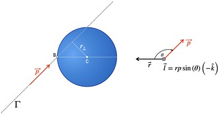
Angular Momentum of a Particle
Orbital angular momentum as opposed to spin angular momentum. It is amazing to think that, on a complex gravitational trajectory like an ellipse, parabola or hyperbola, the vector product of \(\vec{r}\) and \(\vec{p}\) is conserved. The magnitudes of momentum and radial distance and their geometric relationship are controlled by gravity to lock the object into its elliptical, parabolic or hyperbolic orbit.
Work and Power for Rotational Motion
Bypass
Example
Oscillator potential hides in this example!!
A pendulum in the shape of a rod
like a "grandfather clock"

a little bit trickier
an area integral, but not as hard as \(dx\, dy\)
A uniform thin rod with axis at the end
We kind of did this integral in Session 21.
The need to use an infinitesimally small piece of mass dm suggests that we can write the moment of inertia by evaluating an integral over infinitesimal masses
Session 21 intro
In the case of a rigid rotating body, we can divide up any body into a large number of smaller masses,
pixellation
Figure 10.14 (a) Uniform circular motion:
We made a study of this several weeks ago
10.2 Rotation with Constant Angular Acceleration
bypass
Angular Acceleration
We will not dwell too much on angular acc.
Since →rr→\mathbf{\overset{\to }{r}} is constant
not sure this is correct, but magnitude \(r\) is constant in uniform circular motion The real reason that \(\frac{d\vec{r}}{dt}=0\) is that in uniform circular motion, the position vector \(\vec{r}\) only changes in the \(\hat{\theta}\) or \(-\hat{\theta}\) direction, which are parallel or antiparallel to \(\vec{\theta}\). The cross product of parallel or antiparallel vectors is zero!
Figure 10.5 For counterclockwise rotation in the coordinate system shown
A good diagram
These three vectors are related to each other
Vector product aka cross product, using the right hand rule.
Now we expand our description of motion to rotation
...as in the motorcyclist problem.
Find the center of mass
Use linear mass densities 8.0g/m and 2.7 g/m.
the summation becomes an integral:
Use this integral and its associated example to tackle the problem of the one meter rod, using linear mass densities \(\lambda_{iron}=8.0\frac{g}{cm}\) and \(\lambda_{al}=2.7\frac{g}{cm}\)
Two particles of masses m1m1{m}_{1} and m2m2{m}_{2} move uniformly
Try this with \(m_1=1.000\, kg\) and \(m_2=1.500\, kg\). A good study problem.
Two particles of masses m1m1{m}_{1} and m2m2{m}_{2} separated by a horizontal distance D are let go from the same height h at different times
brain burner!
Three point masses
good study problem
no net external force acting on it
unlike the motorcyclist making a jump
Therefore, there is no meaningful application of the center of mass of a unit cell beyond as an exercise.
nice
Suppose we included the sun in the system
I like this example
The radius of Earth is 6.37×10⁶m6.37×106m6.37\times {10}^{6}\,\text{m}, so the center of mass of the Earth-moon system is (6.37 − 4.64) ×106m=1.73×10⁶m=1730km×106m=1.73×10⁶m=1730km×\,{10}^{6}\,\text{m}=1.73\times {10}^{6}\,\text{m}=1730\,\text{km} (roughly 1080 miles) below the surface of Earth.
We discussed this
position of the center of mass has units of meters; that suggests a definition
yup, this is it.
This is Newton’s second law
This is why an astronomer can focus on the trajectory of a star or planet or galaxy as if all of its mass is concentrated at a point located at the center of mass.
Rocket Propulsion
bypass this section
the total kinetic energy of the system is conserved. Such an interaction is called elastic.
Good approximation for an ideal gas, for instance.
Multiple objects can collide and stick together, forming a single object
Like a set of boxcars in the freight yard hooking together and moving off at a new speed.

A single object can explode into multiple objects (one-to-many).
Skateboarder interaction
but those changes are identical in magnitude, though opposite in sign.
Newton's third law is best understood in this way. The "equal but opposite reaction" is encoded quantitatively by the changes of momentum, or exchanges of momenta.
when a force is applied for an infinitesimal time interval dt, it causes an infinitesimal impulse d→JdJ→d\mathbf{\overset{\to }{J}},
So, for instance, the moon exchanges momentum with Earth as it travels around its orbit, but second by second, we can compute the amount of impulse, e.g.,
\(\vec{J}=\Delta \vec{p}=\int_{0.0\,s}^{1.0\,s} \left[ \frac{Gm_{\oplus}m_{moon}}{\left[r\left(t\right)\right]^2}\right]dt\)
An elephant and a hunter are having a confrontation.
good example
The momentum p of an object is the product of its mass and its velocity:
Sir Isaac Newton's invention, "quantity of motion."
the positions where its kinetic energy is zero
turning points in the motion
Finding the force from the potential energy is mathematically easier than finding the potential energy from the force, because differentiating a function is generally easier than integrating one.
Good strategy note
Force due to a Quartic Potential Energy
I like this Example!
In Relativity, we will see that conservation of energy still applies to a non-classical particle, but for that to happen, we have to make a slight adjustment to the definition of energy.
Correctamente! Slight adjustment, indeed, plus E becomes a component of the total relativistic momentum in four dimensions, \(\vec{p}=\left(p_x,\, p_y,\, p_z\right)\longrightarrow \vec{p}=\left(E,\, p_x,\, p_y,\, p_z\right) \).
Ed White tethered to the Space Shuttle
FALSE. Ed White made the first US spacewalk in 1965, on the Gemini 4 mission.
obtain
typo below?
we can rearrange the differentials dt, etc., as algebraic quantities in this expression
This would not be allowed in the math department, however.
The string vibrates around an equilibrium position, and one oscillation is completed when the string starts from the initial position, travels to one of the extreme positions, then to the other extreme position, and returns to its initial position.
Very good description of the periodic motion of a string on a guitar. The frequency of oscillation is in the audible range, e.g., A above middle C is 440 Hz.
If you have observed the classroom demonstration with the spinning bicycle wheel
I hope to do this demonstration during Lecture 16, on Feb. 27.
Atwood Machine
Bypass
Two Attached Blocks
Bypass
What Does the Bathroom Scale Read in an Elevator?
Bypass
First consider the horizontal or x-axis:
I can now see why a few of you, on HW 4, used this notation, \( F_{net\ x}=T_{2x} - T_{1x}=0\) rather than the way I usually write it, \(\sum F_x = T_{2x}-T_{1x}=0\).
This implies
Notice the subtle change of notation here, using the magnitude w as opposed to the vector notation in Fig. 6.3.
Different Tensions at Different Angles
Spider-man problem
Inertial Forces and Noninertial (Accelerated) Frames: The Coriolis Force
Bypass. This section requires Calculus 3 concepts to be done properly, although the weather diagrams, Fig. 6.28 are instructive to view.
Join the ladybug in an exploration of rotational motion. Rotate the merry-go-round to change its angle or choose a constant angular velocity or angular acceleration. Explore how circular motion relates to the bug’s xy-position, velocity, and acceleration using vectors or graphs.
Not sure why this paragraph is here.
the horizontal component of lift
It also accelerates a tide of circulating blood into the pilot -- blackouts occur
due to the force of the air on the wing
"force of the air on the wing" ↔︎ Many scientists describe aerodynamic lift as the pressure differential \(\Delta p\) between the top and bottom of the wing, effecting every square inch of the wing.
the increment of work dW
Here is a mini-differential equation
Often, an analytic solution is intractable or impossible, requiring lengthy numerical solutions or simulations to get approximate results.
MANY scientific jobs require this skill, numerical solution of differential equations.
This means a skydiver with a mass of 75 kg achieves a terminal velocity of about 350 km/h while traveling in a pike (head first) position, minimizing the area and his drag.
about the same as a small 2" sphere
Ferrari Testarossa 0.37 Dodge Ram Pickup 0.43
Amazing comparison.
wind tunnel
Cf., also the NASA Langley Research Center's wind tunnel fact sheet.

but →ww→\mathbf{\overset{\to }{w}} has components along both axes,
The free body diagram on the right is a bit different than the sketches I used in Session 12.<br>
 The author's \(\vec{w}_y\) vector is attached at its tail to the mass point, whereas in my sketch, it is slid over and attaches at the tip of \(\vec{w}\). But both are acceptable and useful. As I have mentioned several times, how you diagram forces etc. can be different from the author's and from my way of diagramming, and still be fine.
Consider the skier on the slope
A good study problem
Newton’s Third Law of Motion
Our demonstration in Session 10, with the two skateboarders out in the hallway, is good to remember here.
changes in motion
By "changes in motion," Newton meant \(\Delta \vec{v}\) and therefore \(\vec{a}=\frac{\Delta \vec{v}}{\Delta t}\)
We can think of this law as preserving the status quo of motion
<3
without the necessity of physical contact between objects
Or, once could redefine contact to mean an interaction "at a distance," as the author mentions here.
A quantitative definition of force can be based on some standard force
This is because force is a derived quantity, based on time, space and mass measurements.
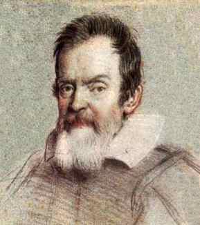
Isaac Newton
Galileo's famous student!
b
Be careful checking your answers here, too.
a
It is not clear to me what this expression is supposed to be. Be careful when checking your answer for h. For example,
$$\frac{24\frac{m}{s}}{9.8 \frac{m}{s^2}}=2.49\, s$$
Olympus Mons
Another planet? No problem. A walk in the park. : )

solid volcanic rocks
also known as "bombs"
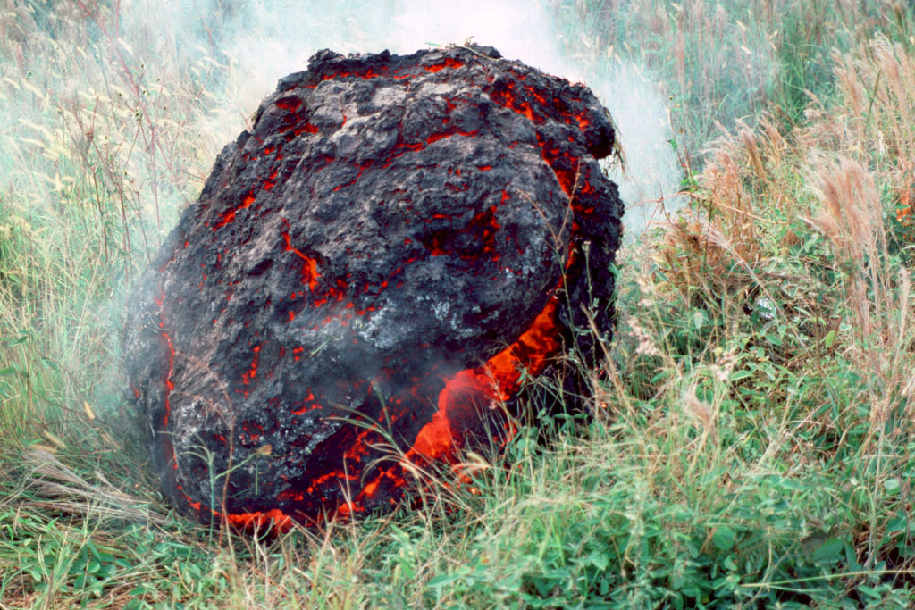 "Accretionary lava ball comes to rest on the grass after rolling off the top of an ‘a‘a flow in Royal Gardens subdivision. Accretionary lava balls form as viscous lava is molded around a core of already solidified lava (photo by J.D. Griggs, 7/2/83, JG2562) (picture #012)."
Mt. Asama, Japan
Another problem that does not come with solution. : )
Mike Powell
No solution offered for this problem, I see.
A projectile
Hmmm. Like the tennis ball classwork problem.
A basketball player
This is a brain burner
A rock
An excellent study problem.
An athlete
WIll be interesting to calculate.
A fastball pitcher

Projectile to satellite.
Newton was the first one to work out this idea of projectile becoming a spacecraft in orbit, depending on initial conditions \(\left(x\left( 0\right),\, y\left( 0 \right)\right)\) and \(\vec{v}\left( 0 \right)\).
If the two golf shots
Would make a nice multiple choice item.
Comparing Golf Shots
I like this combo problem.
Calculating Projectile Motion: Tennis Player
Similar to HW 3, but would be simpler to check.
A Fireworks Projectile Explodes High and Away
I like this problem.
Figure 4.12 (a) We analyze two-dimensional projectile motion by breaking it into two independent one-dimensional motions
This trajectory equation
However, the author does not complete the square, as we did!

This is the time of flight
Hang time
the following equation
I never use this equation. YUKK
A rock is thrown horizontally off a cliff
This example is like driving a car off a cliff, like in a movie.
Do not try this at home.
makes an angle θ with the horizontal
This angle, upon which the author concentrates, is not so important to me.
common variable between the motions is time t.
INCORRECT! The entire curve can be parametrized by \(x\) as we discussed in Session 3 and 4
two independent one-dimensional motions
They are not really independent except mathematically. They are actually coupled. For instance, the horizontal range, \(x_{max}\), is controlled by the size of \(v_y\left(0\right)\)
Vertical Motion
In the fourth equation here,
$$v_y^2=v^2_{0y}-2g\left(y-y_0\right),$$
if you have eyes to see, you can see the remnants of potential energy and kinetic energy terms.
very simple
Note that the author uses a slightly different notation than I use:
Keep this in mind as you study.
Let’s assume all forces except gravity (such as air resistance and friction, for example) are negligible
standard assumption for basic physics like PHY2048
motions along perpendicular axes are independent
...plus the fact that there is no such thing as horizontal gravity!
derivative with respect to time →v(t),v→(t),\mathbf{\overset{\to }{v}}(t), we find
We discussed this in session 7, concerning uniform circular motion. The direction of the acceleration vector \(\vec{a}\left( t\right)\) is the direction of the \(\Delta \vec{v}\left( t\right)\) vector.
Analytical methods of vector addition are exact, contrary to graphical methods, which are approximate.
I.e., draw the sketch then let the numbers do the talking
In many physical situations, we often need to know the direction of a vector.
Simply the vector itself, divided by the magnitude of the vector. $$\hat{u}=\frac{\vec{U}}{U}$$
find components of a resultant of many vectors
This will be a frequent task in PHY2048
In an attempt to escape a desert island
We will discuss this problem on Thursday, among other things.
Figure 2.20 Using polar coordinates
We will occasionally work in polar coordinates.
Unit vectors of the axes
Important geometric tool
50 km in the direction 37∘37∘37^\circ north of east.
...except this is what a pilot would use, a distance and a heading.
Figure 2.13
easy to calculate components from each subdiagram
both vectors have their origins at the same point
tail to tail
unit vector.
another important vocabulary term
antiparallel
Important vocabulary term.
fishing hole 6 km from your tent
 Who does this? Measure distance to a fishing spot from your tent? Really!
bold type with an arrow above it denotes a vector
I just use an arrow, \(\vec{A}\), or boldface B, but not both.
as sentences are a component part of literature.
Ummm, no.
Check to see whether the answer tells you something interesting.
:)
Analytical skills and problem-solving abilities can be applied to new situations whereas a list of facts cannot be made long enough to contain every possible circumstance.
This is why we do not emphasize formula sheets and memorization.
particularly in optics, more accurate numbers are needed and we use more than three significant figures
Cf., e.g, the index of refraction for BK-7 borosilicate crown glass at various wavelengths.
so it would take roughly 109/10−10=1019109/10−10=1019{10}^{9}\text{/}{10}^{-10}={10}^{19} hydrogen atoms to stretch across the diameter of the Sun.
This is news to me, but accurate. Note that this number of hydrogen atoms is much smaller than \(1.00\, mole\). Curious
study of physics makes other sciences easier to understand
This is a polite way of saying, "All science is either physics or stamp collecting," which Prof. Ernest Rutherford said way back in his days of discovering the nuclear structure of matter.
 (Ernest Rutherford)
What is most useful is knowing the basic laws of physics and developing skills in the analytical methods for applying them.
This is how most scientists work:
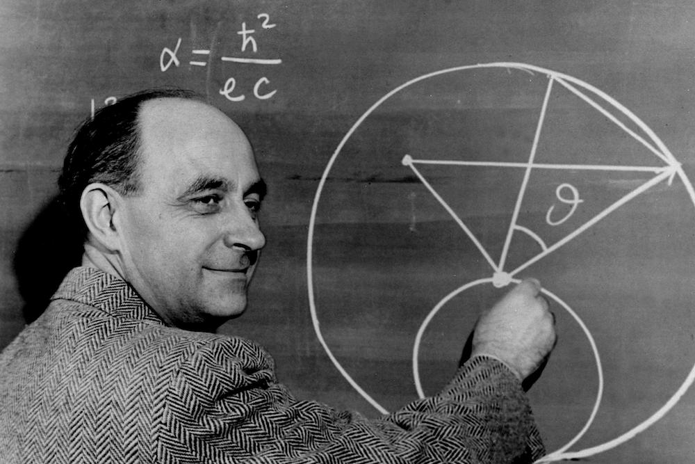 (Enrico Fermi)
This mental process will be helpful
...helpful IF you want to excel.
 (Albert Einstein)
all natural phenomena
Professor Galileo wrote, "Philosophy is written in this grand book — I mean the universe — which stands continually open to our gaze, but it cannot be understood unless one first learns to comprehend the language and interpret the characters in which it it written. It is written in the language of mathematics, and its characters are triangles, circles and other geometrical figures, without which it is humanly impossible to understand a single word of it; without these, one is wandering about in a dark labyrinth.” [(Assayer, VI)]
That is our challenge, the mountain we climb: to understand the grand book of nature.
(https://bibdig.museogalileo.it/Teca/Viewer?an=300984&lang=en)
The reflected rays seem to originate from behind the mirror, locating the virtual image.
Good example of what makes an image virtual. I always describe it this way: if you place a photographic film at the image location (behind the mirror, in this case) and no light rays actually hit the film, which is true in this case, then it is a virtual image.
photon energy is
Yuge
Note that Planck’s constant is a very small number.
important
The number of fringes depends on the wavelength and slit separation.
We observed this with the green laser pointer.
by half a wavelength
$$\frac{\lambda}{2},\:\frac{3\lambda}{2},\text{ etc.}$$
monochromatic
Green laser pointer
two slits provide two coherent light sources
In our sketch, wavelet sources \(S_1\) and \(S_2\).
Young’s double slit experiment.
Sketched out in Session 37, https://youtu.be/BF5e89OmsQQ
Solution
We did this calculation during Session 37, at about 45:11. https://youtu.be/BF5e89OmsQQ
Example 1: Finding a Wavelength from an Interference Pattern
Yuge
1000 Hz
Approximately the B one octave above middle C.
wavelets
purple
Huygens’s principle applied to a straight wavefront.
i.e., plane waves
The view from above
As we sketched plane waves in Session 37.

finite thickness
I.e., a real lens for which thin lens model is just an approximation
Advanced computing techniques
Also, adaptive optics, like the COSTAR optics placed in the Hubble Space Telescope to correct spherical aberration.

The optical components determining the brightness are the diameter of the lens and the diameter of pupils, diaphragms or aperture stops placed in front of lenses.

detect astigmatism
Yup, I have astigmatism, which I noticed during my first year of college.
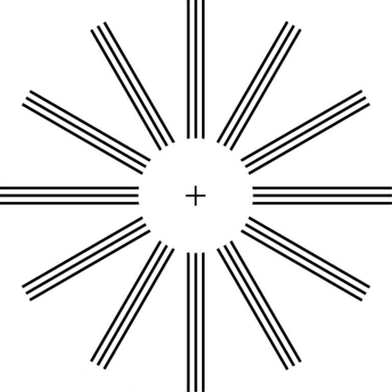 (Test diagram)
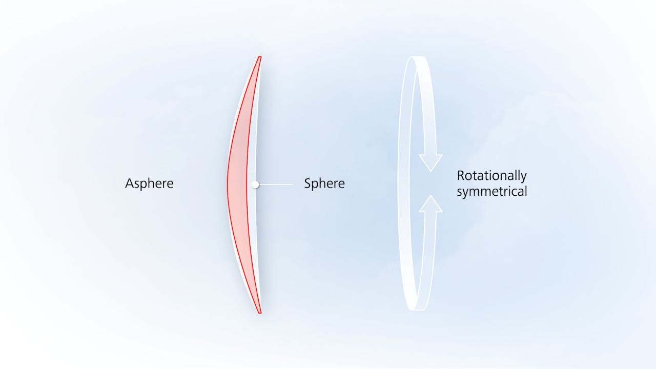
spherical aberration
Interesting simulation of spherical aberration in a microscope system.
Eyeglasses can have aspherical lenses to correct this aberation:
This type of aberration is called a coma
Here is a coma test panel, comparing stars imaged at the center of a Canon 24mm f/1.4L II lens, at intermediate distance and at the edge of the lens:
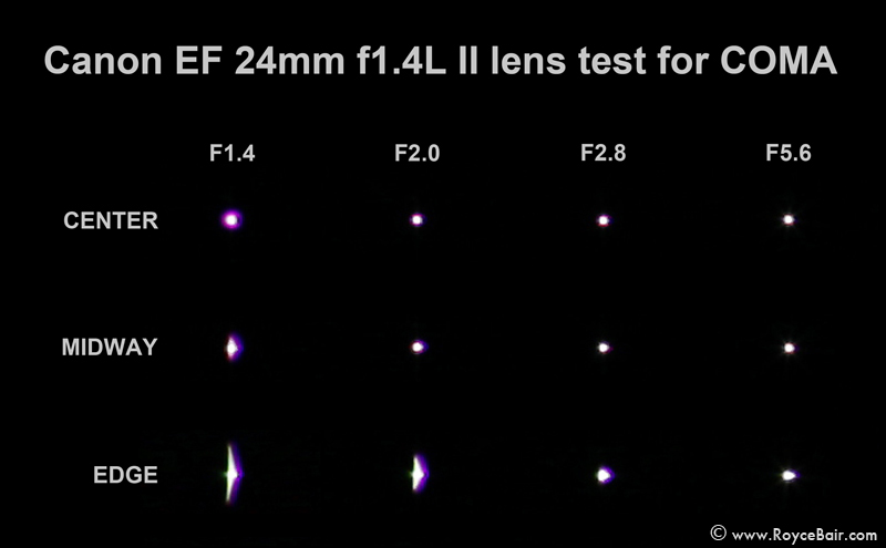
At the edge, you get a lot more coma abberation, but at f2.8, it seems minimized.
For example an achromatic doublet consisting of a converging lens made of crown glass and a diverging lens made of flint glass in contact can dramatically reduce chromatic aberration
E,g., the Zeiss apochromat lens that focuses all colors nicely.
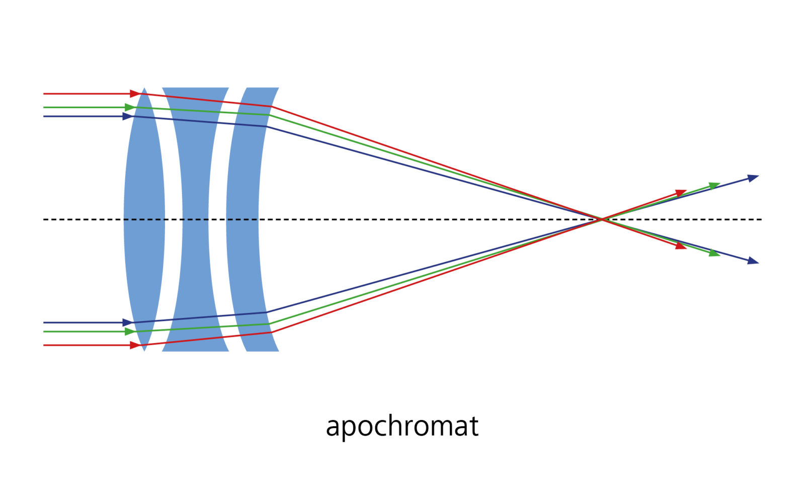
"Achieving this level of correction is not simple. It requires the use of exceptional quality optical materials: long-crown glass (fluor crown glass and calcium fluoride) and special short flint glass."
Chromatic aberration
We have discussed chromatic aberration in class a few times.
Eventually, if the Sun could shrink down to a diameter of about 6 kilometers, only light beams sent out perpendicular to the surface would escape. All others would fall back onto the star ([link]).
Schwarzschild radius" of the Sun. We do not think it will ever get collapsed to this small of a size, because the Sun is not large enough to have a supernova detonation.
If the speed you need to get away is faster than the fastest possible speed in the universe, then nothing, not even light, is able to escape.
This is the classical way of thinking about black holes, and a century after Sir Isaac Newton wrote Principia, another scientist, John Michell, worked it out using non-relativity concepts.
We want to know what speeds are required to escape from the gravitational pull of different objects.
Escape velocity:
object
Diameter of DNA helix is about 2 nanometers. So wavelengths on the order of a nanometer are good to use. Rosalind Franklin probably used \(\lambda = 0.15\:nm\) for her xray diffraction images.

Interference is the hallmark of a wave
Huge
However, when it interacts with smaller objects, it displays its wave characteristics prominently.
E.g., our handheld diffraction gratings,
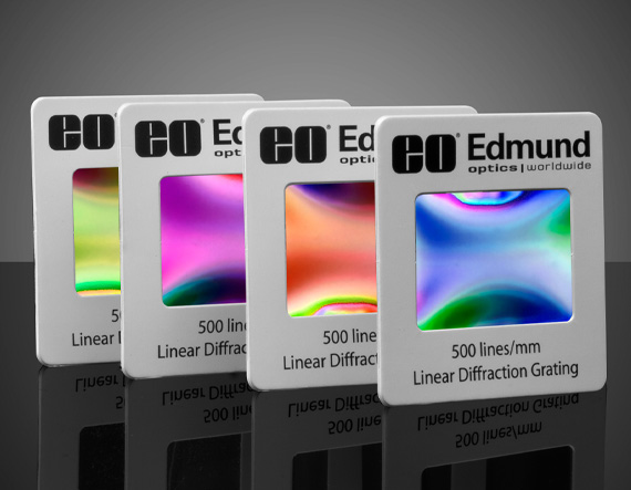
with 500 lines per millimeter. That is about one line every 2000 nm, so just a few times larger than the typical Roy G. Biv wavelengths.
380 to 760 nm
ok
cannot be explained fully by geometric optics
This is like the difference between Newtonian physics and quantum physics.
one of the many phenomena that can only be explained by the wave character of light
"only"
80 MHz to 2 GHz
80 MHz is just below our FM radio band and 2 GHz is in the microwave region of the spectrum.
they can be reflected when incident at small glancing angles
Used to be very highly classified technology.
A telescope can also be made with a concave mirror
Isaac Newton developed this concept.
But a more common arrangement is to use a third convex lens as an eyepiece, increasing the distance between the first two and inverting the image once again
Second flip = nice!
Telescopes gather far more light than the eye
The best way to think of this idea is the concept of aperture: the pupil of your eye, a few millimeters, vs., e.g. the aperture of the Hubble Space Telescope (HST), about 2.4 meters. HST is about 300 times wider, about 90,000 times more area than the human eye's pupil.
The HST is about the size of a school bus.

(Hubble being transferred from the Vertical Assembly Test Area (VATA) to the High Bay at the Lockheed assembly plant in preparation for transport to the Kennedy Space Center (KSC) after final testing and verification.)
Microscope Magnification
We will conclude Ch. 26.4 with this example, then bypass the remainder of Ch. 26.4
The eyepiece forms a case 2 final image
Notice that, in this diagram, the rays are almost parallel coming out of the eyepiece to the eyeball. If the rays are parallel, your eye does not have to strain to focus the image on your retina
several lenses
Or just one in a simple microscope
If the device is composed of thin lenses
Always a big proviso.
the eye is marvelous in its ability to see
An understatement. When we view a star in the night sky, our retina collects very small numbers of Roy G. Biv photons per second.
An ideal thin lens has two refracting surfaces but the lens is thin enough to assume that light rays bend only once.
One refractive interaction, an approximation to the two physical interactions.
23.12 RLC Series AC Circuits
Most of this section is bypassed. However, we discussed LC circuits extensively in terms of oscillation, e.g., in Fig. 5.
phase angle
We discussed "phase" a little bit differently than this.
23.11 Reactance, Inductive and Capacitive
Bypass or skim the diagrams. We talked about oscillating circuits from the standpoint of energy, but we did not get into any detail of this section, 23.11.
Figure 1.
Study this secrion, 23.10. We discussed inductance and RL circuits in Session 27 and other places.
23.8 Electrical Safety: Systems and Devices
Bypass. It won't be on Exam 3, although Florida residents would do well to read about the GFI technology, which many major appliances and pool pumps have.
23.7 Transformers
Bypass
23.6 Back Emf
Bypass
23.5 Electric Generators
We mentioned generators and motors in general terms, but all of the materials in this section we bypassed.
23.4 Eddy Currents and Magnetic Damping
Bypass
Figure 1.
We discussed this briefly in Session 26 in the context of the navy's "rail gun."
Other material in this chapter is bypassed.
8: (a) Using information in Figure 5, find the height of the instructor’s head above the water, noting that you will first have to calculate the angle of incidence. (b) Find the apparent depth of the diver’s head below water as seen by the instructor.
Brain burner deluxe....
Figure 5. A scuba diver in a pool and his trainer look at each other.
Brain burner!! Attempt this diagram at your own risk!! :D
In what substance in Table 1 is the speed of light ?
Nice mental exercise.
What is the speed of light in water? In glycerine?
Basic calculations.
4: Will light change direction toward or away from the perpendicular when it goes from air to water? Water to glass? Glass to air?
I like this question. You can work it out with typical values of indices of refraction, \(n_{air}=1.00,\, n_{water}=1.33,\, n_{glass}=1.5\)