Author response:

The following is the authors’ response to the original reviews.

Reviewer #1 (Public review):

This manuscript provides several important findings that advance our current knowledge about the function of the gustatory cortex (GC). The authors used high-density electrophysiology to record neural activity during a sucrose/NaCl mixture discrimination task. They observed population-based activity capable of representing different mixtures in a linear fashion during the initial stimulus sampling period, as well as representing the behavioral decision (i.e., lick left or right) at a later time point. Analyzing this data at the single neuron level, they observed functional subpopulations capable of encoding the specific mixture (e.g., 45/55), tastant (e.g., sucrose), and behavioral choice (e.g., lick left). To test the functional consequences of these subpopulations, they built a recurrent neural network model in order to "silence" specific functional subpopulations of GC neurons. The virtual ablation of these functional subpopulations altered virtual behavioral performance in a manner predicted by the subpopulation's presumed contribution.

Strengths:

Building a recurrent neural network model of the gustatory cortex allows the impact of the temporal sequence of functionally identifiable populations of neurons to be tested in a manner not otherwise possible. Specifically, the author's model links neural activity at the single neuron and population level with perceptual ability. The electrophysiology methods and analyses used to shape the network model are appropriate. Overall, the conclusions of the manuscript are well supported.

Weaknesses:

One potential concern is the apparent mismatch between the neural and behavioral data. Neural analyses indicate a clear separation of the activity associated with each mixture that is independent of the animal's ultimate choice. This would seemingly indicate that the animals are making errors despite correctly encoding the stimulus. Based solely on the neural data, one would expect the psychometric curve to be more "step-like" with a significantly steeper slope. One potential explanation for this observation is the concentration of the stimuli utilized in the mixture discrimination task. The authors utilize equivalent concentrations, rather than intensity-matched concentrations. In this case, a single stimulus can (theoretically) dominate the perception of a mixture, resulting in a biased behavioral response despite accurate concentration coding at the single neuron level. Given the difficulty of isointensity matching concentrations, this concern is not paramount. However, the apparent mismatch between the neural and behavioral data should be acknowledged/addressed in the text.

We thank the Reviewer for the insightful comments and thoughtful suggestions. Our electrophysiological recordings show that GC dynamically encodes stimulus concentration of mixture elements, dominant perceptual quality, and decisions of directional lick. With regard to the encoding of mixtures, the clear separation of activity associated with each mixture (Figure 3) is present at a trial-averaged pseudo-population level, and average activities associated with more similar, intermediate mixtures are closer to each other in this space. At a single trial level activities evoked by similar, intermediate mixtures are much harder to separate. This increased similarity can lead to behavioral errors resulting from either incorrect encoding of the stimulus or from the inability to interpret the stimulus to guide the correct decision. The psychometric function, which shows that more distinct stimuli (100/0 vs 0/100) lead to fewer mistakes than more ambiguous, intermediate mixtures (55/45 vs 55/45), is consistent with the increased ambiguity of responses to intermediate mixtures.

The Reviewer is correct that there could be a slight mismatch in the perceived intensity of the mixture components. This mismatch could be the reason for the slight asymmetry in our psychometric function (Figure 1B). However, it is not uncommon for mice in these 2AC tasks to also have a motor laterality bias in their responses that manifests itself for the more ambiguous stimuli. We chose not to model this bias given its subtlety and its unknown origin. Rather, we chose to model an ideal scenario in which stimuli have matched intensity and no motor bias exists. In the revised manuscript we discuss this issue.

Reviewer #1 (Recommendations for the authors):

(1) The apparent mismatch between neural and behavioral data. I am providing more details in this section to hopefully better illustrate my concern.

(a) Based on the author's psychometric curve, sucrose appears to be a more salient signal causing the behavior to be shifted (e.g., a 50/50 mixture results in a >60% predicted behavioral performance). If both sucrose and salt were intensity-matched, a 50/50 mixture should result in a behavioral performance near 50%. The increased salience of sucrose could cause the animals to have lower overall performance despite accurate neural encoding. Alternatively, certain animals could display a strong side bias, skewing the data slightly. These issues have seemingly been fixed in the model data, which displays a more balanced psychometric curve. Accordingly, the model data seemingly displays a larger shift in error trials as compared to correct trials (Figure 6A).

The reviewer is correct in observing that the average experimental psychometric curve in Figure 1B shows a slight shift in favor of the sucrose side with a 50/50 mixture. We fit psychometric curves to each session and the mean value of P(Sucrose choice | Stimulus = 50/50) across sessions was significantly different from 0.5 (one-sample t-test, p = 0.003), with 5 probabilities below 0.5 and 18 above it.

This slight bias could be attributed to a slight mismatch in the perceived intensity of the mixture components and/or lateral motor biases. In any case, it is subtle and its origins were not a focus of this study.

Models were not trained to match the animals’ psychometric curves, but rather to choose correctly in an ideal scenario where stimuli have matched intensities. This explains why the model simulations lack the bias observed in animal behavior data.

We do not believe that there is a mismatch between the experimental behavioral and neural data, as trial-averaged pseudo-population trajectories are farther in neural space for more discriminable stimuli and closer in neural space for more similar stimuli, consistent with behavioral performance that is high for more discriminable stimuli and low for more similar stimuli. Moreover, as the model also shows, a clear separation of trial-averaged trajectories still results in a sigmoidal performance function for trial-to-trial behavior.

Finally, subtle behavioral biases would not necessarily be expected to appear in our dPCA analyses since we used this technique to find a single axis that best separates all stimuli conditions regardless of choice when the pseudo-population data are projected upon it. Additional modes of activity that explain less overall variance might better reflect biases.

(b) Although I am not an expert at these analyses, I wonder whether the elevated bump (i.e., >0) in Figure 3C of the 55/45 mixture that occurs early in the stimulus presentation further supports the hypothesis mentioned above and could indicate an early signal of salience/increased intensity?

The reviewer is correct that the 55/45 trajectory features a brief positive wave right after stimulus delivery before going negative. While this may be related to stimuli not being explicitly balanced for intensity, it could also reflect a signal related to ambiguity or balanced mixtures. We are hesitant to interpret this positive deflection as conclusive evidence of a bias in neural activity, given its short duration and the natural variability of neural signals.

(2) The increase in step-perception neurons after the decision period is confusing (Figure 4C). The text states (line 246) "the analysis reveals a small and time-invariant proportion of step-perception neurons". However, the proportion doubles after the decision-making process, which is seemingly a significant change. Why does this occur? This observation is noticeably missing from the network data. Could it be attributed to a mislabeling of "step-choice" neurons, given the correlation between the left/right decision and sweet/salty? Either way, it is very noticeable and should be addressed.

We cannot be sure of the reason for the increase in step-perception neurons after decisions. One possibility is that they are acting as feedback for learning, encoding the percept to compare with choice and outcome to improve performance. The model, which presumably learns the task differently from the animals, does not seem to leverage this signal for its own learning. We have modified the text, now referring to a “small but consistently present proportion” of step-perception neurons, and included this proposed explanation in the Discussion.

(3) Optional: I think the authors are missing an opportunity to analyze the temporal aspect of this multiplex code using their network-based modeling approach. A significant proportion of neurons fall into different categories (i.e., step-perception/linear, etc.) at different time points. However, the virtual ablation experiments remove any neuron that falls into one of these categories at any time. By limiting the cell-specific virtual ablation to specific time windows, you could (I think) provide stronger evidence for the temporal sequence of the encoding of these perceptual aspects.

This was an excellent suggestion for an additional modeling experiment, so we performed it. A new supplemental figure (Figure S8) and additional text in the revised manuscript showcase the results. In summary:

In terms of behavioral results, ablating the linear coding units in the beginning (that is, silencing all units that are labeled linear in any bin within the first 1.2 s after stimulus onset for the entirety of the 1.2 s) significantly reduces performance, as does ablating the step-perception or step-choice coding units at the end (1.2 s prior to choice). The remaining combinations of coding type and timing of the ablation do not affect performance.

Regarding the dynamics of coding types (compare Figure 7A), stimulus coding activity was significantly blunted only by ablating the linear coding units in the beginning, whereas choice coding activity was diminished by ablating the choice coding units at the end or by ablating the linear coding units at either the beginning or the end.

Reviewer #2 (Public review):

Lang et al. investigate the contribution of individual neuronal encoding of specific task features to population dynamics and behavior. Using a taste-based decision-making behavioral task with electrophysiology from the mouse gustatory cortex and computational modeling, the authors reveal that neurons encoding sensory, perceptual, and decision-related information with linear and categorical patterns are essential for driving neural population dynamics and behavioral performance. Their findings suggest that individual linear and categorical coding units have a significant role in cortical dynamics and perceptual decision-making behavior.

Overall, the experimental and analytical work is of very high quality, and the findings are of great interest to the taste coding field, as well as to the broader systems neuroscience field.

I have a couple of suggestions to further enhance the authors' important conclusions:

My main comment is the distinction between constrained and unconstrained units. The authors train a small percentage of units to match the real neural data (constrained units), and then find some unconstrained units that are similar to the real neural data and some that are not. As far as I could tell, the relative fraction of constrained and unconstrained units in the trained RNN is not reported; I assume the constrained ones are a much smaller population, but this is unclear. The selection of different groups of neurons for the RNN ablation experiments appears to be based on their response profiles only. Therefore, if I understood correctly, both constrained and unconstrained units are ablated together for a given response category (e.g., linear or step-perception). It would be useful, therefore, to separately compare the effects of constrained vs. unconstrained RNN units.

We thank the Reviewer for the constructive feedback. The Reviewer is correct that ablations were carried out with respect to response categories only and included both constrained and unconstrained units.

The ratio of total units to constrained units was fixed at 5.88, thus constrained units were ~17% of the network and unconstrained units were ~83%. This value is specified in the Methods (RNN: Components and dynamics), but we have reported it in the Results of the revised manuscript for clarity.

We have also edited the Methods because they wrongly stated that the ratio of unconstrained (rather than total) units to constrained units was 5.88.

Specifically:

(1) For the analyses in the initial version of the manuscript, the authors should specify how many units in each ablation category are constrained and unconstrained.

In the revised manuscript, we have specified the fractions of constrained and unconstrained units within each response category. For convenience, they are reported here: linear = 194 constrained and 691 unconstrained units; step-perception = 147 constrained and 840 unconstrained units; step-choice = 129 constrained and 814 unconstrained units; “other” = 353 constrained and 1739 unconstrained units.

(2) The authors should repeat Figure 6, but only for unconstrained units to test how much of the effects in the initial version of Figure 6 are driven by constrained vs. unconstrained RNN units.

In the revised version we have included two additional supplemental figures (Figures S5-6) where the analyses of Figure 6 are carried out separately for constrained and unconstrained units. In short, the results for the constrained units strongly resemble those for the experimental data, while the results for the unconstrained units strongly resemble those for all model units.

(3) The authors should repeat Figure 7, but performing ablations separately on the constrained and unconstrained units to examine how the network behaves in each case and the resulting "behavioral" effect.

The revised version includes a supplemental figure (Figure S7) with the results of these additional ablation simulations.

In summary:

In terms of behavioral performance, the prior results showing that ablating linear, step-perception, or step-choice units significantly impairs performance, while ablating “other” has no significant effect, hold even if ablation is restricted to only constrained or only unconstrained units. There is a significant main effect of constrained vs unconstrained; on average, ablating the unconstrained population impairs performance more, most likely due to their larger population size.

In terms of dynamics, to impair stimulus coding by ablating step-choice units, you must ablate them all; to impair stimulus coding by ablating linear or step-perception units, however, ablating just the unconstrained ones suffices. As before, ablating linear, step-perception, or step-choice units significantly impairs choice coding activity, while ablating “other” units does not; these results hold even if ablation is restricted to only constrained or only unconstrained units. Finally, there is again a significant main effect of constrained vs unconstrained; on average, ablating the unconstrained population impairs dynamics more, most likely due to the larger population size.

Reviewer #2 (Recommendations for the authors):

(1) In addition to panel 5B, it would be informative to show data from individual mice and the corresponding RNNs trained on each mouse, to assess how closely they match. If available, including one representative example of a good match and one of a less accurate match would help the reader get a better sense of the data.

Figure 5B shows the average behavioral performance of the model. Individual models were not trained directly on the psychometric curves of experimental sessions; they were trained to perform the task correctly. After successful training, model simulations were run with input noise to be able to produce a sigmoidal psychometric curve. However, although the input noise was tuned to capture the overall correct rate of the corresponding experimental session, we did not attempt to match the details of the psychometric curve. See also the next reply.

(2) In addition to panel 5C, it would be useful to add examples of experimentally observed PSTHs and the corresponding activity trajectory for the units in the RNN trained to match them, for all the other coding patterns (step-perception and step-choice).

We note that the PSTH in 5C is not an example of a linear coding unit as the Reviewer implies, but simply one with a good fit, and here the model’s output was produced in the absence of input noise. In order to classify step-perception and step-choice responses one needs error trials, but the model was trained without this input noise that induces errors (and produces a sigmoidal psychometric function) to match experimental PSTHs from correct trials only. Post-training simulations were then run with input noise to induce error trials, and model unit response profiles were classified based on this. However, there is no guarantee that error trials in the model match the error trials in the experiment; therefore, step-perception and step-choice units in the model may or may not be step-perception and step-choice units in the data. Despite this limitation, the revised manuscript includes additional examples, in Figure S2, of experimentally observed PSTHs and their corresponding model activity, to supplement Figure 5C and provide a better sense of the goodness-of-fit.

(3) Electrophysiological data in Figure 2 - It would be helpful to provide statistics on how many neurons change their activity in each session.

In the revised manuscript we have included across-session statistics for proportions of neurons that are taste-responsive and that show decision preparatory activity. We have also included tables (Tables S1 and S3) with the numbers of neurons that are taste-responsive and that show preparatory activity for each session in the experimental and model data.

(4) Peak auROC selection - How was the peak auROC selected? Selecting only one bin for the peak could be potentially problematic and may result in the incorrect identification of an outlier that does not faithfully represent the neuron's overall activity. The peak selection could instead be based on several consecutive bins showing a consistent trend. If this approach was already implemented, the authors should explicitly describe it in the Methods section.

Peak auROC was selected from a single bin (with average duration about 50ms). While it is true that this may result in outlier neurons that transiently prefer one stimulus strongly but more consistently prefer the other, we opted for a simple criterion to sort the neurons into two categories for visualization. Adopting more stringent criteria that consider multiple bins may result in neurons that cannot be placed in either category, and we wanted a way to examine the entire pseudo-population. Also, the entire auROC trace is visualized in the heatmap, so potential outliers are not hidden and can be assessed by eye.

Reviewer #3 (Public review):

Primary taste cortex neurons show a variety of dynamic response profiles during taste decision-making tasks, reflecting both sensory and decision variables. In the present study, Lang et al. set out to determine how neurons with distinct response profiles contribute to perceptual decisions about taste stimuli.

The methods, with reference to the behavioral task and electrophysiological recordings/data analysis, are straightforward, solid, and appropriate. The computational model is presented in a clear and conceptually intuitive manner, although the details are outside of my area of expertise.

The experimental design features a simple 2-alternative forced-choice design that yielded clear psychometric curves across a range of stimuli. In vivo recordings were performed using Neuropixels and yielded an appropriate sample of single neuron responses. The strength of the model lies in the fact that it consists of single neurons whose response profiles mimic those recorded in vivo, and allows neuron-selective manipulation.

By virtually lesioning specific subsets of neurons in the network, the authors demonstrate that a relatively small population of neurons with specific tuning profiles was sufficient to produce the observed neural dynamics and behavioral responses. This effect was selective as lesioning other responsive neurons did not affect overall response dynamics or performance.

These findings provide new insight into the relation between the response profiles of single neurons in sensory cortex, their population-level activity dynamics, and the perceptual decisions they inform.

The approach is particularly innovative as it uses computational modeling to target functionally-defined "cell types", which cannot necessarily be targeted by more conventional genetic approaches.

We thank the Reviewer for the positive assessment of our study.

Reviewer #3 (Recommendations for the authors):

(1) Introduction: I'm missing a clearly stated specific hypothesis and what is predicted on the basis of that hypothesis. What is the alternative?

The null hypothesis is that single neuron activity patterns, even when clearly structured, do not matter for population activity or behavior. Alternatively, they do matter for these phenomena, and our model supports the alternative hypothesis. We have made this hypothesis clearer in the Introduction.

(2) Discussion: Much of the text is a recap of the Introduction and Results sections. Please elaborate on the specific insights gained from the findings. The idea that tuned neurons in the sensory cortex are the basis for perception and perceptual decisions concerning the features being represented by those neurons is generally accepted. What the present study adds to this insight could be described more explicitly. On the other hand, the idea that small populations of tuned neurons are responsible for perception of taste/perceptual decisions about taste appears in contrast with previous accounts where stimulus features/decisions are reflected in correlated changes in activity across distributed populations of taste cortical neurons, including ones that are not necessarily tuned or even overtly responsive. How do the present findings relate to this idea?

This is a very good point about reconciling these findings with past ones that have focused on coordinated changes across ensembles of neurons, i.e., metastable dynamics of internal (hidden) states. There is a brief mention of metastability toward the end of the Discussion, but we agree it deserves elaboration.

This work does emphasize single unit activity, but in the context of, and as relevant to, population activity. We believe that the findings and frameworks of previous studies and those presented here are compatible rather than mutually exclusive. There is no reason why neurons with the coding patterns we studied here cannot coordinate with others to participate in the formation of different metastable states. The question of which—neurons with specific response profiles, or ensemble activity patterns that may involve these neurons?—is necessary and sufficient for producing perception and behavior during the mixture-based decision-making task is interesting but rather difficult to answer because of the single units’ contribution to both alternatives. One would need to utilize a manipulation that disrupts ensemble coordination without disrupting single unit activity to differentiate between them. We have made these points clearer in the Discussion.

(3) Results: RNNs were based on data from single sessions -- how many neurons of each tuning type were observed in each session? In particular, there were 23 sessions but only 25 neurons total tuned to choice, suggesting that modelled choice neurons were based on ~1 neuron.

The revised manuscript includes the session-by-session breakdown of response types for both experiment and model in two supplementary tables (Tables S2 and S4). We note that there are 25 neurons tuned to choice during the last 500 ms of the trial prior to decision, but 114 out of 626 neurons in total are tuned to choice in some time bin in the experimental data.

(4) Minor: Indicate the time windows used for analysis of stimulus sampling, delay, and choice on the figures.

The revised manuscript now includes the illustration of sampling and delay windows in Figure 2C-D, since we averaged the values over these windows for use in a 2-way ANOVA. All other figures either are associated with bin-by-bin analyses and have the first central and lateral licks (T and D) indicated, or have the time windows specified (e.g., Figure 4B, which uses [T, T + 0.5 s] and [D - 0.5 s, D]).

Author response:

The following is the authors’ response to the original reviews.

eLife Assessment

This study provides valuable insights with solid evidence into altered tactile perception in a mouse model of ASD (Fmr1 mice), paralleling sensory abnormalities in Fragile X and autism. Its main strength lies in the use of a novel tactile categorization task and the careful dissection of behavioral performance across training and difficulty levels, suggesting that deficits may stem from an interaction between sensory and cognitive processes. However, while the experiments are well executed, the reported effects are subtle and sometimes non-significant. The interpretation of results may be overextended given the nature of the data (solely behavioral), the reliance on repeated d′ measures may obfuscate some of the results without clearer psychometric or regressionbased analyses, and the absence of mechanistic, causal, or computational approaches limits the strength of the broader conclusions. The work will be relevant to those interested in autism, cognition, and/or sensory processing.

We thank the editors for their positive assessment of the data quality and the novelty of our behavioral task, and for pointing out the limitations inherent in behavioral studies.

We would like to clarify one important point regarding the use of d′ measures. While d′ was included to quantify sensitivity, our conclusions are not based solely on repeated d′ measures. In addition to d′, we analyzed raw behavioral data (correct and incorrect choice rates), and categorization performance was assessed using psychometric curves fitted with logistic regression models. These complementary analyses provide converging evidence and ensure that our interpretations are supported by multiple robust measures.

In the revised manuscript, we have further strengthened the analyses by including additional regression-based assessments, reporting effect sizes for subtle effects, and refining the statistical methods for clarity and transparency.

We fully acknowledge that this work is behavioral and does not directly reveal the underlying neural mechanisms. Nonetheless, the translational framework we have developed establishes a robust foundation for future studies. This platform can be directly applied in clinical research on autism and other neuropsychiatric conditions involving sensory-cognitive interactions, and provides a solid basis for subsequent mechanistic, causal, or computational investigations to uncover the neural circuits mediating these effects.

We greatly appreciate the editors’ and reviewers’ guidance and believe the revisions have clarified and strengthened the manuscript.

Public Reviews:

Reviewer #1 (Public review):

Summary:

This study addresses the important question of how top-down cognitive processes affect tactile perception in autism - specifically, in the Fmr1-/y genetic mouse model of autism. Using a 2AFC tactile task in behaving mice, the study investigated multiple aspects of perceptual processing, including perceptual learning, stimulus categorization and discrimination, as well as the influence of prior experience and attention.

We appreciate the reviewer’s statement highlighting the importance of our study.

Strengths:

The experiments seem well performed, with interesting results. Thus, this study can/will advance our understanding of atypical tactile perception and its relation to cognitive factors in autism.

We thank the reviewer for recognizing the quality of our experiments and the relevance of our findings for understanding tactile perception and cognition in autism.

Weaknesses:

Certain aspects of the analyses (and therefore the results) are unclear, which makes the manuscript difficult to understand. Clearer presentation, with the addition of more standard psychometric analyses, and/or other useful models (like logistic regression) would improve this aspect. The use of d' needs better explanation, both in terms of how and why these analyses are appropriate (and perhaps it should be applied for more specific needs rather than as a ubiquitous measure).

We thank the reviewer for these constructive comments. We acknowledge that aspects of the analyses were previously difficult to follow, and we have reworked the Results section to improve clarity and transparency.

We would like to emphasize that all d′ measures are complemented by analyses of raw response rates (correct and incorrect choices), ensuring that our interpretations are not solely dependent on this metric. In addition, we applied standard psychometric analyses wherever possible. For the training phase, only two stimulus amplitudes were presented, which precluded the construction of full psychometric curves; however, for the categorization phase, psychometric analyses were feasible and are reported in Figure 3. Specifically, psychometric functions were fitted to the data using logistic regression, allowing us to estimate both categorization bias (threshold) and precision (slope) across stimulus intensities. These analyses revealed no evidence of categorization bias or precision in Fmr1^-/y mice across stimulus strengths.

Following the reviewer’s suggestion, we have also added general linear model analyses that account for trial history, providing a complementary perspective on decision-making dynamics. Finally, while the calculation of d′ is detailed in the Methods, we have revised the Results to clearly explain its use and appropriateness in each relevant analysis.

These revisions aim to provide a clearer, more comprehensive picture of the data while ensuring that all conclusions are supported by multiple complementary measures.

Reviewer #2 (Public review):

Summary:

This manuscript presents a tactile categorization task in head-fixed mice to test whether Fmr1 knockout mice display differences in vibrotactile discrimination using the forepaw. Tactile discrimination differences have been previously observed in humans with Fragile X Syndrome, autistic individuals, as well as mice with loss of Fmr1 across multiple studies. The authors show that during training, Fmr1 mutant mice display subtle deficits in perceptual learning of "low salience" stimuli, but not "high salience" stimuli, during the task. Following training, Fmr1 mutant mice displayed an enhanced tactile sensitivity under low-salience conditions but not high-salience stimulus conditions. The authors suggest that, under 'high cognitive load' conditions, Fmr1 mutant mouse performance during the lowest indentation stimuli presentations was affected, proposing an interplay of sensory and cognitive system disruptions that dynamically affect behavioral performance during the task.

Strengths:

The study employs a well-controlled vibrotactile discrimination task for head-fixed mice, which could serve as a platform for future mechanistic investigations. By examining performance across both training stages and stimulus "salience/difficulty" levels, the study provides a more nuanced view of how tactile processing deficits may emerge under different cognitive and sensory demands.

We thank the reviewer for emphasizing the strengths of our task design and analysis approach, and we appreciate that the potential of this platform for future mechanistic investigations is recognized.

Weaknesses:

The study is primarily descriptive. The authors collect behavioral data and fit simple psychometric functions, but provide no neural recordings, causal manipulations, or computational modeling. Without mechanistic evidence, the conclusions remain speculative.

We thank the reviewer for the careful reading of our manuscript and for these constructive comments. We agree that our study is purely behavioral, and we appreciate the opportunity to clarify the scope and interpretation of our findings. The primary goal of this work was to characterize behavioral patterns during tactile discrimination and categorization in a translationally relevant mouse model of autism.

Although we did not include direct neural recordings, causal manipulations, or computational modeling, our analyses combining choice behavior, sensitivity measures from signal detection theory, psychometric curves, and regression-based models of trial history provide a detailed and robust characterization of perceptual learning, stimulus discrimination, categorization, and the interplay of cognitive processes with tactile perception. The manuscript has been revised to explicitly state that our conclusions are behavioral, emphasizing that this work establishes a foundation for future studies aimed at elucidating the neural and circuit mechanisms underlying these sensory–cognitive interactions.

Second, the authors repeatedly make strong claims about "categorical priors," "attention deficits," and "choice biases," but these constructs are inferred indirectly from secondary behavioral measures. Many of the effects are based on non-significant trends, and alternative explanations (such as differences in motivation, fatigue, satiety, stereotyped licking, and/or reward valuation) are not considered.

Alternative explanations for our findings including differences in motivation, fatigue, satiety, stereotyped licking, or reward valuation were carefully considered. As described in the Methods, only testing sessions with >70% correct performance on the training stimuli (12 µm and 26 µm) were included, excluding sessions with reduced motivation, fatigue, satiety, or stereotyped licking that could confound performance on low- or high-salience stimuli.

Although differences in reward valuation could affect learning speed, we observed no genotype differences in training duration (Fig. 1B-D, Fig. S1C-D). Sessions with disengagement were analyzed only during epochs of active task performance (information added to the revised Methods section, lines 619-620). Reward-driven choice biases were unlikely, as no genotype differences were observed in categorization bias (Fig. 3F) and GLM analyses confirmed that previous reward outcome did not affect current choices (Fig. 4D).

Finally, altered reward valuation could increase miss rates. Elevated miss rates in Fmr1^-/y mice were restricted to the lowest-intensity stimulus (12 µm) under high cognitive load, demonstrating a salience- and context-specific effect inconsistent with generalized motivational or reward deficits. The Discussion has been updated to clarify these points and delimit the scope of our interpretations (lines 483-499).

Third, the mapping of the behavioral results onto high-level cognitive constructs is tenuous and overstated. The authors' interpretations suggest that they directly tested cognitive theories such as Load Theory, Adaptive Resonance Theory, or Weak Central Coherence. However, the experiments do not manipulate or measure variables that would allow such theories to be tested. More specific comments are included below.

This was not done intentionally. References to Load Theory were meant to provide conceptual inspiration for assessing attention in high cognitive load conditions during categorization, rather than to indicate a formal test. Moreover, we do not claim to have tested the Weak Central Coherence theory, although our results suggest reduced facilitation of across- category discrimination. Finally, we agree that citing Adaptive Resonance Theory, which is grounded in artificial neural network models, could be misleading, and we have revised the text accordingly.

(1) The authors employ a two-choice behavioral task to assess forepaw tactile sensitivity in Fmr1 knockout mice. The data provide an interesting behavioral observation, but it is a descriptive study. Without mechanistic experiments, it is difficult to draw any conclusions, especially regarding top-down or bottom-up pathway dysfunctions. While the task design is elegant, the data remain correlational and do not advance our mechanistic understanding of Fmr1-related sensory and/or cognitive alterations.

We thank the reviewer for this comment and agree that our study is purely behavioral and does not provide direct mechanistic evidence for top-down pathway dysfunction. In the first version of the manuscript, the term “top-down” was used at the behavioral level, referring to the influence of higher-order cognitive processes (e.g., categorization, attention, sensory and choice history integration) on tactile perception, rather than to imply specific neural circuits.

We acknowledge that identifying the neural pathways underlying these effects would require extensive mechanistic experiments, including identifying the specific top-down pathway that modulates the influence of categorization on discrimination without directly altering categorization itself and performing pathway-specific recordings and manipulations. Such work represents a substantial mechanistic research program beyond the scope of the present study.

To clarify that our study does not provide insights into the neural underpinnings of the studied behavioral processes, we have revised the manuscript, removing the term “top-down” or replacing it with “higher-order processes” where appropriate. We also explicitly noted that future work using neural recordings or causal manipulations will be needed to uncover the neural underpinnings of these behavioral phenomena (lines 508-510).

(2) The conclusions hinge on speculative inferences about "reduced top-down categorization influence" or "choice consistency bias," but no neural, circuit-level, or causal manipulations (e.g., optogenetics, pharmacology, targeted lesions, modeling) are used to support these claims. Without mechanistic data, the translational impact is limited.

We recognize that terms such as “reduced top-down categorization influence” and “choice consistency bias” are derived from behavioral observations. However, we respectfully note that these behavioral inferences are widely used in clinical studies to characterize cognitive tendencies (Soulières et al., 2007; Feigin et al., 2021) and are not inherently speculative.

The translational impact of our work lies in the development of a robust behavioral platform that allows precise dissection of tactile perception and cognitive influences in a manner directly comparable to clinical studies. While we agree that neural, circuit-level, or causal manipulations would provide valuable mechanistic insight, the current study establishes a foundational behavioral framework that can guide and inform future investigations into the underlying neurobiological substrates.

To ensure clarity, we have revised the manuscript throughout to explicitly indicate that all conclusions are based on behavioral measures and do not imply mechanistic evidence.

(3) Statistical analysis:

(a) Several central claims are based on "trends" rather than statistically significant effects (e.g., reduced task sensitivity, reduced across-category facilitation). Building major interpretive arguments on non-significant findings undermines confidence in the conclusions.

We chose to present both statistically significant effects and trends to ensure transparency and to highlight that commonly used aggregate measures, such as d′, can sometimes obscure meaningful underlying patterns. In the text, p-values between 0.05 and 0.1 are described as trends without over-interpreting their significance. To further support interpretation, we have now computed effect sizes (Hedges’ g) for all subtle effects. In the revised manuscript, all interpretations of non-significant effects have been reworded to avoid overstatement.

(b) The n number for both genotypes should be increased. In several experiments (e.g., Figure 1D, 2E), one animal appears to be an outlier. Considering the subtle differences between genotypes, such an outlier could affect the statistical results and subsequent interpretations.

The number of mice used per genotype is consistent with standard practices in behavioral studies of sensory processing. To complement statistical analyses and account for small sample sizes, we have calculated effect sizes (Hedges’ g) for all subtle or trend-level effects (p ≈ 0.05–0.1), providing a measure of effect magnitude independent of sample size.

As the reviewer correctly noted, no animals were excluded as outliers, since observed variability reflects true biological differences rather than experimental or technical errors. In the revised manuscript, we re-examined all datasets for potential outliers, and when identified, analyses were performed both with and without the data point. Any results sensitive to single animals are explicitly reported. This procedure is now detailed in the Methods section (lines 675-679).

(c) The large number of comparisons across salience levels, categories, and trial histories raises concern for false positives. The manuscript does not clearly state how multiple comparisons were controlled.

We thank the reviewer for highlighting this important point. To control for false positives arising from multiple comparisons, we applied the Bonferroni correction. This information has been added to the Methods section (line 682) to ensure transparency and reproducibility of all statistical tests.

(d) The data in Figure 5, shown as separate panels per indentation value, are analyzed separately as t-tests or Mann-Whitney tests. However, individual comparisons are inappropriate for this type of data, as these are repeated stimulus applications across a given session. The data should be analyzed together and post-hoc comparisons reported. Given the very subtle difference in miss rates across control and mutant mice for 'low-salience' stimulus trials, this is unlikely to be a statistically meaningful difference when analyzed using a more appropriate test.

We thank the reviewer for raising this point, as this was not done intentionally. In the revised manuscript, miss rates for high- and low-salience stimuli were reanalyzed using a mixedeffects linear model, which appropriately accounts for repeated measurements within sessions (Fig. 5; Results section: lines 320-340). This analysis confirmed that Fmr1^-/y mice exhibit increased miss rates specifically at the 12 µm amplitude, with the effect disappearing at higher low-salience amplitudes (18 µm). Post-hoc comparisons with Bonferroni correction revealed a strong trend for increased misses at 12 µm (T-test: t = -2.8437, p = 0.058, Hedge’s g = 1.23), while no significant differences were found at other amplitudes. The Methods section has been updated to detail this statistical approach for analyzing miss rates (lines 686687).

(4) Emphasis on theoretical models:

The paper leans heavily on theories such as Adaptive Resonance Theory, Load Theory of Attention, and Weak Central Coherence, but the data do not actually test these frameworks in a rigorous way. The discussion should be reframed to highlight the potential relevance of these frameworks while acknowledging that the current data do not allow them to be assessed.

As mentioned above, our goal was not to directly test theoretical frameworks such as Adaptive Resonance Theory, Load Theory of Attention, or Weak Central Coherence, but rather to provide a context for interpreting our behavioral findings. In the revised manuscript, we have removed references to the Load Theory from the Results section and reframed the Discussion to emphasize that our results are consistent with certain predictions from these cognitive theories, without implying that the experiments directly assessed them. This clarifies that the interpretations are based on observed behavioral patterns, while still acknowledging the potential relevance of these frameworks to better understand tactile perception and cognition in autism.

Reviewer #3 (Public review):

Summary:

Developing consistent and reliable biomarkers is critically important for developing new pharmacological therapies in autism spectrum disorders (ASDs). Altered sensory perception is one of the hallmarks of autism and has been recently added to DSM-5 as one of the core symptoms of autism. Touch is one of the fundamental sensory modalities, yet it is currently understudied. Furthermore, there seems to be a discrepancy between different studies from different groups focusing on tactile discrimination. It is not clear if this discrepancy can be explained by different experimental setups, inconsistent terminology, or the heterogeneity of sensory processing alterations in ASDs. The authors aim to investigate the interplay between tactile discrimination and cognitive processes during perceptual decisions. They have developed a forepaw-based 2-alternative choice task for mice and investigated tactile perception and learning in Fmr1-/y mice.

Strengths:

There are several strengths of this task: translational relevance to human psychophysical protocols, including controlled vibrotactile stimulation. In addition to the experimental setup, there are also several interesting findings: Fmr1-/y mice demonstrated choice consistency bias, which may result in impaired perceptual learning, and enhanced tactile discrimination in low-salience conditions, as well as attentional deficits with increased cognitive load. The increase in the error rates for low salience stimuli is interesting. These observations, together with the behavioral design, may have a promising translational potential and, if confirmed in humans, may be potentially used as biomarkers in ASD.

We appreciate the reviewer’s positive assessment regarding our study’s translational value and the importance of our behavioral findings.

Weaknesses:

Some weaknesses are related to the lack of the original raster plots and density plots of licks under different conditions, learning rate vs time, and evaluation of the learning rate at different stages of learning. Overall, these data would help to answer the question of whether there are differences in learning strategies or neural circuit compensation in Fmr1-/y mice. It is also not clear if reversal learning is impaired in Fmr1-/y mice.

We thank the reviewer for these helpful suggestions. We agree that visualizing behavioral patterns, such as raster and density plots of licks, as well as learning rate over time, provides additional insights into learning dynamics. In response, we have added these analyses to the revised manuscript (Fig. S1, Fig. S2), which illustrate both individual and group-level learning trajectories and trial-by-trial licking patterns.

There was no assessment of reversal learning in Fmr1^-/y mice in this study. While this is an interesting and important question, and is motivated by previous preclinical and clinical findings, it falls outside the scope of the current manuscript.

Recommendations for the authors:

Reviewer #1 (Recommendations for the authors):

Main Comments

(1) This study addresses the important question of how top-down cognitive processes affect tactile perception in autism - specifically, in the Fmr1-/y genetic mouse model of autism vs. WT controls. Using a 2AFC tactile task in behaving mice, the study investigated multiple aspects of perceptual processing, including perceptual learning, stimulus categorization and discrimination, as well as the influence of prior experience and attention. The experiments seem well performed, with interesting results. I found certain aspects of the analysis not clearly explained, which made it difficult at times to understand.

Please see specific details in the comments below.

(2) To measure sensitivity, the authors present many comparisons of d' - sometimes between pairs of stimuli (or sometimes even for a single stimulus level).

(a) Firstly, the calculation of d' for a single stimulus value is unclear (because the same proportion of high/low choices for a given stimulus can result from shifts in bias/criterion).

We agree with the reviewer that calculating d′ for a single stimulus conflates sensitivity with response bias/criterion differences. For this reason, the panels showing d′ for individual stimulus amplitudes during training (Fig. 1F and 1G in the original manuscript) have been removed from the manuscript.

In addition, we revised our d’ (Fig. 1E) and criterion calculations (Fig. 2A), treating the high amplitude stimuli as “signal” and low amplitude stimuli as “noise”, based on the Signal Detection Theory. The formulas used in the revised manuscript take into account correct responses during high amplitude stimuli and wrong responses during low amplitude stimuli to calculate the sensitivity and bias of the mice during discrimination in the training period.

Sensitivity (d′) is now computed as:

d' = z(lick right|high amplitude stimulus) - z(lick right|low amplitude stimulus)

and the criterion (c) as:

c = −1/2 × [z(lick right / high amplitude) + z(lick right / low amplitude)]

(b) Secondly, while calculating d' makes sense for comparing two stimulus levels (like in the training condition), in the test condition (with a spread of stimuli), this becomes a little tedious - at times difficult to follow and unclear.

I would have thought that sensitivity (at least for overall performance) would be better compared using data from all the stimuli - e.g. either using:

(i) the sigma of the psychometric curve (although the downside of that approach is that it ignores history effects), or

(ii) a logistic regression for the choices, given the stimuli, where the weights assigned to the stimulus magnitude indicate sensitivity (the advantage of that approach is that history effects, like the previous trials/choices can be used as regressors in the model). Accordingly, it can simultaneously also quantify the history effects. This could even be expanded to a GLMM (mixed effects for different mice).

We thank the reviewer for this very valuable feedback. Indeed, during the testing phase, we calculated sensitivity d’ to probe the overall categorization sensitivity (Fig. 3H).

(i) This analysis was only complementary to the psychometric curves (fitted on the rightward lick rate for each stimulus amplitude using a general linear model – Fig. 3A). As the reviewer proposes, we had calculated the sigma of the psychometric curve (Fig. 3G, slope) to assess categorization precision. Sensitivity calculations have also now been revised using the aforementioned formula (d' = z(lick right|high amplitude stimulus) - z(lick right|low amplitude stimulus).

(ii) To incorporate history effects, we implemented generalized linear models (GLMs) with a binomial link function to predict high-salience licks (right-lick choices) based on the current stimulus, trial history, genotype, and their interactions. A main-effects model included current stimulus, previous stimulus, previous outcome, previous choice, and genotype, followed by interaction terms to assess genotype-specific modulation of history effects. These analyses are now presented in the new Figure 6.

The resulting coefficients are shown in Fig. 6A. As expected, decisions were primarily driven by current stimulus amplitude (Fig. 6A, B). Both genotypes displayed a tendency to repeat previous choices (Fig. 6A, C), while previous reward outcomes did not influence current choice (Fig. 6A, D). Notably, stimulus amplitude history showed genotype-specific effects: WT mice were negatively influenced by the previous stimulus, whereas Fmr1^-/y mice remained unaffected (Fig. 6A, E).

To clearly visualize these findings, we plotted psychometric curves and marginal effects accounting for current stimulus, previous choice, previous outcome, and previous stimulus (Fig. 6B-E). These analyses are now fully integrated into the Methods (lines 688-702), Results (Fig. 6, lines 341-369), and Discussion (lines 469-479) sections of the revised manuscript.

(3) I find some of the terminology used confusing/misleading:

(a)The term "Categorization thresholds" can be misleading - in psychometric curves, "thresholds" often refer to the sigma (SD) of the fitted curve used to measure sensitivity (inversely related). Here, I think that the meaning is in terms of the PSE/ criterion. Perhaps the terminology can be improved to prevent confusion on this matter. E.g., I think that here the authors mean a measure of bias/criterion/PSE or similar. Correct? Not really a perceptual "threshold".

We thank the reviewer for pointing this out. In our analysis, the term “threshold” referred to the inflection point (i.e., the midpoint parameter μ) of the fitted logistic psychometric function used to categorize high- versus low-amplitude stimuli. We termed it “threshold” in the categorization of high and low amplitude stimuli. We agree with the reviewer that we could also use the term “Categorization bias”. We originally opted to avoid this term, not to confuse the readers when referring to the criterion (signal detection theory) as “response bias”. However, seeing as the term “threshold” may be confusing as well, we adopted the term “Categorization bias” in the updated version of the manuscript (lines 282, 284, 637-638, 785, Fig. 3F).

(b) Similarly, I think that "Categorization accuracy" can be misleading when describing the slope of the psychometric curve. Performance could have a steep slope but still be quite inaccurate (e.g., if there is a big bias). Perhaps "precision" is a better description of the slope?

We thank the reviewer for this suggestion. The slope of the psychometric curve is often referred to as “sensitivity” in the literature (Carandini and Churchland, 2014), but in our original manuscript we used the term “accuracy” to avoid confusion with the d′ measure from signal detection theory. We have revised the manuscript and Figures with the term “precision” as the reviewer suggested (lines 282, 284, 637-638, 786, Fig. 3G).

Minor Comments

(1) Abstract: "determines how autistic individuals engage" - there are other factors too. So, I think that "determines" is a little strong. Perhaps "influences" is more appropriate.

We have incorporated the reviewer’s suggestion (line 7).

(2) Figure 1 F, G. On the one hand, d' is defined as "sensitivity (d') in discriminating between high- and low-salience stimuli" - that seems to make sense. But then d' is also calculated and presented for each salience level on its own. How was this done? Namely, percent correct (or proportion of choices high/low salience) could be affected by criterion shifts as well as sensitivity. This makes calculating the d' for a single (low or high) salience stimulus ambiguous. So, how do these authors make this conclusion?

We agree that calculating d′ for a single stimulus amplitude is ambiguous, because the resulting value conflates true stimulus sensitivity with shifts in response bias or criterion. Consequently, all analyses and figures reporting d′ for individual high- or low-salience stimuli (e.g., Figures 1F and 1G) have been removed from the revised manuscript.

In the updated analyses, d′ is calculated only across high- versus low-salience stimuli, following standard Signal Detection Theory procedures, ensuring that it reflects true discriminability between the two categories (Methods, line 631; Figure 1E).

(3) "Our results showed comparable correct choice rates in Fmr1-/y and WT mice (Fig. 1H), for both high- and low-salience stimuli (Fig. S1C-D). In contrast, Fmr1-/y mice presented a significantly higher rate of incorrect choices (Fig. 1I)." - aren't correct choices and incorrect choices complementary (i.e., 1-x) in a 2AFC? How is this possible?

We thank the reviewer for pointing this out. Correct and incorrect choices are complementary at the single-trial level if miss trials are excluded. However, in our analyses, correct and incorrect choice rates were calculated by normalizing the number of correct or incorrect responses to the total number of trials (including misses), which breaks this complementarity and contributes to the differences observed in Fig. 1H–I. This was clarified in the Methods section (lines 616-617). Moreover, incorrect responses were less frequent than correct ones and are thought to reflect lapses, response bias, and impulsive responding rather than sensory performance, making them more sensitive to genotype-dependent differences in behavioral control. Based on this concept, we further examined whether incorrect choices were preferentially associated with specific stimulus amplitudes and assessed response bias and prior effects.

(4) The conclusion that "they showed a strong trend toward reduced sensitivity for lowsalience stimuli (Fig. 1G)" has a confound - it could be that there was a criterion shift (rather than differences in sensitivity)?

We agree with the reviewer that the previously reported trend in sensitivity for low-salience stimuli could reflect a criterion shift rather than true differences in sensory sensitivity. Because sensitivity estimates for individual stimulus amplitudes are not well-defined in a 2AFC framework, we have removed the sensitivity calculations for high- and low-salience stimuli considered independently. Instead, we now present salience-specific differences using correct and incorrect response rates for each stimulus amplitude, which more directly capture performance differences without assuming changes in sensory sensitivity (Fig. 1G-I, S1E-F).

(5) Figure 3D, E - I stumbled over this in comparison to Figure 3B, C. That is because (a) In D and E, the authors compare right-lick responses (reporting high salience) to stimuli of 12 μm and 14 μm amplitude (Figure 3D) and low-salience lick rates for the same (Figure 3E). I would have thought that these approaches are simply complementary (1-x) - see related minor question above/below. So, what is the advantage of presenting them both?

We presented both panels to clarify the source of the observed differences in performance. Specifically, showing right-lick responses (reporting high-salience choices) alongside low salience lick rates allows us to distinguish whether reduced high-salience reporting arises from an actual shift in choice (e.g., increased leftward licking) versus an increase in miss trials at the lowest amplitude (12 µm). By presenting both, we can demonstrate that the effect is primarily driven by an increase in leftward choices rather than by missed responses, providing a more precise interpretation of behavioral changes. The complementary analysis for leftward choices has now been moved to the supplemental material (Fig. S5A) and the reason for this analysis has been clarified in the Results (lines 275-276).

(b) In B and C, the authors compare two differences in stimulus magnitude (2 and 4 μm), but in Figure 3D and E, only one difference (2 μm) from two perspectives. I was expecting a comparison with stimuli differing by 4 μm in amplitude (comparable to the high stimulus comparison of 26 μm vs. 22 μm stimuli).

We have indeed analyzed the 12 μm versus 16 μm stimulus pair, which corresponds to a 4 μm difference and is reliably discriminated by both genotypes. In the original manuscript, we did not include this comparison because of the differences already seen at a 2 μm amplitude difference. Based on the reviewer’s suggestion, we have now included the 12 μm vs. 16 μm comparison in the revised manuscript (Results, lines 270-272; Fig. 3E) to provide a complementary perspective consistent with the high-salience comparisons (26 μm vs. 22 μm).

(c) "Sensitivity d' for high- and low-salience stimuli was calculated based on the Correct and Incorrect choice rate for high- and low-salience stimuli respectively." How were trials for which the animal did not respond taken into account? Were these part of the denominator? Or were these excluded when calculating proportions? (related to the Q regarding Figure 3 D,E above).

Indeed, the Miss trials were part of the denominator. This is now clarified in the Methods section (line 631).

(d) "c = d'(high)- d'(low)." - I did not understand this fully. There were several high and several slow stimuli - so how were these calculated? Pooled for high and pooled for low? Per stimulus difference?

This was indeed calculated for pooled high and low amplitudes during testing. In the revised manuscript, criterion c has been recalculated based on the average correct high rate (for stimuli of 20-26 µm amplitude) and average incorrect low rate (for stimuli of 12-18 µm amplitude), using the same formula as in the analysis of the training dataset:

c = −1/2 × [z(lick right / high amplitude) + z(lick right / low amplitude)]

Pooling across amplitudes allows us to obtain a single summary measure of response bias toward the right lickport, independent of stimulus discriminability. This approach is consistent with standard signal detection theory practices when multiple stimulus levels are present.

If the inter-trial interval is 5-10s, how is a 5s timeout a punishment?

The 5 s timeout serves as a punishment by temporarily delaying access to the next trial and potential reward, thereby reducing the overall reward rate. Even though the inter-trial interval (ITI) varies between 5 and 10 s, the timeout increases the effective delay before the next opportunity to earn a reward, discouraging incorrect responses. This is consistent with standard operant conditioning procedures, where brief timeouts act as negative consequences without being overly severe. Across most trials, the timeout effectively reduces expected reward rate, though its impact is minimal when the ITI is already long.

Reviewer #2 (Recommendations for the authors):

Task-related questions:

(1) What evidence is there that the 40 Hz, 12 μm stimulus is "low salience: while the 40 Hz, 26 μm stimulus is "high salience"? This seems like an arbitrary distinction without showing sensitivity curves across a group of animals. Better definitions of the stimuli and the actual forces applied are necessary.

We thank the reviewer for this comment. Based on our previous work (Semelidou et al., bioRxiv; Accepted in Advanced Science), both the 40 Hz, 12 µm and 40 Hz, 26 µm stimuli are clearly suprathreshold. In the present study, however, stimulus salience is defined in a relative and operational manner within this suprathreshold range.

Specifically, analysis of miss trials (Fig. S3E) shows that the 40 Hz, 12 μm stimulus consistently elicited a higher proportion of missed responses compared to the 40 Hz, 26 μm stimulus across animals, indicating lower behavioral performance for the lower-amplitude stimulus. We therefore refer to the 12 μm stimulus as “low salience” and the 26 μm stimulus as “high salience” to denote relative differences in perceptual strength and attentional engagement within the suprathreshold range, rather than differences in detectability or absolute sensory sensitivity. This definition has been clarified in the Methods (lines 583-587) and Results sections (lines 115-119; lines 225-227).

(2) Sensitivity curves/detection thresholds for each mouse should be included in the study.

We thank the reviewer for this suggestion. Sensitivity curves and detection thresholds for low-amplitude and low-frequency vibrotactile forepaw stimulation have been systematically characterized in our previous study (Semelidou et al., bioRxiv, Accepted in Advanced Science). In that work, we demonstrated that stimuli with similar amplitudes and even lower frequency (10Hz) than those used in the present study are reliably detectable by mice, confirming that both the 40 Hz, 12 µm and 40 Hz, 26 µm stimuli fall within the suprathreshold range.

Because the goal of the present study was not to determine absolute detection thresholds but rather to examine discrimination and categorization performance within a suprathreshold range, we did not re-establish full psychometric detection curves for each mouse.

We have clarified this rationale in the revised manuscript (Results, lines 108-113; Methods, lines: 577-579).

(3) What force is being applied during stimulus presentations? 12 or 26 μm does not provide enough information about the stimuli applied. What are the physical parameters of the indenter? What material, what tip size?

Vibrotactile stimuli were delivered to the forepaw via a piezoelectric actuator. A 12.7 mm stainless steel post (ThorLabs) was mounted on the actuator vertically and a 0.6 mm stainless steel rod (ThorLabs) was clamped horizontally onto this post. The horizontal rod served as the contact bar on which the animal rested its right forepaw.

Stimuli were sinusoidal vibrations at 40 Hz with peak-to-peak displacements of 12 μm (low salience) or 26 μm (high salience). The actuator displacement was calibrated prior to experiments to ensure accurate vibration amplitudes.

Animals were positioned in the setup to ensure stable and consistent forepaw contact with the rod delivering the vibration. Pilot experiments with an extra sensor to monitor forepaw placement confirmed that the mice did not remove their forepaws from the bar before stimulus delivery. All this information is now added in the Methods section (lines 552-555, 580-582).

(4) Only one vibration stimulus was used (40 Hz) - this preferentially activates specific subsets of low-threshold mechanoreceptors and not others. A range of vibrotactile stimuli (with varying frequencies) would be more useful. From this limited range of stimuli, it is difficult to assess whether the findings would extrapolate to other types of stimuli.

We agree that using a single vibration frequency limits the generalization of our findings across the full range of mechanoreceptor subtypes and vibrotactile stimulus conditions. In the present study, we deliberately focused on amplitude discrimination within the flutter range (<50 Hz), as this frequency preferentially activates subsets of low-threshold mechanoreceptors relevant for flutter perception and is commonly used in clinical studies of tactile amplitude discrimination (Puts et al., 2014, 2017; Asaridou et al., 2022). By holding frequency constant and varying only amplitude, we were able to isolate amplitude-dependent perceptual and decision-making processes while minimizing frequency-dependent variability and to facilitate direct translational comparisons with human studies using similar flutter stimuli.

We acknowledge, however, that extending the paradigm to additional, high frequencies would help determine whether the observed effects generalize across mechanoreceptor channels. We have now added this point as a future direction in the Discussion section (lines 510-514).

(5) The methods indicate that during the implementation of the water-restriction protocol, mice had access to a solid water supplement in their home cage. How did they control for how much water supplement was consumed by each mouse before the testing sessions?

We thank the reviewer for raising this point. The solid water supplement was divided into premeasured individual portions, and each mouse received its allotted amount only after the daily training/testing session. Daily body weight measurements were used to monitor hydration and ensure that all animals maintained stable body weight. If necessary, supplemental water was adjusted to maintain animals within the approved weight range. This procedure is now described in the Methods section (line 567-571).

(6) A control version of the test, perhaps using a different sensory modality, would be useful for making conclusions.

We agree that testing other sensory modalities would provide a useful control for assessing the generalizability of the observed effects. However, in the present study, we intentionally focused on the tactile modality, as touch has been shown to play a critical role in autism across sexes and predict other core behavioral symptoms. This makes touch particularly relevant for investigating translational mechanisms in this model.

By specifically targeting tactile perception, we aimed to investigate the link between sensory discrimination, decision-making, and cognitive modulation within a modality that is strongly implicated in autism. Previous studies in autistic individuals have demonstrated similar interactions between cognitive processes and perceptual decision-making in the visual domain, suggesting that such effects may not be modality-specific. Nevertheless, extending this paradigm to additional sensory systems would be valuable to directly test whether comparable cognitive influences on perception generalize across modalities. We have now incorporated this perspective as a future direction in the Discussion section (lines 514-518).

Reviewer #3 (Recommendations for the authors):

There are several questions:

(1) It is important to show stimulus intensity-response curves representing tactile responses for both WT and Fmr1-/y mice.

We thank the reviewer for this important comment. Detection sensitivity curves for lowamplitude and low-frequency vibrotactile stimulation of the forepaw have been characterized in detail in our previous study (Semelidou et al., bioRxiv; now accepted in Advanced Science). In that work, we showed that stimuli at or above 8 µm amplitude and 10Hz frequency are reliably detected by both WT and Fmr1^-/y mice.

Based on these findings, the current study employed vibrotactile stimuli at a higher frequency (40 Hz) and amplitudes of 12 µm and above, ensuring that all stimuli were well within the suprathreshold range for both genotypes. This experimental choice was made to specifically probe discrimination, categorization, and decision-making processes, rather than basic sensory detection. As a result, the behavioral effects reported here cannot be attributed to differences in stimulus detectability.

We have clarified this rationale in the revised manuscript to make explicit that the absence of full intensity-response curves in the current study reflects a deliberate focus on suprathreshold perceptual and cognitive processes rather than sensory threshold differences (Results, lines 108-113; Methods, lines: 577-579).

(2) There is no difference in the time it takes to learn the task between WT and Fmr1-/y mice. But how does the learning rate curve look? Is there a difference in the slope between WT and Fmr1-/y early vs late into learning?

We thank the reviewer for this suggestion. To directly address whether learning dynamics differed between genotypes, we analyzed learning curves across training.

We first computed the correct choice rate per day for each animal (Fig. S2A) and fit a mixedeffects model including training day, genotype, and their interaction. This analysis revealed no genotype differences in baseline performance or learning rate with minimal Genotype × Day interaction (Fig. S2A-top, Fig. S2C).

We additionally computed the slope of the learning curve for each individual, which also showed no difference across genotypes (Fig. S2B). In addition, within-animal day-to-day performance variability was also comparable across groups (Fig. S2A-bottom, S2D).

These analyses indicate that WT and Fmr1^-/y mice exhibit similar learning trajectories during training. The learning curves are now included in Figure S2, described in the Results (lines 140–151) and detailed in the Methods (lines 644-658).

(3) It would be useful to see raster plots of licks for different trials and the corresponding lick density plots for early vs late trials.

We thank the reviewer for this suggestion. To visualize trial-by-trial behavior, we included example lick traces from an early 100-trial session and a late 100-trial session, alongside the corresponding raster plots of licks (Fig. S1A–B).

(4) Consistent with the first question, examples of intermediate learning stages would help gain more insight into how both WT and Fmr1-/y mice learn.

In line with the reviewer’s suggestion, we examined whether WT and Fmr1^-/y mice showed different performance during intermediate stages of learning. To this end, we defined the middle three days of the training period of each animal as the intermediate learning phase. We compared both the mean correct-choice rate and individual learning slopes across this interval. Statistical analyses revealed no significant genotype differences in either measure, indicating comparable performance and learning dynamics during the intermediate phase of training (lines 152-156).

(5) How does the learning rate change with increased cognitive load for both WT and Fmr1-/y mice?

We thank the reviewer for this question. While our experimental design did not include a manipulation of cognitive load during the learning phase itself, we assessed whether increased cognitive load affected performance by analyzing behavior on the first day of testing, when animals were required to categorize and discriminate among a larger set of stimuli compared to training.

Using performance on the training stimuli during this first testing session as a proxy, we found no significant difference between WT and Fmr1^-/y mice in correct choice rate (Author response image 1). This indicates that increased cognitive load did not differentially affect performance on familiar stimuli across genotypes at this stage.

Because this analysis does not reflect learning rate per se, but rather performance under increased task demands after learning had already occurred, we did not incorporate it into the main Results section. Instead, it is presented here to directly address the reviewer’s question.

Author response image 1.

Correct choice rate for the 12 µm and 26 µm stimuli during the first day of testing when the cognitive load is high.

(6) How does the learning rate change if the sensory stimuli are more challenging for both WT and Fmr1-/y to detect?

We thank the reviewer for this question. In the present study, animals were deliberately trained using well-separated, suprathreshold low- and high-salience stimuli to ensure reliable stimulus detection and to avoid confounding learning rate with perceptual difficulty or discrimination limits.

A recent study (Heimburg et al., 2025) has shown that learning is slower when the difference between the two training stimuli is reduced. Based on these results, we would expect that decreasing the separation between low- and high-salience stimuli would similarly increase training duration for both WT and Fmr1^-/y mice, since our results do not indicate any discrimination or categorization deficits in the mouse model of autism. However, directly testing how stimulus difficulty modulates learning rate would require a dedicated manipulation of stimulus spacing during training and was beyond the scope of the current study.

Editor's note:

Should you choose to revise your manuscript, if you have not already done so, please include full statistical reporting including exact p-values wherever possible alongside the summary statistics (test statistic and df) and, where appropriate, 95% confidence intervals.

These should be reported for all key questions and not only when the p-value is less than 0.05 in the main manuscript.

Note: This response was posted by the corresponding author to Review Commons. The content has not been altered except for formatting.

Learn more at Review Commons

Reply to the reviewers

__ __We thank all reviewers for the valuable feedback and critical insight on our study. We acknowledge the concern that the manuscript, in its initial form, appeared descriptive and did not provide the mechanistic insight inferred from the current data. In the revised manuscript, we will (i) more clearly delineate what mechanistic inferences can be drawn from the existing data, (ii) expand our discussion of the caspase-independent mechanisms, and (iii) incorporate additional experiments/analyses aimed at identifying downstream effectors that mediate the observed phenotypes. In this revision plan, we have included six new figures addressing some of the major issues raised by reviewers.

1. Specifically, to address questions about mechanistic insight, we generated stable ACSL1:HaloTag expressing hESCs. Currently presented as Figure 1A for reviewers____. __ACSL1 is a critical enzyme that catalyzes the first step of fatty acid oxidation at the outer mitochondrial membrane. Our previous analysis and work from the Opferman lab demonstrated that ACSL1 contains a BH3-like domain. Thus, we examined the effects of MCL-1 inhibition on the mitochondrial localization of this enzyme. Our findings pinpoint that MCL-1 inhibition is causing the displacement of ACSL1 from the mitochondria (__Figures 1B-C for reviewers). Our interpretations of the effects of MCL-1 inhibition are 2-fold: 1) as we show in our data, MCL-1 inhibition causes disruption of the mitochondrial cristae, altering the microenvironment for fatty acid oxidation, and 2) as seen in cancer cells, the MCL-1 inhibitor may also displace ACSL1 from the mitochondria. In the new version of the manuscript, we will focus on these 2 mechanisms as mechanistic outcomes of MCL-1 inhibition.
2. We have included data of cells treated with Perhexilin (CPT1/2 inhibitor), and Etomoxir (CPT1a inhibitor) (Figure 2 for reviewers). This experiment determines whether direct perturbation the FAO pathway mimics the effects of the MCL-1i.
3. We have assayed the effects of MCL-1 inhibition on oxygen consumption rates in NPCs. Currently presented as Figure 3 for reviewers.
4. We will perform MCL-1:MICOS proximity ligation assays and/or immunoprecipitation assays to determine whether MCL-1 inhibitors disrupt the association of MCL-1 with MICOS. Preliminary data suggesting an association (albeit, very weak) are shown in Figure 4 for reviewers. __Reviewer #1____ (Evidence, reproducibility and clarity (Required)): __

Summary: This study claims that beyond its canonical anti-apoptotic function, MCL-1 has essential non-apoptotic roles in human neurodevelopment. Pharmacologic inhibition of MCL-1 in human neural stem cells disrupts mitochondrial inner membrane architecture by destabilizing cristae and the OPA1-MICOS complex, leading to swollen mitochondria with disorganized cristae. These structural defects impair fatty acid oxidation and lipid droplet homeostasis, linking cristae integrity to metabolic competence. Independently of apoptosis or proliferation, MCL-1 inhibition selectively depletes intermediate neural progenitors, indicating a direct role in lineage progression. Overall, the work positions MCL-1 as a key regulator of mitochondrial structure-metabolism coupling that instructs neural progenitor identity and human neurogenesis.

Overall: The study does a good job of using (in most assays) caspase inhibition (e.g., QVD treatment) to block apoptotic responses induced by MCL-1 inhibition. As a result, many of the phenotypes caused by inhibition are likely to be independent of caspase activation. As a result, this manuscript would be of interest to researchers that study the topics of the BCL-2 family and cell death signaling, mitochondrial bioenergetics and dynamics, neurodevelopment, and cellular metabolism. However, as currently presented the manuscript is only descriptive and lacks mechanistic insight.

We thank Reviewer 1 for the insightful evaluation of our work. We are encouraged that the reviewer finds the study relevant to investigators in the fields of BCL-2 family biology, mitochondrial dynamics and bioenergetics, neurodevelopment, and cellular metabolism. We also thank the reviewer for pointing out the need to increase the mechanistic insight of our findings. As mentioned above, in the revised manuscript, we are proposing to address this.

Major Concerns:

1) The authors only use a single MCL-1 inhibitor and never use other non-targeting BH3-mimetics (such as venetoclax) as negative controls. This seems like a missed opportunity to demonstrate that the phenotypes observed are MCL-1 dependent.

This is an excellent point. We will include venetoclax (ABT-199) to examine their effect on intermediate progenitors (TBR2 +) and early born neurons (BIII tubulin +).

2) There is no mechanism proposed in this study other than reliance upon QVD as not affecting the phenotypes. As submitted, the manuscript only can speculate that these phenotypes are due to non-apoptotic roles of MCL-1 inhibition. The authors have missed an opportunity to explore MCL-1's non-apoptotic functions directly.

Mechanistically, we propose MCL-1 is acting in 2 ways: 1) as we show in our data, MCL-1 inhibition causes disruption of the mitochondrial cristae, altering the microenvironment for fatty acid oxidation, and 2) as seen in cancer cells, MCL-1 inhibitors may also displace ACSL1 from the mitochondria.

In the past few weeks, since receiving the initial reviews, we have focused on testing the 2nd possibility, since the accumulation of lipids was also seen in cancer cells (see PMID: 38503284). We have successfully generated stable ACSL1:HaloTag expressing hESCs (Figure 1A for reviewers). Our findings included here, ACSL1 is displaced from the mitochondria by MCL-1 inhibition in NPCs (Figures 1B-C for reviewers).

Other concerns exist that weaken the impact of the study.

1. Figure 1 should include the fact that QVD inhibition (shown in Sup Fig 2) does not obviate the phenotype induced by pharmacological inhibition of MCL-1 on mitochondrial morphology. We would like to clarify that QVD does prevent the phenotypes induced by MCL-1 inhibition on mitochondrial morphology. In Fig1B, we report an increase in volume and surface area at 24h and 48h along with a decrease in mitochondrial content at 48h when NPCs were treated with MCL-1i only. However, NPCs co-treated with QVD in Supp Fig 2B did not exhibit any significant morphological phenotypes on average or at min/max values. Reviewer 1 may be referring to Fig 1B’s corresponding min/max values presented in Supp Fig 2A where we reported an increase in __max __volume.

Figure #

Volume

Surface Area

Fig 1B (MCL-1i only, avg values)

Increase (avg vol)

increase (avg)

Supp Fig 2B (MCL-1i+QVD)

no change

no change

Supp Fig 2A (MCL-1i only, max/min values)

increase (max vol)

no change (max)

For clarity, we will move Supplementary Fig 2A into Supplementary Fig 1.

Figure 2 would benefit from evidence that caspase inhibition does not repress the phenotype on mitochondrial cristae morphology (volume and area). Furthermore, the FIB-SEM data are very hard to appreciate as the size precludes visualization of individual mitochondria.

While we included the visualization of the segmented mitochondria and cristae (Figure 2C), as well as snapshots through the z-stack for segmented cristae only (Figure 2E) and segmented mitochondria separately (Supp Figure 3A) in the original manuscript, we are also now attaching the FIB-SEM 3D reconstruction videos (New Supplementary Videos 1-2 for reviewers) (1. Mito and cristae, 2. Cristae only, 3. Mito only) for ease of visualization purposes.

Figure 3 reports that MIC60 and OPA1 appear to be downregulated in response to MCL-1 inhibition, but these appear to be more significant only when QVD is added. Why would the phenotype be obscured in the non-QVD setting (Fig. 2B&C). How does MCL-1 inhibition lead to changes in MIC60/MICOS/OPA1? This seems quite preliminary at this point.

In Figures 3B and 3C, we report decreased protein levels of short-form OPA1 and MIC10 only, not MIC60. We argue that our data with QVD shows that the cell death function of MCL-1 (i.e., inhibiting cell death effectors from initiating the caspase cascade) is not the main trigger of the phenotypes we report (cristae dysregulation and fatty acid oxidation disruption), however, cells without a functional cristae and/or defects in FAO, may not be able to survive long-term. Thus, QVD treatment preserves these cells that may not survive the dismantling of such an essential structure. To confirm this, we have performed immunofluorescence of cleaved caspase 3 (Figure 5 for reviewers). These results show that indeed MCL-1 inhibition at the time points of our study doesn’t result in increased activation of Caspase-3. We reported similar results of MCL-1 inhibition in oligodendrocyte precursor cells (Gil and Hanna et al., Glia, 2025, PMID: 41420072)

The loss of MIC60 and OPA1 should repress electron transport chain function, are such impacts observed in the cultured cells? This could be shown by assessing oxygen consumption, etc. Such data would enhance the authors' conclusion that MCL-1 inhibition leads to defects in mitochondrial physiology*. *

We completely agree with this comment by Reviewer 1. In our revision, we will include an assessment of mitochondrial oxygen consumption rate, using the Seahorse analyzer (mitochondrial stress test), of NPCs treated with MCL-1i. Preliminary data (n=3) are currently presented as Figure 3 for reviewers. Interestingly, these data show a more nuanced cellular response. Consistent with our conclusion that MCL-1 inhibition does not cause apoptotic cell death, MCL-1i did not affect mitochondrial respiration at baseline. The specific deficits appear in spare respiratory capacity and maximal respiration, meaning cells can sustain routine mitochondrial function but lose the ability to respond to increased energetic demand. This suggests MCL-1 loss creates a mitochondrial reserve deficiency rather than a generalized bioenergetic failure. The results with caspase inhibitors show a near-zero OCR across both 24h and 48h timepoints, and significant reductions in maximal respiration, spare respiratory capacity, and non-mitochondrial OCR. Remarkably, these conditions are not detrimental to newborn neurons, as shown in Figure 7. This is very interesting because it suggests that, under severe bioenergetic failure, neural stem cells (PAX6+) can differentiate into newborn neurons in a TBR2-independent manner. More relevant to this study, our results unequivocally demonstrate that TBR2-positive cells depend on the non-apoptotic function of MCL-1

In Figure 4, the differences between transcripts (qPCR data) and protein (immunoblot) data are often confusing and not well explained. Why do the authors propose that mRNA expression is decreasing whereas the protein expression is increasing? Example CPT1. Furthermore, it is unclear what these data mean functionally? Is this reflective of enhanced lipid oxidation or simply a response to inhibition of fatty acid oxidation? Clarification of the impact of these findings is necessary.

We agree with Reviewer 1 that the results could be hard to interpret. However, the effects of MCL-1 inhibitors on the transcription of fatty acid oxidation genes have been widely cited by the work of Opferman and Walensky (PMID: 36198266). We speculate that the effects on transcription are triggered by mitochondrial signaling. The mechanistic insight into this phenomenon would be an interesting next step.

In the case of CPT1, we addressed this comment and found that the difference is due to differential expression of isoforms The RT-qPCR shown in Figure 4, is on CPT1c, whereas the western blot is on CPT1a. Unfortunately, after trying several products, we determined that there are no good antibodies for CPT1c. Thus, since we can’t compare gene and protein expression, we will include CPT1a RT-qPCR data to complement the western blot.

The increase in lipid droplet number induced by MCL-1 inhibition has been previously documented, but it is unclear whether this increase is related to an inability to oxidize lipid (defective fatty acid oxidation) that leads to increases in the cellular abundance or whether this indicates that MCL-1 inhibition leads to enhanced storage. Do other inhibitors of fatty acid oxidation lead to similar increases in lipid droplet size and abundance? Does QVD inhibition affect this phenotype?

This is a great point raised by Reviewer 1, and one we have also wondered about. We conducted an experiment using C16 BODIPY to address this point (Figure 6 for Reviewers). We observed no changes in C16 lipid droplet accumulation in count, volume, or surface area when cells were treated with MCL-1 inhibitor for 24 hours total with or without a starvation period in the last 6 hours of treatment. However, we observed significant pan-lipid droplet accumulation in the same conditions. This contrast suggests that FAO of exogenous LC-fatty acids is not reliant on MCL-1. This finding does not discount from the requirement of MCL-1 for other FAO processes especially given the major limitation of how much C16 BODIPY (fluorescent palmitate) can be administered to the cells (10µM) which was 10-fold less than what we exogenously supplied to the cells for the pan-BODIPY experiment (100µM, see Figure 5). It is entirely possible that this small dose was not enough to detect any lipid droplet accumulation.

We have now also included experiments using etomoxir and perhexiline to assess their effects on TBR2/PAX6 (Figure 2 for reviewers). The results indicate that inhibiting the FAO pathway does not fully mimic the effects of MCL-1i on TBR2. However, we show that MCL-1i displaces ACSL1 from the mitochondria, a step that is upstream of CPT1/2. We suggest a model in which the coordinated non-apoptotic function of MCL-1 at the outer mitochondrial membrane promotes ACSL1 activity and, in the inner mitochondrial membrane, regulates mitochondrial cristae morphology. While our data point to this model, we are limited by the tools to investigate it further, but it will be a great direction for future experiments.

For Figure 6, while these data may be very meaningful, as presented they are very hard to appreciate. Insets that show the neuronal populations would help to convey the point that the differentiation is impacted. Also, are there other methods that could confirm these observations (qPCR to show changes in differentiation).

We agree with Reviewer 1. In the new version of the manuscript, we will include panels that zoom into the cell populations we quantified. The current panels will go to a new Supplemental figure. We will also add the TUBB3 to the qPCR panel in the new version.

Figure 7 is also very hard to appreciate. What is the reader to see? Can these be quantified? It seems that QVD may be rescuing in this figure, does this suggest that MCL-1 inhibition might be inducing death. All of this needs to be quantified.

We will provide quantification of BIII tubulin branching, and it will be included next to the images provided.

BCL-XL has also been implicated in affecting mitochondrial electron transport chain function (See PMID: 19255249, 21926988, 21987637). Can BCL-XL inhibitors affect any of the phenotypes associated here?

We will include experiments to test the effect of BCL-2 and BCL-XL inhibitors on TBR2 cells to address this comment.

Please be carefully avoid using the term "MCL-1 loss", when talking about pharmacological inhibition. Only genetic ablation (e.g. knockout, silencing, etc.) should be termed loss.

We have now removed the reference to MCL-1 loss in line 199.

__*Reviewer #1 (Significance (Required)):

The study advances in human cells the impacts of MCL-1 inhibition. They replicate many impacts previously observed in mouse systems and refine analyses to impacts on MICOS complex, lipid droplet storage, and neuronal differentiation. While these findings are important and would be well received by a wide audience, the study fails to provide almost any mechanistic insight into how these phenotypes are being induced. The only common theme is that blocking caspase activation in many assays fails to block the phenotype.

*__

__Reviewer #2_ (Evidence, reproducibility and clarity (Required)): _*

Summary: This manuscript by Hanna et al. investigates non-apoptotic roles of MCL-1 in human neural stem cells and connects MCL-1 inhibition to mitochondrial cristae formation and beta-oxidation. Connecting these roles to brain development, the authors also show a reduction in the number of progenitor cells upon MCL-1 inhibition, independently of caspase activity. Throughout their work, the authors make use of an impressive array of imaging techniques. While the methods used offer sufficient evidence to connect MCL-1 inhibition to cristae architecture, the mechanistic underpinnings of this effect remain unexplored. *__

We thank Reviewer 2 for the thoughtful and positive assessment of our manuscript. We appreciate the reviewer’s recognition that our study reveals non-apoptotic roles of MCL-1 in human neural stem cells. We are also grateful for the acknowledgment of the imaging approaches employed, which allowed us to connect MCL-1 function to cristae architecture with multiple complementary techniques. We acknowledge the reviewer’s point that the mechanistic basis by which MCL-1 influences cristae structure remains insufficiently defined. In the revised manuscript, we will clarify the limitations of the current data, expand our discussion of potential mechanisms, and incorporate additional analyses to identify downstream effectors that mediate these structural and metabolic changes.

Major comments:

- In Fig. 1B, the very same representative images are shown for both conditions (DMSO and S63845) at 48 hours.

We deeply appreciate Reviewer 2 for catching this unintentional duplication that occurred during figure preparation. We have now corrected this issue.

- For Western Blot analysis, it looks like the authors only quantified the band density of their proteins of interest without considering varying levels of control protein (Actin) levels. Normalizing the protein levels to actin would account for any differences in loaded protein amounts (although a Ponceau staining might be preferable still to exclude this). This is especially relevant for Fig. 4E, where actin levels visibly differ between the conditions.

All WB quantifications were normalized to Actin (this detail is now added to the y-axis of all band density graphs and figure legends). In addition, we will transform the data to a logarithmic scale to “normalize” for gel-to-gel variability.

- The authors offer evidence that MCL-1 inhibition impedes proteolytic cleavage of OPA1-L into the OPA-1-S isoforms, yet do not explore the mechanism behind this. Since OPA1 is cleaved by both OMA1 and YME1L, determination of the levels of these proteases could help shed some light on the mechanism leading to cristae reorganization.

We will follow up on Reviewer 2's comment with a WB analysis of OMA1 and YMEL in cells treated with an MCL-1 inhibitor.

- Generally speaking, while the authors show all those effects (cristae defects, FAO dysfunction) upon MCL-1 inhibition, it would be interesting to see whether any of those effects can be rescued by blocking FA import e.g. through carnitine palmitoyl- transferase 1a (CPT1a) inhibition with etomoxir to understand if they are downstream of altered Fa supply. This could affect cristae morphology through altered Cardiolipin biogenesis.

This is an excellent point, which was also raised by reviewer 1. We have now included experiments using etomoxir and perhexiline to assess their effects on TBR2/PAX6 (Figure 2 for Reviewers). As mentioned above, the results indicate that inhibiting the FAO pathway does not fully mimic the effects of MCL-1i on TBR2. However, we show that MCL-1i displaces ACSL1 from the mitochondria, a step that is upstream of CPT1 and 2. We suggest a model in which the coordinated non-apoptotic function of MCL-1 at the outer mitochondrial membrane promotes ACSL1 activity and, in the inner mitochondrial membrane, regulates mitochondrial cristae morphology. While our data point to this model, we are limited by the tools to investigate it further, but it will be a great direction for future experiments. The suggestion of Reviewer 2 that the effects on FAO could impact cardiolipin biogenesis is a very exciting possibility. However, difficult to test with the tools available.

- In line 262 the authors discuss that mitochondria lose metabolic function upon MCL-1 inhibition. This claim would require additional experiments. While the authors look at lipid droplet accumulation and FAO enzymes, there are many more aspects to mitochondrial metabolic function that should be investigated. While measuring the oxygen consumption rate via Seahorse might require additional resources (optional), measurements of ATP production, ROS generation or determination of the mitochondrial membrane potential should be feasible.

We fully agree with Reviewer 2's comment, which was also raised by Reviewer 1. In our revision, we will include an assessment of the mitochondrial oxygen consumption rate of NPCs treated with MCL-1i, measured using the Seahorse analyzer (mitochondrial stress test). These data are presented as Figure 3 for reviewers. Interestingly, these data show a more nuanced cellular response. While MCL-1i does not globally collapse mitochondrial respiration at baseline, the specific deficits appear in spare respiratory capacity and maximal respiration, meaning cells can sustain routine mitochondrial function but lose the ability to respond to increased energetic demand. This suggests MCL-1 loss creates a mitochondrial reserve deficiency rather than a generalized bioenergetic failure. The results with caspase inhibitors show a near-zero OCR across both 24h and 48h timepoints, and significant reductions in maximal respiration, spare respiratory capacity, and non-mitochondrial OCR. These conditions are detrimental for TBR2-positive NPCs (Figure 6) , but not for newborn neurons (Figure 7).

- While the authors "propose a model in which MCL-1 associates with MICOS", they do not offer direct scientific to support this hypothesis. Co-immunoprecipitation experiments or e.g. proximity ligation assays would better support the proposed model.

We agree with this statement. Preliminary, we have performed proximity ligation assays and immunoprecipitation analyses to test for this interaction (see below and ____Figure 4 for reviewers), and the results indicate an interaction, albeit very weak. In the revised version of the manuscript, we will attempt to repeat these experiments with MCL-1i.

- While Fig. 7 shows representative images, quantification e.g. for the truncation of neuronal processes is missing.

We will provide quantification of BIII tubulin branching, which will be included alongside the images provided.

- In lines 219f. the authors state that they "observed a significant downregulation of PAX6 and EOMES at 24 hours that was not rescued by QVD co-treatment". While there is still a trend towards a downregulation, there is no statistical significance anymore. In fact, PAX6 levels almost mirror those of SOX2 which is not described as "downregulated" by the authors. In order to be more consistent, I would suggest rephrasing this part, or at least reword it to be less absolute.

In the new version, we will clarify that while QVD rescued TBR2 and PAX6 transcript levels at 24h, it did not rescue them at 48h. We will also mention the downregulation of SOX2 at 48h that persists with co-treatment.

- Brinkmann et al. (2025) also investigated cristae structure upon MCL-1 deletion in vivo and found no effect when MCL-1 was replaced with other Bcl-2 family members. It would be interesting to combine MCL-1 inhibition with overexpression of MCL-1 versus BCL-XL to reconsolidate some of the discrepant findings.

While this is a great suggestion for future studies, there are some complications. Specifically, it is likely that the inhibitor may also target the overexpressed MCL-1 and thus, a mutant form is needed.

To address this, we generated a Flag-tagged MCL-1 construct with a mutated BH3 domain, previously described by Kotschy et al. Nature 2016. We validated the construct in HeLa cells, but unfortunately the mutant protein appears to be significantly less stable than the WT construct, complicating analysis of this experiment.

Minor comments:

- In Supp. Fig. 1C the MCL-1 protein is shown both to run above 37kDa (upper panel) and below 37 kDa (lower panel). Could the authors please comment on why this is the case?

The observed variation is caused by drift in the gel during electrophoresis. In Fig 1C, the protein ladder is on the edge of the gel, whereas in Fig 1E, the protein ladder is in the middle of the gel, and the last sample is on the edge and also exhibits edge drift.

- In line 64 of the introduction the authors mention clinical trials yet do not give a citation for these trials making it hard to judge whether the content of these trials is actually related to the brain.

This information is anecdotal, based on an Amgen press release.

- MCL-1 as well as ACSL-1 are sometimes written without the hyphen both in the text and figures.

We will carefully check the manuscript before submission.

- Lines 92-94 and 106-108 essentially highlight the same existing knowledge gap. Maybe the content of these two paragraphs could be combined in order to avoid repetition.

We thank Reviewer 2 for this suggestion. We will do this in the new version of the manuscript.

- In Fig. 1A, the authors provide a schematic for their experimental design. While the figure legend is very thorough, some of this information (like the days of collection) could also be included in the figure itself. The same is true for schematics in the following figures.

We agree with this and will incorporate the suggestion in the new version.

- Fig. 2A includes a typo (analyze) but would maybe also be more suitable for the supplement figures or could even be combined with Fig. 1A as not much new content is added.

We already incorporated these changes in the new version of the manuscript.

- Regarding statistical analysis, could the authors please comment on why they did not consider one-sample t-tests suitable for the cases where control values were set at 1 (e.g. Fig. 4B, C for the relative expression).

This is a valid suggestion. We will rerun RT-qPCR data using a one-sample t-test.

- In lines 247f. the authors state that "inhibition of MCL-1 leads to [...] and disassembly of the MICOS complex as well as OPA1". This sounds like OPA1 is still cleaved upon MCL-1, which is not at all what the authors showed and further discuss. Rewording of the sentence would help in avoiding any misunderstandings.

We agree with this comment and have now reworded the paragraph: “Inhibition of MCL-1 leads to structural collapse of the cristae likely due to the possible disassembly of the MICOS complex, as suggested by decreased MIC10 levels, and interruption of OPA1 cleavage, as suggested by decreased short-form OPA1, two scaffolds required for cristae maintenance.”

- In lines 210f. the authors state that "quantitative imaging increased the average and maximum volume of lipid droplets". While there is definitely a trend towards an increase for the maximum volume, the increase is in fact not statistically significant. This should be reflected in the wording.

We have reworded this to “Quantitative imaging revealed a significant increase in average lipid droplet volume and a trending increase in maximum volume of lipid droplets.”

- In Fig. 6 the overlap between TBR2 and PAX6 is hard to judge when printed out. Including a zoom-in may make it easier to judge.

We agree with Reviewer 2. In the new version of the manuscript, we will include panels that zoom into the cell populations we quantified. The current panels will go to a new Supplemental figure. We will also add the TUBB3 to the qPCR panel in the new version.

- In Fig. 7 the color-coding is listed in the figure legend but is missing from the figure itself. If the authors could include this, as they did for the other figures, it would further improve this figure.

We agree. We have specified the channel color in the new figure.

- Line 238 should reference Fig. 7A, as Fig 7B does not exist.

Thanks for catching this. It is already corrected

- In the figure legends the authors state that biological replicates were used. Were technical replicates also performed?

Yes, technical replicates were performed for RT-qPCR.

Reviewer #2 (Significance (Required)):____ Significance

The authors make use of a wide array of imaging techniques to further elucidate non-apoptotic roles of MCL-1. The study has the potential to offer new insights into mitochondrial biology on the level of basic research rather than translational. While the methods used offer sufficient evidence to connect MCL-1 inhibition to cristae architecture, the mechanistic underpinnings of this effect remain unexplored. Nevertheless, the study offers additional knowledge on the role of MCL-1 in human neural stem cells, whereas previous research mostly focused on cardiomyocytes or cancer cells.

Reviewer #3____ (Evidence, reproducibility and clarity (Required)):

Summary: ____ In this study, Gama et al. describe a non-canonical role for the anti-apoptotic protein Myeloid Cell Leukemia-1 (MCL-1) in mitochondrial cristae organization and suggest a role of MCL-1 in regulating metabolism and neuronal differentiation. Using fluorescence microscopy imaging and electron microscopy, the authors show changes to mitochondrial morphology upon treatment with MCL-1 inhibitor S63845. MCL-1 inhibition results in altered protein and transcript levels of some key proteins involved in mitochondrial cristae organization and fatty acid metabolism. While some of the findings are interesting and indeed point towards a non-canonical role of MCL-1, several key conclusions of the authors are not sufficiently supported by the data shown in the manuscript.

We thank Reviewer 3 for the careful evaluation of our manuscript. We appreciate the reviewer’s recognition that our study identifies a potential non-canonical role for MCL-1 in mitochondrial cristae organization, metabolism, and neuronal differentiation. As with Reviews 1 and 2, we are encouraged that the reviewer finds these observations interesting and suggestive of previously unappreciated functions for MCL-1. We agree that stronger evidence is required to firmly link MCL-1 inhibition to specific changes in MICOS organization and metabolic regulation. In the revised manuscript, we will (i) more clearly distinguish between observations and mechanistic inferences, (ii) temper conclusions where appropriate, and (iii) incorporate additional analyses and controls to better substantiate the proposed model.

Major comments:

1. The authors try to disentangle the apoptotic and non-apoptotic role of MCL-1 through addition of a caspase inhibitor. However, I am not convinced that phenotypes found under the addition of caspase inhibitor are necessarily caused by non-canonical functions independent of apoptosis. It could also be that the observed changes happen upstream of caspase activation. In addition, many of the described finding, such as CPT1 expression changes, only happen in the presence of the caspase inhibitor. If one follows the logic of the authors, changes associated by non-canonical MCL-1 functions should happen under MCL-1 inhibition and caspase inhibition, but not with MCL-1 inhibition only____. __ The reviewer is right that we expected non-canonical functions to happen under MCL-1 inhibition and caspase inhibition. Our data with QVD shows that the cell death function of MCL-1 (i.e., inhibiting cell death effectors from initiating the caspase cascade) is not the main trigger of the phenotypes we report (cristae dysregulation and fatty acid oxidation disruption), however, cells without a functional cristae and/or defects in FAO, may not be able to survive long-term. Thus, QVD treatment preserves these cells that may not survive the dismantling of such an essential structure. To confirm this, we performed immunofluorescence of cleaved caspase 3 (__Figure 5 for reviewers). These results show that, indeed, MCL-1 inhibition at the time points of our study doesn’t result in increased Caspase-3 activation. We reported similar results of MCL-1 inhibition in oligodendrocyte precursor cells (Gil and Hanna et al., Glia, 2025, PMID: 41420072).

The authors show no data on the viability of the cells in response to the MCL-1 inhibitor. To exclude secondary effects of the inhibitor, at least some of the results should be validated with an MCL-1 knock down.

We will include this experiment in our revised manuscript. To check the effects of MCL-1 knockdown on TBR2 positive cells, we tested 5 different ASOs for MCL-1. Knockdown efficiency with ASOs was very low (on average In Figure 1, the authors show immunofluorescence data of mitochondria and nucleus staining and conclude that MCL-1 inhibition alters mitochondrial morphology. Based on the images shown in Fig. 1, I do not think that individual mitochondria can be segmentd to measure their volume and length. In addition, some metrics such as mitochondrial content are not explained in the text or methods.

We can achieve mitochondrial segmentation with a SoRa Spinning Disk Confocal Microscope, which has a lateral (XY) resolution of approximately 120 nm to 150 nm and an axial (Z) resolution of approximately 300 nm–320 nm. All images are first denoised prior to sharpening using the Richardson-Lucy deconvolution algorithm. Additionally, the FIB-SEM data are consistent with the IF data (both show increase in mitochondrial volume and surface area).

We agree with Reviewer 3 that we need to explain some metrics in the revised version. We will specify the meaning of mitochondrial content (count of all mitochondria in FOV, not normalized to Hoechst).

In Fig. 2 B-D, the authors show TEM and FIB-SEM imaging to demonstrate alterations in the cristae architecture upon treatment with MCL-1 inhibitor. However, based on the images shown, it looks that cristae area and density is reduced under S63845 treatment in TEM images, while the FIB-SEM data come to the opposite conclusion. In addition, the quantification of cristae volume quantified as cristae volume in percentage is unclear to me.

We apologize for the confusion. No conclusions about the cristae area and density were made using the TEM data, because TEM data represent a single snapshot section of a mitochondrion without a discernible orientation. Cristae from TEM were described as “aberrant” and preliminarily revealed changes in cristae and were followed up with FIB-SEM, 3D reconstruction of intact mitochondria, and quantification of volume.

In the new version of the manuscript, we will specify that the cristae volume is normalized to the volume of its respective mitochondria (i.e., how much of the mitochondrial volume is attributed to cristae).

The change in CPT1/2 protein levels (Fig. 4) is interesting but does not directly proof that fatty acid oxidation is altered, as concluded by the authors. For this, the authors would need to directly measure fatty acid oxidation for example using Seahorse or metabolic tracing experiments. Also, to prove that the MCL-1 inhibition affects neural differentiation through fatty acid oxidation, a rescue experiment should be performed through CPT1 overexpression.

We agreed that this is an important point. We have optimized the fatty acid oxidation test using Seahorse and will make sure to include it in the revised version of the manuscript.

In Figure 6, the authors show decreased intermediate progenitor cells after MCL-1 inhibition by immunofluorescence staining. I am not convinced that this can be concluded from the data shown, since the concentration of intermediate progenitor cells is very close to the noise levels. Since the MCL-1 treated cells look much less sparse, I don't think the percentages can be compared (total counts are between 2-20). Although this data might give some indication that differentiation could be impaired, the measured effect could be very well due to lower viability of the cells. The authors need to control for this or come up with a different method for measuring differentiation.

The number of TBR2 is low, but we disagree with the reviewer’s assessment of noise levels. We focused on cells expressing only TBR2 and rigorously examined this population of cells. The percentages are compared to account for the lower density of the MCL-1i-treated cultures, as the IPC counts are normalized to the Hoechst total cell count within the FOV. Moreover, the immunofluorescence images are complemented with RT-qPCR, which shows significant downregulation of EOMES (gene encoding TBR2).

Figure 7 is missing quantification

We will include this quantification in the revised version of the manuscript.

Reviewer #3 (Significance (Required)):

General assessment____: The manuscript reports an interesting finding, which suggest a non-canonical role of MCL-1 in mitochondrial remodeling, regulation of fatty acid oxidation and neuronal fate. While this finding would be highly interesting and relevant, the presented data do not sufficiently support this conclusion. Further experiments would have to be performed to proof causality. ____ Advance: Should the authors manage to proof their hypothesis by additional experiments, this would indeed advance the field on mitochondrial remodeling and its effect on neuronal differentiation by

identifying a novel molecular player. ____ Audience: mitochondrial biology, cell biology, developmental neuroscience Own expertise: mitochondrial biology, cell biology, advanced imaging techniques

Reviewer #3 (Public review):

Summary:

The authors aim to compare proposal models of perceptual decision making using a joint modeling approach, where they fit models to both behavioral outcomes as well as CPP. Most notably, they compare a standard evidence accumulation model with models that track the evidence without integrating it over time (extrema detection). The authors report that the joint CPP-behavioral data do not discriminate between two of their proposals.

Strengths:

This is an interesting finding that reinforces the idea that what we believe to see based on aggregation over trials may not be what happens on every single trial. The models are creative, and the simulations are convincing, relating the models to multiple neural markers of decision formation. These include the CPP but also mu/beta power spectra.

Weaknesses:

The paper makes some strong points, and the work seems generally well-executed. The weaknesses that I identified are twofold:

(1) Embedding in the literature/exposition of the main argument.

The focus in the introduction is on the noise-free nature of the stimulus and the prolonged presentation time. However, after reading the paper, I felt these were mostly experimental design choices that enable comparison of the different models using the CPP. Perhaps my misreading of the goals of the paper stems from two other observations:

a) The fact that the stimulus is noise-free does not entail that perception is noise-free. Thus, the argument that using a noise-free stimulus precludes the necessity of temporal integration seems not completely valid. Of course, one could argue that noise is limited in this case, but that makes a noise-free stimulus more of a design choice.

b) The focus on prolonged stimulus presentation, but at the same time the contrast with expanded judgement, did not make sense to me. Perhaps, as a non-native speaker, I am misreading the subtle difference between "protracted sampling" and "longer sampling", but again, the longer duration seems mostly a design choice.

More could be said about the optimality of the extrema detection methods. In particular, decades of work (centuries?) have shown that evidence integration is an optimal decision-making procedure: For example, the Sequential Probability Ratio Test is Bayes-optimal wrt mean RT (Wald, 1946); evidence accumulation together with collapsing threshold serves to maximize rewards in repeated choices (e.g., Bogacz et al., PsychRev, 2006; Boehm et al. APP, 2020). Given all this work, why would the brain have evolved to adopt a different mechanism? I realize that the paper is not about optimal decision making, but some discussion of this point seems warranted.

(2) Modeling choices.

The authors introduce a parameter, sampT, that represents uncertainty in the sampling onset time. It was not clear to me whether this parameter represented an offset of all trials, or a distribution (probably the latter). I wonder how exactly this parameter was integrated into the models, and in particular, if and how it interacts with the starting-point parameters. My intuition is that on a single-trial, IF early sampling occurs, you can model that with either a negative sampT and z at 0, or with sampT at 0 but a shift in z. This would suggest trade-offs between these parameters, making them hard to estimate independently. Since the paper does not depend on the identification of parameter estimates, this may not be a huge problem, but nevertheless it is good to explore the consequences.

The way the Bounded Integration model (BIntg) is formulated seems very close to the EZ-diffusion model (Wagenmakers et al., PBR, 2007). This model states that the proportion of correct responses Pc = 1/(1+exp(-B*D/s^2), with B and D the bound and drift rate parameters, respectively. However, filling in the numbers for the high contrast condition from Table 2, and assuming that s=2 (because the model description states that dt=2, with s undefined), I get a Pc of 80% for the 1.6H condition. This seems substantially less than what Figure 2 suggests.

On some occasions, it is unclear to me what modeling choices are being made:

a) It seems as if the models are fit on accuracy data alone (before introducing the neural data). This seems suboptimal given that the authors do report differences in RT.

b) Are the models fit on all data combined, or on the data of individual participants? Fitting individual participant data is preferred, as combined or aggregated data may be distorted by individual differences.

c) The authors seem to suggest that the diffusion coefficient s is estimated (in the section "Integration models"). Most likely, however, this is set to a fixed value. Obviously, it matters for the model comparison using AIC whether this parameter was freely estimated or not.

Not really a weakness, but I wondered about the effect of stimulus duration on RT. In particular, what hypothesis (or post hoc explanation) do the authors have for these RT effects? I could think of at least three hypotheses that are consistent with the behavioral data:

a) H1: The shorter the evidence duration, the more likely participants are to require a double-check before response execution, reflecting their uncertainty about their decision.<br /> b) H2: There is a collapsing threshold that initiates at stimulus offset, leading to quicker responses on trials where there is more evidence.<br /> c) H3: motor preparation is correlated with the evidence signal, which leads to faster responses on trials with more evidence.

Author response:

The following is the authors’ response to the previous reviews

Public Reviews:

Reviewer #1 (Public review):

Summary:

Here, the authors have addressed the recruitment and firing patterns of motor units (MUs) from the long and lateral heads of the triceps in the mouse. They used their newly developed Myomatrix arrays to record from these muscles during treadmill locomotion at different speeds, and they used template-based spike sorting (Kilosort) to extract units. Between MUs from the two heads, the authors observed differences in their firing rates, recruitment probability, phase of activation within the locomotor cycle, and interspike interval patterning. Examining different walking speeds, the authors find increases in both recruitment probability and firing rates as speed increases. The authors also observed differences in the relation between recruitment and the angle of elbow extension between motor units from each head. These differences indicate meaningful variation between motor units within and across motor pools and may reflect the somewhat distinct joint actions of the two heads of triceps.

Strengths:

The extraction of MU spike timing for many individual units is an exciting new method that has great promise for exposing the fine detail in muscle activation and its control by the motor system. In particular, the methods developed by the authors for this purpose seem to be the only way to reliably resolve single MUs in the mouse, as the methods used previously in humans and in monkeys (e.g. Marshall et al. Nature Neuroscience, 2022) do not seem readily adaptable for use in rodents.

The paper provides a number of interesting observations. There are signs of interesting differences in MU activation profiles for individual muscles here, consistent with those shown by Marshall et al. It is also nice to see fine-scale differences in the activation of different muscle heads, which could relate to their partially distinct functions. The mouse offers greater opportunities for understanding the control of these distinct functions, compared to the other organisms in which functional differences between heads have previously been described.

The Discussion is very thorough, providing a very nice recounting of a great deal of relevant previous results.

We thank the Reviewer for these comments.

Weaknesses:

The findings are limited to one pair of muscle heads. While an important initial finding, the lack of confirmation from analysis of other muscles acting at other joints leaves the general relevance of these findings unclear.

The Reviewer raises a fair point. While outside the scope of this paper, future studies should certainly address a wider range of muscles to better characterize motor unit firing patterns across different sets of effectors with varying anatomical locations. Still, the importance of results from the triceps long and lateral heads should not be understated as this paper, to our knowledge, is the first to capture the difference in firing patterns of motor units across any set of muscles in the locomoting mouse.

While differences between muscle heads with somewhat distinct functions are interesting and relevant to joint control, differences between MUs for individual muscles, like those in Marshall et al., are more striking because they cannot be attributed potentially to differences in each head's function. The present manuscript does show some signs of differences for MUs within individual heads: in Figure 2C, we see what looks like two clusters of motor units within the long head in terms of their recruitment probability. However, a statistical basis for the existence of two distinct subpopulations is not provided, and no subsequent analysis is done to explore the potential for differences among MUs for individual heads.

We agree with the Reviewer and have revised the manuscript to better examine potential subpopulations of units within each muscle as presented in Figure 2C. We performed Hartigan’s dip test on motor units within each muscle to test for multimodal distributions. For both muscles, p > 0.05, so we can not reject the null hypothesis that the units in each muscle come from a multimodal distribution. However, Hartigan’s test and similar statistical methods have poor statistical power for the small sample sizes (n=17 and 16 for long and lateral heads, respectively) considered here, so the failure to achieve statistical significance might reflect either the absence of a true difference or a lack of statistical resolution.

Still, the limited sample size warrants further data collection and analysis since the varying properties across motor units may lead to different activation patterns. Given these results, we have edited the text as follows:

“A subset of units, primarily in the long head, were recruited in under 50% of the total strides and with lower spike counts (Figure 2C). This distribution of recruitment probabilities might reflect a functionally different subpopulation of units. However, the distribution of recruitment probabilities were not found to be significantly multimodal (p>0.05 in both cases, Hartigan’s dip test; Hartigan, 1985). However, Hartigan’s test and similar statistical methods have poor statistical power for the small sample sizes (n=17 and 16 for long and lateral heads, respectively) considered here, so the failure to achieve statistical significance might reflect either the absence of a true difference or a lack of statistical resolution.”

The statistical foundation for some claims is lacking. In addition, the description of key statistical analysis in the Methods is too brief and very hard to understand. This leaves several claims hard to validate.

We thank the Reviewer for these comments and have clarified the text related to key statistical analyses throughout the manuscript, as described in our other responses below.

Reviewer #2 (Public review):

The present study, led by Thomas and collaborators, aims to describe the firing activity of individual motor units in mice during locomotion. To achieve this, they implanted small arrays of eight electrodes in two heads of the triceps and performed spike sorting using a custom implementation of Kilosort. Simultaneously, they tracked the positions of the shoulder, elbow, and wrist using a single camera and a markerless motion capture algorithm (DeepLabCut). Repeated one-minute recordings were conducted in six mice at five different speeds, ranging from 10 to 27.5 cm·s⁻¹.

From these data, the authors reported that:

(1) a significant portion of the identified motor units was not consistently recruited across strides,

(2) motor units identified from the lateral head of the triceps tended to be recruited later than those from the long head,

(3) the number of spikes per stride and peak firing rates were correlated in both muscles, and

(4) the probability of motor unit recruitment and firing rates increased with walking speed.

The authors conclude that these differences can be attributed to the distinct functions of the muscles and the constraints of the task (i.e., speed).

Strengths:

The combination of novel electrode arrays to record intramuscular electromyographic signals from a larger muscle volume with an advanced spike sorting pipeline capable of identifying populations of motor units.

We thank the Reviewer for this comment.

Weaknesses:

(1) There is a lack of information on the number of identified motor units per muscle and per animal.

The Reviewer is correct that this information was not explicitly provided in the prior submission. We have therefore added Table 1 that quantifies the number of motor units per muscle and per animal.

(2) All identified motor units are pooled in the analyses, whereas per-animal analyses would have been valuable, as motor units within an individual likely receive common synaptic inputs. Such analyses would fully leverage the potential of identifying populations of motor units.

Please see our answer to the following point, where we address questions (2) and (3) together.

(3) The current data do not allow for determining which motor units were sampled from each pool. It remains unclear whether the sample is biased toward high-threshold motor units or representative of the full pool.

We thank the Reviewer for these comments. To clarify how motor unit responses were distributed across animals and muscle targets, we updated or added the following figures:  

Figure 2C

Figure 4–figure supplement 1

Figure 5–figure supplement 2

Figure 6–figure supplement 2

These provide a more complete look at the range of activity within each motor pool, suggesting that we do measure from units with different activation thresholds within the same motor pool, rather than this variation being due to cross-animal differences. For example, Figure 2C illustrates that motor units from the same muscle and animal show a wide variety of recruitment probabilities. However, the limited number of motor units recorded from each individual animal does not allow a statistically rigorous test for examining cross-animal differences.

(4) The behavioural analysis of the animals relies solely on kinematics (2D estimates of elbow angle and stride timing). Without ground reaction forces or shoulder angle data, drawing functional conclusions from the results is challenging.

The Reviewer is correct that we did not measure muscular force generation or ground reaction forces in the present study. Although outside the scope of this study, future work might employ buckle force transducers as used in larger animals (Biewener et al., 1988; Karabulut et al., 2020) to examine the complex interplay between neural commands, passive biomechanics, and the complex force-generating properties of muscle tissue.

Major comments:

(1) Spike sorting

The conclusions of the study rely on the accuracy and robustness of the spike sorting algorithm during a highly dynamic task. Although the pipeline was presented in a previous publication (Chung et al., 2023, eLife), a proper validation of the algorithm for identifying motor unit spikes is still lacking. This is particularly important in the present study, as the experimental conditions involve significant dynamic changes. Under such conditions, muscle geometry is altered due to variations in both fibre pennation angles and lengths.

This issue differs from electrode drift, and it is unclear whether the original implementation of Kilosort includes functions to address it. Could the authors provide more details on the various steps of their pipeline, the strategies they employed to ensure consistent tracking of motor unit action potentials despite potential changes in action potential waveforms, and the methods used for manual inspection of the spike sorting algorithm's output?

This is an excellent point and we agree that the dynamic behavior used in this investigation creates potential new challenges for spike sorting. In our analysis, Kilosort 2.5 provides key advantages in comparing unit waveforms across multiple channels and in detecting overlapping spikes. We modified this version of Kilosort to construct unit waveform templates using only the channels within the same muscle (Chung et al., 2023), as clarified in the revised Methods section (see “Electromyography (EMG)”):

“A total of 33 units were identified across all animals. Each unit’s isolation was verified by confirming that no more than 2% of inter-spike intervals violated a 1 ms refractory limit. Additionally, we manually reviewed cross-correlograms to ensure that each waveform was only reported as a single motor unit.”

The Reviewer is correct that our ability to precisely measure a unit’s activity based on its waveform will depend on the relationship between the embedded electrode and the muscle geometry, which alters over the course of the stride. As a follow-up to the original text, we have included new analyses to characterize the waveform activity throughout the experiment and stride (also in Methods):

“We further validated spike sorting by quantifying the stability of each unit’s waveform across time (Figure 1–figure supplement 1). First, we calculated the median waveform of each unit across every trial to capture long-term stability of motor unit waveforms. Additionally, we calculated the median waveform through the stride binned in 50 ms increments using spiking from a single trial. This second metric captures the stability of our spike sorting during the rapid changes in joint angles that occur during the burst of an individual motor unit. In doing so, we calculated each motor unit’s waveforms from the single channel in which that unit’s amplitude was largest and did not attempt to remove overlapping spikes from other units before measuring the median waveform from the data. We then calculated the correlation between a unit’s waveform over either trials or bins in which at least 30 spikes were present. The high correlation of a unit waveform over time, despite potential changes in the electrodes’ position relative to muscle geometry over the dynamic task, provides additional confidence in both the stability of our EMG recordings and the accuracy of our spike sorting.”

We have included a supplementary to Figure 1 to highlight the effectiveness of our spike sorting.

(2) Yield of the spike sorting pipeline and analyses per animal/muscle

A total of 33 motor units were identified from two heads of the triceps in six mice (17 from the long head and 16 from the lateral head). However, precise information on the yield per muscle per animal is not provided. This information is crucial to support the novelty of the study, as the authors claim in the introduction that their electrode arrays enable the identification of populations of motor units. Beyond reporting the number of identified motor units, another way to demonstrate the effectiveness of the spike sorting algorithm would be to compare the recorded EMG signals with the residual signal obtained after subtracting the action potentials of the identified motor units, using a signal-to-residual ratio.

Furthermore, motor units identified from the same muscle and the same animal are likely not independent due to common synaptic inputs. This dependence should be accounted for in the statistical analyses when comparing changes in motor unit properties across speeds and between muscles.

We thank the Reviewer for this comment. Regarding motor unit yield, as described above the newly-added Table 1 displays the yield from each animal and muscle.

Regarding spike sorting, while signal-to-residual is often an excellent metric, it is not ideal for our high-resolution EMG signals since isolated single motor units are typically superimposed on a “bulk” background consisting of the low-amplitude waveforms of other motor units. Because these smaller units typically cannot be sorted, it is challenging to estimate the “true” residual after subtracting (only) the largest motor unit, since subtracting each sorted unit’s waveform typically has a very small effect on the RMS of the total EMG signal. To further address concerns regarding spike sorting quality, we added Figure 1–figure supplement 1 that demonstrates motor units’ consistency over the experiment, highlighting that the waveform maintains its shape within each stride despite muscle/limb dynamics and other possible sources of electrical noise or artifact.

Finally, the Reviewer is correct that individual motor units in the same muscle are very likely to receive common synaptic inputs. These common inputs may reflect in sparse motor units being recruited in overlapping rather than different strides. Indeed, in the following text added to the Results, we identified that motor units are recruited with higher probability when additional units are recruited.

“Probabilistic recruitment is correlated across motor units

Our results show that the recruitment of individual motor units is probabilistic even within a single speed quartile (Figure 5A-C) and predicts body movements (Figure 6), raising the question of whether the recruitment of individual motor units are correlated or independent. Correlated recruitment might reflect shared input onto the population of motor units innervating the muscle (De Luca, 1985; De Luca & Erim, 1994; Farina et al., 2014). For example, two motor units, each with low recruitment probabilities, may still fire during the same set of strides. To assess the independence of motor unit recruitment across the recorded population, we compared each unit’s empirical recruitment probability across all strides to its conditional recruitment probability during strides in which another motor unit from the same muscle was recruited (Figure 7). Doing this for all motor unit pairs revealed that motor units in both muscles were biased towards greater recruitment when additional units were active (p<0.001, Wilcoxon signed-rank tests for both the lateral and long heads of triceps). This finding suggests that probabilistic recruitment reflects common synaptic inputs that covary together across locomotor strides.”

(3) Representativeness of the sample of identified motor units

However, to draw such conclusions, the authors should exclusively compare motor units from the same pool and systematically track violations of the recruitment order. Alternatively, they could demonstrate that the motor units that are intermittently active across strides correspond to the smallest motor units, based on the assumption that these units should always be recruited due to their low activation thresholds.

One way to estimate the size of motor units identified within the same muscle would be to compare the amplitude of their action potentials, assuming that all motor units are relatively close to the electrodes (given the selectivity of the recordings) and that motoneurons innervating more muscle fibres generate larger motor unit action potentials.

We thank the Reviewer for this comment. Below, we provide more detailed analyses of the relationships between motor unit spike amplitude and the recruitment probability as well as latency (relative to stride onset) of activation.

We generated Author response image 1 to illustrate the relationship between the amplitude of motor units and their firing properties. As suspected, units with larger-amplitude waveforms fired with lower probability and produced their first spikes later in the stride. If we were comfortable assuming that larger spike amplitudes mean higher-force units, then this would be consistent with a key prediction of the size principle (i.e. that higher-force units are recruited later). However, we are hesitant to base any conclusions on this assumption or emphasize this point with a main-text figure, since EMG signal amplitude may also vary due to the physical properties of the electrode and distance from muscle fibers. Thus it is possible that a large motor unit may have a smaller waveform amplitude relative to the rest of the motor pool.

Author response image 1.

Relation between motor unit amplitude and (A) recruitment probability and (B) mean first spike time within the stride. Colored lines indicate the outcome of linear regression analyses.

Currently, the data seem to support the idea that motor units that are alternately recruited across strides have recruitment thresholds close to the level of activation or force produced during slow walking. The fact that recruitment probability monotonically increases with speed suggests that the force required to propel the mouse forward exceeds the recruitment threshold of these "large" motor units. This pattern would primarily reflect spatial recruitment following the size principle rather than flexible motor unit control.

We thank the Reviewer for this comment. We agree with this interpretation, particularly in relation to the references suggested in later comments, and have added the following text to the Discussion to better reflect this argument:

“To investigate the neuromuscular control of locomotor speed, we quantified speed-dependent changes in both motor unit recruitment and firing rate. We found that the majority of units were recruited more often and with larger firing rates at faster speeds (Figure 5, Figure5–figure supplement 1). This result may reflect speed-dependent differences in the common input received by populations of motor neurons with varying spiking thresholds (Henneman et al., 1965). In the case of mouse locomotion, faster speeds might reflect a larger common input, increasing the recruitment probability as more neurons, particularly those that are larger and generate more force, exceed threshold for action potentials (Farina et al., 2014).”

(4)    Analysis of recruitment and firing rates

The authors currently report active duration and peak firing rates based on spike trains convolved with a Gaussian kernel. Why not report the peak of the instantaneous firing rates estimated from the inverse of the inter-spike interval? This approach appears to be more aligned with previous studies conducted to describe motor unit behaviour during fast movements (e.g., Desmedt & Godaux, 1977, J Physiol; Van Cutsem et al., 1998, J Physiol; Del Vecchio et al., 2019, J Physiol).

We thank the Reviewer for this comment. In the revised Discussion (see ‘Firing rates in mouse locomotion compared to other species’) we reference several examples of previous studies that quantified spike patterns based on the instantaneous firing rate. We chose to report the peak of the smoothed firing rate because that quantification includes strides with zero spikes or only one spike, which occur regularly in our dataset (and for which ISI rate measures, which require two spikes to define an instantaneous firing rate, cannot be computed). Regardless, in the revised Figure 4B, we present an analysis that uses inter-spike intervals as suggested, which yielded similar ranges of firing rates as the primary analysis.

(5)    Additional analyses of behaviour

The authors currently analyse motor unit recruitment in relation to elbow angle. It would be valuable to include a similar analysis using the angular velocity observed during each stride, re broadly, comparing stride-by-stride changes in firing rates with changes in elbow angular velocity would further strengthen the final analyses presented in the results section.

We thank the Reviewer for this comment. To address this, we have modified Figure 6 and the associated Supplemental Figures, to show relationships in unit activation with both the range of elbow extension and the range of elbow velocity for each stride. These new Supplemental Figures show that the trends shown in main text Figure 6C and 6E (which show data from all speed quartiles on the same axes) are also apparent in both the slower and faster quartiles individually, although single-quartile statistical tests (with smaller sample size than the main analysis) not reach statistical significance in all cases.

Reviewer #3 (Public review):

Summary:

Using the approach of Myomatrix recording, the authors report that:

(1) Motor units are recruited differently in the two types of muscles.

(2) Individual units are probabilistically recruited during the locomotion strides, whereas the population bulk EMG has a more reliable representation of the muscle.

(3) The recruitment of units was proportional to walking speed.

Strengths:

The new technique provides a unique data set, and the data analysis is convincing and well-performed.

We thank the Reviewer for the comment.

Weaknesses:

The implications of "probabilistical recruitment" should be explored, addressed, and analyzed further.

Comments:

One of the study's main findings (perhaps the main finding) is that the motor units are "probabilistically" recruited. The authors do not define what they mean by probabilistically recruited, nor do they present an alternative scenario to such recruitment or discuss why this would be interesting or surprising. However, on page 4, they do indicate that the recruitment of units from both muscles was only active in a subset of strides, i.e., they are not reliably active in every step.

If probabilistic means irregular spiking, this is not new. Variability in spiking has been seen numerous times, for instance in human biceps brachii motor units during isometric contractions (Pascoe, Enoka, Exp physiology 2014) and elsewhere. Perhaps the distinction the authors are seeking is between fluctuation-driven and mean-driven spiking of motor units as previously identified in spinal motor networks (see Petersen and Berg, eLife 2016, and Berg, Frontiers 2017). Here, it was shown that a prominent regime of irregular spiking is present during rhythmic motor activity, which also manifests as a positive skewness in the spike count distribution (i.e., log-normal).

We thank the Reviewer for this comment and have clarified several passages in response. The Reviewer is of course correct that irregular motor unit spiking has been described previously and may reflect motor neurons’ operating in a high-sensitivity (fluctuation-driven) regime. We now cite these papers in the Discussion (see ‘Firing rates in mouse locomotion compared to other species’). Additionally, the revision clarifies that “probabilistically” - as defined in our paper - refers only to the empirical observation that a motor unit spikes during only a subset of strides, either when all locomotor speeds are considered together (Figure 2) or separately (Figure 5A-C):

“Motor units in both muscles exhibited this pattern of probabilistic recruitment (defined as a unit’s firing on only a fraction of strides), but with differing distributions of firing properties across the long and lateral heads (Figure 2).”

“Our findings (Figure 4) highlight that even with the relatively high firing rates observed in mice, there are still significant changes in firing rate and recruitment probability across the spikes within bursts (Figure 4B) and across locomotor speeds (Figure 5F). Future studies should more carefully examine how these rapidly changing spiking patterns derive from both the statistics of synaptic inputs and intrinsic properties of motor neurons (Manuel & Heckman, 2011; Petersen & Berg, 2016; Berg, 2017).”

Recommendations for the authors:

Reviewer #1 (Recommendations for the authors):

As mentioned above, there are several issues with the statistics that need to be corrected to properly support the claims made in the paper.

The authors compare the fractions of MUs that show significant variation across locomotor speeds in their firing rate and recruitment probability. However, it is not statistically founded to compare the results of separate statistical tests based on different kinds of measurements and thus have unconstrained differences in statistical power. The comparison of the fractional changes in firing rates and recruitment across speeds that follow is helpful, though in truth, by contemporary standards, one would like to see error bars on these estimates. These could be generated using bootstrapping.

The Reviewer is correct, and we have revised the manuscript to better clarify which quantities should or should not be compared, including the following passage (see “Motor unit mechanisms of speed control” in Results):

“Speed-dependent increases in peak firing rate were therefore also present in our dataset, although in a smaller fraction of motor units (22/33) than changes in recruitment probability (31/33). Furthermore, the mean (± SE) magnitude of speed-dependent increases was smaller for spike rates (mean rate_fast/rate_slow of 111% ± 20% across all motor units) than for recruitment probabilities (mean p(recruitment)_fast/p(recruitment)_slow of 179% ± 3% across all motor units). While fractional changes in rate and recruitment probability are not readily comparable given their different upper limits, these findings could suggest that while both recruitment and peak rate change across speed quartiles, increased recruitment probability may play a larger role in driving changes in locomotor speed.”

The description in the Methods of the tests for variation in firing rates and recruitment probability across speeds are extremely hard to understand - after reading many times, it is still not clear what was done, or why the method used was chosen. In the main text, the authors quote p-values and then state "bootstrap confidence intervals," which is not a statistical test that yields a p-value. While there are mathematical relationships between confidence intervals and statistical tests such that a one-to-one correspondence between them can exist, the descriptions provided fall short of specifying how they are related in the present instance. For this reason, and those described in what follows, it is not clear what the p-values represent.

Next, the authors refer to fitting a model ("a Poisson distribution") to the data to estimate firing rate and recruitment probability, that the model results agree with their actual data, and that they then bootstrapped from the model estimates to get confidence intervals and compute p-values. Why do this? Why not just do something much simpler, like use the actual spike counts, and resample from those? I understand that it is hard to distinguish between no recruitment and just no spikes given some low Poisson firing rate, but how does that challenge the ability to test if the firing rates or the number of spiking MUs changes significantly across speeds? I can come up with some reasons why I think the authors might have decided to do this, but reasoning like this really should be made explicit.

In addition, the authors would provide an unambiguous description of the model, perhaps using an equation and a description of how it was fit. For the bootstrapping, a clear description of how the resampling was done should be included. The focus on peak firing rate instead of mean (or median) firing rate should also be justified. Since peaks are noisier, I would expect the statistical power to be lower compared to using the mean or median.

We thank the Reviewer for the comments and have revised and expanded our discussion of the statistical tests employed. We expanded and clarified our description of these techniques in the updated Methods section:

“Joint model of rate and recruitment

We modeled the recruitment probability and firing rate based on empirical data to best characterize firing statistics within the stride. Particularly, this allowed for multiple solutions to explain why a motor unit would not spike within a stride. From the empirical data alone, strides with zero spikes would have been assumed to have no recruitment of a unit. However, to create a model of motor unit activity that includes both recruitment and rate, it must be possible that a recruited unit can have a firing rate of zero. To quantify the firing statistics that best represent all spiking and non-spiking patterns, we modeled recruitment probability and peak firing rate along the following piecewise function:

Eq. 1:

Eq. 2:

where y denotes the observed peak firing rate on a given stride (determined by convolving motor unit spike times with a Gaussian kernel as described above), p denotes the probability of recruitment, and λ denotes the expected peak firing rate from a Poisson distribution of outcomes. Thus, an inactive unit on a given stride may be the result of either non-recruitment or recruitment with a stochastically zero firing rate. The above equations were fit by minimizing the negative log-likelihood of the parameters given the data.”

“Permutation test for joint model of rate and recruitment and type 2 regression slopes

To quantify differences in firing patterns across walking speeds, we subdivided each mouse’s total set of strides into speed quartiles and calculated rate (𝜆, Eq. 1 and 2, Fig. 5A-C) and recruitment probability terms (p, Eq. 1 and 2, Fig. 5D-F) for each unit in each speed quartile. Here we calculated the difference in both the rate and recruitment terms across the fastest and slowest speed quartiles (p_fast-p_slow and 𝜆_fast-𝜆_slow). To test whether these model parameters were significantly different depending on locomotor speed, we developed a null model combining strides from both the fastest and slowest speed quartiles. After pooling strides from both quartiles, we randomly distributed the pooled set of strides into two groups with sample sizes equal to the original slow and fast quartiles. We then calculated the null model parameters for each new group and found the difference between like terms. To estimate the distribution of possible differences, we bootstrapped this result using 1000 random redistributions of the pooled set of strides. Following the permutation test, the 95% confidence interval of this final distribution reflects the null hypothesis of no difference between groups. Thus, the null hypothesis can be rejected if the true difference in rate or recruitment terms exceeds this confidence interval.

We followed a similar procedure to quantify cross-muscle differences in the relationship between firing parameters. For each muscle, we estimated the slope across firing parameters for each motor unit using type 2 regression. In this case, the true difference was the difference in slopes between muscles. To test the null hypothesis that there was no difference in slopes, the null model reflected the pooled set of units from both muscles. Again, slopes were calculated for 1000 random resamplings of this pooled data to estimate the 95% confidence interval.”

The argument for delayed activation of the lateral head is interesting, but I am not comfortable saying the nervous system creates a delay just based on observations of the mean time of the first spike, given the potential for differential variability in spike timing across muscles and MUs. One way to make a strong case for a delay would be to show aggregate PSTHs for all the spikes from all the MUs for each of the two heads. That would distinguish between a true delay and more gradual or variable activation between the heads.

This is a good point and we agree that the claim made about the nervous system is too strong given the results. Even with Author response image 2 that the Reviewer suggested, there is still not enough evidence to isolate the role of the nervous system in the muscles’ activation.

Author response image 2.

Aggregate peristimulus time histogram (PSTH) for all motor unit spike times in the long head (top) and lateral head (bottom) within the stride.

In the ideal case, we would have more simultaneous recordings from both muscles to make a more direct claim on the delay. Still, within the current scope of the paper, to correct this and better describe the difference in timing of muscle activity, we edited the text to the following:

“These findings demonstrate that despite the synergistic (extensor) function of the long and lateral heads of the triceps at the elbow, the motor pool for the long head becomes active roughly 100 ms before the motor pool supplying the lateral head during locomotion (Figure 3C).”

The results from Marshall et al. 2022 suggest that the recruitment of some MUs is not just related to muscle force, but also the frequency of force variation - some of their MUs appear to be recruited only at certain frequencies. Figure 5C could have shown signs of this, but it does not appear to. We do not really know the force or its frequency of variation in the measurements here. I wonder whether there is additional analysis that could address whether frequency-dependent recruitment is present. It may not be addressable with the current data set, but this could be a fruitful direction to explore in the future with MU recordings from mice.

We agree that this would be a fruitful direction to explore, however the Reviewer is correct that this is not easily addressable with the dataset. As the Reviewer points out, stride frequency increases with increased speed, potentially offering the opportunity to examine how motor unit activity varies with the frequency, phase, and amplitude of locomotor movements. However, given our lack of force data (either joint torques or ground reaction forces), dissociating the frequency/phase/amplitude of skeletal kinematics from the frequency/phase/amplitude of muscle force. Marshall et al. (2022) mitigated these issues by using an isometric force-production task (Marshall et al., 2022). Therefore, while we agree that it would be a major contribution to extend such investigations to whole-body movements like locomotion, given the complexities described above we believe this is a project for the future, and beyond the scope of the present study.

Minor:

Page 5: "Units often displayed no recruitment in a greater proportion of strides than for any particular spike count when recruited (Figures 2A, B)," - I had to read this several times to understand it. I suggest rephrasing for clarity.

We have changed the text to read:

“Units demonstrated a variety of firing patterns, with some units producing 0 spikes more frequently than any non-zero spike count (Figure 2A, B),...”

Figure 3 legend: "Mean phase ({plus minus} SE) of motor unit burst duration across all strides.": It is unclear what this means - durations are not usually described as having a phase. Do we mean the onset phase?

We have changed the text to read:

“Mean phase ± SE of motor unit burst activity within each stride”

Page 9: "suggesting that the recruitment of individual motor units in the lateral and long heads might have significant (and opposite) effects on elbow angle in strides of similar speed (see Discussion)." I wouldn't say "opposite" here - that makes it sound like the authors are calling the long head a flexor. The authors should rephrase or clarify the sense in which they are opposite.

This is a fair point and we agree we should not describe the muscles as ‘opposite’ when both muscles are extensors. We have removed the phrase ‘and opposite’ from the text.

Page 11: "in these two muscles across in other quadrupedal species" - typo.

We have corrected this error.

Page 16: This reviewer cannot decipher after repeated attempts what the first two sentences of the last paragraph mean. - “Future studies might also use perturbations of muscle activity to dissociate the causal properties of each motor unit’s activity from the complex correlation structure of locomotion. Despite the strong correlations observed between motor unit recruitment and limb kinematics (Fig. 6, Supplemental Fig. 3), these results might reflect covariations of both factors with locomotor speed rather than the causal properties of the recorded motor unit.”

For better clarity, we have changed the text to read:

“Although strong correlations were observed between motor unit recruitment and limb kinematics during locomotion (Figure 6, Figure 6–figure supplement 1), it remains unclear whether such correlations actually reflect the causal contributions that those units make to limb movement. To resolve this ambiguity, future studies could use electrical or optical perturbations of muscle contraction levels (Kim et al., 2024; Lu et al., 2024; Srivastava et al., 2015, 2017) to test directly how motor unit firing patterns shape locomotor movements.The short-latency effects of patterned motor unit stimulation (Srivastava et al., 2017) could then reveal the sensitivity of behavior to changes in muscle spiking and the extent to which the same behaviors can be performed with many different motor commands.”

Reviewer #2 (Recommendations for the authors):

Minor comments:

Introduction:

(1) "Although studies in primates, cats, and zebrafish have shown that both the number of active motor units and motor unit firing rates increase at faster locomotor speeds (Grimby, 1984; Hoffer et al., 1981, 1987; Marshall et al., 2022; Menelaou & McLean, 2012)." I would remove Marshall et al. (2022) as their monkeys performed pulling tasks with the upper limb. You can alternatively remove locomotor from the sentence and replace it with contraction speed.

Thank you for the comment. While we intended to reference this specific paper to highlight the rhythmic activity in muscles, we agree that this deviates from ‘locomotion’ as it is referenced in the other cited papers which study body movement. We have followed the Reviewer’s suggestion to remove the citation to Marshall et al.

(2) "The capability and need for faster force generation during dynamic behavior could implicate motor unit recruitment as a primary mechanism for modulating force output in mice."

The authors could add citations to this sentence, of works that showed that recruitment speed is the main determinant of the rate of force development (see for example Dideriksen et al. (2020) J Neurophysiol; J. L. Dideriksen, A. Del Vecchio, D. Farina, Neural and muscular determinants of maximal rate of force development. J Neurophysiol 123, 149-157 (2020)).

Thank you for pointing out this important reference. We have included this as a citation as recommended.

Results:

(3) "Electrode arrays (32-electrode Myomatrix array model RF-4x8-BHS-5) were implanted in the triceps brachii (note that Figure 1D shows the EMG signal from only one of the 16 bipolar recording channels), and the resulting data were used to identify the spike times of individual motor units (Figure 1E) as described previously (Chung et al., 2023)."

This sentence can be misleading for the reader as the array used by the researchers has 4 threads of 8 electrodes. Would it be possible to specify the number of electrodes implanted per head of interest? I assume 8 per head in most mice (or 4 bipolar channels), even if that's not specifically written in the manuscript.

Thank you for the suggestion. As described above, we have added Table 1, which includes all array locations, and we edited the statement referenced in the comment as follows:

“Electrode arrays (32-electrode Myomatrix array model RF-4x8-BHS-5) were implanted in forelimb muscles (note that Figure 1D shows the EMG signal from only one of the 16 bipolar recording channels), and the resulting data were used to identify the spike times of individual motor units in the triceps brachii long and lateral heads (Table 1, Figure 1E) as described previously (Chung et al., 2023).“

(4) "These findings demonstrate that despite the overlapping biomechanical functions of the long and lateral heads of the triceps, the nervous system creates a consistent, approximately 100 ms delay (Figure 3C) between the activation of the two muscles' motor neuron pools. This timing difference suggests distinct patterns of synaptic input onto motor neurons innervating the lateral and long heads."

Both muscles don't have fully overlapping biomechanical functions, as one of them also acts on the shoulder joint. Please be more specific in this sentence, saying that both muscles are synergistic at the elbow level rather than "have overlapping biomechanical functions".

We agree with the above reasoning and that our manuscript should be clearer on this point. We edited the above text in accordance with the Reviewer suggestion as follows:

"These findings demonstrate that despite the synergistic (extensor) function of the long and lateral heads of the triceps at the elbow, …”

(5) "Together with the differences in burst timing shown in Figure 3B, these results again suggest that the motor pools for the lateral and long heads of the triceps receive distinct patterns of synaptic input, although differences in the intrinsic physiological properties of motor neurons innervating the two muscles might also play an important role."

It is difficult to draw such an affirmative conclusion on the synaptic inputs from the data presented by the authors. The differences in firing rates may solely arise from other factors than distinct synaptic inputs, such as the different intrinsic properties of the motoneurons or the reception of distinct neuromodulatory inputs.

To better explain our findings, we adjusted the above text in the Results (see “Motor unit firing patterns in the long and lateral heads of the triceps”):

“Together with the differences in burst timing shown in Figure 3B, these results again suggest that the motor pools for the lateral and long heads of the triceps receive distinct patterns of synaptic input, although differences in the intrinsic physiological properties of motor neurons innervating the two muscles might also play an important role.”

We also included the following distinction in the Discussion (see “Differences in motor unit activity patterns across two elbow extensors”) to address the other plausible mechanisms mentioned.

“The large differences in burst timing and spike patterning across the muscle heads suggest that the motor pools for each muscle receive distinct inputs. However, differences in the intrinsic physiological properties of motor units and neuromodulatory inputs across motor pools might also make substantial contributions to the structure of motor unit spike patterns (Martínez-Silva et al., 2018; Miles & Sillar, 2011).”

(6) "We next examined whether the probabilistic recruitment of individual motor units in the triceps and elbow extensor muscle predicted stride-by-stride variations in elbow angle kinematics."

I'm not sure that the wording is appropriate here. The analysis does not predict elbow angle variations from parameters extracted from the spiking activity. It rather compares the average elbow angle between two conditions (motor unit active or not active).

We thank the Reviewer for this comment and agree that the wording could be improved here to better reflect our analysis. To lower the strength of our claim, we replaced usage of the word

‘predict’ with ‘correlates’ in the above text and throughout the paper when discussing this result.

Methods:

(7) "Using the four threads on the customizable Myomatrix array (RF-4x8-BHS-5), we implanted a combination of muscles in each mouse, sometimes using multiple threads within the same muscle. [...] Some mice also had threads simultaneously implanted in their ipsilateral or contralateral biceps brachii although no data from the biceps is presented in this study."

A precise description of the localisation of the array (muscles and the number of arrays per muscle) for each animal would be appreciated.

(8) "A total of 33 units were identified and manually verified across all animals." A precise description of the number of motor units concurrently identified per muscle and per animal would be appreciated. Moreover, please add details on the manual inspection. Does it involve the manual selection of missing spikes? What are the criteria for considering an identified motor unit as valid?

As discussed earlier, we added Table 1 to the main text to provide the details mentioned in the above comments.

Regarding spike sorting, given the very large number of spikes recorded, we did not rely on manual adjusting mislabeled spikes. Instead, as described in the revised Methods section, we verified unit isolation by ensuring units had >98% of spikes outside of 1ms of each other. Moreover, as described above we have added new analyses (Figure 1–figure supplement 1) confirming the stability of motor unit waveforms across both the duration of individual recording sessions (roughly 30 minutes) and across the rapid changes in limb position within individual stride cycles (roughly 250 msec).

Reviewer #3 (Recommendations for the authors):

Figure 2 (and supplement) show spike count distributions with strong positive skewness, which is in accordance with the prediction of a fluctuation-driven regime. I suggest plotting these on a logarithmic x-axis (in addition to the linear axis), which should reveal a bell-shaped distribution, maybe even Gaussian, in a majority of the units.

We thank the Reviewer for the suggestion. We present the requested analysis (Author response image 3), which shows bell-shaped distributions for some (but not all) distributions. However, we believe that investigating why some replotted distributions are Gaussian and others are not falls beyond the scope of this paper, and likely requires a larger dataset than the one we were able to obtain.

Author response image 3.

Spike count distributions for each motor unit on a logarithmic x-axis.

Why not more data? I tried to get an overview of how much data was collected.

Supplemental Figure 1 has all the isolated units, which amounts to 38 (are the colors the two muscle types?). Given there are 16 leads in each myomatrix, in two muscles, of six mice, this seems like a low yield. Could the authors comment on the reasons for this low yield?

Regarding motor unit yield, even with multiple electrodes per muscle and a robust sorting algorithm, we often isolated only a few units per muscle. This yield likely reflects two factors. First, because of the highly dynamic nature of locomotion and high levels of muscle contraction, isolating individual spikes reliably across different locomotor speeds is inherently challenging, regardless of the algorithm being employed. Second, because the results of spike-train analyses can be highly sensitive to sorting errors, we have only included the motor units that we can sort with the highest possible confidence across thousands of strides.

Minor:

Figure captions especially Figure 6: The text is excessively long. Can the text be shortened?

We thank the Reviewer for this comment. Generally, we seek to include a description of the methods and results within the figure captions, but we concede that we can condense the information in some cases. In a number of cases, we have moved some of the descriptive text from the caption to the Methods section.

References

Berg, R. W. (2017). Neuronal Population Activity in Spinal Motor Circuits: Greater Than the Sum of Its Parts. Frontiers in Neural Circuits, 11. https://doi.org/10.3389/fncir.2017.00103

Biewener, A. A., Blickhan, R., Perry, A. K., Heglund, N. C., & Taylor, C. R. (1988). Muscle Forces During Locomotion in Kangaroo Rats: Force Platform and Tendon Buckle Measurements Compared. Journal of Experimental Biology, 137(1), 191–205. https://doi.org/10.1242/jeb.137.1.191

Chung, B., Zia, M., Thomas, K. A., Michaels, J. A., Jacob, A., Pack, A., Williams, M. J., Nagapudi, K., Teng, L. H., Arrambide, E., Ouellette, L., Oey, N., Gibbs, R., Anschutz, P., Lu, J., Wu, Y., Kashefi, M., Oya, T., Kersten, R., … Sober, S. J. (2023). Myomatrix arrays for high-definition muscle recording. eLife, 12, RP88551. https://doi.org/10.7554/eLife.88551

De Luca, C. J. (1985). Control properties of motor units. Journal of Experimental Biology, 115(1), 125–136. https://doi.org/10.1242/jeb.115.1.125

De Luca, C. J., & Erim, Z. (1994). Common drive of motor units in regulation of muscle force. Trends in Neurosciences, 17(7), 299–305. https://doi.org/10.1016/0166-2236(94)90064-7

Farina, D., Negro, F., & Dideriksen, J. L. (2014). The effective neural drive to muscles is the common synaptic input to motor neurons. The Journal of Physiology, 592(16), 3427–3441. https://doi.org/10.1113/jphysiol.2014.273581

Hartigan, P. M. (1985). Algorithm AS 217: Computation of the Dip Statistic to Test for Unimodality. Applied Statistics, 34(3), 320. https://doi.org/10.2307/2347485

Henneman, E., Somjen, G., & Carpenter, D. O. (1965). FUNCTIONAL SIGNIFICANCE OF CELL SIZE IN SPINAL MOTONEURONS. Journal of Neurophysiology, 28(3), 560–580. https://doi.org/10.1152/jn.1965.28.3.560

Karabulut, D., Dogru, S. C., Lin, Y.-C., Pandy, M. G., Herzog, W., & Arslan, Y. Z. (2020). Direct Validation of Model-Predicted Muscle Forces in the Cat Hindlimb During Locomotion. Journal of Biomechanical Engineering, 142(5), 051014. https://doi.org/10.1115/1.4045660

Kim, J. J., Wyche, I. S., Olson, W., Lu, J., Bakir, M. S., Sober, S. J., & O’Connor, D. H. (2024). Myo-optogenetics: Optogenetic stimulation and electrical recording in skeletal muscles. https://doi.org/10.1101/2024.06.21.600113

Lu, J., Zia, M., Baig, D. A., Yan, G., Kim, J. J., Nagapudi, K., Anschutz, P., Oh, S., O’Connor, D., Sober, S. J., & Bakir, M. S. (2024). Opto-Myomatrix: μLED integrated microelectrode arrays for optogenetic activation and electrical recording in muscle tissue. https://doi.org/10.1101/2024.07.01.601601

Manuel, M., & Heckman, C. J. (2011). Adult mouse motor units develop almost all of their force in the subprimary range: A new all-or-none strategy for force recruitment? Journal of Neuroscience, 31(42), 15188–15194. https://doi.org/10.1523/JNEUROSCI.2893-11.2011

Marshall, N. J., Glaser, J. I., Trautmann, E. M., Amematsro, E. A., Perkins, S. M., Shadlen, M. N., Abbott, L. F., Cunningham, J. P., & Churchland, M. M. (2022). Flexible neural control of motor units. Nature Neuroscience, 25(11), 1492–1504. https://doi.org/10.1038/s41593-022-01165-8

Martínez-Silva, M. de L., Imhoff-Manuel, R. D., Sharma, A., Heckman, C. J., Shneider, N. A., Roselli, F., Zytnicki, D., & Manuel, M. (2018). Hypoexcitability precedes denervation in the large fast-contracting motor units in two unrelated mouse models of ALS. eLife, 7(2007), 1–26. https://doi.org/10.7554/eLife.30955

Miles, G. B., & Sillar, K. T. (2011). Neuromodulation of Vertebrate Locomotor Control Networks. Physiology, 26(6), 393–411. https://doi.org/10.1152/physiol.00013.2011

Petersen, P. C., & Berg, R. W. (2016). Lognormal firing rate distribution reveals prominent fluctuation–driven regime in spinal motor networks. eLife, 5. https://doi.org/10.7554/elife.18805

Srivastava, K. H., Elemans, C. P. H., & Sober, S. J. (2015). Multifunctional and Context-Dependent Control of Vocal Acoustics by Individual Muscles. The Journal of Neuroscience, 35(42), 14183–14194. https://doi.org/10.1523/JNEUROSCI.3610-14.2015

Srivastava, K. H., Holmes, C. M., Vellema, M., Pack, A. R., Elemans, C. P. H., Nemenman, I., & Sober, S. J. (2017). Motor control by precisely timed spike patterns. Proceedings of the National Academy of Sciences of the United States of America, 114(5), 1171–1176. https://doi.org/10.1073/pnas.1611734114

Author response:

The following is the authors’ response to the current reviews.

We are pleased that Reviewer 3 appreciated our findings and found the temporal lag between the expression of TFF1 and TFF3 during signaling particularly interesting. The reviewer also advised us not to overemphasize that this lag arises from phase separation of ERα at the TFF1 locus, as the use of 1,6-hexanediol alone is not sufficient to conclusively establish whether ERα condensates undergo liquid–liquid phase separation. We agree with this assessment and have revised the manuscript accordingly. Specifically, we have modified the title to remove reference to phase separation and have updated the text throughout the manuscript to avoid claiming that the observed condensates are a result of phase separation. The revised title is: “Ligand-dependent Enhancer Activation Indirectly Modulates Non-target Promoters in a Chromatin Domain.”

With these changes, we are proceeding with the Version of Record using revised version of the manuscript.

———

The following is the authors’ response to the original reviews.

Reviewer #1:

Summary:

The manuscript by Bohra et al. describes the indirect effects of ligand-dependent gene activation on neighboring non-target genes. The authors utilized single-molecule RNA-FISH (targeting both mature and intronic regions), 4C-seq, and enhancer deletions to demonstrate that the non-enhancer-targeted gene TFF3, located in the same TAD as the target gene TFF1, alters its expression when TFF1 expression declines at the end of the estrogen signaling peak. Since the enhancer does not loop with TFF3, the authors conclude that mechanisms other than estrogen receptor or enhancer-driven induction are responsible for TFF3 expression. Moreover, ERα intensity correlations show that both high and low levels of ERα are unfavorable for TFF1 expression. The ERa level correlations are further supported by overexpression of GFP-ERa. The authors conclude that transcriptional machinery used by TFF1 for its acute activation can negatively impact the TFF3 at peak of signaling but once, the condensate dissolves, TFF3 benefits from it for its low expression.

Strengths:

The findings are indeed intriguing. The authors have maintained appropriate experimental controls, and their conclusions are well-supported by the data.

Weaknesses:

There are some major and minor concerns that related to approach, data presentation and discussion. But I think they can be fixed with more efforts.

We thank the reviewer for their positive comments on the paper. We have addressed all their specific recommendations below.  

The deletion of enhancer reveals the absolute reliance of TFF1 on its enhancers for its expression. Authors should elaborate more on this as this is an important finding.

We thank the reviewer for the comment. We have now added a more detailed discussion on the requirement of enhancer for TFF1 expression in the revised manuscript (line 368-385).  

In Fig. 1, TFF3 expression is shown to be induced upon E2 signaling through qRT-PCR, while smFISH does not display a similar pattern. The authors attribute this discrepancy to the overall low expression of TFF3. In my opinion, this argument could be further supported by relevant literature, if available. Additionally, does GRO-seq data reveal any changes in TFF3 expression following estrogen stimulation? The GRO-seq track shown in Fig.1 should be adjusted to TFF3 expression to appreciate its expression changes.

We have now included a browser shot image of TFF3 region showing GRO-Seq signal at E2 time course (Fig. S1C). We observed an increased transcription towards the 3’ end of TFF3 gene body at 3h.  The increased transcription at 3h, corroborates with smFISH data. The relative changes of TFF3 expression measured by qRT-PCR and smFISH for intronic transcripts are somewhat different, we speculate that such biased measurements that are dependent on PCR amplifications could be more for genes that express at low levels and smFISH using intronic probes may be a more sensitive assay to detect such changes.    

Since the mutually exclusive relationship between TFF1 and TFF3 is based on snap shots in fixed cells, can authors comment on whether the same cell that expresses TFF1 at 1h, expresses TFF3 at 3h? Perhaps, the calculations taking total number of cells that express these genes at 1 and 3h would be useful.

Like pointed out by the reviewer, since these are fixed cells, we cannot comment on the fate of the same cell at two time points. To further address this limitation, future work could employ cells with endogenous tags for TFF1 and TFF3 and utilize live cell imaging techniques. In a fixed cell assay, as the reviewer suggests, it can be investigated whether a similar fraction shows high TFF3 expression at 3h, as the fraction that shows high TFF1 expression at 1 h. To quantify the fractions as suggested by the reviewer, we plotted the fraction of cells showing high TFF1 and TFF3 expression at 1h and 3h. We identify truly high expressing cells by taking mean and one standard deviation (for single cell level data) at E2-1hr as the threshold for TFF1 (80 and above transcript counts) and mean and one standard deviation (for single cell level data) at E2-3hr as the threshold for TFF3 (36 and above transcript counts). The fraction with high TFF1 expression at 1h  (12.06 ± 2.1) is indeed comparable to that with high TFF3 expression at 3h (12.50 ± 2.0) (Fig. 2C and Author response image 1). We should note that if the transcript counts were normally distributed, a predetermined fraction would be expected to be above these thresholds and comparable fractions can arise just from underlying statistics. But in our experiments, this is unlikely to be the case given the many outliers that affect both the mean and the standard deviation, and the lack of normality and high dispersion in single cell distributions. Of course, despite the fractions being comparable, we cannot be certain if it is the same set of cells that go from high expression of TFF1 to high expression of TFF3, but definitely that is a possibility. We thank the reviewer for pointing out this comparison.

Author response image 1.

The graph represents the percent of cells that show high expression for TFF1 and TFF3 at 1h and 3h post E2 signaling. The threshold was collected by pooling in absolute RNA counts from 650 analyzed cells (as in Fig. 2C). The mean and standard deviation over single cell data were calculated. Mean plus one standard deviation was used to set the threshold for identifying high expressing cells. For TFF1, as it maximally expresses at 1h the threshold used was 80. For TFF3, as it maximally expresses at 3h the threshold used was 36. Fraction of cells expressing above 80 and 36 for TFF1 and TFF3 respectively were calculated from three different repeats. Mean of means and standard deviations from the three experiments are plotted here.

Authors conclude that TFF3 is not directly regulated by enhancer or estrogen receptor. Does ERa bind on TFF3 promoter? 

The ERa ChIP-seq performed at 1h and 3h of signaling suggests that TFF3 promoter is not bound by ERa as shown in supplementary Fig. 1B and S1B. However, one peak upstream to TFF1 promoter is visible and that is lost at 3h. 

Minor comments:

Reviewer’s comment -The figures would benefit from resizing of panels. There is very little space between the panels.

We have now resized the figures in the revised manuscript.

The discussion section could include an extrapolation on the relationship between ERα concentration and transcriptional regulation. Given that ERα levels have been shown to play a critical role in breast cancer, exploring how varying concentrations of ERα affect gene expression, including the differential regulation of target and non-target genes, would provide valuable insights into the broader implications of this study.

This is a very important point that was missing from the manuscript. We have included this in the discussion in the revised manuscript (line 426-430).

Reviewer #2:

Summary:

In this manuscript by Bohra et al., the authors use the well-established estrogen response in MCF7 cells to interrogate the role of genome architecture, enhancers, and estrogen receptor concentration in transcriptional regulation. They propose there is competition between the genes TFF1 and TFF3 which is mediated by transcriptional condensates. This reviewer does not find these claims persuasive as presented. Moreover, the results are not placed in the context of current knowledge.

Strengths:

High level of ERalpha expression seems to diminish the transcriptional response. Thus, the results in Fig. 4 have potential insight into ER-mediated transcription. Yet, this observation is not pursued in great depth however, for example with mutagenesis of ERalpha. However, this phenomenon - which falls under the general description of non monotonic dose response - is treated at great depth in the literature (i.e. PMID: 22419778). For example, the result the authors describe in Fig. 4 has been reported and in fact mathematically modeled in PMID 23134774. One possible avenue for improving this paper would be to dig into this result at the single-cell level using deletion mutants of ERalpha or by perturbing co-activators.

We thank the reviewer for pointing us to the relevant literature on our observation which will enhance the manuscript. We have discussed these findings in relations to ours in the discussion section (Line 400-413). We thank the reviewer for insight on non-monotonic behavior.

Weaknesses:

There are concerns with the sm-RNA FISH experiments. It is highly unusual to see so much intronic signal away from the site of transcription (Fig. 2) (PMID: 27932455, 30554876), which suggests to me the authors are carrying out incorrect thresholding or have a substantial amount of labelling background. The Cote paper cited in the manuscript is likewise inconsistent with their findings and is cited in a misleading manner: they see splicing within a very small region away from the site of transcription. 

We thank the reviewer for this comment, and apologize if they feel we misrepresented the argument from Cote et al. This has now been rectified in the manuscript. However, we do not agree that the intronic signals away from the site of transcription are an artefact. First, the images presented here are just representative 2D projections of 3D Z-stacks; whereas the full 3D stack is used for spot counting using a widely-used algorithm that reports spot counts that are constant over wide range of thresholds (Raj et al., 2008). The veracity of automated counts was first verified initially by comparison to manual counts. Even for the 2D representations the extragenic intronic signals show up at similar thresholds to the transcription sites. 

The signal is not non-specific arising from background labeling, explained by following reasons:

• To further support the time-course smFISH data and its interpretation without depending on the dispersed intronic signal, we have analyzed the number of alleles firing/site of transcription at a given time in a cell under the three conditions. We counted the sites of transcription in a given cell and calculated the percentage of cells showing 1,2,3,4 or >4 sites. We see that the percent of cells showing a single site of transcription for TFF1 is very high in uninduced cells and this decreases at 1h. At 1h, the cells showing 2, 3 and 4 sites of transcription increase which again goes down at 3h (Author response image 2A). This agrees with the interpretation made from mean intronic counts away from the site of transcription. Similarly, for TFF3, the number of cells showing 2,3 and 4 sites of transcription increase slightly at 3hr compared to uninduced and 1hr (Author response image 2B).  We can also see that several cells have no alleles firing at a given time as has been quantified in the graphs on right showing total fraction of cells with zero versus non-zero alleles firing (Author response image 2A-B). A non-specific signal would be present in all cells.

• There is literature on post-transcriptional splicing of RNA beyond our work, which suggests that intronic signal can be found at relatively large distances away from the site of transcription. Waks et al. showed that some fraction of unspliced RNA could be observed up to 6-10 microns away from the site of transcription suggesting that there can be a delay between transcription and (alternative) splicing (Waks et al., 2011). Pannuclear disperse intronic signals can arise as there can be more than one allele firing at a time in different nuclear locations. The spread of intronic transcripts in our images is also limited in cells in which only 1 allele is firing at E2-1 hour (Author response image 2C) or uninduced cells (Author response image 2D). Furthermore, Cote et al. discuss that “Of note, we see that increased transcription level correlates with intron dispersal, suggesting that the percentage of splicing occurring away from the transcription site is regulated by transcription level for at least some introns. This may explain why we observe posttranscriptional splicing of all genes we measured, as all were highly expressed.” This is in line with our interpretation that intron signal dispersal can occur in case of posttranscriptional splicing (Coté et al., 2023). Additionally, other studies have suggested that transcripts in cells do not necessarily undergo co-transcriptional splicing which leads us to conclude that intronic signal can be found farther away from the site of transcription. Coulon et al. showed that splicing can occur after transcript release from the site and suggested that no strict checkpoint exists to ensure intron removal before release which results in splicing and release being kinetically uncoupled from each other (Coulon et al., 2014). Similarly, using live-cell imaging, it was shown that splicing is not always coupled with transcription, and this could depend on the nature and structural features of transcript (such as blockage of polypyrimidine tract which results in delayed recognition) (Vargas et al., 2011). Drexler  et al. showed that as opposed to drosophila transcripts that are shorter, in mammalian cells, splicing of the terminal intron can occur post-transcriptionally (Drexler et al., 2020). Using RNA polymerase II ChIP-Seq time course data from ERα activation in the MCF-7 cells, Honkela et al. showed that large number of genes can show significant delays between the completion of transcription and mRNA production (Honkela et al., 2015). This was attributed to faster transcription of shorter genes which results in splicing  delays suggesting rapid completion of transcription on shorter genes can lead to splicing-associated delays (Honkela et al., 2015). More recently, comparisons of nascent and mature RNA levels suggested a time lapse between transcription and splicing for the genes that are early responders during signaling (Zambrano et al., 2020). The presence of significant numbers of TFF1 nascent RNA in the nucleus in our data corroborates with above observations. 

• Uniform intensities across many transcripts suggests these are true signal arising from RNA molecules which would not be the case for non-specific, background signal (Author response image 2E).

• Splicing occurs in the nucleus and intron containing pre-transcripts should be nuclear localized. Thus, intronic signals should remain localized to the nucleus unlike the mature mRNA which translocate to the cytoplasm after processing and thus exonic signals can be found both in the nucleus and the cytoplasm. In keeping with this, we observe no signal in the cytoplasm for the intronic probes and it remains localized within the nucleus as expected and can be seen in Author response image 2F, while exonic signals are observed in both compartments. This suggests to us that the signal is coming from true pre-transcripts. There is no reason for non-specific background labelling to remain restricted to the nucleus.

• We observe that the mean intronic label counts for both the genes TFF1 and TFF3 increases upon E2-induction compared to uninduced condition (Fig. 2B). Similarly, the mean intronic count for both genes reduce drastically in the TFF1-enhancer deleted cells (Fig. 3C, D). This change in the number of intronic signal specifically on induction and enhancer deletion suggests that the signal is not an artefact and arises from true nascent transcripts that are sensitive to stimulus or enhancer deletion.

• We expect colocalization of intronic signal with exonic signals in the nucleus, while there can be exonic signals that do not colocalize with intronic, representing more mature mRNA. Indeed, we observe a clear colocalization between the intronic and exonic signals in the nucleus, while exonic signals can occur independent of intronic both in the nucleus and the cytoplasm. This clearly demonstrates that the intronic signals in our experiments are specific and not simply background labelling (Author response image 2G).

These studies and the arguments above lead us to conclude that the presence of intronic transcripts in the nucleus, away from the site of transcription is not an artefact. We hope the reviewer will agree with us. These analyses have now been included in the manuscript as Supplementary Figure 6 and have been added in the manuscript at line numbers 106-111, 201204,  215-217 and line 231-235. We thank the reviewer for raising this important point.

Author response image 2.

Dynamic induction and RNA localization of TFF1 and TFF3 transcription across cell populations using smRNA FISH A. Bar graph depicting the percentage of cells with 1,2,3,4, or greater than 4 sites of transcription for TFF1 (left) is shown. The graph shows the mean of means from different repeats of the experiment, and error bars denote SEM (n>200, N=3). Only the cells with at least one allele firing were counted and cells with no alleles were not included in this. The graph on right shows the number of cells with zero or non-zero number of alleles firing. B. Bar graph depicting the percentage of cells with 1,2,3,4 or greater than 4 sites of transcription for TFF3 (left) is shown. The graph shows the mean of means from different repeats of the experiment, and error bars denote SEM (n>200, N=3). Only the cells with at least one allele firing were counted and cells with no alleles were not included in this. The graph in the middle shows the number of cells with 2,3,4 or greater than 4 sites of transcription for TFF3.The graph on the right shows the number of cells with zero or non-zero number of alleles firing. C. Images from single molecule RNA FISH experiment showing transcripts for InTFF1 in cells induced for 1 hour with E2. The image shows that when a single allele of TFF1 is firing, the transcripts show a more spatially restricted localisation. The scale bar is 5 microns. D. Images from single molecule RNA FISH experiment showing transcripts for InTFF1 in uninduced cells. The image shows that when a single allele of TFF1 is firing and transcription is low, the transcripts show a more spatially restricted localisation. The scale bar is 5 microns. E. Line profile through several transcripts in the nucleus show uniform and similar intensities indicating that these are true signals. F. 60X Representative images from a single molecule RNA FISH experiment showing transcripts for InTFF1 and ExTFF1 (top) and InTFF3 and ExTFF3 (bottom). The image shows that there is no intronic signal in the cytoplasm, while exonic signals can be found both in the nucleus and the cytoplasm. The scale bar is 5 microns. G. 60X Representative images from single molecule RNA FISH experiment showing transcripts for InTFF1 and ExTFF1. The image shows that all intronic signals are colocalized with exonic signals, but all exonic signals are expectedly not colocalized with intronic signals, representing more mature mRNA. The scale bar is 5 microns.

One substantial way to improve the manuscript is to take a careful look at previous single cell analysis of the estrogen response, which in some cases has been done on the exact same genes (PMID: 29476006, 35081348, 30554876, 31930333). In some of these cases, the authors reach different conclusions than those presented in the present manuscript. Likewise, there have been more than a few studies that have characterized these enhancers (the first one I know of is: PMID 18728018). Also, Oh et al. 2021 (cited in the manuscript) did show an interaction between TFF1e and TFF3, which seems to contradict the conclusion from Fig. 3. In summary, the results of this paper are not in dialogue with the field, which is a major shortcoming. 

We thank the reviewer for pointing out these important studies. The studies from Prof. Larson group are particularly very insightful (Rodriguez et al., 2019). We have now included this in the discussion (line 106-111 and line 420-424) where we suggest the differences and similarities between our, Larson’s group and also Mancini’s group (Patange et al., 2022; Stossi et al., 2020). 

The 4C-Seq data from the manuscript Oh et al. 2021 is exactly consistent with our observation from Fig 3 as they also observed little to no interaction between TFF1e and TFF3p in WT cells, only upon TFF1p deletion, did the TFF1e become engaged with the TFF3p. In agreement with this, we also observe little to no interaction between TFF1e and TFF3p in WT cells (Fig.3A). This is also consistent with our competition model for resources between these two genes. Oh et al. shows interaction between TFF1e and TFF3 when the TFF1 promoter is deleted showing that when the primary promoter is not available the enhancer is retargeted to the next available gene (Oh et al., 2021). It does not show that in WT or at any time point of E2 signalling does TFF1e and TFF3 interact.

In the opinion of this reviewer, there are few - if any - experiments to interrogate the existence of LLPS for diffraction-limited spots such as those associated with transcription. This difficulty is a general problem with the field and not specific to the present manuscript. For example, transient binding will also appear as a dynamic 'spot' in the nucleus, independently of any higher-order interactions. As for Fig. 5, I don't think treating cells with 1,6 hexanediol is any longer considered a credible experiment. For example, there are profound effects on chromatin independent of changes in LLPS (PMID: 33536240).  

We are cognizant of and appreciate the limitations pointed out by the reviewer. We and others have previously shown that ERa forms condensates on TFF1 chromatin region using ImmunoFISH assay (Saravanan et al., 2020).  The data below shows the relative mean ERα intensity on TFF1 FISH spots and random regions clearly showing an appearance of the condensate at the TFF1 site. Further, the deletion of TFF1e causes the reduction in size of this condensate. Thus, we expect that these ERα condensates are characterized by higher-order interactions and become disrupted on treatment with 1,6-hexanediol. These condensates are the size of below micron as mentioned by the reviewer, but most TF condensates are of the similar sizes. We agree with the reviewer that 1,6- hexanediol treatment is a brute-force experiment with several irreversible changes to the chromatin. Although we have tried to use it at a low concentration for a short period of time and it has been used in several papers (Chen et al., 2023; Gamliel et al., 2022). The opposite pattern of TFF1 vs. TFF3 expression upon 1,6- hexanediol treatment suggests that there is specificity. Further, to perturb condensates, mutants of ERa can be used (N-terminus IDR truncations) however, the transcriptional response of these mutants is also altered due to perturbed recruitment of coactivators that recognize Nterminus of ER, restricting the distinction between ERa functions and condensate formation.

References:

Chen, L., Zhang, Z., Han, Q., Maity, B. K., Rodrigues, L., Zboril, E., Adhikari, R., Ko, S.-H., Li, X., Yoshida, S. R., Xue, P., Smith, E., Xu, K., Wang, Q., Huang, T. H.-M., Chong, S., & Liu, Z. (2023). Hormone-induced enhancer assembly requires an optimal level of hormone receptor multivalent interactions. Molecular Cell, 83(19), 3438-3456.e12. https://doi.org/10.1016/j.molcel.2023.08.027

Coté, A., O’Farrell, A., Dardani, I., Dunagin, M., Coté, C., Wan, Y., Bayatpour, S., Drexler, H. L., Alexander, K. A., Chen, F., Wassie, A. T., Patel, R., Pham, K., Boyden, E. S., Berger, S., Phillips-Cremins, J., Churchman, L. S., & Raj, A. (2023). Post-transcriptional splicing can occur in a slow-moving zone around the gene. eLife, 12. https://doi.org/10.7554/eLife.91357.2

Coulon, A., Ferguson, M. L., de Turris, V., Palangat, M., Chow, C. C., & Larson, D. R. (2014). Kinetic competition during the transcription cycle results in stochastic RNA processing. eLife, 3, e03939. https://doi.org/10.7554/eLife.03939

Drexler, H. L., Choquet, K., & Churchman, L. S. (2020). Splicing Kinetics and Coordination Revealed by Direct Nascent RNA Sequencing through Nanopores. Molecular Cell, 77(5), 985-998.e8. https://doi.org/10.1016/j.molcel.2019.11.017

Gamliel, A., Meluzzi, D., Oh, S., Jiang, N., Destici, E., Rosenfeld, M. G., & Nair, S. J. (2022). Long-distance association of topological boundaries through nuclear condensates. Proceedings of the National Academy of Sciences of the United States of America, 119(32), e2206216119. https://doi.org/10.1073/pnas.2206216119

Honkela, A., Peltonen, J., Topa, H., Charapitsa, I., Matarese, F., Grote, K., Stunnenberg, H. G., Reid, G., Lawrence, N. D., & Rattray, M. (2015). Genome-wide modeling of transcription kinetics reveals patterns of RNA production delays. Proceedings of the National Academy of Sciences of the United States of America, 112(42), 13115. https://doi.org/10.1073/pnas.1420404112

Oh, S., Shao, J., Mitra, J., Xiong, F., D’Antonio, M., Wang, R., Garcia-Bassets, I., Ma, Q., Zhu, X., Lee, J.-H., Nair, S. J., Yang, F., Ohgi, K., Frazer, K. A., Zhang, Z. D., Li, W., & Rosenfeld, M. G. (2021). Enhancer release and retargeting activates disease-susceptibility genes. Nature, 595(7869), Article 7869. https://doi.org/10.1038/s41586-021-03577-1

Patange, S., Ball, D. A., Wan, Y., Karpova, T. S., Girvan, M., Levens, D., & Larson, D. R. (2022). MYC amplifies gene expression through global changes in transcription factor dynamics. Cell Reports, 38(4). https://doi.org/10.1016/j.celrep.2021.110292

Raj, A., van den Bogaard, P., Rifkin, S. A., van Oudenaarden, A., & Tyagi, S. (2008). Imaging individual mRNA molecules using multiple singly labeled probes. Nature Methods, 5(10), Article 10. https://doi.org/10.1038/nmeth.1253

Rodriguez, J., Ren, G., Day, C. R., Zhao, K., Chow, C. C., & Larson, D. R. (2019). Intrinsic Dynamics of a Human Gene Reveal the Basis of Expression Heterogeneity. Cell, 176(1–2), 213-226.e18. https://doi.org/10.1016/j.cell.2018.11.026

Saravanan, B., Soota, D., Islam, Z., Majumdar, S., Mann, R., Meel, S., Farooq, U., Walavalkar, K., Gayen, S., Singh, A. K., Hannenhalli, S., & Notani, D. (2020). Ligand dependent gene regulation by transient ERα clustered enhancers. PLOS Genetics, 16(1), e1008516. https://doi.org/10.1371/journal.pgen.1008516

Stossi, F., Dandekar, R. D., Mancini, M. G., Gu, G., Fuqua, S. A. W., Nardone, A., De Angelis, C., Fu, X., Schiff, R., Bedford, M. T., Xu, W., Johansson, H. E., Stephan, C. C., & Mancini, M. A. (2020). Estrogeninduced transcription at individual alleles is independent of receptor level and active conformation but can be modulated by coactivators activity. Nucleic Acids Research, 48(4), 1800. https://doi.org/10.1093/nar/gkz1172

Vargas, D. Y., Shah, K., Batish, M., Levandoski, M., Sinha, S., Marras, S. A. E., Schedl, P., & Tyagi, S. (2011). Single-Molecule Imaging of Transcriptionally Coupled and Uncoupled Splicing. Cell, 147(5), 1054–1065. https://doi.org/10.1016/j.cell.2011.10.024

Waks, Z., Klein, A. M., & Silver, P. A. (2011). Cell-to-cell variability of alternative RNA splicing. Molecular Systems Biology, 7(1), 506. https://doi.org/10.1038/msb.2011.32

Zambrano, S., Loffreda, A., Carelli, E., Stefanelli, G., Colombo, F., Bertrand, E., Tacchetti, C., Agresti, A., Bianchi, M. E., Molina, N., & Mazza, D. (2020). First Responders Shape a Prompt and Sharp NF-κB-Mediated Transcriptional Response to TNF-α. iScience, 23(9), 101529. https://doi.org/10.1016/j.isci.2020.101529

Author response:

The following is the authors’ response to the original reviews.

eLife Assessment

This study provides a valuable characterization of individual sarcomere's contractility and synchrony in spontaneously beating cardiomyocytes as a function of substrate stiffness. The authors, however, provide an incomplete explanation for the observed heterogeneous and stochastic dynamics, so that the work remains mainly descriptive. The work will be of interest to scientists working on muscle biophysics, nonlinear dynamics, and synchronization phenomena in biological systems.

We appreciate the reviewer’s insightful comments. A detailed explanation of the described phenomena in the form of a theoretical model and simulations was not included in our manuscript, because we believed it would be most impactful to present a detailed quantitative statistical description of the experiments in one manuscript and then introduce the model, which we already had in preparation, in a separate manuscript to avoid diluting the overall message.

However, following the reviewers’ advice, we have now included a comprehensive model into the revised manuscript. This model qualitatively and quantitatively explains the experimentally observed phenomena and introduces a novel class of coupled relaxation oscillators based on a non-monotonic force-velocity relationship of individual sarcomeres. We believe that this addition significantly strengthens the manuscript.

Public Reviews:

Reviewer #1 (Public Review):

Summary:

In this manuscript, the authors experimentally demonstrated the heterogeneous behavior of sarcomeres in cardiomyocytes and that a stochastic component exists in their contractile activity, which cancels out at the level of myofibrils.

Strengths:

The experiments and data analysis are robust and valid. With very good statistics and unbiased methods, they show cellular activity at the individual level and highlight the heterogeneity between biological networks. The similarity of the results to the study cited in [24] demonstrates the validity of the in vitro setup for answering these questions and the feasibility of such in-vitro systems to extend our knowledge of physiology.

Weaknesses:

Compared to the current literature ([24]), the study does not show a high degree of innovation. It mainly confirms what has been established in the past. The authors complemented the published experiments by developing an in vitro setup with stem cells and by changing the stiffness of the substrate to simulate pathological conditions. However, the experiments they performed do not allow them to explain more than the study in [24], and the conclusions of their study are based on interpretation and speculation about the possible mechanism underlying the observations.

We thank the reviewer for contextualizing our work with the literature. We appreciate the comparison to the study by Kobirumaki-Shimozawa et al. which we cite prominently. They observed stochastically varying beating patterns of individual sarcomeres on a beat-to-beat basis. They propose that this arises from a "titin-based mechanism" operating stochastically, which they interpret as being fundamentally linked to sarcomere-length-dependent effects. This interpretation differs from our model. We feel that the inclusion of our comprehensive model in the revised manuscript will emphasize the significance and novelty of our findings. Our work proposes a distinct alternative mechanistic explanation for the observed stochasticity, grounded in the force-velocity relationship and intrinsic stochasticity, and presents additional novel dynamic phenomena (such as popping and high-frequency oscillations) not reported in the literature yet. We outline the key advancements of our study below:

(1) Physiologically Relevant Human Model System: Our study utilizes human induced pluripotent stem cell-derived cardiomyocytes (hiPSC-CMs). Using a human cell model provides direct relevance for understanding human cardiac physiology and pathophysiology, overcoming limitations inherent in translating findings from rodent models. The hiPSC-CMs exhibit key physiological differences from the mouse ventricular myocytes observed in [24], most notably beating at a significantly lower frequency (~1 Hz or 60 bpm) compared to mice (~5-8 Hz or 300-500 bpm). This difference in timescale is critical as it allowed us to resolve complex intra-beat dynamics that may be different and also harder to observe in mouse cardiomyocytes.

(2) Advanced Experimental Methodology and Resolution: We developed a novel assay incorporating our SarcAsM algorithm for high-throughput tracking and analysis of individual sarcomere dynamics. This approach gave us spatial resolution better than 20 nm at significantly higher sampling rates than previous studies, including Kobirumaki-Shimozawa et al. Furthermore, our high-throughput in vitro approach made it possible to analyze vastly larger datasets than, e.g., the study by Kobirumaki-Shimozawa et al. (which reports observations from fewer than 20 myofibrils, encompassing less than 200 sarcomeres in total). While we recognize that in-vivo tissue studies present unique experimental challenges, the substantially greater statistical power of our study is crucial for reliably characterizing the complex, stochastic dynamics we report. The enhanced resolution and statistical robustness are not merely incremental; they enable the detailed identification and analysis of heterogeneous behaviors that were previously inaccessible or could not be characterized with the same level of confidence.

(3) Novel Observed Phenomena: Our high-resolution data reveals specific dynamic behaviors, such as sarcomere "popping" and high-frequency oscillations during contraction, which, to our knowledge, have not been previously reported or characterized in cardiomyocytes. The resolution limitations and the high beating frequency in mouse models may not have permitted the observation of these subtle, but potentially important phenomena.

(4) Distinct Mechanistic Explanation and Model: Kobirumaki-Shimozawa et al. propose a qualitative model where sarcomere motion variability primarily arises from length-dependent activation. This view is essentially a static one, based on a long history of isometric skeletal muscle experiments, where time-dependent forces are not relevant. We argue that in highly dynamic cardiomyocytes this may not be the most useful approach. While we acknowledge length dependence can play a role, our integrated experimental-theoretical work proposes a different primary mechanism. Our model demonstrates that the observed stochastic heterogeneity and beat-to-beat variations, including the oscillatory motion and popping, can be quantitatively explained by dynamic instabilities arising from a non-monotonic force-velocity relationship of individual sarcomeres in conjunction with intrinsic sarcomere-level stochastic fluctuations. The model emphasizes the active, transient nature of force generation rather than solely assuming length dependence. Our model provides an alternative explanation for the observed dynamics, and a quantitative, mechanism-based understanding.

Reviewer #2 (Public Review):

Summary:

Sarcomeres, the contractile units of skeletal and cardiac muscle, contract in a concerted fashion to power myofibril and thus muscle fiber contraction.

Muscle fiber contraction depends on the stiffness of the elastic substrate of the cell, yet it is not known how this dependence emerges from the collective dynamics of sarcomeres. Here, the authors analyze the contraction time series of individual sarcomeres using live imaging of fluorescently labeled cardiomyocytes cultured on elastic substrates of different stiffness. They find that reduced collective contractility of muscle fibers on unphysiologically stiff substrates is partially explained by a lack of synchronization in the contraction of individual sarcomeres.

This lack of synchronization is at least partially stochastic, consistent with the notion of a tug-of-war between sarcomeres on stiff sarcomeres. A particular irregularity of sarcomere contraction cycles is 'popping', the extension of sarcomeres beyond their rest length. The statistics of 'popping' suggest that this is a purely random process.

Strengths:

This study thus marks an important shift of perspective from whole-cell analysis towards an understanding of the collective dynamics of coupled, stochastic sarcomeres.

Weaknesses:

Further insight into mechanisms could be provided by additional analyses and/or comparisons to mathematical models.

We thank the reviewer for the feedback. We have enhanced the manuscript by a comprehensive dynamic model, that we also contrast with previously proposed models.

Reviewer #3 (Public Review):

Summary:

The manuscript of Haertter and coworkers studied the variation of length of a single sarcomere and the response of microfibrils made by sarcomeres of cardiomyocytes on soft gel substrates of varying stiffnesses.

The measurements at the level of a single sarcomere are an important new result of this manuscript. They are done by combining the labeling of the sarcomeres z line using genetic manipulation and a sophisticated tracking program using machine learning. This single sarcomere analysis shows strong heterogeneities of the sarcomeres that can show fast oscillations not synchronized with the average behavior of the cell and what the authors call popping events which are large amplitude oscillations. Another important result is the fact that cardiomyocyte contractility decreases with the substrate stiffness although the properties of single sarcomeres do not seem to depend on substrate stiffness.

The authors suggest that the cardiomyocyte cell behavior is dominated by sarcomere heterogeneity. They show that the heterogeneity between sarcomeres is stochastic and that the contribution of static heterogeneity (such as composition differences between sarcomeres) is small.

Strengths:

All the results are to my knowledge new and original and deserve attention.

Weaknesses:

However, I find the manuscript a bit frustrating because the authors only give very qualitative explanations of the phenomena that they observe. They mention that popping could be explained by a nonlinear force-velocity relation of the sarcomere leading to a rapid detachment of all motors. However, they do not explicitly provide a theoretical description. How would the popping depend on the parameters and in particular on the substrate stiffness? Would the popping statistics be affected by the stiffness? It is also not clear to me how the dependence on the soft gel stiffness of the cardiomyocyte cell can be explained by the stochasticity of the sarcomere properties. Can any of the results found by the authors be explained by existing theories of cardiomyocytes? The only one I know is that of Safran and coworkers.

I also found the paper very difficult to read. The authors should perhaps reorganize the structure of the presentation in order to highlight what the new and important results are.

We are grateful for this detailed and critical feedback. The observed phenomena (stochastic heterogeneity, popping, high-frequency oscillatory motion) can indeed be explained by a nonmonotonic force-velocity relation along with stochastic fluctuations of individual sarcomeres. At the time of initial submission of this manuscript, we already had a theoretical model in preparation, which both qualitatively and quantitatively explains the observed phenomena. As a result, we included certain interpretations preemptively, which caused some lack of clarity in the absence of the full model. We have now added the model to this manuscript, providing a mechanistic interpretation of our findings. The model is different from prior models in that it emphasizes time-dependent forces, typically disregarded in models built to understand isometric skeletal muscle experiments.

We have shortened, streamlined and restructured our manuscript to improve the readability and accessibility of our study.

Recommendations for the authors:

There is a consensus among reviewers that the link between the stiffness dependence of the observed stochastic dynamics and the proposed tug-of-war mechanism is unclear. More quantitative support and discussion is required, possibly using theoretical modeling.

We are grateful for the insightful and comprehensive feedback by both editor and reviewers. As suggested, we have now added a comprehensive model explaining the observed phenomena and presenting a new conceptual view on cardiac muscle dynamics.

Reviewer #1 (Recommendations For The Authors):

The authors addressed an interesting question related to the dynamics of cardiac cells and their multiscale dynamics. They did a good job in terms of experimental design and data analysis. However, I fear that they do not contribute enough new information to the topic.

The authors should refer to the study in [24] and explain better the difference between these two studies. Although the different approaches are quite obvious, it is not clear to me what additional insights they add to the problem. They conducted their experiments with different stiffnesses. However, the conclusions they draw from the study are based on speculation (e.g. about the behavior of myosin heads in relation to shortening and relaxation), while their data mainly confirm previous studies. They need to address more explicitly the novelty of their study.

Novelty and Comparison with Previous Studies: We understand the concern about distinguishing our contribution from prior work, specifically Kobirumaki-Shimozawa et al., 2021.

As detailed in our public response, these are the key advances:

Use of a medically relevant human iPSC-CM model vs. mouse cardiomyocytes.

Superior spatial and temporal resolution via our SarcAsM algorithm, revealing novel phenomena like popping and high-frequency oscillations not previously reported.

Significantly greater statistical power due to our high-throughput in vitro assay.

We added a distinct mechanistic explanation based on the dynamic force-velocity relationship and sarcomere-level stochasticity, contrasting with the static, deterministic titin/length-dependence focus of previous studies.

Interpretation and Speculation: We acknowledge that without the explicit model, some interpretations in the initial submission appeared speculative. As noted in our public response, we had already started to develop a theoretical model explaining our observations at the time of submission, targeting a second follow-up publication. Including interpretations based on this unpublished model prematurely clearly caused confusion. We now include the full model in the revised manuscript.

Integration of the Theoretical Model: We have now fully integrated the model into the revised manuscript. The model explicitly demonstrates how the non-monotonic force-velocity relationship of individual sarcomeres leads to dynamic instabilities around a critical force threshold. This instability along with stochasticity drives a 'tug-of-war' between coupled sarcomeres, generating complex emergent behaviors.

Mechanistic Explanation Beyond Length-Dependence: Our model quantitatively reproduces all key experimental findings (stochastic heterogeneity, popping, oscillations) without relying on length-dependent activation effects. This strongly supports our conclusion that the active, transient dynamics of individual sarcomeres governed by the force-velocity relationship are fundamental drivers of these complex contractile patterns. We believe this provides a significant conceptual advance, highlighting a potentially underappreciated aspect of sarcomere dynamics. Previous models focused mostly on length-dependence, historically based on skeletal muscle fiber experiments that were often done under static, isometric conditions. We feel that the new model represents a substantial paradigm shift in understanding highly dynamic muscles such as heart muscle.

We are confident that the inclusion of the model addresses the majority of the reviewer's concerns.

Additional comments:

The authors write of a tug-of-war competition between the sarcomeres, and I'm not sure what they mean by that. I would spend more words explaining this point, especially because it seems to be an important point to describe their results. Similarly, they talked about an all-or-nothing phenomenon when they described the elongation of sarcomeres. What do they mean by this?

We have revised the manuscript where clarification was needed and now define the terms mentioned more explicitly.

(1) "Tug-of-War": We used this term metaphorically to describe the mechanical competition between linearly coupled sarcomeres within a myofibril, especially when contracting against rigid external boundary conditions. While it is not a perfect analogy, the metaphor intuitively captures the inherent instability of this interaction: similar to how a team in a real tug-of-war might suddenly yield when one person tires and the rest of team gets overloaded, rather than steadily losing ground, the dynamic instability arising from the non-monotonic force-velocity relationship (detailed in our model, lines 300ff) can cause individual sarcomeres to abruptly change state (e.g., shorten or rapidly lengthen) while under tension from their neighbors. We have removed the term from the title and now use it more sparingly within the manuscript to better reflect its role as an illustrative analogy.

(2) "All-or-Nothing" Elongation (Popping): The term "popping" describes our experimental observation of sudden, rapid, and extensive elongation of individual sarcomeres. This typically occurs late in the contraction cycle during early relaxation, when overall force may be declining, but individual sarcomeres can still experience significant tension from their neighbors. We described this specific type of rapid elongation in the original manuscript as an "all-or-nothing" phenomenon because, typically, sarcomeres in these events yield rapidly and strongly overshoot their resting length without recovering in a given activation cycle. The speed of popping events is substantially higher than the speed of coordinated gradual shortening observed during systoles that is driven by bound myosin heads. This observation strongly suggests an instability-driven, avalanche-like unbinding of myosin heads from the actin filaments during these events.

We agree that the term "all-or-nothing" is not precise, and we have removed it, as it is not essential for describing the observed "popping" dynamics.

The authors claim that the popping frequency increases as a function of stiffness. However, Figure 4E does not really seem to be a common practice in terms of statistical significance. A better description could help to remove this doubt.

We clarified the presentation of popping frequency data and its statistical interpretation.

(1) Popping Frequency vs. Substrate Stiffness (previously Figure 4D, now Figure 3G):

We first corrected that the dependence of popping frequency on substrate stiffness was presented in Figure 4D, not 4E. In the revised, shortened manuscript it can be now found in Fig. 3G. Due to the large number of observations (N) in our dataset, the slight upward trend in popping frequency with increasing substrate stiffness shown in Figure 4D does reach statistical significance using standard tests. For details see Figure captions.

(2) Popping Frequency vs. Sarcomere Resting Length (previously Figure 4E, now Figure 3H):

Figure 4E addresses the relationship between popping frequency and the individual sarcomere's resting length. To generate this plot, we binned sarcomeres based on their measured resting length (in intervals of 0.02 µm) and calculated the mean popping frequency within each bin across all conditions. We have now clarified this in the figure caption.

(3) Interpretation of Length Dependence:

While Figure 3H clearly shows that longer sarcomeres are more prone to popping, we argue this is likely a modulating factor rather than the sole underlying cause. Two key observations support this interpretation:

Even very short sarcomeres (e.g., < 1.65 µm resting length) exhibit a non-zero popping frequency (around 5-10%), indicating that popping is not exclusive to long sarcomeres.

The distribution of resting lengths, now added to the graph, is narrower than the wide range (1.6-2.0 µm) plotted in Figure 3H. Popping still occurs stochastically within a myofibril of sarcomere with relatively similar resting lengths.

Therefore, while length clearly influences the probability of popping, the phenomenon itself appears to be fundamentally stochastic, occurring across a range of lengths. This is consistent with our model in which dynamic instabilities (driven by the non-linear force-velocity relationship) and stochastic fluctuations are the primary triggers, while length affects probability of occurrence.

Changes in Manuscript:

We have revised the text associated with Figures 3G and 3H to clarify the distinction between stiffness and length dependence.

We have added a statement in the Methods section and figure legends (e.g., Legend for Fig 3) explaining our approach to statistical analysis and interpretation for large datasets where standard p-values may be less informative.

We believe these clarifications directly address the reviewer's concerns about the data presentation and interpretation in Figure 3.

Reviewer #2 (Recommendations For The Authors):

This is an interesting study, which however could and should be extended, see below. The current manuscript contains much less information than its length suggests; its figures contain partially redundant data.

Taking into account this critical feedback, we have restructured, streamlined and shortened the manuscript to improve readability and accessibility.

(1) How regular are the cellular contraction cycles?

Have the authors computed a coefficient of variation of cycle durations?

Does this regularity depend on substrate stiffness?

We have substantially improved the detection accuracy of contraction intervals compared to our initial submission (details see SarcAsM, https://www.biorxiv.org/content/10.1101/2025.04.29.650605v1). We calculated the beating rate variability (defined as the standard deviation of cycle durations), and found a low variability of on average less than 0.05 s across the tested conditions. The distribution of this variability is positively skewed, with the majority of values clustering near zero. We have added new panels showing these results to Fig. S2B.

(2) Which experiments could the authors perform to identify the origin of the apparent 3-Hz oscillations?

Would these oscillations persist even if the cardiomyocytes would not beat?

We now address these questions in the revised manuscript.

(1) Active Nature: The ~3 Hz oscillations are clearly linked to active contraction. They are absent in quiescent, non-beating cardiomyocytes observed under identical conditions, confirming that they are not passive fluctuations or baseline cellular tremors.

(2) Signal Fidelity: We are confident these are genuine physiological events, not artifacts. Our high temporal resolution (~15 ms frame time) and tracking accuracy (< 20 nm) allow reliable detection because events are well above system noise. This is now explained in the revised manuscript.

(3) Can the authors augment their study by modeling?

For example, could the experimental data be fitted by a Kuramoto-type model of the form d phi_i / dt = eps*sin( Omega - phi_i ) + lambda*sin( phi_i - phi_i+1 ) + xi_i, combining phase-locking of sarcomere oscillations with phase phi_i to intracellular calcium oscillations with phase Omega, and anti-phase synchronization between neighboring sarcomeres, as well as noise xi?

If yes, how would the coupling strength depend on subtrate stiffness?

We now added a model. While a Kuramoto-type phase model is powerful for studying synchronization, we determined that a more mechanistic approach was required. Crucially, sarcomeres are mechanically coupled in series within a myofibril, and this direct physical linkage is not well-represented by the abstract, phase-based coupling of a Kuramoto model.

Instead, our model comprises serially coupled sarcomeres, each governed by an underdamped Langevin equation. This framework allowed us to infer the force-velocity relation without any prior assumptions directly from our experimental data, revealing a critical non-monotonic characteristic. As we now emphasize in the revised manuscript, this behavior is mathematically equivalent to a Van-der-Pol relaxation oscillator, which reflects the instability-driven nature of the system.

Furthermore, and in line with the reviewer's suggestion, our model incorporates a stochastic noise term which we found essential for reproducing the observed phenomena. Without this noise term, the characteristic sarcomere dynamics do not emerge (Fig. 5).

(4) What is the maximally extended length of titin, and how does this length correspond to the maximal length of popping sarcomeres?

The force-extension curves of titin have been measured in single-molecule experiments (and the packing density of titin is known) - can the authors use this information to infer the forces acting inside sarcomeres?

We thank the reviewer for this thoughtful question. While sarcomere length during popping can be measured, inferring the corresponding intra-sarcomeric force is not straightforward in a living, contracting cardiomyocyte. The relationship between extension and force is complex and dynamic, involving multiple molecular components.

Our data show elongations up to 0.5 μm during popping events. While this magnitude is plausibly within the extensibility range of titin and other mechanically relevant components (Caporizzo & Prosser, 2021; Loescher & Linke, 2023), directly inferring force from this observation is challenging. In such a multi-component system with both active and passive elements, total force comprises several factors that cannot be disentangled from a simple length measurement alone. First, the system is dominated by active, velocity-dependent force generation of cross-bridges, which our model shows is non-monotonic. Second, titin exhibits a restoring force that is strongly strain-rate dependent (Rief et al., 1997), critical during rapid elongation. Third, viscous drag forces within the sarcomere are also highly strain-rate dependent, contributing significantly during rapid length changes. Fourth, other structural elements such as microtubules and intermediate filaments contribute to viscoelastic properties, particularly at high strains (Caporizzo & Prosser, 2021). This complex interplay makes it impossible to map a given sarcomere length to a unique force value using single-molecule titin data alone.

(5) I urge the authors to make their raw data openly available.

We agree on the importance of data availability. While the complete raw imaging dataset is several hundred gigabytes and thus impractical to deposit, we have uploaded a comprehensive dataset to Zenodo to ensure full reproducibility. This repository includes a representative subset of raw imaging data (50 cells per condition), with corresponding sarcomere motion data provided in a readable JSON format. Crucially, the deposition also contains the complete aggregated data underlying all figures and statistical analyses presented in the manuscript. All provided data can be programmatically accessed and analyzed using our `SarcAsM` Python API. The data can be accessed at: https://doi.org/10.5281/zenodo.17564384.

Minor

(1) How did the authors determine the start and end of contraction cycles when analyzing their data?

The start and end points of each contraction cycle were identified using ContractionNet, a custom convolutional neural network we developed for this purpose. This method, used for all analyses in the revised manuscript, detects contraction intervals with high accuracy directly from sarcomere dynamics time-series data and significantly outperforms the threshold-based approach used previously. The complete methodology, algorithm description, and validation of ContractionNet are detailed in our companion paper on the SarcAsM analysis software

(www.biorxiv.org/content/10.1101/2025.04.29.650605v1, see Fig. S6).

(2) What are the measurement errors in determining Delta_SL?

The measurement error for the Z-band trajectories is approximately 17 nm. This high tracking accuracy is achieved with our deep-learning-based Z-band segmentation approach, which employs a 3D convolutional neural network (3D U-Net) to leverage both spatial and temporal context for robust Z-band segmentation in noisy, high-speed recordings. A full description of this validation is available in our SarcAsM companion paper (see Figure S3 therein).

(3) Does popping occur while other sarcomeres are still contracting?

This is an important point. Yes, popping frequently occurs while other sarcomeres within the same myofibril are still actively shortening. This simultaneity is clearly visualized in the newly added Movie M1, which displays a phase-space plot (velocity vs. length change relative to rest) for all tracked sarcomeres over time. In this visualization, popping events appear as trajectories moving into the top-right quadrant (rapid elongation), while concurrently, other sarcomeres are represented by points in the left quadrants (negative velocity), indicating ongoing shortening. We have included Movie M1 as supplementary material.

(4) The authors argue that their data on popping sarcomeres is consistent with homogeneous popping probabilities.

(5) Can the authors assess in simulations how dispersed the popping probabilities of individual sarcomeres could be before they would notice a statistically significant difference to the homogeneous case?

This question touches on a key challenge in analyzing these complex dynamics. A direct statistical test of popping probability for each individual sarcomere is not feasible, as the number of events per sarcomere over our observation time is too low for robust single-unit analysis. Consequently, our approach relies on testing the cumulative distributions of inter-event spatial distances and temporal gaps across all sarcomeres within a given region (LOI).

In nearly half of the analyzed LOIs, these cumulative distributions were statistically indistinguishable (p > 0.05) from the geometric distribution expected for a single, homogeneous stochastic process. This provides strong support for our primary conclusion that popping is fundamentally a random phenomenon.

For the cases that deviate from the homogeneous model, we argue that this does not refute the underlying stochasticity of the events. Instead, we propose this is the expected statistical signature of pooling data from a population of sarcomeres that have slight, intrinsic variations in their individual popping probabilities due to factors like resting length or structural integrity. Even if each sarcomere's popping is a locally random event, a cumulative test performed on a population with varied baseline probabilities is expected to detect a deviation from a simple, homogeneous model.

Regarding the requested simulation study: While we agree this would be methodologically informative, the sensitivity to detect probability dispersion depends on multiple interacting factors (number of sarcomeres per LOI, observation time, event rates, and the assumed form of heterogeneity). Any single simulation scenario would therefore be highly model-dependent and of limited generality. Rather than introducing additional assumptions, we base our conclusions on the observed agreement with the homogeneous model in approximately half of LOIs and the correlation of deviations with measurable properties (Fig. 4E). A comprehensive statistical analysis would constitute a substantial methodological study beyond the scope of this mechanistically focused manuscript.

(6) Can the authors measure sarcomere rest length and check if this rest length is correlated with the popping probability of individual sarcomeres?

Yes, we performed this analysis. As shown in Figure 3H (previously Fig. 4E), we found a positive correlation between sarcomere resting length and popping frequency, confirming that longer sarcomeres have a higher probability of popping.

Importantly, however, the popping probability remains non-zero even for shorter sarcomeres. As detailed in our response to Reviewer #1 regarding this figure, we interpret resting length as a significant modulating factor that influences popping probability, rather than the sole determinant of the phenomenon.

(7) Several mathematical models of sarcomere contraction exist (e.g., crossbridge models).

(8) Could the authors perform computer simulations of several such stochastic sarcomere models coupled in series?

Alternatively, could the authors discuss this?

As I understand, references 16-18 model myofibril contraction assuming static variability of sarcomeres, but do not account for stochasticity in the contractility of individual sarcomeres.

We thank the reviewer for this excellent suggestion. We have performed such simulations, and the theoretical model is a central component of our revised manuscript (new Figures 4 and 5; manuscript lines 316ff).

As the reviewer points out, previous models (e.g., refs 12 and 14 in our manuscript) have often relied on predefined static variability between sarcomeres to explain heterogeneous behavior. Our work takes a fundamentally different approach. We model the myofibril as a chain of serially coupled sarcomeres, where the dynamics of each unit are governed by an underdamped Langevin equation. This formulation inherently incorporates stochasticity and describes the interplay between a non-monotonic, velocity-dependent active force, a length-dependent passive force, and the mechanical coupling to its neighbors.

Crucially, the model parameters were not assumed, but were instead inferred by fitting the model directly to our experimental data using a gradient-free optimization algorithm. This data-driven stochastic model was sufficient to quantitatively reproduce key observed phenomena, including high-frequency oscillations and popping events. Our central finding is that these complex behaviors emerge naturally from the coupled system, driven by the non-monotonic force-velocity relationship and intrinsic stochastic fluctuations. This demonstrates that predefined static heterogeneity is not required to explain the observed dynamics.

(9) The manuscript could be shortened (e.g., lines 52-56 in the introduction provide little extra value).

We have significantly revised the entire manuscript to improve clarity and readability. We have removed sentences in the introduction as suggested and substantially restructured major sections. One of the main reasons for this was the integration of our theoretical model, which was originally prepared as a separate manuscript. This required us to completely reframe the introduction and reorganize the figures and results.

We are confident that these extensive changes have resulted in a stronger, more concise and impactful paper that now integrates our experimental findings with a theoretical model.

(10) Figure 2 is overloaded with data. Several panels could be moved to the SM without compromising the key message.

Introducing the notation in panels Figures 2A-C does not seem ideal to me; maybe add a cartoon?

We agree that the Fig. 2 was dense. We have redesigned panels A-F to improve clarity and better guide the reader. We now use a consistent color-coding scheme to link the extrema in the phase portraits (A-C) to the corresponding distributions of individual sarcomeres (E-G). We have also revised the accompanying text to make the figure's logic more transparent.

We have considered moving panels A-C to the supplementary materials. However, we believe their placement in the main text is crucial for two reasons:

(1) Revealing Core Dynamics: The length-velocity phase portrait is the first visualization that reveals the underlying near-oscillatory dynamics of individual sarcomeres. This was not an assumed behavior but a critical experimental observation that directly motivated our entire theoretical modeling effort. We now also provide animated versions of these plots (Movies X-Y) to further illustrate these complex dynamics.

(2) Enabling Model-Experiment Comparison: A phase portrait is a standard tool for comparing experimental data with theoretical models. Retaining it in the main text allows us to directly compare data and model in our new Figures 4 and 5, providing a clear validation of our model.

(11) Similarly, Figures 4F, G, and H seem dispensable to me.

(I also wonder how clear the analogy of a coin flip is if a biased coin with probabilities p and 1-p needs to be used.)

We agree that the previous Figure 4F, which served a purely illustrative purpose, was dispensable and have removed it. The "coin flip" analogy was potentially confusing and we have removed it.

As part of a broader restructuring of the manuscript, the quantitative analyses from the original Figures 4G and 4H are now presented as Figures 3I and 3J. They provide important supporting evidence for the stochastic nature of the resulting popping events. We believe retaining this quantitative analysis is valuable, and we hope that by streamlining the figure and removing the analogy, we have addressed the reviewer's concerns.

(12) Equation (1) is unnecessarily complicated. The same holds for Equation (2).

It might make sense to separate definitions for serial and mutual correlations.

(This would also simplify the axes labels in Figure 3C.)

(13) The notation used in Equation (1) is not fully clear.

I assume t denotes a unit-less time index and T is the unit-less duration of a contraction cycle, measured in multiples of a fixed time interval?

Regarding comments (12) and (13):

We thank the reviewer for these helpful suggestions. In response to comment (12), we have separated the definitions for the mutual (r_m) and serial (r_s) correlation coefficients, presenting them as distinct calculations rather than as special cases of a single, more complex formula. This makes their definitions more direct and explicit. The calculation for the serial correlation coefficient has also been streamlined into a concise inline definition.

In response to comment (13), we have clarified the notation in Equation (1). In the manuscript text (lines 208f), we now explicitly state that 𝑡 represents the discrete, unitless time index (i.e., the frame number) within a time-series, and 𝑇 is the total number of frames (i.e., the total duration in frames) of a given contraction cycle.

While Equation (1) itself is the standard definition for the uncentered correlation coefficient and cannot be algebraically simplified, we have added text to specify this and justify its use. This metric (equivalent to cosine similarity) is appropriate for our analysis as it assesses the similarity in the shape of motion patterns, independent of their mean values.

Finally, to further streamline the paper, we have removed the velocity correlation analysis and the corresponding parts of Figure 3.

(14) The authors should make clear in all figures what is experiment and what is simulation.

We have now clarified the nature of each graph in the figure captions.

(15) The caption of Figure 3C could be simplified.

We have simplified all figure captions.

(16) I found Figure 3A hard to understand.

We concluded that Figure 3A was confusing and did not add essential information to the manuscript. We have removed it entirely.

Reviewer #3 (Recommendations For The Authors):

In conclusion, l think that the manuscript would gain a lot if some more precise and more quantitative interpretation of the results were given. This might require a collaboration with theorists.

We have integrated a novel theoretical framework into the revised manuscript (new Figures 4 and 5; manuscript lines 300ff as described above.

This new section introduces a data-driven, stochastic dynamical model that simulates the myofibril as a chain of serially coupled sarcomeres. Each sarcomere's motion is governed by an underdamped Langevin equation, a formulation that inherently accounts for stochasticity. Crucially, our model incorporates a non-monotonic force-velocity relationship inferred directly from our experimental data, rather than relying on predefined static variability between sarcomeres a key distinction from previous theoretical work.

This integrated model successfully and quantitatively reproduces all major experimental phenomena described in the paper, including high-frequency oscillations and stochastic "popping" events. It demonstrates that these complex behaviors emerge naturally as dynamic instabilities from the coupled system. This addition elevates the manuscript from a descriptive study to one that provides a predictive, mechanism-driven framework for understanding sarcomere dynamics.

Author response:

Public Reviews:

Reviewer #1 (Public review):

Summary:

The factors that create and maintain diversity in host-associated microbiomes remain poorly understood. A better understanding of these factors will help in the efforts to leverage the adaptive potential of the microbiome to help solve pressing problems in health and agriculture.

Experimental evolution provides a promising path forward as we can track the causes and consequences in the emergence of novel variants, but experimental evolution remains underutilized in host-microbiome interactions. Here, Gracia-Alvira utilizes a long-term experimental evolution study in Drosophila simulans under hot and cold temperature regimes to identify strain-level variation in an important fly bacterium, Lactiplantibacillus plantarum. They identify three strains of L. plantarum, which are most prevalent in their respective three temperature regimes, suggesting that these are locally adapted bacteria. Then, using a combination of genomics, in vitro, and in vivo, Gracia-Alvira et al attempt to understand the factors that led to the differentiation of the hot and cold L. plantarum and their impacts on the fly host.

Strengths:

This is an excellent use of experimental evolution to track the emergence of novelty in the microbiome. The genomic analyses are all solid and appropriate for the data sets. It is especially striking that the comparisons with the other, independent experimental evolution studies in different labs (and across continents between Portugal and South Africa) show a consistent response to temperature. Many have disregarded the microbiome as it is something that is too sensitive to seemingly innocuous variables (particularly in the fly microbiome), such that we cannot find generalities. However, this finding highlights the potential for experimental evolution to uncover these dynamics. The question of how strains emerge and are maintained is timely and is one of the key open questions in host-microbiome evolution currently.

Weaknesses:

(1) The framing in the title and throughout the discussion about "subspecies competition" does not match the data that was collected. The subspecies competition requires actually tracking the competitive outcomes between the hot, cold, and unevolved L. plantarum. In the in vivo work, I can see that mixes of the strains were made, but they did not track whether the cold strain outcompeted the hot strain in vivo under cold conditions, for example.

We thank the reviewer for the honest concern and take this opportunity to defend our claim of "subspecies competition used across the manuscript. As the reviewer states, subspecies competition requires tracking the competitive outcomes between the three clades, and this is what we did by sampling and sequencing across ten years of experimental evolution (Figures 4 and S3). For this reason, we point that the subspecies competition assessment comes from the direct observation of changes in relative abundance across the time series, and not from the follow-up experiments in vivo or in vitro.

While Figure 4 is suggestive that there is ongoing competition in the hot temperature regime, this is not necessarily shown in the cold, which is dominated by the C clade. It could also be that the bacteria cannot survive in the flies at the different temperatures. The growth curve assays hint that the bacteria can grow, but the plate reader couldn't actually maintain the 18 {degree sign}C temperature (line 455). So all of this evidence is very indirect and insufficient to say that strain competition is driving these patterns.

We thank the reviewer for the alternative hypothesis that could explain the observed subspecies dynamic. We rule out that dominance of clade C in the cold occurs because the other two clades cannot grow in this regime based on three pieces of evidence:

(1) In the time series, clades H and U decrease, but never disappear (Figures 4 and S3), even showing some peaks of abundance in specific replicate populations (Figure S3).

(2) We isolated individuals belonging to clade H in the cold-evolved populations, as shown in figure 2. This is a direct evidence that clade H prevails in the cold-evolved populations, although in low abundance.

(3) We did grow the three taxa in fly food petri dishes incubated at both temperature regimes, observing growth in all cases.

We will include the food growth experiment in the revised manuscript as further supporting evidence for growth in both regimes.

(2) The in vivo results are interesting in that there appears to be a fitness cost of clade C, but the explanation is underdeveloped. I say under-developed because in Figure 4, the cold L. plantarum remains much higher throughout adaptation to the hot temperature regime than the hot L. plantarum in the cold regime. The hot L. plantarum is low abundance throughout the cold regime. I felt like this observation was not explained, but it seems relevant to understanding the strain dynamics.

We acknowledge that a strong fitness cost of clade C is observed in axenic D. melanogaster. In the native host, D. simulans, with reduced microbiome, we observed delayed development that could even be an advantage depending on the situation, as pointed out by reviewer 3 in the recommendations.

Even if we assume that flies colonized with clade C are less fit in the experimental evolution, another caveat is whether the flies can actively select for the L. plantarum clade. Under this assumption, a clade that imposes a fitness cost to the fly (clade C) should be selected against over time because the flies colonized by this clade will have less offspring, or develop later than the rest. Alternatively, as the microbiome is shared among all the individuals in the population, the host might not be able to “purge” the pernicious clade, and L. plantarum dynamics might be controlled solely by the relative fitness between clades in the given experimental treatment. We will discuss this hypothesis in the revision as a way to explain the relationship between the abundance of each clade and the effect on the host.

I will also note that this is not the first time that L. plantarum or other Lactobacillus have been shown to exert fitness costs to Drosophila. Gould, PNAS, 2018, shows that both Lactobacillus plantarum and Lactobacillus brevis in mono-association have lower fitness (measured through Leslie matrix projections using lifespan and fecundity) than axenic flies. Many studies of wild Drosophila fail to find Lactobacillus, or it is low abundance (e.g., Chandler, PLoS Genetics, 2014; Wang, Environmental Microbiology Reports, 2018; Henry & Ayroles, Molecular Ecology, 2022; Gale, AEM, 2025). This might help provide useful context for the in vivo results.

We thank the reviewer for the references. These observations will be compared to our phenotypic results and discussed in the revised version of the manuscript.

(3) The data in Figure 4 are compelling to focus on the L. plantarum variants. However, I can see from the methods that the competitive mapping included only other strains of Wolbachia.

We appreciate the thorough reading of the methods by the reviewer. The competitive mapping comprised two steps: first we discarded the reads that mapped to Drosophila, Wolbachia and additional potential contaminants from sequencing facitilies (human, dog...). This step leaves the reads originated from whole the external microbiome of the flies, including L. plantarum. The second competitive mapping step recruits the reads that map any clade of L. plantarum.

It is not clear how other members of the microbiome changed in response to the temperature regimes. As I note in point #2, given that Lactobacillus is often rare, it is not clear what the rest of the microbiome looks like over the course of adaptation. Indeed, it seems like Mazzucco & Schlotterer, PRSB, 2021 did a broader analysis of the microbiome and found that Acetobacter is by far the most common bacterium (I think this data is also part of the data shown here?). Expanding on why or why not in this context is important and will improve this study, particularly if the focus is on connecting these evolutionary dynamics to ecological competition to explain the emergence of strain diversity.

We acknowledge that the rest of the Drosophila microbiome is not addressed in this study, as we wanted to focus the storyline around the intraspecific dynamics found in L. plantarum. We consider that a complete characterization of the whole Drosophila microbiome would unnecessarily elongate the paper and thus we treat it as a constant biotic factor.

We must point out that our dataset is not the one reported by Mazzucco & Schlötterer, which was done in D. melanogaster, rather than D. simulans. Nevertheless, both experiments share the same infrastructure, temperature regimes and fly maintenance.

We will include a list of taxa that were isolated from the populations, as well as to report L. plantarum prevalence and abundance across the experiment in order to provide context of the microbiome, beyond L. plantarum, to the readership.

Reviewer #2 (Public review):

Summary:

In this manuscript, Gracia-Alvira et al. investigated how environmental temperature affects competition among members of the microbiome, with a focus on intraspecific diversity, using the Drosophila model. Notably, the authors identified three clades of Lactiplantibacillus plantarum from a natural population of Drosophila simulans collected in Florida. They tracked the dynamics of these three bacterial clades under two temperature conditions over the course of more than ten years. Using comparative genomics and phylogeny, they showed that these three bacterial clades likely adapted to their host independently in a temperature-specific manner. Further, by combining in vitro culture and in vivo mono-association assays, they demonstrated the functional divergence of these three bacterial clades phenotypically, including their growth dynamics and effects on host fitness. Lastly, they performed pathway analysis and speculated on key genomic variance supporting such functional divergence.

Strengths:

The laboratory evolutionary experiment in response to cold or hot environmental temperature is impressive, given its more than ten years of experimental time period. This collection of achieved microbiome samples paired with the fly host data can be a valuable resource for the field.

Weaknesses:

The laboratory evolutionary experiment can be limited due to its artificial experimental setup. For example, wild flies rely on a more diverse set of food sources and are constantly exposed to new bacterial inoculations, whereas under laboratory conditions, flies live in a more restricted ecosystem. In addition, environmental temperatures differ among different locations, but they also involve seasonal changes within the same region. This manuscript can be strengthened with further discussions that elaborate on these limitations.

As the reviewer has correctly noted, our experimental setting is not exempt from limitations. Lab-reared flies are fed with a defined standard diet. Furthermore, although the system is not completely close to bacterial migration, this is limited as replicate populations are not allowed to mix during the maintenance of the flies. For this reason, we consider our laboratory setting as a compromise between observing wild populations, which undergo all biotic and abiotic stresses but cannot be manipulated, and evolving the bacteria in absence of the host, or in gnobiotic hosts, in which biotic interactions are not fully considered. We will extend on this in the new version of the manuscript.

Moreover, the extent of host effects involved in these experiments remains ambiguous, because it is unclear whether these Lactiplantibacillus plantarum mostly reside within fly guts or on Drosophila medium. The laboratory evolutionary experiment possibly favored better colonizers on Drosophila medium under either cold or hot temperatures, which subsequently can saturate fly guts. As fully dissociating these variables can be experimentally tedious, the authors may want to comment more on these aspects in the discussion. Or they may want to consider some measurements. For example, measuring the growth rate of these bacteria on Drosophila medium under different temperatures, in addition to the current MRS culture experiments, or measuring the portion of the Lactiplantibacillus on Drosophila medium versus these stably colonizing fly guts.

The reviewer's point was briefly addressed in the Results chapter: "Phenotypic differences in liquid culture".

Reviewer #3 (Public review):

Summary:

The study presents an analysis of 297 pangenomes derived from 20 populations of Drosophila simulans, at 19 time points for fast-reproducing individuals in a hot environment, or at 10 time points for slow-reproducing individuals in a cold environment, over a period of more than 10 years. The authors select a particular microbial component of the pangenomes and study the dynamics of Lactiplantibacillus plantarum strains in two environments. They discover that the revealed operational taxonomic units could be divided into three phylogenetic clades, which have their own genomic and genetic features, different adaptive capabilities that depend on the environment, and have a distinct impact on the fitness of the host.

Strengths:

The authors prove that bacterial microbiome components are sensitive to the environment and could rapidly (years) be fixed in eukaryotic populations. This study establishes a tractable model that potentially enables the study of variability of the physiological influence of distinct strains of an important commensal species, Lactiplantibacillus plantarum, on the Drsosophila host. It is clearly shown that this single species consists of several phylogenetically and functionally diverse strains. The authors did not limit their interest to their own model, but rather they have integrated a comparative approach by analysing phylogenetic relationships among 92 described L.plantarum strains.

Overall, the study is novel and delivers important discoveries of a longitudinal, well-replicated experiment, generating a substantial amount of genomic data. It highlights an important dimension of research that environmental selection operates at the subspecies level.

Weaknesses:

Even though the authors show only one particular example by conducting their longitudinal experiment, they honestly acknowledge failures important for interpretation of the biological significance of the results (gnotobiotic mono-association experiments was done with D.melanogaster, but not D. simulans) and therefore they state limitations of their conclusions (weaker effects in the non-axenic flies are due to the presence of other taxa or to higher-order interactions with other members of the microbiome). These interactions could significantly affect bacterial growth, metabolism, and physiological influence on the host.

We agree with the reviewer in that the use gnobiotic animals is a limitation, as by "tuning" the flies' microbiome we are modifying the interactions between members, which can potentially change the phenotypic outcome. Nevertheless, we use it as a complementary approach, rather than the only inference in our study.

The authors exploit the results of their experiment to speculate about a wide range of evolutionary phenomena, like within-species competition, ecological adaptation and evolution of the host, fitness advantage of bacteria to the host, the benefits of parasitism or mutualism, the domestication of the microbiome, etc. At the end, they conclude that their study "highlights that even subspecies diversity plays a key role in adaptation to environmental temperature". However, the potential mechanisms of such adaptation are barely discussed, so that the focus of the study shifts from the temperature-induced changes in microbial population structures toward metabolism-related adaptations of clade representatives that enable them to diversify their carbon and nitrogen sources. The role of the temperature factor remains elusive.

We acknowledge that our study does not fully resolve the mechanism by which a different clade ends up dominating each temperature regime. The MRS liquid experiment was an attempt to answer whether differences in optimal growth temperature could explain the temperature-specific abundance of the two clades. Our experiments showed, however, thatthis was not the case. Beyond this point, it is hard to disentangle the role of the temperature, as it could also act indirectly on the bacteria, for example, through the host or the food.

A second observation in our time series was that a third clade, U, was unfit in both regimes despite starting the experiment in high abundance. For this reason we also studied what made this clade less fit. Based on our analyses, we propose that the decrease of clade U was driven by the shift to a laboratory diet, shared by all experimental populations.

In addition to that, the paper has a clearly minimalistic experimental approach to address functional properties of the revealed L.plantarum strains, so that their own fitness, or their relationship with the Drosophila host, is characterised superficially. Therefore, the authors' discourse can be speculative rather than factual (especially when the authors use the expression "likely" to share their guesses in the "Results" section). Nevertheless, these minor drawbacks do not underscore the novelty of the discovered phenotypes and the importance of their further investigation.

We consider the reviewer's concern and will tone down the phrasing when reporting our findings in the revised version of the manuscript.

R0:

Reviewer #1:

This paper examines factors associated with Shigella-attributed diarrhea among children aged 6–35 months in Malawi, including a novel assessment of seasonal effect modification. The analyses are technically rigorous and appropriately applied to the observational dataset, and the findings provide valuable evidence to guide targeted interventions, including the forthcoming Shigella vaccine rollout. I recommend publication pending a few minor revisions noted below.

• The introduction explicitly situates the burden of Shigella in an economic context, but are there any other lenses, perhaps more human-centric, through which we can think about the implications of this burden? • Please include references for the categorization methods of diarrhea severity and WASH in the “Predictor Variables” section of the Methods. • How did you approach producing age group bins for this study? Was it data driven or decided a priori based on some contextual motivation? • Please add a statement justifying Poisson regression as the chosen analytic method. • Given that some samples were tested by culture, some by qPCR, and some by both it would be beneficial to add more clarification in the methods about the different testing procedures and results classification. For the samples tested by both methods, what happened if one result was positive and the other negative? In the discussion you state “Notably, 43% of qPCR-positive cases were also culture-positive, supporting the clinical relevance of the qPCR-detected cases”, however only 43% overlap between the two methods actually seems quite low – can you point to any other studies that have looked at this? • I believe when using generalized estimating equations (GEE) to account for clustering it is standard to report the number of clusters and distribution of cluster size. • These analyses rely on an assumption of missing data at random/completely at random, however the complete case analysis conducted excludes 32% of children with missing vaccination data. Please elaborate on this missingness in the limitations beyond reduction in sample size to include the potential bias introduced if the data is not in fact missing randomly. Alternatively, it may be worthwhile to consider inclusion of the observations with unknown vaccination status as a third category – which may still have relevant interpretation given the reality of often not knowing children’s vaccination status when designing interventions. • Was there any consideration of prior antibiotic use among patients reporting to the clinic with diarrhea? Please elaborate how this may or may not influence these results (perhaps in the limitations). • Please standardize spelling of “enrollment” throughout the manuscript (sometimes one vs two ls). • In Table 1 the Wasting “None” group percentage needs a decimal instead of a comma.

Reviewer #2:

The findings are interesting but it need through revision considering the following critical points. • Clearly mention the inclusion and exclusion criteria for selection of patients in the current study? • What was the limitation of the study? • Shigella were isolated and identified using culturing. What was the specie distribution of Shigella? • Mention the duration of the study (months/years) in the abstract. • Briefly describe how the culture and qPCR were used for detection of Shigella. Is Shigella DNA directly detected in fecal sample or it is detected from culture? • Define the criteria of Household drinking water source categorization: Improved, Unimproved?? • The abbreviations used in the tables should be defined in the table’s foot note.

Academic Editor:

Two reviewers have evaluated your manuscript and provided their comments below. In particular, please provide more detail in the methods section on the microbiological methods for Shigella detection and add information on any missing critical variables e.g. in the table footnotes. In addition and given the high missingness for vaccination status, conducting a sensitivity analysis for the multivariable models while excluding vaccination would aid with the interpretation of the study findings.

Note: This response was posted by the corresponding author to Review Commons. The content has not been altered except for formatting.

Learn more at Review Commons

Reply to the reviewers

Reviewer #1

Evidence, reproducibility and clarity

1) Summary

This study investigates the mechanochemistry of Arp2/3-mediated branched actin networks at the level of individual branch junctions under load. Using microfluidic single-filament/branch force assays (including constant-force flow and open-chamber imaging) the authors quantify debranching, re‑nucleation, and mother- vs daughter‑interface stability across nucleotide states of Arp2/3 (ADP-Pi, ADP, and an ADP-BeFx proxy for ADP-Pi). They further test effects by two branch regulators (GMF and cortactin). Key findings include: (i) ADP-Pi and ADP complexes share similar force dependence but differ markedly (~20×) in intrinsic dissociation rate; (ii) phosphate turnover on the Arp2/3 complex is rapid ii) affinity for Pi drops when Arp2/3 loses its daughter filament; (iii) quantification from model fits uncovers large stability differences between daughter and mother interfaces of the Arp2/3 complex; (iv) extraordinary high stability of ADP-Pi-like Arp2/3 on the mother filament; and (v) distinct effects of GMF and cortactin on force‑dependent stability. Overall, the work combines technically demanding measurements with mechanistic modeling to probe how nucleotide state and regulatory factors tune branch mechanics.

2) Major comments:

1. Low force kinetics and completeness of survival curves (Figure 1). "For all forces, the surviving curves exhibited a clear single exponential behavior...." While the data can be fitted to monoexponential decay curves, data at low forces is clearly incomplete. >90% of branches have not dissociated by the end of the experiment. For the particular data shown in 1C (F00nN, n=60 total branches) it means that the time information is coming from

Essential; experiment might already be performed. Otherwise straightforward to do (weeks time).

In figure 1B, we indeed show a Survival curve for ADP-Arp2/3 complex branch dissociation at 0 pN up to 900 seconds. As now shown in updated supp figure S2, the data was in fact acquired for at least 5000 seconds for ADP-Arp2/3 and ADP-Pi states (N=2 repeats for each condition, with n = 60 and 90 branches for ADP-Arp2/3 branches, and 90 and 132 branches for ADP-Pi-Arp2/3 branches). The debranching rates reported in the initial submission were already obtained by fitting the surviving curves over the whole duration of the experiments.

1. Stability Analysis (Figure 4). I can follow much of the arguments presented in the stability analysis of the daughter vs mother interfaces, which is in principle extremely interesting! However, there are some concerns here:

i) The authors emphasize the zero force ratio derived from fits (which is linked to the stability difference of the two interfaces in the absence of force) despite this being only weakly constrained by data. Intuitively in the model, the stability difference should grow to very large values as the re-nucleation ratio approaches 1 at low force. This combined with the noise in the data poses an issue in my opinion. Looking at the data and the error margin, I think that the authors cannot state with high confidence that there is a real difference between the relative stability of the daughter and mother interfaces between the two nucleotide states of the complex.

Essential; analysis and textual revision only

We thank the reviewer for this comment. The difference in stability between the two interfaces is strongly constrained by the shape of the branch renucleation ratio versus force curve, and its value at 0 pN. This is illustrated in the figure shown below (new Supp Fig. S8), showing the dissociation rates of the two interfaces (in 'dashed' and 'point-dashed' style) that contribute to the overall debranching rate in each nucleotide condition. Despite the limited force range at which we probed the debranching rate, the branch renucleation ratio curve informs us on which interface is the weakest, and how this evolves with force.

We have assessed the confidence intervals of the parameters obtained from the fits, taking into account the error bars on our experimental datapoints. It seems to indicate that the simultaneous fits of the debranching rate and the branch renucleation ratio curves indeed constrain the parameters quite strongly. These confidence intervals are now reported in the main text and in the summarizing table.

We have repeated branch renucleation experiments for ADP-BeFx- and ADP-Pi-Arp2/3 complex branches (see new figure 4C&D, and our response to the next point). We believe these new measurements allow a better assessment of the relative stability between the two interfaces for Arp2/3 complex branch junctions in the ADP-BeFx state.

Still, we agree with the reviewer that the dispersion of the experimental data does not allow us to have a strong confidence on the crossover force and relative stability difference of the interfaces. Therefore, we have slightly toned down the way we present and discuss the differences in stability when comparing the two nucleotide states.

ii) For ADP-Pi, the renucleation ratio essentially remains flat over the measured force range. Hence, the data can only provide little leverage to estimate both the zero force ratio and, more importantly, the differential distance to the transition state in the slip-bond model in my opinion, which will show in the crossover force. Consequently, the quoted ">100×" stability difference at F=0 and the crossover force >20pN are driven largely by extrapolation rather than direct constraint by data. Given the high number of free parameters in the model, I would anticipate that several crossover forces and differential distances might explain the data nearly equally well. Instead of loosely reporting exact number from fits, I would have hoped for some sort of sensitivity analysis, for instance relying on profile likelihoods. Also parameter values could be reported as bounds (e.g crossover force≫measured range) rather than precise point estimates. This issue re-occurs (albeit not as drastically) for the cortactin experiments (Figure 6).

Essential; analysis and textual revision only

As mentioned in our response to the previous point, we have repeated renucleation experiments for ADP-BeFx- (and also for Arp2/3 complex branches in the presence of 50 mM Pi) (see new figure 4C&D) to better characterize the differential distance between to the transition force. The crossover force for the ADP-BeFx state is now 13.5 pN and the ratio of the stability between the two interfaces is roughly 100 times.

We agree with the reviewer that the dispersion of the experimental data does not allow us to have a strong confidence on the crossover force and relative stability difference of the interfaces. We have thus toned down the way we report these values. We do believe though that the difference we report between the ADP and ADP-BeFx state appears to be significant and needs to be acknowledged.

As a side note, it has proven to be challenging to pull on branches at forces higher than 7 pN. To apply a large force on the branch junction, we need to have a high flow rate. In this case, it appeared that the height of the filaments (both mother and daughter filaments) above the surface seem to deviate from what we have established in our previous studies (Jegou et al, Nat. Comm. 2013 & Wioland et al, PNAS 2019). This may originate from the fact branched filaments have a more complex shape than an individual filament. Characterizing accurately the evolution of the branch height as a function of the flow rate and applied force would require quite extensive additional characterization, which, we believe, is beyond the current focus of this study on the stability of Arp2/3 complexes.

iii) One important expectation from the "two slip bond" model is that branch dissociation rates should not necessarily scale mono-exponentially as they mostly do over the accessible force range of the paper. However, once the "minor" pathway of dissociation from the mother starts to dominate at high forces, rates become more force sensitive. This is nicely recaptured by the model fits in Figure S6 but deserves some explanation in the text. Otherwise, people will simply remember the "ADP-Pi is 20-fold more stable than ADP at all forces" message.

Essential; textual revision only

We now have rephrased the key sentences (in the Abstract and Results sections) to more clearly state that the debranching rate is not increasing mono-exponentially with force.

In the Abstract: "Remarkably, we find that branch junctions are over 30-fold more stable when the Arp2/3 complex is in the ADP-Pi rather than ADP state, and that force accelerates debranching with similar exponential factors in both states."

In the Results section: "The debranching rate seems to increase exponentially with the applied pulling force, in the range of 0 to 6 pN (Fig. 1F; see more refined analysis below). This behaviour is predicted by the Bell-Evans model for a slip bond."

iv) One important prerequisite for the model is that isolated Arp2/3 complexes (without a daughter filament) should dissociate with equal rates from mother filaments at all flow rates. Since the Arp2/3 complex prefers mother filament curvature, forces experienced by the mother might change its off-rate. It would be good to refer to this assumption in the text and experimentally verify it. I could not find it in the paper nor in Ghasemi et al 2024.

Essential; simple experiment (a weeks time).

We thank the reviewer for this important comment.

First, we investigated whether the viscous drag force, applied on the ADP-Arp2/3 complexes which remain bound to mother filaments could affect their stability. We have performed branch renucleation experiments at different flow rates but with the same pulling force on branch junctions (average force 3.9 pN) by adapting the length of the daughter filament. As shown in new supp. figure S11 (shown below), we did not observe any significant differences between 'low' and 'high' flow rates. If the off-rate of the surviving Arp2/3 was significantly affected by the flow, this would have led to a variation of the renucleation ratio with the flow rate.

Second, we have investigated the impact of the tension experienced by the mother filament at the location of the branch junction for ADP-Arp2/3 complex branches, with the same pulling force on the branches (average 4.1 pN pulling force on branches). We have quantified the debranching rate from three groups of branches depending on their position along mother filaments. As shown in new supp. figure S12 (shown below), we can observe a small trend, where the debranching rate decreases with the tension on the mother filament at the branching point.

Doubling the tension on the mother filament from 15 to 30 pN decreases the debranching rate by a third. Though, pairwise logrank tests performed between the survival fractions of the three binned groups do not report any statistical significant difference (all p values > 0.05). One possible explanation for this is the height of the mother filament in the microfluidics flow that increases linearly from the anchoring point to the free barbed end. As a consequence the pulling force on the branches will be higher, as branches experience faster flows.

For these same groups, upon branch dissociation, all remaining-bound Arp2/3 complexes are exposed to the same flow rate; the branch renucleation ratios were similar. Thus branch renucleation ratio seems to not significantly depend on the tension experienced by the mother filament at the branching point.

Similarly, Pandit et al PNAS 2020, Extended figure S1, also reported no detectable impact of the mother filament tension on the debranching rate in their assay.

v) The force dependence of the branch re-nucleation rate (Fig 3D) has been measured previously by the same group (Ghasemi et al). While the data in the older paper has not been fitted by a model, the trend of the data in the previous paper looks conspicuously different. Are there any explanations for this? I speculate that it might be related to actin and ATP not being saturated (low-force re-nucleation rate rarely exceeds 80%) in Ghasemi et al., but it would be good to know what the authors think about this. Essential; textual revision only

This is a good point. We have plotted the data of the renucleation ratio from ADP-Arp2/3 complex from figure 1F of Ghasemi et al, Sc. Adv. 2024 (performed at 0.3 and 1 µM actin), together with the data of the current study from figure 4D (performed at 1.5 µM actin). We feel this comparison could be of interest to the readers, and have thus integrated it in the manuscript as new supp. figure S13 (shown below).

As expected, the branch renucleation ratio is lower with lower concentrations of actin. The experimental data points from Ghasemi et al are similarly well fitted by the branch renucleation function obtained for 1.5 µM multiplied by a scaling parameter, which reflects the fact that the branch renucleation ratio is actin concentration dependent (Fig. 6A in Ghasemi et al). This scaling parameter was the only free parameter of those fits.

Since the branch renucleation ratio depends on the actin concentration as follows, 0.97.kon.([actin] - Cc)kon.([actin] - Cc)+koffATP-Arp2/3 , with kon = 3.4 µM-1.s-1 and koff ATP-Arp2/3 = 0.66 s-1 from (Ghasemi et al. 2024), the scaling parameter obtained by the fits give estimates of the actin concentration in these experiments, of 0.6({plus minus}0.05) and 0.9({plus minus}0.2) µM for the experiments performed at 0.3 and 1 µM respectively in (Ghasemi et al. 2024).

1. Stability of the authentic ADP-Pi-Arp2/3 complex on the mother filament. The extraordinary stability of the isolated ADP-BeFx-Arp2/3 complex on mother filaments is surprising, especially considering that both ATP and ADP states are much more labile (Ghasemi et al 2024). I would recommend repeating this experiment in the authentic ADP-Pi state with labelled Arp2/3 complexes as a more direct readout, even if this would require working with very high phosphate concentrations.

Essential; simple experiment (a weeks time).

We have followed the recommendation of the reviewer and have performed new experiments using fluorescent Arp2/3 complexes for ADP, ADP-BeFx and ADP-Pi states, now displayed in new figure 5C (also shown below).

For fluorescent Arp2/3 complexes remaining bound to the mother filament, the Arp2/3 complex - mother filament interface is ~ 100 times more stable in the ADP-BeFx state (0.0046 s-1) compared to the ADP state (0.56 s-1). We also assessed the dissociation of surviving ADP-BeFx-Arp2/3 complexes using unlabelled Arp2/3 complexes (previously in figure 4B, repeated experiment shown in new supp. figure S10), which also indicates a remarkable stability.

The dissociation curve of surviving Arp2/3 complexes in the presence of 50 mM Pi and 200 µM ATP in solution reflects the mixture of Arp2/3 dissociating in the ADP/ATP state and ADP-Pi-Arp2/3 that can either dissociate in the ADP-Pi state or lose their Pi and dissociate in the ATP state. Despite the presence of 50 mM Pi, the rate at which ADP dissociates and ATP reloads rate is much faster than Pi binding. Fitting this survival curve with a function that accounts for the initial double populations and the evolution of the ADP-Pi population (see Methods) gives a good estimate of the Pi release rate.

OPTIONAL: Further, but beyond the scope of the present paper, would be titrating phosphate in these experiments, which would even allow the authors to independently verify the reduced Pi affinity for Arp2/3 in the mother filament. Of note, this affinity difference is needed to satisfy detailed balance in the reaction scheme (Fig 4 D)!

We thank the reviewer for this suggestion. High concentrations of phosphate in the buffer renders glass surfaces quite sticky in our assays. We've tried several different passivation strategies (BSA, PLL-PEG, K-casein, ...) but none gave satisfactory results. So titrating phosphate, by going beyond 50 mM phosphate, proved to be quite challenging.

Detailed balance, considering the two possible routes connecting the ADP-Pi-Arp2/3 complex branch junction state and the surviving ADP-Arp2/3 complex state, can be written as KPi rel.branch junction . Kdebranching ADP-Arp2/3 = KdebranchingADP-Pi-Arp2/3 . KPi rel.surviving Arp2/3.. Some of these affinity constants are not known, because of the inability to determine reverse reactions rates such as the rebinding of a daughter filament to a surviving Arp2/3. It is thus hard to determine how the affinity of Pi for Arp2/3 complex changes between Arp2/3 complexes at branch junctions and surviving Arp2/3 complexes on mother filaments.

While we cannot determine the affinity constant of Pi for a surviving Arp2.3 complex, our data indicates that the dissociation rate of Pi is higher from Arp2/3 complexes at branch junction (koff = 0.21 s-1) than from surviving Arp2/3 complexes (koff = 0.05 s-1). This unexpected finding indicates that surviving Arp2/3 complexes adopt a conformation where the nucleotides are readily exchanged, but where the 'back door' for Pi release is less open. We now discuss this point in our revised manuscript.

1. Importance of "surviving" ADP-Pi-Arp2/3 complexes. The authors show a) rapid turnover of Pi on the ADP-Arp2/3 complex in both branch- or mother filament-bound state and b) the lowered Pi affinity of the latter. Nonetheless, they emphasize the importance of long-lived "surviving" ADP-Pi bound complexes on the mother (even stated in the abstract). I understand that this fraction shows under some experimental conditions (BeFx), but unless I am missing something, most complexes should rapidly lose their phosphate and either exchange nucleotide or dissociate from the mother under physiological conditions. Please clarify or tone done.

Essential; textual revision only

We thank the reviewer for their remark. We have tried to clarify this aspect in the manuscript.

As shown now with the departure rate of fluorescent surviving Arp2/3 complexes together with branch renucleation data, we show that surviving ADP-Pi-Arp2/3 complexes are quite stable on mother filaments, because they detach and release their Pi slowly, such that branch regrowth will occur provided there is actin in solution. In the absence of actin monomers, as the reviewer correctly points out, the surviving ADP-Pi-Arp2/3 will predominantly release its Pi and thus become a surviving ADP-Arp2/3 complex. We have modified the text to avoid any confusion.

1. GMF mechanism. The authors claim that GMF "...accelerates the departure of the surviving Arp2/3 complex from the mother...". I assume that they infer this from decrease in the re-nucleation ratio. However, alternatively GMF could simply dwell on the complex, inhibiting re-nucleation without promoting dissociation from the mother. The authors should either monitor Arp2/3 dwell times directly to discriminate between these possibilities or be more cautious in their conclusions.

Essential; simple experiment (a weeks time) or textual revision.

In Ghasemi et al. Sci. Adv. 2024, we examined the departure of Arp2/3 from the mother filament after GMF-induced debranching using fluorescent Arp2/3. Most of the fluorescent Arp2/3 dissociated from mother filaments within the same frame as the branch, i.e. within 0.5 seconds after the debranching event, and none were visible after another second . This could be due to Arp2/3 departing with the branch or an accelerated departure after branch dissociation. In any case, this rules out the possibility that GMF would dwell on the surviving complex for a substantial amount of time without promoting dissociation from the mother.

In the present manuscript, we now show that increasing the ATP concentration 10-fold (from 0.2 to 2 mM) is sufficient to restore the branch renucleation ratio to its level without GMF. This shows that GMF does not cause Arp2/3 to leave with the branch, but rather that it (also) acts on the surviving Arp2/3 complex, in a way that is countered by high concentrations of ATP. More specifically, it suggests that GMF accelerates the departure of the surviving ADP-Arp2/3 complex, either directly and by hindering the reloading of ATP, and that GMF does not affect the surviving Arp2/3 complex once it has reloaded ATP.

We now discuss these two non-mutually exclusive possibilities for the accelerated dissociation of the surviving ADP-Arp2/3 complex in the manuscript.

6.Cortactin mechanism and the "leash model". I must say that the cortactin data are the most puzzling part of the paper and hard to reconcile with what we know from structure. I was hoping to find some of this resolved in the discussion. However, I do not understand the "leash model" in the discussion section for cortactin-mediated branch stabilization: "This would explain the observed increase in branch survival compared to the absence of cortactin. As the pulling force is increased, this rebinding mechanism becomes less efficient." According to my understanding of the data, this is opposite to what happens. Cortactin only stabilizes the labile interface at elevated forces! Some re-writing might help here.

Essential; textual revision.

We thank the reviewer for having us think more thoroughly about the model we initially proposed. We now believe that our 'leash' mechanism is not able to fully recapitulate our observations in a simple and satisfactory manner.

We now propose a much simpler model, where the binding of cortactin to the Arp2/3 complex at the branch junction simply changes the energy landscape of the Arp2/3-daughter interface without the need to invoke a rebinding of the daughter filament upon branch departure. We have updated our interpretation of the data in the Discussion section accordingly.

Overall, our results on the impact of cortactin on branch renucleation highlights a surprising behaviour that would require further investigation to fully decipher the underlying molecular mechanism.

3) Minor comments

Organization: - I do not want to impose on how to best tell the story, but I felt that Fig1 A-D and Fig 2 A-B belong to one logical unit (nucleotide dependence), whereas Fig 1 E-F and Fig 2 C belong to the other (Pi binding and exchange). Perhaps consider re-organizing to streamline presentation?

We thank the reviewer for their suggestion. We agree that it flows more naturally as suggested, and have made the changes! Thank you.

Semantics/Typos: - Abstract: „... ADP-Pi and ADP-Arp2/3 detach with the same exponential increase as a function of force...". Increase should refer to the dissociation rate, which should be added to the sentence.

We have corrected this.

Results page 8: "...and the majority of Arp2/3 complexes detach from the mother filament while remaining bound to the branch at the debranching time." "Branch" should likely be daughter here, as there is no branch after dissociation of either interface.

We have corrected this, thank you.

Results page 13: "Exposing ADP-BeFx-Arp2/3 complex branch junctions to a saturating amount of GMF...". It is strange to imply saturation, because GMF likely simply does not bind to the complex in this nucleotide state with appreciable affinity. Suggest to change to "high".

We have made the changes accordingly.

Discussion page 18: "Moreover, in mammalian Arp2/3, His80 in Arp3 (corresponding to His73 in mammalian actin) is not methylated, and corresponds to residue N77 in Arp3, which is also not modified." N77 likely belongs to Arp2?

We have made the changes accordingly.

Discussion page 19: "We showed that Pi affinity for Arp2/3 complexes at branch junctions is around 3.7 mM (Fig. 1), a value which lies within the reported 1-10 mM Pi concentration measured in the cytosol in different mammalian cell types". Notably, this is not too different from F-actin, which should be mentioned. By this measure alone, free inorganic phosphate could also directly regulate actin filament stability!

We now mention this and discuss that intracellular Pi can also impact actin filament nucleotide state.

Future interest (non essential): - It would be utterly exciting (but beyond current scope) to quantify how instantaneous debranching rates evolve for naturally aging branches starting from ATP-Arp2/3 complexes!

We thank the reviewer for this remark. It is indeed quite beyond the scope of the current study, as this would require a way to probe ATP-Arp2/3 complex branches while daughter filaments are still quite short (so pulling on them is difficult). An interesting alternative could be to use ATP analogs, such as App-NHp (aka AMP-PNP), to stabilize this state. However, some studies have mentioned that App-NHp is not very stable.

Significance

General assessment:

This is a compelling and carefully executed study that delivers a clear mechanistic framework for how Arp2/3 branch junctions fail and re‑form under load. The central strength is the tight integration of state‑of‑the‑art reconstitutions with careful and original kinetic analysis. The experimental design is elegant and experiments have been carried out to a masterful standard. The figures are clear, the statistics are appropriate with some exceptions as detailed above. There are very few labs in the world that could have achieved this feat!

A few aspects could be further strengthened, most notably the explanation and application of the "two slip bond" model as well as slightly more restraint in speculating around specific regulatory mechanisms. However, these are minor refinements that do not detract from the important contributions of the paper.

Overall, the clearly work merits publication with high priority after revision; most requested changes are textual/analytical with very few targeted experiments, which would substantially strengthen core claims.

We thank the reviewer for their positive evaluation of our manuscript. We hope that our responses to the detailed points above, along with the corresponding revisions of the manuscript, will alleviate their concerns.

Advance relative to prior literature: The major novel findings of the paper are already summarized above. There is some recent work done on the subject of branch mechanics by the authors (Ghasemi et al 2024, PMID: 38277459) and others (Pandit et al 2020 PMID: 32461373), but the focus of the present work is clearly unique and the there is plenty of novel insight.

Audience and impact: Primary audience: specialists in cytoskeleton dynamics, in vitro reconstitution single molecule biophysics, and mechanobiochemistry. Secondary: researchers in cell motility, morphogenesis and mechanobiology, physicists working on active matter and modelers studying force producing and load-bearing biopolymer networks. The results and analysis framework should inform quantitative models of branched network turnover under load and the interpretation of regulatory factor action in vivo and in cells.

Reviewer expertise: Actin dynamics; biochemical reconstitution; single molecule approaches; biophysics.

Reviewer #2 (Evidence, reproducibility and clarity (Required)):

Xiao et al examine the molecular events occurring when Arp2/3 complex-mediated actin filament branches are removed from mother actin filaments. They do this using microfluidics assay with purified proteins combined with single filament TIRF imaging of branched actin filaments with distinct fluorescent labels. The contribution of different nucleotide states of Arp2/3 complex are tested in conjunction with the relationship force exerted on the branches and regulatory protein involvement from GMF and cortactin. The data seem comprehensive and highly quantified in response to concentration, force, fraction of branches and survival times and branching rates. They find that ADP-BeFx and high phosphate concentrations (leading to the ADP-Pi state) leads to a slower debranching rate at a given level of force applied. The ability to rapidly switch the buffer gives powerful information about response times of debranching compared with other actin remodelling events. They use renucleation experiments to determine that the previous debranching event most often occurs at the Arp2/3 complex/daughter interface, showing that filaments will be ready to re-branch in the stable ADP-Pi bound state. GMF addition allows debranching of the ADP state to occur at a lower force. Cortactin acts similarly to the ADP-Pi state to increase branch stability.

Specific comments

The pulling force on the branches seems to arise from different flow rates in the microfluidics. Viscous drag is mentioned and I can see there is methylcellulose in the buffer. It would be helpful to have the explanation of the conversion between flow and force, even if it has been standard in previous work.

We apologize if this was unclear: in microfluidics experiments, the buffer does not contain methylcellulose. Methylcellulose is only used for 'open chamber' experiments, where no force is applied to Arp2/3 branches, to maintain them in the TIRF field of excitation (Figure S2).

To better clarify the conversion between flow and force, we have rephrased and extended the Methods section to explain how the force on the branch junction is computed based on the local flow velocity and the length of the daughter filament.

Pg 5 - what was the motivation to titrate phosphate? It seems a stretch that intracellular Pi levels are tuning branching inside cells more than protein-mediated control (GMF or cortactin) - can the authors evidence this at all?

We are not claiming that the level of Pi plays a stronger regulatory role than proteins. We show that inorganic phosphate tunes the state of the Arp2/3 complex, which in turn modulates the action of regulatory proteins, such as GMF and cortactin.

Nonetheless, we do show that the contribution of inorganic phosphate is quite central as it can (1) strongly stabilize branch junctions (~30-fold decrease in the dissociation rate), and (2) tune the activity of GMF and cortactin on Arp2/3 complexes at branch junctions as well as on the 'surviving' Arp2/3 complexes that remain bound to mother filaments.

We thus titrated phosphate and found that its impact on Arp2/3 complex stability is significant in the range of Pi concentration that is explored in cells. For the sake of completeness, and following a comment from reviewer #1, we now also mention the affinity of Pi for actin subunits in filaments in the Discussion, and discuss the impact of intracellular Pi on actin itself.

Minor comments

• In the introduction, while the structural and mutagenesis evidence is clearly stated, in other cases a bit more detail would be helpful e.g. 'biochemical studies', which referred measurement of hydrolysis rates using radiolabelling

We have made changes to more precisely define which biochemical assays were used in previous studies.

• Page 3 Figures shouldn't be referenced in the introduction

We have removed the references to the figures from the introduction.

• Page 3 slip bond behaviour needs explanation

We now explain the concept when first using this concept in the manuscript, as follows: "The debranching rate seems to increase exponentially with the applied pulling force, in the range of 0 to 6 pN (Fig. 1F; see more refined analysis below). This behaviour of accelerated debranching with the increase of the applied force is similar to the 'slip bond' concept, as predicted by the Bell-Evans model of the force-dependent lifetime of the interaction between two proteins".

• Figure 1B seems to be a theoretical schematic which is superfluous

We suppose that the reviewer is actually referring to figure 3B of the initial manuscript, describing the energy potential of a molecular interaction as a function of the reaction coordinate. We agree with the reviewer that it is not absolutely required and we have removed it.

• Figure 4D is helpful, different weight lines might help even more to explain the dominant pathways

We have made modifications to the biochemical reaction scheme in this figure (now figure 5F in the revised version). We hope we succeeded in improving its readability. Since the different paths depend on mechano-chemical parameters, there is no real dominant pathway per se.

**Referee cross-commenting**

Rev1 sounds like the specialist here. I can't comment on their requests. Some similar points arise between the reviewers which need addressing.

Reviewer #2 (Significance (Required)):

Significance

Taking a look at references 16 and 19, I do not find it clear what is achieved differently in the current work compared to these papers and what agrees and what disagrees. If it's a species difference I might expect the two species would be analysed side-by-side in this paper.

We thank the reviewer for this important comment. The goal of our study was not to compare the behaviour of mammalian and yeast Arp2/3 complexes.

We now try to better explain that the motivation of the present work is to address how the nucleotide state of the Arp2/3 complex tunes actin branch mechanosensitive stability, and regulates interactions with well known Arp2/3 complex binding proteins. Most of the reactions are quantified here for the first time. Moreover, the experiments with branch junctions in different nucleotide states are done under controlled mechanical conditions, providing the first direct measurements of the force-dependence of the debranching reactions. Our detailed kinetic analysis of the full reaction scheme allows us to model the different binding interfaces of the Arp2/3 complex.

In addition, it is worth noting that:

1. Species matter and this is why ref 16 and 19 can give the impression to disagree on the ability to renucleate branches thanks to the stability of surviving Arp2/3 complexes on mother filaments.
2. In ref 16 (Pandit et al, PNAS 2020) species are mixed (yeast Arp2/3 and mammalian alpha actin from skeletal muscle), likely leading to a different behaviour compared to the only mammalian protein situation we examine in our current work. In particular, with mixed species one misses the ability to renucleate, as shown in our previous study Ghasemi et al (ref 19). However, since mixing species does not correspond to anything physiological, we do not think it is worth repeating these conditions alongside our experiments.
3. Further, the analysis carried out in ref 16 suffers from important limitations: the force was unknown (not calibrated) and the data was fitted by a model that compounded several reactions, providing only an indirect estimation of the rates, in particular at zero force. In contrast, we have worked with calibrated forces (including dedicated experiments at zero force) and we have carried out specific experiments to directly measure several rates.
4. In ref 19 (our earlier work) we did not investigate the impact of the nucleotide state of the branch junction at all, and we did not systematically measure the dissociation rates as a function of force. Contrary to Pandit et al, we directly measure the difference in branch stability at zero force between ADP and ADP-Pi states and show that the ~ 30 fold difference holds true at all probed forces. Last, the force dependence of the branch renucleation success rate gives us crucial information on which of the two Arp2/3 complex interfaces ruptures first.

I'm not understanding how the authors can distinguish effects of adding phosphate and BeFx on Arp 2 and 3 compared to effects on actin. Importantly, are possible accompanying changes in the actin filament a confounding factor?

We have checked that the nucleotide state (ADP-BeFx and ADP-Pi versus ADP) of the mother and daughter filaments have no impact on branch stability:

• In the experiments shown in figure 2F, where the buffer condition to which branches are exposed is quickly changed from phosphate buffer to buffer without phosphate, we observe a rapid change of branch stability. Actin subunits at the branch junction are in F-actin conformation according to recent cyroEM observations (ref. Chavani et al, Nat Comm. 2024; Liu et al, NSMB 2024). These actin subunits, initially in the ADP-Pi state, are expected to age and become ADP with a rate of ~ 0.007 s-1 (ie half-time of 100 s; ref. Jegou et al, PLoS Biology 2011, Ooosterhert et al, NSMB 2023), a much lower rate than the observed change of the debranching rate (0.21 s-1). This means that the debranching rate is independent of the nucleotide state of daughter and mother filaments.

• In new supp. Figure S4, we show that the debranching rate is similar for ADP-Arp2/3 complex branch junctions initiated from ADP- or ADP-BeFx-actin mother filaments.

• In new supp. Figure S9, we initially exposed branch junctions to a BeFx solution then monitored debranching and branch renucleation in our standard buffer (ie without BeFX or Pi). We observed multiple rounds of branch renucleation, the first with ADP-BeFx-actin daughter filaments, and the following with daughter filaments never exposed to BeFx. They all had the same debranching rates and renucleation success rates.

The paper is quite specialist to read and the advance appears to be incremental. My expertise is in molecular pathways to actin regulation outside the main area of the paper.

The results we present in this study are often unexpected, and some go counter long-standing assumptions. The regulation of Arp2/3-nucleated branches is of importance for the stability and the force-generating capabilities of many actin networks in cells. Last, most of the measurements that we present had never been done, mainly because experiments are difficult to achieve, and require specific tools to monitor several events while controlling the applied force.

We believe our results are of broad interest as they go counter long-standing assumptions. We have rewritten the text in several instances to convey our message more clearly.

Reviewer #3 (Evidence, reproducibility and clarity (Required)):

Please find enclosed the review of the manuscript "Inorganic phosphate in Arp2/3 complex acts as a rapid switch for the stability of actin filament branches" by Xiao et al.

The authors provide a detailed investigation of how the nucleotide bound to the Arp2/3 complex affects branch stability under flow force. From a kinetic perspective, this is an elegant study with generally high-quality data, although some conclusions rest on assumptions rather than direct experimental evidence.

We thank the reviewer for their positive feedback. We have improved our manuscript and performed important additional experiments to provide more direct experimental evidence of our conclusions.

A key question concerns the physiological relevance of these findings. For instance, the concept of branch regrowth may not be applicable in cellular contexts, since forces by actin polymerization would displace existing branches away from sites where they generate this active forces. The authors should clarify the relevance of regrowth during active force generation by branched networks.

We thank the reviewer for this comment. Our in vitro results indeed point to a previously unreported property of branched actin networks, i.e. the ability of Arp2/3 complexes to readily renucleate branches in the ADP-Pi state and that it does require reloading ATP within Arp2/3.

Branched actin networks, especially the lamellipodia or endocytotic patches, do exert active force thanks to actin polymerization of the individual branches at the forefront. Though, the whole actin network is exposed to stress, and the architecture of the network (inter-branch distance, crosslink between branches, ...) presumably strongly impact its mechanical properties.

In the case of other types of branched actin networks, such as the actin cortex, myosin motor put the whole network under tension. Such pulling forces on actin branches, depending on the amplitude of the pulling force, can lead to branch regrowth, and network self-repair.

We have modified the text to make the physiological relevance clearer.

Additionally, all experiments employ flow conditions that branches would probably not experience in cells-notably, the flow direction in the cellular context would be reversed. Altering the flow direction relative to the branches could affect not only the relationship between flow rate and branch stability, but potentially other system properties as well.

We agree with the reviewer that in cells branches will not experience flow conditions similar to the ones we use in our in vitro assay. Nonetheless, in cells we expect mechanical stress on the branch junction to be applied in all directions. In lamellipodia, the compressive force applied at the leading edge is expected to result in diverse local orientations of the force on individual branch junctions within the network (as explained in Lappalainen et al. Nat Rev MBC 2022). Also, branch junctions are found in the cell cortex, where they are exposed to pulling forces resulting from the action of myosin motors and crosslinkers on mother and daughter filaments.

This impact of the direction of the flow was addressed in our previous publication (Ghasemi et al, Sc. Adv. 2024, figure 2) and, to a lesser extent, by the lab of Enrique de la Cruz in Pandit et al, PNAS 2020 (ref. 16). We reported that flow direction has a minimal effect, if any, on branch dissociation rate and renucleation ratio.

Reviewer #3 (Significance (Required)):

Furthermore, the study appears not to account for the mother filament (particularly its nucleotide state) or the actin subunit bound to the Arp2/3 complex. The authors should discuss why their interpretation focuses exclusively on the Arp2/3 complex rather than on the actin filaments or Arp2/3-bound actin subunit.

We have checked that the nucleotide state (ADP-BeFx and ADP-Pi versus ADP) of the mother and daughter filaments has no impact on branch stability :

• In the experiments shown in figure 2F, where the buffer condition to which branches are exposed is quickly changed from phosphate buffer to buffer without phosphate, we observe a rapid change of branch stability. Actin subunits at the branch junction are in F-actin conformation according to recent cyroEM observations (ref. Chavani et al, Nat Comm. 2024; Liu et al, NSMB 2024). These actin subunits, initially in the ADP-Pi state, are expected to age and become ADP with a rate of ~ 0.007 s-1 (ie half-time of 100 s; ref. Jegou et al, PLoS Biology 2011, Ooosterhert et al, NSMB 2023), a rate much lower than the observed change of the debranching rate (0.21 s-1). This means that the debranching rate is independent of the nucleotide state of daughter and mother filaments.

• In new supp. Figure S4, we show that the debranching rate is similar for ADP-Arp2/3 complex branch junctions initiated from ADP- or ADP-BeFx-actin mother filaments.

• In new supp. Figure S9, we initially exposed branch junctions to a BeFx solution then monitored debranching and branch renucleation in a regular buffer. We observed multiple rounds of branch renucleation, the first with ADP-BeFx-actin daughter filaments, and the following with daughter filaments never exposed to BeFx. They all had the same debranching rates and renucleation success rates.

An important concern involves the use of KPi (inorganic phosphate). Based our experience, KPi appears to have effects beyond simply impacting nucleotide state-actin filaments seem to assemble differently in the presence of KPi. The authors should exercise caution in their interpretation of KPi-based experiments.

Concentration of KPi (up to 50 mM Pi) did not slow down barbed end elongation rate in our experiments.

Overall, while the technical quality and kinetic analyses are state-of-the-art, relating this work to physiological contexts remains challenging, and some conclusions appear overstated.

We have made changes in the discussion to try to more clearly relate our in vitro observations and conclusions with the cellular context where branch renucleation could have a strong impact on the architecture and mechanics of actin networks.

Reviewer #3 (Public review):

Summary:

In this manuscript, Okuno et al. re-analyze whole-brain imaging data collected in another paper (Brezovec et al., 2024) in the context of the two currently available Drosophila connectome datasets: the partial "FlyEM" (hemibrain) dataset (Scheffer et al., 2020) and the whole-brain "FlyWire" dataset (Dorkenwald et al., 2024). They apply existing fMRI signal processing algorithms to the fly imaging data and compute function-structure correlations across a variety of post-processing parameters (noise reduction methods, ROI size), demonstrating an inverse relationship between ROI size and FC-SC correlation. The authors go on to look at structural connectivity amongst more polarized or less polarized neurons, and suggest that stronger FC-SC correlations are driven by more polarized neurons.

Strengths:

(1) The result that larger mesoscale ROIs have higher correlation with structural data is interesting. This has been previously discussed in Drosophila in Turner et al., 2021, but here it is quantified more extensively.

(2) The quantification of neuron polarization (PPSSI) as applied to these structural data is a promising approach for quantifying differences in spatial synapse distribution. The revision now uses morphological cable length for some analyses rather than straight-line distance, which improves the realism and interpretability of these results.

Weaknesses:

One should not score noise/nuisance removal methods solely by their impact on FC-SC correlation values, because we do not know a priori that direct structural connections correspond with strong functional correlations. In fact, work in C. elegans, where we have access to both a connectome and neuron-resolution functional data, suggests that this relationship is weak (Yemini et al., 2021; Randi et al., 2023). Similarly, I don't think it's appropriate to tune the confidence scores on the EM datasets using FC-SC correlations as an output metric. While it is likely that some FC-SC relationship does exist at large scales, it does not in my view justify use of this metric for evaluating noise removal methods, since such methods may inadvertently remove real neural correlates. This concern remains unaddressed in the revision.

Any discussion of FC-SC comparisons should include an analysis of excitatory/inhibitory neurotransmitters, which are available in the fly connectome dataset. The authors examine the ratios of input and output neurotransmitters in different defined regions. However, I think it would be more useful to integrate the neurotransmitter information more fully into the assessment of SC, for instance: examining the signed weight (excitatory - inhibitory), or by examining the excitatory and inhibitory networks separately.

Comparisons between fly and human MRI data are also premature here. Firstly, the fly connectomes, which are derived from neuron-scale EM reconstructions, are a qualitatively different kind of data from human connectomes, which are derived from DSI imaging of large-scale tracts. Likewise, calcium data and fMRI data are very different functional data acquisition methods-the fact that similar processing steps can be used on time-series data does not make them surprisingly similar, and does not in my view constitute evidence of "similar design concepts."

The comparison of FlyEM/FlyWire connectomes concludes that differences are more likely a result of data processing than of inter-individual variability. If this is the case, the title should not claim that the manuscript covers individual variability.<br /> The analysis of the wedge-AVLP neuron strikes me as highly speculative, given that the alignment precision between the connectome and the functional data is around 5 microns (Brezovec* et al, PNAS 2024).

Author response:

The following is the authors’ response to the original reviews.

Public Reviews:

Reviewer #1 (Public review):

Summary:

In this paper, the authors analyze connectome data from Drosophila and compare the physical wiring with functional connectivity estimated from calcium imaging data. They quantify structure-function relationships as a correlation of the two connectivity modalities. They report correlations roughly comparable to what has been described in the literature on sc/fc relationships in mammalian connectome data at the meso-scale. They then repeat their analysis, focusing on segregated versus unsegregated synapses. They derive separate connectomes using one or the other class of synapse. They show differential contributions to the sc/fc relationships by segregated versus unsegregated synapses.

Strengths:

There is nice synthesis of multimodal imaging data (Ca and EM data from flies and meso-scale data from human and marmoset).

Thank you very much for your comments.

Weaknesses:

(1) The paper is written in an unusual way. The introduction intermingles results with background, making it hard to figure out what precisely is being tested.

Thank you for pointing this out. We have revised the introduction to make it more concise.

(2) There are also major methodological gaps. Though the mammalian connectomes are used as a point of reference, no descriptions of their origins or processing are included.

The reanalysis of marmoset data is presented in Ext. Data Figure. However, as pointed out by other reviewers, the data was obtained in [10], and the processing is also described in [10]. Therefore, we have revised the caption and removed the Ethics Declaration.

(3) A major weakness stems from the actual calculation of the sc/fc correlation. In general, SC is sparse. In the case of the EM connectomes, it is *exceptionally* sparse (most neural elements are not connected to one another). The authors calculated sc/fc coupling by correlating the off-diagonal elements of sc (the logarithm of its edge weights) and fc matrices with one another. The logarithmic transformation yields a value of infinity for all zero entries. The authors simply impute these elements with 0. This makes no sense and, depending on whether these zero elements are distributed systematically versus uniformly random, could either inflate or deflate the sc/fc correlations. Care must be taken here.

Thank you for pointing this out. As you mentioned, the SC matrix becomes increasingly sparse as the number of ROIs increases (Ext. Data Fig.2-2b). In contrast, the FC matrix may contain values even when there are no direct connections between ROIs (indirect connections). We conducted an investigation into this issue. To deal with this issue, Honey et al. (2009) [6] resampled the elements of the SC matrix in rank order using a Gaussian distribution and calculated the FC-SC correlation between this resampled SC and FC.

Ext. Data Fig.2-2a shows a comparison between resampled SC (Honey et al.’s method) and log-scaled SC (our method). Up to 200 ROIs, the proportion of SC matrix elements that are zero is less than 10% (Ext. Data Fig.2-2b), and there is little zero replacement of logarithmic elements. In this situation, replacing with Gaussian arithmetic tends to increase the correlation coefficient (Ext. Data Fig.2-2a). On the other hand, with 10,000 ROIs, where sparsity is extremely high, the proportion of SC matrix elements that are zero exceeds 70%. In this situation, 70-80% of the zeros are randomly assigned from the smaller end of the Gaussian distribution, which causes a lowering of the correlation coefficient (Ext. Data Fig.2-2a, c, d). For these reasons, we believe that log-scaled SC has less bias than resampling with a Gaussian distribution, and conclude that using log-scaled SC as is in this paper is reasonable. Log-scaled SC has also been used in previous studies [9, 68] and is considered a simple method for showing the relationship (correlation) between FC and SC. To show that we have considered this issue, Ext. Data Fig.2-2 has been added to the manuscript.

(4) Further, in constructing the segregated versus unsegregated connectomes, they use absolute thresholds for collecting synapses. It is unclear, however, whether similar numbers of synapses were included in both matrices. If the number is different, that might explain the differential relationship with fc; one matrix has more non-zero entries (and as noted earlier, those zero entries are problematic).

Author response image 1.

a, Sparsity rate histogram of SC matrix with cPPSSI (0-0.1) and subsampled null SC matrices corresponding Fig.4e. Red line indicates sparsity rate of SC matrix with cPPSSI (0-0.1). b, Sparsity rate histogram of SC matrix with cPPSSI (0.9-1) and subsampled null SC matrices corresponding Fig.4f. c, Sparsity rate histogram of SC matrix with reciprocal synapse (≤2𝜇𝑚) and subsampled null SC matrices corresponding Fig.4i.

Thank you for pointing this out. The number of synaptic connections in the SC matrix shows a large difference between those extracted from cPPSSI (0-0.1) and cPPSSI (0.9-1) (Fig. 4e, f). However, when null SC matrices (99) were generated for each and compared with the cPPSSI-extracted matrices, the FC-SC correlation was significantly higher or lower. At this point, since the sparsity rates of the null SC matrices differed a lot from that of the SC matrices extracted by cPPSSI, we regenerated the null SC matrices in Fig. 4e and 4i. As shown in Author response image 1, we ensured that the extracted SCs (red lines) fit within the null-generated matrices. This figure was added to Ext. Data Fig.4-5, and the main text was also revised. The sparsity rates are 0.52 for cPPSSI (0-0.1) and 0.123 for cPPSSI (0.9-1). Since both cases involve comparisons with null SC matrices that have closely similar sparsity rates, we believe comparison using log-scaled SC is appropriate.

(5) There was also considerable text (in the results) describing the processing of the Ca data. In this section, the authors frequently refer to some pipelines as "better" or "worse" (more or less effective). But it is not clear what measures they adopted to assess the effectiveness of a pipeline.

Detailed registration flow of Ca data is described in “Preprocessing of D. melanogaster calcium imaging data” in Materials and Methods section (Ext. Data Fig. 1-1a). Then, optimal nuisance factor removal methods and smoothing size were investigated. We used both correlation analysis (FC-SC correlation) and ROC curve analysis (FC-SC detection). Since signals are assumed to be transmitted between regions based on SC, when SC is treated as the ground truth, we considered a pipeline with a FC-SC higher similarity and higher detection to be better. We updated the Results section to include this point.

Reviewer #2 (Public review):

Summary:

Okuno et al. investigate the structure-function relationship in the fruit fly Drosophila melanogaster. To do so, they combine published data from two recent synapse-level connectomes ("hemibrain" and "FlyWire") with a dataset comprising functional whole-brain calcium imaging and behavioural data. First, they investigate the applicability of fMRI pre-processing techniques on data from calcium imaging. They then cross-correlate this pre-processed functional data with structural data extracted from the connectomes, including a comparison to humans. The authors proceed to compare the two connectomes and find significant differences, which they attribute to differences in the accuracy of the synapse detections. Next, they present a novel algorithm to quantify whether neurons are segregated (pre- and postsynapses are spatially separate) or unsegregated (pre- and postsynapses are mixed). Using this approach, they find that unsegregated neurons may contribute more to function than segregated neurons. Applying a general linear model to the functional dataset suggests that activity in two brain areas (Wedge and AVLP) is suppressed during walking. The authors identify a GABAergic neuron in the connectome that could be responsible for this effect and suggest it may provide feedback to the fly's "compass" in the central complex.

Strengths:

The study tackles a relevant question in connectomics by exploring the relationship between structural and functional connectivity in the Drosophila brain. The authors apply a range of established and adapted analytical methods, including fMRI-style preprocessing and a novel synaptic segregation index. The effort to integrate multiple datasets and to compare across species reflects a broad and methodical approach.

Thank you very much for your comments.

Weaknesses:

The manuscript would benefit from a clearer overarching narrative to unify the various analyses, which currently appear somewhat disjointed. While the technical methods are extensive, the writing is often convoluted and lacks crucial details, making it difficult to follow the logic and interpret key findings. Additionally, the conclusions are relatively incremental and lack a compelling conceptual advance, limiting the overall impact of the work.

(1) The introduction currently contains a number of findings and conclusions that would be better placed in the results and discussion to clearly delineate past findings from new results and speculations.

Thank you for pointing this out. We have revised the introduction to make it more concise.

(2) The narrative would benefit greatly from some clear statements along the lines of "we wanted to find out X, therefore we did Y".

Thank you for pointing this out. In many biology papers, the problem is clear, but as you say, this paper starts by comparing the very fine SC and FC of flies, which makes the problem unclear and the results sporadic. We have revised the structure of the introduction.

(3) More concise terminology would be helpful. For example, the connectomes are currently referred to as either "hemibrain", "FlyEM", "whole-brain", or "FlyWire".

Thank you for pointing this out. We revised the manuscript to separate "hemibrain" and "whole-brain" from "connectome." "hemibrain" and "whole-brain" retain their original meanings.

(4) The abstract claims "a new, more robust method to quantify the degree of pre- and post-synaptic segregation". However, the study fails to provide evidence that this method is indeed more robust than existing methods.

We apologize, but this information was not included in the main figures or the Results section. It is presented in the Methods section and Ext. Data Fig. 4-1i, j. We moved related texts from the Methods to the Results section.

(5) The authors define unsegregated neurons as having mixed pre- and postsynapses in the same space. However, this ignores the neurons' topology: a neuron can exhibit a clearly defined dendrite with (mostly) postsynapses and a clearly defined axon with (mostly) presynapses, which then occupy the same space. This is different from genuinely unsegregated neurons with no distinct dendritic and axonal compartments, such as CT1.

Thank you for pointing this out. Regarding this point, we think it is difficult to discuss the neuron’s topology in this paper. We defined PPSSI and demonstrated only that unsegregated neurons with mixed pre- and post-synapses are scattered throughout the brain (Ext. Data Fig. 4-2e). Further research is needed to determine the relationship with morphology in individual neurons.

One possibility is that inhibitory, non-spiking unsegregated neurons, such as CT1 amacrine cell [24, 27, 28] or interneurons in Antennal Lobe [29], may be widely used throughout the brain (WAGN is also a candidate for this). Grimes et al. [34] mentioned “The retina is a beautiful example of a neural network that optimizes signal processing capacity while minimizing cellular cost.” To maintain the signal dynamic range, A17 amacrine cells must optimize the processing units and wiring costs. If one unit equaled one cell, an enormous number of cell bodies would be required, reducing the number of processing units per volume and increasing the energy cost during development. To optimize this, they proposed arranging units capable of parallel processing within a single cell, thereby maximizing the processing units and wiring costs per volume.

Signal bursts might also occur in the central nervous system (CNS), in which case CNS neurons also require dynamic range adjustment. The concept of optimizing processing units per volume is highly compelling and is thought to apply not only to the retina but throughout the entire brain.

(6) It is not entirely clear where the marmoset dataset originates from. Was it generated for this study? If not, why is there a note in the Ethics Declaration?

Marmoset data were reported in [10] and it was not generated for this study. We therefore removed the Ethics Declaration.

(7) On the differences between hemibrain and FlyWire: What is the "18.8 million post-synapses" for FlyWire referring to? The (thresholded) FlyWire synapse table has 130M connections (=postsynapses). Subsetting that synapse cloud to the hemibrain volume still gives ~47M synapses. Further subsetting to only connections between proofread neurons inside the hemibrain volume gives 19.4M - perhaps the authors did something like that? Similarly, the hemibrain synapse table contains 64M postsynapses. Do the 21M "FlyEM" post-synapses refer to proofread neurons only? If the authors indeed used only (post-)synapses from proofread neurons, they need to make that explicit in results and methods, and account for differences in reconstruction status when making any comparisons. For example, the mushroom body in the hemibrain got a lot more attention than in FlyWire, which would explain the differences reported here. For that reason, connection weights are often expressed as, e.g., a fraction of the target's inputs instead of the total number of synapses when comparing connectivity across connectomic datasets. Furthermore, in Figure 3b, it looks like the FlyWire synapse cloud was not trimmed to the exact hemibrain boundaries: for example, the trimmed FlyWire synapse cloud seems to extend further into the optic lobes than the hemibrain volume does.

Thank you for pointing this out. FlyEM connectome data version 1.2 was downloaded and used as described in Data Availability. This data is provided in the format defined by https://neuprint.janelia.org/public/neuprintuserguide.pdf, and we extracted neurons and synapses from it.

The entire segmentation body is 28M segmentations, and there were 99,644 Traced proofread neurons. In addition, there were 73M (pre- or post- alone) synapses, 87M records in synapseSets and 128M records in synapseSet-to-synapse. When we extracted post-synapses between Traced neurons, the total number was 21.4M (i.e., connections from Traced neurons to other body fragments like Orphans were excluded).

The FlyWire dataset (v783) was downloaded from the flywire codex and Zenodo. This dataset contained 139,255 proofread neurons and 54.5M (pair of pre- and post-) synapses, as described in Dorkenwald et al. [13], with 18.8M post-synapses in the regions corresponding to the hemibrain primary ROIs. We have updated the Results and Methods sections by taking into account your comment.

In Fig. 3b, these images were created using a mask that extended the boundaries of the hemibrain primary ROIs, making the boundaries unclear. Therefore, we corrected the images in Fig. 3b by adjusting the mask so that the boundaries were properly aligned.

Reviewer #3 (Public review):

Summary:

In this manuscript, Okuno et al. re-analyze whole-brain imaging data collected in another paper (Brezovec et al., 2024) in the context of the two currently available Drosophila connectome datasets: the partial "FlyEM" (hemibrain) dataset (Scheffer et al., 2020) and the whole-brain "FlyWire" dataset (Dorkenwald et al., 2024). They apply existing fMRI signal processing algorithms to the fly imaging data and compute function-structure correlations across a variety of post-processing parameters (noise reduction methods, ROI size), demonstrating an inverse relationship between ROI size and FC-SC correlation. The authors go on to look at structural connectivity amongst more polarized or less polarized neurons, and suggest that stronger FC-SC correlations are driven by more polarized neurons.

Strengths:

(1) The result that larger mesoscale ROIs have a higher correlation with structural data is interesting. This has been previously discussed in Drosophila in Turner et al., 2021, but here it is quantified more extensively.

(2) The quantification of neuron polarization (PPSSI) as applied to these structural data is a promising approach for quantifying differences in spatial synapse distribution.

Thank you very much for your comments.

Weaknesses:

One should not score noise/nuisance removal methods solely by their impact on FC-SC correlation values, because we do not know a priori that direct structural connections correspond with strong functional correlations. In fact, work in C. elegans, where we have access to both a connectome and neuron-resolution functional data, suggests that this relationship is weak (Yemini et al., 2021; Randi et al., 2023). Similarly, I don't think it's appropriate to tune the confidence scores on the EM datasets using FC-SC correlations as an output metric.

Thank you for pointing this out. We believe that the FC in C. elegans uses cell body dynamics, which is different from the synaptic population dynamics in a region of fly calcium imaging or fMRI data (BOLD [Blood Oxygenation Level Dependent] signal). The BOLD signal in a region is thought to correspond to the neurovascular coupling of synaptic population dynamics. Furthermore, compartmentalization of a neuron has been observed in C. elegans (Hendricks et al., 2012)*, showing different dynamics across neuron compartments. Thus, the dynamics of the cell body and the dynamics of the synaptic population in other regions are different in C. elegans. We speculate that there is some relationship between FC-SC between regions, because the FC-SC correlation in the fly brain reached r=0.87 with 20 ROIs (Fig. 2d). We believe that this result is different from the cell body dynamics in C. elegans.

*Hendricks et al., “Compartmentalized calcium dynamics in a C. elegans interneuron encode head movement,” Nature 487, 99-103 (2012)

Any discussion of FC-SC comparisons should include an analysis of excitatory/inhibitory neurotransmitters, which are available in the fly connectome dataset. However, here the authors do not perform any analyses with neurotransmitter information.

A comparison between FC-SC and neurotransmitter has been written in the Results section. We investigated the ratios of neurotransmitter input (ExtFig.3-2a) and output (Fig. 3f) in each region, and investigated the relationship between this ratio and FC-SC correlation in each neurotransmitter. This revealed significant correlations for acetylcholine (r=0.39, p=0.0013) and GABA (r=-0.25, p=0.046) (Fig. 3g). That is, the higher the percentage of excitatory connections, the higher the FC-SC correlation; conversely, the higher the percentage of inhibitory connections, the lower the FC-SC correlation.

Comparisons between fly and human MRI data are also premature here. Firstly, the fly connectomes, which are derived from neuron-scale EM reconstructions, are a qualitatively different kind of data from human connectomes, which are derived from DSI imaging of large-scale tracts. Likewise, calcium data and fMRI data are very different functional data acquisition methods-the fact that similar processing steps can be used on time-series data does not make them surprisingly similar, and does not in my view, constitute evidence of "similar design concepts."

Thank you for pointing this out. As you say, fiber bundles of DTI and EM connectome are completely different. Nevertheless, the fact remains that the FC-SC correlation is high in both the fly and human brains. As mentioned above, both regional signal from calcium imaging and BOLD signal from fMRI are based on synaptic population dynamics. It was estimated that 43% of the energy consumption in the gray matter is due to synaptic activity of neurons (Harris et al., 2012), and the BOLD signal fluctuates greatly due to this activity. Furthermore, synaptic activity is thought to be much faster than the activity of microglia and astrocytes, so the FC of fMRI is thought to mainly capture the regional correlation of synaptic activity. In other words, in both flies and humans, although the size is different, the pre-synaptic activity in one region and the pre-synaptic activity in another region via neural fibers are being compared in a common manner in the form of FC-SC.

In addition, non-spiking unsegregated neuron exists in mammals as well, such as the amacrine cell of the retina [34], and even pyramidal cells in the neocortex show local mixtures of pre- and post-synapses (Ext. Data Fig.1-2). If a functional unit is realized by local compartment in a neuron as mentioned in [34], the fly will be a powerful model organism for investigating them, and its functional “design concept” may also be useful for mammals.

Harris et al., “The Energetics of CNS White Matter,” J. Neurosci., 2012, 32 (1) 356-371

The comparison of FlyEM/FlyWire connectomes concludes that differences are more likely a result of data processing than of inter-individual variability. If this is the case, the title should not claim that the manuscript covers individual variability.

Thank you for pointing this out. Inter-individual variability is relevant to both SC and FC. Regarding SC, we think the difference in the number of synapses between the two individuals is due to the difference in detection power caused by differences in the resolution of the electron microscope. Regarding FC, as stated in the Results section, “Spatial smoothing is useful for absorbing inter-individual variability and conducting second-level group analysis.” Increasing the smoothing size improves the correlation and AUC between group-averaged FC and SC, indicating the presence of inter-individual variability in FC (Fig. 2b, Ext. Data Fig. 2-1b, especially when the number of ROIs is high). We added this text in the Introduction and Results sections to address your comment.

The analysis of the wedge-AVLP neuron strikes me as highly speculative, given that the alignment precision between the connectome and the functional data is around 5 microns (Brezovec* et al, PNAS 2024).

As you mentioned, functional analysis has limitations in spatial resolution. In particular, the resolution in the Z axis is 4 μm, which is 1,000 times lower than the resolution of electron microscopy data. This makes it difficult to perfectly match synaptic activity to a synapse in the structural data. Furthermore, spatial smoothing is applied to functional images to absorb inter-individual variability, which can only provide blurred results for group analyses. These are considered limitations of the methods used in fMRI analysis. Despite these limitations, we applied GLM analysis to walking behavior and observed clear inactivity region. This region roughly corresponds to the synaptic cloud of a neuron named WAGN (Fig.5b and c). This neuron also connects to WPNb and ANs in the connectome data, suggesting a possibility that it is related to walking behavior. This is merely a screening reference; therefore, further biological experimentation is needed to pursue this topic.

Recommendations for the authors:

Reviewing Editor Comments:

We should emphasize that the reviewers encouraged revision and resubmission. If the reviewers' comments were to be addressed in full in a revision to strengthen the evidence, this would significantly increase the impact of the findings and the relevance of the work to the fly neuroscience community and to the connectomics field more broadly.

Thank you very much for your comments.

Major Issues:

(1) Structural correlation and functional correlation measure very different aspects of network data, yet a simple correlation between the off-diagonal elements of the two is used. It would be expected that this would not be directly proportional, and it's not clear why this would be a sensible measure. The authors need a better solution for dealing with the zero entries in the SC matrix. Replacing the infinities with zeros and then running the linear regression to get an SC/FC relationship is not appropriate. Even with a better metric, given that both intuition and other studies have shown a weak correlation between FC and SC, using FC-SC correlation as a quality descriptor for other properties is not proper. Furthermore, the authors don't account for neurotransmitter identity in the structural data, which would have strong implications for the relationships between FC and SC.

Thank you for pointing this out. To investigate this issue we compared the FC-SC correlation between the Gaussian resampled SC approach used in Honey et al. (2009) [6] and the log-scaled SC used in this study (Ext. Data Fig.2-2a). With a small number of ROIs, the sparsity rate is low (Ext. Data Fig.2-2b), resulting in less zero replacement. Therefore, log-scaled SC is likely to more accurately represent the FC-SC relationship. Furthermore, with a large number of ROIs, the sparsity rate exceeds 70%, and Gaussian resampled SC randomly assigns a large number of zero elements from the smaller end of the distribution. This tends to lower the correlation (Ext. Data Fig.2-2c, d), suggesting that log-scaled SC provides fairer results. Log-scaled SC has been used in previous studies [9, 68] and is considered a simple method for showing the relationship (correlation) between FC and SC. When zero replacement is undesirable, using connection weights (the proportion of connections originating from the target region among all connections) can yield results similar to log-scaled SC (data not shown). It may be possible to compare various methods, but this is outside the scope of this study and requires further research.

The C. elegans studies presented by Reviewer #3 showed a weak correlation between FC and SC. However, C. elegans neurons do not fire and exhibited different calcium fluctuations depending on the region (Hendricks et al., 2012). This suggested that the cell body and various synaptic terminal regions have different FCs, which is consistent with the objective of our study (neuronal compartmentalization). If a functional unit is locally composed of multiple neurons and synapses, it is expected that SC and FC from that region will show a strong relationship. Larger regions would include multiple functional units, and a relationship between SC and FC would also be found, which is consistent with the results of our study. The C. elegans study compared FC of the cell body (a region) with SC of whole cell (not a same region), which would be inconsistent.

(2) Synaptic segregation on neurons can be topologically present even if pre- and post-synaptic synapses are present in similar regions of space, as an axon branch and dendrite branch can overlap in space but remain distinct along the arbor. The authors emphasize a region-based definition that does not reflect cellular anatomy. Moreover, the authors do not make an argument for their claim of better robustness of their new synaptic segregation measures.

Author response image 2.

Distance calculation for DBSCAN. a, Example synapse pair (black dot) of distance calculation. Red line shows the straight-line distance, and green line shows the morphology-based distance. DBSCAN will places two synapses in the same cluster based on straight-line distance, but they will be in different clusters based on the morphology-based distance.

Thank you for pointing this out. We changed from using DBSCAN based on the straight-line distance between synapses to DBSCAN based on the morphology-based distance via the branch nearest to the synapse (Author response image 2a). This resulted in a synaptic segregation measure that incorporates cellular anatomy. We updated all related figures, such as Figure.4, Ext. Data Figure.4-1, 4-2, 4-3, 4-4, Figure.5h. Also, we updated related text in the Results and Methods sections.

(3) Reviewers found the overall structure of the paper is difficult to follow, with sections appearing disjoint and the aims of different sections not well described. This extended to the paper organization as well, with the introduction not clearly setting up the questions and being distinct from the results. The manuscript would benefit from a clearer overarching narrative to unify the various analyses.

Thank you for pointing this out. We have revised the introduction to make it more concise.

(4) Similarly, there are several descriptions of data and analysis that are unclear or lacking, including the source of the marmoset data and how the FlyWire synapse was subsampled.

As pointed out by other reviewers, the marmoset data was obtained in [10], and the processing is also described in [10]. Therefore, we have revised the caption and removed the Ethics Declaration.

We have updated the Results and Methods sections regarding the extraction of "traced" neurons and synapses in FlyEM connectome data, and the extraction of post-synapses in hemibrain primary ROIs in FlyWire connectome data.

(5) Comparisons between FlyWire and Hemibrain have shown many similarities and some clear examples of inter-individual variability. There was concern that technical decisions with handling FlyWire synapse sampling were responsible for some of the differences observed between the datasets.

In response to Reviewer #2's question, we answered that both FlyEM and FlyWire use proofread neurons and their connecting synapses. We also updated Fig. 3b and the Results and Methods sections.

Reviewer #1 (Recommendations for the authors):

The paper is written in an unusual way. It would be helpful if the introduction read more like a standard introduction. Describe the relevant background that the reader needs to understand the results that come later. Frame the experiments in terms of a question or hypothesis. Results should be relegated to the results section (or, if you like, a final paragraph that summarizes the findings). They should not be intermingled throughout the introduction.

Thank you for pointing this out. We have revised the introduction to make it more concise.

The authors must be more attentive in terms of how they construct the segregated/unsegregated connectomes. I suggest exploring various thresholds/bins, but also considering proportionality thresholds that match the number of synapses.

Thank you for pointing this out. As pointed out by other reviewers, we changed from using DBSCAN based on the straight-line distance between synapses to DBSCAN based on the morphology-based distance via the branch nearest to the synapse (Author response image 2a). This resulted in a synaptic segregation measure that incorporates cellular anatomy.

We also considered about the sparsity rates of the SC matrices. Since the sparsity rates of the null SC matrices differed a lot from that of the SC matrices extracted by cPPSSI, we regenerated the null SC matrices, shown in Fig. 4e and 4i. As shown in Author response image 1, we ensured that the extracted SCs fit within the null-generated matrices. This figure was added to Ext. Data Fig.4-5, and the main text was also revised.

The authors need a better solution for dealing with the zero entries in the sc matrix. Replacing the infinities with zeros and then running the linear regression to get an sc/fc relationship is not appropriate.

Thank you for pointing this out. To investigate this issue, as pointed out by other reviewers, we compared the FC-SC correlation between the Gaussian resampled SC approach used in Honey et al. (2009) [6] and the log-scaled SC used in this study (Ext. Data Fig.2-2a). With a small number of ROIs, the sparsity rate was low (Ext. Data Fig.2-2b), resulting in less zero replacement. Therefore, log-scaled SC is likely to more accurately represent the relationship. Furthermore, with a large number of ROIs, the sparsity rate exceeds 70%, and resampled SC randomly assigns a large number of zero elements from the smaller end of the distribution. This tends to lower the correlation (Ext. Data Fig.2-2c, d), suggesting that log-scaled SC provides fairer results. Using connection weights (the proportion of connections originating from the target region among all connections) can yield results similar to log-scaled SC (data not shown), because this matrix can also be very sparse. It may be possible to compare various methods, but this is outside the scope of this study and requires further research.

It would be useful to include a description of where the human/marmoset datasets came from. It would be useful to describe the processing of those datasets and whether they're comparable to how the fly data was processed.

As pointed out by other reviewers, the marmoset data was obtained in [10], and the processing is also described in [10]. Therefore, we have revised the caption and removed the Ethics Declaration.

The pre-processing of fly calcium imaging data is described in the Methods section. Unfortunately, this processing method is not comparable to that used in humans/marmosets as it was highly customized.

The authors report sc/fc correlations for the human/marmoset datasets based on single papers. However, in the human case, especially, the strength of sc/fc correlations is highly variable. Not just based on number/size of parcels, but based on amount of data, processing pipeline, single-subject versus group averaged (incidentally, single-subject sc/fc is ‘much’* lower than group-averaged, which has big implications for this study, where the fly datasets are, in essence, N=1 studies).

Yes, there are numerous FC-SC correlation studies. We think Honey et al. (2009) [6] to be a highly representative study. It showed r = 0.39 to 0.48 for individual participants in 998 ROIs, and r = 0.36 for averaged one, but it increased r = 0.53 excluding absent or inconsistent structural connections. So, single-subject may not be much lower than group-averaged. Since the SC for a fly is an N=1 study, the FC-SC correlation for the same individual cannot be calculated. We think further research will be necessary.

Reviewer #2 (Recommendations for the authors):

Abstract:

Please introduce the term "ROI"

Thank you for pointing this out. We have revised the Abstract.

Introduction:

(1) On a general note: the introduction reads like an extended abstract (i.e., a mix of results and discussion).

Thank you for pointing this out. We have revised the introduction to make it more concise.

(2) Line 43: Does this mean FC-SC correlation is higher in flies but not significantly so? Please clarify.

We performed Mann-Whitney U test and it was not significant (p= 0.2667).

(3) Line 51: The "confidence" score does not indicate the degree of synaptic detection.

In the NeuPrint user guide, https://neuprint.janelia.org/public/neuprintuserguide.pdf it states “confidence - The certainty that an annotated synapse is correct and valid.” Since “degree of synaptic detection” may be difficult to understand, we changed it to “certainty of an annotated synapse.”

(4) Line 59-61: This statement needs refining: post-synapses do not "receive" neurotransmitters, action potentials aren't conducted along nerve fibres.

We changed “receive” to “sense.” About “action potentials,” we changed “conduct an action potential” to “graded potentials”, and removed “along nerve fibers.”

(5) Line 61: calcium activity as detected via GCaMP correlates with (electric) neuronal activity - please cite relevant GCaMP literature here.

We added F. Helmchen and J. Waters, "Ca2+ imaging in the mammalian brain in vivo," Eur J Pharmacol., vol. 447, pp. 119-129, 2002.

(6) Line 76: "interconnected" is rather vague; just say "many Drosophila neurons are reciprocally connected".

Thank you for pointing this out. Lin et al., (2024) showed motif analysis and there are many reciprocal, three-node and rich-club connections. However, introduction was updated and this sentence was removed.

(7) Line 77: comparing unsegregated vs reciprocal synapses is overly simplistic; these are separate features of the same object - i.e., a synapse can be reciprocal and at the same time be segregated in the presynaptic neuron but unsegregated in the postsynaptic neuron.

Thank you for pointing this out. As you say, the relationship is complicated. In this paper, we are concerned with the degree of segregation of pre- and post-synapses, and we are looking at the segregation within a neuron. In this case, nearby reciprocal synapses (<=2 μm) are included in unsegregated synapses. We have made a correction to the sentence.

(8) Line 79: I don't understand how we get from unsegregated synapses to local activity.

Retinal amacrine cells have extensive unsegregated synapses, which provide local feedback inhibition of burst inputs [34]. We changed the text around these descriptions.

(9) Line 80: What does "more essential function" mean?

We removed this sentence.

(10) Line 85: "as shown earlier": Is this based on results in this study or prior work? See also the general above note on mixing results/discussion into the introduction.

Thank you for pointing this out. We have revised the introduction to make it more concise.

(11) Line 85-87: I don't understand how the applicability of certain fMRI analysis methods in turn means that functional activity is locally compartmentalized. Did you mean to say something along the lines of "we applied common fMRI methods which showed functional activity is locally compartmentalized"?

These sentences discuss the commonality between fMRI (BOLD signal) and calcium signal, which both represent presynaptic population dynamics within a local region (voxel). Furthermore, unsegregated synapses are widespread throughout the fly brain (Ext. Data Fig.4-2) and can also be observed in human pyramidal cells (Ext. Data Fig.1-2). Unsegregated synapses suggest local compartment activity [33, 34, 39, 40] and contribute more to functional activity (Fig.4b). Therefore, the similar trend in FC-SC correlation (Fig.2d) between humans and flies suggest that both species exhibit localized compartmental activity via unsegregated synapses throughout the entire brain.

Because these sentences contain many conclusions, they have been moved from the Introduction to the Discussion section.

(12) Line 87: Please provide a reference for "common among various species".

Thank you for pointing this out. Because these sentences contain many conclusions, they have been moved from the Introduction to the Discussion section.

Results:

(1) Line 91-92:

(a) Please explain where the calcium data came from, how it was generated, etc.

We added the data source and a reference (Brezovec et al. [14]).

(b) Please clarify: what registration method?

This is not simple. Please see the Methods section and Ext. Data Fig.1-1. This is also indicated in the text.

(c) "calcium image" → "calcium image data"?

We changed “calcium image” to “calcium imaging data”.

(d) What is the "FDA template"?

This is a brain template created by Brezovec et al. [14]. JRC2018 is a well-known brain template, but it was created by immunostaining postmortem brains and did not fit well with calcium imaging data from living flies. Therefore, we used the FDA template.

(2) Line 93: Please introduce the term "ROI".

We added “(Region of Interest)” in Line 38.

(3) Line 94: Ito et al., Neuron (2014) "A systematic nomenclature for the insect brain" is a better reference for Drosophila neuropils; for the hemibrain, the ROIs were generated to match that original atlas

Thank you for pointing this out. We added a reference.

(4) Line 95/96: It is unclear what was used as the basis for the k-means/distance-based clustering

This was because we wanted to investigate whether nuisance factor removal methods are robust, even for such diverse types of ROI. We added this point to the text.

(5) Line 120ff: I'm not sure how the total number of ROIs is relevant for comparing flies and humans, given (a) the huge difference in brain size and (b) the difference in resolution of the functional data.

Indeed, the fly brain and the human neocortex are completely different. We are investigating whether there are commonalities between them using a metric called FC-SC correlation. As described in our answer for (11), both the fMRI (BOLD signal) and calcium signal represent presynaptic population dynamics within a local region (voxel). FC represents the synchronization of synaptic activity between regions, and SC represents the structural connectivity of neurons. Both flies and humans showed high SC-FC correlation and showed similar trends (Fig. 2d), so we believe it would be interesting to investigate this phenomenon.

(6) Line 123: "by contrast" is misleading here since, as you say, there isn't really a difference.

We changed “by contrast” to “and.”

(7) Line 141: I'm somewhat worried that the differences between FlyWire and hemibrain synapse counts are due to the issues mentioned above.

Thank you for the comment but we are not sure about “the issues mentioned above” is referring to.

(8) Line 148: There is no evidence that any differences in synapse are due to the resolution or anisotropy (as suggested in the introduction).

We apologize that we don’t have direct evidence for it. We changed this to the sentence “This may be caused by differences in detection accuracy resulting from the resolution of EM scanning, but not to inter-individual variability.”

(9) Line 155: References "39,45" have no brackets.

These are not referencing numbers, but brain regions of Brodmann area 39 and 45.

(10) Line 155-157: I don't think we can infer the composition of brain areas in humans based on a tenuous correlation in flies; this is highly speculative and really should be in the discussion.

In humans, there are areas with strong and weak FC-SC correlations [8], which may be due to the E-I (Excitatory-Inhibitory) balance of connections. We investigated this possibility by comparing the correlation between neurotransmitters and FC-SC correlations in the fly brain. We slightly changed this sentence.

(11) Line 159: I find the first 2-3 sentences in this paragraph confusing. Are you saying that you did all these things in the prior results sections, or that you wanted to look at X and therefore you did Y? Maybe there is an issue with the tense here?

We changed the sentences around this description.

(12) Line 161: "whole-brain" = FlyWire?

We changed “whole-brain” to “FlyWire”.

(13) Line 163: Please explain the "PPSSI" acronym.

This is now explained on Line 75.

(14) Line 165: The description of how the cPPSSI was calculated is hard to follow. For example, what's the "fraction of synapse number".

We changed our sentences around this description to be clearer. The cPPSSI is the degree of segregation within a cluster and is also assigned to each synapse. The PPSSI is then the average of the cPPSSI values of all synapses in a neuron.

(15) Line 166: Is there a difference between "cPPSSI" and "PPSSI"?

Yes, there is. Please see our answer for (14).

(16) Line 167: "The result showed a histogram resembling a normal distribution" → I suggest running a normality test.

Thank you for pointing this out. We tested it by Lilliefors test and the result was p=0.001 (significantly not a normal distribution). Since there are numerous values with PPSSI=1, it is not judged to be a normal distribution. We therefore changed this description.

(17) Line 173: I am somewhat worried about a selection bias in your correlation of segregated vs unsegregated synapses. First, it seems like only a small fraction of neurons are in the 0-0.1 and 0.9-1 PPSSI range. I would suggest running a proper correlation between PPSSI and FC-SC correlation instead of looking at just the two extremes. Second, your examples for segregated neurons (APL + CT1) are large neurons that densely innervate spatially close and functionally very similar neuropils. If the sample of unsegregated neurons consists mainly of these large interneurons, I'm not at all surprised that they contributed strongly to FC-SC correlation.

Thank you for pointing this out. For this work we investigated synapses (not neurons), extracting those with cPPSSI of 0-0.1 and 0.9-1, and performed a rank text with the FC-SC correlation of random sub-sampled synapses. We aimed to demonstrate that unsegregated synapses in particular, strongly contribute to FC-SC, and we hope to investigate overall trends in a future study.

(18) Line 185: I don't think the function of reciprocal synapses is "considered to be clear". There are examples of feedback inhibition through reciprocal synapses, in particular in the visual system, but that does not mean that this is true across the board.

We changed “considered to be clear” to “considered to be clearer than unsegregated synapses.” Of course, the function of reciprocal synapses is unknown for the whole brain, but we think it is more well-studied than unsegregated synapses.

(19) Line 188 / Figure 4h: that figure panel does not appear to show transmitter pairs.

Figure 4h (FlyWire) showed transmitter pairs. Ext. Data Fig.4-1g did not, because FlyEM does not have transmitter information.

(20) Line 192: Please clarify "functionally common".

We changed our sentences to clarify this.

(21) Line 199: "ventral nerve code" → "ventral nerve cord".

We fixed this typo.

(22) Line 201: I don't think you can use "conversely" here.

We changed “Conversely” to “Moreover.”

(23) Line 201: How certain are you that the WAGN neuron is the only candidate? Also, it would be nice to provide the neuron IDs so that people can identify them in the connectome.

Thank you for pointing this out. We added Root ID: 720575940644632087 in the text. Actually, we found several GABA neuron candidates, such as 720575940637611365, 720575940644632087, 720575940613552947, 720575940640333109 and 720575940612264817. We investigated whether ER1(L) was present in these downstream connections and found that 720575940644632087 had the strongest connection with the largest number of synapses, so we adopted this.

(24) Line 207: When you say "the left WAGN was strongly connected", are those connections not also present for the right WAGN?

There is a right WAGN (Root ID: 720575940624377224), but it does not have strong interconnections with WPNb tier 2/3 (left) neurons. For the right WAGN, there are few inputs from WPNb tier 2/3 (left). We added “(left)” in the text.

(25) Line 212: I don't think you can use "however" here.

We removed “however.”

(26) Line 214: "well unsegregated" → "very unsegregated"?

This sentence was removed, because we recalculated Fig. 5h.

Ethics Declaration:

It seems the marmoset data were reported on in [10], so why is there a reference to the generation of the dataset?

Yes, marmoset data were reported in [10], so we removed the Ethics Declaration.

Reviewer #3 (Recommendations for the authors):

(1) In my opinion, the title and framing of this manuscript dramatically overstate the results presented here. Also, the results presented in the different figures in this manuscript seem disjointed and are not very related to each other.

Thank you for pointing this out. We have rewritten our manuscript slightly to address this. Inter-individual variability is relevant to both SC and FC. Regarding SC, we think the difference in the number of synapses between the two individuals is due to the difference in detection power caused by differences in the resolution of the electron microscope. Regarding FC, as stated in the Results section, “Spatial smoothing is useful for absorbing inter-individual variability and conducting second-level group analysis.” Increasing the smoothing size improves the correlation and AUC between group-averaged FC and SC, indicating the presence of inter-individual variability in FC (Fig. 2b, Ext. Data Fig. 2-1b, especially when the number of ROIs is high). We added this text in the Introduction and Results sections.

(2) There are multiple ways to compute structural correlation matrices-the methods the authors implemented should be discussed in greater detail in the manuscript.

Thank you for pointing this out. To investigate this issue, as pointed out by other reviewers, we compared the FC-SC correlation between the Gaussian resampled SC approach, used in Honey et al. (2009) [6] and the log-scaled SC approach, used in this study (Ext. Data Fig.2-2a). With a small number of ROIs, the sparsity rate was low (Ext. Data Fig.2-2b), resulting in fewer zero replacement. Therefore, log-scaled SC is likely to more accurately represent the relationship in our study. Furthermore, with a large number of ROIs, the sparsity rate exceeds 70%, and resampled SC randomly assigns a large number of zero elements from the smaller end of the Gaussian distribution. This tends to lower the correlation (Ext. Data Fig.2-2c, d), suggesting that log-scaled SC provides fairer results. Using connection weights (the proportion of connections originating from the target region among all connections) can yield results similar to log-scaled SC (data not shown), because this matrix can be also very sparse. The log-scaled SC aprroach has been used in previous studies [9, 68] and is considered a simple method for showing the relationship (correlation) between FC and SC. It may be possible to compare various methods in-depth, but this is outside the scope of this study and requires further research.

(3) The use of the FC-SC detection score defined by the authors should be discussed and justified more extensively in the text.

Thank you for pointing this out. This has already been discussed in [10]. We defined our own “FC-SC detection score,” but we consider the overall approach to be well established in the literature. For example, Stafford et al. (2014) carried out FC-SC detection for 168 mouse cortical regions, and obtained 78.26% sensitivity and 81.69% specificity for the top 1% of SC. Hori et al. (2020) also investigated FC-SC detection for 55 cortical regions of the marmoset brain left hemisphere, achieving an AUC of 0.72. We think FC-SC detection is an index that evaluates the relationship between FC and SC from a different angle than FC-SC correlation and is worthwhile.

Hori et al., (2020). Comparison of resting-state functional connectivity in marmosets with tracer-based cellular connectivity. NeuroImage, 204, 116241.

Stafford et al., (2014). Large-scale topology and the default mode network in the mouse connectome. Proc. Natl. Acad. Sci. U.S.A., 111(52), 18745-18750.

Note: This response was posted by the corresponding author to Review Commons. The content has not been altered except for formatting.

Learn more at Review Commons

Reply to the reviewers

Reviewer #1 (Evidence, reproducibility and clarity (Required)):

• *

Background and unknown in the field:

This study investigates how fibroblast alignment influences the migration of intestinal epithelial cells, contributing to tissue integrity and repair. It is well established that intestinal fibroblasts are important regulators in the tissue through their ability to secrete essential paracrine factors for the epithelium. However, it is less well understood if they also play additional structural, tissue architecture instructing role and how the communication between the fibroblasts and the epithelia is regulated.

Advance over state of the art:

Here the authors have set-up an elegant three-component system to investigate this. They have gone beyond the recent advances of culturing intestinal and colonic organoids in 2D (in a manner that preserves- and villus-like organization) and bioengineered epithelial-stromal model comprising organoid-derived intestinal epithelial cells (IECs), primary intestinal fibroblasts, and a basement membrane matrix. Using this model, they have uncovered fibroblasts enhancing the directed and persistent migration of intestinal epithelial cells (IECs). They used scRNAseq to carefully analyse the stromal cell populations present in their co-cultures of primary mouse intestinal subepithelial fibroblasts and organoid-derived intestinal mouse epithelial cells. They observed that this reflected well the stromal cell-type composition as well as the paracrine activity previously reported for these cells in tissue. Using a clever system with Matrigel and an elastomeric barrier, the authors were able to induce non-epithelial gaps in different scenarios (IECs alone or with fibroblasts or with conditioned media) and observe the wound-closure as well as the presence of specific cell types. They observed that the epithelial monolayers showed significant gap closure when in direct contact with fibroblasts compared to controls. Interestingly, the enhanced efficiency of epithelial migration and gap closure, in the presence of fibroblasts, was independent of PGE₂-EP4 signaling and was not due to differences in cell proliferation. Instead, the imaging revealed that the fibroblasts were in direct contact with the epithelium. The authors observed that in the absence of fibroblasts the migration properties of cells in the villus and the crypt regions were dramatically different and the fibroblast presence was necessary to efficiently synchronize these to support gap closure. In addition, the presence of fibroblasts enhanced the directionality of the epithelial cell migration. Detailed imaging and image analyses revealed that gap closure involved activation of the fibroblasts and co-ordinated coalignment of IECs and fibroblasts. They also explored matrix deposition of the fibroblasts during the process and found that they deposited aligned ECM fibers that guide epithelial migration. Mere cell-derived matrix (devoid of live fibroblasts) was able to partially recapitulate the fibroblast-coordinated epithelial migration that the fibroblast generated matrix and its alignment are key contributors to the phenotype.

Comments:

This is overall a very interesting and well-written study. The imaging and the image analysis are state-of-the art and the bioengineered model is an exciting advancement over current methods developed by these researchers and others. This study meets all the criteria for a publication in the since that all the experiments seem to be carefully conducted, with appropriate controls and sufficient quantifications and statistics. The claims made by the authors are supported by the data. This is currently suitable to be published as a method/protocol and as a descriptive study uncovering interesting cross-talk and co-dependencies of epithelial and stromal cells during injury repair. There are of course aspects that could improve the study further like more mechanistic insight into the underpinnings of the direct epithelia-fibroblast interaction and its involvement in the directed IEC migration. However, these may be topics to investigate in a future study.

• *

Reviewer #1 (Significance (Required)):

• *

The strengths of the study are the highly in vivo relevant model system that is amendable to imaging and detailed image analysis of distinct cell populations. This may be adapted by others in in the field and has the potential to transform the way cell dynamics in the intestinal epithelium are visualized and investigated in vitro

• *

We thank the reviewer for their thoughtful and positive assessment of our work, and their recognition of the relevance of the bioengineered epithelial-stromal model and its potential for quantitative imaging and analysis of epithelial and fibroblast dynamics.

We agree that further mechanistic insight into epithelial-fibroblast crosstalk would strengthen the study. While the current manuscript establishes this tractable system and identifies a role for fibroblast organization and matrix alignment in coordinating epithelial migration, we also aim to deepen the mechanistic understanding in the revision. As outlined in our response to Reviewer 2, we will perform additional experiments to further investigate the epithelial-fibroblast crosstalk and force-dependent interactions underlying this process.

We believe that these additions will complement the current findings and strengthen the conceptual contribution of the study beyond its methodological advances.

• *

Reviewer #2 (Evidence, reproducibility and clarity (Required)):

• *

Please find enclosed my review comments on the manuscript entitled "Fibroblast alignment coordinates epithelial migration and maintains intestinal tissue integrity" by Jordi Comelles et al.

In this manuscript, the authors use a bioengineered epithelial-stromal system composed of organoid-derived intestinal epithelial cells, primary intestinal fibroblasts, and a basement membrane matrix to show that direct physical interactions between fibroblasts and epithelial cells drive a large-scale organization of the fibroblast network. This spatial reorganization, in turn, promotes persistent and oriented migration of epithelial cells, ultimately enabling restoration of the intestinal epithelium in an in vitro gap-closure assay. Overall, while the authors use an elegant in vitro model to study intestinal wound closure, and more specifically the role of fibroblasts in this context, I find this manuscript not suitable for publication in its present form. The data are overinterpreted, the novelty is limited, and the molecular mechanisms underlying WAE-fibroblast interactions are insufficiently addressed.

• *

We thank the reviewer for their contribution to the revision process with their valuable assessments. We will address their specific points below.

• *

Figure 1 - What are the units of the "fraction gap closure" shown in panels d and e? Is it expressed as a percentage?

We thank the reviewer for pointing this out. The "fraction of gap closed" was calculated as (A(t = 0h)-A(t))/A(t = 0h), where A(t = 0h) corresponds to the initial gap area and A(t) is the area of the gap measured at the time point t. With this definition, the fraction of gap closed is dimensionless, it is 0 at the initial time point, will reach 1 if the gap is fully closed and will have negative values if the gap area increases beyond the initial size, as observed in some replicates of the control condition. To avoid misinterpretation, we will express this quantity as a percentage (i.e., multiplied by 100), as suggested by the reviewer. Moreover, we realized it was ill defined in the methods section. This will be corrected as well in the revised version.

• *

"Actually, epithelial monolayers achieved the most effective gap closure when cultured in direct physical contact with fibroblasts (Figure 1e and Movies 2 and 3)." From the data shown in panels c, d, and e, it appears that fibroblast-conditioned medium alone promotes efficient gap closure, comparable to the + fibroblast condition.

We agree with the reviewer that the original closing sentence overstated the effect. While both fibroblast-conditioned medium and direct fibroblast contact promote efficient gap closure compared to control conditions, the data do not support a consistent difference between these two conditions. We will therefore remove this statement in the revised version to more accurately reflect the results.

• *

Figure 2 - The use of a cell proliferation inhibitor during the gap-closure assay would help determine the contribution of cell proliferation at the migration front.

We agree with the reviewer that inhibiting proliferation would help assess the contribution of cell proliferation to gap closure. However, in the 2D gap-closure assay, our Ki67 immunostaining showed no significant differences in the proportion of proliferative cells between conditions, either within the monolayer or at the migration front. This suggests that differential proliferation is unlikely to account for the differences in gap closure observed between control and fibroblast-containing conditions.

We note that, in a separate 3D organoid assay, fibroblast-derived signals induced a WAE-like transcriptional program associated with reduced Ki67 mRNA expression, indicating that fibroblasts can promote a more migratory epithelial state without increasing proliferation. Thus, while proliferation may contribute to epithelial homeostasis and repair, our data do not point it as the main determinant of the differences observed in the 2D gap-closure phenotypes.

In addition, pharmacological inhibition of proliferation would likely perturb the homeostasis of the organoid-derived epithelial monolayers, in which proliferative crypt compartments are essential, and would be difficult to restrict to epithelial cells without also affecting fibroblasts in co-culture. For these reasons, although such experiments could inform the general contribution of proliferation to gap closure, we do not think they would directly clarify the differences observed between conditions in our system.

• *

Figure 2f and 2g - Has a dose-dependent effect of PGE2 been tested?

We thank the reviewer for pointing this out. We did not perform a dose-response analysis of PGE2 in this study, as our aim was to assess the involvement of the PGE2-EP4 axis rather than to characterize its quantitative dynamics. We therefore selected a concentration based on previous work demonstrating dose-dependent induction of the WAE program in 3D organoid systems (Miyoshi et al., 2017). In that study, 1 µM PGE2 was sufficient to induce a significant increase in the WAE marker Cldn4, and we used this concentration as a biologically relevant reference condition. We will clarify this in the methods section.

• *

Figure 2i - The + fibroblast + EP4i condition (pink) is missing.

We thank the reviewer for pointing this out. The + fibroblast + EP4i condition is present in the plot but not visually distinguishable because it overlaps with the + fibroblast condition and is therefore masked by it. As shown in Figure S4e, the + fibroblast + EP4i condition falls within the variability range of the + fibroblast condition. To improve clarity, we will revise the figure to ensure that this condition is visually identifiable.

• *

"This suggests a mechanical or contact-mediated role for fibroblasts in preserving epithelial integrity and promoting coordinated migration beyond their paracrine signaling." While PGE2-EP4 signaling does not appear to be involved in the fibroblast-mediated enhancement of gap-closure efficiency, the conclusion that physical interactions are more important than paracrine effects is overstated. For instance, an experimental condition in which fibroblast-conditioned medium is inactivated (boiling for 5 minutes) would strengthen this conclusion. In addition, inhibition of actomyosin contractility in fibroblasts would be informative.

Figure 3 - The data presented here do not convincingly support the dismissal of conditioned medium as a contributing factor. The differences between the + fibroblast-conditioned medium and + fibroblast conditions are modest. In both cases, epithelial cells migrate and gaps close.

We agree with the reviewer that inhibition of actomyosin contractility in fibroblasts would provide valuable insight into the role of force-dependent interactions in epithelial-stromal coupling. However, pharmacological inhibitors of the Rho-ROCK-myosin pathway (e.g., blebbistatin, ML-7, or the ROCK inhibitor Y-27632) would also affect epithelial contractility in our co-culture system, making it difficult to specifically attribute any observed effects to fibroblast mechanics.

We also agree that paracrine signaling plays an important role in epithelial gap closure. Indeed, supplementation of control media with PGE₂ improves gap closure compared to control conditions, although it does not reach the levels observed with fibroblast-conditioned medium, suggesting that additional soluble factors contribute beyond the PGE₂-EP4 axis. However, time-lapse imaging revealed direct and dynamic interactions between fibroblasts and epithelial cells (Movie 6; Figure S5a-d; Movie 7), which prompted us to further investigate the contribution of physical interactions, as addressed in Figure 3.

In Figure 3, we analyzed migration at the single-cell level, in contrast to the tissue-level measurements used for gap closure quantification. In organoid-derived intestinal monolayers, two distinct compartments can be identified: crypt-like and villus-like regions. In vivo, these compartments exhibit different migration behaviors: cells in the crypt are primarily displaced due to crowding, whereas cells in the villus actively migrate, as suggested by the presence of cryptic lamellipodia (Krndija et al., 2019). Consistent with this, tracking individual cells revealed that crypt cells are largely static, while villus cells migrate toward the gap. This compartmentalized behavior was observed in both control and fibroblast-conditioned medium conditions. Strikingly, in the presence of fibroblasts, this differential behavior was reduced, resulting in coordinated migration of both crypt and villus regions.

This mismatch between compartments in control conditions may contribute to the appearance of discontinuities ("holes") within the epithelial layer during migration. In control experiments, these defects failed to close, whereas in conditioned medium they closed slowly or incompletely. In contrast, in the presence of fibroblasts, these disruptions were rapidly and efficiently resolved, indicating improved tissue integrity.

Additionally, analysis of individual trajectories near the migration front showed that cells exhibit significantly increased directional persistence (i.e., movement aligned with the direction of gap closure) in the presence of fibroblasts compared to conditioned medium alone.

Taken together, while paracrine signaling from fibroblasts contributes to epithelial migration and gap closure, the physical presence of fibroblasts induces qualitative changes in epithelial behavior, including coordinated migration across compartments, improved hole closure, and enhanced directional persistence.

• *

Figure 4a - "Upon removal of the barrier (t = 0 h), fibroblasts at the epithelial front were small and evenly distributed, with no prominent α-SMA fibers present." Here, fibroblasts are α-SMA positive but not elongated. α-SMA may therefore not be the most appropriate marker. What are the levels of phosphorylated MLC2? These may increase during wound closure. Also, fibroblasts culture promotes aSMA expression, therefore, it may be possible that the fibroblasts used in this assay may not represent the healthy fibroblasts found in vivo.

We agree with the reviewer that fibroblasts are α-SMA positive at early time points but are not yet elongated. In our system, we observe that α-SMA is already present at t = 0 h, while fibroblasts progressively elongate and reorganize α-SMA into prominent fiber structures over time. This suggests that changes in α-SMA organization, rather than its initial presence, are associated with fibroblast activation during gap closure.

We note that baseline α-SMA expression may be influenced by in vitro culture conditions prior to the assay, which could differ from the state of fibroblasts in vivo. We will clarify this point in the Discussion to better contextualize our observations relative to native fibroblast populations.

In addition, we agree that assessing phosphorylated myosin light chain 2 (pMLC2) levels would provide complementary information on contractile activity. We will therefore perform pMLC2 staining, as suggested, to further evaluate force generation by fibroblasts during the wound closure process.

• *

Figure 5 - Fibroblast alignment could also result from paracrine signals secreted by epithelial cells. This possibility should be tested.

We thank the reviewer for this suggestion. To test whether fibroblast alignment could be driven by epithelial-derived paracrine signals, we will culture fibroblasts in conditioned medium collected from epithelial monolayers undergoing gap closure (control condition without fibroblasts) and quantify their alignment over time. This will be compared to fibroblasts maintained in standard fibroblast medium.

This experiment will directly assess whether epithelial-derived soluble factors are sufficient to induce fibroblast alignment, or whether direct physical interactions are required.

• *

In summary, this manuscript demonstrates that epithelial cells migrate more efficiently on extracellular matrix proteins deposited and oriented by fibroblasts. This concept is not novel. Identifying the molecular mechanisms governing interactions between WAE and subepithelial fibroblasts would significantly enhance the novelty and impact of this study.

• *

Reviewer #2 (Significance (Required)):

• *

In this manuscript, the authors use a bioengineered epithelial-stromal system composed of organoid-derived intestinal epithelial cells, primary intestinal fibroblasts, and a basement membrane matrix to show that direct physical interactions between fibroblasts and epithelial cells drive a large-scale organization of the fibroblast network. This spatial reorganization, in turn, promotes persistent and oriented migration of epithelial cells, ultimately enabling restoration of the intestinal epithelium in an in vitro gap-closure assay. Overall, while the authors use an elegant in vitro model to study intestinal wound closure, and more specifically the role of fibroblasts in this context, I find this manuscript not suitable for publication in its present form. The data are overinterpreted, the novelty is limited, and the molecular mechanisms underlying WAE-fibroblast interactions are insufficiently addressed.

*We thank the reviewer for this thorough and critical assessment. We have clarified the overstatements in the rebuttal and we will modify the text to address concerns regarding overinterpretation and clearly acknowledge the limitations of our approach. In particular, we will refine the framing of the study to better distinguish between the contributions of paracrine signaling and physical epithelial-stromal interactions. *

*To address the reviewer's concerns regarding mechanism and novelty, we will perform additional experiments aimed at further characterizing epithelial-stromal cross-talk, and experiments to assess fibroblast contractility and its contribution to epithelial coordination. *

We believe that these revisions and proposed experiments will strengthen the manuscript and clarify its conceptual contribution.

• *

Reviewer #3 (Evidence, reproducibility and clarity (Required)):

• *

Summary:

- Provide a short summary of the findings and key conclusions (including methodology and model system(s) where appropriate).

The study by Comelles et al. focuses on how primary intestinal fibroblasts contribute to organoid-derived intestinal epithelial migration in wound healing assays. Using fibroblast-epithelial co-cultures in a 2D in vitro gap closure system, the authors found that direct interaction with fibroblasts drives cohesive and directed migration of intestinal epithelia toward the gap. They further propose that long-range fibroblast alignment promotes the deposition of extracellular matrix (ECM) proteins in an oriented fashion, contributing to directed epithelial migration.

Major comments:

- Are the key conclusions convincing?

Some of the key conclusions of this manuscript are not entirely convincing given the available data. The manuscript would benefit from additional evidence and/or clarifications to support their conclusions. See comments below.

• *

- Should the authors qualify some of their claims as preliminary or speculative, or remove them altogether?

(Fig 4a) The authors claim that fibroblasts become activated during gap closure as evidenced by the enhanced assembly of a-SMA fibers 24 hours following barrier removal. Yet, long a-SMA fibers are also observed when fibroblasts are cultured in the absence of epithelial cells or barrier removal (Fig. S1b). To support this conclusion, the authors should consider including additional controls to account for potential time-dependent assembly of a-SMA fibers (e.g., fibroblast-only control).

We thank the reviewer for pointing this out. We agree that a fibroblast-only control would be important to account for potential time-dependent assembly of α-SMA fibers. We will therefore perform additional experiments monitoring α-SMA organization in fibroblasts cultured alone over time, which will allow us to better interpret the dynamics observed in the co-culture conditions.

• *

(Fig. 5a) The authors conclude that fibroblasts align parallel to the direction of epithelial migration during gap closure. While quantifications are convincing, again, a fibroblast-only control accounting for time-dependent spreading and elongation (as seen in Fig. S1) is missing. Including such a control would strengthen their claim that alignment is specific to the gap closure context rather than a time-dependent phenotype.

We agree with the reviewer that, given the intrinsic ability of fibroblasts to form ordered domains with long-range alignment, this control would be highly informative. We will therefore quantify fibroblast alignment over time in fibroblast-only cultures, which will allow us to determine to what extent the long-range organization observed in co-culture is specific to the gap closure context.

• *

(Fig 6) The authors claim that fibroblast-derived aligned ECM drives directional epithelial migration. While fibronectin fibers appear scarce and weakly aligned with the direction of migration, laminin and type IV collagen fibers are barely detectable (Fig. 6f). This may reflect a defect in ECM deposition rather than fiber alignment, which contrasts with Fig. S1, where fibroblasts are shown to deposit and assemble laminin and type IV collagen fibers. One possible explanation is that primary fibroblasts were not cultured long enough to allow robust ECM deposition. Alternatively, the observed effect may be specific to fibronectin, which is consistent with fibroblasts being its major source. The authors should revise their interpretation or provide additional evidence to support their current claim.

We thank the reviewer for this important point. We agree that differences in ECM signal within the gap may reflect not only fiber alignment but also differences in the amount of protein deposited. In the +fibroblast condition, fibroblasts in the gap have more time to secrete ECM compared to the "empty gap" condition, where fibroblasts remain confined beneath the epithelium.

In addition, the presence of Matrigel likely masks the contribution of certain ECM components, making laminin or type IV collagen more apparent than fibronectin. We will therefore revise the interpretation of these results to explicitly acknowledge the contribution of ECM abundance in addition to alignment.

• *

(Fig 6i) The authors propose that the presence of ECM alone within the gap enhances epithelial gap closure compared to empty gap conditions, although gap closure remains less effective than in the presence of primary fibroblasts. From the figure legend and methods, it seems that the decellularized ECM condition is generated using NIH-3T3 fibroblasts cultured for 8 days, whereas the other conditions used primary fibroblasts cultured for 1 day (Fig. 6a-h). This comparison is confounded by differences in cell source and ECM deposition time. If I am misunderstanding this, please clarify, otherwise consider repeating the decellularized ECM condition using primary fibroblasts and matching culture times for a fair comparison. Along these lines, please include images showing that ECM fibers remain intact following decellularization.

We thank the reviewer for this suggestion. We will include additional staining to confirm that ECM fibers remain intact after decellularization in the revised version.

Regarding the use of NIH-3T3 fibroblasts for CDM generation, this choice was made to minimize potential residual paracrine signaling from primary intestinal fibroblasts after decellularization. We acknowledge that this introduces differences in cell source.

Concerning culture time, we followed established protocols for CDM formation, which recommend extended culture periods ({greater than or equal to}8 days) to allow robust ECM deposition (Cukierman et al., 2001; Franco-Barraza et al., 2016; Godeau et al., 2020). We will clarify these points in the revised manuscript and discuss the limitations associated with these differences.

• *

- Would additional experiments be essential to support the claims of the paper? Request additional experiments only where necessary for the paper as it is, and do not ask authors to open new lines of experimentation.

Yes. The additional experiments outlined above would help support the current conclusions of the manuscript, rather than to explore new directions beyond its scope.

• *

- Are the suggested experiments realistic in terms of time and resources? It would help if you could add an estimated cost and time investment for substantial experiments.

Yes, the additional experiments primarily involve the inclusion of controls and additional immunofluorescence imaging to their existing experimental setups. They should be relatively straightforward to implement (~2-3 months).

• *

- Are the data and the methods presented in such a way that they can be reproduced?

Yes.

• *

- Are the experiments adequately replicated and statistical analysis adequate?

Overall, yes. But some plot legends should specify the number of replicates analyzed (e.g. Fig. 2b, Fig. 2d, Fig. 3h).

We will review and correct these issues.

• *

Minor comments:

- Specific experimental issues that are easily addressable.

(Fig. 1c-e) The authors state that intestinal epithelial monolayers exhibit the most effective gap closure when in direct contact with fibroblasts. However, fibroblast-conditioned media and co-cultures show comparable gap closure efficiencies (Fig. 1e). The authors should consider revising this interpretation based on the provided data.

We thank the reviewer for pointing this out, which was also raised by Reviewer 2. As discussed above, we agree that the original statement overstated the effect. Both fibroblast-conditioned medium and direct fibroblast contact promote efficient gap closure compared to control conditions, and we will revise the text accordingly to reflect that no consistent quantitative difference is observed between these two conditions.

• *

(Fig. 3b) The authors suggest that crypt-like epithelial cells undergo migration when grown on fibroblasts, but not in conditioned media alone. This is interesting, but it is not clear how they identify crypt-like cells for tracking. The authors should clarify if crypt-like cells are defined based on markers or inferred from their morphology.

We thank the reviewer for this comment. In these tracking analyses, crypt-like cells were identified based on morphology. As shown in Figure S3 and in Larrañaga et al., 2025, crypt-like cells, defined by specific molecular markers, are significantly smaller than villus-like cells and form high-density regions. These features allow their identification based on morphology in fluorescently labeled monolayers. We will clarify this criterion in the Methods section of the revised manuscript.

• *

(Fig 3f-h) The authors conclude that fibroblasts promote directed epithelial cell motility based on cell trajectory analysis. Although they state that this analysis is performed on epithelial monolayers, their tdTomato epithelial population appears sparse in some conditions (control and conditioned media; Fig. S6a). Such variability in cell density may bias measurements of migration directionality at the cell-level, unless a mixed population is being used for tracking. The authors should clarify whether this analysis was indeed conducted on confluent monolayers.

We thank the reviewer for this comment. For trajectory analysis, we used a mixed population of tdTomato-positive and non-fluorescent epithelial cells in some experiments to facilitate individual cell tracking. Importantly, epithelial monolayers were confluent in all conditions analyzed. We will clarify this in the Methods section.

• *

(Fig 6b) Their gap closure experimental setup indicates that fibroblasts are cultured on a Matrigel-coated surface, which should already contain abundant laminin and type IV collagen. Thus, it is unclear why type IV collagen is not detected underneath fibroblasts. The authors should explain why this is the case for clarity.

We thank the reviewer for pointing out this observation. Indeed, fibroblasts are cultured on a Matrigel-coated surface which contains laminin and collagen type IV among many other components. We observed thick collagen-rich structures between the fibroblasts and the epithelia that we atributed, not only to fibroblasts' secreted collagen, but also a rearrengement of the collagen available in the coated surface. We will clarify this in the discussion of the revised version for clarity.

• *

- Are prior studies referenced appropriately?

Yes

• *

- Are the text and figures clear and accurate?

Mostly. Figures 6d and 6g seem to be duplicated by mistake.

We thank the reviewer for noting this. We will correct this mistake.

• *

- Do you have suggestions that would help the authors improve the presentation of their data and conclusions?

There are some missing frames in Movie 2. If they are not available, it's okay to include black frames, so that the sequence remains consistent with the timestamps.

The authors may consider using asterisks as significance indicators instead of reporting precise p-values directly on their plots. Having this format would facilitate visual comparison of statistical significance across conditions.

Displaying single channels of experiments where co-cultures are used would help to better interpret their data.

We thank the reviewer for pointing out these issues and for their valuable suggestions. We will correct the errors in the movie and improve the presentation as suggested where possible.

• *

Reviewer #3 (Significance (Required)):

• *

- Describe the nature and significance of the advance (e.g. conceptual, technical, clinical) for the field.

This study provides a valuable contribution to understanding how fibroblasts influence intestinal epithelial migration. The main advance lies in the use of a co-culture system combining organoid-derived intestinal epithelial cells that assemble into a crypt-villus organization with primary intestinal fibroblasts in a 2D gap closure system. This approach allows the authors to examine epithelial-fibroblast interactions in a more physiologically relevant context compared to prior work.

We thank the reviewer for their positive assessment of the significance of our work.

• *

- Place the work in the context of the existing literature (provide references, where appropriate).

Addressed above.

• *

- State what audience might be interested in and influenced by the reported findings.

Cell and developmental biology, extracellular matrix biology, tissue regeneration.

• *

- Define your field of expertise with a few keywords to help the authors contextualize your point of view. Indicate if there are any parts of the paper that you do not have sufficient expertise to evaluate.

Tissue morphogenesis, cell motility, extracellular matrix dynamics.

We thank the reviewer for their positive assessment and for their suggestions to improve the manuscript.

• *

Author response:

The following is the authors’ response to the original reviews.

Public Reviews:

Reviewer #1 (Public review):

(1) They start by incubating LFA-1 with iRBCs and show by flow analysis that a substantial population of these iRBCs binds to the LFA-1 (Figure 1C). They do conduct the control with uninfected RBCs, but put this in the supplementary material. As this is a critical control, I think that it should be moved to Figure 1C as it is essential to allow interpretation of the iRBC data. The authors also do not state which strain of P. falciparum they used (line 144). This is critical information as different strains have different variant surface antigens and should be included. With these changes, this data seems convincing.

We thank the reviewer for this important suggestion. We agree that the uninfected RBC (uRBC) control is critical for interpreting the specificity of LFA-1 αI-Fc binding. In the revised manuscript, we have ensured that these control data are clearly presented and appropriately referenced in the main text; however, we have retained them in the Supplementary Information (Supplementary Figure S1) to maintain clarity and avoid overcrowding Figure 1, while still ensuring their visibility and accessibility to the reader. Importantly, these data demonstrate negligible binding of LFA-1 αI-Fc to uRBCs compared to iRBCs, supporting specificity. We have explicitly stated the parasite strain used (Plasmodium falciparum 3D7) in the Methods section (line 475).

(2) They next incubated LFA-1 with the iRBCs, cross-linked and conducted a pulldown, identifying GP130 as a binding partner. Using cross-linkers is a dangerous strategy as it risks non-specific cross-linking. Did they try without cross-linking and find an interaction?

We agree that cross-linking can introduce potential artefacts. To mitigate this, we included hIgG control pulldown experiments performed under identical conditions. Proteins identified in the control eluate were excluded as background (summarized in Supplementary Table S1). Importantly, PfGBP-130 was the only protein specifically enriched in the LFA-1 αI-Fc pulldown across all three biological replicates (Fig. 2A, Venn Diagram). While cross-linking was used to stabilize transient interactions, consistent enrichment of PfGBP-130 across the three biological replicates precludes any concerns of non-specificity.

(3) They raised antibodies to PfGBP and showed IFA, which reveals that these antibodies stain iRBCs (Figure 2Ciii). This experiment lacks a critical control of uninfected RBCs, which needs to be included to show that the staining is specific. Without this, it is not possible to conclude that there is iRBC-specific staining with PfGBP.

The question pertains to Fig. 2Biii. The IFA images include both infected and neighboring uninfected erythrocytes within the same field. No PfGBP-130 staining is observed in uninfected cells. PfGARP staining, specifically done to verify parasite-infected cell and surface localisation, shows complete resonance with PfGBP-130 staining. This unequivocally shows that the antibodies raised specifically recognise only infected RBCs.

(4) They then conduct a pulldown using LFA-Fc, which does show GP130 only in the presence of the LFA-Fc, but not when empty beads are used. This is convincing. BLI measurements are also used to study this interaction (Figure 2Ci). The BLI data is presented in such a way that any association phase is obscured by the y-axis, which makes it impossible to know whether there is binding here. I think that the data needs to be shown with some baseline before the addition of the ligand so that the association can be seen. The data is also a bit messy with a downward drift and the curves showing different shapes, for example, with the 1.0uM curve seeming to have a different association rate. Also, is this n=1? I think that this data needs to be repeated and replicated. As this is the only data which shows a direct interaction between LFA1and GBP, as pulldowns are done with lysates, which might mean bridging components. I think that it is important to repeat the BLI or use additional biophysical methods to assess binding, to obtain more convincing data.

We sincerely thank the reviewer for highlighting this important concern regarding the BLI data presentation and interpretation. We would like to clarify that the baseline signal prior to ligand addition was subtracted during data processing; therefore, the plotted curves represent the net response following ligand association. However, we agree that this may have obscured the visualization of the association phase. Accordingly, in the revised manuscript, we have re-plotted the data with adjusted y-axis scaling to better capture the association kinetics. In addition, to ensure robustness and reproducibility, the BLI experiments were performed in multiple independent replicates (n ≥ 3) using independently purified protein batches. The original figure showed a representative dataset; we have now included averaged sensorgrams along with standard deviation in the calculated KD values [K_D = (1.7 ± 0.22) × 10^-8 M] (Figure 2C (i)). These revisions provide a clearer and more accurate representation of the binding interaction.

(5) The authors next do some modelling of the putative complex. This is done by homology modelling and docking, which is not the most up-to-date method and is over-interpreted. Personally, I would remove this data as I did not find it convincing, and it is not important for the story. If the authors wish to include it, then I think that they should validate the modelling by mutagenesis to show that the residues which the models indicate might bind are involved in the interaction.

We thank the reviewer for this thoughtful comment regarding the modelling analysis. We agree that computational docking and homology-based modelling have inherent limitations and should not be over-interpreted. In our study, these analyses were included strictly as supporting evidence to provide a structural framework for the PfGBP-LFA-1 interaction, while the primary conclusions are based on direct biochemical and functional validation, including pull-down, BLI measurements, receptor knockdown, and cellular inhibition assays. Importantly, the use of docking approaches such as ClusPro, followed by interface analysis and MD simulations, is a widely accepted and routinely used strategy to generate testable hypotheses for protein-protein interactions, particularly when experimental structures are unavailable (e.g., Comeau et al., 2004; Weng et al., 2019). We believe that the current modelling serves as a useful complementary analysis that is consistent with, and supportive of, the experimentally validated interactions.

(6) They next made GP130 and tested the binding of this to THP-1 cells, which are often used as a model for macrophages. They observe greater binding of PfGBP-Fc to these cells when compared with hIgG and show that LFA-1 siRNA reduces this binding. I was a little confused about how the flow plots related to the graph in the bottom right corner of Figure 3Bii. In the flow plots, hIgG control shows 12.8% of cells in the gated region, while the unstained cells has 5.63%, but the MFI data shows a decrease in binding for hIgG vs unstained cells. How is this consistent? Also, the siRNA reduces the number of cells in the gated region from 66.6% to 25.9%, which is still substantially more that 5.63% in the unstained control. This also doesn't seem quite consistent with the MFI data. Could the authors explain this? Also, perhaps an additional experiment would be to add soluble LFA-1 into this assay as an additional control to determine whether this blocks PfGBP binding to the THP-1 cells? It could be that there are additional mechanisms of binding which indicate why the siRNA has a partial effect. The same is true for the NK cell experiments in Figure 3Ci, in which the siRNA has a partial effect. The authors also test binding to HEK, HepG2 and 'stem' cells and claim' only background levels of binding', but in each case, there is more binding to these cells by PfGBP-Fc than by hIgG, albeit less than in THP-1 and NK cells. Why have the authors decided that these increases are not significant? All in all, these experiments do indicate a role for the GBP-LFA1 interaction in the binding of immune cells to iRBCs, but perhaps not as absolutely as is suggested.

We thank the reviewer for this insightful comment. The apparent discrepancy arises because the flow plots depict the percentage of cells within a defined positive gate, whereas the graphs quantify mean fluorescence intensity (MFI) across the entire population. We have revised figure legend accordingly to indicate the same. Regarding the partial reduction in binding upon LFA-1 (CD11a) knockdown, we agree that this indicates LFA-1 is a major but not exclusive contributor, which is biologically plausible given incomplete siRNA depletion and the known avidity-dependent nature of integrin interactions. Importantly, our conclusion is supported by multiple orthogonal approaches (αI-domain binding, LC-MS/MS identification, BLI, docking, receptor knockdown, and functional blockade). We also appreciate the suggestion of soluble LFA-1 competition, which we acknowledge as an important future experiment. Finally, we have revised the text regarding HEK293T, HepG2, and stem cells to reflect that PfGBP-Fc binding is minimal but not absent, consistent with low/non-expression of LFA-1 in non-immune cells. Overall, we have moderated our claims to state that PfGBP-LFA-1 interaction is a dominant and functionally relevant mechanism, while not excluding additional low-affinity or accessory interactions.

Figure legend change: Representative flow plots depict the percentage of cells within a predefined positive gate, whereas the accompanying summary graph quantifies fluorescence intensity across the analyzed population. These two metrics report distinct properties of the distribution and are therefore not expected to be numerically identical.

(7) The authors next produce CHO cells with PfGBP on the surface. These cells bind toLFA-1 specifically. When these cells were incubated with primary NK cells, they did see increases in activation markers, which were reduced by the addition of anti-CD11a, suggesting these to be specific. They also conduct the same experiment with anti-GBP with iRBCs, but this is in a different figure. It would be easier for the reader if Figure 5B were in the same figure as Figure 4B, as it is related data using the same method. I found this data convincing, showing that the LFA1:GBP interaction does contribute to immune cell recognition and activation.

We thank the reviewer for this positive assessment and helpful suggestion regarding figure organization. We agree that the CHO-PfGBP and iRBC-based NK cell activation assays represent conceptually related experiments that both address LFA-1-PfGBP dependent activation using similar readouts. We have retained separate panels to distinguish the reductionist CHO-based system from the physiologically relevant iRBC context. We believe that the combined evidence from both systems strengthens the conclusion that PfGBP-LFA-1 interaction is a key contributor to NK cell recognition and activation.

(8) The authors next conduct an experiment in which they assess parasite growth in the presence of NK cells and in the presence of anti-GBP. They use Heochst staining as a measure of parasite growth and claim that NK cells reduce the number of parasites, but that anti-GBP abolishes this effect (Figure 5A). I found this experiment very unconvincing as there are small effects and no demonstration of significance. More commonly used approaches to study parasite growth are lactate dehydrogenase GIA assays or calcein-AM labelling. I did not find this experiment convincing and would either remove or supplement with additional data using a more robust assay, with repeats and tests of statistical significance.

We respectfully disagree that the assay should be removed, because flow-cytometric quantification of P. falciparum parasitemia using DNA dyes such as Hoechst is a widely used, accepted, and high-throughput approach for measuring infected erythrocytes and parasite growth, with clear separation of infected from uninfected RBCs and good reproducibility across malaria studies (Dent et. al., 2009; Jang et. al., 2014). Importantly, closely related immune-cell killing experiments in the malaria field have used the same general strategy, co-culture with effector cells followed by flow-cytometric enumeration of parasitemia to infer parasite control, including the seminal NK-cell study by Chen et. al., 2014, which our assay design follows conceptually, and later work showing reduced parasitemia after co-incubation with cytotoxic lymphocytes measured by nucleic-acid dye flow cytometry. We therefore believe the experiment is methodologically valid and directly relevant to the biological question, namely whether disrupting PfGBP-LFA-1 engagement alters NK-cell-mediated restriction of parasite expansion.

Reviewer #2 (Public review):

(1) PfGBP-130 is proposed to be a membrane protein based on a single predicted transmembrane domain. Figures 2b and 3a show ribbon schematics with this TM domain at residues 51-68, in agreement with TM prediction algorithms such as TMHMM 2.0 and Phobius. However, this predicted TM is upstream of the PEXEL motif (residues 84-88, sequence RILAE), a conserved sequence for parasite protein export to host cytosol that is proteolytically processed at its 4th residue. Thus, residues 1-87are removed from PfGBP-130 prior to export, yielding a mature protein without predicted TMs. Prior studies have determined that the mature PfGBP-130 lacks TMs and is retained as a soluble protein in host cell cytosol (PMID: 19055692, 35420481). Thus, the authors' model of PfGBP-130 as a surface-exposed membrane protein conflicts with both computational analysis of the mature protein and these prior reporter studies. An important simple experiment would be to evaluate PfGBP-130membrane association in immunoblots using the authors' PfGBP-130 antibody after hypotonic lysis (PMID: 19055692) and after alkaline extraction (e.g. 100 mM NaCO3, pH 11 as frequently used, PMID: 33393463). If the prior studies and computational analyses are correct, the protein will be predominantly in the soluble and/or alkaline supernatant fractions.

We thank the reviewer for this important observation regarding PfGBP-130 topology and export. We agree that the presence of a PEXEL motif supports proteolytic processing and that the mature protein may lack a classical transmembrane domain. However, consistent with our model of surface accessibility, we would like to clarify that in an independent proteomic study performed in our laboratory on the membrane-enriched fraction of Plasmodium falciparum-infected erythrocytes, PfGBP-130 was reproducibly identified by LC-MS/MS among membrane-associated proteins (data not shown; can be provided upon request). These findings support the conclusion that, irrespective of the absence of a canonical transmembrane domain, PfGBP-130 is associated with the iRBC membrane compartment, likely via peripheral or protein-complex–mediated interactions, as described for several exported Plasmodium proteins.

(2) Many findings rely on the specificity of antibodies generated against PfGPB-130 or NK cell receptors. Although the authors have included key controls (use of isotype control antibodies, lack of anti-PfGBP-130 binding to uninfected cells), cross-reactivity between P. falciparum antigens is well-recognized and could significantly undermine the interpretation of experiments (PMID: 2654292 and 1730474 provide key examples of antigens recognized by antibodies raised against other proteins). For example, the surface localization in IFA experiments (Figure 2B(iii)) could reflect anti-PfGBP-130binding to an unrelated parasite surface antigen, a possibility not addressed by any of the authors’ controls. As another example, the iRBC lysate immunoblot using this antibody in Fig. 2B(iv) suggests a MW of 95 kDa, which corresponds to the unprocessed pre-protein before export; cleavage in the PEXEL motif yields a processed mature protein of 85 kDa, which should be readily resolved from the pre-protein in immunoblots (PMID: 19055692). A better immunoblot using immature infected cell stages might show both the pre-protein and the mature protein as a doublet band.

We thank the reviewer for raising this important concern regarding antibody specificity. We agree that cross-reactivity among P. falciparum antigens is a known issue and have taken multiple steps to ensure specificity in our study. First, the anti-PfGBP-130 antibodies were generated against a defined recombinant fragment and show no detectable binding to uninfected RBCs and no signal in hIgG control immunoprecipitates, supporting specificity. Importantly, in our LC-MS/MS analysis of LFA-1 αI-domain pull-downs, PfGBP-130 was specifically enriched and consistently identified across replicates, independently validating the target recognized by the antibody. Furthermore, the same antibody detects a single dominant band in both iRBC lysates and αI pull-down fractions, arguing against widespread cross-reactivity. Regarding the apparent molecular weight (~95 kDa), we agree that this likely corresponds to the precursor form, and that a processed form (~85 kDa) may not be well resolved under our current conditions.

(3) PfGBP-130 is not essential for in vitro cultivation (PMID: 18614010 and MIS of 1.0 in the piggyBac mutagenesis screen as tabulated on plasmodb.org, indicating a highly dispensable gene). The authors should use the knockout line as a control in their IFA localization experiments to address antibody specificity. More fundamentally, their model predicts that NK cells should not recognize or kill infected cells from the knockout line when compared to their untransfected parent. Such results with the knockout line would compellingly support the authors' model without reliance on antibodies that may cross-react with other parasite antigens. PMID: 18614010reported that the PfGBP-130 knockout exhibited increased membrane rigidity, suggesting an intracellular scaffolding protein rather than a surface localization and use as a ligand for LFA-1 interaction and NK cell-mediated killing.

We agree that a PfGBP-130 knockout line would provide a powerful genetic validation of both antibody specificity and the proposed functional role of PfGBP-130 in NK cell recognition. At present, such experiments were not included in this study, and we acknowledge this as an important limitation. However, we would like to emphasize that our conclusion does not rely on antibody-based localization alone; rather, it is supported by multiple orthogonal approaches, including LFA-1 αI-domain pull-down coupled to LC-MS/MS, biophysical interaction analysis, receptor knockdown, and functional blocking assays. In addition, in one of our previous proteomic analyses of the membrane-enriched fraction of infected erythrocytes, PfGBP-130 was identified among the proteins present in the membrane fraction, supporting its association with the iRBC membrane compartment despite lacking a classical mature transmembrane domain.

(4) PfGBP-130 non-essentiality raises the question of why the gene would be retained if it triggers NK cell-mediated killing of infected cells in vivo. Presumably, this killing would pose strong selective pressure against retention of PfGBP-130. Some speculation is warranted to support the model.

We thank the reviewer for this thoughtful evolutionary question. We agree that if PfGBP-130 enhances NK-cell recognition, its retention likely reflects a context-dependent fitness trade-off rather than a simple benefit or cost. This situation is not unusual in P. falciparum: several exported or surface-associated proteins are retained despite being immunogenic because they also provide advantages in other settings, such as erythrocyte remodeling, cytoadhesion, niche adaptation, immune modulation, or transmission. The clearest precedent is the PfEMP1/var system, in which highly immunogenic surface antigens are nevertheless strongly maintained because they mediate sequestration and in vivo fitness, while antigenic variation limits continuous immune exposure (Chew et. al., 2022). Similarly, other variant surface antigens such as STEVOR and RIFIN are retained despite immune recognition because they contribute to erythrocyte binding, antigenic diversity, and immune evasion or modulation (Niang et. al., 2009; Sakoguchi et. al., 2025). More broadly, many P. falciparum genes that appear dispensable in standard in vitro culture are nevertheless preserved because culture does not recapitulate the selective pressures present in vivo, including splenic clearance, endothelial interactions, immune attack, and within-host competition.

Reviewer #3 (Public review):

(1) Anti-GBP130 antibodies are used in the cellular assays to block the interaction between GBP130 and LFA1. They should therefore also block interactions betweenGBP130 and LFA1 recombinant proteins in the biolayer interferometry experiment. Do the authors have data to show this? Similarly, the anti-CD11a antibodies used to block the interaction in the cellular assays should also block the in vitro interaction between recombinant LFA1 and GBP130.

We thank the reviewer for this insightful suggestion. We agree that demonstrating antibody-mediated inhibition of the recombinant PfGBP-LFA-1 interaction would provide an additional orthogonal validation of the interface. While such blocking experiments were not included in the original BLI dataset, our current study already establishes the specificity of this interaction through multiple independent approaches, including αI-domain pull-down and LC-MS/MS identification, BLI-derived high-affinity binding (KD ~10^-8 M), structural docking, receptor knockdown, and antibody-mediated inhibition in cellular systems. We note that antibody-mediated blocking in a purified biophysical system is not always directly comparable to cellular assays, as epitope accessibility, orientation on biosensor surfaces, and conformational states of integrins (which are known to undergo activation-dependent structural changes) can influence inhibition efficiency. Nonetheless, we fully agree that this represents an important validation experiment.

(2) The structural modelling analysis of the predicted complex between GBP130 andLFA1 (Figure 2cii) predicts that the majority of the important GBP130 interface residues are located in the region D509-N607. However, the authors present BLI data for the GBP130-LFA1 interaction, which used the N-terminal fragment of GBP (residues 69-270), which does not include the GBP130 residues predicted to be important for the formation of the complex between the two proteins. Could the authors provide an explanation for how an interaction was observed with theGBP130-N fragment, which does not contain the residues predicted to be important for interacting with LFA1?

We thank the reviewer for this important observation. We agree that the structural model predicts a major interaction interface within the D509-N607 region of PfGBP-130; however, this does not preclude the existence of additional or auxiliary binding determinants within the N-terminal region used in our BLI assays (aa 69-270). PfGBP-130 is a multi-domain, repeat-containing protein, and such proteins frequently exhibit distributed or multivalent interaction interfaces, where individual regions can independently engage binding partners with lower affinity while the full-length protein achieves higher avidity through cooperative interactions. In our study, the BLI data using the N-terminal fragment demonstrate that this region is sufficient to mediate direct interaction with the LFA-1 αI domain, whereas the structural model based on full-length predictions likely captures a dominant or higher-affinity interface in the C-terminal region. Importantly, the interaction is supported by multiple orthogonal datasets, including pull-down/LC-MS/MS, cellular binding assays, and functional inhibition, indicating that the observed binding is not an artefact of fragment choice.

Author response image 1.

To further examine this, we performed docking and binding energy analyses comparing the full-length PfGBP-130-LFA-1 complex with the N-terminal domain-LFA-1 complex. Using the PRODIGY server, the predicted binding affinity for the full-length complex was -9.8 kcal/mol, whereas the N-terminal domain complex exhibited a still favorable binding energy of -5.6 kcal/mol. Similarly, HawkDock (v2) analysis yielded binding energies of -22.2 kcal/mol for the full-length complex and -14.1 kcal/mol for the domain-only complex. While reduced relative to the full-length protein, these values remain well within the range of stable protein-protein interactions, supporting the ability of the N-terminal region to independently contribute to binding. These energy calculations take into account all non-covalent interactions. For clarity, hydrogen bonds have been specifically highlighted in the figure to represent key interaction interface.

(3) There is no section in the materials and methods describing how the BLI was performed; this should be added. The highest concentration ofGBP130 used in the interaction measurements is 1.4uM, almost 100x the measured Kd (0.015uM) for the GBP130-LFA1 interaction. At these high concentrations ofGBP130, I would expect to start seeing saturation of binding, but the interferometry curves show that saturation is not close to being reached. This strongly suggests that the binding of GBP130 to LFA1 is non-specific.

We thank the reviewer for raising these important technical points. We have included a detailed description of the biolayer interferometry (BLI) methodology in the Materials and Methods section in the manuscript. Regarding the concern about lack of saturation at higher analyte concentrations, we respectfully disagree that this necessarily indicates non-specific binding. In BLI assays, incomplete saturation can arise from several well-recognized factors, including suboptimal orientation or partial inaccessibility of immobilized ligand on the biosensor, mass transport limitations, or heterogeneous binding populations particularly relevant for integrins such as LFA-1, whose αI domain exists in multiple conformational states with distinct affinities. Importantly, the interaction exhibits clear concentration-dependent association and dissociation kinetics that fit a 1:1 binding model with a KD in the nanomolar range, which is inconsistent with non-specific interactions that typically show poor fitting and minimal dissociation. Furthermore, the specificity of the PfGBP-LFA-1 interaction is supported by multiple independent lines of evidence in our study, including selective enrichment in αI-domain pull-downs, absence in IgG controls, reduction upon CD11a knockdown, and functional inhibition by blocking antibodies in cellular assays. We have now clarified these points in the revised manuscript and tempered the interpretation to acknowledge potential experimental constraints of BLI while maintaining that the cumulative data strongly support a specific interaction.

Minor points:

(1) For the pulldown experiments, can the authors confirm that cross-linking was also performed for the protein A beads + hIgG control?

Yes, DTSSP cross-linking was performed identically in the protein A beads + hIgG control arm. This is consistent with the control design described in the manuscript.

(2) If the recombinant CD11a I subdomain used as a probe is correctly folded and functional, it should bind ICAM1. Do the authors have this data?

We agree that ICAM-1 binding is an important functional validation for the recombinant CD11a αI probe (Hogg et. al., 1998). The isolated αI domain of LFA-1 is well established as the principal ICAM-1-binding module, and soluble αI-domain reagents have previously been shown to bind/block ICAM-1 interactions. We did not include this control in the current version.

(3) Were the authors able to perform the reciprocal pull-down, using pfGBP130-N-Fc to pull down LFA1 from cell surfaces?

We did not perform a reciprocal pull-down with PfGBP130-N-Fc and native cell-surface LFA-1 in the present study; we agree this would be a useful orthogonal experiment.

(4) After identifying GBP130 as a co-purifying protein in the LFA-1 pull-down experiments, the authors select an N-terminal fragment of GBP130 to recombinantly express and use. How did the authors narrow down which region of GBP130interacted with LFA-1?

The N-terminal PfGBP130 fragment (aa 69-270) was selected empirically as a tractable, soluble recombinant segment containing a defined repeat-containing extracellular region, rather than because we had already mapped the full LFA-1-binding interface. We agree with the reviewer that our structural model suggests that additional residues, including a likely dominant interface outside this fragment, may contribute to the full interaction, and we have clarified that the N-terminal fragment should be interpreted as a minimal binding-competent region, not necessarily the sole binding site.

(5) As erythrocytes age, their surface undergoes biochemical changes, most notably a drop in levels of sialylation, decreasing the net repulsive negative charge, and they generally become more adherent. Can the authors exclude the possibility that, rather than binding to a parasite-derived ligand, LFA alpha 1 is instead binding to a marker of older erythrocytes? In the data presented, increased binding of LFA alpha 1 is observed as parasites progress through the life cycle, but the host erythrocytes will be ageing during parasite replication, which could account for the increased levels of LFA alpha 1 binding. To rule out this explanation, data from LFA alpha 1 staining of age-matched uninfected erythrocytes could be provided.

We agree that erythrocyte aging can alter surface sialylation and adhesiveness, and loss of sialic acid is known to reduce erythrocyte surface charge and increase adhesiveness. However, our data argue against aging alone explaining the signal, because LFA-1 αI-Fc binding was compared with uninfected RBC controls and the interaction led to enrichment of a parasite-derived ligand, PfGBP130, in pull-down/MS analyses.

(6) Figure 3b(i) Surface staining of THP1 cells was performed using GBP-130 Fc as a probe, which should detect all LFA1-positive cells. But no accompanying staining data using an anti-LFA1 antibody are shown, so it is not possible to determine whether staining profiles with GBP-130 Fc match staining profiles with anti-LFA1 antibodies. This is important to show what proportion of LFA1-positive cells can recognise parasite-derived GBP-130 Fc.

(7) Figure 3c(i) Surface staining of peripheral NK cells is performed using GBP-130 Fc as a probe, which should detect all LFA1-positive cells. Here, as well, there are no staining data using an anti-LFA1 antibody. This would allow a comparison between cell population LFA1 staining with an anti-LFA1 antibody and cell population LFA1 staining with GBP-130 Fc. The two staining profiles should be similar as both probes bind the same surface marker. However, it appears this might not be the case because the staining data using GBP-130 Fc show that only a minor proportion of NK cells (~20%) stain positive, but the majority of peripheral NK cells usually express CD11a, as it is a key adhesion molecule in the formation of immune synapses with target cells. This suggests that GBP-130 can only bind to a subset of NK cells, and if it is binding LFA1, then it can only play a role in mediating the formation of an immune synapse with this subpopulation of NK cells. Could the authors include a comment in the manuscript making clear that the GBP-130 only assists a small proportion of NK cells in adhering to parasite-infected erythrocytes? Are there any reasonable hypotheses as to whyGBP-130 was only able to stain a small subpopulation of LFA1-expressing NK cells?

For minor comment 6 and 7

We agree that parallel staining with anti-CD11a would help relate PfGBP130-Fc binding to total LFA-1-positive THP-1 and NK-cell populations. Importantly, LFA-1 expression and ligand binding competence are not equivalent, because integrin binding depends strongly on activation/conformation and avidity state; in NK cells, only a subset can display LFA-1 in a partially activated conformation at baseline despite broader CD11a expression. Thus, a smaller PfGBP130-Fc-positive subset than the total CD11a-positive population is biologically plausible and does not imply inconsistency.

Author response:

The following is the authors’ response to the original reviews.

eLife Assessment

This important study examines the evolution of virulence and antibiotic resistance in Staphylococcus aureus under multiple selection pressures. The evidence presented is convincing, with rigorous data that characterizes the outcomes of the evolution experiments. However, the manuscript's primary weakness is in its presentation, as claims about the causal relationship between genotypes and phenotypes are based on correlational evidence. The manuscript needs to be revised to address these limitations, clarify the implications of the experimental design, and adjust the overall narrative to better reflect the nature of the findings.

Thank you for your feedback. Here, we summarize the major changes made in the revised manuscript:

(1) We did not test causality between mutations and phenotypes in our study. We were intentional about not using causal wording (“mutation X caused/led to/resulted in phenotype Y”), and only discussed these results using the terms “correlation” and “association”, and only when they were statistically significant. We understand that some readers may view these terms as being equivalent to “causation”, thus in the revision, we have modified our wording as suggested (please see below for specific lines).

(2) We agree that experimental evolution in nematodes is not a direct simulation of evolution in humans. The goal of our study was first and foremost, a test of how multiple selective pressures can shape pathogen evolution. This point was presented in the first paragraph, the second to last paragraph of the Introduction (which included our hypotheses), and the last paragraph of the manuscript. References to humans and other mammalian systems were intended to point out similarities between our findings and what had already been found in S. aureus outside the lab. Despite differences between mammals and nematodes, several parallels arose at both the phenotypic and genomic levels, which is interesting from an evolutionary standpoint. We understand that more experiments and tests would be needed before we can make claims about the selective pressures acting on S. aureus outside the lab. We presented some information in the context of humans because a large part of the literature on S. aureus is on its role as a major bacterial pathogen; we did not want to neglect this aspect of its natural life history.

In the revised manuscript, we are more explicit in stating these points, as well as tempering some language regarding human infection, and removing some references to humans. Please see below for specific lines as well as justification for specific references to humans/mammalian systems.

(3) We have including additional details on the experimental design below. We hope this is sufficiently clarifying.

Public Reviews:

Reviewer #1 (Public review):

Summary:

The authors investigate how methicillin-resistant (MRSA) and sensitive (MSSA) Staphylococcus aureus adapt to a new host (C. elegans) in the presence or absence of a low dose of the antibiotic oxacillin. Using an "Evolve and Resequence" design with 48 independently evolving populations, they track changes in virulence, antibiotic resistance, and other fitness-related traits over 12 passages. Their key finding is that selection from both the host and the antibiotic together, rather than either pressure alone, results in the evolution of the most virulent pathogens. Genomically, they find that this adaptation repeatedly involves mutations in a small number of key regulatory genes, most notably codY, agr, and saeRS.

Strengths:

The main advantage of the research lies in its strong and thoroughly replicated experimental framework, enabling significant conclusions to be drawn based on the concept of parallel evolution. The study successfully integrates various phenotypic assays (virulence, growth, hemolysis, biofilm formation) with whole-genome sequencing, offering an extensive perspective on the adaptive landscape. The identification of certain regulatory genes as common targets of selection across distinct lineages is an important result that indicates a level of predictability in how pathogens adapt.

Thank you very much.

Weaknesses:

(1) The main limitation of the paper is that its findings on the function of specific genes are based on correlation, not cause-and-effect evidence. While the parallel evolution evidence is strong, the authors have not yet performed the definitive tests (i.e., reconstruction of ancestral genes) to ensure that the mutations identified in isolation are enough to account for the virulence or resistance changes observed. This makes the conclusions more like firm hypotheses, not confirmed facts.

We have replaced instances of “association” and “correlation” with wording similar to that suggested where applicable, including:

L 342 – 344: “The loss of SCCmec and ACME was more often identified in populations exhibiting an increase in total growth from the ancestor outside the host…”

L 371 – 375: “Mutations in three genes were regularly identified in populations exhibiting significant increases in virulence from the ancestor: codY, gdpP, and pbpA. Mutations in agr in general were not associated with changes in overall virulence, but MSSA populations harboring mutations in this gene were more likely to exhibit greater virulence compared to MRSA populations (Wilcoxon rank sum exact test P = 0.045).”

L 377: “Mutations in specific genes were often found in populations able to hemolyze red blood cells…”

L 379 – 381: “There were also significant differences between the mutations regularly identified in oxacillin-resistant populations evolved from the MSSA ancestor...”

L 384 – 385: “By contrast, mutations in agr were often in populations exhibiting loss of hemolytic activity, consistent with previous findings...”

L 409 – 410: “Mutations that arose during experimental evolution are regularly found in strains associated with human systemic infections.”

We have also stated that ancestral reconstruction is needed:

L 553 – 555: “Future experiments may include introducing these mutations into the ancestral background to directly link the mutations in these genes to evolved virulence.”

(2) In some instances, the claims in the text are not fully supported by the visual data from the figures or are reported with vagueness. For example, the display of phenotypic clusters in the PCA (Figure 6A) and the sweeping generalization about the effect of antibiotics on the mutation rates (Figure S5) can be more precise and nuanced. Such small deviations dilute the overall argument somewhat and must be corrected.

In reference to Fig. 6A, we have revised the statement as suggested: “…where populations exposed to host and sub-MIC oxacillin clustered together, largely separating from all other treatments…” Line 442

In reference to Fig. S5, we conducted statistics to include both MRSA and MSSA populations and examined the effect of oxacillin on the number of mutations. While oxacillin had a significant effect on the number of mutations, we agree with the reviewer that this may be driven by the MRSA populations and have clarified: “Sub-MIC oxacillin selection also resulted in more mutations than in its absence ( = 5.92, P = 0.015), although this is likely driven by MRSA populations.” Lines 310 – 311

Reviewer #2 (Public review):

Summary:

The manuscript describes the results of an evolution experiment where Staphylococcus aureus was experimentally evolved via sequential exposure to an antibiotic followed by passaging through C. elegans hosts. Because infecting C. elegans via ingestion results in lysis of gut cells and an immune response upon infection, the S. aureus were exposed separately across generations to antibiotic stress and host immune stress. Interestingly, the dual selection pressure of antibiotic exposure and adaptation to a nematode host resulted in increased virulence of S. aureus towards C. elegans.

Strengths:

The data presented provide strong evidence that in S. aureus, traits involved in adaptation to a novel host and those involved in antibiotic resistance evolution are not traded off. On the contrary, they seem to be correlated, with strains adapted to antibiotics having higher virulence towards the novel host. As increased virulence is also associated with higher rates of haemolysis, these virulence increases are likely to reflect virulence levels in vertebrate hosts.

Weaknesses:

Right now, the results are presented in the context of human infections being treated with antibiotics, which, in my opinion, is inappropriate. This is because

(1) exposure to the host and antibiotics was sequential, not simultaneous, and thus does not reflect the treatment of infection, and

(2) because the site of infection is different in C. elegans and human hosts.

We have removed the two sentences referencing site of infection:

Introduction: “In the host, antibiotic concentrations will gradually decline after administration due to metabolism and excretion.”

Discussion: “…in addition to infection of antibiotic-treated hosts, where there is uneven distribution of drugs across tissues.”

For our rationale for discussing humans in general, please see below.

Nevertheless, the results are of interest; I just think the interpretation and framing should be adjusted.

Thank you very much.

Reviewer #3 (Public review):

Summary:

Su et al. sought to understand how the opportunistic pathogen Staphylococcus aureus responds to multiple selection pressures during infection. Specifically, the authors were interested in how the host environment and antibiotic exposure impact the evolution of both virulence and antibiotic resistance in S. aureus. To accomplish this, the authors performed an evolution experiment where S. aureus was fed to Caenorhabditis elegans as a model system to study the host environment and then either subjected to the antibiotic oxacillin or not. Additionally, the authors investigated the difference in evolution between an antibiotic-resistant strain, MRSA, and an isogenic susceptible strain, MSSA. They found that MRSA strains evolved in both antibiotic and host conditions became more virulent, and that strains evolved outside these conditions lost virulence. Looking at the strains evolved in just antibiotic conditions, the authors found that S. aureus maintained its ability to lyse blood cells. Mutations in codY, gdpP, and pbpA were found to be associated with increased virulence. Additionally, these mutations identified in these experiments were found in S. aureus strains isolated from human infections.

Strengths:

The data are well-presented, thorough, and are an important addition to the understanding of how certain pathogens might adapt to different selective pressures in complex environments.

Thank you very much.

Weaknesses:

There are a few clarifications that could be made to better understand and contextualize the results. Primarily, when comparing the number of mutations and selection across conditions in an evolution experiment, information about population sizes is important to be able to calculate the mutation supply and number of generations throughout the experiment. These calculations can be difficult in vivo, but since several steps in the methodology require plating and regrowth, those population sizes could be determined. There was also no mention of how the authors controlled the inoculation density of bacteria introduced to each host. This would need to be known to calculate the generation time within the host. These caveats should be addressed in the manuscript.

While the population sizes within hosts and generation time could be determined, we would need to conduct additional experiments (e.g., infecting nematodes with S. aureus, then crushing, plating, and counting colony forming units across time intervals) in order to obtain measurements for pathogen growth in hosts across time. For experimental evolution, we crushed a set number of dead nematodes (30) and all bacteria that were released were allowed to grow in liquid media before an aliquot (25%) was used to seed the next passage. Picking and crushing nematodes across 48 populations for one time point was an arduous task. The additional steps of picking, crushing, and plating nematodes across multiple time intervals at the same time experimental evolution was being performed would not be logistically sound.

In terms of the inoculation density of bacteria, all nematodes were placed on abundant lawns of S. aureus. Nematodes were exposed to full lawns the entire infection step; bacteria remained in abundance. While we do not know the exact inoculum each individual nematode was exposed to, we know that they ingested the bacteria because of the high mortality rate. Furthermore, we followed the same procedure for every replicate across every host-associated treatment. Host individuals within and across passages were also genetically identical to one another. Altogether, these factors allowed for more consistency across the experiment, such that relative inoculum size should be similar across individual hosts. Please refer to the evolution experiment diagram (Author response image 1) for more details.

Ultimately, while knowing the absolute population size, inoculum size, and generation time within the host is interesting, the rounds of selection (the number of times each population was exposed to the selective pressures) is also important in addressing our major question. Every treatment, which started out from one ancestral clone (MRSA or MSSA), was exposed to the same number of bouts of selection (passages), yet we see significant divergence in terms of traits and mutations. Future directions would certainly involve determining the number of steps (e.g., number of generations within hosts) required to reach these end points, but not knowing exactly how many steps were required do not detract from addressing the larger question of determining how pathogens respond to multiple selective pressures.

Another concern is the number of generations the populations of S. aureus spent either with relaxed selection in rich media or under antibiotic pressure in between the host exposure periods. It is probable then that the majority of mutations were selected for in these intervening periods between host infection. Again, a more detailed understanding of population sizes would contribute to the understanding of which phase of the experiment contributed to the mutation profile observed.

We conducted every step of the evolution experiment on the same timeline. For example, all replicates across treatments were grown in liquid media at the same time (see Author response image 1.). All populations were exposed to the same selective pressures at this step of the experiment. We can then compare populations that were subsequently exposed to hosts against those that were not. Populations passaged without a host served as the control. Mutations that were solely unique to host-exposed populations would more likely contribute to the traits of interest, compared to mutations that were in common between the host-exposed and no-host treatments. Similar comparisons could be made with the oxacillin-exposed and no-oxacillin populations.

In general, the only differences between treatments would be driven by the treatments themselves. Given that we are interested in treatment-level effects, any differences in population size or generation time between treatments could contribute to the treatment effects we observe, and thus were not something we aimed to hold uniform across our experiment.

Author response image 1.

Schematic of procedural steps involved in one passage of S. aureus through nematodes (+host -ox) compared to without nematodes (-host -ox).

Recommendations for the authors:

Reviewing Editor Comments:

We encourage you to address all other comments raised by the reviewers; however, the review team has identified the following points as the most critical and fundamental to improve your manuscript:

(i) Reframing the narrative: You will need to adjust the narrative so that the study is presented as a "proof of principle" rather than a direct simulation of a human infection.

While we referenced human infection, we believe the study had been presented as a proof of principle. Examples include:

(1) We discussed the gap of knowledge in the first paragraph: “It is unclear how virulence evolves in the face of more than one selective pressure and whether this trait is constrained or facilitated by antibiotic resistance.” Lines 86 – 88

(2) In the second to last paragraph in the Introduction, we presented the main hypotheses: “Adaptation may require resources to be expended toward either virulence or antibiotic resistance, leading to a trade-off between these traits (Ferenci, 2016). Alternatively, weaker selection from sub-MIC antibiotics may interact synergistically with hosts and facilitate the evolution or maintenance of high virulence and antibiotic resistance.” Lines 176 – 179

(3) The last paragraph concluded with “Our findings ultimately emphasize the importance of considering the host context in the evolution of antibiotic resistance. Integrating multiple traits, such as virulence, antibiotic resistance, and fitness may be critical in identifying the factors that facilitate host shifts and persistence of drug-resistant pathogens.” Lines 613 – 616

These paragraphs, which set up the context for our work, did not primarily discuss human infections.

In the revised manuscript, we have further tempered language regarding human infection:

L 169 - 172: “Experimentally evolving S. aureus in C. elegans thus allows us to track the early stages of virulence and antibiotic resistance evolution in novel host populations with the potential to identify conserved genomic regions underlying evolved traits.”

L 595 – 596: “Additional direct tests are needed to evaluate the role of these mutations in adaptation of S. aureus to different infection sites.”

L 610 – 611: “Pathogen evolution in a tractable invertebrate animal model yielded phenotypes and genotypes similar to those identified in mammalian hosts, highlighting the utility of evolution experiments to identify potential ecological and genetic mechanisms that may give rise to pathogen traits conserved across systems.”

And removed some references to humans:

In the Introduction: “In the host, antibiotic concentrations will gradually decline after administration due to metabolism and excretion.”

In the Discussion: “…in addition to infection of antibiotic-treated hosts, where there is uneven distribution of drugs across tissues.”

Otherwise, our rationale for referencing humans/mammalian systems in our Introduction include:

Setting the context of our study system: we discussed humans and clinical significance when we first introduced S. aureus (lines 132 – 151) and experimental evolution (lines 153 – 172). Much of what is known about S. aureus outside the lab is when it is interacting with humans, thus we weaved in relevant information that has been discovered in other organisms.

Hemolysis: This ability is important for S. aureus virulence toward C. elegans (Sifri et al., 2003).

S. aureus genomic database: we intended to leverage this large-scale database of genomes isolated from S. aureus outside the lab to compare patterns emerging from experimental evolution to those in existing isolates. Due to its relevance as a major bacterial pathogen, most of the isolates happen to be from clinical settings.

(ii) Adjusting the causal language: You will need to soften the language so that correlational claims do not appear to be causal.

We have adjusted language as noted above.

(iii) Clarifying methodological aspects: You will need to provide more details on the methodology, such as population sizes, and clarify the implications of these in the conclusions of the work.

We have provided additional explanation of methodology and the role of control (no host) treatments above.

Reviewer #1 (Recommendations for the authors):

The paper is robust, and the study is of great significance. Tackling the subsequent issues would greatly enhance the paper and elucidate its findings.

Major Recommendations:

(1) Revising Causal Language: The main flaw of the manuscript lies in its presentation of correlational data as if it were causal. We highly suggest a thorough review of the text to soften causal language when connecting genotypes to phenotypes. The absence of ancestral reconstruction should be recognized as a constraint. Assertions ought to be presented as robust, evidence-based hypotheses. For instance, rather than saying a mutation "associated with significant increases in virulence," you might say "was regularly identified in groups that developed increased virulence, strongly suggesting this gene's role in the adaptation." This will more precisely clarify the contribution of the work.

We have softened language and stated that ancestral reconstruction is needed as noted above.

(2) Expand on Parallel Mutations: The examination of parallel evolution in Figure 4A is intriguing but would be notably stronger with additional details. I suggest including an additional supplementary figure or table detailing the specific non-synonymous mutations identified in the highly parallel genes (e.g., codY, agr, gdpP). It is essential for the reader to understand whether parallel evolution is happening at the gene level (different mutations in a single gene) or at the nucleotide level (the precise same mutation appearing again). Kindly specify if any of these mutations were nonsense mutations, as this suggests that the loss-of-function is advantageous.

The full table of mutations is in fig share (10.6084/m9.figshare.28745558). We have added a Supplemental Table (Table S2) containing mutations in genes occurring in more than two populations. Many of these mutations were not the same, indicating parallel evolution at the gene level (lines 315 – 317).

Minor Recommendations for Clarity and Accuracy:

(1) Introduction:

Lines 176-177: Please add a citation for the statement describing the function of the SCCmec cassette, as this is established knowledge.

Done.

(2) Results:

Section Title (Line 254): The title "Host and sub-MIC antibiotic promoted growth..." is imprecise. Figure 3B shows that it is the combination of these factors that promotes growth in MRSA, while oxacillin alone is detrimental. Please revise the title to reflect this synergistic effect.

“Synergistically” has been added to the title: “Host and sub-MIC antibiotic synergistically promoted growth of MRSA…” Lines 269 – 270

Lines 261-263: The description of Figure 3B is incomplete. The text should explicitly state that the -host+ox treatment resulted in the lowest growth for MRSA, which provides a critical contrast and suggests a fitness cost.

We have added “By contrast, exposure to sub-MIC oxacillin alone yielded the lowest growth, suggesting a fitness cost.” Lines 277 – 278

Line 294: The claim that "Sub-MIC oxacillin selection also resulted in more mutations" is a generalization not supported for the MSSA genotype, according to Figure S5. Please revise this sentence to specify that this effect was observed in the MRSA populations.

We have clarified: “Sub-MIC oxacillin selection also resulted in more mutations than in its absence ( = 5.92, P = 0.015), although this is likely driven by MRSA populations.” Lines 310 – 311

Lines 419-421: The claim that the +host+ox populations in Figure 6A "formed a distinct cluster" is an overstatement, as there is visible overlap with one other treatment (e.g., host-ox). Please revise this to more accurately describe the visual data (e.g., "clustered together, largely separating...").

We have revised the statement as suggested: “…where populations exposed to host and sub-MIC oxacillin clustered together, largely separating from all other treatments…” Lines 442 – 443

Lines 422-424: The interpretation of the MRSA PCA (Figure 6A) focuses on the correlation between virulence and sub-MIC growth. However, the correlation between "biofilm production" and "growth without oxacillin" appears visually stronger. Please address this correlation as well for a more complete interpretation.

We have added “For MRSA populations, biofilm production and growth without oxacillin also appeared to be positively correlated.” Lines 447 – 448

(3) Discussion:

Lines 469-470: The statement that "exposure to oxacillin resulted in pathogens causing the greatest host mortality" is imprecise. The data in Figure 2A show that it is the combination of host and oxacillin. Please revise this for accuracy and add a direct citation to Figure 2A here.

We have added clarification: “Nonetheless, we observed differing evolutionary trajectories, where exposure to oxacillin in host-associated treatments resulted in pathogens causing the greatest host mortality.” Lines 496 – 498

Reviewer #2 (Recommendations for the authors):

After reviewing the paper and reading the previous reviews from PLoS Biology, my biggest criticism of the paper is the way the story is told. In principle, the results are interesting and relevant, but the analogy to human infection and immune system/ antibiotic treatment strategies does not fit entirely with the experimental design or the results. I think the motivation needs to be reframed. In the study, antibiotic exposure is purely environmental, i.e., not in the host. How does environmental antibiotic use affect in vivo evolution, as this is not tested? As previous reviewers have pointed out, S. aureus is not an enteric pathogen in humans but most often causes skin infections. Furthermore, much of the results and discussion is focused on haemolysis of red blood cells, a cell type that C. elegans does not have. What the paper does present, on the other hand, and something that is interesting and novel, is a test in a model system of how a bacterial pathogen evolves to competing selection pressures. I might have hypothesised a priori that these competing pressures result in trade-offs, something which there is no evidence of, even though growth rate does not appear to be negatively impacted as a consequence of selection for drug resistance and virulence together. Instead, many traits are correlated and seemingly at the mechanistic level. This is cool and is a proof of principle, even if the system does not completely mirror reality, and I think the story should be told as such.

We agree entirely with the reviewer that testing how pathogens respond to multiple selective pressures and the resulting lack of trade-offs are significant and interesting. We presented this question (lines 86 – 88) and our hypothesis about such trade-off in the Introduction (lines 176 – 179). As stated above, we had framed our paper to highlight these points and have removed references to antibiotic concentrations in treated humans.

We measured and discussed hemolysis because it is important for virulence toward C. elegans (lines 195 – 197) (Sifri et al., 2003). We believe our manuscript contained a reasonable discussion of this trait. For example, three panels of the main figures presented the main hemolysis results (Figures 2B, 2C, and 2D), whereas 23 other panels did not at all involve hemolysis. In the Discussion, hemolysis took up half of the shortest paragraph (lines 509 – 519) and an additional sentence (line 589 – 591), out of seven total paragraphs.

Specific comments:

(1) L137-138. Can S. aureus really survive for long periods of time outside of the host? Can you clarify this statement? Do you mean it is an opportunistic pathogen and can also replicate in the environment?

S. aureus can form biofilms and persist for weeks on inert surfaces (Kramer et al., 2024; Tran et al., 2023), indicating that it may replicate in non-host environments. We have included the phrase “opportunistic pathogen” to clarify (line 145).

(2) L187 - to ascertain

Corrected.

(3) Figure 2B - there seems to be a benefit of haemolysis activity to oxacillin resistance, perhaps a crossover in mechanism? In MSSA, without a host, it goes to complete fixation, whereas it is completely lost when antibiotics aren't present. I know this is discussed later, but I would appreciate a more detailed hypothesis of why this could be.

Antibiotics have been found to induce expression of virulence traits, such as in the case of oxacillin and hemolysis. Thus, it is reasonable that exposure to oxacillin during evolution would maintain MSSA’s hemolytic ability. We hypothesize that the loss of hemolysis in the absence of oxacillin may be due to the cost of hemolysis expression without a stimulant (oxacillin), hemolysis may not be expressed as often and be subject to deleterious mutations. Alternatively, the stress that cells were under favored virulence in some way, rather than the direct action of the antibiotic.

(4) L225-228 - As C. elegans do not have red blood cells, why would we expect this? Do you see increased lysis of C. elegans gut cells? Or could it be due to iron accumulation as you are growing the staph on BHI?

We measured and correlated nematode mortality with hemolytic ability because hemolysis had been found to be involved in virulence toward C. elegans (Sifri et al., 2003). The hemolysis phenotype is a surrogate for S. aureus virulence gene expression.

(5) Figure 3A - There seems to be a growth cost of evolving oxacillin resistance in the absence of a host. Why might this be?

MRSA populations exposed to oxacillin without a host during evolution visually exhibited the lowest growth rate. While this is an interesting question, the result was not statistically significant, so we cannot speculate in the manuscript.

Reviewer #3 (Recommendations for the authors):

(1) Some claims in the introduction are either non cited or not correctly stated. The second sentence has a claim about the interplay between antibiotic resistance and virulence with no citation listed. Additionally, there is a claim about S. aureus "evading detection" by attacking the host's immune cells. That is by definition not avoiding detection. Perhaps phrasing it as resisting host immune function would make it clearer.

We have added a citation (lines 80 – 81) and clarified our wording: “Once inside the host, S. aureus resists host immune function by hindering or lysing immune cells.” Lines 140 – 141

(2) Once in the introduction and in the discussion, the authors referred to S. aureus as a novel pathogen for C. elegans, I do not think enough is known to make this statement.

This S. aureus strain is novel because it was isolated from humans, so at least in its recent evolutionary past, it has not interacted with C. elegans. Furthermore, we used a C. elegans isolate (N2) that had been frozen and maintained in the lab on E. coli, and had not been exposed to other microbes in its recent evolutionary past. Finally, S. aureus has not been found to be a native pathogen of C. elegans in nature (Ekroth et al., 2021).

(3) Key suggestion: Change Figure 1C to reflect the design better. So you could have the +OXA before the host and then have an arrow looping back again to show the cycle of each step. So a figure that would have something like: MRSA > +OXA > +host>+OXA --> MRSA .

We have updated the figure as suggested.

(4) Suggest changing "greatest" on line 191, section header to greater.

Done.

(5) Line 258: Rich media can still provide selective pressures that are difficult to quantify - fast growth, cofactor and other nutrient limitations due to that fast growth

We have adjusted our wording: “Importantly, rich media reduced the risk of introducing additional selective pressures than those being tested.” Lines 273 – 274

(6) Why were intergenic mutations routinely ignored? These can often be very important phenotypically.

We had focused on genes because there was a sufficient number of genes to discuss, but we have added a Supplemental Table (Table S2) containing all mutations (including intergenic and synonymous) appearing in more than 2 populations. We have also added information regarding mecA, an accessory gene, highlighting the role non-core genes may have in shaping bacterial evolution:

“Despite evolving in similar environments, MRSA and MSSA populations differing only in the presence of an intact accessory gene (mecA)—proceeded on divergent evolutionary paths…” Lines 66 – 68

“Carriage of Staphylococcal cassette chromosome mec (SCCmec), which encodes mecA, an accessory gene that provides resistance…” Lines 187 – 188

“As MRSA and MSSA only differed in the presence of an intact mecA gene at the start of the experiment, accessory genes may play important roles in shaping bacterial evolution (Jackson et al., 2011).” Lines 472 – 474

(7) Line 294: more mutations than what?

We have clarified the sentence: “Sub-MIC oxacillin selection also resulted in more mutations than in its absence…” Lines 310 – 311

(8) Lines 295-297: wording is pretty confusing. It seems that the discussion is about increased mutation rates, possibly due to hypermutators resulting from mutL or recA mutations, but this isn't well-thought out and much is implied here. Furthermore, see the above comment about comparing mutations across conditions - it's hard to make inferences of mutation rates without knowing the mutation supply as a result of varying population sizes across conditions and through the experiment.

We have clarified the sentence: “…there were only two mutations in DNA and mismatch repair genes (mutL and recA), suggesting repair genes were not the sole mechanism involved.” Lines 313 – 314

Because all populations evolved from one ancestral clone (either MRSA or MSSA), all mutations that are found at the end of the experiment would have arisen de novo from that ancestor. Since all populations experienced the same number of passages/rounds of selection, we determined mutation rate by counting the number of mutations that were found at the last passage for each replicate population. Populations that acquired significantly more mutations had a higher mutation rate in terms of # of mutations/# of selection rounds.

(9) Line 486: typo "Mutations genes".

Corrected.

(10) Line 487: "antibiotics may allow" is awkward; suggest changing to more precise language, possibly relating to pleiotropy if that is what was meant here.

We had intended to mean “adaptation [to antibiotics] may allow”. We have clarified: “Mutations in genes involved in resistance to antibiotics were found more often in populations with increased virulence, suggesting that antibiotic adaptation may also favor evolution of virulence.” Lines 514 – 516

REFERENCES

Ekroth AKE, Gerth M, Stevens EJ, Ford SA, King KC. 2021. Host genotype and genetic diversity shape the evolution of a novel bacterial infection. ISME Journal 15:2146–2157. DOI: https://doi.org/10.1038/s41396-021-00911-3, PMID: 33603148

Kramer A, Lexow F, Bludau A, Köster AM, Misailovski M, Seifert U, Eggers M, Rutala W, Dancer SJ, Scheithauer S. 2024. How long do bacteria, fungi, protozoa, and viruses retain their replication capacity on inanimate surfaces? A systematic review examining environmental resilience versus healthcare-associated infection risk by “fomite-borne risk assessment.” Clinical Microbiology Reviews. PMID: 39388143

Sifri CD, Begun J, Ausubel FM, Calderwood SB. 2003. Caenorhabditis elegans as a model host for Staphylococcus aureus pathogenesis. Infection and Immunity 71:2208–2217. DOI: https://doi.org/10.1128/IAI.71.4.2208-2217.2003, PMID: 12654843

Tran NN, Morrisette T, Jorgensen SCJ, Orench-Benvenutti JM, Kebriaei R. 2023. Current therapies and challenges for the treatment of Staphylococcus aureus biofilm-related infections. Pharmacotherapy 43:816–832. DOI: https://doi.org/10.1002/phar.2806, PMID: 37133439

Author response:

The following is the authors’ response to the original reviews

Public Reviews:

Reviewer #1 (Public review):

Summary:

Gosselin et al., develop a method to target protein activity using synthetic single-domain nanobodies (sybodies). They screen a library of sybodies using ribosome/ phage display generated against bacillus Smc-ScpAB complex. Specifically, they use an ATP hydrolysis deficient mutant of SMC so as to identify sybodies that will potentially disrupt Smc-ScpAB activity. They next screen their library in vivo, using growth defects in rich media as a read-out for Smc activity perturbation. They identify 14 sybodies that mirror smc deletion phenotype including defective growth in fast-growth conditions, as well as chromosome segregation defects. The authors use a clever approach by making chimeras between bacillus and S. pnuemoniae Smc to narrow-down to specific regions within the bacillus Smc coiled-coil that are likely targets of the sybodies. Using ATPase assays, they find that the sybodies either impede DNA-stimulated ATP hydrolysis or hyperactivate ATP hydrolysis (even in the absence of DNA). The authors propose that the sybodies may likely be locking Smc-ScpAB in the "closed" or "open" state via interaction with the specific coiled-coil region on Smc. I have a few comments that the authors should consider:

Major comments:

(1) Lack of direct in vitro binding measurements:

The authors do not provide measurements of sybody affinities, binding/ unbinding kinetics, stoichiometries with respect to Smc-ScpAB. Additionally, do the sybodies preferentially interact with Smc in ATP/ DNA-bound state? And do the sybodies affect the interaction of ScpAB with SMC?

It is understandable that such measurements for 14 sybodies is challenging, and not essential for this study. Nonetheless, it is informative to have biochemical characterization of sybody interaction with the Smc-ScpAB complex for at least 1-2 candidate sybodies described here.

We agree with the reviewer that adding such data would be reassuring and that obtaining solid data using purified components is not trivial, even for a smaller selection of sybodies. We have now incorporated ELISA data as new Table S1, which shows that most sybodies support clear binding to Smc-ScpAB. Curiously, while (only) some sybodies show a clear preference for ATP-bound or unbound Smc, this is not a strong predictor of the strength of phenotype observed in vivo. We have also attempted to characterize the binding of Smc to sybodies by other methods including pull-downs, cross-linking, and by biophysical methods (GCI). However, we prefer to not include these data as the outcomes are not clear due to inconsistencies in the behaviour of purified sybodies.

(2) Many modes of sybody binding to Smc are plausible

The authors provide an elaborate discussion of sybodies locking the Smc-ScpAB complex in open/ closed states. However, in the absence of structural support, the mechanistic inferences may need to be tempered. For example, is it also not possible for the sybodies to bind the inner interface of the coiled-coil, resulting in steric hinderance to coiled-coil interactions. It is also possible that sybody interaction disrupts ScpAB interaction (as data ruling this possibility out has not been provided). Thus, other potential mechanisms would be worth considering/ discussing. In this direction, did AlphaFold reveal any potential insights into putative binding locations?

We have attempted to map the binding by structure prediction, however, so far, even the latest versions of AlphaFold are not able to clearly delineate the binding interface that we have confidently identified by the mapping using chimeric proteins. Indeed, many ways of binding are possible, including disruption of ScpAB interaction. However, since the mapped binding sites are located on the SMC coiled coils, the later scenario seems unlikely and would be an indirect consequence of altered coiled coil configuration, consistent with our current interpretation.

(3) Sybody expression in vivo

Have the authors estimated sybody expression in vivo? Are they all expressed to similar levels?

We have tagged selected sybodies with gfp and performed live cell imaging. This shows that sybodies without strong phenotypes are similarly expressed at least at low inducer concentration. Moreover, many sybodies localize as foci in the cell presumably by binding to Smc complexes loaded onto the chromosome at ParB/parS sites. We have included example data in the revised version of the manuscript as Figure S4 and Figure S5. Notably, a sybody (Sb007) with a weak growth phenotype shows focal localization at low inducer concentration and high expression levels when fully induced, comparable to sybodies with strong phenotypes. Altogether, this suggests that the lack of phenotype is not due to absence of sybody expression or localization.

(4) Sybodies should phenocopy ATP hydrolysis mutant of Smc

The sybodies were screened against an ATP hydrolysis deficient mutant of Smc, with the rationale that these sybodies would interfere this step of the Smc duty cycle. Does the expression of the sybodies in vivo phenocopy the ATP hydrolysis deficient mutant of Smc? Could the authors consider any phenotypic read-outs that can indicate whether the sybody action results in an smc-null effect or specifically an ATP hydrolysis deficient effect?

As alluded to above, we think that our selection gave rise to sybodies that bind various, possibly multiple Smc conformations. Consistent with this idea, the phenotypes of sybody expression are similar to null mutant rather than the ATP-hydrolysis defective EQ mutant, which display even more severe growth phenotypes in B. subtilis. To highlight this point, we have added the following notes to the text:

“These conditions favour ATP-engaged particles alongside the typically predominant ATP-disengaged rod-shaped state.”

“ELISA data revealed that nearly all clones bind purified Smc-ScpAB (Table 1). However, the ELISA signals of only few Sybodies showed clear dependence on the presence or absence of ATP and DNA (Table S1).”

Significance:

Overall, this is an impressive study that uses an elegant strategy to find inhibitors of protein activity in vivo. The manuscript is clearly written and the experiments are logical and well-designed. The findings from the study will be significant to the broad field of genome biology, synthetic biology and also SMC biology. Specifically, the coiled coil domain of SMC proteins have been proposed to be of high functional value. The authors have elegantly identified key coiled-coil regions that may be important for function, and parallelly exhibited potential of the use of synthetic sybody/designed binders for inhibition of protein activity.

Reviewer #2 (Public review):

Summary:

Structural Maintenance of Chromosome proteins (SMCs), a family of proteins found in almost all organisms, are organizers of DNA. They accomplish this by a process known as loop extrusion, wherein double-stranded DNA is actively reeled in and extruded into loops. Although SMCs are known to have several DNA binding regions, the exact mechanism by which they facilitate loop extrusion is not understood but is believed to entail large conformational changes. There are currently several models for loop extrusion, including one wherein the coiled coil (CC) arms open, but there is a lack of insightful experimentation and analysis to confirm any of these models. The work presented aims to provide much-needed new tools to investigate these questions: conformation-selective sybodies (synthetic nanobodies) that are likely to alter the CC opening and closing reactions.

The authors produced, isolated, and expressed sybodies that specifically bound to Bacillus subtilis Smc-ScpAB. Using chimeric Smc constructs, where the coiled coils were partly replaced with the corresponding sequences from Streptococcus pneumoniae, the authors revealed that the isolated sybodies all targeted the same 4N CC element of the Smc arms. This region is likely disrupted by the sybodies either by stopping the arms from opening (correctly) or forcing them to stay open (enough). Disrupting these functional elements is suggested to cause the Smc-dependent chromosome organization lethal phenotype, implying that arm opening and closing is a key regulatory feature of bacterial Smc-ScpAB.

Significance:

The authors present a new method for trapping bacterial Smc's in certain conformations using synthetic antibodies. Using these antibodies, they have pinpointed the (previously suggested) 4N region of the coiled coils as an essential site for the opening and closing of the Smc coiled coil arms and that hindering these reactions blocks Smc-driven chromosomal organization. The work has important implications for how we might elucidate the mechanism of DNA loop extrusion by SMC complexes.

Reviewer #3 (Public review):

Summary:

Gosselin et al. use the sybody technology to study effects of in vivo inhibition of the Bacillus subtilis SMC complex. Smc proteins are central DNA binding elements of several complexes that are vital for chromosome dynamics in almost all organisms. Sybodies are selected from three different libraries of the single domain antibodies, using the "transition state" mutant Smc. They identify 14 such mutant sybodies that are lethal when expressed in vivo, because they prevent proper function of Smc. The authors present evidence suggesting that all obtained sybodies bind to a coiled-coil region close to the Smc "neck", and thereby interfere with the Smc activity cycle, as evidenced by defective ATPase activity when Smc is bound to DNA.

The study is well done and presented and shows that the strategy is very potent in finding a means to quickly turn off a protein's function in vivo, much quicker than depleting the protein.

The authors also draw conclusions on the molecular mode of action of the SMC complex. The provide a number of suggestive experiments, but in my view mostly indirect evidence for such mechanism.

My main criticism is that the authors have used a single - and catalytically trapped form of SMC. They speculate why they only obtain sybodies from one library, and then only identify sybodies that bind to a rather small part of the large Smc protein. While the approach is definitely valuable, it is biassed towards sybodies that bind to Smc in a quite special way, it seems. Using wild type Smc would be interesting, to make more robust statements about the action of sybodies potentially binding to different parts of Smc.

The reviewer reports (Rev. #1 and Rev. #3) made us realize that the manuscript text was misleading on the this point. Although we used the purified ATP hydrolysis–deficient Smc protein for sybody isolation, this is not expected to restrict the selection to a specific conformation. As described in detail in Vazquez-Nunez et al. (Figure 5), this mutant displays the ATP-engaged conformation only in a smaller fraction of complexes (~25% in the presence of ATP and DNA), consistent with prior in vivo observations reported by Diebold-Durand et al. (Figure 5). Rather than limiting the selection to a particular configuration, our aim was to reduce the prevalence of the predominant rod state in order to broaden the range of conformations represented during sybody selection. Consistent with this interpretation, only a small number of isolated sybodies show strong conformation-specific binding in the presence or absence of ATP/DNA, as observed by ELISA (now included in the manuscript). Notably, the effect size of ATP/DNA on ELISA signals was not a strong predictor to the strength of phenotypes observed in vivo. The text has been revised accordingly. See line 84 and line 92.

We are thus quite confident based prior work (and on the now included ELISA data) that the Smc ATPase mutation did not strongly bias the selection in one way or another. The surprising bias towards coiled coil binding sites has likely other explanations, as they likely form a preferred epitope recognized by sybodies from the loop library.

Line 105: Alternatively, the other libraries did not produce good binders or these sybodies were 106 not stably expressed in B. subtilis. This could be tested using Western blotting - I am assuming sybody antibodies are commercially available. However, this test is not important for the overall study, it would just clarify a minor point.

While there are antibody fragments available to augment the size of sybodies (PMID: 40108246), these recognize 3D-epitopes and are thus not suited for Western blotting. We did not follow up on the negative results of two of the three libraries but would like to point out again that there are several biases that likely emerge for the same reason (bias to library, bias to coiled coil binding site). If correct, then sybodies are likely ineffective in inactivating Smc in B. subtilis, with the notable exceptions of the sybodies that we have isolated and characterized in this manuscript. We have added this notion to the manuscript.

Fig. 2B: is odd to count Spo0J foci per cells, as it is clear from the images that several origins must be present within the fluorescent foci. I am fine with the "counting" method, as the images show there is a clear segregation defect when sybodies are expressed, I believe the authors should state, though, that this is not a replication block, but failure to segregate origins.

We agree that this is an important point. We have added the following statement to clarify this point: “These elongated cells are known to harbour expanded nucleoids, consistent with delayed oriC separation rather than delayed DNA replication”

Testing binding sites of sybodies to the SMC complex is done in an indirect manner, by using chimeric Smc constructs. I am surprised why the authors have not used in vitro crosslinking: the authors can purify Smc, and mass spectrometry analyses would identify sites where sybodies are crosslinked to Smc. Again, I am fine with the indirect method, but the authors make quite concrete statements on binding based on non-inhibition of chimeric Smc; I can see alternative explanations why a chimera may not be targeted.

We have made several attempts of testing direct binding with mixed outcomes and decided to not include those results in the light of the stronger and more relevant in vivo mapping. However, we have added ELISA results (new Table S1) that support a direct interaction.

Smc-disrupting sybodies affect the ATPase activity in one of two ways. Again, rather indirect experiments. This leads to the point Revealing Smc arm dynamics through synthetic binders in the discussion. The authors are quite careful in stating that their experiments are suggestive for a certain mode of action of Smc, which is warranted.

In line 245, they state More broadly, the study demonstrates how synthetic binders can trap, stabilize, or block transient conformations of active chromatin-associated machines, providing a powerful means to probe their mechanisms in living cells. This is off course a possible scenario for the use of sybodies, but the study does not really trap Smc in a transient conformation, at least this is not clearly shown.

We agree and have simplified the statement by removing “stabilize” and “transient”.

Overall, it is an interesting study, with a well-presented novel technology, and a limited gain of knowledge on SMC proteins.

We respectfully disagree with the last point, since our unique results highlight the importance of the Smc coiled coils. which are less well represented in the SMC literature (when compared to the heads and hinge domains for example), likely (at least in part) due the mild effect of single point mutations on coiled coil dynamics.

Significance:

The work describes the gaining and use of single-binder antibodies (sybodies) to interfere with the function of proteins in bacteria. Using this technology for the SMC complex, the authors demonstrate that they can obtain a significant of binders that target a defined region is SMC and thereby interfere with the ATPase cycle.

The study does not present a strong gain of knowledge of the mode of action of the SMC complex.

As pointed out above, we respectfully disagree with this assertion.

Author response:

The following is the authors’ response to the original reviews.

Public Reviews:

Reviewer #1 (Public review):

Summary:

Lumen formation is a fundamental morphogenetic event essential for the function of all tubular organs, notably the vertebrate vascular network, where continuous and patent conduits ensure blood flow and tissue perfusion. The mechanisms by which endothelial cells organize to create and maintain luminal space have historically been categorized into two broad strategies: cell shape changes, which involve alterations in apical-basal polarity and cytoskeletal architecture, and cell rearrangements, wherein intercellular junctions and positional relationships are remodeled to form uninterrupted conduits. The study presented here focuses on the latter process, highlighting a unique morphogenetic module, junction-based lamellipodia (JBL), as the driver for endothelial rearrangements.

Strengths:

The key mechanistic insight from this work is the requirement of the Arp2/3 complex, the classical nucleator of branched actin filament networks, for JBL protrusion. This implicates Arp2/3-mediated actin polymerization in pushing force generation, enabling plasma membrane advancement at junctional sites. The dependence on Arp2/3 positions JBL within the family of lamellipodia-like structures, but the junctional origin and function distinguish them from canonical, leading-edge lamellipodia seen in cell migration.

Weaknesses:

The study primarily presents descriptive observations and includes limited quantitative analyses or genetic modifications. Molecular mechanisms are typically interrogated through the use of pharmacological inhibitors rather than genetic approaches. Furthermore, the precise semantic distinction between JAIL and JBL requires additional clarification, as current evidence suggests their biological relevance may substantially overlap.

We have previously analyzed the effects of different ve-cadherin (cdh5) mutant alleles on EC rearrangements (Paatero et al., 2018; Sauteur et al., 2014).These mutants show complex defects (e.g. hypersprouting, reduced contact inhibition during anastomosis) in EC behavior early in vascular tube formation. We find that analysis of JBL dynamics and function is very difficult in such situations. The use of small molecule inhibitors allows acute interventions within a defined time-window and to avoid pleiotropic effects of genetic ablations. We have expanded our discussion on the distinction between JAIL and JBL and hope that this will clarify why – in our opinion – these terms should be used differentially in different cell biological contexts (see below and lines 348-374 in the manuscript).

Reviewer #2 (Public review):

Summary:

In Maggi et al., the authors investigated the mechanisms that regulate the dynamics of a specialized junctional structure called junction-based lamellipodia (JBL), which they have previously identified during multicellular vascular tube formation in the zebrafish. They identified the Arp2/3 complex to dynamically localize at expanding JBLs and showed that the chemical inhibition of Arp2/3 activity slowed junctional elongation. The authors therefore concluded that actin polymerization at JBLs pushes the distal junction forward to expand the JBL. They further revealed the accumulation of Myl9a/Myl9b (marker for MLC) at the junctional pole, at interjunctional regions, suggesting that contractile activity drives the merging of proximal and distal junctions. Indeed, chemical inhibition of ROCK activity decreased junctional mergence. With these new findings, the authors added new molecular and cellular details into the previously proposed clutch mechanism by proposing that Arp2/3-dependent actin polymerization provides pushing forces while actomyosin contractility drives the merging of proximal and distal junctions, explaining the oscillatory protrusive nature of JBLs.

Strengths:

The authors provide detailed analyses of endothelial cell-cell dynamics through time-lapse imaging of junctional and cytoskeletal components at subcellular resolution. The use of zebrafish as an animal model system is invaluable in identifying novel mechanisms that explain the organizing principles of how blood vessels are formed. The data is well presented, and the manuscript is easy to read.

Weaknesses:

While the data generally support the conclusions reached, some aspects can be strengthened. For the untrained eye, it is unclear where the proximal and distal junctions are in some images, and so it is difficult to follow their dynamics (especially in experiments where Cdh5 is used as the junctional marker). Images would benefit from clear annotation of the two junctions. All perturbation experiments were done using chemical inhibitors; this can be further supported by genetic perturbations.

We have added annotations to several figures and paid particular attention to the proximal and distal junctions.

We have previously analyzed the effects of different ve-cadherin (cdh5) mutant alleles on EC rearrangements (Paatero et al., 2018; Sauteur et al., 2014). These mutants show complex defects (e.g. hypersprouting, reduced contact inhibition during anastomosis) in EC behavior early in vascular tube formation. We find that analysis of JBL dynamics and function is very difficult in such situations. The use of small inhibitors allows acute interventions within a defined time-window and to avoid pleiotropic effects of genetic ablations.

Reviewer #3 (Public review):

The paper by Maggi et al. builds on earlier work by the team (Paatero et al., 2018) on oriented junction-based lamellipodia (JBL). They validate the role of JBLs in guiding endothelial cell rearrangements and utilise high-resolution time-lapse imaging of novel transgenic strains to visualise the formation of distal junctions and their subsequent fusion with proximal junctions. Through functional analyses of Arp2/3 and actomyosin contractility, the study identifies JBLs as localized mechanical hubs, where protrusive forces drive distal junction formation, and actomyosin contractility brings together the distal and proximal junctions. This forward movement provides a unique directionality which would contribute to proper lumen formation, EC orientation, and vessel stability during these early stages of vessel development.

Time-lapse live imaging of VEC, ZO-1, and actin reveals that VEC and ZO-1 are initially deposited at the distal junction, while actin primarily localizes to the region between the proximal and distal sites. Using a photoconvertible Cdh5-mClav2 transgenic line, the origin of the VEC aggregates was examined. This convincingly shows that VE-cadherin was derived from pools outside the proximal junctions. However, in addition to de novo VEC derived from within the photoconverted cell, could some VEC also be contributed by the neighbouring endothelial cell to which the JBL is connected?

Yes, the green (non-converted) VE-cadherin can indeed originate from either of the two cells. The main point we want to make, based on our observations, is that the red (converted) VE-cadherin from the proximal junction (as defined by the ROI) does not contribute to the distal junction.

As seen for JAILs in cultured ECs, the study reveals that Arp2/3 is enhanced when JBLs form by live imaging of Arpc1b-Venus in conjunction with ZO-1 and actin. Therefore Arp2/3 likely contributes to the initial formation of the distal junction in the lamellopodium.

Inhibiting Arp2/3 with CK666 prevents JBL formation, and filopodia form instead of lamellopodia. This loss of JBLs leads to impaired EC rearrangements.

Is the effect of CK666 treatment reversible? Since only a short (30 min) treatment is used, the overall effect on the embryo would be minimal, and thus washing out CK666 might lead to JBL formation and normalized rearrangements, which would further support the role of Arp2/3.

We have performed washout experiments and find that the ectopic filopodia disappear when the inhibitor is removed. This experiment is shown in supplementary Figure 3 and supplementary Movies 12 and 13.

From the images in Figure 4d it appears that ZO-1 levels are increased in the ring after CK666 treatment. Has this been investigated, and could this overall stabilization of adhesion proteins further prevent elongation of the ring?

This is an interesting thought and we haven take a closer look. There is quite a bit of sample-to-sample variation in the ZO1 signal. The quantification (Author response image 1) indicates that there is no increase in the CK666 treated embryos on average.

Author response image 1.

To explore how the distal and proximal junctions merge, imaging of spatiotemporal imaging of Myl9 and VEC is conducted. It indicates that Myl9 is localized at the interjunctional fusion site prior to fusion. This suggests pulling forces are at play to merge the junctions, and indeed Y 27632 treatment reduces or blocks the merging of these junctions.

For this experiment, a truncated version of VEC was use,d which lacks the cytoplasmic domain. Why have the authors chosen to image this line, since lacking the cytoplasmic domain could also impair the efficiency of tension on VEC at both junction sites? This is as described in the discussion (lines 328-332).

This line was used because it labels the entire JBL protrusion more clearly. We have also included an example using the VE-cad-Venus line (supplementary Figure 4b), which shows a Myl-Cherry pattern consistent with the other examples.

Since the time-lapse movies involve high-speed imaging of rather small structures, it is understandable that these are difficult to interpret. Adding labels to indicate certain structures or proteins at essential timepoints in the movies would help the readers understand these.

We have added annotations and labels to all movies. We have also improved annotations in several figures (i.e. Figs. 1, 2, 5, 6 and 7)

Recommendations for the authors:

Reviewing Editor Comments:

Overall, the reviewers are supportive of the manuscript but identify a number of areas where the clarity of the presented data could be improved, and further quantification could be provided to strengthen your conclusions. We would encourage you to address these minor concerns as best you can and to consider the recommendations of all three reviewers when deciding how to revise your manuscript.

Reviewer #1 (Recommendations for the authors):

Lumen formation is a fundamental morphogenetic event essential for the function of all tubular organs, notably the vertebrate vascular network, where continuous and patent conduits ensure blood flow and tissue perfusion. The mechanisms by which endothelial cells organize to create and maintain luminal space have historically been categorized into two broad strategies: cell shape changes, which involve alterations in apical-basal polarity and cytoskeletal architecture, and cell rearrangements, wherein intercellular junctions and positional relationships are remodeled to form uninterrupted conduits. The study presented here focuses on the latter process, highlighting a unique morphogenetic module, junction-based lamellipodia (JBL), as the driver for endothelial rearrangements.

JBL are described as oscillating membrane protrusions emerging at endothelial junctions, operating in a ratchet-like manner to mediate convergent cell movements. This ratchet mechanism allows endothelial cells to approach each other, thereby aligning and joining local luminal segments into a continuous vascular structure. The study employs in vivo high-resolution time-lapse imaging, a technically demanding method that captures spatiotemporal dynamics of cytoskeletal and adhesion complexes during JBL activity with unprecedented detail.

The key mechanistic insight from this work is the requirement of the Arp2/3 complex, the classical nucleator of branched actin filament networks, for JBL protrusion. This implicates Arp2/3-mediated actin polymerization in pushing force generation, enabling plasma membrane advancement at junctional sites. The dependence on Arp2/3 positions JBL within the family of lamellipodia-like structures, but the junctional origin and function distinguish them from canonical, leading-edge lamellipodia seen in cell migration.

An intriguing observation is that a novel junction arises at the distal pole of a JBL. This distal junction is formed from a pool of VE-cadherin that is spatially redistributed from regions outside the initial JBL domain. The distal junction then merges with the proximal junction through a process dependent on actomyosin contractility, as was judged by Myl9 recruitment.

The alternation between pushing forces (Arp2/3-dependent JBL protrusion) and pulling forces (actomyosin-driven junction fusion) defines JBL as a bidirectional mechanical module. Inhibition of actomyosin prevents merging of proximal and distal junctions, thereby stalling lumen continuity. This two-phase system, actin-based extension followed by actomyosin-mediated constriction, ensures both elongation and maturation of endothelial arrangements, ultimately securing vascular patency.

This manuscript represents a robust and thoughtfully executed study that advances our understanding of lumen formation during vascular development. The overarching conclusions are well substantiated, and the results section provides a clear and detailed exposition of the key findings. I appreciate the explanatory movie at the end. Nevertheless, I offer several remarks for further improvement:

(1) The fluorescent images presented are visually compelling, yet lack quantitative analysis in the initial figure. Although quantification is included in Figure 3, it is advisable to incorporate this analysis into Figure 1 as well. Early presentation of quantification will help the reader to appreciate the impact and significance of the findings from the outset.

We appreciate the reviewer’s suggestion and have now added line graphs to measure the spatiotemporal intensities of the Utrophin and ZO-1 reporters in Figure 1b. These measurements demonstrate the sequence of F-actin protrusion and subsequent junctional movement. In Figure 1a, we have added a double-headed arrow which shows the overall movement of the junction towards the dorsal side of the forming DLAV.

(2) For the fluorescence images, further quantitative analysis of membrane overlap, either in terms of width or pixel overlap, would enhance the rigor of the study. Temporal quantification of overlap may provide valuable insights into the stability and reproducibility of the process across experimental replicates.

JBL are quite heterogenous with respect to size, shape and dynamics, which makes quantifications of membrane overlap (JBL size) across experimental replicates difficult. We have published some quantifications on JBL orientation and oscillation in our previous paper (Paatero et al., 2018, Nat. comm. Figures 1 and 2), which are in agreement with our current study.

(3) When referencing the role of Arp2/3, the authors employ an ArpC1b transgenic fish. The results section should thus specifically address the involvement of ArpC1b, rather than generalizing to Arp2/3. In the discussion, it would be appropriate to speculate on the potential involvement of the complete Arp2/3 complex. Notably, the use of CK is acknowledged as a broadly accepted inhibitor of actin polymerization.

As ArpC1b is a subunit of an active Arp2/3 complex (Padrick et al., 2011), we have used an ArpC1b-Venus as a readout for Arp2/3 localization. The construct has been validated before in cell culture (Law et al., 2021) as well as in zebrafish (Malchow et al., 2024) and the spatiotemporal distribution of the reporter shown to be consistent with Arp2/3 complex. We are stating this in the results section (lines 173-178) and subsequently use the term Arp2/3 to facilitate reading of the text. In the corresponding figure legends, we are maintaining the term ArpC1b. CK666 interferes with the dimerization of Arp2 and Arp3 subunits and thus prevents activity of the Arp2/3 complex.

(4) The discussion regarding JAIL versus JBL involvement remains challenging to interpret. If JAIL structures arise from the loss of cell-cell contacts, both JAIL and JBL resemble membrane protrusions and are likely governed by similar molecular mechanisms, predominantly actin polymerization and Arp2/3 activity, with probable contribution from Rac1 signaling. The precise semantic distinction between JAIL and JBL warrants further clarification, as their biological relevance may be overlapping.

We agree with the reviewer. Below we outline the reasons why lamellipodial protrusions that emanate from cell-cell junctions should not be indiscriminately called JAIL, but that JAIL and JBL constitute different cellular activities acting in different tissue contexts. We have modified the text in the Discussion (lines 348-374).

(1) JAIL have originally been described in cell culture experiments (Abu-Taha et al., 2014). According to this and subsequent papers by the same group, local dissolution of endothelial adherens junctions (i.e. downregulation of VE-cadherin) triggers the formation of lamellipodia-like structures. These protrusions eventually retract, followed by the reestablishment of EC junctions.

(2) In our in vivo studies, we observed lamellipodial protrusions during endothelial cell rearrangements, and we call these structures JBL (Paatero et al., 2018). While JBL appear very similar to JAIL in general (i.e. regulation by Arp2/3 and its localization), we also observe two critical differences. For one, JBL form while maintaining the original (proximal) junction. Moreover, a distal junction is formed at the front edge of the JBL, leading to a “double junction” configuration. In our current manuscript, we have examined the role of actomyosin contractility and find that it correlates with and is required for the merging of proximal and distal junctions during JBL cycles. These observations indicates that the proximal and distal junctions are essential components of JBL function during endothelial cell elongation and rearrangements. These salient and distinct features prompted us to adopt the term junction-based-lamellipodia (JBL), in order to differentiate them from JAIL.

(3) We like to argue that JAIL and JBL represent similar but different lamellipodia-like protrusions. JAILs are associated with the maintenance of endothelial integrity, and control permeability and trans-endothelial cell migration, as has been suggested by several publications (Cao et al., 2017; Kipcke et al., 2025; Seebach et al., 2021; Taha et al., 2014). In contrast, JBL drive cell rearrangements, by step-wise elongation of cell junctions leading to convergent cell movements.

(4) Although JAIL have also been implicated in endothelial cell migration (Cao and Schnittler, 2019; Cao et al., 2017; Seebach et al., 2021), neither junctional patterns nor junctional dynamics have been analyzed in this context. We therefore propose that JAIL and JBL are actin-based protrusions forming at endothelial cell-cell junctions, but act in different contexts to provide cell motility (JBL) or endothelial integrity (JAIL).

(5) Some of the quantification plots, specifically in figures 5d and 6c, do not display significant differences or distribution patterns. It would be beneficial to revise these graphs to clearly represent statistical significance and underlying data distributions.

Because of the spatiotemporal heterogeneity, it is difficult to perform statistical quantifications across samples. In Figure 5c/d, we have imaged/analyzed myl9-EGFP in a mosaic situation, in which only one of interacting cells expresses high levels of myl9-EGFP. This is a rare situation and we managed to image only this example. Nevertheless, it is consistent with our other expression data of myl9-reporters and also with our previous photoconversion experiments using photoconvertible UCHD (Paatero et al., 2018, Figure 4), which shows that actin-rich JBL form at the front end of the endothelial cell in the direction of junction elongation. In Figure 5d, we have quantified the average intensity of GFP signal within the region of interest. The newly added error bars indicate the standard deviation between pixel intensities within the ROI.

In Figure 6c, we have analyzed the Myl9b-mCherry intensities and find that it is redistributed during a JBL cycle. The spatial distribution is evident from the heat-map and we have not included a standard deviation. Myl9b-mCherry levels are very heterogenous and is not possible to quantify intensities across samples. We have, however, included four more examples of Myl9b-mCherry distribution in Supplementary Figure 4. The patterns observed in these samples are consistent with those in Figure 6.

(6) The observation of myosin recruitment does not inherently imply a concomitant increase in actomyosin contractile activity. The inclusion of phospho-MLC staining would considerably strengthen the evidence for enhanced actomyosin activity.

This is a good suggestion and we have extensively tried different anti-P-Myl antibodies (and protocols), but did not get them to work reliably on zebrafish embryos. We therefore rely on published work that has established the correlation between the recruitment of myosin light chain and increased actomyosin tension (Fernandez-Gonzalez et al., 2009; Munjal et al., 2015).

Reviewer #2 (Recommendations for the authors):

(1) Figure 1a is not described/mentioned in the Results.

The have corrected this (lines 102-108). We have also added measurements to better present the different dynamics of F-actin (UCHD) and ZO1 within the JBL and the relative endothelial cell movements (see Figure 1b), as suggested by reviewer#1.

(2) In Figure 3a, the authors claim that Arp2/3 is deposited at the distal side of the junction ring. While it is clear where the proximal junction is (ZO1-rich), the distal junction is less so (hardly any ZO1). It is therefore difficult to agree based on this time-lapse imaging that Arpc1b-Venus is at the distal junction. Can the authors please include panels showing merged channels and annotate where the proximal and distal junctions are?

The activation of the Arp2/3 complex and the formation of the distal junction are sequential events. We see that ArpC1b oscillates with an accumulation at the onset and during JBL protrusion. In contrast, the distal junction is formed when the protrusive activity has been stopped. One caveat of the analysis shown in Figure 3a is that our ZO1 reporters label the distal junction only very weakly – this is in particular the case for the ZO1-tdTomato knock-in. The distal junction is better visible in VE-cadherin and UCHD reporters, as shown in Figures 5 to 7.

(3) In Figures 3b and c, it is also difficult to distinguish proximal and distal junctions in these images. Please mark the boundaries in the image panels (Figure 3b) and indicate on the x-axis where the proximal and distal junctions are (Figure 3c).

In Figure 3b, we show ArpC1b-Venus and mRuby-UCHD side-by-side. This Figure demonstrates that the Arp2/3 complex maintains its position at the front of the JBL during the protrusive phase (always distal to the UCHD signal). The imaging is done at very short intervals (1/30sec), which makes it difficult to follow entire oscillations due to photo-bleaching of the ArpC1b reporter.

(4) The treatment of CK666 resulted in perturbed localization of Arpc1b-Venus. Therefore, the inhibition of junctional elongation can also be explained by the mislocalization of Arp2/3, rather than the inhibition of Arp2/3 activity at the junctions. Can the authors discuss this or perform another experiment that is more specific to manipulating Arp2/3 activity?

CK666 is a well-established inhibitor of Arp2/3. Structural and functional analyses have shown that CK666 interferes with the interaction between Arp2 and Arp3, thereby preventing the activation of the complex (Hetrick et al., 2013; Padrick et al., 2011). We therefore conclude that the phenotypes we observe in CK666 treatment are due to Arp2/3 inhibition.

It is possible that CK666 prevents ArpC1b binding to the Arp2/3 complex. However, published work suggests that ArpC1b can bind to Arp2/3 also in its inactive state (Chou et al., 2022). Thus, we can only speculate why we lose localization ArpC1b under CK666. We prefer not to do so.

(5) In Figures 5d and 6c, is the quantification of Myl9 intensity of one cell only? If so, can the authors show the dynamics of average Myl9 intensity i) between forwarding and non-forwarding JBL poles and ii) as the proximal and distal junctions merge several endothelial cells?

Figure 5c/d depicts two interacting cells, expressing different levels of Myl9a-EGFP. This is a rare experimental situation and we managed to image only this example. We quantified the average signal at both poles of the junctional ring within a region of interest. The newly added error bars indicate the standard deviation between pixel intensities within the ROI. The analysis has been done on immunofluorescent images, therefore a dynamic analysis over time is not possible.

In Figure 6c, we have analyzed the Myl9b-mCherry intensities and find that it is redistributed during a JBL cycle. The spatial distribution is evident from the heat-map and we have not included a standard deviation. Myl9b-mCherry levels are very heterogenous and is not possible to quantify intensities across samples. We have, however, included four more examples of Myl9b-mCherry distribution in Supplementary Figure 4. The patterns observed in these samples are consistent with those in Figure 6.

(6) Figure 5. The 'f' in the figure legend should be 'e' since there is no panel 'f'.

We have corrected this.

(7) Figure 7. As the boundaries for proximal and distal junctions are not always clear, especially when Cdh5 appears as clusters, how do you determine where the two junctions are in order to measure the interjunctional space? Please offer a clearer explanation in the Methods.

We have added the following in the M&M. “Junctional merging tracking Speed of junctional merge was evaluated by monitoring isolated junctional rings during DLAV formation. Inhibitor treatment Y-27632 (75 μM) or DMSO (1%) were applied 30 min before mounting. The same concentrations of chemicals were applied to the low-melting-point agarose mounting medium and the E3 medium on top of it before imaging and imaging the junctions for 10-15 min on an Olympus SpinSR spinning disc microscope. Distances were measured using Fiji software. In each frame, the interjunctional distance was defined as the maximum distance between the proximal and distal junctions. A line was manually drawn between the proximal and distal junctions in Fiji, and its length was recorded. The same proximal and distal junction landmarks were used consistently across all time points.”

(8) One would think that upon the inhibition of junctional mergence (by ROCK inhibition), actin polymerization would persist to push the distal junction forward to elongate the JBL. However, there is instead a decrease in junctional elongation (Figure 7b). Can the authors speculate why? Additionally, junction elongation can probably be achieved by continuous "pushing" of the distal junction alone (through actin polymerization). Can the authors speculate why there is a need/what is the benefit of merging proximal and distal junctions for junction elongation?

These are all very interesting questions, but they are quite complex and would require extensive and speculative answers, which is outside the scope of this study. Nevertheless, here are a few quick thoughts on these issues.

(1) When endothelial cells elongate, they have to overcome tensile forces at the junctions (generated by the subjunctional actomyosin belt). JBL are providing a tractive and deforming force, which overcomes the tensile force and thus promotes junctional elongation.

(2) The distal junction is then providing an anchor to which the actin cytoskeleton can attach. The space between proximal and distal junction becomes a compartment of local actomyosin contraction, which provides the force for the ratchet to move the proximal junction forward  junctional mergence.

(3) Thus, it is not the protrusion (pushing) itself that elongates the cell but the elongation of the junction (driven by actomyosin contraction)!

(4) The maintenance of the proximal junction is most likely needed to ensure endothelial integrity during the JBL cycles.

(5) How the frequency and the size of JBLs is regulated is not known. One possible player that might be involved is an internal clock mechanism (e.g. a feedback loop via small GTPases (such as Rac)  Arp2/3 regulation). Another possibility is that JBL size is limited by it sweeping up basally localized VE-cadherin (in cis-configuration). Increasing cell-cell adhesion (by VE-cad trans-interactions between the JBL and the underlying cell) eventually stop the protrusion. It is also possible that an cell-autonomously controlled mechanism of F-actin polymerization (actin pulses) are involved in the regulation of the JBC cycle length.

(9) The animation showing the molecular mechanism of JBL function during endothelial junction elongation (Video 25) is very helpful in understanding the dynamic coupling between junctional proteins, actomyosin cytoskeleton, and junction remodelling. However, I wonder why there are no Myosin II proteins binding to the actin bundles during the merging of proximal and distal junctions (between 0:25 and 0:28), since this is one of the main findings by the authors in this study.

Since we show two JBL cycles, we want to spread the information over both of them.

References:

Cao, J. and Schnittler, H. (2019). Putting VE-cadherin into JAIL for junction remodeling. J. Cell Sci. 132.

Cao, J., Ehling, M., März, S., Seebach, J., Tarbashevich, K., Sixta, T., Pitulescu, M. E., Werner, A. C., Flach, B., Montanez, E., et al. (2017). Polarized actin and VE-cadherin dynamics regulate junctional remodelling and cell migration during sprouting angiogenesis. Nat. Commun. 8, 1–20.

Chou, S. Z., Chatterjee, M. and Pollard, T. D. (2022). Mechanism of actin filament branch formation by Arp2/3 complex revealed by a high-resolution cryo-EM structure of the branch junction. Proc. Natl. Acad. Sci. U. S. A. 119, e2206722119.

Fernandez-Gonzalez, R., Simoes, S. de M., Röper, J. C., Eaton, S. and Zallen, J. A. (2009). Myosin II Dynamics Are Regulated by Tension in Intercalating Cells. Dev. Cell 17, 736–743.

Hetrick, B., Han, M. S., Helgeson, L. A. and Nolen, B. J. (2013). Small molecules CK-666 and CK-869 inhibit actin-related protein 2/3 complex by blocking an activating conformational change. Chem. Biol. 20, 701–712.

Kipcke, J. P., Odenthal-Schnittler, M., Aldirawi, M., Franz, J., Bojovic, V., Seebach, J. and Schnittler, H. (2025). TNF-α induces VE-cadherin-dependent gap/JAIL cycling through an intermediate state essential for neutrophil transmigration. Front. Immunol. 16,.

Law, A. L., Jalal, S., Pallett, T., Mosis, F., Guni, A., Brayford, S., Yolland, L., Marcotti, S., Levitt, J. A., Poland, S. P., et al. (2021). Nance-Horan Syndrome-like 1 protein negatively regulates Scar/WAVE-Arp2/3 activity and inhibits lamellipodia stability and cell migration. Nature Communications 2021 12:1 12, 5687-.

Malchow, J., Eberlein, J., Li, W., Hogan, B. M., Okuda, K. S. and Helker, C. S. M. (2024). Neural progenitor-derived Apelin controls tip cell behavior and vascular patterning. Sci. Adv. 10, 1174.

Munjal, A., Philippe, J. M., Munro, E. and Lecuit, T. (2015). A self-organized biomechanical network drives shape changes during tissue morphogenesis. Nature 524, 351–355.

Paatero, I., Sauteur, L., Lee, M., Lagendijk, A. K., Heutschi, D., Wiesner, C., Guzmán, C., Bieli, D., Hogan, B. M., Affolter, M., et al. (2018). Junction-based lamellipodia drive endothelial cell rearrangements in vivo via a VE-cadherin-F-actin based oscillatory cell-cell interaction. Nat. Commun. 9,.

Padrick, S. B., Doolittle, L. K., Brautigam, C. A., King, D. S. and Rosen, M. K. (2011). Arp2/3 complex is bound and activated by two WASP proteins. Proc. Natl. Acad. Sci. U. S. A. 108, E472–E479.

Sauteur, L., Krudewig, A., Herwig, L., Ehrenfeuchter, N., Lenard, A., Affolter, M. and Belting, H. G. (2014). Cdh5/VE-cadherin promotes endothelial cell interface elongation via cortical actin polymerization during angiogenic sprouting. Cell Rep. 9, 504–513.

Seebach, J., Klusmeier, N. and Schnittler, H. (2021). Autoregulatory “Multitasking” at Endothelial Cell Junctions by Junction-Associated Intermittent Lamellipodia Controls Barrier Properties. Front. Physiol. 11,.

Taha, A. A., Taha, M., Seebach, J. and Schnittler, H. J. (2014). ARP2/3-mediated junction-associated lamellipodia control VE-cadherin-based cell junction dynamics and maintain monolayer integrity. Mol. Biol. Cell 25, 245–256.

Reviewer #2 (Public review):

Summary:

The authors analyzed the temporal dynamics of gene expression patterns within the inflammatory response transcriptome following TNF stimulation, and proposed that the splicing rate of certain introns is a key mechanism of regulating mature mRNA expression rate.

Strengths:

The measurement strategy is generally well-designed to understand the core question of splicing rate and gene expression. The following computation analysis, as well as the mutation or repair studies, further supported the claims. The writing and presentation of the results are also generally clear and easy to follow. I think this manuscript will be of interest to a wide audience.

Weaknesses: 

I do have some questions regarding some of the results and conclusions, and I think either more analysis or more explanation and discussion can make the claims more solid. Please see below for details:<br /> <br /> (1) On the hybrid capture method and the RNA coverage results: The strategy of enriching for the last exon before sequencing does have significance in linking pre-mRNA and mature mRNA. If I understand correctly, this enriches for pre-mRNA molecules that are about to finish the full-length elongation of RNA polymerase. However, is this strategy biased towards measuring the splicing rate variation on introns closer to the 3-prime end? For example, if a gene takes 5 minutes for the RNA polymerase to elongate through the full length of the gene, for intron #1 that's very close to the 5' end, you can't tell if it takes 20s to be spliced out or 4 minutes, as both will show as fully spliced out in the sequencing library. In other words, for introns near the 5' end, a consistent "CoSI=1" pattern in the data doesn't necessarily suggest a true consistent fast splicing of that intron. Do you observe any general pattern of the measured "slowliness" in relation to the 5'-3' location of the introns? If so, should the 5' introns be specially considered or even excluded from certain analyses that use all introns?<br /> <br /> (2) Following on my last point, it may benefit the readers if the author can provide a more detailed comparison of possible sequencing library construction choices. For example, is it feasible to also enrich for other exons for the sequencing library, etc?<br /> <br /> (3) Figure 1C: Are there biological replicates, and should there be error bars and statistics on the plot? Similarly, in places like Figure 2, Supplemental Figure 4C, Supplemental Figure 6, etc., is there any statistical analysis that can be done to show if the claimed differences are statistically significant?<br /> <br /> (4) The logic behind measuring the half-lives of introns seems a little unclear to me.  From the time-dependent RNA coverage plots in Figure 2, it seems that, if we assume a constant transcription elongation rate, then the splicing rate of a specific intron can vary across time after TNF stimulation, as represented by the temporal change of CoSI values, or the heights of the coverage plot relative to neighboring exons. This means the splicing rate or half-life of an intron is not necessarily constant but may be time-dependent, at least in the case of TNF stimulation. Shouldn't the half-life measurements be designed in a way to measure the half-life at multiple time points after TNF stimulation? And maybe the measured half-lives of some introns will show as time-dependent?<br /> <br /> (5) In Supplemental Figure 6, the interpretation is a little confusing to me: If delayed splicing is causing delayed expression of the corresponding gene, shouldn't the non-immediate gene groups (early/intermediate/Late) have low CoSI beginning from the early time points (e.g. 4 minutes)? Why does the slowdown of splicing seem to peak at a later time point? Does it mean immediately after TNF stimulation, there's a different mechanism in delaying the expression of the non-immediate gene groups? Maybe it's better to have more explanation or use a different visualization to show what non-immediate gene groups are experiencing at very early time points.<br /> <br /> (6) On the fine-tuning of the deep sequence model: it's a little unclear whether the input and output are time-dependent. It's stated that expression at multiple time points is used for training, but it's unclear whether the model outputs time-dependent expression patterns and whether the time information is used as input.

Author response:

The following is the authors’ response to the previous reviews

eLife Assessment

This study presents results supporting a model that tumorous germline stem cells (GSCs) in the Drosophila ovary mimic the stem cell niche and inhibit the differentiation of neighboring cells. The valuable findings show that GSC tumors often contain non-mutant cells whose differentiation is suppressed by the GSC tumorous cells. However, the evidence showing that the GSC tumors produce BMP ligands to suppress differentiation of non-mutant cells is incomplete due to concerns about the new HCR data.

Thanks for this assessment. All concerns raised by the reviewers regarding the HCR data and others are followed by our responses below.

Public Reviews:

Reviewer #1 (Public review):

Summary:

This preprint from Shaowei Zhao and colleagues presents results that suggest tumorous germline stem cells (GSCs) in the Drosophila ovary mimic the ovarian stem cell niche and inhibit the differentiation of neighboring non-mutant GSC-like cells. The authors use FRT-mediated clonal analysis driven by a germline-specific gene (nos-Gal4, UASp-flp) to induce GSC-like cells mutant for bam or bam's co-factor bgcn. Bam-mutant or bgcn-mutant germ cells produce tumors in the stem cell compartment (the germarium) of the ovary (Fig. 1). These tumors contain non-mutant cells - termed SGC for single-germ cells. 75% of SGCs do not exhibit signs of differentiation (as assessed by bamP-GFP) (Fig. 2). The authors demonstrate that block in differentiation in SGC is a result of suppression of bam expression (Fig. 2). They present data suggesting that in 73% of SGCs BMP signaling is low (assessed by dad-lacZ) (Fig. 3) and proliferation is less in SGCs vs GSCs. They present genetic evidence that mutations in BMP pathway receptors and transcription factors suppress some of the non-autonomous effects exhibited by SGCs within bam-mutant tumors (Fig. 4). They show data that bam-mutant cells secrete Dpp, but this data is not compelling (see below) (Fig. 5). They provide genetic data that loss of BMP ligands (dpp and gbb) suppresses the appearance of SGCs in bam-mutant tumors (Fig. 6). Taken together, their data support a model in which bam-mutant GSC-like cells produce BMPs that act on non-mutant cells (i.e., SGCs) to prevent their differentiation, similar to what in seen in the ovarian stem cell niche. This preprint from Shaowei Zhao and colleagues presents results that suggest tumorous germline stem cells (GSCs) in the Drosophila ovary mimic the ovarian stem cell niche and inhibit the differentiation of neighboring non-mutant GSC-like cells. The authors use FRT-mediated clonal analysis driven by a germline-specific gene (nos-Gal4, UASp-flp) to induce GSC-like cells mutant for bam or bam's co-factor bgcn. Bam-mutant or bgcn-mutant germ cells produce tumors in the stem cell compartment (the germarium) of the ovary (Fig. 1). These tumors contain non-mutant cells - termed SGC for single-germ cells. 75% of SGCs do not exhibit signs of differentiation (as assessed by bamP-GFP) (Fig. 2). The authors demonstrate that block in differentiation in SGC is a result of suppression of bam expression (Fig. 2). They present data suggesting that in 73% of SGCs BMP signaling is low (assessed by dad-lacZ) (Fig. 3) and proliferation is less in SGCs vs GSCs. They present genetic evidence that mutations in BMP pathway receptors and transcription factors suppress some of the non-autonomous effects exhibited by SGCs within bam-mutant tumors (Fig. 4). They show data that bam-mutant cells secrete Dpp, but this data is not compelling (see below) (Fig. 5). They provide genetic data that loss of BMP ligands (dpp and gbb) suppresses the appearance of SGCs in bam-mutant tumors (Fig. 6). Taken together, their data support a model in which bam-mutant GSC-like cells produce BMPs that act on non-mutant cells (i.e., SGCs) to prevent their differentiation, similar to what in seen in the ovarian stem cell niche.

Strengths:

(1) Use of an excellent and established model for tumorous cells in a stem cell microenvironment

(2) Powerful genetics allow them to test various factors in the tumorous vs non-tumorous cells

(3) Appropriate use of quantification and statistics

Thank you for your valuable comments, and we greatly appreciate them.

Weaknesses:

(1) What is the frequency of SGCs in nos>flp; bam-mutant tumors? For example, are they seen in every germarium, or in some germaria, etc or in a few germaria.

This concern was addressed in the rebuttal. The line number is 106, not line 103.

(2) Does the breakdown in clonality vary when they induce hs-flp clones in adults as opposed to in larvae/pupae?

This concern was addressed in the rebuttal. However, these statements are no on lines 331-335 but instead starting on line 339. Please be accurate about the line numbers cited in the rebuttal. They need to match the line numbers in the revised manuscript.

We have rechecked the line numbers and confirmed that the mismatch arose from the Word-to-PDF conversion process on the eLife website. As this issue has recurred and reviewers’ file-format preferences are unknown to us, we have added a clarifying note at the beginning of each response letter: “Please note that the line numbers cited refer to the revised manuscript in the Microsoft Word format”.

(3) Approximately 20-25% of SGCs are bam+, dad-LacZ+. Firstly, how do the authors explain this? Secondly, of the 70-75% of SGCs that have no/low BMP signaling, the authors should perform additional characterization using markers that are expressed in GSCs (i.e., Sex lethal and nanos).

The authors did not perform additional staining for GSC-enriched protein like Sex lethal and nanos.

The 70-75% of SGCs that have low BMP signaling display the following characteristics: 1) dot-like spectrosomes, 2) positivity for Dad-lacZ, and 3) absence of bamP-GFP expression. This combination of traits is sufficient to classify them as GSC-like cells. Neither Sex lethal nor Nanos is expressed exclusively in GSCs (Chau et al., 2009; Li et al., 2009), rendering them unsuitable for distinguishing GSC-like from cystoblast-like cells.

(4) All experiments except Fig. 1I (where a single germarium with no quantification) were performed with nos-Gal4, UASp-flp. Have the authors performed any of the phenotypic characterizations (i.e., figures other than figure 1) with hs-flp?

In the rebuttal, the authors stated that they used nos>flp for all figures except for Fig. 1I. It would be more convincing for them to prove in Fig. 1 than there is not phenoytpic difference between the two methods and then switch to the nos>FLP method for the rest of the paper.

We appreciate this suggestion. These data are included in Figure 1-figure supplement 3 in the revised manuscript.

(5) Does the number of SGCs change with the age of the female? The experiments were all performed in 14-day old adult females. What happens when they look at young female (like 2-day old). I assume that the nos>flp is working in larval and pupal stages and so the phenotype should be present in young females. Why did the authors choose this later age? For example, is the phenotype more robust in older females? or do you see more SGCs at later time points?

The authors did not supply any data to prove that the clones were larger in 14-day-old flies than in younger flies. Additionally, the age of "younger" flies was not specified. Therefore, the authors did not satisfactorily answer my concern.

We appreciate this critical comment. Figure 1J includes the SGC phenotype data from 1-, 7-, and 14-day-old flies. Both 1- and 7-day-old flies are younger flies in our analyses. The evidence that germline clones were larger in 14-day-old flies than in younger flies was provided in Figure 1-figure supplement 2 in the revised manuscript.

(6) Can the authors distinguish one copy of GFP versus 2 copies of GFP in germ cells of the ovary? This is not possible in the Drosophila testis. I ask because this could impact on the clonal analyses diagrammed in Fig. 4A and 4G and in 6A and B. Additionally, in most of the figures, the GFP is saturated so it is not possible to discern one vs two copies of GFP.

In the rebuttal, the authors stated that they cannot differential one vs two copies of GFP. They used other clone labeling methods in Fig. 4 and 6. I think that the authors should make a statement in the manuscript that they cannot distinguish one vs two copies of GFP for the record.

Thank you for this suggestion. Such statement has been added in the revised manuscript (Lines 177-178).

(7) More evidence is needed to support the claim of elevated Dpp levels in bam or bgcn mutant tumors. The current results with dpp-lacZ enhancer trap in Fig 5A,B are not convincing. First, why is the dpp-lacZ so much brighter in the mosaic analysis (A) than in the no-clone analysis (B); it is expected that the level of dpp-lacZ in cap cells should be invariant between ovaries and yet LacZ is very faint in Fig. 5B. I think that if the settings in A matched those in B, the apparent expression of dpp-lacZ in the tumor would be much lower and likely not statistically significantly. Second, they should use RNA in situ hybridization with a sensitive technique like hybridization chain reactions (HCR) - an approach that has worked well in numerous Drosophila tissues including the ovary.

The HCR FISH in Fig.5 of the revised manuscript needs an explanation for how the mRNA puncta were quantified. Currently, there is no information in the methods. What is meant but relative dpp levels. I think that the authors should report in and unbiased manner "number" of dpp or gbb puncta in TFs. For the germaria, I think that they should report the number of puncta of dpp or gbb divide by the total area in square pixels counted. Additionally, the background fluorescence is noticeably much higher in bamBG/delta86 germaria, which would (falsely) increase the relative intensity of dpp and gbb in bam mutants. Although, I commend the authors for performing HCR FISH, these data are still not convincing to me.

We appreciate these critical comments. Due to variable puncta sizes and frequent clustering in TF and cap cells (see Figure 5A, C), direct quantification of puncta number was unreliable. Therefore, we quantified mean fluorescence intensity instead, as described in the revised figure legend of Figure 5 (Lines 603-604). In Author response image 1 1A, B (modified from Figure 5A, C) , magenta ovals indicate empty background fluorescence areas, which appear similar between w¹¹¹⁸ (wild-type control) and bam^-/- germaria. In Author response image 1, the yellow oval outlines a neighboring germarium, not an empty area (see the DAPI channel).

Author response image 1.

In situ-HCR results of dpp and gbb in wild-type and bam mutant germaria. Magenta ovals indicate empty areas displaying only background fluorescence. In panel (B), the yellow oval outlines a neighboring germarium, not an empty area (see the DAPI channel below).

(8) In Fig 6, the authors report results obtained with the bamBG allele. Do they obtain similar data with another bam allele (i.e., bamdelta86)?

The authors did not try any experiments with the bamdelta86 allele, despite this allele being molecularly defined, where the bamBG allele is not defined.

While we agree that repeating the experiments in Figure 6 with bam^Δ86 would be helpful, our mosaic analysis strategy for two genes on different chromosome arms is technically complex (see genotypes in Source data 1). Switching from bam^BG to bam^Δ86 would necessitate extensive and time-consuming genetic recombination. Given that both alleles induce the SGC phenotype indistinguishably (Figure 1J), we believe that repeating these experiments with bam^Δ86 would not alter our key conclusion. We appreciate your understanding regarding this technical complexity.

Reviewer #2 (Public review):

In the current version, Zhang et al. have made substantial improvements to the manuscript. It is now easier to read, and the data are more solid compared with the previous version, supporting their conclusion that tumor GSCs secrete stemness factors (BMPs and Dpp) to suppress the differentiation of neighboring wild-type GSCs. This study should benefit a broad readership across developmental biology, germ cell biology, stem cell biology, and cancer biology.

Thank you for your valuable comments, and we greatly appreciate them.

However, the following suggestions may further improve the clarity and rigor of the research content:

(1) Clarification of sample size (n).

Each germarium can contain highly variable numbers of SGCs, sometimes reaching 50-100. When reporting "n" values, the authors are encouraged to also indicate the number of germaria analyzed. For example, in lines 126-128:

"Notably, 74% of SGCs (n = 132) were GFP-negative, while the remaining 26% were GFP-positive (Figure 2B, C). This suggests that SGCs can be categorized into two distinct groups: those resembling GSCs (GSC-like) and those resembling cystoblasts (cystoblast-like)." Please clarify how many germaria were examined to obtain n = 132.

We appreciate this comment. In 14-day-old fly ovaries, each germarium that met our criterion for quantifying the SGC phenotype contains approximately 1.5 SGCs (see Figure 1K). For the specific analysis of the “132” SGCs presented in Figure 2C, we did not record the number of germaria from which they originated.

In addition, it is unclear whether the authors intend to suggest that the GFP-negative SGCs are GSC-like or cystoblast-like; this point should be clarified.

Thank you for this suggestion. We intend to suggest that the bamP-GFP-negative SGCs are GSC-like, which information has been added in the revised manuscript (Line 129).

(2) Improvement of Fig. 6 in situ hybridization images.

The in situ hybridization images in Fig. 6 are not fully convincing. The control images, in particular, would benefit from higher resolution and enlarged views of the germarium region.

Thank you for this valuable suggestion. The enlarged views of both the control and bam^-/- germarium regions were included in Figure 5A, C in the revised manuscript.

In panel C, abundant signals are also present outside the germarium, which may complicate interpretation and should be clarified or controlled for.

In the right panel of Figure 5C, the abundant signals noted by the reviewer originate from neighboring germaria (see the DAPI channel), not from empty areas, which would be expected to show only background fluorescence. For more details, please refer to our response to Question (7) raised by Reviewer #1.

Alternatively, the authors could strengthen the in situ analysis by using bam mutants or bam dpp / bam gbb double mutants as controls to better define signal specificity.

We appreciate this comment. Homozygous dpp or gbb mutants are lethal, precluding the generation of dpp bam or gbb bam double-mutant flies. Additionally, the GFP signal was drastically reduced during our HCR processing, preventing mosaic clone analysis.

Reviewer #3 (Public review):

Zhang et al. investigated how germline tumors influence the development of neighboring wild-type (WT) germline stem cells (GSC) in the Drosophila ovary. They report that germline tumors generated by differentiation-arrested mutations (bam and bgcn) inhibit the differentiation of neighboring WT GSCs by arresting them in an undifferentiated state, resulting from reduced expression of the differentiation-promoting factor Bam. They find that these tumor cells produce low levels of the niche-associated signaling molecules Dpp and Gbb, which suppress bam expression and consequently inhibit the differentiation of neighboring WT GSCs non-cell-autonomously. Based on these findings, the authors propose that germline tumors mimic the niche to suppress the differentiation of the neighboring wild-type germline stem cells.

Strengths:

The study uses a well-established in vivo model to address an important biological question concerning the interaction between germline tumor cells and wild-type (WT) germline stem cells in the Drosophila ovary. If the findings are substantiated, this study could provide valuable insights that are applicable to other stem cell systems.

Thank you for your valuable comments, and we greatly appreciate them.

Weaknesses:

The authors have addressed some of my concerns in the revised submission. However, the data presented do not allow the authors to distinguish whether the failed differentiation of WT stem cells/germline cells results from "arrested differentiation due to the loss of the differentiation niche" or from "direct inhibition by tumor-derived expression of niche-associated molecules Dpp and Gbb".

Blocking Dpp or Gbb secretion specifically from germline tumor cells promoted differentiation of neighboring wild-type germ cells (Figure 6). This indicates that BMP ligands secreted by germline tumors are required to inhibit this differentiation. However, we cannot rule out the possibility that disruption of the differentiation niche also contributes to the SGC phenotype, a point highlighted in the manuscript (Line 204).

The critical supporting data, HCR in situ results, are not sufficiently convincing.

Below, we provide a point-by-point reply addressing each of your specific recommendations.

Recommendations for the authors:

Reviewer #3 (Recommendations for the authors):

It's a surprising that the authors failed to induce germline tumors at the adult stage, as this has been reported by many labs and would allow for time course analysis of SGC phenotype. As a result, the data in this manuscript address only events occurring after the germline tumor formation (with clonal induction at larval stage) and and focus on the already presene "arrested wild-type germ cells", without providing insight into the process of by which these arrested germ cells are formed.

In our hands, inducing germline clones by the hs-FLP method at the adult stage was efficient in males but not in females, despite subjecting adult flies to intensive heat-shock at 37°C.

The HCR in situ data exhibit a high background.

Regarding the background issue, please see our response to Reviewer #1’s Question (7).

First, the signal appears stronger in TF cells than in cap cells.

As demonstrated by Li et al. (Li et al., 2016), dpp-lacZ (P4-lacZ) signals are also stronger in TF cells than in cap cells (see their Figure 4D').

Second, both dpp and gbb are detected broadly in somatic cells including escort cells. These observations are inconsistent with published data.

As shown in Figure 5A and C, dpp and gbb were detected broadly in somatic cells of bam^-/- germaria, but not in those of w¹¹¹⁸ (wild-type) controls. To our knowledge, no previous study has reported the expression pattern of these ligands in a bam mutant background.

To demonstrate the tumor-derived dpp and gbb, the HCR in situ analysis could be performed in the germarium with mosaic clones. If these niche-associated molecules are indeed expressed in tumor cells, the authors should observe a mosaic expression pattern of these molecules, with signal "ON" in tumor cells and "OFF" in neighbouring arrested germ cells.

This is a great idea and was indeed our original approach. However, GFP signal was drastically reduced during our HCR processing, ultimately precluding mosaic clone analysis.

References

Chau, J., Kulnane, L.S., and Salz, H.K. (2009). Sex-lethal facilitates the transition from germline stem cell to committed daughter cell in the Drosophila ovary. Genetics 182, 121-132.

Li, X., Yang, F., Chen, H., Deng, B., Li, X., and Xi, R. (2016). Control of germline stem cell differentiation by Polycomb and Trithorax group genes in the niche microenvironment. Development 143, 3449-3458.

Li, Y., Minor, N.T., Park, J.K., McKearin, D.M., and Maines, J.Z. (2009). Bam and Bgcn antagonize Nanos-dependent germ-line stem cell maintenance. Proc Natl Acad Sci U S A 106, 9304-9309.

Author response:

The following is the authors’ response to the original reviews.

Reviewer #1 (Public review):

Summary:

The authors Hall et al. establish a purification method for snake venom metalloproteinases (SVMPs). By generating a generic approach to purify this divergent class of recombinant proteins, they enhance the field's accessibility to larger quantities of SVMPs with confirmed activity and, for some, characterized kinetics. In some cases, the recombinant protein displayed comparable substrate specificity and substrate recognition compared to the native enzyme, providing convincing evidence of the authors' successful recombinant expression strategy. Beyond describing their route towards protein purification, they further provide evidence for self-activation upon Zn2+ incubation. They further provide insights on how to design high-throughput screening (HTS) methods for drug discovery and outline future perspectives for the in-depth characterization of these enzyme classes to enable the development of novel biomedical applications.

Strengths:

The study is well-presented and structured in a compelling way. The purification strategy results in highly pure protein products, well characterized by size exclusion chromatography, SDS page as well as confirmed by mass spectrometry analysis. Further, a significant portion of the manuscript focuses on enzyme activity, thereby validating function. Particularly convincing is the comparability between recombinant vs. native enzymes; this is successfully exemplified by insulin B digestion. By testing the fluorogenic substrate, the authors provide evidence that their production method of recombinant protein can open up possibilities in HTS. Since their purification method can be applied to three structurally variable SVMP classes, this demonstrates the robust nature of the approach.

We thank the reviewer for their positive assessment of our work.

Weaknesses:

The universal applicability of the approach could be emphasized more clearly. The potential for this generic protocol for recombinant SVMP zymogen production to be adapted to other SVMPs is somewhat obscured by the detailed optimization steps. A general schematic overview would strengthen the manuscript, presented as a final model, to illustrate how this strategy can be extended to other targets with similar features. Such a schematic might, for example, outline the propeptide fusion design, including its tags, relevant optimizations during expression, lysis, purification (e.g., strategies for metal ion removal and maintenance of protease inactivity), as well as the controllable auto-activation.

In the revised version of the manuscript, we moved the detailed description of the optimisation of SVMP expression, including mature SVMP expression, Marimastat addition, active site mutations and fusion of propeptides, into the supplement as supplementary text. We hope this improves the clarity and flow. As suggested, we now include a new figure outlining the SVMP production strategy and optimisation steps in the revised manuscript (new Figure S1).

The product obtained from the purification protocol appears to be a heterogeneous mixture of selfactivated and intact protein species. The protocol would benefit from improved control over the selfactivation process. The Methods section does not indicate whether residual metal ions were attempted to be removed during the purification, which could influence premature activation.

We agree that improved control of self-activation would be desirable. However, there is an issue: Previous studies reported that (1) SVMP zymogens are processed within secretory cells of the venom gland (Portes-Junior et al., 2014), and (2) mature SVMPs accumulate in secretory vesicles during venom production (Carneiro et al., 2002). Accordingly, preventing the auto-processing of SVMP zymogens is difficult to achieve because this would require Zn²⁺ depletion within the insect cells during production which would result in cytotoxicity. We have included this information in the updated Discussion section of the revised manuscript.

Additionally, it has not been discussed whether the shift to pH 8 in the purification process is necessary from the initial steps onwards, given that a lower pH would be expected to maintain enzyme latency.

The shift to pH 8 is required for the affinity purification of the SVMP zymogens from the medium, involving the poly-histidine-tag and immobilized metal affinity chromatography (IMAC). At lower pH, the histidines would become protonated, preventing binding of the His-tag to the column. Thus, with the His-tag the shift to pH 7.5 or pH 8 is necessary.

The characterization of PIII activity using the fluorogenic peptide effectively links the project to its broader implications for drug design. However, the absence of comparable solutions for PI and PII classes limits the overall scope and impact of the finding.

We agree that such assays would be extremely useful. However, the development of fluorescence based high-throughput assays to test for PI and PII SVMP activity is beyond the scope of this study. Here, our overarching objective is to report a broadly applicable production method for PI, PII and PIII SVMPs.

Overall, the authors successfully purified active SVMP proteins of all three structurally diverse classes in high quality and provided convincing evidence throughout the manuscript to support their claims. The described method will be of use for a broader community working with self-activating and cytotoxic proteases.

Thank you.

Reviewer #2 (Public review):

Summary:

The aim of the study by Hall et al. was to establish a generic method for the production of Snake Venom Metalloproteases (SVMPs). These have been difficult to purify in the mg quantities required for mechanistic, biochemical, and structural studies.

Strengths:

The authors have successfully applied the MultiBac system and describe with a high level of detail the downstream purification methods applied to purify the SVMP PI, PII, and PIII. The paper carefully presents the non-successful approaches taken (such as expression of mature proteins, the use of protease inhibitors, prodomain segments, and co-expression of disulfide-isomerases) before establishing the construct and expression conditions required. The authors finally convincingly describe various activity assays to demonstrate the activity of the purified enzymes in a variety of established SVMP assays.

We thank the reviewer for their positive assessment of our work.

Weaknesses:

The manuscript suffers from a lack of bottoming out and stringent scientific procedures in the methodology and the characterization of the generated enzymes.

As an example, a further characterization of the generated protein fragments in Figure 3 by intact mass spectroscopy would have aided in accurate mass determination rather than relying on SEC elution volumes against a standard. Protein shape and charge can affect migration in SEC.

We agree that intact MS would be useful to determine the mass of the produced SVMPs. In this manuscript, we performed SEC as a purification step, removing aggregates. Furthermore, SEC allowed determining if the SVMPs form monomers or dimers. MS characterisation of intact SVMPs (and their PTMs) is not trivial and beyond the scope of this manuscript (see below).

Also, the analysis of N-linked glycosylation demonstrates some reactivity of PIII to PNGase F, but fails to conclude whether one or more sites are occupied, or whether other types of glycosylation is present. Again, intact mass experiments would have resolved such issues.

We concur that glycosylation of SVMPs is an important question. However, analysing the glycosylation of the SVMPs is beyond the scope of this manuscript; it is actually a project on its own: Intact MS can indeed provide information on glycosylation but is not very precise. Unambiguous assignment of the number and occupancy of glycosylation sites is more challenging, especially for large, glycosylated proteins such as our PIII SVMP zymogen. In practice, confident mapping of glycosylation sites would require peptide-level mass spectrometry following enzymatic digestion (Trypsin and Multi-Enzymatic Limited Digestion, ideally). Sample preparation, method optimization, MS acquisition, and data analysis together would require a significant investment. Moreover, we do not have access to the native PIII SVMP from Echis carinatus sochureki venom - this is the main point of our manuscript: we describe a protocol to produce SVMPs which could not be purified from venom. Therefore, a comparison of the glycosylation of the recombinant SVMP and the native SVMP cannot be performed unfortunately (see below).

The activity assays in Figure 4 are not performed consistently with kinetic assays and degradation assays performed for some, but not all, enzymes, and there is no Echis ocellatus comparison in Figure 4h.

This is correct. The suggested control experiment is not possible for the PII SVMP and PIII SVMP because we cannot purify the native PII and PIII SVMPs from Echis venom. We have highlighted this information in the revised manuscript in the insulin B degradation section.

Overall, whilst not affecting the main conclusion, this leaves the reader with an impression of preliminary data being presented. For consistency, application of the same assays to all enzymes (high-grade purified) would have provided the reader with a fuller picture.

In the revised manuscript, we included new data showing the requested characterisations of all three SVMPs.

We have included the respective assays in Figure 5 and Supplementary Figure S11. In the original manuscript, we had omitted these assays as the data show no enzymatic activity in the respective assays. Specifically, we show that (1) PII does not cause insulin B degradation (Fig. S11b), (2) that the PI and PII SVMPs do not degrade the fluorogenic peptide which is prototypic for PIII SVMPs and MMPs (Fig. S11a), (3) PI and PIII do not cause platelet aggregation because they lack the entire disintegrin domain (PI) or the RGD motif (PIII) (Fig. 5a), and (4) that the PI and PII SVMPs, like the PIII SVMP, are not pro-coagulant and do not cause blood clotting (Fig. 5d,5e and Fig. S11c). We also included this new information in the main text of our revised manuscript.

Overall, the data presented demonstrates a very credible path for the production of active SVMP for further downstream characterization. The generality of the approach to all SVMP from different snakes remains to be demonstrated by the community, but if generally applicable, the method will enable numerous studies with the aim of either utilizing SVMPS as therapeutic agents or to enable the generation of specific anti-venom reagents, such as antibodies or small molecule inhibitors.

Thank you.

Reviewer #3 (Public review):

Summary:

The presented study describes the long journey towards the expression of members' SVMP toxins from snake venom, which are toxins of major importance in a snakebite scenario. As in the past, their functional analysis relied on challenging isolation; the toxins' heterologous expression offers a potential solution to some major obstacles hindering a better understanding of toxin pathophysiology. Through a series of laborious and elegantly crafted experiments, including the reporting of various failed attempts, the authors establish the expression of all three SVMP subtypes and prove their activity in bioassays. The expression is carried out as naturally occurring zymogens that autocleave upon exposure to zinc, which is a novel modus operandi for yielding fusion proteins and sheds also some new light on the potential mechanism that snakes use to activate enzymatic toxins from zymogenic preforms.

Strengths:

The manuscript draws from an extensive portfolio of well-reasoned and hypothesis-driven experiments that lead to a stepwise solution. The wetlands data generated is outstanding, although not all experiments along this rocky road to victory were successful. A major strength of the paper is that, translationally speaking, it opens up novel routes for biodiscovery since a first reliable platform for expression of an understudied, yet potent toxin class is established. The discovered strategy to pursue expression as zymogens could see broad application in venom biotechnology, where several toxin types are pending successful expression. The work further provides better insights into how snake toxins are processed.

We thank the reviewer for their positive assessment of our work.

Weaknesses:

The manuscript contains several chapters reporting failed experiments, which makes it difficult to follow in places.

Based on a similar comment of Reviewer 1, we now moved the ‘failed’ experiments reporting on SVMP expression optimisation to the supplement as new supplementary text. We hope that the revisions have improved the clarity and overall readability of our manuscript.

The reporting of experimental details, especially sample sizes and replicates, could be optimised.

The number of replicates has now been added to the figure legends in the revised manuscript. Detailed experimental information is found in the revised Methods part.

At the time of writing, it remains unclear whether the glycosilations detected at a pIII SVMP could have an impact on the bioactivities measured, which is a major aspect, and future follow-ups should clarify this.

A detailed analysis of glycosylation of the PIII SVMP is beyond the scope of our manuscript (see above, response to Reviewer 2). Our manuscript describes a generic protocol to produce active SVMPs. Importantly, we cannot purify the native PIII SVMP from Echis carinatus sochureki venom. Therefore, it is not possible to compare our PIII SVMP with the native PIII SVMP.

We agree that this is an important question, and we will aim in the future to perform such a comparison of a different insect cell-produced PIII with a native PIII SVMP that can be readily purified from venom.

Finally, the work, albeit of critical importance, would benefit from a more down-to-earth evaluation of its findings, as still various persistent obstacles that need to be overcome.

We consider cytotoxicity to be the principal bottleneck in SVMP production. In this study, we present a strategy to overcome this bottleneck.

Major comments to the manuscript:

(1) Lines 148-149: "indicating that expressing inactivated SVMPs could be a viable, although inefficient, approach". I think this text serves a good purpose to express some thoughts on the nature of how the current draft is set up. It is quite established that various proteases cause extreme viability losses to their expression host (whether due to toxicity, but surely also because of metabolic burden), which is why their expression as inactive fusion proteins is the default strategy in all cases I have thus far seen. I believe that, especially in venom studies, this is of importance given the increased toxicity often targeting cellular integrity, and especially here, because Echis are known to feed on arthropods at younger life history stages, making it very likely that some venom components are especially active against insects and other invertebrates. With that in mind, I would argue that exploring their production in inactive form is the obvious strategy one would come up with and not really the conclusion of a series of (well-conducted and scientifically sound!) experiments. For me, the insight of inactive expression is largely confirmatory of what is established, unless I miss something in the authors' rationale. If yes, it would be important to clarify that in the online version.

We agree that producing zymogens represents a straightforward strategy and now, in hindsight, would have wished we had tested this first thing, it would have saved us and apparently many others significant effort. However, realising this, and implementing this approach took us considerable time and insight as we described in this manuscript. The alternative strategies we describe in the manuscript, in particular the use of inhibitors and active-site mutation, have been successfully applied for recombinant production of diverse enzymes before, including enzymes that are toxic to host cells.

We have revised the manuscript as requested and moved the optimisation of SVMP expression to the Supplement. We hope this improved the clarity, overall readability of the text and thus addressed the reviewer’s comment.

(2) Line 173: Here, Alphafold 3 was used, whereas in previous sections (e.g., line 153, line 210), it was Alphafold 2. I suggest using one release across the manuscript.

Thank you for bringing this to our attention. In the revised version of the manuscript, we clarified that all models were generated using AlphaFold 3.

(3) Line 252-254: I fully agree, the PIII SVMP is glycosylated. Glycosylation is an important mediator of snake venom activity, and several works have described their importance in the field. This raises the question, which glycosylations have been introduced here in the SVMP, and to verify that these are glycosylations that belong to those found in snakes. This is important as insects facilitate thousands of N- and O- O-glycosylations to modulate the activity of their proteome, of which many are specific to insects. If some of these were integrated into the SVMP, this could have an impact on downstream produced bioassays and also antigenicity (the surface would be somewhat different from natural toxins, causing different selection).

We agree that glycosylation is important and warrants a follow-up in the future.

However, most publications we found reported that de-glycosylation has a negative effect on stability and solubility of SVMPs, which is expected to have a knock-on effect on toxin activity (e.g. AndradeSilva et al., 2025; DOI: 10.1021/acs.jproteome.5c00249). It will be difficult to separate the two effects from each other. We found only a few examples where SVMP glycosylation (sialylation and Nglycosylation) modulated proteolytic and haemorrhagic functions, including interaction with substrates such as e.g. fibrinogen (Schluga et al., 2024; https://doi.org/10.3390/toxins16110486; Chen et al., 2008; 10.1111/j.1742-4658.2008.06540.x; Nikai et al., 2000; DOI: 10.1006/abbi.2000.1795. PMID: 10871038). In our manuscript, we show that our PIII SVMP is very cytotoxic and highly active in casein, fibrinogen and ESO10 degradation assays, with a K_M and k_cat/K_M comparing favourably with other SVMPs and MMPs. We are not aware of a specific substrate for this particular PIII SVMP that depends on a distinct glycosylation pattern. Recombinant production of such SVMPs with specific glycosylation pattern requirement would be a challenge in all commonly used expression systems (yeast, plant, insect cells and mammalian cells). In fact, insect cell expression systems could be advantageous in this respect because the Sf21 and High Five (Hi5) lepidopteran cell lines we utilised are well-characterized for their ability to perform posttranslational modifications on complex secreted proteins:

(1) N-Glycan conservation: Both Sf21 and Hi5 cells typically produce N-glycans that are trimmed to a core 'paucimannose' structure (Man3GlcNAc2), often with an alpha1,6-fucosylation. While snakes can produce more complex, sialylated N-glycans, glycomic studies of native venoms (e.g., Bothrops venom) have demonstrated that high-mannose and paucimannose structures are also prevalent in native SVMPs. Therefore, the recombinant glycoforms produced in our system are not 'unnatural' in the snake venom context but rather represent a subset of the native glycan microheterogeneity.

(2) Occupancy vs structure: The critical function of glycosylation in PIII SVMPs is thought to be often structural, facilitating correct folding and protecting the large metalloprotease and disintegrin-like domains from proteolytic degradation. Because Sf21 and Hi5 cells recognize the same Nglycosylation sequon (Asn-X-Ser/Thr) as reptilian cells, the site-occupancy remains consistent with the native protein, preserving the overall topography of the toxin.

(3) Activity and authentic self-processing: We acknowledge that insect-specific alpha1,3-fucosylation can occur in Hi5 cells and is potentially antigenic. As the recombinant SVMPs will be used for binder selections and for testing in silico designed binders, useful binders will be selected based on neutralising activity against venom toxins. Here, our assays focused on auto-activation and proteolytic activity, which is primarily driven by the catalytic Zn²⁺-site and the protein backbone.

As stated above, analysis of glycosylation pattern of the PIII SVMP is a project on its own and beyond the scope of this manuscript.

We have incorporated some of the above information into the discussion section of the revised manuscript to clarify that insect cell glycosylation does not recapitulate the full diversity of SVMP glycosylation observed in native venoms.

(4) General comment for the bioassays: It would be good to specify the replicates again and report the data, including standard deviations.

We included this information in the figure legends.

Discussion:

I think the data generated in the study is very valuable and will be instrumental for pushing the frontiers in SVMP research, but still I would like to see a bit of modesty in their discussion. As I have pointed out above, it is unclear which effect the glycosilations may have (i.e., are the glycosilations found reminiscent of natural ones?), despite their being functionally important. Also, yes, isolation of SVMPs is challenging, but the reality is that their expression is equally challenging, as evidenced by the heaps of presented negative data (with which I have no problems, I think reporting such is actually important). So far, the "generic" protocol has been used to express one member per structural class of Echis SVMP, but no evidence is provided that it would work equally well on other members from taxonomically more distant snakes (e.g., the pIII known from Naja oxiana). It is very likely, but at the time of writing, purely speculative.

We have expressed additional PIII SVMPs from Echis and Daboia species and will report their production and characterisation in due course.

Lastly, the reality is also that the expression in insect cells can only be carried out by highly specialized labs (even in the expression world, as most laboratories work with bacterial or fungal hosts), whereas the isolation can be attempted in most venom labs. That said, production in insect cells also has economic repercussions as it will be very challenging to generate yields that are economically viable versus other systems, which is pivotal because the authors talk about bioprospecting and the toxins used in snakebite agent research.

We thank the reviewer for this perspective on the practicalities of protein expression. However, we respectfully disagree with the characterization of insect cell expression as an inaccessible or economically non-viable platform for toxin research. We offer the following points:

(1) Prevalence and accessibility: Contrary to the suggestion that insect cell expression is restricted to highly specialized labs, the Baculovirus Expression Vector System (BEVS) has become a cornerstone of modern biologics production, structural biology and biochemistry. For instance, our MultiBac system (which is but one of several systems currently widely in use) is utilised by over 1,000 laboratories and institutions, academic and pharma/biotech, worldwide. The maturation of commercially available kits, automated platforms, and standardized protocols has moved this technology into the mainstream, making it a standard tool for any lab requiring high-quality eukaryotic proteins.

(2) Biological necessity: Bacterial (E. coli) and fungal (P. pastoris) systems are widely accessible, however, they appear to be fundamentally incapable of producing functional SVMPs. SVMPs require complex disulfide-bond formation, intricate folding, and N-glycosylation for stability and solubility. Bacterial systems have been widely tried by us and others but typically result in very low expression or misfolded inclusion bodies. Of note, originally, we had invested significant effort to adapt P. pastoris to the production of eukaryotic proteins we are interested in, without success, before moving on to the MultiBac system. The SVMPs that we analysed here are highly cytotoxic, rendering the baculovirus/insect cell system in a way a logical choice given that the cells are no longer 'living' after infection with the baculovirus (but more akin membrane-enveloped bioreactors). Thus, one can make the argument that insect cells represent the most accessible middle ground that provides folding apparatus and necessary post-translational modifications (PTMs) required for biological relevance, and it is possible to produce mg amounts of SVMP proteins per litre cell culture as reported here in our manuscript.

(3) Economic viability and bioprospecting: Regarding the economic argument, we contend that viability in bioprospecting is defined by functional yield rather than simple volume. Producing large quantities of non-functional or misfolded protein in a cheaper system is economically inefficient. Furthermore, for snakebite research, the ability to produce specific, pure isoforms recombinantly without the contamination of other toxic venom components found in native isolations is essential for high-throughput screening and drug design.

(4) Scalability: Historically, insect cell production was seen as expensive, but current bioreactor technology and reduction in consumables and media costs allow for significant scaling. Many therapeutic reagents (vaccines, viral vectors, protein biologics) are produced routinely in baculovirus/insect cells. For the purposes of bioprospecting and lead identification, the yields provided by our Hi5/Sf21 system are sufficient for rigorous downstream bioassays and structural characterization.

Again, I believe the paper is highly important and excellently crafted, but I think especially the discussion should see some refinement to address the drawbacks and to evaluate the paper's findings with more modesty.

Thank you. We included the discussion about glycosylation patterns.

Recommendations for the authors:

Reviewer #1 (Recommendations for the authors):

(1) It is not entirely clear to me if the final constructs are indeed "fusion-proteins" (line 172, 974), in the sense of chimeric proteins. From the current description, it appears that the prodomain is encoded in the same gene rather than fused as a separate domain. Thus, referring to these constructs as fusion proteins may overstate the degree of protein engineering involved in the study.

This is correct. In the revised manuscript, ‘fusion protein’ is only used in the context of the propeptide SVMP fusion construct to avoid confusion.

(2) Figure 2J: It is difficult to assess how much protein is secreted relative to the intracellular amounts. The blot is surely misleading, as the effective protein dilution differs substantially between intracellularly vs. extracellularly. Providing an estimate of the relative dilution of extracellular protein would help clarify the extent of secretion.

We estimate that the SNP and SN fractions are at least 10-times more concentrated than the media fraction. The blot is analytical and not quantitative.

(3) The manuscript appears to use both alphafold 2 and alphafold 3 for structural predictions. Clarification on the choice of the version and its impact on results would improve consistency.

In the revised version of the manuscript, we clarify that all structural models were generated using AlphaFold 3.

(4) Figure S3b and others: a clear description of the antibodies used in the Western blots would be appreciated (including in the methods).

We included this information in the figure legends and a paragraph in the methods section for Western blots in the revised manuscript.

(5) MTT cytotoxicity testing would be more convincing if done in a concentration-dependent manner.

We repeated this assay using different concentrations of SVMPs and show the results as a new Figure 5f in the revised manuscript.

(6) Figure S3c: It could be interesting to show the sequence coverage to get an impression of what part of the protein is there.

We have included this information as Supplementary Figure S4d in the revised manuscript.

Reviewer #2 (Recommendations for the authors):

Overall, the study is presented in a step-by-step manner, and its conclusions are valid.

(1) As suggested in the public review, further characterization of the purified material would be good, for example, by intact mass-spectroscopy to characterize the enzymes in further detail.

Preliminary MALDI-MS analysis (performed in Loic Quinton’s laboratory) of our PIII SVMP revealed a broad and heterogeneous mass distribution, consistent with heterogeneity caused by the presence of multiple glycoforms (which is not unlike the microheterogeneity in native snake venom). However, owing to the inherent limitations of MALDI-MS for the analysis of glycoproteins, our data do not allow determination of the number of occupied N-glycosylation sites or the identification of additional types of glycosylation.

Moreover, the relatively large molecular mass of these proteins (zymogen 70.2 kDa protein only, mature PIII 50.6 kDa protein only) makes analysis by electrospray ionisation mass spectrometry technically challenging.

An MS-based deep analysis of the glycosylation patterns would therefore be a project on its own, and beyond the scope of the present manuscript.

(2) The studies involving PII appear challenging due to low yields and stability of the enzyme and the mentioned self-degradation. Some studies, such as the casein-degradation, would benefit from working with a well-characterized batch of enzymes to ensure, it is not auto-degrading during the experiment.

We believe that the finding that the PII SVMP degrades itself after incubation with Zn²⁺ is an important observation. It is novel to the best of our knowledge. Moreover, the key message of our manuscript is that we can produce and characterise novel SVMPs that cannot be readily purified from venom (and thus are not well characterised).

Besides, there are very few intact PII SVMPs in venom (e.g. Suntravat et al. BMC Molecular Biol 2016); the vast majority cleaves itself into a PI and a disintegrin.

(3) Figure 4h. Degradation of insulin is only shown for recombinant PIII, not the native enzyme, and therefore doesn't convey any information with respect to how well they compare.

We do not have available any native PII and PIII SVMPs for a comparison with the recombinant SVMPs (in our manuscript we show expression of new, uncharacterised SVMPs). We have included the PIII SVMP in the original manuscript to show that the enzyme is active and has a different specificity compared to PI SVMP. In the revised manuscript, we also included the PII SVMP insulin B degradation assay in Supplementary Figure S11b.

(4) Figure 5a. Inconsistent use of enzymes - data for PII is presented (both as mature protein and Zymogen) and compared to PIII, but not PI, as both zymogen and mature protein. The current data presentation is confusing and gives the idea of the manuscript assembled with figures produced during the exploratory phase of the study, and not from subsequent experiments systematically conducted for the purposes of clarity and completeness.

In the revised manuscript, we included the missing enzymatic characterisations in Figure 5 (panel a and e) and Supplementary Figure S11a-c. These data were initially not included because the respective enzymes are inactive in these assays.

(5) The manuscript would benefit from editing to make it more concise. For an early-career reader, it is of interest and utility to follow the thought and experimental processes that led to the successful solution, but there is a risk of losing the reader's interest along the way by going through expression experiments that did not "work" in the typical sense of the word. To this reviewer, there is no added value in a full paragraph around co-expression with disulfide isomerase, as it did not improve the protein yield. A single sentence, "co-expression with PDI did not improve yields," with a reference to a supplemental figure would convey that message.

We have moved the optimisation of SVMP expression to the Supplementary Information, which we hope has improved the clarity and flow of the main text.

We note that the hypothesis that co-expression of protein disulfide isomerases (PDIs) enhances yields of functional SVMPs, given the high expression of PDIs in snake venom gland cells, is well established in the field. While we consider PDIs (and other chaperones) likely to play an important role in SVMP expression, we were unable to demonstrate this effect using the baculovirus-insect cell expression system and hypothesize that efficient insect and/or baculoviral PDIs are already present.

(6) Similarly with N-linked glycosylation, the section needs a headline (line 241) and firming up of a sentence like "and possibly not all of the glycosylation..." which is vague and appears to state that it was not really of interest to pursue this further. My view is that either an experiment is done properly with a stated aim and purpose, interpreted, and then, based on whether the results are of interest to the main story or not, they are included. If N-linked glycosylation is to be included in the manuscript, it should be with a purpose (e.g., N-linked glycosylation affects enzyme activity). As it stands, the message is "there is some N-linked glycosylation" without further explanation, and this generates information without justifying the inclusion hereof.

Please see our reply above regarding an in-depth characterisation of insect cell glycosylation of the recombinant PIII SVMP without access to the native enzyme for comparison. In our revised manuscript, we confirm that the PIII SVMP is glycosylated and that this at least partly accounts for the apparent discrepancy in molecular weight observed in SEC and SDS PAGE. We have modified the text to clarify the purpose of the PNGase deglycosylation experiment.

(7) The manuscript, in its current form, appears to have been copied from a Thesis with very detailed step-by-step logic and description. While this is useful in a scholarly context, a scientific manuscript should be presented more compactly, assuming the readers know basic biochemistry.

We trust that this Reviewer finds the revised version of our manuscript more compact and concise. 

Reviewer #3 (Recommendations for the authors):

(1) Material and Methods plus Figures:

Please report the number of replicates per experiment and how data is presented (means/ medians/ standard deviation/ others), and add error bars to the plots where needed.

In the revised manuscript we have included the number of repeats in the figure legends.

(2) Abstract

Line 4: I would not say that SVMPs are the most potent viper toxins. This place is probably taken by some of the highly neurotoxic PLA2, such as Crotoxin. Nevertheless, SVMPs are surely some of the most important toxins responsible for pathophysiological effects stemming from viper envenoming, but I would suggest rephrasing for accuracy.

In the revised manuscript, we have modified this sentence.

(3) Introduction

Lines 27-31: I would like to see a reference supporting the existence of all SVMP types across vipers.

We have included references supporting the existence of PI, PII and PIII SVMPs in viper venom. We also rewrote the sentence to state that “representatives of all three sub-classes are present in different viper venoms.” This clarifies that we do not say that all classes are present in all venoms.

Lines 59-60: I am not sure if this should be considered such an important impediment. Essentially, many vipers yield double- to triple-digit mg amounts of crude venom per specimen from only a single milking.

We have rewritten this text in the revised manuscript.

Currently, it is not possible to purify any given SVMP of interest from venom; in particular for E. ocellatus SVMP isoform mixtures are typically purified rather than individual enzymes (see also introduction section of our manuscript line 57ff). Also, many SVMPs are not present in sufficient amounts in the venom. Here, we provide an approach to recombinantly produce any SVMP of interest, independent of its abundance in the venom.

(4) Results

Line 102: The army-fallworms name is Spodoptera, not Spotoptera. Please correct the typo.

Done. Apologies for our oversight.

Line 311: Please provide the data at least as a supplement.

In the revised manuscript, we have included this experiment in Supplementary Figure S6c.

Line 432- 433: It would be useful to clarify whether the protein should have a pro-coagulant activity (or not).

We have changed this sentence as follows in the revised manuscript: This shows that our recombinantly produced SVMPs have no pro-coagulant activity, which was unknown before.

I agree and have personally witnessed this happening to me as a prominent social media user myself. The social media algorithms are programmed so that you spend as much time on their app as possible. To do this, they make sure they have our attention on their platform at all times by showing us content they think we like and therefore will watch the most. For example, recently I have been watching a lot of Instagram videos about the upcoming FIFA World Cup, and not only do I get videos now, but also my friends, whom I have sent reels to, and those who are the closest to me.

I think algorithms are the most important thing to creating a social media. Because that collected data from users and show what they want or mentioned before on their account. Like we are using Facebook and can see friend suggestion or people you may know when we just met someone once or talked about them. Just like Facebook is reading your mind, sounds like creepy in a funny way. So algorithm is working, So if you and someone else have some connections in common, Facebook kind of “guesses” that you might know each other. I wonder how much social media really know about us.

Note: This response was posted by the corresponding author to Review Commons. The content has not been altered except for formatting.

Learn more at Review Commons

Reply to the reviewers

Response to Reviewers

We would like to thank the reviewer for their constructive comments on our manuscript. We have addressed all comments made by the reviewers by additional experimental data, data analyses, and text edits. A detailed point-by-point response to the reviewers is documented below.

Summary of new/amended data panels

Fig 2C (Rev 2): Cell-by-cell quantification of the GFP fluorescence intensity as a surrogate measure of wild-type (WT) vs mutant Pfn1 rescue construct expression levels in B16F1 KO-rescue studies.

Figs 1B, 2A, 3C, 4A, 4C (Rev 1, 3): Inclusion of zoomed images of PIP2 staining of select regions of interests.

Figs 6B, 6D (Rev 2): Quantification of phospho-PKC substrate antibody immunoblots of MDA-231 and B16F1 cells with or without Pfn1 KO.

Fig 3E (not requested by the reviewers): Time-lapse images of PIP2 biosensor and F-actin in HEK-293 cells.

__Fig 3H (Rev 3): __Half-life comparison of LatB-induced PIP2 and F-actin responses

Fig S1 (Rev 1): F-actin and PIP2 staining of MDA-231 cells with or without treatments of myosin inhibitor blebbistatin.

Figs 6G-I (Rev 2, 3): Quantification of various parameters from Ca2+ imaging studies.

Fig 6J-M (Rev 2): __Images and quantification of correlative PIP2 and DAG biosensor studies __in HEK-293 cells.

Fig 7 (not requested by the reviewers)__: __A schematic model of how Pfn1 loss leads to PIP2 reduction in cells.

Fig S2 (not requested by the reviewers): Effect of Pfn1 knockdown on PI4P in HEK-293 cells.

Fig S3B (Rev 2): A list of top 100 (50 up, 50 down) differentially expressed genes in response to Pfn1 KO in MDA-231 cells.

Point-by-Point response

__REVIEWER 1: __

1. "The quantifications of the PIP2 levels were apparently done simply by measuring the fluorescence intensities of wild-type and knockout cells stained with monoclonal actin-PIP2 antibody. However, the knockout cells appear more spread compared to the wild-type cells (Fig. 1B), and this can possibly affect the quantifications (e.g. there may be more plasma membrane ruffles/folds in the wild-type cells). Thus, I recommend that in all critical quantifications the authors would also use a general plasma membrane marker to confirm that the PIP2-density (and not just morphology of the plasma membrane) is indeed affected by Pfn1-depletion". Response: For PM PIP2 analysis, we specifically quantified the total rather than the average PM PIP2 staining intensity (as also previously done in other studies - Hammond et al. J. Cell Science 2006; Biochem. J 2009) for three reasons. First, PIP2 is non-uniformly distributed across the PM, and therefore the average intensity calculation collapses a lot of biologically meaningful spatial information. Second, the average intensity calculation is impacted by significant cell shape and area differences that exist between cells within a group as well as between groups. Third, the integrated PM intensity is a better metric of how much total PIP2 is available for metabolic turnover on a cell-by-cell basis. These justifications are now detailed in the revised manuscript.

In our previous study (Ricci et al., J. Biol. Chem 2024, PMID 38141770), we utilized orthogonal techniques (immunostaining, lipid dot blot) in multiple cell lines to demonstrate that total PIP2 as well as PIP2 intensity at the plasma membrane (PM) (based on manual tracing of hundreds of cells in immunostaining experiments) are reduced by silencing Pfn1 expression, and conversely, elevated upon Pfn1 overexpression. We would like to clarify here that in our present study we used an automated pipeline in "cell profiler" to detect cell edges and quantify integrated PM intensity of PIP2 in control vs Pfn1 knockout (KO) cells, and our present findings in Pfn1 KO setting recapitulated our previous findings in transient knockdown setting. While our cell-profile pipeline accurately detects the cell edges, we address the reviewer's comment on confirmation of findings with a PM marker by providing new experimental data in HEK-293 cells transfected with fluorescence biosensors of PIP2 and DAG along with a PM marker (iRFP-Lyn11), which also shows reduction of PIP2 fluorescence staining at the Lyn11-positive PM regions in Pfn1 knockdown cells relative to control cells (see new data panels Figs 6J, L).

"To get a better idea about which cellular actin filament structures are important for regulating the PIP2-levels at the plasma membrane, one could also use a larger repertoire of actin/myosin inhibitors (CK666, cytochalasin-B, blebbistatin). By using these compounds, one may e.g. uncover if the Arp2/3-nucleated branched actin networks and/or contractile actomyosin structures would specifically contribute to regulation of the plasma membrane PIP2 levels".

Response: We thank the reviewer for this suggestion. We have now evaluated the effect of blebbistatin treatment on PIP2 in MDA-231 cells (now shown supplementary Fig S1). A previous study showed that the major effects of blebbistatin on actin cytoskeleton are disintegration of actin stress fibers, softening of cortical actin, and transformation of lamellipodial actin into loose network of accumulated amorphous actin structures that correspond to membrane ruffles (Shutova et al., 2012). These phenotypes were also recapitulated in our experimental settings. In general, blebbistatin-treated cells exhibited protrusive structures in random directions with PIP2 enrichment in peripheral F-actin-rich regions (consistent with the LatB experimental data) and a higher (p=0.09) overall cell edge PIP2 staining vs vehicle-treated cells further underscoring the impact of actin cytoskeletal perturbation on PM PIP2.

"The effects of PLCb3 silencing on Pfn1-dependent changes in the PIP2 levels are interesting. To gain better insight into the underlying mechanism, one could also check if the levels of active (phosphorylated) PLCb3 are affected upon Pfn1-depletion".

Response: We would like to point out that unlike PLCg, PLCb is not activated by phosphorylation. While literature has documented that certain site-specific phosphorylations of PLCb by PKC (in a feedback manner) and PKA, these phosphorylation events, if at all, have inhibitory effect on PLCb activity. Since our data supports the model that Pfn1 loss leads to an increase in PLC-mediated PIP2 hydrolysis and downstream PKC activation, we feel that probing for such inhibitory feedback phosphorylation events will not provide any mechanistic insights.

"In the 'Discussion', the authors speculate that Pfn1 H119E mutant may have more frequent interactions with PIP2 as compared to wild-type Pfn1. This does not make much sense, because Pfn1 binding to PIP2 is very weak (e.g. ref. 28), and it is unlikely that introducing a negativelycharged glutamate would increase its affinity to negatively charged headgroup of PIP2. Thus, it seems unlikely that Pfn1 would affect the PIP2 content of plasma membrane through direct interactions with PIP2".

Response: __We did not mean to imply that glutamate substitution of H119 residue would necessarily increase Pfn1's __intrinsic affinity to negatively charged PIP2. While PIP2 binding of WT vs H119E-Pfn1 has never been quantified in biochemical assays, we previously (Bae et al. PNAS 2010; PMID 21115820) showed that H119E substation does not affect the membrane fraction of ectopically overexpressed Pfn1 in cells. Along this line, Pascal-Goldschmit and colleagues (PMID: 7673143) also showed that analogous mutant H119D-Pfn1 inhibits PLCg-mediated PIP2 hydrolysis as efficiently as WT-Pfn1, further underscoring the fact that H119D/E-Pfn1 is not defective in membrane phosphoinositide binding. Our data largely supports a model that Pfn1-dependent PIP2 alteration is predominantly related to its actin-regulatory function. However, since Pfn1's binding to actin and PIP2 are mutually exclusive, we cannot absolutely rule out a minor (possibly insignificant) contribution of Pfn1's ability to block PIP2 hydrolysis by direct PM interaction. We therefore offered a hypothetical scenario where H119E-Pfn1 mutant may have more frequent interaction with PM PIP2 simply because it is not able to interact with actin. We have now better clarified this argument in the "Discussion" section of the revision.

"The cell images in Fig. 2A are bit difficult to follow due to the large number of cells in the images. One could perhaps show higher resolution images with few knockout and rescue cells in the same field of view and indicate the rescued cells in these images e.g. with arrows".

Response: As requested by the reviewer, we have now shown zoomed images in Fig 2A in the revision.

"Please clearly describe in each figure legend what the error bars represent"

Response: We have now clearly mentioned in the Statistics section of "Materials and Methods" that all error bars represent standard deviation unless explicitly mentioned otherwise.

REVIEWER 2

1. "The data show that actin binding-deficient mutants of Pfn1 do not rescue the knockdown. In these experiments, it is critical to quantitate the relative expression levels of the mutants. The model that Pfn1 regulation of PIP2 requires interactions with actin is not really clear - is it due to Pfn1 targeting by actin binding, or Pfn1 regulation of actin itself? Either possibility seems possible, and the experiments do not distinguish them". Response: We thank the reviewer for these comments. First, since GFP and Pfn1 rescue constructs are linked by an IRES, we analyzed GFP fluorescence intensity of cells selected for PIP2 analyses as a surrogate measure for comparing the relative expressions of Pfn1 rescue constructs across the various groups. As per these analyses (based on measurements of hundreds of cells from 3 different experiments), the average GFP expression of cells chosen for PIP2 analyses was found to be comparable between the various Pfn1 KO rescue groups (now shown in Fig 2C). Therefore, we argue that our observed phenotypic differences related to PIP2 are not confounded by the expressions of various Pfn1 rescue constructs.

Second, it is known that Pfn1 loss leads to pronounced reduction in lamellipodial F-actin content (as shown in Figs 3A-B). Our LatB experimental data (Figs 3E-G) show that actin depolymerization leads to pronounced PM PIP2 reduction within minutes. Based on these findings, taken together additional evidence for increased basal PLC activity signature readouts in Pfn1-deficient cells (i.e. greater baseline PKC activity, greater PM DAG/PIP2 ratio from biosensor studies as recommended by the reviewer (new data - shown in Figs 6J-M)), we postulate (concurring with Reviewer 3) that disruption of cortical cytoskeleton (possibly also accompanied by removal of PIP2-binding adaptor proteins) may enhance PIP2's accessibility to hydrolytic enzymes. In fact, two previous studies (Cho et al., PNAS, 2005 and Andrade et al., Scientific Reports 2015) have demonstrated that actin filament disruption increases PM mobility of PIP2. There is also evidence for actin depolymerization-induced uncaging of PLC from the cortical actin network (Huang et al, Planta, 2009). Therefore, in principle, Pfn1 loss may cause more frequent PLC-PIP2 interaction and enhance baseline PIP2 hydrolysis by either increasing PM diffusion of PIP2 and/or uncaging of PLC. We have now included a schematic working model (Fig 7) to illustrate this concept and added these points in the discussion. However, a direct demonstration of increased PIP2 accessibility of PLC in Pfn1-deficient cells is beyond the scope of the present - this is something we will pursue in the future.

"The knockdown data on PLCbeta is convincing with regard to its role in PIP2 reductions, but the papers does not explain how actin-Pfn1 interactions regulate PLCbeta".

Response: Please see our detailed response to the previous comment that specifically addresses how we envision Pfn1 negatively regulates PLC-mediated PIP2 hydrolysis via modulating actin cytoskeleton.

"The transcriptome data must be provided along with the data in Figure 5 - otherwise it is impossible for the reader to evaluate. The fact that the data is being used in another paper is not an adequate reason for its omission".

Response: The transcriptomic data is now displayed in Supplementary Figure S3, where we have now listed top 100 (50 up, 50 down) differentially expressed genes in response to Pfn1 KO in MDA-231 cells (see panel B in Fig S2). We are in the process of submitting the FASTA file to GEO database.

"The PKC substrate data is not convincing. The blots are messy, and there is no quantitation".

Response: Since phospho-PKC substrate antibody is supposed to recognize all phosphorylated proteins by PKC, we expect to see multiple bands. The intensity of each lane in entirety is approximative of PKC activity by detecting proteins at multiple molecular weights phosphorylated at their serine residues. We have replaced the B16 generated data with a better-quality blot and added quantifications with statistical analysis (Figs 6B, D).

"The calcium data should include statistical analysis of the differences".

Response: We have now performed statistical analyses of the calcium data. Specifically, we compared the peak amplitude, integrated Ca2+ signal (area under the curve), and the post-stimulation resting value between control and Pfn1 knockdown groups. As per these analyses, we did not see any significant difference in either the peak amplitude or integrated Ca2+ signal between the control and Pfn1 knockdown groups, further underscoring the fact that Pfn1 loss does not necessarily confer cells an increased ability to respond to agonists (i.e. LPA-induced GPCR activation in this specific case). However, we noted that the post-stimulation resting Ca2+ signal was elevated in Pfn1-deficient cells relative to control cells (p2 hydrolysis and/or reduced re-uptake of cytosolic Ca2+ by endoplasmic reticulum and/or reduced efficiency of Ca2+ export. These analyses are now included in Figs 6G-I in the revision.

"The discussion of DAG and PA levels is problematic. As the authors are aware, whole cell lipidomics can easily miss small changes in specific compartments. If the authors think that lipid sensor analysis of PM DAG and PA would strengthen the analysis, then this should be included. The large change in PC levels does seem to suggest an alternative source of PA. While the authors present arguments against a role for PLD, this could be directly tested. In any case, the finding of a nearly 100-fold greater change in PC than in PA raises question about what the whole cell PA measurements is really detecting".

Response: We thank the reviewer for these comments and experimental suggestions__. First__, we completely agree with the reviewer that whole cell lipidomic analyses fail to detect small changes in specific compartment; we mention this point in the revision. In the revision, we have displayed our lipids of interest as individual line plots connecting control and Pfn1 KO group experiment-by-experiment to show the trend of lipid change in each experiment. As per these analyses, in 4 out 5 experiments, the total DAG increased in Pfn1 KO cells. However, the large experiment-to-experiment variability in the absolute content as well as Pfn1-dependent changes in DAG precluded us from achieving statistical significance between the two groups. The large variability in the measured DAG content in our experiments is not totally surprising since cellular DAG level is known to fluctuate with growth and/or impacted by unintended changes in the chemical parameters of culture condition. However, the largest pool of DAG is in ER/golgi, and since whole cell lipidomic measurements fail to reveal PM DAG due to PIP2 hydrolysis, as per reviewer's recommendation, we now include lipid biosensor experimental data (Fig 6J-M) of control vs Pfn1 knockdown HEK-293 cells to demonstrate that PM DAG-to-PIP2 ratio (an indicator of the basal PIP2 hydrolysis efficiency) is increased upon Pfn1 depletion. We believe that these new correlative PIP2/DAG biosensor data further strengthen our conclusion.

Regarding the reviewer's comment on the orders of change in PC vs PA, we clearly mentioned in the original discussion that it is highly unlikely that PA increase in Pfn1-deficient cells is reflective of increased PLD-mediated conversion of PC for two reasons. First, we saw disproportionate orders of magnitude of changes in the content of PA (~3000 pmol/mg increase) vs PC (>200,000 pmol/mg decrease) in response to Pfn1 KO in MDA-231 cells. Second and more importantly, since monomeric actin directly binds to and inhibits the activity of PLD, the expected increased G-to-F-actin ratio in Pfn1-deficient cells, if at all, would likely result in diminished PLD activity reducing PLD-mediated conversion of PC to PA.

In our opinion, since DAG is the direct hydrolysis product of PIP2 and we are now able to demonstrate elevated PM DAG-to-PIP2 ratio in Pfn1-deficient cells in biosensor experiments, PA biosensor studies are not necessary.

REVIEWER #3

1. "General: Scale bar labels are too small, please also provide time-stamps for time course measurements" Response: These concerns have been addressed in the revision.

"As with every antibody stain, there is a remaining risk that a change in the cellular context affects an off-target of the antibody (e.g., a protein phosphorylation site). I think that this is not particularly likely, but I'd control for it, which can be done in a straightforward manner: The authors could do a strong-detergent treatment to rule out a potential off-target effect of the antibody (e.g., 0.1% Triton X-100, 1 h). This should remove all (non-amino-) lipids from the sample, including the phosphoinositides. Overall, binding of the antibody should be strongly reduced, fluorescence images should be much dimmer & the effect of the Pfn1 KO should mostly disappear."

Response: The PIP2 antibody used in the present study is a well-vetted and widely used antibody in literature. Notably, two papers published by Dr. Hammond (one of the co-authors), an expert in phosphoinositide signaling, previously showed selectivity of this antibody by blocking with lipids, neomycin, and PH-domain of PIP2-binding proteins (Hammond et al, J. Cell Sci, 2006; Biochem J. 2009). We cite these papers in the revision.

"Figure 1: Please show images in a larger zoom, cell details are barely visible (same for Figure 3). I also would not use "PM PIP2 levels" in the legend, as nuclei appear visibly lighter, indicating that some PIP2 is likely present in other membranes. The type of PIP2 staining should be specified in either the Figure itself or in the legend."

Response: We would like to clarify here that we used an automated pipeline in "cell profiler" to detect cell edges and quantify integrated PM intensity of PIP2 in control vs Pfn1 knockout (KO) cells; so nuclear membrane PM is not accounted for in the analyses. We have zoomed PIP2 images in Figure 1 as the reviewer suggested. These changes are incorporated in the revision.

"Figure 3: Same comment as for Figure 1, zoomed images would really help, especially for the PM/Cytosol distribution of the PIP2 biosensor"

Response: Zoomed images of Fig 3 have been provided in the revision.

"The lag time in the dissociation of the PIP2 sensor is interesting, as is the fact that the kinetic of PIP2 biosensor release is (visually) slower. I recommend to do a couple of simple fits to quantify these effects. If my impression holds, this would be a strong support of the author's interpretation that actin depolymerization actually leads to a loss of PM PIP2 - a simple binding/unbinding kinetic would be much closer to the actin depolymerization kinetic".

Response: As suggested by the reviewer, we have done curve fitting of these data to calculate the half-life of F-actin and PIP2 (results shown in Fig 3H). As per these calculations, the mean half-life of PIP2 (~ 1min) is significantly longer than that of F-actin (~2.2 min) which further supports our interpretation that actin depolymerization leads to a loss of PM PIP2.

"Figure 4: Same comment as for Figures 1 and 3, zoomed images would be most helpful."

Response: Zoomed images have been provided in the revision.

"Figure 5G: It looks like the two conditions were internally normalized. Given that we're looking at differential levels of PIP2/IP3/DAG, I think it is very possible that baseline Ca levels are also different. I'd either report in au or do a global normalization which would also capture any difference between the two conditions. This should also clarify whether there are differences in post-stimulus steady state Ca levels, as it currently looks like".

Response: Since we used a transfectable Ca2+ biosensor (GCaMP), to account for cell-to-cell variation in the actual expression of the biosensor, we had to baseline-corrected GCaMP fluorescence by normalizing each kinetic datapoint readout to the average pre-stimulation value on a cell-by-cell basis. However, we have now performed additional analyses. Specifically, we calculated the peak amplitude, integrated Ca2+ signal (area under the curve), and the post-stimulation resting value for each of the two groups. As per these analyses, we did not see any significant difference in either the peak amplitude or integrated Ca2+ signal between the control and Pfn1 knockdown groups, further underscoring the fact that Pfn1 loss does not necessarily confer cells an increased ability to respond to agonists (i.e. LPA-induced GPCR activation in this specific case). However, we noted that the post-stimulation resting Ca2+ signal was elevated in Pfn1-deficient cells relative to control cells (p2 hydrolysis and/or reduced re-uptake of cytosolic Ca2+ by endoplasmic reticulum and/or reduced efficiency of Ca2+ export. These analyses are now included in Figs 6G-I in the revision.

"Please increase the font size in Figure 6C, this is barely readable".

Response: We have now replaced that panel with one with bigger font texts.

"Do the authors think that most PIP2 is actually in lipid-protein complexes and actin depolymerization with the corresponding removal of PIP-binding adaptor proteins exposes previously shielded PIP2 molecules to enzymatic hydrolysis?"

Response: Yes, we certainly think that is the most likely scenario. Please see our detailed response to Reviewer 2's comment #1. We have now clearly included this in the discussion and added a schematic mechanistic model to better illustrate our thinking (Figure 7).

"The lipidomic changes are extremely interesting. This could indicate a change in overall cellular architecture which goes beyond PIPs. SM/Chol/PC all go down - I'd interpret that this as a relatively lower content of Plasma membrane and ER. It would be interesting to see if the surface to volume ratio of the cell changes - a comparison with total Cardiolipin as a proxy for mitochondrial membrane size could also be informative. It may very well be that the Pfn1 KO effects on structural membrane lipids are the more important finding - but elucidating that mechanism is beyond the scope of the current manuscript. I look forward to learning about it in the next story".

Response: We thank the reviewer for this insightful comment. However, this is something we would consider as a scope of future studies.

This is the first time I've heard of this theory, and It makes sense that learning requires a certain level of effort for information to be processed deeply and retained. If something is too easy, such as having AI write an essay for you, your brain may not engage as much, which can limit learning. However, I think this depends on how the tool is used. For example, if AI is used as a tool to support studying, such as explaining concepts or organizing ideas, it can still involve active thinking, help in understanding and retaining information. In contrast letting it write a paper requires no thinking skills and requires less active thinking.

Try something like this maybe:

In this chapter, we will consider models where the variance also depends on covariates. This leads to the following model specification:

\begin{gather} Y_i \sim N(\mu_i, \sigma_i^2) \nonumber \ \mu_i = \beta_0 + X_{1i}\beta_1 + X_{2i}\beta_2 + \ldots X_{pi}\beta_p \nonumber \ \sigma^2_i = f(Z_i; \delta) \nonumber \end{gather}

where \sigma_i^2 is written as a function, f(Z_i; \delta), of predictor variables (Z) and additional variance parameters \delta. The set of predictor variables (Z) may overlap with or be distinct from the predictors used in the mean model (X).

If you don't go with this version, I think splitting up that long sentence into a few distinct sentences and removing the appositive expressions separated by "," in favor of something more readable that doesn't break up the flow as much.

Note: This response was posted by the corresponding author to Review Commons. The content has not been altered except for formatting.

Learn more at Review Commons

Reply to the reviewers

---

__Reviewer #1 (Evidence, reproducibility and clarity (Required)):

__Summary: Overall, this study adds a large amount of data for the scyphozoan Aurelia coerulea by producing several single-cell RNA sequencing libraries that cover the transition from polyp to medusa. The study provides a modern view of cell type diversity and cell-specific transcriptome changes during this period of extreme morphological change in this particular cnidarian lineage, which is understudied. Certain unique cell subtypes, including neural cell subtypes and muscle cell subtypes which are specific to different life stages are discussed in detail providing some new insights.

My overall assessment is that the manuscript has good potential to be impactful, but in its current form it is somewhat clunky and overly complex to read, the figures were too crowded and difficult to comprehend, and the authors did not provide enough context regarding the current state of knowledge and what this study adds to it. In particular, Figure 1 and the section about striated and smooth muscles sharing partial transcriptomic profiles need the most work. The results were presented in the context of the anthozoan Nematostella but this should be broadened further to include other cnidarian single-cell studies, such as those from Hydra and Clytia which are both medusozoans like Aurelia. The writing throughout could be streamlined and simplified to better highlight the major findings as described in the abstract of the paper. Several figures were not well presented or clear and could be improved or decluttered to better communicate and support important results. In addition, some methods were totally missing, and I was unable to access the github repository associated with the paper which should detail all analyses described in the paper. In its current form, reproducibility of analyses would be quite limited. I did greatly appreciate the inclusion of the data on the UCSC Cell Browser, which allows anyone to access the single cell data matrix for visual exploration.

Answer: We thank the reviewer for the overall positive assessment and have tried to address all of the comments that follow.

Major comments: The Introduction section was very short - only three paragraphs. I feel that this section could be expanded to give more context about Aurelia as a research organism, and the current resources available. This includes genomic and transcriptomic resources particularly those focused on the transition between life cycle stages (polyp to medusa). Any other relevant background on cell type diversity or if there is anything known about the molecular profile of specific cell types found in different life stages should also be included here . Do marker genes already exist for some of the important cell types discussed in the manuscript? It would be better to present the current state of knowledge, and context for why this study was done, how it builds upon current knowledge, and what it adds to our current understanding so that the study is properly framed from the beginning.

Answer: Introduction was expanded and also includes explanations to which extant medusa specific cell-types were investigated so far. This additional information is highlighted in blue typeface in the manuscript.

In the Results section, I find the sentence on p. 4, "Further, ~70% of these gene models do not have readily identifiable orthologs and thus represent putative orphan genes" to be rather confusing. What analysis was performed to determine this percentage, and which set of organisms were compared? Doesn't this percentage seem rather high for a cnidarian? Or is this referring to orthologs outside of cnidaria? Please comment further on how this percentage was determined and possible explanations for it being this high. Right now, it just feels tacked on to this paragraph with no context or further explanation which leads to the confusion.

__Answer: __This statement originally referred to a lack of any best-blast-hit nor any protein domain annotation found for the sequence. This number has dropped to only 47% with the most recent mapping tool, which is a value also fairly commonly found in other animal genomes. Nonetheless this statement has been removed from the manuscript.

Figure 1. There are many issues with this figure that encompass how I felt generally about the figures of the paper. The figure should ideally take up the entire width of the page rather than squishing some text next to the figure.

__Answer: __The figures are intended to be a full page, they are also included embedded into the text to facilitate review of the manuscript and the full-resolution figures are included for proper review. In the revised version we have kept this comment in mind to ensure the figures are legible.

Figure 1A: The colors of the different developmental stages from which tissue was samples (e.g. polyp1, polyp2, polyp.clover) do not seem to match between legend and figure. For example, the "polyp.clover" stage is circled in blue in the schematic, but given a green dot in the legend. The "medusa.manubrium" is circled in orange in the schematic, but given a purple dot in the legend. Suggest making the colors match between legend and schematics.

__Answer: __ The colors correspond to the grouped stages and colour palette used for the life cycle stage divisions. This has been considered in the revised figure

Figure 1E: In Panel E, the labels showing that the top graph is "polyp" and the bottom graph is "medusa" are much too small. Increase the font size of the labels. The font size for the GO terms themselves are also too small.

__Answer: __This figure has been removed in the revision; Attention has been paid to font sizes in the revised figures.

Figure 1F: The bulk of this study centers around the single-cell RNA sequencing data and resulting analyses from these data. As such, I would expect the cellular atlas resulting from these data to be similarly highlighted. In Figure 1F, the annotated cell atlas as presented is much too small, making it impossible to even add the labels for the different clusters directly on the UMAP. Suggest increasing the size substantially to at least half of the page width, so that it is possible to do so.

__Answer: __This has been removed in the revision; the full distribution of the identified clusters is now figure 2. We do not include all of the population sub-types on the UMAP in this figure as this is simply a visualization tool and the distribution of the sub-types on that map is not necessarily informative. Rather we include the relative proportions of the sub-types/states in the bar plot, and the relationships between these clusters in the tree.

-There should also be a complimentary figure in the supplement that shows all of the individual clusters, each in different colors and clearly annotated with labels, rather than just showing multiple clusters that were combined into the major cell types. There is an example of this in the Clytia single cell paper (see Chari et al. 2021 Figure 2A vs Fig S9).

__Answer: __A fully coloured UMAP with all cell states is available in the supplement figure S3

-The graph on the right of this panel showing the "Distribution of cell types in time and space" is overly complicated with all of the colors and the meaning is quite lost as it is quite difficult to interpret at this very small size. Suggest removing and possibly showing as a supplemental figure so that it's meaning is easier to assess.

__Answer: __This barplot is now larger and includes both the partitions (major cell populations, as seen in the UMAP) and proportion of individual cell clusters. We feel this is an intuitive way to illustrate the relative distributions of all cell type states across the dataset as a whole and so we keep this in the main figures of the manuscript.

-In addition, striated muscles are marked on the overall UMAP; however, it is not noted until later that the smooth muscles are part of the "outer epidermis" cluster. Suggest altering the legend or the text of the figure itself to show where the smooth muscles are thought to be in the overall UMAP, especially since they are specifically discussed in depth later in the manuscript. Exactly which "part" of the outer epidermis cluster includes the smooth muscle cells?

__Answer: __We have added the smooth muscle cluster in the main figure umap.

Figure 1G: Panel G, for example, is not useful in conveying its point as the text labels are too tiny and the figure is overly complex to be squished into a panel of this figure. Suggest removing and making 1G a supplemental figure by itself or perhaps together with 1C (as they are linked) where it is more legible. The figure legend text for Fig 1G is also confusing as it refers to "scyphozoa" in (C) but there is no "scyphozoa" in 1C, only "medusa".

__Answer: __This is now Figure 1D and E and is given increased space in the figure. We feel the message that the medusa-specific gene set is not restricted to medusa-specific cell types is an important one and so we have kept this in the main figure. We provide a table with all gene annotations in the supplement so that it is accessible to anyone with further interest (DS1.1a and DS1.1b).

Text, p. 6: The explanation for how the clusters were annotated in Fig 1 and Fig 2 is much too vague. The text states, 'We identified 9 broadly defined cell populations, for which we assign identities by assessing up-regulated gene lists (Data S1.3)." What does this mean? How exactly were the up-regulated gene lists assessed? This needs to be clarified further. What genes were used to label these clusters or groups as particular cell types? How does the annotation relate to Supplemental Tables S1.3 and S1.3b? Does the previous literature need to be cited to support these annotations based on specific genes? Suggest doing a better job overall and providing more detail and context explaining how the single cell clusters were annotated.

__Answer: __We have expanded our description of how we assigned identities to the nine principal cell type families as follows:

(pg. 8) The inner epithelia, or gastrodermis, expresses several collagens that are a characteristic of the inner cell layer of anthozoans (39); the outer cell layer houses the ring musculature and is rich in contractile proteins. The striated muscle cluster is also rich in contractile protein and is the only principal cell population absent from the polyp-derived samples (Fig. 2C). The mucin gland expresses mucin-like-proteins, whereas the digestive gland expresses other digestive enzymes, and the neural cluster expresses synapsin and other conserved known neural regulators such as ashA. The cnidocytes express mini-collagens and are enriched in pathways targeting the endoplasmic reticulum (40).

Text, starting on p14: "Striated and smooth muscles share partial transcriptomic profiles." This section is highly confusing and could do with some simplification in both text and figures. - The genes for which expression is shown in Fig. 5, 6 and 7 are not properly introduced or given nearly enough context in the text. For example, the text states, "To investigate the dynamics of muscle formation, we further compared phalloidin staining of muscle fields with in situ hybridization detection of specific cluster marker expression in polyps (Fig. 5), strobila (Fig. 6), and ephyra (Fig.7)." However, it is not until the legend of Figure 7 and also much later in the text (in the Discussion, p23) that it is noted what types of muscles each of the genes used in ISH actually mark ("While a small set of genes are shared across the two muscle phenotypes (e.g. stmyhc1 and mrlc2), others are more specific to either phenotype (eg. stmyhc5 in striated muscle; myophilin-like-2 in smooth muscle) (Fig.8A), which were verified by in situ hybridization (Figs.5,6,7)". This needs to be rewritten and improved for flow and clarity purposes.

Answer: Figure 5,6 and 7 were re-assembled in a different structure according to reviewers suggestion. Specifically, we now present the muscle anatomy together first, followed by molecular validations from the atlas data. Marker genes used for in situ hybridization (ish) were introduced as suggested. Text was re-written according to changes in figures. In general, figures and text were simplified to gain more clarity on the muscle chapter.

• Suggest that the authors show an overall UMAP of smooth and striated muscle (perhaps the smooth muscle subtypes are part of the large 'outer epidermis' cluster; see the comment for Figure 5B above), and then include featureplots that show the expression of each of the genes used in ISH in these clusters. This might make it clearer as to what type of muscle the genes should be highlighting within each developmental stage. It might look something similar to what is shown in Figure 7P (although it is unclear how the featureplots shown in this figure relate to the UMAP shown in Figure 5B). In addition, the featureplots in Figure 7P only show 3 out of the 4 genes used in ISH which is not helpful. Featureplots should be clearly shown for all genes discussed. This is essential to linking the pattern in the single-cell data to the expression data and is the minimum required to provide clear understanding.

Answer: We took this suggestion under consideration when re-compiling the figures. Now the feature plots and the insitu’s are found in the same figure (Figure 6).

• The text reads, "To investigate the dynamics of muscle formation, we further compared phalloidin staining of muscle fields with in situ hybridization detection of specific cluster marker expression in polyps (Fig. 5), strobila (Fig. 6), and ephyra (Fig.7)." However, Figure 6 also contains images of ephyra (Fig6. P-S). Suggest that those panels could be included in Figure 7.

Answer: This text no longer appears in the manuscript. The relevant section now reads as follows (p15:17):

“We assessed the anatomic location of the muscle fields by phalloidin staining in Aurelia polyps, strobilae and ephyrae (Fig.5). Polyps have three distinct smooth muscle fields (Fig. 5A,B-G): the radial muscles of the oral disc (Fig. 5D), the longitudinal tentacle muscles (Fig. 5E), and the longitudinal retractor muscles that run along the body column (Fig. 5F,G (35)). During strobilation, fragments of the polyp retractor muscles are retained in the early ephyra (Fig. 5J (35)). Striated muscles appear coronally around the oral disc, oriented radially along the lappets of early detached ephyra (Fig. 5L-N). At the tips of the lappets, the border of the coronal muscle, and at the base of the manubrium, fibres show a mixed organization of smooth and striated myofibrils (Fig. 5O,P). These findings corroborate previous studies that used light- (26) or electron microscopy (24,25).

We next compared expression patterns expected from our single cell data with the phalloidin-based anatomy of smooth and striated muscles. As expected, several genes were shared between the smooth and striated muscle cluster (Fig.6E), while others were highly specific to either smooth (Fig.6C,D) or striated muscle cluster (Fig.6P; Data S1.11). Different calponin paralogs show distinct expression in the different muscle types (Fig. 7A). For example, calponin1 is specific to the smooth retractor muscle of the polyp and no other subpopulation of the smooth muscle type (Fig. 6A-C). At the strobila stage, expression of calponin1 is still visible in fragmented retractor muscles, consistent with the single cell expression profile (Fig. 6F). By comparison, mrlc2 expression marks the locations of all smooth muscle populations in polyps including tentacle muscles, radial muscles of oral disc and retractor muscles of the body column (Fig. 6D,E).”

• There are parts of this section text where reference to the Figures is complicated and not easy for the reader to follow. I got particularly confused in trying to follow this part of the manuscript. For example, a sentence on p15 reads, "mrlc2 and stmyhc1 reads are detected in both muscle types (Fig. 7pFig. 5M, Fig 6C,E,G-P, Fig. 7J-L,N-P), and ISH indicates that the expression is localised to the fields of striated muscles in ephyrae (Fig.7J,K,N), as well as the smooth muscle populations in polyps including longitudinal tentacle muscles, radial muscles of oral disc and retractor muscles of the body column (Fig. 5M, Fig.6H,I,L,M), and the muscles of the manubrium in the meta-ephyra (Fig. 7L,O)." It is quite difficult to keep jumping between Figures and panels to look at this. A better organization of the Figures and much clearer text that doesn't jump around could go a long way to making it easier to follow.

Answer: __ We thank reviewer 1 for the suggested changes. We feel that recombining the results from previous versions of the figures helped to improve the clarity in this section. Single cell data was updated to include an UMAP of the muscle subset and gene expression plots highlighting the differential expression in either smooth- striated or both muscle types corresponding to the in situ hybridization (ish) gene expression profile. The figure (__Fig. 6) is now arranged in a way that allows the reader to easily follow the results for the spatial validation of both muscle types since ish for all life stages is shown in one panel together with the muscle subset UMAP and gene expression plots. Additionally, the two muscle clusters are now labelled also in (Fig. 2A) to provide a better understanding for the reader where muscle clusters are located in the UMAP of the full object.

The text reads now: (Fig. 6, figure caption): (Q) feature plots of all marker genes on the muscle specific subset (R) reference UMAP of whole dataset (left) subset (right) (S) Distribution plot of muscle types across the different Aurelia life stages (left) and medusa tissues (right).

Discussion -The authors do try to put their results into context with the two Aurelia genome papers (Gold et al. 2018, and Khalturin et al. 2019) and two additional bulk transcriptome studies (Fuchs et al. 2014, Brekhman et al. 2015), but not until the first part of the Discussion. In principle, this would be fine. However, in practice, their discussion of these studies is somewhat vague and generalized and did not really provide a clear review or analysis of how adding in cell-type specific data is helping our understanding. The argument about how their results fit with previous findings was confusing and unclear. They start by discussing "genome usage" but then switch to talking about cell type diversity across life stages. The connections between "genome usage", "gene representation", and cell types was not easy to follow. Suggest rewriting this section to clearly discuss the findings in this manuscript in the context of previous studies with straightforward and precise language.

-In the discussion about the neural subtypes, comparisons are only made to Nematostella where there are also two major neural classes. It would be even better to include discussion of single-cell data related to neurons in other cnidarians, such as Hydra, where there is detailed discussion of neuron subtypes in both a published manuscript (Siebert et al. 2019, Science) and a preprint (Primack et al. 2023, biorxiv) and Clytia (Chari et al. 2021, Science Advances). I do see that Clytia and Podocoryna are mentioned in the next section of the Discussion, specifically related to the Otx gene.

Answer: We thank the reviewer for this oversight. We have incorporated comparative observations from the published Hydra dataset in this regard.

Pg 21 “ This contrasts with the distribution of n1 and n2 class neurons in the freshwater hydozoan polyp Hydra vulgaris, of which only three of the fifteen sub-types are of the ins-positive n1 type (“ec2”, “en2”, and “en3”: Fig. S8D; (58)). Similarly in the Clytia medusa only one of the three neuron groups (neuron cells “A” (16) have INSM reads and thus could be considered type 1 neurons as defined here.”

-The section about muscle subtypes in the Discussion would need to be rewritten in accordance to changes suggested above for the Results for this section.

Answer: Discussion was rewritten according to the changes made in the results section like suggested by reviewer1.

Materials and Methods -In the section "Comparison with Nematostella" the authors discuss running OMA to generate the set of identified 1:1 orthologs but never go on to mention how many orthologs were identified. Please report this number so it is clear whether this is a small or large subset of the total analyzed. In a recent study of the Hydra AEP strain (Cazet et al. 2023 Genome Research), a similar analysis was done between Hydra and Clytia and they found 5979 genes with 1:1 orthologs between the two species. There should also be a supplemental datasheet that provides a list of these orthologs (See Supplemental Data S17 provided in Cazet et al. 2023 as an example). I am curious to know how many 1:1 orthologs were found between Aurelia and Nematostella. I would expect there to be a smaller overall number than between Hydra and Clytia due to the larger phylogenetic distance between these two taxa. I also strongly suggest that the Cazet et al. 2023 paper should be referenced, as it was the first time an attempt to compare single-cell datasets between two cnidarian species was done. The current manuscript took an alternative approach to comparing Aurelia to Nematostella, so it would be good to acknowledge this and justify the methods used in this manuscript compared to those used in Cazet et al. 2023.

Answer: We recognize our oversight in not properly referencing the previous study comparing two cnidarian species and have integrated this reference now, and include the requested information regarding our OMA analysis as follows:.

In total 4311 1:1 gene orthologs between the two species were identified (Data S2.). A similar comparison using OrthoFinder (90) between Hydra and Clytia, both members of the Hydrozoa clade, found 5979 1:1 orthologs (66). OMA was preferred in this study over other available orthology databases because it outputs a high-confidence predicted 1:1 gene orthology list that can be used directly to combine multi-species data.

-There are missing descriptions of methods throughout the paper. One example is in the section about Transcription Factor families that are over or underrepresented amongst upregulated genes compared to their distribution in the genome - I could not find any description of the methods used to identify these Transcription Factor families in the dataset of Aurelia upregulated genes. How were these families chosen? How were they identified in this dataset?

Answer: Transcription factors were identified and classified using the Animal Transcription Factor Database version 4. (https://guolab.wchscu.cn/AnimalTFDB4/#/). This information has been added to the manuscript methods.

-I noticed in the Data and materials availability statement and a few other places in the manuscript, a github repository was mentioned: https://github.com/technau/AureliaAtlas. I tried to access this repository to review what was included, but unfortunately it is not accessible. I found seven repositories within github.com/technau but the AureliaAtlas was not one of them. This repository should include all scripts to generate all figures and other analyses in the paper and should be made available to reviewers to better understand exactly how all analyses were completed. A good example of how this could be done is found in the repository related to Cazet et al. 2023 (https://github.com/cejuliano/brown_hydra_genomes), which is very comprehensive and easy to follow. -When I looked through a similar repository https://github.com/technau/CellReports2022/ from the Steger et al. 2022 Cell Reports Nematostella single-cell paper from this same group, I find it to be rather disappointing. They apparently included all code to generate all figures in a single R file that is not easy to follow and not well commented. If this is the same strategy used for this manuscript, I feel that a much stronger effort could be made to make the analyses of this Aurelia manuscript transparent by producing a github that is more like that of https://github.com/cejuliano/brown_hydra_genomes from the Cazet et al. 2023 paper which organizes each type of analysis in a different github subfolder and within each subfolder they include very detailed information and comments explaining each step of each analysis. Doing this would go a long way to making the analyses in this manuscript more transparent and easier to follow and would certainly put some of my concerns to rest.

__Answer: __We thank the reviewer for pointing this out. We have ensured that the github page is publicly accessible. We have provided all of the necessary R scripts to generate the analysis and figures. The structure is improved over the Steger paper; separate scripts are provided for each step, including importing and processing the raw data for the Seurat workflow, data processing to assess the life cycle and first clustering, analyses of each subset, and finally calling results from the previous scripts to generate all figures contained in the manuscript.

Minor comments:

Figures: Figure 2A: In the legend it says "Colour code as in (B) and (C)" but it's really referencing the colors in Figure 1A, correct? It is confusing to have to look back to Figure 1A to understand the colors here.

__Answer: __The original figures 1 and 2 have been modified and combined into a single figure in this version.

Figure 2D: Typo in the word "proteins" in the title of this panel.

__Answer: __This word no longer appears in the revised figures.

Figure 3F: The placement of the tree and the two featureplots for myc3 in Nematostella and Aurelia is confusing. Suggest moving the featureplot for Aurelia myc3 so that it is beside Nematostella (to the right of the tree) or move the featureplot for Nematostella myc3 so that it is beside the Aurelia featureplot (to the left of the tree).

__Answer: __We thank the reviewer for this suggestion and have edited this figure accordingly by moving the myc3 expression plots alongside all of the others.

Figure 4B: The description of this panel reads, "Distribution-histogram across all samples, medusa-specific cell clusters are highlighted with black outline.", however as a reader, the black outline is not very clear. Suggest making it bolder. In addition, this black outline is a little confusing - it should mark the medusa-specific cell clusters; however, the black outline appears in cell clusters in strobila and ephyra?

__Answer: __ The black outline is now increased in width for clarity. Medusa-specific cell types are defined by their absence from the polyp samples because already in the strobila stage medusa-specific tissues are being generated and thus these transcriptomic profiles begin to appear. We added a clause in the figure legend to clarify this, as well as within the main text when medusa-specific cell states are first defined.

Pg.8: “ In total we find 12 cell type states that are not represented (<br /> Figure 5B: It is unclear from where this reference UMAP was derived. Does it come from the overall UMAP, showing the 'outer epidermis' cluster only, with the putative smooth muscle cells in red? Or is it the 'outer epidermis' cluster plus the striated muscle cluster? Suggest making this clearer (see below for larger edits to this section of the manuscript).

Answer: This has been addressed. Figure 6R now includes both the full dataset inset, as well as the muscle-only subset and is consistent with the rest of the manuscript in this regard.

Figure 5K/L/M: It is unclear which parts of the polyp in K is used for the images shown in L or M. Both come from the large red box, but it is unclear from which part L and M were made. In addition, the subtraction of the background from the image (to make it look white) is distracting and makes the image itself look artificial.

Answer: New brightfield images were included to give a better understanding of the region of interest. The images in which the background was subtracted were replaced with the original pictures and contrast was enhanced to brighten the background.

Figure 6C, G-S: - Not sure what the blue boxes around these panels are meant to highlight? - Also not sure what the image in the left of panel C is. Perhaps an oral view of the strobila? The legend or panel itself should mention this. - Again, subtraction of the background from the image (to make it look white) in panels C, D and E is distracting and makes the image itself look artificial.

Answer: The figure was redone and the boxes are not present anymore.

Figure 6J, M, N, O: - For someone not accustomed to looking at images of strobilating polyps, it is unclear what part and what orientation these images are taken of. Suggest including some of these details in the figure legend at least. Fig 6O actually looks like an ephyra, but is annotated as an "advanced strobila"?

Answer: Figure was re-done (fig.6) with appropriate schematics next to the images.

Figure 7H: - Not sure what the white lines in this panel are meant to indicate?

__Answer: __The white lines were removed.

Results: p5 - In this sentence, "Because these four pouches look like a cloverleaf from above, we call this stage the "clover-polyp", suggest changing "clover-polyp" to match the Figure 1A (where it is written as polyp.clover), or change the text in the Figure to match the text in the manuscript.

__Answer: __ We made sure to match this in the revised figure.

p8 - In this sentence, "the bZIP protein family are over-represented as terminal cell type markers, while the number of zinc-finger proteins of the N2C2 class are under-represented", the "N2C2" class the authors refer to is not clear. Is there a typo here? In the figure to which this sentence refers (Figure 2D), the proteins referenced are "zf-H2C2" or "zf-C2H2".

__Answer: __This no longer appears in the current manuscript.

p9 - Typo - should be "medusozoans" rather than "medusazoans".

__Answer: __This has been corrected.

p11+ - Section titled, "Aurelia neural complement reveals two neural classes with similarities to anthozoan neurons" - I found the classification of N1 and N2 to be confusing, since initially they are described as neural clusters, however N1 in particular is shown to consist of primarily secretory, non-neural cell types. For example, when looking at Figure 4A and B, it is evident that N1 contains only a relatively small number of neural cell-types (in shades of orange), while most of the cells are other secretory, but non-neural cell types (in shades of brown). Not sure if the authors should alter the title to reflect this? For example, instead of 'neural' classes, they could be called 'neuro-secretory' or 'mixed neural and secretory classes'?

__Answer: __We appreciate the confusion and have adjusted the heading accordingly. However we choose to maintain the designation as N1 and N2 class to reflect the distinction between insulinoma-positive and pou4-positive major Cnidarian neuroglandular sub-types present as defined in our earlier Nematostella work (Steger et al., 2018). We also include a comment in the discussion regarding the support for this distinction in other published Cnidarian dataset as follows.

”This contrasts with the distribution of n1 and n2 class neurons in the freshwater hydozoan polyp Hydra vulgaris, of which only three of the fifteen sub-types are of the ins-positive n1 type (“ec2”, “en2”, and “en3”: Fig. S8D;(58)).”

p11 - Text reads, "Class 1 neurons in the medusa are also most prevalent within the gastrodermis and manubrium, and includes one subtype that first appears in the strobila and is found in all medusa tissue samples ("n1.3.medusa"; lower black box Fig. 4F).", however there is no "lower black box" in Figure 4F apparent.

__Answer: __Re-evaluation of the detectable cell states after updating the mapping tool, which addresses issues associated with an overabundance of isoforms, results in the dissolution of this putative medusa-specific cell state. This profile is also found within the polyp and so the second half of this sentence has been removed.

p13 - The text reads, "We find that class 2 neurons all express elevated levels of specific alpha- and beta- tubulins (TBA1-like3 and TBB-like-1; Fig. 4D).". Make the capitalization of your gene names (TBA1-like3, etc) consistent between text and figure throughout (in Fig. 4D the gene names are lower case).

__Answer: __We have taken care to be consistent throughout the manuscript.

p14 - In the first paragraph of this page, Fig. 4C is referenced twice, however both times the referencing sentence does not match this panel (most likely the authors meant to reference 4E, F or G).

__Answer: __This has been corrected.

p14 - The final sentence of this upper paragraph, "Specific tubulin-paralog expression within the class n2 neurons suggest that this is the portion of the nervous system labelled by the β-Tubulin antibody." is confusing. Do you mean that the b-tubulin antibody is most likely labelling the product of the tbb-like-1 gene that is shown in the featureplot in Fig 4D? Suggest rewriting this sentence for clarity.

__Answer: __This sentence has been re-written as follows: “Specific tubulin-paralog expression within the class n2 neurons suggests that these two genes are translated into proteins recognised by this commercial β-Tubulin antibody. Furthermore, this antibody labelling suggests that the MNN is composed of N2 class neurons.” pg 14

p14 - on this page and others in the manuscript, there are instances of the word "Aurelia" not being italicized.

__Answer: __This has been corrected.

p14 - In this sentence, "In the sea anemone Nematostella, anemone-specific gene duplications of members of the PaTH (Paraxis, Twist Hand-related) bHLH family of protein coding genes was driving the diversification of muscle cell types (29)." the "was driving" part of the sentence is grammatically clunky. Suggest rewording slightly. (e.g. "...protein coding genes drive the diversification of muscle cell type").

__Answer: __We changed this to ‘drove’.

-Myophilin-like2 in the text of the manuscript is written as myofilin-like2 in the figure panels (e.g. Fig 5L, Fig. 6D). Make consistent between text and figures.

Answer: We changed all references to myophilin to calponin, which is the better known name of the vertebrate ortholog.

p15 - on this page and several instances thereafter, "in situ" is not italicized as it should be.

__Answer: __This has been corrected

p19 - In the line, "Taken all together these data suggest that the contractile apparatus in the Scyphozoa, using here Aurelia as a proxy, is similar to the bilaterian smooth muscle contractile complex (Fig. 8C)." this should really reference Fig. 8 B-C

__Answer: __This has been corrected according to the newest figure.

Reviewer #1 (Significance (Required)):

General assessment:

I believe this manuscript adds a significant amount of useful data and provides some novel insights into scyphozoan cell types across an important life history transition from polyp to medusa in Aurelia. Adding the dataset to the USCS Cell Browser is a strength. I think there is the potential to make this an impactful paper but in its current form, it is pretty messy, and not clearly presented, and lacks some transparency. The greatest weaknesses lie in not framing the work adequately or putting it into enough context with previous work and also not relating it to other medusozoans; in the Figures which are overly crowded, and confusing rather than being clear and supporting the results; and in the lack of explanation for some methods like how cell clusters were annotated, how transcription factor families were determined; and the lack of access to the github data repository, which raises questions of reproducibility. It will take a good amount of restructuring figures and reframing to make the study clear and impactful and the methods and analyses reproducible.

Advance: If the weaknesses are addressed adequately, this study does contribute new insights in the area of further understanding changes across an important scyphozoan life cycle transition in terms of diversity of cell types and their cell-type transcriptomes, opening up further questions which can now be addressed.

Audience: The broader cnidarian community will be interested in this study. People studying cell type evolution and cell type novelty across the tree of life will also be interested. Anyone looking for examples of how to use modern approaches to understanding life cycle changes in animals will be interested.

My expertise is in cnidarian cellular and molecular biology and evolution including working with model cnidarian research organisms and employing techniques and approaches similar to those used in this study.

We thank this reviewer for their detailed comments and suggestions, and feel the manuscript is much improved in its current form. We hope that we have satisfied all concerns raised here.

__Reviewer #2 (Evidence, reproducibility and clarity (Required)):

__This paper is well-written and serves as a valuable resource not only for the cnidarian community but also for researchers studying more broadly cell type identity and evolution. A key cell type enabling the transition from polyp to free-swimming medusa is the cnidarian striated muscle, which has only been morphologically identified in medusozoan jellyfish. While this study does not include functional analyses, it lays the foundation for the Aurelia research community to leverage single-cell atlas data for future investigations.

Key experiments supporting the paper's main conclusions are missing :

•At the beginning of the Results section, the authors mention identifying a previously undescribed developmental stage, which they name "clover-polyp" However, they do not later discuss whether this newly identified stage has a distinct gene expression signature. This point should be addressed in the paper or removed.

__Answer: __We do not find any specific transcriptomic signature specific to this stage. We keep this designation as a morphological indicator of a strobilation-competent polyp, but have re-worded our introduction of this term as follows:

“The first external sign of strobilation is the expansion of the body column into four pouches that are filled with multiple folds of inner cell layer epithelia (Fig. 1A), and resembles a cloverleaf from above; we call this stage the “clover-polyp”.”

•A key reference is missing in the following sentences :

"The anthozoan Nematostella vectensis has two principal neural sub-families that have been described that correspond to those with insulinoma expression (n1) and those with pou4 expression (n2) (13,14)."

"The class n1 family also includes putatively non-neural secretory cell types ("s"), which are enriched in genes associated with digestion and extracellular matrix production (Data S1.10). These data suggest a close relationship between neurons and gland cells, like what has been suggested in other cnidarians (13,27)."

"Thus, similar to that described for the anthozoan Nematostella vectensis (13,14), Class 1 neurons and related secretory cells comprise the predominant type of neuroglandular cells in the polyp stage. Further, these are the primary neuroglandular cells within the gastrodermis of the medusa."

The first functional analysis of NvInsm1+ expressing neurons and secretory cells in Nematostella vectensis was conducted in this study (Tournière, O. et al., 2022), making it essential to cite this work.

__Answer: __We appreciate the reviewer for drawing this oversight to our attention. This has been corrected in the revised manuscript.

• To validate the neuronal component of this single-cell data, it is essential to confirm the N1 and N2 populations and demonstrate that they do not overlap. I recommend performing in situ hybridization or antibody staining for Insm1+ and Pou4+ cells (or any other suitable markers for these populations) to show that they are expressed in distinct cells/region in Aurelia.

__Answer: __We appreciate the reviewers comment, however, there are unfortunately no specific antibodies available for Insm1 or Pou4, or any other n1/n2 specific neuronal marker protein. Moreover, we find in situ hybridization in this system to be very challenging except for highly expressed structural genes. Neurons are particularly difficult, because they are very small cells embedded between many other cell types. We attempted to validate distribution of different neuron populations with colorimetric in situ hybridization, FISH as well as HCR (hybridization chain reaction). However, we were not successful in labelling individual neuron bodies and visualising their cytoplasmic RNA content to distinguish individual cells and therefore individual neuron types. Regardless, to validate at least neuronal cell types, we were able to correlate pan-neuronal tbb-like expression with b-Tubulin antibody staining and of RFamide antibody staining with specific neuronal subpopulations.

•What is labelled in yellow in Figure 5C? The legend should be updated.

Answer: Figure 5C does not exist in the current version of the manuscript.

•Figure 5i, j, and k, are not clear, the paper would benefit with bright field pictures.

__Answer: __Images were replaced and some bright field photos are incorporated into both new figures.

•Each figure should connect specific gene expression at a given stage with the corresponding single-cell expression data in a dot plot. For instance, in Figure 6, myofillin-like 2, mhc1, and mhc2 should be accompanied by their respective single-cell expression data at this stage in a dot plot.

Answer: done!

• The authors repeatedly refer to the polyp as asexual and the medusa as sexual; however, they do not mention any gonadal cluster nor discuss its absence from their single-cell data.

__Answer: __We have added the following sentence to the current manuscript to account for this: “Despite its larger size, this animal was still reproductively immature and so no gonadal tissues were collected.”

•The authors include EdU experiments in Figure S2 but discuss them only briefly in the text. If these experiments provide new insights, they should be elaborated on; otherwise, they could be removed from the manuscript.

__Answer: __We have removed these data from the manuscript.

• As this paper is primarily a resource for the cnidarian community, ensuring easy access is crucial for enabling species comparisons. I recommend making the data openly available through a single-cell portal, as done in Juliano et al. (2019).

__Answer: __We have already released these data on the UCSC cellbrowser platform, as was stated in the manuscript. These data have been updated to reflect the current status of the analyses and is publicly available at www.jellyfish-atlas.cells.ucsc.edu

Reviewer #2 (Significance (Required)): This well-written paper is a valuable resource for the cnidarian community. A key cell type driving the transition from polyp to free-swimming medusa is the cnidarian striated muscle, which has only been morphologically identified in medusozoan jellyfish. While the study lacks functional analyses, further biological validations, such as in situ hybridizations, are needed to confirm the single-cell data. Nevertheless, it lays a strong foundation for the Aurelia research community to utilize single-cell atlas data in future studies. To maximize its impact, the authors should ensure the data is easily accessible to the broader scientific community.

We thank this reviewer for their recognition of the importance of this work. We have ensured that the data are available for download through the UCSC cell browser, and all scripts used in the data analysis are available on our github page. We additionally included our new gene models that are associated with the single cell data on the companion UCSC genome browser website, which now hosts the NCBI genome assembly with our gene models.

Reviewer #3 (Evidence, reproducibility and clarity (Required)):

The manuscript by Link and collaborators presents a well-executed and thorough analysis (statistically significant) of cell types and developmental trajectories in Aurelia coerulea, a cnidarian with a medusa stage. While previous cnidarian cell atlases have focused on embryo-to-polyp development, this study uniquely incorporates adult medusa-stage cells, providing novel insights into cnidarian biology.

The authors successfully identify a broad range of cell types and precursors in both polyp and medusa stages. By comparing transcriptional profiles, they demonstrate the presence of new cell types, such as neurons, in the medusa. Notably, they provide compelling evidence for the coexistence of both striated and smooth muscle within cnidarians-a topic they have explored in previous work. Their morphological analysis further suggests that striated and smooth muscle forms can exist within single cells, which is particularly intriguing. Overall, the results are convincing.

A major strength of this study is the extensive number of cells analyzed and the rigorous classification of cell identities based on transcriptional profiles. Unlike many single-cell studies, the authors complement their findings with morphological, immunochemical, and in situ data, strengthening their conclusions. Conducting such an analysis without a fully annotated genome presents a significant challenge, yet the authors navigate this limitation effectively.

One relative limitation, common to many single-cell studies, is the lack of detailed spatial information on the identified subtypes. While the authors have made efforts in this direction, a higher-resolution atlas that pinpoints these subtypes within the body would enhance the impact of the study. The absence of transgenic tools with cell-type-specific enhancers makes this difficult, but it remains a valuable avenue for future research. Despite this, the study's novelty and quality-particularly its inclusion of medusa-stage data-make it a strong candidate for publication in any journal associated with Review Commons.

Minor Comments: • The term "terminal cell type markers" may not be the most appropriate for transcription factors that regulate state or specification. A more precise term, such as "state or specification transcriptional regulators," might be preferable.

__Answer: __This term does not appear in the revised manuscript.

• The suggestion that cell-type specification is not governed by a random collection of TFs seems self-evident. If not TFs, what alternative regulatory mechanisms (e.g., post-transcriptional regulation, small RNAs) are being implied?

__Answer: __In the revised manuscript we have removed focus on the TFs.

• The rationale behind the observation that "'early' cells separate along three principal trajectories (cnido.1, cnido.2, and cnido.3m), then converge upon a second mature transcriptomic phenotype" could be more clearly explained.

__Answer: __This is a phenomenon that is now well established for cnidarians from the perspective of single cell transcriptomics (Chari et al, 2021: Clytia; Steger et al, 2022, Cole et al 2024, Plessier and Marlow 2026: Nematostella; Cazet et al 2023: Hydra). This phenomena is also described here in terms of the sequence of transcription factors that are activated sequentially in both Aurelia and Nematostella. We have modified the introductory text to better place these observations in context as follows:

Recently we reported that within the sea anemone Nematostella vectensis, specification of the distinct cnidocyte types is marked by a diverging transcriptomic profile corresponding to the formation of the different capsule types, which then undergo a molecular switch demarcated by up-regulation of GFI1B and converge upon a secondary neural-like expression profile (11). Notably, we find a similar forked trajectory within the cnidocyte population of Aurelia. (Fig. 3A). A cluster of SoxC expressing ‘early’ cells separate along two principal trajectories (cnido.1, cnido.2), which then converge upon a second mature transcriptomic phenotype upon activation of jun/fos (Fig. 3E).

• The illustrations of the nervous system in the ephyra and rhopalia are intriguing but lack spatial context for different neuronal populations beyond the positioning of class 2 neurons ("alpha- and beta-tubulin cells").

Answer: We added a better introduction to gain more understanding of the different neuron populations in contrast to various findings of related publications. The text now reads:

This rhopalia nervous system develops during polyp-medusa metamorphosis and is composed of specialized light- (pigment cup) and gravity- sensing (lithocyte/statocyst) cells, segregated into individual compartments with different developmental origins (12). Rhopalia development involves the gene expression of otx1, pit1 and brn3 in the pigment-cup (10),.... p4/5

Further, we used findings from previous studies to add a more elaborate description to our results and we finally discuss it, for example:

The ins-negative populations in both species express pou4 orthologs, also called brn3 (10), that is expressed also within the cnidocyte lineages and thus further supports claims of a close relationship between cnidocytes and insulinoma-negative/pou4-positive n2 neurons (13,14,52). p22

• Muscle characterization is well-supported by phalloidin staining and gene markers, but is there a specific marker for smooth muscle? Myophilin-like-2 is mentioned, but is it definitive?

Answer: Yes, there are many, as tabulated in supplemental Data S1.11. For example myophilin-like-2 [calponin] is a specific marker for smooth muscle cells and this is demonstrated via in situ hybridization in fig.6.

• The finding that ~40% of genes distinguishing smooth and striated muscle lack homologs in other animals is striking. It may be worth investigating their expression patterns via in situ hybridization, particularly for those that differentiate muscle types. The fact that these genes are of unknown affinity does not mean they are uninformative.

__Answer: __There are a variety of reasons that lead to a lack of orthology information amongst the gene models, including fragmented gene models, inclusion of unidentified lncRNAs, amongst others. However, due to this ambiguity and the lack of identification of these rationals we have removed this observation from the current manuscript. In fact, with the updated mapping tool and current gene annotations this number has fallen to only ~28% of the identified muscle-specific gene models, from a total ~38.7% unannotated gene models in the entire transcriptome. This is similar to other cells types in the dataset (between ~20%-35%), and also similar to the number of unannotated genes in the sea anemone Nematostella vectensis (36.5% overall)

• The incompleteness of Aurelia genomes is acknowledged as a limitation. However, since the San Diego strain genome appears to be the most complete, is there a reason it was not used in this study? Was it not possible to recover the same strain?

__Answer: __We have a standing culture in the lab that was used for these collections. While we considered generating a genomic assembly for this laboratory strain, we have concluded that this is not an effective use of resources at this time. We have now updated the reference for mapping however, from a re-analysis of the available Aurelia coerulea isolate AC-2021 genome (NCBI: GCA_039566865.1) annotated with the Gnomon 9.0 automated annotation pipeline, and supplemented with our in-house transcriptome to recover ~5000 additional gene model coordinates on the genome. These are available now via the UCSC genome browser website.

We further thank this reviewer for the overall positive assessment of our work, and hope that the revised version further strengthens the data analysis and contribution to the community as a whole.

__ **Referees cross-commenting**__

Referees, I generally agree with their assessments. Below, I outline my main concerns and suggestions for improvement.

Figures and Data Presentation

I concur with Referee 1 that the figures are overcrowded, making it difficult to interpret individual panels. The excessive number of panels within a single figure creates unnecessary complexity. Some of these could be moved to the supplementary materials to improve readability. It seems that the authors aim to present every possible data analysis, but this is not necessary within the main text. As Referee 1 also noted, the key findings should be clearly visible, allowing the reader to follow the story without getting lost in excessive detail.

__Answer: __We have re-structured most of the figures with this in mind and hope that we have achieved better clarity. Many of the data analyses in the previous versions have been removed if not directly related to the observations highlighted in the current version.

Additionally, the annotation of clusters remains unclear, a concern also raised by other referees. The manuscript would benefit from a more explicit description of how these clusters were assigned.

__Answer: __We have expanded our description of how we assigned identities to the nine principal cell type families as follows:

(pg. 8) The inner epithelia, or gastrodermis, expresses several collagens that is a characteristic of the inner cell layer of anthozoans (39); the outer cell layer houses the ring musculature and is rich in contractile proteins. The striated muscle cluster is also rich in contractile protein and is the only principal cell population absent from the polyp-derived samples (Fig. 2C). The mucin gland expresses mucins, whereas the digestive gland expresses other digestive enzymes, whereas the neural cluster expresses synapsin and other conserved known neural regulators such as ashA. The cnidocytes express mini-collagens and are enriched in pathways targeting the endoplasmic reticulum (40).

Writing and Discussion

While I do not have major concerns with the writing, I suggest expanding the discussion, particularly regarding the relationship between muscle cell types and the diversification of paralogs. If the figures are streamlined, the text can also be made more concise, avoiding exhaustive references to every individual data point.

Clarifications on the Muscle Section

Several aspects of the muscle analysis require clarification: • The differences between muscle cell types are based on a set of differentially expressed genes, 40% of which (in each set) are of unknown affinities. However, it is surprising that the regulatory genes shared between both muscle profiles are expressed in bilaterian smooth muscles. The manuscript does not address whether bilaterian striated muscles share regulatory genes with the Aurelia striated muscle set. This comparison would be valuable.

Answer: __With the latest mapping tool the percentage of muscle-specific genes of unknown affinities has dropped to ~28% and we no longer highlight this observation in the manuscript. Regarding the regulatory genes shared with smooth muscles of bilaterians, we feel this may be a misunderstanding. In Fig. 7 we clarify that these are __structural proteins regulating the contraction of the muscle (e.g. Myosin light chain kinase and calponin). With respect to the developmental regulators, e.g. muscle cell type determining transcription factors, we list several in Data S1.3b, S1.4b. A broader phylogenetic and also functional analysis of these transcription factors in different jellyfish species is the focus of another collaborative study and therefore we do not include an in depth discussion of this topic in the current manuscript.__ __

• The high proportion of unknown genes is concerning. Is this due to issues with the transcriptome assembly, or is it a consequence of insufficient comparative analyses? The statement that "Mapping to this final transcriptome increased confidently mapped genes to 60%" raises questions-does this mean that 40% of differentially expressed genes remain unmapped? This point should be clarified.

__Answer: __With the latest mapping tool, we now recover a confident alignment for ~80% of the sequences (See supplementary data S2.1). With the previous tool this value was only 60%, which means that 40% of the sequence data could not be used at all to generate the expression matrix. This is a different feature of the data analysis than the identity of the gene models. However, the statement mentioned here no longer appears in the current version of the manuscript.

• Given the large number of differentially expressed genes with unknown function, could the authors perform in situ hybridization assays on a subset of these genes? This could provide insights into their spatial expression patterns and potential functional relevance.

Answer: This is an intriguing suggestion, however, given that in situ hybridization for medium and low expressed genes are extremely difficult in this organism, we feel that this is beyond the scope of this study.

• Both muscle types appear to rely on a similar contractile apparatus but exhibit differential usage of paralogs. This finding is intriguing but is not sufficiently discussed. Are other cell types associated with the differential use of paralogs? Expanding this discussion would add depth to the manuscript.

Answer: We thank the reviewer for this insightful comment. Indeed, there is circumstantial evidence that differential usage of paralogs is also found among other cell types, e.g. neurons. We indeed discuss the example of a few other genes, e.g. ATOH-like transcription factors and myc. However, the diversity of neuronal populations is very large, which makes the picture quite complex. We are currently working on a phylogenetic framework of cell type families and also between species to address this point, but this requires more theoretical and methodological work. In this paper, we therefore restricted the analyses to the structural proteins of the two types of muscles, which facilitates the assignment of paralogs to either muscle. We point out that this is reminiscent of the differential expression of paralogs in the fast and slow contracting muscle cell types in Nematostella, suggesting that such a subfunctionalization may generally drive also the physiological diversification of muscle cell types in cnidarians (and of animals in general). Future work is aiming to address this on a broader scale, as suggested by the reviewer.

Neuronal Subtypes

I reiterate my previous comment regarding neuronal types: • The enrichment of neural subtypes in the medusa stage is an interesting, albeit expected, finding. However, the manuscript lacks details regarding their specific spatial distribution within the body. Providing this information would enhance the biological relevance of the findings.

Answer: in situ hybridization for neurons is a challenge in all cnidarians, because the small neurons with very thin neurites are embedded and intermingled between many other cell types. In Aurelia, this has proven to be particularly difficult. At the very best, one might see small cell bodies stained, however, it fails to visualize neurites. We also tried HCR (hybridization chain reaction) in combination with antibody staining (b-Tubulin) to get to single cell resolution. However, the results were not conclusive and we therefore refrain from showing them in the paper. As an alternative we connected the findings of previous studies (Nakanishi et al., 2009, 2010) in terms of certain types of neurons located in different compartments of the rhopalia and corresponding marker genes with our single cell data (introduction/discussion). We acknowledge that more work needs to be done, best by generating specific antibodies against neuronal antigens. However, this is beyond the scope of this paper.

References

I also agree with Referee 2 that some statements require further substantiation with appropriate references. Strengthening these points with supporting literature would improve the rigor of the manuscript.

Answer: We added appropriate references at all places indicated, as detailed above.

Final Remarks

Overall, while the study presents interesting findings, the manuscript would benefit from a clearer organization of figures, a more explicit explanation of muscle and neural subtype findings, and a deeper discussion on the significance of unknown genes and paralog usage. Addressing these concerns will enhance the clarity and impact of the paper.

Reviewer #3 (Significance (Required)):

Overall, this is a significant and well-supported study that advances our understanding of cnidarian cell diversity and muscle evolution. By examining how cell types change across the polyp and medusa stages, this study provides valuable insights not only into cnidarian development but also into broader evolutionary questions regarding the emergence of new body plans and tissue types. As a developmental biologist specializing in invertebrates, I find the results of this work particularly remarkable. It provides valuable insights into the developmental processes occurring in pre-bilaterian animals, shedding light on how cell types emerge and diversify in early-diverging metazoans

Answer: We thank reviewer 3 for this positive evaluation.

__Reviewer #4 (Evidence, reproducibility and clarity (Required)):

__Link et al. have studied cell type diversity in the scyphozoan Aurelia coerulea. More specifically, they compared several stages in the animal's life cycle using single-cell RNA-seq. Many members of the cnidarian clade Medusuzoa (scyphozoans included) have a metagenetic lifecycle that includes a sessile, clonally reproducing polyp and a free swimming, sexually reproducing medusa (jellyfish). The two phases are fundamentally different in their functional morphology, but the cellular basis of this difference has been unknown. The authors generated single cell RNA-seq libraries from eight life-cycle stages of the animal to include polyps, and medusae. Their main finding is that different cell types underlie polyp-medusa transition in this animal. Although expected intuitively, this finding has never been demonstrated experimentally. Moreover, a recent study on a colonial hydrozoan (Salamanca-Diaz et al. 2025) has shown that colony parts, as opposed to different life stages, use largely the same cellular components. Therefore, the current study is of broad interest to developmental and evolutionary biologists. Overall, the experiments and data analyses have been performed to a high standard, the figures are of good quality, and the manuscript is well written. Below are a few minor points to be addressed.

The Aurelia strain used in the study is somewhat ambiguous (suggested to be A. coerulea). The authors' statements on pp. 24, 25 are somewhat confusing--they first say they got over 90% alignment to the San Diego strain genome assembly but then state (in the 'Transcriptome mapping' section) that they got only 40% of their reads aligned, forcing them to use Trinity de novo transcriptome assembly. Please clarify.

__Answer: __Alignment to the genome is different from assignment of the alignment to a gene model. Ambiguous alignment cannot be assigned, and missing gene models would not have an assignment. However, we have switched the mapping tool used for this dataset for one that fits both genome sequence alignment AND gene model assignment better than the previously available choices. We now have ~80% of all sequences unambiguously aligned to the genome.

1. 7--the authors state that some transcription factor families are over/underrepresented as terminal type marker. How do they know which cells are terminally differentiated.

__Answer: __We have removed our focus on transcription factor families in this work and recognize that the definition of a terminally differentiated cell state from single cell transcriptomics has not been clearly defined.

The homeobox gene Tlx has been reported to be associated with medusa development, being absent in taxa without medusae (Travert et al. 2023). Is it expressed in the Aurelia medusa (I couldn't find it in the data), and if so, where?

__Answer: __This is indeed a good point that we were also interested in. However, Tlx is detected ONLY in the ephyra libraries and at very low levels which is why we chose to avoid discussing it as the low detection prevents accurate reporting of the expression and could reflect rather a mapping problem for this gene (mis-annotated 3’ end). As information for this reviewer, the gene model shows some spurious reads specifically in a few neuron subtypes, and outside the ephyra is lowly detected ONLY in the medusa library for medusa neuron n.7 (n2.7m).

I do not quite understand the authors' arguments for independent striated muscle evolution in cnidarians and bilaterians. Key striated muscle genes (e.g., titin) are present in hydrozoan and anthozoan genomes; furthermore, the expression patterns of Otx is not indicative because its function in medusozoans is unknown. What are the arguments against an alternative scenario in which striated muscles evolved before the cnidarian-bilaterian split, but lost in anthozoans?

Answer: This is indeed a complex question, which requires a more thorough and targeted comparative analysis. We note that a BLAST hit for Titin can be misleading due to the many domain repeats of this Titin, which are also found in other proteins. To be more prudent, we removed this part from the manuscript. This will be subject of a future, thorough study.

1. 27, the link https://github.com/technau/AureliaAtlas is broken.

__Answer: __We appreciate this comment and have ensured that the github archive is publicly available with all relevant scripts associated with all versions of the BioRxiV record.

p. 24 (limitations of the study section), the authors refer to "cosmopolitan species"; they probably mean "genus".

__Answer: __We changed to “taxon” and dropped cosmopolitan.

p. 24-25 on two occasions in the M&M sections, the authors put the abbreviation first and the initials in brackets (ASW and BSA).

__Answer: __This has been corrected.

"Metagenic" should be "metagenetic"

__Answer: __This has been corrected.

Reviewer #4 (Significance (Required)):

The study is of broad interest to developmental and evolutionary biologists. It addresses an important question, not dealt with directly in previous studies.

Answer: We thank reviewer 4 for this positive and encouraging assessment.

Reviewer #2 (Public review):

Summary

Previous studies by some of the same authors of the actual manuscript showed that healthy human newborns memorize recently learned nonsense words. They exposed neonates to a familiarization period (several minutes) when multiple repetitions of a bisyllabic word were presented, uttered by the same speaker. Then they exposed neonates to an "interference period" when newborns listened to music or the same speaker uttering a different pseudoword. Finally, neonates were exposed to a test period when infants hear the familiarized word again. Interestingly, when the interference was music, the recognition of the word remained. The word recognition of the word was measured by using the NIRS technique, which estimates the regional brain oxygenation at the scalp level. Specifically, the brain response to the word in the test was reduced, unveiling a familiarity effect, while an increase in regional brain oxygenation corresponds to the detection of a "new word" due to a novelty effect. In previous studies, music does not erase the memory traces for a word (familiarity effect), while a different word uttered by the same speaker does.

The current study aims at exploring whether and how word memory is interfered with by other speech properties, specifically the changes in the speaker, while young children can distinguish speakers by processing the speech. The author's main hypothesis anticipates that new speaker recognition would produce less interference in the familiarized word because somehow neonates "separate" the processing of both words (familiarized uttered by one speaker, and interfering word, uttered by a different speaker), memorizing both words as different auditory events.

From my point of view, this hypothesis is interesting since the results would contribute to estimate the role of the speaker in word learning and speech processing early in life.

Major strengths:

(1) New data from neonates. Exploring neonates' cognitive abilities is a big challenge, and we need more data to enrich the knowledge of the early steps of language acquisition.

(2) The study contributes new data showing the role of speaker (recognition) on word learning (word memory), a quite unexplored factor. The idea that neonates include speakers in speech processing is not new, but its role in word memory has not been evaluated before. The possible interpretation is that neonates integrate the process of the linguistic and communicative aspects of speech at this early age.

(3) The study proposes a quite novel analytic approach. The new mixed models allow exploring the brain response considering an unbalanced design. More than the loss of data, which is frequent in infants' studies, the familiarization, interference and learning processes may take place at different moments of the experiment (e.g. related to changes in behavioural states along the experiment) or expressed in different regions (e.g. related to individual variations in optodes' locations and brain anatomy).

Main weaknesses:

I did not find major weaknesses. However, I would like to have more discussion or explanation in the following points.

(1) It would be fine to report the contribution of each infant to the analysis, i.e. how many good blocks, 1 to 5 in sequence 1 and 2, were provided by each infant.

(2) Why did the factor "blocknumber" range from 0 to 4? The authors should explain what block zero means and why not 1 to 5.

(3) I may suggest intending to integrate the changes in brain activity across the 3 phases. That is, whether changes in familiarization relate to changes in the test and interference phases. For instance, in Figure 2, the brain response distinguishes between same and novel words that occurred over IFG and STG in both hemispheres. However, in the right STG there was no initial increase in the brain response, and the response for the same was higher than the one for novels in the 5th block.

(4) Similarly, it is quite amazing that the brain did not increase the activity with respect to the familiarization during the interference phase, mainly over the left hemisphere, even if both the word and speaker changed. Although the discussion considers these findings, an integrated discussion of the detection of novel words and the detection of a novel speaker over time may benefit from a greater integration of the results.

Appraisal

The authors achieved their aims, because the design and analytic approaches showed significant differences. The conclusions are based on these results. Specifically, the hypothesis that neonates would memorize words after interference, when interfered speech is pronounced by a different speaker was supported by the data, in block 2 and 5 and discussed the potential mechanisms underlying these findings, such as separate processing for different speakers, likely related to the recognition of speaker identity.

I think the discussion is well structured, although I may suggest integrating the changes into the three phases of the study. Maybe comparing with other regions, not related to speech processing.

Evaluating neonates is a challenge. Because physiology is constantly changing. For instance, in 9 minutes newborns may transit from different behavioral states and experience different physiological needs.

This study offers the opportunity to inspire looking for commonalities and individual differences when investigating early memory capacities of newborns.

Comments on revisions:

The authors provided satisfactory answers to my concerns.

I recognize that, because of technical and ethical reasons, the studies with neonates are particularly challenging, however, with a well-balanced design as the one the authors applied, even with small samples the data constitute valuable sources to advance in the field.

Neonate brain works in a particularly state of intense metabolic, functional and structural changes, which we are far to understand. Current data contribute to fill this gap in knowledge.

Author response:

The following is the authors’ response to the original reviews.

Reviewer #1 (Public review)

Summary:

This manuscript investigates whether newborns can use speaker identity to separate verbal memories, aiming to shed light on the earliest mechanisms of language learning and memory formation. The authors employ a well-designed experimental paradigm using functional nearinfrared spectroscopy (fNIRS) to measure neural responses in newborns exposed to familiar and novel words, with careful counterbalancing and acoustic controls. Their main finding is that newborns show differential neural activation to novel versus familiar words, particularly when speaker identity changes, suggesting that even at birth, infants can use indexical cues to support memory.

Strengths:

Major strengths of the work include its innovative approach to a longstanding question in developmental science, the use of appropriate and state-of-the-art neuroimaging methods for this age group, and a thoughtful experimental design that attempts to control for order and acoustic confounds. The study addresses a significant gap in our understanding of how infants process and remember speech, and the data are presented transparently, with clear reporting of both significant and non-significant results.

Weaknesses:

However, there are notable weaknesses that limit the strength of the conclusions. The main recognition effect is restricted to a specific subgroup of participants and emerges only during a particular testing window, raising questions about the robustness and generalizability of the findings. The sample size, while typical for infant neuroimaging, is modest, and the statistical power is further reduced by missing data and group-dependent effects. Additionally, the claims regarding episodic memory and evolutionary implications are somewhat overstated, as the paradigm primarily demonstrates memory retention over a few minutes without evidence of the rich, contextually bound recall characteristic of fully developed episodic memory.

Overall, the authors have achieved their primary aim of demonstrating that speaker identity can facilitate memory separation in newborns, providing valuable preliminary evidence for early indexical processing in language learning. The results are intriguing and likely to stimulate further research, but the limitations in effect robustness and theoretical interpretation mean that the findings should be viewed as an important step forward rather than a definitive answer. The methods and data will be of interest to researchers studying infant cognition, memory, and language, and the study highlights both the promise and the challenges of probing complex cognitive processes in the earliest stages of life.

We thank the reviewer for their thoughtful and positive assessment of our work, and for giving us the opportunity to clarify points that may have been unclear in the original manuscript.

First, considering that the recognition response was quite consistent in previous studies, we expected the effect to emerge within a specific testing window, in either the first or the second block, depending on task difficulty. Accordingly, our analytical approach was designed to reflect this expectation, which was subsequently confirmed by the results. Second, the main recognition effect is not restricted to a specific subgroup of participants. Recognition responses were observed in both groups in the left IFG and bilateral STG. The only group-specific modulation was found in the right IFG, where the effect was primarily driven by Group A. This suggests that activity in this specific region may be influenced by contextual factors such as the nature and amount of recently processed stimuli. We have clarified these points in the revised manuscript to avoid the impression that the core effect is limited to a subset of participants or not generalizable across studies. 

Regarding the sample size, a formal calculation was initially attempted based on the effect size reported in a closely related ANOVA-based study (Benavides-Varela et al., 2011; Study 2: Word recognition after intervening melodies, main effect for the comparison same vs novel word [F(1,26) = 19.318; p<0.0001 effect size f =.87). However, inputting this information into a dedicated software (G*power; α = 0.05; number of groups =1; number of measurements = 2) leads to an estimated sample size of N = 5 to 7 (depending on the desired power, range = 0.800.95). This sample size is unrealistically small and not representative of current research standards in the field. A proper formal power analysis for the LMM is otherwise hard to perform, as we lack information about the expected variance and random-effects structure. We therefore aligned our sample size with prior newborn studies using similar stimuli and experimental designs, and with fNIRS studies in newborns and infants (for recent metanalysis see De Roever et al., 2018; Boek et al., 2023; Gemignani et al., 2023; which examined studies with mean N =24; N range= 186 and sample sizes often including various conditions and groups). Note also that our design includes a within-subject comparison, our analytical approach models subject-level variance and handles unbalanced datasets and missing data (which are common in infant studies), thereby improving statistical sensitivity. We have now explicitly clarified this choice in the Introduction.

Finally, we revised the discussion to ensure that interpretations are aligned with our findings, by including a limitations section and a more explicit note regarding theories of memory.

Episodic memory is a multifaceted construct that matures over time through the integration of the what–who-where–when information. The present study does not aim to demonstrate the presence of a fully developed episodic memory system at birth; rather, it shows that specific features of episodic-like processing (i.e., what–who) are already bound from the first days of life. Future studies may track the progressive integration of additional episodic-related components leading to a mature episodic memory system.

Reviewer #1 (Recommendations for the authors):

(1) I wonder why a control condition with same-speaker interference was not included. Adding such a control would allow you to directly test whether the observed effects are truly due to speaker changes, rather than other acoustic or procedural factors. If it is not feasible to add this condition, please discuss its absence explicitly and clarify how it impacts the interpretation of your findings.

We thank the reviewer for raising the issue of a same-speaker interference control. A similar control has been tested previously using a closely related paradigm, showing that recognition does not persist when neonates hear another word produced by the same speaker during the retention period (Benavides-Varela et al., 2011). As noted in the manuscript, there were some methodological differences between that study and the current one. Most importantly, in the present study familiarization was reduced (from ten to five blocks) and the retention interval increased (two to three minutes), making the current paradigm more demanding. We reasoned that, if newborns forgot the word under the prior (less challenging) study, they would also forget it here if a same-speaker interference control would have been implemented. With the current manipulation, despite the difficulty of the paradigm, the recognition response was observed. This pattern suggests that speaker change, rather than general procedural factors, is central to the observed effect. Given these prior findings and the ethical constraints of testing newborns, we believe that adding a new same-speaker control is not essential. We have now made this rationale more explicit in the manuscript (discussion section, limitations, p. 16), hoping that this clarification will make our methodological choices clearer.

(2) It wasn't clear if Group A and Group B have the same number of infants, and whether they were randomly assigned. Please specify.

Participants were initially assigned to Group A or Group B in a counterbalanced way to maintain comparable group sizes. Due to attrition and subsequent exclusion for various reasons (e.g., low signal quality, fussiness, technical issues), the final sample consisted of 17 infants in Group A and 15 infants in Group B. We have now specified this information in the revised manuscript (p. 20).

(3) Please specify the exact number of fNIRS channels assigned to each region of interest (ROI), as it is currently difficult to map the channel numbers in Supplementary Table 2 to the optode montage shown in Figure 2. Additionally, report the percentage of usable channels after quality control.

The inferior frontal gyrus left and right ROIs comprised 4 channels each, the superior temporal gyrus left and right ROIs 5 channels each, and the parietal lobe left and right ROIs 7 channels each. This information has been added to the methods section, along with the average number of channels contributing to each ROI after data rejection and the percentage of channels rejected throughout the recording (p. 23).

(4) Also, a formal power analysis to justify your sample size would be helpful for evaluating the reliability of your findings and is increasingly expected in developmental neuroimaging research.

Thanks for this suggestion. As stated in the public response, we agree that power analyses constitute an important component of methodological rigor in the field. In our case, a formal calculation was initially attempted based on the effect size reported in a closely related ANOVAbased study (Benavides-Varela et al., 2011; Study. 2: Word recognition after intervening melodies, main effect for the comparison same vs novel word [F(1,26) = 19.318; p<0.0001 effect size f =.87).

However, inputting this information into a dedicated software (G’power; α = 0.05; power range = 0.80-0.95; number of groups =1; number of measurements = 2) leads to an estimated sample size of N = 5 to 7, which is unrealistically small and not representative of current research standards in the field. A proper formal power analysis for the LMM is otherwise hard to perform, as we lack information about the expected variance and random-effects structure. We therefore aligned our sample size with prior newborn studies using similar stimuli and experimental designs, and with fNIRS studies in newborns and infants (for recent metanalysis see De Roever et al., 2018; Boek et al., 2023; Gemignani et al., 2023; which examined studies with mean N =24; N range= 1-86 and sample sizes often including various conditions and groups. Note also that our design includes a within-subject comparison, and our analytical approach models subject-level variance and handles unbalanced datasets and missing data (which are common in infant studies), thereby improving statistical sensitivity.

(5) The manuscript references episodic memory explicitly in the abstract and introduction, emphasizing the role of speaker identity in enabling episodic-like memory from birth. However, this concept is not sufficiently addressed or delineated in the discussion. Episodic memory is generally understood as recalling events with contextual details, involving complex integrative processes that extend beyond simple recognition of auditory stimuli. Your paradigm demonstrates memory retention over a few minutes but does not provide strong evidence for the hallmark features of episodic memory, such as contextual binding or autobiographical recollection. Moreover, infant speech recognition and memory formation in early life are influenced by the immediacy and complexity of sensory input, which may not necessarily engage fully developed episodic systems. Clarifying these distinctions and making sure your interpretations and claims are consistent with them would enhance the conceptual clarity of the manuscript.

We agree that episodic memory is a multifaceted construct that, in its mature form, entails the ability to retrieve past events with contextual detail, typically involving autobiographical recollection and the integration of what–-who-where–when information (Tulving, 1993). Our study does not aim to demonstrate the presence of a fully developed episodic memory system at birth, nor do we claim that newborns’ performance satisfies all hallmark criteria of mature episodic memory. 

Here, we focused on sensitivity to speaker identity as a contextual dimension relevant to memory formation. Within this narrower sense, both, the patterns of activation and the localization of the response provide evidence for early source–content binding (i.e., what–who), which can be considered a foundational aspect of episodic-like processing. Following up on this foundational step, future studies may track the gradual integration of additional aspects (where-when), ultimately leading to the maturation of a fully functional human episodic memory system.

We have now clarified this point in the revised manuscript (p. 17)

(6) Please add a dedicated limitations section. This should address the group-dependent nature of your main effects, the timing-specific recognition response, and any other methodological constraints that may impact the generalizability of your results.

We thank the reviewer for this comment. We have made our best to expose the limitations of our study in the text (p.16), specifically regarding the reasons for the lack of a control condition and the effects of frequent changes in sleeping states in newborns. 

(7) Consider revising sections where claims may be overstated, particularly regarding episodic memory and evolutionary implications.

These sections have now been revised in the abstract and throughout the manuscript to ensure that interpretations remain proportionate to the data and consistent with current theoretical frameworks.

Reviewer #2 (Public review):

Summary:

Previous studies by some of the same authors of the actual manuscript showed that healthy human newborns memorize recently learned nonsense words. They exposed neonates to a familiarization period (several minutes) when multiple repetitions of a bisyllabic word were presented, uttered by the same speaker. Then they exposed neonates to an "interference period" when newborns listened to music or the same speaker uttering a different pseudoword. Finally, neonates were exposed to a test period when infants hear the familiarized word again. Interestingly, when the interference was music, the recognition of the word remained. The word recognition of the word was measured by using the NIRS technique, which estimates the regional brain oxygenation at the scalp level. Specifically, the brain response to the word in the test was reduced, unveiling a familiarity effect, while an increase in regional brain oxygenation corresponds to the detection of a "new word" due to a novelty effect. In previous studies, music does not erase the memory traces for a word (familiarity effect), while a different word uttered by the same speaker does.

The current study aims at exploring whether and how word memory is interfered with by other speech properties, specifically the changes in the speaker, while young children can distinguish speakers by processing the speech. The author's main hypothesis anticipates that new speaker recognition would produce less interference in the familiarized word because somehow neonates "separate" the processing of both words (familiarized uttered by one speaker, and interfering word, uttered by a different speaker), memorizing both words as different auditory events.

From my point of view, this hypothesis is interesting, since the results would contribute to estimating the role of the speaker in word learning and speech processing early in life.

Strengths:

(1) New data from neonates. Exploring neonates' cognitive abilities is a big challenge, and we need more data to enrich the knowledge of the early steps of language acquisition.

(2) The study contributes new data showing the role of speaker (recognition) on word learning (word memory), a quite unexplored factor. The idea that neonates include speakers in speech processing is not new, but its role in word memory has not been evaluated before. The possible interpretation is that neonates integrate the process of the linguistic and communicative aspects of speech at this early age.

(3) The study proposes a quite novel analytic approach. The new mixed models allow exploring the brain response considering an unbalanced design. More than the loss of data, which is frequent in infants' studies, the familiarization, interference and learning processes may take place at different moments of the experiment (e.g. related to changes in behavioural states along the experiment) or expressed in different regions (e.g. related to individual variations in optodes' locations and brain anatomy).

Weaknesses:

I did not find major weaknesses. However, I would like to have more discussion or explanation on the following points.

(1) It would be fine to report the contribution of each infant to the analysis, i.e. how many good blocks, 1 to 5 in sequence 1 and 2, were provided by each infant.

(2) Why did the factor "blocknumber" range from 0 to 4? The authors should explain what block zero means and why not 1 to 5.

(3) I may suggest intending to integrate the changes in brain activity across the 3 phases. That is, whether changes in familiarization relate to changes in the test and interference phases. For instance, in Figure 2, the brain response distinguishes between same and novel words that occurred over IFG and STG in both hemispheres. However, in the right STG there was no initial increase in the brain response, and the response for the same was higher than the one for novels in the 5th block.

(4) Similarly, it is quite amazing that the brain did not increase the activity with respect to the familiarization during the interference phase, mainly over the left hemisphere, even if both the word and speaker changed. Although the discussion considers these findings, an integrated discussion of the detection of novel words and the detection of a novel speaker over time may benefit from a greater integration of the results.

Appraisal:

The authors achieved their aims because the design and analytic approaches showed significant differences. The conclusions are based on these results. Specifically, the hypothesis that neonates would memorize words after interference, when interfered speech is pronounced by a different speaker, was supported by the data in blocks 2 and 5, and the potential mechanisms underlying these findings were discussed, such as separate processing for different speakers, likely related to the recognition of speaker identity.

I think the discussion is well-structured, although I may suggest integrating the changes into the three phases of the study. Maybe comparing with other regions, not related to speech processing.

Evaluating neonates is a challenge. Because physiology is constantly changing. For instance, in 9 minutes, newborns may transit from different behavioral states and experience different physiological needs.

We thank the reviewer for their constructive and positive appraisal of our work and for drawing attention to points that benefited from further clarification or discussion in the manuscript.

In the following, we address each point in turn, using the numbering of the reviewer’s identified concerns.

(1) In the Methods section (“Data Processing and Analysis”, p. 22), we have added detailed information about the number of data points contributed by each infant to the analyses.

(2) The factor “blocknumber” ranged from 0 to 4 for statistical purposes, allowing Block 0 to serve as the reference (intercept) in the model. This coding facilitated the interpretation of parameter estimates. We now clarify this in the revised manuscript (p. 7).

(3) Thanks for this relevant suggestion. In the Discussion, we now explicitly discuss the relationship across phases. We also acknowledged that a thorough examination of these issues lies beyond the scope of the present study as it will require future work based on multivariate and connectivity analyses.

(4) We thank the reviewer for this comment. In the revised manuscript, we have expanded the Discussion to clarify the absence of a strong novelty response during interference. The discussion highlights how the temporal properties of the hemodynamic response and the functional demands of each phase jointly shape the observable fNIRS signal in newborns, with purely sensory novelty effects likely increasing with maturation.

Finally, we agree that evaluating the transitions of sleeping states can further strengthen and clarify the results obtained in the present study. This has now been added as one of the limitations of this study.

Author response:

[These author responses are to reviews from another journal.]

Reviewer #1:

This manuscript investigates the behaviour of a variety of clock proteins in cultured cells when epitope tagged and transiently expressed and try to draw general implications for endogenous function of circadian clock proteins.

Clock proteins are expressed at low levels in most cells, and so the clock interacting proteins (other kinases, phosphatases, ubiquitin-conjugated enzymes, etc.) are likewise probably at low abundance. Over-expression of one or two or even three components of a multicomponent system is going to produce odd and obscure non-physiological imbalances. The authors do not extend detailed study of these imbalances to more physiologic levels so the importance of their observations to clock function is not clear, and importantly, they are not tested in more biologically relevant models.

To study the function of components within a system, the steady state must be perturbed in one way or another. This can be achieved through pharmacological treatment, mutagenesis, downregulation, or overexpression. Such interventions are inherently non-physiological, and the relevance of the resulting observations must therefore be carefully validated.

In our study, the purpose of PER2 overexpression was to investigate its subcellular dynamics in the absence and presence of CRYs, specifically CRY1. This is far less trivial than it might appear at first glance, because our data clearly show that PER2 overexpression triggers, within 24 h, the accumulation of endogenous CRY1 (Fig. 1A), due to PER2-mediated stabilization of CRY1 (Fig. 4). PER2 overexpression also induces the accumulation of endogenous PER1, CK1, and BMAL1 (Fig. 2).

This effect was not considered in previous studies, such as Yagita et al. (2002), in which PER2 subcellular localization was assessed at a single time point following transient transfection. Yagita et al. found roughly equal proportions of cells with PER2 exclusively in the nucleus, exclusively in the cytoplasm, or distributed between both compartments. Such extreme cell-to-cell variability cannot be explained solely by PER2’s shuttling dynamics, as that would imply synchronous export in one cell and synchronous import in another.

Our time-resolved analysis of DOX-induced PER2 expression strongly suggests that the variability reported by Yagita et al. reflects a heterogeneous population of unsynchronized cells at different temporal stages along a trajectory from cytoplasmic PER2 (unbound) to nuclear PER2 fully saturated with CRYs (bound), owing to stabilization of endogenous CRYs. Similarly, Öllinger et al. (2014) analyzed PER2 nuclear export in cells constitutively expressing PER2-Dendra. Under such steady-state conditions, PER2-Dendra is already in complex with endogenous CRYs. The slow export rate and lack of dependence on additional CRY1 expression therefore likely reflect export of the complex, which is intrinsically slow.

Thus, prior to our work, no data on the true shuttling dynamics of PER2 were available.

Importantly, our results show not only that CRY1 promotes nuclear accumulation of PER2 (as reported by Öllinger et al.) but also that, conversely, PER2 promotes cytosolic accumulation of CRY1, depending on their expression ratio. Since CRY1 is predominantly nuclear and PER2 predominantly cytosolic, and because a PER2 dimer can bind one or two CRY1 molecules, our data suggest that the shuttling equilibrium depends on PER2 saturation state: a PER2 dimer bound to one CRY1 remains cytosolic, whereas a dimer bound to two CRY1 is nuclear.

These observations are novel and have not been reported previously. They were only possible through time-resolved analysis of overexpressed proteins.

A number of the findings are confirmatory rather than novel - the phosphorylation-regulated nuclear-cytoplasmic shuttling of CK1 and PER proteins is long known, and it's not clearly stated what is novel here. 

We acknowledge prior work by Milne et al. (2001), who showed that kinase-dead CK1 is predominantly nuclear and that prolonged treatment with leptomycin B (16 h) enhances its nuclear localization. We cite this study at the beginning of the relevant paragraph. While we confirm these earlier observations, our work extends them in several important and novel ways:

(1) Rapid dynamics of CK1 localization – We show that pharmacological inhibition of CK1 with PF670 induces rapid (within 1 h) depletion of CK1δ from the centrosome, accompanied by nuclear accumulation and elevated CK1δ levels. These kinetics have not previously been reported. We also show that proteasome inhibition with MG132 enhance centrosomal staining, indicating that centrosomal binding sites are not saturated. Together, the data show that CK1δ equilibrates rapidly between its binding partners. 

(2) Integration of localization with protein stability – We relate the known localization patterns of WT CK1 and the kinase-dead mutant K38R to CK1 degradation dynamics and further compare them to the tau-like kinase mutant CK1δ-R1178Q. This integration of subcellular localization data with turnover mechanisms provides new mechanistic insight.

(3) Comprehensive regulatory model – In the revised manuscript, we now include a schematic summarizing how CK1δ is posttranslationally regulated via subcellular shuttling, nuclear degradation, and dynamic interactions with binding partners (Figure EV5C). To our knowledge, such a comprehensive view of CK1δ regulation, linking localization, stability, and partner association, has not been presented before.

We believe these additions clearly distinguish our findings from prior reports and highlight the novel aspects of our study.

The formation of PER and CRY and CK1 complexes likewise is well established. The finding that formation of multiprotein complexes stabilize otherwise unstable over-expressed proteins is interesting but not novel.

We fully agree that the existence of PER–CRY–CK1 complexes is well established. It is also known that PER2 stabilizes CRY1 by occupying the FBXL3 binding site and that CRY1 promotes the nuclear accumulation of PER2. We do not present these established interactions as novel findings.

Our novel contribution, as outlined above, is the discovery that the shuttling and subcellular localization of PER2 and CRY1 are mutually dependent on their expression ratio. Specifically, we show for the first time that the steady-state shuttling distribution PER2 alone is cytosolic due to its rapid nuclear export wherease CRY1 is predominantly nuclear (known). Given that CRY1 facilitates the nuclear import of PER2 (known) and that a PER2 dimer can bind either one or two CRY1 molecules, our data showing that cytoplasmic PER2-CRY1 foci contain less CRY1 than nuclear foci lead us to conclude that cytoplasmic PER2 complexes contain one CRY1 molecule, while nuclear complexes contain two.

This model provides a mechanistic explanation for the distribution of PER2 between the cytosol and nucleus and for the relatively lower cytosolic CRY1 levels. Moost importantly, we further show (for the first time) that CK1-mediated phosphorylation of PER2 displaces CRY1. This phosphorylation event would produce PER2 dimers with one or no CRY1 bound, promoting their export to the cytosol. We believe this represents a novel and potentially important mechanism for regulating circadian clock function.

The results from many of the imaging assays are not quantitated, and the figures often show single cells. It's hard to draw statistical significance from these.

The phenotypes we report here are result of multiple technical and biological replicates (n >3). Image analysis and statistical analysis was performed when required. We show additional examples in the EVs.

There are a number of phenomena seen whose physiological relevance is unclear. In figure 1, forced over-expression of CRY1 and PER2 leads to formation of nuclear foci. It is unlikely these foci form at non-overexpressed levels, and so the general interest and relevance is not high nor investigated. This reduces the impact of the finding.

It has been shown that PERs and CRYs do not form thermodynamically stable, large (detectable) foci under physiological conditions, as we have stated in the manuscript. Whether these proteins have the propensity to form smaller, more dynamic structures of physiological relevance is an interesting question that could be explored elsewhere, but it is not relevant to our study. In our work, these foci are simply convenient markers for analyzing the interaction and subcellular (co)localization of clock proteins under investigation. In the revised version, we have kept the analysis of these foci and the discussion of their potential relevance to a minimum in order to avoid confusion and unnecessary discussions.

The finding that CK1δ is keep in the dephosphorylated state by binding to PER has been established previously by Johnson and colleagues and should perhaps be mentioned (Qin JBR 2015 (doi: 10.1177/0748730415582127).

There is clearly a misunderstanding here. Qin et al.’s data show that, in a cell-free system, CK1ε phosphorylates PER2 and also autophosphorylates its C-terminal tail (autoradiograph, Fig. 1E).  

However, because PER2 phosphorylation is carried out by CK1ε that is tightly anchored to PER2, there is competition between PER2 phosphorylation and tail autophosphorylation. As a result, the kinetics of tail phosphorylation are slower (Fig. 3B and quantification in C) than those observed with free CK1ε (as seen in the presence of the p53 substrate, Fig. 3A,C). We believe that his is also happening in the cell.

Author response image 1.

Our data, in contrast, address a different point. It has been known from the Virshup lab for decades that CK1δ/ε undergo futile cycles of (auto)phosphorylation and dephosphorylation, resulting in an active, dephosphorylated kinase in cells because cellular phosphatases are more efficient than CK1 autophosphorylation. We now show that CK1δ is also efficiently dephosphorylated when bound to PER2 (Fig. 3). Nevertheless, despite dephosphorylation of PER2-bound CK1δ, PER2 itself becomes hyperphosphorylated, indicating that cellular phosphatases act differently on these two substrates. To clarify this point, we inhibited phosphatases with calyculin A (CalA). Under these conditions, both PER2 and PER2-bound CK1δ became efficiently hyperphosphorylated (new Fig. 3).

The degradation of kinase-active but not inactive CK1 is only shown here with 50-fold overexpressed protein so it's interesting, but the relevance to circadian biology is not made clear. The fact that over-expressed CK1 is degraded primarily in the nucleus is interesting, but needs further characterization - is this affected by the epitope tag? Is it true of endogenous CK1 or only over-expressed CK1? Is this not seen with e.g. other forms of CK1, e.g. lacking the C-terminus?

The observation that unassembled kinase is rapidly degraded is most clearly demonstrated by overexpression experiments. However, Fig. 3 shows that overexpression of CRY1 and PER2 leads to the accumulation of elevated levels of endogenous CK1δ (untagged), indicating that endogenous kinase is likewise degraded in the absence of a stabilizing binding partner. In addition, we present data showing that overexpression of tagged CK1δ reduces the levels of endogenous, untagged CK1δ, further supporting the conclusion that unassembled endogenous CK1δ is unstable and subject to degradation.

Further characterization of the CK1 degradation pathway is of considerable interest and could form the basis of a separate study, particularly to identify the components that mediate activity-dependent nuclear export and activity-dependent nuclear degradation. The Δ-tail kinase is expressed at very low levels, although interpretation is complicated by the possibility that this reflects pleiotropic effects.

The final figure, showing that nuclear CK1 is the form responsible for shortening rhythms, is interesting. Is this because massive increases in nuclear CK1 alter PER, or BMAL/CLOCK, or proteasome activity?  

Our data show that cells expressing either nuclear or cytosolic CK1 are viable, proliferate normally, and maintain a functional circadian clock. Therefore, overexpression of the kinase does not produce pleiotropic effects.

To assume it's due to PER phosphorylation is in disagreement with the studies of Meng et al. Neuron 2008 DOI 10.1016/j.neuron.2008.01.019.

The data are not in disagreement with Meng et al.; in fact, they align quite well. Meng et al. showed that CK1ε-tau shortens the circadian period, which we had also previously reported for CK1δ-tau-like (Marzoll et al., 2022). We now demonstrate that CK1δtau-like is enriched in the nucleus, contributing to its period-shortening phenotype. Furthermore, we show that active CK1δ (but not CK1δ-K38R) promotes cytoplasmic accumulation of PER:CRY complexes, consistent with PER2 degradation in the cytosol as described by Meng et al.

Taken together, these findings suggest that PER proteins acquire their CK1 in the nucleus, and this interaction determines the circadian period length. Following a time delay—set by the kinetics of PER2 phosphorylation—PER2:CRY complexes are exported to the cytosol along with their bound CK1, where they are subsequently degraded.

Reviewer #2:

Interactions between the circadian clock proteins PER1/2 with CK1d/e and CRY1/2 influence each of their stability, subcellular localization, and activity, as countless studies over the last two decades have shown. However, many questions still remain, especially in light of newer models of the transcription-translation feedback loop (TTFL) in which the repression phase relies on two distinct mechanisms, a phosphorylation-dependent displacement of the transcription factor by CK1-PER-CRY complexes from DNA early in repression, and a CRY1dependent sequestration of the transcription factor activation domain later in repression. In particular, questions remain about mechanisms triggering nuclear entry/export and activity of these proteins in the cytoplasm and nucleus. 

Here, the authors utilize a system of induced and/or transient overexpression of proteins with or without with fluorophores to track subcellular localization, stability, and interactions. As the authors point out throughout the manuscript, the overexpression of these clock proteins often causes them to behave differently from the endogenous proteins. It looks as though the authors have done their best to account for these changes, and they have certainly been rigorous in pointing them out, but there is concern that some of the conclusions may be influenced by this overexpression. For example, the relevance of work related to the overexpression-dependent foci is unclear. 

Same answer as to Reviewer 1: It has been shown that PERs and CRYs do not form thermodynamically stable, large (detectable) foci under physiological conditions, as we have stated in the manuscript. Whether these proteins have the propensity to form smaller, more dynamic structures of physiological relevance is an interesting question that could be explored elsewhere, but it is not relevant to our study. In our work, these foci are simply convenient markers for analyzing the interaction and subcellular (co)localization of the clock proteins under investigation. In the revised version, we have kept the analysis of these foci and the discussion of their potential relevance to a minimum in order to avoid confusion.

The findings that the stability of the kinase depend on localization, its intrinsic activity, and interaction with PER2 are interesting and important. Use of the CKBD deletion to show that CK1 stabilization depends on its anchoring interaction with PER2 is a nice touch. The authors bring up an excellent point that most of the potential phosphorylation sites on PER1 and PER2 have not been functionally characterized aside from the phosphoswitch mechanism. Their observation that CK1 eventually induces cytoplasmic localization of the CK1-PER-CRY1 complex and the release of CRY1 is intriguing. In particular, the finding that pretreatment of PER2 with CK1 in vitro blocked its ability to interact with CRY1 is very interesting. However, the absence of mechanistic data to explore this in more detail limits the impact of this conclusion. Using the system they have established here to identify the site(s) on PER2 and/or CRY1 that lead to this would help to solidify this work and increase the impact of this work. Overall, there are some interesting findings here but the inclusion of some competing viewpoints and mechanistic data would strengthen the impact of the work.

Major

(1) The characterization of the tau-like CK1 mutant R178C as less active than the wild type enzyme is not entirely correct-it is less active on the FASP region as described, but it has increased activity on S478 in the phosphodegron that is independent of inhibition from the FASP region (Gallego et al. PNAS, 2007 and Philpott et al. eLife, 2020). It is still possible that some of the period shortening effects of the mutant could arise from enhanced nuclear accumulation, but the oversimplified description of the mutant as less active should be corrected.  

In the revised version, we discuss that the enhanced nuclear localization of the Tau-like kinase may contribute, at least in part, to period shortening, similar to how forced nuclear overexpression of wild-type kinase also shortens the period. We emphasize, however, that CK1 Tau is compromised in its priming-dependent activity, whereas its priming-independent activity is context-specific and enhanced toward the β-TrCP site.

(2) One of main conclusions from the paper, that CK1 induces cytoplasmic localization of the CK1-PER2-CRY1 complex and subsequent release of CRY1 would be strengthened significantly by identifying the phosphorylation site(s) responsible for the cytoplasmic localization of the complex and the release of CRY1. The system they have developed here seems ideal to identify these sites.

We fully agree with the reviewer. We substituted the known phosphorylation sites in PER2 surrounding the CRY-binding domain, but this had no effect on the phosphorylationdependent release of CRY1. Therefore, a more systematic analysis will be required, including the possibility that phosphorylations in CRY1 itself may contribute. To this end, we are generating PER2 and CRY1 variants in which all Ser/Thr residues are replaced by Ala. Using these constructs alongside the wild-type versions, we will by PCR systematically create hybrids in which specific regions containing phosphorylation sites are exchanged.

Nevertheless, this will require considerable time and effort, and we believe this investigation exceeds the scope of the present manuscript and will address it in future work.

(3) The concept of delayed release of CRY1 presented here is an interesting one. It's unclear why the authors have also not incorporated prior findings (Ukai-Tadenuma et al. Cell, 2012, Koike et al. Science, 2012) that peak levels of CRY1 are expressed in a later phase than CRY2, PER1, and PER2. It seems like figure EV6 should reflect the observation that CRY2 is the predominant cryptochrome present during early repression (Koike et al. Science, 2012).

The reviewer is absolutely right: the expression phases of CRY1, CRY2, PER1, and PER2 are important. I have recently discussed these issues in detail in a News & Views article in The EMBO Journal, commenting on a paper by Smyllie et al. In this News & Views article, I discuss that the presently available data suggest that CRY1 is always present throughout the circadian cycle and keeps circadian transcription partially repressed even at peak phases of expression. In the revised version, I refer to these publications, including those mentioned by the reviewer. However, I would like to keep the model presented in the supplementary figure as simple as possible and specifically focused on the work presented in this manuscript, rather than presenting a comprehensive conceptual model of the circadian clock.

(4) The model presented in figure EV6 and described throughout the text shows that PER-CRY complexes interact with CK1 in the nucleus, and not in the cytoplasm prior to nuclear entry. Prior work on endogenous protein complexes has shown that CK1-PER-CRY complexes exist in the cytoplasm very early on in the repression phase (Aryal et al. Mol Cell, 2017-ref. 14 in the manuscript). Work by Sancar and colleagues (Cao et al. PNAS, 2020) also shows with endogenous proteins that CK1d has a circadian pattern of nuclear entry (or possibly retention) concomitant with PER2 that is dependent on the presence of PERs and CRYs. Together, these data seem to be inconsistent with your model. 

We think the data are not inconsistent. The recent Smyllie et al. paper in EMBO Journal shows that PER2 is present in both the cytosol and the nucleus at all times when it is expressed, but cytosolic PER2 is not saturated with CRY, which is more nuclear. Our data demonstrate that PER2 shuttles between the cytosol and the nucleus depending on its occupancy with CRYs (see schematic Fig. 1). Occupancy, in turn, depends on expression levels and binding affinities, including those of CRY2 and PER1. Consequently, PER2 complexes could shuttle continuously throughout the circadian cycle—either because they are not saturated with CRYs due to the balance between expression levels, freely available CRY, and binding affinity, or later in the cycle because CRYs are displaced by phosphorylation. If PER2 acquires casein kinase in the nucleus early in the cycle, it will shuttle out to the cytosol together with the bound CK1. We believe this does occur, but early in the circadian cycle the saturation of PER2 with casein kinase is likely to be very low due to the limited availability of CK1 in the nucleus. I am aware that not everyone will share this interpretation point by point, but discussing it in greater length and detail exceeds the scope of the present manuscript.

Reviewer #3:

This manuscript by Serrano and co-workers is a tight body of work that provides much needed insights into the regulation of clock proteins by CK1D, and into the regulation of CK1D itself. While the whole paper relies on artificial overexpression of chimeric/tagged proteins that may have significant differences in the function, the stability and subcellular distribution of the endogenous proteins they are suppose to model, this limitation was been clearly stated by the authors, and nevertheless their study still provides important insights. 

While the authors have specified which Ck1d isoform (Ck1d1) they are overexpressing in their model cell lines, they may have thought to consider that the overexpression of one Ck1 homologue may affect the endogenous expression of the other homologues and their isoforms, e.g. ck1d1 overexpression may cause an increase in Ck1d2 or Ck1e, which would in turn affect the conclusions. 

We show in revised Fig. 3 that overexpression of CK1δ1 reduces the expression of endogenous CK1δ1/2. This is consistent with our prediction that overexpressed and endogenous CK1 (including CK1ε) compete for the same stabilizing binding partners, leading to rapid degradation of unassembled kinases.

Moreover, the antibody they used for endogenous Ck1d (which is ab85320, also mentioned as AF12G4 but that is the clone number, not the catalogue number) is discontinued and its specificity against Ck1d1, Ck1d2 or even the highly identical Ck1e, has not been clearly demonstrated. We know from Fig 3 that it can detect Ck1d1 but it would be great if the authors would provide additional evidence for the specificity of this antibody, for example by overexpressing Ck1d1/Ck1d2/Ck1e to see really which "endogenous" Ck1 we are seeing.

Are the three bands for example seen in Fig 4A corresponding to the different isoforms? This simple experiment would reinforce the conclusions. 

We show in the revised figure that the antibody recognizes CK1δ1 and CK1δ2, but not CK1ε. In U2OS cells, the antibody detects a single band (Figure); we do not know whether this represents predominantly one splice isoform or both, which are not resolved. However, this distinction is not relevant for our interpretation, because overexpression of tagged CK1δ1 reduces the expression of whichever endogenous kinase is present.

There are no minor comments, as the figures, the figure legends and main text are all of good quality and ready for publication.

Reviewers’ Responses to Point-by-Point Response to Peer Review 

Referee #1:

I appreciated the additional efforts by the authors to improve the manuscript. Unfortunately, the underlying approach of forced over-expression remains artifact-prone, and has been largely supplanted by readily available knockin and targeted mutagenesis methods. Over-expression may give clues, but I think more rigorous mechanistic validation is needed to make this compelling. I cannot support publication of this manuscript.

Referee #2:

In their response to reviewers, the authors make the valid point that the steady state of a system is usually perturbed to study it. In this study, they have used overexpression of the clock proteins PER2, CRY1 and CK1 to study their effects on subcellular dynamics and stability. In justifying this choice, they refer to several papers that similarly overexpressed at least one of these components, stating that their time-resolved approach brings novel insights. However, there is a missed opportunity here to translate any lessons learned from overexpression studies to a system where the proteins are expressed at physiological levels and stoichiometry.

The authors reply to reviewer 1 stating that they conclude PER proteins acquire CK1 in the nucleus, but this does not account for other studies showing an apparent PER-CK1 complex in the cytoplasm during the early phases of repression and/or a pattern of PER-dependent nuclear entry of CK1 (Lee et al. 2001, Cell; Aryal et al. 2017 Mol Cell; Cao et al. 2021 PNAS). Given that all 3 of these studies were done with native expression levels, it seems incumbent upon the authors to demonstrate that their conclusions from the overexpression study are physiologically relevant by translating them in some way to a more native system. This also addresses a point made by reviewer 2, major concern 4 that was not satisfactorily addressed by the authors. Perhaps they could validate their hypothesis of PER shuttling and interactions with CK1 or CRY1 that alter this in a native system similar to Aryal or Cao et al. with the use of nuclear export inhibitors?

The response to reviewer 2, major concern 1 is thoughtful and much appreciated. However, simplifying the effects of the tau mutation on CK1 as having a decreased rate on priming-dependent phosphorylation but not priming-independent is not quite true-the tau mutation also decreases the rate of priming-independent phosphorylation of S662 (in humans) (Philpott et al. 2020, eLife).

Other papers appearing in this journal seem to all include at least one major new mechanistic insight. Although the authors do a diligent job in characterizing the overexpressed proteins in this system, some of their conclusions are at odds with prior studies of the system in more native conditions, so the potential impact of this work is unclear. To verify these conclusions or test new ones (ie, that CK1 disrupts PER-CRY1 interactions), they should use their insights to generate mutations or make perturbations in a native system and demonstrate that they still hold.

Referee #3:

The authors have adequately addressed the reviewers' comments, and it is my opinion that the manuscript is ready for publication. It is true, as previously mentioned by other reviewers, that the evidence presented rely on overexpression, which for the other reviewers seem to preclude publication. However, I find this to be a too strict opinion.

If the authors had indeed provided evidence using crispr-cas9-mediated genetic manipulation and tagging/mutating endogenous genes for all their experiments, thereby providing more physiological evidence of how clock proteins interact, they would probably have submitted their manuscript to an alternative journal with a higher impact.

As it stands, it is my opinion that, considering the evidence and limitations of the study, this manuscript is a good match for the journal.

Author Rebuttal:

Apologies for the delayed reply regarding our manuscript. In the meantime, we have added several new experiments which address the comments of the reviewers and more. These are now included as Figures 1C, EV3, 4D, 6E, 6F, EV6D, and EV7.

Figure 1C reinforces our observations from Figure 1B showing that induction of stably-integrated PER2 also results in accumulation of endogenous CRY1 at a timescale that is compatible with the gradual localization of overexpressed PER2 into the nucleus.

Figure EV3 addresses several technical comments from Reviewers #3 and #1, respectively: Figure EV3A shows that our CK1δ antibody recognizes CK1δ1 and CK1δ2, but not CK1ε. Figures EV 3B and C clearly show how overexpression of our transgenic CK1δ results in decreased endogenous CK1δ which further demonstrates the rapid turnover of active kinase.

Figure 4D addresses the comment from Reviewer #2. We clearly show that CK1δ is not kept in a dephosphorylated state by binding to PER. In addition to our direct comment to this point, Figure 4D shows that CK1δ regardless if it is expressed alone or in complex with PER2 is phosphorylated to a similar extent when the cells are treated with the phosphatase inhibitor CalA. As indicated in our direct response, we are rather more interested in the observation that cellular phosphatases act differently on PER2 compared to CK1δ despite being in the same PER:CK1δ complex (as shown by the clear stabilization of overexpressed CK1δ by co-expression of PER2).

Figures 6E, 6F, and EV6D demonstrate that our observations from overexpression systems are also observed in a more physiological context, addressing comments from Reviewers #1 and #2. Figure 6E shows that dephosphorylation of PER2 leads to its relocalization from the cytosol to the nucleus, while Figure 6F analyzes the subcellular localization of PER2 in the context of a functional circadian clock in U2OS cells. The latter demonstrates that PER2 is predominantly nuclear early in the circadian cycle, but redistributes to the cytosol at later time points. We included these experiments in response to the reviewer’s request for a more physiological context. Since we are not a mouse lab, this cell-based system represents the most physiological model we can provide. Figure 6F show the dynamics of endogenous PER2 from DEX-synchronized cells. At early timepoints, PER2 is predominantly nuclear likely due to the incorporation of CRY1 forming the PER:CRY complex. At later timepoints PER2 is redistributed between the cytoplasm and nucleus due to PER2 phosphorylation. Importantly, these results are consistent with and recontextualize the results from Liu et al. (Xie et al., PNAS, 2023) showing the hypophosphorylated PER2 at early timepoints post-DEX is predominantly nuclear and hyperphosphoryated PER2, that appear later post-DEX is predominantly cytoplasmic.

Finally, Figure EV7 provides a model how the subcellular distribution of CK1δ affects its assembly into the PER:CRY complex emphasizing how nuclear kinase enacts its role in the circadian clock.

Response to Reviewers:

We were disappointed by the categorical rejection of overexpression experiments. Without a specific discussion of why they would be inappropriate or not sufficient in the context of the work presented here, the blanket assertion that overexpression inevitably produces artifacts functions more as a rhetorical device than as a substantiated scientific argument. The fact that the term ‘physiological’ generally carries a positive connotation, whereas ‘overexpression’ is often perceived negatively, does not in itself justify the categorical rejection of experiments.

While we appreciate that some reviewers may personally prefer alternative strategies, we believe that the suitability of any approach must be evaluated in light of the specific biological questions being addressed. I cannot see a single specific point in the reviewers’ responses indicating that any of our experiments yielded artificial results. It is true that targeted knock-in and mutagenesis methods are available, however, these approaches are simply not suited to the questions raised in this manuscript. We also fully agree that, whenever possible, insights from overexpression studies should be validated in systems with a functional clock where proteins are expressed at physiological levels, which we did using U2OS cells, and noting the compatibility of our results with those in the literature using endogenously-tagged constructs. We have cited several recent studies that have investigated the subcellular distribution and circadian dynamics of endogenous or endogenously-tagged clock proteins in mice (Cao et al, 2021; Smyllie et al, 2022, 2016, 2025) and U2OS cells (Öllinger et al, 2014; Gabriel et al, 2021; Xie et al, 2023). While we cannot substantially expand on these previous observations, we confirm them in the revised version by demonstrating the nuclear-to-cytoplasmic relocalization of PER2 in U2OS cells over the course of a circadian cycle. In addition, we show that this process is, in principle, reversible: when CK1 is inhibited with PF670, overexpressed hyperphosphorylated cytosolic PER2 becomes dephosphorylated and accumulates in the nucleus.

Overall, we consider our approach not only complementary but also essential, as it enables us to address two key questions that would otherwise be difficult or even impossible to resolve:

(1) Mutual impact of PER2 and CRY1 on subcellular dynamics and the role of PER2 phosphorylation

Evidence from mouse liver (Cao et al, 2021), mouse SCN (Smyllie et al, 2022, 2025), and U2OS cells (Xie et al, 2023) indicates that a substantial fraction of PER2 remains cytoplasmic throughout its expression cycle, even in the presence of CRY1, which promotes PER’s nuclear import. The mechanisms underlying this cytoplasmic retention remain unclear, and no circadian function has yet been attributed to the cytosolic PER2 pool. Our study addresses how PER2 abundance, phosphorylation state, and stoichiometry relative to CRY1 govern their interaction and subcellular dynamics. This is physiologically relevant because PER1/2 and CRY1/2 proteins oscillate in expression and degradation out of phase, such that their concentrations, stoichiometry, and phosphorylation state vary systematically over the circadian cycle. Transient transfection and inducible overexpression combined with time-lapse microscopy are essential here, as they uniquely allow modulation of protein ratios and CK1δ levels and to resolve their dynamics.

Previous work established that CRY1 is nuclear and promotes PER2 nuclear accumulation (Smyllie et al, 2022). Our data extend this by showing that subcellular distribution is determined by the CRY1:PER2 ratio. While CRY1 alone is nuclear we show that PER2 alone is cytoplasmic due to rapid nuclear export. Mixed conditions reveal ratio-dependent shifts: at low CRY1-to-PER2 ratios, CRY1 relocalizes to the cytoplasm, whereas at high ratios, PER2 is retained in the nucleus. We explain this behavior by PER2 dimerization: dimers bound to two CRY1 molecules remain nuclear, while dimers bound to a single CRY1 localize to the cytosol. Such species can be expected to form in a physiological context depending on binding affinities and rhythmic expression levels and ratios across circadian time. Importantly, we show that CK1δ-mediated phosphorylation destabilizes PER2 and CRY1 interactions. From this, we infer that PER2 dimers with only a single bound CRY1 transiently form and accumulate in the cytosol, consistent with the lower CRY1-to-PER2 ratio we observe in the cytosol and that has also been reported in the SCN (Smyllie et al, 2025). With continued phosphorylation, PER2 dimers lose CRY1 altogether, while the released CRY1 accumulates in the nucleus. We suggest that this mechanism supports and extends the late repressive phase of the circadian cycle. Recent data show that hypophosphorylated PER2 is predominantly nuclear, whereas hyperphosphorylated PER2 is largely cytoplasmic in mouse liver (Cao et al, 2021; Xie et al, 2023), linking our data to a physiological context.

Taken together, these findings suggest a mechanism whereby stoichiometry, subunit composition, and CK1δ phosphorylation determine PER:CRY complex composition and localization. Crucially, these complexes and their dynamic relocalization could only be observed using inducible overexpression; knock-in strategies at endogenous levels would not be able to capture such states.

(2) Posttranslational regulation and subcellular homeostasis of CK1δ and impact on the clock

Previous work has shown that nuclear export of CK1δ depends on its kinase activity (Milne et al, 2001). Here, we further demonstrate that unassembled CK1δ is subject to degradation, with nuclear turnover accelerated by its catalytic activity. Thus, when evaluating the impact of CK1δ mutants on the circadian clock, one must consider not only kinase activity but also protein stability and subcellular distribution. We find that CK1δ availability for PER2 differs between cytosol and nucleus. In particular, nuclear CK1δ is limiting, and its abundance directly determines circadian period length. This is significant because subcellular CK1δ availability and posttranslational regulation have not previously been examined or incorporated into circadian clock models, as the kinase has been assumed to be non-limiting given its constant expression throughout the circadian cycle. Complex formation between CK1δ and PER is a well-established determinant of circadian timing, with CK1δ overexpression known to shorten period length. Our data explain why: the binding equilibrium between CK1δ and PER must be finely tuned. Previous studies suggested that PER associates with CK1δ in the cytosol and enters the nucleus as a PER:CRY:CK1δ complex (Lee et al, 2001; Aryal et al, 2017). Our data suggest that nuclear PER is not saturated with CK1δ. This is because levels of free, active CK1δ in the nucleus are low, owing to its rapid export or degradation by the nuclear proteasome, which limits its availability for PER binding.

Our overexpression studies support this mechanism. NES-tagged CK1δ overexpression does not alter circadian period length, because it fails to increase nuclear CK1δ levels: Each PER molecule can coimport only one kinase, a process already occurring in wild-type cells, and the few co-imported molecules rapidly equilibrate with the nuclear pool, where they are subject to export or degradation. In contrast, NLS-tagged CK1δ overexpression directly increases nuclear kinase abundance by antagonizing export, thereby enhancing PER binding and shortening circadian period. This multilayered regulation of CK1δ stability and localization and its consequences for PER2 availability would not have been revealed without targeted overexpression. Our findings therefore fill a key knowledge gap and remain fully consistent with previous studies (Lee et al, 2001; Aryal et al, 2017; Cao et al, 2021).

Conclusion: In sum, our findings are novel and physiologically relevant, aligning with data from mouse liver and SCN. While studies at strictly endogenous protein levels are important and necessary, perturbation of steady state is a standard strategy to uncover and observe novel mechanisms. Endogenous-level experiments would demand technically unrealistic systems (for example, even the simplest case, analyzing the subcellular dynamics of PER2 alone, would require cells lacking PER1, CRY1/2, and CK1δ/ε). Moreover, adjustment of PER2-to-CRY1 ratios cannot be achieved with stably integrated genes and of course not at physiological expression levels. Thus, inducible overexpression is not merely practical but currently the most feasible approach to dissect these dynamics. We complement our findings with data from U2OS cells with a functional clock, showing that the availability of nuclear CK1δ directly determines circadian period length. Although specific aspects of our extended model require further experimental validation, no published evidence contradicts it to date. Mechanistic discussions of the circadian clock have so far focused primarily on PER protein degradation. Our model broadens this perspective by incorporating CK1δ homeostasis, PER:CRY complex composition, subcellular localization, and their regulation by phosphorylation. In doing so, it provides a detailed framework to be critically tested and refined in future studies.

Author response:

The following is the authors’ response to the original reviews.

Public Reviews:

Reviewer #1 (Public review):

The manuscript presents a compelling new in vitro system based on isogenic co-cultures of human iPSC-derived hepatocytes and macrophages, enabling the modelling of hepatic immune responses with unprecedented physiological relevance. The authors show that co-culture leads to enhanced maturation of hepatocytes and tissue-resident macrophage identity, which cannot be achieved through conditioned media alone. Using this system, they functionally validate immune-driven hepatotoxic responses to a panel of drugs and compare the system's predictive power to that of monocyte-derived macrophages. The results underscore the necessity of macrophage-hepatocyte crosstalk for accurate modelling of liver inflammation and drug toxicity in vitro.

The manuscript is clearly written and addresses a key limitation in liver organoid systems: the lack of immune complexity and tissue-specific macrophage imprinting. Nevertheless, several conclusions would benefit from a more careful interpretation of the data, and some important controls or explanations are missing, particularly in the flow cytometry gating strategies, stress marker validation, and cluster interpretations.

Strengths:

(1) Novelty and Relevance: The study presents a highly innovative co-culture system based on isogenic human iPSCs, addressing an unmet need in modelling immune-mediated hepatotoxicity.

(2) Mechanistic Insight: The reciprocal reprogramming between iHeps and iMacs, including induction of KC-specific pathways and hepatocyte maturation markers, is convincingly demonstrated.

(3) Functional Readouts: The application of the model to detect IL-6 responses to hepatotoxic compounds enhances its translational relevance.

Weaknesses:

(1) Several key claims, particularly those derived from PCA plots and DEG analyses, are overinterpreted and require more conservative language or further validation.

We agree that PCA does not allow for maturation trajectories and mentioned that it was a hypothesis that the co-culture was promoting maturation, which we later validated by looking at the expression of key hepatocyte markers as well as by pearson correlation comparison with fetal hepatocytes.

(2) The purity of sorted hepatocytes and macrophages is not convincingly demonstrated; contamination across gates may confound transcriptomic readouts.

We agree and have highlighted and addressed this limitation in our discussion. Unfortunately, this is a limitation of bulk sequencing that a small amount of contamination might be present, however the TPM values of ALB for example in the iMacs is extremely low especially when compared to the hepatocytes, indicating that the level of contamination is likely to be very low. Likewise, the expression of CSF1R in the co-cultured iHeps is also extremely low. This has been included in Supp Fig 1F and G.

(3) Stress response genes and ER stress/apoptosis signatures are not properly assessed, despite being potentially activated in the system.

This has been included in Supp Fig 2C, where we’ve included the expression of ATF4, CASP3 and CASP9. Although there’s a significant difference in ATF4 expression between Day 0 and Day 7 iHep only/Co-culture, there is no significant difference between the Day 7 iHep only and Day 7 iHep Co-culture. There are no significant differences in CASP3 and CASP9 expression across all the samples.

(4) Some figure panels and legends lack statistical annotations, and microscopy validation of morphological changes is missing.

Although we agree that the morphology changes would be interesting, we think that this question is unfortunately outside of the scope of our question. Although Kupffer cells are in direct contact with hepatocytes, they migrate from the liver parenchyma into the sinusoidal spaces where they primarily reside. We do not think that the morphology would add much to the paper, especially given that this is a 2D model as well.

(5) The co-culture model with monocyte-derived macrophages is not fully characterised, making comparisons less informative.

Although we agree that it would be interesting to look more closely at the monocyte-derived macrophage co-cultures as well, we think that this would be more suited to a future study as the transcriptomic analysis would likely include confounding effects of patient specific transcriptomic changes, and our primary focus was on developing an isogenic co-culture system.

Reviewer #2 (Public review):

Summary:

This study builds on work by Glass and Guilliams showing that mouse Kupffer cells depend on the surrounding cells, including endothelium, hepatocytes, and stellate cells, for their identity. Herein, the authors extend the work to human systems. It nicely highlights why taking monocyte-derived macrophages and pretending they are Kupffer cells is simply misleading.

Strengths:

Many, including human cells, difficult culture assays, and important new data.

Weaknesses:

This reviewer identified minor queries only, rather than 'weaknesses' as such.

Reviewer #3 (Public review):

Summary:

In this study, the authors establish a human in vitro liver model by co-culturing induced hepatocyte-like cells (iHEPs) with induced macrophages (iMACs). Through flow cytometry-based sorting of cell populations at days 3 and 7 of co-culture, followed by bulk RNA sequencing, they demonstrate that bidirectional interactions between these two cell types drive functional maturation. Specifically, the presence of iMACs accelerates the hepatic maturation program of iHEPs, while contact-dependent cues from iHEPs enhance the acquisition of Kupffer cell identity in iMACs, indicating that direct cell-cell interactions are critical for establishing tissue-resident macrophage characteristics.

Functionally, the authors show that iMAC-derived Kupffer-like cells respond to pathological stimuli by producing interleukin-6 (IL-6), a hallmark cytokine of hepatic immune activation. When exposed to a panel of clinically relevant hepatotoxic drugs, the co-culture system exhibited concentration-dependent modulation of IL-6 secretion consistent with reported drug-induced liver injury (DILI) phenotypes. Notably, this response was absent when hepatocytes were co-cultured with monocyte-derived macrophages from peripheral blood, underscoring the liver-specific phenotype and functional relevance of the iMAC-derived Kupffer-like cells. Collectively, the study proposes this co-culture platform as a more physiologically relevant model for interrogating macrophage-hepatocyte crosstalk and assessing immune-mediated hepatotoxicity in vitro.

Strengths:

A major strength of this study lies in its systematic dissection of cell-cell interactions within the co-culture system. By isolating each cell type following co-culture and performing comprehensive transcriptomic analyses, the authors provide direct evidence of bidirectional crosstalk between iMACs and iHEPs. The comparison with single-culture controls is particularly valuable, as it clearly demonstrates how co-culture enhances functional maturation and lineage-specific gene expression in both cell types. This approach allows for a more mechanistic understanding of how hepatocyte-macrophage interactions contribute to the acquisition of tissue-specific phenotypes.

Weaknesses:

(1) Overreliance on bulk RNA-seq data:

The primary evidence supporting cell maturation is derived from bulk RNA sequencing, which has inherent limitations in resolving heterogeneous cellular states and functional maturation. The conclusions regarding hepatocyte maturation are based largely on increased expression of a subset of CYP genes and decreased AFP levels - markers that, while suggestive, are insufficient on their own to substantiate functional maturation. Additional phenotypic or functional assays (e.g., metabolic activity, protein-level validation) would significantly strengthen these claims.

We have added a discussion on the limitations of our study.

(2) Insufficient characterization of input cell populations:

The manuscript lacks adequate validation of the cellular identities prior to co-culture. Although the authors reference previously published protocols for generating iHEPs and iMACs, it remains unclear whether the cells used in this study faithfully retain expected lineage characteristics. For example, hepatocyte preparations should be characterized by flow cytometry for ALB and AFP expression, while iMACs should be assessed for canonical macrophage markers such as CD45, CD11b, and CD14 before co-culture. Without these baseline data, it is difficult to interpret the magnitude or significance of any co-culture-induced changes.

We apologise for this oversight, some of the markers were used in determining the purity of the iMacs before co-culture, and we did not end up including these plots for brevity. We have added the purity plots in Supp Fig 2E now, showing that the iMacs were more than 90% pure before co-culture. We acknowledge the concern about cross-contamination for bulk sequencing, and have added in Supp Fig 2G and H the expression of ALB in the iMac fraction, as well as the expression of CSF1R in the iHep fraction, showing minimal contamination with our gating strategy.

(3) Quantitative assessment of IL-6 production is insufficient:

The analysis of drug-induced IL-6 responses is based primarily on relative changes compared to control conditions. However, percentage changes alone are inadequate to capture the biological relevance of these responses. Absolute cytokine production levels - particularly in response to LPS stimulation - should be reported and directly compared to PBMC-derived macrophages to determine whether iMAC-derived Kupffer-like cells exhibit enhanced cytokine output. Moreover, the Methods section should clearly describe how ELISA results were normalized or corrected to account for potential differences in cell number, viability, or culture conditions.

We apologise if this was unclear. The cytokine production from dosed cells was normalized based on the viability of cells measured from the same well.

(4) Unclear mechanistic interpretation of IL-6 modulation:

The observed changes in IL-6 production upon drug treatment cannot be interpreted solely as evidence of Kupffer cell-specific functionality. For instance, IL-6 suppression by NSAIDs such as diclofenac is well known to result from altered prostaglandin synthesis due to COX inhibition, while leflunomide's effects are linked to metabolite-induced modulation of immune cell proliferation and broader cytokine networks. These mechanisms are distinct from Kupffer cell identity and may not directly reflect liver-specific macrophage function. Consequently, changes in IL-6 secretion alone - particularly without additional mechanistic evidence or analysis of other cytokines - are insufficient to conclude that co-culture with hepatocytes drives the acquisition of bona fide Kupffer cell maturity.

We fully agree with the reviewer and have highlighted this in our discussion.

Recommendations for the authors:

Reviewer #1 (Recommendations for the authors):

(1) GSE ID for RNA-seq data has not been provided.

This has been included.

(2) Line 291: Can the authors specify what they mean by "state-of-the-art"?

What we mean here is what others in the field have also recently described. We have rewritten this to be clearer.

(3) Lines 299-300: check sentence for grammar mistakes.

We have rewritten and clarified this.

(4) Figure 1B: The PCA does not really allow for following maturation trajectories. Also, all samples (day 3 Co-iHep, day 7 Co-iHep, day 7 iHep) look as if they cluster more or less together. Therefore, the conclusion drawn in lines 303-305 does not hold. Why is day 3 iHep not also shown here?

We agree that PCA does not allow for maturation trajectories and mentioned that it was a hypothesis that the co-culture was promoting maturation, which we later validated by looking at the expression of key hepatocyte markers as well as by pearson correlation comparison with fetal hepatocytes.

(5) Can the authors show that the cells that they are sorting in the double negative gate are indeed hepatocytes? Typically, these cells are big in cell size; therefore, showing the FSC/SSC gate would also be important.

We have added the FSC/SSC gate in supp fig. 1E to show that the populations have different sizes.

(6) Can the authors provide microscopy pictures of iHeps, iMacs, and the co-cultured cells for the reader to appreciate whether the morphology of cells already changes during the co-culture experiments?

Although we agree that the morphology changes would be interesting, we think that this question is unfortunately outside of the scope of our question. Although Kupffer cells are in direct contact with hepatocytes, they migrate from the liver parenchyma into the sinusoidal spaces where they primarily reside. We do not think that the morphology would add much to the paper, especially given that this is a 2D model as well.

(7) Please show expression of apoptotic and ER stress genes comparing Day7 iHeps and Co-iHeps, since genes such as c-Fos and Ppp2r3b can also be associated with cellular stress.

This has been included in Supp Fig 2C, where we’ve included the expression of ATF4, CASP3 and CASP9. Although there’s a significant difference in ATF4 expression between Day 0 and Day 7 iHep only/Co-culture, there is no significant difference between the Day 7 iHep only and Day 7 iHep Co-culture. There are no significant differences in CASP3 and CASP9 expression across all the samples.

(8) In addition to the genes shown in Figure 1E, could the authors extract a longer gene list of maturing hepatocytes and display them all in bar graphs or heatmaps, or similar? E.g., Albumin expression is shown later, but why not show it already here?

There are not many differences in the canonical hepatocyte markers, which is why we chose only to show the interesting genes that were different, as seen in the later ALB expression plot where there wasn’t a difference in ALB expression after 7 days of co-culture. Instead, we have included a new heatmap in Supp Fig 2B showing the top 40 genes that are contributing to the similarity by pearson correlation.

(9) Along these lines, how do the authors ensure that they are culturing only hepatocytes and do not have a mixture of cells that may "dilute" the hepatocyte signature?

Unfortunately, this is an limitation of our methodology, although the expression of key hepatic markers are routinely confirmed by qPCR to ensure that the majority of the cells are hepatocyte-like.

(10) Lines 347-350: similar to the interpretation of the PCA for hepatocytes, this is a completely random interpretation. The expression of ALB in the co-cultured iMacs indicates that there are some hepatocytes that ended up in the macrophage gate.

We agree and have highlighted and addressed this limitation in our discussion. Unfortunately, this is a limitation of bulk sequencing that a small amount of contamination might be present, however the TPM values of ALB for example in the iMacs is extremely low especially when compared to the hepatocytes, indicating that the level of contamination is likely to be very low. Likewise, the expression of CSF1R in the co-cultured iHeps is also extremely low. This has been included in Supp Fig 1F and G.

(11) Figure 2D: Among the pathways shown, there are also stress pathways (acute phase response, HMGB1). Also for these cells, control of apoptotic and ER stress signatures is necessary.

As mentioned, we have included some stress genes in Supp Fig 2C to address this.

(12) Lines 385-386: Why would FCGRA3 indicate tissue residency? Is there literature to support this statement?

CD16 is a marker often used to distinguish Kupffer cells from the surrounding cells, although it also expressed by non-classical monocytes, we have clarified the text here (Lines 356-357).

(13) Figure 3E: ALB and other genes were at the same or even lower levels expressed in D7 compared to D3. Why is that? Are the cells starting to de-differentiate after 7 days? Please discuss.

This is a very interesting question that we were wondering ourselves as well, although sadly we do not have an answer yet. We hypothesized that this might be due to the activation of cell proliferation/developmental programmes as the cells are kept longer together, as shown by the expression of morphogens like OSM and IGF-2 after co-culture. We have added some discussion for this (Lines 532-540)

(14) Line 459: Word "in" is double

We thank the reviewer for catching this, this has been corrected

(15) Figure 5: The findings are interesting, but the co-culture model remains somewhat unclear. Can the authors show, e.g., using qRT-PCR, how hepatocytes are developing in this culture system? If the development with monocyte-derived macrophages is altered, then one would expect that also the cellular response is different.

We agree with the reviewer, but we think that this question would be better answered in a follow-up study. We were looking to answer if the addition of isogenic iMacs would change the drug response of iHeps, and were using the PBMC-derived macrophages here as a control. A more complete study taking into account the genetic background of the donor PBMC-derived macrophages would be much more informative, but sadly outside of the scope of our present study.

(16) Lines 482-484: The authors talk about LPS-treated cultures and refer to Figure 4. However, there is no graph shown for LPS.

We apologise for being unclear here, but the co-cultures were co-treated with LPS during the drug stimulation assays, as it had been shown that LPS increases the sensitivity of the liver toward hepatotoxic drugs. We have clarified this in the main text (Lines 435-437).

Reviewer #2 (Recommendations for the authors):

(1) It would be nice to add some protein production by the hepatocytes. For example, can they produce albumin or some other protein that can be measured? Perhaps I missed this.

The protein expression of Albumin and Urea were assessed in the hepatocytes prior to co-culture in Supp Fig 1C; however we did not measure the protein level changes after co-culture as the co-culture would have a significant number of macrophages as well which we thought might affect the readout. Instead, after co-culture the primary analysis was done on the RNA levels of ALB and other cytochrome genes after sorting in Fig 3.

(2) Was there an increase in hepatocyte number? Did one cell outgrow the other, or did they maintain numbers?

The relative proportion of the iHeps remained the same, although we did see an expansion in the iMac population after 7 days by flow cytometry in Fig 1D.

(3) What happens if the iMACs and the iHeps are grown in Costar chambers with pore sizes too small to allow for cell contact, but allowing supernatant to be continuously exposed to both cell types?

We were primarily focused on the acquisition of KC-like phenotype in the iMacs with regards the question of direct contact, which was why we chose to use conditioned iHep media as part of the iMac experimental set up. However, it would be very interesting to see if the converse is also true, and whether secreted factors from the iMacs alone would be sufficient to drive the changes we observed in the iHeps after co-culture in a follow-up study.

(4) The discussion could use a brief paragraph on some limitations and what could be added to the co-culture system. For example, could stellate cells and sinusoidal endothelium also impart KC identity? Would growing KCs on endothelium provide a more natural substratum?

Once again, these are very interesting questions which are unfortunately outside of the scope of our study. However, we have included a short section discussing this in the paper, as we do think that it would be interesting to look at iMacs educated by hepatocyte vs stellate cells for example (Lines 530-536).

(5) The axonal guidance pathway in early iMACs is interesting. A recent report in vivo showed that macrophages migrate from the liver parenchyma into the sinusoids in neonates when they are still immature. The process could be chemotaxis, or it could be repulsion by parenchyma. Numerous axonal guidance molecules are repulsive, pushing axons away (robo/slit, etc). The migration of Kupffer cells into sinusoids could be a repulsive rather than a chemoattractant pathway. Did the RNA seq data provide any interesting molecules in this regard?

Reviewer #3 (Recommendations for the authors):

This manuscript presents a conceptually well-designed approach to modeling hepatocyte-macrophage crosstalk in vitro. The authors develop a co-culture system aimed at recapitulating key aspects of Kupffer cell (KC) identity and hepatocyte maturation. The data convincingly show that macrophages acquire KC-like features under co-culture conditions. However, several major issues limit the strength of the conclusions, the depth of mechanistic insight, and the translational impact of the work.

First, the study relies heavily on bulk RNA-seq data with minimal functional or protein-level validation - particularly for hepatocyte maturation. To substantiate claims of functional maturation, additional assays measuring albumin secretion, urea production, and CYP activity are essential. Furthermore, the omission of zonation-associated markers (e.g., GLUL, CPS1, CYP2E1) leaves a critical gap in assessing whether the iHEPs achieve physiologically relevant functional states.

Second, statistical interpretation and reporting are inconsistent. Significant and non-significant findings are frequently conflated, which risks overinterpretation. For instance, the reported reduction in HNF4A expression is not statistically significant, and AFP expression is only significantly reduced in Day 7 co-iHEPs - yet these distinctions are not clearly stated.

Third, although the authors emphasize the role of cell-cell contact in promoting KC identity, no experiments (e.g., transwell separation, adhesion-blocking assays) directly test this claim. As a result, the mechanistic basis for this conclusion remains speculative.

Finally, while the data support enhanced macrophage differentiation toward a KC-like phenotype, the evidence that co-culture significantly promotes hepatocyte maturation is far less convincing and requires additional functional, mechanistic, and statistical validation before firm conclusions can be drawn.

Minor comments:

(1) Methodology: The choice of a 2.5:1 iHEP:iMAC ratio is not justified. This proportion does not reflect physiological hepatocyte-to-KC ratios in vivo and should be either rationalized or benchmarked against native liver composition.

We admit that the ratio here is on the higher side of things, but it has been previously reported that there can be between 20 to 40 macrophages per 100 hepatocytes (1:5 to 1:2.5) in the adult mouse liver (Baratta et al., 2009), while admittedly in the developing mouse liver the ratio is closer to 1:4 (Lopez et al., 2011). We chose 1:2.5 as we anticipated that not all of the macrophages would be able to attach, and would thus be lost during media change, as evident by the flow cytometry of the co-culture on Day 3 of the co-culture, where only 20% of the cells had clear CD45 and CD14 expression. We have clarified our methodology in paper (Lines 141-143).

(2) Effect of iMAC on iHEP (Section 3.2, Supplementary Figure 1E):

(2.1) The authors should explain why Day 3 co-cultured iHEPs show stronger transcriptomic similarity to primary hepatocytes than Day 7 cells. Possible biological mechanisms (e.g., transient paracrine signaling or temporal changes in maturation dynamics) should be discussed.

We have added some discussion for this (Lines 309-311, 536-540).

(2.2) The figure legend refers to "fetal hepatocytes," while the correlation map states "hepatocytes." This discrepancy must be clarified. Moreover, if fetal hepatocytes are used as the reference, and the goal is to assess maturation, comparisons to adult hepatocytes are necessary. 

The comparison was done against fetal hepatocytes, and has been clarified in the figure. We chose to use fetal hepatocytes here as it would be unfair to compare iPSC-derived cells that are less than 3 weeks old to adult human tissue, and any similarity or differences between the mono/co-cultures to the adult tissue might be due to the shifting transcriptomic landscape during development. However, we do recognise the nuanced nature of using “maturation” here, and what we mean is that the iPSC-derived cells become more similar to their in-vivo counterparts.

(2.3) Baseline characterization of both cell types before co-culture is insufficient. For iHEPs, flow cytometry data on ALB and AFP positivity rates should be presented, along with post-co-culture changes. For iMACs, marker expression (CD45, CD11b, CD14) should be shown before and after co-culture. The methods mention CD163, CX3CR1, and CD11b, but these data are absent from the results. Additionally, the gating strategy for cell sorting prior to bulk RNA-seq must be clearly described - including how potential cross-contamination of cell fractions (e.g., macrophages in the hepatocyte population) was excluded.

We apologise for this oversight, some of the markers were used in determining the purity of the iMacs before co-culture, and we did not end up including these plots for brevity. We have added the purity plots in Supp Fig 2E now, showing that the iMacs were more than 90% pure before co-culture. We acknowledge the concern about cross-contamination for bulk sequencing, and have added in Supp Fig 2G and H the expression of ALB in the iMac fraction, as well as the expression of CSF1R in the iHep fraction, showing minimal contamination with our gating strategy.

(3) IGF2 Expression: The observed upregulation of IGF2, a fetal marker, contradicts the conclusion that co-culture promotes hepatocyte maturation. This inconsistency should be addressed, and possible explanations (e.g., transient fetal-like activation driven by macrophage-derived signals) discussed. The lack of statistical significance for this finding must also be explicitly noted.

We thank the reviewer for pointing this out. The expression of IGF2 was actually significantly different when comparing the Day 0 Hepatocyte only and Day 7 Hepatocyte only to the Day 3 Co-cultured Hepatocytes, but the significance is lost with the Day 7 co-cultured Hepatocytes. One possible explanation is as the reviewer suggested, that there is a transient program that is activated upon co-culture that is subsequently downregulated. We have updated the figure and text, and added some discussion to reflect this (Lines 309-311, 536-540).

(4) Effect of iHEP on iMAC: The reported upregulation of KC-related genes is overstated. Changes in LYVE1 and ID1 are not statistically significant (Figure 2G), yet they are presented as meaningful. Clear separation of statistically significant results from non-significant trends is critical to avoid overinterpretation.

We apologise for this, as it was never our intention to present these markers as significant, but rather we presented these markers because we thought that these markers would be of interest to the audience. We have clarified the text to reflect that these are trends and non-significant (Lines 367-369).

(5) Mimicking In Vivo Clinical Responses:

(5.1) The authors' conclusion that IL-6 responses are not recapitulated when iMACs are replaced by monocyte-derived macrophages (MoMs) is not fully supported by the data presented. In fact, the MoM co-cultures exhibit a noticeable trend toward increased IL-6 production (e.g., approximately 150% with LTG at 66.6 µM and 400 µM), suggesting that some degree of responsiveness is retained. To substantiate the claim that the observed cytokine modulation is unique to iKC-containing co-cultures, the authors should perform direct statistical comparisons of absolute IL-6 secretion levels between iKC and MoM co-cultures at each drug concentration. Such analyses are essential to determine whether the differences are statistically significant and biologically meaningful, and to clarify whether the observed effects truly reflect KC-specific functionality rather than general macrophage activation.

(5.2) The effects of drug exposure on hepatocytes themselves are not addressed. It is important to evaluate whether the co-culture remains viable under treatment, whether it recovers after drug withdrawal, and whether there is evidence of cytotoxicity or irreversible phenotypic loss.

(6) Interpretation of IL-6 Modulation and Model Specificity:

The authors show that IL-6 secretion in their co-culture system varies in response to multiple hepatotoxic drugs and parallels some reported clinical trends - notably, a concentration-dependent decrease with diclofenac (DIC) and leflunomide (LFM). They further report that this pattern is not observed in hepatocyte-PBMC-derived macrophage co-cultures, and they conclude that iMAC/iKC-like cells are essential for capturing immune-mediated hepatotoxic responses. However, the data presented do not fully justify such a conclusion. Several key mechanistic issues weaken the interpretation:

(6.1) Mechanistic ambiguity in the DIC response: The decrease in IL-6 following DIC exposure is most likely attributable to reduced prostaglandin E₂ (PGE₂) production via COX inhibition, which secondarily suppresses IL-6 signaling. This effect is a general pharmacological property of NSAIDs and is not necessarily reflective of Kupffer cell-specific pathways. Direct evidence - such as prostanoid quantification or PGE₂ rescue experiments - is required to establish that the observed effects are liver-specific rather than nonspecific NSAID responses.

(6.2) Pharmacogenetic complexity in the LFM response: LFM-induced hepatotoxicity is highly variable and largely dependent on CYP2C9 polymorphisms, which determine conversion to the active metabolite teriflunomide. Because hepatotoxicity and the associated cytokine responses are not universal among patients, a simplified co-culture model lacking metabolic diversity cannot be assumed to faithfully reproduce patient-specific immune responses. The observed IL-6 suppression could arise from differences in metabolic activation, intracellular exposure, or indirect signaling changes rather than from intrinsic KC-specific mechanisms.

These points significantly undermine the authors' claim that IL-6 modulation provides definitive evidence of model specificity or predictive value. At minimum, the manuscript should (i) explicitly acknowledge these mechanistic limitations, (ii) include supporting data such as prostanoid profiling, CYP2C9 modulation, or teriflunomide quantification, and (iii) temper its claims regarding the model's capacity to recapitulate immune-mediated hepatotoxicity. Without such evidence, the current interpretation risks overstating the functional significance and translational relevance of the co-culture system.

We fully agree with the reviewer and have highlighted this in our discussion (Lines 540 – 551).

Author response:

The following is the authors’ response to the original reviews.

eLife Assessment

The analysis of neural morphology across Heliconiini butterfly species revealed brain area specific changes associated with new foraging behaviours. While the volume of the centre for learning and memory, the mushroom bodies, was known to vary widely across species, new, valuable results show conservation of the volume of a center for navigation, the central complex. The presented evidence is convincing for both volumetric conservation in the central complex and fine neuroanatomical differences associated with pollen feeding, delivered by experimental approaches that are applicable to other insect species. This work will be of interest to evolutionary biologists, entomologists, and neuroscientists.

Many thanks for your assessment and time handling this manuscript. We value the constructive input of both reviewers and believe that the result is an improved publication.

Public Reviews:

Reviewer #1 (Public review):

The authors previously reported that Heliconius, one genus of the Heliconiini butterflies, evolved to be efficient foragers to feed pollen of specific plants and have massively expanded mushroom bodies. Using the same image dataset, the authors segmented the central complex and associated brain regions and found that the volume of the central complex relative to the rest of the brain is largely conserved across the Heliconiini butterflies. By performing immunostaining to label a specific subset of neurons, the authors found several potential sites of evolutionary divergence in the central complex neural circuits, including the number of GABAergic ellipsoid body ring neurons and the innervation patterns of Allatostatin A expressing neurons in the noduli. These neuroanatomical data will be helpful to guide future studies to understand the evolution of the neural circuits for vector-based navigation.

We thank Reviewer 1 for the constructive feedback and criticism, which will have strengthened this publication.

Strengths:

The authors used a sufficiently large scale of dataset from 307 individuals of 41 species of Heliconiini butterflies to solidify the quantitative conclusions and present new microscopy data for fine neuroanatomical comparison of the central complex.

Weaknesses:

(1) Although the figures display a concise summary of anatomical findings, it would be difficult for non-experts to learn from this manuscript to identify the same neuronal processes in the raw confocal stacks. It would be helpful to have instructive movies to show a step-by-step guide for identification of neurons of interest, segmentations, and 3D visualizations (rotation) for several examples, including ER neurons (to supplement texts in line 347-353) and Allatostatin A neurons.

We approached this with the following logic:

All 3D segmentations were animated, to illustrate how they are generated from raw imaging data. This means we are providing a video file for each major species group (Heliconius/outgroup-Heliconiini) for Figure 4 (general CX anatomy), Figure 7 (ER neuron projections), Figure S5 (ER neuron/bulb anatomy). This visual connection should help the reader relate 3D segmentations to image stacks. We have also added a reference to these videos in the relevant Figure captions.

We also annotated image stacks, but did so selectively. We annotated key stacks of Figure 4 (general CX anatomy), Figure 7 (ER neuron projections), Figure S5 (ER neuron/bulb anatomy) and include a reference in figure caption to them.

We refrained from annotating stacks of Figures 5, 6, 8 and S4. This is because we believe that the annotations we have performed in the figure panels will be sufficient for readers interested in the finer detail of these anatomies who are familiar with general CX anatomy.

We believe that our approach will help the reader to gain a visual illustration of those parts of the manuscript which report key results and novel insights, such as ER neuronal variation, and that the data and figures collectively provide accessible information sufficient for this purpose.

Text changes in Figure captions 4, 7 and S5: “See animated 3D segmentations and annotated stacks in file repository.”

(2) Related to (1), it was difficult for me to assess if the data in Figure 7 support the author's conclusions that ER neuron number increased in Heliconius Melpomene. By my understanding, the resolution of this dataset isn't high enough to trace individual axons and therefore authors do not rule out that the portion of "ER ring neurons" in Heliconius may not innervate the ER, as stated in Line 635 "Importantly, we also found that some ER neurons bypass the ellipsoid body and give rise to dense branches within distinct layers in the fan-shaped body (ER-FB)". If they don't innervate the ellipsoid body, why are they named as "ER neurons"?

Thanks for pointing to this. We believe this is primarily a nomenclature issue but have tried to specify in the text.

Ultimately, neurons from this group that project to the EB forming the actual ring neurons and those that project to the FB with unclear function, thus far, emerge through the same lineage, DALv2 (as determined by Kandimalla et al 2023) and therefore have common developmental origin (also noted by Homberg et al 2018). To acknowledge their common developmental origin and to simplify nomenclature, and therefore also provide easier comprehension by non-experts, we specify which DALv2 progeny project to which areas, but refer to both adult neuron populations to “ER neurons”. We have changed the following text to acknowledge our definition specifically, which we hope mitigates the understandable confusion.

Lines 354-357: “Here, we refer to these neurons, as well as those neurons projecting to the fan-shaped body (GU neurons in [66]), as ER neurons due to their common developmental origin [45,66] and to simplify anatomical descriptions.”

Lines 386-387: “Whether these ER neurons solely branch in the fan-shaped body, as shown for GU neurons elsewhere [66] or have additional side branches entering the ellipsoid body is not clear.”

(3) Discussions around the lines 577-584 require the assumption that each ellipsoid body (EB) ring neuron typically arborises in a single microglomerulus to form a largely one-to-one connection with TuBu neurons within the bulb (BU), and therefore, the number of BU microglomeruli should provide an estimation of the number of ER neurons. Explain this key assumption or provide an alternative explanation.

Thanks for this. We do not think that our hypothesis necessarily requires any specific assumptions regarding the ratio of microglomerulus to ER or TuBu neurons. Even in Drosophila the ratio of ER to MG is only approximately 1:1, as some microglomeruli seem to combine into one. In other species this relationship might be very different. Indeed, our data suggests that in outgroup-Heliconiini the ratio is 4.4 microglomeruli to 1 ER neuron, and in Heliconius it is 3.4. However, as these MG numbers are extrapolated and cannot be precisely counted, they may be too imprecise to come to a definite conclusion, hence why we do not mention this in the text. Importantly, extrapolation in the current form is a valid additional way for us to describe overall bulb anatomy (next to bulb volume, average microglomerulus size).

In any case, the inference we make here is that a conserved bulb anatomy in volume, MG numbers and size supports our assumption that the additional neurons in the ER neuron group/DALv2 progeny do not arborize in the bulb, but do so in the SMP/SLP region and in the fanshaped body. We believe we have described this inference accurately in the current manuscript.

An additional point, not mentioned in the manuscript, but emerging through lineage annotations of connectome data, is that some DALv2 progeny have been identified as MBONs as well as being GABA-ergic, which could potentially be the ER-FB neurons that we describe (Schlegel et al 2024 Nature). We refrain from mentioning this here, as its too speculatory, but we thought the reviewer may be interested in this observation.

(4) The details of antibody information are missing in the Key resource table. Instead of citing papers, list the catalogue numbers and identifier for commercially available antibodies, and describe the antigen, and whether they are monoclonal or polyclonal. Are antigens conserved across species?

We have now added substantial information to Table 2, including research resource identifiers (RRIDs) and antigen descriptions, as well as information about specificity and conservation. In the text itself, in line 757, we already provide publications that have illustrated conservation very extensively.

We believe that with the additional information provided in Table 2, all necessary information is now provided.

(5) I did not understand why authors assume that foraging to feed on pollens is a more difficult cognitive task than foraging to feed on nectar. Would it be possible that they are equally demanding tasks, but pollen feeding allows Heliconius to pass more proteins and nucleic acids to their offspring and therefore they can develop larger mushroom bodies?

This is an excellent point. Our current understanding is that pollen feeding is a cognitively more demanding task, because, a) the density of pollen resources is lower than nectar resources, and b) the competition for pollen is higher (pollen is depleted quickly, and Heliconius compete with each other, and other taxa including hummingbirds). There is therefore a benefit to high foraging efficiency, which favours the evolution of learning. This is likely reinforced by the long lives of Heliconius which live up to a year, compared to ~4 weeks for most outgroups and the temporal stability of major pollen resources, resulting in a memorised location providing benefit for the long periods of time (Young and Montgomery 2020 Proc B).

We now refer to an additional publication (Young and Montgomery 2020 Proc B) in lines 103-104 for a fuller description of the ecology of pollen feeding, and in the current manuscript simply focus on the impact of mushroom body expansion on the CX.

Reviewer #2 (Public review):

Summary:

In this study, Farnsworth et al. ask whether the previously established expansion of mushroom bodies in the pollen foraging Heliconius genus of Heliconiini butterflies co-evolved with adaptations in the central complex. Heliconius trap line foraging strategies to acquire pollen as a novel resource require advanced spatial memory mediated by larger mushroom bodies, but the authors show that related navigation circuits in the central complex are highly conserved across the Heliconiini tribe, with a few interesting exceptions. Using general immunohistochemical stains and 3D reconstruction, the authors compared volumes of central complex regions, and unlike the mushroom bodies, there was no evidence of expansion associated with pollen feeding. However, a second dataset of neuromodulator and neuropeptide antibody labeling reveals more subtle differences between pollen and non-pollen foragers and highlights sub-circuits that may mediate species-specific differences in behavior. Specifically, the authors found an expansion of GABAergic ER neurons projecting to the fanshaped body in Heliconius, which may enhance their ability to path-integrate. They also found differences in Allatostatin A immunoreactivity, particularly increased expression in the noduli associated with pollen feeding. These differences warrant closer examination in future studies to determine their functional implication on navigation and foraging behaviors.

We thank Reviewer 2 for the constructive and thorough review. We believe that addressing these criticisms will have improved this publication.

Strengths:

The authors leveraged a large morphological data set from the Heliconiini to achieve excellent phylogenetic coverage across the tribe with 41 species represented. Their high-quality histology resolves anatomical details to the level of specific, identifiable tracts and cell body clusters. They revealed differences at a circuit level, which would not be obvious from a volumetric comparison. The discussion of these adaptations in the context of central complex models is useful for generating new hypotheses for future studies on the function of ER-FB neurons and the role of Allatostatin A modulation in navigation.

The conclusions drawn in this paper are measured and supported by rigorous statistics and evidence from micrographs.

Weaknesses:

The majority of results in this study do not reveal adaptations in the central complex associated with pollen foraging. However, reporting conserved traits is useful and illustrates where developmental or functional constraints may be acting. The implied hypothesis in the introduction is that expansion of mushroom bodies in Heliconius co-evolved with central complex adaptations, so it may be helpful to set up the alternate hypotheses in the beginning.

Thank you for this relevant comment. We have added to the text in lines 124-128, as follows

“Indeed, these circumstances permit us to test the hypotheses that modifications in the mushroom bodies either occurred in isolation from other integrative centres, or that they occurred in concert with specific changes in centres, such as the central complex. This provides insights into the functional flexibility of two interacting, integrative centres across evolutionary time.”

In the main text, the authors describe differences in GABAergic neurons "across several species" but only one Heliconius and one outgroup species seem to be represented in the figures. ER numbers in Figure 7H are only compared for these two species. If this data is available for other species, it would strengthen the paper to add them to the analysis, since this was one of the most intriguing findings in the study. I would want to know if the increased ER number is a trend in Heliconius or specific to H. melpomene.

This points to imprecise phrasing. We indeed have additional data in other species, but unfortunately not to an extent that would permit quantification of cell numbers, which is why we chose to put these data into the supplement, Fig. S4.

We modified the text to more directly point at the additional data in Fig S4, now reading in lines 362-368

“…, we noticed a pronounced difference in a portion of projections leading into the fan-shaped body and a strong difference in signal inside layer III in our two focal species H. Melpomene and D. iulia, as well as other representatives of the Heliconiini tribe (Figure S4A-B, Figure 7). To understand how these differences could have occurred, we quantified ER neuron numbers in our focal species, and identified a significant difference, reflecting a 35% increase in Heliconius (t = 4.221, P = 0.004; Figure 7H).”

Recommendations for the authors:

Reviewer #1 (Recommendations for the authors):

(1) Add a detailed description about each of the tiff files that were deposited at https://doi.org/10.5281/zenodo.15304965. It was hard for me to relate these raw images with the Figure panels. For instance, "Melp_GAD_26-F_detailed_conc.tif" in the Figure 7 folder seems to be used to make Figure 7L and N, but that information is cryptic.

We agree with the reviewer. We added further descriptions, and have created a detailed readme file which explains which original file refers to which figure. Together with the efforts for Reviewer 1’s first comment, we hope that this updated version of our repository is easier to understand.

In addition, we made additional changes in image orientation in some of the files supplied, and which were originally incorrect.

(2) Add descriptions about the dataset for large-scale volumetric analysis. With the current methods and texts, it is hard to understand what kinds of staining and microscopes were used. I initially thought that they could be micro-CT data.

We have made two improvements:

We have added an additional readme file to explain the different datasets, and which datasets were used for each figure, to relate them to the original data deposited at zenodo.org (see your previous comment).

We have added descriptions in several places in the manuscript file, i.e.

Lines 133-135, now reading “To assess evidence of volumetric changes in the central complex and associated neuropils, we drew data from a large dataset of immunostained brains from 307 individuals of 41 species, …”

Lines 144-149, now reading “We used a combination of phylogenetic comparative analysis across a large dataset of brains immunostained against the structural marker synapsin in 41 species and 307 individuals, and more targeted sampling of species that represent the behavioural and neuroanatomical diversity of Heliconiini for more fine-scale assessments of patterns of divergence in substructures of the CX with various antibodies (Figure 1A-B).”

(3) Line 275: Non-expert readers would need an explanation about what the gamma lobe is.

Agreed and added in line 273

“Some of the ventral projections seemed to directly originate from the γ lobe, a portion of the mushroom body, thus potentially labelling projections of mushroom body output neurons into the fan-shaped body (Figure 5a-c) [12,21].”

(4) Figures 4 I-L are missing.

We modified the figure caption accordingly, and address annotated differences more directly. This section now reads

“G/H: Labelling reveals two distinguishable layers in the fan-shaped body while additional staining elsewhere reveals further detail (arrows in G/H-2/3). Thicker tract conflations indicate the columnar architecture determined through the four columnar neuron bundles (arrowheads in G/H-3). Labelling in the EB reveals two pronounced layers (arrows in G/H-1/2), while obvious columns could not be indicated. PB protocerebral bridge, FB fan-shaped body, EB ellipsoid body. A anterior, P posterior. Scale bars are 50 μm.”

(5) In the current version of Figure 1B, AOTU is displayed with the mushroom body. The authors can emphasize its relation to the central complex by showing it on the right side of panels together with the central complex.

Great suggestion. We have done this now. We have kept the AOTU at the scale of the MB, indicated by the different scale bars of the bottom of the figure, as we’re showing the CX at a slightly larger scale.

(6) Figure 1C: What do the colors of the lines represent?

We now changed these colours so that they correspond to the colours chosen in Figures 2 and S2 as well as in a previous publication of the lab, added an asterisk next to Heliconius aoede, and added text to the figure legend:

“Colour indicates focal groups here and elsewhere [29]. The asterisk at the branch of H. aoede indicates a secondary loss of pollen feeding.”

(7) Figures 2A and B: What does the size of the circles represent? I guess that small ones are individuals, and larger ones are species averages. Plots with only species averages would be easier to see. It is difficult to distinguish Heliconius and Helicononius aoede in these panels. It would be easier if Heliconius circles were outlined with thin black lines. 

Thanks for this. We wanted to keep both the averages and individual data points in one figure, as to not overcrowd the manuscript with additional figures. We still hope that the changes we made address the confusion sufficiently. We made the following modifications to Figure 2 and S1 and S2:

(1) Added text in the figure legend clarifying what solid and transparent circles indicate (“Solid data points indicate species averages, while opaque circles indicate individual data points.”)

(2) Added, as suggested, additional contours, to all Heliconius data points, and added corresponding text to the legend (“Black contours indicate Heliconius sp. data points.”)

(3) Changed opacity settings of individual data points.

Reviewer #2 (Recommendations for the authors):

(1) Line 391 and Methods. It was unclear how the extrapolated microglomeruli numbers were calculated. Please clarify this in the methods.

Agreed. We substantially modified the text to address this.

Lines 392-396: “We generated high resolution images of the bulb to determine its size (Figure S5 C-F), and 3D segmented seven microglomeruli per individual with which we generated an extrapolated approximation of total microglomeruli number by dividing bulb volume with average microglomerulus volume. This was necessary as most microglomeruli were not discernible from each other (Figure S5 G-H).”

Lines 862-873: “To segment the bulb, we created high resolution images and were particularly careful to only segment the area of the bulb that comprised large synapses/glomeruli, excluding parts of the LEa/IT projection. This was essential, because we relied on extrapolating the total number of microglomeruli from a subset of segmented microglomeruli and the total volume that contained microglomeruli, which means any section containing tracts and not glomerular structures would skew the estimated total number of microglomeruli. Extrapolation was necessary, as not all microglomeruli were visually discernible. We achieved an unskewed bulb volume by leaving out dense pieces of tubulin-positive tract material. We segmented seven microglomeruli per individual from the posterior section of the bulb, where they were most clearly visible, to get the most comparable impression across individuals and species. We then calculated average microglomerulus size and divided this by bulb volume to determine an approximation of microglomeruli number.”

(2) Line 439. It would be helpful to add that Kaiser et al. studied honeybees.

Agreed! Now reads in lines 443-444

“Moreover, Kaiser et al. [75] identified Allatostatin A expression in three fan-shaped and two ellipsoid body layers in the honey bee brain, …”

(3) Line 492. "outcome" should be "outcomes".

We believe that this refers to original line 481. Corrected. Thank you.

(4) Figure 3B. If there is significance to the colors and triangle directions, please include a key/legend.

We have added:

“Cell type depictions are examples with localisation inside each neuropil being purely visual (as well as their colour), while triangles indicate approximate output sites.”

We also corrected the following issues that were noted during our revisions:

line 587, wrong reference.

We updated references 37 and 44, which are now respectively

Hodge, E. A. et al. Modality-specific long-term memory enhancement in Heliconius butterflies. Philos Trans R Soc Lond B Biol Sci 380, 20240119 (2025).

Hodge, E. A. et al. Conservation of sensory pathways implies a localised change in the mushroom bodies is associated with cognitive evolution in Heliconius butterflies. Evol qpag005 (2026) doi:10.1093/evolut/qpag005.

Figure S5 had an error in panels C and D, where the pictures in C were actually for H. Melpomene in D and the reverse; the other panels were correct. We have corrected this.

In the data submitted on Zenodo: we corrected a few inconsistencies in channel colours and orientation in the .tiff files for Fig 6, 8 and S4.

We added important bulb 3D segmentation files to the repository on Zenodo.

Author response:

The following is the authors’ response to the original reviews.

eLife Assessment

This is an important paper that reports in vivo physiological abnormalities in the hippocampus of a rat model of traumatic brain injury (TBI). In this study, authors focused on changes in theta-gamma phase coupling and action potential entrainment to theta, phenomena hypothesized to be critical for cognition. While the authors provide solid evidence of deficits in both features post-TBI, the study would have been stronger with a more hypothesis-driven approach and consideration of alterations of the animal's behavioral state or sensorimotor deficits beyond memory processes.

We would like to thank the reviewers for their comments on our manuscript. By incorporating their feedback, we were able to make our hypotheses more clear, expand our analyses to compare physiological processes across similar behavioral states, and address extra hippocampal input and potential sensorimotor confounds in our data.

Specifically, we have added new data in Figure 5 showing how theta amplitude correlates with theta-gamma PAC and entrainment strength. We have also added supplementary Figure 1 demonstrating that there are no differences in exploration or movement velocity in injured animals compared to shams. Supplementary Figures 2, 3, and 4 were added to compare oscillatory power while animals were still, moving at a higher velocity, and following a broadband power shift correction respectively. We also added Supplementary Figure 7 demonstrating that there were no differences in firing rates between sham and injured animals while they were still or moving and Supplementary Figure 8 showing no changes in pyramidal cell bursting. Finally, we added Supplementary Figure 10 showing that there was no difference in velocity or distance traveled during testing in the MWM between sham and injured animals and that learning curves were similar across groups before sham/injury surgery. We believe that the addition of this data significantly improves our manuscript by more strongly controlling for the animal’s behavioral state in our analyses and provides strong evidence that significant sensory/motor deficits were not present in injured animals at this injury level and time point post injury. Below we address specific points raised by the reviewers.

Reviewer #1 (Public review):

Summary:

This study investigated how traumatic brain injury affects oscillatory and single-unit hippocampal activity in awake-behaving rats.

Strengths:

The use of high-density laminar electrodes enabled precise localization of recording sites. To ensure an unbiased, rigorous approach, single-unit analysis was performed by a reviewer who was blind to experimental conditions. A proof of concept study was undertaken to characterize the pathology that resulted from the specific TBI model used in the main study. There was an effort to link abnormalities in hippocampal activity to memory disruption by running a cohort of rats on the Morris Water Maze task.

Weaknesses:

The paper is written as if the experiment was exploratory and not hypothesis-driven despite the fact that there is a wealth of experimental evidence about this TBI model that could have informed very specific predictions to test a hypothesis that is only hinted at in the discussion. The number of rats used for the spatial working memory experiment is not reported. Some of the statistics are not completely reported. It is also unclear what the rationale was for recording single units in a novel and familiar environment. Furthermore, this analysis comparing single-unit activity between familiar and novel environments is quite rudimentary. There are much more rigorous analyses to answer the question of how hippocampal single-unit firing patterns differ across changes in environments. There are details lacking about the number of units recorded per session and per rat, all of which are usually reported in studies that record single units. Spatial working memory assessment is delegated to a single panel of a supplementary figure. More importantly, there is no effort to dissociate between spatial working memory deficits and other motor, motivational, or sensory deficits that could have been driving the lower "memory score" in the experimental group.

In order to address these important concerns, we have made the following changes:

(1) We have updated the results section to include more rationale for the recordings and analyses used to clarify our hypotheses. In addition, we hope that our extensive characterization will lay the groundwork to inform future studies investigating circuit-specific disruptions following TBI and neuromodulatory therapies.

(2) The number of rats used for the spatial working memory experiment is reported in the text and figure legend.

(3) We have added supplemental Table 2 to include the requested statistical information (t-statistic, degrees of freedom, and 1 vs 2-tailed analyses).

(4) Unfortunately, we did not have adequate occupancy to robustly extract and compare place cell properties across groups and environments which obscured the rationale of our study design and limited us to more rudimentary analyses. While animals did actively explore the two environments, the relatively short recording time limited the spatial sampling of the two-dimensional environment. We were able to extract putative place cells and found some evidence that place cells in TBI rats had lower spatial information content than in shams (as has previously been described). However, we did not feel that place cell analyses were rigorous enough to include in this manuscript due to the limited spatial sampling. Future studies in the lab will assess how TBI affects place cell information content, stability, and phase precession with better occupancy.

(5) We have added Supplemental Table 1 that includes the total number of units recorded for each animal.

(6) The spatial working memory deficit we report in the MWM is not a novel finding in this model of TBI. However, we wanted to ensure that _LFPI in our hands at this injury level reproduced this known deficit. Importantly, the swim speed and distance traveled during testing did not differ between groups, suggesting that differences were not due to motor deficits. Additionally, the learning curves before sham/_LFPI surgery were the same across groups. This data has been added to the manuscript in Supplementary Figure 10. While we did not test animals in a version of the task where the platform was visibly marked, previous studies have demonstrated that sham and injured rats perform comparably in a version of the MWM where the platform is visible or when a constant start location is used. These citations have been added to the manuscript.

Reviewer #1 (Recommendations for the authors):

For a more rigorous way of analyzing changes in hippocampal firing patterns across environments, see Wills et al 2005 for example.

Addressed in point 4 above

Spatial working memory tasks should always be compared with a control task to rule out confounding performance variables. Examples would be to use a variant of the MWM task that does not require the hippocampus such as using a visible escape platform.

Addressed in point 6 above

Statistics are typically reported including a t-statistic and degrees of freedom, not just the p-value. In addition, the authors should indicate whether the t-test is one or two-tailed.

Addressed in point 3 above

Reviewer #2 (Public review):

Summary:

The authors investigate changes in theta-gamma phase amplitude coupling, and action potential entrainment to theta following traumatic brain injury (TBI). Both phenomena are widely hypothesized to be important for cognition, and the authors report deficits in both after TBI. The manuscript is well-written, the figures are well-constructed, and the author's use of high-level analysis methods for TBI EEG data collected from awake, behaving animals is welcome.

Major Comments:

The animal n's are small (4 sham and 5 injured). In Figure 3, for instance, one wonders if panels D and E might have shown significant differences if more animals had been recorded.

There are conflicting reports regarding the effect of _LFPI on single cell firing rates. This is likely due to differential task demands and variations in _LFPI severity across studies. We agree that the firing rates do appear to be trending; however, overall firing rate changes can be difficult to interpret. Because firing rates are influenced by behavior and brain state, we further separated firing rates into epochs when animals were moving or still and found similar trends that did not reach significance (data added in Supplementary Figure 7). We also assessed bursting in pyramidal cells to investigate whether potential changes in bursting influenced overall firing rates, and we found no differences between sham and injured animals across conditions (data added in Supplementary Figure 8). While the n’s are small when considered by animal, the number of units is actually fairly large, so if there were robust effects (as there were for the entrainment analyses), we would expect to see significant differences.

The text focuses on deficits in the theta and gamma bands, but the reduction in power appears to be broadband (see Figure 1F, especially Pyramidal cell layer panel). Therefore, the overall decrease in broadband (in the injured population) must be normalized between sham and injured animals before a selective comparison between sham and injured animals can be conducted. That is the only way that selective narrow bands i.e., theta and low gamma can be compared between the two cohorts. A brief discussion of the significance of a broadband decrease would be appreciated.

This is an excellent point that has now been addressed with the addition of Supplementary Figure 4. We used a well-established method (Donoghue et al 2020) to flatten power spectra in order to compare specific frequency bands in the context of a broadband shift. After applying this correction, we show that theta power is still reduced in injured rats compared to shams. While there is no difference in gamma power between groups in the corrected power spectra, this result should be interpreted with caution especially since there is not a large distinct peak in the gamma frequency range in the power spectrum of either sham or injured animals. However, if this is interpreted to mean that gamma power is not different between sham and injured animals, it makes the PAC data even more compelling. While there is clearly a broadband shift, the frequency range of this shift is still limited in the frequency domain to ~4-90Hz which contains physiologically relevant frequencies associated with synaptic currents. Importantly, the power spectra of sham and injured animals converge at low (<4Hz) and high (>100Hz) frequencies. This suggests that slow oscillations which could include delta and respiration-associated oscillations are not affected by TBI (though sleep recordings would be needed to properly address this). High-frequency activity can include ripples and HFOs which need to be separately extracted when comparing between groups due to their transient nature. However, overall spiking activity including the depolarizing spike and the after hyperpolarization significantly contribute to power in the high frequency range. Because this general high-frequency power is not different between groups, it suggests that the limited range of the broadband power reduction still contains important physiological signals. This broadband shift may result from a global reduction in or desynchronization of synaptic input to CA1. The specific mechanisms behind this broadband shift and the consequences it has on coding information in the hippocampus are fascinating questions that we hope will be specifically investigated in future studies. This point is now addressed in the Discussion.

Reviewer #2 (Recommendations for the authors):

Minor Comments:

Please define your reference waveform for theta - is it theta recorded on the channel containing the cell? Average theta for all electrodes in SP? SP + SO? Theta for the nominal "St. pyr." channel? Please define.

For all entrainment analyses, entrainment was measured referenced to the theta oscillation recorded from st. pyr. on the specific shank where the unit was detected. We added clarification in the results and methods sections regarding this point.

Similarly, even though the peak of the theta wave appears from the figures to be taken as 0 degrees, please explicitly state this in the text.

This has been added to the results and methods.

Did the authors check for any difference between interneurons in SP and interneurons in SO?

This is an excellent suggestion that we had hoped to investigate as it could inform whether specific interneuron populations were affected. However, we did not record enough units in st. ori to make this comparison.

On page 8, Figures 3E and 3F are incorrectly labeled 4E and 4F.

This has been fixed.

Figure 1, panel C: please add a numerical scale to the colored scale bar.

This has been added

Figure 1, panel F: how was the significance between the frequency bands calculated?

Statistics were done using a t-test at each frequency point with significance set at α=0.01 for multiple comparisons. This has been clarified in the figure legend and methods.

Figure 3, panel A legend: Please add "Spike at 0 ms omitted for clarity.”

This has been added

Figure 4, panel A, right side: please provide the MVL for this cell, so that readers have a benchmark for evaluating the MVL as a parameter. A sample poorly entrained cell, with MVL, would also be informative.

We added the MVL for this cell. We were unable to add a poorly entrained cell without making the figure more confusing.

Raw data must be provided for the Morris Water Maze experiments described in Supplementary Figure 3.

We added data showing no difference in the swim velocity or distance traveled between the sham and injured groups during memory testing as well as data showing that the two groups had similar learning curves during training before sham/injury surgery. See Supplementary Figure 10.

Antibody 22C11 for APP has been shown to be non-specific when used for immunocytochemistry (it may be fine for Westerns). In addition, using a biotinylated secondary with an ABC kit for visualization risks contamination by post-injury changes in biotin. Reviewed in Xiong et al., 2023, https://www.ncbi.nlm.nih.gov/pmc/articles/PMC10580020/.

As is standard practice in neuropathology, negative controls were run for all of these experiments (identical preparations minus the primary antibody.) No non-specific staining was present that could be mis-interpreted as APP-positive axonal profiles in either sham or injured tissue. While beyond the scope of this response, there are many reasons the authors of the cited paper may have had non-specific staining, including a concentration 450X that of the one utilized here and the absence of an antigen-retrieval technique in their protocol.

Tummala et al. used in vivo calcium-imaging after TBI and also investigated single-cell activity in familiar and novel environments, and when moving or still. The authors could consider discussing their work.

We have added a citation for this paper

Reviewer #3 (Public review):

Summary:

In this study, the authors studied the effects of traumatic brain injury created by LFPI procedure on the CA1 at the network level. The major findings in this study seem to be that the TBI reduces theta and gamma powers in CA1, reduces phase-amplitude coupling in between theta and gamma bands as well as disrupts the gamma entrainment of interneurons. I think the authors have made some important discoveries that could help advance the understanding of TBI effects at the physiological level, however, more investigations into deciphering the relationship of the behavioral and brain states to the observed effects would help clarify the interpretations for the readers.

Strengths:

The authors in this study were able to combine behavioral verification of the TBI model with the laminar electrophysiological recordings of the CA1 region to bring forward network-level anomalies such as the temporal coordination of network-level oscillations as well as in the firing of the interneurons. Indeed, it seems that the findings may serve future studies to functionally better understand and/or refine the therapies for the TBI.

Weaknesses:

Discoveries made in the paper and their broad interpretations can be helped with further characterization and comparison among the brain and behavioral states both during immobility and movement. The impact of brain injury in several parts of the brain can alter brain-wide LFP and/or behavior. The altered behavior and/or LFP patterns might then lead to reduced spiking and unreliable LFP oscillations in the hippocampus. Hence, claims made in the abstract such as "These results reveal deficits in information encoding and retrieval schemes essential to cognition that likely underlie TBI-associated learning and memory impairments, and elucidate potential targets for future neuromodulation therapies" do not have enough evidence to test whether the disruptions were information encoding and retrieval related or due to sensorymotor and/or behavioral deficits that could also occur during TBI.

Movement velocity is already known to be correlated to the entrainment of spikes with the theta rhythm and also in some cases with the gamma oscillations. So, it is important to disentangle the differences in behavioral variables and the observed effects. As an example, the author's claims of disrupted temporal coding (as shown in the graphical abstract) might have suffered from these confounds. The observed results of reduced entrainment might, on one hand, be due to the decreased LFP power (induced by injury in different brain areas) resulting in altered behavior and/or the unreliable oscillations of the LFP bands such as theta and gamma, rather than memory encoding and retrieval related disruption of spikes synchrony to the rhythms, while on the other hand, they may simply be due to reduced excitability in the neurons particularly in the behavioral and brain state in which the effects were observed, rather than disrupted temporal code. Hence, further investigations into dissociating these factors could help readers mechanistically understand the interesting results observed by the authors.

We appreciate the Reviewer’s insights into disentangling the complex interactions between power, entrainment, and excitability, and have attempted to dissociate these further in our analyses. Regarding the broad effects of TBI, we agree that TBI affects many brain regions outside of the hippocampus as well as white matter pathways containing axons from areas where pathology is not visible, which likely results in widespread changes to LFPs across regions and altered behavior. Here we report disrupted network activity in the hippocampus which is likely a consequence of numerous pathologies across multiple brain regions. In the discussion, we speculate that disrupted power and coupling comes from desynchronization of inputs (especially those from the mEC and MS) as well as changes to local circuits within the hippocampus which combine to disrupt temporal coding. While the disrupted processes we report in the hippocampus are implicated in computational processes thought to support learning and memory, we acknowledge that results from this study do not causally reveal a specific mechanism that is directly responsible for cognitive impairments. We have changed the language of the quoted sentence from the abstract to make our claim less causal as we agree that the direct effects of these results on cognition are difficult to quantify due to the fact that animals were not performing a spatial navigation task with measurable outcomes during recordings. We have also removed the graphical abstract as we believe it is an oversimplification of the results given new analyses.

Regarding the possible contribution of sensory and motor deficits or differences in behavioral states to the observed changes, we agree that it is essential to consider potential sensorimotor deficits as well as the animal’s behavioral state when comparing oscillations and single unit activity in the hippocampus, especially since these phenomena have been extensively liked to movement velocity and exploration. To address this, we have added Supplementary Figure 1 showing that there are no differences in movement velocity or exploration time between sham and injured animals. Because animals were simply foraging during electrophysiological experiments we do not expect there to be any major additional behavioral differences that would influence oscillations or spiking once locomotion is controlled for, though differences in attention or arousal cannot be ruled out. Additionally, analyses throughout the manuscript are performed independently during periods when animals were moving or still. Data in Figures 1 and 2 also only include data from the familiar environment to rule out any effects of novelty on hippocampal oscillations. Supplementary Figures 2 and 3 were added to demonstrate that TBI-associated reductions in power were consistent when animals were still and when a higher threshold for movement (>20 cm/sec) was used. Finally, supplementary Figure 10 was added showing no differences in swim velocity or distance traveled in the MWM between sham and injured animals, further suggesting that there are no significant sensorimotor deficits at this injury level and timepoint. Additionally, previous studies have demonstrated that sham and injured rats perform comparably in a version of the MWM where the platform is visible or when a constant start location is used, which provides further support that sensorimotor deficits are not responsible for memory deficits in this task (see above).

Regarding the contribution of neuronal excitability to the reported changes, we agree that changes in the excitability of neurons could have a strong effect on entrainment. Importantly, we show that the disrupted oscillations recorded in the injured hippocampus do not coincide with significant changes in neuronal firing rates between sham and injured animals. We have added Supplementary Figure 7 demonstrating this holds true both when animals are still and when they are moving. Additionally, we have added Supplementary Figure 8 showing no differences in pyramidal cell bursting between sham and injured animals. While this suggests that there are not major changes in excitability, homeostatic plasticity mechanisms may impact firing rates and bursting, and the extent of these effects and their role on entrainment are unclear. This point was added to the Discussion.

To address the effects of LFP power on entrainment strength, Figure 5 has been updated to show theta and gamma entrainment strength as well as theta-gamma PAC as a function of theta amplitude. We found that, during periods of comparable theta power, interneurons from sham and injured animals are similarly entrained to theta, but pyramidal cells from injured animals become significantly more entrained to theta than in shams. We address the potential implications of these results in the Discussion.

Reviewer #3 (Recommendations for the authors):

The authors have stated on page 7 and Figure 2E, "Taken together, injured rats show a decrease in the strength of theta-gamma PAC that is specific to st. pyr, and a shift in peak gamma amplitude to a later phase of theta in both st. pyr and st. rad". Is the shift in the peak position greater than expected by chance?

We are unaware of a rigorous method that would allow us to compare this shift statistically. We have reported the observed shift and avoided calling the shift significant for that reason.

The authors state on page 9 "cells (sham familiar=1.63{plus minus}0.23 Hz, n=51, injured familiar=2.11{plus minus}0.20 Hz, n=141, p=0.446; sham novel=1.84{plus minus}0.18 Hz, n=55, injured novel=2.23{plus minus}0.21 Hz, n=134, p=0.170; mean{plus minus}SEM; ks-test; Fig 4E) between sham and injured groups, but a higher percentage of pyramidal cells were active (firing rate >0.1Hz) in both the familiar and novel environment in injured rats compared to shams (sham=74%, injured=87%, p=0.025, Fisher's exact test; Fig 4F)." Do the authors mean Figures 3E and 3F respectively in place of Figures 4E and 4F?

This has been fixed.

Regarding the finding of similar firing rates and differences in the overlap of the neurons that were active in between injured and control animals, it is imperative to study the differences in behaviors of the animals. First of all, it seems appropriate to quantify and compare the immobility and mobile periods as well as the movement velocity of the animals in both groups. Then, it would be interesting to see if any behavioral variables correlate with the firing characteristics of the cells in both the sham and the injured animals. Since hippocampal cells have been known to have different levels of recruitment and firing rates according to different behavioral states such as movement velocity, some of the similarities or differences in neural findings might as well be attributed to the differences in behaviors in between the groups. However, some differences may be observed in the injured rats despite similar behavior and the LFP powers. In other words, studying the effects of injury during similar behavioral (e.g. firing rate as a function of movement velocity) and brain states (e.g. categorical effects of awake theta state, type two theta, and ripple states on firing rates and the entrainment) might help dissociate some effects that might only be due to difference in the behavior caused by the injury throughout the brain and might as well have less to do with specific injury induced local circuits level deficits in the hippocampus. The results in Figures 4, 5, and 6 reveal such interesting differences and hence, it becomes even more important to quantify and correlate behavioral states (movement velocity and theta/ripple) to the neuronal characteristics (LFP power, PAC, firing rates, and entrainment) presented in Figure 3.

These are excellent points, and we have addressed them in the following ways:

We added Supplementary Figure 1 demonstrating that there were no differences in movement velocity between sham and injured animals during electrophysiological recordings.

Power and PAC analyses were done exclusively when the animal was moving to compare across similar behavioral states. Additionally, these analyses were constrained to recordings from the familiar environment to rule out any effects of novelty. Because animals were simply foraging during recordings we do not expect other behavioral factors besides movement velocity to play a major role in these processes. We have also added Supplementary Figures 2 and 3 which demonstrate that TBI-associated differences in oscillatory power follow similar trends when animals are still (Sup. Fig 2) or when a higher movement threshold (>20cm/sec) is used (Sup Fig 3). We also added Supplementary Figures 7 and 8 showing that there were no significant differences in firing rates or bursting while animals were still or while they were moving.

The Discussion was expanded to discuss how TBI may disrupt circuits outside the hippocampus which may contribute to our findings. Additionally, we acknowledge the limitation that these recordings were not obtained while animals were doing a quantitatively measurable spatial navigation task which limits our ability to assess whether changes are truly behaviorally relevant.

We have also updated Figure 5 to show entrainment across different levels of theta power.

Elaborating on the abovementioned point, Figures 4B and 4E depict a finding that mean entrainment is reduced in the injured during immobility. The following factors may contribute to the results:

(1) Reduction in theta power during immobility (reduced attention and/or LFP profile due to brain-wide injury), which makes theta cycles unreliable, which can contribute to the results.

(2) Changes in neural firing properties during immobility, such as reduced burst rates or firing rates during immobility.

(3) As the authors claimed in the graphical abstract, there might be an actual disruption of temporal code associated with the memory encoding. It would be awesome if the temporal disruption could be investigated during the comparable theta power and behavioral states. This analysis would test whether there is an unconfounded disruption in the temporal code in the hippocampus due to the injury. In any case, it would be ideal to isolate the epochs during sleep in which animals were in theta state and exclude ripple states to make a definitive assessment of the aforementioned factors. These further investigations would also help the interpretations made by authors in the discussion section such as "This can disrupt type II theta which occurs when animals are not actively moving and exploring the environment. We found that single unit entrainment to theta was substantially decreased in injured rats when they were not moving, a phenomenon not seen in shams, which suggests a disruption in type II theta. This provides further evidence that cholinergic signaling may be dysfunctional following TBI."

(1) While theta power is reduced in injured animals, it can still be reliably detected even at rest. We added Supplementary Figure 2 showing power spectra while animals were not moving, and a distinct peak can be seen in the theta frequency range. Additionally, clear peaks in entrainment can be seen in the theta frequency band in Fig 4B while animals were still. This suggests that theta can still be reliably detected in injured animals even when they are not moving. However, we agree that reduced attention or arousal could contribute to these changes, and this point has been added to the Discussion.

(2) We added Supplementary Figures 7 and 8 showing no differences in firing rates or bursting parameters between groups during periods of immobility.

(3) We updated Figure 5 which now shows entrainment strength as a function of theta amplitude. We found that the theta entrainment strength of both pyramidal cells and interneurons increased with increasing theta amplitudes. We address potential implications of these changes in the Discussion.

On page 10 the authors state, "theta entrainment strength drastically increased when rats began moving in injured but not sham animals." It is unclear if the effect was confined to the periods when rats started movement. Also, it would be of interest to investigate whether movement epochs and velocity were affected in the periods when the effects were observed.

This was not confined to the exact points when the rats started moving. We removed the word “began” for clarity. See point regarding velocity above.

On page 12 the authors state, "On test day, injured rats had a lower memory score than shams (sham=114.8 {plus minus} 21.8, n=9; injured=51.5{plus minus}6.8, n=14; p=0.020; mean {plus minus} SEM; Welch's t-test) indicating poor spatial memory (Sup Fig 3A)." The result is the validation of the TBI injury on a hippocampal-dependent Morris water maze task. However, it would be nice to see the quantification of the movement velocity in the water maze and the trajectory length in each group to further dissect whether animals were constrained in the movement and hence, they could not get to the platform or they forgot where it was located. Also, it would help to compare the rats' performance after sham or TBI surgeries to their performance during the training before the surgeries (assuming the data during the training periods were recorded as well).

We have added Supplemental Figure 10 to include all of this information. Importantly, movement velocity and distance traveled were not different between groups on testing day, and the learning curves of both groups were the same before sham/injury surgery.

Author response:

The following is the authors’ response to the previous reviews

Public Reviews:

Reviewer #1 (Public review):

Summary:

This study utilises fNIRS to investigate the effects of undernutrition on functional connectivity patterns in infants from a rural population in Gambia. fNIRS resting-state data recording spanned ages 5 to 24 months, while growth measures were collected from birth to 24 months. Additionally, executive functioning tasks were administered at 3 or 5 years of age. The results show an increase in left and right frontal-middle and right frontal-posterior connections with age and, contrary to previous findings in high-income countries, a decrease in frontal interhemispheric connectivity. Restricted growth during the first months of life was associated with stronger frontal interhemispheric connectivity and weaker right frontal-posterior connectivity at 24 months of age. Additionally, the study describes some connectivity patterns, including stronger frontal interhemispheric connectivity, which is associated with better cognitive flexibility at preschool age.

Strengths:

The study analyses longitudinal data from a large cohort (n = 204) of infants living in a rural area of Gambia. This already represents a large sample for most infant studies, and it is impressive, considering it was collected outside the lab in a population that is underrepresented in the literature. The research question regarding the effect of early nutritional deficiency on brain development is highly relevant and may highlight the importance of early interventions. The study may also encourage further research on different underrepresented infant populations (i.e., infants not residing in Western high-income countries) or in settings where fMRI is not feasible.

The preprocessing and analysis steps are carefully described, which is very welcome in the fNIRS field, where well-defined standards for preprocessing and analysis are still lacking.

We thank the reviewer for highlighting the strengths of this work.

Weaknesses:

While the study provides a solid description of the functional connectivity changes in the first two years of life at the group level and investigates how restricted growth influences connectivity patterns at 24 months, it does not explore the links between adverse situations and developmental trajectories for functional connectivity. Considering the longitudinal nature of the dataset, it would have been interesting to apply more sophisticated analytical tools to link undernutrition to specific developmental trajectories in functional connectivity. The authors mention that they lack the statistical power to separate infants into groups according to their growing profiles. However, I wonder if this aspect could not have been better explored using other modelling strategies and dimensional reduction techniques. I can think about methods such as partial least squares correlation, with age included as a numerical variable and measures of undernutrition.

We agree with the reviewer that this complex and rich longitudinal dataset would benefit from more sophisticated analytical approaches to characterise developmental trajectories in functional connectivity and to more directly link them to measures of undernutrition. However, conducting such analyses would require substantial additional methodological development, model validation, and careful interpretation, which fall beyond the scope and timeline of the present manuscript. Our aim here was to provide a clear and robust characterisation of functional connectivity changes during the first two years of life and to examine associations with growth outcomes at a specific developmental stage, while ensuring methodological transparency and statistical reliability. Importantly, these more advanced trajectory-based analyses are currently being pursued in the final phase of the BRIGHT project (BRIGHT IMPACT), in collaboration with expert statisticians and data scientists. This ongoing work aims specifically to leverage the longitudinal richness of the dataset to model developmental trajectories and their associations with early-life adversity and nutritional factors. We therefore see the present study as an important foundation for these forthcoming analyses.

Connectivity was assessed in 6 big ROIs. While the authors justify this choice to reduce variability due to head size and optodes placement, this also implies a significant reduction in spatial resolution. Individual digitalisation and co-registration of the optodes to the head model, followed by image reconstruction, could have provided better spatial resolution. This is not a weakness specific to this study but rather a limitation common to most fNIRS studies, which typically analyse data at the channel level since digitalisation and co-registration can be challenging, especially in complex setups like this. However, the BRIGHT project has demonstrated that it is possible and that differences in placement affect activation patterns, which become more localised when data is co-registered at the subject level (Collins-Jones et al., 2021). Could the co-registration of individual data have increased sensitivity, particularly given that longitudinal effects are being investigated?

We agree with the reviewer that the fNIRS community should work toward more precise methods for spatial registration of optodes, not only at the group level but also at the subject level, in order to make more precise inferences about the locations of activations. However, we followed a very thorough offline procedure to model headgear placement based on each participant’s photographs, which we believe complements the coregistration work performed by Collins-Jones in 2021. As reported in the fNIRS data acquisition section “Infants were excluded from further analysis if the band was excessively high over the front above the eyebrows” (line 409, methods section). Moreover channels displacement was measured from the photos, and if it was “equal or greater than 1.6 cm were renumbered, so that each channel was shifted either backward or forward one full channel location in space” (line 413, methods section). While these practices are thoroughly followed in the BRIGHT project, we are aware that they are not part of the standard procedure in many infant fNIRS studies. We hope that this work provides guidance for other researchers on how to coregister infant fNIRS data.

Considering the spatial resolution of fNIRS, which is on the order of centimetres, and the thorough procedure combining fNIRS–MRI coregistration with channel displacement assessment based on photographs, we do not think that individual-level coregistration would have significantly increased the sensitivity of the results.

I believe that a further discussion in the manuscript on the application of global signal regression and its effects could have been beneficial for future research and for readers to better understand the negative correlations described in the results. Since systemic physiological changes affect HbO/HbR concentrations, resulting in an overestimation of functional connectivity, regressing the global signal before connectivity computation is a common strategy in fNIRS and fMRI studies. However, the recommendation for this step remains controversial, likely depending on the case (Murphy & Fox, 2017). I understand that different reasons justify its application in the current study. In addition to systemic physiological changes originating from brain tissue, fNIRS recordings are contaminated by changes occurring in superficial layers (i.e., the scalp and skull). While having short-distance channels could have helped to quantify extracerebral changes, challenges exist in using them in infant populations, especially in a longitudinal study such as the one presented here. The optimal source-detector distance that minimises sensitivity to changes originating from the brain would increase with head size, and very young participants would require significantly shorter source-detector distances (Brigadoi & Cooper, 2015). Thus, having them would have been challenging. Under these circumstances (i.e., lack of short channels and external physiological measures), and considering that the amount the signal is affected by physiological noise (either coming from the brain or superficial tissue) might change through development, the choice of applying global signal regression is justified. Nevertheless, since the method introduces negative correlations in the data by forcing connectivity to average to zero, I believe a further discussion of these points would have enriched the interpretation of the results.

We added a paragraph discussing the choice of using GSR in our pipeline in the discussion of the manuscript as follows: “Importantly, these results remained significant even without GSR, indicating that our findings are not solely driven by preprocessing choices. While the use of GSR in FC studies remains debated (Murphy & Fox, 2017), in the absence of short channels (which are difficult to use reliably with infants (Emberson et al., 2016)) and external physiological measures, applying GSR represented the most appropriate preprocessing option. In fact, failure to correct for systemic physiological fluctuations can, in fact, lead to artificially elevated connectivity estimates in fNIRS data (Abdalmalak et al., 2022)” (line 250, discussion section).

Reviewer #2 (Public review):

Strengths:

The article addresses a topic of significant importance, focusing on early life growth faltering in low-income countries-a key marker of undernutrition-and its impact on brain functional connectivity (FC) and cognitive development. The study's strengths include the laborious data collection process, as well as the rigorous data preprocessing methods employed to ensure high data quality. The use of cutting-edge preprocessing techniques further enhances the reliability and validity of the findings, making this a valuable contribution to the field of developmental neuroscience and global health.

We thank the reviewer for highlighting the strengths of this work.

Weaknesses:

The study fails to fully leverage its longitudinal design to explore neurodevelopmental changes or trajectories, as highlighted by all three reviewers. The revised manuscript still primarily focuses on FC values at a single age stage (i.e., 24 months) rather than utilizing the longitudinal data to investigate how FC evolves over time or predicts cognitive development. Although the authors acknowledge that analyzing changes in FC (ΔFC) would reduce degrees of freedom (to ~30) and risk interpretability, they do not report or discuss these results, even as exploratory findings.

As suggested, we added the table reporting the results of the associations between changes in functional connectivity (DFC) between 5 and 24 months and cognitive flexibility in the supplementary materials (Table SI3). We additionally explored the relationship between changes in growth and cognitive flexibility as suggested by Reviewer #3 and we reported these additional analyses in the text as follows: “We also explored whether changes in growth and changes in functional connectivity between 5 and 24 months were associated with cognitive flexibility at preschool age, but we did not find any significant association (Table SI3 and Table SI4).” (line 213, results section).

Furthermore, the study lacks specificity in identifying which specific brain networks are affected by growth faltering, as the current exploratory analyses mainly provide an overall conclusion that infant brain network development is impacted without pinpointing the precise neural mechanisms or networks involved.

We added this limitation in the discussion as follows: “While the impact of undernutrition on brain development has been documented in LMICs (46), herein, we provided empirical evidence that growth faltering specifically in infants younger than five months of age impacts observable development of functional brain networks in the second year of life. Future studies may be needed to pinpoint which specific brain networks are impacted” (line 279, discussion section).

Reviewer #3 (Public review):

Summary

This study aimed to investigate whether the development of functional connectivity (FC) is modulated by early physical growth, and whether these might impact cognitive development in childhood. This question was investigated by studying a large group of infants (N=204) assessed in Gambia with fNIRS at 5 visits between 5 and 24 months of age. Given the complexity of data acquisition at these ages and following data processing, data could be analyzed for 53 to 97 infants per age group. FC was analyzed considering 6 ensembles of brain regions and thus 21 types of connections. Results suggested that: i) compared to previously studied groups, this group of Gambian infants have different FC trajectory, in particular with a change in frontal inter-hemispheric FC with age from positive to null values; ii) early physical growth, measured through weight-for-length z-scores from birth on, is associated with FC at 24 months. Some relationships were further observed between FC during the first two years and cognitive flexibility, in different ways between 4- and 5-year-old preschoolers, but results did not survive corrections for multiple comparisons.

Strengths

The question investigated in this article is important for understanding the role of early growth and undernutrition on brain and behavioral development in infants and children. The longitudinal approach considered is highly relevant to investigate neurodevelopmental trajectories. Furthermore, this study targets a little studied population from a low-/middle-income country, which was made possible by the use of fNIRS outside the lab environment. The collected dataset is thus impressive and it opens up a wide range of analytical possibilities.

We thank the reviewer for highlighting the strengths of this work.

Weaknesses

Data analyses were constrained by the limited number of children with longitudinal data on NIRS functional connectivity. Nevertheless, considering more advanced statistical modelling approaches would be relevant to further explore neurodevelopmental trajectories as well as relationships with early growth and later cognitive development.

While in this study we selected specific FC and outcome variables based on our hypothesis, the final phase of the BRIGHT project, known as BRIGHT IMPACT, aims to apply advanced statistical models to integrate a range of project variables into a single comprehensive analysis. We have acknowledged this in the discussion as follows: “Applying more advanced statistical modelling methods and structural equation modelling analyses may provide greater insight with further investigations in contexts of adversity and, in turn, establish which outcomes are predicted by FC” (line 309, discussion section).

The abstract and end of the discussion should make it clearer that the associations between FC and cognitive flexibility are results that need to be confirmed, insofar as they did not survive correction for multiple comparisons.

We have acknowledged this in the abstract as follows: “Our results highlight the measurable effects that poor growth in early infancy has on brain development and the possible subsequent impact on pre-school age cognitive development, underscoring the need for early life interventions throughout global settings of adversity”.

We have acknowledged this in the discussion as follows: “While our results are consistent with previous studies, we acknowledge that the significant associations between early FC and later cognitive flexibility do not withstand multiple comparisons. Therefore, we encourage future studies that may replicate these findings with a larger sample” (line 300, discussion section).

Recommendations for the authors:

Reviewer #1 (Recommendations for the authors):

(1) In Figure 1 B and C the authors should indicate that the results refer to HbO.

We have added the suggested specification in the caption of the figure as suggested.

(2) Figure SI2. Please indicate in the caption that these are the results when pre-processing did not include global signal regression.

We have added the suggested specification in the caption of the figure as suggested.

Reviewer #3 (Recommendations for the authors):

(1) The sentence l529-531 ("To investigate whether FC early in life predicted...") should be more explicit as it is not clear which of the two variables is regressed by the other: is it the measure of cognitive flexibility that is regressed by FC, as the hypothesis suggests? Were other variables considered in the regression model? (For linear regression with only one "prediction" variable, the square root of the coefficient of determination 𝑅2 is equal to the correlation between the two variables.)

Yes, it is the measure of cognitive flexibility that is regressed by FC. We have rephrased it in the text as follows: “we regressed later cognitive flexibility against FC that showed a significant change across the first two years of life”. There were no other variables in the regression model.

(2) A summary table of the statistical results for FC-cognitive flexibility associations should be included as for other analyses, in addition to Figure 3B.

We added a table of the results for the association between FC and cognitive flexibility in the supplementary materials (Table SI2, page 10), matching the same colours of Table 2. We referenced the table in the text in the main manuscript (line 211, result section).

(3) Figure 3B: The legend should precise that these results did not survive corrections for multiple comparisons.

We have specified this in the legend of Figure 3 as suggested.

(4) For the young pre-schooler group, it seems that the age is around 4 years (age mean +/- SD=47.96 +/- 2.77 months) and not 3 years as indicated at several places in the manuscript.

We found only once instance in which we erroneously said that the younger preschoolers were around 3 years. We replaced “Gambian infants from BRIGHT were cross-sectionally assessed at the age of 3 or 5 years for cognitive flexibility” with Gambian infants from BRIGHT were cross-sectionally assessed between the age of 3 and 5 years for cognitive flexibility (line 489, method section).

(5) The authors use the term "intra-hemispheric" connections for the ones within each of the 6 sections. This might be misleading since fronto-posterior connections are also intra-hemispheric ones. Specifying "short-range" or "within-section" connections might be clearer.

As suggested by the reviewer, we replaced “intra-hemispheric” with “intra-hemispheric within section” where appropriate through the whole manuscript.

(6) Abstract: what is the justification for using the term "optimal" for describing developmental trajectories of FC?

The term “optimal” refers to knowledge about typical developmental trajectories, coming especially from fMRI studies, as mentioned in the introduction: “Based on data from fMRI, current models hypothesize that FC patterns mature throughout early development (23–27), where in typically developing brains, adult-like networks emerge over the first years of life as long-range functional connections between pre-frontal, parietal, temporal, and occipital regions become stronger and more selective (28–31). [...]. Importantly, normative developmental patterns may be disrupted and even reversed in clinical conditions that impact development; e.g., increased short-range and reduced long-range FC have been observed in preterm infants (36) and in children with autism spectrum disorder (37, 38)” (line 93-106, introduction).

(7) The confidence interval should be added in Figure SI3.

As suggested, confidence intervals have been added in Figure SI3.

(8) Other scatterplot examples of associations might be added as supplementary information.

As suggested, we added several additional scatterplots to Figure SI3 (with confidence intervals as noted in the comment above) to show other associations between changes in growth and FC at 24 months.

(9) Figure SI6: % in x-axis is still indicated.

We apology for the oversight, all the percentage signs have now been removed from the x-axis tick labels.

(10) The authors might show the (even not significant) results of the associations between changes in growth and cognitive flexibility in supplementary information.

As suggested, we added the table reporting the results of the associations between changes in growth (DWLZ) and cognitive flexibility in the supplementary materials (Table SI3). We additionally explored the relationship between changes in functional connectivity and cognitive flexibility as suggested by Reviewer #2 and we reported these additional analyses in the text as follows: “We also explored whether changes in growth and changes in functional connectivity between 5 and 24 months were associated with cognitive flexibility at preschool age, but we did not find any significant association (Table SI3 and Table SI4).” (line 213, results section).

I can see why the concept of "parent involvement" was changed to "family engagement" and I think the term is all the better for the word change. Because its true that there are some ML students who may be living with extended family rather than with their parents, they could be living with an aunt and uncle or their house could involve both their parents and their extended family all under one roof. And having the ML students family "engaged" instead of "involved" sends a more positive message of wanting to give the family a chance to not only be included in their own child's education but also the class as a whole. An ML student's family sharing their experiences can benefit the non-ML students as well and help them understand the culture their ML students come from.

Author response:

The following is the authors’ response to the original reviews.

Reviewer #1 (Public review):

Weaknesses:

In my view, the presentation of the data is in some cases not ideal. The phrasing of some conclusions (e.g., group-attacks and wolf-pack-hunting by the bacteria) is in my opinion too strong based on the herein provided data.

We agree with your comment and have replaced the terms “Group-attacks” and “wolf-pack-hunting by “attacks” throughout the manuscript.

Reviewer #1 (Recommendations for the authors):

(1) Figure 2AB, please add the name of the statistical test and the number of replicates that the data is based on to the figure legend.

We thank Reviewer#1 for highlighting the need for more detail. We have revised the manuscript accordingly. The captions of figures 2, 3, 4 and S1 were revised to include the name of the statistical test and the number of replicates. Asterisks indicate significant differences in a multiple comparison test (One -way ANOVA with post hoc Tukey test),* P ≤ 0.05, ** P≤0.01, *** P≤ 0.001

(2) Figure 2C is this figure referred to in the text?

We apologize for this oversight. Figure 2C was replaced by new figures 2C and 2D and the old figure 2C is now referenced in the manuscript as Fig 3B1.

(3) Movie 1, could the movie please also be provided as .mp4? I suggest including individual images across time in the main figure so that readers do not rely on opening a supplementary file for this key finding of the study.

In the revised manuscript, all the videos were converted to mp4 format and individual images across time were included in Figure 2C and 2D (Chronological snapshots of one attack) and in figure 3B1 (Chronological snapshots of the complete event), thereby improving the readability of the manuscript.

(4) Figure 3A2 (text l. 355), I am afraid I do not find this figure.

Fig. 3A2 which previously corresponded to Fig. 3B1, correspond now to Fig. 2C and Fig. 2D. This has been corrected in the revised version of the manuscript.

(5) Lines 356ff, I am afraid that I find it hard to follow what the authors refer to as the right cell or the left cell. I suggest either adding labels to the movies or providing individual images across multiple timepoints into the main figure that can be labelled and bring across the point.

Arrows have been added to videos 3–5 to clearly indicate the cells referred to in the text and facilitate tracking across time.

(6) In general, for all the microscopy, on how many cells have these phenomena been observed? What is n=x? Has this been quantified?

We thank the reviewer for pointing this out.

In caption of Fig. 3, the sentence “(A) Percentage of motile A. pacificum ACT03. (B) A. pacificum ACT03 attacked by V. atlanticus LGP32 and (C) A. pacificum ACT03 lysis after 0, 15, 30, 45 and 60 min of interaction. “was replaced by “(A) Cumulative percentage of motile A. pacificum ACT03 cells. (B) Cumulative number of cells attacked by V. atlanticus LGP32 and (C) Cumulative cell lysis after 0, 15, 30, 45 and 60 minutes of interaction.”. In Fig. 3 caption, the sentence “All percentages were determined based on a minimum of 2,000 cells of A. pacificum ACT03.” was also added.

In Fig. 4 caption, the sentence “All percentages were determined based on a minimum of 2,000 cells of A. pacificum ACT03.” was added.

In Fig. S1 caption, the sentence “All percentages were determined based on a minimum of 2,000 cells of A. pacificum ACT03.” was added.

(7) Figure S1A, does this figure show means plus/minus standard deviation? If yes, please add this to the figure legends.

In Fig. S1 caption, the sentence “Error bars represent the standard deviation of the mean of three independent experiments” was added.

How do the authors explain the big variation in the test condition and not in the control?

Regarding the higher variation observed in the test condition compared to the control, this may, on the one hand, reflect biological variability between independent batches of 60-h V. atlanticus cultures used to prepare the supernatants, and, on the other hand, a heterogeneity in the physiological status of independent algal batches (N = 3 ; 2 × 10^4 cells ; see Materials and Methods, Co-culture assay), which may not be perfectly synchronized . In contrast, the control condition consists of A. pacificum cultures incubated in fresh medium without bacterial supernatant, for which algal motility is highly reproducible and thus shows very little variation.

(8) Line 375, "The lysis phase corresponded to initial vesicle formation followed by the bursting of A. pacificum ACT03 cells (Movie 5) and was induced by the old-starved culture supernatant of V. atlanticus LGP32 (Fig. S1)." Is this reference to Figure S1 correct? S1 shows motility, doesn't it? I don't see how this data supports the statement made in this sentence.

We apologize for this unclear message.

"The lysis phase corresponded to initial vesicle formation followed by the bursting of A. pacificum ACT03 cells (Video 5) and was induced by the old-starved culture supernatant of V. atlanticus LGP32 (Fig. S1)." was replaced by "The lysis phase corresponded to initial vesicle formation followed by the bursting of A. pacificum ACT03 cells (Fig. 3C and 3C1).

And “We next tested whether this lytic effect was mediated by thermostable molecule (s) secreted by Vibrio. “was replaced by “We next tested whether this lytic effect was linked to Vibrio culture supernatant and mediated by thermostable molecule (s) secreted by Vibrio.

(9) Line 388ff, "Group attacks were observed on non-degraded A. pacificum ACT03 cells, but not on previously lysed cells." No reference to a figure is provided. I am afraid I don't see the data that this statement is based on.

As it is impossible to show a lack of attack, we just clarified the basis of our experiment.

“To this end, A. pacificum ACT03 in exponential growth phase was first exposed for 30 minutes to the supernatant of a 60-hour culture of V. atlanticus LGP32, which induced 25% lysis of A. pacificum ACT03 cells. Next, the corresponding V. atlanticus LGP32 cells were added. During exposure, attacks were observed only on undegraded A. pacificum ACT03 cells, but not on previously lysed cells” was replaced by “To this end, A. pacificum ACT03 in exponential growth phase was first exposed for 30 minutes to the supernatant of a 126-hour culture of V. atlanticus LGP32, which induced lysis of 70% of the A. pacificum ACT03 cells (Figures 3C and 3C1, arrow 2 and video 4). Next, cells of V. atlanticus LGP32 from a 60-hour culture, capable of attacking A. pacificum ACT03 cells (Fig. 3B), were added. For 1 hour of exposure, no attack was observed on the previously lysed algae.”

(10) Figure 4a, Based on the labeling of the figure, in particular the x-axis, it is not fully clear to me what I am looking at.

Figure 4A has been reworked and its legend modified. We hope that this graph is clearer now.

(11) Line 428, did the authors consider complementing the pvuD deletion mutant and testing for gain of function when providing the gene in trans?

We did not investigate pvuD in this study and did not construct a pvuD deletion mutant. We therefore assume that the recommendation refers to pvuB, which was the focus of our work. Unfortunately, we did not perform this experiment. However, several lines of evidence support the implication of PvuB and the vibrioferrin uptake system in this process: (i) the loss of attack behaviour is specific to the mutant in the vibrioferrin uptake pathway and (ii) our expression and proteomic data show a strong induction of vibrioferrin uptake components under starvation and iron-manipulated conditions, which correlate with the attack phenotype.

(12) Use of the term "group attack" in parentheses in the text, but in the section header and title. Is there really sufficient actual data to say that this is a "group attack"? What exactly are the indications for this being a behaviour of a group?

We agree with you. The terms “group attacks” and “wolf-pack hunting” were replaced by the more neutral term “attacks” throughout the manuscript.

(13) Table S1 and S2, those tables give a nice overview. Do the authors provide the raw data based on which they make a claim on "+" and "-" in the individual categories? I would prefer to see the actual data or at least have the possibility to look into this.

In the revised versions of Tables 1 and 2, we have improved the captions and clarified the meaning of each column in order to avoid any ambiguity between the results of this study and the bibliographic information.

Specifically regarding Table 2 :

We do not present any visuals of the interaction between Vibrio and Alexandrium because these species all look alike. Regarding the other algae species tested in interaction with Vibrio, phenomena other than lysis or cell attack have been observed and are the subject of specific laboratory studies.

(14) Line 456 "first study", line 40f "first evidence of a new mechanism". I suggest toning this down a bit and being clearer in the abstract about this being a working model that can be suggested based on individual bits of data.

We thank Reviewer #1 for this helpful suggestion.

In the summary:

“This is the first evidence of a new mechanism that could to be involved in regulating Alexandrium spp. blooms and giving Vibrio a competitive advantage in obtaining nutrients from the environment.” was replaced by “The interaction model we propose here suggests that Vibrio could play a role in regulating the proliferation of Alexandrium spp., giving it a competitive advantage in obtaining nutrients from the environment.”

In the discussion:

Considering predator as a free organism that feeds at the expense of another, this study is the first evidence of the capacity of some Vibrio to develop a predatory strategy against an alga. This behaviour differs from parasitism, because the survival of Vibrio is not exclusively dependent on algae in environment” was replaced by “Consider a predator as a free-living organism that kills its prey and feeds on it, this study provides data suggesting the ability of Vibrios to develop an original predator-like behaviour to kill and feed on algae.”

(15) Line 469 "Overall, these observations show that V. atlanticus LGP32 is able of wolf-pack hunting behaviour." I see the similarities. I feel that the term "show" is a bit too strong here, or I suggest referring to "wolf-pack-like behaviour".

The sentence “Overall, these observations show that V. atlanticus LGP32 is able of wolf-pack hunting attack behaviour” was replaced by “Overall, these observations suggest that V. atlanticus LGP32 can exhibit a predator-like behaviour”

Reviewer #2 (Public review):

As Weaknesses Reviewer #2 include:

(1) A lack of early, clear definitions for several important terms used in the paper, including 'predation', 'coordination' and 'coordinated action', 'group attack', and 'wolf-pack hunting', along with a corresponding lack of criteria for what evidence would warrant use of some of these labels. (For example, does mere simultaneity of attacks of an A. pacificum cell by many V. atlanticus cells constitute "coordination"? Or, as it seems to us, does coordination require some form of signalling between predator cells?)

The term “Coordinate” was replaced by “simultaneous” throughout the manuscript

The terms “Group attack” and “wolf pack hunting” were replaced by “attack” throughout the manuscript

(2) Absence of controls for cell density in the test for starvation effects on predatory behaviour; unclear how the length of incubation affects the density of V. atlanticus cells.

We thank the reviewer for pointing this out.

Cells density experiment was already performed (cf. Fig. 4A).

The sentence. ”All percentages were determined based on a minimum of 2,000 cells of A. pacificum ACT03.“ was added in captions of Fig. 3, Fig. 4 and Fig S1

(3) Lack of clarity in some of the methodological descriptions

The Methodology has been checked and some improvements have been made.

Reviewer #2 (Recommendations for the authors):

(A) Title

(1) Could 'induces' be better than 'promotes'?

We agree with Reviewer #2. The initial title, “Starvation of the bacterium Vibrio atlanticus promotes lightning group-attacks on the dinoflagellate Alexandrium pacificum”, was replaced by “Starvation of the bacterium Vibrio atlanticus induces simultaneous attacks on the dinoflagellate Alexandrium pacificum”.

(B) Abstract

(1) Perhaps define pycosphere in the abstract - many readers might not know this word.

We have revised the abstract to define the term phycosphere and added the sentence “This occurs in the microenvironment surrounding phytoplankton cells, the phycosphere. An interface rich in nutrients and organic molecules exuded by the cell.”

(2) Perhaps "on dinoflagellates".

We thank Reviewer #2 for this suggestion. We have revised the abstract by replacing “on the dinoflagellates species” with “on dinoflagellates”.

(3) Line 33 - The word 'prey' is used without a claim of predation having yet been made; only killing has been claimed so far.

We agree and have replaced the word “prey” by “algae” in the abstract.

(4) Line 34 - It is unclear whether the description refers to the 'attack stage' or to 'wolf-pack attack' in general. The sentence is written in such a way that it seems to refer to 'wolf-pack attack'. However, this would seem to be incorrect, with the description being specific to V. atlanticus.

To avoid this ambiguity, we have removed the sentence “resembles the ‘wolf-pack attack’ strategy” from the abstract.

(5) Line 35 - Should there be a 'consumption phase'?

We agree with the reviewer #2, “degradation” was replaced by “consumption”.

(6) If predation is claimed later in the manuscript (which it is), it should be explicitly claimed in the abstract.

We thank Reviewer #2 for this helpful suggestion.

We have revised the abstract. The sentence “Results showed that Vibrio atlanticus was able to coordinate lightning group attacks then kill the dinoflagellate Alexandrium pacificum ACT03” was replaced by “The results showed that Vibrio atlanticus was capable of attacking and killing the dinoflagellate Alexandrium pacificum ACT03”.

(C) Main text

(1) Line 54 - Perhaps "Among HAB-causing organisms...".

We agree with the reviewer’s suggestion and have revised the wording.

(2) Line 56 - "that, together with..., form the "Alexandrium tamarense" complex".

We agree with the reviewer’s suggestion and have revised the sentence.

(3) Line 57 - What this "complex" is and its significance should be explained.

“Among them, Alexandrium pacificum is a flagellated eukaryotic unicellular organism that together with Alexandrium tamarense and Alexandrium fundyense form the "Alexandrium tamarense" complex (Hadjadji et al., 2020)” was replaced by

“Among them, Alexandrium pacificum is a flagellated eukaryotic unicellular organism that together with Alexandrium tamarense and Alexandrium fundyense form the "Alexandrium tamarense" complex, responsible for paralytic shellfish poisoning worldwide (Hadjadji et al., 2020)”

(4) Line 58 - What is a Rephy survey?

We clarified this point, “by rephy survey” was replaced by “by the French phytoplankton observation and monitoring network (Rephy)”

(5) Line 59 - 'resulting in' instead of 'resulting of'.

We agree with the reviewer and have replaced “resulting of” with “resulting in”.

(6) Line 65 - It seems that ', influencing the time of appearance of blooms' would be more correct than the current phrasing. The current phrasing is unclear regarding the relation between species, tolerance range, and the time of appearance of blooms.

To address this point, “Depending on the phytoplankton species, the tolerance range of physicochemical parameters is different and influences the time of appearance of blooms” was replaced by “Depending on the species of phytoplankton, tolerance to physicochemical parameters varies, which influences when blooms occur.”

(7) Line 76 - Run-on sentence which should probably be split after the reference to Wang et al., 2020.

We agree with the reviewer and have split the sentence.

(8) Line 89 - What are these observations?

This sentence was reformulated.

“Based on observations from the natural environment showing a potent relationship between Vibrio and Alexandrium algae bloom events, this study aim to determine in vitro, the main factors implicated in this relationship” was replaced by ”This study aims to describe observations made in the natural environment between Vibrio bacteria and Alexandrium algal blooms, and to determine in vitro the main factors involved in this relationship.”

(9) Line 94 - This is the first clear reference to a predator-prey interaction, and it is stated as if it's established. Is it not a central goal of the study to demonstrate that predation is even happening?

Based on the title and abstract, I would have expected the major claims of the paper highlighted in the abstract to be:

(i) that predation of algae by bacteria occurs in this system,

(ii) there is a social component of predation,

(iii) claims about what induces this predatory behaviour.

The summary has been amended accordingly, and the term “predation” has been removed, along with all sentences referring to it.

(10) Line 99 - What does n.d. mean?

This point was addressed in the revised version.

(11) Line 97 section - specify qPCR.

This point was clarified in the revised version.

(12) Line 139 - Mentioning the oligonucleotides in this part of the methods seems out of place. Would this not fit better in the section on Gene expression analysis?

This sentence was discarded from this paragraph.

(13) Line 147 - Where did the co-cultured phytoplankton species come from?

To answer this point, reference to Table 2 was added

(14) Line 149 - Is it known if the phytoplankton strains had all grown to the same density after 24 hours?

The doubling time of dinoflagellates in laboratory culture is between 5 and 7 days. During the duration of the experiments, the dinoflagellate concentration did not change significantly.

The sentence “(doubling time between 5 and 7 days)” was added

(15) Line 150 - Was the density of the Vibrio cultures at the different incubation times measured? Density might play an important role in predation, and so it would be important to control for density in these assays.

The concentrations of live vibrio in each individual culture were not actually measured. However, the role of vibrio density in attacks was measured and is shown in Figure 4A and observed in Fig 2B.

(16) Line 153 - How long was the co-incubation?

The incubation times were added in the revised version.

(17) Line 158 - What is mean by "independent experiments", more exactly?

To clarify this point, “Data are the means of three independent experiments” was replaced by “The data come from three independent experiments using independent phytoplankton cultures and independent bacterial cultures.”

(18) Line 161 - Perhaps give the source information about the Vibrio strain at its first mention.

A reference has been added in the revised preprint.

(19) Line 163 - line 141 refer to multiple non-axenic species, whereas here "the algal strain" is referred to.

And

(20) Line 164 - language phrasing throughout the manuscript could use some polishing, e.g., "this means that additional bacteria...".

To address this comment, “As the algal strain used in the study is not axenic, means that additional bacteria, other than the V. atlanticus LGP32, are potentially present in the experiments.” was replaced by “As the A. pacificum ACT03 strain (table 2) used in the study is not axenic, there is potential for bacteria other than V. atlanticus LGP32 to be present in the experiments.”

(21) Line 208 - Why were both magnitude and p-value criteria used rather than just p-values?

In the present proteomic approach each experimental condition was measured six times, and the average (mean) value was used to reduce random noise. Then we selected differences that had to be large enough to matter biologically, this is a central criterion and at least a 2-fold change was considered to focus exclusively on biologically relevant differences, which allowed us to control for the effect size. However, the differences also had to be statistically significant, we applied a statistical confidence at P < 0.01, to be sure that there is less than a 1% chance the result happened randomly. In the present proteomic approach each experimental condition was measured six times, and the average (mean) value was used to reduce random noise.

Then we selected differences that had to be large enough to matter biologically, this is a central criteria and at least a 2-fold change was considered to focus exclusively on biologically relevant differences, which allowed us to control for the effect size. However, the differences also had to be statistically significant, we applied a statistical confidence at P < 0.01, to be sure that there is less than a 1% chance the result happened randomly. We considered that using both criteria makes the results meaningful and trustworthy, not just a small or random fluctuation.

(22) Line 270 - Were these three replicate experiments also "independent"; if yes, in what sense?

“All experiments were conducted in triplicate” was replaced by “The experiments were performed using biological triplicates, each of which was analyzed in triplicate.”

(23) Line 296 - Perhaps "the temperature-sensitivity (or resistance) of" rather than "the nature of".

The modification was made in the new manuscript.

(24) Line 307 - The sentence mentions only one influential period that was removed from the dataset, but the word 'whenever' suggests multiple occurrences.

We agree, “whenever” was replaced by “because”.

(25) Line 325 - line 327 - The rationale behind the first part of the following sentence isn't clear to me, and what is meant by the second part is also not clear.

To clarify this point, “This result is consistent with the difficulty that Vibrio has in growing at temperatures below 20°C and with the complex interacting factors driving bloom dynamics (Laanaia et al., 2013)” was replaced by “This result is consistent with the difficulty Vibrio has in growing at temperatures below 20°C and with the many environmental factors that influence the dynamics of algae proliferation (Laanaia et al., 2013)."

(26) Line 327 - line 328 - Hard to interpret; does this refer to living algal cells, or all algal cells, living and degraded?

To improve clarity, “Interestingly, in spring 2015, the mean densities of all Alexandrium cells and of free-living Vibrio were positively correlated” was replaced by “Interestingly, in spring 2015, the mean densities of Alexandrium cells (living and degraded) and of free-living Vibrio were positively correlated”

(27) Figure 2 - These results strongly point to predation, but why the Vibrio population would already be elevated in the co-culture treatment relative to the control immediately after inoculation (0 hrs) is not clear.

The experiments were not conducted at the same time, and the first value on the graphs corresponds to the concentration of vibrio determined after 1 hour of exposure/incubation and not at time 0. Figures 2A and 2B have been modified accordingly, and substantial changes have been made to the relevant section of the results.

(28) Line 348 - There's no mention of Figure 2C in the main text, or of the statistical test associated with it in the Figure 2 legend.

To address this comment, Figure 2C has now been cited in the main text, and the statistical analysis method has been added to the Figure 2 caption.

(29) Line 352 - Text descriptions of videos are not easy to connect with the video content. Label the file names the same as how they are referred to in the text.

We agree with you, the sentence “Epifluorescence microscopy observation of GFP-labelled V. atlanticus LGP32 (previously grown in Zobell medium) in interaction showed that A. pacificum ACT03 cells that had lost their motility were attacked individually by V. atlanticus LGP32 before being lysed (Fig, 2C and Video 1). “was rephrased and replaced by “Epifluorescence microscopy observation of GFP-labelled V. atlanticus LGP32 (previously grow in Zobell medium) in interaction showed that V. atlanticus LGP32 simultaneously attacks A. pacificum ACT03 cells (Fig, 2C and Video 1).”

(30) Movie 1 could be cut to remove uninteresting footage at the start. What indicates lysis? Is the deformation of the cells an indication of lysis?

To respond to this comment, Video 1 has been shortened and in the caption, “degraded” was replaced by “lysed”

(31) Line 353 - Video could be zoomed in more on a few typical attacks to remove visual noise.

A chronological overview of an attack has been added to Figure 2 corresponding to Figure 2D, and a chronological overview of the overall event has been added to Figure 3 corresponding to Figure 3B1.

(32) Line 355 - There does not seem to be a Figure 3A2.

To address this point, the Fig. 2 and Fig. 3 has been revised for more clarity. See above

(33) Figure 3 - Can the authors fully exclude an effect of bacterial density as distinct from an effect of growth/starvation phase? It would be helpful to determine bacterial viable population densities at 12, 36, 60, and 126 hrs of incubation in Zobell medium, and to control for density in testing for effects on algae.

Information on Vibrio densities incubated in Zobell medium for 12, 36, 60, and 126 hours has been now included in the results section “Attack of A. pacificum ACT03 is activated by V. atlanticus LGP32 starvation.”

(34) Line 363 - It is unclear how the degradation of the flagella is apparent from movie 3. It would be helpful to have a comparison with healthy flagella.

Alexandrium cells with intact flagella move so quickly that it is impossible for us to follow them and film their flagella with the tools at our disposal.

For greater clarity, arrows have been added to videos 3, 4 and 5.

(35) Line 364 - Sudden change from referring to the recording as 'video' instead of movie. What is meant by erratic swimming? The cell does not seem to move much.

To address this comment, “Movie” was replaced by “Video” throughout the manuscript and “erratic swimming” was replaced by “irregular swimming”

(36) Line 365 - How did you observe the detachment of the flagellum?

The detachment of the flagellum can be observed using a confocal microscope. This process was filmed and presented in Video 3. Arrows have been added to the video to clearly indicate the flagellum detachment.

(37) Line 368 - Perhaps this is due to it not being clear regarding which movie is meant, but there is no clear attack visible in movie 4.

To make this clearer, arrows have been added to the video 4 to indicate attached cells.

And the sentence in the caption of the video 4 “Vibrio, filmed under a confocal microscope, attacks in groups one immobilized Alexandrium cell then moves on to attack — still as a group — another cell without touching the other whole cells, suggesting active communication between Vibrio cells” was rewritten and replaced by “This video, recorded under a confocal microscope, shows Vibrios simultaneously attacking a first immobilized Alexandrium cell, then moving on to attack a second cell without ever targeting the other cells present, suggesting active communication between the Vibrio bacteria.”

(38) Line 369 - It seems the peak attach % was reached at 45 minutes, not 15-30 minutes.

Sorry for the confusion. In fig. 3 for more clarity, the sentence “(A) Percentage of A. pacificum ACT03 motile cells. (B) cells attacked by V. atlanticus LGP32 and (C) cells lysis after 0, 15, 30, 45 and 60 min of interaction” was replaced by “(A) Cumulative percentage of motile A. pacificum ACT03 cells. (B) Cumulative number of cells attacked by V. atlanticus LGP32 and (C) Cumulative cell lysis after 0, 15, 30, 45 and 60 minutes of interaction.”

(39) Line 382 - "clearly show role of nutrient limitation", see comment re controlling for any role of bacterial density.

To address this point, information’s on Vibrio densities were added in the manuscript. See cf comment 33.

(40) Line 385 - line 386 - Phrasing unclear.

We have revised the text accordingly, “To this aim, A. pacificum ACT03 in exponential growth phase was first exposed for 30 min to supernatant from 60 hours starved V. atlanticus LGP32 Zobell media that induced 25% lysis of A. pacificum ACT03 cells and next to the corresponding V. atlanticus LGP32 cells. Group attacks were observed on non-degraded A. pacificum ACT03 cells, but not on lysed cells.“ was replaced by “To this end, A. pacificum ACT03 in exponential growth phase was first exposed for 30 minutes to the supernatant of a 126-hour culture of V. atlanticus LGP32, which induced lysis of 70% of the A. pacificum ACT03 cells (Figures 3C and 3C1, arrow 2 and video 4). Next, cells of V. atlanticus LGP32 from a 60-hour culture, capable of attacking A. pacificum ACT03 cells (Fig. 3B), were added. For 1 hour of exposure, no attack was observed on the previously lysed algae.”

(41) Line 413 - Is this the only pathway for quorum sensing in V. atlanticus?

Indeed, the last two sentences of this paragraph are unclear.

To address this point:

“By targeted mutagenesis of key genes involved in QS pathways ΔluxM (HAI-1 production), ΔluxS (AI-2 production) and ΔluxR (high-density QS master regulator) did not lead to any change in the attack behaviour of V. atlanticus LGP32 (Fig. 4C).” was replaced by “Targeted mutagenesis of key genes involved in two of the three known QS pathways in vibrios (Fig. S3), ΔluxM (HAI-1 production), ΔluxS (AI-2 production), and ΔluxR (main high-density QS regulator), did not result in any changes in the attack behavior of V. atlanticus LGP32 (Fig. 4C).”

And “Taken together these results showed that attack by V. atlanticus LGP32 is not link to QS.” was replaced by. “Combined with the absence of overexpression of the CqsS gene (inducible by CAI-1) involved in the last known QS pathway in Vibrio (Fig. S3), these results indicated that the attack by V. atlanticus LGP32 is most likely unrelated to QS.”

(42) The references to tropism aren't clear.

You're right, there's no reason to use the term tropism here. We have removed it.

(43) Line 439 - Why was H3BO4 used as a control for the addition of FeCl3?

For clarity, the sentence “Boron being known to be a regulator or capable of being transported by vibrioferrin (Romano et al., 2013; Weerasinghe et al., 2013), we tested its potential involvement in the interaction but no effect was evidenced here.” was replaced by “Given that boron is known for its role in regulating a global bacterial cellular response to phytoplankton and to bind to vibrioferrin (Romano et al., 2013; Weerasinghe et al., 2013), we tested its potential involvement in simultaneous vibrio attacks. Compared to the Zobell control, no effect on the number of attacks was observed”

(44) Line 441 - line 449 - Should explicitly say in text that no attacks were observed for any species other than the Alexandrium and Gymnodinium species.

We agree and have explicitly stated in the text that no attacks were observed for any species other than Alexandrium and Gymnodinium.

(45) Line 454 - line 455 - The last part of this sentence seems a strange statement, since

(i) it has long been know that predatory bacteria can eat a wide range of eukaryotes, ii) one of the cited papers (Perez et al) actually highlights a case of bacterial predation on algae, and iii) in the next paragraph the authors themselves highlight Streptomyces predation of algae.

To make this clearer, « Among predators, predatory bacteria are found in a wide variety of environments, and like bacteriophages and predatory protists, they have been reported to prey exclusively on other bacteria » was replaced by “Among predators, predatory bacteria are found in a wide variety of environments and, like bacteriophages and predatory protists, feed primarily on other bacteria, although a few cases of predation on microbial eukaryotes have also been reported.”

(46) Line 455 - Better to clarify the authors' definition of a predator at the start of the paper. The offered definition seems more like a definition of 'consumer' than 'predator', as the latter normally involves both the killing and consumption of other organisms, not just consumption with some kind of "expense".

To address this comment:

- “predator behaviour” was replaced by “predator-like behaviour”

- and “Considering predator as a free organism that feeds at the expense of another, this study is the first evidence of the capacity of some Vibrio to develop a predatory strategy against an alga. This behaviour differs from parasitism, because the survival of Vibrio is not exclusively dependent on algae in environment” was replaced by “Consider a predator as a free-living organism that kills its prey and feeds on it, this study provides data suggesting the ability of Vibrios to develop an original predator-like behaviour to kill and feed on algae.”

(47) Line 457 - Don't see the benefit of trying to distinguish from parasitism here, especially since parasitism can be facultative, whereas the authors' phrasing suggests that it is always obligate.

You are right, this sentence has been deleted.

(48) Line 463 - line 464 - The authors should clearly explain exactly what detailed aspects of Myxococcus and Lysobacter predation they think the "attack stage" of V. atlanticus resembles.

Accordingly, “The second stage, the ‘attack stage’ corresponding to physical contact between Vibrio and Alexandrium resembles the ‘wolf-pack attack’ strategy described for Myxococcus xanthus and Lysobacter regardless of the prey species used, M. xanthus must be in close proximity to prey cells in order to induce their lysis and to benefit from their biomass (Martin, 2002; Perez et al., 2014)” was replaced by “The second stage, the ‘attack stage’ corresponding to the physical contact between Vibrios and Alexandrium, is similar to the strategy used by Myxococcus xanthus and Lysobacter. These bacteria must be in close proximity to their prey in order to cause lysis and utilize their biomass, regardless of the prey's species (Martin, 2002; Genovesi et al., 2013; Perez et al., 2016; Zhang et al., 2020)”

(49) Line 466 - line 467 - The comparison to bacteria clustering around lysed cells is surprising since the authors show that V. atlanticus does not attack already lysed cells.

The sentence was rephrased, “This phenomenon is comparable to that of bacteria clustering around lysed ciliate cells “was replaced by “Visually, this phenomenon resembles bacteria clustering around lysed ciliate cells.”

(50) Line 469 - Missing is a statement of exactly what criteria constitute "wolf-pack hunting behaviour" and exactly how V. atlanticus meets those criteria.

To address this point, “wolf-pack hunting behaviour” was replaced by “predator-like behaviour”

'Able of' should be corrected to 'Capable of'.

We agree and have reworded the sentence.

(51) Line 470 - Consider starting a new paragraph for the material on quorum sensing.

Accordingly, we have separated the section concerning QS pathway from the section concerning iron pathway.

(52) As part of their discussion on the role of iron uptake, can the authors comment on any relationship between starvation and iron uptake, and in particular the observations that, while general nutrient deprivation induces attacks, supplementation with a specific nutrient (iron) also induces attacks (Figure 4D)? Do bacteria starved for general growth substrates take up more iron than growing bacteria?

To respond to this comment, “Future study could demonstrate further the role of vibrioferrin in group attack, by adding iron-saturated vibrioferrin to algae-Vibrio co-cultures.” was replaced by “Interestingly, if a general nutrient deficiency causes attacks, iron supplementation increases the number of attacks (Figure 4D), suggesting the importance of iron absorption in the attack behavior. Future studies should determine whether nutrient deficiency increases the iron absorption capacity of Vibrios and whether this plays a major role in the attack mechanism.”

(53) Line 486 - Of what is boron known to be a regulator?

To respond to this comment, “Given that boron is known for its regulatory properties and for being transportable by vibrioferrin“ was replaced by “Given that boron is known for its role in regulating a global bacterial cellular response to phytoplankton and to bind to vibrioferrin”.

Note: This response was posted by the corresponding author to Review Commons. The content has not been altered except for formatting.

Learn more at Review Commons

Reply to the reviewers

Reviewer #1 (Evidence, reproducibility and clarity (Required)):

This paper describes the localisation of DNA repair proteins, which carry out their DNA repair function in the nucleus, to the cytoplasmic Golgi apparatus. Using the Human Protein Atlas to identify candidates, the authors use antibody localisation to show that a significant number of DNA repair proteins also localise at the Golgi. It appears that proteins involved in common DNA repair pathways localise to common regions of the Golgi. The Golgi-nucleus distribution of the DNA repairs proteins changes upon DNA damage, indicating a dynamic relationship. The authors focus on the DNA repair protein RAD51C and show that its loss from the Golgi and translocation to the nucleus upon DNA damage is mediated by the ATM kinase. Anchoring at the Golgi is shown to be mediated by the golgin giantin. A functional role for giantin in DNA repair is shown in knockdown studies, supporting a mechanism whereby Golgi anchoring of RAD51C, and possibly other DNA repair proteins, by giantin, is required to maintain proper control of DNA repair. The data are clear and support the authors' conclusions. The data are carefully quantified throughout. I found the text easy to read.

• Major points:*

• 1.) To validate the Golgi localisation, KD using siRNA was used. It was deemed that a signal reduction of 25% was enough to indicate specific antibody labelling. This seems like a low number, and not very stringent. For some of the hits, expressing tagged versions of the proteins would greatly strengthen the Golgi assignment. This may not be possible for all, but for RAD51C would seem an important experiment. *

Response: We thank the reviewer for raising the important issue of antibody validation stringency. We agree that for a single-candidate study, a larger reduction after knockdown would generally be preferable. In our case, the 25% cutoff was used only in the primary high-content screening step as part of an intentionally inclusive two-stage workflow, for the following reasons:

First, because this dataset is generated in a screening format across hundreds of targets, knockdown-efficiency, protein turnover, and the relative size of the Golgi associated pool are unknown and highly variable between genes. For many proteins the Golgi pool represents a small fraction of total cellular signal, and a modest change in total abundance can translate into a smaller absolute change in the Golgi ROI after segmentation, background subtraction, and imaging noise. We therefore selected a permissive cutoff to reduce false negatives and ensure we did not systematically miss candidates with slower turnover, partial knockdown, or small Golgi pools. This strategy is consistent with large scale subcellular mapping efforts, including the Human Protein Atlas, where genetic depletion by siRNA is used as a key validation pillar for immunofluorescence localization and is combined with additional validation strategies when deeper confidence is required (Stadler et al, 2012). Furthermore, it is important to note that this validation was performed in a high-content screening format in which fixation, permeabilisation, antibody concentration, and blocking conditions were kept uniform across all candidates rather than optimised for each individual antibody. In standard single-target immunofluorescence experiments, these parameters would be titrated to maximise signal-to-noise for the specific antibody and antigen in question. Under non-optimised screening conditions, the absolute magnitude of signal change upon knockdown is inherently attenuated compared to what would be expected from a purpose-optimised assay. We therefore consider a 25% reduction threshold under these uniform, non-optimised screening conditions to be a meaningful and appropriately calibrated criterion.

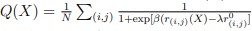
Second, we wish to clarify that the primary intent of our screen was not to validate the Golgi-nuclear localisation of any single protein in isolation, but rather to identify whether entire functional pathways are represented at the two organelles. This is precisely why the bioinformatic network analysis was performed as an integral part of the workflow, and not as an afterthought. The finding that the validated hit list is significantly enriched for coherent functional clusters, most notably a network spanning multiple core DNA repair pathways (HR, MMR, BER, MMEJ) serves as an in silico validation of the dataset as a whole. The emergence of pathway-level organisation, with proteins from the same repair pathways co-associating, localising to the same Golgi sub-compartments, and redistributing in the same direction upon genotoxic stimuli, provides biological coherence that goes beyond what individual antibody validation can offer, and substantially reduces the likelihood that the Golgi signal represents a collection of unrelated false positives.

Third, our mechanistic conclusions do not rely on the 25% screening threshold. For RAD51C, we used multiple orthogonal validation approaches, including independent antibodies recognizing distinct RAD51C epitopes and genetic depletion, supported by biochemical evidence.

In response to this comment, we have provided the full screening validation dataset as source data (Supplementary____Table S1), including intensity changes for the candidates, so that readers can inspect the distributions and apply their own thresholds. We have also clarified in the Results section the rationale behind our screening strategy (lines 128-139) and the role of the bioinformatic network analysis as an integral validation step (lines 141-156).

Turning to the specific suggestion of tagged RAD51C, we fully agree that tagged proteins can provide valuable orthogonal validation. We attempted endogenous tagging using CRISPR-mediated homologous recombination but were unable to obtain viable colonies following editing, consistent with the essential role of RAD51C in homologous recombination. We also attempted ectopic expression of tagged RAD51C but were unable to obtain constructs that preserved physiological expression levels, maintained robust cell viability or produced interpretable localization. This difficulty is not unique to our laboratory: colleagues working on RAD51 paralog complexes have reported that tagging or overexpression of RAD51C perturbs both its localisation and its ability to form functional paralog complexes (Greenhough et al, 2023; Rawal et al, 2023; Somyajit et al, 2015; Berti et al, 2020) all use purified complexes or untagged proteins for functional assays. We discussed these challenges extensively with experts in the DNA damage repair field at several international meetings (EMBO Sounio, Keystone Symposia, German DNA Repair Society). For these reasons, we relied on orthogonal approaches that do not require tagging (genetic depletion plus independent antibodies, and biochemical fractionation) to support the Golgi localization claim. We agree with the reviewer that this represents a limitation of this study, and we addressed these concerns in the discussion of our revised manuscript (lines 630-641).

*2.) The total signal should be quantified for each DNA repair protein upon genotoxic stress, in addition to the Golgi to nucleus ratio. For many of the proteins it looks like the total signal goes down, which could influence interpretation. *

Response: __We thank the reviewer for this important point. We wish to clarify that our imaging pipeline uses marker-based segmentation throughout, the Golgi compartment is segmented using GM130 and the nucleus using Hoechst, as unsegmented whole-cell masks without organelle markers yield unreliable intensity measurements in this experimental setup. True total cellular signal is therefore not directly accessible in this dataset. In the revised manuscript we provide the absolute fluorescence intensities for both the Golgi and nuclear compartments separately. In addition, we now include total (Golgi + nuclear) intensity measurements for each protein (__Supplementary Figures 3D, 4D, __and 5E__) as the most reliable proxy for overall protein distribution. These data are presented alongside the redistribution ratio to enable comprehensive interpretation.

As the reviewer correctly notes, a subset of proteins shows a reduction in total signal after treatment, particularly with doxorubicin. This is consistent with known effects of doxorubicin-induced DNA damage on cellular proteostasis, including widespread ubiquitination and suppression of protein translation (Halim et al, 2018). Several DDR regulators are subject to ubiquitin-dependent turnover following genotoxic stress, such as CHK1 (Zhang et al, 2005). More broadly, ubiquitin and proteasome mediated regulation is an integral component of the DNA damage response and can affect the abundance and detectability of DDR factors (Brinkmann et al, 2015). Changes in abundance are therefore an expected biological feature of the response. For this reason, we used the Golgi-to-nucleus ratio as the primary redistribution readout, as it captures relative compartmental partitioning independently of changes in total protein levels.

*3.) The study would benefit from live imaging of the Golgi to nucleus translocation of RAD51C. This would give a better indication of dynamics. *

__Response: __We agree that live imaging would directly visualize the dynamics of RAD51C redistribution between the Golgi and the nucleus. This was indeed one of our initial goals following the identification of the Golgi-associated RAD51C pool. However, as described above in our response to Major Comment 1, live imaging requires a fluorescently tagged RAD51C construct, and all tagging strategies we attempted, both endogenous CRISPR-mediated tagging and ectopic expression, failed to yield cell lines with robust signal while preserving physiological behaviour. This appears to be a broader challenge for highly conserved and functionally constrained DNA repair proteins, and is not unique to our laboratory.

Given these constraints, we focused on tag-independent approaches: multiple independent RAD51C antibodies combined with genetic depletion controls, quantitative fixed-cell time courses, and biochemical fractionation. These orthogonal datasets together support compartment-specific changes over time in a manner consistent with redistribution. We have clarified this limitation explicitly in the manuscript and avoided any wording that could be interpreted as implying direct single-molecule tracking in live cells. We present this as an important avenue for future work, contingent on the development of viable RAD51C-expressing cell lines (lines 630-641).

*4.) The double depletion experiments suggest a functional relationship between giantin and RAD51C. But they do not formally show it. Experiments to more directly address the functional role of the interaction between these two proteins would strengthen the study. *

Response: We agree with the reviewer that double depletion alone cannot formally prove that the physical Giantin-RAD51C interaction is the sole determinant of the observed DDR phenotypes. However, we would like to highlight the breadth of evidence we have assembled in support of this functional relationship:

• Physical interaction between endogenous Giantin and RAD51C demonstrated by colocalisation (Figure 4F-G) and co-immunoprecipitation (Figure 4H-I).
• Damage-induced dissociation of the Giantin-RAD51C complex that is prevented by ATM inhibition or Importazole treatment, directly linking the interaction to the DDR signalling axis (Figure 3K-P)
• Premature nuclear accumulation of RAD51C upon Giantin depletion, producing aberrant nuclear foci lacking canonical HR markers and impaired ATM signalling (Figure 4B-E & J-M)
• DR-GFP reporter assay confirming that Giantin depletion reduces HR efficiency to approximately 60% of control, consistent with the reduction previously reported in the genome-wide HR screen (Adamson et al. 2012) and validating the functional significance of Giantin in HR (Figure 5L).
• Partial rescue of ATM phosphorylation, genomic instability and proliferation phenotypes by RAD51C co-depletion, arguing for RAD51C as a functionally relevant conduit of the Giantin-dependent phenotype (Figures 5M-5P). These observations are further supported by the established literature on RAD51C function, its roles in CHK2 phosphorylation, replication fork stabilisation, and RAD51 filament formation (Badie et al, 2009; Somyajit et al, 2015; Prakash et al, 2022) providing a mechanistically coherent framework in which mislocalisation of RAD51C, whether directly or indirectly through Giantin, leads to dysregulation of DDR signalling and repair capacity, as we directly demonstrate with the HR efficiency assay.

Nonetheless, we fully agree that the most direct proof of the functional relevance of the physical Giantin-RAD51C interaction would come from separation-of-function experiments, ideally using an interaction-deficient Giantin mutant or an RAD51C variant unable to bind Giantin. We wish to be transparent that both approaches face substantial technical barriers in this system. RAD51C tagging consistently compromised cell viability and protein function, precluding the generation of interaction-deficient variants at physiological expression levels. Engineering an interaction-deficient Giantin mutant presents an independent challenge: Giantin is one of the largest Golgi matrix proteins (~376 kDa), composed almost entirely of extended coiled-coil domains that are resistant to structural prediction, and identifying a discrete RAD51C interaction interface without disrupting broader scaffolding function would require a dedicated structural and biochemical programme. We have framed these explicitly as the most important future priorities in the Discussion (lines 555-564), rather than over-interpreting the current data.

*5.) The Kaplan-Meier plots in Fig S9 seems to be quite selective in that only breast cancer is shown. Does giantin reduction correlate with poor prognosis in other cancers? *

__Response: __We thank the reviewer for this suggestion. We initially focused on breast cancer because RAD51C is a clinically established hereditary breast and ovarian cancer susceptibility gene (Meindl et al, 2010; Ghannoum et al, 2023), providing direct clinical context for a study centred on RAD51C dynamics and genome stability. We agree however that restricting the survival analysis to a single cancer type can appear selective.

To address this directly, we expanded the in-silico survival analysis of Giantin (GOLGB1) using GEPIA2 (Tang et al, 2019) across all available TCGA cohorts (overall survival, median cutoff, FDR correction). In the pooled pan-cancer analysis, higher GOLGB1 expression is significantly associated with improved overall survival (HR(high) = 0.75, p = 6.6 × 10⁻¹⁵). When stratified by tumour type, the majority of individual associations do not reach statistical significance. The two most robust statistically significant associations are kidney renal clear cell carcinoma (KIRC; HR(high) = 0.57, p = 3.4 × 10⁻⁴), where high GOLGB1 expression is associated with improved survival, and lower-grade glioma (LGG; HR(high) = 1.5, p = 0.036), where the association is in the opposite direction. A significant association is also observed in thymoma (THYM; HR(high) = 7.3, p = 0.031), though this should be interpreted with caution given the small cohort size (n = 59). Notably, the breast cancer association observed in the KM Plotter analysis (HR = 0.71, p = 1.8 × 10⁻¹¹; n = 4,929) does not reach significance in the TCGA BRCA cohort (HR = 1.1, p = 0.68; n = 1,070), most likely reflecting the substantially smaller sample size of the TCGA cohort, which is approximately 4.6-fold smaller and therefore underpowered to detect a modest effect. These context-dependent associations are consistent with the tumour-type-specific roles of Golgi scaffolding proteins and are discussed accordingly in the revised manuscript.

In the revised manuscript we have retained the original breast cancer Kaplan-Meier plots and supplemented them with a pan-cancer survival map across all TCGA cohorts (lines 611-625; Figure S9G) and a summary table (Supplementary Table 3) reporting hazard ratios, sample sizes, and p-values for each tumour type, allowing readers to assess the clinical relevance of GOLGB1 expression.

*Minor points: There are a few grammatical errors here and there. The figures do not appear in the correct order in the text, which makes the early parts of the paper a bit difficult to follow. Some of the figures don't seem to clearly match the text. For example, it is mentioned that RAD51C labelling was done with 3 different antibodies. I could not find this data. *

Response: __We thank the reviewer for these helpful observations. In the revised manuscript we have (i) carefully proofread the text and corrected grammatical errors throughout; (ii) revised the Results section to ensure that figures and supplementary figures are cited in sequential order and that each panel is explicitly introduced before being discussed, improving readability in the early sections. and (iii) corrected figure callouts to ensure they match the text. In particular, the statement that RAD51C labeling was performed with three different antibodies has been linked to the corresponding figure panels in the Results section. Antibody identifiers, sources, and dilutions are clearly reported in the Methods and in the table in __Supplementary Table S1.

__ Reviewer #1 (Significance (Required)):__

*This paper is novel and should be of significant interest to the field. It has important implications for how we think about the Golgi apparatus, and for how DNA repair pathways may be controlled. The pattern is clearly complex, with many DNA repair proteins localising to the Golgi, and some showing opposite dynamics. However, by focussing on RAD51C and giantin, the paper nicely demonstrates a novel mechanism for controlling DNA repair by these proteins. *

Reviewer #2 (Evidence, reproducibility and clarity (Required)):

Background - Eukaryotic cells rely on tightly regulated DNA repair pathways to preserve genome stability under the constant threat of both endogenous and exogenous genotoxic stress. While the nucleus, and to a lesser extent the mitochondria, is the primary site where DNA damage is detected and repaired, accumulating evidence indicates that extranuclear organelles, particularly the Golgi apparatus, play a surprisingly important role in modulating stress signaling, proteostasis, and the trafficking/activation of key DNA repair factors.

• Emerging evidence has shown that genotoxic stress can result in a major remodeling of the Golgi apparatus; however, the crosstalk between the Golgi and the nucleus, and its contribution to the DNA damage response, remains poorly defined. The present study offers timely insight by examining the spatiotemporal behavior of DNA repair proteins that shuttle between the Golgi and the nucleus, and how this trafficking contributes to the maintenance of genomic stability.*

Main findings - The authors employed the Human Protein Atlas (HPA) project to shortlist proteins that might link Golgi-nuclear function and validated each candidate using an siRNA-mediated antibody-validation pipeline, thereby identifying 163 proteins that localize to both the Golgi and the nucleus. Bioinformatic analysis of these candidates revealed a significant enrichment for DNA damage response (DDR) regulators, including multiple factors from core DNA repair pathways, suggesting that a portion of the DDR machinery may reside in the Golgi at steady state. Interestingly, the authors observed that dual-localizing DDR proteins undergo lesion-specific redistribution between the Golgi and the nucleus in response to specific types of DNA injuries. For instance, BER and MMEJ proteins shifted from nucleus to Golgi in response to doxorubicin, whereas MMR and HR proteins redistributed from Golgi to nucleus. This trend was reversed with H2O2 or KBrO3 treatments.

• To gain further insight into the link between the DDR and Golgi-nuclear communication, the authors focused on the HR factor RAD51C, which also plays a key role during the replicative stress response. The authors noticed that RAD51 is significantly associated with the Golgi, in addition to its known nuclear pool. Interestingly, they demonstrated that doxorubicin triggers the ATM-dependent release of this Golgi-tethered RAD51C pool and its Importin-β-mediated import into the nucleus, where it forms repair-associated foci. They further identified Giantin as the Golgi scaffold that anchors RAD51C at steady state in this subcellular compartment and showed that its depletion leads to premature nuclear accumulation of RAD51C, formation of aberrant RAD51C foci lacking canonical HR markers, reduced ATM activation, elevated genomic instability, and increased cell proliferation. *

Together, this study revealed an underappreciated and functionally meaningful spatiotemporal level of regulation within the DDR, suggesting that the Golgi, rather than functioning solely as a trafficking organelle, acts as a platform that anchors, releases, and temporally controls the availability of key DNA repair factors in response to genotoxic stress. In particular, the authors demonstrated that the timely and regulated release of RAD51C from the Golgi is essential for maintaining genome stability and is dependent on canonical DDR signaling pathways, including ATM activation and Importin-β-mediated nuclear import.

• Overall Critique - This manuscript offers a novel and compelling perspective on the regulation of the DDR by positioning the Golgi as an active participant in the spatiotemporal control of DNA repair factors. By integrating multiple experimental layers, including a systematic localization screening, a sub-Golgi mapping, several dynamic redistribution assays, and functional perturbation read-outs, the authors built a strong and coherent case for a biologically meaningful Golgi-nucleus communication axis during the DDR. Therefore, the study is timely and highly relevant for the DNA repair field, with broader implications for our understanding of how subcellular organelles coordinate genome maintenance and cellular homeostasis.

While the manuscript is clearly written and the figures are coherent and supportive of the main findings of the study, several issues should be addressed to ensure full interpretability and reproducibility.

Major Comments*

*1. Limited use of agents causing genotoxic stress - The authors report intriguing lesion-specific shifts in Golgi-nuclear redistribution, yet much of the mechanistic work relies heavily on doxorubicin, a pleiotropic drug that induces diverse forms of DNA damage beyond DSBs. Expanding the core analysis of the study to include a broader panel of mechanistically defined genotoxins (e.g., etoposide, camptothecin, neocarzinostatin, or ionizing radiation) would substantially strengthen the conclusion that the trafficking patterns reflect damage-type specificity rather than drug-specific off-target effects. Such broader analysis would also clarify whether Golgi-nucleus communication responds differentially to replication-associated breaks, Topo II-dependent lesions, oxidative stress, or crosslinks. *

__Response: __We thank the reviewer for this important point. We would first note that while doxorubicin is indeed pleiotropic, its primary and best-established mechanism of action is the poisoning of Topoisomerase II, leading to DNA double-strand breaks, a mechanism it shares with etoposide (van der Zanden et al, 2021; Thorn et al, 2011). The additional effects of doxorubicin, including reactive oxygen species generation and chromatin remodelling, are well-documented but secondary to this DSB-inducing activity, as we note in the revised manuscript. Nonetheless the goal of this study was not to comprehensively map lesion-specific trafficking for every DDR protein, but rather to establish the existence of a dynamic Golgi-nucleus redistribution axis and then focus mechanistically on the validated targets, in this case RAD51C. The lesion-dependent redistribution patterns are therefore presented as an initial, hypothesis-generating observation emerging from our screening and characterisation framework. A systematic, lesion-by-lesion dissection of redistribution kinetics across the broader DDR network would represent a substantial additional study and is beyond the scope of the present work.

Importantly, our key mechanistic observations for RAD51C are not restricted to doxorubicin. We tested a panel of genotoxic agents covering mechanistically distinct lesion classes: camptothecin (CPT; Topoisomerase I-associated replication breaks), etoposide (ETO; Topoisomerase II-dependent DSBs), and mitomycin C (MMC; interstrand crosslinks) (Figures S8A-S8I). Across all DSB-inducing agents, RAD51C consistently redistributed from the Golgi to the nucleus, demonstrating that this response is not a doxorubicin-specific off-target effect. Notably, RAD51C did not redistribute in response to oxidative lesions induced by hydrogen peroxide or potassium bromate, consistent with its established role in homologous recombination and DSB repair rather than oxidative damage pathways, as discussed in the manuscript. This lesion-type selectivity provides additional evidence that the Golgi-nuclear redistribution we observe is a biologically specific response rather than a non-selective stress effect.

*2. Functional implications of RAD51C redistribution for HR efficiency - Although the study convincingly demonstrates a release of RAD51C from the Golgi and its subsequent nuclear foci formation, it remains unclear how this redistribution influences HR efficiency. Incorporating a functional HR assay (e.g., DR-GFP reporter, RAD51 filament assembly, or fork protection assays) would help determine whether Golgi-anchored RAD51C release is directly required for HR or instead primarily modulates upstream DDR signaling. *

Response: __We thank the reviewer for this important suggestion. We have performed DR-GFP reporter assays to directly assess HR efficiency following Giantin and RAD51C depletion. Depletion of Giantin reduced HR efficiency to approximately 60% of control levels, and RAD51C depletion to approximately 40%, consistent with the HR reduction previously reported in the genome-wide HR screen (Adamson et al, 2012). Co-depletion of Giantin and RAD51C reduced HR to levels comparable to RAD51C depletion alone, suggesting that the effect of Giantin on HR is mediated primarily through RAD51C, consistent with RAD51C being the key effector of the Giantin-dependent spatial regulatory mechanism we describe. These data are included in the revised manuscript (__lines 455-465; Figure 5L).

*In addition, the manuscript does not fully reconcile how Golgi-tethering of RAD51C fits with its well-established nuclear roles during replication stress, where timely availability of RAD51C is essential for fork stabilization and restart. *

Response: __We agree that the nuclear function of RAD51C during replication stress is well established and important to reconcile with our findings. Our imaging data consistently show a detectable nuclear RAD51C population at steady state across all cell lines examined, and we do not propose that RAD51C is exclusively Golgi-localised. We suggest that the two pools serve distinct functional purposes: the constitutive nuclear pool supports ongoing replication fork stabilisation and restart, processes that require RAD51C availability independently of acute DNA damage, while the Golgi-tethered fraction represents a damage-responsive reserve that is released acutely upon DSB induction in an ATM-dependent manner. We wish to be transparent that this two-pool model is speculative at present, formally distinguishing the contributions of each pool would require direct labelling of the Golgi-anchored fraction, which was not technically feasible in this system as discussed above. Nonetheless, this model is consistent with established principles of signal-responsive protein sequestration in cell biology, and is directly supported by our Giantin depletion data: premature release of the Golgi pool leads to aberrant nuclear RAD51C foci lacking canonical HR markers and impaired ATM signalling, demonstrating that unscheduled nuclear accumulation is actively detrimental rather than simply redundant. We have added a paragraph to the revised Discussion explicitly framing the two-pool distinction as a working model and identifying direct pool-identity tracking as an important future direction (__lines 566-587).

*3. Specificity of Giantin-related phenotypes - The phenotypes observed upon Giantin depletion (e.g., increased micronuclei, comet tail moments, impaired ATM signaling, and elevated proliferation) could partially reflect a global dysfunction of the Golgi rather than RAD51C-specific tethering defects. Although co-depletion of RAD51C provides partial rescue, additional controls examining Golgi integrity, trafficking competence, or rescue with siRNA-resistant Giantin would help confirm specificity and distinguish direct from indirect effects. *

__Response: __We thank the reviewer for raising this important concern, which was a central consideration throughout our investigation. We address it through three complementary lines of evidence.

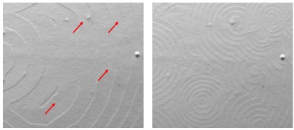
First, regarding Golgi structural integrity and trafficking competence: as previously reported, Giantin depletion has not been associated with strong Golgi fragmentation or major morphological alterations (Koreishi et al, 2013; Bergen et al, 2017; Stevenson et al, 2021), and we observed no significant Golgi fragmentation upon Giantin knockdown in our system. Consistent with the literature, Giantin has been implicated in specific cargo trafficking, most notably collagen secretion, rather than general secretory pathway function (Stevenson et al, 2021). To directly confirm that general Golgi trafficking competence was preserved in our experimental system, we performed the VSV-G-YFP trafficking assay (Presley et al, 1997), a well-established functional readout of general secretory trafficking. Giantin depletion did not result in a significant change in trafficking efficiency compared to control siRNA (Rebuttal Figure 1), consistent with the literature and arguing against a general collapse of Golgi function as the basis for the phenotypes observed.

Rebuttal ____Figure 1. VSV-G-YFP trafficking assay.

(A) Representative images of cells treated with control siRNA or giantin siRNA. Nuclei are stained with Hoechst. Total VSV-G-YFP (YFP-tsO45G) signal is shown together with antibody staining against VSV-G in non-permeabilized cells to assess cell surface levels. Scale bars, 10 μm.

(B) Quantification of VSV-G trafficking from two independent biological replicates.

Second, the phenotypes are RAD51C-dependent and not a generic Golgi dysfunction: the genomic instability and DDR signalling defects we observe upon Giantin depletion are not phenocopied by GMAP210 depletion, another Golgin family member, indicating that the phenotypes are not a generic consequence of Golgin loss. Critically, we now directly demonstrate using the DR-GFP reporter assay that Giantin depletion reduces HR efficiency to approximately 60% of control, and that co-depletion of RAD51C produces no further reduction beyond RAD51C depletion alone, consistent with RAD51C epistasis over Giantin for HR capacity (Figure 5L). This functional epistasis, together with the physical interaction between Giantin and RAD51C by co-immunoprecipitation, their co-localisation within the same Golgi sub-compartment, and the partial rescue of ATM phosphorylation, micronuclei formation and proliferation phenotypes upon RAD51C co-depletion, provides a coherent mechanistic chain linking Giantin specifically to RAD51C-dependent DDR outcomes. While we cannot formally exclude indirect contributions from other Giantin-associated factors, none of our observations are consistent with the phenotype arising from non-specific Golgi perturbation.

Third, Giantin may play a broader role in connecting DDR signalling to cytoplasmic and Golgi-resident processes, beyond RAD51C tethering alone: we consider this a feature of the biology rather than a confound. Golgins are well established as multi-cargo scaffolding platforms, and Giantin in particular occupies a strategic position where several processes converge: the tethering of DDR factors, the regulation of damage-induced signalling cascades, and the directional trafficking of repair factors between compartments. This would explain why Giantin depletion produces a phenotype that extends beyond what RAD51C co-depletion alone can fully rescue, and is consistent with the pathway-level coherence we observe across our screen. Understanding the full complement of Giantin-associated DDR interactions represents one of the most compelling directions emerging from this work.

In response to this comment, we have expanded the Discussion (lines 545-565) to explicitly propose that Giantin functions as a broader organisational node coordinating multiple DDR factors, while our data specifically and consistently implicate RAD51C as a primary conduit.

*4. Positioning of ATM in the Golgi-nuclear signaling - While ATM inhibition prevents RAD51C release, its spatial and mechanistic basis of this regulation remains obscure. It is not clear whether ATM acts locally at the Golgi, through cytoplasmic pools, or indirectly via nuclear feedback signaling. Clarifying or discussing this point in more depth would improve the mechanistic coherence of the proposed model. *

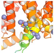
__Response: __We thank the reviewer for raising this important mechanistic question. The spatial basis of ATM action at the Golgi is indeed an emerging and exciting area of cell biology. A growing body of evidence demonstrates that ATM associates with the Golgi membrane through binding to phosphatidylinositol-4-phosphate (PI4P), and that this Golgi-resident pool modulates the magnitude and kinetics of the nuclear DDR (Ovejero et al, 2023). Importantly, the most recent work in this area demonstrates that Golgi-associated ATM is not merely a passive reservoir but is enzymatically active and capable of phosphorylating Golgi-resident substrates (Soulet et al, 2026), providing a compelling mechanistic basis for how damage-induced ATM signalling could reach the Golgi to license RAD51C release.

To directly examine whether ATM localises to the Golgi in our system and whether its activation state changes upon DNA damage, we performed a biochemical Golgi enrichment assay using the Minute{trade mark, serif} Golgi Apparatus EnrichmentKit (Cat #: GO-037) to examine ATM distribution across cis- and trans-Golgi fractions. Fraction purity was validated using GM130 (cis-Golgi), TGN46 (trans-Golgi), and HSP60 (membrane fraction) (Rebuttal Figure 2A). This analysis revealed that ATM is detectable in the total membrane fraction and enriched in the cis-Golgi fraction under basal conditions (Rebuttal Figure 2A). Under normal physiological conditions, activated ATM (pATM) was absent from Golgi-enriched fractions (Rebuttal Figure 2B), but was detectable in the cis-Golgi fraction following doxorubicin-induced genotoxic stress (Rebuttal Figure 2C). While these observations are preliminary and require further validation, they are consistent with the emerging literature and raise the intriguing possibility that ATM is recruited to and activated at the Golgi in a damage-dependent manner, where it could act locally to license RAD51C release.

Rebuttal Figure 2. Biochemical Golgi fractionation confirms ATM enrichment in cis-Golgi compartments.

*Western blot of HeLa-K fractions enriched for cis- and trans-Golgi membranes, probing for (A) ATM under basal conditions, and (B and C) pATM under basal conditions and (B) pATM (C) after treatment with DOX (40 μM) (markers: GM130 for cis-Golgi, TGN46 for trans-Golgi, HSP60 for membrane fraction (MEM). *

We consider the precise spatial and mechanistic dissection of ATM signalling at the Golgi and its relationship to nuclear feedback, one of the most exciting directions to emerge from this work, and one that we hope our study has helped to open. We have expanded the Discussion (lines 525-543) accordingly to place our findings in the context of the emerging Golgi-ATM literature and to frame this as an important unresolved question for future investigation.

*5. RAD51C is examined in silo, without consideration for the BCDX2 complex - RAD51C is exclusively analyzed in isolation, despite its well-established function as part of the BCDX2 paralog complex (RAD51B-RAD51C-RAD51D-XRCC2). Because RAD51C does not normally operate as a standalone factor, it is unclear why only RAD51C, among all paralogs, would be subjected to Golgi tethering, ATM-dependent release, and Importin-β-driven nuclear import. This raises important mechanistic questions: Are other BCDX2 members also Golgi-associated? Do they undergo similar trafficking dynamics? Does Golgi tethering selectively regulate RAD51C, or does the complex translocate together? Addressing these points would greatly strengthen the biological plausibility and mechanistic coherence of the proposed model. *

Response: We thank the reviewer for raising this important point. We fully agree that RAD51C functions as a core component of the BCDX2 (RAD51B-RAD51C-RAD51D-XRCC2) and CX3 (RAD51C-XRCC3) paralog complexes, and that its canonical roles in HR and replication fork protection occur within these assemblies. Our decision to focus on RAD51C was driven by the screening data: of the DDR proteins identified, RAD51C displayed the most robust Golgi-associated pool, the clearest damage-induced redistribution dynamics, and a tractable anchoring interaction with Giantin that could be interrogated biochemically.

We would also note that extending this analysis to other RAD51 paralogs is not straightforward with current tools. The available commercial antibodies against RAD51B, RAD51D and XRCC2 perform poorly in immunofluorescence applications, and most localisation studies for these proteins have relied on overexpression of tagged constructs, a strategy that, as discussed above, risks perturbing both localisation and complex assembly. The lack of reliable antibodies for endogenous paralog detection at the resolution required for Golgi localisation analysis represents a genuine technical barrier that we encountered directly during this study.

Whether Golgi association and ATM-dependent release involve RAD51C alone or extend to other BCDX2 or CX3 members is therefore a genuinely open and important question. We note that our co-immunoprecipitation data were performed on total cell lysate and cannot distinguish whether the Golgi-associated RAD51C is complexed with other paralogs or represents a monomeric subpopulation. Golgins are well established as multi-cargo scaffolding platforms, and it is entirely plausible that Giantin organises a broader paralog module rather than tethering RAD51C as an isolated subunit. A systematic analysis of RAD51 paralogs for Golgi localisation and lesion-dependent trafficking enabled by improved reagents such as proximity labelling or endogenous tagging approaches compatible with essential proteins would determine whether the BCDX2 complex translocates as a unit or whether individual subunits are differentially regulated, with potentially distinct consequences for HR fidelity. We have revised the manuscript accordingly and identify this as an explicit priority for future work in the revised Discussion (lines 583-602).

Minor Comments

1. Pathway-specific sub-Golgi localization patterns - The finding that DDR proteins map to distinct cis/trans Golgi subdomains is an interesting and potentially important observation. However, the dataset is limited to 15 proteins, making the proposed pathway-level trends (e.g., HR factors enriched in cis-Golgi; BER/MMEJ factors enriched in trans-Golgi) preliminary. Strengthening this conclusion by increasing the number of DDR proteins analyzed would help determine whether sub-Golgi compartmentalization contributes meaningfully to DNA repair pathway regulation.

Response: We thank the reviewer for this constructive suggestion. We agree that extending sub-Golgi mapping to a larger number of DDR proteins would be valuable, and we present the current dataset explicitly as a first, hypothesis-generating map rather than a definitive pathway atlas.

We would like to highlight, however, that the value of this observation lies not simply in the number of proteins mapped, but in the biological coherence of the patterns that emerge. The finding that proteins from the same repair pathway tend to occupy the same Golgi sub-compartment: BER and MMEJ factors enriching in the trans-Golgi, HR factors in the medial/cis-Golgi, and that this sub-compartmental positioning correlates with the direction of their redistribution upon genotoxic stress, is a pattern that would be unlikely to arise by chance across 15 independently validated proteins. This internal consistency argues that the sub-Golgi organisation reflects genuine pathway-level biology rather than noise, even if the dataset is not yet exhaustive. Together with the bioinformatic network analysis, which independently supports pathway-level clustering across the broader validated hit list, these observations reinforce each other as complementary layers of evidence.

2. Is the Golgi-released RAD51C indeed the pool that enters the nucleus? The major assumption of the study is that the RAD51C population released from the Golgi upon DNA damage is the same pool that subsequently accumulates in the nucleus to form repair foci. While the imaging and fractionation data are consistent with this model, the study does not directly track or distinguish Golgi-derived RAD51C from cytoplasmic or pre-existing nuclear pools. Without a method to specifically label, pulse-chase, or track the Golgi-anchored fraction, it remains formally possible that nuclear RAD51C originates from other subcellular reservoirs.

__Response: __We thank the reviewer for highlighting this important mechanistic point, which we agree cannot be fully resolved with the current dataset. Several independent lines of evidence are nonetheless consistent with a model in which the Golgi-associated pool contributes directly to damage-induced nuclear accumulation.

• Our time-resolved imaging demonstrates a reciprocal decrease at the Golgi and a concurrent increase in the nucleus following genotoxic stress, consistent with redistribution rather than independent compartment-specific changes (Figures 3E-3I).
• Biochemical fractionation provides an orthogonal readout of the same reciprocal shift under identical conditions (Figures 3J and S6D).
• ATM inhibition simultaneously prevents Golgi loss and blunts nuclear accumulation, while Importin-β perturbation blocks nuclear entry, together supporting an active and regulated translocation route (Figures 3K-3P).
• Giantin depletion, which releases the Golgi-tethered RAD51C pool prematurely, leads to aberrant nuclear RAD51C foci lacking canonical HR markers and impaired ATM signalling, strongly supporting that the Golgi-tethered fraction has functional consequences in the nucleus consistent with it being the relevant pool (Figures 4B-4E and 4J-4M).
• In the revised manuscript we have included cytoplasmic RAD51C signal quantification across the doxorubicin time course (Figure 3H). The cytoplasmic signal shows only a moderate and gradual reduction that is kinetically distinct from the sharp Golgi decrease and does not precede the nuclear increase. This pattern is inconsistent with a large pre-existing cytoplasmic reservoir driving the nuclear accumulation; if the cytoplasmic pool were the primary source, one would expect a rapid and prominent cytoplasmic decrease coinciding with or preceding nuclear accumulation, which we do not observe. Instead, the data are more consistent with rapid transit of Golgi-released RAD51C through the cytoplasm rather than stable cytoplasmic accumulation prior to nuclear entry. We acknowledge that definitive pool-identity tracking would require spatially restricted labelling approaches such as Giantin-proximal TurboID or photoactivatable tagging strategies, which are precluded by the technical constraints on RAD51C tagging described above. We have revised the manuscript to avoid overstatement on this point and identify these approaches as important future directions (lines 297-305 & lines 715-719).

Reviewer #2 (Significance (Required)):

General assessment - This study presents a novel and conceptually compelling view of the DNA damage response (DDR) by positioning the Golgi apparatus as an active regulator of the spatiotemporal availability of DNA repair factors. The strongest aspects of the work include its integration of a systematic immune-localization screening, a sub-Golgi compartment mapping, dynamic redistribution assays, and functional perturbations to build a coherent model of Golgi-nucleus communication during genotoxic stress. The mechanistic focus on RAD51C provides a clear case study linking organelle-level regulation to genome stability.

• Advance - To my knowledge, this is the first comprehensive demonstration that the Golgi can serve as a spatiotemporal coordination node for DDR proteins, including those involved in HR. The identification of a substantial pool of RAD51C, and reportedly other DDR factors, anchored within specific Golgi subdomains represents a significant conceptual advance. The demonstration that Golgi-tethered RAD51C is released in an ATM-dependent manner and subsequently participates in nuclear foci formation suggests a previously unrecognized organelle-level regulatory checkpoint in genome maintenance. This work therefore extends current models of the DDR by revealing a layer of intracellular coordination that bridges classical nuclear pathways with cytoplasmic organelle function.*

• Audience - This study will be of strong interest to a specialized audience in the fields of DNA repair, genome stability, and cell biology, particularly those studying the spatial organization of repair pathways and intracellular stress signaling. It will also appeal to researchers investigating organelle biology, intracellular trafficking, and the broader coordination of cytoplasmic and nuclear responses to stress. Beyond these communities, the work may be relevant to cancer, as it suggests new mechanisms by which organelle perturbations or Golgi-associated scaffolding proteins could influence therapeutic responses or genomic instability.

Reviewer expertise - Field of expertise: DNA repair, genome stability, organelle biology, cancer cell biology.*

Reviewer #3 (Evidence, reproducibility and clarity (Required)):

*This study investigates the communication between the Golgi complex and the nucleus of the cell, which remains a largely unexplored field. The authors used publicly available siRNA and antibody data from the Human Protein Atlas as a basis for finding overlap between the proteomes of the two cellular compartments. In validating the data from the HPA, the study finds a novel cluster of DNA repair proteins present in the Golgi, which they validate and resolve to sub-compartmental localization. To do so they use immunofluorescence (IF) localization on ¬cis- and trans-Golgi cisternae marked by GM130 and TGN46, respectively. The authors find that many of the fully validated proteins present in both the nucleus and Golgi redistribute between the Golgi and the nucleus dependent on the protein and the type of DNA lesion. They focused on RAD51C, a recombination factor. They show that RAD51C resides in both the ¬cis- and trans- subsections prior to damage and responds to DNA damage in an ATM-dependent manner via release of a Golgi-based pool bound to Giantin, which is then imported into the nucleus via Importin-β. Knockdown experiments showed that Giantin regulates RAD51C spatially and temporally. The work reveals a dynamic interchange of proteins between the Golgi and nucleus that controls cell functions beyond the classic secretory, membrane trafficking, and PTM roles of the Golgi. The authors build on prior work on Golgi impacts on DDR, offering an alternative cellular compartment for storage of DDR factors prior to damage. Overall, the data is timely and relevant, as it finds new roles for the Golgi in DNA damage response (DDR) regulation. The data is largely convincing and well controlled. The IF data is presented in black and white single channels and merged in color, which allows good comparison of the different protein stains. The scope of the initial screen of HPA antibodies and Golgi/Nuclear dual proteomes is impressive, and the overlap of DDR proteins is characterized for fifteen different proteins at a sub-compartmental level. The focus on RAD51C as a member of the HR pathway was a strong choice, and the study presents interesting information on its regulation by Golgi complex members, as well as a feedback look with pATM. The possibility of the Golgi storing specific DDR factors in specific compartments is well-supported and intriguing. There are a few major and minor points that should strengthen the paper and improve clarity prior to publication. *

Major Comments:

*1. Much of the strength of the IF data is lost in the choice of scale for presentation of the data. In almost all cases, enlarged sections should be shown of the areas currently indicated by arrow, in all channels. This is done well in Figure 3A, where an area of the Golgi is enlarged and the overlap of RAD51C in the GM130-marked Golgi is clearly visible in the merged channel, even when printed out. I would highly recommend including the white box and enlarged in all images and channels, while keeping the representative fields as is (e.g. if the image is 40mm, draw a 7mm box around representative cells/Golgi, and enlarge to 15mm in the bottom left). This change should be made to F1E, F2F, F3E, F3J, and F3M, as well as having enlarged figures in the corners in all supplementary data IF figures. Where possible, a fully enlarged image of the bounding box could also be included. Some of the IF data would be strengthened by using the nuclei stain to draw a masking outline to include in the black and white channels, to clearly delaminate what is Golgi-localized and what is nuclear. *

Response: We thank the reviewer for this helpful suggestion and fully agree that enlarged insets substantially improve the visibility of Golgi-localised signal, particularly when figures are printed. We share the reviewer's view that alternative display formats with larger insets would be preferable, and we have implemented enlarged boxed regions wherever space constraints permitted.

Specifically, we have added boxed regions with enlarged insets to Figure 1E, all panels of Figure 3. For Figure 2, the number of conditions and proteins displayed simultaneously within the constraints of standard journal figure dimensions made it impractical to include enlarged insets for all panels without reducing the overall field size to the point of losing contextual information. We have nonetheless improved the visibility of the Golgi signal in Figure 2 as much as possible within these constraints, and note that the final figure layout will be further optimised in line with the journal's specific formatting guidelines. In addition, all figures have been provided as high-resolution image files to allow electronic magnification, enabling readers to inspect the Golgi-localised signal in detail beyond what is visible in the printed version.

Regarding the use of nuclear outline masks in single-channel images, we tested this approach but found that given the number of structures present within each field, including Golgi stacks, nuclear foci, and cytoplasmic signal, overlaying nuclear outlines on individual channels added visual complexity that made the images harder rather than easier to interpret. As an alternative, we have included a full-colour merged panel, when possible, which we consider a cleaner way to delineate nuclear versus Golgi-localised signal and allows the reader to directly compare compartment-specific distributions across channels.

• 1. *There is a lack of consistency in the representative images shown by IF. For example, Figure 1 gives the impression of very little RAD51C in the nucleus but this is rightly shown to not be the case in Supp. Fig 2A. The same is true of the various images of LIG1. The authors should use representative data that better reflects the distribution of the proteins being studied and maintain consistency across images. If there is a lot of variation in staining patterns, the authors should show images and percentages corresponding to the variations especially for the key gene studied, RAD51C.

Response: We agree and have replaced the representative IF panels for RAD51C and LIG1 with images that better reflect the quantified distributions across biological replicates. The revised panels were selected to match the quantified compartment intensities shown in the accompanying graphs rather than representing outlier cells. We would also note that the apparent discrepancy between Figure 1E and Supplementary Figure S2A partly reflects a difference in imaging conditions: Supplementary Figure S2A __and __Figure 2F were acquired directly from the high-content screening pipeline under uniform, non-optimised antibody and fixation conditions at widefield resolution, whereas Figure 1E shows representative single optical section confocal images acquired after candidate identification with antibody conditions optimised for each individual protein. The improved signal-to-noise in the optimised confocal images more faithfully captures the dual Golgi and nuclear localisation of RAD51C, and the apparent difference between the two image sets is therefore expected rather than inconsistent. We have updated the figure legends to clarify the imaging modality and conditions for each panel. Furthermore, the quantified distribution of RAD51C across Golgi, nuclear and cytoplasmic compartments across multiple cell lines is shown in Figure 3B and 3D, providing a population-level representation of the dual localisation that complements the representative images shown in Figure 1E.

• 1. *The initial screening by siRNA-mediated knockdown pipeline that validated and confirmed dual Golgi and nuclear localization of 163 of the 329 dual-localization HPA proteins does not have any data included. This seems like a very large amount of data to gloss over and not include even as supplementary data. This should be included as source data, and discussion of the in-text information should be strengthened. The data included with the networking of these validated proteins is strong, but the process of elimination and validation has not been shown. In addition, the antibody information included in the supplementary data does not include dilution factors or blocking factors is not included, which would be beneficial to future studies to include.

Response: We agree and have addressed this in full. We note that the HPA antibody validation data, including immunofluorescence images and siRNA knockdown results, are publicly available for inspection on the Human Protein Atlas website (www.proteinatlas.org) for the majority of candidates, providing an independent layer of verification. In the revised submission, we additionally provide the complete siRNA-mediated validation dataset generated in our laboratory as source data (Table S1; lines 1025-1041), including for each candidate the HPA antibody identifier, gene symbol, Ensembl ID, antibody staining pattern, siRNA identifier, cell number per replicate, and normalised Golgi and nuclear signal ratios for both experimental replicates. This allows readers to inspect the validation metrics directly and apply alternative thresholds if desired. We have also expanded the antibody information to include diluent conditions (4% FBS in 0.1% Triton-X100 for all HPA antibodies used at 2 μg/ml in the screening pipeline), enabling reproducibility and reuse of the dataset by the community.

• 1. *The authors should expand upon the paragraph lines 155-162 to include more discussion on Figure S2A and S2B. The expanse of this data is some of the strongest in the paper, and it should be further discussed in-text. Also, the rationale behind the choice in the specific proteins that are included in these analysis / figures is not always clear in -text, and more attention should be spent on the narrowing down of the analysis to the final proteins. This is also especially important as many of the DDR proteins chosen are not the most common DDR proteins. Also note in text that the Golgi marker GM130 (presumably) was used for the screening, which means that some proteins which are only localizing to the TGN46 trans Golgi might have been lost in the validation step (or, explain why this is not the case).

Response: __We expanded the Results text (__lines 141-163) to discuss Figures S2A and S2B in more depth and clarified the rationale for selecting the final set of DDR proteins taken forward, including considerations of pathway representation, bioinformatic annotations, literature-described roles in DNA repair. We would also note that the identity of the DDR proteins identified in this screen was determined by the HPA dataset and the unbiased validation pipeline rather than by prior assumptions about which repair factors would be present at the Golgi. The presence of less commonly studied DDR factors is therefore a direct reflection of the screen output, and we consider this one of the strengths of the approach.

We would also like to address the reviewer's concern about potential GM130-based bias directly: at the widefield or confocal resolution used in the high-content screening pipeline, the Golgi apparatus appears as a single perinuclear structure and cis- and trans-Golgi subdomains cannot be resolved. GM130 was therefore used purely as a segmentation marker to define the Golgi compartment as a whole rather than to selectively label the cis-Golgi cisternae. The resulting Golgi mask captures signals from the entire Golgi ribbon, including trans-Golgi regions, meaning that proteins with exclusively trans-Golgi localisation would not have been systematically excluded at the screening stage. Sub-compartmental resolution of cis versus trans localisation was only possible in subsequent analyses using nocodazole-dispersed mini-stacks imaged by confocal microscopy with co-staining for both GM130 and TGN46.

*5. The relationship between Giantin loss, increased cell proliferation, and elevated endogenous DNA damage as it relates to RAD51C remains insufficiently resolved and requires further clarification. Several of the proliferation assays used are not optimal for addressing changes in cell growth. For example, Figure 5O appears to quantify cell numbers by counting fields from IF images, which is an unconventional approach. This should be done by growth curves, luminescent viability or colony formation assays. In addition, this point will be greatly strengthened by performing rescue experiments for Giantin directly (instead of co-depletion as a means of rescue) and/or using a mutant of RAD51C that does not bind to Giantin. If these additional experiments are beyond the current scope, the conclusions should be softened in the discussion. *

Response: We thank the reviewer for raising these important points, which we address in turn:

Giantin-RAD51C relationship and mechanistic interpretation. __We acknowledge that establishing the full causal chain between Giantin loss, RAD51C mislocalisation, elevated endogenous DNA damage and increased cell proliferation is challenging within the scope of a single study, and we discuss this openly in the Discussion (__lines 555-564). Our evidence collectively includes: physical interaction between endogenous Giantin and RAD51C by co-immunoprecipitation (Figures 4H and 4I), premature nuclear accumulation of RAD51C upon Giantin depletion (Figures 4B-4E and 4J-4M), new additional experiment showing direct reduction of HR efficiency in the DR-GFP assay (Figure 5L), impaired ATM signalling (Figures 5J and 5M), elevated genomic instability (Figures 5A-5E), and epistatic rescue by RAD51C co-depletion (Figures 5M-5P). These observations are further contextualised by the established literature on RAD51C function: RAD51C is known to regulate CHK2 phosphorylation and cell cycle checkpoint signalling (Badie et al, 2009), stabilise replication forks (Somyajit et al, 2015), and promote RAD51 filament formation required for DSB repair (Prakash et al, 2015). Dysregulation of these functions through Giantin-dependent mislocalisation provides a mechanistically coherent explanation for the elevated genomic instability and altered proliferation we observe, and is entirely consistent with our model. Together, the experimental evidence and the published biology of RAD51C support a model in which Giantin spatially regulates RAD51C to maintain proper DDR signalling and HR capacity.

We agree that separation-of-function tools would further strengthen this model and identify these as important future priorities. We wish to note however that both approaches face substantial technical barriers in this system. As described in our response to Reviewer 1 Major Comment 1, RAD51C tagging, whether by CRISPR-mediated endogenous editing or ectopic expression, consistently compromised cell viability and protein function, precluding the generation of interaction-deficient variants at physiological expression levels. Engineering an interaction-deficient Giantin mutant presents an independent and considerable challenge: Giantin is one of the largest Golgi matrix proteins (~376 kDa), composed almost entirely of extended coiled-coil domains that are intrinsically difficult to model structurally, and identifying a discrete interaction interface with RAD51C without disrupting the broader scaffolding function of the protein would require a dedicated structural and biochemical programme. We therefore consider these important but substantial future directions rather than straightforward experimental additions to the current study.

Proliferation assays. Colony formation assays provide a rigorous readout of long-term proliferative capacity, and these data are presented for single knockdown conditions in Figures 5F-5I. The cell number quantification in Figure 5P was specifically included to assess the double knockdown of Giantin and RAD51C simultaneously, a condition not covered by the colony formation assay. We respectfully note that automated fluorescence microscopy-based nuclear counting is a well-established approach for measuring cell proliferation in siRNA screening contexts. Nuclear counting from high-content imaging has been used as a direct readout of cell growth and proliferation in RNAi screens (Boutros et al, 2004; Martin et al, 2014; Garvey et al, 2016; Mikheeva et al, 2024), and has been shown to produce results comparable to or superior to conventional viability assays including MTT and flow cytometry-based methods (Mikheeva et al, 2024). We have nonetheless clarified in the revised figure legend that Figure 5P reports relative cell number quantified by automated nuclear counting from high-content imaging fields as a secondary concordant measure alongside the colony formation data, rather than a standalone proliferation assay.

*6. It is unclear from the discussion and from presented data whether proteins are directly transported between the Golgi and the nucleus, or whether they go into the cytoplasm for a transient period, presumably when they could interact with Importin β. There is also some data where cytoplasm signal could be quantified to address this (Figure 3E-I). *

Response: We thank the reviewer for this mechanistic point. In the revised manuscript we have included cytoplasmic RAD51C signal quantification alongside Golgi and nuclear measurements for the doxorubicin time course (lines 297-305; Figure 3H). The cytoplasmic signal shows a moderate and gradual reduction distinct in both magnitude and kinetics from the sharp Golgi decrease, consistent with a transient cytoplasmic intermediate rather than a stable pool. Regarding the identity of the translocating pool, two observations directly support a Golgi origin. First, Importazole treatment prevents RAD51C release from the Golgi following genotoxic stress and simultaneously reduces nuclear RAD51C foci formation, demonstrating that Importin-β-mediated import is required both for Golgi clearance and for productive nuclear accumulation. Second, Giantin depletion which prematurely releases the Golgi-tethered pool, leads to aberrant nuclear RAD51C foci, directly linking the Golgi-anchored fraction to nuclear accumulation. Together these data support a model in which Golgi-resident RAD51C transits through the cytoplasm for Importin-β-mediated nuclear import. We acknowledge that without direct labelling of the Golgi-anchored fraction, the precise contribution of each subcellular pool to the nuclear accumulation cannot be fully resolved with the current dataset. We discuss the development of appropriate tagging strategies as an important future direction to dissect the dynamics of this process in further detail.

*7. Statistical analysis on experiments with more than two samples need to be performed with ANOVA and a follow up post-hoc test, not with two-tailed unpaired Student's t-test, which only compares the control and each individual sample. This type of analysis inflates the Type 1 error rates (false positives) in your datasets. For example, the two-tailed unpaired Student's t-test is appropriate in Figure 2F-H, but not in Figure 3 when the samples are timepoints. In this case, a One-way ANOVA with Tukey's post-hoc test (if you want to show all coparisons), or Bonferroni/Sidak if you only need to compare several samples). *

Response: We agree with the reviewer and thank them for highlighting this important statistical issue. We have revised the statistical analysis for all experiments involving more than two groups to avoid inflation of Type I error rates caused by multiple pairwise Student's t tests. Specifically, for Figures 3F-I, 4C-E, and Figure 5, the data were reanalysed using one way ANOVA followed by the appropriate multiple comparisons post hoc test. The Methods section and corresponding figure legends have been updated to clearly state the statistical tests used for each dataset.

Minor Comments: General 1. Throughout the text, the reference to many figures and supplementary figures in the same sentence, with little discussion of the data therein makes it hard to follow. In-text referencing is particularly confusing in the section "Dual-localising DDR proteins dynamically redistribute between the Golgi and nucleus in response to specific types of DNA injuries," where the reader is switching between multiple figures and supplementary figures.

__Response: __We thank the reviewer for this helpful comment. In the revised manuscript, we have improved the readability of the text and revised the figure references to make them clearer. We hope these revisions make the manuscript easier to follow and allow readers to better inspect the figures.

1. In figures that display technical replicates as individual data points, consider distinguishing each replicate by using different marker shapes (e.g., repeat 1 = upright triangle; repeat 2 = inverted triangle; repeat 3 = diamond). This would provide additional clarity regarding the consistency and repeatability of each technical repeat.

__Response: __We thank the reviewer for this suggestion. We have updated the data presentation to distinguish biological replicates using different marker shapes in datasets where replicate tracking is of particular relevance to the interpretation. For datasets where individual replicate values are already clearly separable, we have maintained the existing presentation to avoid unnecessary visual complexity.

1. Make sure all western blot data includes the marker size (F3C and F5L has none, F4H/I have size of proteins not size of markers).

__Response: __We added missing marker sizes to our western blot data in the revised manuscript.

1. Be consistent with use of capitalization in figure legends and graph/figure labels.

__Response: __We made sure that the capitalisation is consistent in figure legends, graph and figure legends in the revised manuscript.

Figure 2

In Figure 2A, please include in the figure itself that GM130 is the cis Golgi, and TGN46 is the trans Golgi (Figures should not be dependent on the text for full understanding).

__Response: __We revised Figure 2A and 2C to label GM130 as cis-Golgi and TGN46 as trans-Golgi within the figure, making it self-explanatory.

1. Why are LRIG2 and LRRIQ3 not included in the 2E cis vs trans Golgi data, when all other proteins from F1D are included? Include, or comment on in-text.

__Response: __Both LRIG2 and LRRIQ3 are included in 2E in both the original and revised manuscript.

1. Be sure to include scale bar data in each figure legend (F2A-E is currently missing it), and include updated scales included in the enlarged data.

__Response: __Scale bar data is now included in each figure legend in the revised manuscript.

1. In Figure 2F, make sure that the merged green channel is presented at the same intensity as it is in the single black and white channel, as the green looks very overexposed in several of the merged (CCAR1 DMSO merged is the most noticeable).

__Response: __We agree and thank you for pointing this out. We have now revised the images and corrected the issue by updating all image panels in the figure.

1. In Figure 2G, include the grey label in the figure legend.

__Response: __We thank the reviewer for this comment. The grey label has now been included in the figure legend in the revised manuscript.

1. In Figure 2G-H, the method of data presentation in the graphs coupled with the statistical analysis is confusing and should be expanded upon in the legend.

__Response: __We agree that the amount of data presented may appear overwhelming. In the revised figure, we have adjusted the placement of the statistical annotations to improve clarity. Also, we improved the figure legend, to make the figure easier to read and interpret.

Figure 3

Figure E/F/G: Is there cytoplasmic quantification as well? Your rationale is that the Golgi RAD51C goes into the nucleus, but via the cytoplasm (due to Importin β import); do you see the cytoplasmic levels increase? Or is it too dilute to notice a difference? At least, this omission needs to be mentioned in-text.

Figure H/I also include the quantification of the cytoplasmic fraction. It is mentioned in-text on line 272, but not quantified. This comes up as a big question: Do the proteins go directly between the Golgi and nucleus, or do they go through the cytoplasm?

__Response: __We thank the reviewer for both of these related points. As described in our response to Major Comment 6 above, we have added cytoplasmic RAD51C signal quantification to the doxorubicin time course in the revised manuscript (Figure 3H) and discuss the implications for the proposed translocation route.

Figure 3A, 3E, and if the data is present for 3J and 3M, could all benefit from using the nuclei staining as a mask to draw an outline around the nucleus in the other channels, and then show a merge in full color instead of a nuclei-only channel. Also note from the major comments, that this data especially is so small to see without enlarged images.

__Response: __We thank the reviewer for this suggestion. Regarding nuclear outline masks, we tested this approach but found that the number of structures present in each field, including Golgi stacks, nuclear foci and cytoplasmic signal, made overlaid outlines visually confusing rather than clarifying. We have instead included a full-colour merged panel in Figure 3E, which we consider a cleaner way to distinguish nuclear from Golgi-localised signal while preserving the spatial context of the data.

Regarding image size, we have added enlarged insets to Figures 3E, 3J and 3M in the revised manuscript. We have chosen to display multiple cells per panel rather than a single enlarged cell in order to capture the heterogeneity of the cell population, which we consider important for an accurate representation of the data. All figures have been provided as high-resolution image files to allow electronic magnification, enabling detailed inspection of the signal beyond what is visible in the printed version. We acknowledge that the constraints of standard journal figure dimensions limit how large individual panels can be, and the final layout will be optimised in line with the journal's formatting guidelines.

*In-text discussion of the results from Figure 3 has an in-depth discussion of the NLS and NES in RAD51C, but this is not followed up on with site-directed mutagenesis or any data; perhaps move this to the discussion instead of results section. *

__Response: __We have removed the discussion of the NLS and NES from the Results section.

Figure 4

Comments from earlier figures hold, with size of enlarged events and using the nuclei as an outline in the single channels. E.g. Figure 4F arrows appear to point to nothing at the chosen scale. The zoom in 4G is insufficient, as the chosen feature is so small it is not even visible in full fields.

__Response: __We thank the reviewer for this comment. The arrows in Figure 4F indicate individual nocodazole-dispersed Golgi mini-stacks, which are displayed at higher magnification in Figure 4G. The full field in Figure 4F is intentionally shown to illustrate the degree of Golgi dispersion achieved by nocodazole treatment, a context that may be unfamiliar to readers outside the Golgi field, before zooming into a single representative mini-stack in Figure 4G for the cisternal localisation analysis.

• Figure 4H and 4I need to show the size of the markers *

__Response: __The size of the markers are now included in the revised manuscript.

*The representative image in 4L for siGiantin pATM has no pATM foci, while the quantification in 4M has a reduction from ~50% to ~25%, so this image is not representative of this data, or the data quantification is not as strong as the actual data. *

__Response: __We thank the reviewer for this observation. We wish to clarify that the quantification in Figure 4M reports the mean percentage of RAD51C foci co-localising with pATM across the entire cell population from three independent biological replicates. A reduction from ~50% to ~25% therefore reflects a population-level shift in co-localisation frequency, not that every individual cell shows exactly 25% co-localisation. Given the inherent cell-to-cell variability in foci number and co-localisation, individual cells will span a range of values around this mean, and the representative image shown in Figure 4L reflects one such cell.

Figure 5

*Figure 5A has overexposure of the nuclei stain in order to visualize micronuclei. Readjust the levels, and enlarge the images for better visualization. (is this DAPI-stained? Please label). *

__Response: __The display levels of the nuclear stain in Figure 5A are intentionally set to allow visualisation of micronuclei, which are significantly dimmer than the main nucleus and would not be detectable at display settings optimised for the primary nuclear signal. This is standard practice in micronuclei quantification studies and is necessary to accurately identify and score these structures. The nuclear stain is Hoechst 33342, and this has been explicitly labelled in the revised figure legend.

*Figure 5A-C: Figure 5A does not show siRAD51, but it is included in the DMSO only graph. Please either show RAD51 data in 5A and 5C, or do not include in 5B. If the DMSO and ETO experiments were performed separately and that accounts for this discrepancy, then show separately. *

__Response: __We thank the reviewer for this observation. The siRAD51C condition is included in Figure 5B as an internal positive control, consistent with its well-established role in genome stability. RAD51C depletion combined with etoposide treatment resulted in severe cellular toxicity and insufficient cell numbers for reliable quantification, and this condition was therefore excluded from Figure 5C. This has been clarified in the revised figure legend.

*Figure 5M the white label is difficult to see in the green box. *

__Response: __We have updated the label colour in Figure 5M to improve visibility against the green background in the revised manuscript.

* Supplementary Figures*

Consider reordering/ subdividing supplementary figures for ease of reference during reading.

Response: We thank the reviewer for this suggestion. The current supplementary figure structure was intentionally designed to minimise the total number of supplementary figures and maintain a logical correspondence with the main figures, avoiding a situation where readers need to navigate an extensive supplementary section, a concern the reviewer raised regarding figure presentation. We believe the current organisation achieves a reasonable balance between completeness and accessibility.

SF1 and SF2A: Include enlarged boxes or full images so that data is visible.

__Response: __As described in our response to Major Comment 1, all figures have been provided as high-resolution image files to allow electronic magnification. Space constraints within standard journal figure dimensions preclude the addition of enlarged insets to all supplementary panels without substantially reducing the contextual field of view.

*SF3A, SF4A, and SF5A: Include enlarged images, include nuclei marker if possible (otherwise, the nuclear intensity is not proven nuclear). *

Response: We appreciate the suggestion, but adding enlarged insets and nuclei markers to all panels in Figures S3A, S4A and S5A would disproportionately increase the length and complexity of the supplementary section, making it harder rather than easier to navigate. The nuclear intensity measurements are derived from automated segmentation of the Hoechst channel using CellProfiler, which reliably defines nuclear boundaries independently of the antibody channel, and are therefore not dependent on visual confirmation of nuclear localisation in each representative image.

*SF3B-C, SF4B-C, and SF5 B-D: Change the data presentation in the same method as changed for F2G-H. *

Response: We have updated the figure legends for Figures S3B-C, S4B-C and S5B-D to improve readability.

SF3D: List proteins in the same order as in B and C.

Response: The proteins in Figure S3D are listed in the same order as in Figures S3B and S3C.

SF6D: Label M N and C more clearly. Include size labels.

Response: We have added clearer labels for the membrane (M), nuclear (N) and cytoplasmic (C) fractions and included molecular weight size markers in the revised Figure S6D.

*SF7A-B: Include enlarged. *

Response: We respectfully note that the purpose of Figures S7A-B is to display the overall cellular response to inhibitor treatments across the cell population, rather than to highlight specific subcellular structures. Enlarged insets would reduce the number of cells visible per panel and would not add scientific value in this context. The Golgi and nuclear signals are clearly visible at the chosen magnification.

*SF8: Include arrows as in previous experiments, include enlarge. *

Response: Arrows have been added to Figure S8 to indicate Golgi and nuclear RAD51C signal, consistent with the annotation style used in the main figures. The images already show two representative cells per condition to maximise the visible detail at the chosen scale.

*SF9G: G is labelled, but not included. *

Response: Figure S9G has been added in the revised manuscript, showing the pan-cancer overall survival map for GOLGB1 expression across all TCGA cohorts generated using GEPIA2. The figure legend has been updated accordingly.

*Reviewer #3 (Significance (Required)): *

* The work finds new roles for the Golgi in regulation of DNA damage responses and the screen could be an important dataset (but results need to be made available) for the DNA repair community. The scope of the initial screen of HPA antibodies and Golgi/Nuclear dual proteomes is impressive, and the overlap of DDR proteins is characterized for fifteen different proteins at a sub-compartmental level. The work provides important insights into RAD51C regulation, however, there are key mechanistic insights and control experiments missing from the studies involving RAD51C and Giantin, dampening its impact. The idea of an alternative cellular compartment for storage of DDR factors prior to damage is interesting, and suggests the spatial regulation of specific lesion responses are stored in specific sub-compartments of the Golgi, which could contribute to repair regulation.*

References:

Adamson B, Smogorzewska A, Sigoillot FD, King RW & Elledge SJ (2012) A genome-wide homologous recombination screen identifies the RNA-binding protein RBMX as a component of the DNA-damage response. Nat Cell Biol 14: 318-328

Badie S, Liao C, Thanasoula M, Barber P, Hill MA & Tarsounas M (2009) RAD51C facilitates checkpoint signaling by promoting CHK2 phosphorylation. J Cell Biol 185: 587-600

Bergen DJM, Stevenson NL, Skinner REH, Stephens DJ & Hammond CL (2017) The Golgi matrix protein giantin is required for normal cilia function in zebrafish. Biol Open 6: 1180-1189

Berti M, Teloni F, Mijic S, Ursich S, Fuchs J, Palumbieri MD, Krietsch J, Schmid JA, Garcin EB, Gon S, et al (2020) Sequential role of RAD51 paralog complexes in replication fork remodeling and restart. Nat Commun 11: 3531

Boutros M, Kiger AA, Armknecht S, Kerr K, Hild M, Koch B, Haas SA, Paro R, Perrimon N & Heidelberg Fly Array Consortium (2004) Genome-wide RNAi analysis of growth and viability in Drosophila cells. Science 303: 832-835

Brinkmann K, Schell M, Hoppe T & Kashkar H (2015) Regulation of the DNA damage response by ubiquitin conjugation. Front Genet 6: 98

Garvey CM, Spiller E, Lindsay D, Chiang C-T, Choi NC, Agus DB, Mallick P, Foo J & Mumenthaler SM (2016) A high-content image-based method for quantitatively studying context-dependent cell population dynamics. Sci Rep 6: 29752

Ghannoum S, Fantini D, Zahoor M, Reiterer V, Phuyal S, Leoncio Netto W, Sørensen Ø, Iyer A, Sengupta D, Prasmickaite L, et al (2023) A combined experimental-computational approach uncovers a role for the Golgi matrix protein Giantin in breast cancer progression. PLoS Comput Biol 19: e1010995

Greenhough LA, Liang C-C, Belan O, Kunzelmann S, Maslen S, Rodrigo-Brenni MC, Anand R, Skehel M, Boulton SJ & West SC (2023) Structure and function of the RAD51B-RAD51C-RAD51D-XRCC2 tumour suppressor. Nature619: 650-657

Halim VA, García-Santisteban I, Warmerdam DO, van den Broek B, Heck AJR, Mohammed S & Medema RH (2018) Doxorubicin-induced DNA damage causes extensive ubiquitination of ribosomal proteins associated with a decrease in protein translation. Mol Cell Proteomics 17: 2297-2308

Koreishi M, Gniadek TJ, Yu S, Masuda J, Honjo Y & Satoh A (2013) The golgin tether giantin regulates the secretory pathway by controlling stack organization within Golgi apparatus. PLoS One 8: e59821

Martin HL, Adams M, Higgins J, Bond J, Morrison EE, Bell SM, Warriner S, Nelson A & Tomlinson DC (2014) High-content, high-throughput screening for the identification of cytotoxic compounds based on cell morphology and cell proliferation markers. PLoS One 9: e88338

Meindl A, Hellebrand H, Wiek C, Erven V, Wappenschmidt B, Niederacher D, Freund M, Lichtner P, Hartmann L, Schaal H, et al (2010) Germline mutations in breast and ovarian cancer pedigrees establish RAD51C as a human cancer susceptibility gene. Nat Genet 42: 410-414

Mikheeva AM, Bogomolov MA, Gasca VA, Sementsov MV, Spirin PV, Prassolov VS & Lebedev TD (2024) Improving the power of drug toxicity measurements by quantitative nuclei imaging. Cell Death Discov 10: 181

Ovejero S, Kumanski S, Soulet C, Azarli J, Pardo B, Santt O, Constantinou A, Pasero P & Moriel-Carretero M (2023) A sterol-PI(4)P exchanger modulates the Tel1/ATM axis of the DNA damage response. EMBO J 42: e112684

Prakash R, Rawal Y, Sullivan MR, Grundy MK, Bret H, Mihalevic MJ, Rein HL, Baird JM, Darrah K, Zhang F, et al(2022) Homologous recombination-deficient mutation cluster in tumor suppressor RAD51C identified by comprehensive analysis of cancer variants. Proc Natl Acad Sci U S A 119: e2202727119

Prakash R, Zhang Y, Feng W & Jasin M (2015) Homologous recombination and human health: the roles of BRCA1, BRCA2, and associated proteins. Cold Spring Harb Perspect Biol 7: a016600

Presley JF, Cole NB, Schroer TA, Hirschberg K, Zaal KJM & Lippincott-Schwartz J (1997) ER-to-Golgi transport visualized in living cells. Nature 389: 81-85

Rawal Y, Jia L, Meir A, Zhou S, Kaur H, Ruben EA, Kwon Y, Bernstein KA, Jasin M, Taylor AB, et al (2023) Structural insights into BCDX2 complex function in homologous recombination. Nature 619: 640-649

Somyajit K, Saxena S, Babu S, Mishra A & Nagaraju G (2015) Mammalian RAD51 paralogs protect nascent DNA at stalled forks and mediate replication restart. Nucleic Acids Res 43: 9835-9855

Soulet C, Catalan J & Moriel-Carretero M (2026) The DNA Damage Response kinase ATM restricts Golgi extension. bioRxiv

Stadler C, Hjelmare M, Neumann B, Jonasson K, Pepperkok R, Uhlén M & Lundberg E (2012) Systematic validation of antibody binding and protein subcellular localization using siRNA and confocal microscopy. J Proteomics 75: 2236-2251

Stevenson NL, Bergen DJM, Lu Y, Prada-Sanchez ME, Kadler KE, Hammond CL & Stephens DJ (2021) Correction: Giantin is required for intracellular N-terminal processing of type I procollagen. J Cell Biol 220

Tang Z, Kang B, Li C, Chen T & Zhang Z (2019) GEPIA2: an enhanced web server for large-scale expression profiling and interactive analysis. Nucleic Acids Res 47: W556-W560

Thorn CF, Oshiro C, Marsh S, Hernandez-Boussard T, McLeod H, Klein TE & Altman RB (2011) Doxorubicin pathways: pharmacodynamics and adverse effects. Pharmacogenet Genomics 21: 440-446

van der Zanden SY, Qiao X & Neefjes J (2021) New insights into the activities and toxicities of the old anticancer drug doxorubicin. FEBS J 288: 6095-6111

Zhang Y-W, Otterness DM, Chiang GG, Xie W, Liu Y-C, Mercurio F & Abraham RT (2005) Genotoxic stress targets human Chk1 for degradation by the ubiquitin-proteasome pathway. Mol Cell 19: 607-618

This is interesting and makes me think of other instances outside of writing where I may experience that paradoxical reluctance.

Author response:

The following is the authors’ response to the original reviews.

Reviewer #1 (Public review):

Summary:

This work demonstrates that MORC2 undergoes phase separation (PS) in cells to form nuclear condensates, and the authors demonstrate convincingly the interactions responsible for this phase separation. Specifically, the authors make good use of crystallography and NMR to identify multiple protein: protein interactions and use EMSA to confirm protein: DNA interactions. These interactions work together to promote in vitro and in cell phase separation and boost ATPase activity by the catalytic domain of MORC2.

However, the authors have very weak evidence supporting their potentially valuable claim that MORC2 PS is important for the appropriate gene regulatory role of MORC2 in cells. Exploring causal links between PS and function is an important need in the phase separation field, particularly as regards the role of condensates in gene regulation, and is a non-trivial matter. Any study with convincing data on this matter will be very important. For this reason, it is crucial to properly explore the alternative possibility that soluble complexes, existing in the same conditions as phase-separated condensates, are the functional species. It is also critical to keep in mind that, while a specific protein domain may be essential for PS, this does not mean its only important function pertains to PS.

In this study, the authors do not sufficiently explore the role that soluble MORC2 complexes may play alongside MORC2 condensates. Neither do they include enough data to solidly show that domain deletion leads to phenotypes via a loss of phase separation per se, rather than the loss of phase separation being a microscopically visible result, not cause, of an underlying shift in protein function. For these reasons, the authors' conclusions regarding the functional role of MORC2 condensates are based on incomplete data. This also dampens the utility of this work as a whole, since the very nice work detailing the mechanism of MORC2 PS is not paired with strong data showing the importance of this observation.

We thank the reviewer for this thoughtful and constructive critique. We agree that establishing a causal link between phase separation (PS) and biological function—particularly in transcriptional regulation—is a central and non-trivial challenge in the condensate field. We also appreciate the reviewer’s emphasis on two critical alternative interpretations: (i) that soluble MORC2 complexes, rather than condensates, may represent the primary functional species, and (ii) that loss of phase separation upon domain deletion could reflect a downstream consequence of altered protein function rather than its cause.

To address these concerns, we have performed a series of new experiments specifically designed to decouple condensate formation, and condensate dynamics, thereby allowing us to more rigorously interrogate the functional relevance of MORC2 condensates.

First, to overcome the limitation of domain deletions which may affect MORC2 function beyond phase separation we introduced a micropeptide-based kill switch (KS) to the C terminus of MORC2. This strategy has recently emerged as a powerful approach to selectively reduce condensate dynamics without disrupting protein expression, folding, or domain architecture [1]. Importantly, unlike CC3 or IDRa deletions, MORC2+KS robustly form nuclear condensates but exhibits markedly reduced internal dynamics, as demonstrated by FRAP analyses showing minimal fluorescence recovery after photo bleaching (Fig. 6a-c). This strategy therefore allows us to perturb condensate material properties independently of MORC2 domain integrity.

Second, we systematically compared the transcriptional consequences of rescuing MORC2-knockout HeLa cells with MORC2FL, condensation-deficient mutants (ΔCC3 and ΔIDRa), and the dynamics-defective MORC2+KS (Fig. 6d). Despite being expressed at substantially higher levels than MORC2FL (Fig. 6e), all three mutants showed a striking and consistent failure to restore MORC2-dependent transcriptional regulation (Fig. 6f-h). This effect was particularly pronounced for transcriptionally repressed genes, including two sets of high-confidence MORC2 targets reported in prior studies (Fig. 6i and Fig.S10). These findings demonstrate that neither increased protein abundance nor the mere presence of condensate-like structures alone is sufficient to restore MORC2 function.

Third, our data instead support a model in which both soluble MORC2 complexes and dynamic MORC2 condensates are required for full transcriptional regulation activity. While soluble MORC2 is likely involved in target recognition and complex assembly, our results indicate that proper condensate formation—and critically, condensate dynamics—are essential for effective transcriptional repression and activation. The inability of the MORC2+KS mutant to rescue transcriptional defects, despite intact condensate formation, points away from a model in which MORC2 condensates represent only microscopically visible byproducts of MORC2 activity.

We believe these new data strengthen the manuscript by pairing the detailed mechanistic dissection of MORC2 phase separation with direct functional evidence, enhancing the conceptual impact and biological significance of the study.

Strengths:

Static light scattering and crystallography are nicely used to demonstrate the dimerization of MORC2FL and to discover the structure of the CC3 domain dimer, presumably responsible for the dimerization of MORC2FL (Figure 1).

Extensive use of deletion mutants in multiple cell lines is used to identify regions of MORC2 that are important for forming condensates in the nucleus: the IBD, IDR, and CC3 domains are found to be essential for condensate formation, while the CW domain plays an unknown role in condensate morphology (Figure 3). The authors use NMR to further identify that the IBD domain seems to interact with the first third of the centrally located IDR, termed IDRa, but not with the latter two-thirds of the IDR domain (Figure 4). This leads them to propose that phase separation is the product of IDB:IDRa interaction, CC3 dimerization, and an unknown but important role for the CW domain.

Based on the observation that removal of the NLS resulted in diffuse cytoplasmic localization, they hypothesized that DNA may play an important role in MORC2 PS. EMSA was used to demonstrate interaction between DNA and several MORC2 domains: CC1, CC2, IDR, and TCD-CC3-IBD. Further in vitro microscopy with purified MORC2 showed that DNA addition significantly reduces MORC2 saturation concentration (Figure 5).

These assays convincingly demonstrate that MORC2 phase separates in cells, and identify the protein domains and interactions responsible for this phenomenon, with the notable caveat that the role of the CW domain here is left unexplored.

We appreciate the reviewer for their positive and detailed assessment of the strengths of our study. Our understanding of the CW domain’s function remains preliminary. Although we observed that the CW domain can influence condensate size, the IDR, IBD, and CC3 domains constitute the core structural elements driving phase separation. Consequently, the CW domain was not a primary focus of the current study. Nonetheless, investigating its functional contributions represents an interesting avenue for future work.

Weaknesses:

Although the authors demonstrated phase separation of MORC2FL, their evidence that this plays a functional role in the cell is incomplete.

Firstly, looking at differentially upregulated genes under MORC2FL overexpression, the authors acknowledge that only 10% are shared with differentially regulated genes identified in other MORC2FL overexpression studies (Figure 6c, d). No explanation is given for why this overlap is so low, making it difficult to trust conclusions from this data set.

We thank the reviewer for raising this important concern. In response, we have improved the quality and robustness of our RNA-seq analysis by repeating the experiments with optimized sample handling and increased sequencing depth. Using this updated dataset, we identified a considerably higher overlap between MORC2-regulated genes in our study and those reported previously.

Specifically, we observed 84 overlapping genes with the study by Nikole L. Fendler et al. [2], corresponding to approximately 32% of the MORC2-regulated genes reported in that work (Fig. 6i). In addition, we identified 102 overlapping genes with the dataset reported by Iva A. Tchasovnikarova et al. [3], representing approximately 22% of the genes identified in that study (Fig. S10b).

We note that complete concordance with previous reports is not expected, given substantial differences in experimental design. For example, Fendler et al. employed a doxycycline-inducible MORC2 expression system [2], whereas our study relies on transient overexpression in MORC2-knockout HeLa cells. In contrast, Tchasovnikarova et al. compared transcriptomes between MORC2 knockout and wild-type cells [3], rather than MORC2 rescue conditions. Moreover, RNA-seq results are inherently influenced by cell line batch variability, sequencing depth, and analysis pipelines, all of which differ across studies.

Taken together, we consider an overlap in the range of ~20–30% to be reasonable and biologically meaningful in the context of these experimental differences, and we believe that the revised RNA-seq data provide a more reliable foundation for our conclusions regarding MORC2-dependent transcriptional regulation.

Secondly, of the 21 genes shared in this study and in earlier studies, the authors note that the differential regulation is less pronounced when a phase-separation-deficient MORC2 mutant is overexpressed, rather than MORC2FL (Figure 6e). This is taken as evidence that phase separation is important for the proper function of MORC2. However, no consideration is made for the alternative possibility that the mutant, lacking the CC3 dimerization domain, may result in non-functional complexes involving MORC2, eliminating the need for a PS-centric conclusion. To take the overexpression data as solid evidence for a functional role of MORC2 PS, the authors would need to test the alternative, soluble complex hypothesis. Furthermore, there seems to be low replicate consistency for the MORC2 mutant condition (Figure S6a), with replicate 3 being markedly upregulated when compared to replicates 1 and 2.

We thank the reviewer for raising these important concerns. In the revised manuscript, we have substantially strengthened both the experimental evidence and the data presentation to directly address the alternative “soluble complex” interpretation as well as the issue of replicate consistency. Specifically, we now provide data that clarify the functional impact of phase-separation-deficient MORC2 mutants and explicitly show replicate-level RNA-seq analyses. The Fig. 6 and Fig. S10support these improvements and enhance both the robustness and transparency of our transcriptional analyses. Collectively, these revisions directly address the reviewer’s concerns regarding the functional interpretation of MORC2 phase separation.

Thirdly, the authors close by examining the in-cell PS capabilities and ATPase activity of several disease-associated mutants of MORC2 (Figure 7). However, the relevance of these mutants to the past 6 figures is unclear. None of these mutations is in regions identified as important for PS. Two of the mutations result in a higher percentage of the cell population being condensate-positive, but this is not seemingly connected to ATPase activity, as only one of these two mutants has increased ATPase activity. Figure 7 does not add any support to the main hypotheses in the paper, and nowhere in the paper do the authors investigate the protein regions where the mutations in Figure 7 are found.

We thank the reviewer for raising this point regarding Fig. 7. At the current stage, the results for disease-associated mutations are primarily descriptive. While we observed that certain mutations clustered at the N-terminus can affect MORC2 condensate formation, ATPase activity, and DNA binding, we did not identify a mechanistic explanation for these correlations. Notably, the T424R mutation, previously reported to significantly enhance ATPase activity [4], also increased both intracellular condensate formation and in vitro DNA binding in our experiments. In contrast, other mutations did not show such consistent effects. Previous studies have established that MORC2’s ATP-binding and DNA-binding activities are independent [4]. Our results further suggest that MORC2’s phase separation behavior is independent of both ATP and DNA binding affinity, although existing evidence hints at potential cross-regulatory interactions among these three functions.

We would also like to emphasize an additional observation that may help contextualize the relevance of N-terminal mutations. Although deletion of the MORC2 N-terminus does not prevent the remaining C-terminal region from forming nuclear condensates, these C-terminal condensates exhibit a marked loss of fluorescence recovery in FRAP assays (Fig. S11). This finding suggests that while the N-terminus is not strictly required for condensate assembly, it plays an important role in regulating condensate fluidity. Accordingly, disease-associated mutations distributed across the N-terminal region may influence MORC2 function by modulating condensate material properties rather than condensate formation per se. Based on this hypothesis, we evaluated the fluidity of condensates formed by the E236G and T424R mutants. FRAP measurements indicated substantially reduced fluorescence recovery in E236G, whereas T424R exerted minimal effects (Fig. 7e, f).

Overall, our interpretation of the results in Fig. 7 is still at a preliminary stage. Nevertheless, the role of the MORC2 N-terminus in modulating condensate fluidity, together with the observed impairment caused by the E236G mutation, appears to be robust, although the underlying mechanism remains to be elucidated. We have incorporated additional discussion on this point and consider it an important direction for future study.

Reviewer #1 (Recommendations for the authors):

(1) Why does MORC2 overexpression lead to changes in gene regulation that are so different from past MORC2 overexpression studies? This is unsettling to me.

(2) Likewise, why is replicate 3 for the MORC2ΔCC3 variant so different from replicates 1 and 2? Perhaps repeating this experiment would be helpful, both for showing better repeatability and perhaps as regards pulling out a stronger phenotype.

We have repeated the experiments and obtained improved data quality.

(3) A better explanation of the relevance of Figure 7 to the story of the rest of the paper, especially the phase-separation of MORC2, would be important to improving this paper.

We thank the reviewer for this suggestion. We have performed additional experiments and expanded the discussion.

(4) Are expression levels of mutant proteins in Figure 7 uniform between mutants? If not, is it possible that expression levels might account for the difference in condensate-positive cells between mutants?

We cannot fully exclude the possibility that differences in expression levels may contribute to the observed differences among mutants. In our experiments, equal amounts of plasmid DNA were used for transfection across all conditions. Although we did not directly quantify post-transfection protein expression levels by immunoblotting or similar approaches, even if certain mutations were to affect protein expression, it would be technically challenging to further optimize the strategy to fully normalize expression levels across mutants.

Importantly, we note that MORC2 does not form condensates in all transfected cells, even when EGFP fluorescence indicates robust expression levels that are comparable to, or even exceed, those observed in condensate-positive cells. This observation suggests that high expression alone is not sufficient to drive MORC2 phase separation in cells. Therefore, we do not favor the interpretation that the E236K and T424R mutations enhance MORC2 condensation simply by increasing MORC2 protein expression levels.

Minor:

(1) I would suggest considering using the term "dynamic" rather than "liquid-like", as FRAP is technically a measurement of the dynamicity of a protein within a volume, rather than a measurement of the actual fluidity of that volume.

We thank the reviewer for this helpful suggestion. We agree that FRAP measurements primarily report protein mobility and condensate dynamics rather than the physical fluidity of the condensates. We have therefore revised the manuscript to replace “liquid-like” with “dynamic” where conclusions are based on FRAP analyses.

(2) A further investigation of the role of the CW domain would be very interesting, since it clearly has a major role in condensate morphology. Perhaps CW confers important heterotypic interactions which contribute to compositional control of the MORC2 condensates, and thus function and morphology? However, due to the complexity of this specific question and the potentially marginal improvement offered by this paper, I do not think this is a critical addition.

We thank the reviewer for this insightful suggestion. We have noted this possibility in the Discussion as an important avenue for future investigation.

(3) Why is TCD not tested alone by EMSA for affinity to DNA in Figure 5?

Our inference regarding the DNA-binding capacity of the TCD domain was based on comparative EMSA analyses. Specifically, we found that the TCD–CC3–IBD fragment was able to bind DNA, whereas the CC3–IBD fragment alone showed no detectable DNA binding. From this comparison, we inferred that the TCD domain is responsible for the observed DNA-binding activity.

Because the TCD domain does not affect MORC2 condensate formation, it was not a central focus of the present study, which primarily aims to elucidate the mechanisms underlying MORC2 phase separation and its functional relevance. For this reason, we did not further test TCD alone by EMSA in Figure 5.

Reviewer #2 (Public review):

Summary:

The study by Zhang et al. focuses on how phase separation of a chromatin-associated protein MORC2, could regulate gene expression. Their study shows that MORC2 forms dynamic nuclear condensates in cells. In vitro, MORC2 phase separation is driven by dimerization and multivalent interactions involving the C-terminal domain. A key finding is that the intrinsically disordered region (IDR) of MORC2 exhibits strong DNA binding. They report that DNA binding enhances MORC2's phase separation and its ATPase activity, offering new insights into how MORC2 contributes to chromatin organization and gene regulation. The authors try to correlate MORC2's condensate-forming ability with its gene silencing function, but this warrants additional controls and validation. Moreover, they investigate the effect of disease-linked mutations in the N-terminal domain of MORC2 on its ability to form cellular condensates, ATPase activity, and DNA-binding, though the findings appear inconclusive in the manuscript's current form.

Thank you for your thorough and constructive review of our manuscript. In response to the concerns raised regarding the functional relevance of MORC2 condensate formation, we have redesigned and expanded the experiments presented in Fig. 6 and Fig. S6 to directly link MORC2’s condensate-forming capacity with its transcriptional regulatory function. These new experiments provide additional controls and validation, strengthening the causal relationship between MORC2 condensate dynamics and gene regulation.

At the current stage, the results for disease-associated mutations are descriptive. While we observed that certain mutations clustered at the N-terminus can affect MORC2 condensate formation, ATPase activity, and DNA binding, we did not identify a mechanistic explanation for these correlations. Notably, the T424R mutation, previously reported to significantly enhance ATPase activity [4], also increased both intracellular condensate formation and in vitro DNA binding in our experiments. In contrast, other mutations did not show such consistent effects. Previous studies have established that MORC2’s ATP-binding and DNA-binding activities are independent [4]. Our results further suggest that MORC2’s phase separation behavior is also independent of both ATP and DNA binding, although existing evidence hints at potential cross-regulatory interactions among these three functions.

Strengths:

The authors determined a 3.1 Å resolution crystal structure of the dimeric coiled-coil 3 (CC3) domain of MORC2, revealing a hydrophobic interface that stabilizes dimer formation. They present extensive evidence that MORC2 undergoes liquid-liquid phase separation (LLPS) across multiple contexts, including in vitro, in cellulo, and in vivo. Through systematic cellular screening, they identified the C-terminal domain of MORC2 as a key driver of condensate formation. Biophysical and biochemical analyses further show that the IDR within the C-terminal domain interacts with the C-terminal end region (IBD) and also exhibits strong DNA-binding capacity, both of which promote MORC2 phase separation. Together, this study emphasizes that interactions mediated by multiple domains-CC3, IDR, and IBD- drives MORC2 phase separation. Finally, the authors quantified the effect of removing the CC3 on the upregulation and downregulation of target gene expression.

We thank the reviewer for their appreciation of the key findings presented in this manuscript.

Weaknesses:

Though the findings appear compelling in isolation, the study lacks discussion on how its findings compare with previous studies. Particularly in the context of MORC2-DNA binding, there are previous studies extensively exploring MORC2-DNA binding (Tan, W., Park, J., Venugopal, H. et al. Nat Commun 2025), and its effect on ATPase activity (ref 22). The contradictory results in ref 22 about the impact of DNA-binding on ATPase activity, and ATPase activity on transcriptional repression, warrant proper discussion. The authors performed extensive in-cellulo screening for the investigation of domain contribution in MORC2 condensate formation, but the study does not consider/discuss the possibility of some indirect contributions from the complex cellular environment. Alternatively, the domain-specific contributions could be quantified in vitro by comparing phase diagrams for their variants. While the basis of this study is to investigate the mechanism of MORC2 condensate-mediated gene silencing, the findings in Figure 6 appear incomplete because the CC3 deletion not only affects phase separation of MORC2 but also dimerization. Furthermore, their investigation on disease-linked MORC2 mutations appears very preliminary and inconclusive because there are no obvious trends from the data. Overall, the discussion appears weak as it is missing references to previous studies and, most importantly, how their findings compare to others'.

We thank the reviewer for their careful assessment of MORC2’s DNA-binding properties and its relationship with ATPase and transcriptional activities. We would like to offer the following clarifications to address these concerns, which will also be incorporated into the Discussion section of the revised manuscript.

First, recent work by Tan et al. [5] similarly identified multiple DNA-binding sites in MORC2, consistent with our findings, though there are discrepancies in the precise binding regions. In particular, they reported that isolated CC1 and CC2 domains do not bind 60 bp dsDNA, which contrasts with our observations. We attribute this difference to the types of DNA used in the assays. In our study, we employed 601 DNA, a defined nucleosome-positioning sequence, which differs substantially from randomly designed short dsDNA. For instance, prior work by Christopher H. Douse et al. [54] also confirmed that MORC2’s CC1 domain can bind 601 DNA.

Second, in the study by Fendler et al. [2], DNA binding was reported to reduce MORC2’s ATPase activity—an observation that appears inconsistent with the results presented in our Fig. 5j. A critical distinction between the two studies lies in the experimental systems used: Fendler et al. [2] employed MORC2 constructs and 35 bp double-stranded DNA (dsDNA), whereas our experiments utilized full-length MORC2 and 601 bp DNA (a sequence with high nucleosome assembly potential). These differences including the absence of potentially regulatory C-terminal regions in the truncated construct and the varying length/structural properties of the DNA substrates introduce variables that substantially complicate direct comparative analysis of ATPase activity outcomes.

Separately, Douse et al. [4] demonstrated that the efficiency of HUSH complex-dependent epigenetic silencing decreases as MORC2’s ATP hydrolysis rate increases, implying an inverse relationship between ATPase activity and silencing function. Notably, our current work has not established a direct mechanistic link between MORC2 phase separation and its ATPase activity. Thus, we refrain from inferring that the effect of MORC2 phase separation on transcriptional repression is mediated through modulation of its ATPase function this remains an important question to address in future studies.

Finally, we have redesigned and expanded the experiments presented in Fig. 6 and Fig. S6 to directly link MORC2’s condensate-forming capacity with its transcriptional regulatory function.

Reviewer #2 (Recommendations for the authors):

Major concerns:

(1) Unaddressed discrepancies with the previous study:

(a) Inadequate discussion of Reference 22 and apparent contradictions. Notably, Reference 22 provides evidence for reduced ATPase activity upon DNA binding, in contrast to the current study's observations. Moreover, Reference 22 demonstrates that ATP hydrolysis (ATPase activity) is inversely associated with MORC2-mediated gene silencing, whereas this study concludes that 'the silencing function of MORC2 requires its ATPase activity'. These apparent contradictions warrant a more thorough discussion to reconcile the differences, including potential mechanistic explanations and experimental context that could account for the discrepancies. Additionally, the authors should discuss potential reasons why Ref. 22 may not have observed phase separation during MORC2 biophysical analysis. For instance, in Ref. 22, SEC-MALS was performed at 2 mg/mL (~16 µM) MORC2 FL in the presence of 150 mM NaCl, conditions that could influence phase behavior based on the current manuscript's results. Addressing whether differences in protein construct, buffer composition, or experimental design might account for this discrepancy would strengthen the discussion.

We thank the reviewer for pointing out the apparent discrepancies between our results and those reported in Ref. 22. We agree that these differences warrant explicit discussion, and we have revised the Discussion accordingly to clarify the experimental and conceptual distinctions between the two studies.

First, regarding the effect of DNA binding on ATPase activity, Ref. 22 examined MORC2 ATPase activity under conditions where MORC2 does not undergo detectable phase separation, whereas our ATPase assays were performed under conditions in which MORC2 readily forms condensates in the presence of DNA. We therefore propose that the observed increase in ATPase activity in our study may reflect a distinct biochemical regime in which phase separation and/or high local protein concentration modulates enzymatic activity. Importantly, our data do not exclude the possibility that DNA binding per se can inhibit ATPase activity under non-condensing conditions, as reported in Ref. 22.

Second, with respect to transcriptional repression, Ref. 22 reported an inverse correlation between ATP hydrolysis and MORC2-mediated silencing, whereas our study finds that ATPase activity is required for efficient repression. We suggest that these observations are not necessarily contradictory but may reflect different regulatory layers of MORC2 function. Specifically, ATP binding and hydrolysis may be required for MORC2 structural remodeling and chromatin engagement, while excessive or dysregulated ATP hydrolysis could impair stable silencing complexes, as suggested previously [4]. We now explicitly discuss this possibility in the revised manuscript.

Finally, we appreciate the reviewer’s suggestion regarding the absence of phase separation in Ref. 22. Indeed, SEC-MALS experiments in Ref. 22 were conducted at ~16 µM MORC2 in the presence of 150 mM NaCl (the purification condition is 500 mM NaCl, 10% glycerol), conditions that based on our phase diagrams—are close to or above the saturation concentration but also strongly influenced by ionic strength. This combination of factors explains why the UV peak from SEC-MALS is not indicative of a homogeneous sample [3].

(b) The DNA binding capacity of individual MORC2 domains was tested in Fig. 5. IDR appears to be the strongest DNA binder among others. Is this the effect of IDR being isolated from the rest of the protein? A recent paper (Tan, W., Park, J., Venugopal, H. et al. Nat Commun 2025) also investigated DNA binding capacity of different regions of MORC2 using hydrogen-deuterium exchange experiments and EMSA. Interestingly, it can be seen in Figure S9 that the DNA binding capacity of different regions changes when compared together to when in isolation (MORC2 1-603 vs 1-265; 1-495; 496-603). In line with the above, MORC2 IDR's interaction with DNA warrants additional investigation, taking the system as a whole to avoid misinterpretation arising from non-specific interactions.

We appreciate the reviewer’s insightful comments regarding domain-specific DNA binding and the potential caveats of studying isolated regions. In Figure 5, our EMSA analyses show that the isolated IDR exhibits the strongest DNA-binding signal among the tested fragments. We agree that this observation may, at least in part, reflect the removal of structural or regulatory constraints imposed by the full-length protein.

Consistent with the reviewer’s point, Tan et al. [5] demonstrated that DNA-binding behavior of MORC2 regions differs when analyzed in isolation versus in the context of larger constructs. We have now incorporated this comparison into the Discussion and explicitly note that DNA binding by the IDR should be interpreted as a contextual and potentially cooperative property rather than an autonomous function.

Importantly, our conclusions do not rely on the IDR acting as an independent DNA-binding module in vivo. Rather, we propose that the IDR contributes to DNA engagement and phase behavior within the architectural framework of full-length MORC2. We now emphasize this limitation and highlight the need for future studies that probe DNA binding in the context of intact MORC2 or minimally perturbed constructs.

(2) MORC2 DNA binding impacting phase separation and ATPase activity:

While it is clear that MORC2: DNA interaction facilitates MORC2 phase separation, the impact on ATPase activity is not conclusive. First, they observe an opposite trend (compared to ref. 22) for DNA binding on MORC2's ATPase activity. Secondly, it is not clear if the increase in ATPase activity is mediated by DNA binding or phase separation. The ATPase activity was measured at 1 µM MORC2 protein concentration in the presence of DNA, where MORC2 appears to phase separate. To draw more definitive conclusions, additional controls are necessary. Specifically, a phase separation-deficient mutant (from this study) and a DNA-binding-deficient mutant (see ref. 22) should be included to disentangle the contributions of DNA binding and phase separation to ATPase activity. The choice of ATP-binding-deficient mutant N39A as a negative control seems inconclusive in this regard. Additionally, why is there an increase in ATP hydrolysis rate for the ATP-binding-deficient mutant in the presence of DNA, resulting in ATP hydrolysis rates similar to WT MORC2? This raises further questions about the underlying mechanism.

We agree with the reviewer that disentangling the contributions of DNA binding and phase separation to ATPase activity is challenging and that our current data do not fully resolve this issue. As noted, ATPase assays were performed at protein concentrations (1 µM) where MORC2 undergoes DNA-induced phase separation, making it difficult to distinguish whether enhanced ATP hydrolysis arises directly from DNA binding or indirectly from condensate formation.

We acknowledge that inclusion of additional mutants such as phase separation deficient or DNA-binding deficient variants would provide a more definitive mechanistic separation of these effects. However, generating and validating such mutants in a manner that preserves overall protein integrity is beyond the scope of the current study. Accordingly, we have revised the text to present our findings more cautiously and to frame the observed ATPase enhancement as a correlation rather than a causal mechanism.

Regarding the ATP-binding–deficient N39A mutant, we agree that its behavior in the presence of DNA raises interesting mechanistic questions. We now explicitly note this unexpected observation and discuss possible explanations, including partial ATP binding, altered oligomeric states, or indirect effects mediated by condensate formation.

(3) Dissecting the domain-specific contribution in MORC2 phase separation:

(a) While in cellulo data indicate that the presence of IDR, NLS, CC3, and IBD is all essential for MORC2 condensate formation, it is not clear if this is the effect of the complex cellular environment or whether it is intrinsic for MORC2 phase separation ability. In lines 256-259, the authors suggest IDRa interaction with IBD may serve as a nucleation mechanism for LLPS. In other places, it has been mentioned that CC3 dimerization acts as a scaffold for condensate formation. It is not clear if all of these are essential for MORC2 phase separation, or one of them is essential while the other domain(s) facilitates the phase separation. Though Figure 3 provides a qualitative overview of the contribution of different regions in MORC2 phase separation in cellulo-influenced by the complex cellular environment and substrate interactions, the absolute domain contribution in phase separation would be better studied in vitro by quantitatively comparing phase diagrams (for example, c-sat vs temperature) of different domain deletion constructs.

We thank the reviewer for highlighting the distinction between intrinsic phase separation propensity and cellular context dependent effects. Our in cellular screening was designed to identify regions required for condensate formation under physiological conditions, where chromatin, binding partners, and macromolecular crowding are present. We agree that this approach does not directly quantify the intrinsic phase separation contribution of individual domains.

While CC3 dimerization, IDR–IBD interactions, and nuclear localization all contribute to condensate formation, our data do not imply that these elements are mechanistically equivalent. Rather, we propose that CC3 provides a structural scaffold, while IDR-mediated interactions lower the energetic barrier for condensation. We have revised the manuscript to clarify this hierarchical model and to avoid implying that all domains contribute equally or independently.

We agree that quantitative in vitro phase diagrams would provide valuable insight into intrinsic domain contributions. Whereas the MORC2ΔCC3-IBD (1–900) and CC3-IBD (900-1032) fragment fails to induce phase separation, the IDR mix CC3–IBD fragment drives robust phase separation; additionally, phase separation is entirely abrogated in the absence of domain–domain interactions. These observations collectively verify that phase separation is contingent on specific domain combinations and their interactions.

(b) Similarly, for line 228-231: 'Notably, condensates formed exclusively in the nucleus and not in the cytoplasm of transfected HeLa cells, suggesting that chromatin-associated nuclear factors, such as DNA, may contribute to the nucleation or stabilization of MORC2 condensates.' This is an important observation made by the authors. Since MORC2 readily phase separates in vitro under physiological conditions, it is important to discuss why MORC2 does not make condensates in the cytoplasm (in the case of MORC2deltaNLS). In this regard, how does the concentration of overexpressed EGFP-MORC2 constructs compare with in vitro tested droplets of MORC2?

We thank the reviewer for highlighting this important conceptual point. Although MORC2 readily undergoes phase separation in vitro under physiological buffer conditions, the absence of condensate formation in the cytoplasm of cells expressing MORC2ΔNLS underscores the importance of the nuclear environment in promoting MORC2 assembly.

The cytoplasm differs fundamentally from the nucleus not only in overall molecular composition but also in the availability of high-valency scaffolds such as chromatin. We propose that chromatin-associated components, particularly DNA, provide a platform that locally concentrates MORC2 and increases its effective valency, thereby facilitating nucleation or stabilization of condensates in the nucleus. In contrast, the cytoplasm lacks such scaffolds, even when MORC2 is expressed at appreciable levels. In cultured cells, MORC2 is seldom observed in the cytoplasm. While specific experimental contexts may facilitate its cytoplasmic localization, such observations are rarely reported [6]. In transfection-based systems, MORC2 predominantly displays droplet-like behavior in the nucleus. Notably, in endogenous EGFP–MORC2 chimeric mice, we detected punctate MORC2 structures in the neuronal cytoplasm of the brain and spinal cord. The functional significance and biophysical state of cytoplasmic MORC2 remain largely unexplored.

With respect to protein concentration, while EGFP-MORC2 is robustly expressed in cells, direct comparison between cellular expression levels and the protein concentrations used in vitro is inherently challenging. Importantly, in vitro phase separation is driven by bulk protein concentration under defined conditions, whereas in cells, effective local concentration and interaction valency are strongly shaped by spatial confinement and chromatin association. We have revised the manuscript text to emphasize this distinction and to avoid interpreting nuclear specificity as a purely concentration-dependent phenomenon.

(c) Lines 227-228: '... CW domain restricts condensate overgrowth or fusion', this inference is based on CTDdeltaCW puncta being larger in size (Figure 3a). However, in Figure 4h MORC2deltaIDRb and MORC2deltaIDRc also result in larger puncta. Making a final conclusion that the CW domain restricts condensate overgrowth or fusion warrants additional investigation.

We thank the reviewer for pointing out the limitation of our original conclusion. We agree that the enlarged puncta in both CTDΔCW (Figure 3a) indicate that condensate size regulation involves the CW domain was insufficiently rigorous.

Re-analysis of existing data identifies clear phenotypic disparities between the mutants: MORC2ΔIDRb/ΔIDRc mutants show two distinct phenotypes (reduced puncta number with enlarged size, or unchanged puncta number with uniform enlargement), and their total puncta area per cell is comparable to the WT. By contrast, CTDΔCW mutants display markedly larger puncta relative to the WT. Based on this distinction, we have revised our conclusion to a more cautious formulation: "These observations suggest that the CW domain may participate in regulating initial nucleation size and the exact molecular mechanisms require further investigation."

(4) MORC2 condensate-mediated gene silencing:

This is one of the key investigations of this study where the authors evaluate the ability of MORC2 condensates to regulate gene silencing (transcriptional repression). The major concern here is that the authors are drawing their conclusion based on a CC3 domain deletion mutant of MORC2 and comparing it with wild-type MORC2. Notably, the CC3 domain is responsible for MORC2 dimerization, and as the authors quote, 'The dimeric assembly of CC3 is essential for maintaining the structural integrity of the protein', the absence of CC3 would have a direct impact on its function (such as ATPase activity). With these considerations, it is not clear whether the effect of CC3 domain deletion on gene regulation is an effect of no phase separation or a consequence of loss of function. This necessitates additional validation by including other controls, such as IBD domain deletion mutant, IDRa domain deletion mutant, where the phase separation is impeded without affecting dimerization.

We appreciate the reviewer’s concern regarding the interpretation of CC3 deletion experiments. We agree that CC3 deletion affects both dimerization and phase separation, complicating attribution of gene regulatory effects solely to condensate formation. Our intention was not to claim that loss of repression arises exclusively from impaired phase separation, but rather to demonstrate that disrupting condensate-dynamic capacity correlates with impaired silencing.

To directly address these concerns, we have performed a series of new experiments specifically designed to decouple condensate formation, condensate dynamics, and protein abundance, thereby allowing us to more rigorously interrogate the functional relevance of MORC2 condensates.

First, to overcome the limitation of domain deletions which may affect MORC2 function beyond phase separation we introduced a micropeptide-based kill switch (KS) to the C terminus of MORC2. This strategy has recently emerged as a powerful approach to selectively reduce condensate dynamics without disrupting protein expression, folding, or domain architecture [1]. Importantly, unlike CC3 or IDRa deletions, MORC2+KS robustly form nuclear condensates but exhibits markedly reduced internal dynamics, as demonstrated by FRAP analyses showing minimal fluorescence recovery after photo bleaching (Fig. 6a-c). This strategy therefore allows us to perturb condensate material properties independently of MORC2 domain integrity.

Second, we systematically compared the transcriptional consequences of rescuing MORC2-knockout HeLa cells with MORC2FL, condensation-deficient mutants (ΔCC3 and ΔIDRa), and the dynamics-defective MORC2+KS (Fig. 6d). Despite being expressed at substantially higher levels than MORC2FL (Fig. 6e), all three mutants showed a striking and consistent failure to restore MORC2-dependent transcriptional regulation (Fig. 6f-h). This effect was particularly pronounced for transcriptionally repressed genes, including two sets of high-confidence MORC2 targets reported in prior studies (Fig. 6i and Fig. S10). These findings demonstrate that neither increased protein abundance nor the mere presence of condensate-like structures alone is sufficient to restore MORC2 function.

Third, our data instead support a model in which both soluble MORC2 complexes and dynamic MORC2 condensates are required for full transcriptional activity. While soluble MORC2 is likely involved in target recognition and complex assembly, our results indicate that proper condensate formation and critically, condensate dynamics are essential for effective transcriptional repression and activation. The inability of the MORC2+KS mutant to rescue transcriptional defects, despite intact condensate formation, points away from a model in which MORC2 condensates represent only microscopically visible byproducts of MORC2 activity.

We believe these new data strengthen the manuscript by pairing the detailed mechanistic dissection of MORC2 phase separation with direct functional evidence, enhancing the conceptual impact and biological significance of the study.

(5) Uncertain impact of pathogenic MORC2 mutations:

Line 356-365: While the statements such as "disease-associated mutations primarily affect enzymatic and phase behaviors rather than DNA affinity" and "these findings provide mechanistic insight into how specific mutations may contribute to distinct pathological outcomes" are conceptually compelling, the data presented in Figure 7b-d do not appear to fully support these conclusions. For many of the mutants, the differences from WT across key parameters-condensation, ATPase activity, and DNA binding-are either modest or statistically insignificant. As such, drawing a unified mechanistic conclusion from these datasets may overstate what the data actually support.

We agree that the effects of disease-associated MORC2 mutations described in Fig. 7 are modest and, in some cases, statistically insignificant. Our intention was to document observable trends rather than to propose a unified mechanistic framework. We have revised the manuscript to temper these conclusions and to emphasize the descriptive nature of these data.

(6) Important conceptual clarifications:

(a) Intrinsically disordered regions (IDRs) are not synonymous with phase separation. As the authors show, it is a combination of IDR-mediated interactions and CC3 dimerization that contributes towards the phase separation of MORC2. While IDRs can act as scaffolds for multivalent weak interactions that may promote biomolecular condensate formation, many IDRs serve other roles-such as mediating transient interactions, signaling, or regulatory functions-without undergoing phase separation. Researchers should avoid generalizing the assumption that the mere presence of IDRs in a protein implies its ability for phase separation. In this regard, authors should consider restructuring some of their generalized statements: Line 87-88: 'Recent studies suggest that intrinsically disordered regions (IDRs) can drive liquid-liquid phase separation (LLPS)' and Line 159-161: 'we noticed a long unstructured region at its C-terminus (Fig. S1b), a characteristic often associated with proteins capable of phase separation'.

We agree that IDRs are not synonymous with phase separation and have revised the Introduction to avoid generalized statements. The revised text now emphasizes that IDRs can contribute to phase separation in a context-dependent manner and act in concert with structured oligomerization domains such as CC3-IBD.

(b) Liquid-liquid phase separation: I would suggest switching the phrase to just phase separation. The rationale is that the in vitro studies of MORC2 (FRAP, droplet imaging) do not show liquid-like behavior, but perhaps liquid-solid. The FRAP studies suggest liquid-like behavior for some of the constructs. Given the differences in viscoelastic properties across the in vitro and in cellulo studies, it is better to generalize to "phase separation". Movies for droplet fusion and FRAP, wherever applicable, would be much appreciated. As the nature of in vitro MORC2 droplets appears different than in cells, movie representations of the above would enable readers to better assess the viscoelastic nature of the droplets (whether liquid, gel, etc).

We appreciate the reviewer’s insight regarding the viscoelastic properties of MORC2. Our experimental data indeed show a disparity in dynamics between the two environments: while in vitro MORC2-FL condensates exhibit relatively low internal mobility, the in cellulo MORC2-FL puncta display high dynamics, characterized by rapid internal recovery in FRAP assays and droplet fusion events (Fig. S2f).

This contrast suggests that the intracellular microenvironment plays a critical role in regulating the material state of MORC2 condensates. Consequently, we have focused on providing in vivo fusion data, as we believe in vitro characterizations (such as fusion or FRAP under various artificial conditions) may not faithfully represent the physiological behavior of MORC2. We have revised the manuscript to use the more general term “phase separation” or “condensation” and have added a discussion on these limitations to avoid overinterpreting the material properties observed in vitro.

(7) Methods:

(a) Figure 6 S2b: If phase separation occurs at, say, 1.8 µM protein concentration, this indicates that the protein has reached its saturation concentration (c-sat). Beyond c-sat, any additional protein should partition into the dense phase, while the concentration of the dilute phase remains constant. However, in this figure, the dilute phase concentration appears to increase with increasing total protein concentration, which is inconsistent with expected phase separation behavior. As the methods section does not have any sub-section for the sedimentation assay, it becomes difficult to understand how this experiment was performed, whether there is any technical discrepancy in the way soluble and pellet fractions were handled and processed for loading onto the gels. This is also the case with Figure 3d.

We thank the reviewer for carefully examining the sedimentation assay and for raising this important conceptual point. We agree that, for an ideal two-phase system at thermodynamic equilibrium, the concentration of the dilute phase is expected to remain constant once the saturation concentration (c-sat) is reached.

In our study, the sedimentation assay was used as an operational readout to assess concentration-dependent partitioning rather than to quantitatively define equilibrium phase boundaries. The assay involves centrifugation-based separation of supernatant and pellet fractions followed by SDS–PAGE analysis, and therefore does not necessarily report the equilibrium concentrations of coexisting dilute and dense phases. In particular, this approach can be influenced by incomplete physical separation of phases, kinetic trapping, and redistribution of material during handling, especially in systems where condensate maturation or internal reorganization occurs on longer timescales.

Consequently, the apparent increase in the supernatant fraction with increasing total protein concentration likely stems from kinetic limitations and inherent technical constraints of the sedimentation assay, rather than a genuine deviation from classical phase separation behavior. These caveats are now explicitly clarified in the Methods section, with similar limitations of centrifugation-based assays for defining equilibrium phase behavior of biomolecular condensates reported previously.

(b) Figure 4: The NMR comparisons appear to be primarily qualitative, lacking quantitative analyses such as chemical shift perturbation (CSP) and intensity ratio plots, which would offer deeper mechanistic insights. The NMR spectra detailing interactions among the IDR domains need to be quantified.

We thank the reviewer for the suggestion. We have now performed quantitative CSP analyses for the NMR data shown in Fig. 4, and the corresponding CSP plots have been added to the revised manuscript (Fig. S7).

As expected for interactions mediated by intrinsically disordered regions involved in phase separation, the observed CSPs are generally small. Notably, the CSP profile of IDRa closely matches that observed for the full-length IDR, whereas IDRb and IDRc show minimal perturbations. These results indicate that the interaction is primarily mediated by IDRa, with little contribution from the remaining regions.

Peak intensity analyses were also examined but did not reveal additional residue-specific trends. Together, the quantitative CSP data support our conclusion that the interaction is weak, dynamic, and region-specific, consistent with an IDR-driven, phase-separation-related mechanism. We add this statement in method: CSPs were calculated in Hz at 600 MHz using the following equation:

Minor comments:

(1) Line 59-60: The Authors mention the HUSH-complex and then the MORC protein family, but do not discuss the relation between the two.

We thank the reviewer for this comment. We have revised the Introduction to explicitly state that MORC2 may serve as a component of the HUSH complex and to clarify the functional relationship between MORC family proteins and HUSH-mediated transcriptional repression.

(2) Line 74: 'Despite their structural similarities...', similarities between what all?

We agree that this statement was ambiguous. We have revised the text to explicitly specify that the comparison refers to structural similarities among MORC family members.

(3) Line 75: 'MORC-mediated repression remains...', this is the first time the word 'repression' is mentioned in the text and directly as an outstanding question.

We have revised the Introduction to introduce the concept of transcriptional repression earlier and to provide appropriate context before posing it as an outstanding question.

(4) The third paragraph does address issues in comments 1 and 3 to some extent, but the introduction needs some restructuring to provide a proper flow of information.

We agree that the Introduction required restructuring. We have revised this section to improve logical flow, better integrate prior studies, and more clearly articulate the motivation and scope of the present work.

(5) Line 83-85: How does the presence of IDRs suggest potential regulatory mechanisms?

We have revised this sentence to clarify that IDRs may contribute to regulatory mechanisms by enabling multivalent and dynamic interactions, rather than implying that IDRs inherently confer regulatory function or phase separation capability.

(6) Line 106-107: 'To determine whether MORC2 has N- and C-terminal dimerization interfaces similar to those...', reference 14 has already established that CC3 (denoted as CC4 in ref 14) is responsible for dimerization. Consider acknowledging their work in this regard?

We thank the reviewer for this reminder. We have now explicitly acknowledged Ref. 14, which previously established the role of CC3 (denoted CC4 in that study) in MORC2 dimerization.

(7) Lines 117-122: Are the authors comparing morphology from negative stain EM with AlphaFold predicted structure (Figure S1a and S1b)? If so, providing a zoomed-in inset from Figure S1a would be helpful.

Yes, the comparison was intended to relate the negative-stain EM morphology to the AlphaFold-predicted architecture. We have added a zoomed-in inset in Fig. S1a to facilitate clearer comparison.

(8) Line 152-153: '...even under varying physiological conditions', what are these varying conditions? Are the authors trying to point towards any of their specific results?

We have revised this phrase to explicitly refer to variations in salt concentration and protein concentration tested in our in vitro assays.

(9) Line 154-155: 'The dimeric assembly of CC3 is essential for maintaining the structural integrity of the protein', if it has been established, then please provide a reference.

We thank the reviewer for this suggestion. For MORC family proteins, C-terminal coiled-coil–mediated dimerization is necessary for correct homodimer formation and functional stability (Xie et al., 2019, Cell Commun Signal. 17:160, Ref 14 in the revised manuscript).

(10) Line 159-161: 'we noticed a long unstructured region at its C-terminus (Figure S1b), a characteristic often associated with proteins capable of phase separation25.', again authors are generalizing a statement which is, in most cases, context-dependent. For example, ref 25 mentions that unstructured regions or IDRs serve as a scaffold for multivalent interactions.

We agree with the reviewer and have revised this sentence to avoid generalization. The revised text now emphasizes that IDRs may facilitate multivalent interactions in a context-dependent manner, rather than being intrinsically indicative of phase separation. Additionally, we have explicitly cited the mechanistic insight from Reference 25 that IDRs serve as scaffolds for multivalent interactions, to strengthen the logical link between the structural feature and its potential functional relevance.

(11) Methods section for NMR (Line 665-667) mentions that nucleotides were added to a final concentration of 10 mM. There is no figure or section for MORC2 NMR with added nucleotides/DNA.

We thank the reviewer for pointing this out. The nucleotide (ATP) addition was part of preliminary NMR trials and is not directly associated with the figures presented. We have deleted this in the Methods section to avoid confusion.

(12) Line 285-294: Authors compare the effect of DNA binding on the phase separation of both MORC2FL and MORC2 CTDdeltaCW and conclude that DNA-induced condensation is primarily mediated through interactions with the IDR-NLS region. This appears not to be backed by proper control experiments. The authors do not show whether DNA binding mediates any phase separation for the isolated NTD or not? Similarly, what is the effect of DNA binding on MORC2 deltaIDR?

We thank the reviewer for this insightful comment and agree that additional controls are essential for rigorously dissecting the contribution of DNA binding to MORC2 phase separation. Our interpretation that DNA-enhanced condensation is primarily mediated through the IDR–NLS region was based on comparative analyses of MORC2FL and MORC2 CTDΔCW, together with EMSA results demonstrating that DNA binding activity is conferred by the IDR–NLS–containing region. We acknowledge, however, that DNA binding alone is not sufficient to infer phase separation behavior.

To address this point, we have performed additional analyses using the isolated NTD’ (residues 1–536) and MORC2 ΔIDR–NLS mutants (Fig. S6). The isolated NTD’ exhibited detectable DNA binding [4] but did not undergo DNA-induced condensation under conditions while MORC2FL or MORC2 CTDΔCW (residues 537-1032) readily formed condensates, indicating that DNA binding by itself is insufficient to drive phase separation. In parallel, MORC2 ΔIDR–NLS mutants showed severely compromised solubility and stability in vitro, which limited their quantitative characterization in phase separation assays. Nevertheless, under the conditions tested, these mutants did not display DNA-enhanced condensation comparable to MORC2FL.

Taken together, these observations support a model in which the IDR–NLS region plays a critical role in coupling DNA binding to condensation, while additional domains are required to sustain robust phase separation. We have revised the manuscript text to clarify the experimental scope and to avoid overinterpreting the contribution of DNA binding in the absence of fully reconstituted control systems.

(13) How did the authors assign the backbone amide NMR chemical shifts for MORC2?

Backbone assignments of MORC2 IBD (1004-1032) were obtained using SOFAST versions of standard triple-resonance experiments, including HNCACB and CBCACONH, recorded at 298 K. Residual assignment ambiguities were resolved using [15] N-edited HMQC-NOESY-HMQC spectra.

(14) Line 256: 'The partial compaction of IDRa...', what does the author mean here with 'partial compaction'? How did they measure compaction here?

Regarding the term “partial compaction” mentioned previously, we apologize for the typographical error this phrase was erroneously used in place of “key component”.

(15) Line 312-315: Why is there even a MORC2 readout for MORC2 KO cells with only EGFP? Also, the authors suggest that IDR deletion may impair mRNA stability or transcription; however, the expression levels of MORC2 deltaIDR and MORC2 deltaCC3 do not appear drastically different in Figure 3a.

We thank the reviewer for raising these points. The apparent MORC2 signal in MORC2 knockout cells transfected with EGFP alone is due to the presence of residual MORC2 mRNA. Although CRISPR–Cas9–mediated knockout introduces a frameshift that prevents MORC2 protein expression, the mRNA can still be detected by RNA-seq. This is because nonsense-mediated decay (NMD), which targets transcripts with premature stop codons for degradation, is not always 100% efficient. Therefore, some MORC2 transcripts remain and produce detectable RNA-seq reads, even though no functional protein is expressed.

Regarding the apparent discrepancy in expression levels, Fig. 3a displays only EGFP-positive cells, within which the fluorescence intensity of MORC2ΔIDR and MORC2ΔCC3 appears comparable to that of WT MORC2. However, the overall fraction of EGFP-positive cells is markedly reduced for these mutants compared to WT. Thus, while expression levels among successfully transfected cells are similar, fewer cells express detectable levels of the ΔIDR or ΔCC3 constructs across the total population. We therefore interpret this reduction in EGFP-positive cell fraction as reflecting impaired expression efficiency of these mutants, potentially arising from altered transcriptional output, mRNA stability, or protein stability. We have revised the manuscript text to clarify this distinction and to avoid overinterpreting the underlying mechanism in the absence of direct measurements.

Author response image 1.

EGFP, EGFP–MORC2 (FL), EGFP–MORC2 (ΔCC3), and EGFP–MORC2 (ΔIDR) were re-expressed in MORC2-knockout HeLa cells. Confocal imaging revealed that full-length MORC2 formed condensates in the nucleus, whereas mutants lacking either the CC3 or IDR domain failed to exhibit such behavior. Notably, under identical experimental conditions, we observed a marked reduction in the transfection efficiency of the EGFP-MORC2 (ΔIDR) construct. In contrast to the other variants, EGFP signals for ΔIDR were detectable in only a small fraction of the total cell population, despite consistent DNA loading and protocol synchronization. This observation suggests that the IDR might be required not only for biomolecular condensation but also for maintaining the steady-state levels of the MORC2 mRNA/protein or overall cellular fitness.

(16) Line 330: 'MORC2 deltaCC3 failed to repress any of the 18 downregulated targets...'. This does not appear to be entirely true as repression of some targets (LBH, TGFB2, GADD45A) are closer to MORC2 FL than the EGFP control.

We thank the reviewer for pointing out this inconsistency and for highlighting the need for precise wording. We have updated the dataset and revised the text to describe the results more accurately. We now describe that the mutants impair MORC2FL-mediated transcriptional regulation, consistent with the overall trend observed across these target genes.

(17) Line 347-350: Based on the percent of cells with condensates, the authors conclude that CMT2Z-linked E236G and SMA-linked T424R mutants promote MORC2 phase separation. Again, the effect of these mutations on MORC2 condensation in cells may be direct or indirect. This can be investigated by comparing the in vitro effect of these mutations on MORC2 phase separation.

We thank the reviewer for raising this important point and fully agree that the effects of disease-associated MORC2 mutations on condensate formation in cells may arise from either direct alteration in intrinsic phase separation propensity or indirect influences mediated by the cellular environment.

In our study, disease-associated MORC2 mutants were assessed for condensate formation in HEK293F cells. Attempts were made to characterize these mutants in vitro; however, the E236G mutant exhibited markedly reduced solubility and stability upon purification, which precluded reliable in vitro phase separation analysis. We therefore evaluated the impact of E236G in cells and found that this mutation significantly impaired the dynamics of nuclear MORC2 condensates. For the T424R mutant, we note that its intracellular condensates displayed FRAP recovery kinetics comparable to those of WT MORC2, suggesting broadly similar dynamic properties of the assemblies formed in cells, but not necessarily implying a direct enhancement of intrinsic phase separation.

In light of these considerations, we have revised the text in Lines 347–350 to avoid attributing a direct causal role of these mutations in promoting MORC2 phase separation. Instead, we now describe the observed increase in the fraction of cells containing condensates as a descriptive cellular correlation. We further emphasize that systematic in vitro characterization of disease-associated MORC2 mutants will be required to distinguish direct from indirect effects and represents an important direction for future investigation.

(18) The discussion section lacks referencing to individual figures in the results section as well as previous literature.

We agree with the reviewer that the Discussion would benefit from clearer integration with both the Results figures and prior literature. In the revised manuscript, we have substantially restructured the Discussion to explicitly reference key figures when interpreting experimental findings and to more clearly distinguish conclusions drawn from specific datasets. In addition, we have expanded citations to previous studies where relevant, particularly in the context of MORC2 DNA binding, ATPase regulation, chromatin association, and disease-linked mutations. These revisions aim to better situate our findings within the existing literature and to guide readers more clearly between experimental observations and their interpretation.

Reviewer #3 (Public review):

Summary:

The manuscript by Zhang et al. demonstrates that MORC2 undergoes liquid-liquid phase separation (LLPS) to form nuclear condensates critical for transcriptional repression. Using a combination of in vitro LLPS assays, cellular studies, NMR spectroscopy, and crystallography, the authors show that a dimeric scaffold formed by CC3 drives phase separation, while multivalent interactions between an intrinsically disordered region (IDR) and a newly defined IDR-binding domain (IBD) further promote condensate formation. Notably, LLPS enhances MORC2 ATPase activity in a DNA-dependent manner and contributes to transcriptional regulation, establishing a functional link between phase separation, DNA binding, and transcriptional control. Overall, the manuscript is well-organized and logically structured, offering mechanistic insights into MORC2 function, and most conclusions are supported by the presented data. Nevertheless, some of the claims are not sufficiently supported by the current data and would benefit from additional evidence to strengthen the conclusions.

Thank you for your insightful review and constructive suggestions, which have been invaluable in refining our manuscript.

The following suggestions may help strengthen the manuscript:

Major comments:

(1) The central model proposes that multivalent interactions between the IDR and IBD promote MORC2 LLPS. However, the characterization of these interactions is currently limited. It is recommended that the authors perform more systematic analyses to investigate the contribution of these interactions to LLPS, for example, by in vitro assays assessing how the IDR or IBD individually influence MORC2 phase separation.

We appreciate the reviewer’s insightful comment regarding the characterization of IDR–IBD interactions. In this study, we combined NMR spectroscopy, domain deletion analysis (in vivo), and in vitro phase separation assays to demonstrate that interactions between the IDR and IBD contribute to MORC2 condensate formation. To systematically assess the individual contributions of the IDR and IBD to MORC2 phase separation, we performed in vitro reconstitution assays using purified domain constructs (Fig. S6). Neither the isolated IDR nor the IBD alone exhibited phase separation under buffer conditions approximating the physiological environment, indicating that each domain is individually insufficient to drive condensation. Upon the addition of 10% PEG8000, phase separation was selectively observed for the IDR but not for the IBD, suggesting that the IDR possesses an intrinsic propensity for phase separation that can be enhanced by crowding molecular. Importantly, when the IDR and IBD were mixed, phase separation was robustly induced, supporting a model in which cooperative inter-domain interactions between the IDR and IBD promote MORC2 condensation. In the absence of PEG, no phase separation was observed for the IDR–IBD mixture. These observations imply that IDR–IBD interactions cannot drive phase separation on their own, but require cooperation with CC3-mediated dimerization to achieve this process, which is the central point we wish to emphasize.

(2) The authors mention that DNA binding can promote MORC2 LLPS. It is recommended that they generate a phase diagram to systematically assess how DNA influences phase separation.

We agree that constructing a full phase diagram would provide a more systematic evaluation of the effect of DNA on MORC2 phase separation. In the current study, we assessed DNA-dependent condensation across multiple protein and DNA concentrations, which consistently showed that DNA enhances MORC2 phase separation. At low protein concentration (0.5 µM), phase separation requires sufficient DNA, whereas increasing either DNA or protein concentration promotes liquid droplet formation. At high DNA and protein concentrations, amorphous structures dominate, indicating a transition away from dynamic assemblies. We have clarified this point in the Results and Discussion sections and now note that a comprehensive phase diagram analysis represents an important direction for future work.

(3) The authors use the N39A mutant as a negative control to study the effect of DNA binding on ATP hydrolysis. Given that N39A is defective in DNA binding, it could also be employed to directly test whether DNA binding influences MORC2 phase separation.

We thank you for your constructive suggestions. The purified wild-type MORC2(1–603) exhibited weak but detectable ATPase activity, whereas the N39A mutant was completely inactive [5]. Based on this characteristic, the N39A mutant was used as a negative control for the ATP-binding-deficient mutant in this study [3]. However, no evidence has been provided to demonstrate that the N39A mutant is defective in DNA binding. Importantly, both our results and previous studies [5-6] indicate that MORC2 engages DNA via multiple domains, suggesting that a single-point mutation is unlikely to significantly compromise its overall DNA-binding capacity.

(4) Many of the cellular and in vitro LLPS experiments employ EGFP fusions. The authors should evaluate whether the EGFP tag influences MORC2 phase separation behavior.

We appreciate the reviewer’s concern regarding the potential influence of the EGFP tag. The use of EGFP fusions in our study was primarily to maintain consistency with the in-cell experiments. Importantly, we confirmed that EGFP alone does not undergo phase separation in cells, and this observation is consistent with previous studies [7]. Additionally, in vitro phase separation of MORC2 was independently validated using Cy3–labeled CTD (Fig. S5), which recapitulated the condensate formation seen with EGFP-fused protein. Together, these results indicate that the EGFP tag does not significantly influence MORC2 phase separation, supporting the validity of our conclusions.

Reviewer #3 (Recommendations for the authors):

(1) The authors claim to have obtained nucleic acid-free protein, but no data are provided to support this assertion. It is recommended that they include appropriate validation to confirm the absence of nucleic acids.

We thank the reviewer for highlighting this point. To validate that the purified MORC2 protein is indeed free of nucleic acid contamination, we have additional experimental evidence (e.g., A260/280 measurements, agarose gel analysis, or EMSA in Fig. 5), which has been added to the Methods section and Table S2.

Note: Agarose gel analysis for MORC2 constructs to confirm the absence of nucleic acids. The pET32 vector as the positive control, the protein preparation for analysis is 0.05 mg. E means E. coli and H means HEK293F.

(2) The FRAP recovery curves are not normalized to 0, making comparison difficult. The authors should normalize the post-bleach intensity to 0 and re-plot the curves to allow a more standard interpretation of mobile fractions.

We agree with the reviewer and have now normalized the FRAP recovery curves by setting the post-bleach intensity to 0. The revised plots are presented in the Figures (2f, j, l; 6c, 7f), allowing for more direct comparison of mobile fractions across different conditions.

(3) The HSQC spectra for IBD appear inconsistent: the peak positions in Fig. 4C do not align with those shown in panels D-F. The authors should verify the spectral assignments and ensure consistency across figures.

We thank the reviewer for pointing this out. The apparent inconsistency arose from the fact that different spectral regions were displayed in Fig. 4c versus Fig. 4d-f for visualization purposes, which may have given the impression of mismatched peak positions. The spectral assignments themselves are consistent across all panels.

To avoid confusion, we have now adjusted the spectral window shown in Fig. 4c to match that used in Fig. 4d-f. The revised figure ensures consistent presentation of the same spectral region across all panels.

Reference:

(1) Zhang, Y., Stöppelkamp, I., Fernandez-Pernas, P. et al. Probing condensate microenvironments with a micropeptide killswitch. Nature 643, 1107–1116 (2025).

(2) Fendler NL, Ly J, Welp L, et al. Identification and characterization of a human MORC2 DNA binding region that is required for gene silencing. Nucleic Acids Res.53(4):gkae1273 (2025).

(3) Tchasovnikarova, I., Timms, R., Douse, C. et al. Hyperactivation of HUSH complex function by Charcot–Marie–Tooth disease mutation in MORC2. Nat Genet 49, 1035–1044 (2017).

(4) Douse, C. H. et al. Neuropathic MORC2 mutations perturb GHKL ATPase dimerization dynamics and epigenetic silencing by multiple structural mechanisms. Nat Commun 9, 651 (2018).

(5) Tan, W., Park, J., Venugopal, H. et al. MORC2 is a phosphorylation-dependent DNA compaction machine. Nat Commun 16, 5606 (2025).

(6) Sánchez-Solana B, Li DQ, Kumar R. Cytosolic functions of MORC2 in lipogenesis and adipogenesis. Biochim Biophys Acta. 1843(2):316-326 (2014).

(7) Li, C.H., Coffey, E.L., Dall’Agnese, A. et al. MeCP2 links heterochromatin condensates and neurodevelopmental disease. Nature 586, 440–444 (2020).