Author response:
The following is the authors’ response to the original reviews.
Reviewer #1 (Public review):
Strengths:
This is an ambitious study that provides a quantitative dissociation of the roles of phasic and tonic pain in adaptive behavior, by integrating ecological neuroscience, motivational theory, and computational modeling. The use of immersive VR combined with a freeoperant foraging task offers a more ecologically valid context to study pain-related behavior compared to traditional paradigms. Furthermore, the study employs a multimodal approach by combining behavioral data, computational frameworks, physiological signals, and EEG. In particular, one of the main strengths of the study is the use of sophisticated computational modeling to capture phasic and tonic pain effects. The experiment codes are available on GitHub, increasing reproducibility.
We appreciate the reviewers’ recognition of the study’s ambition, the integration of ecological and computational approaches, and our efforts to support reproducibility through open code.
Weaknesses:
The main limitations of this article are that it provides insufficient detail on VR implementation. The design of the VR environment is, at this stage, under-described. Crucial information is missing, such as the number of pineapples per block, timing precision, details on how motion is mapped to the virtual movement, etc. This aspect strongly limits the reproducibility of the experiments.
We thank the reviewer for highlighting the importance of detailed reporting to ensure reproducibility. In response to this valuable feedback, we have taken the following steps:
(1) Open Access to Software and Data: We have now uploaded the full software and hardware specifications used in our study to a public GitHub repository: https://github.com/ShuangyiTong/PineappleStudy2025ReplicationSoftware. This includes the complete VR implementation, allowing readers to directly experience the task using a commercially available VR headset. The repository also contains the raw data and analysis scripts to facilitate full replication of our results. These links have been updated in “Data and Code Availability” section.
(2) Expanded Methodological Details: We have revised the Methods section to include the specific details requested, such as:
(a) The number of pineapples presented per block,
(b) The temporal resolution and precision of the data collection,
(c) The mapping between physical motion and virtual movement within the VR environment.
Specifically, the paragraph containing the changes is following: “At the beginning of each one-minute block, a total number of 150 virtual pineapples of varying heights from 0.33 to 1 m were randomly generated in a circle centred around the participant with a diameter of 6.67 m. Five identical baskets were placed within the space. Spatial locations of trees and vegetation were generated using the game engine's default tree painting tool (Unity Technologies, San Francisco, US).”
We hope these updates address the reviewer’s concerns and significantly improve the transparency and reproducibility of our experimental design.
A second limitation lies in the lack of clarity regarding the study hypotheses. Although two overarching hypotheses can be inferred, they are not explicitly formulated. To this end, it is unclear which analyses were merely exploratory, especially for physiological and EEG outcomes.
We thank the reviewer for this constructive feedback. We agree that making the hypotheses more explicit—particularly regarding the computational framework and the role of physiological measures—strengthens the manuscript. We have significantly revised the final section of the Introduction to explicitly formulate our two primary hypotheses and operationalise the associated behavioural and neurophysiological measures.
(1) Phasic Pain Hypothesis: We hypothesised that phasic pain serves as a discrete valuation signal that updates the state-action value of specific actions. We predicted this would be evidenced behaviourally by reduced choice probability and increased ‘distance bias’ for pain-associated targets. Neurally and physiologically, we predicted that these aversive values would be tracked by skin conductance responses (SCRs) and the amplitude of pain event-related potentials (ERPs), which serve as established markers for the encoding of aversive magnitude and salience.
(2) Tonic Pain Hypothesis: We hypothesised that tonic pain acts as a coefficient modulating the trade-off between opportunity cost and vigour cost. This was tested by applying tonic pain to the non-dominant (non-task) limb to ensure that any observed changes were motivational rather than mechanical. We predicted a global reduction in motivational vigour, operationalised as decreased movement velocities and foraging rates.
By framing the study this way, we clarify that the physiological and EEG outcomes were used to quantitatively test whether the brain and body implement the computations (valuation and vigour-regulation) defined by our model. We have updated the text in the Introduction (see below) to reflect these explicit formulations.
Updated paragraphs: “Our first hypothesis was that phasic pain provides a distinct valuation signal that updates the value of specific actions within complex environments. In our task, this was implemented by associating specific fruit (distinguishable by colour) with a brief electrical stimulus to the grasping hand, emulating thorns. In our computational model, this was defined as an aversive utility term incorporated into the state-action value evaluation process. We predicted that this computational mechanism would manifest behaviourally as a reduction in choice probability for pain-associated targets and an increase in ‘choice distance bias’ (the willingness to travel further for pain-free options). Neurally and physiologically, we predicted that these aversive values would be tracked by skin conductance responses (SCRs) and the amplitude of nociceptive event-related potentials (ERPs), specifically the N1-P2 complex (Favero et al., 2023).
Second, we hypothesised that tonic pain acts as a coefficient modulating the tradeoff between opportunity cost and vigour cost, thereby serving a recuperative function. To test this in Experiment 2, we delivered continuous tonic pressure to the non-dominant arm via an inflated cuff to emulate a background state of injury. Within our free-operant framework, tonic pain was modelled as a weighting factor that shifts the optimal balance toward reduced energy expenditure. Because the stimulus was applied to the non-task limb, we specifically predicted a global reduction in motivational vigour—operationalised as decreased movement velocities and foraging rates—rather than a direct mechanical impairment. By applying this formal computational approach, we move beyond exploratory observations to provide a rigorous, mechanism-based explanation for how distinct pain states adaptively govern choice and action.”
In Experiment 2, the reduction in vigor during tonic pain could plausibly reflect attentional load rather than pain per se. As recognized by the authors, there is no control condition involving an innocuous salient stimulus to rule out non-specific effects of distraction. Perhaps a tonic non-painful but salient somatosensory stimulus (e.g., a strong vibrotactile stimulus applied on the same arm) could have been used as a control stimulus.
We agree that examining the potential role of attentional load on the interaction between tonic and phasic pain is an important area of future investigation. The inclusion of additional control conditions matched for attentional salience with additional experiments is possible but introduces other confounds related to their different qualities (e.g. a salient vibrotactile stimulus might invigorate behaviour). More fundamentally, attentional processes are a core part of pain function, and should not necessarily be viewed as a confound (i.e. the way that pain mediates some of its core functional effects may directly be through its salient attentional nature). This view is formalised in Wall and Melzack’s classical tripartite model of pain, and distinguishes pain from purely sensory systems such as somatosensation, vision and so on.
Reviewer #1 (Recommendations for the authors):
(1) Computational models may be difficult to follow without prior familiarity. Including simplified explanations could make the approach more accessible.
We thank the reviewer for this constructive suggestion. To make the computational framework more accessible to a broader audience, we have added two new schematic diagrams (Figure 2 and Figure 8) that provide a visual overview of the models used in Experiment 1 and Experiment 2, respectively. These figures illustrate the state-action transitions and provide a clear decomposition of the payoff components—including reward, pain, and temporal costs. We believe these additions significantly clarify the modelling logic and help ground the mathematical descriptions in a more intuitive visual context.
(2) Lines 220-222: I don't think it is possible to talk about "objective measures of pain" as pain is, by definition, subjective. I suggest rephrasing the sentence.
We thank the reviewer for this thoughtful observation regarding our terminology. We recognise that the phrase ‘objective measures of pain’ may be misintepreted. Our intention was to highlight the distinction between the internal, reported experience and the behavioural manifestations of pain that our computational method reveals.
To avoid ambiguity and to better align the text with the core focus of our study, which is the motivational function of pain, we have rephrased the sentence as suggested. We have shifted the emphasis from ‘measuring pain’ to quantifying its specific impact on behaviour.
Original lines 220-222 have been revised as follows:
"Taken together, this indicates the composite nature of overall aversiveness and highlights the benefit of combining subjective ratings with model-based measures of its motivational impact on behaviour."
We believe this revision more accurately reflects our approach of using choice and movement as objective indices of the motivational value of pain.
(3) The explanation for choosing the foraging task is very interesting, but should be provided in the Introduction rather than in the Methods section. In contrast, the Methods section should include the details of the VR implementation.
We thank the reviewer for these constructive suggestions regarding the manuscript structure.
Regarding the rationale for the foraging task: We agree that providing the theoretical justification for the task earlier in the manuscript improves the narrative flow. We have revised the Introduction to explicitly outline why a foraging paradigm was chosen by added the following sentences:
“A foraging paradigm provides a robust, free-operant framework that captures the core components of adaptive behaviour: it is goal-directed, involves complex movement, and requires the learning of an optimal strategy to maximise rewards. This allows us to computationally dissociate how different types of pain influence the control of action.”
We believe this addition clarifies the link between our computational hypotheses and the experimental design.
Regarding the VR implementation: We have updated the Methods section to include the specific experimental parameters requested in the reviewer's previous comments (e.g., timing precision, stimulus counts, and motion mapping) to ensure full reproducibility. However, we have opted not to include the exhaustive engineering details of the underlying software architecture and communication protocols. To ensure complete transparency, the full software and firmware source code, which allows for the exact replication of the environment, is available in our public GitHub repository shown in the code and data availability section.
(4) It is unclear how the sample size was determined. This information should be included.
We thank the Reviewer for this comment. For the present study, an a priori power analysis was not conducted due to the novelty of the investigation and the complexity of the analyses. Standard power analyses are not commonly conducted for studies where computational modelling is the primary focus, as results would be potentially misleading. Instead, we based our sample size estimate of N ≈ 30 participants on previous studies using computational modelling of neurophysiological data [6], as well as EEG, SCR and pain studies [7, 8] and studies in our group using combined neurophysiological recordings and VR [9]. This approach represented a pragmatic balance which ensured the credibility of our results and the stability of our model estimates while accounting for the high persubject cost and the depth of the data collected from each individual. This has now been described more accurately in the Method section:
“An a priori power analysis was not conducted due to the novelty of the investigation and the complexity of the analyses. Instead, we based our target sample size (N ≈ 30 per experiment) on previous studies using computational modelling of neurophysiological data (Mahajan et al., 2025), as well as EEG, SCR, and pain studies (Schulz351 et al., 2015; Zhang et al., 2018), and studies from our group using combined neurophysiological recordings and VR (Hewitt et al., 2026). This approach represents a pragmatic balance that ensures the credibility of the results and the stability of model estimates while accounting for the high per-subject cost and depth of data collected from each individual.”
(5) Please clarify how / when the monetary performance incentive was provided.
We thank the reviewer for the opportunity to clarify the incentive structure. The monetary performance incentive is detailed below:
Participants were informed at the start of the study that they would earn a performance-based bonus of up to £10, determined by the points they collected during the foraging task. To ensure that motivation remained consistent across the entire session for all individuals—regardless of their baseline foraging speed—the specific exchange rate between points and currency was not disclosed. This prevented potential 'ceiling effects', where a high-performing subject might stop exertive effort after reaching the maximum bonus early, or 'floor effects', where a subject might perceive the reward for an individual action as too small to be motivating.
Following the completion of the experimental session, all participants were compensated with the full £10 bonus in addition to their base payment for participation.
We have updated the Methods section to reflect these details:
“Participants were informed at the start of the experiment that their total points would be rewarded with a monetary incentive of up to £10. To maintain a constant level of motivation throughout the task, the exact point-to-currency exchange rate was not specified. Upon completion of the session, all participants were awarded the maximum bonus of £10.”
Reviewer #2 (Public review):
Strengths:
Overall, this study aims to address an important topic and is generally well written.
We thank the Reviewer for the generally positive evaluation of our work.
Weaknesses:
First, phasic pain was induced using electrical stimulation, which typically elicits somatosensory evoked potentials (SEPs). These responses may not reflect pain-specific processes and thus complicate interpretation. This issue bears directly on the study's conclusions, especially when discussing interactions between phasic and tonic pain. For example, tonic pain is known to reduce perceived intensity or cortical responses to phasic pain stimuli delivered elsewhere on the body - an effect not expected for SEPs elicited by electrical stimuli.
We acknowledge the reviewer’s concern regarding the specificity of evoked potentials elicited by electrical stimulation. We agree that traditional SEPs— particularly those evoked by large surface electrodes—primarily reflect activation of non-nociceptive A-beta fibres and thus may not reliably index pain-specific processes or be modulated by tonic pain via descending nociceptive control. However, we would like to clarify that phasic pain was administered in the present study using small-diameter concentric ‘Wasp’ electrodes. These are comparable to intraepidermal electrodes shown to preferentially activate nociceptive A-delta fibres, thereby eliciting ERPs more closely associated with nociceptive processing rather than mixed somatosensory input [1, 2]. Accordingly, our ERP results demonstrated a reliable increase in N1-P2 amplitude with higher phasic pain intensity, suggesting that the evoked responses captured stimulus-evoked nociceptive processing.
We acknowledge that these ERPs may still reflect mixed sensory processing and thus may not be fully modulated by tonic pain. Previous studies have shown that ERPs elicited by nociceptive electrical stimulation can be attenuated during tonic pain using cold-water immersion in CPM paradigms [3, 4]. However, these studies typically employ passive tasks, whereas our paradigm involved continuous voluntary behaviour during sustained tonic pressure pain. This difference in task context may engage distinct modulatory systems, possibly prioritising behavioural adaptation over sensory gating.
We have revised the Discussion and Methods sections to explicitly clarify the electrode design and address the lack of ERP modulation by tonic pain in the context of active behaviour:
Discussion: “Although we utilised concentric ‘Wasp’ electrodes designed to selectively activate nociceptive A-delta fibres, and confirmed that the resulting ERPs (N1-P2) were significantly modulated by phasic intensity (Figure 6E, F), we observed no such attenuation by tonic pain (Fig. 6G, H).”
Methods: “These electrodes preferentially activate nociceptive A-delta fibres, thereby eliciting ERPs that more accurately reflect nociceptive processing compared to standard bipolar stimulation (Inui et al., 2002; Mørch et al., 2011).”
Second, additional control experiments are necessary to rule out alternative explanations. For instance, the authors are suggested to deliver phasic pain to the contralateral arm (e.g., at 1-2 Hz), which might also reduce action velocity. Similarly, tonic pain applied to the grasping hand should be tested to disentangle hand-specific effects.
We thank the reviewer for these suggestions regarding the spatial configuration of stimuli. The decision to deliver phasic pain to the grasping hand and tonic pain to the contralateral arm was a deliberate feature of our experimental design.
First, delivering phasic pain to the grasping hand ensured spatial congruency between the virtual stimulus (the fruit) and the physical consequence (the pain). This congruency is essential for subjects to form a coherent representation of the 'painful' object; a contralateral delivery would have introduced a sensory-motor mismatch that could complicate the interpretation of the learning and choice data.
Second, tonic pain was applied to the contralateral arm specifically to avoid mechanical interference with the grasping action. Applying sustained pressure to the ipsilateral limb would likely have impeded the manual dexterity and fine motor control required to operate the controller buttons. This would have introduced a physical confound, making it difficult to determine if changes in behaviour were due to motivational vigour or simply the mechanical difficulty of performing the grasp while the arm was under pressure.
We agree that exploring the spatial generalisation of these effects is an important future direction, and we have added a paragraph to the Discussion to clarify these design choices:
“It is also important to consider the spatial configuration of the stimuli used in this study. Phasic pain was delivered to the grasping hand to maintain spatial congruency with the virtual fruit, ensuring a coherent nociceptive feedback signal for the interactive task. Additionally, tonic pain was applied to the contralateral arm to prevent mechanical interference with motor execution, which would have occurred if pressure were applied to the ipsilateral limb used for grasping the controller. Whilst this design promotes spatial congruency and avoids mechanical confounds, future studies might explore how these effects generalise across different body parts, for which VR experiments serve as a promising tool to test relevant hypotheses (Hewitt et al., 2026).”
Reviewer #2 (Recommendations for the authors):
(1) First, the abstract mentions only EEG, yet Experiment 1 employed skin conductance response (SCR) measures while Experiment 2 utilized EEG. Also, the rationale for using SCR in Experiment 1 and EEG in Experiment 2 is not provided and should be explicitly stated.
We thank the reviewer for identifying the discrepancy between the physiological signals reported in Experiment 1 and Experiment 2. We have revised the Abstract and Methods section to clarify the rationale for these measures.
In Abstract, the following sentence has been revised: This could be explained by a free-operant computational framework that formalises and quantifies the function of tonic and phasic pain in terms of motivational vigour and decision value, and model parameters correlated with EEG “physiological and neural responses.”
Regarding the rationale for the measurements, the following sentences were inserted into the Methods section: “Experiment 1 was designed to establish the robust behavioural effects of the foraging task while ensuring the collection of reliable physiological data. We chose SCR as it is a well-validated index of autonomic arousal that we were confident would provide a clear peripheral measure of pain-related processing in this novel VR paradigm.”
For Experiment 2, we aimed to build on these findings by adding EEG. This was intended as a complementary piece of neural evidence to provide insights into the underlying central neural mechanisms of phasic and tonic pain interactions.
(2) Second, the quality of both SCR (Figure 3A) and EEG/ERP data (Figure 5A-D) appears compromised by low SNR. For instance, ERP signals show baseline drift at low frequencies, potentially due to movement-related artifacts. The authors are encouraged to enhance data quality and provide cleaner, more interpretable results.
We thank the reviewer for this observation. We acknowledge that our recordings exhibit a lower SNR compared to conventional, stationary EEG studies. This is a recognized characteristic of Mobile Brain-Body Imaging (MoBI), particularly in immersive VR experiments where participants are physically active [10]. However, previous research has demonstrated that it is possible to recover valid, interpretable neural signals in active settings using modern cleaning methods including trained ICA labels which we have adopted for artefacts cleaning [11]. We also believe we should be restrained from over cleaning the EEG data as pointed out by Delorme in the paper ‘EEG is better left alone’ [12]. Therefore, we have added a new paragraph in the Discussion:
“It is important to acknowledge that the signal-to-noise ratio in both our physiological and neural recordings is lower than that typically observed in conventional, stationary laboratory experiments (Gramann et al., 2011). This is primarily due to the motion artefacts inherent in an immersive and active virtual reality environment. Whilst we utilised robust cleaning and artefact-correction methods (Klug and Gramann, 2021), the elevated noise floor may limit our capacity to detect more subtle neural effects or interactions. These challenges highlight a critical area for future methodological research, particularly in the development of hardware and signal-processing tools designed to isolate neural signals during complex, mobile behavioural tasks.”
Another factor contributing to the appearance of the raw signal is the "free-operant" nature of our task. Unlike conventional neurophysiological study paradigms with fixed, sufficient intervals between trials, our participants were free to move and interact with fruit at their own pace. This means that neurophysiological signals from successive actions (e.g., picking up one fruit followed quickly by another) can overlap. For the SCR analysis, we addressed this by using a canonical response function (CRF) to model and "unfold" the overlapping signals with GLM to produce our final results [13]. While we did not perform a similar deconvolution for the EEG data, we focused our analysis on the early, salient components (N1-P2 and early time-frequency changes < 500ms) which are less susceptible to overlap from subsequent actions than the much slower SCR.
In summary, while significant efforts representing the state-of-the-art approach for MoBI analyses have been taken to minimise the contributions of noise to the dataset, residual noise does remain in the final data. We have employed a combination of robust preprocessing and model-based analytical methods to account for the complexities of a free-operant task. We believe these results represent the best possible balance between signal clarity and the ecological validity of an active foraging task, and we have called for future research to continue improving these tools for immersive VR environments.
(3) Third, although the authors state that time-frequency analysis was conducted on the EEG data, no corresponding results are presented in Figure 8 or elsewhere. Furthermore, the statistical maps shown appear noisy and require further clarification and possible denoising.
We thank the reviewer for pointing this out. The time-frequency results are indeed presented in Figure 8 (now Figure 10); however, they are depicted as topographic maps of the t-statistics derived from our LMM rather than raw power change plots.
The application of EEG to a novel, free-operant task represents a significant methodological development in this study. Unlike conventional EEG experiments where variables are strictly controlled and a "clean" pre-stimulus baseline is easily obtained, our task involves continuous participant engagement and movement. In this context, for the decision-making event, a stable baseline is unattainable as multiple variables, most notably head movements, are constantly in effect.
Therefore, we believe that presenting the LMM statistical maps in the main text is the most appropriate and rigorous interpretation of the time-frequency results, as these maps represent the signal after accounting for these complex fixed and random effects. This approach was also adopted in previous pain studies [7]. We also updated the figure legend and caption specifically saying that the figure represented correlation between band power and variables we were investigating to improve clarity.
Second, for more salient stimuli like phasic pain stimulation, we can indeed obtain a highly interpretable time-frequency analysis without further LMM analysis. We have added induced oscillatory responses to phasic pain stimuli to the Supplementary Material (section: Induced oscillatory responses to phasic pain stimuli). The results showed that, consistent with our ERP findings, the intensity of phasic pain significantly modulated induced responses, while the background tonic pain state did not significantly alter the induced oscillatory response to the phasic pain stimulus.
Regarding the SNR and Denoising Strategy, we acknowledge that the statistical maps appear noisier than those from stationary studies. This is a direct consequence of the lower signal-to-noise ratio (SNR) inherent in mobile VR. Moving EEG from strictly controlled laboratory settings to ecologically valid, "real-world" VR scenarios introduces higher levels of noise, which we believe represents a key frontier for future methodology research. Regarding the denoising process, the maps in the main text represent the data after our full pipeline (including ICA-based artifact rejection and high-pass filtering). Regarding further denoising, we have deliberately chosen not to apply excessive spatial or temporal smoothing [12]. Also, it is important to note that the LMM framework itself serves as a powerful statistical "filter." By including head movement velocity as a regressor and accounting for random intercepts across subjects, the model effectively "cleans" the signal by partitioning out noise components not related to the task conditions.
Reviewer #3 (Public review):
Strengths:
The experimental paradigm is highly innovative. Assessing human behaviour in a naturalistic yet highly controlled setting represents a promising approach to pain research. Notably, assessing pain magnitude implicitly, via its motivational value, offers insights about the overall pain experience that are not usually accessible via common pain ratings.
Weaknesses:
Despite these strengths, the manuscript would benefit significantly from more precise definitions of key concepts and an overall clearer, more coherent presentation of its main arguments. The writing, in its current form, often presents claims that are too vague or insufficiently connected with the experimental findings. Moreover, certain aspects of the computational modeling and statistical analysis appear flawed or inadequately justified.
We thank the Reviewer for the generally positive evaluation of the manuscript.
Reviewer #3 (Recommendations for the authors):
(1) The analyses presented in the section
"Results/Additional cost of effort associated with movement" require clearer explanations. The intention here appears to be to assess the association between moving distances and pain intensity to test the hypothesis that the higher the average pain ratings within blocks, the longer the distances moved (i.e., the higher the effort to avoid pain). It is unclear why and how exactly "egocentric distance differences between painful and non-painful fruits" were computed.
We thank the reviewer for pointing out the need for a clearer definition of the egocentric distance calculation. As the reviewer correctly identified, this analysis tests the hypothesis that subjects would trade off physical effort (distance) for pain avoidance. To compute this, we used a blockwise approach: for each one-minute block, we calculated the average egocentric distance travelled to pick up non-painful fruits and subtracted the average distance travelled to pick up painful fruits. This difference (labelled as "Choice Distance Bias" in Figure 3B) represents the additional effort subjects were willing to exert to reach a pain-free option. We have clarified the computation method and our motivation for using it in the revised text:
“As shown in Figure 3B, the vertical axis represents the 'choice distance bias', calculated as the difference between the average egocentric distance to non-painful fruits and the average egocentric distance to painful fruits within each block. The egocentric distance is the fruit distance relative to the participant. This metric was computed to test whether subjects would trade off physical effort for pain avoidance; specifically, a positive bias indicates that subjects were willing to bypass closer painful fruits to reach more distant pain-free ones. As hypothesised, we found that as the pain intensity (VAS) of the aversive fruits increased, this distance bias grew significantly, confirming that subjects exerted greater movement effort to avoid higher levels of pain.”
We have also updated the text in the beginning of " Avoidance increases with increasing phasic pain intensity" section to emphasize the calculation is analysed at the block level to clarify the computation procedure:
“For this analysis, both aversive choice probabilities and subjective pain ratings were estimated at the block level.”
(2) In its current form, the explanation of the first optimality equation lacks precision and transparency. Consider the following improvements:
(a) Precisely define the features that characterize a state/decision point: e.g., i) memory of available options (= set of 7 fruits that were seen but not picked up) and ii) subject's current position, iii) pain intensity associated with green fruit in the current block.
(b) Precisely define the set of values the action variable a can assume.
(c) Precisely define the function u(a) in mathematical notation, including its hyperparameters. The fact that a is likely a categorical variable, while u(a) is later described as a sigmoid function (i.e., as a function of a continuous variable), is confusing. In my understanding (see Figure 2F), u is actually a function of the stimulus intensity associated with a given fruit. Since the stimulus intensity depends on the current state s (and varies from block to block), the phasic pain utility function technically also depends on s.
(d) Precisely define the function d(a) in mathematical notation, including its hyperparameters.
(e) Precisely describe how the separate horizontal and vertical components of C_m enter the equation.
(f) Provide a summary of all parameters and hyperparameters being optimized. Are parameters and hyperparameters optimized jointly? What distinguishes parameters and hyperparameters practically?
We thank the reviewer for this insightful critique. We agree that the original presentation of the optimality equation was insufficiently formal. We have now added a dedicated subsection, "Experiment 1 model summary", which includes a comprehensive table (Table 2) and supporting text to address these points with mathematical precision.
Specifically, we have implemented the following clarifications in the revised manuscript:
State and Action Space (a, b): We have formally defined the state s as an ordered memory list M_s of up to 7 items, governed by a FIFO principle. The action a is now explicitly defined as a one-to-one mapping from these memory items to physical reach trajectories.
Utility and Cost Functions (c, d, e): We have provided the full mathematical notation for the phasic pain utility u(a) and the effort cost d(a). We have clarified that while the choice of fruit (a) is categorical, it serves as an indicator variable that determines the application of a continuous sigmoid utility function based on the block-level pain intensity (x_stim). We have also explicitly decomposed the effort cost into its horizontal (C_h) and vertical (C_v) egocentric components.
Parameters and Hyperparameters (f): We have clarified that because our model focuses on steady-state motivational trade-offs rather than online learning, the hyperparameters listed are the only variables subject to optimisation. These are fixed for each subject across the duration of the experiment.
We believe these additions, centred around the new Table 2, provide the transparency and precision requested.
Furthermore, we would like to clarify a subtle caveat regarding the assumption of a fixed x_stim for the entirety of a block. While participants were aware that green pineapples were aversive, the specific stimulation intensity for a given block was only fully revealed upon picking up the first green pineapple.
To ensure our model-fitting remains robust despite this 'information lag', we considered several computational alternatives:
(1) Prior Estimation Modelling: Modelling a participant’s prior estimation of pain stimulation based on previous blocks. We found this unsuitable due to the independent block design and the limited number of trials available to establish a stable prior.
(2) Data Trimming: Excluding all decisions made before the first green pineapple pickup. While theoretically 'cleaner', this approach introduces significant data imbalance and ignores blocks where a participant—dissuaded by high pain— only picked up a single green fruit before ceasing (approx. 8.75% of blocks).
Crucially, we performed a sensitivity analysis by re-running the model-fitting procedure using only the data collected after the first green pineapple was harvested in each block. This analysis yielded the same qualitative statistical results as the full-block model presented in the main text. We have added a detailed discussion of this caveat and the alternative study designs we explored (such as pre-block stimulation or stochastic choice paradigms) to the Supplementary Material (Section Discussion of pain intensity information and model robustness). We believe this confirms that our current approach provides a faithful representation of the underlying motivational trade-offs.
(3) The statistical method selected for assessing the association between decision values and pain ratings is problematic (Figure 2G): Since there are multiple data points from multiple subjects, which introduces dependence between data points, a multilevel instead of a single-level linear regression should be employed.
We appreciate the reviewer’s suggestion to utilise a multilevel modelling approach. We agree that a single-level regression does not fully account for the nested structure of our data.
In response, we re-analysed the association using a linear mixed-effects model with a maximal random effects structure. Specifically, we included both random intercepts and random slopes for Ratings grouped by Subject (in R syntax: PainFunc ~ Ratings + (1 + Ratings | Subject)).
The results of this mixed effect model are consistent with our original findings, showing a significant relationship between decision values and pain ratings (p = .001). We have updated the Figure caption (now Figure 3G) to reflect these multilevel model statistics. We believe this addition addresses the concern regarding data dependence and provides a more rigorous validation of our conclusions.
(4) The statistical method selected for assessing how decision values/pain ratings relate to SCR coefficients is problematic (Figures 3B and C): Again, a multilevel regression method should be used.
We thank the reviewer for this important point. We agree that a multilevel approach is more appropriate for our nested data structure, and that the interpretation of the SCR data required more explicit justification in the context of the divergence between decision values and ratings.
We have now re-analysed the relationship between SCR coefficients (both fixationevoked and shock-evoked), decision values, and subjective ratings using a multilevel (mixed-effects) regression model. This model included random intercepts and random slopes for each participant to account for individual variability. We have updated Figure 4 (previously Figure 3) caption and the corresponding Results and Discussion sections to reflect these findings (revised text are copied to the response to next comment (5) below. This more rigorous approach provided a clearer and more nuanced picture of the data. Specifically, while the simple regression previously suggested that both measures correlated with fixation-evoked SCR, the multilevel model reveals a dissociation: fixationevoked SCR is significantly associated with decision values, but not with subjective ratings.
(5) The interpretation of the skin conductance analysis results as evidence of "dissociation between expected and experienced utility" is vague and not well-supported given the presented data and statistical shortcomings. The low R2 in Figure 2G already indicates divergence between decision values and pain ratings. It is unclear what the decision values' differential association with shock-evoked SCR coefficients adds to this insight.
The reviewer correctly notes that the low R^2 in the correlation between decision values and pain ratings (Figure 3G) already suggests a divergence between these two measures. We agree that this is one of the key findings, as it highlights that decision values provide a dimension of pain assessment that is not fully captured by subjective report. However, we believe the SCR results add crucial physiological evidence to explain why and how these measures diverge. The updated multilevel results provide a more concrete double dissociation that aligns with the distinction between decision utility and experienced utility:
Experienced Utility (Shock-evoked SCR): This measure of physiological arousal during the painful event was significantly predicted by subjective pain ratings (beta = 0.0154, p = .006) but not by decision values (p = .672). This suggests that ratings are more closely tied to the immediate, experienced aversiveness of the stimulus.
Decision Utility (Fixation-evoked SCR): In contrast, arousal during the period of evaluation/fixation was a significant predictor of decision values (beta = -0.0739, p = .009) but was not significantly associated with subjective ratings (p = .105).
By using a more rigorous statistical method, we found that decision values are actually a more robust predictor of anticipatory/evaluative arousal (fixation) than subjective ratings are. This supports our interpretation that decision values and ratings capture different temporal and functional aspects of pain processing— specifically, the evaluation of potential outcomes (decision utility) versus the reaction to the outcome itself (experienced utility). We have revised the Discussion to be more conservative regarding the strength of this evidence while clearly articulating how these physiological results provide a mechanistic grounding for the divergence observed in the behavioural data.
Summary of changes in the manuscript:
Figure 4 Caption: Updated to report multilevel regression statistics (beta, 95% CI, t, and p-values) instead of R^2 from simple linear regression.
Results Section: Updated the text to describe the mixed-effects model results, highlighting the dissociation between fixation-evoked and shock-evoked SCRs. Revised text:
“Analysis using a multilevel linear mixed-effects model revealed a clear dissociation in the relationship between physiological responses and motivational parameters. Fixation-evoked SCR coefficients were significantly associated with decision values, but not with subjective pain ratings (Fig. 4B). Conversely, shock-evoked SCR coefficients showed a significant association with subjective pain ratings, while the association with decision values was not significant (Fig. 4C). This double dissociation suggests a notable divergence between the physiological correlates of expected utility (at the decision level) and experienced utility (the actual pain experience). Taken together, these findings highlight the composite nature of the overall aversiveness of pain and underscore the benefit of combining subjective ratings with model-based measures to capture its distinct impacts on behaviour.”
Discussion Section: Revised the paragraph discussing decision versus experienced utility to include the "further hint" provided by the divergent SCR correlations.
Revised text:
“In our task we get a further hint of this in the SCR measures in experiment 1, whereby a discrepancy exists between decision values and pain ratings in their respective associations with fixation-evoked SCRs and phasic pain-evoked (shock) SCRs. Taken together, this indicates the composite nature of overall aversiveness of pain, and highlights the benefit of combining subjective ratings with model-based measures of its motivational impact on behaviour.”
(6) When investigating the effects of tonic pain on the neural processing of phasic pain (Figure 5), why were only ERPs analyzed and not induced oscillatory responses?
We thank the reviewer for this insightful suggestion. We initially focused our analysis on Event-Related Potentials (ERPs) because the N1-P2 amplitude is an established and robust marker in pain research, providing a clear and reliable metric for comparing phasic pain processing across conditions.
However, we agree that induced oscillatory responses provide a more comprehensive view of cortical dynamics. Following your suggestion, we have performed a Time-Frequency Representation (TFR) analysis at electrode Cz. These results, now included in the Supplementary Material (Figure S4, S5), are entirely consistent with our ERP findings. Specifically:
Phasic Modulation: Both ERP amplitudes and induced oscillatory power (notably in the theta and gamma bands) were significantly modulated by the intensity of the phasic pain stimulus.
Tonic Independence: Consistent with the ERP results, the presence of background tonic pain did not significantly modulate the induced oscillatory responses to phasic stimuli.
We believe this additional analysis significantly strengthens the manuscript by demonstrating that the observed effects are consistent across both phase-locked and non-phase-locked neural domains. We have amended the ERP results section to reflect the addition of induced oscillatory responses in supplementary materials: “We focused our neural analysis of phasic pain on ERPs as phasic stimuli are well characterised by these time-locked evoked potentials. Nevertheless, to ensure a comprehensive assessment of the neural response, we also examined induced oscillatory responses. These results were consistent with the ERP findings and are detailed in the Supplementary Materials (Fig. S4, S5).”
(7) The explanation of the second optimality equation (involving motivational vigour) requires substantial clarification. Besides the points mentioned for the previous optimality equation, specific opportunities to improve the explanations include the following:
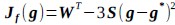
- In the provided formula, C_v and C_m appear indistinguishable given they are multiplied together, rendering this an ill-posed optimization problem. This should be clarified.
- In my understanding, d(a)/V_speed corresponds to the temporal delay associated with picking fruit a. Then, what is tau, and why compute the sum tau + d(a)/V_speed?
- V* is not introduced properly. Is V*(s') = Q*(s', a, tau)? If so, why introduce V*? Moreover, the notational similarity between V_speed and V* is confusing.
- Gamma = 0 still holds?
- Summarize all parameters and hyperparameters that are optimized to model the data and more precisely describe the method used for optimization.
We thank the reviewer for these insightful comments. We agree that the transition from a standard reinforcement learning framework to one incorporating motivational vigour requires precise definitions to ensure the model is well-posed and interpretable. We have addressed these points as follows:
(1) Clarification of C_v and C_m: We have clarified C_m and d(a) in the newly added Experiment 1 model summary table. Specifically, C_v is the scalar vigour constant and C_m is a unit vector representing the horizontal and vertical components. Because C_m is a unit vector, the optimization does not suffer from a collinearity issue from the scalar multiplication between C_v and C_m.
(2) Bridging Theory to Practice (tau and Total Delay): In the theoretical framework of Niv et al. (2007), "delay" is an abstract sum encompassing both waiting and execution. In practice, when fitting to real-world VR data with variable execution times , we must distinguish between the waiting time tau (time spent stationary or searching) and the execution time (||d(a)|| / V_speed). This is necessary because participants take time to look around the forest to search for fruits before deciding to commit to an action. The sum tau + ||d(a)|| / V_speed represents the total delay between two actions, which directly aligns with the notion of opportunity cost of time. We have added a table (Table 3) and added a new Figure 8 to clarify these distinctions.
(3) V*, Q*, and gamma: The reviewer is correct that V*(s') = max_{a’, tau’} Q*(s', a', tau'). We previously used V* for simplicity. Since the notation of V* and V_speed was confusing, we have updated the term to max_{a’, tau’} Q*(s', a', tau') in the optimality equation. We confirm that gamma = 0 (a greedy policy) still holds for the Experiment 2 framework to maintain focus on steady-state motivational trade-offs. We have added this statement to the method section.
(4) Summary of Parameters and Optimization: We have summarized the hyperparameters {k, x_0, C_p, C_v, h, v} in the new summary table for Experiment 2.
(8) It is not clear what the results of the modelling approach presented in Figure 7a+b concretely add to the comparison of movement velocities and collection rates in Figure 6.
We appreciate the reviewer's comment regarding the relationship between the raw behavioral metrics and the computational results. While both sets of findings support the argument for reduced motivational vigour in the tonic pain condition, we believe the modeling approach provides distinct and essential value:
(1) Finer-Grained Analysis Tool: The computational model acts as a more sophisticated analysis tool than simple velocity or rate averages. Unlike Figure 9a+b (in the revised manuscript, previously Figure 7), which summarizes overall performance, the model accounts for the trial-by-trial trade-off between opportunity costs, movement effort, and choice values. This allows us to isolate vigour from other confounding components.
(2) Direct vs. Indirect Measurement: If we assume that motivational vigour in a free-operant task can be quantified through an RL framework, as established in animal studies, then the model's vigour constant (C_v) serves as a direct, concrete estimate of that internal state. In contrast, overall speed and collection rates are indirect markers that can be influenced by multiple factors, such as different choice sets available to the participants as the fruits locations are randomly generated.
In summary, the computational approach provides a rigorous, parameterized bridge between observable behavior and the underlying neuro-computational mechanisms of recuperative pain. We have updated the Discussion section to more explicitly state how the computational approach provides a controlled measure that is isolated from the other confounders of the task. Added text to the Discussion:
“Compared to overall speed and collection rate, which can be influenced by multiple factors, such as different choice sets available to participants as the fruit locations are randomly generated, the model's fitted parameters (e.g. vigour constant C_v) in theory serves as a direct, concrete estimate of that internal state.”
(9) Claims made in the discussion should be more thoroughly and closely linked to the results presented previously. Specifically, experimental outcomes supporting the following claims should be directly referenced:
- "tonic and phasic pain serve different motivational functions".
- "phasic pain provides a punishment teaching signal that directs avoidance".
- "tonic pain reduces motivational vigour".
- "these two functions [punishment teaching signals and reduction of motivational vigour?] can be formally distinguished and quantified".
- "We did not see interactions between tonic and phasic pain".
We have revised the Discussion to more explicitly link these claims to our experimental results. Revised text:
“The experiments show that tonic and phasic pain serve different motivational functions during adaptive behaviour, in line with ecological and evolutionary theories of pain (Bolles and Fanselow, 1980; Walters and Williams, 2019). Specifically, our findings point towards phasic pain providing a punishment teaching signal that directs avoidance through value-based learning, balancing the cost of future harm alongside potential reward. This is supported by the observation that increasing phasic pain intensity significantly reduced choice probability and increased distance bias between choices, whereby participants were willing to travel further to reach a pain-free fruit. In contrast, we found that tonic pain reduces motivational vigour, which supports energy conservation and recuperation in the context of bodily damage. This claim is directly evidenced by the reduction in taskrelated movement velocities and fruit collection rates during tonic pain blocks. The experiments are the first to show that these two functions can be formally distinguished and quantified during ongoing behaviour. By utilising a free-operant RL computational framework, we were able to dissociate these roles phasic pain was quantified as a generally negative utility term affecting choice values, while tonic pain was formalised as a change in vigour constants that were significantly higher (increasing delays between actions) in tonic pain condition. This illustrates how pain simultaneously acts in different ways to serve self-protection.”
“One notable aspect of our results is that we did not see interactions between tonic and phasic pain at either the behavioural or neural level. Behaviourally, we observed that average aversive choice probabilities remained similar regardless of the presence of tonic pain, with no significant interaction effect on punishment sensitivity. Furthermore, our model-fitting confirmed that tonic pain did not significantly modulate the fitted phasic pain utility values. There are two contexts in which these might be predicted. First, in `conditioned pain modulation' paradigms (Kennedy et al., 2016), a tonic pain stimulus is sometimes seen to reduce both the perceived intensity and the cortical evoked responses to phasic pain stimuli delivered somewhere else on the body (Hoffken et al., 2017; Enax-Krumova et al., 2020). Although we utilised concentric ‘Wasp’ electrodes designed to selectively activate nociceptive A-delta fibres (Inui et al., 2002), and confirmed that the resulting ERPs (N1-P2) were significantly modulated by phasic intensity, we observed no such attenuation by tonic pain. Indeed, neither subjective pain ratings nor the N1-P2 amplitude showed a significant modulation by the tonic pressure pain stimulus. In contrast, our results were more compatible with a trend in the other direction.”
(10) The paragraph in the discussion "A concern that is sometimes raised..." (lines 243 - 254) raises interesting points, but its particular relevance to the study at hand is unclear.
We appreciate the reviewer's feedback. The motivation for including this discussion is to address a common critique we received for the study: whether the observed reduction in vigour under tonic pain is "simply" due to distraction or cognitive load, rather than being a specific functional output of the pain system. We have revised this paragraph to link the concern to our paper’s specific finding.
Our central argument is that for tonic pain, distraction is not a confounding "sideeffect" but rather the primary mechanism of action. By being inherently "distracting," tonic pain successfully withdraws resources from ongoing tasks (like foraging) to promote the energy conservation required for recuperation.
(11) The clinical perspective of the methodological framework presented at the end of the discussion is interesting and could be expanded.
We thank the reviewer for this encouraging comment. We have expanded the final paragraph of the Discussion to more explicitly state the clinical utility of our framework. Specifically, we now contrast our approach with standard clinical assessments such as Quantitative Sensory Testing (QST). We highlight that while QST is a valuable tool, it can lack ecological validity; in contrast, our VR-based task allows for a more realistic, behaviourally sensitive assessment of how pain impacts a patient’s daily functional activities and motivational state. We believe this represents a significant step towards more objective and "real-world" clinical pain phenotyping.
(12) The statistical analyses part in the methods section should provide a clear definition of dependent and independent variables and clearly state which test was used for which analysis, e.g., by referencing the corresponding subfigure in the main text.
We agree that a more structured summary of the statistical approach would improve the clarity of the Methods section. We have now included a comprehensive summary table (Table 1) in the Statistical Analysis subsection. This table explicitly defines the dependent and independent variables for each analysis, identifies the specific statistical model used (e.g. Linear Mixed Models or repeated measures ANOVA), and directly maps these to the corresponding figures in the results section.
Minor comments:
(1) Introduction:
(a) The introduction should elaborate more on the advantages of employing an "ecologically meaningful context".
We thank the reviewer for suggesting further elaboration on the advantages of employing an "ecologically meaningful context". We have updated the introduction to provide additional reasoning of choosing an ecologically valid context for the study:
“One of the challenges in studying adaptive functions of pain is the difficulty of embedding experiments within ecologically meaningful contexts. To solve this, we designed an immersive foraging task using virtual reality (VR), in which humans search a forest to collect fruits from the low-lying bushes at varying heights. A foraging paradigm provides a robust, free-operant framework that captures the core components of adaptive behaviour: it is goal-directed, involves complex movement, and requires the learning of an optimal strategy to maximise rewards. This allows us to computationally dissociate how different types of pain influence the control of action.”
(b) It would be helpful to clarify why tonic pain applied to a limb not involved in the task is expected to influence the motivational vigour with respect to the task.
We thank the reviewer for pointing out additional clarification for applying tonic pain to the non-dominant arm. We have added the following text to the introduction clarifying our hypothesis and why it was applied to the non-task limb:
“Second, we hypothesised that tonic pain acts as a coefficient modulating the tradeoff between opportunity cost and vigour cost, thereby serving a recuperative function. To test this in Experiment 2, we delivered continuous tonic pressure to the non-dominant arm via an inflated cuff to emulate a background state of injury. Within our free-operant framework, tonic pain was modelled as a weighting factor that shifts the optimal balance toward reduced energy expenditure. Because the stimulus was applied to the non-task limb, we specifically predicted a global reduction in motivational vigour—operationalised as decreased movement velocities and foraging rates—rather than a direct mechanical impairment.”
(2) Results/Experiment 1:
(a) How were monetary rewards implemented exactly? How much money per fruit?
We thank the reviewer for the opportunity to clarify the incentive structure. Participants were informed at the start of the study that they would earn a performance-based bonus of up to £10, determined by the points they collected during the foraging task. To ensure that motivation remained consistent across the entire session for all individuals—regardless of their baseline foraging speed—the specific exchange rate between points and currency was not disclosed. This prevented potential 'ceiling effects', where a high-performing subject might stop exertive effort after reaching the maximum bonus early, or 'floor effects', where a subject might perceive the reward for an individual action as too small to be motivating.
Following the completion of the experimental session, all participants were compensated with the full £10 bonus in addition to their base payment for participation. We have updated the Methods section to reflect these details:
“Participants were informed at the start of the experiment that their total points would be rewarded with a monetary incentive of up to £10. To maintain a constant level of motivation throughout the task, the exact point-to-currency exchange rate was not specified. Upon completion of the session, all participants were awarded the maximum bonus of £10.”
(b) A green pine apple is not ripe and, in a naturalistic context, possesses some aversive value, even in the absence of phasic pain stimuli. Why was the color coding not counterbalanced across individuals? To what degree could this have confounded the results?
We thank the reviewer for this insightful point. We acknowledge that the lack of counter-balancing for fruit colour (green vs. yellow) is a limitation of the current study design. However, we believe the potential confounding effect of "unripe" green pineapples on the final analysed data is minimal due to the principles of associative learning.
While a naturalistic heuristic (green = unripe) might establish a weak prior bias, fundamental associative learning [14] and reinforcement learning models [15] demonstrate that extensive training with a highly salient unconditioned stimulus (such as pain) rapidly overrides mild initial priors. The task objective focused strictly on maximizing reward points, and participants underwent extensive training (10 blocks in Experiment 1; 6 blocks in Experiment 2) before the analysed sessions began. During this time, the strong, explicit contingencies (green = pain, yellow = safe) were learned and verbally verified. Therefore, by the time the main experimental data was collected, any weak baseline aversion to green had been overshadowed by the explicit task contingencies, making the learned associative value the primary driver of behaviour. We have added a statement acknowledging this limitation and outlining this theoretical rationale in the Methods section.
“While the colour association (green for painful, yellow for pain-free) was not counter-balanced across subjects, any inherent aversive value of green pineapples (e.g., as 'unripe' fruit) is expected to have a minimal confounding effect on the analysed data. In associative learning frameworks, while mild prior biases may influence initial value estimations, extensive training with a highly salient unconditioned stimulus (e.g. phasic pain) rapidly updates these values, driving them toward an asymptote determined entirely by the explicit task contingencies (Rescorla & Wagner, 1972; Sutton & Barto, 2018). Because participants underwent extensive training (10 blocks in Experiment 1 and 6 blocks in Experiment 2) to establish the explicit pain associations prior to the analysed sessions, the observed avoidance behaviour was predominantly driven by the learned phasic pain contingencies rather than baseline colour preferences.”
(c) In the "Avoidance increases with increasing phasic pain intensity" section, clarify upfront that pain ratings and choice probabilities were estimated at the block level. This information is provided only in a later section.
We agree with the reviewer that this information should be stated earlier for clarity. We have updated the beginning of the "Avoidance increases with increasing phasic pain intensity" section to specify that these metrics were estimated at the block level:
“For this analysis, both aversive choice probabilities and subjective pain ratings were estimated at the block level.”
(3) Results/Experiment 2:
(a) ERP visualizations (Figure 5) should include standard error indicators.
We have updated Figure 5 (now Figure 6) to include 95% confidence intervals for standard error of the mean across subjects for all ERP traces. This provides a clearer visualization of the variance in the neural response.
(b) In the section "A unified model...", clarify what is meant by saying that the unified model is "validated by the behavioural data", since behavioral data is what is being modeled in the first place.
We clarify that "validation" in this context refers to the consistency between the parameters estimated by our generative unified model and the results obtained from the independent, model-free regression analysis of the raw behavioural data. While both approaches use the same source data, the unified model provides a finer-grained analysis of latent internal states (like motivational vigour), whereas the regression provides a direct empirical benchmark (more details were discussed in the response to major comment (8)). We have rephrased this section to better describe this as a consistency check against empirical regression results.
(c) In the context of Figure 8a, the term "correlations" is misleading if referring to pairwise comparisons.
We appreciate the opportunity to clarify our terminology. The results presented in Figure 8a (and the associated text) are derived from a Linear Mixed Model (LMM) where the tonic pain condition was treated as a binary independent variable. The term "correlation" was used to describe the statistical association (represented by the t-values) between the presence of tonic pain and EEG band power, accounting for subject-level random effects. It does not refer to simple pairwise comparisons (like t-tests). However, we agree that "correlation" can be ambiguous when applied to a binary predictor. We have revised the text and figure legends to use the terms "associated with" or "predicted by" to more accurately reflect the LMM framework.
(d) Based on the presented data, there is no evidence for the section headings claim "Neural activities link to vigour".
We agree with the reviewer that our results primarily provide evidence for a significant neural association with the tonic pain condition rather than a direct, statistically robust correlation with the vigour parameter itself (after Bonferroni correction). While tonic pain is associated with reduced vigour behaviourally, the EEG markers we identified are more accurately described as signatures of the pain state. We have revised the section heading and the corresponding text to focus on the characterisation of the tonic pain state to ensure our claims are strictly supported by the statistical evidence.
(4) Methods:
In the supplementary materials, the headings pertaining to different LMMs are confusing and not consistent with the Figure labeling in the manuscript (e.g., 4(ii)b likely corresponds to Figure 4d).
We thank the reviewer for identifying these inconsistencies in the supplementary material. We apologize for the confusion caused by the labelling errors during reformatting the manuscript. We have now thoroughly audited the supplementary headings and updated them to ensure they correspond directly and consistently with the figure labels in the main manuscript.
References
(1) Inui, K., Tran, T. D., Hoshiyama, M., & Kakigi, R. (2002). Preferential stimulation of Adelta fibers by intra-epidermal needle electrode in humans. Pain, 96(3), 247–252. https://doi.org/10.1016/S0304-3959(01)00453-5
(2) Mørch, C.D., Hennings, K. & Andersen, O.K. Estimating nerve excitation thresholds to cutaneous electrical stimulation by finite element modeling combined with a stochastic branching nerve fiber model. Med Biol Eng Comput 49, 385–395 (2011). https://doi.org/10.1007/s11517-010-0725-8
(3) Höffken, O., Özgül, Ö.S., Enax-Krumova, E.K. et al. Evoked potentials after painful cutaneous electrical stimulation depict pain relief during a conditioned pain modulation. BMC Neurol 17, 167 (2017). https://doi.org/10.1186/s12883-017-0946-7
(4) Enax-Krumova, E., Plaga, A.-C., Schmidt, K., Özgül, Ö. S., Eitner, L. B., Tegenthoff, M., & Höffken, O. (2020). Painful Cutaneous Electrical Stimulation vs. Heat Pain as Test Stimuli in Conditioned Pain Modulation . Brain Sciences, 10(10), 684. https://doi.org/10.3390/brainsci10100684
(5) Enrico Schulz, Elisabeth S. May, Martina Postorino, Laura Tiemann, Moritz M. Nickel, Viktor Witkovsky, Paul Schmidt, Joachim Gross, Markus Ploner, Prefrontal Gamma Oscillations Encode Tonic Pain in Humans, Cerebral Cortex, Volume 25, Issue 11, November 2015, Pages 4407–4414, https://doi.org/10.1093/cercor/bhv043
(6) Mahajan Pranav, Tong Shuangyi, Lee Sang Wan, Seymour Ben (2024) Balancing safety and efficiency in human decision making eLife 13:RP101371 https://doi.org/10.7554/eLife.101371.2
(7) Enrico Schulz, Elisabeth S. May, Martina Postorino, Laura Tiemann, Moritz M. Nickel, Viktor Witkovsky, Paul Schmidt, Joachim Gross, Markus Ploner, Prefrontal Gamma Oscillations Encode Tonic Pain in Humans, Cerebral Cortex, Volume 25, Issue 11, November 2015, Pages 4407–4414
(8) Suyi Zhang, Hiroaki Mano, Michael Lee, Wako Yoshida, Mitsuo Kawato, Trevor W Robbins, Ben Seymour (2018) The control of tonic pain by active relief learning eLife 7:e31949
(9) Hewitt, D., Tong, S., Schreiber, S., & Seymour, B. (2026). Tonic pain modulates neural correlates of associative phasic pain memories. PAIN. DOI: 10.1097/j.pain.0000000000003917
(10) Gramann, K., Gwin, J. T., Ferris, D. P., Oie, K., Jung, T.-P., Lin, C.-T., Liao, L.-D., and Makeig, S. (2011). Cognition in action: imaging brain/body dynamics in mobile humans. Reviews in the Neurosciences, 22(6):593–582.
(11) Klug, M. and Gramann, K. (2021). Identifying key factors for improving ica-based decomposition of eeg data in mobile and stationary experiments. European Journal of Neuroscience, 54(12):8406–8420.
(12) Delorme, A. EEG is better left alone. Sci Rep 13, 2372 (2023). https://doi.org/10.1038/s41598-023-27528-0
(13) Bach, D. R., Flandin, G., Friston, K. J., and Dolan, R. J. (2010). Modelling event-related skin conductance responses. International Journal of Psychophysiology, 75(3):349–356.
(14) Rescorla, R. and Wagner, A. (1972). A theory of Pavlovian conditioning: Variations in the effectiveness of reinforcement and nonreinforcement, volume Vol. 2
(15) Sutton, R. S. and Barto, A. G. (2018). Reinforcement learning: An introduction, 2nd ed. Adaptive computation and machine learning. The MIT Press, Cambridge, MA, US.